Author Archives: author

New Medical Technology: A Mind Genomics Cartography of How to Present Ideas to Consumers and to Investors

DOI: 10.31038/PSYJ.2021312

Introduction

Today’s world is awash in technology. The opportunities for making money through technology emerge when the benefits of the technology can be communicated either to users or to investors or both. In the world of startup accelerators, hungry investors, and the public which has learned to accept the blistering pace of innovation as part of today. It has become increasingly important to communicate one’s invention in a way which convinces the listener and excites the potential investor. It should not be surprising then that there are classes on creating the so-called ‘pitch deck,’ the document designed to excite investors. There is a lot less interest in finding out just what information might excite the prospective purchasers, simply because, in the scheme of things, starting up and raising money are more important than initial and then repeat sales. It is no wonder that many companies know what to say to investors about the financial aspects of the product but do not know what to say about the product itself. That is, these start-ups but also many later stage companies are at a loss to describe the mind of their investors and/or the mind of their customers. This means that, when challenged, virtually all startups struggle, having overlooked the relatively minor effort to really understand in a scientific, discipline manner, people’s reactions to what they are offering. With that in mind, the opportunity arose to use Mind Genomics for a new product idea, patented in the U.S. (Patent No. US 10,340,546 B1) on Jul 2, 2019 (Figure 1). Simply put, the device is a biocompatible, self-recharging micro battery, as small as a grain of rice, that can be safely and effectively implanted within the human body to power at least one implanted medical device, using the patient’s own body fluids. This micro-battery can communicate with the physician, giving advance warning of an imminent heart attack or the presence of a serious communicable disease. The idea is new, revolutionary, and is in the pre-seed phase. The question is what kinds of messages about this product will excite people. To reiterate, messages mean the messages about the product, in terms of what it does, and what that means to the world of health. The Mind Genomics process described here required about four hours of investment, from start to end, a minor monetary investment. The paper describes the process, shows what was learned, and underscores the opportunity to use Mind Genomics and allied sciences of the mind to increase the likely success of an early-stage venture. Similar approaches have been over the last decade to create products, to help horticulture, etc. [1,2].

fig 1

Figure 1: The patent for the biofuel cell.

Mind Genomics as an Emerging Science

Mind Genomics traces its history to the marriage of several disciplines, beginning with experimental psychology (especially psychophysics), merging with mathematical psychology (conjoint measurement), statistics, and applied consumer research [2]. The objective was and remains to understand the way people make decisions about topics, these topics being of the everyday [3-5]. Mind Genomics focuses on the specifics of a topic, a focus which forces the researcher to deal with the granular aspects, rather than with the grand vision. In other words, the researcher studies the actual product or service itself and, specifically, the minutiae that might otherwise be overlooked in the grand sweep of the ‘elevator pitch.’ Indeed, the granularity of the information provided by Mind Genomics in effect generates a ‘wiki of the topic,’ or an ‘MRI of the mind’ with respect to the product. The importance of such granularity of knowledge is overlooked again and again in the heat of excitement, the haste to get investors, and the omnipresent motivator in business, FUD (fear, uncertainty, doubt). The best way to understand the application of Mind Genomics to startups and pitches, the warp and woof of the venture world, may be through a worked case example, where there is little knowledge at the start of the effort. The body of the paper shows how to understand ‘what works,’ at the level of the structure of the messages (contribution of the individual elements and their combinations), and structure of the mind (influence of who the person is, how the person thinks). The result of the effort is a tool, the PVI (personal viewpoint identifier), which provides the inventor(s) or group raising capital the necessary knowledge of what specific aspects of the invention most promise market success.

As the reader follows the steps, it should be kept in mind that the process takes far longer to describe than it does to execute.  Furthermore, the speed of the processes increases with practice and as the person becomes increasingly facile with the method.

Step 1: Choose the Topic. In this Case the Topic is the Patent, and Specifically What it Does

Step 2: Ask Four Questions Which Tell a Story

It is as this point that many people become ‘stuck, for the simple reason that people are not accustomed to think in a structured and creative manner, viz., to think analytically while at time having fun doing so.

Although one’s obsessive nature may demand that there be five, six, or even more questions, a key aspect of Mind Genomics is the requirement to keep the questions to a number that can be managed easily. In the early days, around year 2000, it was possible to do long interviews by web, with interviews lasting 15 minutes. The longer time required evaluating 48 to 60 vignettes is no longer feasible unless the respondents are well recompensed. Furthermore, as a practical issue, the longer studies with more questions and more answers (viz., 6 questions x 6 answers/question, or 36 elements) somehow ‘never seem to get done.’ They implode because everyone feels that she or he must make a ‘contribution’ to feel part of the process. Too many cooks do really spoil this broth. It is better in terms of process to run three smaller studies in one day, each small, but iterative, rather than that one comprehensive study which never seems to reach the execution phase because of yet another revision and the need for the different parties to agree. The smaller number of elements in the 4×4 design,16 elements, removes much time wasting, back and forth discussion, no matter how deeply people feel that they must discuss and ‘get it perfect’ before the effort, which itself will be done much more quickly, about 1-2 hours.

Table 1 shows the four questions and the 16 elements. These elements may or may not be the correct. One need not know. The underlying Mind Genomics process is quick, powerful, inexpensive. There is no need to be right. One needs to do the study. The data will quickly reveal which types of elements perform well. Subsequent iterations, when they occur, are simply built on the winning elements from the iteration before, the losers discarded, and new elements tried.

Table 1: The four question and the four answers (elements) to each question.

Question A: WHAT is the biofuel cell?
A1 WHAT: Cell gets its energy from my own body fluids
A2 WHAT: Cell is size of a grain of rice
A3 WHAT: Cell implanted in a blood vessel in my body
A4 WHAT: It is painless …. can save my life
Question B: HOW does the biofuel cell work?
B1 HOW: Early warning system for infections & heart attacks…programmed to detect viruses to help me and prevent spread
B2 HOW: Uses my body fluids to generate electricity … no need for battery
B3 HOW: Runs my insulin pump and/or pacemaker … no need for battery
B4 HOW: Delivers medication to my body at right time … uses tiny computer chip
Question C: WHY should I want the biofuel cell?
C1 WHY: Peace of mind about having or not having a communicable disease
C2 WHY: Peace of mind about having or not having a heart attack soon
C3 WHY: Automatically contacts doctor via computer chip if it detects problem with me
C4 WHY: Prevents me from infecting others by telling me if I have a disease, even before symptoms appear
Question D: WHO will pay for the biofuel?
D1 PAY: I will pay for it
D2 PAY: My insurance company will pay for it in part
D3 PAY: The government will pay for it in part
D4 PAY: I will work with my insurance company and the government to get it paid

Step 3: Combine the Elements into Vignettes, According to an Underlying Experimental Design

The experimental design specifies exactly 24 combinations, some having two elements, some having three elements, and the remaining having four elements. A vignette can have at most one element or answer from a question, but in many vignettes an answer from one of the four questions is missing. The strategy for this ‘incompleteness’ is that the structure of the combinations, the 24 vignettes, is such that all 16 elements are statistically independent of each other. That means that the absolute contribution of each of the 16 elements can be computed from the regression, making the approach of Mind Genomics exceptionally powerful in the nature of the information that it delivers. Finally, each respondent evaluates a totally unique set of the vignettes, created by permuting or shuffling the elements [6]. The benefit of that permutation approach is that a single study can cover a lot of the different vignettes. The pattern emerges much like the pattern of an MRI in medicine, emerging after combining the different snapshots of the mind, each snapshot from one of the experimental designs. The happy outcome is that the Mind Genomics process needs no basic understanding of the topic. The ease of setting up the Mind Genomics study (minutes), the cost (low), the speed (hours from start to end) make it possible to iterate several times to understand the topic, not by being right at the start, but by iterating to a solution almost painlessly.

Step 4: Select a Rating Question Pertaining to the Topic

Traditional approaches have asked simple, unidimensional questions, either using a rating sale (viz., how interested are you, 1=not interested … 5=interested; how much would you pay? 1=nothing …5= 10$). New methods include selecting an answer from a group of possible answers (viz., 1=sad, 2=happy, 3 = irritated, 4=curious, 5=excited), and so forth.

For this study we explored a two-dimensional answer, dealing with believing the information and buying the product, respectively. The reason was the relevance of these two dimensions both to understand the response to the product/service as marketers and the information to the investors, demonstrating knowledge of the product, and its economic potential.

Here is a new product to help you. It is a small fuel cell for your body!! Read each combination and rate on this scale:

1 = No way

2 = Believe: NO; Buy: NO.

3 = Believe: NO, Buy: YES

4 = Believe: YES; Buy: NO

5 = Believe: YES; Buy: YES

Step 5: Create a Short Classification Questionnaire to Further Understand the Respondent

These small-scale studies are meant to provide quick, deep answers to what interests the respondent, doing so in a study of three minutes or faster. The classification questions, answered at the start of the study, require only information about the respondent (gender, age), as well as an optional third question, with up to four answers. In our Biofuel study, we chose to ask the respondent about her or his medical situation (not relevant, think about situation occasionally, think about situation frequently, or currently monitoring a condition, respectively.)

Step 6: Launch the Product among a Group of Respondents Who are Members of a Large Panel (>10 million) for a 3-minute Experiment in the Form of an Interview

It is a false economy to use one’s own respondents as a panel unless they constitute individual who are otherwise difficult. Both in terms of time and ultimately in terms of money, it is far more practical to use external panels, provided by companies which charge a reasonable, relatively low fee on a per-respondent basis. The panel respondents in this study were provided by Luc.id, Inc., in the United States. The respondents provided can have any desired geographical, age, and other qualifications. The requirement was to work with respondents 50 years or older. These would be the individuals likely to need the product. The self-reported health concern (question 3) would be able to provide the response by individuals who say that they are actively monitoring conditions. Once the researcher has thought about the problem the mechanics involved in setting up, launching, and receiving data are virtually automatic, programmed, simple, fast, and after one or two experiences error-minimizing. It is not the doing, but the thinking which is difficult. Structured thinking of this type, no matter how seeming obvious it turns out to be, must be a conscious, formal part of the development of a communication program about WHY the new idea, and the economic benefits, here specifically, WHO wants the product. The Mind Genomics process forces the respondent to think deeply about the problem, and think quickly, both being important. There is no excuse in Mind Genomics for delay since the process is simple, templated, fast (hours), cost-effective, all leading to iterations. One need not know anything at the start of the iterations, but by three, four, or five iterations, one will have assembled the powerful insights and precise messages.

Step 7: Prepare the Data for Analysis

Each respondent generates 24 rows of data, one row for each of the 24 vignettes.

For our evaluation of the selling messages for the new biofuel cell, we create three key dependent variables:

Believe/Buy (Rate 5). This variable will be 100 when the rating for a vignette is 5, and 0 otherwise.

Neither Believe nor Buy (Rate 1,2). This variable will be 100 when the rating for a vignette is 1 or 2, and 0 otherwise.

Response time. This is the response time in seconds, to the nearest 10th of a second, for each vignette.

Table 2 shows the data from the study, data ready for the statistical analysis below. The table shows three rows of data from each of two respondents. The table begins with the row number, the panelist number, and the structure of vignette, viz., which questions does the vignette comprise. The middle of Table 2 comprises 16 columns to code the elements, with the value 1 corresponding to the element present in the vignette, and the value 0 corresponding to the element absent from the vignette. After the 16 columns come two columns, Rating from the 5-point scale, and the measured Response Time, respectively. Beyond 16 columns to code the input variables and the two original responses (Rating, Response Time), we find two new data columns. The first new data column corresponds to the most positive response, rating 5 (Do believe, Will buy). When the respondent selected the rating ‘5’ on the scale, this cell for the vignette in column Rate 5 is given the value 100, but when the respondent selected rating 1,2,3, or 4, this cell is given the value 0. The second new data column corresponds to the two most negative responses, rating 1 or 2. When the rating is 1 or 2, the cell for the vignette in this column is give the value 100. When the rating is 3,4, or 5, the cell is given the rating 0. A small random number is added to the values 0 or 100, simply to introduce some small but necessary variability in the binary ratings, in preparation for the analysis.

Table 2: Example of a data matrix showing three rows of data from each of two respondents.

Row

Respondent # Design Structure

A1

A2 A3 A4 B1 B2 B3 B4 C1 C2 C3 C4 D1 D2 D3

D4

Rating Response Time Rate5

Rate12

1

1 ABC 0 0 1 0 0 0 1 0 0 0 0 1 0 1 0 0 1 7.9 0

100

5

1 ACD 0 1 0 0 0 1 0 0 0 0 0 0 1 0 0 0 3 3.1 0

0

8

1 ACD 0 1 0 0 0 1 0 0 1 0 0 0 0 0 0 0 4 4.4 0 0
25 2 ABCD 1 0 0 0 0 0 0 1 0 0 0 1 0 1 0 0 1 9.0 0

100

32

2 ABD 0 1 0 0 0 0 1 0 0 0 0 0 1 0 0 0 2 8.0 0 100
33 2 ABCD 0 0 0 1 1 0 0 0 0 0 1 0 0 0 1 0 2 3.4 0

100

Step 8: External Analysis – Do the Groups of Respondents or Vignettes differ from Each Other?

By looking at the structure of the vignette we can learn about how the respondent makes decisions. Recall that each respondent evaluated a unique set of 24 vignettes, and that across the set of 121 respondents and 2904 combinations there are relatively few duplicate combinations. The strategy of covering a wide number of combinations (covering the ‘design space’) avoids repeat combinations in favor of more the combinations to be testing. Thus, it is, as yet, difficult to compare two or more groups on the score of the same test stimuli simply because there are few test stimuli. The objective in the design was to create as many unique vignettes as possible. It is possible and instructive to compare the averages of three key dependent variables across all key groups, if only to get a sense of the average values of the key dependent variables. Table 3 shows the averages for the three variables across all the relevant respondents in the group. Table 3 show two additional pairs. The first is the averages from vignettes 1-12 vs the averages from vignettes 13-24. This information tells us whether there is a change in the criteria as the experiment proceeds, with the respondent evaluating 24 vignettes. The second pair of data comes from the responses to vignettes read quickly (non-engaging, response time operationally defined as less than 2.25 seconds) vs read slow (engaging, response time operationally defined as more than 2.25 seconds).

Table 3: Average of the three dependent variables for all vignettes appropriate for the subgroup.


Rate5

Rate12

RT Seconds

Total

22

21

4.48

First 12 vignettes

0

42

4.43

Second 12 Vignettes

43

0

4.53

Slow RT > 2.25 Sec

21

19

5.97

Fast RT < 2.25 Sec

22

26

1.35

Female

22

21

4.52

Male

22

21

4.41

Age 50-59

22

21

4.44

Age 60+

22

21

4.55

Q3 3Often

22

21

4.33

Q3 4Monitoring

21

21

4.71

Q3 1No issue

22

21

4.42

Q3 2Sometimes

22

21

4.52

Rate5 Mind-Set 1

22

21

4.49

Rate5 Mind-Set 2

22

21

4.41

Rate5 Mind-Set 3

22

21

4.54

The Total panel generates these three averages across all 2904 vignettes.

Rate5 = 22, viz., 22% of the vignettes are assigned a rating of 5, so that 78% of the vignettes are assigned ratings of 1, 2, 3 or 4, respectively.

Rate12 = 21%, viz. 21% of the vignettes are assigned a rating of 1 or 2, so that 79% of the vignettes are assigned ratings of 3, 4 or 5.

RT = 4.5 meaning that on average the respondent rated a vignette 4.5 seconds after seeing the vignette. This suggests that it took the respondent about 108 seconds, or nearly two minutes to evaluate all 24 vignettes. The rest of the time was occupied with self-profiling classification, and so-forth, making the total time of about three minutes quite reasonable.

Table 3 shows the average responses of the three dependent variables, across Total Panel, Gender, Age, Health Concern (question #3 in the classification), and finally three mind-sets which emerged by clustering together respondents showing similar patterns of strong positive responses towards the elements (mind-sets from clustering). The averages are remarkably similar, except for the responses obtained for the first 12 vignettes vs the second 12 vignettes, and the pattern of rejection (Rate12), for those vignettes read quickly (26% of the vignettes rejected) vs those vignettes read slowly (19% rejected).

Step 9: External Analysis – Does the Structure of the Vignette “Drive the Rating”?

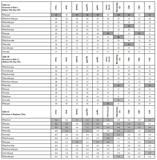
Our first external suggested minor differences across groups, except for the order of the vignette in the set of 24, or the rate of reading the vignette. It helps to understand how the structure of the vignette, the types of elements combined, drives the dependent variables, and whether there are any group differences. Knowing the impact of the interaction gives the researcher a sense of which types of combinations will, in general, drive positive or negative responses from the respondent (or customer or investor). In turn, Knowing the nature of the interaction between structure and subgroup with respect to response time tells us the groups who will be paying close attention to the messaging. It is important to reiterate that, at least yet, we have not seen detailed information about the elements. That information will come later. Our goal here is to better understand the types of messages as they are perceived by the respondents and as they engage the respondent in terms of paying attention. It is also important to note that the respondent does not think in terms of the structure of the vignette, since on average the respondent pays about 4.5 seconds attention to each vignette, sufficient time to read and assign an intuitive, ‘gut reaction.’ Longer response times than 4.5 seconds suggest that the vignette structure presents information which arrests the respondents speed through the interview and may represent a structure of information which strongly engages the respondent. Table 4 presents the averages of the three dependent variables (columns) by the 11 different structures used by the 4×4 Mind Genomics design. Table 4 is divided into three sections, Table 4A for the Rate5, Table 4B for the Rate12, and Table 4C for Response Time. The rows in each section of Table 4 are sorted by the Total Panel, allowing us to get a sense of what interests the respondents, what turns them off, and what engages them. In turn, the subgroups give us a sense of any key differences. To make the inspection of Table 4 easier we have darkened the key cells, respectively cells with averages of 30 or higher for the two binary transformed variables (Rate5, Rate12), and cells with response times of 5.0 seconds or longer. The data reveal patterns very quickly, patterns relevant to investors and marketers alike. The most striking is the importance of the combination of What it is and How it will be paid (AD). The least important is How it works and How will it be paid (BD). The ‘magic’ comes from the combinations of the elements, and that certain combinations are simply strong. When it comes to an outright rejection (Rating12, Not Believe, Not Pay), most of the cells are low. There are a few exceptions, especially for those who are monitoring a condition. When the vignette contains an element of ‘What it is’ and ‘Why should I use it,’ those monitoring a condition find this offensive. In fact, they find both ‘What Why’ and ‘How Why’ to be turnoffs, something that should be remembered when talking to a prospective buyer, but also key information to present to the funding group. Finally, respondents take different amounts of time to process the information. The most engaging vignettes are those with two elements, What How, Why Pay, and How Pay, respectively. The longer vignettes, the one with four elements, but a few with three elements, tend to be glossed over, or at least are less engaging. These results suggest that a great deal of information about the proper presentation can be gleaned simply by understanding the pattern of responses for the three key dependent measures, Rate5, Rate12, and Response Time. Despite the fact that we do not yet know the specific messages to put into the vignette, we should have a sense that the optimal vignette will incorporate ‘What it is’, and ‘How it’s paid for.’

Table 4: How the structure of the vignette ‘drives’ the ratings. The table shows the average values for three key dependent variables, by structure of the vignette (row) and by key group (column).

table 4

Step 10: Internal Analysis, to Understand How Elements Drive the Dependent Variables

The original rationale for Mind Genomics was founded on the premise that people could not tell the interviewer what guided their decisions but would likely try to please the interviewer by confabulating one. Such efforts would be especially obvious when the respondent would be asked about the criteria used to guide decision in the routine behaviors, those labelled ‘System 1’ by Nobel Laureate Daniel Kahneman [7]. According to Kahneman, but clearly observed every day, we make thousands of decisions, perhaps many more, simply during our daily lives, doing so virtually automatically. To create a science of the everyday requires an approach beyond observation (too limited, too expensive), and beyond questionnaires and surveys (subject to judgment biases, memory biases, etc.). First a short recapitulation is in order, in order to lay out the rationale for these next steps in the analysis. Mind Genomics works by presenting the respondent with the different vignettes, created by experimental design, doing so in a rapid pace. We saw that the average time for evaluation was approximately 4.5 seconds, from the time that the vignette appeared, and the judgment was assigned. During these 4-5 seconds, on average, the respondent read, thought (almost automatically), and rated the vignette. When these vignettes are presented rapidly, and when the vignettes are created by experimental design, it becomes difficult to think; one simply responds at an intuitive level. The happy result is judgment untainted by most of the cognitive biases which pervade the everyday research. One cannot change the judgment criterion to accord with the specific nature of an element (viz., price versus feature vs benefit, etc.) In contrast, the conventional, one-at-a-time approach the respondent can switch criteria rapidly, depending upon the nature of the element so as to give the ‘right answer.’ Not so with Mind Genomics, which combines these elements into wholes, gestalts, vignettes, each judged, de facto, by the same criterion. The respondent ends up neither able to nor even wants to be ‘correct’ or ‘consistent.’ The respondent simply wants to finish the task, typically doing so in a state of relative indifference, and thus answering honestly, or at least answering in an intuitive way. The benefit is that attempts to ‘game the system’, to ‘please the interviewer,’ to ‘get it right,’ are simply not possible. Armed with the foregoing, we now look at the deconstruction of the vignettes into the part-worth contributions of the elements, doing so by key groups. Each group was self-defined, except by the mid-sets. The mind-sets were discovered by doing the modeling at the individual respondent level, creating 121 models, and then clustering together individual respondents showing the same pattern of coefficients for their 16 elements as those elements drove ‘Rate5,’ viz Believe/Buy. The reader is referred to the in-depth treatments of the clustering method (k-means) in a variety of published papers [8-10].

The actual deconstruction of the vignettes is done by the statistical method of OLS, ordinary least-squares regression. The regression attempts to relate the presence/absence of the 16 elements to the dependent variable. The equations are written as follows:

Rate5 (Believe/Buy) = k0 + k1(A1) + k2(A2) … k16(D4)

Rate12 (Do Not Believe/Will Not Buy = k0 +k1(A1) + k2(A2)… k16(D4)

Response Time = k1(A1) + k2(A2) … k16(D4)

The OLS regression uses the entire data set from the relevant respondents to estimate the additive constant (k0) and the 16 element-linked coefficients (k1 … k16).

It is important to keep in mind that there is an additive constant for the regression model for Rate5 (propensity to believe/buy in the absence of elements), and for Rate12 (propensity to not believe / not buy in the absence of elements). For response there is no additive constant because there is no propensity to respond to a test vignette unless there are elements in the vignette.

Finally, one could create equations without additive constants for both Rate5 and Rate12. The conclusions would be the same, but the data would be someone less easy to understand.

Armed with the foregoing approach, we use the standard method of OLS regression to create models for nine defined subgroups. These are the ones that are most meaningful:

  1. The Total Panel… all respondents who participated.
  2. The three mind-sets MS1, MS2, MS3, which emerged from clustering together respondents with similar patterns of coefficients, based upon the models for Rate5 (Believe/Buy). Extensive studies using Mind Genomics suggest that the groupings emerging from this type of clustering generate clear, consistent, and interpretable patterns, pointing to radically different ways of thinking about a topic. These are the so-called mental primaries for a topic, albeit primaries emerging from patterns of response to a granular topic, rather than grand patterns across many topics. Mind Genomics works at the granular level, where the relevant stimuli are likely to be clear, and the relevant behaviors likely to emerge.
  3. Gender, age, health groups, those who have no concerns (answer 1 to question #3 in the classification), and those who are monitoring a condition (answer 4 to question #3 in the classification).

Step 10: Define the Meaning of the Coefficients, and Present Data in an Interpretable Format

The analysis in Mind Genomics generates a great deal of data because each element generates nine coefficients, one coefficient for each subgroup. Thus, the analyses involve three different groupings; three dependent variable (Rate5, Rate12, Response Time), nine key subgroups, and 16 elements. This total 3x9x16 or 432 cells of data to inspect to uncover strong performing elements and discern patterns.

To make the analyses easier we do the following:

  1. Present the subgroups in a new order, with Total and mind-sets first, because it will be with mind-sets that the major group-differences emerge.
  2. Blank out any coefficient which is 0 or lower, because the element with that coefficient is not a driver of Believe/Buy or Not Believe/Not Buy, respectively. A negative coefficient for Rate5 (Believe/Buy) means that the element may either be irrelevant (originally rated 3 or 4) or actively push away (originally rated 1 or 2). In turn, a negative coefficient for Rate12 (Do Not Believe / Would Not Buy) means that the element may be irrelevant (originally rated 3 or 4) or actively push away (originally rated 5)
  3. Shade all cells with coefficients of 6 or higher for Rate5 or Rate 12. Shad all cells with response times for the element of 1.5 seconds or longer.

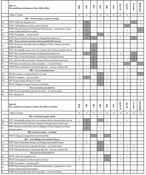
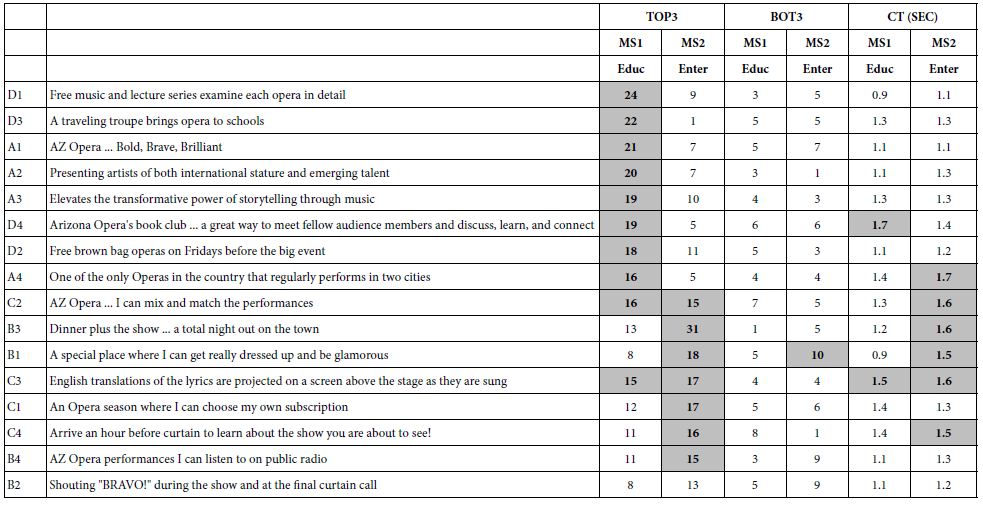
Armed with this information, we can now look at the strong messages for the Biofuel invention. Table 5 is sorted in descending order for the positive elements of the three mind-sets. Occasionally an element appears twice in a table, scoring strongly in two of the three mind-sets (viz., coefficient of +6 or higher).

The rationale for presenting the data in descending order by mind-set is that only through mind-set do we see sufficient strong performing elements which, in turn, seem to cohere together to tell a meaningful ‘story.’ Keep in mind that the mind-sets are created through purely statistical methods, without any connection to what the mind-sets or clusters really mean. The researcher’s task is to select the minimum number of clusters which make sense and uncover the latent pattern. For our data, the assignment of the respondent mind-sets showed the clearest pattern when the clustering was done using the coefficients for Rate5 (believe/buy), and when three mind-sets were extracted. The three clusters thus become three new, non-overlapping groups. The separate data was used to create models for Rate5 (the original basis of the clustering), as well as models for Rate12, and models for Response Time. The compositions of the three mind-sets are fixed at after the clustering analysis. The compositions of the other groups are fixed at the time of classification, viz., the before the actual experiment. Once we know the respondents in each group, it is straightforward to create a summary model or equation for each group for each of the three dependent variables. The final act is to create the summary tables, doing so based on the three mind-sets, which carry most of the interpretable patterns. The other subgroups are presented as backup data. The actual interpretation of the data is not relevant for this research exercise, but is extremely relevant for the inventor, marketer, and the investor. Through understanding what specific aspects do very well (viz., high coefficients for a mind-set) it becomes straight to identify a lot more of the potential of the invention. One knows what to say, how to say it, and now to whom. The researcher may stop at one iteration or move quickly (or slowly) to the next iteration, simply deleting poorly performing elements and them. Over time guesswork turns into solid knowledge.

Step 11: Finding these Mind-sets in the Population

As Table 5 shows, especially Table 5A, it is in the mind-sets that one discovers the important messages. It is clear in this study as in most Mind Genomics studies. that the mind-sets are far more important than anything else about the respondent . Knowing the mind-set enables one to present the necessary information to engage that mind-set, to convince that mind-set, and to avoid saying the wrong thing, something that might immediately turn a prospect into a rejector. The traditional thinking of market researchers, political pollsters and the like is that ‘birds of a feather’ think the same way. That is, lacking a deeper understanding of how people think about the world of the everyday, those looking to understand why people differ from each other in known ways generally look at WHO the person is, what the person may THINK in general terms about a topic (e.g., attitudes towards health, or how a person BEHAVES (viz., what does a person search for on the Internet when exploring a topic). The effort towards classifying a group of people by WHO, by THINK and by BEHAVE is significant, usually reserved for large-scale problems. Mind-Genomics, dealing as it does with the granular aspects of the world, and often with the very ordinary (not in the case of the Biofuel Cell!) suffers from the paradox of being able to discover important mind-sets in the population in the short space of a few hours, but then grapples with the problem of generalizing this discovery so that it moves beyond simply a scientific fact, to be applied, whether for knowledge building, or action generating or hopefully both. The mind-sets are reasonably clear from Table 5 and could become the basis of three distinct sets of communications, whether to a customer or to an investor. ‘What to say to convince’ becomes a matter of research, not a matter of a dearly held opinion, possibly irrelevant or even worse, possibly counter-productive. Just consult Table 5B to see what ‘doesn’t work.’ On the other hand, what is the marketer to do when the distribution of the three mind-sets in the population is similar for each key subgroup, whether gender, age, or even monitoring a condition (Question #3, answer 4)? Table 6 suggests that it will be almost impossible to find the way to assign a new person to the proper mind-set. That impossibility discourages the wider use of a rapid, inexpensive, iterative, knowledge-developing system.

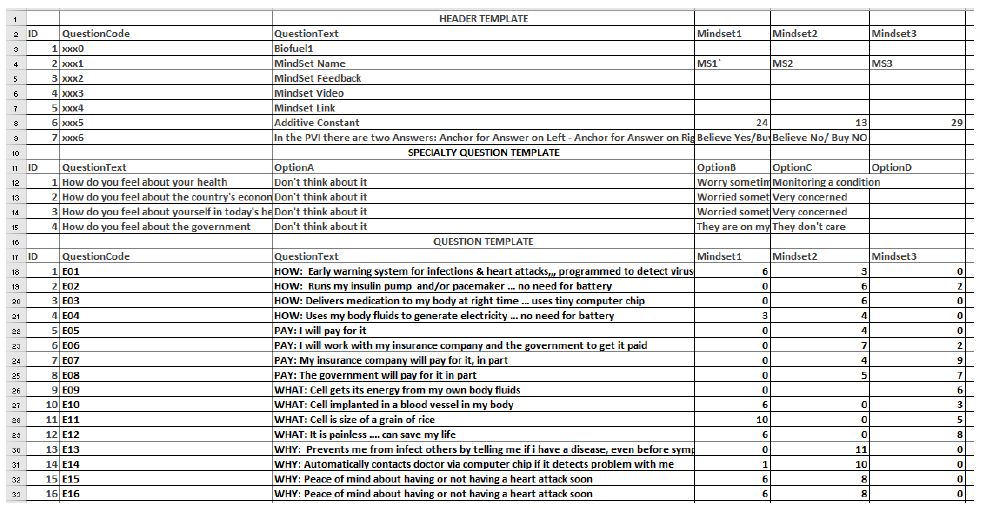
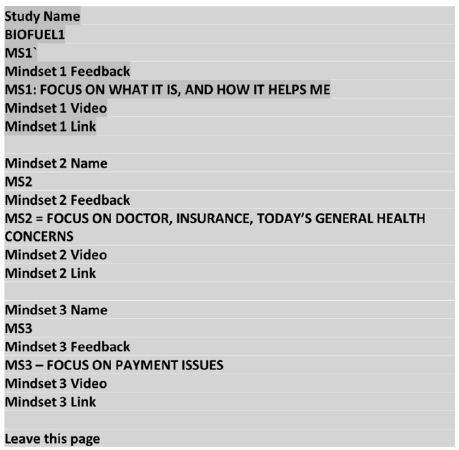
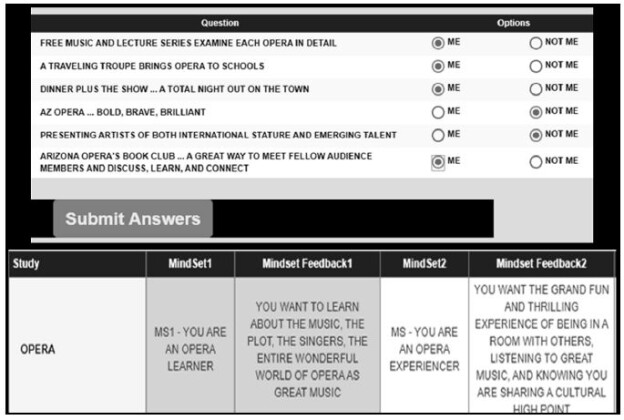
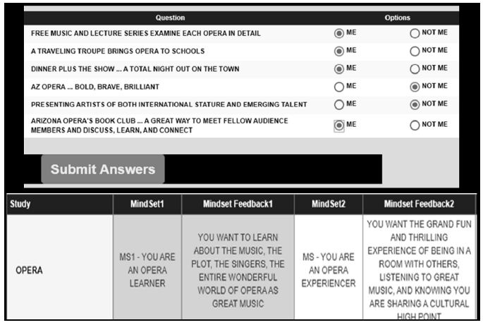
During the past four years, since 2016, authors Gere and Moskowitz have introduced and applied a new approach to assign a new individual to one of the mind-sets. The approach is known as the PVI, the Personal Viewpoint Identifier. The PVI uses the table of coefficients (Table 5A), summarizing the coefficients for the mind-sets. The underlying thinking is that the small study presented here provides insight into the basic mind-sets of a topic, viz., combinations of ideas which naturally go together, as can be seen with the small population. These can be likened to ‘mental primaries’, albeit primaries for a limited, quite granular topic, empirically uncovered from experiments. The issue is now to discover the distribution of these primaries across the world, and the lability of these primaries as a function perhaps of experience, of life-situation, etc. A secondary set of goals, not discussed here, is to relate these ‘mental primaries’ to relevant behaviors exhibited by people, viz., the expression of these primaries in everyday life. A third set of goals, also not discussed here, is to these ‘mental primaries’ primaries to genes, to uncover links between genetics and the mind, for defined topics where there is a suspicion that one or another gene might be involved in certain behaviors. Our focus here will simply be the presentation of the PVI, as a ready-to-use tool, one based upon the actual elements used to define the mind-sets. The PVI does not need any theoretical bridge between the mind-sets and the PVI composition. The components of the PVI are the same elements used in the study, with perhaps a slight editing to generalize them where needed. The mathematics underlying the PVI first creates noisy data by adding random variability to the original means, doing so many times, according to a Monte Carlo system. The analysis uses a decision tree to determine which elements and what weighting factors best assign the average individual in each mind-set to the correct mind-set. The scheme which works best across the thousands of perturbations is the scheme used for the PVI. The output emerges in the form of a link to the specific PVI designed for the study. That is the granular data are used as inputs to the assignment program. The PVI emerges with six questions taken from the elements of the study, and put into the form of a statement, with one of two answers. The pattern of the six answers assigns the new respondent to one of the three mind-sets. In studies comprising two mind-sets rather than three, the pattern of the six answers assigns the respondent to one of the two mind-sets. Figure 1 shows the set-up page, configured to be used with the Mind Genomics output. The set-up uses the data from the Mind Genomics study but requires the researcher to assign names to the mind-sets, to create a Yes/No rating question, and an introduction to the task given to the respondent. The actual PVI set-up is presented as an Excel® worksheet, in color, to make the process easy to do, fast, and subject to fewer errors. As part of the set-up, the researcher can specify a video and/or a landing page to which the respondent is immediately directed after the mind-set has been assigned by the PVI program for the specific individual (Figures 2-5).

Table 5: Coefficients relating the presence/absence of the 16 elements to the three dependent variables (5A for Rate5, 5B for Rate 12, 5C for Response Time). The table shows the total panel and key subgroups. Only positive coefficients are shown. Strong performing elements are shown by highlighted cells (coefficient +6 or higher for Rate5 and Rate12; response time of 1.5 seconds or longer).

table 5

Table 6: Distribution of the total panel and three mind-sets across the different self-defined subgroups in the population.


Total

MS1 MS2

MS3

Total

121

41 41

39

 
Female

75

27 26

22

Male

46

14 15

17

Age50x59x

76

27 25

24

Age60x

45

14 16

15

Q32Sometimes

47

18 13

16

Q33Often

31

9 13

9

Q31No issues

24

8 9

7

Q34Monitoring

19

6 6

7

fig 2

Figure 2: The researcher set-up for the PVI, using the output from the Mind Genomics study.

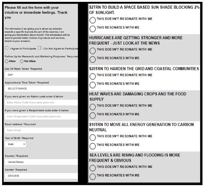
The orientation page for the respondent, as well as background information. The PVI can be configured to send the data to a database, as well as to the respondent, and to a staff person. The orientation page takes approximately 30 seconds to complete. Individual fields of data, e.g., gender, age, telephone, etc. can be suppressed to ensure privacy. Figure 3 shows the actual PVI, with four background or attitude questions, and the six questions emerging from the Monte Carlo algorithm. The PVI questionnaire also takes about 30 seconds to complete.

fig 3

Figure 3: The orientation page for the PVI (personal viewpoint identifier) The link to the PVI is: https://www.pvi360.com/TypingToolPage.aspx?projectid=1267&userid=2018.

fig 4

Figure 4: The actual PVI questionnaire, beginning with three questions about one’s attitudes toward health and finishing with six questions.

fig 5

Figure 5: The feedback from the PVI. The data are stored in a database, along with the information from Figures 2 and 3. The respondent’s mind-set determined by the PVI is shaded (MS1).

The feedback for one respondent. This respondent was assigned to Mind-Set 1 based on the pattern of the responses. Figure 4 shows spaces for both a landing page and a link to a video stored in YouTube. Thus, at the time of deploying the PVI, the researcher may show the respondent a video and drive the respondent to a landing page. In the world of social issues, the PVI becomes a game, wherein the respondent finds out about himself or herself and is exposed to messages through video or landing pages.

Discussion and Conclusion

The ingoing rationale for the paper was the observation that in both the private sector with start-ups and in the public sector with major issues, there seem to be few ways to obtain affordable, solid, actionable data in the realistic framework of need for speed and clarity. The ‘soft’ data from people, used to back up major investments and scientific breakthroughs, seem again and again to be remarkably weak. ‘Subjective, soft data’ are perceived to be a necessary nuisance, either impossible to obtain because the data would take years to obtain or because the data simply is not valued. Often the data presented is qualitative, coming from a limited number of respondents or participants in a set of focus groups or depth interviews. Those data are important to set the stage, but they do not give the inventor, the business owners, the investors, or the government a sense of the ‘there there,’ in the immortal quip of Gertrude Stein. There is no need to discuss the specific data from the study. The data are simply of the type that the process delivers, with the nature of the data similar in general form from study to study, but sufficient in depth for any study to provide the necessary guidance. The study is the first of its kind, from the group associated with the inventor, author Samuel Messinger. Rather than polishing the results, it seemed most appropriate to take the results and explicate them, step by step, so that the paper becomes a guide to interpreting the results, a vade mecum. One outcome is that the reader gets a sense of how to do the study and what will emerge from the study step by step. The other outcome is the ease with which the reader can look at the data tables, to identify what to say, what not to say, whether it matters to whom, and ‘who are the relevant whom’.

Note

The Mind Genomics program (BimiLeap) is available at www.BimiLeap.com.

The Personal Viewpoint Identifier (PVI) is available at www.PVI360.com.

Acknowledgment

Attila Gere thanks the support of Premium Postdoctoral Research Program of the Hungarian Academy of Sciences.

References

  1. Levin LA, Langer KM, Clark DG, Colquhoun TA, Callaway JL, et al. (2012) Using mind genomics® to identify essential elements of a flower product. Horticulture Science 47: 1658-1665.
  2. Gofman A (2012) Putting RDE on the R&D Map: A Survey of approaches to consumer-driven new product development. In: A. Gofman & H. R. Moskowitz (Eds.). Rule Developing Experimentation: A Systematic Approach to Understand & Engineer the Consumer Mind, 72-89. Bentham Books. https://doi.org/10.2174/97816080528441120101
  3. Moskowitz HR (2012) ‘Mind Genomics’: The experimental, inductive science of the ordinary, and its application to aspects of food and feeding. Physiology & Behavior 107: 606-613. [crossref]
  4. Moskowitz HR, Gofman A, Beckley J, and Ashman H, (2006) Founding a new science: Mind Genomics. Journal of Sensory Studies 21: 266-307.
  5. Moskowitz HR, Porretta S, Silcher M (2008) Concept Research in Food Product Design and Development. John Wiley & Sons,
  6. Gofman A, Moskowitz H (2010) Isomorphic permuted experimental designs and their application in conjoint analysis. Journal of Sensory Studies 25: 127-145. https://doi.org/10.1111/j.1745-459X.2009.00258.x
  7. Kahneman D (2011) Thinking, Fast and Slow. Macmillan.
  8. Gere A, Zemel R, Papajorgji P, Moskowitz H, (2019) “Candy Is dandy”: The mind of sexuality as suggested by a Mind Genomics experiment. In Sex, Smoke, and Spirits: The Role of Chemistry pg: 17-31, American Chemical Society.
  9. Jain AK, Dubes RC (1988) Algorithms for Clustering Data. Prentice-Hall, Inc.
  10. Porretta S, Gere A, Radványi D, Moskowitz H (2019) Mind Genomics (Conjoint Analysis): The new concept research in the analysis of consumer behaviour and choice. Trends in Food Science & Technology 84: 29-33.

Thinking Climate – A Mind Genomics Cartography

DOI: 10.31038/ESCC.2020213

Abstract

The paper deals with the inner mind of the respondent about climate change, using Mind Genomics. Respondents evaluated different combinations of messages about problems and solutions touching on current and future climate change. Respondents rated each combination on a two-dimensional scale regarding believability and workability. The ratings were deconstructed into the linkage between each message and believability vs. workability, respectively. Two mind-sets emerged,Alarmists who focus on the problems that are obvious to climate change, and Investors who focus on a limited number of feasible solutions.These two mind-sets distribute across the population, but can be uncovered through a PVI, personal mind-set identifier.

Introduction

Importance of the Weather and Climate

As of this writing, the concerns keep mounting about climate change, as can be seen in published material, whether the news or academic papers, respectively.As of this writing, the concerns keep mounting about climate change, as can be seen in published material, whether the news or academic papers, respectively.A search during mid-December 2020 reveal 416 million hits for ‘global warming,’ 350 million hits for ‘global cooling’ 886 million his for ‘weather storms’ and 608 million hits for ‘global weather change.’ The academic literature shows the parallel level of interest in weather and its changes. A retrospective of issues about climate change shows the increasing number of ‘hit’ over the past 20 years, as Table 1 shows. These hits suggest that issues regarding climate change are high on the list of people’s concerns.

Table 1a: Number of ‘hits’ on Google Scholar for different aspects of climate change.

Year

Global Warming Global Cooling Weather Storms

Global Weather Change

2000

14,900 22,300 8,370

34,300

2002

30,900 111,900 10,400

61,500

2004

39,900 126,00 13,100

75,300

2006

52,200 129,000 14,600

92,300

2008

82,200 132,000 19,600

111,000

2010

105,000 153,000 23,700

128,000

2012

112,000 154,000 26,700

137,000

2014

109,000 154,000 28,200

136,000

2016

96,300 131,000 27,900

114,000

2018

77,900 85,200 27,400

81,200

Table 1b: The four questions and the four answers to each question.

Question A: What climate impacts do people see today?
A1 Sea Levels are rising and flooding is more frequent & obvious
A2 Hurricanes are getting stronger and more frequent – just look at the news
A3 Heat Waves are damaging crops and the food supply
A4 Wildfires are more massive and keep burning down neighborhoods
Question B: What are the underlying risks in 20 years?
B1 Coastal property investments lose money
B2 Children will live in a much lousier world
B3 Governments will start being destabilized
B4 People will turn from optimistic to pessimistic
Question C: What are some actions we can take to avoid these problems?
C1 Right now, implement a global carbon tax
C2 Over time, transfer 10% of global wealth to an environment fund
C3 Create a unified global climate technology consortium for technological change.
C4 Build a solar shade that blocks 2% of sunlight
Question D: What’s the general nature of the system that will mitigate these risks today?
D1 $10trn to move all energy generation to carbon neutral
D2 $20trn to harden the grid and coastal communities
D3 $2trn to build a space based sunshade blocking 2% of sunlight.
D4 $0.02trn to spray particulate into atmosphere to block 2% of sunlight.

Beyond Surveys to the Inside of the Mind

The typical news story about climate changes is predicated on storytelling, combining historical overviews, current economic concerns, description of behavior from a social psychology or sociological viewpoint, and often adoom and gloom prediction which demands immediate action in ordertoday to be forestalled.All aspects are correct, in theory.What is missing is a deeper understanding of the inner thinking of a person when confronting the issue of climate change. There are some papers which do deal with the ‘mind’ of the consumer, usually from the point of view of social psychology, rather than experimental psychology [1].

Most conversations about climate change are general, because of the lack of specific knowledge, and the inability of people to deal with the topic in depth. The topic of climate change and the potential upheavals remains important, but people tend to react in an emotional way, often accepting everything or rejecting what sounds reasonable or what does not sound reasonable, respectively. The result is the ongoing lack of specific information, compounding the growth of anxiety, and the increasingly strident rejectionism by those who fail to respond to a believed impending catastrophe. Another result, just as inaction, is a deep, perplexing, often consuming discourse on the problem, written in way which demonstrates scholarship and rhetorical proficiency, but does not lead to insights or answers, rather to well justified polemics [2-6].The study reported here, a Mind Genomics ‘cartography’ delves into the mind of the average person, to determine what specifics of climate change are believable, what solutions are deemed to be workable, and what elements or messages about climate change engage a person’s attention. The objective is to understand the response to the notion of climate change by focusing of reactions to specifics about climate change, specifics presented to the respondent in the form of small combinations of ‘facts’ about climate [7-9].

Researchers studying how people think about climate follow two approaches, the first being the qualitative approach which is a guided, but free-flowing interview or discussion, the second being a structured questionnaire. The traditional qualitative approach requires the respondent to talk in a group about feelings towards specifics, or even talk an in in-depth, 1:1 interview. These are the accepted methods to explore thinking, so-called focus groups and in-depth interviews. Traditional discussion puts stress on the respondentto recall and state, or, in the language of the experimental psychologist, to produce and to recite. In contrast, the traditional survey presents the respondent with a topic, and asks a variety of questions, to which the respondent selects the appropriate answer, either by choice, or by providing the information.All in all, conventional research gives a sense of the idea, but from the outside in. Reading a book by research can provide extensive information from the outside. Some information from the inside can be obtained from comments by individuals about their feelings.Yet it will be… clearly from the outside, rather than a sense of peering out from the inside of the mind. The qualitative methods may reach into the mind somewhat more deeply because the respondent is asked to talk about a topic and must ‘produce’ information from inside. Both the qualitative and the quantitative methods produce valuable information, but information of a general nature. The insights which may emerge from the qualitative and quantitative methods have a sense of emerging from the ‘outside-in.’ That is, there is insight, but there is not the depth of specific material relevant to the topic, since the qualitative information is in the form of diluted ideas, ideas diluted in a discussion, whereas the quantitative information is structured description with a sense of deep specificity.

The Contribution of Mind Genomics

Mind Genomics is an emerging science, with origins in experimental psychology, consumer research, and statistics.The foundational notion of Mind Genomics is that we can uncover the ways that people make decisions about every-day topics using simple experiments, where people respond to combinations of messages abut the different aspects of the topic. These combinations, created by experimental design, present information to the respondent in a rapid fashion, requiring the respondent to make a quick judgment. The mixture of different messages in a hard-to-disentangle fashion, using experimental design, makes it both impossible to ‘game’ the system, and straightforward to identify which pieces of information drive the judgment.Furthermore, one can discover mind-sets of individuals quite easily, groups of people with similar pattern of what they deem to be important. The approach here, Mind Genomics, makes the respondents job easier, to recognize and react. The messages are shown to the respondent’s job easier, the respondents evaluate the combination, and the analysis identifies which messages are critical, viz, which messages about weather change are important. Mind Genomics approaches the problem by combining messages about a topic, messages which are specific. Thus, Mind Genomics combines the richness of ideas obtained from qualitative research with the statistical rigor of quantitative research found in surveys. Beyond that combination, Mind Genomics is grounded in the world of experiment, allowing the researcher to easily understand the linkage between the qualitatively, rich, nuanced information, presented in the experiment, and the reaction of the respondent, doing so in a manner which cannot be ‘gamed’ by the respondent, in a manner which reveals both cognitive responses (agree/disagree) and non-cognitive response (engagement with the information as measured by response time.)

Mind Genomics follows a straightforward path to understand the way people think about the everyday. Mind Genomics is fast (hours), inexpensive, iterative, and data-intensive, allowing for rapid, up-front analysis and deeper post-study analysis.Mind Genomics has been crafted with the vision of a system which would allow anyone to understand the mind of people, even without technical training. The grand vision of Mind Genomics is to create a science of the mind, a science available to everyone in the world, easy-to-do, a science which creates a ‘wiki of the mind’, a living database of how people think about all sorts of topics.

Doing a Simple Cartography – The Steps

Step 1 – Create the Raw Materials; Topic, Four Questions, Four Answers to Each Question

The cartography process begins with the selection of a topic, here the mind of people with respect to climate change. The topic is only a tool by which to focus the researcher’s mind on the bigger areas.

Following the selection of the topic, the researcher is requested to think of four questions which are relevant to the topic. The creation of these questions may sound straightforward, but it is here that the respondent must exercise create and critical thinking (got rid of word ‘some’), to identify a sequence of questions which ‘tell a story.’ The reality is that it takes about 2-3 small experiments, the cartographies,before the researcher ‘gets it,’ but once the researcher understands how to craft the questions relative to the topic, the researcher’s critical faculty and thinking patterns have forever changed. The process endows the world of research with a new, powerful, simultaneous analytic-synthetic ways to think about a topic, and to solve a problem.Once the four questions are decided upon, the researcher’s next task is to come up with four answers. The perennial issue now arises regarding ‘how do I know I have the right or correct answers?’ The simple answer is one does not. One simply does the experiment, finds out ‘what works,’ and proceeds with the next step of stimuli.After two, three, four, even five or six iterations, each taking 90 minutes, it is likely that one has learned what works and what does not. The iteration consists of eliminating ideas or directions which do not work, trying more of the type of ideas which do work, as well as other exploring other but related directions with other types of ideas.

It is important to emphasize the radically different thinking behind Mind Genomics, which is meant to be fast and iterative, and not merely to rubber stamp or confirm one’s thinking. Speed and iteration lead to a wider form of knowledge, a sense of the boundaries of a topic. In contrast, the more conventional and focused thinking lead to rejection or confirmation, but little real learning.

Step 2 – Combine the Elements into Small Vignettes that will be Evaluatedby the Respondents

The typical approach to evaluation would be to present each of the elements in Table 2 to the respondent, one element at a time, instructing the respondent to rate the element alone, using a scale.Although the approach of isolate and measure is appropriate in science, the approach carries with it the potential of misleading results, based upon the desire of most respondents to give the ‘right answer.’

Mind Genomics works according to an entirely different principle. Mind Genomics presents the answers or elements in what appear to be random combinations, but nothing could be further from the truth. The combinations are well designed, presenting different types of information. It will be the rating of the combination, and then the deconstruction of that rating into the contributions of the 16 individual elements which reveal the mind of the respondent.The experimental design simply ensures that the elements are thrown together in a known but apparently haphazard way, forcing the respondent to rely on intuitive or ‘gut responses,’ the type judgment which governs most of everyday life. Nobel Laureate Daniel Kahnemancalls this ‘System 1’ Thinking, the automatic evaluation of information in an almost subconscious but consistent and practical manner [10].

The underlying experimental design used by Mind Genomics requires each respondent to evaluate 24 different vignettes, or combinations, with a vignette comprising 2-4 elements. Only one element or answer to a question can appear in a single vignette, ensuring that a vignette does not present elements which directly contradict each other, viz., by comprising two elements from the question or silo, presenting two alternative and contradictory answers to the question. The experimental design might be considered as a form of advanced bookkeeping[11].

Many researchers feel strongly that every vignette must have exactly one element or answer from each question.Their point of view is that otherwise the vignettes are not ‘balanced’, viz., some vignettes have more information, some vignettes have less information. Their point of view is acceptable, but by having incomplete vignettes, the underlying statistics, OLS (ordinary least-squares) regression cannotestimate absolute values for coefficients. By forcing each vignette to comprise exactly one element or answer from each question, the OLS regression will not work because the system is ‘multi-collinear.’The coefficients can only be estimated in a relative sense, and not comparable across questions for the study, nor comparable across studies in the same topic, and of course not comparable for different topics.That lack of comparability defeats the ultimate vision of Mind Genomics, viz., to create a ‘wiki of the mind.’A further point regarding the underlying experimental design is that Mind Genomics explores a great deal of the design space, rather than testing the same 24 vignettes with each respondent.Covering the design space means giving up precision obtained by reducing variability through averaging, the strategy followed by most researchers who replicate or repeat the study dozens of times, with the vignettes in different orders, but nonetheless with the same vignettes. The underlying rationale is to average out the noise, albeit at the expense of testing a limited number of vignettes again and again.

Step 3 – Select an Introduction to the Topic and a Rating Scale

The introduction to the topic appears below. The introduction is minimal, setting up as few expectations as possible. It will the job of the elements to convey the information.

Please read the sentences as a single idea about our climate. Please tell us how you feel.

1) No way.

2) Don’t believe, and this won’t work.

3) Believe, but this won’t work.

4) Don’t really believe, but this will work.

5) I believe, and this will work.

The scale for this study is anchored at all five points, rather than at the lowest and at the highest point.The scale deals with both belief in that which iswritten, and belief that the strategy will work.The respondent is required to select one scale point out of the five for each vignette, respectively. The scale allows the researcher to capture both belief in the facts and belief in the solutions.

Step 4 – Invite Respondents to Participate

The respondents are invited to participate by an email. The respondents are member of Luc.id, an aggregator of online panels, with over 20 million panelists. Luc.id, located in Louisiana, in the United States, allows the researcher to tailor the specifications of the respondents. No specifics other than being US residentswere imposed on the panel. The respondents began with a short self-profiling classification questionnaire, regarding age and gender, as well as the answer to the question below:

How involved are you in thinking about the future?

1=Worried about my personal situation with my family

2=Worried about business stability

3=Worried about climate and ecological stability

4=Worried about government stability.

The respondent then proceeded to rate the 24 unique combinations from the permuted experimental design, with the typical time for each vignette lasting about 5-6 seconds, including the actual appearance time, and the wait time before the next appearance[12].The actual experiment thus lasted 2-3 minutes.

Step 6 – Acquire the Ratings and Transform the Data in Preparation for Model

In the typical project the focus of interest is on the responses to the specific test stimuli, whether there be a limited number of test vignettes (viz., not systematically permuted, but rather fixed), or answers to a fixed set of questions.The order of the stimuli or the test questions might be varied but there is a fixed, limited number. With Mind Genomics the focus will be on the contribution of the elements to the responses.Typically, the responses are transformed from a scale of magnitude (e.g., 1-5, not interested to interested), so that the data are binary (viz., 1-3 transformed to 100 to show that the respondents are not interested; 4-5 transformed to 0 to show that the respondent is interested.

As noted above, there are two scales intertwined, a belief in the proposition, and a belief that the action proposed will work. The two scales generate two new binary variables, rather than one binary variable:

Believe:Ratings of 1,2, 4 converted to 0 (do not believe the statements), ratings of 3,5 converted to 100 (believe the statements

Work (Efficacious) Ratings of 1,2,3 converted to 0 (do not believe the solution will work), ratings 4,5 converted to 100 (believe the proposed solution will work).

In these rapid evaluations we do not expect the respondent to stop and think. Rather, it turns out that ‘Believe’ is simply ‘’does it sound true?’ and Work” is simply ‘does it seem to propel people to solve the problem?Both of these are emotional responses. The end-product is a matrix of 24 rows for each respondent, one row for each vignette tested by that respondent. The matrix comprises 16 columns, one column for each of the 16 elements. The cell for a particular row (vignette) and for a particular column (element) is either 0 (element absent from that vignette) or 1 (element present in that vignette). The last four columns of the matrix are the rating (1-5), the response time (in seconds, to the nearest 10th of a second), and the two new binary values for the scales ‘Believe’ and ‘Work’ respectively (0 for not believe or not work, 100 for believe or work, depending upon the rating, plus a small random number < 10-5).

Step 7 – Create Two Models (Equations) for Each Respondent, a Model for Believe, and a Model for Work, and then Cluster the Respondents Twice, First for the Individual ‘Believe’ Models, Second for the Individual ‘Work’ Models

The experimental design underlying the creation of the 24 vignettes for each respondent allows us to create an equation at the respondent level for Believe (Binary) = k0 + k1(A1) + k2(A2) …. + k16(D4).The dependent variable is either 0 or 100, depending upon the value of the specific rating in Step 6.The small random number added to each binary transformed number ensures that there is variation in the dependent variable.

  1. Believe Models. For the variable Believe, applying OLS regression generates the 16 coefficients (k1 – k16) and the additive constant, for each of the 55 respondents. A clustering algorithm (k-means clustering, Distance = (1 – Pearson Correlation)) divides the respondents into two groups. We selected the two groups (called mind-sets) because the meanings of the two groups were clear. Each respondent was then assigned to one of the two emergent groups, viz., mind-sets,based on the respondent’s coefficients for Believe as a dependent variable[13].
  2. Work Models. A totally separate analysis was done, following the same process, but this time using the transformed variable ‘Work’.The respondents were then assigned to one of the two newly developedmind-sets, based only on the coefficient for work.

As a rule of thumb, one can extract many different sets of complementary clusters (mind-sets), but a good practice is to keep the number of such selected sets to a minimum, the minimum based upon the interpretability of the mind-sets. In the interests of parsimony, one should stop as soon as the mind-sets make clear sense.

Step 8 – CreateGroup Equations; Three Models or Equations, One for Believe, One for Work, One for Response Time

Create these sets of three models each for Total Panel, Male, Female, Younger (age 18-39), Older (age 40+), and the mind-sets.Theequations are similar in format, but not identical:

Believe = k0 + k1(A1) + k2(A2) … k16(D4)

Work = k0 + k1(A1) + k2(A2) … k16(D4)

Response Time=k1(A1) + k2(A2) … k16(D4)

For the mind-sets,create two models only.

Mind-Set based on ‘believe’:

Believe = k0 + k1(A1) + k2(A2) … k16(D4)

Response Time= k1(A1) + k2(A2) … k16(D4)

Mind-set based on ‘work’

Work =k0 + k1(A1) + k2(A2) … k16(D4))

Response Time =k1(A1) + k2(A2) … k16(D4).

Results

External Analysis

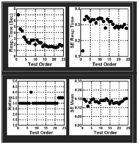
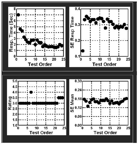
The external analysis looks at the ratings, independent of the nature of the vignettes, either structure or composition of the vignette in terms of specific elements. We focus here on a topic which is deeply emotion to some. The first analysis that we will focuses on the stability of the data for this deeply emotional topic. As noted above, the Mind Genomics process requires the respondent to evaluate a unique set of 24 vignettes. Are the ratings stable over time or is there so much random variability that by the time the respondent has completed the study the respondent is not paying any more attention, and simply pressing the rating button?We cannot plot the rating of the same vignette across the different positions for the same reason that each respondent tested a totally unique set of combinations. We can track the average rating, the average response time, and then the standard errors of both, across the 24 positions. If the respondent somehow stops paying attention, then the rating should show less variation over time.

Figure 1 shows the averages and standard errors for the two measures, the ratings actively assigned by the respondent, and the response time, not directly a product of the respondent’s ‘judgment,’ but rather a measure of the time taken to respond. The abscissa shows the order in the test, from 1 to 24, and the ordinate shows the statistic.The data show that the response time is longer for the first few vignettes (viz., test order 1-3), but then stabilizes.The data further show that for the most part, the ratings themselves are stable, although there are effects at the start and at the end. Figure 1 suggests remarkable stability, a stability that has been observed for almost all Mind Genomics studies, when the respondents are members of an on-line panel, and remunerated by the panel provided for their participation.

fig 1

Figure 1: The relation between test order (abscissa) and key measures. The top panel shows the analysis of the response times (mean RT on left, standard error of the mean on the right).The bottom panel shows the analysis of theratings (mean rating on the left, standard error of the mean on the right).

The second external analysis shows the distribution of ratings by key subgroups across all of the vignettes evaluated by each key subgroup. For each key subgroup (rows), Table 2 shows the distribution of the five scale points (A), distribution of the two scale points (3,5) points which reflect belief (3,5) distribution of the two scale points (4,5) reflecting positive feeling that the idea ‘works’ The patterns of ratings suggest that a little fewer than half the responses are believe or work. However, we do not know the specific details about which types of messages drive these positive responses. We need a different level of inquiry, an internal analysis into what patterns of elements drive the responses.

Table 2: Distribution of ratings on Net Believe Yes, and Net Work YES five-point scale, by key groups, and by key clusters of scale points.


Net Believe YES(% Rating 3 or 5)

Net Work YES(% Rating 4 or 5)

Total

45

44

Vignettes 1-12

43

43

Vignettes 13-24

47

45

Male

46

52

Female

44

36

Age 24x-9

47

49

Age 40+

43

38

Worry business

43

31

Worry about climate

50

52

Worry about family

45

48

Worry about government

43

39

Worry about ‘outside’ (business + climate)

43

35

Worry about ‘inside’ (family + government)

46

49

Belief – MS1

44

48

Belief MS2

47

40

Work – MS 3

46

47

Work – MS4

45

39

Internal Analysis – What Specific Elements Drive or Link with ‘Believe’ and ‘Work’ Respectively?

Up to now we have considered only the surface aspect of the data, namely the reliability of the data across test order (Figure 1), and the distribution of the ratings by key subgroup (Table 2). There is no sense of the inner mind of the respondent, about what elements link with believability of the facts, with agreement that the solution will work, or how deeply the respondent engages in the processing of the message, as suggested by response time. The deeper knowledge comes from OLS (ordinary least squares) regression analysis, which relates the presence/absence of the 16 messages to the ratings, as explicated in Step 8 above.

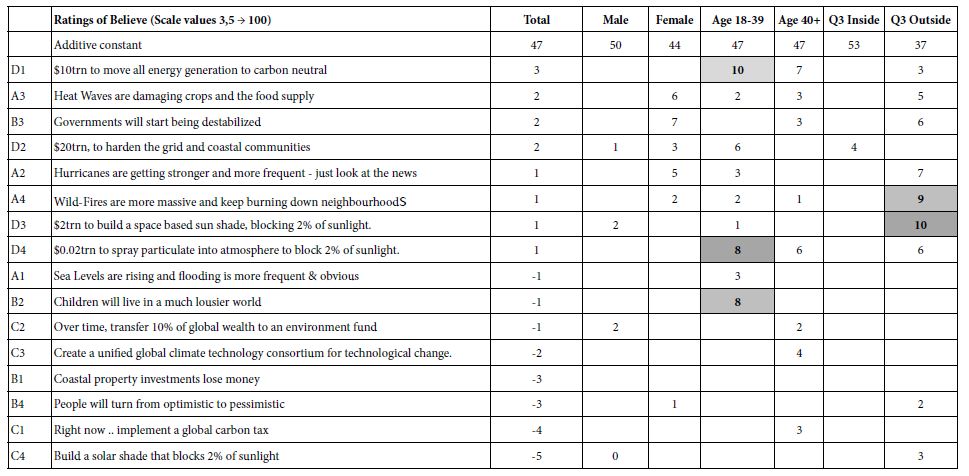
Table 3 shows the first table of results, the elements which drive ‘believability.’ Recall from the methods section that the 5-point scale had two points with the respondent ‘believing,’ and that these ratings (3,5) generated a transformed value of 100 for the scale of ‘believe’, whereas the other three rating points (1,2,4) were converted to 0.The self-profiling classification also provides the means to assign a respondent based upon what the respondent said was most concerning, worry about self (family, government), worry about other/outside (business, climate).Table 3 shows the additive constant, and the coefficients for each group. Only the Total Panel shows coefficients which are 0 or negative. The other groups show only coefficients which are positive. Furthermore, the table is sorted by the magnitude of the coefficient for the Total Panel.In this way, one need only focus on those elements which drive ‘belief’, viz., elements which demonstrate a positive coefficient. Elements which have a 0 negative coefficient are those which have no impact on believability. They may even militate against believability. Our focus is strictly what drives a person to say ‘I believe what I am reading.’

Table 3: Elements which drive ‘belief ’. Only positive coefficients are shown. Strong performing elements are shown in shaded cells.

table 3

We begin with the additive constant across all of the key groups in Table 3. The additive constants tell us the likelihood that a person will rate a vignette as ‘I believe it’ in the absence of elements. The additive constant is a purely estimated parameter, the ‘intercept’ in the language of statistics. All vignettes comprised 2-4 elements by the underlying experimental design. Nonetheless, the additive constant provides a good sense of basic proclivity to believe in the absence of elements. The additive constants hover between 40 and 50 with two small exceptions of 37 and 53. The additive constant tells us that the respondent is prepared to believe, but only somewhat. In operational terms, an additive constant of 45, for example, means that out of the next 100 ratings for vignettes, 45 will be ratings corresponding to ‘believe,’ viz., selection of rating points 3 or 5, respectively.The story of what makes a person believe lies in the meaning of the elements. Elements whose coefficient value is +8 or higher are strongly ‘significant’ in the world of inferential statistics, based upon the ‘T test’ versus a coefficient with value 0.There are only a few of these elements which drive strong belief.

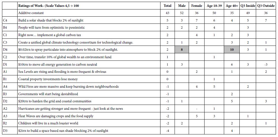
The most noteworthy finding is that respondents in Q3 Inside (worried about issues close to them) start out with a high propensity to believe (additive constant = 53), but then show no differentiations among the elements. They do not believe anything. In contrast, respondents who say they worry about issues outside of them start with low belief (additive constant = 53), but there are a several of elements which strongly drive their belief (e.g., A4:Wild-Firesare more massive and keep burning down neighborhoods.)They are critical, but willing to believe in what they see, and in what is promised to them.  Table 4 shows the second table of results, elements which drive ‘work’. These elements generate positive coefficients when the ratings 4 or 5 were transformed to 100, and the remaining ratings (1,2,3) were transformed to 0. Only some elements give a sense of a solution, even If not directly a solution.The additive constants showdifferences in magnitude for complementary groups. Since the scale is ‘work’ vs. ‘not work’, the additive constant is the basic belief that a solution will work. The additive constant is higher for males than for females (52 vs. 36), higher younger vs. older (50 v 35), and higher for those who worry about themselves versus those who were about others (49 vs. 36).

Table 4: Elements which drive ‘work’. Only positive coefficients are shown. Strong performing elements are shown in shaded cells.

table 4

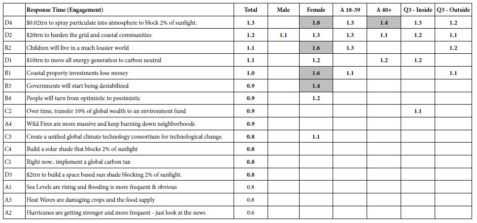
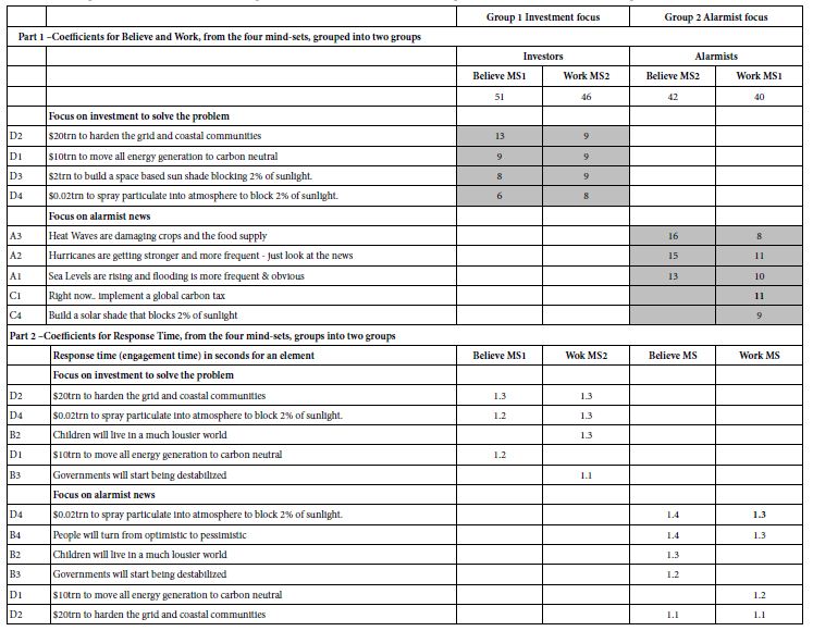
The key finding for ‘work’ is that there some positives on two strong ones. The respondents are not optimistic. There is only one element which is dramatic, however, D4, the plan to spray particulates into the atmosphere to block 2% of the sunlight. This element or plan performs strongly among males, and among the older respondents, 40 years and older, although in the range of studies conducted previously, coefficients of 8-10 are statistically significant but not dramatic, especially when they belong to only one element.  Our third group model concerns the response time associated with each element. The Mind Genomics program measured the total time between the presentation of the vignette and the response to the vignette. Response times of 8 seconds or longer were truncated to the value 8. OLS regression was applied to the data of the self-defined subgroups. The form of the equation for OLS regression was: Response Time = k1(A1) + k2(A2) … k16(D4). The key difference moving from binary rating to response time is the removal of the additive constant. The rationale is that we want to see the number of seconds ascribed to each element, for each group. The longer response times mean that the element is more engaging. Table 5 shows the response times for the total panel, the genders, ages, and the two groups defined by what they say worries them.Table 3 shows only those time coefficients of 1.1 second or more, response times or engagement times that are deemed to be relevant and capture the attention.The strongly engaging elements are shown in the shaded cells.

Table 5: Response times of 1.1second or longer for each element by key self-defined subgroups.

table 5

Table 5 suggests that the description of building something can engage all groups

$10trn to move all energy generation to carbon neutral

$20trn to harden the grid and coastal communities

Women alone are strongly engaged when a clear picture is painted, a picture at the personal level:

Coastal property investments lose money

Children will live in a much lousier world

Governments will start being destabilized.

One of the key features of Mind Genomics is its proposal that in every aspect of daily living people vary r in the way they respond to information. These different ways emerge from studies of granular behavior or attitudes, as well as from studies of macro-behavior or attitudes. Traditional segment-seeking research looks for mindsets in the population, trying to find them by knowing their geodemographics.  Both the traditional way of segmentation and the traditional efforts to find these segments in the population end up being rather blunt instruments. The traditional segmentation begins at a high level, encompassing a wide variety of different issues pertaining to the climate, the future, and so forth. The likelihood is minimal of finding the mind-sets with the clear granularity of these mind-sets is low, simply because in the larger scale studies there is no room for the granular, as there is in Mind Genomics, such as this study which deals with 16 elements of stability and destabilization.

Mind Genomics uses a simple k-means clustering divide individuals based upon the pattern of coefficients. The experimental design used in permuted form for each respondent allows the researcher to apply OLS regression to the binary-transformed data of each respondent.The k-means clustering was applied separately to the 55 models for Believe, and separately once again to the 55 models for Work.Both clustering programs came out with similar patterns, two mind-sets for each. The pattern suggested one be called ‘Investment focus’ and the other be called alarmist focus. The strongest performing elements from this study come from the mind-sets, classifying the respondent by the way the respondent ‘thinks’ about the topic, rather than how the respondent ‘classifies’ herself or himself, whether gender, age, or even self-chosen topic of major concern. The mind-sets are named for the strongest performing element. Group 1 (Believed MS1, Work MS4) show elementswhich suggest an ‘investment focus’.Group 2 (Believe MS2, Work MS3) shows elements which suggest an alarmist focus.

Table 6 shows the strong performing elements for the four mind-sets, as well as the most engaging elements for the mind-sets. The reader can get a quick sense of the nature of the mind-sets, both in terms of what they think(coefficients for Believe and for Work, respectively), as well as what occupies their attention and engages them (Response Time) [14].

Table 6: Strong performing coefficients for the two groups of emergent mind-sets after clustering on responses (Part1), and after clustering on response time, viz., engagement (Part 2).

table 6

The mind-sets emerging from Mind Genomics studies do not distribute in the simple fashion that one might expect, based upon today’s culture of Big Data. That is, just knowing WHO a person is does not tell us how a person THINKS. The reality is that there are no simple cross-tabulations or even more complex tabulations which directly assign a person to a mind-set.Topics such as the environment, for example, may have dozens of different facets. Knowing the mind of a person regarding one facet, one specific topic, does not necessarily tell us about the mind of that same person with respect to a different, but related facet.Table 7 gives a sense of the complexity of the distribution, and the probable difficulty of finding these mind-sets in the population based upon simple classifications of WHO is a person is.

Table 7: Distribution of key mind-sets (Investors, Alarmists).


Total

Investor (Belief) Investor (Work) Alarmist (Belief)

Alarmist (Work)

Total

56

30 24 26

32

Male

27

15 12 12

15

Female

29

15 12 14

17

Age24-39

31

14 12 17

19

Age40+

25

16 12 9

13

Worry aboutfamily

23

12 8 11

15

Worry about climate

12

8 4 4

8

Worry about government

11

7 6 4

5

Worry about business

10

3 6 7

4

Worry Other (business and climate)

21

10 12 11

9

Worry Self (Family, Government)

35

20 12 15

23

Invest from Believe

30

30 11 0

19

Invest from Work

24

11 24 13

0

Alarm from Work

32

19 0 13

32

Alarm from Believe

26

0 13 26

13

During the past four years authors Gere and Moskowitz have developed a tool to assign new people to the mind-sets. The tool, called the PVI, the personal viewpoint identifier, uses the summary data from the different mind-sets, perturbing these summary data with noise (random variability), and creating a decision tree based upon a Monte Carlo simulation. The decade PVI allows for 64 patterns of responses of six questions answered on a 2-point. The Monte simulation combined with the decision tree returns with a system to identify mind-set member in15-20 seconds.Figure 2 shows a screen shot of the PVI for this study, comprising the introduction, the additional background information stored for the respondent (option), and the six questions, patterns of answers to which assign the respondent immediately to the of the two mind-sets.

fig 2

Figure 2: The PVI for the study.

Discussion and Conclusion

The study described here has been presented in the spirit of an exploration, a cartography, a way to understand a problem without having to invoke the ritual of hypothesis. In most study of the everyday life the reality is that the focus should be on what is happening, not on presenting an hypothesis simply for the sake of conforming to a scientific approach which is many cases is simply not appropriate.The issue of climate change is an important one, as a perusalof the news of the day will reveal just about any day. The issues about the weather, climate change, and the very changes in ‘mother earth’ are real, political, scientific, and challenge all people. Mind Genomics does not deal with the science of weather, but rather the mind of the individual, doing so by experiments in communication.It is through these experiments, simple to do, easy to interpret, that we begin to understand the nature of people, an understanding which should not, however, surprise.The notion of investors and alarmists makes intuitive sense. These are not the only mind-sets, but they emerge clearly from one limited experiment, one limited cartography.One could only imagine the depth of understanding of people as they confront the changes in the weather and indeed in ‘mother earth.’ Mind Genomics will not solve those problems, but Mind Genomics will allow the problems to be discussed in a way sensitive to the predispositions of the listener, whether in this case the listener be a person interested in investment to solve the problem or the person be interested in the hue and the cry of the alarmist. Both are valid ways of listening, and for effective communication the messages directed towards each should be tailored to the predisposition of the listener’s mind. Thus, a Mind Genomics approach to the problem presents both understanding and suggestion for actionable solution, or at least the messages surrounding that actionable solution [2,15-19].

As a final note this paper introduces a novel way to understand the respondent’s mind on two dimensions, not just one. The typical Likert Scale presents the respondent with a set of graded choices, from none to a low, disagree to agree, and so forth. The Likert Scale for the typical study is uni-dimensional. Yet, there are often several response dimensions of interest.This study features two response dimensions, belief in the message, and belief that the solution will work.These response dimensions may or may not be intertwined.Other examples might be belief vs. action (would buy).By using a response scale comprising two dimensions, rather than one, it becomes possible to more profoundly understand the way a person thinks, considering the data from two aspects. The first is the message presented, the stimulus. The second is the decisions of the respondent, to select none, one, or both responses, belief in the problem and/or, belief that the solution will work

Acknowledgement

Attila Gere thanks the support of Premium Postdoctoral Research Program.

References

  1. Tobler C, Visschers VH, Siegrist M (2012) Addressing climate change: Determinants of consumers’ willingness to act and to support policy measures. Journal of Environmental Psychology 32: 197-207.
  2. Creutzig F, Fernandez B, Haberl H, Khosla R, Mulugetta Y,et al (2016) Beyond technology: demand-side solutions for climate change mitigation. Annual Review of Environment and Resources 41: 173-198.
  3. Lidskog R, Berg M, Gustafsson KM, Löfmarck E (2020) Cold Science Meets Hot Weather: Environmental Threats, Emotional Messages and Scientific Storytelling. Media and Communication 1: 118-128.
  4. Nyilasy G, Reid LN (2007) The academician–practitioner gap in advertising. International Journal of Advertising 26: 425-445.
  5. Reyes A (2011) Strategies of legitimization in political discourse: From words to actions. Discourse & Society 22: 781-807.
  6. Taleb NN (2007) The black swan: The impact of the highly improbable, Random house, Vol:2.
  7. Moskowitz HR (2012) ‘Mind genomics’: Theexperimental, inductive science of the ordinary, and its application to aspects of food and feeding. Physiology & Behavior 107: 606-613.
  8. Moskowitz HR, Gofman A, Beckley J, Ashman H (2006) Founding a new science: Mind Genomics. Journal of Sensory Studies 21: 266-307.
  9. Moskowitz HR, Gofman A (2007) Selling blue elephants: How to make great products that people want before they even know they want them. Pearson Education.
  10. Kahneman D (2011) Thinking, fast and slow. Macmillan.
  11. Box GE, Hunter WH, Hunter S (1978) Statistics for Experimenters, New York: John Wiley Vol: 664.
  12. Gofman A, Moskowitz H (2010) Isomorphic permuted experimental designs and their application in conjoint analysis. Journal of Sensory Studies 25: 127-145.
  13. Jain AK, Dubes RC (1988) Algorithms for Clustering Data. Prentice-Hall, Inc.
  14. Schweickert R (1999) Response time distributions: Some simple effects of factors selectively influencing mental processes. Psychonomic Bulletin & Review 6: 269-288.
  15. Acosta Lilibeth A, Nelson H Enano Jr, Damasa B Magcale-Macandog, Kathreena G Engay, Maria Noriza Q Herrera, et al. (2013) How sustainable is bioenergy production in the Philippines? A conjoint analysis of knowledge and opinions of people with different typologies. Applied Energy 102: 241-253.
  16. Lomborg B (2010) Smart solutions to climate change: Comparing costs and benefits. Cambridge University Press.
  17. Nerlich B, Koteyko N, Brown B (2010) Theory and language of climate change communication. Wiley Interdisciplinary Reviews: Climate Change 1: 97-110.
  18. Tol RS (2009) The economic effects of climate change. Journal of Economic Perspectives 23: 29-51.
  19. Warren R (2011) The role of interactions in a world implementing adaptation and mitigation solutions to climate change. Philosophical Transactions of the Royal Society A: Mathematical, Physical and Engineering Sciences 369: 217-241.

Mind Genomics Cartography of the Hong Kong Goldfish Market: A Beginner’s Psychological Anthropology of an Everyday Experience

DOI: 10.31038/PSYJ.2021311

Abstract

Respondents in Hong Kong evaluated sets of 24 unique vignettes about the Hong Kong Goldfish Market, rating each vignette on ME (agree) or NOT ME (disagree). The vignettes were created by systematically combining elements (messages) from four different categories, into small combinations comprising 2-4 elements each. The experimental design prevented the respondent from ‘gaming’, viz., giving the appropriate answers because the vignette comprises different messages. The deconstruction of the responses by regression showed the contribution of every element to three dependent variables; agree, disagree, and response time (engagement) revealed different types of decision rules for agree versus disagree. Two mind-sets emerged, based on the pattern of responses to the 16 elements; those interested in low price, and the afficionados. The study showed that the engagement times, viz., response times to individual elements were far longer for Mind-Set 2 (afficionados). The study shows the power of simple experiments to create a database of people’s perceptions of the every-day experiences, a ‘Wiki of Daily Life’.

Introduction

An exploration of the world of experimental psychology, social psychology, sociology, and anthropology reveal an ongoing interest in the world of the everyday specially by researchers in sociology and anthropology, as well as social psychology. There is some experimentation by social psychologists and experimental psychologists, generally of a limited nature, often to understand a general principle, and usually with situations that are unusual. The crossing of experimentation with the world of the ordinary is not particularly common, because experimentation looks for general principles of behavior.

During the past two decades, the world of experimentation in psychology has come to embrace new areas, not perhaps in a formal matter, but at least accepting research which shows the everyday. The research may not appear in highly rated journals because of the quotidian nature of the topic, but nonetheless the research plays an important role in our understand of the lives of contemporary people. Some of the work may be found in the topics covered by behavioral economics, other part of the effort may appear in topics covered by consumer research.

Recently, author Moskowitz has suggested that a new discipline of experimental psychology be developed, one called Mind Genomics [1] Moskowitz et. al., 2007). The effort is to understand the drivers of decision about the quotidian topics of everyday life, not so much to develop grand schemes of behavior, but rather simply to catalog the myriad different aspects of daily behavior. The effort looks at the world of the granular, from the bottom up, from the specific, limited topics which make up the warp and woof of our daily behavior, topics which would not ordinarily be thought to be the appropriate topics of psychology. The topics might be those of interest to an anthropologist who describes these topics in a discussion of behavior, but issue to explore the topic in depth, to understand the facets of a topic, and the different ways to look at the topic.

Early efforts to study daily behavior focused on things, primarily things one might eat or drink. The objective was to understand the different patterns of preferences regarding food. The underlying reason for choosing food was that studies of preferences for food and studies of eating in restaurants and dining halls were well known, well accepted by the world of scientists [2]. The effort soon expanded to other situations, usually products (e.g., financial industry; [3], but eventually moved into experience itself. As far back as 1957, for example, sociologist William Foote Whyte was recording the sociology of the everyday, producing such classics as the Organization Man [4]. The effort continues, with such evaluation of landmark groups, such as the Baby Boomers [5].

Science need not be focused on the traditional topic, such as foods, topics with a long intellectual and academic history. Anyone with a sensitivity to social issues is typically interested both in general patterns and in specific stories. The general patterns are usually reported in good scientific fashion, with appropriate statistics, general conclusions, and foundational knowledge. The stories are often more interesting, sketchy but real world, and used to make the general science more interesting. The science of Mind Genomics, used here to evaluate a common pet market, the Hong Kong (HK) Goldfish Market, provides a way to introduce rigor into the study of what otherwise might simply an interesting vignette, introduced as part of a deeper presentation of a culture, a society, or a hobby. The HK Goldfish Market has been the topic of studies, primarily of a sociological/business nature [6,7] There does not seem to be a deep understanding of the response of individuals to the both the market itself, and to their spending patterns, perhaps because of the localized nature of the topic, and the fact that the ‘mind’ of the individual regarding the HK Goldfish Market is simply not sufficiently important in the world of science.

Despite its minor position as a topic of study, the HK Goldfish Market is an important market. According to the Wikipedia article ‘History of Goldfish Market, Hong Kong, 2012’:

Hong Kong is one of the leading exporters of Goldfish and other tropical fish for aquarists and fish keepers around the world. In Tung Choi Street Goldish shops have congregated for many years…Originally the interest in fish, particularly goldfish, in Hong Kong was related to the needs of Fung Shui, the ancient Chinese system to bring harmony to a house. Under this system Goldfish are particularly important so therefore there has always been a demand for goldfish in Hong Kong more than typical in other countries… During the 1970s and 1980s the keeping of goldfish alongside other types of tropical fish such as butterfly fish became a very suitable hobby for the majority of Hong Kong’s population who lived in flats in high rise apartments. Without the space to keep pet cats or dogs the keeping of tropical fish, both freshwater and less commonly sea fish, became very popular. (Source: Wikipedia, 2020)

The Mind Genomics Approach to Understanding the HK Goldfish Market

Mind Genomics is an emerging science, philosophically descended from experimental psychology, with an admixture of sociology, anthropology, consumer research, and statistics. The notion is that one should be able to create a ‘wiki of the mind’, a searchable database of how people think and make decisions in their daily lives. These decisions are made with respect to the ordinary events of lives, the daily flotsam and jetsam which constitutes the everyday, the banal activities. As noted above, seminal works emerge from the observation of everyday behaviors, such as eating, using financial services, going to work, and so forth. Those are the inspirations. What Mind Genomics provides is a rapid, focused, experimentation-inspired approach to fill in the gaps, to under the features driving a person’s decision. One might think of Mind Genomics as the experimental science of the everyday, or the mechanism by which to create a ‘Wikipedia of Everyday Life.’

The topic is a cartography or limited exploration of a topic, here the perception of the Hong Kong Goldfish Market as responded by people in Hong Kong. The issue to understand their behavior towards the Goldfish market in terms of spending, and what they would like to see in the market. The ingoing vision was to treat the topic as a combination of anthropology (individual behavior), sociology (dealing with a well known establishment), psychology (how does the respondent think about the topics, what topics or messages engage), and economics (what does the person spend, and how does that interact with features of the market.)

It is important to note that Mind Genomics can be scaled to cover many different aspects of society, from the combined points of view of anthropology, sociology, psychology, and economics. The studies are small (base sizes of 20-30 respondents suffice for a basic understanding), are quick to set up (30 minutes), quick to execute in the field with a panel provider (approximately 60 minutes), and with data that are clear and easy to understand, returned to the researcher in both a PowerPoint® report ready to share, as well as a database in Excel® read for further analysis. As such, the approach of Mind Genomics presented here for the Hong Kong Goldfish Market is a template for many such studies, creating in its wake that ‘wiki of the mind’, or more correctly a ‘wiki of the mind and society’ so relevant to record and understand daily life in an era.

Mind Genomics follows a series of simple steps, with the steps ‘templated’ on the computer interface (www.bimileap.com). Mind Genomics forces the researcher to think of a topic in terms of totality, then break the topic down to four questions which tell a story, and then provide four answers to each question. The rationale is that the sequence forces the researcher to think about the problem in an analytical fashion, rather than in a holistic fashion. The result of the Mind Genomic will be the importance of each of the answers to driving a response. Rather than generating a single answer, Mind Genomics will generate the ‘underlying plans’ of the topic, allowing the person to understand the topic in depth, and to reconstruct the topic in new ways. The Mind Genomics interface has been simplified to follow an easy-to- use template, with the suggest type of answer shown as a suggestion, easily overwritten by the researcher who ‘gets the general idea of what is needed at that step’ from the suggestion. By the end of 2-3 ‘tries,’ viz., set-ups of different topics, the research is proficient, the researcher’s mind forever ‘rewired’ to think in a structure yet creative manner. The explanation for the 2-3 tries is that in every skill there is a learning period. It is difficult to create a computer program forcing a person to exercise ‘creative and critical thinking’, and have a person perform excellently the first time the person uses the program.

Step 1 – Define the Topic

Step 1 is easy, because it requires the researcher to pick a topic of interest, without doing any ‘disciplined thinking.’ The topic here is the above-mentioned HK Goldfish Market, a topic that can be addressed by young researchers and older researchers alike. The fact that the topic is easy approachable, and NOT fear-inducing, allows students to realize that science and research can be fun, and be ‘theirs.’ Students can work with Mind Genomics to explore virtually any topic of interest to them, make discoveries, and ‘own’ knowledge and creative thought, rather than simply hearing about the joy and knowing, thinking, and creating.

Step 2 – Create Four Questions which Tell a Story

It is at this juncture that the researcher is challenged to think in both a critical way and in a creative way. The questions must pertain to the topic (Hong Kong Goldfish Market) but must tell a story which is connected. Experience with this stage suggests that it is at Step 2 that most beginners become frustrated because they never have been required to think in this deconstructive, analytic fashion, breaking down a topic into components. They may have been exposed to topics with components but have never had to exert themselves to define a topic in terms of components. It is at Step 2 when people feel challenged, overwhelmed, and want to drop the topic because they are out of their ‘comfort zone.’ Those who continue, those who do two or three set ups of different studies, report that they ‘overcome’ this block, and feel that the demands of Step 2 force them to learn how to think in a different way, a more structured way, a way that makes them feel proud.

Step 3 – For Each Question, Instruct the Researcher to Provide Four Answers, Preferably Phrases

As Table 1 shows, the phrases for beginners tend to be short, and not descriptive. With practice, however, the researcher feels liberated, and grows more creative. Figure 1 shows the questions and the answers for one question. Table 1 shows the four questions and the four answers. It is important to emphasize that Mind Genomics studies are easy and quick to set-up, inexpensive to run. These simple studies, really scientific experiments, lend themselves to iterations. The life lesson is that nothing is permanent, and that experience can be shown to build ultimate success. In terms of Mind Genomics, one can repeat the study several times, several iterations, at each iteration keeping elements or ideas which just showed themselves to ‘work’, viz., perform well or in interesting ways, and in turn discarding and replacing elements which perform poorly, or which do not teach anything. The elements, phrases in Table 1, represent a first effort to explore the HK Goldfish Market using Mind Genomics. It is important to note that no Mind Genomics experiment is ever ‘too early’ or ‘too late’ in the process of developing an understanding of a topic. The iterative nature of Mind Genomics encourages exploration to the depth of understanding one wishes to achieve.

Table 1: The four questions and four answers to each question (elements).

Question A:What are youNow spending at the HK Goldfish market?
A1  Spend money at HK Goldfish Market:Spend about the same as 5 years ago
A2  Spend money at HK Goldfish Market:Spend more than 5 years ago
A3  Spend money at HK Goldfish Market:Spend less than 5 years ago
A4 Spend money at HK Goldfish Market:Never spent money there
Question B: How much do you typically spend at the HK Goldfish market
B1 Annual Spend at HK Goldfish Market: Less than 1,000 HKD at the shops
B2 Annual Spend at HK Goldfish Market: 1,000 HKD – 2,500 HKD at the shops
B3 Annual Spend at HK Goldfish Market: 2,500 HKD – 5,000 HKD at the shops
B4 Annual Spend at HK Goldfish Market: More than 5,000 HKD
Question C: What would you like to see in the HK Goldfish Market?
C1 My wish for the HK Goldfish Market: Larger variety of animals
C2 My wish for the HK Goldfish Market: More exclusive/rare fish
C3 My wish for the HK Goldfish Market:Teachvarious aspects of aquarium … aqua-scaping, maintenance, specialty fish etc.
C4 My wish for the HK Goldfish Market: ready-made aquariums and/or aquarium maintenance.
Question D: What is specialabout the HK Goldfish Market?
D1 The HK Goldfish Market: Offer better advice
D2 The HK Goldfish Market:Big variety of shops
D3 The HK Goldfish Market: Fun to shop
D4 The HK Goldfish Market: Find exclusive/specialty fish

fig 1

Figure 1: Distribution of responses (left panel) and response times (right panel).

Step 4 – Combine the Answers into Vignettes according to an Experimental Design

Mind Genomics differs from the typical way one would study the HK Goldfish Market. The conventional practice is that the researcher would identify aspects about a topic, create questions pertaining to each aspect, and instruct the respondent to answer the battery of questions, one question at a time. The pattern of answers gives a sense of how the respondent feels about the topic. This approach, known as ‘isolate and study’ may work for most topics, but when it comes to study aspects of daily life it is impossible to prevent a respondent from changing the criteria of judgment. An example comes from two of the questions in Table 1 (Question A, Question B) deal with price. Two of the Questions in Table 2 (A,B) deal with spending, and two deal with features (C,D). It is hard to use the same criterion to judge these two types of questions.

Table 2: examples of three vignettes created by experimental design, and the binary coding of the vignette and the data to prepare for statistical analysis.

Vig#1

Vig#2 Vig#3

Vig#4

The actual vignette in the way the respondent sees but…but wider, so no element takes up more than two lines on the screen. The letters and the numbers (viz., A, or A1) are never seen by the respondent

A

Spend money at HK Goldfish Market:Spend less than 5 years ago Spend money at HK Goldfish Market:Never spent money there Spend money at HK Goldfish Market:Never spent money there

Spend money at HK Goldfish Market:Spend more than 5 years ago

B

Annual Spend at HK Goldfish Market: 1,000 HKD – 2,500 HKD at the shops Annual Spend at HK Goldfish Market: 2,500 HKD – 5,000 HKD at the shops Annual Spend at HK Goldfish Market: Less than 1,000 HKD at the shops

Annual Spend at HK Goldfish Market: Less than 1,000 HKD at the shops

C

Absent from the vignette My wish for the HK Goldfish Market: ready-made aquariums and/or aquarium maintenance. Absent from vignette

My wish for the HK Goldfish Market:Teachvarious aspects of aquarium … aqua-scaping, maintenance, specialty fish etc.

D

The HK Goldfish Market: Fun to shop The HK Goldfish Market: Fun to shop The HK Goldfish Market: Find exclusive/specialty fish

Absent from the vignette

Dummy variable coding (0,1) to prepare the data for OLS (ordinary least-squares) regression

A1

0 0 0

0

A2

0 0 0

1

A3

1 0 0

0

A4

0 1 1

0

B1

0 0 1

1

B2

1 0 0 0
B3 0 1 0

0

B4

0 0 0 0
C1 0 0 0

0

C2

0 0 0 0
C3 0 0 0

1

C4

0 1 0 0
D1 0 0 0

0

D2

0 0 0 0
D3 1 1 0

0

D4

0 0 1

0

Response acquired by the program

Rating

5 4 2 5
RT Sec 2.0 0.9 1.0

0.6

Binary transformed rating including the small random number added for prophylactic reasons

Top2 ME

100.0002 100.0001 0.0002 100.0003
Bot2 NOT ME 0.0002 0.0003 100.0001

0.0009

The experimental design mixes the different answers into vignettes, combinations, comprising both statements about spending and pricing (Questions 1,2), and statements about features (Questions 3,4). Table 2 shows an example of the vignettes and the underlying experimental design. A respondent shown this combination maintains a single focus, a single criterion, when judging the entire vignette. The analysis turns out to be much simpler, much more direct, as we see below.

The texts on experimental designs provide different recommended designs. The specific design used for Mind Genomics is a so-called main-effects design, permuted into 500 different designs having the same structure, but featuring different combinations of the 16 elements. The benefit of the permuted design is that is covers a great deal of the design space, the possible combinations, a strategy to discover underlying patterns [8].

The actual experimental design comprises four independent variables (the four questions), and four ‘options’ or ‘levels’ of each independent variable (viz., the four answers or elements). There are 16 elements in total. Each respondent evaluates a unique set of 24 vignette created according to a main-effects design, in which the 16 elements are each presented five times, in 24 vignettes, and absent 19 times from the 24 vignettes. The design ensures that a vignette comprises 2-4 elements, at most one element from each question. The design further ensures that the 16 answers or elements will be presented in a way that makes them statistically independent of each other. The property of statistical independence is important when one wants to deduce the contribution of each of the 16 elements to the overall rating, using the method of OLS (ordinary least-squares) regression. Ensuring that the 16 elements are independent of each other at the start makes the analysis quite straightforward, virtually automatic, with the results ‘figuratively’ jumping out at the researcher.

In many scientific studies the objective is to obtain data which has as little extraneous variation as possible, so-called error variability. To the degree that the researcher can reduce the error variability, the patterns underneath will emerge more clearly. The standard way to do this error reduction is to either suppress the noise by careful testing (impossible to do with people), or to average out the variability by testing the same set of vignettes with hundreds of people, so that the random variation cancels out. The Mind Genomics worldview goes contrary to the traditional approaches. Mind Genomics is metaphorically an ‘MRI of the mind.’ The patterns of responses generated from the different respondents (here 30 different responses) give information from different perspectives to the same topic. The information can be combined by computer to generate a much more robust, comprehensive, multi-aspect view of the problem. The patterns emerging from the Mind Genomics effort literally ‘jump out’ as we will see below.

Step 5 – Create an Orientation Paragraph

The paragraph introduces the topic and provides the respondent with the scale. The best practices for orientation paragraphs depend upon the specific use. For most situations, the less one says the better. The rationale for ‘saying little’ is that the key information should come from the elements. The paragraph below presents the orientation:

Everyone these days is talking about the HK Goldfish Market. We would like you to have fun with us. We are doing a study on what people REALLY think about the HK Goldfish Market. Please read the whole screen below, and rate the combination… There is no right or wrong. JUST YOUR OPINION, no one else. Don’t think too long…just look, read, rate!

How do YOU feel about this set of statements TOGETHER>?

1=1 = Doesn’t agree at all with MY opinion of the HK Goldfish Market …

5=5 = Perfectly agrees with MY opinion of the HK Goldfish Market

Step 6 – Run the Study

The study can be run among friends, or through a panel service. This study here was run with a panel service, with respondents from Hong Kong, familiar with the HK Goldfish Market. The respondents who agree to participate open the link, read the introduction, complete a short introductory survey (classification) about age gender, and frequency of visiting the HK Goldfish Market. The respondent then rates the 24 different vignettes created for the respondent, doing so in about three to four minutes. The computer records the rating and measures the time between the appearance of the vignette on the computer screen and the respondent’s rating. The actual interview, the experiment, required about three minutes of the respondent’s time.

Results

Mind Genomics data provide a rich bed of test stimuli. Each respondent evaluated 24 different vignettes. The 30 respondents generated 720 different combinations of elements, answers to the question, with, each combination designed to be different from all the others. An initial analysis revealed that three respondents assigned virtually the same rating to all 24 vignettes that were presented to them. The data from these three respondents were eliminated, leaving 27 respondents, sufficient for a quite rich analysis, as will be see below.

Step 7: Transform the Rating Data to Two Binary Scales, the Agreement Scale, and the Disagreement Scale, Respectively

Over the past decades, researchers have come to rely on two types of scales. The first is a graded scale, called a Likert scale, or category scale. The notion is that the scale comprises a set of discrete points. The respondent is required to rate the test stimulus assigning a rating point. The presumption is that the scale points are equally spaced in terms of psychological distances, and thus averaging and statistics are acceptable. The 5-point scale is an example. Consumer researchers recognize that these scale points are neither equally spaced, nor in fact can be readily interpreted by anyone. Users of the scale always ask, for example, “what does Rating X (e.g., 5) mean on the 5-point scale?” In the absence of extensive studies of the scale, it is easier to divide the category or Likert scale into ranges calling one part 0 and the other part 100. The division may not be truly equal, but managers understand the notion of two scale points. For this study, the analysis divided the scale in two ways, both generating a two-point scale easy to understand:

Describes Me scale. Ratings 1-3 transformed to 0 (does not describe me), ratings 4-5 transformed to 100 (does describe me). A small random number is added to every transformed scale value in order to ensure that the data will never generate a situation where all of the transformed ratings are either 0 or 100. There must be some variation in the scale data for the subsequent regression analyses to work.

Does NOT Describe Me Scale. Ratings 1-2 transformed to 100 (do not agree; does not describe me), ratings 3—5 transformed to 100 (agree; does NOT not describe me)

Step 8: External Analyses – Looking at the Patterns of the Data, but Not at individual Elements

As a note about the practice of science, it is always a good practice to plot one’s data, whether the study comprises a few hundred data points, such as this study on the HK Goldfish Market, or the study comprises hundreds of thousands, or even millions of data points. The first step should be to familiarize oneself with the data, to explore the data, to become familiar with it, to find general patterns. Only then, after familiarization, does it make good research sense to start testing for differences, to make substantive conclusions about patterns and so forth.

The first external analysis plots out the distribution of responses, as shown in Figure 1. The left panel shows the distribution of ratings on the 5-point Likert scale. The right panel shows the distribution of responses times. Figure 1 suggests that there are more agreements (describes me, ratings 4-5) and far fewer disagreements (does not describe me, ratings 1-2). Figure 1 further suggests that the responses evaluate the vignettes quite quickly, most taking about 2 seconds or less to rate a vignette. The large number of ratings at 7 seconds correspond to those vignettes which took longer than 7 seconds. The assumption was that these vignettes represent situations during which the respondent was not paying attention to the task.

The summary data shown in Figure 1 tells us just a little about the different aspects of the HK Goldfish Market. We understand that the phrases generate agreement, and that the information is easy and quickly processed. As of yet, we do not know the ‘internal’ aspects of the data, specifically the ‘mind’ of the respondent who is assigning the rating. We can see from ‘outside’, but we do not necessary get a sense of what is going on ‘inside.’ To get a sense of what is going on in the respondent’s mind requires us to understand how the specific elements in the vignette ‘drive’ the ratings. The learning emerging from linking elements to responses which give us a sense of how the respondent is thinking (rating), and what is engaging the respondent’s attention (response time). The former, ratings, is under the control of the respondent’s conscious mind. The latter, response time, is not under control of the respondent’s conscious mind, but rather an uncontrolled behavior reflecting attention to, and engagement with, the task.

Continuing our ‘external analysis’, we can learn more from the data, specifically the average responses. We create four new averages, one for each respondent, based upon the 24 vignettes rated by the respondent. Although each respondent evaluated different 24 unique vignettes, we can get a sense of the general response to the topic. The four new averages are, respectively, the ratings (1-5), the response times (after truncation to move all responses times to a maximum of 7 seconds), average Top2 (Describes ME, viz., agree), and average Bot2 (Does not describe ME, viz., disagree). We will find deeper insights when we plot these averages by respondent.

One of the first questions emerging from the introduction of Top2 and Bot2 is the degree to which these averages parallel the averages that would have been obtained by working with the original 5-point Likert scale. That is, when we average responses for the binary scales, do we see the same pattern as we would see when we average the ratings themselves? Or does the binary transformation lose so much granular information that the transformation creates new problems of ‘meaning’, despite the easier interpretation is easier! Figure 2 shows us the plot from the 27 respondents. Each circle corresponds to one of the 27 respondents. We would make the same decision based upon the patterns of all three plots. The only difference is that the binary transforms of ME (Top2) and Not ME (Bot2) are less clear because we exclude all ratings of ‘3’ from both. Yet can be fair confident that our qualitative conclusions will be the same when we use the 5-Ponit Likert Scale or the Binary Transformed Scale. The binary scale will be easier to interpret, however.
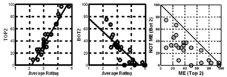
fig 2

Figure 2: Average ratings for 24 vignettes for each of 27 respondents. Each circle is a respondent. The patterns are similar for Likert Rating Scale vs Binary Scale, noisier for the two binary scales.

The second external analysis searches for relations between response time and either the actual ratings on the original 1-5 scale, or the binary transformed scale. Figure 3 shows a noisy but discernible relation between the average response time from the respondents and the average transformed rating assigned by the respondent. It should be kept in mind that these results come from averaging response times and ratings from a unique set of 24 vignettes for each respondent.
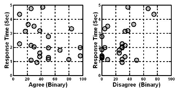
fig 3

Figure 3: Relation between average binary scale (Top2 – Agree, ME; Bot2 – Disagree, NOT ME) and response time. Each point corresponds to the average of one respondent’s rating of 24 vignettes.

On average, respondents who showed the highest average agreement showed the shortest response times.

On average respondents who showed the highest average disagreement showed the longest response times.

Step 9: Internal Analysis Relating Each Element to the Binary Transformed Rating’s

Had the data been simply combinations of elements without cognitive ‘meaning’ the analysis would have stopped at the external analysis, simply because there is nothing to be learned from the properties of a specific stimulus. The stimulus would just be part of the set of stimuli picked for the analysis to discern a general pattern.

Mind Genomics moves beyond the external, simply because the elements themselves have cognitive richness, meaning in what they communicate, meaning in their sentence structure, meaning in the words, and so forth. The richness need not be explicated at the start of the Mind Genomics study. It suffices only that the elements be chosen for a reason germane to the topic. In this study, there are two questions pertaining to pattern of spending and amount of spending, and two questions about attitude, specifically what one wants in the market, and how one feels shopping in the market. These questions are never asked directly, but rather represent by cognitively rich statements to which the respondent reacts by assigning a rating, doing the assignment rapidly in what Nobel Laureate Daniel Kahneman called System 1 behavior [9].

The experimental design enables the research to create equations relating the presence/absence of the 16 elements to the four dependent variables, whether these be the actual ratings on the 5-point Likert scale, the binary transformed ratings for Agree (Describes ME, Top2), the binary transformed ratings for Disagree (Does NOT Describe Me, Bot2), or response time.

The first analysis using OLS (ordinary least-squares) regression creates equations for each individual, with the binary transformed rating of Agree (Top2) as the dependent variable. The rationale for the individual-level modeling is that the 27 different models will generate the data needed to divide the respondents into two complementary groups, mind-sets, based upon what specific elements they feel describes them.

The general form of the equation is: Top2 = k0 + k1(A1) + k2(A2) + k3(A3)…k16(D4)

The foregoing equation can be estimated at the level of each respondent (27 different equations), or at the level of groups such as Total Panel (one equation), gender (two equations), age (two equations), and finally mind-sets emerging from clustering the respondents by the pattern of their coefficients (two equations).

The OLS (ordinary least-squares) regression model emerges with the additive constant, and 16 coefficients. The ‘rules’ for interpreting the parameters are as follows when the dependent variable is either the Top2, ( Agree, ME) or the Bot2 (Disagree, NOT ME)

The additive constant is the estimate percent of times that the rating will be ‘describes me’ (viz., 4 and 5), when there are no elements. Clearly the experimental design ensures that each of the 24 vignettes comprises 2-4 elements, so the additive constant is a purely estimated parameter. One can consider the additive to be a baseline likelihood to agree (Top2) or a baseline likelihood to disagree (Bot2) even before information is presented. In some ways the additive constant can be considered an indication of the way people think about a topic, in general, without specifics.

The coefficient shows the additional percent of responses are added to the dependent variable when the element is inserted into the vignette. Thus, a coefficient element of +6 means that an additional 6% of the responses will be added to the response when the element is inserted. A coefficient of -5 means that 5% fewer of the responses will move away from the dependent variable.

The additive constant and the coefficients sum together. Thus, for the situation of the dependent variable Bot2 (Disagree, Not Me), when the additive constant is 37 and the coefficient is -6, the expected percent of responses for Bot2 for that 1-element vignette is 37 – 6 or 31. In this case the element takes away from Bot2. In contrast, when the coefficient is +9, then the expected percent of responses for Bot2 for that 1-element vignette is 37+9 or 46, meaning there will be 46% of the Bot2 responses for that 1-element vignette.

The vignettes comprised 2-4 elements, meaning that one can combine 2-4 elements to create a new vignette, and estimate the likely rating, making sure that the elements come from different questions. The estimated value is simply the arithmetic sum of the additive constant and the elements.

The strategy for presenting the results will be to show only the elements which are positive, viz., greater than 0, for either Top2 or Bot2, for any subgroup. The rationale is that we are interested in learning about the pattern of elements which drive the response. Showing only positive numbers lets the patterns emerge clearly. Highlighting strong performing elements (coefficients of +8 or higher for the binary transformation) further allows the patterns to emerge in greater relief.

A further strategy when presenting the data will be to sort the data in descending order by the two mind-sets, highlighting the strong performing elements by shading the cells in which coefficients are +8 or more. A coefficient of +8 corresponds to an element which is around two standard errors beyond the coefficient of 0, and suggests a strong impact of the element on the binary rating

Table 3 presents the results for the Top2 binary variable, defined as: Agree, or ME. we begin with the additive constant

  1. Total Panel – About Half of the responses will agree (additive constant = 46).
  2. Males show a strong propensity to agree (additive constant = 70), females show a moderate propensity (additive constant = 43).
  3. Younger respondents (17-29) and older respondents (30+) show similar propensities to agree (additive constants of 45 for younger and 42 for older).
  4. Respondents who never frequented the HK Goldfish Market show a strong propensity to agree (additive constant = 76), frequent shoppers show a moderate propensity to agree (additive constant = 40).
  5. Mind-Set 1 (focus on low price, easy maintenance) show a moderate propensity to agree (additive constant = 40), Mind-Set (True Afficionados) show a strong propensity to agree (additive constant = 63).

In terms of the performance of the elements, many elements are positive, meaning that the respondent feels that they describe the respondent’s feelings. There are, however, a great number of elements with zero or negative coefficients.

  1. The most consistently strong element is C4: My wish for the HK Goldfish Market: ready-made aquariums and/or aquarium maintenance.
  2. A variety of other elements emerge as strong for the different geo-demographic and behavioral groups, but not consistent pattern that lends itself to easy identification.
  3. When we divide the respondents by the pattern of what describes them, creating two mind-sets, we find two clear groups. Mind-Set 1 focuses on easy maintenance, appearing to spend less money or no money. They have a lower additive constant, 40, meaning that they are not likely to agree, to feel that the phrases in the vignette apply to them. In contrast, Mind-Set 2 spends a lot of money, and wants high quality, interesting fish, and equipment. Furthermore, Mind-Set 2 has an additive constant of 63, meaning that they are ready to agree. We present the mind-sets as the final two columns of data, sorting the table by mind-set to reveal the patterns, which emerge clearly after the sorting. There is no such clarity of pattern for any other grouping of the respondents, viz. WHO they are or what they DO.

The approach to creating mind-sets using Mind Genomics has been previously described in previous papers [10]. The ingoing assumption is that respondents with similar patterns of coefficients for the 16 elements on Top2 (agree) belong to the same mind-set. Respondents with dissimilar patterns of coefficients belong in different mind-sets. The data from these studies suggest two clearly different mind-sets. Using mind-sets to organize data is not limited to Mind Genomics but has been shown to be a stimulus to creative thought [11].

4. By focusing only on the positive elements, and highlighting the strong performers, the nature of the mind of the respondent becomes clearly with respect to the HK Goldfish Market, in a way hard to capture by conventional anthropological observation, sociological analysis, or market research. One begins to sense the structure of the people for this granular part of the Hong Kong ‘every day.’

Table 4 present the reverse scale focusing on disagree. The groups are the same, total, gender, age, frequency of visit, and the two emergent mind-sets from clustering the respondents on Top2. Again, only the positive coefficients are shown except for the additive constants.

In contrast to the clarity of results from Table 3, showing agreement (ME), the pattern of additive constants and coefficients in Table 4 is confusing. The difficult of discovering a clear pattern may emerge because responses focus on what they agree with. What they fail to agree upon may either be irrelevant, or important. In either case, respondent appears to focus on using only one side of the scale. The respondent may not be ‘weighing’ the entire set of elements to come up with a single composite judgment, but rather may simply focus on finding the key element, ignoring everything else. In such a case the pattern would be one-sided, clearer when the respondent focuses primarily on agreement. To test this hypothesis may simply require a parallel study with the respondent instructed to focus either on agreement in one test cell, or disagreement in another test cell.

Table 3: Coefficients for the ‘Top2’ model, relating the presence/absence of the elements to the Top2 value. In the interest of clarity, only the positive coefficients are shown.
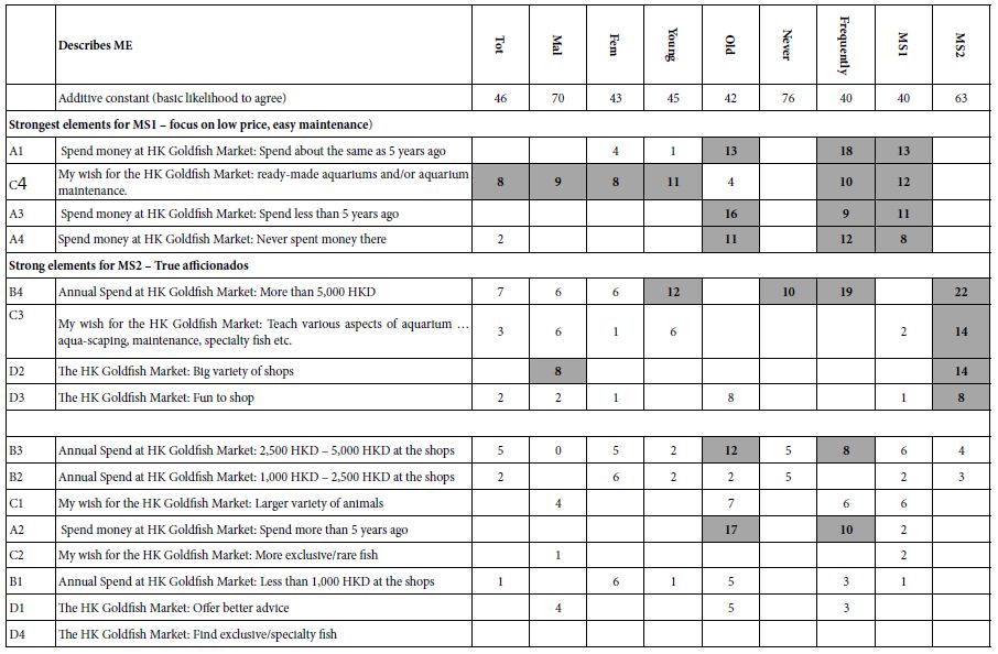
table 3

Table 4: Coefficients for the ‘Bot2’ model, relating the presence/absence of the elements to the Bot2 value. In the interest of clarity, only the positive coefficients are shown.
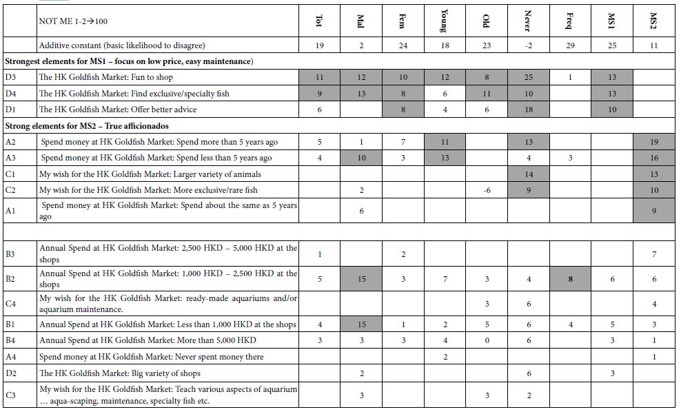
table 4

The final analysis of groups looks at the response time, defined operationally as the number of seconds between the appearance of the vignette on the screen and the assignment of a rating by the respondent. The modeling is the same as that for Top2 and Bot2, with one exception. The exception is that the additive constant is omitted from the model for the response time vs elements. The rationale is that in the absence of elements there is no response.

Table 5 shows the estimated response times assignable to each element. The first data column, for Total Panel, shows all 16 coefficients. The range of coefficients goes from a low of 0.3 seconds (A3: Spend money at HK Goldfish Market: Spend less than 5 years ago) to a high of 0.9 seconds, such as D2 (The HK Goldfish Market: Big variety of shops), C1 (My wish for the HK Goldfish Market: Larger variety of animals). B3 (Annual Spend at HK Goldfish Market: 2,500 HKD – 5,000 HKD at the shops), and so forth. There is no clear pattern for the Total Panel, other than perhaps that the elements describing the offerings tend to engage the respondent a little long.

Table 5: Coefficients for the ‘Response Time’ model, relating the presence/absence of the elements to the measured response time. With the exception of the Total Panel, onlypositive coefficients are shown, in the interest of clarity and simplicity.
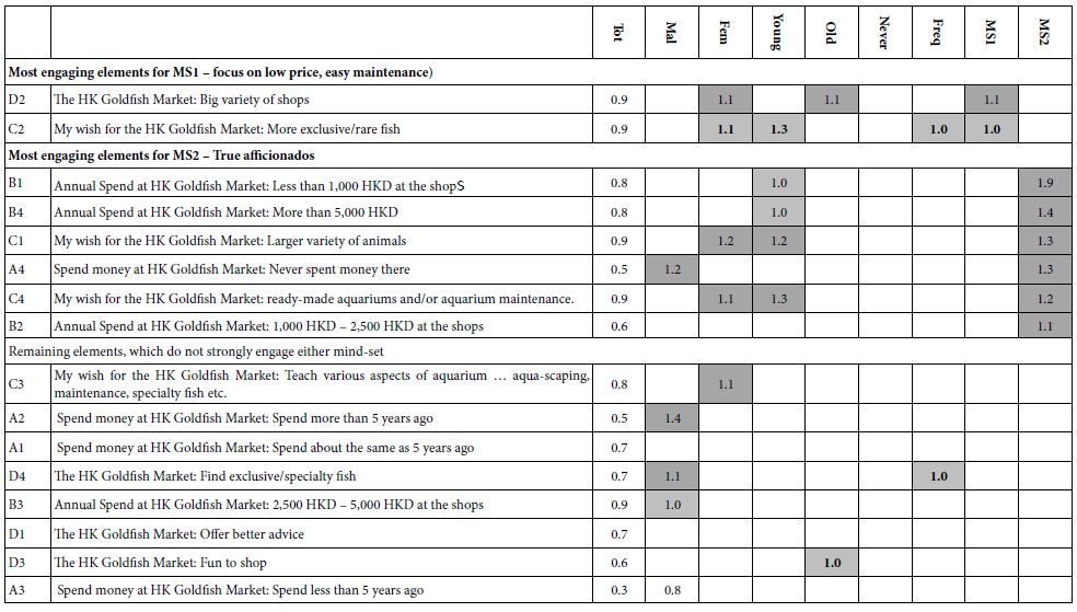
table 5

As done for Tables 2 and 3, the rest of Table 4 shows only those elements which are deemed to be ‘engaging,’ viz., show response times of 1.0 seconds or longer. The cut-off of 1.0 seconds is strictly an operational, giving a sense of the types of elements which engage.

  1. Males seem to be more engaged by elements dealing with price. Females seem to be more engaged by elements dealing with features.
  2. Young respondents are far more likely to be engaged by elements, older respondents are not.
  3. Those who say they never frequent the HK Goldfish Market are not engaged by any elements. Those visit frequently are engaged by only one element, D4 (The HK Goldfish Market: Find exclusive/specialty fish)is
  4. Mind-Set 1, (focus on low price & easy maintenance), is engaged by two elements, D2 and C2, dealing with variety. Mind-Set 2 (true afficionados) is engaged by both price and features, showing deeper engagement as reflected by response time. The deepest engagement is 1.9 seconds, B1 (Annual Spend at HK Goldfish Market: Less than 1,000 HKD at the shops). This element may surprise and intrigue, because it is so contrary to the behavior and interests of the afficionado.

Generalizing the Results – Finding these Mind-sets in the Population for Science and Business. With a small group of 27 respondents, the distribution of respondents into mind-sets will be error prone. The small base size of respondents finds it best use as a tool to uncover hitherto-unexpected mind-sets. The small number of respondents used for discovery does not suffice to estimate the proportion of these mind-sets across the population, especially in different countries. Thus, with small base sizes, the distribution of mind-sets across relevant subgroups is at best a rough estimate. Table 6 shows this distribution. Mind-Set 1 comprises most of the respondents. Furthermore, that the most outstanding aspect of the distribution is that of the seven respondents in Mind-Set 2 (True Afficionados), six are older respondents, far more than would have been expected.

Table 6: Distribution of respondents from the total panel and two mind-sets across gender, age, and frequency of visiting the HK Goldfish Market.
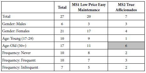
table 6

Given the distribution of mind-sets shown by Table 6, how can the researcher or digital marketer assign a new person to one of the two mind-sets for this granular topic of a pet market? Recently, author Moskowitz in collaboration with Hungarian researcher Attila Gere developed an approached called the PVI, the Personal Viewpoint Identifier. The PVI is based upon the data from Table 4, the coefficients from the transformed data (Top2). The PVI uses simulation and decision trees to create a system which assigns a new person to one of the two (or three) emergent mind-sets from a Mind Genomics study [10-14].

Figure 4 shows the introduction to the PVI. These data can be customized, so that the data are entirely anonymized, or the data can include such information at telephone or email, for follows-ups. Figure 5 shows the set of informational questions about the respondent, and then the six questions comprising the PVI itself. The four first questions, ‘information’, are equivalent to the types of questions researchers ask about attitudes and usage for topics of interest. Figure 6 shows the format of the template used to transfer data from the Mind Genomics study to the PVI. Note that after the data from the respondent are stored in a database, and the respondent is sent an email of results, the respondent may be guided to a video stored in YouTube, or to a landing page. Thus, the PVI serves both as an information-gathering system, and as a tool for e-commerce.

fig 4

Figure 4: Introduction to the PVI for a ‘pet market’. https://www.pvi360.com/TypingToolPage.aspx?projectid=1269&userid=2
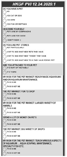
fig 5

Figure 5: Classification questions and the PVI itself. The first four questions are classification (attitude and usage). The second six questions constitute the PVI.
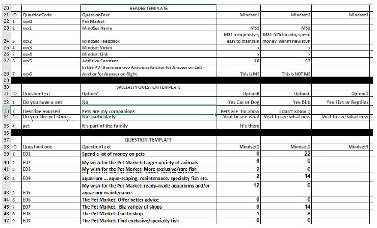
fig 6

Figure 6: The Excel® based template, allowing the researcher to select the elements, the classification questions, the binary PVI questions, and the post-PVI experience with a video or landing page. The PVI is computed after the template is completed.

Discussion and Conclusions

For most of the history of psychology, experiments have presented the respondent with artificial situations to uncover rules of behavior. The experiments are crafted from theory, to prove or disprove a hypothesis. The study presented here on the HK Goldfish Market reveals the potential of increasing our understanding of the granular, every-day, unremarkable experience, revealing patterns of decision-making, and emergent understanding at several levels.

Taking its cue from consumer research, anthropology, sociology, as well as statistics, the newly emerging science of Mind Genomics works in a different way, one that might be called a cartographic analysis. The objective is to not to develop general hypotheses about behavior, and either show that they describe the data, or falsify the hypothesis. Rather, Mind Genomics uses the methods of experimental science to understand how people react.

The experiments in Mind Genomics are easy to perform, and the subject matter is boundless. As a consequence one need not create a hypothesis and test that hypothesis by manipulation to prove or disprove the hypothesis, or even conjecture It is adequate to act like an explorer, a cartographer, mapping the land, finding interesting areas, unusual formations, and the ‘stuff’ worth talking about. Mind Genomics as a science should appeal to those who are not interested in the traditional tasks of ‘filling holes in the literature,’ nor responding to calls to answer key issues. Instead, and in the spirit of the early Baconian philosophers of natural science, it is sufficient to map the topic, to study the different aspects, without being forced to justify one’s scientific curiosity by first putting up a hypothesis to be proved or disproved, the hallmark of today’s hypothetico-deductive method (Grimes, 1990).

References

  1. Moskowitz HR (2012) ‘Mind genomics’: The experimental, inductive science of the ordinary, and its application to aspects of food and feeding. Physiology & Behavior 107: 606-613. [crossref]
  2. Warde A (2016) The practice of eating. John Wiley & Sons.
  3. Carruthers BG, Kim JC (2011) The sociology of finance. Annual Review of Sociology 37: 239-259.
  4. Whyte W (1957) The Organization Man. Garden City. NY Doubleday.
  5. Moschis GP, Mathur A (2007) Baby boomers and their parents: Surprising findings about their lifestyles, mindsets, and well-being. Paramount Market Publishing.
  6. Han Z, Lai LW, Fan J (2002) The ornamental fish retail market in Hong Kong: its evolution and evaluation. Aquaculture Economics & Management 6: 231-247.
  7. Lam KKH, Lai LWC (2002) Goldfish (Chin‐yu or Kin‐yu) culture practice in Hong Kong. Aquaculture Economics & Management 6: 275-293.
  8. Gofman A, Moskowitz H (2010) Isomorphic permuted experimental designs and their application in conjoint analysis. Journal of Sensory Studies 25: 127-145.
  9. Kahneman D (2011) Thinking, fast and slow. Macmillan.
  10. Porretta S, Gere A, Radványi D, Moskowitz H (2019) Mind Genomics (Conjoint Analysis): The new concept research in the analysis of consumer behaviour and choice. Trends in Food Science & Technology 84: 29-33.
  11. Boaler J (2015) Mathematical mindsets: Unleashing students’ potential through creative math, inspiring messages and innovative teaching. John Wiley & Sons.
  12. Grimes TR (1990) Truth, content, and the hypothetico-deductive method. Philosophy of Science 57: 514-522.
  13. Moskowitz HR, Gofman A, Beckley J, Ashman H (2006) Founding a new science: Mind Genomics. Journal of Sensory Studies 21: 266-307.
  14. Moskowitz Howard R, Sebastiano Porretta, Matthias Silcher (2008) Concept research in food product design and development. John Wiley & Sons.
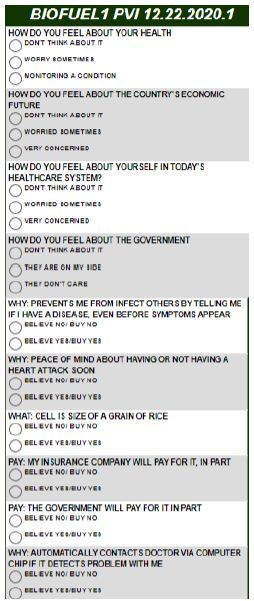
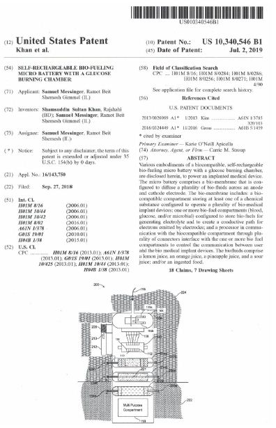
Importance of Single Nucleotide Polymorphisms (SNPs) of Insulin-like Growth Factor-1 (IGF-I) and Ovocalyxin-32 (OCX-32) Genes for Production Traits in Mazandaran Indigenous Chicken

DOI: 10.31038/JMG.2020333

Abstract

We suggested two important proteins (insulin-like growth factor-I (IGF-I) and ovocalyxin-32 (OCX-32) have crucial effects on muscle differentiation, growth, and reproductive traits in chicken production. On the association between IGF-I gene polymorphism and production traits, the evaluation of the associations between SNPs with reproductive traits suggests a positive effect of genotype AC with average egg weight at age of 30 (EW30) (P < 0.05) compared with genotype CC. We confirmed that the g.570 C > A polymorphism is significantly associated with average egg weight at age of 30 (EW30). On the other hand, for the association between OCX-32 gene polymorphism and production traits, two single nucleotide polymorphisms (SNPs) c.381G > C and c.494 A > C, were confirmed. Associations of OCX-32 genotypes with egg number (EN) were significant (p<0.05). From these findings we concluded that these markers should be considered for growth and production traits in chicken.

Keywords

Production traits, Chicken, IGF-I, OCX-32, PCR-RFLP

Introduction

Economically important livestock products are dependent on production and reproductive traits in domestic animals, which are under the control of multiple genes, mapping and analyzing polymorphisms of genes involved in the main metabolic pathways related to animal growth and distribution of nutrients to different tissues [1,2]. Understanding the genetic information of related genes is helpful for the selection and breeding course through marker assisted selection (MAS) in domestic animals. Candidate genes have well-known biological functions related to the development or physiology of important traits [3]. Such genes can encode structural proteins or a member in a regulatory or biochemical pathway affecting the expression of the trait [4] and can be tested as putative QTLs [5].

For poultry industry, meat and eggs are main products, for which some genes impact on such as insulin-like growth factor (IGF-I) and ovocalyxin-32 (OCX-32) have crucial roles on muscle differentiation, growth and reproduction. The presence of IGF-I in blood was detected as one of skeletal growth factors that produced in the liver tissue [6]. Therefore, insulin-like growth factor 1 is a key growth factor involved in a variety of biological processes [7,8]. Some study has shown that IGF-I mRNA levels were significantly lower in the low growth rate line than in the high growth rate line [9].

Recent studies on a single nucleotide polymorphism (SNP) in the chicken IGF-I gene have reported that there are significant associations between a polymorphism in this gene and its promoter in production and reproduction traits in poultry [10-12]. And the other hands, one group of detected eggshell matrix proteins related to major proteins of the egg white. Ovalbumin was the first egg white protein that explained in the matrix of the eggshell [13]. A second group contains proteins such as osteopontin that are also found in other tissues [14]. Finally, a third group of proteins includes those specific to the uterine tissue and to the eggshell that have only been detected in extracts of eggshell. Recent studies have shown associations between single nucleotide polymorphism of ovocalyxin-32 gene its family genes and egg production traits [15-18]. The eggshell contains some eggshell-specific matrix proteins such as ovocleidin-17, ovocleidin-116, ovocalyxin-32 and ovocalyxin-36 [14,19]. It was demonstrated that ovocalyxin-32 (OCX-32) is a 32 kDa protein that found in the outer region and cuticle of the shell [20]. Dunn et al. [16] reported that a single nucleotide polymorphism in the intron of the OCX-32 gene was associated with the thicknesses of the mammillary layer. Some studies have shown that low egg production strains expressed more transcripts of the OCX-32 gene in comparison of high strains at egg-laying stages and offered that the OCX-32 gene is a crucial marker that associated with egg production [21,22].

The objectives of the present study was 1) to detect SNPs of IGF-I and OCX-32 genes by developing PCR-RFLP methods, and 2) to investigate and analyze associations between those SNPs and growth and egg production traits in Mazandaran indigenous chicken.

Material and Methods

Growth and Egg Production Traits

The evaluated traits and their descriptions were presented in Table 1.

Experimental Population and Sampling

Chickens were raised in Native Chicken Breeding Station of Mazandaran, and they belonged to generation 19 of the breeding station pedigreed animals. Blood sample (1 mL) was taken in an EDTA-containing tube and all samples were freeze. Whole DNA was extracted by using DNA Extraction Kit [23]. The DNA samples were stored at -20ºC for use.

Primer Synthesis and PCR–RFLP Reactions

IGF-I analysis: Promoter region of the IGF-I gene amplified to a product of 361 bp using the oligonucleotide design tool Primer 5.0 software based on the IGF-I gene sequence of the fowl (Accession number: M74176). Primers were F: 5′-CTCTGCCACGAATGAAATGTGC-3′ and R: 5′-GGGAGCATTTGCCTTCTCTC-3′ for IGF-I gene. PCR method was used to optimize the reaction accuracy: 94ºC for 2 min, 30 cycles of 98ºC for 30 s, annealing at 55ºC for 30 s, 68ºC for 40 s, and a final extension at 72ºC for 7 min. Finally, PCR products were electrophoretically separated on 2% agarose gel (5 V/cm) and stained with ethidium bromide.

The fragment was amplified for PCR–restriction fragment length polymorphism (RFLP) analysis. An amplified fragment was digested by HinfI for detecting the g.570C > A genotypes. The restriction enzyme digestion was incubated at 37°C for 4 h.

OCX-32 Analysis

With forward primer 5′-CTCCAAACGTATGCTTCACTTA-3′ and reverse primer 5′-ATTCTTGTGTTCGGTTACTTGT-3′, approximately 342 bp covering complete exon-3 was obtained. As well as forward primer 5′-TGTTTCTGATGAAGAGCCAGA-3′ and reverse primer 5′-CTTTGCCACTCTGTAGGCTGT-3′, approximately 250 bp covering exon-4 was obtained. Two fragments containing the OCX-32 polymorphisms (NM_204534: c.381G>C; and NM_204534: c.494A>C) were amplified for PCR-RFLP analysis. An amplified fragment was digested with NcoI for detecting the c.381G>C and c.494A>C genotypes, respectively. The restriction enzyme digestions were incubated at 37°C for 4 h.

Statistical Analyses

The relationship between genes polymorphism and related traits were calculated using general linear model of SAS 9.0 (SAS Inc., Cary, NC, USA). The used models in matrix notation were as follows:

Y = Xb + Za + e

Where, Y is the vector of observations; b the vector of fixed effects of generation, sex and hatch; a the vector of random direct genetic effects; e the vector of random residual effects; X and Z are incidence matrices relating the observations to the respective fixed and direct genetic effects.

Results

The Production Traits

The means and SD of the traits measured in the chickens are shown in Table 1.

Table 1: Statistical description of data set for growth and egg production traits.

Traits

No. of animal Mean

Coefficient of variation

BW1 (gr)

34,277 34.53

8.13

BW8 (gr)

42,057 553.7

17.12

BW12 (gr)

37,207 943.9

14.51

WSM (gr)

30,137 1684

11.92

ASM (day)

30,339 155.5

9.25

EN (number)

30,349 36.66

39.76

EW1 (gr)

26,284 40.21

15.77

EW28 (gr)

16,215 45.91

8.43

EW30 (gr)

18,021 47.12

8.52

EW32 (gr)

17,945 48.22

8.31

EW12 (gr)

17,837 48.62

9.34

AV (gr)

27,715 45.84

13.34

EM (gr)

27,725 1758

39.13

EINT (%)

30,339 53.07

33.33

BW1, BW8, BW12 = Body Weight at Birth, 8, 12 weeks of age, WSM = Body Weight at sexual maturity, ASM = Age at first egg, EN = Egg Number, EW1 = Weight of First Egg, EW28, EW30 and EW32 = Average Egg Weight at 28, 30 and 32weeks of age respectively, EW12 = Average egg weight for First 12 weeks of production, AV = Average for EW28, 30 and 32, EM = Egg Mass (=EN×EW12), EINT = Egg Production Intensity (=Egg Number/Days Recording)×100).

Phenotypic Analysis and Sequence Analysis

IGF-I

The single nucleotide polymorphisms was located in the promoter region and produced an A→C substitution at base 570 (accession number M74176), which was the same mutation identified in previous studies [10,11,24]. Genotypes of chickens were investigated by PCR-RFLP (Figure 1). Genotype and allele frequencies of the SNP in chickens are shown in Table 2. In this population, the AA genotype had the highest frequency (0.62), followed by AC (0.32) and CC (0.06), and the A and C allele frequencies were 0.78 and 0.22, respectively.

fig 1

Figure 1: Representative genotyping of IGF-1 gene at locus g.570C > A. by agarous gel electrophoresis. Strands with 361 for CC genotype, 117, 244 and 361 for AC genotype and 117 and 244 for AA genotype appeared at this locus.

Table 2: Genotypic and gene frequency of IGF-I gene.

IGF-I

Frequency

Allele Frequency No.

Genotype

0.78

A 0.62 113

AA

0.22

C 0.32 59

AC

0.06 11

CC

1 183

Total

OCX-32

The SNPs in exon 3 and 4 were a C→G substitution at base 381 (c.381 G > C; accession number NM_204534) in exon 3, and C→A substitution at base 494 (accession number NM_204534) in exon 4, respectively, which was the same mutation reported in the previous study [21].

We observed 3 band on gel for OCX-32 exon 3 (Figure 2). Three genotypes in this segment GG, GC and CC had the genotypic frequencies of 0.61, 0.26 and 0.13, respectively (Table 3). Two band patterns for OCX-32 exon-4 (Figure 3) were observed. Three genotypes in this segment AA, AC and CC had the genotypic frequencies of 0.11, 0.36 and 0.53, respectively (Table 3).

fig 2

Figure 2: Representative genotyping of OCX-32 gene at locus c.381 G>C. by agarous gel electrophoresis. Strands with 342 for CC genotype, 155, 187 and 342 for GC genotype and 155 and 187 for GG genotype appeared at this locus.

fig 3

Figure 3: Representative genotyping of OCX-32 gene at locus c.494 A > C. by agarous gel electrophoresis. Strands with 250 for AA genotype, 56, 194 and 250 for AC genotype and 56 and 194 for CC genotype appeared at this locus.

Table 3: Genotypic and gene frequency of OCX-32 gene.

SNP

Frequency genotype

Frequency allele

c.381G>C

GG GC CC G

C

0.61

0.26 0.13 0.74

0.26

c.494A>C

AA AC CC A

C


0.11

0.36 0.53 0.29

0.71

Associations between Genotypes and Production Traits or Breeding Values

IGF-I

Results on the effects of IGF-I SNP on production and growth traits are shown in Table 4. The g.570 C > A genotype was significantly associated with average egg weight at age of 30 (EW30) (P < 0.05) in this population. No significant association was found between the IGF-I SNP and other traits (Table 4).

Table 4: Association of the IGF-I genotypes at the growth and egg production traits (Mean ± S.E.).

Traits


Genotype AA

Genotype AC

Genotype CC

WSM

1726.18 ± 20.22

1740.25 ± 17.84

1765.15 ± 42.12

ASM

175.81 ± 1.06

177.97 ± 0.79

174.68 ± 2.79

EN

39.28 ± 0.89

40.07 ± 0.80

40.09 ± 1.70

EW28

44.30 ± 0.52

45.51 ± 0.46

43.10 ± 1.01

EW30

48.44 ± 0.49 ab

48.41 ± 0.45 a

46.27 ± 0.96 b

AV

51.91 ± 0.44

51.38 ± 0.40

51.03 ± 0.83

EM

1929.45 ± 446.35

2019.28 ± 41.43

1958.00 ± 87.54

EINT

59.29 ± 2.64

61.26 ± 1.49

61.03 ± 3.07

a,bValues with different superscripts within the same row differ significantly (P<0.05).

OCX-32

Results on the effects of OCX-32 SNP on growth and production traits are shown in Table 5. At exon 3, genotype GC had higher egg number compared with genotype GG (P < 0.05, Table 5). At exon 4, genotype CC was significantly associated with egg number (P < 0.05, Table 5) compared with genotype AC.

Table 5: Effects of c.381G>C and c.494A>C SNPs of the OCX-32 gene on growth and production traits (least squares means ± SE).

SNP

c.381G>C

c.494A<C

Genotype

GG GC CC AA AC

CC

BW12 (gr)

751.33 ± 14.36 733.25 ± 16.24 707.71 ± 29.69 688.82 ± 26.03 732.47 ± 14.62

756.56 ± 13.50

WSM (gr)

1738.36 ± 21.54 1729.77 ± 26.07 1706.98 ± 53.00 1685.13 ± 46.32 1713.00 ± 24.07

1761.97 ± 23.05

ASM (day)

175.37 ± 1.66 177.76 ± 1.10 179.32 ± 3.25 172.34 ± 1.83 173.24 ± 1.99

172.42 ± 1.90

EN (number)

41.30 ± 0.79 b 43.64 ± 0.96 a 43.42 ± 1.95 ab 41.83 ± 1.72ab 43.54 ± 0.89 a

341.39 ± 0.85 b

EW28 (gr)

44.56 ± 0.45 44.62 ± 0.57 45.51 ± 1.16 43.29 ± 0.98 44.53 ± 0.50

45.18 ± 0.50

EW30 (gr)

48.25 ± 0.35 47.84 ± 0.44 49.31 ± 1.01 46.81 ± 0.82 48.65 ± 0.49

48.13 ± 0.49

EW32 (gr)

52.56 ± 0.43 52.01 ± 0.52 49.70 ± 1.06 51.10 ± 0.97 52.06 ± 0.49

52.54 ± 0.47

EW84 (gr)

51.68 ± 0.49 51.46 ± 0.60 49.71 ± 1.21 49.38 ± 1.10 50.31 ± 0.56

51.81 ± 0.53

AV (gr)

50.22 ± 0.38 50.19 ± 0.46 48.19 ± 0.94 48.26 ± 0.83 50.03 ± 0.43

50.47 ± 0.41

EM (gr)

1947.08 ± 40.96 2070.16 ± 49.21 1987.59 ± 100.22 1907.50 ± 88.20 2061.73 ± 45.84

1958.06 ± 44.32

a,bValues with different superscripts within the same row differ significantly (P<0.05).

Discussion

In the present study, the g.570 A < C polymorphism of the IGF-I promoter was detected in Mazandaran indigenous chicken: allele frequencies for A and C were 0.78 and 0.22, respectively. The g.570 A < C polymorphism has been reported as a candidate mutation influencing growth and carcass traits [10,11,25]. Previous studies have shown that the g.570 A > C polymorphism is significantly related to body weight at 107 days of age [10], 2, 4, 6 and 8 weeks of age [11], and 5 weeks of age [25].

For production traits, however, no significant differences were found in the association between the g.570 A < C polymorphism and other traits. In contrast, the g.570 A < C polymorphism is strongly assumed to be involved in 30 weeks (EW30). These results support the notion that selection of average egg weight at age of 30 weeks (EW30), is a powerful method to increase production traits and the g.570 A<C polymorphism might become a marker for elevating average egg weight at age of 30 (EW30). In particular, we propose that the identification of g.570 A < C genotypes may be useful in the selection for reproductive traits. To make further progress, it is necessary to investigate the associations between the g.570 A<C genotypes and production traits in the other breed.

The relationship between the IGF-I promoter mutation and growth or carcass traits has been studied in some breeds of chicken and cattle. For example, effects of the polymorphism IGF-I gene were surveyed on egg quality in Wenchang chicken [12]. Some results showed single nucleotide polymorphisms 512-bp upstream from the start codon had significant associations with weight gain during the first 20 days after weaning and on-test weight in Angus cattle [26]. Furthermore, the same report indicated that the g.570 C > A substitution A→C in the promoter region involved the suppression of one potential CdxA transcription factor binding site. Hence, the different alleles detected in the present study might alter the transcription rate and the gene expression level of IGF-I, thereby affecting circulating IGF-I concentrations and muscle development.

An association between the single nucleotide polymorphisms of the OCX-32 gene and the thicknesses of the mammillary layer was recently reported by Dunn et al. [16]. In the present study, the SNP of the OCX-32 gene were significantly associated with body weight at age of 12 weeks, average of EW28, EW30 and EW32, egg number and average egg weight at age of 32 and 84 weeks. We did not find any significant association between these single nucleotide polymorphisms and the other investigated traits. In the case of c.494 A > C SNP in exon 4 implied that the chicken OCX-32 gene may affect reproductive and production traits related traits simultaneously. Yang et al. [22] showed that the OCX-32 expression levels and EPR were related. Therefore, to confirm the causal mutation derived by only a single SNP, we need to evaluate the effects in different breeds and lines of chickens and investigate the function of this gene in detail. Our results show that detection and utilization of candidate gene mutations and DNA markers obtained by whole-genome scanning may directly improve growth, production traits and other economic traits within the same breeds. In particular, we propose that the identification of genotypes may be useful in the selection for production and reproduction traits. To make further progress, it is necessary to investigate the associations between the genotypes and traits in the other breeds. This result shows that OCX-32 gene can be used as a candidate marker in marker-assisted selection. Further functional analysis is essential to ascertain the effects of the OCX-32 exon polymorphism.

Abbreviations

IGF-I: Insulin-like growth factor-1

OCX-32: Ovocalyxin-32

BW1, BW8, BW12: Body Weight at Birth, 8, 12 weeks of age

WSM: Body Weight at sexual maturity

ASM: Age at first egg

EN: Egg Number

EW1: Weight of First Egg

EW28, EW30 and EW32: Average Egg Weight at 28, 30 and 32weeks of age respectively

EW12: Average egg weight for First 12 weeks of production

AV: Average for EW28, 30 and 32

EM: Egg Mass

EINT: Egg Production Intensity

Acknowledgement

The authors are thankful to the researcher, F. Marandi for positive feedback on this research project.

References

  1. Schwerin M, Brockmann G, Vanselow J, Seyfert HM (1995) Perspectives of molecular genome analysis in livestock improvement-an overview. Animal Research Development 42: 14-26.
  2. Bahrami A, Miraei-Ashtiani SR, Mehrabani-Yeganeh H, Banani-Rad H, Behzadi SH (2014) The association between polymorphism of the GH1 gene and changes in protein structure and carcass traits in Mehraban sheep (Ovis aries). Anim Prod Sci 55: 661-665.
  3. Rothschild MF, Soller M (1997) Candidate gene analysis to detect genes controlling traits of economic importance in domestic livestock. Probe 8: 13-20.
  4. Bryne PF, Mcmullen MD (1996) Defining genes for agricultural traits: QTL analyses and the candidate gene approach. Probe 7: 24-27.
  5. Yao J, Aggrey SE, Zadworny D, Hayes JF, Kühnlein U (1996) Sequence variations in the bovine growth hormone gene characterized by Single-Strand Conformation Polymorphism (SSCP) analyses and their association with milk production traits in Holstein. Genetics 144: 1809-1816. [crossref]
  6. Daughaday WH, Salmon WD (1999) The origins and development of the somatomedin hypothesis. In: Contemporary Endocrinology: The IGF System, Rosenfeld, R. Roberts (Eds.). Humana Press Inc Totowa NJ 1-15.
  7. Adam CL, Gadd TS, Findlay PA, Wathes DC (2000) IGF-I stimulation of luteinizing hormone secretion, IGF-binding proteins (igfbps) and expression of mrnas for igfs, IGF receptors and igfbps in the bovine pituitary gland. Journal of Endocrinology 166: 247-254. [crossref]
  8. Shen WH, Wisniowski P, Ahmed L, Boyle DW, Denne SC, et al. (2003) Protein anabolic effects of insulin and IGF-I in the ovine fetus. American Journal of Physiology and Endocrinology Metabolism 284: 748-756. [crossref]
  9. Beccavin C, Chevalier B, Cogburn LA, Simon J, Duclos MJ (2001) Insulin-like growth factors and body growth in chickens divergently selected for high or low growth rate. Journal of Endocrinology 168:297-306. [crossref]
  10. Amills M, Jimenez N, Villalba D, Tor M, Molina E (2003) Identification of three single nucleotide polymorphisms in the chicken insulinlike growth factor 1 and 2 genes and their associations with growth and feeding traits. Poultry Science 82: 1485-1493. [crossref]
  11. Zhou H, Mitchell AD, Mcmurtry JP, Ashwell CM, Lamont SJ (2005) Insulin-like growth factor-I gene polymorphism associations with growth, body composition, skeleton integrity, and metabolic traits in chickens. Poultry Science 84: 212-219. [crossref]
  12. Lei M, Luo C, Peng X, Fang M, Nie Q, et al. (2007) Polymorphism of growth-correlated genes associated with fatness and muscle fiber traits in chickens. Poultry Science 86: 835-842. [crossref]
  13. Hincke MT, Tsang CPW, Courtney M, Hill V, Narbaitz R (1995) Purification and characterization of a soluble matrix protein of the chicken eggshell (ovocleidin 17). Calcif Tissue Int 56: 578-583. [crossref]
  14. Pines M, Knopov V, Bar A (1995) Involvement of osteopontin in egg shell formation in the laying chicken. Matrix Biology 14: 765-771.
  15. Dunn IC, Miao YW, Morris A, Romanov MN, Wilson PW, et al. (2004) A study of association between genetic markers in candidate genes and reproductive traits in one generation of a commercial broiler breeder hen population. Heredity 92: 128-134. [crossref]
  16. Dunn IC, Joseph NT, Bain M, Edmond A, Wilson PW, et al. (2008) Polymorphisms in eggshell organic matrix genes are associated with eggshell quality measurements in pedigree Rhode Island Red hens. Animal Genetics 40: 110-114. [crossref]
  17. Honkatukia M, Reese K, Preisinger R, Tuiskula-Haavisto M, Weigend S, et al. (2005) Fishy taint in chicken eggs is associated with a substitution within a conserved motif of the FMO3 gene. Genomics 86: 225-232. [crossref]
  18. Cui JX, Du HL, Liang Y, Deng XM, Li N, et al. (2006) Association of polymorphisms in the promoter region of chicken prolactin with egg production. Poultry Science 85: 26-31. [crossref]
  19. Gautron J, Hincke MT, Dominguez-Vera JM, Garcia-Ruiz JM, Nys Y (2001) Ovotransferrin is a matrix protein of the hen eggshell membranes and basal calcified layer. Conn Tissue Research 42: 255-267. [crossref]
  20. Gautron J, Murayama E, Hincke MT, Nys Y (2005) Chicken eggshell matrix proteins related to anti-bacterial protein families. Proceedings of the 11th European Symposium on the Quality of Eggs and Egg Products, Doorwerth, Netherlands.
  21. Uemoto Y, Suzuki C, Sato S, Ohtake T, Sasaki O, et al. (2009) Polymorphism of the ovocalyxin-32 gene and its association with egg production traits in the chicken. Poultry Science 88: 2512-2517. [crossref]
  22. Yang KT, Lin CY, Liou JS, Fan YH, Chiou SH (2007) Differentially expressed transcripts in shell glands from low and high egg production strains of chickens using cdna microarrays. Animal Reproduction Science 101: 113-124.
  23. Miller SA, Dykes DD, Polesky HF (1988) A simple salting out procedure for extracting DNA from human nucleated cells. Nucloic Acids Research 16: 1215. [crossref]
  24. Shinichi S, Tsuyoshi O, Yoshinobu U, Yumi O, Eiji K (2012) Polymorphism of insulin-like growth factor 1 gene is associated with breast muscle yields in chickens. Animal science journal 83: 1-6. [crossref]
  25. Bennett AK, Hester PY, Spurlock DE (2006) Polymorphisms in Vitamin D receptor, osteopontin, insulin-like growth factor 1 and insulin, and their associations with bone, egg and growth traits in a layer – broiler cross in chickens. Animal Genetics 37: 283-286. [crossref]
  26. Mann K, Gautron J, Nys Y, Mckee MD, Bajari T, et al. (2003) Disulfide-linked heterodimeric clusterin is a component of the chicken eggshell matrix and egg white. Matrix Biology 22: 397-407. [crossref]

What to Say to Drive Opera Attendance: A Mind Genomics Cartography

DOI: 10.31038/ASMHS.2020413

Abstract

We present a novel approach to arts marketing, using Mind Genomics, demonstrating the use with a study conducted for the Arizona Opera. Respondents evaluated different messages about opera, rating combinations of these messages, the combinations created according to experimental design. The deconstruction of the responses revealed the part-worth contribution of each element to interesting the respondent in opera. The deconstruction of the response time showed the elements which engaged the respondent’s attention. Two mind-sets emerged, those interested in the educational aspects of opera, and those interested in the entertainment value of the experience. We introduce the PVI, the personal viewpoint identifier, a tool to assign new individuals to one of the two mind-sets, and suggest how the PVI may contribute to a more effective digital marketing campaign.

Introduction

Patrons of the arts, especially opera but also of the other arts, are well aware of the need of those who both fund and stage the artistic efforts to understand the mind of their audiences. When it comes to the more conventional things that are marketed, the objective is stated in economic terms, such as maximizing share, or maximizing profit. The economic aspects are paramount. When it comes to certain other aspects of human effort, such as culture, and specifically in our case, opera, the introduction of the ‘marketing concept’ is fraught with more equivocation, more tension. Some of this may come from the nature of the topic, and the realization that the marketing concept is a crude, unfeeling alternative to the higher order efforts of that which is being marketed, namely ‘culture.’

When we move to marketing for non-profits, and especially those dealing with the arts, we move from working with products and services delivering concrete benefits to products and services existing because they deliver aesthetic experiences to their audiences. How does one deal with these experiences? Is the marketing effort to be geared to the experience as an economic construct, or as an experience construct? Is there a measure of pleasure?

The literature of marketing and the arts is quite rich, perhaps because those in the arts realize how important it is to gain the patronage of those who enjoy the arts. Arts marketing is not necessarily as rich in academic studies, but arts marketing has its array of practical work, and books. Thus, we have titles such as Diggles’ 1986 book on ‘Guide to Arts Marketing: The Principles and Practice of Marketing as They Apply to Arts’ (Diggles, 1986), going in hand in with books about non-profit organizations such as Rados’ 1996 book ‘Marketing for Non-Profit Organizations’ (Rados, 1996).

When it comes to arts and marketing in the academic literature, there are few studies reported in the spirit of what we would call an experiment. The studies tend to deal with the topic of marketing from the point of view of sociology (e.g., Butler, 2007; Colbert, 2003; Ventakatesh & Meamber, 2006). That is, the studies report about what is being done in society at large. The spirit of the research focuses on the common patterns of behavior used by those trying to raise money from subscribers or patrons.

One possible reason for the lack of literature featuring ‘experiment’ is the nature of art. Art is an expression of the nobler characteristics of the human spirit. Hirschman (1983) put it this way:

It is proposed that the marketing concept, as a normative framework, is not applicable to two broad classes of producers because of the personal values and social norms that characterize the production process. These two classes of producers are artists and ideologists. Artists are those who create primarily to express their subjective conceptions of beauty, emotion or some other aesthetic ideal. Ideologists are those who put forward an integrated set of positive and normative statements that describe what the world is and what it should be.

Steps in the Mind Genomics Process

The study reported here focuses on what can be said specifically about the Arizona opera to drive positive behaviors, either in terms of attitude or in terms of action. The study can be best described as an experiment, to understand how the specific communications drive responses. The study follows the tenets of Mind Genomics, an emerging science which deals with the way we respond to the specifics of ordinary, daily life, such as the opera. Mind Genomics focuses on the responses to messages about the different topics of daily life, not to show the rationality or irrationality of people, but rather to discover the aspects of daily life to which people pay attention when asked to make a decision (Moskowitz & Gofman, 2007; Moskowitz et. al., 2006).

Mind Genomics is evolving to a set of defined steps in order to understand the everyday ‘mind’ of an individual faced with information about the ordinary information that must be used to make a decision. The steps are not ‘fixed in stone.’ Rather, the steps reflect a work in progress, a system to develop a deeper understanding of how a person weighs specific ‘pieces of information’ to make a decision (Moskowitz, 2012; Moskowitz et. al., 2006; Moskowitz & Gofman, 2007.)

Step 1: Define the Topic

The topic is ‘What to say to prospective opera attendee to make that individual want to subscribe to the Arizona Opera’. It is clear that the topic is limited and specific. Often, the depth of information to be gained ends up far greater and more useful when the researcher focuses on specifics, and limits the topic. With the limitation, it becomes possible to probe deeply, testing many different specific messages relevant only to the subscription to the Arizona Opera. If the topic were more general, such as ‘what makes a good opera experience,’ we might have many elements as well, but we would lack the specifics which make the idea real in the mind of the reader. We might end up testing generalities which lack the cognitive richness of the particular.

Step 2: Create a Set of Four Questions, and for Each Question, Provide Four Answers

The questions should ‘tell a story,’ and be answered by a phrase, not just yes/no nor just a single word. The rationale for requiring a phrase for the answer is that later, during the actual Mind Genomics experiment, the answers, now elements, will be mixed and matched to create vignettes. It is easier when the pieces of information can be read as phrases, the combination of which ‘tells a story.’

Table 1 presents the four questions, and the four answers. The selection of questions, and then the four answers for each question, is done with the full understanding that this specific set of questions and answers is only a small fraction of the possible questions and answers. The terms ‘answers’, ‘messages’, and ‘elements’ will be used interchangeably in the rest of this paper.

Table 1: The four questions about attending opera, and the four answers to each question.

Question A: What is it?
A1 AZ Opera … Bold, Brave, Brilliant
A2 Presenting artists of both international stature and emerging talent
A3 Elevates the transformative power of storytelling through music
A4 One of the only Operas in the country that regularly performs in two cities
Question B: Why do I like it?
B1 a special place where I can get really dressed up and be glamorous
B2 Shouting “BRAVO!” during the show and at the final curtain call
B3 Dinner plus the show … a total night out on the town
B4 AZ Opera performances I can listen to on public radio
Question C: How do I do it?
C1 An Opera season where I can choose my own subscription
C2 AZ Opera … I can mix and match the performances
C3 English translations of the lyrics are projected on a screen above the stage as they are sung
C4 Arrive an hour before curtain to learn about the show you are about to see!
Question D: Why does it matter to the community?
D1 Free music and lecture series examine each opera in detail
D2 Free brown bag operas on Fridays before the big event
D3 A traveling troupe brings opera to schools
D4 Arizona Opera’s book club … a great way to meet fellow audience members and discuss, learn, and connect

Step 3: Create Vignettes

The vignettes comprise combinations of elements (viz., answers), arranged one on top of the other, centered. A vignette comprises at most one element or answer from each of the four questions. The vignette comprises 2-4 elements but often, and by design, no answer from one or two questions. The vignettes are created according to an experimental design, with each design comprising 24 different vignettes. The mathematical structure underlying the experimental design ensures that the 16 elements or answers are statistically independent of each other (Heller, 1986). In the actual experiment, each respondent will be presented with a permutation of the basic design, a permutation which maintains the same statistical benefits (independence of elements, individual-level experimental design). In actuality, the permutation simply creates different sets of combinations from respondents, allowing the researcher to explore a many possible combinations, and build up knowledge by exploring the topic broadly, rather than build up knowledge by exploring one little region of the topic with precision by replicating the same set of 24 vignettes across many respondents. The permuted experimental design ensures that one can analyze the data from as few as one respondent to obtain clear information. The permuted experimental design is a key feature of Mind Genomics (Gofman & Moskowitz, 2010), and metaphorically can be likened to understanding the topic using an MRI (magnetic resonance). The MRI takes pictures of the tissue from many angles, and puts the data together to create a single, coherent picture.

Step 4: Invite Respondents to Participate

Mind Genomics experiments typically require about five minutes of a respondent’s time. Although it seems a good idea to invite respondents from among one’s friends and associates, the reality is the abysmally low response rate, usually around 10% or lower. People simply do not want to volunteer their time in a world where many factors compete for a person’s attention. The solution to this conundrum is to work with a panel company, which specializes recruiting and compensating individuals for these studies. The Mind Genomics study was executed among respondents provided by Luc.id, Inc. a company specializing in these studies. The respondents were invited to participate by email.

Step 5: The Test Stimuli and the Respondent Instructions

The Mind Genomics experiment comprises the evaluation of 24 different vignettes, rating each vignette as a single ‘message’ or single ‘idea.’ As noted above, the vignettes are combinations, comprising 2-4 elements, so it is impossible for a respondent to ‘game’ the system by rating the single vignette in the way that the respondent believes the researcher wants to hear. The vignettes are compounds of different messages, each message pulling in its own direction. The respondent may begin by trying to be consistent and ‘politically correct,’ but ends up disinterested, responding to the vignette in an indifferent, almost automatic fashion. That condition of ‘disinterest’ ends up ensuring that the data represent what the respondent truly feels.

The Mind Genomics experiment prefaces each vignette with the same simple instructions about what to do:

You will be presented with a series of statements. Please respond to the statements with your initial reaction. Use the number scale where 1 means I don’t like it at all and 9 means I love it.

Step 6 – Transform the Data

The Mind Genomics study generates ratings on a 9-point scale. Best practices in the world of applied consumer research suggest that it is easier to understand data when the data presented in binary form, no/yes, 0/100. For this study using the 9-point rating scale as the dependent variable, the typical transformation is ratings of 1-6 transformed to 0, and ratings of 7-9 transformed to 100. This is called TOP3. A second transformation changed ratings of 1-3 to 100, and ratings of 4-9 to 0. This is called BOT3 to reflect the elements which drive people away from opera. Finally, the Mind Genomics program also measures the Consideration Time (aka Response Time), defined as the time in seconds between the appearance of the vignette and the respondent’s rating. The Consideration Time is measured to the nearest tenth of a second.

Step 7 – Create Individual Level Models Relating the Transformed Rating (Binary) to the Presence/Absence of the 16 Elements, and then Cluster the Respondents on the Basis of the 16 Coefficients, k1 – k16

The experimental design used to create the 24 vignettes for each respondent ensures that the 16 elements are statistically independent of each other. The first statistical analysis uses OLS (ordinary least-squares) regression to create an equation describing how each of the 16 elements contributes to the binary transformed rating. The equation is expressed as: Rating = k1(A1) + k2(A2) … k16(D4). There is NO additive constant used in the modeling. The individual level modeling generates a matrix, in which each row is a respondent and each column is an element. The numbers in the body of the matrix are the coefficients for the 16 elements, on a respondent by respondent basis. The additive constant is not retained for this first analysis.

The second statistical analysis uses clustering to divide the respondents into two, and then three complementary groups, based upon the pattern of the 16 coefficients. The coefficients for TOP3 are used in the clustering. The clustering program computes a distance between respondents (D=(1-Pearson R)). Pairs of respondents with similar patterns of coefficients show a high Pearson R (Pearson correlation coefficient), and assigned to the same cluster. Pairs of respondents with different patterns of coefficients show a low Pearson R and are assigned to different clusters (Jain & Dubes, 1988).

Step 7 is done completely automatically, without any interpretation about what the cluster might actually be called. Everything in Step 7 is done under strictly mathematical rules.

Step 8: Define the Key Subgroups

These subgroups may be the standard ones of age and gender, obtained by a short classification questionnaire which is part of the Mind Genomics experiment. The subgroups may also correspond to the clusters determined from Step 7. The latter subgroups, emerging from clustering the TOP3 coefficients, are renamed ‘Mind-Sets’ to reflect the fact that they represent groups of individuals who view the topic in different ways. For this study on marketing the Arizona Opera, we end up with the Total panel and six key subgroups. The subgroups are:

From self-classification:                                     Gender                  Male vs Female

From self-classification:                                     Age                       19-29 years old vs 30 years and older

Emergent from clustering coefficients:                Mind-Set                MS1 (Learning) vs MS2 (Entertainment).

Step 9: Relate the Elements to the Dependent Variables, Using Regression

For all the respondents in either the Total Panel or key subgroup, combine the data into one file, and use OLS regression to relate the presence/absence of the 16 elements to three dependent variables: TOP3 (Interested), BOT3 (NOT Interested), and CT (consideration time). The OLS regression estimates the model using all of the data for the key group, rather than estimating individual level models.

The model is written without an additive constant, in order to allow comparisons across groups, and across dependent variables.

The equation is expressed as: Dependent Variable = k1(A1) + k2(A2) … k16(D4)

Step 10: Extract the ‘Story’ from the Coefficients

The data emerging from Mind Genomics comprise elements and their coefficients, the latter estimated by regression. The data is doubly rich. First there are the elements and their respective coefficients. Each element stands by itself. Simply knowing the element and its coefficient for a specific dependent variable, tells the researcher either how important the element is in terms of attitude (TOP3 = Like; BOT3 = Dislike), or in terms of engaging attention (Consideration Time). Second, the pattern linking together the strongest performing elements also tells a story, this time a more general one. There may or may not be a coherent story linking together the strongest performing elements. The absence of a story does not weaken the data, but simply prevents the discovery of the general pattern.

The data are shown in tabular form. For the binary dependent variables (Like, TOP3; Dislike, BOT3), coefficients appear in shaded cells when the coefficient is 15 or higher. For the Consideration Time (CT), coefficients appear in shaded cells when the consideration time or engagement time is 1.5 seconds or higher for the element. The selection of a coefficient of 15 or higher is based upon independent analysis which related the coefficients of the 16 elements estimated in the absence of an additive constant to the coefficients of the same 16 elements estimated with the equation containing an additive constant. A coefficient of 7.5 for the latter (with additive constant) is statistically significant (p<0.05), and corresponds to an additive constant of approximately 16 for the former (without an additive constant). The selection of the Consideration Time of 1.5 seconds is based on judgment, and the search for a meaningful, easy-to-understand pattern.

Results – Total Panel

What to say (TOP3) – set of easy to customize social occasions where one learns and enjoys (Table 2)

Table 2: Performance of the 16 elements across the total panel.

table 2

B3                Dinner plus the show … a total night out on the town

C3                English translations of the lyrics are projected on a screen above the stage as they are sung

C2                AZ Opera … I can mix and match the performances

D1                Free music and lecture series examines each opera in detail

C1                An Opera season where I can choose my own subscription

What not to say (BOT3) – don’t overdo the ‘kitschy’ aspect

B1                 a special place where I can get really dressed up and be glamorous

B2                 Shouting “BRAVO!” during the show and at the final curtain call

What engages (CT) – talk about the learning and knowing opportunities

D4              Arizona Opera’s book club … a great way to meet fellow audience members and discuss, learn                       and connect

A4                One of the only Operas in the country that regularly performs in two cities

C2                AZ Opera … I can mix and match the performances

C3                English translations of the lyrics are projected on a screen above the stage as they are sung

C4                Arrive an hour before curtain to learn about the show you are about to see!

By Gender and Age

The analysis for total panel can be repeated for four key subgroups, one group at a time. The same criteria were used, namely a coefficient > 15 for TOP3 and BOT3, and a Consideration Time of 1.5 or longer. Table 3 shows the messaging which increase attendance (TOP3), and a suggestion of the common theme.

Table 3: Performance of the elements as drivers of interested (TOP3). Data from key geo-demographic subgroups. Only elements strongly interesting at least one subgroup are shown.

table 3

Males – Entertainment and Other Occasions for Listening

B3                 Dinner plus the show … a total night out on the town

B4                 AZ Opera performances I can listen to on public radio

Females – Many Elements, Especially Entertainment and Learning

B3                Dinner plus the show … a total night out on the town

C2                AZ Opera … I can mix and match the performances

D1                Free music and lecture series examines each opera in detail

C3                English translations of the lyrics are projected on a screen above the stage as they are sung

C1                An Opera season where I can choose my own subscription

C4                Arrive an hour before curtain to learn about the show you are about to see!

A1                AZ Opera … Bold, Brave, Brilliant

D2                Free brown bag operas on Fridays before the big event

A3                Elevates the transformative power of storytelling through music.

Age 19-29 – Entertainment and Learning

B3                Dinner plus the show … a total night out on the town

D1                Free music and lecture series examines each opera in detail

A3                Elevates the transformative power of storytelling through music

C2                AZ Opera … I can mix and match the performances

A2                 Presenting artists of both international stature and emerging talent

Age 30+ Entertainment

B3                Dinner plus the show … a total night out on the town

C3                English translations of the lyrics are projected on a screen above the stage as they are sung

C1                An Opera season where I can choose my own subscription

Table 4 shows what not to say. There are no strong elements. When we lower the criteria to a value of 10 or higher, rather than 15 or higher, we end up with two elements, B1 and C2, which tell no story.

Table 4: Performance of the two strong performing elements driving not-interested (BOT3). Data from key geo-demographic subgroups.

table 4

Table 5 shows what engages, operationally defined as elements which have Consideration Times of 1.5 seconds or longer.

Table 5: Performance of the elements which engage the respondent. Data from key geo-demographic subgroups.

table 5

Males – engaged strongly by five of the elements, with the most engaging elements dealing with what the person can do. That is, males are engaged by elements which get the reader to think about what to do.

Females – engaged strongly by five elements, with the most engaging elements dealing with learning and discussing.

Age 19-29 – engaged strong by two elements, both focusing on socializing.

Age 30+ – engaged strongly by seven elements, combining both the act of creating one’s series, and the act of learning and seeing others learn.

The Two Emergent Mind Sets Based on Interest

The clustering program generated two mind sets, based upon ‘interest’ (TOP3). Table 6 shows that many of the elements are strong performers, albeit in only one of the two mind-sets. Mind-Set1 can be labelled those who are interested in the educational aspects of the opera. Mind-Set 2 can be labelled those who focus on the entertainment experience.

Table 6: Performance of the 16 elements across the two mind-sets. MS = Education Focused, MS2 = Entertainment Focused.

table 6

It is clear from Table 6 (columns labelled TOP3) that what strongly appeals to one mind-set (e.g., education) tends not to appeal to the other mind-set (viz., entertainment). Furthermore, the strong and rather polar nature of the elements, in terms of how they drive the response of the mind-sets, suggests that there are at least two clear groups in the world of respondents to whom one must appeal. What appeals to one mind-set will not generally appear to the other mind-set.

When we turn to what does not appeal to the two mind-sets (BOT3) we see no pattern.

When we turn to what engages (Consideration Time we see that Mind-Set 2 (Entertainment) seems more likely to be engaged by what interests them, and that Mind-Set 1 (Education) seems to be less engaged by what interests them. This pattern emerges when we compare strong performing elements (high TOP3) to the level of Engagement (CT). The correlation between TOP3 coefficient and CT coefficient across the 16 elements is +0.04 for Mind-Set 1 (Education) and +0.39 for Mind-Set 2 (Entertainment). The difference in the magnitude of the correlation suggests radically different strategies to engage the respective attentions of individuals in the two mind-sets.

Finding Mind-sets in the Population

In today’s world of abundant data, a world filled with questionnaires, where interviews abound, and where it seems one can hardly do anything without a follow-up request to rate the product or rate service, one might think that we can find these mind-sets easily. The answer is that we cannot. The mind-sets uncovered above, the education vs experience mind-sets, are particular to the experience of opera. The two mind-sets may be reflections of different ways of enjoying public performances of the arts, but it would take massive efforts and monetary expenditure to establish that, and then use the findings to guide marketing. In the meanwhile, the Mind Genomics study reported here was set up, executed, and completely reported in less than three hours. The paradox is that it becomes almost a ‘trivial’ effort to establish valuable information for science and for marketing, but a very difficult, labor-intensive, resource-intensive effort to apply the findings. Simply said, databases do not have fields for ‘the way the person enjoys the performing arts.’

Table 7 shows the distribution of respondents by mind-set, as well as by gender, age, and self-profiling of interest in opera. It is extremely difficult to predict the messages to give to a respondent, knowing gender, age, and even general behavior with respect to attending opera. The messages themselves are straightforward, emerging from the Mind Genomics effort. It is the assignment of an individual to a mind-set which is difficult. Knowing who a person “IS” does not predict how a person “THINKS.”

Table 7: Cross tabulation showing the distribution of respondents into age, gender, and responses to the up-front classification question about opera attendance. The classification information was collected at the start of the Mind Genomics experiment.

  Total MS1 Education MS 2 Entertainment
Total 100 45 55
Gender: Male 52 23 29
Gender: Female 48 22 26
Age: 18-29 22 11 11
Age: 30+ 78 34 44
Opera – Season subscriber 3 2 1
Opera – A few shows a year 28 15 13
Opera – Not subscriber but would like to be 36 14 22
Opera – Not subscriber, not interested 29 14 15

Recently, authors Gere and Moskowitz have developed an implemented a rapid technique to assign new people to one of two (or three) mind-sets. The approach uses the basic sets of coefficients for the two mind-sets, shown in Table 6 (columns marked Top 3). The approach adds ‘noise’ to the set of coefficients, and identifies the pattern of response ‘under noise’ which best differentiates the mind-sets and reproduces the original results. This Monte-Carlo simulation is followed by the creation of a simple 6-question matrix, shown in Figure 1. The matrix requires the respondent to answer using a two-point scale, the anchors of which are chosen by the researcher. The pattern of responses of responses determines the mind-set to which the new person is assigned. The respondent begins by providing classification information, information that can be suppressed and not required if so desired. The respondent then answers the six questions in different orders to reduce order bias, as well as answering other, optional questions about the topic. Finally, the respondent submits the completed form, and immediately receives feedback regarding the mind-set to which the respondent belongs. The information is stored in a database for subsequent personalized marketing. The PVI opens up new opportunities for marketing, especially for digital marketing, which can change the content of an advertising piece as soon as the PVI assigns the new person to one of the two mind-sets.

fig 1

Figure 1: The PVI (personal viewpoint identifier), and the feedback to the participant.

Applying Mind Genomics Knowledge to Create an Effective Digital Media Strategy

A key benefit of the Mind Genomics science is its immersion in the world of the everyday, and the opportunity therefore to use the results in practical application. The principles emerging from Mind Genomics teach us about the mind-sets of people, in this paper the mind-sets related to opera. The elements are phrases having meaning to the average person, and thus to the potential opera fan, or at least the potential opera attendee. Unlike other types of studies to understand the person, studies which use artificial stimuli of little cognitive richness, Mind Genomics attempts to work within the structure that has every day meaning.

One consequence of the everyday meaningfulness of Mind Genomics cartographies is the potential application of the findings for opera companies in social media, the application being called ‘digital media strategy.’ Digital media strategy divides into two areas, paid advertising where the goal is to directly broadcast to convince the audience, and organic digital strategy with content placed on websites and other media, which convince by the nature of the facts conveyed, and their efforts to inform.

Let us first look at the ‘Organic Digital Strategy,’ namely websites and social media other than paid advertising. This organic digital strategy typically constitutes the foundation of an organization’s ONLINE presence. It is difficult, if not impossible, to segment individuals on social media platforms, at least in terms of the specifics for the opera. The optimal strategy for the Arizona Opera would thus be to use the most persuasive language across the Total Panel. It is here, at the stage of messaging, that the granularity of Mind Genomics does best. The four strongest performing elements promise the greatest positive response, in the absence of any additional information. These are the specific messages:

A3: Elevates the transformative power of storytelling through music

B3: Dinner plus the show… a total night out on the town

C3: English translations of the lyrics are projected on a screen above the stage as they are sung

D1: Free music and lecture series examine each opera in detail.

Using this language ensures the highest probability of converting website visitors and social media followers to Arizona Opera attendees and subscribers. The elements which strongly resonate across all viewers can enhance the “About” section of the Arizona Opera’s social media channels and website, executed through the captions of the content (e.g. images, videos, and GIFs), as well as within the content itself.

Paid Digital Strategy synergizes with the organic digital efforts but produces benefits regardless of the organic strategy. For the Arizona Opera, the likelihood of high returns may be accomplished by focusing the advertising budget on Facebook Ads, especially when the ads can be targeted to specific demographics of age and gender, with the proper messages. The messages below show elements with coefficients around 20 or higher for each group. These messages are expected to perform best. Note that the four demographic subgroups show different numbers of strongly appealing messages. Other elements may be substituted, but may be expected to perform less impactfully (Table 3). The key benefit here of Mind Genomics is the ability to provide a reservoir of possible messages, each pre-tested, at least in the Mind Genomics experiment.

Males

B3          Dinner plus the show … a total night out on the town

Females

B3          Dinner plus the show … a total night out on the town

C2          AZ Opera … I can mix and match the performances

D1          Free music and lecture series examine each opera in detail

Age 19-29

B3          Dinner plus the show … a total night out on the town

D1          Free music and lecture series examine each opera in detail

Age 30+

B3          Dinner plus the show … a total night out on the town

The data presented here provide the opportunity to create a potentially powerful, and more individualized campaign. One example is a campaign working with Facebook. Within Facebook Ads, marketers who create conversion campaigns can track the path of user behavior. Using the example of Arizona Opera ad, it is first seen on a social media platform. The ideal end of the path is the purchase of a ticket. By launching a campaign, Facebook’s ‘internal learning processes’ discover the commonalities (known to Facebook) among those individuals who purchase the tickets to the Arizona Opera. The operating assumption is that ‘birds of a feather behave similarly,’ i.e., people who are like each other will act similarly. The belief is that by finding out what is similar among those who purchased tickets for the Arizona Opera, one can fine-tune the advertising, selecting only people with similar profiles, at least profiles known to Facebook.

The PVI, personal viewpoint identifier, makes a contribution to digital marketing campaigns, albeit in a different way. By knowing the mind-set of an individual, either ahead of time from a previous campaign, or during the current campaign, the marketer for the Arizona Opera need not invoke the learning algorithm. One already knows far more about the opera-relevant messages for the individual, and need only pull out the appropriate messages, either for Mind-Set 1 or Mind-Set 2. Thus, the combination of topic, speed and ease of Mind Genomics knowledge development, and the deployment of the PVI, produce a new vista for digital marketing.

Discussion and Conclusions

The combination of arts marketing and Mind Genomics opens up a new opportunity to understand people, as well as to enhance the cultural offerings of a region. The literature of arts marketing provides a sense of the ‘touch points’ of a relatively ambiguous topic, the topic being an entity which is both a business and a social good. Arts marketing is vital for the culture to maintain its soul and vitality, but at the same time arts marketing is a business, feeding people and organizations.

The introduction of Mind Genomics to the issues involved in arts marketing, typified by the study of the messaging for the Arizona Opera, suggest that it may be possible to move arts marketing to a new level of effectiveness by understanding the mind of the prospective opera-goer. Mind Genomics provides solid, concrete, and specific knowledge about a person’s response to messages about opera. The academic foundations of Mind Genomics, especially those studying trade-offs and choice (Green & Srinivasan, 1991) are enhanced by focus on everyday decision making using our ‘fast thinking’, viz., System 1, in the words of Nobel Laureate psychologist, Daniel Kahneman (Kahneman, 2011). The two emergent benefits are, respectively, a deep understanding of the topic for science and arts, as well as a practical database to drive a person’s behavior by the proper messaging.

As the present study shows, such information can move from question to study to results, and even to the PVI, in a matter of a day or even a few hours. The output of one of these studies can help the opera, as well as provide deep information about the mind of the opera-goer, or prospective opera-goer. The output of a set of these studies provides a fuller profile of the mind of the typical person with respect to the performing areas, and, in turn, what effective messages should be communicated. Finally, putting the data about mind-set into the digital marketing effort, as customer-volunteered information, means that the marketing efforts are directed at people with similar mind-sets, not similar demographics.

References

  1. Butler P (2000) By popular demand: marketing the arts. Journal of Marketing Management 16: 343-364.
  2. Colbert F (2003) Entrepreneurship and leadership in marketing the arts. International Jouqrnal of Arts Management 6: 30-39.
  3. Diggles K (1986) Guide to Arts Marketing: The principles and practice of marketing as they apply to arts. London: Rhinegold Pub. Limited.
  4. Gofman A, Moskowitz H (2010) Isomorphic permuted experimental designs and their application in conjoint analysis. Journal of Sensory Studies 25: 127-145.
  5. Green PE, Srinivasan V (1990) Conjoint analysis in marketing: new developments with implications for research and practice. Journal of Marketing 54: 3-19.
  6. Heller B (1986) Statistics for experimenters, an introduction to design, data analysis, and model building: GEP Box, WG Hunter and JS Hunter, John Wiley and Sons, New York, NY. 1978.
  7. Hirschman EC (1983) Aesthetics, ideologies and the limits of the marketing concept. Journal of Marketing 47: 45-55.
  8. Jain AK, Dubes RC (1988) Algorithms for Clustering Data. Prentice-Hall, Inc.
  9. Kahneman D (2011) Thinking, Fast and Slow. Macmillan.
  10. Moskowitz HR, Gofman A (2007) Selling blue elephants: How to make great products that people want before they even know they want them. Pearson Education.
  11. Moskowitz HR, Gofman A, Beckley J, Ashman H (2006) Founding a new science: Mind genomics. Journal of Sensory Studies 21: 266-307.
  12. Moskowitz HR (2012) ‘Mind genomics’: The experimental, inductive science of the ordinary, and its application to aspects of food and feeding. Physiology & Behavior 107: 606-613. [crossref]
  13. Rados DL (1996) Marketing for Nonprofit Organizations. Praeger Pub Text.
  14. Venkatesh A, Meamber LA (2006) Arts and aesthetics: Marketing and cultural production. Marketing Theory 6: 11-39.

Opinion: Why Should We Care about Endocrine Disruptors?

DOI: 10.31038/CST.2022711


The Endocrine Disruptors (EDCs) are defined as “exogenous chemical, or mixture of chemicals, that interfere with any aspect of hormone action”, and in 2015, the Endocrine Society convened a large group of experts to review in-depth the state of science on EDCs [1]. Over the years a massive accumulation of data supports growing concern on EDCs’ harmful effects on humans and all other living organisms. 

A. Why Do We Care so much about EDCs?

  1. We care because EDCs interfere with the normal function of the endocrine system and can harm every organ of a living organism.
  2. EDCs are especially dangerous for the developing fetus and their effects can persist to affect early life, adulthood, and even follow to the next generations.
  3. EDCs are present in food, water, air, soil, cosmetics, medicines, toys, and other items. They accumulate in living organisms and the aquatic species are particularly vulnerable. 

B. What Do We Need to Know for Efficient Detection and Monitoring of EDCs?

  1. The status on the methods of detection 

C. Why Do We Need Public Awareness of EDCs Effects?

Because their presence in the environment is not well sufficiently regulated, and the screening methods do not always include a biological read-out. An excellent example is Bisphenol A (BPA) which was synthesized in 1936 as an estrogenic compound. Subsequently it was discovered that BPA activates other nuclear receptors, including thyroid receptor (TR). Despite recent restrictions, BPA is one of the highest production-volume chemicals used in manufacturing polycarbonate plastics and epoxy resins.

  1. Several major manufacturers of baby bottles removed BPA from their products after a public outcry.
  2. Unfortunately, all of us have BPA in our bodies because it is in food, household, and industrial items, including linings of canned foods and drinks.

D. Why are We Still Deliberating about Harmful Effects of EDCs?

  1. The major reasons are that we lack uniform agreement among scientific community on “safe” levels of EDCs. Some consider that any exposure is unacceptable, while others call for establishing a low dose limit for specific products.
  2. Regulatory agencies world-wide have not provided sufficient restrain for continuing accumulation of EDCs in the environment.
  3. Industry and environmental non-government organizations present conflicting information, and the lay press oversimplifies the research results, leading to a confusing state of information for many EDCs.

A. Why Do We Care so much about EDCs?

The endocrine system evolved to respond to very low levels of hormones [2-4]. Because of common receptor-mediated mechanisms, EDCs that mimic natural hormones are likely to have biological effects in humans and other species [4-6]. Moreover, small changes in hormonal concentrations can have biologically important consequences [2,4]. Thus, EDCs can have adverse effects on living organisms, and even low doses of contaminants cannot be ignored.

Many EDCs exert their effects as agonists or antagonists by direct interaction with hormonal receptors: estrogen (ERs), progesterone (PR), androgen (ARs), thyroid hormone (TRs), and with nuclear receptors that regulate metabolism and differentiation, such as aryl hydrocarbon (AhR), retinoid X (RXR), peroxisome proliferator-activated (PPARs), liver X (LXRs), and farsenoid X receptors (FXRs) [7]. Following ligand binding, the receptors become transcription factors that regulate expression of many genes.

The most sensitive time for exposure to EDCs is during fetal development [8]. Some EDCs affect fetal development in late pregnancy [9] whereas others are harmful even before the woman is aware of her pregnancy [10,11]. EDCs can also lead to harmful traits carried over to future generations (transgenerational effects) [12], although they do not induce changes in DNA sequence [13]. Thus, the harmful effects may not be immediately apparent, which makes it difficult to discern from other causes.

Long-lasting effects on male and female fertility in several species are particularly of concern [14,15] and the decline in male and female fertility has been detected world-wide [16]. Detection of EDCs in blood, urine, milk, and tissues showed alarming results reflecting global exposure [10].

EDCs can harm every organ in the body. Let’s start with the brain. EDCs can change the expression, abundance, and distribution of steroid hormones and other nuclear receptors in the developing brain. There are multiple documented functional consequences of altered receptor action in fish brain and the most widely studied compounds are BPA and polychlorinated biphenyls (PCBs) [17,18]. All living organisms that consume untreated water are exposed because water is frequently contaminated by pollutants originating from municipal and industrial wastewater effluents, as well as runoffs from livestock and agricultural areas.

In addition to harmful effects on the brain, perinatal exposure to low doses of BPA causes metabolic derangements: increased body weight; adiposity; alterations in blood levels of insulin, leptin, and adiponectin; as well as a decrease in glucose tolerance and insulin sensitivity in an age-dependent manner [19-21].

One of most studied group of EDCs are estrogenic compounds which regulate estrogen receptor (ER) with broad effects on bone mineralization, immunity, male and female reproduction, metabolism, and many other biological processes. The presence of estrogenic substances in the environment has been known for over a century and increased significantly across the globe in the last 50 years. Clover species were documented to contain high amounts of estrogen receptor-activating compounds leading to reproductive disorders in cows and sheep fed with clover-rich diet [22]. Because hormonal synthesis and their world-wide use exploded during the 1940’s, toxicologists noticed their presence in the environment and described the effects on organisms. In US, studies in 1965 [23], in 1970 [24] and thereafter increased public concern for estrogenic chemicals. Although in 1990 the United States Congress updated the US Safe Drinking Water Act to include screening programs to detect estrogenic contaminants, harmful effects of estrogens [25,26] and progestogens, specifically on fish reproduction, have been increasingly documented [27,28].

Thyroid hormone (TH) disruptors are also of particular concern because they govern neurodevelopment and metabolic homeostasis. Exposure during pregnancy has been linked to the rise in autism and cognitive disorders [29-32], as well as increased risk to develop thyroid cancer [33]. Because TH cooperates with progesterone during implantation, TH disruptors also impair pregnancy [34]. Thyroid receptor interacting compounds are widely spread in the US rivers [35,36]. The agonists and antagonists are especially prevalent in water downstream of intense urbanization and livestock production. Triiodothyronine (T3)-like activity are reported in effluents from water treatment plants (WWTP) in Japan [37], and anti-T3 hormonal activity was found in WWTP effluent in Thailand [38].

Weakened immune systems with increased susceptibility to infections are likely due to exposures to glucocorticoids alone or in combination with other EDCs, have been associated with fish kills [39-42].

These are only a few examples of well-documented studies on harmful effects of EDCs.

B. What Do We Need to Know for Efficient Detection and Monitoring of EDCs?

Because of the growing concern on contamination of the environment [1,37,38,43-46], significant attention and investment has been devoted to their detection [47]. Laborious chemical methods of isolation and identifications by a combination of HPLC, liquid or gas chromatography and/or mass spectroscopy, were followed by “omic” approaches (genomics, transcriptomics, proteomics, and/or metabolomics) in fish and other affected organisms [48,49]. Unfortunately, these assays are laborious, costly and identify only a single compound. In addition, lack of uniform quantification and uncertainty of their biological effects limit their use. Thus, analytical strategies based on target chemical analyses have been insufficient to depict meaningful environmental contamination.

Technical innovations using luciferase reporters or fluorescent tags in genetically engineered yeast, mammalian cell lines, or whole organisms, such as zebra fish, led to development of assays in which the read-out is a biological effect elicited by a specific receptor [35,36,50-53]. Many of these methods are sensitive in the below nanomolar range, amenable to high throughput and do not require identification of ligand’s chemical structure.

C. Why Do We Need Public Awareness of EDCs Effects?

Extensive documentation on the adverse effects of exposure to BPA on reproduction and development, cardiovascular, neurological, metabolic, and immune systems [54,55], led to reduction of reference dose by European Food Safety Authority, stronger restrictions and regulations on the production and usage of BPA in North America in 1990, European Union and in Canada in 2010 [56]. It was estimated that 93% of Americans have measurable amounts of BPA in urine [57,58] and because of the wide-spread contamination with BPA, these levels are likely to persist. After substantial public pressure, in 2008 six major manufacturers of baby bottles removed BPA from their products and the trend continues in developing BPA-free goods and materials.

However, many recently developed BPA analogues have also been detected in the environment. Some have similar estrogenic, antiandrogenic and TH disrupting activities [59]. Thus, sustained public awareness and negative publicity is needed to remove BPA and its analogs to prevent further environmental contamination and human exposure.

D. Why are We Still Deliberating about Harmful Effects of EDCs?

Lack of consensus in the scientific community on quantitative methods for detection and “safe” levels of sex hormones in the environment and other EDCs is a major obstacle for development of a rational policy for efficient monitoring and establishing safety limits to protect wildlife and human health. Scientific evidence indicates complex mechanisms operating at low doses showing nonmonotonic dose-response curves (2). A largely unexplored issue is the combined effect of a mixture of EDCs detected in the same sample. Many water sites have several EDCs that interact with glucocorticoid, estrogen, progesterone, thyroid, aryl hydrocarbon and other nuclear receptors [35,52,60-63]. The combinations further modify the biological outcomes as these mixtures are likely to have unexplored effects on target tissues [4,64]. Interactions with receptors, nuclear cofactors, and chromatin remodelers through “assisted loading” mechanisms further modify gene expression [47,65,66]. Some of these epigenetic changes may be long-lasting and possibly inheritable.

As presented in this Opinion, scientific evidence linking EDCs to health effects is strong, but regulations have not kept up with the endocrine science. Despite EPA regulation in US, and WHO efforts in periodic updates (most recently in 2012) the state of science on contamination of water, air and soil, EDCs threaten the integrity of the planet’s ecosystems and pose serious concerns for human and animal health [1,46].

The potential to link epidemiological studies with individual exposure assessments is now feasible. Current eHealth programs, such as All-of-Us, can be critical in evaluating pathophysiology and establishing the temporal relationship between markers of exposure and long-term effects. This is the time for high-level meetings to bring together all critical players with the twin goal of sharing information and considering options for investment in global EDCs detection and monitoring. Only then we can advise on regulatory policies with particular emphasis in relation to human disease. Virtual platforms, popular since 2020 during the COVID-19 pandemic, can make such efforts possible. Scientific knowledge gives national and international agencies an informed opinion on controlling specific aspects of environmental contaminants. A coordinated program encompassing governmental and public organizations and industry leaders with scientists would enable a science-based approach to better understand and halt the impact of EDCs pollution on ecosystems and human health.

References

  1. Gore AC, Chappell VA, Fenton SE, Flaws JA, Nadal A, et al. (2015) EDC-2: The Endocrine Society’s Second Scientific Statement on Endocrine-Disrupting Chemicals. Endocr Rev 36: E1-E150. [crossref]
  2. Vandenberg LN, Colborn T, Hayes TB, Heindel JJ, Jacobs DR, et al. (2012) Hormones and endocrine-disrupting chemicals: low-dose effects and nonmonotonic dose responses. Endocr Rev 33: 378-455.
  3. Eick GN, Thornton JW (2011) Evolution of steroid receptors from an estrogen-sensitive ancestral receptor. Mol Cell Endocrinol 334: 31-38. [crossref]
  4. Welshons WV, Thayer KA, Judy BM, Taylor JA, Curran EM, et al. (2003) Large effects from small exposures. I. Mechanisms for endocrine-disrupting chemicals with estrogenic activity. Environ Health Perspect 111: 994-1006. [crossref]
  5. Hayes TB, Anderson LL, Beasley VR, Solla SRD, Iguchi T, et al. (2011) Demasculinization and feminization of male gonads by atrazine: consistent effects across vertebrate classes. J Steroid Biochem Mol Biol 127: 64-73. [crossref]
  6. Sheehan DM (2000) Activity of environmentally relevant low doses of endocrine disruptors and the bisphenol A controversy: initial results confirmed. Proc Soc Exp Biol Med 224: 57-60. [crossref]
  7. Swedenborg E, Ruegg J, Makela S, Pongratz I (2009) Endocrine disruptive chemicals: mechanisms of action and involvement in metabolic disorders. J Mol Endocrinol 43: 1-10. [crossref]
  8. Philippat C, Nakiwala D, Calafat AM, Botton J, Agostini MD, et al. (2017) Prenatal Exposure to Nonpersistent Endocrine Disruptors and Behavior in Boys at 3 and 5 Years. Environ Health Perspect 125: 097014. [crossref]
  9. Ohtani N, Suda K, Tsuji E, Tanemura K, Yokota H, et al. (2018) Late pregnancy is vulnerable period for exposure to BPA. J Vet Med Sci 80: 536-543. [crossref]
  10. Fucic A, Galea KS, Duca RC, Yamani ME, Frery N, et al. (2018) Potential Health Risk of Endocrine Disruptors in Construction Sector and Plastics Industry: A New Paradigm in Occupational Health. Int J Environ Res Public Health 15: 1229. [crossref]
  11. Grindler NM, Vanderlinden L, Karthikraj R, Kannan K, Teal S, et al. (2018) Exposure to Phthalate, an Endocrine Disrupting Chemical, Alters the First Trimester Placental Methylome and Transcriptome in Women. Sci Rep 8: 6086.
  12. Brehm E, Flaws JA (2019) Transgenerational Effects of Endocrine-Disrupting Chemicals on Male and Female Reproduction. Endocrinology 160: 1421-1435. [crossref]
  13. Ankolkar M, Balasinor NH (2016) Endocrine control of epigenetic mechanisms in male reproduction. Horm Mol Biol Clin Investig 25: 65-70.
  14. Rattan, S. Zhou C, Chiang C, Mahalingam S, Brehm E, et al. (2017) Exposure to endocrine disruptors during adulthood: consequences for female fertility. J Endocrinol 233: R109-R129. [crossref]
  15. Zoeller RT, Bergman A, Becher G, Bjerregaard P, Bornman R, et al. (2014) A path forward in the debate over health impacts of endocrine disrupting chemicals. Environ Health 13: 118.
  16. Vander Borght M, Wyns C (2018) Fertility and infertility: Definition and epidemiology. Clin Biochem 62: 2-10. [crossref]
  17. Page YL, Vosges M, Servili A, Brion F, Kah O (2011) Neuroendocrine effects of endocrine disruptors in teleost fish. J Toxicol Environ Health B Crit Rev 14: 370-386. [crossref]
  18. Segner H, Ayako CN, Kase R, Tyler CR (2013) Impact of environmental estrogens on Yfish considering the diversity of estrogen signaling. Gen Comp Endocrinol 191: 190-201. [crossref]
  19. Long Z, Fan J, Wu G, Liu X, Wu H, et al. (2021) Gestational bisphenol A exposure induces fatty liver development in male offspring mice through the inhibition of HNF1b and upregulation of PPARgamma. Cell Biol Toxicol 37: 65-84. [crossref]
  20. MacKay H, Patterson ZR, Abizaid A (2017) Perinatal Exposure to Low-Dose Bisphenol-A Disrupts the Structural and Functional Development of the Hypothalamic Feeding Circuitry. Endocrinology 158: 768-777. [crossref]
  21. Rubin BS, Soto AM (2009) Bisphenol A: Perinatal exposure and body weight. Mol Cell Endocrinol 304: 55-62. [crossref]
  22. Adams AL, Harris B Jr, Van Horn HH, Wilcox CJ (1995) Effects of varying forage types on milk production responses to whole cottonseed, tallow, and yeast. J Dairy Sci 78: 573-581. [crossref]
  23. Stumm-Zollinger E, Fair GM (1965) Biodegradation of steroid hormones. J Water Pollut Control Fed 37: 1506-1510.
  24. Tabak HH, Bunch RL (1970) Steroid hormones as water pollutants. Metabolism of natural and synthetic ovulation-inhibiting hormones by microorganisms of activated sludge and primary settled sewage. Developments in Industrial Microbiology 11: 367-376.
  25. Alvarez DA, Cranor WL, Perkins SD, Schroeder VL, Iwanowicz LR, et al. (2009) Reproductive health of bass in the Potomac, U.S.A. drainage: part 2. Seasonal occurrence of persistent and emerging organic contaminants. Environ Toxicol Chem 28: 1084-1095. [crossref]
  26. Blazer VS, Pinkney AE, Jenkins JA, Iwanowicz LR, Minkkinen S, et al. (2013) Reproductive health of yellow perch Perca flavescens in selected tributaries of the Chesapeake Bay. Sci Total Environ 447: 198-209. [crossref]
  27. Paulos P, Runnalls TJ, Nallani G, La Point T, Scott AP, et al. (2010) Reproductive responses in fathead minnow and Japanese medaka following exposure to a synthetic progestin, Norethindrone. Aquat Toxicol 99: 256-262. [crossref]
  28. Zeilinger J, Steger-Hartmann T, Maser E, Goller S, Vonk R, et al. (2009) Effects of synthetic gestagens on fish reproduction. Environ Toxicol Chem 28: 2663-2670. [crossref]
  29. Ghassabian A, Trasande L (2018) Disruption in Thyroid Signaling Pathway: A Mechanism for the Effect of Endocrine-Disrupting Chemicals on Child Neurodevelopment. Front Endocrinol (Lausanne) 9: 204. [crossref]
  30. Levie D, Korevaar TIM, Bath SC, Dalmau-Bueno A, Murcia M, et al. (2018) Thyroid Function in Early Pregnancy, Child IQ, and Autistic Traits: A Meta-Analysis of Individual Participant Data. J Clin Endocrinol Metab 103: 2967-2979. [crossref]
  31. Ozzola G (2016) Pollution, the thyroid and neurodevelopment. Clin Ter 167: 191-197. [crossref]
  32. Salazar P, Villaseca P, Cisternas P, Inestrosa NC (2021) Neurodevelopmental impact of the offspring by thyroid hormone system-disrupting environmental chemicals during pregnancy. Environ Res 200: 111345. [crossref]
  33. Alsen M, Sinclair C, Cooke P, Ziadkhanpour K, Genden E, et al. (2021) Endocrine Disrupting Chemicals and Thyroid Cancer: An Overview. Toxics 9: 14. [crossref]
  34. Kakita-Kobayashi M, Murata H, Nishigaki A, Hashimoto Y, Komiya S, et al. (2020) Thyroid Hormone Facilitates in vitro Decidualization of Human Endometrial Stromal Cells via Thyroid Hormone Receptors. Endocrinology 161: 40. [crossref]
  35. Stavreva DA, Collins M, McGowan A, Varticovski L, Raziuddin R, et al. (2021) Mapping multiple endocrine disrupting activities in Virginia rivers using effect-based assays. Sci Total Environ 773: 145602. [crossref]
  36. Stavreva DA, Varticovski L, Levkova L, George AA, Davis L, et al. (2016) Novel cell-based assay for detection of thyroid receptor beta-interacting environmental contaminants. Toxicology 368-369: 69-79. [crossref]
  37. Murata T, Yamauchi K (2008) 3,3′,5-Triiodo-L-thyronine-like activity in effluents from domestic sewage treatment plants detected by in vitro and in vivo bioassays. Toxicol Appl Pharmacol 226: 309-317. [crossref]
  38. Ishihara A, Rahman FB, Leelawatwattana L, Prapunpoj P, Yamauchi K (2009) In vitro thyroid hormone-disrupting activity in effluents and surface waters in Thailand. Environ Toxicol Chem 28: 586-594. [crossref]
  39. Ankley GT, Jensen KM, Makynen EA, Kahl MD, Korte JJ, et al. (2003) Effects of the androgenic growth promoter 17-beta-trenbolone on fecundity and reproductive endocrinology of the fathead minnow. Environ Toxicol Chem 22: 1350-1360. [crossref]
  40. Blazer VS, Iwanowicz LR, Starliper CE, Iwanowicz DD, Barbash P, et al. (2010) Mortality of centrarchid fishes in the Potomac drainage: survey results and overview of potential contributing factors. J Aquat Anim Health 22: 190-218. [crossref]
  41. Ripley J, Iwanowicz L, Blazer V, Foran C (2008) Utilization of protein expression profiles as indicators of environmental impairment of smallmouth bass (Micropterus dolomieu) from the Shenandoah River, Virginia, USA. Environ Toxicol Chem 27: 1756-1767. [crossref]
  42. Zhang J, Yang Y, Liu W, Schlenk D, Liu J (2019) Glucocorticoid and mineralocorticoid receptors and corticosteroid homeostasis are potential targets for endocrine-disrupting chemicals. Environ Int 133: 105133. [crossref]
  43. Diamanti-Kandarakis E, Bourguignon JP, Giudice LC, Hauser R, Prins GS, et al. (2009) Endocrine-disrupting chemicals: an Endocrine Society scientific statement. Endocr Rev 30: 293-342.
  44. Kusk KO, Kruger T, Long M, Taxvig C, Lykkesfeldt AE, et al. (2011) Endocrine potency of wastewater: contents of endocrine disrupting chemicals and effects measured by in vivo and in vitro assays. Environ Toxicol Chem 30: 413-426. [crossref]
  45. Van der Linden SC, Heringa MB, Man HY, Sonneveld E, Puijker LM, et al. (2008) Detection of multiple hormonal activities in wastewater effluents and surface water, using a panel of steroid receptor CALUX bioassays. Environ Sci Technol 42: 5814-5820. [crossref]
  46. Bergman Åea (2013) State of the science of endocrine disrupting chemicals 2012: summary for decision-makers. World Health Organization, WHO/HSE/PHE/IHE/2013.1, 180.
  47. Varticovski L, Stavreva DA, McGowan A, Raziuddin R, Hager GL (2022) Endocrine disruptors of sex hormone activities. Mol Cell Endocrinol 539: 111415. [crossref]
  48. Jordan KW, Adkins CB, Cheng LL, Faquin WC (2011) Application of magnetic-resonance-spectroscopy- based metabolomics to the fine-needle aspiration diagnosis of papillary thyroid carcinoma. Acta Cytol 55: 584-589.
  49. Mansilha C, Melo A, Rebelo H, Ferreira IM, Pinho O, et al. (2010) Quantification of endocrine disruptors and pesticides in water by gas chromatography-tandem mass spectrometry. Method validation using weighted linear regression schemes. J Chromatogr A 1217: 6681-6691.
  50. Escher BI, Allinson M, Altenburger R, Bain PA, Alaguer P, et al. (2014) Benchmarking organic micropollutants in wastewater, recycled water and drinking water with in vitro bioassays. Environ Sci Technol 48: 1940-1956. [crossref]
  51. Zhao Y, Zhang K, Fent K (2016) Corticosteroid Fludrocortisone Acetate Targets Multiple End Points in Zebrafish (Danio rerio) at Low Concentrations. Environ Sci Technol 50: 10245-10254. [crossref]
  52. Stavreva DA, George AA, Klausmeyer P, Varticovski L, Sack D, et al. (2012) Prevalent glucocorticoid and androgen activity in US water sources. Sci Rep 2: 937.
  53. Brack W, Klamer HJC, Alda MLD, Barcelo D (2007) Effect-directed analysis of key toxicants in European river basins a review. Environ Sci Pollut Res Int 14: 30-38. [crossref]
  54. Vandenberg LN, Hauser R, Marcus M, Olea N, Wlshons WV (2007) Human exposure to bisphenol A (BPA). Reprod Toxicol 24: 139-177. [crossref]
  55. vom Saal FS, Akingbemi BT, Belcher SM, Birnbaum LS, Crain DA, et al. (2007) Chapel Hill bisphenol A expert panel consensus statement: integration of mechanisms, effects in animals and potential to impact human health at current levels of exposure. Reprod Toxicol 24: 131-138. [crossref]
  56. Resnik DB, Elliott KC, Bisphenol A (2015) and risk management ethics. Bioethics 29: 182-189. [crossref]
  57. Calafat AM, Ye X, Wong LY, Reidy JA, Needham LL (2008) Exposure of the U.S. population to bisphenol A and 4-tertiary-octylphenol: 2003-2004. Environ Health Perspect 116: 39-44. [crossref]
  58. Dekant W, Volkel W (2008) Human exposure to bisphenol A by biomonitoring: methods, results and assessment of environmental exposures. Toxicol Appl Pharmacol 228: 114-134. [crossref]
  59. Chen D, Kannan K, Tan H, Zheng Z, Feng YL, et al. (2016) Bisphenol Analogues Other Than BPA: Environmental Occurrence, Human Exposure, and Toxicity-A Review. Environ Sci Technol 50: 5438-5453. [crossref]
  60. Jones RR, Stavreva DA, Weyer PJ, Varticovski L, Inoue-choj M, et al. (2020) Pilot study of global endocrine disrupting activity in Iowa public drinking water utilities using cell-based assays. Sci Total Environ 714: 136317. [crossref]
  61. Cavallin JE, Durhan EJ, Evans N, Jensen KM, Kahl MD, et al. (2014) Integrated assessment of runoff from livestock farming operations: Analytical chemistry, in vitro bioassays, and in vivo fish exposures. Environ Toxicol Chem 33: 1849-1857.
  62. Hotchkiss AK, Rider CV, Blystone C, Wilson VS, Hartig PC, et al. (2008) Fifteen years after “Wingspread”–environmental endocrine disrupters and human and wildlife health: where we are today and where we need to go. Toxicol Sci 105: 235-259.
  63. Kolpin DW, Furlong ET, Meyer MT, Thurman EM, Zaugg SD, et al. (2002) Pharmaceuticals, hormones, and other organic wastewater contaminants in U.S. streams, 1999-2000: a national reconnaissance. Environ Sci Technol 36: 1202-1211. [crossref]
  64. Delfosse V, Grimaldi M, Pons JL, Boulahtouf A, Maire AL, et al. (2012) Structural and mechanistic insights into bisphenols action provide guidelines for risk assessment and discovery of bisphenol A substitutes. Proc Natl Acad Sci U S A 109: 14930-14935. [crossref]
  65. Goldstein I, Paakinaho V, Baek S, Myong-Hee S, Hager GL (2017) Synergistic gene expression during the acute phase response is characterized by transcription factor assisted loading. Nat Commun 8: 1849.
  66. Voss TC, Schiltz RL, Sung MH, Yen PM, Stamatoyannopoulos JA, et al. (2011) Dynamic exchange at regulatory elements during chromatin remodeling underlies assisted loading mechanism. Cell 146: 544-54. [crossref]

A Case of Severe Exercise Associated Hyponatremia after Running Marathon

DOI: 10.31038/IJNUS.2020213

Abstract

Exercise associated hyponatremia (EAH) can cause serious neurological manifestations. We report a case of EAH presented with convulsion and drowsiness after running marathon. The patient’s plasma sodium level on presentation was 119 mmol/L. He was given intravenous hypertonic saline infusion for 2 times. His conscious level improved after hypertonic saline and plasma sodium level corrected. He regained full consciousness 3 days after admission and was discharged in good condition. In this report, we reviewed the underlying pathophysiology, clinical features, risk factors, prevention measures, and treatment options of this disease entity. Early recognition of this disease entity and timely treatment with hypertonic saline is life saving.

Background

Exercise associated hyponatremia (EAH) is not uncommon and can cause serious neurological manifestations and even death. Early recognition of the diagnosis and timely treatment can be life saving. We here report a case of EAH and review the management for this disease entity.

Case Report

A 39-year-old gentleman with good past health was admitted to Princess Margaret Hospital after developing an episode of tonic clonic seizure. On the day of admission, he had been participating in a marathon run from 8:30 am till 4:30 pm. He did not have any fever, headache, neck pain, photophobia, weakness or numbness beforehand. He took an over-the-counter “Japanese medication” before the race, which was suspected to be a non-steroidal anti-inflammatory drug (NSAID). Otherwise he did not have any history of drug abuse or herbal medication consumption. He had no family or personal history of epilepsy.

On arrival at the emergency department, the patient was drowsy with Glasgow Coma Scale (GCS) of E2V1M4. His seizure had aborted spontaneously. He was normothermic with stable hemodynamics. Blood pressure was 135/75 mmHg and pulse 65/min. His spot glucose was 8.6 mmol/L. On physical examination, he was well hydrated. His pupils were equal and reactive to light and there were no focal neurological deficits or meningism. ECG and CXR were unremarkable. CT brain showed mild cerebral edema. Blood tests revealed a plasma sodium (Na) level of 119 mmol/L. His plasma potassium, urea, creatinine, and creatinine kinase were 3.4 mmol/L, 7.2 mmol/L, 85 µmol/L, and 2732 U/L respectively. Urine myoglobin was negative. White cell count was 17 x 109/L, otherwise the complete blood count and liver function tests were normal. Further workup for hyponatremia were performed. Paired plasma osmolality, urine osmolality, and spot urine sodium checked 5 hours later were 244 mmol/Kg, 580 mmol/Kg, and 46 mmol/L respectively. There were no adrenal insufficiency or hypothyroidism.

Hypertonic saline (HTS) 20 ml 5.85% sodium chloride (NaCl) in 100 ml normal saline infused intravenously over 2 hours was given for 2 times. The patient’s conscious level improved as the plasma sodium level was corrected and his plasma sodium level normalized to 137 mmol/L. He regained full consciousness 3 days after admission and was subsequently discharged home on the third day.

Discussion

Incidence

Exercise associated hyponatremia is defined as hyponatremia that occurs during or up to 24 hours after physical activities, especially after endurance events [1]. It has been reported in marathons, military training, long distance hiking, and even yoga [1]. It is unheard of until 1981, as historically, runners are advised to restrict fluid intake during races [2]. After 1981, runners were advised to consume as much fluid as possible, so asymptomatic EAH is common with an incidence of 12-15% [3,4], and up to 50% among ultramarathon runners [5,6]. Symptomatic EAH is less common with incidence range from 0.1-1% [6,7], but can be as high as 38% in longer distance events [8]. Deaths are rare though, with only 14 reported in literature [7,9].

Pathophysiology

The mechanism leading to hyponatremia during exercise is mainly by dilution [7]. During exercise, fluid ingestion is driven by thirst and conditioned behavior. The abundant fluid supply during the race and the recommendation to drink in order to avoid dehydration can result in excessive fluid ingestion relative to fluid loss. The hypotonic replacement fluid results in an increase in total body water (TBW) relative to total body exchangeable sodium. Metabolism of glycogen store and triglyceride also produce free water. As a result, hyponatremia occurs due to dilution. Overhydration alone, however cannot fully explain the pathophysiology of EAH as hyponatremia can still occur in athletes who drink less than the maximum water excretion capacity [7]. This suggests that a defect in renal water excretion through an increase in antidiuretic hormone (ADH) also play a role in the development of EAH. ADH during exercise is not just stimulated by volume depletion, but also by other nonspecific stresses like physical exercise, pain, emotion, and cytokine release during muscle injury [10]. Therefore the ADH level can be inappropriately elevated during marathon running even when volume depletion is not present, resulting in hyponatremia [3]. Catecholamine and angiotensin II release during exercise may also impair the dilution capacity of the kidneys. This explained why the urine osmolality of our patient was inappropriately high.

Exchangable sodium stores also play a role in EAH. Although overhydration is a feature of EAH, 70% athletes with increased TBW did not develop hyponatremia in a study done by Noakes et al [7]. The author suggested that some people can mobilize osmotically inactive sodium from bone and cartilages so as to maintain normonatremia. EAH may develop if the body is unable to mobilize osmotically inactive sodium [7].

Overhydration is the number one risk factor for developing EAH as evident by a fall in the incidence after revising the upper limit of fluid consumption to 1-1.5 L/hour [11]. Intra-race weight gain is suggestive of overhydration. Participants with smaller body weight are also at risk as they tend to ingest more fluids relative to TBW [12]. Exercise duration of longer than 4 hours or in slow runners correlate with increased water consumption and increased sodium loss [13]. All these risk factors contribute to the development of hyponatremia in EAH. NSAID is also found to be associated with EAH in some studies by theoretically potentiating the effect of ADH [14-16]. Our patient ran for 8 hours and was suspected to have taken NSAID. He also had significant muscle injury as evident by the elevated creatinine kinase level, which might have further stimulated ADH release [10]. All these predisposed him to develop EAH.

Clinical Features

Most patients with EAH are asymptomatic or have non-specific symptoms like dizziness, nausea, and headache only. Symptoms are more likely to occur if Na <126 mmol/L, but the rate and extend of the drop in extracellular tonicity are more important determinants [1]. Severe symptoms including confusion, seizure, and altered mental state are caused by cerebral edema secondary to hyponatremia. Respiratory distress due to non-cardiogenic pulmonary edema may also occur.

Treatment

Vigilance of the diagnosis is most important. Ideally, medical facilities at endurance events should be equipped to measure serum Na. In the absence of Na level, empirical treatment should be initiated if clinically suspicious [9].

For asymptomatic patients, fluid restriction till urination is enough. If the serum Na <130 mmol/L, oral HTS with 3% NaCl 100 ml or 4 broth cubes dissolved in ½ cup water may be administered to reduce risk of progression to symptomatic EAH [9,17]. Mildly symptomatic patients should be given oral HTS [9,17,18]. Hydration with normal saline may cause further decrease in Na level if ADH level remain elevated and therefore should not be given until diuresis occur [17].

For severe symptomatic patients, HTS 3% saline 100 ml administered every 10 minutes until clinical improvement is recommended [17]. In patients with significant antidiuresis, higher dose of HTS 3-4 ml/kg/hr with administration of loop diuretics may be necessary [1]. In Hong Kong, we use 5.85% (1 mmol/ml) HTS. Since EAH develops acutely, rapid correction of hyponatremia is safe and no cases of osmotic demyelination syndrome have been reported [17].

For the prevention of EAH, recommendation by the Statement of the Third International EAH Consensus Development Conference 2015 is to drink according to thirst [9]. Using the innate thirst mechanism to guide fluid consumption should limit drinking in excess and developing hyponatremia while providing sufficient fluid to prevent excessive dehydration [9]. Measuring serial body weights during training can guide the amount of fluid replacement. Sports drinks are hypotonic fluids and will not prevent EAH in runners who overdrink, as all sports drinks have a significant lower Na level (10-38 mmol/L) than serum (~140 mmol/L) [9]. Education is the cornerstone for preventing EAH.

Timely administration of HTS is paramount in treatment of severe EAH. For those runners presenting with symptoms of severe EAH, emergent treatment with intravenous HTS is necessary and should not be delayed pending laboratory measurement of serum Na level [9]. Medical practitioners, especially medics who work at the field during endurance events should be well aware of this disease and be familiar with its treatment.

References

  1. Rosner MH, Kirven J (2007) Exercise-associated hyponatremia. Clin J Am Soc Nephrol 2: 151-161.
  2. Noakes TD (2003) Overconsumption of fluids by athletes. BMJ 327: 113-114.
  3. Hew-Butler T, Dugas JP, Noakes TD, Verbalis JG (2010) Changes in plasma arginine vasopressin concentrations in cyclists participating in a 109-km cycle race. Br J Sports Med 44: 594-597. [crossref]
  4. Speedy DB, Noakes TD, Rogers IR, Thompson JM, Campbell RG et al. (1999) Hyponatremia in ultradistance triathletes. Med Sci Sports Exerc 31: 809-815. [crossref]
  5. Lebus DK, Casazza GA, Hoffman MD, Van Loan MD (2010) Can changes in body mass and total body water accurately predict hyponatremia after a 161-km running race? Clin J Sport Med 20: 193-199. [crossref]
  6. Hoffman MD, Hew-Butler T, Stuempfle KJ (2013) Exercise-associated hyponatremia and hydration status in 161-km ultramarathoners. Med Sci Sports Exerc 45: 784-791. [crossref]
  7. Noakes TD, Sharwood K, Speedy D, Hew T, Reid S, et al. (2005) Three independent biological mechanisms cause exercise-associated hyponatremia: evidence from 2,135 weighed competitive athletic performances. Proc Natl Acad Sci U S A 102: 18550-18555. [crossref]
  8. Lee JK, Nio AQ, Ang WH, Johnson C, Aziz AR, et al. (2011) First reported cases of exercise-associated hyponatremia in Asia. Int J Sports Med 32: 297-302. [crossref]
  9. Hew-Butler T, Rosner MH, Fowkes-Godek S, Dugas JP, Hoffman MD et al. (2015) Statement of the 3rd International Exercise-Associated Hyponatremia Consensus Development Conference, Carlsbad, California, 2015. Br J Sports Med 49: 1432-1446. [crossref]
  10. Robertson GL (2006) Regulation of arginine vasopressin in the syndrome of inappropriate antidiuresis. Am J Med 119 (suppl 1): S36-42. [crossref]
  11. Noakes TD, Speedy DB (2006) Case proven: exercise associated hyponatraemia is due to overdrinking. So why did it take 20 years before the original evidence was accepted? Br J Sports Med 40: 567-572. [crossref]
  12. Almond CS, Shin AY, Fortescue EB, Maniix RC, Wypij D, et al. (2005) Hyponatremia among runners in the Boston Marathon. N Engl J Med 352: 1550-1556. [crossref]
  13. Hew TD, Chorley JN, Cianca JC, Divine JG (2003) The incidence, risk factors, and clinical manifestations of hyponatremia in marathon runners. Clin J Sport Med 13: 41-47. [crossref]
  14. Wharam PC, Speedy DB, Noakes TD, Thompson JM, Reid SA, et al. (2006) NSAID use increases the risk of developing hyponatremia during an Ironman triathlon. Med Sci Sports Exerc 38: 618-622. [crossref]
  15. Ayus JC, Varon J, Arieff AI (2000) Hyponatremia, cerebral edema, and noncardiogenic pulmonary edema in marathon runners. Ann Intern Med 132: 711-714. [crossref]
  16. Whatmough S, Mears S, Kipps C (2018) Serum sodium changes in marathon participants who use NSAIDs. BMJ Open Sport Exerc Med 4: e000364.
  17. Hew-Butler T, Loi V, Pani A, Rosner MH (2017) Exercise-Associated Hyponatremia: 2017 Update. Front Med (Lausanne) 4: 21. [crossref]
  18. Bridges E, Altherwi T, Correa JA, Hew-Butler T (2020) Oral Hypertonic Saline Is Effective in Reversing Acute Mild-to-Moderate Symptomatic Exercise-Associated Hyponatremia. Clin J Sport Med 30: 8-13.

Identity Style and Academic Burnout with Internet Addiction in Students

DOI: 10.31038/ASMHS.2020414

Abstract

Introduction: In a world becoming more complex, the necessity of using the internet for human especially students is more than ever, because the internet can play a major role in gaining mastery. Students as those who can have an important role in current situation and especially the future of a country in order to be favorable conditions for using cyberspace are undoubtedly more vulnerable to the dangers of cyberspace. Therefore, this research intends to determine whether identity styles and academic burnout are effective on internet addiction in students?

Method: To investigate this, we used the correlation research method and the Pearson and regression statistical method. And among all students of the Islamic Azad University of Sari, three sample groups were selected 155 people equally as examples and were used to collect data required from the ISI Browinsky identity questionnaire and for educational assessment of the questionnaire and to measure the Internet addiction assay from the Kimberly Young questionnaire.

Conclusion: There is a relation between identity styles and Internet addiction in students, it is found that the link between the style of identity and normative information identity with Internet addiction is negative. It may be because the use of the internet is slowly addicted to the negative attractiveness of the internet, creating the impression that it can provide psychological and emotional needs. It is also found that there is a correlation between academic exhaustion with Internet addiction and increasing the Internet addiction، Perhaps the reason for this is that the Internet addiction has the ability to recruit an individual as it tries to pay attention to the educational tasks

Introduction

Computer and internet as essential tools of life are responsible for facilitating the lives of people who have created new dangers that one of these risks is the creation of neglect or academic burnout in students [1]. In a world becoming more complex, the necessity of using the internet for human especially students is more than ever, because the internet can play a major role in gaining mastery [2]. On the other hand, anonymity appears on the internet and virtual communities to give people a chance to play with their identity or build a new identity so that they can have different personalities and affect the lifestyle of people and their types of emotions, and studies have shown that technology addiction affects the actual purposes of technology users. This is primarily due to the maladaptive understanding that is thus shaped as a result of technology addiction [3]. Also the results of research have shown that social networks lead to changes in the lifestyle of youth in the fields such as leisure time, attention and tendency to the body to how to cover, style of speech, creating conditions for communication with opposite sex and gaining ability of the day in attitude toward the world. People with low-risk seeking experience enjoy a healthier lifestyle [4]. Student as those who can play an important role in the current situation and especially the future of a country, the students are more likely to be exposed to the dangers of cyberspace to be conducive to the use of cyberspace. As the main pillar of the educational system of the country in achieving the goals of the educational system, they have a special role and status, so paying attention to this huge and young people of society, fertility and prosperity have the most educational system in society. The main objective of any educational system is to create suitable ground for learning and actualization of potential human potential. On the other hand, gaining success and learning needs to have a healthy and lively spirit and all the efforts done in the process of education tend to develop healthy personality of students [5]. Considering the negative role of internet addiction in the desire to educate [6] and also the role of internet addiction in reducing academic performance [7], this research intends to determine whether the style of identity and academic burnout with internet addiction is effective in students? In this regard, by reviewing the literature and literature, some basic hypotheses have been formed and that there is a relationship between identity styles and internet addiction. Also there is relation between identity styles and academic burnout in students. And some other research hypotheses…

Method and Result

To examine this issue, correlation research method and the Pearson and regression statistical method was used. Of all students of the Islamic Azad University of Sari, three sample groups were selected 155 people equally as examples. To collect data required from the ISI Brownsky identity style questionnaires and for educational assessment academic burnout questionnaire, and the extent to which Internet addiction Kimberly Young questionnaire has been used, and finally to investigate the first process of research using Pearson correlation test, the following techniques were extracted.


Styles Number Coefficient of correlation Research coefficient Probability value
Information identity style 155 -0.454 0.206 0.000
Normative identity style 155 -0.426 0.181 0.000
Confused identity style 155 -0.464 0.215 0.000


On the basis of these data, the relationship between identity styles and internet addiction is confirmed and also for the study of the second process, the relationship between academic burnout and internet addiction has been used and the following data were extracted.


Variable Number Coefficient of correlation Probability value
Academic burnout 155 0.461 0.000


Accordingly, the relationship between academic burnout and internet addiction is confirmed.

To investigate the relationship between identity styles and academic burnout, Pearson correlation statistical method was used.


Styles Number Coefficient of correlation Determination coefficient Probability value
Information identity style 155 -0.460 0.184 0.000
Normative identity style 155 -0.420 0.176 0.000
Confused identity style 155 -0.467 0.218 0.000


According to the above data, the relationship between identity styles with academic burnout is also confirmed.

It is also used to examine the fourth hypothesis, each of the identity styles in the prediction of Internet addiction in different students from a step- by- step analysis method between identity styles and Internet addiction. And the result has shown that each of the identity styles is different in explaining Internet addiction.

Conclusion

The main purpose of this study was to investigate the relationship between identity styles and academic burnout with internet addiction in Azad university students. According to the proposed hypotheses, we discuss each of these hypotheses. The first hypothesis is that there is a relationship between identity styles and internet addiction among students, it was found that the relationship between informational and normative identity style with internet addiction is negative, This finding is inconsistent with Jamshidei and Sarvqad’s [8] findings, and its direction is positive in relation to the confused identity with the Internet addiction that aligns with findings of Jamshidei and Sarvqad [8] and Piri [9] and Kamali et al. [10]. The reason for this can be explained by Dastjerdi’s [11] research under the title An Investigation of the role of Cyber Networks in Cultural Identity of Students at the University of Isfahan, based on the false attractiveness of the internet, which creates the impression that it can provide psychological and emotional needs.

Therefore, replacing social networks on the internet instead of presence and interaction with people in the real world will cause users social and emotional relationships to be disrupted.

In the study of the second hypothesis that academic exhaustion with Internet addiction has been found on students, there is a relationship between them. The results of this study are based on the results of Ganji [6] and Pourmirzai [7] based on the negative role of addiction to internet and performance and education; in explaining this, it can be concluded Jin et al. [12] and Shahbaziyan [1] researches; that there is a positive and significant relationship between procrastination in preparing academic term papers with dependence on internet and a negative and significant relationship with academic self- efficacy. Procrastination in preparing for the exam is not correlated with Internet dependence and academic efficiency, but between Internet dependence and academic self-efficacy plays a major role in predicting the degree of Internet dependence, and in the second step, procrastination in homework could play a significant role. Based on the findings, male students reported more Internet dependence than female students, which is in line with the process presented in this section. In examining the third hypothesis; Based on that; there is a relationship between identity styles and academic burnout in students, according to the results, it was found that there is a negative relationship between informational and normative identity style and academic burnout. In the context of this finding based on Bruce [13] results, it can be said that stress and avoidance of academic burnout that several factors such as social support failure, stress over size and personality traits can be the cause of academic burnout. The fourth hypothesis is that the contribution of each identity style to internet addiction is different in students. In examining the fourth hypothesis that the contribution of each identity style in predicting Internet addiction in students is different. The data show that identity styles are simultaneously effective in the occurrence of Internet addiction and the share of each identity style among Internet addiction is different, which can be concluded based on the results of Sadeghi and et al. [14] and Thomas [15] explained. According to this study, identity style has a significant negative relationship with information identity with Internet addiction and confused identity style has a positive relationship with Internet addiction, and therefore the relationship between normative identity style and Internet addiction is not significant.

References

  1. Shabaziyan A (2017) Distinguish between students with academic procrastination and ordinary students based on Internet addiction. Daneshvar Medicine 131: 1-10.
  2. Sindermann C, Peterka J, Sha P, Zho M, Montag C (2019) The relationship between internet use disorder, depression and burnout among Chinese and German college students. Addictive Behaviors 89: 188-99.
  3. Chen L, Nath R (2016) Understanding the underlying factors of Internet addiction across culture. ‏Electronic Commerce Research and Applications 17: 38-48.
  4. Muchacka A, Tomaszek K (2020) Examinating the relationship between student school burnout and problematic internet use. Education Sciences 20: 16-31.
  5. Bahadori J, Hashemi T (2012) Internet attachment styles, coping strategies and mental health with Internet addiction. Iranian Developmental Psychology 8: 177-188.
  6. Ganji B, Asadi S, Babak F (2016) Investigating the relationship between Internet addiction and students’ academic motivation. Journal of Educational Strategies in Medical Sciences 9:150-155.
  7. Pourmirzai H, Asgari G (2017) Predicting Internet Addiction as a Factor Affecting Academic Performance Based on D-Personality Type and Humorous Styles in Medical Students. Iranian Journal of Medical Education 17: 1-10.
  8. Jamshidi M, Sarvqad S (2015) The mediating role of identity styles in relationship between differentiation of self and internet addiction. Journal of psychological methods and models 6: 37-54.
  9. Piri Z, Amiri M (2019) The mediating role of coping strategies in the relationship between emotion difficulty and Internet addiction. Ofogh Danesh Scientific Research Journal 26: 38-53.
  10. Kamali N, Houseini F (2020) A study of the relationship between neuroticism and Internet addiction among young people. Study of Borazjan Azad University students. Bushehr Disciplinary Science Quarterly 10: 69-75.
  11. Dastjerdi N (2014) An investigation of the role of Cyber network in cultural identity of students at the university of Isfahan. Applied Sociology 25: 159-70.
  12. Liu S, Jin C (2018) The relationship between college students mobile phone addiction and learning burnout: personality as a moderator. Chinese Journal of Special Education 2: 86-91.
  13. Bruce S (2016) Recognizing stress and avoiding Burnout. Currents in Pharmacy Teaching and Learning 1: 57-64.
  14. Doostani P, Sadeghi A (2019) Predicting career goal discrepancy based on career- related stress, career goal feedback, and field of study in students. Journal of Counseling Research 17: 22-43.
  15. Thomas D (2016) Cellphone addiction and academic stress among university students in Thailand. International Forum 19: 80-96.

Mapping Contextual Drivers of HIV Vulnerability: A Qualitative Study of African, Caribbean, Black Youth in Windsor, Canada

DOI: 10.31038/AWHC.2020353

Abstract

Background: Based on POWER study: Promoting and owning empowerment and resilience among African, Caribbean, and Black Canadian (ACB) youth, this paper explored the contextual factors that expose ACB youth to HIV infection.

Method: We conducted six focused community-mapping sessions with 43 purposively drawn ACB youth living in Windsor, Canada. Based on socio-environmental approach, we investigated a number of issues including, where to find ACB people, places afraid to go, places to find casual partners, where they spend leisure time, healthy and unhealthy places.

Results: The findings showed that ACB population mainly resides in poor areas, with close proximity to bars, strip shops, recreational/sports places. And, multifaceted factors, such as economic deprivation, marginalization, discrimination, and substance use provided an enabling environment for ACB youth exposure to HIV/AIDS. Conclusion: Future HIV/AIDS prevention must be locality specific and culturally sensitive, by taking into account individual, structural, environmental and socio-cultural factors in future HIV prevention strategies.

Keywords

HIV/AIDS, ACB youth, Community mapping, Contextual factors

Introduction

According to 2018 HIV surveillance report in Canada, Ontario accounted for the highest population of HIV cases (39.2%), with the second highest reported cases among 20-29 at 22.5% Gay, bisexual and men who have sex with men (gbMSM) continue to account for the highest exposure to HIV 58.1%, while heterosexual transmission accounts for 32.3%, of which 15.4% are from HIV endemic countries [1]. Similarly in 2017, Ontario accounted for the highest population of new HIV cases (38.9%), and ACB people infected with HIV through heterosexual contact account for 20% of the estimated total of all HIV-positive people, and youth aged 15 to 29 accounted for 23% of HIV cases, and between 2016 to 2017 a 17% increase in 15 to 19 and 4% decrease among 20 to 29 [2]. More so, the Black population, which makes up 3.9% of the population accounts for 22.5% of persons living with HIV in the province [3]. It also has been estimated that in Ontario, Windsor diagnosis of HIV new cases of 5.7 was fifth, with Toronto having the highest diagnosis rate of 15.7 [4].

Community-based and participatory action research programs on HIV/AIDS risk behaviors have reported that mapping of locations with high concentrations of bars, shops, strip clubs, trucking places, sex workers and other geographical places is crucial in identifying at-risk places, groups, as well as, in designing and implementing effective and sustainable HIV prevention interventions [5]. Community mapping has been used to address development and health issues across multidisciplinary sectors, particularly health issues like infectious diseases [6-8] and HIV/AIDS [9,10]. Other focus of community mapping includes HIV prevention intervention [11,12], and health promotion [13], sex and HIV education [14].

However, mapping as a social research approach has become a growing basis for many interventions in developing countries/contexts, on development interventions to promote HIV prevention [15-17]. Community mapping is a mixed method approach that involves brainstorming and geographical mapping to visually present ACB youth ideas and perceptions of their vulnerability and resilience to HIV/AIDS. Participants actively participated in ensuring that the maps are explicit, representing and providing adequate knowledge that represents the diverse views of participants.

The present paper explores the factors that expose young ACB youth to HIV infection in a border city, Windsor, Ontario Canada. It focuses on individual, interpersonal, societal and environmental factors (e.g. access to resources, oppression, discrimination, poverty, and racism) that are often beyond the control of individuals [18-21].

Theoretical Perspectives

Based on socio-environmental approach, this paper recognizes that individual and collective health are intertwined, such that health disparities are the outcomes of intersecting social determinants including neighborhoods, access to economic and social resources, everyday encounters of discrimination and racism, and social exclusion [22]. Integral to this paper are the concepts of masculinity and vulnerabilities. According to UNAIDS [23], people’s vulnerability to HIV depends on their personal circumstances, societal factors such as disempowering cultural practices and laws, and the extent to which they have access to appropriate services and supports. However, the UNAIDS definition of HIV vulnerability neglects the role of structural determinants, such as various forms of social oppression, deprivation, and poverty [24]. This paper measures vulnerability in terms of individual attributes such as self-esteem, personal competence, optimism, and related attributes. The focus on individual factors makes invisible those situational and socio-environmental factors (e.g. cultural safety, access to resources, social capital, intergenerational trauma) that are often beyond the control of individuals [21].

Methodology

Study Community

Windsor, located in southwestern region of Ontario, and has also been identified as has one the highest rates of immigrants proportional to its population, having the sixth largest concentration of people who have ancestral ties to Africa [25]. According to Statistics Canada (2011) [26], Windsor has the highest proportion (33.3%) of low-income population living in very low-income neighborhoods. Windsor with the fifth highest HIV diagnosis rate (5.7) among new cases is also a border town with Detroit, Michigan, USA, which has 603 positive sero-status persons per 100,000 people [27]. In addition, its low legal age for alcohol and tobacco consumption, attracts young Americans to visit Windsor bars regularly on weekends and has opened more avenues for social and sexual networking [28]. This networking is likely to create unique local issues. Therefore, it becomes crucial to conduct a study that focuses on Windsor because issues such as youth’s and parents’ socioeconomic status, inter-country migration or mobility, social hubs, and diversity may nurture cross-border politics and relations.

This study is based on the community mapping of a larger CIHR (2009-2012) funded project on “Promoting and owning empowerment and resilience among African, Caribbean and Black youth in Windsor (POWER)”. Engagement process began by organizing a public forum for ACB youth and community based organizations and stakeholders. At the public forum, we developed a list of volunteers to serve in the Youth Advisory Committee (YAC). YAC became a bridge that links the project to the study communities, target population (youth) and promoted participatory involvement of youth at all levels of the research process. We provided a brief overview of the project and particularly the community-based approach that focus on partnering with the communities and target group as significant actors in the project implementation.

Data Collection

Two investigators and three staff undertook six focused community mapping group sessions between May and November 2015 with 18-24 years ACB youth living in Windsor. The six group sessions comprised of Youth Advisory Committee (YAC) of university of Windsor students (7), St Claire College (7), Caribbean non-students (7), Black non-students (8) and African non-student (7). Purposive sampling was used to recruit a total of 43 participants. Each group session comprised of homogenous participants in terms of racial/ethnic groups and student status. Two project staff facilitated after being trained over one-week training on community mapping. Each focused group session included seven to eight participants of the same ethno-racial group organizations and student status. Two staff and one investigator facilitated the focused sessions. To begin each session, facilitators introduced the community mapping methodology, including a de-briefing on what the project purpose and goals. Facilitators used a focused semi-structured guide containing prompt questions to lead the discussions, exploring commonalities and differences across the conversation. After each session, the project team debriefed with facilitators, providing additional coaching on issues or ideas that arose during the session. Going around the table, each participant was giving the opportunity to contribute to the discussions. Participants were provided with sticky notes to put down their response if too shy to speak out. Participants had ample uninterrupted time to respond promptly. Participants as a group placed some of their answers on the map of Windsor. Each session lasted between 90 and 120 minutes. The language of communication was English. We took notes and audio taped the discussions. We served snacks and paid participants stipend of $25, which included $5 for transportation.

Data Analysis

The staff transcribed the audio recordings verbatim. Two investigators verified the transcripts for accuracy. Project coordinator created the codebook used for coding the transcripts. We used pattern coding by Miles and Huberman (1991) to summarize each transcript. Codes were compiled to record the experiences and perceptions of barriers that tend to expose ACB youth to HIV/AIDS. Staff and two investigators re-examined the coded transcripts for accuracy. And, N6 qualitative software, online coding and data management was used to organize and code the transcripts. The coding process resulted in the identification of the data supporting the emergent themes and the corresponding quotations buttressing the arguments. We made a table of emergent themes, sub-themes and corresponding quotations, which was further reviewed by staff and one investigator for validation. The team overseeing the community mapping read and re-read the themes against the quotations to identify the pattern of arguments.

Results and Discussion

Background of Participants

Table 1 shows that participants of African heritage make up the majority (51.2 percent), those of Black heritage were 23.3%, while Caribbean were 20.9% and only 4.6% classified themselves as of mixed heritage. Additionally, in terms of gender, males were 55.8% and females were 19%. All the sessions were held in a place of close proximity to the participants. For example for university of Windsor and St. Claire College, the sessions were held in the two campuses, while others tended to be held at downtown Windsor.

Table 1: Participants’ Background Characteristics.

Characteristics

Frequency

Percent

Race/Ethnicity (N= 43)

No.


African

22

51.2

Black

10

23.3

Caribbean

9

20.9

Mixed

2

4.6

Gender (N=43)
Female

19

44.2

Male

24

55.8

Places to Find ACB People

The study probed for the places where ACB people commonly lived. The participants reported that ACB people commonly resided in places where there were affordable housing, with close proximity to social institutions and amenities such as schools, recreations centers. Government provided most of affordable housing tailored to income of tenants. Public maintenance of these housings was timely and at no extra cost to the tenant. More importantly, it was a common practice for newcomers to seek and identify residential places populated by ACB people. Participants identified the west, around sandwich, central and downtown areas as the places to find most ACB people, while they are sparsely located in South Wood Lake area, where the wealthy and affluent ACB families reside. More ACB people are congregated in the west end/Sandwich, central and downtown, which are crime and poverty-ridden areas. They also noted that a high population of ACB youth, as students, wage earners and those not gainfully employed resided in these areas, either alone or with parents/guardians. Participants also reported a number of social vices such as availability and accessibility to drugs like marijuana, partying, and sex work, which are common around affordable housing places. These social vices expose ACB youth to risk behavior and HIV infection.

In terms of their opinion on living in these places, there were varied ideas. In the Black Canadian mapping session, participants described these areas as: Dirty, lot of prostitutes, Rough area that used to be more violent back in (10), it’s a bad area, prostitution, people get robbed beat up all the time (13), it’s so retched, ghetto, lots of poverty, No money or jobs are here, A lot of drugs and violence.

The YAC Group Noted That

There are a lot of young people; a lot of influence, peer pressure, drugs, sports, unprotected sex, good or poor academics, some of the neighborhoods are associated with public housing, immigrant settlement, Glengarry has a waterpark, STAG, community centers, where people can go, ———————, black people are excluded from networking (union)

In the University Students’ Session, a Participant Noted

Relatively impoverished; roads and everything is poorly cared; not much of the city funds go there; a little dangerous; its more affordable; but there is always some type of altercation on my lawn or across the street; I just assumed I would find something more affordable in West Windsor; familiar; they might also feel they can find someone they can relate to (Female Caribbean).

While in the Non-student Group Session, a Participant Added

Black people are spread out in little areas; West Windsor; bad; but I think it is inclusive, culturally sensitive a good place; unkempt; drugs, boarded houses; not true; there is Windsor housing for immigrants.

Discrimination and Contact with the Police

Despite the importance of social networking with friends and peers, participants reported that the presence of ACB youth in predominantly white residential neighborhoods at out-skirts of Windsor, high-end stores, and electronic sections/units of departmental stores, grocery stores and around police stations raises suspicion. Other places identified where teen health center and blood clinic (cited by University group), and prisons (African non-students). The common reasons provided for avoiding these areas are to avoid confrontations with the police, and confrontations involving wrong identity. Participant noted that “If a conflict/confrontation occurs- automatically the Black person(s) will be confronted even though the fight was from another race” (African female session). Other youth reported that “violence and crime” are high at downtown Windsor, and ACB youth are often the first suspects.

Participants also reiterated their experiences with the police in a number of places such as residential areas around downtown, west end, university areas; clubs – Boom Boom, house parties; highways and other places such as the mall and stores. Often such encounters with peers and relatives end up as mistaken identity, or it involves highway offense and road checks. A youth noted that with police in Windsor, “they think all Blacks look alike” (African Female, AF). A participant reported that there was a time when a “girl’s house was robbed; a dozen police car were present, the last one had a gun pulled out, stopped us for an hour, asked foolish questions, and said you fit the description”.

A participant also noted an incident downtown, where ACB boys were hanging out at “McDonalds with white girls, cops harassed us, told us to go home or be arrested for loitering, and promised to call the girl’s parents.” Police officers would stop an ACB youth and say, “Are you up to something? Are you from Somalia?” (African Male) A student participant also noted: “walking home from university, 20 minutes-walk from home, 2am I was questioned about seeing someone in the area” (AM).

Where do Youth Spend their Free Time?

In response to the question, “where do youth spend their free time?” participants highlighted a number of places in west of Windsor, such as Sandwich and downtown areas where ACB youth most frequently spend their free time. These places included bars, clubs, strip shops, parks, and sport centers like St. Denis center at the University of Windsor and YMCA, house parties, malls, University library – Leddy and at the theaters. These were common meeting places where they engage in social and sexual networking with each other. Data also showed gender differences as males frequented more places for sports and clubbing, while females tended to patronize places that are less costly, for dancing and were often in company with older siblings and friends. During the walking tours of these areas, the research team and staff were informed that other ACB youth residing in other places in Windsor tended to visit and congregate in these areas to be in company of other peers and friends. We also probed for healthy and unhealthy places in Windsor. The participants reported diverse settings. The healthy places ranged from sport places like gyms at YMCA and St. Denis of the University of Windsor; leisure places like STAG, water front located at downtown Windsor; faith-based institutions-churches and mosques, NGO offices like Windsor Women Working With Immigrant Women, Women Entrepreneur Skills Training, New Canadian Center for Excellence, AIDS Committee of Windsor, Youth Connection Association, Salvation Army, and community centers like STAG, Caribbean center. For these youth, these places provided low cost services and were safe and fun places. However, they noted that unhealthy places included parks; downtown area, street allies, and places where many sex workers line the streets, and house parties. The reasons provided ranges from availability of drugs, sexual networking, and exposure to unhealthy behaviors such as sexual activities, drugs and despicable behaviors such as sexing in public places like parks. A participant in identifying what makes these places unhealthy said: Downtown; drugs and alcohol; white women approach Black men; border city; girls from Cincinnati, Pittsburgh, Detroit; 1 in 4 Americans have an STI; Black women give stink eye because it’s not healthy (sexually networking with men who have exposed themselves to “risky” White women); strip clubs; studio 4; Teasers; human and drug trafficking; leopards owns 2 houses; keep green cards in safe; European girls; you don’t know what they have; police department; racial profiling; west end (street level crime); university of Windsor; break ins and misdemeanours (Caribbean Black Male).

Where to Find Casual Sex Partners

Participants identified downtown area and facilities -bars, strip clubs, house parties, Studio 4, casino, riverside after hour, massage parlors, parking lots, university library and residences, High school, St Clair, workplaces – factories, street corners – next to Bistro, shops – sex shops (Maxine, Dougall), residential Areas – condos downtown, restaurants – McDonalds (Escorts) as places to find casual sex partners. These places have close proximity to places where ACB people reside provided easy access to “alcohol and casual sexual activity” (African Female, AF). A participant in the University community mapping session said:

You will be surprised at what goes on at this campus. A friend finds a message at Leddy “for a good time call this number” (African Male, AM).

Another participant added, “campus for variety and safety” (African Female, AF)

A participant from the university also said:

AM: bars, strip clubs; university (you would be surprised at what goes on at this campus); speaks about friend who finds a message at Leddy; “for a good time call this number; meet at a house;” (African Male, AM)

Silvers on Seminole, Casino (Caribbean Female, CF).

Secret Places for Secret Things

To the probe on the secret places where ACB visit and/or congregate to do secret things, not to be heard or known by their parents/guardians, the participants reported bars/s clubs, located in the Sandwich and downtown areas, and specifically university and college campuses where a variety of activities occurred including “alcohol and casual sexual activity” (AF), and youth solicitation for sexual activity. Other activities included drugs, illicit sex, unsafe sex, and prostitution, which are unhealthy and expose persons to STIs including HIV/AIDS. The common reason given for engaging in these activities at these places is that they are “away from home and parents and no need to keep good name”.

P4 AF: residence; houses near campus; sell drugs; Askin street near the university; friends of friends; word of mouth

P1 BM: university; residence; college life involves it; alcohol and weed; houses right by campus

P6 CF: apartments on Peter Street; people come in and out at odd hours

P5 ACF: parks; accessible for sex and drugs

P7 AM; coronation school pike park; when house party ends, can go there to be loud or drink

CBM: Riverfront (car sex); hotels on Huron church (strippers from Ottawa, nova scotia); downtown Windsor condos by police station (drugs); Wyandotte and Windermere (S and M club); massage parlours downtown; houses in west end (coke spots); south Windsor (behind Devonshire mall area; cocaine); Banwell (ecstasy).

Discussion

Community mapping sessions and walking tours provided the researchers and staff a journey into the lived experiences and observations of ACB youth in Windsor, Ontario. The common thread in these accounts and activities was the social inequality, which was more along racial lines that tended to create social exclusion, perpetuating feelings of discrimination and overt racism, which have been reported to have serious impact on ACB communities particularly youth [18,19,29,30] and their attitude to the police [31]. Although these experiences results in lack of entitlement and privilege, thus threatening the social existential survival of ACB population, particularly youth, the community mapping strategies, gave back to these youth some elements of power not just as research participants but also as researchers in the front drive of data collection, informing and making contributions to all stages in the project.

The findings that neighborhoods’ context and organization promote ACB youth vulnerability to HIV infection has been buttressed by similar findings from existing studies from the United States and Canada depicting the influence of neighborhood environment and social disorder [19,20,32] neighborhood economic disadvantage [33-35] on HIV exposure.

The study also reported that the proliferation of some neighborhoods densely populated by ACB populations with bars, street allies, abandoned houses, availability and accessibility to drugs and alcohol, perpetuate risky behaviors like drug and alcohol use, accessibility and availability of female sex workers. Of significance is the report by participants that there have been rape cases of male and female victims in such neighborhoods due to bad people hiding in abandoned properties, and coercing or luring young persons and children into such places. Similarly, a few studies [36-38] suggest that physical environment influences sexual risk and HIV vulnerability. For instance [36], study notes that characteristics of the urban environment influence a wide variety of health behaviors and disease outcomes. They contend that the physical, social and cultural characteristics of urban environment have tolerant social policies through which behaviors and identities may be enacted with less fear. Also noted that inadequately housed individuals tend to be socially isolated or involved in networks that support risky behaviors such as drug use, unstable intimate relationships, multiple sex partners, casual sex exchange and low rates of marriage [39].

The present study also found that a majority of ACB population resides in affordable housing for low to medium very income people families. According to Statistics Canada (2011) [26], Windsor as a town has the highest proportion of low-income populations living in very low-income neighborhoods. Research evidence also shows that people living in very low-income neighborhoods appear to have higher HIV risk profile than those living in higher income areas [18]. Similarly, studies from North America also bear credence to the findings by its association of poverty from social and economic deprivation with HIV risk behaviors [39,40].

Of great importance are past evidence that local bars in Windsor, which attracts youth across the border due to its lower age for alcohol consumption increases the scope of social and sexual networking among Canadian and American youth [28]. Noting that the HIV prevalence rate is very high across Windsor’s border city of Detroit (35 new cases per 100,000 residents), and coupled with the early initiation of sex in youth and the poor attitude to and low use of condoms [27,41] the networking between the two cities is likely to increase the exposure of youth to HIV infection. In addition, participants reported going to hidden places away from parents and homes to use drugs, party and indulge in sexual activity. These findings have been documented in other empirical studies showing that young boys and girls use drugs like marijuana and alcohol, which may affect their decision-making [42], and invariable lead to risky behaviors including anal sex [43-46], violence [47-51], unprotected sex [52], and having casual and/or opportunistic sex [53-58].

Finally, low parent-child communication on sex also matters. It has been well documented that there is lack of sex talks in families and particularly between parents and children [59-61]. This gap exposes younger ACB youth to risky sexual behaviors such as low condom use and ability to negotiate sex, which has been reported to have serious sexual and reproductive heath consequences like exposure to sexually transmitted infections including HIV/AIDS. However, existing studies on Caribbean population have shown parents willingness to talk about sex and related issues with children [62]. And, it has been reported that parents talk about sex with children leads to abstinence, postponement of sexual initiation, positive attitude to safe sex practices including condom use, and engagement in monogamous relationships [63-68]. Invariably, parent-child communication about sex better prepares children when faced with the decision to have or not to have sex [69]. On the contrary, other studies however reported that some parents feel talking about sex matters with their children and adolescents will introduce them into sexual activities and therefore, they avoid such conversations [64,70]. Although studies remain inconclusive on the outcomes of parent-child talk about sex matters, parental efficacy to improve effective parent-child communication about sex matters remains important [71-85].

Conclusion

For decades, many HIV prevention research focused on determining, planning and implementing interventions to address individual-level risk behaviors that expose individuals to HIV infection. This present study indicates the importance in examining the environment, social and cultural impediments influencing risky behaviors. African, Caribbean and Black youth in Windsor, specifically young men face pressure from parents and families on children to conform to the social and cultural gendered expectations that makes you a woman (practicing abstinence) and a real man, like being the provider, economically stable, having multiple sex partners, and engaging in unprotected sex, which invariably are likely to increase exposure to HIV infection. This gives credence to this study that engaged AB youth as both research participants and as researchers, through membership in the Youth Advisory Committee, and actively engaged in recruiting and participating in community mapping and walking tours. More future research need to adopt a mixed method approach, which includes community and/or concept mapping, and other qualitative methods like focus groups, in-depth interviews, photovoice, and questionnaire to study specific subgroups of ACB population like self-identified heterosexual ACB youth, men and women, on a broader scale, provincially or regionally. So doing, we will then be able to establish the differences and similarities across space, neighborhood, race/ethnic subgroups, religion, class and gender in the general population.

The mapping and construction of factors in the environment, neighborhoods, social and cultural contexts among ACB boys, men, girls and women would gain immensely from further investigations. Such interests may provide broader-based data on perceptions of HIV vulnerability, environment and neighborhood factors, with issues of masculinity, specifically perceptions of black masculinity and sexuality that affect sexual scripts, what having sex means, condom use decision making, opportunistic sex, and perceptions of HIV testing.

Furthermore, the findings from this study can begin to inform HIV prevention strategies among ACB youth on how best to increase HIV prevention services. Such programs will focus efforts on addressing multi-level factors by adopting multidimensional, effective and sustainable interventions, which address individual, social, cultural and environmental risky behaviors, like unsafe sexual practices (having multiple sex partners, lack of effective condom use), while also addressing and implementing policies and interventions to improve the environment, neighborhoods, and socio-cultural factors like perceptions of a real black man that hamper the delivery of HIV services aimed at buttressing the sexual and reproductive health of ACB population, specifically youth.

Acknowledgements

Canadian Institutes of Health Research (CIHR) provided the funding. The ACBY team includes Kenny Gbadebo, Youth Connection Association; Eleanor Maticka-Tyndale, University of Windsor; Valerie Pierre-Pierre, African Caribbean Council of HIV in Ontario; Robb Travers, Wilfrid Laurier University; Jelani Kerr, University of Louisville, Louisville, KY. Thanks to the study participants for their contribution. The content is solely the responsibility of the author.

References

  1. Haddad N, Robert A, Weeks A, Popovic N, Siu W, et al. (2019) HIV in Canada-Surveillance Report, 2018. Canadian Communicable Respiratory Diseases 45: 304-312. [crossref]
  2. Haddad N, Li JS, Totten S, McGuire M (2018) HIV in Canada-surveillance report, 2017. Centre for Communicable Diseases Research (CCDR) 44: 348-356. [crossref]
  3. Wilton J, Liu J, Sullivan A, Sider D, Kroch A (2017) New HIV diagnoses in Ontario: Preliminary Update, 2016. Ontario HIV Epidemiology and Surveillance Initiative, Toronto, Ontario, October 2017.
  4. OHESI Ontario HIV Epidemiology and Surveillance Initiative 2018. HIV in Ontario by public health unit: Testing, new diagnoses and care cascade. November 2018. Toronto, Canada.
  5. Campbell C, Foulis C, Maimane S, Sibiya Z (2005) I have an evil child in my house: Stigma and HIV/AIDS management in a South African Community. American Journal of Public Health 95: 808-815. [crossref]
  6. Pigott DM, Golding N, Mylne A, Huang Z, Henry AJ, Weiss DJ, et al. (2015a) Mapping the zoonotic niche of Ebola virus disease in Africa. Transactions of the Royal Society of Tropical Medicine and Hygiene 109: 486-492. [crossref]
  7. Pigott DM, Golding N, Mylne A, Huang Z, Weiss DJ, et al (2015b). Mapping the zoonotic niche of Marburg virus disease in Africa. Transactions of the Royal Society of Tropical Medicine and Hygiene 109: 366-378. [crossref]
  8. Gagnon M, Guta A (2012) Mapping HIV community viral load: Space, power and the government of bodies. Critical Public Health 22: 471-483. [crossref]
  9. Dubois-Arber F, Jeannin A, Spencer B, Gervasoni J, Graz B, et al. (2010) Mapping HIV/STI behavioural surveillance in Europe. BMC Infectious Diseases 10: 290.
  10. Manda S, Masenyetse L, Cai B, Meyer R (2015) Mapping HIV prevalence using population and antenatal sentinel-based HIV surveys: a multi-stage approach. Population Health Metrics 13: 1-15.
  11. Lorway R, Khan S (2014) Reassembling epidemiology: Mapping, monitoring and making-up people in the context of HIV prevention in India. Social Science & Medicine 112: 51-62. [crossref]
  12. Corbie-Smith G, Akers A, Blumenthal C, Council B, M. Wynn, et al. (2010) Intervention mapping as a participatory approach to developing an HIV prevention intervention in rural African American communities. AIDS Education Prevention 22: 184-202. [crossref]
  13. Kruger DJ, Lewis Y, Schlemmer E (2010) Mapping a message for faith leaders: encouraging … Health Promotion Practice 11: 837-844. [crossref]
  14. Mpofu E, Mutepfa M, Hallfors D (2012) Mapping structural influences on sex and HIV education in church and secular schools. Evaluation and the Health Professions 35: 346-359. [crossref]
  15. Abdul-Quader AS, Collins C (2011) Identification of structural interventions for HIV/AIDS prevention: The concept mapping exercisePublic Health Reports 126: 777-788. [crossref]
  16. Ridings JW, Powell DM, Johnson JE, Pullie CJ, Jones CM, et al. (2008) Using concept mapping to promote community building:The African American initiative at RoselandJournal of Community Practice 16: 39-63.
  17. Ridings JW, Piedra LM, Capeles JC, Rodríguez R, Freire F (2010) Building a Latino youth program: Using concept mapping to identify community-based strategies for successJournal of Social Service Research 37: 34-49.
  18. Baidoobonso S, Bauer GR, Speechley KN, Lawson E (2013) HIV risk perception and distribution of HIV risk among African, Caribbean and Other Black people in a Canadian City: Mixed methods results from the BLACCH study. BMC Public Health 13: 184. [crossref]
  19. Kerr J, Maticka E -Tyndale, Bynum S, Mihan R (2017) Sexual networking and partner characteristics among single, African, Caribbean, and black youth in Windsor, Ontario. Archives of Sexual Behaviour 46: 1891-1899. [crossref]
  20. Kerr J, Northington T, Sockdjou T, Maticka-Tyndale E (2018) Perceived neighborhood quality and HIV-related stigma among African diasporic youth: Results from African,            Caribbean, and Black youth (ACBY) study. Journal of Health Care for the Poor and Underserved 29: 651-653. [crossref]
  21. Prince-Embury S, Courville T (2008) Comparison of one-, two-, and three-factor models of personal resiliency using the resiliency scales for children and adolescents. Canadian Journal of School Psychology 23: 11-25.
  22. Marmot M, Friel S, Bell R, TAJ Houweling, Taylor S (2008) Closing the gap in a generation: Health equity through action on the social determinants of health. Public Health 372: 1661-1669.
  23. Szekeres G (2008) The next 5 years of global HIV/AIDS policy: Critical gaps and strategies for effective responsesAIDS 22: S9-S17. [crossref]
  24. Doyal L, Anderson J, Paparini S (2009) ‘You are not yourself’: Exploring masculinities among heterosexual African men living with HIV in London. Social Science & Medicine S8: 1901-1907. [crossref]
  25. Maticka-Tyndale E, Kerr J, Mihan R, the ACBY Team (2016) A profile of the sexual experiences of African, Caribbean and Black Canadian youth in the context of Canadian youth sexuality. The Canadian Journal of Human Sexuality 25: 41-52.
  26. Statistics Canada 2011. Immigration and ethnocultural diversity in Canada: 2011 National household surveyCatalogue number 99-010-X2011001. Accessed June 3 2015.
  27. Michigan State Government (2015) Annual HIV Surveillance Report, Michigan. 2015. Lansing, MI: Michigan Department of Health and Human Services.
  28. Omorodion F, Gbadebo K, Ishak P (2007) HIV vulnerability and sexual risk among African youth in Windsor, Canada. Culture, Health & Sexuality 9: 429-437. [crossref]
  29. Bowleg L, Neilands TB, Tabb LP, Burkholder GJ, Malebranche DJ, et al. (2014) Neighborhood context and Black heterosexual men’s sexual HIV risk behaviors. AIDS Behaviour 18: 2207-2218. [crossref]
  30. Husbands W, Oakes W, Mbulaheni T, Ongoïba F, Pierre-Pierre V, et al. (2017) Resourceful masculinities: Exploring heterosexual Black men’s vulnerability to HIV in Ontario, Canada. Ethnicity & Health 25: 1-17. [crossref]
  31. Peirone A, Maticka E -Tyndale, Gbadebo K, Kerr J (2017) The social environment of daily life and perceptions of police and/or court discrimination among African, Caribbean, and Black Youth. Canadian Journal of Criminology and Criminal Justice 59: 346-372.
  32. Bowen A, Agboatwalla M, Luby S, Tobery T, Ayers T, et al. (2012) Improvements in child development following a cluster-randomized, controlled trial of intensive hand washing promotion in Karachi, Pakistan. Archives of Pediatrics and Adolescent Medicine 166: 1037-1044.
  33. Hyndman J, Holman J (2001) Accessibility and spatial distribution of general practice services in an Australian city by level of social disadvantage. Social Science and Medicine 53: 1599-1609. [crossref]
  34. Hendryx M, Ahern M, Lovrich N, McCurdy A (2002) Access to healthcare and community social capital. Health Services Research 37: 87-103.
  35. Kaukinen C, Fulcher C (2006) Mapping the social demography and location of HIV services across Toronto neighbourhoodsHealth and Social Care in the Community 14: 37-48. [crossref]
  36. Frye V, et al. (2006) The urban environment and sexual risk behavior among men who have sex with men. Journal of Urban Health 83: 308-324. [crossref]
  37. Marshall BDL (2008) The contextual determinants of sexually transmissible infections among street‐involved youth in North America. Culture, Health & Sexuality 10: 787-799. [crossref]
  38. Sanders T, Campbell R (2007) Designing out vulnerability, building in respect: violence, safety and sex work policy. British Journal of Sociology 58: 1-19. [crossref]
  39. Aidala AA, Lee G, Abramson DM, Messeri P, Siegler A (2007) Housing need, housing assistance and connection to HIV medical care. AIDS and Behaviour 11: S101-S115. [crossref]
  40. Adimora AA, Schoenbach VJ (2002) Contextual factors and the Black-White disparity in heterosexual HIV transmission. Epidemiology 13: 707-712. [crossref]
  41. Vincent W, Gordon DM, Campbell C, Ward NL, Albritton T, et al (2016) Adherence to traditionally masculine norms and condom-related beliefs: Emphasis on African American and Hispanic men. Psychology of Men & Masculinity 17: 42-53. [crossref]
  42. Wells BE, Kelly BC, Rendina HJ, Parsons JT (2016) Prescription drug misuse and sexual behavior among young adults. Journal of Sex Research 52: 659-668. [crossref]
  43. Jenness SM, Begier EM, Neaigus A, Murrill CS, Wendel T, et al. (2010) Unprotected anal intercourse and sexually transmitted diseases in high-risk heterosexual women. American Journal of Public Health 101: 745-750. [crossref]
  44. McBride KR, Fortenberry JD (2010) Heterosexual anal sexuality and anal sexual behaviours: A review. Journal of Sex Research 47: 123-136. [crossref]
  45. Baggaley RK, Dimitrov D, Owen BN, Pickles M, Butler AR, et al. (2014) Heterosexual anal intercourse: A neglected risk factor for HIV? American Journal of Reproductive Immunology 69: 95-105. [crossref]
  46. Marston C, Lewis R (2014) Anal heterosex among young people and implications for health promotion: A qualitative study in the UK. British Medical Journal 4: 1-7.
  47. Callands TA, Sipsma HL, Betancourt TS, Hansen NB (2013) Experiences and acceptance of intimate partner violence: Associations with sexually transmitted infection symptoms and ability to negotiate sexual safety among young Liberian women. Culture, Health & Sexuality 15: 680-694. [crossref]
  48. Casey EA, Quema K, Masters NT, Beadnell B, et al. (2016) Patterns of IPV and sexual behaviour among young heterosexually active men. Journal of Sex Research 53: 239-250. [crossref]
  49. Levesque S, Rodrique C, Beaulieu-Prevost D, Blais M, Boislard M, et al. (2016) Intimate partner violence, sexual assault, and reproductive health among university women. The Canadian Journal of Human Sexuality 25: 9-20.
  50. Moya EM, Chavez-Baray S, Martinez O (2014) Intimate partner violence and sexual health: Voices and images of Latina immigrant survivors in South-western United States. Health Promotion Practice 15: 881-893. [crossref]
  51. Stockman JK, Lucea MB, Draughon JE, Sabri B, Andersen JC, et al. (2013) Intimate partner violence and HIV risk factors among African-American and African-Caribbean women in clinic-based settings. AIDS Care 25: 472-480. [crossref]
  52. Roye CF, Krauss BJ, Silverman PL (2010) Prevalence and correlates of heterosexual anal intercourse among Black and Latina female adolescents Journal of the Association of Nurses in AIDS Care 21: 291-301. [crossref]
  53. Barnett JP, Maticka E -Tyndale, HP4RY (2011) The gift of agency: Sexual exchange scripts among Nigerian youth. Journal of Sex Research 48: 349-359. [crossref]
  54. Devries KM, Free C (2010) ‘I told him not to use condoms’: masculinities, femininities and sexual health of Aboriginal Canadian young people. Sociology of Health & Illness 32: 827-842. [crossref]
  55. Homma Y, Saewyc EM, Wong ST, Zumbo BD (2013) Sexual health and risk behaviour among East Asian adolescents in British Columbia. The Canadian Journal of Human Sexuality 22: 13-24. [crossref]
  56. Lavee E (2016) Exchanging sex for material resources: Reinforcement of gender and oppressive survival strategy. Women’s Studies International Forum 56: 83-91.
  57. Norbelius A, Kalina B, Pool B, Whitworth J, Chesters J, et al. (2010) ‘‘You still need to give her a token of appreciation’’: The meaning of the exchange of money in the sexual relationships of out-of-school adolescents in rural southwest Uganda. Journal of Sex Research 47: 490-503. [crossref]
  58. Poon C, Smith A, Saewyc E, McCreary Centre Society (2015) Sexual health of youth in BC. Vancouver, BC: McCreary Centre Society.
  59. Davis AN, Gahagan JC, George C (2013) Everyone just keeps their eyes closed and their fingers crossed: Sexual health communication among black parents and children in Nova Scotia, Canada. International Journal for Equity in Health 12: 55. [crossref]
  60. Izugbara CO, Undie C (2008) Masculinity scripts and the sexual vulnerability of male youth in Malawi. International Journal of Sexual Health 20: 281-294.
  61. Kuvalanka KA, Weiner JL, Mahan D (2014) Child, family, and community transformations: Findings from interviews with mothers of transgender girls. Journal of GLBT Family Studies 10: 354-379.
  62. Wang B, Stanton B, Deveaux L, X Li, Koci V, et al. (2014) The impact of parent involvement in an effective adolescent risk reduction intervention on sexual risk communication and adolescent outcomes. AIDS Education Prevention 26: 500-520.
  63. Blake SM, Simkin L, Ledsky R, Perkins C, Calabrese JM (2001) Effects of a parent-child communications intervention on young adolescents’ risk for early onset of sexual intercourse. Family Planning Perspectives 33: 52-61. [crossref]
  64. DiIorio C, Kelley M, Hockenberry-Eaton M (1999) Communication about sexual issues: Mothers, fathers, and friends. Journal of Adolescent Health 24: 181-189. [crossref]
  65. Ford CA, Pence BW, Miller WC, Resnick MD, Bearinger LH, et al. (2005) Predicting adolescents’ longitudinal risk for sexually transmitted infection: Results from the National Longitudinal Study of Adolescent Health. Archives of Pediatric Adolescent Medicine 159: 657-664. [crossref]
  66. McNeely C, Shew ML, Beuhring T, Sieving R, Miller BC, RVM Blum (2002) Mothers’ influence on the timing of first sex among 14- and 15-year-olds. Journal of Adolescent Health 31: 256-265. [crossref]
  67. O’Donnell L, Wilson-Simmons R, Dash K, Jeanbaptiste V, Myint UA, et al. (2007) Saving Sex for Later: developing a parent-child communication intervention to delay sexual initiation among young adolescents. Sex Education 7: 107-125.
  68. Zhang L, Li X, Shah IH, Baldwin W, Stanton B (2007) Parent-adolescent sex communication in China. The European Journal of Contraception & Reproductive Health Care: The Official Journal of the European Society of Contraception 12: 138-147. [crossref]
  69. Haffner DW, Tartaglione AH (2008) Beyond the big talk: Every parent’s guide to raising sexually healthy teens-from middle school to high school and beyond. New York, NY: Newmarket Press.
  70. Marcell AV, Ford CA, Pleck JH, Sonenstein FL (2007) Masculine beliefs, parental communication, and male adolescents’ health care use. Pediatrics 119: e966-e975. [crossref]
  71. Wyckoff SC, Miller KS, Forehand R, Bau JJ, Fastula A, et al. (2008) Patterns of sexuality communication between preadolescents and their mothers and fathers. Journal of Child & Family Studies 17: 649-662. [crossref]
  72. African and Caribbean Council on HIV/AIDS in Ontario (2013) Ontario HIV/AIDS strategy for African, Caribbean and Black communities 2013-2018. Toronto: African and Caribbean Council on HIV/AIDS in Ontario.
  73. Adimora AA, Schoenbach VJ, FEA Martinson, Coyne-Beasley T, Doherty I, et al. (2006) Heterosexually transmitted HIV infection among African Americans in North Carolina. Journal of Acquired Immune Deficiency Syndrome 41: 616-623. [crossref]
  74. Challacombe L (2016) The epidemiology of HIV in females. Accessed June 29.
  75. DiClemente RJ, Wingood GM, Crosby R, Cobb BK, Harrington K, et al. (2001) Parent- adolescent communication and sexual risk behaviours among African-American adolescent females. Journal of Pediatrics 139: 407-412. [crossref]
  76. Ford K, Wirawan DN, Muliawan P (2002) Social influence, AIDS/STD knowledge, and condom use among male clients of female sex workers in Bali. AIDS Education Prevention 14: 496-504. [crossref]
  77. Frisch M (2016) Higher frequency of unprotected insertive anal sex among young Black MSM who are circumcised. AIDS Behavior 20: 2543-2544. [crossref]
  78. Hess KL, DiNenno E, Sionean C, Ivy W, Paz-Bailey G (2016) Prevalence and correlates of heterosexual anal intercourse among men and women, 20 U.S. cities. AIDS Behavior 20: 2966-2975. [crossref]
  79. Hutchinson MK (2002) The influence of sexual risk communication between parents and daughters on sexual risk behaviour. Family Relations 51: 238-247.
  80. Hutchinson MK, Jemmott JB, Jemmott LS, Braverman P, Fong GT (2003) The role of mother-daughter sexual risk communication in reducing sexual risk behaviors among urban adolescent females: A prospective study. Journal of Adolescent Health 33: 98e107. [crossref]
  81. Kaul R, Cohen CR, Chege D, Yi TJ, Tharao W, McKinnon LR, et al. 2011. Biological factors that may contribute to regional and racial disparities in HIV prevalence. American Journal Reproductive Immunology 5: 317-324. [crossref]
  82. Miles M, Huberman A (1994) An expanded source book: Qualitative data analysis.(2nd ed). London: Sage.
  83. Remis R, Swantee C, Liu J (2012) Report on HIV/AIDS in Ontario 2009. Ontario HIV Epidemiologic Monitoring Unit.
  84. Tuckett A (2005) Part II: Rigour in qualitative research- complexities and solutions. Nurse Researcher 13: 29-42. [crossref]
  85. Vingilis E, McLeod AI, Seeley J, Mann R, Voas R, et al. (2006) The Impact of Ontario’s extended drinking hours on cross-border cities of Windsor and Detroit. Accident Analysis & Prevention 38: 63-70. [crossref]

Application of Drainage Position Ventilation and Real- Time Bedside Monitoring in Mechanical Ventilation of Patients Infected with nCov-19

DOI: 10.31038/IMROJ.2020543

Abstract

At present, the new coronavirus has spread to more than 200 countries and regions around the world. Up to now, no specific antiviral drugs are proved effective in defeating the new coronavirus, some measures, such as postural drainage ventilation, real-time bedside pulmonary ultrasound and chest electrical impedance monitoring may provide some new ideas for mechanical ventilation patients infected with new coronavirus.

Keywords

New coronavirus, ARDS, Mechanical ventilation, Bioelectrical impedance tomography, Pulmonary ultrasound

Etiology and Pathogenesis

The novel coronavirus (2019-nCoV) belongs to the beta genus of coronavirus, the S protein of the new coronavirus binds to the angiotensin-converting enzyme 2 (ACE2) receptor of human alveolar type II epithelial cells, and then enters into the cell to replicate and spread through respiratory droplets and contact [1].

Clinical Manifestation

Fever, dry cough and fatigue are the main symptoms of the people infected with novel coronavirus. Critically ill patients usually have dyspnea and (or) hypoxemia one week after the onset of the disease. Some patients can rapidly progress to acute respiratory distress syndrome, septic shock, uncorrectable metabolic acidosis, coagulation dysfunction and multiple organ failure [1].

Chest Imaging

Chest radiographs showed multiple small patch shadows and interstitial changes in the lungs, especially in the lateral pulmonary zone in the early stage of the patients infected with new coronavirus. Then it developed into multiple ground glass shadows and infiltration shadows in both lungs, and in severe cases, lung consolidation could occur [1-3].

Pulmonary Pathophysiology

Lung pathology showed focal hemorrhage and necrosis, marked proliferation of the type II alveolar epithelial cells in the lung tissue. Serous, fibrin exudates, and hyaline membrane formation were seen in the alveolar cavity; it could also be observed that the alveolar septal vascular congestion and edema, and some alveolar exudates organization and pulmonary interstitial fibrosis. Part of the bronchial mucosa epithelium was shed; mucus and mucus emboli could be seen in the bronchial lumen. A small number of alveoli were over-inflated, the alveolar septum was broken or the cysts were formed [4].

Thus, critically ill patients infected with new coronavirus may present abnormal pathophysiological changes such as obstructive ventilation disorder, lung gas exchange disorder, imbalanced ventilation blood flow ratio, and increased shunt.

Antiviral Therapy

During the emergency clinical trial of antiviral drugs, a number of randomized, double-blind, antiviral-placebo controlled studies have been carried out, but no antiviral drugs proved effective in treating the new coronavirus infection.

Mechanical Ventilation

Early and appropriate invasive mechanical ventilation is an important treatment for critically ill patients. In general, when PaO2/FiO2 is less than 150 mmHg, the effect of high flow oxygen therapy or noninvasive ventilation is not good, endotracheal intubation should be considered in time for invasive mechanical ventilation in severe and critical ill cases [2]. The strategies of lung protective mechanical ventilation and lung recruitment are implemented. If there is no contraindication, it is suggested to implement prone position ventilation at the same time. Prone position ventilation can improve oxygenation in patients with ARDS by increasing functional residual volume, improving ventilation/blood flow ratio (V/Q), reducing shunt (Qs/Qt), improving diaphragmatic movement and promoting secretion excretion. In the airway management, posture drainage and sputum suction by bronchoscope should be adopted to promote the sputum drainage and lung rehabilitation [2].

Lung Protective Mechanical Ventilation Strategy

The individualized strategy of mechanical ventilation is to adopt the most suitable methods or parameters in ventilation mode, lung recruitment, tidal volume, PEEP and mechanical ventilation posture for patients according to their different pathophysiological conditions, so as to achieve the best treatment effect. At present, low tidal volume, high PEEP, lung recruitment and prone position ventilation are widely used in patients infected with new coronavirus [2]. The characteristics of severe new coronavirus cases, such as inflammatory serous and fibrin exudate, exudate organization, pulmonary fibrosis, alveolar septum destruction, atelectasis and pulmonary bullae, coexist in the patients’ lung [4]. Large tidal volume is not suitable for patients infected with new coronavirus due to the potential mechanical ventilation lung injury [2]. The selection of PEEP should be guided by the best pulmonary mechanics, the reduction of pulmonary shunt, the improvement of oxygenation and the function of stable circulation, while the effect of pulmonary recruitment should be examined by CT, MRI, bioelectrical impedance tomography (EIT) and ultrasound imaging. In the process of lung recruitment, there is the possibility of lung over inflation and the original pulmonary injury aggravation, and the effect on the hemodynamics should be concerned at the same time. The optimal method, opportunity and parameters of lung recruitment have not been determined, but it is necessary to judge the potential of pulmonary reinflation under real-time bedside EIT and ultrasound pulmonary monitoring.

The Advantage of Real Time Bedside Monitoring of EIT and Ultrasound

The goal-oriented mechanical ventilation is to adjust the mechanical ventilation strategy in time with the aim of imaging, respiratory and oxygen dynamics monitoring, blood gas examination, the function of circulatory system and the condition of other organs [2]. Blood oxygen saturation, blood gas, hemodynamics and respiratory mechanics are still routine and convenient monitoring methods of mechanical ventilation. Traditional lung images, such as X-ray, CT, MRI, certainly have the characteristics of clear images and easy analysis and diagnosis, but they are complicated to operate under the special circumstances of isolation and transportation of patients infected with new coronavirus. The chest electrical impedance tomography cannot provide clear image, but it is convenient to operate and can be continuously imaged [5]. Ultrasound lung images also have unique advantages in the diagnosis of pneumonia and the effect of ventilation [6]. These two methods can be real-time bedside monitoring, which are simple and practical to guide lung recruitment, to diagnose pneumonia, and to evaluate the mechanical ventilation effectiveness. In addition, while monitoring respiratory mechanics and oxygenation parameters during mechanical ventilation, we should pay close attention to the corresponding changes in the circulatory system and make timely adjustments.

Electrical Impedance Tomography

Electrical Impedance Tomography (EIT) is to use the impedance changes of living organisms or biological tissues, biological organs, and biological cells under the action of a safe current below the excitability threshold to obtain the organism internal resistance rate of distribution and changing images through image reconstruction [5,7]. The resistivity of different tissues or the same tissue under different physiological and pathological conditions is different. The periodic changes of air and blood flow in the lungs together determine the changes in the electrical impedance of the chest. The advantage of EIT lies in the use of the rich physiological and pathological information carried by bio-impedance to obtain damage-free functional imaging and medical image monitoring. Chest X-rays and CT are widely used in the diagnosis of lung infections. But they cannot monitor lung lesions in real time, cannot measure lung ventilation status, and most importantly cannot be used in patients with severe pneumonia and respiratory failure who cannot easily access these examination, so their application are limited. Lung EIT, as a brand new medical imaging technology, which is different from traditional imaging technology and conventional lung function monitoring, has outstanding features such as injury-free, portable, low-cost, functional imaging, and image monitoring. EIT can real-time dynamic monitor the pulmonary ventilation and blood flow distribution, evaluate the effectiveness of clinical treatment methods such as mechanical ventilation by measuring electrical resistance under different ventilation conditions [5,7].

At present, the commonly used methods to monitor the effectiveness of lung recruitment strategy and the suitability of PEEP include arterial blood gas analysis, peripheral oxygen saturation, pulmonary and chest maximum compliance, static pressure volume curve and so on, but these methods cannot meet the requirements of dynamic monitoring of regional lung perfusion. A number of studies have showed that in mechanical ventilation patients with ARDS, EIT has been used to accurately measure the whole lung and regional lung ventilation distribution, to show the influence of PEEP changes on alveolar expansion and collapse by gradually increasing and decreasing PEEP level, and in the end to obtain the optimal value of PEEP, which improves the ratio of ventilation and blood flow (V/Q), and plays an important role in individulized lung protective ventilation strategy [5,7].

Pulmonary Ultrasound

Bedside lung ultrasound can be used for the diagnosis and differential diagnosis of various lung diseases by using a low-frequency convex probe of 3 to 5 MHz and a high-frequency linear probe of 8 to 12 MHz [8]. Normal lung ultrasound images include bat sign, lung sliding sign, and A-line. Pathological images mainly include abnormal pleural lines, pulmonary consolidation, interstitial syndrome, fragmentation sign, dynamic bronchial signs, pleural effusion and so on [9].

With the development of ultrasound technology, pulmonary ultrasound is gradually found to be of great value in diagnosing acute respiratory distress syndrome, pulmonary edema, pneumonia, pneumothorax, pulmonary embolism and so on [6,10,11]. It can be used to monitor the changes in lung ventilation, to guide clinical fluid management and evaluate prognosis, especially in patients with severe diseases. Since chest X-rays and CT examinations are unsuitable for rapid diagnosis of critical diseases due to the shortages of inconvenient carrying, radiation exposition, poor reproducibility, position limitations, and high costs, and compared with chest CT, bedside lung ultrasound has advantages of non-invasive, dynamic and repeatable observation of patients with lung disease.

The Advantage of Drainage Position Ventilation

At present, prone position mechanical ventilation is widely used in patients infected with new coronavirus, which may be helpful to the drainage of pulmonary inflammation and the reduction of pulmonary shunt volume [2]. So far, no effective antiviral drugs have been found in defeating new coronavirus, so drainage becomes an important treatment for pulmonary inflammatory lesions. Because of inflammatory lesions in different parts of the lung, prone position ventilation is not suitable for all patients, and it may be more beneficial to adopt drainage position mechanical ventilation combined with tracheal suction with the infected side of lung lesions upper side. For example, the lateral and head-down position mechanical ventilation with the inflammatory lung upper side according to the characteristics of pulmonary imaging of some patients infected with new coronavirus. The lateral prone position can be tried to improve the inflammatory side lung ventilation, reduce pulmonary shunt, increase blood reflux and improve hemodynamics. However, it is important to avoid excessive head down, which increases abdominal pressure on the chest cavity.

In summary, based on the autopsy, clinical manifestations, lung pathological characteristics and present treatment of the patients infected with the new coronavirus, this article describes some possible improvement measures for the mechanical ventilation strategy. We believe that postural drainage ventilation, real-time bedside pulmonary ultrasound and chest electrical impedance monitoring will improve the clinical treatment of critical patients based on the previous guidelines for ARDS treatment. These methods provide some new ideas for clinical treatment and need to be used and verified in future clinical work.

References

  1. Guan WJ, Ni ZY, Hu Y, Liang WH, Ou CQ, et al. (2020) Clinical characteristics of coronavirus disease 2019 in China. N Engl J Med.
  2. Lingzhong Meng, Haibo Qiu, Li Wan, Yuhang Ai, Zhanggang Xue, et al. (2020) Intubation and Ventilation amid the COVID-19 Outbreak: Wuhan’s Experience. Anesthesiology 132: 1317-1332. [crossref]
  3. Huang C, Wang Y, Li X, Ren L, Zhao J, et al. (2020) Clinical features of patients infected with 2019 novel coronavirus in Wuhan, China. Lancet 395: 497-506.
  4. Qin Liu, Rongshuai wang, Guoqiang Qu, Yunyun wang, Pan Liu, et al. (2020) Gross Observation Report on the Autopsy of a nCov-2019 Pneumonia Death. Journal of Forensic Medicine (Chinese) 36: 21-23. [crossref]
  5. Hsu CF, Cheng JS, Lin WC, Cheng KS, Lin SH, et al. (2016) Electrical impedance tomography monitoring in acute respiratory distress syndrome patients with mechanical ventilation during prolonged positive end-expiratory pressure adjustments [J]. J Formos Med Assoc 115: 195-202. [crossref]
  6. Staub LJ, Mazzali Biscaro RR, Kaszubowski E, Maurici R (2019) Lung ultrasound for the emergency diagnosis of pneumonia, acute heart failure, and exacerbations of chronic obstructive pulmonary disease / asthma in adults: a systematic review and meta-analysis. J Emerg Med 56: 53-69. [crossref]
  7. Heines SJH, Strauch U, Van de Poll MCG, Paul MHJR, Dennis CJJB (2018) Clinical implementation of electric impedance tomography in the treatment of ARDS: a single centre experience [J]. J Clin Monit Comput. [crossref]
  8. Rouby JJ, Arbelot C, Gao YZ, Zhang M, Lv J, et al. (2018) APECHO Study Group. Training for lung ultrasound score measurement in critically ill patients. Am J Respir Crit Care Med 198: 398-401. [crossref]
  9. Lichtenstein DA (2015) BLUE-protocol and FALLS-protocol: two applications of lung ultrasound in the critically ill. Chest 147: 1659-1670.
  10. Chavez MA, Shams N, Ellington LE, Naithani N, Gilman RH, et al. (2014) Lung ultrasound for the diagnosis of pneumonia in adults: a systematic review and meta-analysis. Respir Res 15: 50. [crossref]
  11. Long L, Zhao HT, Zhang ZY, Wang GY, Zhao HL (2017) Lung ultrasound for the diagnosis of pneumonia in adults: a meta-analysis. Medicine (Baltimore) 96: e5713. [crossref]