Monthly Archives: November 2021

fig 1(1)

Quantifying the Effect of Adding Alkaline Phosphatase Enzyme to Silicate/Phosphate Glass Mixtures to Enhance Bone Regeneration

DOI: 10.31038/JDMR.2021425

Abstract

Bioactive silicate glass-based (PerioGlas®) has been previously used to enhance periodontal bone regeneration. However, the degradation of this glass in the body fluid generates a high pH (>8) which may enhance the growth of periodontopathic bacteria, such as Porphyromonas gingivalis (P. gingivalis) thereby inhibiting osteoblastic activity. The aim of this study was to: (i) develop a mixture of a phosphate and silicate glass to produce a more neutral pH environment where the alkaline pH arising from the bioactive silicate glass can be offset by the acidity of phosphate glass, (ii) whether the alkaline phosphatase enzyme (ALP) when added to the silicate/phosphate glass mixture can enzymatically hydrolyse the Q2 metaphosphate chains to release Q0 orthophosphate species that can be used in forming apatite and bone mineralization. For this purpose, nine compositions of bioactive silicate/phosphate glass-mixtures were prepared. The glass bioactivity was performed by immersing the prepared glass mixtures in ALP containing Tris buffer solution. The pH change in solutions was measured as a function of time. The glass mixtures degradation and apatite formation were investigated by 31P Solid and 31P Solution Nuclear Magnetic Resonance (NMR) spectroscopies. The results showed that the pH behaviour was modulated by immersing the glass-mixtures in buffered solutions. Solid and Solution NMR revealed that the terminal Q1 species belonging to the Q2-metaphosphate chains was hydrolysed by the ALP and converted into a Q0 orthophosphate species. In conclusion, the glass mixtures regulated the pH through its degradation stepwise on immersion. The output of the NMR spectra significantly supported the enzymatic degradation of glass mixtures with ALP enabling apatite precipitation for new bone formation. The concept of using silicate/phosphate glass mixtures with ALP is innovative and pioneering technology, suggesting its potentiality to develop new biomedical materials for different applications.

Keywords

Silicate glass, Phosphate glass, ALP activity, Apatite, Bone remineralisation

Introduction

Periodontal disease(s) can initiate irreversible damage to the underlying periodontal tissues as manifested by a loss of the attachment apparatus and alveolar bone resorption [1]. Bone loss is regarded as a serious clinical problem in dentistry (periodontology). The repair of damaged osseous tissues by using bioactive glass material as an alternative synthetic bone graft substance was a significant shift in perspective towards developing novel products for dental use [2]. A variety of biomaterials were developed for the application of both periodontal tissue regeneration and osseo-integration procedures in the defect site. These include materials such as barrier membrane, growth factors, bone graft material and combined procedures [3].

Bioactive silicate glass (PerioGlas®) has been used in the surgical treatment of periodontal bony defects as a synthetic bone graft substitute [4,5]. When PerioGlas® was implanted in vivo, an immediate exchange of ions occurs between the implanted glass and the surrounding environment. This resulted in the release of ions such as Ca2+ and PO43- which are then precipitated into a bone-like apatite on the glass surface [6-8]. The release of ions such as Na+ and Ca2+ may however, generate a rapid pH rise within the confines of the periodontal pocket, which was not previously considered in the published studies. One of the drawbacks of a high alkaline pH generated by PerioGlas® is the potential growth of P. gingivalis, which grows optimally at higher pH ≈ 8.3 [9]. Although this fact was widely acknowledged in the microbiological community working with these bacteria, it appears to have been completely overlooked within the dental materials community. Furthermore, this high alkaline pH inhibits the apatite formation by suppressing the ion exchange process of bioactive glass dissolution [10]. The high pH also retards bone formation through the inhibition of osteoblast activity and suppression of osteogenic differentiation/proliferation in the local biological environment [11].

Alkaline Phosphatase (ALP) has the unique feature of being involved in both pathogenic processes as well as in bone regenerative processes [12] and has been identified in gingival crevicular fluid (GCF), saliva and dental plaque bacteria [13]. Increased levels of ALP are also associated with the progression of periodontal disease from the healthy periodontium to a chronic periodontitis state indicating that this enzyme may be of diagnostic value in the diagnosis of periodontal diseases or at the very least a monitor of decreased/increased activity during periodontal treatment. It has been reported that there is a direct relationship between the elevated level of ALP and the severity of the periodontal disease [13,14]. ALP is released from active osteoblast, salivary glands, polymorphonuclear leukocytes, and periodontal bacteria [13,15]. To date, there is no biomaterial used in periodontal treatment that would account for the presence of elevated levels of ALP in periodontal bony defects. ALP is also known for its biological role in cleaving the P-O-P linkages in phosphate containing compounds. Grover et al., however demonstrated that Q0 orthophosphate species formed from the Q1-pyrophosphate species in presence of the ALP [16].

Therefore, the question to be addressed is whether ALP when added to a silicate/phosphate glass mixture can enzymatically hydrolyse the straight Q2-metaphosphate chain by cleaving Q1 terminal phosphate groups to release Q0 orthophosphate species. The Q0 orthophosphate species are the form of phosphate found in the mineral phase of natural bone, and therefore their formation may facilitate apatite precipitation and ultimately bone formation.

Materials and Methods

Glass Design and Synthesis

The design strategy of glass mixtures used in the present study is based on mixing one silicate glass (S-glass) composition with three compositions of phosphate glass (P-glass). Table 1 shows the compositions of the silicate glass and the three phosphate glasses in mole percent.

Table 1: Glass compositions used in the study (unit of mole%).

Mol%

SiO2 P2O5 SrO Na2O K2O

CaO

S-glass

51.45

0 0 23.1 0

25.46

P-glass (P1)

0

55 30 0 15

0

P-glass (P2)

0

55 0 0 15

30

P-glass (P3)

0

55 10 0 15

20

Three ratios of P-glass to S-glass in the glass mixtures studied were used namely: 10/90, 25/75 and 50/50 by weight. Therefore, nine compositions of silicate/phosphate glass-mixtures were prepared. The 50/50 ratio utilized in the present study was the preferred ratio compared to the other two ratios based on experimental findings. The silicate glass has a coarse particle size (100-400 µm), whereas all three phosphate glasses have a fine particle size (<38 µm).

The ALP enzyme in Tris Buffer solution was made by adding 1.53 microliter of bovine ALP (Sigma-Aldrich) into a 100 ml Tris buffer solution. This addition was based on the calculated concentration of ALP enzyme identified in the GCF of periodontal bony defects [13]. The resulting solution was then stored in an incubator shaker (IKA® KS 4000i control, Germany) at a temperature of 37ºC and a pH 7.35 and subsequently used in the immersion test.

Immersion Protocol

0.15 g of the silicate/phosphate glass mixture was immersed in 10 ml of Tris Buffer to measure the pH change and 10 ml of ALP containing Tris Buffer to test the glass bioactivity. The suspended solutions were placed in plastic containers and these containers were stored in a shaking incubator at 37ºC for a specific period based on the range of immersion time points of the experiment. At the end of each immersion time point, the samples were removed from the incubator and the pH change in solutions measured with a pH meter (Oakton Instruments, Nijkerk, Netherlands). The suspended solution was then filtered using filter paper (Fisher Scientific) and the collected solid powders were placed in Petri dishes and stored in the drying cabinet at 37ºC overnight. The filtered solutions were kept in falcon tubes (Fisher Scientific) and stored in a fridge at 4ºC. The dried collected solid powders were characterized by 31P MAS-NMR, whilst the filtered solutions were characterized by 31P Solution NMR.

Magic Angle Spinning-Nuclear Magnetic Resonance (MAS-NMR)

The 31P MAS-NMR was performed using a Bruker probe and 600MHz Bruker spectrometer with a permanent magnetic field of 14.1 Tesla at the resonance frequency of 242.9 MHz. The spinning speed was 12 kHz and the solid sample was run for 16 minutes with 4 mm rotor.  The recycle delay of 60s was used. The reference of the chemical shift was 85% H3PO4. The chemical species of 31P nucleus and glass structure were interpreted by the chemical shift and the intensity of the peaks. Both untreated and treated glass samples were investigated by this technique.

P Solution State NMR spectroscopy

The 31P solution NMR was run on a Bruker Avance III 400 MHz spectrometer. The frequency for 31P was 162.0 MHz. 32 scans acquired with a spectral width of 395.7 ppm (64102 Hz) were used prior to acquisition. The important NMR point being that ~10% Heavy Water D2O was added to the samples for the field/frequency lock. This analysis was performed by transferring 500 microliters of the aqueous samples required to be run into the NMR tubes (Wilmad® NMR tubes 5 mm diameter) together with 50 microliters of D2O using a Gilson pipette.

Results

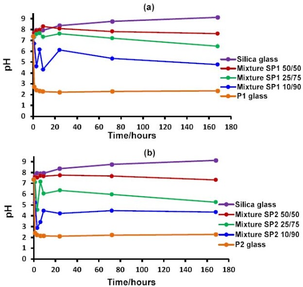
Measurements of the pH trends of the three glass mixtures SP1, SP2 and SP3 together with their three ratios are demonstrated in Figure 1a, 1b and 1c respectively. The glass mixtures SP1, SP2 and SP3 with their three ratios (10/90, 50/50 and 25/75) exhibited smart modulation in pH behaviour in between the two undesirable extremes acidic and alkaline. The pH dropped initially with the phosphate glass. The phosphate glass reacts and dissolves faster and this is aided by a much smaller particle size than the silicate glass. In contrast the silicate glass results in an increase in pH.

It was clearly observed from Figure 1a, 1b and 1c that the initial pH drop can be manipulated by varying the ratios of glass mixtures 10/90, 50/50 and 25/75. The highest pH drop was with the ratio 10/90 where the phosphate glass was 90%, whereas the smaller pH drop was observed with the 25/75 ratio followed by 50/50 ratio, which regulated the pH around the physiological range.

fig 1(1)

fig 1(2)

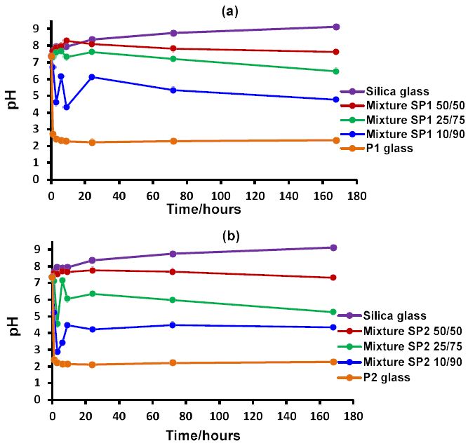
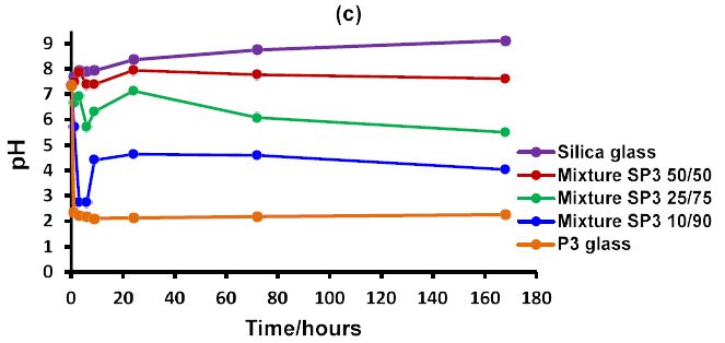
Figure 1: The pH behaviour in Tris buffer solution as a function of time of the three different ratios for each glass mixture together with discrete silicate and phosphate glasses: (a) glass mixture SP1; (b) glass mixture SP2 and (c) glass mixture SP3.

Therefore, based on the experimental pH data of glass mixtures provided above, the question of how to regulate this pH behaviour by varying the ratio of these glass mixtures should be explored in future studies.

Figure 2a and 2b shows the 31P MAS-NMR spectra of the solid material from the experimental glass mixture SP2 with the 50/50 ratio before and after ALP treatment as a function of time up to seven days. The signal at the position between (-26.4 ppm to -20 ppm) corresponds to the chemical shift of Q2-metaphosphate species [17,18]. The signal at the peak position between (-7.7 and -6.0 ppm) corresponds to the chemical shift of the Q1-phosphate species [17,18]. A minor signal around 2-3 ppm corresponds to the Q0-orthophosphate species [17,18]. Figure 2a shows the disappearance of Q2 peak at the expense of an increase in Q1 phosphates for different immersion times. However, there is also growth of a small Q0 calcium orthophosphate peak in the range 2-3 ppm although by seven days there is very little Q2 phosphates left.

On adding ALP, the spectra are similar, but there is an increased amount of Q0 calcium orthophosphate, and the peak is sharper and closer to the chemical shift for apatite of 2.9 ppm as shown in Figure 2b. Generally, the appearance of the Q0 signal in the sample immersed with ALP was sharper specifically in the seven-day immersion period.

fig 2

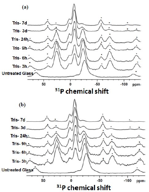
Figure 2: The 31P MAS-NMR spectra of the studied glass mixture SP2 with a 50/50 ratio before (a) and after (b) treatment with the ALP enzyme plotted for the immersion time points. Asterisks show spinning side bands; the spinning speed of 12 kHz was used for both (a) and (b).

Figure 3a and 3b shows the 31P solution NMR spectra of the experimental glass mixture SP2 with the 50/50 ratio before and after glass mixture treatment with ALP respectively as a function of time up to seven days. Three types of the signals were identified in the spectra. The signals with the chemical shift between (-25.2 ppm and -21.7 ppm) were assigned to the Q2-metaphosphate species [19]. The signal between (-9.8 ppm and -6.2 ppm) was assigned to the Q1-phosphate species [19]. Furthermore, the third signal with the position around 3 ppm corresponds to the Q0-orthophosphate species [19]. It can be observed according to the solution NMR spectra in Figure 3b that the higher amounts of the Q0-orthophosphate species were produced after treatment SP2 50/50 with the ALP enzyme compared to the spectra with no enzyme.

fig 3

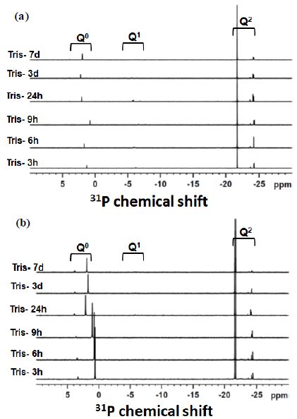
Figure 3: The 31P Solution NMR spectra of the solution remained after immersion of the glass mixture SP2 with a 50/50 ratio (a) without ALP treatment and (b) with ALP treatment. Immersion time points are indicated next to the spectra.

Figure 4 shows the 31P solution NMR integrals of the experimental glass mixture SP2 50/50 ratio with and without treatment with ALP as a function of time. With the glass mixture ratio without the enzyme treatment, the highest proportion of species released into the solution was Q2-metaphosphate (≈90%). Followed by the Q0-orthophosphate and the lowest proportion was the Q1 species. This was in good agreement with the study of Ahmed et al. [20].  In the presence of the enzyme, the proportion of the Q2 species decreased and the proportion of the Q0 species increased. There was also a reduction in the Q1 species after enzyme treatment.

fig 4

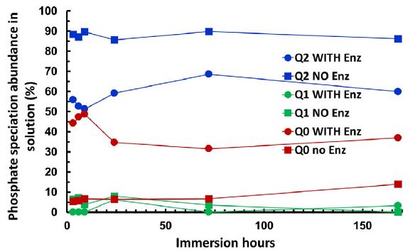
Figure 4: The integrals of three types of phosphate speciation Q2-Q1-Q0 seen in the 31P Solution NMR spectra of the studied glass mixture SP2 together with and without ALP treatment plotted as a function of time for 50/50 ratio. The error bar was estimated to be ± 0.02 for the data point.

Figure 5 compares the evolution of the decrease in Q2-metaphosphate species, with the increase in Q0-orthophosphate species and shows the decrease in both the Q2 and Q1 species together versus time. As can be observed from Figure 5 there were some differences between the proportion of the Q2 species lost (the blue points) and the proportion of the Q0 species gained (the orange points) as a function of time. In other words, the fraction of Q2 species did not match exactly with the Q0 species gained. However, there was a good match between the proportion of the (Q2 + Q1) lost (the grey points) and the proportion of the Q0 gained.

fig 5

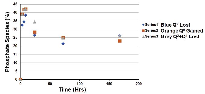
Figure 5: Illustrating the Q species lost or gained after treatment glass mixture SP2 50/50 ratio with ALP as a function of time.

Simple linear correlation coefficient and simple linear regression were used to describe the relationship between the Q species. Figure 6 demonstrates the correlation between the (Q2 + Q1) loss against the Q0 gained. This correlation is linear (R2 ≈ 0.97) and the slope is (0.986) which is close to (1.0). In other words, with the enzyme treatment the amount of (Q2 + Q1) loss was approximately equal to the amount of Q0 gained.

fig 6

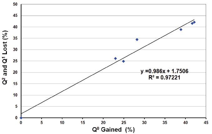
Figure 6: Illustrating the correlation of Q2 + Q1 loss after ALP treatment vs. the Q0 gained.

Discussion

The phosphate glass results in an acidic pH on dissolution, whereas the silicate glass produces an alkaline pH. The newly developed mixtures provide intermediate pH values. As the phosphate glass has a smaller particle size and degrades more rapidly there is a sharp reduction in pH initially followed by a slight rise in pH. The acidic pH produced by the phosphate glass accelerates the dissolution of the silicate glass. The data indicates how the pH can be adjusted by varying the proportions of the phosphate and silicate glasses. Enzymatic degradation of the P-O-P bond by the ALP is recognised for the Q1 pyrophosphate species. Grover et al. however demonstrated that Q0 formed from the Q1-pyrophosphate species in the presence of the ALP [16]. The solid state 31P MAS-NMR spectra showed that in the presence of ALP, the Q2-metaphosphate in the glass decreased much faster than when immersion without the ALP. Therefore, on adding ALP to the 50/50 mixture, the proportion of Q2 reduces and the proportion of Q0 increases, which is shown with the solution 31P NMR spectra. This suggests that the Q2 chains are hydrolysed by ALP where the Q2 species are being converted to Q0. The solution 31P NMR spectra showed several signals corresponding to each phosphate speciation. The results presented above reveal changes between three phosphate speciation(s) (Q2-Q1-Q0) in solution. For instance, the increase in the Q0 speciation can be identified as due to a strong increase in the Q0 signal at around 1-2 ppm in the presence of ALP.

The proposed mode of phosphate glass dissolution in solutions has been previously reported in a study by Ahmed et al. [20]. In the Ahmed study, the amount of the released phosphate species into the solution upon phosphate glass degradation has been investigated using ion chromatography. Based on the chromatogram data, Ahmed et al. [20] also stated that the phosphate species released into the solution after phosphate glass dissolution can be identified as the following: (i) a high proportion of the Q2-metaphosphate species which could be either linear chain or ring structure (unbranched) and the latter was suggested to be the predominant species in solution; followed by (ii) the Q0-orthophosphate species (PO43-); and (iii) a low proportion of the Q1-pyrophosphate species (dimer P2O7 4-). This would suggest that the Q1 observed from 31P NMR both in solution and the solid state are largely from Q1 end groups of Q2 chains. Moreover, the presence of both metaphosphate chains and rings in solution containing dissolution products of phosphate glasses in the 31P solution NMR were identified by Döhler et al. [19].

The presence of only a small fraction of Q1-phosphate was observed in the solution NMR spectra which would suggest that this fraction is more likely to be a terminal end of the Q2-metaphosphate chains rather than the pyrophosphate (dimer P2O7 4-)(each chain has two terminal Q1 phosphorus atoms). Additionally, some of the time points had no detectable fractions of Q1 even in the ALP-free samples in solution NMR spectra.

Based on the results presented above it is proposed that ALP cleaves the Q0 orthophosphate species from the terminal Q1 phosphate group of the Q2 metaphosphate linear chain. Therefore, the proportion of the Q1 species in solution is the lowest since it is no longer available in the solution. Each Q2 chain has two Q1 end groups and the Q1 end group is hydrolysed creating a new Q1 and a Q0 orthophosphate. This is shown schematically in Figure 7. The enzymatic hydrolysis continues until the chain is completely hydrolysed. However, a high proportion of the Q2 remained in solution NMR spectra even after seven days. This suggests that some Q2 species are not capable of being hydrolysed by ALP, although some are. We propose that Q2 chains are hydrolysed by ALP whereas Q2 cyclic phosphates contain no Q1 end groups and are therefore not capable of being enzymatically hydrolysed by ALP.

fig 7

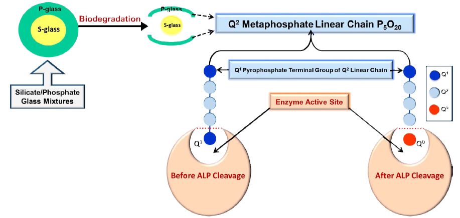
Figure 7: Schematic demonstration of the ALP enzyme activity in solution, describing the insertion of the Q2 metaphosphate linear chain in the active site of the ALP enzyme and the Q1 end group can be hydrolysed off to release Q0 orthophosphate species.

It would, however, be desirable to produce Q2 phosphate glasses that do not have any Q2 cyclic phosphates present but only linear chain phosphates. These glasses would then degrade to Q0 orthophosphate in vivo when ALP is present, such as in bone and in periodontal pockets and provide Q0 orthophosphate (PO43-) for apatite formation and bone mineralization.

Conclusion

Mixing a phosphate glass with silicate bioactive glasses can be used to avoid the undesirable low pH of phosphate glasses and the undesirable high pH generated by silica based bioactive glasses.

ALP hydrolyses the straight Q2 metaphosphate chain by cleaving Q1 terminal phosphate group to release Q0 orthophosphate (PO43-). The released Q0 orthophosphate ions are essential for apatite crystal formation. ALP should therefore be included in in vitro studies of the degradation of phosphate glasses to closely mimic their perceived in vivo behavior.

Acknowledgements

The Authors would like to thank Dr Harold Toms, (NMR facility manager) for his expert technical assistance. This study was part of a PhD funded by the Iraqi Ministry of Higher Education and Scientific Research.

References

  1. Socransky SS, Haffajee AD (1997) The nature of periodontal diseases. Annals of Periodontology 2: 3-10. [crossref]
  2. Aboelsaad NS, Soory M, Gadalla LMA, Ragab LI, Dunne S, et al. (2009) Effect of soft laser and bioactive glass on bone regeneration in the treatment of infra-bony defects (a clinical study). Lasers in Medical Science 24: 387-395. [crossref]
  3. Cho YD, Seol YJ, Lee YM, Rhyu IC, Ryoo HM, et al. (2017) An overview of biomaterials in periodontology and implant dentistry. Advances in Materials Science and Engineering 2017.
  4. Chacko NL, Abraham S, Rao HS, Sridhar N, Moon N et al. (2014) A clinical and radiographic evaluation of periodontal regenerative potential of PerioGlas®: a synthetic, resorbable material in treating periodontal infrabony defects. Journal of International Oral Health 6: 20. [crossref]
  5. Satyanarayanav K, Anuradha B, Srikanth G, Chandra P, Anupama T, et al. (2012) Clinical evaluation of intrabony defects in localized aggressive periodontitis patients with and without bioglass-an in-vivo study. Kathmandu Univ Med J 37: 11-15. [crossref]
  6. Wheeler D, Stokes K, Hoellrich R, Chamberland D, McLoughlin S (1998) Effect of bioactive glass particle size on osseous regeneration of cancellous defects. Journal of Biomedical Materials Research: An Official Journal of The Society for Biomaterials, The Japanese Society for Biomaterials, and the Australian Society for Biomaterials 41: 527-533. [crossref]
  7. Hench L. L, Polak JM  (2002) Third-generation biomedical materials. Science 295: 1014-1017. [crossref]
  8. Profeta AC, G. M. Prucher (2015) Bioactive-glass in periodontal surgery and implant dentistry. Dental Materials Journal 34: 559-571. [crossref]
  9. Takahashi N, Schachtele C (1990) Effect of pH on the growth and proteolytic activity of Porphyromonas gingivalis and Bacteroides intermedius. Journal of Dental Research 69: 1266-1269. [crossref]
  10. Bingel L, Groh D, Karpukhina N, Brauer DS (2015) Influence of dissolution medium pH on ion release and apatite formation of Bioglass® 45S5. Materials Letters 143: 279-282,.
  11. L-E Monfoulet, P Becquart, D Marchat, K Vandamme, M Bourguignon, E Pacard et al., (2014) The pH in the microenvironment of human mesenchymal stem cells is a critical factor for optimal osteogenesis in tissue-engineered constructs. Tissue Engineering Part A 20: 1827-1840. [crossref]
  12. Groeneveld M, Bos T, Everts V, Beertsen W (1996) Cell‐bound and extracellular matrix‐associated alkaline phosphatase activity in rat periodontal ligament. Journal of Periodontal Research 31: 73-79. [crossref]
  13. Sanikop S, Patil S, Agrawal P (2012) Gingival crevicular fluid alkaline phosphatase as a potential diagnostic marker of periodontal disease. Journal of Indian Society of Periodontology 16: 513. [crossref]
  14. Bezerra Júnior AA, D. Pallos, J. R. Cortelli, and C. H. C. Saraceni (2010) Evaluation of organic and inorganic compounds in the saliva of patients with chronic periodontal disease. Revista Odonto Ciência 25: 234-238.
  15. Daltaban Ö, Saygun I, Bal B, Baloş K, Serdar M (2006) Gingival crevicular fluid alkaline phosphatase levels in postmenopausal women: effects of phase I periodontal treatment. Journal of Periodontology 77: 67-72. [crossref]
  16. Grover LM, Wright AJ, Gbureck U, Bolarinwa A, Song J, et al. (2013) The effect of amorphous pyrophosphate on calcium phosphate cement resorption and bone generation. Biomaterials 34: 6631-6637.
  17. Kirkpatrick RJ, Brow RK (1995) Nuclear magnetic resonance investigation of the structures of phosphate and phosphate-containing glasses: a review. Solid State Nuclear Magnetic Resonance 5: 9-21.
  18. MacKenzie KJ, Smith ME (2002) Multinuclear solid-state nuclear magnetic resonance of inorganic materials. Elsevier.
  19. Döhler F, Mandlule A, van Wüllen L, Friedrich M, Brauer DS (2015) 31 P NMR characterisation of phosphate fragments during dissolution of calcium sodium phosphate glasses. Journal of Materials Chemistry B 3: 1125-1134.
  20. Ahmed I, Lewis M, Nazhat S, Knowles J (2005) Quantification of anion and cation release from a range of ternary phosphate-based glasses with fixed 45 mol% P2O5. Journal of Biomaterials Applications 20: 65-80. [crossref]
fig 1

Chylooperitoneum in the Cardiovascular Possurgical: Presentation of a Case

DOI: 10.31038/JCCP.2021426

Abstract

Introduction: Chyloperitoneum  is defined as the presence of lymph of thoracic or intestinal origin in the abdominal cavity. It is reported infrequently and is a rare manifestation of multiple deseases. Most of the cases are secondary and are associated with direct trauma to the peritoneal dialysis. Renal replacement therapy is necessary in up to 10% of children who undergo cardiac surgery with extracorporeal circulation, indicated in cases of water overload, acute renal dysfunction or ionic alterations.

Objective: To report the case of a 15-day-old newborn, operated on for Transposition of the Great Vessels, who presented as a postoperative complication, dicharge of chylous content through  the Tenckhoff, after a peritoneal dialysis regimen due to acute renal failure and fluid overload.

Results: Despite the therapeutic measures taken, the patient maintains centuries-old losses of  lymph, which lead to nutritional and immunological deterioration  with the consequent multiple organ dysfunction and death.

Conclusions: The perpetuation of lymph losses in the postoperative period of cardiovascular surgery produces a nutritional and immunological deterioration of the patient, with a high risk of mortality due to sepsis.

Keywords

Chyloperitoneum, Peritoneal dialysis, Acute renal dysfunction

Introduction

Chylous ascites, or chyloperitoneum, is a rare form of ascites, characterized by a milky-looking fluid that contains high levels of triglycerides and exceeds those found in plasma (>200 mg/100 ml). Its incidence ranges from 1 in 20,000 to 1 in 187,000 admissions, in referral hospitals and specialized care [1].

Clinical Case

Newborn, from a dystocic delivery at 39 weeks of gestation, with a postnatal diagnosis of simple Transposition of the Great Vessels (TGV) and a weight of 3300 g.

At 15 days of age, he underwent surgery and anatomical correction was performed by Arterial Switch with extracorporeal circulation time 141 minutes, aortic clamping time 85 minutes, at 28 degrees of temperature and conventional hemofiltration (200 ml) and modified (150 ml) after cardiopulmonary bypass. He left the operating room with a Tenckhoff catheter in place, open sternum and supported with inotropics: epinephrine 0.2 Mcg/kg/min and norepinephrine 0.3 Mcg/kg/min. Antimicrobial treatment was started with Cefazolin and Gentamicin.

Physical Exam

Blood Pressure 92/50 mmHg; heart rate 189/min. Mechanical Ventilation: Pins 30 cm H2O, FiO20.8%, PEEP 8 cm H2O, respiratory rate 35/min. SaO2: 96%

Patient in critical condition, with pale skin, livedo reticularis and blood aspirations since surgery. Chest and lungs: respiratory excursions and symmetrical vesicular murmur in both lung fields with transmitted sounds. Cardiovascular: rhythmic heart sounds, III/VI systolic murmur on the left sternal border. Jugular engorgement was not evidenced; Peripheral arterial pulses present. Abdomen: Globulous, soft, depressible, hepatomegaly of 3 cm with blunt edges and air-fluid noises (RHA) missing. Subcutaneous cellular tissue: generalized crescendo edema. Nervous system: under sedation, miotic pupils.

Complementary Exams

Hemoglobin 12.5 g/dl; 10.3 x 10⁹ L leukocytes; 48% segmented, 52% lymphocytes; platelets 160 x 109 l. Prothrombin time C-13.2 P-35.6. Glycemia 9.4 mmol/l; creatinine 81 mmol/l; total protein 43 g/l, albumin 55 g/l. Glutamic oxaloacetic serum transaminase (SGOT) 22 U/L, serum glutamic pyruvic transaminase (SGPT) 109 U/L; CRP: 4.2 mg/dl; triglycerides 96 mg/dl; PVC: 20 mmHg; IAP (indirectly measured through a femoral catheter at the level of the inferior vena cava): 18 mmHg.

Arterial gases: PO2: 39.5 mmHg, PCO2: 54.3 mmHg, SaO2: 73.3%. pH 7.27, HCO3 23.2 mEq/L, EB -2.8 mEq/L, sodium 161 mEq/L, potassium 2.6 mEq/L, chlorine 108 mEq/L, ionic calcium 0.88 mg/dl. Chest X-ray: diffuse veil opacity of the left lung.

Postoperative echocardiogram: preserved biventricular function, patent outflow tracts of both ventricles, without residual pathological gradient. Wide AIC with preferential left-to-right shorting. No pericardial effusion.

As complications in the immediate postoperative period, the patient presented low cardiac output and systemic capillary extravasation, so early peritoneal dialysis was started in the first 24 hours of a continuous type with 14 daily baths.

At 72 hours, complementary tests were repeated with creatinine values of 162 mmol/l and a diuretic rhythm of 0.4 mg/kg/24, and acute kidney damage was diagnosed according to the RIFLE scale [2].

The generalized edema persists so the dialysis baths lasted for 20 days. After this time, clinical improvement was observed, the recovery of the diuretic rhythm, hemodynamic stability and decreased edema, which is why they are interrupted and leakage of a milky-looking liquid is observed through the Tenckhoff (Figure 1) and a culture attached to this tracheal secretion was positive for the growth of Enterobacter cloacae, for which antibiotic treatment with Meronem and Vancomycin was started for 10 days.

fig 1

Figure 1: Peritoneal fluid.

Peritoneal Fluid Studies Reported

Cytochemical: opaline color; Slightly cloudy appearance; Pandy XX; Glucose 4.4 mmol/l; Triglycerides 433.6 mg/dl. Bacteriological: no bacterial growth, so the possibility of bacterial peritonitis is ruled out. A chyloperitoneum is diagnosed. Abdominal ultrasound: No associated tumor lesions are observed. Little free fluid in the abdominal cavity. The conduct was to keep peritoneal dialysis suspended due to the recovery of renal function with creatinine values of 91 mmol/l and a diuretic rhythm of 1.5 ml/kg/day. The Tenckhoff is maintained with losses of around 300 ml/day; The enteral route is suspended, guaranteeing parenteral nutritional support for 14 days in which the Tenckhoff debit remained at centennial figures. Albumin is added to the treatment to replace protein loss and is supported with Biomodulin T to reinforce the immune response. Severe right ventricular dysfunction; evident by hepatomegaly, wet rales in both lung fields, pleural effusion, gallop rhythm, ascites, and capillary leakage; they perpetuate the picture. Petechial lesions appear in the abdomen suggestive of fungal sepsis, continuous with high ventilatory parameters, increased edema, large losses due to Tenckhoff and manifestations of digestive bleeding, peritoneum and urinary tract. A picture of super added sepsis is presented, with a positive blood culture for yeast growth, and Amphotericin B is added to medical treatment.

Despite the strategies taken, the losses by the Tenckhoff were higher than the patient’s blood volume. The patient does not respond to antimicrobial therapy and it is decided  change of antibiotic for Tazocín and Colistin without achieving favorable results. Secondary to multiple organ dysfunction, significant metabolic disturbances in the patient destroy life. The infrequent presentation of this entity in the postoperative period of Cardiovascular Surgery, associated with its difficult management, motivates the presentation of the case.

Discussion

There is an anatomical structure in the body called the thoracic duct responsible for absorbing and transporting lymph from the lymphatic vessels. When there is a disruption in lymphatic emptying, either due to loss of continuity or obstruction in these ducts at the abdominal level, it is called chylous ascites or chyloperitoneum. (1,3) It is a rare complication published in the literature and is first reported in an article published in 1961 by Morton, after performing a paracentesis in an 18-month-old male patient with disseminated tuberculosis [3].

The etiology of chyloperitoneum is well known and among the factors that determine it are congenital causes, fibrotic causes (hematologic diseases, sarcomas, and metastases), and acquired causes. Among the latter are those that cause an increase in lymph production, such as cirrhosis and heart disease, as well as those that cause a disruption or obstruction of the thoracic duct, such as trauma, abdominal surgeries, infectious (filariasis, tuberculosis) and radiotherapy [4]. There are three pathophysiological mechanisms of chylous ascites: a lymphatic alteration, fibrosis of the lymphatic system concomitant with malignant processes and of congenital origin [5-8]. Peritoneal dialysis is sometimes associated as a causative agent of the leakage of milky-looking fluid from the Tenckhoff catheter. In 2019 a study revealed a series of 22 cases, secondary to the insertion of the peritoneal catheter or peritoneal dialysis [8-10].

In this case, the authors considered that the factors that favored the appearance of chyloperitoneum were: hyperpressure of the lymphatic vessels secondary to peritoneal dialysis, associated with a systemic venous congestion caused by right ventricular dysfunction, with disruption of the lymphatic vessels and the consequent lymph outflow. The characteristics of the milky liquid on physical examination and opaline cloudy in the cytochemical examination; were determined by an increase in triglyceride values of 433.6 mg/dl, making a differential diagnosis with bacterial peritonitis.

The consequences derived from the disturbances that are produced by associated loss of immunoglobulins and proteins cause mortality to exceed 40% due to sepsis and malnutrition [11]. At the William Soler Pediatric Cardiocenter, chyloperitoneum is not frequent, so we do not have a statistical record related to mortality.

Physiological correction surgery for transposition of the great vessels (Arterial Switch or Jatene) performed in the first 20 days of life exposes the patient to multiple risks due to age, extracorporeal circulation time and aortic clamping, which are also risk factors mortality [12]. In cardiovascular surgery, the chylothorax is observed more frequently, then the chyloperitoneum and the chylopericardium more rarely [13].

With the exit of chyle, fluids, electrolytes, proteins, fats, fat-soluble vitamins and T lymphocytes are depleted, which conditions an alteration of variable severity in nutritional status and humoral and cellular immunity, which predisposes to occurrence of opportunistic infections [14]. There is a correlation between chyle loss rates and survival; determining factor in this case, since chyle losses exceeded 100 ml every day, more than a third of the patient’s blood volume, perpetuated for more than 10 days.

Dietary management and metabolic correction, as well as the use of substances that decrease lymph production are the mainstays of treatment. The medical treatment that is described in the bibliography, includes modifications in the diet (low in fat or with medium chain fatty acids or total parenteral nutrition), intravenous medication with somatostatin and/or analogues such as octreotide, proposed by Ulibarri et al. (0.1 mg/8 hrs); with a mechanism of action that decreases gastric, pancreatic, intestinal secretion, portal and splanchnic blood flow, helping to decrease lymphatic production [5,10,11,13].

Medical treatment consisted of suspending the enteral route, guaranteeing an adequate parenteral intake, which must have produced a decrease in lymphatic flow. Albumin was used to replace the losses, since hypoalbuminemia encourages the fluid to pass into the interstitial tissues with excess protein and higher colloid osmotic pressure [15]. Biomodulin T was used to optimize the immunity, since they promote the maturation, the activity of T lymphocytes and the release by these cells of IL1, IL2, IL6, IL7, GM-CSF and others. In this case we do not have the availability of this medicine.

No response was obtained with the measures used in the patient.

Losses of nutritional, immune, and metabolic factors led to multiple organ failure and death.

Conclusions

The perpetuation of lymph losses in the postoperative period of cardiovascular surgery produces a nutritional and immunological deterioration of the patient, with a high risk of mortality due to sepsis.

References

  1. Caravaca-García A, Rodríguez-Contreras D, Elhendi-Halaw W (2016) Ductus torácico: vecino desconocido e incómodo. Acta Otorrinolaringol Gallega 9: 98-102.
  2. Díaz de León-Ponce MA, Briones-Garduño JC, Carrillo-Esper R, Moreno-Santillán A, Pérez-Calatayud A (2017) Insuficiencia renal aguda (IRA) clasificación, fisiopatología, histopatología, cuadro clínico diagnóstico y tratamiento una versión lógica. Rev Mex Anestes 40: 280-287.
  3. Rodrigo del Valle Ruiz S, González Valverde FM, Tamayo Rodríguez ME, Medina Manuel E, Albarracín Marín-Blázquez A. Quiloperitoneo incidental asociado a hernia de Petersen en paciente operada de bypass gástrico laparoscópico. Elsevier Rev Cir Esp 97: 351-353.
  4. Lizaola B, Bonder A, Trivedi HD, Tapper EB, Cardenas A (2017) Review article: the diagnostic approach and current management of chylous ascites. Aliment Pharmacol Ther 46: 816-824. [crossref]
  5. Uribe J, Sepúlveda R, Cruz R, Illanes P, Trucco C, Le Roy C (2018) Ascitis quilosa post cirugía abdominal: caso clínico y revisión de la literatura. Gastroenterol latinoam 29: 193-199.
  6. Vilar-Tabanera A, García-Angarita F, Mendía-Conde E, Gómez-Ramírez J (2019) Ascitis quilosa tras colecistectomía. Presentación de un caso. Rev Cir 71: 253-256.
  7. Roa Colomo A, Caballero Mateos A, Vidal Vílchez B, Cervilla Sáez de Tejada E (2021) Varón de 60 años que debuta con ascitis quilosa. 44.
  8. Rodríguez-Sánchez MP, Hurtado-Uriarte M, Díaz-Ruiz JE, Vergara C, Cuestas JA, et al. (2019) Quiloperitoneo en diálisis peritoneal: reporte de caso y revisión de la literatura. Rev Nefrol Dial Traspl 39: 115-119.
  9. Moro K, Koyama Y, Kosugi Si, Ishikawa T, Ichikawa H, et al. (2016) Low fat-containing elemental formula is effective for postoperative recovery and potentially useful for preventing chyle leak during postoperative early enteral nutrition after esophagectomy. Clin Nutr 35: 1423-1428. [crossref]
  10. Olivar Roldán J, Fernández Martínez A, Martínez Sancho E, Díaz Gómez J, Martín Borge V, et al. (2009) Tratamiento dietético de la ascitis quilosa postquirúrgica: caso clínico y revisión de la literatura. Nutr Hosp 24: 748-750.
  11. Castillo F., Marín D., Linares F., Osorio A (2018) Ascitis quilosa postraumática tratada con nutrición parenteral total y octreotido, Revista Cubana de Cirugía 57: 1-7.
  12. Jatene Vera F, Sarria E, Ortiz A, Ruiz E (2021) Cirugía de la transposición de las grandes arterias en periodo neonatal. Cirugía Cardiovascular 28: 3-7,
  13. Ruz M, Guzmán M, Gómez López de Mesa C, Betancur L (2010) Quilopericardio secundario a cirugía cardiovascular. Rev Colomb Cardiol 17: 191-194.
  14. Valenzuela MJ, Jofré P, Reimer C, Valdés S, Grassi B (2020) Manejo nutricional de ascitis quilosa: Serie de casos y revisión de la literatura. Rev Chil Nutr 47: 1038-1042.
  15. Lozano González Y (2007) Linfedema. Rev Méd Electron [Seriada en línea] 29.
fig 1

Effect of Capsaicin on the Barrier Functions of Porcine Intestinal Epithelial Cells (IPEC-J2)

DOI: 10.31038/JPPR.2021444

Abstract

Due to the antibiotic resistance context, it is becoming necessary to ensure the good health of farm animals while decreasing antibiotics prescription. The use of feed supplements is among these methods. These supplements improve animal performance and health by stimulating physiological processes, such as immune function and stress resistance. Capsaicinoids are derivatives produced by plants of the genus Capsicum and members of the vanilloid family. Capsaicin strengthens the immune system, has anti-inflammatory properties and limits oxidation and is known to improve the growth rate in pigs. The purpose of this study was to assess the permeability and transport characteristics of capsaicin in pig intestinal cells (IPEC-J2). We confirmed the absence of active transport of capsaicin and its derivatives with an impact on the intestinal epithelium resulting in an increase in permeability. This alteration of the permeability of the intestinal barrier is observed in another reference line, the Caco-2 cell line. Then, we also investigated the modulation of the expression of transporters for multidrug resistance and tight junction protein by capsaicin. Prolonged exposure to low doses of capsaicin seems to be responsible for a modification of the expression of transport proteins. The results showed a significant increase on PGP expression after 24 h of capsaicin exposure at 10 µM and a slightly significant induction in the mRNA expression levels of MRP1 was observed after 24h. Despite the short exposure time (90 min), 10 µM capsaicin exposure led to a slight induction of Occludin and Zo-1 mRNA expression.

Keywords

Intestinal absorption, In vitro model, Tight junctions, ABC transporters

Introduction

Antimicrobial drugs are currently used to treat or prevent bacterial infections in the livestock industry; in some countries they are also used for growth promotion in food animals. This widespread use of antimicrobials in particular in intensive livestock farming contributes to the emergence of antimicrobial resistance with significant public health implications. Prevalence of resistant bacteria in animals and humans seems to be correlated with the levels of antimicrobial use in animals [1-4]. In the future, predictions for global antibiotic use do not seem to be moving towards a decrease [5]. Alternative for use of antibiotic in food producing animals, especially intensive livestock (swine, poultry) represent an issue while preserving health and welfare of animals. Plant extracts or phytochemicals are one of the solutions being explored at the World Organization for Animal Health in Paris, France, December 12-15, 2016. Phytochemicals are natural bioactive compounds that are originated from plants and incorporated into animal feed to enhance productivity and healthy. Their role in the production of digestive secretions, nutrient absorption and modulation of gut microbiote and immunity are the main mechanisms suggested. Due to variation in the composition of plant extracts, it remains difficult to compare their efficiency. The composition and concentration of the bioactive compounds depend on the plant, parts of the plant, geographical origin, harvesting season, environmental factors, storage conditions, and processing techniques. A wide variety of herbs and spices are used for this purpose [6,7]. Anethol, carvacrol, cinnamaldehyde, curcumin, eugenol, thymol and capsaicin are still the main constituents studied [8]. Capsaicin and dihydrocapsaicin are the main representative capsaicinoid derivatives and members of the vanilloid family. These molecules are produced by plants of the genus Capsicum, also known as chili pepper fruit. Capsaicin is responsible for the spicy taste and feelings of hotness. Its action is especially mediated by transient receptor potential vanilloid subfamily member 1 (TRPV1), a nonselective ligand-gated cation channel. Activation of this receptor is also mediated by other plant bioactives such as menthol [9] and leads to the opening of ion channels and the entry of cations such as Na+ and Ca2+ into neurons. Dunshea et al. (2003) [10] demonstrated that capsaicinoids may improve the growth rate in pigs. Few studies have reported the same results [11] and one patent has been pending since 2008 [12]. More recently, the benefits of dietary supplementation with Capsicum oleoresin were demonstrated on heat stress on pig performance [13]. Previous studies indicate that capsaicin is rapidly absorbed from the stomach and intestine by a passive process, with a total absorption capacity between 50 and 90% in different rodent studies [14,15]. However, capsaicin causes structural changes in the Caco-2 cell monolayer by increasing epithelial permeability [16-18]. Capsaicin could inhibit and upregulate P-glycoprotein, which could influence the bioavailability of the P-gp substrate [19,20].

In the present study, we examined the effect of capsaicin on the IPEC-J2 cell line, a permanent nontransformed intestinal cell line isolated from the jejunum of neonatal unsuckled piglets. This cell line was chosen based on the use of capsaicin as feed additive in piglets before in vivo investigation. IPEC-J2 cells grew on permeable inserts and formed a polarized monolayer similar to Caco-2 cells [21]. This model is already used to investigate compounds having a negative effect on epithelial function [22] and monolayer permeability [21]. The purpose of this study was to assess the permeability and transport characteristics of capsaicin in IPEC-J2 cells. After characterization of the expression of transporters for multidrug resistance, we investigated the modulation of ABC transporters (P-gp, MRP1, MRP2, BCRP) and tight junction proteins by capsaicin.

Materials and Methods

Chemicals

A certified standard with high purity capsaicin (CAPS) was purchased from Sigma-Aldrich (St. Quentin Fallavier, France). Methanol and acetonitrile (MeCN) (HPLC gradient grade) used for the mobile phase were provided by VWR Chemicals (Fontenay-sous-Bois, France). Water for HPLC was supplied by a demineralized water system from an aquadem (Veolia Water Technologies, Antony, France). Individual stock solutions at 1000 mg L-1 were prepared in MeCN, and a standard mixture with all analytes at 10 mg L-1 was prepared in MeCN and stored at -18°C.

Cell Culture

The IPEC-J2 line was obtained from Leibnitz Institute (DSMZ, Germany) and was used between passages 2 and 8. The cell line was maintained in DMEM/F-12 medium supplemented with 10% fetal calf serum, 1% penicillin/streptomycin, and 1% insulin-transferrin-selenium in a humidified atmosphere of 95% air and 5% CO2 at 37°C. Culture medium was changed three times a week. Cells were subcultured at 80%-100% confluency using trypsin-EDTA. The human colon adenocarcinoma cell line Caco-2 was obtained from the American Type Culture collection (ATCC N°HTB37). Cells were routinely maintained and grown in Dulbecco’s modified Eagle’s medium Glutamax containing 10% heat-inactivated fetal calf serum, 1% nonessential amino acids, 5% penicillin (100 U/ml) and streptomycin (100 mg/ml) in a humidified atmosphere of 95% air and 5% CO2 at 37°C. For the transport studies, cells were seeded on polycarbonate membrane inserts (0.4 μm pore diameter, 30 mm diameter; Millipore, Dutscher, Denmark). Transepithelial electrical resistance (TEER) was checked every 5 days using a millicell ERS ohmmeter (Millipore, Molsheim, France). Apical (AP) and basolateral (BL) chamber volumes were maintained at 1.5 and 2 ml, respectively. Cells were used for transport experiments when TEER values were above 1000 Ohm/cm2 for IPEC-J2 cells and at days 21-22 postseeding for Caco-2 cells.

TEER was calculated from the following equation:

form 1

where TEERcell is the cell monolayer and polycarbonate porous membrane resistance, TEERblank is the polycarbonate porous membrane resistance (without a cell monolayer), and A is the polycarbonate porous membrane surface area (4.2 cm²). Cell culture media and reagents were obtained from Fisher Scientific (Illkirch, France). Culture flasks and plates were purchased from Falcon (VWR International, Strasbourg, France).

Cytotoxicity

Cell cytotoxicity was assessed by the CCK-8 assay (Sigma Aldrich, Saint Quentin Fallavier, France) according to the manufacturer’s instructions. Cells were seeded in 96-well plates (1.105 cells/well) and maintained in a humidified atmosphere of 95% air and 5% CO2 at 37°C until they reached 90% confluence. The IPEC J2 cell line was exposed to capsaicin at concentrations ranging from 0.1 µM to 1 mM. Two exposure times (24 h and 48 h) were tested. Absorbance at 490 nm was read using a Multiskan Microplate reader.

Instrumentation and Chromatographic Conditions

The HPLC system consisted of an Agilent 1260 affinity II with a 100 μl sample loop and a G7121B fluorescence detector at an excitation wavelength of 281 nm and emission of 312 nm (Agilent Technologies, les Ulis, France). Chromatography was performed using partial-loop injection of a 50 μl sample on an ACE Excel 5 C18-PFP (150 x 4.6-5 µm) (VWR international Fontenay sous bois, France) at 40°C. The mobile phase consisted of water (A) and acetonitrile (B). A flow rate of 1 ml/min was maintained, and capsaisinoids were eluted using the following program: 0-2 min isocratic hold 35% B, 2-10 min linear gradient 35-65% B. The retention times were 9.9, 10.2 and 11.3 min for NDHC, CAPS, and DHC, respectively.

Permeability Studies

Cells seeded on membrane inserts were exposed to fluorescein (2 µg/ml) on the apical side. Fluorescein passage was evaluated in the basolateral compartment at 15, 30, 45, and 60 min. The chromatographic conditions for the quantification of fluorescein were as follows: VWR Lichrospher® C18 column (250 mm x 4.6 mm inner diameter, particle size 5 μm), mobile phase consisting of acetonitrile (A) and water (B) with a linear gradient from 20 to 65% of A in 4 min. The flow rate was 1.0 ml/min, the temperature of the column furnace was set at 40°C, and the injection volume was 10 μl. The excitation wavelength of the fluorescence detector was set to 485 nm, and the emission wavelength was set to 515 nm. The method exhibited linearity in the range of 50 to 2000 ng/ml (r² = 0.9938). Precision and accuracy were also adequate, with intra- and interdaily variations of up to 10%. No interferences were noted, demonstrating the selectivity and specificity of the method.

Transport Studies

After transepithelial electrical resistance (TEER) measurement, cell monolayers were preincubated for 30 min at 37°C in Hank’s balanced salt solution (HBSS). For transport studies, apical (AP) and basolateral (BL) chamber volumes were maintained at 1.5 and 2 ml HBSS, respectively. Transepithelial transport of capsaicin was assayed by adding 10 μM capsaicin either to the apical or basolateral compartment and measured over 4 h. The permeability of capsaicin was estimated by calculating the values of Papp as follows:

form 2

where A = membrane surface area (4.2 cm2), C0 = initial concentration in the donor compartment, and dQ/dT = permeability rate in receiver solution [23], calculated using linear regression (Microsoft Excel function, Excel: PC 2010).

The efflux ratio is determined by the following equations:

form 3

where Papp (BL−AP) is Papp in the secretory direction and Papp (AP−BL) is Papp in the absorptive direction.

Total RNA Extraction and cDNA Synthesis

Cells were collected in RNA protect cell buffer (Qiagen, Courtaboeuf France) and stored at -20°C until total RNA extraction. Total cell RNA was isolated and purified with the NucleoSpin RNA plus kit (Macherey-Nagel, Hoerdt, France) according to the manufacturer’s instructions. All extractions were performed with a genomic DNA elimination step. Total RNA was quantified with a Biodrop µLite spectrophotometer (Biochrom, UK). cDNA was synthesized by reverse transcription with the PrimeScript RT reagent Kit (TaKaRa Bio, Ozyme France) according to the manufacturer’s protocol. Reverse transcription was carried out on 0.5 μg to 1 μg of total RNA.

Quantitative Real-time PCR

Real-time quantitative PCR was performed using a QTower3 thermal cycler (Analytik Jena, Deutschland) and Eurobiogreen Master mix (Eurobio, Courtaboeuf). The amount of cDNA was 20 ng. Primer concentrations were 200 nM. Primer sequences and product size are indicated in Table 1. The thermal cycling comprised a PCR activation step for 3 min at 95°C and 40 cycles with denaturing step at 95°C for 5 s, annealing step at 60°C (PGP, MRP1, MRP2, BCRP, GAPDH), 50°C (Occludin and Zonula occludens ZO-1) or 58°C (Claudin) for 30 s, and an extending step lasting 30 s at 72°C. Primer pair specificity was tested at the end of every run by melting curve analysis, and amplification specificity was confirmed by electrophoresis in a 2% agarose gel. PCR efficiencies were calculated for each gene, allowing efficiency-corrected comparative quantification (Pfaffl, 2001). The relative mRNA levels in each sample were normalized to the housekeeping gene glyceraldehyde-3-phosphate dehydrogenase (GAPDH) and expressed relative to a control (untreated sample). Reactions are carried out in duplicate.

Table 1: Sequence of primers used for real-time quantitative PCR.

Gene

Primer sequence (5′-3′) Amplicon length (pb)

Accession number

GAPDH FP: AGCAATGCCTCCTGTACCACCAACTG

200

AF017079

RP: GCAGCACCAGTAGAAGCAGGGATGAT
PGP FP: TTGGCTGGAAAAGTGCTAATTGACGG

259

AY825267

RP: GCTGCGTTCCTTTGTCTCCCACTCTG
MRP1 FP: TTCCGCGCACTCGTGGTTCAGCTTAT

112

CF368015

RP: GGACCCGTTCAGCCAGTACTCAGAGG
MRP2 FP: TACGAGGTGACAGAGGGCGGTGACAA

159

DQ530510

RP: TTGGATGGTCGTCTGGATGAGGTGAT
BCRP FP: GGACAAAACTTCTGCCCGGGACTCAA

178

NM_214010

RP: TCAGGTAGGCGATCGTCAGGAAAATG
Occludin FP: ATCAACAAAGGCAACTCT

157

XM_005672522.3

RP: GCAGCAGCCATGTACTCT
Claudin-1 FP: GCAGCAGCTTCTTGCTTCTC

664

NM_001244539.1

RP: CTGGCATTGACTGGGGTCAT
ZO-1 FP: GAGTTTGATAGTGGCGTT

298

NM_001244539.1

RP: GTGGGAGGATGCTGTTGT

Statistical Analysis

All results are expressed as the mean ± SD (n=3). Pairwise comparisons were calculated by unpaired Student’s t-tests (XLSTAT-PRO 2010). A p value of <0.05 was considered statistically significant.

Results

Cytotoxicity

The results of the CCK-8 assay revealed that IPEC-J2 cell viability was reduced in a time- and dose-dependent manner following capsaicin treatment (Figure 1). Compared with the vehicle (0.1% ethanol) controls, following cell treatment with 1 to 1000 µM capsaicin for 24 h, cell viability was reduced from 102.06 ± 9.83 to 36.98 ± 4.00%. The same results were observed at 48 h post treatment, with 1 to 500 µM decreasing cell viability from 85.37 ± 3.28 to 21.13 ± 1.22%. Considering these results, capsaicin at concentrations greater than or equal to 10 µM had a significant effect on cell viability at 48 h.

fig 1

Figure 1: Effect of capsaicin on IPEC-J2 cell viability.
IPEC-J2 cell monolayers were exposed to capsaicin (1–1000 μM) for 24 hrs (dark gray) and 48 hrs (light gray). Data are means ± S.D. (n = 8) expressed as % of control response. Statistically significantly different from control cell monolayers, *p<0.05.

Permeability Studies

To evaluate the impairment of barrier function by capsaicin, we examined the flux of fluorescein across an IPEC-J2 monolayer (Figure 2). Untreated IPEC-J2 monolayers exhibited high paracellular passage in addition to a TEER value above >1000 Ohm/cm2. Upon treatment with 10 µM capsaicin for 90 min, monolayer permeability significantly increased up to 70% of the control without cells (Table 2).

fig 2

Figure 2: Effect of capsaicin on monolayer permeability to fluorescein.
Data are expressed as the mean ± S.D. (n = 3). Statistically different from control cell monolayers, *p < 0.05.

Table 2: Apparent permeability coefficient (Papp x 10-5 cm/s) and net efflux of capsaicin transport across IPEC-J2 and Caco-2 cell monolayers. Data are expressed as the mean ± S.D. (n = 3).

Papp (x 10-5 cm/s)

Ratio
AP → BL BL →AP

BL →AP/AP → BL

IPEC-J2 Capsaicin 1 µM

4.71 ± 0.91

6.27 ± 0.11

1.12 ± 0.33

Capsaicin 10 µM

5.92 ± 1.93

6.57 ± 1.66

1.13 ± 0.19

Caco-2 Capsaicin 10 µM

4.21 ± 1.04

3.92 ± 0.73

0.94 ± 0.007

Transport Studies

The kinetics of capsaicin were investigated by performing transepithelial transport studies at increasing concentrations. The AP-BL and BL-AP efflux of 10 µM capsaicin through IPEC-J2 and Caco-2 cell monolayers was measured for 2 h. As shown in Table 1, transepithelial transfer of capsaicin was quite rapid, with high transepithelial permeability. Bidirectional transport is not mediated by ATP-dependent transport systems: no difference was observed between AP-BL and BL-AP transfers.

ABC Transporter mRNA Expression

As the expression of ABC transporters has not been described in IPEC-J2 cells, we investigated the basal expression of these proteins at the mRNA level and explored the effect of the cell polarization process. Relative expression of ABC transporter mRNA in IPEC-J2 cells demonstrated a high level of MRP2 and BCRP mRNA expression compared to other ABC transporters (Figure 3A). Significant increases in MRP2 and BCRP mRNA expression were observed in differentiated cells grown on permeable support. As capsaicin could influence the expression level of ABC transporters, we studied the effect of 1 and 10 µM capsaicin on ABC transporter mRNA expression in IPEC-J2 cells after 24 h and 48 h of exposure (Figure 3B). The results showed a significant effect on ABC transporter expression after 24 h of capsaicin exposure at 10 µM. A slightly significant induction in the mRNA expression levels of MRP1 was observed.

Tight Junction Proteins mRNA Expression

IPEC-J2 cells were exposed to capsaicin to determine whether there was any alteration in the tight junction proteins Claudin-1, Occludin, and Zo-1 (Figure 3C). Tight junctions are known to regulate the intestinal epithelial paracellular pathway and play a role in intestinal permeability. The exposure times correspond to those of the kinetic and fluorescein permeability tests. Despite the short exposure time, capsaicin exposure led to a slight induction of Occludin and Zo-1.

fig 3

Figure 3: ABC transporter and tight junction proteins mRNA expression.
A) Expression of the ABC transporter at the mRNA level (n = 4). Statistically significantly different from cells seeded on plates, *p<0.05. B) Effect of capsaicin on ABC transporter mRNA expression in IPEC-J2 cells. The data shown are the means ± SD from 3 independent experiments. Statistically significantly different from control cells (unexposed), *p<0.05. C) Effect of capsaicin exposure on the mRNA expression level of tight junction proteins. The data shown are the means ± SD from 3 independent experiments. Statistically significantly different from control cells (unexposed), *p<0.05.

Discussion

Capsaicinoids represent a group of molecules responsible for the spicy taste of hot chili peppers. This group is composed of several molecules, the main ones being capsaicin, dihydrocapsaicin and nordihydrocapsaicin. The pharmacological activity of capsaicin is dependent on the dose and route of administration and is partly mediated by transient receptor potential vanilloid (TRPV) ion-channel receptors. Among the properties of capsaicin are its anti-inflammatory, antioxidant and analgesic effects. In human medicine, a beneficial role of capsaicin is reported in pain relief, weight reduction and various cancers [24]. Several studies have shown that capsaicin is rapidly absorbed in the intestine following oral administration [15]. Active transporters do not seem to be involved in this absorption process. However, in rodents, the absorption rates are between 50% and 95% depending on the animal models used [25,26]. Despite the use of capsaicin as a feed additive for pigs to improve growth and health, no data have been published on its absorption in this species. In the present study, the kinetics of capsaicin transport across epithelial layers were investigated, and its effect on monolayers was explored. Usually, this type of in vitro study is conducted on Caco-2 cells. Caco-2 cells grown on semipermeable supports are considered a relevant cell model to study passive and active permeability mechanisms at the cellular level [27]. However, it is a cell line from human colon adenocarcinoma. As capsaicin is used in pigs, it is more relevant to use an in vitro model originating from pigs. The IPEC-J2 cell line is a recent nontransformed and nontumorigenic intestinal porcine epithelial cell line. This model is considered a better model because cells maintain their differentiated characteristics and exhibit strong similarities to primary intestinal epithelial cells. Moreover, even if the IPEC-J2 cell line demonstrates functional resemblance to Caco-2 cells, this system is expected to facilitate comparison with the in vivo situation [28].

The IPEC-J2 cell line is a small intestinal porcine epithelial cell line currently used to study porcine intestinal pathogen host interactions, porcine-specific pathogenesis, innate immune responses and alteration of epithelial permeability [22,29]. The integrity of the epithelial monolayer is essential to guarantee the absorption of nutrients and ensure organism protection against food contaminants and microbes [30]. Grown on permeable support, cells are intended to differentiate into a single monolayer of polarized enterocytes and express tight junction proteins [28,31]. Compared to Caco-2 cells, TEER increases greatly (> 1 kW.cm2) with a shorter growing time. The measurement of TEERs is a classically used method to assess the integrity of cellular barrier model systems, especially before evaluation of drug transepithelial transport studies. It is a noninvasive method linked to the ionic conductance of the paracellular pathway in the monolayer [32]. We measured TEER during cell growth, and our results are in accordance with data from the literature [33]. To assess the permeability of the barrier, TEER measurement is associated with the use of paracellular tracer compounds such as fluorescein. This compound is used to detect the contribution of paracellular pathway permeability to Caco-2 cells in vitro models [34,35]. Na-fluorescein is a fluorescent dye with a molecular mass of 376 Da and a complex size of 4.5 Å. Under our conditions, we used sodium fluorescein to assess the effect of capsaicin on the permeability of the epithelium. We observed an intensive transfer of this marker in the absence of capsaicin in IPEC-J2 cells. This is the first time this type of measurement has been performed on IPEC-J2 cells. These results may be explained by the fact that the permeation of this marker is dependent on pH and an apically located absorptive transporter. This protein is not expressed in Caco-2 cells, as already described by Berginc et al. (2007) [34]. Under our conditions, the transport of fluorescein towards a Caco-2 cell monolayer was lower than that observed in the IPEC-J2 model, which confirms this hypothesis (data not shown). Expression of a fluorescein transporter needs to be confirmed in IPEC-J2 cells. Despite this first result, transepithelial transfer of fluorescein is significantly increased when the epithelium is exposed to capsaicin for 90 min. This result is in agreement with Tsukura Y. et al.’s (2007) [20] study conducted on Caco-2 cells at doses higher than 100 mM. The authors concluded that permeability is increased by cell death or the formation of large open wounds on the epithelial surface. This result was also confirmed by Isoda H. et al. (2001) [16] with less exposure time to capsaicin at doses from 300 mM to 500 mM. This effect is associated with a decrease of TEER.

The mechanism involved seems to be mediated by the activation of HSP47 and the TRPV1 receptor [16,17]. Nagumo et al. (2007 and 2008) [36,37] also reported that capsaicin induced Ca2+ influx which induced cofilin dephosphorylation and tight-junction opening in Caco-2 cells model. In our model, the mRNA expression of TRPV1 was not detected whereas it was expressed in porcine intestine (see supplementary data). Paracellular transfer between enterocytes is limited by tight junctions, and capsaicin (100 mM) is able to induce the expression of occludin and claudin-1 proteins [18]. Our results tend to confirm these data, with a slight induction of Occludin mRNA after 4 h of exposure to capsaicin 10 mM. Shorter exposure times and lower doses may explain why induction is not truly important. Zo-1 mRNA seems to be more influenced by treatment with capsaicin. The relationship between permeability increase and induction of tight junction protein expression has already been described [38]. Few studies have reported the use of the IPEC-J2 cell line to explore the transfer of xenobiotics compared to the Caco-2 cell model [39,40]. Caco-2 cells express numerous efflux transporters in particular (BCRP and ABCG2) and multidrug resistance-associated proteins (MRPs and ABCCs) in addition to P-gp (ABCC1) [41,42]. These proteins regulate the transcellular pathway through enterocytes of many substrates. BCRP, MRP2 and P-gp are expressed in the apical membrane of enterocytes and reduce oral bioavailability of their substrate, whereas MRP1 is expressed on the basal side [43]. The implication of these proteins in capsaicin transfer through the intestinal epithelium has not yet been considered because of their rapid gastrointestinal absorption demonstrated in vivo. However, the rate of absorption ranges from 50% to 90% and has been studied only in rodents or humans. Taking into account species variability and limiting the use of animals, we investigated the kinetics of capsaicin transport across an epithelial layer of IPEC-J2 cells. The results obtained in the IPEC-J2 cell model show that capsaicin easily crossed epithelia with an absorptive Papp higher than 10−6 cm/s, suggesting efficient and complete absorption, as supposed by many authors but not experimentally studied. Duan L. et al. (2018) [44] reported an apparent permeability of 0.80 x 10⁻⁶ cm/s across the jejunal membrane. This value is close to our value obtained with our model. This high permeability is observed at low concentrations, suggesting that active transport is not involved. Moreover, the efflux ratios are not significantly different from 1. The same results were obtained in a Caco-2 cell model, which is known to express active transporters. Because the expression of these proteins has not been described in the IPEC-J2 cell line, we investigated their expression at the transcriptomic level. Our results showed that the expression of P-gp and MRP1 was very low compared to the expression of MRP2 and BCRP, even if cells were seeded in transwells. Compared to intestinal expression of ABC transporter in porcine intestine, MRP1 is greatly expressed whereas other transporters was not detected (see supplementary data). These results confirm the need to develop a transfected model with the MDR1 gene encoding human P-gp [22,45,46]. Finally, as induction of P-gp expression after capsaicin exposure has already been reported, we investigated the influence of capsaicin exposure on the mRNA expression level of ABC transporters. The induction of P-gp was confirmed at 48 h under our conditions, even at lower concentrations. This induction was associated with an increase in the mRNA level of MRP1 after 24 h of exposure to 10 µM capsaicin. These results suggest that adding capsaicin to food may have an impact on the absorption of drugs or other nutrients administered at the same time.

Conclusion

In conclusion, our study showed that a low dose of capsaicin can upregulate the expression of P-glycoprotein and MRP1. The consequences for the activity of these proteins need to be confirmed. In addition, the permeability of capsaicin through the intestinal epithelium is mediated by passive diffusion. As previously observed, capsaicin, even at low doses, may alter the epithelial permeability of the intestinal epithelium.

References

  1. Aarestrup FM (2005) Veterinary drug usage and antimicrobial resistance in bacteria of animal origin. Basic Clin Pharmacol Toxicol 96: 271-281. [crossref]
  2. Schwarz S, Kehrenberg C, Walsh TR (2001) Use of antimicrobial agents in veterinary medicine and food animal production. Int J Antimicrob Agents 17: 431-437. [crossref]
  3. Chantziaras I, Boyen F, Callens B, Dewulf J (2014) Correlation between veterinary antimicrobial use and antimicrobial resistance in food-producing animals: A report on seven countries. J Antimicrob Chemother 69: 827-834.
  4. You Y, Silbergeld EK (2014) Learning from agriculture: Understanding low-dose antimicrobials as drivers of resistome expansion. Front Microbiol 5. [crossref]
  5. Van Boeckel TP, Brower C, Gilbert M, Grenfell BT, Levin SA (2015) Global trends in antimicrobial use in food animals. Proceedings of the National Academy of Sciences of the United States of America, 112: 5649-5654.
  6. Lillehoj H, Liu H, Calsamiglia S, Fernandez-Miyakawa ME, Chi F, et al. (2018) Phytochemicals as antibiotic alternatives to promote growth and enhance host health. Vet Res 49.
  7. Zeng Z, Zhang S, Wang H, Piao X (2015) Essential oil and aromatic plants as feed additives in non-ruminant nutrition: a review. J Anim Sci Biotech 6. [crossref]
  8. Liu Y, Espinosa CD, Abelilla JJ, Casas GA, Lagos LV, et al. (2018) Navarro DMDL, Jaworski NW, Stein, H.H. Non-antibiotic feed additives in diets for pigs: A review. Animal Nutrition 4: 113-125. [crossref]
  9. Geiger S, Patra AK, Schrapers KT, Braun HS, Aschenbach JR (2021) Menthol stimulates calcium absorption in the rumen but not in the jejunum of sheep. J Dairy Sci 104: 3067-3081.
  10. Dunshea FD, Suster DJ, Kerton, Leury B (2003) A capsaicin analogue improves growth and dressing rate in pigs, particularly gilts. Conference: Australasian Pig Science Association At: Fremantle ed J. Paterson Volume: “Manipulating Pig Production IX” 26.
  11. Jarupan T, Rakangthong C, Bunchasak C, Poeikhampha T, Kromkhun P (2018) Effect of Colistin and Liquid Methionine with Capsaicin Supplementation in Diets on Growth Performance and Intestinal Morphology of Nursery Pigs. Int J Pharm Med Biol Sci 7: 46-51.
  12. Application of capsaicine for producing pig feed additive.
  13. Biggs ME, Kroscher KA, Zhao LD, Zhang Z, Wall EH, Bravo DM, Rhoads RP (2020) Dietary supplementation of artificial sweetener and capsicum oleoresin as a strategy to mitigate the negative consequences of heat stress on pig performance. J Animal Sci 98: 1-12.
  14. Leelahuta Y, Glinsukon T, Wangpanish W (1983) In vitro capsaicin metabolism in the rat, mouse and hamster. Toxicon 21: 245-248.
  15. Kawada T, Suzuki T, Takahashi M, Iwai K (1984) Gastrointestinal absorption and metabolism of capsaicin and dihydrocapsaicin in rats. Toxicol Applied Pharmacol 72: 449-456. [crossref]
  16. Isoda H, Han J, Tominaga M, Maekawa T (2001) Effects of capsaicin on human intestinal cell line Caco-2. Cytotechnology 36: 155-161. [crossref]
  17. Han J, Isoda H, Maekawa T (2002) Analysis of the mechanism of the tight junctional permeability increase by capsaicin treatment on the intestinal Caco-2 cells. Cytotechnology 40: 93-98. [crossref]
  18. Uchida R, Han J, Isoda H (2009) Effect of capsaicin on the tight junctional permeability of the human intestinal cells. J Arid Land Studies 19: 89-92. [crossref]
  19. Han Y, Tan TM, Lim LY (2006) Effects of capsaicin on P-gp function and expression in Caco-2 cells. Biochem Pharmacol 71: 1727-1734. [crossref]
  20. Tsukura Y, Mori M, Hirotani Y, Ikeda K, Amano F, et al. (2007) Effects of capsaicin on cellular damage and monolayer permeability in human intestinal Caco-2 cells. Biol Pharm Bull;30(10),1982-1986. [crossref]
  21. Vergauwen H (2015) The IPEC-J2 cell line. The Impact of Food Bioactives on Health 125-134.
  22. Chen Z, Chen H, Li X, Yuan Q, Su J, Yang L, Ning L, Lei H (2019) Fumonisin B1 damages the barrier functions of porcine intestinal epithelial cells in vitro. J Biochem Mol Toxicol 33. [crossref]
  23. Ozgür B, Saaby L, Langthaler K, Brodin B (2018) Characterization of the IPEC-J2 MDR1 (iP-gp) cell line as a tool for identification of P-gp substrates. Eur J Pharm Sci;112:112-121. [crossref]
  24. Artursson P, Karlsson J (1991) Correlation between oral drug absorption in humans and apparent drug permeability coefficients in human intestinal epithelial (Caco-2) cells. Biochem Biophys Res Commun;175: 880-88 [crossref]
  25. Sharma SK, Vij AS, Sharma M (2013) Mechanisms and clinical uses of capsaicin. Eur J Pharmacol 720: 55-62. [crossref]
  26. Rollyson WD, Stover CA, Brown KC, Perry HE, Stevenson CD, et al. (2014) Bioavailability of capsaicin and its implications for drug delivery. J Control Release 196: 96-105. [crossref]
  27. Suresh D, Srinivasan K (2010) Tissue distribution & elimination of capsaicin, piperine & curcumin following oral intake in rats. Ind J Med Res 131: 682-691. [crossref]
  28. Volpe DA (2011) Drug-permeability and transporter assays in Caco-2 and MDCK cell lines. Future Med Chem 3: 2063-2077. [crossref]
  29. Geens MM, Niewold TA (2011) Optimizing culture conditions of a porcine epithelial cell line IPEC-J2 through a histological and physiological characterization. Cytotechnology 63: 415-423. [crossref].
  30. Brosnahan AJ, Brown DR (2012) Porcine IPEC-J2 intestinal epithelial cells in microbiological investigations. Vet Microbiol 156: 229-237. [crossref]
  31. Baumgart DC, Dignass AU (2002) Intestinal barrier function. Curr Opin Clin Nutr Metab Care 5: 685-694.
  32. He C, Deng J, Hu X, Zhou S, Wu J, et al. (2019) Vitamin A inhibits the action of LPS on intestinal epithelial barrie function and tight junction proteins. Food & Funct 10: 1235-1242. [crossref]
  33. Srinivasan B, Kolli AR, Esch MB, Abaci HE, Shuler ML, et al. (2015) TEER measurement techniques for in vitro barrier model systems. J Lab Autom 20: 107-126. [crossref]
  34. Zakrzewski SS, Richter JF, Krug SM, Jebautzke B, Lee IM, et al. (2013) Improved cell line IPEC-J2, characterized as a model for porcine jejunal epithelium. PLoS One 8. [crossref]
  35. Berginc K, Zakelj S, Levstik S, Ursic L, Kristl A. (2007) Fluorescein transport properties across artificial lipid membranes, Caco-2 cell monolayers and rat jejunum. Eur J Pharm and Biopharm 66: 281-285. [crossref]
  36. Molenda N, Urbanova K, Weiser N, Kusche-Vihrog K, Gunzel D, et al. (2014) Paracellular Transport through Healthy and Cystic Fibrosis Bronchial Epithelial Cell Lines – Do We Have a Proper Model?. PLoS ONE 9. [crossref]
  37. Nagumo Y, Han J, Bellila A, Isoda H, Tanaka T (2008) Colifin mediates tight-junction opening by redistributing actin and tight-junction proteins. Biochem Biophys Res Comm 377: 921-925. [crossref]
  38. Nagumo Y, Han, J, Arimoto M, Isoda H, Tanaka, T (2007) Capsaicin induces colifin dephosphorylation in human intestinal cells. The triggering role of colifin in tight junction signaling. Biochem Biophys Res Comms 355: 520-525. [crossref]
  39. Wang Y, Mumm JB, Herbst R, Kolbeck R, Wang Y (2017) IL-22 Increases Permeability of Intestinal Epithelial Tight Junctions by Enhancing Claudin-2 Expression. J Immunol;199: 3316-3325. [crossref]
  40. Pisal DS, Yellepeddi VK, Kumar A, Palakurthi S (2008) Transport of Surface Engineered Polyamidoamine (PAMAM) Dendrimers Across IPEC-J2 Cell Monolayers. Drug Delivery 15: 515-522. [crossref]
  41. Devreese M, Pasmans F, De Backer P, Croubels S (2013) An in vitro model using the IPEC-J2 cell line for efficacy and drug interaction testing of mycotoxin detoxifying agents. Toxicol In Vitro 27: 157-163. [crossref]
  42. Elsby R, Surry DD, Smith VN, Gray AG (2008) Validation and application of Caco-2 assays for the in vitro evaluation of development candidate drugs as substrates or inhibitors of P-glycoprotein to support regulatory submissions. Xenobiotica 38: 1140-1164. [crossref]
  43. Taipalensuu J, Törnblom H, Lindberg G, Einarsson C, Sjöqvist F, et al. (2001) Correlation of Gene Expression of Ten Drug Efflux Proteins of the ATP-Binding Cassette Transporter Family in Normal Human Jejunum and in Human Intestinal Epithelial Caco-2 Cell Monolayers. J Pharmacol Exp Ther 299: 164-170. [crossref]
  44. Dietrich CG, Geier A, Oude Elferink RPJ (2003) ABC of oral bioavailibility: transporters as gatekeepers in the gut. Gut 52: 1788-1795. [crossref]
  45. Duan L, Peng H, Li G, Wang R, Chen Y (2018) Utility of in vitro and in vivo systems for studying the permeability of capsaicin and nonivamide through different intestinal regions. Xenobiotica 48: 541-545. [crossref]
  46. Saaby L, Cederberg Helms HC, Brodin B (2016) IPEC-J2 MDR1, a novel high-resistance cell line with functional expression of human P‑glycoprotein (ABCB1) for drug screening studies. Mol Pharm 13: 640-652. [crossref]

Behavior of Pregnancy in Adolescence, Mantilla Health Area, 2019-2020

DOI: 10.31038/IGOJ.2021442

Abstract

Introduction: Pregnancy in adolescence is a problem of alarming dimensions that demands comprehensive multisectoral care. The incidence of pregnancy in adolescents has grown and no previous studies on the entity were found.

Objective: To describe the behavior of adolescent pregnancy in the Mantilla health area.

Method: Observational, descriptive, cross-sectional study of a universe of 82 pregnant adolescents from the Mantilla health area from April 2019 to November 2020. A survey and test of perception of family functioning were applied, which were processed using Descriptive Statistics techniques.

Results: 57.3% of the pregnant women were between 17 and 19 years old, 53.7% had not completed the pre-university or intermediate technical level and 75.6% did not wish to interrupt their pregnancy.

Conclusions: Pregnancies in adolescence are unplanned and therefore unwanted; the vast majority of adolescents admit that they are incapable of facing pregnancy and what it means for their later life.

Keywords

Pregnancy, Adolescence, Primary care, Family

Introduction

Since their children are born, parents struggle to help them build a better future. They want a good education, a job, and of course, happiness. But the road is difficult and often full of obstacles. Teen pregnancy can frustrate many of these dreams and aspirations. About 2 out of 5 women get pregnant at least once before their 20th birthday. It is certainly a sensitive issue where parents play a primary role in guiding their teenage children at such an important time in their lives. Although pregnancy at any age constitutes a very important biopsychosocial event, during adolescence it is a considerable challenge that leads to situations that can threaten both the health of the mother and that of the child [1]. The World Health Organization (WHO) defines adolescence as the stage of life between 10 and 19 years of age. Adolescence is a stage of transcendental importance in the life of the human being, it is a period between childhood and adulthood that begins with pubertal changes and is characterized by deep biological, psychological and social transformations, many of them generating crises, conflicts and contradictions. It is not only a phase of adaptation to bodily changes, but of great determinations towards greater psychological and social independence. There are no precise parameters to establish when adolescence begins or ends [2,3].

Adolescence should be considered as a stage of life in itself, like childhood, adulthood, or old age, and not as a period of transition from one state to another during which the child becomes an adult. Therefore, and following the WHO criteria, it is considered as the stage that elapses from puberty to 19 years of age. The following two subdivisions or phases have been proposed [3,4]:

  • Early adolescence. Between 10 and 14 years.
  • Late adolescence. Between 15 and 19 years old. In this phase, the period known as «youth» occurs, which takes place between 15 and 24 years of age.

Pregnancy in adolescence is that pregnancy that takes place during the adolescence stage, or what is the same, that which occurs in women from menarche to 19 years of age, regardless of gynecological age. Sánchez Camps refers that it is that pregnancy that occurs during the first two years of gynecological age of the woman and when the adolescent maintains a total economic dependence, or one of these cases [5]. Cuba is among the nations that have a low global fertility rate, its value is 1.6. However, it is among the nations with a high rate of fertility, its value is 1.6. However, it is among the nations with a high fertility rate (42.5 per 1000 women of childbearing age), drawing attention to the fact that in the age group between 15 and 19 years, this rate rises to the figure of 52.3 per every 1000 women belonging to that age group [6]. However, world averages mask important regional differences. Adolescent births – as a percentage of all births – ranged from around 2% in China to 18% in Latin America and the Caribbean; [3] in 2015, of the 5,800,000 adolescents living in the territory 800,000 were pregnant in Peru [7]. Despite progress, contraceptive use rates remain low in sub-Saharan Africa, North Africa, and the Middle East; even in countries like Kenya or Ghana, they have multiplied by 5 in the course of the last 20 years [4]. The high incidence of adolescent pregnancies in Latin America, surpassed only by Africa, persists and has an increasing trend. Venezuela is the country in South America with the highest rate of teenage pregnancy. According to data from the United Nations [4]. In Cuba, teenage pregnancy continues to rise despite the progress made in the field of health, which should be a matter of concern for the Ministry of Health Cuban public. Pregnancy in adolescence constitutes an important public health problem worldwide since it is an unexpected result in the reproduction process whose causes must be found in biological, sociological, psychological, cultural and other factors that must be analyzed in its evolution. secular. [8]. Today’s adolescents are more likely to face pregnancy, desired or not, but the process itself entails, among other problems: premarital conceptions, early marriage or union, a higher rate of marital separation, school dropout or job deviation, increased abortion and its sequelae, a high obstetric risk, as well as an increase in peri-natal and maternal-infant morbidity and mortality [9]. From the psychosocial point of view, adolescent pregnancy, an unwanted pregnancy that the man does not face in many cases because he considers that “being pregnant is not his problem, it is she who did not take care of herself”, ends usually with an abortion that the family ignores or supports; or if she accepts the pregnancy, it means dropping out of school and frustration at not being able to continue her studies, or the boy becomes the grandmother’s son, she takes care of him, takes care of him so that her daughter can move on and the young woman she does not live or enjoy the responsibility of being a mother or what it entails [10]. Virtually all adolescent reproductive health problems are linked to their tendency to practice risky sexual behaviors [11,12]. Family functionality is achieved when the objectives Family members are reached, it must be a satisfactory environment where there is appropriate communication, they listen to each other, respect each other, behave responsibly and maintain shared values [13]. For all of the above and for the high frequency of pregnant adolescents in the Arroyo Naranjo municipality and particularly in the Mantilla health area, in addition to the fact that no reports of previous studies were found on the behavior of the entity in said territory, this investigation is considered timely.

Methods

An observational, descriptive, cross-sectional study was carried out in 82 pregnant adolescents belonging to the Mantilla Polyclinic, Arroyo Naranjo municipality, Havana, from April 2019 to November 2020, with the aim of characterizing the behavior of pregnancy in the aforementioned adolescents.

Inclusion criteria:

  • Age 10 to 19 years
  • That the pregnant woman and her guardian agree to cooperate with the study by signing the informed consent.
  • That the pregnant woman is in full mental capacity.

Exclusion criteria:

  • Pregnant woman with unstable residence in the Mantilla health area.

To collect the data, a survey was applied to each of the adolescent pregnant women involved in the study, taking into account the information collected in the family health records, individual medical records and charge sheets. The Family Functioning Perception Test or FF-SIL Test was also applied to the person from the family nucleus of the pregnant woman with the required qualities -according to the author of the research – to provide relevant data for the study. This test consists of 14 items, with 5 possible answers for each one: almost never, few times, sometimes, many times, almost always. These answers have a score:

  • Almost always 5
  • Many times 4
  • Sometimes 3
  • Rarely 2
  • Almost never 1
  • The final score of the test is obtained from the sum of the points by items, which allows to reach the diagnosis of family functioning; this is shown below.
  • Category Score
  • Functional. (75-57)
  • Moderately functional. (56-43)
  • Dysfunctional. (42-27)
  • Severely dysfunctional. (26-14).

The data of each pregnant woman were dumped into a spreadsheet created with Microsoft Excel 2013 on Windows 7. For processing, descriptive statistics techniques were applied to calculate absolute and relative frequency distributions expressed in percent. The results obtained were presented in tables for better understanding. This research was carried out respecting ethical considerations related to the autonomy and self-determination of the people under study, taking into account that they gave their approval to participate in the study by signing the adolescent pregnant woman and her guardian in the informed consent model, informing them that the results of such research would be used for purely scientific purposes. Clear, simple and understandable language was used by the participants. No aggressive techniques were used and the modesty of the pregnant women was taken care of at all times, respecting anonymity with permanent application of strict professional ethics.

Results

The present study was carried out during the period April 2019-November 2020, with 82 pregnant women between the ages of 10 and 19, belonging to the Mantilla Polyclinic of the Municipality of Arroyo Naranjo in Havana.

Table 1 shows that more than half of the pregnant women in the study belonged to the age group corresponding to late adolescence -between 17 and 19 years – (57.3%), followed by 37.8% belonging to intermediate adolescence and 4.9% to early adolescence.

Table 1: Adolescent pregnant women according to age. Mantilla Polyclinic, April 2019-November 2020.

Age

Absolute Frequency

Percentage

10-13

4

4.9

14-16

31

37.8

17-19

47

57.3

Total

82

100.0

Table 2 reflects that of the total of the pregnant women studied, half are adolescents who live in consensual union with their partner, of which 40.4% are between 17 and 19 years of age; very closely, with more than 45% single women appear and only almost 5% are married.

Table 2: Pregnant teenagers according to marital status and age. Mantilla Polyclinic, April 2019-November 2020.

Marital Estatus

Age Total
10-13 years 14-16 years

17-19 years

Absolute Frequency

Percentage Absolute Frequency Percentage Absolute Frequency Percentage Absolute Frequency Percentage
Single

0

0.0 3 3.7 34 41.4 37

45.1

Married

0

0.0 0 0.0 4 4.9 4

4.9

In unión consensus

2

2.4 6 7.2 33 40.4 41

50.0

Divorce

0

0.0 0 0.0 0 0.00 0

0.0

Widow

0

0.0 0 0.0 0 0.00 0

0.0

Total

2

2.4 9 10.9 71 86.7 82

100.0

Table 3 shows that the highest percentages correspond to the non-acceptance of the pregnancy both by the adolescent, as well as by the couple and their guardian or relative in charge.

Table 3: Adolescent pregnant women according to acceptance of pregnancy by the pregnant woman, the couple and the guardian. Mantilla Polyclinic, January 2018-January 2019.

Categoríes

Acceptance of Pregnancy Total
Yes No

No sé

Absolute Frequency

Percentage Absolute Frequency Percentage Absolute Frequency Percentage Absolute Frequency

Percentage

Pregnant

32

39.0 50 61.0 0 0 82

100.0

Couple

19

23.2 33 40.2 30 36.6 82

100.0

Tutor

8

9.8 42 51.2 32 39.0 82

100.0

From the study carried out, it was obtained in Table 4 that the main reason why the pregnant woman let the pregnancy progress was because she wanted it, it was her personal decision (48.8%), which is due to the fact that a high percentage of adolescent pregnant women did not want to interrupt it.

Table 4: Adolescent pregnant women according to the reason for the continuation of the pregnancy. Mantilla Polyclinic, January 2018-January 2019.

Cause

Absolute Frequency

Percentage

Only you wanted It

40

48.8

Only his partner wanted It

0

0.0

They both wanted It

18

22.0

The parents or guardian wanted IT

9

11.0

Everyone wanted It

5

6.1

Could not terminate due to advanced pregnancy

3

3.7

His religión prevented him

1

1.2

Anemia or other condition

2

2.4

Fear of complications from discantimation

4

4.9

Total

82

100

Table 5 shows that more than 70% of the adolescent pregnant women in the study received family support, almost 60% of them coming from moderately functional families.

Table 5: Adolescent pregnant women according to family functioning and support. Mantilla Polyclinic, April 2019-November 2020.

Family Functioning

Family Support Total
Yes No

Occasionally

Absolute Frequency

Percentage Absolute Frequency Percentage Absolute Frequency Percentage Absolute Frequency

Percentage

Functional

15

18.3 0 0.0 0 0.0 15

18.3

Moderately functional

40

48.8 4 4.9 5 6.1 49

59.8

Dysfunctional

2

2.4 6 7.3 4 4.9 12

14.6

Severely dysfunctional

1

1.2 3 3.7 2 2.4 6

7.3

Total

58

70.7 13 15.9 11 13.4 82

100

Discussion

In the investigation a predominance was observed that shows that more than half of the pregnant women studied belonged to the age group corresponding to late adolescence – between 17 and 19 years of age. In a study carried out on 718 adolescent mothers at the Guanabacoa Gyneco-obstetric Teaching Hospital in Havana, during the 2014-2016 triennium, Alonso Uría et al. Found that 65.8% corresponded to late adolescence [1]. Paz Fuentes and collaborators in the study carried out on a universe of 148 pregnant adolescents, found that 1.4% had ages of 10-13 years, 16.2% between 14-15 years, 20.9 % between 16-17 years old and 61.5% between 18-19 years old [14,15]. Of the 148 pregnant teenagers involved in the study that Paz Fuentes et al. Carried out in Santiago de Cuba, 43.9% corresponded to single women, followed immediately by those who maintained a consensual union with 43.2% and only 12, 9% were married [14-16]. An article published in 2017 by Gálvez et al. Reported the study of 45 pregnant women between the ages of 12 and 19, of which 60% corresponded to the range 17-19 years, 28.9% were between 14 and 16 years and 11.1% were not over 13 years of age [17]. In the Dominican Republic, 20% of adolescents between 15 and 19 years of age dropped out of school because they were pregnant and 45.5% were attending the general secondary level of education [18]. Salvent and collaborators, in a study carried out at the “Félix Peña Pérez” University Polyclinic of San Antonio del Sur in Guantánamo, found that in the prenatal consultation, of a total of 60 adolescent pregnant women, 50% had poor knowledge About the risks to which they were exposed, 45% had a medium level and only 5% had knowledge classified as good [19]. Gálvez et al. Found a predominance of pregnant women without a partner (25 cases; 55.6%) -mainly single-, in relation to pregnant women with a partner (20 cases; 44.4%) where the majority maintained a stable unión [17]. Quintero Paredes manifests in his study the criterion that pregnancy at these ages is mostly unwanted, and that abortion as a way of ending it is also a health problem that occurs with great frequency. Its causes are usually psychosocial and the consequences of its complications are medical [9]. Rojas Riera, in a study on preconception risk, found that only 25% of adolescent pregnant women allowed their pregnancy to progress because it is frequently unwanted pregnancies, in families that have a low social status, practice inadequate perinatal care and have poor nutritional status [20]. Mirabal Martínez and collaborators in a study on the biological, psychological and social repercussions of pregnancy in adolescence, carried out in the offices of the “Manuel González Díaz” teaching polyclinic of the Bahía Honda municipality, Pinar del Río province, to a universe of 150 pregnant teenagers , found that 85.3% had to let the pregnancy progress because they realized it late and 38.7% were afraid to undergo curettage [21], which are reasons of substantial weight for the continuity of the pregnancy. In the study by Mirabal Martínez et al. Carried out on 150 pregnant adolescents at the “Manuel González Díaz” teaching polyclinic in Pinar del Río, 85.3% received family support once the pregnancy had allowed to progress [22,23].

Conclusions

Pregnancy in adolescence prevailed in the ages between 17 and 19 years old, with a medium to complete technical level, and who maintain consensual union with their partners. The non-acceptance of the pregnancy prevailed both by the adolescent, her partner and her guardian or relative in charge of her, without express desire to interrupt it at any time. Most of the families to which the pregnant women under study belong are moderately functional. The behavior of the causes of pregnancy evolution in adolescent pregnant women is highly variable, it is influenced by the degree of schooling of the pregnant woman, the functioning of the family where it is inserted, depends on the society where it is located, religious beliefs, among other. Teenage pregnancies are unplanned, and therefore unwanted; the vast majority of adolescent girls admit that they are incapable of coping with pregnancy and what it means for later life.

References

  1. Alonso Uría RM, Rodríguez Alonso B, Yanes Morales CD, Castillo Isaac E (2018) Caracterización del neonato bajo peso hijo de madre adolescente. Revista Cubana de Obstetricia y Ginecología 44.
  2. Cabezas Cruz E, Oliva Rodríguez JA, Ortega Blanco M, Piloto Padrón M, Álvarez Fumero R, et al. (2017) Salud sexual y reproductiva. Manual de procedimientos. 2ª ed. La Habana: Editorial Ciencias Médicas 84-85.
  3. Organización Mundial de la Salud (OMS) (2015) Estadísticas sanitarias mundiales. Ginebra: Ediciones de la OMS 168-169.
  4. Rodríguez Rodríguez N, Cala Bayeux A, Nápoles Pérez JL, Milán Arenado Y, Aguilar Tito M (2017) Factores de riesgo asociados al embarazo en adolescentes. Rev Inf Cient 96: 29-37.
  5. Sánchez Camps ML (2015) Interrupción voluntaria del embarazo y alteraciones psicológicas: análisis de factores de riesgo. Tesis doctoral. Universidad Católica de Murcia 17-19.
  6. Ministerio de Salud Pública. Dirección Nacional de Estadísticas. Anuario Estadístico de Salud 2019 [Internet] 2020 [citado 16 nov 2020]. La Habana: MINSAP; 2020.
  7. Grupo de salud familiar Perú. Encuesta Demográfica y de Salud Familiar. Lima: ENDES PERU; 2015.
  8. Rodríguez Rodríguez N, Cala Bayeux A, Nápoles Pérez JL, Milán Arenado Y, Aguilar Tito M (2017) Factores de riesgo asociados al embarazo en adolescentes. RevInfCient 96: 29-37.
  9. Quintero Paredes PP (2016) Caracterización de los factores de riesgo del embarazo en la adolescencia en el Policlínico Universitario “Pedro Borrás Astorga”. Revista Cubana de Obstetricia y Ginecología 42.
  10. Ministerio de Salud Pública y Bienestar Social de Paraguay. Adolescencia Manual Clínico. Asunción: Ministerio de Salud Pública y Bienestar Social 2014.
  11. Serrano Angulo A, Concepción Feria L (2014) Embarazo en adolescentes: fisiología y desarrollo cognitivo. Correo Científico Médico 18.
  12. Gálvez Espinosa M, Rodríguez Arévalo L, Rodríguez Sánchez CO (2016) El embarazo en la adolescencia desde las perspectivas salud y sociedad. Revista Cubana de Medicina General Integral 35.
  13. Toro-Huamanchumo CJ, Torres-Román JS, Bendezú-Quispe G (2016) Embarazo en la adolescencia: abordando la epidemia. Revista Cubana de Medicina General Integral 32.
  14. Álvarez Vázquez L, Salomón Avich N (2017) El embarazo en adolescentes. Progresos de Obstetricia y Ginecología 60: 22-28.
  15. Paz Fuentes M, CruzatCruzat H, Barriera Quiaba M (2013) Embarazo en edades tempranas. Algunas consideraciones al respecto. Rev Per GinecolObstet 59.
  16. Pires R, Araujo-Pedrosa A, Canavarro MC (2017) Examining the links between perceived impact of pregnancy, depressive symptoms, and quality of life during adolescent pregnancy: The buffering role of social support. Matern ChildHealth J 21: 789-800.
  17. Gálvez Henry F, Rodríguez Sánchez BA, Lugones Botell M, Altunaga Palacio M (2017) Características epidemiológicas del embarazo en la adolescencia. Revista Cubana de Obstetricia y Ginecología 43: e414.
  18. Unidad de Desarrollo Humano Sostenible del Programa de Desarrollo de las Naciones Unidas. El embarazo en adolescentes: un desafío multidimensional para generar oportunidades en el ciclo de vida. Programa de las Naciones Unidas para el Desarrollo República Dominicana; 2017.
  19. SalventTames A, Rodríguez Lara O, Esrom Rodríguez N, Ramos Tamayo L, Soler Ortiz IM (2013) Adolescencia e Interrupción de embarazo. Policlínico Universitario “Félix Peña Pérez”. San Antonio del Sur. Guantánamo. Revista Cubana de Medicina General Integral 17.
  20. Rojas Riera JM. Diseño de estrategia de intervención educativa sobre riesgo preconcepcional. Consultorio N°28. Parroquia Pascuales. 2016. [Tesis de Especialista en Medicina Familiar y Comunitaria]. Guayaquil: Universidad Católica de Santiago de Guayaquil 2017.
  21. Mirabel Martínez G, Modesta Martínez M, Pérez Domínguez D (2015) Repercusión biológica, psíquica y social del embarazo en la adolescencia. Policlínico Docente “Manuel González Díaz”. Pinar del Río. 2013. Revista Cubana de Medicina General Integral 19.
  22. Pérez Robles RC, Morales A (2015) Prevención del embarazo en adolescentes, un reto para la enfermería comunitaria. Rev Cubana Enfermer 31.
  23. Ministerio de Salud Pública (2018) Programa de Atención Materno Infantil. Propuesta de medidas intersectoriales para reducir el embarazo en la adolescencia. La Habana: MINSAP.
fig 6

Generation of Hydrogen along the Mid-Atlantic Ridge: Onshore and Offshore

DOI: 10.31038/GEMS.2021343

Abstract

Since the 1980s, oceanic ridges have been proven to be sites at which diagenetic processes (such as serpentinization) result in the generation of natural hydrogen, which escapes through oceanic vents. The water depths in this setting and the location of ocean ridges far offshore would seem to preclude exploitation of this resource, but similar geological contexts are found onshore. Iceland is located along the axis of the Mid-Atlantic Ridge (MAR) and is also a hot spot. As a result, the emerging ridge allows for the study of hydrogen generation within this specific oceanic extensional context. Geothermal energy is well developed in Iceland; accordingly, the presence of natural hydrogen is known based on data from numerous geothermal wells which allowed us to constrain the hydrogen occurrences and compare them with MAR emissions. The results show that H2 contents are high only in the neo-volcanic zone and very low outside the immediate vicinity of this active axis. Values reaching 198 mmol H2/kg fluid have been recorded in Landmannalaugar. Farther north, the gas mixture in the Námafjall area reaches up to 57 vol% hydrogen. These well data are in the same range as those along the MAR. The oxidation of ferrous minerals, combined with the reduction of water, allows for the formation of hydrogen. In Iceland, H2 concentrations in steam seem to be enhanced by both the low concentrations of NaCl in hydrothermal fluids and the strong fracturing of the upper crust, which provides a rapid and constant supply of meteoric fluids for oxidation reactions.

Keywords

Iceland, Natural hydrogen, Oxidation, Mid-Atlantic ridge, Basalts

Introduction

Dihydrogen or H2 (also referred to here as hydrogen) is at the center of many plans for a greener planet. Today, hydrogen is essentially a raw material extracted from CH4 and other hydrocarbons by vapocracking or coal gasification; within the new energy mix, it serves as a fuel for green mobility. However, if H2 production continues to generate CO2, it merely displaces pollutant emissions. Thus, the production of H2 without greenhouse gas (GHG) emission is desirable; this can be achieved via electrolysis or plasma technology, an alternative is the exploration and production of natural H2 [1]. This natural H2 exploration is now active in various places, particularly in intracratonic contexts, after the fortuitous discovery of an accumulation in Mali [2]. In fact, numerous H2 emanations have been observed above Precambrian basins, including in Russia [3-10]. The geological conditions allowing large accumulation and/or production rates remain open to question [11]. However, the first H2 generation zones discovered were not above such basins, but were associated with mid-oceanic smokers [12,13]. Ten years ago, some pioneers made evaluation of the MOR (mid-ocean ridge) but in term of exploration the MOR have not been targeted since the water depths and distances from land in these settings appeared to preclude economic production. In addition, assessments of MOR resources have produced differing results, up to 3 order of magnitude [14] and for some authors the potential resources were low, in comparison of the H2 world consumption, for other ones it is very large and enough have the potential to replace the manufactured hydrogen. Offshore exploration is clearly more expensive than onshore exploration, but the geological characteristics of MORs are similar to those of the ridges present in Iceland or at the Afar Triple Junction, where the Red Sea Ridge and the Aden Ridge outcrop onshore. Here, we revisit MORs and present an analysis of H2 emanations in Iceland. Many wells have been drilled in this country thanks to the geothermal energy industry, and subsurface data are numerous. We mapped these data, compared H2 emanations in Iceland with those at the Mid-Atlantic Ridge (MAR).

Geology of Iceland

Geological Setting

Iceland is part of the North Atlantic Igneous Province and owes its development during the middle Miocene to interaction between the MAR and a hot spot [15]. The island is crossed by a neo-volcanic zone, which is centered on the hot spot and divided into three rift segments (Figure 1): the North Volcanic Zone (NVZ), East Volcanic Zone (EVZ), and West Volcanic Zone (WVZ). The WVZ is the onshore continuation of the Reykjanes Ridge in the southwest. In the north, the NVZ is connected to the Kolbeinsey Ridge by the Tjörnes Fracture Zone (TFZ), a dextral transform fault typical of oceanic ridges. In the south, the South Iceland Seismic Zone (SISZ) is also a transform fault marked by high seismicity (Figure 1). The TFZ, together with the SISZ, accommodates extension due to the presence of the ridge [16].

The simultaneous presence of the MOR and the hot spot has enhanced magmatic activity since the middle Miocene. The crust has a maximum thickness of 30 km in the northernmost, easternmost, and westernmost parts of the island; in contrast, crustal thickness in the center of the rift is approximately 8–10 km [17,18]. The oldest rocks are located in the northwest of the island and are from the Middle Miocene (15–16 Ma), but the most widespread rocks are Plio–Pleistocene in age (Figure 1); 90% of these are basic rocks, most commonly basalts. There are three groups of basalts: tholeiites (olivine 6.6 vol%), transitional alkali (olivine 0.2 vol%), and alkali olivine basalts (14.8 vol%). The tholeiites are mostly found along the axis of the ridge, while the others are mostly found on the margins of the volcanic zone [19]. Some of the rocks found are intermediate, such as basaltic andesites or andesites, while some are acidic, such as rhyolite [20]. Plio–Pleistocene rocks are abundant because of increased magmatic activity at that time. The last glaciation in the Northern Hemisphere started ~100 ka in the Weichselian, with a last glacial maximum occurring ~21 ka [21]. This glacial loading/unloading, which during the last glaciation impacted an Icelandic lithosphere already weakened by the mantle plume, has been proposed to explain the enhanced magmatic activity during the Plio–Pleistocene [22]. The neo-volcanic zone is composed of an en echelon active volcanic system (Figure 1) [23]. Such systems are composed of a main volcano producing basic to acidic lavas and secondary volcanoes with overwhelmingly basaltic lavas. During subglacial eruptions, these volcanoes can produce hyaloclastites and pillow lavas [24]. The hyaloclastites are breccias consisting of glass fragments formed during subglacial eruptions. All of these volcanoes are intersected by fracture and fault swarms [24].

Geothermal Systems

Icelandic geothermal systems can be classified according to the base temperature of their fluids [25], which corresponds to the highest temperature of fluid that can be produced. As fluid transport within the reservoir is mainly convective, this temperature corresponds to the fluids located at the base of the convective cell. Low-temperature systems (i.e., those below 150°C) do not produce electricity efficiently and are thus typically used for heating; these systems appear to be located both inside and outside the neo-volcanic zone. In contrast, high-temperature (HT) systems, whose steam is used to produce electricity, are systematically located inside the volcanic zone (Figure 1), and their base temperature exceeds 200°C. Some poorly explored areas with base temperatures between 150 and 200°C also exist [26,27].

fig 1

Figure 1: Geological and structural map of Iceland (data from IINH) [17]

Another way to describe high temperature (HT) geothermal systems is to focus on their geological features, including their heat source and heat transfer mode, reservoir characteristics, the fluids, drainage characteristics, cap rock, and surface manifestations. In Iceland, the heat source is of magmatic origin, and heat transfer is assumed to be achieved primarily by the convection of fluids within the crust (Figure 2). In the upper part, the convective fluid is primarily water that circulates within the brittle and highly fractured upper crust, which lies above the magma chamber. A thin, almost purely conductive layer is present between the magmatic body and the upper part; hydrothermal fluids circulate down to this layer. Its low thickness allows for exchange between the volatile components of the magma and the hydrothermal fluids [28]. The “reservoir” is defined as the layer in which convection of water-based fluids occurs and where production may take place. In Iceland, this reservoir is composed primarily of basalts [23] with some rhyolites, which are formed by the partial fusion of basalts. The recharge of the hydrothermal fluids is assumed to be rapid owing to the numerous fracture/fault swarms that have been observed within the Icelandic crust; these structures increase the permeability of the crust. However, there is a strong anisotropy of permeability [29]. Vertical permeability is enhanced by fractures, faults, and damaged zones, whereas horizontal permeability is lower and roughly equal to the basalt bulk permeability. Hence, tectonic characteristics control the downward flow of fluids within hydrothermal systems and allow meteoric fluids or seawater to circulate within the Icelandic crust [30]. The reservoir is covered by layers of hydrothermally altered hyaloclastites [31]. Primary porosity is often infilled by secondary minerals such as smectites. These layers of altered hyaloclastites act as barriers to hydrothermal fluids [31]. However, this seal is not perfect, and leakages are numerous, resulting in the surface manifestations including fumaroles, boiling springs, hot or acidic springs, mud pools, sulfide deposits, siliceous sintering above convective cells, CO2 springs, and travertines (particularly at the rims of hydrothermal basins). Geothermal systems are driven by fluid convective cells. In Iceland, the fluids of these geothermal systems are typically divided into two groups: primary fluids (or reservoir fluids) and secondary fluids [28,32]). The primary fluids are formed by the direct mixing of water with the volatile components of magma. Secondary fluids are produced by water/rock interaction during the ascent of the primary fluids. For example, secondary fluids can oxidize rocks and produce hydrogen, as follows.

H2O + 3FeO → Fe2O3 + H2                 (1)

fig 2

Figure 2: Schematic fluid migration pathway resulting in the geothermal system in Iceland. Within the conductive upper zone, the fracture network enhances the circulation toward the hot conductive layer, in its contact the fluid is warmed up. Water infill is insured by the rain and the ice cap.

Icelandic Hydrothermal Systems

Well Data

We gathered data published from 1950 to 2011 [26, 33-40]. Here, we present a summary of these data for a dozen HT areas in Iceland, including gas compositions, liquid characteristics (such as pH), surface temperatures, and isotopic data (including formation temperature). The fluids were sampled either from the surface (fumaroles and springs) or subsurface (wells), and their temperatures ranged from those of hot steams to those of warm springs. Gas compositions of the vapor phase are listed in Tables 1 and 2 in mmol/kg of fluid and vol%, respectively. In the literature, some data are given in vol%, while others are in mmol/kg H2O. While vol% corresponds to the volume occupied by a chemical species within a mixture, mmol/kg H2O corresponds to the quantity of a species contained in 1000 g of H2O. We tried to convert all of the published values to the same units; however, the available data did not allow us to gather corresponding information such as pressure, temperature, and bulk chemical composition for each site. Thus, it was impossible for us to convert vol% values into mmol/kg H2O and vice versa. Furthermore, the % data values reported sometimes referred to the ratio within the gas present in steam without considering the H2O itself. A more advanced evaluation and comparison between these fluids, from wells and from fumaroles may be fund [41]. To evaluate potential hydrogen production quantitatively, we used kg of H2/year. All available data suggest that hydrogen production varies temporally; thus, the currently available data, mainly sporadic, will allow us to determine only approximate trends.

Table 1: Gas concentrations in mmol/kg of fluid within the steam phase, W is for well and F is for fumarole [26,34,36,39].

table 1


Table 2: Gas concentrations, vol% and ppm. G is for non-condensable gas of well discharge [35,37,38,41].

table 2

In some areas of note, gas mixtures exhibit remarkable hydrogen contents, reaching 64% and 57% of total gas volume at Namaskard [38] and Námafjall [37], respectively. At Landmannalaugar, H2 concentrations reached a maximum of 198 mmol/kg H2O, which is seven times higher than the concentrations observed within the Ashadze site along the MAR [42]. As seen in (Figure 3), this hydrogen is systematically associated with minor concentrations of CH4 and N2. CO2 is always a major component in the vapor phase (Figures 3 and 4), reaching 93% at Krafla [37]. While hydrogen sulfides are negligible at Krafla [37], H2S concentrations may reach 10% in other areas studied (Figure 4), reaching 22% at Krisuvik [38]. As shown in Tables 1 and 2, H2S concentrations are mostly similar to or lower than H2 concentrations; when they exceed H2 concentrations, as seen at Hellisheidi or Krisuvik, they remain within the same order of magnitude.

fig 3

Figure 3: CO2, H2S, H2, CH4, N2, O2, and Ar concentrations (mmol/kg) for nine high- temperature hydrothermal sites (see data in tables)

fig 4

Figure 4: Ternary diagram with relative proportions of CO2, H2S, and H2 for nine high-temperature areas in Iceland [32, 35, 37, 38].

Characteristics of liquid phases are listed in Table 3 for Theistareykir [34], Hveragerdi, Nesjavellir, Námafjall [35, 36] and Hellisheidi [39] only owing to a lack of data for the other sites. The pH of these fluids is between neutral and alkaline and the corresponding surface temperatures do not exceed 25°C. NaCl concentrations for these areas are always lower than 500 ppm.

Table 3: Liquid-phase composition, WS is for warm spring [34-36,39].

table 3

Additional Data from Námafjall and Reykjanes Areas

Additional data from these sites mirror the trends exhibited by the published data described above, as seen in Tables 4 and 5. Table 4 contains data from the Námafjall area, which has a basaltic host rock, experiences meteoric water infiltration, and is located inside the neo-volcanic zone. Table 5 contains data from the Reykjanes area, which also has a basaltic host rock and is located inside the neo-volcanic zone but experiences seawater infiltration. Tables 4 and 5 present the gas compositions and liquid characteristics of wells from these areas. The Námafjall site has pH values between 6.6 and 9.7 and surface temperatures between 14 and 25.8°C. The Na and Cl contents for this site are both lower than 500 ppm (Figure 1). The vapor phase is mostly composed of CO2. The H2S and H2 contents here are relatively high, reaching between 12.6 and 121 mmol/kg of fluid. CH4 and N2 contents are non-negligible but never exceed 18 and 115 mmol/kg, respectively. Tables 4 and 5 show that the gas concentration values are variable with time. For instance, in well N°11, H2 has been measured at 31, 48, 55, 80, and 121 mmol/kg H2O over a period of 18 years. These data indicate that this is an active and dynamic system and that monitoring will be necessary before any quantification of flow or annual flux.

Table 4: Námafjall steam phase compositions and liquid characteristics.

table 4


Table 5: Reykjanes steam phase compositions and liquid characteristics.

table 5

In contrast is the Reykjanes site, the pH values for this site are lower than those for Námafjall and define the fluids as being acidic. Surface temperatures at Reykjanes are between 20.9 and 22.4°C. The fluids from the two sites also differ in terms of their NaCl content; in Reykjanes, NaCl concentrations far exceed 500 ppm. We also found considerable differences in vapor phase composition. While CO2 concentrations are also high at Reykjanes (between 100 and 1000 mmol/kg), H2S and H2 concentrations are lower, rarely exceeding 10 mmol/kg of fluid for H2S and 1 mmol/kg of fluid for H2 .

Isotopic Data

We also collected isotopic data (including 𝛿𝐷 of H2 and H2O and 𝛿13𝐶 of CO2 and CH4) and their corresponding calculated temperatures from the literature. 𝛿𝐷𝐻2 and 𝛿𝐷𝐻2O values have been calculated according to the following equations and are listed in Table 6:

𝛿𝐷𝐻2(‰)=((𝐷/𝐻)𝑒𝑐ℎ/(𝐷𝐻)𝑠𝑡𝑑−1)× 1000 𝑎𝑛𝑑 𝛿𝐷𝐻2𝑂(‰)=((𝐷/𝐻)𝑒𝑐ℎ/(𝐷𝐻)𝑠𝑡𝑑−1)× 1000,     (2)

𝛿𝐶𝐶𝑂2(‰)=((𝐷/𝐻)𝑒𝑐ℎ/(𝐷𝐻)𝑠𝑡𝑑−1)× 1000 𝑎𝑛𝑑 𝛿𝐷𝐶𝐻4(‰)=((𝐷/𝐻)𝑒𝑐ℎ/(𝐷𝐻)𝑠𝑡𝑑−1)× 1000.    (3)

Table 6.1 & 6.2: Isotopic data and calculated temperature from them, HS = Hot Spring [33,37].

table 6.1

table 6.2

The H2–H2O equilibrium is a geothermometer used to determine the equilibrium temperature reached by H2–H2O, which can be simplified as the formation temperature of hydrogen. Arnason used the H2–H2O geothermometer based on Bottinga’s work (1969) to calculate the hydrogen formation temperature. The fractionation factor used between H2 and H2O is as follows:

∝𝐻2−𝐻20 = [𝐻𝐷𝑂]/[H2O]/([𝐻𝐷]/[𝐻2]).            (4)

Sano et al. calculated isotopic temperatures from the difference between 𝛿13C of CO2 and CH4 following Bottinga’s work on the fractionation factor between CO2 and CH4:

∝𝐶𝑂2−𝐶𝐻4 = [𝐷/𝐻]2/[𝐷/𝐻]𝐶𝐻4.                        (5)

At Námafjall [34], Krisuvik, Hveragerdi, Nesjavellir, Namaskard, Torfajökull, and Reykjanes [33], these isotopic values are between –358.0‰ and –631.0‰, yielding isotopic formation temperatures of 385 and 114°C, respectively. These calculated formation temperatures are represented as a function of H2 concentration in Figure 5.

fig 5

Figure 5: Formation temperature as a function of H2 concentration for six HT areas (data Table 6)

The maximum geothermal gradient inside the rift zone in Iceland is 150°C/km [44]. Based on this gradient and the formation temperatures calculated as above, it is possible to determine the likely depth of hydrogen formation, which tends to occur between 0.8 and 2.5 km. Isotopic data relating to H2O can also provide information about the source of hydrothermal fluids. The 𝛿𝐷𝐻2O values were found to be between –50.9 ‰ and –97.7‰; these negative values indicate that the water within the hydrothermal system is not derived from seawater but is mostly of meteoric origin. The specific value for Reykjanes (–22.5‰) can be explained by the mixing of seawater with water with lower deuterium content, such as meteoric water [33].

Our comparison of data from the literature has allowed us to highlight the most H2-rich areas in Iceland (Figure 6). We considered twelve sites, as follows:

– Theistareykir, Krafla, Námafjall, Namaskard, and Kverkfjoll in the NVZ;

– Landmannalaugar and Torfajökull in the EVZ;

– Hengill, Nesjavellir, Hellisheidi, Krisuvik, and Hveragerdi in the WVZ.

fig 6

Figure 6: Map of natural H2 emanations in Iceland. Concentration is high in the active volcanic zone and low outside.

Interpretation

Generation of H2

The literature highlights how H2 production is a function of the host rock and its mineralogical composition [45]. The presence of minerals rich in ferromagnesian elements in the host rock allows for the oxidation reaction at the origin of hydrogen generation. In Iceland, the host rock can be divided in three groups: tholeiites, transitional alkali basalts, and alkali olivine basalts. These rocks can contain as much as 15% olivine. [19]. Rhyolite, formed by partial melting of basalts, can be considered a fourth host rock. The presence of olivine, being a ferromagnesian mineral, should allow hydrogen production in Icelandic hydrothermal systems via the oxidation of iron. In addition, in these systems, when the Cl concentration in hydrothermal fluids is low (<500 ppm), the prevailing secondary minerals include the following [36]: pyrite (FeS), pyrrhotite (FeS2), epidote (Ca2(Al2,Fe3+)(SiO4)(Si2O7)O(OH)), and prehnite (Ca2Al2(SiO4)(Si3O10)(OH)2). These minerals are rich in iron and sulfide, which allow for the following reaction:

4FeS + 2 Ca2Al2Si3 O10(OH)2 + 2H2O → 2 FeS2 + 2Ca2FeAl2Si3O12(OH) + 3H2       (6)

For waters with higher Cl concentrations (>500 ppm), the minerals involved include the following: pyrite, epidote, prehnite, magnetite (Fe2+Fe3+2O4), and chlorite. Thus, natural hydrogen is likely produced by the oxidation of ferrous, sulfide-rich minerals, and its concentration is controlled by the mineral–fluid equilibrium, which is controlled by fluid–rock interactions, as proposed by [32]. It is also possible that magmatic degassing and other processes, such as crystallization, can take place during hydrogen production.

H2 Transport

Hydrogen is considered a mobile, reactive, and poorly soluble gas. In fact, its solubility increases above 57°C, which is the temperature at which the minimum solubility of H2 is reached. For P > 30 MPa and 200 < T < 300°C, hydrogen is more easily contained in the gas phase than in the liquid phase [46]. Pressure also plays a role, as greater pressures (i.e., greater depths) lead to greater hydrogen solubilities. Similarly, salinity plays a major role in hydrogen solubility, as described by the “salting-out” effect [47]; in particular, when NaCl concentration increases, hydrogen solubility decreases. As a result, in subsurface at depths greater than a few kilometers, the quantity of H2 in the associated hydrothermal fluid may be large.

Comparison with the Mid-Atlantic Ridge and Its Hydrothermal Systems

Hydrothermal Sites of the MAR

For the last 30 years, hydrothermal smokers along the MAR have been known to be places of natural gas emission, including CH4 and H2 (Figure 7 and Table 7) [12]. In addition to H2 and CH4, these smokers emit primarily CO2, H2S, and trace quantities of Ar and N2 (Figure 8). The maximum hydrogen content recorded to date was 26.5 mmol/kg fluid for the Ashadze site [42]; see location Figure 7).

fig 7

Figure 7: Mapping of gas emanations along the Mid-Atlantic Ridge

Table 7: MAR H2 concentrations and temperatures [42,48-53].

table 7

fig 8

Figure 8: CO2, H2S, H2, CH4, N2, and Ar concentrations for hydrothermal vents along the MAR [42, 48-53].

The hydrogen gas escapes through smokers located on fractured and faulted basic to ultrabasic basement. These rocks are variably enriched in ferromagnesian elements, and hydrogen is produced by their serpentinization. Typically, a magmatic body in this setting develops into an ultramafic outcrop. The heat coming from the magmatic body warms up the fluids present in the upper part of the crust. The optimum temperature for the serpentinization reaction is between 200 and 350°C [13]. Fluids interact with the rocks such that the ferromagnesian minerals present in the rock (e.g., olivine, Mg1.8Fe0.2SiO4) are hydrated and destabilized. Simultaneously, water is reduced and the ferrous minerals are oxidized into ferric minerals, which leads to the formation of secondary minerals (e.g., serpentine, Mg3Si2O5(OH)4; magnetite, Fe3O4; and brucite, Mg(OH)2) and the liberation of hydrogen [42], as shown below:

3Mg1.8FeO.2SiO4 + 4.1 H2O = 1,5 Mg3Si2O5(OH)4 + 0.9 Mg(OH)2 + 0.2 Fe3O4 + 0.2 H2  (7)

Within approximately the same temperature range, a process of phase separation takes place in the oceanic crust. The vapor phase, which is lighter, rapidly migrates upward through the crust due to the fracture network. In contrast, the liquid phase, which is over-concentrated in chemical elements, remains trapped in pores. While the magmatic body cools, the fluid temperature cools also. The newly established pressure and temperature differences generate a convective fluid cell, which allows the fluid phase to be released through the crust and to the ocean floor [54]. The brine then mixes with colder seawater, and the sulfide elements precipitate to form hydrothermal vents of two types: black smokers and white smokers [55]. The black smokers, such as Rainbow and Logatchev, emit HT (>350°C) anoxic fluids. They are also rich in metallic elements such as iron, manganese, and copper, and their CH4 and H2 concentrations are large. The fluids of white smokers are alkaline and colder, with temperatures as low as 70°C (e.g., Lost City). Even when these smokers are located on the seafloor (i.e., at depths of 3 km), life is prevalent in this environment (Menez [56] and reference inside). The fluids of white smokers are also rich in CaS, CaCO3, and CH4, and their H2 concentrations are higher than those of black smokers.

Geological Commonalities/Differences between Hydrothermal Sites of Iceland and the MAR

This synthesis shows some commonalities between the black smokers along the MAR and Icelandic hydrothermal systems (Figure 9). In particular, their fluid temperatures are similar (Tables 1 and 7), approximatively between 200 and 350°C, and their fluids are alkaline. In both cases, the heat source is magmatic, fluid transfer is ensured by convective cells, and permeability can be attributed primarily to fractures and faults. Furthermore, H2 generation is ensured by the oxidation of ferrous or other mineral-rich materials during H2O reduction. In contrast, the data show some interesting differences between the hydrothermal systems of the MAR and Iceland (Figure 9). In Iceland, all of the H2-rich sites are located in the neo-volcanic zone and, therefore, in an HT area. Landmannalaugar and Torfajökull are located on acidic outcrops of rhyolite, while the other 10 sites are located on intermediate to basic outcrops predominantly comprising basalt. Therefore, unlike the H2-releasing sites along the MAR, which are located on ultrabasic outcrops, H2-rich areas in Iceland are mostly situated on basic outcrops. Furthermore, Icelandic H2-releasing areas are always composed of hydrothermally altered hyaloclastite outcrops, which provide a good cap rock.

fig 9

Figure 9: Schematic illustration of the Mid-Atlantic Ridge (A) and Iceland (B) illustrating the architecture of the active volcanic zone

Discussion of Key Parameters of Hydrogen Formation in Iceland

Some geological differences exist between the MAR and Icelandic hydrothermal systems; however, we believe that these differences are not the main factors controlling the differences in H2 concentrations between the two settings. The Icelandic context is remarkable in that precipitation rates are high and ice caps are extensive. Most of the water infiltrating the upper crust is meteoric in origin or directly linked to the ice caps [33]. Arnason showed that the residence time of these fluids (i.e., the time since their precipitation) varies significantly, ranging from a few decades to thousands of years (i.e., the last glaciation). Furthermore, the crust here is highly fractured with a very high anisotropy of permeability and hydrogen formation temperatures that are between 200 and 350°C.

Thereby, this synthesis allows us to propose an explanation for the higher H2 concentrations observed for the HT hydrothermal systems in Iceland relative to the MAR systems. We propose the following.

– First, large quantities of water are available in the Iceland systems, which facilitates a rapid and significant water flux for oxidation reactions in the crust.

– Second, owing to the meteoric characteristics of the water flux, NaCl concentrations in the fluid are very low (mostly <500 ppm), resulting in higher hydrogen solubility in the Icelandic fluids. As seen in Figure 4, H2 concentrations are higher in Námafjall, where Cl concentrations are lowest, than in Reykjavik or along the MAR.

– Third, owing to their formation temperatures, Icelandic fluids containing hydrogen are mostly in gaseous form with a minor liquid phase, with the former phase typically containing more hydrogen than the latter [46].

These factors boost hydrogen production such that Icelandic H2 concentrations are higher in many places than those recorded along the MAR.

Conclusion

Our review of the literature allowed us to map the preferred areas for natural hydrogen emissions within Iceland (Figure 6); all of these areas are located within the neo-volcanic zone of this HT geothermal system. The presence of H2-rich zones within the active axis has been also noted for the Goubhet–Asal area, where the Aden Ridge outcrops within the Republic of Djibouti [57]. In the similar context of the Mid-Pacific Ridge, within Socorro Island, H2 values reaching 20% within the vent have been also described [58]. The authors also noted the influence of rainwater and the presence of abiotic CH4. H2-enriched fluids are alkaline and poor in NaCl. Isotopic data and formation temperatures for these fluids can help constrain the conditions of hydrogen formation. The isotopic data show that hydrogen is typically formed at temperatures between 385 and 114°C, which is equivalent to depths between 0.8 and 2.5 km; this makes hydrogen formation a relatively shallow process. Under these conditions, hydrogen formation occurs due to the oxidation of the ferrous minerals of the acidic to basic host rock. In the basic reservoir rocks of Iceland, the primary minerals oxidized during H2 formation include iron sulfides, epidote, and prehnite. Even if this reaction is not considered today as the main one, sulfide oxidation could be particularly important in the formation of H2, particularly when H2S is present. Additionally, H2 can also be produced by the degassing of magma as suggested by Larin [3] and Zgonnik [4]. The H2-producing areas in Iceland and along the MAR appear to be relatively similar; however, the gas concentrations in Icelandic hydrothermal steams tend to be significantly higher than those along the MAR. We posit that this difference is due to the availability of freshwater in Iceland, which does not affect H2 production directly but does affect the solubility of H2, which is higher in freshwater. Finally, it is important to note the high fracture density of the basalt in Iceland, which allows a rapid and constant supply of meteoric waters for reactions. These parameters influence hydrogen concentrations. The presented data also highlight temporal variation in hydrogen concentrations. Although the HT hydrothermal systems considered here appear to be active and dynamic, it would be useful to monitor and quantify the real H2 flux as has been done in Brazil, where structures from the São Francisco Basin emit hydrogen [6,7]. We would not expect to find the various periodicities registered in the monitored fairy circles (e.g., 24 h and sporadic pulses) in the subsurface (where wells are monitored), either directly at the surface or where the soil cover is absent. Nevertheless, further data will be required to characterize changes in H2 flow in the geothermal fluids in Iceland. Finally, the geothermal industry is well established in Iceland, with several important geothermal power plants located in the neo-volcanic zone that allow for electricity production and the heating of farms and other buildings. These power plants release non-condensable gas into the atmosphere, including CO2, H2S, and H2. The Hellisheidi geothermal power plant produced 640 tons of H2 in 2011. In future, the production of natural hydrogen without significant emissions could be possible using classical gas separation processes.

Acknowledgement

The authors gratefully acknowledge Andry Stefansson for the collaboration and the access to the Reykjanes and Namafjall data set, Dr. Dan. Levy and PhD student Gabriel Pasquet, both from E2S UPPA, for many interesting discussions on natural H2. This work is extracted from the Master’s Thesis of Valentine Combaudon, funded by Engie. We thank Isotope Editing for providing specialist scientific editing services for a draft of this manuscript.

References

  1. Moretti I (2019) H2: energy vector or source?. (L’actualité chimique n° 442, July-Aout, p 15-16.
  2. Prinzhofer A, Cissé CST, Diallo AB (2018) Discovery of a large accumulation of natural hydrogen in Bourakebougou (Mali). International Journal of Hydrogen Energy 43: 19315-19326.
  3. Larin N, Zgonnik V, Rodina S, Eric D, Alain P, et al. (2015) Natural molecular hydrogen seepage associated with surficial, rounded depressions on the European craton in Russia. Natural Resources Research. 24: 369-383.
  4. Zgonnik V (2020) The occurrence and geoscience of natural hydrogen: A comprehensive review. Earth-Science Reviews 243.
  5. Zgonnik V, Beaumont V, Deville E, Nikolay L, Daniel P, et al. (2015) Evidence for natural molecular hydrogen seepage associated with Carolina bays (surficial, ovoid depressions on the Atlantic Coastal Plain, Province of the USA). Progress in Earth and Planetary Science 2.
  6. Prinzhofer A, Moretti I, Francolin J, Cleuton P, Angélique D’A, et al. (2019) Natural hydrogen continuous emission from sedimentary basins: The example of a Brazilian H2-emitting structure. International Journal of Hydrogen Energy 44: 5676-5685.
  7. Moretti I, Prinzhofer A, Françolin J, Cleuton P, Maria R, et al. (2021) Long-term monitoring of natural hydrogen superficial emissions in a brazilian cratonic environment. Sporadic large pulses versus daily periodic emissions. International Journal of Hydrogen Energy 46: 3615-3628.
  8. Moretti I, Brouilly E, Loiseau K, et al. (2021) Hydrogen Emanations in Intracratonic Areas: New Guidelines for Early Exploration Basin Screening. Geosciences 11.
  9. Frery E, Langhi L, Maison M, et al. (2021) Natural hydrogen seeps identified in the North Perth Basin, Western Australia. International Journal of Hydrogen Energy 46: 31158-31173.
  10. Boreham CJ, Edwards DS, Czado K, Rollett N, Wang L, et al. (2021) Hydrogen in Australian natural gas: occurrences, sources and resource. Journal of the Australian Production and Petroleum Exploration Association 61.
  11. Klein F, Tarnas J, Bach W (2020) Abiotic Sources of Molecular Hydrogen on Earth. Elements 16: 19-24.
  12. Charlou JL, Donval JP, Fouquet Y, Jean-Baptiste P, Holm N (2002) Geochemistry of high H2 and CH4 vent fluids issuing from ultramafic rocks at the Rainbow hydrothermal field (36°14’N, MAR). Chemical Geology 191: 345-359.
  13. Cannat M, Fontaine F, Escartin J (2010) Serpentinization and associated hydrogen and methane fluxes at slow spreading ridges. Advancing Earth and Space Science.
  14. Worman SL, Pratson J, Karson, Schlesinger W (2020) Abiotic hydrogen (H2) sources and sinks near the Mid-Ocean Ridge (MOR) with implications for the subseafloor biosphere. Proceedings of the National Academy of Sciences of the United States of America.
  15. Martin E, Paquette JL, Bosse V, Ruffet G, Tiepolo M, (2011) et al. Geodynamics of rift–plume interaction in Iceland as constrained by new 40Ar/39Ar and in situ U–Pb zircon ages. Earth and Planetary Science Letters 311: 28-38.
  16. Garcia S, Arnaud N, Angelier, J, Françoise B, Catherine H, et al. (2003) Rift jump process in Northern Iceland since 10 Ma from 40Ar/39Ar geochronology. Earth and Planetary Science Letters 214: 529-544.
  17. IINH (2020) – Metadatas and download https://en.ni.is/node/27919
  18. Björnsson A (1985) Dynamics of crustal rifting in NE Iceland. Journal of Geophysical Research: Solid Earth 90: 10151-10162.
  19. Jakobsson SP (1972) Chemistry and distribution pattern of recent basaltic rocks in Iceland. Lithos 5: 365-386.
  20. Sigmundsson F, Einarsson P, Hjartardóttir ÁR, Vincent D, Kristín J, et al. (2021) Geodynamics of Iceland and the signatures of plate spreading. Journal of Volcanology and Geothermal Research 391.
  21. Bourgeois O, Dauteuil O, Vliet‐lanoë BV (2000) Geothermal control on flow patterns in the Last Glacial Maximum ice sheet of Iceland. Earth Surface Processes and Landforms: The Journal of the British Geomorphological Research Group 25: 59-76.
  22. Garcia S, Angelier J, Bergerat F, Catherine H, Olivier D, et al. (2008) Influence of rift jump and excess loading on the structural evolution of northern Iceland. Tectonics. 27.
  23. MORTENSEN, A. Geological mapping in volcanic regions: Iceland as an example. Short Course on Conceptual Modelling of Geothermal Systems, organized by UNU-GTP and LaGeo, in Santa Tecla, El Salvador, 2013.
  24. Gudmundsson A. (2000) Dynamics of volcanic systems in Iceland: example of tectonism and volcanism at juxtaposed hot spot and mid-ocean ridge systems. Annual Review of Earth and Planetary Sciences 28: 107-140.
  25. Bodvarsson G (1961) Physical characteristics of natural heat resources in Iceland. Jökull 11: 29-38.
  26. Ármannsson H, Benjamínsson J, Jeffrey A (1989) Gas changes in the Krafla geothermal system, Iceland. Chemical Geology 76: 175-196.
  27. Ármannsson H (2016) The fluid geochemistry of Icelandic high temperature geothermal areas. Applied Geochemistry 66:14-64.
  28. Arnórsson S, Stefánsson A, Bjarnason, JÖ (2007) Fluid-fluid interactions in geothermal systems. Reviews in Mineralogy and Geochemistry 65: 259-312.
  29. Árnason K (2020) New Conceptual Model for the Magma-Hydrothermal-Tectonic System of Krafla, NE Iceland. Geosciences 10.
  30. Pope EC, Bird DK, Arnorsson S, et al. (2016) Hydrogeology of the Krafla geothermal system, northeast Iceland. Geofluids 16: 175-197.
  31. Thien BMJ, Kosakowski G, Kulik DA (2015) Differential alteration of basaltic lava flows and hyaloclastites in Icelandic hydrothermal systems. Geothermal Energy 3.
  32. Stefánsson A (2017) Gas chemistry of Icelandic thermal fluids. Journal of Volcanology and Geothermal Research 346: 81-94.
  33. Arnason B (1977) The hydrogen-water isotope thermometer applied to geothermal areas in Iceland. Geothermics 5: 75-80.
  34. Ármannsson H, Gíslason G, Torfason H (1986) Surface exploration of the Theistareykir high-temperature geothermal area, Iceland, with special reference to the application of geochemical methods. Applied geochemistry 1: 47-64.
  35. Arnórsson S, Grönvold K, Sigurdsson S (1978) Aquifer chemistry of four high-temperature geothermal systems in Iceland. Geochimica et Cosmochimica Acta 42: 523-536.
  36. Arnórsson S, Gunnlaugsson E (1985) New gas geothermometers for geothermal exploration—calibration and application. Geochimica et Cosmochimica Acta 49: 1307-1325.
  37. Sano Y, Urabe A, Wakita H, Hitoshi C, Hitoshi S (1985) Chemical and isotopic compositions of gases in geothermal fluids in Iceland. Geochemical journal 19: 135-148.
  38. Sigvaldason GE (1966) Chemistry of thermal waters and gases in Iceland. Bulletin Volcanologique 29: 589-604.
  39. Stefánsson A, Arnórsson S, Gunnarsson I, Hanna K, Einar G (2011) The geochemistry and sequestration of H2S into the geothermal system at Hellisheidi, Iceland. Journal of Volcanology and Geothermal Research 202: 179-188.
  40. Arnórsson S (1986) Chemistry of gases associated with geothermal activity and volcanism in Iceland: A review. Journal of Geophysical Research: Solid Earth 91: 12261-12268.
  41. Combaudon V, Moretti I, Kleine B, Stefansson A (2021) Hydrogen emissions from hydrothermal fields in Iceland and comparison with the Mid-Atlantic Ridge, Submitted to International Journal of Hydrogen Energy.
  42. Charlou JL, Donval JP, Konn C, et al. (2010) High production and fluxes of H 2 and CH 4 and evidence of abiotic hydrocarbon synthesis by serpentinization in ultramafic-hosted hydrothermal systems on the Mid-Atlantic Ridge. GMS 188: 265-296.
  43. Bottinga Y (1969) Calculated fractionation factors for carbon and hydrogen isotope exchange in the system calcite-carbon dioxide-graphite-methane-hydrogen-water vapor. Geochimica et Cosmochimica Acta 33: 49-64.
  44. Flóvenz ÓG, Saemundsson K (1993) Heat flow and geothermal processes in Iceland. Tectonophysics 225: 123-138.
  45. Klein F, Bach W, Mccollom T (2013) Compositional controls on hydrogen generation during serpentinization of ultramafic rocks. LITHOS 178: 55-69.
  46. Bazarkina EF, Chou IM, Goncharov AF (2020) The Behavior of H2 in Aqueous Fluids under High Temperature and Pressure. Elements: An International Magazine of Mineralogy, Geochemistry, and Petrology 16: 33-38.
  47. Lopez-lazaro C, Bachaud P, Moretti I, et al. (2019) Predicting the phase behavior of hydrogen in NaCl brines by molecular simulation for geological applications. Prédiction par simulation moléculaire des équilibres de phase de l’hydrogène dans des saumures de NaCl pour des applications géologiques. Bulletin de la Société Géologique de France 190.
  48. Reeves EP, Mcdermott JM, Seewald JS (2014) The origin of methanethiol in midocean ridge hydrothermal fluids. Proceedings of the National Academy of Sciences 111: 5474-5479.
  49. Proskurowski G, Lilley MD, Kelley DS, et al. (2006) Low temperature volatile production at the Lost City Hydrothermal Field, evidence from a hydrogen stable isotope geothermometer. Chemical Geology 229: 331-343.
  50. Kelley DS, Karson JA, Früh-green GL, et al. (2005) A serpentinite-hosted ecosystem: The Lost City hydrothermal field. Science 307: 1428-1434.
  51. James RH, Elderfield H, Palmer MR (1995) The chemistry of hydrothermal fluids from the Broken Spur site, 29 N Mid-Atlantic Ridge. Geochimica et Cosmochimica Acta 59: 651-659.
  52. Charlou JL, Donval JP, Douville E, et al. (2000) Compared geochemical signatures and the evolution of Menez Gwen (37 50′ N) and Lucky Strike (37 17′ N) hydrothermal fluids, south of the Azores Triple Junction on the Mid-Atlantic Ridge. Chemical geology 171: 49-75.
  53. Campbell AC, Palmer MR, Klinkhammer GP, et al. (1988) Chemistry of hot springs on the Mid-Atlantic Ridge. Nature 335: 514-519.
  54. Coumou D, Driesner T, Weis P, et al. (2009) Phase separation, brine formation, and salinity variation at Black Smoker hydrothermal systems. Journal of Geophysical Research: Solid Earth 1143.
  55. Corliss JB, Dymond J, Gordon LI, et al. (1979) Submarine thermal springs on the Galapagos Rift. Science 203: 1073-1083.
  56. Menez B (2020) Abiotic Hydrogen and Methane: Fuels for Life. Elements 16: 39-40.
  57. Pasquet G, Houssein H, Sissmann O, et al. (2021)An attempt to study natural H2 resources across an oceanic ridge penetrating a continent: The Asal–Ghoubbet Rift (Republic of Djibouti), Submitted to Journal of African Earth Science.
  58. Taran Z, Varley N, Inguaggiato S, Cienfuegos E (2010) Geochemistry of H2- and CH4-enriched hydrothermal fluids of Socorro Island, Revillagigedo Archipelago, Mexico. Evidence for serpentinization and abiogenic methane, Geofluid 10: 542-555.
fig 1

Application of Artificial Intelligence in the Diagnosis and Treatment of COVID-19 Lung Disease

DOI: 10.31038/JIPC.2021122

Introduction

COVID-19 disease spread worldwide in 2019 from Wuhan, China, for unknown reasons [1,2]. The disease was caused by the SARS-CoV-2 virus and infected many people in different parts of the world in a short time. According to global statistics, about 255 million people have been infected with the illness so far, and 5.12 million people have died from it [3]. Emergencies have led health professionals and centers to develop guidelines to prevent the transmission of the sickness chain and to treat people. Common symptoms include fever, cough, tiredness, and loss of smell or taste. In addition, patients may experience sore throat, headache, irritated eyes, and diarrhea. More severe cases of the disease can include chest pain and shortness of breath which the person should go to a doctor and hospital immediately [4]. Since its inception, the virus has shown mutations that have led to increased transmission and severity of the disease, which has ultimately increased mortality. Some obvious variants are Alpha, Beta, Gamma, and Delta species which the Delta mutation has become more intense. Although the process of universal vaccination has made humans more resistant to the virus, the disease is now leading to injury and death [5].

Methods of Diagnosis

One of the most important things to deal with COVID-19 is the process of its diagnosis. So that diagnosis in the early stages of the conflict plays an important role in the treatment of patients. A variety of methods have been used for this purpose, the most common of which is the RT-PCR test [6]. Another commonly used solution is to use medical CT scans and X-rays, which doctors can use to identify areas of lung involvement and severity [7]. The significant problem with this method is that pulmonary symptoms do not usually occur in the early stages of the illness. Therefore, this method leads to delays in the treatment process of patients [8]. Among other procedures, the diagnostic approach is based on blood tests, which are further discussed in this study. Performing this test has advantages over other methods, including the cost of performing it compared to other ways is less and the result is available in a shorter time [9]. Combining artificial intelligence techniques with diagnostic tests can significantly increase the accuracy and speed of detection [10]. For example, deep convolutional neural networks can categorize and segment medical images based on symptoms and infections in the lungs [11] or analyze and categorize medical and statistical data using various machine learning methods and multilayer perceptron networks [12].

Data Information

The data used in this study include 1104 cases, of which 531 samples are related to persons with COVID-19 and 573 samples are related to people who do not have this disease. The blood parameters used include CRP, Lymphocyte, Platelet, W.B.C, and LDH. The target label corresponding to each blood test sample includes zero or one, which distinguishes between the two categories. Data and labels have been prepared and provided by specialists and physicians of Masih Daneshvari hospital located in Iran.

Details of Experiment

The mechanism used in the classifier design is the K-Fold criterion (K = 5). Thus, at each stage, 80% of the data is used to train and design the categorizer and 20% to test it. The above method repeats the training process five times and the final results are obtained based on the average of these steps. Various methods were implemented on blood test data, and the best result was obtained by the ensemble approach, which is the result of combining the three methods of K-nearest-neighborhood, random forest, and multilayer perceptron. This method determines the final class by voting between the three mentioned categories. K-nearest-neighborhood and random forest methods are common machine learning methods that are available in (13)and (14), respectively. Information about the multilayer perceptron network is also available in (15).

Results

The classification results are based on the confusion matrix and the criteria including accuracy, precision, recall, and F1-score which are represented in 1 to 4 equations. `Negative` corresponds to people who do not have COVID-19 and Positive is related to ones with this disease.

formula correction

The Confusion matrices of Trian and test are represented in Figure 1. Element 11 of matrices belong to the number of non-COVID persons that are classified correctly and element 22 is related to the number of COVID-19 patients who have been correctly diagnosed.

fig 1

Figure 1: Confusion matrices of train (left-side) and test (right side).

Conclusion

According to the results, only several blood parameters can be used to successfully diagnose COVID-19 disease with 82.7% accuracy, 84.9% recall, 80.4% precision, and 82.6% F1-score, on average. The more valid data available, the higher the percentages of accuracy and sensitivity. On the other hand, due to the diversity of artificial intelligence structures, the performance of the classifier can be improved with appropriate changes. This method can be used by the public at a lower cost in areas that do not have sufficient facilities.

References

  1. Chaolin Huang, Yeming Wang, Xingwang Li, Lili Ren, et al. (2020)  Clinical features of patients infected with 2019 novel coronavirus in Wuhan, China. The Lancet Journal 497-506.
  2. Wu, F., Zhao, S., Yu, B, Chen YM, Wang W, et al. (2020) A new coronavirus associated with human respiratory disease in China. Nature 580: 7. [crossref]
  3. Ritchie H, Mathieu E, Rodés-Guirao L, Appel C, et al. (2020) Coronavirus Pandemic (COVID-19). Our World in Data.
  4. Singhal T (2020) A Review of Coronavirus Disease. The Indian Journal of Pediatrics 1-6.
  5. Forchette L, William S, Liu T (2021) A comprehensive review of COVID-19 virology, vaccines, variants, and therapeutics., Curr Med Sci 9: 1-15. [crossref]
  6. Kasteren PBV, Veer BVD, Brink SVD, Wijsman L, Jong JD, et al. (2020) Comparison of seven commercial RT-PCR diagnostic kits for COVID-19. Clinical Virology 128: 104412. [crossref]
  7. Shah FM, Joy SKS, Ahmed F, Hossain T, Humaira M, et al. (2021) A Comprehensive Survey of COVID-19 Detection Using Medical Images. SN comput Sci 2: 434. [crossref]
  8. Bernheim A, Mei X, Huang M, Yang Y, Fayad ZA, et al. (2020) Chest CT Findings in Coronavirus Disease-19 (COVID-19): Relationship to Duration of Infection. Radiology 295: 200463.
  9. Mehralian S, Zaferani J, Effat, Shahrzad S, Kashefinishabouri Farnaz, et al. (2021) Rapid COVID-19 Screening Based on the Blood Test using Artificial Intelligence Methods. Journal of Control 14.
  10. Hussain AA, Bouachir O, Turjman FA, Aloqaily M (2020) AI techniques for COVID-19. IEEE Access 8: 128776-128795.
  11. Rahman T, Khandakar A, Qiblawey Y, Tahir A, Kiranyaz S, et al. (2021) Exploring the effect of image enhancement techniques on COVID-19 detection using chest X-ray images. Computers in Biology and Medicine 132: 104319. [crossref]
  12. Borghi, PH, Zakordonets O, Teixeira JP (2021) A COVID-19 time series forecasting model based on MLP ANN. Procedia Computer Science 181: 940-947. [crossref]
  13. Theodoridis, Konstantinos KS (2009) Pattern Recognition. Fourth 56-59.
  14. Breiman L (2001) Random forests. Machine learning 45: 5-32.
  15. Mohammad Teshnehlab, Pourya Jafari (2015) Neural Networks and Advanced Neuro-Controllers. Tehran: KN Toosi University of Technology.
Featured Image2

Single Dose Acute Toxicology in a Preclinical Trial: The Basic Step in Drug Discovery and Development

DOI: 10.31038/JPPR.2021443


Extended Abstract: 21st European Biotechnology congress 2018, Moscow, Russia

The dose in a preclinical trial literally refers to the amount of a test compound that has to be administered to a study subject to evaluate its pharmacological suitability. Depending on the objective of the trial, different levels of doses have to be prepared and separately administered to the study animals to be able to determine the suitable dose of a test compound for the next phase of a trial. There is, however, scientific misconception about the role of a dose in experimental pharmacology in which it is considered to be the fundamental concept of toxicology that avoids the poison of a test compound which is far from scientific reality due to the fact that the nature of a test compound could not be changed by simply quantification. The natural property of a compound could neither be changed nor eliminated by limiting the amount of a dose that has to be administered to a study animal. It is a contradiction to the scientific law of physics which states that “matter can neither be created nor destroyed but rather it can be transformed into other form of matter by the use of energy”. The basic principle of toxicology is, however, deviated from this scientific reality by the fact that it judges to create a compound with different pharmacological property from a single test compound by simply quantification. In other words, it uses a hypothetical concept in experimental pharmacology in which the lower dose is considered to be safe when the higher dose of the same test compound is unsafe for life. It is important to note that only one molecule of a test compound binds with the binding domain of a drug receptor to trigger a biological signal. The pharmacologic property of one molecule of a test compound, therefore, could not be different from the pharmacologic property of multiple molecules of the same compound despite the magnitude of a biological response that could be able to manifest on study animals within the shortest possible time in the course of metabolism. This means that one molecule of a test compound could trigger the same physio-pharmacological mechanisms as ten molecules of the same test compound within the biological processes of an organism. However, the magnitude of a biological response against ten molecules of a test compound could be ten times higher than the magnitude of a biological response of one molecule of the same test compound administered to study animals with similar biological functionality and strength of natural immunity. If we administered a higher dose to a study animal, we could easily notice a response in a short period of time as compared to a lower dose of the same test compound. The adverse effect of a dose of a test compound administered to a study animal is directly proportional to the magnitude of immunoglobulins immune response against its harmful molecules [1]. Immunoglobulins are cell signalling proteins embedded in the cell membrane with the ability to detect the harmful molecules of a test compound against which it responds by activating B lymphocytes to proliferate and produce new immunoglobulin molecules. Immunoglobulins also exist freely in the plasma but it does not involve in cell signalling and cell activation mechanisms [2]. The amount of newly formed immunoglobulins would increase in blood serum as the number of harmful molecules of a test compound interacted with signalling proteins has also increased except with a test compound that has a depressant effect on the metabolic system of an organism that could also depress the amount of immunoglobulin molecules in blood serum as the immune and metabolic systems are directly interrelated. However, the amount of immunoglobulins in blood serum usually declines when the toxic severity of a dose administered to a study animal has reached at its peak in which the signalling mechanisms of immunoglobulins seemingly desensitised as the number of toxic molecules of a dose interacted with signalling proteins has increased [1]. Thus, immunoglobulins response is crucial in experimental pharmacology and toxicology to determine the toxic severity of a dose that is again enabling us to decide the safety pharmacology of a test compound. The dose of a test compound is said to be safe when the magnitude of its toxic severity is ≤0.

The previous studies conducted in 2011 and 2019 have shown that the pharmacological property of any amount of administered test material into study Balb c mice remained intact whether it was high or very low in amount [1-3]. The amount of administered dose, however, changed the magnitude of a biological response and the length of time at which undesired effect was manifested on Balb c mice treated orally. The pharmacological effect of a dose starts at the biochemical and molecular level of exposed organism which perhaps cause biological response at the cellular level which eventually leads to biological response at the organismal level as the reactive dose in the natural process of an organism increases all of which has regulatory mechanism at each level [4]. The biological effect of lower doses perhaps limited at the molecular level which impacts the health of exposed organisms in the long run as genetic disorders or metabolic disorders or cancer of different types depending on the site of damage introduced to the biological system. Disease such as cancer may result from an abnormality in function or structure of a single cell induced by a dose of noxious chemicals. This implies to the fact that the amount of a dose could not avoid or eliminate the harmful property of a drug that has to be administered to a study animal. In the previous experimental studies, all tested chemicals were toxic at any amount with different intensity which was computed using biological responses as toxic reaction rate and toxic severity during the course of metabolism [1,3]. This biological approach was considered one independent and two dependant research variables in order to be able to compute toxic severity and toxic reaction rate of a dose administered to study Balb c mice orally. The independent and dependent research variables respectively used were: [3], the administered dose, [1], elapsed time for the manifestation of recognisable adverse effect in the biological system of treated Balb c mice and [3], the changes in the amount of immunoglobulins in blood serum after dosing. The pharmacological property of tested chemicals were determined by the computed result of both toxic reaction rate and toxic severity rather than by the amount of a test chemical that has been administered to the study Balb c mice. The toxic reaction rate refers to the number of harmful molecules of administered dose that has been interacted with its receptor and has manifested undesired biological response on a study animal which was computed using a mathematical formula formula 1 mg/sec whereas the toxic severity refers to the magnitude of a biological harm or injury caused by the dose of a drug that has been administered to a study animal which was also computed using a mathematical formula formula 2 %/sec where r is toxic reaction rate, s is toxic severity, d is administered dose, t is elapsed time for adverse effect manifestation and formula 3 is the changes in immune response after dosing. The study has revealed that the toxic severity of a dose was the reason for the limited lifespan of treated animals whereas the toxic reaction rate accounted for the safety pharmacology of tested chemicals. The higher the amount of a dose administered to a study animal, the higher the toxic severity was that had influenced the lifespan of exposed Balb c mice.  This implies to the fact that the dose doesn’t determine safety but rather lifespan of study animals in its natural environment. This means that the harmful effect of a test chemical within the biologic process of an organism is determined by the chemical nature rather than by the amount of a dose administered. The amount of a dose, however, could speed up the time at which biochemical and physio-pathological changes would be manifested on treated animals. Since the higher dose could manifest undesirable biological response within a short period of time and the lower dose after a long period of time on treated animals, categorising of a single test chemical into minimum lethal dose (LD50) and maximum effective does (ED50) has no scientific ground to declare at a point of time that the lower dose is safe and the higher dose is unsafe for life. The undesirable biological effect of lower doses of a test compound is likely to be manifested in the late ages of an organism which could be the reason why cancer is more prevalent in the elderly population. The etiologic agent perhaps introduced to our biological process in early ages and its undesired effect possibly manifested in the late ages. This means that if the higher dose is lethal to a study animal, there is no scientific reason to declare that the lower dose is safe. A test compound is said to be toxic not only when it has caused death but also undesirable biological mechanism in the study animals.

Evolution has showed that all living things inherited desirable and typical genetic material from their predecessors through reproduction which naturally makes the difference among themselves [5]. Today, however, there are thousands and millions of humans and animals with anomalies and disabilities which might be either hereditary or nonhereditary depending on the site of damage introduced into the cell, tissue or organ system in which drug is one of the highest risk factors for the incidence. Therapeutic drugs such as valproic acid, thalidomide and warfarin have been proved to be teratogens after being on market for many years [4]. There are thousands and millions of other diseases caused by chromosomal abnormalities and gene defects such as Cri du chat syndrome, Down syndrome and Achondroplasia, fragile-x syndrome respectively [5]. The genetic changes that causes these diseases can be a whole additional chromosome or a whole missing chromosome or a change of a single base in a gene sequence [5]. However, there is no specifically defined cause, other than speculation, about the abnormal chromosomes and defected genes which are causing these diseases. There are many chemical agents that can cause damage to the nucleus of a cell and other cell organelles such as adverse effects of prescribed medications, poisons, environmental pollutants and recreational drugs like alcohol which are high risk factors for genetic disorders causing these diseases.  In general, the drug’s mode of damaging the biological structure of an organism is diverse depending on the diverse chemical nature of the drug and nature of biological component of an organism responded to it. The undesirable effect of a drug might be manifested at the biochemical, cellular or organismal level depending on the amount of administered drug in which categorizing a single test material into minimum lethal dose (LD50) and maximum effective dose (ED50) could not ensure the safety pharmacology of any test drug.

References

  1. Yilkal Tariku Belay (2019) Study of the principles in the first phase of experimental pharmacology: The basic step with assumption hypothesis. BMC Pharmacology and Toxicology.
  2. Schroeder H. and Cavacini (2013) Structure and function of the immunoglobulins, J Allergy Clin Immunol 125: S41-S52. [crossref]
  3. Belay Y (2011) Study of safety and effectiveness of traditional dosage forms of the seed of Aristolochia elegans mast against malaria and laboratory investigation of pharmaco-toxicological properties and chemical constituents of its crude extracts. Ann Trop Med Public Health 4: 33-41.
  4. Yilkal Tariku Belay (2019) Misconception about the role of a dose in pharmacology, Short review report on the biological and clinical effects. Adv Bioeng Biomed Sci Res (ABBR) 2.
  5. Huelsenbeck JP, Ronquist F, Nielsen R, Bollback (2001) Bayesian Inference of Phylogeny and Its Impact on Evolutionary Biology. Science 294: 2310-2314. [crossref]
fig 1

Accommodating Evidence of Traditional Use for Medicines Within Risk-Based Regulation in Australia

DOI: 10.31038/JPPR.2021442


For reasons including affordability, accessibility, cultural heritage and health benefits, traditional medicines are still important contributors to health care. As the regulation of medicines becomes increasingly evidence and risk based, regulators have the challenge of dealing with the role of traditional use evidence in assessing the safety and efficacy of traditional medicines. Regulators must protect the consumer while also respecting the rights of consumers to have access as far as possible to medicines of their choice. Evidence for the safety and efficacy of traditionally used medicines is based largely on observation and experience over extended periods, sometimes gained over centuries of use. If Traditional Chinese Medicine (TCM) is used as an example, the evidence has evolved over millennia of use, and is still evolving, and the information is passed on through documentation such as in treatises and the education and training of practitioners (Figure 1).

fig 1

Figure 1: Rationale for considering evidence based on traditional use in Chinese medicine.

However, in recent times more reliable scientific methods for establishing the safety and efficacy of medicines and medical treatments have been developed. While there is considerable activity by industry and researchers in using these newer methods to substantiate the safety and efficacy of traditional medicines, evidence of traditional use will still be used to justify the supply of many of traditional medicines due to their compositional complexity such as from using raw herbs and the lack of incentives to conduct expensive clinical studies when the intellectual property from studies on natural materials may not be able to be protected. A dilemma is that traditional use evidence, while an important source of information, ranks quite lowly on the scale of reliability of evidence (Figure 2).

fig 2

Figure 2: Levels of evidence – position of traditional use evidence.

The challenge for regulators therefore is how to apply adequate care to protect consumers from unsafe or ineffective medicines without denying access to traditional medicines. While some countries have avoided the issue by classifying such products as foods or unregulated products, Australia has taken a pragmatic approach towards their risk management for both the supply of proprietary medicines and the individualised formulation of prescriptions by practitioners.

Accommodating Traditional Use Evidence in Risk-based Regulation of Proprietary Medicines

Premarket Regulation

In Australia, medicines other than some very low risk classes, must be entered onto an Australian Register of Therapeutic Goods (ARTG) based on to their acceptable quality, safety and efficacy before they can be supplied into the market.All medicines on the ARTG are expected to be manufactured in compliance with Good Manufacturing Practice by licensed manufacturers. For dealing with quality and safety, there are two levels of entry into the ARTG; ‘listed’ medicines for lower risk products and ‘registered’ medicines for higher risk products. Any medicine whose safety and efficacy are based on traditional use evidence is classified as a listed medicine and can only contain active ingredients in a defined list for which safety is well established [1], is limited to therapeutic claims in a defined list which mainly refer to the treatment of minor, self-limiting conditions [2] and the supplier must be able to provide the traditional use evidence upon which the therapeutic claims are based. The product label must indicate that the intended purpose of the medicine is based on traditional use. If the supplier wishes to make more substantial therapeutic claims outside this framework, the justification must be based on scientific evidence.

Post Market Regulation

The channels of supply of medicines in the marketplace is determined through a Standard for the Uniform Scheduling of Medicines and Poisons (SUSMP) [3] which restricts the supply of certain substances to the prescription of primarily western medical practitioners or to supply through a pharmacy or to supply directly by a pharmacist. Most proprietary traditional medicines because of the premarket controls to minimise their risk are unscheduled thus allowing unrestricted supply. Advertising of non-prescription medicines to the public is limited to their therapeutic claims included in the ARTG and must indicate that the claims are based on traditional use evidence [4]. The regulator (the Therapeutic Goods Administration) monitors and responds to adverse events to medicines.

Accommodating Traditional Use Evidence in the Regulation of Traditional Medicine Practitioners

TCM practitioners are a nationally regulated, allied health profession under the jurisdiction of the National Registration and Accreditation Scheme (NRAS) [5]. They must be registered to practice subject to similar educational and professional practice standards as other important health professions such as practitioners in medicine, nursing, dentistry and pharmacy. While the level of evidence to support professional health services provided by the practitioner to a patient is not defined in law, individualised prescriptions based on traditionally used ingredients cannot contain ingredients restricted by the SUSMP and the practitioner’s registration standards require that appropriate informed consent is given by the patient after receiving information about their intended treatment and any associated risks. While advertising of professional health services to the public can refer to more substantial medical conditions, the advertising must be able to be supported by scientific evidence, not just traditional evidence. This is because advertising to the public is providing information usually without any consultation with the practitioner. Traditional health professions other than TCM come under the regulation of each Australian State or Territory. These practitioners operate via negative licensing whereby they can practise without being registered but are subject to a national Code of Conduct for Health Care Workers [6] which contains similar principles for practice and advertising to those required for health professions subject to the NRAS. There are strong complaint systems in place whereby anyone can submit concerns about individual practitioners (Figure 3).

fig 3

Figure 3: Levels of evidence and risk based regulation.

Conclusion

The primary role of health regulators is to apply a regulatory scheme that moderates risks sufficiently to protect consumers without inappropriate hindrance to access or to industry. This paper describes the procedures used in Australia to moderate risks when relying on evidence based on traditional use for the efficacy and safety of traditional medicines.

References

  1. Therapeutic Goods (Permissible Ingredients) Determination: https://www.legislation.gov.au/Details/F2021L01108
  2. Therapeutic Goods (Permissible Indications) Determination, tables 14 and 15: https://www.legislation.gov.au/Details/F2021L00056
  3. Standard for the Uniform Scheduling of Medicines and Poisons (SUSMP): https://www.tga.gov.au/publications/poisons-standard-susmp
  4. Therapeutic Good Advertising Code: https://www.legislation.gov.au/Details/F2021C00845
  5. National Registration and Accreditation Scheme (NRAS): https://www.coaghealthcouncil.gov.au/NRAS
  6. National Code of Conduct for Health Care Workers: https://www.coaghealthcouncil.gov.au/NationalCodeOfConductForHealthCareWorkers
fig 4

An Overview of the First Organic Shrimp Model in the Mekong Delta of Vietnam

DOI: 10.31038/AFS.2021344

Abstract

Organic agriculture has become a global trend when the demand for cleaner products is on the increase worldwide. This paper reviews several important aspects and assesses the possibility of further expansion of the first internationally certified organic shrimp model in the coastal part of the Mekong delta of Vietnam. The model seems appropriate in physical terms (quality of water, sediment, and soils; mangrove growth) and shrimp yields. However, managerial challenges (e.g. assessment methods for certification, mechanism of payment, benefit sharing, social, and environmental benefits) still exist and make its efficacy questionable. Accordingly, the model has not been very interesting to the coastal communities. Although strongly favored by the natural conditions and supported by international organizations and the government, the model would be expanded further in the coastal part of the Mekong delta of Vietnam if these challenges are mitigated.

Organic Shrimp Models for Cleaner Products

Organic agriculture has developed rapidly and become a trend worldwide recently in the context of increasing demands for cleaner products [1,2]. In aquaculture sector, organic shrimp models are introduced in which shrimps and mangroves are raised in the same farms in a near-natural environment [3-5]. These models have been developed in the coastal areas of many countries in the tropics, such as Thailand, Bangladesh, Indonesia, India, Madagascar, and Vietnam [3,6-8]. In general, shrimps are raised in polyculture systems without using antibiotics and chemicals, and with special emphasis on the protection of mangrove forests and mangrove ecosystems [9]. Shrimps harvested from the models are examined and certified as ‘organic shrimp’ by several organizations such as the Ecocert (France), IMO – Institute of Market Ecology (Switzerland), National Programme for Organic Production (India), and Japanese Agricultural Organic Standard (Japan). With the rising health and environmental awareness of global consumers, these models are expected to grow faster in the near future [10,11].

Naturland is one of the world’s leading international associations for organic agriculture [9,12]. The principles of Naturland for organic aquaculture are composed of:

  1. Careful selection of sites for aquaculture farms.
  2. Protection of adjacent ecosystems
  3. Active avoidance of conflicts with other users of the aquatic resources (e.g. fishermen)
  4. Prohibition of chemicals (e.g. as anti-fouling agents in net pens)
  5. Natural remedies and treatments in the case of disease
  6. Feedstuff from organic agriculture
  7. Fishmeal and fish oil in feed derived from by-products of fish processed for human consumption (no dedicated feed fishery)
  8. Prohibition of genetically modified organisms (GMOs), either in feedstuff or in the stock itself
  9. Processing according to organic standards [9,13].

The First Organic Shrimp Model in the Mekong Delta of Vietnam

Introduction of the Model

The Mekong delta of Vietnam has a long coastline along which mangrove forests reside. In this coastal part, shrimp aquaculture has a long history and plays a key role in the coastal economy [13-15]. On the basis of the mixed shrimp-mangrove systems developed from the 1980s, the first organic shrimp model was introduced to Tam Giang commune, Nam Can district, Camau province, Mekong delta of Vietnam in 1999 and certified in 2001 by Naturland [9,16] (Figure 1). By 2010, around 1,000 integrated shrimp-mangrove farms had been certified by the German organic certification scheme Naturland and audited by the certification body IMO [17,18] in this area. The shift from non-organic to organic farms in this province does not require large changes in farm’s infrastructure or management because these characteristics have been similar between the two [19].

fig 1

Figure 1: Mekong delta of Vietnam (left) and location of the first Naturland’s organic farm (right).

In this model, most farms range from 4–5 ha in size. Mangroves in the farms are pure stands of replanted Rhizophora (Rhizophora apiculata Blume) with an averaged density of 10,000 trees.ha-1, and the forest ratio must be of at least 50% of the whole pond area [16]. Black tiger shrimp (Penaeus monodon Fabricius, 1798) are cultured at low densities in mixed pattern with the mangroves (Figure 2), often with marine crab (Scylla serrata Forskal, 1775), blood cockle (Anadara granosa Linnaeus, 1758), and wild shrimps [3,4]. A typical organic shrimp model and its sluice gate are shown in Figure 3.

fig 2

Figure 2: Layout of the first organic shrimp model in Tam Giang commune, Nam Can district.

fig 3

Figure 3: A typical organic shrimp model (left) and its sluice gate (right).

Black tiger shrimps harvested from the model are expected to meet the current international organic standards (e.g. EU organic regulations, Naturland standard, or Bio Suisse standard) and have been accepted in Swiss and EU markets [4,16]. After exporting to EU, the value of these shrimps will increase 20% from which the shrimp farmers, traders, and processing factories receive respectively 15%, 2%, and 3% [20]. Wild shrimps from the model are sold in the local market [4].

Cropping Calendar, Stocking Density, and Farm Management

A new production cycle starts in September and ends in July the following year. Farm water is taken from the rivers at high tides with the use of a net (1 cm × 1 cm) to prevent undesired objects and aggressive fish. The 15-day postlarvae of black tiger shrimp are screened for subclinical levels of pathogens [21] before stocking. The stocking density at the start of the production cycle was from 3-5 postlarvae.m-2 and about 50% more postlarvae were supplemented in the following months until February–March. Wild shrimps (Penaeus indicus H. Milne Edwards, 1837, Penaeus merguiensis de Man, 1888 [in de Man, 1887-1888], Metapenaeus ensis (De Haan, 1844 [in De Haan, 1833-1850]) and Metapenaeus lysianassa (de Man, 1888 [in de Man, 1887-1888])), estimated of less than 1 postlarvae.m-3 of water in 1996 [15] are also introduced to the farms during water intake. Farmers release marine crabs (Scylla serrata Forskal, 1775) to the farms (0.1–0.2 individual.m-2) after every 3 months. There is no regular water exchange, no chemical use, and shrimps rely completely on natural food. Four to five months after stocking, farmers harvest market-sized shrimps by draining out part of the farm water twice a month (3-4 consecutive days each at the end/start and the middle of the lunar months). As a result of continuous stocking and partial-harvesting method, shrimps of different ages and sizes are present in the farms at a certain point of time during the production cycle. In August, accumulated sediment in the channel is dredged and deposited on the dikes, and quicklime (CaO) is usually used to disinfect the farm bottom after sediment removal [4,16].

Water Depth and Water Characteristics

The averaged water depth is 68.8±3.4 cm [22]. Pond water is alkaline (pH 7.59 ± 0.07) and highly buffered [4,11], similar to other shrimp-mangrove systems in the Mekong delta [23,24]. The pH is high in the middle of the dry season (7.68 ± 0.07) but drops at the start of the wet season (7.40 ± 0.06) before stabilizes in the transition between the wet and the dry season (7.70 ± 0.18). In contrast, total iron is lowest in the middle of the dry season (0.41 mg/l) but increases sharply at the start of the wet season (1.06 mg/l) [11,22]. The pH drop at the start of the wet season was due to the reception of acidic components washed down from the dikes, a phenomenon commonly observed in aquaculture ponds on acid sulfate soils in the Mekong delta [25-27]. Although seasonal changes are observed, pH of farm water is still within the limits (7-9) for shrimp growth [28]. Because the seasonal pH drop is not serious, effects of toxic components (e.g. Al, Fe, Mn) on aquaculture species would still be low in the model [4,11].

Characteristics of Channel Sediment

Silt (0.063-0.002 mm) and clay (<0.002 mm) are dominant, suggesting that suspended matter from intake water is one of the main sources of the sediment. The annual sediment removal does not significantly influence the particle size distribution, revealing that this practice removes only part of the accumulated sediment during the production cycle [4,29]. As shown from Table 1 [29], the sediment is reduced with a high Fe2+/Fe3+ ratio and almost neutral, with low exchange acidity. Organic matter (OM) and total nitrogen (N) are high, and the C/N ratio varies largely, suggesting a high diversity of organic matter sources [30,31].

Table 1: Basic parameters of channel sediment in the organic shrimp model [29].

Parameter Min Max 95% Confidence interval
Redox potential (mV) -299.00 -1.00 -177.75 ± 14.75
pH of fresh sediment 6.05 7.64 7.20 ± 0.07
pHH2O 6.63 7.78 7.20 ± 0.06
pHKCl 6.35 7.43 6.92 ± 0.07
Exchange acidity (cmolc kg-1) 0.03 0.12 0.05 ± 0.00
Fe2+/Fe3+ 0.55 93.30 9.89 ± 3.35
OM (%) 2.41 9.30 4.20 ± 0.33
Total Nitrogen (%) 0.18 0.51 0.30 ± 0.02
C/N 3.90 12.16 8.12 ± 0.36

Characteristics of Mangrove Soils

Mangrove soils to 60 cm depth are heavily reduced with redox potential ranging from -321 mV to -52 mV [29]. According to [32], sulfate reduction (optimal at -100mV) and methanogenesis (optimal at -200mV) are dominant processes in this condition. The soils are acidic (pHH2O 5.63 ± 0.15, pHKCl 5.27 ± 0.18) as a result of pyrite oxidation when exposed to the open air (Eq. 1). The presence of pyritic material in the soils was confirmed by the sign of pyrite oxidation (Figure 4) and the high acidity of soils deposited on the dikes (Table 2). Pyrite oxidation forms precipitated Fe(OH)3, which is harmful to shrimps because it adheres to the gills and retards shrimp respiration [33]. The problem is, however, rather mild because the farms are inundated for most of the time during the production cycle.

4FeS2 + 15O2 + 14H2O → 4Fe(OH)3 + 8SO42- + 16H+                   (1)

 
fig 4

Figure 4: Mangrove soils (with clear signs of pyrite oxidation) on the dikes of the model.

Table 2: Acidity of mangrove soils deposited on the dikes [29].

Parameter

pHH2O pHKCl Exchange acidity Exchangeable Al3+
      cmolc kg-1

cmolc kg-1

Range

1.97-3.21

1.81-2.14 8.90-13.48

4.45-7.49

95% Confidence interval

2.51 ± 0.72

2.03 ± 0.21 11.56 ± 2.69

6.03 ± 1.72

Soil organic carbon (SOC) (5.19 ± 0.59%) is high in the top sediment as a result of an abundant supply from mangrove debris but drops sharply from a 80 cm depth. High exchange acidity is found in mangrove soils rich in SOC [4,29].

Shrimp Yields and Relationships with Physico-Chemical Properties

The total shrimp yield was low (355.4 kg ha-1 year-1). The wild shrimps (Penaeus indicus H. Milne Edwards, 1837, Penaeus merguiensis de Man, 1888 [in de Man, 1887-1888], Metapenaeus ensis (De Haan, 1844 [in De Haan, 1833-1850]) and Metapenaeus lysianassa (de Man, 1888 [in de Man, 1887-1888])) contributed 55% to the total shrimp yield [11]. Shrimp yield of this model is similar or even somewhat higher compared to those in integrated shrimp-mangrove systems in the Mekong deta of Vietnam [15,17,34,35] and Indonesia [36]. The model is, however, no longer as productive as it was in a recent past (550–600 kg ha-1 year-1) [16]. As there was no marked difference in stocking densities between now and the past, the most probable reason for this could be a decline in water and sediment quality of the model.

There are positive correlations (p < 0.05) between total shrimp yield/wild shrimp yield and water depths [11], in agreement with previous findings in similar systems in the Mekong delta where the water depths ranged between 50-80cm [15,37]. The finding suggests that the model should be made deeper, such as to a depth of about 80-90 cm [4]. Positive correlations between total shrimp yield with pHH2O (p < 0.05) and pHKCl (p < 0.001) suggest that shrimps grow well in neutral or near-neutral pond bottom [11], similar to previous findings in aquaculture ponds [38,39]. Turbidity is positively correlated with wild shrimp yield [11], most probably due to the positive relationship between turbidity and organic matter content in pond water [40,41]. Inverse relationships between total shrimp yield/black tiger shrimp yield and Fe2+ [11] confirm the negative impacts of iron to shrimp growth as shown in previous research [33,42]. [5] found that forest ratios have a direct impact on the total shrimp yield, and that these ratios should be 50%, well in accordance with the guidelines for this model [16]. In the same model in Rach Goc commune, Ngoc Hien district, Camau province, farmers claimed that the best mangrove coverage on their farms should lie between 30-50% for the highest productivity [43].

Income from the Model

Shrimps provide short-term income while mangroves provide the long-term for the local shrimp farmers. Currently, data of benefits from shrimps is not available. Regarding the forest, farmers are allowed to exploit the mature mangroves (≥ 10 years old) by trimming (up to ≤50% forest area) or complete logging followed by reforestation. Farmers would receive all benefits from the mangroves if they invest and take care of the forests by themselves. In case farmers rent the land and receive supports (capital, techniques, etc.) from the Board of forest management for reforestation, they are to receive 30% benefits from the mangroves. According to the local shrimp farmers in Camau province, it was worth about 50,000 USD ha-1 of mangrove forest in the model (10,000 mature trees on average) in 2016 [4].

Can this Organic Shrimp Model be Expanded Further in the Mekong Delta of Vietnam?

Organic agriculture in Vietnam is still at an early stage and has not developed rapidly [44,45]. However, the Vietnamese government has issued new policies to encourage organic agriculture development in the Mekong Delta and the whole country [46-48]. Given the favorable physical and socio-economic conditions and as supported by FAO, the government has planned to expand organic certification to integrated shrimp-mangrove farming systems along the coast of the Mekong delta of Vietnam [19,49].

The physical conditions of the organic shrimp model are in general appropriate to shrimp growth, although several drawbacks (e.g. iron content and turbidity in the water, precipitated Fe(OH)3 from pyrite oxidation, water depth, and forest ratios) might affect shrimp yields [5,11,29]. While the model seems appropriate in physical terms, several managerial challenges still exist. For examples, according to the local shrimp farmers, there are still illogicalities in the regulations for the forest ratios (calculated for each household, not a group of households using the same water sources), total farm areas (not accepting farms of less than 3 ha), assessment methods for certification of the IMO, inappropriate mechanism of payment, benefit sharing, and the sharing of mangrove products (e.g. wood and other forest products) between shrimp farmers and the Board of forest management [4,20]. Accordingly, this model has been not very interesting to the local communities [4]. In Ngoc Hien district (Camau province), certified farms of this model do not show significant differences to non-certified farms in terms of social and environmental benefits [43]. The author suggests that rather than being a tool for improvement, ‘Naturland’ certification for integrated shrimp–mangrove systems in Camau province has become an end in itself. Although being strongly supported by the government, this model would be largely expanded in the coastal part in the Mekong delta of Vietnam if these issues are properly solved.

References

  1. Willer H, Lernoud J (2019) The World of Organic Agriculture – Statistics and Emerging Trends 2019. Research Institute of Organic Agriculture (FiBL), Frick, and IFOAM – Organics International, Bonn, Germany.
  2. FAO (2021) Family Farming Knowledge Platform – The World of Organic Agriculture 2021.
  3. Jonell M, Henriksson PJG (2015) Mangrove-shrimp farms in Vietnam-comparing organic and conventional systems using life cycle assessment. Aquaculture 447: 66-75.
  4. Tho N (2016) Assessing the natural food basis for shrimps in relation to the hydrogeochemical characteristics of the organic shrimp model in Nam Can district, Camau province -Proposing solutions to improve the model. Vietnam Academy of Science and Technology. Project coded VAST.CTG.06/14-16.
  5. Thai TT, Tho N, Yen NTM, Quang NX, Thao NTP, et al. (2021) Effect of Mangrove Cover on Shrimp Yield in Integrated Mangrove-Shrimp Farming. Asian Fisheries Science 34: 269-277.
  6. Willer H, Lernoud J, Kilcher L (2014) The world of organic agriculture – Statistics and emerging trends 2014: Frick. Switzerland: Research Institute of Organic Agriculture (FiBL) & Bonn: International Federation of Organic Agriculture Movements (IFOAM).
  7. iPFES (2015) Study report – Economic valuation of ecosystem services to develop payment for forest environmental service mechanism on aquaculture in Lao Cai, Thua Thien Hue and Ca Mau provinces. Vietnam Forest Protection and Development Fund (Vnff), Vietnam 188.
  8. Ahmed N, Thompson S, Glaser M (2018) Integrated mangrove-shrimp cultivation: Potential for blue carbon sequestration. Ambio 47: 441-452. [crossref]
  9. Naturland (2019) Naturland standards organic aquaculture.
  10. Mukul AZA, Afrin S, Hassan MM (2013) Factors affecting consumers’ perceptions about organic food and their prevalence in Bangladeshi organic preference. Journal of Business and Management Sciences 1: 112-118.
  11. Tho N, Tu TTK, Chi NTH (2019) Shrimp yield in relation to the ecological parameters of an organic shrimp model in the Mekong delta of Vietnam: A case study. Asian Fisheries Science 32: 154-161.
  12. Naturland (2008) Naturland Standards for Organic Aquaculture.
  13. McEwin A, McNally R (2014) Organic Shrimp Certification and Carbon Financing: An Assessment for the Mangroves and Markets Project in Ca Mau Province, Vietnam. International Climate Initiative (IKI), SNV Smart Development Works.
  14. Brennan D, Clayton H, Be TT (2000) Economic characteristics of extensive shrimp farms in the Mekong delta. Aquaculture Economics & Management 4: 127-139.
  15. Johnston D, Trong NV, Tien DV, Xuan TT (2000) Shrimp yields and harvest characteristics of mixed shrimp-mangrove forestry farms in southern Vietnam: factors affecting production. Aquaculture 188: 263-284.
  16. Camimex (2012) Internal control system, Camimex – Ngoc Hien organic project.
  17. Ha TTT, van Dijk H, Bush SR (2012a) Mangrove conservation or shrimp farmer’s livelihood? The devolution of forest management and benefit sharing in the Mekong Delta, Vietnam. Ocean & Coastal Management 69: 185-193.
  18. Omoto R (2012) Small-scale producers and the governance of certified organic seafood production in Vietnam’s Mekong Delta. PhD Thesis, University of Waterloo.
  19. Ha TTT, Bush SR, Mol APJ, van Dijk H (2012b) Organic Coasts? Regulatory Challenges of Certifying Integrated Shrimp-Mangrove Production Systems in Vietnam. Journal of Rural Studies 28: 631-639.
  20. Ha TTT (2015) Naturland organic shrimp certification in protecting mangrove forests in Camau – Prospects and challenges. Journal of Science and Forestry Technology 3: 101-109.
  21. FAO (2007) Improving Penaeus monodon hatchery practices – Manual based on experience in India. FAO Fisheries Technical Paper 446.
  22. Tho N, Khanh DNN (2018) Assessing the hydrochemical characteristics of the organic shrimp model at Tam Giang commune, Nam Can district, Ca Mau province. Journal of Marine Science and Technology, Vietnam Academy of Science and Technology 18: 205-213.
  23. Loc NX, Nga TT, Tinh HQ (2008) Water quality in extensive shrimp ponds (Penaeus monodon) in Tam Giang I forestry–fisheries enterprises, Ngoc Hien district, Camau province. Science Journal of Can Tho University 99: 202-209.
  24. Toan LB (2011) Studying the mixed mangrove-shrimp systems in Ngoc Hien district, Camau province. PhD Thesis, Ho Chi Minh City University of Agriculture and Forestry 144.
  25. Minh LQ, Tuong TP, van Mensvoort MEF, Bouma J (1997) Tillage and water management for riceland productivity in acid sulfate soils of the Mekong delta, Soil and Tillage Research 42: 1-14.
  26. Tuong TP, Minh LQ, Ni DV, van Mensvoort MEF (1998) Reducing acid pollution from reclaimed acid sulphate soils: experiences from the Mekong delta, Vietnam. In: LS. Pereira, JW Gowing (1998) Water and the Environment: Innovation Issues in Irrigation and Drainage. E. and FN. Spon, London 75-83.
  27. Phong ND, Tuong TP, Phu ND, Nang ND, Hoanh CT (2013) Quantifying Source and Dynamics of Acidic Pollution in a Coastal Acid Sulphate Soil Area. Water, Air, & Soil Pollution 224: 1765.
  28. Haws MC, Boyd CE (2001) Methods for improving shrimp farming in Central America. Central American University Press-UCA, 292.
  29. Tho N, Khanh DNN, Tu TTK (2017) Risk of acidification of the organic shrimp model at Tam Giang commune, Nam Can district, Ca Mau province. Science & Technology Development 20.
  30. Meyers PA (1997) Organic geochemical proxies of paleoceanographic, paleolimnologic, and paleoclimatic Org Geochem 27: 213-250.
  31. Lamb AL, Wilson GP, Leng MJ (2006) A review of coastal palaeoclimate and relative sea-level reconstructions using d13C and C/N ratios in organic material. Earth Sci Rev 75: 29-57.
  32. Avnimelech Y, Ritvo G (2003) Shrimp and fish pond soils: processes and management. Aquaculture 220: 549-567.
  33. Boyd CE (2008) Iron Important To Pond Water, Bottom Quality. Global Aquaculture Advocate 59-60.
  34. Binh CT, Phillips MJ, Demaine H (1997) Integrated shrimp-mangrove farming systems in the Mekong delta of Vietnam. Aquaculture Research 28: 599-610.
  35. Bosma RH, Nguyen TH, Siahainenia AJ, Tran HT, Tran HN (2014) Shrimp-based livelihoods in mangrove silvo-aquaculture farming systems. Reviews in Aquaculture 8: 43-60.
  36. Fitzgerald WJ (2000) Integrated mangrove forest and aquaculture systems in Indonesia. In Proceedings of the workshop on mangrove-friendly aquaculture. (eds. Primavera JH., Garcia LMB., Castaños MT., Surtida MB.) 21-34. Iloilo City, Philippines.
  37. Minh TH, Yakupitiyage A, Macintosh DJ (2001) Management of the integrated mangrove-aquaculture farming systems in the Mekong Delta of Vietnam. Food and Agriculture Organization of the United Nations 24.
  38. Banerjea SM (1967) Water quality and soil conditions of fish ponds in some states of India in relation to fish production. Indian Journal of Fisheries 14: 114-115.
  39. Boyd CE (1995) Bottom soils, sediment and pond aquaculture. Chapman and Hall, New York 348.
  40. Azim ME, Verdegem MC, van Dam AA, Beveridge MC (2005) Periphyton: ecology, exploitation and management. CABI Publishing, New York 325.
  41. Shaari AL, Surif M, Latiff FA, Omar WM, Ahmad MN (2011) Monitoring of water quality and microalgae species composition of Penaeus monodon ponds in Pulau Pinang, Malaysia. Tropical Life Sciences Research 22: 51-69. [crossref]
  42. Poernomo A (1990) Technical constraints in shrimp culture and how to overcome them. In Proceedings of the shrimp culture industry workshop. (ed. Yap, W.G.) 59-66. FAO Fisheries and Aquaculture Department, Jepara City, Indonesia.
  43. Baumgartner U, Nguyen TH (2017) Organic certification for shrimp value chains in Ca Mau, Vietnam: a means for improvement or an end in itself? Environ Dev Sustain 19: 987-1002.
  44. British Council (2016) Vietnam Social Enterprise Casebook.
  45. Presilla M (2018) The development of organic farming in Vietnam. Jurnal Kajian Wilayah 9: 20-32.
  46. Toan PV, Minh ND, Thong DV (2019) Organic Fertilizer Production and Application in Vietnam. In: Larramendy M and Soloneski S. (eds): Organic Fertilizers – History, Production and Applications.
  47. Nguyen CT, Van TTT (2021) Development of Organic Agriculture in the Mekong Delta – Opportunities and Challenges. European Journal of Development Studies 1: 29-35.
  48. GIZ (2021) The potential of digital tools to promote sustainable production in the shrimp aquaculture sector: A case study of the Mekong Delta, Viet Nam. Mekong Delta Climate Resilience Programme (MCRP). Hanoi, October 2021.
  49. FAO (2015) Sustainable Shrimp farming project.

Effect of Nutrition Education on Improving Knowledge and Practice Regarding IYCF among Mothers with 6-24 Months Children

DOI: 10.31038/IJNM.2021241

Abstract

Food insecurity and poor infant and young child feeding (IYCF) practices contribute to under nutrition. Nutrition during early years of life is crucial for children to survive, grow and develop into healthy adults who can lead rewarding lives and productively contribute to their communities. Infant and Young Child Feeding (IYCF) is a critical component of care in childhood. It is a major determinant of short- and long-term health outcomes in individuals, and hence of social and economic development of communities and nations. Objective of the study was to assess effectiveness of nutritional education intervention on improving knowledge and practice regarding IYCF among mothers having 6-24 months children. A Quantitative research approach and Quasi experimental design were used in this study, convenient sampling method with 30 samples were participated in the study, data was collected by structured questionnaire and observational checklist. Data was analyzed by descriptive and inferential statistics. The finding of the study revealed that the mean post-test knowledge score was higher than mean pre-test knowledge score with the mean difference of 11.67 which revealed that nutritional education intervention was effective in terms of knowledge among mothers. The mean post-test practice score was higher than mean pre-test practice score with the mean difference of 16.75 which revealed that mothers were doing correct practice after nutritional education.

Keywords

Nutrition education, Knowledge, Practice, IYCF, Weaning

Introduction

“Breastfeeding is warmth, nutrition and love all rolled into one. It is a mother’s gift to herself, her baby and the earth.” Food insecurity and poor infant and young child feeding (IYCF) practices contribute to undernutrition. Nutrition during early years of life is crucial for children to survive, grow and develop into healthy adults who can lead rewarding lives and productively contribute to their communities. The period from birth to two years of age is considered as a “critical window” of opportunity as during this period the foundation for healthy growth and development in later years is laid down. Thus, adequate nutrition through this period has been recognized as national and international priority [1] and Young Child Feeding (IYCF) is a critical component of care in childhood. It is a major determinant of short- and long-term health outcomes in individuals, and hence of social and economic development of communities and nations [2]. Realizing this need, World Health Organization (WHO) recommends that optimal nutrition practices for infants and children include early initiation of breastfeeding i.e. within one hour of birth, exclusive breastfeeding for the first six months of life, followed by the addition of nutritionally adequate, safe, and appropriate complementary foods with continuation of breastfeeding for one year and longer.3However, even after constantly emphasizing the importance of implementing these recommendations, the nation fails to elevate the status of Infant and Child Feeding which is necessary for attaining a better and yielding future. Optimal nutrition and hearty feeding are imperative for healthy growth and development of infants and young children. Globally, more than one-third of childhood deaths are attributed to undernutrition, which is more prevalent in low- and lower-middle-income countries [1,2]. In India, the third National and Family Health Survey [3] indicated that 46% of children below the age of three were underweight, 38% were stunted, and 19% were wasted. India is a country of various cultures and traditions. A lot of the customs and practices have their effect on our health including infant feeding practices. By assessing the knowledge, attitude and practices of mothers regarding their child’s feeding, an overview can be obtained about the areas which need modification and hence specific intervention strategies can be made to correct the same.

Problem Statement

A explorative study to assess effectiveness of Nutrition educational intervention on improving Knowledge and practice regarding IYCF among mothers with 6-24 months at New Civil Hospital, Surat.

Objectives

The objectives of the study were:

  1. Assess existing knowledge and practice regarding IYCF among mothers with 6-24 months at New Civil Hospital, Surat
  2. Develop and implement nutrition educational intervention regarding IYCF among mothers with 6-24 months
  3. Determine correlation between knowledge and practice on nutritional educational intervention regarding IVCF among mothers with 6-24 months at New Civil Hospital, Surat
  4. Find out association between pretest knowledge and practice regarding IYCF among mothers with 6-24 months at New Civil Hospital, surat with selected socio demographic variables.

Assumption

  • Mothers don’t have enough knowledge regarding IYCF and not doing correct practice towards IYCF.
  • Nutritional education intervention helpful for improvement of knowledge and practice regarding IYCF which will be highly significant for growth and development of child.

Delimitation

  • The study was delimited only mothers those who are having 6- 24 months old child.
  • Those who are available and willing to participate in study at the time of the data collection.
  • Study was delimited to pediatric ward, New Civil Hospital Surat, Gujarat.

Research Methodology

  • Research approach: Quantitative evaluative Research Approach was used to assess effectiveness of nutrition educational intervention.
  • Research design: Quasi experimental research design with one group pretest post Design
  • Research setting: New Civil Hospital Surat, Gujarat
  • Sampling technique: Convenient non probability sampling technique.
  • Sample size:

Sampling Criteria

Inclusion Criteria

  • Mothers who are able to communicate in Gujarati and Hindi.
  • Mothers who are willing to participate in the study.
  • . Mother of children under age group 6-24 months.
  • Mothers who visited in New Civil Hospital, Surat
  • Exclusion Criteria
  • Mother who are not willing to participate.
  • Mothers of children above age group of 6-24 months.
  • Mothers who are not available at the time of data collection.

Description of Data

  • Section-I: demographic variables of subject – age, religion, education, qualification, Occupation, income of the family, parity, types of family, any information regarding IYCF
  • Section –II: Self structured knowledge questionnaire- total 30 questionnaires related to IYCF
  • Section- III: Observational practice Checklist for IYCF
  • Section –IV: develop nutritional educational intervention

Validity of data: Validated by 10 experts in the field of nursing.

Reliability: The reliability of the tool was calculate by using Split half method and the value were 0.89, 0.92, respectively.

Ethics and consent: informed consent taken to all subject. Before conducting this study took permission from Medical Superitendentant, New civil Hospital, Surat.

Results and Discussion

  • Considering correlation between mothers posttest knowledge score and posttest practice score was a statistically significant, moderate positive correlation between them(r=0.52 P≤01.)

The association between post-test knowledge score and demographic variables Age, education and occupational status had association with their demographic data, and posttest practice score age, education, monthly income and parity had association with their demographical data (Tables 1 and 2).

Table 1: Finding related to analysis of demographic variable of mothers

Sr. No.

Variables Frequency

Percentage

1.

Age (in years)

·                     18-23 years

·                     24-29 years

·                     30-35 years

·               Above 35 years


09

14

06

01


30%

47%

20%

03%

2. Religious :

·                     Hindu

·                     Muslim

·                     Christian

·                     Others


20

10

00

00


66%

34%

3. Education

·        Illiterate

·        Primary education

·        Higher secondary

·        Graduate and more than


06

12

10

02


20%

 40%

 34%

06%

4. Occupation

·                     Housewife

·                     Government job

·                     Private job

·                     Other


25

00

01

04


83%

 –

 04%

 13%

5. Community

·                     Urban

·                     Rural


17

13


57%

43%

6. Monthly Income (rupees) < 5000/-

5000-10000/-

10000-15000/-

>15000/-


06

18

08

00


20%

53%

27%

 –

7. Parity

·                     1st child

·                     2nd child

·                     >3 child


08

12

10


27%

40%

33%

8. Family

·                     Nuclear family

·                     Joint family


16

14


53%

47%

9 Source of information regarding IYCF

·      Journals and magazine

·      Social Media

·      T.V and Radio

·      Any others

8

16

6

27

53

20

Table 2: Comparison of pretest and posttest knowledge and practice score regarding IYCF.

Variables

Pretest (n= 30) Posttest (n=30) Mean Difference Student paired t-test
Mean score Standard Deviation Mean score

Standard Deviation

Knowledge

15.26

2.41 26.93 2.04 11.67 t=22.46  P=01*(S)
Practice

29.46

2.99 46.21 2.21 16.75

t=52.36  P=01*(S)

The finding coincides with the findings that study on effect of nutrition education on knowledge, complementary feeding and hygiene practices of mothers with moderate acutely malnourished children in Uganda. Result of study was Mean scores for knowledge, dietary diversity, and meal frequencies were higher at end line compared to baseline (P<0.001). Handwashing did not improve significantly (P=0.183), while boiling water to enhance water quality improved (P<0.001).

Recommendation

  1. Train to the grass root health workers on IYCF policies of WHO and MoHFW GOI, stressing on the benefits of appropriate feeding practices by hospital, CHC, PHC, HWC and making these services universally available with IEC.
  2. Health care personnel traditionally encourage mothers to breastfeed by giving knowledge regarding benefits of breast feeding to infants as well mothers.
  3. Breast feeding may be affected by religious ideologies, therefore it must be modified behavior and attitude of the mothers by giving counseling by reinforcing the cultural and religious practices.
  4. Use of local religious techniques can bring positive changes in the implementation of health programs.
  5. Government and other partners working on sustainable child nutrition reduction should focus on the nutrition education to improve the knowledge and appropriate complementary feeding practice including daycare centers [4-8].

Conclusion

Nutrition Education intervention was effective on improving knowledge and practice regarding IYCF. Its improved knowledge of mothers and they were doing correct practice of IYCF.

References

  1. UNICEF/WHO/World Bank. Levels and Trends in Child Malnutrition: Key Findings of the 2019 Edition of the Joint Child Malnutrition Estimates. Geneva, Switzerland: World Health Organization; 2019.
  2. WHO (2000) Effect of breastfeeding on infant and child mortality due to infectious diseases in less developed countries: a pooled analysis. Collaborative Study Team on the role of breastfeeding on the prevention of infant mortality. Lancet 355: 451-455. [crossref]
  3. Dewey KG, Vitta BS (2013) Strategies for Ensuring Adequate Nutrient Intake for Infants and Young Children during the Period of Complementary Feeding. Washington, DC, USA: Alive & Thrive.
  4. Beyene S, Willis MS, Mamo M, Belaineh L, Teshome R, Tsegaye T, et al. (2019) Nutritional status of children aged 0–60 months in two drought-prone areas of Ethiopia. South African Journal of Clinical Nutrition.
  5. Jukes M, McGuire J, Method F, Sternberg R Nutrition: a Foundation for Development. Geneva, Switzerland.
  6. Drake L, Maier C, Jukes M, et al. (2002) School-age children: their nutrition and health. Partnership for Child Development 25: 4-30.
  7. Hoddinott J, Alderman H, Behrman JR, Haddad L, Horton S (2013) The economic rationale for investing in stunting reduction. Maternal & Child Nutrition 9: 69-82. [crossref]
  8. Black RE, Morris SS, Bryce J (2003) Where and why are 10 million children dying every year? Lancet 361: 2226-2234. [crossref]