Monthly Archives: March 2023

FIG 4

Frames of Identity for Young People: A Mind Genomics Exploration

DOI: 10.31038/PSYJ.2023534

Abstract

This research explored the social frames through which young people form their “selves.” Young respondents (age 17-21) from either Alabama or New York each evaluated unique sets of vignettes, combinations of metaphors, descriptions of people or actions with which they could either identify or not identify. The vignettes were created using experimental design, with each of the 127 respondents evaluating a unique set of 24 such vignettes. Deconstruction of the vignettes into the contribution of the different elements revealed how each element drove the responses of either identification (‘like me/like others’) or differentiation (like me/not like others; not like me/like others). Clustering the respondents revealed three clear mind-sets, but only when the metric was ‘differentiation’. These young respondents fell into three clear groups based upon how they saw themselves as different from others. The three groups (mind-sets) are: (MS1=Feelings about people surrounding me; MS2=Feelings about gender; MS3=Feelings about my country).

Introduction

It appears to anyone viewing the news that United States is fracturing, fault lines appear everywhere, whether political, social, educational, religious, and so forth. An ancient Chinese curse is appropriate for this world: ‘may you live in interesting times.’ We are living in the interesting times. The issue is how we can understand the mind of people within these times when people are so conscious of the world around them through the public media, the internet, and the veritable flood of information threatening to drown us every day with its biases and hysterics.

Faced with the opportunity to study people in ‘interesting times’ the authors used the emerging science of Mind Genomics to explore the mind of young people ages 17-21, living in either New York or Alabama, two states deemed to be dramatically different from each other when one reads the tomes of statistics which attempt to quantify today’s life.

Mind Genomics is an emerging science which explores and systematizes the way people make decisions about ordinary daily issues, topics one might explore but usually does not because of the absolutely quotidian nature. For example, in previous Mind Genomics studies the topics explored ranged from what the third-grade mathematics class might be in ten years to what one should say about food to make it interesting. Studied or not, these are the kinds of everyday themes which shape lives, their ordinariness ensuring somehow that they escape the eye of science, although certainly they rarely escape the mouth of opinion [1,2].

Our science, Mind Genomics, particularly suited to study the mind of today, emerged from three interrelated strands of science and research.

a.  Experimental Psychology, More Specifically the Discipline of Psychophysics

Psychophysics attempts to link together psychological magnitude of perception (viz., the sweetness of a beverage) with physical stimuli (viz., the concentration of sweetener in the beverage). The underlying notion is the measurement of a percept. The traditional approach has been to have respondent evaluate stimuli of different physical magnitudes such solutions of sucrose (cane sugar) of different concentrations, or the perceived seriousness of crimes (REF), and the traditional effort of linking the magnitude of that percept to the measured magnitude of a physical stimulus associated with the stimuli. For the first, sugar in water, the physical stimulus is the concentration of the solution. For the second, seriousness of crimes, the physical stimulus is the punishment imposed by the court. This effort is what S.S. Stevens, late Professor of Psychophysics at Harvard, called ‘outer psychophysics’ [3]. Mind Genomics attempts to create what Stevens called the ‘inner psychophysics,’ measuring the strength of ideas.

b.  Statistics, Specifically the Discipline of Experimental Design

Experimental design enables the researcher to mix independent variables (elements or phrases about the topic) into combinations called vignettes, present these vignettes to people, elicit and record ratings of these vignettes, and then deconstruct the ratings of vignettes into the part-worth contribution of each of element. Experimental design ensures the proper set of combinations, created with the prospect of submitting the array of vignettes and responses to statistical analysis (regression modeling). Rather than working with single elements, rated one at a time, Mind Genomics works with combinations of verbal messages, the combination made according to an underlying system. Those mixtures simulate the compound and complex nature of our reality. Although one might think that simply asking a person to rate each idea one at a time would do just as well, the reality is that this ‘one at a time’ approach enables the respondent to adjust the criterion of judgment for each idea. When some ideas are emotion-laden the researcher might use a different judgment criterion than those cases were the ideas to be taken from a less emotional topic. Presenting the respondent with combinations of ideas, vignettes in the language of Mind Genomics, forestalls this tendency to subconsciously shift the criterion of judgment to be more appropriate for the nature of the phase or topic being rated. Creating combinations when it might be easier to evaluate single elements seems to be a great deal of effort, but the reality is that the evaluation of vignettes ends up producing more solid data, resulting from making it impossible for the respondent to ‘game’ the system (Craven & Islam, 2011; Easterling, 2015) [4,5].

c.  Consumer Science

The third source for Mind Genomics is the discipline of consumer science, the study of what consumers want, what they do and why they do it [6,7]. Consumer science is best exemplified by the nature of the work they do, which is to study the mind of the consumer, as that mind interacts with needs, information, and opportunities. Rather than working with artificial situations set up to demonstrate some principle, as is the practice of many psychology researchers, consumer science ends up working with what exists, or with a meaningful variation of what currently exists. It is the very focus on the quotidian, the daily, the ordinary, which has become the north star of Mind Genomics

Mind Genomics studies follow a template approach, the objective of which is to create an easy-to-implement experiment, along with an easy-to-understand set of results that anyone can use and build-upon. The goal is to democratize research, making it inexpensive, easy, fast, and iterative, with the ability to scale the study from a small sample of say 20-30 respondents in a local area to a world-wide study with dozens or more countries, each with hundreds of respondents. Rather than re-inventing the research process again and again, making the process specific for a topic, the development of Mind Genomics was done with the vision of creating a DIY, do-it-yourself knowledge-&-insight acquisition system. The approach is the ultimate in the much maligned, misunderstood, and overlook ‘cookie cutter approach.’ The vision underlying Mind Genomics was the industrial-scale creation of deep knowledge through systematized data structures.

Our focus in this paper is on what young people think about themselves in terms of descriptions. The description is not psychology nor behavior, but rather what types of general ‘metaphors’ best describe them. General metaphors encapsulate a great deal of descriptive information into a phrase. The result is that we can learn about the ‘hooks of identity’ for young people.

We proceed now with the exploratory study. As the data will reveal, one study can lead to dozens, each just as easily implemented as this, exploring a new world efficiently, and with the excitement to spark and maintain the interest of students as well as professionals.

Method

The Mind Genomics program is embodied in a website, www.BimiLeap.com, openly available, with the only charges being the processing costs (including recruitment of respondents, if desire). All screen shots come from that website.

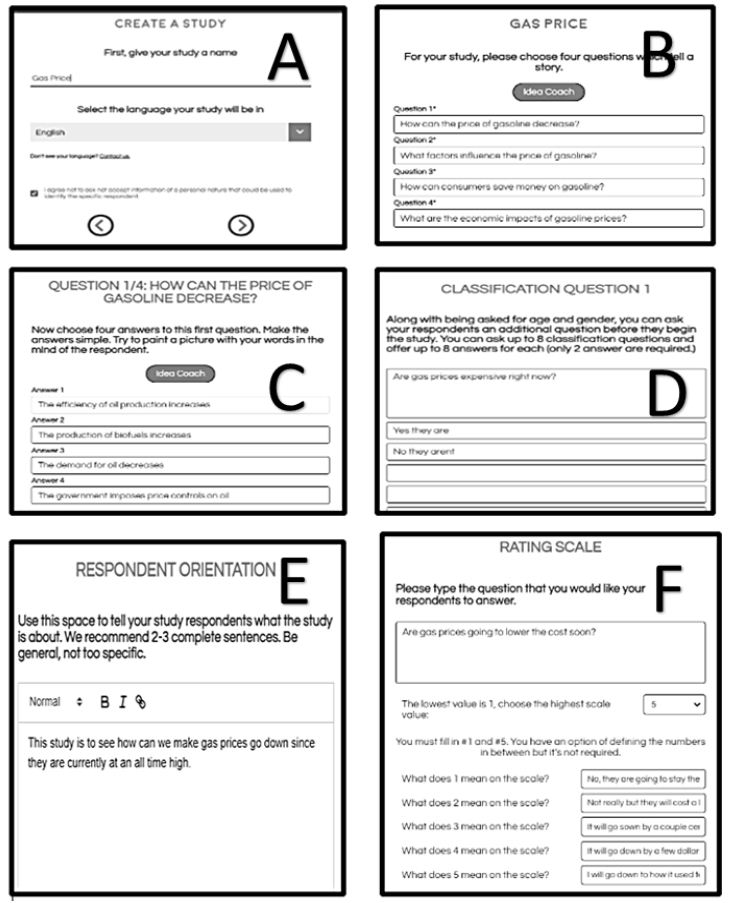
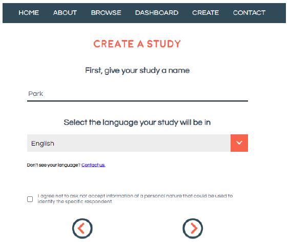
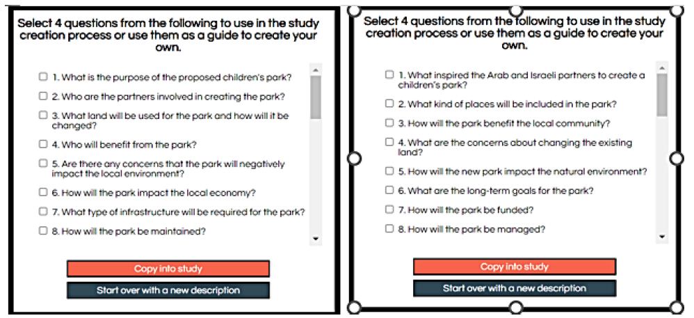
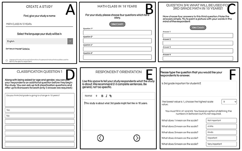
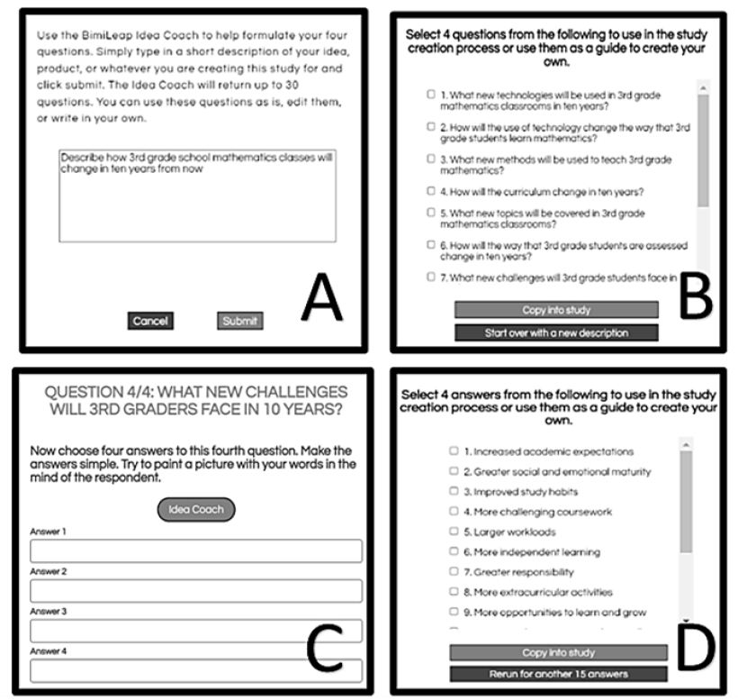
Step 1: Give the Study a Name (Figure 1, Left Panel)

This step may seem vacuous, but it is not. Naming a study forces the researcher to think about the issues. The name of this study reflects that thinking. The effort to name the study ended up producing a simple, non-descriptive name, Study 1, because the author struggled without success to create a shortened name. It is worth noting that the more fundamental studies of Mind Genomics end up being hard to name, and that experienced difficulty in naming a study is itself something to explore. Either one does not know the topic, has not thought deeply about the topic, or perhaps the topic is going into very new areas which are terra incognita and cannot really be encapsulated by a name (Figure 1).

FIG 1

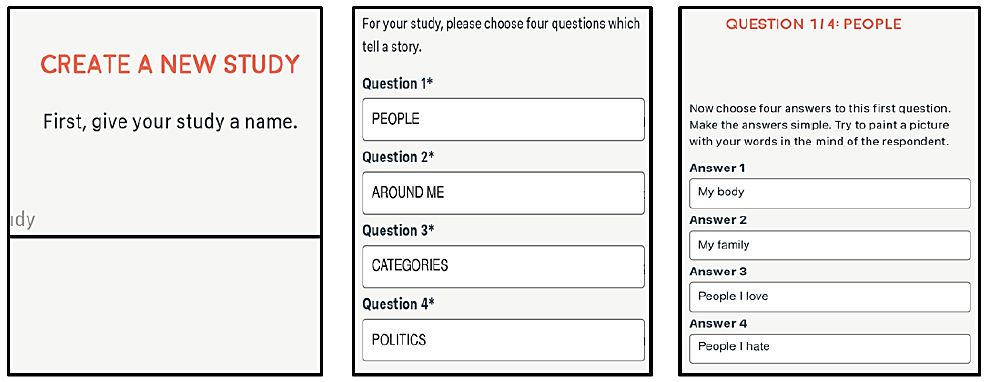
Figure 1: Set up for a Mind Genomics study. Left panel = assign the study a name. Middle panel = provide four questions which tell a story. Right panel = provide four answers to each question.

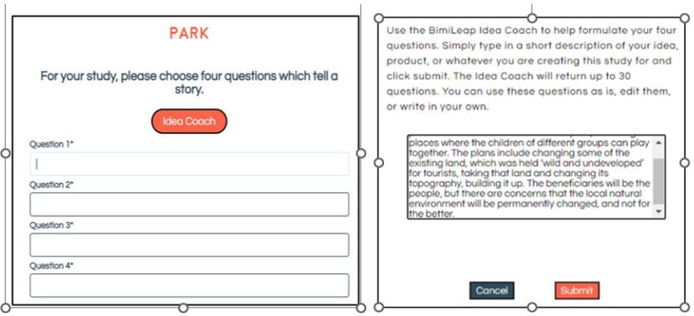
Step 2: Create four questions or topics which are logically connected, or which tell a story (Figure 1, middle panel)

The questions explore different aspects of the topic. The respondent never sees the questions. Rather, the questions are developed by the research (and as of 2023, with the aid of AI), to create the framework of answers The four questions can be considered both a way to guide the researcher, and the abovementioned bookkeeping device, which ensure that two or more answers of the same type (viz., from the same question) never appear in the same vignette. This bookkeeping action will be important when the Mind Genomics process creates vignettes, combinations of answers.

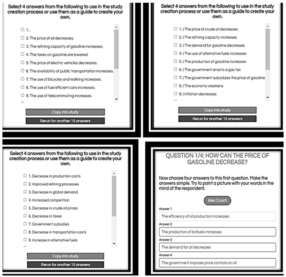
Step 3: For Each Question Provide Four Different Answers (Figure 1, Right Panel)

The answers must address the question. They may be mutually contradictory answers because they will never appear together. Ideally, the answers should consist of phrases rather than single words. The phrases should paint a word picture, if possible. Once the questions are selected the answers are straightforward to create, unless the topic requires technical knowledge. In most cases, however, by the time the researcher has created the four questions, the four sets of answers are easy to develop. The hard thinking has been done already in the act of constructing the questions.

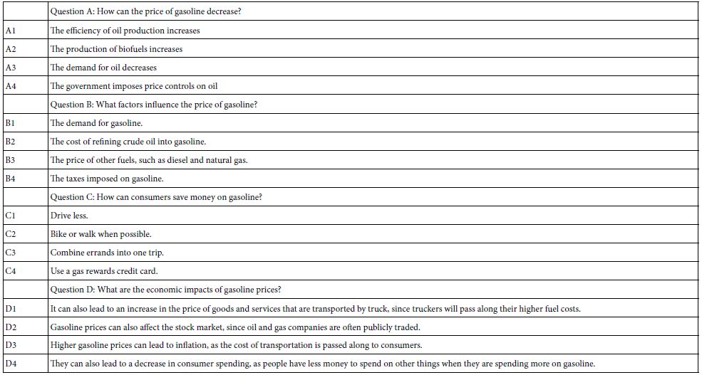
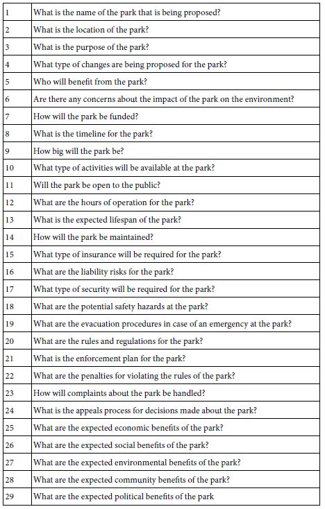
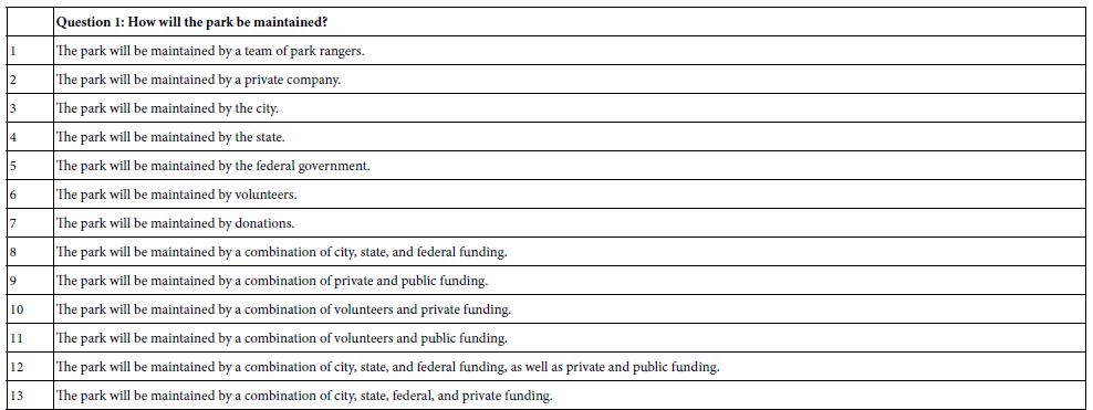
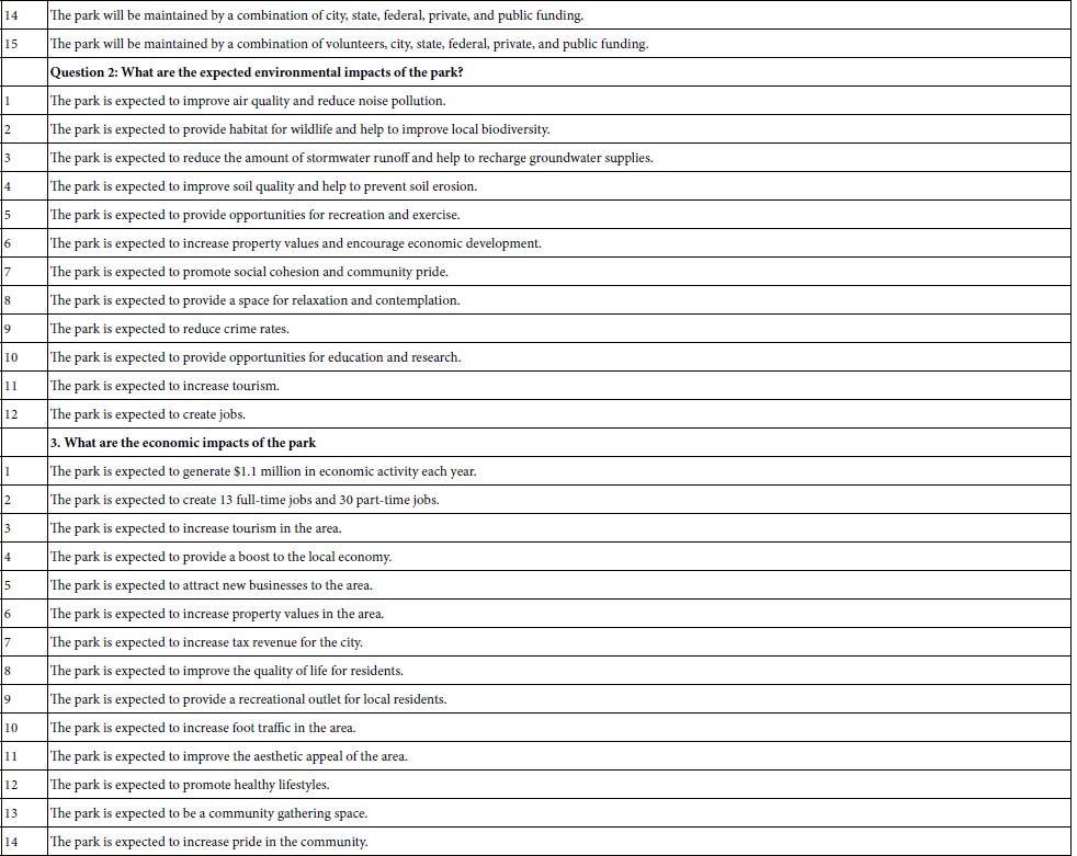
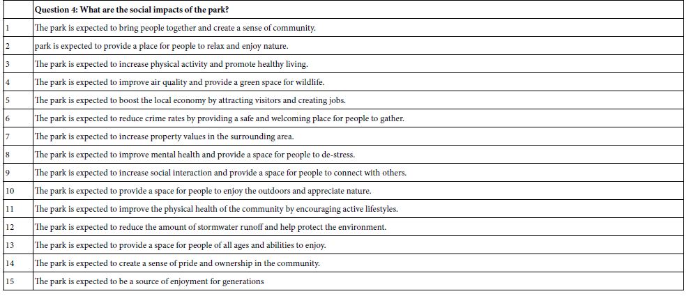
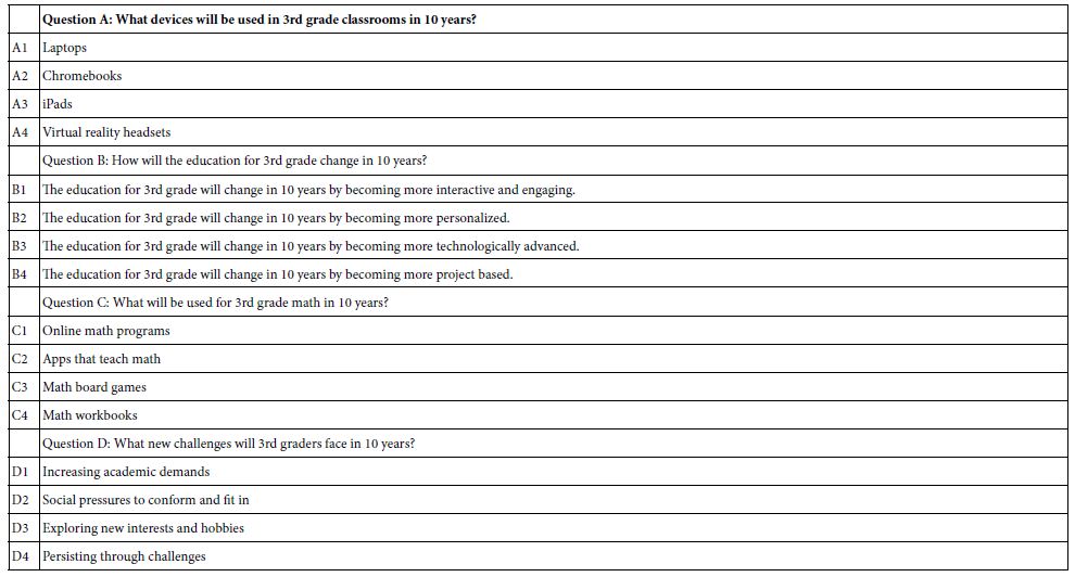
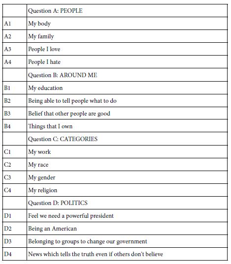
Table 1 presents the questions and the answers. As noted above, the questions are abbreviated phrases rather than full questions. Since the questions are not shown to the respondent the abbreviated format of the questions makes little practical difference to the study itself. The answers are simple phrases which create a word picture, but one of a very general nature. The answers could be refined and particularized should the researcher wish to do so. In this study it was sufficient to put in a general phrase.

Table 1: The four questions (topics), and the four answers (elements) for each question

TAB 1

Step 4: Create Test Vignettes according to an Underlying Experimental Design

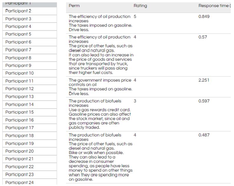
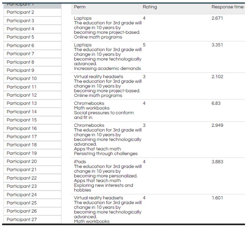
Mind Genomics ‘works’ by creating combinations of elements (messages, answers), testing these combinations (called vignettes) among respondents, and using the combination of experimental design and ratings to create a model or equation showing how each element ‘drives’ a response. Step 4 prescribes the composition of the vignettes. Each respondent ends up testing exactly 24 different vignettes. The experimental design ensures that of elements, so that each vignette comprises a minimum of two elements, a maximum of four elements, and that each question contributes at most one element or answer to a specific vignette. In the end, for each respondent, every element appears exactly five times in 24 elements. Thus, a question contributes 4 (elements) x 5 (appearances per element), viz., contributes to 20 out of 24 vignettes, and does not contribute to four out of 24 vignettes. The 16 elements appear in a statistically independent fashion. Finally, each respondent evaluates a unique set of vignettes, created by permuting the combinations, but keeping the mathematical structure the same. This is called a permuted design [8]. Figure 2 shows a set of vignettes, along with the rating assigned by the respondent, and the response time, defined as the time (in seconds) elapsing between the presentation of the vignette to the respondent and the time that the respondent assigns the rating. Figure 2 comes from a database, created after the study. The actual screen shot of the vignette presented in the study appears Figure 4 (right panel).

FIG 2

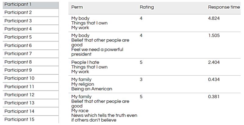
Figure 2: Example of vignettes presented to the respondent, based upon the permuted experimental design.

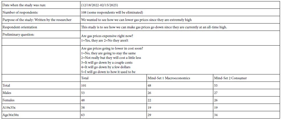
Step 5: Create a Self-profiling Questionnaire (Figure 3, Left Panel)

Social researchers often want to learn more about the people who participate in their studies. To do so, they create what is known as a self-profiling questionnaire, which instructs the respondent to answer certain questions about WHO she/is, what she/he THINKS, what she/he DOES, and so forth. Often this material is used to divide the respondent population into new subgroups, each subgroup studied separately, and the results compared, hopefully revealing relevant group to group differences which knowledge adds to the contribution of the study.

The Mind Genomics program, BimiLeap, is programmed to obtain the gender and age of the respondent in every study, doing so automatically. The researcher can ask an additional 1-8 questions, each question allowing 2-8 answers. The self-profiling questionnaire is completed at the start of the study, before the respondent has read/rated the vignettes. As the third self-profiling questionnaire, BimiLeap instructed the respondent to provide a sense of the respondent’s mental horizon.

FIG 3

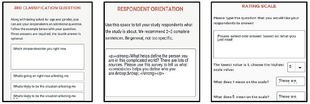
Figure 3: Screen shot of the self-profiling classification question (left panel), the respondent orientation (middle panel), and the rating scale (right panel).

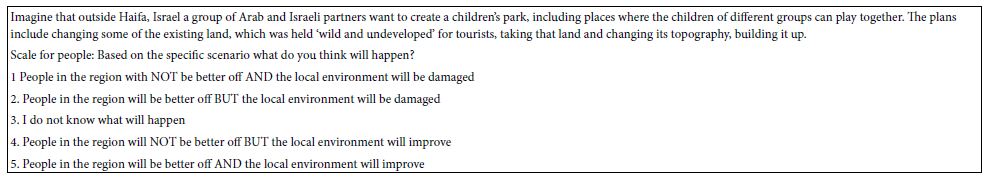
Step 6: Create the Orientation Page

Most respondents coming into a Mind Genomics study do not know what is expected of them. The the act of reading paragraphs of information is well known, but not the somewhat artificial situation of reading lists of messages, 2-4 messages in each list, with no effort to link together the messages into to a coherent whole. The respondent must be introduced to what to do and how to evaluate through an explanation, the ‘orientation.’ Figure 3 (middle panel) shows the orientation for this study.

Step 7: Create the Rating Scale (Figure 3, Right Panel)

The scale is a 5-point scale.

The original aim was to have five different scale points as shown below.

R1=These are NOT important to define both me and NOT to define other people

R2=These are not important to define me but important to define other people

R3=Can’t answer about these

R4=These are important to define only me but not to define other people

R5=These are important to define both me and to define other people

By accident, the word ‘NOT’ was omitted from R1, so that R1 and R5 are the same. Thus, in the analysis we will refer to the two scales as R51, and will merge their data, leaving us with a 4-point scale.

R2=These are not important to define me but important to define other people

R3=Can’t answer about these

R4=These are important to define only me but not to define other people

R5 & R1 (R51)=These are important to define both me and to define other people

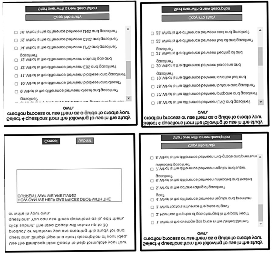
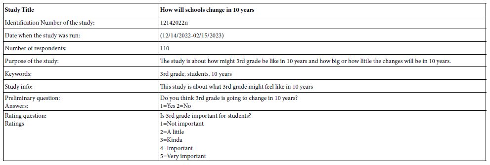
Step 8: Record Final Thoughts about the Project (Figure 4, Left Panel)

This section in the Mind Genomics study is reserved for the research as an ‘aide memoire’ for the study. Quite often studies are run, but the researcher may or may not recall some of the issues involved, or the subtleties recognize at the start of the experiment. The final thoughts serve as a written record of the study.

FIG 4

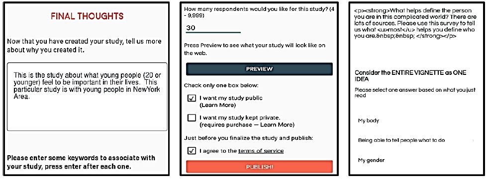
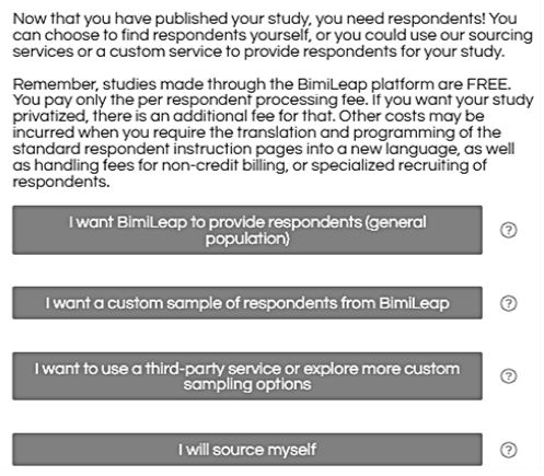
Figure 4: Screen shots showing the requirement for the researcher to describe the study for archival purposes (left panel), the number of respondents to be select, and the request for privatization if desired (middle panel), and an example of how the program is instructed to present a vignette to the respondent (right panel).

Step 9: Select the Number of Respondents, How the Respondents Will Be Chosen, and Whether or Not the Study Results Will Be Made Private (Figure 4, Middle Panel)

The study called for 30 respondents from New York, and 30 respondents from Alabama, ages 16-21. The ingoing hypothesis was that there might emerge big differences in geography, based upon the common belief that the ‘coasts’ generate different ways of thinking from the ‘heartland’ of America, including the less developed south. Alabama was chosen as the state to represent the south, a hypothesized opposite world from New York.

Step 10: Invite the Respondents to Participate, have Them Go Through the Self-profiling Classification, Read the Orientation and then Evaluate 24 Vignettes

Figure 4 (right panel) shows an example of a vignette as the respondent might see it on the screen of a smartphone. The screen shot shows the text with the information that the BimiLeap program uses to adjust the font. In the actual experiment the instructions at the top are shown in simple text format without the formatting instructions used by BimiLeap.

The respondents are invited to participate by a local field service or provided by the researcher. Experience of over 40 years suggests that it is best to work with specialists who can recruit respondents to participate. Rather than saving money by depending upon the good will of a person to participate, it almost always proves more beneficial to incentivize the respondent, and to work with a the specialty company which delivers respondents eager to participate. The study presented here took about 45 minutes to complete, after launching, with the respondents recruited by Luc.id Inc., the specialty company. Lucid contracts with field services worldwide to direct panelists to a study, efficiency far greater than realized any other way. Furthermore, Luc.id itself is only one of a growing number of companies specializing in providing respondents for the on-line studies.

Step 11: Create a Database for the Study, Similar in Form to an Excel File

Each respondent generates 24 rows of data, one row for each of the 24 vignettes.

a. Column 1=study name

b. Column 2=panelist identification number (later recoded, when multiple studies are combined into a single database

c. Column 3 and 4 – gender and age of the respondent

d. Column 5 and 6 – state where the respondent lives and answers how the respondent feels.

e. Column 7 Test order of vignette (01-24).

f. Column 8 – 23 Reserved for the structure of the vignette. Each column of the 16 columns is reserved for one of the 16 elements. A ‘1’ in the cell means that the element is present in that vignette. A ‘0’ in the cell means that the element is absent from that vignette.

g. Column 24 – The rating assigned to the vignette on the 5-point scale.

h. Column 25 – The response time for the specific vignette.

i. Note that Columns 1-6 are repeated 24 times, once for each of the 24 vignettes evaluated by the respondent. The information does not change.

Afterwards, create five new variables, which are binary transformations based upon the rating to the vignette assigned by the respondent:

a. R2=100 when the rating is 2, otherwise R2=0 (when the rating is not 2).

b. R3=100 when the rating is 3, otherwise R3=0.

c. R4=100 when the rating is 4, otherwise R4=0.

d. R51=100 when the rating is either 1 or 5, otherwise R51=0. This transformation codes those responses where the respondent feels that she/he is the same as others.

e. R42=100 when the rating is either 4 or 2, otherwise R42=0. This transformation codes those responses where the respondent feels that she/he differs from others.

f. To each of the newly created binary transformed variables add a vanishingly small random number (<10-5), to ensure that there will be some minimum level of variation in the binary transformed variable. That minimum level of variation ensures that the binary transformed variable will allow the regression analysis. Regression analysis fails when the dependent variable has no variation (when are the ratings are the same, e.g., R51 is all 0’s or all 100’s).

Step 12: Create Models (Equations) Which Relate the Presence/Absence of Elements to Ratings

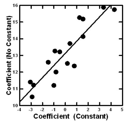
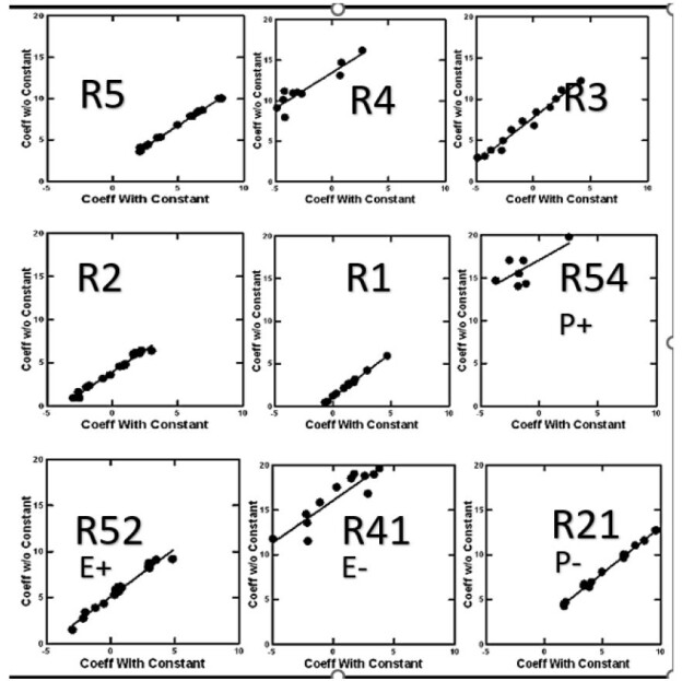
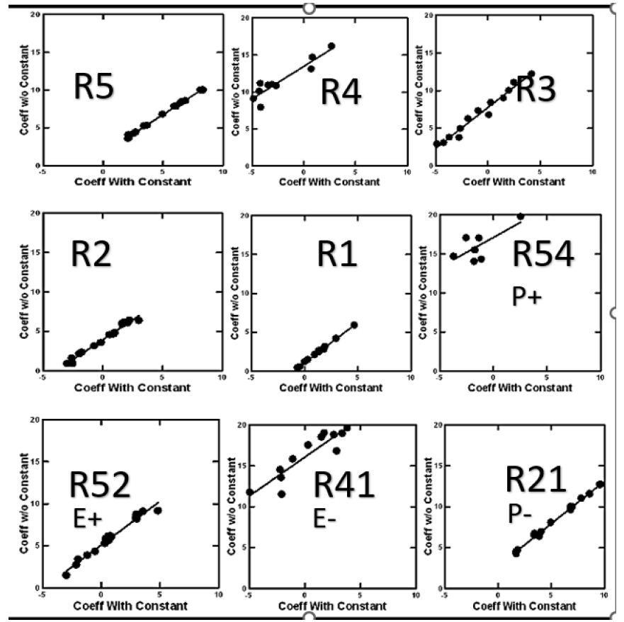
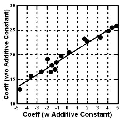
By creating the vignettes according to a permuted design, the researcher makes it possible to use statistical methods to deconstruct the rating into the contributions of the 16 elements. The most common method is OLS (ordinary least-squares) regression. The equation is expressed as: DV (Dependent variable, viz. The binary transformed rating)=k1(A1) + k2(A2) … k16(A16). The equation is estimated without an additive constant. Estimating the equation with an additive constant will generate a high correlated set of 16 coefficient, but the coefficients estimated without the additive constant will be systematically higher than the same coefficients estimated with an additive constant. It becomes easier to understand the ‘meaning’ of the coefficients without using an additive constant. The equation can be created either at the level of the Total Panel (all respondents), at the level of a self-defined subgroup (e.g., age, gender, response to the self-profiling classification), or at the level of the individual respondent.

Step 13: Retain Strong Performing Element by Key Self-defined Subgroup, Based on R51 (Like Me)

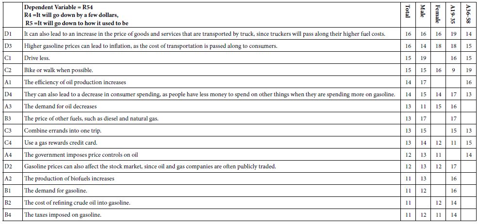
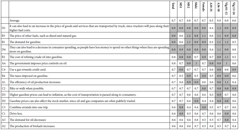
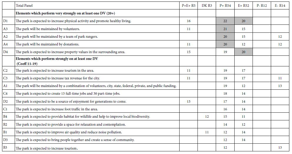
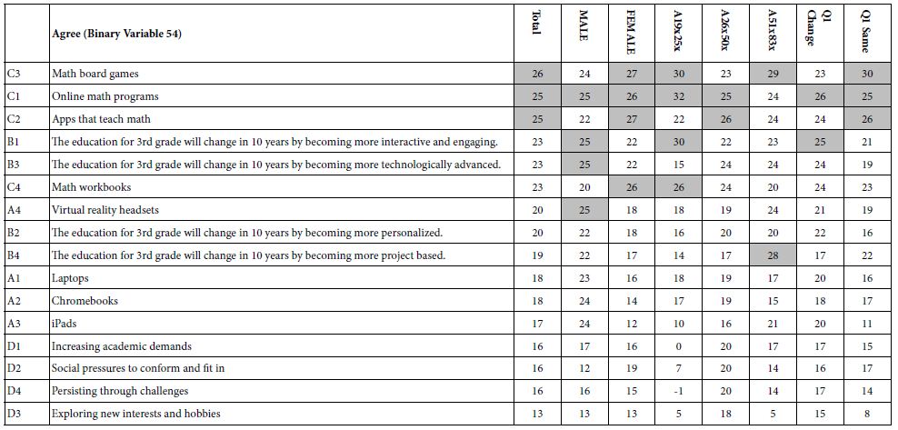
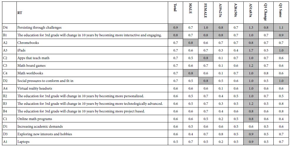
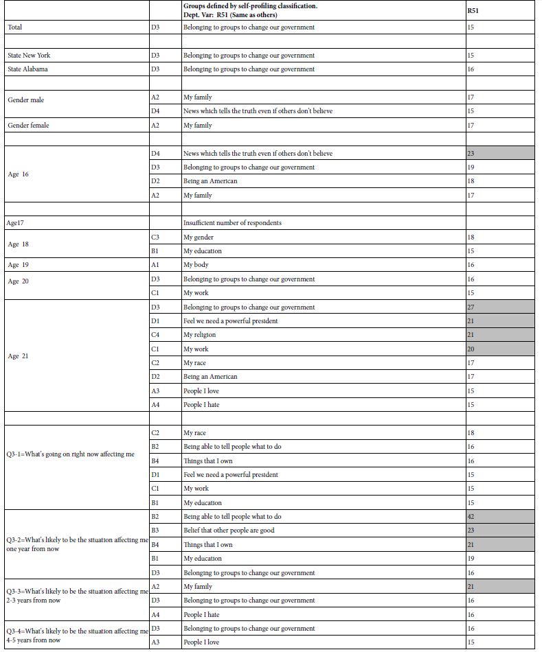
Mind Genomics studies comprising coefficients for 16 elements by many groups returns a great deal of data from even the simplest analysis. All too often the plethora of coefficients obscures important patterns which exist in the data, but simply fail to be detected, the signal masked by the noise. It is often best to eliminate the weaker performing elements, suppressing the noise, to let the signal through. For this analysis and for the subsequent analyses, we eliminate all coefficients 14 or lower. These elements may be relevant, but with enough of these weaker scoring elements retained in the data, the pattern fails to emerge. Table 2 shows the strong elements for each group. Even with the effort to prune out weaker performing elements it becomes clear from Table 2 that no strong patterns are to be discerned.

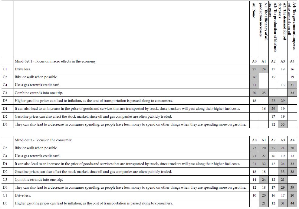
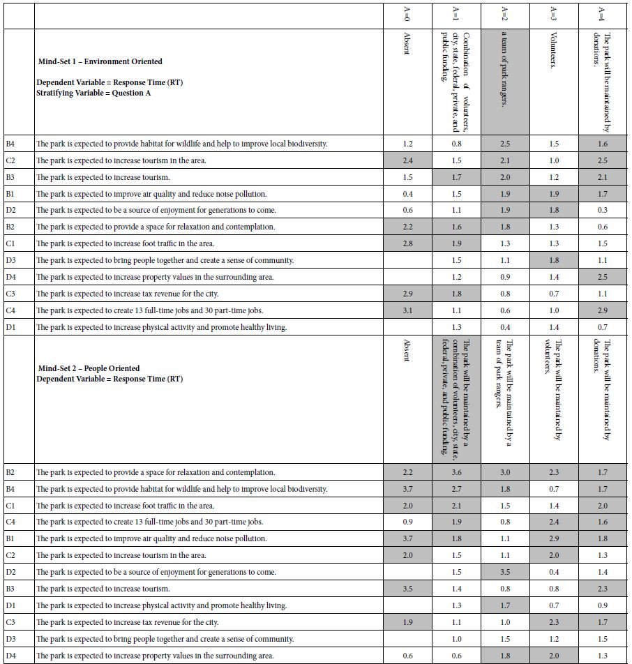
Table 2: Strong performing elements describing WHO I AM (R51 as the dependent variable). The respondents are self-defined by who they ARE, and by what occupies their mind when THINKING ABOUT THE FUTURE. Very strong performing elements (coefficients of 20 or higher) are shown in shaded cells.

TAB 2

Step 14: Identify New to the World Mind-sets by Creating Individual-level Models & Clustering

The permuted design used by Mind Genomics ensures that each respondent evaluates a different set of 24 vignettes, but with each respondent evaluating the exact right set of vignettes to generate an equation for that respondent. The individual-level model thus enables the researcher to create a database of coefficients for the different respondents, and use the patterns generated by the coefficients to create or discover a limited number of patterns that can be interpreted.

We will use two dependent variables, R51 (same as me), and R42 (different from me). We can create these equations because we set up the 24 vignettes for each respondent by experiment design, and because we added a vanishingly small number to the value of R51 and another vanishingly small number of the value of R42. We create these two groups of coefficients because we do not know whether we will be success. We don’t know how young people think. Do they think in terms of ‘like me,’ or in terms of ‘different from me.’

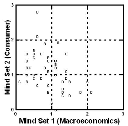
The data processing is the same for each group, the first group with R51 as the dependent variable, the second group with R42 as the dependent variable. Clustering is a well-accepted procedure in exploratory statistics to identify groups [9]. The computation is done without considering the ‘meaning’ of the clusters, but rather simply use the clustering procedure in an ‘automatic’ fashion, and only later try to name the clusters. The emergent clusters may be considered to be different, interpretable regions of what really ends up being a ‘cloud.’ That is, the emergent clusters may not really exist as hard and fast, totally separable groups. This is some ‘wiggle room’ at the borders of the clusters. Nonetheless, clustering is a good way to get a sense of the nature of the dependent variable by identifying a small number of different levels/examples of the dependent variables.

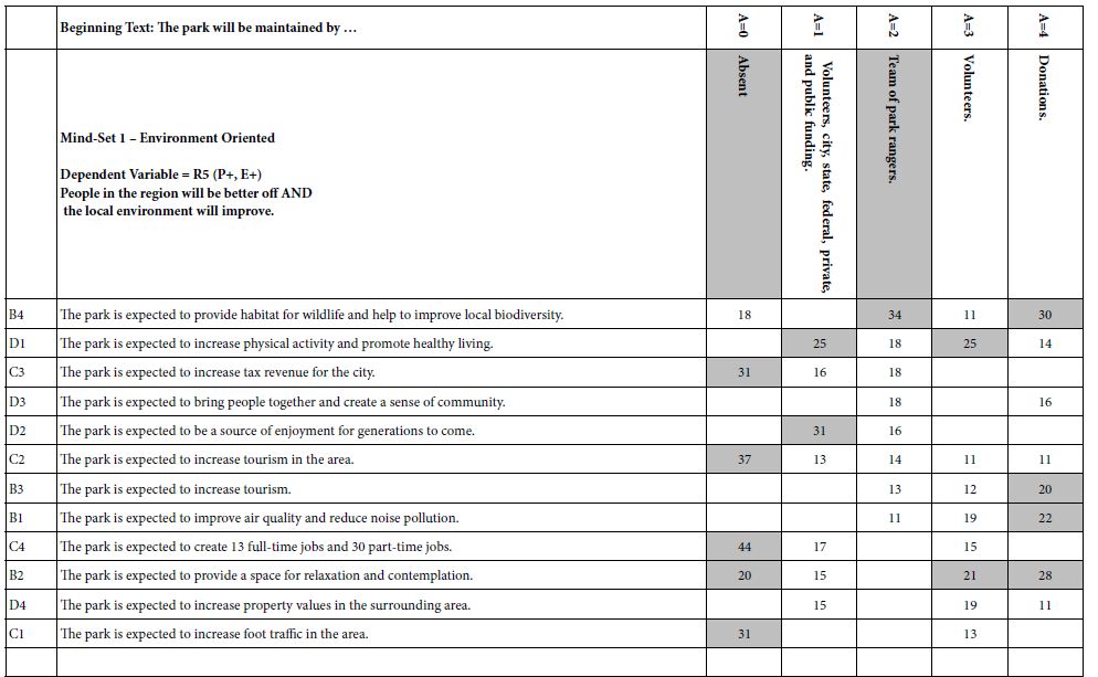
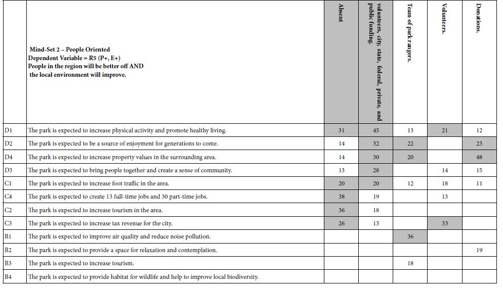
Step 15: Discover Mind-based Upon Strong Performing Elements

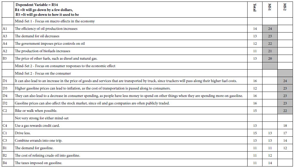
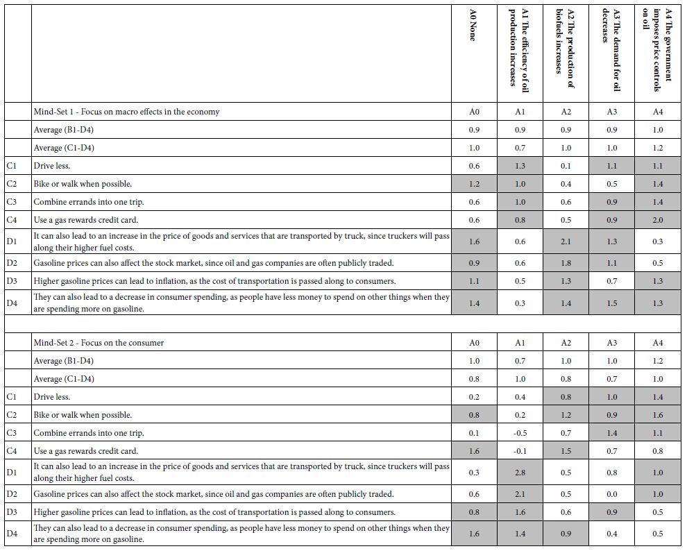
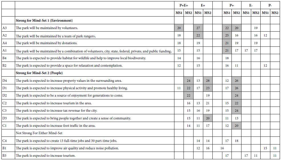
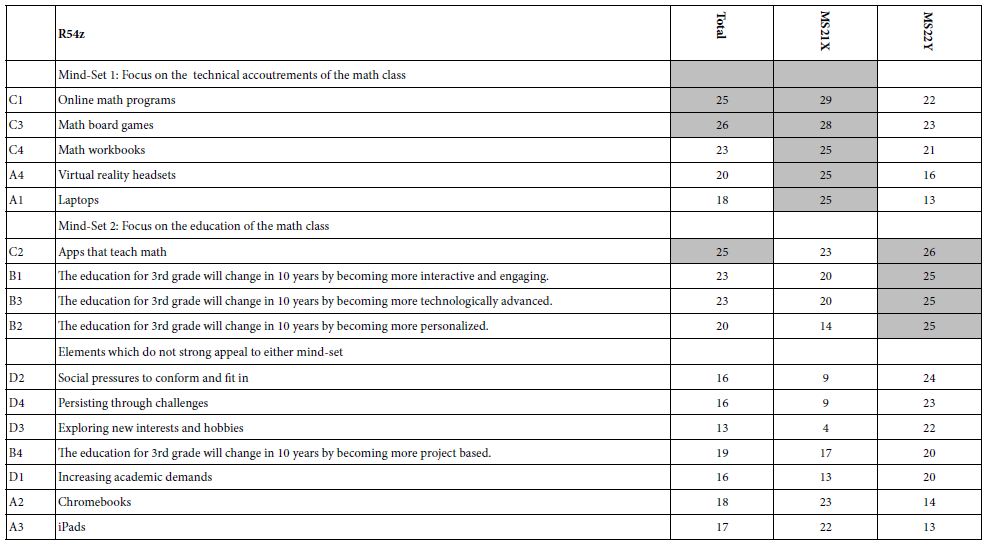
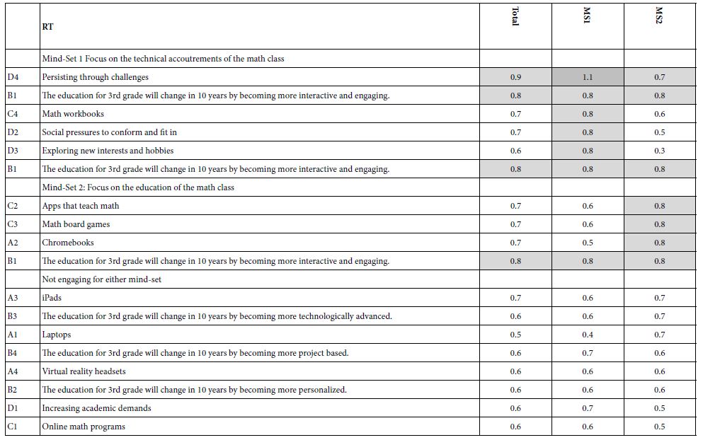
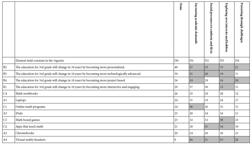
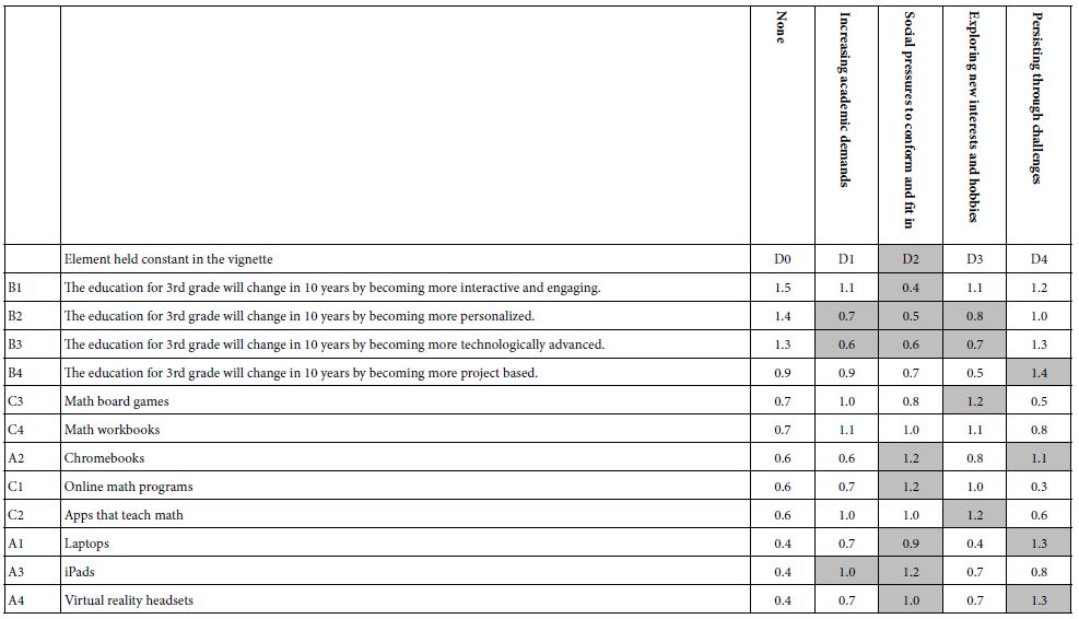
Table 3A shows the emergence of two seemingly hard-to-interpret clusters (mind-sets) based upon clustering using R51 (Like Me). Table 3B shows the emergence of three easier-to-interpret clusters based upon clustering using R42 (Not Like Me). Table 4 shows the base sizes of the mind-sets based upon Total Panel as well as the mind-set emerging from using R54 (Different From Me) as the dependent variable.

Table 3: Very Strong performing elements emerging when the respondents are segmented based on R51 (Same as Me) versus segmented based on R42 (Different From Me).

TAB 3

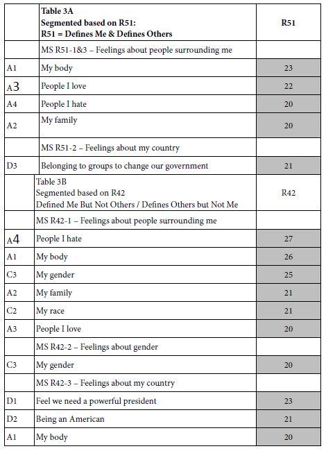
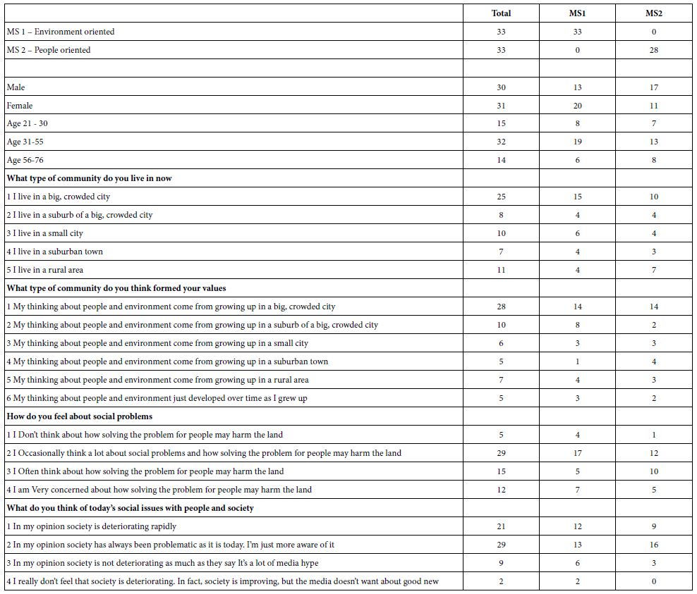
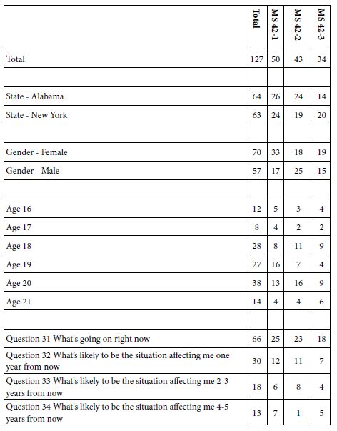
Table 4: Base size of respondents for Total Panel and the three mind-sets emerging from using R42 (Different From Me) as the dependent variable in the individual-level regression modeling.

TAB 4

Discussion and Conclusions

The study presented here breaks new ground in the application of Mind Genomics to the development of the person. Traditionally, Mind Genomics has been used to understand how people respond to external stimuli, such as products, or more recently student expectations of what 3rd grade mathematics will be like in the years to come (Mendoza et. al., 2023). Mind Genomics has explored people in society, and the mind of the juror evaluating facts of a case [10-12].

With this paper Mind Genomics is moving into a new area, the study of how young people think about themselves. Rather than asking the respondent to introspect or rather than having an expert assess the individual based upon the expert’s experience and training, Mind Genomics approach works with the person evaluating her or his reaction to an ambiguous statement, a metaphor. Rather than asking the respondent to describe how she or he defines himself, the ‘production’ approach of psychology, we present the respondent with combinations of metaphors, such as family, work, etc. All we require the respondent to do is assign the combination to one of four groups, the four answers. It is impossible for the respondent to ‘game the system’, or to ‘freeze up’. Tables 3B shows that despite this seemingly to-respondent meaningful to these sets of 24 different combinations, the results appear to make sense, and give insight into the nature of the way the respondent thinks.

If we were to the future for new directions, perhaps the best result from this study is the infusion of a new way of experimenting with the already well-trod field of metaphors as tools to understand psychological processes. Just a few references should suffice to show the scope of what has been done, both in understanding the young person’s trip into maturity [13,14], as well as understand a person’s mind through a new lens [15-17]. Add to that the power of experimentation through Mind Genomics and we may be at the threshold of a new direction for psychology, coupling a deep study of the mind and experimentation using metaphors.

References

  1. Mendoza C, Mendoza C, Deitel Y, Rappaport SD, Moskowitz HR (2023) Empowering young researchers through Mind Genomics: What will third grade mathematics look like in 10 years? Psychology Journal, Research Open 5: 1-15.
  2. Porretta S, Gere A, Radványi D, Moskowitz H (2019) Mind Genomics (Conjoint Analysis): The new concept research in the analysis of consumer behaviour and choice. Trends in Food Science & Technology 84: 29-33.
  3. Stevens SS (1975) Psychophysics: Introduction to Its Perceptual, Neural and Social Prospects. John Wiley & Sons.
  4. Craven BD, Islam SM (2011) Ordinary least-squares regression. The SAGE Dictionary of Quantitative Management Research 224-228.
  5. Easterling RG (2015) Fundamentals of Statistical Experimental Design and Analysis. John Wiley & Sons.
  6. Moskowitz HR, Gofman A, Beckley J, Ashman H (2006) Founding a new science: Mind genomics. Journal of Sensory Studies 21: 266-307.
  7. Moskowitz HR, Gofman A, Lieberman LE, Ray I, Onufrey SR (2011) Sequencing the genome of the customer mind by RDE and intervention testing. Journal of Academic and Business Ethics 3: 4-14.
  8. Gofman A, Moskowitz H (2010) Isomorphic permuted experimental designs and their application in conjoint analysis. Journal of Sensory Studies 25: 127-145.
  9. Likas A, Vlassis N, Verbeek JJ (2003) The global k-means clustering algorithm. Pattern Recognition 36: 451-461.
  10. Green PE, Srinivasan V (1990) Conjoint analysis in marketing: new developments with implications for research and practice. Journal of Marketing 54: 3-19.
  11. Moskowitz H, Kover A, Papajorgji P. eds., (2022) Applying Mind Genomics to Social Sciences. IGI Global.
  12. Moskowitz HR, Wren J, Papajorgji P (2020) Mind Genomics and the Law. LAP LAMBERT Academic Publishing.
  13. Evans K, Furlong A (2019) Metaphors of youth transitions: niches, pathways, trajectories, or navigations. In Youth, Citizenship and Social Change in a European Context. Routledge 17-41.
  14. Wyn J, Lantz S, Harris A (2012) Beyond the ‘transitions’ metaphor: Family relations and young people in late modernity. Journal of Sociology 48: 3-22.
  15. Barker P (1992) Using metaphors in psychotherapy. Psychology Press.
  16. Kopp RR (1995) Metaphor Therapy: Using Client-Generated Metaphors in Psychotherapy. Psychology Press.
  17. Tay D (2017) Exploring the metaphor-body-psychotherapy relationship. Metaphor and Symbol 32: 178-191.
fig

Aqueous Nasal Spray in Treatment of Rhinitis and Rhinosinusitis: Adverse Event Focusing on Epistaxis

DOI: 10.31038/JCRM.2023612

Abstract

Introduction: Rhinitis and rhinosinusitis are common in the general population and Intranasal corticosteroid (INCS) sprays are generally safe and effective in the treatment of these conditions. However, they are often burdened by side effects that can reduce compliance with therapy, one of the most common of which is epistaxis.

Objective: To review the current literature about the most common adverse events of beclometasone dipropionato aqueous nasal sprays therapy in chronic rhinosinusitis and allergic rhinitis, focusing on epistaxis.

Material and Methods: Using different search engines, the most common adverse events were reviewed and a total of 64 full-length articles were examined for eligibility. After applying inclusion and exclusion criteria, a total of 2 articles were reviewed.

Results: BDP is counted among the group of INCS with the lowest frequency of epistaxis reported as a side effect in the studies analyzed.

Conclusion: BDP aqueous nasal spray is one of the most frequently prescribed INC for rhinitis and rhinosinusitis, with a low frequency of epistaxis. The otolaryngologist and the general physicians should therefore consider prescribing this active principle, particularly to a target group of patients at increased risk of epistaxis.

Introduction

INCS are supported by level-1 evidence for medical management of numerous chronic nasal diseases such allergic rhinitis (AR) and chronic rhinosinusitis (CRS) reducing airway inflammation and improving symptom control [1]. The ability to undergo multiple formulations, such as nasal sprays, aerosols, dry powder inhalers, and ointments means that they can deliver a powerful local anti-inflammatory effect [2].

The intranasal administration of drugs, used for many centuries, has been increasing widespread in recent years, both due to the availability of molecules with specific activity on the airways and the numerous technological innovations that have increased the efficiency of devices available in clinical practice.

The success of inflammatory disease management with intranasal medications depends on the activity of the drug, its pharmacokinetic and pharmacodynamic properties [2]. However, the clinical efficacy of topic INCS is conditioned by some limitations related to possible side effects, due to the bioavailability of the drug. For INCS, these adverse events (AEs) are certainly less frequent and less serious than those observed with oral steroids, but they can considerably limit adherence to treatment, especially in pediatric patients, adolescents and the elderly [3]. The most common AE of INCS treatment is epistaxis [4]. Regardless of the cause, epistaxis is a common emergency encountered by primary care physicians. Up to 60% of the general population experience epistaxis, and 6% seek medical attention for it [5]. Possible causes are factors that damage the lining of the nasal mucosa, affect the walls of the vessels or alter the coagulability of the blood and related drugs such as nasal steroids [6].

Among the various molecules available for the treatment of CRS and AR, beclometasone dipropionato aqueous (BDP) nasal spray represents a possible “first choice”, since this molecule has an excellent efficacy and safety profile boasting decades of use experience [7]. The potential drug interaction risk of beclomethasone dipropionate is low as the drug has limited systemic bioavailability: Paul H. et al. confirmed this showing lower systemic exposure with intranasal administration than with oral inhalation [8]. Patients with nasal chronic inflammatory diseases often require long-term strategies to control symptoms: although the efficacy and safety of INCs are well established, concerns remain regarding systemic AEs including epistaxis, headache, anosmia, ageusia/dysgeusia, among others [9]. The aim of this review is to evaluate the BDP nasal spray adverse event reported in the literature, focusing on epistaxis.

Materials and Methods

To evaluate the studies that analyzed epistaxis as a side effect of BDP in the treatment of inflammatory sinonasal disease, a Pubmed research was conducted searching for articles written by 2010 and 2022, exclusively in English language, including randomized clinical trials, cohort studies, meta-analyses, case reports, and case series and excluding non- English studies, abstract and articles about non nasal Inhalation corticosteroids.

Search criteria included all occurrences of the following terms in the title or abstract: beclometasone dipropionato aqueous; one between “epistaxis”, “adverse event”, “adverse effect” and “complications”.

The corresponding results in the literature dating back to the last 10 years were examined for eligibility and 64 articles were identified: 53 articles were assessed for eligibility. Finally, after applying the above-mentioned inclusion/exclusion criteria, 2 reviews were analyzed [9,10].

fig

Results

The first article analyzed was published by Salma Ahsanuddin and addressed the Proportional Reporting Ratios (PRR) and Reporting Odds Ratios (ROR) for different AEs related to different drugs used to treat CRS and AR, referring to the “Adverse Event Food and Drug Administration Reporting System” and evaluating the relationship between AEs and 10 different INCSs.

BDP nasal spray collocates in the group with least adverse event, accounting for only 1,4% of the total AEs founded, contrary to Fluticasone Propionate and Mometasone, which instead represented the majority of the side effects identified in the analysis, representing 47,7% and 16,7% of total AEs, respectively.

Epistaxis was listed among the top 300 AE for each medication studied together with headache.

The PRR value for epistaxis of the INCs analyzed ranged from 1 to 27,2, with an average value of 4,64: the PRR value of epistaxis due to BDP was 1,5.

Similarly, the ROR value for epistaxis ranged from 1 to 30.8, with an average value of 5: the ROR value of epistaxis due to BDP was 1,5 (Table 1, modified).

Table 1: Intranasal corticosteroid Spray and Reported Epistaxis in FAERS

Corticosteroid

N. patients

PRR (95%CI)

ROR (95% CI)

Fluticasone propionate 50 mcg

578

2.88 (2.65, 3.12)

2.90(2.67, 3.15)

Fluticasone propionate 90 mcg

211

4.66 (4.08, 5.33)

4.73(4.13, 5.42)

Mometasone

142

2.02 (1.72, 2.38)

2.03(1.72, 2.39)

Budesonide

81

1.55 (1.25, 1.93)

1.56(1.25, 1.94)

Triamcinolone

42

1.32 (0.98, 1.79)

1.33(0.98, 1.79)

Fluticasone furoate

15

27.24(16.93,43.82)

30.76(18.54,51.03)

Beclometasone dipropionato

9

1.49(0.78, 2.87)

1.50(0.78, 2.88)

From: Adverse Events Associated with Intranasal Sprays: An Analysis of the Food and Drug Administration Database and Literature Review. Ahsanuddin S et al. 2021.

The second study analyzed was written by Wu EL et al and identified randomized control trials of INCs for treatment of AR that reported incidence of epistaxis: 72 articles with 82 distinct INCS-versus-placebo comparisons were included for meta-analysis.

For all the included comparisons, the meta-analysis demonstrated an overall risk ratio of 1.48 (95% CI, 1.32-1.67) for epistaxis.

In the studies analyzed, the INCSs associated with an increased risk of epistaxis after comparison with placebo were beclomethasone HFA, fluticasone furoate, mometasone furoate, and fluticasone propionate, while patients treated with BDP, ciclesonide HFA, and ciclesonide aqueous did not shown an elevated risk of epistaxis compared to patients treated with placebo (Table 2, modified).

Table 2: INCS-Related Epistaxis: Meta-analyses


Studies in Review, n

Epistaxis


INCS

Quantitative (82)

RR (1,48)

95% CI (1.32-1.67)

P value (<.001)

Beclomethasone HFA

6

2,35

1,06-5,20

.03

Fluticasone furoato

15

1,85

1,46-2,34

>.001

Mometasone furoato

14

1,48

1,06-2,07

.02

Fluticasone propionato

17

1,36

1,00-1,85

.05

Ciclesonide HFA

4

1,26

0.87-1.83

.22

Beclomethasone acqueous

8

1,24

0,84-1,81

.28

Ciclesonide acqueous

10

1,16

0,83-1,62

.39

Budesonide

5

2,49

0,91-6,79

.07

Triamcinolone

3

1,87

0,16-22,88

.62

Flunisolide

0

N/A

N/A

N/A

From: Epistaxis Risk Associated with Intranasal Corticosteroid Sprays: A Systematic Review and Meta-analysis. Wu EL et al. 2019.

Discussion

The most frequent adverse events in the treatment of AR and rhinosinusitis in the literature are revealed to be due to intranasal antihistamines and intranasal steroids, even if these AEs seem well tolerated. Many articles in literature report that epistaxis is the most frequent AEs following intranasal corticosteroids therapy. Epistaxis, while often minor and self-limiting, can result in lack of medication compliance, leading to patient and provider’s frustration resulting in additional procedures, medications, or ineffective treatments [11]. The possible causes are to be found among the thinning of the mucosa due to the vasoconstrictor effect or the direct trauma to the tip of the applicator at the level of the Kiesselbach’s plexus [9].

Conclusions

Intranasal corticosteroids are accepted as a safe and effective first line therapy for allergic rhinitis and rhinosinusitis [12,13], improving to decrease comorbidities and costs. Studies in literature have shown that satisfaction and comfort with an intranasal treatment device are likely to enhance adherence to that treatment among patients with AR and rhinosinusitis. Therapeutic compliance of these drugs depends on several factors, among which there are odor, taste, comfort of delivery, delivery devices (aerosol versus aqueous), patient cost [14] and the possible side effect such as epistaxis, headache, anosmia, ageusia/dysgeusia [9,15]. Waddell AN et al analyzed 16 randomized controlled trials which compared the efficacy of INCs and oral antihistamines in the treatment of allergic rhinitis, and found and incidence of epistaxis due to INCs between 17% and 23% versus an appreciable rate of placebo spray between 10% to 15% [16]. As pointed out by Wu E L, prescribers should be aware of which INCSs may place patients at a higher risk for epistaxis, and they should consider selecting an INCS with a lower risk of this side effect for patients with recurrent or persistent nose bleeding [10]. Only a few articles analyzed the frequency of epistaxis due to BDP, and agree that BDP is among the INCs who cause epistaxis less frequently.

In conclusion, patients with allergic rhinitis and rhinosinusitis represent a high portion of the population and they must chronically continue topical therapy to have optimal symptom control. Since epistaxis is one of the most common side effects of INCs, the otolaryngologist and the general physicians should consider those active principles that are least related to epistaxis, such as BDP.

References

  1. Eugenio De Corso, Pipolo C, Cantone E, Ottaviano G, Gallo S, et al. (2022) Survey on Use of Local and Systemic Corticosteroids in the Management of Chronic Rhinosinusitis with Nasal Polyps: Identification of Unmet Clinical Needs. Identification of Unmet Clinical Needs. J Pers Med 12: 897. [crossref]
  2. Peter J (2014) Barnes Glucocorticoids History of Allergy. Chem Immunol Allergy 100: 311-316. [crossref]
  3. Carlo C, Giovanni AR (2017) Efficacy and safety of beclomethasone dipropionate Suppl. Recenti Prog Med 108: S1-S11.
  4. Corren J (1999) Intranasal corticosteroids for allergic rhinitis: how do different agents compare? J Allergy Clin Immunol 104: S144-9. [crossref]
  5. Womack JP, Kropa J, Stabile MJ (2018) Epistaxis: Outpatient Management. Am Fam Physician 98: 240-245. [crossref]
  6. Paul M (2004) Epistaxis Emerg Med Australas 16: 428-440.
  7. James Fowler, Brian W Rotenberg, Leigh J Sowerby (2021) The subtle nuances of intranasal corticosteroids. Journal of Otolaryngology – Head and Neck Surgery 50: 18. [crossref]
  8. Paul HR, Melchior A, Dunbar SA, Tantry SK, Dorinsky PM (2012) Pharmacokinetic Profile of Beclomethasone Dipropionate Hydrofluoroalkane after Intranasal Administration Versus Oral Inhalation in Healthy Subjects: Results of a Single-Dose Randomized, Open-Label, 3-Period Crossover Study. Clinical Therapeutics 4: 1422-1431. [crossref]
  9. Ahsanuddin S, Povolotskiy R, Tayyab R, Nasser W, Barinsky GL, et al. (2021) Adverse Events Associated with Intranasal Sprays: An Analysis of the Food and Drug Administration Database and Literature Review. Ann Otol Rhinol Laryngol 130: 1292-1301. [crossref]
  10. Wu EL, Harris WC, Babcock CM, Alexander BH, Riley CA, et al. (2019) Epistaxis Risk Associated with Intranasal Corticosteroid Sprays: A Systematic Review and Meta-analysis. Otolaryngol Head Neck Surg 161: 18-27. [crossref]
  11. Bridgeman MB (2017) Overcoming barriers to intranasal corticosteroid use in patients with uncontrolled allergic rhinitis. Integr Pharm Res Pract 6: 109-119. [crossref]
  12. EPOS 2020
  13. Management of allergic rhinitis and its impact on asthma. ARIA guidelines, 2019.
  14. Sher ER, Ross JA (2014) Intranasal corticosteroids: the role of patient preference and satisfaction. Allergy Asthma Proc 35: 24-33. [crossref]
  15. Eli O Meltzer, Greg W, Bensch, William W Storms (2014) New intranasal formulations for the treatment of allergic rhinitis. Allergy Asthma Proc 35: S11-S19. [crossref]
  16. Waddell AN, Patel SK, Toma AG, Maw AR (2003) Intranasal steroid sprays in the treatment of rhinitis: is one better than another? J Laryngol Otol 117: 843-855. [crossref]

Solitude Approach in the Digital Era

DOI: 10.31038/IJNM.2023413


Human entrance into a natural world evolves through an end facing next to something neither perceptible nor elucidated, as for all animate and inanimate surroundings. Sex difference ensures the individual’s continuation in a natural, audible, visible world. Love brings humans together, and a common interest or concern unifies them. More people join in matrimony, others remain allied without the official marriage document, or different amalgamated groups prefer physical and mental relations. Love remains a passionate attraction and a desire for someone, which can start a romantic relationship. A child develops in a climate offered by his biological parents, surrogate mother, or adoptive parents, with or without being relatives. No one can replace biological parents. Usually, their substitutes offer excessive affection, but sometimes it may be disapprovingly and adversely working. Biological parents recognize themselves as a part of their child’s thinking, action, and construction and readily accept and correct possible child’s genetic errors or mistakes. Still, the feelings of adoptive parents in such circumstances generate various effects that dissatisfy over a prolonged period. The child grows up; scientific, cultural, and social development depends on genetics, environmental characteristics, social networking, financial power, and ventures.
 

Human love is changeable over time; initial attraction and passion then convey affection for the child or nephew, making some parents feel differently. Many people experience loneliness sooner or later, even in their family, since diverse circumstances and various disorders modify the individual judgment. The deceptive ambiance and the impression of illusory feelings produce suffering in the heart and affect mental health. Pondering thoughts’ power to improve life quality and expectancy is necessary. In the digital era, no one can be alone. Other attractions can act concurrently through a bright existence. IT advancement put forward ideas of allure for choice. There is a variety of programs available online with the opportunity to watch on-demand-communications for fervour, relaxation, or instruction; instant connection with selected people, discussions, lectures of interest, movies, celeb paintings, games, and chosen musical programs according to personal preferences make an individual absorbed by other facts and the time to come back to the gloom-generating blue devils decreases. Another competitor for relaxing and improving well-being is walking. Nature expresses perfect creation; its soundness and colour harmony charm the individual. He takes great pleasure in watching the water flow, sun, and moon’s rays going over; the flowers’ scent and impressive trees surrounding produce enchantment. Physical exercise is a convenient tool for improving a person’s life quality and maintaining health, but it must be adjusted to the personal medical history and demographic data. We are assessing our beliefs and must accept the uncertain existence and its game that firms up the lifecycle as an unending night-day in seasons. All come in greatness and pass on. Reflecting more on the divine creation and selecting the procedures for peaceful moments in troubled times adds value to a better inner life. Contemplation on the beauty around, forgiveness, and kind-heartedness open the door through an individual sunny universe making shadows quietly end up.

FIG 1

Perceptions of Job Happiness of Nurses Working in Hospitals

DOI: 10.31038/IJNM.2023412

Abstract

Objective: In recent years, the rate of nurses changing jobs has continued to exceed that of new graduates entering the workforce. Kato (2019) identified happiness as an individual-level factor accounting for this trend, but the happiness nurses derive from their work has not been fully examined. Therefore, this study examined the constructs and factor structure of the sense of job happiness of nurses.

Methods: A self-administered questionnaire was administered to 1099 nurses working in 28 facilities. The study period was from October 2021 to January 2022. The survey included 109 items on the perception of job happiness of nurses (Tanaka & Fuse, 2022), and an exploratory factor analysis was conducted.

Results: The number of valid responses was 486 (valid response rate: 77.0%). A main factor analysis with Promax rotation was conducted, and three factors with 37 items were extracted. The first factor consisted of 18 items and was named feeling of job satisfaction (α=0.94). The second factor consisted of 13 items and was named supportive supervisor and coworker (α=0.94). The third factor consisted of six items and was named whether there is a physician in a collaborative relationship (α=0.92).

Conclusion: The results suggest that the perception of job happiness of nurses is shaped by three aspects: feeling of job satisfaction, supportive supervisor and coworker, and whether there is a physician in a collaborative relationship.

Keywords

Nurse, Turnover, Happiness

Introduction

The nursing industry is characterized by a high turnover of personnel because it is easier than in other industries for people to leave and re-enter the workforce. In recent years, the rate of nurses changing jobs has continued to exceed that of new graduates entering the workforce, and further promotion of the acceptance of people changing jobs or re-entering the workforce is required to secure human resources (Ministry of Health, Labour and Welfare, 2018) [1]. Previous studies on job change have examined the factors that increase individual job satisfaction and their causal relationships to retain personnel, and have sought to improve factors on the organizational side that decrease job satisfaction. However, when looking at the relationship between job satisfaction and intention to change jobs, it is evident that a high level of job satisfaction does not necessarily encourage retention. According to a previous study, people sometimes change jobs even when they are highly satisfied with their professional status [2]. Teramoto [3] reported that more than half of the nurses surveyed felt a sense of satisfaction and fulfillment in their work, yet more than 80% of them wanted to change jobs. These results suggest that a high level of commitment to the nursing profession and satisfaction with daily tasks are not sufficient to predict or evaluate the likelihood of retention in an organization. Tanaka and Fuse [4] focused on nurses who repeatedly change jobs while showing satisfaction and high commitment to their workplace. They showed that these nurses were motivated by personal factors and changed jobs to fulfill self-actualization values. They further stated that individual factors matter more than organizational factors, as previously indicated, and pointed out the need for research that considers individual factors. Kato [5] identified happiness as one of the personal factors that encourage people to stay in the same workplace. According to Seligman [6], a pioneer of positive psychology, happiness can be categorized into three measurable elements, namely “enjoyment,” “being engaged,” and “finding meaning,” and pursuing only one of these elements will not produce happiness. In other words, happiness is a concept that encompasses satisfaction, and we believe that it is necessary to incorporate the perspective of happiness in one’s professional life to comprehensively examine the retention of human resources in the study of job change. To facilitate research on happiness, the WHO developed a self-assessment questionnaire (Subjective Well-Being Inventory), which is mainly used in the field of psychiatry to measure the degree of fatigue. Therefore, a psychological well-being scale was developed by Nishida (2000) [7] to measure the mental health of nurses. This scale assesses overall well-being in life and consists of six dimensions: “personal growth,” “purpose in life,” “autonomy,” “self-acceptance,” “ability to control environment,” and “positive relationships with others.” However, a construct validity problem has been pointed out in that there are factors that belong to neither psychological wellbeing nor subjective happiness [8]. In the area of nursing, the happiness that nurses experience in their work has not been sufficiently examined. Studies related to job change have focused on the relationship with job satisfaction and organizational commitment, and we found no studies that examined the relationship between individual nurses’ happiness and their intention to change jobs. We believe that it would be useful for retention management to clarify the concepts that constitute nurses’ happiness and to examine the relationship of this variable with nurses’ intention to change jobs.

Objective

We extracted the constructs of the sense of job happiness of nurses working in hospitals and examined the factor structure model.

Operational Definitions of Terms

Job change: Many nurses start working for another medical institution within five years after leaving their jobs (Japan Medical Association, 2008) [9]. Therefore, a job change for a nurse is like a transfer to a new company by changing only the place of work, regardless of the length of time until the nurse is reemployed. Accordingly, in this study, a job change is defined as “a transfer to another organization as a nursing professional, regardless of the period of unemployment.” Happiness: In this study, happiness is defined as “enjoyment, being engaged, and finding meaning” based on the definition by Martin Seligman, the pioneer of positive psychology.

Methods

Surveyed Facilities

A simple random sampling method was used to select 184 facilities from hospitals with at least 20 beds nationwide. Among these, consent was obtained from 28 facilities (14.7%), which were selected for the survey.

Participants

The study sample consisted of 1099 nurses working in hospitals with 20 or more beds throughout Japan who provided their consent to participate in the study. The survey method was a self-administered questionnaire by mail. We asked the representatives of the nursing departments of the facilities that had provided their consent to cooperate in the study to specify the number of nurses to be included in the study and sent a survey request for the number of participants, a survey form, and a return envelope to the representatives. The questionnaires were collected at the participants’ discretion using the enclosed return envelope. Individual nurses’ consent to cooperate in the study was confirmed if the consent box on the cover page of the survey form was marked when returned.

Survey Period

The survey period was from October 2021 to March 2022.

Survey Items

Attributes of Participants

The questionnaire included questions on gender, age, years of experience as a nurse, years of experience, position, assigned patient care area and work pattern at the current hospital, highest level of education in nursing, number of job changes as a nurse, whether having a spouse, whether having a child, whether providing a family member nursing care, household income in the last 12 months, and the level of happiness.

Design of a Questionnaire on the Sense of Job Happiness of Nurses

Tanaka and Fuse (2022) [10] examined items on the perception of job happiness of nurses by using a quantitative analysis method with a quantification on qualitative data, using the text mining software KH Coder developed by Higuchi et al. In total, 351 statements regarding happiness were extracted and categorized into 10 variables: salary, professional status, nursing management, nurses’ relationship with each other, doctor–nurse relationship, patient–nurse relationship, professional autonomy, nursing work, work–life balance, and self-actualization. A hierarchical cluster analysis was performed, and from each cluster 109 important sentences that reflect the concept of the cluster were extracted. These 109 statements were selected as the items for our survey. The participants were asked to rate on a five-point scale how important the 109 items were for their own happiness: “Not important at all” (1 point), “Somewhat unimportant” (2 points), “Neither important nor unimportant” (3 points), “Somewhat important” (4 points), and “Very important” (5 points).

Analysis Methods

The statistical software SPSS (version 22 for Windows) and AMOS (version 22) were used to conduct the analyses.

Analysis of Question Items

All questions were tabulated to calculate frequencies and percentages, as well as means and standard deviations. The test was two-tailed, and p < .05 was considered statistically significant.

Happiness Assessment

The Cantril ladder scale (Cantril, 1965) [11], which assesses cognitive judgments about the extent to which respondents currently feel happiness, was used for the happiness assessment. This scale requires respondents to reflect on their lives to date and make deliberate judgments, and has been widely used since its development. The respondents were asked to provide ratings on an 11-point scale ranging from 0 to 10, with 0 being the most unhappy and 10 being the most happy.

Factor Analysis

Selection of Question Items

We examined the ceiling/floor effect of the responses to the 109 items on the perception of job happiness of nurses.

Exploratory Factor Analysis

An exploratory factor analysis was conducted using a main factor analysis with Promax rotation to ascertain the factor structure of the perception of job happiness of nurses. A G-P analysis was conducted to examine the reliability of the questionnaire items. To examine internal consistency, Cronbach’s alpha coefficients for the questions of the extracted factors were calculated.

Confirmatory Factor Analysis

A covariance structure analysis was performed as a confirmatory factor analysis. The chi-square value, GFI (Goodness of Index), AGFI (Adjusted Goodness of Fit Index), CFI (Comparative Fit Index), and RMSEA (Root Mean Square of Approximation) were used as fit indexes for the factor structure. The factor structure was partially evaluated with the test statistic, and the criterion was that the absolute value of the test statistic should meet or exceed 1.96, p < .05 [12].

Ethical Considerations

This study was conducted with the approval of the Ethical Review Committee of the organization that the researchers belong to. The following were explained in writing to the representative of the nursing department of each surveyed facility and to the participants of the survey: the purpose of the study, the method, the time required, that participation in the study is voluntary and that the participants will not be disadvantaged if they decline, that the responses are anonymous, that the data obtained will be processed statistically and that it will not be possible to identify individuals, that the responses will not be used for any purpose other than this survey, whether or not the respondents provide their consent to participate in the survey and their responses will not affect any individual or the institution to which the individual belongs, that it will be determined that consent has been obtained if the consent box on the cover page of the survey form was marked when returned, and that there are no conflicts of interest related to this research. The survey form and return envelope did not include the names of the participants or the names of institutions, and were strictly sealed and addressed to the researcher for return. The questionnaires and electronic media containing the recorded data were kept locked until the study was completed to protect personal information.

Results

The survey forms were distributed to 1099 nurses, and 631 were returned (57.4% response rate). Data from 145 respondents with inappropriate or missing answers on the survey form were excluded. As a result of the above process, the number of valid responses was 486 (valid response rate: 77.0%).

Attributes of the Participants

There were 433 female (89.1%) and 53 male (10.9%) participants. The mean age was 41.1 ± 10.9 years, and the mean years of nursing experience was 18.1 ± 10.5 years. As for the means of the other variables, 303 (62.3%) had a spouse, 258 (53.1%) had at least one child, and 131 (27.0%) had household incomes between 3 and 5 million yen, and the level of happiness was moderate, being 5.7 ± 1.7 (Table 1).

Table 1


n = 486


n

(%)

Gender Female

433

(89.1)

a Male

53

(10.9)

Age Mean ± standard deviation

41.1 ± 10.9

Years of experience as a nurse Mean ± standard deviation

18.1 ± 10.5

Years of experience at the current hospital Mean ± standard deviation

 12.3 ± 9.9

Position at the current hospital Staff

319

(65.6)

Assistant chief nurse

7

(1.4)

Chief nurse

66

(13.6)

Vice nurse manager

42

(8.6)

Nurse manager

38

(7.8)

Other

13

(2.7)

N/A

1

(0.2)

Assigned patient care area at the current hospital Ward

357

(73.5)

Outpatient

49

(10.1)

ICU

6

(1.2)

ER

8

(1.6)

Operating room

24

(4.9)

Home-based care

6

(1.2)

Other

36

(7.4)

Work pattern at the current hospital Three-shift system

148

(30.5)

Two-shift system

195

(40.1)

Day shift only

77

(15.8)

Night shift/ evening shift

1

(0.2)

Other

64

(13.2)

N/A

1

(0.2)

Highest level of education in nursing High school, nursing major

40

(8.2)

Two-year program for nurses (Training school/college)

84

(17.3)

Training school for nurses, three-year program

265

(54.5)

Nursing college, three-year program

24

(4.9)

Nursing university

34

(7.0)

Public health nurse/midwifery school

17

(3.5)

Graduate school of nursing

5

(1.0)

Other

15

(3.1)

N/A

2

(0.4)

Number of job changes as a nurse Mean ± standard deviation

1.2 ± 1.6

Whether having a spouse Yes

303

(62.3)

No

182

(37.4)

N/A

1

(0.2)

Whether having a child Yes

258

(53.1)

No

228

(46.9)

Whether providing a family member nursing care Yes

33

(6.8)

No

451

(92.8)

N/A

2

(0.4)

Household income Under 3 million yen

41

(8.4)

3 million to under 5 million yen

131

(27.0)

5 million to under 7 million yen

121

(24.9)

7 million to under 10 million yen

125

(25.7)

10 million yen or more

57

(11.7)

N/A

11

(2.3)

The level of happiness Mean ± standard deviation

5.7 ± 1.7

Factor Structure of Job Happiness of Nurses Working in Hospitals

Exploratory Factor Analysis

To clarify the factor structure of the sense of job happiness of nurses, an exploratory factor analysis was conducted on 109 questions using a main factor analysis with Promax rotation. First, we calculated the means and standard deviations of 109 items on the sense of job happiness of nurses and checked the distribution of scores. Sixteen items with ceiling or floor effects were excluded from the analysis. Next, a main factor analysis with Promax rotation was conducted for the remaining 93 items. The number of factors was determined by referring to the scree plot and the decay of eigenvalues in the initial solution, and 3 factors were extracted. Three factors were assumed, and items that showed factor loadings of below .40 and two or more factors of .40 or higher were excluded from the analysis. Finally, three factors were extracted consisting of 37 items with factor loadings of .40 or higher for only one factor. The final factor patterns and inter-factor correlation after Promax rotation are shown in Table 2.

Table 2

n = 486


Factor 1

Factor 2

Factor 3

Factor 1: Feeling of job satisfaction
Being able to provide care from a nursing perspective

0.75

-0.10

.07

Being able to organize your own work without being told what to do by others

0.72

-0.06

-0.04

Being able to make decisions and take actions related to nursing practice on your own

0.71

-0.04

-0.01

Being able to engage with a sense of commitment in supporting a large part of the patient’s daily life

0.71

-0.04

0.09

Being able to support team members according to the surrounding situation

0.70

-0.02

0.06

Being able to communicate to the physician the patient’s condition based on your own observations and judgments

0.70

-0.02

0.12

Being able to collaborate with multiple professionals while respecting each other’s roles

0.69

-0.03

0.13

Being able to consciously reflect on work and cases to reassess nursing involvement

0.69

-0.07

0.13

Being able to bridge the gap between doctor and patient

0.68

0.02

0.01

Being able to obtain evaluations and responses from patients regarding the nursing care you have provided

0.66

0.12

0.06

Being able to express an opinion about what is best for the patient, even when disagreeing with the doctor

0.66

-0.10

0.18

Feeling that it is a worthwhile job

0.66

.13

-0.27

Being able to provide mental health care for patients

0.55

.08

0.14

Being able to independently learn about diseases and nursing methods

0.55

-0.03

0.18

Enjoying caring for and nursing patients

0.55

-0.09

0.12

Being able to establish a good rapport with patients

0.54

-0.05

0.30

Even if the patient’s facial expression does not change, be able to feel the patient’s physical reaction change due to nursing assistance

0.52

-0.02

0.26

Being able to feel a healthy level of stress and derive a sense of fulfillment from work

0.51

.10

0.07

Factor 2: Supportive supervisor and co-worker
Have a supervisor who is easy to talk to about work-related matters

-0.05

0.86

0.08

Have a supervisor who listens to your personal situation

0.01

0.85

-0.08

Have a supervisor who often cares about you

-0.02

0.84

0.04

Have a supervisor who reflects the staff’s opinions in the work

-0.01

0.80

0.03

Have a supervisor who gives me a warning in a friendly tone

-0.19

0.77

0.01

Have a supervisor who is willing to take your personal situation into consideration for your work

0.01

0.70

0.14

Have a supervisor who takes the initiative to do the work himself/herself

-0.08

0.70

0.01

Have a supervisor who adjusts the environment to allow you to grow without rushing

0.03

0.64

0.17

Have a colleague who is easy to talk to about work-related matters

0.09

0.60

0.06

Have a colleague who listens to your personal situation

0.10

0.58

0.04

Have a colleague who helps me on a one-on-one basis

0.15

0.58

0.02

Have a colleague who cares about me

0.11

0.58

-0.02

Have a supervisor who is skilled at directing duties

0.03

0.53

0.19

Factor 3: Whether there is a physician in a collaborative relationship
There is a doctor who casually follows up and creates a comfortable working atmosphere

-0.01

0.07

0.81

There is a doctor who is compassionate and caring

-0.01

0.09

0.80

There is a doctor who uses nurses’ opinions to guide treatment decisions

0.04

0.09

0.76

There is a doctor who will assist you in any situation if you request assistance

-0.02

0.14

0.72

There is a doctor who says “thank you”

0.01

0.05

0.70

There is a doctor who has influenced your view on nursing

0.10

0.10

0.64

Factor correlation matrix     Factor 1

1.00

0.62**

0.41**

Factor 2

1.00

.51**

Factor 3

1.00

Reliability coefficient (Cronbach’s α)

0.94

0.94

0.91

Factor extraction method: Main factor analysis, Rotation method: Promax rotation
The percentage of the total variance of the 37 items explained by the three factors before rotation is 51.06%
KMO sample validity: 0.90
*:p < 0.05, **p < 0.01

The percentage of the total variance of 37 items explained by the three factors before rotation was 51.06%. The KMO measure of sampling adequacy, which indicates factor validity, was .90. A G-P analysis was conducted to examine the reliability of the questionnaire items. The results showed that the mean scores for the top 25% of the 37 items were significantly higher than those for the bottom 25% (p=0.00). Therefore, we determined that sufficient reliability was obtained.

Factor Naming

The first factor consisted of 18 items, including “be able to provide care from a nursing perspective,” “be able to organize your own work without being told what to do by others,” and “be able to make decisions and take actions related to nursing practice on your own.” These items showed high loadings on attitudes and behaviors toward working autonomously, positive self-evaluation of work, and being able to feel fulfilled. Therefore, we named the factor feeling of job satisfaction based on the semantic content of each item. The second factor consisted of 13 items, including “have a supervisor who is easy to talk to about work-related matters,” “have a supervisor who listens to your personal situation,” and “have a supervisor who often cares about you.” These items showed high loadings on the content of seeking direct and indirect extra care from supervisors and peers and being a supportive presence physically, mentally, and emotionally in their workplace. Therefore, based on the semantic content of each item, we named the factor supportive supervisors and coworker. The third factor consisted of six items, including “there is a doctor who casually follows up and creates a comfortable working atmosphere,” “there is a doctor who is compassionate and caring,” and “there is a doctor who uses nurses’ opinions to guide treatment decisions.” These items showed high loadings on the content that required physicians and nurses to collaborate in caring for the patient and have a mutually respectful relationship. Therefore, based on the semantic content of each item, we named it whether there is a physician in a collaborative relationship. Cronbach’s alpha coefficients for each factor were α=0.94 for feeling of job satisfaction, α=0.94 for supportive supervisor and coworker, and α=0.91 for whether there is a physician in a collaborative relationship, confirming a high degree of internal consistency.

Examination of Construct Validity

In the primary survey, the perception of job happiness of nurses was investigated by means of an open-ended questionnaire and interviews, and the questions were developed by content analysis. We compared the items falling into the 10 categories extracted when developing the questionnaire (Tanaka & Fuse, 2022) [10] with the items in the three factors extracted by the exploratory factor analysis. The results showed that feeling of job satisfaction corresponded to the concepts of “professional autonomy,” “nursing work,” “self-actualization,” and “patient–nurse relationship”; supportive supervisors and coworker to “nursing management” and “mutual influence among nurses”; and whether there is a physician in a collaborative relationship to “doctor–nurse relationship.” To examine construct validity, a covariance structure analysis was conducted as a confirmatory factor analysis. The three factors extracted in the exploratory factor analysis were used as latent variables, and the analysis was conducted assuming that there was a correlation among the three factors based on the results of the inter-factor correlation. The resulting fit index was χ2=2475.30, p=0.00. The χ-square value has the tendency of being rejected as the number of samples increases. After checking other fit indices, GFI=0.77, AGFI=0.74, and RMSEA=0.07, which met statistically acceptable levels, we concluded that construct validity was confirmed. The test statistic was 1.96 or higher for all items (Figure 1).

FIG 1

Figure 1: Results of a covariance structure analysis of the sense of job happiness of nurses

Discussion

Evaluation of the Reliability and Validity of the Factor Structure Model

In evaluating content validity, the primary survey was conducted, supervised by an expert panel to determine whether it captured the perception of job happiness of nurses, and the questionnaire was developed and modified. This ensured content validity. Construct validity determines whether the scale is actually measuring the construct that it is assumed to be measuring. Comparing the three factors extracted by the exploratory factor analysis with the 10 categories extracted when the questionnaire was developed, the results showed a decrease in the number of items, but the categories consisted of almost similar items. The percentage explaining the total variance of the 37 items of the three factors before rotation was 51.06%; this indicates that the three factors measure the level of happiness that nurses feel in the workplace. To examine the internal consistency reliability of the three factors, Cronbach’s alpha coefficient was calculated: α=0.94 for feeling of job satisfaction, α=0.94 for supportive supervisor and coworker, α=0.91 for whether there is a physician in a collaborative relationship. Since Cronbach’s alpha coefficient is considered to indicate high internal consistency if it is greater than 0.7 [13], the reliability of each factor in this study is considered high. In the covariance structure analysis, the fit indices were GFI=0.77, AGFI=0.74, and RMSEA=0.07. The closer the values of GFI and AGFI are to 1, the better the fit to the data, and models with significantly lower AGFI compared to GFI are not preferred [14]. Based on the overall evaluation of the fit indices, we believe that the validity of the 37 items of the three factors has been verified. Based on the above, it was concluded that the factor structure model of happiness among nurses working in hospitals was reliable and valid.

Three Factor Characteristics of Job Happiness of Nurses Working in Hospitals

The first factor feeling of job satisfaction consisted of items such as “be able to provide care from a nursing perspective,” “be able to organize your own work without being told what to do by others,” and “be able to make decisions and take actions related to nursing practice on your own.” Ryan and Deci (2000) [15] stated that the desire to choose one’s own actions in life must be satisfied in order to be reflected in the performance of one’s work duties. Feeling of job satisfaction includes gaining high self-esteem and confidence in performing their duties while proactively gaining experience as a nurse and finding satisfaction in their own nursing method through providing care, regardless of their patient’s awareness. These findings suggest that nurses perceive happiness as an internal reward based on their own approach to and evaluation of nursing. The second factor, supportive supervisor and coworker, consisted of items such as “have a supervisor who is easy to talk to about work-related matters,” “have a supervisor who listens to your personal situation,” and “have a supervisor who often cares about you.” Social relationships are particularly powerful enhancers of happiness [16] and it has been reported that happiness is amplified when an individual’s desire to maintain close and stable relationships in social settings is satisfied [15]. The factor supportive supervisor and coworker focuses on the most familiar relationships in the work environment, particularly supervisors and coworkers, and includes a desire for these relationships to be a source of support for the individual nurse and a place where tolerance and passivity are acceptable. This suggests that nurses perceive happiness from an adaptive aspect, passively accepting the support of others in their workplace relationships. The third factor, whether there is a physician in a collaborative relationship, consisted of items such as “there is a doctor who casually follows up and creates a comfortable working atmosphere,” “there is a doctor who is compassionate and caring,” and “there is a doctor who uses nurses’ opinions to guide treatment decisions.” Yoshii (2003) examined the collaboration between physicians and nurses through a literature review of nursing research in Europe and the United States, and found that it is necessary to respect the opinions and concerns of both their own profession and those of the other profession in establishing an equal power relationship. Kusakari et al. [17] stated that the relationship and collaboration between physicians and nurses directly relates to the job satisfaction of nurses, suggesting that a collaborative physician is a key person for nurses. The factor whether there is a physician in a collaborative relationship includes nurses’ hope that they are not subordinate to the physician, but rather influence the physician’s decision-making, and that a collegial relationship is achieved. These findings suggest that nurses perceive happiness in terms of aspects related to the formation of relationships with physicians.

Significance and Potential Use of Factor Structure Models

Nurses who are satisfied with the organization they are currently employed by but have a high intention to change jobs prioritize the acquisition of a sense of well-being in their professional life and are willing to change jobs in pursuit of self-fulfillment [15]. Therefore, it is meaningful to examine the sense of job happiness of nurses in considering future interventions to support nurses’ retention in the organization. In this study, a questionnaire was developed using a combination of interviews and open-ended questionnaire surveys to analyze the sense of job happiness of nurses. We believe that this finding is useful in understanding the relationship between individual nurses’ level of happiness in their work and their intention to change jobs. In addition, it may be possible to identify the characteristics of happy nurses that lead to retention by analyzing the relationship between the three factors constituting happiness and personal attributes, intention to change jobs, and level of happiness. Furthermore, this study is expected to clarify assessment items to support retention management and to guide the examination and development of effective measures to support nurse retention.

Limitations of This Study

In this study, we clarified the factor structure of the sense of job happiness of nurses and elucidated the characteristics of their happiness. As this study was a cross-sectional analysis only, it was not possible to estimate the effects of job changes and other life events on happiness. Future studies are needed to examine changes in the levels of happiness over the course of one’s career and life, using follow-up surveys.

Conclusion

  1. The mean age of the nurses was 41.1 ± 10.9 years, the mean years of nursing experience was 18.1 ± 10.5 years, and the mean level of well-being was 5.7 ± 1.7.
  2. An exploratory factor analysis revealed that the sense of job happiness of nurses consisted of 18 items (α=0.94) for feeling of job satisfaction, 13 items (α=0.94) for supportive supervisor and coworker, and six items (α=0.91) for whether there is a physician in a collaborative relationship, resulting in a total of 37 items comprising three factors.
  3. A confirmatory factor analysis showed that the factor structure fit index of the sense of job happiness of nurses was GFI=0.77, AGFI=0.74, and RMSEA=0.07, indicating the validity of the factor structure.

Acknowledgement

We would like to express our sincere gratitude to all the nurses who participated in this study.

References

  1. Ministry of Health, Labour and Welfare (2018) Nenrei ni kakawari nai tensyoku saishusyoku-sya no ukeire sokusin no tame no sisin [Guidelines for promoting the acceptance of people changing jobs or re-entering the workforce regardless of age].
  2. a)  Shokugyouanteikyoku-Koyouseisakuka/0000200624.pdf

    b)  (Retrieved on March 15, 2022)

  3. Sawada T, Hatano H, Sakai J. (2002) Zyosei kangosi no syokumu manzoku to sono eikyou insi. Kyoubunsankouzoubunseki wo motiita inga moderu no kensyo [Job satisfaction of female nurses and its influencing factors: A causal model using covariance structure analysis]. Bulletin of Ehime College of Health Science 15: 1-9.
  4. Teramoto K, Kita I, Yamaoka K (2006) Tyuken kangosi no risyoku genin wo tyousa suru. Tyuken kangosi no teityaku-ritu wo takameru tame ni [The causes of job turnover of mid-career nurses: to increase the retention rate]. Proceedings of the Japanese Nursing Association, Nursing Management, 37.
  5. Tanaka S, Fuse J (2019) Keikaku-teki kodo riron ni motodzuku kangoshi no tenshoku ishi kettei moderu no kochiku [Development of a Decision-Making Model of Job Change in Nurses Based on the Theory of Planned Behavior]. Journal of International Nursing Research 42: 787-802.
  6. Kato T (2019) Naze anata bakari turai me ni au noka? [Why do only you have a hard time?]. Asahi Shimbun Publishing.
  7. Seligman ME (2004) Authentic happiness: Using the new positive psychology to realize your potential for lasting fulfillment. Simon and Schuster.
  8. Nishida Y (2000) Seizin zyosei no tayou na raihusutairu to sinriteki well-being ni kansuru kenkyu [Studies on Diverse Lifestyles and Psychological Well-Being in Adult Women]. The Japanese Journal of Educational Psychology 48: 433-443.
  9. Sawada T (2013) Kankoshi no Well-being to komittomento shokuba no ningen kankei to no kanren-sei [The relationships among occupational and organizational commitment, human relations in the workplace, and well-being in nurses]. Japanese Journal of Educational Psychology 84: 468-476. [crossref]
  10. Japan Medical Association (2008) Senzai kango shokuin saishugyu shien moderu jigyo hokoku-sho [Report on the 2008 model project to support re-employment of potential nursing staff.] (Retrieved on March 15, 2022)
  11. Tanaka S, Fuse J (2021) Byouin kinmu no kangosi wo taisyo to sita syokumumanzokudo kenkyu no kadai [Issues in job satisfaction research for nurses working in hospitals]. Journal of North Japan Academy of Nursing Science 24: 1-10.
  12. Cantril H (1965) The pattern of human concerns. Rutgers University Press.
  13. Toyoda H, Maeda T, Yanai H (1992) Genin wo saguru toukei-gaku [Statistics to find the cause: Introduction to covariance structure analysis]. Kodansha.
  14. Oda T (2013) Urutora-bigina no tame no SPSS ni yoru toukei kaiseki nyumon [An introduction to statistical analysis with SPSS for ultra-beginners]. Pleiades Publishing.
  15. Oshio A (2012) SPSS to Amos ni yoru sinri tyousa deta kaiseki dai 2 han [Psychological and survey data analysis using SPSS and Amos] (2nd ed). Tokyo Tosho.
  16. Ryan RM, Deci EL (2000) Self-determination theory and the Facilitation of intrinsic motivation, social development and well-being. American Psychologist 55: 68-78.
  17. Boniwell I (2012) Positive psychology in a nutshell: The science of happiness: The science of happiness. McGraw-Hill Education (UK).
  18. Kusakari J, Mamada T, Yanagibori R, Oshima Y, Sato ES, et al. (2004). Kango-shoku ― ishi no kyodo to ishi oyobi kangoshoku no shokumu manzokudo to no kanren no kento Aichi ken nai no byoin o taisho to shita chosa no kekka kara [A study of associations between nurse-physician collaboration and their job satisfaction based on a survey at hospitals in Aichi Prefecture]. Bulletin of Aichi Prefectural University School of Nursing & Health 10: 19-25.
FIG 5

Empowering Young Students to Become Researchers: Thinking of Today’s Gasoline Prices

DOI: 10.31038/MGSPE.2023312

Abstract

16 messages (elements) about the rising prices of gasoline and its effects on the economy and on consumer behavior were created by a school age researcher, using Idea Coach, an artificial intelligence program embedded in the Mind Genomics system. The elements were combined into vignettes, with each respondent evaluated 24 unique vignettes. Regression analysis and clustering revealed two clearly different mind-sets in the population of 101 respondents, about half responding strongly to messages about the macroeconomic causes and effects, and the other responding strongly to messages about consumer reactions. The coupling of artificial intelligence to help students select ideas and Mind Genomics to test these ideas with real people provide the communities with a new way to understand the mind of young people regarding the ‘real world’, as well as a novel tool to encourage learning and education through the experience of one’s own research.

Introduction

At the time of this writing, February 2023, gasoline prices have increased dramatically since the election of President Joseph Biden. It is almost impossible to avoid hearing about the increasing and then oscillating price of energy, and at the same time the cacophony surrounding the introduction of electric cars as a savior of the environment. The combination of economics and environment creates a perfect storm, one where the two aspects, economics and environment, are at odds with each other.

The popular press as well as the academic press are filled with learned disquisitions on the economics of energy and policy, along with the plaints of the ordinary citizen in the street, frustrated, befuddled, often frightened. Almost all of the discourse is run by adults, with adults. Young people hear about the energy issues, but not being drivers themselves, they can only see the responses of adults who are juggling their own daily lives as a consequence of the energy issue, and especially the gasoline prices. It is a rare family whose adult driver does not, at the time of filling up the tank, note and remark, however short, on the price of gas (Gillingham, 2014; Geotzke & Vance, 2021).

With the foregoing in mind, we turn now to how younger people, school-age students, respond to this issue of today’s energy pricing. The previous papers in this series use the emerging science of Mind Genomics to understand how young people can explore a serious topic, using a student-oriented, and student-friendly application, www.BimiLeap.com (Mendoza et al., a, b, c). Rather than simply ignoring young people, or asking them questions about energy through the lens of an adult, the young people being the respondent, the ongoing project in Mind Genomics is to understand how young people of school age understand a topic by becoming researchers, and investigating that topic. The approach is different from the conventional methods of studying children because we let the students ask the questions, select relevant answers, and then let the students test out the answers with real people. The process teaches about the topic, the student’s conception of the topic, and the response of the adult word to the topic.

The Mind Genomics Approach to Answering Questions

Mind Genomics is an emerging science about the way people make decisions about the granular aspects of their lives. Rather than dealing with issues from the way an academic or a policy professional might do, with various arguments, counterarguments, suppositions and facts, Mind Genomics works at the level of the daily, the ordinary. The test stimuli are statements about an issue, statements created in a systematic manner ahead of the experiment, and then tested in vignettes. These vignettes are combinations of statements. Thus, the respondent, the person who is taking part as a test subject ends up seeing combinations of messages about a topic, reading this combination, and rating the combination on a scale. The analysis determines which of the messages or elements drive the respondent to make a judgment.

The actual process will be presented below in an example created by the senior author, Cledwin Mendoza. The uniqueness of the process is that it is the student, not the professional, who determines the structure of the study. It will be regular people, individuals ages xx-58, who will respond to the test stimuli, the vignettes, but it will be the student who chooses the types of elements to put into the vignette. One of the happy consequences of this approach is a new way to understand how people think about problems, about what issues they choose to explore.

The steps in Mind Genomics are summarized in Figures 1 and 2. Figure 1 shows the sequence of screens in the Mind Genomics ‘app’, available on the web (www.BimiLeap.com). Table 1 provides the information in text form.

FIG 1

Figure 1: The six steps in the set-up process for a Mind Genomics study using www.BimiLeap.com.

FIG 2

Figure 2: Five vignettes evaluated by Participant #1. The figure shows the participant, the text, the rating, and the response time in seconds.

Table 1: Study information

TAB 1

Screen A – Select a topic.

Screen B – Create four questions. The researcher supplies four questions which ‘tell a story’. It is as this point that artificial intelligence in the form of ‘Idea Coach’ will be used to augment the process (see below).

Screen C – For each question create four answers. The combinations of these answers will become the test stimuli, read and rated by the respondent (see Figure 2 for an example of different combinations).

Screen D – The researcher can instruct the respondent to answer up to ten additional questions, called self-profiling questions. Each question has from two to eight answers. The respondent selects only one answer from the set. Two self-profiling classifications are mandatory in each study, gender and age, respectively. The two Gender and age questions are automatically ‘built in’ to the BimiLeap program.

Screen E – The researcher provides a short introduction to the respondent, telling the respondent about the study. It is good research practice to provide the respondent with just enough information about the topic to make the test combinations (vignettes) meaningful. For well-known situations such as the price of gasoline dealt with in this study objective is to learn as much as possible from the reaction of respondents to the specific elements. In other situations, such as a legal case, it might be important to create a much deeper background, and so the orientation would be more detailed.

Screen F – The rating question, the scale, and when desired, anchor points on the scale.

Figure 2 shows examples of the type of test stimuli that the respondent evaluates (middle panel, combinations of test estimates), and then both the rating on a 5-point scale, and the response time, defined as the number of seconds to the nearest thousandth of a second elapsing between the time the vignette appeared on the screen and the time that the respondent assigned a rating.

As Figure 1 shows, the actual steps that the researcher takes, from start to finish, have been put into an easy-to-use template. When Mind Genomics was first introduced in the 1980’s, a key issue to emerge was to create the raw materials, the elements, or the answers. These would be combined into vignettes, in the manner shown in Figure 2. The effort involved in designing the original Mind Genomics projects was so great, the focus so strong on the design and the analysis, that the creation of the elements themselves was seen as the most relaxing, enjoyable part of the study. The elements would be created leisurely, often after two or three focus groups or in-depth interviews in which a skilled interviewer could ‘tease out’ key aspects and language of a topic to be used in the Mind Genomics project. The analysis in those days, four decades ago, might take a day or two.

The creation of a DIY (do it yourself) system for Mind Genomics, during the 1990’s, ended up revealing the need for researchers to think more quickly, and more globally. Rather than the leisurely pace of the 1980’s and the decades before, research was speeded up. The analysis could be speeded up, and made automatic, as it has been for today’s Mind Genomics program, the program embedded in www.BimiLeap.com. The speed revealed one major problem pointed out dozens of times to author HRM over the decades, the problem of ‘where do we get elements to test?’ Unrealized for all the years before was the fact that the Mind Genomics studies were ‘testing’ the response to information already known. In these traditional, slow, now-seemingly-arduous studies, thinking quickly about the content being tested was not critical. Research was slow, and by the time the research process began those who commissioned the research project pretty well ‘knew’ the topic, experiencing no problem in developing the test elements.

As the Mind Genomics process streamlined, both with DIY and with better Internet panel providers, it became obvious that one could do a study in about 1-2 hours, from start to finish. The key problem was how to find the elements to incorporate into the study. The computer could accelerate the process, but not creative thinking. It was at this point, in the of 2022 that the effort was made to create a system using AI, in which AI would be automatically prompted through a short paragraph about the topic, the result of that prompting being 30 questions to ask. Furthermore, with the same technology, the effort would be made even easier by using same the AI to supply up to 15 answers to any question. The development of the Idea Coach was the realization of this approach, a system which provided the researchers 30 questions for each short paragraph describing the topic/problem, and a system which provider the researcher with 15 answers for each question, doing so each time, and providing different answers.

Three decades of experience with Mind Genomics have allowed the streamlining of the process, along with the inclusion of aids to the researcher, such as Idea Coach, which provide suggestions for the study, using artificial intelligence. Experience with Idea Coach since its introduction in the Fall of 2022 showed that its primary values were both to help the project along, and for some researchers, a way to understand the topic using their natural curiosity with the Idea Coach helping teach by the Socratic method, question and answer, question and answer.

Figure 3a shows (top left panel) shows a screen shot of Idea Coach preparing the researcher to develop the four questions. The panel simply requests that the researcher write about the topic. Experience with Idea Coach continues to suggest that researchers can formulate good descriptions of their project, even at the start of the project, and with no experience, either in using the BimiLeap program, or even in thinking about the topic in any structured fashion. As the researcher becomes increasingly experience either in the topic or in BimiLeap, often the researcher opts to skip the Idea Coach entirely for the formulation of questions, having developed sufficient self-confidence to create the questions without any aid. This latter state, a researcher with confidence and no need for Idea Coach, happens with regularity, and the Idea Coach ends up being perceived as an unnecessary step.

FIG 3

Once the four questions have been formulated and put into the template, the researcher can again use Idea Coach to create answers. For each query with a single question Idea Coach returns with up 10-15 ‘answers’ based upon that question, as well as a place to put in one’s own answer. Figure 4 shows the first page of three separate queries to the question ‘How can the price of gasoline decrease?’ Once again the query can be made again and again for each of the four selected questions in the BimiLeap template, providing both a way to help the research progress the study, as well as a simple way to teach, using the Socratic method.
Figure 3a: Idea Coach questions formulated from a topic statement.

The remaining three panels show different questions emerging from the first ‘query’ of Idea Coach, based on the text in the set-up box. Typically, Idea Coach generates 10-30 questions for each query submitted. The research can become educated in questions by repeating the query several times, getting a variety of new answers, or changing the query and resubmitting the request to Idea Coach. In other words, the researcher’s ‘education’ in the topic can begin with Idea Coach, and remain there for a while as the researcher explores the topic from the vantage point of questions that can be asked about the topic, the topic itself modified each time to explore nuances.

The actual process of a Mind Genomics study follows a set of steps designed to reveal the mind of the respondent. The next section of this paper presents the approach, illustrated by the case history of studying responses to reducing gasoline prices (Figure 3b).

FIG 3B

Figure 3b: Idea Coach answers formulated from a single question. The figure shows three sets of answers (1-8), for Question #1.

Step 1: Develop the Study Topic, Create Four Questions, and Create Four Answers to Each Question

The entire study was set up by the senior author, a student going into middle school. The researcher had previously set up six studies and was familiar with the process. No effort was made to change the language, to explore the feasibility of having a young researcher with little life-experience create the entire study, front to back Table 2 presents the questions emerging from the Idea Coach, and the answers to each question chosen by the researcher.

Table 2: The four questions and the four answers to each question

TAB 2

Step 2: Create the Orientation Phrasing and the Rating Scale

Table 1 shows the actual language used. As noted above, the orientation phrasing is minimal, although it need not be. Furthermore, in this study each of the five rating scale points was labelled, although the only labelling that is really required is the labelling of the anchors, rating scale value 5 and rating scale value 1.

Step 3: Create the self-profiling classification questionnaire, if desired, also shown in Table 1.

Step 4: Create 24 Vignettes, Using Experimental Design, to Specify the Combinations

Experimental design ensures that each of the elements in the study appears equally often, and that each of the 16 elements is statistically independent of the other 15 elements. The experimental design here ends up producing vignettes comprising 2, 3, or 4 elements, with at most one element or answer from a question, but often no answer from a specific question. Each element ends up appearing five times in 24 vignettes, absent 19 times. Each question contributes exactly 20 answers, appearing in 20 vignettes, and is absent from 4 vignettes. Finally, each respondent evaluates a unique set of 24 vignettes, most or all vignettes different from the vignettes evaluated by the other respondents, for base sizes of 200 respondents or fewer. This method of testing different vignettes for each respondent ensures that the research covers a great deal of the possible ‘design space’, allowing the research to be exploratory rather than confirmational. The approach is called permuted designs (Gofman & Moskowitz, 2010). Figure 2 shows an example of these vignettes for a respondent.

Step 5: Execute the Study on the Internet

For this study, the respondents were provided by Luc.id, Inc., to be between the ages of 19-60. Luc.id, Inc. is an aggregator of on-line panelists, working all over the world. Using the API or interface provided in the BimiLeap program, the researcher can specify a number of different self-profiling demographic features that the respondent should possess. The requirement for this study was that it be done in the United States, among the general population ages 18-60. The BimiLeap program works efficiently with the inputs to create the test stimuli at the site of the respondent’s computer to minimize communication issues, presents the stimuli one at a time, acquire the rating, and measure the response time defined as the number seconds to the nearest thousandth of a second between the time the stimulus vignette was presented and the time the respondent assigned rating.

Step 6: Acquire the Data, Create a Database to Prepare for Statistical Analysis

The BimiLeap program creates the database on a record-by-record basis. Each record comprises the same type of information, specifically the name of the study, the respondent ‘ID’ number (assigned by the program in order of completion), the self-profiling information (gender, age, response to the self-profiling question created by the researcher). All of the pieces of information remain the same for the 24 rows of data. The remaining columns comprise the order of testing (01-24), 16 columns coding the elements, one column per element (‘1’ when element is present in the vignette, ‘0’ when element is absent from the vignette), one column for the actual rating, one column for the response time (truncated to 0-9 seconds, two decimal places). Finally, the program creates two new binary variables, TOP2 (rating 5-4 → 100, rating 1-3 → 0), and BOT2 (rating of 1-2 → 100; rating 3-5 → 0). To the transformed binary variables, TOP2 and BOT2, a vanishingly small random number is added (<10-4), in order to ensure some minimal variation in these two variables, which will become the dependent variables in regression analysis.

Step 7: Create Models (Equations) Relating the Presence/Absence of Elements to the Newly Created Variable R54 (R4 =It will go Down by a Few Dollars, R5 =It will go Down to How it Used to be)

The equation is straightforward to estimate, either at the level of the individual respondent, or at the level of the self-defined subgroup (e.g., gender, age). The equation is written as: R54 = k1(A1) + k2(B2) … k16(D4). The equation lacks an additive constant. In earlier studies, the equation was estimated with an additive constant. It makes minor difference whether the additive constant is estimated or not estimated, if one is consistent. The coefficients (A1 – A16) highly correlate with each other when estimated with versus without each an additive constant (Figure 4).

FIG 4

Figure 4: Scatterplot showing the coefficients for R54 estimated with an additive constant versus without an additive constant. Each point corresponds to one of the 16 elements.

Step 8: Estimate the Models for the Self-defined Subgroups

These subgroups are self-defined by gender, and age, respectively. Table 3 shows the statistically significant elements, operationally defined here as a coefficient of 11 or higher. Strong performing elements are operationally defined here as a coefficient of 20 or higher. Table 4 suggests only a moderate range of significant elements, and no strong performing elements.

Table 3: Coefficients for the Total Panel and key subgroups emerging from the self-profiling of WHO the person is (gender, age).

TAB 3

The two strongest performing elements for the Total Panel (D1, D3) paint word pictures in the mind of the respondent:

It can also lead to an increase in the price of goods and services that are transported by truck, since truckers will pass along their higher fuel costs.

Higher gasoline prices can lead to inflation, as the cost of transportation is passed along to consumers.

Only one of the four weakest performing elements paints a word picture.

The production of biofuels increases.

Three pf the four weakest performing elements for the Total Panel are simply ‘factoids.’

The demand for gasoline.

The cost of refining crude oil into gasoline.

The taxes imposed on gasoline.

The key to strong performance is to paint a word picture which is both obvious and convincing.

Step 9: Uncover Mind-sets and Create a Model for Each Mind-set

The hallmark contribution of Mind Genomics is the discovery of mind-sets in the world of the everyday. Researchers have long recognized that people think differently and have used methods such as clustering to divide people into groups or clusters, based upon factors about the people that can be measured, such as demographics. Demographic clustering assumes people who on the surface ‘look like each other’ should probably think like each other. This is not the case, requiring clustering to move more deeply into the way people think. . Often the clustering focuses on the way people define themselves on large-scale topics, such as the way they think about finances, health, and so forth. The studies which create clusters of different ways of thinking end up being large, expensive, and global. By global means, the studies do not easily deal with a simple granular issue. It is left to the ingenuity of the researcher and marketing manager to figure out what to communicate to a person belonging to a specific cluster, regarding local, granular topics (Kadyan et al., 2012).

Mind Genomics works at the local level, looking at the pattern of coefficients generated by different people reacting to the specifics of a topic. For our study here, the reaction of people to the issue of gasoline prices, a sufficiently granular topic, the challenge becomes the task of uncovering clusters in this specific area. The objective is to find different ways of thinking about a simple problem, without worrying about the issue of generalizing the clusters to other topics that may be related.

Mind Genomics creates clusters of like-responding individuals, based upon the use of the well accepted statistical procedure called cluster analysis. These like-responding groups are called ‘mind-sets’ because they show how a person thinks about a specific topic. The mechanics of the approach have been presented in books and papers (Moskowitz et al., 2006; Moskowitz & Gofman, 2007; Porretta et al., 2019). A simple way to think about the discovery of mind-sets to is think about the ingoing data, which is simply a set of 16 coefficients for each respondent. Rather than creating the equation for Total Panel, or for males, or females, simply create the equation for each respondent, which is straightforward because each respondent evaluated the appropriate set of 24 vignettes which ensured that all 16 elements appeared in uncorrelated form.

The actual steps involve creating the 101 individual-level models, measuring the ‘distance’ or dissimilarity between pairs of respondents (Distance = 1 – Pearson Correlation), and then using so-called k-means clustering to divide the respondents into two or perhaps three groups, clusters, called ‘mind-sets’ (Likas et al., 2003). Each cluster comprises individuals who show similar patterns. Each respondent falls into exactly one of two clusters for a two-cluster solution, or one of three clusters for a three-cluster solution, etc. The mathematics of clustering is ‘objective’, based upon minimizing the ‘distances’ within a cluster across the respondents, while maximizing the distance between/among the centroids of the cluster. It is the job of the researcher to determine the number of clusters, and to name them. A good way to approach the task is to opt for as few clusters (viz., mind-sets) as possible (parsimony), while at the same time ensuring that the components of the cluster make sense and tell a story (interpretability).

Table 4 shows the emergent solution from clustering, suggesting two mind-sets. There are a fair number of elements in Table 4 which perform very strongly in one or the other mind-set, with ‘strong performance’ operationally defined as a coefficient of 20 or higher. There are no strong performing elements for the Total Panel or for the self-defined subgroups, presumably because the mind-sets end up being attenuated because different mind-sets are ‘fighting each other’ in the Total Panel and in each group, respectively. It is only when the mind-sets are separated, put into different groups, that we see the mind-sets more clearly. In Table 4 the mind-sets are labelled according to the commonalities of the elements which perform strongly.

Table 4: Performance of the 16 elements in the two mind-sets. Only coefficients of 11 or higher are shown

TAB 4

Step 10: Uncover Pairwise Interactions Using Scenario Analysis

Traditionally, researchers interested in communication have stopped at the measurement of how each element by itself contributes to the response. Even the approach thus far using experimental design has and t treated each element as an individual contributor, without considering the effects of combinations of elements. The ‘avoidance’ of searching for pairwise interactions emerges from the reality of traditional research, which uses a fixed set of combinations in the research. One almost has to ‘know’ or at least hypothesize the nature of the pairwise interactions, create these pairwise interactions, and somehow insert them into the test combinations (vignettes). It is possible to do so, but the effort is worthwhile only when there is a compelling reason ahead of time to select certain combinations to test. A good example of this is testing interactions of brand names and features. In the majority of cases there is no reason to create specific combinations to test, in order to reveal pairwise interactions.

Mind Genomics becomes a feasible way to discover pairwise interactions, due to the nature of the underlying experimental design. The aforementioned ‘permuted design’ (Gofman & Moskowitz, 2010) creates many different combinations. Each respondent evaluates a unique set of combinations. In 2007, Moskowitz & Gofman introduced the notion of ‘scenario analysis’ to test for strong interactions between pairs of elements. We use that analysis here because of its simplicity to reveal how one element affects other elements (Moskowitz & Gofman, 2007).

Scenario analysis simply divides the data set into the five ‘strata’ defined by the different elements (or answers) for a single question. Scenario analysis then creates the model for each stratum. The researcher need only look at the coefficients of a specific element across the five strata. The five coefficients show the interaction. In operational terms, the researcher follows these specific sets, all easily done with the raw data available. Table 5 shows the results for the scenario analysis for both mind-sets.

Table 5: Results from the scenario analysis for two mind-sets, and using Question A as the defining variable for the five strata.

TAB 5

Step a. Identify the question or variable that will define the strata. Here the question is ‘A’, the macroeconomic result of higher gasoline prices. Any of the four questions can become the defining variable for the five strata.

Step b. Sort the database by the five elements corresponding to A0 (question A does not contribute an element), A1, A2, A3 and A4, respectively.

Step c. For each stratum create the equation relating the presence/absence of the 12 elements to the rating. Each stratum has only 12 independent variables (B1-D4) because for the stratum ‘A’ is held constant. The coefficients A1-A4 are not estimated. The equation is expressed as: R54 = k1(B1) + k2(B2) … k12(D4). The nomenclature for the coefficients is kept as before.,

Step d. Although we estimate the coefficients of the remaining 12 elements, Table 5 shows only the coefficients for C1-D4, because elements B1-B4 do not paint a word picture.

Step e. Table 5 shows only coefficients of 11 or higher and highlights the elements of coefficient 20 or higher. There are many elements which score very highly (coefficients of 25 or higher) when their contributions to vignettes are evaluated in the proper mind-set, and in the proper stratum. Consider, for example, D4: They can also lead to a decrease in consumer spending, as people have less money to spend on other things when they are spending more on gasoline. For the total panel the coefficient is +14, and across age and gender, the coefficient ranges from a low of 13 to a high of 17. Consider the performance of this element in Mind-Set 2 (focus on the consumer), pair the element with A4 (The government imposes price controls on oil) and the coefficient for more than doubles, to 39. Yet, as Table 5 shows, it is only with specific combinations that we see this synergy emerging.

The importance of scenario analysis is its ability to identify synergisms without having the researcher even suspect that they exist. The researcher need not know anything about the topic, and yet discover these synergisms. As a consequence, the exploratory value of Mind Genomics moves from studying messages to studying how the person processes these messages. One might imagine future studies with the elements more carefully crafted, in order to understand how the tonalities of pairs of elements interact with each other, e.g. the combination of two positive tonalities, two negative tonalities, or one positive tonality and one negative tonality.

Step 11: Estimate Response Time for Each Element

Researchers are always interested in potential processes for decision making which are not under the conscious control of the respondent. There is the assumption that ‘somehow’ there is a deeper reality when the metric is not a verbal one. To this end, the study of response time has a long history in psychology (Silverman, 2010). The assumption is that long response times show an underlying, presumably non-verbal aspect of decision making, such as the below-conscious effort to be correct, to please the researcher. Indeed, there is a growing school of researchers who look at response times to understand the ‘underlying truth’ of a response (Bassili, & Fletcher, 1991).

In the spirit of exploration, we close this paper with an analysis of response times attributable to each element, for the total panel, mind-sets, self-defined classificaiton (gender, age), and order of testing. We have not looked at the order of testing in this paper, but a continuing observation is that people get faster at making decisions as they practice the task. With 24 vignettes one has 24 clearly defined practice sessions, so the analysis can be on the response time as a function of order of task.

The response times are estimated in the same way that the coefficients were estimated for the dependent variable, R54. The BimiLeap program records the time when the vignette appeared on the respondent’s screen, and the time when the respondent assigned a rating. The elapsed time was defined as the response time. Response times greater than 9 seconds were truncated to 9. Figure 5 shows the distribution of response times for each of the responses (R1 – R5), as well as for Total Panel.

FIG 5

Figure 5: Distribution of response times by total panel, and by the rating assigned to the vignette

It is clear from Figure 5 that except for these morphological differences among the distributions, there is little to glean from the plot of the response distribution. It is only when we deconstruct the response time to a vignette into the component response times that we see patterns. The equation is the same as above. Only the dependent variable changes from the transformed binary variable R54 to the response time, viz. RT = k1(A1) + k2(A2) … k16(D4).

Table 6 shows the estimated response times for the 16 elements by Total, mind-set, gender, age, and order of testing (first 12 vs. last 12 vignettes). The first row shows the average response time across the 16 elements. The average response time changes by group. The interesting comparisons are by age (younger respondents, 19-35 years old respondent much more quickly than do older responses, 36-58 years old), and by order of testing (the same element is responded to more slowly when it appears in the first half of the evaluations, and respondent to more quickly when it appears in the second half of the evaluations).

Table 6: Response times of elements by Total Panel and key subgroups

TAB 6

Two other patterns should be noted:

Long elements with explanations generate longer response times, perhaps because they must be reasoned through.

D1     It can also lead to an increase in the price of goods and services that are transported by truck, since truckers will pass along their higher fuel costs.

D4     They can also lead to a decrease in consumer spending, as people have less money to spend on other things when they are spending more on gasoline.

Elements which paint a common word picture generate longer response times, perhaps because they distract the reasoning as the mental picture is formed.

B3      The price of other fuels, such as diesel and natural gas.

B1      The demand for gasoline.

Step 12: Measure Response Time of Interacting Elements

The final analysis looks at the interaction between pairs of elements and response times, again using Scenario Analysis. Table 7 shows the response time to each pair of elements, with the element defined by the column staying constant, but paired, respectively, with each element defined by the row. The table is divided into two parts, the top of the table presenting the estimated response times for Mind-Set 1 (focus on macro effects in the economy), and the bottom of the table presenting the estimated response times for Mind-Set 2 (focus on the consumer response). Despite the differences in the difference in patterns of ratings, generating two mind-sets, the patterns of response times do not show clear patterns (Figure 6). The letters in the plot show the response time from Mind-Set 1 versus the response time for the same element from mind-set 2. Each of three questions (B, C or D) contributes 16 points (e.g., B1, B2, B3, B4), coming from four elements per question, and interacting with A1, A2, A3, or A4, respectively.

Table 7: Scenario analysis for the two mind-sets, with response time as the dependent variable

TAB 7


FIG 6

Figure 6: Scatterplot of the coefficients for response time from scenario analysis. The letters in the plot show the response time from Mind-Set 1 versus the response time for the same element from mind-set 2. Each of three questions (B, C or D) contributes 16 points (e.g., B1, B2, B3, B4), coming from four elements per question, and interacting with A1, A2, A3, or A4, respectively.

Discussion and Conclusions

A common theme in Mind Genomics studies with students as researchers is the interest in understanding the world in a new way. The developmental psychologist, Piaget, discussed the necessity of understanding the world through the eyes of a child (Gopnik, 1996). Such understanding produces insights, but cannot be easily transformed to a scalable database with the potential that such a database can teach. At the same time a child is a child, and not an adult. The child thinks in one fashion, with the task of the child psychologist to decipher the child’s thinking in a way which is faithful to the child’s conception of the world, but at the same time reveals patterns that can be compared to the patterns of adult thinking about the same topic.

As noted in the introduction, there is a growing realization that the education of children can be improved by experiencing active involvement in research, or at least in efforts wherein the student has to explore new areas (Gardner, 2011; Hogan & Fisherkeller, 1996; Kerry, 1983).In that spirit, the Mind Genomics project is simply a way to make the process smoother, more fluid, more automatic, ensuring that the effort returns with new to the world knowledge. The present study might be considered either a way to introduce students to problems of society (Hämeen-Anttila et al., 2006; Sonnewald et al., 2001; Swartz, 2020; Walstad & Watts, 2015), or even a way to introduce students to economics, indeed to what might be called experimental economics (Croson, & Gächter, 2010; Guala, 2005)).

When considering the results, it is important to keep in mind that the Mind Genomics approach in the hands of a student is not necessarily going to yield the same results as it does when a seasoned professional does the study. Students are young, inexperienced, and focusing on what they see, hear and read. They do not yet have the ability of the professional, nor of course the life experience. They have not yet even gone to college nor in some cases high school. The result is that their experience with the selection process of elements will differ from the way a seasoned professional selects elements. Rather than focusing on the student becoming the seasoned professional the use of Mind Genomics + Idea Coach allows us to understand way a student thinks about a problem versus the way the seasoned professional or even just an adult thinks about the problem. One can simply imagine what might happen were various groups of individuals to be given this same task, and the nature of the four questions and 16 answers might be, even without doing the actual experiment with respondents.

References

  1. Bassili JN, Fletcher JF (1991) Response-time measurement in survey research a method for CATI and a new look at nonattitudes. Public Opinion Quarterly 55: 331-346.
  2. Croson R, Gächter S (2010) The science of experimental economics. Journal of Economic Behavior, Organization 73: 122-131.
  3. Gardner HE (2011) The Unschooled Mind: How Children Think and How Schools Should Teach. Basic books.
  4. Gillingham K (2014) Identifying the elasticity of driving: evidence from a gasoline price shock in California. Regional Science and Urban Economics 47: 13-24.
  5. Goetzke F, Vance C (2021) An increasing gasoline price elasticity in the United States? Energy Economics 95.
  6. Gofman A, Moskowitz H (2010) Isomorphic permuted experimental designs and their application in conjoint analysis. Journal of Sensory Studies 25: 127-145.
  7. Gopnik A (1996) The post-Piaget era. Psychological Science 7: 221-225.
  8. Guala F (2005) The Methodology of Experimental Economics. Cambridge University Press.
  9. Hämeen-Anttila K, Juvonen M, Ahonen R, Bush PJ, Airaksinen M (2006) How well can children understand medicine related topics? Patient education and counseling 60: 171-178. [crossref]
  10. Hogan K, Fisherkeller J (1996) Representing students’ thinking about nutrient cycling in ecosystems: Bidimensional coding of a complex topic. Journal of Research in Science Teaching: The Official Journal of the National Association for Research in Science Teaching 33: 941-970.
  11. Kadyan R, Arora N, Chhabra P (2012) An overview of data mining. International Journal of Scientific and Engineering Research 3: 1-7.
  12. Kerry T (1983) Developing pupils’ thinking through topic work. Education 3: 13: 11 4-7.
  13. Likas A, Vlassis N, Verbeek JJ (2003) The global k-means clustering algorithm. Pattern Recognition 36: 451-461.
  14. Mendoza C, Deitel J, Braun M, Rappaport S, Moskowitz HR. 92023)(a) Empowering young researchers: Exploring and understanding responses to the jobs of home aide for a young child. Pediatric Studies Care3: 1-9.
  15. Mendoza C, Mendoza C, Deitel Y, Rappaport S, Moskowitz HR (2023)(b) Empowering young people to become Researchers: What does it take to become a police officer? Psychology Journal Research Open 5: 1-12.
  16. Mendoza C, Mendoza C, Rappaport S, Deitel J, Moskowitz HR (2023)(c) Empowering young researchers to think critically: Exploring reactions to the ‘Inspirational Charge to the Newly-Minted Physician’. Psychology Journal, Research Open 2: 1-9.
  17. Moskowitz HR, Gofman A (2007) Selling Blue Elephants: How to Make Great Products that People Want Before They Even Know They Want Them. Pearson Education.
  18. Moskowitz HR, Gofman A, Beckley J, Ashman H (2006) Founding a new science: Mind genomics. Journal of Sensory Studies 21: 266-307.
  19. Porretta S, Gere A, Radványi D, Moskowitz H (2019) Mind Genomics (Conjoint Analysis): The new concept research in the analysis of consumer behaviour and choice. Trends in Food Science, Technology 84: 29-33.
  20. Silverman IW (2010) Simple reaction time: It is not what it used to be. The American Journal of Psychology 123: 39-50. [crossref]
  21. Sonnenwald DH, Wildemuth BS, Harmon GL (2001) A research method to investigate information seeking using the concept of Information Horizons: An example from a study of lower socio-economic students’ information seeking behavior. The New Review of Information Behavior Research 2: 65-86.
  22. Swartz L (2020) Teaching Tough Topics: How Do I Use Children’s Literature to Build A Deeper Understanding of Social Justice, Equity and Diversity? Pembroke Publishers Limited.
  23. Walstad WB, Watts M (2015) Perspectives on economics in the school curriculum: Coursework, content, and research. The Journal of Economic Education 46: 324-339.
FIG 1

An Examination of Occupational Exposures and Reproductive Health among Women Firefighters: A Literature Review

DOI: 10.31038/AWHC.2023613

Abstract

This review identifies and summarizes the current state of the literature on the reproductive health of women firefighters. Several alarming exposures were noted including chemical, biological, and non-chemical occupational risk factors. The existing literature supports an association between firefighting and higher rates of miscarriage, birth defects, labor and delivery difficulties, fetal mortality, possible fertility issues, and newborn health complications (e.g., jaundice, low birth weight). A significant gap in the literature was identified despite the growing concern among women firefighters regarding reproductive health, signaling the crucial need for further research. Consequently, the lack of research has precipitated uncertainty concerning appropriate firefighting duties during pregnancy and safe return to work post-partum, leading to an absence of effective policy and, in some cases, no policy within fire departments.

Introduction

The fire service is, by nature, an extremely dangerous job. Though touted as an exceptionally close-knit brotherhood, this ‘brotherhood’ employs the fewest women of all tactical occupations (including law enforcement and the military). Even the Marine Corps, where all members must be combat certified, outnumbers the fire service with its prevalence of women (9%) [1]. Women represent 11% of the volunteer fire service and only 5% of the career fire service [2]. With such a relatively small proportion of women, there is little evidence-based information detailing how the dangerous nature of the job impacts them specifically. More explicitly, there is a dearth of data regarding women-specific injury rates, mental health, substance use, cancer, and reproductive health.

As firefighter health research has expanded, there has been emerging interest in the health of women firefighters. Jahnke and colleagues [3] published data from a population-based epidemiologic cohort study that found that overall, women firefighters (n=31) were relatively healthy compared to their male counterparts. For instance, women evidenced a lower rate of overweight and obesity than men firefighters and were less likely to be obese when compared to women in the general population (civilians). Most women firefighters also exhibited good or excellent flexibility (66.6% career and 53.9% volunteer) and were in the “high” range of strength (70.6% career, 69.2% volunteer) on standardized tests of flexibility and torso strength, although the sample size was small, limiting generalizability [3]. Calls for additional research specific to the health of women firefighters and the unique, gender-specific impacts of occupational exposures are noted as critical research needs in the most recent National Fire Service Research Agenda [4].

Concerns about the impact of firefighting on reproductive issues among women were raised in the 1980-90s [5-8], but with little scientific follow-up. Potential reproductive health risks identified as possibly contributing to increased maternal complications include chemical, biological, and radiologic exposures from responding to incidents [5,7-9], as well as non-exposure related risks, such as the unique shift schedules common in the fire service, the extreme physiologic strain of emergency responses, and working in situations with high ambient temperatures and noise volumes [7]. Reproductive health is an emerging area of concern for firefighters, both men and women [10-13].

Currently, no guidelines for physicians and other health care providers outline the dangers of firefighting with specific considerations for pregnant firefighters. As a result, there is widespread confusion among women firefighters regarding when to limit or restrict firefighting duties when pregnant and when it is appropriate to return to work after giving birth. Recent research found that nearly 30% of fire departments do not have a policy for pregnant firefighters [10,12]. Potential injuries to firefighters and their offspring may occur due to insufficient information and guidance. In addition, the lack of literature may impact recruitment and retention in the fire service, further confounding finding reliable workers to fill open positions. The purpose of this project was to conduct a state of the science review of the current research available on women’s reproductive health and occupational exposures to serve as a foundation for additional work and as a reference for firefighters, departmental leadership, health and wellness personnel, occupational medical physicians, and obstetrics/gynecologists.

Methods

Researchers synthesized current literature in a systematic review. PubMed, a free resource containing more than 35 million citations and abstracts of biomedical literature, was used to search the below combinations of key terms (Table 1) in April-May 2022. All fields of publications were searched with any of the key fire terms and any of the reproductive keywords [e.g.: (fire) AND (reproductive health)]; (Table 1). Inclusion criteria included: English version of the abstract available; peer-reviewed article; contains research on firefighter-specific exposures; and included a reproductive health outcome. If more than one article with overlapping populations was retrieved, preference was given to the article with more comprehensive information. Review articles were included. Letters to the editor, commentaries, reports, theses/dissertations, and conference presentations/abstracts were excluded. Articles that did not explicitly include firefighters as their population were not included, though a table was added with several relevant articles as comparisons for discussion and as a source of additional information.

Table 1: Keywords

Fire Keywords

Reproductive Keywords

Fire Reproductive health
Firefighter Maternal and child health
Arson investigator Reproduction
Arson investigation Fertility
Fire trainer
Fire instructor
Airport fire
Airport firefighter
Wildland firefighter
Military firefighter

Results

A total of 1,254 records were returned from the search of PubMed. Duplicate records (n=176) were removed prior to screening (See Figure 1, Prisma Diagram). A total of 1,078 article titles were screened for relevance; 1,056 were excluded (not relevant or did not include firefighters). Twenty-two articles were sought for retrieval, one was not available (there was no abstract or article, only a title/citation). The remaining 21 articles were assessed for eligibility. One report was excluded as it was a letter to the editor and not a peer-reviewed article, and five reports were removed due to relevance (not firefighter specific). A total of 15 articles are included in the review. Additionally, the references (n=44) from an unpublished literature review from Dr. Jahnke, a known expert in the field of firefighter health, were searched. Six reports were sought for retrieval and assessed for eligibility. Six articles were duplicates from the present literature search, and one was not firefighter specific. The remaining article was added to the list of eligible firefighter articles for this review (n=16; Table 2). An additional six studies that were not specific to firefighters are included in a separate table (Table 3) as they provide relevant exposure information related to pregnancy outcomes.

Table 2: Firefighter Studies Included in Review

Study ID

Author (Year)

Journal

Article Type

Country/State

Number of Participants

Key Takeaways

1 Agnew

(1991)

Am J Ind Med Review USA Summary of potential non-chemical hazards on FF reproductive health including heat, physical activity, noise, psychological stress, radiation, and biological agents.
2 Clarity

(2021)

Environ Health Epidemiologic USA N=84 women FFs FFs had higher concentrations of PFOA, PFOS which impacted telomere length. Certain chemical exposures may affect carcinogenesis and other adverse health outcomes.
3 Davidson (2022) Int J Environ Res Epidemiologic USA N=106 Firefighters had a 33% lower AMH value than non-firefighters. Years of firefighting was not associated with a decrease in AMH.
4 Engelsman (2021) Reproduction and Fertility Exploratory epidemiologic Australia N=20 male FFs FF semen parameters were below WHO reference values for men. Increased frequency of fire exposure was associated with a reduction in normal forms, volume, sperm concentration, and count.
5 Evanoff

(1986)

Am J Ind Med Review USA Summarizes hazards faced by pregnant FFs (i.e.: physical exertion, hyperthermia, toxic agents, irritant gases, asphyxiant gases, other toxins) and recommends policy change.
6 Jahnke (2018) Matern Child Health J Epidemiologic USA N=1,821 women FFs Nearly 25% of pregnancies ended in miscarriage for women FFs and rates of pre-term birth were also high.
7 Jung (2021) Environ Health Epidemiologic USA N=3,181 women FFs 22% of FF pregnancies ended in miscarriage. FFs had 2.33 times greater risk of miscarriage compared to nurses. Structural Vol FFs had 1.42 times greater risk of miscarriage compared to Car. Among WL/WUI FFs, Vol FFs had 2.53 x the risk of miscarriage compared to Car.
8 Kehler (2018) IFSJLM Qualitative USA N=87 Female FF reproductive health is of significant concern among FFs.
9 McDiarmid (1995) Occ Med Review USA There are male and female-mediated reproductive health effects of firefighting due to a number of different chemical and non-chemical hazards.
10 McDiarmid (1991) Am J Ind Med Review USA There are a number of chemical exposures that may contribute to adverse reproductive health outcomes in FFs.
11 Olshan (1990) Am J Epidemiol Epidemiologic Canada N=22,192 FF offspring Among 20 birth defect groups studied, an association was found for paternal employment as a FF (relative to all other occupations) and increased risks were observed for ventricular septal defects and atrial septal defects among offspring.
12 Park (2020) Ann Occup Environ Med Epidemiologic Korea N=1,766 female FFs Female FFs showed high rates of puerperium outcomes. Reproductive risks include shift work, sleep disruption, hyperthermia, noise, and physical tension.
13 Petersen (2019) Am J Epidemiol Epidemiologic Denmark N=4,710 Among the full-time firefighters, the risk of male-factor infertility was increased in comparison with the sample of employees. Increase in infertility seemed restricted to duration of time employed as a firefighter.
14 Trowbridge (2022) Environ Sci Technol Epidemiologic USA N=86 Thyroid hormone indicates biological changes potentially related to exposure to toxic chemicals. Women FFs had higher levels of flame retardants than office workers. High BDCPP exposure was associated with decreased thyroid hormone levels.
15 Trowbridge (2020) Environ Sci Technol Epidemiologic USA N=86 FFs had higher mean concentrations of PFAS compared to office workers. It is unknown how PFAS effects reproductive health.
16 Watkins (2019) WHI Epidemiologic Multiple N=840 women FFs There is a need for research and education into gynecological issues, heat exposure, and their effects on women FFs’ fertility and cancer risk.

Table Notes: FF: firefighter. Vol: Volunteer. PFOA: Perfluorooctanoic Acid. PFOS: Perfluorooctane sulfonic acid. Car: Career. AMH: Anti-Müllerian Hormone. WHO: World Health Organization. WL/WUI: wildland/wildland urban interface. BDCPP: bis(1,3-dichloro-2-propyl)phosphate, a flame retardant metabolite. PFAS: per-and polyfluoroalkyl substances.

Table 3: Non-Firefighter or Non-Reproductive Studies Included in Review

ID

Author (Year)

Journal

Article Type

Country/State

Number of Participants

Key Takeaways

17 Abdo (2019) Int J Environ Res Public Health Epidemiologic USA N=535,895 Exposure to wildfire smoke PM2.5 during the 2nd trimester was associated with increased rates of preterm birth. Maternal outcomes (gestational diabetes, hypertension) were also associated with wildfire smoke exposure.
18 Amjad (2021) Environ Int Review Multiple There is some evidence indicating that maternal wildfire exposure is associated with reduced birth weight and preterm birth.
19 Di Renzo (2015) Int J Gynaecol Obstet Review International With accumulating evidence of exposures and adverse health impacts related to toxic environmental chemicals, the International Federation of Gynecology and Obstetrics (FIGO) joins other leading reproductive health professionals in calling for action. FIGO recommends that reproductive and other health professionals advocate for policies to prevent exposure to toxic environmental chemicals.
20 Fabian (2010) UL Technical Report USA There are a number of exposures of concern to FFs that impact respiratory and cardiovascular health. These have been linked to acute and chronic effects. This report explores the size distribution of smoke particles generated in fires and the nature of chemical absorption.
21 Murphy (2021) Int J Environ Res Public Health Review Multiple Bushfire smoke is associated with poor pregnancy outcomes including reduced birth weight and increased risk of prematurity.
22 Perera (2005) Environ Health Perspect Epidemiologic USA N=373 PAH exposure during pregnancy may have contributed to reduced fetal growth in women exposed to the WTC event.
23 Treitman (2010) Am Ind Hyg Assoc J Epidemiologic USA The concentrations of eight air contaminants suspected of causing acute and chronic health problems for firefighters were measured in over 200 fires in the City of Boston using a personal air sampler.

Table Notes: FFs: Firefighters. PM2.5: fine particulate matter. PAH: polycyclic aromatic hydrocarbons. WTC: World Trade Center.

FIG 1

Figure 1: Prisma flow diagram.
*Citations examined from previous unpublished literature review (Jahnke, 2014)
**Records excluded did not meet inclusion criteria (not relevant [non-firefighter related, did not mention reproductive outcomes]; was not a peer-reviewed article; etc.)
From: Page MJ, McKenzie JE, Bossuyt PM, Boutron I, Hoffmann TC, Mulrow CD, et al. The PRISMA 2020 statement: an updated guideline for reporting systematic reviews. BMJ 2021; 372: n71. doi: 10.1136/bmj.n71. For more information, visit: http://www.prisma-statement.org/

Current research suggests significant reproductive dangers associated with firefighting can injure firefighters and harm their offspring. McDiarmid and colleagues [8] identified numerous male and female-mediated reproductive health effects due to firefighting, including various chemical and non-chemical hazards. The International Federation of Gynecology and Obstetrics has identified chemical exposures during pregnancy and breastfeeding as a threat to healthy human reproduction and development with implications for fertility, pregnancy, neurodevelopment, and cancer later in life [14]. Firefighters are potentially exposed to a plethora of toxic chemicals, both during active firefighting and while on-scene conducting overhaul activities after the fire is extinguished [15]. Chemicals present on the fireground include allergens and irritants (e.g., ammonia, hydrogen chloride, sulfur dioxide, phenol), asphyxiants (e.g., carbon monoxide, hydrogen sulfide, and carbon dioxide), and known carcinogens (e.g., polycyclic aromatic hydrocarbons and chromium) [5,9,15]. Recent research suggests that sub-micron sized chemical particles are still present during overhaul even when firefighters cannot see visible smoke [15]. In addition to the inhaled chemicals, firefighters face risks associated with exposure to residues of the products of combustion that become embedded in their personal protective equipment and are absorbed on their skin post-incident [15].

Several of the chemicals identified as key risks to pregnant women are the same as those found to be present on the fireground. For instance, preliminary data from the 1980s indicated that exposure to carbon monoxide increases the risk of birth defects among pregnant women firefighters [8,16]. McDiarmid et al. [16] and Evanoff and Rosenstock [5] cited several known products of combustion that are believed to impact reproductive health in either animal or human models including: aldehydes (e.g., acetaldehyde, formaldehyde, acrolein), benzene, carbon dioxide, chloroform, dichlorofluoromethane, hydrogen chloride, hydrogen cyanide, methylene chloride, nitrogen dioxide, nitrogen oxide, perchloroethylene, sulfur dioxide, toluene, trichloroethylene, and trichlorophenol.

Recent concerns regarding perfluoroalkyl substances (PFAS) and firefighter health have emerged. Though evidence is limited regarding how much of these “forever chemicals” are “safe” in the human body, there are concerns related to PFAS and human health. Through the Women Firefighters Biomonitoring Collaborative, Trowbridge and colleagues [17] measured serum concentrations of PFAS in women firefighters compared to office workers and found firefighters had higher mean concentrations of PFAS. Clarity and colleagues [18] measured serum concentrations of PFAS and found significant associations between perfluorooctanoic acid (PFOA) and perfluorooctanesulfonic acid (PFOS; both kinds of PFAS) and telomere length. Telomere length is associated with fertility (longer telomeres indicating fertility). When stratified by occupation, there were stronger associations among firefighters compared to office workers, meaning firefighters were more likely to have reduced telomere length indicating potential infertility. Trowbridge and colleagues [19] also examined exposure to flame retardants (a class of suspected endocrine-disrupting chemicals) and thyroid hormone dysregulation among women firefighters. They found higher levels of flame retardants among women firefighters, which was associated with decreased thyroid hormone levels. Though thyroid hormone dysregulation can lead to endocrine disruption and breast cancer risk, more research is necessary to understand the mechanisms by which exposure to flame retardants may impact firefighter health and fertility.

Davidson and colleagues [13] recently examined anti-mullerian hormone (AMH), which measures ovarian reserve and can indicate fertility. AMH indicates a woman’s ability to produce eggs that can be fertilized for pregnancy; this number peaks during childbearing years and decreases with age. AMH levels help show how many potential egg cells a woman has left and may be a useful biomarker for measuring the effects of exposures that target the ovaries. A reduction in AMH has been associated with inhaled environmental toxicants such as cigarette smoking, burning fuels indoors for cooking, and the use of pesticides. Firefighters had a 33% lower AMH value compared to non-firefighters, potentially indicating issues with fertility [13]. More research is necessary to determine the mechanisms by which firefighting could impact AMH levels and affect fertility.

In addition to fertility, women firefighters are concerned about returning to work and continuing to breastfeed their offspring. Burgess and colleagues released unpublished preliminary results from a small pilot trial examining women firefighters’ breastmilk. Preliminary recommendations suggested that women firefighters who are breastfeeding should not be exposed to “Immediately Dangerous to Life or Health” (IDLH) environments to protect exposing their offspring to toxins (Aryl Hydrocarbon Receptor, AhR) that can be found in breastmilk for up to 72 hours post-incident. However, a larger, more recent study [20] found no variation in polybrominated diphenyl ethers (PBDEs) or AhR response in breastmilk extracts of firefighters and non-firefighters. There was no significant variation after fire exposure, further confounding recommendations for breast feeding after returning to work. It is important to note that these studies only examined specific chemical exposures. Women firefighters may choose to “pump and dump” (pumping to expel breastmilk but discarding it due to potential presence of carcinogens) after returning to work if they have been exposed to live fire conditions (IDLH atmosphere or other chemicals present). More research is necessary to examine all possible chemicals present in breast milk after fire exposure.

Park and colleagues [21] examined hospital admissions for pregnancy, childbirth, and puerperium (the period approximately 6 weeks after childbirth) outcomes among women firefighters in Korea. They found, compared to the general population of women in Korea, the women firefighters’ standardized admission ratios (SARs) were higher in all admissions for puerperium outcomes; pregnancy and abortive outcomes; maternal disorders related to pregnancy; maternal hospitalization for adverse outcomes related to the fetus and amniotic cavity; labor and delivery complications; and complications related to puerperium.

Other non-chemical occupational risks also may impact reproductive health. Evanoff and Rosenstock [5] identified reproductive hazards associated with firefighting as early as 1986. Agnew and colleagues [7] also summarized potential non-chemical hazards associated with firefighter reproductive health in 1991. Collectively, they include heat, physical activity, noise, psychological stress, radiation, and biological agents. The physiologic strain of fire and rescue activities can negatively impact reproductive health [22]. Given the changes in a woman’s body as a result of pregnancy, extreme physical activity can put them at risk for injury [22]. Evidence also suggests that pregnant women’s exposure to loud noises (e.g., air horns, sirens) may lead to lower fetal weight and increased risk of fetal mortality [22,23]. In an international survey of women firefighters, Watkins and colleagues [24] found women firefighters in North America reported a higher prevalence of lower back (49%) and lower limb (51%) injuries than the other groups (United Kingdom, Ireland, Australia, and mainland Europe). North American firefighters reported more heat-related illnesses (45%) than respondents from other countries (36%). Thirty-nine percent of respondents thought their menstrual cycle and menopause affected work. It is important to note that both men and women firefighters suffer from fireground and training injuries and heat illness; however, women firefighters also must accommodate changing hormonal cycles which can impact fertility and the body’s ability to handle heat stress. More research is necessary to ensure women firefighters are protected from these dangers if/when they decide to become pregnant while in the fire service.

Women firefighters have exhibited significant concern regarding their reproductive health [25] and have identified a lack of available resources [10]. In a study of 1,821 women firefighters [10], participants reported between 22.6% and 31.7% of pregnancies ended in miscarriage. The crude overall rate of miscarriage across pregnancies while in the fire service was 27.0%, two times higher than the US national average [10]. Jahnke and colleagues also found high rates of pre-term birth, jaundice, and low birth weight among women firefighters [10]. Alarmingly, nearly a quarter of respondents (23.9%) reported their department had no policy related to pregnancy, and 20% reported their department had no policy related to maternity leave. Jung and colleagues [12] found similar results in a follow-up study; 22% of firefighters in the sample of 1,074 women firefighters had experienced a miscarriage. As women aged, this risk increased; the age-standardized prevalence of miscarriage was 2.33 times greater compared to an occupational cohort of US nurses. Volunteer firefighters had 1.42 times the risk of self-reported miscarriage compared to career firefighters. Among wildland/wildland urban interface (WUI) firefighters, volunteers had 2.53 times the risk of miscarriage compared to their career counterparts [12].

Of note, fireground exposure risks are not limited to women. Research by Olshan and colleagues [23] in a cohort of firefighters suggested that toxic exposures experienced by men firefighters may increase the likelihood of birth defects among their offspring. More recently, Petersen and colleagues [11] found that full-time firefighters had an increased risk of infertility compared to non-firefighters, and this risk appeared to be associated with the length of time in the occupation of firefighting. Engelsman and colleagues [26] examined the fertility of firefighters via survey and semen analysis. In an exploratory study, they found that, overall, firefighter semen parameters were below World Health Organization reference values designated for fertility in men. Firefighters younger than 45 had a higher incidence of abnormal semen parameters (42%) than those aged 45 years or greater (9%). Increased frequency of fire exposure was associated with a reduction in normal forms, volume, sperm concentration, and total sperm count. While this is only an exploratory study (small sample size), results suggest an association between firefighting and male-factor fertility.

Discussion

Firefighting is a known dangerous occupation; however, specific considerations must be paid to firefighter reproductive health, including potential health concerns for firefighters’ offspring. While not specific to firefighters, our literature review returned several articles with relevant exposure data. While firefighters are provided with self-contained breathing apparatus (SCBA) to combat inhaled exposures, the air available is time-limited, and evidence suggests firefighters do not always use them consistently [27]. In particular, many firefighters remove their SCBAs during the overhaul period when the air appears clear [27]. Fent and colleagues have demonstrated the presence of numerous toxicants present in the air and on firefighters’ personal protective ensembles after the fire is extinguished [28-30].

Many of the chemicals and products of combustion associated with firefighting are also associated with adverse reproductive health outcomes, which can lead to miscarriage, low birth weight, developmental disorders, or infertility [31]. In particular, exposures during the first three months have been linked to miscarriage and birth defects, while exposures during the last six months may slow fetal growth, impede brain development, or lead to premature labor [31]. Treitman and associates [32] monitored personal air sampling devices among Boston firefighters and found carbon disulfide, which has been found to lead to changes in the menstrual cycle of women and, in turn, may contribute to fertility issues [31]. Of particular concern is the finding that even small exposures, if they occur during a particularly vulnerable period of time, can trigger lasting adverse health consequences [33].

Of note, the International Agency for Research on Cancer (IARC) recently updated its classification of the occupation of firefighting as “carcinogenic to humans” (Group 1) based on “sufficient” evidence [34]. There was “sufficient” evidence in humans for mesothelioma and bladder cancer. There was “limited” evidence for colon, prostate, and testicular cancers, melanoma, and non-Hodgkin lymphoma. There was also “strong” mechanistic evidence that occupational exposure as a firefighter induces epigenetic alterations, oxidative stress, and chronic inflammation, modulates receptor-mediated effects, and is genotoxic. Prenatal exposure to environmental factors that affect the epigenome (stress, infection, toxins) can disrupt gene expression programming in the embryo/fetus, resulting in developmental deficits, including abnormal brain development that can lead to later-life behavioral disorders [35].

Though not specific to firefighters, shift work has been recognized as deleterious to health by interrupting the body’s circadian rhythms [36,37]. It has been posited that disruptions in the endogenous timing system, through its interaction with the hypothalamic-pituitary axis, can interrupt the reproductive cycle of women working shift work [38]. While results are somewhat mixed, evidence suggests a possible link between shift work and miscarriage, low birth weight, and pre-term delivery [39,40].

While exercise during pregnancy has been found to have a beneficial impact on fetal development overall [41], guidelines recommend caution for strenuous activities such as those required by firefighting and rescue activities [31,42,43] because they may result in spontaneous abortion, pre-term birth, and low birth weight [44-46]. High ambient temperatures such as those experienced by firefighters while wearing encapsulating gear inside fires can increase core temperature to extremely high levels [47]. Evidence suggests even an eighteen-minute bout of firefighting will raise core temperature 1.2°C (0.67°F) [47,48] and that, among instructors exposed to repeated firefighting tasks, core temperature rises to an average of 38.9°C (102.02°F) [48] which is the temperature identified as the threshold for posing a teratogenic effect on an embryo or fetus [42]. Finally, evidence also suggests that pregnant women’s exposure to loud noises (e.g., air horns, sirens) may lead to lower fetal weight, increased risk of fetal mortality [22,23], and increased risk of hearing impairment among their offspring [49].

Another notable concern for women firefighters is the discrimination they experience regarding pregnancy and pregnancy-related issues [50]. While organizations such as the International Association of Firefighters (IAFF), the union which represents the majority of career firefighters, encourages accommodations for all women throughout their pregnancy and after the birth of their children [51], and federal law has protected workers against pregnancy discrimination since 1978 (e.g., Pregnancy Discrimination Act of 1978) [52], it is not clear that departments follow such non-discrimination policies [53]. Research indicates that hostility and discriminatory attitudes are common for women in the workplace, particularly male-dominated professions [54].

Organizations are increasingly sensitive to the challenges women face both physically and emotionally related to pregnancy, and the impact of policy on retention. For instance, the Secretary of the United States Air Force (USAF) recently released a memorandum extending the post-pregnancy deployment deferment from six months to a year to assist new mothers in managing the work/life balance and as a means of increasing diversity in the USAF [55]. In response to the physical challenges resulting from pregnancy, the USAF extended the deferment of participation in fitness testing from six months to a year for new moms and women who have experienced a miscarriage after 20 weeks. Anecdotal evidence and fire service trade journals suggest that similar accommodations have not yet been developed by the fire service [53]. Despite recommendations from national organizations [51], it does not seem that policies are consistently implemented [53], although data on policies nationally is lacking.

This review found a large gap in the literature examining reproductive health outcomes of firefighters published between the early 1990s and the present (starting in 2018). There has been significant work examining the exposures firefighters face (both chemical and non-chemical), and there is non-firefighter data to support the adverse reproductive effects of many of the exposures common on the fireground (chemical, biological, heat, noise, radiation, extreme physical work). Subsequently, there is an absence of information for physicians and healthcare providers to fully grasp the risks women firefighters face. This lack of data specifically on reproductive health for women firefighters has also led to minimal policy recommendations (i.e., when to restrict duties during pregnancy, guidance for breastfeeding, post-partum return to work, etc.) implemented in fire departments, if any at all. Future research should examine other potential hazards of firefighting on reproductive health. Male and female-mediated factors will be essential to examine.

Strengths

Limited research has examined reproductive health among firefighters. Moreover, minimal reviews have been published since the late 1980s and early 1990s. A noted strength of this review is amalgamating the relevant literature into one place and providing a thorough review of what exists and what still needs to be examined. Though limited, the research to date presents consistent findings that there are adverse reproductive health issues associated with the occupation of firefighting. Miscarriage and pre-term birth rates were consistently found among large samples of women firefighters in the US. Research both nationally and internationally highlights concerns for women and men firefighters. More research is necessary to examine specific mechanistic pathways for adverse reproductive health outcomes as well as how this information can impact policy and procedure in the fire service.

Limitations

Though this study has several strengths, the authors also acknowledge limitations. Though researchers used only one database for this literature review, the use of PubMed, which comprises more than 35 million citations for biomedical literature from MEDLINE, life science journals, and online books, provides a comprehensive picture of the available literature. There are also limitations when drawing conclusions from the examination of chemical exposure. The complexity of chemicals associated with firefighting may make it difficult to examine all pregnancy outcomes and chemical relationships properly. For example, while Jung and colleagues [20] recently found no difference in chemicals present in the breastmilk of women firefighters compared to women in the general population, only PBDEs and AhR response were examined. Future research must examine a wider range of chemicals to which firefighters are exposed to determine if they are present in breastmilk after fire exposure. Very little literature exists examining reproductive outcomes of firefighter among men. This is an area for future exploration.

References

  1. Department of Defense. Portrait of Active Duty Women. Department of Defense Office for Diversity, Equity, and Inclusion; 2021.
  2. Fahy R, Evarts B, Stein G (2022) US Fire Department Profile 2020. National Fire Protection Association.
  3. Jahnke S, Poston W, Haddock C, Jitnarin N, Hyder ML, Horvath C (2012) The health of women in the US fire service. BMC Womens Health 12: 39. [crossref]
  4. National Fallen Firefighters Foundation. 2021 National Fire Service Research Agenda; 2022. http://www.everyonegoeshome.com/wp-content/uploads/sites/2/2022/01/research-agenda-symposium-4-report.pdf.
  5. Evanoff BA, Rosenstock L (1986) Reproductive Hazards in the Workplace: A Case Study of Women Firefighters. Am J Ind Med 9: 503-515. [crossref]
  6. Olshan A, Teschke K, Baird P (1990) Birth defects among offsrping of firemen. Am J Epidemiol 131: 312-321. [crossref]
  7. Agnew J, McDiarmid MA, Lees PSJ, Duffy R (1991) Reproductive hazards of fire fighting I. Non-chemical hazards. Am J Ind Med 19: 433-445. [crossref]
  8. McDiarmid MA (1995) Reproductive hazards and firefighters. Occup Med 10: 829.
  9. McDiarmid MA, Lees P, Agnew J, Midzenski M, Duffy R (1991) Reproductive hazards of fire fighting II. Chemical hazards. Am J Ind Med 19: 447-472. [crossref]
  10. Jahnke SA, Poston W, Jitnarin N, Haddock CK (2018) Maternal and Child Health among Female Firefighters in the U.S. Matern Child Health J 22: 922-931. [crossref]
  11. Petersen KU, Hansen J, Ebbehoej NE, Bonde JP (2019) Infertility in a Cohort of Male Danish Firefighters: A Register-Based Study. Am J Epidemiol 188: 339-346. [crossref]
  12. Jung A (2021) Adverse Reproductive Health Outcomes in the US Fire Service: Results from a Survey of Women Firefighters. University of Arizona.
  13. Davidson S, Jahnke S, Burgess J, Jacobs E, Billheimer D, et al. (2022) Anti-Müllerian Hormone Levels among Female Firefighters. Int J Environ Res Public Health 19: 5981. [crossref]
  14. Di Renzo GC, Conry JA, Blake J, DeFrancesco MS, DeNicola N, et al. (2015) International Federation of Gynecology and Obstetrics opinion on reproductive health impacts of exposure to toxic environmental chemicals. Int J Gynaecol Obstet 131: 219-225. [crossref]
  15. Fabian T, Borgerson JL, Kerber SI, et al. (2010) Firefighter Exposure to Smoke Particulates. Underwriters Laboratories.
  16. McDiarmid MA, Lees PS, Agnew J, Midzenski M, Duffy R (1991) Reproductive hazards of fire fighting II. Chemical hazards. Am J Ind Med 19: 447-472. [crossref]
  17. Trowbridge J, Gerona R, Lin T, Rudel RA, Bessonneau V, et al. (2020) Exposure to Perfluoroalkyl Substances in a Cohort of Women Firefighters and Office Workers in San Francisco. Environ Sci Technol 54: 3363-3374. [crossref]
  18. Clarity C, Trowbridge J, Gerona R, Ona K, McMaster M, et al. (2021) Associations between polyfluoroalkyl substance and organophosphate flame retardant exposures and telomere length in a cohort of women firefighters and office workers in San Francisco. Environ Health 20. [crossref]
  19. Trowbridge J, Gerona R, McMaster M, Ona K, Clarity C, et al. (2022) Organophosphate and Organohalogen Flame-Retardant Exposure and Thyroid Hormone Disruption in a Cross-Sectional Study of Female Firefighters and Office Workers from San Francisco. Environ Sci Technol 56: 440-450. [crossref]
  20. Jung A, Beitel S, Gutenkunst S, Billheimer D, Jahnke SA, et al. (2023) Excretion of polybrominated diphenyl ethers and AhR activation in breastmilk among firefighters. Toxicol Sci. [crossref]
  21. Park J, Ahn Y, Kim M (2020) Pregnancy, childbirth, and puerperium outcomes in female firefighters in Korea. Ann Occup Environ Med 32(e8). [crossref]
  22. Agnew J, McDiarmid MA, Lees PS, Duffy R (1991) Reproductive hazards of fire fighting I. Non-chemical hazards. Am J Ind Med 19: 433-445. [crossref]
  23. Olshan AF, Teschke K, Baird PA (1990) Birth defects among offspring of firemen. Am J Epidemiol 131: 312-321. [crossref]
  24. Watkins E, Walker A, Mol E, Jahnke S, Richardson A (2019) Women Firefighters’ Health and Well-Being: An International Survey. Womens Health Issues 29: 424-431. [crossref]
  25. Kehler A, Jahnke SA, Haddock CK, Poston W, Jitnarin N, et al. (2018) Reproductive Health Concerns Among Female Firefighters. Int Fire Serv J 12: 15-29. [crossref]
  26. Engelsman M, Toms L, Wang X, Banks A, Blake D (2021) Effects of firefighting on semen parameters: an exploratory study. Reprod Fertil 2: L13-15. [crossref]
  27. Haddock CK, Jahnke SA, Poston WSC, Jitnarin N, Kaipust CM, et al. (2012) Alcohol use among firefighters in the Central United States. Occup Med Oxf Engl 62: 661-664. [crossref]
  28. Fent KW, Evans DE, Booher D, Pleil JD, Stiegel MA, et al. (2015) Volatile Organic Compounds Off-gassing from Firefighters’ Personal Protective Equipment Ensembles after Use. J Occup Environ Hyg 12: 404-414. [crossref]
  29. Fent KW, Evans DE, Babik K, Striley C, Bertke S, et al. (2018) Airborne contaminants during controlled residential fires. J Occup Environ Hyg 15: 399-412. [crossref]
  30. Fent KW, LaGuardia M, Luellen D, McCormick S, Mayer A, et al. (2020) Flame retardants, dioxins, and furans in air and on firefighters’ protective ensembles during controlled residential firefighting. Environ Int 140: 105756. [crossref]
  31. National Institute for Occupational Safety and Health (NIOSH). (1999) The Effects of Workplace Hazards on Female Reproductive Health. National Institute of Occupational Safety and Health.
  32. Treitman RD, Burgess WA, Gold A (1980) Air contaminants encountered by firefighters. Am Ind Hyg Assoc J 41: 796-802. [crossref]
  33. Grandjean P, Bellinger D, Bergman Å, Cordier S, Davey-Smith G, et al. (2007) The Faroes Statement: Human Health Effects of Developmental Exposure to Chemicals in Our Environment. Basic Clin Pharmacol Toxicol. [crossref]
  34. Demmers P, DeMarini D, Fent K, Glass DC, Hansen J, et al. (2022) Carcinogenicity of occupational exposure as a firefighter. Lancet Oncol 23: 985-986. [crossref]
  35. Kundakovic M, Jaric I (2017) The Epigenetic Link between Prenatal Adverse Environments and Neurodevelopmental Disorders. Genes 8: 104. [crossref]
  36. Amani R, Gill T (2013) Shift working, nutrition and obesity: implications for workforce health- a systematic review. Asia Pac J Clin Nutr 22: 505-515. [crossref]
  37. Puttonen S, Härmä M, Hublin C (2010) Shift work and cardiovascular disease – pathways from circadian stress to morbidity. Scand J Work Environ Health 36: 96-108. [crossref]
  38. Mahoney MM (2010) Shift Work, Jet Lag, and Female Reproduction Shift Work, Jet Lag, and Female Reproduction. Int J Endocrinol Int J Endocrinol 2010: e813764. [crossref]
  39. Mozurkewich EL, Luke B, Avni M, Wolf FM (2000) Working conditions and adverse pregnancy outcome: a meta-analysis. Obstet Gynecol 95: 623-635. [crossref]
  40. Nurminen T (1998) Shift work and reproductive health. Scand J Work Environ Health 24: 28-34. [crossref]
  41. Nascimento SL, Surita FG, Cecatti JG (2012) Physical exercise during pregnancy: a systematic review. Curr Opin Obstet Gynecol 24: 387-394. [crossref]
  42. American Medical Association (AMA) (1984) Effects of pregnancy on work performance. JAMA 251: 1995-1997. [crossref]
  43. MacDonald LA, Waters TR, Napolitano PG, et al. (2013) Clinical guidelines for occupational lifting in pregnancy: evidence summary and provisional recommendations. Am J Obstet Gynecol 209: 80-88. [crossref]
  44. Mamelle N, Laumon B, Lazar P (1984) Prematurity and occupational activity during pregnancy. Am J Epidemiol 119: 309-322. [crossref]
  45. Naeye RL, Peters EC (1982) Working during Pregnancy: Effects on the Fetus. Pediatrics 69: 724-727. [crossref]
  46. Taskinen H, Lindbohm ML, Hemminki K (1986) Spontaneous abortions among women working in the pharmaceutical industry. Br J Ind Med 43: 199-205. [crossref]
  47. Horn GP, Blevins S, Fernhall B, Smith DL (2013) Core temperature and heart rate response to repeated bouts of firefighting activities. Ergonomics 56: 1465-1473. [crossref]
  48. Smith DL, Horn G, Goldstein E, Petruzzello SJ (2008) Firefighter Fatalities and Injuries: The Role of Heat Stress and PPE. University of Illinois Fire Service Institute, Firefighter Life Safety Research Center; 2008. Accessed January 29, 2016.
  49. Lalande NM, Hétu R, Lambert J (1986) Is occupational noise exposure during pregnancy a risk factor of damage to the auditory system of the fetus? Am J Ind Med 10: 427-435. [crossref]
  50. Jahnke SA, Haddock CK, Jitnarin N, Kaipust CM, Hollerbach BS, et al. (2019) The Prevalence and Health Impacts of Frequent Work Discrimination and Harassment among Women Firefighters in the US Fire Service. BioMed Res Int 2019: 6740207. [crossref]
  51. International Association of Firefighters (IAFF). Reproductive Hazards: IAFF Pregnancy Policy. IAFF; 2012.
  52. S. Equal Employment Opportunity Commission (EEOC). Enforcement Guidance: Pregnancy Discrimination And Related Issues. U.S. Equal Employment Opportunity Commission, 2015.
  53. Willing L (2013) How to deal with the pregnant firefighter. FireRecruit.com. Published online May 1, 2013. Accessed January 24, 2016.
  54. Hebl MR, King EB, Glick P, Singletary SL, Kazama S (2007) Hostile and benevolent reactions toward pregnant women: Complementary interpersonal punishments and rewards that maintain traditional roles. J Appl Psychol 92: 1499-1511. [crossref]
  55. James DL, Welsh M, Cody J (2015) Diversity & Inclusion Initiative. United States Air Force.
FIG 5

Understanding Policy Issues in a Local but Complex Environment – An Exploration of a Marriage between Artificial Intelligence and Mind Genomics

DOI: 10.31038/AWHC.2023612

Abstract

Focusing on the need to develop rapid ways to understand and solve social problems, the study reported here had 61 respondents each evaluate a set of 24 vignettes systematically created to represent different aspects of the problem. The topic was the expected impact of a park to be built in northern Israel, in Haifa, a simulated problem typical of local social issues world-wide. The objective was to demonstrate the ability of the emerging science of Mind Genomics to evaluate different aspects of a local issue, with rapid, affordable experiments. The study, done within the period of a few hours from start to finish, including data analysis, revealed two mind-sets of respondents, one group focusing on issues of environmental impact, the other focusing on the benefits to people. The process shows how to probe deeply into the minds of people, even when the people cannot easily express their concerns.

Introduction – A World of Issues and Prospective Answers

We live in a world rife with issues, with problems whose solutions may in their wake create other problems, or perhaps simply exacerbate these other problems. How does one approach this issue, where the solution to problems creates other problems? History seems to be the story of this problem-solution balancing acts. Philosophers such as the German romantic, Hegel, recognized this delicate balance as an ongoing pattern which characterizes history [1]. Hegel put the issue elegantly as ‘thesis, antithesis, combining to yield synthesis’, a process and balancing act which lies at the essence of world progress.

This paper reports efforts to adapt an emerging discipline, Mind Genomics, to the study of policy, using a combination of experimental psychology, statistical design of ideas, and consumer research methods, respectively. The paper is crafted as a demonstration of what could be accomplished by using the Mind Genomics approach, coupled with artificial intelligence, to investigate different aspects of a problem, structure a way to understand these aspects, and assess the response of people to various solutions. The paper also demonstrates a practical way to approach issues of public policy, in a way which is inexpensive, fast, and most of all powerful because of the ability to iterate to answers, rather than spending great time learning, hypothesizing, and then confirming or falsifying one’s conjectures.

The unpleasant reality confronting the world and its inhabitants, not to mention engineers of policy, is that for most problems there is probably no perfect solution. The language of everyday recognizes the reality that solutions come with their own problems. Truisms such as ‘there’s no free lunch’, or ‘the piper must be paid’ are tribute to this reality. And, of course, even when the objective is noble, such as helping others to escape poverty, there is always the issue of negative consequences, expected or unexpected. One need only recognize that in the history of society’s efforts to advance materially come at the price of damage to the environment [2]. There are the big picture issues, such as the deforestation of the amazon rainforest, a possibly dubious necessity there are to be farms to grow food for people to eat [3].

The issue addressed here is how to ‘surface’ the issues involved when there is a conflict between the noble effort to improve the lot of people and the effect that this effort has or could have on the local environment. Can we develop an approach to answer this everyday problem, not so much to paint a ‘grand picture’ but instead actively address a local, small, seemingly irrelevant issue? Instead of spending efforts ‘tilting at windmills’ with long, philosophically driven, coffee-powered discussions of grand issues, can we create a system which can address a real problem, small in comparison, local in nature, but equally fractious and important to those involved. In other words, do something when something should be done.

The One-at-a-Time Effort and Its Evolution to the Systematic Studies Using Mixtures

Today’s researchers are taught the ‘scientific method’, reinforced again and again that the ideal way to ‘understand’ the nature of something, some phenomenon consists of isolating that ‘something’, and studying the isolated something, to understand it deeply. Where possible, it Is important to reduce ‘noise’ around the phenomenon, whether that noise reduction be accomplished by removing all sources of variation, so that the phenomenon can be explored and its different facets revealed, or by averaging out the noise. When the phenomenon in question is one driven by behavior, the idea is to isolate the person, one way to reduce noise, and make many measurements of th same phenomena, the phenomenon being affected by different types of factors. The former strategy reduces the noise, the latter averages out the noise.

The reality of behavior is that cancelling the noise by isolating the person in an experiment may be attractive, but it is not the best way to understand how people react to the real world around them, and how people make decisions. The reality is that decision-making must work in a world of complexity, in a world presenting different choices. To understand how people make decisions, especially those involving ‘soft’ facts, such as policy issues demands that the researcher consider the many types of information presented, their interactions which inevitably mess up the isolation, and the possibility that there is no single ‘best answer’ or certainly no single ‘right answer, rather there are many ‘best answers,’ many ‘right answers.

Statisticians have long recognized that it is vital to study mixtures in many areas, those studies of mixtures teaching a great deal about the nature of the components that the mixture comprises. In the world of statistics, this topic is known as ‘experimental design’ [4]. The ingoing assumption of experimental design is that to understand the variables it is important to understand how these variables behave when they are combined, forced to interact, and then yield a result. Statisticians also realize that if one variable is studied in ‘splendid isolation’ the knowledge thus obtained will not be valid because the variable occurs in conjunction with many other variables. What nature presents to the researcher is the outcome of the interactions, the competition and cooperation of these variables as “drivers” of that which is measured.

Applying the Studies of Systematically Created Mixtures to Options in Public Policy

This paper focuses on the study of mixtures of ideas to understand responses to public policy, and to a simple situation, the creation of a child’s park outside a major city (Haifa, in Israel). The actual experiment is real, but the situation, creation of the park, is chosen simply as a topic which is meaningful to people. The paper will show the way one can incorporate thinking about mixtures of policy ideas to optimize public policy and understand the nature of variations in response to a policy idea.

The approach used here, Mind Genomics, is as an emerging branch of experimental psychology, with the focus on how people make decisions when they are faced with alternatives. Mind Genomics is empirical, not positing theory about why people make decisions, but rather focusing on how to measure the thinking of people who are instructed to make these decisions. Rather than positing that people behave in a certain way to optimize some criteria, Mind Genomics looks at a topic issue, constructs an experiment to observe decision behavior regarding topics involving this issue, and emerges with empirical results to understand the topic. The goal of Mind Genomics is thus to restructure the issue in a way amenable to a certain type of test, do the testing, come up with the results, and finally use the research to reveal how people make decisions at the specific, granular level of the situation, viz., where the activity of decision making really takes place [5,6].

Mind Genomics studies follow a simple protocol based upon the belief that the study is designed to identify areas of interest, rather than to affirm or to falsify a hypothesis, viz. to explore the unknown territory. Mind Genomics is inductive, empirical, building from the ground up, seeking patterns. Rather than following ‘calls from the literature to fill gaps in our knowledge, to fill holes in the literature as the activity is often described, Mind Genomics attempts to describe the interaction of variables in a system as drivers of a phenomenon of human experience. The discipline is experimental design. There are no intervening variables nor hypothetical constructs. There are only emergent patterns, patterns to be described and perhaps understood in a deep fashion. There may be an underlying pattern which lends itself to theory, but that theory is of secondary importance in Mind Genomics. Of primary interest is the enticing repetition of in nature, patterns which make sense, patterns which reaffirm a regularity in the universe.

Following the foregoing viewpoint, that the focus be on regularity which informs and teachers, not on slavishly affirming or falsifying a hypothesis, we now move to a demonstration of the approach. To make the study interesting, beyond just the facts, we can add a level of excitement by framing Mind Genomics as a process which demonstrates an ‘industrial-scale production of knowledge. As part of the project reported here, we also focus on the exceptional speedy creation of knowledge, and what that means for the project of science.

Mind Genomics for Industrial-Scale Production of Knowledge Regarding How People Think

We now proceed by running an experiment using Mind Genomics to set up the study, and then doing the study with 50 respondents. The Mind Genomics process follows a templated format, designed to simplify the process of thinking about the topic, generating questions, and generating answers. These different aspects will be explained as the paper proceeds.

Step 1: Name the Study

Mind Genomics begins by creating a new project, giving the project a name, and agreeing not to record personal information about the respondent. If personal information is desired, then the respondent can be asked permission, and the respondent must provide that information. Figure 1 shows an example of this page.

FIG 1

Figure 1: Example of the front page

Step 2: Create Four Targeted Questions about the Topic

The questions require information-rich answers in the form of phrases, not just yes/no. is at this point in the process that the researcher feels stymied, simply because all too often education does not often teach a person how to think in an investigative way. Sadly, thinking ends up being displaced by memorization. To help the thinking along, Mind Genomics has made a provision (Idea Coach), in which the researcher can type the background of the study, and in return the underlying AI will generate up to 30 questions. Idea Coach can be resubmitted, until the researcher has selected the requisite four questions.

The paragraph below shows the description of the problem submitted to Idea Coach. Figure 2 (left panel) shows the request for four questions to be used for the Mind Genomics study. Figure 2 (right panel) shows the last part of the paragraph embedded in the Idea Coach screen, Outside Haifa, Israel a group of Arab and Israeli partners want to create a children’s park, including places where the children of different groups can play together. The plans include changing some of the existing land, which was held ‘wild and undeveloped’ for tourists, taking that land and changing its topography, building it up. The beneficiaries will be the people, but there are concerns that the local natural environment will be permanently changed, and not for the better.

FIG 2

Figure 2: The request for the four questions (left panel) and part of the background paragraph typed into Idea Coach (right panel).

Idea Coach turns with a set of 25-30 questions for the specific paragraph entered into the Idea Coach ‘box.’ Figure 3 shows the first eight of 25-30 questions returned by Idea Coach when the same paragraph was used. Idea Coach returns with different, albeit overlapping sets of questions for each iteration of the same description. Table 1 shows the set of 29 questions returned by Mind Genomics in the actual run of the study.

FIG 3

Figure 3: Idea Coach returns with sets of 25-30 questions for a specific background paragraph

From the set of 29 questions shown in Table 1, or from a new set, or from one’s own thinking, select four questions. The questions need not be from the set presented, but can be edited versions of the questions, or even new questions constructed by the researcher after reading the different question emerging from the AI of Idea Coach. It is at this point that the value of artificial intelligence begins to show itself. One need not know anything. Idea Coach can either be used directly to select questions, or to augment existing questions, or even better, to stimulate thinking. The four questions selected for further evaluation by Mind Genomics were:

How will the park be maintained?

What are the expected environmental impacts made by the park?

What are the expected economic impacts made by the park?

What are the expected social impacts made by the park?

Table 1: The 29 questions about the topic returned by Idea Coach

TAB 1

Step 3: For Each Question Selected, Create Four Answers, Expressed as Simple Declarative Statements

Once again Idea Coach can be used to select the questions, or to jump-start creative thinking (Figure 4) Table 2 presents four questions and up to 15 answers, exactly in the way AI-based Idea Coach returned the list. Table 2 shows the answers as they emerged from the Idea Coach.

FIG 4

Figure 4: Screen shots showing the four questions, Question 1 of 4, and two sets of answers from Idea Coach for Question 1 of 4.

Table 2: The answers to each question, exactly in the language returned by Idea Coach

TAB 2(1)

TAB 2(2)

TAB 2(3)

Step 4: Create a Self-profiling Classification Questionnaire

The self-profiling questionnaire will be to capture ‘who’ the respondent IS, and how the respondent FEELS about certain issues. Table 3 shows the distribution of responses, from Total Panel, as well as from two emergent mind-sets.

Table 3: Self profiling questionnaire and number of respondents in each group

TAB 3

Step 5: Lay Out the Combinations of Elements (So-called Vignettes)

Mind Genomics works by presenting respondents with combinations of elements, specified by the underlying plan called the experimental design. The design used by Mind Genomics for this specific set of four questions and four elements (answers) for each question is known as a permuted design [7]. Each respondent evaluates exactly 24 vignettes, with each vignette comprising either two, three, or four elements, with at most one element from a question, but often no elements from a question. The permuted design presents each of the 16 elements five times in 24 vignettes. Furthermore, each question contributes one element or answer to 20 of the 24 vignettes and contributes no answer to four of the 24 vignettes. Each respondent evaluates a totally unique set of 24 vignettes, with each of the 16 elements statistically independent of every other vignette. The happy consequence is that the researcher can estimate an equation either for a specified group of respondent or even for each respondent separately. The latter ability to estimate the individual-level respondent will allow the researcher to divide the respondents by the pattern of their responses, more correctly by the pattern of the coefficients for an equation relating the presence/absence of the elements to the ratings. That regression strategy is explained below.

Step 6: Create the Orientation and Rating Scale

Create a short paragraph introducing the topic and a scale of five questions from which the ‘respondent’ must choose the ‘appropriate answer’ for each of 24 vignettes. Table 4 shows the introduction (also presented above) and the rating scale.

Table 4: The orientation for the respondent

TAB 4

Step 7: Run the Experiment with Respondents Who Represent the Target Audience

For this study the respondents belong to a multi-million-person database run by Luc.id Inc., located in Louisiana, USA. The respondents used by Luc.id, Inc. came from other panels. Luc.id is the panel aggregator. The Mind Genomics program (www.BimiLeap.com) features a link which makes it easy to create specific requirements for the respondent panel and recruit those respondents. The entire process, from launch to the completion of the field work requires approximately 1-2 hours, with the individual ‘interaction with each respondent lasting about 3-4 minutes.

Step 8: Create the Database in a Format that Will Be Ready for Downstream Statistical Analysis

The data for each respondent comprises 24 rows, one row for each vignette. The information contained in each row groups of columns. The first group of columns in the database comprises information about the respondent from the self-profiling classification. The second group of columns comprises information about the composition of the vignette (16 additional columns, ‘1’ coding element present in vignette, ‘0’ coding element absent from the vignette). The third group of columns comprises information about the response to the vignette (the order of the vignette for the respondent from 01 to 24, the rating assigned by the respondent, and the response time for the vignette, defined as the number of hundredths of seconds between the appearance of the vignette and the assigned rating.)

Update the database by creating new variables, R1, R2, R3, R4, and R5, respectively. These new variables, R1-R5, are binary transformations of the ratings. The rationale for the transformed variables comes from the experience of author HRM, with users of the Mind Genomics results. Most users want to make decisions using the data. To do so, the user must ‘understand’ the meaning of the results. An average score on a scale does not help the user. The user is far more likely to understand the average when the average is couched in the language of ‘yes/no.’ Thus, it has become common practice to convert the ratings to a binary scale. For these data, each of the five rating points has been made into its own binary scale, generating five new binary transformation scales, R1 – R5. For example, when the respondent assigned a rating of ‘5’ to the vignette, variable R5 becomes ‘100’, whereas variables R1-R4 each become ‘0’. For purposes of subsequent statistical analysis, a vanishingly small random number (<10-4) is added to the newly created binary transformed scale. In this fashion the data are prepared for subsequent statistical analysis with the out of that statistical analysis immediately understandable to the user of the data.

Step 9: Relate the Presence/Absence of the 16 Elements to the Transformed Dependent Variable

OLS (ordinary least-squares) regression, also known as ‘curve fitting,’ is a standard analytic technique in statistics. OLS regression attempts to determine the contribution of each of the 16 elements to the transformed binary rating. For the analyses run in this study, we will use a variation of OLS regression which forces the equation through the origin, rather than estimating an additive constant. The traditional analysis for Mind Genomics studies has been to fit an equation of the form below to the data, with the additive constant, k0, showing the estimated value of the transformed variable in the absence of any elements. The additive constant, k0, has been treated as the baseline value, the value of the dependent transformed variable in the absence of elements. All vignettes comprise 2-4 elements, according to the underlying design, so that the additive constant is statistically correct, but may not necessarily add much information, since the focus is on the contribution of the elements themselves, not on the baseline value.

Transformed Variable with additive constant (e.g., R5)=k0 + k1(A1) + k2(A2) … k16(D4)

Transformed Variable without additive constant (e.g., R5)=k1(A1) + k2A2) … k16(D4)

To assess the impact of using an equation without the additive constant (called ‘forcing the equation through the origin’) we created nine dependent variables, as shown in Figure 5. The first five dependent variables were R5 – R1 The second set of four dependent variables were binary sums of the binary variables, to denote responses of ‘people better off’ (P+) ‘environment improved (E+), ‘people not better off’ (P-), and ‘environment damaged’ (E-). Figure 5 shows that the values of the coefficients (k1-k16) may differ, but in all cases the coefficients are virtually parallel, albeit with different values. This demonstration gives us the confidence to work with the equations lacking an additive constant.

FIG 5

Figure 5: Scatterplot of coefficients for Total Panel for nine binary dependent variables, for equations with vs without an additive constant.

Step 10: Analyze the Results from the Total Panel

In a sense the major effort of the Mind Genomics exercise is to discover how the different elements drive the response. For our study we focus on six different responses, expressed by the dependent variables. These are positive and negative responses to the elements in terms of people and environment, respectively, as well as the rating of ‘don’t know’. Tables 5 and 6 show all coefficients of +11 or higher. These are elements which would be ‘statistically significant’ for equations without an additive constant, the T statistic being 2 or higher. Table 5 also shows all coefficients of 20 or higher in shaded cells to highlight the fact that they are to be considered ‘very strong performers.’

Table 5: Coefficients for selected equations relating the presence/absence of elements to key dependent variables. Strong performing elements are shown in shaded cells. Elements with coefficients 10 and lower are not shown.

TAB 5

Table 6: Coefficients for the 16 elements, estimated for the two mind-sets on five dependent variables

TAB 6

Table 5 shows only one element which performs well for the total panel, D1, The park is expected to increase physical activity and promote healthy living. This element performs well on both driving personal well-being (P+) and driving good for the environment (E+).

Two elements are seen to be both positive for the environment (E+) as well as negative for the environment (E-).

A2             The park will be maintained by a team of park rangers.

A4             The park will be maintained by donations.

In contrast, no element is seen to be negative for the people (P-), perhaps because the concept was developed for people, with the environmental impact as an afterthought.

During the setup of the study, and quite inadvertently, the topic of ‘tourism’ was included twice, one as a general statement, the other time as a specific statement. The coefficients for these elements differed. The coefficient for element B3 ‘The park is expected to increase tourism’ emerged as positive for the people (coefficient +12 for dependent variable P+) but negative for the environment (coefficient + 13 for dependent variable E-). In contrast, when the text was changed in element C2 ‘The park is expected to increase tourism in the area’ the pattern of coefficients changes. C2 now generated a coefficient of +11 for dependent variable P+E+, and coefficients +19 for dependent variable P+ and +17 for dependent E+, respectively. This finding suggests that in the mind of the respondent it is not only the action but also an enhanced explanation of the action which ends up driving the response.

Step 11: Uncovering Mind-sets, viz. Respondents Who Think Similarly about the Granular Topic of this Park

The world of consumer research has long recognized that people are different from each other, but for many years the researchers relied on differences in the way people described themselves. A hallmark of Mind Genomics is the effort uncover mind-sets, different ways of thinking about the same granular level topic. By mind-set we refer to data-based patterns which seem to ‘tell a coherent’ story (interpretability), and which seem to require only a few of these patterns (parsimony).

The mind-sets are uncovered by creating individual-level models of the type shown in Table 5, but with each respondent generating a complete model comprising 16 coefficients. The dependent is R5 (good for the people; good for the environment). The coefficients can be positive, zero or negative, depending upon the data set. The OLS regression modeling creates one equation for each of the 61 respondents, able to do so because the underlying permuted experimental design creates a valid design for each respondent. The data for each respondent can be analyzed, person-by-person, to estimate the values of each of the 16 coefficients.

The only steps left are to divide the 61 respondents for this study into two (or possibly more) groups, based upon an objective viz., non-judgment-based metric. The metric is (1-Pearson R), computed on the 16 pairs of corresponding coefficients for two respondents. The analysis returns with the measure (1-R), where R is the Pearson coefficient computed for the 16 pairs of coefficients. R measures degree of relation. When the variables are parallel to each other, they are almost indistinguishable. They probably measure the same thing, and the value (1-R) is 0 because R=1. In contrast, when the variables are opposite, then they are probably measuring different things, and the value (1-R) is 2 because R=-1.

An underlying clustering program assigns the 61 respondents first to two different groups, and then to three different groups, based upon the pattern of their distances from each other. The clustering program [8] uses objective criteria. It is the job of the researcher to interpret these mind-sets which emerge. Table 6 shows the coefficients for two mind-sets, M1 and M2. There clusters emerging appeared to be clear, obviating the need for a third cluster. Mind-Set 1 (M1) appears to respond more strongly to environmental issues and implications. Mind-Set 2 (M2) appears to respondent more strongly to the welfare of the people who will use the park.

Step 12: Scenario Analysis to Uncover Pairwise Interactions among Elements

An ongoing issue in the study of communications and decision making is to understand how ideas or messages interact with each other [9]. The importance of interactions is well known in the world of physical design when an actual object is created. When the interactions ‘work’ there is a positive response to the combination. When the interaction does not ‘work’, there is a sense of something wrong with the combination, and the designer or fabricator tries another combination. When the topic turns to language, the issue of interactions becomes less clear.

The Mind Genomics process enables the discovery of how one element affects another element. We illustrate the study of the interactions with our data on the park. The process will work when the researcher uses the permuted design. We illustrate the approach using the interactions of the four elements from Question A (how the park is cared for), with each of the remaining 12 elements, four each from Questions B, C, and D, respectively.

  1. Create a new variable. We call this variable ‘ByA.’ For each vignette tested, this new variable takes on one of five values, depending upon the which of element The variable takes on one of five values, 0-4, depending upon the which of the four elements from Question A appears in the vignette, or when Question A does not contribute to the vignette.
  2. Separate the data into five strata, depending upon the value of ByA.
  3. For each stratum, create an equation expressed as: R5=k5(B1) + k6(B2) .. k16 (D4).
  4. Put the do this analysis for any defined group. For our study we compare the results across the two emergent mind-sets, Mind-Set 1 who were defined as ‘environment’ oriented, and Mind-Set 2 who were defined as People Oriented.
  5. Table 7 shows the parameters of the equations. Table 7 shows five columns of coefficients, one column for each element contributed (or not contributed) by Question. Table 8 divides into two parts, the top for Mind-Set 1 (Environment focused) and the bottom for Mind-Set 2 (People focused).
  6. Scenario analysis is simple a method to look at interactions, generating a great deal of data. It is important to arrange the output in a way which generates relevant insights. The header rows in Table 7 show the relevant comparisons in shade.

Table 7: Summary worksheet for Scenario analysis. The defining stratum is Question A

TAB 7(1)

TAB 7(2)

Table 8: Presents the two set of response times, the top for Mind-Set 1 (environment oriented), the bottom for Mind-Set 2 (people oriented).

TAB 8

Mind-Set 1 (Environment oriented) – compare column A=0 (no element about maintenance) to column A=2 (The park will be maintained by a team of park rangers). We would expect that adding ‘team of park rangers’ to the vignette would ‘synergize’ with the other elements, increasing their magnitude. The coefficients are sorted by their magnitude when in the presence of A2 (team of park rangers). The synergistic effect is dramatic, as shown by the highest scoring element. This element is B4, ‘The park is expected to provide habitat for wildlife and help improve local biodiversity’. In the absence of any element from maintenance, B4 is still a strong performer, with a coefficient of +18. When, however, the ‘team of park rangers’, is added to the vignette, the coefficient for B4 virtually doubles, from 18 to 34. Unfortunately, however, for Mind-Set 1 focusing on the environment, synergisms are not common. This relatively rarity of synergisms suggests the possibility that the ‘way of thinking’ of Mind-Set 1 may be ‘particularistic’, looking at one item at a time, the key item.

Mind-Set 2 (People oriented) – compare column A=0 (no element about maintenance) to column A=1 (The park will be maintained by a combination of volunteers, city, state, federal, private, and public funding). There are four synergisms, all from Question D, about what the park will provide to people. Mind-Set 2 may be ‘integrative’, looking at combinations of items, rather than focusing on the one aspect, viz., the environment.

Step 13: Scenario Analysis Applied to Response Time

The Mind Genomics program, www.BimiLeap.com, measures the times between the appearance of a vignette of the respondent’s computer screen and the assignment of the response. For two centuries, researchers have used the response time as a measure of internal psychological processes that may or may not be readily explained [10]. The assumption made by researchers is that the response time elapsing between the stimulus appearance and the response is an indicator of underlying psychological processes. For the most part, the response times are either to posit the existence of some underlying psychological process, or to show differences in the speed of response due to external factors imposed on the respondent.

The pattern of responses times for the two mind-sets suggests different priorities in what engages attention.

When we look at Mind-Set 1, focus on the environment, and pay attention to the potentially synergistic effects with element A2 (The park will be maintained by a team of park rangers) we find a lot more engagement (viz., longer response times) emerging with elements dealing with the general public good.

The park is expected to provide habitat for wildlife and help to improve local biodiversity.

The park is expected to increase tourism in the area.

The park is expected to increase tourism.

When we look at Mind-Set 2, focus on people, and pay attention to the potentially synergistic effects with element A1 (The park will be maintained by a combination of volunteers, city, state, federal, private, and public funding). we find more engagement (viz., longer response times) emerging with elements dealing with the public good.

The park is expected to provide a space for relaxation and contemplation.

The park is expected to provide habitat for wildlife and help to improve local biodiversity.

The park is expected to increase foot traffic in the area.

Discussion and Conclusions

The use of research to deal with issues of public policy is well accepted. What is not so well accepted is the ability to use so-called ‘high powered’ research methods for local problems. Typically, when local issues arise there might be a referendum called, with people answering a few questions on an easily tabulated questionnaire or showing up for a town-hall type meeting where the topic is discussed, and a vote taken. These methods are the working of local democracy and occupy a hallowed place in the machinery of local government.

The advent of DIY (do it yourself) research has made it attractive to use stronger methods to understand people. For example the small problem of public opinion about the effects of the park has been elevated from an opportunity to measure responses to a momentary issue to a deeper way to understand the way people think. The scale of the problem is important. The world abounds in small-scale problems, important to some, but most important ‘real’. Rather than simply creating an artificial test situation to explore how we make decisions, or perhaps waiting for very rare major events to occur, the researcher can now apply powerful tools to everyday issues to extract information about the mind of the average citizen for real-world but minor issues.

A popular method for approaching problems is called scenario analysis [11]. It is from the conventional scenario analysis that the name was adopted for Mind Genomics. The notion is to lay out the combinations of different factors, not necessarily in the fashion of experimental design, but still lay out reasonably complete, and alternative combinations. An analysis of these scenarios gives a sense of what alternatives are optimal in a world where one can choose different paths. The standard methods have been used in areas such as hospital design [12], the environment [13], and as a method for risk analysis [14].

Armed with these new tools such as Mind Genomics, and applying these tools to many types of problems, and in many countries, one can only speculate on the further evolution of our knowledge of the ‘mind of society.’ It may well turn out that topics which produce a great deal of ‘heat’ through argumentation from different viewpoints may end up producing knowledge of different ‘minds’, and the opportunity to find middle-positions through the research, positions allowing for constructive solutions.

References

  1. Perkins RL (1984) History and System: Hegel’s Philosophy of History. State University of New York Press.
  2. Eismont O (1994) Economic growth with environmental damage and technical progress. Environmental and Resource Economics 4: 241-249.
  3. Malhi Y, Roberts JT, Betts RA, Killeen TJ, et al. (2008) Climate change, deforestation, and the fate of the Amazon. Science 319: 169-172.
  4. Easterling RG (2015) Fundamentals of Statistical Experimental Design and Analysis. John Wiley & Sons.
  5. Moskowitz HR, Gofman A, Beckley J, Ashman H (2006) Founding a new science: Mind genomics. Journal of Sensory Studies 21: 266-307.
  6. Moskowitz HR, Gofman A (2007) Selling Blue Elephants: How to Make Great Products that People Want Before They Even Know They Want Them. Pearson Education.
  7. Gofman A, Moskowitz H (2010) Isomorphic permuted experimental designs and their application in conjoint analysis. Journal of Sensory Studies 25: 127-145.
  8. Likas A, Vlassis N, Verbeek JJ (2003) The global k-means clustering algorithm. Pattern Recognition 36: 451-461.
  9. Egami N, Imai K (2018) Causal interaction in factorial experiments: Application to conjoint analysis. Journal of the American Statistical Association 114.
  10. Bassili JN, Fletcher JF (1991) Response-time measurement in survey research a method for CATI and a new look at nonattitudes. Public Opinion Quarterly 55: 331-346.
  11. Huss WR (1988) A move toward scenario analysis. International journal of forecasting 4: 377-388.
  12. Capolongo S, Buffoli M, di Noia M, Gola M, Rostagno M (2015) Current scenario analysis. Improving Sustainability during Hospital Design and Operation: A Multidisciplinary Evaluation Tool 11-22.
  13. Duinker PN, Greig LA (2007) Scenario analysis in environmental impact assessment: Improving explorations of the future. Environmental Impact Assessment Review 27: 206-219.
  14. Hassani B, Hassani BK (2016) Scenario analysis in risk management. Springer International Publishing Switzerland.
FIG 3

Revitalisation of Postmenopausal Labia Majora, Vulvovaginal Atrophy Symptoms: The PN-HPT® Option Confirmed

DOI: 10.31038/AWHC.2023611

Abstract

Introduction: The symptom complex caused by vulvovaginal atrophy negatively impacts postmenopausal women’s quality of life. Several studies have already conferred a solid base to the rationale for vulvovaginal restructuring and control of atrophy-related symptoms thanks to a few sessions of PN-HPT® injected in the vulvar skin dermis and mucosal lamina propria in combination with hyaluronic acid.

Methods: A real-world cohort of 60 ambulatory women spontaneously seeking help to alleviate their menopausal vulvovaginal atrophy symptoms. Treatment: a five-session cycle of vulvar injections with a Class-III CE-mark medical device (NewGyn®, Mastelli, Sanremo, Italy)—PN-HPT® (10 mg per mL), HA (10 mg per mL), mannitol (220 micromoles per mL). Assessments: vaginal dryness, irritation, dyspareunia, itching, tenderness and tingling, blood losses, urgency, dysuria, recurrent urinary infections; scoring with 10-cm visual analogue scales (VAS, 0=no symptom, 10=unbearable symptom).

Results: The typical VVA symptoms that were more severe at baseline improved markedly over the 90-day follow-up period: –63.5% for vaginal dryness, –57.7% for irritation, –59.4% for dyspareunia,–68.8% for itching, and –70.0% for tenderness/tingling. The occasional mild local pain and irritation at the injection site, expected and known in the previous PN-HPT® literature, were of no clinical significance and rapidly transitory.

Conclusions: Once again, the outcomes of this real-world cohort study suggest that the PN-HPT® bio-restructuring properties in connective tissues and the documented synergy between PN-HPT® and hyaluronic acid translate into a fine control of vulvovaginal atrophy symptoms.

Keywords

Hyaluronic acid, PN-HPT®, Polynucleotides Highly Purified Technology, Vulvovaginal atrophy, Vulvar skin quality

Introduction

Embryologically, the female genital and lower urinary tract share a common origin, with the trigone, vulvar vestibule, upper vagina, and urethra and bladder deriving from the primitive urogenital sinus tissue rich in estrogen receptors [1]. Unfortunately, only a little circulating oestradiol survives in the postmenopausal woman—less than 30 pg/mL indirectly originating from adrenal androgens after conversion via estrone in adipose tissue [2,3].

The atrophic vulvovaginal symptoms and signs, experienced by middle-aged women and often extended to the bladder and urethral areas, do not subside without treatment. The resulting severe burden on the woman’s quality of life is a troubling perspective, both socially and individually, since Western women can reasonably expect to live almost 40% of their existence in the menopausal condition [4].

The labia, clitoris, vestibule, introitus, and vagina, but also the urethra and bladder, change in up to 50% of menopausal women. The collective label of Genitourinary Syndrome of Menopause (GSM) summarises the related symptom cohort of genital dryness with burning and irritation, lack of lubrication leading to discomfort or frank dyspareunia during sexual activity, and dysuria, urgency, and recurrent urinary tract infections [1,4].

Symptomatic vulvovaginal atrophy (VVA) dominates the GSM picture. Several surveys have documented the impact of VVA on postmenopausal women’s life. Recent examples are the “Real Women’s Views of Treatment Options for Menopausal Vaginal Changes” (REVIVE) in 3,046 US women or the multinational “Vaginal Health: Insights, Views & Attitudes” (VIVA) online survey in 3,520 women [5,6]. In the VIVA survey, 80% of women reported a negative effect on their lives, including severe interference with sexual intimacy for almost all of them, but also “feeling less sexual” and attractive (68%) and, often and dramatically for self-confidence, “feeling old” (26%) [6].

The label PN-HPT® indicates a mixture of highly purified DNA polynucleotides extracted from male salmon trout gonads; advanced purification and high‐temperature sterilisation procedures ensure the high PN-HPT® safety [7-9]. Intradermal vulvar injections of PN-HPT® in combination with hyaluronic acid, a technically simple and safe procedure, already showed to improve VVA symptoms with a visually evident restructuring of local connective tissues and improvement of genital atrophy and related symptoms [10,11]. A recent study focused on the disrupted sexual life and couple relationship of menopausal women showed great benefits, assessed with the internationally validated “Personal Assessment of Intimacy in Relationships” (PAIR) scale, from a five-session course of technically simple PN-HPT®/HA vulvar injections every fifteen days [11].

This cohort study followed and complemented the previous investigation in a similar cohort of menopausal women centred on the sexual problems of menopause and the benefits of PN-HPT® and HA protected with mannitol [11]. This new study aimed to complement the previous information with more data about PN-HPT®/HA/mannitol vulvar rejuvenation and benefits for VVA symptoms.

Methods

Study Design

A prospective real-world cohort of 60 ambulatory menopausal women with prominent VVA symptoms spontaneously looking to alleviate postmenopausal vaginal dryness and other disturbing atrophy symptoms like thinning or loss of rugae, mucosal pallor, petechiae, and tenderness of the vaginal introitus. The adopted experimental design qualifies the study as observational. Preserving the real-world nature of the investigation required adopting only a few exclusion criteria—genitourinary infections, pelvic organ prolapse surpassing the hymenal ring, vulvar dermatitis or dystrophy causing vulvodynia or chronic vulvar pain, viral infections, and high risk for human Papillomavirus infections, positive Papanicolau test, hormone replacement therapy and all local treatment aimed at the control of vulvovaginal symptoms.

The office-based study respected the Helsinki Declaration and Good Clinical Practice principles. All study materials, which included informed consent forms, study protocol, and case report forms, were preliminarily peer-reviewed for ethical problems.

Vulvar Injection Technique

After full disclosure and written acceptance, by signing an informed consent form, of the foreseeable benefits and risks of vulvar PN-HPT®/HA injections, all enrolled women underwent a five-session cycle of PN-HPT®/HA injections in the skin dermis and mucosal lamina propria of the vulva. Content of the Class-III CE-mark medical device chosen for the study (NewGyn®, Mastelli, Sanremo, Italy)—PN-HPT® (10 mg per mL), HA (molecular weight, 1000-1500 kDa; 10 mg per mL), and mannitol as an inhibitor of enzymatic and oxidative HA degradation (220 micromoles per mL). Formulation: isotonic viscoelastic gel in 2-mL prefilled single-use sterile apyrogenic syringes with 30G/13 mm needles.

As in the previous study that focused on VVA disruption of personal sexual gratification and couple relationships [11], linear retrograde injections were the usual technique in the labia majora area, while micro-wheals were the preferred technique in the labia minora area and around the vaginal meatus and peri-clitoral areas (0.1 mL per wheal with wheals distanced 0.5-1 cm). Needle inclination during intradermal injections: 30-45 degrees.

The usual procedure involved no more than two injections below the posterior labial commissure overlying the perineal body and one or two injections at the anterior labial commissure below the mons pubis. The usual technique calls for injecting the residual syringe content in several small hives on the labia minora at the side of the vestibule and towards the prepuce. Other injection techniques (fan-like pattern, reticular pattern, mixed) were occasionally helpful in individual cases.

The preliminary preparation involved local disinfection and, if needed, a galenic (e.g., 30% lidocaine gel) or proprietary anaesthetic cream applied at the smallest dose sufficient to numb the target vulvar area 30 minutes before the injection. All sessions ended with a prolonged massage of the treated areas to help the local gel diffusion, the suggestion of self-administering further PN-HPT® topically as either vaginal pessaries or vaginal cream at home, and the recommendation of avoiding intercourse and other activities involving rubbing or pressure on treated areas for some days.

Clinical Assessments, Timing, and Parameters

Assessment of demographics and vulvovaginal symptoms — vaginal dryness, irritation, dyspareunia, itching, tenderness/tingling, blood losses, vaginal discharge, urgency, dysuria, recurrent urinary infections; scoring with 10-cm visual analogue scales (VAS, 0=no symptom, 10=unbearable symptom) — was planned at baseline (T0) and after 21, 35, 50, 70 and 90 days (T21, T35, T50, T70 and T90, respectively).

The investigator carefully questioned for side effects and complications at all study visits.

Statistics

The sample size was estimated with the G*Power statistical program version 3.14 based on the worst-case hypothesis, two effect sizes, and the assumption of a 90% power of avoiding false-negative type II errors (ß=0.10) [12]. The sample size was estimated considering a fictional cumulative VAS symptom score and conservatively assuming a conservative 60% estimated improvement at the end of the PN-HPT®/protected HA treatment course. Under these assumptions, the statistical power to detect a significant (two-tailed) divergence in clinical evolution (curves of symptom VAS scores) in 60 postmenopausal women would have been greater than 0.85.

Descriptive data were tabulated as means ± standard errors of the mean (SEM). The statistical analysis was based on the general linear model for repeated measures (Kruskal-Wallis test for independent samples or non-parametric one-way ANOVA on ranks) to assess how PN-HPT®/HA treatment influenced the symptom curves. After detecting a significant divergence from the null-hypothesis lack of treatment effect, pairwise post-hoc Šidák multiple comparisons identified the exact time points of divergence during the follow-up period. All statistical tests were two-tailed 5% significance level [13].

Results

The mean age of the 60 cohort women was 57.6 ± 5.13 years old (median 58.5 years old; range 48-68), with a standard body framework for middle-aged women (weight 64.5 ± 6.60 kg; median 64.0, range 49-78). A natural, usual-age menopause (45 to 53 years old) occurred in 50 women and late natural menopause in five women 55 to 56 years old, while five women underwent surgical menopause because of total hysterectomy in the previous five years. All women of the prospective cohort completed the study; compliance to injections, verified at all visits, was always excellent, and all women completed the planned study sessions.

Figure 1 illustrates the evolution of VAS scores at different assessment times between baseline (T0) and T90 for the more typical and troubling VVA symptoms that presented most severely at baseline—vaginal dryness, irritation, dyspareunia, itching, and tenderness/tingling. At the first short-term follow-up visit after the first intradermal injection (T21), the mean vaginal dryness, dyspareunia, and itching VAS scores had already decreased significantly by 24.0%, 24.7%, and 30.5%, respectively, vs the T0 baseline session. All VVA symptom scores but vaginal dryness and irritation were highly significant at the third treatment session (T50). Secondary VVA symptoms (vaginal discharge, dysuria, frequency, urge incontinence, recurrent urinary tract infections); yet, all women informally reported improvement of those secondary symptoms.

FIG 1

Figure 1: Evolution of mean VVA symptom scores for vaginal dryness, irritation, dyspareunia, itching, tenderness/tingling over the 90-day follow-up period.
* p <0.05 vs baseline; ** p <0.01 vs baseline

Table 1 analytically shows the per cent changes for all VVA symptoms over the study period. When questioned, the cohort women almost unanimously reported pain during intercourse as the most fastidious VVA symptom; only a few women reported itching as the most troubling. When considering the delicate area treated by injection, however minimally invasive, the women’s final judgements about general satisfaction and overall comfort and tolerability were satisfactory: 8.3 ± 8.0 and 6.9 ± 7.0, respectively.

Table 1: Per cent improvements of mean scores for the most representative VVA symptoms between the baseline assessment and treatment session (T0) and the last follow-up session (T90).

All VVA symptoms: per cent variations over the study vs baseline


T21 (first treatment session)

T35 (second treatment session)

T50 (third treatment session)

T70 (fourth treatment session)

T90 (fifth treatment session)

Vaginal dryness

–24.0*

–41.3*

–50.2

–57.7

–63.5**

Irritation

–22.0

–41.1*

–44.4

–52.1

–57.7**

Dyspareunia

–24.7*

–43.3**

–51.2

–55.7

–59.4**

Itching

–30.5*

–48.7**

–55.4

–66.0

–68.8**

Tenderness/tingling

–22.7

–49.7**

–57.6

–70.7

–70.0**

* p <0.05 vs baseline, ** p <0.01 vs baseline

Figure 2 shows one example of what to expect as aesthetic outcomes on labial atrophy after the five-session PN-HPT®/HA/mannitol treatment cycle.

FIG 2

Figure 2: Labial aesthetic improvement at the final assessment session (T90, right photograph) compared to baseline (T0, left photograph).

The investigator and treated women consistently deemed the procedure easy with no unexpected technical difficulty, trouble or discomfort. The occasional, mild side effects at the injection site — local pain, oedema, ecchymosis, and erythema — were expected, of no clinical significance, and resolved rapidly. No other complication of the bio-revitalisation protocol occurred during the 90-day study period. Informally questioned over the study period, all women reported at least a good level of satisfaction with the vulvovaginal aesthetic outcomes.

Discussion

After Japan, Italy is the world’s most rapidly ageing country. An Italian epidemiological study of hospital outpatient services revealed an overall VVA prevalence in postmenopausal women of 79-81%, surging from 65% to 85% after, respectively, one and five years after menopause [1,14]. Regarding the phenotypic expressions of postmenopausal vulvar involution — depletion of labia majora adiposity, blundering of interlabial sulci, loss of pigmentation and hair, reduced density of sweat and sebaceous production, preputial retraction with clitoral exposure and chronic irritation, and overall dysfunction of the vaginal ecosystem — the symptoms are a burden on the woman’s self-confidence and self-image. Microscopically, the fragmentation and fusion of elastin fibres, collagen hyalinisation, and extracellular matrix depletion depict the VVA picture [1,14].

The hydrophilic PN-HPT® polymers reorganise in tissues into a three-dimensional gel that binds water with a moisturising and volume-increasing effect.7-9 Over the longer term, PN-HPT® facilitate the production of new collagen fibres—the rationale for exploring the PN-HPT®/HA option to antagonise the postmenopausal vulvar involution [7-9].

The PN-HPT® passive action develops by replenishing the fibroblast pool of nitrogen bases, nucleosides, and nucleotide precursors and supporting the dermal fibroblast viability.7 PN-HPT® are more potent on collagen production than hyaluronic acid (Figure 3); however, the two principles synergise in co-formulation [7].

FIG 3

Figure 3: Assessment with transmitted and polarised light and Sirius Red staining for collagen (upper and lower microphotographs, respectively): in the PN-HPT® group, the repair is almost complete with well-organised mature collagen fibres and uniform extracellular matrix (ECM) deposition. Wound healing is incomplete in the hyaluronic acid group, with only sparse collagen fibres and ECM deposition. In contrast, the torpid wound still shows no new collagen fibres and ECM in the control group. Magnification= 4X [7].

Even if rejuvenation was only limited to the vulva, a simple and safe procedure, most cohort women experienced at least some appreciable restructuring of genital connectives and alleviation of atrophy, confirmed by the rapid relief from postmenopausal VVA symptoms afforded by the HPT®/HA/mannitol device. The first weeks of the follow-up period — until T35 and the two first intradermal injections — saw much of the overall improvement. Statistical significance vs baseline severity was attained between twenty-one and thirty-five days after the baseline session, with T35 scores falling between −40.7% for vaginal drying and −50% for tenderness/tingling compared with score improvements between −57.1% for dyspareunia and −66.7% for itching and tenderness/tingling at T90. These outcomes confirm those already perceived in the first exploratory study on VVA symptoms and a more recent study focused on sexual gratification [10,11]: a much shorter treatment course than that tested in those studies can already lead to excellent VVA symptom outcomes. Confirming the favourable impact on the often markedly disrupted sexual life, a derived study involving a subgroup of 47 women belonging to this study cohort demonstrated a significant improvement in personal sexual gratification and couple relationship with an internationally validated specific assessment instrument, the “Personal Assessment of Intimacy in Relationships” (PAIR) scale [11].

A series of maintenance treatment sessions should follow the suggested treatment course to preserve the VVA symptom and sexual gratification benefits-for instance, one maintenance session every two months or the whole three-session cycle twice yearly, according to how the clinical and morphological pictures might evolve over the following months.

The overall study cohort was not homogeneous regarding the menopause age (cohort range, 45 to 56 years old), meaning that the outcomes may have a universal value for all menopausal women. The lack of a control group is a bias; however, the bias impact may not be so severe because the study outcomes are pretty like those of the first exploratory study in menopausal VVA women treated with vulvar PN-HPT® injections [10].

The leading study bias is resorting to impromptu non-validated VAS scoring to assess atrophy-related symptoms. Still, the highly favourable outcomes, uniformly consistent for all investigated symptoms, might lessen the bias severity. Unfortunately, no Italian-language validated translation is available for validated English-language tools like the Vulvovaginal Symptoms Questionnaire (VSQ), the Vulvovaginal Atrophy Questionnaire (VVAQ), and similar questionnaires [15-17]. The single-arm design with a lack of controls, even only a no-treatment control group, and the lack of independent evaluators are other limitations of the study.

As a final summary, the study further supports the previously explored HPT®/HA/mannitol efficacy in restoring vulvar skin quality [18]. This is most likely the biological event underlying the VVA symptom improvement, including the disrupted female sexual life that is by now solidly established [10,11]. However, establishing the comparative effectiveness of HPT®/HA/mannitol and other anti-VVA options must wait for future, well-designed studies.

Acknowledgements

Mastelli S.r.l., Sanremo, Italy, is the patent holder of the PN-HPT® technology and the gel formulations of PN-HPT® injectable polynucleotides used in the study. The authors acknowledge the contribution of Mastelli S.r.l. for supporting the publication costs.

References

  1. NAMS Position Statement. The 2020 genitourinary syndrome of menopause position statement of The North American Menopause Society. Menopause 27: 976-992. [crossref]
  2. Labrie F (2010) DHEA, important source of sex steroids in men and even more in women. Prog Brain Res 182: 97-148. [crossref]
  3. Labrie F (2015) All sex steroids are made intracellularly in peripheral tissues by the mechanisms of intracrinology after menopause. J Steroid Biochem Mol Biol 145: 133-138. [crossref]
  4. Kagan R, Kellogg-Spadt S, Parish SJ (2019) Practical treatment considerations in the management of genitourinary syndrome of menopause. Drugs & Aging 36: 897-908. [crossref]
  5. Shifren JL, Zincavage R, Cho EL, Magnavita A, Portman DJ, et al. (2018) Women’s experience of vulvovaginal symptoms associated with menopause. Menopause 26: 341-349. [crossref]
  6. Nappi RE, Davis SR (2012) The use of hormone therapy for s urogynecological and sexual health post WHI. Climacteric 15: 267-274. [crossref]
  7. Colangelo MT, Govoni P, Belletti S, Squadrito F, Guizzardi S, et al. (2021) Polynucleotide biogel enhances tissue repair, matrix deposition and organisation. J Biol Regul Homeost Agents 35: 355-362. [crossref]
  8. Cavallini M, Bartoletti E, members of The Polynucleotides HPT™ Priming Board, Collegio Italiano delle Società Scientifiche di Medicina Estetica (Italian College of the Aesthetic Medicine Scientific Societies) — SIME, AGORÀ, SIES (2021) Consensus report on the use of PN-HPT™ (polynucleotides highly purified technology) in aesthetic medicine. J Cosmet Dermatol 20: 922-928. [crossref]
  9. Bartoletti E, Cavallini M, Maioli L, et al. (2020) Introduction to Polynucleotides Highly Purified Technology. Aesthetic Medicine 6: 43-47.
  10. Palmieri IP, Raichi M (2019) Biorevitalization of postmenopausal labia majora, the polynucleotide/hyaluronic acid option. Obstet Gynecol Rep 2019.
  11. Palmieri IP, Raichi M (2022) Vulvar rejuvenation with polynucleotides HPT® and benefits on postmenopausal sexual life disruption. Obstet Gynecol Rep 2022.
  12. Faul F, Erdfelder E, Buchner A, Lang AG (2009) Statistical power analyses using G*Power 3.1: Tests for correlation and regression analyses. Behav Res Methods 41: 1149-1160. [crossref]
  13. Statistical software downloaded from https://www.analystsoft.com/en/products/statplus/#statfeatures
  14. Cagnacci A, Gallo M, Lello S, Società Italiana della Menopausa (Italian Menopause Society, SIM) and Società Italiana di Ginecologia della Terza Età (Italian Society of the Third-Age Gynecology, SIGiTE) (2019) Joint recommendations for the diagnosis and treatment of vulvo-vaginal atrophy in women in the peri- and postmenopausal phases from the Società Italiana per la Menopausa (SIM) and the Società Italiana della Terza Età (SIGiTE). Minerva Ginecol 71: 345-352. [crossref]
  15. Erekson EA, Yip SO, Wedderburn TS, Martin DK, Li FY, et al. (2013) The VSQ: a questionnaire to measure vulvovaginal symptoms in postmenopausal women. Menopause 20: 973-979. [crossref]
  16. Williams RE, Levine KB, Kalilani L, et al. Menopause-specific questionnaire assessment in US population-based study shows negative impact on health-related quality of life. Maturitas 2009, DOI: 10.1016/j.maturitas.2008.12.006.
  17. Shifren J, Portman D, Krychman M, et al. The Vulvovaginal Atrophy Questionnaire (VVAQ): a novel Patient-Reported Outcome (PRO) for assessing symptoms of vulvovaginal atrophy in menopausal women. Menopause 2017, http://www.menopause.org/docs/default-source/agm/2017-poster-prizer-winners.pdf.
  18. Goldie K, Kerscher M, et al. Skin Quality – A holistic 360° view: consensus results. Clin Cosmet Investig Dermatol 2021, DOI: 10.2147/CCID.S309374.
fig 3

On Potential Application of Metallomesogen Materials in Liquid Crystal Displays

DOI: 10.31038/NAMS.2023614

Abstract

In this work, we present a new approach for development of metallomesogen (MOM) eutectic mixtures for potential applications in liquid crystal display devices. Through molecular engineering and physical mixing techniques, we aimed to resolve the major drawbacks of MOMs including their inaccessable transition temperature and low solubility in liquid crystal hosts. Accordingly, we studied the phase diagrams of blends of model structures of rod-like MOMs based on a mono-ligand Pd alkyl/alkoxy-azobenzene complex and bi-ligand Cu, Ni and Pd salicylal-diaminate complexes. These phase diagrams indicate mesogenic miscibility, distinct eutectic points and wide mesogenic range. In addition, the phase diagrams of a eutectic MOM mixture with commercial TN10427, TNO623 and E43 liquid crystals exhibit complete mesogenic miscibility, which geneally qualifies MOMs as potential guest materials to improve the performance of commercial liquid crystal materials in display devices.

Keywords

Metallomesogens, Eutectic mixture, Miscibility, Ligand, Commercial nematics, Guest-host

Introduction

The metal-containing liquid crystals, known as “metallomesogens” (MOMs) incorporating metal centres into selected organic structures have been studied for decades as potential and effective materials for technological applications. It has been demonstrated that the presence of metal complexation in liquid crystal chemical structures could add many physical and optical features not present in organic mesogenic systems. Such features have been the main driving forces for potential applications of MOMs in a wide range of electrooptical applications including additional selective absorptions; large electrical polarizability, refractive indices and birefringences; high order parameters, mesogenic stability and dichroic ratios, which by a combination of the supramolecular mesogenic ordering of organic with additional presence of metal complexation provide new opportunity for utilization of MOMs in liquid crystal display devices.

In spite of many previous studies on the chemistry of MOMs, there have been only few practical attempts on their potential applications [1-8]. In recent years a great variety of MOM materials with photoluminescence and water-free proton conduction, electroluminescence, magnetic and electric properties have been synthesised. Some scientific and patent literature are also reported on the potential applications of calamitic and discotic MOMs as dichroic dyes, non-linear optics, thermal recording, thermochromism, passive optical filters, photo-sensing, laser addressing, optical and thermal recording, polarizing flms, radiation absorbing films, ferroelectricity, ferromagneticity, electroconductivity, reaction catalysts, LC intermediates, ink jet and security printing, medicinal and agricultural components [9-27].

In spite of these developments in synthesis and characterization of MOMs, however these scientific works have not yet been able to provide proper materials for commercial applications, even in the simplest guest-host systems. Some of the major problems in development of MOMs have been due to their inaccessible and high transition temperatures, risk of decompositions at high temperatures, small mesophase range and low chemical stability. Therefore, the key to application of MOMs is not only through their molecular engineering, synthesis and chemical structure, but rather through blending and miscibility by physical and chemical mixing approach to overcome their above mentioned drawbacks. In order to develop MOMs for application, one requires to provide appropriate materials and systematic characterization to qualify for specific device applications. The real challenge to qualify MOMs for application is not necessary in finding the properties found in organic mesogens or coordination chemistry, but also to discover new features that are not found in either material. In the present study, we studied the physical mixing of few rod-like MOM model structures based on mono-ligands alkyl/alkoxy-azobenzene Pd metal-complex and bi-ligands based on Cu, Ni and Pd complex salicylal-diaminates chemistries. Accordingly, we studied the binary phase diagrams, mesogenic miscibility and eutectic behaviour in these model MOM materials. In addition, we utilized a eutectic mono-ligand MOM-ligand mixture and studied its phase diagrams with two MOMs and three commercial nematic mixtures TN10427, TNO623 and E43, in order to demonstrade their potential MOMs in commercial liquid crystal materials. The results of these studies are mentioned in the following sections.

Materials and Methods

Materials

The general chemical formula of ligands and mono-ligand MOMs based on a common class of Palladium (Pd) metal complex and alkyl/alkoxy-azobenzenes are presented in Figure 1. The structural variations are obtained by changing the structure of the ligand’s terminal groups R and R’, which may be also different in the same molecule, as well as variations of coordinated metal complex. The details of the synthetic procedures of this class of ligands and MOMs have been mentioned elsewhere [28-30]. The utilized commercial liquid crystal mixtures TN10427, TNO623 where procured from Hofmann LaRoche and E43 was purchased from Merck. All materials were used as such. According to Figure 1, the chemical structures of MOMs are obtained by three different ligands incorporated in three Pd-alkyl/alkoxy-azobenzene complex chemical structures. With reference to the general formula of Figure 1, the nomenclature and chemical structures of utilized parent ligand and MOMs in this study are as follows:

  • HL2: R:C6H13, R’: O(CH2)2CH=CH2
  • Pd-L2: R:C6H13; R’: O(CH2)2CH=CH2
  • Pd-L5: R: OC7H15; R’: O(CH2)3CH2CH=C(CH3)2
  • Pd-L6: R: OC7H15;R’: O(CH2)2CH(CH3)-(CH2) 2CH=C(CH3)2

fig 1

Figure 1: The general formula of ligand and MOM

In Table 1, we tabulate the crystal-mesogenic and mesogenic-isotropic transition temperatures on heating (TCM and TMI) and cooling (TMC and TIM) modes, as well as the mesogenic phases of the ligand, MOMs and utilized commercial nematic materials. All three commercial liquid crystals TN10427, TNO623 and E43 exhibit enantiotropic nematic phase. The synthesized bi-ligand MOM compounds pertain to a common class of salicylaldiminates metal complexes which corresponds to the general chemical formula presented in Figure 2. The structural variations of the general formula in Figure 2 are obtained by changing the structure of the ligand’s terminal groups R and R’, which are different or the same having the same or different metal complex ion M. The details of general synthetic procedures of this class of MOM’s chemistry, as part of an extensive industrial research and development projects, have been reported elsewhere [31-35]. With reference to the general formula mentioned in Figure 1, the nomenclature and chemical structures of synthesized MOMs based on Ni and Pd complexes and their ligands (R and R’) are as follows:

  • A11O-6ON-Ni: R=-(CH2)3-O-CH2-CH3; R’=-O-(CH2)11-OOC-CH=CH2);
  • A11O-6ON-Pd: R=-(CH2)3-O-CH2-CH3; R’=-O-(CH2)11-OOC-CH=CH2.

Table 1: The transition temperatures of ligand, MOMs and commercial liquid crystals on cooling mode

Compound

Transition Temperature (°C)

Mesophase

TIN

TNC

H-L2

48.1

14.8

Monotropic Nematic
Pd-L2

43.1

– 12

Monotropic Nematic
Pd-L5

39.1

23.8

Monotropic Nematic
Pd-L6

63.6

33.8

Enantiotropic Chiral Nematic
TN10427

114.5

– 40

Enatiotropic Nematic
TNO623

101.9

– 35

Enantiotropic Nematic
E43

77.8

– 4.5

Enantiotropic Nematic

fig 2

Figure 2: The general formula of the salicylaldiminates MOMs

In Table 2, we tabulate the nematic-crystal (TNC) and isotropic-nematic (TIN) transition temperatures of the studied MOM components obtained by DSC at 5°/min on cooling mode. All four synthesized bi-ligand MOM materials exhibit enantriotropic nematic phase with overall mesogenic stability within 80-150°C range.

Table 2: The phase transitions of bi-ligand MOM components on cooling mode

MOM Compound

Transition Temperature (°C)

Mesophase

TIN

TNC

12-8N-Cu

129

103.5

Enatiotropic Nematic
A6O-N8-Cu

116

81.6

Enatiotropic Nematic
A11O-6ON-Ni

124

107

Enatiotropic Nematic
A11O-6ON-VO

144

119

Enatiotropic Nematic

Methods

The phase transition temperatures of the MOM mixtures, including the nematic-crystal (TNC) and isotropic-nematic (TIN) transition temperatures were determined by a Perkin Elmer DSC7 Differential Scanning Calorimeter (DSC) and Nikon Eclipse-50i polarizing optical microscope (POM) equipped with a temperature-controlled Mettler FP5 microscopic hot stage. The binary MOM mixtures were prepared by physical mixing method of binary MOM components. The phase diagrams of the mixtures were carried out by direct weigting of the components in the DSC pan through repeated heating (at 10°C/min) and cooling (at 5°C/min) scanning rates until there was no change in their thermograms and mixings were completed.

Results and Discussion

Momo-Ligand MOMs Mixtures

According to Table 1, the studied ligand (HL2) and MOMs (Pd-L2, Pd-L5 and Pd-L6) exhibit low temperatures transitions. With respect to mesogenic type, the ligand HL2 exhibits an entantiotrpic nematic phase, the MOM components Pd-HL2 and Pd-HL5 exhibit monotropic nematic phase, whille Pd-HL6 shows an enantiotropic chiral nematic phase. The phase diagrams of binary and ternary of mono-ligand MOMs were carried out on the following mixtures:

  • Binary MOM and parent liqand: Pd-L2+HL2
  • Ternary eutectic Pd-L2+HL2 and MOMs: Pd-L2/HL2/Pd-L5, Pd-L2/HL2/Pd-L6
  • Ternary eutectic Pd-L2+HL2 and commercial liquid crystals: TN10427, TNO623 and

In Figure 3 we present the phase diagram of binary Pd-L2 MOM and H-L2 ligand mixtures at cooling modes. Both H-L2 and Pd-L2 exhibit similar isotropic-nematic (TIN) transitions, whereas the presence of metal complex in PD-L2 shows a wider nematic range (52°C) and lower than that of H-L2 ligand (33°C), which is due to supper cooling of Pd-L2 and lowering of nematic-crystal (TNC) to -12°C. Also according to Figure 3, the Pd-L2/H-L2 phase diagram shows a complete linear trend of TIN transitions within the whole composition range, which is due to total nematic miscibility of MOM and ligand. In addition, this mixture also exhibits a distinct eutectic point at the composition of around Pd-L 2=62.5%wt. At the eutectic point the nematic range is expanded to 80°C with TNC=-35°C and TIN=45.9°C, which makes this eutectic mixture itself as a potential candidate material for application in commercial liquid crystals.

fig 3

Figure 3: The phase diagram of Pd-L2 / HL2 mixtures

In Figure 4, we provide the phase diagrams of ternary mixtures consisting of eutectic composition Pd-L2/L2 (62.5/37.5) with Pd-L5 and Pd-L6 MOMs at the cooling modes. According to Figure 4, the Pd-L2/HL2-Pd-L5 mixtures show nematic miscibility of the components due to predominantly linear trends of their TIN transions and a small eutectic point at around Pd-L5=50%wt with TNC=-38°C. The nematic stability range at this eutectic composition is around 73°C. On the other hand, the phase diagram of Pd-L2/L2-Pd-L6 exhibits a chiral nematic (cholesteric) phase within the total composition range. The chiral nematic miscibility is the result of a predominantly linear trend of their TIN* transition. This tertiary mixture also exhibits a small eutectic point at the composition of around Pd-L6=10%wt and a mesomorphic stability range of around 79°C. Although the addition of Pd-L5 and Pd-L6 to the eutectic Pd-L2/HL2 do not substantially improve the mesogenic stability in the present model mixtures, but it provides the possibilty of developing alternative MOM mixtures with appropriate ligand and metal complex, as well as stable chemical structures to provide the benefits of in potential MOMs material for wide range of applications.

fig 4

Figure 4: The ternary phase diagrams of eutectic Pd-L2/HL2 with Pd-L5 and Pd-L6 materials

Bi-Ligand MOMs Mixtures

In Figure 5, we present the transition temperatures and phase diagrams of 12-8N-Cu/A6O-8N-Cu and A11O-6ON-Ni/A11O-6ON-Pd binary mixtures, respectively. It should be noticed that, the former mixture consists of the same Cu complex with different ligands (M-L1/M-L2), whereas the latter mixture contains different Ni and Pd complexes (M1-L/M2-L) with the same ligand. According to Figure 5, the linear trends of isotropic-nematic (TIN) transitions within the whole composition range of both phase diagrams is the clear indication of complete mesogenic miscibility of the MOM components. It is also noticed that, both MOM mixtures in Figure 5 exhibit strong eutectic behavior with the lowest nematic-crystal (TNC) transitions and largest nematic stability range. The eutectic composition of 12-8N-Cu/A6O-8N-Cu mixrure appears at around 12-8N-Cu=25%wt, resulting to an expansion of nematic phase to around 46.5°C. The eutectic point of A11O-6ON-Ni/A11O-6ON-Pd mixture occurs at around A6O-6ON-Ni=40%wt with similar nematic phase extension of around 46.0°C.

fig 5

Figure 5: Phase diagrams of 12-8N-Cu/A6O-8N-Cu and A11O-6ON-Ni/A11O-6ON-Pd mixtures

At the eutectic points, the phase diagrams in both MOM mixtures exhibit widest nematic range and lowest TCN transition temperatures than those of single MOM components. In addition, a comparison between the eutectic compositions of the two MOM mixtures indicate that, although both systems exhibit the same range of nematic expansion, the occurrence of eutectic composition in A11O-6ON-Ni/A11O-6ON-Pd mixture at 40% demonstrates the more crystalline structure similarities of its components with respect to 12-8N-Cu/A6O-8N-Cu mixture. This difference indicates that, the same ligand of A11O-6ON-Ni/A11O-6ON-Pd mixture contributes more to similarity of their crystalline structure than the same metal of 12-8N-Cu/A6O-8N-Cu mixture.

MOMs and Commercial Nematics

In Figure 6, we provide examples of phase diagrams of ternary mixtures consisting of eutectic Pd-L2/L2 (62.5/37.5) MOM and three commercial nematic TN10427, TNO623 and E43 mixtures. According to Figure 6, the phase diagrams of these ternary mixtures indicates that, due to linear trends of their TIN transitions within the whole composition range of phase diagrams and the eutectic Pd-L2/H-L2 is completely miscible in all three commercial nematic hosts. It is also noticed that, the TNC transitions of this mixtures exhibit the linear trends with no ulterior eutectic behavior. The nematic stability of these model mixtures is relatively constant and dependent on the TIN transitions of the nature of the host commercial nematic material.

fig 6

Figure 6: Phase diagrams of eutectic Pd-L2/H-L2 and commercial liquid crystals

Conclusion

In the present study, we utilized few nematic MOMs as model structures and through physical mixing method their binary and ternary phase diagrams, which exhibited eutectic behavior. In addition, we utilized a eutectic MOM/ligand mixture and mixed it with other nematic MOMs, as well as with few commercial nemtic liquid crystals and provided new mixtures with the following criteria:

    • Binary MOM/ligand mixtures showed a complete nematic miscibility having a distinct eutectic behavior with mesogenic range of around 80°C.
    • Ternary eutectic MOM/ligand-MOM mixtures also exhibited nemtic miscibility, eutectic behavior and mesogenic sability within 73-79°C
    • Ternary eutectic MOM/ligand and three commercial nematic liquid crystals also exhibited complete nematic The lack of a distinct eutectic behavior in these mixtures was due to nemtic-crystal transitions, which are not optimized by the present MOMs chemical structures.

Accordingly, we presented the potential introduction of MOM mixtures as guest in the commercial liquid crystal materials, not only to expand the transition temperatures and mesophase range of host liquid crystals but also to exploit the other unique properties of MOMs, such as additional selective absorptions, large electrical polarizability, refractive indices and birefringences; high order parameters and dichroic ratios, for improving the electrooptical properties of commercial liquid crystal materials. Ultimately, if the mesogenic range of eutectic MOM mixtures would be larger or even comparable to those of commercial nematic materials, the eutectic MOMs mixtures could partially or totally substitute the commercial liquid crystals as alternative materials for vast electro-optical applications.

Acknowledgment

The authors would like to acknowledge the Electro-Optical Film Group of Snia Riceche, Snia BPD (Fiat Group), Via Pomarico, Pisticci Scalo (MT), Italy, who sponsored and financed the research and development projects on Metallomesogens under collaborations with Prof. M. Ghedini at Universita di Calabria and professors A. Sirigu and A. Roviello at Universita di Napoli, during 1993-1996 period.

References

    1. Serrano JL (1996) Metallomesogens: Synthesis, Properties and Wiley.
    2. Donnio B, Bruce DW (1999) Liquid Crystals II Mingos .Springer
    3. Donnio B, Guillon D, Deschenaux R, Bruce DW (2003) Metallomesogens, Comprehensive Coordination Chemistry II, Oxford: Elsevier.
    4. Date RW, Iglesias EF, Rowe KE, Elliott JM, Duncan WB (2003) Dalton
    5. Bruce D W, Deschenaux R, Donnio B, Guillon D (2006) In Comprehensive Organometallic Chemistry III, Oxford.
    6. Porta B, Khamsi J, Noveron JC (2008) Curr Org Chem. V12, 1298.
    7. Wang Y, Shi J, Chen J, Zhu W, Baranoff E (2015) J Mater Chem C 3: 7993.
    8. Wang Y, Fan J, Shi J, Qi H, Baranoff E et al. (2016) Dyes Pigments 133: 238.
    9. Krikorian M, Liu S, Swager TM (2014) J Am Chem Soc 136: 2952.
    10. Geng H, Luo K, Cheng H, Zhang S, Ni H. (2017) RSC Adv 7: 11389.
    11. Materials Cristián Cuerva de Alaíz, PhD thesis, Deprtment of Inorganic Chemistry, University of Madrid.
    12. Liu SHS, Lin MS, Chen LY, Hong YH, Tsai CH, et al. (2011) Org Electron 12: 15.
    13. Seredyuk M, Muñoz MC, Ksenofontov V, Gütlich P, Galyametdinov Y, et al. (2014) Inorg Chem 53: 8442.
    14. Fitzpatrick AJ, Martinho PN, Gildea BJ, Holbrey JD, Morgan GG (2016) Eur J Inorg Chem2025.
    15. Ionescu A, Godbert N, Crispini A, Termine R, Golemme A et al. (2012) J Mater Chem 22: 23617.
    16. Su PYS, Tseng JCW, Lee KM, Wang JC, Lin IJB (2014) Inorg Chem 53: 5902.
    17. Su PYS, Hsu SJ, Tseng JCW, Hsu HF, Wang WJ et al. (2016) Chem Eur J 22: 323.
    18. Ginord-Godquin M, Maitlis PM (1991) Angew Chem Int Engl 30: 375-402.
    19. Bruce DW (1992) “Inorganic Materials” W. Bruce & D. O’Hare Eds.
    20. Blanca Ros. “Metallomesogens – Synthesis, Properties & Applications”, Ed. J. L. Serrano.
    21. Hakemi, M. Caporusso, M. Santangelo, EP 0747 461 A1.
    22. Roviello Centore, B, Panunzi, H. Hakemi, IT1394422.
    23. Hakemi, A. Lofer & E. Peso; US62/065,805; PCT47459 WO2016/06327.
    24. Hakemi, A. Lofer, E. Peso & D. Gal-Fuss; US62/076,002.
    25. Binnemans K (2010) Inorganic Materials Series, 61-133.
    26. Gimenez R, Lydon Serrano JL (2022) Current Opinion in Solid State & Materials Science, 6: 527.
    27. Ghedini M, Pucci D, Neve F (1996) Chem Commun137.
    28. Ghedini M, Morrone S, Neve F, Pucci D (1996) Gazz Chim 126: 511.
    29. Hakemi H (2022) Journal of Materials & Polymer Science 2: 1-6.
    30. Caruso U, Roviello A, Sirigu A (1990) Liquid Crystals 7: 421.
    31. Caruso U, Roviello A, Sirigu A (1991) Liquid Crystals 10: 85.
    32. Caruso U, Roviello A, Sirigu A (1991) Macromoleculess 24: 2606.
    33. Caruso U, Centore R, Roviello A, Sirigu A (1992) Macromoleculess, 25: 2290.
    34. Caruso U, Necca, Roviello A, Sirigu A (1995) New Polymeric Mater 4: 309.
FIG 6

Empowering Young Researchers through Mind Genomics: What Will Third Grade Mathematics Look Like in 10 Years?

DOI: 10.31038/PSYJ.2023533

Abstract

Using a templated Mind Genomics program coupled with artificial intelligence, school age students created an experiment to assess what ordinary people think will be the situation of the 3rd grade mathematics class. Artificial intelligence (Idea Coach) enabled the researchers to create four questions about the nature of the mathematics class, and for each question to create four answers. A total of 110 respondents of varying ages each evaluated systematically created, unique combinations of the answers, with the process enabling the researcher to create individual level equations (models) for each respondent, one model for ‘agreement’ based on direct ratings, the second model for ‘engagement’ based on response time. Two clear mind-sets of people emerged; MS1 focusing on the predicted technical accoutrements of the 3rd grade math class, MS2 focusing on the predicted education process of the 3rd grade math class. The templated Mind Genomics approach opens up a new vista of opportunities for educating students how to think about problems, as well as letting the curiosity of students produce insights into their daily lives from topics that are relevant to them.

Introduction

One can scarcely read stories about education without getting a sense that the K-12 education in the United States may be deteriorating [1], and that one of the most severe issues is the decline in the mathematical performance of young people [2]. Educators struggle with how to remedy this situation [3,4], as many simply throw up their hands in frustration. Going in a different direction, the authors have pioneered the use of research to understand the social issues of today as seen by young people [5]. We are so accustomed to reading research designed by professionals about topics relevant to education and similar ‘worlds of the young’ that we fail to realize that we might well learn a great deal by having the young people act as researchers, rather than having fully developed professionals do the research. Of course, the immediate reaction might be that only a professional knows how to ask the right question, use the appropriate scale, and interpret the results. Young students might be observed and talked to but are not typically considered to be able to do independent research about a topic, or if they are, the research is couched in a simplistic style deemed appropriate for the not-quite-intellectually-developed student researcher.

In a previous set of studies, the authors have begun to work with school age students as researchers, with these researchers familiar with the process, and using a template which guides them. The process is called Mind Genomics, an emerging science of everyday life, a science which allows people to create everyday scenarios of what reality might be like, and have real people respond to these scenarios [5,6]. Mind Genomics began as a branch of mathematical psychology [7], but within a decade its ability to uncover how people respond to mixtures of ideas or features brought it to the attention of consumer researchers at The Wharton School of The University of Pennsylvania. The outcome was the migration of the esoteric field of ‘conjoint measurement – a basic form of fundamental measurement’ into the world of applications of everyday life [8].

The Mind Genomics process proceeds in a step-wise manner, using a templated program, along with an artificial intelligence ‘Idea Coach’. The process is arranged in a fashion which encourages the young researcher, teaching the topic, as well as well as allowing the researcher to do the empirical testing of the stimuli, and receive a report in real time, and a full analysis with 30 minutes after the end of the study.

We present the results of a study designed by the senior author, a third-grade student in a local public school in the Bronx, New York, USA. It is important to note that when young students are the researchers, following a templated approach but at the same time with new material, they are experiencing the specifics, the discipline, and intellectual excitement and the professional development of a science. Finally, as we proceed into the method, it is important to realize that the structured approach embedded in the Mind Genomics process ends up producing results worthy of publishing, with such results giving information both about how a young person thinks about the world, and about the strength of that thinking in the minds of older people.

The Mind Genomics process follows a series of steps, from design to analysis. Figure 1 shows the process in simple summary. The six screen shots show the process from naming the study (Panel A), choosing the four questions (Panel B), choosing four answers to a question (Panel C), creating a self-profiling questionnaire (Panel D), introducing the topic to the respondent (Panel E), and presenting the rating question and the rating scale (Panel F). It is important to keep in mind that these panels prevent the templated system for Mind Genomics, and were completed, without any help, by an eight-year third grade student, who had previous experience with setting up Mind Genomics studies on the BimiLep platform. No effort was made to edit the setup, reflected in the language used by the research for the introduction to the topic and the rating scale.

FIG 1

Figure 1: The template for the BimiLeap project set up

During the three plus decades of the evolution of Mind Genomics, a continuing block has been the inability of researchers to think in a critical manner, developing questions and answers. Often, with practice, the individual becomes facile in developing a ‘story’ from a set of questions. The answers to the questions are easy, but it is the story, the questions, which are difficult, and often lead the prospective research to abandon the effort.

The recent efforts in artificial intelligence have created the possibility to develop questions and answers. Artificial intelligence is embedded in a query system, Idea Coach, itself now an integral part of the BimiLeap platform. Figure 2 shows the use of Idea Coach to describe the topic in a special ‘box’ (Panel A), after which the Idea Coach returns with up to 30 questions shown in part in Panel B. Scrolling down would reveal the additional questions which Idea Coach generated. The process can be repeated, either with the same text shown Panel A for a number of new questions along with dome old questions, or with new text. Panel C and D show the same process. The researcher has already selected the four questions. When it comes time to create four answers to each question, the researcher can either provide her or his answers, or use Idea Coach to suggest 15 answers to the question. The researcher can select several and return for another 15 answers.

The importance of an Idea Coach for young researchers cannot be overstated. The Idea Coach does exactly what it says it does, namely coaches the student in the process. Observations with the young students as researchers reveals that they begin by relying on the Idea Coach, but at some point, they ‘get it’, and begin to combine Idea Coach with their own ideas, and then stop using Idea Coach for certain types of issues and questions.

FIG 2

Figure 2: The Idea Coach process to develop questions based on the description of a topic (Panels A and B), and to develop answers based upon a specific question (Panels C and D).

Explicating the Mind Genomics Process: Case History of Mathematics I the 3rd grade

The best way to understand the emerging science of Mind Genomics is through case histories, studies of topics that might well be disregarded as being overly simple, almost trivial. Yet properly designed and executed, the studies reveal both the mind of the researcher and the mind of the respondent who is testing the stimuli developed by the researcher. Our study of the future of mathematics in the third grade is just such as example. It tells us the topics of interest to a young researcher, herself in the 3rd grade, and the reactions of people to her ideas. The actual study can be found in www.BimiLeap.com. The study itself can be easily replicated or modified, quickly and inexpensively. We present the results from one such study, designed in December 2022, run with five respondents, that part taking about 90 minutes, and then the completion of the study in February 2023, that part taking about 30 minutes.

Step 1

Give the study a name. Figure 1, panel A, shows the first screenshot, instructing the respondent to choose a name, select a language for the respondent-facing screens, and then agree not to ask for personal information that could identify the respondent. For those cases when the respondent is to be identified, there is an open-ended question where the respondent can provide identifying information, but only at the discretion of the respondent.

Step 2: Create/Select four Questions

Figure 1, panel B, shows the next screenshot, instructing the researcher to provide questions which tell a story. At first, researchers reporting having a difficult time at first. It is at this stage that the researcher becomes nervous. Figure 2 screens A and B show the Idea Coach, which enables the researcher to type in a description of the study (Figure 2, Panel A, top). Idea Coach returns with up to 30 questions, and does so several times if desired. The researcher can use the same description or a different description each time in Figure 2, Panel A. Each time, whether the description is repeated is changed, Idea Coach will come back with a new set of 30 questions, some the same, many different. Figure 2, Panel B shows an example of the questions as returned from one run of the Idea Coach. Table 1 shows the four questions finally selected.

Table 1: The four questions and the four answers (elements) for each question. The questions and their answers were generated by the Idea Coach using artificial intelligence.

TAB 1

Step 3

Select/create four answers to each question. Creating answers to questions appears to be easier for researchers than creating questions, perhaps because of our education which stresses answering direct questions. Figure 1C shows the BimiLeap screen requesting four answers from question C: What will be used for 3rd grade math in 10 years? The researcher can either create four answers or use the Idea Coach to create answers that can be edited (see Figure 2C and 2D). The Idea Coach has been set up to use artificial intelligence to provide sets of 15 answers to each question. The Idea Coach can be interrogated several times to get a sense of the variety of answers available for the question. Thus the Idea Coach serves both as a facilitator of the research process, and as a way to help the researcher learn the topic by the traditional question/answer process, the Socratic method.

Step 4: Create a Set of Self-profiling Questions

The questions deal with WHO the respondent is (demographics), what the respondent DOES (behaviors), what the respondent BELIEVES (attitudes). The BimiLeap program is automatically set to ask for the respondent’s gender and age, leaving eight open questions, each with eight possible answers. Figure 1D shows the only classification question inserted by the researcher ‘Do you think the 3rd grade is going to change in 10 years?

Step 5: Create an Orientation Statement Which Introduces the Respondent to the Topic (Figure 1E)

The objective of Mind Genomics is to determine how the different elements or answers ‘drive’ the response. The standard strategy is to provide the respondents with as little up-front information as possible, indeed simply introducing the topic. For other uses, such as the law (REF), the respondent introduction might be far more detailed because of the necessity of ensuring that the background to the case is understood. That is not the issue for most research, however.

Step 6: Create a Rating Scale (Figure 1F)

The rating scale is typically a short category or Likert scale, as many as nine answers, but shorter scales as well, comprising seven or five scales. Other scales with other points can be used, but for the most part author HRM, with thirty years of experience, has found that shorter scales are easier for the respondent to use, and often can be labelled, as done here. Note once again that the labelling was done by the elementary school-age researcher, without any guidance. Thus the monotonicity of the scale is maintained, but the language is that of a third grade student.

Step 7: Instruct the Respondent to Answer an Open-ended Question

The open-ended question is ‘how will the 3rd grade be different in 10 years?’. The Appendix shows these answers.

At this point, the study is set up. Table 2 shows the information for the study.

Table 2: Study information extracted from the set up

TAB 2

Step 8: Create 24 Unique Vignettes for Each Respondent, Using a Permutable Experimental Design

Mind Genomics works by presenting respondent with combinations of messages, so-called vignettes, comprising a minimum of two elements, and a maximum of four elements. Each question contributes at most one element (answer) to a vignette, but often contributes no element to the vignette. The composition of each vignette is dictated by an underlying experimental design, called a permutable design [9]. The design specifies the 24 combinations of elements, each element appearing exactly five times and absent 19 times. Each question contributes to 20 vignettes and does not contribute to four vignettes. Finally, the design is structured so that all 16 elements appear independently in a statistical sense, allowing the researcher (or, in our case, the BimiLeap program) to create an equation for each respondent, using statistical methods.

Each respondent evaluates a different set of 24 combinations, with a similar mathematical structure, but the composition of each of the vignettes for a respondent differs from the composition of each vignette, from every other respondent. In effect, the permutable design ends up with a similar, powerful design for each respondent, with the specific vignettes differing from one respondent. A good analogy is the MRI tool used in medicine, which takes pictures of the same tissue, the pictures from different angles. Each picture taken from a unique angle corresponds to a respondent. Eventually, one will be able to put the data together by regression to come up with a single coherent picture of the mind of the respondent.

Step 9: Execute the Study by Sending Out an Invitation to Respondents

The email invitation contains the link to the study. Figure 3 shows a screen shot of the page allowing the researcher to select the source of the respondent. Another set of screens allows the researcher to select the number of respondents, as well as the general qualifications of the respondents (country, gender, age, education, income, number of children). For more specific respondent qualifications the researcher has to go to a specialist panel provider.

FIG 3

Figure 3: Respondent ‘sourcing’ page

Step 10: Acquire the Rating and the Response Time and Create a Database for Analysis

Each respondent evaluates 24 vignettes, and for each vignette assigns a rating on the 5-point scale. The BimiLeap program also records the response time, defined as the number of seconds elapsing between the moments that that the vignette appears on the respondent’s screen and the moment that the respondent assigns a rating. At that point, the screen automatically advances. Figure 4 shows a screen shot of the data available to the researcher.

FIG 4

Figure 4: Screen shot of the first seven vignettes of participant (respondent) #1, along with the rating, and the measured response time in seconds.

As the respondents proceed to evaluate the 24 vignettes, some changes in the criteria may emerge. Figure 5 shows the average rating by test position, for the raw rating on the 5-point scale, for the two binary transformation (R54=Agree; R12=Disagree), and for the response time. As respondents read the vignettes from first to last, they respond more quickly, and end up agreeing more with the description. It is for that reason that we look at the data across the entire set of 24 vignettes evaluated by a respondent. Presumably, the order bias will be dissipating by then.

FIG 5

Figure 5: Average rating, transformed rating, and response time across the 24 vignettes evaluated by each individual.

One of the ongoing complaints of respondents is that they feel ‘unsure’ that they assigned the ‘right answer.’ At first, hearing that respondents want to give the ‘right answer’ may sound encouraging, the actuality is that when respondents can intuit the right answer’ the researcher may end up with a flawed study, one wherein the judgments are driven by the what the respondent feels to be a researcher expectation or acceptance. Survey research is filled with these types of biases [10], with respondents taking a stand in terms of what is the ‘politically correct’ answer, one that would be socially acceptable. Fortunately, the Mind Genomics paradigm prevents this expectation bias from exerting a strong effect because the vignettes comprise mixtures, a ‘blooming, buzzing confusion,’ in the worlds of Harvard psychologist Wm James when describing the perceptual world of a baby.

Step 11: Prepare the Database for Analysis by Regression Modeling

The objective of Mind Genomics is to link the elements in the vignette to the rating, and to the response time, respectively. In order to do this linking, viz., deconstruct the response to the vignettes into the contribution of the different elements, it is important that the data be in the correct form for the statistical analysis. The experimental design already ensures that the responses to the test stimuli can be linked to the 16 individual elements, but the data are not in the correct format.

The BimiLeap program creates a file shown in ’90 degree’ rotated form in Table 3. The columns are actually rows, and the rows are actually columns. In Table 2 the columns correspond to the vignettes, the rows correspond to the information about each vignette, Table 2 shows the first six vignettes evaluated by respondent #1. Each respondent generates 24 columns of data. The rows have information about the study, the respondent number, the information about the respondent obtained from the self-classification (gender, age, feel about the 3rd grade in 10 years), then the design of the vignette, expressed in elements present/absent (1=present, shaded; 0=absent, unshaded). The final set of rows show the response time, the rating, and the binary transform of the rating to positive/agree (R54, 5 or 4 → 100, 1, 2 or 3 →0) or negative/disagree (R12, 1 or 2 → 100, 3, 4, or 5 →0). A vanishingly small random number is added to each binary transformed rating, in order that there will be some variation in the binary variable when it acts as a dependent variable in the regression analysis.

Table 3: Example of the part of the data set. The data set is shown rotated 90 degrees

TAB 3

Step: 12: Create Equations Relating the Elements to the Transformed Rating

The key to the analysis is using OLS (ordinary least-squares) regression, which deconstructs the transformed binary response to the presence/absence of the 16 elements. The equation can be written either as

R54=k0 + k1(A1) + k2(A2) … k16(D4) (abscissa of Figure 5) or as R4=k1(A1) + k2(A2) … k16(D4)

The former is estimated with an additive constant, the latter is estimated without an additive constant (Figure 6).

FIG 6

Figure 6: Scatterplot of coefficients for the total panel relating transformed binary variable R54 to the presence/absence of the 16 elements. The abscissa shows the coefficients estimated with an additive constant, the ordinate shows the coefficients for the same data estimated without an additive constant.

By transforming the five points on the Likert Scale to a binary scale we enable the user of the data to understand the results of the study more quickly. The reality of research is that whereas the Likert scale (viz., our 1-5 scale) is easy to create, it is hard to interpret. What exactly does a 3.5 mean. Managers who use the research are not accustomed to that type of thinking, and instead want a simple interpretation. Transforming the scale to a binary scale means that when we have a coefficient such as +26 for C3 (math board games, total pane) we can say that 26% of the time people will agree that this is likely to be the future of the 3rd grade mathematics class in 10 years. In contrast, the phrases which have little real meaning, but rather talk about challenges (D1-D4) end up generating the lowest coefficients for R54, what school will be like. Keep in mind that the respondents could not have ‘gamed’ the study

Table 4 shows the coefficients for the model relating R54 (Agree this will be the case in 10 years) to the elements. The columns show the different subgroups, viz., by gender, by age, and response to Question 1. Statements about problems (Question D) generated the lowest agreement, perhaps because they cannot be visualized.

Table 4: The coefficients for the 16 elements for Total Panel, and for each key self-defined subgroup

TAB 4

Step 13: Uncovering Mind-sets for the Granular Topic

A hallmark of Mind Genomics is the focus on the granular topics of the everyday, coupled with a search for different mind-sets, defined as groups of people who think in specific ways. In statistics, these mind-sets are called ‘clusters’ (REF). Clustering is usually reserved for bigger topics, especially in consumer research where the focus is on a ‘macro-level’ understanding of the differences among people in a big domain, such as ‘education in general.’ The notion of clustering people into mind-sets for the smaller, granular level issues of every day is not typically considered, usually because the effort to do the study and the large number of respondents required are prohibitive for the small-scale, local issues. The creation of Mind Genomics as an inexpensive, DIY (do-it-yourself) process, with rapid turnaround, allows Mind Genomics to approach the everyday problems with an eye towards how people make decisions, and the possible existence of different groups of mind-sets.

The process of uncovering mind-sets moves away from looking at people in terms of WJHO they are, and instead looks at people in terms of how they THINK, and more specifically how they think about a particular focused situation. Our study on what the mathematics class of the 3rd grade will look like typifies one of these granular=level examples.

The mathematics is very simple, following these well-accepted steps in clustering.

  1. Decide what the criterion will be. The criterion here is the pattern of values for the 16 coefficients relating the presence/absence of the element to the positive response R54.
  2. For each respondent, create an individual-level model relating the respondents rating of 54 to each of the 16 elements. The approach is simply regression but this time using only the data from one respondent, rather than the data from all respondents. We can use the data from one respondent because the underlying experimental design was used to construct the 24 vignettes evaluated by each respondent. Furthermore. We added a vanishingly small random number to the transformed rating (R54), whether the transformed value was 0 or 100,respectively. The small random number ensured that there would be some level of variability in the dependent variable, preventing the computer from crashing.
  3. The data file which emerges comprises 110 rows, one per respondent, and 16 columns, one per element The numbers in the rows are the coefficients of the equation for that individual: R54=k1(A1) + k2(A2) … k16(D4).
  4. The next analysis looks for common patterns across the 110 respondents, based upon the pattern of the coefficients. This analysis, clustering, is purely mathematical in nature. For the clustering used here, so-called k-means clustering [11], the computer program computed the ‘distance’ between every pair of respondents in the group of 110. The measure of distance is the quantity (1 – Pearson R) where the Pearson R is the linear correlation between two sets of numbers, here the two respondents each of whom is defined by 16 coefficients. When the correlation is perfectly linear (R=1), the distance is 0 (1 – 1=0). When the correlation is perfectly inverse (R=-1), the distance is 2 (1 – – 1=2).
  5. The k-means clustering program is purely objective, and has no input from the researcher. The program assigns each respondent first to one of two exhaustive and non-overlapping clusters, then to one of three exhaustive and non-overlapping clusters, etc. The assignment uses mathematical criteria.
  6. It is the task of the researcher to select the cluster and name it. The ideal is to use as few clusters as possible, but clusters which are clearly different and can be readily named.
  7. For this study, two clearly different clusters emerged, and could be named. Mind-Set 1 focuses on accoutrements and technology. Mind-Set 2 focuses on the process of education.
  8. Table 5 shows the mind-sets sorted by ‘strong’, for each mind-set, and then the elements which are not strong for either mind-set. Although the respondents may have thought that they were just guessing, the segmentation reveals clearly different, clearly meaningful mind-sets, based on the clustering.

Table 5: The coefficients for the 16 elements for Total Panel, and the two mind-sets

TAB 5

Step 14: Response Time and the Measurement of Engagement

In the history of experimental psychology and then later in the world of psychology in general, the notion of response time or reaction time has been considered to represent underlying, often non-conscious activities, such as engagement with the material [12,13] or active blocking of content [14]. In the world of consumer research a great deal of interest has been expended at various times to use the non-conscious measures as a perhaps a less cognitively biased measure of how a person feels. Whether these behaviors outside of conscious control are anything more than interesting measures is not relevant to this paper. What is relevant is that we know what the stimuli mean because they are phrases, we know how they drive agreement because we measure agreement, and we can estimate how much time they take to process because we measure response time to vignettes of known composition.

The equation relating the measured response time to a vignette (RT), versus the presence/absence of the elements is the same equation that we have used above: RT=k1(A1) + k2(A2) .. k16(D4).

Table 6 presents the coefficients for the response time for the total panel and for the key self-defined subgroups, gender, age, and prediction about the change in the third grade ten years out. To identify patterns, we select long response times, considering these long response times to represent engaging statements. ‘Long’ response time has been set arbitrarily at 0.8 seconds. With that in mind, Table 6 suggests two elements which are engaging, but perhaps for different reasons:

Table 6: Response times for the 16 elements, for Total Panel and for key self-defined subgroups

TAB 6

An element which paints a word picture, forcing one to think about that word picture because it describes a universally meaningful situation and presumably summons to consciousness meaningful experience: D4 Persisting through challenges.

An element which is simple, real, and meaningful. B1: The education for 3rd grade will change in 10 years by becoming more interactive and engaging.

Table 6 also reveals that the typical response time for older respondents (age 51-83) is far longer than the response time of the younger respondents. Even among the older respondents, however, some element are far more engaging than others:

A3         iPads

D4         Persisting through challenges.

C3         Math board games

B3         The education for 3rd grade will change in 10 years by becoming more technologically advanced.

Table 7 presents the response-time coefficients for the two emergent mind-sets. What is remarkable is the seeming inverse relation.

Table 7: Response times for the 16 elements, for Total Panel and for the two emergent mind-sets

TAB 7

Mind-Set 1 (MS1), who appear to be focused on the technology (accoutrements of the math class) show the longest response time for elements dealing with the process and experience of education.

Mind-Set 2 (MS2), who appear to be focused on the process of education show the longest response times for elements dealing with technology.

We may have in Table 7 interesting evidence for underlying cognitive processes, namely that in an important social topic like education, people take the task seriously, and ‘figuratively’ are having difficulty processing elements with which they do not perceive to be part of the future of education.

Step 15: Uncovering Pairwise Interactions through Systematics Using Scenario Analysis

We end these steps of the Mind Genomics process by searching for hitherto unknown, often unexpected pairwise interactions between elements. Conventional research designs do not enable the research to uncover interactions unless these interactions are inserted into the study as defined test stimuli, the reaction to which can be assessed as being statistically significant or not. The key here is that that researcher must ‘know’ what pair or pairs of elements are expected to synergize with each other, or to suppress each other. The implication is that the researcher should know a great amount of topic in order to build in the interactions that can be measured.

A key benefit of the Mind Genomics process is that each respondent evaluates different combinations of elements. That means that across the 110 respondents it is likely that 90% of the combinations are different from each other. The reason for that feature is the permutation scheme, which ends up producing these different combinations. The researcher can benefit from this larger set of different combinations by selecting one specific question (e.g., Question D), and sorting the database into five groups or strata of vignettes. Each stratum of the five comprises one of the five answers to Question D (D=no answer, D1-D4=the four different answers).

Once the five strata are defined, one can create an equation for each stratum. Within a stratum the element or answer from Question D is fixed, so the independent variables are the 12 elements, A1-C4. The equation is of the same form as before: Dependent Variable=k1(A1) + k2(A2) … k12(C4). There are five such equations, whose parameters are shown in Table 8 for the dependent variable being R54 (agree), and in Table 9 for the dependent variable being RT (response time).

Table 8: Scenario analysis showing the interactive effect of the column element (difficulty) with the row element as a driver of agreement (R54).

TAB 8

Our analysis focuses on differences due to interactions. The column elements are the difficulties that might be faced in 10 years in the 3rd grade. The column labelled D=0 corresponds to the values of the 12 elements in the absence of any element from Question D. We are searching for any element from Question D which generates more than a 10 point or greater change in either direction. The 10 points correspond to a major change.

  1. Agreement (R54) What is most striking is the interaction between the changes to be expected (Question B) and the difficulties to be encountered (columns). The agreement with the changes drops as one introduces the difficulties (Table 8).
  2. Response time (RT). A similar pattern emerges with response time. The response time gets shorter with the introduction of difficulties. It may be that to understand and comprehend difficulties takes away the attention from the other elements, such as change to be expected (Table 9).

Table 9: Scenario analysis showing the interactive effect of the column element (difficulty) with the row element as a driver of response time (RT).

TAB 9

Discussion and Conclusions

The literature on education is filled with studies of students and mathematics, how they learn [15,16], how to work with challenged students, and so forth [17]. These studies are done from the point of view of adults, whether those interested in the psychology of the child as the child grows (REF), or those interested in the process of education [18]. Some topics deal with the child, others with the curriculum, and best practices [19-21].

What may be missing, however, is the experimental analysis of the world according to the student. There are papers reporting observations of the student [22-25] and interviews with students [26] but few books or papers wherein the student is allowed to formulate questions as a researcher [27]. The formulation of the questions itself provides insight into the student. Just as important is the evaluation of these questions by other people, and the insights about the education from the mind of the student, as evaluated either by adults (done here), or by other students (not done here) (Table 10).

Table 10: Appendix – Responses to open-ended question about what the 3rd grade will be like in 10 years

TAB 10(1)

TAB 10(2)

TAB 10(3)

References

  1. García E, Weiss E (2019) US Schools Struggle to Hire and Retain Teachers. The Second Report in” The Perfect Storm in the Teacher Labor Market” Series. Economic Policy Institute.
  2. Freeman B, Marginson S, Tytler R (2019) An international view of STEM education. In: STEM Education 2.0, Brill 350-363.
  3. Rege M, Hanselman P, Solli IF, Dweck CS, Ludvigsen S (2021) How can we inspire nations of learners? An investigation of growth mindset and challenge-seeking in two countries. American Psychologist 76: 755-767. [crossref]
  4. Mendoza C, Mendoza C, Rappaport S, Deitel J, Moskowitz H (2023) Empowering young researchers to think critically: Exploring reactions to the ‘Inspirational Charge to the Newly-Minted Physician’. Psychology Journal, Research Open 5: 1-9.
  5. Moskowitz HR, Gofman A, Beckley J, Ashman H (2006) Founding a new science: Mind genomics. Journal of Sensory Studies 21: 266-307.
  6. Porretta S, Gere A, Radványi D, Moskowitz H (2019) Mind Genomics (Conjoint Analysis): The new concept research in the analysis of consumer behaviour and choice. Trends in Food Science & Technology 84: 29-33.
  7. Green PE, Srinivasan V (1990) Conjoint analysis in marketing: new developments with implications for research and practice. Journal of Marketing 54: 3-19.
  8. Gofman A, Moskowitz H (2010) Isomorphic permuted experimental designs and their application in conjoint analysis. Journal of Sensory Studies 25: 127-145.
  9. Suchman EA (1962) An analysis of “bias” in survey research. Public Opinion Quarterly 26: 102-111.
  10. Likas A, Vlassis N, Verbeek JJ (2003) The global k-means clustering algorithm. Pattern recognition 36: 451-461.
  11. Bassili JN, Fletcher JF (1991) Response-time measurement in survey research a method for CATI and a new look at nonattitudes. Public Opinion Quarterly 55: 331-346.
  12. Read B, Wolters L, Berinsky AJ (2022) Racing the clock: Using response time as a proxy for attentiveness on self-administered surveys. Political Analysis 30: 550-569.
  13. Solarz AK (1960) Latency of instrumental responses as a function of compatibility with the meaning of eliciting verbal signs. Journal of Experimental Psychology 59: 239-245. [crossref]
  14. Blanton M, Stephens A, Knuth E, Gardiner AM, Isler I, et al. (2015) The development of children’s algebraic thinking: The impact of a comprehensive early algebra intervention in third grade. Journal for Research in Mathematics Education 46: 39-87.
  15. Campos IS, Almeida LS, Ferreira AI, Martinez LF, Ramalho G (2013) Cognitive processes and math performance: A study with children at third grade of basic education. European Journal of Psychology of Education 28: 421-436.
  16. Zeleke S (2004) Differences in self‐concept among children with mathematics disabilities and their average and high achieving peers. International Journal of Disability, Development and Education 51: 253-269.
  17. Gardner H (2006) The Development and Education of Mind. Taylor & Francis Limited.
  18. Akerson V, Nargund-Joshi V, Weiland I, Pongsanon K, Avsar B (2014) What third-grade students of differing ability levels learn about the nature of science after a year of instruction. International Journal of Science Education 36: 244-276.
  19. Hanich LB, Jordan NC (2004) Achievement-related beliefs of third-grade children with mathematics and reading difficulties. The Journal of Educational Research 97: 227-234.
  20. Steffe LP, Gale J (1995) Constructivism in Education (1st ed) Routledge.
  21. Corno L, Mandinach E (1983) The role of cognitive engagement in classroom learning and motivation, Educational Psychologist 18: 88-108.
  22. Fredricks JA, Blumenfeld P, Friedel J, Paris A (2005) School Engagement. In: Moore, K.A., Lippman, L.H (eds) What Do Children Need to Flourish? The Search Institute Series on Developmentally Attentive Community and Society, Springer.
  23. Meece J, Blumenfeld PC, Hoyle RH (1988) Students’ goal orientation and cognitive ngagement in classroom activities. Journal of Educational Psychology 80: 514-523.
  24. Skinner E, Belmont MJ (1993) Motivation in the classroom: Reciprocal effect of teacher behavior and student engagement across the school year. Journal of Educational Psychology 85: 571-581.
  25. Gill P, Stewart K, Treasure E, Chadwick B (2008) Conducting qualitative interviews with school children in dental research. British Dental Journal 204: 371-374.[crossref]
  26. Kellett, Mary (2005) How to Develop Children as Researchers: A Step by Step Guide to Teaching the Research Process Sage Publications Ltd.
  27. Luce RD, Tukey JW (1964) Simultaneous conjoint measurement: A new type of fundamental measurement. Journal of Mathematical Psychology 1: 1-27.