Monthly Archives: May 2019

Abstract

One way of reducing the cost for screw-retained implant-supported dental prosthesis is to avoid the use of prosthetic abutments. However, concerns have been raised that this might lead to complications such as extensive marginal bone loss resorption and implant loss. The aim of the study was to retrospectively evaluate a cohort of consecutive patients treated with implant-level prosthetic constructions after 5 years in function. A total of 49 consecutive patients previously treated with 102 hydrophilic dental implants (Neoss Proactive, Neoss Ltd, Harrogate, UK) in two private dental clinics were included in the study. Fifty-four implants were installed in maxillae and 48 in mandibles to replace single teeth (n = 21), to support partial bridges (n = 26), total maxillary bridges (n = 2), or mandibular overdentures (n = 2). The majority of patients (n = 37) had implants placed in healed sites without any adjunctive procedures. In 12 patients, implants were immediately placed in extraction sockets or in conjunction with maxillary sinus floor augmentation. A submerged healing period of 3 to 4 months was used before healing abutments were connected to the implants. Impressions were taken after 7 to 10 days. Baseline (abutment connection surgery), 1- and 5-year intraoral radiographs were used to measure marginal bone levels and calculate bone loss. Two mandibular implants were lost (2%) during the 5 years in function. The average marginal bone loss amounted to 0.7 ± 0.7 mm after 1 year and 0.9 ± 1.1 mm after 5 years. There was no correlation between insertion depth and bone loss. It is concluded that the use of screw-retained implant-level prosthetic constructions resulted in high implant survival rate and minimal marginal bone loss after 5 years in function.

Keywords

Dental Implants, Follow-Up Study, Implant-Level, Marginal Bone Resorption, Screw-Retained Prosthesis

Introduction

Dental implants is a first choice treatment modality for replacement of missing teeth and an integrated part of treatment planning and also executed in many modern dental clinics. The patients expect a rapid and affordable treatment with a long-lasting result with few complications during clinical function. One way of reducing costs for the patient is to avoid the use of costly prosthetic abutments and hence attaching the screw-retained prosthetic construction directly to the implant [1]. However, authors have argued that more complications may be seen without the use of prosthetic abutments. For instance, experimental studies have demonstrated that the presence of a micro-gap near the marginal bone may result in bone resorption due to violation of the “biological width” [2]. Moreover, repeated detachment of healing abutments, i.e. repeated insults to the “biological width”, resulted in marginal bone resorption in another animal study [3]. Some authors have suggested that implant-level prosthetic constructions are predisposed to inaccuracy and misfit, which could result in unfavourable stresses and strains leading to screw fracture, framework fracture, implant fracture, marginal bone loss, and even implant loss [4]. Indeed, clinical studies have shown less marginal bone resorption at implants with than without prosthetic abutments [4, 5]. For instance, Toia et al demonstrated significantly less marginal bone loss at implants with (0.005 mm) than without (0.086 mm) abutments after one year of function. However, as the difference was less than one tenth of a millimetre. It can be argued that the difference in that study was not clinically relevant. Other studies have shown good clinical outcomes and few complications with implant-level restored implants [6].

The Neoss implant system was introduced without the use of prosthetic abutments. The implant has a 1.9 mm high collar, which can be fully submerged or left above the bone level. Impressions are taken at implant level and healing abutments used between appointments. The final construction is screw-retained directly to the implant(s) through a flat-to-flat connection using a torque of 30 Ncm with no other attempts to seal the micro-gap. Thus, depending on the level of submerging the prosthesis/implant gap is theoretically violating the biological width, which according to the theories described above may result in marginal bone loss. Previous studies on this implant design with a smooth surface topography (Bimodal) have shown minimal bone resorption after 1 to 5 years of follow-up [7, 8]. Since 2009 the Neoss implant has a hydrophilic surface produced by blasting and acid-etching. Short-term studies have demonstrated small changes of the marginal bone levels during the first year in function [9, 10]. However, no long-term studies have yet been performed.

The aim of the investigation was to study the 5-year implant survival and changes of marginal bone levels in a group of consecutive patients treated with hydrophilic implants and implant level screw-retained fixed constructions.

Materials and Methods

A total of 49 consecutive patients previously treated with 102 hydrophilic dental implants (Neoss Proactive, Neoss Ltd, Harrogate, UK) in two private dental clinics were retrospectively evaluated with regard to survival rate and marginal bone loss after five years of loading (Table 1). The surgical and prosthetic procedures and one-year outcomes of the same patient group have been presented in detail in a previous publication [9]. All patients had been thoroughly informed and gave their written consent to the proposed therapy and follow-up routines including annual check-ups. No extra measures were taken for the purpose of the study. For quality assurance purposes, all implant treatments in the clinics are routinely documented using a computerized system (MS Excel, MicroSoft, Redmond, USA) from which the data used in the study could be extracted. The study followed the directives given by the Ethical Committee at the Feltre Hospital, Feltre, Italy and in accordance with the World Medical Association Declaration of Helsinki.

Table 1. Type and number of implants used in the study. Failed implants within parentheses.

Implant diameter	Implant length					Total
Implant diameter	7 mm	9 mm	11 mm	13 mm	15 mm	Total
3.5 mm		1	1(1)	1		3
4.0 mm		14	29	23	7	73
4.5 mm	1	4	6	2		13
5.0 mm		7(1)	6			13
Total	1	21	42	25	7	102

Fifty-four of the 102 implants were installed in maxillae and 48 in mandibles to replace single teeth (n = 21), to support partial bridges (n = 26), total maxillary bridges (n = 2), or mandibular overdentures (n = 2) (Table 2).

Table 2. Type of prosthetic constructions.

	Mandible	Maxilla
Single tooth replacement	12	9
Fixed partial prosthesis	12	14
Fixed total prosthesis	2	–
Overdenture	–	2

The majority of patients (n = 37) had implants placed in healed sites without any adjunctive procedures. In 12 patients, implants were immediately placed in extraction sockets or in conjunction with maxillary sinus floor augmentation. A submerged healing period of 3 to 4 months was used before healing abutments were connected to the implants. Impressions were taken after 7 to 10 days. All prosthetic constructions were screw-retained on implant level without the use of abutments (Figure 1).

JDMR-19-118- Lars Sennerby_ Sweden_F1

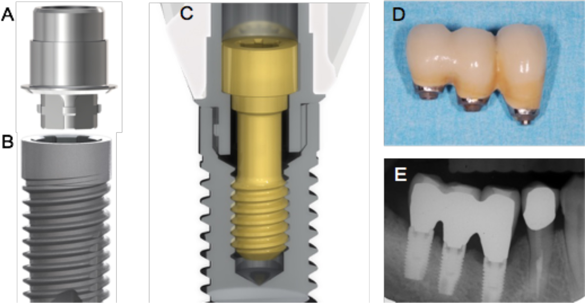
Figure 1. Showing the prosthetic connection of the Neoss implant system. A. The NeoLink component. B. Implant C. Crossection through a single crown, NeoLink with prosthetic goldscrew and implant. D. Clinical and E. radiographic view of an implant-level three-unit bridge.

Baseline (abutment connection surgery), 1- and 5-year intraoral radiographs were used to measure marginal bone levels and calculate bone loss. Only implants with measurements from all three time points were used for calculations. The upper corner of the coronal shoulder of the implant was used as reference point, and measurements from the reference point to the first bone contact at the mesial and distal aspects of the implant were performed using a PC and specially designed software (Image-J, National Institutes of Health, Bethesda, MD, USA) (Figure 2). A mean value was calculated for each implant and time point.

JDMR-19-118- Lars Sennerby_ Sweden_F2

Figure 2. Radiographs of the same case at baseline and after 1 and 5 years of follow-up. The mesial implant shows some bone loss, while the distal implant show no bone loss.

The Spearman correlation test was used to evaluate a possible correlation between depth of implant placement and marginal bone loss after 5 years. A significance level p<0.05 was used for the test.

Results

Two implants were lost, giving a cumulative survival rate (CSR) of 98.0% after 5 years. Both failures occurred in the posterior mandible and all maxillary implants were successful (Table 1). One implant (3.5/11 mm), which had been accidentally placed close to a neighbouring root, was removed after 3 months of loading. The patient could maintain the partial bridge on two implants and a new implant was inserted after healing and eventually connected to a new bridge. The second failed implant (5/9 mm) was removed during the fifth year due to marginal bone loss, suppuration and discomfort.

The radiographs from a total of 79 implants (77.5% of all implants) could be measured at baseline, after one and five years (Figure 3). The marginal bone levels were situated 0.3 ± 0.4 mm, 1.0 ± 0.6 mm and 1.2 ± 1.0 mm below the implant shoulder at baseline and after 1 and 5 years, respectively (Table 3). The average marginal bone loss amounted to 0.7 ± 0.7 mm with 3.8% of the implants showing more than 2 mm and no implant more than 3 mm bone loss after 1 year (Table 3). After 5 years, the average bone loss was 0.9 ± 1.1 mm with 3.8 % of implants showing more than 2 mm bone loss and 3.8% more than 3 mm bone loss (Table 3). The majority of implants showed bone level gain (34.2%) or no and up to 1 mm of bone loss (55.7) from the 1st to the 5th year (Table 3). There was no correlation between insertion depth and bone loss.

JDMR-19-118- Lars Sennerby_ Sweden_F3

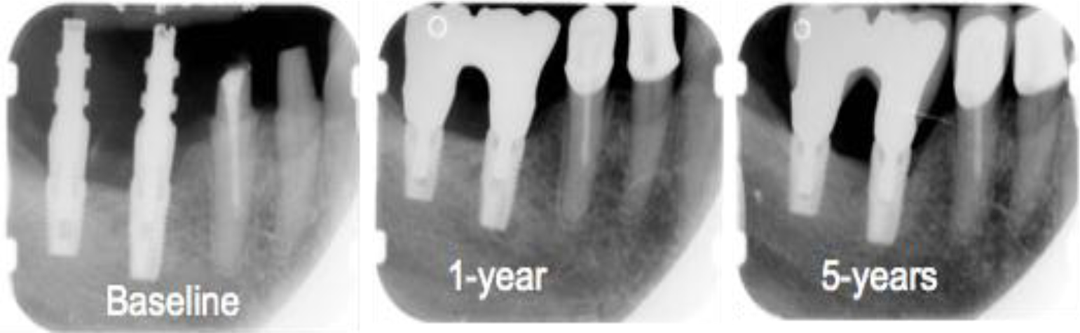
Figure 3. Schematic showing the reference point for bone level measurements. The collar of the implant is 1.9 mm.

Table 3. Marginal bone level and bone resorption based on 79 implants with readable radiographs from all three time points.

	Baseline mm±SD	1 year mm±SD	5 years mm±SD
Bone level	0.3 ± 0.4	1.0 ± 0.6	1.2 ± 1.0
Bone loss		0.7 ± 0.7	0.9 ± 1.1
Frequency of bone loss		n (%)	n (%)
< 0 mm		8 (10.1)	11(13.9)
0–1 mm		49 (62.0)	41 (51.9)
1.1–2 mm		19 (24.1)	21 (26.6)
2.1–3 mm		3 (3.8)	3 (3.8)
> 3 mm		0	3 (3.8)

Discussion

The present study group was evaluated after one year and the results presented in a previous publication, where one implant failure was reported⁹. The present follow-up showed one additional implant failure giving a total implant survival rate of 98.0 % after five years of function. This is in line with the outcomes from 5-year follow-up studies of the same and other modern dental implant systems [8, 11–13].

Only one of the failures was related to the performance of the implant as the first failure was due to a surgical mistake. The second implant was removed due to extensive marginal bone loss, suppuration and discomfort. The infection occurred during the 5^th year of function after a continuous slow and asymptomatic bone loss from implant placement. This implies that the reason for bone loss was other than infection, which likely was a secondary phenomenon. This is in accordance with another publication in where causes for marginal bone resorption were discussed [14]. Other authors have argued that bone loss at implants is biofilm-mediated and advocate the use of periodontal indices to diagnose mucositis and peri-implantitis in analogy with gingivitis and periodontitis at teeth [15]. However, a recent review could not find any evidences that probing is an effective means of diagnosing peri-implant disease or predicting implant failure [16]. In contrast, the authors expressed concerns that the use of probing could lead to over-diagnosis of disease and unnecessary treatment of healthy implants. Nevertheless, also when applying liberal definitions of peri-implant infection [17] the condition requiring removal of the implant in the study can be judged as “peri-implantitis”. Hence, peri-implantitis was seen in 1% of the implants of the present study. Based on a previous literature search, the frequency of implants with reported peri-implant infection and significant bone loss leading to implant removal or other surgical intervention was on average 2.7% after 7 to 16 years [18].

Only implants with radiographs available from all observation time points were evaluated with regard to marginal bone levels in the present study. The present authors believe this results in more accurate data than using mean values from all available radiographs from the different time points. Some marginal bone remodelling was observed during the first year of function followed by a minor further change up to the fifth year check-up, which is in line with many other studies [12, 19]. The average marginal bone loss amounted to 0.7 ± 0.7 mm after 1 year and 0.9 ± 1.1 mm after 5 years. The majority of implants showed bone level gain (34.2%) or no and up to 1 mm of bone loss (55.7) from the 1st to the 5th year.

Our study showed less bone loss than in a previous study, where Brånemark implants with and without prosthetic abutments were evaluated after 5 years [20]. In their comparative investigation, the least amount of bone loss was found at implants with a machined-surfaced abutment after 5 years. The bone loss amounted to 1.6 mm compared to 0.9 mm in our study in spite of using implant-level prosthetic constructions. However, it should be pointed out that our baseline radiographs where taken at abutment or prosthesis connection and that implant surgery was used as baseline in the Göthberg et al study [20]. Therefore, any bone loss occurring from surgery to our baseline was not accounted for. However, the mean marginal bone level was still located more coronal in our study after 5 years, i.e. 1.2 mm vs 1.6 mm. An average of 0.2 mm of marginal bone was lost from the 1^st to the 5^th year in the present study, while about 0.6 mm was lost when pooling all implants in the Göthberg et al study [20]. Interestingly, the least bone loss from the one to the five-year follow-up was seen for implants restored at implant level in that study, indicating that most of the changes occurred during the first year in function [20]. In a comparative study using AstraTech implants, the bone loss at implants with or without prosthetic abutments was less than 0.1 mm after one year [4]. However, since there was a statistically significant difference in favour of the use of abutments together with less bleeding on probing, the authors argued that it is safer to use abutments rather than restoring the implants at implant level. However, in light of the discussion above neither initial bone loss nor the presence of bleeding on probing seems to reflect or predict clinically relevant problems and, according to the present authors, the use of prosthetic abutments cannot be justified. Moreover, a 5-year clinical follow-up study reported few complications of implant-level restorations [6], which corroborates with our findings.

Continuous marginal bone loss and related long-term complications is an obvious threat to the longevity of an implant and is the main reason why many historical implant designs are not used any longer [21, 22]. It is well known that also different modern implant designs show different amounts of marginal bone remodelling during the first year in function but that small differences are observed from the 1^st year and onwards [19]. In a meta-analysis where Straumann, Brånemark and AstraTech implants were analysed based on published 5-year follow-up studies, all three designs seemed to result in excellent long-term outcomes in spite of measureable differences of initial marginal bone loss [12]. Hence, steady marginal bone levels after the first year seems more important than the amount of bone that is lost during the first year. So if the goal is to minimize initial marginal bone resorption, the choice of implant seems more effective than if using prosthetic abutments or not. This is also exemplified by the studies by Toia et al [4] and Göthberg et al [20], which showed greater differences between implant systems than between prosthetic protocols.

Implant placement depth did not have any effect on marginal bone resorption in the present study. This is in contrast to a 5-year study on Nobel Replace implants, where less bone loss was reported if the 2 mm smooth surfaced collar was placed above below the bone level compared to implants placed at or below the bone level [23]. The bone level shifted to the first thread for all implants over time, which indicated that the smooth surfaced collar could not retain the bone. It is likely that the surface topography played a role for the maintenance of the bone level at the collar in the present study. However, studies on other implant designs with moderately rough surfaces on the collar have shown both minimal [12] and extensive bone loss [24, 25], which indicates that other factors such as collar geometry and drilling protocols are of equal importance. Since it is difficult to draw general conclusions from one implant type, each individual design needs to be evaluated in clinical follow-up studies. Within the limitations of the present study, it is concluded that the evaluated implant system performs well when restored at implant level.

References

Hellden LB, Derand T (1998) Description and evaluation of a simplified method to achieve passive fit between cast titanium frameworks and implants. Int J Oral Maxillofac Implants 13: 190–196. [crossref]
Cochran DL, Hermann JS, Schenk RK, Higginbottom FL, Buser D (1997) Biologic width around titanium implants. A histometric analysis of the implanto-gingival junction around unloaded and loaded nonsubmerged implants in the canine mandible. J Periodontol 68: 186–198. [crossref]
Abrahamsson I, Berglundh T, Sekino S, Lindhe J (2003) Tissue reactions to abutment shift: an experimental study in dogs. Clin Implant Dent Relat Res 5: 82–88. [crossref]
Toia M, Stocchero M, Becktor JP, Chrcanovic B, Wennerberg A (2019) Implant vs abutment level connection in implant supported screw-retained fixed partial dentures with cobalt-chrome framework: 1-year interim results of a randomized clinical study. Clin Implant Dent Relat Res 21: 238–246. [crossref]
Göthberg C, Gröndahl K, Omar O Thomsen P, Slotte C (2018) Bone and soft tissue outcomes, risk factors, and complications of implant-supported prostheses: 5-Years RCT with different abutment types and loading protocols. Clin Implant Dent Relat Res 20: 313–321. [crossref]
Hellden L, Ericson G, Elliot A, Fornell J, Holmgren K, et al. (2003) A prospective 5-year multicenter study of the Cresco implantol-ogy concept. Int J Prosthodont 16: 554–562. [crossref]
Sennerby L, Andersson P, Verrocchi D, Viinamäki R (2012) One-year outcomes of Neoss bimodal implants. A prospective clinical, radiographic, and RFA study. Clin Implant Dent Relat Res 14: 313–320. [crossref]
Zumstein T, Billström C, Sennerby L (2012) A 4- to 5-year retrospective clinical and radiographic study of Neoss implants placed with or without GBR procedures. Clin Implant Dent Relat Res 14: 480–490. [crossref]
Degasperi W, Andersson P, Verrocchi D, Sennerby L (2014) One-year clinical and radiographic results with a novel hydrophilic titanium dental implant. Clin Implant Dent Relat Res 16: 511–519. [crossref]
Zumstein T, Sennerby L (2016) A 1-Year Clinical and Radiographic Study on Hydrophilic Dental Implants Placed with and without Bone Augmentation Procedures. Clin Implant Dent Relat Res 18: 498–506. [crossref]
Andersson P, Pagliani L, Verrocchi D, Volpe S, Sahlin H et al (2019) Factors Influencing Resonance Frequency Analysis (RFA) Measurements and 5-Year Survival of Neoss Dental Implants. International Journal of Dentistry 2019: Article ID 3209872, 9 pages.
Laurell L, Lundgren D (2011) Marginal bone level changes at dental implants after 5 years in function: a meta-analysis. Clin Implant Dent Relat Res 13: 19–28. [[crossref]
Derks J, Håkansson J, Wennström JL, Tomasi C, Larsson M, et al. (2015) Effectiveness of implant therapy analyzed in a Swedish population: early and late implant loss. J Dent Res 94: 44–51. crossref]
Albrektsson T, Dahlin C, Jemt T, Sennerby L, Turri A, et al. (2014) Is marginal bone loss around oral implants the result of a provoked foreign body reaction? Clin Implant Dent Relat Res 16: 155–165. [crossref]
Lindhe J, Meyle J, Group D of European workshop on periodontology (2008) Peri-implant diseases: Consensus Report of the Sixth European Workshop on Periodontology. J Clin Periodontol 35: 282–285. [crossref]
Coli P, Christiaens V, Sennerby L, Bruyn H (2017) Reliability of periodontal diagnostic tools for monitoring peri-implant health and disease. Periodontol 2000 73: 203–217. [crossref]
Albrektsson T, Buser D, Chen ST, Cochran D, DeBruyn H, et al (2012) Statements from the Estepona consensus meeting on peri-implantitis, February 2–4, 2012. Clin Implant Dent Relat Res 14: 781–782.
Albrektsson T, Buser D, Sennerby L (2012) Crestal bone loss and oral implants. Clin Implant Dent Relat Res 14: 783–791. [crossref]
Oh TJ, Yoon J, Misch CE, Wang HL (2002) The causes of early implant bone loss: myth or science? J Periodontol 73: 322–333. [crossref]
Göthberg C, Gröndahl K, Omar O Thomsen P, Slotte C (2018) Bone and soft tissue outcomes, risk factors, and complications of implant-supported prostheses: 5-Years RCT with different abutment types and loading protocols. Clin Implant Dent Relat Res 20: 313–321. [crossref]
d’Hoedt B, Schulte W (1989) A comparative study of results with various endosseous implant systems. Int J Oral Maxillofac Implants 4: 95–105. [crossref]
Albrektsson T, Sennerby L (1991) State of the art in oral implants. J Clin Periodontol 18: 474–481. [crossref]
Pettersson P, Sennerby L (2015) A 5-year retrospective study on Replace Select Tapered dental implants. Clin Implant Dent Relat Res 17: 286–295. [crossref]
Ostman PO, Hellman M, Albrektsson T, Sennerby L (2007) Direct loading of Nobel Direct and Nobel Perfect one-piece implants: a 1-year prospective clinical and radiographic study. Clin Oral Implants Res 18: 409–418. [crossref]
Nowzari H, Chee W, Yi K, Pak M, Chung W, et al. (2006) Scalloped dental implants: a retrospective analysis of radiographic and clinical outcomes of 17 Nobel Perfect implants in 6 patients. Clin Implant Dent Relat Res 8: 1–10. [crossref]

Thought on the Present Molecular Genetics

Leave a reply

DOI: 10.31038/JMG.2019213

Mini Review

The working of molecular genetics is involved in finding out the genetic components, their structures, mechanism, dynamics and pathologic alterations in the disease. The final aim is to rectify to normal for the health of human being.

The components are the genetic flows that start from the DNA, which manifests the storage site of all the genes, replication, transcription and translation. Extensive work on DNA sequencing reached the milestone of completing 3 × 10⁹ nucleotide sequences in human and complete genomic sequences from many species. General mechanisms of replication by DNA polymerases and involved factors have been elegantly defined. The structure of four RNA polymerases (pol I, II, III and mitochondrial RNA polymerases) are well characterized. Hundreds offactors are known for co-transcriptional and post transcriptional processing, modifications and splicing.

To understand the progresses made so far, the present is a good time to define some specificity of factors involved in specific gene expression. For example, in replication, how the replication origins are recognized and what may be disturbed in cancer and other diseases. The RNA involvement in replication origin is different from the Okazaki RNA fragment and has not been well characterized. It is interesting to note that the changes in nucleolar transcription system during carcinogenesis is fascinating. But we still don’t know enough what specific aberrations may occur. Replication origins are interdigitated in rRNA genes. In human the rRNA genes are in 5 acrocentric chromosomes (chromosomes 13–15, 21 and 22) which place the rRNA genes in close proximity to centromeres and telomeres. The nucleolus is the site where rRNA is synthesized by RNA polymerase I but have been demonstrated that some of RNA polymerase II activity has effect on nucleolar RNA polymerase I activity such as aluRNA [2].

In the tumor cells, pre-rRNA is accumulating in the nucleolus which may be due to transcriptional hyperactivity but may be also involved in some mutations in the processing factors.

In the system of mRNA transcription, many diseases have been reported caused by altered transcription factors which include general transcription factors as well as specific transcription factors. The promoter mutations also causes the diseases.

The modifications of mRNA are also involved in processing as well as its translational activity.

More importantly, the splicing mechanisms of pre-mRNA are extensively worked out and found that > 300 different proteins may be involved.

Are the splicing mechanisms are universally same throughout the different pre-mRNAs or are there specific factors involved in for specific pre-mRNA splicing? The spliceosomes, EJC complex and other protein involved in mRNA maturation have been well characterized structurally.

It is interesting to note that the order of splicing is not always from 5’ to 3’ direction and one of well characterized splicing order is in the ovomucoid pre-mRNA maturation. The order of splicing sites are from first to last to be in order of 5/6→7/4→2/1→3 (or 5/6→7/4→2→3/1) [5, 7]. Efficient splicing is involved splicing code (GU, branch site, AG), enhancers, suppressors, RNA sequences, secondary structure and tertiary structures. It was interesting to find that SF2/ASF are more abundant in early spliced site at the splice sites 5/6 and SC35 is enriched in late splice site 3 in ovomucoid pre-mRNA.

	SF2/ASF	SC35	SRp40	SRp55	hnRNP A1
1	8.3	6.7	3.3	6.7	3.3
2	6.0	6.0	2.0	4.0	5.3
3	0.4	10.0	4.0	8.0	3.3
4	6.7	3.3	5.0	5.0	4.2
5	13.3	8.3	5.0	5.0	6.7
6	6.7	5.0	8.3	6.7	6.7
7	10.0	3.3	10.0	5.0	3.3

Motifs are analyzes 60 nucleotide at the splice sites (total 120 nucleotide by adding 5’ splice site and 3’ splice site). Due to short exon 2 (20 nucleotides) the 3’ splice site 1 and 5’ splice site 2 are 50 nucleotides each). The above values are expressed in number of motifs per 100 nucleotides.

(ESE are screened by ESE finder 3 CSHL and hnRNP A1 is screened by HSF3; Human Splicing Factor finder 3)

Balance between enhancers and suppressors show impact on splicing but how these regulators are distributed in the genes are not well characterized. For example, although, hnRNP A1 has been reported to be suppressor of splicing, it may also confer some RNA structural stability in the complexes.

Although some people stress that RNA transcription is taking place near the nuclear membrane and exit to the cytoplasm, it is well known that chromosomal domains in the nuclear geography are not all at the nuclear membrane. Transcription sites in different chromosomes are located throughout within dynamic nucleoplasm [3, 6, 1]. The location of pre-mRNP maturation stays not as the static site but it is mobile in dynamic movement. The co-transcriptional splicing progresses when pre-mRNP is still attached to the transcription complex, and post transcriptional splicing is taking place after detachment from the transcription complex on the way out to the cytoplasm. The splicing regulators are also dynamic, moving from the storage site to the transcription site [8]. On the other hand, the dynamic pre-mRNP movement after detachment from the transcription site may encounter the splicing factor storage sites where additional splicing and maturation may take place. In the course of dynamic movement of mRNP from the transcription site, it is interesting that SF2/ASF sites are more abundant in early transcription region, and next followed by SC35 and other factors such as SRp40 and SRp55.

SF2/ASF and SC35 are binding not only to RNA but also to DNA and are there intronic active TSS are present?

Research on the stem-cell therapy, gene therapy, gene editing, antisense oligonucleotide therapy are very active with FDA approved nusinersen (Spinraza) for SMA and Exondys 51 for DMD and more to come.

Recent development on targeted protein degradation by small molecules may have future for the specific degradation of proteins with dominant negative mutations [4].

References

Bolzer A, Kreth G, Solovei I, Koehler D and Saracoglu K (2005) Three-Dimensional Maps of All Chromosomes in Human Male Fibroblast Nuclei and Prometaphase Rosettes. PLos Biology. 3: 0826–0842, e157.
Caudron-Herger M, Pankert T, Seiler J, Németh A and Voit R et al (2015) Alu element-containing RNAs maintain nucleolar structure and function. EMBO J. 34: 2758–2774.
Cmarko D, Verchure PJ, Martin TE, Dahmus ME and Krause S et al (1999) Ultrastructural Analysis of Transcription and Splicing in the Cell Nucleus after Bromo-UTP Microinjection. Mol. Biol Cell. 10: 211–223.
Cromm PM and Crews CM (2017) Targeted Protein Degradation: From Chemical Biology to Drug Discovery. Cell Chem Biol. 24(9), 1181–1190.
Lewin B (1994, 2008) RNA Splicing and Processing. Gene IX, Chapter 26, Pearson Prentice Hall, Peason Education, Inc. pp667–705.
Pombo et al (1998) EMBO J. 17(6) 1768–1778
Ro-Choi TS and Choi YC (2009) Thermodynamic Analyses of the Constitutive Splicing Pathway for Ovomucoid Pre-mRNA. Mol. Cells. 27, 1–10.
Spector DL and Lamond AI (2011) Nuclear Speckles in the book The Nucleus.

PD-1 Inhibitors: To Go or To Stop? ; Review Articles

Leave a reply

DOI: 10.31038/CST.2019423

Abstract

PD-1 receptor as one of the programmed cell death protein 1 receptor was firstly designated in the early 1990s assumed its manifestation through out initiation of programmed cell death in a T-cell hybridoma. Subsequently its early detection, numerous groups have recognized that arrangement of PD-1 through its ligand, programmed death ligand 1 (PD-L1), negatively regulates T-cell-mediated immune responses. Early preclinical indication proposed that stimulation of PD-1/PD-L1 signaling might work as a mechanism for tumors to escape “an antigen-specific T-cell immunologic response”. Accordingly, the Atezolizumab is one of a novel immunotherapy medication called “checkpoint inhibitors”. It functioning through interfering with the tumor’s ability to deactivate cancer combat immune cells called (T-cells). It objects a “protein hypothesis was developed that PD-1/PD-L1 blockade may be an effective cancer immunotherapy.

For instance, several PD-1/PD-L1 inhibitors stays to develop, predictive biomarkers, mechanisms of resistance, management interval and therapy up on disease progression and immune-related side effects, are main ideasessential of additional attention to enhance the anticancer effects of this group of immunotherapy.

Keywords

PD-1/ PD-L1 inhibitor, Immune checkpoint, Treatment beyond progression, Immune-related toxicity

Introduction

The main role of T cells is to differentiate healthy cells from diseased or malignant cells by the activation or deactivation of numerous receptors on the T-cell surface. As stated before, the malignant cells can escape recognition through “cell surface molecules” that interact with the receptors on T cells to, in essence, mimic the signals released by healthy cells. So, the immune system that rests inactive against malignant cells, allowing their un-regulated development and proliferation.

As these molecules and their associated receptors on T cells keep the immune system ‘‘in check,” by “inhibiting immune functioning”, they are mutually called “checkpoint proteins”. The Checkpoint inhibitors inhibit the effects of these checkpoint proteins.

Types of checkpoint Inhibitors

Three different groups that targets different checkpoint proteins (1) PD-L1: Programmed Death Ligand-1, (2) PD-1: Programmed Cell Death Protein-1 and (3) CTLA-4; Cytotoxic T-Lymphocyte Associated Protein 4, have been the chief target of investigation for the management of cancer patients with immunotherapy as new era.CTLA-4 and PD-1 are found on T cells. PD-L1 are on cancer cells (Figure- 1).

CST 2019-111 - Ayman Egypt_F1

Figure 1. PD-1 and PD-L1 sites of action

Immune checkpoint inhibitor. Checkpoint proteins, such as PD-L1 on tumor cells and PD-1 on T cells, help keep immune responses in check. The binding of PD-L1 to PD-1 keeps T cells from killing tumor cells in the body (left panel). Blocking the binding of PD-L1 to PD-1 with an immune checkpoint inhibitor (anti-PD-L1 or anti-PD-1) allows the T cells to kill tumor cells (right panel).

https: //www.cancer.gov/publications/dictionaries/cancer-terms/def/immune-checkpoint-inhibitor.

PD-1 and its Immune-inhibitory Mechanism

The programmed cell death 1 (PD-1) receptor is expressed on activated T cells, B cells, macrophages, regulatory T cells (Tregs), and natural killer (NK) cells. Binding of PD-1 to its B7 family of ligands, programmed death ligand 1 (PDL1 or B7-H1) or PD-L2 (B7-DC) results in suppression of proliferation and immune response of T cells. Activation of PD-1/PD-L1 signaling serves as a principal mechanism by which tumors evade antigen-specific T-cell immunologic responses. Antibody blockade of PD-1 or PD-L1 reverses this process and enhances antitumor immune activity. TCR, T-cell receptor; MHC, major histocompatibility complex; APC, antigen-presenting cell.

PD-1 functions through regulation of late-phase immune responses. The management is as suggested by the activation-induced expression of PD-1. The control of immune reactions also takes place in the peripheral tissues. PD-1 contains single IgV-like domains as in its extracellular region. The region also includes ITIM and ITSM. PD-1 requires ligation with the physiological ligand to suppress T-cell activation (Figure- 1).

PD-1 Function

PD-1 and CTLA-4 can be applied at a diverse phase of immune reaction. They are also induced on the activated T-cells. PD-1 is shown on activated T-cells at a late effectors stage. In the condition of the chronic viral condition, there is a high persistence of PD-1 expression on CD8⁺ T-cells. Despite their distinct features, the CTLA-4 and PD-1 are both immune checkpoints.

They also regulate the immune responses at different stages. CTLA-4 can effectively block the activation of T-cells in the lymphoid organs. PD-1 functions effectively by inhibiting the effectors T-cells at a later stage of immune responses (Figure-2).

CST 2019-111 - Ayman Egypt_F2

Figure 2. PD-1 and CTLA-4 sites of action

jim-Allison-who-first-used-CTLA4-blockade-for-cancer-treatment-and-Honjo-who-originally-discovered-PD-1-new-Nobel-Laureates-of-Medicine-this-year-Custom-Graphic

Control of Cancerous Immunity by PD-1

PD-1 is essential for dampening the immune-surveillance for tumours. Tumors can express the PD-L1 and thus escaping the immune surveillance. PD-L1 interacts with PD-1 on T-cells and therefore and thus negatively regulates the immune responses [5].

There is also a correlation between poor prognosis and high expression of PD-1 ligands on tumors. PD-1 blockade has previously successfully been used on metastatic tumors. Additionally, PD-1 has been identified to contain a higher therapeutic capacity than CTLA-4 blockade (Figure-3).

CST 2019-111 - Ayman Egypt_F3

Figure 3. PD-1 Function and Action

jim-Allison-who-first-used-CTLA4-blockade-for-cancer-treatment-and-Honjo-who-originally-discovered-PD-1-new-Nobel-Laureates-of-Medicine-this-year-Custom-Graphic

CST 2019-111 - Ayman Egypt_F4

Figure 4. PD-1 Inhibitors Side Effect

https: //www.esmo.org/content/download/124130/2352601/file/ESMO-Patient-Guide-on-Immunotherapy-Side-Effects.pdf

Role of PD-1 inhibitors in the treatment of cancer patients

1-Pembrolizumab (Keytruda) was developed by Merck and first approved by the Food and Drug Administration in 2014 for the treatment of melanoma. It was later approved for metastatic non-small cell lung cancer and head and neck squamous cell carcinoma. In 2017, it became the first immunotherapy drug approved for use based on the genetic mutations of the tumor rather than the site of the tumour.

Indications

Indicated for the treatment of patients with unresectable or metastatic melanoma.
Indicated for the adjuvant treatment of patients with melanoma with involvement of lymph node(s) following complete resection.
In combination with pemetrexed and platinum chemotherapy, is indicated for the first-line treatment of patients with metastatic non-squamous non‒small cell lung cancer (NSCLC), with no EGFR or ALK genomic tumor aberrations.
In combination with carboplatin and either paclitaxel or nabpaclitaxel, is indicated for the firstline treatment of patients with metastatic squamous NSCLC.
As a single agent, is indicated for the first-line treatment of patients with metastatic NSCLC whose tumors have high PD-L1 expression [tumor proportion score (TPS) ≥ 50%] as determined by an FDA-approved test, with no EGFR or ALK genomic tumor aberrations.
As a single agent, is indicated for the treatment of patients with metastatic NSCLC whose tumors express PD-L1 (TPS ≥1%) as determined by an FDA-approved test, with disease progression on or after platinum-containing chemotherapy. Patients with EGFR or ALK genomic tumor aberrations should have disease progression on FDA-approved therapy for these aberrations prior to receiving KEYTRUDA.
Indicated for the treatment of patients with recurrent or metastatic head and neck squamous cell carcinoma (HNSCC) with disease progression on or after platinum-containing chemotherapy. This indication is approved under accelerated approval based on tumor response rate and durability of response. Continued approval for this indication may be contingent upon verification and description of clinical benefit in the confirmatory trials.
Indicated for the treatment of adult and pediatric patients with refractory classical Hodgkin lymphoma (cHL), or who have relapsed after 3 or more prior lines of therapy. This indication is approved under accelerated approval based on tumor response rate and durability of response.
Indicated for the treatment of adult and pediatric patients with refractory primary mediastinal large B-cell lymphoma (PMBCL), or who have relapsed after 2 or more prior lines of therapy. This indication is approved under accelerated approval based on tumor response rate and durability of response. Continued approval for this indication may be contingent upon verification and description of clinical benefit in confirmatory trials.
Indicated for the treatment of patients with locally advanced or metastatic urothelial carcinoma (mUC) who are not eligible for cisplatin-containing chemotherapy and whose tumors express PD-L1 [combined positive score (CPS) ≥10], as determined by an FDA-approved test, or in patients who are not eligible for any platinum-containing chemotherapy regardless of PD-L1 status. This indication is approved under accelerated approval based on tumor response rate and duration of response. Continued approval for this indication may be contingent upon verification and description of clinical benefit in confirmatory trials.
Indicated for the treatment of patients with locally advanced or metastatic urothelial carcinoma (mUC) who have disease progression during or following platinum-containing chemotherapy or within 12 months of neoadjuvant or adjuvant treatment with platinum-containing chemotherapy.
Indicated for the treatment of adult and pediatric patients with unresectable or metastatic microsatellite instability-high (MSI-H) or mismatch repair deficient (dMMR)solid tumours that have progressed following prior treatment and who have no satisfactory alternative treatment options, or colorectal cancer that has progressed following treatment with fluoropyrimidine, oxaliplatin, and irinotecan.

2-Nivolumab (Opdivo) was developed by Bristol-Myers Squibb and first approved by the FDA in 2014 for the treatment of melanoma.

Indications

As a single agent is indicated for the treatment of patients with BRAF V600 mutation-positive un-resectable or metastatic melanoma. This indication is approved under accelerated approval based on progression-free survival. Continued approval for this indication may be contingent upon verification and description of clinical benefit in the confirmatory trials.
As a single agent is indicated for the treatment of patients with BRAF V600 wild-type un-resectable or metastatic melanoma.
In combination with YERVOY® (ipilimumab), is indicated for the treatment of patients with un-resectable or metastatic melanoma. This indication is approved under accelerated approval based on progression-free survival. Continued approval for this indication may be contingent upon verification and description of clinical benefit in the confirmatory trials.
Is indicated for the treatment of patients with metastatic non-small cell lung cancer (NSCLC) with progression on or after platinum-based chemotherapy. Patients with EGFR or ALK genomic tumor aberrations should have disease progression on FDA-approved therapy for these aberrations prior to receiving OPDIVO.
Indicated for the treatment of patients with advanced renal cell carcinoma (RCC) who have received prior anti-angiogenic therapy.
Indicated for the treatment of adult patients with classical Hodgkin lymphoma (cHL) that has relapsed or progressed after autologous hematopoietic stem cell transplantation (HSCT) and brentuximabvedotin or after 3 or more lines of systemic therapy that includes autologous HSCT. This indication is approved under accelerated approval based on overall response rate. Continued approval for this indication may be contingent upon verification and description of clinical benefit in confirmatory trials.
Indicated for the treatment of patients with recurrent or metastatic squamous cell carcinoma of the head and neck (SCCHN) with disease progression on or after platinum-based therapy.
Indicated for the treatment of patients with locally advanced or metastatic urothelial carcinoma who have disease progression during or following platinum-containing chemotherapy or have disease progression within 12 months of neoadjuvant or adjuvant treatment with platinum-containing chemotherapy. This indication is approved under accelerated approval based on tumor response rate and duration of response. Continued approval for this indication may be contingent upon verification and description of clinical benefit in confirmatory trials.
Indicated for the treatment of adult and pediatric (12 years and older) patients with microsatellite instability high (MSI-H) or mismatch repair deficient (dMMR) metastatic colorectal cancer (CRC) that has progressed following treatment with a fluoropyrimidine, oxaliplatin, and irinotecan. This indication is approved under accelerated approval based on overall response rate and duration of response. Continued approval for this indication may be contingent upon verification and description of clinical benefit in confirmatory trials.
Indicated for the treatment of patients with hepatocellular carcinoma (HCC) who have been previously treated with sorafenib. This indication is approved under accelerated approval based on tumor response rate and durability of response. Continued approval for this indication may be contingent upon verification and description of clinical benefit in the confirmatory trials.
Indicated for the adjuvant treatment of patients with melanoma with involvement of lymph nodes or metastatic disease who have undergone complete resection.

3-Cemiplimab (Libtayo) is a human programmed death receptor-1 (PD-1) monoclonal antibody that binds to PD-1 and blocks its interaction with programmed death ligands 1 (PD-L1) and 2 (PD-L2). The drug is being investigated as a treatment for various cancers and in September 2018 received approval in the USA for the treatment of patients with metastatic cutaneous squamous cell carcinoma or locally advanced cutaneous squamous cell carcinoma who are not candidates for curative surgery or curative radiation. This article summarizes the milestones in the development of cemiplimab leading to this first global approval for the treatment of advanced cutaneous squamous cell carcinoma.

Side Effects of PD-1 Inhibitors

Side effects from treatment with checkpoint inhibitors typically appear within weeks or a few months of starting treatment but can persist or first appear after treatment has finished. Immune-related side effects (sometimes referred to as immune-related adverse effects or irAEs) arising from treatment with checkpoint inhibitors can affect any organ or tissue, but most commonly affect the skin, colon, lungs, liver and endocrine organs (such as the pituitary gland or thyroid gland) [7]. Most immune-related side effects are mild to moderate and reversible if detected early and addressed appropriately.

Management of side effects

There are other side effects to checkpoint inhibitors which occur infrequently, but of which you should be aware, as follows [7]:

Neurological symptoms – according to an analysis of data from many clinical trials, these occur in approximately 4%–6% of people treated with CTLA-4 inhibitors or PD-1 inhibitors, or in up to 12% if treated with both types in combination, and manifests in a wide range of different ways (including muscle weakness, numbness and breathing difficulties); treatment for symptoms of Grade 2 or higher is based mainly on increasing strength oral or intravenous corticosteroids.
Rheumatological symptoms – mild or moderate muscle or joint pain occurs in 2%–12% of people treated with checkpoint inhibitors, more commonly with PD-1 inhibitors; treatment is mainly with oral analgesics (mild-to-moderate symptoms), low-dose oral corticosteroids (moderate symptoms), or for severe symptoms, consultation with a specialist and high-dose corticosteroids or intravenous immunosuppressive drugs may be necessary. Treatment with checkpoint inhibitors may need to be interrupted or stopped, depending on symptom severity.
Kidney symptoms – fewer than 1% of people treated with CTLA-4 inhibitors or PD-1 inhibitors experience kidney problems (although approximately 5% do so if treated with the two types of checkpoint inhibitors in combination); significant impairment of kidney function is treated with intravenous corticosteroids and specialist intervention, and may require checkpoint inhibitor treatment to be interrupted or stopped.
Cardiac symptoms – seen in less than 1% of people treated with CTLA-4 inhibitors or PD-1 inhibitors and includes a wide range of different types; these require early referral to a cardiologist and treatment with high-dose corticosteroids or other immunosuppressive drugs.

Conclusion

In the immunotherapy era, PD-1 inhibitors achieved strong response for many cancer patients either as an adjuvant or palliative treatment. The side effects appear as mild to moderate and can be managed as discovered early.

References

Khanna P, Blais N, Gaudreau P, Corrales-Rodriguez L (2017) Immunotherapy Comes of Age in Lung Cancer. Clinical Lung Cancer. 2017; 18(1): 13–22.
Iwai Y, Hamanishi J, Chamoto K, HonjoT (2017) Cancer immunotherapies targeting the PD-1 signaling pathway. Journal of Biomedical Science. 2017; 24(1).
Zhang R, Li P, Li Q, Qiao Y and Xu T et al (2018) Radiotherapy improves the survival of patients with stage IV NSCLC: A propensity score matched analysis of the SEER database. Cancer Medicine. 2018; 7(10): 5015–5026.
Almutairi A, Alsaid N, Martin J, Babiker H and McBride A et al (2018) Comparative efficacy and safety of immunotherapies targeting PD-1/PD-L1 pathway for previously treated advanced non-small cell lung cancer: Bayesian network meta-analysis. Journal of Clinical Oncology. 2018; 36(15_suppl): e21012-e21012.
Ferris R. PD-1 targeting in cancer immunotherapy (2012) Cancer.; 119(23): E1-E3.
TogashiY (2017). ISY9-2Translational research for predictive biomarkers and novel cancer immunotherapies beyond PD-1/PD-L1 blockade therapies. Annals of Oncology. 2017; 28 (suppl_9).
Haanen JBAG, Carbonnel F, Robert C, et al (2017) Management of toxicities from immunotherapy: ESMO Clinical Practice Guidelines for diagnosis, treatment and follow-up. Ann Oncol 2017; 28(suppl_4): iv119-iv142.

Expectations and Attitudes Regarding Chronic Pain Control: An Exploration Using Mind Genomics

Leave a reply

Abstract

We present the emerging science of Mind Genomics, to understand people’s responses to health-related issues, specifically pain. Mind Genomics emerge out of short, affordable, scalable, east-to-run experiments. The topic, here pain, is deconstructed into four questions, each with four separate answers (elements.) The answers are combined into vignettes, presented to respondents, who rate the entire vignette. Emerging from the study are the ratings and the response times to the vignettes, both of which are deconstructed into the contributions of the different underlying elements which the vignettes comprise. The answers cannot be gamed, and the data quickly reveal what is important to the individual, as well as revealing the existence of new-to-the-world mind-sets which differ in the pattern of elements that they find important. Mind Genomics provides the opportunity to understand the person’s needs and wants for specific health as well as other experiential situations where human judgment is relevant.

Introduction

Pain is an inevitable companion in our life’s journey. Pain is defined through its association with actual or potential tissue damage, denoting it as a necessary characteristic of the experience, but also recognizing that events other than tissue damage can serve as determinants, consistent with a bio psychosocial model of pain [1,2]. This definition of pain denotes multiple causal factors underlying pain, beyond the issue pathology.

There is no dearth of studies on pain, whether these studies are report of pain from one’s everyday life [3], a topic dealt with in medicine [4], and a topic of scientific investigation [5]. When we talk about pain, can we probe into the mind of the person beyond simply the report, beyond a simplistic scale? Can we move beyond simple indicators, approaching a more detailed description of one’s pain but yet not forcing the respondent to become a scientist?

Pain, a highly subjective phenomenon, often refers to a sensory experience resulting from actual damage to the body or from non-bodily damage [6]. Pain may be influenced by psychological mechanisms such as: attention, emotion, beliefs and expectations [7].

In general, there are two different classifications of physical pain, visceral and somatic. Visceral pain originates in the internal organs whereas somatic pain stems from skin, muscle, soft tissue, and bone. There are many types of pain which fall under these categories. A person’s pain can also be classified as acute or chronic. Pain can be described as nerve pain, psychogenic pain, muscle pain, abdominal pain, back pain, pelvic pain, etc.

Subjective pain is influenced by its intensity and by interventions to treat the pain. Expectations and attitudes towards pain, may stem from psychological processes that are fundamental to learning across various sensory experiences and affect. Understanding expectations and attitudes towards pain may help us form communication messaging to help individuals deal more effectively with their chronic pain.

The subjective nature of pain makes it difficult to test the actual nature of perceived pain across populations, within a country, and in different countries. There are accepted methods of testing the actual perception of pain, specifically pain thresholds and pain tolerance, as well as psychophysical scaling of pain. One example is measuring the time one can submerge a limb in an ice bath, to test the ability of subjects to tolerate pain under varying conditions, most notable with the testing of analgesics of anesthetics. These methods give a measure of the all-or-none response to pain, and even the qualitative nature of the pain, but do not give a sense of the mind of the person who is undergoing the pain.

Increase in pain accompanies one’s beliefs that a certain treatment will cause pain or increase one’s symptoms overtime [7]. Negative beliefs regarding pain and its effects may occur in some types of chronic pains. To test whether expectations affect pain, studies tested the extent to which expectations influenced physiological responses among individuals. Placebo treatments truly reduced pain intensity [8–12]. These studies also indicated that short-term expectations varied and strongly affected perceptions of pain and pain-evoked responses [13].

Other studies linked differences in expectations regarding pain to the magnitude of responses to pain treatments [14]. Research on the relationship between expectations and pain experiences, showed that expectations about treatments and painful stimuli profoundly influenced behavioral markers of pain perception [7].

Pain treatments also bring positive changes in negative emotions [15]. Expectations affect pain through attention, executive functioning, value learning, anxiety and negative emotions [16]. Attitudes towards pain such as anxiety raised subjective pain. Pain is, thus a complex experience, involving sensory, motivational, and cognitive components. Affect any one of these components may change one’s attitudes towards pain [7].

Whereas studies indicate that beliefs influenced pain experience, it is unclear to what extent psychological processes such as attention, anxiety and emotions affect choice of treatments and what communication messages may mediate the effects of these psychological processes. This study tests communication messaging that affect emotion, attitudes towards pain and choice of treatment for pain.

In his book, Pain: The Gift Nobody Wants, author Paul Brand, MD describes his observations across cultures. Growing up as the child of missionaries in India and then moving to the US, Brand noted the difference in pain and suffering that existed in the East versus the West. He noted that, “as a society gained the ability to limit suffering, it lost the ability to cope with what suffering remains”. He stated that he believed that Easterners have learned to control pain at the level of the mind and spirit whereas, Westerners tend to view pain and suffering as an injustice or failure and an infringement on their right to happiness [17].

In the newly developing science of Mind Genomics we attempt to demonstrate a richer understanding of one’s inner life by presenting the respondent (or ill/healthy pain sufferer, here) with vignettes describing the inner experience, instructing the respondent to rate the fit of the vignettes, one at a time, and then estimating the degree to which each of the elements of the vignette ‘fits’ the respondent.

Method

Mind Genomics as an emerging science has been previously presented [18]. Mind Genomics works by presenting respondents with vignettes, combinations of statements which together tell a story. The respondent is instructed to judge the vignette, rating the vignette as a totality. The rating scale for this study is simply ‘How well does this describe you?’

The statements, elements in the language of Mind Genomics, present simple ideas. The approach requires the construction of four questions which ‘tell a story.’ For each question, the researcher is required to provide four answers, all expressed in simple language. Table 1 presents the four questions, and the four answers to each question. Ideally, the questions and answers should deal with the topic, here pain, but need not mention pain directly. Rather, the questions and answers should be relevant to the topic.

Table 1. The four questions and the four answers to each question.

Question A: how would you describe the nature of pain you are feeling?

Pain bothers me all over my body

The pain is localized but intolerable

The pain radiates and makes it difficult to function

The pain is minor but frequent and annoying

Question B: Describe a situation that would make you feel more comfortable

The doctor explains to me how to deal with the pain

I try to deal with the pain to work through it

I’m happy when I can use a device that delivers therapeutic solution

I just like taking a pill that deals with the pain.

Question C: Describe how would you like to to avoid future pain

I would like to have a diet that is tailored to reduce my pain

I would like exercises and stretches that reduce pain

I would like regular therapy sessions to reduce my pain

I would like a prescription that gives me the medication I need to feel better

Question D: Describe what you would like the doctor to do

The doctor should give me advice

The doctor should give me a shot that delivers long term relief

The doctor should set me up with a system for me to follow

The doctor should give me a regular schedule of visits to treat my pain

The answers in Table 1 are combined by experimental design into a set of 24 vignettes, with each vignette comprising 2–4 elements. Table 2 shows an example of the first six vignettes. The elements appear an equal number of times. Each of the 16 elements is, by design, statistically independent of every other element.

Table 2. The first seven vignettes for the first respondent, created by the experimental design. The table shows the combinations, then the combinations transformed into binary, and then the ratings.

	Vig1	Vig2	Vig3	Vig4	Vig5	Vig6	Vig7
A	4	0	4	3	1	0	0
B	3	2	1	2	1	1	3
C	4	2	0	0	4	4	3
D	2	3	4	0	3	1	4
Binary
A1	0	0	0	0	1	0	0
A2	0	0	0	0	0	0	0
A3	0	0	0	1	0	0	0
A4	1	0	1	0	0	0	0
B1	0	0	1	0	1	1	0
B2	0	1	0	1	0	0	0
B3	1	0	0	0	0	0	1
B4	0	0	0	0	0	0	0
C1	0	0	0	0	0	0	0
C2	0	1	0	0	0	0	0
C3	0	0	0	0	0	0	1
C4	1	0	0	0	1	1	0
D1	0	0	0	0	0	1	0
D2	1	0	0	0	0	0	0
D3	0	1	0	0	1	0	0
D4	0	0	1	0	0	0	1
Rating	7	8	4	7	9	7	9
Binary	100	100	0	100	100	100	100
RT (response time) in seconds	10	6	9	6	10	8	7

Each respondent evaluates a unique set of 24 vignettes. The underlying mathematical structure of the experimental design is maintained, but the specific combinations are changed, in a permutation scheme which preserves the mathematical properties of the design [19]. The permutation covers many more combinations of elements compared to the standard approach of creating one experimental design and presenting that design to many respondents. The Mind Genomics achieves stability by testing many combinations, each a single time, but the expanded coverage ensures that a great of the ‘space of combinations’ is covered. It is difficult to be very ‘wrong’ with a Mind Genomics study because the scope. In contrast, traditional research works with a very small experimental design, e.g., equivalent to the combinations tested by one person, but the combinations are tested by many respondents in order to obtain a stable estimate of the value for each combination.

Mind Genomics and traditional statistics are on opposite sides in terms of what generates valid data. Is valid data obtained by sampling a few of the many possible combinations, albeit with stability for each point (traditional), or by sampling a great many of the combinations, albeit with less stability at any point. A good analogy to Mind Genomics is, metaphorically, the MRI, which discovers the configuration of tissue by taking different ‘snapshots’ and integrating them into one picture. With the permuted experimental one need not ‘be sure’ that the limited number of combinations is the correct set to represent the total set of possible alternatives. With as few as 25 respondents, the number of respondents participating, generating a total of 720 different combinations has covered the space quite well.

Running the Mind Genomics experiment

The experiment is run on the web, typically with respondents from a specific population who have agreed to participate (e.g., those being treated for a condition), or more typically with respondents recruited from the general population, when the objective is a quick ‘scan’ of what is important. The base sizes of these studies range from 25 for an exploration to 500 for a massive deconstruction of the population into different mind-sets. The more typical base size of 25–50 respondents reveals quite a bit about the nature of people’s minds with regard to a particular issue. This study shows the type of learning emerging from this small base size of respondents from the general population, and can be followed with many different studies to follow up on various interesting aspects.

The elements, answers to the questions, are created by experimental design [20]. The 16 elements are combined into 24 combinations or vignettes, similar in structure to the vignettes shown schematically in Table 2. The vignette can be presented on smartphones, tablets, or PC’s.

Although the respondent might feel that the vignettes are created in a random fashion, the reality is just the opposite. The vignettes are created within the framework of the design, which prescribe the exact combinations. The elements are placed one atop the other, centered, without any connectives, making the respondent’s task easier as the respondent ‘grazes for information’.

The experimental design ensures that the elements are statistically independent; appear several times against different backgrounds provided by the other elements in the vignette. Each respondent evaluates a unique set of 24 vignettes, permuted as noted above, so that the design structure is maintained but the specific combinations are new. The permutation system allows a great deal of the design space, or combinations, to be tested, and allows the information to emerge even when the researcher has absolutely no idea what will be important and what won’t. In other words, Mind Genomics is a discovery system, and not a confirmation system. One can learn quickly from a base of zero knowledge, simply by doing 1–4 easy studies of different facets of a topic.

The respondents who participated were US residents, members of a 10+ million world-wide panel of Luc.id Inc., who had previously agreed to participate in these studies for a reward administered by the panel provider. All respondents participated anonymously. The only information about the respondent was age, gender, and the answer to the third question about what type of pain they had. There were five answers to the third question, three dealing with chronic pain of various sorts, and two saying either ‘no pain,’ or ‘not applicable.’ All respondents were classified by gender, age, and by either pain/yes versus pain/no.

Preparing the data for analysis

The respondent assigns a rating to assess ‘How much does this describe how you feel’. The low anchor, 1, is ‘not at all.’ The high anchor, 9, is ‘very much.’ The Mind Genomics program bifurcates the scale, dividing it into the lower part, ratings of 1–6, transformed to 0, plus a very small random number (<10^–5), and a high part, ratings of 7–9, transformed to 100, plus a very small random number. The bifurcation comes from the decades of experience which suggest that managers and scientists alike do not ‘understand’ the meaning or use of the Likert or category scale, but they easily understand the meaning of a no/yes, binary scale. The choice of where to bifurcate is left to the researcher. Thirty-five years of experiments suggest that a 2/3 vs 1/3 division seems to work well. The small random number added to the binary transformed data ensures that when it is time to run the OLS (ordinary least-squares) regression on the data at the level of the individual respondent, there will not be a ‘crash’ of the regression program when the respondent confined the ratings to either the low range (1–6) or to the high range (7–9.) Either of those two cases produces all 0’s or all 1’s, crashing the regression. The small random number ensures that there is variability in the dependent variable, the binary transformed data.

How the different elements drive the binary transformed rating

Table 3 shows the parameters and relevant statistics for the additive model created from the ratings of the total panel, after transformation to a binary scale. The model itself is a simple linear equation of the form: Binary Rating = k₀ + k₁(A1) + k₂(A2) … K₁₆(D4). The experimental design allows us to create the model either at the level of the individual respondent or at the grand level, combining all of the data from the ‘relevant’ respondents, with relevant being

Table 3. Parameters of the model for ‘Fits Me’ after binary transformation. The data come from the Total Panel (720 observations, 24 tested vignettes from each of 30 respondents.) The table is sorted in descending order of coefficient for ‘describes me.’ At the right is the associated coefficient for response time.

		Coeff Desc.	T-stat	P-Value	Coeff RT
	Additive constant	46	4.68	0.00
C2	I would like exercises and stretches that reduce pain	6	0.95	0.34	0.9
D3	The doctor should set me up with a system for me to follow	2	0.39	0.69	2.1
B2	I try to deal with the pain to work through it	2	0.39	0.70	1.9
A1	Pain bothers me all over my body	1	0.23	0.82	1.3
A3	The pain radiates and makes it difficult to function	0	0.05	0.96	1.6
C3	I would like regular therapy sessions to reduce my pain	-2	-0.28	0.78	1.7
D2	The doctor should give me a shot that delivers long term relief	-3	-0.53	0.59	1.8
D4	The doctor should give me a regular schedule of visits to treat my pain	-3	-0.58	0.56	1.7
B3	I’m happy when I can use a device that delivers therapeutic solution	-4	-0.65	0.52	2.1
D1	The doctor should give me advice	-4	-0.69	0.49	1.5
B1	The doctor explains to me how to deal with the pain	-4	-0.73	0.47	1.8
A4	The pain is minor but frequent and annoying	-5	-0.90	0.37	2.1
A2	The pain is localized but intolerable	-6	-0.95	0.34	1.2
C4	I would like a prescription that gives me the medication I need to feel better	-7	-1.19	0.24	1.4
C1	I would like to have a diet that is tailored to reduce my pain	-7	-1.22	0.22	1.4
B4	I just like taking a pill that deals with the pain.	-8	-1.35	0.18	1.6

The analysis suggests the following:

Additive constant, the expected binary value in the absence of elements: Without any elements, the likely response that the vignette will ‘describe me’ is about 46%. By design, all vignettes comprised 2–4 elements, so the additive constant is an estimated parameter. Thus, the value of 46 for additive constant says that half the time respondents will answer that whatever appears will describe them. It is the elements which must do the work to move beyond this almost 50% agreement rate. It is worthwhile commenting here that this baseline of 46% is modest. When the topic is credit cards and the rating is ‘interested in acquiring this credit card,’ the additive constant plummets to about 10–15. When the topic is pizza and the rating is ‘interested in eating this pizza,’ the additive constant skyrockets to 60–70.
There are no very strong elements for the total panel: That is, no element drives the description of ‘me.’ This weakness can either be the result of choosing the wrong elements, or the result of dealing with two or perhaps even three or more different populations, who describe their impressions by different terms, and who may live in quite different worlds of pain.
The highest scoring element is C2, I would like exercises and stretches that reduce pain. This element generates a coefficient of only 6, and has a t-statistic of 0.95, with a probability of 0.34 that it came from a distribution with a true mean of 0. That is, it’s quite likely that were we to do this study again, we would come up with a coefficient much lower than 6, probably 0 or thereabouts.
The remaining elements do not ‘fit’ the respondent: It may well be that the elements are simply incorrect and others will fit the respondent better, or more likely that we are dealing with a segmented population of individuals, some of whom feel that an element ‘fits them,’ whereas others feel that the same element ‘does not fit them.’ In such a situation the responses cancel each other, and we are left with a coefficient around 0, denoting ‘no fit.’

Key subgroups

We know three additional things about the respondent based upon the self-profiling questions completed during the study. The first is gender, the second is age, and the third is whether or not they suffer pain on a regular basis. In this computerized application, the respondent is required to select one of two genders (male/female), and required to put in the year of birth, which provides age. The third question is left to the discretion of the researcher. In this study is the selection of pain, with five options. Two options are defined as ‘no pain’ (actual selection of ‘no pain’ as an answer, selection of not applicable). The remaining three options as pain (i.e. pain in the limbs, back, etc.). We will look at gender, age, and self-reported pain as the three self-defined subgroups. We will also explore two new subgroups, mind-sets inherent in the population but revealed by understanding patterns of responses, behavioral patterns, rather than self-classification.

The focus of interest in Mind Genomics studies is on the additive constant as the ‘baseline,’ and then on the ‘story’ told by the winning elements. These elements are operationally defined as having a value of +6.51 or higher, which becomes 7 when rounded to the nearest whole number.

Gender

Males show a higher additive constant than do females (57 vs 38). In the absence of elements, men are more likely to say that a vignette ‘describes ME.’ Women are less likely to say that, and require more specification.
We get a good sense of what is important by looking at the elements which are most positive (most like me), and most negative (least like me)
For men, the single phrase which most describes them is
C2: I would like exercises and stretches that reduce pain
For men, the single phrase which least describes them is
C1: I would like to have a diet that is tailored to reduce my pain
For women, the two phrases phrase which most describe them are
B2: I try to deal with the pain to work through it,

A1: Pain bothers me all over my body. The degree of fit is less, however, for these elements than the corresponding best fits for males.
For women, the phrase which least describes them is
B4: I just like taking a pill that deals with the pain.

Age: Under 50 versus 50+

Respondents provided the year of their birth. One respondent did not provide the year and was eliminated from this particular analysis by age.

Surprisingly, the additive constant is much higher for the younger respondents versus the for the older respondents (48 vs 31.)
For the younger respondents, there are no strong elements which fit them. The two elements which most describe them are those which suggest control over the pain:
C2: I would like exercises and stretches that reduce pain

D3: The doctor should set me up with a system for me to follow
For the younger respondents, the two elements which least describe them are those which suggest passivity, and no control over the pain.
B1: The doctor explains to me how to deal with the pain

B4: I just like taking a pill that deals with the pain.
For the older respondents, the two elements which most describe them are actual experience to reduce the pain, as well as a description of the experience.
A3: The pain radiates and makes it difficult to function

C2: I would like exercises and stretches that reduce pain
For the older respondents, the three elements which least describe them is passivity
D1: The doctor should give me advice

C4: I would like a prescription that gives me the medication I need to feel better

C1: I would like to have a diet that is tailored to reduce my pain

No pain versus pain

As part of the self-profiling classification, the respondents selected the type of pain, if any, afflicting them. The respondents who check any of the three types of pain assigned to the group saying YES. The remaining respondents were assigned to the group saying NO.

The additive constant is virtually the same, 46 vs 48, meaning that in the absence of elements in the vignette; a little fewer than 50% of the responses will be ‘describes me.’
For those with pain, the phrase which most describes them is
C2: I would like exercises and stretches that reduce pain.
For those with pain, the element which least describes
C1: I would like to have a diet that is tailored to reduce my pain
For those with no pain, virtually no element most describes them
For those with no pain, many elements least describe. The strong element which least describes is
C4: I would like a prescription that gives me the medication I need to feel better

Mind-Sets: Dividing respondents by the patterns of their coefficients for a specific topic

We have just seen that there are some differences in terms of ‘describes me’ across genders, and across those who define themselves as having pain versus no pain. These are ways that people describe themselves. People may differ in ways that the researcher cannot describe in simple terms, or even in way that they themselves don’t understand.

A major tenet of Mind Genomics is that within any topic area, such as the description of pain presented here, there are fundamental differences across people, differences that are obvious once demonstrated, but differences limited to a single topic area. This is the case of the data here. Even within the small sample of 30 respondents we can extract two, possibly three different mind-sets. The method for extracting mind-sets has been previously described [21]. Quite simply, the technique is a matter of clustering the respondents into two or three groups based upon the pattern of their 16 coefficients. The statistical method of clustering is well accepted [22] All that remains is the clustering, extracting the small groups with the property that these mutually exclusive groups represent different ways of thinking about the topic.

Table 4 shows the results for the two mind-set segments emerging from the clustering of the 30 respondents. A base size of 25–30 suffices to reveal the nature of these different mind-sets, especially because the segments are so obviously different and interpretable.

Table 4. Coefficients for the binary-transformed scale ‘Describes me’ across gender, age, pain, and mind-set, respectively. Coefficients of +7 or more are presented in bold, and shaded.

		Male	Female	Age<50	Age 50+	Pain Yes	Pain No	Mind Set 1: Wants a cure	Mind Set 2: Simplicity through the doctor
	Additive constant	57	38	58	31	46	48	37	54
A1	Pain bothers me all over my body	1	4	-1	3	6	-9	10	-9
A2	The pain is localized but intolerable	-4	-4	-9	0	-3	-11	-2	-9
A3	The pain radiates and makes it difficult to function	1	1	-7	9	2	-4	10	-11
A4	The pain is minor but frequent and annoying	-11	2	-5	-2	-2	-12	-3	-8
B1	The doctor explains to me how to deal with the pain	-8	-1	-11	2	-7	1	3	-12
B2	I try to deal with the pain to work through it	-2	4	-1	4	4	-2	8	-3
B3	I’m happy when I can use a device that delivers therapeutic solution	-6	-3	-7	-1	-4	-2	1	-9
B4	I just like taking a pill that deals with the pain.	-9	-8	-12	-5	-7	-11	-16	1
C1	I would like to have a diet that is tailored to reduce my pain	-15	0	-5	-10	-10	-3	2	-17
C2	I would like exercises and stretches that reduce pain	13	-3	5	7	10	-5	9	3
C3	I would like regular therapy sessions to reduce my pain	-1	-3	-3	1	-2	-2	3	-7
C4	I would like a prescription that gives me the medication I need to feel better	-11	-4	-4	-9	-5	-14	-9	-5
D1	The doctor should give me advice	-7	-5	-1	-9	-4	-3	-2	-4
D2	The doctor should give me a shot that delivers long term relief	-9	0	-1	-5	-3	-3	-6	3
D3	The doctor should set me up with a system for me to follow	-1	2	5	-1	4	-2	-4	10
D4	The doctor should give me a regular schedule of visits to treat my pain	-10	1	0	-5	-2	-6	-8	4

Mind-Set 1 (wants a cure) begins with a low additive constant, 37. To them, it’s not the general response which ‘describes me’ but rather the specific phrase. Mind-Set 1 suffers pain, and wants a cure. Here are the elements which Mind-Set 1 feels best describes them:
A1: Pain bothers me all over my body

A3: The pain radiates and makes it difficult to function

C2: I would like exercises and stretches that reduce the pain
Mind-Set 1 do not want simple medical treatment which will alleviate their pain. Here is the element which is they feel least describes them:
B4: I just like taking a pill that deals with the pain.
Mind Set 2 (simplicity through the doctor) shows a higher additive constant, 54. Mind-Set 2 is less discriminating among elements. Mind-Set 2 wants simplicity. Here is the one element that they feel best describes them:
D3: The doctor should set me up with a system for me to follow
Mind Set 2 does not want to take responsibility. Here are the elements that they feel least describe them:
C1: I would like to have a diet that is tailored to reduce my pain

B1: The doctor explains to me how to deal with the pain

A3: The pain radiates and makes it difficult to function

Response times as a measure of cognitive processing of information

At the same time that the respondents were reading the vignettes, the response time was being measured. Response time is operationally defined as the time between the appearance of the vignette and the assignment of the rating. The experiment was executed on the internet.

The respondent was unaware of response time being measured, being instructed simply read the vignette and assign a ‘gut-level’ judgment. Occasionally, in about 10% of the cases, the response time was longer than 10 seconds, suggesting that the respondent was doing something as well, so-called multi-tasking. Those response times of 10 seconds or longer were recoded as 10 seconds. Figure 1 shows the distribution of the 720 response times (30 respondents, each evaluating 24 vignettes)

Mind Genomics-008 IMROJ Journal_F1

Figure 1. Distribution of response times for the total panel of 30 respondents, each rating 24 unique vignettes.

Response time patterns for different subgroups

The measurement of response times as a key feature of Mind Genomics began during the summer of 2019. In the studies run since that introduction, the response time data suggests that when the topic deals with an important health issue, the respondents spend a long time reading the vignette, and thus their response times are long, often 1.0 seconds or longer. When the topic deals with something commercial or ‘fun’ the response times are very short, around 0.2 – 0.7 seconds.

Table 5 presents the response time coefficients for the key subgroups. The model for response time is written in the same way as the model for the binary transformed rating, with the key difference being that that the model for response time does not have an additive constant. The ingoing assumption is that the response time is 0 when there are no elements in the vignette.

Table 5. The coefficients for the response time models. The models do not feature an additive constant.

		Male	Female	Age <50	Age 50+	Pain YES	Pain NO	Mind-Set 1: Wants a cure	Mind-Set 2: Simplicity through the doctor
A1	Pain bothers me all over my body	1.3	1.1	1.0	1.6	1.0	2.0	1.3	1.3
A2	The pain is localized but intolerable	1.0	1.2	1.3	1.1	1.1	1.5	1.0	1.4
A3	The pain radiates and makes it difficult to function	1.7	1.5	1.8	1.4	1.8	1.2	1.6	1.7
A4	The pain is minor but frequent and annoying	2.5	1.7	1.9	2.5	1.9	2.7	1.8	2.6
B1	The doctor explains to me how to deal with the pain	1.8	1.9	1.2	2.6	1.9	1.6	1.8	1.7
B2	I try to deal with the pain to work through it	2.3	1.6	1.6	2.1	2.1	1.5	2.1	1.7
B3	I’m happy when I can use a device that delivers therapeutic solution	2.1	2.3	1.8	2.7	2.3	1.8	2.0	2.2
B4	I just like taking a pill that deals with the pain.	2.0	1.0	1.1	2.2	1.9	0.8	1.4	1.8
C1	I would like to have a diet that is tailored to reduce my pain	1.6	1.0	1.5	1.5	1.7	0.5	1.3	1.4
C2	I would like exercises and stretches that reduce pain	1.2	0.6	1.2	0.8	1.3	-0.1	0.9	1.0
C3	I would like regular therapy sessions to reduce my pain	1.9	1.5	1.7	1.9	2.0	0.9	1.4	1.9
C4	I would like a prescription that gives me the medication I need to feel better	2.1	0.6	1.7	1.6	2.0	0.0	1.2	1.7
D1	The doctor should give me advice	1.5	1.5	1.4	1.5	1.5	1.3	1.4	1.6
D2	The doctor should give me a shot that delivers long term relief	1.5	2.1	1.6	2.0	1.9	1.5	1.7	1.9
D3	The doctor should set me up with a system for me to follow	1.7	2.7	2.0	2.2	2.0	2.2	2.4	1.8
D4	The doctor should give me a regular schedule of visits to treat my pain	1.7	1.8	1.4	2.0	1.8	1.4	1.3	2.1

In Table, coefficients of 2.0 or higher are shaded and shown in bold. These are the elements to which the respondent pays attention. There are some simple patterns which emerge from visual inspection of these elements that are processed ‘more slowly.’

For gender, males focus on the description of symptoms.
A4 The pain is minor but frequent and annoying

B2   I try to deal with the pain to work through it

B3   I’m happy when I can use a device that delivers therapeutic solution

C4 I would like a prescription that gives me the medication I need to feel better

B4   I just like taking a pill that deals with the pain.
For gender, females want a relationship, or at least someone/something external to them.
D3 The doctor should set me up with a system for me to follow

B3 I’m happy when I can use a device that delivers therapeutic solution

D2 The doctor should give me a shot that delivers long term relief
For age, those under 50 focus on only one element:
D3 The doctor should set me up with a system for me to follow
For age, those 50+ focus on a number of phrases, most dealing with methods to assure pain reduction
B3   I’m happy when I can use a device that delivers therapeutic solution

B1   The doctor explains to me how to deal with the pain

A4 The pain is minor but frequent and annoying

B4   I just like taking a pill that deals with the pain.

D3 The doctor should set me up with a system for me to follow

B2   I try to deal with the pain to work through it

D4 The doctor should give me a regular schedule of visits to treat my pain

D2 The doctor should give me a shot that delivers long term relief
For pain, those with PAIN YES, i.e., who say they suffer from one or another pain, the focus is on what stops the pain, i.e., assure pain reduction
B3 I ‘m happy when I can use a device that delivers therapeutic solution

B2 I try to deal with the pain to work through it

D3 The doctor should set me up with a system for me to follow

C3 I would like regular therapy sessions to reduce my pain

C4 I would like a prescription that gives me the medication I need to feel better
For pain, those with PAIN NO, i.e., who say that they do not suffer from pain, the focus is on descriptions of pain
A4 The pain is minor but frequent and annoying

D3 The doctor should set me up with a system for me to follow

A1 Pain bothers me all over my body
For Mind-Sets, Mind-Set 1 (Wants a cure)
D3 The doctor should set me up with a system for me to follow

B2 I try to deal with the pain to work through it

B3 I’m happy when I can use a device that delivers therapeutic solution
For Mind-Sets, Mind-Set 2 (Simplicity through the doctor)
A4 The pain is minor but frequent and annoying

B3 I’m happy when I can use a device that delivers therapeutic solution

D4 The doctor should give me a regular schedule of visits to treat my pain

Finding the mind-sets in the population using a PVI (Personal Viewpoint Identifier)

The mind-sets reveal different ways of perceiving the nature of pain. The mind-sets represent a way to divide what is likely a continuum of feelings and points of view into at least two distinct groups, a division which may provide further understanding, and certain a division that can be used to deal with patients in different, and possibly more appropriate fashion.

Table 6 shows, however, that it’s unlikely to identify mind-sets by their age and gender. It is also quite possible that there are no direct classifications of who a person ‘is’ or what a person ‘experiences’ which can easily assign a person to one of these two mind-sets.

Table 6. How the two emergent mind-sets for pain distribute on the self-profiling classification in terms of age, sex, and experience of pain.

	Mind-Set1 Wants a cure	Mind-Set2 Simplicity through the doctor	Total
Male	6	10	16
Female	9	5	14
Total	15	15	30

Under 50	7	9	16
50+	7	6	13
Total	14	15	29

NOPAIN	6	3	9
YESPAIN	9	12	21
Total	15	15	30

An alternative way to assign new individuals to mind-set has been developed by author Gere. It is called the PVI, the personal viewpoint identifier. The PVI comprises a set of six questions, answered with one of two answers, no or yes. The pattern of the answers to the six questions assigns the respondent to one of the two mind-sets. Figure 2 shows the PVI questionnaire at the left, and the response emerging, given either to the physician and/or to the patient/client. The questions themselves are taken from the actual study. These are the answers or elements, now turned into questions.

The PVI can be deployed along with additional information obtained during the questions. Thus, Figure 2 shows that the respondent, a new person not part of the previous study establishing the PVI, is asked for his or her email. Other questions can be asked, to relate mind-set membership to external variables, whether of a medical/health nature, or of a life-style nature.

Discussion & Conclusions

Since pain is a complex sensation involving sensory, motivational, and cognitive components, and affecting any one of these may change one’s attitudes towards pain [7]; we tested the effect of communication messaging, across mind-set segments towards pain. We tested how each min-set segment we identified emotionally responds to chronic pain, and which treatment choices are preferred by attitudinal mind-sets towards pain.

People who belong to the first mind-set segment feel the pain as radiating and challenging their daily functioning. The pain is very bothersome, but they choose to alleviate it by exercises and stretching. They chose to avoid medical treatment to simply deal with the pain and its ramifications. People belonging to the second mind-set segment also view their chronic pain as radiating and challenging their daily functioning. They, however, choose to simply take pain medication their doctor will prescribe. They expect their doctor to also set them up with a system to follow. In addition, they do not want to take responsibility for self-managing the illness which causes their pain. They prefer to avoid a diet that is tailored to reduce their pain.

Mind Genomics-008 IMROJ Journal_F2

Figure 2. The PVI created for the pain study. The link for the PVI as of this writing (Feb. 2019) is: http://162.243.165.37:3838/TT13/

This study also illustrated how a medical professional may easily identify the mind-set segment to which a patient belongs and accord communication messaging to patient choices and values. Identification of the mind-set to which a patient belongs may assist in building patient-physician trust resulting in higher patient adherence and better implementation of patient-centered care [21].

Mind Genomics provides the ability to segment out populations that share a common mind type and thereby help identify the possibility of determining the types of pain that a person is most likely to experience. It may help answer the question of why people with the same disease experience pain in profoundly different ways. By mind-typing patients who share ailments, Mind Genomics may aid in helping tailor a treatment plan best suited to that individual lying within a disease spectrum.

In light of the current opioid epidemic, it more important, now more than ever, to address how to customize pain treatments to individuals. There are many modalities to treat pain. In the West, pain medications are the first line of treatment. These medications include narcotics/opiates, Non-Steroidal Anti-Inflammatory Drugs (NSAIDs), acetaminophen, certain antidepressants, muscle relaxants, anticonvulsants, corticosteroids, local anesthetics, and most recently medical marijuana. Other modalities such as Transcutaneous Nerve Stimulation (TENS), implantable spinal cord stimulators, meditation and biofeedback are also used to help combat pain. Health care professionals who specialize in pain management use experience and training to try and help tailor treatment regimens to the individual patient. But a tool like Mind Genomics may help the practitioner go beyond the current protocols and prejudices of current practice. Mind Genomics may provide a “cheat sheet” to the patient’s mind and help provide a short cut to success by focusing on pathways that will more likely work for a given patient and eliminating the pathways that will waste time and resources.

References

Hadjistavropoulos T, Craig KD, Duck S, Cano A, Goubert, L, et al. (2011) A biopsychosocial formulation of pain communication. Psychological bulletin 137: 9.
Williams AC, Craig KD (2016) Updating the definition of pain. Pain 157: 2420– 2423. [crossref]
Baker KS, Gibson S, Georgiou-Karistianis N, Roth RM, Giummarra MJ (2016) Everyday executive functioning in chronic pain: specific deficits in working memory and emotion control, predicted by mood, medications, and pain interference. The Clinical Journal of Pain 32: 673–680.
Morrison RS, Maroney-Galin C, Kralovec PD, Meier (2005) The growth of palliative care programs in United States hospitals. Journal of Palliative Medicine 8: 1127–1134.
Schug SA, Palmer GM, Scott DA, Halliwell R, Trinca J (2016) Acute pain management: scientific evidence, 2015. Medical Journal of Australia 204: 315–317.
Loeser JD, Treede RD (2008) The Kyoto protocol of IASP Basic Pain Terminology. Pain 137: 473–477. [crossref]
Atlas LY, Wager TD (2012) How expectations shape pain. Neurosci Lett 520:140–148. [crossref]
Goffaux P, de Souza JB, Potvin S, Marchand S (2009) Pain relief through expectation supersedes descending inhibitory deficits in fibromyalgia patients. Pain 145: 18–23.
Goffaux P, Redmond WJ, Rainville P, Marchand S (2007) Descending analgesia–when the spine echoes what the brain expects. Pain 130: 137–143. [crossref]
Matre D, Casey KL, Knardahl S (2006) Placebo-induced changes in spinal cord pain processing. Journal of Neuroscience 26: 559–563.
Price DD, Craggs J, Verne GN, Perlstein WM, Robinson ME (2007) Placebo analgesia is accompanied by large reductions in pain-related brain activity in irritable bowel syndrome patients. Pain 127: 63–72.
Alkes L. Price, Arti Tandon, Nick Patterson, Kathleen C. Barnes, Nicholas Rafaels, et al (2009) Sensitive Detection of Chromosomal Segments of Distinct Ancestry in Admixed Populations. PLoS Genet 5: 1000519.
Atlas LY, Bolger N, Lindquist MA, Wager TD (2010) Brain mediators of predictive cue effects on perceived pain. J Neurosci 30: 12964–12977. [crossref]
Watson A, El-Deredy W, Iannetti GD, Lloyd D, Tracey I, et al. (2009) Placebo conditioning and placebo analgesia modulate a common brain network during pain anticipation and perception. PAIN 145: 24–30.
Wager TD, Atlas LY, Leotti LA, Rilling JK (2011) Predicting individual differences in placebo analgesia: contributions of brain activity during anticipation and pain experience. Journal of Neuroscience 31: 439–452.
Flaten MA, Aslaksen PM, Lyby PS, Bjørkedal E (2011) The relation of emotions to placebo responses. Philosophical Transactions of the Royal Society B: Biological Sciences 366: 1818–1827.
Brand PW, Yancey P (1993) Pain: the gift nobody wants. New York, HarperCollins Publishers.
Moskowitz HR, Gofman A, Beckley J, Ashman H (2006) Founding a new science: Mind genomics. Journal of sensory studies 21: 266–307.
Gofman A, Moskowitz HR (2010) Isomorphic permuted experimental designs and their application in conjoint analysis. Journal of Sensory Studies 25: 127–145.
Box GE, Hunter JS, Hunter WG (2005) Statistics for experimenters: design, innovation, and discovery (Vol. 2). New York: Wiley-Interscience.
Gabay G, Moskowitz HR, Silcher M, Galanter E (2017) The New Novum Organum: Policies, Perceptions and Emotions in Health. Pardes-Ann Harbor Publishing.
Moskowitz HR, Martin DM (1993) How computer aided design and presentation of concepts speeds up the product development process. Paper presented at the ESOMAR Congress, September, 1993, Copenhagen.
Eippert F, Finsterbusch J, Bingel U, Büchel C (2009) Direct evidence for spinal cord involvement in placebo analgesia. Science 326: 404. [crossref]
Moskowitz, HR (2012) ‘Mind genomics’: The experimental, inductive science of the ordinary, and its application to aspects of food and feeding. Physiology & behavior 107: 606–613.

Feeding Broccoli Floret Residues on Layers: II. Effects on Fatty Acid Deposition

Leave a reply

DOI: 10.31038/IJVB.2019312

Abstract

A study was conducted to determine the effects of feeding Dried Broccoli Florets (DBF) to layers on egg yolk fatty acid deposition. Seventy-two layers were randomly allotted to four dietary treatments (six cage replicates with three hens each) and fed diets containing 0, 4, 8, and 12% DBF for 56 days. Results showed that inclusion of DBF decreased (linear effect, P< 0.001) concentrations of Saturated Fatty Acids (SFA) and increased (linear effect, P< 0.001) concentrations of poly-unsaturated fatty acids (PUFA). Egg yolk concentration of palmitic acid decreased (linear effect, P< 0.001) while linoleic (quadratic effect, P = 0.003) and linolenic (linear effect, P < 0.001) acid concentrations increased as the level of DBF in the diet increased. It was concluded that feeding DBF at 12% of the diet increased PUFA concentrations and decreased those of SFA.

Introduction

Broccoli (Brassica oleracea L. var. italica) is an important vegetable crop in Canada with an annual production of 32,000 tons. As with other vegetables, large amounts of broccoli wastes are generated during harvest, packaging and marketing. It has been estimated that about 40 to 50% of total broccoli produced is discarded during processing as a result of the high standards imposed by consumers and retailers, and due to consumer refusal at the retail level. Additional losses occur in the field, generating large quantities of florets, stems and leaves as crop residues. As broccoli production increases, there is a concomitant increase in the quantity of residues produced. These residues are often discarded into the environment where they pose major environmental concerns. There is growing interest in developing new feeds from waste vegetable such as broccoli by-products to replace conventional feeds. Recent research showed that broccoli residues such as broccoli leaves and stems and broccoli florets can be incorporated in layer diets to substitute conventional feeds such as soybean meal. Incorporation of dried broccoli leaves and stems up to 9% of the diets had no effect on egg production, but significantly improved egg quality with higher yolk xanthophyll and lower yolk cholesterol concentrations [1], In more recent study, [2] reported that feeding Dried Broccoli Florets (DBF) up to 12% of the diet had no negative effects on feed intake, egg production and feed efficiency and improve egg yolk color and α-tocopherol. Chemical analysis of different broccoli parts showed that florets contained higher CP (22.4%) but lower crude fiber (11.7%) concentrations than broccoli leaves and stems [3]. Broccoli florets are also a rich source of poly-unsaturated fatty acids which constitute 62% of the total fatty acids [3]. Inclusion of feeds rich in PUFA has been shown to increase n-3 PUFA deposition in egg yolks without compromising egg production [4–6]. To the best of our knowledge, no studies have investigated the effects of dried broccoli floret (DBF) residues on egg yolk fatty acid profile.

Materials and Methods

Birds and housing

All animal procedures were approved by the Animal Care Committee of the Faculty of Agricultural and Environmental Sciences of McGill University. This study was part of larger study in evaluating the effects of feeding DBF on layer performance and total tract nutrient retention [2]. Preparation, processing and chemical composition were reported [2]. A Total of 72 (64-week-old) White Leghorn laying hens were weighed and placed in 24 cages (3 birds/cage) with six cage replicates. Each cage representing one replicate, was assigned to one of four experimental diets containing 0, 4, 8 and 12% DBF for 56 days. Dried broccoli florets partially replaced corn and soy bean meal (Table 2). All diets were formulated to be iso-caloric and iso-nitrogenous according to [7] and were offered in a mash form. Feed and water were provided ad libitum. Birds. Birds received equal daily lighting time (16L: 8D) at constant room temperature.

Sample collection

Feed intake was measured by-weekly. Two eggs from each cage replicates were collected at random, cracked, and yolks were separated from the whites. Samples of pooled egg yolks (2 eggs/cage replicates/treatment) for each treatment were collected at week 2, 4, 6, and 8 of the experiment (n = 48). The yolk samples were frozen at −20 °C, freeze dried, and finely ground before fatty acid analysis. Methyl esters of fatty acids were prepared from yolk, feed, and DBF samples according to [8]. Acid composition of methyl esters was determined by gas chromatography as described by [6]

Statistical Analysis

Data were analyzed using the PROC MIXED procedure [9] with the following model:

Yijk = μ + Ti + Cij + eijk

Where: Y_ijk= observation, μ = overall mean,

T_i= fixed effect of i^thtreatment (i= 1, 2, 3 or 4),

C_ij= random effect of j^thcage within i^thtreatment (j = 1, 2, 3, 4, 5 or 6),

e_ijk= residual error (k = 1 or 2),

e_ijk ~ N (0, σ 2e).

The least significant difference method was used to identify statistically different means (P <0.05). Orthogonal contrasts were used to test for linear and quadratic effects of adding DBF to the diet. The least square mean method was used to identify differences among treatment means and statistical differences were declared at p < 0.05.

Data were analyzed by one-way ANOVA using the GLM procedure [9] with cages as experimental units. Least significant difference method was used to identify statistically different means (P < 0.05). Orthogonal contrasts were used to test for linear and quadratic effects of adding DBF to the diet.

Results

Linolenic acid (C18: 3n3) was the most abundant fatty acid followed by palmitic and oleic acid, respectively (Table 2). Dietary C18: 3n3 increased by 8.2, 24.5, and 61.2% as BDF increased by 4, 8, and 12%, respectively (Table 1).

Table 1. Ingredients and chemical composition of dietary treatments

	Broccoli floret residue inclusion (%)
	0.0	4.0	8.0	12.0
Ingredients (%)
Corn	53.68	51.64	49.61	47.57
Soybean	31.47	29.10	26.73	24.37
Dried broccoli floret residues	0.0	4.00	8.00	12.00
Limestone	10.31	10.29	10.27	10.25
Soybean oil	2.18	2.61	3.04	3.47
Mono-calcium phosphate	1.25	1.22	1.20	1.17
Mineral-vitamin mix¹	0.50	0.50	0.50	0.50
Salt	0.27	0.28	0.29	0.30
Choline chloride	0.10	0.10	0.10	0.10
Sodium carbonate	0.08	0.08	0.08	0.08
Methionine	0.01	0.02	0.03	0.04
Calculated analysis
Metabolizable energy (kcal/kg)	2775.00	2775.00	2775.00	2775.00
Crude protein (%)	19.00	19.00	19.00	19.00
Total lysine, (%)	1.10	1.10	1.10	1.10
Total methionine (%)	0.30	0.30	0.30	0.30
Total Ca (%)	4.30	4.30	4.30	3.00
Total P (%)	0.60	0.60	0.60	0.60
Analyzed fatty acids (% of fatty acids)
C16: 0	13.4	12.4	12.5	12.5
C16: 1	0.1	0.1	0.1	0.1
C18: 0	2.5	2.5	2.6	3.0
C18: 1	21.2	21.6	20.9	18.8
C18: 2	54.9	54.9	54.1	53.6
C18: 3	4.9	5.3	6.1	7.9
C20: 4	0.2	0.7	0.7	0.9
C22: 6	0.1	0.3	0.3	0.3

¹Composition of premix: Vitamin A 11,530 IU/kg; Vitamin D 2,400 IU/kg; Vitamin E 74.168 IU/kg; Cu 24mg/kg; Fe 200mg/kg; Mg 122mg/kg; Se 0.38mg/kg; Zn 131mg/kg; Co 0.46mg/kg; F 19mg/kg; I 0.80mg/kg.

Table 2. Chemical composition of broccoli floret residues

Parameters	%
Fatty acids (% of fatty acids)
C12: 0	0.2
C14: 0	5.4
C15: 0	0.3
C16: 0	22.8
C16: 1	3.6
C18: 0	2.1
C18: 1	17.6
C18: 2	15.1
C18: 3	35.4
C20: 0	0.5
C22: 0	10.3
C24: 0	0.5
Fatty acids (%)	1.8

Saturated (SFA) and mono-unsaturated (MUFA) fatty acids of egg yolk decreased (linear effect, P < 0.0001) with increasing dietary DBF (Table 5). The reductions in SFA and MUFA were mainly due to the declines in palmitic (quadratic effect, P = 0.0838) and oleic (linear effect, P < 0.0001) acids, respectively. In contrast, poly-unsaturated fatty acid (PUFA) concentrations in egg yolk increased (linear effect, P< 0.0001) as the level of dietary DBF increased.

Consequently, SFA: PUFA ratio decreased (linear effect, P< 0.0001) in yolks produced by layers fed DBF. As the level of dietary DBF increased, yolk linolenic acid content (quadratic effect, P = 0.011) with highest concentrations being achieved for layers fed 8 and 12% DBF diets. A similar increase in yolk linoleic (linear effect, P< 0.0001) content was also observed as the level of dietary DBF increased.

Discussion

Linolenic acid concentration of DBF constitutes 35.4% of the total fatty acids, which is consistent with the values reported for broccoli florets [9,10], The Fatty acid profile of egg yolk reflected the dietary fatty acid composition. The increase in PUFA and linolenic acid concentrations is likely due to the high levels of linolenic acid concentration in DBF-based diets (Table 1) and DBF (Table 2). Inclusion of DBF at 4, 8, and 12% of the diet were accompanied with significant increases (i.e. 23.3, 66.3, and 68.6%, respectively) in egg yolk deposition of linolenic acid when compared with the control diet. Feeding layers diets rich in linolenic acid such as cabbage residues [11], pasture [12], and flaxseed [4, 6] has been successfully used to increase the concentration of linolenic acid as well as other health promoting fatty acids in egg yolk. The lower egg yolk SFA and MUFA concentrations produced by layers fed DBF diets can be attributed to their lower concentrations in DBF diets and \ or the inhibitory effects of PUFA. It is well documented that PUFA inhibit the activity of ⁹∆ desaturase which is involved in MUFA synthesis [13, 14].

Table 3. Effects of broccoli floret residue inclusion on egg yolk fatty acid composition (% of fatty acids)¹

	Broccoli floret residue inclusion (%)					Inclusion effect
	0.0	4.0	8.0	12.0	SEM	L²	Q³
Saturated fatty acids
C14: 0	0.26^a	0.26^a	0.24^b	0.24^b	0.005	0.005	< 0.001
C16: 0	27.21^a	26.65^b	26.^06c	26.01^c	0.143	<0.001	0.084
C18: 0	8.41	8.48	8.12	8.36	0.134	0.507	0.779
Mono-unsaturated fatty acids
C16: 1	2.55	2.35	2.11	2.14	0.12	0.423	0.633
C18: 1	38.76^a	38.65^a	36.13^b	35.59^b	0.282	<0.001	0.412
Poly-unsaturated fatty acids
C18: 2n-6	17.50^b	18.74^b	22.27^a	22.03^a	0.48	<0.001	0.138
C18: 3n-3	0.86^c	1.06^b	1.43^a	1.45^a	0.033	<0.001	0.011
C20: 2n-6	0.18	0.16	0.20	0.19	0.03	0.004	0.199
C20: 3n-6	0.18	0.17	0.19	0.19	0.004	0.154	0.536
C22: 1	1.89^ab	1.87^ab	1.80^b	2.00^a	0.046	0.216	0.020
C22: 6n3	1.07^c	1.19^b	1.20^ab	1.28^a	0.024	< 0.001	0.411
C24: 1	0.11	0.10	0.11	0.11	0.002	0.247	0.046
SFA⁴	35.87^a	35.40^a	34.50^b	34.61^b	0.175	<0.001	0.190
MUFA⁵	43.20	42.86	40.04	39.73	0.294	<0.001	0.985
PUFA⁶	20.61^b	21.41^b	25.39^a	25.26^a	0.314	<0.001	0.165
SFA: PUFA	1.75^a	1.66^a	1.36^b	1.38^b	0.025	<0.0001	0.0675

^a-cMeans in the same row with different superscripts are different.
¹The values are means of 6 replicate cages
²L: Linear effect
³Q: Quadratic effect
⁴SFA³: Saturated fatty acids
⁵MUFA: Mono-unsaturated fatty acids
⁶PUFA: Poly-unsaturated fatty acids

Conclusions

It was concluded that incorporation of DBF in layer diets reduced egg yolk concentrations of SFA and increased those of PUFA. Greater deposition of omega-3 fatty acids (e.g. C18: 3n3) can be achieved by 6 or 9% DBF.

References

Hu C, Zou A, Wang D, Pan H, Zheng B, et al (2011) Effects of broccoli stems and leaves meal on production performance and egg quality of laying hens. Animal Feed Science and Technology 170: 117–121.
Mustafa A, Baurhoo B (2018) Effect of feeding broccoli floret residues on leghorn layer performance and egg quality and nutrient digestibility. British Poultry Science 59: 430–434
Campas-Baypoli ON, Nchez-Machado DS, Solano CB, Gaste´Lum JE, Reyes-Moreno C, et al (2009) Biochemical composition and physicochemical properties of broccoli flours. Int J Food SciNutr 60: 163–173.
Jia W, Slominki BA, Guenter W, Humphreys A, Jones O (2008) The effect of enzyme supplementation on egg production parameters and omega-3 fatty acid deposition in laying hens fed flaxseed and canola seed. Poultry Science 87: 2005–2014.
Nain S, Renema RA, Korver DR, Zuidhof MJ (2012) Characterisation of the n-3 polyunsaturated fatty acid Enrichment in laying hens fed an extruded flax enrichment source. Poultry Science 91: 1720–1732
Huang S, Baurhoo B, Mustafa A (2018). Effects of extruded flaxseed on layer performance, nutrient digestibility, and yolk fatty acid composition. British Poultry Science 59: 463–469.
NRC (1994) Nutrient Requirements of Poultry, 9^th rev. ed. Nat. Acad. Press. Washington
O’Fallon JV, Busboom JR, Nelson ML, Gaskins CT (2007) A direct method of fatty acid methyl ester synthesis: Application of wet meat tissues, oils and feedstuffs. J AnimSci 85: 1511–1521.
Zhuang H, Hildebrand DF, Barth MM (1995) Senescence of broccoli buds is related to changes in lipid peroxidation. J Agric Food Chem 4310: 2585–2591.
Murcia MA, Lo´pez-Ayerra B, Garc´ıa-Carmona F (1999). Effect of processing methods and different blanching times on broccoli: proximate composition and fatty acids. LWT J Food SciTechnol 32: 238–243
Mustafa, A. and Baurhoo, B. (2017) Evaluation of dried vegetable residues for poultry: III Effects of feeding cabbage leaf residues on laying performance, egg quality, and apparent total tract digestibility. Journal of Applied Poultry Research, 27: 145–151
Lopez-Bote CJ, Sanz Arias R, Rey AI, Castano A, Isabel B, et al (1998) Effect of free-range feeding on n-3 fatty acid and α-tocopherol content and oxidative stability of eggs. Anim Feed SciTechnol 72: 33–40
Mahfouz MM, Smith TL, Kummerow FA (1984) Effect of dietary fats on desaturase activities and the bio-synthesis of fatty acids in rat-liver microsomes. Lipids 19: 214–222.
Garg ML, Sebokova E, Wierzbicki A,Thomson AB, Clandinin MT (1988) Differential effects of dietary linoleic andα-linolenic acid on lipid metabolism in rat tissues. Lipids 23: 847–852.

How safe is your DNA extract?

Leave a reply

DOI: 10.31038/IJVB.2019311

Abstract

Three of four extraction methods yielding high quality DNA from blood failed to remove all live Bacillus anthracis from the extraction arm of a molecular assay that provided a partial molecular fingerprint of endemic B. anthracis in Israel and distinguished B. anthracis from closely related gram-positive bacteria.

Key words

Bacillus anthracis; DNA extraction; biosafety, sequence analysis

Introduction

Anthrax is an infectious disease caused by the non-motile, gram-positive, spore forming bacterium, Bacillus anthracis. Three forms of infection occur depending on the route of infection; cutaneous (skin), inhalation (lungs) and gastrointestinal. Edema toxin, lethal toxin, protective antigen, and capsular antigen are the virulence factors associated with B. anthracis pathogenesis. These factors are encoded on two plasmids, pX01 [1] and pX02 [2, 3]. The pX01 plasmid (185 kb) encodes the protective antigen, pag [4], the lethal factor, lef [5], and the edema factor, cyc [6], while the pX02 plasmid (95 kb) encodes three genes required for capsule formation, Cap A, Cap B, and Cap C [7]. Both plasmids must be present for B. anthracis to be pathogenic. Non-pathogenic, live B. anthracis agricultural vaccines have been produced from B. anthracis strains that lack either the plasmid pX01 (Pasteur vaccine strains) or pX02 (Sterne vaccine strains).

B. anthracis produces very stable spores when growth conditions become less than optimal. These spores remain viable in the soil for years and can infect domestic and wild animal. Humans can become infected with anthrax accidentally after coming in contact with the spores, by handling products from infected animals, by inhaling anthrax spores from contaminated animal products, and by eating undercooked meat from infected animals. Exposure can also be deliberate by acts of war or bioterrorism.

In any suspected anthrax outbreak (infection of one or more organism in an anthrax free region) it is important to know within a clinically relevant time whether pathogenic B. anthracis is actually present and in which organisms. A rapid molecular identification technique involves extracting DNA and characterizing it after PCR amplification using published B. anthracis specific primers validated for natural and weaponized anthrax and using commercially available extraction systems. The first requirement when establishing such an identification protocol is to determine whether the extracted DNA needs to be treated as a potential biological hazard (e.g., still contained infectious bacteria or spores) or just as a biochemical hazard (e.g., non-infectious DNA that might produce a false positive if reaction mixtures became contaminated).

Methods

Extraction of DNA from clinical samples spiked with B. anthracis

Bacteremia was mimicked by spiking fresh human blood from blood count Vacutainer^® (Becton, Dickinson and Company, USA) tubes with bacteria from overnight liquid broth cultures of seven Israeli veterinary bovine isolates of B. anthracis isolated between 1980 and1990, obtained from the Clinical Bacteriology Laboratory, The Kimron Veterinary Institute, Israel, from seven non-B. anthracis, gram-positive clinical bacterial isolates obtained from the Bacteriology Laboratory, Sheba Medical Center, Tel Hashomer, Israel, and from Pasteur and Stern B. anthracis vaccine strains. PCR-quality DNA was prepared using four different procedures: DNA extraction using GeneReleaser (Bio Ventures, Incorporated, Murfreesboro, TN, USA), High Pure DNA Extraction Kits (Roche Diagnostics, Mannheim, Germany), and DNA Easy Tissue Kits (QIAGEN GMBH, Hilden, Germany), or by pre-heating aliquots of spiked blood at 95°C for 15 minutes before adding the PCR reaction mix.

Biosefety of DNA extracts

Aliquots of DNA from each procedure were shaken overnight in broth at 37C to determine whether they still contained any viable B. anthracis.

Molecular identification of B. anthracis genomic and plasmid DNA

The genomic and plasmid primers used in this study for PCR amplification, listed in Table 1, were chosen for the reasons outlined below.

Table 1. PCR primers used to amplify Bacillis anthracis genomic and plasmid DNAs.

Primer name	Primer sequence
Genomic: vrrA [Ref (8, 9)]
GPR1	5’-CGT AGT TCA CGA ACT GCA TCT-3’
GPR2	5’-ATG ATG TAT CTA ATG CGG CGT-3’
EWA1	5’-TAT ggT Tgg TAT TgC Tg-3’
EWA2	5’-Atg gTT CCg CCT TAT Cg-3’
GPR4	5’-ACA ACT ACC ACC gAT ggC-3’
GPR5	5’-TTA TTT ATC ATA TTA gTT ggA TTC g-3’
Genomic: BA813 [Ref (11, 15, 14)]
Ba813 R1	5’-TTA ATT CAC TTG CAA CTg ATg gg-3’
Ba813 R2	5’-AAC gAT AgC TCC TAC ATT Tgg Ag-3’
*Plasmid X01: pag* [Ref (11, 15, 14)]**
pag67	5’-CAg AAT CAA gTT CCC Agg gg-3’
pag68	5-’TCg gAT AAg CTg CCA CAA gg-3’
Pag23	5’-CTA Cag ggg ATT TAT CTA TTC C-3’
Pag24	5’-ATT gTT ACA TgA TTA TCA gCg g-3’
*Plasmid X02: Cap A* [Ref (8)**]
CapA-F	5’-CAG AAg CAg TAg CAC CAg TAA-3’
CapA-R	5’-ATT TTC ACC AgC ACC CAC-3’
CapA-Fnes	5’-TgA CgA Tgg TTg gTg ACA-3’
CapA-Rnes	5’-CCT TAT TgT ATC TTT AgT TCC C-3’

B. anthracis Genomic DNA

The 1110 nt vrrA template defined by primer pair GPR1 / GPR2 was chosen for the genomic template since it was reported to contain two to six copies of a variable number tandem repeat (VNTR) of 5’caatatcaacaa-3’ and primers recognizing this template had been shown to distinguished B. anthracis from closely related gram positive bacteria such as Bacillus cereus, B. thuringiensis and B. mycoides [8, 9]. A further advantage is that since the copy number is conserved in progeny [9], the VNTR vrrA copy number would provide a partial B. anthracis fingerprint. A full molecular fingerprint of any B. anthracis isolate would require a series of PCR reactions targeting this vrrA template and 5 additional genomic and 2 plasmid VNTR sites [10]. While these additional reactions might help distinguish endemic strains from introduced strains, they are not necessary for rapid primary identification of B. anthracis infections. Two internal primer pairs were chosen. Depending on VNTR copy number, the GPR4 / GPR5 primer pair amplifies a 378 to 426 nt sub-fragment of vrrA, while the EWA1 / EWA2 pair amplifies a 142 to 190 nt sub-fragment within the GPR4 / GPR5 template. The advantage of using the GPR4/GPR5 primer pair stems from the fact that it had been validated for weaponized anthrax in an outbreak in the USSR [8], whereas it is easier to distinguish VNTR copy number by gel electrophoresis with the shorter EWA1 / EWA2 pair. Results were compared with the BA813R1 BA3R2 primer pair that amplified another genomic template BA813.

B. anthracis Plasmid DNA

One genomic template from each plasmid was chosen since pathogenicity required the presence of both plasmids. Specifically, pag and Cap A were chosen to represent the pX01 and pX02 plasmids, respectively, from among published PCR and nested PCR procedures for identifying pag, lef, cyc, and Cap A genes [11–14] since the primers for pag had been validated for many diverse strains including suspected weapon-modified organisms and a large database of sequence information existed for comparative molecular epidemiology of both [13, 7].

Preparation of positive control DNA for PCR

PCR amplification products from genomic DNA, Cap A, and pag from a field isolate of B. anthracis amplified using GPR-F / GPR-R , CAP-R / CAP F, and PAG67 / PAG 68 primer pairs, respectively, were cloned in pGEM-T-easy plasmids (Promega, Madison WI, USA) and transfected into JM109 competent bacteria (Promega, Madison WI, USA) according to manufacturers instructions. Plasmid DNA purified using Wizard Plus SV Minipreps DNA Purification System. (Promega, Madison, WI) and overnight cultures of transfected bacteria served as positive controls for all PCR reactions. The expected sizes were 377–425 nt, 397 nt, and 747 nt, respectively.

PCR Amplification

Two different PCR reactions were chosen, one based on a single tube Ready-to-go PCR bead assay (GE Healthcare Amersham Biosciences, Piscataway, NJ, USA) where all reagents except primers are stored at room temperature and the other using a commercial combination of Taq polymerases, in this study AmpliTaq Gold (Applied Biosystems by Life Technologies, Foster City, CA, USA), and optimized five-fold concentrated Taq reaction buffer chosen from among buffers A to H from a PCR Optimizer Kit (Invitrogen Ltd, Paisley, UK). The optimal buffers for PCR for genomic DNA were buffers E and to a lesser extent B for primer pair EWA1 / EWA2, buffer B for pag primers, and buffers A and B for Cap A primers (12 – 25 pmol of each primer per reaction mix). To simplify and unify procedures, all further amplifications with AmpliTaq Gold were with 5x B buffer (300 mM Tris-HCl, 75 mM ammonium sulfate, and 10 mM magnesium chloride at pH 8.5). The following amplification conditions were used for PCR: Activation at 93°C for 10 min; 60° for 2 min; 72° for 2 min; 35 cycles of 93°C for 45 seconds, 55°C for 45 seconds, and 72°C for 90 seconds; and a final elongation at 72°C for 10 minutes. PCR products were visualized by ethidium bromide staining after gel electrophoresis on 2% agarose gels.

DNA sequencing

The consensus sequences for pag and Cap A amplification products of 701 and 359 nt, respectively, were determined for templates amplified with external primer pairs. PCR products were purified after gel electrophoresis using QIAgen MiniElute PCR product kits (QIAgen GMBH, Hilden, Germany), and sequenced on an automatic ABI sequencer (Applied Biosystems Inc., Foster City, CA) by the Biological Services Department of the Weizmann Institute of Science, Rehovot, Israel. The Cap A, pag and vrrA sequences from two isolates have been deposited in the GenBank (accession numbers HQ536626 to HQ53631.

Results

Biosafety of DNA preparations

Aliquots of DNA were incubated to determine whether the biohazardous mixture of blood and B. anthracis had been converted into a non-viable biochemical by each of four DNA extraction procedures. Aliquots of DNA were incubated overnight in broth. No viable bacteria were recovered from DNA solutions extracted with the QIAgen DNA Easy Tissue Kit when manufacturers’ instructions were followed. In contrast, viable B. anthracis was recovered in overnight cultures of DNA prepared from B. anthracis-spiked blood cultures using GeneReleaser (Bio Ventures, Incorporated , Murfreesboro, TN, USA) and High Pure DNA Extraction Kit (Roche Diagnostics, Mannheim, Germany) according to manufacturers’ recommendations or after incubation at 95°C for 15 minutes. To further reduce the chance for viable bacteria remaining in extracted DNA and to increase DNA yield from gram-positive bacteria, we used the QAIgen DNA Easy Tissue Kit for all further preparations and added a manufacturer-suggested option of a 30-minute pre-digestion with 20 mg/ml lysozyme (Sigma) as a mandatory part of the DNA preparation protocol.

All four DNA preparation procedures yielded PCR quality DNA that was amplifiable by all of the primer sets described in Table 1 in both PCR assays. BA813 genomic primer pairs were able to detect as few as 15 to 40 colony-forming units, whereas vrrA, pag (PAG67/PAG68) and Cap A (EWA1/EWA2) primer pairs required ten-fold more bacteria in both PCR systems. In non-nested single reaction AmpliTaq Gold PCR, internal primer pairs were much better than external pairs when intensities of amplification products were compared. There was a lower threshold of detection when nested PCR was used for both assays, however in the Ready-to-go assay, a single PCR using internal primers gave bands only slightly less intense than those for nested PCR.

PCR of DNA from all blood samples spiked with Israeli field isolates of B. anthracis yielded bands of the expected sizes for vrrA, pag and Cap A for each pair of template specific primers. Those spiked with vaccine strains yielded vrrA and only the appropriate plasmid-encoded genes. Specifically pag template was absent for Pasteur vaccine and Cap A template was absent for Stern vaccine. The consensus sequences for pag, Cap A, and genomic DNA amplification products of 701nt, 348 nt, and 127 nt respectively, from seven Israeli veterinary B. anthracis strains isolated between 1980 and 1990 were determined for templates amplified with external primer pairs for pag and Cap A, and internal primers WA1 and WA2 for genomic DNA. All seven Israeli isolates had identical pag sequences, except for nucleotide 50 that was either a C or a T. All seven isolates had identical Cap A sequences. Finally, there were four perfect repeats of a 5’-CAATATCAACAA-3’ VNTR in the vrrA genomic sequence as determined by electrophoresis of GPR4 / GPR5 PCR products on 2% agarose gels and by sequencing. The four perfect repeats were flanked by imperfect repeat elements 5’- CAATATCAACAg-3’ and 5’-CAATAcCcgCAA-3’ upstream and downstream of the 4 perfect repeats, i.e. the sequence was 5’- CAATATCAACAg CAATATCAACAA CAATATCAACAA CAATATCAACAA CAATATCAACAA CAATAcCcgCAA-3’. Sequences for all three regions from isolates representing the two variants of pag are available from the GenBank nucleotide sequence database HQ536626 to HQ536630.

Discussion

We have described conditions for extraction of DNA for Bacillus anthracis diagnosis that can be performed in level 2 national clinical and veterinary laboratories using easily acquired commercial kits and components that can be easily transported to level 1 hospital or field hospitals in an emergency. All four DNA preparation procedures produced PCR quality DNA from spiked blood samples designed to mimic B. anthracis bacteremia. Both sets of B. anthracis genomic primers amplified the correct template in DNA from all Israeli B. anthracis isolates.

Diagnostic results should be provided in a clinical relevant time within the framework of practical biosafety procedures. Biosafety is always an issue when using a procedure to convert a biohazardous biological into a non-biohazardous biochemical. Preparation of PCR–quality B. anthracis DNA is no exception. Three of the four DNA preparation procedures evaluated left viable B. anthracis in the DNA solution. The addition of a pre-extraction lysozyme digestion step to further insure destruction of viable bacteria adds only 45 to 60 minutes to a PCR diagnostic procedure that can be completed within five and a half hours.

All of the four DNA extraction procedures may be used, provided that appropriate levels of personal protective equipment and environmental protective measures suitable for potential biohazards from viable B. anthracis are used at all times. Equipment must be decontaminated immediately after use and all biological and biochemical material must be disposed under strict isolation and decontamination procedures in less than 24 hours to prevent spore formation by any bacteria that remained viable. DNA solutions may be stored frozen, but unless specifically tested must be considered as biohazardous even when a given procedure has been repeatedly proven safe in the past. This is best illustrated by a recent PubMed notification (X-Promed-Id: 20090331.1226) from March 31, 2009 7: 22: 47 AM IDT, entitled ANTHRAX, LABORATORY EXPOSURE – FRANCE (02) that described exposure from an inadequately heat inactivated sample where “As before, a check loopfull was plated out on sheep agar for each supernatant, but because of the many hundreds of times this had been done before without anything growing [the culture had always been killed], the technician took the 6 vials of heated supernatant out of the Level 3+ lab and went to the Level 2 DNA laboratory before she had read the check plates the next day…” which in this instance were positive. Testing aliquots for viable B. anthracis delays results by a day and precludes moving the assay to level 1 laboratory. When overnight broth cultures are positive, the amplified stock of B. anthracis must be safely disposed.

In conclusion, don’t assume that your DNA extract is free from infectious pathogens; test it routinely to be sure.

Acknowledgement

The Israel Ministries of Health and Agriculture supported this work. Special thanks for the support of the late Dr. Avraham Mates who headed the Israeli Public Health Services Laboratories.

Conflicts of Interest: The authors affirm that there are no conflicts of interest.

References

Mikesell P, BE Ivins, J D Ristroph, and T M Dreier (1983) Evidence for plasmid-mediated toxin production in Bacillus anthracis. Infect Immun 39: 371–6.
Green BD, L Battisti, TM Koehler, CB Thorne and BE Ivins (1985) Demonstration of a capsule plasmid in Bacillus anthracis. Infect Immun 49: 291–7.
Uchida I, T Sekizaki, K Hashimoto, and N Terakado (1985) Association of the encapsulation of Bacillus anthracis with a 60 megadalton plasmid. J Gen Microbiol 131: 363–7.
Vodkin M H and SH Leppla (1983) Cloning of the protective antigen gene of Bacillus anthracis. Cell 34: 693–7.
Robertson DL and SH Leppla (1986) Molecular cloning and expression in Escherichia coli of the lethal factor gene of Bacillus anthracis. Gene 44: 71–8.
Mock M, E Labruyere, P Glaser, A Danchin, and A Ullmann (1988) Cloning and expression of the calmodulin-sensitive Bacillus anthracis adenylate cyclase in Escherichia coli.Gene 64: 277–84.
Makino S, C Sasakawa, I Uchida, N Terakado, and M Yoshikawa (1988) Cloning and CO2-dependent expression of the genetic region for encapsulation from Bacillus anthracis. Mol Microbiol 2: 371–6.
Jackson PJ, ME Hugh-Jones, DM Adair, G Green, KK Hill et al (1998) PCR analysis of tissue samples from the 1979 Sverdlovsk anthrax victims: the presence of multiple Bacillus anthracis strains in different victims. Proc Natl Acad Sci USA 95: 1224–9.
Jackson PJ, EA Walthers, AS Kalif, KL Richmond, DM Adair et al (1997) Characterization of the variable-number tandem repeats in vrrA from different Bacillus anthracis isolates. Appl Environ Microbiol 63: 1400–5.
Keim P, L B Price, AM Klevytska, K L Smith, J M Schupp et al (2000) Multiple-locus variable-number tandem repeat analysis reveals genetic relationships within Bacillus anthracis. J Bacteriol 182: 2928–36.
Fasanella A, S Losito, T Trotta, R. Adone, S Massa et al (2001) Detection of anthrax vaccine virulence factors by polymerase chain reaction. Vaccine 19: 4214–8.
Keim P, A M Klevytska, L B Price, J M Schupp, G Zinser, et al (1999) Molecular diversity in Bacillus anthracis. J Appl Microbiol 87: 215–7.
Price LB, M Hugh-Jones, PJ Jackson, and P Keim (1999) Genetic diversity in the protective antigen gene of Bacillus anthracis. J Bacteriol 181: 2358–62.
Ramisse V, G Patra, H Garrigue, J L Guesdon, and M Mock (1996) Identification and characterization of Bacillus anthracis by multiplex PCR analysis of sequences on plasmids pXO1 and pXO2 and chromosomal DNA. FEMS Microbiol Lett 145: 9–16.
Patra G, P Sylvestre, V Ramisse, J Therasse, and J L Guesdon (1996) Isolation of a specific chromosomic DNA sequence of Bacillus anthracis and its possible use in diagnosis. FEMS Immunol Med Microbiol 15: 223–31.

Usability Testing of the Online Stress Management Intervention (STREAM) for Cancer Patients: Results and Implementations

Leave a reply

DOI: 10.31038/CST.2019422

Abstract

Background: Online health interventions are becoming increasingly frequent. However, to prove effective and satisfy the specific needs of cancer patients, the standardized steps of development are crucial. This includes structured usability testing to identify potential usability issues in the patient-specific context early during the development process of a new program.

Methods: Usability of a newly developed online stress management program was prospectively assessed in patients with solid tumors undergoing systemic treatment. In an academic computer-lab facility, each patient was asked to fulfill 16 tasks, which covered key components of the program including website navigation, login-in to secure area, filling-in forms, accessing audio files, and contacting the trial team. Usability problems during these tasks were identified via the think-aloud method and video recording and categorized. General usability was tested with the System Usability Scale (SUS).

Results: A total of 165 tasks from 11 patients were analyzed. Overall usability was high (mean System Usability Scale score 83.6) exceeding the pre-defined cut-off of 70. Participants solved 97% (160/165) of all tasks, the majority (76%) independently. A total of 122 specific usability problems were identified, predominantly concerning website functionality (50.8%) and navigation (29.5%).

Conclusions: Structured usability testing of a novel online intervention in the target population of cancer patients allowed for identification and subsequent correction of a significant number of usability problems. This crucial step allowed for a patient-friendly, self-explanatory online program with enhanced user-specific functionality, navigation and terminology before embarking on the subsequent randomized trial.

Keywords

Cancer, internet-based, online, healthcare, usability, technical implications

Introduction

The use of internet-based health care interventions is growing rapidly enabling certain aspects of mental health care to be delivered to the patient without the need for face-to-face interactions. Internet-based cognitive behavioral therapy for common mental health problems such as anxiety disorders and depression can provide effective, acceptable and practical health care for those who otherwise might remain untreated [1]. Internet interventions can also fill an important gap in cancer care. Cancer patients and their caregivers frequently use the Internet as a source of information [2, 3] and appropriately designed online tools can augment and increase the availability of psychosocial care by making participation convenient, confidential and less stigmatizing [2, 4]. Nevertheless, problems with high dropout rates [5, 6] and low level of engagement have been reported with some internet interventions [7]. The usability of an internet intervention is a key aspect that determines whether it will be used by the patient or not [7]. The few existing guidelines stress the importance of conducting formalized usability testing of internet-based health care interventions in the target population, hereby assessing whether the end user can work with the webpage during specific tasks [2]. Usability is defined as ‘‘the extent to which a product can be used by specified users to achieve specified goals with effectiveness, efficiency, and satisfaction in a specified context of use’ (ISO 9241-11) [8]. In formalized usability testing the observed usability problems are grouped to identify flaws within the system, ultimately leading to design improvements that remove these barriers [9].

Aim of our study

Usability testing was conducted as part of the development process of the web-based stress management program for newly diagnosed cancer patients undergoing treatment “STREAM” (STRess Aktiv Mindern; Active Stress Reduction). The aim was to improve the final website (www.stress-aktiv-mindern.ch) specifically for use by cancer patients in a subsequent randomized trial. Here we describe the usability testing process, and identify key aspects of online intervention tools that are relevant for the development process of other online interventions for cancer patients.

Patients and Methods

Cancer patients (Table 1) who were undergoing systemic anti-cancer treatment at the Medical Oncology outpatient department of the University Hospital Basel were invited to participate in this study. The usability trial was conducted at the computer laboratory of the Center of Human-Computer Interaction of the Department of Psychology at the University of Basel. The Ethics Committee northwest/central Switzerland (EKNZ) approved the study and informed consent was obtained from all participant.

Table 1. Information on socio-demographics, medical history, internet skills and usage

Demographics		Age group <65 years (N = 5)	Age group ≥ 65 years (N = 6)	Total (N = 11)
Age	Mean (SD), range	51 (10.4), 37–63	70.5 (3.4), 68–77	61.64 (12.35), 37–77
Gender	Female	2	3	5
Gender	Male	3	3	6
Highest educational level	Apprenticeship	2	–	2
	Business Academy	2	3	5
	College	–	3	3
	University	1	–	1
Medical information
Cancer type	Breast Cancer	2	2	4
	Prostate Cancer	–	1	1
	Lung Cancer	–	2	2
	Ovarian Cancer	–	1	1
	Colon Cancer	1	–	1
	Glioblastoma	1	–	1
	Hodgkin Lymphoma	1	–	1
Current treatment^a	Surgery	1	3	4
	Radiotherapy	–	1	1
	Chemotherapy	3	4	7
	Hormonal treatment	2	2	4
	Other	1	2	3
Ongoing side effects		5	5	10
Internet skills
Internet Usage (Years)	Mean (SD), range	15.8 (9.0), 5–35	16.17 (7.37), 8–25	16 (7.71), 5–30
Internet Usage (Frequency)^b	Mean (SD), range	3 (0), 3–3	2.67 (.52), 2–3	2.82 (.41), 2–3

^a) Patients might undergo more than one treatment
^b) 0 = several times per month, 1 = once a week, 2 = several times per week, 3 = daily

Patients first completed a pre-test questionnaire that assessed socio-demographic data, medical history, and computer skills. Patients then executed 16 tasks (for an overview see Table 2) on the website using the ‘think-aloud’ method. This method encourages patients to think aloud while solving a problem, thereby giving observers an insight into the participant’s cognitive processes. A task designed to familiarize patients with the think-aloud method was also included. The 16 tasks covered the most important steps within the public area of the website (including the website overview, registration, and login function) and included a sample module of the secured area of the website that covered website navigation, filling-in forms, use of audio files, and contacting the trial team. Literature suggests that the majority of usability problems and flaws can be identified with as few as eight to ten subjects [9]. Overall usability was assessed with the validated System Usability Scale (SUS) questionnaire [10]. All usability tasks were videotaped and the recordings were used to assess usability. A coding manual for the analyses of behavior and performance was created by consensual expert judgment and later applied by these experts to each participant and task.

Table 2. Overview of usability problems and implications

Overall Usability Problems	Number of problems (N = 122)		*100%*
Category Terminology (T) Navigation (N) Content (C) Functionality (F) Other (O)	11 36 5 62 8		9.0 29.5 4.1 50.8 6.6
Problem description	Number of users affected	Category	Severity^a	Implications
Overall
Required form fields were not filled out	10 /11	F	I	Mark mandatory form fields using color or asterisks
Unclear error messages	6 / 11	T	I	Define terms clearly and use them consequently
Text was not read	3 / 11	C/T	II	Reduce text to a minimum and use simple-to-understand language
Cursor orientation (e.g. participants started typing while mouse cursor was not yet in a form field)	5 / 11	F/ N	II	Automatically place the cursor in the first form field
Specific for public area
Substantial information was overlooked	4 / 11	C	I	Display important information within user’s view, without the need to scroll
Label confusion (e.g. “sign up” versus “register”)	7 / 11	T	I	Define terms clearly and use them consistently
Specific for private area
Unintentional logouts	6 / 11	F	I	Prevent unintentional logouts
No feedback was given upon successful saving processes	4 / 11	F	I	Give feedback to inform the user about the system’s current status
System feedback was not noticed	5 / 11	F	I	Place system feedback within users focus of attention
Sequentially navigation within module was not intuitive	11 / 11	N	I	Use color to differentiate between visited subsites and not yet visited subsites
New interaction possibility (e.g. lightbox) caused disorientation	6 / 11	F	II	Use known and established interaction patterns
Mapping between labels and form field unclear	6 / 11	N	II	Place labels visually close to the form field
Scale labeling unclear	2 / 11	T	II	Define terms clearly and use them consistently

^a Classification of problem severity: (I) Major problems that have a large impact on the user’s interaction and are experienced by many users = Immediate changes needed; (II) Medium problems experienced by only a few users but with a large impact on the user interaction or experienced by many users but with a small impact on the user interaction = Should be changed

Effectiveness was measured by task success and characterized by the degree of help needed (“some help” and “a lot of help”). Problems were categorized in terms of terminology, navigation, content, functionality, and ‘others’. The severity of each specific usability problem was rated by a usability expert based on the impact each problem had on the user [9]. Major problems were defined as those that had a large impact on the user’s interaction such as creating significant delay and frustration or had an impact on a persons’ workflow and were experienced by many users. Medium problems were those experienced by only a few users that had a large impact on the user interaction, or those experienced by many users but with a small impact on the user interaction. Efficacy was assessed by measuring the time-on-task and the time for navigating to the right place for task completion. Self-reported data concerning satisfaction with the STREAM tool were collected using a Likert Scale (1–6) and after every task.

Results

Data from 11 participants (Table 1) who solved 165 tasks (Table 2) were analyzed. Data analyses according to pre-specified age groups (<65/ ≥65 years) did not reveal any significant differences (data not shown).

Overall usability

The mean SUS score was 83.6 indicating that the overall usability of the STREAM web-based stress management program clearly exceeded the pre-defined cut-off for good overall usability of 70 [11].

Effectiveness and efficacy

Participants solved 97% (160/165) of all tasks (Table 2). Thereof, 76% (121) tasks were solved independently, 16% (26) with some help, and 8% (13) with a lot of help. The mean time spent on tasks was 39 minutes 47 seconds (SD: 78: 03; range 26: 13–64: 47 minutes).

Specific usability problems

A total of 122 specific usability problems were identified (Table 2). These predominantly concerned website functionality (50.8%) and navigation (29.5%).

Satisfaction

Participants indicated they were satisfied with the platform with an overall rating of 4.91 (on a scale 1–6). They described the intervention as clear, structured, and professional. Moreover, 73% (8/11) of the participants indicated that they would continue to use the program themselves and all participants stated they would recommend the platform to other cancer patient.

Discussion and implications

Our results show that structured usability testing with the target population is an important step during the standardized development of online health interventions. Our online stress management program STREAM is aimed at cancer patients who are undergoing active treatment. The overall usability of the STREAM website was rated as good and well above the pre-defined cut-off for usability; however, our analysis identified 122 specific usability problems.

A multidisciplinary team consisting of an oncologist, psychologists, human-computer interaction researchers, and software engineering specialists analyzed and subsequently solved these problems. The solutions to these problems were all relatively straightforward. Therefore, the crucial step is to first identify the problems, and this is greatly facilitated by evaluating the usability of the tool by the target patient population. Interestingly, usability in terms of solving tasks independently (effectiveness), the time spent on tasks (efficacy), and user satisfaction did not differ between young (<65 years) and older (≥65 years) patients. The likely explanation for this is that participants in both age groups had a similar frequency and duration of Internet use (Table 1). The specific usability problems identified in this analysis allow some general recommendations: First, it is essential to introduce simple but specific wording and use it consistently throughout the program. Second, users should be able to view the entire page without using the scroll function. To enable this, text should be concise and written in simple to understand language. Third, the intuitive use of a webpage is essential and this will solve the majority of minor usability problems (Table 2). Finally, a close collaboration with the software engineering specialist is extremely important to find good and affordable implementation solutions. A limitation of this study is that the testing was done in the laboratory and may not reflect the use of the program at home. If problems occurred during the use of the online program, participants were able to ask for assistance. Second, the small sample size may also limit the generalizability of our results. However, it is important to note that usability tests are qualitative methods that aim to reveal the most important issues that may arise during a patient’s interaction with a webpage.

In conclusion, our study highlights the importance of conducting a professional usability test with the target population during the development of an online intervention, as recommended by current guidelines [2]. This preparative step allowed for identifying several important but easy to resolve usability problems by integrating the end user (cancer patients) with the development of the STREAM online program. It influenced the development process and enabled us to implement a revised version of this tool prior to launching the randomized controlled trial (clinicaltrials.gov NCT02289014) assessing the efficacy and feasibility [12, 13] of the STREAM tool for newly diagnosed cancer patients.

Authorship

Grossert A: Conceptualization, Data Curation, Formal Analysis, Investigation, Methodology, Validation, Visualization, Writing –Original Draft Preparation, Writing – Review & Editing

Heinz S: Conceptualization, Data Curation, Formal Analysis, Investigation, Methodology, Validation, Visualization, Writing –Original Draft Preparation, Writing – Review & Editing

Müller L: Data Curation, Formal Analysis, Investigation, Writing – Review & Editing

Gaab J: Writing – Review & Editing

Urech C: Writing – Review & Editing, Financial support

Berger Th: Writing – Original Draft Preparation, Writing – Review & Editing

Hess V: Conceptualization, Formal Analysis, Methodology, Validation, Writing – Original Draft Preparation, Writing – Review & Editing, Financial support

Acknowledgements

This study was supported by the Swiss National Science Foundation (PP00P3_139155/1 to VH; PP00P1_144824 to TB) and Swiss Cancer Research (KFS-3260-08-2013). We thank Sebastian Westhues and Laurin Stoll of YooApplications AG Basel for their innovative software solutions. We thank Jamie Ashman of Prism Ideas for language editing of the manuscript. We also thank the patients and their families for participating in this study.

Abbreviations

STREAM STRess Aktiv Mindern; Active Stress Reduction

EKNZ Ethics Committee northwest/central Switzerland

SUS System Usability Scale

Competing interests

The authors declare that they have no conflicts of interest.

Funding Information

The Swiss National Science Foundation (PP00P3_139155/1 to VH; PP00P1_144824 to TB) and Swiss Cancer Research (KFS-3260-08-2013) supported this study.

References

Andrews G, Cuijpers P, Craske MG, McEvoy P et al. (2010) Computer therapy for the anxiety and depressive disorders is effective, acceptable and practical health care: a meta-analysis. PloS one. 5(10): e1319610.1371/journal.pone.0013196. [Crossref]
Leykin Y, Thekdi SM, Shumay DM, Munoz RF et al. (2012) Internet interventions for improving psychological well-being in psycho-oncology: review and recommendations. Psycho-oncology. 21(9): 1016-102510.1002/pon.1993. [Crossref]
van de Poll-Franse LV, van Eenbergen MC. (2008) Internet use by cancer survivors: current use and future wishes. Supportive care in cancer: official journal of the Multinational Association of Supportive Care in Cancer. 16(10): 1189–119510.1007/s00520-008-0419-z. [Crossref]
Owen JE, Klapow JC, Roth DL, Nabell L et al. (2004) Improving the effectiveness of adjuvant psychological treatment for women with breast cancer: the feasibility of providing online support. Psycho-oncology. 13(4): 281–29210.1002/pon.733. [Crossref]
David N, Schlenker P, Prudlo U, Larbig W (2013) Internet-based program for coping with cancer: a randomized controlled trial with hematologic cancer patients. Psycho-oncology. 22(5): 1064-107210.1002/pon.3104. [Crossref]
Carpenter KM, Stoner SA, Schmitz K, McGregor BA et al (2012) An online stress management workbook for breast cancer. Journal of behavioral medicine. 10.1007/s10865-012-9481-6. [Crossref]
Gorlick A, Bantum EO, Owen JE. (2014) Internet-based interventions for cancer-related distress: exploring the experiences of those whose needs are not met. Psycho-oncology. 23(4): 452-45810.1002/pon.3443. [Crossref]
ISO 9241-11, Ergonomic requirements for office work with visual display terminals (VDTs), Part 11: Guidance on usability, vol. 2017. Geneva, Switzerland: International Standardization Organization (ISO); 1998.
Tullis T, Albert B (2013) Measuring the User Experience. Collecting, Analyzing, and Presenting Usability Metrics. Waltham, USA: Morgan Kaufmann;
Kortum PT, Bangor A (2013) Usability Ratings for Everyday Products Measured With the System Usability Scale. International Journal of Human–Computer Interaction. 29(2): 67-7610.1080/10447318.2012.681221.
Measuring Usability with the System Usability Scale (SUS) http: //www.measuringu.com/sus.php. 2017/1/11.
Urech C, Grossert A, Alder J, Scherer S et al. (2018) Web-Based Stress Management for Newly Diagnosed Patients With Cancer (STREAM): A Randomized, Wait-List Controlled Intervention Study. Journal of clinical oncology: official journal of the American Society of Clinical Oncology. 36(8): 780-78810.1200/JCO.2017.74.8491. [Crossref]
Grossert A, Urech C, Alder J, Gaab J et al. (2016) Web-based stress management for newly diagnosed cancer patients (STREAM-1): a randomized, wait-list controlled intervention study. BMC cancer. 16(1): 83810.1186/s12885-016-2866-0. [Crossref]

MN Virus

Leave a reply

DOI: 10.31038/CST.2019421

My Hypothesis: is the

CST 2019-102 - Raja Tunisia_F1

“The agent na + acts constantly on the circulatory rotation of the neurons, which accentuates the operational deficiency of the cellular rhythm in normal state, the agent ca acts on the bone system and indirectly on the cardiac rhythm. Body Gravity is based on the magnetic field of each neuron. Neurons provide the transmission of a bioelectric signal called nerve impulse. Neurons have two physiological properties: excitability or the ability to respond to stimulations and convert them into nerve impulses, and conductivity, which is the ability to transmit impulses. The source of the body’s energies is the mitochondria, the power plant of the cells. This relativity provokes the law of body weight with respect to the atmospheric deficiency.”

The human body encompasses three functional energies:

1- Energy A CST 2019-102 - Raja Tunisia_F2 Cognition

It is a substantial energy; it acts on the level of the blood circulation by allowing it to renew itself. The component cells circulate at a steady rate at the heart rate and react according to the intensity of the body’s magnetic energy. It is the level crossing of the blood system, it deteriorates the infectious level of blood while proceeding to the multiplication of red and white blood cells, the functional ion of this energy are located at the level of the central axis of the liver. The substantial energy acts at the level of the blood circulation allowing it to renew itself. The component cells circulate at a steady rate at the heart rate and react according to the intensity of the magnetic energy and that in the parallel direction of the sun. This explains that the rejection of toxins at the level of the lymph acts on the protection of the body of any destructive energy.

2- Energy B CST 2019-102 - Raja Tunisia_F2 Body

It is functional and self-defense energy of the body, the rejection of toxins at the level of the lymph acts on the protection of the body from all destructive energy at the moment when the radioactive rays act directly on the vision of the producing cells.

3- Energy C CST 2019-102 - Raja Tunisia_F2 Brain

It is an impulsive energy that allows the elimination of any toxic body accessing the envelopment of neurons that are made of a very thin but very strong connective and protective tissue acting on the lymph. Its texture is formed from chromosomes very rich in proteins and iron, it mainly participates in the constitution of embryonic cells, this element projects rays that act directly on the gray matter fighting in this way any radioactive body or viral foreign For this reason, in the event of failure, a malfunction occurs which in turn causes the elimination of the agent, so a substantial imbalance in the bones appears. This imbalance subsequently affects the spinal cord and causes lesions via atmospheric radioactive waves.

The Relativity

Substantial energy has some cellular fragments of the lymph and it is at this level that the nerve of the senses is located which is the motor of the brain. The root is located at the spine L5 / S1 which is the most important region because it is the center of gravity and is the source of any organic failure. The gray matter is the only essence of the bone mechanism. This liquid contains 1 billion 175,000 active cells, each cell contains a neuron, each neuron comprises the set of: an atom of oxygen + an atom of iron + a volume of magnesium ,each atom is enveloped by a thin wall containing an electric charge this charge represents the life of the body. Impulsive energy propagates very powerful and undetectable rays that act on the gray matter and cause heat that is distributed at the body level and expands as a function of the body’s magnetic field; these rays are propagated by solar energy. It acts on the circulatory rotation of the neurons, which accentuates the operational deficiency of the cellular rhythm in a normal state; the calcium reacts on the bone circuit and indirectly on the cardiac rhythm thing which controls the law of the gravity of the organism compared to atmospheric deficiency. The electrical intensity expands the circuits feeding the gray matter; this pressure causes a force of gravity on the cells composing the tissues and proceeds to the electric charge of the chromosomes that makes a movement: The functional energy.

CST 2019-102 - Raja Tunisia_F3

Pain Syndrome

In case the Body energies’ Relativity fails as soon as the toxins roll up carbon, which weakens the activity of the oxygen agent and leads to an imbalance in the iron rate in the body the pain takes place. It is caused by an atmospheric virus: MN originating from an atmospheric failure and affecting in depth the body metabolism. The cure must be fixed on a Remedy that is placed under an external application that reacts on the lymph and spreads to the Gray matter. Its active effect at the level of the organism will not allow any shaking of the defensive cells at the level of the organism and reacts directly on the gray matter and act on the heart and cell rhythm and goes up to the neurons.

A – The Definition of Pain:

Pain is a feeling of strong pressure that unites discomfort and choking from the outside to the inside with a higher than normal vibration of the energy of the body which causes a cooling or warming of the affected tip.

B – Different types of pain:

Pain is localized or spread = Inflammatory pain.
Pain is transverse = Viral pain.

In Practice

The medical therapy must be based on natural agents. The destruction of the cell itself must be fixed on a remedy that is placed under an external application that reacts on the lymph and spreads to the gray matter. Its active effect at the level of the organism will not allow any shaking of the defensive cells at the level of the organism and reacts directly on the gray matter and its detection will only be positive if the body is really impoverished in iron, the agent act on the heart and cell rhythm and goes up to the radiation of neurons. As a result to my Hypothesis I innovated a product as a gel for external application, its composition is natural, gives tenacity and rebalances the body energies and leaves room for remarkable body immunity.

The proposed treatment is based on natural therapy. Gravity G- is an Energetic treatment product is presented as a cream or gel, for external application; its composition is natural, gives tenacity and rebalances the body energies that leaves place for remarkable body immunity. Gravity G- Gel will be the cure therapy rebalancing. It fights the body energy affects. It acts on several levels.

Example: Used As a Pain treatment: When applied to the affected area of the body to eliminate pain in extreme intensity. And annihilates the perception of the pain or its translation in terms of intensity.

Conclusion

Pain is an infection caused by an external atmospheric virus originating from an atmospheric failure and affecting in depth the body metabolism. Summarizing, relativity leads us to study in an innovative way the human body movement and its coordination with the cognition and brain.

The excess of carbon attributes to an immune weakness at the level of the antibodies and subsequently at the level of the nervous system which becomes compressed by the continuous influx of the arterial pressure, The Main cause of the failure in the Body energies’ relativity Is the MN Atmospheric virus , the components of this viral cell are spheric virus derivative from APOPHIS. Previously known by Asteroid 2004 MN4.

The Impact of Accountable Care Units on Patient Outcomes

Leave a reply

DOI: 10.31038/IMROJ.2019414

Abstract

Background: Effective hospital teams can improve outcomes, yet, traditional hospital staffing, leadership, and rounding practices discourage effective teamwork and communication. Under the Accountable Care Unit model, physicians are assigned to units, team members conduct daily structured interdisciplinary bedside rounds, and physicians and nurses are jointly responsible for unit outcomes.

Objectives: To evaluate the impact of ACUs on patient outcomes.

Design: Retrospective, pre-post design with concurrent controls.

Patients: 23,406 patients admitted to ACU and non-ACU medical wards at a large academic medical center between January 1, 2008 and December 31, 2012.

Measures: In-hospital mortality and discharge to hospice, length of stay, 30-day readmission.

Results: Patients admitted to ACUs were less likely to be discharged dead or to hospice (-1.8 percentage point decline [95% CI: -3.3, -0.3; p = .015]) ACUs did not reduce 30 day readmission rates or have a significant effect on length-of-stay.

Conclusions: Results suggest ACUs improved patient outcomes. However, it is difficult to identify the impact of ACUs against a backdrop of low inpatient mortality and the development of a hospice unit during the study period.

Keywords

quality improvement, teamwork, hospital medicine, care standardization

Introduction

Under the traditional model of inpatient staffing, hospitals nurses and allied health professionals are assigned to a unit, while hospital medicine physicians treat patients on multiple units. Care is delivered asynchronously. Physicians see patients when their schedules permit, usually early in the morning or in the late afternoon and update orders at those times. Nurses and other professionals care for patients separately. They may not see the physician during rounds, and their priorities for patient care may be different from those of the physician. In our experience, they often obtain information from second-hand sources or the often difficult-to-decipher notes in patients’ charts.

The traditional, physician-centric model of inpatient care poses significant coordination and incentive problems. Beginning in October 2010, Emory University Hospital re-organized two medical units into Accountable Care Units (ACU® units). In the ACU care model, hospital-based physicians are assigned to a home unit where they can focus on the patients in the unit and work with the same nurse team. By assigning physicians to home units with other unit-based personnel such as nurses and having teams engage in structured interdisciplinary bedside rounds, ACUs enable clinicians to recognize preventable hospital complications and signs of deterioration or diagnostic error that might otherwise have been missed and implement a coordinated response.

Previous publications on the ACU model have been mostly descriptive in nature [1–4]. Using electronic medical records and a pre-post study design with concurrent controls, we retrospectively evaluated the effect of ACUs on patient mortality, length of stay, and readmissions at Emory University Hospital.

Methods

Intervention

Emory University Hospital is a 500 bed teaching hospital in Atlanta, Georgia. Prior to the implementation of ACUs, hospital medicine physicians at Emory University Hospital treated patients in as many as eight units. In the first unit to be organized into an ACU, patients were divided between five physician care teams prior the re-organization. Beginning in October 2010, Emory University Hospital assigned two physician care teams to each of two newly-constituted ACU units. ACUs combine a number of interventions, some of which have been implemented at other hospitals [5–8] , into a single, cohesive bundle.

ACU physician teams were assigned to units and included one hospital medicine attending physician, one internal medicine resident, and three interns. Within an ACU, two teams rotated call schedules over a 24 hour period. The team on-call admitted every patient who arrived at the unit. The same nurse teams continued to staff each unit as before the reorganization.

ACUs standardize communication through a series of brief but highly scripted intra- and inter-professional exchanges to review patients’ conditions and care plans. Each shift change begins with a five minute huddle where the departing staff hands over the unit to the incoming staff. During the huddle, the departing staff alerts the incoming staff to patient- and quality-related issues. After the huddle, nurses hand over individual patients at the bedside using a structured format, highlighting patient-level factors that might indicate patient instability or are outside the expected range. Once a day, each patient’s care team meets for structured interdisciplinary bedside rounds. Structured interdisciplinary bedside rounds bring the bedside nurse, attending physician, and unit-based allied health professionals to the bedside every day with the patient and family members to review the patient’s current condition, response to treatment, care plan, and discharge plan collaboratively [5–8]. Evidence-based actions, such as “bundles” to prevent hospital acquired conditions, are embedded in structured interdisciplinary bedside rounds, and reported on by the patient’s nurse. A scripted, standard communication protocol reduces extraneous communication and focuses the structured interdisciplinary bedside round team’s attention on aspects of patients’ conditions that are responsive to staff attention and effort.

A unit leadership dyad, consisting of a nurse manager and senior physician, set explicit expectations for staff and manage unit process and performance. Physicians operating in the traditional model may be unaware of unit-level quality protocols and outcome measures. As part of the re-organization, a data analyst prepared quarterly unit-level performance reports describing rates of in-hospital mortality, blood stream infections, 30-day readmissions and patient satisfaction scores and length of stay. These reports are used by hospital administrators to set goals for the ACU leadership team and may figure into the performance evaluations of ACU administrators. Readers interested in additional details about the ACU model are urged to consult previous publications [1–4].

Following implementation of ACUs, physician teams assigned to ACUs saw patients on only 1.5 units, with 90% of their patients located in the ACUs, compared to non-ACU physician teams, which cared for patients spread across 6 to 8 units every day.¹ The number of patient encounters per day for the ACU physician teams increased from 11.8 in the year before the ACUs (when the teams were not unit based) to 12.9 in the four years following implementation [1]. No changes were made to nurse staffing levels (1 to 4 or 5 nurses per patient).

During the study period, Emory University Hospital created two ACUs, but medical patients were also admitted to seven other units in the hospital. The units that became ACUs were selected because nearly all the patients were under the care of hospital medicine attending physicians so we could designate them as hospital medicine units. In other units, hospital medicine patients were mixed in with patients from other specialties (for example, cardiology). The assignment of patients to ACUs or other medical units was determined by bed control officers based on a mix of criteria that can include bed availability, relative patient wait times, and individual judgement. Bed managers know patients’ names, medical record number, and admitting diagnosis when they assign patients to units. They do not know have access to other prognostic indicators.

Study Sample

The study sample includes patients ages 18 and older admitted to the medical units of Emory University Hospital between January 1, 2008 and December 31, 2013. Following an intent-to-treat framework, we grouped patients who were transferred into ACUs during their hospital stay with non-ACU patients. Patients admitted to surgical, orthopedic, observation, or other specialty units (e.g. medical oncology) were excluded from the analysis, as were patients with cystic fibrosis who are treated only within one of the two ACUs. Patients in the control group were spread across 38 units, though 70% were in just 8 of these units.

Data and Outcome Variables

All study variables are captured in Emory’s internal electronic medical record and administrative data systems. We evaluated the impact of ACUs on in-hospital mortality, discharge to hospice, length of stay, readmission or emergency department visit to Emory University hospital within 30 days, and hospital-acquired urinary tract infection and deep vein thrombosis and pulmonary embolism. We counted a patient as having hospital-acquired urinary tract infection and deep vein thrombosis and pulmonary embolism if their records listed ICD-9 codes for these condition but not if they were among the present-on-admission ICD-9 codes.

Emory University Hospital opened an on-site hospice during the study period in November 2010, potentially reducing the barriers to transferring patients from the hospital to hospice care. While discharge to hospice is in many cases an indication of appropriate care, the opening of the inpatient hospice complicates efforts to measure trends in in-patient mortality. The opening of the unit may be responsible for changes in the site of death for patients admitted to the hospital over time. For this reason, we highlight the impact of ACUs on the combined outcome of in-hospital death or discharge to hospice.

Statistical Analysis

We compared patient characteristics between ACUs and control units using chi-squared tests. We estimated the impact of ACUs on these outcomes using a difference-in-difference study design (equivalently, a pre/post study with a concurrent control group). The pre period was January 1, 2008 to October 31, 2010. The post period was November 1, 2010 to December 31, 2012. We calculated the change in outcomes between the pre and post periods among patients admitted to the units that became ACUs and the change among patients in the control group. The difference of these changes is the difference-in-difference estimator. It assesses changes in outcomes in the units that became ACUs relative to changes in the control group. It assumes that absent any change in policy (i.e., the implementation of ACUs), trends in outcomes among patients admitted to the ACUs would have mirrored trends among patients in the control group. We calculated 95% confidence intervals for unadjusted estimates using z-tests. We used logistic regression with robust standard errors to estimate adjusted effects for in-hospital mortality and hospice discharges and readmissions. We used Poisson regression with robust standard errors to estimate adjusted effects for length of stay. We calculated standard errors and 95% confidence intervals for the difference-in-difference estimator using the Delta method [9].

In multivariable analysis, we adjusted estimates for patient age group, sex, race, primary payer, admission source (hospital or skilled nursing facility versus other), and Elixhauser comorbidities (based on all diagnosis codes) [10] that were present in at least 2.5% of patients in the sample. About one-third of the sample had missing values for admission source. We included each Elixhauser comorbidities as a separate variable in the model rather than collapsing the conditions into a count to avoid imposing unnecessary restrictions on the relationship between conditions and outcomes. Conditions are not mutually exclusive.

Estimates from difference-in-difference models may be biased if there are pre-existing trends in outcomes that differ between ACU and non-ACU units. We tested for pre-existing trends by estimating a model that included, in addition to the variables described above, indicators for the years in the pre-period (2008 to 2010) and these year indicators interacted with treatment group (ACU versus non ACU). We assessed the significance of the year-group interactions and used a likelihood ratio test to compare the model fit with a model that omitted the year-group interactions [11].

Estimates of the impact of ACUs on in-hospital mortality and hospice discharge rates may be biased by differences in length of stay. An intervention that reduces length of stay but does not affect mortality rates will reduce in-hospital mortality rates by shifting the place of death from the hospital to the community. In a sensitivity analysis we assessed the robustness of logistic regression estimates by estimating a Weibull survival model with robust standard errors of the time to hospice discharge or in-hospital death. Records for patients who were not discharged to hospice or dead are censored.

Results

There were 23,403 patients included in the study sample, of whom 10,639 were admitted to the ACU units (including patients admitted to the units before they became ACUs) and 12,764 patients in the control group. There are significant differences in some of the characteristics of ACU and control group patients in the pre and post periods (Table 1), but most differences are qualitatively small. There are some clinically meaningful differences in patients’ diagnoses. For example, in the pre-ACU period, 8.2% of patients in the control group had a solid tumor compared to 6.7% in the ACU group.

The unadjusted proportion of ACU patients discharged to hospice or dead declined from 7.7% to 5.8% (Figure 1) or -2.0 (95% CI: -2.9, -1.0) percentage points. The unadjusted proportion of patients discharged to hospice and dead both declined. A reduction in in-hospital mortality rates accounted for 70% of the decline (= [2.5–1.1] ÷ 2).

IMROJ 2019-105 - Jason Stein USA_figure1

Figure 1. Discharge destination in ACUs and control units

Table 1. Sample characteristics

				Pre					Post
		All		Control patients		ACU patients		P-value	Control patients		ACU patients		P-value
		N (%)		N (%)					N (%)

N		23,403		6,219		5,499			6,545		5,140
Age								<0.001					.043
	18–49	6,580	(28.1)	1,721	(27.7)	1,577	(28.7)		1,827	(27.9)	1,455	(28.3)
	50–64	5,760	(24.6)	1,459	(23.5)	1,477	(26.9)		1,582	(24.2)	1,242	(24.2)
	65–74	3,900	(16.7)	1,000	(16.1)	904	(16.4)		1,089	(16.6)	907	(17.6)
	75–84	3,850	(16.5)	1,063	(17.1)	883	(16.1)		1,051	(16.1)	853	(16.6)
	85+	3,313	(14.2)	976	(15.7)	658	(12.0)		996	(15.2)	683	(13.3)
White		11,719	(50.1)	3,314	(53.3)	2,796	(50.8)	.008	3,195	(48.8)	2,414	(47.0)	.047
Male		9,939	(42.5)	2,542	(40.9)	2,393	(43.5)	.004	2,746	(42.0)	2,258	(43.9)	.032
Insurance status								.024					.965
	Medicare	12,079	(51.6)	3,144	(50.5)	2,728	(49.6)		3,470	(53.0)	2,737	(53.2)
	Medicaid	2801	(12.0)	632	(10.2)	642	(11.7)		849	(13.0)	677	(13.2)
	Self-pay	1598	(6.8)	416	(6.7)	400	(7.3)		439	(6.7)	343	(6.7)
	Private/Other	2504	(10.7)	5,171	(83.1)	4,457	(81.1)		5,257	(80.3)	4,120	(80.2)
Admitted from facility		2504	(10.7)	798	(12.8)	503	(9.1)	<0.001	730	(11.2)	473	(9.2)	0.001
Diagnoses
	Congestive heart failure	1,998	(8.5)	438	(7.0)	389	(7.1)	.948	653	(10.0)	518	(10.1)	.857
	Pulmonary circulation disorders	1,211	(5.2)	331	(5.3)	252	(4.6)	.066	399	(6.1)	229	(4.5)	<0.001
	Hypertension	719	(3.1)	148	(2.4)	179	(3.3)	.004	217	(3.3)	175	(3.4)	.790
	Other neurological disorders	2,869	(12.3)	530	(8.5)	631	(11.5)	<0.001	867	(13.2)	841	(16.4)	<0.001
	Chronic pulmonary disease	1,205	(5.1)	287	(4.6)	268	(4.9)	.511	352	(5.4)	298	(5.8)	.326
	Diabetes	895	(3.8)	188	(3.0)	201	(3.7)	.057	258	(3.9)	248	(4.8)	.020
	Renal failure	1,531	(6.5)	234	(3.8)	315	(5.7)	<0.001	473	(7.2)	509	(9.9)	<0.001
	Liver disease	796	(3.4)	142	(2.3)	215	(3.9)	<0.001	211	(3.2)	228	(4.4)	.001
	Metastatic cancer	694	(3.0)	248	(4.0)	170	(3.1)	.009	152	(2.3)	124	(2.4)	.750
	Solid tumor	1,548	(6.6)	512	(8.2)	371	(6.7)	.002	365	(5.6)	300	(5.8)	.547
	Fluid and electrolyte disorders	1,814	(7.8)	410	(6.6)	379	(6.9)	.519	506	(7.7)	519	(10.1)	<0.001
	Deficiency anemias	672	(2.9)	150	(2.4)	176	(3.2)	.010	179	(2.7)	167	(3.2)	.104

The unadjusted proportion of patients in the control group discharged to hospice or dead declined from 7.9% to 7.1%, or -0.8 (95% CI: -1.7, 0.1) percentage points. A decline in the proportion of patients discharged dead was offset by an increase in the proportion discharged to hospice.

Adjusted estimates of the impact of ACUs are displayed in the last columns of Table 2. (Full regression results are available in the Appendix Table.) The adjusted estimate of the impact of ACUs on the composite outcome of discharged dead or to hospice is -1.8 (95% CI: -3.3, -0.3; p = .015) percentage points. The adjusted difference-in-difference estimate of the impact of ACUs on length of stay is negative but not statistically significant (-0.5 days [95% CI: -1.2, -0.3; p =.21]). The estimates for 30 day readmissions and hospital-acquired urinary tract infections are close to 0. The estimate of the impact of ACUs on the occurrence of pulmonary embolism/deep vein thrombosis was positive and borderline significant (0.6 percentage points [95% CI: -0.05, 1.3] p = .07).

Table 2. Changes in outcomes among ACU and non-ACU patients

					Time period
			Pre-ACU				Post-ACU		Unadjusted difference			P-value	Adjusted difference			P-value
In-hospital mortality (%)
	ACU	2.5	(2.1,	2.9)		1.1	(0.8,	1.4)	-1.4	(-1.9,	-0.9)
	Control	3.5	(3.0,	4.0)		2.0	(1.6,	2.3)	-1.5	(-2.1,	-1.0)
	Difference	-1.0	(-1.6,	-0.4)		-0.9	(-1.3,	-0.4)	0.1	(-0.6,	0.9)	.765	-0.1	(-0.7,	0.8)	0.88
Hospice discharge (%)
	ACU	5.2	(4.6,	5.8)		4.6	(4.1,	5.2)	-0.6	(-1.4,	0.3)
	Control	4.4	(3.9,	4.9)		5.1	(4.6,	5.6)	0.7	(0.0,	1.5)
	Difference	0.8	(0.1,	1.6)		-0.5	(-1.2,	0.3)	-1.3	(-2.4,	-0.2)	.023	-1.8	(-3.2,	-0.4)	0.013
In-hospital mortality and hospice discharge (%)
	ACU	7.7	(7.0,	8.5)		5.8	(5.1,	6.4)	-2.0	(-2.9,	-1.0)
	Control	7.9	(7.2,	8.6)		7.1	(6.5,	7.7)	-0.8	(-1.7,	0.1)
	Difference	-0.1	(-1.1,	0.8)		-1.3	(-2.2,	-0.4)	-1.2	(-2.5,	0.2)	.083	-1.8	(-3.3,	-0.3)	0.015
Length of stay (days)
	ACU	6.5	(6.3,	6.7)		6.4	(6.2,	6.6)	-0.1	(-0.4,	0.2)
	Control	5.1	(4.6,	5.7)		5.4	(5.2,	5.5)	0.2	(-0.3,	0.8)
	Difference	1.4	(0.8,	2.0)		1.0	(0.8,	1.3)	-0.4	(-1.0,	0.3)	.281	-0.5	(-1.2,	0.3)	0.21
30 day readmissions (%)
	ACU	22.2	(21.1,	23.3)		21.0	(19.8,	22.1)	-1.2	(-2.8,	0.3)
	Control	22.3	(21.3,	23.4)		20.9	(19.9,	21.9)	-1.4	(-2.9,	0.0)

	Difference	-0.1	(-1.7,	1.4)		0.1	(-1.4,	1.5)	0.2	(-1.9,	2.3)	.852	0.3	(-1.8,	2.4)	0.80
Urinary tract infection (%)
	ACU	5.2	(4.6,	5.8)		6.6	(6.0,	7.3)	1.4	(0.5,	2.3)
	Control	5.5	(4.9,	6.0)		6.7	(6.1,	7.3)	1.3	(0.4,	2.1)
	Difference	-0.2	(-1.1,	0.6)		-0.1	(-1.0,	0.8)	0.1	(-1.1,	1.4)	.819	0.01	(-1.2,	1.2)	0.99
Pulmonary embolism/Deep vein thrombosis (%)
	ACU	1.8	(1.4,	2.2)		2.0	(1.7,	2.4)	0.2	(-0.3,	0.8)
	Control	1.8	(1.5,	2.2)		1.6	(1.3,	1.9)	-0.2	(-0.7,	0.2)
	Difference	0.0	(-0.5,	0.4)		0.4	(-0.1,	0.9)	0.5	(-0.2,	1.2)	.167	0.6	(-0.05,	1.3)	0.07

Models that included year-group interactions rejected the hypothesis of pre-existing trends for discharge status and readmissions (see Appendix for details). In the survival model estimating time to in-hospital death or discharge to hospice, the hazard ratio for the interaction of the ACU group indicator and the post period indicator was less than one but did not achieve significance at α = 0.05 threshold (0.80 [95% CI: .63 to 1.00]; p = .052).

Discussion

Results indicate that ACUs reduced the proportion of patients discharged dead or to hospice. Length of stay declined in ACUs relative to control units, but the effect was mostly driven by an increase in length of stay in control units rather than a decrease in ACUs. ACUs did not appear to affect readmission rates. The opening of an inpatient hospice unit coincided with the introduction of ACUs, making it more difficult to identify the discrete impact of ACUs. However, physicians in all units of the hospital could transfer patients to the inpatient hospice unit, and so it should not have differentially affected outcomes in ACU versus non-ACU patients. The proportion of patients discharged to hospice actually declined slightly in the units that implemented ACUs. This pattern may reflect mean-reversion (the hospice discharge rate was higher in ACU units in the pre-period).

Given the low rates of in-hospital mortality in this patient population and hospital-wide efforts to reduce in-hospital mortality, patient discharge status may not be particularly sensitive to the quality of care. The regular rotation of residents and movement of other unit staff through the hospital may have spread some of the features of ACUs and their processes, resulting in hospital-wide improvements in outcomes.

Consistent with our predetermined analysis plan, we evaluated trends in ACU units relative to trends in control units. However, there were baseline differences in mortality rates and length of stay.

ACUs did not reduce the occurrence of hospital-acquired urinary tract infections and pulmonary embolism/deep vein thrombosis, at least as measured from billing records. It is unclear whether these results reflect a failure of ACUs to improve care or whether they reflect “surveillance bias” [12] : ACU teams may be more likely to recognize and diagnose patients with these conditions. The hospital implemented an initiative to more accurately document patients’ conditions during the study period, which may account for the increase in urinary tract infection rates.

Lacking access to information about patient health after discharge, we were unable to determine the impact of being admitted to an ACU on long-term outcomes. Patients discharged too early may experience adverse outcomes. We found that readmission rates were similar between the ACU and control groups, suggesting that patients were not being discharged from ACUs prematurely.

Although we evaluated the impact of ACUs in a single, large academic medical center, there are no elements or features of the ACU model that would prevent it from being expanded to other care settings. ACUs have already been implemented in community hospitals in the US, Canada (see http: //www.rqhealth.ca/department/patient-flow/accountable-care-unit accessed April 19th 2019) and Australia (see http: //www.cec.health.nsw.gov.au/quality-improvement/team-effectiveness/insafehands accessed April 19^th 2019).

Most prior studies on teams in inpatient and outpatient settings focus on single specialty teams (e.g. psychiatric care) and teams designed to address a specific quality issue (e.g., hospital acquired infections) [13,14].A recent report on the implementation of an Accountable Care Teams model, which shares many of the features of ACUs, at Indiana University Health Methodist Hospital found that implementation was associated with reductions in length of stay and costs but did not affect readmission rates or patient satisfaction [15].The assignment of hospitalists to units at Northwestern Memorial Hospital improved communication but did not increase physician-nurse agreement on patients’ care plans [16].

High risk industries with excellent safety records have recognized the value of teams to improving outcomes. ACUs, with their emphasis on patient-centered, interprofessional collaboration, were designed to address shortcomings of the traditional model of hospital organization. Our findings suggest that these and other features of the model were associated with reductions in the proportion of patients discharged dead or to hospice but did not affect other outcomes. Unfortunately, we were unable to assess the degree of fidelity of the study units to all features of the ACU model. Futures studies should include estimates of the extent to which units are implementing all four essential components of the model in estimating the effects of the model on distal outcomes.

Funding: Agency for Healthcare Research and Quality, R03 HS 022595-01

Conflicts of Interest: Dr Stein and Dr Chadwick are officers of 1Unit, a company that helps hospitals set up and run Accountable Care Units. Drs Howard, Shapiro, Murphy, and Ms Overton do not have any conflicts of interest.

References

Stein J, Murphy DJ, Payne C et al. (2015) A Remedy for fragmented hospital care. Harvard Business Review-New England Journal of Medicine Online Forum: Leading Healthcare Innovation.
Stein J, Payne C, Methvin A, et al. (2015) Reorganizing a Hospital Ward as an Accountable Care Unit. J Hosp Med 10: 36–40.
Castle B, Shapiro S (2016) Accountable Care Units: A Disruptive Innovation in Acute Care delivery. Nurs Adm Q 40: 14–23.
Shapiro S (2015) Accountable care at Emory Healthcare: Nurse-led interprofessional collaborative practice. VOICE of Nursing Leadership 13: 6–9
Pronovost P, Berenholtz S, Dorman T, et al. (2003) Improving communication in the ICU using daily goals. J Crit Care 18: 71–75.
O’Mahony S, Mazur E, Charney P, et al. (2007) Use of multidisciplinary rounds to simultaneously improve quality outcomes, enhance resident education, and shorten length of stay. J Gen Intern Med 22: 1073–1079.
Cowan M, Shapiro M, Hays R, et al. (2006) The effect of a multidisciplinary hospitalist/physician and advanced practice nurse collaboration on hospital costs. J Nurs Adm 36: 79–85.
Vazirani S, Hays RD, Shapiro MF, et al. (2005) Effect of a multidisciplinary intervention on communication and collaboration among physicians and nurses. Am J Crit Care 14: 71–77
Dowd BE, Greene WH, Norton EC (2014) Computation of Standard Errors. Health Serv Res 49: 731–750.
Elixhauser A, Steiner C, Harris DR, Coffey RM (1998) Comorbidity measures for use with administrative data. Med Care 36: 8–27.
Volpp KG, Small DS, Romano PS (2013) Teaching hospital five-year mortality trends in the wake of duty hour reforms. J Gen Intern Med 28: 1048–1055.
Bilimoria KY, Chung J, Ju MH, et al. (2013) Evaluation of surveillance bias and the validity of the venous thromboembolism quality measure. JAMA 310: 1482–1489.
Bosch M, Faber M, Cruijsberg J, et al. (2009) Effectiveness of patient care teams and the role of clinical expertise and coordination: a literature review. Med Care Res Rev 66: 5S-35S.
Pannick S, Davis R, Ashrafian H, Byrne BE, Beveridge I, et al (2015) Effects of Interdisciplinary Team Care Interventions on General Medical Wards: A Systematic Review. JAMA Intern Med. 175: 1288–98.
Kara A, Johnson C, Nicely A, Neimeier MR, Hui SL (2015) Redesigning inpatient care: Testing the effectiveness of an Accountable Care Team model. Journal of Hospital Medicine 10: 773–779.
O’Leary KJ, Wayne DB, Landler MP, et al. (2009) Impact of localizing physicians to hospital units on nurse-physician communication and agreement on the plan of care. J Gen Intern Med 24: 1223–1227.

LDL and beyond: New emerging LDL biomarkers in lipidology

Leave a reply

DOI: 10.31038/JCRM.2019225

Abstract

Lipidology as super-specialty is evolving both in terms of risk prediction but also to uncover the hidden mysteries within humans suffering from atherosclerotic cardiovascular disease (ASCVD) associated complication with apparently similar LDL concentration and particle size. Over decades since LDL discovery in 1950, the science has covered miles to allow us to learn more about the villainous nature of LDL lipoprotein i.e., ApoB, size wise fractions of LDL particles especially the small dense and large buoyant LDL types and oxidized LDLs. However, the recent evidence suggest exploring the morphology of LDLp within plaques suggest the varying concentration of sphingolipids to phosphatidylcholine in LDL-aggregates. This discovery has allowed newer insights into the pathophysiological mechanisms leading to plaque instability and rupture though an accelerated atherosclerotic mechanistic phenomena. This newer development will also allow us to segregate individuals with similar LDL phenotypes in terms of concentration and particle size to end up with ASCVD related complications. This brief communication discusses briefly discusses the recent LDL-plaque relationship and highlights new lipid biomarkers to further allow personalized segregation of cardiovascular disease (CVD) risk.

Key words

LDL-cholesterol (LDLc), small dense LDL-cholesterol (sdLDLc), Large buoyant LDL-cholesterol (lbLDLc), LDL-aggregates, Oxidized LDL, Lipoprotein associated phospholipase A2 (Lp-LPA2), ApoB

1. Introduction

While cholesterol was acknowledged as one of the components being present in the blood from 16^th century onwards, it was Oncley et al in 1950 who isolated the beta globulin from fraction-III by means of ultracentrifugation. [1] Since then it was realized that the increasing LDL lipoprotein concentration emerged strongly as a risk for various atherosclerotic cardiovascular diseases (ASCVD) and was thus included as a primary prevention target parameter. [2] Though multiple studies have highlighted LDL lipoprotein concentration as the culprit, but later research further dissected LDL fractions to identify particle size to be more related with ASCVD. [3] Down the line researchers were able to segregate LDL particles between two broad categories including small dense LDL particles (sdLDc) and large buoyant LDL particles (lbLDLc), where the former category is associated with more atherogenicity and ASCVD. [4] Guidelines followed the initial research and quickly adopted the concept of particle size and some labs even marketed the LDL-particle size as of now. [5] The traditional concept of LDL cholesterol concentration measurements is still, however in vogue across the world and evolved from calculation based methods to directly measuring techniques which have improved at least the precision of LDL measurement. [6] Form the point of view developing and under developed economies the strategy still remains the most cost-effective, well-understood in terms of data interpretation and feasibility in terms of instrument availability. While the reliance on conventional lipid profile data currently seem to be the logical option for many set ups across the globe still, there are gaps with this “LDL concentration approach” to predict ASCVD risk. [7] LDL Lipoprotein structure has more to offer, than just the cholesterol content as the origin from VLDL to movement within circulation and with dumping down physiologically through LDL receptors into liver and pathologically into vasculature is highly variable between subjects. [8] Data suggest simple LDL concentration measures does not provide optimal appraisal of ASCVD in many subjects. Ramasamy et al in his very recent publication has clearly highlighted the limitations in lipid measurement technologies to highlight the need to develop biomarkers to better predict cardio vascular disease (CVD) risk. [7] Lawler et al using Nuclear Magnetic Resonance (NMR) Spectroscopy evaluated different fractions of LDL particles and concluded that small LDL particle was associated with CVD risk.[9] Finally literature at least now clearly acknowledges the LDL sub-fractions to be differently linked with ASCVD, and the whole lipoprotein risk evaluation using traditional lipid markers are poorly equated with future CVD prediction. [10]

2. Emerging biomarkers in Lipidology

a. Small dense LDL-cholesterol (sdLDLc)

The initial search comes in through discovery of LDL-fractions where an initial broader categorization was made as to segregate LDL particles into two categories i.e., sdLDLc and large buoyant LDL cholesterol (lbLDLc). sdLDLc in current research has been considered as risk for CVD. [11] However, lbLDLc were not considered atherogenic which clearly challenges the use of LDLc in clinics for identifying ASCVD risk.

b. ApoB measurements

Alongside the protein components within lipoprotein also entered clinical market as ApoA as surrogate for HDLc and ApoB for LDLc. The Insulin Resistance Atherosclerosis Study (IRAS) have graded ApoB measurements to be more predicative than LDLc.[12] However, research shows ApoB not to provide any additional information than conventional LDLc. [13,14]

c. Lipoprotein associated phospholipase A2 (Lp-LPA2)

This enzyme is found mainly in LDLc where it helps contributes to atherosclerosis but confers some anti-atherogenic advantages to HDLc as well. Lp-PLA(2) studies collaboration group have identified a strong association of enzyme activity and mass with various ASCVD adverse outcomes like stroke, heart diseases and hypertension. Similarly, Anderson J et al have demonstrated Lp-LPA2 as an independent risk factor for predicting coronary artery disease (CAD). [16] Though appealing in terms of its role to cleave oxidized phospholipids and acting as a chemo-attractant to bring inflammatory proteins and cells to unstable plaque, still large trials like JUPITER and HPS have not found additional benefit of its utilization for both primary and secondary prevention of ASCVD than conventional LDLc. [17,18] Another issues haunting Lp-PLA(2) is the measurement variability due to assay formats, which stands mandatory before its clinical use in routine. [19] So it seems that Lp-PLA(2) use in clinical arena is bound to face delays or may never be used due to incoming better markers.

d. LDL Particles

Over the last 2 decades LDL particles have been found to have multiple sizes, where the literature has identified varying atherogenic potential for LDL-sub particles. Gourgari et al have identified in a study LDL-particle size to be higher in polycystic ovarian syndrome subjects (PCOS) in comparison to controls which was related with markers of inflammation and insulin resistance. [20] Similarly others have highlighted LDL particles to be more related with ASCVD. [3] However, the contrasting evidence highlighted in the Multi-Ethnic Study of Atherosclerosis(MESA) observed slightly greater benefit by using LDLp/HDLp ratio but identified this risk prediction for coronary heart disease (CHD) to get attenuated after adjustment of standard lipid variables. [21]

e. Oxidized LDL

For some time researchers did thrive on the concept of LDL concentration and particle size, but emerging evidence from kinetic studies identified various post-translational modifications like oxidative changes. [22, 23] These oxidized LDL (oxLDLc) are considered to result in certain “damage associated molecular patterns” (DAMP), which are later to result in vascular inflammation. [22] So oxLDLc within vessel walls can act as new LDL biomarkers; however, no standardized lipid lowering therapy is yet available to prevent this oxidative damage in LDL.[23]

f. LDL-aggregates

Within vessel wall it has been demonstrated that LDL particles aggregate. [24] These aggregates of LDL particles within arterial walls are quite atherogenic and can cause changes like conversion of macrophages into foam cells and accumulation within smooth muscles to cause accelerated atherosclerosis and plaque formation by the enzyme sphingomyelinase (SMase). [24, 23] LDL-aggregates, though not in correlation with conventional lipid and inflammatory markers but still have been observed to change with lifestyle modifications, use of PCSK9 inhibitors and other treatment modalities. These LDL-aggregates are distinguished by the fact that they have increase sphingolipids to phospatidylcholine ratio, which accelerates the process of atherosclerosis and in turn predispose plaques to rupture.Therefore, LDL-aggregates may emerge as powerful diagnostic and monitoring tool in future. [23–25]

3. Futuristic incorporation in lipid clinic care pathways

While current clinical market poses both economic issues and lack of quality research, still visibility is now here that conventional lipid markers are not able to predict ASCVD in multiple cases and the need is ever appreciated for advance lipid biomarkers to address both personalized medicine and health economics. The below mentioned algorithm is meant for a dedicated lipid clinic where an individualized diagnosis of lipid pathology could be diagnosed to avoid pan-medical trials and to provide specific interventional approached to reduce ASCVD risk for the patients and genetic solutions for the family members.

This data, albeit discussed recently in literature replies to the critical question raised in the clinics that “why ASCVD prevalence did not correspond with LDL concentration and particle size?” Deeper insight intoLDLp interaction within plaque, ratio of sphingolipid / phosphatidylcholine as prevails within LDLp and the activity of sphingomyelinase (SMase) all finally converge towards plaque progression, rupture and thus the acute consequences resulting from the ASCVD. It is anticipated that SMase activity and genetic alterations in LDL aggregation will probably follow these phenotypic changes to clarify the mutations and polymorphisms underlying the varying development of plaques and onward ASCVD risk among individuals.

4. Closing remarks

Incorporation overtime to address one of the crucial villains to cause ASCVD would require additional biomarker arsenal to allow meaningful data to segregate risk prediction among individuals with similarities baseline LDL phenotypes i.e., Aggregation-prone LDLp and Aggregation-resistant LDLp. In this regard advanced lipid clinics can extend help to incorporate LDL particle measurements, phenotyping of LDL classes, functional assays to asses to learn LDL aggregation and oxidized LDL types. Molecular diagnostics can also be added to specifically diagnose the underlying genetic pathology. A one-time assessment can help predict risk for ASCVD related morbidity and mortality along with avoiding people with unnecessary lifelong medication, concerns and as a very powerful primary prevention tool. Perhaps larger tertiary care set ups in country should develop tools and arsenals to perform advanced lipid testing within dedicated lipid clinics to address the multifactorial pathogenesis of ASCVD to address the pushing needs to “personalized medicine”, cost-effective care provision and finally to segregate .patients who need lipid lowering treatment or otherwise.

Consent for publication: Not applicable (No individual data was presented)

Competing interests: The author has no competing interests to declare.

Data funding: There are no funding sources to disclose.

JCRM 2019-108 - SikhindharKhan UK_F1

Figure 1. The process of LDLp entry into carotid intima, to changeswithin the plaque resulting in plaque instability and onward rupture.

JCRM 2019-108 - SikhindharKhan UK_F2

Figure 2. Evolution LDL biomarkers for predicting adverse ASCVD consequences

References

Oncley JL, Gurd FRM, Melin M (1950) Preparation and properties of serum and plasma proteins XXV. Composition and properties of human serum β-lipoprotein. J. Am. Chem. Soc. 68: 458–464.
Piepoli MF, Hoes AW, Agewall S, Albus C, Brotons C, Catapano AL, et al. (2016) ESC Scientific Document Group. 2016 European Guidelines on cardiovascular disease prevention in clinical practice: The Sixth Joint Task Force of the European Society of Cardiology and Other Societies on Cardio vascular Disease Prevention in Clinical Practice (constituted by representatives of 10 societies and by invited experts) Developed with the special contribution of the European Association for Cardiovascular Prevention & Rehabilitation (EACPR). Eur Heart J. 37(29): 2315–2381. doi: 10.1093/eurheartj/ehw106. [Crossref]
Otvos JD, Mora S, Shalaurova I, Greenland P, Mackey RH, Goff DC Jr. (2011) Clinical implications of discordance between low-density lipoprotein cholesterol and particle number. J Clin Lipidol. 5(2): 105–13. doi: 10.1016/j.jacl.2011.02.001. [Crossref]
Srisawasdi P, Vanavanan S, Rochanawutanon M, Kruthkul K, Kotani K, Kroll MH (2015) Small-dense LDL/large-buoyant LDL ratio associates with the metabolic syndrome. Clin Biochem. 48(7–8): 495–502. doi: 10.1016/j.clinbiochem.2015.01.011. [Crossref]
Kulkarni KR (2006) Cholesterol profile measurement by vertical auto profile method. Clin Lab Med. 26(4): 787–802. [Crossref]
Miller WG, Myers GL, Sakurabayashi I, Bachmann LM, Caudill SP, Dziekonski A, et al. (2010) Seven direct methods for measuring HDL and LDL cholesterol compared with ultracentrifugation reference measurement procedures. Clin Chem. 56(6): 977–86. doi: 10.1373/clinchem.2009.142810. [Crossref]
Ramasamy I (2018) Update on the laboratory investigation of dyslipidemias. Clin Chim Acta. 479: 103–125. doi: 10.1016/j.cca.2018.01.015. [Crossref]
Silva IT, Almeida-Pititto Bd, Ferreira SR (2015) Reassessing lipid metabolism and its potentialities in the prediction of cardiovascular risk. Arch Endocrinol Metab. 59(2): 171–80. doi: 10.1590/2359-3997000000031. [Crossref]
Lawler PR, Akinkuolie AO, Chu AY, Shah SH, Kraus WE, Craig D, et al. (2017) Atherogenic Lipoprotein Determinants of Cardiovascular Disease and Residual Risk Among Individuals With Low Low-Density Lipoprotein Cholesterol. J Am Heart Assoc. 6(7). pii: e005549. doi: 10.1161/JAHA.117.005549. [Crossref]
Diffenderfer MR, Schaefer EJ (2014) The composition and metabolism of large and small LDL. Curr Opin Lipidol. 25(3): 221–6. doi: 10.1097/MOL.0000000000000067. [Crossref]
Gerber PA, Nikolic D, Rizzo M (2017) Small dense LDL: an update. Curr Opin Cardiol. 32(4): 454–459. doi: 10.1097/HCO.0000000000000410. [Crossref]
Williams K, Sniderman AD, Sattar N, D’Agostino R Jr, Wagenknecht LE, Haffner SM (2003) Comparison of the associations of apolipoprotein B and low-density lipoprotein cholesterol with other cardiovascular risk factors in the Insulin Resistance Atherosclerosis Study (IRAS). Circulation. 108(19): 2312–6. [Crossref]
Fernández-Friera L, Fuster V, López-Melgar B, Oliva B, García-Ruiz JM, Mendiguren J, et al. (2017) Normal LDL-Cholesterol Levels Are Associated With Subclinical Atherosclerosis in the Absence of Risk Factors. J Am Coll Cardiol. 70(24): 2979–2991. doi: 10.1016/j.jacc.2017.10.024. [Crossref]
Sniderman AD, Robinson JG (2018) ApoB in clinical care: Pro and Con. Atherosclerosis. pii: S0021-9150(18)31456-4. doi: 10.1016/j. atherosclerosis.2018.11.001. [Crossref]
Lp-PLA (2) Studies Collaboration, Thompson A, Gao P, Orfei L, Watson S, Di Angelantonio E, Kaptoge S, et al. (2010) Lipoprotein-associated phospholipase A(2) and risk of coronary disease, stroke, and mortality: collaborative analysis of 32 prospective studies. Lancet. 375(9725): 1536–44. doi: 10.1016/S0140-6736(10)60319-4. [Crossref]
Anderson JL (2008) Lipoprotein-associated phospholipase A2: an independent predictor of coronary artery disease events in primary and secondary prevention. Am J Cardiol. 101(12A): 23F-33F. doi: 10.1016/j.amjcard.2008.04.015. [Crossref]
Ridker PM, MacFadyen JG, Wolfert RL, Koenig W (2012) Relationship of lipoprotein-associated phospholipase A2mass and activity with incident vascular events among primary prevention patients allocated to placebo or to statin therapy: an analysis from the JUPITER trial. Clin Chem 58: 877–86.
Heart Protection Study Collaborative Group. Lipoprotein-associated phospholipase A2 activity and mass in relation to vascular disease and nonvascular mortality. J Intern Med 2010;268: 348–58. [Crossref]
McConnell JP, Jaffe AS (2008) Variability of lipoprotein-associated phospholipase A2 measurements. Clin Chem. 54(5): 932–3. doi: 10.1373/clinchem.2008.103358. [Crossref]
Gourgari E, Lodish M ,Shamburek R, Keil M, Wesley R, Walter M, et al. (2015) Lipoprotein Particles in Adolescents and Young Women With PCOS Provide Insights Into Their Cardiovascular Risk. J Clin Endocrinol Metab. 100(11): 4291–8. doi: 10.1210/jc.2015–2566. [Crossref]
Steffen BT, Guan W, Remaley AT, Paramsothy P, Heckbert SR, McClelland RL, et al. (2015) Use of lipoprotein particle measures for assessing coronary heart disease risk post-American Heart Association/American College of Cardiology guidelines: the Multi-Ethnic Study of Atherosclerosis. Arterioscler Thromb Vasc Biol. 35(2): 448–54. doi: 10.1161/ATVBAHA.114.304349. [Crossref]
Choi SH, Sviridov D, Miller YI (2017) Oxidized cholesteryl esters and inflammation. Biochim Biophys Acta Mol Cell Biol Lipids. 1862(4): 393–397. doi: 10.1016/j.bbalip.2016.06.020. [Crossref]
Laufs U, Weingärtner O (2018) Pathological phenotypes of LDL particles. Eur Heart J. 39(27): 2574–2576. doi: 10.1093/eurheartj/ehy387.
Deevska GM , Sunkara M, Morris AJ, Nikolova-Karakashian MN (2012) Characterization of secretory sphingomyelinase activity, lipoprotein sphingolipid content and LDL aggregation in ldlr-/- mice fed on a high-fat diet. Biosci Rep. 32(5): 479–90. doi: 10.1042/BSR20120036. [Crossref]
Ruuth M, Nguyen SD, Vihervaara T, Hilvo M, Laajala TD, Kondadi PK, et al. (2018) Susceptibility of low-density lipoprotein particles to aggregate depends on particle lipidome, is modifiable, and associates with future cardiovascular deaths. Eur Heart J. 39(27): 2562–2573. doi: 10.1093/eurheartj/ehy319. [Crossref]