DOI: 10.31038/NAMS.2020313

Abstract

The textile wastewaters could not be treated effectively with conventional treatment processes due to high polyphenol and aromatic compounds and colour content. In this study, by doping of NiCO₂O₄ to  Bi₂O₂CO₃ the generated NiCO₂O₄to Bi₂O₂CO₃nanocomposite was used for the photocatalytic oxidation of COD components (COD_total, CODdissolved, COD_inert), color, organophenols and organoaromatic compounds from a textile industry wastewaters (TW) at different operational conditions such as, at different photooxidation times (5 min, 15 min, 30 min, 60 min, 80 min and 100 min), at diferent NiCO₂O₄ratios (0.5wt% , 1wt%, 1.5wt%, 2wt%), at different NiCO₂O₄ / Bi₂O₂CO₃nanocomposite concentrations (1, 5, 15, 30 and 45 mg/L), under 10, 30, 50 and 100 W solar irradiations, respectively. The maximum COD_total, COD_inert, total flavonols, total aromatic amines (TAAs) and color photooxidation yields were 99%, 92%, 91%, 98% and 99% respectively, under the optimized conditions, at 30 mg/L Ni/BiO nanocomposite with a Ni mass ratio of 1.5 wt% under 50 W UV (ultraviolet) light, after 60 min photooxidation time, at 25°C. The photooxidation yields of kaempferol (KPL), quercetin (QEN), patuletin (PTN), rhamnetin (RMN) and rhamnazin (RHAZ) from flavonols and 2-methoxy-5-methylaniline (MMA), 2,4-diaminoanisole(DAA); 4,40-diamino diphenyl ether (DDE), o-aminoazotoluene (OAAT), and 4-aminoazobenzol (AAB) from polyaromatic amines were > 82%.The pollutants of textile industry wastewater were effectively degraded with Ni doped BiO nanocomposite.

Keywords

Flavonols; Nickel cobaltite NiCO₂O₄ nanocomposite; bismuth subcarbonate (Bi₂O₂CO₃) nanocomposite; Photooxidation; Polyaromatic amines; Ultraviolet (UV) light irradiation.

Biographical notes

Delia Teresa Sponza is a Professor at the Department of Environmental Engineering, Engineering Faculty, Dokuz Eylül University,İzmir, Turkey. She graduated her MSc and PhD degrees from Dokuz Eylül University, Turkey, in Environmental Engineering. Her research interests are environmental microbiology,environmental sciences and toxicity. She has published a number ofresearch papers at the national and international journals.

Rukiye Oztekin is a Researcher at the Department of Environmental Engineering, Engineering Faculty, Dokuz Eylül University, İzmir, Turkey. She graduated her MSc and PhD degrees from Dokuz Eylül University, Turkey, in Environmental Engineering. Her research interestsinclude environmetal sciences and toxic industrial wastewater treatment.

Introduction

Textile industry is one of those industries that consume large amounts of water in the manufacturing process [1] and, also, discharge great amounts of effluents with synthetic dyes to the environment causing public concern and legislation problems. Synthetic dyes that make up the majority (60–70%) of the dyes applied in textile processing industries [2] are considered to be serious health risk factors. Apart from the aesthetic deterioration of water bodies, many colorants and their breakdown products are toxic to aquatic life [3] and can cause harmful effects to humans [4,5]. Several physico-chemical and biological methods for dye removal from wastewater have been investigated [6-8] and seem that each technique faces the facts of technical and economical limitations [7]. The traditional physical, chemical and biologic means of wastewater treatment often have little degradation effect on this kind of pollutants. On the contrary, the technology of nanoparticulate photodegradation has been proved to be effective to them. Compared with the other conventional wastewater treatment means, this technology has such advantages as: (1) wide application, especially to the molecule structure-complexed contaminants which cannot be easily degraded by the traditional methods; (2) the nanoparticles itself have no toxicity to the health of our human livings and (3) it demonstrates a strong destructive power to the pollutants and can mineralize the pollutants into carbondipxide (CO₂) and water (H₂O) [9].

Bi₂O₂CO₃ has gained much attention due to its promising photocatalytic activity for wastewater treatment [10-12]. Although Bi₂O₂CO₃ has been widely studied in the photocatalytic degradation of wastewater, little attention has been poured to investigate the microwave catalytic performance of Bi₂O₂CO₃ for microwave catalytic oxidation degradation of wastewater, up to now. At the same time, the magnetic NiCO₂O₄ has intriguing advantages, such as excellent microwave absorption performance, low cost, magnetically separable property, and high stability [13]. To the best of our knowledge, NiCO₂O₄-Bi₂O₂CO₃ composite as microwave catalyst for degradation o more semiconductor photocatalysts have been found to be capable of photocatalytic degradation of organic macromolecular contaminants in wastewater [14, 15]. Therefore, photocatalytic degradation has become the most environmentally friendly, energy-saving, and efficient water pollution treatment method. In view of the fact that the traditional photocatalysts (such as TiO₂) have large band gap energy and low response to visible light, their application is greatly limited. Among these miconducting photocatalysts, bismuth molybdate (Bi₂MoO₆) as a ternary oxide compound of Aurivillius phase becomes one of the promising materials. This is because it has a unique layered structure sandwiched between the perovskite octahedral (MoO₄)₂⁻sheets and bismuth oxide layers of (Bi2O₂)²⁺ [16-18]. Its dielectric property, ion conductivity, and catalytic performance have obvious advantages in bismuth-based semiconductors [19, 20]. Nevertheless, the light absorption property of the pure Bi₂MoO₆ primarily appears in the ultraviolet light region, which is only a small part of the solar spectra. Meanwhile, it presents a high recombination rate of electronhole
pairs in the process of photocatalytic reaction [21]. Therefore, researchers have improved the performance of Bi₂MoO₆ by means of
morphology controlling, semiconductor compounding, and doping modification [22]. Among these measures, doping has proven to be an effective method to ameliorate the surface properties of photocatalysts and enhance photocatalytic performance.

It was reported that carbon-doped Bi₂MoO₆ exhibited significantly enhanced and stable photocatalytic properties compared with Bi₂MoO₆ [23], which carbon replaced the O₂⁻anion in the lattice of Bi₂MoO₆, resulting in lattice expansion and grain diameter reduction, enhancement of specific surface area [24]. prepared Graphene-Bi₂MoO₆ (G-Bi₂MoO₆) hybridphotocatalysts by a simple one-step process, and an increase in photocatalytic activity was observed for G-Bi₂MoO₆ hybrids compared with pure Bi₂MoO₆ under visible light. Xing et al., (2017) reported the photocatalytic activity of 0.5% Pd–3C/BMO was robustly enhanced about 5-fold for Rhodamine B (RhB) degradation within 40 min under UV + visible light irradiation and 29-fold for O-phenylphenol (OPP) degradation within 120 min under visible light irradiation in comparison with pristine Bi₂MoO₆, respectively. [25] prepared a B-doped Bi₂MoO₆ photocatalyst with hydrothermal method by using HBO₃ as a dopant source. It was found that B-doping increases the amount of Bi⁵⁺ and oxygen vacancies, so that the visible light absorption of catalyst is stronger, and the band gap energy is lower, which significantly improves the photocatalytic activity of Bi₂MoO₆. [26] successfully synthesized sulfur-doped copper-cobalt bimetal oxide by coprecipitation method, which significantly improved the catalytic performance and stability of the catalyst. [27] fabricated Bi₂MoO₆ surface co-doped with Ni²⁺ and Ti⁴⁺ ions through an incipient-wetness impregnation technology and calcination method, with the results suggesting Ni²⁺ and Ti⁴⁺ codoping increases visible-light absorption by Bi₂MoO₆ and promotes the separation of photogenerated charge carriers. Density functional theory calculations and systematical characterization results revealed that Biself-doping could not only promote the separation and transfer of photo generated electron-hole pairs of Bi₂MoO₆ but also alter the position of valence and conduction band without changing its preferential crystal orientations, morphology, visible light absorption, as well as band gap energy [28, 29] synthesized pure and various contents of Ce³⁺ doped Bi₂MoO₆ nano structures by a facile hydrothermal method. The 0.5%Ce³⁺ doped Bi₂MoO₆ exhibitsthe best photocatalytic activity of 96.6% within 20 min for RhB removal.

The photocatalytic performance of NiCO₂O₄-doped Bi₂MoO₆ nanoparticles has not been investigated extensively for the removals of aromatics and polyphenols from a textile industry. In this work, the phsicochemical properties of NiCO₂O₄ doped Bi₂O₂CO₃ nanocomposite was investigated using microscope (SEM), transmission electron microscopy (TEM), Fourier transform infrared spectroscopy (FT-IR), X-ray photoelectron spectroscopy (XPS), photoluminescence spectra (PL), N2 adsorption–desorption, elemental mapping, Raman and diffused reflectances pectra (DRS) analysis. The photocatalytic oxidation of pollutant parameters [COD components (COD_total, CODdissolved, COD_inert), flavonols (kaempferol, quercetin, patuletin, rhamnetin and rhamnazin), polyaromatic amines (2-methoxy-5-methylaniline, 2,4-diaminoanisole, 4,40-diamino diphenyl ether, o-aminoazotoluene, and 4-aminoazobenzol) and color] from the TW at different operational conditions such as, at increasing photooxidation times (5 min, 15 min, 30 min, 60 min, 80 min and 100 min), at diferent Ni mass ratios (0.5wt% , 1wt%, 1.5wt%, 2wt%), at different Ni-BiO photocatalyst concentrations (1, 5, 15, 30 and 45 mg/L), at different pH ranges (4, 6, 8, 10) under 10, 30, 50 and 100 W UV light irradiations, respectively, were investigated .

Materials and methods

Raw wastewater

The characterization of raw TW was given in Table 1.

Table 1. Characterization values of TW at pH=5.7 (n=3, mean values ± SD). (SD: standard deviation; n: the repeat number of experiments in this study).

Chemical structure of flavonols and poliaromatics present in the TW

The structure of flavonols in the TW was shown in Figure 1. The structure of polyaromatics in the TW was given Figure 2.

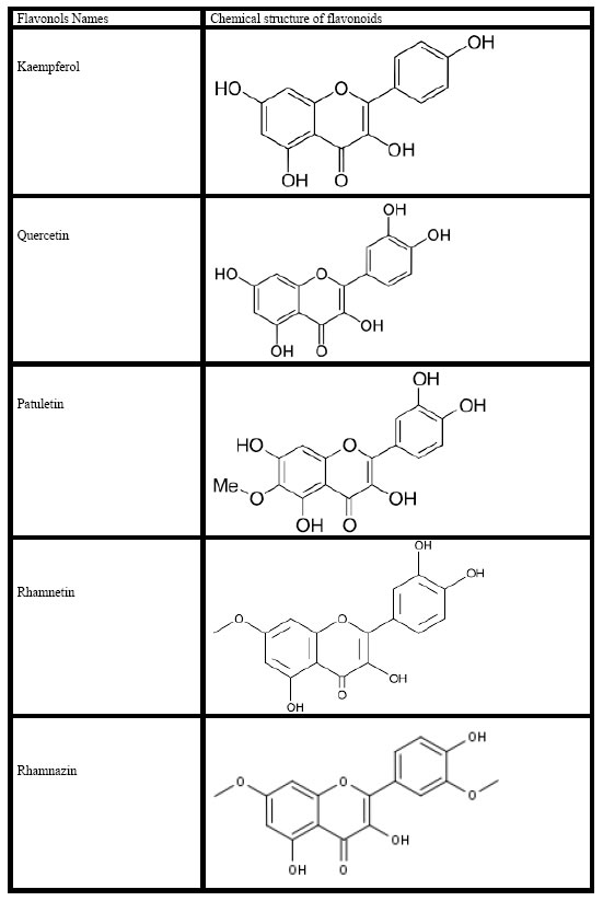
Figure 1. Chemical structure of flavonoids in the TW.

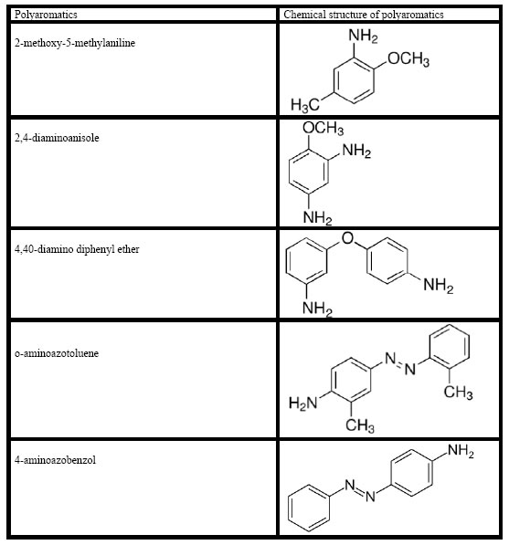
Figure 2. Chemical structure of polyaromatics in the TW

Preparation of photocatalysts

Ni-doped BiO nano particles were prepared by co-precipitation method using nickel nitrate hexahydrate [Ni(NO₃)₂.6H₂O] (Analytical grade, Merck ) and Bismuthnitrate hexahydrate [Bi(NO₃)₂·6H₂O] (Sigma, Aldrich) as the precursors of nickel and bismuth, respectively. Ni(NO₃)₂.6H₂O and sodium carbonate anhydrous (Na₂CO₃) were dissolved separately in double distilled H₂O to obtain 0.5 mol/Lsolutions. Nickel nitrate solution (250 mL of 0.5 mol/L) was slowly added into vigorously stirred 250 mL of 0.5 mol/L Na₂CO₃ solution. Nickel nitrate in the required stoichiometry was slowly added into the above solution and a white precipitate was obtained. The precipitate was filtered, repeatedly rinsed with distilled H₂O and then washed twice with ethanol. The resultant solid product was dried at 100°C for 12 h and calcined at 300°C for 2 h. BiO particles were also prepared by the same procedure without the addition of nickel nitrate solution. The doping Ni mass ratios of Bismuth are expressed as wt%.

X-Ray diffraction (XRD) analysis

XRD patterns of the samples are going to carry out using a D/Max-2400Rigaku X-ray powder diffractometer operated in the reflection mode with Cu Ka (λ = 0.15418 nm) radiation through scan angle (2θ) from 20° to 80°.

Scanning electron microscopy (SEM) analysis

The morphological structures of the Ni-BiO nanocomposites before photocatalytic degradation with UV light irradiations and after photocatalytic degradation with UV by means of a SEM.

Fourier transform infrared spectroscopy (FTIR)analysis

The FTIR spectra of Ni, BiO and Ni-BiO samples were measured with FTIR spectroscopy measurements.

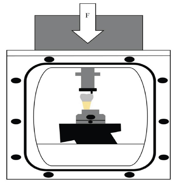
Photocatalytic degradation reactor

A 2 L cylinder kuvars glass reactor was used for the photodegradation experiments in the TW under different UV powers, at different operational conditions. 1000 mL TW was filled for experimental studies and the photocatalyst were added to the cylinder glass reactor. The photocatalytic reaction was operated with constant stirring during the photocatalytic degradation process. 10 mL of the reacting solution were sampled and centrifugated (at 10000 rpm) at different time intervals.

Used chemicals

Ni(NO₃)₂.6H₂O (Analytical Grade, Merck, Germany) and Bi(NO₃)3·6H₂O (Analytical grade, Merck, Germany) were used as nickel and bismuth sources, respectively. Na₂CO₃ was purchased from Merck (Analytical grade). Helium, He(g) (GC grade, 99.98%) and nitrogen, N₂(g) (GC grade, 99.98%) was purchased from Linde, (Germany). Kaempferol (99%), quercetin (99%), patuletin (99%), rhamnetin (99%), rhamnazin (99%), 2-methoxy-5-methylaniline (99%), 2,4-diaminoanisole (99%), 4,40-diamino diphenyl-ether (99%), o-aminoazotoluene (99%), 4-aminoazobenzol (99%) were purchased from Aldrich, (Germany).

Analytical methods

pH, T(°C), ORP, DO, BOD5, COD_total, CODdissolved, total suspended solids (TSS), Total-N, NH₃-N, NO₃-N, NO₂^–N, Total-P and PO₄-P measurements were monitored following the Standard Methods 2310, 2320, 2550, 2580, 4500-O, 5210 B, 5220 D, 2540 D, 4500-N, 4500-NH3, 4500-NO₃, 4500-NO₂ and 4500-P [30]. Inert COD was measured according to glucose comparison method [31]. The samples were analyzed by high pressure liquid chromatography (HPLC) with photodiode array and mass spectrometric detection using an Agilent 1100 high performance liquid chromatography system consisting of an automatic injector, a gradient pump, a Hewlett–Packard series 1100 photodiode array detector, and an Agilent series 1100 VL on-line atmospheric pressure ionization electrospray ionization mass spectrometer to detect flavonols namely kaempferol, quercetin, patuletin, rhamnetin, rhamnazin and polyaromatics namely, 2-methoxy-5-methylaniline, 2,4-diaminoanisole, 4,40-diamino diphenyl-ether, o-aminoazotoluene, 4-aminoazobenzol, respectively. All the  metabolites were measured in the same HPLC by mass spectrometric detections. Operation of the system and data analysis were done using ChemStation software, and detection was generally done in the negative ion [M − H]– mode, which gave less complex spectra, although the positive ion mode was sometimes used to reveal fragmentation patterns—especially patterns of sugar attachment. Separation of flavonol components was made on a Vydac C18 reversed phase column (2.1 μm dia. × 250 mm long; 5-μm particle size). Columns were eluted with acetonitrile-water gradients containing 0.1% formic acid in both solvents. The quality of the raw (un-treated) and photooxidated wastewater were determined by measuring the absorbances of the supernatans at wavelengths varying between 200 nm, 250 nm, 300 nm, 350 nm and 540 nmusing an Aquamate Termoelectron Corporation UV-vis spectrophotometer.

Measurement of photonic efficiency (lr) of Ni doped BiO

The relative photonic efficiency of the catalyst is obtained by comparing the photonic efficiency of Ni-doped BiO with that of the standard photocatalyst (BiO). In order to evaluate lr, a solution of 1-Methylcyclopropene-MCP (40 mg/L) with a pH of 10 was irradiated with 100 mg of BiO and Ni-doped BiO for 60 min. From the degradation results, Ir was calculated as follows (Eq. 1).

Operational conditions

Under 10-30-50 and 100 W  UV light powers the photocatalytic oxidation of the pollutant parameters in the TW at different operational conditions such as at increasing Ni mass ratios in the Ni-BiOnanocomposite(0.5wt% , 1wt%, 1.5wt%, 2wt%), at increasing photooxidation times (5 min, 15 min, 30, 60 min, 80 min and 100 min), at different Ni-BiOphotocatalyst concentrations (1, 5, 15, 30 and 45 mg/L), under acidic, neutral and basic conditions, respectively.

All the experiments were carried out following the batch-wise procedure. All experiments were carried out three times and the results were given as the means of triplicate sampling with standard deviation (SD) values.

Results and analysis

XRD Analysis results

The powder XRD patterns of BiO and Ni-doped BiO with different lanthanum mass ratios are shown in Figure 3. The XRD patterns of all the Ni-doped BiO catalysts are almost similar to that of BiO, suggesting that there is no change in the crystal structure upon Ni loading. This also indicates that Ni⁺² is uniformly dispersed on BiO nanoparticles in the form of small Ni2O₂ cluster. However the Ni-doped samples have a wider and lower intense diffraction peaks than pure BiO. Moreover, the XRD peaks of Ni-doped BiO continuously get broader with increasing the Ni loading up to a mass ratio of 2%wt.

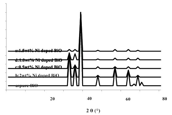
Figure 3. XRD patterns of BiO and Ni doped BiO (a) pure BiO, (b) 2 wt% Ni doped BiO, (c) 0.5wt% Ni doped BiO, (d) 1.0wt% Ni doped BiO, and (e) 1.5wt% Ni doped BiO.

SEM Analysis results

The morphology of nanocomposite particles is analyzed by SEM. Figure 4 shows that the nanocomposite material is partly composed of clusters containing composite nanoparticles adhering to each other with a mean size of around 20-80 nm before photooxidation process (Figure 4a) while the size increased to 24-86 nm after photooxidation (Figure 4b) with intermediates and remaining not photodegraded pollutants.

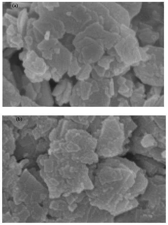
Figure 4. SEM micrographs of pure and nickel modified BiO, (a) pure BiO at 25°C, (b) Ni doped BiO at 25°C.

FTIR Analysis results

Figure 5 shows the FTIR spectrum of BiO and Ni-doped BiO, BiO powder synthesized under laboratory conditions. The peak between 400 and 700 cm^-1 give the information of Bi–O and Ni–Bi–O on the FTIR spectra. The peak at 437–455 cm^-1 give the information about stretching vibration of crystalline hexagonal zinc oxide (Bi–O stretching, vibration) and the peaks from 902 to 1020 cm^-1 are attributed to the bond between lanthanum and oxygen (Ni–O). The broad peak between 3400 to 3900 cm^-1 indicate the OH groups, due to the H₂O which indicates the existence of atmospheric H₂O adsorbed on the surface of nanocrystalline powder. An absorption band and a peak have been observed at 2350 cm^-1, respectively, which arises from the absorption of atmospheric CO₂ on the metal cations.

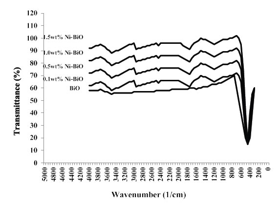
Figure 5. FTIR Spectra of pure BiO and Ni-doped BiO nanoparticles, with different concentration of dopant

Results and Discussions

Effect of increasing Ni-BiOnanocomposite concentrations on the removals of TW pollutants

The effects of increasing Ni-BiO nanocomposite concentrations (1 mg/L, 5 mg/L, 15 mg/L, 30 mg/L and 45 mg/L), on the photocatalytic oxidation of polutant parameters in the TW was investigated. The preliminary studies showed that the maximum removal of COD with 20 mg/L Ni-BiO nanocomposite was 89% with 70 min photooxidation time at pH=7.8 with 40 W UV power (Data not shown). Based on these yields the operational conditions for photocatalytic time were choosen as 60 min at a power of 50 W and at a pH of 8. The maximum photocatalytic oxidation removals for all pollutants in the TW were observed at 30 mg/L Ni-BiO nanocomposite concentrations, at pH=8.0, after 60 min photooxidation time and at 25°C at a power of 50 W (Figure 6). Removal efficiencies slightly decreased at 45 mg/L Ni-BiO nanocomposite concentration, because over load of surface area of Ni-BiO nanocomposites (Figure 6). This limiting the power of UV irradiation. Lower photo-removal efficiencies was measured for 1, 5, and 15 mg/L Ni-BiO concentrations due to low surface areas in the nanocomposite. On the contrarily, the surface area is high at 30 mg/L Ni-BiO nanocomposite concentrations. Therefore, the maximum photodegradation yield was observed in this nanocomposite concentration. The COD_total, COD_inert, total flavonols, total aromatic amines and color removals increased linearly as the Ni-BiO nanocomposite concentrations were increased from 1 mg/L up to 5 mg/L, to 15 mg/L, and up to 30 mg/L, respectively (Table 2 and Figure 6). Furher increase of nanocomposite concentration to 45 mg/L affect negatively the all the pollutant yields. The reason for this is the optimum amount of catalyst increases the number of active sites on the photocatalyst surface, which in turn increase the number of OH^● and superoxide radicals (O₂^– ●) to degrade pollutant parameters (COD components, flavonols, polyaromatics, color). When the concentration of the catalyst increases above the optimum value, the degradation decreases due to the interception of the light by the suspension [32]. reported that as the excess catalyst (turbidity) prevent the illumination of light, OH^●, a primary oxidant in the photocatalytic system decreased and the efficiency of the degradation reduced accordingly. Furthermore, the increase in catalyst concentration beyond the optimum may result in the agglomeration of catalyst particles; hence, the part of the catalyst surface becomes unavailable for photon absorption, and thereby, photocatalytic oxidation efficiency decreases [33]. Maximum COD_total, COD_inert, total flavonols, TAAs and color removal efficiencies were obtained after 60 min photooxidation process with yields of 99%, 92%, 91%, 98% and 99%, respectively, at pH=8.0, at 30 mg/L Ni-BiO nanocomposite concentration at 50 W power and at 25°C (Figure 6). Flavonols such as kaempferol, quercetin, patuletin, rhamnetin, rhamnazin removal efficiencies were 87%, 88%, 90%, 87% and 85% respectively, after 60 min photooxidation time, at pH=8.0, at 30 mg/L Ni-BiO nanocomposite concentration and at 25°C temperature (Table 2). Polyaromatic amines such as, 2-methoxy-5-methylaniline, 2,4-diaminoanisole, 4,40-diamino diphenyl ether, o-aminoazotoluene, 4-aminoazobenzol removal efficiencies after photooxidation process were 93%, 95%, 87%, 84% and 82%, respectively, after 60 min photooxidation time, at pH=8.0, at 30 mg/L Ni-BiO nanocomposite concentration at 50 W  UV power and at 25°C (Table 2).

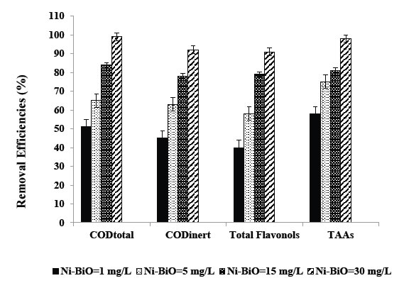
Figure 6. Removal efficiencies of COD_total, COD_inert, total flavonols and TAAs at Ni-BiO=1 mg/L, BiO=5 mg/L, BiO=15 mg/L and BiO=30 mg/L.

Table 2. Effect of increasing Ni-BiO nanocomposite concentrations on the TW during photooxidation process after 60 min, at 50 W UV irradiation, at pH=8.0, at 25°C.

Kaempferol metabolies such as, 3-O-[2-O,6-O-bis(α-L-rhamnosyl)-( β-D-glucosyl] quercetin, 3-O-[6-O-(α-L -rhamnosyl)-( β-D-  glucosyl]quercetin, 3-O-{2-O-[6-O-(p-hydroxy-trans-cinnamoyl)-{ )-, β-D-glucosyl]- á-L-rhamnosyl}kaempferol decreased from 5.7 mg/L to 0.86 mg/L, from 5.7 mg/L to 1.08 mg/L, from 5.7 mg/L to 1.25 mg/L, respectively, after 60 min photooxidation time, at pH=8.0, at 30 mg/L Ni-BiO nanocomposite concentration at 50 W  UV power and at 25°C (Table 3). Quercetin metabolites such as, 3-O-[6-O-( α-L -rhamnosyl)- )-(β-D-glucosyl]quercetin, 3-O-{2-O-[6-O-(p-hydroxy-trans-cinnamoyl)-( β-D -glucosyl]– á-L-rhamnosyl}quercetin reduced from 9.2 mg/L to 1.28 mg/L, from 9.2 mg/L to 2.30 mg/L, respectively, after 60 min photooxidation time, at pH=8.0, at 30 mg/L Ni-BiO nanocomposite concentration at 50 W  UV power and at 25°C (Table 3). Patuletin metabolites such as, (E)-ascladiol, (Z)-ascladiol dropped off from 10.3 mg/L to 1.55 mg/L, from 10.3 mg/L to 1.85, respectively, after 60 min photooxidation time, at pH=8.0, at 30 mg/L Ni-BiO nanocomposite concentration at 50 W  UV power and at 25°C (Table 3). Rhamnetin metabolites such as, methyl quercetin, tetrahydroxy-7-methoxyflavone decreased from 7.2 mg/L to 1.15 mg/L, from 7.2 mg/L to 1.44 mg/L, respectively, after 60 min photooxidation time, at pH=8.0, at 30 mg/L Ni-BiO nanocomposite concentration at 50 W  UV power and at 25°C (Table 3). Rhamnazin metabolites such as, Rhamnazin-3-0-β-D-glucopyranosyl-(l →5)- α-L-arabinofuranoside, Rhamnazin-3-O-β-D- glucopyranosyl-(l—»5)-[β-D-apiofuranosyl-(-1→2)]-α -L-arabinofuranoside reduced from 6.5 mg/L to 1.42 mg/L, from 6.5 mg/L to 1.66 mg/L, respectively, after 60 min photooxidation time, at pH=8.0, at 30 mg/L Ni-BiO nanocomposite concentration at 50 W  UV power and at 25°C (Table 3).

Table 3. The metabolites of flavonols in the TW.

2-methoxy-5-methylaniline metabolite such as, 5-nitro-o-toluidine decreased from 134.6 mg/L to 36.34, after 60 min photooxidation time, at pH=8.0, at 30 mg/L Ni-BiO nanocomposite concentration at 50 W  UV power and at 25°C (Table 4). 2,4-diaminoanisole such as, 4-acetylamino-2-aminoanisole, 2,4-diacetylaminoanisole reduced from 275.8 mg/L to 22.06 mg/L, from 275.8 mg/L to 38.61 mg/L, respectively, after 60 min photooxidation time, at pH=8.0, at 30 mg/L Ni-BiO nanocomposite concentration at 50 W  UV power and at 25°C (Table 4). 4,40-diamino diphenyl ether metabolites such as, N,NI-diacetyl-4,4I-diaminobenzhydrol, N,NI-diacetyl-4,4 I –diaminophenylmethane dropped off from 156 mg/L to 28.08 mg/L, from 156 mg/L to 40.56 mg/L, respectively, after 60 min photooxidation time, at pH=8.0, at 30 mg/L Ni-BiO nanocomposite concentration at 50 W  UV power and at 25°C (Table 4). o-aminoazotoluene metabolites such as, hydroxy-OAT (I), 4′-hydroxy-OAAT,  2′-hydroxymethyl-3-methyl-4-aminoazobenzene, 4, 4′-bis(otolylazo)-2, 2′ -dimethylazoxybenzene decreased from 293.6 mg/L to 58.72 mg/L, from 293.6 mg/L to 79.27 mg/L, from 293.6 mg/L to 85.14 mg/L, from 293.6 mg/L to 117.44 mg/L, respectively, after 60 min photooxidation time, at pH=8.0, at 30 mg/L La-ZnO nanocomposite concentration at 50 W  UV power and at 25°C (Table 4). 4-aminoazobenzol metabolites such as phenylhydroxylamine, nitrosobenzol reduced from 178 mg/L to 39.16 mg/L, from 178 mg/L to 44.5 mg/L, respectively, after 60 min photooxidation time, at pH=8.0, at 30 mg/L Ni-BiO nanocomposite concentration at 50 W  UV power and at 25°C (Table 4).

Table 4. The metabolites of polyaromatic amines in the TW.

[34] researched the photocatalytic activity of pure and Ni⁺²-doped BiO samples for the degradation of Rhodamine B (RhB). The effect of Ni⁺² doping concentration on the photocatalytic activity of RhB wasalso investigated. 9 g/L Ni⁺²-doped BiO with a mass ratio of 2wt% had high photocatalytic efficiency [34]. 4-nitrophenol degradation was studied in the presence of Ni doped BiO nanoparticles with a Ni mass ratio of 4% [35]. 78.26% 4-nitrophenol removal was observed the aforementioned nanocomposite after 195 min photodegradation time and at 30 W  UV light irradiation at pH=8 [35]. 68.57% Acid Yellow 29 55% Coomassie Brilliant Blue G250 and 37.27% Acid Green 25 degradations was obtained after 120 min of irradiation in the presence of 0.9% Ni-doped BiO, at 500 W UV light irradiation, under atmospheric oxygen, at 25°C, respectively [36]. The color and pollutant yields obtained in our study exhibited higher yields compared to the studies given above with low Ni-BiO nanocomposite concentrations.

Effect of increasing Ni mass ratios on 30 mg/L Ni doped BiO nanocomposite for photodegradation of TW pollutants

Were researched the effects of different La mass ratios (0.5wt%, 1wt%, 1.5wt% and 2wt% ) in 30 mg/L Ni-BiO nanocomposite concentrations on the photooxidation yields of all pollutants in the TW during photooxidation experiments. Maximum COD_total, COD_inert, total flavonols, TAAs and color removal efficiencies were 99%, 92%, 91%, 98% and 99%, respectively, after 60 min photooxidation time, at pH=8.0, at 1.5wt% Ni mass ratio and at 25°C (Table 5 and Figure 7). Removal efficiencies increased as the Ni mass ratio in the Ni doped BiO nanocomposite were increased from 0.5wt% to 1wt% and to 1.5wt%. Maximum removal efficiencies was measured at 1.5wt% Ni mass ratio in the nanocomposite. The photocatalytic degradation efficiency of BiO nanoparticles increases with an increase in the Ni loading and shows a maximum activity at 1.5 wt%. Then decreases in photooxidation yield was observed on further Ni doping (to 2 wt%). The reason of this can be explained as follows: excessive amounts of dopants can retard the photocatalysis process, because excess amount of dopants deposited on the surface of BiO increases the recombination rate of free electrons and energized holes, thus inhibiting the photodegradation process. Hence, further increase in Ni doping to 2wt% results in the decrease of photocatalytic degradation efficiency.

Table 5. Effect of increasing Ni mass ratios on the TW during photooxidation process after 60 min, at 50 W UV irradiation, 30 mg/L Ni-BiO nanocomposite concentrations, at pH=8.0, at 25°C.

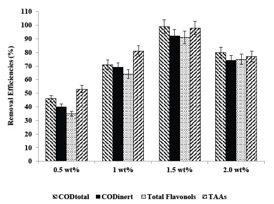
Figure 7. Removal efficiencies of COD_total, COD_inert, total flavonols and TAAs at 0.5wt%, 1wt%, 1.5wt%, and 2 wt% Ni mass ratio.

The synthesized Ni-doped BiO catalyst possesses smaller particle size distribution than pure BiO nanoparticles. Apart from their small size, as Ni⁺² was doped in BiO, more surface defects are produced as reported by [37]. Consequently, the migration of the photo-induced electrons and holes toward surface defects is reasonable [37]. Thus, the separation efficiency of the electron–hole pairs of Ni-doped BiO with more oxygen defects should be more than that of the pure BiO nanoparticles. Therefore, the enhancement in the photocatalytic degradation efficiency of Ni doping BiO increases due to small particle size and higher defect concentration compared to BiO alone.

UV absorbances of Ni-doped BiO

The UV–vis absorption spectra of BiO and Ni-doped BiO are shown in Figure 8. It can be clearly seen from Figure 8. The maximum absorbance shifts is 410 nm for pure nano BiO while the maximum absorbance of Ni-doped BiO with a Ni mass ratio 0.5wt% is observed at a wavelentgh of 380 nm. The wave of absorbance of Ni-doped BiO also increases gradually with increasing the Ni loading and is much higher as compared to that of pure BiO. This could be mainly attributed to the quantum size effect as well as the strong interaction between the surface oxides of Bi and Ni. These observations strongly suggest that the Ni doping significantly affects the absorbance properties.

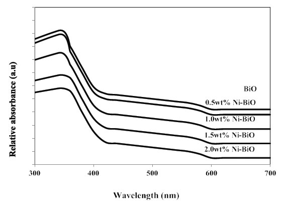
Figure 8. UV-vis absorption spectra of Ni doped BiO catalysts

The strong UV band gap emission (375–395 nm) results from the radiative recombination of an excited electron in the conduction band with the valence band hole. The broad visible or deep-trap state emissions (410–440 nm and 540–580 nm) are commonly defined as the recombination of the electron-hole pair from localized states with energy levels deep in the band gap, resulting in lower energy emission. These deep-trap emissions indicate the presence of defects or oxygen vacancies of BiO nanostructures [38]. Since the band gap excitation of electrons in BiO or Ni-doped BiO with 254 nm can promote electrons to the conduction band with high kinetic energy, they can reach the solid-liquid interface easily, suppressing electron–hole recombination in comparison with 365 nm. Hence, the observation of low rate at 254 nm is therefore unexpected [39]. The UV band gap emission of Ni-doped BiO nanostructures was increased between 380 and 410 nm after the photocatalytic process of pollutant parameters. The results show that 1.5 wt% Ni-doped BiO has maximum activity as compared to other photocatalysts.

Effect of increasing photooxidation time on the photooxidation yields of pollutants in the TW

Six different photooxidation times (5 min, 15 min, 30 min, 60 min, 80 min and 100 min) was examined during photocatalytic oxidation of the pollutants in the TW. To determine the optimum time for maximum removals these pollutant parameters in the TW. The maximum photocatalytic oxidation removals was observed at 60 min photooxidation time, at pH=8.0 using 30 mg/L Ni doped BiO with a La mass ratio of 1.5wt% at an UV power of 50 W (Figure 9). The removals of COD_total, COD_inert, total flavonols, total aromatic amines and color were found to increase linearly with increase in retention time from 5 min up to 80 min. A further increase in retention time to and 100 min lead to a decrease in yields of pollutant parameters. In other words the removal efficiencies of pollutant parameters (COD components, flavonols, polyaromatics, color) decreased for photooxidation time > 60 min since at long irradiation times since the surface energy of Ni doped – BiO decreases [40]. The photooxidation can form small molecules such as H₂O, carbonmonoxide (CO), CO₂ and benzene etc. after long irradiation; it will lead to the decrease of the polar groups and the oxygen content of pollutant surface. The dispersive component of surface energy, the density of polymer surface has great influence on dispersivity of pollutants in the TW. However, the rate of photodegradation of Ni doped-BiO blends increases with the increase of irradiation time, and is higher than that of photocrosslinking after long irradiation time, leading to the decrease of the density of the polymer surface and the dispersivity of COD, dyes and other pollutants to Ni doped–BiO [41]. The photooxidation can form small molecules such as H₂O, CO, CO₂ and benzene etc. after long irradiation; it will lead to the decrease of the polar groups and the oxygen content of polymer surface, therefore the dispersivity decreaeses resulting in low photooxidation yields [41]. Aromatic and phenolic metabolites which would adsorb strongly onto titania surface and block significant part of photoreactive sites.

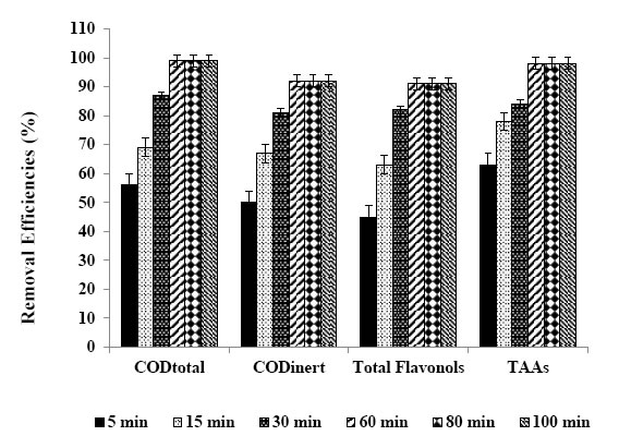
Figure 9. Removal efficiencies of COD_total, COD_inert total flavonols and TAAs after 5, 15, 30, 60, 80 and 100 min retention times.

The maximum COD_total, COD_inert, total flavonols, total aromatic amines and color removal efficiencies were 99%, 92%, 91%, 98% and 99%, respectively, after 60 min photooxidation time, at 1.5 wt% Ni mass ratio in 30 mg/L Ni-BiO nanocomposite concentration, at pH=8.0 and at 25°C under 50 W irradiation (Table 6). Also, flavonols such as kaempferol, quercetin, patuletin, rhamnetin, rhamnazin removal efficiencies were 87%, 88%, 90%, 87% and 85%, respectively (Table 6). The photooxidation removals of polyaromatic amines such as, 2-methoxy-5-methylaniline, 2.4-diaminoanisole, 4.40-diamino diphenyl ether, o-aminoazotoluene, 4-aminoazobenzol were 93%, 95%, 87%, 84% and 82%, respectively, after 60 min at pH=8.0 and at 25°C (Table 6). Kaempferol, quercetin, patuletin, rhamnetin, rhamnazin concentrations decreased from 5.7 to 0.741 mg/L, from 9.2 to 1.104 mg/L, from 10.3 to 1.03 mg/L, from 7.2 to 0.936 mg/L, from 6.15 to 0.923 mg/L, respectively. 2-methoxy-5-methylaniline, 2.4-diaminoanisole, 4.40-diamino diphenyl ether, o-aminoazotoluene, 4-aminoazobenzol concentrations decreased from 134.6 to 9.422 mg/L, from 275.8 to 13.79 mg/L, from 156 to 5.46 mg/L, from 293.6 to 10.28, from 178 to 6.23 mg/L, respectively.

Table 6. Effect of increasing photooxidation time on the TW during photooxidation process, at 50 W UV irradiation, at pH=8.0, 30 mg/L Ni-BiO nanocomposite concentrations, 1.5 wt% Ni mass ratio, at 25°C.

The color yields obtained in this study for TW are higher than the studies given below: [42] investigated the effects of Bi0.95Ni0.05O and Bi0.90Ni0.10O on the treatment of Methylene Blue (MB) dyestuff removal under 18 UV irradiation for 1 h. 81% color yields were observed for the aforementioned Ni-Bi-O nanocomposites, respectively [42]. [43] found 80% color yields based on Reactive Black 5 after 60 min irradiation time under 90 W irradiation using Bi-Ni nanocomposite.

Effect of increasing UV powers on the yields of pollutants in the TW

In this study, four UV light powers were used (10 W, 30 W, 50 W and 100 W) to detect the optimum UV irradiation power for maximum photo-removal of the pollutant parameters in the TW using 30 mg/L Ni doped BiO nanocomposite with a Ni mass ratio of 1,5%w. The maximum photocatalytic oxidation removals was observed at 50 W  UV light irradiation, at pH=8.0, after 30 min photooxidation time and at 25°C (Table 7 and Figure 10). The COD_total, COD_inert total flavonols, total aromatic amines and color were found to increase linearly with increase in UV light irradiation from 10 W, up to 30 W, up to 50 W, respectively (Table 7 and Figure 10). Further increase of UV power up to 100 W did not affect positively the pollutant yields. Maximum COD_total, COD_inert, total flavonols, TAAs and color removal efficiencies after photooxidation process were 99%, 92%, 91%, 98% and 99%, respectively, for the aforementioned operational conditions (Figure 10). Flavonols such as kaempferol, quercetin, patuletin, rhamnetin, rhamnazin removal efficiencies were 87%, 88%, 90%, 87% and 85%, respectively, after 60 min photooxidation time, at 50 W  UV light, at pH=8.0, at 30 mg/L Ni-BiO nanocomposite concentration and at 25°C (Table 7). Polyaromatic amines such as, 2-methoxy-5-methylaniline, 2, 4-diaminoanisole, 4, 40-diamino diphenyl ether, o-aminoazotoluene, 4-aminoazobenzol removal efficiencies after photooxidation process were 93%, 95%, 87%, 84% and 82%, respectively (Table 7).

Table 7. Effect of increasing UV light irradiations on the TW during photooxidation process after 60 min, at 30 mg/L Ni-BiO photocatalyst concentration, at pH=8.0, at 25°C.

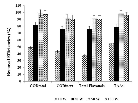
Figure 10. Removal efficiencies of COD_total, COD_inert, total flavonols and TAAs at 10 W, 30 W, 50 W and at 100 W.

The UV power determines the extent of light absorption by the semiconductor catalyst at a given wavelength. During initiation of photocatalysis, electron–hole formation in the photochemical reaction is strongly dependent on the optimum light intensity [44]. In this study, as the UV power increase from 10 W up to 50 W might favor a high-level surface defects, which account for the increase in the defect emission relative to the UV emission as reported by [39]. Higher UV powers > 50 W decrease the defects in the surface of the nanoparticle by disturbing the active holes.

Effect of increasing pH values on the pollutant yields in the TW

The effects of increasing pH values (4.0, 6.0, 8.0 and 10.0) on the photocatalytic oxidation of polutant parameters in TW was examined by considering the solubility of BiO nanoparticles in acidic as well as in highly basic solutions. The maximum photocatalytic oxidation removals was obtained at pH=8.0, after 60 min photooxidation time with a Ni mass ratio 1.5wt% using 30 mg/L Ni-BiO nanocomposite concentration at 50 W  UV power (Table 8 and Figure 11). In acidic medium, less photocatalytic degradation of pollutant parameters (COD components, flavonols, polyaromatics, color) was observed. The extent of photocatalytic degradation of polutant parameters was found to increase with increase in initial pH to 8.0 and a decrease in maximum photocatalytic degradation was found at pH 10. The possible explanation of this is that the pH at zero point charge (zpc) of BiO is 9.0 ± 0.3 [45]. Below pH 8.0, active sites on the positively charged catalyst surface are preferentially covered by pollutant molecules. Thus, surface concentration of the polutant parameters (COD components, flavonols, polyaromatics, color) is relatively high, while those of OH^– and OH^● are low. Hence, photocatalytic degradation decreases at acidic pH. On the other hand, above pH 8.0, catalyst surface is negatively charged by means of metal-bound OH^–, consequently the surface concentration of the polutant parameters (COD components, flavonols, polyaromatics, color) is low, and OH^● is high. In addition, polutant parameters are not protonated above pH 8.0. The electrostatic repulsion between the surface charges and Ni doped BiO nanocomposite hinders the amount of polutant parameters and the adsorption, consequently surface concentration of the polutant parameters decreases, which results in the decrease of photocatalytic degradation at pH 10.0. In conclusion, pH 8.0 can provide moderate surface concentration of polutant parameters which react with the holes to form OH^●.

Table 8. Effect of increasing pH values on the TW during photooxidation process, at 50 W UV irradiation, after 60 min, at 25°C.

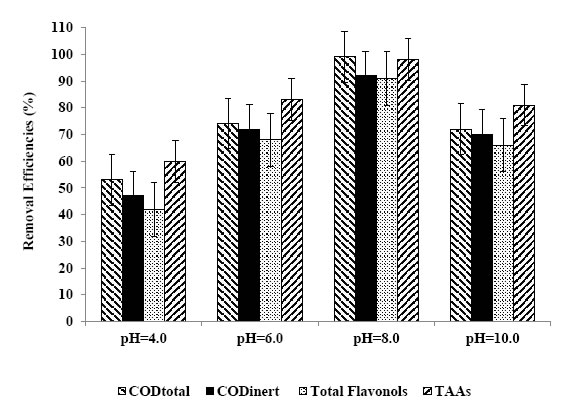
Figure 11. Removal efficiencies of COD_total, COD_inert, total flavonols and TAAs at pH=4.0, pH=6.0, pH=8.0, pH=10.0.

Photocatalytic oxidation mechanisms of Ni doped BiOnanocomposite

The higher activity of Ni doped BiO can beattributed to successful e⁻–h⁺ separation and production of ●O₂⁻ and OH^●. Ni-modified BiO sample manifests the highest efficiency, which may be explained by the highest number of O₂ vacancies (related to the different charge and electronegativity of Ni and Bi ions) and as a result of stronger adsorption of OH⁻ions onto the BiO surface [46]. This favors the formation of OH^● by reaction of hole and OH⁻. The OH^● and photogenerated ●O₂⁻has extremely strong non-selective oxidants lead to the degradation of the organic pollutant at the surface of Ni modified BiO [41]. The photocatalytic degradation mechanism starts with the illumination of BiO nanoparticles and production of electron–hole pairs in Eq. (2):

Major roles of metal ions in this study are to increase the concentration of BiO on the surface of the catalyst and to prolong the individual life-time of electrons and holes and hence, inhibit their recombination. The ability of Ni⁺³ to scavenge photogenerated electrons is as follows: (Eq. 3):

However, stabilities of Ni⁺³ ions may be disturbed in their reduced forms (Ni⁺²). This can be achieved by transferring the trapped electron to O₂ [Eq. (4)]:

The produced O₂⁻● is responsible from the generation of OH^●, known as highly reactive electrophilic oxidants [Eqs. (5-7)]:

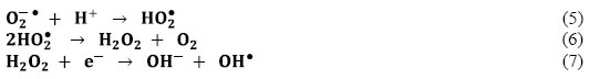
In the meantime, photogenerated holes may react with H₂O molecules and produce OH^● (Eq. 8):

The color removal by photooxidation of dyes reactions were given in Eqs (9-14):

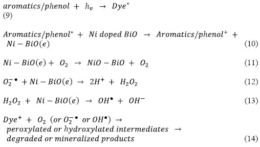
Thus, loading of metal ions such as Ni on the surface of BiO matrix can suppress the recombination of photoinduced charge carriers either with only electron capture ability or with steps forward to produce OH^●. For Ni–BiO, electron accepting ability, production of more OH^●, the highest surface roughness value and the higher dark adsorption capacity result in pronounced photoactivity. The decay profile of the products includes the subsequent attacks of OH^●, known as highly reactive electrophilic oxidants. The main reaction pathway (60% of OH^●) is the addition of the OH^● to the double bond of the azo group, resulting in the rapid disappearance of color; however, addition to the aromatic ring also occurs (40% of OH^●) [47, 48]. Further OH^● attacks and the increment in OH^● concentration in the solution increase the yield of OH^–adduct in the degradation progress of each product. The opening of the dye aromatic rings due to consecutive oxidation reactions leads to low-molecular weight compounds [49].

Photonic efficiency of Ni doped BiO

In order to evaluate the relative photonic efficiency (Ir), a solution of MCP (40 mg/L) adjusted to pH 10 was irradiated with 100 mg BiO (Merck) and Ni-doped BiO, separately. The relative photonic efficiencies of light of wavelengths 254 and 365 nm for BiO and Ni-doped BiO are presented in Table 9. For comparison, the relative photonic efficiency of TiO₂ is also presented in Table 9. The relative photonic efficiencies of Ni-doped BiO are greater as compared to those of BiO and TiO₂, revealing the effectiveness of metal-doped systems. It is also interesting to note that the relative photonic efficiency for Ni-doped BiO for light of wavelength 254 nm are much higher as compared to that for 365 nm. The results are in good agreement with degradation and mineralization studies. Comparing the high efficiency of Ni doped BiO catalysts with standard BiO and TiO₂ catalyst, the photocatalytic efficiency of 1.5 wt% Ni-doped BiO is higher as compared to that of BiO and TiO₂ and other Ni doped BiO nanacomposites.

Table 9. Comparison of relative photonic efficiencies in the photodegradation of pollutants in TW by BiO and Ni-doped BiO photocatalysts (*)

Reusability of Ni doped BiO

As shown in Figure 12, after the first cycle of photocatalytic oxidation within 60 min, 99% of the Ni doped BiO with a mass ratio of 1.5wt% was recovered. After three cycles, the phoooxidation ability of Ni doped BiO nanocomposite was retained at 93% of the original value. After 8th cycles the nanocomposite was reatined at 80%. One of the reasons for the slight decline in photooxidation is that the surface of the reused photocatalysts may exist with some low residual substances which did not occupy the photocatalytic sites and did not block the adsorption. The presence of Ni significantly changed the binding site of the pollutant molecules. It is possible that the oxygen atom in Ni-BiO was bound to the dopant Ni [50]. The speedily recovering of the photodegradation capacity of Ni doped BiO for pollutans photodegradation will benefit to their photocatalytic activity.

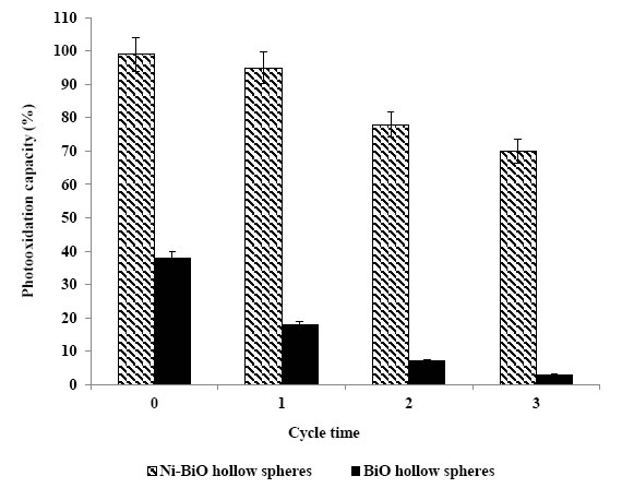
Figure 12. The reusability of Ni doped BiO

Conclusions

By using 30 mg/L Ni-BiO with a Ni mass ratio of 1.5w% the COD_total, COD_inert, flavonols, polyaromatics and color were photodegraded with yields as high as 82-99% within 60 min photooxidation time, at 25°C under 50 W  UV power, at pH=8.0. The addition of Ni to BiO lead to enhance the photocatalytic activity by increasing the total surface area. The flavonoids and polyaromatic amines and their metabolites in the TW were firstly determined photodegraded with high rates and photonic efficiency using 30 mg/L Ni-BiO with a Ni mass ratio of 1.5w% at pH 8.

References

1. Lin SH, Chen ML (1997) Treatment of textile wastewater by chemical methods for reuse.Water Research31: 868-876.
2. Van der Zee FP, Bouwman RHM, Strik DP, Lettinga G, Field JA (2001) Application of redox mediators to accelerate the transformation of reactive azo dyes in anaerobic bioreactors.Biotechnology and Bioengineering75: 691-701.[Crossref]
3. Chung KT, Stevens SEJ (1993) Degradation of azo dyes by environmental microorganisms and helminthes.Environmental Toxicology and Chemistry 12: 2121-2132.
4. Weisburger JH (2002) Comments on the history and importance of aromatic and heterocyclic amines in public health.Mutation Research-Fundamental and Molecular Mechanisms of Mutagenesis506: 9-20.[Crossref]
5. Oliveira DP, Carneiro PA, Sakagami MK, Zanoni MVB, Umbuzeiro GA (2007) Chemical characterization of a dye processing plant effluent–identification of the mutagenic components.Mutation Research-Fundamental and Molecular Mechanisms of Mutagenesis626: 135-142.
6. Robinson T, McMullan G, Marchant R, Nigam P (2001) Remediation of dyes in textile effluent: a critical review on current treatment technologies with a proposed alternative.Bioresource Technology77: 247-255.[Crossref]
7. Van der Zee FP, Villaverde S (2005) Combined anaerobic–aerobic treatment of azo dyes—a short review of bioreactor studies.Water Research39: 1425-1440.[Crossref]
8. Roosta M, Ghaedi M, Shokri N, Daneshfar A, Sahraei R, Asghari A (2014) ‘Experimental design based response surface methodology optimization of ultrasonic assisted adsorption of safaranin o by tin sulfide nanoparticle loaded on activated carbon. Spectrochimica Acta – Part A: Molecular and Biomolecular Spectroscopy 122:  223-231.
9. Tavakkoli H, Moayedipour T (2014) Fabrication of perovskite-type oxide La0.5Pb0.5MnO₃ nanoparticles and its dye removal performance. Journal of Nanostructure in Chemistry4: 116-124.
10. Qi X, Zhou J, Yue Z, Gui Z, Li L (2003) Auto-combustion synthesis of nanocrystalline LaFeO₃.Materials Chemistry and Physics78: 25-29.
11. Deganello F, Marcì G, Deganello G (2009) Cipate–nitrate auto-combustion synthesis of perovskite-type nanopowders: A systematic approach.Journal of the European Ceramic Society29: 439-450.
12. Jadhav LD, Patil SP, Chavan AU, Jamale AP, Puri VR (2011)Solution combustion synthesis of Cu nanoparticles; a role of oxidant-to-fuel ratio.Micro & Nano Letters6:812-815.
13. Shea LE, McKittrick J, Lopez OA, Sluzky E (1996) Synthesis of red-emitting, small particle size luminescent oxides using an optimized combustion process.Journal of the American Ceramic Society 79: 3257-3265.
14. Dong SY, Feng JL, Fan MH, Pi Y, Hu L, et al. (2015) Recent developments in heterogeneous photocatalytic water treatment using visible light-responsive photocatalysts: A review.RSC Advances5: 14610-14630.
15. Wang HL, Xu LJ, Liu CL, Lu Y, Feng Q, et al. (2019) Composite magnetic photocatalyst Bi5O7I/MnxZn1-xFe2O₄:Hydrothermal-roasting preparation and enhanced photocatalytic activity.Nanomaterials 9: 118-131.
16. Li HH, Li KW, Wang H (2009) Hydrothermal synthesis and photocatalytic properties of bismuth molybdate materials.Materials Chemistry and Physics116: 134-142.
17. Ren J, Wang W, Shang M, Sun S, Gao E (2011) Heterostructured bismuth molybdate composite: Preparation and improved photocatalytic activity under visible-light irradiation.ACS Applied Materials & Interfaces 3: 2529-2533. [Crossref]
18. Zhang T, Huang JF, Zhou S, Ouyang HB, Cao LY,et al. (2013) Microwave hydrothermal synthesis and optical properties of flower-like Bi₂MoO₆ crystallites.Ceramics International39: 7391-7394.
19. Meng XC, Zhang ZS (2016) Bismuth-based photocatalytic semiconductors: Introduction, challenges and possible approaches.Journal of Molecular Catalysis A-Chemical423: 533-549.
20. Jia YL, Ma Y, Tang JZ, Shi W (2018) Hierarchical nanosheet-based Bi₂MoO₆ microboxes for efficient photocatalytic performance.Dalton Transactions47: 5542-5547.
21. Zhou TF, Hu JC, Li JL (2011) Er³⁺ doped bismuth molybdate nanosheets with exposed {010} facets and enhanced photocatalytic performance.Applied Catalysis B: Environmental110: 221-230.
22. Wang QY, Lu QF, Wei MZ, Wei M, Guo E, et al. (2018) ZnO/-Bi₂MoO₆ heterostructured nanotubes: Electrospinning fabrication and highly enhanced photoelectrocatalytic properties under visible-light irradiation.Journal of Sol-Gel Scıence and Technology85: 84-92.
23. Zhong Y, He ZT, Chen DM, Hao D, Hao W, (2019) Enhancement of photocatalytic activity of Bi₂MoO₆ by fluorine substitution.Applications of Surface Science467: 740-748.
24. Wang PF, Ao YH, Wang C, Hou J, Qian J (2012) A one-pot method for the preparation of graphene- Bi₂MoO₆ hybrid photocatalysts that are responsive to visible-light and have excellent photocatalytic activity in the degradation of organic pollutants.Carbon50: 5256-5264.
25. Wang M, Han J, Guo PY, Sun MZ, Zhang Y, et al. (2018) Hydrothermal synthesis of B-doped Bi₂MoO₆ and its high photocatalytic performance for the degradation of Rhodamine B.Journal of Physics and Chemistry of Solids 113: 86-93.
26. Chen C, Liu L, Guo J, Zhou LX, Lan YQ (2019) Sulfur-doped copper-cobalt bimetallic oxides with abundant Cu (I): A novel peroxymonosulfate activator for chloramphenicol degradation.Chemical Engineering Journal361: 1304-1316.
27. Wang J, Sun YG, Wu CC, Cui Z, Rao PH(2019) Enhancing photocatalytic activity of Bi₂MoO₆ via surface co-doping with Ni2+ and Ti4+ ions.Journal of Physics and Chemistry of Solids129: 209-216.
28. Ding X, Ho WK, Shang J, Zhang LZ (2016) Self doping promoted photocatalytic removal of no under visible light with Bi₂MoO₆: Indispensable role of superoxide ions.Applied Catalysis B: Environmental182: 316-325.
29. Zhang XH, Zhang HR, Jiang HT, Yu F, Shang ZR (2019) Hydrothermal synthesis and characterization of Ce³⁺ doped Bi₂MoO₆ for water treatment.Catalysis Letters1-11.
30. Eaton AD, Clesceri LS, Rice EW, Greenberg AE, Franson MAH (2005) Standard Methods for the Examination of Water and Wastewater’, Ed. by Franson MAH, (21th ed.), American Public Health Association (APHA), American Water Works Association (AWWA), Water Environment Federation (WEF), American Public Health Association (APHA) 800 I Street, NW, Washington, DC: 20001-3770, USA.
31. Germirli F, Orhon D, Artan N (1991) Assessment of the initial inert soluble COD in industrial wastewater.Water Science and Technology 23: 1077-1086.
32. Sun J, Qiao L, Sun S, Wang G (2008) Photocatalytic degradation of orange g on nitrogen-doped TiO₂ catalysts under visible light and sunlight irradiation.Journal of Hazardous Materials 155: 312-319.[Crossref]
33. Huang M, Xu C, Wu Z, Huang Y, Lin J, et al. (2008) Photocatalytic discolorization of methyl orange solution by Pt modified TiO₂ loaded on natural zeolite.Dyes and Pigments77: 327-334.
34. Jia T, Wang W, Long F, Fu Z, Wang H, Zhang Q (2009) Fabrication, characterization and photocatalytic activity of La-doped ZnO nanowires.Journal of Alloys and Compounds484: 410-415.
35. Khatamian M, Khandar AA, Divband B, Haghighi M, Ebrahimiasl S (2012) Heterogeneous photocatalytic degradation of 4-nitrophenol in aqueous suspension by Ln (La³⁺, Nd³⁺ or Sm³⁺) doped ZnO nanoparticles.Journal of Molecular Catalysis A: Chemical365: 120-127.
36. Raza W, Haque MM, Muneer M (2014) Synthesis of visible light driven ZnO: characterization and photocatalytic performance. Applications of Surface Science322: 215-224.
37. Zheng Y, Chen C, Zhan Y, Lin X, Zheng Q, et al. (2007) Luminescence and photocatalytic activity of ZnO nanocrystals:  correlation between structure and property.Inorganic Chemistry 46: 6675-6682.
38. Bohle DS, Spina CJ (2009) Cationic and anionic surface binding sites on nanocrystalline zinc oxide: surface influence on photoluminescence and photocatalysis.Journal of the American Chemical Society131: 4397-4404.
39. Selvam NCS, Vijaya JJ, Kennedy LJ, (2013) Comparative studies on influence of morphology and La doping on structural, optical, and photocatalytic properties of zinc oxide nanostructures.Journal of Colloid and Interface Science407: 215-224.
40. Fox MA, Dulay MT (1993) Hetereogeneous photocatalysis.Chemical Reviews93: 341-357.
41. Korake PV, Dhabbe RS, Kadam AN, Gaikwad YB, Garadkar KM (2014) Highly active lanthanum doped ZnO nanorods for photodegradation of metasystox.Journal of Photochemistry and Photobiology B-Biology130: 11-19.
42. Suwanboon S, Amornpitoksuk P, Bangrak P, Muensit N (2013) Optical, photocatalytic and bactericidal properties of Zn1-xLaxO and Zn1-xMgxO nanostructures prepared by a sol–gel method.Ceramics International39: 5597-5608.
43. Kaneva N, Bojinova A, Papazova K, Dimitrov D (2015) Photocatalytic purification of dye contaminated sea water by lanthanide (La³⁺, Ce³⁺, Eu³⁺) modified ZnO.Catalysis Today252: 113-119.
44. Cassano AE, Alfano OM (2000) Reaction engineering of suspended solid heterogenous photocatalytic reactors.Catalysis Today58: 167-197.
45. Anandan S, Vinu A, Venkatachalam N, Arabindoo B, Murugesan V (2006) Photocatalytic activity of ZnO impregnated Hâ and mechanical mix of ZnO/Hâ in the degradation of monocrotophos in aqueous solution.Journal of Molecular Catalysis A: Chemical256: 312-320.
46. Anandan S, Vinu A, Mori T, Gokulakrishnan N, Srinivasu P, et al. (2007) Photocatalytic degradation of 2,4,6-trichlorophenol using lanthanum doped ZnO in aqueous suspension.Catalysis Communications8: 1377-1382.
47. Joseph JM, Destaillats H, Hung H, Hoffmann MR (2000) The sonochemical degradation of azobenzene and related azo dyes:  rate enhancements via fenton’s reactions.Journal of Physical Chemistry A104: 301-307.
48. Spadaro JT, Isabelle L, Renganathan V (1994) Hydroxyl radical mediated degradation of azo dyes: evidence for benzene generation.Environmental Science & Technology28: 1389-1393.
49. Galindo C, Jacques P, Kalt A (2000) Photodegradation of the aminobenzene Acid Orange 52 by three advanced oxidation processes: UV/H₂O₂, UV/TiO₂ and VIS/TiO₂: comparative mechanistic and kinetic investigations.Journal of Photochemistry and Photobiology A-Chemistry 130: 35-47.
50. Pala RGS, Metiu H (2007) The structure and energy of oxygen vacancy formation in clean and doped, very thin films of ZnO.Journal of Physical Chemistry C111: 12715-12722.
51. Battle PD, Cheetham AK, Goodenough JB (1979)A neutron diffraction study of the ferrimagnetic spinel NiCO₂O₄.Materials Research. Bulletin14: 1013-1024.
52. Roosta M, Ghaedi M, Daneshfar A, Darafarin S, Sahraei R,et al. (2014b) Simultaneous ultrasound-assisted removal of sunset yellow and erythrosine by ZnS:Ni nanoparticles loaded on activated carbon: optimization by central composite design.Ultrasonics Sonochemistry21: 1441-1450.
53. Verma S, Joshi HM, Jagadale T, Chawla A, Chandra R, et al. (2008) Nearly monodispersed multifunctional NiCO₂O₄ spinel nanoparticles: magnetism, infrared transparency, and radio frequency absorption.The Journal of Physical Chemistry C112: 15106-15112.
54. Wu Z, Zhu Y, Ji X (2014) NiCO₂O₄-based materials for electrochemical supercapacitors.Journal of Materials Chemistry A2: 14759-14772.
55. Xing YX, Zhan J, Liu ZL,Du CF (2017) Steering photoinduced charge kinetics via anionic group doping in Bi₂MoO₆ for e_cient photocatalytic removal of water organic pollutants.RSC Advances7: 35883-35896.

DOI: 10.31038/NAMS.2020312

Abstract

Marine litter is a widespread problem affecting all the oceans of the world. Plastics represent around 90% of marine litter, and it is estimated that there are between 15 and 51 trillion plastic particles floating on the surface of the oceans. The objectives of this study are to: (i) identify and characterize the main categories of floating items sampled in surface waters off the Cap Corse peninsula, (ii) provide estimates of the occurrence of floating items in this area, and (iii) get an overview of the potential areas of litter accumulation. We highlighted a heterogeneous distribution of floating litter as the plastic density characterizing the area between Bastia and Macinaggio (27 027 items/km²) was, on average, 2.31 times higher than the density estimated between Macinaggio and Pino (11 688 items.km²). Several studies highlighted that spatio-temporal variability of plastic densities and sizes of plastics (micro, meso, macroplastics) could be tightly linked with hydrodynamics and wind regime, distance to land, coastal human population and maritime traffic. Beyond the need to further raise awareness, providing more evidences and information regarding such marine pollution may hopefully foster urgent management strategies, whereby the most effective mitigation strategy implies reducing the input at its source.

Keywords

Plastic, marine litter, manta-net, Mediterranean Sea.

Introduction

Marine litter is a widespread problem affecting all the oceans of the world. Plastic pollution has gained attention by scientists and public perception in the last decade [1, 2]. Plastics represent around 90% of marine litter [3], and it is estimated that there are between 15 and 51 trillion plastic particles floating on the surface of the oceans [4].Global plastic production increased from 5 million tonnes in 1950 to 322 million tonnes in 2015 [5] It is considered that, on average, around 80–90% of ocean plastic comes from land-based sources, including via rivers, with a smaller proportion arising from ocean-based sources such as fisheries, ships and aquaculture. Plastic inputs from land to ocean was estimated to represent at least 4.8 to 12.7 million tonnes in the year 2010 [6]. Because of their abundance, durability and persistence, marine plastics constitute today a major threat to the marine environment [7].

The most visible impacts of marine plastics are the ingestion, suffocation and entanglement of hundreds of marine species, including species listed on the IUCN Red List as near threatened or above [8]. Microplastics (less than 5 mm in diameter), in particular, have recently become a source of concern, as their ingestion has been observed in a wide variety of taxa including zooplankton, marine invertebrates, fish, turtles, seabirds, and marine mammals [9–11]. Once ingested, microplastics can cause starvation, alterations in intestinal functions, a reduction in feeding capacity, energy reserves and reproductive output [12]. Also, contaminated preys can be consumed by predators leading to the transfer of plastics accross trophic levels [13]. Moreover plastics are polymers that may contain a large variety of chemical additives and contaminants, including organic pollutants and endocrine disruptors, that pollute the environment [14] and can be harmful to marine biota [15, 16].

Floating marine litter also plays an important role in the spread of marine or terrestrial organisms, including the dispersal of invasive species that may pose a threat to local ecosystems [17]. Also, the hydrophobic nature of plastics stimulates the formation of biofilms and allows the establishment of numerous organisms, called “epiplastic” organisms, which constitute a new marine ecosystem called “plastisphere”[18]. It can host different groups, in particular microbial organismsincluding pathogenic viruses or bacteria but also fungi, algae, molluscs, cnidarians, and crustaceans [19–21]. The surge in the number of litter introduced into the marine environment currently offers a great variability of objects that may serve as « novel habitat » or as « hitch-hiking raft »  [22, 23].

In addition to causing harm and threatening marine ecosystems, marine litter, especially plastic, can also negatively affect human wellbeing, food security and socioeconomic sectors such as tourism, aquaculture, fishing and navigation [24-26].

The Mediterranean Sea is considered as a biodiversity hotspot [27], besieged by multiple human pressures. Indeed, its shores are home to around 10% of the world’s coastal population and around 100 million people live within 10 km of the coast [28]. Moreover, the Mediterranean basin is one of the busiest shipping routes in the world and receives the waters of densely populated watersheds, e.g. the Nile, the Ebro, the Po [29]. It is therefore not surprising that the basin is nowadays described as one of the areas most affected by marine litter in the world, whereby the average density of plastic as well as its frequency of occurrence throughout the basin were comparable to accumulation zones in ocean gyres [29–31]. In Europe, various regulatory directives have been put in place to limit and reduce this pollution, such as the Marine Strategy Framework Directive (MSFD). In order to define the concept of « Good Environmental Status », the MSFD proposed 11 descriptors including descriptor n° 10 describing good status for marine litter as follows: “Properties and quantities of marine litter do not cause harm to the coastal and marine environment” [32]. Also new knowledge on this topic may have impact in the implementation of other environmental regulations such as the new European Strategy for Plastics in a Circular Economy (COM/ 2018/028 final), which has recently agreed on banning certain single use plastic (SUP) items.

To develop and validate indices of ecosystem status or pollution, it is necessary to have access to areas with low human impact and then validate them along local pressure gradients [33]. Corsica, is a privileged area in the North-Western Mediterranean. It is at the centre of one of the most touristic regions in the world still sheltered from heavy pollution of anthropic origin. This area should come closer to the concept of Good Ecological Status in terms of pollution by plastic marine litter. Our study intends to provide further information on marine litter regarding the northeastern waters of Corsica, part of the Cap Corse and Agriate Marine Natural Park (PNMCCA). This area is also comprised within the Pelagos Sanctuary, a large marine area subject to an agreement between Italy, Monaco and France for the protection of marine mammals.

In detail, the objectives of this study are to: (i) identify and characterize the main categories of floating items sampled in surface waters off the Cap Corse peninsula, (ii) provide estimates of the occurrence of floating items in this area, and (iii) get an overview of the potential areas of litter accumulation.

Material and method

In August 2019, the Corsican Blue Project team carried out a marine litter sampling campaign  within the perimeter of the Cap Corse and Agriate Marine Natural Park (PNMCCA). A total of six manta-net tows were conducted along the coast of the Cap Corse peninsula between Bastia and Pino, including three transects along the eastern coast (Bastia-Macinaggio) and three transects along the northwestern coast (Pino-Macinaggio). The manta-net, characterized by a rectangular opening of 86 x 46 cm and a net opening of 330 μm, was deployed at the surface beyond the boats’ wake at an average speed of 2.2 to 2.4 knots and for about 30 min per tow. General characteristics of each transect were recorded. After each sampling, the entire net was thoroughly rinsed with seawater from the opening to the collection bag to ensure that all the debris were concentrated in the cod end before being retrieved.

Collected samples were sent for analysis to the STARESO (STAtion de REcherches Sous-marines et Océanographique) research station.In the laboratory, the samples were rinsed with seawater on a 300 μm sieve.Then the mesh was rinsed with tap water and the sample was collected. Sampling consists of direct extraction from the environment of items that are recognizable by the naked eye. Several steps have been taken to separate the litter from the biological matrix and water [34]. Litter was manually separated from natural debris by removing the largest pieces of biological material (leaves, algae, wood …) and rinsing them with water that underwent a second sorting to avoid any loss of debris [35]. Items that were visually identified as litter were collected using fine forceps and then counted. To avoid misidentification and underestimation of microplastics it is necessary to standardize the plastic particle selection, following certain criteria to guarantee proper identification [34]. Plastics were identified according morphological characteristics and physical response features (e.g. response to physical stress; microplastics were bendable or soft, colors) [34, 36]. Identified plastic items were measured over their largest cross-section (total length) in order to be classified into three categories: microplastics (<5 mm), mesoplastics (5-200 mm) and macroplastics (> 200 mm) [37]. Plastic items were also classified, as proposed by [21], into six categories according to their visual characteristics:

1. Fragment: this category is generally the most abundant. They are rigid, thick, with sharp, pointed edges and an irregular shape. They can be of different colors.

2. Film: they also appear in irregular shapes, but compared to the fragments, they are fine and flexible and generally transparent.

3. Pellet: they are generally from the plastics industry. These are irregular round shapes, about 5 mm in diameter. They are generally flat on one side and can be of different colors.

4. Granule: they have a regular round shape and generally smaller, around 1 mm in diameter. They appear in natural colors (white, beige, brown).

5. Filament: these are, with the fragments, the most abundant type of particles. They can be short or long, with different thicknesses and colors.

6. Foam: they most often come from large particles of polystyrene foam. They have a soft, irregular shape and are white to yellow in color.

The surface of the surveyed area was estimated by multiplying the observation width by the transect distance, and litter density (items/km²) was calculated by dividing the items count with the surveyed area surface [29].

Results and discussion

In this study, plastic litter was encountered in 100% of the hauls made off Cap Corse, representing a total of 238 itemsand a mean density of 19357 items/ km².

We highlighted a heterogeneous distribution of floating litter as the plastic density characterizing the area between Bastia and Macinaggio (27 027 items/km²) was, on average, 2.31 times higher than the density estimated between Macinaggio and Pino (11 688 items.km²) (Fig.1). Several studies highlighted that spatio-temporal variability of plastic densities and sizes of plastics (micro, meso, macroplastics)could be tightly linked withhydrodynamics and wind regime [31, 38], distance to land [29, 39], coastal human population [40, 41] and maritime traffic [23]. In our case, the difference in densities found between the regions Bastia-Macinaggio and Macinaggio-Pino, could be consistent with coastal human population pressurewhereby the area with an estimated higher density is located close to Bastia, a city of more than 44 000 inhabitants.As an example, a sampling campaign conducted in the Ligurian Sea, mainly along the French continental coast, reported that highest densities were found in front of Nice [40]. Corsica has been identified as a reference area where contamination by microplastics was lower compared to other regions off the French Mediterranean coasts (e.g. Antibes, Marseille, Toulon) [42].

Figure 1. Average concentration of plastic litter, expressed as debrits per km², in surface water off Cap Corse.

Moreover, the area between Corsica and Elba has been identified as displaying the highest natural marine debris concentration throughout the Central Western Mediterranean, suggesting therefore that the area is under great influence of terrigenous input [43]. However, the identification of the source of the collected litter remains challenging without the consideration of dispersion models, and items being subject to surface water circulation [44] may drift from their source of input. Indeed, studies investigating on debris transport and dispersion due to marine circulation strongly suggest that floating litter might drift during periods ranging from a few weeks to several years before eventually sinking or beaching [45]. Taking into account thatthe Tyrrhenian Sea has been identified as an important accumulation zone [23] and that the eastern coast of Corsica  is under the influence of the Tyrrhenian sea current which flows along the Italian coast before entering the Corsica channel [46] it is very likely that the area between Bastia and Macinaggiois supplied by debris drifting northwards.

It remains particularly challenging to compare our litter concentrations with those reported inother studies given the large variety of sampling methodologies. However, based on the same sampling methodology, sampled in the northern coast of Corsica, at the same season and at a rather similar distance to land, and concentrations were found to be in a same order of magnitude, ranging from tens of thousands to hundreds of thousands of items per square kilometer [30, 31, 40] (Table 1). However, in our case, densitieswere overall lower, andhigherdensities in the Bay of Calvi might be linked tothe different demographic pressures. Indeed, during summer season, population in Calvi may rise up to 60 000 inhabitants while the northwestern part of Cap Corse does not have such large population centre. However, these densities might also be linked to thedifference inwind stress during the sampling campaign [38], and also, as previously mentionned, to the water circulation properties of the considered coastal areas.

Table 1. Literature data on floating plastic densities for stations along the northen Corsican coast.

Regarding size classes, 62% of the total number of items was smaller than 5mm (microplastics), 26% measured between 5 and 200mm (mesoplastics), and 12% was bigger than 200mm (macroplastics) (Fig.2). In other words microplastics were 2.4 times more abundant than mesoplastics,and 5.3 times more abundant than macroplastics (> 200 mm).Such proportion is very similar to the study carried out in the Bay of Calvi, reporting that microplastics, mesoplastics and macroplastics accounted for 54%, 28% and 18% of total collected items, respectively [38].

Figure 2. Size class of the litter found during the sampling campaign.

Beyond the size-based classification,items were additionnaly classified according to their shape and appearance and it was found that fragments were largely predominant (62%), followed by films (26%), filaments (9%), foams (2%) and pellets (1%) (Fig.3). No granule was found. Such proportion is consistent with previous results reported [39] and it was highlighted that the proportion of fragments was especially important in the north of Corsica compared to other stations throughout the Western Mediterranean Sea [31].

Figure 3. Main categories of litter found during the sampling campaign.

While on land, the island of Corsica is currently facing a major litter crisis,  due to overloaded garbage dumps, its coastal marine waters are not exempted from marine litter pollution. In this context and despite a relatively small sampling effort compared to other major sea campaigns, our study provides information regarding the type and occurrence of marine litter and plastics in the local coastal waters off the Cap Corse peninsula. While the average density and types of litter items were in agreement with other comparable studies, we highlighted a potential heterogeneous distribution within the Cap Corse marine waters, with higher densities found in the transects of the eastern coast than in those from the northwestern area of the peninsula. To this, different explanations were proposed, such as terrestrial inputs and the influence of large population centres or the influx of debris through the marine circulation and wind forcing.

Conclusion

We highly advise further marine litter sampling campaigns to be conducted within these waters that are positionned at a bio-geogaphical crossroad where several major currents meet. Moreover such study would be scientifically supported and potentially technically facilitated given the fact that the Cap Corse waters are included within the Cap Corse and Agriate Marine Natural Park and the Pelagos Sanctuary. Field information could, for example, be useful in the risk assessment of whale or mammals exposure to microplastics by validating simulated plastic distribution, in parallel to whale habitat models [47]. Moreover, Corsica is also subject to high tourist flows during summer which also translates into an increment of boating, maritime shipping and passengers transport. It would therefore be advisable to conduct sampling all year round, to highlight any annual variability. This study also intends to promote and encourage further « participatory sciences » by which citizens are involved in data collection, in association with the scientific world.

Beyond the need to further raise awareness, providing more evidences and information regarding such marine pollution may hopefully foster urgent management strategies, whereby the most effective mitigation strategy implies reducing the input at its source.

Acknowledgments

This research was funded by the “Agence de l’eau Rhône Méditerranée Corse” and the “Collectivité de Corse” (CdC), as part of the STARE CAPMED project research.

References

1. De-la-Torre GE (2019) Microplastics: an emerging threat to food security and human health. J Food Sci Technol.
2. Gabriel EnriqueDe-la-Torrea, Diana CarolinaDioses-Salinas, JasminMarlithCastro, RosabelAntay, NaomyYupanquiFernández, et al (2020) Abundance and distribution of microplastics on sandy beaches of Lima, Peru. Marine Pollution Bulletin 151:110877.
3. Laurent C.M.Lebreton, Joost van der Zwet, Jan-Willem Damsteeg, Boyan Slat, Anthony Andrady, et al (2017) River plastic emissions to the world’s oceans. Nat Commun 8:15611.
4. Van Sebille E, Wilcox C, Lebreton L,Maximenko N, Denise Hardesty B, et al (2015) A global inventory of small floating plastic debris. Environ Res Lett 10:124006.
5. PlasticsEurope E (2016) Plastics-the facts 2016. An analysis of European plastics production, demand and waste data. Brussels Belgium.
6. Jambeck JR, Geyer R, Wilcox C,Theodore Siegler R, Perryman M, et al (2015) Plastic waste inputs from land into the ocean. Science 347: 768-771.
7. Gregory MR (2009) Environmental implications of plastic debris in marine settings—entanglement, ingestion, smothering, hangers-on, hitch-hiking and alien invasions. Philosophical Transactions of the Royal Society B.Biological Sciences 364: 2013-2025.
8. Gall SC, Thompson RC (2015) The impact of debris on marine life. Marine pollution bulletin 92: 170-179.
9. Amélineau F, Bonnet D, Heitz O, Mortreux V, Harding AMA, et al (2016) Microplastic pollution in the Greenland Sea: Background levels and selective contamination of planktivorous diving seabirds. Environmental Pollution 219: 1131-1139. [Crossref]
10. Duncan EM, Broderick AC, Fuller WJ,Galloway ST, Godfrey HM,et al (2019) Microplastic ingestion ubiquitous in marine turtles. Global change biology 25: 744-752.
11. Lusher AL, Hernandez-Milian G, O’Brien J,Berrow S, O’ Connor I et al (2015) Microplastic and macroplastic ingestion by a deep diving, oceanic cetacean: the True’s beaked whale Mesoplodonmirus. Environmental Pollution 199: 185-191.
12. Guzzetti E, Sureda A, Tejada S, Faggio C (2018) Microplastic in marine organism: Environmental and toxicological effects. Environmental toxicology and pharmacology 64: 164-171.
13. Setälä O, Fleming-Lehtinen V, Lehtiniemi M (2014) Ingestion and transfer of microplastics in the planktonic food web.Environmental pollution 185: 77-83.
14. Gallo F, Fossi C, Weber R, Santillo D, Sousa J, et al (2018) Marine litter plastics and microplastics and their toxic chemicals components: the need for urgent preventive measures. Environmental Sciences Europe 30:13. [Crossref]
15. Hellmann JJ, Byers JE, Bierwagen BG, Dukes JS (2008) Five Potential Consequences of Climate Change for Invasive Species. Conservation Biology 22: 534-543. [Crossref]
16. Orsi AH, Whitworth III T, NowlinJr WD (1995) On the meridional extent and fronts of the Antarctic Circumpolar Current. Deep Sea Research Part I: Oceanographic Research Papers 42: 641-673.
17. Miralles L, Gomez-Agenjo M, Rayon-Viña F, Gyraite G, Garcia-Vazquez E (2018) Alert calling in port areas: Marine litter as possible secondary dispersal vector for hitchhiking invasive species. Journal for Nature Conservation 42: 12-18.
18. Zettler ER, Mincer TJ, Amaral-Zettler LA (2013) Life in the “Plastisphere”: Microbial Communities on Plastic Marine Debris. Environ SciTechnol 47: 7137-7146.
19. Quero GM, Luna GM (2017) Surfing and dining on the “plastisphere”: Microbial life on plastic marine debris. Advances in Oceanography and Limnology.
20. Reisser J, Shaw J, Hallegraeff G,Proietti M, David Barnes KA, et al (2014) Millimeter-Sized Marine Plastics: A New Pelagic Habitat for Microorganisms and Invertebrates. PLoS ONE 9.
21. Viršek M, Palatinus A, Koren Š, Peterlin M, Horvat P,et al (2016) Protocol for Microplastics Sampling on the Sea Surface and Sample Analysis. JoVE 16: 118.[Crossref]
22. Aliani S, Molcard A (2003) Hitch-hiking on floating marine debris: macrobenthic species in the Western Mediterranean Sea. Hydrobiologia 503: 59-67.
23. Mansui J (2015) Observation etmodélisation des macro-déchets en merMéditerranée, de la large échelle aux échellescôtière et littorale.
24. Rochman CM, Browne MA, Halpern BS, Hentschel BT, Hoh E, et al (2013) Classify plastic waste as hazardous. Nature 494: 169-171.
25. Sheavly SB, Register KM (2007) Marine debris & plastics: environmental concerns, sources, impacts and solutions. Journal of Polymers and the Environment 15: 301-305.
26. Werner S, Budziak A, Van Franeker JA, GALGANI Francois, HANKE Georg, et al (2016) Harm caused by marine litter.
27. Giorgi F (2006) Climate change hot‐spots. Geophysical research letters 33.
28. Richards LM (2008) CIESIN, Center for International Earth Science Information Network at Columbia University. Reference Reviews.
29. Cózar A, Sanz-Martín M, Martí E, Ignacio González-Gordillo J, Bárbara Ubeda, et al (2015) Plastic accumulation in the Mediterranean Sea. PLoS One 10.
30. Amandine Collignon, Jean-Henri Hecq, François Glagani, Pierre Voisin, France Collard, et al (2012) Neustonicmicroplastic and zooplankton in the North Western Mediterranean Sea. Marine pollution bulletin 64: 861-864.
31. Faure F, Saini C, Potter G, Galgani F, de Alencastro LF, et al (2015) An evaluation of surface micro-and mesoplastic pollution in pelagic ecosystems of the Western Mediterranean Sea. Environmental Science and Pollution Research 22: 12190-12197. [Crossref]
32. EU Commission (2010) On criteria and methodological standards on good environmental status of marine waters. Official Journal of the European Union, L 232: 14-24.
33. Gobert S, Richir J (2019) Des indices pour la définition de l’état des masses d’eau en milieu marin: mises au point, applications et aide à la gestion. Geo-Eco-Trop 353-364.
34. Hidalgo-Ruz V, Gutow L, Thompson RC, Thiel M (2012) Microplastics in the Marine Environment: A Review of the Methods Used for Identification and Quantification. Environ SciTechnol 46: 3060-3075.
35. Herrera A, Garrido-Amador P, Martínez I,María Dolores Samper, Juan López-Martínez, et al (2018) Novel methodology to isolate microplastics from vegetal-rich samples. Marine pollution bulletin 129:61-69.
36. Desforges J-PW, Galbraith M, Dangerfield N, Ross PS (2014) Widespread distribution of microplastics in subsurface seawater in the NE Pacific Ocean. Marine Pollution Bulletin 79: 94-99.
37. Ana LacerdaLdF, Rodrigues lds, Erik van Sebille, Fábio Rodrigues L, LourençoRibeiro, et al (2019) Plastics in sea surface waters around the Antarctic Peninsula. Scientific reports 9:1-12.
38. Collignon A, Hecq J-H, Galgani F, et al (2014) Annual variation in neustonic micro-and meso-plastic particles and zooplankton in the Bay of Calvi (Mediterranean–Corsica). Marine Pollution Bulletin 79: 293-298.
39. Zeri C, Adamopoulou A, Varezić DB,Fortibuoni T, KovačViršek M, et al (2018) Floating plastics in Adriatic waters (Mediterranean Sea): From the macro-to the micro-scale. Marine pollution bulletin 136:341-350.
40. Pedrotti ML, Petit S, Elineau A,Bruzaud S, Crebessa JC, et al (2016) Changes in the floating plastic pollution of the Mediterranean Sea in relation to the distance to land. PloS one 11.
41. Ruiz-Orejón LF, Sardá R, Ramis-Pujol J (2016) Floating plastic debris in the Central and Western Mediterranean Sea. Marine Environmental Research 120: 136-144. [Crossref]
42. Gérigny O, Maryvonne H, Tomasino C, Galgani F (2018) Rapport IndicateurMicroplastiquesdans le cadre des campagnes Directive Cadre Eau MéditerranéeOccidentale (DCE) 2018.
43. Suaria G, Aliani S (2014) Floating debris in the Mediterranean Sea. Marine Pollution Bulletin 86: 494-504.
44. Millot C, Taupier-Letage I (2005) Circulation in the Mediterranean sea. The Mediterranean Sea29-66.
45. Zambianchi E, Trani M, Falco P (2017) Lagrangian transport of marine litter in the Mediterranean Sea. Frontiers in Environmental Science 5:5.
46. Gerigny O (2010) Hydrologieethydrodynamismedans les bouches de Bonifacio: mesures in-situ, modélisation, influence sur la biomasse. 441.
47. Fossi MC, Romeo T, Baini M,Cristina Panti, LetiziaMarsili, et al (2017) Plastic debris occurrence, convergence areas and fin whales feeding ground in the Mediterranean marine protected area Pelagos sanctuary: A modeling approach. Frontiers in Marine Science 4:167.

References

1. https://www.ecdc.europa.eu/en/cases-2019-ncov-eueea.
2. Ezekiel JE, Govind Persad JD, Ross Upshur, Beatriz Thome, Michael Parker, et al. (2020) Fair Allocation of Scarce Medical Resources in the Time of Covid-19. The NEW ENGLAND Journal of Medicine. [Crossref]
3. Pengfei Sun, Xiaosheng Lu, Chao Xu, Wenjuan Sun, Bo Pan (2020) Understanding of COVID‐19 based on current evidence. Journal of Medical Virology. [Crossref]
4. Dumitraș CA (2020) Warning – Italy mortality of 32.35%. EdituraSfântulNicolae. http://librariascriitorilor.ro/Lectura/Atentie%20Italia%20mortalitate%20%2032,35_/index.html
5. DumitraşHuţanu CA, Zaharia M, Pintilie O (2013) Quenching of Tryptophan Fluorescence in the Presence of 2, 4-DNP, 2,6-DNP, 2,4-DNA and DNOC and Their Mechanism of Toxicity. Molecules 18: 2266-2280. [Crossref]
6. Report of the WHO-China Joint Mission on Coronavirus Disease 2019 (COVID-19).
7. Dumitraş CA (2015) Poluanți majori ai mediului: dinitrofenoli și dinitrofenil eteri, sinteză, caracterizarechimică, activitate biologică, Ed MatrixRom, București.
8. waqi.info/ro.
CoVid-19 its Impact on Healthcare Workers and the Need for Occupational Healthcare Provision
DOI: 10.31038/IMROJ.2020523
The world woke up in November 2019 [1] to the arrival of a new “enemy” in its parade of infectious pathogens, firstly in China and in an ominous fashion, now across the globe – the coronavirus, named CoVid-19 by the WHO [2,3]. A dreaded new pandemic [4] has now announced its presence, swept through the globe with an unimaginable speed [5] and savagely wreaked havocto healthcare systems, financial sectors and lives [6] across the world.It has disrupted life as we knew it before the crisis, to an extent we have never imagined possible. The magnitude of this disaster and its multifaceted ramifications, together with its speed of spread [5] is a new and novel experience in history. Life cannot be the same again.
The healthcare worker (HCW) has now suddenly been thrown into the frontline of this storm again, battling a terrible new foe that has crossed the paradigm between its natural host to man. Many of us are not prepared for this [7]
The health of the HCW is of paramount importance in this war. The sheer lack of systemic support for the HCW is obvious in many countries. In developing countries, a lack of investment in systemic development, in manpower development, resource allocation, professional recognition and support in Occupational Health will now manifest itself and the price is costly in terms of lives. The ravage to the HCW will translate to lives lost for both the patient and the HCW. The economic impact [8] and cost of this will be in millions of lives impacted or lost [9,10].
“More than 4,000 people have died worldwide [9] reaching 7529 as of 17 Mar 2020 [10] and more than 113,000 cases on 10th Mar 2020 (reaching 184,976 as of 17th Mar 2020) [10], have been confirmed in over 110 countries  [10]. But unfortunately, the economic impacts also have dramatic effects on the wellbeing of families and communities. For vulnerable families, lost income due to an outbreak can translate to spikes in poverty, missed meals for children, and reduced access to healthcare far beyond COVID-19. While the spread in the United States and Europe absorbs much of the media coverage, confirmed cases [9] from Bangladesh to Brazil, from Cameroon to Costa Rica, and in many other low- and middle-income countries mean that many of the economic impacts may affect the world’s most vulnerable populations”[8].
The outcry to develop a robust Occupational Health system that provides guidance tohealth at work [11] in particular in the Healthcare system itself, has now escalated to a scream. Where governmental and private healthcare systems did not and will not invest in this area, a desperate stage will arrive when default or demise from the frontline will lead to massive losses in healthcare provision itself for the population in a crisis. The healthcare workforce can be destitute when it goes into war with an unprepared workforce.
We need to galvanise development in this area at a rapid and sadly, crisis mode if this has not been done previously.  In many countries, Occupational Medical services do not exist. Even in many modern healthcare systems, the presence of a doctor who is trained to look after HCWs within the healthcare system is itself lacking. Circumstances now prove that healthcare provision for the HCW is an essential component of healthcare delivery as it is now being tested to its limits.  Our priorities need to reorganise as we realise that to win this battle, the HCW needs to survive the crisis.
The essentials of a viable Occupational Health Service within the healthcare system fundamentally comprise two critical components – a clinical service and an administrative occupational health governance / policy structure. The latter is often neglected but is essential to provide guidance and drives the priorities of the Occupational Health system. Creating the structures and funding these,providing manpower, training and logistic supportarecritical to our survival in a crisis.
One demonstration of thisgap, that has become obvious even to the public,is the need for respiratory protection and personal protective equipment for the healthcare worker. Respirators and masks have become scarce resources. How many of our HCWs knew the fundamental differences between a mask and a respirator before the crisis?
HCWs can become tired and fatigued. Physical and mental exhaustion can take its toll and superheroes will also die.  How about the families and psychological needs of those that toll?  What is the price for heroes fallen in this travesty? HCWs are human and will also need care. We need to act rapidly. We must not forget that we too, are human.  As my young colleague in the frontline opined, “We also want to live”.
1. First Covid-19 case happened in November, China government records show – report. South Morning China Post, 13th Mar 2020.
2. What’s in a name? Why WHO’s formal name for the new corona virus disease matters- WHO, 11th Feb 2020
3. A Joint Statement on Tourism and COVID-19 – UNWTO and WHO Call for Responsibility and Coordination. WHO 27th Feb 2020
4. Cucinotta D, Vanelli M (2020) WHO announces COVID-19 outbreak a pandemic. Acta Biomed 91:157-160. [crossref]
5. Wu J, Leung K, Leung GM et al. (2020) Now-casting and forecasting the potential domestic and international spread of the 2019-nCoV outbreak originating in Wuhan, China- a modelling study. The Lancet 395: 689-697.
6. Weiss P, Murdoch DR (2020) Clinical course and mortality risk of severe CoVid19. Lancet 395:1014-1015. [crossref]
7. Chaolin Huang, Yeming Wang, Xingwang Li, Ren L, Zhao Jet al. (2020) Clinical features of patients infected with 2019 novel corona virus in Wuhan, China. Lancet 395: 497-506.[crossref]
8. The Economic Impact of COVID-19 in Low- and Middle-Income Countries. Evans, Over M. Center for Global Development (CDG), USA.  12th Mar 2020.
9. Corona virus disease 2019 (COVID-19) Situation Report – 50. WHO 10th Mar 2020
10. Novel Corona virus (COVID-19) Situation WHO 17th Mar 2020
11. Guidance on Preparing Workplaces for COVID-19. U.S Department of Labour Occupational Safety and Health Administration OSHA 3990-03 2020.
Minimally invasive proximal cavities restored with a hybrid, flowable and low-shrinking composite: effect of marginal ridge preservation on failure pattern
DOI: 10.31038/JDMR.2020314
Abstract
Objectives: The present study assessed the restorative potential of silorane, flowable or hybrid-based composite resin for the ultraconservative occlusal fossa technique.
Materials and methods: Thirty-two intact human molars received in the proximal ridge a 1x2x4 mm size occlusal cavity leaving the enamel ridge intact. The bur was then tilted at 30° alongside enamel ridge to simulate a typical carious cavity. After enamel etching and application of adhesive system, cavities were filled with three composites and then, a 0.8 mm diameter hole was prepared beneath the proximal contact area to simulate an incipient enamel carious lesion. Restored molars were submitted to mechanical loading. The adhesive interfaces before and after loading were evaluated with SEM. The fracture test was performed on fatigued molars and maximum breaking loads were recorded.
Results: The hybrid and silorane composites showed, after the fatigue test, higher percentages of continuous margins (81±12 and 75±17, respectively) in comparison to flowable material (53±24). Similar fracture resistance was recorded by the three composite types, but significantly lower than the fracture resistance of the non-restored group. Nevertheless, a trend to a ductile behaviour, i.e. better capacity for elastic deformation, was observed in the group restored with the hybrid composite.
Conclusions: Minimally invasive occlusal restorations with marginal ridge preservation and simulated proximal decay can be efficiently restored with hybrid and low shrinking composites. The flowable composite might not be indicated in this cavity type, in view of the marginal degradation observed after the fatigue test.
Clinical relevance: The ultraconservative occlusal fossa restorations realized with hybrid composite or silorane, may be a valid alternative to conventional class II restorations.
Keywords
Occlusal fossa technique, modified class II cavities, interproximal carious lesions, minimal invasive, marginal adaptation, resin composite, marginal ridge preservation.
1. Black GV (1891) Management of enamel margins. Dent Cosmos 33:85-100.
2. Reeh ES, Messer HH, Douglas WH (1989) Reduction in tooth stiffness as a result of endodontic and restorative procedures. J Endod 15:512-516. [crossref]
3. Lussi A, Gygax M (1998) Iatrogenic damage to adjacent teeth during classical approximal box preparation. J Dent 26:435-441. [crossref]
4. Medeiros VA, Seddon RP (2000) Iatrogenic damage to approximal surfaces in contact with class II restorations. J Dent 28:103-110. [crossref]
5. Qvist V, Johannessen L, Bruun M (1992) Progression of approximal caries in relation to iatrogenic preparation damage. J Dent Res 71:1370-1373. [crossref]
6. Gilmore N, Sheiham A (1971) Overhanging dental restorations and peridontal disease. J Periodontol 42:8-12. [crossref]
7. Hasselrot L (1998) Tunnel restorations in permanent teeth. A 7 year follow up study. Swed Dent J 22:1-7.[crossref]
8. Kielbassa AM, Müller J, Gernhardt CR (2009) Closing the gap between oral hygiene and minimally invasive dentistry: A review on the resin infiltration technique of incipient (proximal) enamel lesions. Quintessence Int 40:663-681. [crossref]
9. Tyas MJ, Anusavice KJ, Frencken JE, Mount GJ (2000) Minimal intervention dentistry- a review. Int Dent J 50:1-12. [crossref]
10. Wiegand A, Attin T (2007) Treatment of proximal caries lesions by tunnel restorations. Dent Mater 23:1461-1467. [crossref]
11. Papa J, Cain C, Messer HH, Wilson PR (1993) Tunnel restorations versus class II restorations for small proximal lesions: A comparison of tooth strengths. Quintessence Int 24:93-98. [crossref]
12. Mount GJ (2003) Minimal intervetion dentistry: Rationale of cavity design. Oper Dent 28:92-99. [crossref]
13. Ardu S, Perroud R, Krejci I (2006) Extended sealing of interproximal caries lesions. Quintessence Int 37:423-427.  [crossref]
14. Strand GV, Nordbø H, Tveit AB et al (1996) A 3-year clinical study of tunnel restorations. Eur J Oral Sci 104:384-389. [crossref]
15. Peters MC, McLean ME (2001) Minimally invasive operative care. I. minimal intervention and concepts for minimally invasive cavity preparations. J Adhes Dent 3:7-16. [crossref]
16. Wilson AD, McLean JW (1988) Glass-ionomer cement. Quintessence Publishing Co, Chicago.
17. Hunt PR (1984) A modified class II cavity preparation for glass ionomer restorative materials. Quintessence Int 15:1011-1018. [crossref]
18. Strand GV, Nordbø H, Leirskar J, von der Fehr FR, Eide GE (2000) Tunnel restorations placed in routine practice and observed for 24 to 54 months. Quintessence Int 31:453-460. [crossref]
19. Hasselrot L (1993) Tunnel restorations. Swed Dent J 17:173-182.
20. Versluis A, Tantbirojn D, Douglas WH (1998) Do dental composites always shrink toward the light? J Dent Res 77:1435-1445.[crossref]
21. Mine A, De Munck J, Van Ende A, Cardoso MV, Kuboki T et al. (2010) TEM characterization of a silorane composite bonded to enamel/dentin. Dent Mater 26:524-532.[crossref]
22. Duarte S, Phark JH, Varjao FM, Sadan A (2009) Nanoleakage, ultramorphological characteristics, and microtensile bond strengths of a new low-shrinkage composite to dentin after artificial aging. Dent Mater 25:589-600.[crossref]
23. Ivanovas S, Hickel R, Ilie N (2010) How to repair fillings made by silorane-based composites. Clin Oral Invest 16:102-105.
24. Samimi P, Alizadeh V, Fathpour K, Mazaheri H, Mortazavi V (2016) In-vitro comparison of the effect of different bonding strategies on the micro-shear bond strength of a silorane-based composite resin to dentin. Dent Res J (Isfahan) 13:124-131.[crossref]
25. Tezvergil-Mutluay A, Lassila LV, Vallittu PK (2008) Incremental layers bonding of silorane composite: The initial bonding properties. J Dent 36:560-563.[crossref]
26. Krejci I, Reich T, Lutz F, Albertoni M (1990) In-vitro testverfahrenzur evaluation dentalerrestaurationssysteme. SchweizMonatsschrZahnmed 100:953-960. [crossref]
27. Darvell BW (2009) Materials Science for dentistry, 9th edn. CRC Press, Cambridge, chapter 1, page 16.
28. Magalhães AC, Moron BM, Comar LP, Wiegand A, Buchalla W et al. (2009) Comparison of cross-sectional hardness and transverse microradiography of artificial carious enamel lesions induced by different demineralising solutions and gels. Caries Res 43:474-483. [crossref]
29. Ferracane JL (2005) Developing a more complete understanding of stresses produced in dental composites during polymerization. Dent Mater 21:36-42. [crossref]
30. Garcia-Godoy F, Krämer N, Feilzer A, Frankenberger R (2010) Long-term degradation of enamel and dentin bonds: 6-year results in vitro vs. in vivo. Dent Mater 26:1113-1118. [crossref]
31. Arola D, Galles LA, Sarubin MF (2001) A comparison of the mechanical behavior of posterior teeth with amalgam and composite MOD restorations. J Dent 29:63-73. [crossref]
32. Benetti AR, Peutzfeldt A, Lussi A, Flury S (2014) Resin composites: Modulus of elasticity and marginal quality. J Dent 42:1185-1192. [crossref]
33. Pecie R, Onisor I, Krejci I, Bortolotto T (2013) Marginal adaptation of direct class II composite restorations with different caity liners. Oper Dent 38:E210-220. [crossref]
34. Bowen RL, Rodriguez MS (1962) Tensile strength and modulus of elasticity of tooth structure and several restorative materials. J Am Dent Assoc 64:378-387. [crossref]
35. De Munck J, Van Landuyt K, Peumans M, Poitevin A, Lambrechts P et al. (2005) A critical review of the durability of adhesion to tooth tissue: Methods and results. J Dent Res 84:118-132. [crossref]
36. Asmussen E, Peutzfeldt A (2008) Class I and class II restorations of resin composite: An FE analysis of the influence of modulus of elasticity on stresses generated by occlusal loading. Dent Mater 24:600-605. [crossref]
37. Chuang SF, Jin YT, Liu JK, Chang CH, Shieh DB (2004) Influence of flowable composite lining thickness on class II composite restorations. Oper Dent 29:301-308. [crossref]
38. Ilie N, Hickel R (2011) Investigations on a methacrylate-based flowable composite based on SDR™ technology. Dent Mater 27:348-355. [crossref]
39. Feilzer AJ, De Gee AJ, Davidson CL (1993) Setting stresses in composites for two different curing modes. Dent Mater 9:2-5. [crossref]
40. Feilzer AJ, De Gee AJ, Davidson CL (1990) Quantitative determination of stress reduction by flow in composite restorations. Dent Mater 6:167-171. [crossref]
41. Masouras K, Silikas N, Watts DC (2008) Correlation of filler content and elastic properties of resin-composites. Dent Mater 24:932-939. [crossref]
42. Miyazaki M, Hinoura K, Onose H, Moore BK (1991) Effect of filler content of light-cured composites on bond strength to bovine dentine. J Dent 19:301-303. [crossref]
43. Ausiello P, Apicella A, Davidson CL, Rengo S (2001) 3D-finite element analyses of cusp movements in a human upper premolar, restored with adhesive resin-based composites. J Biomech 34:1269-1277. [crossref]
44. Lutz F, Krejci I, Barbakow F (1991) Quality and durability of marginal adaptation in bonded composite restorations. Dent Mater 7:107-113. [crossref]
45. Ausiello P, Rengo S, Davidson CL, Watts DC (2004) Stress distributions in adhesively cemented ceramic and resin-composite class II inlay restorations: A 3D-FEA study. Dent Mater 20:862-872. [crossref]
46. Dietschi D, Argente A, Krejci I, Mandikos M (2013) In vitro performance of class I and II composite restorations: A literature review on nondestructive laboratory trials–part II. Oper Dent 38:E182-200. [crossref]
47. Dietschi D, Argente A, Krejci I, Mandikos M (2013) In vitro performance of class I and II composite restorations: A literature review on nondestructive laboratory trials–part I. Oper Dent 38:E166-181. [crossref]
48. Lambrechts P, Braem M, Vanherle G (1987) Evaluation of clinical performance for posterior composite resins and dentin adhesives. Oper Dent 12:53-78. [crossref]
49. Purk JH, Eick JD, Roberts M, Chappell RP, Moore DL (1990) Fracture strength of class I versus class II restored premolars tested at the marginal ridge. 2. cavosurface bonding and cavosurface plus internal enamel bonding. Quintessence Int 21:655-662. [crossref]
50. Covey D, Schulein TM, Kohout FJ (1989) Marginal ridge strength of restored teeth with modified class II cavity preparations. J Am Dent Assoc 118:199-202. [crossref]
51. Fasbinder DJ, Davis RD, Burgess JO (1991) Marginal ridge strength in class II tunnel restorations. Am J Dent 4:77-82.[crossref]
52. Ramírez-Sebastià A, Bortolotto T, Cattani-Lorente M, Giner L, Roig M et al. (2014) Adhesive restoration of anterior endodontically treated teeth: Influence of post length on fracture strength. Clin Oral Investig 18:545-554. [crossref]
53. Duyck J, Van Oosterwyck H, De Cooman M, Puers R, Vander Sloten J et al. (2000) Three-dimensional force measurements on oral implants: A methodological study. J Oral Rehabil 27:744-753. [crossref]
54. Howell AH, Brudevold F (1950) Vertical forces used during chewing of food. J Dent Res 29:133-136. [crossref]
55. Howell AH, Manly RS (1948) An electronic strain gauge for measuring oral forces. J Dent Res 27:705-712.
56. De Boever JA, McCall WD Jr, Holden S, Ash MM Jr (1978) Functional occlusal forces: An investigation by telemetry. J Prosthet Dent 40:326-333. [crossref]
57. Palamara JEA, Palamara D, Messer HH (2002) Strains in the marginal ridge during occlusal loading. Aust Dent J 47:218-222. [crossref]
58. Chai H, Lee JJ, Kwon JY, Lucas PW, Lawn BR (2009) A simple model for enamel fracture from margin crackss. ActaBiomater 5:1663-1667.[crossref]
Errors in Diagnosing Types of Diabetes in Young Adult Patients – Constantly Valid Topic
DOI: 10.31038/EDMJ.2020421
The correct differentiation of diabetes types is still a problem. This is especially true for groups of young adult patients between 20 and 55 years old. In this group of patients Type 2 diabetes is still routinely diagnosed, without a thorough analysis of the patient’s history, phenotype, as well as disregarding the need to perform all necessary laboratory tests. Such diagnostic irregularities lead to taking wrong therapeutic decisions. As far as the patient’s history is concerned, attention should be paid to the incidence or non-incidence of a positive history of diabetes in the patient’s family. In the autoimmune diabetes such incidence usually does not occur. In Type 2 diabetes it is usually high, whereas most often it occurs on the patient’s mother’s and well as father’s side. A feature that is usually very characteristic is high incidence on one side of the family, typical for monogenic diabetes. A very important indicator is the occurrence or non-occurrence of obesity. Clear obesity suggests the diagnosis of Type 2 diabetes, whereas in patients without obesity LADA or MODY diabetes needs to be taken into account. Conclusive in this respect are the results of tests checking the levels of C-peptide and the titre of autoantibodies, predominantly of a/GAD. When MODY diabetes is suspected, it is necessary to run genetic tests. It is extremely important to undertake efforts aiming at a correct diagnosis of the etiological cause of diabetes, i.e. determining whether we deal with the autoimmunization process, insulin resistance, or with a genetic defect, as it influences therapeutic decisions. In the presence of the autoimmunization process, it is recommended to provide the insulin therapy at an early stage. In patients with clearly marked insulin resistance an early onset of the insulin therapy should be avoided. The first choice drugs in this condition are metformin, incretin drugs, as well as drugs from the group of SGLT-2 inhibitors. In monogenic diabetes therapeutic decisions depend on the type of the genetic defect.
diabetes, C peptide, anti-GAD antibodies, LADA diabetes, type 2 diabetes, MODY diabetes
1. American Diabetes Association (2017) Classification and Diagnosis of Diabetes. Diabetes Care.40(Suppl 1):S11-S24.
2. Małecki M, Skupień J (2008) Problems in differential diagnosis of diabetes types. Pol Arch Med Wewn.118:435-440.
3. Otto-Buczkowska E (2012) Diabetes – what type? PrzewLek.15:27-32 [ISSN 1505-8409].
4. Thomas CC, Philipson LH (2015) Update on diabetes classification. Med Clin. North Am.99:1-16.
5. Vionnet AC, Jornayvaz FR (2015) Classification of diabetes: an increasing heterogeneity. Rev Med Suisse.11:1234-1237.
6. Jachimowicz-Duda O, Zorena K, Myśliwiec M (2014) The use of low doses oflong-acting insulin as an effective therapy in latent autoimmune diabetes in adults — cases report. Diabet.Clin. 3, 2: 79–83.
7. Yeung RO, Hannah-Shmouni F, Niederhoffer K, Walker MA (2018) Not quite type 1 or type 2, what now? Review of monogenic, mitochondrial, and syndromic diabetes. Rev EndocrMetabDisord. Mar 19(1):35-52.
8. Jones AG, Hattersley AT (2013) The clinical utility of C-peptide measurement in the care of patients with diabetes. Diabet Med.30:803-817.
9. Li X, Huang G, Lin J, Yang L, Zhou Z (2013) Variation of C peptide decay rate in diabetic patients with positive glutamic acid decarboxylase antibody: better discrimination with initial fasting C peptide. BMC EndocrDisord.13:10.
10. Otto-Buczkowska E (2015) The clinical utility of C-peptide measurement in diabetology. PediatrEndocrinol Diabetes Metab.20:63-68.
11. Rogowicz-Frontczak A, Zozulińska-Ziółkiewicz D, Niedźwiecki P, Litwinowicz M, Wierusz-Wysocka B (2012) Does glucagon stimulation test help to predict autoimmunity in newly diagnosed non obese adults with diabetes? ExpClinEndocrinol Diabetes.120:428-434.
12. Stasiak T, Krzymień J, Karnafel W (2014) Clinical significance of the C peptide assay.  Terapia.22:13-16.
13. Jones AG, Shields BM, Dennis JM, Hattersley AT, McDonald TJ1, Thomas NJ1 (2020) The challenge of diagnosing type 1 diabetes in older adults.  Diabet Med.Feb 11.
14. Wan M, Wang Y, Zhan L, Fan J, Hu TY (2020) MALDI-TOF mass spectrometry-based quantification of C-peptide in diabetes patients. Eur J Mass Spectrom (Chichester).26(1):55-62.
15. Chaillous L, Bouhanick B, Kerlan V, Mathieu E, Lecomte P, Ducluzeau PH, et al. (2010) Clinical and metabolic characteristics of patients with latent autoimmune diabetes in adults (LADA): absence of rapid beta-cell loss in patients with tight metabolic control. Diabetes Metab.36:64-70.
16. Sørgjerd EP, Skorpen F, Kvaløy K, Midthjell K, Grill V (2012) Time dynamics of autoantibodies are coupled to phenotypes and add to the heterogeneity of autoimmune diabetes in adults: the HUNT study, Norway.  Diabetologia.55:1310-1318.
17. Szepietowska B, Głębocka A, Puch U, Górska M, Szelachowska M (2012) Latent autoimmune diabetes in adults in a population-based cohort of Polish patients with newly diagnosed diabetes mellitus. Arch Med Sci.8:491-495.
18. Banu S1, Jabir NR, Manjunath CN, Shakil S, Kamal MA (2011) C-peptide and its correlation to parameters of insulin resistance in the metabolic syndrome. CNS NeurolDisord Drug Targets.10:921-927.
19. Owen KR (2013) RD Lawrence lecture 2012: assessing aetiology in diabetes: how C-peptide, CRP and fucosylation came to the party!  Diabet Med. 30:260-266.
20. Owen KR (2018) Monogenic diabetes in adults: what are the new developments?CurrOpin Genet Dev.50:103-110.
21. Thanabalasingham G, Pal A, Selwood MP, Dudley C, Fisher K, Bingley PJ, et al. (2012) Systematic assessment of etiology in adults with a clinical diagnosis of young-onset type 2 diabetes is a successful strategy for identifying maturity-onset diabetes of the young. Diabetes Care.35:1206-1212.
22. Brophy S, Davies H, Dunseath G, Stephens JW, Platts J, Lane H. et al. (2011) Experience of the introduction of routine antibody testing in primary care and of running a trial for latent autoimmune diabetes in adults (LADA). Diabetes Res ClinPract.93:e49-52.
23. Garnier L, Marchand L, Benoit M, Nicolino M, Bendelac N, Wright C. et al. (2018) Screening of ZnT8 autoantibodies in the diagnosis of autoimmune diabetes in a large French cohort. Clin Chim Acta.478:162-165.
24. Sørgjerd EP (2019) Type 1 Diabetes-related Autoantibodies in Different Forms of Diabetes. Curr Diabetes Rev.15(3):199-204.
25. Zhang S, Sun Q, Feng K, Fu Y, Wang O, Ping F, Li Y (2012) Clinical, biochemical, and immunological characteristics of newly diagnosed nonobese diabetic patients aged 18-45 years in China. J Diabetes Complications.26:40
26. Hawa MI, Kolb H, Schloot N, Beyan H, Paschou SA, Buzzetti R. et al. (2013) Action LADA consortium. Adult-onset autoimmune diabetes in Europe is prevalent with a broad clinical phenotype: Action LADA 7. Diabetes Care. Apr 36(4):908-913.
27. Otto-Buczkowska E (2013) Type LADA diabetes – interrogation points. PrzeglLek. 70:25-27 [ISSN 1641-6565] [ICID: 1037026].
28. Liang H, Cheng Y, Tang W, Cui Q, Yuan J, Huang G, et al. (2019) Clinical manifestation and islet β-cell function of a subtype of latent autoimmune diabetes in adults (LADA): positive for T cell responses in phenotypic type 2 diabetes. ActaDiabetol.56(11):1225-1230.
29. Pozzilli P, Pieralice S (2018) Latent Autoimmune Diabetes in Adults: Current Status and New Horizons.EndocrinolMetab (Seoul).33(2):147-159.
30. Niu X, Luo S, Li X, Xie Z, Xiang Y, Huang G. et al.( 2019) Identification of a distinct phenotype of elderly latent autoimmune diabetes in adults: LADA China Study 8.  Diabetes Metab Res Rev.35(1):e3068.
31. Yohena S, Penas-Steinhardt A, Muller C, Faccinetti NI,Cerrone GE, Lovecchio S et al.(2019) Immunological and clinical characteristics of latent autoimmune diabetes in the elderly. Diabetes Metab Res Rev.35(5):e3137.
32. Achenbach P, Hawa MI, Krause S6, Lampasona V,Jerram ST, Williams AJK et al. (2018) Action LADA consortium. Autoantibodies to N-terminally truncated GAD improve clinical phenotyping of individuals with adult-onset diabetes: Action LADA 12.  Diabetologia.61(7):1644-1649.
33. McDonald TJ, Colclough K, Brown R, Shields B, Shepherd M, Bingley P, et al. (2011) Islet autoantibodies can discriminate maturity-onset diabetes of the young (MODY) from Type 1 diabetes.  Diabet Med.28:1028-1033.
34. Carlsson S (2019) Etiology and Pathogenesis of Latent Autoimmune Diabetes in Adults (LADA) Compared to Type 2 Diabetes. Front Physiol.10:320.
35. Naik R G, Brooks-Worrell B M, Palmer J P (2009) Latent autoimmune diabetes in adults.  J. Clin. Endocrinol.Metab.94: 4635–4644.
36. Chwalba A, Otto-Buczkowska E (2015) Type LADA diabetes – still even diagnostic problem in general practice. Med. Metabol. 19:34-40 [ISSN 1428-1430].
37. Grill V, Åsvold BO (2019) A form of Autoimmune Diabetes in Adults Named LADA – An Update on Essential Features and Controversies. Curr Diabetes Rev.15 (3):172-173.
38. Otto-Buczkowska E, Marciniak-Brzezińska M (2013) Type LADA diabetes – what does his mean? Med. Rodz. 16:23-26 [ISSN 1505-3768].
39. Cernea S, Buzetti R, Pozzilli P (2009) Beta-cell protection and therapy for latent autoimmune diabetes in adults. Diabetes Care.32 Suppl 2:S246-52.
40. Liu B, Xiang Y, Liu Z, Zhou Z (2020) Past, present and future of latent autoimmune diabetes in adults. DiabetesMetab Res Rev.36(1):e3205.
41. Pieralice S, Pozzilli P (2018) Latent Autoimmune Diabetes in Adults: A Review on Clinical Implications and Management. Diabetes Metab J. Dec42(6):451-464.
42. Poudel R R (2012) Latent autoimmune diabetes of adults: From oral hypoglycemic agents to early insulin. Indian J. Endocrinol.Metab.16 (supl. 1): S41–S46.
43. Borowiec M, Fendler W, Antosik K,  Ciepiela A, Baranowska A, Hogendorf A.  et al. (2010) Optimization of monogenic diabetes screening programme–initial report on recruitment efficacy of the TEAM project. PediatrEndocrinol Diabetes Metab.16:73-76.
44. Fendler W, Małachowska B, Baranowska-Jazwiecka A, Borowiec M, Wyka K, Malecki MT. et al. (2014) PolPeDiab Study Group. Population-based estimates for double diabetes amongst people with glucokinase monogenic diabetes, GCK-MODY.Diabet Med.31:881-883.
45. Gaál Z, Balogh I (2019) Monogenic Forms of Diabetes Mellitus.Exp Suppl.111:385-416.
46. Małachowska B, Borowiec M, Antosik K, Michalak A, Baranowska-Jaźwiecka A, Deja G. et al. (2018) Monogenic diabetes prevalence among Polish children-Summary of 11 years-long nationwide genetic screening program. Pediatr Diabetes.19(1):53-58.
47. Schwitzgebel VM (2014) Many faces of monogenic diabetes.J Diabetes Investig.5: 121-133.
48. Wang X, Wang T, Yu M, Zhang H, Ping F, Zhang Q.  et al. (2019) Screening of HNF1A and HNF4A mutation and clinical phenotype analysis in a large cohort of Chinese patients with maturity-onset diabetes of the young.  ActaDiabetol.56(3):281-288.
49. Wędrychowicz A, Tobór E, Wilk M, Ziółkowska-Ledwith E, Rams A, Wzorek K. et al. (2017) Phenotype Heterogeneity in Glucokinase-Maturity-Onset Diabetes of the Young (GCK-MODY) Patients. J Clin Res PediatrEndocrinol.9(3):246-252.
50. Fu J, Wang T, Liu J, Wang X, Zhang Q, Li M, Xiao X (2019) Using Clinical Indices to Distinguish MODY2 (GCK Mutation) and MODY3 (HNF1A Mutation) from Type 1 Diabetes in a Young Chinese Population. Diabetes Ther.Aug 10(4):1381-1390.
51. Szopa M, Klupa T, Kapusta M, Matejko B, Ucieklak D, Glodzik W. et al. (2019) A decision algorithm to identify patients with high probability of monogenic diabetes due to HNF1A mutations. Endocrine.64(1):75-81.
52. Biesecker LG (2018) Genomic screening for monogenic forms of diabetes.BMC Med.16(1):25.
53. Pinés Corrales PJ, López Garrido MP, Louhibi Rubio L, Aznar Rodríguez S, López Jiménez LM, Lamas Oliveira C.  et al. (2011) Importance of clinical variables in the diagnosis of MODY2 and MODY3. EndocrinolNutr. 58:341-346.
54. Clissold RL, Hamilton AJ, Hattersley AT, Ellard S, Bingham C (2015) HNF1B-associated renal and extra-renal disease-an expanding clinical spectrum.  Nat Rev Nephrol.11:102-112.
55. Musetti C, Quaglia M, Mellone S, Pagani A, Fusco I, Monzani A. et al. (2014) Chronic renal failure of unknown origin is caused by HNF1B mutations in 9% of adult patients: a single centre cohort analysis.  Nephrology (Carlton).19:202-209.
56. Raaijmakers A, Corveleyn A, Devriendt K, van Tienoven TP, Allegaert K, VanDyck M.  et al. (2015) Criteria for HNF1B analysis in patients with congenital abnormalities of kidney and urinary tract.  Nephrol Dial Transplant.30:835-842.
57. Otto-Buczkowska E, Marciniak-Brzezińska M (2015) Mody (maturity onset diabetes of the young) should be also considered in adult persons, casual presentation. Med Metabol 19:25-28 [ISSN 1428-1430].
58. Otto-Buczkowska E, Stańczyk J (2015) About MODY (Maturity onset diabetes of the young) one should also think in adults patients – Complementary causal description (II). Med. Metabol 19:41-43 [ISSN 1428-1430].
Global Approach to Neuroendocrine Tumors Neoplasms
DOI: 10.31038/MIP.2020122
1. Chan DL, Moody L, Segelov E, Metz D, Strosberg J, Pavlakis N, et al. (2018) Follow-up for resected gastroenteropancreatic neuroendocrine tumours (GEP-NETs): a practice survey of the Commonwealth Neuroendocrine collaboration (CommNETs) and North American Neuroendocrine Tumor Society (NANETS). Neuroendocrinology107(1):32–41.
2. Caplin MEPavel MĆwikła JBPhan ATRaderer M, et al. (2014)  Lanreotide in metastatic enteropancreatic neuroendocrine tumors.N Engl J Med371:224-33.
3. Strosberg J, El-Haddad G, Wolin E, Hendifar A, Yao J, Chasen B, et al. (2017) Phase 3 trial of 177Lu-dotatate for midgut neuroendocrine tumors. N Engl J Med376:125–35
Exosome Extracellular Vesicles: A Vehicle for Simultaneous Immune and Genetic Therapy
DOI: 10.31038/MIP.2020121
Short Review
Exosomes are newly recognized universal minute nanosize particles made by all cells in all species that transfer genetic instructions between cells. They additionally can be made immune specific by antibody coating to achieve dual specific antigen targeting of particular acceptor cells, as well as being vehicles to deliver genetic information as RNAs to alter targeted cell function. Because of exceptional resistance properties, some therapeutic exosomes can be administered orally.
What are exosomes?
Exosomes are minute nano-sized lipid sacs called vesicles that are produced and then secreted by all cell types in all animal species. They are a sensational biologic discovery. As universal nano-particles of life, they are very small, but a big thing since they seem to be involved in nearly all biological and clinical processes. Importantly, these Nanovesicles may lead to new and highly advantageous therapies. Exosomes are the most common subset among a large very diverse group that exists outside of cells called extracellular vesicles. Exosomes are tiny spheres with an average diameter of 100 Nano meters, or about one hundredth the sizes of the producing cells (Figure 1). Production and release of extracellular vesicles, occurs in all animals, plants, fish, fungi and also in the basic single cell forms of life; such as bacteria and even most primitive archaea (Figure 2).
MIP-2-1-203-g001
Figure 1. Scanning electron microscopy of individual exosome that are spheres in their native state but here distorted in processing.
MIP-2-1-203-g002
Figure 2. Staphylococcus aureus outer membrane exosome-like vesicles pinched out from the surface of the bacteria.
The exosome nano world
Therefore, exosomes and other diverse extracellular vesicles from many cell types are present in all body fluids and can be described as a cloud of mixed nano particles between cells (Figure 4). In humans and mice, exosomes in the peripheral blood are about a billion per milliliter compared to white blood cells that are present at ten thousand per milliliter. Among the myriad of extracellular vesicle subsets, exosomes have been show to alter functions in targeted cells. The main and entirely new biologic function of exosomes is their ability to enter other acceptor cells, near or far via the blood stream, in order to transfer the genetic-acting molecules they carry [1-5].
In particular, they transfer micro RNAs (miRNAs) that are small ribonucleotide polymers of only about 22 base pairs (Figure 3). These exosomes carry and transfer extracellular miRNAs can produce modifications of the DNA in the nucleus of the acceptor cells to alter their genetic mediated production of proteins that in turn alters target cell function. In sum, exosomes are a completely unanticipated nano entity that can mediate entirely new biological processes, and alter molecular and metabolic pathways of acceptor cells. As such, they are likely involved in many diseases.
MIP-2-1-203-g003
Figure 3. Cross section of an individual idealized exosome showing surface signature of various adhesion molecules that can include antigen specific antibodies. These respectively can mediate semi-specific binding to comparable receptors on the surface of acceptor cells, or antigen specific targeting of acceptor cells. Inside the exosome are various RNAs, including miRNAs and proteins..
MIP-2-1-203-g004
Figure 4. Intercellular tissue cloud of various extracellular vesicles between the cells, of which some are secreted exosomes.
Clinical consequences
As the dominant mechanism for inter cellular transfer of genetic function, exosomes have great medical importance. They introduce many new possibilities; such as: better understanding of disease mechanisms, new ways for making diagnoses after isolation from blood and body fluids (so called liquid biopsies) and then analyzed molecularly, and as vehicles for new natural nano vesicle therapies. Appropois of this last point they have great advantages over the current numerous problems associated with designing artificial nano therapeutic particles that lack specificity, are unable to cross tissue barriers, and are rapidly eliminated by natural mechanisms that detect their artificiality.
Exosome therapies
Exosomes are a very promising therapy because of their very small size, their ability to cross natural tissue barriers such as those that protect the brain, and when administered into the circulation have prolonged life over days. This is because they are natural nanovesicles that are able to avoid host cells that remove the artificial particles. Compared to cells used for therapy, exosomes have unusual stability; resistance to noxious environments, and long storage ability of biologically active genetic contents. Exosome vesicles are a physiological natural system for delivering genetic and antiinflammatory molecules; thus constituting new treatment modalities for a variety of diseases.
Exosomes can be isolated from healthy individuals and easily enriched for delivery to individuals with a disease. Further, exosomes in some instances can be used across species, or even from plants can be used without concern for immunologic or genetic incompatibility, since the miRNAs are often universal across species. They usually contain no DNA and thus are without danger of transformation to cancers; compared to therapies with cells. New work in a variety of fields indicates that exosomes may be effective therapy for cancers, arthritis, stroke, spinal cord injury, myocardial infarction, lung fibrosis, and other diseases. Also, investigations have begun in autoimmune conditions, such as multiple sclerosis, and in degenerative conditions, such as Alzheimer’s or Parkinson’s diseases, and even in autism.
Exosomes have unusual durability, stability and ability to resist harsh conditions
Unlike cells, exosomes have special membranes composed of unusual proportions of lipid components, resulting in high surface viscosity and rigidity. This enables them to resist harsh conditions that cells cannot survive. These properties of resistance are postulated to be derived from their ancient origins near the beginning of biologic evolution. Some current exosomes are proposed as being related to the “pro cells” from that primordial era that existed before the development of bacteria.
Other unusual related properties of some current day exosomes, that are derived from activated immune cells, include the ability to bind antigen-specific antibody chains on their surface, and further accept added selected miRNAs. Together, these abilities can achieve unprecedented combined immune antigen-specific cell targeting via the surface antibodies binding the acceptor cells, as well as subsequent exosome delivery of particular gene-altering functional miRNAs.
Exosomes in milk survive harsh conditions of gastric digestion
Mothers breast milk is an outstanding example of the strong resistance of exosomes to harsh conditions. Milk is loaded with exosomes carrying diverse and unusual miRNAs, and have strong resistance to the noxious environment in the neonatal stomach. This consists of the combined actions of a variety of digestive enzymes in high acidity. Surviving this noxious gastric environment, the breast milk exosomes can be intestinally absorped by the neonate for subsequent transfer of their miRNAs to potentially regulate a variety of developing systems.
Successful therapy with exosomes; including dual immune and gene specific oral treatment
The unusual property of resistance to stomach degradation can allow oral administration of therapeutic exosomes to patients. These natural nano-vesicles can be constructed to be immune Ag-specific suppressive exosomes by surface sbinding of chosen antibody for specific acceptor cell targeting. Further, these exosomes can be constructed to carry chosen particular inhibitory miRNAs. After intestinal absorption, such exosomes can strongly suppress immune inflammatory antigen-specific T cell allergy responses in the skin of recipients for several days, as demonstrated in Figure 5.
MIP-2-1-203-g005
Figure 5.The figure shows experiments with milk protein (casein) allergy, expressed as swelling in the ear skin of mice following local injection. Systemic treatments with exosomes from suppressor T cells were begun at the 24 hour height of the positive ear swelling response (black line). These immune allergic tissue swelling responses and were strongly inhibited for the subsequent four days by administration of exosomes that were casein antigen-specific via surface antibody chains, and miRNA-150 transferring. They were adminisered by several routes, and were most strongly inhibitory when given orally (PO, red line), compared to the usually employed systemic routes of administration; such as intravenous (IV, orange line), or into the peritoneum (IP, purple line), or subcutaneous at a skin site distant from the ears (intradermal, ID, green line).
The oral route of administration has been superior (black line) compared to the usual intravenous, intraperitoneal and subcutaneous routes. This evidence suggests that oral treatment is a more physiological route of administration, compared to the usual injection routes. To our knowledge, such chosen dual antigen-specific and selected miRNA mediated gene expression altering exosome therapy has not been achieved previously. The prospect of efficacious oral administration would undoubtedly have greater patient acceptance and comfort, especially in children. For example, in treatment of cancers, exosome’s ability to target specific cells and regulate protein synthesis in combination with chemotherapy and radiotherapy, likely will allow their reduced dose which in turn lessens toxicity of these existing therapeutic approaches. (1114 words)
Acknowledgement
The author is grateful for grant support from the NIH, the hard laboratory work of Krzysztof Bryniarski and Katarzyna Nazimek who produced the quoted and presented data. I am particularly indebted to Dr. Irwin Braverman for his thorough review and recommendations.
1. Krzysztof  Bryniarski, WlodzimierzPtak, Emilia  Sikora, KatarzynaNazimek, et al. (2018) Free extracellular  miRNA  functionally targets cells by transfecting exosomes  from  their  companion  cells, PLoS One 10:e0122991.
2. Bryniarski K, Ptak W, Jayakumar A, Tuschl T, Hafner M, Püllmann K, et al. (2013) Antibody light chain coated antigen-specific exosomes deliver suppressor T cell-derived miRNA-150 to inhibit effector T cells. J Allergy ClinImmunol132:170-81.
3. Krzysztof  Bryniarski, KatarzynaNazimek, WlodzimierzPtak, Tom Groot Kormelink, and Philip W Askenase (2020)Orally Administered T and B cell Antigen-Specific Suppressor Exosomes Deliver miRNA-150 to Inhibit DTH Via Their Surface Antibody Light Chains Binding Antigen Peptides in MHC on APC Targeted Cells.
4. Magdalena Wąsik , KatarzynaNazimek , Bernadeta Nowak , Philip W Askenase , and Krzysztof Bryniarski (2019) Delayed-Type Hypersensitivity Underlying Casein Allergy Is Suppressed by Extracellular Vesicles Carrying miRNA-150.Nutrients11:9
5. Carolina de la Torre Gomez , Renee V Goreham, Joan J Bech Serra, Thomas Nann and Martin Kussmann (2018)“Exosomics”—A Review of Biophysics, Biology and Biochemistry of Exosomes With a Focus on Human Breast Milk.Front Genet 27.
6. Kamerkar S, LeBleu V, Sugimoto H. et al. (2017) Exosomes facilitate therapeutic targeting of oncogenic KRAS in pancreatic cancer. Nature 546: 498–503.
7. Jeppesen DK, FenixAM, Franklin JL, et al. (2019) Reassessment of Exosome Composition. Cell177:428–445.e18.
8. Sukhvinder Gill, Ryan Catchpole and Patrick Forterre (2019) Extracellular membrane vesicles in the three domains of life and beyond.FEMS Microbiology Reviews43: 273–303
9. Carmen Schwechheimer and Meta J Kuehn (2015) Outer-membrane vesicles from Gram-negative bacteria: biogenesis and functions. Nat Rev Microbiol13:605-19.
10. Jack W Szostak (2016)On the origin of life. MEDICINA (Buenos Aires)76: 199-203
11. Raposo G, Stoorvogel W (2019) Extracellular vesicles: exosomes, microvesicles, and friends. J Cell Biol200:373-383.
12. ClotildeThéry (2011) Exosomes: secreted vesicles and intercellular communications. F1000 Biol Rep3:15.
Commercial fisheries in the Mediterranean, focusing on the environmental status and the corresponding management measures
DOI: 10.31038/AFS.2020214
The Mediterranean Sea is the largest semi-enclosed European sea with an area of 2.5 million km² and bordered by 23 countries. The basin exhibits two openings, towards the Atlantic Ocean and towards the Indian Ocean through the Red Sea. It is known to be a sea rich in oxygen, oligotrophic and with higher salinity than other European marine waters. Its heterogeneity and isolation allowed the generation of a large number of habitats, leading to a high biodiversity and in turn, provision and sustenance of natural services and resources such as fisheries. Fisheries in the Mediterranean Sea are characterized by a fishing fleet of approximately 82000 vessels, of which small-scale accounts for 80 % of the total. The total catch from the Mediterranean marine fisheries rose from 420,000 tonnes in 1950 to approximately 1,000,000 tonnes in the 1980s, with a peak of 1,093,000 tonnes in 1995. Ever since, the level of catches has been slowly decreasing until today. The total landed value follows a similar pattern, with a clear peak in 1985 at US$ 3 billion followed by an almost-constant decrease trend, down to US$ 1.5 billion. Mediterranean fishery sector is very important from the social and economic view of supporting small rural fisheries-dependent communities, without at the same time, being an important part of the agriculture GDP of the bordering countries. Most of these fisheries are exploited at an unsustainable level, which directly threatens stocks with overexploitation, increasing economic costs and employment losses and creating negative rents. Within a period of 15 years (1991-2006) overexploitation of the Mediterranean fishery resources reached 60% with negative effects mainly on benthic-pelagic species and apex predators (tunas etc.). This is evident mainly for the north Mediterranean countries due to technological progress and high investment values.
1. Margalef R (1985) Introduction to the Mediterranean, In: Western Mediterranean, (R. Margalef Ed.)Pergamon Press, Oxford.1-16.
2. Dugdale RC and Wilkerson FR (1988) Nutrient sources and primary production in the Eastern Mediterranean. OceanologicaActa9: 179-184
3. Papaconstantinou C (1990) The spreading of Lessepsian fish migrants into the Aegean Sea (Greece). Scientia Marina 54:313-316.
4. Galil BS (2007) Loss or gain? Invasive aliens and biodiversity in the Mediterranean Sea. Marine Pollution Bulletin55:314-322.
5. Zenetos A, Meric E, Verlaque M, Galil P, Boudouresque CF, et al. (2008) Additions to the annotated list of marine alien biota in the Mediterranean with special emphasis on Foraminifera and Parasites. Mediterranean Marine Science9: 119-165.
6. Galil BS,Froglia C, Noel P (2002) CIESM Atlas of Exotic Species in the Mediterranean. Crustaceans: decapods and stomatops2:192.
7. Zenetos A (2010) Trend in aliens species in the Mediterranean. An answer to Galil (2009) Taking stock: inventory of alien species in the Mediterranean Sea». Biological Invasions12: 3379-3381.
8. Galil BS (2009) Taking stock: inventory of alien species in the Mediterranean Sea. Biological Invasions11: 359-372.
9. Tortonese E (1958b) Elenco dei Leptocardi, Ciclostomi, Pesci cartilaginei ed ossei del Mare Mediterraneo. Atti Società Italiana Di Scienze Naturale E Museo Civico Di Storia Naturale di Milano 97: 309-345.
10. Tortonese E (1987) Pesci del Mediterraneo. Recenti studi intorno alla sistematica e distribuzione.Quaderni dell’ Istituto di Idriobiologia e Acquacoltura ‘G. Brunelli’, Numero Speciale: 111
11. Quignard JP (1978) Introduction à l’ichtyologie méditerranéenne: aspect général edu peuplement. Bulletin de l’Office National des Pêches, Tunisie, 2 : 3-21.
12. Fred, G and Maurin, C (1987) Les poissons dans la banque de données MEDIFAUNE. Application a l’étude des caractéristiques de la faune ichthyologique méditerranéenne. Cybium11: 217-302.
13. Quignard JP, Tomasini JA (2000) Mediterranean Fish Biodiversity. Biologia Marina Mediterranea7 : 1- 66.
14. Psomadakis PN, Giustino S, Vacchi M (2012) Mediterranean fish biodiversity: an updated inventory with focus on the Ligurian and Tyrrhenian seas. Zootaxa 3263: 1-46.
15. Lleonart J (1997) Critical review of methodology, 40-51. In: Coordination of fisheries research in the Eastern Mediterranean, (G. Tserpes Ed.), IMBC & EE/DG XIV: 75
16. Betrand JA, De Sola LG, Papaconstantinou C, Relini G and Souplet A (2002)The general specification of the MEDITS surveys. Scientia Marina(Suppl.2)9-17.
17. ICES (1992) Reports of the ICES Advisory Committee on Fishery Management.
18. Caddy JF (1990)Recent trends in the fisheries and environment in the General Fisheries Council for the Mediterranean (GFCM) Studies & Reviews 66: 142.
19. FAO (2018)The state of Mediterranean and Black Sea fisheries. General Fisheries Commission for the Mediterranean Rome, 172.
20. UNEP/MAP/Plan Bleu (2013) Greening the Mediterranean fisheries:  tentative assessment of the economic leeway. Technical Report,   Plan Bleu: 42
21. European Commission (2016) Consolidated treaties, charter of fundamental Rights. European Council 412.
22. Sauzade D, Rousset (2013) Greening the Mediterranean fisheries: tentative assessment of theeconomic leeway. Plan  Bleu, Valbonne, France.
23. EEA (2006) Annual Report. European Environmental Agency, Copenhagen.
24. PapaconstantinouC, Farrugio H (2000) Fisheries in the Mediterranean. Mediterranean Marine Science1: 5-18.
25. Spedicato MT, Massuti E, Merigot B, Tserpes G, Jadaud A and Relini G (2019) The MEDITS trawlsurveyspecifications in an ecosystemapproach to fishery management.  Scientia Marina83S1 : 9-20.