Monthly Archives: May 2023

FIG 3

Subjective Responses to Retail Analytics: Applying AI + Mind Genomics to Thinking about Everyday Issues

DOI: 10.31038/PSYJ.2023551

Abstract

Through the use of Mind Genomics coupled with AI (artificial intelligence), the researchers explored responses to an almost totally new topic, retail analytics, specifically what might be the applications in the business environment. AI generated four questions about the use of retail analytics, and subsequently four answers (elements) to each question. These AI-generated answers were combined into unique sets of 24 vignettes, one set for each of 50 respondents. The ratings of the respondents in terms of ‘interests me’ were then deconstructed into the contribution of each element to the rating. The deconstruction by regression analysis was done for total panel, for two viewpoints about what a company would do with the data (better prices; better service), and three mind-sets or ways of thinking about the topic (MS1 – Focus on price/profitability; MS2 – Focus on innovation/operations; MS3 – Focus on outside world behavior, MS 3). The paper concludes with AI analysis and summarization of the strong performing elements for each identified group, using the same six queries for summarization. The paper demonstrates the potential for rapid, insightful learning for new topics, a learning promoted by AI and by human ‘validation’ of the ideas generated.

Introduction

This paper presents an exploration into what might be considered a specialized topic, subjective responses to retail analytics.

“Retail analytics involves using software to collect and analyze data from physical, online, and catalog outlets to provide retailers with insights into customer behavior and shopping trends. It can also be used to inform and improve decisions about pricing, inventory, marketing, merchandising, and store operations by applying predictive algorithms.” [1]

As this definition shows, retail analytics involves extensive data collection, complex analysis and presentation so that executives can make decisions for the benefit of their retail operations. For the analytics, there is the analyzed. Today’s marketing savvy consumers know that data is collected from them, and they expect the data to be used for their benefit, viz. personalized services and an improved shopping experience [2]. It’s an implicit contract.

For years now, retailers and most brands, promote their goal to be “consumer-centric,” i.e., putting the consumer at the center of everything a retailer or brand does, in effect placing the consumer in the driver’s seat, a position allowing them to tell brands how to shape brand experiences for them. Oddly, when it comes to retail analytics, the conversations are about executives interpreting consumer data – sales, trends, satisfaction levels to name three, but we could not find examples where the views of consumers about the use of – and how to use – retail analytics, which is derived from their data, to improve their shopping experiences. This gap provided the novel opportunity to contribute new knowledge by turning the research of subjective responses to retail analytics on its head – to explicate the bottom-up perspectives of consumers to executives, leaders who may then become even more consumer-centric in ways that benefit their operations and improve their customers’ experiences.

Our modern age continues to grow in technological capabilities, empowered as it is by the computer, by the Internet, by the so-called Internet of Things, and by the hyperfocus on optimizing in real time. One can scarcely go through a day without being exposed to ceaseless streams of advertisements and calls to take a buying action. Often, the advertisements are for items already purchased, for items recently viewed or for items abandoned in an e-commerce shopping cart, such advertisements and calls to act emerging from rapid, micro-second analysis of people’s shopping behaviors. Indeed, the analytic capabilities are so strong that the previous fad for gaining substantial insight, big data, looks almost antiquated in terms of the ability to deal with small, immediate, personalized data, generated nonstop.

It is no wonder that the world is awash in data. Our ability to formulate scientific questions, to track trends, to subject this rapid life to the slow majesty of scientific inquiry seems to vanish as the speeds and volumes of data feeds increase to an accelerating beat. It is difficult, indeed, to, ‘think slowly’ while in in the throes of massive data, massive opportunities to optimize.

We are accustomed to the slow, majestic, ingrained, now entrenched system of hypothetico-deductive reasoning [3]. The basic idea is that science, or perhaps even people personally, ‘advance’ by forming a hypothesis about something, and rigorously testing that hypothesis, attempting to falsify Whatever is not falsified begins to have the ring of truth to it. At the same time as technology is speeding up data production and acquisition, there is a need to speed up knowledge acquisition and thinking. It may require exceptional innovation to create knowledge in the hard sciences, such as biology and chemistry, but to create valuable knowledge in the softer human-centered sciences may be less of a problem. Indeed, with the advances already made in computers some of the paradigm changes may be within today’s grasp.

Mind Genomics, the Promise of AI, and a Vision of the Future

The study is part of the new effort in Mind Genomics to accelerate the acquisition of knowledge and insight for the world of the everyday, and for topics involving human feelings about situations and activities that we often overlook because of their sheer invisibility, such as our present topic of subjective feelings towards retail analytics. There is another motivation as well, the desire to demonstrate through an ongoing research program, whether the combination of artificial intelligence with systematized testing among humans can reveal new aspects of daily life, and even point to weak signals of attitudes which are evolving.

The underlying science, Mind Genomics, is an emerging discipline with rooms in a number of areas, including experimental psychology to search for causation of behavior, statistics which allow researchers to work with combinations of independent variables in the way which often occurs in nature, and finally consumer research which looks at how people make decisions about the world of the ‘ordinary’, the quotidian reality in which people actually live, function, thrive or fail.

The history of how Mind Genomics emerged or better ‘evolved’ has been told before, in detail. The story is simple, involving the basic question of how people respond when asked to evaluate a compound stimulus comprising a variety of features. The question is simple, and even the thinking is rudimentary. The sole focus is simply to see ‘what happens.’ The effort is simply to find patterns in nature. There is no effort to create a theory, to prove or disprove a theory, although those noble efforts can certainly occur. The worldview underneath searching for patterns in nature come from psychophysics, the branch of experimental psychology, which searches for regularities in nature, such as the perceived sweetness of different concentration of sucrose in a water solution [4], or perhaps more of interest to industrial concerns, the perceived sweetness of different combinations and concentrations of artificial, high-potency sweeteners, in beverages. The effort is to discover relations in nature, regularities. The mass of such discoveries, especially in a defined and coherent field, becomes technological know-how and even the basis of science.

The project itself was run on an accelerated timetable, the total involvement being less than three hours, although spread over two periods, the first being the set up and empirical experiment, the second being the automated analysis using artificial intelligence. These two together constituted the period of less than three hours. The writing of the paper took considerably longer, but plans are underway to make the writing as quick as the design and the field research. In that way the Mind Genomics approach can be a living instantiation of what studies are, namely decision making in real time in the real world of the everyday. It is worth noting that the first use of AI in Mind Genomics goes back four years, with the process being long because it was a handcrafted combination of AI and Mind Genomics [5].

Part 1 – The Creation of the Study, and the Execution with Respondents

Mind Genomics studies are now scripted, following a templated procedure which reduces both the effort to acquire data as well as the ‘angst’ involved in doing an experiment. A half-century of experience by author Moskowitz in the world of science has continued to reveal that anxiety reported by individuals who are not scientists in their daily lives but are asked to ‘do science’ for a specific objective.

The scripting for Mind Genomics is set up to ensure that the researcher can provide the necessary information, in the proper format. The actual experiment involves combining relevant ‘messages’ about a topic (called ‘elements’) into small, easy to read ‘vignettes’, a vignette comprising 2-4 such messages. The combinations are then evaluated by people, using a rating scale. The respondents each end up evaluating 24 different vignettes, the vignettes for one respondent different from the vignettes for another respondent, but the set of elements being the same. Each respondent rates a unique set of 24 vignettes [6].

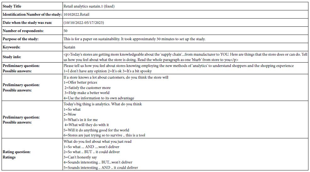
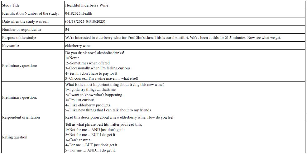
Mind Genomics studies are now scripted so that the studies can be set up on either a computer or a smartphone, run, and results downloaded with a short period of time. Table 1 provides key information about the study, information that will be explicated. The text in Table 1 comes directly from the report, contained in an Excel workbook, which can be downloaded either immediately for partial analysis (without the artificial intelligence summarizer), or after 30 minutes for complete analysis (with the artificial intelligence summarizer).

Table 1: Key information about the study provided by the Excel report.

TAB 1

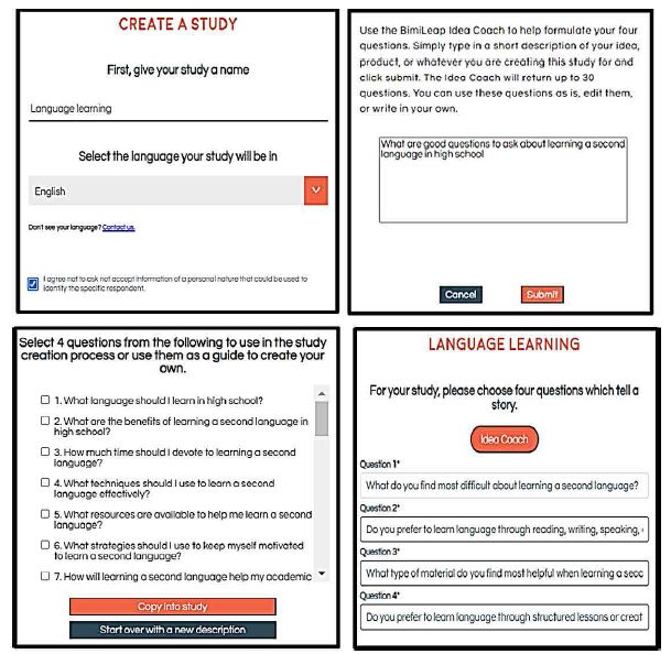
The set-up begins with the naming of the study, and then the instruction to provide four questions germane to the study topic. The researcher is prompted to structure the four questions so that they ‘tell a story.’ During more than a decade, from the time that Mind Genomics was opened to the public as a ‘software as a service,’ there has been increasing number of situations where researchers seemed to have been overwhelmed by the task of creating elements. With the advent of artificial intelligence, such as Chat GPT, it has become easy to use AI to create questions. All the researcher has to do is write down a short paragraph in the Idea Coach ‘box’ in the Mind Genomics template, and the AI returns with 30 different questions.

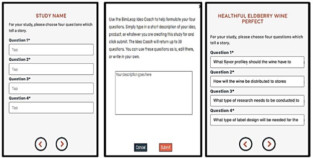
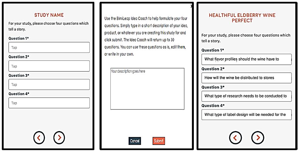
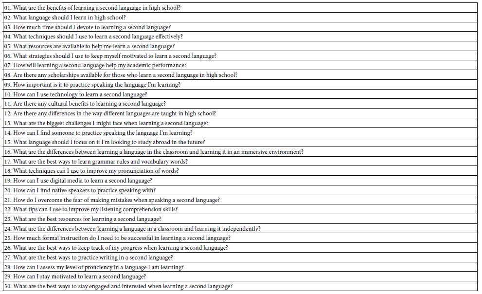
Figure 1 shows the request for four questions (left panel), and the four questions provided by the researcher (right panel). Table 2 shows one run of the Idea Coach, returning with the 30 questions after the AI has been prompted by a short description of the project. The actual time for this first step with the Idea Coach is approximately one 60-90 seconds after the researcher provides the Idea Coach with the small description. The researcher can select 0-4 questions. The questions selected are automatically put into the template. The researcher can then repeat the action to get other answers. The actions are independent of each other, so that each use of the Idea Coach to provide questions is independent of the previous use. In this way a person new to the topic can learn a great deal about the topic, even without selecting questions. It is the sheer number of different questions presented in a short period of time which constitutes an ‘education’ for the researcher on the very topic being studied. It is for that reason that the approach is considered ‘Socratic.’

FIG 1

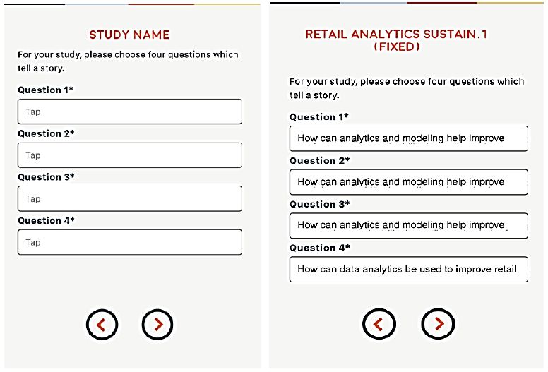
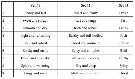
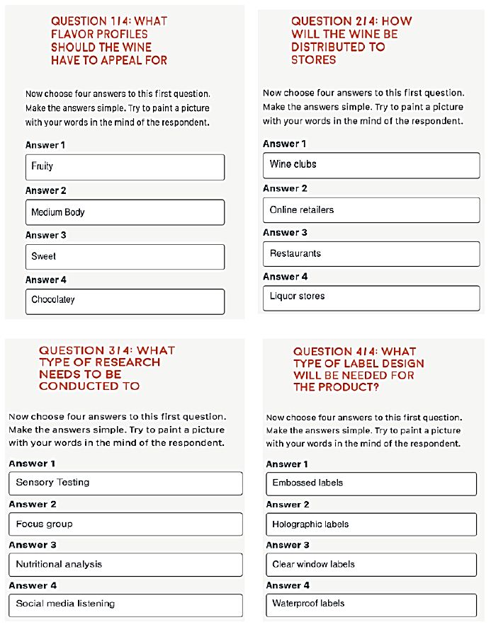
Figure 1: The templated request for four questions (left panel), and the four questions provided by the Idea Coach (right panel).

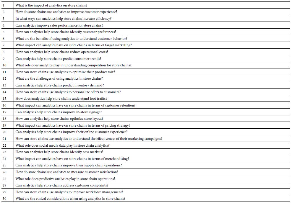
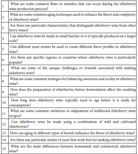
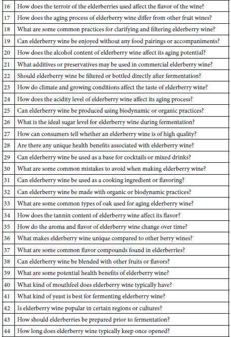
Table 2: The 30 questions returned by Idea Coach after being prompted by a small paragraph about the purpose of the study.

TAB 2

The next step consists of providing four answers to each question. Once again the Idea Coach comes into play. This time the information provided to Idea Coach is in the form of a query, that query created directly from the text of the specific question. When the researcher wants to change the query, it becomes a simple task of editing the question.

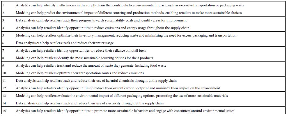
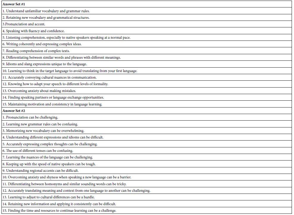
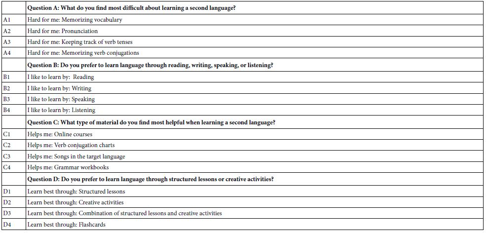
Figure 2 shows the formatted screen for Idea Coach, with the left panel showing the request for four answers, and the panel showing the completed set of answers used in the study. Table 3, in turn, shows 15 answers generated from one run of the Idea Coach, with the first question. The time elapsed in about 30 seconds.

FIG 2

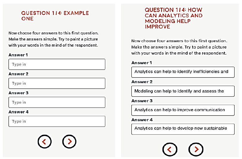
Figure 2: The templated request for four answers for question #1 (left panel), and the four questions provided by the Idea Coach (right panel).

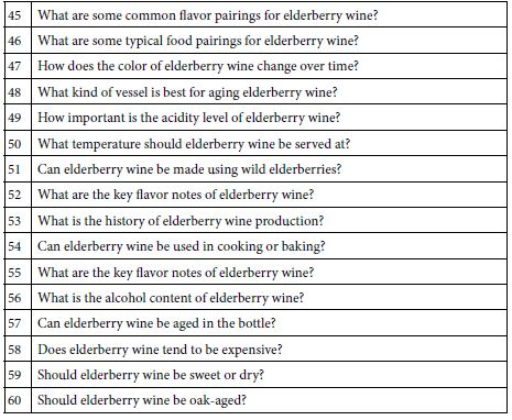
Table 3: The 15 answers returned by Idea Coach after being prompted by Question #1.

TAB 3

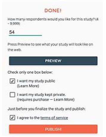
Once the study has been launched with the appropriate respondents, done easily within the BimiLeap program, the researcher selects the source of respondents, using the screen shown in Figure 3.

FIG 3

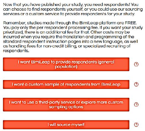
Figure 3: Source of respondents, selected by the researcher as the last part of the project set-up.

The respondent is ‘sourced’ from a panel provider specializing in on-line surveys. Across the world there are many such panel providers. These providers have lists of respondents and qualifications, individuals who have agreed to participate in similar studies for a reward provided by the supplier. The researcher need not know the agreement. All that is necessary is for the panel provider to source the correct respondent.

The Mind Genomics study can have elements (questions and answers) from different languages, and different alphabets, although the instructions for the actual set-up as done by the research are currently available in just a few languages (e.g., English, Chinese, Arabic Hebrew.

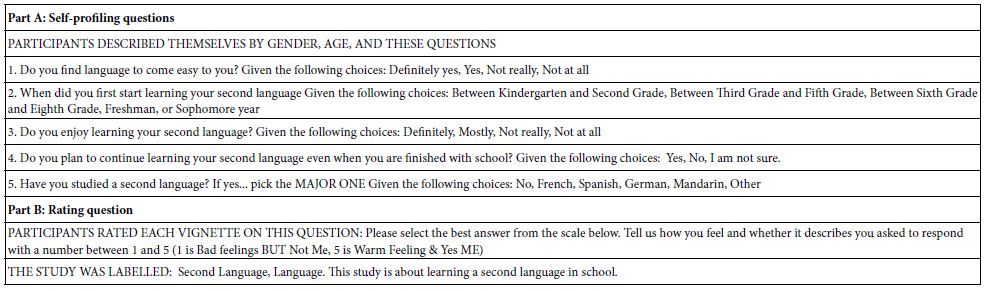
The actual experiment with the participant lasted approximately 3-5 minutes. The experiment begins with a short orientation provided by the researcher, obtains responses to the self-profiling questions (including age and gender, not shown here), and then presents the respondent with the 24 different, systematically designed vignettes. The vignettes comprise 2-4 answers (elements), at most one answer from a question, but often no answers from a question.

The experimental design ensures that the ratings from each respondent can be analyzed separately, as well as being able to be analyzed as part of the group. The vignettes are set up so that each individual evaluates a unique set of 24 vignettes, a design structure which enables the researcher to explore many different aspects of an issue, without having to choose what combination of elements give the best chance of discovery.

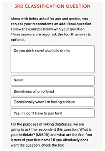
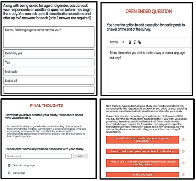
It is important at this juncture to keep in mind that the effort is more in the world of ‘hypothesis-generating’ than in the world of ‘hypothesis-testing.’ Quite often researchers really have no hypotheses to test but are constrained to do the study as if it were guided by a hypothesis. Mind Genomics disposes with that, freely representing that it is a discovery tool, to identify patterns which may be of interest in the way people think about a topic. The respondent sees an introduction to the study, usually presented in shortened form so that the specific information must come from the elements selected by the researcher. Figure 4 (top panel) shows the orientation question. Figure 4 (bottom panel) shows the five-point scale used by the researcher. Some of the text is cut off from the scale description. Figure 5 (top panel) shows the additional self-profiling questions as these appear to the respondent at the start of the evaluation by the respondent. Figure 5 (bottom panel) shows a clear reproduction of a vignette, as prescribed by an underlying experimental design. To the respondent there is no ’underlying pattern’ to be discovered. Rather, the vignette itself looks like it was randomly assembled, in virtually a haphazard manner.

FIG 4

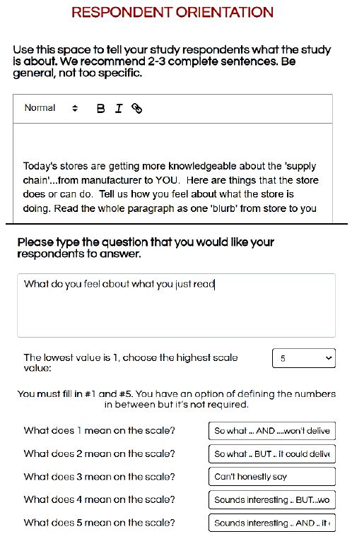
Figure 4: Respondent orientation screen in set-up program (top panel), and rating scale specifics in set up program (bottom panel).

FIG 5

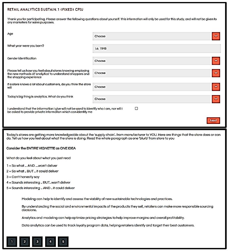
Figure 5: Screen shot for the pull-down menu of self-describing questions (top pane), and example of a four-element vignette plus rating question/scale as the respondent would see it on a full screen (bottom panel).

Database Structure, Analysis, and Reports – Total Panel

Almost fifty years ago, it was possible to accelerate the acquisition of data and even the preliminary analysis of such data. One could gather data quickly, and using mark sense cards and later electronic input one could analyze the data by programs then available, usually programs which specialized in descriptive analysis. The objective for this exercise is to move dramatically beyond that simple original analysis, pushing the limits by making use of smart experimental design, clustering, and applied artificial intelligence using GPT.

The actual data analysis is straightforward, made so by the judicious use of the experimental design, pre-selected so that the different sets of 24 combinations are really isomorphs of each other. Although the actual combinations, the vignettes, all differ from each other, mathematically the structure of each set of 24 vignettes is the same. In this way the researcher is assured of having a powerful analytic tool, which explores a great deal of the ‘design space’ (the possible combinations). Clearly, more individuals, more respondents means more of the design space is covered.

The analysis is made possible by the creation of a simple to use database. Each row of the database corresponds to one of the 24 vignettes tested by a respondent. Thus, for this study, comprising as it does the responses of 50 individuals, the database contains 50×24 or 1200 rows of data. The columns themselves are divided not bookkeeping columns (row number, study name, respondent number, test order number for the respondent, via 1-24), then 16 columns devoted to showing absence of element (value 0) or presence of element (value 1), and finally, the rating assigned, and the response time. Response time is defined as the number of seconds from the appearance of the vignette to the actual response assigned.

After the data are collected, the program creates new variables, specifically a binary variable TOP (ratings 5 and 4 transformed to 100; ratings 3, 2 and 1 transformed to 0), and a second binary variable BOT (ratings 1 and 2 transformed to 100, ratings 3, 4 and 5 transformed to 0). The BimiLeap program adds a vanishingly small random number (<10-4) to each BOT and TOP value, in order to ensure variation in the values of TOP and BOT. This prophylactic action ensures that there will be the necessary variability even when the respondent rated all vignettes either 1 or 2, or 3, 4 or 5,.

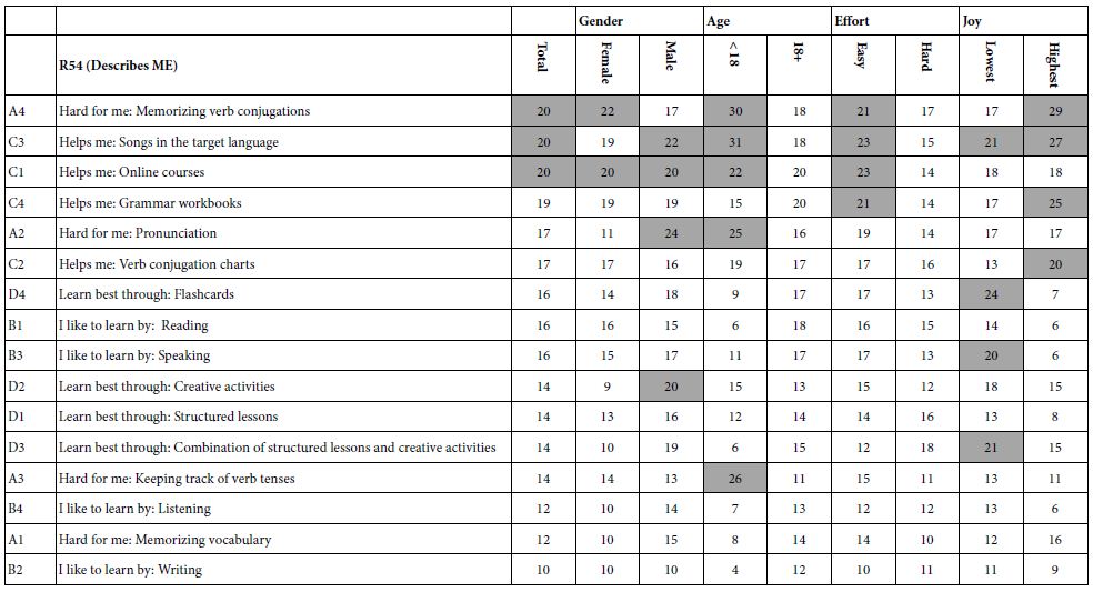
The first analysis generates an equation relating the presence/absence of the 16 elements to the newly created dependent variable TOP. Table 4 shows the parameters of the equation, expressed as: TOP = k0 + k1(A1) + k2(A2) … k16(D4). . The use of an experimental design, permuted across the 50 respondents to create 1200 vignettes, ensures that the OLS regression will not encounter any problems in terms of variables correlated with each other. The coefficients have absolute value, viz., a 5 is half the value of a 10. This is important. Often it is only differences in coefficient values which are relevant, e.g., when the experimental design calls for each vignette to have exactly one element from each question. That ‘tempting’ requirement substantially weakens the results.

Table 4: Elements for the Total Panel which drive TOP (Sounds interesting).

TAB 4

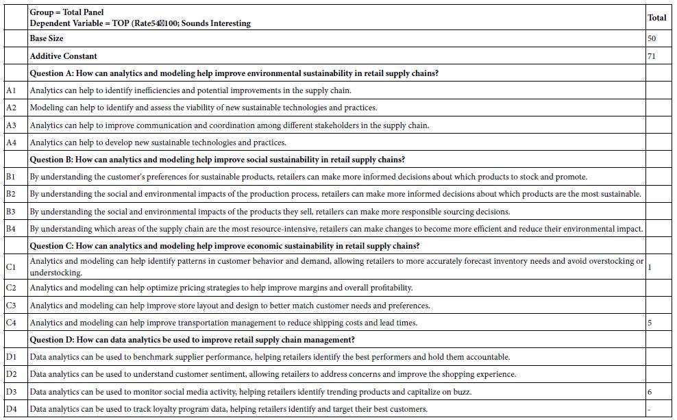
With the recognition of these properties of the regression results, the researcher can quickly understand the dynamics revealed in the experiment. The results are immediate and obvious once the meaning of the coefficients is understood. The coefficients tell us the proportion of times a response to the vignette will be 5 or 4 (here … ‘sounds interesting’) when the element is put into the vignette.

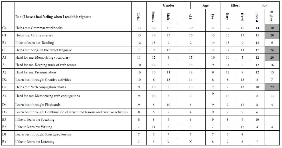
Note: Other binary dependent variables can be created

BOT = rating 1,2 transformed to 100. ‘Does not sound interesting’

RATE52 = rating 5,2 transformed to 100. ‘Could deliver’

RATE 41 = rating 4, 1 transformed to 100. ‘Won’t deliver’

Table 4 shows us 17 numbers, the additive constant and 16 coefficients. Mind Genomics studies generate a large number of coefficients. We are not interested in the coefficients which are 0 or lower. These low coefficients say that the presence of the element in the vignette ‘does not add’. It does not mean that the element actually detracts, or perhaps just as likely, the element is irrelevant, leading to a rating of 3.

The additive constant tells us the proclivity of the respondents to say ‘sounds interesting’ in the absence of any elements in the vignette. By underlying design, the vignettes all comprise a minimum of two elements and a maximum of four elements. Therefore, the additive constant is simply a correction factor in statistics. ON the other hand, we can use it as a baseline, a proclivity for the respondent to say, ‘sounds interesting’. We will use it to gain that insight. Table 4 shows the additive constant to be 70, meaning that when it comes to knowing that the topic will be store analytics, 70% of the respondents will be strongly positive. Had we done this type of experiment across years ago we could have measured the change in this additive constant to get a sense of how new ideas are accepted.

Only three of the 16 elements generate coefficients of 1 or above. The remaining generate coefficients of 0 or negative. For the sake of clarity, and for the sake of allowing patterns to come through, we do not show any 0 or negative coefficients. If we discard the element with coefficient 1, quite close to 0, we are left with the finding that of our 16 best guesses using artificial intelligence, edited by a human researcher, we end up with only two strong performing elements, and indeed only modest performers at that.

Shown these results and presented with the Mind Genomics approach for the first time, the critic of artificial intelligence might aver, perhaps even strongly aver, that these results contradict the claims of AI proponents that AI can be as good or better than people. The reality is not as positive, however. When a person selects the elements alone, quite often the person does about as poorly, or perhaps slightly better.

C4: Analytics and modeling can help improve transportation management to reduce shipping costs and lead times.

D3: Data analytics can be used to monitor social media activity, helping retailers identify trending products and capitalize on buzz.

Before moving on to an analysis of subgroups and mind-sets, it is instructive to see what AI can provide in terms of a standardized interpretation of the results. The analysis by AI should be considered simply as tentative observations made by a heuristic. It will still take a person to go through the data, but in the interests of speed, one might employ the AI heuristic to get a sense of the answers before spending time with the results.

Table 5 shows the response of AI to six queries. These queries are listed below.

  1. Interested in
  2. Create a label for this segment
  3. Describe this segment
  4. Describe the attractiveness of this segment as a target audience:
  5. Explain why this segment might not be attractive as a target audience:
  6. Which messages will interest this segment?

Table 5: AI first scan and interpretation of the strong performing elements (6 and higher) for the Total Panel, on six queries.

TAB 5

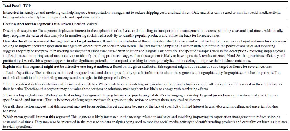
The queries look only at the moderate and higher elements, viz., those with coefficients of +5 or higher. Elements with coefficients of 4 or lower are ignored. For our data in Table 4 using the Total Panel the AI uses only two of the 16 elements to write its analysis.

Results from Self-profiling Questionnaire – What will the Store Do with the New Analytics

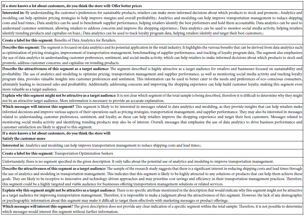
Our second analysis parallels the first, this time focusing on how the respondent feels about what the store will do with the analytic information. The actual question and answers appear below. Out of four possible answers, most of the respondents (43 of 50) chose only two, better price and better service, respectively.

If a store knows a lot about customers, do you think the store will

1=Offer better prices

2=Satisfy the customer more

3=Help make a better world

4=Use the information to its own advantage

Two groups or segments emerge, those who feel that the store will offer better prices using the analytics data (15 of 50), and those who feel that the store with use the information to better satisfy customers (29 of 50). Both have similar additive constants (63 and 69) but respondent in radically different ways to the elements.

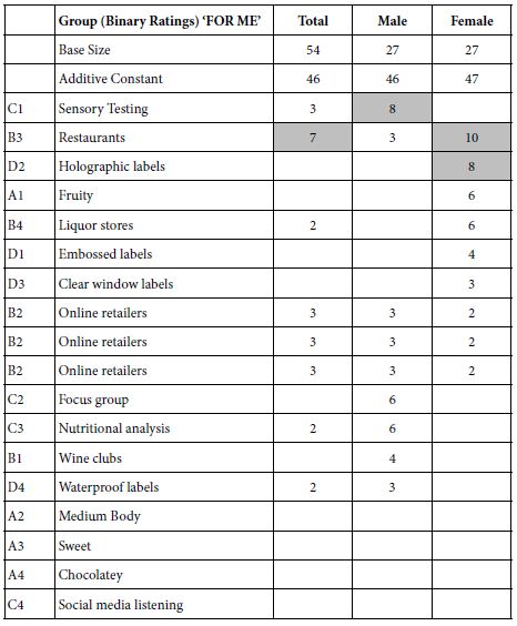
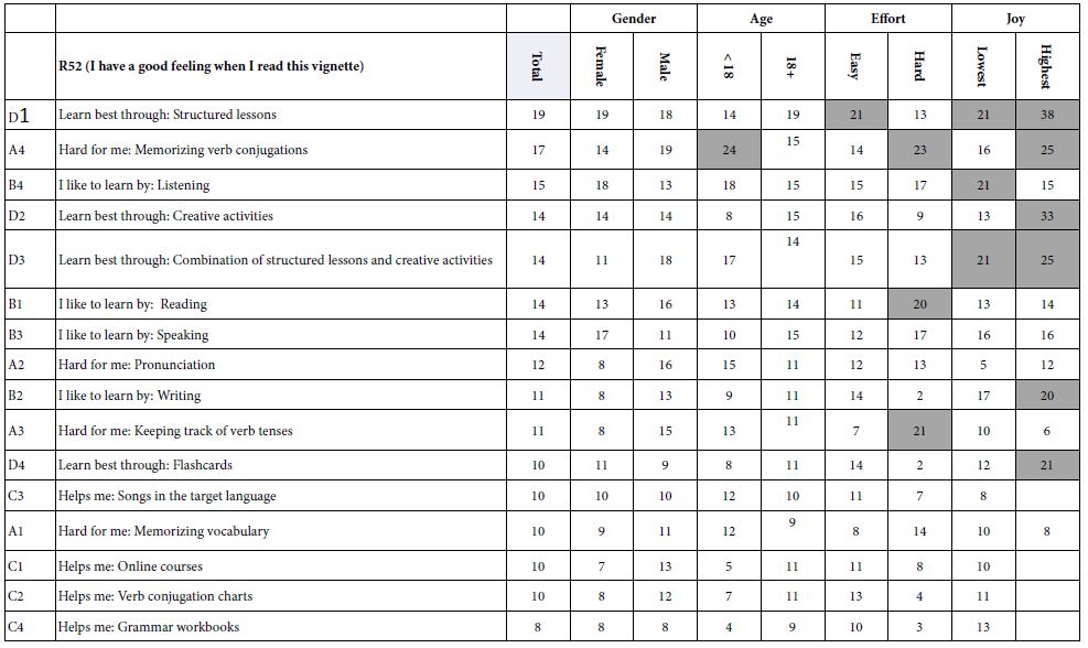
The data for this new analysis comparing different points of view on what will the store do with the analytics appear in Table 6 for the coefficients, and Table 7for the AI summarization. Once again all coefficients of 1 or lower are not shown. In the interests of simplicity, all elements without at least one coefficient of ‘2’ Table 6 suggests that the response of those in Segment 1 (believe the store will offer better prices) are strong and focused, whereas there are no strong performing elements for Segment 2 (believe that the operations will be better) (Table 7).

Table 6: Elements which drive TOP (Sounds interesting) for the two segments emerging from the question self-profiling question: If a store knows a lot about customers, do you think the store will…

TAB 6

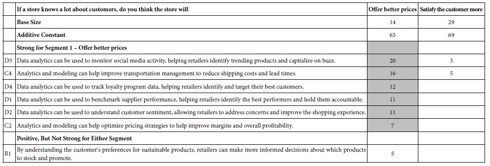
Table 7: First scan and interpretation of the strong performing elements (6 and higher) by for the two segments, based on the self-profiling question of what the store will do with the results from the data analytic.

TAB 7

Results from Dividing Respondents into Mind-Sets Based Upon the Pattern of Coefficients

Our final data analysis will focus on the creation of mind-sets, groups of respondents who are put together by the k-means clustering program [7], based upon the similarity of the patterns made by their coefficients. For the clustering we use all 16 coefficients, whether positive or negative, although we only show the positive coefficients in the results. Clustering does not use the additive constant.

The clustering program is embedded in the BimiLeap program, generating at first two mind-sets, and then totally once again, three mind-sets. Each respondent is assigned to only one of the two or three mind-sets. Furthermore, the mind-sets encompass all respondents.

The objective of the clustering exercise is to discover hitherto unexpected groups of respondents based upon the patterns of their coefficients from thousands of small studies clustering based on coefficients emerges with meaningful, interpretable groups of respondents, even though the process is purely mechanical and mathematical.

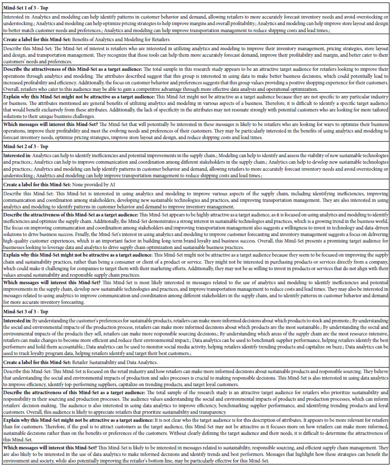
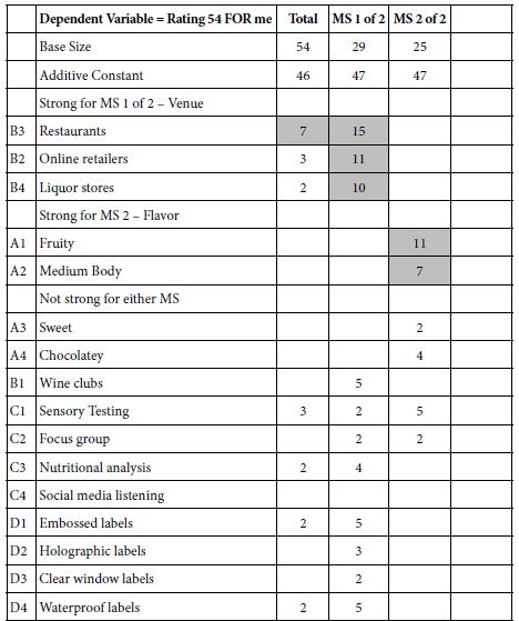
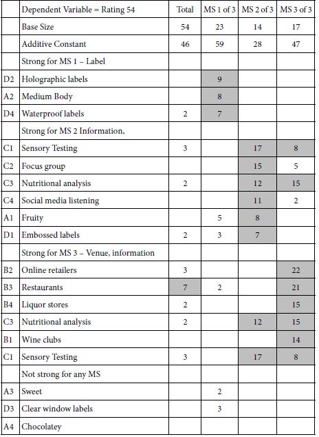
Table 8 shows the positive performing elements for the three-mind-solution. The two-mind-solution is not shown in the interest of space. Table 9 once again shows the AI interpretation of the results, obtained by applying six queries to each of the three mind-sets.

Table 8: Elements which drive TOP (Sounds interesting) for the three mind-sets, emerging from k-means clustering of all the element coefficients from the 50 respondents. Only those elements with at least one coefficient of 2 or higher are shown.

TAB 8

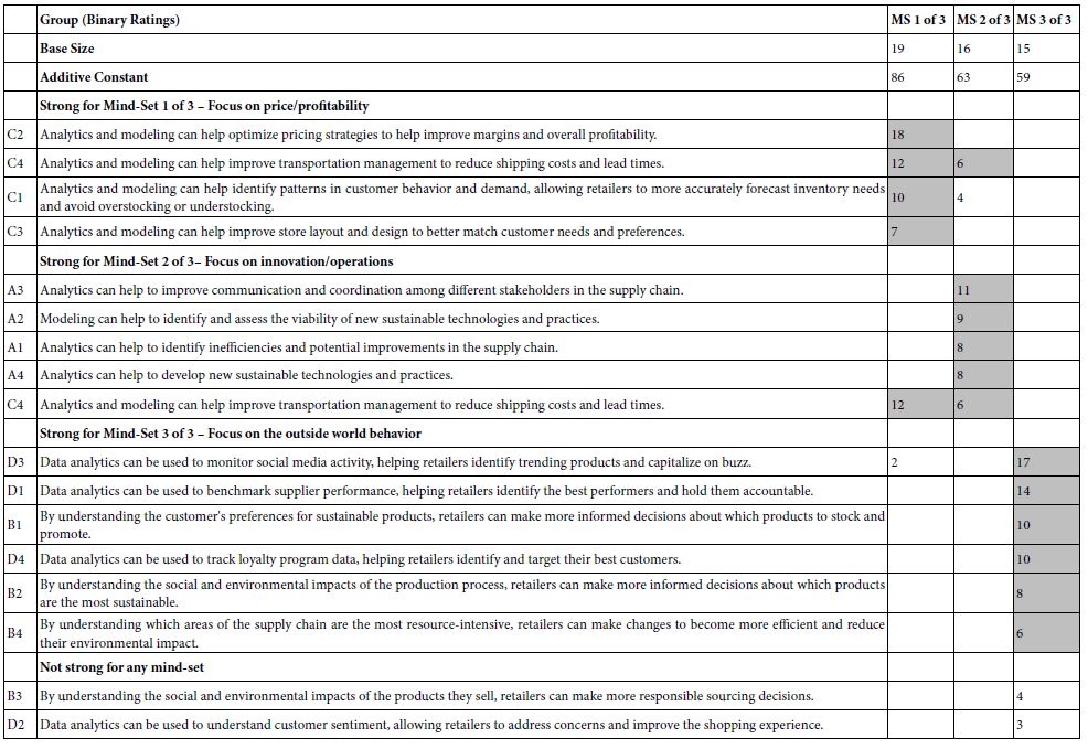
Table 9: AI interpretation of the strong performing elements (6 and higher) by AI for the three-mind-set solution.

TAB 9

In contrast to the data from the Total Panel, and the data from the Self-Defined Segments regarding what the company will do with the segments, the division by the pattern of coefficients shows strong performing coefficients, and meaningful stories which repeat from the two-mind-set solution (data not shown in the interest of space.).

Beyond Interpretation to Understanding Performance at a Glance

A continuing issue emerging from these small-scale studies is ‘How did we do?’ The same question is asked by researchers in most areas, with the underlying issue touching on ‘did the experiment work?’ With Mind Genomics coupled with AI at the very early stages, and available world-wide at the press of a key, the issue becomes the degree to which the study generated anything of value. The notion of ‘value’ is not the personal value of the data to the researcher, nor value in terms of scientific reproducibility and validity, but rather did the effort lead to any strong performing elements. We learn that when we have strong performing elements there is a strong link between an element and the rating question. That linkage is what the researcher seeks in these studies. Knowing that some elements get high scores and other elements get low scores tells the researcher she or he can move in the direction of the high scoring elements. It is in those elements that the relevant issue can be further understood, at least in the minds of the people who are the respondents.

As part of the effort to ‘systematize’ the use of Mind Genomics in this era of easy-to-use techniques empowered by AI, we present the IDT, Index of Divergent Thought.

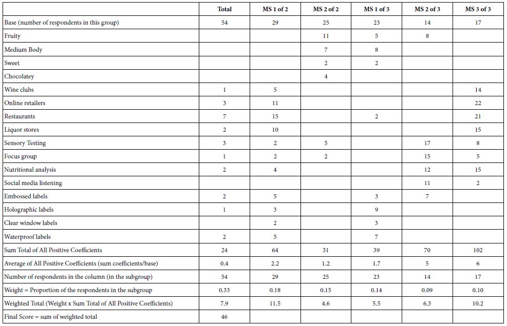
The objective of IDT is to measure the impact of the elements. The IDT generates a simple index, shown in Table 10. Each positive element is weighted by the relative number of respondents when we consider the entire study as six groups (Total, Mind-Sets 1 and 2 in the 2-Mind-Set solution, and Mind-Sets 1, 2 and 3 in the 3-Mind-Set Solution). Each of the six groups has a specific number of respondents, which add up to 3x the base size, or 3×50, viz. 150. The IDT is simply the weighted sum of the positive coefficients, the weight being the ratio of the number of respondents in a group versus the total number of 150. Note that the two-mind-set solution was developed, but not shown in the interest of space.

Table 10: The IDT, Index of Diverged Thought, showing the performance of the elements, and thus the strength of the thinking behind the specific Mind Genomics study.

TAB 10

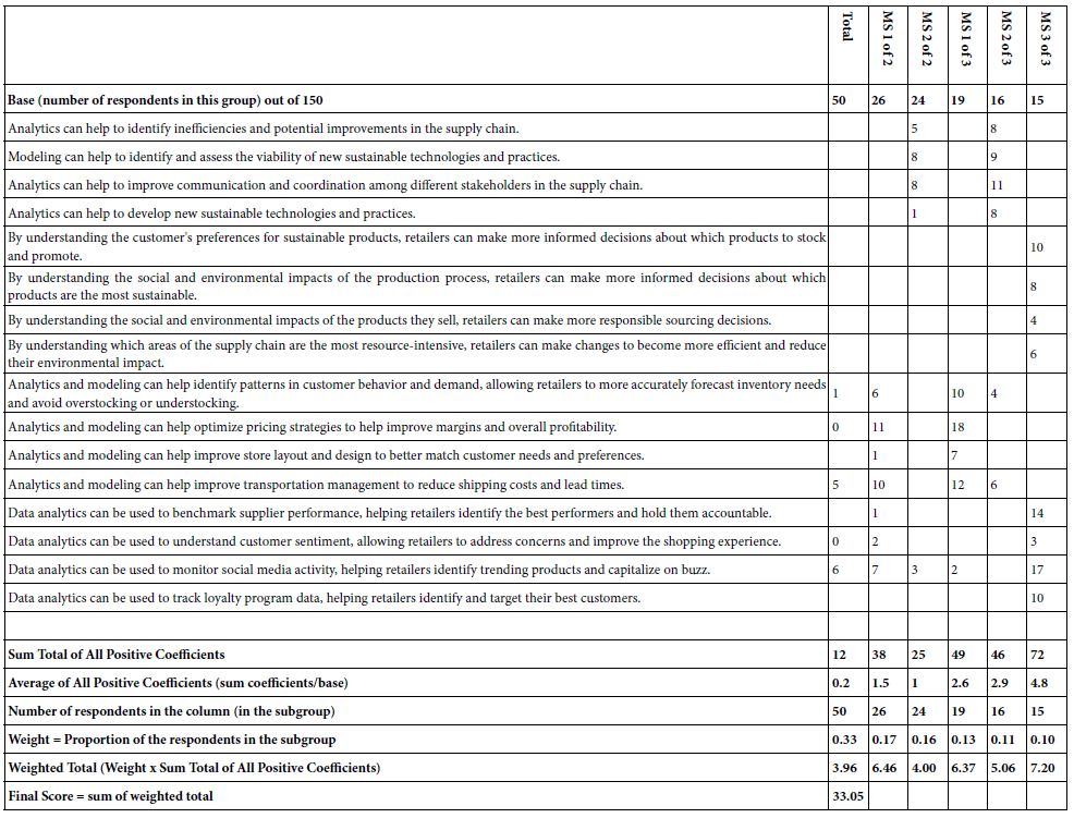
The ideal use of the IDT at these early days of implementation is to determine how good was the choice of elements. The IDT for this study is 33.05, on the low side. Keeping in mind that the elements were obtained from AI, and only modestly edited, we have with the IDT a way to quantify the strength of the ideas as they are perceived by people.

Discussion and Conclusions

As emphasized above, this study was undertaken as a study of an experience, the experience being the efforts to learn about a topic new to the senior author, viz., sustainability in the world of retail analytics. The original idea for this study came from a call for papers from the newly founded journal ‘Sustainability.’ The fact that the senior author had little experience with the topic of retail analytics, and indeed scarcely, if ever, thought about the topic, made the study more interesting. As a senior scientist, with 54 years of experience after the PhD., the topic was interesting simply because it asked the question ‘what really could be learned by and contributed by a novice, albeit a novice with professional experience.’

In fact, we learned that our respondents, who are also consumers, can easily grasp the features and uses of retail analytics, and that they reveal three distinct Mind-sets towards retail analytics. Mind-set 1: Focus on price/profitability; Mind-set 2: Focus on innovation/operations; and Mind-set 3: Focus on the outside world behavior. Each of these newly discovered mind-sets educates retail executives with knowledge never known to them before, guidance from consumers about how they might leverage retail analytics for their customers’ benefit and, perhaps, unleashing innovation benefitting both the shopper and the retailer. They can break from past tradition of analyzing from on high what they think is best for their shoppers.

The actual study was easy to implement. The use of the Idea Coach made things easier, although it was not clear to whether these were the ‘right questions’ to ask. The answers were not the issue. Rather, it was the questions, leading to the realization that emphasis is research should be put on asking an appropriate, meaningful question. So many of the AI generated questions seemed real until thought through, with the question of ‘what type of answer would this question engender’

The actual process itself revealed some unexpected benefits. The key benefit might be said to be ‘sharpening’ and improving the question, until one reaches a powerful question. The reality of this single powerful question is important. We are not taught important, seminal questions to ask. And all too often, when these questions are asked, their importance is often unrecognized.

To sum up, this paper demonstrates the increasing ease with which a novice can use computer technology to learn by exploration. The templated version of Mind Genomics makes it possible for the novice to move quickly from issue to empirical results. At the front-end AI provides a Socratic way of creating questions, that create an education on the topic. At the back end, the AI allows the researcher to understand the results from a variety of perspectives, provided by the different queries.

If we were to surmise the potential of the approach, we might find its greatest use in the world of education, to teach [8]. Teaching may not be limited to students, but rather ‘teaching’ here is used in the general sense, to instruct a person about a specific topic [9,10]. The unique combination of AI at the front and back, coupled with real human responses, provides a powerful tool to explore many dimensions of being, from the simplest to the profound, rapidly, iteratively, and with the potential of opening entirely new disciplines as the information from related studies is aggregated into a coherent whole with many different facets.

References

  1. Oracle Corporation (2023) “What Is Retail Analytics? The Ultimate Guide.”
  2. Kinsey MC & Co. (2021) “The value of getting personalization right—or wrong—is multiplying.”
  3. Sprenger J (2011) Hypothetico‐deductive confirmation. Philosophy Compass, 6: 497-508.
  4. Moskowitz HR (1971) The sweetness and pleasantness of sugars. The American Journal of Psychology, 84: 387-405.
  5. Zemel R, Choudhuri SG, Gere A, Upreti H, Deitel Y, et al. (2019) Mind, Consumers, and Dairy: Applying Artificial Intelligence, Mind Genomics, and Predictive Viewpoint Typing. In Current Issues and Challenges in the Dairy Industry. Intech Open.
  6. Gofman A, Moskowitz H (2010) Isomorphic permuted experimental designs and their application in conjoint analysis. Journal of Sensory Studies 25: 127-145.
  7. Likas A, Vlassis N, Verbeek JJ (2003) The global k-means clustering algorithm. Pattern Recognition 36: 451-461.
  8. Clancey WJ, Hoffman RR (2021) Methods and standards for research on explainable artificial intelligence: lessons from intelligent tutoring systems. Applied AI Letters 2:53.
  9. Kim TW, Mejia S (2019) From artificial intelligence to artificial wisdom: what Socrates teaches us. Computer 52: 70-74.
  10. Lara F, Deckers J (2020) Artificial intelligence as a socratic assistant for moral enhancement. Neuroethics 13: 275-287.
FIG 1

Empowering Students in a University through Rapid Design: A Demonstration Involving the Creation of Messaging about Elderberry Wine

DOI: 10.31038/PSYJ.2023544

Abstract

54 respondents from an internet-based panel across the United States each evaluated uniquely different sets of 24 systematically varied ‘vignettes,’ (combinations of messages) about elderberry wine. The messages were created by artificial intelligence (Idea Coach), and afterwards combined into the vignettes according to an underlying experimental design which prescribed the appropriate combinations to use for subsequent regression analysis. Respondents rated each vignette using a two-dimensional rating scale, one dimension representing fit to the respondent (for me vs not for me), the second dimension representing understandability of the message. The data reveal three mind-sets. The study demonstrated the simplicity, speed, and economics of combining artificial intelligence, experimental design, and subsequent human evaluation. The output becomes a scalable bank of subjective information on a topic which is unfamiliar (elderberry wine), with this bank of information combining Socratic learning in a new topic coupled with feedback from real consumers about the information developed through artificial intelligence.

Introduction

The development of new products in the world of commerce is often costly, error-filled, and unduly long. Some of the issues may result from risk-avoidance, a phenomenon rampant in corporations, especially in slow-moving categories such as foods and beverages. When a company in electronics, for example, fails to avail itself of important technology to create new products that company is likely to suffer, often quickly, as its competitors rush to overtake it, doing so at hot speed. Not so in the world of food, even the world-of food start-ups, where the feeling is that there is not really much risk, that the competition moves slowly, and the technology is really not as valuable as the instincts and intuitions of the entrepreneur or the corporate president. The foregoing holds in classic, multi-layer multi-nationals as well as in the starts powered by the ingenue entrepreneur.

At the same time that the world of food development moves cautiously, there is an evolving world of speed, at almost any price. This world has emerged during the past decades due to the confluence of three factors, respectively the computer for processing, the internet for connection, and most recently artificial intelligence (AI) for rapid ‘thinking’ or at least rapid and seeming intelligent processing of text information in a way which seems intelligent. These three factors are making it possible to create ideas, test these ideas, and even expand them in what figuratively be an ‘eyeblink’ in the corporate timeline. What took hours, days, weeks, now can take minutes and seconds.

With the foregoing paragraphs as background, the author has begun a series of studies, small studies to be sure, on topics of daily life. The approach uses experimental design of ideas, mixtures of ideas presented to the respondent, the ratings of these mixtures revealing how each idea or message ‘drives’ the interest of the respondent. Using these tools of computer, internet, and now artificial intelligence, the author has pushed the study of ideas in the food industry down from a pedestal of scientific perfection to an act that even a grade school student can do, and even master after a moderate amount of practice [1-3].

The Mind Genomics Approach – Steps Towards Rapid Ideation

In order to demonstrate the power of new methods for product design, the author conducted a class experiment in April 2023, with students from the University of Florida in Gainesville. The approach was a DIY (do-it-yourself) approach for an advanced version of conjoint measurement, Mind Genomics. The specifics of Mind Genomics have been presented in detail in various papers published since the early days of the 21st century. The reader is encouraged to look at the different topics covered. This paper will once again present the method, and the new development enabled by popular and available methods for artificial intelligence using the popular Chat GPT [4-6].

The ingoing, perhaps heretical and counterintuitive assumption, was that one could do a study within two hours, a study beginning with little or no knowledge about a field and emerge after those two hours with deep information about a topic. The topic chosen during the active initial back and forth was ‘elderberry wine,’ a wine of Asian origin (No et. al., 1980). The students who designed study had heard of elderberry wine, but were not familiar with the wine, making the exercise a challenge and enjoyable learning experience. The choice of elderberry wine emerges after about an unmoderated, 20-second class ‘discussion’ about ‘a topic, any topic having to do with foods.’

There is a modest-sized literature about elderberry wine, but a growing one, because of due to evolving consumer interest. At the same time, elderberry has received attention by horticulturists as well in part because of the increasing recognition of its health properties [7-11].

Table 1 presents the input information about the study. The table comes from a summarized report of the study automatically generated at the completion of the field work. The table provides the study title, date, purpose of the study as the researcher defines it, keywords for later sorting, self-profiling attitude questions, the respondent orientation (kept very simple), and the rating scale. All of this information is automatically incorporated into the Excel report.

The Mind Genomics process is templated, following choreographed sets which set up the experiment, run the actual experiment, and automatically analyze the data.

Table 1: Information about the study provided by the Excel report returned to the researcher at the end of the field work.

TAB 1

Introduce to the Process and Select the Topic (Elderberry Wine)

The exercise was set up so that the students would be introduced to the Mind Genomics process through a two-minute ‘elevator pitch’. The class was told that they would choose a topic, run a study, get results, and discuss the preliminary results. The students we unprepared, but as noted above, the decision was made to study elderberry wine. It is important to note that in no way was the topic to be focused on a so-called ‘burning issue’ or ‘hole in’ literature. The topic was selected almost randomly. It was at this point that the study had been registered as ‘elderberry wine’, the class as researchers filled out some checklists on using English as the language, and agreeing to not obtain information that could identify the respondents, except with the permission of the respondents.

Create Four Questions through Idea Coach

Mind Genomics works by a Socratic method, posing questions to obtain answers, combining the answers, and having respondents evaluate the combinations. Figure 1 shows the screen requesting the four questions (left panel), and the four questions actually selected (right panel).

FIG 1

Figure 1: The request for four questions dealing with elderberry wine (left panel), the Idea Coach for generating questions through AI (middle panel) and the four questions selected from the AI suggestions (right panel).

To generate the four questions in Table 1 is generally a function of one’s familiarity with the topic, and the predilection of the research group to come to an agreement. Often the group is unfamiliar with the topic, necessitating what ends up being interminable discussion and delay as the individuals in the group grapple with the appropriate questions to ask. The issue becomes even more vexing when the parties feel that they only have ‘one chance’ to run the experiment. It is at that point, the feeling of one-chance-only, that the participants in the research program end up ‘freezing’, often with the unhappy consequence that the project falls apart.

During the past several years users have continued to request, and eventually insist that the set-up of a Mind Genomics experiment be more ‘user-friendly.’ Almost all suggestions have included something about making it easier to generate questions, and to a lesser degree, to generate answers to the questions. As an aside, it appears that instead of trusting their own intuition and thinking, many individuals prefer ideas that have somehow been ‘vetted.’ This desire to have assistance in creating questions and answers, that assistance provided by an electronic ‘third party’, led to the creation of the Idea Coach. The Idea Coach is simply a set of AI prompts, based upon the ‘squib’ written about the topic. The squib is submitted to the AI program embedded in the setup, and generates 25-30 questions. Table 2 shows 60 unique questions emerging from four passes though the Idea Coach. With 30 questions there should have been 120 questions, but only 60 were different from each other.

Table 2: 60 unique questions emerging from four runs of the Idea Coach, each run returning a set of 30 questions about elderberry wine.

TAB 2(1)

TAB 2(2)

TAB 2(3)

Create Four Answers to Each Question through Idea Coach

Idea Coach once again uses artificial intelligence to generate sets of 15 answers to each question. The researcher can select the answers of interest and edit them. Table 3 shows the answers for the first question (flavor profile) from three consecutive iterations of answers. In this case the 45 answers differ from each other. Figure 2 shows the screenshots of the final set of answers to the four questions selected.

Table 3: Three sets of answers to the first question (flavor profile)

TAB 3


FIG 2

Figure 2: Screen shots of the four answers to each question

The mechanism by which Idea Coach provides the questions and answers remains a trade secret of the company providing the AI system. What is important, however, is the rapid ‘learning’ by the Socratic method, question-and-answer, although here the learning might be in from parallel questions and answers, as the squib generates 25-30 questions, and the question generates 15 answers. One might happily imagine the potential of educating oneself on a topic such as elderberry, simply by two, three, four, or even five iterations of squib → 25-30 candidate questions → 15 candidate answers for each candidate question.

Create an Experimental Design Which Specifies the Combinations of Elements (Answers)

Rather than instructing the respondent to rate each of the 16 elements, one element at a time, the Mind Genomics approach presents combinations of these elements, short descriptions of the wine. Short descriptions are easier to judge because they tell a more complete story than do single elements. The respondent will evaluate a set of 24 vignettes, the aforementioned combinations.

In the experimental design element (viz., answer) appears five times in the 24 vignettes and is absent 19 times. No vignette comprises more than one element from any question. As a consequence, 20 of the 24 vignettes contain one answer from a question, whereas four vignettes of 24 are absent answers. Finally, across all 24 vignettes there are combinations comprising two answers, three answers, and finally four answers, but no vignette with only one answer. This specific design ensures that the researcher can analyze the data using standard statistical tools such as OLS (ordinary least squares) regression [12].

A unique, patented aspect of Mind Genomics is that each respondent evaluates a different set of combinations. The mathematical structure of the combination remains the same, but the specific combinations differ from one respondent to another. This difference is created by a permutation scheme described by [13]. The benefit of the permutation scheme is that the researcher need not know anything about the topic. The experiment allows the researcher to explore a great many combinations, analyze the data at the level of the individual respondent, and as a result uncover patterns that might not even have been imagined at the start of the study.

Create an Orientation and then Create the Rating Question that the Respondent Uses to Evaluate the Vignette. The Orientation is Simple: Read this Description about a New Elderberry Wine. How Do You Feel?

The rating scale actually comprises two dimensions. The first dimension is interest (Not for me vs For me). The second dimension is understandability (don’t get it versus get it). The two dimensions allow the researcher to understand the mind of the respondent more deeply, both in terms of emotion (for me / not for me) and intellect (get it / don’t get it).

Tell us what phrase best fits …after you read this.

1=Not for me … AND just don’t get it

2=Not for me … BUT I do get it

3=Can’t answer

4=For me … BUT just don’t get it

5=For me … AND… I do get it.

Create Self-profiling Questions

The Mind Genomics process enables the respondent to profile herself or himself on attitudes that would not be known from knowing who the response IS. At the start of the study the researcher can create up to eight such self-profiling questions. In addition, the Mind Genomics process automatically asks the respondent’s age and gender. The foregoing information (self-profiling as well as age and gender) are attached to the data provided by the respondent when rating the vignette. The self-profiling information will be used to create subgroups. Figure 3 shows an example of a self-profiling question. The Mind Genomics program allows the researcher to create up to eight such self-profiling questions, each with eight answers.

FIG 3

Figure 3: One of the self-profiling questions

‘Field the Study’ with Respondents

Figure 4 shows the information that the researcher provides to the Mind Genomics program. This information includes the number of respondents, how the respondents will be sourced, and whether or not the researcher wants to ‘privatize’ the respondent data. As of this writing (May 2023), the Mind Genomics platform is very low cost for the artificial intelligence (Idea Coach and summarization in the results). The researcher can either provide her or his own respondents at a low cost ($2/respondent for processing), use a third-party group ($2/respondent for processing), or use a Mind-Genomics approved supplier (Luc.id), with an approximate per respondent fee of $4-$6 for recruiting and processing. The researcher can make the data fully private for an extra $2/respondent. In this way the Mind Genomics fees can be kept very low, a boon to students who can explore a topic in depth, and actually run a small (or large study) on elements of interest, if desired.

Not shown is the set of screens which allow the researcher to specify country, age range, gender, education, income, children, and so forth for the respondent. The typical ‘field time’ to execute the experiment is about 60 minutes for 100-200 easy to find respondents.

FIG 4

Figure 4: The researcher specifies parameters about the field execution

Create the Database

Each record of the database corresponds to a vignette. The record has these columns:

Column 1 – Study name

Column 2 – Respondent identification number

Columns 3,4 – Age, Gender Columns 5-6 – Answers to the two self-profiling questions created by the researcher

Columns 8-23 – One column for each of th 16 elements. When the element is absent from the particular vignette, the cell has the value 0. When the element is present in the particular vignette the cell has the value 1. This is called ‘dummy coding’.

Column 24 – Test order of the vignette. Each respondent rated 24 vignettes, so the test order ranged from the first vignette tested (coded 01) to the last vignette tested (coded 24)

Column 25 – Rating assigned by the respondent to the vignette.

Column 26 – Response time in 100ths of a second, defined as the elapsed time between the presentation of the vignette on the screen and the time that the respondent assigned the rating.

Column 27-30 – Create four new binary variables by a re-code of the rating to a binary valuer 0 or 100 (as well as the addition of a vanishingly small random number to the newly created binary variable)

Column 27 – Create variable ‘For Me.’ Ratings 5, 4 re-coded to 100, rating 3, 2,1 re-coded to 0.

Column 28 – Create variable ‘Not for Me’. Ratings 1, 2 re-coded to 100, 3,4,5 re-coded to 0.

Column 29 – Create variable ‘Get It’. Ratings 5,2 recorded to 100, rating 4, 3, 1 re-coded to 0.

Column 30 – Create variable ‘Don’t Get It’. Ratings 4,1 re-coded to 100. Ratings 5,3,2 re-coded to 0.

The database is set up for dummy variable regression analysis, either at the level of the individual respondent or at the level of the group. The original experimental design specified 24 different combinations, with the combinations being precisely those which ensure that each element appears equally often, and that each of the 16 elements are statistically independent.

The analysis will focus only on the ‘For Me’ ratings.

Create Equations (Models) Relating the Presence/Absence of Elements to Ratings

The equations are estimated using OLS (ordinary least squares) regression. For this analysis we express the equation in the standard way, using an additive constant:

Binary Variable = k0 + k1(A1) + k2(A2) … k16(D4)

The additive constant, k0, shows the expected percent of responses to be assigned if there were no elements in the vignette. Of course, by design, all vignettes comprise a minimum of two and a maximum of four elements so that the additive constant should be considered a baseline.

Search for the Patterns

The patterns should emerge from the coefficients for the dependent variable ‘For Me’ (ratings 5 and 4 converted to 100, ratings 1,2 and 3 converted to 0). Table 4 shows the coefficients for total panel and for binary gender (male vs female). Mind Genomics returns with a great many coefficients. Table 4 and the remaining tables of coefficients (for mind-sets) show only the positive coefficients, viz, those 2 or higher.

Table 4: Performance of the elements by total and gender using R54 (For me) as the dependent variable. Only positive coefficients, 2 or higher, are shown.

TAB 4

The additive constant gives a sense of the percent of responses that would be 5 or 4 for vignettes that were empty, viz, absent elements. By design this is not possible, but the regression process can estimate this additive constant, which is typically considered to be a correction factor (Burton, 2021). Table 4 shows the additive constant to be about 46-47, suggesting that half of the time we can expect a rating of 4 or 5 for vignette or concept about elderberry wine, even when no elements to deeper detail.

Table 4 suggests that in terms of ‘interest’ (viz., For Me), a few elements perform strongly, and in fact elements that might not have been even thought of without the use of the AI-powered Idea Coach. These are ‘sensory testing’ for males, and ‘restaurant’ and ‘holographic labels’ for females. The benefit of creating elements with the assistance of AI is just this ‘out of the box’ thinking, with the researcher having the power to accept the suggestion or reject the suggestion by simple choice, and indeed to test the suggestion again in an easily run of the study with some new elements, new respondents.

Uncovering New-to-the-World Mind-Sets through Clustering

It is in the DNA of the scientific mind to look for basic causes, fundamentals of a situation. Although scientists and consumer researchers have attempted to develop profiles of archetypes, idealized profiles, these archetypes are too general, and fail to capture the granularity of everyday experience. Indeed, any attempt to divide people from the ‘top down’ is destined to fail because at the level of actual experience there are so many idiosyncratic factors that the archetypes simply do not have the ability to address [14].

The Mind Genomics approach works in the opposite direction, starting at the level of granular for a specific issue or situation, looking at the different dimensions of that granular situation, testing alternatives or expressions of each dimension, and then uncovering parallel groups of individuals or clusters for that situation. The clusters can be thought of as archetypes, not general ones, but archetypes of a specific situation, mind-sets in the language of Mind Genomics.

The statistics of Mind Genomics readily enable the researcher to discover these mind-sets, even without any ingoing knowledge. The approach simply creates individual level models of the type above shown for the total panel, or for any subgroup. Each individual generates a model, a model which is statistically valid because the 24 vignettes for each respondent had been created according to an underlying experimental design. The 24 vignettes are precisely arrayed to allow for OLS regression to be done on the data from each respondent. Each respondent produces 16 coefficients and an additive constant. Afterwards, the respondents are clustered by k-means clustering [15] first into two non-overlapping and exhaustive groups, (2-mindset solution), and then into three non-overlapping and exhaustive solutions (3-indset solution).

Clustering it follows purely mathematical criteria, e.g., minimize the sum of ‘distances’ between people in a cluster while at the same time maximize the distances between the centroids of the different clusters. It is left to the researcher to choose the number of clusters or mind-sets, and to name each cluster. Two good criteria are parsimony (fewer clusters are better), and interpretability (the clusters must tell a reasonably clear story).

For Mind Genomics studies, the measure of distance is the expression (1-Pearson Correlation). The Pearson Correlation coefficient measures the strength and nature of the linear relation between two sets of numbers, in our case the numbers coming from the 16 coefficients. The distance is small, viz., 0, when the Pearson correlation is +1 (1-1 = 0), occurring when the two sets of coefficients are parallel to each other. The distance is greatest, viz., 2 when the Pearson correlation is -1 (1 – 1 = 2), occurring when the two sets of coefficients go in precisely opposite directions.

Mind Genomics clustering usually reveals quite simple groups, the patterns often clear, ‘jumping out’ at the researcher. Table 5 shows the strong performing elements for the two and then the three mind-sets (abbreviated MS). The two mind-sets solution shows a very simple pattern, namely that which is familiar (venue for MS1 versus flavor for MS2). The three-mind-set solution is more intriguing, suggesting Label, Information, Venue, respectively. The three-mind-set solution is not perfect, since there are some strong-performing elements appealing to the mind-set slightly ‘off’ from the main interest of the mind-set.

Table 5 once again shows the ability of the OLS regression to uncover relevant coefficients, often coefficients which ‘make sense’ in their similarity to each other for a specific mind-set.

Table 5: Performance of the elements by total and both two and three mind-sets. gender using R54 (For me) as the dependent variable. Only positive coefficients, 2 or higher, are shown.

TAB 5(1)

TAB 5(2)

How Good are the Results?

Experienced researchers working in the world of inferential statistics and hypothesis testing measure their ‘performance’ by the likelihood that their hypothesis has not been falsified (Sprenger, 2011). The hypothetico deductive system of science is geared toward the creation, testing, acceptance/abandonment of hypothesis as the science moves slowly along. As famed scientist Max Planck opined ‘science advances one funeral at a time’ [16]. an experienced-based aphorism similar to the somewhat longer, more poetic but equally powerful idea from Tennyson’s Le morte d’Arthur “The old order changeth, yielding place to new, … Lest one good custom should corrupt the world “ (Sider, 2013).

With the evolution of research and its introduction into the world of education and application, the introductions often geared to ‘newbies’ (people without research experience), a common question is ‘how did we do?’. These newbies, students, others, do not have the wealth of experience, the years of data analysis, and the know-how about going to the extant ‘literature’ to compare their findings with what has been done. These newbies, aspiring researchers, need reinforcement about their work, e.g., a ‘score’ which tells them just how good their data are. In our over-measured society people use scores as an index of performance and a measure of growth.

One of the developments of Mind Genomics is the IDT, the index of divergent thought. The organizing principal underneath the IDT is that the positive coefficients, or more correctly the weighted positive coefficients, show how strongly the element ‘drives’ the rating. In other words, the IDT show how ‘on target’ the researcher has been by choosing elements to drive a dependent variable, that dependent variable here being ‘For Me.’

The IDT computations appear in Table 6. The total panel results account for 1/3 of the weight; the two mind-sets together account for 1/3 of the weight, and finally the three mind-sets together account for 1/3 of the weight. The stronger the performance of the coefficient for the total panel, the higher will be the IDT because that single high coefficient will in turn be multiplied by the value 0.33 for the total panel. In contrast, consider the value of that same high coefficient, but this time for MS 2 of 3, with 14 respondents, and a weight around 0.10. The contribution will be a lot lower. For this study the IDT is 46, reasonable. Unpublished values for the IDT in other studies have ranged from a high around to a low around 20.

Table 6: The IDT (Index of Divergent Thought)

TAB 6

Were the researcher to systematically vary aspects of the study and then measure the IDT for each aspect, the studies would move beyond informing about the world, and become a measure of the ‘impact’ of the different variables. Perhaps, most important for students is a measure of how well they understand the topic based upon the elements they select, the rating scale they use, the respondents they choose, and their experience as they iterate from one study to the next with clear human feedback. Much remains to be done.

Summarizing the Results Using Artificial Intelligence

The original objective of the study was to demonstrate the speed, power, and cost of Mind Genomics. As such, one of the goals was to see how quickly the key insights could be given to the reader in a format immediately ready for further efforts, including application or follow-on research. The first requirement was that the insight to be presented had to emerge in a robust way from the data, thus linking the insights to the actual experiment. The second requirement was that the insight had to be multifaceted, produced by clearly stated queries. The third requirement is that the insights had to be scalable, emerging from a few to many queries (many being > 10), with the insights emerging automatically. The effort stopped short of automatically creating a preliminary summarization document in the form of a ‘working paper’, but that next step is increasingly within reach. This first step to summarize the results used six queries provided to the AI program, with the instruction to look only at elements scoring +6 or higher for the subgroup.

The six summarization queries were submitted to the AI program, with the summarization done for each defined subgroup in the population, and done twice, once for the ‘TOP” (ratings 5,4 → 100), once for the ‘BOT’ (ratings 1,2→ 100). The defined subgroups were gender, age, response to the various questions in the self-defining questionnaire at the start of the study and finally to the two and the three mind-set solutions. Table 7 shows the summarization of the results for each of the three mind-sets for the TOP values (Rating 5,4, for ME).

Table 7: AI summarization of the three mind-sets

TAB 7

Discussion and Conclusions

The tradition of scientific research has become increasingly professionalized during the past centuries. What started out as the explorations of amateurs into a world hardly known has evolved into the world of science and academe that we know today., replete with societies, with journals, with the inevitable issue of who can publish what, and of course what exact constitutes publishable work. If that is not sufficient, the issues emerging involve the invisible networks of researchers who know each other and give each other help or in some unhappy cases just the opposite. And finally, there is the issue of funding research, funding publication and the need to survive the publish-or-perish world. In the words of an unnamed colleague, ‘we are all fighting for a sliver of the unpredictable funding pie.’

Within this world of discomfort and competitive behavior, the efforts of students, aspiring professionals, end up being crushed more often than not by an invisible college and rules of what makes science valid. All too often, the focus on being safe and correct ends up discouraging the researcher. Within this world, the Mind Genomics effort produces a system which expands the vision and hope of the amateur researcher, providing the potential of systematized, scientific, often even interesting exploration. It is within that spirit that this paper is presented, not so much as the convenient but hardly explored topic of elderberry wine as much as the exploration of what people just might do if given tools to empower their curiosity.

References

  1. Mendoza C, Mendoza C, Deitel Y, Rappaport SD, Moskowitz HR (2023) A. Empowering young people to become researchers: What does it take to become a police officer? Psychology Journal Research Open 5(2): 1-12.
  2. Mendoza C, Mendoza C, Deitel Y, Rappaport S, Moskowitz HR (2023) B, Empowering Young researchers through Mind Genomics: What will third grade mathematics look like in 10 years? Psychology Journal Research Open 5(3): 1-15.
  3. Mendoza C, Mendoza C, Rappaport S, Deitel Y, Moskowitz H (2023) C, Empowering young researchers: Cognitive economics and the features associated with minimum wage. Ageing Science and Mental Health Studies 7(1): 1-9
  4. Gere A, Radványi D, Moskowitz H (2019) Consumer Perspectives about innovations in traditional foods. In Innovations in Traditional Foods, 53: 84. Woodhead Publishing (2019).
  5. Lieberman, L.E, Moskowitz, D.I, Moskowitz, H.R (2012) Consumer research in the wine industry: New applications of conjoint measurement. In: Alcoholic Beverages. 395- Woodhead Publishing.
  6. Moskowitz, H.R. Gofman A. Beckley J, Ashman H (2006) Founding a new science: Mind genomics. Journal of Sensory Studies 21: 266-307.
  7. Cernusca, M.M. Gold, M.A, 7 Godsey, L.D (2011) Elderberry Market Research.
  8. Cernusca, M.M, Gold, M.A, Godsey, L.D (2012) Using the Porter model to analyze the US elderberry industry. Agroforest Systems 86: 365-377.
  9. Byers, P.L, Thomas, A.L (2005) Elderberry research and production in Missouri. N Y Berry News 4: 11.
  10. Charlebois D, Byers P, Finn, C.E, Thomas, A.L (2010) Elderberry: botany, horticulture, potential. Horticultural Review 37: 213-280
  11. Finn CE, Thomas AL, Byers PL, Kemal M (2008) Evaluation of American Sambucus canadensis and European S. nigra elderberry genotypes grown in diverse environments and implications for cultivar development. Horticultural Science 435: 1385-1391.
  12. Burton AL (2021) OLS Linear regression. The Encyclopedia of Research Methods in Criminology and Criminal Justice 2: 509-514.
  13. Gofman A, Moskowitz H (2010) Isomorphic permuted experimental designs and their application in conjoint analysis. Journal of Sensory Studies 251: 127-145.
  14. Lloyd S, Woodside AG (2013) Animals, archetypes, and advertising A3: The theory and the practice of customer brand symbolism. Journal of Marketing Management, 29: 5-25.
  15. Likas A, Vlassis N, Verbeek JJ (2003) The global k-means clustering algorithm. Pattern Recognition 362: 451-461.
  16. Azoulay, P.Graff-Zivin J, Uzzi, B. Wang, D. Williams H, Evans, J.A, Jin, G.Z, Lu, S.F, Jones, B.F, Börner K, Lakhani, K.R, 2018. Toward a more scientific science. Science, 361: 1194-1197. [crossref]
fig 1

Hyperuricemia and the Severity of Coronavirus Disease 2019 in Japan: A Retrospective Cohort Study – An Inseparable Relation with Hypertension and Chronic Kidney Disease

DOI: 10.31038/EDMJ.2023721

Abstract

Introduction: This study aimed to explore the impact of comorbid hyperuricemia on disease severity in Japanese patients with coronavirus disease 2019 (COVID-19). This retrospective cohort study included patients with COVID-19 between July 2020 and February 2021.

Methods: We divided patients into mild, moderate, and severe groups according to the degree of disease severity. Clinical and biochemical parameters on admission and comorbidities were compared between the mild and severe groups.

Results: We enrolled 146 patients in this study: 36 patients were allocated to the mild group, 96 to the moderate group, and 14 to the severe group. The male sex, age, body mass index (BMI), systolic blood pressure, pulse rate, white blood cell counts, levels of serum urea nitrogen and uric acid were significantly higher in the severe group than in the mild group (p<0.05), while lymphocyte counts and estimated glomerular filtration rate were significantly lower (p<0.05). As for comorbidities, malignant tumor, diabetes mellitus, hypertension, chronic kidney disease (CKD), hyperlipidemia, and hyperuricemia were associated with COVID-19 severity. Logistic regression analysis indicated that hyperuricemia was significantly positively associated with the severity of COVID-19 independent of age, sex, BMI, comorbidities of diabetes mellitus, and malignant tumor. However, the association between hyperuricemia and COVID-19 severity was eliminated by correction with hypertension or CKD.

Conclusion: These data suggested that comorbidities of hyperuricemia may indicate an increased risk of COVID-19 progression. Furthermore, patients with hyperuricemia comorbidities may require careful and intensive multidisciplinary treatment for hyperuricemia and hypertension and/or CKD to prevent progression of COVID-19.

Keywords

Chronic kidney disease, COVID-19, Hyperuricemia, Hypertension

Introduction

Coronavirus disease 2019 (COVID-19) caused by the severe acute respiratory syndrome coronavirus 2 (SARS-CoV-2) has rapidly spread worldwide, promoting the World Health Organization (WHO) to declare COVID-19 a pandemic and a public health emergency [1]. As of 29 May 2022, WHO reported over 526 million confirmed COVID-19 cases. Furthermore, over six million COVID-19-related deaths have been identified around the world [2]. The high contagiousness of SARS-CoV-2 and severity of COVID-19 are serious challenges of this infectious disease.

Several factors have previously been reported as severity risk factors of COVID-19, such as advanced age, obesity, hypertension, diabetes, smoking, malignancy, coronary heart disease, chronic liver disease, chronic obstructive pulmonary disease, and chronic kidney disease (CKD) [3-6]. Conflicting reports exists on the association between serum uric acid (UA) levels and severity of COVID-19. One study showed that hyperuricemia is an independent risk factor for COVID-19-related death [7], while another found that hypouricemia is positively associated with COVID-19 severity [8]. In addition, a U-shape phenomenon between serum UA levels and the COVID-19 severity has been reported [9]. The variability in the results of previous studies may be attributed to the fluctuation of serum UA levels at different times of measurement. Therefore, the aim of the current study was to investigate if and how comorbidity of hyperuricemia is associated with disease severity in Japanese patients with COVID-19.

Materials and Methods

Patients

This study was conducted at Tokyo Women’s Medical University Hospital, Tokyo, Japan. The institutional ethics committee approved the study protocol (approval #: 5612-R). In this retrospective cohort study, adult Japanese patients with COVID-19 admitted to Tokyo Women’s Medical University Hospital between July 2020 and February 2021 were included. The diagnosis of COVID-19 was confirmed when the result of a real-time reverse-transcriptase polymerase-chain-reaction assay for SARS-CoV-2 virus was positive. Information on clinical and biochemical parameters on admission and comorbidities were collected. The patients were divided into 3 groups based on the degree of COVID-19 severity: mild (negative computed tomography [CT] findings and saturation of percutaneous oxygen [SpO2] ≥ 94% on admission), moderate (positive CT findings or SpO2 <94% on admission), and severe (requirement of admission to the intensive care unit [ICU] or oxygen inhalation >10 L/h).

Data Collection

Data on patient characteristics, such as sex, smoking, alcohol use, and comorbidities were retrospectively collected from medical records. Clinical data were obtained on admission and laboratory data were obtained within the first 24 hours of admission. Additionally, clinical data such as body mass index (BMI), SpO2, blood pressure, and pulse rate were collected. BMI was calculated as a person’s weight in kilograms divided by the square of the height in meters. Blood cell counts, urea nitrogen (UN), alanine aminotransferase, UA, c-reactive protein (CRP), d-dimer, and creatinine were measured using standard laboratory methods at our clinical laboratory. The estimated glomerular filtration rate (eGFR) was calculated using the following equation: eGFR (mL/min/1.73 m2) = 194 × creatinine−1.094 × age−0.287 (×0.739, if female) [10]. The amount of oxygen required and admission to the ICU were retrospectively followed up during the hospitalized period from medical records.

Statistical Analyses

Data are expressed as the median with interquartile range (IQR). Baseline characteristics between the mild and severe groups were compared using the chi-squared or Fisher’s test. The correlation between UA level and the odds ratio (OR) for COVID-19 severity was investigated using Spearman’s rank correlation by calculating the OR using the following formula: OR = (true positive rate/false negative rate)/(false positive rate/true negative rate). Comorbidities were compared by logistic regression analysis between mild and severe groups and odds ratios for severity were calculated. Logistic regression analyses were subsequently applied to compare the strength of the relationship with the risk of COVID-19 severity between hyperuricemia and age, male sex, BMI, malignant tumor, diabetes mellitus, CKD, or hypertension. Patient characteristics, antiviral treatment, and outcome were compared between the patients with and without comorbidity of hyperuricemia using the Fisher’s test. Significance was defined as p<0.05. All statistical analyses were carried out using JMP pro version 15 (SAS Institute Inc., Cary, NC, USA).

Results

Patient Characteristics and Severity of COVID-19

Table 1 shows the characteristics of our COVID-19 patients upon admission who were classified into the mild (n=36), moderate (n=96), or severe group (n=14). Compared to those in the mild group, patients in the severe group were older, more likely to be men, had a higher BMI, systolic blood pressure, pulse rate, white blood cell counts, neutrophil counts, levels of serum UN, UA, and CRP, plasma d-dimer levels, and had lower lymphocyte counts and eGFR. Figure 1 reveals the scattergram showing the relationship between the serum UA level on admission and the OR for severe COVID-19. There was a positive linear correlation (R2=0.5285, p<0.0001).

Table 1: Characteristics of COVID-19 patients on admission

tab 1

Data are expressed as median (interquartile range), or n (%).
BMI: Body Mass Index; SpO2: Percutaneous Oxygen Saturation; sBP: Systolic Blood Pressure; dBP: Diastolic Blood Pressure; PR: Pulse Rate; bpm: Beats per Minute; WBC: White Blood Cell; LYMP: Lymphocyte; NEUT: Neutrophil; eGFR: Estimated Glomerular Filtration Rate; UN: Urea Nitrogen; ALT: Alanine Aminotransferase; UA: Uric Acid; CRP: c-Reactive Protein.
*p-value: comparing mild versus severe groups.

fig 1

Figure 1: Scattergram showing the relationship between serum uric acid level on admission and odds ratio for severe COVID-19.
R2=0.5285, p<0.0001.
COVID-19: Coronavirus Disease 2019.

Relationships between Comorbidities and Severity of COVID-19

Table 2 shows the comorbidities of the COVID-19 patients included in this study. Patients in the severe group presented a higher complication rate of diabetes mellitus, CKD, hypertension, and hyperuricemia than the mild group. There were no significant differences in the complication rate of liver disorder, heart failure, smoking, or alcohol use between the mild and severe groups.

Table 2: Comorbidities of COVID-19 patients

tab 2

Data are expressed n (%).
OR: Odds Ratio; CI: Confidence Interval.

Single correlation analyses showed that the serum UA level and comorbidity of hyperuricemia were significantly correlated with COVID-19 severity (Tables 1 and 2). Table 3 shows prevalences of comorbidities in patients with or without hyperuricemia. Prevalences of diabetes mellitus, CKD, heart failure and hypertension were significantly higher in patients with hyperuricemia than those without hyperuricemia. To determine whether the correlation between comorbidity of hyperuricemia and COVID-19 severity was independent of other factors, multiple regression analyses were conducted (Table 4). Comorbidity of hyperuricemia was significantly associated with COVID-19 severity independent of age (Model 1), male sex (Model 2), BMI (Model 3), comorbidity of malignant tumor (Model 4), and diabetes mellitus (Model 5), while the association between hyperuricemia and severity of COVID-19 was eliminated by correction with hypertension (Model 6) or CKD (Model 7). Table 5 shows relationships between COVID-19 severity and comorbidity of hyperuricemia in all patients, patients without hypertension or CKD. In all patients, the prevalence of comorbidity of hyperuricemia was significantly higher in the severe COVID-19 group than the mild COVID-19 group. However, the prevalence of comorbidity of hyperuricemia were not significantly different between the two groups when the patients were limited to those without hypertension or CKD.

Table 3: Comorbidities of COVID-19 patients with or without hyperuricemia

tab 3

Data are expressed n (%).
HU: Hiperuricemia; OR: Odds Ratio; CI: Confidence Interval.

Table 4: Comparison of the relationship between COVID-19 severity and comorbidity of hyperuricemia and other parameters.

tab 4

OR: Odds ratio; CI: Confidence interval; BMI: Body mass index

Table 5: COVID-19 severity and comorbidity of hyperuricemia in all patients, patients without hypertension or chronic kidney disease.

tab 5

HU: Hyperuricemia; CKD: Chronic Kidney Disease.
*p-value: comparing mild versus severe groups.

Relationships between the Comorbidity of Hyperuricemia and Treatment or Outcome of COVID-19

The treatment and outcome of COVID-19 was compared between patients with and without comorbidity of hyperuricemia (Table 6). Regarding treatment with antiviral agents such as favipiravir, ciclesonide, and remdesivir, treatment with favipiravir and remdesivir was significantly higher in patients with comorbidity of hyperuricemia than those without hyperuricemia. In addition, the rate of patients who had severe COVID-19 or died of COVID-19 was significantly greater in patients with comorbidity of hyperuricemia than those without hyperuricemia.

Table 6: Treatment and outcome comparisons between patients with and without comorbidity of hyperuricemia.

tab 6

Data are expressed as n (%).
HU: Hyperuricemia; COVID-19: Coronavirus Disease 2019.

Discussion

This study showed that patients with severe COVID-19 had a higher serum UA level (Table 1) and higher incidence of comorbidity of hyperuricemia (Table 2) than patients with mild COVID-19. Comorbidity of hyperuricemia was associated with the risk for severe COVID-19 independent of age, sex, BMI, comorbidity of malignant tumor, and diabetes mellitus (Table 4). However, the association between hyperuricemia and COVID-19 severity disappeared by correction with hypertension or CKD (Table 4), suggesting that as a risk factor of COVID-19 progression, comorbidity of hyperuricemia may be confounded by hypertension and/or CKD.

Hyperuricemia is more frequently observed in men and is caused by aging, obesity, alcohol and purine body intake, hypertension and reduced excretion due to kidney dysfunction [11]. These causes may overlap with known risk factors of COVID-19 severity such as male sex, advanced age, obesity, hypertension and CKD (5,6), while some reports showed that hypertension is not a risk factor for severe COVID-19 [12-14].

Previous studies have shown that hyperuricemia, hypertension, and CKD are inseparable, and that the relationship between hyperuricemia and kidney dysfunction is bidirectional [15]. The kidney eliminates 70% of the body’s daily UA production. CKD and hyperuricemia coexist because UA is excreted by the kidney and serum UA levels are negatively associated with GFR [15], while hyperuricemia is an early detection marker for renal dysfunction [16]. One possible mechanism by which hyperuricemia causes renal dysfunction may be via the formation of UA crystals in the renal tubules [17]. Hyperuricemia may also be involved in hypertension [18-21]. These strong associations among hyperuricemia, hypertension, and CKD may account for the phenomenon observed in our study where the relationship between hyperuricemia and COVID-19 severity was eliminated by correction with hypertension or CKD.

Furthermore, inflammation plays a key role in the relationship between UA and COVID-19 pneumonia. COVID-19 progresses to severe acute respiratory syndrome (ARDS) via hyperinflammation responses [22]. During ARDS, the abnormal generation of reactive oxygen species (ROS) occurs and causes organ damage [23] which may be counteracted by UA’s strong antioxidant capabilities [24]. A recent study reported a higher incidence of severe COVID-19 symptoms in individuals with low serum UA levels [8], suggesting that low serum UA levels may progress organ damage due to the reduction in ROS scavenging. High UA levels were also associated with a high incidence of severe COVID-19 [7]. Hyperuricemia is associated with systemic inflammatory markers and also higher CRP levels [25], both of which are observed in severe COVID-19 patients. Altogether, these findings suggest that both low and high serum UA levels are associated with severe COVID-19 [9]. In our study, serum UA levels were higher in the severe group upon admission compared to the mild group (Table 1); however, no U-shape association with UA and odds ratio for COVID-19 severity was observed (Figure 1).

UA levels upon admission may also be modified by dehydration and other factors. Favipiravir, an antiviral agent undergoing clinical trials for the treatment COVID-19 in Japan, is known to elevate UA levels [26]. We initially speculated that attending physicians may have hesitated to prescribe favipiravir in patients with hyperuricemia to avoid worsening both the condition and progression of COVID-19. However, this was not the case because the rate of patients treated with this agent was significantly higher in patients with comorbidity of hyperuricemia than those without comorbidity of hyperuricemia.

This study has some limitations. First, the study was conducted as a single center study and the sample size was relatively small. Second, owing to the retrospective cohort design of the study, we could not determine the causal relationship between hyperuricemia or comorbidity of hyperuricemia and COVID-19 severity; therefore, larger-scale prospective studies are needed to investigate this further.

Conclusion

Overall, we demonstrated that serum UA levels upon admission and comorbidity of hyperuricemia were associated with COVID-19 severity in Japanese patients, although the hyperuricemia comorbidity association was confounded by hypertension or CKD. These data suggest that comorbidity of hyperuricemia may indicate a risk of COVID-19 progression. Furthermore, patients with hyperuricemia comorbidity may require careful and intensive multidisciplinary treatment for hyperuricemia and hypertension and/or CKD to prevent progression of COVID-19.

Statements

Statement of Ethics

Study approval statement: This study protocol was reviewed and approved by Tokyo women’s medical university ethics committee, approval number 5612-R.

Consent to Participate Statement

Written informed consent was obtained by all the participants.

Conflict of Interest Statement

The authors have no conflicts of interest to declare.

Authorship

All authors (1) made substantial contributions to the study concept or the data analysis or interpretation; (2) drafted the manuscript or revised it critically for important intellectual content; (3) approved the final version of the manuscript to be published; and (4) agreed to be accountable for all aspects of the work.

Acknowledgment

We would like to thank the ward staff and doctors who cared for the patients enrolled in this study. We thank Editage (www.editage.com) for English language editing.

References

  1. World Health Organization. Coronavirus disease (COVID-19) outbreak. https://www.who.int/health-topics/coronavirus [Accessed 7 June 2022].
  2. WHO (2022) COVID-19 weekly epidemiological update. World Heal Organ 58: 1-23.
  3. Lippi G, Henry BM (2020) Chronic obstructive pulmonary disease is associated with severe coronavirus disease 2019 (COVID-19). Respir Med 167: 105941. [crossref]
  4. Berlin I, Thomas D, Le Faou A-L, Cornuz J (2020) COVID-19 and Smoking. Nicotine Tob Res 22: 1650-1652.
  5. Rodacki M (2020) Severity of COVID-19 and diabetes mellitus: there is still a lot to be learned. Arch Endocrinol Metab 64: 195-196.
  6. Li X, Zhong X, Wang Y, Zeng X, Luo T, et al. (2021) Clinical determinants of the severity of COVID-19: A systematic review and meta-analysis. PLoS One 16: e0253894. [crossref]
  7. Ishii M, Terai H, Kabata H, Masaki K, Chubachi S, et al. (2020) Clinical characteristics of 345 patients with coronavirus disease 2019 in Japan: A multicenter retrospective study. J Infect 81: e3-5. [crossref]
  8. Hu F, Guo Y, Lin J, Zeng Y, Wang J, et al. (2021) Association of serum uric acid levels with COVID-19 severity. BMC Endocr Disord 21: 97. [crossref]
  9. Chen B, Lu C, Gu HQ, Li Y, Zhang G, et al. (2021) Serum Uric Acid Concentrations and Risk of Adverse Outcomes in Patients With COVID-19. Front Endocrinol (Lausanne) 12: 633-767. [crossref]
  10. Matsuo S, Imai E, Horio M, Yasuda Y, Tomita K, et al. (2009) Revised Equations for Estimated GFR from Serum Creatinine in Japan. Am J Kidney Dis 53: 982-992. [crossref]
  11. BT E (1996) The management of gout. N Engl J Med 334: 445-451. [crossref]
  12. Mcfarlane E, Linschoten M, W. Asselbergs F, Lacy PS, et al. (2022) The impact of pre-existing hypertension and its treatment on outcomes in patients admitted to hospital with COVID-19. Hypertens Res 45: 834-845.
  13. Zhang S, Zhong Y, Wang L, Yin X, et al. (2022) Anxiety, home blood pressure monitoring, and cardiovascular events among older hypertension patients during the COVID-19 pandemic On behalf of the STEP Study Group. Hypertens Res 45: 856-865.
  14. Kow CS, Ramachandram SD, Hasan SS (2022) Clinical outcomes of hypertensive patients with COVID-19 receiving calcium channel blockers: a systematic review and meta-analysis. Hypertens Res 45: 360-363. [crossref]
  15. Russo E, Viazzi F, Pontremoli R, Barbagallo CM, Bombelli M, et al. (2021) Serum Uric Acid and Kidney Disease Measures Independently Predict Cardiovascular and Total Mortality: The Uric Acid Right for Heart Health (URRAH) Project. Front Cardiovasc Med 8: 713652. [crossref]
  16. Iseki K, Oshiro S, Tozawa M, Iseki C, Ikemiya Y, et al. (2001) Significance of hyperuricemia on the early detection of renal failure in a cohort of screened subjects. Hypertens Res 24: 691-697. [crossref]
  17. Umekawa T, Chegini N, Khan SR (2003) Increased expression of monocyte chemoattractant protein-1 (MCP-1) by renal epithelial cells in culture on exposure to calcium oxalate, phosphate and uric acid crystals. Nephrol Dial Transpl 18: 664-669. [crossref]
  18. Sato Y, Fujimoto S, Iseki K, Konta T, Moriyama T, et al. (2020) Higher baseline uric acid concentration is associated with non-attainment of optimal blood pressure. PLoS One 15: e0236602. [crossref]
  19. Kuwabara M, Hisatome I, Niwa K, Hara S, Roncal-Jimenez CA, et al. (2018) Uric Acid Is a Strong Risk Marker for Developing Hypertension from Prehypertension: A 5-Year Japanese Cohort Study. Hypertension 71: 78-86. [crossref]
  20. Kawasoe S, Kubozono T, Ojima S, Kawabata T, Miyahara H, et al. (2021) J-shaped curve for the association between serum uric acid levels and the prevalence of blood pressure abnormalities. Hypertens Res 44: 1186-1193. [crossref]
  21. Mori K, Furuhashi M, Tanaka M, Higashiura Y, Koyama M, et al. (2022) Serum uric acid level is associated with an increase in systolic blood pressure over time in female subjects: Linear mixed-effects model analyses. Hypertens Res 45: 344-353. [crossref]
  22. Mehta P, McAuley DF, Brown M, Sanchez E, Tattersall RS, et al. (2020) COVID-19: consider cytokine storm syndromes and immunosuppression. Lancet 395: 1033-1034. [crossref]
  23. Kellner M, Noonepalle S, Lu Q, Srivastava A, Zemskov E, et al. (2017) ROS signaling in the pathogenesis of Acute Lung Injury (ALI) and Acute Respiratory Distress Syndrome (ARDS). Adv Exp Med Biol 967: 105-137. [crossref]
  24. Bowman GL, Shannon J, Frei B, Kaye JA, Zemskov E et al. (2010) Uric acid as a CNS antioxidant. J Alzheimer’s Dis 19: 1331-1336. [crossref]
  25. Chen PH, Chen YW, Liu WJ, Hsu SW, Lee CL (2019) Approximate mortality risks between hyperuricemia and diabetes in the United States. J Clin Med 8: 1-13. [crossref]
  26. Mishima E, Anzai N, Miyazaki M, Abe T (2020) Uric acid elevation by favipiravir, an antiviral drug. Tohoku J Exp Med 251: 87-90. [crossref]
fig 1

Evaluation of the Fulfilment of the Therapeutic Objectives in Type 2 Diabetes People Attended in Primary Care Centres in Northwest Spain

DOI: 10.31038/EDMJ.2023714

Abstract

Objective: To know the degree of fulfilment of the treatment goals for DM2 patients.

Methods: Adult DM2 patients. Descriptive, observational and transversal design. Study variables: Process: % of patients with determination of BMI, abdominal perimeter, foot exploration, arterial pressure, EKG, ophthalmoscopy and HbA1c, lipid profile, microalbuminuria, glomerular filtration rate. Intermediate results: % of patients with overweight/obesity, active smokers, HbA1c value <7%, blood pressure <140/90, normal lipid profile, negative microalbuminuria. Final results: % of patients with foot ulcers, amputation, diabetic retinopathy, renal failure, coronary disease, cerebrovascular disease, peripheral arteriopathy and acute complications.

Results: The study include 1,029 DM patients 55% male, mean age 67 ± 0.8 years old. The % of patients with overweight, obesity, hypertension, dyslipemia, were 32.5%, 59.4%, 63.8%, and 64% respectively. The 94% have HbA1c determination, 47% ophthalmoscopy, while only 2.2% foot examination. The percent of patients with <HbA1c, blood pressure <140/90, normal lipid profile, and active smokers were 72.6%, 54.5%, 50% and 26% respectively. While 11.5%, 5%, 3.5%, 2.1% and 8.6% had cardiovascular disease, ictus, peripheral arteriopathy, foot ulcers and renal failure respectively.

Conclusions: The present study shows that in the primary care centers in northwestern Spain, a high percent of patients had good metabolic control and almost all the objectives of the treatment for patients with DM2 are met except the examination of the feet. Actions need to be promoted in order to meet the mentioned objective, including recording educational activities.

Keywords

Type 2 diabetes, Primary care centers, Compliance therapeutic objectives

Introduction

Type 2 diabetes mellitus (T2DM) is a chronic and progressive disease with high prevalence in the general population worldwide. In Spain, the Di@bet.es study [1] estimated the prevalence of DM at around 13.8% in the adult population, with 43.5% of cases not known. DM2 is associated with high morbidity and mortality due to associated vascular disease, both microvascular (retinopathy, nephropathy and neuropathy) and macrovascular disease (cerebral stroke, peripheral arthropathy and ischemic heart disease) [2]. Several years before the diagnosis of T2DM, there is already endothelial dysfunction, insulin-resistance and hyperinsulinemia in patients with DM2, factors that accelerate atherogenesis [3,4]. Therefore, since the main cause of mortality in patients with T2DM is cardiovascular disease, many clinicians think that T2DM is a cardiovascular disease [5]. In addition, T2DM is associated with factors that increase the risk of cardiovascular disease such as obesity, hypertension and dyslipidemia [6]. The UKPDS study showed that intensive glycemic control in people with type 2 diabetes reduced the incidence of microvascular disease, but macrovascular disease did not [7]. For all the above, patients with DM2 in addition to glycemic control require treatment of other cardiovascular risk factors. Several studies in Spain have observed a high percentage of patients with DM2 with poor glycemic control [8,9]. Previous studies have shown that the prevalence of cardiovascular risk factors is higher in long-term patients compared to newly diagnosed patients [10] and that their control was insufficient [11]. More recent studies show that this situation persists [12] or shows slight improvement [13].

The objective of this research was to know the degree of compliance with the treatment objectives of patients with DM2 treated in primary care centers in Northwestern Spain, with special emphasis on the degree of metabolic control and classic cardiovascular risk factors or comorbidities.

Subjects and Methods

The present is a cross-sectional descriptive observational study, which includes a randomized sample of patients with DM2, treated and followed by Primary Care (PC) physicians from the health area of Vigo, territory of southern Galicia, autonomous community of northwestern Spain.

The population of the Vigo Health Area, according to the Municipal Register of Inhabitants of January 1, 2017, was 608,841 inhabitants, of which 48.3% were men and 51.7% women. Of these, 511,724 were over the age of 18. In the computerized registry of the health area, Electronic Medical Record of Galicia (IANUS), there were 41,450 patients with DM2 over 18 years of age. Therefore, the target population includes the aforementioned 41,210 that met the inclusion criteria: Reside in the Vigo area, at least 12 months before the start date of the study, be over 18 years old, be type 2 diabetics receiving antidiabetic treatment. 240 were excluded from the study because they had some exclusion criteria: Patients with diabetes 2 who have not attended their nursing doctor in the last year. Immobilized or bedridden patients. Terminal patients (metastatic cancer, terminal heart failure, highly advanced COPD). Advanced dementias.

Sampling and Calculation of Sample Size

We want to estimate the prevalence of good control of diabetes mellitus and set up a cohort for monitoring micro- and macro-vascular events. With an estimated number of people with diabetes in the Vigo Area of 41,000, for an event ratio of 20%, and with an error of ±3% in the estimation and a confidence level of 95% (alpha=0.05), the necessary number of subjects to study was 672. Estimating data losses of 15% of the total, 773 patients would have to be selected. From the database of Electronic Medical History of Galicia (IANUS) a list was prepared, which included patients who included the episode or clinical problem of diabetes or who had prescribed an antidiabetic drug.

Once the list was cleaned, the sample of patients was randomly selected with replacement.

Study Variables

The study aims to obtain information on the different aspects of the follow-up and control of patients with type 2 diabetes in Primary Care:

Variables of Process

Body Mass Index (BMI) assessment in the last year. Assessment of the Abdominal Perimeter (BP) in the last year. Existence of two determinations of glycohemoglobin (Hb1Ac) in the last year. Performing an electrocardiogram (ECG) in the last year. Measurement of blood pressure in the last year. Measurement of blood pressure in the last year. Realization of a lipid profile in the last year. Determination of glomerular filtration rate and microalbuminuria in the last year. Existence of an eye fundus or ophthalmologist consultation in the last 2 years. Diabetic foot assessment in the last year. % correctly vaccinated against influenza and pneumococcus.

Intermediate Variable

Percentage of patients with obesity or overweight (BMI > 25 Kg/m2). Percentage of patients Smokers in the last year, percentages of patients with adequate HbA1c levels (HbA1c <7%), percentage of patients with controlled blood pressure in the last year (Blood Pressure ≤140/90), percentage of patients with good lipid control in the last year (LDL<100), percentage of patients with normal glomerular filtration rate (>60 mi/min) in the last year. Percentage of patients with negative microalbuminuria in the past year.

Final Outcome

Percentage of patients with foot ulcers, amputees, diabetic retinopathy, renal failure, coronary heart disease, cerebrovascular disease, peripheral artery disease, or acute complications (hospitalizations for hypoglycemia or hyperosmolar coma).

Statistical Analysis

For the analysis of the data, the statistical package SPSS v19.0 (SPSS, Chicago, IL) and the Epidat v4.2 package were used. Initially, a descriptive analysis of all the variables recorded in the study was performed. The numerical variables will be described by mean and standard deviation if they have normal or median distribution and quartile deviation if they do not. Categorical variables will be described by absolute frequency and percentage.

The numerical variables will be compared using the t-student test or the non-parametric Mann-Whitney U test. Categorical variables were compared using the chi-square test or Fisher’s exact test. Multivariate binary logistic regression analysis was performed to describe the variables associated with good diabetes control, establishing this as a dichotomous variable.

Ethical and Legal Aspects

The study was conducted according to the standards of good practice in research. During the preparation of this study, the fundamental principles of the Declaration of Helsinki and the Oviedo Convention of the Council of Europe on Human Rights and Biomedicine, as well as all existing legislation, were respected. The current legislation was complied with at all times (Law 3/2001, of March 28 -modified by Law 3/2005 of March 7-, regulating informed consent and the rights of patients and Decree 29/2009, of February 5, which regulates the use and access to electronic medical records) and no personal identification data will be included in the data collection notebook (CRD), that will be dissociated, so the analysis will be carried out in a completely anonymized way, the subjects cannot be identified, in accordance with Organic Law 15/1999, of December 13, on the Protection of Personal Data.

Results

The sample of patients studied was 1,029 people with DM2, 55% of who were males, the mean age of the patients was 67± 0.8 years, being significantly higher in women (Table 1). Thirty-two point 5% of the patients were overweight and 59.4% obese. Sixty-three point eight % of patients were hypertensives and 64 % had dyslipidemia, 26% were active smokers and 20% were former smokers (Table 1).

Table 1: Main characteristic of the sample of T2DM patients

Sample characteristics

Number of patients 1029
Men (n/%) 563/55 P<0.001
Women (n/%) 466/45
Age (years) 67 (±0.8)
Men 6.4 (±1.0) P<0.001
Women 69.0 (±1.1)
HbA1c mean (%) 6.7 (±0.1)
BMI (kg/m2) 31.5 (±0.4)
Men (kg/m2) 31.1 (±0.25) p: 0.03
Women (kg/m2) 32.0 (±0.34)
Normal weight (%) 8.1
Overweight (%) 32.5%
Obesity/BMI 30-39 (%) 54.3%
Morbid obesity/IMC ≥40 (%) 5.1%
Hypertension (%) 63.8 (±3.0)
Dyslipidaemia (%) 64.2 (±3.0)
Total cholesterol (mg/dl) 183. 0 (±2.6)
LDL-cholesterol (mg/dl) 105.4 (±2.2)
HDL-chol (mg/dl) 48,7 (±0,8)
Triglycerides (mg/dl) 151.0 (±6.3)
Smoking (%)
Non smoker 54 (±4.1)
Former smoker 20 (±2.9)
Smoker 26 (±4.2)
Ischemic heart disease (%) 11.5 (±1.9)
Stroke (%) 5.0 (±1.5)
Peripheral arterial disease (%) 3.5 (±1.3)
Heart failure (%) 5.4 (±1.6)
Renal insufficiency (%) 8,6 (±1,9)
Creatinine (mg/dl) 0.92 (±0.4)
Glomerular filtration (ml/min) 79.2 (±1.0)
Alb/Cr urine > 30 mg/gr (%) 33.8 (±2.9)
Foot ulcer (%) 2.1 (±0.7)
Cancer (%) 10.2 (±1.8)
Mental illness (%) 8.4 (±1.8)
Thyroid disease (%) 7.1 (±1.7)

Regarding the process indicators, 94% of the patients had at least 2 HbA1c determinations in their history, while 47% of the patients had undergone ophthalmological examination in the last 2 years, 40.6% had registered body weight control, while the examination of the feet was the indicator of lower compliance in only 2.2% of the patients (Figure 1).

fig 1

Figure 1: Fulfillment of the process objectives (%)

Regarding the intermediate outcome indicators, 72.6% of patients had mean HbA1c values lower than 7% (Table 2), good blood pressure control 54.5%, with 26% of the sample being active smokers, while good control of dyslipidemia was evident in about 50% of patients (Figure 2).

Table 2: Degree of glycemic control and its relationship with the number of antidiabetic drugs used

HbA1c

% of patients

Number of antidiabetic drugs

< 6.5% 57.0 (±3.0) 0.9 ± 0.7
6.6 -7% 17.9 (±2.6) 1.2 ± 0.7
7.1 – 7.5% 7.1 (±1.8) 1.6 ± 1.1
7.6 – 8% 5.4 (±1.6) 1.8 ± 0.8
>8% 12.6 (±2.4) 1.8 ± 2.6
P < 0.001

fig 2

Figure 2: Fulfillment of the intermediate objectives (%)

Most patients had their blood pressure monitored by determining clinical blood pressure (Table 3).

Table 3: Degree of blood pressure control in the whole sample of patients

%

SBP day mmHG

DBP day mmHG

SBP night mmHG

DBP night mmHG

Good daytime control %

Good night control %

ABPM 8,4 (±1,8) 138,6 (±4,1) 83,0 (±2,6) 125,7 (±4,7) 72,9 (±3,1) 52 (±10,3) 81,2 (±7,1)
SMPM 3,5 (±1,2) 139,2 (±5,7) 83,6 (±2,9) 36,7 (±15,8)
CBP 87,3 (±1,9) 135,6 (±1,1) 79,2 (±0,7) 54,5 (±3,2)

ABPM: Ambulatory blood pressure monitoring, CBP: Clinical blood pressure, DBP: Diastolic blood pressure, SBP: Systolic blood pressure, SMBP: Self-monitoring blood pressure.

Finally, with regard to the final indicators, 11.5% of our patients had ischemic heart disease, 5% stroke, 3.5% peripheral artery disease, foot ulcers in 2.1% and 8.6% renal failure (Table 1).

Another objective of the present study was to know the frequency of the different vascular risk factors. Dyslipidemia and hypertension were the most prevalent factors, 64.2% and 63.8% respectively, followed by obesity in 59% of cases and active smoking in 26.1%. 14% of patients had 3 or 4 CVR factors in addition to diabetes (Table 4).

Table 4: Presence of cardiovascular risk factors (CVRF) in the sample of T2DM patients

CVRF

%

Diabetes 100.0
Hypertension 63.8 (±3.2)
Dyslipidemia 64.2 (±2.8)
Obesity 59.0 (±3.0)
Smoking 26.1 (±3.9)
Diabetes +
1 CVRF 34.8 (±3.2)
2 CVRF 37.6 (±2.4)
3 CVRF 13.0 (±2.0)
4 CVRF 1.0 (±0.8)

Discussion

In the present observational, descriptive and cross-sectional study, a representative sample of patients with DM2 treated in the health area of northwestern Spain was obtained through the random selection of patients with DM2, these data being similar to those found in previous studies in our country [9-13]. The objectives of the study were to know the main socio-demographic and clinical characteristics of patients with type 2 diabetes mellitus (DM2), as well as to obtain information on the degree of compliance with the parameters of the treatment protocol and follow-up of patients attended in primary care centers in the health area of Vigo, with special emphasis on the degree of metabolic control and classic cardiovascular risk factors or comorbidities.

The pillars in the treatment and prevention of comorbidities in patients with T2DM are based on lifestyle changes, pharmacotherapy and education. The available evidence suggests that intensive treatment, mainly from the moment of diagnosis, is effective in preventing microangiopathic complications and cardiovascular events [14].

The variables analyzed in this study are the indicators of quality of care in diabetes mellitus recommended by the Network of Diabetes Study Groups in Primary Health Care (redGDPS) [15], based on the Declaration of Saint Vincent [16]. The comparison with previous studies carried out in our country showed greater compliance with respect to HbA1c measurements, similar results on eye fundus examination, and lower compliance with weight control, and especially with systematic examination of the feet [11,15,17-19]. As the authors of the guide of the GDPS network point out, the indicators are not a direct measure of quality, but allow to detect problems that require an in-depth analysis, in this case the reason for the low compliance of the foot scan.

Compared to the aforementioned studies [15,17-19], there was a clear improvement in glycemic control, while hypertension control was slightly lower, and control of dyslipidemia and smoking habits frankly improvable. Only 6.6% of our patients had a correct comprehensive control, which included glycemic control and the rest of CVRF. In this sense, it should be noted that 72.4% of patients had 1 or 2 associated cardiovascular risk factors and only 14% 3 or more risk factors.

The frequency of macrovascular and microvascular complications was similar to that of previous studies, with less frequent ulcerated lesions on the feet.

The frequency of dyslipidemia and hypertension was lower than that observed in two recent studies conducted in Catalonia and Cantabria health areas in Spain [20,21]. While the frequency of obesity and smoking habit was higher [11,20,21]. The results indicate some improvement, but still far from desirable for our patients. A factor that may condition the comparability of different studies is the fact that the frequency of risk factors depends on the time of evolution of diabetes [10].

The main limitation of the present research is that the study is cross-sectional and we cannot analyze the evolution of the degree of compliance with the treatment objectives in the same sample of patients, however, since the selection of patients has followed a rigorous selection process, it makes the sample representative of the patients seen in our Primary Care Centers, and the review of the history represents an audit of our work, which allows us to draw conclusions about the aspects that we must improve.

In conclusion, our study shows that in the health area of Vigo, a high percentage of patients have good metabolic control and generally meet the treatment objectives, But with regard to the continuous improvement of the quality of the care process, in the section on process indicators, specifically the annual examination of the feet, it is necessary to introduce actions that improve this parameter, as well as the registration of educational interventions and achieve a decrease in the percentage of patients with obesity and active smokers.

References

  1. Soriguer F, Goday A, Bosh-Comas A, Bordiu E, Calle-Pascual A, et al. (2022) Prevalence of diabetes mellitus and impaired glucose regulation in Spain. The Dia@bet.es Study. Diabetologia 55: 88-93. [crossref]
  2. Kannel WB, McGee DL (1979) Diabetes and cardivascular disease- The Framinghan study. JAMA 241: 2035-2038. [crossref]
  3. Hedblad B, Nilsson P, Janzon L, Bergland G (2000) Relationship between insulin resistance and carotid intima media thickness and stenosis in non diabetic subjects. Results from a cross sectional study in Malmo, Sweden. Diabetic Med 17: 299-307. [crossref]
  4. Beck-Nielsen H, Groop LC (1994) Metabolic and genetic characterization of prediabetes states. Sequence of events leading to non-insulin-dependent diabetes mellitus. J Clin Invest 94: 1714-1721. [crossref]
  5. Haffner SM, Letho S, Rönnemaa T, Pyörala K, Laaskso M (1998) Mortality from coronary heart disease in subjects with type 2 diabetes and in non-diabetic subjects with and without prior myocardial infarction. N Eng J Med 33: 229-234. [crossref]
  6. De Fronzo R, Ferranini E (1991) Insulin resistance. A multifaceted syndrome responsible for NIDDM, obesity, hypertension, dislipemia and atherosclerotic cardiovascular disease. Diabetes Care 14: 173-194. [crossref]
  7. UK Prospective Diabetes Study (UKPDS) Group (1998) Intensive blood glucose control with suphonilureas or insulin compared with conventional treatment and risk of complications in patients with type 2 diabetes (UKPDS 33). Lancet 352: 837-853. [crossref]
  8. Mata-Cases M, Benito-Badorrey B, Roura Olmeda P, Coll de Tuero C, Pepio-Vilarubí JM, et al. (2010) Fifteen years of improvement in process and outcome indicators in the management of type 2 diabetes mellitus in primary care centers in Catalonia, Spain. Diabetologia 53: 407 S. [crossref]
  9. De Pablos P, Franch J, Banegas JR, Fernández Anaya S, Sierras Mainard A, et al. (2009) Estudio epidemiológico del perfil clínico y control glucémico del pacientes diabético atendido en centros de atención primaria en España (estudio EPIDIAP). Endocrinol Nutr 56: 233-240.
  10. García-Mayor RV, Benito P, Faure E, Pallardo LF, Puig-Domingo M, et al. (2003) Cardiovascular risk factors in type 2 diabetic patients in Spain. Av Diabetol 19: 161-165.
  11. Benito López P, García-Mayor RV, Puig-Domingo M, Mesa Menteca J, Pallardo Sánchez LF, et al. (2004) Perfil de los pacientes con diabetes mellitus tipo 2, en la atención primaria españ Rev Clin Esp 204: 18-24.
  12. Vázquez LA, Rodríguez A, Salvador J, Ascaso JF, Petto H, et al. (2014) Relationships between obesity, glycemic control, and cardiovascular risk factors: a pooled analysis of cross-sectional data from Spanish patients with type 2 diabetes in the proinsulin stage. BMC Cardiovas Dis 14: 153-160. [crossref]
  13. Vinagre I, Mata-Cases M, Hermosilla E, Morros R, Fina F, et al. (2012) Control of glycemia and cardiovascular risk factors in patients with type 2 diabetes in Primary Care in Catalonia (Spain). Diabetes Care 774-779. [crossref]
  14. Patel A, MacMahon S, et al. (2008) ADVANCE Collaborative Group, Intensive blood glucose control and vascular outcomes in patients with type 2 diabetes. N Engl J Med 358: 2560-2570. [crossref]
  15. Franch J, Artola S, Díez J, Mata M, redGDPS (2010) Evolución de los indicadores de calidad asistencial al diabético tipo 2 en Atención primaria (1996-2007). Programa de mejora continua de calidad de la Red de Grupos de Estudio de la Diabetes en Atención Primaria de la Salud. Med Clin (Barc) 135: 600-607.
  16. Krans HMJ, Porta M, Keen H (1992) Diabetes Care and Research in Europe. The Saint Vincent Declaration Action Programme. Ginebra: WHO Regional office for Europe.
  17. ELIPSE (2005) Efectividad en el control de factores de riesgo cardiovascular en diabéticos tipo 2 de la provincia de Ciudad Real. Rev Clin Esp 2005: 218-222. [crossref]
  18. De la Calle H, Costa A, Diez-Espiño J, Franch J, Goday A (2003) Evaluación del cumplimiento de los objetivos de control metabólico de la diabetes mellitus tipo 2. Esudio TransSTAR. Med Clin (Barc) 120: 446-450.
  19. Orozco-Beltrán D, Gil Guillen VG, Quirce F, Navarro-Pérez J, Pineda M, et al. (2007) Collaborative Diabetes Study investigators. Control of diabetes and cardiovascular risk factors in patients with type 2 diabetes in primary care. The gap between guidelines and reality in Spain. Int J Clin Pract 61: 909-915. [crossref]
  20. Díaz Vera AS, Abellán Alemán J, Segura Fragoso A, Martínez de Esteban JP, Lameiro Couso FJ, et al. (2020) Prevalencia y factroes de riesgo asociados a la dislipidemia en pacientes diabéticos tipo 2 de la Comunidad de Cantabria. Endocrinol Diabetes Nutr 67: 102-112.
  21. Mata-Cases M, Franch Nadal J, Real J, Cedenillo M, Mauricio D (2019) Prevalence and coprevalence of chronic comorbid conditions in patients with type 2 diabetes in Catalonia: a population-based cross-sectional study. BMJ Open 9: e031281. [crossref]
FIG 3

Empowering Young Researchers: Exploration of Teen Responses to Learning a Second Language

DOI: 10.31038/PSYJ.2023543

Abstract

Respondents ages 15-21 each rated 24 vignettes, combinations of messages about the experience of learning a second language in high school. The vignettes were created according to an experimental design, developed from four aspects (questions), each with four elements (answers to the questions). The vignettes comprised combinations of 2-4 elements, at most one element from each aspect, rating each vignette on a two-dimensional scale (Describes me vs Does not describe me; Leaves me with a good feeling when I read vs leaves me with a bad feeling when I read it). The elements were chosen by a high school sophomore, to represent how a young researcher would approach the topic, and how the researcher could work with respondents of approximately the same age. The approach reveals differences in personal experience with learning a second language, across genders, age groups, and across emotional response to the experience. A few elements emerged as important when the respondents were divided by WHO they were (self-profiling). Stronger, more insight-driving differences emerged when the respondents were clustered into Mind-Sets, based upon the patterns of their responses. The experiment suggests the potential for having young researchers study their contemporaries, using a templated approach, but with the contribution of artificial intelligence (Idea Coach) to help the process while still keeping the young researcher deeply involved, and in control.

Introduction

The study reported here on the feelings about learning a second language emerged from a discussion between authors Kornstein and Moskowitz about the system of education, especially regarding the student experience, specifically language education. There is significant literature on the different aspects involved in learning a second language in high school, most of practical nature. There are many facets of the issue, although most of the literature focuses on issues involving how to teach the language, especially today with on-line classes , what to teach and how to with student issues [1-7].

Although the literature does have relevant papers on language learning from the perspective of the student, a great number of these are geared to solving issues which emerge from difficulties experienced by the student . There is little in the way of simple but scientific understanding of the quotidian, everyday experience. Such understanding is left to literature, often autobiographical but just as often fiction written from the point of view of the student in the experiential ‘moment’ of learning the language [8-11].

It is to the disciplined study of one’s recollection of learning a second language that we turn to in this paper. Rather than focusing on the nature of problems, we look at the actual experience using the emerging science of Mind Genomics. The objective is to lay out the alternative aspects of what is experienced, see what the respondents choose as their experience, and their feelings towards that which is experienced. The Mind Genomics approach provides a new approach to augment existing approaches in education. Mind Genomics has already been used to explore education in third grade mathematics, not done by teachers or scientists looking into the experience, but rather from the mind of an eight-year-old researcher, looking out from her own experience, to forecast what might happen in a decade (Mendoza et. al., 2023B). The foregoing applications of Mind Genomics to the quotidian world, the world of the everyday, is just one of a number of papers appearing now, papers which demonstrate the ability of the student researcher to approach the world in rational, scientific manner [12].

The Mind Genomics Worldview of Daily Experience

Mind Genomics is an emerging science of everyday experience, areas of daily life that are overlooked because of the nature of their sheer ordinariness. We live, however, in the world of the everyday when we make our decisions. Indeed, most of our world runs reasonably smoothly because people recognize the regularities of nature, including the regularities of the world around as created by other people. At the same time, one could ask a scientist to list out the key factors in almost an experience, classify them, and then explain how people make decisions regarding these regularities. The level of lack of knowledge will amaze. We know at an intuitive level, or more correctly, we are probably able to surmise what are the key factors in everyday life. On the other hand, for a specific situation, e.g., when trying to sell something to another person, a few moments of being challenged about what exactly to say to make the sale quickly reveals glaring gaps in practical knowledge.

It is to refocus one; s attention on the science of the sheer ordinary that Mind Genomics was born in the 1980’s. A great deal of the literature at that time was emerging from laboratories of behavioral science, where the test subject was presented to specific test stimuli in an artificial situation, to understand one or another behavioral principle. It was in this situation that Skinner’s Behaviorism began [13], with principles of reinforcement and continued behavior demonstrated through unusual situations, e.g., pre-defined ‘schedules of reinforcement’ to illustrate specific aspects of behavior.

At the same time as Behaviorism was uncovering principles of behavior using artificially created situations, there was another set of developments, best referred to as consumer psychology or consumer behavior. A great deal of that topic was developed to study how people make real world decisions. The stimuli might be ordinary, or systematically varied, but the topic was the essentials of everyday life, the things, and the experiences relevant to people. The interest was in the rules governing the ordinary, the behavior of the person as an everyday consumer. The interest in consumer psychology was motivated by science and by business at the same time. The key, however, remains the sheer real nature of the focus. What do consumers really want? [14-16].

The Mind Genomics Approach – Explicating it through a Study on Education

An easy way to understand the approach, results and implications of Mind Genomics is through a study. Studies with Mind Genomics are easy to set up, quick and inexpensive to implement, and rich with data revealing patterns, some already known, others delightfully new. The study presented here deals with the experience of students studying a second language in high school. The approach is to let a high school student be the researcher, let high school age and slightly older students be respondents, and uncover the mind of students perhaps not before well understood.

When developing the idea for this study on education, the selection of the ideas was specifically left to author Kornstein, a second-year high school student. Rather than imposing one’s ideas on the research, the decision was made to avoid any input except for technical (grammatical) changes of the raw materials (questions and answers/elements). The only outside input to the study was the creation of the two-sided rating scale, explained below. The strategy of making the study reflect the mind and interests of the high school student provides a new way to understand a topic, an understanding not so much from the outside in (adult studying the student), but rather from the inside studying the inside (student studying the student).

Step 1: Select the Name of the Study

Although one might consider naming to be minor, that is not the case. From many Mind Genomics studies the observation has continued to emerge that ‘naming’ the study is an important first step in focusing the researcher on the topic. All too often the first attempt to name the study ends up with the student providing an entire sentence about what is to be studied. Naming the study forces the student to become more open, not to focus on specifics. Parenthetically, the same issue occurs in today’s PhD researchers, who define themselves, their ‘field of study’ by the method that they use to gather the data, rather than by the science to which they are trying to contribute. These students and often newly minted researchers think of their science as their research method rather than the underlying research problem.

Figure 1 (top row, left panel) shows a screen shot of the BimiLeap program (www.BimiLeap.com), the program which allows the researcher to do the study by following a template.

FIG 1

Figure 1: Set up for the Mind Genomics study on studying a second language

Step 2 is the hardest part of the study for the researcher, often for the simple reason that we are not taught to ask questions, but rather taught to answer questions that are posed to us. Therefore, our thinking ends up being scattered. We can ‘tell a story’ if we are asked to do so, but we usually don’t think of a topic in terms of a story which unfolds, within a structure. Were we to be educated to do so, we might begin investigations with a series of questions allowing us to paint a simplified picture of a topic. Mind genomics works in that way.

In previous versions of Mind Genomics, the effort to create these ‘questions’ was so great that quite often the aspiring user simply ‘gave up,’ with a statement of resignation about simply not being able to create thee questions. Other researchers kept going, and in most cases afterwards successfully developed questions, after what seems in retrospect to have been a harrowing, frustrating experience.

Since the end of 2022 the Mind Genomics program, BimiLeap, has incorporated the Idea Coach, using artificial intelligence. The researcher simply types in something about the topic, preferably that ‘something’ being close to the specifics. Figure 1 (top row, right panel) shows the ‘squib’ or little paragraph describing the issue. Figure 1 (bottom row, left panel) shows some of the 30 questions emerging from Idea Coach. Figure 1 (bottom row, right panel) shows the four questions selected by the researcher.

A sense of a set of 30 questions emerging from Idea Coach appears in Table 1. Using Idea Coach with the same ‘squib; (top row, right panel) a second and third time will produce a different set of questions. Table 2, in turn, shows two sets of 15 answers to question 1, these answers produced by the same query to the Idea Coach, with Idea Coach returning with two different sets of answers.

Table 1: 30 questions emerging from Idea Coach when presented with the statement: What are good questions to ask about learning a second language in high school.

TAB 1

Table 2: Two sets of 15 answers each for question 1 (what is hard for me when learning a second language).

TAB 2

The actual questions and answers appear in Table 3. These are provided by the researcher, or provided by the Idea Coach, with the researcher enabled to modify them.

Table 3: The four questions and the four answers (elements) to each question as selected by the researcher and used in the study.

TAB 3

The actual test stimuli, however, moves beyond the single elements, and into combinations of elements. The combinations themselves are not random, although to an untrained eye they might appear to be a ‘blooming, buzzing confusion’ in the words of Harvard psychologist, William James [17]. Nothing could be further from the truth. The combinations or vignettes are put together using an underlying experimental design, a set of planned combinations, with the combinations set up to allow further statistical analyses. Figure 2 shows a screen shot of some combinations tested, that screen shot coming from the drop-down menu of the actual study, available to the researcher after the study is completed.

Each respondent evaluates a set of 24 vignettes, the vignettes set up with the following properties:

  1. The 16 elements are statistically independent of each other. This statistical independence means that the data from each respondent can be analyzed by OLS (ordinary least-squares) regression modeling [18].
  2. Each element appears exactly five times in the 24 vignettes evaluated by a respondent and is absent from 19 of the vignettes.
  3. Each vignette comprises at most one element or answer from a question, but many vignettes comprise two or three elements, not four. This property, incompleteness, allows the researcher to use OLS regression to estimate the absolute contribution of each element to the rating or to a transformed rating, as will be discussed below.
  4. Each respondent evaluates a different set of combinations, but mathematically the combinations evaluated by the respondent are ‘formally’ identical. That is, the system creates one basic design, the kernel design, and permutes the design so that each respondent ends up evaluating different combinations, but the design is of the same structure. That mathematics is powerful, because now everyone can be separately analyzed. Furthermore, and metaphorically like MRI (magnetic resonance imaging), the researcher can explore different combinations, and will end up with a better ‘picture’ of responses to the underlying elements. In other words, the researcher can explore the ideas, rather than simply waste money ‘testing’ the correctness of an idea. This latter thinking, exploration rather than confirmation, is a potential ‘game changing’ notion for psychological science [19].

FIG 2

Figure 2: A screen shot of four vignettes

Step 3: Create Self-profiling Questions, Create the Rating Scale, Record One’s Own Thoughts a about the Study, and Select the Source of Respondents for the Study, When the Study is Executed ‘in the Field’

Table 4 (Part A) presents these questions. They provide information about the respondent that would not be otherwise obtainable, since the identity of the respondent is confidential, maintained so by the on-line panel provider (Luc.id Inc.).

Table 4: Key information about the reported back as part of the results of the study. The table summarizes key features of the study, providing a record for the researcher.

TAB 4

Table 4 (Part B) presents the actual rating scale. The rating scale comprises two parts, a section dealing with whether the respondent feels that the test vignette describes the respondent (rating 5 and 4) or does not describe the respondent (rating 1 and 2). The second part of the scale deals with the feeling of the respondents about what is read, whether the feeling of a positive experience (ratings 5 and 2) or feeling of a negative experience (ratings 4 and 1).

Figure 3 shows four screen shots for different parts of the set up.

  1. The top left panel shows a screen shot for one of the self-=profiling questions. The researcher needs simply to type the question in the large rectangle above, and type alternative answers in the small rectangles below.
  2. The top right panel shows the open-ended question.
  3. The bottom left panel shows the space where the researcher must provide some information about the study from the researcher’s own point of view. The information is often important to record at the start of the study, just after the study has been set up, so that the background for the research is ‘fresh’ in the researcher’s mind.
  4. The bottom right panel shows the options about getting respondents, and about privatizing the data so no one can see the results.

FIG 3

Figure 3: Questions, final thoughts written by the researcher as a record, and choice of respondents

Step 4: Executing the Study with Respondents

The respondents are invited to participate by a company specializing in so-called on-line panels, viz., individuals who have agreed to participate in these studies The respondents are compensated by the panel provider. The identity of the respondent is unknown. The Mind Genomics researcher can specify aspects of the respondent, such gender, age, location (country, state), income and so forth. These selection criteria are built into the Mind Genomics system. Other features of recruiting can be done but require additional effort.

For this study, the objective was to work with students of high school age, and recent graduates, with a low of 14 years old and a high of 19 years old. The actual study returned 104 respondents, but 16 were eliminated from the database because they were either too old or too young, leaving 88 qualified respondents. The age was known because the respondent had to select the year of birth.

The study set up took about 90 minutes. The actual study in the ‘field’ was about 60 minutes from invitation to the respondent by the panel provider (Luc.id) to the completion of the study with 104 respondents. It is worth noting that many organizations prefer to use their own panelists which make sense, but which end up taking days, weeks, and sometimes never completes. With on-line panel providers involved, the weeks and days shrink to hours and minutes.

Create ‘Meaningful’ New Dependent Variables by Transforming the Rating

It is the nature of researchers to want to work with the numerical response scales that they use. After all, goes the thinking, the scale has been set up with a great deal of effort. Furthermore, in the mind of the researcher the scale is even more attractive because the ratings can be readily analyzed by the powerful statistical programs to which researchers have become accustomed.

There is only one negative to the foregoing pictures, something that practitioners learn, often painfully. That negative is the demonstration in action that the ‘client’ who will use the information, usually a manager, cannot easily interpret the data. No matter how one proudly proclaims the power of the scale, the bottom line is that many managers ask a simple, almost naïve question, the general sense being ‘what does this number mean? Is it good or bad? Should I worry?

The foregoing question ‘what does this number mean’ is not to be sneered at. The question is serious because often the manager has to make a business decision based upon the data. The decision IS NOT embedded in an appeal to statistical significance. Users of data don’t understand that type of talk, not really. What they do understand is ‘Am I ok or am I in trouble.’ Maybe the words differ from person to person, but the essence of the question of ‘what do I do with these numbers?’

Over decade of experience implementing these studies and sharing/explaining the results, researchers have often ended up saying ‘good or bad’. It is much easier for a user of the data to understand good and bad as scale anchors and perhaps a percentage of the population choosing one or other, good vs bad, pass vs fail, promising vs not promising.

When setting up the scale, the researchers chose to combine two dimensions into one scale, and to explore the opposites of each dimension. The first dimension is ‘fits me’ versus doesn’t fit me’. Rather than focusing on graduation of ‘fit’ vs ‘doesn’t fit, we look at a yes/no response, namely does fit (5 or 4) or does not fit (1 or 2). The second dimension is how I feel when I read the description. Ratings 1 4 are ‘feel bad’, ratings 2 and 4 are ‘feel good.’ Scale point 3 is a catch-all for the inability of the respondent to decide.

One might think that this use of two scales is difficult for the respondent. That supposition is correct, but after the first few evaluations the respondent feels comfortable. The benefit of using the two scales emerges when the researcher can use different types of dependent variables, one having to do with the degree to which the respondent ‘identifies’ with the messages, the others having to do with the emotions generated by the messages, viz., positive versus negative.

Relate the Elements to the Responses Using Regression Modeling

The essence of Mind Genomics is to assign numbers to ideas, viz., to messages, with these numbers reflecting how the respondent thinks about the specific message. Rather than asking the respondents to rate the separate ideas using a scale, Mind Genomics approaches the task in a more natural way, one less prone to bias, far less prone to guesswork by the respondent. The respondent evaluates combinations of messages, rating each combination on a scale. The respondent simply knows the criterion for the rating (e.g., applies to me vs does not apply to me, or gives me a warm feeling versus a bad feeling).

The Mind Genomics system cannot be ‘gamed’. The respondent cannot guess the correct answer. Within one or two vignettes the respondent stops trying to intellectualize the process, settling down to a simple S-R behavior, stimulus-response. The respondent receives a vignette, and almost without thinking, the respondent ends up answering using the scale. One might think that the results would be a meaningless jumble, making no sense, but the results make a great deal of sense as we see below. The objective to measure the real feeling of the respondent is in sight.

The actual analysis is done by means of statistical analysis, specifically ‘OLS’ (ordinary least squares) regression (Alma, 2011), a widely available, easily to use, easy to understand statistical procedure. The independent variables are the 16 elements, the data are set or sets of 24 rows of data. The 24 rows ‘coded’ the presence/absence of the elements. A ‘1’ in a row for a specific element means that the element is present in that vignette. In contrast, a ‘0’ in a row for that specific element means that the element is absent.

The regression procedure estimates the 16 coefficients. We do not use an additive constant. Thus, the story is entirely within the pattern of the 16 coefficients. The output is an equation of the form: DV (dependent variable) = k1(A1) + k2(A2) … + k16(D4)

Patterns of Responses

Tables 5-7 present the summarized data for the self-described groups. These groups are gender, age, effort, and the joy in learning (lowest versus highest). The strong performing elements (coefficients of 20 or higher) are shown in the shaded cells. Mind Genomics studies produce a great deal of data (viz., 16 coefficients for each group), requiring a strategy to present data in a way easy for the user to ‘get the picture.’ For this project, a coefficient +20 is significant in a statistical sense and seems to be meaningful from inspections of coefficients from previous experiments.

Table 5: Coefficients for models showing the degree to which each element is judged to describe the respondent assigning the rating. Each column refers to a specific subgroup of respondents, as the respondents describe themselves.

TAB 5

Table 6: Coefficients for models showing the degree to which each element is judged to generate a GOOD FEELING by the respondent. Each column refers to a specific subgroup of respondents, as the respondents describe themselves.

TAB 6

Table 7: Coefficients for models showing the degree to which each element is judged to generate a BAD FEELING by the respondent. Each column refers to a specific subgroup of respondents, as the respondents describe themselves.

TAB 7

Describes Me

Table 5 shows the elements which the respondent felt to describe them (ratings 5 and 4), whether the elements described a positive experience (rating 5) or a negative experience (rating 4). Strong performing elements appear in almost all self-defined groups. Overall, the three elements with which the respondents most frequently identified are:

A4                  Hard for me: Memorizing verb conjugations

C3                  Helps me: Songs in the target language

C1                  Helps me: Online courses

It is important to keep in mind that the data are a snapshot of a person’s mind. There are no hypotheses in these studies, although they are conjectures that might be substantiated. Mind Genomics is set up as a system to explore the way people think about experience, rather than as a system to prove or disprove a hypothesis.

I have a good feeling I read this vignette,

A Good Feeling after Reading the Vignette (R52)

Table 6 shows the same type of analysis, this time for those scale points which reflect the respondent’s rating of having a good feeling after reading the vignette, whether or not the respondent identifies with the vignette. Again, the strong performing elements are shown in shaded cells. All cells with coefficients of 0 or lower are left blank in order to allow the pattern to emerge more clearly.

The patterns which emerge are less clear. The first pattern is the absence of clearly strong performing elements for total panel, for genders, and for ages. The second pattern is the emergence of strong performing elements among those respondents who say that they found it hard to learn a second language. The third pattern, and the one potentially most instructive, is the one which emerges when we look at the responses of individuals who say that they were very unhappy when they learned a second language. There were three ways to learn language that these respondents felt gave them a good feeling when they read them:

D1          Learn best through: Structured lessons                                                                                  21

B4          I like to learn by: Listening                                                                                                        21

D3          Learn best through: Combination of structured lessons and creative activities                  21

A Bad Feeling after Reading the Vignette (R14)

Table 7 shows the same type of analysis, this time for those elements which reflect the respondent’s rating of having a bad feeling after reading the vignette, whether or not the respondent identifies with the vignette. Once again, we are confronted with some paradoxical results. The strong negative feelings emerge for four elements, and, paradoxically, only among those respondents who felt that they were very happy when learning the second language. These strong, negative feelings emerged for

C4        Helps me: Grammar workbooks                                      30

C1        Helps me: Online courses                                                 20

C3        Helps me: Songs in the target language                       26

A1         Hard for me: Memorizing vocabulary                           20

Deeper Understanding by Uncovering Mind-sets

A hallmark of Mind Genomics is the focus on mind-sets, defined operationally as groups of individuals who differ from each other in clear ways, when they are deciding about everyday issues or activities. In other words, different ways of thinking about the world of everyday. Mind Genomics moves beyond dividing people by WHO they are, or WHAT they do, or even how they THINK about general topics, focusing instead of the granular aspects of everyday life.

The project reported here on the way people think about learning a second language is set up for the discovery of mind-sets using the Mind Genomics methods. The actual process to discover the mind-sets has already been templated and is incorporated into the BimiLeap program. The only difference is that the ‘go-forward’ approach for Mind Genomics is to estimate regression models without the additive constant.

  1. Using OLS (ordinary least-squares) regression, estimate the 16 coefficients for an equation on a respondent-by-respondent basis. Even though each of the 88 respondents in this study ended up with a different set of 24 vignettes, the underlying experimental design ensured that those 24 vignettes would be exactly the 24 needed for a valid regression model, with all 16 predictor variables (presence/absence of elements) statistically independent of each, with equal numbers of appearance (n=5) for each element, and the presence of ‘zero’ conditions, to allow the estimation of absolute values for the 16 coefficients
  2. With the database of 88 rows of coefficients, use k-means clustering to generate exactly two groups, those groups defined by the ‘distance’ metric (1-Pearson R). The clustering was instructed to create two groups, whether the groups were interpretable or not. By definition, the clusters satisfied the appropriate mathematical criteria, viz., that according to the distance criterion, the respondents in a cluster were close together (minimize the distance between pairs of respondents), whereas the average profile of the 16 coefficients for the two clusters were as different as possible. This is the k-means clustering routine [20-23]. The results are two clusters, known as ‘mind-sets,’ in the language of Mind Genomics.
  3. Table 8 shows the pairs of mind-sets for the three important dependent variables: R54 (Describes Me), R52 (Good Feeling after reading the vignette), and R41 (Bad Feeling after reading the vignette. Once again, the strong performing elements are shaded (coefficient of 20 or higher), and very low coefficients (1 or lower) and shown by empty cells.

Table 8: Coefficients for pairs of complementary mind-sets (clusters)

TAB 8(1)

TAB 8(2)

The creation of mind-sets allows radically different groups to emerge.

Describes Me (Rating 54) reveals that Mind=Set A describes themselves as learning through active participation, whereas Mind-Set B describes themselves as learning by listening and doing grammar exercises. A three-cluster solution (not shown) shows the same overlap of features describing how the mind=sets see themselves. It may well be that students do not really know how they best learn.

Gives me a good feeling (Rating 52) reveals that Mind-Set C feels best with traditional methods, whereas Mind-Set D feels best with creative activities woven into the learning process.

Gives me a BAD feeling (Rating 14) reveals that Mind-Set E feels worst with traditional methods, whereas Mind-Set F feels worst with on-line courses.

Discussion and Conclusions

Our knowledge about the experience of learning a second language in high school typically comes from adults, either teachers who observe the process of a student being educated, or from professionals who interview the student, filter/digest the information, and finally interpret and report what they heard. The literature is large, as one might expect, because of the singular importance of education to our society.

This study provides a new direction for understanding education, as well as other topics. The study is titled ‘Empowering young researchers: Exploration of teen responses to learning a second language’. The objective is to let the student be the researcher, select the topics to be researched, and use the Mind Genomics tool to streamline the research process, converting into learning, rather than onerous data preparation.. The template makes the research easy to do, allowing the student research to focus on the topic, and not be intimated by difficulties either in starting the process, doing the actual research, and analyzing the results.

With the above taken into consideration, it becomes clear that learning a second language is not a simple thing, not a ‘cut and dried’ process. Although messages are clear, and although mind-sets emerge, it is clear that even to a respondent presented with vignettes, there is no clear division of respondents into different mind-sets. The experience of learning a language appears to be amorphous, fluid, not something which is clear. The clarity of thinking and polarization of mind-sets revealed by student researchers using Mind Genomics does not emerge when we deal with high school and slightly older respondents rating vignettes about learning a second language. Whether that is a failure of the method, a possibility, or indication of a far more complex word needing significantly expanded efforts, remains to be seen. Clearly, however, people do identify with different ways of learning the language and do have memories. It is simply the overall patterns which may elude us. Mind Genomics makes it possible for everyone to learn and discover, whether professional, student, even interested layperson.

References

  1. Fathman AK, Kessler (1992) Cooperative language learning in school contexts. Annual Review of Applied Linguistics, 13: 127-140.
  2. Jones J, Coffey (2016) Modern Foreign Languages 5: 11: A Guide For Teachers. Taylor & Francis.
  3. Pachler N, Redondo A (2007) A Practical Guide to Teaching Modern Foreign Languages In the Secondary School. Routledge.
  4. Tochon FV (2015) Mobile experiences of an adolescent learning Spanish online in a twenty-first century high school. International Journal of Pedagogies and Learning 10: 91-106.
  5. Bailey P, Onwuegbuzie AJ, Daley CE (2000) Correlates of anxiety at three stages of the foreign language learning process. Journal of language and Social Psychology 19: 474-490.
  6. McCafferty SG (2006) Cooperative Learning and Second Language Teaching. Cambridge University Press.
  7. Noels KA (2003) Learning Spanish as a second language: Learners’ orientations and perceptions of their teachers’ communication style. Language Learning 53: 97-136
  8. Ehrman ME (1996) Understanding Second Language Learning Difficulties. Sage.
  9. Raja B, Selvi K (2011) Causes of problems in learning English as a second language as perceived by higher secondary school students. Journal of English Language Teaching 1: 40-45.
  10. Trang TTT, Baldauf Jr. RB, Moni K (2013) Investigating the development of foreign language anxiety: An autobiographical approach. Journal of Multilingual and Multicultural Development 34: 709-726.
  11. Porras González NI (2010) Teaching English through stories: A meaningful and fun way for children to learn the language. Profile Issues in Teacher’s Professional Development 12: 95-106.
  12. Mendoza C, Mendoza C, Rappaport S, Deitel Y, Moskowitz H (2023) (C) Empowering young researchers: Cognitive economics and the features associated with minimum wage. Ageing Science and Mental Health Studies 7(1): 1-9.
  13. Smith LD, Woodward WR (1996) B.F. Skinner and behaviorism in American culture. Associated University Presses.
  14. Moskowitz HR, Gofman A, Beckley J, Ashman H (2006) Founding a new science: Mind Genomics. Journal of Sensory Studies 21: 266-307.
  15. Moskowitz HR (2012) Mind Genomics: The experimental inductive science of the ordinary and its application to aspects of food and feeding. Physiology & Behaviour 107: 606-613. [crossref]
  16. Porretta S, Gere A, Radványi D, Moskowitz H (2019) Mind Genomics (Conjoint Analysis) The new concept research in the analysis of consumer behaviour and choice. Trends in Food Science & Technology 84: 29-33.
  17. Dember WN (1990) William James on Sensation and Perception. Psychological Science 1: 163-166.
  18. Alma ÖG (2011) Comparison of robust regression methods in linear regression. International Journal of Contemporary Mathematical Sciences 6: 409-421.
  19. Gofman A, Moskowitz H (2010) Isomorphic permuted experimental designs and their application in conjoint analysis. Journal of Sensory Studies 25: 127-145.
  20. Likas A, Vlassis N, Verbeek JJ (2003) The global k-means clustering algorithm. Pattern Recognition 36: 451-461.
  21. Kissau SP, Kolano LQ, Wang C (2010) Perceptions of gender differences in high school students’ motivation to learn Spanish. Foreign Language Annals 43: 703-721.
  22. Mendoza C, Mendoza C, Deitel Y, Rappaport SD, Moskowitz H (2023) (A) Empowering young people to become researchers: What does it take to become a police officer? Psychology Journal Research Open 5(2): 1-12.
  23. Mendoza C, Mendoza C, Deitel Y, Rappaport S, Moskowitz HR (2023) Empowering young researchers through Mind Genomics: What will third grade mathematics look like in 10 years? Psychology Journal Research Open 5(3): 1-15.
fig 5

Complex Compound of Zinc with Mercazolil

DOI: 10.31038/NAMS.2023631

Abstract

Determinations were realized by the iteration method, the values of formation constants of coordination substances of their degree of accumulation were determined on a computer using the Excel program. The synthesis of complex compounds of zinc (II) with mercazolil was carried out in aqueous solutions at pH 6,0-6,5 and a molar ratio of Zn (II) components: mercazolil – 1:1; 1:2, 1:3, 1:4, 1:5. When the ratio of zinc to mercazolil is 1:1, a white precipitate is precipitated from the solution, for which, according to the data of elemental analysis, one mole of silver accounts for one mole of zinc. But when the amounts of ligand were increased i.e. with an increase in the concentration of the ligand (zinc and mercazolil in a ratio of 1:4), a white precipitate is formed, for which there are two moles of mercazolil per mole of the metal complexing agent. The individuality of the synthesized compounds was established by the data of elemental and X-ray phase analyzes, cryoscopy, as well as using modern physicochemical research methods. IR spectra of the formed coordination substances and initial ligands were recorded on “SPECORD IR-75”and “SHIMADZU” spectrometers at wavelengths from 400 to 4000 cm-1, the samples were prepared in the form of KBr tablets in vaseline oil and in the form of a suspension. The results of the studies (elemental analysis, conductometry, thermogravimetry, IR spectroscopy) revealed that at an ionic strength of 0,1 mol/L, a temperature of 308 K, concentration of zinc C Zn (II)=1 * 10-4, mol/L and mercazolil СHmerc=1*10-2 mol/L the following complex particles exist; ZnHL(H2O)3]2+(pH=4.0-,4,8), [Zn(HL)2(H2O)2]2+(pH=4,8.0-5.4), [Zn(HL)OH]+ (pH=5.4-6.0) and [ZnHL(OH)2H2O].

Conductometric studies were carried out in glass closed cells (AC bridge R-5021, frequency 1·104Hz). Antimicrobial activity and toxic properties of complex compounds were determined by the method of serial dilutions and Pershin. It has been shown that the complex compound of zinc with mercazolil belongs to the categories of low-toxic drugs for laboratory and farm animals, when administered orally in therapeutic doses.

Keywords

Zinc, Mercazolil, IR spectrum, Electrical conductivity, Antimicrobial activity

Introduction

Zinc compounds, due to their unique physicochemical properties, have found wide application in various fields of industry and the national economy. In addition, it is known [1] that for the normal development of living organisms, micro-amounts of various metals, the so-called “metals of life”, are required. In addition to widespread elements such as sodium, potassium, magnesium, calcium and iron, these include the so-called trace elements: copper, zinc, molybdenum, cobalt, manganese, chromium and some other d-elements. Zinc (II) compounds with azoles play an important role in veterinary medicine. For example, antimicrobial activity was found in zinc (II) compounds with azoles, which are used in veterinary practice as antiparasitic, anthelmintic, and antifungal drugs. However, the search for new, more effective existing anthelmintics and their improvement of a wide spectrum of action all over the world is urgent. In recent years, on a global scale, along with the search for new anthelmintics, there has been intensive work to increase the effectiveness of known therapeutic and prophylactic drugs.

Since the early 1980s, albendazole has become the most popular among benzimidazole drugs. However, in the last 2-3 years, an opinion has been increasingly expressed about the lack of effectiveness of albendazole in some trematodes of ruminants, especially in fascioliasis and dicroceliosis. One of the main reasons is the administration of a dose to the animal that is obviously lower than the therapeutic dose. In addition, a large number of drugs based on albendazole have appeared on the market, containing fillers (chalk, talc, zeolites), which reduce the bioavailability of the active substance, and without that does not exceed 50%. Among organic ligands for chemistry of zinc (II) coordination compounds, a heterocyclic compound is of particular interest. This is due to the presence of several donor atoms in their composition and their widespread use in medical practice, as pharmaceuticals, and in industry. [2]. Albendazole is structurally similar to mebendazole. The main mechanism of action of albendazole is associated with the selective suppression of β-tubulin polymerization, which leads to the destruction of cytoplasmic microtubules of cells of the intestinal tract of helminths; inhibits the utilization of glucose and inhibits the ATP synthesis, blocks the movement of secretory granules and other organelles in the muscle cells of roundworms, causing their death There is no information in the literature on coordination compounds of zinc (II) with derivative azoles, especially with albendazole. In this regard, the development of optimal conditions for the synthesis of coordination compounds of zinc (II) using organic ligands and the study of their composition and properties is an urgent task that makes it possible to develop an understanding of the nature of chemical bonds as a result of coordination of ligands to the central ion and processes of mutual substitution of ligands, as well as thermal stability of the synthesized compounds.

Materials and Method

Carrying out experimental measurements provided for the following preliminary work: preparation and testing of silver chloride and zinc electrodes; In addition, the electrode function of an amalgamated zinc electrode has been established, measuring the oxidation potential of the system depending on various concentrations of zinc (II). The starting reagent was zinc (II) sulfate of the grade “p.a.”, which was purified by recrystallization from a saturated aqueous solution. The concentration of zinc (II) in aqueous solutions was determined by titration with a 0,1 N solution of a dibasic salt of ethylenediaminetetraacetic acid (EDTA) in the presence of a black chromogen indicator.

Methods

Potentiometric
IR spectroscopy
Okislitel’nyy potentsial
Okislitel’naya fuktsiya
Metod itteratsiya

For amalgamation, the surface of the zinc electrode was ground with fine emery paper, washed with distilled water, processed for degreasing with a magnesium paste, and washed again with distilled water. The prepared in this way surface of the zinc electrode was amalgamated by immersing it for some time in a vessel with pure mercury. Carefully shaking the drops of mercury from the electrode surface, they rubbed the mercury over the entire surface of the electrode, using filtered paper. The mercury used for amalgamation was periodically purified by filtration and decantation with 0,25% nitric acid solutions and water. The amalgamated electrode was stored in a 0,1 M nitric acid solution. Evaluation of the electrode function, otherwise the calibration of the zinc electrode was to check its obedience to the Nernst equation. Since zinc (II) ions undergo hydrolysis at pH ≤ 5.5, the EMF of the system was measured at strictly fixed pH and ionic strength values using two working solutions with the same pH and ionic strength at different values of the zinc (II) concentration. Measurement of the EMF of a galvanic cell composed of zinc and silver chloride electrodes was carried out using the equation:

φ Zn (II)/Zn/Zn(II)=Е – φAg/AgCl, Cl. (1),

where E is the electromotive force of a galvanic cell, φ Zn (0)/Zn/Zn (II) is the potential of a copper electrode, φAg/AgCl, Cl – is the potential of a chlorine-plated electrode.

The analysis of the dependence φ Zn(Hg)/Zn/Zn (II) showed that in aqueous solutions in the absence of complexing ligands within the concentration of zinc (II) from 1 х10-1 до 1 х 10-4, this electrode is an electrode of the first kind.

Results and Discussion

This work presents the results of a study of the process of complexation of zinc (II) with mercazolil in an aqueous solution at 308 K and an ionic strength of a solution of 0,1 mol/L created by sodium sulfate, by the oxredmetric method. The maximum number of coordinated mercazolil molecules attached to the zinc ion was determined from the slope of the φ versus – lgCL dependence. The shape of the curves of the dependence of ∆E on -pH indicates the stepwise nature of the complexation between zinc (II) and mercazolil. The joint analysis of the experimentally obtained dependences of the oxidation potential of the system (φ) on pH, the concentration of oxidized and reduced forms of zinc, mercazolil, the creation of a stoichiometric matrix (mathematical model) of existing equilibria in the solution showed that complexes of various compositions are formed in the system. The composition and constants of formation of coordination compounds, their degree of accumulation were refined using the Yusupov oxidation function by the iteration method. The coincidence of the experimental and theoretical oxidative functions confirmed the correctness of the definite composition of the complexes, as well as the reliability of the values of the constants of their formation. As can be seen from Figure 1, the formation of several straight sections with slopes equal to 0, ϑ/2, ϑ is observed on the curves of φ-рН dependence, which indicates the successive addition of one, two or more ligands to the central ion of the complexing agent. Moreover, the numerical values of the slope factors determine the number of attached ligands. Here it follows that the values ϑ=RT/F*2,303=63 mV. Since two electrons are involved in the transfer reaction, the contribution of one ligand to a decrease in the oxidation potential is 31,5 mV. A further decrease in the oxidative potential at pH greater than 6,0 can be associated with the formation of poorly soluble hydrolysis forms of zinc (II) compounds.

fig 1

Figure 1: Dependence of oxidizing potential (j) on pН. CZn(II)=1*10-4 mol/L, I=0,1 mol/L, СHMer=1*10-2 mol/L, T=308 K

In an acidic medium up to pH <4.0 (Figure 1), complexation of zinc with mercazolil does not occur and this corresponds to the literature data. Zn (II) ions to pH <4.0 are in the form of zinc (II) aqua complexes.

From pH> 4.0, zinc complexation with mercazolil begins. In the pH range from 4,5 to 6,0, mono- and binuclear coordination compounds of the following composition are presumably formed: [ZnHmerc]2+, [Zn(Hmerc)2]2+. After pH> 6.0, zinc(II) hydroxo-complexes are presumably formed with mercazolil [Zn(Hmerc)OH]+ и [Zn(Hmerc)2OH]+. ϕTo determine the number of nuclei in coordination compounds, the experimental dependences of ϕ on рCZn2+ were taken, which are shown in Figure 2. To determine the coordinated number of mercazolil groups in complex particles, the experimental dependences of the oxidation potential on the inverse logarithm of the mercazolil concentration were taken (Figure 2) The slope values ​​and the composition of the set coordination compounds are shown in Table 1.

fig 2

Figure 2: Dependence of the oxidation potential (j) on pCОХ. CZn(II)=1*10-4 mol/L, I=0,1 mol/L, СHmerc=1*10-2 mol/L, T=308 K

As can be seen from the dependence of (j) on pCZn (Figure 2), with an increase in the concentration of the metal of the complexing agent, the potential of the system increases, which indicates the participation of the metal of the complexing agent zinc in the complexation.

As can be seen from the dependence of (j) on pCL (Figure 3), the increases of the ligand concentration decrease the potential of the system, which indicates the participation of the ligand in the complexation process.

fig 3

Figure 3: Dependence of oxidation potential (j) on pCL. CZn(II)=1*10-4 mol/L, I=0,1 mol/L, СHMer=1*10-2 mol/L, T=308 K

Thus, the partial derivatives of the equation:partial equation
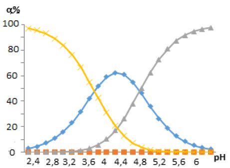
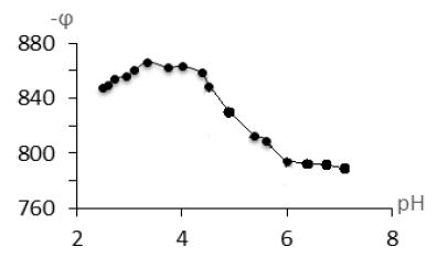
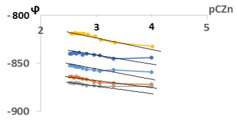
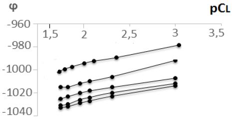
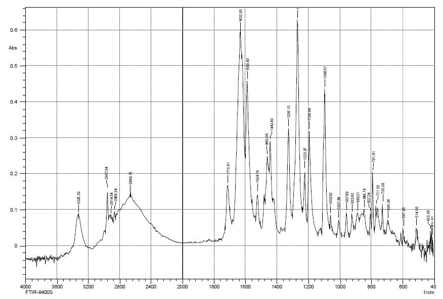
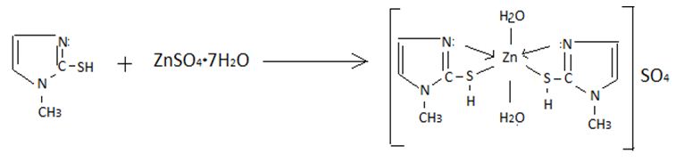
, and the results of the experiment showed that in the pH range from 4,5 to 6 in the system under study, complex particles of zinc with mercazolil are formed, the preliminary composition of which is given in Table 1.

The theoretical oxidation function was used to calculate the equilibrium in the system and to calculate the stability constants of the complexes:

1

The experimental oxidation function f0e was calculated using the equation:

2

According to Eqs. (1) and (2), the values of the experimental and theoretical oxidation function were calculated, which made it possible to plot the dependence of the oxidation function lgfe, t on pH. Graphs of dependences lgfe, t on pH at ionic strengths and temperatures are shown in Figure 4.

fig 4

Figure 4: Dependence of the logarithms of the experimental (f0e) and theoretical (f0t) oxidation function on pH of Zn(Hg)-Zn(II)-merc-H2O solution system CZn(II)=1*10-4 mol/L, I=0,1 mol/L, Сmerc=1*10-2 mol/L, T=308 K.

The coincidence of the experimental f0e and theoretical f0t curves indicates that the composition of the formed coordination compounds has been established quite accurately. Then the calculation of the formation constants of prepared complex particles is started. In addition, when calculating the theoretical oxidation function and calculating the constants of the formation of complexes, approximations were made to the values of the equilibrium concentrations of the complex and zinc ions; therefore, we adopted the confidence probability (P) equal to 0,75. The calculated numerical values of the formation constants of the established coordination compounds (Tables 1 and 2) using equation (1,2), as well as the equilibrium concentrations of free and bound zinc ions in the binuclear complex , calculated by the method of successive approximation, made it possible to calculate the molar fractions of free and bound zinc (II) ions in the complex. Distribution diagrams are shown in Figure 5 in the form of the dependence of the degree of accumulation aqpslk on pH. The molar fractions of equilibrium particles in the investigated redox system were calculated based on the general formula Ni=ni/Snij. Based on this expression, we represent the molar fractions of the complexes in the form of the following equations:

3

Table 1: The composition of the complex compound of zinc with mercazolil in the system Zn(Hg)- CZn(II)=1*10-4 mol / L, I=0,1 mol/L, СHmerc=1*10-2 mol/L, T=308 K.


рН

Tangents of slope angles of dependencies

Composition of the complexes

ϕ-pH

ϕ-pCZn

ϕ-pCL

3,7-4  0 n/2 n/2, -n ZnL;ZnL
4,0-4,5 -n n/2 n/2, -n ZnL;ZnL2
4,5-5,4 -n n/2 n/2, -n ZnL; ZnL2
5,4-6,0 -n n/2 n/2 ZnL

Table 2: The chemical model of the Zn(Hg) -Zn(II) – merc- H2O system at CZn(II)=1*10-4 mol/L, I=0,1 mol/L, СHмерк=1*10-2mol/L, T=308 K.

п/п

Fe 2+

H+

L

ОН

Composition of the complexes

bqslk

Equilibria of fragments in the redox system

q

s

l

K

1

1

0

0

1

Zn (H2O)4]2+ b1001 nlg(h3+b1001h2)

2

1

1

1

0

[ZnHL(H2O)3]2+ b1110 nlg(h3+b1110K1Ca1h2)

3

1

2

2

0

[Zn(HL)2(H2O)2]2+ b1220 nlg(h3+b1220K1Ca1h)

4

1

1

1

1

[ZnHLOH(H2O)2]+ b1111 nlg(h3+b1111K1Ca1h)

In equations (3) and (4) Сcomplex is the equilibrium concentration of the complex, Сo and aZn(II) are the mole fractions of zinc ions. The equations (3-4) made it possible to calculate the molar fractions of free and bound zinc ions in the complex at different ionic strengths and temperatures, which are presented in the form of distribution diagrams which are shown in Figure 5.

fig 5

Figure 5: Diagrams of the distribution of free and bound Zn (II) ions in coordination compounds. The curves are designated as follows: 1)Zn(H2O)4]2+; 2)[ZnHL(H2O)3]2+ ; 3)[Zn(HL)2(H2O)2]2+; 4) [ZnHLOH(H2O)2]+.

The analysis of the presented distribution diagram and the results of oxredmetry show that with an increase in the pH of solutions in the system under study, coordination particles of different composition, stability and of regions of dominance are gradually formed. For example, the complex particle [Zn(HL)2(H2O)2]2+ is formed in the pH range 4,6-5,5, and its maximum content is at pH 5,0, etc. Thus, the composition of the new coordination compounds was established by the methods of oxedmetry, and the formation constants and the regions of dominance of zinc (II) complexes with mercazolil and hydroxyl ions were determined using the oxidative function, which also made it possible to reveal the thermodynamic conditions for the synthesis of the binuclear mercazolylate complex of zinc (II), which has the highest numerical value of the formation constant. It was found that at an ionic strength of 0,1 mol/L, a temperature of 308 K, zinc concentration C Zn (II)=1 * 10-4, mol/L and mercazolil С Hmerc=1 * 10-2 mol/L, the following complex particles exist; ZnHL(H2O)3]2+(pH=4.0-,4,8), [Zn(HL)2(H2O)2]2+(pH=4,8.0-5.4), [Zn(HL)OH]+ (pH=5.4-6.0) and [ZnHL(OH)2H2O].

Synthesis of New Coordinate Compounds of Zinc(II) with Mercazolil

We used double recrystallized ZnSO4·7H2O as starting compounds in the synthesis of zinc (II) coordination compounds, and mercazolil (chemically pure) as ligands. Other organic solvents were purified according to the procedure. Before determining the halogen content, a weighed portion of the complex was decomposed with a nitric acid solution. The nitrogen content was determined by the Dume micromethod, carbon and hydrogen by burning a sample of the complex in a stream of purified oxygen. The sulfur content was determined gravimetrically, according to the method.

Synthesis of [Zn(HL)2]SO4 · 7H2O

1,14 g of mercazolil (0,005 mol) was dissolved in 5 ml of water, and a solution of 1,44 g (0,005 mol) of ZnSO4· 7H2O was added in 5 ml of water with vigorous stirring. The molar ratio of the reacting components of the system was 1:2. The reaction mixture was heated in a water bath for 4 hours until the color of the solution changed and a precipitate formed. The precipitated white precipitate was filtered off, washed with ethanol (25 ml), acetone (20 ml), ether (30 ml), and dried in a vacuum desiccator over solid KOH to constant weight. The resulting compound is readily soluble in water, DMSO and poorly soluble in ethanol, in DMF and insoluble in acetone,. The yield is 90%. Found,%: Zn-31,5; S-29; (N– 5,6;) H2O– 3,33; For [ZnLSO4] · 7H2O calculated,%: Zn – 13,80; S – 6,79; N- 5,940; H2O– 7,64. The formation of a zinc coordination compound in an aqueous ethanol medium is described by the following reaction:

Discussion of the Results

The synthesis of complex compounds of zinc with mercazolil was carried out in an aqueous solution at pH=5,5-6,0. Figure 6 shows the distribution diagrams of different forms of mercazolil (pKa=3,88) in a wide pH range. From the distribution diagram it follows that the neutral form of mercazolil is in the range of pH=3,88-6,0. In this form, mercazolil enters the complexation reaction with zinc.

fig 6

Figure 6: Particle distribution diagram of mercazolil in aqueous solution at 298 K

The synthesis of complex compounds of zinc with mercazolil was carried out depending on the ratio of the reacting components. When the zinc-mercazolil ratio is 1:2, a white precipitate is released from the solution. The reaction of the formation of this compound, based on the data of elemental analysis and the carried out physicochemical studies, can be represented by the equation:

ZnSO4+Merc+H2O↔[Zn(Merc)SO4]·H2O

If the concentration of mercazolil in the solution is increased and the ratio of the reacting components is increased to 1:2, then a cotton-like precipitate is formed, in which, according to elemental analysis, there are two moles of ligand per mole of zinc. The reaction of the formation of this complex can be represented by the equation:

ZnSO4 + 2 HMerc + 2H2O →  [Zn(Merc)2]SO4 · + 2H2O

With an excess of mercazolil in the solution, when the ratio of zinc to ligand becomes 1:5, a white precipitate is first formed and then completely dissolved. The complex formation reaction can be represented by the equation:

ZnSO4 + 5 HMerc + 2H2O →  [Zn(Merc)2]SO4 · + 2H2O

To determine the type of electrolyte, which includes the complex with the composition [Zn(НL)2(H2O)2]SO4, we studied its electrical conductivity in water at different temperatures and solution concentrations. Studies have shown that the electrical conductivity of [Zn(НL)2(H2O)2]SO4 in the temperature range of 20-45°С varies within 126,6-188,6 Оm-1·cm2·mol-1, which corresponds to type 1:1 electrolytes.

The study of thermal transformations of coordination compounds of zinc (II) with mercazolil showed that their character of thermal transformation is rather complicated and differs significantly from the process of thermal decomposition of uncoordinated mercazolil.

Thermal decomposition proceeds in several stages, which are characterized by weight loss, endo- and exothermic effects. Thus, thermal dehydration of the [Zn(HL2(H2O)2]SO4·H2O complex in an air atmosphere proceeds in the range of 100°С with a weight loss equal to – 10%. There is an endothermic effect on the DTA curve of the complex in this region. Theoretically, a weight loss of 4,5% corresponds to removal of one mole of water from the complex according to the equation:

[Zn(HL)2(H2O)2]SO4·H2O=[Zn(HL)2(H2O)2]SO4

The second stage of thermal decomposition of the complex occurs at 180-340°С. In this temperature range, according to the TG curve, the mass of the complex decreases by 63%. The complex heated at 340°С under isothermal conditions changes its color and becomes rustic.

The heated complex turns black and loses 63% of its mass. Taking into account the mass loss of the complex, elemental analysis data and IR spectroscopy (the absence of bands typical for mercazolil), it can be assumed that in the temperature range of 180-350°С there is a complete combustion of mercazolil molecules and formation of zinc sulfate according to the scheme:

[Zn(HL)2(H2O)2]SO4·=[Zn SO4]+2HL +2H2O

There are two exothermic effects on the DTA curve in this temperature range. In order to more accurately determine the processes occurring in the region of 500°С, 0,5 g of the complex was kept under exothermic conditions in an oven for 2,5-3 hours up to constant weight. An exoeffect is observed on the DTA curve in this temperature range. The reaction product, according to elemental analysis data, consists of metallic zinc. At the third stage of thermal decomposition, metallic zinc is formed according to the equation:

Zn SO4→ Zn +SO2+O2.

The thermogram of the complex [Zn(HL)2(H2O)2]SO4·H2O (Figure 7) in the temperature range of 100 -110°С is characterized by an endothermic effect, which corresponds to a weight loss of 4,5% on the TG curve.

fig 7

Figure 7: Thermogravigram of the complex with the composition [Zn(HL)2(H2O)2]SO4·H2O

The studies have shown that the thermal decomposition of mercazolil zinc complexes in air proceeds in three stages and covers the process of dehydration, thermal decomposition of mercazolil molecules in the complexes, decomposition of sulfate and the formation of metallic zinc. The comparison of the IR spectra of zinc sulfate, mercazolil, and the resulting complex indicates the formation of a new compound, in which characteristic bands related to stretching and bending vibrations of the starting substances appear with some changes. Infrared spectra of mercazolil, mercozincate in the frequency range from 4000 до 400 cm-1 were obtained to determine the functional groups of the studied ligands involved in complexation with zinc ions. The IR spectra (Figures 8 and 9) of the studied compounds revealed absorption bands typical for the monosubstituted benzene ring, methylene group and heterocyclic system. The shift or disappearance of characteristic absorption bands in the IR spectra of mercozincate in comparison with the spectra of zinc sulfate and mercazolil indicates the participation of specific functional groups in the formation of coordination compounds. For example, absorption bands in the range of 1619 – 1624 cm-1 characterize the stretching vibrations of the C=N bond of the conjugated aromatic system. After the formation of coordination compounds, it shifts from 1624 cm-1 in the IR spectrum of mercazolil to 1523 cm-1 in the IR spectra of mercozincate. Signs of coordination of mercazolil to zinc through a sulfur atom is proved by the fact that in the IR spectra of [Zn(HL)2(H2O)2]SO4·H2O there is a high-frequency shift of the band responsible for vibrations of C=S by 12-15 cm-1. The bands related to ν (-N (H) -C=S) in the spectra of the complex also undergo a change. The band of mercazolil at 1246 cm-1 in the spectra of the complexes completely disappears, and the band at 1276 cm-1 undergoes an insignificant high-frequency shift.

fig 8

Figure 8: IR spectrum of mercazolil at 4000 cm-1-650 cm-1

fig 9

Figure 9: IR spectrum at 4000 cm-1-650 cm-1 synthesis of zinc with mercazolil

Thus, it has been shown that the coordination bond between the zinc ion with mercazolil occurs due to the thiol group of the sulfur atom.

Due to polycrystallinity of the obtained coordination compounds of zinc (II), X-ray phase studies of a number of synthesized coordination compounds of zinc (II) with the indicated organic ligands were carried out. The value of the molar electrical conductivity of dimethylformamide solutions of oxalate complexes with the composition [Zn(НL)2 (H2O)4] SO4 obtained in water-ethanol solutions at 25°С is anomalously high and amounts to 110-180 Om-1 cm2 mol-1, which is not typical for electrolytes. The study of the concentration dependence of the molar electrical conductivity of aqueous and dimethylformamide solutions of the studied zinc (II) compounds showed that their molar electrical conductivity is inversely related to the concentration of all coordination compounds. The obtained experimental data indicate that upon dilution of the solutions of the complexes, water or DMF molecules with donor abilities enter the inner sphere of the complexes by displacing acidoligands due to which the value of the molar electrical conductivity of the corresponding complexes increases.

The joint consideration of the results of quantitative analysis, given on the determination of water content by Fisher method and thermogravimetry and IR spectroscopy allowed us to assume the structure of the obtained coordination compounds.

The chemical name of the new chemical compound we have received is merzincate.

merzinicate

Recently, medical microelementology has begun to develop significantly. The correction of microelement status improves the condition of patients with various diseases. The synthesized coordination compound of zinc with mercazolil can be used as an antibacterial, antifungal, agent for the treatment of endocrine diseases of the thyroid gland. In this direction, we have investigated the harmlessness, toxicity and therapeutic activity of the compounds. The harmlessness of the complex compound of zinc sulfate and mercazolil was studied in accordance with the “Methodological guidelines for the determination of the toxic properties of drugs used in veterinary medicine and animal husbandry. “The experiment was carried out on 10 heads of rabbits and 50 heads of white mice. In order to assess the harmlessness of the preparation in an approximate therapeutic dose of 0,05 g/kg of body weight with water orally (in the form of a 10% suspension in saline solution) white mice were administered in a volume of 0,1-1,6 ml (weighing 18-20 g, n=6), rabbits of the chinchilla breed – 10 ml (weighing 2,5-2,7 kg, n=5) 2 times a day for 7 days.

The laboratory animals were observed for 14 days, taking into account the general condition, appearance, behavioral reactions, food and water intake, rhythm and heart rate, and the number of respiratory movements. The harmlessness of the approximate therapeutic dose of the preparation obtained from zinc and mercazolil is evidenced by the results of observation of animals for 14 days: there was not a single case of death of animals. The acute toxicity of a complex compound of zinc with mercazolil was studied in experiments on rabbits (weighing 1,6-2,2 kg, n=12) of which, according to the principle of paired analogs, 4 groups were formed. Before the start of the study, laboratory animals that were kept under normal conditions were observed for 14 days. The last time food was given in the evening on the eve of the experiment, water intake was not limited. The substance was administered to rabbits in the form of a 10% suspension in saline solution once orally in a volume of 0.5 ml at doses of 0,05 g/kg of body weight (group 1), 0,1 (2nd), 0,5 (3rd), 1,2 (4th), 2,5 (5th), 3,5 g/kg of body weight (6th). Control animals were administered with physiological saline in appropriate volumes.6 hours after the administration of the preparation, the rabbits were given food again, which were subsequently transferred to the usual mode (Table 3).

Table 3: Acute toxicity test results for zinc with mercazolil

Substance dose, g/kg of weight of lab. animals

Actual effect

LD (%)

0,05 0/6 00
0,1 0/6 00
0,4 1/6 14,6
0,6 2/6 30,3
1,2 3/6 50
1,6 6/6 100

During the observation (14 days) of laboratory animals, the general condition, appearance, behavioral reactions, food and water intake, rhythm and heart rate, and the number of respiratory movements were taken into account. On the 2nd-3rd day, all animals of the 6th group died, from the animals of the 3rd group, 1 rabbit died on the 6th day, on the 5th and 7th days, 2 rabbits from the 4th group, and also during the experimental period, 3 animals from the 5th group. On examination of the internal organs of the dead animals, the gastric mucosa was hyperemic and filled with fodder, the liver was unchanged, and there was pinpoint hemorrhage in the tips of the lungs. The death of the rest of the experimental animals was not observed, the clinical state of the 1st and 2nd experimental groups and the control animals did not differ, the pathological changes in acute poisoning were absent in the animals.

Thus, according to the results of toxicological studies, it was determined that a complex compound of zinc with mercazolil 1,6 g/kg of body weight causes death of all experimental animals (LD100-1,6 g/kg) and at a dose of 1,2 g/kg causes death of 50 % of animals.

Effects on the Skin and Mucous Membranes

A single application was made of a 10% suspension of zinc with mercazolil on the skin of mice (weighing 18–20 g, n=8). The study of the repeated local irritating effect of this synthesized substance was carried out on mice (females, weighing 18 – 20 g, n=8), which daily on a clipped skin area in the interscapular region were applied 1 drop of a 10% zinc suspension with mercazolil for 14 days, and animals of the control group (n=8) – one drop of sunflower oil. The animals of both groups were observed for 30 days.

The repeated local action of zinc with mercazolil was also studied on rabbits (females, weighing 2,5-2,7 kg, n=8), which were daily applied to the skin with 2 drops of a 10% suspension of zinc with mercazolil for 21 days.

Animals of the control group (n=8) were given 2 drops of sunflower oil by the same method. Rabbits of both groups were observed for 60 days. As a result of the experiments, it was found that the substance obtained by us does not cause even minor phenomena of hyperemia, edema, scratching at the site of application. The animals did not show signs of toxicosis during the cutaneous application of the preparation.

Thus, no skin irritant and skin resorptive action was revealed in the complex compound of zinc with mercazolil. The effect of a complex compound of zinc with mercazolil on the mucous membrane of the eye was studied on rabbits (females, weighing 2,1-2,6 kg), which were divided into two groups (n=8). Animals of the first group in the conjunctival sac were once instilled with 10% suspension of the resulting complex compound in the amount of one drop, the second (control) group – instilled water in the same amount. It has been set that the local irritating effect of a complex compound of zinc with mercazolil on the mucous membranes of the eyes with a single administration is weak [3-25].

Conclusion

Based on the foregoing, it can be concluded that the complex compound of zinc with mercazolil belongs to the categories of low-toxic compounds for laboratory and farm animals, when administered orally in therapeutic doses.

References

  1. Ivansky VI (1978) Chemistry of heterocyclic compounds. p. 202.
  2. Berezina GR (2003) Complexes of cobalt (II) and zinc (II) with heterocyclic compounds based on 1,3-indandione. Journal of General Chemistry 73: 1567-1569.
  3. Rajabov UR, Yormamadova SG, Rakhimova RN, Kozikhonov AU (20-14) Complexation of copper with azoles derivatives at 298K/Collection of abstracts of the VIII International Scientific Conference “Kinetics and mechanism of crystallization. Crystallization as a form of self-organization of matter “, Ivanovo, Russia p. 51-52.
  4. Berezin BD, Nurmatov AA, Semeykina AS, Berezin MB (1994) Replacement of acetylacetonate ligands in the coordination sphere of copper and zinc with porphyrins. Coordination Chemistry. 20: 391-396.
  5. Olekhnovichi RY, Korobov MS, Lyubchenko SN, Suukholenko EV, Raskina PA, et al. (1992) Degenerate configurational r↔E isolating sterically hindered orta-indoaniline ligands in tetrahedral metal chelates Zn (II) and Cd (II). Journal of General Chemistry 62: 901-902.
  6. Tsapkov VI, Tarkogiel Mianperen, Samus NM (1993) Intra-complex compounds of cobalt (II), nickel (II), copper (II) and zinc with 5-nitrofuryl-2-methylene hydrazole isoamine. Journal of General Chemistry. 63: 1165-1166.
  7. Ilyasov SG, Lobanova AA, Popov NI, Kazantsev IV (2006) Synthesis and properties of intra-complex compounds of 4-nitrosemicarbazide with Fe (II), Ni (II), Co (II) and Zn (II). Journal of General Chemistry 76: 1795-1796.
  8. Pridchin SN, Kochergina AA (2006) Complex formation of zinc, cadmium and manganese (II) with 2-hydroxypropylene-1,3-diamine-N, N, N, N-tetraacetic acid. Journal of General Chemistry 76: 600-601.
  9. Skopenko VV (2007) Coordination chemistry. Akademkniga 487 p.
  10. Remy G. Course of inorganic chemistry/G. Remy. – M: Mir, 1966. V. 2. – p. 836.
  11. Dyuga G, Penny K (1983) Chemical approaches to the mechanism of action of enzymes. Bioorganic Chemistry. 512 p.
  12. Knorre DG, Myzina SD (2000) Biological chemistry: a textbook for chem. biol. and med. special universities. p. 8-26.
  13. Shabaldova AD, Bolshinkova TA, Kornienko GK, Trushina EK (1989) Complexes of copper with N-O-containing ligands, new reagents and biologically active substances. Abstracts of the report. III All-Union Conference. on chemical reagents. Ashgabat p. 87.
  14. Vasilyev VP, Zaytseva GA (1979) Protonation of imidazole in aqueous solution Problems of solvation and complexation. – Ivanovo p. 94-97.
  15. Perekalin VV, Zonis SA (1982) Prosveshenie Organic chemistry 575 p.
  16. Traven VF (2006) Organic chemistry. Akademkniga 2: 85-95.
  17. Beloborodov VL (2002) Organic chemistry: Basic course. Book. 1. p. 31-46.
  18. Cotton F, Wilkinson J (1969) Modern inorganic chemistry. Chemistry of transition elements. 592 p.
  19. Akhmetov NS (2001) General and inorganic chemistry. 743 p.
  20. Glebov AE, Dyachkova TA, Tarasov OY (1994) Chemistry of heterovalent complexes 120 p.
  21. Lumme P, Virtanen P (1969) Thermodynamics of the protolysis of imidazole in aqueous Solutions. Suomen Kemistilehti 42: 333-338.
  22. Greenberg AA (1966) Introduction to the chemistry of complex compounds “Chemistry”631 p.
  23. Chemistry of coordination compounds. Ed. J. Baylar, D. Bush. Trans. from English Ed. I.I. Chernyaev. M., IL, 1969.695 p.
  24. Belikov VG (1991) Pharmaceutical chemistry. 768 p.
  25. Zinc in pediatric practice (textbook) 2001, 84 p.

Reducing Anxiety with Student Nurses – Building Partnerships within a University and Clinical Settings

DOI: 10.31038/JCRM.2023614

Abstract

Anxiety is a common experience for many student nurses, especially during clinical placements [1]. The high stress and unpredictability of the placements, combined with the added pressure of learning new skills and adapting to new environments, can cause significant levels of anxiety in student nurses. A university and hospital-based clinical team worked collaboratively to address student, preceptor, and faculty concerns about anxiety and stress within the clinical placement. This article will explore five strategies a university and the clinical preceptors, through collaboration took to reduce anxiety in student nurses during their clinical placement.

Anxiety is a common experience for many student nurses, especially during clinical placements [1]. The high stress and unpredictability of the placements, combined with the added pressure of learning new skills and adapting to new environments, can cause significant levels of anxiety in student nurses. Furthermore, anxiety can have a significant impact on nursing students’ academic performance, emotional well-being, and overall quality of life [2]. Additionally, it can lead to decreased motivation, concentration, and memory recall, making it difficult for students to learn and retain information. It can also cause physical symptoms such as headaches, fatigue, and gastrointestinal problems (McDermott et al., 2021). However, reducing anxiety is essential for promoting optimal learning and in turn, providing patient-centered care. This article will explore five strategies a university and clinical preceptors, through collaboration took to reduce anxiety in student nurses during their clinical placement.

Background

Student anxiety in the clinical area is a well-documented phenomenon that has been studied extensively in literature [1-4]. Clinical settings can refer to a wide range of healthcare environments, such as hospitals, clinics, and community settings, where students are required to interact with patients, healthcare professionals, and other stakeholders in the real-world environment. Although supervised and supported through preceptors or mentors this imposes additional anxiety on the nursing student.

One study by Aloufi et al. (2021) explored nursing students’ experiences with anxiety in clinical settings. The study found that many nursing students experienced anxiety related to clinical experiences, particularly when it came to providing direct patient care. The authors suggest that interventions such as simulation, or practice out of the clinical areas and superior mentorship can help alleviate this anxiety. Similarly, performance and anxiety were examined by Al-Ghareeb, McKenna and Cooper (2019) [5]. This study found that students who experienced higher levels of anxiety had a poorer clinical performance. The suggestion was to provide opportunities for practice in low-stakes assessments and practice cognitive-behavioral therapy to reduce anxiety levels. Congruent to other studies, a review by Judd et al. (2019) suggested that simulation-based education, mindfulness interventions, and debriefing sessions were shown to be effective in reducing anxiety in nursing students. Finally, a study by Wong et al (2019) explored the impact of a clinical anxiety management program on nursing students’ anxiety levels. The study found that the program was effective in reducing anxiety levels in nursing students. The authors suggest that such programs can be useful tools for addressing anxiety in clinical settings. Overall, the literature suggests that anxiety is a common issue among nursing students in clinical settings independent of experience, geographical or clinical setting. It also suggests that interventions such as mindfulness-based, simulation, or anxiety management programs have been found to be effective in reducing anxiety levels and improving clinical performance. The team reviewed this and decided that a number of interventions should be intentionally and systematically implemented to reduce anxiety in our nursing students.

Implementation

A university and hospital based clinical team worked collaboratively to address student, preceptor and faculty concerns of anxiety and stress within the clinical placement. A systematic approach through collaborative meetings, inclusive discussion, and evidence-based interventions was used to address this issue.

Once identified that anxiety was affecting student performance five practical, cost-effective, and evidence-based interventions were implemented. This was in collaboration with the clinical team and was key to the success of the project. Each intervention will be described. Firstly, providing students with a supportive learning environment. Clinical preceptors can create a safe space for students by demonstrating empathy and actively listening to their concerns. The team undertook a series of workshops to bridge the gap in understanding. Through a series of role play and open discussion preceptors were ‘taken back’ to what it was like to be a student and how to support and empathize with the undergraduate. Students who feel heard and valued are more likely to feel comfortable and confident in their abilities, which can help reduce anxiety. Additionally, preceptors can use positive reinforcement to acknowledge and celebrate students’ successes, which can also boost their confidence and reduce anxiety. Faculty and preceptors worked together to find ways to acknowledge students learning through guided de-brief. Another strategy introduced to reduce anxiety was to provide student nurses with clear expectations and guidance. Students who are unsure of what is expected of them or who lack clear guidance may feel anxious about making mistakes or falling short of expectations. To address this clear and weekly clinical objectives were devised, mirroring the didactic and theoretical concepts covered. The clinical preceptors provided the students with detailed instructions and clear expectations for their roles and responsibilities in a newly devised ‘pre-brief’. Additionally, objectives were provided at the beginning of the term on the learning platform to reinforce and aid understanding. On evaluation, this was proven to help students feel more prepared and confident in their abilities. Next, in collaboration with the clinical preceptor’s communication and feedback strategies were examined. A workshop on clear, concise, and respectful manners. This was to encourage students to communicate their concerns and ask questions which can help alleviate anxiety and prevent misunderstandings. Additionally, education and best practice on providing students with feedback on their performance to highlight areas of strength and offer constructive criticism for areas that need improvement. Debrief has been shown where learning takes place Cantrell, (2008) [6-8] suggests that feedback has been shown to help students feel more confident. A formal debrief in the clinical areas to mirror the simulation center was implemented. As the students were familiar with this method it was quickly assimilated. Next, incorporating realization techniques into the learning environment was another effective strategy for reducing anxiety in student nurses. With the help of the University’s wellness center stress-reducing techniques such as deep breathing exercises, meditation, and yoga were introduced to the nursing students. In collaboration with the clinical preceptors were encouraged to practice these techniques with the students during placement. Finally, there was a recognition that the hospital-based clinical preceptors were not fully aware of the university services open to students to reduce anxiety. The resources, such as the wellness center, and counseling services were readily shared so the preceptors could provide access to these resources and help the students feel more supported and empowered to manage their anxiety reducing its impact on their learning and overall well-being.

Although in the initial stages, informal feedback and reports from both preceptors and the students appear to suggest the interventions are reducing anxiety. Also, the collaborative response has initiated more of a team-based rather than silo response to student issues.

In conclusion, anxiety is a common experience for many students’ nurses during their clinical placements. However, it is essential to reduce anxiety levels to promote optimal learning. Working collaboratively with the clinical preceptors to create a supportive learning environment, providing clear expectations and guidance, effective communication incorporating relaxation techniques and providing resources can all help reduce anxiety in student nurses. By collaborating and demonstrating evidence-based strategies clinical preceptors felt better equipped to support the students in their learning and help them manage the challenges of their clinical placements.

References

  1. Labrague LJ, McEnroe-Petitte DM, Gloe D, Thomas L, Papathanasiou IV, et al. (2017) A literature review on stress and coping strategies in nursing students. Journal of Mental Health 26: 471-480. [crossref]
  2. Aloufi MA, Jarden RJ, Gerdtz MF, Kapp S (2021) Reducing stress, anxiety and depression in undergraduate nursing students: Systematic review. Nurse Education Today 102: 104877.
  3. O’Driscoll M, Byrne S, Byrne S (2020) The effectiveness of mindfulness-based interventions for reducing anxiety in nursing students: A systematic review and meta-analysis. Journal of Advanced Nursing 76: 73-87.
  4. Zhang Y, Wu Y, Wang L, Zhang Y (2021) Effect of mindfulness-based interventions on anxiety in nursing students: A systematic review and meta-analysis. International Journal of Environmental Research and Public Health 18: 3622. [crossref]
  5. Al-Ghareeb A, McKenna L, Cooper S (2019) The influence of anxiety on student nurse performance in a simulated clinical setting: A mixed methods design. International journal of nursing studies 98: 57-66. [crossref]
  6. Cantrell MA (2008) The importance of debriefing in clinical simulations. Clinical simulation in nursing 4: e19-e23.
  7. Asadi-Lari M, Saeedi M, Vaezi M, Fathabadi J (2021) The effectiveness of cognitive-behavioral therapy on anxiety in nursing students: A systematic review and meta-analysis. Nurse Education Today 99: 104872. [crossref]
  8. Feng X, Shi S (2022) Mindfulness-based interventions for reducing anxiety in nursing students: A systematic review and meta-analysis of randomized controlled trials. Nurse Education Today 108: 105198.

A Modern Approach Towards Efficient Antifouling Coating Technologies

DOI: 10.31038/NAMS.2023624

Abstract

Marine fouling is a worldwide problem with various economic and environmental threats. Most current antifouling technologies suffer from poor performance. It is evident that more efficient antifouling technologies under both static and dynamic conditions have to be developed. These should effectively combine diverse characteristics and functions. The incorporation of conductive and electrically anisotropic moieties into water soluble resins may prove a drastic solution to this on-going problem.

Keywords

Antifouling paints, Biofouling, Conductive coatings, Electrical anisotropy

Discussion

Biofouling poses major technical, scientific and economic challenges to various maritime sectors. Within the marine environment, any surface in contact with seawater suffers from biofouling. The biofilm can form in as little as 48 hours [1-3] giving rise to macrofouling, i.e., the attachment of marine organisms, such as algae and barnacles to the hull of a ship, which compromises performance of the vessel. Fouling on ships’ hulls decreases speed and maneuverability and significantly increases fuel consumption [4]. Hard (calcareous) fouling especially, can result in power loses exceeding 85% and ultimately, engine failure.This natural phenomenon constitutes a huge economic problem for marine industries, as it raises the costs related to materials’ maintenance and repair [5-7], since dry-docking for cleaning is more frequently necessary.

There are also unintended ecological effects when a bio-fouled ship moves between ports, since non-indigenous species are transferred from one region to another.Biofouling of the ship’s reefs is directly related to the roughness of its reefs. It has been calculated that for each increase in reef roughness by 10-20 μm, the friction resistance increases by 0.5% for ships at high speeds. In general, the surface roughness of the reefs is increased by mechanical detachments or structural defects [8].

Thus, the development of innovative low-drag antifouling coatings for the hulls of ships, vessels, and speed crafts is essential [9-13]. Numerous attempts have been made to develop efficient antifouling coatings, which exploit recent adcances in biοlogy, physics, marine chemistry and materials science. More specifically, biological methods [14] involve the use of a variety of enzymes or metabolites, secreted by cells, as substitutes for traditional biocides. The organic secretions inhibit the growth of their competitors and are biodegradable. This approach however has, up to now, limited success, since crucial technical obstacles, such as designing of an appropriate coating matrix or balancing of the effectiveness and lifespan of the coating still remain. Moreover, it is difficult to predict the impact of metabolites and enzymes on the marine environment if these are broadly applied to ships. Furthermore, with regards to the physical methods employed in antifouling coatings, electrolysis of seawater, with the coating acting as the anode, is perhaps the most common one. When such equipment is available on ships, hypochlorous acid (HClO), ozone bubbles, hydrogen peroxide or even bromine can be produced. Because of their strong oxidizing ability these compounds spread all over the ship’s hull and eliminate fouling. However, due to large voltage drop across the surface, steel corrosion is intensified and efficiency of these systems is limited.Traditionally, chemical biocides have been regarded as the standard approach to control marine biofouling. Compounds such as tributyltin oxide (C24H54OSn2) and tributyltin fluoride (C12H27FSn) are incorporated into polymeric matrixes to produce antifouling paints for ships’ hulls. When the International Maritime Organization (IMO) banned the use of effective but environmentally damaging coatings containing TBT in 2008, the development of non-toxic coatings became more important than ever [15]. Due to the lack of effective alternatives, biocidal antifouling paints, such as those based on copper, which are considered as a transition between toxic and non-toxic coatings, have dominated the antifouling paint market. Copper oxide has been recommended by the Environment Protection Agents (EPA) as a suitable replacement of TBT, since it can be bound in water with other substances and thus, its toxicity is reduced. However, materials for marine applications have to comply with new stricter rules with regards to protection of environment, aquatic organisms and human health [16]. Therefore, that nonbiocidal antifouling coatings are in high demand.

Besides toxicity of its ingredients, a well-designed antifouling coating should adequately address issues, such as efficiency of antifouling performance and application costs. With regards to antifouling efficiency, it has to be noted that this is an unambiguous prerequisite under both static and dynamic conditions. Unfortunately, current antifouling paints fail to perform sufficiently under static conditions, with the majority of them having a useful lifetime of just 30-40 days. With regards to application costs, they should also include the cost of surface priming (and perhaps the cost of tie coating) as well as the cost of removing older paint coats. In addition, complexity of the method used to apply the coating should not be neglected. Finally, the special characteristics of the coating used, such as the drying time or the number of coating layers required in order a functional thickness to be obtained should be also taken into account in order to accurately evaluate sustainability and potential economies of scale.It should be also noted that seawater parameters, such as salinity, temperature and pH fluctuations, substantially affect the ability of microorganisms, algae, and plants to adhere and settle on a surface [17,18]. For example, pH variations affect solubility of biocides and the rate of corrosion of the coating [6]. Annual fluctuations and seasonal changes in temperature significantly affect the reproductive cycles of the microorganisms, and consequently the species of the growing microorganisms, the rate of corrosion and the extent of the biofouling [19]. Therefore, an efficient antifouling coating should be fully functional under a broad range of conditions [20].

It is evident that more efficient antifouling technologies have to be developed. A promising alternative are antifouling nanocomposites based on conductive and electrically anisotropic antimicrobial nanostructures, which can effectively combine the primary advantages of the various methods within a single multifunctional approach. In further analyzing the above concept, a short introduction on conductive polymers should be made. More specifically, electric conductive polymers have been employed in the manufacture of protective coatings, mainly against corrosion of metals. It has been also reported that, such polymers may also find use as additives in antifouling paints [21]. Towards this prospect, the most significant obstacle is that their electronic conductivity slowly decreases due to the dissolution in water of anionic dopants. Thus, antifouling efficiency also decreases. It has been reported [22] though, that when conductive polymers are doped and/or mixed with certain nanostructured materials, such as TiO2 or ZnO they exhibit perfect electrochemical reversibility for long periods of time. It has been also recommended that they can be used as a copper alternative for electrolyzing seawater.Among possible candidates, polyaniline (PAni) in its doped form is the most promising one. Its low price, facile synthesis process, unique conductive properties and high thermal stability make PAni a highly attractive anti-foulant. The antibacterial activity of PAni is based on various factors, such as the length of its long polymer chain, the low molecular weight, and the presence of amino groups [23]. It has been found [24] that paints formulated with Pani, which was doped with HCl, and zinc biocides were effective against marine fouling for more than twelve months; longer that the period used by common commercial paints. In its doped form PAni is also able to protect steel against corrosion by an anodic protection mechanism, owing to the formation of a layer consisting of iron oxides. In the case of coating failure, doped Pani is also able to regenerate the metal oxide layer. This feature is of crucial importance, since application of all modern antifouling coatings presents a serious drawback: the necessity of using a primer coat and sometimes, a second coat, namely a tie coat, prior to application of the antifouling paint. Undercoats provide mechanical robustness to the entire coating’s structure, but their main functionality is to provide anticorrosion protection to the steel substrate. It goes without saying that the application of a single durable coating providing both antimicrobial and anticorrosion properties would be a truly breakthrough in the maritime coating technology.

In addition, when PAni is combined with TiO2 especially, synergistic phenomena may enhance both conductivity and antimicrobial performance of the coating. The latter is promoted by the photocatalytically active TiO2 mineralogical form, i.e. anatase. In this case, visible light adsorbs on the coating’s surface leading to generation of H2O2. The latter disintegrates shortly into H2O and O2, therefore poses no threat to the environment. In addition, the large surface area of nanosized materials means that the development of coatings with low amounts of photocatalysts is achievable. In addition, such coatings may possess an amphiphilic behavior, since they can combine within adjacent heterogeneous nanoscale regions the low surface energy and the resistance to protein adsorption of Pani with the high surface energy and foul-release properties of TiO2 nanoparticles.

Anti-fouling properties may be further enhanced by the incorporation of carbon nanofibers (CNFs) or graphene oxide (GO) sheets within the coating’s matrix. Nanomaterials of acrbon allotropes have shown promise for electrochemical biofouling reduction due to superior conductivity and cytotoxicity arising from generation of reactive oxygen species [14]. Their nanosize allows facile dispersion in a wide range of matrices, as well as a reduced material demand, while exhibiting strong antibacterial activity. In addition, they can act as fillers providing mechanical reinforcement to the coating’s matrix. Cylindrical carbon structures with sub-micrometer diameters and lengths within the 30-100 μm range can be readily prepared. A modern antifouling approach may thus result by externally decorating polyaniline nanorods with magnetite nanoparticles and then magnetically align the resulting nanocomposite out of the coating’s plane, which is defined by the structural growth orientation of carbon allotrope sheets or plates. The latter can be further modified with anatase nanoparticles, in order to develop a conductive and photocatalytically active matrix with enhanced in-plane antimicrobial and antifouling performance. The resulting nanostructure can then be easily incorporated into a soluble polymer matrix by wet chemical methods.

Within this approach chemical antifouling mode of actions can be coupled to mechanical ones through triggering of fur-like phenomena. More specifically, PAni nanotubes (or nanorods) can be filled with magnetite NPs to align them, by a weak magnetic field, in an out-of-plane configuration, during curing of the coating’s resin. Magnetic orientation has advantages over the use of an electric field because magnetic forces are non-contact, do not cause chemical changes and are not sensitive to pH changes. The aim of such modification is to confer to the matrix a foul-release activity, too. It has been demonstrated [25] that fiber coatings containing piles of flexible thorns, such as polyamide, can provide a strong antifouling effect due to their fur-like surface, which enables tiny swaying movements in water and therefore detachment of fouling organisms by tidal currents and waves. Although fiber dimensions are in the mm range, it was found that the control of fiber’s stiffness, which is directly dependent on the thickness to length ratio, is the critical parameter in enhancing antifouling properties. Therefore, the same mode of action can be also exhibited by nanofibers or nanorods, provided that a functional ratio of nanotube diameter and length is found. Our team is currently working on the discovery of such optimum ratios of PAni tubes, which have been functionalized by magnetite nanoparticles and embedded on graphene oxide matrices modified by anatase nanoparticles. The out-of-plane configuration of PAni tubes may have a similar functionality role to the thorn-like structure of common fiber coatings. Towards this end, a fundamental requirement is the utilization of a soluble paint matrix. Soluble matrixes are characterized by the fact that the binder is dissolved in water; therefore, the coating’s thickness is decreased during immersion and PAni nanorods are gradually revealed. The above mechanism is similar to the primary mode of action of common self-polishing antifouling paints.

Due to the aforementioned arrangement, the problem of biofouling can be addressed at its root, i.e. before the onset of primary biofilm formation. In particular, the first stages of colonization can be prevented due to the high in-plane conductivity, evoked by modified GO sheets. The photocatalytically active TiO2 nanoparticles can further contribute to the in-plane anti-fouling ability of the coating. At the same time, the developed electrical anisotropy enables charge dissipation, thus limiting electrostatic attractions and preventing early adsorption of bacteria and microorganisms through their negatively-charged outer membrane.

Αs the coating’s binder dissolves an increasing part of vertically aligned PAni nanorods is revealed. As a result, the coating’s out-of-plane conductivity becomes increasingly important. Colonization is now effectively addressed through direct contact of microorganisms with the PAni nanorods. Beyond a certain limit, the exposure of most of the nanorods makes them flexible and prone to microscopic oscillatory movements in the water, which facilitate the detachment of macrofouling under the influence of tidal currents and waves. The above mechanism provides a second anti-fouling defence based on foul-release properties. The importance of this mechanism is obviously smaller compared to the chemical antifouling mode of action and valid only in dynamic conditions However, it can prolong the useful lifetime of the coating, especially when its initial antifouling efficiency starts to fade. Even more importantly, an additional mechanism of action is present when surface biofouling is already there. The afore-mentioned process constantly exposes a fresh coating’s surface; thus, the antifouling behavior of the coating remains sufficient for long periods of time.

The development of antifouling coatings based on the above approach has industrial potentiality. Nanotubes of PAni can be readily synthesized by the template free method. First, carboxyl-modified aniline dimers are prepared. Subsequently, they are functionalized by magnetite nanoparticles with diameters in the 10-30 nm range developed by ultrasonic (20 kHz) co-precipitation of iron (II) and iron (III) precursors. Then, polymerization of functionalized dimers follows. Furthermore, modified graphene oxide sheets can be prepared by sonication of an acidified graphene oxide colloidal emulsion in the presence of titanium isopropoxide Ti[OCH(CH3)2]4. The graphene oxide emulsion can be prepared by the modified Hummers method. The above nanocomposites can be directly added to aqueous dispersions of commercially available water-soluble resins in order to produce the antifouling paint. The latter can be easily applied to solid substrates, such as naval steel by traditional spraying methods, e.g., airless spraying.

Our research team is currently conducting a series of tests in the Mediterranean coastline to evaluate real-field performance of such nanocomposite coatings. The experimental verification of the above approach will allow for the development of an environmentally friendly coating with long lifespan and robust performance, possessing both antifouling and foul release properties. Preliminary studies have shown enhanced functionality, which is attributed to the synergistic effects of antimicrobial attributes with anisotropic electrical conductivity. Moreover, the developed coatings have a distinct advantage over state-of-the-art competition: they can be applied directly to metal substrates providing anticorrosive properties without the use of primers.

The successful implementation of the afore-mentioned strategy into marine paints could provide an eco-friendly and efficient alternative to contemporary antifouling technologies. It could also considerably reduce the time required for compliance certification procedures according to international standards and facilitate fast implementation of similar technologies in other industrial sectors as well.

Conclusions

It seems that no antifouling technology alone can yield the performance required to address biofouling under a variety of conditions, either static or dynamic. Environmentally friendly nanocomposite materials which combine conductive, electrically anisotropic and antimicrobial functions and can be incorporated into water soluble matrices is a highly promising approach. The resulting antifouling paint exhibits both antifouling and foul release properties and can be applied directly to metal substrates without the use of a primer providing anticorrosive protection to the underlying surface. It is also expected to be cost efficient, not only in terms of being economical to apply and maintain, but also in terms of saving fuel costs, reducing out-of-operation time for the marine vessel and requiring minimal drydocking.

Acknowledgment

This research has been co-financed by the European Regional Development Fund of the European Union and Greek national funds through the Operational Program Competitiveness, Entrepreneurship, and Innovation, under the call RESEARCH – CREATE – INNOVATE (project code: T2EDK-00868).

Conflicts of Interest

All authors declare no conflicts of interest in this paper.

References

  1. Steffi AP, Balaji R, Chen SM, Prakash N, Narendhar C (2021) Rational Construction of SiO2/MoS2/TiO2 Composite Nanostructures for Anti-Biofouling and Anti-Corrosion Applications. ChemistrySelect 6: 917-927.
  2. Alghamdi S, Cordova RAQ (2019) The Impact of Biofouling on Marine Environment: A Qualitative Review of the Current Antifouling Technologies. Master’s Dissertation, World Maritime University, Malmö, Sweden.
  3. Manoj S, Mahesh S, Srikanth N (2019) Review of Biofouling Paints on the Marine Vessel, 2018 Asian Conf. Energy. Power Transp Electrif ACEPT 1-6.
  4. Schultz MP , Bendick JA, Holm ER, Hertel WM (2011) Economic impact of biofouling on a naval surface ship, Biofouling 27: 87-98.
  5. De Castro MCT, Vance T, Yunnie ALE, Fileman TW, Hall-Spencer JM (2018) Low salinity as a biosecurity tool for minimizing biofouling on ship sea chests. Ocean Sci 14: 661-667.
  6. Sarkar PK, Pawar SS, Rath SK, Kandasubramanian B (2022) Anti-barnacle biofouling coatings for the protection of marine vessels: Synthesis and progress. Environ Sci Pollut Res 29: 26078-26112.
  7. Pistone A, Scolaro C, Visco A (2021) Mechanical properties of protective coatings against marine fouling: A review. Polymers 13: 173. [crossref]
  8. Bezek K,Nipič D, Torkar KG, Oder M, Dražić G, et al. (2019) Biofouling of stainless steel surfaces by four common pathogens: The effects of glucose concentration, temperature and surface roughness. Biofouling 35: 273-283.[crossref]
  9. Oliveira DR, Granhag L (2020) Ship hull in-water cleaning and its effects on fouling-control coatings. Biofouling 36: 332-350.
  10. Gu Y, Yu L, Mou J, Wu D, Xu M, et al. (2020) Research strategies to develop environmentally friendly marine antifouling coatings. Mar Drugs 18: 371. [crossref]
  11. Ali A, Jamil MI, Jiang J, Shoaib M, Amin BU.et al. (2020) An overview of controlled-biocide-release coating based on polymer resin for marine antifouling applications. J Polym Res 27: 1-7.
  12. Hu P, Xie Q, Ma C, Zhang G.(2020) Silicone-Based Fouling-Release Coatings for Marine Antifouling. Langmuir 36: 2170-2183. [crossref]
  13. Selim MS, El-Safty SA, Shenashen MA, Higazy SA, Elmarakbi A (2020) Progress in biomimetic leverages for marine antifouling using nanocomposite coatings. J Mater Chem B 8: 3701-3732. [crossref]
  14. Camps M, Barani A, Gregori G, Bouchez A, Le Berre B.et al. (2014) Antifouling Coatings Influence both Abundance and Community Structure of Colonizing Biofilms: a Case Study in the Northwestern Mediterranean Sea. Appl Environ Microbiol 80: 4821-4831.
  15. Cao S, Wang J, Chen S, Chen R (2011) Progress of marine biofouling and antifouling technologies. Chin Sci Bull 56: 598-612.
  16. Brooks S, Waldock M, Hellio C, Yebra D (2009) The use of copper as a biocide in marine antifouling paints. In Advances in Marine Antifouling Coatings and Technologies Woodhead Publishing 492-521.
  17. Armendáriz-Ontiveros MM, Álvarez-Sánchez J, Dévora-Isiordia GE, García A, Fimbres Weihs GA (2020) Effect of seawater variability on endemic bacterial biofouling of a reverse osmosis membrane coated with iron nanoparticles (FeNPs) Chem Eng Sci 223: 115753.
  18. Dobretsov S, Coutinho R, Rittschof D, Salta M, Ragazzola F, Hellio C (2019) The oceans are changing: Impact of ocean warming and acidification on biofouling communities. Biofouling 35: 585-595. [crossref]
  19. Quagliarini E,Gianangeli A, D’Orazio M, Gregorini B, Osimani A, et al. (2019) Effect of temperature and relative humidity on algae biofouling on different fired brick surfaces. Constr Build Mater 199: 396-405.
  20. Falara PP, Papadopoulos ND, Vourna P (2022) Microstructure and Performance of Antibiofouling Coatings on High-Strength Steel Substrates Immersed in the Marine Environment, Micro 2: 277-294.
  21. Wang X-H, Li J, Zhang JY, Sun ZC, Yu L, et al. (1999) Polyaniline as marine antifouling and corrosion-prevention agent. Synth Met 102: 1377-1380.
  22. Mostafaei A, Nasirpouri F (2013) Preparation and characterization of a novel conducting nanocomposite blended with epoxy coating for antifouling and antibacterial applications J Coat Technol Res 10: 679-694.
  23. Shubha LN, Madgula K, Rao PM (2016) Synthesis, characterization by AC conduction and antibacterial properties of polyaniline fibers. Der Pharmacia Lettre, 8: 214-219.
  24. Baldissera AF., De Miranda KL, Bressy C, Martin C, Margaillan A, et al. (2015) Using Conducting Polymers as Active Agents for Marine Antifouling Paints. Mater Res 18: 1129-1139.
  25. Breur HJA (2012) Antifouling fibre coatings for marine constructions. US Patent 8: 278-226 B2.
fig 2

Understanding Shale Instability through the Lens of Clay Mineralogy and Zeta Potential

DOI: 10.31038/GEMS.2023524

Abstract

Shale, a significant rock formation with potential as a source and reservoir rock, presents challenges in drilling due to its unique chemical composition and mechanical properties. To address the instability caused by shale mineralogy, various shale inhibitors are used as drilling fluid additives, interacting with clay minerals to stabilize the clay by neutralizing surface charges. While numerous research groups have extensively studied shale stabilization, clay chemistry, and novel inhibitors, there remains a gap in comprehensive studies that correlate evidence of shale instability from recent literature with clay mineralogy and Zeta potential. This review article fills this gap by presenting pioneering work and recent evidence from literature to provide a clear rationale behind the role of clay mineralogy in shale instability. Notably, a novel correlation has been developed that predicts clay swelling based on Zeta potential for sodium bentonite clay with a smectite percentage ranging from 70-90%. This review work serves as a foundation for future researchers in selecting appropriate shale samples for their shale stabilization studies and estimating clay swelling based on Zeta potential. Ultimately, it presents a more nuanced understanding of the mechanism of shale swelling inhibition, contributing to the advancement of knowledge in this field with a cerebral approach.

Keywords

Clay mineralogy; Shale instability; Shale swelling; Shale hydration

Introduction

Shale is the most abundant clastic sedimentary rock roughly accounting for 70 % of the sedimentary rock type in the Earth’s crust [1]. Shale is a laminated and fissile rock comprising of clay and silt size particles ranging from 0.02 – 0.05 mm in diameter [2,3]. Shales are often located with the layers of limestone or sandstone and typically generate in the environment where silts, muds and other sediments were deposited by the mellow currents followed by the compaction e.g., basins of shallow oceans, payas, river flood plans and floor of deep-oceans [4,5]. The permeability and porosity of shale rocks depend upon the size of the constituent grain particles while their colour is mainly attributed by their composition e.g., the higher the organic content of the clay, the darker will be its colour; purple and reddish colour is due to the existence of hematite and limonite, blackish, brown, and blue hues correspond to the presence of iron ores while calcareous shale are yellowish or light grey [6,7]. Organic shales containing kerogens (a complicated mixture of hydrocarbons generated from animals and plants remains) in substantial quantity, produce oil when subjected to pyrolysis, are called oil shales [8-10]. The term shale oil is also used for the crude oil which is produced from oil bearing shale formations with low permeability and to avoid the confusion with the generic crude oil, the term ‘tight oil’ can be used for shale-oil [11]. The shale oil reservoirs are usually classified by the (Vitrinite reflectance) Ro = 0.6%-1.2%, TOC (Total organic content) > 2% and having complex mineral composition with ultra low permeability (0.001-0.0001) mD and low porosity (<5%) [12,13]. Though, shale is an important reservoir and source rock but drilling through shale formation is a havoc due to its brittle nature. Roughly 70% of the wellbore instability issues are associated with the shale dispersion, swelling and sloughing [14,15]. Wellbore instability issues may arise due to bit balling, pipe stucking, caving and lost circulation which predominantly happens due to shale swelling [16,17]. Shales can undergo through instability mainly due to its chemical composition or mechanical failure [18]. However, in this detailed review, shale instability has been related with the clay chemistry. The pieces of evidence have been collected from the recent literature which directly correlates the clay mineral content with shale instability. Moreover, this review paper also sheds lights on the pioneer work carried out which basically laid the foundation of the role of mineralogy in shale hydration. More importantly, this paper also relates the shale types with its mineralogy and ultimately with instability, paving way for the researchers to choose the suitable candidate for their shale stabilization studies.

Structure of Paper

To begin with, a concise introduction to shale has been presented, followed by an in-depth discussion of clay chemistry and its pivotal role in shale instability, drawing on pioneering research. Next, the impact of clay mineralogy on different types of shales and their resultant instability has been extensively examined. Furthermore, recent literature has been cited to demonstrate the effects of clay chemistry on shale instability. A new correlation, known as the M.H. correlation, has been developed, which establishes a link between clay instability and zeta potential. Finally, the study concludes with a summary of the key findings in the conclusion section.

Clay Chemistry

Understand the Term ‘Shale Instability’

Since, in this section clay chemistry will be discussed in context of ‘shale instability’ thus it is imperative to understand this term before moving forward. The term ‘instability’ is subjective; therefore, it is important to understand this term to make a clear narrative. In context of shale, the shale instability can be depicted by two phenomena: (1) dispersion (2) sloughing. Sloughing or swelling mainly takes place in swelling shale containing expandable clays such as smectite. Generally, cations with high valences are strongly adsorbed to the clay and thus are less prone to swelling as compared to the clay containing low valence exchangeable cations [19]. Unlike swelling, dispersion is mainly the continual disintegration of the shale which is induced when the bonding between clay layers is weakened when it hydrates [20,21]. This leads to the strength reduction of the shale formation which may collapse the wellbore [22].

Clay Mineralogy

Shale is comprised of many mineral grains which are predominantly clay-sized granules. IBorysenko (2009) presented the mineral composition for Pierre shale as: quartz (29%); kaolinite and chlorite (8%); illite, muscovite and smectite (28%); dolomite, albite, orthoclase (13%); and mica (24%) [23]. All these clay minerals can be classified based upon the configuration of alumino-phyllosilicate sheets as 1:1 or 2:1 [24,25]. A 1:1 clay consists of one octahedral and one tetrahedral sheet which are uncharged (neutral) and are bonded by hydrogen bonding e.g., kaolin group (kaolinite, nacrite, halloysite, dickite etc.) [26]. However, 2:1 configure d clay minerals are comprised of an octahedral sheet which is sandwiched between two tetrahedral sheets bonded with cations such as K+ (in illite) or Ca+/Na+ (in smectite) and overall having a negatively charged surface e.g., smectite, illite and chlorite as shown in Figure 1 [27]. Swelling clays have exchangeable cations and layers are always lacking in positive charge due to cationic substitution and thus cations in interlayer are deemed to counter-balance the negative charge in clay layers [28].

fig 1

Figure 1: 1:1 and 2:1 configuration of clay mineral layers

Shale is composed of various clay minerals [29]. Among these minerals, smectite minerals and smectite/illite mixed layer are deemed to be the main reason behind clay swelling mainly due to their 2:1 configuration and cationic exchange capacity. O’Brien and Chenevert (1973) were one of the pioneers for their significant contribution in qualitatively relating shale swelling and its dispersion behaviour with its mineralogical composition. According to their qualitative study, shales rich in illite/smectite (S/I mixed layer) are more prone to dispersion and swelling. However, illite won’t alone result into sloughing, although it may result into the dispersion of the shale. They also found out that shales rich in S/I (mixed) layers are more prone to dispersion and sloughing. This is because at higher burial depth and certain conditions of temperature, illitization of smectite starts. Firstly, smectite converts to S/I (mixed) layer than to fully illite [30]. Therefore, matured shales hardly contain any smectite content. Table 1 adopted after O’Brien and Chenevert (1973) shows the relation between shale mineralogy and instability issues.

Table 1 shows that shales rich in mixed layer S/I (Smectite/illite) are more prone to dispersion and sloughing. However, shale containing no smectite originally will not undergo through illitization thus no mixed layer will be formed and eventually no prominent shale instability issues will rise [31].

Table 1: Role of clay mineralogy in shale instability

#

Mineralogy

Appearance

Dispersion

Sloughing

1 High smectite with little illite Soft High Not observed
2 High illite with high smectite Soft High Not observed
3 High S/I + illite + chlorite Medium hard Moderate High
4 Moderate chlorite and illite Hard Little Moderate
5 High illite + moderate chlorite Very hard Not observed Not observed

Before discussing the significant shale plays and their mineralogical composition, Table 2 summarizes the properties of various clay minerals which are usually found in the shale followed by a detailed discussion pertaining to all minerals. As a scope of this review, the discussion will be limited to Smectite, Illite, Chlorite and Kaolinite.

Table 2: Surface and chemical properties of problem causing slay minerals

#

Mineral

Layer Confg.

Surface Charge mC/m2 [57]

Cationic exchange capacity (meq/100g)

[58]

Basal spacing Ao [59,60]

Chemical Formula

Specific surface area m2/gm [61]

Octahedral layer

Tetrahedral Layer

Coordination s

1 Montmorillonite

2:1

−6.03 ± 1.5

80-120

12.34

[(Na,Ca)0.33(Al,Mg)2(Si4O10)(OH)2·nH2O]

40-800

Al1.7Mg0.3

Si3.9Al0.1

O10(OH)2

2 Illite

2:1

20-40

10

(K,H3O)(Al,Mg,Fe)2(Si,Al)4O10[(OH)2·(H2O)],

10-100

Al2

Si3.2Al0.8

O10(OH)2

3 Kaolinite

1:1

−3.5 ± 1.5

1-10

10.6

Al2O3·2SiO2·2H2O

5-40

Al2

Si2

O5(OH)4

4 Chlorite

2:2

20-40

14

(Mg,Fe)3(Si,Al)4O10(OH)2·(Mg,Fe)3(OH)6

10-55

Mg2.6Fe0.4

Si2.5Al

O10(OH)2

Montmorillonite is a significant member of the smectite mineral comprising silica tetrahedron and aluminum octahedral depicted in Figure 2A. The smectite group has wide spaces between base units and feeble bonding which makes it prone to swelling by intercalation of water cations into the lattice. The swelling can be reduced by substituting the counter-cations such as Ca+ and Na+. Smectite is mainly found in shallow intervals and at deep intervals it converts to illite which can also show swelling tendency.

fig 2

Figure 2: Scanning Electron Microscopy results of A) Smectite B) Kaolinite C) Illite [32] D) S/I mixed layer [33].

Illite has lesser tendency to swell in water even though it contains the same base unit as montmorillonite mainly because of strong electrostatic force of attraction and bonding between layers as shown in Figure 2C. Ion exchange may take place at the surface, but the volume expansion caused by this hydration is insignificant as compared to volume expansion in montmorillonite. They are formed by the weathering of muscovite and feldspar and its layers are bonded by poorly hydrated K+ ions which keeps it stable against hydration. However, the other type of illite which forms from smectite at HTHP conditions in deep interval has more tendency to swell as compared to the original version.

Chlorite and   Kaolinite, unlike the other clay minerals, do not possess the hydration ability, although kaolinite shows a little dispersive behaviour. Kaolinite clays have lower swelling tendency and show poor ionic exchange capability. Shales rich in kaolinite are brittle in nature and are mainly the subject of mechanical failure in the formation. Not all shales contain every mineral which is responsible for shale instability.

But do shales really swell? It is also very important to mention here that shale doesn’t really swell in in-situ drilling conditions unless there are micro-fractures, exposed internal surface due to overburden or they are already drilled (in the form of cuttings). This above statement has always been a very important topic to debate among various research groups till now. However, the wellbore instability issues, and Non-productive time (NPT) caused by shale dispersion and its sloughing are something that everyone agrees on.

Since, from the pioneer work of O’Brien, it is established that chlorite doesn’t have much to do with the shale instability but infact these are mixed layers (S/I) and Illite which result into shale instability. Now, it is imperative to note if these types of minerals are found in major shale plays around the world. Table 3 presents a few of the major shale plays in North and Central America which depicts illite is usually the common mineral in most of major shale plays. Vermilion and Anahuac shale since is at lower burial depth thus it contains smectite while Atoka and Midway owing to the high burial depth, exhibit the process of illitization in the form of S/I (mixed layer).

Table 3: Mineralogical clay composition of major shale plays in North and Central America [34-36]

#

Shale

Smectite %

Illite %

S/I mixed layer %

Chlorite %

Kaolinite %

1 Vermilion

25.4

5.5

6.7

2 Anahuac

40.4

5.5

3 Atoka

38.8

18.2

13

12

4 Midway

35

15.0

15

15

5 Wolfcamp

14.8

3.2

19

6 Canadian Hard

48.3

8.3

10

7 Barnett

1-5%

27

8

Significance of Diffused Double Layer (DDL)

Smectite contains montmorillonite which has the tendency to swell as shown in Table 1, due to weak bonding and 2:1 layer configuration which renders a negative charge on clay surface [37,38]. This negative charge is responsible for attracting water and other cations and thus leading to the swelling of the shale [39]. To understand the swelling caused by smectite mineral in shale, it is crucial to understand how the 2:1 configured negatively charged clay minerals formulate diffused double layer (DDL) or electrical double layer in first place. Clays are predominantly alumino-silicates in which silicon and aluminum ions are continuously being substituted by other cations leaving a net negative charge [21,40]. When clay particles are hydrated (or dispersed in a solution), they are surrounded by thin layer of cations (hydrosphere) from water [22]. Now, an electrical double layer will be formed which includes (i) negatively charged surface, (ii) surrounding cations (Stern layer) and (iii) a thin film of dispersing medium which contains high concentration of counter-ions as shown in Figure 3. Various shale inhibitors alter the DDL and neutralize the charge on clay surface to stabilize the clay against hydration [41,42].

fig 3

Figure 3: Components of Electrical Double Layer [43,44]

Shale Types and Clay Chemistry

Based upon shale appearance and its response to hydration it can be categorized into various categories to rationalize the swelling mechanism in a more comprehensible way [45].

Brittle Shales

Although they are quite cemented rocks, brittle shales crumble into tiny pieces when exposed to water. However, in the water, these parts don’t swell or get softer [46]. Brittle failure is brought on by: due to hydration of bedding planes and microfracture surfaces, shales first become weak, and clay then fails when surrounded by a matrix of non-swelling minerals like quartz and feldspar [47]. Brittle shales often have a high concentration of kaolinite, illite, and chlorite, all of which are unstable in high-pH surroundings [48]. The shape of cutting and bore hole instability might be severe depending upon the drilling direction (attack angle) with respect to drilling plane and the degree of rock anisotropy [49,50]. A brittle shale may act as a potential source rock for hydrocarbons, particularly gas deposits. Though, the age and brittleness of shales, which are determined by their elastic properties and mineral dominance, are the key factors that determine the success of production under these conditions. Generally, the success of hydraulic fracturing increases with increasing brittleness index [51]. The process includes creating fracture networks in the shale matrix, which would lead to the improvement in recovery factor of these extremely tight formations [52].

Swelling Shales

Although hydration (swelling) and dispersion are linked phenomena, however, the quantity and kind of clays present in the shale’s structure play a significant role in determining when they occur. Osmotic and surface (crystalline) hydrations induce swelling to occur [53,54]. Surface hydration which merely results in a small expansion brought on by the addition of a few water molecules on the surfaces of the clays, is not frequently thought to be of major relevance [55]. In this type of hydration, layers of water molecules form a quasi-crystalline structure between unit layers, increasing the c-spacing, and hydrogen bonds hold the water molecules to the oxygen atoms [56]. On the other hand, osmotic hydration is the main issue that results in the considerable expansion of clays and closure of the borehole [57]. It occurs when cation concentration between unit layers in a clay mineral is higher than those in the surrounding water. Consequently, water intercalates between the unit layers and causes the rise in c-spacing osmotically [38]. Osmotic swellings causes more swelling than caused by surface hydration, but only expandable clays like Montmorillonite can swell on exposure to hydration. Generally, most cations with high valences than those with low valences are more firmly adsorbed. Consequently, low-valence clays without exchangeable cations tend to swell less than clays with exchangeable cations possess high valences [53,58].

High Pressured Shales

Shales can produce abnormally pressured areas when: i) the pore pressure of the surrounding sandstones is slowly transferred over geological time to the shales [59]. When thick shales are compacted, the fluid cannot escape, leading to a considerable increase in pore pressure in deep intervals. ii) Any sandstone formations interbedded with or connected to the shale might produce a pressured zone if it is fully isolated [60]. When drilling through shale at abnormal pressures, shale shakers often show chipped drill cuttings. These small, thin, sharp cuttings are formed when the hydrostatic pressure of the drilling fluid is less than the pore pressure in the shale [61]. Under these circumstances, pore pressure fractures the shale downhole into a long, spalled, concave shape [59]. Hole enlargement from this type of failure would mean complete washout of the hole wall, and unlike hole failure in brittle shale, it does not only occur in certain directions [62]. In the case of stress anisotropy, more faulting could occur in certain directions, but the entire perimeter of the well will still be affected. As mentioned earlier, this failure is caused by incorrect mud weight selection and can be prevented by increasing the mud weight.

Tectonically Stressed Shales

This type of shale is often seen in regions where there is a large-scale deformation of Earth’s crust by natural processes [63]. Shales under these circumstances tend to have bed planes oriented in the direction of the applied stress. This stress, when released, will cause excessive downhole shear failure. The failure severity can increase if the cohesion of the bedding planes decreases due to adsorption of water. The type of cementation e.g. amorphous silica, aluminum or calcium silicate, or organic materials) can also play a critical role in stabilizing or disintegrating shale formations under stress [64]. Tectonically stressed shales usually have low mechanical strength, sub-compaction with a low degree of consolidation, strong tectonic stresses leading to ductile deformation and increasing pore pressure and structural pinnacle for dissolving water and hydrocarbons.

Significance of Clay Minerals in Various Shale Types for Shale Swelling

The above section briefly explains various types of shales usually encountered during exploration and drilling. Brittle shales are well cemented and consolidated, so they don’t tend to swell, however, they are prone to dispersion due to hydration because of the presence of illite and kaolinite which tend to disperse on hydration. Swelling shales usually contain illite, semectite/illite (mixed layer) formulated through illitiization, thus they are prone to swelling as well as disperse. However, in abnormally pressured and tectonically stressed shale; there may be instability due to clay mineralogy, but the main factor for shale instability in fore-mentioned shales is mechanical failure. For such type of shales, only adding shale inhibitors in drilling mud might not be the only solution but sealing the formation, controlling temperature and pressure might be other possible solutions to avoid shale from mechanical failures.

Pieces of Evidence on Clay Chemistry Linking to Shale Instability

From the recent literature, various evidences have been collected which helps in solidify the narrative which was created from the previous discussion. Though, many a research groups have studied shale stability instability but not all of them reported the clay mineralogy in their respective works thus the work summarized is not extensive, but it is enough to establish a clear narrative. Table 4 has been extracted from the available literature and thus has been used to correlate the clay minerals with the shale recovery (dispersion test) and linear swelling results.

Table 4: Pieces of evidence from literature relating shale instability and clay mineralogy

Author year

Sample

Clay Composition

Shale recovery

Shale swelling

Smectite

illite

kaolinite

Mixed layer

Chlorite

Mica

[65] 20% w/w bentonite powder

ü

ü

ü

x

x

x

84.3%

x

[66] Tanuma shale

x

ü

ü

x

x

x

76.4%

5%

[67] Agbada shale A

ü?2.90%

ü 14.90%

ü 10.10%

ü?19.30%

x

x

38%

35

Agbada Shale b B

x

ü?17.10

ü?6.40

ü?20.10

x

x

39%

42

[68] Taikang shale

x

ü?19.01

ü?14.15

ü?66.64

x

x

12%

54%

[69] shale

x

ü?12

ü?3

ü?82

x

x

50.4%

55

[70] Shizhu shale

x

ü?8.47

x

ü?1.14

x

x

x

35

Pengshui Shale

x

ü?14.63

x

ü?7.44

x

x

x

6.54

[71] Paraíba shale 1

x

ü

ü

x

ü

ü

35%

x

Paraíba shale 2

x

ü

ü

ü

ü

ü

40

x

Paraíba shale 3

ü

ü

ü

ü

ü

ü

56

x

Paraíba shale 4

ü

ü

ü

ü

ü

ü

42

x

Paraíba shale 5

x

ü

ü

ü

ü

ü

51

x

Paraíba shale 6

ü

x

x

x

x

x

82

x

From the above data, the relation between clay mineral and clay dispersion and swellings has been analyzed. Figure 4 shows the higher the content of illite is observed, the more shales are prone to less recovery (more dispersion) because illite tends to disperse. Similarly, the Figure 5 shows the higher the content of the Smectite/illite (S/1) mixed layer is, the higher trend in swelling is observed. The Figures 4 and 5 are in accordance with the discussion carried out above.

fig 4

Figure 4: Effect of illite content in shale on shale recovery

fig 5

Figure 5: Effect of (S/1) mixed layer content on shale swelling

Shale Sampling for Stabilization Studies

The most tiresome task for shale stabilization studies is the choice of a proper shale sample especially when the role of any novel inhibitor is being studied. Because it will be useless to perform swelling experiments on shale outcrop which doesn’t have any smectite content or haven’t undergone through illitization [72-82]. Similarly, for shale samples which are low in illite and kaolinite, they shouldn’t be the suitable candidates for shale recovery test because illite and kaolinite rich shales tend to disperse more as compared to chlorite rich shales. Similarly, smectite (montmorillonite) or mixed layer shales tend to swell more as compared to only illite dominant shales. Shales usually have sandstone bedding between them, thus getting the virgin shale cores from subsurface might not be possible. More importantly, shale softens down thus getting consolidated shale cores isn’t really an easy task. Therefore, various researchers prefer bentonite wafers to mimic the effect of shale mainly during linear swelling tests because bentonite is rich in Montmorillonite thus making it a suitable candidate for shale swelling studies. However, for shale recovery test (to measure the extent of dispersion), shale samples which are rich in illite must be used.

M.H. Correlation for Predicting Clay Swelling based Upon Zeta Potential

Based upon the limited data available, a new correlation i.e. M.H. correlation has been developed which can help to estimate the clay swelling in Na-Bt hydrated slurry for the smectite (montmorillonite) content ranging from 70-90%. The data reported in Table 5 is carefully selected for only those research groups where simple Na-Bentonite slurry (with no additives) have been used for clay/shale swelling studies. Therefore, the reported data is limited, however, it helps in making a clear rationale in understanding the relationship between clay swelling and zeta potential. The relationship between zeta potential and clay swelling is complex and highly dependent on various factors such as the type of clay mineral, the properties of the surrounding solution, and the measurement techniques used to quantify zeta potential and swelling. In general, a higher absolute value of the zeta potential indicates a greater electrostatic repulsion between the clay particles, which can inhibit swelling as shown in Figure 6. This is because the repulsive forces between the clay particles prevent them from coming into close contact with each other, which limits the amount of water that can be absorbed into the interlayer space and reduces swelling. Conversely, a lower absolute value of the zeta potential, or a positive zeta potential, can promote swelling by reducing the electrostatic repulsion between the particles and allowing them to come into closer contact with each other. This can increase the amount of water absorbed into the interlayer space and promote swelling. However, the quantitative relationship between zeta potential and clay swelling is not straightforward and can vary depending on the specific conditions but an effort has been made to generalize the relation between clay swelling and Zeta potential as shown in Figure 6, Table 5 and eq. 1.

Shale swelling (%) = 3.25 (Z.P) + 194.3                        (1)

(Where Z.P. is zeta potential in mV and the relation is only valid for Na-bentonite clay where smectite content is between 70-90%).

fig 6

Figure 6: Relation between shale recovery and zeta potential

Table 5: Relation between Zeta potential and clay swelling

Research Group

Zeta Potential (mv)

Shale Swelling (%)

(Barati et al., 2017) [73]

-40

80

(Li et al., 2020) [74]

-37.75

84

(Zhong et al., 2015) [75]

-34

80

(Zhong et al., 2013) [76]

-32

85

(Rasool, Ahmad, & Abbas, 2022) [77]

-32

88

(An & Yu, 2018) [78]

-30.1

90

(Xuan et al., 2015) [79]

-30

95

(An & Yu, 2018) [78]

-29.1

100

(Murtaza et al., 2020) [80]

-24

120

(An et al., 2015) [81]

-21

130

(Xuan et al., 2013[82]

-20

130

It is also worth mentioning here that the pH and ionic strength of the surrounding solution can greatly affect the zeta potential and swelling behavior of clay particles. At low pH values, the surface charge of clay particles may be positive, which can promote swelling. At high pH values, the surface charge may be negative, which can inhibit swelling. Additionally, changes in the ionic strength of the surrounding solution can affect the zeta potential and swelling behavior by altering the balance of attractive and repulsive forces between the clay particles. Furthermore, the relationship between zeta potential and clay swelling may be affected by the specific measurement techniques used to quantify these properties. Different techniques may yield different results due to variations in the assumptions, models, and experimental conditions used. Overall, while there is a general correlation between zeta potential and clay swelling, the quantitative relationship between these properties is complex and highly dependent on a variety of factors.

Conclusion

This review articles mainly focusses on presenting proofs from recent literature relating clay mineralogy with shale instability. The following conclusions can be drawn from the fore-mentioned discussion

  1. Shale instability either due to mechanical or chemical effect, is mainly its dispersion and sloughing (swelling).
  2. To foretell, either shale will fail mechanically or will show instability due to its mineralogy, shale types play a vital role. Brittle shales contain illite and are well consolidated, they don’t swell mainly but only disperse when water intercalates between layers and thus weakening the bonding. Swelling shales have S/1 mixed layers which, as the name indicates, makes them prone to swelling. However, abnormally pressured shales and tectonically stressed shales mainly undergo mechanical failures.
  3. Bentonite wafers can be used for shale swelling tests as finding a real time consolidated core from deep interval with high smectite content is hard. However, for shale recovery test, shale outcrop samples rich in illite can be used.
  4. The recent literature also exhibit the fact that the shales rich in S/I mixed layer will tend to swell more. It is also interesting to note here, that at high burial depth, smectite has already started converting to illite through illlitization, thus the illite formulate through this process also tend to swell.
  5. A M.H correlation for predicting clay recovery based upon zeta potential values can be used with limited application of bentonite clay with smectite content of 70-90%.

Recommendations

  1. Various shale types can be collected with their mineralogy known and they can undergo swelling and dispersion tests to empirically observe the effect of shale types and clay chemistry on shale instability.
  2. The effect of water content and its role on shale swelling can be studied in detail.
  3. The study on illitization and its role on dispersion and swelling can be studied.
  4. More work on categorizing the shale based upon mechanical failure and instability due to mineralogy can be done.
  5. Applications of Machine Learning can be used to categorize shale based upon mineralogy and thus predicting the shale instability behaviour.
  6. The combined effect of fracking and swelling can be studied on the shales with expandable clays.
  7. Case studies from the field can be collected reporting wellbore failure incidents due to shale instability and thus role of clay mineralogy can be analyzed in all case studies.

Acknowledgement

We would like to pay utmost gratitude to YUPT 015LC0-326 to provide financial assistance for this work.

Declaration Statement

The authors don’t have any conflict of interest to declare.

Authors’ Contributions

Muhammad Hammad Rasool: Writing original draft, conceptualizing, analysis; Maqsood Ahamad: Supervision, investigation.

References

  1. Chaturvedi KR, Singh AK, Sharma T (2019) Impact of shale on properties and oil recovery potential of sandstone formation for low‐salinity water flooding applications. AsiaPacific Journal of Chemical Engineering 14.
  2. Woo J, Lee HS, Ozyer C, Rhee CW (2021) Effect of lamination on shale reservoir properties: Case study of the Montney Formation, Canada. Geofluids 2021.
  3. Kang Z, Zhao Y, Yang D (2020) Review of oil shale in-situ conversion technology. Applied Energy 269.
  4. Li M, Wu S, Hu S, Zhu R, Meng S, et al. (2021) Lamination Texture and Its Effects on Reservoir and Geochemical Properties of the Palaeogene Kongdian Formation in the Cangdong Sag, Bohai Bay Basin, China. Minerals 11.
  5. Wan B, et al. (2020) A tale of three taphonomic modes: the Ediacaran fossil Flabellophyton preserved in limestone, black shale, and sandstone. Gondwana Research 84: 296-314.
  6. Yongsheng M, Xunyu C, Peirong Z (2018) China’s shale gas exploration and development: Understanding and practice. Petroleum Exploration and Development 45: 589-603.
  7. Dan MFM, Amaran SA, Madun A, Idris UA, Abu Talib MK, et al. (2020) The Impact of Mechanical Weathering on the Durability Strength Index of Ayer Hitam Shale Under Various Weathering Grades and Conditions. Journal of Computational and Theoretical Nanoscience 17: 1070-1078.
  8. Zou C, et al. (2019) Organic-matter-rich shales of China. Earth-Science Reviews189: 51-78.
  9. Hu T, et al. (2021) Movable oil content evaluation of lacustrine organic-rich shales: Methods and a novel quantitative evaluation model. Earth-Science Reviews. 214.
  10. Zhao Z, Tao L, Zhao Y, Halifu M, Chen C (2020) Mechanism of water imbibition in organic shale: an experimental study,” in Abu Dhabi International Petroleum Exhibition & Conference,: OnePetro.
  11. Song Z, et al. (2020) “A critical review of CO2 enhanced oil recovery in tight oil reservoirs of North America and China,” in SPE/IATMI Asia Pacific Oil & gas conference and exhibition,: OnePetro.
  12. Begum M, Yassin MR, Dehghanpour H, and U of Alberta (2019) Effect of kerogen maturity on organic shale wettability: A Duvernay case study. Marine and Petroleum Geology 110: 483-496.
  13. Wenzhi Z, Rukai Z, Suyun H, Lianhua H, Songtao W (2020) Accumulation contribution differences between lacustrine organic-rich shales and mudstones and their significance in shale oil evaluation. Petroleum Exploration and Development 47: 1160-1171.
  14. Rasool MH, et al. (2022) Rheological characterization of potassium carbonate deep eutectic solvent (DES) based drilling mud. Journal of Petroleum Exploration and Production Technology 12: 1785-1795.
  15. Rasool MH, Zamir A, Elraies KA, Ahmad M, Ayoub M, et al. (2021) Potassium carbonate based deep eutectic solvent (DES) as a potential drilling fluid additive in deep water drilling applications. Petroleum Science and Technology 39: 612-631.
  16. Abbas MA, et al. (2022) Characterization of nano based drilling fluid for shale swelling inhibition. Petroleum Science and Technology.
  17. Zamir A, et al. (2021) Influence of alkyl chain length in ionic liquid based drilling mud for rheology modification: a review. Journal of Petroleum Exploration and Production Technology.
  18. Guo Y, Huang L, Li X, Chen J, Sun J (2020) Experimental investigation on the effects of thermal treatment on the physical and mechanical properties of shale. Journal of Natural Gas Science and Engineering 82.
  19. Marsh A, Heath A, Patureau P, Evernden M, Walker P (2018) Alkali activation behaviour of un-calcined montmorillonite and illite clay minerals. Applied Clay Science 166: 250-261.
  20. Rana A, Arfaj MK, Saleh TA (2020) Graphene grafted with glucopyranose as a shale swelling inhibitor in water-based drilling mud. Applied Clay Science 199.
  21. Lei M, et al. (2020) Synthesis of carboxymethyl chitosan as an eco-friendly amphoteric shale inhibitor in water-based drilling fluid and an assessment of its inhibition mechanism. Applied Clay Science 193.
  22. Du J, Hu L, Meegoda JN, Zhang G (2018) Shale softening: Observations, phenomenological behavior, and mechanisms. Applied Clay Science 161: 290-300.
  23. Borysenko A, et al. (2009) Experimental investigations of the wettability of clays and shales. Journal of Geophysical Research: Solid Earth 114.
  24. Lutyński M, Waszczuk P, Słomski P, Szczepański J (2017) CO2 sorption of Pomeranian gas bearing shales–the effect of clay minerals. Energy Procedia 125: 457-466.
  25. Diaz-Perez A, Cortes-Monroy I, Roegiers J (2007) The role of water/clay interaction in the shale characterization. Journal of Petroleum Science and Engineering 58: 83-98.
  26. Schaef HT, et al. (2015) Competitive sorption of CO2 and H2O in 2: 1 layer phyllosilicates. Geochimica et Cosmochimica Acta 161: 248-257.
  27. Berthonneau J, Hoover CG, Grauby O, Baronnet A, Pellenq RJM, Ulm FJ (2017) Crystal-chemistry control of the mechanical properties of 2: 1 clay minerals. Applied Clay Science 143: 387-398.
  28. Wang G, et al. (2021) Technical development of characterization methods provides insights into clay mineral-water interactions: A comprehensive review. Applied Clay Science 206.
  29. Chen S, Han Y, Fu C, Zhu Y, Zuo Z (2016) Micro and nano-size pores of clay minerals in shale reservoirs: Implication for the accumulation of shale gas. Sedimentary geology 342: 180-190.
  30. Du J, Cai J, Chao Q, Song M, Wang X (2021) Variations and geological significance of solid acidity during smectite illitization. Applied Clay Science 204.
  31. Du J, Cai J, Chen Z, Lei T, Zhang S, et al. (2019) A contrastive study of effects of different organic matter on the smectite illitization in hydrothermal experiments. Applied Clay Science 168: 249-259.
  32. Gualtieri AF, et al. (2008) Structural characterization of the clay mineral illite-1M. Journal of Applied Crystallography 41: 402-415.
  33. Huggett JM (1995) Formation of authigenic illite in palaeocene mudrocks from the central North Sea: A study by high resolution electron microscopy. Clays and clay minerals 43: 682-692.
  34. O’Brien DE, Chenevert ME (1973) Stabilizing sensitive shales with inhibited, potassium-based drilling fluids. Journal of petroleum technology 25: 1089-1100.
  35. Chenevert ME (1970) Shale alteration by water adsorption. Journal of petroleum technology 22: 1141-1148.
  36. Wilson M, Wilson L (2014) Clay mineralogy and shale instability: an alternative conceptual analysis. Clay Minerals 49: 127-145.
  37. Stillinger FH Jr, Kirkwood JG (1960) Theory of the diffuse double layer. The Journal of Chemical Physics 33:1282-1290.
  38. Al-Bazali T (2021) Insight on the inhibitive property of potassium ion on the stability of shale: a diffuse double-layer thickness (κ−1) perspective. Journal of Petroleum Exploration and Production Technology 11: 2709-2723.
  39. AL-Bazali T (2022) Insight into Debye Hückel length (κ− 1): smart gravimetric and swelling techniques reveals discrepancy of diffuse double layer theory at high ionic concentrations. Journal of Petroleum Exploration and Production Technology 12: 461-471.
  40. Muhammed NS, Olayiwola T, Elkatatny S (2021) A review on clay chemistry, characterization and shale inhibitors for water-based drilling fluids. Journal of Petroleum Science and Engineering 206.
  41. Song H, Liu H, Bu H, Liu D, Li Y, et al. (2021) Effects of montmorillonite charge reduction on the high-temperature/high-pressure pyrolysis of organic matter. Applied Clay Science 213.
  42. Rasool MH, Zamir A. Elraies KA, Ahmad M, Ayoub M, et al. (2022) A Deep Eutectic Solvent based novel drilling mud with modified rheology for hydrates inhibition in deep water drilling. Journal of Petroleum Science and Engineering 211.
  43. Tawari SL, Koch DL, Cohen C (2001) Electrical double-layer effects on the Brownian diffusivity and aggregation rate of Laponite clay particles. Journal of Colloid and Interface Science 240: 54-66.
  44. Park SJ, Seo MK (2011) Interface science and composites. Academic Press.
  45. Gholami R, Elochukwu H, Fakhari N, Sarmadivaleh M (2018) A review on borehole instability in active shale formations: Interactions, mechanisms and inhibitors. Earth-Science Reviews 177: 2-13.
  46. Yongxue SBXBL, Jiang X (2012) CT imaging and mechanism analysis of crack development by hydration in hard-brittle shale formations. Acta Petrolei Sinica 33.
  47. Han S, Gao Q, Cheng Y, Yan C, Han Z, et al. (2020) Experimental study on brittle response of shale to cryogenic fluid nitrogen treatment. Journal of Petroleum Science and Engineering 194.
  48. Wang D, Wang X, Ge H, Sun D, Yu B (2020.) Insights into the effect of spontaneous fluid imbibition on the formation mechanism of fracture networks in brittle shale: An experimental investigation. ACS omega 5: 8847-8857.
  49. Zhang J, Yu Q, Li Y, Pan Z, Liu B (2022) Hydraulic Fracture Vertical Propagation Mechanism in Interlayered Brittle Shale Formations: An Experimental Investigation. Rock Mechanics and Rock Engineering.
  50. Gui J, Ma T, Chen P, Yuan H, Guo Z (2018) Anisotropic damage to hard brittle shale with stress and hydration coupling. Energies 11.
  51. Yan X, You L, Kang Y, Li X, Xu C, et al. (2018) Impact of drilling fluids on friction coefficient of brittle gas shale. International Journal of Rock Mechanics and Mining Sciences 106: 144-152.
  52. Liu T, Liu H, Meng Y, Han X, Cui S, Yu A (2020) Multi-coupling stress field and evaluation of borehole stability in deep brittle shale. Arabian Journal of Geosciences 13: 1-9.
  53. Ahmed HM, Kamal SM, Al-Harthi M (2019) Polymeric and low molecular weight shale inhibitors: A review. Fuel 251: 187-217.
  54. Li Z, et al. (2021) The influence of shale swelling on casing deformation during hydraulic fracturing. Journal of Petroleum Science and Engineering 205.
  55. Rasool MH, Ahmad M, Ayoub M, Zamir A, Abbas MA (2022) A review of the usage of deep eutectic solvents as shale inhibitors in drilling mud. Journal of Molecular Liquids .
  56. Abbas MA, Zamir A, Elraies KA, Mahmood SM, Rasool MH (2021) A critical parametric review of polymers as shale inhibitors in water-based drilling fluids. Journal of Petroleum Science and Engineering 204.
  57. Cao H, Zhang Z, Bao T, Sun P, Wang T, et al. (2019) “Experimental investigation of the effects of drilling fluid activity on the hydration behavior of shale reservoirs in Northwestern Hunan, China. Energies 12.
  58. Rezaei A, Shadizadeh SR (2021) State-of-the-art drilling fluid made of produced formation water for prevention of clay swelling: experimental investigation. Chemical Engineering Research and Design 170: 350-365.
  59. Li J, et al. (2021) Origin of abnormal pressure in the Upper Paleozoic shale of the Ordos Basin, China. Marine and Petroleum Geology 110:162-177.
  60. Mingshui S, Huimin L, Yong W, Yali L (2020) Enrichment rules and exploration practices of Paleogene shale oil in Jiyang Depression, Bohai Bay Basin, China. Petroleum Exploration and Development 47: 242-253.
  61. Jinhua F, Shixiang L, Xiaobing N, Xiuqin D, Xinping Z (2020) Geological characteristics and exploration of shale oil in Chang 7 member of Triassic Yanchang Formation, Ordos Basin, NW China. Petroleum Exploration and Development 47: 931-945.
  62. Ju W, et al. (2020) Predicting the present-day in situ stress distribution within the Yanchang Formation Chang 7 shale oil reservoir of Ordos Basin, central China. Petroleum Science 17: 912-924.
  63. Hu L (2022) A review of mechanical mechanism and prediction of natural fracture in shale. Arabian Journal of Geosciences 15: 1-16.
  64. Liu R, et al. (2020) Influence of tectonic exhumation on porosity of Wufeng–Longmaxi shale in the Fuling gas field of the eastern Sichuan Basin, China. AAPG Bulletin 104: 939-959.
  65. Beg M, Haider MB, Thakur NK, Husein M, Sharma S, et al. (2021) Clay-water interaction inhibition using amine and glycol-based deep eutectic solvents for efficient drilling of shale formations. Journal of Molecular Liquids 340.
  66. Mohammed K, Alwassiti AA, Al-Bidry MA (2019) Experimental Study on Tanuma Shale Stability Using Drilling Fluids with Different Additives, in IOP Conference Series: Materials Science and Engineering, , vol. 579, no. 1: IOP Publishing, p. 012002.
  67. Okoro EE, Dosunmu A (2014) Experimental analysis of shale for evaluating shale drilling fluid interaction in Agbada formation. British Journal of Applied Science & Technology 4.
  68. Jia H, et al. (2019) Investigation of inhibition mechanism of three deep eutectic solvents as potential shale inhibitors in water-based drilling fluids. Fuel 244: 403-411.
  69. Xu Jg, Qiu Z, Zhao X, Mou T, Zhong H, et al. (2018) A polymer microsphere emulsion as a high-performance shale stabilizer for water-based drilling fluids. RSC advances 8: 20852-20861.
  70. Shi X, Wang L, Guo J, Su Q, Zhuo X (2019) Effects of inhibitor KCl on shale expansibility and mechanical properties. Petroleum 5: 407-412.
  71. Leal C, Brunet M, Amorim L, Lira H, Nogueira F, et al. (2019) Influence of reactivity and mineralogical composition on instability due to the disintegration of shales from Paraíba and Ceará States, Brazil. Cerâmica 65: 400-406.
  72. Krinari G, Khramchenko M (2018) Interstratified illite-smectite phases: formation mechanisms and practical applications. Russian Geology and Geophysics 59: 1120-1128.
  73. Barati P, Shahbazi K, Kamari M, Aghajafari A (2017) Shale hydration inhibition characteristics and mechanism of a new amine-based additive in water-based drilling fluids. Petroleum 3: 476-482.
  74. Li X, Jiang G, Wang J, Ni X (2020) Inhibitive properties comparison of different polyamino acids in water-based drilling fluids. Journal of Natural Gas Science and Engineering 83.
  75. Zhong H, Qiu Z, Sun D, Zhang D, Huang W (2015) Inhibitive properties comparison of different polyetheramines in water-based drilling fluid. Journal of Natural Gas Science and Engineering 26: 99-107.
  76. Zhong H, Qiu Z, Huang W, Xie B, Wang W (2013) Bis (hexamethylene) triamine as potential shale inhibitor in water-based drilling fluid. The Open Petroleum Engineering Journal 6.
  77. Rasool MH, Ahmad M, Abbas MA (2022) A Double Action PD (Polymer-Deep Eutectic Solvent) Based Shale Inhibitor in Drilling Mud. Journal of Advanced Research in Fluid Mechanics and Thermal Sciences 99: 149-157.
  78. An Y, Yu P (2018) A strong inhibition of polyethyleneimine as shale inhibitor in drilling fluid. Journal of Petroleum Science and Engineering 161: 1-8.
  79. Xuan Y, Jiang G, Li Y, Yang L, Zhang X (2015) Biodegradable oligo (poly-l-lysine) as a high-performance hydration inhibitor for shale. RSC Advances 5: 84947-84958.
  80. Murtaza M, Kamal MS, Hussain SMS, Mahmoud M, Syed NA (2020) Quaternary ammonium gemini surfactants having different spacer length as clay swelling inhibitors: Mechanism and performance evaluation. Journal of Molecular Liquids 308.
  81. An Y, Jiang G, Ren Y, Zhang L, Qi Y, et al. (2015) An environmental friendly and biodegradable shale inhibitor based on chitosan quaternary ammonium salt. Journal of Petroleum Science and Engineering 135: 253-260.
  82. Xuan Y, Jiang G, Li Y, Wang J, Geng H (2013) Inhibiting effect of dopamine adsorption and polymerization on hydrated swelling of montmorillonite. Colloids and Surfaces A: Physicochemical and Engineering Aspects 422: 50-60.

Examining the Prevalence of Disordered Eating among Menopausal and Post-Menopausal Women

DOI: 10.31038/AWHC.2023614

Abstract

Disordered eating has been a heavily studied topic for many years, especially among the younger female population. Recently, however, there has been an increase in research dedicated to studying the prevalence of disordered eating among aging women. Specifically, studies have demonstrated that women in the perimenopausal, menopausal, and postmenopausal age groups are susceptible to disordered and restrictive eating patterns. This paper discusses and analyzes recent studies that focus on perimenopausal, menopausal, and postmenopausal women and the factors that may contribute to the increasing prevalence of disordered eating among this population. This paper also provides a comparative approach with women and the prevalence of disordered eating across the lifespan.

Keywords

Disordered eating, Eating disorders, Restrictive eating, Body image dissatisfaction, Menopause, Perimenopausal, Postmenopausal

Major Life Changes in a Woman’s Life: Adolescence and Menopause

Adolescence is a major life change for young women and generally occurs during the ages of 10-18, or from puberty to adulthood [1]. This transitional period in life is characterized by hormonal fluctuations, which lead to physical growth and changes in body weight and shape. It is also during adolescence that a young girl experiences many social, emotional and psychological changes, all of which can lead to a drive for control over these changes. Disordered eating patterns, such as restrictive eating, may manifest during this period in life as a means to limit weight gain or as a means to lose weight in an attempt to return to a pre-adolescent weight [2]. Other unhealthy compensatory behaviors, such as compulsive exercising, use and abuse of weight loss pills and/or laxatives, and smoking can also increase during this time.

Another major life change for women is that of menopause. According to the National Institute of Aging [3], menopause is a point in time 12 months after a woman’s last period. The transition to menopause is a natural process of aging for women and generally begins in their 40’s or 50’s. This transition period is called “perimenopause.” It is during this transition time, hormone levels fluctuate once again, and as a result, women in perimenopause can experience various negative symptoms. These symptoms can include hot flashes, night sweats, disturbed sleep patterns, low energy levels, decreased libido, vaginal dryness, changes in body composition (especially increased abdominal fat and loss of muscle), and mood disturbances. Mood disturbances can manifest into depression and anxiety [4]. Similar to adolescence, women find themselves trying to cope with these physical and mental changes. Some may adopt unhealthy, compensatory behaviors, like disordered eating patterns (e.g. restrictive eating and dieting) and excessive exercising to control for changes in body composition [5]. Individuals who have a history of restrictive or disordered eating patterns are at an increased risk for lapsing into pathological eating disorders [5,6].

Clinical eating disorders include anorexia nervosa, bulimia nervosa, and binge eating disorders. However, according to the Diagnostic and Statistical Manual of Mental Disorders (DSM-5) individuals may not fit the specific diagnostic threshold for these three clinical eating disorders. They, therefore, will fall into the category “other specified feeding and eating disorders” [7]. Thus, an apparent continuum may exist, and even though an individual does not fit into a clinical eating disorder, their behaviors still elicit attention. Furthermore, eating disorders often present with other mental disorders, most commonly mood and anxiety disorders, obsessive-compulsive disorder, and alcohol and drug abuse problems. Given the symptomology that surrounds the time of menopause (including peri- and post-), clinicians and other health professionals who work with women in this life stage, should be well aware of the possible development of disordered eating patterns and/or clinical eating disorders.

Much of the literature about eating disorders, body image dissatisfaction, and body image distortion target the younger, adolescent female population. Given the similarities between the major life changes in adolescence and the major life changes in perimenopause, (e.g. hormonal, physical, and psychological changes) research into the prevalence of disordered eating and body image dissatisfaction among older women has gained interest over time.

Causes of Disordered Eating in Older Women

Disordered eating refers to a range of irregular eating behaviors that may or may not warrant a diagnosis of a specific eating disorder [8]. Causes of disordered eating among women have been identified in the research to include sociocultural (the thin ideal or defined standard of beauty), biological (body weight and shape), and psychological (self-esteem, depression) factors [9-11]. The literature supports a connection between self-esteem, negative emotions (e.g. depression) and body image satisfaction [11]; furthermore, body image dissatisfaction is strongly correlated with increased disordered eating behaviors among younger women [12]. Depressive disorders and symptoms are common among middle age women, as are increased reports of anxiety. However, it is unclear as to what causes the increased depression and anxiety. Llaneza and colleagues determined that there is interplay of multiple factors that women experience during the transitional period of menopause, which can lead to increased depression and anxiety; however, depression and anxiety can also influence the clinical course of menopausal symptoms [9].

In an effort to assess how women respond to the transitional period around menopause, Makara-Studzinska and colleagues measured various psycho-social variables among women aged 45-65 years old [10]. They used the Menopause Rating Scale (MRS), which divides symptoms into three categories: psychological symptoms, somato-vegetative symptoms, and urogenital symptoms. Psychological symptoms include feelings of depression, irritation, anxiety and fatigue. Somato-vegetative symptoms include physical symptoms, such as hot flashes, heart palpitations, sleep disorders and muscular complaints. Urogenital symptoms include sexual problems, urological problems, and vaginal dryness. Subjects were asked to identify the symptoms they were experiencing, and rated the symptoms on a given scale of intensity. The results showed that depressive mood was most observed across all age groups, with 82.9 percent of the subjects experiencing the symptom, followed by physical discomfort in the muscles and joints (82.4%), and physical and mental fatigue (82.4%).

Women across the lifespan can experience symptoms of depression, and while inconclusive, some studies show patterns of increasing prevalence with changes in hormone levels. Large hormonal fluctuations occur particularly during three major periods in the lives of women: puberty, pregnancy, and menopause. In a review by Vivian-Taylor and Hickey, evidence indicates that the menopausal transition period yields many significant physical, psychological and social changes, but there are findings that suggest that at least in part there is a biological basis for a relationship between hormonal changes and increased depressive symptoms and disorders [13]. Similar to the findings of Llaneza and colleagues, these authors conclude that it is the interplay between all of the changes that women go through during the menopausal transition stage that put some at increased risk for the onset or recurrence of depression [9].

Depression can play a role in lower self-esteem, increased body dissatisfaction, and disordered eating, especially among women [11]. Drobnjak and colleagues identified that menopause itself is an associated factor in restrained eating among older women [14]. In their study, they examined eating behaviors and self-esteem among normal weight, middle-aged women (aged 40-66). They used the Eating Disorder Examination-Questionnaire (EDE-Q) to assess eating behaviors in premenopausal and postmenopausal women. Participants rated their self-esteem using the Rosenberg Self-Esteem Scale (RSE). The results of this study showed that restrained eating was a relatively frequent behavior among middle-aged women with 15.7% of all participants reporting restrained eating scores in a clinically meaningful range. Furthermore, they found that compared to premenopausal women, postmenopausal women reported decreased self-esteem and higher levels of restrained eating. What was most interesting in this study was that participants were of normal weight. Similarly, other studies have also demonstrated that negative body image and eating disorders may appear in older women [15]. Survey research among 60-70 year old women revealed that 48% of women with a mean BMI of 25.1 desired a mean BMI of 23.3. More than 80% controlled their weight and over 60% stated body dissatisfaction. Moreover, 3.8% met the criteria for eating disorders and 4.4% reported single symptoms of an eating disorder [15].

In a Canadian study of women 50 years and older, Gadalla examined the prevalence of disordered eating symptomatology and disordered eating symptomatology with comorbid mood disorders, anxiety disorders and alcohol dependence [6]. In this sample, 2.6% of women 50-64 years old and 1.8% of women 65 years or older exhibited elevated frequencies of dieting behaviors and preoccupation with food intake and body shape. Disordered eating symptomatology was positively associated with stress level and negatively associated with physical health. Furthermore, risk of eating disorders was strongly associated with mood and anxiety disorders.

While it is clear that several psychological factors play a role in disordered eating behaviors in both young and middle aged women, Midlarsky and Nitzburg sought to distinguish differences between the causes of disordered eating among older women compared to adolescent women [16]. They believed that stressors specific to midlife, could better explain eating pathology among older women. In a sample of 290 middle-aged women aged 45-60 years, they assessed disordered eating symptomatology, sociocultural pressure to be thin, aging-related concerns about appearance, body dissatisfaction, perfectionism, life stress, and depression. They found that eating pathology among women in midlife was associated with the same factors related to eating disorders in younger women. Results of the study showed that pathological eating by middle-aged women was a reflection of their susceptibility to body image-related factors (such as sociocultural pressures to be thin and body dissatisfaction) along with perfectionism. Depression was not related to eating pathology among this sample of older women. Thus, these authors recommend that despite age, women across the lifespan are at risk for the development of eating pathologies for the same reasons/stressors as are their younger counterparts and therefore, should not be ignored.

Objectification Theory and Older Women

Constructs of the Objectification Theory have been used to assess disordered eating among younger women. Augustus-Horvath and Tylka set out to determine if the same core constructs, which include sexual objectification, self-objectification, body shame, and interoceptive awareness, could be used to predict disordered eating in older women [17]. Objectification theory is based on “sexual objectification” and is defined by Fredrickson and Roberts [18] as occurring when “women are treated as bodies, and in particular, as bodies that exist for the use and pleasure of others.” Further, these sexual objectification messages appear in media images that define attractiveness and tell women that their appearance defines their worth. When women internalize these messages of sexual objectification, self-objectification occurs. This then leads to body shame and appearance anxiety and ultimately reduces interoceptive awareness (such as hunger, satiety, and emotions). This study separated a sample of women into two groups: aged 18-24 and aged 25-68. Results showed that the constructs of the objectification theory can be applied to older women, but what takes place within the model is different between the younger and the older women. The older women demonstrated a greater relationship of body shame to disordered eating compared to the younger women. As noted earlier physical changes occur during the menopause transition, which include increased body weight, increased body fat, especially around the abdominal area and arms, and increases in wrinkles. These authors postulate that as women age, they move further away from the cultural images of beauty, which may lead some to experience greater body shame. These women may be more likely to engage in maladaptive weight control strategies characteristic of eating disorders due to this shame.

Conclusion

It is clear that eating disturbances and body image preoccupation occur in older women, particularly those in the menopausal transition period. Factors that contribute to this increased prevalence of disordered eating among older women have been discussed. Samuels, Maine and Tantillo re-emphasize that woman at midlife experience significant life changes, which lead to increased stress and anxiety [19]. Additionally, many women have practiced dieting and weight suppression their entire lives, which only intensify with the predictable weight gain at midlife. Finally, society itself idealizes a standard of beauty and continuously inundates women of all ages with messages of dieting and weight control, which only leads to body image despair in older women. Because older women may not be aware that restrained eating, disordered eating, or other extreme means of controlling weight (e.g. compulsive exercise or weight loss supplements) can have significant health consequences, they may not make connections to any negative symptoms (gastrointestinal disorders, muscle and joint pain, low bone mineral density). Furthermore, women may not disclose their disordered eating behaviors to their health care providers.

Risk of eating disorders is strongly associated with mood and anxiety disorders. The literature indicates that the risk of having eating disorders is a lifelong concern [6]. Depression, too, is a lifelong condition, and is associated with severe comorbid conditions. It may be advisable to monitor a woman’s mental health during the menopause transition to prevent a depressive disorder from having long-term negative consequences [9]. Health care professionals and clinicians need to be educated and prepared to screen for symptoms of body dissatisfaction, eating disorders and associated psychiatric comorbidities in older women, especially if they present with weight loss, weight phobia, and/or vomiting [15,19,20].

References

  1. Stehlik T (2018) Educational Philosophy for 21st Century Teachers. Springer ISBN 978-3319759692.
  2. Neumark-Sztainer D, Wall M, Larson NI, Eisenberg ME, Loth K (2011) Dieting and Disordered Eating Behaviors from Adolescence to Young Adulthood: Findings from a 10-Year Longitudinal Study. Am. Diet. Assoc 111: 1004-1011. [crossref]
  3. NIH National Institute of Aging. (2021, September 30) What is Menopause?
  4. Gracia CR, Freeman EW (2018) Onset of the Menopause Transition: The Earliest Signs and Symptoms. Obstet Gynecol Clin North Am 45: 585-597. [crossref]
  5. Ostrzyzek A (2013) Impact of eating disorders on quality of life of women during the perimenopausal period. Menopausal Review 4: 343-346.
  6. Gadalla TM (2008) Eating disorders and associated psychiatric comorbidity in elderly Canadian women. Arch Womens Ment Health 11: 357-362. [crossref]
  7. Diagnostic and Statistical Manual of Mental Disorders, 5th, ed. American Psychiatric Publishing, 2013. DSM-V.
  8. Anderson M (2018) What Is Disordered Eating? Academy of Nutrition and Dietetics.
  9. Llaneza P, García-Portilla MP, Llaneza-Suárez D, Armott B, Pérez-López FR (2012) Depressive disorders and the menopause transition. Maturitas 71: 120-130. [crossref]
  10. Makara-Studzinska M, Krys-Noszczyk K, Jakiel G (2015) The influence of selected socio-demographic variables on symptoms occurring during menopause. Prz Menopausalny 14: 20-26. [crossref]
  11. Brechan I, Kvalem IL (2015) Relationship between body dissatisfaction and disordered eating: mediating role of self-esteem and depression. Eat Behav 17: 49-58. [crossref]
  12. Wertheim EH, Koerner J, Paxton SJ (2001) Longitudinal predictors of restrictive eating and bulimic tendencies in three different age groups of adolescent girls. Journal of Youth and Adolescence 30: 69-81.
  13. Vivian-Taylor J, Hickey M (2014) Menopause and depression: Is there a link? Maturitas 79: 142-146. [crossref]
  14. Drobnjak S, Atsiz S, Ditzen B, Tuschen-Caffier B, Ehlert U (2014) Restrained eating and self-esteem in premenopausal and postmenopausal women. J Eat Disord 2: 23. [crossref]
  15. Mangweth-Matzek B, Rupp CI, Hausmann A, Assmayr K, Mariacher E, et al. (2006) Never too old for eating disorders or body dissatisfaction: a community study of elderly women. Int J Eat Disord 39: 583-586. [crossref]
  16. Midlarsky E, Nitzburg G (2008) Eating Disorders in Middle-Aged Women. The J Gen Psychol 135: 393-407.
  17. Augustus-Horvath C, Tylka T (2009) A Test and Extension of Objectification Theory as It Predicts Disordered Eating: Does Women’s Age Matter? J Couns Psychol 56: 253-265.
  18. Fredrickson BL, Roberts T-A (1997) Objectification Theory: Toward Understanding Women’s Lived Experiences and Mental Health Risks. Psychol Women Quar 21: 173-206.
  19. Samuels KL, Maine MM, Tantillo M (2019) Disordered Eating, Eating Disorders, and Body Image in Midlife and Older Women. Current Psychiatry Reports 21: 70. [crossref]
  20. Maguen S, Hebenstreit C, Li Y, Dinh J, Donalson R, et al. (2018) Screen for disordered eating: improving the accuracy of eating disorder screening in primary care. General Hospital Psychiatry 50: 20-25. [crossref]