Monthly Archives: September 2023

fig 3

Acute Toxicity, Sub-Chronic Toxicity and Identification of Anti-Inflammatory Compounds in Pterocarpus osun Heart Wood

DOI: 10.31038/IMROJ.2023823

Abstract

Introduction: Pterocarpus osun is a deciduous leguminous plant that has been used overtime in ethno medicine in the treatment of different types of ailments including inflammatory diseases.

Aim: The aim of this study is to identify the anti-inflammatory compounds present in Pterocarpus osun heartwood organic extract and to determine the acute and sub-chronic toxicity effects of the plant extract.

Method: The phytochemical constituents of the plant were determined using gas chromatograph-flame ionization detector. The acute and sub-chronic toxicity study was conducted using modified Lorke’s method. The anti-inflammatory activities of the plant extract were determined using fresh egg-albumin induced rat paw oedema method. Gas chromatography-mass spectrometry (GC-MS) was used to determine the non-polar compounds present in the plant organic extract.

Result: The GC-FID revealed that the organic extract contains more of flavonoid. Acute toxicity evaluation showed that the organic extract LD50 is >5000 mg/kg. The sub-chronic toxicity study revealed that the long term use of the extract is toxic to the kidney and liver tissue. GC-MS analysis of Pterocarpus osun heartwood eluted eight non polar compounds. The compounds responsible for the anti-inflammatory activity the plant extract could be 9,12-Octadecadienoic acid (Z,Z)- Linoelaidic acid (38.41%), and Homopterocarpin (5.03%).

Conclusion: The 9,12-Octadecadienoic acid (Z,Z)- Linoelaidic acid (38.41%), and Homopterocarpin (5.03%) present in Pterocarpus osun heartwood extract may be responsible for the plant’s anti-inflammatory activity. Also, single dose of the plant is safe while the long-term use is toxic to the kidney and liver.

Keywords

Anti-inflammatory, LD50, Sub-chronic toxicity, Gas chromatography-flame ionization detector (GC-FID) and gas chromatography-mass spectrometry (GC-MS)

Introduction

Among the costs associated with inflammatory disorders include the high prevalence of comorbid ailments, lost workdays, poor quality of life, financial load, and shorter lifespan [1]. Inflammation is a major risk factor for the emergence of chronic illnesses such as cancer, diabetes, cardiovascular disease, alzheimer’s, dementia, chronic obstructive pulmonary disease, endometriosis, inflammatory bowel disease, autoimmune diseases, etc. Conventional anti-inflammatory medications are used to treat inflammatory illnesses, although their usage is discouraged due to their unfavourable side effects like gastro intestinal irritation. There medicinal plants that are used to treat inflammatory diseases in traditional medicine without side effects. Pterocarpus osun is among the medicinal plants that are used to treat inflammation in traditional medicine. It is a leguminous tree that belongs to the Fabaceae family and genus Pterocarpus. The ethnopharmacological qualities of the genus Pterocarpus have been diversified, and nearly all plant components, including the bark, root, leaves, and sap, have been used in the traditional treatment of numerous ailments [2]. Pterocarpus osun is found in lowland evergreen and semi-deciduous forests in southern Nigeria, African savannahs, Cameroon, Asia, and Equatorial Guinea [3]. It is also known by the names Bloodwood (English), Akwara (Igbo), Osun dudu, Gbingbin (Yoruba), Ukme (Edo), Madubiya (Hausa), Isele (Delta), Ukpa (Efik), Vene (French), Palissandre (Senegal), Kino (Gambia), Bani or Banuhi (Burkina Faso), and others [3]. The stem is a component of traditional medicines used in ethnomedicine to treat sickle-cell disease, amenorrhea, anaemia, cough, ulcer, diarrhoea, and asthma. Collagen fibres are coloured using a dye made from the stem bark extract [4]. Heartwood, stem bark, leaves, and root powder are applied topically to the skin to cure rashes, skin infections, acne, rheumatism, mental abnormalities, chicken pox, and dislocated joints [5]. The dry leaf is one of the ingredients in traditional black soap called Dudu Osun soap. In the Eastern part of Nigeria, children with chicken pox are treated using P. osun’s crude extract [6]. Johnson-Ajinwo et al. [7] had showed that Pterocarpus osun has anti-inflammatory activity. This study is expected to throw more light on the anti-inflammatory effect of Pterocarpus osun heartwood extract using fractionated guided activity to determine where the anti-inflammatory activity lies. This study will also provide information on the acute toxicity and sub-chronic toxicity of Pterocarpus osun heartwood extract. This study aim is to determine the anti-inflammatory compounds present in the organic plant extract.

Methods and Materials

Collection of Plant Materials

The plant material was collected in March, 2021 from a bioreservior in Delta state, Nigeria. It was identified by a botanist, Dr. Suleiman Mikailu of the Department of Pharmacognosy and Phytotherapy, University of Port Harcourt. It was then cleaned, dried and pulverized into powdered form by use of an electric blender. The plant powder was stored in airtight container.

Extraction of the Plant Materials

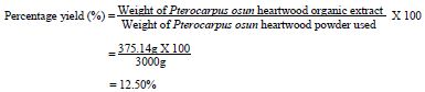
Using the American National Cancer Institute (NCI) method of extraction [8].  Three thousand grams (3000 g) of the pulverized plant materials was macerated in 1:1 mixture of dichloromethane and methanol for 24 hours. After which, the extract was filtered out from the residue. Using rotary evaporator, the organic solvent was evaporated from the organic extract which was further dried in a desiccator at 40°C to remove any trace of solvent. The extract was weighed, stored in airtight container and preserved in refrigerator for further analysis. The percentage yield of the extract was calculated using the formula below.

The method of extraction used was maceration method.

Weight of Pterocarpus osun heartwood powder used=3000 g

Weight of Pterocarpus osun heartwood organic extract obtained=375.14 g

for 1

Materials and Apparatus

Grinding machine, weighing balance, measuring cylinders, wide mouth bottles, spatula, foils, rotary evaporator, water bath, fresh egg albumin, digital Vernier caliper, hand towels, needle and syringes, nose mask, hand gloves, Wistar rats (male and female), desiccator, airtight container, separating funnel etc.

Drugs, Chemicals and Reagents

Dichloromethane (Sigma-Aldrich brand), methanol (Sigma-Aldrich brand), water, n-hexane (Sigma-Aldrich brand), dimethylsulfoxide, (JHD company, Guangdong. Guanghua Sci-Tech. Co. Ltd. China), ethyl acetate (Sigma-Aldrich brand), n-butanol (Sigma-Aldrich brand), hydrochloric acid, magnesium metal, sodium hydroxide, ferric chloride, dragendorff’s reagent, wagner’s reagent, olive oil, hydrochloride acid, chloroform, acetic anhydride, sulphuric acid, fehling’s solution a + b, molisch reagent, million’s reagent, glacial acetic acid, picric acid solution, distilled water, diclofenac injection 20 mg/kg (Novartis brand) etc.

Fractionation of Organic Extract

To produce the n-hexane fraction, ethyl acetate fraction and n-butanol fraction of the organic extract, organic extract (50 g) was sequentially partitioned with organic solvents based on increasing order of polarity. Methanol, n-hexane, ethyl acetate and n-butanol are the chemicals utilized in the fractionation process.

Qualitative Phytochemical Screening

The organic extract was phytochemically screened using the method described by Trease and Evans [9].

Gas Chromatography-Flame ionization Detector (GC-FID) Analysis

Methanol (15 ml) was used to dissolve 100 mg of organic extract of Pterocarpus osun heartwood. The GC-FID device was test run to make sure it is in good operating condition and is free of impurities. Injecting 1 ul of the sample solution into the gas chromatograph caused it to evaporate quickly into the gaseous phase and separate into its components. As the separated components exit the GC column, they are combined with hydrogen and an appropriate oxidant (oxygen) in the flame-ionization chamber. This mixture is then burned with a hydrogen flame, causing any chemical components of the organic extract to become ionized and giving them a positive charge. Above the flame was a negatively charged collecting plate. As the positive ions emerge, they are accelerated towards the negatively charged collector plate where, upon making contact, they induce an electric current. This current was measured, with the amount of current being related to the number of carbon atoms burned and quantity of each component present in the organic extract. The GC has 15 m x 250 0.15 RESTEK MXT-1 column. Helium 5.0 p.a.s was used as the carrier gas, flowing at a rate of 40 ml/min, with a splitless injection of 1 ul of sample at a linear velocity of 30 cm/s. The 280°C was the temperature of the injector. At first, the oven was operating at 200°C, it was then increased to 330°C at a rate of 3°C per minute, and this temperature was maintained for 5 min. An operating temperature of 320°C was used by the detector.

Acute Toxicological Evaluation

A total of twelve wistar rats of both sexes with an average weight of 155 g were used for the study. The rats were obtained from animal house of the department of Experimental Pharmacology and Toxicology, Faculty of Pharmaceutical Sciences, University of Port Harcourt, Rivers state. The rats were allowed to get acclimatised for one week. The animals were allotted into three groups of four animals each and had continuous access to feed and water throughout the study period. Pterocarpus osun heartwood organic extract was administered in doses of 1000, 2000, and 5000 mg/kg to Groups 1-3, respectively via the oral route. The rats were placed under observation for 48 hours to check if mortality would occur. No death was recorded. Following that, the rats were further observed for 14 days for signs of mortality. No fatalities were noted. Lorke’s [10] method was modified and used to evaluate the acute toxicity for the determination of LD50.

Evaluation of Anti-inflammatory Activities

Fifty healthy Wistar rats of both sex with the average weight of 125 g were used for this study. The rats were obtained from animal house of Pharmacology and Toxicology department, Faculty of Pharmaceutical Sciences, University of Port Harcourt, Rivers state. They were allowed to get acclimatised with the environment for two weeks. They had free access to feed and water continuously throughout the period of the study. The rats were grouped into 8 test groups and 2 control groups with 5 rats per group and weighed respectively. The extract was given to the rats intraperitonealy.

Group 1 received distilled water (1 ml/kg), group 2 received diclofenac (20 mg/kg), group 3 and 4 received 200 mg/kg and 400 mg/kg of Pterocarpus osun heartwood organic extract respectively. Group 5 and 6 received 200 mg/kg and 400 mg/kg of n-hexane fraction respectively. Group 7 and 8 received 200 mg/kg and 400 mg/kg of ethyl acetate fraction respectively. Group 9 and 10 received 200 mg/kg and 400 mg/kg of n-butanol fraction respectively.

After allotting the rats into groups, the initial paw size was measured before the induction of inflammation. Acute Inflammation (edema) was induced in the right paws of the animals by administering 0.1 ml egg albumin to rats plantar. After 30 minutes of inducing edema, the paw thickness was measured and treatments were given to the rats intraperitoneally according to their body weights after which their paw thickness were determined at time intervals (T) of 1 hour, 2 hours, 3 hours and 4 hours using a digital vernier caliper. A modification of the Barung et al. [11] method used by Johnson-Ajinwo et al. 2021, was employed to evaluate the anti-inflammatory activity of Pterocarpus osun heartwood in this study. The percentage inhibition was determined and recorded.

The percentage reductions of inflammation were calculated using the formula below:

Percentage Reduction %=
for 2

Where; Tc=Mean paw size in control group (distilled water group)

Tc initial paw size=Mean initial paw size in control group (distilled water group)

Tt=Mean paw size in the treatment group

Tt initial paw size=Mean initial paw size in the treatment group

Sub-chronic Toxicological Evaluation

Wistar rats of both sexes with average weight of 150 g were assigned randomly to four groups (n=6/group). Group i received distilled water (1 ml/kg) while Groups ii – iv received 250, 500 and 1000 mg/kg of the Pterocarpus osun heartwood organic extract respectively. Using stainless steel feeding needle, the rats were dosed by oral gavage for 28 days. The rats had free access to feed and water continuously throughout the period of the study. Their feed and water intake pattern were monitored through the period of the study. The rats were sacrificed on day 29. Shorinwa et al. 2020 method of sub chronic toxicity evaluation was used [12].

Histopathological Evaluation

The liver and kidneys tissues were excised and then fixed in Bouin’s solution for histological analysis. The tissue samples of liver and kidney were dehydrated in an ascending series of alcohol, cleared in xylene, and embedded in paraffin wax melting at 60°C. Serial sections (5 μm thick) obtained by sectioning the embedded tissue with a microtome were mounted on slides coated with 3-aminopropyltriethylsilane and dried at 37°C for 24 hours. Sections on slides were deparaffinised with xylene and hydrated with a descending alcohol series. They were then stained with Mayer’s hematoxylin and eosin stain, dried, and mounted on a light microscope (x400) for histopathological examination.

Gas Chromatography-Mass Spectrometry (GC-MS) Analysis

Blank runs were carried out on the GC-MS device thrice by injecting 1 ul of methanol into the injection port of the instrument during each program run. 0.1 g of organic Pterocarpus osun heartwood extract was dissolved in 15 ml of methanol and filtered before analysis on the GC-MS. Three times, the microsyringe was rinsed with the sample solution before commencement of the program run. 1 ul of the sample solution was injected into the GC inlet where it was vaporized and swept onto a chromatographic column by the carrier gas (usually helium). The sample flows through the column and the compounds present in Pterocarpus osun heartwood organic extract were separated based on their interaction with the coating of the column (stationary phase) and the carrier gas (mobile phase). The final part of the column is connected to the ion source where compounds eluted from the column were converted to ions. Finally, the detector displayed the number of compounds present in Pterocarpus osun heartwood and their molecular weights. The GC−MS system used for this study consist of an Agilent 7890A GC system with split injection (250°C; 1:10), coupled to an Agilent MS model 5975C mass selective detector (MSD) with a triple axis detector. The system was fitted with a 30 m HP5-MS column [(5% phenyl)-methylpolysiloxane, with an internal diameter of 0.25 mm and a film thickness (df) of 0.25 μm, (Agilent Technologies, Santa Clara, CA). Mass spectra was acquired using MSD ChemStation. Spectroscopic detection by GC-MS required an electron ionization system using high-energy electrons (70 eV). Helium gas (99.995% pure) with a flow rate of 1 ml/min was used as the carrier gas. Relative quantity of the chemical compounds present in the organic extracts of Pterocarpus osun was expressed as percentage based on peak area produced in the chromatogram. Bioactive compounds were identified based on GC retention time on HP5-MS column and matching of the spectra with the NIST 11 MS Library, (National Institute of Standards and Technology Library).

Statistical Analysis

The means and standard error of mean (SEM), was determined for all animal-based experiments carried out using Graph pad PRISM version 8. The statistical difference between the treatment groups and the control groups, were determined using Two-way analysis of variance (ANOVA); with Greisser-Greenhouse used as post hoc test. P<0.05 was considered statistically significant.

Results and Discussion

The results of this study were presented in Tables and Figures.

Percentage Yield of Extraction

Pterocarpus osun (3000 g) yield 12.50% extract as shown in Table 1. This was a good yield.

Table 1: Percentage yield of Pterocarpus osun using Dichloromethane + Methanol (organic extract)

Solvent

Weight of Pterocarpus osun heartwood powder

Weight of Pterocarpus osun heartwood organic extract

Percentage yield (%)

Dichloromethane+Methanol (organic extract) 3000 g 375.14 g 12.50

Qualitative Phytochemical Analysis

The qualitative phytochemical analysis of Pterocarpus osun heartwood organic extract revealed that secondary metabolites: carbohydrates, steroids, anthraquinones, saponins, triterpenoids, cardiac glycosides, phenols, flavonoids, proteins, cyanogenic glycosides and tannins are present in the organic extract as shown in Table 2.

Table 2: Qualitative phytochemical profile of Pterocarpus osun heartwood organic extract

S/N

Test

Observation

1 Steroids

+

2 Anthraquinones

+

3 Saponins +
4 Triterpenoids +
5 Cardiac glycosides +
6 Phenols +
7 Flavonoids +
8 Proteins +
9 Tannins +
10 Carbohydrate +
 11 Cyanogenic glycoside +

Key: Present; +

This indicates that this plant is a rich source of phytochemical agents.

Gas chromatography – Flame Ionization Detector Analysis

The GC-FID revealed that plant extract contained high level of cyanogenic glycosides compound (15.91 μg/ml) followed by steroids (15.31 μg/ml). Another compounds that were present in appreciable quantity include anthocyanin (11.62 μg/ml), Rutin (11.26 μg/ml), Naringin (10.54 μg/ml), Kaempferol (9.01 μg/ml), Flavone (8.90 μg/ml), epicathechin (7.84 μg/ml), flavonones (7.55 μg/ml) proanthocyanin (7.19 μg/ml), oxalate (7.18 μg/ml), as well as sapogernin (7.15 μg/ml). Other constituents such as Resveratol (4.42 μg/ml), Lunamarine (4.36 μg/ml), Naringenin (1.68 μg/ml), Tannin (1.09 μg/ml), Flavan-3-ol (4.42 μg/ml), sparteine (2.63 μg/ml), and cardiac glycosides (1.36 μg/ml) were present in trace quantity. Pterocarpus osun heartwood organic extract contained high quantities of polyphenol; flavonoids, stilbene and tannin compared to other phytochemical constituents as showed in Table 3. Alkaloids, saponins, steroids, oxalate, glycosides and phytate are also present in the organic plant extract.

Table 3: GC-FID profile of Pterocarpus osun heartwood extract

Type of Phytochemical

Phytochemical compounds

Concentration (µg/ml)

Stillbenes (0.17 µg/ml) Resveratol 0.17
Flavonoids (90.56 µg/ml) Naringenin 1.68
Flavan-3-ol 4.42
Rutin 11.27
Anthocyanin 11.62
Naringin 10.54
Flavonones 7.55
Naringin 10.54
Kaemferol 9.01
Flavone 8.90
Epicatechin 7.84
Proanthocyanin 7.19
Tannin (1.09 µg/ml) Tannin 1.09
Glycosides (17.27 µg/ml) Cardiac glycosides 1.36
Cyanogenic glycosides 15.91
Alkaloids (6.99 µg/ml) Lunamarine 4.36
Sparteine 2.63
Saponins (13.39 µg/ml) Sapogenix 6.24
Sapogernin 7.15
Steriods (15.31 µg/ml) Steroids 15.31
Anti-nutrient (14.36 µg/ml) Phytate 7.18
Oxalate 7.18

Key: microgram/millilitre; μg/ml

Acute Toxicity Evaluation

Modified Lorke’s method (1983) was used in the acute toxicity evaluation [10]. Acute toxicity evaluation showed that Pterocarpus osun heartwood organic extract recorded zero mortality in the rats used in the study, as shown in Table 4. Also there were no changes in the behavior and physiology of the rats throughout the period of the study. This means that the single dose of Pterocarpus osun heartwood is safe and the LD50 exceeded 5000 mg/kg.

Table 4: Acute toxicity of Pterocarpus osun heartwood organic extract (n = 4)

Duration (days)

Dose (mg/kg )

No of rats per group

No of death

14 1000 4 0
2000 4 0
5000 4 0

Evaluation of Anti-inflammation

This study revealed that the organic extract and fractions reduced inflammation induced by fresh egg albumin as shown in Table 5 and Figure 1 below.

Table 5: Mean paw size(mm) ± standard error of mean

TREATMENT

Dose

(mg/kg)

Mean paw size (mm) ± standard error of mean


Initial

Paw size (mm)

30 minutes

I hr

2 hrs

3 hrs

4 hrs

Negative control (distilled water) 1ml 2.74 ± 0.07 6.78 ± 0.15 6.73 ± 0.03 6.68 ± 0.03 6.63 ± 0.07 6.47 ± 0.05
Diclofenac 20 2.74 ± 0.14 5.34 ± 0.03 4.11 ± 0.12 3.72 ± 0.02 3.47 ± 0.01 3.30 ± 0.44
Organic extract 200 2.40 ± 0.09 5.58 ± 0.33 5.06 ± 0.33 3.77 ± 0.07 3.14 ± 0.03

**

3.14 ± 0.03

*

Organic extract 400 2.69 ± 0.07 5.52 ± 0.04 4.01 ± 0.06


3.70 ± 0.03 3.31 ± 0.03


2.93 ± 0.03

N-hexane 200 2.68 ± 0.21 7.37 ± 0.33 4.86 ± 0.14

**

4.39 ± 0.16

**

3.76 ± 0.14

**

3.24 ± 0.12
N-hexane 400 2.66 ± 0.07 6.13 ± 0.10 4.32 ± 0.05

*

3.71 ± 0.06 3.50 ± 0.08

3.36 ± 0.02

*

Ethyl acetate 200 2.76 ± 0.12 7.32 ± 0.13 5.06 ± 0.02

*

**

4.29 ± 0.24

*

**

3.75 ± 0.06

*

**

3.11 ± 0.05
Ethyl acetate 400 2.85 ± 0.09 6.06 ± 0.07 4.89 ± 0.31 3.56 ± 0.10 3.37 ± 0.08 2.96 ± 0.20
N-butanol 200 2.73 ± 0.06


7.49 ± 0.10 4.93 ± 0.14

**

4.50 ± 0.13

*

**

4.27 ± 0.05

*

**

3.13 ± 0.30
N-butanol 400 2.45 ± 0.06 5.69 ± 0.14 4.90 ± 0.06

**

3.78 ± 0.18 3.36 ± 0.11 2.75 ± 0.30

fig 1

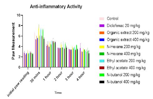
Figure 1: Mean paw size against time

The mean paw size decreased with increase in time as observed in Figure 1. This means that Pterocarpus osun had time-dependent effect.

Also, 400 mg/kg dose demonstrated better anti-inflammatory effect compared to 200 mg/kg. This implies that Pterocarpus osun had dose-dependent effect as observed in Table 6. The ethyl-acetate fraction 400 mg/kg had the highest percentage inhibition followed by organic extract 400 mg/kg and other fractions as presented in Table 6. By implication, ethyl-acetate fraction and organic extract were better than diclofenac. Also 400 mg/kg of organic extract had the enhanced anti-inflammation effect at 1 hour while the 400 mg/kg ethyl acetate achieved optimum anti-inflammatory effects at 2 hours, 3 hours and 4 hours compared to Diclofenac 20 mg/kg. This showed that Pterocarpus osun had fast onset of action compared to Diclofenac 20 mg/kg as shown in Table 6.

Table 6: Percentage reduction of inflammation (%)

Treatment

DOSE (mg/kg)

Percentage reduction of inflammation (%).


1hr

2 hrs

3 hrs

4 hrs

Control 1ml 0.7 1.5 2.2 4.6
Diclofenac 20 65.67 75.13 81.23 84.98
Organic extract 200 33.33 65.23 69.15 80.16
Organic extract 400 66.92 74.37 84.06 93.57
N-hexane 200 45.36 56.60 72.23 81.77
N-hexane 400 58.40 73.35 78.41 84.45
Ethyl acetate 200 46.62 61.17 74.55 90.62
Ethyl acetate 400 44.61 81.97 86.63 97.05
n-butanol 200 44.61 55.08 60.41 89.28
n-butanol 400 38.59 66.24 76.61 91.96

The 400 mg/kg dose had a better anti-inflammatory effect compared to 200 mg/kg for all the extracts and fractions. This means that Pterocarpus osun had dose-dependent effect as observed in Figure 2.

fig 2

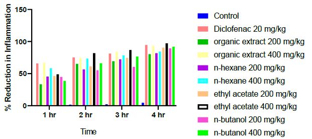
Figure 2: Percentage reduction of inflammation of the different treatment at time intervals

Ethyl-acetate 400 mg/kg had the highest percentage reduction of inflammation while the organic extract, n-hexane and n-butanol at 200 mg/kg doses had low percentage reductions as presented in Figure 3. This implies that ethyl acetate 400 mg/kg demonstrated optimum activity compared to the organic extract/fractions and diclofenac.

fig 3

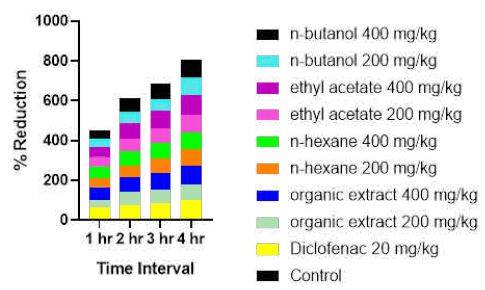
Figure 3: Percentage reduction of inflammation of the different treatment at time intervals

Hourly comparison of the activities of the extract/fractions was carried out and the results displayed in Figure 3. The 400 mg/kg of organic extract displayed early onset of anti-inflammatory activity with optimum effect at 1 hour while the 400 mg/kg ethyl acetate demonstrated superior anti-inflammatory effects from 2 hour to 4 hour compared to Diclofenac 20 mg/kg. This showed that Pterocarpus osun had fast onset of action compared to Diclofenac 20 mg/kg (Figure 3).

Sub-chronic Toxicological Evaluation

Shorinwa et al. method of sub chronic toxicity evaluation was used [12]. No mortality was recorded throughout the period of the study. There was no change in the rat behavior and physiology. No change in food and water intake as compared to control group.

Histopathology of the Kidney

The kidney tissue of the rats in control group showed normal morphology. The kidney section at 250 mg/kg of Pterocarpus osun heartwood organic extract showed mild inflammatory cell infiltration, 500 mg/kg showed interstitial edema and mild inflammatory cell infiltration and 1000 mg/kg showed glomerular degeneration as observed in Figure 4. This implies that long term use of Pterocarpus osun heartwood is toxic to the kidney.

fig 4

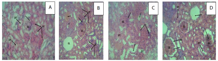
Figure 4: Photomicrograph (H&E X400) of the rat’s kidney in control and treated groups.
Key; A: A cross section of the rat kidney in control group with arrows showing normal showing glomerulus (GL), proximal tubules (PT) and distal tubules (DT); (arrows) enclosed bowman’s space (arrow). B: A cross section of the rat kidney treated with 250 mg/kg of the organic extract of Pterocarpus osun with arrows showing glomerulus (GL), proximal tubules (PT) and distal tubules (DT); complete loss of the glomeruli: mild inflammatory cell infiltration, with blood deposit in the interstitium. C: A cross section of the rat kidney treated with 500 mg/kg of the organic extract of Pterocarpus osun with arrows showing interstitial oedema of the renal tubules; mild inflammatory cell infiltration of the renal tubules and glomerulus. D: A cross section of the rat kidney treated with 1000 mg/kg organic extract of Pterocarpus osun with arrows showing glomerulus (GL), bowman’s space (BS), Proximal (PT) and distal tubules (DT) with moderately diffused renal tubular inflammatory cell infiltration, glomerular degeneration (complete loss and glomeruli shrinkage).

Histopathology of the Liver

The liver tissue of the rats in control group showed normal morphology.

The liver section at 250 mg/kg of Pterocarpus osun heartwood organic extract showed mild inflammatory cell infiltration, 500 mg/kg showed moderate distortion of the periportal area associated with hepatocyte degeneration and 1000 mg/kg showed moderate cytoplasmic degeneration as presented in Figure 5. This implies that long term use of Pterocarpus osun heartwood may be toxic to the liver.

fig 5

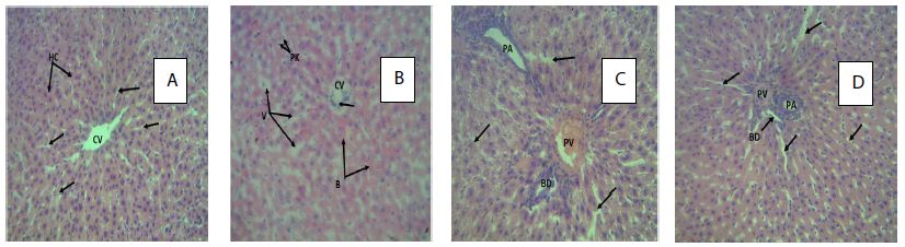
Figure 5: Photomicrograph (H&E X400) of the rat’s liver in control and treated groups.
Key; A: A cross section of the rat liver in control group with the arrows showing normal structure of the centrilobar area of the central venules (CV): visible hepatocytes (HC), and sinusoids (arrows). B: A cross section of the rat liver treated with 250 mg/kg of the organic extract of Pterocarpus osun heartwood. The arrows showing vacoulation of the hepatic lobules (V) with pyknosis of cell nucleus (PK): mild diffused blood deposit in the sinusoids (B) associated with inflammatory hepatocyte infiltration of the central vein (CV). C: A cross section of the rat liver treated with 500 mg/kg of organic extract of Pterocarpus osun heartwood. The arrows showing distortion and constriction of the Portal area (portal vein (PV), portal artery (PA) and bile duct (BD)). Diffused cytoplasmic and hepatocyte degeneration (arrows) D: A cross section of the rat liver treated with 1000 mg/kg of the organic extract of Pterocarpus osun heartwood. The arrows showing moderate constriction of the portal area (portal vein (PV), portal artery (PA) causing collapsing of the bile duct (BD)): with cytoplasmic degeneration associated with sinusoids dilation (arrows).

Gas Chromatography-Mass Spectrometry (GC-MS) Analysis Results

This study showed that Pterocarpus osun heartwood continued eight (8) compounds: 1,1-Dodecanediol, diaconate (9.99%), 2-Acetamido-2-deoxy-d-mannolactone (10.0%), cis-9-Hexadecenal (0.07%), E,E-10,12-Hexadecadien-1-ol acetate (0.07%), 9-Methyl-z,z-10,12-hexadecadien-1-ol acetate (0.24%), Homopterocarpin (5.03%), 9,12-Octadecadienoic acid (Z,Z) (38.41%) and Z-1,9-Hexadecadiene (36.13%).

The major phytochemical compound present is: 9,12-Octadecadienoic acid (Z,Z) (38.41%) followed by Z-1,9-Hexadecadiene (36.13%), 2-Acetamido-2-deoxy-d-mannolactone (10.0%), 1,1-Dodecanediol,diaconate (9.99%) and Homopterocarpin (5.03%) as shown in Table 7 and Figure 6.

Table 7: GC-MS Profile of Pterocarpus osun heartwood organic extract

S/N

Non-polar compounds

Molecular weight (g)

Molecular formula

Retention time (minutes)

Area percentage (%)

Biological activities

1 1,1-Dodecanediol, diacetate 275 C15H30O2 19.361  9.99 Unknown activity
2 2-Acetamido-2-deoxy-d-mannolactone 217 C8H11NO6 19.897 10.06  Unknown activity
3 cis-9-Hexadecenal 238 C16H30O 29.354 0.07 Antifungal activity,antimicrobia[13]
4 E,E-10,12-Hexadecadien-1-ol acetate 280 C18H32O2 30.042 0.07 Unknown activity
5 9-Methyl-Z,Z-10,12-hexadecadien-1-ol acetate 294 C19H34O2 30.474 0.24 Unknown activity
6 Homopterocarpin 284 C16H17O4 31.996 5.03 Anti-inflammatory, anticancer, anti-oxidant, antimicrobial and anti-ulcer activities. [14,15]
7 9,12-Octadecadienoic acid (Z,Z)- Linoelaidic acid 280.5 C18H32O 33.276 38.41 Anti-inflammatory analgesic, antioxidant activity, Anti-cancer, and anti-microbial activities[16,17].
8 Z-1,9-Hexadecadiene 222.4 C16H30 36.790 36.13 Unknown activity

Key: P value <0.05 is significance at a given time. (n= 5)
* means negative control significance.
**means positive control significance.

fig 6

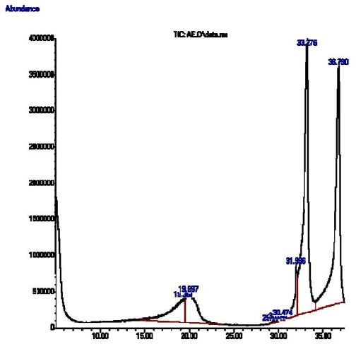
Figure 6: GC-MS profile of Pterocarpus osun

Discussion

The use of medicinal plants extract to treat acute and chronic inflammation is on increase. This is due to the unwanted side effects that are associated with conventional anti-inflammatory drugs like steroidal and non-steroidal anti-inflammatory drugs.

The 3000 g of heartwood of P. osun extracted with organic solvents (1:1 ratio of methanol and dichloromethane) yielded 12.50% extract (Table 1). This was a good yield and is in consonance with another study that reported that the use of equal volumes of polar and non-polar solvent for extraction enhances the yield of the extract [13-18].

The phytochemical evaluation of the plant Pterocarpus osun heartwood extracts revealed the presence of various Phytoactive compounds such as carbohydrates, steroids, anthraquinones, saponins, triterpenoids, cardiac glycosides, cyanogenic glycosides, phenols, flavonoids, proteins and tannins (Table 2). The presence of a wide range of phytoactive compounds in Pterocarpus osun heartwood indicated that the plant would be useful as a medicinal plant.

The GC-FID analysis revealed the presence of Polyphenols, alkaloids, saponins, steroids, glycosides, cyanogenic glycosides, phytate and oxalate in Pterocarpus osun heartwood Organic extract (Table 3). This extract contained mainly flavonoids (90.56 µg/ml). Flavonoids are known to have anti-inflammatory, antioxidant and anticancer activities. This means that the synergistic activities of flavonoids and other phytochemical constituents present in the plant extract is responsible for its anti-inflammatory activity. The hydroxyl functional groups in flavonoids donate electrons through resonance to stabilize free radicals and mediate antioxidant protection which contribute to the anti-inflammatory activity of the plant extract. Phytochemicals known as anti-nutrients are also present in the plant organic extract. Anti-nutrients such as tannins, phytate and oxalate are known to inhibit nutrient absorption for example oxalate inhibit calcium absorption [19]. These constituents tend to react with calcium and form calcium oxalate crystals that can accumulate in the body and cause kidney stones. The GC-FID evaluation also revealed the presence of high content of cyanogenic glycosides. Hence, it should be used with caution to avoid cyanide poisoning.

The acute toxicity evaluation of Pterocarpus osun heartwood organic extract that was administered to Wistar rats orally at various doses of 1000 mg/kg, 2000 mg/kg and 5000 mg/kg showed that none of the doses recorded any fatality in the tested animals (Table 4). Therefore, it could be inferred that oral LD50 of the organic extract is greater than 5000 mg/kg body weight of the tested Wistar rats. Thus, the organic extract could be said to have high safety margins since substances possessing LD50 higher than 5000 mg/kg were considered practically non-toxic [20,21].

An evaluation of the anti-inflammatory activity showed that Pterocarpus osun heartwood organic extract has anti-inflammatory effect which is dose dependent. The maximal inhibition of inflammation was observed at 4 hrs by 400 mg/kg dose of extract. The organic extract and fractions all exhibited anti-inflammatory activity but the Ethyl acetate demonstrated optimum anti-inflammatory effect, (Table 6). Johnson-Ajinwo et al. [7] previously reported that the anti-inflammatory effect of organic extract (400 mg/kg) of P. osun heartwood was better than that of indomethacin in fresh egg-albumin induced rat paw oedema method (acute inflammation). This study revealed that the anti-inflammatory effect of 400 mg/kg ethyl acetate fraction and the organic extract of P. osun heartwood were better than that of diclofenac in egg albumin induced rat paw oedema method (Table 6). This showed that P. osun heartwood extract might display superior anti-inflammatory activities than NSAIDs in the treatment of acute inflammatory conditions. An added advantage of P. osun over NSAIDS in the treatment of inflammation is its use as an antiulcer antidote in ethnomedicine.

Usually chronic disease conditions require repeated daily dose and daily dosing can be accumulated in the body and gradually affect the body tissues and organs. Acute toxicity data usually does not provide information on the effect of the plant extract on the body organ and blood. Therefore, sub-acute toxicity study was carried out to determine the effect of Pterocarpus osun heartwood organic extract on liver and kidney. Histological evaluations of the rats’ kidneys and livers showed that long term use of low dose of Pterocarpus osun heartwood organic extract may cause toxic effect to liver and kidney. The toxicity effects are dose dependent. The dose with the highest toxicity effect is 1000 mg/kg followed by 500 mg/kg while the least was 250 mg/kg. This implies that the plant extract should be taken with caution since healthy kidney and liver are important for the survival of animals. In addition, it should not be given to patients with existing liver and kidney disease because it will worsen their disease condition.

The Gas chromatography and mass spectrometry (GC-MS) analysis of organic extracts of heartwood of P. osun elicited 8 individual compounds. The major phytochemical compound present in Pterocarpus osun heartwood extract is: 9,12-Octadecadienoic acid (Z,Z), Linoelaidic acid (38.41%) followed by Z-1,9-Hexadecadiene (36.13%), 2-Acetamido-2-deoxy-d-mannolactone (10.0%), 1,1 Dodecanediol,diaconate (9.99%) and Homopterocarpin (5.03%). The 9,12-Octadecadienoic acid (Z,Z), Linoelaidic acid (38.41%) and Homopterocarpin (5.03%) have been reported to have Anti-inflammatory, anticancer, anti-oxidant, hepatoprotective, antimicrobial and anti-ulcer activities [22-26]. This implies that 9,12-Octadecadienoic acid (Z,Z) and Homopterocarpin are the anti-inflammatory compounds present in the Pterocarpus osun heartwood organic extract. Free radicals are implicated in inflammation and these compounds may be responsible for the antioxidant effects of P. osun leaf extract that was reported by Ajiboye et al. [27].

The cis-9-Hexadecenal is an organic compound that belongs to aldehyde groups. It is an aliphatic long chain aldehyde. It has antimelanogenic, antimicrobial and anti-fungi activities [28-30]. It was also reported that the anti-microbial activities of aldehydes seem to depend on the presence of the alpha, beta-double bond and on the chain length from the enal group [23]. This may be responsible for the antimicrobial activities of Pterocarpus osun that was reported by Adewale et al. [5].

Conclusion

This study conducted revealed that the anti-inflammatory compounds present in Pterocarpus osun heartwood are 9,12-Octadecadienoic acid (Z,Z), Linoelaidic acid (38.41%) and Homopterocarpin (5.03%). Single dose of the plant extract is safe, but using it for an extended period of time is toxic to the kidneys and liver. Hence, the plant extract should be used with caution and should be avoided in patient with kidney and liver diseases. It is recommended that the haematological and biochemical effect of the plant extract should be studied.

Conflict of Interest

The study’s authors affirm that there were no financial or commercial ties that might be viewed as having a potential conflict of interest.

References

  1. CDRG (2023) Chronic inflammation is related to a wide variety of conditions, from arteriosclerosis to diabetes. International Committee of Medical Journal Editors.
  2. Tchamadeu MC, Dzeufiet PD, Nana P, Kouambou Nouga CC, Ngueguim Tsofack F, et al. (2011) Acute and sub-chronic oral toxicity studies of an aqueous stem bark extract of Pterocarpus soyauxii Taub (Papilionaceae) in rodents. J Ethnopharmacol 133: 329-35. [crossref]
  3. Shobayo B, Ojo D, Agboola D (2015) Antibacterial Activity of Pterocarpus osun L. on Multi-Drug Resistant (MDR) Escherichia coli from Wound Infections in Abeokuta, South-West Nigeria. Open Access Library Journal 2: 1-6.
  4. Avwioro OG, Aloamaka PC, Ojianya NU, Oduola T, Ekpo EO (2005) Extracts of Pterocarpus osun as a histological stain for collagen fibres. African Journal of Biotechnology 4: 460-462.
  5. Adewale EF, Oluremi IA, Olatunbosun A (2022) Nutrients, Phytochemical, Antioxidant and Antimicrobial Analysis of Pterocarpus osun Stem Bark and Leaf for Their Nutritional, Medicinal Capacity. Nigeria. Indo J Chem Res 10: 58-67.
  6. Ezeokonkwo MA, Okoro UC (2012) New dyes for petroleum products. J Emerg Trends Eng Appl Sci 3: 8-11.
  7. Johnson–Ajinwo OR, Udofia CE (2021) Chemical characterization, phytochemical evaluation and in vivo antinflammatory activities of Pterocarpus osun. IJMSIR 6: 239-249.
  8. Evans JR, Akee RK, Chanana S, McConachie GD, Thornburg CC, et al. (2023) National Cancer Institute (NCI) Program for Natural Product Discovery: Exploring NCI-60 Screening Data of Natural Product Samples with Artificial Neural Networks. ACS Omega 8: 9250-9256.
  9. Trease and Evans Pharmacognosy, 15th Ed, India: Elseiver pp. 191-393, 2002.
  10. Lorke D (1983) A new approach to practical acute toxicity testing. Arch Toxicol54: 275-87. [crossref]
  11. Barung EN, Dumanauw JM, Duri MF, Kalonio DE (2021) Egg white-induced inflammation models: A study of edema profile and histological change of rat’s paw. J Adv Pharm Technol Res 12: 109-112. [crossref]
  12. Shorinwa OA, Monsi B (2020) Toxicological implications of the fruit of Harungana madagascariensis on wistar rats. Clin Phytosci 6: 2.
  13. Galli C, Calder PC (2009) Effects of fat and fatty acid intake on inflammatory and immune responses: a critical review. Ann Nutr Metab 55: 123-39. [crossref]
  14. Kim B-R, Kim HM, Jin CH, Kang S-Y, Kim J-B, et al. (2020) Composition and Antioxidant Activities of Volatile Organic Compounds in Radiation-Bred Coreopsis Cultivars. Plants 9: 717. [crossref]
  15. Kapoor A, Jambheshwar G, Narasimhan B (2014) Antibacterial and antifungal evaluation of synthesized 9,12-octadecadienoic acid derivatives. Der Pharmacia Lettre 6: 246-251.
  16. Jiang T, Li K, Liu H, Yang L (2018) Extraction of biomedical compounds from the wood of Pterocarpus macarocarpus Kurz heartwood. Pak J Pharm Sci 31: 913-918.
  17. Oh JM, Jang H-J, Kang M-G, Mun S-K, Park D, et al. (2023) Medicarpin and Homopterocarpin Isolated from Canavalia lineata as Potent and Competitive Reversible Inhibitors of Human Monoamine Oxidase-B. Molecules 28: 258. [crossref]
  18. Ryckebosch E, Muylaert K, Foubert I (2012) Optimization of an Analytical Procedure for Extraction of Lipids from Microalgae. Journal of the American Oil Chemists’ Society 89: 189-198.
  19. Okoli EC, Umaru IJ, Otitoju O (2022) Phytochemical Screening, Antibacterial Effects and Antioxidant Activities of Ethanolic Stem Bark Extract of Pterocarpus erinaceus. Singapore Journal of Scientific Research 12: 170-179.
  20. Loomis TA, Hayes AW (1996) Loomis’s Essentials of Toxicology. (4th ed.), Academic Press, CA Google Scholar.
  21. The Organization of Economic Co-operation and Development (OECD) (1981) The OECD Guide-line for Testing of Chemical: 408 Subchronic Oral Toxicity-Rodent: 90-day Study, France.Google Scholar.
  22. Jiang T, Li K, Liu H, Yang L (2018) Extraction of biomedical compounds from the wood of Pterocarpus macarocarpus Kurz heartwood. Pak J Pharm Sci 31: 913-918. [crossref]
  23. Olaleye MT, Akinmoladun AC, Crown OO, Ahonsi KE, Adetuyi AO (2013) Homopterocarpin contributes to the restoration of gastric homeostasis by Pterocarpus erinaceus following indomethacin intoxication in rats. Asian Pac J Trop Med 6: 200-204.
  24. Kapoor R, Huang YS (2006) Gamma linolenic acid: an antiinflammatory omega-6 fatty acid. Curr Pharm Biotechnol 7: 531-4. [crossref]
  25. Galli C, Calder PC (2009) Effects of fat and fatty acid intake on inflammatory and immune responses: a critical review. Ann Nutr Metab 55: 123-39. [crossref]
  26. Kim B-R, Kim HM, Jin CH, Kang S-Y, Kim J-B, et al. (2020) Composition and Antioxidant Activities of Volatile Organic Compounds in Radiation-Bred Coreopsis Cultivars. Plants 9: 717.
  27. Ajiboye TO, Salau AK, Yakubu MT, Oladiji AT, Akanji MA, et al. (2010) Acetaminophen perturbed redox homeostasis in Wistar rat liver: protective role of aqueous Pterocarpus osun leaf extract. Drug Chem Toxicol 33: 77-87.
  28. Oh JM, Jang H-J, Kang M-G, Mun S-K, Park D, et al. (2023) Medicarpin and Homopterocarpin Isolated from Canavalia lineata as Potent and Competitive Reversible Inhibitors of Human Monoamine Oxidase-B. Molecules 28: 258. [crossref]
  29. Shults EE, Shakirov MM, Pokrovsky MA, Petrova TN, Pokrovsky AG, et al. (2016) Phenolic compounds from Glycyrrhiza pallidiflora Maxim and their cytotoxic activity. Nat Prod Res 31: 445-452. [crossref]
  30. Kapoor A, Jambheshwar G, Narasimhan B (2014) Antibacterial and antifungal evaluation of synthesized 9,12-octadecadienoic acid derivatives. Der Pharmacia Lettre 6: 246-251.

Self-Concept Inventories Measure More Than Just Psychological Traits

DOI: 10.31038/PSYJ.2023564

Abstract

In this brief article, I summarize results from two recent studies in which popular multidimensional self-concept measures were administered to large samples of university students. Scores from all 26 subscales examined across instruments were affected, but to varying degrees, by factors other than the targeted constructs that included states, methods, and unrelated measurement error. I also direct readers to instructional and computer resources that would enable them to conduct analyses that isolates and takes these factors into account.

Self-Concept Inventories Measure More Than Just Psychological Traits

Self-concept, broadly defined, represents the totality of beliefs about oneself, often paraphrased as the answer to the question of “Who are I?”. Although there are many theories about the nature of self-concept and its development, strong evidence supports the view that self-concept is multidimensional and a powerful predictor of life outcomes [1-5]. To capture the complexity of such broad beliefs, researchers have developed numerous instruments designed to measure multiple aspects of self [6]. Prominent among such multidimensional measures are the Self-Description Questionnaires developed by Herbert Marsh [7-9] and Self-Perception Profiles developed by Susan Harter and colleagues [10-13].

What do Self-Concept Inventories Really Measure?

Although perceptions of self can certainly change over time, most components of self-concept measured within self-concept inventories are expected to remain reasonably stable, especially over short time intervals. That is, these measures are presumed to measure psychological traits rather than states. However, in practice, scores from such measures likely reflect a combination of stable traits, fleeting states, and other unrelated effects [14]. To separate these influences on scores, researchers often employ structural equation modeling techniques based on latent state-trait-theory [15-18].

Empirical Examples

For a recent presentation at the annual conference of the American Psychological Association, colleagues and I [19] applied latent state-trait theory procedures when analyzing scores obtained from large samples of college students who completed the Self-Description Questionnaire-III (SDQ-III; Marsh, 1992c; n=1790; [9]) or Self-Perception Profile for College Students (SPPCS; (Neemann and Harter, 2012; n=821; [12]) on two occasions separated by a week. Each inventory has 13 subscales with one intended to measure overall self-esteem (General Self in the SDQ-III and Global Self-Worth in the SPPCS) and the remaining subscales within each instrument targeted at more domain-specific aspects of self-concept as described in Table 1. The SDQ-III includes 10-12 items for each subscale answered along a Likert-style, 8-point response metric (1=Definitely True, and 8=Definitely False), whereas the SPPCS has 4-6 items for each subscale answered using four unique forced-choice options for each item.

Table 1: Partitioning of Observed Score Variance for SDQ-III and SPPCS Scores

Instrument, Subscale, and Index

SDQ-III (n=1740)


SPPCS (n=821)

Subscale

# of Items

Trait

State

Method

Error


Subscale

# of Items

Trait

State

Method

Error

General academic skills

10

.833

.082

.037

.048

Scholastic competence

4

.782

.049

.049

.120

Verbal skills

10

.809

.048

.085

.058

Intellectual ability

4

.813

.073

.025

.089

Math skills

10

.930

.028

.018

.024

Job competence

4

.657

.037

.113

.193

Problem-solving skills

10

.790

.053

.079

.078

Creativity

4

.828

.092

.014

.066

Honesty-trustworthiness

12

.730

.080

.097

.094

Humor

4

.782

.090

.027

.100

Religious-spiritual values

12

.930

.028

.023

.020

Morality

4

.775

.102

.024

.100

Opposite-sex relations

10

.855

.052

.043

.050

Social acceptance

4

.791

.040

.069

.100

Same-sex relations

10

.785

.079

.040

.062

Romantic relationships

4

.832

.102

.006

.061

Parental relations

10

.877

.049

.039

.035

Close friendships

4

.816

.072

.026

.085

Physical ability

10

.924

.036

.016

.024

Parent relationships

4

.830

.030

.061

.078

Physical appearance

10

.885

.052

.043

.050

Appearance

4

.852

.019

.058

.070

Emotional stability

10

.851

.058

.047

.043

Athletic competence

4

.887

.049

.011

.053

General self

12

.891

.071

.012

.026

Global self-worth

6

.840

.061

.022

.077

Mean

10.46

.856

.055

.045

.047

Mean

4.15

.807

.063

.039

.092

Note. SDQ-III=Self-Description Questionnaire-III (Marsh, 1992c); SPPCS: Self-Perception Profile for College Students; # of items: Number of Items. Values under trait, state, method, and error represent proportions of explained observed score variances. Proportions for trait, state, method, and error variance do not always sum to 1.00 due to rounding.

In Table 1, I summarize partial results from our presentation that represent proportions of observed score variance accounted for by trait, state, method, and unrelated measurement error effects for each self-concept scale. In the present context, proportions of trait effects would be analogous to omega reliability estimates [20] that account for both item and occasion differences in scores. For both inventories, trait effects account for the majority of observed score variance ranging in proportions from 0.730 (Honesty) to 0.930 (Math Skills) for the SDQ-III (Mean=0.856) and from 0.667 (Job Competence) to 0.887 (Athletic Competence) for the SPPCS (Mean=0.807). Higher proportions of trait variance for the SDQ-III are likely due to its subscales having more response options and at least twice as many items.

Nevertheless, subscale scores from both inventories are also affected by non-trivial state, method, and unrelated error effects that on average respectively account proportions of variance equaling 0.055, 0.045, and 0.047 for the SDQ-III and 0.063, 0.039, and 0.092 for the SPPCS. Moreover, effects of states, methods, and error vary widely across subscales. For the SDQ-III, General Academic Skills (0.082) has the highest proportion of state variance and Honesty has the highest proportions of both method (0.097) and error (0.094) variance. For the SPPCS, Morality and Romantic Relationships have the highest proportion of state variance (0.102) and Job Competence has the highest proportions of both method (0.113) and error (0.193) variance. When revising instruments to represent traits more reliably, proportions of state and method effects can be compared to determine the best ways to alter a measurement procedure. Increasing items would usually better serve that purpose when method effects exceed state effects, whereas pooling results across occasions would do so when the reverse is true.

Conclusion

Overall, the findings summarized here confirm that the SDQ-III and SPPCS predominantly measure traits over short time intervals but that scores from both inventories are influenced by a variety of other factors. These findings are consistent with Hertzog and Nesselroade’s [14] argument that measures of psychological constructs rarely measure purely traits or states and further demonstrate that such measures are susceptible to method effects related to how the constructs are being measured (see [21] for a more in-depth discussion of such effects). Unless measures are administered over two or more occasions using multiple items, effects of traits, states, methods, and unrelated measurement error cannot be disentangled. When objectively scored assessments are administered only on single occasions, as is typically the case, trait and state effects are confounded and treated as reliable variance, whereas method affects become part of measurement error variance. When administering measures in the ways prescribed here, contributions of trait, state, method, and error can be separated to determine their individual effects on observed scores. Researchers and practitioners need to be aware of such complexities when measuring psychological traits to properly interpret results from such measures. To learn more about latent trait-state theory and other methods for partitioning observed score variance into multiple categories and how to run such analyses, I direct readers to a recently published tutorial and accompanying instructional online supplement developed by our research group at the University of Iowa [18,22] and to other relevant articles and resources related to these procedures cited earlier here and within that tutorial.

References

  1. Hattie J (2014) Self-concept. Psychological Press.
  2. Marsh HW (1990) A multidimensional, hierarchical self-concept: Theoretical and empirical justification. Educational Psychology Review 2: 77-172.
  3. Marsh HW (2007) Self-concept theory, measurement and research into practice: The role of self-concept in educational psychology. Leicester, UK: British Psychological Society.
  4. Marsh HW, Craven RG (2006) Reciprocal effects of self-concept and performance from a multidimensional perspective: Beyond seductive pleasure and unidimensional perspectives. Perspectives on Psychological Science 1: 133-163.
  5. Shavelson RJ, Hubner JJ, Stanton GC (1976) Self-concept: Validation of construct interpretations. Review of Educational Research 46: 407-441.
  6. Byrne BM (1996) Measuring self-concept across the life span: Issues and instrumentation. American Psychological Association.
  7. Marsh HW (1992a) The Self-Description Questionnaire (SDQ) I: A theoretical and empirical basis for the measurement of multiple dimensions of preadolescent self-concept: A test manual and research monograph. Macarthur, New South Wales, Australia: University of Western Sydney, Faculty of Education.
  8. Marsh HW (1992b) Self-Description Questionnaire (SDQ) II: A theoretical and empirical basis for the measurement of multiple dimensions of adolescent self-concept: An interim test manual and a research monograph. Macarthur, New South Wales, Australia: University of Western Sydney, Faculty of Education.
  9. Marsh HW (1992c) Self-Description Questionnaire (SDQ) III: A theoretical and empirical basis for the measurement of multiple dimensions of late adolescent self-concept: An interim test manual and a research monograph. Macarthur, New South Wales, Australia: University of Western Sydney, Faculty of Education.
  10. Harter S (2012a) Self-Perception Profile for Children (Grades 3-8): Manual and questionnaires (revised) Denver, CO: University of Denver.
  11. Harter S (2012b) Self-Perception Profile for Adolescents: Manual and questionnaires (revised) Denver, CO: University of Denver.
  12. Neemann J, Harter S (2012) Self-Perception Profile for College Students: Manual and questionnaires (revised) Denver, CO: University of Denver.
  13. Messer B, Harter S (2012) Self-Perception Profile for Adults: Manual and questionnaires (revised) Denver, CO: University of Denver.
  14. Hertzog C, Nesselroade JR (1987) Beyond autoregressive models: Some implications of the trait-state distinction for the structural modeling of developmental change. Child Development 58: 93-109.
  15. Steyer R, Ferring D, Schmitt MJ (1992) States and traits in psychological European Journal of Psychological Assessment 8: 79-98.
  16. Steyer R, Geiser C, Fiege C (2012) Latent state-trait models. In H. Copper (Ed.), Handbook of research methods in psychology. Data Analysis and Research Publication 3: 291-308.
  17. Steyer R, Mayer A, Geiser C, Cole DA (2015) A theory of states and traits—Revised. Annual Review of Clinical Psychology 11: 71-98.
  18. Vispoel WP, Xu G, Schneider WS (2022a) Interrelationships between latent state- trait theory and generalizability theory in a structural equation modeling Psychological Methods 27: 773-803. [crossref]
  19. Vispoel WP, Xu G, Schneider WS, Kilinc M, Zhang M (2021, August) A latent state-trait analysis of responses to multidimensional self-concept measures (Paper presented at the annual meeting of the American Psychological Association).
  20. McDonald RP (1999) Test theory: A unified approach.
  21. Geiser C, Lockhart G (2012) A comparison of four approaches to account for method effects in latent state-trait Psychological Methods 17: 255-283. [crossref]
  22. Vispoel WP, Xu G, Schneider WS (2022b) Instructional online supplement to “Interrelationships between latent state-trait theory and generalizability theory in a structural equation modeling framework.” Psychological Methods 1-56.
fig 1

Template-Driven System Incorporating AI and Mind Genomics to Help a Design a Course in Geography

DOI: 10.31038/GEMS.2023567

Abstract

The paper introduces a novel, Socratic approach to creating research studies, combining the emerging science of Mind Genomics with AI embedded in the Mind Coach system. The templated system instructs the researcher to describe a topic. AI (Idea Coach) synthesizes sets of 15 questions based upon the topic description, and then requires the respondent to select four of the questions. Afterwards, the system instructs the respondent to create four answers to each question, once again providing AI help through the suggestion of 15 answers. This first Idea Coach steps can be repeated as many times as the researcher desires, with each step returning 15 questions, many different, along with a later and automatic synthesis of patterns in the 15 questions through seven standard AI queries. The experiment with actual people presents each study participant with a set of 24 vignettes, combinations of the aforementioned answers. Each respondent evaluates a unique set of 24 different vignettes created by an underlying permuted experimental design. The ratings are analyzed by dummy variable regression analysis to show how each element or answer ‘drives’ the rating. The respondents are further clusters into like-minded groups (mind-sets), based upon their coefficients. The templated approach creates a rapid (2-4 hour) process to go from a state of almost zero knowledge to understanding a topic through AI, geography in this particular instance, to produce the test stimuli, and through human reactions to these test stimuli determine and describe the mindsets respondents hold towards geography that can be organized into courses of specific interest to each mind-set.

Keywords

Mind genomics, AI, Socratic method, Question creation

Introduction

In the “project of science,” research studies are assumed to be efforts which contribute to a picture of “how the world works.” The assumption is that the researcher can identify what might be the next experiment to perform. The experiments often end up as simple reports, supported by statistics, and introduced by detailed literature reviews. Those who publish their investigations are often described as “filling gaps in our knowledge.” Indeed, the much of the edifice of science rests on the practice of what is called the “hypothetico-deductive” system, the system which requires that the researcher propose a hypothesis and do the experiment to either support the hypothesis or falsify it. It is by the accretion of such studies that the edifice of science is created, the picture of the world [1], a picture created by a disciplined approach.

At the other side of the project of science is grounded theory [2,3]. Here the researcher does a study or reports a set of observations. It is from those observations that hypotheses emerge. Once again, however, the effort assumes at the start that the researcher does the experiment, and thus implicitly assumes that the researcher is beginning with a knowledgeable conjecture.

What then happens in those increasingly frequent cases where the issues are new, or at least new combinations of old issues, and where there has not been sufficient time to create a literature, or even to develop grounded theory and hypotheses? Can a method be developed which allows the exploration of issues in a manner which is quick, simple, yet profound in the depth of information and insight that it can promote, and even create? This paper presents such an approach with a worked example, and a timetable of events. The topic is creating an understanding one can create a course in geography, starting with little knowledge, and obtain early-stage feedback. The objective is to test out a general system, Mind Genomics, which has evolved over the past 30+ years, keep pace with developments in statistical computation, and the trend to DIY (do-it-yourself). The impetus for the focus on geography was reading about the launch of a new journal on geography, and the author’s own experience with geography and earth science during the formative high school years. The literature focusing on the teaching of geography provided some of the necessary background [4-6]. Further impetus from the study came from work on horticulture [7] and on travel to Albania and the focus on the pleasant weather of Albania [8].

The approach presented here, Mind Genomics, comes from a combination of three disciplines, and has evolved since the 1990”s [9,10]. The disciplines are:

  1. Mathematical psychology and psychophysics; The study of how we subjectively “measure external stimuli and situations in our mind,” to create an algebra of the mind. For the current topic of geography, mathematical psychology and psychophysics will help us create the structure of how we think about topics.
  2. Statistics, specifically experimental design. This is the study of how we can combine different variables to represent alternative “realities,” these realities equivalent to different descriptions of how the world works. The normal, everyday experience of the world comes in packets of stimuli, not in single ideas. Rather than surveying the person, giving that person single questions, we create combinations of those questions, and give the person these combinations. The person then rates the combinations. It will be from the deconstruction of the responses to these mixtures of ideas into the contribution of the individual “elements” that we will learn about the mind of the respondent.
  3. Consumer research. Consumer research focuses on the world of the everyday, the normal. Rather than creating an artificial situation to elucidate an issue, putting the subject in the situation and then observing behavior, the consumer researcher looks for the world of what people typically experience.

Mind Genomics emerged as a science of the everyday, spurred on by the aforementioned three sciences to measure how people think about ordinary experience. The objective of Mind Genomics is to measure the value of an idea, following the spirit of traditional psychophysics, which focuses on measuring sensory experience. In other words, can we measure the “intensity” of an idea?

Mind Genomics moves away from the conventional approach of surveys, which instruct survey-takers (henceforth called respondents) to rate the importance of different factors, using a scale. The typical use of surveys is to focus a person’s mind on one aspect at a time, one experience, or one’s attitudes regarding a topic. Typically, the survey instructs the survey taker to think of large aspects of the experience and rate the aspect as a totality. Sometimes the desired focus is finer. For example, by dividing the topic into small, “bite-size” ideas of single focus (e.g., aspects of health in a polluted area), a survey can have the survey taker quantify many of the simple aspects of the experience.

The problem of surveys, and the stepping off point of Mind Genomics, is that the experience is not a set of individual aspects but rather combinations of aspects. People do not naturally respond to single ideas, although when instructed they can intellectualize their experience, and come up with a best guess. The typical survey situation is sterile, lacking the richness of experience because the phrases in the survey are “general.” If one were to summarize the thinking involved in survey development, it would be “top down,” wherein the researcher wants the survey taker to abstract, rather than deal with the granular richness.

Mind Genomics works from the bottom up, from the world of the granular, not from the world of the general. A Mind Genomics study first creates a set of phrases describing the granular aspects of the topic. It is impossible, of course, to capture all of the granular aspects of an experience or topic, so the operationalized approach is to focus on four aspects of a topic, each aspect “brought to life” with four granular and different statements. The aspects can be considered “questions, the statements can be considered “answers” or “elements. In other words, the Mind Genomics process thus assembles four questions, each with four answers, hopefully the questions providing a story.

The execution of the Mind Genomics is straightforward. The researcher creates the questions, the researcher creates the answers, types both of these into a template (www.BimiLeap.com), along with a rating question. The BimiLeap program then creates 24 different combinations of answers for each respondent. These combinations are called “vignettes,” and comprise 2-4 elements, at most one element or answer for each question, but often no answer from one or two questions.

Each respondent ends up evaluating virtually a totally different set of 24 vignettes. Each set of vignettes is set up to be structurally identical to every other set of 24 vignettes, at least on a mathematical basis. The differences among the various sets of 24 vignettes are that the elements are permuted. For example, considering respondent (survey taker) #1, A1, A2, A3 and A4 correspond to four different elements. For the second respondent #2, permutation goes into effect. The element previously A1 becomes element A3, the element previously A2 becomes A4, the element previously A3 becomes A1, and the element previously A4 becomes A2. Each set of vignettes is constructed to ensure that the 16 elements are statistically independent of each.

The subsequent processes explicated below, comprise presenting these test vignettes to respondents, obtaining ratings, transforming the ratings to create new “binary variables”, and finally using both regression analysis and to reveal how people perceive different aspects of a topic, and how people end up falling into different groups, so-called “mind-sets”, operationally defined as groups of people who think of the topic in quite different ways.

Difficulties Encountered in the Creation of Ideas, and the Help Provided by Artificial Intelligence

During the evolution of the Mind Genomics platform from its beginnings in the 1990’s under the name IdeaMap, one behavior has continued to repeat study after study, especially among the beginners using Mind Genomics. Simply stated, the difficulty is coming up with the four questions, and to a lesser degree coming up with the four answers for each question. Even accomplished researchers unfamiliar with the Mind Genomics approach report difficulty during the first time that they try this exercise. Quite often the difficulties encountered in the sheer effort of “thinking through the problem” suffice to so strongly discourage that the researcher abandons the task. On the other hand, one the researcher pushes through and creates several sets of questions, the discouragement vanishes, often leading to curiosity and excitement.

The story is a bit different for the second part of the effort, providing answers to the questions. Creating the questions was the hard part. Providing four answers is the easy part, perhaps because we are taught to answer questions, not to pose them. The only thing one has to learn when creating answers is to write the answers in such a way that they can be scanned, almost like a menu.

The remainder of this paper deals with the creation of the relevant set of questions through the Idea Coach, and the explication of the output provided to the researcher, both through inspection of the results, and through AI-enhanced summarizations.

Method

The actual process of creating the test elements begins with the request to provide four questions (Figure 1, Panel A). It is as this point that the researcher needs the help of the provided by the AI in the Idea Coach. Figure 1, Panel B shows the request to Idea Coach, inserted by the researcher.

fig 1

Figure 1: Panel A presents the request to provide four questions. Panel B presents the paragraph written by the researcher to direct the AI powering Idea Coach.

Table 1 presents the first set of 15 questions generated by the Idea Coach. The Idea Coach is set up to allow the researcher to select from no questions to all four questions from this first “run” of Idea Coach. The Idea Coach can run many times as the researcher searches for the best four questions. For each “run” the Idea Coach returns with some new questions, and some old questions. Each run of the Idea Coach is separate, unconnected with the previous run. The researcher is free to edit the question before accepting it, and even to write some or all herself or himself.

Table 1: Questions emerging from the first run of Idea Coach. The Idea Coach is presented with a topic, and instructed to return 15 questions.

tab 1

An additional feature of Idea Coach is the use of AI to summarize the questions for each set of 15 questions. Table 2 shows a partial table of this additional summarization. Each time the Idea Coach is run to generate questions, the 15 questions generated are summarized anew. As a happy consequence, the researcher who runs the Idea Coach 5-10 times to generate questions will also receive a detailed summarization of the topics from the AI embedded in Idea Coach.

Table 2: Some AI-based summarizations of the first set of 15 questions. In the interest of space only the first two or three items from each summarization are shown.

tab 2

Once the researcher has generated the four questions, each question appears, one at a time, in a format similar to Figure 1, Panel B. The researcher is instructed to provide four answers to the question. The Idea Coach, viz., the AI, provides sets of 15 answers to the researcher who once again must select four answers for each question Figure 2 shows the process. Panel A shows the text of the first question, and the four spaces for the answer. Panel B shows the request to Idea Coach for the four answers. There is no need for a “box” for the researcher to write in the text of the question since that information is already in the system from the creation of the questions. Panel C shows some of the output from Idea Coach. Panel D shows the four answers to Question #1, after they have been received from Idea Coach, selected to be put into the program, and then edited if necessary by the researcher to make sure the answers are in the proper format, viz., a meaningful phrase or better a meaningful and simple sentence.

fig 2

Figure 2: The process followed by the Mind Genomics program to generate and select answers to a question, using Idea Coach.

The Idea Coach can be used many times, allowing the underlying AI to produce different sets of 15 questions, each time responding to a single “squib” or problem statement, as well as different sets of 15 answers to the same question. Across the repeated set of questions or answers, some questions or answers will repeat, but others will be new. Each set of 15 returned questions or returned answers to a question is further summarized by AI, according to a variety of queries to the Idea Coach. It simply requires that the user formulate the questions and answers. For this example, and in a period of less than 15 minutes, it was possible to set up the program, type in the description in Idea Coach, iterate through three sets of 15 questions each, select the four questions during the course of the four iterations, and then once again use Idea Coach to provide the four answers to each question, with three iterations chosen for each question. The result is that within 20-30 minutes it was possible to create a set of 15 such inquiries, with each inquiry comprising 15 “returns” from the AI embedded in Idea Coach. Afterwards, the Mind Genomics program emailed the researcher with the “Idea Book” of 15 pages, one page for each set of 15 questions or answers produced by Idea Coach, as well as additional AI-based summarizations of the 15 questions and answers.

The actual study proceeds with the creation of the classification scale, and then the rating scale and the anchored scale points. Table 3 presents the specifics of these scales, along with the orientation that the respondents read. It is important to keep in mind that for Mind Genomics the vast amount of information comes from the response to the particular elements. The orientation simply tells the respondent what to do. Generally, the orientation is “skimpy,” requiring the respondent to use the information in the test stimuli when they make their rating.

Table 3: The self-profiling classification scale, the respondent orientation to the Mind Genomics evlauations, and the rating used to evaluate the test vignettes.

tab 3

The Respondent Experience, and the Construction Strategy Underlying the Vignettes

After the research finishes the study set-up, following the template, choosing questions/answers, creating the self-profiling questions, the orientation to the respondent and the rating scale, the research launches the study. The researcher can choose the source of respondents, either from panel providers who specialize in “on-line” research, or from other sources, such as colleagues or students.

Figure 3, Panel A shows the first screen emerging after the welcome to the study. The panel shows the self-profiling questions as a series of pull-down menus. The appearance on the screen of this self-profiling questionnaire is deliberately made to be as “clean” as possible, in order not to intimidate the respondent.

fig 3

Figure 3: Panel A shows the drop-down menu of the self-profiling classification. Panel B shows one screen shot of a test vignette shown to the respondent, along with the question and the 5-point rating scale.

The next set of 24 screens is the vignettes, shown as an example in Figure 3, Panel B. The screen appears to be a randomized combination of four answers from Table 1. The combination is called a “vignette.” The respondent is instructed to read the vignette, consider all the elements of the vignette to be part of the same idea, and then to rate the vignette on the 5-point scale, following the instructions provided by the rating scale. Note that the vignette has no questions, just answers (elements). Nor does the vignette have any logical or even forced connection between the four elements.

To virtually all participants in these Mind Genomic studies the test stimulus shown in Panel B seems to be random. When faced with a set of 24 such test stimuli, one after another, with no seeming theme, many respondents feel that they have just gone through a set of random combinations. Indeed, the word “random” is often used to describe these vignettes. It is simply impossible to detect a pattern.

The power of the underlying experimental design comes from the way it is constructed.

  1. All elements appear equally often.
  2. The combinations for each respondent are set up to be a complete experimental design. That is, the researcher can use the data from one respondent to create an equation showing the contribution of each of the q6 elements or answers.
  3. Each respondent evaluates a totally different set of 24 combinations. This is known as a permuted experimental design [11]. The benefit of the permuted design is that the researcher gets to cover a great deal of the possible design space. The practical outcome is that the researcher need not know anything about the topic when the research begins. The researcher ends up “exploring” the topic from many angles. The analogy here is the MRI, used to take multiple snapshots of an item from different perspectives, and then combine these snapshots to create a three-dimensional image.
  4. Each of the 16 answers or elements appears precisely five times in the 24 combinations and is absent from 19 of the vignettes.
  5. Each vignette comprises a minimum of two elements and a maximum of four elements.
  6. One question can contribute at most one answer or element to a vignette. This prophylactic ensures that the vignette does not contain two mutually contradicting statements, different alternatives or answers from the same question,
  7. Panel B of Figure 3 shows the sparse design of the vignette. The questions do not appear. Only the combinations of answers appears, along with the rating question and the rating scale. Often those who commission the research want to have more “fleshed out” vignettes, with connectives and with sentences. The objective of Mind Genomics is to understand what the specific elements are, or really specific ideas, which drive the response. It is easier for the respondent to be given series of vignettes similar to those shown in Panel B. The respondent ends up grazing, looking at the ideas, and then assigning a rating
  8. The foregoing strategy ends up with different combinations of elements evaluated by the respondents, with the analysis valid at the individual level as well as the group level. It will be the power of analysis at the group level which will enable the researcher to discover important patterns, even in those all-to-common situations where the researcher is a beginner, even a school-age student.
  9. The final benefit to be surfaced here is the ability of the experimental design to frustrate attempts to “game” the system. Post-study comments by many respondents, often unsolicited, is that they could not game the system, that the system seemed entirely random, that the same elements kept appearing, and that after one or two vignettes were evaluated the respondent claimed to have lost interest and simply guessed the answers. Although one might be perturbed at this admission, especially professionals who want the project to be totally “rational,” the loss of interest means that the respondent reacts at almost a “gut level” to the vignettes, in the same way that the respondent reactions at a relaxed, non-involved way, to the outside world. It is this loss of focus on the “right answer” which allows Mind Genomics to identify how people really think about the topic, rather than spend their time trying to outsmart the researcher.

Relating the Presence/Absence of the Elements to the Rating

The aim of Mind Genomics is to measure the impact of the elements on a scale, or in this study actually on two scales. The five-point scale shows two rating points recording that the respondent is interested (rating 5 and rating 4, respectively), and two rating points recording that others are interested (rating 5 and rating 2, respectively). Furthermore, the five-point scale shows two rating points recording that the respondent is not interested (rating 2 and rating 1), and two rating points recording that others are not interested (rating 4 and rating 1). Finally, rating 3 shows that respondent simply cannot answer those questions.

To link the ratings to the elements requires that we create new scales, called “binary transformed scales.” These are not metric scales of “amount” yes/no scales. The transformations are shown below. They allow the researcher to understand how each of the elements drives interest or disinterest. The transformations are followed by the addition of a vanishingly small random number, that number added to each transformed variable. The addition of the vanishing small random number is a prophylactic step to ensure that every one of the newly created five binary variables shows some marginal or higher degree of variability.

After the ratings are transformed into the five new binary variables, one can run an OLS (ordinary least squares) regression, relating the presence/absence of the elements to the binary transformed rating. The regression will work for each of the five binary variables because the vignettes at the level of each respondent were created to conform to an individual-level experimental design. Thus, the 16 elements (A1-D4) are statistically independent of each other and set up for OLS regression (Craven & Islam, 2011).

The particular “flavor” of the OLS regression is called dummy variable modeling (Hardy, 1993). The term “dummy variable” comes from the coding of the variable. Rather than “amount of,” which is meaningless in this analysis, the coding refers to “presence” (coded as 1), or absence (coded as 0).

The equation is expressed as: Binary Variable = k1A1 + k2A2 … k16D4

From various studies with the foregoing equation, one lacking the additive constant, the general operating procedure has been to look at elements of coefficient lower than 2 (viz., 1, 0, negative) as “irrelevant,” to look at coefficients of 21 or higher as “important”, and the coefficients between 2 and 20 as interesting, perhaps as part of a story. These operational rules come from both statistical regression modeling and observations of how these elements seem to perform in the daily world.

Table 4 shows the coefficients for the total panel, with the five binary transformed variables, as well as with response time as the sixth dependent variable. Strong performing elements, those with coefficients of 21 or higher, have been shaded. Table 4 suggests a fair number of elements end up interesting the respondents, all four from Question B (Explain how understanding geography helps explore current events linked to geography and the physical world), and three of the four from Question C (Go into detail about learning about scientific methodologies and tools used in geographical research). In contrast, no elements from Question A or Question D drive interest.

Table 4: Coefficients of the equation relating the presence/absence of the 16 elements to the newly created binary dependent variables.

tab 4

The same search for strong performing elements may be done for the other binary transformed variables. Respondents in this study did not know how to respond when the question involved other people, and when the question involved disliking the element. We could stop there, were we to be focusing on the research as a way to help us decide what to feature in this publication on geography. Or we could move on to hypothesize that it may not be productive to ask people about what other people think, or even to ask people what they themselves dislike.

Table 5 continues the analysis, this time looking at the way people describe their interest in geography. The respondents were instructed to check one of four types of interest in geography. Only two of the four classifications were chosen by 10 or more respondents; It’s ok… i know some… but really only the stuff i read in the press, and I know to understand some of the fine points. Table 5 shows that there are some elements which appeal far more strongly to one group than the other, but the strong differences in patterns of preference among the elements fail to materialize.

Table 5: Performance of the elements by two self-defined groups of respondents, the criterion being to describe the nature of their interest in geography.

tab 5

Beyond WHO to Mind-sets and to Measures of Overall Performance Enhanced by Mind-sets

If these data were to be simply type of messages, but without the content of the messages, the researcher might be happy to discover that some messages perform strongly among the total panel, but that different messages perform strongly by how the respondent describes his or her interest. Tables 4 and 5 provide meaningful data, as least at the level of specifics. The data point out which messages or elements are important. The meaning of the messages tell us even more, namely the content of the messages which are important to the total panel versus the groups. What is missing, however, is a powerful unifying pattern, one which need not be synthesized, but rather is compelling. In the words of Harvard’s Professor of Psychophysics, SS Stevens, the patterns should emerge with “ocular trauma,” namely they should hit you between the eyes with their clarity!” [12].

Unifying patterns emerge when the Mind Genomics data are analyzed with an eye towards discovering groups of people who think about the topic in a similar way. Keep in mind that the Mind Genomics ‘program’, viz., the Mind Genomics effort, focuses on the world of the granular, the world where people feel comfortable because it is the world of the everyday. With that in mind, the search for these mind-sets ends up producing far clearer patterns, and in turn, ends up generating a stronger data set, as will be shown.

Mind-sets are defined as groups of individuals who show similar patterns of thinking about a granular topic, these similar patterns operationally defined as similar patterns of coefficients. Each respondent generates a set of 16 coefficients, based upon the equation relating the presence/absence of the elements to the binary dependent variable. For this study, the binary dependent variable was selected as ‘For Me.’ Viz., ratings 5 and 4 transformed to 100, ratings 1, 2, and 3 transformed to 0.

The actual statistics fall into the category of clustering [13], the specific form being k-means clustering. Through k-means clustering, the statistical program operationally defines the ‘distance’ between pairs of individuals by the statistic: (1-Pearson Correlation), where the Pearson Correlation is computed across the 16 pairs of coefficients. A perfect linear relationship means that the respondents are virtually similar in what appeals to them about geography and what does not. The perfect linear relationship has a Pearson Correlation coefficient of 1.0, and thus the distance between the two respondents is defined as 1-1 or 0. Similarly, when the two respondents show precisely opposite patterns of coefficients, the Pearson Correlation Coefficient is -1, and the distance is 2.0.

The k-means clustering program was instructed to put the 50 respondents into two groups or clusters, and then into three groups or clusters. The computer program [14] divides items (here people) on a purely mathematical basis, according to rules which have nothing to do with meaning of the variables that it uses (here the meaning of the elements who coefficients are used).

When the cluster generates two groups, and then three groups, each respondent is assigned to one of the groups. Table 6 shows the coefficients for the two-cluster solutions, and then the three-cluster solution. The table is sorted by the two-cluster solution.

Table 6: The performance of the elements for Total Panel, Two Mind-Sets, and 3 Mind-Sets, along with the computation of the IDT, Index of Divergent Thought, a measure of ‘how strong the elements performed’ for this clustering solution.

tab 6

When we look at the two-cluster solution, the patterns becomes far clearer. Here are the very strong elements from the two clusters.

Mind-Set 1 of 2 – focus on the physical world

Physical world topics like natural disasters attract interest through fascination, while human-environment interactions like sustainability challenges appeal through relevance and urgency.

Topics about the physical world intrigue with their unpredictable and powerful forces, while human-environment interactions captivate with their complexity and interdependence.

Physical world subjects draw interest by highlighting the Earth’s forces, whereas human-environment interactions fascinate by exploring the interconnectedness of our actions.

Natural disasters intrigue with their devastating impact, while sustainability challenges inspire us to rethink and protect our environment.

Mind-Set 2 of 2 – Geography helps understand current events and a focus on the methods

Geography enables the exploration of the relationship between resources and economic development in different regions.

Geography provides context for understanding the location and significance of current events.

Geography offers understanding of regional disparities in educational, healthcare, and infrastructure development.

Geography studies regions prone to political instability or unrest.

Understanding scientific methodologies in geography involves exploring techniques for data collection, analysis, and interpretation.

Geographical research employs statistical analysis and data visualization tools to identify trends and patterns.

Geographical research also involves qualitative methods like interviews, surveys, and case studies for a comprehensive understanding of different phenomena.

When we move to three mind-sets, we reduce the parsimony by adding an additional mind-set, but we also increase the interpretability of the mind-sets.

Mind-Set 1 of 3: Focus on the human-environment interaction’

Physical world topics like natural disasters attract interest through fascination, while human-environment interactions like sustainability challenges appeal through relevance and urgency.

Natural disasters intrigue with their devastating impact, while sustainability challenges inspire us to rethink and protect our environment.

Geography unveils the relationship between human behavior and environmental conditions.

Geography helps explain the distribution of resources and their influence on economic development.

Topics about the physical world intrigue with their unpredictable and powerful forces, while human-environment interactions captivate with their complexity and interdependence.

Geography provides insights into the formation and evolution of cities.

Geography illuminates the spatial patterns of human migration and cultural diffusion.

Physical world subjects draw interest by highlighting the Earth’s forces, whereas human-environment interactions fascinate by exploring the interconnectedness of our actions.

Geographical research also involves qualitative methods like interviews, surveys, and case studies for a comprehensive understanding of different phenomena.

Geography studies regions prone to political instability or unrest.

Mind-Set 2 of 3: Focus on geography and society

Geography enables the exploration of the relationship between resources and economic development in different regions.

Geography offers understanding of regional disparities in educational, healthcare, and infrastructure development.

Geography provides context for understanding the location and significance of current events.

Geography studies regions prone to political instability or unrest.

Understanding scientific methodologies in geography involves exploring techniques for data collection, analysis, and interpretation.

Geographical research employs statistical analysis and data visualization tools to identify trends and patterns.

Geographical research also involves qualitative methods like interviews, surveys, and case studies for a comprehensive understanding of different phenomena.

Mind-Set 3 of 3: Focus on research

Geographical research employs statistical analysis and data visualization tools to identify trends and patterns.

Physical world topics like natural disasters attract interest through fascination, while human-environment interactions like sustainability challenges appeal through relevance and urgency.

Understanding scientific methodologies in geography involves exploring techniques for data collection, analysis, and interpretation.

Field surveys, observations, and experiments are conducted to gather primary data for geographical research.

Geographical research also involves qualitative methods like interviews, surveys, and case studies for a comprehensive understanding of different phenomena.

The ability of clustering to pull out these easy-to-interpret groups is worth noting, if only for the fact that to many people participating in these Mind-Genomics studies, the results seem to emerge from guessing.

Table 6: How the elements drive interest when the respondents are clustered or segmented into two, and then into three mind-sets by a statistical algorithm which does not take ‘meaning’ of the elements into account.

At the bottom of Table 6 appear a series of numbers, reflecting computations. These computations are done on the coefficients for the 16 elements, appearing in Table 6 The computations work on the squares of all elements with coefficients of 1 or higher. The computation treats the dataset as if it comprised three groups of 50 respondents each, looks at the sum of squares of coefficients for each column, and weights that column-based sum of squares by the relative proportion of respondents, assuming a set of 3×50 or 150 respondents. The bottom two rows show the weighted sum of squares, and then the square root of the weighted sum of squares.

The final number is the IDT, Index of Divergent Thought. The IDT can only get higher when the elements have high coefficients. The elements can only have high coefficients when all the respondents are thinking in the same way. Thus, the IDT is a measure of the goodness of thinking. The value for the square root is 83. Previous studies suggest that this value of 83 is ‘respectable’ but not exceptionally high. The IDT ends up being a way to measure performance, and the increase of performance over time and practice.

Once the mind-sets are developed, the Mind Genomics program finishes the analysis by summarizing the strong performing elements for each mind-set on a set of queries sent to the embedded AI program. The program answers the queries using only those elements which generated coefficients of +21 or higher. Table 7 presents the AI summarization for the two-mind-set solution.

Table 7: AI summarization of the strong performing elements for the two-mind-set solution

tab 7(1)

tab 7(2)
 

Finding These Mind-sets in the Population at Large

The development of knowledge for Mind Genomics is done rapidly, inexpensively, and with easy to reach samples of respondents. Often as few as 50 respondents is needed. Once the knowledge is obtained, however, how can one broaden the impact of the discovery? It is not reasonable to do the Mind Genomics experiment again and again. The knowledge is already in one’s hands. What is missing is the use of the knowledge to mind-type millions of people, prospective readers of a magazine on geography, or a product related to geography. How then can one assign a new person to one of the two mind-sets, with the objective of interacting with this new person, this prospect, on matters relevant to the study?

The idea of an identifying tool, a typing tool, is not new. Typing tools are important in the world of commerce to assign people to relevant groups. Typing tools are used in many applications to assign people to the relevant group. The chances for success working with people is assumed to be higher when the correct messages are sent to the people, messages which resonate with the mind-set to which the person belongs.

Figure 4 shows a mind-set assignment tool, based upon the strong performing elements. The approach, detailed in previous publications [15,16] enables the researcher to identify actual phrases from the study, develop a simple two-point scale (Yes/No), apply that scale to the six questions taken from the study, and then with reasonable confidences (around 70% or higher) assign new people to one of the two mind-sets. Panel A shows the introductory information about the respondent. Each item is optional, but important for practical application. Panel B shows the actual six questions, which are randomized across respondents. It is the pattern of responses to the six questions which drives the assignment. It is with the assignment or typing tool that the Mind Genomics moves from an efficient creator or knowledge to a facilitating mechanism which enhances communication.

fig 4

Figure 4: The mind-set assigner. Panel A shows the background questions. Panel B shows the six questions, patterns of reaction to which assign a person to one of the two mind-sets.

Discussion and Conclusion

The origin of this paper comes from the opportunity to understand a topic more deeply, the specific topic being geography. Rather than focusing on the substantive issues involved in geography, the paper considers the topic from the point of view of the mind of people. The paper opens up the possibility of incorporating a new viewpoint into studies, the topic-related worldview of the researchers who do the studies. Science is presumed to be objective. Mind Genomics applied to the topic enables a deeper understanding of the research for this very reason.

With a tool such as Mind Genomics in the hands of ordinary people, it is tempting to think what this study about a magazine, or a journal could be. The study as run here comprises only 16 elements, chosen from a great number, and chosen to be run in the United States. One could only imagine the amount of learning one could get about the magazine or journal if one were to explore each of the possible topics in depth, topics such as geography itself, or the relation of geography to economics, geography to social behavior, geography to health, and so forth. Furthermore, the ability to run these studies in different countries, also inexpensively, means that it is well within the realm of possibility to expand this exploration to many different countries. Finally, the ability to run these studies again and again means that the studies can be done for years, as used as a measure of the change of people’s thinking over time.

The second issue is the nature of the respondents. The respondents were chosen virtually at random. The study might have used ordinary people, or just as easily used professionals, or even those involved in geography in one or another fashion. The respondents could have been teachers or geography vs. parents, and so forth. One could put all of the different types of respondents together into one group, done the clustering to generate segments, and determine the degree to which segmentation falls along lines demarcated by one’s profession versus lines demarcated by one’s interest, independent of profession, especially independent of professions as they cross with the topics of geography. In other words, do there exist more profound mind-sets?

The third and final topic is the coming use of artificial or synthetic respondents rather than real people. The use of AI to generate questions and answers at the start of the study through Idea Coach and the ability of AI to summarize the results in the same way, using strong performing elements as the raw materials, both suggest that AI can play an important role in the Mind Genomics effort. The final challenge is AI as the respondent, complementing the contribution as the designer of research inputs, and the analyst of research output. And, if A I can be programmed to act like respondents, does this final step in the AI evolution of Mind Genomics promise new vistas, especially for the world of students, where studies can be thought up, designed, executed, analyzed, and summarized in a matter of hours. What might be the nature of journals and of magazines when AI can be programmed to reflect a specific type of mind. One might get a sense of this future by seeing what types of elements perform well when the AI is instructed to assume a variety of different ‘personas,’ and in the spirit of Mind Genomics, personas designed with attention to the granularity of detail various aspects.

References

  1. Lawson AE (1993) Inductive-deductive versus Hypothetico-deductive reasoning: A reply to Yore. Journal of Research in Science Teaching 30: 613-614.
  2. Backman K, Kyngäs HA (1999) Challenges of the grounded theory approach to a novice researcher. Nursing & Health Sciences. [crossref].
  3. Ellis D (1993) Modeling the information-seeking patterns of academic researchers: A grounded theory approach. The Library Quarterly 63: 469-486.
  4. Pickering S (2016) Keeping geography messy. In Teaching Geography Creatively 212-224, Routledge.
  5. Scoffham S (2012) Geography and creativity: Developing joyful and imaginative learners. In: Contemporary Issues in Primary Education, 21-33, Routledge.
  6. Scoffham S (2016) Teaching Geography Creatively. Routledge.
  7. Levin LA, Langer KM, Clark DG, Colquhoun TA, Callaway JL, et al. (2012) Using Mind Genomics® to identify essential elements of a flower product. Horticulture Science 47: 1658-1665.
  8. lollari O, Papajorgji P, Civici A (2019) Using Mind Genomics to advertise tourism in .Albania. In: 1st UNICART, Interdisciplinary International Conference on ‘Tourism Management and Development of Territory, Bari, Italy. 270-287.
  9. Moskowitz HR (2012) ‘Mind Henomics’: The experimental, inductive science of the ordinary, and its application to aspects of food and feeding. Physiology & Behavior. [crossref]
  10. Moskowitz HR, Gofman A, Beckley J, Ashman H (2006) Founding a new science: Mind Genomics. Journal of Sensory Studies 21: 266-307.
  11. Gofman A, Moskowitz H (2010) Isomorphic permuted experimental designs and their application in conjoint analysis. Journal of Sensory Studies 25: 127-145.
  12. Stevens SS (1966) Personal communication to author Howard Moskowitz.
  13. Likas A, Vlassis N, Verbeek J.J (2003) The global k-means clustering algorithm. Pattern Recognition 36: 451-461.
  14. Wilkinson L (2010) Systat. Wiley Interdisciplinary Reviews: Computational Statistics, 2: 256-257.
  15. Moskowitz H, Gere H (2020) Selling to the mind of the insurance prospect: A mind genomics cartography of insurance for home project contracts. Edelweiss Psy Open Access 4: 22-28.
  16. Porretta S, Gere A, Radványi D, Moskowitz H (2019) Mind Genomics (Conjoint Analysis): The new concept research in the analysis of consumer behaviour and choice. Trends in Food Science & Technology 84: 29-33.
FIG 1

Cross-regional Nexus Perspective in Anthropocene

DOI: 10.31038/GEMS.2023566

Abstract

In the context of global mobility, the traditional research framework based on a fixed location perspective is facing the need for adaptive innovation and change. In order to deepen the understanding of the evolution of the Anthropocene stratigraphic record and surface landscapes, this paper argues that the nexus approach and the systematic integration of spatial dimensions should be combined in the context of the Anthropocene to form a cross-regional nexus approach, to better cope with the complex issues and global challenges of the Anthropocene.

Keywords

Nexus approach, Cross-regional nexus perspective, Telecoupling, Metacoupling, Spatially dimensional systems integration, Anthropocene

Human beings are ever extending their activity space largely thanks to the technology progress in energy utilization, transport and information communication. The trajectory of human development since the 1760s indicated that the increasing enhancement of regional linkages and connectivity, and the growing higher human and resource mobility have become the prevailing trend and dominated pattern over the world. In these transformative changes, cities play a leading role as engine of the world technology advancement and the regional center for global production and consumption. The increasing connectivity and mobility have also gradually transformed the rural society based on local ecosystem services into the urban society based on non-ecosystem services and long-distance resource redistribution, and have profoundly changed the way humans interacting with nature. One of the most important changes in human-nature interrelationships, especially since the middle of the twentieth century, is the increasing interaction of coupled human and natural systems (CHANS) over long distances [1], and another is the fact that humans are influencing and modifying ecosystems to a greater extent than at any other time in history [2]. Over the past 70 years, human activities have greatly accelerated erosion and weathering on land; greenhouse gas emissions from agricultural, industrial and consumer activities are changing at an unprecedented rate, and the resulting fluctuations in the carbon cycle and climate change are threatening biodiversity and human survival. The changes taking place in the oceans are equally worrisome, and in addition to the widespread concerns about sea-level rise, ocean acidification and marine litter pollution, the recent release of nuclear-contaminated water from Fukushima, which was not sampled by scientists from neighboring countries, has created new uncertainties for marine ecosystems and human survival.

Given that these challenges cross the boundaries of culture, social governance and ecosystems, there is a need to re-examine human-environment interactions from a new perspective. The “Anthropocene” is a geological concept based on the fact that human activities have had a global impact on climate and ecosystems. Since the introduction of the concept of the Anthropocene [3], the field has attracted a wide range of research interest, with recent attempts to establish an Anthropocene gold spike profile being particularly noteworthy [4]. It is worth noting that the anthropogenic factors driving the evolution of stratigraphic records and surface landscapes in Anthropocene have transcended the boundaries of specific regions in the context of evolving globalization and continuing urbanization, making the traditional research framework in the field of Earth sciences based on a fixed locational perspective is facing the need for adaptive innovation and change. In the last decade or so, a series of illuminating research work has been carried out in the nexus approach and spatially dimensional systems integration in order to better understand the interactions between coupled human and natural systems over distances and their resulting socio-economic and environmental impacts across regions. Hoff first introduced the concept of the water-energy-food (WEF) nexus at the Bonn Conference in 2011 [5] to better deals with the challenges posed by global changes from a multi-sectoral perspective. Subsequently, the nexus approach aroused widespread academic interest. In the same year, Liu Jianguo and others proposed the comprehensive concept of Telecoupling at the symposium on “Telecoupling of Human and Natural Systems” at the meeting of the American Association for the Advancement of Science [6]. This theoretical framework for describing socio-economic and environmental interactions at a distance between coupled human and natural systems was elaborated in the later paper “Framing sustainability in a telecoupled world” [7].

The theoretical idea reflected in telecoupling has attracted widespread academic attention, and a series of related theoretical models have emerged in the global academic community in the same period of time that the theory was put forward and thereafter, typically representing “interregional sustainability” [8,9], urban land teleconnections [10,11], local- and tele-coupling [12], metacoupling [13], as well as the Coupled Human and Natural Cube [14]. Among them, metacoupling is a natural extension to the study of telecoupling, and the theoretical framework is actually an integration of intracoupling, pericoupling and telecoupling [13]. It takes into account human-nature interactions within a given system and across spatial distances by incorporating all target coupled systems from near to far, essentially integrating the study of “flow space” and place space [15], and thus not only overcoming the inherent limitations of single-system studies in the classical propositions of human-nature relations, but also compensating for some of the shortcomings of the telecoupling framework [16]. Although many advances have been made in research on the Anthropocene, the nexus approach, and spatial dimensional systems integration, respectively, the combination of the three remains little discussed in the literature. In the context of the Anthropocene, the nexus approach extended to multiple regions – i.e., cross-regional nexus analysis can deepen the understanding of the evolution of the Anthropocene stratigraphic record and surface landscapes. For example, in the framework of the “water-land-food-energy” nexus, water is needed for irrigation and is consumed by energy production that provides electricity for irrigation, while the trend towards the energization of food creates tensions between bioenergy and food production over land resources [17].

These problems of factor clamping and conflict arising from the competitive use of resources affect the food security of distal regions, such as urban areas, through the food system. Conversely, in the process of urbanization, there is also competitive use of soil and water resources in urban areas between different uses. For example, more soil and water resources for urban development or ecological construction means less soil and water resources that can be used for agricultural production. The result is naturally a reduction in the self-sufficiency rate of food in urban areas and a shift in the resource and environmental pressure on food supply to other regions, thus creating a process of cross-regional nexus between natural and human elements [18] (Figure 1). In conclusion, the cross-regional nexus perspective in Anthropocene provides a concrete entry point for revealing the implicit connection and indirect feedback between human beings and the environment in the “flow space”, which is of great significance to the study of human-earth relationship network system under the perspective of metacoupling, and its policy application is of great practical value in solving the many challenges of the Anthropocene and promoting sustainable development. Thus, theoretical and empirical research on cross-regional nexus in Anthropocene deserves the attention of scholars.

FIG 1

Figure 1: A typical case of cross regional nexus – urban food system

Authorship Contribution Statement

Enpu Ma: Conceptualization, Writing original draft, Funding acquisition. Liuwen Liao: Conceptualization, Funding acquisition. Yiwen Ji and Sen Yu: Discussing, Drawing.

Declaration of Competing Interest

The authors declare that they have no known competing financial interests or personal relationships that could have appeared to influence the work reported in this original manuscript.

Acknowledgement

This research was funded by the National Natural Science Foundation of China (Grant No. 42101267 and 42101198).

References

  1. Liu J, Dietz T, Carpenter SR, et al. (2007) Coupled human and natural systems. AMBIO 36: 593-596.
  2. Millennium Ecosystem Assessment Panel. Ecosystem and human well-being: Synthesis. (2005) Washington DC, USA: Island Press.
  3. Crutzen P (2002) Geology of mankind. Nature 415.
  4. Colin NW, Jan Z, Colin S, Ian JF, Neil LR, et al. (2018) Global Boundary Stratotype Section and Point (GSSP) for the Anthropocene Series: Where and how to look for potential candidates. Earth-Science Reviews 178: 379-429.
  5. Hoff H (2011) Understanding the Nexus. Background Paper for the Bonn2011 Conference: The Water, Energy and Food Security Nexus. Stockholm Environment Institute, Stockholm.
  6. Liu J, McConnell W, Baerwald T, et al. (2011) Symposium on “Telecoupling of Human and Natural Systems” at the meeting of the American Association for the Advancement of Science.
  7. Liu J, Hull V, Batistella M, Mateus B, Ruth D, Thomas D, et al. (2013) Framing sustainability in a telecoupled world. Ecology and Society 18.
  8. Kissinger M, Rees WE (2010) An interregional ecological approach for modelling sustainability in a globalizing world: Reviewing existing approaches and emerging directions. Ecological Modelling 221: 2615-2623.
  9. Kissinger M, Rees WE, Timmer V (2011) Interregional sustainability: Governance and policy in an ecologically interdependent world. Environmental Science & Policy 14: 965-976.
  10. Seto KC, Reenberg A, Boone CG, Michail F, Dagmar H, Tobias L, et al. (2012) Urban land teleconnections and sustainability. Proceedings of the National Academy of Sciences of the United States of America. 109: 7687-7692.
  11. Guneralp B, Seto KC, Ramachandran M (2013) Evidence of urban land teleconnections and impacts on hinterlands. Current Opinion in Environmental Sustainability 5: 445-451.
  12. Fang CL, Zhou CH, Gu CL, Chen L, et al. (2016) Theoretical analysis of interactive coupled effects between urbanization and eco-environment in mega-urban agglomerations. Acta Geographica Sinica, 71: 531-550.
  13. Liu J (2017) Integration across a metacoupled world. Ecology and Society 22.
  14. Liu HM, Fang CL, Li YH (2019) The Coupled Human and Natural Cube: A conceptual framework for analyzing urbanization and eco-environment interactions. Acta Geographica Sinica 74: 1-19.
  15. Ma EP, Ye WY, Liao LW, Cai JM, et al. (2022) Human-land coupling enlightenment and driving forces of urban food system evolution: A case study of Beijing food system. Journal of Natural Resources 37: 2617-2635.
  16. Ma EP, Cai JM, Han Y, Liao LW, Lin J, et al. (2020) Research progress and prospect of telecoupling of Human-Earth system. Progress in Geography 39: 310-326.
  17. Food and Agriculture Organization of the United Nations. Bioenergy and food security (2008). China Agricultural Information 6: 4-6.
  18. Ma EP, Cai JM, Guo H, Lin J, Liao LW, et al. (2021) Theoretical framework and research priorities on food system couplings in an urbanization context. Acta Geographica Sinica 76: 2343-2359.
FIG 3

SARS-CoV-2: Prolonged Viral Shedding and Persistent PCR Positivity: A Case Study from Pakistan

DOI: 10.31038/MIP.2023412

Abstract

Introduction: Prolonged viral persistency and shedding are the major concerns associated with emerging variants of SARS-CoV-2. Complete viruses and viral fragments may persist for unusual and longer periods in both symptomatic and non-symptomatic patients.

Case presentation: In this study, we have reported unusual persistency of SARS-CoV-2 in 26 years old young patient from Islamabad, Pakistan.

Conclusion: In conclusion, to avoid viral persistency for a long duration, precise treatment and immune-boosting therapies must be recommended. Further, nontherapeutic interventions and preventive measures are necessary to avoid viral transmission and possible reinfection.

Keywords

COVID-19, Immunocompromised, Persistency, Viral shedding

Introduction

Severe Acute Respiratory Syndrome Coronavirus 2 (SARS-CoV-2), the causative agent of Coronavirus disease 2019 (COVID-19) is a major concern of twenty first century [1]. This detrimental zoonotic and highly transmissible virus is responsible for the ongoing pandemic and poses threats to public health globally [2]. Continuous efforts revealed the epidemiology, pathogenicity, presiding results, genomic sequences, and precise diagnostic approaches of SARS-CoV-2 infections. Despite these facts, the burden of pandemic is still increasing due to the emerging variants[3,4], microbial coinfections [5], recrudescence [6], reinfections [7], prolonged viral shedding [8] and persistent RNA positivity [9] (Table 1).

Table 1: Definitions

Terms

Descriptions

Persistency Unusual and prolonged presence of viral RNA in the body fluids.
Re-positivity Detecting the presence of viral RNA following negative RT-PCR tests up to 90 days.
Recrudescence Reactivation/ relapse of infection after clinical improvement within 90 days of first infection due to persisting viral fragments.
Reinfection Infection caused by same or phylogenetically distinct respiratory and non-respiratory viruses after natural immunity and or vaccination.

Recently, patients with COVID-19 revealed persistently positive SARS-CoV-2 nucleic acid test results despite resolved clinical symptoms have attracted a lot of attention [10]. Researchers assumed long-term persistency of virus in the human body even after apparent recovery or negative results of nasopharyngeal specimens via PCR. Viral load appeared to be higher in the upper respiratory tract within the first week after symptom onset, and later in the lower respiratory tract. Viral shedding and viral load are important determinants of disease progression and transmission [11].

In this study, we reported a ruled-out case of SARS-CoV-2 in young male patient of 26 years from Islamabad Pakistan, with extremely prolonged and persistent viral shedding for six weeks.

Case Presentation

A young student of 26 years with past medical history of respiratory tract problems including pulmonary tuberculosis, recovered in 2019 with COVID-19 symptoms including cough, fatigue, body pain and mild dyspnea introduced for the diagnosis of SARS-CoV-2 infection. The RT-PCR of nasopharyngeal samples were tested positive initially on April 20, 2021. Self-isolation was suggested with symptoms resolving treatment (paracetamol). The test was performed after RNA extraction (Qiagen Viral RNA Mini Kit) on ABI 7500 Real-Time PCR detection system with internal and external positive controls via the SARS-CoV-2 detection protocols.

After initial diagnosis, the patient was again COVID-19 positive after five days i.e. on April 25, 2021. At this stage, no clinical or physical examinations were performed while antibiotic treatment was recommended for five days. The symptoms were resolved during first week of antibiotic treatment. On May 18, 2021, persistency for SARS-CoV-2 with altered and mild symptoms were observed again. The major symptoms were anosmia and dyspnea (Figure 1 – Case timeline). Empirical antibiotic treatment was recommended to overcome the possible health problems i.e. Azithromycin 500 mg/day with two-fold increase compared to initial dose of 250 mg/day.

FIG 1

Figure 1: Case timeline of patient 1 (male, age 26 years)

To investigate the patients’ health status and immune response, recommended biochemical tests were performed on 33rd day of infection i.e. on May 22, 2021. Anti-SARS-CoV-2 antibody test was performed on Cobas e411 analyzer (Diagnostic Roche), a fully automated instrument employing Electro Chemiluminescence (ECL) technology for immunoassay analysis using FDA approved kits in human serum and plasma, revealed development of SARS-CoV-2 antibodies (titer 15.13 cut of index COI > 1).

The health status was normal with mild morbidity as the biochemical markers associated with COVID-19 including Ferritin, C-reactive proteins (CRP) and D-dimers were normal (Table 2). Complete blood count revealed drop in neutrophil counts while lymphocytes level was high (Table 3). Fortunately, the patient was declared recovered according to general discharge criteria (Figure 2) [12] on 43rd day of primary infection.

Table 2: Biochemical tests

Tests

Value

Reference value

Interpretation

Ferritin

160.9 ng/ml

14-250

Normal

CRP

0.13 mg/l

0.00-10.00

Normal

FDPs (D-Dimer)

0.1 mg/l

0.00-0.50

Normal

Antibodies

15.13 COI

Cut off 1.00

Reactive

Abbreviations: CRP: C-reactive proteins; FDPs: Fibrin Degradation Products, COI: Cut Off Index.

Table 3: Complete blood count

Parameters (units)

Reference value

Value

White blood cells (TLC) (10⁹/L)

4.00-11.00

5.8

Neutrophils (%)

50.00-70.00

40

Lymphocytes (%)

20.00-40.00

48

Monocytes (%)

3.00-12.00

10

Eosinophils (%)

0.50-5.00

02

Basophils (%)

0.00-1.00

0.0

Red blood cells, count (Mil/Cm)

4.00-6.00

5.02

Hemoglobin (Hb) (Gm/dl)

11.00-16.00

14.0

Hematocrit (PCV) (%)

37.00-54.00

46.5

MCV (f/L)

80.00-100.00

93.0

MCH (Pgm)

27.00-34.00

27.8

MCHC (g/L)

30.00-36.00

30.0

Platelets (10⁹/L)

150.00-450.00

333

MPV (f/L)

7.00-11.00

7.5

PDW (f/L)

8.30-25.00

16.2

Procalcitonin (mL/L)

1.08-2.82

1.82

Abbreviations: TLC: Total Leucocytes Counts, PCV: Packed Cells Volume, MCV: Mean Corpuscular Volume, MCH: Mean Corpuscular Hemoglobin, MCHC: Mean Corpuscular Hemoglobin Concentration, MPV: Mean Platelet Volume, PDW: Platelet Distribution Width.

FIG 2

Figure 2: Criteria of discharge/declaring recovered

Discussion

Viral load remains high in upper respiratory tract during first week of infection or onset of symptoms and tends to decrease with time. Virus median duration of shedding is 8 days post onset of symptoms and drops below 5% after 15.2 days post onset of symptoms [13]. However, recent studies demonstrated viral shedding for long duration in immune-compromised individuals [14] in both symptomatic and asymptomatic patients of older age [15]. The current study reported unexpected and persistent infection of SARS-CoV-2 in young patient of 26 years for more than six weeks. To our understanding, this is the first report addressing prolonged and persistent viral positivity from Pakistan.

RT-RNA based repeated RNA positivity was considered primary indication of persistent infection as documented in previous studies [16]. Persistent shedding was significantly associated with persistent dyspnea and anosmia. Detection of viral RNA and confirmed retest positivity for SARS-CoV-2 in recovered patients is clinical indication of prolonged viral persistency or relapse of infection [17]. Analgesics and Azithromycin were recommended to eradicate disease morbidity. In persistent COVID-19 treatment, azithromycin plus hydroxychloroquine were more efficient previously [18].

In contrast to our findings, a study reported SARS-CoV-2 persistency for 59 days in young female patient with the age of 25 years [16]. The patient recovered without any antibiotic and antiviral therapy as no consequences were observed with health issues and underlying morbidities. Another case report from Thailand revealed prolonged SARS-CoV-2 shedding in asymptomatic patient (age 30 years) for 110 days [15]. Symptoms resolution with shedding duration or asymptomatic patient could promote disease transmission and hence asymptomatic virus carriers can be still infectious [19]. Therefore, there is need of monitoring the surroundings of patients to prevent the risk of viral transmission.

Immunodeficiency plays a major role in prolonged viral shedding that can be observed even in asymptomatic individuals with weak immune system [14,20]. We demonstrated that delayed treatment, low dose medication, previous medical history, higher susceptibility due to weak immune system were responsible for persistent viral infection. Similarly, viral clearance in COVID-19 patients varies and delayed in patients with older age, multiple re-exposure, underlying comorbidities such as diabetes [21] respective therapies [22] and myeloma [23] etc. (Figure 3).

FIG 3

Figure 3: Major reasons of that can contribute to prolonged viral shedding (SARS-CoV-2)

The worldwide discharge criteria (Figure 2) are improved clinical symptoms and two PCR negative test, needs modification for accurate and precise diagnosis [12]. Various studies emphasize precise and accurate decision of prolonged viral shedding and true infection. Confirmation and differentiating these hurdles might provide an insight of infection and beneficial support to the physician while treating the victim [24].

In addition, the patients experiencing only mild symptoms with extreme infection develops a weaker immune response which might explain predisposition to the reinfection [25]. Prolonged viral shedding and its particles poses diagnostic challenges. It might complicate infection control, treatment and might significantly contribute its role in morbidity and mortality associated with COVID-19 [26].

We declared patient recovered based on general discharge criteria (Figure 2). Laboratory biochemical tests, development of antibodies and clearance of symptoms are major factors which helped declaring recovery of patient from this regime. In summary, the possibility of prolonged viral shedding is significantly associated with health status of patient, timely diagnosis, and treatment strategies without any discrimination of age and gender. Further, patients recovered in long duration should be vaccinated after few weeks of recovery to prevent reinfection with emerging variants of SARS-CoV-2.

Conclusion

Comorbidities, immunodeficiency, unspecific drugs, drug discontinuation and wanning immunity are the major contributors of prolonged and persistent viral infection. These regimes might further increase the susceptibility of patient for reinfection with various emerging variants. In this ruled out situation, the unusual persistency of SARS-CoV-2 and delayed viral clearance could be due to weak immune system, previous history of lung infection (tuberculosis) and drug discontinuation. In conclusion, to avoid viral persistency for long duration, precise treatment and immune boasting therapies must be recommended.

Funding

No funding or grant was received

Conflict of Interest

The authors declare no competing interest

References

  1. da Costa VG, Moreli ML, Saivish MV (2020) The emergence of SARS, MERS and novel SARS-2 coronaviruses in the 21st century. Arch Virol. [crossref]
  2. Hu B, Guo H, Zhou P, Shi ZL (2020) Characteristics of SARS-CoV-2 and COVID-19. Nat Rev Microbiol.[crossref]
  3. Nonaka CKV et al (2021) Genomic Evidence of SARS-CoV-2 Reinfection Involving E484K Spike Mutation, Brazil. Emerg Infect Dis. [crossref]
  4. Hafeez S, Din M, Zia F, Ali M, Shinwari ZK (2021) Emerging concerns regarding COVID-19; second wave and new variant. J Med Virol. [crossref]
  5. Chen X et al.(2020) The microbial coinfection in COVID-19. Appl Microbiol Biotechnol. [crossref]
  6. Yuan B et al.(2021) Recurrence of positive SARS-CoV-2 viral RNA in recovered COVID-19 patients during medical isolation observation. Sci Rep. [crossref]
  7. Brehm TT et al.(2021) Sars-cov-2 reinfection in a healthcare worker despite the presence of detectable neutralizing antibodies. Viruses. [crossref]
  8. Li J, Zhang L, Liu B, Song D (2020) Case Report : Viral Shedding for 60 Days in a Woman with COVID-19. Am J Trop Med Hyg. [crossref]
  9. Yang JR, Deng DT, Wu N, Yang B, et al. (2020) Persistent viral RNA positivity during the recovery period of a patient with SARS-CoV-2 infection. J Med Virol. [crossref]
  10. Wang W et al.(2020) Persistent SARS-COV-2 RNA positivity in a patient for 92 days after disease onset: A case report. Medicine (Baltimore) [crossref]
  11. Cevik M, Tate M, Lloyd O, Maraolo AE, et al. (2020) SARS-CoV-2, SARS-CoV, and MERS-CoV viral load dynamics, duration of viral shedding, and infectiousness: a systematic review and meta-analysis. The Lancet Microbe. [crossref]
  12. Falahi S and Kenarkoohi A (2020) COVID-19 reinfection: prolonged shedding or true reinfection? . New Microbes New Infect. [crossref]
  13. van Kampen JJA et al. (2021) Duration and key determinants of infectious virus shedding in hospitalized patients with coronavirus disease-2019 (COVID-19) . Nat Commun. [crossref]
  14. Tarhini H et al. (2021) Long-Term Severe Acute Respiratory Syndrome Coronavirus 2 (SARS-CoV-2) Infectiousness Among Three Immunocompromised Patients: From Prolonged Viral Shedding to SARS-CoV-2 Superinfection. J Infect Dis. [crossref]
  15. Individual A, Study AC, Kewcharoenwong C, Khamduang W,et al.(2022) Prolonged Detection of SARS-CoV-2 RNA in An. Emerg Infect Dis. [crossref]
  16. Penchenat A, Alavi Z, Payan C, and Pers JO (2020) Prolonged 59-day course of COVID-19: The case of a SARS-CoV-2 shedding persistency in a healthcare provider. Clin Case Reports. [crossref]
  17. Yahav D et al.(2022) Definitions for coronavirus disease 2019 reinfection, relapse and PCR re-positivity. Clin Microbiol Infect. [crossref]
  18. Drancourt M et al.(2021) SARS-CoV-2 persistent viral shedding in the context of hydroxychloroquine-azithromycin treatment. Viruses. [crossref]
  19. Zhang L, Li C, Zhou Y, Wang B, et al.(2020) Persistent viral shedding lasting over 60 days in a mild COVID-19 patient with ongoing positive SARS-CoV-2. Quant Imaging Med Surg. [crossref]
  20. Alsaud AE et al.(2021) Case report: Prolonged viral shedding in six COVID-19 patients. Am J Trop Med Hyg. [crossref]
  21. Buetti N et al.(2020) Diabetes mellitus is a risk factor for prolonged SARS-CoV-2 viral shedding in lower respiratory tract samples of critically ill patients. Endocrine. [crossref]
  22. Xiao AT, Tong YX, and Zhang S (2020) False negative of RT-PCR and prolonged nucleic acid conversion in COVID-19: Rather than recurrence. J Med Virol. [crossref]
  23. Bellesso M, Bruniera FR, Trunkel AT, and Nicodemo IP (2020) Second COVID-19 infection in a patient with multiple myeloma in Brazil – reinfection or reactivation?. Hematol Transfus Cell Ther. [crossref]
  24. William A, Kaur R, and William A (2021) COVID-19 Reinfection and its Diagnostic Approach. vol. 31, 2021, doi: 10.3844/ajassp.2021.71.78.
  25. Roberts AT, Piani F, Longo B, Andreini R, et al.(2021) Reinfection of SARS-CoV-2 – analysis of 23 cases from the literature. Infect Dis (Auckl) [crossref]
  26. Elzein F et al.(2020) Reinfection, recurrence, or delayed presentation of COVID-19? Case series and review of the literature. J Infect Public Health. [crossref]
FIG 1

Social Intelligence and Significant Others Representations

DOI: 10.31038/PSYJ.2023563

Abstract

Despite the large number of publications devoted to this issue, modern psychology lacks valid methods for measuring social intelligence. We have developed a methodology for measuring social intelligence based on the assumption that social intelligence is reflected in the process of selecting an optimal strategy for overcoming conflict situations. A positive role of social intelligence in the structure of predictors of the professional activity of plant employees and learning activity of university students as well as negative correlations of social intelligence with the level of disharmony of interpersonal relationships was discovered. The level of social intelligence did not form significant correlations with the scales of the NEO-FFI questionnaire and also with the level of intelligence according to Raven’s test. The main purpose of our investigation was to explore the correlations between social intelligence and significant others representations. For this purpose, we have used a questionnaire that was developed by Markey, Funder and Ozer and was designed for the investigation of dyadic interpersonal relations. The list of significant others included father, mother, classmate, professor and course leader. Significant positive correlation was obtained between the accuracy of assessments of significant others in terms of friendliness and the level of social intelligence of students. In addition to observation by octants, the degree of compliance of the scores on the interpersonal behavior questionnaire was calculated separately for each element from the list of significant others. The regression equation was calculated, the predictor of which is the level of social intelligence, and the regressor is the degree of observation accuracy of the professor estimates.

Introduction

As a result of the review of various approaches to the study of social intelligence, it is possible to state a kind of theoretical pluralism in understanding the specifics of social intelligence. In particular, we note the absence of clear dividing lines between social and practical intelligence [1], attempts to integrate social and emotional intelligence [2], the identification of social and academic intelligence [3,4]. In the processes of social thinking and intelligence perceptions of oneself and others are of paramount importance. Namely: the “internal working model” according to Bowlby [5], representations of “generalized other” according to Cronbach and of “significant others” according to Chen, etc. [6,7]. Unlike scientific concepts, social representations can be fuzzy and based on episodic memories and specific examples. For example, Ford assigns an important role to “significant episodes of behavior”. These are representations of episodes related to the implementation of certain goals in a certain context. Coordination and optimization of goals (win-win fashion) is the most important condition for achieving success both in interpersonal relationships and in professional activities [8]. In fact, the choice of an effective strategy for overcoming a conflict situation is based on taking into account the already established features of the relationships between the parties of the conflict, involves assessing the nature of future relationships depending on the status, role and other characteristics of the opponents.

We assumed that the best response choice of the subjects in the selected episodes reflects the level of conflict competence and social intelligence of plant employees and university students and is an effective predictor of their professional and learning competence. We have made a suggestion that social intelligence as an important factor of social and communicative competence plays a significant role in the process of making decisions in conflict situations. In order to verify this assumption, we have worked out a method of strategies evaluation in conflict situations. Each experimental situation provided seven variants of answer. Every type of answers corresponded to certain conflict strategies and should be evaluated from one point up to seven points. In addition to the well-known strategies, such as “giving up”, “confrontation”, “compromise”, “cooperation”, “making concessions” and “consulting” we added “caustic remark” possibility. Every type of answers should be evaluated from one point up to seven points.

Social Intelligence Indexes

We used a correspondence degree of every subject answer with the so called “medians group profile”. A median of every test answer was computed. Euclid metrics as a measure of the correspondence of every respondent with the median group profile was used. The results of measuring social intelligence were compared with personality traits, the level of psychometric intelligence, indicators of the harmony of relationships, and a structural assessment of the professional competence of Ufa distillery plant employees and educational performance of the students of Ufa University of Science and Technology. Several assumptions put forward in our previous research work were confirmed based on the performed correlation studies, namely: 1. negative relationship between social intelligence and the level of disharmony in interpersonal relationships; 2. the important positive role of social intelligence in the structure of predictors of the efficiency of students and engineers; 3. the proposed assumption on the independent conceptual status of social intelligence has also found its partial empirical support. A total of 35 engineers and 100 students participated in the correlation study.

Social Intelligence: Cognitive Ability or Personal Feature?

However, the level of social intelligence did not form significant correlations either with the scales of the NEO-FFI questionnaire or with the level of psychometric intelligence (Table 1). As a result, the assumption put forward by us about the independent conceptual status of social intelligence also found its empirical confirmation [9,10].

Table 1: Coefficients of Spearman rank correlation between indicators of social and psychometric intelligence and personality traits of engineers.

Psychometric intelligence

N

E

O

A

C

Social intelligence

0.01

-0.05

-0.01

-0.02

-0.13

-0.16

Materials and Methods

Theoretical Assumptions and Methods of Investigation

Emphasizing the importance of ‘mental organization’ in the structure of personality and pointing out the significance of reckoning the life context of the particular individual, Allport endows the individual with such abilities that are inherent in social intelligence: the ability to quickly and adequately assess a person, to predict possible behavior, etc. [11]. As for Vernon [12] one of the characteristics of a socially intelligent person was that he or she was an outstanding judge of personality, whereas the implicit theories of personality also lie at the basis of such perception. Cronbach has argued that one’s implicit theory of personality consisted on his or her knowledge of “generalized other”: a mental list of important personality dimensions [13]. Kosmitski and John have marked out the main components of social intelligence. These are cognitive elements (forecasting, men comprehension, knowledge of social rules, openness in human relations) and behavioral abilities (social adjustment, warm-heartedness and etc.) [14].

Social Intelligence, the PAP Paradigm and Significant Other Representations

The principal-agent paradigm (PAP) assesses the ability of an agent to evaluate the preferences of a principal, based on known values that the principal holds for different features of the decision event. The PAP originated in the economics literature to assess how well an agent can learn how much value the principal attaches to different attributes of a set of objects. The agent observes several examples of the principal’s choices between exemplars of the set of objects in complex situations, and then must decide what the principal’s preferences would be in a new complex situation. Today such paradigm is widely used in emotional intelligence investigations [15]. We think that PAP is also important for the research in the social intelligence domain because this paradigm is connected with the concept of “significant other”. Significant other is a person that is important for an individual. According to Sullivan, personality is inextricably tied to social situations; to understand personality, it is important to examine reoccurring patterns of social relations in real social contexts.

Methods of Investigation

The main purpose of our investigation was to explore the correlations between social intelligence and significant others representations. We made an assumption that there is a significant correlation between social intelligence and the power of observation of the significant others. For this purpose, we have used a questionnaire that was developed by Markey, Funder and Ozer [16] for the investigation of dyadic interpersonal relations. As we know, Leary introduced a circular ordering of interpersonal variables known as the interpersonal circumplex. This circumplex structure implies that variables that measure interpersonal relations are arranged on the circumference of a circle orientated by the primary dominant-submissive and hostile-friendly dimensions [17]. We translated this test into Russian and used it for the measuring of student’s power of observation of the list of the significant others: father, mother, classmate, professor and course leader. We used a correspondence degree of every answer with the medians group profile as a measure of student’s observational ability of the assessment of the whole list of the significant others.

Results

The interpersonal behaviors questionnaire consists of 24 items and has 8 scales: (PA) Assured-Dominant, (BC) Arrogant-Calculating, (DE) Cold-Hearted, (FG) Aloof-Introverted, (HI) Unassured-Submissive, (JK) Unassuming-Ingenuous, (LM) Warm-Agreeable, (NO) Gregarious-Extraverted. 123 undergraduate students (74 girls and 49 boys, average age – 21.3 years) of the psychology department of the Ufa University of Science and Technology took part in our investigation. The subjects evaluated the above characters on all scales of this questionnaire. In Table 2 the results of averaging the scores for all five significant others by octants are presented. As a result, it can be concluded that the FG (M=5.24), BC (M=5.77) and HI (M=5.78) scales received the lowest scores, and the LM (M=9.96) and NO (M=9.54) scales received the highest score. In addition, the results of diagnostics on the PA scale (SD=1.55) turned out to be the most stable, and the LM scale (SD=2.14) is characterized by the greatest variability. Table 3 shows the Spearman correlation coefficients between the level of social intelligence and the indicators of students’ general accuracy of assessment, calculated by octants. As we can easily see the significant correlation between social intelligence and LM (Warm-Agreeable) has been discovered.

Table 2: Means and standard deviations of averaging the scores for all five significant others by octants


M

SD

PA

8.34

1.55

BC

5.77

1.91

DE

6.15

1.89

FG

5.24

2.09

HI

5.78

2.00

JK

8.39

2.04

LM

9.96

2.14

NO

9.54

1.85

Table 3: Spearmen rank coefficients between the level of social intelligence and the accuracy of the assessments by octants.

PA

BC

DE

FG

HI

JK

LM

NO

Social intelligence

0.14

0.09

0.16

0.11

-0.01

0.10

0.31*

0.02

*Correlation is significant at .01 level (2-tailed)

In addition to observation by octants, the degree of compliance of the scores of the interpersonal behavior questionnaire was calculated separately for each element from the list of significant others. Table 4 shows the coefficients of Spearman’s rank correlation between the level of social intelligence and the accuracy of assessments of the significant others. Despite the absence of significant correlations at least at the five percent level, we can state three correlation coefficients, highlighted in italics, the significance of which is close to critical. However, the normality of the distribution of observation indices allowed us to use linear regression analysis in addition to nonparametric correlations. Figure 1 shows a diagram of the regression equation that is significant at the level of p=0.05, the predictor of which is the level of social intelligence, and the regressor is the degree of accuracy of professor estimates. Thus, social intelligence turns out to be a predictor of the second indicator of observation accuracy.

Table 4: Spearmen rank coefficients between the level of social intelligence and the accuracy of the assessments of significant others.

Observation accuracy of mother

Observation accuracy of father

Observation accuracy of classmate

Observation accuracy of course leader

Observation accuracy of professor

Social intelligence

0.07

0.03

0.21

0.21

0.21

p-value

0.56

0.79

0.07

0.07

0.07

FIG 1

Figure 1: Graph of the regression equation between the level of social intelligence and the accuracy of professor assessments.

Conclusions, Suppositions and Future Research

Thus, we have proved the importance of the adequate cognitive significant others representations in the structure of social intelligence. Social intelligence as an important factor of social and communicative competence turned out to be a predictor of the power of observation of the significant others. We believe that these results can be considered as a confirmation of the ideas of Kihlstrom and Cantor, who offer a “knowledge view of social intelligence” and indicate the need to take into account the contexts in which certain life tasks are solved [18]. Thus, the solution of conflict situations in educational settings involves an assessment of the interpersonal characteristics of university students and lecturers. We need further investigations in order to understand why the only one LM index of the eight octants of the interpersonal circumplex is correlated with social intelligence. In this regard, it should be noted the work of Scandinavian researchers, who put forward and confirmed an interesting assumption about the positive relationship between social intelligence and the so-called “indirect” aggression. It turns out that socially intelligent individuals choose the safest behaviors. Along with a peace-loving strategy, indirect aggression is the best way to respond to conflicts [19]. Besides, we may consider these results as the confirmation of Riggio [20] suppositions about the tight connection between social intelligence and the “cognitive empathy” level. The important role of cognitive empathy in the structure of social intelligence is also noted by Rahim [21].

In this regard, the study of the psychological mechanisms of complementarity as a factor in the effectiveness of interpersonal communication is very promising [22,23]. In particular, we have developed a methodology for predicting relationships in conflict situations in the human-computer dialogue in the Dolphin Smalltalk programming system for Windows. The choice of one or another variant of relations in the dyad, made with the help of a computer mouse, was accompanied by appropriate graphic and sound illustrations demonstrating various gradations of dominance-submission and cooperation-alienation. Statistically significant positive correlations between the level of social intelligence of students and complementarity in affiliation in the «student – assistant lecturer” and “student – assistant professor” dyads were obtained [24].

Our study of imaginary interactions and situational patterns of complementarity with the help of human-computer dialogue found that classical complementary patterns of interaction turned out to be correlates of social intelligence only for interpersonal situations with assistant lecturers and assistant professors. The selective nature of the correlations between social intelligence and situational patterns of complementary relationships allows us to assume that classical complementarity models do not always sufficiently describe the picture of interpersonal interaction. For example, Schaefer noted that investigations of both parent-child and marital dyads consistently revealed two fundamental dimensions that were labeled autonomy and relatedness [25]. Moreover, the SASB model proposed by Benjamin describes both interpersonal (an individual relating to another) and intrapsychic (an individual relating to him or herself) behaviors [26]. Nevertheless, we believe that the development of methods for researching interpersonal communication through human-computer dialogue opens up the prospect of a broader and more systematic approach to the study of social and emotional intelligence.

Acknowledgements

This work was supported in part by a grant of Russian Humanitarian Scientific Fund «Social intelligence and professional competence of engineering and technical workers» No. 10-06-00525A and by a grant of Russian Fund of Fundamental Research “Social Intelligence and Complementarity of Interpersonal Relations”, project No. 13-06-00354A.

References

  1. Wagner RK (1987) Tacit knowledge in everyday intelligent behavior. Journal of Personality and Social Psychology 52: 1236-1247.
  2. Bar-On R (2006) The Bar-On model of emotional-social intelligence (ESI). Psicothema 18: 13-25. [crossref]
  3. Eysenck H (2018) Intelligence: A new look. Routledge.
  4. Wechsler D (1975) Intelligence defined and undefined: A relativistic appraisal. American Psychologist 30: 135-139.
  5. Bowlby J (1980) Attachment and loss. Vol. III. Loss: Sadness and depression. Hogarth.
  6. Cronbach LJ (1955) Processes affecting scores on “understanding of others” and “assumed similarity.” Psychological Bulletin 52: 17-193. [crossref]
  7. Chen S (2003) Psychological-state theories about significant others: Implications for the content and structure of significant-other representations. Personality and social psychology bulletin 29: 1285-1302.
  8. Ford ME (1995) Intelligence and personality in social behavior. In International handbook of personality and intelligence Springer US.
  9. Scherbakov SV (2011) Social intelligence and professional competence of engineering and technical workers: monograph. Ufa: RIC BashSU (in Russian).
  10. Scherbakov SV (2021) Students social intelligence and the choice of behavioral strategies in conflict resolution. Schizophr. Relat. Psychoses 15: 3.
  11. Allport GW (1968) The Person in Psychology: Selected Essays. Boston: Beacon Press.
  12. Vernon PE (1933) Some characteristics of the good judge of personality. The Journal of Social Psychology 4: 42-58.
  13. Cronbach LJ (1955) Processes affecting scores on “understanding of others” and “assumed similarity.” Psychological Bulletin 52: 177-193. [crossref]
  14. Kosmitzki C, John OP (1993) The implicit use of explicit conceptions of social intelligence. Personality and Individual Differences 15: 11-23.
  15. Orchard B, MacCann C, Schulze R, Matthews G, Zeidner M.et al (2009) New directions and alternative approaches to the measurement of emotional intelligence. Assessing emotional intelligence: Theory, research, and applications (pp. 321-344).
  16. Markey PM, Funder DC, Ozer DJ (2003) Complementarity of Interpersonal Behaviors in Dyadic Interactions. Personality and Social Psychology Bulletin 29: 1082-1090. [crossref]
  17. Leary T (2004) Interpersonal diagnosis of personality: A functional theory and methodology for personality evaluation. Wipf and Stock Publishers.
  18. Kihlstrom JF, Cantor N (2000) Social intelligence. In R. J. Sternberg (Ed.), Handbook of intelligence (pp. 359-379). Cambridge University Press.
  19. Björkqvist K, Österman K, Kaukiainen A (2000) Social intelligence− empathy= aggression? Aggression and Violent Behavior 5: 191-200.
  20. Riggio RE, Tucker J, Coffaro D (1989) Social skills and empathy. Personality and Individual Differences 10: 93-99.
  21. Rahim MA, Cox SR, Rutner SM (2022) Small business and the supply chain: the influence of social intelligence on relationship resilience. Small Business Institute Journal 18: 28-40.
  22. Kiesler DJ (1983) The 1982 Interpersonal Circle: A taxonomy for complementarity in human transactions. Psychological Review 90: 185-214.
  23. Sadler P, Ethier N, Woody E (2011) Interpersonal complementarity. In L. M. Horowitz & S. Strack (Eds.), Handbook of interpersonal psychology: Theory, research, assessment, and therapeutic interventions (pp. 123-142). John Wiley & Sons, Inc.
  24. Scherbakov SV (2013) Social intelligence and prediction of relationships in conflict situations. Bulletin of the Bashkir University 18: 1260-1266 (in Russian).
  25. Schaefer ES (1997) Integration of configurational and factorial models for family relationships and child behavior. In R. Plutchik & H. R. Conte (Eds.), Circumplex models of personality and emotions.
  26. Benjamin L S, Rothweiler JC, Critchfield KL (2006) The use of structural analysis of social behavior (SASB) as an assessment tool. Rev. Clin. Psychol. 2: 83-109. [crossref]
fig 9

Snow Patches and Glaciers in Japan – Commentary on the Definition and Classification of Glaciers

DOI: 10.31038/GEMS.2023563

Abstract

Glaciological studies have been conducted on several snow patches in Japan since 1910th,, including a recent report with the conclusion that some perennial snow patches in the Hida Mountains in north-central Japan are identified as glaciers. The identification was supported by all Japanese glaciologists at an open symposium organized by the Data Center for Glacier Research of the Japanese Society of Snow and Ice, recognizing that the snow patches have considerable amount of ice mass in the lower part of the snow patch, which shows the evidence of flow downwards along the valley. The international cryosphere-related organizations, however define the glacier as “stagnant or flowing ice mass”, and the international classification of glaciers published by the International Commission of Snow and Ice (ICSI) shows the necessity of flow only for some classes of glaciers such as the valley glacier, outlet glacier etc., and thus, the flowing is found not principally necessary to identify some groups of glaciers. Examining comparatively the pilot study in the Himalayan region given by the ICSI, several snow patches with ice masses in Japan are considered to belong the valley glacier, mountain glacier, or glacieret. However, the ICSI classification above includes vagueness on flow, size and thickness of the ice mass, distinction among valley glacier, mountain glacier, glacieret and snow patch. Those points should be examined and clarified for the better definition and classification of snow and ice masses on the earth.

Introduction

There is a variety of snow and ice masses on the globe. Some of them have been regarded as the glacier. However, the definition and classification of the glacier is not clearly understood even in researchers of related sciences. In Figures 1-3 some typical glaciers, which should be understood generally as the valley glacier, mountain glacier, and ice sheet with an outlet glacier are given.

fig 1

Figure 1: Aretsch Glacier in the Swiss Alps, view of the middle reaches. Far above, uppermost cirques are seen (Photo provided by R. Naruse, taken in July 2018).

fig 2

Figure 2: West side view of Arakam tse, Everest area, with typical mountain glaciers on the west slope. A small valley glacier is seen on southeast of the peak and a large Nojumba Glacier is seen on the bottom of the picture. (Photo taken in October 2007).

fig 3

Figure 3: Antarctic ice sheet in eastern Queen Maud Land and Skallen outlet glacier, February. 1970

In 2012, 3 perennial snow patches in Tateyama-Tsurugi range of Hida Mountains in north-central Japan were identified as active glaciers by Fukui and Iida (2012) [1]. About one hundred glaciologists in Japan assembled and discussed on the report at an open symposium [Perennial snow patches and glaciers in Japan – past studies and future researches organized by the Data Center for Glacier Research of the Japanese Society of Snow and Ice (JSSI) [2]. The summary of the symposium is that the participants of the symposium do not object to call these 3 snow patches as the glacier.

The present author has had some experiences of observing glaciers worldwide as a geologist and a mountaineer since the 1960s, and has been interested in the active glaciers reported by Fukui and Iida. It is found that there are some vagueness to be clarified on the definition and classification of glaciers. The present author proposed in 2019 (Yoshida, 2019-2020) [3,4] to call the above kind of snow patches as the “snow patch glacier” (abbreviated as SPG from here onwards in this paper). Recent researches in Japan on SPGs are considered useful to contribute the understanding of similar SPGs, which are distributed widely in some areas of the earth.

Glaciological Research on Perennial Snow Patches in Japan

The beginning of glaciological studies on perennial snow patches in Japan was the report by Ohzeki (1917) [5] on a perennial snow patch (designated as PSP below onwards) in Mt. Gassan in Northeast Japan. Ohzeki showed the shape, structure, and size of the ice mass within a large perennial snow patch known as “Ohyukijiro” (big snow castle, in Japanese meaning), and pointed out a possibility that the snow patch is similar with the glacieret distributed at several places in European Alps.

Since then several glaciological studies on snow patches in Japan including the report of identification of glaciers or glacierets were conducted [1,6-31] in mountains in Hokkaido, Northeast Japan and north central Japan, etc.

After around 1970, a systematic study project of snow patches in Japan started led by Prof. K. Higuchi of Nagoya University. The study project was related with the International Hydrological Decade (IHD, 1963-1974) and Intergovernmental Hydrological Programme (IHP, 1975-) that aimed to clarify the actual situation of water resources and to contribute to the examination of their relationship with climatic changes. Due to the studies of the above Japanese project, the outline of perennial snow patches distributed throughout Japan was clarified and detailed studies of several snow patches were also conducted. All these studies contributed to the IHD-IHP projects for the formation of the world glacier inventory.

The glaciological researches in Japan had been influenced by the general idea of Japanese geomorphologists that there should be no glaciers in Japan referring the suggestion of Hoshiai and Kobayashi (1957) [32] that the equilibrium line altitude (snow line) in Japan is 4000 meters, which is nearly one thousand meters higher than the Japanese highest mountain range. Several glaciological researches in Japan, however, have been conducted even after 1957. It is first because field evidence of glaciologic characteristics of some snow patches were noticed, and second because the idea that the snow line might change locally due to differences in local climate and topography, which affect in large differences in the amount of snow accumulation and melting. The above idea was further clearly pointed out recently by Ono [33].

In 2012, Fukui and Iida [1] reported 3 PSPs in Tateyama-Tsurugi range in the Hida Mountains (Japanese North Alps) in north-central Japan are identified as active glaciers. These PSPs are several hundred to over one km in length, have a thick (25 – 45 meters thick) ice bodies in the lower horizons, and are flowing downwards some meters per year. They showed mesoscopic and microscopic inner structure of the ice mass and figured out the mechanism of ductile flow of the mass. Fukui and Iida (2012) [1] pointed out that the above signatures are conformable with the definition of glaciers.

An open symposium [Perennial snow patches and glaciers in Japan- past studies and future researches] was held in 2012 at the Data Center for Glacier Research of JSSI to discuss on the report of Fukui and Iida (2012) [1], and about 100 members of the society assembled.

During the symposium, several lectures and discussions were presented in relation to the report of Fukui and Iida (2012) [1]. At the end of the symposium, the chairman summarized that all the participants did not deny that 3 PSPs reported by Fukui and Iida could be called as the glacier, but one PSP has to be further examined, because the flow of the PSP is not clear [34]. In the symposium, however, there appeared to have been no discussion on the criteria of definition and classification of glaciers, and further, no discussion referring those by international organizations such as the International Glaciological Society (IGS), ICSI, etc. Almost all participants of the symposium appeared to have had the understanding on the definition of glaciers as that given in the so far published dictionaries of JSSI [35].

Fukui and others [29] and Arie and others (2019) [30] further reported additional 4 PSPs in the Hida Mountains with the conclusion that they also have signatures to be identified as glaciers. Similar PSPs in the Hida Mountains are under the survey by the same authors and will shortly be reported. The distribution of these snow patches are shown on topographic maps in Figures 4-6. In these maps, all large snow patches shown on the 1:25000 topographic map of the Geospacial Information Authority of Japan (2018) [36] are delineated by the present author. Snow patches, which were so far reported [1,29-31] that they have or should have an ice mass are shown as SPG. Field photos of some of the above SPGs are given in Figures 7-9. A detailed topographic sketch and a cross section of one of the SPGs are shown in Figure 10a and 10b, citing after Fukui et al. [29].

fig 4

Figure 4: Distribution of SPGs and a PSP surrounding Mt. Tateyama in the northwestern Hida Mountains. A: Ikenotani SPG, B: Komado SPG, C: San-no-mado SPG, D: Tsurugisawa PSP, E: Bessanzawa PSP, F: Hamaguriyuki SPG, G: Kuranosukesawa SPG, H: Gozensawa SPG.

fig 5

Figure 5: Distribution of SPGs and PSPs on the eastern slope of Mts.Shiroumadake-Karamatsudake in theNortheastern Hida Mountains. A: Hakubasawa migimata PSP, B: Hakubasawa SPG, C: Daisekkei PSP, D: Shakushizawa SPG, E: Tengusawa PSP, F: Kaerazusawa SPG, G: Karamatsuzawa SPG.

fig 6

Figure 6: Distribution of SPGs and PSPs in eastern slopes of Mts.Karamatsudake-Kashimayarigatake, northeastern Hida Mountains.A: Karamatsuzawa SPG, B: Ohgurozawa-migimatamigi PSP, C.

fig 7

Figure 7: San-no-mado SPG and Komado SPG on the eastern slope of Mt. Tsurugidake (Aerial Photo Provided by J. Akabane)

fig 8

Figure 8: Karamatsuzawa SPG and Kaerazuawa SPG on the eastern slope of the north ridge of Mt.

fig 9

Figure 9: Kakunezato SPG on the north- east slope of Mt. Kashimayarigatake, northeastern Hida Mountains

fig 10a

Figure 10a: Horizontal sketch of Kakunezato SPG in October 2015 (after Fukui et al., 2018)

fig 10b

Figure 10b: Cross section of the Kakunezato SPG (Referred to Fukui et al., 2018)

Commentary on the Definition and Classification of Glaciers

There is so far no definition or criteria of recognition of glaciers officially decided by international as well as Japanese academic societies of related sciences. Merrian-Webster Dictionary [37] gives the definition of the glacier as “large ice body flowing slowly on the slope or along a valley, or large ice body on a large gentle land and flows outside from the land”, and a Japanese dictionary of earth science [38] describes “ice body existing on the surface of the earth and flowing continuously”. These descriptions may give a general understating of a glacier to people. However, we have to examine the correct definition, which is acceptable by scientists of related fields from the cryospheric academic point of view.

In the cryospheric world of Japan, explanations given by Ageta [35] and Shiraiwa [39] appeared in dictionaries of snow and ice convened by JSSI could generally be accepted by Japanese researchers of related fields, although Naruse [40], citing the definition of Flint [41], gives the explanation of a glacier as 1) large mass composed of snow and ice, and 2) existing on land and flows presently or flowed in the past.

The definition given by Flint [41] in his book Glacial and Quaternary Geology, “a large mass of snow and ice accumulated naturally and is mostly existing on the land, and is flowing presently or flowed in the past” is often referred to internationally. Reisco [42] pointed out that the International Association of Cryospheric Sciences and Intergovernmental Panel on Climate Change (IPCC) also show the similar definition.

In contrast, the IGS [43] has declared the agreement upon the Standard Practice Guide used by the Argentine Institute of Nivology, Glaciology and Environmental Sciences for making the National Glacier Inventory of Argentine, ① “a snow and ice mass with the dimension of less than 0.01 km2 is not included in the inventory, and ② definition of glaciers as “glacier is a perennial ice mass either stable or flowing” that appeared in the Argentinean Glacial Law. Raup [44] showed a candidate definition of the glacier related with the GLIMS (Global Land Ice Measurements from Space) Project of NSIDC (National Snow and Ice Data Center of US) [45] as “an ice mass existing over several years and has the dimension of more than 0.01km2 after the melting in summer”, and no description on the flow of the ice mass is given. The amount and thickness of ice mass within the snow and ice mass are considered to be critical for the recognition of a glacier, however, are not referred to in any descriptions of definition of glaciers so far disclosed. This point will be discussed in a later section.

Thus, there are two different ideas on the definition of glaciers regarding its flow signature, i.e., either “an ice mass stable or flowing” or “an ice mass flowing presently or flowed in the past”. The author prefers the former, because it is often almost impossible to clarify either an ice mass is a remnant of a past glacier or not. Since an ice mass has existed in a snow patch during this warm interglacial stage, it is possible that the ice mass of a past glacier of the glacial epoch have not disappeared and existed continuously throughout the interglacial stage. In such a case, it does not matter whether ice crystals forming the mass might have renewed time to time and no old crystals formed during the glacier epoch might have survived or not.

The principal classification of glaciers is based on temperature conditions (e.g., Ahlmann [46]; Journal of Glaciology, 1957) [47]. However, for snow and ice masses occurring in a restricted area, the above classification has almost no importance and instead, classifications based on the topographic characteristics are generally adopted (e.g., United Stage Geological Survey, 2004).

The International Committee on Snow and Ice (ICSI) planned under the International Hydrologic Decade (IHD, 1965-1974), with the objective to outline all snow and ice masses of the earth, and disclosed in 1967 a table of classification of glaciers (Table 1, UNESCO-IASH, 1970, described as ICSI table below) as the standard practice guide for making a world catalogue of snow and ice masses (the world glacier inventory) on the surface and sub-ground of the earth. The program of making the world inventory of glaciers has been succeeded to the IHP (1975), and in 1995 NSIDC started the renewal of the world glacier inventory project (GLIPS Project) [48], and the first report was delivered in 2014. In all the above international projects, the ICSI table has actively been used.

Table 1: Classification of snow and ice masses (UNESCO/IASH, 1970)


Digit 1 Primary classification

Digit 1 Form

Digit 3 Frontal characteristics

Digit 4

Longitudinal profile


Digit 5

Major source of nourishment


Digit 6

Activity of tongue


0 Uncertain or misc.

Uncertain or misc.

Normal or misc.

Uncertain or misc.

Uncertain or misc.

Uncertain or misc.

1 Continental ice sheet

Compound basins

Piedmont

Even; regular

Snow and/or drift snow.


Marked retreat


2 Ice-field

Compound basin

Expanded foot

Hanging

Avalanche ice and/ or avalanche snow

Slight retreat

3 Ice cap

Simeple basin

Lobed


Cascading


Superimposed ice

Stationary

4 Outlet glacier

Cirque

Calving

Ice-fall

Slight advance

5 Valley glacier

Niche

Coalescing, non-contributing

Interrupted


Marked advance

6 Mountain glacier

Crater

Possible surge

7 Glaieiret & Snow field

Ice apron

Known surge

8 Ice shelf

Group of small unites

Oscilating

9 Rock glacier

Remnant

The ICSI table has been used widely in the snow and ice academic world (e.g., Rau et al., [49]; JSSI, 2019). This table, however, was principally prepared to include all masses of snow and ice of the earth. That means that it includes not only all kinds of glaciers but also snow and ice masses such as snowfield, snow patch, ice shelf, etc., which are obviously not glaciers, and is thus practically the table for perennial snow and ice masses. The GLIMS Project disclosed a table principally same as the ICSI table, however, is supplemented by detailed explanations for each kind of snow and ice masses, and thus enables to give common and detailed classification of snow and ice masses in the world.

The constitution of the ICSI table, as shown on the Table 1 is briefly explained below. The table consists of 6 digits. In digit 1, all snow and ice masses on the earth are classified into 9 primary classes. Digits 2 to digit 6 are composed of characteristics of frontal shape, longitudinal profile, major source of nourishment, and activity of tongue of the 9 classes above, such as existence/absence, strength, size, etc. in 4 to 10 levels. Simple sketches and explanations are given for each class. Some explanations of the classes, which appear to be related with PSPs and SPGs of Japan mentioned above, are given below extracted from the explanations attached with the ICSI table.

Valley glacier: The glaciers of this class flow in the valley, and have clear nourishment area. Both side slopes of the valley are generally not covered by ice.

Mountain glacier: This class includes cirque, niche, and crater glaciers as major kinds, and apron, hanging and group glaciers also belong the same class. The topography of these glaciers does not show the development into the valley shape, however, the distinction between the valley and mountain glaciers are sometimes not easy.

Glacieret and snowfield: This class includes small masses of snow and ice with a variety of shapes that resist existing over 2 years. They are formed by drift, avalanche, or unusual precipitation on depressions, valley floor, or sun or window shades. They generally have no indication of flow. It is difficult to clearly distinguish between the glacieret and snow patch. Nourishment and ablation areas are sometimes not identified.

The explanation of ICSI table given on the glacieret appears difficult to understand because the table explains altogether with glacieret and snowfield. The Cryosphere Glossary given by NSIDC, which is considered to be intimately related with the GLIMS Project describes the glacieret as “a very small glacier”. To examine altogether the above, we understand that the glacieret and snowfield given in the ICSI table is composed of two groups, i.e., the glacieret, which is a very small glacier, and the snowfield, which includes snowfield, snow patch, and snow deposit. There is no clear evidence of flow in both of the above groups.

The ICSI table is, as mentioned above, completely different from proper dictionaries cited above. It classifies all kinds of snow and ice masses and gives detailed explanations. Further the manual of glacier classification by GLIMS cited above gives further detailed explanations on many kinds of glaciers of the table. In this classification, all snow and ice masses except snowfield, snow patch, ice field and ice field are identified as glaciers. That means that a snow and ice mass which is classed into either one of the classes 1, 3, 4, 5, 6, 9, and glacieret of 7 of the ICSI table is identified internationally as a class of the glaciers. In conclusion, the ICSI table is further useful and clear than ordinary dictionaries of related science world to define either a snow and ice mass is the glacier or not, and in what class of the glacier it belongs.

To avoid confusion on the definition and classification of glaciers, the usage of the international definition of glaciers (IGS, 2017) [43] and ICSI table is preferable. Actually in Japan, JSSI discloses the same table (with Japanese translation by G. Wakahama – [50]) as the model for the world inventory of snow and ice masses.

In the above ICSI table including detailed explanations of GLIMS, indexes on the size of the snow and ice mass and speed of flow are not shown, and thus, a variety of snow and ice masses with no flow and with a variety of sizes are included. There is no description on the flow signature for the mountain glacier, and for the glacieret, a description “no obvious flow is recognized” is given. For other glaciers, for which the flow of the mass is mentioned, there is no constraint on the speed and mechanism of the flow and the inner structure of the mass, and even on what part of the snow and ice mass flows is not given. Further for all snow and ice masses, no description on the past or future flow is given.

It may be reasonable that the description on the flow is not necessary in the ICSI table, since the table was principally made with the objective (UNESCO/IAASH, 1970) [51] of clarifying the amount and the income and outcome of snow and ice of the earth. However, since the table is to be used now, to cover all snow and ice masses of the earth and to show their major signatures apart from its original objective, existence/absence of and speed of the flow, size, and amount of ice mass of a snow and ice mass are expected to be added to the ICSI table as the 7th-9th digits.

UNESCO/IASH (1970) [51] disclosed examples of usage of the ICSI table for making the world glacier inventory for snow and ice masses, in the North Polar region, Rocky Mountains and Himalaya in pilot field studies, showed general examples of field evidence of dimensions and ice thicknesses for some classes of glaciers as follows.

Valley glaciers: 1-100 km2 in dimension and 30-120 m in ice thickness.

Mountain glaciers: 0-20 km2 in dimension and 20-120 m in ice thickness.

Glacierets: 0-2 km2 in dimension and 10-25 m in ice thickness.

As mentioned above, the critical smallest limit for the dimension of a snow and ice mass as 0.01km2 is considered to have become used worldwide for making the world inventory (e.g., Paul et al. [52]; IGS, 2017) [43]. The Journal of Glaciology [47] once showed the idea that an ice mass of less than 15m in thickness could not be included in the inventory. However after that, the ice thickness of 15 meters appears not become common for the registration in the inventory. Muller (1970) [53-56] in his pilot study in the Himalaya showed several glaciers with the ice thickness of 8 meters, although the thickness was not practically measured.

Muller [53] in his study of glaciers in the Everest area of eastern Himalaya as the pilot study of UNESCO/IASH (1970) [41], showed many examples of signature (length, width, ice thickness, etc.) of glaciers. Some examples of his description are given in Figures 11, 12 and Table 2. In his study, the valley glaciers develop generally in a large, long and gentle valley and the snow and ice mass is very large, thus, the distinction from mountain glaciers are generally clear. However, there are found some exceptional cases that a short glacier developed on a steep mountain slope is also classed as the valley glacier. Almost all mountain glaciers are classed as the cirque glacier or unclassed, and only 2 glaciers among 121 mountain glaciers are classed as the niche glacier. Only 2 glacierets are shown in the report and they develop on steep mountain slopes and the distinction from the mountain glacier is not clear.

fig 11

Figure 11: Glaciers surrounding Kyajo Ri, west of Dudhu Koshi, Everest area. Numbers show glacier numbers and locations reported by Muller, 1970.

fig 12

Figure 12: The western slope of Kyajo Ri, with glaciers (numbered) described by Muller (1970)

Table 2: Description of glaciers in the area of Fig. 10 (surrounding Kyajo Ri) by Muller (1970). The classification numerical numbers are given by Muller following the Table 1.

Glacier No.


Classification


Length km


Dims km2


Ice thick m


NEA45C-55

600011

1

0.29

13

NEA45C-56

600011

1.1

0.36

14

NEA45C-57

602311

1.4

0.52

18

NEA45C-58

600210

0.8

0.06

10

NEA45C-59

640020

0.4

0.06

10

NEA45C-60

640021

1

0.24

20

NEA45C-61

700210

0.9

0.11

10

NEA45C-62

600210

0.5

0.13

12

NEA45C-63

600210

0.2

0.06

10

NEA45C-64

600310

1.1

0.06

10

NEA45C-65

640022

0.4

0.15

12

Referring all the above, SPGs of Japan developed in small valleys and have been identified as glaciers are considered to belong the mountain glacier, glacieret, or valley glacier. Fukui et al. [29] classed all 6 SPGs they reported to belong the mountain glacier, among which 4 glaciers as the niche, and 2 as the cirque glaciers. The author, however, prefers to classify most of those glaciers as the valley glacier, since these SPGs develop in deep and clear valley topography, which are different from niche.

The cirque glacier is considered to be the glacier that contributed principally to form the cirque topography. Two glaciers classed as the cirque glacier by Fukui et al. [29] are not clear either they contributed to the formation of the concerned cirque topography or not, and therefore they could be provisionally classed as the valley glacier or glacieret.

Summary and Discussion

  1. The glaciological study on perennial snow patches (PSPs) in Japan has been conducted continuously since around 1917. Since 1970, glaciologic data were summarized by K. Higuchi and others for wide areas in Japan. In 2012, 3 PSPs in the Hida Mountains were identified as the active glacier, and the Data Center for Glacier Research of JSSI had an open symposium to examine the above identification. The symposium positively recognized it, appreciating the existence of distinct flow of the ice mass as the important criterion for the identification of the glacier.
  2. The definition and classification of glaciers are examined referring various references. There are two different ideas on the definition of glaciers regarding its flow signature, i.e., either “an ice mass stable or flowing” or “an ice mass flowing presently or flowed in the past”. The author prefers the former, because it is often almost impossible to clarify either an ice mass is a remnant of a past glacier or not. Regarding the dimension, 0.01 km2 is also the widely accepted criterion as the smallest limit, and there is no constraint on the dimension and thickness of the ice mass within a snow and ice mass.
  3. The definition of a glacier given in common dictionaries gives only a general signature of glaciers and does not include all kinds of glaciers. The glacier classification table by ICSI, in contrast, includes all kinds of glaciers and provides detailed characterization of them, and therefore useful to define, identify and classify all kinds of glaciers and snow and ice masses, although the table includes snow and ice masses such as snowfield and iceshelf, which do not clearly belong the glacier.
  4. The international glacier classification table of ICSI has been used widely in international bodies and projects. This table, however, was made with the objective of classifying all kinds of snow and ice masses of the earth, and therefore includes all kinds of glaciers as well as snowfield, snow patch, ice shelf etc., which are obviously not the glacier.
  5. Large (larger than 0.01km2 in dimension) perennial snow patches in Japan with considerable size of ice mass within it are classified as glacieret, mountain glacier or valley glacier. The distinction among the above three kinds of glaciers, however, includes some uncertainties, and ideas of classification is not definite at present.
  6. Judgement criteria to identify a snow and ice mass as the glacier is simple following the international definition. Size of the ice mass within a snow and ice mass, identification of flow, speed of flow, inner structure, and mechanism of flow of the ice mass are important to understand the glaciological signature of the ice mass, but not necessary for the identification of the glacier.
  7. The present international classification table of glaciers (ICSI table) includes some uncertainties and needs to include some components in the criterial signatures such as: existence/absence of flow of ice, and size of the ice mass. Further, some more characterizations for the discriminations among valley glacier and mountain glacier, mountain glacier and glacieret, niche glacier, glacieret and snow patch are considered necessary. The present nomenclature of one of the principal classes of the ICSI table, the mountain glacier, is confusing, because it is generally understood as glacier developed in mountains. An appropriate name such as the mountain slope glacier proposed by G. Wakahama (in JSSI, 1970) may be worth consideration. These points are important to clearly classify a snow and ice mass and requested to be examined in the related science world.

Acknowledgement

The present author is indebted to Dr. Renji Naruse of the Glacier and Cryospheric Environment Research Laboratory in Japan, who gave important advices at the beginning of the precursory Japanese manuscript and also provided a photo of the Aretch Glacier, and Mr. Jinyu Akabane and Dr. Chiyuki Narama who provided photos of snow patch glaciers of the Hida Mountains.

Reference

  1. Fukui K, Iida H (2012) Identifying active glaciers in Mt. Tateyama and Mt. Tsurugi in the northern Japanese Alps, central Japan (in Japanese).Seppyo ( Jap. Soc. Snow Ice) 74: 213-222.
  2. Japanese Society of Snow and Ice home page, 2018].
  3. Yoshida Masaru (2019) Glaciers of Japan and world-from an excursion to view the Kakunezato glacier, 1 and 2 (in Japanese). Chigaku kyoiku to kagaku undoh (Education in Geoscience and Movement for Science) 83: 56-62 and 84: 64-70.
  4. Yoshida Masaru (2020) Active glaciers in Japan-Definition and classification of glaciers (in Japanese)*. Chishitugaku zasshi ( Geol. Soc. Japan) 126: 149-156.
  5. Ohzeki K (1917) On perennial snow patches in Gassan, Uzenkoku* (in Japanese). Chishitugaku Zasshi ( Geol. Soc. Jap) 24: 366-373.
  6. Imanishi K (1929) On perennial snow of Tsurugizawa*(in Japanese). Chikyu (The Earth) 11: 267-
  7. Sakita R (1931) On an ice mass lying at the valley head of Gozenzawa, Tateyama* (in Japanese). Chirigaku hyouron ( Rev., Jap.) 7: 734-747.
  8. Iozawa T (1959) A note on Kakunezato (in Japanese).Chiri (The Geography) 4: 96-104.
  9. Ogasawara K (1964) Glaciers in the Northern Japanese Alps: a proposal of the distinctive temperate glaciers* (in Japanese). Toyama Daigaku Gakujutu Chosa-dan, (Academic Research Group of Toyama Univ.)* Ed, Pg: 5-34. Kokon Shoin, Tokyo.
  10. Yoshida J (1964) Glaciological survey of perennial snow patches in Tateyama* (in Japanese). Toyama Daigaku Gakujutu Chosa-dan, ed. Tateyama no mannenyuki no.
  11. Wakahama G, Endo Y, Yamada T, Ushiki H, Naruse R (1968) Studies of firn on Mt. Daisetsu in summer,III (in Japanese). Low Temperature Science, A, 26: 215-229.
  12. Higuchi K (1968) A review of the glaciological studies on perennial ice and snow masses in Japan (in Japanese). Seppyo ( Jap. Soc. Snow Ice)30: 195-207.
  13. Higuchi K (1979) Collected papers on perennial snow patches in Japan (1) (in Japanese). Seppyo ( Jap. Soc. Snow Ice) 41:1-7.
  14. Higuchi K, Watanabe O, Ushiki H, Okudaira H, Ageta Y (1971) Glaciological studies on the perennial snow patches in Tsurugizawa, Part I -Glaciological studies on the perennial snow patches in Tsurugizawa, Part I- (in Japanese). Seppyo ( Jap. Soc. Snow Ice) 32: 129-146.
  15. Higuchi K, Ohata T, Watanabe O (1979a) Change in the size of the “Hamaguriyuki” perennial snow patch on Mount Tsurugi, central Japan (in Japanese).Seppyo ( Jap. Soc. Snow Ice) 41: 77-84.
  16. Higuchi K, Wakahama G, Yamada T, Naruse R, et al., (1979b) A summary on the studies of perennial snow patches in Japan (in Japanese). Seppyo ( Jap. Soc. Snow Ice) 41: 181-197.
  17. Tsuchiya I. (1974) Survey on glacierets in Chokaizan* (in Japanese). Chiri (The Geography) 19: 51-59.
  18. Tsuchiya I (1976a) Kaigata Glacieret in Chokaizan (in Japanese). Chiri (The Geography) 26: 19-28.
  19. Tsuchiya I (1976b) Annual deviation and its meteorological analysis of glacierets in Chokaizan* (in Japanese).Tenki (The Weather) 23: 53-56.
  20. Tsuchiya I (1976c) Airborne photogrametrical estimations of extraordinary snow depths in Mts Iide, Gassan and Chokai and a preliminary report n the birth of a small glacier. Seppyo ( Jap. Soc. Snow Ice) 38: 22-31.
  21. Tsuchiya I (1977) The Glacio-climatological study on the Kaigata Glacieret, Mt. Chokai (1) Inter annual variation and structure of annual boundary layers (in Japanese). Seppyo ( Jap. Soc. Snow Ice) 39: 201-212.
  22. Tsuchiya I (1978a) The glacio-climatological study on the Kaigata Glacieret, Mt. Chokai 2, Instrumental surveys of shape and size and movement measurements (in Japanese). Seppyo ( Jap. Soc. Snow Ice) 40: 1-9.
  23. Tsuchiya I (1978b) The Glacio-Climatological Study on the Kaigata Glacieret, Mt. Chokai (3) Thermal analysis in combination with remote sensing and some features as glacier (in Japanese). Seppyo ( Jap. Soc. Snow Ice) 40: 10-21.
  24. Tsuchiya I (1999) Nihon no mannenyuki (Perennial snow patches in Japan)* (in Japanese). Kokon Shoin, Tokyo
  25. Matsuda M (1976) Structure of perennial snow patches in Mt. Daisetsu area, Hokkaido (in Japanese). Seppyo 38: 115-126.
  26. Yoshida, Minoru, Yamamoto K, Higuchi K, Iida H, et al., (1990) First discovery of fossil ice of 1000-1700 year B.P. in Japan. Glaciol. 36: 258-259.
  27. Kawashima K, Noguchi Y, Kobayashi T, Sato M (2000) Glaciological investigations of the Yamunaisawa perennial snow patch by means of shallow core drillings (in Japanese).Rishiri Kenkyu (Rishiri Research) 19: 79-87.
  28. Fukui K, Iida H, (2013) Reply to “Comments on identifying active glaciers in Mt. Tateyama and Mt. Tsurugidake in the northern Japanese Alps, central Japan” by I. Tsuchiya (in Japanese). Seppyo ( Jap. Soc. Snow Ice) 75: 147-149.]
  29. Fukui K, Iida H, Kosaka K (2018) Newly identifying active glaciers in the northern Japanese Alps and their characteristics (in Japanese). Chirigaku hyouron ( Rev. Jap.) Ser A 91: 43-61.
  30. Arie K, Narama C, Fukui K, Iida H, Takahashi K (2019) Ice thickness and flow of the Karamatsuzawa snow patch, northern Hida Mountains. Seppyo ( Jap. Soc of Snow and Ice) 81: 283-295.
  31. Yoshida Masaru (2022) Snow patch glaciers surrounding Hakuba village, Nagano Prefecture―possibility of forming a glacier park/geopark (in Japanese)*. Chigaku kyoiku to kagaku undoh (Education in Geoscience and Movement for Science) 89: 25-34.
  32. Hoshiai M, Kobayashi K (1957) A theoretical discussion on the so-called “snow line”, with reference to the temperature reduction during the Last Glacial Age in Japan. Japanese Journal of geology and Geography, 28: 61-75.
  33. Ono Y (2012) Studies on glacial landforms in Japan between 1960 and 2010: Personal review (in Japanese). Chigaku Zasshi ( Geogr) 121: 187-214.
  34. Shiraiwa T, Naito N, Iida H, Fukui K (2012) Report of the Public Symposium of the Center for the Glacier Research Information: Perennial snow patches and glaciers in Japan-Previous research and a future view* (in Japanese). Seppyo ( Jap. Soc. Snow Ice) 74: 353-357.
  35. Ageta Y (1990) [Glacier] and [Glacier flow], in Japanese Society of Snow and Ice (Ed.), Dictionary of Snow and Ice (in Japanese), Kokon Shoin, Tokyo, p. 100 and p.103.
  36. Geospacial Information Authority of Japan (2018) Denshikokudo.
  37. Merrian-Webster Dictionary (2018) Definition of glacier.
  38. Toya H, Iwata S (1996) Chigaku Jiten, New Edition* (in Japanese), Ed. Commit Chigaku Jiten (Dictionary of Geoscience). Geol. Collab. Jap 1993.
  39. Shiraiwa T (2005) Definition, Classification and Movement of Glacier* (in Japanese). Japanese Soc. Snow Ice (superv)*, Dictionary of Snow and Ice*, 277-287.
  40. Naruse R (2013) Dictionary of Glacier and Cryosphere, 5th Edition (in Japanese). Glacier and Cryospheric Environment Research Laboratory HP, 2018.
  41. Flint RF (1971) Glacial and Quaternary Geology. Wiley and Sons NY 39-44.
  42. Reisco M (2015) Glacier resources law and policy: A case of transboundary management. In: International Water Resources Association (IWRA) HP.
  43. International Glaciological Society (2017) Position paper of the International Glaciological Society on standard practices regarding glacier inventories. IGS-HP.
  44. Raup B (2006) Proposed GLIMS Definition of “Glacier”.
  45. NSIDC (National Snow and Ice Data Center), 2019, Cryosphere Glossary. In: NSIDC HP.
  46. Ahlmann H (1935) Contribution to the physics of glaciers. J 86: 97-113.
  47. Journal of Glaciology (1957) The Classification of Glaciers. Glaciology 3: 21, 2-7.
  48. Pfeffer WT, Arendt AA, Bliss A, Bolch T (2014) The Randolph Glacier Inventory: a globally complete inventory of glaciers. Glaciology 60: 537-552.
  49. Rau F, Mauz F, Vogt S, Khalsa SJS, Raup B (2005) Illustrated GLIMS glacier classification manual. GLIMS Regional Center ‘Antarctic Peninsula’, Pg: 1-36.
  50. Wakahama G (1978) Translation from “A guide for compilation and assemblage of data for a world inventory, IHD Resolution, 1967” (in Japanese). Soc. Snow & Ice HP.
  51. UNESCO-IASH (1970) Technical papers in hydrology, 1. Perennial ice and snow masses, a compilation to the International Hydrological Decade. UNESCO, Paris, Pg: 1-53.
  52. Paul F, Barry RG, Cogley JG, Frey H, et al., (2009) Recommendations for the compilation of glacier inventory data from digital sources. Annals of Glaciology 50: 119-126.
  53. Müller P (1970) A pilot study for an inventory of the glaciers in the Eastern Himalaya. In: UNESCO-IASH, 1970, Perennial ice and snow masses Pg: 47-59.
  54. Fountain AG (2006) Proposed GLIMS definition of “glacier”. In: NSIDC-HP, 2019.
  55. USGS (United States Geological Survey) (2017) Types of glaciers. In: Glossary of Glaciers Terminology – text version, USGS Homepage.
  56. seppyogakuteki chousa (cryospherical survey of perennial snow patches in Tateyama). In Tateyama no Shizen (Nature of Mt. Tateyama)*, 5-34.Kokon Shoin, Tokyo.
FIG 1

Person-Centred Care Should Be Visible in Stem Cell Transplantation According to Patient’s Subjective Experiences – A Qualitative Study

DOI: 10.31038/CHBT.2023211

Abstract

Background: The hematopoietic stem cell transplant affected the patients’ physical, mental, and spiritual well-being. Taking patients’ needs into account can improve the care experience and alleviate the impact of difficulties during the transplant period. According to the Swedish Patient Act (2014: 821), patients have the right to be involved in their care

Purpose: To describe patients’ subjective experiences, reported in a study specific questionnaire with open-ended questions, when being treated and cared for during autologous hematopoietic stem cell transplantation and to further discuss the importance of person-centred care in a clinical context.

Methods: Sixty-four patients were asked to participate in the study and chose to take part. Fifty-two patients fulfilled the study specific questionnaire (81%). A thematic analysis, was performed with the support of Braun and Clarke, including both inductive and semantic approaches. This is secondary data, part of a larger project evaluating patient experience of safety and security in care during autologous hematopoietic stem cell transplantation regardless of inpatient or outpatient care. The study has a qualitative, pragmatic, comparative design.

Results: Three themes emerged from the analysed data: subjectively perceived positive information and support; subjectively perceived negative information and support; subjective desired increased possibility of person-centred care.

Conclusions: The results of the upcoming study can design new functional tools to support person-centred care in the care of patients undergoing hematopoietic stem cell transplantation or cared for in the haematology department. The results revealed, despite unequally distributed groups, similar subjective experiences of care.

Keywords

Patient, Hematopoietic stem cell transplantation, Person-centred care, Subjective experiences

Introduction

Illnesses requiring hematopoietic stem cell transplantation (hSCT) such as myeloma or lymphoma, require a long-lasting relationship with caregivers. Until now, most high-dose therapy and supportive care while awaiting hematopoietic recovery has been performed entirely in hospital, with a stay of approximately 14 days for autologous hSCT and 30 days for allogeneic hSCT. This can cause a reduction in the patient’s functional capacity and an increased risk of nosocomial infections, particularly relevant for allogeneic transplant patients when they are immunosuppressed [1,2].

Background

The hematopoietic stem cell transplant affected the patients’ physical, mental, and spiritual well-being. Transplantation also had an impact on the patients’ outlook on life and way of thinking. Taking patients’ needs into account can improve the care experience and alleviate the impact of difficulties during the transplant period, thereby improving the experience [3]. Evidence is found on improved health outcomes and quality of life, on enhanced safety and effectiveness and on reduced overall costs and hospital stays, with similar results on overall survival rates comparing both models for autologous and allogeneic patients. It is also stated that the outpatient Hematopoietic Stem Cell Transplantation is a safe practice as well as less costly, it requires fewer days of hospital stay both for autologous and allogeneic transplantations. Incorporating outpatient models could improve the quality of care for people requiring Hematopoietic Stem Cell Transplantation programs [4]. A study showed that most patients treated in hospital in connection with stem cell transplantation were alone during the period of care, no relatives or friends stayed with them, compared to patients who were at home in connection with stem cell transplantation where the majority lived together with close relatives or friends. Almost all patients who were cared for in hospital and who responded to the study-specific questionnaire experienced anxiety during the care period compared to patients who were cared for in the home environment, where the vast majority did not experience any anxiety during the care period [5]. According to the Swedish Patient Act (2014: 821) [6], patients have the right to be involved in their care. Autologous and allogeneic HCT patients are usually grouped in studies, but patients’ experiences and recovery abilities are different [7-10]. Deficiencies in caregivers to focus on patients’ specific psychological, social, and emotional concerns has emerged [11-14].

In a Swedish context, person-centred care is defined as a partnership between patients/relatives and professionals in health care. The starting point is to listen to the patient’s stories, which together with other examinations form the basis for a health plan (https://www.gu.se/gpcc) [15]. In 2020, a European standard for person-centred care was added to ensure patient participation in quality indicators and improvement work in all operational and strategic levels within healthcare (BS EN 17398) [16]. To facilitate and understand the use of person-centred care in a clinical context, the eight principles of patient-centred care is highlighted in research conducted by the Picker Institute and Harvard Medical School (Institute of Medicine (US) Committee on Quality of Health Care in America) [17].

The aim of this study was to describe patients’ subjective experiences, reported in a study specific questionnaire with open-ended questions, when being treated and cared for during SCT and to further discuss the importance of PCC in a clinical context.

Methods

Design

This secondary analysis is part of a larger study [5] and regards patient’s perceived experience of care during autologous hematopoietic stem cell transplantation (SCT) regardless of inpatient (IP) care or outpatient (OP) care. The study has a pragmatic, comparative design.

Theoretical Framework

The practice of caring for patients and their families, Patient-centered care (PCC), includes listening to, informing and involving patients in their care, in ways that are meaningful and valuable to the individual patient. The Institute of Medicine (IOM) defines PCC as: “Providing care that is respectful of, and responsive to, individual patient preferences, needs and values, and ensuring that patient values guide all clinical decisions” (Institute of Medicine (US) Committee on Quality of Health Care in America) [17].

With the support of focus groups (patients, family members, physicians, and health professionals) and relevant literature, researchers defined eight principles of PCC. Based on the eight principles, the researchers developed the instrument, Picker’s Eight Principles of Patient-Centered care to help and support in care to apply PCC (Institute of Medicine (US) Committee on Quality of Health Care in America) [17] (Figure 1).

FIG 1

Figure 1: Picker`s Eight Principles of Patient-Centered Care

How to Practise Person-centred Care (PCC)?

A useful framework for how to practise person-centred care (PCC) is Ekman’s conceptual framework, including the three domains of initiate, integrate and safeguard to establish PCC in daily clinical practice to ensure that PCC is systematically and consistently practiced [18]. The framework in this article will be used for a discussion of the study’s results, and therefore further explained here. Initiate – initiating the partnership: patient narratives which means that the patient’s story is the sick one the person’s personal account of his/her illness, symptoms, and its impact on her/his life. It captures the person’s suffering in an everyday context, as opposed to medical narratives such as reflects the process of diagnosing and treating the disease. Our experience is that the patient story is the start for PCC and lays the foundation for a partnership in healthcare. Integrate – Considering the nature of the diseases and the need for overall disease management, it is important that the profession and patients (often also relatives) develop a collaboration to reach jointly agreed goals. At the time of diagnosis, the care team, including the patient, should present and evaluate all aspects of care, considering treatment options tailored to the patient’s lifestyle, preference, beliefs, values, and health concerns. Safeguard – Documenting the patient’s preferences, beliefs, and values as well as his involvement in care and treatment decisions in patient records gives strong legitimacy to the patient perspective. Makes the interaction between patient and caregiver transparent and facilitates continuity of care. Documenting such information must be considered as mandatory as clinical and laboratory findings [18].

Study Setting and Recruitment

Patients diagnosed with myeloma or lymphoma, scheduled for autologous hSCT at a University Hospital in Sweden between February 2017 and February 2019, were consecutively asked to participate. Sixty-four patients were asked to participate in the study and chose to take part. Fifty-two patients fulfilled the study specific questionnaire (81%) (Table 1).

Table 1: Patient characteristics, diagnosis, outpatient and inpatient care

Diagnosis

Myeloma

Lymphoma

Total (n=64)

Women

14

8

22

Men

30

12

42

Age, under 60 yrs of age (range 44-60)

15

12

27

Age, over 50 yrs of (range 61-71)

29

8

37

Outpatient care

32

10

42

Inpatient care

12

10

22

Inclusion and-or Exclusion

Inclusion criteria were age ≥18 years and diagnosed with myeloma or lymphoma and planned for hSCT. The patients would also understand the Swedish language in speech, reading and writing. Exclusion criteria were whether the patient did not meet the requirements for OP care during hSCT.

Data Collection

Data were collected from a previous study published in Journal of Nursing & Care. An invitation to participate in the study was given to the patients when they were enrolled in the University hospital in Sweden, for autologous hSCT during the period February 2017 to February 2019. Information about the study was received at enrollment and the patients had the opportunity to ask questions about the content of the study. The patients who chose to join the study gave their consent in writing. The patients answered the study specific questionnaire at discharge [5].

Data Analysis

For demographic data descriptive statistics were used (Table 1). The answers from the open-ended questions were transcribed verbatim by the two authors. Guided by the aim of the study, the authors independently read all the material several times. A thematic analysis, was performed with the support of Braun and Clarke, including both inductive and semantic approaches [19]. First, with the support of the study’s aim the authors independently read all the study questionnaires several times. Second, all substantial features in the text were assigned a code, with all relevant data collected under the same code. Third, codes were deployed into tentative themes. Before entering the fourth step, data from questionnaires were added into the analysis by performing steps 1 to 3. Fourth, themes were evaluated by going back to the codes and the transcribed text. A thematic map was produced to visualise the analysis. Fifth, themes were defined and labelled, i.e. continued analysis and refinement of the specific content and definitions of each theme (Figure 1). Finally, the result report was written, with quotes exemplifying the raw data (Figure 2).

FIG 2

Figure 2: Final thematic map, showing final three themes and six subthemes

Ethical Consideration

The study rests on the ethical principles; World medical association declaration of Helsinki [20]. The study was approved by the regional Research Ethics Committee, Uppsala, D no; 2016/521.

Results

Three themes emerged from the analysed data: subjectively perceived positive information and support; subjectively perceived negative information and support; subjective desired increased possibility of PCC.

Subjectively Perceived Positive Information and Support

Patients (IP and OP) reported that they were satisfied with information in connection with their planned hSCT. The information was given early and frequently both orally and in writing. Patients expressed it important to have time to understand and prepare any accompanying relatives for a long-term stay in an apartment if the care environment was outside the hospital. The perceived support of caring by nursing staff and relatives regarding daily life, for example nutrition and activity, was assessed as safe and secure.

“Positive experience of information by post with the summons and upon admission”. (IP)

“Good with both oral and written information because you forget a lot with oral information” (IP)

Good to have time to understand the information and prepare any accompanying relatives for a long-term stay in an apartment” (OP)

I had close relatives with me who cooked and made sure I ate even when it was problematic” (OP)

“I received all the support I needed by nurses, but the illness meant I couldn’t eat. Absolutely nothing wrong with the food”. (IP)

Subjectively Perceived Negative Information and Support

Patients (IP and OP) reported that they were unsatisfied with information in connection with their planned hSCT. The information was sometimes incomplete and incorrect. The patient’s subjective experience of support from healthcare professionals and relatives was sometimes perceived as unsatisfactory both with reference to healthcare hygiene and psychosocial support.

“Got some different information in the written booklet. Got 2 different ones” (OP)

“However, information was lacking” (IP)

“Some nurse was a little too busy. If you can’t eat, you can’t” (IP)

“During the three weeks I was in the ward, no one asked how I was feeling mentally, which is an important part of care. It must not be forgotten” (IP)

“The hardest thing when you were alone was shopping and cooking when you felt sick and nothing tasted good. Then there was no support from the nursing staff” (OP)

Subjective Desired Increased Possibility of Person Centered Care (PCC)

Several wishes regarding care during hSCT were expressed by both patients in IP and OP care to increase the possibility of PCC. Patients indicate that they wish to be listened to and to be informed and involved in their care, in ways that are meaningful and valuable to them. To be able to achieve optimal PCC, there was a request for developed IT support. The patients raised requests for increased physical and psychological support as well as nutrition and physical activity advice about daily life.

“Above all, support from the care staff when walking – a shorter turn – as I was unsure how much I could handle” (IP)

“Opportunity to control wishes around food. For example, change lunch/dinner to yogurt or sour milk” (IP)

“When the needle in the port à cat was to be inserted, no one asked if I wanted pain patches first. I had to tell the nurses all the time”. (IP)

“Using modern technology for communication is great “a department xxx channel” on TV with the possibility to see the person you are talking to can partly replace visits” (OP)

“Better information about how I handle food and exercise when I’m discharged and have to fend for myself” (OP)

I lacked proper information about how weak and tired you would become after the stem cell transplant” (OP)

Discussion

The themes emerged from the analysed data: perceived information and support; desired increased possibility of PCC is in accordance with the Swedish Patient Act (2014: 821) [6] that highlights patients right to be involved in their care. The patients in this study have experienced deficiencies in psychological, social, and emotional concerns, which is in line with previous studies [11-14].

Shared decision-making is based on the trust of the partnership between patient and caregiver. The patient story is the first step in establishing a partnership with the patient. Documentation in patient records not only highlights the value of this story, but also contributes to the continuity and transparency of the partnership between provider and patient [18]. The results show that patients regardless IP or OP care felt a need for developed PCC. It was highlighted that information about diet and activity such as PCC was not paid attention to in hSCT care and that support to independently exercise in daily physical activities and communication around food and drink is not prioritized.

The three domains of initiate, integrate and safeguard to establish PCC in daily clinical practice [18] could be a help to establish PCC in the care of patients undergoing hSCT. This initially requires an effort by nursing staff and care planners, which in the long run can give the patient an experience of security and to feel supported by the care staff in being at home during a large part of the care period. Initiation captures the patient’s own story about the perceived condition and the subjective suffering in an everyday context, unlike the medical story that describes the diagnosis and treatment of illness The patients’ subjective experiences differ on certain points between IP and OP care environments. There is, however, very little difference in how they experience some shortcomings in the desired support from the health care staff. Integration means developing cooperation between the patient and care to achieve jointly agreed goals. The care team should, in collaboration with the patient and any relatives, describe all aspects of the care, considering treatment options adapted to the patient’s lifestyle, preferences, beliefs, values and health problems. It can be a challenge for healthcare to find instruments to facilitate the practice of PCC and a support for patients and healthcare practitioners to follow a thought pattern within PCC. Safeguard includes documenting the patient’s story in the patient record as the beginning of a good PCC and describes the patient’s participation in care and treatment decisions, which gives strong legitimacy to the patient’s own will. This leads to transparency between patient and care provider and facilitates continuity of care. The Institute of Medicine (IOM) defines PCC as: “Providing care that is respectful of, and responsive to, individual patient preferences, needs and values, and ensuring that patient values guide all clinical decisions” (Institute of Medicine (US) Committee on Quality of Health Care in America) [17]. As patients today are often alone when staying in the care unit during hSCT and some patients in home care, planning for PCC is needed to strengthen the patient’s self-care possibilities. To facilitate the introduction and maintenance of PCC by healthcare professionals, the instrument, Picker’s eight principles of patient-centered care to help and support in care, can be used. With respect to quality-of-life results, in the autologous studies, the psychological, physical, social, and financial well-being has been reported with higher scores in the outpatient model [21]. This is in accordance with the previously published study [5] regarding anxiety. It was estimated lower in patients treated in hospital (IP). Thru the introduction of PCC, patients can experience increased security in care regardless of the form of care, which can also lead to improved health economics.

Strength and Limitations of the Work

This is a study where the patient’s own voice comes to the fore. Response participation in the study was high, which may indicate patients’ need to be able to express subjective experiences about care. The study is easy to apply as there is a study-specific questionnaire prepared for the specific patient group undergoing hSCT. The results of the study may be helpful in developing PCC in the care of patients undergoing hSCT

A limitation with this study could be the small sample size and the uneven distribution of the groups where patients treated in hospital (IP) were fewer than in the outpatient group (OP). Another limitation is that only one university hospital out of a possible six was involved in the study.

However, patients in this study shared both positive and negative experiences about their period of care, which may indicate that they provided honest and reflective written input in the study-specific questionnaire. The results can be of importance as it gives an insight into patients’ subjective experience of care.

Recommendations for Further Research

More participating university hospitals is needed for a larger base of patients which may lead to improved PCC for patients undergoing hSCT. Complement the study-specific questionnaires with in-depth interviews to capture more subjective experiences to help strengthen PCC. Interview healthcare professionals to strengthen transparency in conversations when caring for patients undergoing hSCT. Overall, the results of the present study may form the basis for the design of new functional tools to support PCC in the care of patients undergoing hSCT or cared for in the hematology department.

Conclusion

Taken together, the results of the upcoming study can design new functional tools to support PCC in the care of patients undergoing hSCT or cared for in the hematology department. The results revealed, despite unequally distributed groups (IP and OP), generally similar subjective experiences of the care context the patient was in. Patients indicate that they want to be listened to and informed and involved in their care, in a way that is meaningful and valuable to them. To achieve optimal PCC, there was, for example, a desire for developed IT support. Previous experiences of PCC in hSCT care have not been exposed within a care context, which together with the desire for developed transparency between patient and care provider should benefit health care leaders.

Relevance to Clinical Practice

To maintain and ensure the patient’s rights according to the Swedish Patient Act (2014: 821), patients have the right to be involved in their care. Therefore, the results from this study can be a help for health care professionals to gain an insight into how patients subjectively describe experiences of care today when they undergo hSCT at a university hospital in Sweden. This might promote the healthcare provider’s intention to introduce PCC based on the patient’s own qualifications. As a routine during patient enrolment, patient-nurse-physician conversations should include Ekman’s conceptual framework, including the three domains of initiate, integrate, and ensure, to guarantee that PCC is practiced systematically and consistently. Caring for patients undergoing hSCT is and should be a team effort in which dietitians and physiotherapists have an obvious place. Using an instrument such as Picker’s eight principles of patient-centered care can facilitate the team.

Statements and Declarations

Authorship

Design: ACS, AEW; Data collection and drafting the manuscript: ACS, AEW; Data analysis: ACS, AEW; Critical reviewing the manuscript: ACS, AEW. All authors approved the final version of the manuscript.

Funding

The authors declare that no funds, grants, or other supports were received during the preparation of this manuscript.

Competing Interests

The authors have no relevant financial or non-financial interests to disclose.

Ethical Consideration

The study rests on the ethical principles; World medical association declaration of Helsinki [20]. The study was approved by the regional Research Ethics Committee, Uppsala, D no; 2016/521

Consent to Participate

Written informed consent was obtained from all individual participants included in the study.

Consent to Publish

A statement confirming that consent to publish has been received from all participants.

Conflict of Interest

The authors declare no conflict of interest.

References

  1. Owattanapanich W, Suphadirekkul K, Kunacheewa C, Ungprasert P, et al. (2018) Risk of febrile neutropenia among patients with multiple myeloma or lymphoma who undergo inpatient versus outpatient autologous stem cell transplantation: a systematic review and meta-analysis. BMC Cancer 18: 1126. [crossref]
  2. Svahn BM, Ringde´n O, Remberger M (2005) Long-term follow-up of patients treated at home during the pancytopenic phase after allogeneic haematopoietic stem cell transplantation. Bone Marrow Transplant 36: 511-516. [crossref]
  3. Alnasser Q, Abu Kharmah SD, Attia M, Aljafari A, et al. (2018) The lived experience of autologous stem cell-transplanted patients: Posttransplantation and before discharge. J Clin Nurs 27: e1508-e1518. [crossref]
  4. Gonza´lez MJ, Urizar E, Urtaran-Laresgoiti M, Nuño-Solinı´s R, et al. (2021) Hospital and outpatient models for Hematopoietic Stem Cell Transplantation: A systematic review of comparative studies for health outcomes, experience of care and costs. PLoS ONE 16: e0254135. [crossref]
  5. Svanberg, Anncarin,Alexandra Eilegård Wallin (2022) Patients’ Subjective Experiences of Outpatient- and Inpatient Care during Autologous Hematopoietic Stem Cell Transplantation – A Quantitative Questionnaire Study. J Nurs Care 11: 562.
  6. Patient Act, SFS 2014: 821 (2015)
  7. Pidala J, Anasetti C, Jim H (2009) Quality of life after allogeneic hematopoietic cell transplantation. Blood 114: 7-19.
  8. Luebbert K, Dahme B, Hasenbring M (2001) The effectiveness of relaxation training in reducing treatment-related symptoms and improving emotional adjustment in acute non-surgical cancer treatment: a metaanalytical review. Psychooncology10: 490-502. [crossref]
  9. Packman W, Weber S, Wallace J, Bugescu N (2010) Psychological effects of hematopoietic SCT on pediatric patients, siblings, and parents: a review. Bone Marrow Transplant 45: 1134-1146. [crossref]
  10. Baliousis M, Rennoldson M, Snowden JA (2016) Psychological interventions for distress in adults undergoing haematopoietic stem cell transplantation: a systematic review with meta-analysis. Psychooncology 25: 400- 411. [crossref]
  11. Beattie S, Lebel S (2011) The experience of caregivers of hematologic cancer patients undergoing a hematopoietic stem cell transplant: a comprehensive literature review. Psychooncology 20: 1137-1150. [crossref]
  12. Gemmill R, Cooke L, Williams AC, Grant M (2011) Informal caregivers of hematopoietic cell transplant patients: a review and recommendations for interventions and research. Cancer Nurs 34: E13-E21.[crossref]
  13. Bevans M, Wehrlen L, Castro K, Prince P, et al. (2014) A problem-solving education intervention in caregivers and patients during allogeneic hematopoietic stem cell transplantation. J Health Psychol 19: 602-617. [crossref]
  14. Laudenslager ML, Simoneau TL, Kilbourn K, Natvig C, et al. (2015) A randomized control trial of a psychosocial intervention for caregivers of allogeneic hematopoietic stem cell transplant patients: effects on distress. Bone Marrow Transplant 50: 1110-1118. [crossref]
  15. https: //www.gu.se/gpcc
  16. Patient involvement in healthcare – Minimum requirements for person-centred care (CEN/TC 450)
  17. Institute of Medicine (US) Committee on Quality of Health Care in America. Crossing the Quality Chasm: A New Health System for the 21st Century. Washington (DC): National Academies Press (US); 2001. PMID: 25057539)
  18. Ekman I, Swedberg K, Taft C, Lindseth A, et al. (2011) Person-Centered Care — Ready for Prime Time. European Journal of Cardiovascular Nursing 10: 248-251.
  19. Braun V, Clarke V (2006) Using thematic analysis in psychology. Qualitative Research in Psychology 3: 77-101.
  20. World Medical A (2013) World medical association declaration of helsinki: Ethical principles for medical research involving human subjects. JAMA 310: 2191-4. [crossref]
  21. Ferna´ndez-Avile´s F, Carreras E, Urbano-Ispizua A, Rovira M, et al. (2006) Case-Control Comparison of At-Home to Total Hospital Care for Autologous Stem-Cell Transplantation for Hematologic Malignancies. J Clin Oncol 24: 4855-4861. [crossref]
graph 1

Findings Associated with Detection of H-Pylori in Egyptian Patients Recruited for Liver Transplantation

DOI: 10.31038/IMROJ.2023822

Abstract

Helicobacter pylori is considered one of major carcinogens organisms which cause gastric, pancreatic and lung cancers. Arising studies are still to understand about relationship between H-pylori and tumor markers. Patients undergoing liver transplantation are put under a full investigation protocol for exclusion criteria, yet H-pylori infection is not well considered.

Objectives: To study findings associated with detection of H-pylori in Egyptian patients recruited for liver transplantation and taking into consideration their prognostic value.

Material and methods: a retrospective study of 40 cases of patients recruited for liver transplantation at the National Hepatology and Tropical Medicine Research Institute (NHTMRI). Data include patient Age and sex, Blood group, Hepatitis viral markers, Tumor markers (CA125, CA19.9, CEA, and AFP), Bilharzial Ag/Ab and Autoimmune profile (ASMA, ANA and AMA). Histopathologic and immunohistochemical assessment of H-Pylori expression in hepatic tissue and pre hepatic lymph nodes.

Results: there was a significant relation between Anti-H-pylori Antibody expression in lymph node tissue to the tumor marker (CA 19.9) in studied cases with significant (P value 0.046). More than 80% of studied cases that showed dysplasia in liver tissue express Anti-H-pylori antibody in liver tissue. The relation between Anti-H-pylori Antibody expression in lymph nodes and dysplasia in liver tissue of studied cases was statistically significant (p value=0.037).

Conclusion: H-pylori infection should be considered among the causes of CA 19-9 elevation so that needless interventions and health expenses can be prevented. While in case of transplantation, presence of H-pylori as a carcinogen should be fully evaluated with consideration to other tumor markers and serological markers with new scoring formulation strategies.

Abbreviations: AFP: Alpha Feto Protein; AMA: Anti-Mitochondrial Antibody; ANA: Anti-Nuclear Antibody; ASMA: Anti-Smooth Muscle Antibody; CA: Carbohydrate Antigen; CEA: Carcino-Embryonic Antigen; CMV: Cytomegalovirus; EBV: Epstein-Barr Virus; HBV: Hepatitis B Virus; HCC: Hepatocellular Carcinoma; HCV: Hepatitis C Virus; IgG: Immunoglobulin G; LN: Lymph Nodes; MALT: Mucosa Associated Lymphoid Tissue Lymphoma; AILD: Autoimmune Liver Disease; TGFB: Transforming Growth factor B1

Introduction

As Liver transplantation survival rates frequency has been increased, postoperative management of recipients requires more attention. Increasing reports about de novo gastric cancer after transplantation and there are many studies about critical role of H-pylori infection as a gastric carcinogen. Chronic inflammation, Immune stimulation and cellular proliferation have been always implicated in tumors pathogenesis, thus this pathogenesis progression should always be investigated and monitored in post transplantation patients [1-3].

Other long-term complications of H-pylori should also be well investigated, studying serological findings associated with detection of H-pylori in Egyptian patients recruited for liver transplantation is a key step to predict and prevent complications and their pathogenesis.

Material and Methods

A retrospective study of 40 cases of cirrhotic patients with decompensated end stage liver disease recruited for liver transplantation collected from the National Hepatology and Tropical Medicine Research Institute (NHTMRI). The study protocol was approved by The Research Ethics committee (REC) GOTHI on 13 -1- 2021. Data were collected from reports regarding personal data (age and sex), clinical, laboratory and pathological data. data were collected and tabulated. The following data and investigations were collected and done at NHTMRI: – Age and sex of patient. – Blood group. – Hepatitis viral markers. – Tumor markers (CA125, CA19.9, CEA and AFP). – Bilharzial Ag/Ab. – Autoimmune profile (ASMA, ANA and AMA). – Histopathological findings in the liver (Cholestasis, Dysplasia and HCC). – Etiology of cirrhosis. Histopathologic, Staining and Immunohistochemical Assessment of Anti-H-pylori antibody expression in hepatic tissue and enlarged prehepatic LNs.

Statistical Method

The collected data was revised, coded tabulated and introduced to a PC using Statistical package for Social Science (SPSS 25)

Results

Demographic Data

Results showed that the majority (36 cases) of studied liver cirrhotic cases were male patients. As for age in our study ranges between 20 and 60 years old with mean age about 44years. With 70% of them above the age of 40 years.

Blood Group

Blood groups are shown in the below Graph 1.

graph 1

Graph 1: Distribution of cases according to the blood group of studied cases: 40% of cases were blood group B.

Virology Profile

More than half of cases were HCV positive.

  • All patients were EBV IgG (Epstein-Barr virus) CMV (Cytomegalovirus) IgG positive (Graph 2).

graph 2

Graph 2: Distribution of cases according to viral markers (HBV and HCV) of studied cases.

Bilharziasis

More than 70% of cases were negative bilharzial Ag/Ab.

Etiology of Cirrhosis

Regarding etiology of cirrhosis, more than 50% of cases were HCV related cirrhosis.

Tumor Markers

  • Tumor markers showed average values at time of transplantation; cases showed normal level of CA125 (50%), AFP level (62%), CEA level (92%) and CA19.9 (72%) (Table 1).

Table 1: Tumor markers of total studied group at time of transplantation.

tab 1

Autoimmune Profile

Regarding autoimmune profile, more than half of studied cases were positive for ASMA (Anti smooth muscle antibody) and > 72% were negative for ANA (Antinuclear antibody). All patients were AMA negative.

Pathological Data

Regarding to histopathological findings in liver tissue, more than 50% of studied cases were positive cholestasis, 40% of them were positive dysplasia while 25% were positive for hepatocellular carcinoma (Graph 3).

graph 3

Graph 3: Distribution of cases according to liver findings (cholestasis, dysplasia, and HCC) in studied cases.

Anti H-pylori Antibodies

85% of studied cases were positive for anti H-pylori antibodies in liver tissue while 70% of studied cases were positive for anti H-pylori antibodies in the LN tissue (Graph 4).

graph 4

Graph 4: Distribution of cases according to Anti-H. Antibody expression in liver and LN tissues of studied cases.

Expression of Anti H-pylori Antibodies with Age

The relation between age groups and Anti-H. Antibody expression in liver of studied cases was statistically significant (p value=0.006). About 80% of cases with positive anti H antibodies in liver were above age of forty (Graph 5).

graph 5

Graph 5: Relation between age group and Anti-H. Antibody expression in liver of studied cases.

Expression of Anti H-pylori Antibodies with Blood Groups

  • All blood group A and O cases express Anti-H antibody in liver tissue, while less than forty percent of blood group B cases didn’t express Anti-H antibody in liver tissue.

A statistically significant relationship was obtained between Anti-H. Antibody expression in liver and (O) blood group in studied cases (p value=0.006) while the relation between Anti-H. Antibody expression in lymph nodes and (O) blood group in studied cases was statistically insignificant (p value=0.908) (Graph 6).

graph 6

Graph 6: Relation between Anti-H. Antibody expression in liver and blood groups in studied cases.

Expression of Anti H-pylori Antibodies with Tumor Markers

Relation between Anti-H-pylori Antibody expression in lymph node tissue to the tumor marker (CA 19.9) in studied cases was significant (P value 0.046) (Table 2).

Table 2: Relation of Anti-H. Antibody expression in lymph node to age group and tumor markers in studied cases.

tab 2

Relation of Anti-H

Antibody expression in liver to age group: mean age positive cases was 47 years with ±13 in contrast with 30 years with SD ±14 negative cases with significant P value (0.007). Relation of Anti-H. Antibody expression in liver to tumor markers in studied cases was Insignificant (Table 3).

Table 3: Relation of Anti-H. Antibody expression in liver to age group and tumor markers in studied cases.

tab 3

Pathological Findings

Expression of anti H-pylori Antibodies with Dysplasia

50% of studied cases that showed dysplasia in liver tissue expressed Anti-H. Pylori antibody in the lymph nodes. The relation between Anti-H. Pylori Antibody expression in lymph nodes and dysplasia in liver tissue of studied cases was statistically significant (p value=0.037).

More than 80% of studied cases that showed dysplasia in liver tissue express Anti-H. Pylori antibody in liver tissue. 17% of studied cases that were negative for dysplasia in liver tissue didn’t express Anti-H. Pylori antibody in liver tissue (Graph 7).

graph 7

Graph 7: Relation between Anti-H. Antibody expression in lymph nodes and dysplasia in studied cases.

Expression of anti H-pylori antibodies with HCC

60% of cases that were positive HCC in liver expressed Anti-H. antibody in lymph nodes. A statistically significant relationship was obtained between Anti H-pylori antibody expression in lymph nodes and HCC in liver of studied cases (p value=0.041).

All cases that showed HCC in liver tissue express Anti-H. Pylori antibody in the liver tissue while 29% of the cases that were negative for HCC in liver tissue didn’t express Anti-H. Pylori antibody in the lymph nodes. A statistically insignificant relationship was obtained between Anti-H. Pylori Antibody expression in lymph nodes and HCC in liver tissue of studied cases (p value=0.307) (Graph 8).

graph 8

Graph 8: Relation between Anti-H. Antibody expression in lymph nodes and presence of HCC in liver of studied cases.

Discussion

This study, alongside earlier investigations, showed that H. pylori is a liver carcinogen and plays a crucial role in the genesis of several liver diseases. Because it increases the risk of developing hepatocellular carcinoma (HCC), which has a high mortality and morbidity rate, hepatic cirrhosis is particularly significant [4]. Mekonnen et al. [5] state that H. pylori infection should be viewed as a liver oncogenic organism similar to HCV because it is more prevalent in HCC patients than in controls. Another study that identified H-pylori and its related groups in hepatic tissue samples from patients with cholangiocarcinoma and HCC agreed with that [6]. H-pylori infection increased HCC development passing through increased vascular mediators and inflammatory markers. Furthermore, eliminating it might lower the likelihood of these side effects [7]. CA 19-9 is also produced by ductal cells in the pancreatic and biliary system, as well as epithelial cells in the stomach, colon, uterus, and salivary glands. Although high amounts of CA 19-9 can be found in a number of gastrointestinal and gynaecological cancers, it is particularly useful as a marker for pancreaticobiliary tumours [8]. CA 19-9 is utilised to monitor pancreatic cancer patients since it is elevated in various gastrointestinal malignancies, such as colorectal, hepatic, and esophageal cancers.

Awama et al. [9] found that the relationship between Helicobacter pylori infection and levels of CA 19-9 showed no significance in patients with benign gastrointestinal diseases, another study agreed [10] and concluded that CA19.9 was unable to predict the presence of HP. In our study, CA19.9 showed unexplained significant relationship with Anti-H-pylori Ab expression in LN tissue. Anti-H. pylori Antibody Expression in Lymph Nodes and HCC in the Liver Tissue of Studied Cases were Found to Be Statistically Insignificantly Associated in This Study (p value=0.307). A study mentioned that in some conditions of benign cases of pancreatic and gastric disorders there is a notable high increase in CA 19-9 serum level that returns normal after effective treatment which may result in rapid serum CA 19-9 levels normalization. The proliferation of epithelial cells under those circumstances may explain this elevation, and that H-pylori infection-related inflammatory cytokines are a significant contributor to this elevation., specially it was noted that CA 19-9 returns to normal levels after eradication of H-pylori infection. It is challenging to detect the precise cause of the CA 19-9 elevation whether due to benign versus malignant conditions. So that CA19-9 is not considered a sensitive tumor marker on its own and combined use of other tumor markers as CEA and CA125 is recommended to overcome the confusion caused by CA19-9 elevation. But this suggestion is not widely accepted yet.

Another case report study found a significant rise of CA19.9 in a 68-year man infected with H-pylori suis [11], they mentioned that in cases of high CA19.9, in addition to H-pylori, infection with non-human H-pylori species should be considered. Its implication in carcinogenesis is also patent. While more data is required to confirm a direct relationship, this CA 19-9 elevation is assumed to be related to the same factors: gastric epithelial cells proliferation and inflammatory cytokines. After treatment and condition improvement, the biological follow-up showed CA 19-9 levels normalization.

The development of gastric mucosa associated lymphoid tissue (MALT) lymphoma is a multistep process as H. pylori infection is followed by the recruitment of immune cells to the stomach mucosa. [12]. Due to the presence of H. pylori, persistent inflammation is frequently linked to gastric MALT lymphoma. The pathophysiology of non-gastric MALT lymphomas is likewise thought to include chronic immunological activation, therefore autoimmune diseases are frequently present. Neoplastic cells present in epithelial structures and subsequent damage to the glandular architecture, resulting in lymphoepithelial lesions, are distinguishing characteristics of MALT lymphoma [13]. In the same scope, antibodies as AMA, ANA and ASMA have been associated with range of diseases that respond to these autoantibodies leading to inflammation and initiation of the hepatic tissue injury in autoimmune liver disease (AILD) patients. Earlier studies found that positive rates of ANA, AMA and SMA were higher in H-pylori infected patients than in patients with negative H-pylori infection [14]. Such findings suggest that immunological disturbances could be associated with future risk of pathogenesis and development of lymphomatous neoplasms, AILD and possible graft rejection.

In the current study, the lymph nodes of 70% of cases were having anti-H. pylori antibodies. Ito et al. [15] found that macrophages in 85% of patients’ lamina propria and in 63% of patients’ paracortical regions of their gastric LNs

Conclusion

In developing countries as Egypt, H-pylori infection is a common health problem with many well-known sequences and other undetermined ones. H-pylori must be considered as a cause of elevation of ca19-9 and ASMA titre elevation. And so, a lot of needless investigations and health care expenses could be saved. While in case of transplantation, presence of H-pylori as a carcinogen should be fully evaluated with consideration to other tumor markers and serological markers with new scoring formulation strategies.

References

  1. Nasser GN, Mara K, Watt KD (2021) ‘De novo colorectal and pancreatic cancer in liver‐transplant recipients: Identifying the higher‐risk populations’. Hepatology 74: 1003-1013. [crossref]
  2. Tempera PJ, et al. (2022) ‘Gastric cancer due to chronic H-pylori infection: What we know and where we are going’. Diseases 10: 57. [crossref]
  3. Zhao H et al. (2021) ‘Inflammation and tumor progression: Signaling pathways and targeted intervention’. Signal Transduction and Targeted Therapy 6: 1.
  4. Goo MJ, Ki MR, Lee HR et al. (2009) Helicobacter pylori promotes hepatic fibrosis in the animal model. Lab Invest 89: 1291-1303.
  5. Mekonnen HD, Fisseha H, Getinet T et al. (2018) Helicobacter pylori Infection as a Risk Factor for Hepatocellular Carcinoma: A Case-Control Study in Ethiopia. Int J Hepatol. [crossref]
  6. Nilsson HO, Mulchandani R, Tranberg KG et al, (2001) Helicobacter species identified in liver from patients with cholangiocarcinoma and hepatocellular carcinoma. Gastroenterology 120: 323-324. [crossref]
  7. Abdel RA, Mousa N, Elhelaly R (2020) Helicobacter pylori as an Initiating Factor of Complications in Patients with Cirrhosis: A Single-Center Observational Study. Front Med (Lausanne) [crossref]
  8. Lee T, Teng TZ, Shelat VG (2020) World Journal of Gastrointestinal Surgery 12: 468-490. [crossref]
  9. Awama M, Makhlouf S, Karamya ZA (2021) A Study of the Relationship between CA 19-9 Level and Infection with H-pylori in Patients with Benign Gastrointestinal Diseases. Journal for Research and Scientific Studies – Health Sciences Series.43: 1.
  10. TAŞÇI B, GÜRLER M (2022) Retrospective Evaluation of the Role of CA19 Hematological Parameters in the Prediction of Helicobacter Pylori 9, CEA and Gastritis Etiology and Endoscopic Lesions. Ulutas Med J 8: 1.
  11. Capirchio L, Huang TD, De C, Witte, et al. (2022) Elevated carbohydrate antigen 19-9 following helicobacter suis gastritis and normalization after eradication: first case report and review of the literature. Acta Gastroenterol Belg 85: 403-405. [crossref]
  12. Navsaria L, Badillo A, Wang M (2020) ‘Second cancers in a patient with gastric malt lymphoma’, Case Reports in Medicine 1-4.
  13. Troppan K, et al. (2015) Molecular pathogenesis of Malt Lymphoma, Gastroenterology research and practice. [crossref]
  14. Ito T, Kobayashi D, Uchida K et al. (2008) Helicobacter pylori invades the gastric mucosa and translocates to the gastric lymph nodes.664-681. [crossref]
  15. Beretta-Piccoli BT, Mieli-Vergani G, Vergani D (2021) Autoimmune hepatitis: Serum autoantibodies in clinical practice. Clinical Reviews in Allergy &amp; Immunology 63: 124-137. [crossref]
  16. Pilotto A, Franceschi M (2014) Helicobacter infection in older people. World J Gastroenterol 20: 6364-6373. [crossref]
  17. Chakrani Z, Robinson K, Taye B et al. (2018) Association between ABO Blood Groups and Helicobacter pylori Infection: A Meta-Analysis. Sci Rep 8: 17604.
fig 1

Analysis of C-section Rates Using Robson’s Ten Group Classification System (RTGCS) in Pakistan: A Review

DOI: 10.31038/AWHC.2023634

Introduction

For a long period of time, cesarean sections were primarily performed in situations where they were medically necessary to safeguard the lives of both mothers and infants. However, over the past few decades, the prevalence of this surgical procedure has notably increased. According to the Lancet series on Cesarean section, there were approximately 141 million babies born around the world in 2015 – 29 million of them (21%) were delivered through a Cesarean section [1]. The escalation in cesarean section rates is attributable to a complex interplay of factors, which vary widely between and within countries. The World Health Organization highlights the importance of conducting research to identify and define the specific drivers of rising cesarean section rates in distinct settings. This research should also explore the local factors influencing cesarean births and consider the perspectives and cultural norms of both women and healthcare providers [2].

The proportion of caesarean sections at the population level is a measure of assessing progress in maternal and infant health and in monitoring emergency obstetric care. It is however challenging to determine the optimal or adequate rate of caesarean sections in a country [3].

WHO conducted a systematic review of studies to find this rate, and recommended that no more than 10-15 percent deliveries are justifiable by C section in any population [1,4]. The advice emphasized performing Cesarean sections solely when medically required and refrained from suggesting a specific population-level target rate. This was due to the potential for debate regarding the definition of underuse and overuse rates [5]. Still countries have used certain cut-off levels to show high or low C section rates in any population. Less than 5 percent of C section in any population indicates low antenatal and maternal care and hence account for delivery complications and even maternal mortality [6]. For nearly 30 years, the international healthcare community considered the ideal rate for caesarean sections to be between 10% and 15% based on the World Health Organization recommendation of 1985. However, with the changing demographics of the world population, especially in high- and middle-income countries the 10% to 15% rates don’t seem optimal [7]. Studies have shown that until now there is no evidence of benefit for the health of mothers and babies in populations with values of CS above 15%, regarding the lower limit, it has been argued that CS rates of 5% could achieve major improvement on maternal outcomes. However, for neonatal health, rates between 5% and 10% have been reported to attain better outcomes [5].

Pakistan presents a similar picture and the CS rates have increased from 3.1% to 22.3% in the last two decades [7] with reported rural and urban CS rates as 18% and 32% respectively. Equity analysis showed that women in the highest wealth quintile were more likely to be delivered by CS (46%) compared to women in the lowest quintile (8%). Further, more developed, and urban provinces like Punjab have higher CS rates (29%) than the less developed province like Baluchistan (4%). Private health facilities (38%) report higher CS rates as compared to public health facilities (25%) [8]. The factors contributing to the rise in CS rate are complex and identifying interventions to reduce this rate is challenging. One of the main referred difficulties was the lack of a classification tool that would be feasible to be used internationally, to allow audit feedback and setting an optimal CS rate over countries. Till the end of 2010, there was no standard classification system for caesarean section that would allow the comparison of caesarean section rates across different facilities, cities, countries, or regions in a useful and action-oriented manner. In 2011 the World Health Organization (WHO) conducted a systematic review that identified 27 different systems to classify CS. These classifications looked at “who” (woman-based), “why” (indication-based), “when” (urgency-based), as well as “where”, “how” and “by whom” a CS was performed [1]. This systematic review of system concluded the Robson classification is the most appropriate system to fulfil current international and local needs [5].

Based on the review WHO recommended the “Robson’s Ten Group Classification System” (RTGCS) for comparing CS rates for the purpose of audit and monitoring interventions needed to reduce the Cesarean section rates globally [9]. The classification is simple, robust, reproducible, clinically relevant, and prospective – which means that every woman admitted for delivery can be immediately classified into one of the 10 groups based on the following basic characteristics: parity (nulliparous, multiparous with and without previous caesarean section); onset of labor (spontaneous, induced or pre-labor caesarean section); gestational age (preterm or term); fetal presentation (cephalic, breech or transverse); and number of fetuses (single or multiple). This allows a comparison and analysis of caesarean section rates within and across these groups. Unlike classifications based on indications for CS, the Robson Classification is for “all women” who deliver at a specific setting (e.g., a maternity or a region) and not only for the women who deliver by CS. It is a complete perinatal classification [6].

Robson Classification Data Collection and Implementation

For implementation of Robson group classification in institutions the simplest way is:

i) Collect data on the six variables as shown in Robson Classification Manual(World Health Organization, 2017) [6], from obstetrical history or from case sheet of client.

ii) Classify each woman into one of the 10 groups. This can be done manually or recording the core variables in electronic client record using a software application that automatically assigns the specific Robson group shown in Table 1 based on pre-established formulas.

iii) Data collection then is conducted on the information of mode of delivery, vaginal or Cesarean section. The 10-group classification could be used to create the Robson report Table 1 and assess the C/section rate in each group and then possibly bring about changes in management that may alter the caesarean section rate.

The implementation of this classification is simple and helped healthcare facilities to: Identify and analyze the groups of women which contribute most and least to overall caesarean section rates; Compare practice in these groups of women with other units who have more desirable results and consider changes in practice; Assess the effectiveness of strategies or interventions targeted at optimizing the use of caesarean section; Assess the quality of care and of clinical management practices by analyzing outcomes by groups of women [10].

Despite of WHO’s recommendation that all health care facilities should use the Robson classification system for women admitted to give birth and to monitor the rates of caesarean sections there is little done in this regard. To ensure the adoption of the key recommendations in Pakistan, and to prevent cases of unnecessary caesarean section, there is little published experience on the practical utilization of the WHO Robson classification and no concrete experience reported so far on how to use and implement Robson classification in an action-oriented manner in health facilities.

We conducted a literature review to identify and appraise the studies that included Robson Classification as a system for categorizing and analyzing the data in clinical audits, as interventions to help reduce and optimize CS rates.

Methodology

This review of literature was conducted using two data bases; PubMed, Google Scholar, and grey literature, it was then reported according to recommendations of PRISMA framework.

Types of Studies

Any study that used the Robson classification within clinical audit or as an intervention to reduce or optimize CS rate, were eligible for inclusion. CS rate had to be part as one of the outcomes in each study. We included studies regardless of study design, sample size, duration of study, and type of setting for example, nationwide or facility-based etc.

Type of Participants

Studies presenting the use of the Robson classification in any group of women were eligible for inclusion regardless of obstetric characteristics, level of risk, socio-economic status.

Type of Implementation of the Robson Classification

We considered studies demonstrating the use of the Robson classification including any number of patients, study duration, in a group of women regardless of the women’s obstetric characteristics, level of risk or socio-economic status. Studies using variations of Robson Classification like (splitting or combining groups e.g., 2a, 2b etc.). Only those studies were incorporated which used Robson classification for clinical audit or to assess trends and outcomes (CS rate, group size, group CS rates etc.)

Exclusion Criteria

We excluded studies that were not conducted in Pakistan and did not provide any quantitative data on the effects of the use of Robson Classification in clinical audit or intervention to optimize CS rates. Studies that had unclear definitions or groups categorization were also excluded.

Search Strategy

An electronic search was conducted using two electronic databases; PubMed and Google Scholar for studies published between January 2010 and January 2023. Only studies in English language were included. The electronic search was complemented by screening the references of all articles chosen for full-text evaluation.

Screening, Data Extraction Template

All citations identified from the electronic searches were downloaded into Reference Manager and duplicates were deleted. Relevant citations for full text readings were then selected. The selected articles were then independently read by two reviewers and those fulfilling the aforementioned selection criteria were included in the review. A standardized data extraction template was designed for this review and data was extracted by two reviewers.

Information recorded for each article included: (1) study design; (2) study objectives; (3) place of study, year, setting, type of institution, time duration; (4) number of women or deliveries included; (5) source of data; (6) description of the intervention; (7) CS rates pre and post intervention(s); (8) conclusions according to the author; (9) observations, comments for using the classification system.

WHO recommends the adoption of updated Robson classification including its 10 groups and ensures its implementation at health facility as a tool to facilitate the classification system to monitor and compare CS rates at facility level in a standardized, reliable, consistent, and action-oriented manner.

Table 1: Studies in Pakistan using Robson Classification included in review

SN

Study Site

Deliveries

Use of Robson

1 Abbasi Shaheed Hospital Karachi (ASH-KHI) (Imtiaz, Husain, & Izhar, 2018) [17]

1960

To compare the rate at health facility for 2013 and then in 2016 after simple interventions
  Abbasi Shaheed Hospital Karachi (ASH-KHI) (Imtiaz, Husain, & Izhar, 2018) [17]

1560

2 CMH Abbottabad, (CMH-AB) (Tahir N, 2018) [18]

2340

 To see what proportion of CS cases fall into each group, from Sep 2016 to Mar 2017
3 Pakistan Institute of Medical Sciences, Islamabad (PIMS-ISB) (Gilani, Mazhar, Zafar, & Mazhar, 2020) [19]

6155

To identify and analyze the groups of women which contribute most and least to overall CS rates, from October,2016, to September 2017
4 Pak Emirates Military Hospital Rawalpindi (PEMH, RWP) (Ansari A, 2019) [20]

7206

To assess the effectiveness of strategies. The audit cycle was completed from Jan to June 2017 by identifying the problem areas, and devising & implementing recommendations. A re-audit was conducted after 6 months to analyze the changes from July to Dec 2017
5 Khan Research Laboratories (KRL-ISB) (Khan, Sohail, & Habib, 2020) [21]

964

To analyze the trends of cesarean sections from Nov 2017 to April 2018
6 Holy Family Hospital – Unit 1, Rawalpindi, (HFH-UI)

1458

To compare rate in ten groups of women with other units and health facilities in 2019
Holy Family Hospital – Unit 1, Rawalpindi, (HFH-U2)

1521

Benazir Bhutto Hospital, Rawalpindi (BBH-RWP)

1528

District Head Quarter, Rawalpindi (DHQ-RWP) (Chaudri, et al., 2019) [22]

1096

 7  Unit B Mchc, Ath Abbottabad (Afridi SA, 2022) [23]

 352

The analysis of unjustified C/S rate is done by Using Robson’s Ten Group Classification system

August 2021-jan 2022

8 Lahore General Hospital (Sabir, et al., 2020) [24]

3660

A Retrospective descriptive study is carried out in gynecology unit 2 of Lahore General Hospital Lahore. Records of all patients who delivered in gynecology unit two over a period of one year from 1st January 2021 to 31st December2021 are collected and analyzed.
9 Hayatabad Medical Complex (Ali, Khattak, Sadaf, Begum, & Kishwar, 2021) [25]

5611

Retrospective study done in the Department of Obstetrics and Gynecology Hayatabad Medical Complex

Hospital Peshawar, a tertiary care hospital, from a period of 1

st January 2019 till 31

st December 2019.

10 Allama Iqbal Memorial Teaching Hospital, Sialkot (Bano, et al., 2022) [26]

5787

It is a retrospective study conductedatKhawaja Muhammad Safdar Medical College, Allama Iqbal Memorial Teaching Hospital Sialkot,from January 2022 to June 2022
11 Jinnah postgraduate medical center Karachi (JPMC) (Majid E, 2022) [27]

1242

To determine the frequency of caesarean section with its indication by grouping according to Modified Robson’s Criteria at JPMC.

1st Jan to 30th June 2018

12 MTI, LRH Peshawar (Fatima SS, 2022) [28]

1679

To analyze CS rate in Department of Obstetrics and Gynecology MTI, LRH, Peshawar; according to RTGCS. This will help understand the major contributory groups to the overall CS rate and to formulate strategies to optimize the escalating rates

Jan 2021-Dec 2021


13 Hayatabad medical complex Peshawar-Unit B (Akhtar R, 2021) [29]

1258

To determine the caesarean section rate and frequency of different indications of caesarian section (CS) in a tertiary care hospital.

1st January2019 to 31st December2019

14 Holy Family Hospital, Karachi, Pakistan. (Abidi SM, 2023) [30]

1464

To identify areas for improvement in obstetric care practices and facilitate the development of strategies to optimize obstetric care and reduce CS rates, thereby improving maternal and neonatal outcomes.

January 1st, 2022, to December 31st, 2022

15


CMH Quetta (Khanum F, 2021) [31]

714

To find out the incidence of C-Section rate and reducing it after auditing by use of Modified Robson Criteria

January 2020-June 2020

853

To find out the incidence of C-Section rate and reducing it after auditing by use of Modified Robson Criteria

August 2020-January 2021

16 Khyber teaching hospital Peshawar (Afridi F, 2022) [32]

330

To determine the frequency of various groups of patients undergoing C-section in a tertiary care hospital in Peshawar, using WHO Ten Group ROBSON Classification of C section. January-March 2019

Results

An electronic search yielded 597 studies using two Databases. After screening of records, 35 studies fulfilled the inclusion criteria and all other studies that were either not conducted in Pakistan or did not use Robson Classification system for clinical audit were excluded. After reading full-texts 16 studies were included in our review. Our review also highlights the limited number of studies published in Pakistan using the RTGCS Figure 1.

fig 1

Figure 1: Study Flowchart.
*Reasons for exclusion include duplication, not including Pakistan, not using Robson Classification.

Two-third of the studies included more than 1000 women and were hospital record data. Majority of the studies (2/3rd) were cross sectional study designs while were three studies each used trend analysis and audit. The figure below, Figure 2, shows the studies that are included in the review of C-Section rates in Pakistan. All these studies showed the utility of Robson’s ten group classification system for caesarean section as an auditing tool. Most of the studies were cross-sectional designs and audits, two were a trend-analysis. All the studies are single center/facility studies. It helped in identifying the groups which are contributing to high cesarean rates. Effort then directed towards those groups, strategies devised, and policies and practices modified to help reduce the LSCS rate.

fig 2

Figure 2: A review of results from various studies on RTGCS in Pakistan

The bars in the above graph represent the upper proportion limit of CS rates in each of the Robson groups (except for groups 6 &7). It was based on the source developed by Michael Robson, based on his international experience since 1990. It was used merely to interpret range of CS rates in Robson report table, rather than recommendations. Each colored dot represents the proportion of Cesarean section reported by each reviewed study. In above mentioned sites, over all primary caesarean delivery rates in group 1, 2, 3 and 4 were higher than the recommended Robson’s guidelines, except in two hospitals for group 1 and group 2 and in one hospital for group 3. In group 5 (had previous one or more sections) all studies reported a very high rate that ranged from 57% to 98%. In all sites almost 75% of women in group 6 and 7 (women with breech presentations) had Cesarean sections. Group 9 (transverse lie) which is recommended to be 100% and shows quality of data and understanding of Robson Classification leading to misclassification of women. CS rates in each group will vary in different hospitals and settings depending on their capacity level of complexity, the epidemiological characteristics of the population served and the local clinical management guidelines, among other factors Figure 3.

fig 3

Figure 3: Overall CS rates in each health facility

Results show that the overall C/S rate in all targeted health facilities ranged between 26.4% to 64% which is many points higher than the recommended 5 to 15% CS rate by Robson Guidelines. Studies that were clinical audits showed decrease in overall CS rates, for example, a study in CMH Quetta showed a 12% decrease in overall CS rates and a similar trend was observed in a tertiary care facility in Karachi. We, however, know that c/section rates higher than 10-15% are not associated with reductions in maternal and neonatal mortality rates.

Discussion

This review included 16 studies from Pakistan presenting the experiences of users for adoption, interpretation, and implementation of Robson classification in their health facility. The findings of our review suggests that despite lack of official endorsement from the government of Pakistan, the use of Robosn Classification is increasing rapidly globally and in Pakistan for optimization of CS rates. All the studies in our review include experiences from tertiary care facilities. The Robson classification system classifies every woman who is admitted for delivery into 10 groups to identify and categorize women to understand the underlying factors for the increased CS deliveries, to design interventions according to groups, in turn optimizing the overall CS rates [9].

WHO has proposed health facilities to use the Robson classification system as a gold standard to assess the Cesarean section rates in a country [6]. Despite WHO’s recommendation that all health care facilities should use the Robson classification system for women admitted giving birth, to monitor the rates of caesarean sections there is little done in this regard. To ensure the adoption of the key recommendations in Pakistan, and to prevent cases of unnecessary caesarean section, there is little published experience on the practical utilization of the WHO Robson classification and no concrete experience reported so far on how to use and implement Robson classification in an action-oriented manner in health facilities.

In studies included, over all primary caesarean delivery rates in group 1, 2, 3 and 4 were higher than the recommended Robson’s guidelines, except in two hospitals for group 1 and group 2 and in one hospital for group 3 [11]. The primary caesarean delivery for these groups in targeted health facilities raised a specific concern. In Group 1 and 3 (women admitted in spontaneous labor) primary Cesarean sections can be explained by inappropriate indication to Cesarean section (CTG misinterpretation or suspected fetal distress). An area needing improvement was thus brought to light. High rates in group 1 and 3 for primary caesarean section can be lowered by the presence of senior consultants [12]. Cesarean section rates in groups 2 and 4 (women who had induction of labor or pre labor C/S) were higher in all sites than Robson except at only one site for group 2 . This may be possibly due to poor choice of women to induce or poor success rates for induction or inappropriate indications to Cesarean section in IOL and pre-labor Cesarean section. Absence of consensus on what constitutes a failed induction, the standard inducing agent, duration of induction and improper counselling regarding expectation of the women is a reason quoted for failed inductions [13].

In group 5 (had previous one or more sections) all studies reported a very high rate that ranged between 57% and 98%. It needs to be mentioned that the recommended rate of CS in this group is between 50-60%. The high rate in this group has been a matter of discussion and has attracted a lot of criticism towards the community regarding the promotion of vaginal birth after caesarean section. The vaginal birth after caesarean section (VBAC) is a valid option for women with nonrecurring indications and is safe if a delivery is conducted at a hospital [14].

In all studies almost 75% of women in group 6 and 7 (women with breech presentations) had Cesarean sections. By identifying the high rate in these groups clinical interventions, such as external cephalic version for breech delivery at term, vaginal breech delivery in appropriately selected women could reduce the frequency of CS use.

Variations in group 8 (had multiple pregnancy) depends on the type of twin pregnancy and ratio of nulliparous/multiparous with or without a previous scar. In Group 9 (women with transverse lie) should be 100% as showed in studies. In group 10, the rates had a huge variation and ranged between 6.6% and 56.9%. The recommended rate in this group is 5%, thus a very high rate in this group is seen.

In addition to the studies mentioned above, an intervention study was conducted in Abbasi Shaheed Hospital, Karachi. Two sets of data were collected each in year 2013 and 2016. The CS rates of both years were compared in terms of RTGCS. After the initial audit in 2013, three interventions were implemented, and the audit cycle repeated. The overall C/S rate fell from 30.7% to 26.4% and C/S rate in each group also reduced in three years just by implementing simple measures such as 24-hour senior registrar presence; structured counselling for women with previous caesarean delivery during the antenatal visits regarding vaginal birth after caesarean and review of all women with failed induction by a senior obstetrician [15].

In this context, WHO conducted a systematic review in 2014 which included 73 studies from 31 countries that reported on the use of Robson Classification between 2000-2013 [16]. The review assessed the challenges faced by countries in the adoption, implementation and interpretation of the Robson’s classification and identified various barriers and facilitators of its adaptation and implementation. The main strengths of this classification reported are its simplicity, robustness, reliability, and flexibility. An inherent advantage of the classification is that it allows self-validation since some groups can act as controls. For instance, group 9 (women with a fetus in a transverse or oblique lie) is expected to represent less than 1% of all women admitted for delivery and to have a CS rate of close to 100%. The resources, software and variables needed to implement the classification are considered minimal, making it suitable for low resource settings. In addition, ‘‘not requiring indications for CS’’ is an advantage because of the variability and potential subjectivity when using indications to classify CS, and because these are insufficiently registered in some settings. Some of the limitations included focus of more than two third of these studies in developed regions (Europe, North America, and Oceania). The classification also does not consider other maternal and fetal factors that significantly influence the rate of CS (e.g., maternal age, pre-existing conditions such as BMI or complications) and therefore additional statistical methods (e.g., adjusting) are necessary to account for these factors.

These multiple global reviews suggest that the basic Robson classification identifies the contributors to the CS rate but does not provide insight into the reasons (indications) or explanations for the differences observed. Several suggested modifications could be useful to help facilities and countries as they work towards its implementation. If used on a continuous basis, some studies suggest that this classification system can provide critical assessment of care at delivery and be used to change.

The RTGCS can also be used to monitor and compare caesarean section rates within provinces, states as well as assess the progress within selected health care facilities over time. However, there is a constant debate about the usefulness of the Robson’s CD rates especially because it is difficult to conclude that much progress has been made or consensus on its effectiveness.

Conclusion

To conclude all studies reviewed showed exceptionally high rates of Cesarean sections, overall as well as across all different groups. However, it is important to realize that all these studies were conducted in tertiary care hospitals, receiving referral of high-risk obstetric population.

References

  1. Wiklund I, Malata A, Cheung N, Cadee F (2018) Appropriate use of caesarean section globally requires a different approach. Lancet 392: 1288-1289. [crossref]
  2. Wagman H (1993) Caesarean section rates. Lancet 342: 1490.
  3. Betrán AP, Ye J, Moller AB, Zhang J, Gülmezoglu AM, et al. (2016) The increasing trend in caesarean section rates: Global, regional and national estimates: 1990-2014. . PLoS One 11: 1-12. [crossref]
  4. Belizán JM, Minckas N, McClure EM, Saleem S, Moore JL, et al. (2018) An approach to identify a minimum and rational proportion of caesarean sections in resource-poor settings: a global network study. Lancet Glob Heal 6: e894-e901. [crossref]
  5. Torloni MR, Betran AP, Souza JP, Widmer M, Allen T, et al. (2011) Classifications for Cesarean Section: A Systematic Review. PLoS One 6. [crossref]
  6. World Health Organization. (2017). Robson Classification: Implementation Manual.
  7. Mumtaz S, Bahk J, Khang YH (2017) Rising trends and inequalities in cesarean section rates in Pakistan: Evidence from Pakistan Demographic and Health Surveys, 1990-2013. PLoS One 12: 1-14. [crossref]
  8. NIPS (2017) Pakistan Demographic Heath Survey 2017-18. Retrieved from http://nips.org.pk/abstract_files/PDHS 2017-18 – key findings.pdf
  9. Robson M (2001) Classification of caesarean sections. Fetal and Maternal Medicine Review 12: 23-39.
  10. Abubeker FA, Gashawbeza B, Gebre TM, Wondafrash M, Teklu AM, et al. (2020) Analysis of cesarean section rates using Robson ten group classification system in a tertiary teaching hospital, Addis Ababa, Ethiopia: a cross-sectional study. BMC Pregnancy 20: 1-7. [crossref]
  11. Boatin AA, Cullinane F, Torloni MR, Betrán AP (2018) Audit and feedback using the Robson classification to reduce caesarean section rates: a systematic review. BJOG An Int J Obstet Gynaecol 125: 36-42. [crossref]
  12. Lewis EA, Barr C, Thomas K (2011) The mode of delivery in women taken to theatre at full dilatation: Does consultant presence make a difference? J Obstet Gynaecol (Lahore) 31: 229-231. [crossref]
  13. Talaulikar VS, Arulkumaran S (2011) Failed induction of labor: strategies to improve the success rates. Obstetrical & gynecological survey 66: 717-728. [crossref]
  14. Senturk MB, Cakmak Y, Atac H, Budak MS (2015) Factors associated with successful vaginal birth after cesarean section and outcomes in rural area of Anatolia. Int J Womens Health 7: 693-697. [crossref]
  15. Parveen R, Khakwani M, Naz A, Bhatti R, (2021) Analysis of Cesarean Sections using Robson’s Ten Group Classification System. Pakistan Journal of Medical Sciences 37: 567. [crossref]
  16. Vogel JP, Betrán AP, Vindevoghel N, Souza JP, Torloni MR, et al. (2015) Use of the robson classification to assess caesarean section trends in 21 countries: A secondary analysis of two WHO multicountry surveys. Lancet Glob Heal 3: e260-e270. [crossref]
  17. Imtiaz R, Husain S, Izhar R (2018) Adoption of Robson’s Ten Group Classification. Annals Abbasi Shaheed Hospital & Karachi Medical & Dental College 23: 191.
  18. Tahir NAM (2018) Caesarian Sections: Frequency and Indications at Peripheral Tertiary Care Hospital. Pak Armed Forces Med J 68: 273-279.
  19. Gilani S, Mazhar S, Zafar M, Mazhar T (2020) The modified Robson criteria for caesarean section audit at mother and child health center Pakistan Institute of Medical Sciences Islamabad. J Pak Med Assoc 70: 200-303. [crossref]
  20. Ansari A, Baqai S, Imran R (2019) An audit of caesarean section rate using modified Robson criteria at a tertiary care hospital. J Coll Physicians Surg Pak 29: 768-770. [crossref]
  21. Khan MA, Sohail I, Habib M (2020) Auditing the cesarean section rate by Robson’s ten group classification system at Tertiary Care Hospital. The Professional Medical Journal 27: 700-706. [crossref]
  22. Chaudri R, Hanif K, Bilqis H, Reza T, Uzma Q, et al. (2019) Analysis of Caesearian section rates using the Robson’s ten group classification at tertiary level facility in Rawalpindi Pakistan: A cross-sectional study. Unpublished.
  23. Afridi SAAK (2022) Analysis of Caesarean Sections Rates Using Robson’s Ten Group Classification System, Unit B Mchc, Ath Abbottabad. J Ayub Med Coll Abbottabad 34: 537-539.
  24. Sabir S, Baig F, Safdar Z, Zeb S, Tariq F, et al. (2020) Rising Cesarean Section Rate, Need to Revisit Cesarean Section Indications. Pakistan Journal of Medical and Health Sciences 16: 687-690.
  25. Ali S, Khattak S, Sadaf R, Begum S, Kishwar N (2021) Caesarean Section Rate and Frequencies of Indications using Robson’s Ten Classifications. Journal of Gandhara Medical and Dental Sciences 8: 43-47.
  26. Bano N, Tufail N, Ali S, Salman N, Ghafoor N, et al. (2022) Robson Ten Group Classification System and Fetal Distress as the Indication for Caesarean Section. Pakistan Journal of Medical and Health Sciences 16: 822-824.
  27. Majid E, Kulsoom S, Fatima S, Zuberi BF (2022) To evaluate the rising caesarean section rate and factors contributing to it by using modified Robson’s Crtiteria at a tertiary care hospital. Pak J Med Sci 38: 2021-2025. [crossref]
  28. Fatima SS,ZL (2022) Analysis of Caesarean Section Rate According to Robson Classification Criteria: A Cross Sectional Study in a Tertiary Care Hospital. Ajhmn 7: 18-27.
  29. Akhtar RSG (2021) Analysis of Caesarean Section Rates in a Tertiary Care Hospital through Robson’s Ten Group Classification System (RTGCS). Adv Basic Med Sci 5: 11-14.
  30. Abidi SM, AS (2023) Application of the Robson classification in assessing cesarean section rates: An audit of a tertiary care hospital’s gynecology department in Karachi, Pakistan. MedRxiv
  31. Khanum F, AU (2021) Use of Modified Robson Criteria for an audit of Caesarean Section at a Tertiary Care Hospital. Pakistan Journal of Medical and Health Sciences 15: 3627-3629.
  32. Afridi F, ZA (2022) Determining the Indications of C Section Based on who Robson Classification-an Experience in a Tertiary Care Hospital In Peshawar. Journal of Medical Sciences 30.