Monthly Archives: February 2022

Corporate Reputation of the Schools and Faculties of Social Work around Training by Competences of Intellectual Capital

DOI: 10.31038/ASMHS.2022615

Abstract

Corporate governance as a knowledge management system has been approached from the organizational reputation as a result of alliances with institutions. In the health sector, the demand for quality service has led to a system of professional internships and deregulated social service in which the image of the universities and health centers involved is in question. The objective of the present work was to contrast a model for the study of the phenomenon with the intention of specifying the relationships between variables. A non-experimental, exploratory and cross-sectional study was carried out with a non-probabilistic and intentional sample of 1018 administrators, professionals and students from the health sector. It was found that the case monitoring factor reflected the image of universities as trainers of intellectual capital by competencies. In relation to the consulted literature, lines of research are proposed to specify the model.

Keywords

Corporation, Training, Reputation, Competencies, Responsibility

Introduction

Within the framework of human development, health is a fundamental item for observing the corporate reputation of the School and Faculties of Social Work, understanding that it is about expectations of users, administrators, professionals and students regarding the quality of service public and depending on spending on prevention and care [1].

Mexico occupies the third last place in terms of health, public, social works, prepayments, out-of-pocket expenses, among other items related to prevention and care, which add up to 6% of the Gross Domestic Product (GDP) [2].

The corporate reputation of Public Health Institutions (ISP) and Higher Education Institutions (HEI) can be established if spending is associated with user expectations [3]. The 2015 economic census and the survey on the quality of public services note a medium and low performance of public centers and hospitals [4].

The average expenditure on medications and medical consultation is in second place once food and personal hydration have been paid for [5].

If it is considered that spending on hydration accounts for 20% of income for the popular, marginalized and excluded sectors, the prevention of diseases transmitted by hydration, when associated with spending on professional medical care, as well as on medicines, accounts for 40% for areas peri-urban areas from where they move to central cities to work, study or seek employment and education opportunities [6].

Regarding the formation of intellectual capital, Mexico occupies the penultimate place in the OECD in terms of adolescents and young people who do not have access to study or work, which is added to 14% of expectations of low quality of public education [6].

It is possible to infer that the reputation of corporate governance, health and medical assistance institutions, as well as the formation of intellectual capital, are on the decline, and a diagnosis of the HEIs that train health professionals is urgent, among which are the Schools and Faculties of Social Work [7].

Corporate Reputation Theory

Figure 1 shows the theoretical and conceptual frameworks that explain corporate reputation understood as the expectations of employees, directors and clients alluding to effective responses to environmental contingencies, context requirements or social demands [8].

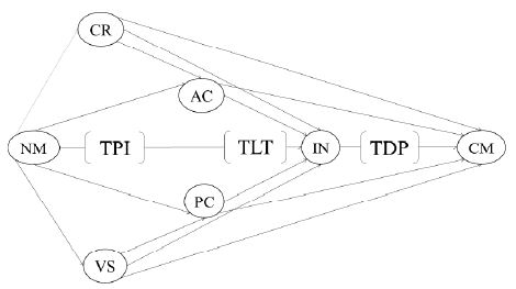
Figure 1: Corporate Reputation Theory.
TPI = Stakeholder Theory, TLT = Transformative Leadership Theory, TDP = Prospective Decision Theory: NM = Norms, VS = Values, CR = Beliefs, AC = Attitudes, PC = Perceptions, IN = Intentions, CM = Behaviors
Source: Self made.

The Stakeholders Theory warns that employees, shareholders, leaders and clients not only have a direct and significant participation in the company but also confront peripheral actors such as protesters, the media or institutions that seek to counteract the prestige of the company. institution in order to increase its credibility and position itself in the market [9].

Around the conflict between the interested parties and external factors to public health institutions, corporate governance is created as a shield of empathy, trust, commitment and satisfaction that guarantees the union of shareholders, leaders, employees and clients against the environmental threats, but it is in terms of reputation and prestige that differences and similarities between internal and external actors are resolved [10].

However, it is known that adhocratic organizational cultures, as well as traditional leadership, promote internal asymmetries in the face of external threats to the detriment of corporate reputation and prestige [11].

It will be the transforming cultures and leaderships who will manage knowledge to establish competitive advantages in the formation of intangible assets such as training and training of intellectual capital, future artificial and emotional intelligence cadres that will be decisive in entrepreneurship and innovation [12].

In such a context and scenario of cultures and transformative leaderships, decision makers are oriented towards vision and prospective missions as a second competitive advantage coupled with the formation of intangible assets [13].

This is the case of strategic alliances and knowledge management between HEIs and community, public or collective health institutions where systems of professional practices and social service are established in order to train future health professionals, among whom are social workers [14].

The Theory of Prospective Decisions posits that organizations prefer intentions and decisions aimed at maximizing risks and profits over strategies to reduce risks and reduce benefits [15].

In the case of the formation of human capital, a prospective decision suggests risks in the formation with high benefits in the prestige and reputation of the HEI or the health center. These are early professional internship strategies for students who have not covered the minimum credits, or social services who have not accredited seminars or basic subjects [16].

Another aspect to consider refers to the lack of resources for the hiring of professionals and the employment of interns and social workers to remedy the deficit of attention to public health services, or their use in health promotion, campaigns of prevention or allocation of medications to vulnerable groups [17].

In sum, stakeholder theory, transformational leadership theory, and prospective decision theory suggest the need for a comprehensive, specific, and up-to-date diagnosis of corporate governance, reputation, and institutional prestige, as well as expectations. of shareholders, directors, talents and users of HEIs in strategic alliances with collective health centers [18].

Given that corporate governance in general and training reputation and prestige in particular are little studied objects in the HEIs where the Schools and Faculties of Social Work are located, it is necessary to carry out a comprehensive diagnosis of the skills of future professionals with the purpose of inferring the intangible value of public universities in strategic alliances with health centers, as well as their differences and similarities in terms of professional skills [19].

Formulation

Will there be significant differences between HEIs in central, western and northern Mexico in terms of training skills for health services?

Hypothesis

Null Hypothesis

There will be significant differences between the HEIs studied with respect to the professional training of skills for public health services

Alternate Hypothesis

There will be no significant differences between the study HEIs regarding the professional training of skills for public health services

Method

An exploratory study was carried out with a sample of students, directors and professionals of the Social Work of Health in HEIs in the center, west and northeast of Mexico, considering their affiliation to a public university with an internship system in health centers, accreditation of the minimum percentage for social service and professional practices (Table 1).

Table 1: Descriptions of the study sample

	Students	professionals	Administrative	Sex	Age	Entry
UAEH	93	37	14	Female(45%) Male(55%)	M=25.3 SD=3.89	M=$346.1 SD=$9.3
UAEM	91	3. 4	12	Female(57%) Male(43%)	M=29.8 SD=4.78	M=342.1 DE=$8.3
UAEMEX	90	33	eleven	Female(67%) Male(33%)	M=27.3 SD=3.80	M=$432.1 SD=$7.1
UAM	89	30	10	Female(49%) Male(51%)	M=28.6 SD=2.79	M=367.2 DE=$8.2
UAQ	87	29	9	Female(44%) Male(56%)	M=36.1 SD=1.32	M=$342.1 SD=9.3
UAT	85	27	8	Female(52%) Male(48%)	M=33.1 SD=1.67	M=$396.1 SD=$10.4
UNAM	84	25	7	Female(43%) Male(57%)	M=37.1 SD=4.35	M=$354.1 SD=71.1
USON	83	24	6	Female(60%) Male(40%)	M=39.8 SD=2.34	M=$359.8 SD=$5.4

Source: Prepared with study data

The Corporate Reputation Scale (ERC-28) was built based on items selected from the consulted literature, which measured expectations of the parties involved regarding objectives, tasks and goals related to entrepreneurial and innovative knowledge skills such as collaborative work. professional (Table 2).

Table 2: Construction of the ERC-28

Competence	Definition	Indicator	Coding	Interpretation
Accompaniment	It refers to an emotional ability to establish a bond of social, family or personal support with the user of the health service (Vaquero, 2012)	Data relating to cases of self-medication or self-harm	0=“not at all likely” to 5=“quite likely”	High scores refer to a corporate governance focused on the reputation and professional training prestige of the accompaniment
Accession	It refers to the ability to motivate the user to use the health service in terms of consultation requests, medications and advice. (Kolade, Olakkeke, & Omotayo, 2014)	(Data referring to the cases of rehabilitation and desertion to treatments	0=“not at all likely” to 5=“quite likely”	High scores refer to a corporate governance focused on the reputation and professional training prestige of adherence to treatment
Advisory	It refers to an ability to establish effective and accessible processing routes for health service users (Rondeaeu, 2017)	Data alluding to the time of delay in each of the phases of the health service from the request for care to the rehabilitation	0=“not at all likely” to 5=“quite likely”	High scores refer to a corporate governance focused on the reputation and professional training prestige of the management consultancy
Interview	It refers to an ability to establish empathy with the user of health services, their needs, shortcomings and opportunities for a risk-free life (Olajide, 2014)	Data alluding to the user’s detachment and trust towards health professionals, bureaucracy and administrative managers	0=“not at all likely” to 5=“quite likely”	High scores refer to a corporate governance focused on the reputation and professional training prestige of the diagnostic interview
Mediation	It refers to an ability to reduce differences and conflicts, as well as to establish points of agreement between the parties (Kelinde, 2012).	Data related to conflicts and conciliations	0=“not at all likely” to 5=“quite likely”	High scores refer to a corporate governance focused on the reputation and professional training prestige of conflict mediation
Promotion	It refers to an ability to disseminate data and prevention strategies for illnesses and accidents for a risk-free life (Jinfeng, Runtian, & Quian, 2014).	Data alluding to illnesses and accidents that affect occupational, emotional or biophysical health	0=“not at all likely” to 5=“quite likely”	High scores refer to a corporate governance focused on the professional training reputation and prestige of health promotion
Follow-up	It refers to an ability to establish parameters of quality of care in terms of satisfaction of the user of the health service (Melero and López, 2017)	Data alluding to the quality of care and customer satisfaction	0=“not at all likely” to 5=“quite likely”	High scores refer to a corporate governance focused on the reputation and professional training prestige of case monitoring

Source: Self made

The surveys were carried out in the facilities of the HEIs and health centers with a prior written guarantee of confidentiality, anonymity and non-affectation of the results. The information was processed in the Statistical Package for Social Sciences (SPSS version 25.0).

Reliability and validity analyzes of the instrument, hypothesis tests for differences between groups, as well as correlations, general linear models and structural equation models were carried out to establish the trajectories of dependency relationships between the variables and indicators of the ERC-15.

The following parameters were estimated: 1) mean, 2) standard deviation, 3) bias, 4) kurtosis, 5) asymmetry, 6) Crombach ‘s alpha , 7) Student’s t – test, 8) analysis of variance F-test, 9) KMO test, 10) Bartlett test, 11) Pearson correlations, 12) beta regressions, 13) goodness of fit, and 14) residuals.

Results

Table 3 shows the statistical properties of the ERC-28 in which reliability alpha values higher than the indispensable minimum of .700 are observed for the general instrument (alpha of .780) and the subscales (respective alphas of .776; .781); .756; .790; .719; .750; .732).

Table 3: Descriptives of the CKD-28

R	M	D	yes	C	TO	F1	F2	F3	F4	F5	F6	F7
R1	1.32	,821	1.59	1.54	,782							,360
R2	1.25	.943	1.65	1.65	,793							.469
R3	1.43	.972	1.67	1.29	,784							,540
R4	1.39	,784	1.83	1.03	,763							.457
R5	4.37	1.30	1.75	1.17	,751						,564
R6	4.21	1.21	1.60	1.81	,759						.439
R7	4.21	1.43	1.73	1.43	,783						,406
R8	4.43	1.46	1.83	1.12	.752						.326
R9	3.45	,864	1.95	1.14	,714					.435
R10	3.50	.975	1.61	1.03	,750					.329
R11	3.56	,931	1.68	1.05	,762					.438
R12	3.52	,831	1.92	1.24	,741					,384
R13	1.39	4.36	1.61	1.16	,739				.438
R14	1.45	4.18	1.74	1.46	.752				.548
R15	1.46	4.39	1.82	1.67	,751				,324
R16	1.21	4.39	1.93	1.02	,754				.455
R17	4.56	1.52	1.62	1.13	,749			.421
R18	4.35	1.48	1.79	1.15	,731			,486
R19	4.25	1.32	1.73	1.15	,743			,340
R20	4.67	1.14	1.82	1.45	,724			,389
R21	2.46	2.35	1.70	1.24	,743		,398
R22	2.57	2.14	1.82	1.13	,763		.412
R23	2.54	2.43	1.71	1.15	,716		,378
R24	2.14	2.87	1.94	1.17	,730		,420
R25	4.50	,871	1.84	1.06	,753	.423
R26	4.67	.943	1.74	1.09	,726	,379
R27	4.18	,921	1.92	1.17	,743	.421
R28	4.39	.953	1.75	1.18	,750	.347

R=Reactive, M=Mean, D=Standard Deviation, S=Skew, C=Kurtosis, A=Alpha removing the value of the item. Adequacy (KMO=.732), Sphericity ⌠X2=23.6 (5df) p=.000⌡Extraction method: principal axes, rotation: promax. F1=Accompaniment (18% of the total variance explained), F2=Adherence (17% of the total variance explained), F3=Advice (15% of the total variance explained), F4=Interview (13% of the total variance explained), F5=Mediation (11% of the total variance explained), F6=Promotion (8% of the total variance explained), F7=Follow-up (5% of the total variance explained). All items are answered with one of five options: 0=“not at all likely” to 5=“quite likely”.
Source: Self made.

The correlation matrix shows discriminant validity by including values close to zero, but the covariance matrix warns of the possibility of excluding other factors due to values close to unity (Table 4).

Table 4: Correlation and covariance matrices

	F1	F2	F3	F4	F5	F6	F7	F1	F2	F3	F4	F5	F6	F7
F1	1,000							1.59
F2	2. 3. 4*	1,000						,743	1.83
F3	,313	.246	1,000					,831	.674	1.79
F4	.435*	,318	.239	1,000				.932	,756	,794	1.68
F5	,294	.268**	.217***	.246	1,000			,748	.865	,874	,608	1.50
F6	.105	.106	.443	.128	.319*	1,000		,693	,608	,792	,704	,893	1.68
F7	,392	.146	.329	.236*	.246	.246	1,000	,761	.642	.775	.872	,768	,798	1.72

F1=Accompaniment, F2=Adhesion, F3=Counseling, F4=Interview, F5=Mediation, F6=Promotion, F7=Follow-up: * p <.01; ** p <.001; *** p <.0001.
Source: Prepared with study data.

The sum of the percentages of explained variance (87%) revealed the preponderance of seven factors that can converge in a common factor of the second order (Figure 2).

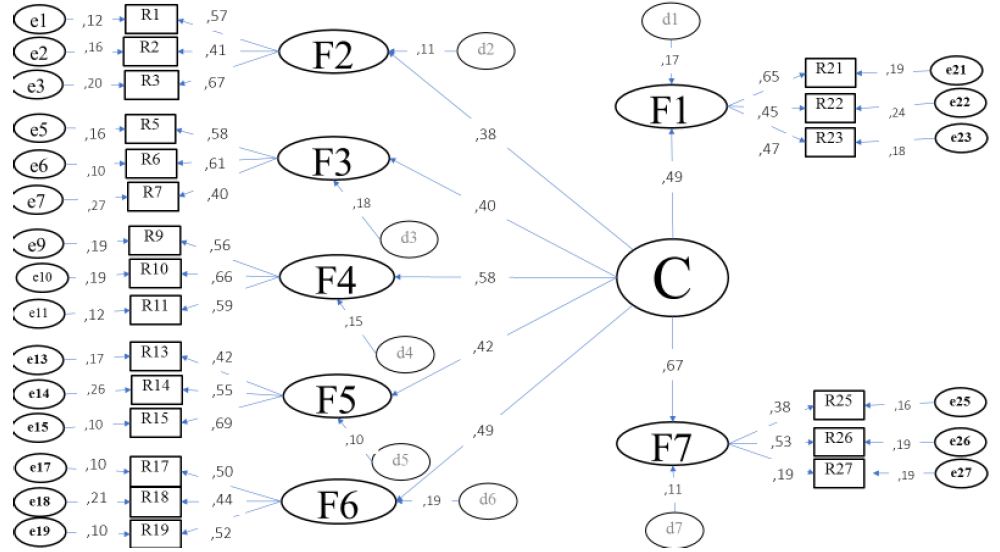
Figure 2: Structural model of trajectories of dependency and reflective relationships.
C = Corporate Reputation: F1 = Accompaniment, F2 = Adhesion, F3 = Advice, F4 = Interview, F5 = Mediation, F6 = Promotion, F7 = Follow-up; r = Reactive, d = Disturbance, e = Measurement error
Source: Prepared with study data.

The second-order factor related to corporate reputation included the eight first-order factors established from the review of the literature. The structural model included as a reflective factor the competence of case follow-up (.67). In other words, the corporate reputation of the social work public service is centered on the academic and administrative training of monitoring skills rather than on the skills of support, adherence, advice, interview, mediation and health promotion.

The fit and residual parameters ⌠X²=345.23 (56df) p=.008; GFI=.997; CFI=.990; NFI=.995; RMSEA=.009; RMR=.007⌡ suggest the non-rejection of the null hypothesis regarding the differences between the competencies reviewed in the literature with respect to the structural model.

Discussion

The present work has established the contrast of a model for the study of seven exploratory factorial dimensions of corporate reputation in HEIs in central, western and northern Mexico, although the type of non-experimental study, the type of intentional selection and the type of exploratory factor analysis limit the results to the study sample, suggesting lines of research and intervention related to the follow-up of cases as a factor reflecting the organizational phenomenon.

[1,3,19-28] contrasted models to observe corporate reputation in its reflective dimensions: 1) aversive or entrepreneurship and real innovation of the organization; 3) responsive or ecological footprint of the organizational production; 3) prospective or expected future of the organization, concluding that organizations seem to go through a process that goes from aversion to risks indicated by cultures, leaderships and adhocratic climates towards a propensity for the future indicated by cultures, leaderships and conciliatory climates of the organization image of collaborative knowledge networks.

In the present work, an exploratory model of seven factors has been contrasted in which the institutional follow-up of user cases is the hallmark of HEIs that, in alliance with health centers, train future operational-administrative cadres. The factor reflecting the follow-up of cases is part of the dimension of responsiveness cited in the literature.

Therefore, it is necessary to: a) build an instrument to explore the indicators of the responsive dimension as a preponderant factor of corporate reputation; b) contrast an exploratory model in order to establish the convergent and divergent validity of the scale; c) associate the responsive dimension with the aversive and prospective dimensions in order to build an integral model.

Conclusion

The present work has contrasted a model of seven dimensions reflecting the reputation of HEIs specialized in Social Work in Health, which is centered on the competence of case follow-up. In relation to the findings reported in the literature, the model can be specified in the responsive dimension, this being the one that would explain the distance or closeness that the respondents refer to as the competitive advantage of their academic and professional training.

References

Bustos JM, Ganga F, Llamas B, Juárez M (2018) Contrast of a prospective decision model in implications for a university governance of sustainability. Margin 89: 1-16.
Garcia C (2018a) Reliability and validity of an instrument that measures knowledge management in a public university in central Mexico. Tlatemoani 27: 285-304.
Sánchez R, Villegas E, Sánchez A, Espinosa F, García C (2018) Model for the study of organizational clarity and corporate social responsibility. Synchrony 22: 467-483.
García C, Espinosa F, Carreón J (2018) Model of intangible assets and capitals in organizations. International Journal of Research in Humanities and Social Studies 5: 1-12.
Garcia C (2018b) Interpretations of knowledge management discourses for the understanding of narratives of innovative entrepreneurship. Inclusions 5: 96-111.
Garcia C, Martinez E, Rivera PE (2018) Labor flexibility in higher education. Inclusions 5: 51-69.
Villegas E, Garcia C, Hernandez TJ (2018) Establishment of a science and technology policy for the incubation of innovative knowledge micro-enterprises. Inclusions 5: 19-26.
Rubio A, Jiménez IC, Mercado C (2017) Online corporate reputation in the hotel industry: The case of tripadvisor. Market Economic & Business Journal 48: 579-593.
Perrini F, Vurro C (2013) Stakeholders orientation and corporate reputation: A quantitative study on US companies. Emerging Issues in Management 1: 53-65.
Babie V, Arslanagic M, Mehic E (2013) Importance of internal marketing for service companies’ corporate reputation and customer satisfaction. Journal of Business Administration research 12: 49-57.
Barnnett M, Jermier JM, Lafferty BA (2006) Corporate reputation: The definitional landscape. Corporate Population Review 9: 26-38.
Blajer A (2014) Corporate reputation and economic performance the evidence from Poland. Economic & Sociology 7: 194-207.
Cariton R, Moura RC (2012) The impact of R&D intensity on corporate reputation: interaction effect of motivation with high social benefit. Intangible Capital 8: 216-238.
Beheshtifar M, Korouki A (2013) Reputation: An important component of corporation value. International Journal of Academic Research in Business & Social Science 3: 15-20.
Casimiro MC, Matos A (2017) The impact of corporate reputation in a dairy company. Business & Economics Journal 8: 1-11.
Marquina P, Arellano R, Velázquez I (2014) A new approach for measuring corporate reputation. Administration 54: 53-66.
Martinez P, Rodriguez I (2013) Intellectual capital and relational capital: The role of sustainability in developing corporate reputation. Intangible Capital 9: 262-280.
Fiala R, Prokov M (2013) The relationships among reputation, inter-organizational trust and alliance performance. University Act 99: 899-908.
Hernández TJ, Sánchez A, Espinosa F, Sánchez R, García C (2018) Model of lucidity, entrepreneurship and innovation in coffee microenterprises in central Mexico. Eureka 15: 96-107.
Garcia C, Rivera PE, Martinez E (2018) Institutionalist academic culture in Cuernavaca, Modelos (Mexico). Inclusions, 5: 84-96.
Garcia C, Rivera PE, Martinez E (2018) Institutionalist academic culture in Cuernavaca, Modelos (Mexico). Inclusions, 5: 84-96.
Jinfeng L, Runtian J, Quian C (2014) Antecedents of corporate reputation and customer citizenship behavior. International Business & Management 9: 128-132.
Kelinde O (2012) Organizational culture and its corporate image: A model juxtaposition. Business & Management Research 1: 121-132.
Kolade OJ, Olakkeke O, Omotayo O (2014) Organizational cityzenship behavior, hospital corporate image and performance. Journal of Competitiveness 6: 36-49.
Melero I, Lopez ML (2017) Identifying link between corporate social responsibility and reputation: Some considerations family firms. Journal Evolutionary Studies in Business 2: 191-230.
Olajide FS (2014) Corporate social responsibility practices and stakeholders’ expectations. Research in Business & Management 1: 13-31.
Rondeau KV (2017) The impact of world ranking systems on graduate schools of business: promoting the manipulation of image over the management of substance. World Journal of Education 7: 62-73.
Cowboy A (2012) Online reputation in the framework of corporate communication. An insight into research trends and career prospects. Communication 3: 49-63.

Spatial Variability of Elemental Concentrations in Three Marine Fishes along the Coastal Waters of Andhra Pradesh

Leave a reply

DOI: 10.31038/JPPR.2022512

Abstract

In the presented study, three different marine ﬁsh species were collected from four locations along the coastal waters of Andhra Pradesh. The samples were analysed using Hand-held XRF. Concentrations of ten elements (As, Cd, Cu, Fe, Mn, Se, Zn, Ca, K and Mg) were quantiﬁed in muscle, liver and gill tissues of Rastrelliger kanagurta, Euthynnnus affinis and Saurida tumbil collected from Visakhapatnam harbour, Kakinada harbour, Pudimadaka and Bheemili. There was a clear spatial variation in the concentration of elements collected from different locations. However, signiﬁcant differences in elemental concentrations among the three studied species and tissues were observed and these may be related to different accumulation patterns of the species. The results showed that concentrations of As and Cd were above the threshold limits. However, the exposure for the population depends on their dietary habits and continued exposure to the heavy metals may cause adverse effects.

Keywords

Marine fish, HHXRF, Heavy metal

Introduction

During the last few years, aquatic ecosystems have been affected by various types of contaminations due to garbage and effluents delivering by different sectors like domestic, agricultural, commercial, and pharmaceutical and other industrial activities of human beings living around the coastal lines. In recent years [1], much attention has been paid to study about health benefits of essential elements (Fe, Zn, Cu, Mn) derived from fishes of the marine environment due to consumption of sea fishes and change in their concentration due to pollution impact causing associated health hazards besides the accumulation of non-essential elements or heavy metals (Hg, Cd, Pb) in the fishes. Nutritionists consider fish products to be a major source of quality protein, vitamins, minerals and long-chain polyunsaturated fatty acids (omega-3), docosahexaenoic acid (DHA) and also contain organic and inorganic micronutrients like vitamin D, selenium etc. [2]. Fishes are recommended mainly to the elderly, infant’s brain and nerves function, cardiac patients i.e., abnormal heart strokes and those with digestive problems due to their reduced energy levels and higher mineral content [3]. Consuming fish may decrease the risk of depression, Alzheimer’s disease, arthritis and diabetes etc. On the other hand, Toxicologists tend to regard aquatic pollution as a major vector for non-essential elements like Hg, Cd, Pb accumulation [4]. These elements are mainly present in marine environments due to industrial wastewater loads, soil erosion, municipal sewage discharges from rural and urban areas, agricultural land runoff [5]. Natural phenomena such as earthquakes, landslides, tornadoes, cyclones, and weathering of rocks also contribute towards heavy elements contribution for pollution. The contaminated water is the major source of elements bioaccumulation in the various vital organs (Liver, Kidney, gills) of the fish. Discharge of agricultural wastes like agrochemicals, Organic matter and industrial wastewater without pre-treatment into lakes, rivers and oceans resulting in an increase of non-essential elemental concentration in such water environments exhibiting damage on aquatic life [6]. Elemental pollutants as particles, elemental ions; inorganic and organic compounds in rivers and oceans also damage aquatic life [7,8]. Heavy elements, which especially collected in the organs of fishes, such as spleen and kidneys may be transmitted and accumulated in human organs through their consumption [9] and can cause a risk of kidney, brain and nervous system damage to human beings. Therefore, the introduction of non-essential elements into the food chain threatens human health and also to aquatic life. Essential elements may also become toxic to the human body if their intake is higher than the standard values of WHO [10].

The consumption of fish is significant for human beings living in coastal areas like Visakhapatnam and constitutes an important component in the intake of food items. Hence, continuous monitoring and analysing elemental concentration levels in fish belong to coastal areas became vital to understand the pollution impact on human beings those who consume frequently or regularly. Research on the detection of elements in fishes of these coastal areas is important because elemental concentration could cause growth disorders, reproductive disorders, immune suppression and histopathological alteration in the gills, kidney, liver and skin, as well as abnormalities in fish bones [11]. The health hazards associated with the consumption of contaminated fishes are up to 20-40 times greater than those associated with contaminated drinking water [12]. This is because fish have the ability to contain elemental concentration up to ten times higher than the observed environmental value [13]. Thus, fish may be considered biological indicators of elemental pollution and as a potential risk factor if contaminated fish are consumed by human beings. Absorption of elemental ions takes place through the skin, gills and digestive tract of fishes, which are transmitted to other parts of the body through the blood [14]. Muscles have been widely analysed for elemental concentration as they constitute the most edible portion of fish that poses a risk to human health who consumes them [15]. However, the liver, gills and kidneys collect the elements more effectively than the muscles since they are active metabolic tissues and primary organs for accumulating the majority of elements in fish [16]. The concentration level of elements in the gills indicate their concentration presented in the water in which the fish are found, and the liver’s concentration represents the retention of the elements, whereas the muscle is not regarded to be active tissue in the accumulation of elements [17]. Many organizations like the United States Food and Drug Administration (USFDA), the Food and Agriculture Organization (FAO) and the World Health Organization (WHO) have established limitations for human consumption of trace elements. The FAO/WHO Committee on Food Additives has set the provisional values of tolerable weekly intake (PTWI) and the dietary intakes of food additives and certain food contaminants. These specific values are significant for the safety levels of these elements in humans [18].

Materials and Methods

Samples Collection and Preparation

In the present study, three marine fishes commonly consuming by the people of Andhra Pradesh namely (Rastrelliger kanagurta (22-24 cm, TL), Euthynnus affinis (28-32 cm, TL) and Saurida tumbil (30-34 cm, TL) were collected freshly from four locations of coastal waters namely Visakhapatnam harbour (Geographical coordinates (17.6958° N, 83.3025° E), Kakinada harbour (16°58′30″N, 82°16′44″E), Pudimadaka fish landing centre (17.4927° N, 83.0028° E) and Bheemili fish landing centre (17.890382°N 83.455465°E). The sample collection areas along the coastal waters of Andhra Pradesh are shown in Figure 1. Photographs of the collected marine fishes belong to the Visakhapatnam harbour is presented in Figure 2. These fishes were individually packaged into polythene bags, stored in an ice box and brought to the laboratory. The selected species were collected three times during the winter season. The collected fishes were washed with distilled water and carefully dissected to obtain the muscle, gills and liver of the fish; subjected for determination of elemental concentrations accumulated in the respective parts. These samples were then kept at around -20°C in a deep freezer overnight in the laboratory. The frozen samples were lyophilized in a microprocessor-controlled freezing method. The lyophilization works at around -50°C which absorbs water molecules from the samples, drains off the samples making them completely dry. Then the dried specimens were ground using agate mortar and pestle to obtain fine powder with minimal contamination. The samples were kept separately with unique identification number in airtight packets.

Figure 1: Sample collection areas along the coastal waters of Andhra Pradesh

Figure 2: Fish Samples collected at Vishakapatnam fishing harbour

Experimental Method

The experimental work was carried out in BARC (Division of Nuclear Physics), Mumbai with Hand-held XRF (HHXRF) technique. In the XRF spectrometer, samples were excited by the X-rays emanating from an X-ray tube (Rh X-ray tube) having enough energy for ejecting electrons from various inner shells belonging to the atoms in the specimen. The vacancies in the inner shells of atoms are then occupied by electrons coming from the outer shells of the atoms causing the emission of characteristic X-rays; conventionally it can be referred to as X-ray fluorescence (XRF). In HHXRF, a silicon drift detector (SDD) was employed for the measurement of X-ray energies. The Silicon Drift Detector (SDD) contains graphene window that enables the detection of low Z elements (Al, S and P). These low Z elements usually cannot be detected by the conventional XRF system which uses a beryllium window. The powdered samples were placed in a cubic box and irradiated by Rhodium X-ray tube. Spectrum has been obtained for each sample in twenty seconds. The energy of the beams used for beam 1 is between 12 and 36 keV, whereas for beam 2, it varies between 0 to 12 KeV [19]. The HHXRF experimental set-up is as shown in Figure 3. The validity of the HHXRF set up was performed by analyzing Certified reference material (CRM) obtained from European Commision – Joint Research Centre, Institute for Reference Materials and Measurements – (ERMBB422 – Fish muscle) – was used for quantification of the elements and verifying the reliability of the data obtained by the present system.

Figure 3: HHXRF set up

Results and Discussion

Concentrations of accumulated elements namely As, Cd, Cu, Fe, Mn, Se, Zn, Ca, K and Mg in different tissues belong to the fishes collected from four different locations are determined by using the obtained spectra. The observed results relating to the fishes collected from Visakhapatnam fishing harbour are compared with those collected from Kakinada fishing harbour, Pudimadaka, Bheemili as displayed in the Table 1. There is a clear spatial variation in the concentration of elements collected from different locations, however significant differences in elemental concentrations among the three studied species are observed; which may be related to different accumulation patterns of the species. The obtained XRF spectrum of the certified reference material (ERMBB422) is shown in Figure 4. The correlation coefficients among the evaluated average concentration values of various elements observed due to the three species are computed and shown in Tables 2-4.

Table 1: Concentrations of elements present in three different fish species collected at four locations

Element	Species	Tissue	Visakhapatnam	Kakinada	Pudimadaka	Bheemili
As	Rastrelliger kanagurta	Muscle	BDL	BDL	BDL	BDL
		Liver	6.0 ± 4.4	8.3 ± 5.8	5.3 ± 4.0	BDL
		Gills	9.3 ± 6.7	BDL	BDL	BDL
	Euthynnus affinis	Muscle	11.0 ± 2.8	5.3 ± 0.6	7.3 ± 4.9	BDL
		Liver	45.5 ± 2.1	15.7 ± 2.1	28.0 ± 16.5	37.7 ± 26.3
		Gills	6.7 ± 4.6	2.7 ± 2.1	7.5 ± 0.7	BDL
	Saurida tumbil	Muscle	4.0 ± 2.6	BDL	2.7 ± 2.1	4.3 ± 3.2
		Liver	17.0 ± 2.8	14.3 ± 10.1	18.0 ± 14.1	11.0 ± 4.4
		Gills	7.3 ± 4.9	16.0 ± 11.3	BDL	12.7 ± 3.8
Cd	Rastrelliger kanagurta	Muscle	29.5 ± 4.9	25.7 ± 3.1	23.0 ± 5.0	30.0 ± 1.4
		Liver	31.5 ± 10.6	29.0 ± 5.3	22.7 ± 3.8	29.0 ± 9.9
		Gills	11.7 ± 8.1	15.0 ± 10.4	13.7 ± 9.8	15.3 ± 11.0
	Euthynnus affinis	Muscle	28.0 ± 2.6	26.3 ± 3.5	25.3 ± 5.7	15.3 ± 11.0
		Liver	42.3 ± 11.2	38.7 ± 16.2	35.3 ± 4.2	14.3 ± 10.1
		Gills	BDL	BDL	BDL	15.0 ± 10.4
	Saurida tumbil	Muscle	25.5 ± 3.5	21.7 ± 3.2	27.5 ± 6.4	25.3 ± 2.5
		Liver	31.0 ± 7.0	23.0 ± 2.8	27.0 ± 5.7	12.3 ± 8.4
		Gills	BDL	15.7 ± 11.5	15.0 ± 10.4	15.0 ± 10.4
Cu	Rastrelliger kanagurta	Muscle	BDL	BDL	BDL	BDL
		Liver	52.5 ± 16.3	69.3 ± 24.5	66.0 ± 33.4	47.5 ± 16.3
		Gills	35.3 ± 24.8	BDL	BDL	BDL
	Euthynnus affinis	Muscle	11.0 ± 7.8	14.5 ± 6.4	6.0 ± 4.4	BDL
		Liver	58.0 ± 45.6	81.3 ± 31.5	38.7 ± 18.8	44.3 ± 30.9
		Gills	8.3 ± 5.8	BDL	BDL	BDL
	Saurida tumbil	Muscle	BDL	BDL	BDL	BDL
		Liver	39.7 ± 21.6	42.7 ± 30.6	48.0 ± 7.1	21.0 ± 4.0
		Gills	BDL	BDL	BDL	BDL
Fe	Rastrelliger kanagurta	Muscle	113.7 ± 47.3	94.7 ± 24.0	106.7 ± 14.5	97.5 ± 3.5
		Liver	1574.0 ± 596.8	1538.7 ± 567.0	1910.7 ± 593.7	1311.5 ± 509.8
		Gills	1304.0 ± 1304.2	950.3 ± 325.4	595.7 ± 98.0	550.0 ± 69.3
	Euthynnus affinis	Muscle	193.0 ± 174.0	287.0 ± 87.9	177.3 ± 98.9	45.3 ± 31.8
		Liver	1628.7 ± 1638.4	3430.0 ± 1841.3	2097.0 ± 2065.0	2090.0 ± 1524.2
		Gills	519.0 ± 70.7	589.7 ± 128.2	4047.7 ± 5345.8	302.0 ± 209.6
	Saurida tumbil	Muscle	BDL	13.3 ± 9.2	BDL	BDL
		Liver	940.0 ± 546.5	1383.3 ± 858.2	1382.0 ± 745.3	748.3 ± 212.1
		Gills	487.0 ± 208.1	450.3 ± 111.1	518.5 ± 157.7	418.7 ± 269.1
Mn	Rastrelliger kanagurta	Muscle	23.7 ± 16.7	BDL	BDL	17.0 ± 12.1
		Liver	19.3 ± 13.6	BDL	37.0 ± 9.9	35.5 ± 9.2
		Gills	41.0 ± 7.1	53.5 ± 3.5	57.0 ± 5.7	70.5 ± 14.8
	Euthynnus affinis	Muscle	BDL	BDL	BDL	18.3 ± 12.7
		Liver	17.0 ± 12.1	20.3 ± 14.4	40.5 ± 0.7	BDL
		Gills	72.5 ± 38.9	52.3 ± 9.1	104.5 ± 53.0	20.7 ± 14.2
	Saurida tumbil	Muscle	17.0 ± 12.1	18.7 ± 13.3	15.0 ± 10.4	26.3 ± 1.2
		Liver	24.0 ± 16.5	15.3 ± 11.0	BDL	BDL
		Gills	88.0 ± 10.5	68.3 ± 1.2	93.0 ± 41.0	75.7 ± 23.0
Se	Rastrelliger kanagurta	Muscle	BDL	BDL	1.5 ± 0.7	BDL
		Liver	15.0 ± 11.3	17.7 ± 10.8	21.7 ± 10.7	20.0 ± 15.6
		Gills	15.3 ± 13.8	7.7 ± 2.5	5.7 ± 1.2	8.0 ± 2.8
	Euthynnus affinis	Muscle	3.7 ± 2.1	6.0 ± 3.0	5.3 ± 4.9	BDL
		Liver	26.7 ± 20.4	16.7 ± 11.7	26.3 ± 13.8	2.7 ± 2.1
		Gills	10.5 ± 3.5	8.3 ± 3.1	6.3 ± 2.9	1.7 ± 1.2
	Saurida tumbil	Muscle	BDL	BDL	1.5 ± 0.7	BDL
		Liver	2.7 ± 1.2	2.7 ± 1.2	2.0 ± 1.4	1.7 ± 0.6
		Gills	BDL	1.7 ± 1.2	BDL	1.7 ± 1.2
Zn	Rastrelliger kanagurta	Muscle	113.7 ± 82.6	87.3 ± 31.8	76.3 ± 1.2	59.0 ± 1.4
		Liver	326.0 ± 36.8	334.7 ± 101.6	312.7 ± 116.2	263.5 ± 72.8
		Gills	618.7 ± 681.0	262.3 ± 14.6	269.7 ± 40.4	305.0 ± 8.5
	Euthynnus affinis	Muscle	56.7 ± 9.1	61.7 ± 16.5	47.3 ± 4.7	20.3 ± 14.4
		Liver	577.7 ± 270.8	568.3 ± 290.8	835.3 ± 512.6	295.7 ± 205.5
		Gills	286.3 ± 117.0	359.3 ± 71.0	290.7 ± 54.8	88.3 ± 61.2
	Saurida tumbil	Muscle	43.3 ± 8.4	35.3 ± 0.6	34.5 ± 4.9	36.0 ± 1.0
		Liver	198.7 ± 64.3	176.7 ± 38.1	145.5 ± 37.5	130.7 ± 14.0
		Gills	172.0 ± 7.5	167.0 ± 4.6	147.0 ± 4.2	159.7 ± 18.5
Ca	Rastrelliger kanagurta	Muscle	0.78 ± 1.14	0.08 ± 0.01	0.07 ± 0.02	0.06 ± 0.05
		Liver	0.10 ± 0.10	0.09 ± 0.03	0.06 ± 0.01	0.05 ± 0.04
		Gills	4.02 ± 3.47	7.11 ± 0.55	7.16 ± 1.41	5.00 ± 4.33
	Euthynnus affinis	Muscle	0.05 ± 0.02	0.10 ± 0.08	0.07 ± 0.02	0.02 ± 0.01
		Liver	0.16 ± 0.05	0.18 ± 0.13	0.79 ± 0.71	0.02 ± 0.02
		Gills	8.87 ± 0.98	7.79 ± 0.52	6.79 ± 1.01	2.96 ± 2.05
	Saurida tumbil	Muscle	0.69 ± 0.91	0.15 ± 0.07	0.06 ± 0.07	0.22 ± 0.10
		Liver	0.08 ± 0.06	0.05 ± 0.03	0.04 ± 0.04	0.03 ± 0.01
		Gills	6.46 ± 0.83	5.49 ± 0.33	3.93 ± 3.48	5.04 ± 0.59
K	Rastrelliger kanagurta	Muscle	1.33 ± 0.41	2.13 ± 1.17	2.54 ± 0.88	1.80 ± 1.56
		Liver	1.15 ± 1.00	1.63 ± 0.38	1.85 ± 0.48	1.05 ± 0.91
		Gills	1.30 ± 0.75	0.82 ± 0.03	0.79 ± 0.08	0.54 ± 0.47
	Euthynnus affinis	Muscle	2.26 ± 0.10	2.08 ± 0.42	2.62 ± 0.10	1.42 ± 0.99
		Liver	1.81 ± 0.18	1.90 ± 0.39	1.79 ± 0.23	1.22 ± 0.84
		Gills	0.55 ± 0.20	0.67 ± 0.17	0.65 ± 0.13	0.50 ± 0.34
	Saurida tumbil	Muscle	2.85 ± 0.29	2.35 ± 0.41	1.71 ± 1.50	2.81 ± 0.14
		Liver	5.84 ± 7.66	1.19 ± 0.24	0.65 ± 0.60	1.30 ± 0.19
		Gills	0.99 ± 0.08	1.02 ± 0.08	0.60 ± 0.52	1.16 ± 0.22
Mg	Rastrelliger kanagurta	Muscle	0.62 ± 0.43	BDL	BDL	BDL
		Liver	BDL	BDL	0.72 ± 0.50	0.76 ± 0.53
		Gills	0.83 ± 0.58	1.77 ± 0.06	2.50 ± 0.26	1.63 ± 1.46
	Euthynnus affinis	Muscle	0.66 ± 0.46	0.53 ± 0.37	BDL	BDL
		Liver	BDL	BDL	0.72 ± 0.50	BDL
		Gills	0.89 ± 0.62	1.03 ± 0.91	1.61 ± 1.12	0.67 ± 0.46
	Saurida tumbil	Muscle	BDL	BDL	BDL	BDL
		Liver	0.67 ± 0.46	0.74 ± 0.66	0.64 ± 0.45	0.72 ± 0.50
		Gills	0.78 ± 0.54	1.10 ± 1.05	0.83 ± 0.72	0.67 ± 0.46

BDL: below detection limit.
Concentration of As, Cd, Cu, Fe, Mn, Se and Zn are in ppm.
Concentration of Ca, K and Mg are in %.

Figure 4: Spectra of muscle tissue of Rastrelliger kanagurta collected from Visakhapatnam (a), Kakinada (b), Pudimadaka (c) and Bheemili (d)

Table 2: Correlation between elements present in tissues of Rastrelliger kanagurta

	As	Cd	Cu	Fe	Mn	Se	Zn	Ca	K	Mg
As	1
Cd	-0.537	1
Cu	-0.499	0.555	1
Fe	-0.882	-0.011	0.746	1
Mn	0.508	-0.833	-0.259	-0.023	1
Se	-0.535	0.473	0.505	0.936	-0.716	1
Zn	0.770	-0.506	-0.653	0.721	0.330	0.485	1
Ca	0.736	-0.861	-0.755	-0.055	0.820	-0.525	0.361	1
K	-0.290	0.408	0.721	-0.238	-0.748	0.002	-0.453	-0.700	1
Mg	1	-0.643	-0.963	-0.351	0.785	-0.923	-0.094	0.886	-0.718	1

Table 3: Correlation between elements present in tissues of Euthynnus affinis

	As	Cd	Cu	Fe	Mn	Se	Zn	Ca	K	Mg
As	1
Cd	0.192	1
Cu	0.610	0.519	1
Fe	0.284	0.532	0.944	1
Mn	-0.660	0.196	-0.929	0.398	1
Se	0.564	0.864	0.571	0.338	-0.405	1
Zn	0.558	0.705	0.708	0.609	-0.060	0.888	1
Ca	-0.496	-0.295	-0.345	0.087	0.796	-0.169	0.037	1
K	0.134	0.522	-0.066	-0.148	-0.582	0.215	-0.027	-0.789	1
Mg	-0.253	0.205	-0.101	0.815	0.910	-0.060	0.162	0.677	-0.569	1

Table 4: Correlation between elements present in tissues of Saurida tumbil

	As	Cd	Cu	Fe	Mn	Se	Zn	Ca	K	Mg
As	1
Cd	-0.140	1
Cu	0.889	0.832	1
Fe	0.531	0.503	0.873	1
Mn	0.254	-0.853	-1.000	-0.367	1
Se	0.555	0.510	0.547	0.660	-0.498	1
Zn	0.839	-0.241	0.463	0.546	0.533	0.678	1
Ca	0.080	-0.643	0.382	-0.487	0.934	-0.407	0.450	1
K	-0.010	0.628	0.015	0.023	-0.557	0.562	-0.090	-0.431	1
Mg	0.008	-0.429	-0.501	-0.483	0.311	-0.327	0.031	0.548	-0.271	1

From the evaluated results that displayed in the Table 1, comprehensively one can draw the following statements:

As expected, accumulation levels of heavy metals namely arsenic and cadmium belonging to Visakhapatnam fishing harbour are higher relative to other places indicating higher pollution levels as commercial activities and anthropogenic garbage discharge are more than other places leading to more exposure to pollution
In the case of nutritional elements such as copper (Cu) and iron (Fe) concentration levels are found to be more in the fish species collected from Kakinada fishing harbour followed by Pudimadaka (Saurida tumbil and Rastrelliger kanagurta for Cu and Fe respectively).
Se, Zn and Ca contents were found in higher concentrations among the fish species belonging to Visakhapatnam fishing harbour followed by Pudimadaka
Detection of Mn, K and Mg seems to be higher in the species related to Pudimadaka when compared with the other places.
Fish species belonging to Bheemili are reflecting no nutritional elements higher relative to other places.
Though the commercial activities due to domestic transport and international export of goods besides thrown of garbage by local habitants are higher, some of the nutritional elements and antioxidants at Kakinada fishing harbour and Visakhapatnam fishing harbour found to be higher, indicating the need to develop effective pollution management systems at these places.

Detection of Heavy Metals

Arsenic

Arsenic (As) is widely distributed in the environment as a result of anthropogenic and naturally occurring processes. This is a trace element that is potentially toxic to all living beings; however, its toxicity varies based on its different chemical forms [20]. The United States Food and Drug Administration [21] reported that seafood products including fish constitute 90% of overall exposure to arsenic. Accumulated arsenic concentration among various tissues of the selected species of ﬁsh taken from the above-mentioned locations are analysed for monitoring the level of pollution and the obtained concentrations found to vary between 2.7 ± 2.1 ppm to 45.5 ± 2.1 ppm. The highest concentration is detected in the liver tissue of Euthynnus affinis species collected from Visakhapatnam. However, the arsenic level is below the limit of detection relating to the muscle tissue of Rastrelliger kanagurta belong to all the locations. It is also clear that the concentration of all the tissues pertaining to Rastrelliger kanagurta related to Bheemili is below the detection limit. The Australia New Zealand Food Standards Code [22] states that the maximum allowable concentration of As is 2.0 mg/kg ww. The species Euthynnus affinis was collected in Visakhapatnam (assuming that the muscle is the only edible part) exceeded the ANZFA recommended value (9.6 mg/kg) dw (assumed to be 79% moisture). The EPA has established 1.3 mg/kg of arsenic in fresh water fish tissue as the basis for protecting human health [23]. The maximum concentration of As in fish according to Brazilian legislation is 1.0 mg/kg [24]. Sharif et al. [25] investigated the concentration of arsenic in tropic marine fish species from Bangladesh with reported values varied between 2.84 and 3.92 mg/kg dw.

Cadmium

Cadmium also considered as one of the toxic elements that could present in ﬁsh organs at higher concentrations [26]. It leads to chronic toxicity although it occurs at a concentration level of 1 mg/kg [27]. Christensen et. al [28] considered cadmium to be potentially more hazardous than other metals. The National Health and Medical Research Council (ANHMRC) standard for Cd concentration in seafood products in Australia is 2.0 mg/kg [29], while the authorities of Western Australia suggested 5.5 mg/kg concentration for Cd [30]. Under Spanish legislation Cd concentrations are limited to 1 mg/kg [31]. The maximum concentration of Cd for ﬁsh laid down by Brazilian legislation amounts to 1.0 mg/kg [32]. The concentration of Cd in ﬁsh samples in this study varies from 11.7 ± 8.1 ppm to 42.3 ± 11.2 ppm. The liver of Euthynnus affinis that collected from Visakhapatnam is found to show the highest level of cadmium. Based on the results obtained in the present experimental study; it can be understood that the observed Cd in ﬁshes collected from all the four locations exceeds the aforementioned standard values and longer period of Cd accumulation in ﬁshes may be hazardous to health.

Detection of NUTRITIONAL Elements

Copper

Copper is vital and necessary for synthesizing of haemoglobin [33]. Its deﬁciency may cause disorders in blood and nervous system in adults [34]. However, high consumption of Cu would result in adverse health effects [35]. The observed concentration of Cu in the present study ranges from 6.0 ± 4.4 ppm to 81.3 ± 31.5 ppm, however, it was found to be less than the limit of detection in muscle tissues of Rastrelliger kanagurta and Saurida tumbil related to all the three locations of the present study. The liver tissue of Euthynnus affinis that belong to Kakinada is found to have the highest level of Cu. The maximum permitted Cu limit proposed by FAO and ANHMRC is 30 mg/kg fresh weight [36,37]. The UK Food Standards Committee report states that the Cu content of food must be less than 20 mg/kg wet weight [38]. Legislation has also been passed in some countries about the maximum permissible Cu concentration in meals. For instance, Turkish law has set the Cu concentration as 5 mg/kg, while Spanish law suggested the concentration of 20 mg/kg ww [39]. The Australian Food Standard Code has set a maximum level of Cu to 10 mg/kg ww [40]. Taking into account the water content of 79% of ﬁsh muscles, no species studied exceeded prescribed limits of different agencies (assuming the muscle as the only edible part).

Iron

Iron deﬁciency frequently results with anaemia causing reduced levels of working capacity besides impaired mental development. The recommended daily allowance for children and adults (males and females) is 11 mg/day and 18 mg/day, respectively [41]. The concentration levels of iron in the present study ranges in between 13.3 ± 9.2 ppm to 4047.7 ± 534.5 ppm. The highest concentration of Fe is found in gills of Euthynnus affinis that procured from Pudimadaka. Earlier Karadede et al. [42] and Chale [43] observed values of iron concentration are 200.86 µg/g and 125 µg/g respectively. Reported these data are exhibiting fair agreement with the values of Iron observed in the present studies. The values for iron reported by Tariq et al. [44] and Asharaf et al. [45] are 0.782 to 4.217 and 1.550 to 6.715 µg/g respectively. These values are lower than the present values of iron. Iron is a mineral and essential for life. An adequate dietary intake of iron is extremely important in reducing anaemia. The deficiency of iron occurs when there is a high demand for it, e.g., while growing, in pregnancy periods and during menstrual loss, the intake usually is not adequate or contains minerals that prevent iron from being absorbed [46]. The low bioavailability of iron is regarded as a major factor leading to its deﬁciency in many countries.

Manganese

Manganese is used in iron alloys, electric coils, dry battery cells and glass ceramics etc. which may be regarded as the mains sources of pollution of the manganese. While manganese is a low-toxicity element, it has significant biological interest. There are no established manganese limits in the ﬁsh samples. The obtained Mn concentration in the present work ranges in the range 15.0 ± 10.4 ppm to 104.5 ± 53.0 ppm. The highest level of Mn is found in gills of Euthynnus affinis that collected from Pudimadaka while the lowest concentration found be in muscle tissue of Saurida tumbil procured from Pudimadaka. However, it is not detected in muscle tissue of Euthynnus affinis that collected from Visakhapatnam, Kakinada and Pudimadaka. Manganese can be present in any body tissue that has contributed to the functioning of many organic systems. Manganese is required to support normal immune function, to regulate blood glucose levels and cellular energy, digestion, reproduction, bone growth and even as a cellular antioxidant [47]. Although elevated levels of Mn can cause toxicity in humans, no RDA was established. The US National Academy of Sciences [48] determined adequate intakes (AI) of Mn as 2.3 and 1.8 mg/day for adult males and females respectively. The observed Mn concentration is consistent with the values for the ﬁsh collected from the Gumti River in Bangladesh [49].

Selenium

Selenium is an essential trace element for living organisms as a nutrition. It is known as an antioxidant and protection agent against toxic elements, heart disease and cancer. Selenium deﬁciency may cause multiple pathologic conditions. However, depending upon the concentration, it may also become toxic to humans, certain plants and animals [50]. In the present study, the observed concentration of Se the analysed samples ranged from 1.5 ± 0.7 ppm to 26.7 ± 20.4 ppm. However, the concentration of Se is below the detection limit in the muscle tissue of Rastrelliger kanagurta and Saurida tumbil that collected from Visakhapatnam, Kakinada and Bheemili. The RDA for adult men and women is 55 mg per day [51]. In Brazil, no maximum level of Se in fish is established.

Zinc

Being heavy metal, Zn has the tendency to bioaccumulate in fatty tissue of marine ﬁsh and known to impact their reproductive physiology [52]. Chronic exposure to Zn and Cu has been reported as related to Parkinson’s disease [53] and they may act on their own or together for a period of time to cause the illness [54]. The concentration of Zn in the muscle tissue of Rastrelliger kanagurta is much higher than the other two species collected from all the four locations of the present study. The liver of Euthynnus affinis that belongs to Pudimadaka is found to have highest level of Zn while the lowest concentration observed in muscle tissue of Euthynnus affinis procured from Bheemili. The quantity of Zn found in all ﬁsh samples is well below 1000 mg/kg standard established by ANHMRC [55,56] and WHO [56]. Zinc is a significant trace element of human nutrition and in a wide range of biochemical functions of human metabolism. The deﬁciency of Zn in humans leads to many disorders, but excessive consumption can cause adverse effects [57]. The RDA for Zn intake is 11 mg/day and 8 mg/day for men and women up to age 19, respectively, and Tolerable Upper Level of Intake (UL) is 40 mg/d for that age group [58].

Calcium

Ca is extremely essential to human body and is required to build teeth and healthy bones. It affects the coagulation of the body, stimulates muscles and nervous systems; works as a cofactor of vitamin D and also for the functioning of the parathyroid gland. Muscles cannot contract without calcium. Calcium is vital to regulate heart rate, maintains normal blood pressure and allows the control of electrical impulses in the brain [59]. The concentration of Ca in the present study ranges in between 0.02 ± 0.01 %. to 8.87 ± 0.98 %. The highest concentration of Ca is found in the gills of Euthynnus affinis that collected from Visakhapatnam while the lowest concentration observed in the muscle and liver tissues of Euthynnus affinis procured from Bheemili. The recommended levels of individual intake of Ca for adults (19 y to 50 y) is 1000 mg/d and tolerable upper intake level is 2.5 g/d. [60].

Potassium

Potassium (K) is very important for the cells, and without it one would not be able to survive. It is mainly found in intracellular fluids. Potassium stimulates neural impulses; muscular contractions and is significant for maintaining osmotic pressure. Potassium regulates the acid-alkaline balance of the body, stimulates the functioning of the kidneys and adrenals, and also helps in the conversion of glucose into glycogen. It is necessary for biosynthesis of proteins. Potassium is the third most abundant mineral in the human body [59]. The recommended mean intake of K is 2300 mg/day in adult females and 3100 mg/day in adult males. The concentration of K in the present study lies in the range 0.50 ± 0.34 % to 5.84 ± 7.66 %. The concentration of K is found highest in the liver tissue of Saurida tumbil collected from Visakhapatnam and lowest concentration found in the gills of Euthynnus affinis that brought from Bheemili.

Magnesium

Magnesium is required for over 300 bio-chemical reactions in human body. It helps in the maintenance of normal nerve and muscle functions, supports the healthy immune system, maintains a stable heart rate, and is useful for bones to stay strong. It is also required to adjust blood sugar levels. It helps to produce energy and protein. In the present study, the Mg concentration ranges from 0.53 ± 0.37 % to 2.50 ± 0.26 %. The highest concentration is found in the gills of Rastrelliger kanagurta that belong to Pudimadaka while the lowest concentration is obtained in the muscle tissue of Euthynnus affinis that collected from Kakinada. The recommended levels of individual intake of Mg for males (19-30 y) is 400 mg/d; above 31 y allowed to take 420 mg/d; in case of females (19-30 y) it is 310 mg/d while beyond 31 y 320 mg/d may be taken up. The tolerable upper intake level is 350 mg/d for all the adults beyond 19 y.

Statistical Analysis

The Pearson correlation coefficients among the heavy metals observed related to Rastrelliger kanagurta, Euthynnus affinis and Saurida tumbil were calculated and shown in Tables 2, 3 and 4 respectively. A strong correlation between any two elements suggests a common absorption mechanism, or a common source and may also be a lack of metabolism regulation. For Rastrelliger kanagurta, arsenic (As) found to show significant positive correlation with Mg (1), Ca (0.736) Zn (0.77) and strong negative correlation with Fe (-0.882). Similarly, Cd also showing strong negative correlation with Ca (-0.861) and Mn (-0.833). Copper is exhibiting positive correlation with Fe (0.746) and K (0.721) while indicating strong negative correlation with Mg (-0.963) and Ca (-0.755). Fe showed strong positive correlation with Se (0.936) and Zn (0.721). Mn indicating strong positive correlation with Ca (0.820) and Mg (0.785) and moderate negative correlation with K (-0.748) and Se (-0.716). Se showed strong negative correlation with Mg (-0.923). Ca found to show strong positive correlation with Mg (0.886) and moderate negative correlation with K (-0.7). K exhibits moderate negative correlation with Mg (-0.718). For Euthynnus affinis, cadmium (Cd) indicating strong positive correlation with Se (0.864) and Zn (0.705). Cu showed strong positive correlation with Fe (0.944) and Zn (0.708) and strong negative correlation with Mn (-0.929). Fe exhibited strong positive correlation with Mg (0.815). Mn indic ating strong positive correlation with Mg (0.910) and Ca (0.796). Se showed strong positive correlation with Zn (0.888) while Ca exhibited moderate negative correlation with K (-0.789).

In the case of Saurida tumbil, strong positive correlation has been obtained between As-Cu (0.889), As-Zn (0.839), Cd-Cu (0.832), Cu-Fe (0.873), Mn-Ca (0.934) and a strong negative correlation also been observed between Cd-Mn (-0.853) and Cu-Mn (-1).

The results obtained through the statistical analysis are shown in Tables 2-4 for the fishes Rastrelliger kanagurta, Euthynnus affinis, Saurida tumbil respectively. Based on the linkages/association of heavy metals with the nutritional elements that observed in this correlation studies, the following statements can be made for the interpretation of observed data.

The observed arsenic (As) concentration of Rastrelliger kanagurta, Euthynnus affinis and Saurida tumbil is beyond the threshold value and strongly assosiated with nutritional elements Mg, Cu and Zn. Cadmium (Cd) is also associated with Mn, Ca, Se and Cu. So, these heavy metals toxicological impact not only show directly but also affect indirectly through the nutritional elements on consumers.
Among the three fishes studied in the present investigations, As is associated significantly showing positive correlation with the nutritional elements namely Zn and Cu in the Saurida tumbil fish species and Mg in the case of Rastrelliger kanagurta. Some nutritional elements such as Fe, Se, Mn etc. found to show positive correlation with arsenic in one fish species while those elements exhibiting negative correlation or assosication exhibiting antagonish behaviour in the other fish species. This type of behaviour may be understood on the lines of physiology and metabolic system of respective fish species. Hence this type of results show indirect effect on consumers by the nutritional elements due to the As and Cd contents.
Copper (Cu) is showing positive correlation with iron (Fe) and negative association with Mn in all the three fishes studied in the present studies. Similarly Mn is exhibiting positive correlation with calcium (Ca) and Mg in all the fishes, further Ca also found to show positive association with Mg for all the fish species.
Interestingly important nutritional elements found to reflect useful behaviour with the presence of them relating with one another in all the fishes.

Conclusion

Concentrations of ten elements (As, Cd, Cu, Fe, Mn, Se, Zn, Ca, K and Mg) are quantiﬁed in the muscle, liver and gill tissues of Rastrelliger kanagurta, Euthynnus affinis and Saurida tumbil collected from Visakhapatnam harbour, Kakinada harbour, Pudimadaka and Bheemili. There is a clear spatial variation in the concentration of observed elements related to the fish species/samples collected from different locations. In the present study, signiﬁcant differences in elemental concentrations have been observed in three fish species and these may be related to different accumulation patterns of the species besides anthropogenic garbage, industrial effluents, variation in local climatic conditions that show impact on the various elements/metals’ accumulation in water, which in turn might enter into fish organs. The evaluated results are showing the higher levels or concentrations of As and Cd accumulation beyond the threshold limits of them. However, exposure is a function of dietary habits of consumers and continued exposure to these heavy elements can lead to adverse effects.

Acknowledgment

The authors would like to thank DST-SERB, New Delhi for the financial support in the form of a project.

Conflicts of Interest

The authors do not have any relevant financial or non-financial competing interest.

References

Amal H, Azza K (2014) Determination of metals in tuna species and bivalves from Alexandria, Egypt. The Egyptian Journal of Aquatic Research 40: 9-17.
Afonso C, Lourenco HM, Cardoso C, Bandarra NM, Carvalho ML, et al. (2013) From fish chemical characterization to the benefit- risk assessment-part A. Food Chem 137: 99-107. [crossref]
Cahu C, Salen P, Lorgeril M de (2004) Farmed and wild fish in the prevention of cardiovascular diseases: assessing possible differences in lipid nutritional values. Nutrition, Metabolism and Cardiovascular Diseases 14: 34-41. [crossref]
Guérin T, Sirot V, Volatier JL, Leblanc JC (2007). Organotin levels in seafood and its implications for health risk in high-seafood consumers. Science of the Total Environment 388: 66-77. [crossref]
Altundag H, Dundar MS (2009) Determination of thallium after preconcentration on amberlite IR-120 by ICP-MS. Fresenius Environmental Bulletin 18: 98-101.
Aydemir F, Altundag H, Imamoglu M (2012) Removal of Cr (VI) from aqueous solution by hazelnut husk carbon. Fresenius Environmental Bulletin 21: 3589-3594.
Ozparlak H, Arslan G, Arslan E, (2012) Determination of some metal levels in muscle tissue of nine fish species from Beys，ehir Lake, Turkey. Turkish Journal of Fisheries and Aquatic Sciences 4: 761-770.
Dundar MS, Altundag H (2002) Heavy metal determinations of house dusts in Adapazari City, Turkey after Earthquake. Trace Elements and Electrolytes 19: 55-58.
Altundag H, Dundar MS, Dogancı S, Celik M, Tuzen M (2013) The use of a sequential extraction procedure for heavy metal analysis of house dusts by atomic absorption spectrometry. Journal of AOAC International 96: 166-170.
Celik U, Oehlenschlager J (2007) High contents of cadmium, lead, zinc and copper in popular fishery products sold in Turkish supermarkets. Food Control 18: 258-261.
Vitek T, Spurny P, Mares J, Zokova A (2007) Acta Vet. Brno 76.
Foran JA (1990) Toxic substances in surface waters. Environ Sci Technol 24:604-608.
Yilmaz F, Ozdemir N, Demirak A, Tuna AL (2006) Heavy metal levels in two fish species Leuciscus cephalus and Lepomis gibbosus. Food Chem 100: 830-835.
Khan B, Hizbullah K, Said M, Tariq K (2012). Heavy metals concentration trends in three fish species from Shah Alam River (Khyber Pakhtunkhwa Provine, Pakistan). Journal of Natural and Environmental Sciences 3: 1-8.
Rajeshkumar S, Liu Y, Zhang X, Ravikumar B, Bai G, et al. (2008) Studies on seasonal pollution of heavy metals in water, sediment, fish and oyster from the Meiliang Bay of Taihu Lake in China. Chemosphere 191: 626-638.
Chovanec A, Hofer R, Schiemer F (2003) Chapter 18 fish as bioindicators, in: trace metals and other contaminants in the environment. Elsevier, pg: 639-676.
Alhashemi AH, Sekhavatjou MS, Kiabi BH, Karbassi AR (2012). Bioaccumulation of trace elements in water, sediment, and six fish species from a freshwater wetland, Iran. Microchemical journal 104: 1-6.
Cot-Committee on Toxicology (2004), Advise on fish consumption: Benefits and risks. Food standards Agency and the Department of Health. Norwich, UK.
Paul S, Joseph D, Majumdar M (2021) Health risk assessment of Macro, Trace-elements and heavy metal in various Indian Antidiabetic Polyherbal formulations. Sci. Pollut. Res. 28: 40929-40937. [crossref]
Devesa V, Vélez D, Montoro R (2008). Effect of thermal treatments on arsenic species contents in food. Food and Chemical Toxicology 46: 1-8. [crossref]
USFDA (1993) Guidance document for arsenic in shellﬁsh (pg: 25-27). Washington, DC: US Food and Drug Administration.
ANZFA (2011) Australian and New Zealand Food Standards Code, Standard 1.4.1- Contaminants and Natural Toxicants (F2011C00542).
Burger J, Gochfeld M (2005) Heavy metals in commercial ﬁsh in New Jersey. Environmental Research, 99: 403-412. [crossref]
ANVISA (1998) Agência Nacional de Vigilância Sanitária. Portaria Ns.
Sharif AKM, Alamgir M, Krishnamoorthy KR, Mustafe AI (1993b) Determination of Arsenic, Mercury, Selenium and Zinc in Tropical Marine Fish by Neutron Activation. Journal of Radioanalytical and Nuclear Chemistry 170: 299-307.
Türkmen M, Türkmen A, Tepe Y, Töre Y, & Ates A (2009). Determination of metals in ﬁsh species from Aegean and Mediterranean Seas. Food Chemistry 113s.
Friberg L, Piscator M, Nordberg Gs (1971). Cadmium in the Environment. Cleveland, Ohio: The Chemical Rubber Co, Press.
Christensen FC, Olson EC (1957) Cadmium poisoning; report of a fatal case, with discussion of pathology and clinical aspects. Archives of Industrial Health 16: 8-13. [crossref]
Plaskett D, Potter IC (1979). Heavy metal concentrations in the muscle tissue of 12 species of teleost from Cockburn Sound, Western Australia. Australian Journal of Marine and Freshwater Research 30: 607-616.
Demirak A, Yilmaz F, Tuna AL, Ozdemir N (2006) Heavy metals in water, sediment and tissues of Leciscuscephalus from a stream in southwestern Turkey. Chemosphere 63: 1451-1458. [crossref]
ANVISA (1998) Agência Nacional de VigilânciaSanitária. Portaria N.
Sivaperumal P, Sankar TV, Nair PGV (2007). Heavy metal concentrations in ﬁsh, shellﬁsh and ﬁsh products from internal markets of India vis-a-vis international standards. Food Chemistry 102: 612-620.
Dabbaghmanesh H, Salehi NM, Siadatan J, Omrani GR (2011). Copper concentration in a healthy urban adult population of Southern Iran Mohammad. Biological Trace Element Research 144: 217-224. [crossref]
Gorell JM, Johnson CC, Rybicki BA, Peterson EL, Kortsha GX, et al. (1997) Occupational exposures to metals as risk factors for Parkinson’s disease. Neurology 48: 650-658. [crossref]
Bebbington GN, Mackay NJ, Chvojka R, Williams RJ, Dunn A, et al. (1977). Heavy metals, selenium and arsenic in nine species of Australian commercial ﬁsh. Australian Journal of Marine and Freshwater Research 28: 277-286.
Dural M, Goksu MZL, Ozak AA (2007) Investigation of heavy metal levels in economically important fish species captured from the Tuzla lagoon. Food Chemistry 102: 415-421.
Cronin M, Davies IM, Newton A, Pirie JM, Topping G, et al. (1998). Trace metal concentrations in deep sea ﬁsh from the North Atlantic. Marine Environmental Research 45: 225-238.
Demirak A, Yilmaz F, Tuna AL, Ozdemir N (2006) Heavy metals in water, sediment and tissues of Leciscuscephalus from a stream in southwestern Turkey. Chemosphere 63: 1451-1458. [crossref]
Alam MGM, Tanaka A, Allinson G, Laurenson LJB, Stagnitti F, et al. (2002) A comparison of trace element concentrations in cultured and wild carp (Cyprinus carpio) of Lake Kasumigaura, Japan. Ecotoxicology and Environmental Safety 53: 348-354. [crossref]
Schümann K, Ettle T, Szegner B, Elsenhans B, Solomons NW (2007). On risks and beneﬁts of iron supplementation recommendations for iron intake revisited. Journal of Trace Elements in Medicine and Biology 21. [crossref]
Karadede H, Oymak, SA, Ünlü E (2004) Heavy metals in mullet, Liza abu, and catﬁsh, Silurustriostegus, from the Atatürk Dam Lake (Euphrates), Turkey. Environ. Int. 2004, 183–188.
Chale FMM (2002) Trace metal concentrations in water, sediments and ﬁsh tissue from Lake Tanganyika. Total Environ 299: 115-121. [crossref]
Tariq J, Jaffar M, Ashraf M (1994) Trace metal concentration, distribution and correlation in water, sediment and ﬁsh from the Ravi River, Pakistan. Res. 19: 131-139.
Ashraf M, Tariq J, Jaffar M (1991) Contents of trace metals in ﬁsh, sediment and water from three freshwater reservoirs on the Indus River, Pakistan. Res. 12: 355-364.
Lynch SR, Baynes RD (1996) Deliberations and evaluations of the approaches, endpoints and paradigms for iron dietary recommendations. American Institute of Nutrition 2404S, 2409S.
Aschner J, Aschner M (2005). Nutritional aspects of manganese homeostasis. Molecular Aspects of Medicine 26: 353-362. [crossref]
National Academy of Sciences (2001) Dietary Reference Intakes for vitamin A, vitamin K, arsenic, boron, chromium, copper, iodine, iron, manganese, molybdenum, nickel, silicon, vanadium, and zinc. A report of the panel on micronutrients, subcommittees on upper reference levels of nutrients and of interpretation and use of dietary reference intakes, and the standing committee on the scientiﬁc evaluation of dietary reference intakes. Washington DC: National Academy Press.
Amin MN, Begum A, Mondal MGK (2011) Trace element concentrations present in ﬁve species of freshwater ﬁsh of Bangladesh. Bangladesh journal of scientiﬁc and industrial research 46: 27-32.
Al-Saleh I (2000). Selenium status in Saudi Arabia. Journal of Trace Elements in Medicine and Biology 14.
Institute of Medicine (2001) Dietary reference intakes for vitamin C, vitamin E, selenium, and carotenoids. Food and Nutrition Board. Washington, DC: The National Academies Press.
Ghosh BB, Mukhopandhyay MK, Bagchi MM (1985). Proc. National Seminar on Pollution Control and Environmental Management (pg: 194-199).
Gorell JM, Johnson C C, Rybicki BA, Peterson EL, Kortsha GX, et al. (1997). Occupational exposures to metals as risk factors for Parkinson’s disease. Neurology 48: 650-658. [crossref]
Prasad AS (1983) The role of Zinc in gastrointestinal and liver disease. Clinics in Gastroenterology 12: 713-741. [crossref]
Bebbington GN, Mackay NJ, Chvojka R, Williams RJ, Dunn A, et al. (1977). Heavy metals, selenium and arsenic in nine species of Australian commercial ﬁsh. Australian Journal of Marine and Freshwater Research 28: 277-286.
Cliton HI, Ujagwung GU, Michael H (2008) Trace metals in the tissues and shells of TympanotonusFuscatus var. Radula from the Mangrove Swamps of the Bukuma Oil Field, Niger Delta. European journal of Scientiﬁc Research 24: 468-476.
Scherz H, Kirchhoff E (2006). Trace elements in foods: zinc contents of raw foods – a comparison of data originating from different geographical regions of the world. Journal of Food Composition and Analysis 19.
Institute of Medicine (2001) Dietary reference intakes for vitamin C, vitamin E, selenium, and carotenoids. Food and Nutrition Board. Washington, DC: The National Academies Press.
Garbunov AV, Lyapunov SM, Okina OI, Frontasyeva MV, Pavlov SS, Nuclear and related analytical techniques in ecology: Impact of geological factors on the balance of trace elements in the human organism.
Allison A, Yates PhD, Rdsandra A, Schlicker PhD, Carol W, et al. (1998) Dietary Reference Intakes: The New Basis for Recommendations for Calcium and Related Nutrients, B Vitamins, and Choline. Journal of the American Dietetic Association. 98: 699-706. [crossref]

Barley Stripe Mosaic Virus

Leave a reply

DOI: 10.31038/MGJ.2022513

Abstract

The aim of this study was to express TaSTP13 in wheat leaf by (pst). Some abnormal behaviors of TaSTP13 are concentrated in the plasma membrane and act as a homoligomer. Seizure of TaSTP13 reduces wheat susceptibility to Pst by gene silencing (VIGS) by barley bar mosaic virus. Molecular mechanisms and regulatory genes are needed to improve tolerance to environmental stress in products. The new 4-component version (with very high expression) and the 3-component version (with low expression) contain a barley mosaic virus (BSMV) virus-based system, which is used for the functional characterization of finger protein on the C2H2 type in wheat. The four-component version, which contains a system based on the barley bar mosaic virus, has a high load capacity for the rapid and stable expression of recombinant proteins in various plant species. Excessive expression of TaSTP13 increases the susceptibility of Arabidopsis to powdery mildew and leads to increased glucose accumulation in the leaves.

Keywords

Homo ligomer, Gene silencing, Zinc finger protein and Arabidopsis

Introduction

The aim of this study was to express TaSTP13 in wheat leaf by Puccinia striiformis f.sp.tritici (pst). For example, is TaSTP13 involved in wheat susceptibility to rust and mildew? Is the decrease in glucose uptake related to wheat resistance due to Lr67? In this study, the expression of TaSTP13 homologues was specifically induced in wheat leaves challenged by the Pst pathotype, CYR31, and abiotic treatments. Intracellular localization analysis shows that TaSTP13 is located in the plasma membrane. Some of the abiotic behaviors of TaSTP13 are concentrated in the plasma membrane and act as hemoligomers [1-4].

To increase crop yield, genetic and molecular mechanisms that have mechanisms to withstand various environmental stresses should be increased in products. Most genomic research has focused on plant models or products with diploid genomes (such as Arabidopsis and Oryza sativa) [1].

To improve crop performance, special attention should be paid to the underlying genetic and molecular mechanisms of responses and mechanisms for tolerating various abiotic stresses in products [1].

Gene function is further manifested by transgenic gene expression or gene silencing in transgenic products. This process (gene function) in cereals is a time-consuming method. Plant viral expression systems can be used to rapidly express proteins [2].

BSMV virus is a triple-positive (alfa, beta, gama) stranded RNA virus with RNAs coated at the end of ‘5 (3). A barley mosaic virus (BSMV) virus-based gRNA delivery system targets mutant, wheat, and corn mutants for short, regular, clustered cross-repetitive palindromic replication (CRISPR)/cas9 [5].

The gRNA maintains the Cas9 interaction structure and the ability to identify target genes. In plants, gRNAs direct the Cas9 protein to cut double-stranded target DNA in cells to create double-stranded fractures that can be amplified by a non-identical end-binding pathway and/or a matched repair pathway for repair or mutation. Gives target genes [5].

Material and Method

The three- or four-component barley mosaic virus system is used to produce wheat. Functional properties of finger transcription factor on C2H2 type in response to wheat environmental stress using the new 4-component BSMV system (with very high expression) and the three-component BSMV system is focused on gene regulation. To enhance the expression profile of TaSTP13, qRT-PCR measurement system is used.

Conclusion

The TaSTP13 gene is a protein encoder that carries sugar for wheat. Some of the abiotic behaviors of TaSTP13 are concentrated in the plasma membrane and act as hemoligomers.

References

Cheuk A, Ouellet F, Houde M (2020) The barley stripe mosaic virus expression system reveals the wheat C2H2 zinc finger protein TaZFP1B as a key regulator of drought tolerance. BMC Plant Biology 20: 144.
Cheuk A, Houde M (2018) A New Barley Stripe Mosaic Virus Allows Large Protein Overexpression for Rapid Function Analysis. Plant Physiol 176: 1919-1931. [crossref]
Cheuk A, Houde M (2017) A rapid and efficient method for uniform gene expression using the barley stripe mosaic virus. Plant method 13: 24. [crossref]
Huai B, Yang Q, Wei X, Pan Q, Kang Z, et al. (2020) TaSTP13 contributes to wheat susceptibility to stripe rust possibly by increasing cytoplasmic hexose concentration. BMC Plant Biology 20: 49. [crossref]
Hu J, Li s, Li H, Li Z, Song W, et al. (2019) A barley stripe mosaic virus‐based guide RNA delivery system for targeted mutagenesis in wheat and maize. Mol Plant Pathol 20: 1463-1474. [crossref]

The Complete Mitogenome of the Comma Butterfly Polygonia c-aureum Provides Insights into the Phylogenetic Relationships and Divergence Time Estimation within the Nymphalidae

Leave a reply

DOI: 10.31038/MGJ.2022512

Abstract

The complete mitochondrial genome (mitogenome) of the comma butterfly, Polygonia c-aureum (Lepidoptera: Nymphalidae) is determined in this study. It is a circular molecule of 15,208 bp, containing 13 protein-coding genes, 2 ribosomal RNA (rRNA) genes, 22 transfer RNA (tRNA) genes, and an A+T-rich region, which is a common feature of lepidopteran mitogenomes. Based on nucleotide sequences of 13 protein-coding genes, we reconstructed the phylogenetic relationships among 87 species of the family Nymphalidae using Bayesian Inference (BI) and Maximum Likelihood (ML) methods, and calculated the divergence times using multiple fossil calibrations. The phylogenetic analyses supported the sister-group relationship between the subfamilies Nymphalinae and Cyrestinae. Moreover, monophyly of the Nymphalidae was strongly supported. The results were highly consistent with the traditional relationships within the Nymphalidae from morphological data. For the first time, our results suggest that the genus Polygonia diverged from the common ancestor of the rest of Nymphalinae at 45.64 Ma. In addition, the first divergence time in the Nymphalidae is in the Early Cretaceous, about 89.72 Ma.

Keywords

Mitochondrial genome, Molecular phylogeny, Divergence time, Nymphalidae, Polygonia c-aureum

Introduction

The Nymphalidae is the largest family of butterflies, including 7,200 species belonging to 600 genera and 12 subfamilies [1-6]. Consequently, it has been the subject of intense studies [7-9]. Nymphalidae is the first taxa that helped us to begin to understand the complex relationships between insects and their host plants [10], the effects of habitat fragmentation on the population dynamics of endangered species [11], and the genetic mechanisms behind the developmental pathways of morphological features [12], and the coevolutionary interactions between organisms in mimicry rings and aposematic coloration [13,14]. Especially the butterflies of the subfamily Nymphalinae [5] have extensively contributed to our knowledge on ecological and evolutionary processes [15-18]. However, the phylogenetic relationships among the different subfamilies and tribes have been chaotic because of the variable shapes and life cycles, it made them become the argue focus for taxonmists [6,19-21]. There are still several competing classification schemes based on different data sets and researchers [5,21,22]. With the development of sequencing technologies and increasing number of molecular data set, more and more researches investigated the phylogenetic relationships of butterflies. For example, [23] using the wingless gene, and [5] using COI, EF-1α and wingless genes, both including good taxonomic coverage of the Nymphalidae, showed that many of the traditional subgroups are monophyletic. [7] inferred a robust phylogenetic hypothesis based on 10 genes and 235 morphological characters.

Meanwhile, there are many difficulities in the research of orgin and evolution in most of the families, in view of the lack of fossils data. [7] used a surprisingly good fossil record for the Nymphalinae to estimate the ages of diversification major lineages using Bayesian relaxed clock methods, suggesting that the age of Nymphalidae is older than 70 million years. [24] explored the divergence time in butterflies using the sequences of ultraviolet-sensitive (UVRh), blue-sensitive (BRh), long-wavelength sensitive (LWRh) opsins, EF-1α and COI obtained from 27 taxa representing the five major butterfly families.

The comma butterfly, Polygonia c-aureum, is a major defoliator leaf pest on the scandent hostlant Humulus scandens (Lour.) Merr., which is used for medicine in China [25]. Here, we sequenced the complete mitochondrial genome (mitogenome), which could can be used to develop molecular markers for phylogenetics and, identification, and also to examine the evolution of Nymphalidae. In addition, we hope our study would be useful for the prevention and control of insect pests.

In this study, based on the complete mitogenome sequences of P. c-aureumy and additional homologous sequences of 86 species downloaded from GenBank, we estimated the divergence times of Nymphalidae, to enhance our understanding of the origin and evolution of this family, and to provide a relative accurate results for estimating divergence times of butterflies.

Materials and Methods

Sample Collection and DNA Extraction

The adult specimens of P. c-aureum were collected from Nanjing, Jiangsu Province in China. After an examination of external morphology for identification, the fresh adult specimens were directly frozen and maintained at -80°C until DNA extraction. Total genomic DNA was extracted from adult butterfly tissues, typically thorax or abdomen, using the Wizard Genomic DNA Purification Kit (Promega, Beijing, China) according to the manufacturer’s instruction. The extracted DNA was stored at -20°C and used for PCR amplification of the complete mitogenome.

Primers Design, PCR Amplification and DNA Sequencing

In order to amplify the complete mitogenome of P. c-aureum, nineteen pairs primers were designed and synthesized. Among them, four pairs are lepidoptera universal primers [26,27], twelve pairs specific primers for this study were designed using Primer Premier 5.0 software [28] and the remainder of three pairs primers were the combination of universal primers and specific primers. Detailed information about primers used in this study are shown in Table 1.

Table 1: Primers used for amplification of the Polygonia c-aureum mitogenome

Fragment	Region	Primer (J/N)	Primer sequence (J/N) 5’→3’
P1	ND2	N2-J1^c/N2-N1^c	ATAAGCTAAATAAGCTTTTGGGTTCATA/ATTATTAATGCAGATAATATTCATCCTAAATT
P2	ND2—COI	J-556^c/N-2904^c	AATAGGATCAGCACCAT/CAAGAAATGTTGAGGGA
P3	COI—COII	C1-J-2167^a/N-3649^a	TTGATTTTTCGGACATCCTGAAGT/CCGCAAATTTCTGAACATTGACCA
P4	COII—ATP8	J-3241^c/N-3849^c	TTGATTTTTCGGACATCCTGAAGT/CCGCAAATTTCTGAACATTGACCA
P5	COII—ATP6	J-3455^c/N4734^c	TATTGCACTCCCATCCC/GTTCTTCTAAGGAGGGT
P6	ATP6	C2-J^c/C3-N^c	ATTTGTGGAGCTAATCATAG/GGTCAGGGACTATAATCTAC
P7	ATP6—COIII	J-4556^c/N-5346^c	TTACCCTCCTTAGAAGAACA/AAATGTCGGATAAAGCAAGT
P8	COIII—ND3	C2-J-3696^a/N3-N-5731^a	GAAATTTGTGGAGCAAATCATAG/TTTGGATCAAACCCACATTC
P9	ND3—ND5	C3-N5-5407^c/N5-N-7793^b	GCTGCAGCTTGATATTGACA/TTGGGTTGGGATGGTTTAGG
P10	ND5—ND4	N5-J-7572^a/N4-N-9153^a	AAAAGGAATTTGAGCTCTTTTAGT/TGAGGTTATCAACCAGAGCG
P11	ND4—Cytb	N4-J-8502^a/CB-N-11328^a	GTAGGAGGAGCTGCTATATTAG/GGCAAATAGGAAATATCATTC
P12	ND4—Cytb	N4-J2^c/CB-N2^c	CCCTAATAATAAAGGCAATG/TTATCAACAGCAAATCCACC
P13	Cytb	CB-J-10933^a/N-11526^c	GTTTTACCATGAGGTCAAATATC/TTCTACAGGTCGGGCTCCGATTCA
P14	Cytb—ND1	J-11338^c/N-12051^c	CATATTAAACCCGAATGATATTT/GTATTTGCTGAAGGTGAATCAGA
P15	ND1—16S	N1-16S-J11876^b/N-13000^c	CGAGGTAAAGTACCACGAACTCA/TTACCTTAGGGATAACAGCGTAA
P16	16S	J-12609^c/N-13554^c	ACCATTACATTTATCTGCCA/ATTTTAGGGGATAAGCTTTA
P17	16S	J-13310^c/N-14094^c	ATCAGGGGGCAGATTAAACTTTAA/CTAGAAAGATCAAATTAGAGCT
P18	16S—12S	J-13653^c/N-14360^c	CGATTAACATTTCATTTC/ATTGATAATCCACGAAT
P19	12S—ND2	12S-N2-J^c/N2-N^c	CTCTACTTTGTTACGACTTATT/TCTAGGCCAATTCAACAACC

a: Primers modified from Simon et al. (1994) up to this mtgenome
b: Primers from Simon et al. (2006)
c: Primers newly designed for this genome

Some PCR reactions (the target fragments <2 kb) were performed in a 25 μL volume with 0.2 μL rTaq (TaKaRa Co., Dalian, China), 1 μL of DNA, 2.0 μL dNTPs, 2.0 μL 25 mM MgCl₂, 2.5 μL 10× rTaq buffer (Mg²⁺ free), 0.5 μL each primer and 16.3 μL sterile distilled H₂O. The PCR amplification was performed using the following cycling protocol: an initial denaturation for 5 min at 94°C, followed by 35 cycles of denaturation at 94°C for 30 seconds, annealing at 50°C~59°C (depending on primer pairs) for 30 seconds, extension at 72°C for 1~2 min, with a subsequent 10 min final extension at 72°C. Besides, the other PCR reactions (the target fragments ≥ 2 kb) were carried out with 25 μL reaction volume containing 0.2 μL of LATaq (TaKaRa Co., Dalian, China), 1 μL of DNA, 4.0 μL dNTPs, 2.5 μL 10×Taq buffer (Mg²⁺ plus), 16.3 μL sterile distilled H₂O and 0.5 μL each primer. The fragments were amplified under the following cycling protocol: 5 min of initial denaturation at 94°C, followed by 35 cycles of denaturation for 30 seconds at 94°C, annealing at 50°C~59°C (depending on primer pairs) for 30 seconds, extension at 72°C for 1~2 min, with additional 5 seconds for each cycle, and a final extension for 10 min at 72°C.

Products were examined by electrophoresis on 1% agarose gel. All the PCR fragments were directly sequenced from both strands by Jin Si Rui Company, Nanjing, China and Sheng Gong Company, Shanghai, China with the PCR primers.

Sequence Assembling and Annotation

The raw sequences files were proofread and assembled manually using the SeqMan module of the Lasergene 8.0 software (DNASTAR, Madison, WI, USA) [29]. The probable locations of the sequences were confirmed by BLAST search function on the NCBI website and comparison with the other lepidopteran sequences which can be obtained in GenBank. By using MEGA7.0, we determined the translation of 13 PCGs open reading frames [30]. The base composition of nucleotide sequences was described by skewness and measured according to the formulas (AT skew = [A−T]/[A+T], GC skew = [G−C]/[G+C]) [31]. 22 tRNA were confirmed using the program tRNAscan-SE. The proposed cloverleaf secondary structures within these tRNA genes and anticodon sequences were calculated using the tRNAscan-SE Search Server available online (http://lowelab.ucsc.edu/tRNAscan-SE/) [32]. We drew the secondary structure of tRNA by using the RNA structure program DNASIS MAX v.3.0 [33]. The secondary structure of the tRNA^Ser ^(AGN) was developed as proposed by [34]. Annotation was checked by comparison with tRNA determined for other lepidopteran species. Ribosomal RNA genes (rRNAs) were identified by NCBI Internet BLAST search.

Phylogenetic Analyses

To further probe into the phylogenetic relationship of Nymphalidae, a total of 84 complete mitogenomes and three uncomplete mitogenomes were chosen for the phylogenetic analyses based on the concatenated set of amino acid from 13 protein coding genes. The GenBank accession numbers used in this study were listed in Table 2. Among the 87 species, Coreana raphaelis (DQ102703.1), Japonica lutea (KM655768.1), Eurema hecabe (KC257480.1), Colias erate (KP715146.1), Curetis bulis (JX262888.1), Papilio bianor (KF859738.1), P. machaon (HM243594.1) and Leptidea morsei (JX274648.1) were selected as outgroups (Table 2). The PCG sequences of 87 species were aligned by using MEGA7.0 [30]. Sites with more than 90% gaps were excluded from the analysis. We chose two analysis approaches, Bayesian Inference (BI) and Maximum Likelihood (ML) to reconstruct phylogenetic relationships. We used the MrModeltest 2.3 [35] to select the best model for the ML and BI analyses. Thirteen datasets were established to calculate the best model for each PCG. According to the Akaike information criterion, the GTR + G model was selected as the most model appropriate for ND4L, and the GTR+I+G model was selected for other genes. The BI analysis was performed using MrBayes vers. 3.1.2 [36] under both of the models. The analysis were run twice simultaneously for 10,000,000 generations with every 1000 trees sampled. We discarded the first 1000,000 generations (1000 samples) as burn-in (based on visual inspection of the convergence and stability of the log likelihood values of the two independent runs). The ML analysis were performed using the program MEGA7.0 [30] with the same model. The bootstrap analysis were performed with 1000 replicates. Resulting tree files were inspected in FigTree v1.4.2 (http://tree.bio.ed.ac.uk/software/figtree/).

Table 2: Taxonomy, GenBank accession numbers, and mitogenome sizes of 87 the mitochondrial genomes used for the phylogenetic analysis, sourced from GenBank databases.

Subfamily	Species	Genome size (bp)	GenBank accession no.
Nymphalinae	Polygonia c-aureum	15208	KX096653
	Inachis io	15250	KM592970.1
	Junonia orithya	15214	KF199862.1
	Yoma sabina	15330	KF590535.1
	Hypolimnas bolina	15260	KF990127.1
	Melitaea cinxia	15170	GQ398377.1
	Kallima inachus	15150	HM243591.1
Cyrestinae	Cyrestis thyodamas	15254	KF990125.1
Cyrestinae	Dichorragia nesimachus	14367	KF990126.1
Biblidinae	Ariadne ariadne	15179	KF990123.1
Biblidinae	Hamadryas epinome	15207	KM378244.1
Apaturinae	Sasakia charonda	15244	AP011824.1
	Sasakia charonda kuriyamaensis	15222	AP011825.1
	Sasakia funebris	15233	JX131328.1
	Euripus nyctelius	15417	KR020515.1
	Apatura ilia	15242	JF437925.1
	Apatura metis	15236	JF801742.1
	Timelaea maculata	15178	KC572131.1
	Chitoria ulupi	15279	KP284544.1
Limenitidinae	Athyma kasa	15230	KF590524.1
	Athyma cama	15269	KF590526.1
	Athyma perius	15277	KF590528.1
	Athyma opalina	15240	KF590551.1
	Athyma selenophora	15208	KF590529.1
	Pandita sinope	15257	KF590530.1
	Athyma sulpitia	15268	JQ347260.1
	Parasarpa dudu	15236	KF590537.1
	Athyma asura	15181	KF590542.1
	Abrota ganga	15356	KF590536.1
	Lexias dirtea	15250	KF590531.1
	Tanaecia julii	15316	KF590548.1
	Dophla evelina	15320	KF590532.1
	Euthalia irrubescens	15365	KF590527.1
	Neptis philyra	15164	KF590552.1
	Neptis clinia	15189	KM244664.1
	Neptis soma	15130	KF590533.1
	Pantoporia hordonia	15603	KF590534.1
	Bhagadatta austenia	15615	KF590545.1
	Parthenos sylvia	15249	KF590550.1
Heliconiinae	Fabriciana nerippe	15140	JF504707.1
	Argynnis paphia	15208	KM592975.1
	Argynnis hyperbius	15156	JF439070.1
	Argynnis childreni	15131	KF590547.1
	Issoria lathonia	15172	HM243590.1
	Cethosia biblis	15286	KR066948.1
	Acraea issoria	15245	GQ376195.1
	Heliconius pachinus	15369	KM014809.1
	Heliconius cydno	15367	KM208636.1
	Heliconius melpomene rosina	15327	KP100653.1
	Heliconius melpomene	15328	HE579083.1
	Heliconius ismenius	15346	KP294327.1
	Heliconius hecale	15338	KM068091.1
	Heliconius clysonymus	15302	KP784455.1
	Heliconius sara	15372	KP281778.1
Satyrinae	Stichophthalma louisa	15721	KP247523.1
	Elymnias hypermnestra	15167	KF906484.1
	Triphysa phryne	15143	KF906487.1
	Lethe dura	15259	KF906485.1
	Mycalesis mineus	15267	KM244676.1
	Neope pulaha	15209	KF590543.1
	Ninguta schrenckii	15261	KF881052.1
	Pararge aegeria aegeria	15240	KJ547676.1
	Callerebia suroia	15208	KF906483.1
	Hipparchia autonoe	15489	GQ868707.1
	Melanargia asiatica	15142	KF906486.1
	Ypthima akragas	15227	KF590553.1
	Melanitis phedima	15142	KF590538.1
	Melanitis leda	15122	JF905446.1
Charaxinae	Polyura arja	15363	KF590540.1
Charaxinae	Polyura nepenthes	15333	KF990128.1
Calinaginae	Calinaga davidis	15267	HQ658143.1
Danainae	Danaus plexippus	15314	KC836923.1
	Danaus chrysippus	15236	KF690637.1
	Tirumala limniace	15285	KJ784473.1
	Parantica sita	15211	KF590544.1
	Ideopsis similis	15200	KJ476729.1
	Euploea midamus	15187	KJ866207.1
	Euploea mulciber	15166	HQ378507.1
Libytheinae	Libythea celtis	15164	HQ378508.1
Out groups Theclinae	Coreana raphaelis	15314	DQ102703.1
Out groups Theclinae	Japonica lutea	15225	KM655768.1
Curetinae	Curetis bulis	15162	JX262888.1
Papilioninae	Papilio bianor	15357	KF859738.1
Papilioninae	Papilio machaon	15185	HM243594.1
Dismorphiinae	Leptidea morsei	15122	JX274648.1
Coliadinae	Eurema hecabe	15160	KC257480.1
	Colias erate	15184	KP715146.1

Divergence Time Estimation

The analyses were performed based on sequences of 13 PCGs from 87 species, including eight outgroups. The program BEAST 2 [37] was used to estimate divergence times, with calibrations using five fossils nodes. Three fossils of Vanessa amerindica, Prodryas persephone and Lithopsyche styx were found in the Florissant formation in Colorado, which were formed in the early Oligocene and were thought to be related to the extant genus Hypanartia about 34 Ma in age. The fourth fossil is a hind wing that has been assigned to the extant genus Aglais, which was found in the Karagan deposits from the Miocene and has been dated at 14 Ma [38]. The last fossil is Dynamine alexaen deposits from the Miocene [39]. In addition, we used the results from Wahlberg et al. as secondary calibration point to calibrate the age of the first split in Nymphalidae at 90 Ma [7] and Papilionoidea at 104 Ma [40]. According to the result of our study, the Bayesian relaxed clock analyses were carried out with the program BEAST 2 [37]. The XML file for the beast analysis was created using BEAUti (in the BEAST package) with the following non-default settings and priors: the site model was set to the GTR +Γ distribution with default parameters, the clock model was set to a relaxed clock with uncorrelated rates, the tree model was set to a Yule process of speciation. The Markov chain Monte Carlo (MCMC) analyses were run for 100 million generations, sampling every 2000 generations and the first 25% discarded as burn-in. We used Tracer v1.5 to assess whether the likelihood traces of the four runs had converged to a stable equilibrium and that ESS values were above 200 for all parameters.

Results and Discussion

Genome Organization, Gene Arrangement, and Base Composition

The mitogenome of P. c-aureum (GenBank accession no. KX096653) is a closed circular molecule of 15,208 bp in size and similar to a typical insect mitogenome. The organization of the skipper mitogenome was shown in Figure 1. It contains the complete set of 37 genes, including 13 protein-coding genes (ND1-6, ND4L, COI-III, Cytb, ATP6, ATP8), 2 rRNA genes (12S and 16S), 22 putative tRNA genes, and an A+T-rich region (Figure 1). Similar to many insect mitogenomes, the majority (J) strand encodes more genes (9 PCGs and 14 tRNAs), whereas the minority (N) strand encodes lesser genes (4 PCGs, 8 tRNAs and 2 rRNAs) (Table 3). The order of genes and the orientation of the mitogenome of P. c-aureum are consistent with those sequenced lepidopteran mitogenomes. The nucleotide composition of the mitogenome of P. c-aureum is: A = 40.08%, T = 40.56%, G = 7.44% and C = 11.92% (Table 4). A + T content is 80.64%. Like other lepidopterans, the nucleotide composition of the P. c-aureum mitogenome is also biased toward A or T. This value is well in the range of the lepidopteran mitogenome, from 77.84 to 82.66%, which show a remarkable variability. Nucleotide skew statistics for the complete majority strand of P. c-aureum is AT-skew = −0.06 and GC-skew = −0.23 (Table 4), indicating slight A or T skews. A similar trend has been observed in many previously sequenced lepidopteran mitogenomes that the value of AT-skew varies from −0.031 (Eriogyna pyretorum) to 0.059 (Bombyx mori) and the GC-skew is always negative ranging from −0.318 (Ochrogaster lunifer) to −0.178 (Adoxophyes honmai) [41].

Figure 1: Map of the circular mitochondrial genome of Polygonia c-aureum. Different colors represent different regions. The abbreviations for the genes are as follows: COI-III stands for cytochrome oxidase subunits, Cytb for cytochrome b, and ND1-6 for NADH dehydrogenase Components. tRNAs are indicated by one-letter symbol according to the IUPAC-IUB single letter amino acid codes

Table 3: Annotation and gene organization of the Polygonia c-aureum mitogenome. Strands of the genes are presented as J for majority and N for minority strand. IN, negative numbers indicate that adjacent genes overlap, positive numbers indicate that intergenic sequences

Gene	Strand	Nucleotide no.	Size(bp)	IN	Anticodon	Start codon	Stop codon
tRNA^Met	J	1-68	68	0	CAT	–	–
tRNA^Ile	J	69-133	65	1	GAT	–	–
tRNA^Gln	N	135-203	69	46	TTG	–	–
ND2	J	250-1263	1014	-2	–	ATT	TAA
Trna^Trp	J	1262-1330	69	-8	TCA	–	–
tRNA^Cys	N	1323-1384	62	-1	GCA	–	–
tRNA^Tyr	N	1384-1448	65	4	GTA	–	–
COI	J	1453-2983	1531	0	–	CGA	T–
tRNA^Leu(UUR)	J	2984-3050	67	0	TAA	–	–
COII	J	3051-3726	676	0	–	ATG	T–
tRNA^Lys	J	3727-3797	71	-1	CTT	–	–
tRNA^Asp	J	3797-3862	66	0	GTC	–	–
ATP8	J	3863-4036	174	-7	–	ATT	TAA
ATP6	J	4030-4707	678	-1	–	ATG	TAA
COIII	J	4707-5495	789	2	–	ATG	TAA
tRNA^Gly	J	5498-5566	69	-3	TCC	–	–
ND3	J	5564-5920	357	0	–	ATA	TAA
tRNA^Ala	J	5921-5991	71	-1	TGC	–	–
tRNA^Arg	J	5991-6055	65	0	TCG	–	–
tRNA^Asn	J	6056-6121	66	2	GTT	–	–
tRNA^Ser(AGN)	J	6120-6179	60	9	GCT	–	–
tRNA^Glu	J	6189-6254	65	10	TTC	–	–
tRNA^Phe	N	6265-6329	65	-2	GAA	–	–
ND5	N	6328-8061	1734	0	–	ATT	TAT
tRNA^His	N	8062-8127	66	-1	GTG	–	–
ND4	N	8127-9466	1340	3	–	ATG	TA-
ND4L	N	9470-9757	288	2	–	ATG	TAA
tRNA^Thr	J	9760-9824	65	0	TGT	–	–
tRNA^Pro	N	9825-9889	65	2	TGG	–	–
ND6	J	9992-10419	528	16	–	ATT	TAA
Cytb	J	10436-11587	1152	0	–	ATG	TAA
tRNA^Ser(UCN)	J	11588-11655	68	20	TGA	–	–
ND1	N	11676-12614	939	1	–	ATG	TAT
tRNA^Leu(CUN)	N	12616-12684	69	-1	TAG	–	–
16S	N	12684-14019	1336	-1	–	–	–
tRNA^Val	N	14019-14082	64	0	TAC	–	–
12S	N	14083-14857	775	0	–	–	–
A+T-rich	–	14858-15208	388	–	–	–	–

Table 4: Composition and skewness of Polygonia c-aureum mitogenome regions. # = position

Nt	Whole mtDNA	PCG			rRNAs	tRNAs
Nt	Whole mtDNA	1^st#	2^nd#	3^rd#	rRNAs	tRNAs
A %	40.08	30.93	33.89	35.60	39.74	40.73
T %	40.55	47.43	46.53	43.42	45.00	40.25
C %	11.92	10.71	9.43	10.21	10.18	10.88
G %	7.44	10.93	10.15	10.77	5.07	8.15
A+T %	80.64	78.36	80.42	79.02	84.75	80.97
C+G %	19.36	21.64	19.58	20.98	15.25	19.03
AT-Skew	-0.0058	-0.2105	-0.1572	-0.0990	-0.062	0.006
GC-Skew	-0.2314	0.0099	0.0369	0.0268	-0.335	-0.144

Protein-coding Genes

The PCGs of the P. c-aureum mitogenome include 7 NADH dehydrogenase subunits, 3 cytochrome c oxidase subunits, 2 ATPase subunits, and one cytochrome b gene. The PCGs of the mitogenome consists of 3,715 codons in total, except the termination codons. The start and stop codons of the 13 PCGs in the P. c-aureum mitogenome are shown in Table 3. Seven PCGs share the start codon ATG (COII, ATP6, COIII, ND4, ND4L, Cytb and ND1), four genes start with ATT (ND2, ATP8, ND5 and ND6), ND3 gene starts with ATA, and COI starts with CGA (Table 3). Among 13 PCGs, nine genes (ND2, COI, COII, ATP8, ATP6, COIII, ND3, ND6, Cytb) are coded on the majority strand, while the rest (ND5, ND4, ND4L, ND1) are coded on the minority strand. Three PCGs (COI, COII and ND4) have incomplete stop codons consisting of a T- or TA- nucleotide, two PCGs (ND5, ND1) stop with standard terminal codon (TAT) and the other PCGs stop with standard terminal codon (TAA) (Table 4). A recent study has used expressed sequence tag to explain that COI may start with CGA [42]. COI and COII usually have an incomplete stop codon in lepidopteran species, such as in A. honmai [43], M. sexta [44], Artogeia melete [45], Phthonandria atrilineata [46], O. lunifer [47], Hyphantria cunea [48] and A. emma [49]. Between ATP8 gene and ATP6 gene of the P. c-aureum mitogenome, we found seven overlapping nucleotides which is a common feature for all lepidopteran mitogenomes known to date (Table 3).

The A+T contents of three codon positions of the PCGs were calculated and were showed in Table 5. The second position has a relatively high A +T content (80.42%), while the first and the third positions have 78.36 % and 79.02 % respectively. In addition, both the positions have negative AT-skew and postive GC-skew. Relative Synonymous Codon Usage (RSCU) for the P. c-aureum mitogenome is showed in Table 5. The results show that RSCU has a distinct bias towards T/A for 13 PCGs. Among the 64 available codons, the four most used codons are Phenylalanine (F, UUU, 11.20%), Leucine (L, UUA, 8.17%), Isoleucine (I, AUU, 8.14%), and Methionine (M, AUA, 4.77%).

Table 5: Codon usage of the protein-coding genes in Polygonia c-aureum

Codon（aa）	n	%	RSCU	Codon(aa)	n	%	RSCU
UUU(F)	418	11.20	1.7	UAU(Y)	253	6.78	1.72
UUC(F)	74	1.98	0.3	UAC(Y)	41	1.10	0.28
UUA(L)	305	8.17	3.26	UAA(*)	248	6.64	1.55
UUG(L)	67	1.79	0.72	UAG(*)	72	1.93	0.45
CUU(L)	82	2.20	0.88	CAU(H)	50	1.34	1.72
CUC(L)	25	0.67	0.27	CAC(H)	8	0.21	0.28
CUA(L)	62	1.66	0.66	CAA(Q)	40	1.07	1.33
CUG(L)	21	0.56	0.22	CAG(Q)	20	0.54	0.67
AUU(I)	304	8.14	1.71	AAU(N)	200	5.36	1.71
AUC(I)	51	1.37	0.29	AAC(N)	34	0.91	0.29
AUA(M)	178	4.77	1.58	AAA(K)	99	2.65	1.52
AUG(M)	47	1.26	0.42	AAG(K)	31	0.83	0.48
GUU(V)	55	1.47	2.14	GAU(D)	66	1.77	1.53
GUC(V)	7	0.19	0.27	GAC(D)	20	0.54	0.47
GUA(V)	31	0.83	1.2	GAA(E)	65	1.74	1.57
GUG(V)	10	0.27	0.39	GAG(E)	18	0.48	0.43
UCU(S)	45	1.21	1.29	UGU(C)	26	0.70	1.21
UCC(S)	31	0.83	0.89	UGC(C)	17	0.46	0.79
UCA(S)	61	1.63	1.74	UGA(W)	66	1.77	1.42
UCG(S)	19	0.51	0.54	UGG(W)	27	0.72	0.58
CCU(P)	24	0.64	1.35	CGU(R)	3	0.08	0.57
CCC(P)	22	0.59	1.24	CGC(R)	2	0.05	0.38
CCA(P)	23	0.62	1.3	CGA(R)	13	0.35	2.48
CCG(P)	2	0.05	0.11	CGG(R)	3	0.08	0.57
ACU(T)	25	0.67	1.15	AGU(S)	31	0.83	0.89
ACC(T)	25	0.67	1.15	AGC(S)	19	0.51	0.54
ACA(T)	31	0.83	1.43	AGA(S)	37	0.99	1.06
ACG(T)	6	0.16	0.28	AGG(S)	37	0.99	1.06
GCU(A)	19	0.51	2	GGU(G)	20	0.54	0.82
GCC(A)	1	0.03	0.11	GGC(G)	4	0.11	0.16
GCA(A)	17	0.46	1.79	GGA(G)	53	1.42	2.16
GCG(A)	1	0.03	0.11	GGG(G)	21	0.56	0.86

A total of 3,733codons were analyzed.
RSCU, relative synonymous codon usage.
*= termination codon.

Transfer RNA and Ribosomal RNA Genes

The P. c-aureum mitogenome contains the set of 22 tRNA genes as shown in Figure 1, in which 14 tRNAs are coded on the J-strand and eight on the N-strand (Table 3). All the tRNAs have the typical clover-leaf structure, except for the tRNA^Ser (AGN) that lacking the Dihydrouridine (DHU) arm of which forms a simple loop (Figure 3). In addition, all their anticodons are similar to those found in lepidopteran insects. We can not find a complete typical clover-leaf structure of tRNA^{Ser (AGN)} by using tRNAscan-SE, as in some animal mitogenomes [50], especially in insects. The P. c-aureum mitogenome is as most of lepidopteran mitogenomes though the feature is not very conserved in the animal mitogenomes. However, there are two exceptions, showing typical clover leaf secondary structures, appeared in the tRNAs of lepidopteran insects, i.e. Diaphania pyloalis [41] and A. honmai [43]. The 22 tRNA molecules varied between 62 bp (tRNA^Cys) and 71 bp (tRNA^Lys) in length (Table 3), showing a highly A+T content of 80.97% and exhibiting positive AT-skew (0.006) (Table 4).

Figure 3: Predicted secondary clover-leaf structure for the 22 tRNA genes of Polygonia c-aureum. The tRNAs are labeled with the names of their corresponding amino acids. The minus sign (-) indicates Watson-Crick base pairing and the plus sign (+) indicates unmatched base pairing.

The A+T-rich Region

The A+T-rich region of P. c-aureum is 351 bp long (Table 3) with 94.02% A+T content and locates between the 16S and tRNA^Met (Figure 1). This shorter region is similar to 458 bp A+T-rich region of Papilio protenor [51]. Some conserved structures found in other Nymphalidae mitogenomes were also observed in the A+T-rich region of P. c-aureum mitogenome, shown in Figure 2. It contains the motif ATAGA followed by a 19 bp poly-T stretch and contains a relatively conservative microsatellite (AT)n element (n=25). However, we did not find a poly-A (in majority strand) which is often located upstream of tRNA^Metin some lepidopteran insects.

Figure 2: a) Alignment of the initiation codons of COI genes of 29 species in the study. The arrow shows the initial direction of COI genes. B) Alignment of overlapping region between ATP8 and ATP6 across Nymphalidae. C) The features present in the A+T-rich region of Polygonia c-aureum.

Phylogenetic Relationships

Different optimality criteria and dataset compilation techniques have been applied to find the best method of analyzing complex mitogenomic data [52-54]. A total of 87 available mitogenomes, including the newly sequenced mitogenome, were applied to the phylogenetic analysis (Table 1). The results of the BI and ML analyses revealed the relationships of 11 Nymphalidae subfamily lineages (Biblidinae, Apaturinae, Nymphalinae, Cyrestidinae, Limenitidinae, Heliconiinae, Satyrinae, Charaxinae, Calinaginae, Danainae and Libytheinae) with very high nodal supports, shown in Figures 4 and 5.

Figure 4: Phylogenetic relationship of Nymphalidae. Phylogenetic tree inferrd from nucleotide sequences of 13 PCGs using Bayesian Inference (BI) method. Number at each node show bootstrap values. The branches are coloured and their content indicated at the subfamily level.

Figure 5: Inferred phylogenetic relationship among 87 species based on mitogenome sequences of 13 PCGs using Maximum Likehood (ML) method. Number at each node show bootstrap values. The branches are coloured and their content indicated at the subfamily level.

The phylogenetic analyses by BI method showed the relationships of the subfamilies of Nymphalidae, i.e. (((((Biblidinae + Apaturinae) + (Nymphalinae+ Cyrestidinae)) + (Limenitidinae + Heliconiinae)) + (((Satyrinae + Charaxinae)+ Calinaginae)+ Danainae)) + Libytheinae), with well high nodal supports. The result was consistent with the [7] whose phylogenetic analyses were based on ten nuclear genes.

Within the Nymphalidae, almost all nodes were supported by more than 0.80 supports in the BI tree. Our results showed clearly the relationships that Limenitidinae and Heliconiinae are sisters, with quite well supported by both BI (posterior probabilities =1) and ML (bootstrap =100) analyses. The results were identical to [23] and [7]. Moreover, the relationships (Calinaginae + (Charaxinae + Satyrinae)) were strongly supported by borh BI and ML trees. In addition, we found the subfamily Libytheinae located at the base of the phylogenetic tree of the Nymphalidae, which is the same as most previous hypotheses based on adult morphological studies [55-57] and molecular phylogenetic studies [7,58,59].

Though the supports were high in this study, the future studies need more samples and data to build a more powerful phylogenetic framework for Nymphalidae.

Divergence Time Estimation

The estimated divergence times among the Nymphalidae were shown in Figure 6. Our result suggested the first divergence in Nymphalidae occureded during the Cretaceous, at 89.72 Ma, and most clades appeared to have been diverged during the Cretaceous, at 86.9 Ma. The conclusion consisted with the previous result based on fossils and historical biogeography events by [38]. Besides, the Nymphalinae seems to be diverged from the group ((Biblidinae + Apaturinae) + Cyrestidinae) during the Cretaceous, at 75 Ma. These results were similar with the report of [24], and more accurated than the result of [38].

Figure 6: Estimated times of divergence for the family of Nymphalidae. The bootstrap values are shown at branching point. The time scale shows ages in million years (My) before present.

In this study, we found that the Heliconiinae clade and the Limenitidinae clade appeared to be approximately the same age about 70 Myrs. This result is consistent with the recent studies [24,40]. Our results situate the split between Limenitidinae and Heliconiinae about 69-76 Ma, which is consistent with the results of [24] who estimated this split to have occurred at 55.0-93.1 Ma. Moreover, the split between Satyrinae and Charaxinae at 66.03–72.98 Ma. We estimated that the Danainae diverged from the group (Calinaginae+ (Charaxinae + Satyrinae)) to be situated between 85–75 Ma, consistent with [24]. The Libytheinae arised as basal to the Nymphalidae diverged from the other subfamilies of Nymphalidae at 87.92 Ma. This is also consistent with [24]. In addition，for the first time, our analyses suggest that the genus Polygonia began to diversify, with the other lineage off from the common ancestor of the rest of Nymphalinae, at about 45.64 Ma.

Conclusions

In summary, we have shown that a complete mitogenome of the Asian comma butterfly, P c-aureum. The formerly identified conserved elements of Lepidoptera mitogenomes, i.e. the motif ‘ATAGA’ and poly-T stretch in the A+T-rich region, the long intergenic spacer upstream of ND2 and the 7 bp overlapping between ATP8 and ATP6, are present in P. c-aureum, only with some subtle differences in both of the size of genes and of the intergenic regions. The phylogenetic relationships based on nucleotide sequences of 13 PCGs by using BI and ML methods clarified the taxonomic status of Nymphalidae with a robust support. Furthermore, our results indicated that the complete mitogenome can be as an effective molecular marker to resolve the relationships of subfamilies within a family of butterflies. Our research is consistent with previous studies on the phylogenetic relationships of Nymphalidae. For the first time, we found that the genus Polygonia began to diversify at about 45.64 Ma. In addition, as in previous molecular studies, the subfamilies within Nymphalidae maybe diverged from each other in the Early Cretaceous, at about 90 Ma. We hope our results would be useful for the further phylogenetic analyses of insects and for the prevention and control of insect pests as well. Consequently, excellent phylogenetic resolution will come from larger integrated datasets. Predicatively, greater integration of nuclear and mitogenome studies is necessary to further our understanding for insect evolution.

Acknowledgments

This work was supported by grants from the Natural Science Foundation of China (No. 31572246) to Guo-Fang Jiang.

References

Chou I (1994) Monograph of Chinese Butterflies (in Chinese). Henan Scientific and Technological Publishing House.
Chou I (1998) Classification and Identification of Chinese Butterflies (in Chinese). Henan Scientific and Technological Publishing House.
Freitas AVL, Oliveira PS (1992) Biology and behavior of the neotropical butterfly Eunica bechina (Nymphalidae) with special reference to larval defence against ant predation. Journal of Research on the Lepidoptera 31: 1-11.
Braby MF (1994) Phenotypic variation in adult Mycalesis Hübner (Lepidoptera: Nymphalidae: Satyrinae) from the Australian wet-dry tropics. Australian Journal of Entomology 33: 327-336.
Wahlberg N, Weingartner E, Nylin S (2003) Towards a better of the understanding higher systematics of Nymphalidae (Lepidoptera: Papilionoidea). Molecular Phylogenetics & Evolution 28: 473-484. [crossref]
Freitas AVL, Brown KS (2004) Phylogeny of the Nymphalidae (Lepidoptera). Systematic Biology 53: 363-383. [crossref]
Wahlberg N, Leneveu J, Kodandaramaiah U, Peña C, Nylin S, et al. (2009) Nymphalid butterflies diversify following near demise at the Cretaceous/Tertiary boundary. Proceedings Biological Sciences 276: 4295-4302.
Brower AVZ, Wahlberg N, Ogawa JR, Boppré M, Vane-Wright RI (2010) Phylogenetic relationships among genera of danaine butterflies (Lepidoptera: Nymphalidae) as implied by morphology and DNA sequences. Systematics and Biodiversity 8: 75-89.
Penz CM, Mohammadi N, Wahlberg N (2011) Neotropical Blepolenis butterflies: wing pattern elements, phylogeny, and Pleistocene diversification (Lepidoptera, Nymphalidae). Zootaxa 17: 5326.
Ehrlich PR, Raven PH (1964) Butterflies and plants: a study in coevolution. Evolution 18: 586-608.
Hanski I (1999) Metapopulation ecology. Oxford University Press.
Beldade P, Koops K, Brakefield PM (2002) Developmental constraints versus flexibility in morphological evolution. Nature 416: 844-847.
Brower AVZ (1996) A new mimetic species of Heliconius (Lepidoptera: Nymphalidae), from southeastern Colombia, revealed by cladistic analysis of mitochondrial DNA sequences. Zoological Journal of the Linnean Society 116: 317-332.
Mallet J, McMillan WO, Jiggins CD (1998) Mimicry and warning color at the boundary between races and species. In: Endless forms: species and speciation. New York: Oxford 390-403.
Forbes WTM (1928) Variation in Junonia lavinia (Lepidoptera: Nymphalidae). Journal of the New York Entomological Society 36: 305-320.
Silberglied RE (1984) Visual communication and sexual selection among butterflies. Symposia of the Royal Entomological Society of London.
Dasmahaptra KK, Blum MJ, Aiello A, Hackwell S, Davies N, et al. (2002) Inferences from a rapidly moving hybrid zone. Evolution 56: 741-753. [crossref]
Austin GT, Murphy DD, Baughman JF, Launer AE, Fleishman E (2003) Hybridization of checkerspot butterflies in the Great Basin. Journal of the Lepidopterists Society 57: 176-192.
Li CL, Zhu BY (1992) The profile of butterflies in China (in Chinese). Shanghai Yuandong Press.
Wahlberg N, Brower AVZ, Nylin S (2005) Phylogenetic relationships and historical biogeography of tribes & genera in the subfamily Nymphalinae (Lepidoptera: Nymphalidae). Biological Journal of the Linnean Society 86: 227-251.
Ackery, P.R. (1988) Hostplants and classification: a review of nymphalid butterflies. Biological Journal of the Linnean Society 33: 95-203.
Kuznetzov VI, Stekolnikov AA (2001) New approaches to the system of Lepidoptera of world fauna. Proceedings of the Zoological Institute of St. Petersburg 282: 1-462.
Brower AVZ (2000) Phylogenetic relationships among the Nymphalidae (Lepidoptera) inferred from partial sequences of the wingless gene. Proceedings Biological Sciences 267: 1201-1211. [crossref]
Pohl N, Sison-Mangus MP, Yee EN, Liswi SW, Briscoe AD (2009) Impact of duplicate gene copies on phylogenetic analysis and divergence time estimates in butterflies. BMC Evolutionary Biology 9: 99-115. [crossref]
Shen RW, Wang JG, Zhan GX (1991) Studies on the biology of Polygoniac-aureum Acta Agriculturae Universitatis Jiangxiensis 1: 3.
Simon C, Frati F, Bekenbach A, Crespi B, Liu H, et al. (1994) Evolution, weighting, and phylogenetic utility of mitochondrial gene sequences and a compilation of conserved polymerase chainreaction primers. Annals of the Entomological Society of America 87: 651-701.
Simon C, Buckley TR, Frati F, Stewart JB, Beckenbach AT (2006) Incorporating molecular evolution into phylogenetic analysis, and a new compilation of conserved polymerase chain reaction primers for animal mitochondrial DNA. Annual Review of Ecology, Evolution & Systematics 37: 545-579.
Singh, V.K., Mangalam, A.K., Dwivedi, S. & Naik, S. (1998) Primer premier: program for design of degenerate primers from a protein sequence. Biotechniques, 24, 318-319. [crossref]
Burland TG (1999) DNASTAR’s lasergene sequence analysis software. Bioinformatics Methods and Protocols 132: 71-91.
Kumar S, Stecher G, Tamura K (2016) MEGA7: Molecular evolutionary genetics analysis version7.0 for bigger datasets. Molecular Biology and Evolution 33: 1870-1874. [crossref]
Junqueira AC, Lessinger AC, Torres TT, Silva FR, Vettore AL, et al. (2004) The mitochondrial genome of the blowfly ChrysoMa chloropyga (Diptera: Calliphoridae). Gene 339: 7-15. [crossref]
Lowe TM, Chan PP (2016) tRNAscan-SE On-line: integrating search & context for analysis of transfer RNA genes.Nucleic Acids Research 44: W54-57. [crossref]
Wickware P (1997) DNasis for Windows—Sequence Analysis Software User’s Manual. Hitachi Software Genetic Systems 25-211.
Steinberg S, Cedergren R (1994) Structural compensation in atypical mitochondrial tRNAs. Nature Structural Biology 1: 507-510. [crossref]
Nylander JAA (2004) MrModeltest v2. Program distributed by the author. Evolutionary Biology Centre.
Ronquist F, Huelsenbeck JP (2003) MrBayes 3: Bayesian phylogenetic inference under mixed models. Bioinformatics 19: 1572-1574. [crossref]
Bouckaert R, Heled J, Kühnert D, Vaughan T, Wu CH, et al. (2014) BEAST 2: a software platform for Bayesian evolutionary analysis. PLoS Computational Biology 10: e1003537. [crossref]
Wahlberg N (2006) That awkward age for butterflies: insights from the age of the butterfly subfamily Nymphalinae (Lepidoptera: Nymphalidae). Systematic Biology 55: 703-714. [crossref]
Peñalver, E. & Grimaldi, D.A. (2006) New data on Miocene butterflies in Dominican amber (Lepidoptera: Riodinidae and Nymphalidae) with the description of a new nymphalid. American Museum Novitates 3519: 1-17.
Wahlberg N, Wheat CW, Peña C (2013) Timing and patterns in the taxonomic diversification of Lepidoptera (butterflies and moths). PLoS ONE 8: e80875.
Zhu BJ, Liu QN, Dai LS, Wang L, Sun Y, et al. (2013) Characterization of the complete mitochondrial genome of Diaphania pyloalis (Lepidoptera: Pyralididae). Gene 527: 283-291. [crossref]
Margam VM, Coates BS, Hellmich RL, Agunbiade T, Seufferheld MJ (2011) Mitochondrial genome sequence and expression profiling for the legume pod borer Maruca vitrata (Lepidoptera: Crambidae). PLoS ONE 6: e16444. [crossref]
Lee ES, Shin KS, Kim MS, Park H, Cho S, et al. (2006) The mitochondrial genome of the smaller tea tortrix Adoxophyes honmai (Lepidoptera: Tortricidae). Gene 373: 52-57. [crossref]
Cameron SL, Whiting MF (2008) The complete mitochondrial genome of the tobacco hornworm, Manduca sexta (Insecta: Lepidoptera: Sphingidae), and an examination of mitochondrial gene variability within butterflies and moths. Gene 408: 112-123. [crossref]
Hong G, Jiang S, Yu M, Yang Y, Li F, et al. (2009) The complete nucleotide sequence of the mitochondrial genome of the cabbage butterfly, Artogeia melete (Lepidoptera: Pieridae). Acta Biochimical et Biophysical Sinica 41: 446-455.
Yang L, Wei ZJ, Hong GY, Jiang ST, Wen LP (2009) The complete nucleotide sequence of the mitochondrial genome of Phthonandria atrilineata (Lepidoptera: Geometridae). Molecular Biology Reports 36: 1441-1449. [crossref]
Salvato P, Simonato M, Battisti A, Negrisolo E (2008) The complete mitochondrial genome of the bag-shelter moth Ochrogaster lunifer (Lepidoptera, Notodontidae). BMC Genomics 9: 331. [crossref]
Liao F, Wang L (2010) The complete mitochondrial genome of the fall webworm, Hyphantria cunea (Lepidoptera: Arctiidae). International Journal of Biological Sciences 6: 172.
Lu HF, Su TJ, Luo AR, Zhu CD, Wu CS (2013) Characterization of the complete mitochondrion genome of diurnal moth Amata emma (Butler) (Lepidoptera: Erebidae) and its phylogenetic implications. PLoS ONE 8: e72410. [crossref]
Wolstenholme DR (1992) Animal mitochondrial DNA: structure and evolution. International Review of Cytology 141: 173-216. [crossref]
Liu NY, Wu YH, Yang XJ, Wu J, Zheng SZ, et al. (2017) Complete mitochondrial genome of Papilio protenor (Lepidoptera, Papilionidae) & implications for Papilionidae taxonomy. Journal of Insect Science 17: 1-8.
Castro LR, Dowton M (2005) The position of the Hymenoptera within the Holometabola as inferred from the mitochondrial genome of Perga condei (Hymenoptera: Symphyta: Pergidae). Molecular Phylogenetics and Evolution 34: 469-479. [crossref]
Kim I, Lee EM, Seol KY, Yun EY, Lee YB, et al. (2006) The mitochondrial genome of the Korean hairstreak, Coreana raphaelis (Lepidoptera: Lycaenidae). Insect Molecular Biology 15: 217-225. [crossref]
Stewart JB, Beckenbach AT (2005) Insect mitochondrial genomics: the complete mitochondrial genome sequence of the meadow spittlebug Philaenus spumarius (Hemiptera: Auchenorrhyncha: Cercopoidae). Genome 48: 46-54. [crossref]
Ehrlich PR (1958) The morphology, phylogeny, and higher classification of butterflies (Lepidoptera: Papilionoidea). University of Kansas Science Bulletin 39: 305-370.
Scott, J.A. (1984) The phylogeny of butterﬂies (Papilionoidea and Hesperoidea). Journal of Research on the Lepidoptera 23: 241-281.
De Jong R, Vane-Wright RI, Ackery PR (1996) The higher classification of butterflies (Lepidoptera): problems and prospects. Insect Systematics Evolution 27: 65-101.
Weller SJ, Pashley DP, Martin JA (1996) Reassessment of butterfly family relationships using independent genes and morphology. Annals of the Entomological Society of America 89: 184-192.
Wahlberg N, Klemetti T, Selonen V, Hanski I (2002) Metapopulation structure and movements in five species of checkerspot butterflies. Oecologia 130: 130-343.

Biosynthesis of Silver Nanoparticles by Green Chemistry from Ectoine-compatible Solute

Leave a reply

DOI: 10.31038/MGJ.2022511

Abstract

The unique ultrafast easy and consistent bio synthesis process was established for the synthesis of nanoparticles using haloalkaliphilic bacteria. The strain used was Halomonas organivorans, which was characterized by 16S rRNA sequencing having the NCBI Accession No. JQ906721. This strain accumulates the compatible solutes – ectoine in response to high salinity. In the present study ectoine based silver nanoparticles was obtained within seconds which showed rapid synthesis of nanoparticles using sunlight. Synthesis of the silver (Ag) nanoparticles is aimed at the innovative probable artistic applications in the field of Bio-nanotechnology. Sunlight was converged using convex lens into the sample containing AgNO3, compatible solute – ectoine. Rapid change in colour was observed in 3-5 seconds which designated the formation of silver nanoparticles and was further characterized by UV-visible spectroscopy, FTIR and AFM.

Keywords

Ectoine, Halomonas organivoarans, UV-Vis. and AFM

Introduction

Development of consistent technology to produce nanoparticles is an important aspect of nanotechnology. Biological synthesis provides a wide range of environmentally suitable procedure, low-cost production with minutest time required. Biosynthesis of silver-based nanoparticles fascinated the attention of the Scientists for the ultrafast green synthesis. Due to the unique physicochemical properties and their potential applications in biotechnology, medical biotechnology, material science, chemistry and physics have led to the revolution of synthesizing novel generation miniscule particles with noble properties. The thirst among the researchers for the new approaches for the synthesis of silver nanoparticles was observed for the antimicrobial activity. Several biological methods employed for the synthesis are eco-friendly in nature and are nontoxic to environment, whereas chemical methods are dangerous to environment [1]. There are substantial reports suggesting the use of biological material for the synthesis of nanoparticles by bacteria, fungi, plant extract and yeast. Recently Scientists have used microorganisms and their intracellular and extracellular preparations for the synthesis of silver nanoparticles and whole cells were also known to reduce Ag+ ions to produce silver nanoparticles.

In our present investigation, marine isolate Halomonas organivornas accumulates higher quantity of compatible solutes in response to counter balance the extracellular NaCl concentration. Compatible solute based ultrafast green synthesis of silver nanoparticles was carried out by convergence of the irradiated sunlight into the solution resulting in the formation of silver nanoparticles within (3-5) seconds.

Materials and Methods

Bacterial Culture

The strain Halomonas organivorans was isolated in our laboratory and deposited in (NCBI Accession No. JQ906721) cultivated in Halophilic media containing 10 g Peptone, 10 g Yeast extract, 20 g MgSO_4, 2 g KCl, 3 g tri-sodium citrate, incubated at 37°C for 24 h. H. organivorans was then inoculated into 100 ml Halophilic broth and incubated at 37°C in a shaking incubator. The bacterial biomass obtained was centrifuged at 10,000 rpm for 10 min at 4°C and was used for the extraction of the osmolytes.

Purification of the Compatible Solute-ectoine

50 ml of the bacterial culture was centrifuged at 10,000 rpm for 10 min at 4°C cell pellet obtained was suspended in the double distilled sterile water for 20 min. The extract was separated by repeating the centrifugation step and the supernatant was collected. The extract obtained was filtered through 0.2 µ filter and finally a colourless extract was obtained and scanned by UV-VIS for the detection of synthesis of nanoparticles (UV region 210-230 nm) and stored at 4°C until further use.

Biosynthesis of Silver Nanoparticles

In a typical biosynthesis of silver nanoparticles, 1 ml of compatible solute-ectoine was mixed with 20 ml aqueous solution of 1 mM silver nitrate (AgNO3). The sunlight was converged using the convex lens into the sample mixture then within 3-5 seconds change in colour of the solution to brown was observed, thus, this indicated the formation of silver nanoparticles.

Optimization of Reaction Time

Silver nanoparticle synthesis was assessed at different reaction time of 2, 3, 4, 5 and 60 Sec using UV–Vis spectroscopy which showed the colour changes of silver nanoparticles in different reaction. Sunlight irradiation time was accurately monitored, increase in the time of exposure led to the formation of particle agglutination and thus rapid change in colour was measured indicating the formation of silver nanoparticles.

Characterization of Nanoparticles UV-VIS Visible Analysis

The reduction of silver ions was monitored by visual observation, actual reduction and formation of nanoparticles were examined by the UV-VIS spectroscopy scan from 200 nm to 800 nm.

Fourier Transform Infrared Spectroscopy (FTIR) Analysis

FTIR is highly diverse molecular spectroscopy technique employed for the analysis of biological and chemical properties. AgNPs are reduced with different biomolecules in the reaction mixture, hence understanding the precise functional group of biomolecules produced and FTIR spectra shed more information on nature of the AgNPs synthesized and were well documented in various studies. FTIR System used in this study was Shimadzu FTIR-8201 PC instrument and it was run in the diffuse reflectance mode at a resolution of 4 cm^-1 in KBR pellets.

Atomic Force Microscope (AFM) Studies

The samples were diluted to 10 times with distilled water and then dropped onto the glass slides, followed by vacuum drying at 30°C for 24 h. The measurements of the height of nanoparticles were observed by AFM image analysis software. The surface properties of the biosynthesized nanoparticles were visualized by an atomic force microscope, under the normal atmospheric conditions. Explorer atomic force microscope was in tapping mode, using high-resonant-frequency for the analysis, the study was carried out at central instrumentation center, Karnataka University, Dharwad. AFM imaging in UHV and in ambient air, the dynamic mode (DM-AFM), sometimes also termed the ‘‘tapping mode’’ is the method of choice for imaging surfaces.

Scanning Electron Microscope (SEM) Studies

The bacterial cells of Halomonas organivorans were obtained by centrifuging at 5,000 rev/min and the cells were washed twice with potassium phosphate buffer (50 mM, pH 7.0). Bacterial cells were then fixed with immersion in 2.5% glutaraldehyde in potassium phosphate buffer (50 mM, pH 7) overnight at 4°C. The specimens were washed twice with buffer and dehydrated with an ethanol series (v/v) ranging from 30, 40, 50, 60, 70, 80, 90 and 100% and stored in 100% ethanol. For SEM, the specimens were dried to critical point, coated with gold and examined with an S-200C scanning electron microscope.

Transmission Electron Microscopy (TEM) Studies

Transmission electron micrographs reveals the morphology of the nanoparticles under examination, substantial morphology of the silver nanoparticles synthesized were spherical in shape, appeared in bulk and this was carried out at SAIF, Cochin. TEM studies were performed using an electron microscope operating at an accelerating voltage of 90 kV. The dimensions of the silver nanoparticles were carried out by TEM by adding a drop of the solution containing the particles and was placed on a copper grid covered with amorphous carbon. Allow the film to stand for 2 min and the extra solution was removed by means of blotting paper and the grid was allowed to drying before using in the microscope. The nanoparticle films were also formed on carbon coated copper grids (40 μm × 40 μm mesh size) and transmission electron microscopy (TEM) images of the films were scanned on a JEOL 1200 EX instrument operated at an accelerated voltage of 120 kV.

Results and Discussion

In the present study synthesis of AgNPs from compatible solute – Ectoine was produced by Halomonas organivorans (No. JQ906721) and the phylogenetic tree as shown in Figure 1. this study is reported for the first-time using convergence of the irradiated sunlight as per our knowledge as shown in Figure 2. We are contributing a simple ultrafast green biosynthesis of AgNPs using converged photon irradiation. AgNPs have appeared as a promising candidate in the field of medical because of their physically illustrious size and shape, nanoparticles exhibit different properties when compared with the bulk material.

Figure 1: Phylogenetic tree of Halomonas organivorans (No. JQ906721)

Figure 2: Synthesis of silver nanoparticles with photon irradiation

Synthesis of the nanoparticles was carried out by chemical, biological and radiation methods, but there is always a scope for the development of easy, swift, safe and green synthesis of Nanoparticles. Hence, our existing study proves to be a noteworthy ultrafast, easy economic step in the of biological synthesis of nanoparticles.

UV-VIS Visible Analysis

This technique is based on the Surface Plasmon Resonance phenomenon (SPR), the change in colour of the nanoparticles has its derivation in collective electron excitation when related to external excitation which arises when external electromagnetic wave focuses on the particle. This creates an oscillation and each wavelength produces different oscillations in the electron cloud, which may be resonant or non-resonant. The specific wavelength of the electromagnetic radiation converted into thermal energy is the SPR peak obtained.

In the current work extracellular biosynthesis of AgNPs using the compatible solute ectoine extract and 20 ml of 1 mM AgNO3 were used. Colour changed from white to dark-brown within 3-5 sec after exposure to the condensed sunlight using convex lens. The UV–Vis spectrophotometer analysis showed the absorbance peak at round 400 nm as shown in Figure 3 which was specific for the synthesis of AgNPs. These findings are similar to the report of [2], in which the Capsicum annuum L. extract reacted with aqueous silver ions, the reaction mixture containing AgNPs showed the absorption peak at about 410 nm due to the excitation of longitudinal plasmon resonance vibration.

Figure 3: UV Spectral Characterization of nanoparticles

The maximum absorbance band at 412 nm [3] showed the surface plasmon resonance band for silver colloid thus the peak confirms the formation of spherical structures of the silver nanoparticles [4]. The intensity of the absorbed peak for silver nanoparticle exhibits the peculiar surface plasmon resonance peak between 400 to 430 nm was well known phenomenon for AgNP characterization in various studies. Most of the studies use UV Visible to identify the presence and production of Nanoparticles as well identify the size and shape of the NP [5,6].

Fourier Transform Infrared Spectroscopy (FTIR)

The biomolecule responsible for the reduction and formation of silver nanoparticles was identified by evaluating and interpreting the FTIR data analysis. The IR bands observed at 3,427 cm^-1 indicated the O-H stretch of carboxylic acid, or phenols, band at 2924 cm^-1 corresponding to C-H stretch and the bands at 1,626 cm^-1 corresponding to primary and secondary amides [7,8]. And 1384 cm^-1 indicated the presence of methyl group, the bands in the fingerprint region at 1102, 1023 cm^-1 is as shown in Figure 4 which represented the involvement of C-N aliphatic amine assessment from the bands indicated the presence of peptide bound AgNPs. Hence the conceivable reduction with the ectoine molecules in the compatible solute occurred.

Figure 4: FTIR analysis of silver nanoparticles

Atomic Force Microscopy (AFM) Studies

Atomic force microscopy (AFM) documents the imaging of the surface of samples on a nanometer scale in ultrahigh vacuum (UHV), ambient air, and liquids. The measurement of very small structures by AFM in air implies a relatively constant environment in terms of temperature and humidity. The slightest air drift or temperature shift during the measurement can cause a drift in the image. Therefore, an isolating box was built around the microscope which maintains a constant humidity inside and keep the temperature fluctuations to minimum. In addition, the box containing the microscope was put on top of an active damping table to prevent vibration. Humidity was reduced by placing silica gel inside the box; humidity and temperature were monitored by a Lab-view programme. Imaging was done in the non-contact dynamic mode at ambient conditions with humidity of 30−40% and all the images have been processed for better quality.

Atomic force microscopy has been used to study the silver nanoparticles morphology and surface topology as shown in Figure 5. AgNP’s are spherical in shape and exhibit smooth surface which was observed by atomic force microscope under tapping mode. The silver nanoparticles prepared from the compatible solute solution showed smooth topology as recorded by [9]. AFM Surface morphology of the formulated nanoparticles studied under AFM are displaying spherical shape of nanoparticles with smooth surface, without any pinholes or cracks.

Figure 5: The topology of the Ectoine silver nanoparticles by AFM

Scanning Electron Microscopy (SEM) studies

The interpretation of scanning electron microscopy shows the size of the particles and they were nanosized as spherical in shape ranging from 1.63 to 1.85 µm as shown in Figure 6. Predominantly most of the structures are spherical and the silver nanoparticles synthesized from the reaction of silver ions and compatible solutes were stable even after 1-2 months of storage. [10] the size of the nanoparticle synthesised were closely relevant with extracellular silver nanoparticles from Azadirachta indica (Plant) 50–100 nm. Extracellular nanoparticles from Colletotrichum sp. with 20–40 nm was reported by [11] and extracellular silver nanoparticles of Nitrate reductases from Fusarium oxysporum, was 10–35 nm.

Figure 6: Scanning Electron Microscopy of silver nanoparticles

Transmission Electron Microscopy

Transmission Electron micrographs reveals the morphology of the nanoparticles which showed the shape and size of Nanoparticles of 30-55 nm with spherical shape and appeared in bulk as shown in Figure 7. This was similar to the result observed by Bacillus lichiniformis mediated silver nanoparticles reported by [12]. The Synthesis of nanoparticles outside the cell extracellularly has many applications and the microbial synthesis of the metal nanoparticles depends upon the localization of the reductive components of the cell. When the cell wall reductive enzymes or soluble secreted enzymes are involved in the reductive process of metal ions then it is obvious to find the metal nanoparticles. It is one of the simple and eco-friendly method when compared to the chemical and physical method as it is cost effective and there are no side effects.

Figure 7: TEM of AgNPs biosynthesis from compatible solute

Conclusion

The present investigation demonstrates the rapid biosynthesis of silver nanoparticles from the compatible solutes ectoine using converged photon irradiation, an eco-friendly, green and ultrafast protocol for the biosynthesis of AgNP’s.
Halomonas organivorans (No. JQ906721) stores ectoine intracellularly to encounter the high concentration of NaCl extracellularly. The reduction of silver nitrate to AgNPs is facilitated by the presence of the ectoine, a pyrimidine carboxylic acid present in the compatible
The Ectoine molecule present in the reaction mixture, in presence of high photon energy was reduced to ectoine–bonded Silver Nanoparticles and was detected at the UV absorbance peak at 400 nm. The intensity of the absorbed peak for silver nanoparticle exhibits the peculiar surface plasmon resonance peak between 400 to 430
This is the first report for the biosynthesis of AgNPs using converged photon irradiation using the biological method in just few seconds (3-5). There are no reports about the use of converged light for the synthesis of AgNPs, from the available literature, comparing to the current method of the synthesis, this method is very precise, swift and
The O-H stretch of carboxylic acid, or phenols bands in the fingerprint region at 1102, 1023 cm^-1 represented the involvement of C-N aliphatic amine assessment, from the bands indicated the presence of peptide bound AgNPs which were confirmed by (FTIR).
AgNP’s are spherical in shape and exhibit smooth surface which was observed by atomic force microscope under tapping mode. AFM Surface morphology of the formulated nanoparticles studied under AFM are displaying spherical shape of nanoparticles with smooth surface, without any pinholes or
The interpretation of scanning electron microscopy (SEM) shows the size of the particles and they were nanosized as spherical in shape ranging from 1.63 to 1.85 µm. Predominantly most of the structures are spherical and the silver nanoparticles synthesized from the reaction of silver ions and compatible solutes were stable even after 1-2 months of storage.

Transmission Electron micrographs reveals the morphology of the nanoparticles which showed the shape and size of Nanoparticles of 30-55 nm with spherical shape and appeared in bulk. The increase in polydispersity and broad size distribution with increase in metal ion concentration was evident from TEM image. It consisted of almost uniformly sized spherical nanoparticles of average size of 15 nm with diameter ranging from 7 to 25 nm.

References

Dubey SP, Lahtinen M, Sillanpaa E (2010b). Tansy fruit mediated greener synthesis of silver and gold Process Biochem 45: 1065-1071.
Shikuo Li, Yuhua Shen, Anjian Xie, Xuerong Yu, Lingguang Qiu, et al. (2007) Green synthesis of silver nanoparticles using Capsicum annuum extract. Green Chemistry 9: 852-858.
Dipanwita Maity Md, Masud Rahaman Mollick, Biplab Bhowmick, Dibyendu Mondal, Mrinal Kanti Bain, et al. (2012) Green Synthesis of Silver Nanoparticles Using Paederia foetida Leaf Extract and Assessment of their Antimicrobial Activities. International Journal of Green Nanotechnology 4: 230-239.
Gautam A, Mukherjee Shaibal, Ram S (2010) Controlled Novel Route to Synthesis and Characterization of Silver Nanorods. Journal of Nanoscience and Nanotechnology 10: 4329-4334. [crossref]
Sileikaite A, Prosycevas I, Puiso J, Juraitis A, Guobiene A (2006) Analysis of silver nanoparticles produced by chemical reduction of silver salt solution. Sci 12: 287-291.
Asta Sileikaite, Igoris Prosycevas, Judita Puiso, Asta Guobiene (2009) Analysis of Silver Nanoparticles Produced by Chemical Reduction of Silver Salt Solution. Materials Science 12.
Dubey SP, Lahtinen M, Sarkka H, Sillanpaa M (2010) Bioprospective of Sorbus aucuparia leaf extract in development of silver and gold nanocolloids. Colloid B 80: 26-33. [crossref]
Benjamin N. Philip, Andor J. Kiss and Richard E. Lee, Jr. (2011). The protective role of aquaporins in the freeze-tolerant insect Eurosta solidaginis: functional characterization and tissue abundance of EsAQP1. Journal of experimental biology 214: 848-857. [crossref]
Ravishankar Bhat, Sharanabasava Vishwanath Ganachari, Raghunandan Deshpande, Venkataraman Abbaraju (2013) Rapid Biosynthesis of Silver Nanoparticles Using Areca Nut (Areca catechu) Extract Under Microwave-Assistance. Journal of Cluster Science 24: 107-114.
Li G, He D, Qian Y, Guan B, Gao S, et al. (2012) Fungus-mediated green synthesis of silver nanoparticles using Aspergillus Int. J. Mol. Sci 13: 466-476. [crossref]
Shankar S, Rai A, Ahmad A, Sastry M (2004) Rapid synthesis of Au, Ag, and bimetallic Au core–Ag shell nanoparticles using Neem (Azadirachta indica) leaf Journal of Colloid and Interface Science 275: 496-502. [crossref]
Kalpana D, Han JH, Park WS, Lee SM, Wahab R, et al. (2019) Green biosynthesis of silver nanoparticles using Torreya nucifera and their antimicrobial activity. Arab J Chem 12: 1722-1732.

Obesity & Women Health

Leave a reply

DOI: 10.31038/AWHC.2022512

Introduction

The WHO website clearly states that the prevalence of obesity has tripled from 1975 and most of the world’s populations live in countries where overweight and obesity kills more people than underweight [1]. The 2030 Agenda for Sustainable Development recognizes non-communicable diseases as a major challenge for sustainable development, with obesity being the most important one, affecting families, communities and causing immense cost burden on economies globally.

Even though both men and women across all ages are equally affected, it is more prevalent among women than men in the United States [2]. It becomes an becomes an issue of grave concern when women of reproductive age group are affected as there is intergenerational transmission of obesity and other metabolic disorders to children [3]. It is thus a matter of concern as the future generations are. This article aims to detail the extent, implications and causes of this preventable problem and how prevention strategies can be strengthened by improving awareness.

There are 3 ways commonly used to categories obesity. These are Body Mass Index (BMI), waist to hip ratio and percentage body fat. BMI, defined as a person’s weight in kilograms divided by the square of his height in meters (kg/m²), is considered the standard to define over-weight and obesity as it is the same in both men and women. A BMI of 18.5 to 24.9 is normal weight. Overweight is defined as a BMI of 25 to 29.9, and BMI of 30 or greater is considered obese.

What Predisposes to Obesity

Genetic Predisposition

There is a strong genetic component to the likelihood of having obesity. A landmark study by Stunkard et al. followed 540 adult Danish adoptees and found that while there was no relationship between the adoptees’ BMI and the BMI of their adoptee parents, there was a strong correlation to the BMI of their biological parents [4].

Obese women who are pregnant with high maternal circulating lipids transfer a larger amount of lipids across their placentas to the fetuses, creating an increased risk for metabolic disease in childhood. Brian et al also state that maternal macronutrient intake in the prenatal period correlates well with offspring macronutrient intake at 10 years of age, and maternal fat intake is a strong predictor of offspring fat mass [5].

Recent evidence also indicates that father’s BMI is also predictive of obesity. Fathers with obesity have children who are at higher risk of developing metabolic disease later in life, independent of the body weight of the mother [6].

Diet

Energy imbalance due to over nutrition and lack of physical activity contributes to this growing problem.

Sleep

Rahe et al., established through their study that poor quality sleep (Pittsburg scale used) can be a predictor for general obesity and increased body fat mass [7]. Harry et al found that both sleep quality and duration (<7 hours) are related to higher body weight, and that could possibly be related to what Doo et al quoted in their study that the short sleepers consumed significantly more dietary carbohydrates (CHO) than those with normal sleep durations [8].

What is alarming is that among those who were obese, sleep durations shorter than and longer than 7-8 hours were also associated with higher all-cause mortality [9], Koo et al through a multivariate logistic regression analyses showed that high outdoor ALAN (Artificial Light at Night) was significantly associated with obesity after adjusting for age and sex. Examples of ALAN are lights from electronic devices, lights, or TV and also lights coming into room from outside (example in crowded cities) [10].

The importance sleep cannot be overemphasized .Both good duration of sleep (7-8hours) and quality is essential to remain healthy and avoid becoming obese.

Consequences

Effects

Childhood obesity is an important contributor of adolescent obesity and premature death. Adolescent obesity is associated with significant comorbidities like risk of fractures, hypertension, cardiovascular diseases and insulin resistance as also, Sleep-Related Breathing Disorders (SRBD), such as habitual snoring, Obstructive Sleep Apnea (OSA), upper airway resistance syndrome and hypoventilation, which affect their growth development and daytime functioning. Future skills of such adolescents can be compromised too [11].

Obese adults can get sick with cardiovascular diseases (mainly heart disease and stroke), diabetes, musculoskeletal disorders (especially osteoarthritis); some cancers (including endometrial, breast, ovarian, prostate, liver, gallbladder, kidney, and colon).

Obese women can have alterations in the reproductive cycle with an increased risk of Polycystic Ovarian Syndrome (PCOS), infrequent or no ovulation and a resulting reduction in fertility. A tendency towards insulin resistance starts then making them prone to developing diabetes, particularly in later life. The treatment of infertility becomes more complicated and less successful in such women [12] with a very challenging reproductive period and pregnancy being high risk, with increased chances of cesarean section, depression after childbirth, breast feeding problems, etc.

Being obese is for women complicates their lives and affects the family as a whole much more.

Is There a Role of Prevention?

Obesity is a multifactorial complex problem with many health theories and ideas in the minds of people living in different socio-structural circumstances, making it worse to find one solution.

Weight management through lifestyle modifications is the need of the hour, especially in the most vulnerable sections of the population-women and children. Dinsdale et al concluded that often women were not averse to weight management intervention during and after pregnancy, provided they are well communicated and offer constructive, individualised advice and support [13]. The role of societal institutions, such as the food industry and the media, cannot be highlighted more. Citizen engagement by the media to create awareness about good lifestyle and eating habits is one intervention that supports government initiatives .Weight management support services should be welcoming so that more women are inspired to join. Developing healthy food options and their affordability with access to fresh fruits and vegetables enables people to consider them in dietary preferences.

Social initiatives are very important to enforce individual determination in maintaining optimal BMI. Campaigns like “The Healthy People 2010 goal” from the US and “Fitness Challenge” from UAE are only two examples to emphasise that promoting physical activity should bedone in a way that masses join in. Educational banners and session specifying atleast 150minutes of active exercise per week help people find ways to remain active in their respective homes or areas. Sports facilities should be accessible and affordable.

Conclusion

It is imperative for governments across the globe to encourage the population to increased levels of physical activity, better their eating habits and ensure regularity in their daily lives. Though we are dealing with an outbreak of infectious diseases after many years, it is time to act in time to prevent non-communicable diseases like Obesity, ready to cause one. Women are more vulnerable due to various phases in their lives like pregnancy, etc buthave more responsibility of ensuring optimal BMI to as it can affect the next generation. The growing importance of god sleeps in avoiding Obesity and ways to avid ALAN are interesting and worth further research.

References

WHO WEBSITE.
Lebrun LA, Chowdhury J, Sripipatana A, Nair S, Tomoyasu N, et al. (2013) Overweight/obesity and weight-related treatment among patients in U.S. federally supported health centers. Obes Res Clin Pract 7: e377-390. [crossref]
Tauqeer Z, Gomez G, Stanford FC (2018) Obesity in Women: Insights for the Clinician. J Womens Health (Larchmt) 27: 444-457. [crossref]
Stunkard AJ, Sørensen TI, Hanis C, Teasdale TW, Chakraborty R, et al. (1986) An adoption study of human obesity. N Engl J Med 314: 193-198. [crossref]
Brion MJ, Ness AR, Rogers I, Emmett P, Cribb V, et al. (2010) Maternal macronutrient and energy intakes in pregnancy and offspring intake at 10 y: exploring parental comparisons and prenatal effects. Am J Clin Nutr 91: 748-756. [crossref]
Donkin I, Versteyhe S, Ingerslev LR, Qian K, Mechta M, et al. (2016) Obesity and Bariatric Surgery Drive Epigenetic Variation of Spermatozoa in Humans. Cell Metab 23: 369-378. [crossref]
Rahe C, Czira ME, Teismann H, Berger K (2015) Associations between poor sleep quality and different measures of obesity. Sleep Med 16: 1225-1228. [crossref]
Doo M, Kim Y (2016) Sleep duration and dietary macronutrient consumption can modify the cardiovascular disease for Korean women but not for men. Lipids Health Dis 15: 17. [crossref]
Xiao Q, Keadle SK, Hollenbeck AR, Matthews CE (2014) Sleep duration and total and cause-specific mortality in a large US cohort: interrelationships with physical activity, sedentary behavior, and body mass index. Am J Epidemiol 80: 997-1006. [crossref]
Koo YS, Song JY, Joo EY, Lee HJ, Lee E, et al. (2016) Outdoor artificial light at night, obesity, and sleep health: Cross-sectional analysis in the KoGES study. Chronobiol Int 33: 301-314. [crossref]
Ma Y, Peng L, Kou C, Hua S, Yuan H (2017) Associations of Overweight, Obesity and Related Factors with Sleep-Related Breathing Disorders and Snoring in Adolescents: A Cross-Sectional Survey. J. Environ. Res. Public Health 14: 194. [crossref]
Sam S (2007) Obesity and Polycystic Ovary Syndrome. Obes Manag 3: 69-73. [crossref]
Dinsdale S, Branch K, Cook L, Shucksmith J (2016) “As soon as you’ve had the baby that’s it…” a qualitative study of 24 postnatal women on their experience of maternal obesity care pathways. BMC Public Health 16: 625. [crossref]

Prevalence of Depression among Patients with Diabetes Mellitus Type 2 Attending a Tertiary Care Teaching Hospital in Oman

Leave a reply

DOI: 10.31038/ASMHS.2022614

Abstract

Background: Presently, there is an abundance of research indicating that depressive symptoms are a common occurrence in people with Diabetes Mellitus (T2DM). However, the mechanism by which this occurs is yet to be established. And although many studies of this sort have emerged the world over, this topic has still been under-researched in the Arabian Gulf, a region with a high preponderance of T2DM.

Aims: To establish the psychometric properties of an instrument for soliciting depressive symptoms among patients with T2DM, to calculate the prevalence of depressive symptoms and to tease out the factors that contribute to variations in depressive symptoms.

Method: A receiver operating characteristic (ROC) analysis was conducted to establish the cut-off for case-ness or otherwise. Variations in depressive symptoms were solicited using the Beck Depression Inventory (BDI-21) and clinical variables and risk factors were sought from medical records.

Results: One hundred and four individuals fulfilled the study criteria (response rate = 69%). The ROC-suggested cut-off ≥13 on the BDI-21 matched with 94% sensitivity and 71% specificity. Using this cut-off, 7.7% of the sample endorsed depressive symptoms. Age, marital status, and income were found to strongly moderate the depressive symptoms.

Conclusion: The low prevalence rate observed in the present study places the results of this study on the lower ranges when compared to the international trend. Nevertheless, mechanisms are needed to mitigate the presence of depressive symptoms among people seeking consultation in diabetic clinics in Oman.

Keywords

Depressive symptoms, Diabetes mellitus-type2, Prevalence, Beck depression inventory, Oman

Introduction

Globally, Diabetes Mellitus (T2DM) is increasingly being recognized as a life-limiting disease, fulfilling all the characteristics of a multimorbidity condition [1,2]. T2DM has become a fairly common non-communicable disease in many emerging economies and Oman is no exception [3]. According to the Diabetes Atlas, a nationally representative survey has indicated 10.7% of Omanis to have T2DM [4]. This figure, however, is likely to be an underestimation of the magnitude since the available numbers have been based on oral glucose tolerance tests. The current predictions are bleak as the region that includes Oman is expected to have a 110% increase in the number of people with T2DM by 2045 [4].

Despite their amorphous nature, depressive symptoms have now been recognized as being common among people with T2DM [5]. Depressive symptoms also tend to heighten the risk of diabetes complications and, in that regard, act as the harbingers of poor quality of life along with the morbidity and mortality [6]. Available literature has unequivocally suggested that depressive symptoms are twice as common among people with T2DM compared to the general population [7]. A particularly disheartening circumstance is that the presence of the two conditions of T2DM and depression can have the mutual negative effect of one heightening the other, together with leading to poor quality of life and mortality [8]. Most studies examining the presence of depression in T2DM generally emanate from Western Europe and the North American and Asian Pacific regions [9]. Recent systematic reviews and meta-analyses [2] have all indicated the lack of studies from developing economies. Most significantly, a majority of studies have quantified the presence of depression without considering the application of the measures tapping into depressive symptoms [2]. To fill this gap in the literature, this study aimed to (i) establish the psychometric properties of BDI-21 among attendees with T2DM, (ii) to solicit the prevalence of depressive symptoms, and (iii) to tease out the factors contributing to variations in depressive symptoms.

Methods

Study Setting, Time, and Participants

This cross-sectional study was conducted between March and May 2017. All participants were among attendees seeking consultation from a diabetes clinic at a teaching hospital located in the nation’s capital, Muscat. The algorithm for the universal free healthcare system for all citizens in Oman is divided into three tiers. The first tier constitutes primary healthcare centers that are distributed across all regions of the country. The second tier constitutes secondary care where they cater to referrals from primary healthcare centers. The final tier is the tertiary care sector with a catchment area of referrals from all over the country. The patients here are usually those with more intransigent and debilitating types of illnesses that often require specialized services. Individuals are also referred here for diagnostic or scanning purposes.

Participants who fulfilled the inclusion criteria and agreed to participate in this study were asked to sign an informed consent form. They were then handed out the study proforma. A research assistant oversaw the process in a private room where the consenting participant completed the questionnaire by themselves.

Inclusion/Exclusion Criteria

All patients attending the clinic during the study period diagnosed with T2DM and were over 18 years of age were included in this study. Exclusion criteria entailed pregnancy or a previous diagnosis of a severe mental illness.

Sample Size and Sampling Method

The required sample size was calculated using Open Epi software. Following this, the prevalence of depression among patients with T2DM was considered to be around 10% with a precision of 5% and a confidence interval level of 95%. It was calculated that the minimum sample size required for this study was 139. A total of 104 participants were able to fill the questionnaire from the distribution of 150.

Outcome Measure

The Arabic-version of the Beck Depression Inventory scale (BDI-21) was employed to solicit the presence of depressive symptoms. The BDI has been extensively used among Arabic- speaking populations using various dialects [10,11]. However, existing literature has not identified the optimal cut-off point of BDI-21 for Omanis. In order to fill this gap in existing literature, this study has embarked to establish the psychometric property of BDI-21 among people with T2DM. As the background for this study, a 2-phase survey using receiver operating characteristic (ROC) analysis was conducted to shed light on the sensitivity and specificity of Arabic-version of BDI-21 [12]. Patients with T2DM (n=75) were examined for the presence of depressive symptoms using the protocol exemplified by our previous studies [13,14]. The Composite International Diagnostic Interview (CIDI) was operationalized as the gold-standard for depressive symptoms for this study [15,16]. The researcher performed CIDI ‘blinded’ from the score of BDI-21. Among the pooled scores from CIDI and BDI-21, the ROC curve was calculated to discriminate between the sensitivity and specificity for BDI-21 for every possible threshold score. This protracted exercise suggested that a cut-off of ≥ 13 on the BDI- 21 yielded 94% sensitivity and 71% specificity. Thus, ≥ 13 appears to adequately vet case-ness and non-case-ness.

In addition to the BDI, the study proforma, designed to obtain information regarding participants’ demographic and clinical variables, contained the following: Gender ( ‘Male’, ‘Female’), Marital status (‘married’, ‘single’, ‘divorced’, ‘widowed’), duration of diagnosis in years, current treatment intake (‘tablets’, ‘injections’, and ‘both’), having other diseases (‘heart disease’, ‘hyperlipidemia’, ‘others’), having Complications of DMT2 (‘yes’, ‘no’), having a positive family history of the depressive symptom (‘yes’, ‘no’). Due to the lack of a standardized calculation for socioeconomic status, the patient’s monthly income was solicited and calculated in Oman Rials (OMR): ‘<500 OMR’, 501-1000 OMR, >1000 OMR). In comparison to US currency, the present level of income corresponds to approximately 1298 USD, 1298-2596 USD, and 2596 USD, respectively. In general, those with ≤500 OMR were considered to be low-income

Data Collection

Ethics and Ethical Considerations

This work has been granted ethical approval by the Ethics Committee of the College of Medicine & Health Sciences, Sultan Qaboos University (SQU-EC/045/17). Following best practice, any participant who scored above ≥13 on the BDI-21 was referred to the treatment team for further assessment and appropriate management.

Statistical Analysis

A descriptive analysis of the categorized variables was presented as numbers and percentages and continuous variables were reported as mean and standard deviation. The prevalence was presented as a percentage with a 95% confidence interval (95% CI). The association between depression and demographic factors was compared using the Chi-squared test and the Mann-Whitney test. A p-value <0.05 was considered to be statistically significant.

Result

Table 1 presents the demographic characteristics of the participants. A total of 104 participants were able to complete the questionnaire, resulting in a response rate of about 69% (104/150). The mean age was 43 and about two-thirds of them were married. In terms of socio-economic status, which for the present purpose was calculated in terms of income, half the participants were categorized as having the low income (<500 OMR). About 8% (95% C.I. 3.4-14.6) of the participants were diagnosed with a complication of DM, 3% were diagnosed with depression and 1% had a severe type of depression.

Table 1: Distribution of demographic and clinical variables among attendees at a diabetic clinic in a tertiary care center in Oman

Variables

Age (Mean (sd))

43.08 (10.34)

Gender

Male

Female

53.8

46.2

Marital status

Married

Single

Divorced

Widowed

78.8

14.4

1.9

4.8

Income (OMR)

<500

501-1000

>1000

49.5

30.1

20.4

When did you diagnose with DM in years (median, IQR)

6 (3,10)

Treatment of DM

Tablets

Injections

Both

50.5

24.3

25.2

Other diseases

HTN

Heart disease

Hyperlipidemia

Others

17.6

2.9

6.9

72.5

Complications of DM

Yes

7.8

92.8

Have you ever diagnosed with depression?

Yes

2.9

97.1

Has anyone in the family has ever been diagnosed with depression?

Yes

3.9

96.1

BDI-21

<13 (Non-caseness)

≥13 (Caseness)

92.3

7.7

Table 2 demonstrates the association between depression and demographic factors of the participants. On one hand, a statistically significant association was observed between their age, marital status, and income. There was also a statistically significant difference observed between depressed and non-depressed groups in their mean age, 44 years, and 32 years, respectively. Participants with “Single” marital status showed higher levels of depression as compared to those that were married. On the other hand, no association was found between having a BDI-21 score (≥13) and the treatment of diabetes or its complications.

Table 2: Association between demographic factors and depressive symptoms among attendees at a diabetic clinic in a tertiary care center in Oman

Variables

Depression status

p-value

No depression

Depressed

Age (Mean, sd)

44.0 (9.49)

31.9 (14.1)

0.018*

Gender

Male

Female

94.6

89.6

5.4

10.4

0.466

Marital Status

Single

Married

73.3

95.5

26.7

4.5

0.014

Income (OMR)

<500

501-1000

>1000

92.2

100.0

81.0

–

7.8

–

19.0

0.021

Treatment of DM

Tablets

Injections

Both

96.2

84.0

96.2

3.8

16.0

3.8

0.154

Complications of DM

Yes

75.0

94.7

25.0

5.3

0.091

Have you ever diagnosed with depression?

Yes

66.7

93.9

33.3

6.1

0.194

Has anyone in the family has ever been diagnosed with depression?

Yes

100.0

92.9

–

7.1

1.000

*Mann-Whitney Test.

Discussion

The primary goals of this study included (i) establishing the psychometric properties of the Beck Depression Inventory scale (BDI-21), (ii) soliciting the prevalence of depressive symptoms, and (iii) teasing out the factors contributing to variations in depressive symptoms.

To lay the groundwork for the present study, it was essential to establish the psychometric property of the BDI-2I. From the protracted exercise via receiver operating characteristic (ROC) analysis, a cut-off of ≥ 13 on the BDI- 21 appeared to optimally balance sensitivity and specificity. The establishment of an optimal cut-off point for BDI-21 has been marred with inconsistent results [10,11]. This implies a lack of agreement on the differentiation between a case and non-case. In their systematic review of studies examining the prevalence of depressive symptoms in non-western countries, Mendenhall et al. [9] identified ‘fifteen depression inventories’ used to solicit depressive symptoms in T2DM.

A previous study in Oman has suggested that the prevalence of T2DM in Oman has been recorded to range from 10.4% to 21.1% [17]. The data on the prevalence of depressive symptoms among people with T2DM has not been forthcoming in Oman. Among medical clinic attendees, the prevalence of depressive symptoms was reported to be 8.1% [18]. This study suggests that 7.7% of the participants with T2DM endorsed themselves of having depressive symptoms using the presently defined cut-off ≥13. Since the magnitude of depressive symptoms differ by measures employed to solicit the presence of depression [2], the present pursuit of comparison with the international trend will focus on the BDI-21. Previously the focus on the depressive symptoms among people with T2DM has been limited to the Western European, Northern American and Asian-Pacific regions where studies have predominantly utilized the Center for Epidemiologic Studies – Depression (CESD) scale [2]. Some studies from developing economies that utilized BDI-21 have emerged. In the UAE, 17% of the attendees of diabetic clinics in one of the principalities of UAE endorsed depressive symptoms [19] while Iran, Lebanon and Saudi Arabia have reported 46.3% [20], 28.8% [21] and 37.9% [22] respectively. In the Indian State of West Bengal, a percentage of 38.8% [23] was reported. These studies from the aforementioned emerging economies have suggested higher percentages than the present study. According to a recent systematic review and meta-analysis [2], in general, most of the studies examining depressive symptoms in T2DM are fraught with spurious results.

The final interrelated aim of this study was to tease the socio-demographic factors that contributed to endorsing the presence of depressive symptoms. Socio-demographic variables tend to have a direct bearing on functionality and quality of life [24]. This study suggested that age strongly contributed to the presence of depressive symptoms. In Oman, there is emerging evidence to suggest that T2DM is increasingly affecting younger populations [25]. This identification of age as part of the trajectory of T2DM and depressive symptoms has been previously noted in other studies [26,27]. It is the younger generations that are typically expected to contribute to the future of an emerging economy. According to Erik Erikson [28], such an age group is also expected to undergo important milestones, namely, the consolidation of relationships with others. Hence, the presence of diabetes and the complications it entails at a young age is likely to dent the quality of this important milestone and cause the development of afflictive emotion. The second socio-demographic factor that was associated with depressive symptoms was marital status. The present data suggest that those identifying as being “single” showed higher rates of depression as compared to those that were married. Previous studies have suggested that the score of depressive symptoms are often moderated by marital status [29]. Another socio-demographic variable commonly associated with depressive symptoms is income. In today’s capitalist, modern cash economy, income is known to define one’s identity and it is therefore not surprising that variations in income affect the trajectory of depressive symptoms and T2DM. The present findings appear consistent with findings from other studies. For example, Dismuke & Egede [30] reported that T2DM and depressive symptoms are associated with lower personal income in a US population.

Limitations

Much like any such scientific venture of this sort, this study too had its limitations. Firstly, the present cohort comprised of those seeking consultation from a specialized clinic, thus potentially restricting the generalizability of this study. Being in tertiary care might imply that the patient’s condition was more debilitating and intransigent, hence requiring specialized care. One way to circumvent the present limitation is for future studies to recruit people with diabetes in the community. Such an undertaking is certainly warranted. Secondly, the response rate (69%) in this study appears to fall short of the required threshold of ≥ 75. Therefore, the generality of this study should once again be considered with caution. Third, this study has explored the cut-off point for the BDI-21, but the instrument could be hampered by certain subtle conceptual misunderstandings as well as perceptions associated with mental illness. Many studies from the current regions have suggested depressive symptoms that are often equated with weakness of character and thus stigma is rife. Relevant to this, previous studies have suggested that psychological symptoms, an integral part of BDI-21, are not endorsed. Existing socio-cultural beliefs have led to the use of somatic language to explain the manifestation of psychological distress. This might explain why the cut-off of BDI-21 was generally low compared to other studies. The BDI-21 has a two-factored structure, namely, psychological and somatic symptoms of depression [31]. Studies that explore whether non-somatic symptoms of BDI-17 are less endorsed in those societies where distress is often expressed in somatic terms are certainly required.

Conclusion

This study embarked on establishing the optimal cut-off point for BDI. The prevalence of depressive symptoms (7.7%) appears to be in the lower range as compared to international data. Age, marital status, and income appear to influence the variations in depressive symptoms. While the literature suggests more studies are needed to quantify the presence of depressive symptoms in non-western societies, the fact remains that depressive symptoms do exist. Hence, efforts are needed to reduce the burden of this psychologically debilitating condition.

References

Teljeur C, Smith SM, Paul G, Kelly A, Dowd TO (2013) Multimorbidity in a cohort of patients with type 2 diabetes. Eur J Gen Pract 19: 17-22. [crossref]
Graham EA, Deschênes SS, Khalil MN, Danna S, Filion KB, et al. (2020) Measures of depression and risk of type 2 diabetes: A systematic review and meta-analysis. J Affect Disord 265: 224-232. [crossref]
Kalan Farmanfarma KH, Ansari-Moghaddam A, Zareban I, Adineh HA (2020) Prevalence of type 2 diabetes in Middle-East: Systematic review& meta-analysis. Prim Care Diabetes 14: 297-304.
International Diabetes Federation. IDF Diabetes Atlas. 9th ed. Brussels, Belgium: International Diabetes Federation; 2019
Saydah SH, Brancati FL, Golden SH, Fradkin J, Harris MI (2003) Depressive symptoms and the risk of type 2 diabetes mellitus in a US sample. Diabetes Metab Res Rev 19: 202-208. [crossref]
Wu CS, Hsu LY, Wang SH (2020) Association of depression and diabetes complications and mortality: a population-based cohort study. Epidemiol Psychiatr Sci 29: 96. [crossref]
Ali S, Stone MA, Peters JL, Davies MJ, Khunti K (2006) The prevalence of co-morbid depression in adults with Type 2 diabetes: a systematic review and meta-analysis. Diabet Med 23: 1165-1173. [crossref]
Egede LE, Ellis C (2010) Diabetes and depression: global perspectives. Diabetes Res Clin Pract 87: 302-312. [crossref]
Mendenhall E, Norris SA, Shidhaye R, Prabhakaran D (2014) Depression and type 2 diabetes in low- and middle-income countries: a systematic review. Diabetes Res Clin Pract 103: 276-285. [crossref]
Naja S, Al-Kubaisi N, Chehab M, Al-Dahshan A, Abuhashem N, et al. (2019) Psychometric properties of the Arabic version of EPDS and BDI-II as a screening tool for antenatal depression: evidence from Qatar. BMJ Open 9: 030365.
Donnelly TT, Al Suwaidi JM, Al-Qahtani A, Asaad N, Fung T, et al. (2016) Mood disturbance and depression in Arab women following hospitalisation from acute cardiac conditions: a cross-sectional study from Qatar. BMJ Open 6: 011873. [crossref]
Al-Sharbati M, Al-Adawi S, Petrini K, Amer ASB, Suleimani AA, et al. (2012) Two-phase survey to determine social anxiety and gender differences in Omani adolescents. Asia Pac Psychiatry 4: 131-139.
Al-Adawi S, Dorvlo AS, Burke DT, Moosa S, Al-Bahlani S (2002) A survey of anorexia nervosa using the Arabic version of the EAT-26 and “gold standard” interviews among Omani adolescents. Eat Weight Disord 7: 304-311. [crossref]
Al-Ghafri G, Al-Sinawi H, Al-Muniri A, Dorvlo ASS, Farsi YMA, et al. (2014) Prevalence of depressive symptoms as elicited by Patient Health Questionnaire (PHQ-9) among medical trainees in Oman. Asian J Psychiatr 8: 59-62. [crossref]
Jaju S, Al-Adawi S, Al-Kharusi H, Morsi M, Al-Riyami A (2009) Prevalence and age-of-onset distributions of DSM IV mental disorders and their severity among school going Omani adolescents and youths: WMH-CIDI findings. Child Adolesc Psychiatry Ment Health 3: 29. [crossref]
World Health Organization (1993) Composite International Diagnostic Interview. Geneva: WHO.
Al-Lawati JA, Panduranga P, Al-Shaikh HA, Morsi M, Mohsin N, et al. (2015) Epidemiology of Diabetes Mellitus in Oman: Results from two decades of research. Sultan Qaboos Univ Med J 15: 226-233. [crossref]
Al-Salmani A, Juma T, Al-Noobi A, Farsi YA, Jaafar N, et al. (2015) Characterization of depression among patients at urban primary healthcare centers in Oman. Int J Psychiatry Med 49: 1-18. [crossref]
Alajmani DSA, Alkaabi AM, Alhosani MW, Folad AA, Abdouli FA, et al. (2019) Prevalence of Undiagnosed Depression in Patients With Type 2 Diabetes. Front Endocrinol (Lausanne) 10: 259. [crossref]
Mansori K, Shiravand N, Shadmani FK, Moradi Y, Allahmoradi M, et al. (2019) Association between depression with glycemic control and its complications in type 2 diabetes. Diabetes Metab Syndr 13: 1555-1560. [crossref]
Ahmadieh H, Itani H, Itani S, Sidani K, Kassem M, et al. (2018) Diabetes and depression in Lebanon and association with glycemic control: a cross-sectional study. Diabetes Metab Syndr Obes 11: 717-728. [crossref]
Gemeay EM, Moawed SA, Mansour EA, Ebrahiem NE, Moussa IM, et al. (2015) The association between diabetes and depression. Saudi Med J 36: 1210-1215.
Roy M, Sengupta N, Sahana PK, Das C, Talukdar P, et al. (2018) Type 2 diabetes and influence of diabetes-specific distress on depression. Diabetes Res Clin Pract 143: 194-198. [crossref]
Koukouli S, Vlachonikolis IG, Philalithis A (2002) Socio-demographic factors and self-reported functional status: the significance of social support. BMC Health Serv Res 2: 20. [crossref]
Al-Sinawi H, Al-Alawi M, Al-Lawati R, Al-Harrasi A, Al-Shafaee M, et al. (2012) Emerging Burden of Frail Young and Elderly Persons in Oman: For whom the bell tolls? Sultan Qaboos Univ Med J 12: 169-176. [crossref]
Demakakos P, Pierce MB, Hardy R (2010) Depressive symptoms and risk of type 2 diabetes in a national sample of middle-aged and older adults: the English longitudinal study of aging. Diabetes Care 33: 792-797. [crossref]
Rotella F, Mannucci E (2013) Depression as a risk factor for diabetes: a meta-analysis of longitudinal studies. J Clin Psychiatry 74: 31-37. [crossref]
Batra S (2013) The psychosocial development of children: Implications for education and society—Erik Erikson in context. Contemporary Education Dialogue 10: 249-78.
Kaholokula JK, Haynes SN, Grandinetti A, Chang HK (2003) Biological, psychosocial, and sociodemographic variables associated with depressive symptoms in persons with type 2 diabetes. J Behav Med 26: 435-458. [crossref]
Dismuke CE, Egede LE (2010) Association between major depression, depressive symptoms and personal income in US adults with diabetes. Gen Hosp Psychiatry 32: 484-491. [crossref]
Storch EA, Roberti JW, Roth DA (2004) Factor structure, concurrent validity, and internal consistency of the Beck Depression Inventory-Second Edition in a sample of college students. Depress Anxiety 19: 187-189. [crossref]

An Overview of Silurus glanis Linnaeus, 1758

Leave a reply

DOI: 10.31038/AFS.2022416

Abstract

The taxonomy, morphology, some physiological aspects, distribution, behavioral and economic importance of Silurus glanis in Iran are described. It has been reported from Eastern Europe to Central Asia. Up to now, Wels catfish recorded from the Urmia Lake and the Caspian Sea basins. This species is thought to be the largest fish in inland water of Iran. In the most part of Iran being scale less, it could not be eaten for religious reasons.

Keywords

Siluridae, Biology, Morphology, Distribution, Iran

Introduction

Wels catfish, scientifically known as Silurus glanis, belongs to the family Siluridae and is distributed in Eastern Europe, Asia Minor and Central Asia. In Iran, this fish is found in the Basins of the Urmia Lake and the Caspian Sea, Aras to Atrak Rivers [1,2]. It is found mainly in large lakes and rivers and sometimes in the brackish waters of the Black and Baltic Seas. It has been found that this fish feeds on ducks, mice, tall freshwater crabs and small fish at night and spawns in the waters of the Aral Sea as well as in freshwater. This fish is one of the most important commercial fishing items in Anzali wetland, so that it is ranked fifth among 25 species of economic fish in Anzali wetland. Catched fish is mainly eaten fresh, frozen and canned. In addition to the economic exploitation of natural waters from natural waters, it is also considered as a species of farming and recreational fishing.

Classification:

← Class: Actinopterygii

← Infraclass: Teleostei

← Order: Siluriformes

← Family: Siluridae

Physical, Behavioral and Physiological Characteristics of Wels Catfish

Body Shape

It has an elongated body and a sinus that is compressed at the end. S. glanis is said to be a poisonous fish. The dorsal fin is very small and has 3 to 5 soft radii. The anus is very long and reaches up to two thirds of the total length of the fish. The number of soft radii in it is 77 to 92 and its color is the same color as the dorsal surface. The caudal fin is oval in shape and has a slight curvature. The pectoral fin has a thorn and 14 to 17 soft radii. There are probably toxic glands under the base of the breast fin. The ventral fin is darker and smaller than the pectoral fin and has a soft radius of 11 to 13. It has a pair of long whiskers in the upper jaw and two pairs of smaller whiskers below the mandible. There is a row of abrasive teeth on each jaw. Each row of teeth has hundreds of tiny teeth. It also has teeth on the roof of the mouth. It has a large, expandable stomach to swallow large prey and a very large, wide mouth. It has two pairs of relatively large nostrils on the back of the head and near the base of the whiskers. The fin is small breasts under the gill cover. The paws of the pair are round and paddle-like. The caudal fin has more or less two branches and 19 radii [3].

Size

The largest “permanent” fish is freshwater. In the world, the largest reported size is 500 cm (5 m) and the maximum reported weight is 306 kg. A study of skeletal bones shows that it can grow up to 450 kg, but such skeletons have never been trapped [4].

In Iran, the largest size recorded with a hook (with a certificate) weighed 104 kg. In Guilan, S. glanis up to 90 kg are still caught. In the Aras River, with nets, 2.5 meters long and weighing 245 kg have been caught.

Life Span

The maximum age of the Wels cast fish is 80 years. S. glanis bones have been found that are estimated to have lived 100 years before the fish died. Different populations of S. glanis follow different age patterns [5,6].

Food

In different parts of the world: from bony fish such as Abramis, Alburnus, Alosa, Barbus, Capoetobrama, Carassius, Cyprinus, Esox, Neogobius, Perca, Pungitius, Rutilus, Scardinius, Tinca, Vimba, small aquatic mammals, birds, waste and excrement [7-9]. It also feeds on invertebrates, eggs and larvae of other fish, groups of insects, a variety of bipeds and crustaceans during the larval and juvenile stages. Because Wels catfish feeds various range of foods e.g., fishes, amphipods, invertebrates, birds, etc., the chances of plastic particles being transferred from the prey to itself are very high [10-16].

In Iran, its diet consists mostly of bony fish, species such as Cyprinus, Abramis, Carassius, Perca, Liza, Rutilus, Esox, Alosa, frogs, birds and small aquatic mammals, etc. [17-23].

Behavioral Characteristics

Predation

The Wels catfish is semi-voluntarily constantly chasing stimuli until the brain detects one of them and commands it to react. The Wels catfish has very small eyes, a feature that reflects the fact that the Wels catfish is a nocturnal hunter and that its eyes are depleted due to the lack of use of eyes for hunting. Mustache also plays a role in hunting: High mustache is used to hunt and avoid obstacles, and it also has the ability to receive specific vibrations of the body of weak fish. The lower whiskers mostly transfer the condition of the litter to the fish. There are also taste buds on the whiskers.

Wels catfish can track prey directly through audio receivers. It also has the ability to detect the sounds of ordinary fish and weak or trapped fish (for example, on hooks). Wels catfish are often fish eaters, but they welcome any other type of food! Remains of the human body have been found in the viscera, although it may have been dead before being eaten. But there have been numerous reports of equine attacks on dogs that have been drinking water. It has a strong olfactory system, some odors are alarming for Wels catfish: for example, the smell of perch can be a warning to stay away from the spines of this fish.

The units of the taste system in the Wels catfish are the taste buds. Unlike humans, where taste buds are found only on the tongue, in Wels catfish these buds are also on the whiskers and around the mouth. The sense of taste works in harmony with other senses, especially the sense of smell, that is, first the olfactory system detects the presence of food and then the taste system determines its quality. The presence of external taste receptors gives the Wels catfish the ability to taste food without the need to ingest it. This is especially important for Wels catfish, which live in the dark.

Wels catfish live alone, but are seen in pairs or groups during the breeding season.

Reported Wels Catfish Habitats

In the World

Wels catfish are naturally distributed throughout Eastern Europe and Western Asia. This fish is distributed in all rivers from the upper Rhine to the east, i.e. the northern, Baltic, Black, Azov, Aral and Caspian lakes, but its density is in the catchments of the Volga and Danube rivers.

In Iran

In addition to the Caspian Sea, Wels catfish are found in all rivers in northern Iran from the Atrak River in the northeast to Aras in the northwest [22]. In addition, the rivers leading to Lake Urmia are also home to this fish. The northern parts of Karun, parts of Kurdistan and the Ghezel Ozan tributaries in Zanjan are other areas of distribution of this fish in Iran (Figures 1 and 2).

Figure 1: Distribution map of S. glanis in Iran; green circle: current distribution, yellow circle: previous distribution

Figure 2: S. glanis, Recorded from Aras dam (Photo by: Jouladeh-Roudbar).

One of the most important habitats of Wels catfish in Iran is Aras Dam Lake in West Azerbaijan. In studies conducted on this river, Wels catfish have been caught from 6 selected stations in 3 stations along this river. There are also many hills above the dam lake, especially in the area called Cheshmeh Soraya, which is a border region between Iran, Turkey and Nakhchivan, where Wels catfish are concentrated. The river’s potential for the Wels catfish to live behind the Aras Dam has also been proven by scientists in the Republic of Azerbaijan. According to these studies, when the Nakhchivan water reservoir was built on the river in 1973, the predominant fish in the region were the Capoeta capoeta and Barbus cyri, but in 1976 the Wels catfish had the highest weight after the carp. The great depth of the reservoir along with its great length and width has been the cause of this growth.

Another Wels catfish habitat is the Manjil Dam Lake. The trout branches in Zanjan are also one of the places where there are many Wels catfish. The Atrak River in Golestan Province, the Tajan River in Sari, and the Bahnmir River on the outskirts of Babolsar are other Wels catfish habitats in Iran. Valiabad Tonekabon River, Amirkalayeh Wetland and most importantly Anzali Wetland are other places of life of this fish. The Fereydunkenar River was once the most important river in the life of the Wels catfish. In Azerbaijan, the Zarrinehrood, Siminehrood and Talkhehrud rivers (before the drought) were the habitats of the Wels catfish.

Reproduction

Fish usually reach sexual maturity in the second to fourth year of life, at which age the Wels catfish is about 60 to 70 cm long and weighs 900 to 2,000 grams. Wels catfish sometimes migrate up to 25 km for spawning. Wels catfish the male has a drooping skin at the end of the abdomen. In material, this part is smaller but thicker. Males are larger and have the task of caring for the egg and the baby. Wels catfish reproduces once a year. Reproduction takes place at a temperature of 18 to 20 degrees, which if this temperature is not provided, and reproduction will be delayed. Pairs play reproductive games before reproduction, including chasing and jumping out of water.

Wels catfish eggs are yellow and sticky, 3 mm in diameter, and attach to plants. Wels catfish nest. The relative uniformity is high and can reach up to 330,000 per kilogram, indicating that many eggs and larvae are killed. The absolute uniformity of small and medium-sized Wels catfish is from 480 to 11,000. The eggs are concentrated in clusters in the nest and the male fish, which has few sperm, fertilizes them and takes care of them until the larvae hatch (hatch). The incubation period of the eggs is 3 to 5 days (often 50 hours) at a temperature of 24 degrees Celsius. The larvae are about eight and a half millimeters long after hatching. The larvae do not leave the nest until they have absorbed the yolk sac. The eggs, and especially the Wels catfish larvae, like all larvae that live in the nest, have found special respiratory adaptations to withstand the lack of oxygen in the nest. Wels catfish grow very fast in the first year of life.

References

Jouladeh-Roudbar A, Eagderi S, Vatandoust S (2015) First record of Paraschistura alta (Nalbant and Bianco, 1998) from Eastern Iran and providing its COI barcode region sequences (Teleostei: Nemacheilidae). Iranian Journal of Ichthyology 2: 235-243.
Jouladeh-Roudbar A, Vatandoust S, Eagderi S, Jafari-Kenari S, Mousavi-Sabet H (2015) Freshwater fishes of Iran; an updated checklist. Aquaculture, Aquarium, Conservation & Legislation 8: 855-909.
Jouladeh-Roudbar A, Eagderi S, Esmaeili HR (2016a) First record of the striped bystranka, Alburnoides taeniatus (Kessler, 1874) from the Hari River basin, Iran (Teleostei: Cyprinidae). Journal of Entomology and Zoology studies 4: 788-791.
Jouladeh-Roudbar A, Eagderi S, Hosseinpour T (2016b) Oxynoemacheilus freyhofi, a new nemacheilid species (Teleostei, Nemacheilidae) from the Tigris basin, Iran. FishTaxa 1: 94-107.
Jouladeh-Roudbar A, Eagderi S, Soleimani A (2017a) First record of Petroleuciscus esfahani Coad and Bogutskaya, 2010 (Actinopterygii: Cyprinidae) from the Karun River drainage, Persian Gulf basin, Iran. International Journal of Aquatic Biology 4: 400-405.
Jouladeh-Roudbar A, Eagderi S, Ghanavi HR, Doadrio I (2017b) A new species of the genus Capoeta Valenciennes, 1842 from the Caspian Sea basin in Iran (Teleostei, Cyprinidae). ZooKeys 682: 137.
Jouladeh-Roudbar A, Eagderi S, Ghanavi HR, Doadrio I (2016c) Taxonomic review of the genus Capoeta Valenciennes, 1842 (Actinopterygii, Cyprinidae) from central Iran with the description of a new species. FishTaxa 1: 166-175.
Jouladeh-Roudbar A, Eagderi S, Murillo-Ramos L, Ghanavi HR, Doadrio I (2017c) Three new species of algae-scraping cyprinid from Tigris River drainage in Iran (Teleostei: Cyprinidae). FishTaxa 2: 134-155.
Jouladeh-Roudbar A, Eagderi S, Sayyadzadeh G, Esmaeili HR (2017d) Cobitis keyvani, a junior synonym of Cobitis faridpaki (Teleostei: Cobitidae). Zootaxa 4244: 118-126.
Jouladeh-Roudbar A, Ghanavi HR, Doadrio I (2020) Ichthyofauna from Iranian freshwater: Annotated checklist, diagnosis, taxonomy, distribution and conservation assessment. Zoological Studies 59: e21.
Vajargah MF, Namin JI, Mohsenpour R, Yalsuyi AM, Prokić MD, et al. (2021) Histological effects of sublethal concentrations of insecticide Lindane on intestinal tissue of grass carp (Ctenopharyngodon idella). Veterinary Research Communications 45: 373-380. [crossref]
Yalsuyi AM, Vajargah MF, Hajimoradloo A, Galangash MM, Prokić MD, et al. (2021) Evaluation of behavioral changes and tissue damages in common carp (Cyprinus carpio) after exposure to the herbicide glyphosate. Veterinary Sciences 8: 218. [crossref]
Vajargah MF, Mohsenpour R, Yalsuyi AM, Galangash MM, Faggio C (2021) Evaluation of histopathological effect of roach (Rutilus rutilus caspicus) in exposure to sub-lethal concentrations of Abamectin. Water, Air, & Soil Pollution 232: 1-8.
Vajargah MF (2021) A Review on the Effects of Heavy Metals on Aquatic Animals. ENVIRONMENTAL SCIENCES 2.
Vajargah MF, Yalsuyi AM, Hedayati A (2018) Effects of dietary Kemin multi-enzyme on survival rate of common carp (Cyprinus carpio) exposed to abamectin. Iranian Journal of Fisheries Sciences 17: 564-572.
Vajargah MF, Hedayati A (2017) Toxicity Effects of Cadmium in Grass Carp () and Big Head Carp (). Transylvanian Review of Systematical and Ecological Research 19: 43-48.
Yalsuyi AM, Hedayati A, Vajargah MF, Mousavi-Sabet H (2017) Examining the toxicity of cadmium chloride in common carp (Cyprinus carpio) and goldfish (Carassius auratus). Journal of Environmental Treatment Techniques 5: 83-86.
Vajargah MF (2022) Familiarity with Caspian Kutum (Rutilus kutum). Aquac Fish Stud 4: 1-2.
Sattari M, Imanpour Namin J, Bibak M, Forouhar Vajargah M, Bakhshalizadeh S, et al. (2020) Determination of trace element accumulation in gonads of Rutilus kutum (Kamensky, 1901) from the south Caspian Sea trace element contaminations in gonads. Proceedings of the National Academy of Sciences, India Section B: Biological Sciences 90: 777-784.
Sattari M, Bibak M, Bakhshalizadeh S, Forouhar Vajargah M (2020) Element accumulations in liver and kidney tissues of some bony fish species in the Southwest Caspian Sea. Journal of Cell and Molecular Research 12: 33-40.
Sattari M, Bibak M, Forouhar Vajargah M (2020) Evaluation of trace elements contaminations in muscles of Rutilus kutum (Pisces: Cyprinidae) from the Southern shores of the Caspian Sea. Environmental Health Engineering and Management Journal 7: 89-96.
Vajargah MF, Hossaini SA, Niazie EHN, Hedayati A, Vesaghi MJ (2013) Acute toxicity of two pesticides Diazinon and Deltamethrin on Tench (Tinca tinca) larvae and fingerling. International Journal of Aquatic Biology 1: 138-142.
Yousefi M, Jouladeh-Roudbar A, Kafash A (2020) Using endemic freshwater fishes as proxies of their ecosystems to identify high priority rivers for conservation under climate change. Ecological Indicators 112: 106137.

Abundance and Biodiversity of Zooplankton in Salimpur Coast, Bangladesh

Leave a reply

DOI: 10.31038/AFS.2022415

Abstract

An investigation was carried out at three selected stations in Salimpur sea beach in the Bay of Bengal, Chittagong, with special reference to abundance, composition, and a taxonomic group of zooplankton. Samples were collected from three stations these are ship-breaking yard, Salimpur mangrove forest area, fishery ghat Salimpur during monsoon (15/10/2019), and post-monsoon (15/01/2020). A total of 7 groups of zooplankton were identified. Copepods were the most important constituents of the zooplankton in all areas. Copepods accounted for 30.71%, 32.81%, 34.05% during monsoon and 25.75%, 25.96%, 27.31% during post-monsoon of the total zooplankton population. The other dominant constituents were Fish larvae (20.71%), Shrimp larvae (20.18%), Crab larvae (16.84%), sagitta (5.14%) which are the maximum of the total zooplankton population. The minimum density of Copepod is (55.89 ind/m³⁾ and the maximum density is (71.84ind/m³) recorded in January. During October this transverse into (65.64 ind/m³) in minimum and (101.94 ind/m³) in maximum. The high density of copepods shows a significant relationship between zooplankton and the environmental condition that work as an indicator of pollution.

Keywords

Zooplankton; Mangrove; Post-monsoon; Abundance; Biodiversity

Introduction

Zooplankton is microscopic animals that act as primary and secondary links in the food webs of all aquatic ecosystems. They feed on phytoplankton which directly provides a food source for larval vertebrates and invertebrates as well as related to the growth of juvenile and larger fish. Zooplankton is a marine microorganism with a swimming pool against major currents. Though limited in their ability to swim, they move day and night at intervals of hundreds of feet. They prefer to feed at night on the surface of the water and successfully feed on phytoplankton, which is why they are called living organisms. They tend to represent important interactions between the parasitic particles and large grazers [1]. In the tropics lead to fish production from human exploitation. Natural marine life is linked to the abundance of zooplankton and biodiversity. The viability of pelagic marine fish directly or indirectly depends on the discovery of zooplankton. In aquatic waters, zooplankton is used as an indicator of physiological, chemical, and biological processes due to its widespread distribution, small size, and rapid growth rates [2], high density, short life span, ecological diversity, of various types and tolerances of stress [3]. In food webs, organisms of the zooplankton represent a link from autochthonous material to higher trophic levels, e.g. juvenile riverine fish, which use backwaters as feeding grounds [4].

FAO’s survey report (1985) stated that Bangladesh’s tidal areas are rich in zooplankton. The abundance of zooplankton and its ecosystems in Bangladesh’s coast and harbors is rarely studied. [5] studied zooplankton in the northeastern part of the Bangladesh coast and found 18 genera and 18 species. [6] observed the macro-zooplankter of the continental shelf in the Bay of Bengal and reported on the occurrence and distribution of 18 calanoid copies. [7] recorded occasional variations of zooplankton in coastal waters in the southeastern part of Bangladesh. The major groups of zooplankton are copepods, Decapoda, Chaetognatha, cladocerans and fish, and shellfish. Zooplankton diversity of the saltwater area of the Bakkhali river, Cox’s Bazar, Bangladesh was also studied by [8]. The coastal area contains sensitive land and aquatic areas, such as mangrove forests, wetlands, and wet flats. On the shores of Sitakunda in the Chittagong region, the northeastern part of the Bay of Bengal is located near the Sandwip Chanel, which has wave particles, shipwrecks, and a community of fishermen and an important source of fishery resources. The purpose of this study is to provide more information on the quantity and structure of the zooplankton community in the coastal waters of Salimpur coast, north of the city of Chittagong, currently involved in coastal shipping operations.

As an important link in the conversion of energy from producers to consumers, free-living zooplanktonic organisms are a fundamental element of the aquatic environment. Organic zooplanktonic organisms are indicators of water quality bio due to their growth and distribution are closely related to natural boundaries. Zooplankton communities are often used as important tools to find changes in water quality and to assess the health of rural aquatic bodies.

The Zooplankton site is a group of different heterotrophic species that consume phytoplankton that stimulate nutrients through their metabolism and transfer energy to higher trophic levels (Deborah et al, 2010). Zooplanktons are playing a significant role in the ecosystem, as they are the second-largest food chain in the world. They play a key role in the transfer of power within their environment. They are found in the pelagic area of lakes, lakes, rivers, and the sea where light enters. Zooplankton releases much organic matter, which dissolves and converts into the biomass of various bacteria. The zooplankton community is made up of major and second-largest consumers. They provide a direct link between early producers and high trophic levels as almost all fish depend on zooplankton for food during their caterpillar phase, while other fish continue to consume zooplankton throughout their lives (Madin et al. 2001).

The purpose of this study is to provide more information on the quantity and structure of the zooplankton community in the coastal waters of Salimpur coast, north of the city of Chittagong, currently involved in coastal shipping operations, to identify critical issues affecting the potential of zooplankton community structures, and to provide a monitoring tool to improve the water quality of water for future studies.

Objectives of the Study

To identify and get an account of the zooplankton community of the Salimpur coast.
To determine the abundance and distribution of zooplankton along with some Physico-chemical parameters of the study area.

The Study Area

Zooplankton collection and finding the quantity of zooplankton assigned to be 3 areas selected. The stations were a Salimpur ship-breaking yard, the Salimpur mangrove area, and the Salimpur fishery ghat area.

Station 1: Sampling station 1 is Salimpur ship breaking yard. It is a polluted area with heavy metal and oil pollution.

Station 2: This station is salimpur mangrove forest area, highly vegetation with biologically enhanced site.

Station 3: Sampling station 3 is fishery ghat of salimpur.

Geological position of three stations (Figure 1 and Table 1).

Figure 1: Study area

Table 1: GPS location of the study area

Station No.	GPS Coordinate
01.	22°21ʹ26ʺ N, 91°44ʹ59ʺ E
02.	22°22ʹ39ʺ N, 91°44ʹ45ʺ E
03.	22°23ʹ42ʺ N, 91°44ʹ28ʺ E

Methods and Materials

Sampling Period

In Post Monsoon (October 15)
In monsoon (January 15)

Investigation in Salimpur was carried out during Post Monsoon (October) and Monsoon (January) periods. Samples are collected from three selected stations. All samples were taken during high tide.

The sample was collected from three stations Salimpur sea beach. From post-monsoon October 15 2019 to winter 15 January 2020, two sampling data were collected. In this data collection, 3 stations were under data collection. All samples were taken during high tide. We have used mechanized boats to collect samples and to measure the other parameters of seawater like water temperature, water pH, water salinity, water transparency, DO.

Collection and Preservation of Zooplankton

Zooplankton sampling was carried out with the help of a conical zooplankton net made of Nylon Silk of 335-micrometer mesh size and having 12 cm circular mouth opening fitted with a plastic bucket at the cod. A digital flow meter was set up at the mouth of the net to record the amount of water filtered through the net during sampling. Samples were collected at the three sampling stations from the surface water for 10 to 15 min. After collecting samples were preserved in 5% formalin.

Staining and Sorting

For efficient sorting, the samples were stained with eosin and left for over the night. All the zooplankton attained reddish color rendering easy identification. The stained plankton was stored out from debris with a fine brush, needle, forceps and low power microscope was used during sorting. The sorted organisms were preserved in 70% ethanol.

Identification and Counting

The sorted organisms were brought under microscope and identified following [9-14] etc. In each catch, the total number of the individual count was done either by complete counting or by sub-sampling.

Interpretation of Data

The zooplankton concentration was calculated at individuals/m³. Where the total volume of water (m³) filtered through the net was calculated by using the following equation:

Total volume of water (m)={(FR-IR) × coefficient} × 2πr^2

Where,

FR=Final Reading

IR=Initial Reading

Co-efficient=0.3

π=3.1416

r=Radius of ring of used at plankton net=12 cm

The abundance of Zooplankton (individuals/m³)=Number of species in each group/volume of water.

Physiochemical Parameters

Sample Collection and Preservation

Water samples were taken from the surface with a bucket for the determination of different Physicochemical parameters. Data collection was collected by a different digital machine.

In situ Determination of Physicochemical Factor

Air and Water Temperature. Air and water temperature was measured by using a graduated centigrade thermometer.

Water Salinity. The water salinity was determined by using a Salinity Refractometer (tank new-100) and a digital salinity meter.

Hydrogen ion concentration of water (pH). For determining hydrogen ion concentration (pH), a digital pH meter was used.

Transparency. Water Transparency was determined by using a white Secchi disk of 30 cm diameter.

Determination of dissolved oxygen (DO). For determining dissolved oxygen (D.O), a digital DO meter was used.

Determination of TDS (mg/l). For determining Total Dissolved Solids (TDS), a digital TDS meter was used.

Determination of TSS (mg/l). At first, a filter paper was oven-dried for moisture-free at 60°C for 30 minutes. Then it will be kept into desiccators for cooling and then it will be weighted by an electric balance. Then a thoroughly mixed 100 ml samples will be filtered through the weighted filter paper. The filter paper will be allowed to dry completely and reweighted. The weight change will be multiplied by 10, thus total suspended solids (T.S.S) in 1L of water sample will be obtained.

Species Diversity Analysis

Zooplankton assemblage data were analyzed with the Plymouth Routines in Multivariate Ecological Research (PRIMER) statistical package version 6 (Clarke and Warwick, 06). Diversity of the species assemblage was analyzed by the Shannon-Wiener index (H’) [15-21], species richness was measured by Margalef index (d) and evenness was measured by Pielou’s index (J’) (Pielou, 1966). The value of the Shannon-Wiener index, Margalef index, and Pielou’s index calculated by the following formula:

Shannon-Wiener Diversity Index (H’)

H’=-∑ Pi × ln (Pi)

Where,

H’=Shannon-Wiener diversity index;

Pi=n/N; [n=No. Of individuals of species]

N=Total individuals;

Margalef Richness Index (d):

d=(s-1)/ln (n)

where,

S=Total species;

N=Total individuals;

Pielou’s Evenness Index (J’)

J’=H(s)/H(max)

Where,

H(s)=Shannon-Wiener information function

H(max)=The theoretical maximum value for H(s), if all species in the samples are equally abundant.

Result

Data Collection of Monsoon

Data Collection of Monsoon is shown in Figures 2-5 and Tables 2-9.

Figure 2: Abundance of zooplankton during Monsoon (Station-1)

Figure 3: Abundance of zooplankton in Monsoon ( Station-2)

Figure 4: Abundance of zooplankton in Station-3 during Monsoon

Figure 5: Comparison of species found in three stations during monsoon period

Table 2: Physiochemical parameters in Station- 1 during monsoon

Water temperature	22º c
Air temperature	25º c
Water transparency	6 cm
pH	7.9
Salinity	19 PPT
DO	2.48 mg/L
BOD	1.42 mg/L
TDS	21.88 g/L
TSS	276 mg/L
EC	33.68 ms/cm
PO₄-P	0.64 ug/L
NO₂-N	0.95 ug/L

Table 3: Species composition in station-1 during monsoon

Station- 01
Name of Species	Number of Individuals	Abundance (Ind/m³)	Percentage (%)
Copepod	109	55.89	30.71
Fish Larvae	65	33.30	18.29
Shrimp Larvae	47	24.10	13.24
Crab Larvae	67	34.36	18.88
Sagitta	19	9.74	5.35
Lucifer	25	12.82	7.04
Mysid	21	10.77	5.92
Unidentified	2	1.03	0.57
	=265	=182.01	=100%

Table 4: Physiochemical parameters in Station- 2 during monsoon

Water temperature	22 c
Air temperature	26 c
Water transparency	6 cm
pH	7.8
Salinity	21 PPT
DO	2.95 mg/L
BOD	1.2 mg/L
TDS	18.36 g/L
TSS	311 mg/L
EC	32.40 ms/cm
PO4-P	0.81 ug/L
NO2-N	1.12 ug/L

Table 5: Species composition in station- 2 during monsoon

Station- 02
Name of Species	Number of Individuals	Abundance (Ind/m³)	Percentage (%)
Copepod	148	71.84	32.81
Fish Larvae	79	38.35	17.52
Shrimp Larvae	53	25.73	11.61
Crab Larvae	73	35.44	16.19
Sagitta	26	12.62	5.76
Lucifer	36	17.48	7.98
Mysid	32	15.53	7.09
Unidentified	4	1.94	0.87
	=321	=218.93	=100%

Table 6: Physiochemical parameters at Station- 3 during monsoon

Water temperature	23 c
Air temperature	26 c
Water transparency	7 cm
pH	7.9
Salinity	22 PPT
DO	3.36 mg/L
BOD	1.18 mg/L
TDS	22.09 g/L
TSS	214 mg/L
EC	33.23 ms/cm
PO4-P	0.92 ug/L
NO2-N	1.45 ug/L

Table 7: Species composition in station- 3 during monsoon

Station- 03
Name of Species	Number of Individuals	Abundance (Ind/m^3)	Percentage (%)
Copepod	126	62.69	34.05
Fish Larvae	62	30.85	16.76
Shrimp Larvae	52	25.87	14.05
Crab Larvae	57	28.36	15.41
Sagitta	16	7.96	4.32
Lucifer	29	14.43	7.84
Mysid	26	12.94	7.03
Unidentified	2	0.99	0.54
	=370	=184.09	=100%

Table 8: Comparison of physiochemical parameters in three stations during monsoon

Parameters	Station 1	Station 2	Station 3
Water temperature	22º c	22 c	23 c
Air temperature	25º c	26 c	26 c
Water transparency	6 cm	6 cm	7 cm
pH	7.9	7.8	7.9
Salinity	19 PPT	21 PPT	22 PPT
DO	2.48 mg/L	2.95 mg/L	3.36 mg/L
BOD	1.42 mg/L	1.2 mg/L	1.18 mg/L
TDS	21.88 g/L	18.36 g/L	22.09 g/L
TSS	276 mg/L	311 mg/L	214 mg/L
EC	33.68 ms/cm	32.40 ms/cm	33.23 ms/cm
PO₄P	0.64 ug/L	0.81 ug/L	0.92 ug/L
NO₂N	0.95 ug/L	1.12 ug/L	1.45 ug/L

Table 9: Comparison of species found in three stations during monsoon period

Name of Species	Percentage			Average
Name of Species	Station- 01	Station- 02	Station- 03	Average
Copepod	30.71	32.81	34.05	32.52
Fish Larvae	18.29	17.52	16.76	17.52
Shrimp Larvae	13.24	11.61	14.05	12.96
Crab Larvae	18.88	16.19	15.41	16.83
Sagitta	5.35	5.76	4.32	5.14
Lucifer	7.04	7.98	7.84	7.62
Mysid	5.92	7.09	7.03	6.68
Unidentified	0.57	0.87	0.54	0.66

Data Collection of Post-Monsoon

Data Collection of Post-Monsoon is shown in Figures 6-10 and Tables 10-17.

Figure 6: Abundance of zooplankton in station-1 during post-monsoon

Figure 7: Abundance of zooplankton in Station-2 during post-monsoon

Figure 8: Abundance of zooplankton in station-3 during post-monsoon

Figure 9: Comparison of species found (%) in three stations during Post-monsoon

Figure 10: Abundance Variation of zooplankton between post-monsoon & monsoon

Table 10: Physiochemical parameters at Station-1 during post-monsoon

Water temperature	29º c
Air temperature	32º c
Water transparency	10 cm
pH	7.6
Salinity	14 PPT
DO	5.12 mg/L
BOD	2.90 mg/L
TDS	2.02 g/L
TSS	182 mg/L
EC	3.40 ms/cm
PO4-P	2.80 ug/L
NO2-N	2.58 ug/L

Table 11: Species found in station-1 during Post-monsoon

Station- 01
Name of Species	Number of Individuals	Abundance (Ind/m³)	Percentage (%)
Copepod	128	65.64	25.75
Fish Larvae	103	52.82	20.72
Shrimp Larvae	98	50.26	19.72
Crab Larvae	84	43.08	16.90
Sagitta	19	9.74	3.82
Lucifer	25	12.82	5.03
Mysid	38	19.49	7.65
Unidentified	2	1.03	0.40
	=497	=254.88	=100%

Table 12: Physiochemical parameters at Station-2 during post-monsoon

Water temperature	29 ºc
Air temperature	32º c
Water transparency	12 cm
pH	7.4
Salinity	14 PPT
DO	5.71 mg/L
BOD	2.50 mg/L
TDS	2.42 g/L
TSS	114 mg/L
EC	4.56 ms/cm
PO4-P	2.36 ug/L
NO2-N	2.58 ug/L

Table 13: Species found in station-2 during post-monsoon

Station- 02
Name of Species	Number of Individuals	Abundance (Ind/m³)	Percentage (%)
Copepod	210	101.94	25.96
Fish Larvae	169	82.04	20.89
Shrimp Larvae	153	74.27	18.91
Crab Larvae	141	68.45	17.43
Sagitta	45	21.84	5.56
Lucifer	36	17.48	4.45
Mysid	52	25.24	6.43
Unidentified	3	1.46	0.37
	=809	=392.72	=100%

Table 14: Physicochemical parameters in station-3 during post monsoon

Water temperature	31º c
Air temperature	33º c
Water transparency	13 cm
pH	7.4
Salinity	15 PPT
DO	5.88 mg/L
BOD	2.32 mg/L
TDS	2.88 g/L
TSS	110 mg/L
EC	4.99 ms/cm
PO4-P	2.18 ug/L
NO2-N	1.92 ug/L

Table 15: Species found in station-3 during post-monsoon

Station- 03
Name of Species	Number of Individuals	Abundance (Ind/m³)	Percentage (%)
Copepod	177	88.06	27.31
Fish Larvae	133	66.17	20.52
Shrimp Larvae	142	70.65	21.91
Crab Larvae	105	52.24	16.20
Sagitta	28	13.93	4.32
Lucifer	17	8.46	2.62
Mysid	44	21.89	6.79
Unidentified	2	0.99	0.31
	=648	=322.39	=100%

Table 16: Comparison of physiochemical parameter during Post-monsoon

Post Monsoon
Parameters	Station 1	Station 2	Station 3
Water temperature	29º c	29 ºc	31º c
Air temperature	32º c	32º c	33º c
Water transparency	10 cm	12 cm	13 cm
pH	7.6	7.4	7.4
Salinity	14 PPT	14 PPT	15 PPT
DO	5.12 mg/L	5.71 mg/L	5.88 mg/L
BOD	2.90 mg/L	2.50 mg/L	2.32 mg/L
TDS	2.02 g/L	2.42 g/L	2.88 g/L
TSS	182 mg/L	114 mg/L	110 mg/L
EC	3.40 ms/cm	4.56 ms/cm	4.99 ms/cm
PO4-P	2.80 ug/L	2.36 ug/L	2.18 ug/L
NO2-N	2.58 ug/L	2.58 ug/L	1.92 ug/L

Table 17: Comparison of species found in three stations during Post-monsoon

Name of Species	Percentage			Average
Name of Species	Station-01	Station- 02	Station- 03	Average
Copepod	25.75	25.96	27.31	26.34
Fish Larvae	20.72	20.89	20.52	20.71
Shrimp Larvae	19.72	18.91	21.91	20.18
Crab Larvae	16.90	17.43	16.20	16.84
Sagitta	3.82	5.56	4.32	4.56
Lucifer	5.03	4.45	2.62	4.03
Mysid	7.65	6.43	6.79	6.96
Unidentified	0.40	0.37	0.31	0.36

Biodiversity Index

Shannon-Wiener Diversity Index

H’=-∑ pi× ln (pi)

Where,

H’=Shannon-Wiener diversity index;

Pi=n/N; [n=No. Of individuals of species]

N=Total individuals;

Shannon-Wiener Diversity Index

Station	Post Monsoon	Monsoon
01	1.7900	1.7956
02	1.7930	1.8131
03	1.7996	1.7797

Margalef Richness index (d):

d=(s-1)/ln(n)

where:

S=Total species

N=Total individuals

Richness

Station	Post Monsoon	Monsoon
01	1.2885	1.3642
02	1.3441	1.6363
03	1.2357	1.3528

Pielou’s Evenness Index (J’)

J’=H(s)/H(max)

Where,

H(s)=Shannon-Wiener information function;

H(max)=The theoretical maximum value for H(s), if all species in the samples are equally abundant.

Evenness

Station	Post Monsoon	Monsoon
01	0.8147	0.8172
02	0.7787	0.7561
03	0.8190	0.8099

Discussion

Distribution and Abundance of Zooplankton

Zooplankton samples were sorted out into 7 major groups namely Copepod, Fish larvae, shrimp larvae, Crab larvae, Sagitta, Lucifer, mysid.

Total number of zooplankton varied from 182.01 Ind/m³ to 392.72 Ind/m³in studied are throughout the research period.

Copepods

The number of Copepods during monsoon was recorded 34.05 % as the highest percentage. The lowest amount was found in post monsoon which is 26. 34%. The abundance density was found 55.89 ind/m³, 71.84 ind/m³, 62.69 ind/m³ in monsoon and 65.64 ind/m³, 101.94 ind/m³, 88.06 ind/m³ in post monsoon.

Fish Larvae

From the recorded data, we saw that the percentage of fish larvae in post monsoon is higher than the percentage in monsoon. It is 20.71 % and 17.52 %. The abundance density in post monsoon was 52.82 ind/m³, 82.04 ind/ m³ and 66.17 ind/ m³. And 33.30 ind/ m³, 38.35 ind/ m³, 30.85 ind/ m³ in monsoon.

Shrimp Larvae

In monsoon, the amount of shrimp larvae was 12.96% and in post monsoon it increased to 20.18%. It was a little bit lower in monsoon than in post monsoon.

Crab Larvae

The percentages of crab larvae during post monsoon were 16.90% 17.43% 16.20%and in monsoon were 18.88%, 16.19%, 15.41%. That is the average is almost close in post monsoon and monsoon.

Sagitta

The amount of Sagitta in post monsoon was recorded 5.14% and in monsoon it was 4.56 %.That is in monsoon it was a little bit more than post monsoon. The abundance density was found 9.74 ind/ m³, 21.84 ind/ m³, 13.93 ind/ m³ in post monsoon and 9.74 ind/ m³, 12.62 ind/ m³, 7.96 ind/ m³ in monsoon.

Lucifer

From the recorded information, in monsoon it was quite a large amount of Lucifer then In post monsoon. 7.62 % in monsoon and 4.03% in post monsoon.

Mysid

Both in monsoon and post monsoon, percentages were almost the same. In monsoon it was 6.88 % and in post monsoon it was 6.96%. The abundance density was 19.49 ind/ m³ , 25.24 ind/ m³ and 21.89 ind/ m³ in post monsoon. And in monsoon it was 10.77 ind/ m³, 15.53 ind/ m³ and 12.94 ind/ m³ .

Shannon Diversity

In Shannon diversity index(H¢) the highest value was recorded 1.8131 at station-2 during Monsoon, and the lowest value was recorded 1.7797 at station-3 during monsoon. . As the value was higher in station-2 it is well diverse than others station.

In post-monsoon the highest value was recorded 1.7996 at station-3 and lowest value was 1.7900 at station-1. As the value was higher in station-3 it is well diverse than others station.

Pielou¢s Evenness Index

The evenness (J¢) was ranges between 0.7561 to 0.8172 during monsoon and 0.7787 to 0.8190 during post monsoon in the study area.

The highest value was found in Station 3 during post monsoon.

Margalef Richness Index

The richness (d) was found in a range of 1.35 to 1.63 at monsoon and 1.23 to 1.34 during post monsoon.

The highest value was found in Station 02 during monsoon.

Hydrological Parameters

Temperature

Water temperature is very important for aquatic organism. In the monsoon season the water temp was around 29-31°C and the air temperature was around 31-33°C. In winter season the water temperature was recorded 22-24°C and the air temperature was around 24-26°C.

PH is one of the major factor for aquatic environment .The highest value was found 7.9 and lowest was recorded 7.4.

Water Transparency

The highest transparency of water was highest recorded 13 cm and lowest was 6 cm.

Dissolved Oxygen

In post monsoon season the dissolved oxygen (DO) was recorded 5.12-5.88 ml/L and in the monsoon 2.48-3.36 mg/L.

Salinity

In the post monsoon season the salinity was recorded around 14-16 PPT and in the monsoon season the salinity was recorded around 19-23 PPT.

BOD

In post monsoon season the Biological oxygen demand (BOD) was recorded 2.32-2.90 mg/L and In monsoon the Biological oxygen demand (BOD) was recorded 1.18-1.42 mg/L.

TDS

In post monsoon season the total dissolved solid (TDS) was recorded 2.02-2.88 mg/L and in monsoon, total dissolved solid was recorded 19.88-22.23 mg/L.

TSS

In post monsoon season total suspended solids (TSS) was recorded 110-182 mg/L and in monsoon season total suspended solids was recorded 214-311 mg/L.

Limitation of the Study

Currently in the current study on the inequality of sampling and disruption therefore due to the covid-19 pandemic condition. Further study is needed for a concrete conclusion

Conclusion

There are some differences between the three stations. The abundance of zooplankton is higher in station-02 which is mangrove forest area coast, Salimpur. Abundance is high here because of suitable parameters & nutrients, and it is a less polluted station than others. From the research, it is clear that the abundance in station-03 is a bit low and station-01 is the lowest. Station-03 is a fishery ghat and station 01 is a ship breaking yard. Such an environment is risky for the abundance of zooplankton.

Acknowledgement

I would like to thank our honourable director Dr, Md. Shafiqul Islam who gave me this opportunity to do this research and our lab technician for helping us at the time of lab analysis and all whom helped us in this research.

References

Laval-Peuto Michèle, John F Heinbokel, Roger Anderson O, Fereidoun Rassoulzadegan, Barry Sherr F (1986) Role of Micro- and Nanozooplankton in Marine Food Webs. International Journal of Tropical Insect Science 7: 387-395.
Heinbokel JF (1978) Studies on the Functional Role of Tintinnids in the Southern California Bight. I. Grazing and Growth Rates in Laboratory Cultures. Marine Biology 53: 23-32.
Gajbhiye SN (2002) Zooplankton Study Methods,Importance and Significant Observations. Proceedings of the National Seminar on Creeks, Estuaries and Mangroves – Pollution and Conservation 21-27.
Kurmayer R, Keckeis H, Schrutka S, Zweimueller I (1996) Macro- and microhabitat used by 0+ fish in a side-arm of the River Danube Arch. Hyrobiol Suppl 113: 425-432.
Islam AKMN, Aziz A (1975) A preliminary study on zooplankton of the North-eastern Bay of Bengal. Bangladesh journal of Zoology 3: 125-138.
Bhuiyan AL, Mohis A, Das NG (1982) Macro zooplanktons of the continental shelf of The Bay of Bengal. Ctg. Uni. Studies, part (ii) 651: 59.
Ali A, Shukanta S, Mahmood N (1985) Seasonal abundance of plankton in Moheshkhali channel, Bay of Bengal. In proceedings of SAARC seminar on Protection of Environment from Degradation, Dhaka, Bangladesh 128- 140.
Ali M (2006) Zooplankton diversity of salt marsh habitat in the Bakkhali river estuary, Cox’s Bazar, Bangladesh. 4th year project paper, Institute of Marine Sciences and Fisheries (IMSF), University of Chittagong, 56.
Zafar M (1986) Study on the zooplankton of Shatkhira estuarine system in the vicinity of aquaculture farms with special reference to penaiedpost larvae. M.Sc. thesis, Institute of Marine Sciences and Fisheries, University of Chittagong 238.
Smith SV, Hollibaugh JT (1993) Coastal Metabolism and the Oceanic Organic Carbon Balance. Reviews of Geophysics 31: 75-89.
Afrin R (2006) Study on diurnal and tidal variation of zooplankton in the eastern coast of Saint Martin’s Island. Research paper, Institute of Marine Sciences and Fisheries, University of Chittagong 6.
Kurmayer R, Keckeis H, Schrutka S, Zweimueller I (1996) Macro- and microhabitat used by 0+ fish in a side-arm of the River Danube Arch. Hyrobiol Suppl 113: 425-432.
Madaputra M, Nair SRR, Achuthankutty CT, Nai VR (1981) Zooplankton abundance of around the Andaman-Nicoberisland. J. Mar. SC 17: 75-77.
Sikder SC (1976) Taxonomy of cyclopoid copepods of the Karnaphuli river estuary. M.Sc. 45 Project (unpublished), Institute of Marine Sciences and Fisheries, University of Chittagong 22.
Zafar M (2000) Study on Sergestid shrimp Acetes in the vicinity of Matamuhuri river confluence, Bangladesh. PhD. Thesis, (2000), University of Chittagong, Studies Sci 13: 115-122.
Das S (1977) Taxonomy of calanoid copepods of Karnaphuli river estuary. M.Sc. project (unpublished), Institute of Marine Sciences and Fisheries, University of Chittagong 22.
Goswami SC, Devassy VP (1991) Seasonal fluctuation in the occurrence of cladocera in the Madorizuari estuarine waters of Goa. J. Mar. Sci 20: 138-142.
Mustafa S, Nair VR, Govinda V (1999) Zooplankton community of Bhayander and Thane saltplans around Bombay. Indian J. Mar. Sci. 28: 184-191.
Khan MSK, Uddin SA, Haque MA (2015) Abundance and composition of zooplankton at Shitakundo coast in Chittagong, Bangladesh. Agric. Livest. Fish 2: 151-160.
Mahmood N, Khan YSA (1980) On the occurrence of post larvae and juvenile Penaeid shrimp at Bakkhali river estuary. Final report of UGC research, Dhaka, Bangladesh 26.
Khair SA, Bhuiyan AL, Das NG (1979) Distribution of Schmackeria lobipes of the Karnaphuli river estuary. M.Sc. thesis (unpublished), Institute of Marine Sciences and Fisheries, University of Chittagong 82.

Effect of Short-term Elevation Temperature and Salinity Stress on Caspian Roach, Rutilus caspicus

Leave a reply

DOI: 10.31038/AFS.2022414

Abstract

Caspian roach, Rutilus caspicus must have adaptive mechanisms to control internal homeostasis over a broad range of ambient various such as the heat shock (HS) and salinity changes. This experiment was carried out in two stages. In first stage, thirty juveniles fish (3.2 ± 0.34 g) transferred to 20 L circular tanks, containing three different salinity (5, 10, 15 ppt). Initially, half of the treatments exposed to a HS (26°C for 2 h) while the range of normal temperature was 16.5-17.5°C. At 96 h after transferring, survival rate, hematocrit, plasma Na⁺, K⁺ and Cl^– and osmolality and gill NKA activity were determined. In the second stage (second 96 h), all of the first treatments were transferred to 15 ppt and similar sampling was done. In first stage, no mortality in 5 and 10 ppt of both non heat shock (NHS) and HS treatments and higher plasma osmolality, ions (except K⁺), and hematocrit were observed. Mortality was observed in 15 ppt of NHS and in second stage, both treatments of 15 ppt showed mortality (15-20%). In NHS, significant increase of gill NKA found at in 10 ppt of second stage while in HS treatment was in 10 ppt of first stage. Changes in plasma osmolality and electrolytes in HS treatment were more less similar to NHS treatment. Together, it seems HS and salinity changes resulted to disturbances from an internal fluid shift thus a stress situation and Caspian roach juveniles need to complete ion-osmo regulation systems for adaptation with brackish water.

Keywords

Heat shock, Salinity, Osmoregulation, Gills, Na⁺/K⁺-ATPase activity

Introduction

In teleost fishes, highly efficient ion/osmoregulatory mechanisms lead to maintenance of body fluid homeostasis, which is necessary for the normal operation of cellular biochemical/physiological processes [1]. Approximately 5% of teleost fish are euryhaline while the most teleost fish are stenohaline and cannot tolerate large changes in salinity [2,3]. Euryhaline teleosts have the ability to adapt to different environmental salinities while maintaining essentially constant their internal milieu by the activation of several osmoregulatory mechanisms, namely in the branchial and renal epithelia [4,5]. Gills, kidney and digestive tract are the main osmoregulatory organs in teleost fishes [4,6]. The rapid response and/or acute transition to changing environmental salinity become a crucial challenge for avoiding significant internal osmotic disturbances. There are two periods of acclimation for euryhaline teleosts to hyperosmotic environments: a) a crisis period (minutes to hours) involving a rapid increase in gill-ion fluxes, activating exist proteins, water transport and/or other mechanisms [7], and elevated plasma ions and osmolality followed by b) a regulatory period (hours to days onward) including increases of gill Na⁺/K⁺-ATPase (NKA) activity accompanied by a proliferation and development of mitochondrion-rich cells (MRCs) presumably hormonally regulated allowing for increased transport capacity [8], increasing net Na⁺ and Cl^– efflux and restoring plasma ions balance [9,10]. Na⁺/K⁺-ATPase, primary driving force for flux of intra and extra cellular NaCl which is specifically present in high concentrations on the basolateral side of MRCs, plays important roles in maintaining the cell membrane potential by pumping Na⁺out and K⁺in through active transport [9]. Changes in gill NKA activity are observed 2-3 days after transfer from a hypoosmotic to hyperosmotic environment in euryhaline teleosts [11]. In anadromous species [12,13], activation of gill NKA takes place 3-7 days after transfer to SW and also in mullet and killifish, gill NKA activity elevated rapidly within 3 h after transfer from FW to BW or SW [14]. In both of FW and seawater (SW), the regulation of the ion levels and osmolality of body fluids of fishes are doing actively [2]. The plasma osmolalities of euryhaline teleost species of FW and SW origin vary [15] and in a number of euryhaline teleosts showed the effects of changing salinity on plasma osmolality and circulating electrolytes [16-21].

Since the most organisms on Earth are ectotherms, such as fish, surviving and adaptation to temperature fluctuations are crucial for them (Somero, 2010; Tang et al., 2014). Rapid water temperature changes (exceeds the optimal temperature range) or exposures to sustained temperatures outside the optimal range (thus, sub-optimal) often result in thermal stresses or lethal conditions (Portz et al., 2006). The fishes can be classified into two groups including eurythermal and stenothermal species which tolerance wide and narrow ranges of temperature, respectively [22,23]. Internal electrolyte and osmotic homeostasis in aquatic ectotherms can be influenced by environmental temperature [17,24,25] which is contributed to the regulation of ion-transporting mechanisms by many proteins while stenothermal species have marginally stable of cellular proteins in a limited range of temperature [17,24,26].

The Caspian roach, Rutilus caspicus (Yakovlev 1870) belongs to the Cyprinidae, the largest family among FW teleosts, is moderately euryhaline, omnivorous feeding on small crustacea and insect larvae and often lives in areas close to the estuary where water is brackish. Spring and fall migrations, from sea to the river and sea inner migration for spawning and wintering, occur in its life, respectively [27] and also considered as a significant food source for beluga sturgeon, Huso huso (L. 1758) in the Caspian Sea [10,28]. This species has been considered for inclusion in the list of threatened species for the region due to over fishing and deterioration of its spawning ground [29]. Since reproduction and sustainability of teleosts species stocks such as Caspian roach negatively are affected due to the human activities in the southern of Caspian Sea, moreover the critical importance of reconstruction such resources, fisheries organization in Iran, using artificial propagation program for releasing millions of different kinds of teleosts larva and juveniles, derived through artificial propagation, to connected rivers to the Caspian sea [10]. Being a eurythermal fish, Caspian roach like cyprinus carpio L. must have adaptive mechanisms to control internal homeostasis over a broad range of ambient temperatures particularly in releasing time (May-July) while the fish exposing to the heat shock and salinity changes in transferring processes.

The main goals of the present study were to determine the effects of short-term elevation temperature and direct salinity transferring stresses on the osmoregulatory capability of Caspian roach. Considering the value of gill NKA response it is worth to study of the impact of to environmental stresses such as temperature and salinity on osmoregulatory responses in Caspian roach. The selected salinity treatments were base of the salinity range that Caspian roach are likely to encounter in Bandare Torkaman coastal area, Gorgan bay, southeastern of the Caspian Sea, Iran.

Material and Methods

Animals

Approximately 600 juvenile (aged between 3 and 4 months) Caspian Roach, were obtained from the Sijual Teleost Fish Propagation and Rearing Center, close to the Bandare Torkaman, southeast of the Caspian Sea, Iran. The fish were transferred to Aquaculture research center of the Faculty of Fisheries and Environmental Sciences, Gorgan University of Agricultural Sciences and Natural Resources, Gorgan, Iran. All fish were acclimatized to laboratory conditions for at least two weeks prior to experiments in six 400 l fiberglass tanks, with approximately 150 juveniles in each tank, to avoid the potentially confounding effects of handling stress (e.g. high blood cortisol) on osmoregulation [30]. Fish were fed twice daily with a commercial diet, biomar (0.8; Nersac, France) during holding. Fish were not fed during the experiment. Fish were exposed to ambient photoperiod of approximately 14 h light:10 h dark.

Dechlorinated tap water was used during the experiment and Caspian seawater (SW) with maximum salinity of 15 ppt (obtained from Bandare Torkaman sea shore, Gorgan Bay, Iran) were used for preparing waters of different salinities, ppt. Salinity, temperature (range 16.5-17.5°C), pH (range 8.2-8.6) and dissolved O₂ (7.6-13.3 mg l⁻¹) were measured daily to the nearest 0.1‰, 0.1°C, 0.1 pH unit, 0.1 mg l^–¹, respectively using a water quality meter (U-10, Horiba Ltd, Japan).

Salinity Acclimation Experiment

The experiment was carried out in two stages including three salinity treatments with three replicates. Feeding was stopped 24 hour before starvation. After adaptation with experimental conditions, initially, half of the treatments exposed to the heat shock (HS), 26°C for 2 hours (h), while the range of normal temperature was 16.5-17.5°C. In first stage, thirty juveniles fish (3.20 ± 0.34 g) directly transferred to the 20 L volume plastic circular tanks, containing three different salinity (5, 10 and 15 ppt). At 96 h after transferring, survival rate, haematocrit, Na⁺, K⁺, Cl^–and osmolality concentrations and gill NKA activity were determined.

In the second phase, all of the first phase individuals were transferred to 15 ppt. At second 96 h after transferring, similar sampling mentioned above were performed. Twelve individuals were sampled two times, just before transferring to other salinities (second phase). About 24 individuals, per treatment groups, of this specie were used for the experiment.

Sampling

The six fish from each treatment were anesthetized with clove powder (100 mg/l) and samples of the blood were taken immediately into a 75 mm heparinised capillary tubes by caudal transaction. Capillary tubes with blood samples were centrifuged at 5000g (Hettich: D_78532 Tuttlingen, Germany) for 15 min at 4°C, for the measurement of haematocrit (Hct) and aliquots of plasma were stored at -80°C [10].

Analytical Techniques

Plasma Ion and Osmolality Measurements

Plasma Na⁺, K⁺ and Cl^– concentrations were measured using an ion-selective electrodes (Electrolit analyzer mod EI-99IE, Germany) and results reported in mEq·l⁻¹. Plasma osmolality was determined in fresh samples using a freezing point depression (OSMOMETER AUTOMATIC model. Roebling, Germany) and reported as mOsmo1. l⁻¹ [10].

Gill Na⁺/K⁺-ATPase Activity

Gill NKA activity was measured according to the McCormick (1993) microassay protocol with some modifications [10,31]. Gill filament samples from the leftside second arch were served by fine point scissors, from the anesthetized fish and immersed in 100 μl of ice-cold SEI buffer (150 mmol.l^–1 sucrose, 10 mmol.l^–1 EDTA, 50 mmol.l^–1 imidazole, pH 7.3) and frozen at -80°C.

The thawed filaments were homogenized with pestle in SEI buffer containing 0.1% deoxycholic acid and centrifuged at 8000g for 60 s to remove large debris. For the assay 25 μl of the supernatant were added to 500 μl of assay mixture (Imidazole buffer (50 mM) Phosphoenolpyruvate (2.8 mM), NADH (0.22 mM), ATP (0.7 mM), Lactic Dehydrogenase (4.0 U), Pyruvate Kinase (5.0 U). Assays were run in two sets of duplicates, one set containing the assay mixture and the other assay mixture plus ouabain (1.0 mM; Sigma-Aldrich Chemical Co., St. Louis, MO, USA) to specifically inhibit NKA activity. ATPase activity was detected by enzymatic coupling of ATP dephosphorylation to NADH oxidation measured at 340 nm with a spectrophotometer (Photometer clinic Π, Iran) for 10 min at 30°C. Total protein concentrations were determined by modification of the Bradford (1976) dye binding assay with a bovine serum albumin (BSA) standard at 630 nm and the results expressed as mmoles ADP/mg protein/hour.

Statistical Analysis

All the data are expressed as means with standard deviation (SD). Analysis the data of plasma ions, osmolality and gill NKA activity between groups was carried out using one-way analysis of variance (ANOVA) by SPSS (17) in individuals. Statistically significant differences were expressed as p < 0.05.

Ethical Statement

The collection and use of experimental animals in this study complied with Iranian animal welfare laws, guidelines and policies, and was approved by the Gorgan University of Agricultural Sciences and Natural resources, College of Fisheries and Environment, Gorgan, Iran and the Portuguese Animal Welfare Law (Decreto-Lei no.197/96) and animal protocols were approved by CIIMAR/UP.

Results

Survival

No mortality occurred in 5 and 10 ppt of non-heat shock (NHS) treatments in first stage (Figure 1). However, after 96 h exposure mortality was significantly higher in 15 ppt of NHS treatments in first stage (Figure 1). There were a non-significant mortality in 5 and 10 ppt of heat shock (HS) treatments in first stage (Figure 1). In the second stage, a significant mortality was observed in 10 ppt of HS treatment and 15 ppt of both NHS and HS treatments (Figure 1).

Figure 1: Mortality percentage of R. caspicus in the first (96 h) and second stages (192 h), dotted bars, of salinity acclimation in 5, 10 and 15 ppt with (HS) and non-heat shock (NHS). Values are means + s.d. (n = 6). Bars with the same lower case letters are not significantly different from each other (P < 0·05).

Osmoregulatory Indicators: Plasma Ions and Osmolality

Blood parameters from stages 1 and 2 are presented in Figures 2 and 3, respectively. Plasma Na⁺ and Cl⁻levels increased significantly in most of treatments compared with control in first and second stages (Figures 2a, 2b, 3a and 3b) except Cl⁻levels in 5 and 10 ppt of fist stages (Figure 2b). Plasma K⁺ levels were not altered by 96 h acclimation (first stage) to 5, 10 or 15 ppt (Figure 2c) however were significantly lower following second stage except in 5 ppt of HS treatment (Figure 3c). Plasma osmolality showed an significant increase only in 15 ppt of NHS at first stage (Figure 2d) however all of treatment in the second stage showed significant increase (Figure 3d).

Blood haematocrit showed significant increase in in 5 and 15 ppt of NHS while there was not significant change at HS treatment at first stage (Figure 2e). The all treatments in second stage showed significant increase compare to control group (Figure 3e).

Gill NKA Activity

Na⁺/K⁺-ATPase activity in gill was rather similar to the initial levels in the FW control treatment after 96 exposures in 5, 10 or 15 ppt and only HS treatment at 10 ppt showed significant increase in first stage (Figure 2f). At the second stage (192 h), only 10 ppt of NHS showed a significant increase in gill NKA activity compared with the control group (Figure 3f). In NHS treatment, 5 and 10 ppt showed higher NKA activity rather than 15 ppt while in HS treatment NKA activity of individuals at 15 ppt was higher than 5 ppt (Figure 3f). In each salinity, NKA activity of 5 and 10 ppt at NHS were higher than HS treatments while it was inverse at 15 ppt (Figure 3f).

Figure 2: Plasma (a) sodium, (b) chloride and (c) potassium concentrations (mEq·l^-1), (d) osmolality (mosmo.kg⁻¹) and (e) haematocrit (%) as well as (f) gill Na⁺/K⁺-ATPase activity (mmoles ADP/mg protein/hour) of R. caspicus transferred from 0 to 5, 10 and 15ppt and acclimated for 96h at each salinity, first stage. Dotted bars represent heat shock (HS) treatment. Values are means ± S.E.M. (n=6 whole times). Bars with the same lower case letters are not significantly different from each other (P<0.05).

Figure 3: Plasma (a) sodium, (b) chloride and (c) potassium concentrations (mEq·l^-1), and (d) osmolality (mosmo.kg⁻¹) and (e) haematocrit (%) as well as (f) gill Na⁺/K⁺-ATPase activity (mmoles ADP/mg protein/hour) of R. caspicus transferred from first stage ( 0 to 5, 10 and 15ppt) to second stage (15 ppt) and acclimated for second 96h (192h) at given salinity (5, 10 and 15ppt). Dotted bars represent heat shock (HS) treatment. Values are means ± S.E.M. (n=6 whole times). Bars with the same lower case letters are not significantly different from each other (P<0.05).

Discussion

Acclimated R. caspicus to higher salinity had higher plasma osmolality and ions (except K⁺), and hematocrit. Salinity of 5 and 10 ppt represents the more natural salinity range of Caspian roach. However, acclimation to 15 ppt has allowed us to test the osmoregulatory abilities of R. caspius under more challenging conditions. In the first stage, the direct transfer to 5 and 10 ppt in both NHS and HS treatments resulted to no mortality which might indicate relative ability of Caspian roach to tolerate such environmental condition changes. However, the observed mortality in 15 ppt of NHS and/or HS treatment might express imposed stress due to synergism effect of stressors. In NHS, two times increase in gill NKA found in 10 ppt after transferring from first to second stage which might be contributed to rather intermediate salinity at first stage then increase positively with salinity at the second stage. In HS treatment, detected higher gill NKA at 10 ppt at first stage might be related to the stress of HS and requiring stabilizing the energy consuming then reduced to the half in second stage as regulatory period. Changes in plasma osmolality and electrolytes in HS treatment were more less similar to NHS treatment which might be occurring of initial dehydration. However, it seems that HS and salinity changes have some physiological effects on ion regulation in this fish. Together, these data representing disturbances from an internal fluid shift potentially due to water loss and elevated plasma osmolality which may be problematic resulting in a stress situation and mortality.

Survival

The observation of no mortality duration of direct transfer to 5 and 10 ppt in both NHS and HS treatments at the first stage, indicating relative ability of this fish to tolerate such salinity changes. [32] expressed the metabolic cost of osmoregulation is reduced in brackish water (BW), because the blood-medium osmotic gradient is minimal. In contrast, gradual transfer of Caspian roach to different salinities (5, 10 or 15 ppt) resulted no mortality [10]. The goldfish Carassius auratus (L. 1758) showed high survival under chronic exposure to salinities of 5 and 10 ppt while significant mortality was observed at salinities of 15 and 20 ppt [33]. Such observation might be related to different level of endocrine and ionoregulatory pathways developing, as has been suggested in some works [34] on smoltification in salmonids or due to social hierarchies, which can also influence ionoregulatory capacity [35] and also change in chloride cells morphology and restoration of homeostasis [36,37]. The direct transferring of Common carp, Cyprinus carpio (L.). to environmental salinity (2.5, 5, and 7.5‰) showed a great adaptation and higher survival rate [38]. [39] reported survival rates of lake trout (S. namaycush), brook trout (S. fontinalis) and Atlantic salmon (Salmo salar) were 80%, 50% and 100%, respectively following direct transferring to 30 ppt. [40] reported direct transfer of FW-adapted white sturgeon juveniles from FW to 16 ppt was associated with 25 to 30% mortality, indicating that these fish have some ability to tolerate large changes in salinity for up to 5 days. [32] reported Nile tilapia, Oreochromis niloticus, which were transferred directly to full strength SW (36 ppt) for 14 days whole mortality occurred in this period. However, O. mossambicus and its hybrids showed not survive by direct transfer to salinities of 35 psu [25,41]. The observed mortalities in 15 ppt of NHS treatments might be related to osmotic shock of direct transfer to this salinity and also delay in gill NKA activation in response to osmotic challenge that is proposed to reflect changing gene expression but also transcript expression and protein synthesis [42-45]. In second stage, both treatments of 15 ppt showed mortality (15-20%) which might be indicted to imposed stress because of HS and subsequent apoptosis [46] and also osmotic challenge of transferring to this salinity on the other word synergism effect of stressors.

Osmoregulatory Indicators: Plasma Ions and Osmolality

Salinity challenges typically alter plasma osmolality and electrolytes levels in euryhaline teleosts with an initial crisis stage followed by a regulatory stage [7,10,11,12,20]. The observed plasma ion concentrations were in the range of other teleost fish species [47]; see reviews by [48]. The elevated plasma osmolality, and electrolytes (except plasma K⁺) of Caspian roach in the most treatments of both stages might be contributed to the occurring of initial dehydration due to osmotic efflux of water from the fish by osmosis and diffusional ion influx of electrolytes from the environment [39,45,49]. Blood osmolality in teleost fish is 280-360 mmol kg⁻¹, and is tightly regulated in a species-dependent range of salinities [15]. In present study based on comparison to euryhaline fish, the values of Na⁺, Cl^– and osmolality are relatively high suggesting that the fish have relatively poor salinity tolerance, or that they are in a temporary state of ion imbalance. Also increased levels of electrolytes concentrations had not returned to initial concentration (control treatment) as has been reported in [50]. The rather similar results observed in gradual transferring of Caspian roach to different salinity levels (5, 10 or 15 ppt) [10].

In general changes in hematology can be explained by changes in ionoregulatory status [40] and it is one of the secondary stress responses in fish [51,52]. Hematocrit showed a positive correlation with salinity in both stages, as has been reported by (Platichthy flesus: [53]; Gymnocypris przewalskii: [10,20,54,55] and in most anadromous teleosts studied to date (Oncorhynchus mykis: [56]; O. tshawytscha: [57]; S. salar: [58]) or sturgeon (Acipenser oxyrinchus, A. brevirostrum: Baker et al., 2005). By attention to previous finding which indicating to the important role of effective hormones such as cortisol, prolactin, in acclimation phase to osmotic and environmental challenges (several hours to several days after stress) [8], this result might be interpreted by measuring hormonal changes but not done in the present study thus measuring hormones which are involving in response to environmental challenges could be helpful in future study.

Gill Na⁺/K⁺-ATPase Activity

The assessment of osmoregulatory status/ability of teleosts has been achieved by using the branchial NKA activity responses (mRNA and protein expression) [1,59]. The alterations in gill NKA activity in relation to environmental salinity are diverse, but two typical situations seem to prevail: (i) a direct relationship, characteristic of anadromous species, in which higher salinities induce higher values of NKA activity [60] and (ii) a U-shaped relationship, described for some euryhaline teleosts, in which lower values of NKA activity occur at intermediate salinities and higher values at low and high salinities [10,11,45,61-63]. There are various reports which express/state no effect of salinity on NKA activity (Gillichthys mirabilis: [64]), conversely, strong effect of medium salinity on gill NKA activity (Scophthalmus maximus: [65]), positive correlation between environmental salinity and NKA activity (Oreochromis mossambicus: [66]; Onchorhynchus keta: [67]) and negative correlation (F. heteroclitus: [68]; O. mossambicus: [20,69]). Short- and long term acclimation to environmental salinity have examined intermediate metabolism changes in euryhaline fishes [70-74]. Gaumet et al. (1995) suggested that NKA activity is generally lowest in fish living in a medium whose salinity is equivalent to that of the blood. An ecologically theory would state that fish would be adapted to spend the least amount of osmoregulatory energy in environmental salinities they evolved to live in. Also, physiologically we would expect the energy consuming NKA activity to be minimal at environmental salinities isosmotic to blood [10,75]. According our results most changes occurred in 10 ppt of NHS treatments (Figure 2f). The observed two times increase in gill NKA of 10 ppt after transferring from the first to second stage (15 ppt) might be contributed to rather intermediate salinity at first stage then increase positively with salinity at second stage. Adaptation of Caspian roach individuals to different salinity presumably can be results increasing the number of entering ions to the body thus occurring water loss by osmosis. In continue, increasing/or tendency to increase in gill NKA activity occurring to absorb water from the external environment [21] however, decreased significantly at the salinity of 15 ppt. The latter might be due to the increase of plasma Na⁺ and Cl^– as the major electrolytes in the body fluid and their critical role in osmoregulation [59] which result to increase plasma osmolality under higher salinity condition thus decrease of NKA activity. The similar results have been reported in the juvenile largemouth bass adapted to saline waters [21] and Mozambique tilapia [76]. In juvenile turbot (Scophthalmus maximus) reduced gill NKA activity at 15‰ salinity levels would lead to reduced energy expenditures [65]. In another experiment, gill NKA activity of Caspian roach decreased with salinity in the short term with activity being the lowest in fish kept 48 h at 15 ppt although with longer acclimation (+96h) returned to control levels [10]. Furthermore, the results of this study might be indicating that Caspian roach are a bit intolerant of salinity. Some studies revealed that the source of changing NKA activity upon salinity challenge might be alterations on mRNA level [43,77], or protein level (O. mossambicus: [78,79], or both levels [80]; O. mossambicus: [69]). In general, related to the effect of abrupt transfer to different salinities on physiologic /osmoregulatory functions more studies are required. Perhaps, Caspian roach like salmonids, anadromous species, [45] activation of gill NKA takes place 3-7 days after transfer to higher salinity or that 15 ppt is just not enough salinity to induce increases. It would be of interest to see if the fish can survive long term exposure (2 weeks or more) to 15 ppt (or more) and what the levels of plasma ions and gill NKA activity are after this acclimation.

Heat Shock (HS)

The ambient temperature can effect on the internal ionic and osmotic balance of fish [17,24,81,82]. Rapid temperature changes, heat or cold shocks, are among the stressors with a high physiological impact on fish [83,84]. Changes in plasma osmolality and electrolytes in HS treatment were more less similar to NHS treatment which might be occurring of initial dehydration. A reduction was observed in plasma K⁺ level accompanied by salinity increase in the second stage. It has been shown that in SW the fish gills are permeable to K⁺that efflux is greater than influx [85]. This would indicate that reduced uptake, rather than increased loss of K⁺, is the more important factor contributing to the poor performance of fish [10,86]. Also, change in gill NKA activity [45] and passive efflux of K⁺ from kidney segments [87] can be potential reasons for such reduction. After exposure of R. caspicus to short term increasing temperature condition, ascending trend in first stage and significant increase of plasma osmolality at second stage were found (Figure 2d and 3d). Even though the gill NKA was not affected (Figure 2f). Moreover, NKA activity was assayed at the higher level than exposure temperature of the fish that might show the apparent NKA activity not provide a physiological interpretation of our results. The protein conformation, kinetic properties, and assembly can be affected by influencing of temperature on the reactivity of molecules [88]. The activation of ion transporter system is energy-required while the main process for energy providing, the rate of cellular respiration, is temperature-dependent [89]. Therefore, detected higher gill NKA at 10 ppt at first stage might be related to the stress of HS and requiring stabilizing the energy consuming then reduced to the half in second stage as regulatory period (Figure 2f) which potentially reflected that metabolically-dependency of ion transporter proteins to temperature change rather susceptible to passive ion diffusion [89-92]. Furthermore, inhabitation of specific activity of NKA by temperature was found in the Mozambique tilapia and common carp [88]. It was found that a lower apparent NKA activity was compensated by strongly enhanced NKA expression [17,24]. The present study was difficult to rule out the possibility of heat shock having much of an impact on overall ion regulation although clear responses to salinity can be found. Study on the heat shock proteins (HSP70, 90) by suing immunoblotting and gene expression (PCR-qPCR) considering response to the environmental stress such as heat shock or salinity changes, measurement the plasma cortisol, lactate and glucose might be interest for future works.

Conclusion

It seems that Caspian roach juveniles need to complete ion-osmo regulation systems for adaptation with BW and biochemistry-physiologic parameters of juveniles are determinant their adjustment to the natural conditions. According the management point of view, it seems that HS and salinity changes have some physiological effects concern ion regulation in this fish. Although for more confidence, study various salinities, different time of sampling and other environmental tolerances such as temperature, culture density, diet and also focus on the expression patterns of ion transporters such as NKA, Na⁺/K⁺/2Cl⁻ (NKCC), cystic fibrosis transmembrane conductance regulator (CFTR, chloride channel), V-ATPase proton pump in the gills, kidney and digestive tract [24,55] are needed.

Acknowledgments

The study was supported by the University of Gorgan. We are very grateful to Mrs. Yalda Sheikh for assistance in preparation of solutions. We would also like to thank Dr. Stephen McCormick and Dr. Vahid Khori for their advises and comments. We would like to thank anonymous referees for comments on an earlier version of the manuscript.

References

Hwang PP, Lee TH (2007) New insights into fish ion regulation and mitochondrion-rich cells. Comparative Biochemistry and Physiology – Part A: Molecular & Integrative Physiology 148: 479-497. [crossref]
Edwards SL, Marshall WS (2012) Principles and patterns of osmoregulation and euryhalinity in fishes,” in SC McCormick, AP Farrell, CJ Brauner (eds.) Fish Physiology-Euryhaline Fishes (London: Academic Press) 32: 1-44.
Hiroi J, Yasumasu S, McCormick SD, Hwang PP, Kaneko T (2008) Evidence for an apical Na-Cl cotransporter involved in ion uptake in a teleost fish. Journal of Experimental Biology 211: 2584-2599. [crossref]
Marshall WS, Grosell M (2006) Ion transport, osmoregulation and acid-base balance,” in (Eds.), DH Evans and JB Claiborne. The Physiology of Fishes (Boca Raton, FL: CRC Press), 177-230.
Schultz ET, McCormick SD (2013) Euryhalinity in an evolutionary context. In SD McCormick, AP Farrell, CJ Brauner (EDs.). Fish Physiol. 32. Academic Press, pp. 477-533.
Takei Y, Hwang PP (2016) Homeostatic Responses to Osmotic Stress. In: CB Schreck, L Tort, AP Farrell, CJ Brauner (Eds.) Fish Physiology-Biology of stress in fish. 35 Academic Press Inc San Diego, United States Elsevier 208-237.
Wang PJ, Lin CH, Hwang LY, Huang CL, Lee TH, et al. (2009) Differential responses in gills of euryhaline tilapia, Oreochromis mossambicus, to various hyperosmotic shocks. Comparative Biochemistry and Physiology – Part A: Molecular & Integrative Physiology 152: 544-551. [crossref]
McCormick SD, Bradshaw D (2006) Hormonal control of salt and water balance in vertebrates. General Comparative Endocrinology 147: 3-8. [crossref]
Evans DH, Piermarini PM, Choe KP (2005) The multifunctional fish gill: dominant site of gas exchange, osmoregulation, acid–base regulation, and excretion of nitrogenous waste. Physiological Review 85: 97-177. [crossref]
Malakpour Kolbadinezhad S, Hajimoradloo A, Ghorbani R, Joshaghani H, Wilsonm JM (2012) Effects of gradual salinity increase on osmoregulation in Caspian roach Rutilus caspicus. Journal of Fish Biology 81: 125-134. [crossref]
Jensen MK, Madsen SS, Kristiannsen K (1998) Osmoregulation and salinity effects on the expression and activity of Na+/K+-ATPase in gills of European sea bass (Dicentrachus labrax) L. Journal of Experimental Zoology 282: 290-300.
Madsen SS, Naamansen ET (1989) Plasma ionic regulation and gill Na+/K+–ATPase changes during rapid transfer to sea water of yearling rainbow trout (Salmo gairdneri): time course and seasonal variation. Journal of Fish Biology 34: 829-840.
Berge AI, Berg A, Fyhn HJ, Barnung T, Hansen T, et al. (1995) Development of salinity tolerance in underyearling smolts of Atlantic salmon (Salmo salar) reared under different photoperiods. Canadian Journal of Fisheries and Aquatic Sciences 52: 243-251.
Mancera JM, McCormick SD (2000) Rapid activation of gill Na+/K+-ATPase in the euryhaline teleost (Fundulus heteroclitus). Journal of Experimental Zoology 287: 263-274. [crossref]
Varsamos S, Wendelaar Bonga SE, Charmantier G, Flik G (2004) Drinking and Na+/K+-ATPase activity during early development of European sea bass (Dicentrarchus labrax): ontogeny and short–term regulation following acute salinity changes. Journal of Experimental Marine Biology and Ecology 311: 189-200.
Kang CK, Tsai SC, Lee TH, Hwang PP (2008) Differential expression of branchial Na+/K+-ATPase of two medaka species, Oryzias latipes and Oryzias dancena, with different salinity tolerances acclimated to fresh water, brackish water and seawater. Comparative Biochemistry and Physiology 151: 566-575.
Sardella BA, Kültz D, Cech J Jr, Brauner C (2008a) Salinity-dependent changes in Na+/K+-ATPase content of mitochondria-rich cells contribute to differences in thermal tolerance of Mozambique tilapia. Journal of Comparative Physiology 178: 249-256.
Christensen AK, Hiroi J, Schultz ET, McCormick SD (2012) Branchial ionocyte organization and ion-transport protein expression in juvenile alewives acclimated to freshwater or seawater. Journal of Experimental Biology 215: 642-652. [crossref]
Tait JC, Mercer Evan W, Gerber L, Robertson GN, Marshall WS (2017) Osmotic versus adrenergic control of ion transport by ionocytes of Fundulus heteroclitus in the cold. Comp Biochem Physiol A Mol Integr Physiol 203: 255-261. [crossref]
Malakpour Kolbadinezhad S, Coimbra J, Wilson JM (2018a) Osmoregulation in the Plotosidae catfish: role of the salt secreting dendritic organ. Frontiers in Physiology 9: 761.
Yi H, Chen X, Liu S, Han L, Liang J, et al. (2021) Growth, osmoregulatory and hypothalamic–pituitary–somatotropic (HPS) axis response of the juvenile largemouth bass (Micropterus salmoides), reared under different salinities Aquaculture Reports 20.
Somero GN (2010) The physiology of climate change: how potentials for acclimatization and genetic adaptation will determine ‘winners’ and ‘losers’. Journal of Experimental Biology 213: 912-920.
Long Y, Li L, Li Q, He X, Cui Z (2012) Transcriptomic characterization of temperature stress responses in larval zebrafish. PLoS ONE 7: 37209. [crossref]
Metz JR, van der Burg EH, Wendelaar-Bonga SE, Flik G (2003) Regulation of branchial Na+/K+-ATPase in common carp Cyprinus carpio acclimated to different temperatures. Journal of Experimental Biology 206: 2273-2280. [crossref]
Sardella BA, Matey V, Cooper J, Gonzalez RJ, Brauner CJ (2004) Physiological, biochemical and morphological indicators of osmoregulatory stress in `California Mozambique tilapia (Oreochromis mossambicus x O. urolepis hornorum) exposed to hypersaline water. Journal of Experimental Biology 207: 1399-1413. [crossref]
Crockett EL, Londraville RL (2006) Temperature, in: Evans DH, Claiborne JB (Eds.), The Physiology of Fishes, Marine Biology Series. CRC, Taylor & Francis, Boca Raton, 497 FL 231-269.
Sattari M (2002) Ichtiology (1), Anatomy and Physiology. Gilan University Publication. 378p (in Persian).
Keyvanshokooh S, Ghasemi A, Shahriari-Moghadam M, Nazari RM, Rahimpour M (2007) Genetic analysis of Rutilus rutilus caspicus (Jakowlew 1870) populations in Iran by microsatellite markers. Aquaculture Research 38: 953-956.
Kiabi BH, Abdoli A, Naderi M (1999) Status of the fish fauna in the South Caspian basin of Iran. Zoology in the Middle East 18: 57-65.
Biswas AK, Seoka M, Takii K, Maita M, Kumai K (2006) Stress response of red sea bream (Pagrus major) to acute handling and chronic photoperiod manipulation. Aquaculture 252: 566-572.
Wilson JM, Leitão A, Gonçalves AF, Ferreira C, Reis-Santos P (2007) Modulation of branchial ion transporter protein expression by salinity in glass eels Anguilla anguilla L. Marine Biology 151: 1633-1645.
Guner Y, Ozden O, Cagiran H, Altunko M, Kizak V (2005) Effect of salinity on the osmoregulation function of the gill in Nile tilapia (Orechormic niluticus). J. Vet. Anim. Sci 29: 1259-1266.
Schofield PJ, Brown ME, Fuller PL (2006) Salinity tolerance of goldfish, Carassius auratus, a non-native fish in the United States. JSTOR 69: 258-268.
Beckman BR, Larsen DA, Dickhoff WW (2003) Life history plasticity in Chinook salmon: relation of size and growth rate to autumnal smolting. Aquaculture 222: 149-165.
Sloman KA, Scott GR, Diao Z, Rouleau C, Wood CM, et al. (2003a) Cadmium affects the social behaviour of rainbow trout (Oncorhynchus mykiss). Aquatic Toxicology 65: 171-185. [crossref]
Kelly SP, Woo NYS (1999) The response of sea bream following abrupt hypoosmotic exposure. Journal of Fish Biology 55: 732-750.
Ouattara N, Bodinier C, Negre-Sadargues G, D’Cotta H, Messad S, et al. (2009) Changes in gill ionocyte morphology and function following transfer from fresh to hypersaline waters in the tilapia Sarotherodon melanotheron. Aquauculture 290: 155-164.
Saravanan M, Ramesh M, Petkam R, Poopal RK (2018) Influence of environmental salinity and cortisol pretreatment on gill Na+/K+ -ATPase activity and survival and growth rates in Cyprinus carpio. Aquaculture Reports 11: 1-7.
Hiroi J, McCormick SD (2007) Variation in salinity tolerance, gill Na+/K+-ATPase, Na+/K+/2Cl–cotransporter and mitochondria–rich cell distribution in three salmonids (Salvelinus namaycush, Salvelinus fontinalis and Salmo salar). Journal of Experimental Biology 210: 1015-1024. [crossref]
Mojazi Amiri B, Baker DW, Morgan JD, Brauner CJ (2009) Size dependent early salinity tolerance in two sizes of juvenile white sturgeon (Acipenser transmontanus). Aquaculture 286: 121-126.
Hwang P, Sun CM, Wu SM (1989) Changes of plasma osmolarity, chloride concentration and gill Na+/K+-ATPase activity in tilapia (Oreochromis mossambicus) during seawater acclimation. Marine Biology 100: 295-299.
Lee TH, Hwang PP, Shieh YE, Lin CH (2000) The relationship between ‘‘deep-hole’’ mitochondria-rich cells and salinity adaptation in the euryhaline teleost (Oreochromis mossambicus). Fish Physiology and Biochemistry 23: 133-140.
Seidelin M, Madsen SS, Blenstrup H, Tipsmark CK (2000) Time-course changes in the expression of Na+/K+-ATPase in gills and pyloric caeca of brown trout (Salmo trutta) during acclimation to seawater. Physiological and Biochemical Zoology 73: 446-453. [crossref]
Tipsmar CK, Madsen SS, Seidelin M, Christensen AS, Cutler CP, et al. (2002) Dynamics of Na+‏/K+‏/2Cl- cotransporter and Na+/K+-ATPase expression in the branchial epithelium of brown trout (Salmo trutta) and Atlantic salmon (Salmo salar). Journal of Experimental Zoology 293: 106-118.
Laiz–Carrión R, Guerreiro PM, Fuentes J, Canario AVM, Martín del Río MP, et al. (2005) Branchial osmoregulatory response to salinity in the gilthead sea bream (Sparus auratus). Journal of Experimental Zoology 303: 563-576. [crossref]
DuBeau SF, Pan F, Tremblay GC, Bradley TM (1998) Thermal shock of salmon in vivo induces the heat shock protein (Hsp70) and confers protection against osmotic shock. Aquaculture 168: 311-323.
Whittamore JM (2012) Osmoregulation and epithelial water transport: lessons from the intestine of marine teleost fish. Journal of Comparative Physiology B 182: 1-39.
Freire CA, Prodocimo V (2007) Special challenges to teleost fish osmoregulation inenvironmentally extreme or unstable habitats. in: B Baldisserotto, JM Mancera, BG Kapoor (Eds.), Fish Osmoregulation. Science Publishers, Enfield, 249-276.
Fielder DS, Allan GL, Pepperalla D, Parkhurst PM (2007) The effect of changes in salinity on osmoregulation and chloride cell morphology of juvenile Australian snapper (Pagrus auratus). Aquaculture 272: 656-666.
Martinez-Alvarez RM, Sanz A, Garcia-Gallego M, Domezain A, Domezain J, et al. (2005) Adaptive branchial mechanisms in the sturgeon (Acipenser naccarii) during acclimation to saltwater. Comp Biochem Physiol A Mol Integr Physiol 141: 183-190. [crossref]
Portz DE, Woodley CM, Cech Jr JJ (2006) Stress-associated impacts of short-term holding on fishes. Reviews in Fish Biology and Fisheries 16: 125-170.
Sopinka NM, Donaldson MR, O’Connor CM, Suski CD, Cooke SJ (2016) Stress Indicators in Fish. In: CB Schreck, L Tort, AP Farrell, CJ Brauner (Eds.) Fish Physiology – Biology of stress in fish. 35 Academic Press Inc San Diego, United States Elsevier. pp: 405-462.
Jensen FB, Lecklin T, Busk M, Bury NR, Wilson R, et al. (2002) Physiological impact of salinity increase at organism and red blood cell levels in European flounder (Platichthy flesus). Journal of Experimental Marine Biology and Ecology 274: 159-174.
Wang YS, Gonzalez RJ, Patrick ML, Grosell M, Zhang C, et al. (2003) Unusual Physioliology of scale-less carp (Gymnocypris przewalskii) in lake Qinghai: a high altitude alkaline saline lake. Comparative Biochemistry and Physiology A 134: 409-421.
Malakpour Kolbadinezhad S, Coimbra J, Wilson JM (2018b) Effect of dendritic organ ligation on striped eel catfish Plotosus lineatus osmoregulation. PLoS One 13: e0206206. [crossref]
Wang Y, Heigenhauser GJF, Wood CM (1994) Integrated responses to exhaustive exercise and recovery in rainbow trout white muscle: acid–base, phosphogen, carbohydrate, lipid, ammonia, fluid volume and electrolyte metabolism. Journal of Experimental Biology 195: 227-258.
Gallaugher PE, Thorarensen H, Kiessling A, Farrell AP (2001) Effects of high intensity training on cardiovascular function, oxygen uptake, internal oxygen transport and osmotic balance in Chinook salmon (Oncorhynchus tshawytscha) during critical speed swimming. Journal of Experimental Biology 204: 2861-2872. [crossref]
Kieffer JD, Rossiter AM, Kieffer CA, Davidson K, Tufts BL (2002) Physiology and survival of Atlantic salmon following exhaustive exercise in hard and softer water: implications for the catch-and -release sport fishery. North American Journal of Fisheries Management 22: 132-144.
Kaneko T, Watanabe S, Lee KM (2008) Functional morphology of mitochondrion-rich cells in euryhaline and stenohaline teleosts. Aquatic Bioscience Monographs (ABSM) 1: 1-62.
McCormick SD (1995) Hormonal control of gill Na+/K+-ATPase and chloride cell function. In: CM Wood, TJ Shuttlewoth, (Eds.), Fish Physiology 14. San Diego, CA: Academic Press. Pp. 285-315.
Lisboa V, Barcarolli IF, Sampaio LA, Bianchini A (2015) Effect of salinity on survival, growth and biochemical parameters in juvenile Lebranch mullet Mugil liza (Perciformes: Mugilidae). Neotropical Ichthyology 13: 447-452.
Zhang YT, Huang S, Qiu HT, Li Z, Mao Y, et al. (2017) Optimal salinity for rearing Chinese black sleeper (Bostrychus sinensis) fry. Aquaculture 476: 37-43.
Liu B, Guo HY, Zhu K, Guo L, Liu B, et al. (2019) Growth, physiological, and molecular responses of golden pompano Trachinotus ovatus (Linnaeus, 1758) reared at different salinities. Fish Physiology and Biochemistry 45: 1879-1893. [crossref]
Yoshikawa JSM, McCormick SD, Young G, Bern HA (1993) Effects of salinity on chloride cells and Na+/K+-ATPase activity in the teleost (Gillichthys mirabilis). Comp Biochem Physiol Comp Physiol 105: 311-317. [crossref]
Imsland AK, Gunnarsson S, Foss A, Stefansson SO (2003) Gill Na+/K+-ATPase activity, plasma chloride and osmolality in juvenile turbot (Scophthalmus maximus) reared at different temperatures and salinities. Aquaculture 218: 671-683.
Kültz D, Bastrop R, Jürss K, Siebers D (1992) Mitochondria–rich (MR) cells and the activities of the Na+/K+-ATPase and carbonic anhydrase in the gill and opercular epithelium of (Oreochromis mossambicus) adapted to various salinities. Comparative Biochemistry and Physiology 102: 293-301.
Uchida K, Kaneko T, Yamauchi K, Ogasawara T, Hirano T (1997) Reduced hypoosmoregulatory ability and alteration in gill chloride cell distribution in mature chum salmon (Onchorhynchus keta) migrating upstream for spawning. Marine Biology 129: 247-253.
Marshall WS, Emberley TR, Singer TD, Bryson SE, McCormick SD (1999) Time course of salinity adaptation in a strongly euryhaline estuarine teleost (Fundulus heteroclitus): a multivariable approach. Journal of Experimental Biology 202: 1535-1544. [crossref]
Lin CH, Huang CL, Yang CH, Lee TH, Hwang PP (2004) Time–course changes in the expression of Na+/K+-ATPase and the morphometry of mitochondrion–rich cells in gills of euryhaline tilapia (Oreochromis mossambicus) during freshwater acclimation. Journal of Experimental Zoology 301: 85-96. [crossref]
Sangiao-Alvarellos S, Laiz-Carrion R, Guzman JM, Martın del Rio MP, Mancera JM, et al. (2003) Acclimation of Sparus aurata to various salinities alters energy metabolism of osmoregulatory and nonosmoregulatory organs. American Journal of Physiology 285: 897-907. [crossref]
Sangiao-Alvarellos S, Arjona FJ, Martín del Río MP, Míguez JM, Mancera JM, et al. (2005). Time course of osmoregulatory and metabolic changes during osmotic acclimation in Sparus auratus. Journal of Experimental Biology 208: 4291-4304. [crossref]
Arjona FJ, Vargas-Chacoff L, Ruiz-Jarabo I, Martin del Rio MP, Mancera JM (2007) Osmoregulatory response of Senegalase sole (Solea senegalensis, Kaup 1858) to changes in auratus L., a non-native fish in the United States. Florida Scientist 69: 258-268.
Herrera M, Vargas-Chacoff L, Hachero I, Ruı´z-Jarabo I, Rodiles A, et al. (2009) Osmoregulatory changes in wedge sole (Dicologoglossa cuneata, Moreau 1881) after acclimation to different environmental salinities. Aquaculture Research 40: 762-771.
Vargas-Chacoff L, Arjona FJ, Polakof S, Martin del Rio MP, Soengas JL, et al. (2009) Interactive effects of environmental salinity and temperature on metabolic responses of gilthead sea bream Sparus aurata. Comparative Biochemistry and Physiology A Mol Integr Physiol 154: 417-424. [crossref]
Saoud IP, Kreydiyyeh S, Chalfoun A, Fakih M (2007) Influence of salinity on survival, growth, plasma osmolality and gill Na+/K+-ATPase activity in the rabbit fish (Siganus rivalatus). Journal of Experimental Marine Biology and Ecology 348: 183-190.
Vonck APMA, Wendelaar Bonga SE, Flik G (1998) Sodium and calcium balance in Mozambique tilapia, Oreochromis mossambicus, raised at different salinities. Comp Biochem Physiol A Mol Integr Physiol 119: 441-449. [crossref]
Scott GR, Richards JG, Forbush B, Isenring P, Schulte PM (2004) Changes in gene expression in gills of the euryhaline killifish (Fundulus heteroclitus) after abrupt salinity transfer. American Journal of Physiology 287: 300-309. [crossref]
Lee TH, Feng SH, Lin CH, Hwang YH, Huang CL, et al. (2003) Ambient salinity modulates the expression of sodium pumps in branchial mitochondria–rich cells of Mozambique tilapia (Oreochromis mossambicus). Zoological Science 20: 29-36. [crossref]
Lin YM, Chen CN, Lee TH (2003) The expression of gill Na+/K+-ATPase in milkfish (Chanos chanos) acclimated to seawater, brackish water and fresh water. Comparative Biochemistry and Physiology A Mol Integr Physiol 135: 489-497. [crossref]
D’Cotta H, Valotaire C, Le Gac F, Prunet P (2000) Synthesis of gill Na+/K+-ATPase in Atlantic salmon smolts: differences in a-mRNA and a-protein levels. American Journal of Physiology 278: 101-110. [crossref]
Fiess JC, Kunkel-Patterson A, Mathias L, Riley LG, Yancey PH, et al. (2007) Effects of environmental salinity and temperature on osmoregulatory ability, organic osmolytes, and plasma hormone profiles in the Mozambique tilapia (Oreochromis mossambicus). Comparative Biochemistry and Physiology – Part A: Molecular & Integrative Physiology 146: 252-264. [crossref]
Sardella BA, Sanmarti E, Kültz D (2008b) The acute temperature tolerance of green sturgeon (Acipenser medirostris) and the effect of environmental salinity. Journal of Experimental Zoology. A. Ecol genet Physiol 309: 477-483. [crossref]
Crawshaw LI (1979) Responses to rapid temperature change in vertebrate ectotherms. Ameriacn Zoology 19: 225-237.
Tanck MWT, Booms GHR, Eding EH, Bonga SEW, Komen J (2000) Cold shocks: a stressor for common carp. Journal of Fish Biology. 57: 881-894.
Sanders MJ, Kirschner LB (1983) Potassium metabolism in seawater teleosts II. Evidence for active potassium transport extrusion across the gill. Journal of Experimental Biology 104: 29-40.
Partridge GJ, Lymbery AJ (2008) The effect of salinity on the requirement for potassium by barramundi, Lates calcarifer, in saline groundwater. Aquaculture 278: 164-170.
Schwarzbaum PJ, Wieser W, Niederstatter H (1991) Contrasting effects of temperature acclimation on mechanisms of ionic regulation in a eurythermic and a stenothermic species of freshwater fish (Rutilus rutilus) and (Salvelinus alpinus). Comparative Biochemistry and Physiology 98: 483-489.
Tang CH, Leu MY, Shao K, Hwang LY, Chang WB (2014) Short-term effects of thermal stress on the responses of branchial protein quality control and osmoregulation in a reef-associated fish, Chromis viridis. Zoological Studies 53: 21.
Hochachka PW, Somero GN (2002) Biochemical adaptation: mechanism and process in physiological evolution 480. Oxford University Press, New York.
Schreck CB, Tort L (2016) The Concept of Stress in Fish. In Fish Physiology – Biology of In: CB Schreck, L Tort, AP Farrell, CJ Brauner (Eds.) Fish Physiology-Biology of stress in fish. 35 Academic Press Inc San Diego, United States Elsevier. pp. 1-34.
Martínez-Montaño E, Pontigo JP, Yáñez A, Ruiz-Jarabo I, Mancera JM, et al. (2015) Effects on the metabolism, growth, digestive capacity and osmoregulation of juvenile of Sub-Antarctic Notothenioid fish Eleginops maclovinus acclimated at different salinities. Fish Physiol Biochem 41: 1369-1381. [crossref]
Wang PJ, Lin CH, Hwang HH, Lee TH (2008) Branchial FXYD protein expression in response to salinity change and its interaction with Na+/K+-ATPase of the euryhaline teleost Tetraodon nigroviridis. Journal of Experimental Biology 211: 3750-3758. [crossref]