Monthly Archives: February 2022

fig 5

Arizona Reopening Phase 3 and COVID-19: One Year Later

DOI: 10.31038/JCRM.2022511

Abstract

Arizona’s COVID-19 Reopening Phase 3 began on March 5, 2021. It is the sixth largest in size of the United States 50 states about the same size as Italy. There were declines in the weekly COVID-19 cases during the spring and early summer. There were three case surges — in the summer and fall with Delta variant and the winter with Omicron variant. This one-year longitudinal study examined changes in the number of new COVID-19 cases, hospitalized cases, deaths, vaccinations, and COVID-19 tests. There was an increase of more than one million cases during the study period. The data source used was from the Arizona Department of Health Services COVID-19 dashboard database. Even with the case surges, the new normal was low number of severe cases, manageable hospitalization numbers, and low number of deaths

Keywords

COVID-19; Arizona returning to normal; Longitudinal study; Arizona and COVID-19

Introduction

On March 9, 2022, Johns Hopkins University reports that there are 451,611,588 total COVID-19 cases and 6,022,199 deaths associated with the virus in the world. The United States has the highest total cases (79,406,602) and deaths (963,819) in the world [1]. COVID-19 (coronavirus) is a respiratory disease (attacks primarily the lungs) that spreads by person to person through respiratory droplets (coughs, sneezes, and talks) and contaminated surfaces or objects.

The world combats the virus with vaccines and therapeutics as well as encourages the public to practice preventive health behaviors that reduce the risks of getting respiratory infections (e.g., coronavirus, flu, and cold). The behaviors include, but not limited to, practicing physical and social distancing, washing hands frequently and thoroughly, and wearing face masks. Johns Hopkins reports that more than 10.63 billion vaccine doses administered in the world (March 9) [1]. The United States (U.S.) ranks third in the world in vaccine doses administered following China and India [1].

Of the 50 U.S. states, Arizona is ranked 13th in total COVID-19 cases (1,980,769) and 11th in total deaths (28,090) on March 9 [1]. During Arizona’s Reopening Phase 2 winter surge, ABC and NBC News report that the state has the highest new cases per capital in the world [2,3]. Arizona is the sixth largest in size (113,990 square miles / 295,233 square kilometers) of the U.S. 50 states [4]. It is about the same size as Italy (301,340 square kilometer) [5]. The state population estimate is 7,276,316 on July 1, 2021 [6].

The United States requires a partnership between the federal government and each of the 50 states to address the COVID-19 pandemic [7]. The federal government provides the national guidance and needed logistical support (e.g., provide federal supplemental funding, needed medical personnel and resources, and other needed assistance), while the states decide on what actions to take and when to carry out those actions; the state COVID-19 restrictions; and when to carry out each reopening phase; and the state vaccination plan.

On March 5, 2021, Arizona Governor Douglas Ducey begin Reopening Phase 3 after the state had administered more than two million vaccine doses and several weeks of declining cases [8,9]. This begins the next phase of easing of COVID-19 restrictions. As more people become vaccinated and those infected recovered and have immunity against the virus; the numbers of cases, hospitalizations, and deaths will be low; COVID-19 will be manageable; and the state will be able to return to normal.

To get back to normal, the state needs to reach high enough population immunity to reduce the ease of the virus transmission (herd immunity level). The remainder of the paper examined Arizona Reopening Phase 3 (March 5, 2021 to March 9, 2022) looking at changes in the number of new COVID-19 cases, hospitalizations, and deaths.

Methods

This was a one-year longitudinal study. It examined the changes in the numbers of new COVID-19 cases, hospitalized cases, deaths, vaccines administered, and tests given. The data source for the study was from the Arizona Department of Health Services (the state health department) COVID-19 dashboard database.

There were several data limitations. The COVID-19 case numbers represented the numbers of positive tests reported. When more than one test given to the same person (e.g., during hospitalization, at work, and mandatory testing), there were individual case duplications. Aggressive testing resulted in increases in false positive and false negative testing results. There were delays in the data submitted daily to the state health department that affected the timeliness of data reported and caused fluctuations in the number of cases, hospitalizations, deaths, and vaccinations. The state health department continued to adjust the reported numbers that may take more than a month to correct the numbers. The deaths associated with the coronavirus may cause by more than one serious underlying medical condition, and the virus may not be the primary cause of death.

Results

A case could be mild (no symptoms), moderate (sick, but can recover at home), and severe (require hospitalization and/or result in death). There were three case surges during the Reopening Phase 3: summers, fall, and winters (Figure 1). Unlike 2020 summer and winter surges, there was no significant decline in cases during the 2021 summer, fall, and winter surges. The 2022 winter surge peak was twice as high as 2020-21 winters. Figure 1 shows the Arizona weekly COVID-19 cases during January 1, 2020 to March 6, 2022.

fig 1

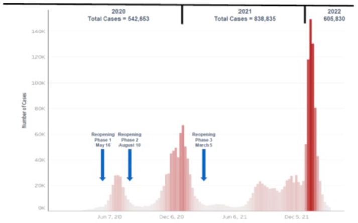
Figure 1: Arizona Reopening Phases 1-3 Weekly COVID-19 Cases: January 1, 2020 to March 6, 2022.
Source: Arizona Department of Health Services Arizona COVID-19 Weekly Case Graph.

At the end of the first year of Arizona Reopening Phase 3 (March, 9, 2021), there were 1,162,199 COVID-19 cases, 49,894 case hospitalizations, and 11,767 deaths associated with the virus in Arizona (Table 1). There were more cases, hospitalizations, and deaths in the second half of the year than the first half, but the percent of hospitalizations and deaths for those diagnosed with COVID-19 were lower in the second half.

Table 1: Arizona Reopening Phase 3 Total Numbers of COVID-19 Cases, Hospitalizations, and Deaths: March 7, 2021 to March 9, 2022.

Time Period

Cases Hospitalizations

Deaths

March 7, 2021 to September 4, 2021

202,240

14,859

(7.35%)

2,674

(1.32%)

September 5, 2021 to March 9, 2022

959,959

35,035

(3.65%)

9,093

(0.95%)

March 7, 2021 to March 9, 2022

1,162,199

49,894

11,767

Source: Arizona Department of Health Services COVID-19 Dashboard.
Arizona 2021 population estimate is 7,276,316, July 1, 2021 – U.S. Census.

Tables 2 and 3 track tri-weekly total and weekly numbers of COVID-19 cases, hospitalized cases, deaths, fully vaccinated individuals, and test given. The largest numbers of cases (141,475) and hospitalizations (3,514) occurred in the week of January 16 to 22, 2022, while the largest weekly number of deaths occurred in week of January 23 to 29 (626).

Table 2: Arizona Reopening Phase 3 Tri-Weekly State Total and Weekly Numbers of COVID-19 Cases, Hospitalizations, and Deaths: February 28, 2021 to February 26, 2022.

Week

Total Cases Wk. Case Total Hospital Wk. Hospital Total Deaths

Wk. Deaths

02-28 to 03-06

825,119

9,412 57,863 355 16,323

356

03-21 to 03-27

839,334

3,569 58,912 242 16,912

179

04-11 to 04-17

853,050

4,029 59,604 282 17,151

59

05-02 to 05-08

868,382

4,811 60,700 369 17,407

69

05-23 to 05-29

880,466

4,055 61,651 377 17,628

81

06-13 to 06-19

889,342

2,938 62,518 305 17,838

77

07-04 to 07-10

900,636

4,118 65,951 273 18,029

54

07-25 to 07-31

927,235

11,575 67,191 608 18,246

76

08-15 to 08-21

982,775

20,365 70,143 1,220 18,597

135

09-05 to 09-11

1,045,835

18,476 74,501 1,779 19,183

186

09-26 to 10-02

1,100,167

18,377 77,411 688 20,134

328

10-17 to 10-23

1,148,341

16,365 79,295 628 20,851

351

11-07 to 11-13

1,211,333

24,856 81,600 848 21,651

243

11-28 to 12-04

1,288,234

25,660 87,517 2,363 22,561

337

12-19 to 12-25

1,354,708

20,647 90,300 774 23,983

467

01-09 to 01-15

1,588,155

126,522 96,160 1,993 25,171

467

01-30 to 02-05

1,911,655

66,743 103,031 1,416 26,628 445
02-20 to 02-26

1,976,890

11,231 106,496 436 27,946 328

Source: Arizona Department of Health Services Coronavirus Database.
Arizona 2021 population estimate is 7,276,316, July 1, 2021 – U.S. Census.

Table 3: Arizona Reopening Phase 3 Tri-Weekly State Total and Weekly Numbers of Fully Vaccinated Persons and COVID-19 Testing: February 27, 2021 to February 26, 2022.

Week

Total Vaccine Week Vaccine Week Total Testing

Week Testing

02-27 to 03-05

711,074

214,577 02-28 to 03-06 4,271,425

85,839

03-20 to 03-26

1,211,279

136,567 03-21 to 03-27 4,473,079

51,621

04-10 to 04-16

1,812,090

197,061 04-11 to 04-17 4,630,490

51,273

05-01 to 05-07

2,416,859

144,358 05-02 to 05-08 4,783,625

50,407

05-22 to 05-28

2,759,177

60,481 05-23 to 05-29 4,921,306

45,655

06-12 to 06-18

3,041,625

85,694 06-13 to 06-19 5,039,927

38,162

07-03 to 07-09

3,192,966

37,218 07-04 to 07-10 5,144,503

31,929

07-24 to 07-30

3,341,364

28,211 07-25 to 07-31 5,273,201

51,388

08-14 to 08-20

3,451,880

44,584 08-15 to 08-21 5,516,055

97,680

09-04 to 09-10

3,588,303

32,433 09-05 to 09-11 5,796,559

76,540

09-25 to 10-01

3,703,834

38,345 09-26 to 10-02 6,029,558

76,008

10-16 to 10-22

3,675,384

10,300 10-17 to 10-23 13,422,057

200.955

11-06 to 11-12

3,820,202

22,862 11-07 to 11-13 14,098,439

248,598

11-27 to 12-03

3,883,284

23,029 11-28 to 12-04 14,767,374

222,428

12-18 to 12-24

3,940,418

17,536 12-19 to 12-25 15,447,386

233,443

01-08 to 01-14

4,005,295

28,316 01-09 to 01-15 16,459,838

468,734

01-29 to 02-04

4,196,274

144,853 01-30 to 02-05 17,701,703

338,584

02-19 to 02-25

4,284,855

30,044 02-20 to 02-26 18,277,270

151,628

Source: Arizona Department of Health Services Coronavirus Database.
Arizona 2021 population estimate is 7,276,316, July 1, 2021 – U.S. Census.

During the year, there were increases in the numbers of fully vaccinated individuals – 3,605,435 (March 6, 2021 to March 9, 2022) and testing – 14,190,759 (March 7, 2021 to March 9, 2022). The largest numbers of fully vaccinated person occurred in the week of April 17 to 23, 2021 (249,755). The week of January 15 to 21, 2022 had the largest weekly numbers of tests done (492,774).

Figures 2-4 compare the numbers of COVID-19 cases, hospitalized cases, and deaths by age groups on March 6, 2021 and March 9, 2022. A case could be mild, moderate, and severe. Most people recovered and did not require hospitalization. There was an increase of 1,162,199 cases during the study period. The 20-44 years age group had the largest number of cases and had an increase of 480,268 (Figure 2). There were more females (52.4%) than males (47.6%) who got the virus on March 9, 2022.

fig 2

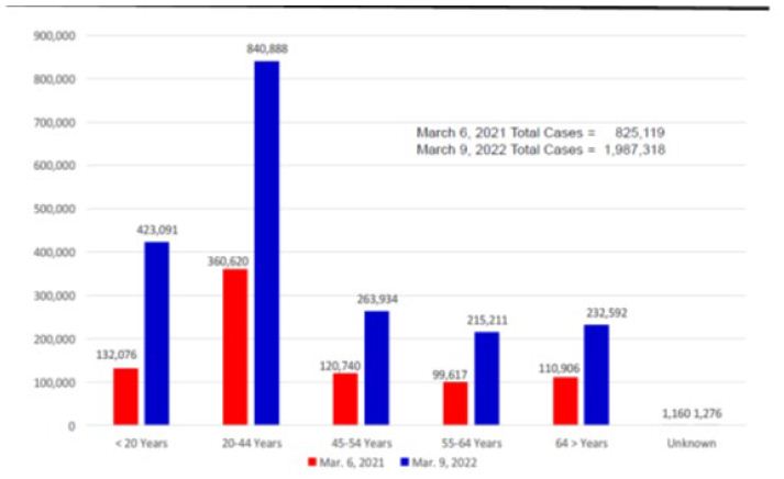
Figure 2: Arizona Reopening Phases 3 COVID-19 Cases by Age Groups on March 6, 2021 and March 9, 2022.
Source: Arizona Department of Health Services COVID-19 Cases by Age Groups Statistics.

The percentages of total hospitalized cases (severe cases) decrease from 7 percent on March 6, 2021 to 5 percent on March 9, 2022. The case hospitalizations had increased from 57,863 to 107,757. As expected, seniors had the highest numbers of the total hospitalizations (42.5% on March 9) and those under 20 years of age had the lowest numbers (4.4%). Twenty percent (19.7%) of seniors diagnosed with COVID-19 hospitalized, while 1.1 percent of those less than 20 years of age hospitalized. There were more males (52.3%) than females (47.7%) hospitalized. Figure 3 shows the hospitalization numbers for each age group with the virus on March 6 and March 9.

fig 3

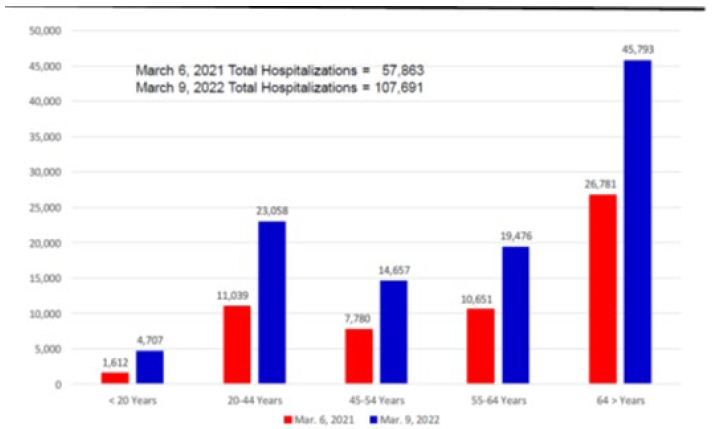
Figure 3: Arizona Reopening Phases 3 Hospitalized COVID-19 Cases by Age Groups on March 6, 2021 and March 9, 2022.
Source: Arizona Department of Health Services Hospitalized COVID-19 Cases by Age Groups Statistic.

The numbers of deaths had increased from 16,323 on March 6 to 28,090 on March 9. The rates of fatalities per 100,000 population increased 227.05 to 390.70. As expected, seniors had the highest numbers of total deaths (70.5% on March 9) and those under 20 years of age had the lowest numbers — 0.2% (Figure 4). Eight percent (8.5%) of the seniors diagnosed with COVID-19 died, while 0.01 percent of those under 20 years of age died. There were more males (59%) than females (41%) who died.

fig 4

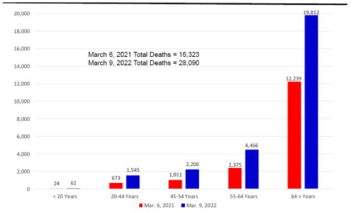
Figure 4: Arizona Reopening Phases 3 Weekly COVID-19 Deaths by Age Groups on March 6, 2021 and March 9, 2022.
Source: Arizona Department of Health Services COVID-19 Deaths by Age Groups Statistics.

The first U.S. COVID-19 vaccine, Pfizer/BioNTech, approved for emergency use authorization on December 11, 2020. In late December, Arizona began to administer vaccines. During Reopening Phase 3 (March 5, 2021 to March 9, 2022), there were 9,071,320 vaccine doses administered, and 3,605,435 fully vaccinated against the virus. Three vaccines were available in Arizona (Pfizer/BioNTech, Moderna, and Johnson & Johnson). The vaccines provided different levels of protection against COVID-19 and its variants. The vaccination percentages of those who had received at least one dose by five age groups were less than 20 years — 33.7%; 20-44 years — 65.0%; 45-54 years — 73.2%; 55-64 years – 79.8%; and 65 years and older — 97.2% on March 9. Figure 5 shows the numbers of COVID-19 vaccines given in Arizona (total doses given, persons receiving at least 1 dose, and persons fully vaccinated) during Reopening Phase 3.

fig 5

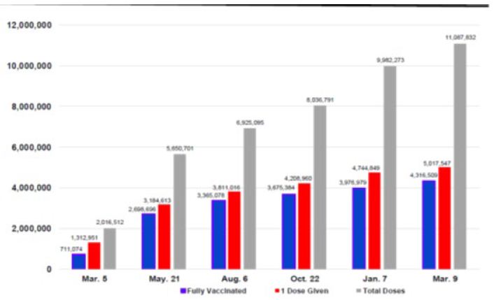
Figure 5: Arizona Reopening Phases 3 COVID-19 Vaccination Numbers: March 5, 2021 to March 9, 2022*.
Source: Arizona Department of Health Services COVID-19 Testing Statistics.
*Dates reported at 6-week intervals. Time period between February 5 and March 9 is 4½ weeks.

The number of COVID-19 tests done in Arizona had increased by 14,190,759 from March 6, 2021 to March 9, 2022 (Figure 6). On March 9, there were 18,462,184 total tests done.

fig 6

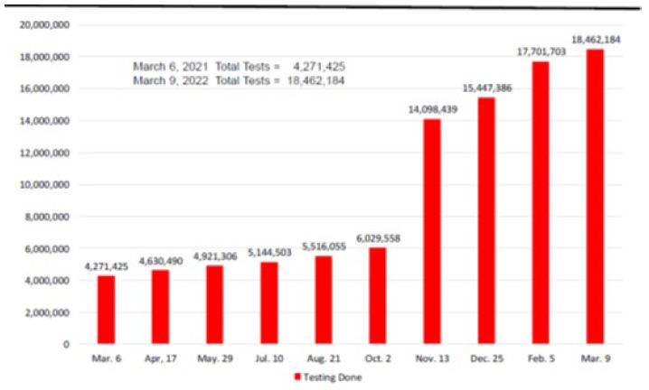
Figure 6: Arizona Reopening Phases 3 COVID-19 Testing Numbers: March 6, 2021 and March 9, 2022*.
Source: Arizona Department of Health Services COVID-19 Testing Statistics.
*Dates reported at 6-week intervals. Time period between February 5 and March 9 is 4½ weeks.

Discussion

The United States declared the COVID-19 pandemic as a national emergency on March 13, 2020 [10-12]. Since then, almost two years later, there had been 1,987,318 COVID-19 cases, 107,757 case hospitalizations, 28,090 deaths associated with the virus, and 11,087,832 vaccine doses administered in Arizona (March 9, 2022). More than 1 million new cases occurred during the Reopening Phase 3.

On March 5, 2021, the Arizona Governor began Reopening Phase 3 after the state had administered more than two million vaccine doses and several weeks of declining cases [8,9]. The state continued its efforts to vaccinate its population. The number of vaccine dosages administered had increase from 2,016,512 on March 5, 2021 to 11,087,832 on March 9, 2022. Fifty-nine percent (4,316,509) of the state population were fully vaccinated. The largest numbers of fully vaccinated persons occurred in the week of April 17 to 23, 2021 (249,755). The pace of vaccination began to slow down in June.

Arizona case numbers had decreased in the spring and early summer. At the end of June, the Arizona State Legislature and Governor had rescinded many of the state COVID-19 restrictions. During the month of July, the highly contagious Delta variant appeared in the state and began the summer surge.

The state and locate health departments increased their vaccination efforts as the Delta variant rose. The number of vaccination sites expanded throughout the state that included pharmacy chains, doctor offices, and community centers and clinics. The state targeted vaccination efforts to hard-to-reach minority and rural communities. The local governments, schools and universities, and private employers acted on their own to address the virus increases.

Even with the increase vaccination efforts and other actions, they were not enough to stop the Delta variant. The easing of the COVID-19 restrictions (e.g., those working at home returning to their workplaces, children and college students returning to in person classroom learning, and fans attending sport and entertainment events) made it easier for the virus to spread. This resulted in the fall surge and the case remained high in November. In December, the Omicron variant appeared in the state and surge in January and the cases remained high into early March. The Centers for Disease Control and Prevention (CDC) changed the COVID-19 transmission risk level for most of the state from high to medium on March 3. Medium transmission is 10 to 50 cases per 100,000 people or a positive rate between 5 and 8 percent for seven days.

There were many factors that contribute to the increase of cases. The Omicron variant was more contagious than the Delta variant. Even through 4,316,509 were fully vaccinated, there were significant number of state residents not vaccinated (40.8% as of March 9). Some of these unvaccinated had acquired natural immunity. Most of new cases were unvaccinated individuals. There were breakthrough infections of fully vaccinated or/and those received booster shots. Many who believe Omicron variant is a mild virus decided not to adhere to the preventive health protocols. Aggressive COVID-19 testing resulted in high number of identified cases. There was influx of out-of-state visitors (e.g., snowbirds and those attending Arizona events from out of state) who had or exposed to the virus.

Even though the case numbers rose, the numbers of hospitalizations and deaths were low because of COVID-19 vaccines and therapeutic drugs. The number of severe cases was low because significant numbers of the high-risk individuals and elderly vaccinated. On March 9, there were 97.2 percent of adults 65 and older had received 1 or 2 COVID-19 vaccine shots. There were several drugs approved by the FDA for treating COVID-19 (e.g., remdesivir, nirmatrelvir/ritonavir and molnupiavir) that reduced hospital length of stay and deaths.

Conclusion

The three vaccines and therapeutics kept the number of hospitalizations and deaths low. Even with the occasion case surges, the state normal were low number of severe cases, manageable hospitalization numbers, and low number of deaths.

References

  1. Johns Hopkins University Coronavirus Resource Center, https://coronavirus.jhu.edu/.
  2. Deliso Meredith (2021) “Arizona ‘hottest hot spot’ for COVID-19 as health officials warn of hospital strain: The state has the highest infections per capita globally, based on JHU data, ABC News. 2021. https://abcnews.go.com/US/arizona-hottest-hot-spot-covid-19-health-officials/story?id=75062175.
  3. Chow Denise, Joe Murphy (2021) These three states have the worst Covid infection rates of anywhere in the world: Arizona currently has the highest per capita rate of new Covid-19 infections, with 785 cases per 100,000 people over the past seven days, followed closely by California and Rhode Island, NBC News. https://www.nbcnews.com/science/science-news/these-three-states-have-worst-covid-infection-rates-anywhere-world-n1252861.
  4. Britannica, Arizona state, United States, https://www.britannica.com/place/Arizona-state.
  5. My Life Elsewhere, Arizona is around the same size as Italy.
  6. https://www.mylifeelsewhere.com/country-size-comparison/arizona-usa/italy.
  7. United States Census Bureau, Quick Facts, https://www.census.gov/quickfacts/AZ.
  8. Eng H (2020) Arizona and COVID-19. Medical & Clinical Research 5: 175-178.
  9. Eng H (2021) Arizona Reopening Phase 2: Rise and Fall of COVID-19 Cases. Medical & Clinical Research 6: 114-118.
  10. Eng H (2021) Arizona Reopening Phase 3 and COVID-19: Returning to Normal. Medical & Clinical Research 6: 687-669.
  11. White House Proclamation on Declaring a National Emergency Concerning the Novel Coronavirus Disease (COVID-19) Outbreak. 2020.
  12. https://www.whitehouse.gov/presidential-actions/proclamation-declaring-national-emergency-concerning-novel-coronavirus-disease-covid-19-outbreak/.
fig 1

Teens Evaluating Tag Lines of Foods: The Relevance of Seemingly ‘Throw Away’ Messages Revealed by Mind Genomics Cartography

DOI: 10.31038/NRFSJ.2022513

Abstract

In a large-scale study of teen food cravings using Mind Genomics, respondents evaluated short vignettes comprising 2-4 messages each, created by combining 36 elements about food. The source elements fell into, four silos of nine elements each (food, situation, taglines for emotions, brand/benefits). Silo C, taglines, was previously thought to be irrelevant to respondents who paid attention primarily to the descriptions of the food and the eating experience. Reanalysis of the data at the level of the individual respondent, and focusing only on the taglines for the products, revealed a rich source of information about how respondents feel about products, how males differ from females, how self-rated hunger drives different pattern of responses to the taglines, and uncovered three new-to-the-world mind-sets. The results suggest that taglines, often assumed to be ‘throw aways’ in test concepts, can actually provide a measure of the way the respondent feels about the food, this measure obtained in a subtle, almost projective fashion, with the focus on the internals of the person, not on the externals of describing the food and the eating.

Introduction

Researchers who focus on attitudes towards food do so from many angles, with interest ranging from the influence of physiological status on food, to the identification of what is important to a person’s decision making, and even to the messaging which drives decision making. The latter is especially important in the world of business, where it is critical to know what to communicate about food. Most of the research comprises questionnaires about how a person feels, whether this feeling is a simple acceptance scale [1], or deeper questions, such as what the respondent thinks about during the moments of craving a food [2-4]. The literature of attitudes towards foods has produced many thousands of papers, if not more, has been the subject of scientific investigation for hundreds of years, and a topic of interest in the popular media for decades, simply because we almost all enjoy food.

Two decades ago, during the early years of the 21st century, the senior author partnered with colleagues to create database of the mind of the consumer, focusing on food. The idea was to study 20-30 foods (or beverages), using the newly emerging science of Mind Genomics, to identify what was important to the consumer respondent. Rather than instructing the respondent to directly rate aspect by aspect in terms of importance to food, and especially to craving the food, the strategy was to create mixtures of messages, of the type that people encounter in everyday life. The messages comprised aspects such as the description of the food, the ambiance of consumption, the brand, and what was then considered a ‘throw-away’ space filler, but one which was oriented towards the fun of eating. This was ‘Silo C’, the ‘tagline’.

The research proceeded by mixing together these messages according to an underlying set of recipes, the so-called experimental design (REF). Figure 1 shows an example of the stimulus. The respondent did not see the boxes at the left, but simply saw combinations of elements, the messages, shown in the center of Figure 1. The respondent’s task was simply to read the vignette, and assign a rating. The task required the respondent to read and evaluate 60 different combinations, a task which took 10-12 minutes. Although the array of combinations, the so-called ‘vignettes’ seems like a set of randomly constructed combinations, the reality was and remains that in these Mind Genomics experiments great care is taken to create systematic combinations, each combination or set of 60 vignettes different from every other set, and each vignette comprising precisely the correct set of combinations to allow analysis by OLS (ordinary least-squares) analysis, even at the level of the individual respondent [5]. This design is called a permuted experimental design.

fig 1

Figure 1: Example of a vignette

To the respondent, the test combinations may appear to be haphazard combinations of messages the respondent was simply asked to read the combination, and rate the combination. The rating was ‘How intense is your craving for this FOOD NAME HERE IN CAPS). Most respondents looking at Figure 1 (without the call outs, but simply with the material present on the screen) begin by trying to ‘give the right answer’, but in the end the task to discern the pattern gives ways to a pattern of ‘read and rate.’ For the most part the respondent pays attention, but is not engaged in the task. The respondent is doing the task, but with little clear involvement, something which occasionally worries the researcher who would rather see a deeply engaged respondent. It is hard to be engaged when one has to evaluate 60 of these systematically created vignettes, but respondents do it, especially when they are motivated by rewards. The pattern makes it impossible for the respondent to game the system; Mind Genomics uses the statistical discipline of experimental design to create the combinations. When the study with 30 foods was done in 2002, the design used then was the so-called 4×9. The 4×9 design called for four silos or questions, each silo or question populated by nine different answers, or elements. The underlying experimental design called for 60 vignettes for each respondent, most comprising four elements, some comprising three elements, and some comprising two elements. Each respondent was given a different, permuted set of combinations, so that the combinations cover a great deal of the design space (rather than focusing on a narrow set of combinations, reducing the variability around those combinations, assuming those combinations are the correct ones to investigate.

The expectation was that the respondent would respond most strongly to the elements in Category 1 (product features), and perhaps secondly, to elements in Category 4 (brand, benefit). It was not clear what would be the response to elements in Category 2 (situation, mood), and especially those elements in Category 3 (emotional attribute, hereafter call ‘taglines’).

With this introduction, we now proceed to the actual experiment. Keep in mind that the analyses of these data is really a reanalysis of the results almost 20 years later, bringing into the work experience from two decades, and the evolution of thinking about what these data mean. The focus here is no longer on the rest of the data, but rather on what can be learned from the data of Category C, the ‘taglines’ or the emotional elements. The study here focused on teens, a continuation of an earlier studier of the same type, dealing with adults, using the same material, but focusing on older respondents [6]. The work with teens at that time was part of the expansion of Mind Genomics across test populations, especially beyond North American adults. Research among teens was the first major effort in this expansion, with the focus beyond foods to entertainment such teen e-zines [7].

The study reported here moves beyond the simple report presented first in 2002 to the IFT (Institute of Food Technologists), and appearing in a cursory overview in the journal Appetite in 2009 [8]. Those early presentations were made to a world of researchers who had never seen the It! studies, and were presented with a superficial view of this new approach to understanding people. It suffices simply to present the study is brief, since there was nothing like these new-to-the-world It! studies.

The analysis now focuses on the taglines, the nine emotion descriptors (C1-C9), previously considered minor. In It! studies these types of elements usually generated coefficients, utility values, hovering around 0, sometimes positive (viz., driving craving), sometimes negative (viz., not driving craving). In the interests of the science of that time, the formative years 2001-2005, these elements were ignore because of their poor performance in terms of their ability to drive rating ‘craving.’ With the increasing focus on clustering people with like patterns of response to these elements, and with the opportunity to compare the same elements across the many foods of the study, the reanalysis beckoned.

Method

Mind Genomics project are set up in a certain fashion, and analyzed to reveal patterns [9]. Over the years, the design has been modified made shorter Yet, despite the evolution towards simplicity, the Mind Genomics approach has become routinized, and the analysis made simpler, almost following a script [10]. The benefit of that ‘processization’ is that the research can focus on the data, the findings, and not on dealing method again and again. We present the process as the skeleton for reanalyzing the data.

Step 1: Choose the Foods to Study

Figure 2 shows the list of foods. Figure 2 comes from landing page to which the response is directed, for those respondents who choose to participate. As yet, the respondents do not know anything about the study. They are simply invited to participate, choosing the food they want. The objective was to have the respondent evaluate the foods that she or he liked. When the quota was filled (95 participants), the food and its button ‘disappeared’ from the screen, forcing the respondent to choose another food. The foods were the same as were used in the previous study, this time with adults [11].

fig 2

Figure 2: The 30 foods available for the respondent. The teen respondent went to the site, and chose the study which seemed most interesting

Step 2: Create the Design Structure and the Elements

The It! studies run 20 years ago were characterized by the 4×9 design, four ‘silos’ (categories in Figure 1) each with nine ‘elements’. The experimental design for Mind Genomics is set up to ensure that mutually incompatible elements are never allowed to appear together. That is the function of experimental design serves both a science role to allow for strong analysis at the level of the respondents (within subjects design) and a bookkeeping role to ensure that certain mutually incompatible combinations never occur, such as two different foods appearing together. Table 1 lists the key features of the 4×9 design.

Table 1: Key features of the design

table 1

Step 3: Combine the Elements into Vignettes, according to an Experimental Design

The typical approach espoused by researchers is to isolate the variable and study the variable in depth. The reality, however, is that the respondents don’t think about most things in their lives as being one-dimensional since meaningful things in their lives are combinations of features. If we want to learn about the relevance of each of the variables, the most practical thing to do is to systematically change the nature of the variables, creating several combinations, and then evaluate the combinations. This more practical strategy calls for experimental design.

The objective of experimental design is three-fold:

  1. Balanced, equal number of presentations of each element.
  2. Statistical independence, so that individual elements appear in a pattern making them statistically independent of each other, even at the level of the individual respondent. This first objective ensures that the data can be analyzed by OLS (ordinary least-squares) regression, at the level of the individual respondent, allowing for deep analyses. The ‘incompleteness of vignettes’ ensures that the coefficients emerging from the OLS regression possess the property of being absolute numbers, comparable across different studies.
  3. Bookkeeping, ensuring that mutually contradictory elements never appear together, such as two different stores in which the product is sold, or two different moods.

Step 4: Launch the Study, Collect the Ratings

Although there has been an ongoing effort to source market research respondents from individuals who volunteer their time (viz., using messages such as ‘your opinion counts’) the reality is that the studies are easier when one sources the respondents from company specializing in online research. These panel providers work with many respondents, and deliver respondents for a fee.

It is worth noting that the respondents were provided by a Canadian company, Open Venue, Ltd., in Toronto, Open Venue specialized in recruiting respondents for these types of online studies. It might seem more economical to recruit one’s own respondents, but the truth is that the study takes a very long time to complete. With Open Venue, and with the popular topic of food among teens, the 30 studies required a day or two to complete. The entire study took about three or four days in 2002.

The screening specifications were only about half males, half females, ages 16-20. The gender and ages were the proprietary information of Open Venue, Ltd. As is typically the case, the ages may have been somewhat out of date, so some respondents were older than their panel information would have one believe, simply because the ages were not updated every day.

The respondents were invited, went to the site shown in Figure 2. This first landing page invited the respondents to choose food. After the respondent chose the food, the respondent read the orientation page. All 30 studies began with the same orientation page, albeit individualized with the specific food name. The orientation page presents little information about the study. The reason for such paucity of information in the set -up is that the respondents are to be judging the food, and their craving for the food strictly on the basis of the information provided in the test vignette (Figure 2).

Figure 1 presents an example of a 4-element vignette, showing the category (viz., silo) from which, each element originates. The actual vignettes do not show the silo or the identification number of the element. Rather, the vignette simply shows the elements prescribed by the experimental design, in unconnected form. Having connectives in the vignette is neither necessary nor productive. Respondents inspecting a vignette do not need to have the sentences connected. They simply need to have the information available in an easy to discover way. Figure 1, in its spare fashion (without explanatory material with arrows), does just that.

Steps 5 and 6 – Create the Database Showing Respondent, Vignettes, Rating, and Answers to Classification Question

Mind Genomics is set up to acquire data in a structure, rapid, and efficient fashion, almost ready for statistical analysis after two transformations. Each respondent who participated was assigned a panelist identification number. The respondent’s data from the 60 vignettes were put into a database to which each respondent contributed 60 rows of data. Each row corresponds to a respondent and a vignette presented and evaluated. The Mind Genomics program constructed the vignettes ‘on the fly’ as the study was progressing, presented the stimulus, acquired the response, and populated the database, all in real time. The construction of the database appears in Table 2.

Table 2: Construction of Mind Genomics data for the Teen Crave it study

table 2

Step 7 – Result for Total

The database constituting the focus of our attention be the database emerging from the use of the OLS (Ordinary Least Squares) regression on the data of each individual. Thus, we will deal with 2000+ equations, and in the same form, different only by the respondent who generated the equation and the food. Our focus will be only on the coefficients of C1-C9, the tag lines as we have called them.

The rationale for focusing only on the tagline is that in study after study, these taglines never perform as well as the elements which describe the product. Yet, the advertising agencies focus on these elements. In previous studies of this type, and in virtually every study, the emotions, and taglines, so often felt to be important by salespeople, but technical people as well, score poorly. By ‘poor’ is meant low values for the coefficients. The ingoing explanation is that people focus on the food, and not on the feelings about the experience. In the worlds of poetess Gertrude Stein who opined for many objects and people ‘‘there’s no there there’. Certainly, there is a point to that statement since there is nothing about real food and real life in tagline elements, C1-C9.

Table 3 shows the summarized results of food (row) by tagline (column). The data come from the summary table of coefficients described in the bottom part of Table 2, dealing with the databasing of the summary models. The table presents only positive coefficients of 2 or higher. The negative and zero coefficients are not shown. Thus, these positive coefficients are those which drive craving. The coefficients in Table 3 are averages from all of the respondents who participated in the particular study. All coefficients of 8 or higher are shaded, corresponding to the fact that these coefficients are statistically significant (p<0.95).

Table 3: The foods and the elements, showing only those combinations with coefficients 2 or higher. The foods are sorted in descending by the sum of the coefficients across the elements. The elements are sorted in descending order by the sum of the coefficients across the foods

table 3

The foods are sorted from top to bottom by the sum of the positive coefficients (+2 or higher), as shown in Table 3. Thus, the food with the highest sum of coefficients is popcorn, the lowest is cinnamon rolls. Then the columns are sorted from left to right in descending order, so that the element with the highest sum of coefficients (When you think about it, you have to have it … and after you have it, you can’t stop eating it) is at the left, and the element with the lowest sum of coefficients is at the right (When you’re sad, it makes you glad).

The table as constructed from the Total Panel provides virtually no insight, except for the observation that only six elements generate coefficients of +8 or higher, and only among one of the nine tagline elements, C1-C9. It should come as no surprise that for virtually of the It! studies reanalyzed during the past 20 years, these ‘tag lines’ have been discarded, because they seem not to have any profound insight about the mind of the respondent. The coefficients are low, and even when they are studied together with other elements, such as the names of foods, and the health benefits, these ‘tag lines’ seem to vanish into irrelevance. Parenthetically, it would take 20 years, and a separate way of thinking about Mind Genomics data of this type, in a specific format, to provide the impetus to reanalyze the data, and to reveal new findings and patterns reported here.

Step 8 – Results by Gender

Respondents classified themselves by gender. Thus, it was straightforward to compute the average for each of the nine elements by gender and by food. Rather than total, we present the results for by gender. When we separate the respondents by gender we have many more elements with positive coefficients. The patterns are easier to discern when we retain for consideration only those average coefficients of 10 or higher, for a specific gender/food/element combination. The other averages, 9 or lower, are eliminated from the table. We also eliminate any element whose sum of positive coefficients is 23 or lower. (Parenthetically, the original cut-off point for sum of positive coefficients for an element was 24 or lower, but that would have eliminated males.

Table 4 shows a dramatic pattern. Teen Females show far more strong performing combinations, and the magnitudes of the coefficients are higher. The difference is simple. Teen females appear to crave meat; teen males appear to crave chocolate and sugar.

Table 4: Strongest cravings for genders based upon the tag lines

table 4

Step 9 – Results by Self-rated Hunger at the Time of Participation

The respondents were instructed to rate their hunger on a 4-point scale. Table 5 compares the coefficients for the elements by food, again showing only coefficients which are 10 or higher. Unexpectedly, few foods show strong coefficients for the taglines, perhaps because there may be other elements, such as food description, which are more salient when a respondent is hungry. When we look through the lens of the tag line, we see only three emerging. For those with low hunger the foods are steak and nuts, and the taglines are celebration. For those with moderate to high hunger the only element which really satisfies the requirement is an olive, perhaps because of the noticeable salt taste.

Table 5: Strongest cravings during hunger state, based upon the tag lines

table 5

Step 10 – Identify Mind-sets in the Population Showing different Patterns of Coefficients

A hallmark of Mind Genomics is the discovery of mind-sets, similar patterns of responses to elements from respondents who seem otherwise not related to each other by the pattern of their self-described profiles in a classification questionnaire. Typically, a study may generate 2-3 mind-sets when the topic is multi-faceted. More mind-sets or clusters can be generated but with the increasing number of mind-sets the power of the clustering decreases because the results become increasingly harder to use.

The clustering here is done independent of the specific food, viz., incorporates all of respondents into one dataset, and clusters that dataset. The only information used for the cluster is the set of nine coefficients. Furthermore, those respondents whose coefficients were all 0 for the nine coefficients were eliminated ahead of the clustering, because they showed no pattern of differentiation among nine tag line elements, C1-C9.

The k-means clustering program computed the pairwise ‘distance’ between each pair of respondents, by computing the Pearson correlation. The correlation, in turn, is a measure of the strength of a linear relation, with a high of +1 to denote a perfect linear relation between the coefficients of two respondents, down to a 0 to denote no relation, down to a low of -1 to denote a perfect inverse relation. The distance (defined as 1-Pearson R) goes from a value of 0 when two respondents show perfect correlation in their coefficients, up to a value of 2 when two respondents show perfect inverse correlation [12].

The clustering was done on the nine coefficients for each respondent, independent of the specific product the respondent was evaluating in the Mind Genomics experiment. Each respondent generated additive constant and 36 coefficients, one for each element. The analysis kept only the coefficients C1-C9, which constitute the focus of this analysis. In most Mind Genomics studies the deconstruction of the respondent population into mind-sets allows the different, often opposite-acting groups, to emerge. The groups no longer cancel themselves out. This can be said for the mind-sets developed out the tag lines. Table 6 shows three clearly different groups, with higher coefficients for the different foods. Furthermore, the groups make intuitive sense.

Table 6: Strongest cravings during hunger state, based upon the three emergent mind-sets

table 6

MS1, Mind-Set 1, appears to respond to elements C7 and C5, focusing on eating as recreations. The foods make sense.

MS2 appears to response to elements talking about an internal strong response, a ‘high’. The foods are unexpected, popcorn, steak, and water, respectively. The reason for this is not obvious at this time.

MS3 appears to respond to elements about eating as sensory pleasure. The three foods are all laden with sugar and are soft in text or even liquid; peanut butter, ice cream, and cola.

Classification

Table 7 presents the classification of respondents into the three mind-sets, by total, then by gender, self-reported hunger and food, respectively. There are patterns of mind-sets vs. food, e.g., for hot dog 51% of the respondents fall into MS1, whereas for cola 51`% of the respondents fall into MS2, and for olives 43% fall into MS3. There are no clear patterns, but the Mind Genomics approach permits the researcher to move beyond the conventional psychographic clustering often heralded as a major advance beyond clustering based upon geo-demographics [13].

Table 7: Distribution of the three mind-sets by key groups (total, gender, self-reported hunger, food study in which the respondent participated)

table 7

Discussion and Conclusions

The original analysis for the Crave It! studies focused on the strongest performing elements, looking at the different foods, as well as the different groups within each study, specifically gender. The effort to discover mind-sets had originally motivated all of the It! studies, the Teen Crave It! no different than any of the others.

The results of the early studies revealed that the respondents divided most strongly on the response to the food and to the eating experience. The ‘tag lines’, shown in Table 2, were low in comparison to the coefficients for the different foods and in each study. Again and again, the foods themselves and the eating situations showed double-digit positive coefficients, and an occasional negative coefficient. The obvious conclusion at that time was that the tag lines are unimportant, at least during the early 2000’s when the It! studies were run.

The observation leading to this paper was not so much an observation as a question. The question was simply ‘what would happen if we were to look at the coefficients of the tag lines’, not from the total panel, but broken out into foods, gender, stated hunger, and even use the coefficients of these tag lines (C1-C9), alone, by themselves, to generate mind-sets? The decades of experience of with Mind Genomics had revealed, again and again, that the simple and rather startling result that of coefficients around 0 often hid profound, interpretable, and instructive differences between groups, occasionally differences that could be labelled ‘remarkable.’

The analysis with the tag lines reveals a world of insight lurking below the surface of these relative low coefficients, doing so for elements which do not at the surface pertain to food in the way that food names and eating situations do (Elements A1-A9, and elements B1-B9).

The most difficult part of the analysis was to enable the discovery by paring away the extra numbers. It is one thing to pare away noise which is clearly noise, elements which are negative or close to zero. The focus is on the food. The elements which score high with regard to that food, especially on the rated attribute of craving, allow the pattern to come through. In this analysis, however, we are searching for a more amorphous pattern, not one easily observed. The issue becomes to create criteria which allow fair elimination of a lot of the data, without so-called ‘p-hacking’ or searching for effects, and then claiming those effects to have emerged as reportable outputs from the study and expressed within the original hypothesis. For these data the discovery of the patterns is a matter of paring away different sets of coefficients, pertaining either to foods (rows) or elements (columns), so that the underlying pattern makes sense. That approach, subjective in nature, consists of eliminating foods which generated low coefficients across elements, and eliminating elements which generated low coefficients across foods do so in an iterative fashion until the patterns become stable, and the story emerges, perhaps even compelling.

Thus, the analysis closes; the ‘story’ now expands to promote the relevance of tag lines as a new way to understand the mind of the consumer in the case thinking about foods. It may be these taglines, almost throwaway, amorphous statements, which provide new insights. In a sense, the tagline becomes the screen onto which the other aspects of the respondent’s mind are projected; witness the emergence of the three mind-sets.

References

  1. Pilgrim FJ, Peryam DR (1958) Sensory testing methods: A manual (No. 25-58). ASTM International.
  2. Harvey K, Kemps E, Tiggemann M (2005) The nature of imagery processes underlying food cravings. British Journal of Health Psychology 10: 49-56. [Crossref]
  3. Tiggemann M, Kemps E (2005) The phenomenology of food cravings: the role of mental imagery. Appetite 45: 305-313. [Crossref]
  4. Weingarten HP, Elston D (1991) Food cravings in a college population. Appetite 17: 167-175. [Crossref]
  5. Gofman A, Moskowitz H (2010) Isomorphic permuted experimental designs and their application in conjoint analysis. Journal of Sensory Studies 25: 127-145.
  6. Moskowitz H, Silcher M, Beckley J, Minkus-McKenna D, Mascuch T (2005) Sensory benefits, emotions and usage patterns for olives: using Internet-based conjoint analysis and segmentation to understand patterns of response. Food Quality and Preference 16: 369-382.
  7. Moskowitz H, Itty B, Ewald J (2003) Teens on the Internet-Commercial application of a deconstructive analysis of ‘teen zine’ features. Journal of Consumer Behaviour: An International Research Review 3: 296-310.
  8. Foley M, Beckley J, Ashman H, Moskowitz HR (2009) The mind-set of teens towards food communications revealed by conjoint measurement and multi-food databases. Appetite 52: 554-560. [Crossref]
  9. Moskowitz HR, Gofman A, Beckley J, Ashman H (2006) Founding a new science: Mind Genomics. Journal of Sensory Studies21: 266-307.
  10. Biró B, Gere A (2021) Purchasing bakery goods during COVID-19: A Mind Genomics cartography of Hungarian consumers. Agronomy 11: 1645.
  11. Moskowitz H, Beckley J, Adams J (2002) What makes people crave fast foods?. Nutrition Today37: 237-242.
  12. Likas A, Vlassis N, Verbeek JJ (2003) The global k-means clustering algorithm. Pattern Recognition 36: 451-461.
  13. Wells WD (2011) Life Style and Psychographics, Chapter 13: Life Style and Psychographics.

Characterization in Adolescent from Families’ Consumers of Alcohol in a Community of Health

DOI: 10.31038/JCRM.2021433

Abstract

Context: To improve the life styles from the Cuban community context of family health is a reality linked with the medical sciences.

Objective: To characterize in adolescents from families consumers of alcohol in a community of health. This process embraced the period of September 2018 to June 2019. The qualitative methodology was used, with a descriptive and traverse study. The universe the 45 adolescents in families of studies, selected in an intentional way.

Methods: Observation, interview and revision of clinic history and the techniques were: test of family operation.

Results: It was evidence that toxic styles of life exist. The male sex was the more affected for 56% by alcoholic relatives. The most frequent causing lifestyles of family dysfunction were the daily ingestion of alcoholic drinks.

Conclusions: The families present difficulty in the family relations. The addiction to the alcohol is related with the tolerance and consumed by day that it generates in the life style from the family operation.

Keywords

Alcoholism, Adolescent, Addiction, Family relations, Styles of life, Health

Introduction

The family is the most important social group in any society, it is the place where the formation of the personality begins and where the affections are committed with the interactions among their members. The economic, biological, educational and satisfaction functions of affective and spiritual needs that the family group plays are of marked importance because, through them, values, beliefs, knowledge, criteria and judgments that determine the health of individuals and the collective are developed and its members; a disease such as alcoholism in one of its members affects the dynamics of this family group. The World Health Organization (WHO) defines alcoholism as a disease characterized by the excessive and frequent ingestion of alcoholic beverages whose consumption can cause the phenomena of tolerance and dependence that cause biological, psychological and social damage in the individual [1,2].

Alcoholism is a chronic disease that damages the organism, family and social functioning and can be a cause of violence, antisocial behavior, family disagreements, accidents and even homicides. The best places to avoid the excessive consumption of alcoholic beverages are the family and the community, because there the individual must learn healthy lifestyles, among which the excessive consumption of alcohol does not enter. The addiction continues being a dysfunction caused by a substance able to produce dependence, the alcohol. In the medical sciences the health is defined as the state of beneath bio psychosocial and spiritual and not the absence of illnesses. The addiction continues to be a dysfunction caused by a substance able to produce dependence, the alcohol. In the medical sciences the health is defined as the state of bio psychosocial and spiritual and not the absence of illnesses. Adolescence is a stage of life between childhood and adulthood that is intimately related to both since many characteristics of the previous stages are present with other new ones evidenced until then. In adolescents, alcohol consumption is often associated with fun, self-determination, leisure and modernity and constitutes an element that gives status to their group of members, which makes it more difficult to eliminate them despite negative consequences derived from excessive consumption. For teenagers, among whom the most popular drug is alcohol, this is undoubtedly a dangerous drug with consequences that can endanger life; hence it is called drug porter and model [3-5].

Cuba, do not escape this problem. Research studies have been conducted where a significant number of adolescents are at risk of becoming alcoholics at some point in their adult lives; hence it was decided to conduct a study aimed at knowing if the functioning of the families of adolescents’ risk of alcoholism influences his behavior before this toxic. In such a sense thinks about the following scientific problem: How characteristic it presents the adolescents from families’ consumers of alcohol in a community of health? The general objective that thinks about is to characterize in adolescents from families consumers of alcohol in a community of health.

Methods

The families was carried out a descriptive study, traverse with adolescents from a context of community family health of the municipality Santa Clara, Cuba in the understood period of September 2018 to June 2019, with the objective to characterize in adolescents from families consumers of alcohol in a community of health. It was study object a universe constituted by 45 adolescents and families of studies, selected in an intentional way. Methods of the theoretical level: Analytic synthetic: It facilitated the interpretation of the texts and to establish the corresponding generalizations. Inductive-deductive: facilitated to go of the peculiar to the general thing in each one of the analyses carried out in the theoretical study. Generalization: It allowed the establishment of the regularities that showed in the carried out study.

Empiric Level

Revision of Family Records

It constitutes a legal document, doctor and official zed of great personal and acquisitive value, to be registered the entire relative one prior to the clinical history of the family, gathering and obtaining more reliable and richer information for the investigation.

Clinic History

It is applied with the objective of measuring the indicators that influence teen alcohol consumption.

Test of Family Operation

It is applied with the objective of measuring the level and incidence of some determinant of the health in the context of the family, talkative relationships and life styles.

Inclusion Approaches

I. Adolescents with families’ consumers of alcohol.

II. That they resided in the area of chosen health.

Exclusion Approaches

III. Families that emigrate of their residence place during the study.

Exit Approaches

IV. Adolescents and families that abandon the investigation voluntarily.

Statistical Analysis

The information was stored in a file of data in SPSS version 12.0 and it is presented in statistical chart; for the description it was calculated with the method statistic of Fisher.

The absolute and relative frequencies were determined. For the analysis of the qualitative variables, the X² statistic was used to determine the independence between factors and for goodness of fit with a level of significance α = 0.05; there are significant differences when ρ<0.05 and not significant when ρ>0.05.

Results

Chart 1 refers to indicators according to behavior and sex, where it was appreciated that the most common reason was the group contagion given in a typical camaraderie code of this psychological age represented by depression (97,6%), followed by the presence of frustration feeling (75,6%) and undervaluation with 70,7%.

Chart 1: Distribution of adolescents according to indicators of behavior and sex

Indicators of the behavior in adolescents

Sex

Female

Male

Total

No.

% No. % No.

%

Depression

11

91,6 29 100,0 40

97,6

Frustration feeling

9

75,0 22 75,9 31

75,6

Undervaluation

8

66,7 21 72,4 29

70,7

low self-esteem

8

66,7 20 68,7 28

68,3

Anxiety

5

41,7 14 48,3 19

46,3

Group imitation

3 7,3 3

7,3

Source: Clinic history

It is important to highlight that adolescents who feel depressed have a high probability of consuming alcohol as aversive way, which was reflected in the present work, where 68,3% of the subjects admitted that they had done it for causes of low self-esteem.

Discussion

Among the students surveyed, an average age of 13 years was observed, with a greater predominance for males, which coincides with other studies related to psycho-affective and social disorders in adolescents with alcoholic relatives. These results can be justified because at this stage of life adolescents feel invulnerable and assume omnipotent behaviors, almost always generators of risk; In turn, the school group in which it operates has great influence and its behavior will be highly influenced by the opinion of the same when making decisions and undertaking a task. The group constitutes a way of transmitting norms, behaviors and values that, on occasions, is more influential than the family itself. In such a sense the members of the family should contribute with appropriate attitudes to the improvement of an effective communication that allows a dynamic and systematic. The majority of adolescents presented several situations prone to consume alcoholic beverages, which justifies inadequate coping styles that adversely affect family functioning and their integral health. Family arguments and domestic violence are an impediment to the adolescent’s training and, at the same time, situations that tend to give the adolescent a risk behavior when faced with alcohol consumption. In many cases one of the members of the family was a consumer of alcohol, which is a factor that triggers stress and changes in family functioning. Similar results were found when reviewing the studies of several authors in the country that consider alcoholism, together with conflicts in the family nucleus, as a risk factor of considerable value for families to lose their structural and functional stability. Great social impact has the fact that adolescents are deformed in their behavior, caused by the family environment, it was shown that the ingestion of alcoholic beverages is an important factor causing family dysfunction [6-12].

For the majority of adolescents alcoholism is not a disease, only a low percentage of them recognize it that way, so the little perception of risk that the studied patients present is worrisome, although most of them see it as a drug, a vice, a dependency and a bad habit; It is alarming that many of the adolescents see it as a way to share with friends, as a feature of manhood and as a pleasure, all linked to the risk factors present in these families. In adolescents, alcohol consumption is often associated with self-determination, fun, leisure and modernity and constitutes an element that gives status to their group of members, which makes it more difficult to eliminate them despite the consequences negative consequences of excessive consumption and not to consider it as a scourge that harms human values. Many authors have studied the family dynamics in the home of origin of the alcoholic and point out the coincidence of several alterations when they characterize the children and adolescents who live with these patients. Many of the children who have behavioral difficulties grow up in an inadequate family environment and learn to survive, although not to thrive. Children raised in such circumstances arrive at school without possessing experience, nor the necessary aptitude for a methodical instruction and they do little in school [13,14].

Conclusions

Keeping in mind the individual values and the reference group to that belong, for what becomes necessary to carry out strategies educative that allow a well-being bio psychosocial and spiritual to these adolescents coming from families dysfunctional. Although these adolescents come from families dysfunctional he biggest percent they are independent, this can be associated to that the adolescence is a stage difficult of the development where the independence can be favored, the freedom in the taking of decisions or the imitation to the adults from the family operation. By way of conclusion according to like the internal and external conditions are developed starting from the interaction with the diverse subjective configurations from the family context. The families present difficulty in the family relations. The addiction to the alcohol is related with the tolerance and consumed by day that it generates in the life style.

Conflict of Interest

The author declares no conflict of interest

References

  1. López RM, Quirantes MMJ, Pérez MJA (2006) Pesquisaje de alcoholismo en un área de salud II. Rev Cubana Med Gen Integr 22: 2
  2. Colectivo de autores. Alcoholismo, Cuida tu salud. Cuba, Ciudad de la Habana: Edición Digital; 2006.
  3. Barnow S, Schuckit MA, Lucht M, John U, Freyberger HJ (2002) The importance of a positive family history of alcoholism, parental rejection and emotional warmth, behavioral problems and peer substance use for alcohol problems in teenagers: a path analysis. J Stud Alcohol 6: 305-15. [crossref]
  4. García PRP, Toribio MA, Méndez SJM, Moreno AA (2004) El alcoholismo y su comportamiento en cinco Consultorios Populares de Caracas en el año. Med Gen 187: 522-28.
  5. Gruenewald PJ, Russell M, Light J, Lipton R, Searles J, et al. (2002) One drink to a lifetime of drinking: temporal structures of drinking patterns. Alcohol Clin Exp Res 26: 916-25.
  6. Sánchez CME, Ramírez TA, González ED, Castellanos VE, Ojeda RJ (2006) Trastornos psicoafectivos y sociales en adolescentes con familiares alcohólicos. Rev AMC 10: 1
  7. González R (2005) Secretos para prevenir, detectar y vencer las drogadicciones. La Habana: Científico- Técnica.
  8. Bolet AM (2000) La prevención del alcoholismo en los adolescentes. Rev Cubana Med Gen Integr 16: 406-409.
  9. Martínez HAM. (2008) Alcoholismo, hombre y sociedad. 2da parte y final. Adicciones, Salud y vida.
  10. Ortiz GMT, Louro BI. Jiménez CL. Silva ALC. (1999) La salud familiar.Caracterización en un área de salud.
  11. Pereira JI, Sardiñas Montes de O. (1999) Comportamiento de la violencia intrafamiliar sobre adolescentes en un área de salud. Rev Cubana Med Gen Integr 15: 3
  12. Mancilla C, Pereira C (2002) Un estudio de factores psicológicos, socioculturales e individuales. Chile: Universidad Valparaíso.
  13. Otaño FY, Valdés RY (2004) Algunas reflexiones sobre el alcoholismo en la comunidad. Rev Cubana Enfermer 20: 3.
  14. Sánchez MA (1998) Modalidades de conducta ante el alcohol en adolescentes. MEDISAN 2: 3.

Late Life Depression: Review of Perception, Assessment and Management in Community Dwellers

DOI: 10.31038/ASMHS.2022613

Abstract

Depression is one of the mental health conditions identified and projected to be the second leading cause of burden of disease in late life and unfortunately concerns for its debilitating consequences have birthed the need for continuous studies into its etiology, risk factors and management options (WHO, 2017). As the world aged population increases (by 2 billion persons in the next 30 years from 7.7 billion currently to 9.7 billion in 2050), number of older adults aged 65 years and over is projected to proportionately grow by 50% from about 727 million in 2020 to more than 1.5 billion by 2050 (United Nations, 2020) invariably implying that one in six people worldwide will be aged 65 years and over. Averagely, the number of older adults manifesting symptoms of mental disorders such as depression is set to increase proportionately among the estimated population.

The sudden but precipitated increase in incidences of depression across all ages had necessitated the need for constant reviews of mental health disorders. Factors that informed the mental health decisions of community dwelling older adults are hinged on their personal convictions on the presence of the disease and not just another somatic related illness. These convictions are quite germane to the kind of treatment they sought for and could invariably be the major reason why geriatric depression has consistently been misdiagnosed or undertreated very often among community dwelling older adults.

Keywords

Late life depression, Mental health, Burden of disease, Community dwelling older adults

Introduction

Depression is one of the mental health conditions identified and projected to be the second leading cause of burden of disease in late life and unfortunately concerns for its debilitating consequences have birthed the need for continuous studies into its etiology, risk factors and management options across all populations and samples [1]. As the world aged population increases (by 2 billion persons in the next 30 years from 7.7 billion currently to 9.7 billion in 2050), number of older adults aged 65 years and over is projected to proportionately grow by 50% from about 727 million in 2020 to more than 1.5 billion by 2050 [2] invariably implying that one in six people worldwide will be aged 65 years and over. Averagely, the number of older adults manifesting symptoms of mental disorders such as depression is set to increase proportionately among the estimated population. Good news however is that mental health issues in late life has been explored within different population of older adults globally.

Specifically, literature exploring late life depression in community samples and in clinical trials have been widely explored [3-7]. Though comparison in case reports from continents varies as limited number of accounts of depression among older adults in Africa constitute a major setback in reports and management [7]. Despite the disparities in reports and studies conducted all over the world, the goal of research in bridging gaps in findings had been successfully achieved; studies had established the etiology of late life depression, consequences of untreated depression and management options had also been widely appraised. This review will address types of depression relative to older adults, diagnosis and complications of undiagnosed late life depression, the interpretation and assessment of depressive symptoms and experience of depression in some Nigerian communities will also be explored. Publications on the psychological management and implications of culture on the expression of depression in community samples of older adults will also be appraised in relation to their clinical and research implications.

Late Life Depression

Psychological issues have remained an issue met with lots of reluctance and ignorance which older adults are always embarrassed to describe. Presentation of depression in late life which often include insomnia (complaints about difficulties in recall and identification), social withdrawal (lack of interest in social activities and behavioural changes characteristic of hostility (irritability), frequent unexplained falls, hallucination, agitation etc. are often missed for age-related illnesses or somatic complaints [8]. The Diagnostic and Statistical Manual of Mental Disorders (DSM–5), gave a clear description of Major Depressive Disorder (MDD) as: “a manifestation of multiple major depressive fits”. A depressive fit is described in the DSM-5 as mood change characterized by variations in emotions resulting in a continuous manifestation of multiple characteristics of depressive behaviours usually exhibited concurrently for two weeks. Other accompanying symptoms may include daily display of a characteristically low emotional state observed either by the sufferer or observation made by others [9]. Anhedonia, described as an identifiable attention shift from all or from about all activities of choice, spanning throughout the day or on daily basis. Drastic loss or gain of body weight, daily amnesia or hypermnesia [10], daily mental degeneration, daily burnout (feeling stressed), excessive or inappropriate self-attribution of guilt and or cognitive retardation [11].

There must be an accompanying diagnosable distress or discomfort and social withdrawal following the listed symptoms to meet the criteria of the DSM-5. Of the five symptoms, the sufferer must either have a “depressed mood” or totally lose interest in pleasure or social activities. Other symptoms typical of late life depression include somatic complaints, cognitive impairment, persistent anhedonia or loss of pleasure, behavior changes and the pronounced presentation of negative personality traits [12,13]. There has been an age long societal misconception about aging and its accompanying misery. Coincidentally, this reflection has been documented in literature, myths and beliefs of people across diverse communities all over the world [9]. [14] in his argument for the inclusion of counseling sessions in the proper diagnosis and treatment of age related physical and mental illnesses established that many physical manifestations of late life depression could mimic the symptoms of illnesses peculiar with old age making depression diagnosis relatively difficult [10].

Depressive Disorders in Late Life

Major Depression

Major depression, also referred to as depression is a mental health disorder characterized by at least two weeks of consistent negative mood swings observed across the individual’s activities of daily living. It is characterized by poor self-esteem, loss of interest in normally enjoyable activities, fatigue, and bodily ache [15]. There is a close similarity between the DSM-IV-TR [16] criteria for major depression in both old and younger individuals and the DSM-5. Major depression in older adults may be preceded by cognitive impairment that may develop after the onset of depression, this condition is described in [17] as dementia syndrome of depression, because of the obvious cognitive deficits.

Vascular Depression

Vascular depression is the comorbid presence of heart related complications in depressed older adults diagnosed with their first onset of depression [18]. There is the hypothesis that manifestation of late life depression with associating vascular risk factors is complicating to both the sufferer and the clinicians. The risks of misdiagnosis for clinicians are higher, medication interference, and nihilistic attitude from the patient are all compounding for vascular depressive patients [19].

Psychotic Depression

Clinically diagnosed psychotic depression is any form of depression associated with physical characteristics like hallucination, delusions and violent agitation. Psychotic depression is most common in late life; it includes many difficult to treat symptoms like hallucinations, delusions paranoia, and weight loss due to not eating and dehydration due to not drinking [20].

Dysthymia

Late onset of dysthymia in late life have a higher prevalence and comorbid factor of cardiovascular disease but are otherwise similar to older patients with late onset depression [21]. Dysthymia is a psychological disorder with presenting symptoms closely mimicking depression with a repeated occurrence lasting through several days or years. Dysthymia is associated with the risk of the development of major depression in older adults, so-called “double-depression,” and may be particularly treatment resistant [18].

Diagnosis and Complications Late Life Depression

Depression assessment for older adults can be challenging, especially in the physically frail and cognitively impaired. Coexisting medical conditions typical with old age can increase older adult’s susceptibility to depression [22]. Proper assessment to rule out the possibilities of other physical health conditions such as hypothyroidism, alcohol use, incontinence, falls, partial and total stroke, cardiac related issues, drug abuse etc. that may contribute to depression need be done before the major depressive disorder diagnosis [23]. Researchers and caregivers are daily challenged on the choice of assessment techniques, diagnosis and identification of depression pointers. For clinicians working with older adults, identifying the prognostic consequences of comorbid medical illnesses in geriatric depression is essential to management and treatment planning [20]. These accompanying medical illnesses poses great difficulties in diagnosing depression having established the interference of medical conditions overlapping affective disorder symptoms. Clinicians must attain a balance when assessing older adults for depression between assumptions [24] (misunderstanding the psychomotor decline in Parkinson disease for a depressive disorder) and outrightly exclusive (erroneously dismissing an older adult’s mood swings as “understandable” and typical with old age).

Additionally, for the geriatric population, a number of medications are believed to have interactive effect on their emotions and psychological dispositions thereby igniting a depressive disorder. Use of prescribed medications in old age if not religiously taken may have associating consequences [10]. Depression is a state of emotional disequilibrium which can be managed with clinically prescribed antidepressants. Antidepressant use is known to have a higher interference effects with other medications prescribed for use in old age. [25] reported that sampled cases, market survey reports and reflective studies have carefully examined the relative effects of medications like antipsychotics, corticosteroids, endocrine-altering medications, stimulants etc. with late life depression. Other factors hindering proper diagnosis of geriatric depression may include poor and incoherent communication skills in the elderly [24], presence of multiple somatic complaints not well expressed (Isabella & Henrietta, 2008), time constraints during clinical visits among others.

Geriatric depression left untreated or undiagnosed predisposes older adults to chronic effects of the disorder. Complications of untreated geriatric depression identified in literature may include:

Worsening Emotional Well Being

Old age is presumably a time when older adults are assumed to observe lots of fun activities to relieve already suppressed emotions. It is presumed to be a time to reminiscence and relish the accompanying relief of leaving an active phase of life. Unfortunately, aging and its accompanying complexities are not always perfect as assumed. Sporadic turn of events accompanying physical frailty, systemic degeneration, osteoporosis, incontinence etc. are not in totality very tolerable, they tend to weigh heavily on older adult’s psychological disposition [27]. Geriatric depression is a psychological disorder that requires a balance in cognition, attitude and genetic composition. Older adult’s inability to maintain a balanced emotion are at a greater risk of having a depressive episode with its associating risk factors [28].

Suicidal Ideation, Act and Behaviour

Suicide is unarguably the commonest and an extreme psychiatric emergency [29]. The World Health Organization (2000) definition of suicide as a self-attempt to kill and deliberately terminate life initiated and orchestrated by the individual having a full knowledge of the consequences and fatality is just a total summation of the act and its consequence. [30] in their documentation of the incidence and prevalence rates of suicide in the geriatric population presented a figure that is non-comparable with the younger population across most countries. Expressively implying that older adults are at a greater risk of death by self-suicide than the younger population. For every suicide attempted, the margin of those successfully completed is higher in the geriatric population as with a suicide reported in about twelve attempts, four will be effectively completed [31]. In other words, suicide attempts among the geriatric population should be seen as a serious health concern.

Reports on suicide and suicidal attempts in Nigeria taking instances from the stories of an unidentified medical doctor’s suicide on the Third Mainland Bridge in Lagos reported by [32], the story of a final year student of Ladoke Akintola University of Technology, Ogbomosho, with a ‘First Class’ who died of self-poisoning, a woman reported to have been rescued from suicidal attempt on the same mainland bridge who confessed to hearing voices calling her to come to the bridge and jump etc. The disappointing part of these stories which foregrounds the difficulty in tackling depression-induced deaths was the comment of an unnamed friend of the medical doctor whose case seemed to be most recent, about the deceased being very funny and lively [24]. In advanced stage of depression especially in older adults, they cover up with laughter and tend to be extroverted when around people so as to hide deeper psychological ‘injury’. Sadly, this type of comment follows virtually every case of suicide reported in Nigeria, [32]. Psycho-pathologically, in a deeply cultural and religious Nigerian society where awkward death by suicide are never taken as a possible negative response of mental disorders, it is not surprising to see people attributing suicide to witchcraft. While the possibility of such a cause cannot be entirely ruled out due to the deep connection Nigerian society shares with religious rites and the belief in metaphysical powers, the fact that it cannot be scientifically proven makes it unreliable [33].

Interpretation and Assessment of Depression in Some Nigerian Communities

Owing to the diversities in culture and traditions in Nigeria, clinicians and medical professionals have reported ethnic variances in reporting and diagnosing geriatric depression. [34] in his report of the nature and diagnosis of depressive disorders in Nigerian elderly highlighted differences in older adult’s expression of depression based on cultural diversities, religion and social groupings. Over sixty percent of the Nigerian population will readily employ the services of traditional healers before consulting the conventional medical experts. This submission reported by [35] alluded to the general consensus that traditional or alternative medicine is widely perceived as a more affordable and accessible form of health care than the highly overrated conventional medicine. [36] argued the sensitivity of traditional health care services offered by traditionalists like sorcerers, witches, diviners etc. to the human emotional, environmental and spiritual consciousness. Their argument considered in some quarters to have been stretched beyond biological influences of medical practice, has unfortunately remained highly efficient and available in every society till date.

Postulations from the World Health Organization [37] about depression assuming a widespread status of highly acclaimed mental illness by 2020 invariably projecting depression as a fast-rising epidemic. [38] believed that cultural beliefs and societal values will dictate the behavioural trends, individual conceptualization, modes of treatment and pattern of recovery to be adopted by individuals towards depression and its consequences. This supposition is further buttressed by Kessing referenced in [39] whose definition of culture encompasses a cluster of ideas, laws and interpretations underlying human existence and interactions. His definition further expressed a clear understanding of individual’s views of his surroundings, his expression of emotions towards events, occurrences, people around and beyond, towards higher beings, spiritual forces and his ability to maintain an equilibrium. Cultural studies across the world however presents a contrasting opinion on the influence of culture on the expression of depression. In their view, culture can be interpreted and accepted differently, in other words presenting the uniqueness of culture to different people across tribes and settlements. For instance, depressive mood in a community context in Nigeria is often ascribed to contravention of cultural interdictions, spiritual truculence, evil machinations, intrusion of objects, afflictions by god/sorcery, spiritual/religious influence, family retribution, cultural traditional abuse, consequences of disobedience to traditional beliefs [36]. Community dwelling older adults may be limited in their need to seek help for mental health conditions that seemingly defy ordinary reasoning. There are however alternative traditional means employed over time and documented in literature to be traditionally effective in managing mental health related issues some of which are use of purgatives, making bodily incision, offering sacrifices/appeasing the Gods, fasting and prayers, organizing deliverance sessions, performing exorcisms etc. Comparatively, [40] reported that African traditionalists will report symptoms of geriatric depression as gloominess, head/lead formication, neuralgic sensations, bloating etc. Contrary to these beleifs, depressive symptoms as listed in [41] are indicative of consistent emotional roller-coaster, disappointment, loss of self-esteem and boredom.

Late Life Depression Management

The disadvantage for adults diagnosed with depression might have been considered enormous due to conflicts in diagnoses, identification, management and treatment. Advocacy for proper management and treatment plans for depression implores clinicians to take into cognizance the patient’s treatment of choice, anecdotal records, entry data, mental and physical health status in relation to age and socio-economic status. Before initiating diagnosis, it behoves of clinicians to investigate patient’s reactions to treatment models available and put into consideration their fear of medication and treatment reaction. Older adults need to be reassured about their worries of drug dependence and addiction. Contrary to the general misconceptions, antidepressants are not inhibitors. Obvious emotional reactions to a loss of a significant other, to poverty and wants cannot be suppressed by antidepressant or medication use [42]. Concerns and issues relating to depression management can be resolved successfully by a thorough and not selective listening, awareness and regular reassurance.

Available evidences indicated that geriatric depression can be effectively managed in and out of a clinical environment with psychotherapies, pharmacotherapies, electroconvulsive therapy (ECT) or more effectively psychotherapies can be combined with pharmacotherapies for enhanced results [43,44]. A general specification employed by geriatric psychiatrists globally proposed the use of the combination of drugs (antidepressants) with psychological interventions (CBT, reminiscence therapy, interpersonal therapy etc.) for effective outcome of a reduced depression [45]. There was an initial classification of antidepressant use as a standalone treatment regimen considered as another management option for depression [10]. Electroconvulsive therapy became another relative management option for chronic depressive disorders in the event of antidepressant use and psychotherapeutic failure or on occasion of the presence of suicidal intentions or life-threatening medical comorbidities. Psychotherapy is a talking treatment between the psychotherapist and a client i.e. the depressed individual. However, the topic and the treatment plan depend on the type of therapy being utilized.

Pharmacotherapy

In Nigeria, over twenty antidepressants (depression induced medications) have been authorized and certified safe by the National Agency for Food, Drug Administration and Control (NAFDAC) for depression in the elderly [46]. Antidepressants had been the official prescription for depression in most health facilities in Nigeria. Its wider acceptability is not void of complaints of side effects like excessive weight gain, dizzy spells, bowel irritation, anxiety etc. Although complaints of complications from the use of antidepressants in old age have been received in various quarters, complications of medications for geriatric depression treatment can be fueled by different factors which include multifarious use of medications more than the younger population, increased potential interactions of multiple prescriptions and age [47].

Electroconvulsive Therapy

The efficacy of the electroconvulsive therapy in a number of controlled studies on late life depression have been expressed in a percentage range of 60-80% [43,45]. Electroconvulsive therapy is a psychological intervention that involves the passage of tiny voltage of electric current through to the brain triggering a short but reflexive seizure, the procedure is generally done under anesthesia. ECT is selectively suggested for patients with diagnosable resistant depression whose cases is considered a risk to self and people around. It is a form of psychotherapy that involves a complete alteration of the brain composition causing an immediate reverse of depressive symptoms. Treatment duration is usually between six to twelve weeks of hospital stay which in most cases is in a psychiatric facility. ECT intervention is not totally free of treatment side-effects, patients record complaints of mild to severe headache, delusion, temporary amnesia all of which persists for few days and responds to analgesics and corresponding medications. In severe cases of side effects, mortality rates for the utilization of ECT is minus 1% death in 10,000 depressed patients treated putting the ratio at 1:10 [43]. Experts thus advise that following each session of ECT, a maintenance medication should immediately be commenced to avert and put in check consequent relapse.

Psychotherapy

The talking treatment as it is referred to in some climes, psychotherapy is the process of engaging in an in-depth discussion (sessions) with a patient referred to as client to obtain facts and information regarding his current emotional state. Studies on depression in both young and older populations have established the effectiveness of psychotherapies as a treatment regimen. Its efficacy in resolving psychological disorders have established its empirical relevance across cultures [24]. Cognitive behavioral therapy, interpersonal psychotherapy, cognitive reminiscence therapy, problem-solving therapy are few empirically supported psychotherapies effective for managing geriatric depression. Other evidence-based therapies established to be adequately effective but not extensively explored for the management of geriatric depression carefully considering cognitive challenges, cardiac implications, limitations in function and physical illness in old age include supportive therapy, laughter therapy, psychodrama, music therapy, dance and movement therapy, humor therapy etc. Psychotherapies are structured discussion between a professional trained in the act and a client, psychotherapeutic sessions are usually between six to twelve sessions delivered within a period of six to eight weeks. Comparisons in the effectiveness of psychotherapies and pharmacotherapy cannot be effectively established in literature as about 45%-70% patients who underwent a therapeutic session recorded success rate that is quite similar to statistics observed across patients treated with antidepressants [48].

Conclusion

The sudden but precipitated increase in incidences of depression across all ages had necessitated the need for constant reviews of mental health disorders. Factors that informed the mental health decisions of community dwelling older adults are hinged on their personal convictions on the presence of the disease and not just another somatic related illness. These convictions are quite germane to the kind of treatment they sought for and could invariably be the major reason why geriatric depression has consistently been misdiagnosed or undertreated very often among community dwelling older adults. There is a constant basis for disagreement between mental health professionals, medical experts and psychotherapists alike on the construction of experience of depression especially by rural community dwellers. This is particularly relevant in Nigeria especially in communities surrounded with diverse cultures and beliefs confirming the age long belief in herbal mixtures and concussion, which seems to be appealing and realistic enough to be accepted as the immediate choice of health care. More studies exploring assessment, diagnosis and management of late life depression in rural community samples of older adults are therefore necessary to further establish their needs.

Acknowledgments

The author will like to acknowledge the University of Ibadan for the resources

References

  1. WHO (2017) Depression and other common mental disorders: Global Health Estimates. World Health Organization, Geneva 2.
  2. United Nations World Population Ageing Highlights https://ww.un.org/development/desa/pd/#UN Accessed December, 2020.
  3. Blazer DG (2003) Depression in late life: Review and commentary. Journal of Gerontology 58: 249-265. [crossref]
  4. Morgan JH (2013) Late Life Depression and Counselling Agenda. Exploring Geriatric Logotheraphy as a Treatment Modality. International Journal of Psychological Resources 6: 94-101.
  5. Fredrick JT, Steinman LE, Prohaska T, Unutzer J, Snowden M (2007) Community-Based Treatment of Late life Depression: An Expert Panel-Informed Literature Review. American Journal of Preventive Medicine 33: 222-249. [crossref]
  6. Allan CL, Ebmeier KP (2013) Review of treatment for late life Depression. Advances in Psychiatric Treatment 19: 302-309.
  7. Thapa SB, Martinez P, Clausen T (2014) Depression and its Correlates in South Africa and Ghana among people aged 50 and above. Findings from the WHO study on Global Aging and Adult Health. Journal of Psychiatry 17: 1000167.
  8. Damme AV, Declercq T, Lemey L, Tandt H, Petrovic M (2018) Late Life Depression: Issues for the General Practitioner. International Journal of General Medicine 11: 113-120. [crossref]
  9. Sun SM, Stewart E (2009) Health Locus of Control and Cholesterol Representations in Older Adults: Results of the FRACTION survey. Encephale 30: 331-341. [crossref]
  10. Alexopoulos GS (2019) Mechanisms and Treatment of Late Life Depression. Translational Psychiatry 9: 188. [crossref]
  11. Osimade OM (2010) Effectiveness of Laughter Therapy and Music Intervention in the Psychological Management of Geriatric Depression among Rural Community Dwelling Older Adults in Oyo State, Southwest Nigeria. Journal of Psychology and Psychotherapy 10: 376.
  12. Elderly Suicide Prevention Network 2005 Available at: http://www.ausinet.com/factsheet/espn. Accessed August 8, 2020.
  13. Blazer D (2005) Depression in late life: Review and Commentary. Journal of Gerontology: Medical Sciences 58: 249-265. [crossref]
  14. Adeniyi OO (2013) Urbanization and Mental Health Problems in Nigeria: Implications for Counselling. International Review of Sociology 25: 43-54.
  15. Onya O and Stanley P (2013) Risk Factors for Depressive Illness among Elderly Gopd Attendees at Upth, Port Harcourt, Nigeria. IOSR Journal of Dental and Medical Sciences 5: 77-86.
  16. American Psychiatric Association. Diagnostic and Statistical Manual of Mental Disorders (5th ed) 2013.
  17. Mahony JM, Lippman J (2010) Older Age and The Underreporting of Depressive Symptoms. Journal of the American Geriatrics Society 43: 216-221.
  18. Miller F, Paradis S, Housck M (2010) The Influence of Background Music on the Performance of the Mini Mental State Examination with Patients Diagnosed with Alzheimer’s Disease. Journal of Music Therapy 3: 196-206. [crossref]
  19. Frazini LM (2001) A Psychological Intervention Reduces Inflammatory Markers by Alleviating Depressive Symptoms: Secondary Analysis of a Randomized Controlled Trial. Psychosomatic Medical Journal 71: 715-724. [crossref]
  20. Fanous L, Gardner A (2012) Neuroticism and Major Depression in Late Life: A Population Based Twin Study. Social Indicators Research 40: 285-298.
  21. Moradipanah F, Mohammadi E, Mohammadil AZ (2009) Effect of Music on Anxiety, Stress and Depression Levels in Patients Undergoing Coronary Angiography. Eastern Mediterranean Health Journal 5: 639-647. [crossref]
  22. Blackburn P, Wikins HM, Wiese B (2017) Depression in older adults: diagnosis and management. BCMJ 59: 171-177.
  23. Shah A, Herbert R, Lewis S, Mahendran R, Platt J, et al. (2007) Screening for Depression among Acutely Ill Geriatric in-patients with a short Geriatric Depression Scale. Age and Aging 26: 217-221. [crossref]
  24. Osimade OM (2020) Laughter Psychotherapy: An Adjunct to Clinical Management of Geriatric Depression among Rural Community Dwellers in Oyo State, Southwest Nigeria. Journal of Gerontology and Geriatric Research 9: 522.
  25. Tisdale N (2010) Biological Risk actors of Late Life Depression. European Journal of Epidemiology 18: 745-750.
  26. Isabella B, Henriette E (2008) The Relation between Depressive Symptoms and Age among older Europeans. Findings from SHARE. Vienna Institute of Demography: Working Papers.
  27. Girma M, Hailu M, Wakwoya A, Yohannis M, Ebrahim J (2016) Geriatric Depression in Ethiopia: Prevalence and Associated Factors. Journal of Psychiatry 20: 1-5.
  28. Robinson R, Price T (2013) Post-stroke depressive disorders: a follow-up study of 103 patients. Stroke. Journal of Mental Health 13: 635-641. [crossref]
  29. Fiske A, O’Riley A, Widoe R (2008) Physical Health and Suicide in Late Life. Clinical Gerontology 31: 31-50.
  30. National Survey on Drug Use and Health Report (2009) Suicidal Thoughts and Behaviour among adults. Available at http://oas.samhsa.gov/. Accessed: September, 2016
  31. Wanyioke BW (2014) Depression as a Cause of Suicide. The Journal of Language, Technology and Entrepreneurship in Africa
  32. Jokotade M (2017) The more we talk about depression-induced suicide, the better.
  33. Nwosu S, Odesanmi W (2001) Pattern of Suicide in Ile Ife, Nigeria. West African Journal of Medicine 20: 259-262. [crossref]
  34. Morakinyo O (2002) The Nature and Diagnosis of Depressive Disorders in Africans. In Morakinyo O. (ed) Handbook for students on Mental Health, Obafemi Awolowo University Teaching Hospital Complex.
  35. Sloan R, Bagiella E, Powell T (1999) Religion, Spirituality, and Medicine.Lancet 353: 664-667.
  36. Yusuf A, Adeoye M (2012) Prevalence and Causes of Depression Among Civil Servants in Osun State: Implications for Counselling. Edo Journal of Counselling 4: 2.
  37. WHO (2009) Pharmacological treatment of mental disorders in primary health care. World Health Organization. Geneva1 – 68.
  38. Rose SR (2012) The Psychological Effects of Anxiolytic Music/Imagery on Anxiety and Depression Following Cardiac Surgery. PhD Thesis, Walden University, Minneapolis, MN 345-355.
  39. Tjale AE (2004) Psychotherapy and Religious Values. Journal of Consulting and Clinical Psychology 48: 95-105.
  40. Ayorinde O, Gureje O, Lawal R (2004)Psychiatric Research in Nigeria: Bridging Tradition and Modernization. British Journal of Psychiatry 184: 536-538. [crossref]
  41. Busari AO (2007) Evaluating the Relationship between Gender, Age, Depression and Academic Performance among Adolescents. Scholarly Journal of Education 6-12.
  42. Walker J (2011) Control and the Psychology of Health. City Open University Press Buckingham.
  43. Frazer C, Christenssen H, Griffiths KM (2005) Effectiveness of Treatments for Depression in Older people. Medical Journal Aust 182: 627- 632. [crossref]
  44. Unutzer S, Katon W, Callahan CM, Williams JW, Hunkeler E, et al. (2002) Collaborative Management of Late Life Depression in the Primary Care Settings: A Randomized Controlled Trial. JAMA 12: 2836-2845.
  45. Crawford M, Prince M, Menezes P, Mann A (2012) The Recognition and Treatment of Geriatric Depression in Primary Care. International Journal of Geriatric Psychiatry. Epidemiology 36: 613-620.
  46. Nigerian Standard Treatment Guidelines. 2008. In Standard Treatment Guidelines (Nigeria) Nigerian Federal Ministry of Health in collaboration with the World Health Organization (WHO), EC, DFID.
  47. George L, Social Factors, Depression, and Aging. In R. H. Binstock and L.K. George (Eds.), Handbook of Aging and the Social Sciences 7th Edition 2011. 149-162. San Diego: Academic Press.
  48. Kelly A, Zissleman I (2000) Combined Pharmacotherapy and Psychotherapy as Maintenance Treatment for Late-Life Depression: Effects on Social Adjustment. American Journal of Psychiatry 159: 466-468.

The Role of Surgery in Epithelial Ovarian Cancer

DOI: 10.31038/CST.2022721

Abstract

The standard of care advanced ovarian cancer is complete surgical cytoredution followed by systemic chemotherapy. Most important factor is the correct pre-surgical staging in order to choice the optimal therapeutic route. Complete tumor cytoreduction has shown an improvement in survival. Optimism patient selection for primary cytoreduction, the role of neo-adjuvant chemotherapy with interval cytoreduction and the role of secondary cytoreduction in relapse disease are the main topics of this article.

Keywords

Ovarian cancer, Cytoreductive surgery, Neoadjuvant chemotherapy

Introduction

Ovarian cancer remains a lethal cancer among the women and is the 7th most common cancer and the 8th cause of death worldwide [1]. Every year 300.000 new cases and 158.000 deaths are observed all around the world. Despite of multitude of genomic and medical advances in the understanding and management of E.O.C. over the past 20 years, the primary cytoreductive surgery remains one of the most important prognostic factors for overall survival [2]. Ovarian cancer arises from ovarian surface and spreads by exfoliation or through the abdominal or pelvic lymphatic system, finally cancer cells initially implant throughout the pelvis, right parabolic gutter and across the right diaphragm to the great omentum and gastrointestinal organs [3,4].

Therefore complete resection of all visible disease has become the goal standard of surgery [5]. There are 3 types of surgery. Primary cytoreduction, when the disease is removed upfront before any treatment, interval cytoreduction after 3 or 4 cycles of neo-adjuvant chemotherapy and secondary cytoreduction for the cases of cancer rearrange.

Primary Cytoreduction

The treatment of a new diagnosis of ovarian cancer is a complete cytoreductive surgery and platinum/taxane systemic chemotherapy followed by maintenance therapy with PARP inhibitors or bevacizumab.

Cytoreduction may include a variety of surgical procedures, as peritonectonies, as described by Sugarbaker in middle 90’s [6]. Some times in 30-50% of cases recto sigmoid resections is necessary [7]. The completeness of cytoreduction in most important factor which improves the overall survival and depends on the location of tumor spread (upper abdomen), surgical team experience and patients performance status and comorbidities [8]. Complete Ro (CCo) cytoreduction offers a longest median overall survival 64 months versus 29 months in women with less of 1 cm residual disease. This aggressive surgery is associated with increased morbidity but not increase mortality [9]. Laparoscopy is a useful tool to predict cytoreduction feasibility and outcomes. The evaluation of peritoneal cancer index (PCI) score to evaluate the achievement of Completeness of Cytoreduction zero (CCo) is the main procedure in our institution. Patient with E.O.C. and laparoscopic PCI less than 12 is the main factor to perform primary cytoreduction [10].

Fagotti et al. [11,12] proposed a Predictive Index Value (PIV) based on objective parameters determined during the pre-cytoreduction laparoscopy. With this modal, the likelihood that a patient would have a suboptimal surgical result (PPV) is 100% with a PIV≥8. They evaluated several features and gave to them a score: peritoneal carcinomatosis (score 0 for carcinomatosis involving a limited area and surgically removable by peritonectomy; score 2 for unrespectable massive peritoneal involvement and with a military pattern of distribution), diaphragmatic disease (score 0 for no infiltrating carcinomatosis and no nodules confluent with the most part of the diaphragmatic surface;) score 2 for widespread infiltrating carcinomatosis and no nodules confluent with the most part of the diaphragmatic surface), mesenteric disease (score 0 for no large infiltrating nodules and no involvement of the root of the mesentery as would be indicated by limited movement of the various intestinal segments; score 2 for large infiltrating nodules or involvement of the root of the mesentery indicated by limited movement of the various intestinal segments), omental disease (score 0 for no tumour diffusion observed along the omentum up to the large stomach curvature; score 2 for tumour diffusion observed along the omentum up to the large stomach curvature), bowel infiltration (score 0 for no bowel resection was assumed and no military carcinomatosis on the ansae observed; score 2 for bowel resection assumed or military carcinomatosis on the ansae observed), stomach infiltration (score 0 for no obvious neoplastic involvement of the gastric wall; score 2 for obvious neoplastic involvement of the gastric wall) and liver metastases (score 0 for no surface lesions; score 2 for any surface lesion).

Two main anatomical areas are important during primary cytoreduction, the mesenteric roof and disease above the diaphragm. In our institution for all mesenteric areas we destroy the implants with ablation using argon beam coagulator as useful adjunct to traditional surgery. The diaphragmatic stripping is the main procedure used in upper abdominal cytoreductive surgery with a 10-15 % of diaphragmatic partial resection [13]. In conclusion primary cytoreduction can be done in the primary setting of treatment for advanced ovarian cancer in an experience surgical unit.

Interval Cytoreduction

In many patients some factors makes primary cytoreduction difficult to achieve complete (CCo) resection. These patients are candidates for neoadjuvant chemotherapy. The role of neoadjuvant chemotherapy is to improve the perioperative morbidity and down staging the tumor to achieve optimal results. A potential problem using chemotherapy before surgery is the formation of fibrosis and liver chemo sensitivity (chemo-liver) which will make the operation more difficult [14].

Thera are two randomized, controlled, prospective trials conducted by the (EORTC) and The Medical Research Council (MRC) Clinical trials Unit, which show no significant differences in overall survival between the groups with primary cytoreductive surgery and the one with neoadjuvant chemotherapy before surgery. Vergote et al. (14), showed no differences in mortality between the groups that underwent incomplete primary cytoreduction and the one that received neoadjuvant treatment before surgery. The median overall survival (OS) was 29 months and 30 months, respectively. The median progression free survival (PFS) was 12 months for both groups. The overall survival was higher in the group who achieved complete primary surgery. The most frequent sites for residual disease after primary or interval surgery are the diaphragm, the abdominal peritoneum and the pelvis (pouch of Douglas, uterus, bladder, rectum, and sigmoid).

The laparoscopy-based score of Fagotti et al. [15] has an important role in the prediction of optimal cytoreduction among women undergoing interval cytoreductive surgery. With a PIV>4, the probability of optimally resecting the disease at laparotomy was equal to 0. Within the rate of 3-6 cycles, each incremental chemotherapy cycle was associated with a decrease in 40.1 months in median survival, so the surgery ought to be done as early in the treatment programme as possible [16]. Some guides recommend three cycles of chemotherapy. After this, patients undergo surgery, and receive another three cycles after it [17]. In conclusion the performance status, co-morbidities and surgeon experience are the main factors to decision for apply neoadjuvant chemotherapy.

Secondary Cytoreduction

Almost more than 50% of patients with EOC will have a recurrence. Recurrent ovarian cancer is treatable but rarely curable. (RR) The recurrent rates depend on the stage at initial diagnosis reaching 10% in stage I, 30% in stage II, 70-90% for stage III and 90-95% for stage IV (10). The main factor of recurrence is the tumor biology, the chemo sensitivity and the completeness of primary/interval cytoreduction. Recently our group demonstrates that a statistical significant difference in survival relapse ovarian cancer between RESIDUAL (incomplete cytoreduction) disease and RECURRENT (after CCo reaction) disease (9). There are four types of patients depending on the recurrence (16): the ones who progress during the chemotherapy treatment, called platinum-refractory patients; the ones who progress in the first 6 months after the drug treatment, called platinum-resistant patients [18]. The ROVAR score [19] includes four variable and is designed for predicting recurrence after primary treatment with surgical cytoreduction and platinum-based chemotherapy. These four variables are tumour stage at diagnosis, tumour grade at diagnosis, CA 125 serum levels at diagnosis and the presence of residual disease on CT scan after chemotherapy treatment. The ROVAR score has a sensibility and specificity of 94% and 61%, respectively. It is suggested by some researchers as it is not still validated. The most important theoretical result concerning the benefit of secondary cytoreduction is more likely to be effective and removal of poor vascularized disease, eliminating pharmacological sanctuarities. A study by Van de Laar et al. [20], in which two predictive models of complete secondary cytoreductive surgery were evaluated, showed that a good performance status and the absence of ascites were two prognostic factors associated with complete secondary surgery. They conclude that more studies are needed before these two predictive models can be applied in daily clinical practice. This study also showed the importance of complete secondary cytoreduction surgery, with a better survival rate in patients with complete resection than in patients who underwent incomplete secondary cytoreductive surgery.

Chi et al. [21] give guidelines and selection criteria to select patients for secondary cytoreduction in recurrent, platinum-sensitive EOC. The goal is to achieve less than 0.5 cm residual disease. For operable patients, the selection criteria suggested are as follows: for patients with only one site of recurrence, with a disease-free interval of 6 months, secondary cytoreduction is the best option; from patients with multiple recurrence sites but no carcinomatosis with a disease-free interval of 12 months, secondary cytoreduction must be offered; and, for patients with carcinomatosis who have a disease-free interval of at least 30 months secondary cytoreduction is also beneficial. They do not recommend offering secondary cytoreduction to patients who have a disease-free interval from 6 to 12 months with carcinomatosis. For patients who have multiple sites of recurrence and a disease-free interval from 6 to 12 months or who have carcinomatoiss with a disease-free interval of 13 to 30 months, secondary cytoreduction may be considered, and the decision may be individualized based on various factors, such as the exact disease-free interval (closer to 6 or to 30 months), patients age, performance status, overall general medical condition, and the patient’s preferences.

Response rate to second line chemotherapy after recurrence for platinum-sensitive patients is 30% or more, while for platinum-resistant patients, the response rate is lower (from 10 to 25%) [22]. Braicu et al. [23] compared primary with secondary cytoreduction. Complete tumour debulking was achieved more often during primary surgery (77% vs. 50%) with equivalent morbidity, but with maximal surgical effort, residual effort, residual tumour significantly correlates between the two procedures. Residual tumour after primary surgery was related with residual tomour after secondary cytoreduction. Patients with recurrence have significantly higher rates of involvement of the gastric serosa, serosa of small bowel, and mesentery. As shown, there are heterogeneous opinions and results of different studies. There are two multicentric and international studies, GOG 213 (a phase-III randomized controlled trial of carboplatin and paclitaxel alone or in combination with bevacizumab followed by bevacizumab and secondary cytoreduction surgery in platinum-sensitive recurrent ovarian, peritoneal primary and fallopian tube cancer) and DESKOP III AGO-OVAR (a randomized trial evaluating cytoreductive surgery in patients with platinum-sensitive recurrent ovarian cancer) that will define the results and indications in this heterogeneous group of patients.

Future Directions

There are five main types of ovarian carcinoma based on molecular genetic alterations that account for the 95% of the cases: high-grade serous (70%), endometrioid (10%), clear cell (10%), mucinous (3%), and low-grade serous carcinomas (<5%) [24]. They all have different epidemiology, genetic risk factors, precursor lesions, patterns of spread, molecular events during oncogenesis, response to chemotherapy, and prognosis. The different cellular mechanisms associated with ovarian oncogenesis and progression are that target of this new therapies [24]. There are other new molecular therapies being developed: antifolate receptor-mediated therapies (ferletuzumab, EC 145), death receptor-mediated (conatumumab) and histone and histone deacetylase (HDAC) inhibitors (vorinostat, valproic acid). In addition, antibody-based tumour vaccines and cytokine-based therapies have verified an improvement in host immune activity in order to eradicate cancer cells [25,26].

References

  1. Ushijima K (2010) Treatment for recurrent ovarian cancer at first relapse. Journal of Onology. [crossref]
  2. Straubhar A, Chi D, Long KR (2020) Update on the role of surgery in the management of advanced epithelial ovarian cancer. Clinical Advances in hematology & Oncology 18: 11. [crossref]
  3. Romanidis K, Nagorni EA, Halkia E (2014) The role of cytoreductive surgery in advanced ovarian cancer: the general surgeon’s perspectiva. J BUON 19: 598-604. [crossref]
  4. Martin-Camean M, Delgado-Sanchez E, Pinera A (2016) The role of surgery in advanced epithelial ovarian cancer.
  5. Narasimhulu DM, Khoury-Collado F, Chi DS (2015) Radical surgery in ovarian cancer. Curr Oncol Rep 17: 16 [crossref]
  6. Sugarbaker P (1995) Peritonectomy procedures. Ann Surg 22: 29-42. [crossref]
  7. Perlatka P, Sienko J, Czajkowskik (2016) Results of optimal debunking surgery with bowel resection in patients with advanced ovarian care. Worldwide J Surg Oncol 14: 58.
  8. Laios A, Gryparis A, Leach C (2020) Predicting complete cytoreduction for advanced ovarian cancer patients using nearest-neighbor models. J Ovarian Res 13: 117 [crossref]
  9. Spiliotis J, Iavazzo Ch, Kopanakis D, Christopoulou A (2019) Secondary debulking for ovarian carcinoma relapse: The R-R dilemma-is the prognosis different for residual or recurrent disease. [crossref]
  10. Jafari MD, Halabi WJ, Stamos MJ, Nguyen VQ (2014) Surgical outcomes of hyperthermic intraperitoneal chemotherapy: Analysis of the American College of Surgeons national surgical quality improvement program. JAMA Surg 149: 170-175[crossref]
  11. Fagotti A, Ferrandina G and Fanfani F (2006) A laparoscopy based score to predict surgical outcome in patients with advanced ovarian carcinoma: A Pilot Study. Ann Surg Oncol 13: 1156-1161 [crossref]
  12. Fagotti A, Vizzielli G, Constantini B (2011) Learning curve and pitfalls of a laparoscopic score to describe peritoneal carcinomatosis in advanced ovarian cancer. Acta Obstet Gynecol Scand 90: 1126-1131 [crossref]
  13. Ye S, He I, Liang S (2017) Diaphragmatic Surgery and related complications in primaus cytoreduction for advanced Ovarian, tubal and peritoneal carcinoma. BMC Cancer 17: 317 [crossref]
  14. Vergote I, Trope CG, Amant F (2010) Neoadjuvant chemotherapy or primary surgery in stage III or IV ovarian cancer. N Engl J Med 363: 943-953 [crossref]
  15. Rutten MJ, Van de Vrie R, Bruining A (2015) Predicting surgical outcome in patients with international federation of gynecology and obstretics stage III or IV ovarian cancer using computed tomography. A systematic review of prediction models. Int J Gunecol Cancer 25: 407-415 [crossref]
  16. Bristow RE, Chi DS (2006) Platinum-based neoadjuvant chemotherapy and interval surgical cytoreduction for advanced ovarian cancer: a meta-analysis. Gynecol Oncol 103: 1070-6 [crossref]
  17. Oncoguia SEGO: Cancer Epitelial de ovario, trompa y peritoneo. Guias de practica clinica en cancer ginecologico y mamario Publicaciones SEGO. Octubre 2014
  18. Rutten MJ, Van de Vrie R, Bruining A (2015) Predicting surgical outcome in patients with international federation of gynecology and obstetrics stage III or IV ovarian cancer using computing tomography: a systematic review of prediction models. Int J Gynecol Cancer 25: 407-415 [crossref]
  19. Rizzuto I, Stavraka C, Chatterjee J (2015) Risk of ovarian cancer relapse score: a prognostic algorithm to predict relapse following treatment for advanced ovarian cancer. Int J Gynecol Cancer 25: 416-422.
  20. Van de Laar R, Massuger LF, Van Gorp T (2015) External validation of two prediction models of complete secondary cytoreductive surgery in patients with recurrent epithelial ovarian cancer. Gynecol Oncol 137: 210-215 [crossref]
  21. Chi DS, McCaughty K, Diaz JP (2006) Guidelines and selection criteria for secondary cytoreductive surgery in patients with recurrent, platinum-sensitive epithelial ovarian carcinoma. Cancer 106: 1933-1939
  22. Vargas-Hernandez VM, Moreno-Eutimio MA, Acosta-Altamirano G (2014) Management of recurrent epithelial ovarian cancer. Gland Surg 3: 198-202 [crossref]
  23. Braicu El, Sehouli J, Richter R (2012) Primary versus secondary cytoreduction for epithelial ovarian cancer: a paied analysis of tumour pattern and surgical outcome. Eur j Cancer 48: 687-694 [crossref]
  24. Ziebarth AJ, Landen CN, Aalvarez RD (2012) Molecular/genetic therapies in ovarian cancer: future opportunities and challenges. Clin Obstet Gynecol 55: 156-172 [crossref]
  25. Konner JA, Bell-McGuinn KM, Sabbatini P (2010) Farletuzumab, a humanized monoclonal antibody against folate receptor alpha, in epithelial ovarian cancer: a phase I study. Clin Cancer Res 16: 5288-5295 [crossref]
  26. Schmeler KM, Vadhan-Raj S, Ramirez PT (2009) A phase II study of GM-Csf and rlFN-gamma1b plus carboplatin for the treatment of recurrent, platinum-sensitive ovarian, fallopian tube and primary peritoneal cancer. Gynecol Oncol 113: 210-215. [crossref]

A Sociology of Alzheimer’s Disease: Questioning the Etiology

DOI: 10.31038/ASMHS.2022612

Abstract

Even though French sociology has long been interested in Alzheimer’s disease, most studies have been carried out “for” or “in support of” disease treatment, with the aim of analyzing the impact of the disease on the life of patients. This article offers some elements for the sociological study “of” Alzheimer’s disease. Based on a literature analysis centered on the information file on Alzheimer’s disease published by INSERM and on scientific articles and communications addressing the etiology of the disease, this paper aims to show how the entity “Alzheimer’s disease” is constructed today. After examining the way the figures on the disease have been produced, it will show how the etiology is constituted by advances in “diagnostic techniques” and research protocols.

Keywords

Sociologie, Alzheimer, Étiologie, Sociology, Alzheimer, Etiology

Introduction

It is now nearly 30 years since the first studies on Alzheimer’s disease referring to sociology or drawing from its methods were published. Apart from the work of [1], these first articles were often written by doctors working in the field of gerontology and public health [2,3], using methodologies (i.e. focus groups) derived from the social sciences. They focused, among other things, on the way in which the disease impacts the patient’s life course and his/her social network and the way in which he/she learns to cope with the illness. In France, the first sociological publications dealing specifically with Alzheimer’s disease date from the early 2000s [4,5]. After the disease was placed on the political agenda following the 2001 Girard report [6] and with incentives being given to conduct multi- or even inter-disciplinary research, numerous research projects have developed in sociology on the “big issues” model, reflecting the influence of the Anglo-Saxon model on the world of French research.

To obtain funding, sociologists have thus been invited to submit proposals to calls from large associations such as Médéric Alzheimer or France Alzheimer or from public funders such as the Caisse Nationale de Solidarité à l’Autonomie (CNSA – National Solidarity Fund for Autonomy) and the Fondation de Coopération Scientifique pour le plan Alzheimer (Foundation for Scientific Cooperation for the Alzheimer Plan). They have also taken part in programmes led by biomedical science or clinical research laboratories. Patient associations have been largely instrumental in ensuring that research should not confine itself to providing medical answers but should also answer the specific social needs of patients. The third (2004-2007) and fourth (2008-2012) Alzheimer Plan resulted in calls for even more inter-disciplinary research.

In such context, French sociological research has mostly been working “for” or “in support” of disease treatment, rather than dealing with the sociological study “of” the disease : while sociological work “in support” of Alzheimer’s disease treatment mainly aims to shed light on the experience of the patient (which is often little understood by medical professionals), sociology “of” the disease needs to examine the historical, social and scientific construction of what is called Alzheimer’s disease. Despite their theoretical and methodological differences, the former studies shared the common objective of furthering understanding of the disease. They have challenged strictly medical interpretations by showing, among other things, the way in which social context and social status (gender, age, family or professional status) have an impact on the announcement and reception of diagnosis and on adherence to treatment, and, more broadly, on the strategies devised by patients and their relatives to cope with their conditions. They have also shed light on the experience of caretakers and patients which had hitherto been overlooked areas of study [7]. This type of sociological work could also be described as sociological studies of sickness or illness, with “sickness” referring to the social role of sick people as defined by their relatives and professional colleagues and “illness” to the subjective experience of patients.

This paper, on the other hand, undertakes a sociological analysis of Alzheimer’s disease in the sense that it aims to question the way “Alzheimer’s disease” – a disease with biological and/or clinical specificities – has been constituted. Its approach is inspired by the sociology of science approach taken by [8] and Lock [9]. Based on the idea that “the facts of science are made, constructed, modeled and refined to produce data and a stable meaning” [8] p. 182) and that the sociologist’s role is to describe and decode them (Pestre, Ibid), I wish here to examine a few elements related to the etiology of the disease. In order to do so, I use the information file on Alzheimer’s disease published by the Institut National de la Santé et de la Recherche Médicale (INSERM- National Institute of Health and Medical Research). This file synthetizes the scientific knowledge on the disease and is mainly, though not exclusively, based on French research. As it is produced by the leading health research centre in France and signed by prominent French specialists in the field, it qualifies as scientific authority [10]. The aim of this paper is to examine the information presented in this report using scientific publications and presentations and show what data and hypotheses it rests on. I will first take a look at the figures (the prevalence) of the disease and the links with age. This will shed light on the way the figures have been “constructed” and suggest the way age has been used as one of the “explanatory” factors of the disease. Then I will discuss the issues raised, among other things, by advances in “diagnostic techniques” as to the etiology of the disease. Finally, I will suggest that some of the methodological limitations in the clinical investigation of sporadic forms result in the development of scientific protocols that ultimately reinforce the idea of biological and genetic causality.

Age and the Number of Patients

Age is very often used in the literature on Alzheimer’s disease to account for the prevalence of the disease among different age groups as well as to generate hypotheses as to its etiology.

Estimated Prevalence of the Disease by Age

After a short introduction, the section “understanding the disease” in the INSERM file opens with the following paragraph:

Rare before the age of 65, Alzheimer’s disease begins with loss memory, followed over the years by more general and disabling cognitive disorders (…) After 65, the incidence rate of the disease rises from 2 to 4% of the general population. It rises rapidly to reach 15% of the population at age 80. About 900,000 people suffer from Alzheimer’s disease in France today. The number should reach 1, 3 million in 2020, given the increase in life expectancy.

It should first be observed that there are no explanations given for the two age limits chosen – 65 and 80 – which merely seem to refer to the distinction that is commonly made in everyday language between senior citizens and elderly dependents. Age is only considered here in a chronological way. This understanding of age thus seems to derive from convention rather than scientific results or hypotheses about biological deterioration or the effects of social or psychological aging.

As for prevalence, the reading of scientific papers helps trace the way the figures have been established. The most widely cited paper [11] (i.e. cited about 150 times) estimated the proportion of sick people to be 17,8% among people aged 75 or more in 2003, which amounted to 769,000 people. A later, also much cited (47 times), paper [12] indicated that there were about 850,000 cases of Alzheimer’s disease and related syndromes at the time. To support these figures, the second paper referred to the same source as the first one, a survey entitled Personne âgée quid (Paquid). This population-based cohort study, initiated in 1988, targeted 3,777 people aged 65 or more in towns and villages of the Gironde and Dordogne departments and consisted in an epidemiological study of cognitive and functional aging. Dementia and its level of severity were measured using a clinical test, the Mini Mental State (MMS). The number of sick people given by the Paquid survey was then estimated through a projection by age to the general population. The 900,000 cases announced in the INSERM report thus do not correspond to diagnosed cases – I will come back to the meaning of this term below – but to estimates based on a clinical test carried out on a limited sample as pointed out by [13].

Population and Diagnostic Differences Behind Age

As Ankri pointed out, the epidemiological studies giving the incidence and prevalence rates of the disease by age present strong methodological limitations. Apart from the fact that it is difficult to constitute representative samples, they are based on very different patient populations. Ankri explains that the estimated rates often result from the collection of data from surveys of populations affected by very different physio-pathological types of dementia. Moreover, the diagnoses and measurement tools differ depending on the protocols used:

Estimates are most frequently based on nonrepresentative samples and case identification procedures vary with the evolution of diagnostic criteria and the availability of imaging or biological markers. Moreover, whether studies of mild or severe forms of dementia or residents of institutions are included or not can have a strong impact on the results (Ankri, op.cit. p. 458)

While age groups are considered as uniform categories, they include people suffering from different degrees and sometimes even types of dementia. Under chronological age are subsumed different cases, as if people from the same age group were “medically comparable” even though there can be a great number of different risk factors associated to different types of dementia (vascular, Lewy Body, Alzheimer). Moreover, from a methodological point of view, the motivations for taking part (or refusing to take part) in a survey are known to be diverse and to have an impact on the results of clinical tests. When age – merely viewed in its chronological aspect – is used to constitute groupings, researchers lose sight of its social dimension and of its potential influence on the data collected.

Age: A Mere Variable or a Risk Factor?

When these epidemiological data are used, chronological age is considered as a risk factor since incidence rate seems to increase with age. In statistical terms, age even appears to be the main risk factor. Let us look more closely at the findings of epidemiology [14]. The works based on cohort analysis confirm that age is the main risk factor and add that incidence doubles “practically for every five-year age group after 65” (Ibid., p. 738). They also confirm that the incidence rate is higher among women, while indicating that “In the Paquid survey, the incidence of Alzheimer’s disease was higher among men than women before 80, whereas the reverse was true after 80” (Ibid., p. 739). The difference between men and women is accounted for in the following way:

Life expectancy, which is higher for women than men, might explain the results, assuming that men, with increased longevity, are more resistant to neurodegenerative diseases. It can be observed that in some countries like the United States where the gap between life expectancy for men and women is smaller, there is no gender difference in the incidence of Alzheimer’s disease. (Ibid., p. 739)

This is a classical hypothesis in longevity research, which suggests that the selection effect might be stronger for men and that, as a result only the most physically and cognitively strong might reach advanced age [15].

Moreover, interpreting these age-related findings is a complex task because a risk factor means a notable frequency of simultaneous occurrence of two variables, here age and a negative result in a clinical and/or neuropsychological test like the MMS. The risk factor is measured for a population but implies no causality at the individual level. In order to interpret this correlation as causality, other aspects of age must be considered beside its mere chronological reality.

Age as a Cause of the Disease?

Since the literature on Alzheimer’s disease is mostly based on medical and biological research, age is viewed from a physiological point of view. The passage of time is considered as responsible for physiological wear and tear and biogenetic damage and alterations of the human body and brain. It is believed, then, that alterations multiply with age, which is why the prevalence of dementia is understood to increase with chronological age. According to some researchers [16], most of the clinical studies that have investigated the cognitive capacities of centenarians have concluded that 50 to 75% of them suffered from “cognitive impairments”. Although they are a rapidly growing population, centenarians have so far rarely been considered as subjects for the study of Alzheimer’s disease. There are many reasons for this. First, they are considered to be statistically too few in number and to have too short a life expectancy for cohort analysis, and, second, they seem difficult to study. [13] drew the following conclusion:

Finally, because of the increase of prevalence and incidence with age, another source of uncertainty lies in the low representation of the very elderly (over 90 years old) in epidemiological studies, which makes estimation of prevalence and incidence at the most advanced ages uncertain. (…) the lack of data about the very elderly leaves two questions open: either there is an exponential increase of incidence in dementia with age, which means for some that it is an aging-related phenomenon rather than a disease; or the decrease of incidence beyond a certain age, after quasi-exponential growth, shows that it is rather an age-related disease.

The quasi-linear increase of dementia prevalence with age remains a major focus of reflection since it raises questions about the very essence of what is called “Alzheimer’s disease”. According to some researchers [17], what is called Alzheimer’s disease is not in fact a disease (i.e. a clearly defined pathology with a proven etiology), but rather a syndrome, i.e. a set of more or less unified symptoms grouped under the same generic term. These symptoms might then simply be an effect of senescence and manifest themselves with great interindividual variety. This hypothesis stands all the more if the diagnosis – and the subsequent labelling process [18] – rests on clinical tests in which failure is correlated with senescence. As [19], this hypothesis questions the social and political construction of the disease, which is based on a distinction between Alzheimer’s disease, senility and senescence.

In such context, diagnosis is a crucial stage to distinguish between “Alzheimer’s disease” and other possible causes of dementia. Yet diagnostic procedures are intrinsically linked to the etiology of the disease: they depend one on the other.

The Etiology and Diagnosis of the Disease

To understand “diagnostic procedures” and the etiological issues they raise, it is useful to trace the history of the way the disease was defined.

Senile or Presenile Dementia?

One of the oldest and most famous debates about the etiology of Alzheimer’s disease also has to do with the link between age and disease. In his history of Alzheimer’s disease, [20] charts the process of construction of what is called “Alzheimer’s disease” and points out that it was first considered as “presenile dementia”. There were many reasons for this. Continuing the work of Aloïs Alzheimer on the “first patient” Auguste D, Perusini observed correspondences as well as morphological (cerebral modifications) and symptomatic differences with senile dementia. Yet this is not what really motivated the distinction. Berrios (1989, quoted by Gzil. Op. cit.) points out that the anatomopathological features (amyloid plaques and neurofibrillary tangles) that Aloïs Alzheimer considered to be possible specificities had already been identified by Ficher and that he considered them to be relatively frequent occurrences in dementia in elderly people. He therefore proposed the name of “presbyophrenic dementia” for all types of senile and presenile dementia in which plaques and sometimes fibrillary alterations could be observed. The reasons why Alzheimer’s disease was distinguished from senile dementia lie first in the fact that Aloïs Alzheimer had no occasion to conduct histological examinations of elderly patients (as he himself recognized). Another reason was the then popular conception of mental illness, inherited from Kahlnaum (Krepelin’s mentor, Krepelin being himself Alzheimer’s mentor), according to which there were specific diseases for every stage of life. As Gzil points out, in the 19th century, many psychiatrists believed that mental disease was related to age.

The table presented by [20] listing the cases of Alzheimer’s disease published between 1907 and 1914 can provide further insights. The table lists 22 cases, with the youngest patient having been diagnosed at 32 and the oldest at 63. The average age at diagnosis was 57 and, apart from 3 cases, they were all diagnosed after 48. Today most of these people would be considered as young patients, but what did these ages mean in the early 19th century in biological, demographic and social terms? In demographic terms, with life expectancy at birth being about 50 at the time, it is debatable whether these patients could be described as young. If the average age at diagnosis were 7 years higher than life expectancy at birth today, it would be 87. Would the people diagnosed at that age be considered as young patients? Moreover, biologically (wear and tear) and sociologically (status and role in society) speaking, were these people young? It is quite difficult to answer this question, which in turn raises the issue of how to define old age [21].

Whether Alzheimer’s disease is a form of senile or presenile dementia was not decided on the basis of age but of the anatomopathological features of the disease. While clinicians believed there were two separate diseases, at the end of the 1960s, anatomopathologists justified the “merging” of the two on account of their biological manifestations. [19] showed that community and pharmaceutical lobbying also supported this classification under a single label. Today, the only age-related distinction is based on genetic arguments and establishes a separation between autosomal (genetic) and sporadic forms.

Biological Markers: The Causes of the Disease?

The features that Aloïs Alzheimer identified in Auguste D (and Fischer in other patients), i.e. amyloid plaques and neurofibrillary degeneration, are still considered today as the hallmarks of Alzheimer’s disease. The INSERM file indicates that:

Study of the brains of patients with Alzheimer’s disease shows the presence of two types of lesions which make diagnosis of Alzheimer’s disease a certainty: amyloid plaques and neurofibrillary degeneration.

It is important to insist on the fact that these biological features are what makes diagnosis certain because diagnosing the disease is not an easy task as Pr. Philippe Amouvel, one of the French experts of the disease, explained: “Today, we are used to referring to any memory disorder as Alzheimer’s disease while in reality, it takes a very long, very complex work to make a diagnosis” [22]. While in Aloïs Alzheimer’s time, such “alterations” (amyloid plaques and neurofibrillary tangles) could only be identified post mortem, new medical techniques have been developed in order to trace the lesions at the root of cognitive disorders that can then be identified through the use of clinical tests. Two main types of “diagnostic techniques” can be distinguished: the identification of biological and/or genetic markers thanks to lumbar puncture and medical imaging. These examinations are performed on living subjects, either subjects experiencing clinically assessed health problems, or healthy subjects being tested for research purposes. As underlined by some publications [23], the possibilities offered by these technical advances have reinforced a biological understanding of the disease, in which biomarkers are considered both as signs and causes of the disease. This so-called improvement in diagnosis certainty actually results in enhancing the biological aspects of “Alzheimer’s disease” and supporting an etiology based on the “amyloid cascade” hypothesis. This hypothesis posits that the deposition of amyloid-beta peptide in the brain leads to brain disorders. Although this hypothesis is sometimes debated [24], the causal process it describes constitutes the focus of most of the research today. The INSERM file specifies that:

Amyloid beta protein, naturally present in the brain, accumulates over the years under the influence of various genetic and environmental factors, until it forms amyloid plaques (also called “senile plaques”). According to the “amyloid cascade” hypothesis, it would seem that the accumulation of this amyloid peptide induces toxicity in nerve cells, resulting in increased phosphorylation. (…) Hyperphosphorylation of tau protein leads to a disorganization of neuron structure and so-called “neurofibrillary” degeneration which will itself lead, in the long run, to the death of the nerve cell.

While a few years ago, diagnosis was based on the clinical signs of the disease, today clinical-biological criteria are used, leading to an ATN classification system. The deposition of amyloids (A), Tau protein (T) and Neurodegeneration (N) (cerebral modifications) are considered as both biomarkers and causes of the disease. Medical neuroimaging (magnetic resonance imaging and positron emission tomography) makes it possible to visualize cerebral atrophies and hypometabolism which are considered as signs of neuronal and synaptic dysfunction [25].

From a clinical point of view, it is important to detect the biomarkers at an early stage in order to identify “the people who have these biomarkers and are worried about their memory and to offer them, long before they decline, long before they enter the clinical disease stage, strategies to avoid cognitive decline” (Dr. Audrey Gabelle, Pr. of neurology and neuroscience, University of Montpellier, 01/04/2021).

Biological Lesions and Clinical Disorders: An Etiological Paradox?

The significance of early detection rests on the theory that there is a prodromal stage of Alzheimer’s disease in which biological signs are present in the brains of the “patients” even though they do not experience any problem or present any clinically identifiable symptom. Yet some studies have suggested that there is no such clear link between biomarkers and clinically assessed disorders:

Several studies have shown that the extent of neuropathological changes and the degree of cognitive impairment were poorly related in the very elderly. In examinations conducted on centenarians it has been shown that several subjects did not present any cognitive impairment despite extensive neuropathological abnormalities and conversely, that several subjects who presented significant cognitive impairment did not have neuropathological abnormalities. In this context, even beyond the issue of correct interpretation of the epidemiological data, some have raised the conceptual question of whether dementia should be considered as an age-related phenomenon (generally occurring around a specific age) or a normal consequence of aging [26].

On this point, the “Nun Study” sparked considerable discussion in the scientific literature, especially the case of Sister Mary [27]. The study was based on a population of 678 nuns aged from 75 to 103. It focused on nuns in order to better control the environmental (social status) and behavioral (tobacco and alcohol consumption) factors that can have an impact on cognitive impairment. Sister Mary died at 101. Until her death, she had had high scores in cognitive tests and appeared to be “cognitively intact”. Yet the autopsy (the currently used “diagnostic techniques” were not as advanced then as they are now) of her brain revealed large numbers of neurofibrillary tangles and amyloid plaques. Sister Mary is not, in fact, an isolated case. Several studies based on post mortem anatomopathological data have shown that in a significant number of cases, there is no link between the presence or absence of amyloid plaques and neurofibrillary degeneration and the presence or absence of cognitive disorders. The study conducted by Zekri et al. (2005) on 209 autopsied subjects (100 demented and 109 non-demented subjects) indicated that “even more surprising were the observations made in 109 non-demented subjects: in 33% of the cases, the density of neurofibrillary degeneration of the isocortex was equivalent to that of demented subjects” (p. 253). In this study, the brains of 1/3 of the subjects with no clinical sign of dementia had the same biophysiological markers as those of subjects with Alzheimer’s disease.

While the idea that there is a pre-symptomatic stage of the disease has been challenged by these studies, on account of the mismatch between the number of lesions and the presence of cognitive disorder, some suggest that this paradox might be explained through the notions of brain plasticity and cognitive reserve. They believe that some brains have the ability to offset or stave off lesions and continue to function “in a normal way”.

Towards a “Geneticization” of Alzheimer’s Disease?

Another explanation is also used to account for this paradox, whose effect is to redefine the etiology and reinforce the idea that the disease might have genetic origins.

Genetic Causes for the Appearance of Biological Lesions?

In their analysis of the origins of Alzheimer’s disease, some researchers [28] underline the fact that while there is no correlation between the presence of amyloid peptide and the existence of symptoms, the symptoms are correlated with neuronal death which they believe is caused by an abnormal amount of Tau protein. This leads to a rather different causal pattern. In this perspective, genetic factors – particularly the APOE gene [29] – and environmental factors are believed to be responsible for the amyloid cascade and the abnormal production of amyloid peptide affecting Tau protein and leading to neuronal death. This gives rise to a much clearer causal pattern with the following successive, rather than concomitant, stages: genetic (and environmental) factors à amyloid à Tau à neuronal death à clinical symptoms. It should be said that this causal pattern is causing debate among researchers for several reasons. First, some studies [30] point out that the causal succession of amyloid plaques and Tau phosphorylation must be reexamined since Tau protein can appear before the plaques do. Moreover, accumulated Tau protein can also be found in “the brains of elderly and cognitively healthy subjects but in relatively moderate quantities” (Wallon, op. cit). Yet these observations do not call into question the idea that there is a pre-symptomatic stage during which the disease develops in invisible ways. There have been much cited hypotheses and models [31] to describe this development process but researchers do not have sufficient longitudinal data to confirm them yet.

From Genetic Models to Sporadic Forms

Faced with this methodological problem which makes it difficult to confirm or refute the hypotheses and models being discussed, some researchers have turned to genetic models. The first genetic model is based on autosomal Alzheimer’s disease. According to the INSERM file: “Hereditary forms of Alzheimer’s disease account for 1,5% to 2% of the cases. They almost always occur before 65, often around 45 years old. In half of the cases, rare mutations have been identified as the root of the disease”. Researchers have been able to follow the evolution of the disease in these patients carrying a rare genetic marker causing the development of lesions (amyloid and Tau), leading them to think that the pathology might begin 15 years before the clinical signs appear. On this basis, the genetic forms of the disease have been considered as a model to approach sporadic forms. Yet this approach can be questioned since in the general population, 50% of the study subjects with biomarkers (amyloid and Tau) of the disease did not develop any symptom over a ten years’ period [32].

The other genetic model used is an animal model. Several studies of Alzheimer’s disease, including those which gave rise to the amyloid cascade hypothesis [33], are based on in vitro experiments conducted on the brains of mice or other marsupials such as mouse lemurs. They rely on the assumption that the results obtained from mouse brains can be “transferred” to the human brain. Yet comparing the two is by no means easy since mice do not “naturally” develop Alzheimer’s disease as it is today defined and it is debatable whether clinical tests performed on animals can be assimilated to those used to make a diagnosis on human subjects. The mice used in laboratories are “models”, i.e. they have been genetically modified so as to develop Alzheimer’s disease. The studies in immunotherapy carried out by [34] made this point very clear. The mice used, APPswe/PS1ΔE9 models, overexpressed mutated forms of the human APP gene and the human PSEN1 gene and were compared to so-called “wild-type” mice from the Jackson Laboratory.

In addition to the fact that this model appears to be far removed from the reality of sporadic Alzheimer’s disease, it is also questionable whether its results can be used because it completely overlooks “environmental” risk factors in order to promote an exclusively genetic explanation. The limitations inherent in investigations of human and sporadic forms of the disease thus result in the construction of models which are based on comparison and end up eliminating one of the factors that was initially considered as responsible for the disease. This paper suggests that the development of such models is to be understood within a broader movement towards defining the elderly as biologically specific individuals.

Conclusion

Through analysis of the etiological construction of Alzheimer’s disease, this paper provides some insights for a sociological study of Alzheimer’s disease, following previous work in anthropology [35] and sociological studies of other biomedical subjects such as procreation [36]. This approach reveals that natural sciences – however hard they may be considered to be – also construct their research subjects on the basis of technical advances and out of the necessity of bypassing existing methodological obstacles.

This paper has shown that the way age is understood and used in research on Alzheimer’s disease can result in shortcuts, whereby statistical correlations are transformed into causal links, and in classification of the patients into falsely unifying categories. It has also questioned the boundaries between early dementia, late dementia and senescence by showing that the difficult interpretation of chronological age and the almost total lack of data about certain age groups are barriers to reflection and raise questions as to the very nature of what we call “Alzheimer’s disease”.

The medicalization of society which has long been observed by health sociologists is today compounded, in the case of Alzheimer’s disease (but not only), by increasingly biological [37] and genetic interpretations of the human being. Yet, while study of the biomarkers triggering amyloid cascade can yield helpful results, this line of research needs to be carefully scrutinized just as research seeking to identify prognostic biomarkers for psychiatric disorder in children has been [38]. Individuals in the asymptomatic phase are not, clinically speaking, sick. The desire to prevent development of the disease should not blind researchers to the possible social and human consequences. Similarly, advances in genetics should not cause unquestioning acceptance of genomic medicine [39-42] and its probabilistic interpretations of individual fates. I believe that, even before looking at the possible social and political effects of biomedical paradigms and practices on society and individuals, a sociology of Alzheimer’s disease should focus its attention on the research being conducted and show its historicity, constructions and controversial issues as a way to shed light on the modern forms of biopower. Yet, this type of work doesn’t appear to be in line with funders’ and research institutes’ demand for interdisciplinary research. Multi-disciplinary research, which means looking at the same subject from different points of view based on specific epistemological principles, certainly needs to be pursued; on the other hand, inter-disciplinary research, which means orienting different types of disciplinary research towards the same direction, appears to me to be highly counter-productive while trans-disciplinarity (which blurs or erases historical and epistemological differences between disciplines) can be considered as dystopian.

References

  1. Bury M (1988) Arguments about ageing: long life and its consequences in N. WELLS, C. FREER (dir.), The Ageing Population, London, Palgrave 17-31.
  2. Barnes Rf, Raskind MA, Scott M, Murphy C (1981) Problems of families caring for Alzheimer patients: Use of a support group. Journal of the American Geriatrics Society 29: 80-85. [crossref]
  3. Lazarus LW, Stafford B, Cooper K, Cohler B, Dysken M (1981) A pilot study of an Alzheimer patients’ relatives discussion group. The Gerontologist 4: 353-358.
  4. SOUN E (1999) Des trajectoires de maladie d’Alzheimer, Thèse de doctorat en sociologie, Brest, Université de Bretagne.
  5. Ngatcha-Ribert L (2007) La sortie de l’oubli: la maladie d’Alzheimer comme nouveau problème public. Sciences, discours et politiques, Thèse de doctorat de sociologie, Paris, Université Paris-Descartes.
  6. Ngatcha-Ribert L (2012) Alzheimer : la construction sociale d’une maladie, Paris, Dunod.
  7. Chamahian A, Caradec V (2014) Vivre « avec » la maladie d’Alzheimer : des expériences en rupture avec les représentations usuelles de la maladie. Retraite et Société 3: 17-37.
  8. Pestre D (2001) Études sociales des sciences, politique et retour sur soi éléments. Revue du MAUSS 1: 180-196.
  9. Lock M, Gordon D (2012) Biomedicine examined, New York, Springer Science & Business Media.
  10. Bourdieu P (1975) La spécificité du champ scientifique et les conditions sociales du progrès de la raison. Sociologie et sociétés 7 : 91-118.
  11. Ramaroson H, Helmer C, Barberger-Gateau P, Letenneur L, Dartigues JF (2003) Prévalence de la démence et de la maladie d’Alzheimer chez les personnes de 75 ans et plus: données réactualisées de la cohorte Paquid. Revue Neurologique 159: 405-411.
  12. Helmer C, Pasquier F, Dartigues JF (2003) Épidémiologie de la maladie d’Alzheimer et des syndromes apparentés. Médecine/sciences 22: 288-296.
  13. Ankri J (2016) Maladie D’Alzheimer, l’enjeu des données épidémiologiques. Bulletin Hebdomadaire d’Epidémiologie 458-459.
  14. Dartigues JF, Berr C, Helmer C, Letenneur L (2002) Épidémiologie de la maladie d’Alzheimer. Médecine/sciences 18 : 737-743.
  15. Balard F (2013) Des hommes chênes et des femmes roseaux : hypothèse de recherche pour expliquer le paradoxe du genre au grand âge », in I. VOLERY, M. LEGRAND (dir.), Genre et parcours de vie, vers une nouvelle police des corps et des âges 100-106.
  16. Poon LW, Jazwinski M, Green RC, Woodard JL, Martin P, et al. (2007) Methodological considerations in studying centenarians: lessons learned from the Georgia centenarian studies. Annual review of gerontology & geriatrics 27: 231-264.
  17. Whitehouse PJ, George D, Van Der Linden ACJ, Vander Linden M (2009) Le mythe de la maladie d’Alzheimer : ce qu’on ne vous dit pas sur ce diagnostic tant redouté, Louvain la Neuve, Éditions Solal.
  18. Ehrenhberg A (2004) Remarques pour éclaircir le concept de santé mentale. Revue française des affaires sociales 1: 77-88.
  19. Fox P (1989) From senility to Alzheimer’s disease: The rise of the Alzheimer’s disease movement. The Milbank Quarterly 67: 58-102. [crossref]
  20. Gzil F (2009) La maladie d’Alzheimer : problèmes philosophiques, Paris, Presses universitaires de France.
  21. Bourdelais P (1993) L’Âge de la vieillesse, Paris, Odile Jacob.
  22. AMOUYEL P (2020) Avons-nous les outils pour faire un diagnostic dès les premiers signes de la maladie d’Alzheimer ? Troisième conférence de la fondation Alzheimer, le 01/04/2021.
  23. Burnham SC, Colona PM, Li QX, Collins S, Savage G, et al. (2019) Application of the NIA-AA research framework: towards a biological definition of Alzheimer’s disease using cerebrospinal fluid biomarkers in the AIBL study. The journal of prevention of Alzheimer’s disease 6: 248-255. [crossref]
  24. Chételat G (2013) Reply: The amyloid cascade is not the only pathway to AD. Nature Reviews Neurology 9: 356. [crossref]
  25. Chételat G, Arbizu J, Barthel H, Garibotto V, Law I, et al. (2020) Amyloid-PET and 18F-FDG-PET in the diagnostic investigation of Alzheimer’s disease and other dementias. The Lancet Neurology 19: 951-962. [crossref]
  26. Ankri J (2006) Epidémiologie des démences et de la maladie d’Alzheimer. La santé des personnes âgées 42: 42-44.
  27. Snowdon DA (1997) Aging and Alzheimer’s disease: lessons from the Nun Study. The Gerontologist 37: 150-156. [crossref]
  28. Wallon D (2020) Avons-nous les outils pour faire un diagnostic dès les premiers signes de la maladie d’Alzheimer? Troisième conférence de la fondation Alzheimer, le 01/04/2021.
  29. Genin E, Hannequin D, Wallon D, Sleegers K, Hiltunen M, et al. (2011) APOE and Alzheimer disease: a major gene with semi-dominant inheritance. Molecular psychiatry 16: 903-907. [crossref]
  30. Morris GP, Clark IA, Vissel B (2018) Questions concerning the role of amyloid-β in the definition, aetiology and diagnosis of Alzheimer’s disease. Acta neuropathologica 136: 663-689. [crossref]
  31. Jack jr CR., Knopman DS, Jagust WJ, Shaw LM, Aisen PS, et al. (2010) Hypothetical model of dynamic biomarkers of the Alzheimer’s pathological cascade. The Lancet Neurology 9: 119-128. [crossref]
  32. Stomrud E, Minthon L, Zetterberg H, Blennow K, Hansson O (2015) Longitudinal cerebrospinal fluid biomarker measurements in preclinical sporadic Alzheimer’s disease: A prospective 9-year study. Alzheimer’s & Dementia: Diagnosis, Assessment & Disease Monitoring 1: 403-411. [crossref]
  33. Janus C, Pearson J, Mclaurin J, Mathews PM, Jiang Y, et al. (2000) Aβ peptide immunization reduces behavioural impairment and plaques in a model of Alzheimer’s disease. Nature 408: 979-982. [crossref]
  34. Alves S, Churlaud G, Audrain M, Michaelsen-Preusse K, Fol R, et al. (2017) Interleukin-2 improves amyloid pathology, synaptic failure and memory in Alzheimer’s disease mice. Brain 140: 826-842. [crossref]
  35. Droz Mendelzweig (2009) Constructing the Alzheimer patient: Bridging the gap between symptomatology and diagnosis. Science & Technology Studies 2 : 55-79.
  36. Déchaux JH (2019) L’individualisme génétique: marché du test génétique, biotechnologies et transhumanisme. Revue française de sociologie 60 : 103-115.
  37. Rose N (2013) The human sciences in a biological age. Theory, culture & society 30: 31-34.
  38. Singh I, Rose N (2009) Biomarkers in psychiatry. Nature 460: 202-207.
  39. Déchaux JH (2018) Le gène à l’assaut de la parenté ? Revue des politiques sociales et familiales 126: 35-47.
  40. Bateman RJ, Xiong C, Benzinger Tl, Fagan Am, Goate A, et al. (2012) Clinical and biomarker changes in dominantly inherited Alzheimer’s disease. N Engl J Med 367: 795-804. [crossref]
  41. Gabelle A (2020) Avons-nous les outils pour faire un diagnostic dès les premiers signes de la maladie d’Alzheimer ? Troisième conférence de la fondation Alzheimer, le 01/04/2021.
  42. TREMBLAY MA (1990) L’anthropologie de la clinique dans le domaine de la santé mentale au Québec. Quelques repères historiques et leurs cadres institutionnels, 1950-1990. Anthropologie et sociétés 14: 125-146.
fig 2

Radiation Risk Communication by Nurses

DOI: 10.31038/IJNM.2022312

Abstract

Risk communication is defined by the National Research Council as an interactive process of exchange of information and opinion among individuals, groups, and institutions. Experts do not push risk information on the people involved, but the expert assumes the role of presenting all the options to those involved, carefully explaining the advantages and disadvantages of the options, and then discussing them based on that explanation. After the Fukushima Daiichi Nuclear Power Station disaster, radiation risk communication initiatives were launched using the risk communication approach. Many residents were anxious not only about radiation health risks but also their whole health, including mental illness and lifestyle-related diseases. Thus, nurses play an important role as radiation risk communicators because they can practice radiation risk communication as part of a health consultation. However, nurses in Japan have not been educated about radiation, thus they have anxiety about radiation. To get consultation from those who have radiation anxiety, nurses must have some minimum knowledge on radiation. Similarly, the education of specialists in the field of radiation risk communication is essential and urgent.

What is Risk Communication?

Risk communication is defined by the National Research Council as an interactive process of exchange of information and opinion among individuals, groups, and institutions [1]. “Interactive” does not refer to one-way communication from experts from central and/or municipal governments, companies, and scientists, but rather to many individuals, affiliates, and institutions discussing issues and opinions about risk, i.e., exchanging risk information and coming to a decision among those involved [2]. The most important component in risk communication is to not impose an opinion, but to discuss among the various individuals involved, and then use various measures to arrive at the best decision. Thus, the expert assumes the role of presenting all the options to those involved, carefully explaining their advantages and disadvantages, and then discussing them based on that explanation. In general, there are several phases of risk communication. These are: “raising awareness about the problem,” “providing and sharing information,” “discussing and co-considering,” “building trust,” “stimulating behavioral change,” and “building consensus” [3-5] (Figure 1).

fig 1

Figure 1: Phase of risk communication

Specifically, in “raising awareness about the problem” and “providing and sharing information” the goal is to get the information to those involved through lectures and printed materials. Recently, there have also been reports on the effectiveness of risk communication through lectures using web meeting systems [5], quartet games, and other games used in class to acquire knowledge [6]. However, if the audience is not interested in the information in the first place, there is a high possibility that it will not reach them. Moving to the “discussing and co-considering” phase, this phase should bring about more educational effects by allowing discussion with those involved while co-considering and interacting with them. Furthermore, if we move to the “building trust” phase in the course of repeated dialogues, those involved trust the communicator, and the communicator trusts them, leading to a mutual understanding and trust that should further stimulate risk communication discussions. From this phase of risk communication, we can move to the “stimulating behavioral change” and “building consensus” phases. Risk communication is established through these phases and the processes of dialogue, co-consideration, and collaboration. Therefore, it is important to emphasize and practice “individuality” and “trust” [7].

What is Radiation Risk Communication?

Since the 1986 Chernobyl nuclear power plant accident and that of the 2011 TEPCO Fukushima Daiichi Nuclear Power Station, radiation risk communication has received special attention [8,9]. Radiation risk communication has been targeted at patients undergoing medical radiotherapy and examinations; since the Fukushima Daiichi Nuclear Power Station accident, however, it has been increasingly used in the field of public health. Specifically, after the Fukushima Daiichi accident in 2011, the government announced a policy on radiation risk communication [10], and it is now being practiced more actively. However, until then, radiation experts did not have any knowledge about risk communication, creating a gap between the experts and the people involved [11].

Radiation Risk Communication after the Fukushima Disaster for Fukushima Residents

Immediately after the accident, the International Commission on Radiological Protection (ICRP), which had gained experience from the Chernobyl disaster, launched dialogues with local residents [12] and specialists from universities, which had been conducting research on radiation for a long time, practiced risk communication [13-15]. Thereafter, Japan’s Ministry of the Environment created a facility called the “Radiation Risk Communication Counselor Support Center,” and a system to support local government officials in dealing with residents was established [16]. As a result, it has been reported that the perception of radiation risk among people of the Fukushima Prefecture is improving [17] through the implementation of radiation risk communication by international organizations, universities, research institutes, and central government agencies to local residents, and we believe that certain results have been achieved. Ten years after the accident, many residents have gained knowledge about radiation and seem to have overcome their radiation anxiety; however, latent anxiety remains, which may manifest itself when the topic of radiation is raised. For example, in the aftermath of Typhoon Hagibis in 2019, anxiety rose around concerns that radioactive materials, which had adhered to the soil may have migrated into living spaces [18]. As 10 years have passed since the accident, the degree and causes of anxiety have become different for each individual, and a more individualized approach is becoming necessary. In addition, as each individual’s opinion grows more fixed and complicated, it is necessary to build a relationship of trust to approach them and to continue to respond to them over a long period.

Radiation Risk Communication after the Fukushima Disaster for Evacuees Living Outside of Fukushima Prefecture

As of December 2021, the number of evacuees from Fukushima Prefecture was reported to be about 27,000 nationwide, and many Fukushima residents are still living outside of the prefecture [19]. Eleven years will soon have passed since the accident, and although many residents have moved from “evacuation” to “migration,” there are also those who are living outside of Fukushima Prefecture with feelings for their hometowns. It is estimated that people living outside the Fukushima Prefecture have less information about radiation than those living in it, and that there have been no improvements in radiation risk perception based on correct knowledge—there are many people who still misperceive radiation risks. For instance, evacuees from outside the prefecture often evacuate multiple times, moving from one place to another in the prefecture, and then evacuating to the Kanto region, making it difficult for the local governments where they lived before the accident to keep track of them. As a result, evacuees have not been approached, and residents who want to return to their hometowns often find themselves in an isolated state. These evacuees form communities with fellow evacuees, and psychologists and other professionals support these communities, but radiation specialists rarely intervene. Thus, when a radiation expert nurse practiced risk communication, evacuees raised questions about the situation in Fukushima Prefecture based on misperceptions, and it was assumed that information was not reaching them and that their perceptions were fixed (Figure 2).

fig 2

Figure 2: Radiation risk communication with evacuees by specialists in the field of radiation risk communication

Do Nurses Play a Role as Risk Communicators after Nuclear/Radiation Disaster?

Previous reports have suggested that nurses are the most appropriate professionals to lead radiation risk communication [20,21]. This is because nurses, who look after the whole person’s health, are able to assess each person individually and provide the necessary information. Since the nuclear accident, it has become clear that the rate of mental illness and lifestyle-related diseases among Fukushima residents is increasing [17,22], and it was considered that nurses have the advantage of being able to implement radiation risk communication as part of health counseling. However, nurses in Japan are not educated about the health effects of radiation during their nursing studies. As a result, reports indicate that many nurses have little knowledge on radiation, and it has been shown that nurses themselves have anxiety about radiation [23]. Therefore, it is necessary to provide radiation education in the incumbent education of nurses and to equip them with the knowledge and skills needed to practice radiation risk communication. Furthermore, along with the dissemination of knowledge on radiation and education on risk communication to general nurses, there is an urgent need to train nurses who can respond in a more specialized manner. In Japan, the education of certified nurse specialists (CNS) in radiological nursing has begun [24], and it is hoped that these nurses will have a high level of knowledge on radiation to deal with more difficult cases and will be available to consult with general nurses about radiation risk communication.

According to a study by the Mitsubishi Research Institute (MRI), about half of Tokyo residents believe that the Fukushima accident will cause delayed effects, such as cancer, in people living in the Fukushima Prefecture, and/or that there will be hereditary effects on their children and grandchildren [25]. Many people misunderstand the radiation health risks and situation of the Fukushima Prefecture after the nuclear disaster. Since such misperceptions may lead to discrimination and prejudice, nurses need to play a role in individualizing risk communication to those who are concerned about radiation.

Conclusion

Risk communication has several phases, and its effect differs by phase. Thus, it is necessary to plan and implement risk communication by considering the content based on the type of target and the purpose of the communication. After a nuclear disaster, radiation risk communication plays an important role in relieving those affected and reducing radiation health anxiety. In the wake of the Fukushima Daiichi nuclear disaster, many people were anxious not only about the health effects of radiation but also that of the whole person. Thus, nurses who are able to consult on general health and radiation health effects, among others, play an important role as risk communicators. Nuclear disasters are extremely rare, but it is hoped that all nurses acquire the minimum knowledge necessary on radiation health effects due to their role as risk communicators. It is also necessary to educate not only generalists but also specialist nurses.

References

  1. National Research Council Improving Risk Communication. Washington, DC: The National Academies Press (1989).
  2. World Health Organization. Risk communications.
  3. International Risk Governance Council. IRGC risk governance framework.
  4. Consumer Affairs Agency (2016) Japan. Effectiveness of Risk Communication Provided by Dr. Kanagawa.
  5. Yamaguchi T, Sekijima H, Naruta S, Ebara M, Tanaka M, et al. Radiation Risk Communication for Nursing Students – The learning effects of an online lecture. The Journal of Radiological Nursing Society of Japan.
  6. Yamaguchi T, Horiguchi I (2021) Radiation risk communication initiatives using the “Quartet Game” among elementary school children living in Fukushima Prefecture. Japanese Journal of Health and Human Ecology 87: 274-285.
  7. World Health Organization (2017) Communicating risk in public health emergencies: A WHO guideline for emergency risk communication (ERC) policy and practice.
  8. Lochard J (2007) Rehabilitation of living conditions in territories contaminated by the Chernobyl accident: The ETHOS project. Health Physics 93: 522-526. [crossref]
  9. Yamaguchi I, Shimura T, Terada H, Svendsen ER, Kunugita N (2018) Lessons learned from radiation risk communication activities regarding the Fukushima nuclear accident. Journal of the National Institute of Public Health 67: 93-102.
  10. 1Reconstruction Agency (2017) Japan. Strategies for Dispelling Rumors and Strengthening Risk Communication.
  11. Kanda R (2014) Risk communication in the field of radiation. Journal of Disaster Research 9: 608-618.
  12. International Commission on Radiological Protection ICRP and Fukushima.
  13. Takamura N, Orita M, Taira Y, Fukushima Y, Yamashita S (2018) Recovery from nuclear disaster in Fukushima: Collaboration model. Radiation Protection Dosimetry 182: 49-52. [crossref]
  14. Tokonami S, Miura T, Akata N, Tazoe H, Hosoda M, Chutima K, et al. (2021) Support activities in Namie Town, Fukushima undertaken by Hirosaki University. Annals of the ICRP 50: 102-108.
  15. Murakami M, Sato A, Matsui S, Goto A, Kumagai A, Tsubokura M, et al. (2017) Communicating with residents about risks following the Fukushima nuclear accident. Asia-Pacific Journal of Public Health 29: 74S-89S. [crossref]
  16. Ministry of the Environment (2015) Japan 5.1 Status of Implementation of Decontamination Projects.
  17. Ministry of the Environment Japan. BOOKLET to Provide Basic Information Regarding Health Effects of Radiation (1st edition).
  18. Taira Y, Matsuo M, Yamaguchi T, Yamada Y, Orita M, et al. (2020) Radiocesium levels in contaminated forests has remained stable, even after heavy rains due to typhoons and localized downpours. Scientific Reports 10. [crossref]
  19. Fukushima Prefecture. The number of evacuees from Fukushima Prefecture.
  20. Sato Y, Hayashida N, Orita M, Urata H, Shinkawa T, et al. (2015) Factors associated with nurses’ intention to leave their jobs after the Fukushima Daiichi Nuclear power plant accident. PLOS ONE 10.
  21. Yamaguchi T, Orita M, Urata H, Shinkawa T, Taira Y, et al. (2018) Factors affecting public health nurses’ satisfaction with the preparedness and response of disaster relief operations at nuclear emergencies. Journal of Radiation Research 59: 240-241.
  22. Takahashi A, Ohira T, Okazaki K, Yasumura S, Sakai A, et al. (2020) Effects of psychological and lifestyle factors on metabolic syndrome following the Fukushima Daiichi nuclear power plant accident: The Fukushima health management survey. Journal of Atherosclerosis and Thrombosis 27: 1010-1018. [crossref]
  23. Nagatomi M, Yamaguchi T, Shinkawa T, Taira Y, Urata H, Orita M et al. (2019) Radiation education for nurses working at middle-sized hospitals in Japan. Journal of Radiation Research 60: 717-718. [crossref]
  24. Nishizawa Y, Noto Y, Ichinohe T, Urata H, Matsunari Y, Itaki C et al. (2015) The framework and future prospects of radiological nursing as advanced practice nursing care. The Journal of Radiological Nursing Society of Japan 3: 2-9.
  25. Mitsubishi Research Institute, Inc. Fukushima reconstruction: Current status and radiation health risks.
fig 2

Creating Mindsets for a Carpet Product – Thoughts on the Practical Effects of Clustering Method

DOI: 10.31038/PSYJ.2022415

Abstract

927 respondents each rated purchase interest for each of 48 vignettes about a carpeting product, each vignette comprising 3-4 phrases from a set of 36 phrases, each vignette specified by an underlying experimental design. The results suggest that using terms written by copyrighters for advertising produces strong performing elements, leading to the conclusion that both the ideas in the study and the writing execution make a difference. Two clustering analyses were done, the first using the data from all 36 elements (FULL), the second using six orthogonal factor generated to replace the original 36 elements (FACTOR). The FULL clusters were more intuitive, and easier to suggesting that despite the attractiveness of using orthogonal variable in clustering, it may be better at a practical level to use the original data.

Introduction

The world of business operates on the recognition that people differ from each other. These differences can emerge from who the people ARE, what the people DO, how the people THINK, and so forth. The discovery of meaningful differences across people comprises on of the basic tenets of science, as well as differences in how one will behave, viz., important both at the level of theory and the level of application. One need only look at the Greek philosophers Plato to discover the importance of differences among people in the nature of their ‘rulers,’ [1], or at Aristotle’s science oeuvre [2], which based itself on classification as the first step.

The importance of difference among people found its key business use in the world of marketing. Consumer researchers, tasked with ‘understanding the market’ would instruct respondents to profile themselves on a variety of different characteristics, these ranging from geo-demographics (Who they are), to behavior (what they do, e.g., on the internet search and purchase), to what they believe.

Since the 1960’s consumer researchers have formally recognized the emerging discipline of psychographics, the method dividing people by how they think about the world The early efforts in psychographics assumed that the divisions among people provided a strong new way to think about marketing [3,4]. This belief in major divisions would lead to books such as the Nine Nations of North America [5], and at the most complex, the dozens of different groupings of people in the Prizm, offered by Claritas [6]. The recognition that people differ as much or more by their proclivities, by how they thank rather than by who they are, is to be applauded, even if the massive divisions of people into groups do not predict the precise language to which each group will be attracted when a particular product is offered.

The efforts of consumer researchers to find ‘basic groups’ in the population was not driven as much by science as by the effort to find the ‘magic key’ to a product. It was clear in concept tests (about new products), in product tests (how well did a product perform), and in tracking studies (attitudes and practices) that people who bought the same type of product, or even the same product, often differed in terms of who they were. That difference was an obstacle to even better product performance, because the marketer and the product developer were left with two or more groups wanting the product but wanting substantially different variations.. If the researcher could discover the ‘nature’ of the different physical product and then communication desired by a group of targeted consumers, it would be possible to create the best product for each group and communicate what each group needed to here. Such would be the opportunity for better market performance, especially when talented product designers and talent advertising agencies could work together after understanding the range preferences in a population for this same product. The knowledge-specifics about these different ‘mind-sets’ has a practical consequences of a positive nature in the in the business world.

Mind Genomics and the Focus on the Everyday

The discovery of mind-sets for a product or service has been a long, expensive research task, one which deals with high level issues, then brought to the level of the individual product or service through subsequent smaller scale research building off these large studies. One consequence of the size and expense of the studies is that they are buried in the corporate archives, used well or poorly for business purposes, to guide advertising/marketing, and even new product development. The result ends up being little knowledge about these mind-sets that a non-businessperson can access.

Mind Genomics, the emerging science of the everyday, has as its focus the study of what is relevant in terms of the specifics of everyday experience, as well as the discovery of mind-sets revolving around that experience. The approach differs dramatically from the conventional efforts. Conventional efforts, reflected in big studies, attempt to divide the minds of the consuming public in a grand way, to establish basic groups applicable to many aspects of a person’s behavior The goal is to find a few mind-sets which are relevant across a many different but related topics, such as mind-set of house decorating, mind-sets of the automobile experience, mind-sets of the financial experience, and so forth. In contrast, .Mind Genomics works in the opposite way, from the bottom up, in the style of a pointillist painter. For the Mind Genomics researcher, the focus is the basics, the specifics of a situation, and the existence of mind-sets relevant to that situation.

A great deal has been appeared on Mind Genomics, especially since 2006 [7,8]. The topic of this paper is in the spirit of ‘methodology,’ specifically the study of methods. The essential output of Mind Genomics is the reduction of the population of different people into a set of non-overlapping groups, these groups emerging from the pattern of responses to a set of stimuli emerging from a choice experiment. We will use the templated approach, considering two topics, the nature of mind-sets emerging when the clustering method generates 2, 3 or 4 mindsets, and the type of information and useful of the results if one tried to pre-process the data ahead of time to make the inputs more statistically robust.

The Mind Genomics science traces its origins to methods known collectively as conjoint measurement. Originally an effort in mathematical psychology to create a better form of measurement (Luce & Tukey, 1964), conjoint measurement would go on to spur a great deal of creative work, but in method and in application, spearheaded first by the late Professor Paul Green of Wharton School of Business at the University of Pennsylvania), and carried out and expanded by his colleagues at Wharton and later at other universities around the world [9-13].

The Mind Genomics Process to Understand What to Communicate, and to Whom

At the level of execution, the process is templated, and straightforward. The remaining sections of this paper will deal with the issue of understanding the nature of what is learned, when the research extracts different numbers of mind-sets from the same data (viz., 2 vs 3 vs 4 mind-sets), and when the research pre-processes data to produce what might be thought of as a more tractable set of variables (viz., six orthogonal factors vs 36 original coefficients as inputs for clustering).

1. Choose the Topic

The researcher chooses a topic. typically, the topics of Mind Genomics are of limited scope. The limited scope comes from the conscious decision to create a science from specifics, hypothesis generating, not hypothesis testing. The limited topic, something from the everyday, is not typically of interest to the researcher trying to understand a broad topic such as human decision making under stress, but rather limited to a topic that is often overlooked, such as decision making about the purchase of a flooring item. That topic, usually relegated to the world of business, and often simply overlooked by scientists as irrelevant the larger proscenium arch of behavior, happens to be an important part, or at least a relevant part, of the real world in which people live and behave. The topic of floor coverings has been studied by academics and business because it is so important in daily life, because it has business implications for sales, and because the topics it touches range from ecology, to choice, to the fascination of the mind of the do-it-yourself amateur [14-17]

2. Create the Raw Material, following a Template:

Mind Genomics prescribes a set of inputs, following a template. The templated design selects a certain number of variables (called questions or dimensions). The variables or questions ‘tell a story’. The questions never appear in the study. The questions are used only to guide the researcher who must provide answers to the questions. Sometimes, such as the case with this study, the questions or dimensions are simply bookkeeping tools to make sure that mutually contradictory elements can never appear together in a vignette. For this study, the researchers selected the so-called 6×6 design. as shown in Table 1. The elements are stand-alone phrases, painting a word picture.

Table 1: The six questions and the six elements (answers) for each group (viz. answers). The structure is only a bookkeeping device to ensure that mutually contradictory elements will not appear together in a vignette

table 1

3. Use an Experimental Design to Specific the Combinations

Mind Genomics works by presenting the individual with a large set of vignettes created by the experimental design. The design prescribes the precise combinations, doing so in a which makes each element appear equally often, appear statistically independently of every other element, and in a manner that the combinations evaluated by one person differ from the combinations evaluated by another person. This approach, permuted experiment design [18] ensures that the study covers a great deal of the possible combinations. The experiment design combined these 36 elements into 48 vignettes, combinations of element, with the properties that 36 of the 48 vignettes comprised four elements (at most one element or answer from a question). whereas the remaining 12 of the 48 vignettes comprised three elements (again, at most one element from a question).

4. The Mind Genomics System Creates the Test Stimuli to be Evaluated by the Respondents

Figure 1 shows one of the vignettes. The vignette seems a haphazard collection of elements, presented in a strange, centered format without connectives. To professional marketers this type of format may best disconcerting. The reality, however, is that the format is exactly what is needed to present the relevant information. The respondent cannot ‘guess’ the right answer. Shortly after the start of the evaluation of 48 vignettes, the respondent stops trying to ‘be right’, and simply responds at an intuitive, gut level. it is precisely this gut response, which best matches the ordinary behavior of individuals faced with the task of selecting a product. Despite the feeling of marketers that their ‘offering’ is special, and engages the customer, and despite the best efforts of advertising agencies their ‘creative’ these mundane situations generate are generally faced with indifference. It is decision within the world of indifference that must be understood, not decision making occurring when a mundane situation is focused upon, and unusual amounts of attention to something that would be simply considered, a decision made, and the person then move on.

fig 1

Figure 1: Example of a vignette comprising four elements. The rating scale appears below, showing a 9-point purchase scale (1=Not likely to purchase… 9=Very likely to purchase

5. Orient the Respondents

The respondents were oriented by a screen which provided just enough background information to alert the respondent to the nature of the product whose messages were being tested with Mind Genomics. For the purposes of this paper on method, it is not necessary to identify the manufacturer, but it was identified at the actual study. Figure 2 shows the orientation page.

fig 2

Figure 2: The orientation screen

Analytics

6. Transform the Responses to a More Tractable Form

Our first step of analysis is to consider whether we will keep the 9-point scale, or whether we will change the scale to something more tractable. Most researchers familiar with the 9-point Likert scale, or indeed with any category scale or ratio scale, will wonder why the need for change. It is easier to begin with a good scale, with good anchors and stay with that scale. At the level of science, the suggestion is correct. At the level of the manager working with the data, nothing could be further from reality. Managers are interested in what the scale numbers mean. The statistical tractability of the 9-point scale is a matter of passing interest. It’s the meaning, the usefulness of the data as an aid to make decision which is important.

The conventional approach in consumer research is to transform the data, so that the data becomes a binary scale, yes/no. The manager is more familiar with, and more comfortable with yes/no decisions. There is no issue of ‘what do the numbers’ mean. In the spirit of this ease of use of binary scales, yes/no, the data were transformed. Ratings of 1-6 were transformed to ‘0’ to denote ‘no’, different gradations of not purchasing. Ratings of 7-9 were transformed to ‘0’ to denote ‘yes’. To each of these transformed numbers was added a vanishingly small random number (10-5). That action becomes prophylactic, preventing any individual respondent from generating all 0’s or all 100’s across the 48 vignettes evaluated by the individual. If the respondent were to rate all the vignettes 1-6, showing variation, the transformation would bring these to 0, and the regression analysis to follow would ‘crash.’ In the same way, were the respondent to rate all vignettes 7-9, the transformation would bring these to 100. In the actual data, 12 respondents generated all 0’s, but 284 respondents generated all 100’s because they found enough appealing in each vignette to assign the rating of 7-9.

7. Relate the Response (TOP3) to the Presence/Absence of the Elements Using ALL the Data

Mind Genomics uses so-called dummy variable regression, a variation of OLS (ordinary least squares regression Hutcheson, 2019). The analysis is first done at the level of the total panel. The independent variables are all 36 elements. Each respondent generates 48 rows of data, each row corresponding to one of the 48 vignettes the respondent evaluated. The data matrix for each respondent comprises 36 columns, one column for each element. The cell for a particular vignette has the number ‘0’ when the element is absent from the vignette, and the number ‘1’ when the element is present. There is no interest in the meaning the element. It is simply a case of being presence (1) or absent (0). The objective of the analysis is to determine the ‘weights’ or coefficients of the 36 elements, from the total panel.

The data are now ready for the first pass, viz., combining all the data into one database comprising 48 rows for each respondent, and 927 respondents. The equation is: TOP3 = k0 +k1(A1) +k2(A2) … k6(F6). Although the respondent evaluated combinations comprising three and four elements in a vignette, the OLS regression is easily able to pull out the part-worth contributions, the coefficients. The first estimated parameter, k0, is the so-called the additive constant. The remaining estimated parameters, coefficients k1-k36, are the weights for respective elements.

The coefficients are additive, viz., they can be added to the additive constant. The combination (additive constant + sum of elements in the vignette) provides a measure of how well the vignette is expected to perform. The only requirement is that the vignette comprises 3-4 elements.

8. Interpret the Results from the First Modeling

Table 2 shows the coefficients for the 36 elements as well as for the additive constant. Note that this will be the only time that the full set of 36 coefficients and the additive constant will be shown, to give a sense of the impact of each element. The Mind Genomics process produces what could become an overwhelming volume of data, the sheer wall of numbers disguising the strong performing elements.

Table 2: Coefficients of the 36 elements, sorted by the value in descending. The three strongest performing elements are shown as shaded cells

table 2

The additive constant, 49, is the estimated proportion of times people will rate the vignette as 7-9 (likely to purchase or very likely to purchase) in the absence of elements. The additive constant is a purely estimated parameter because by design all vignettes comprised 3-4 elements. Nonetheless, the additive constant gives a sense of the predisposition to buy. The value 49 means that about 49% viz., about half the people are likely to say to buy, even in the absence of elements which provide information. The additive constant of 50 is typical for a commercial product of moderate interest. s reference points, the additive constant for credit cards is around 10, the additive constant for pizza is about 65. Our first conclusion is that there is a moderate basic interest in the carpet design squares. The elements will have to do a fair amount of work to drive interest. The ‘work’ comprises the discovery of strong elements.

The coefficients in Table 2 may initially disappoint the researcher because out of 36 elements only three elements perform strongly from the total panel of 927 individuals. There might be at least two things going on to produce such poor performing elements. The first is that the messages are simply mediocre, despite the best effort of copyrighters and professionals to offer what they believe to be good messages. In such a case there is no option but to return to the drawing board and start again. The problem is in which direction, and how? The second is that we are dealing with groups of people in the population, mind-sets, who pay attention to different messages. The poor performance may emerge because we mix these people together, and their patterns of preferred elements cancel each, like streams colliding, preventing each other from continuing on their respective paths. In other words, the poor performance from the total panel may emerge from mutual cancellation of what otherwise be strong performance of some elements.

Clustering the Respondents into Two, Three, and Four Mind-sets

9. Create 927 Individual-levels to Prepare for Clustering into Mind-sets

The permuted experimental design is set up so that each respondent evaluated the precise types of combinations needed to run the OLS regression on the data of that individual. Thus, by running the 927 regressions, one per respondent, one gets a signature of the respondent in terms of the respondent’s mind-set regarding the product. The next step in the analysis runs the 927 different OLS regressions, storing them in a single matrix along with the self-profiling classification that the respondent did at the end of the evaluations.

10. Clustering the Respondents

Clustering is a popular technique to divide ‘things’ by the features that they have. Things, e.g., respondents, can be defined by the pattern of their 36 coefficients. Respondents with similar patterns belong in the same cluster, which will be called ‘mind-set’ because the clusters show what the respondents feel to be important for this flooring product. The respondents may not be similar at all in any way, but they are similar in their pattern of responses in this study.

11. Use K-Means Clustering (Likas et. al., 2003)

K-Means measures the distance between two respondents, based upon the similarity of their 36 coefficients. K-Means clustering tries to maximize the ‘distance’ between the two centroids of 36 numbers each computed on the respondents in the cluster, while at the same time minimize the sum of the pairwise distances within a cluster. ‘Distance’ between two respondents based upon the 36 coefficients was operationally defined as the quantity (1-Pearson Correlation Value). The Pearson correlation takes on the value of 1.00 when the 36 elements are perfectly linearly related to each other, making the distance (1-R)= 0. The Pearson correlation takes on the value 0f -1 when the 36 elements are perfectly inversely related to each other, making the distance (1-R)=2 (1 – – 1 = 2).

12. Interpret the Data

Table 3 shows the strong performing elements from three segmentation exercises: breaking the data into two mind-sets (clusters), breaking the data into three mind-sets,), and breaking the data into four mind-sets . There is an abundance of strong performing element within each cluster. We have created an artificial cutoff point of coefficients of 16 or higher being strong, and coefficients of 15 or lower being less relevant. The reality of the product, and the nature of the respondents presented with a real product show the strong performance of elements, performance hard to obtain with theory-based ideas. For this study, the elements in the table are selling points of real products, relevant to everyday life, not theory-based ideas lacking the life-giving power of reality and everyday importance.

Table 3: Strong performing elements four two, three, and four mind-sets emerging from the clustering the original 36 coefficients

table 3

It is important to recognize that the mind-sets are easy to name. The strongly performing coefficients share some ideas in common. Based upon the strong performing elements one gets a sense of the respondent’s way of thinking in each mind-sets. it is also important to note that there is no ‘one correct’ number of mind-sets. The mind-sets tend to repeat but increasingly finer distinctions emerge between and among mind-sets as the number go from two to four

From 36 Down to 6 – Can We Improve the Clustering by Creating Fewer but Uncorrelated Predictors?

13. Hypothesis Based Upon the Efforts to Find ‘Primaries’

Although the 36 elements were put together in a way which may their appearances statistically independent of each other, the reality is that the elements might be skewed to one or another aspect, such as fewer elements in one topic area, and many more elements in another topic area. The Mind Genomics system tries to instill a balance in the nature of the elements used by forcing an equal number of elements or answers for each question. That strategy works for academic subjects but may not be the appropriate when the businessperson is trying to understand the mind of the customer.

With 36 elements, it may be advantageous to reduce the number of elements to a smaller set of ‘pseudo-elements,’ mathematical entities called factors which are uncorrelated with each other [19]. The application of principal components factor analysis to these data, with a moderate but not severe criterion for extracting a factor (eigenvalue > 2) produced a set of six uncorrelated ‘pseudo elements,’ the factors. The six emergent factors were uncorrelated with each other by the process of factor analysis. The factor structure was further simplified by rotating the six factors to a simple form, using Quartimax rotation. Finally, each of the 927 respondents become a point in this new six-dimensional space, where the rotated factor because the new ‘elements’, and thus name pseudo elements.

A Technical Note

The method of reducing the 36 elements to uncorrelated factors involves a great number of alternative choices, as does the method for creating the clusters of mind-sets. This paper simply chooses one way for exploratory purposes. Other factor analyses decisions might lead to different clusters, and a different decision. The foremost stated, this exploration is simply looking at a possible way to improve our knowledge emerging from the experiment, not as a method for ultimate discover of the ‘one array of mind-sets.

14. Interpret the Data

Table 4 recreates the two, three, and four mind-sets, this time using the clustering based upon the six factor scores of each of the 927 respondents, rather than on the original 36 coefficients for each of the 927 respondents. The results at first look promising in terms of many more elements emerging.. We see several interesting departures from what we saw in Table 3, which showed the same clustering, but with the full set of 36 coefficients. Returning to Table 4 we see that one of the additive constants is always high, suggesting that there is one mind-sets which is strongly predisposed to the items. Generally, this group will respond to most elements because their basic interest is high. The other one, two or three mind-sets show much lower constants, but many strong performing elements. The second observation is that these mind-set created after factor analysis are harder to name, because they comprise many more elements. The greater number of viable elements may have emerged because the additive constants are low, however.

Table 4: Strong performing elements among four two, three, and four mind-sets emerging from the clustering the six factor scores emerging from the 36 coefficients

table 4

15. Basic Composition of Mind-sets, Gender and Age

Mind Genomics continues to reveal that there is no simple relation between who a person IS and the mind-set to which a person belongs. Table 5 shows the composition of the mind-sets, by gender and by age. The patterns which emerge from Table 5 can be augmented by much more in-depth tabulations, beginning with more details about WHO the person is, what the person DOES at home regarding home decor, attitudes and behavior regarding SHOPPING, and so forth. The important thing is that by knowing more in-depth about the respondents, as well as the respondent membership, it might be possible to assign a new person to one of the segments.

Table 5: composition of the mind-sets by gender and by age, respectively

table 5

Discussion

16. The thrust of this paper is methodology, the study of method in the true sense of the word. The effort to understand method began with a simple question, ‘how many clusters or mind-sets to extract.’ It devolved into two questions of the same sort, one dealing with extracting mind-sets with the elements as is, and the other with extracting mind-sets after the elements have been reduced to orthogonality through factor analysis. And finally, the third and not directly stated question, why do the elements score so highly in this study, whereas in most Mind Genomics studies the elements rarely score this highly.

17. Question 1: Why do These Elements Score So Well, When in Most Mind Genomics Studies the Elements Score Poorly?

The answer to this comes from two aspects and can be best considered as conjectures. The topic of floor coverings is interesting, comprising interesting stand-alone elements which educate and intrigue people. In contrast, most of the topics worked on by Mind Genomics are more generic, deal with topics that are not so interesting, and fail to incorporate engaging information to present to the respondent. So, for the first answer the conjectures are we are dealing with an interested population, in a topic which can provide interesting information, rather than dealing with a topic whose ideas are usually watered down so that they provide little ‘juicy’ information to think about. In other words, it may be that conventional studies are simply bland.

18. Question 2: How Many Mind-sets to Extract

When we look at Tables 3 and 4, the results from the clustering our issue is that we just don’t know whether we should opt to call the mind-set by the most prevalent type of element in the mind-set, or whether we should accept the mind-set as comprising a mélange of different meanings. This problem of a mélange of different meanings will stop being a problem when we end up allowing six, seven eight or more clusters.

19. In the words of Harvard’s eminent psychology and founder of Modern-day Psychophysics, S.S. Stevens (d. 1973) ‘Validity is a matter of opinion.’ In Stevens’ words, as long as the experiments are performed correctly the answers are valid. All four solutions, Total, two, three and four mind-sets, would be equally valid if one were dealing with stimuli having no cognitive richness. The clustering algorithm does not pay attention to the underlying nuanced meanings of the element. If we were to assume that the elements are in some unknown language, and we extract two, three and found mind-sets, which solution would be correct? All would be equally valid in mathematical terms.

20. The issue is quite different when we work with elements. These elements have a great deal of meaning, cognitive richness. When we extract the clusters, we can look at the meaning of the element, and from the meaning decide upon the nature of the cluster. Based upon Table 3 the best strategy is work with four mind-sets, if these mind-sets can be identified. Each mind-set focuses on a different aspect of floor materials.

21. Question 3: Do Orthogonal Variables, Presumably Balancing Out Different Ideas, Produce More Interpretable, Tighter Clusters or Mind-sets?

Is it better to work with the original set of elements when creating mind-sets, or should we reduce the elements to a set of mathematically independent variables, such as our six factors? Table 4 suggests that it was difficult to find a simple guiding theme for each cluster or mind-set, despite the emergence of high positive coefficients. As a result, it is probably better to work with the original set of elements, and not perform the factor analysis to produce a smaller group. In the end, we want to make sure that the mind-sets we identify are real and meaningful, and that the combinations generated from these mind-sets make sense and score as high as possible.

References

  1. Kamtekar R (2013) Plato: Philosopher-Rulers. In: Routledge Companion to Ancient Philosophy (pp. 229-242). Routledge.
  2. Bayer G, (1998) Classification and explanation in Aristotle’s theory of definition. Journal of the History of Philosophy 36: 487-505.
  3. Gajanova L, Nadanyiova M, Moravcikova D (2019) The use of demographic and psychographic segmentation to creating marketing strategy of brand loyalty. Scientific Annals of Economics and Business 66: 65-84.
  4. Wells WD (1975) Psychographics: A critical review. Journal of Marketing Research 12: 196-213.
  5. Garreau J (1981) The Nine Nations of North America. Avon Books.
  6. Webber R, Sleight P (1999) Fusion of market research and database marketing. Interactive Marketing 1: 9-22.
  7. Moskowitz HR, Gofman A, Beckley J, Ashman H (2006) Founding a new science: Mind Genomics. Journal of Sensory Studies 21: 266-307.
  8. Moskowitz HR, Silcher M (2006) The applications of conjoint analysis and their possible uses in Sensometrics. Food Quality and Preference 17: 145-165.
  9. Carroll JD, Green PE (1995) Green Psychometric methods in marketing research: Part I, conjoint analysis.” Journal of marketing Research 32: 385-391.
  10. Gofman A, Moskowitz HR (2010a) Improving customers targeting with short intervention testing. International Journal of Innovation Management 14: 435-448.
  11. Goldberg SM, Green PE, Wind Y (1984) Conjoint analysis of price premiums for hotel amenities. Journal of Business S111-S132.
  12. Green PE, Krieger AM, Wind Y (2001) Thirty years of conjoint analysis: Reflections and prospects. Interfaces 31: S56-S73.
  13. Wind J, Green PE, Shifflet D, Scarbrough M (1989) Courtyard by Marriott: Designing a hotel facility with consumer-based marketing models. Interfaces 19: 25-47.
  14. Laparra-Hernández J, Belda-Lois JM, Medina E, Campos N, Poveda R (2009) EMG and GSR signals for evaluating user’s perception of different types of ceramic flooring. International Journal of Industrial Ergonomics 39: 326-332.
  15. Macias N, Knowles C (2011) Examining the effect of environmental certification, wood source, and price on architects’ preferences of hardwood flooring. Silva Fennica 45: 97-109.
  16. Roos A, Hugosson M (2008) Consumer preferences for wooden and laminate flooring. Wood Material Science and Engineering 3: 29-37.
  17. Zamora T, Alcántara, E, Artacho MA, Cloquell V (2008) Influence of pavement design parameters in safety perception in the elderly. International Journal of Industrial Ergonomics 38: 992-998.
  18. Gofman, Alex, and Howard Moskowitz (2010b) Isomorphic permuted experimental designs and their application in conjoint analysis. Journal of Sensory Studies 25: 127-145.
  19. Cureton EE, D’Agostino RB (2013) Factor Analysis: An Applied Approach. Psychology Press.
fig 3

Negotiating to Buy an Economy Car, KIA: A Mind Genomics Cartography of Sales Messages and Dealer Concessions

DOI: 10.31038/MGSPE.2022213

Abstract

Respondents evaluated systematically varied vignettes describing an automobile from brand KIA. The elements, component messages, presented stand-alone information about the product, performance, service, etc. Each respondent evaluated 48 unique vignettes, rating each vignette on purchase intent, and on the monetary concession that the dealer would have to provide to generate a rating of ‘definitely buy’ for that particular vignette. As the respondent proceeded through the sequential evaluation, the average rating of purchase intent decreased but so did the average dollar concession requested from the dealer. Deconstruction of the ratings into the part-worth contributions of each element revealed two minds-sets of equal size for when the mind-sets were derived from purchase intent (MS1 – Focus on car; MS2 – Focus on driver & situation), and two other mind-sets when derived from price concession (MS3 – Focus on the driving feeling of good product, good experience, good interaction with dealer; MS4 – Responds to deferential dealer, and boast-worthy car). A Mind Genomics cartography of a conventional scenario, e.g., person buying a car, can provide additional, easy-to-develop understanding of how the respondent negotiates, as well as reveal the specific messages which drive a respondent to say YES, MAYBE, or NO.

Introduction

With today’s improvements in technology, new opportunities are emerging to improve the skills of negotiation, ranging from courses on negotiation to electronic-based negotiation [1-3], as well as approaches, such as artificial intelligence. It should come as no surprise that along with the developments in the world of sales capabilities, a great deal of research has been published on the mind of the car buyer. The volume of information should not be surprising for the simple reason that cars are so important to the economy of the world. Next to a house, and education of one’s children, it is the car which often is the most expensive discretionary purchase of ‘something’. It should be no wonder that there has been much published [4]. A Google(r) search for ‘buying an automobile’ generates 907,000 hits for Google Scholar (r) and an astonishing 157 million hits for Google(r), both as of January 9, 2022.

This paper approached the issue of car buying from the point of view of one car, KIA. The objective was to understand from a general population what would be the most compelling messages, both in terms of ability to drive purchase intent, and , in a novel twist, the ability to create motivating price concessions from dealers [5]. Rather than qualifying a respondent ahead of time as interested or not interested in buying a KIA (pre-study screening based on one qualifying question), the study worked with a cross-sectional group of respondents, selecting in the end one or approximately four respondents would, when shown vignettes about KIA, rated at least one vignette ‘9’ (definitely buy), and one vignette ‘1’ (definitely not buy).

How Mind Genomics Works, and Differs from Conventional Attitude Research

Mind Genomics studies present respondents with combinations of messages, so-called vignettes, acquire the respondent’s reactions to these vignettes, and show the link between each element in the study, and the response which is engenders. Side analyses are also feasible and often illuminating, especially when the respondent assigns two types of ratings to the same vignette. In this study the respondent rated both purchase intent and amount of monetary concession from the dealer required to drive a rating of the vignette to ‘definitely buy.’ The Mind Genomics study is really an ‘experiment’, although couched in the form of an online research study, almost a survey although quite different from the classical surveys. The approach has been successfully implemented to create landing pages, and marketing messages for museums [6,7]. The approach provides a general way to understand the different points of view in the negotiation [8]. The overarching world-view of Mind Genomics is to create a usable, searchable, and scalable database about a topic that would seem ordinary, often under-explored, but in actuality reflects a relevant and often important aspect of daily life [9].

The Mind Genomics Method Applied to a Situation – Presenting Information about Brand KIA

The easiest way to understand the study is to follow the study process step by step for a study. The study introduced some departures from the standard Mind Genomics process, departures because of the initial commercial focus of the study, and from the realization that one had to work with respondents who could be persuaded to change their minds, rating at least one vignette 1 (definitely not buy), and rating at least one vignette 9 (definitely buy). If respondents could not be persuaded, the study would not allow us to assume we were dealing with individuals who could be persuaded. The criterion of at least one rating of ‘1’ (definitely not buy) along with at least one rating of ‘9’ (definitely buy) allowed us to reduce the set of respondents from 251 to 63. Thus, we can look at the larger study as the ‘screener’ from which we take only respondents who behaviorally could be swayed at least once. The observation that we discard 75% of the data is tempered by the fact that the data is more relevant to KIA because of this criterion.

Step 1: Create the Raw Materials for the Experiment

Select the topic, create six questions or topics relevant to the topic, and for each question provide six answers. Mind Genomics takes this raw material, the answers (not the questions), combines the raw material into vignettes, small combinations of messages, presents the combinations to the respondent and obtains a rating. Table 1 shows the raw material, put into the form of a table, comprising the six questions and the six answers (also called elements) to each question.

Table 1: The elements for the KIA study

table 1

It is important to keep in mind that the format of question and answer helps to drive the creation of the answers, viz., the raw material that will be shown to the respondent. When Mind Genomics was first introduced in the 1990’s, some thirty years ago, the request by users was to create a system which could handle many alternatives, while at the same time ensuring that a test stimulus, the so-called vignette or combination of elements, would never present mutually contradictory elements. By putting all mutually contradictory elements into a single question, and by ensuring that vignette would comprise at most one answer to a question, it was certain that the mutually contradictory elements would not appear together.

The second reason for the question and answer format is that it made creating the elements easier. Rather having to think about the topic in the abstract, the evolving Mind Genomics applications began feature a template, allowing the researcher to create a story. The respondent had to fill in the questions for the story (different aspects of the same topic), and the answers (elements) for each question. The process was easier because the researcher was given a structure within which to work (Table 1).

Step 2: Create Vignettes, Combining Messages, These Vignettes to be Evaluated by Respondents

Rather than instructing the respondent to rate each message one at a time, of course in random order to reduce bias, Mind Genomics works with combinations of messages, the vignettes. The vignettes are prescribed by an underlying experimental design, a recipe book, specifically created for Mind Genomics. Rather than creating the vignettes by randomly combining the elements, the underlying experimental design ensures that that each element appears equally often, that the combinations of elements allow for the analysis at the level of the respondent, and that the actual vignettes evaluated by each respondent differ from the vignettes evaluated by the other respondents. In this way the experimental design investigates much of the possible combinations (space filling), increasing the chances of discovery by testing more of the design albeit with less precision, instead of small parti of the design space but with more precision (Gofman & Moskowitz, 2011). Mind Genomics is best suited for finding out what really works, in a simulated real world situation where the test stimuli are compound, as they are in nature.

The experimental design prescribes by Mind Genomics for the array of six questions and six answers (elements) per question requires 48 different vignettes. The 48 vignettes comprise 36 vignettes having four elements, and 12 vignettes having the three elements. No question contributed more than one element to a vignette. The experimental design prescribed 36 vignettes in which two questions of six did not contribute an element, and 12 vignettes in which three questions did not contribute an element. The specific elements absented from the combination was dictated by the underlying experimental design, making the entire process straightforward, creatable by a template.

The benefit of the design as described above, viz. 3-4 elements, is that the design allows the researcher to estimate the absolute value of the coefficient, simply because the elements are not collinear. The issue may seem purely ‘theoretical’ until one realizes that many managers demand that their vignettes be complete, incorporating exactly one element from each question (in our case vignettes each of six elements), not realizing that this demand reduces the power of the analysis. Fortunately, Mind Genomics avoid the collinearity issue entirely.

Figure 1A shows an example of a vignette, instructing the respondent to rate the vignette on the Likert scale of likely to buy. The scale is anchored at both ends, but not in the middle. The respondent reads the vignette as a single offering, and rate the vignette on the 9-point scale. The effort is easy because the respondent is presented with a vignette, a combination of elements. It makes ‘sense’ to rate the combination. One does not have to have a lot of information to rate the combination; it suffices simply to have a sense that this could be a real offering. It should be kept in mind that the scale below presents the two ends of the scale, not the middle. The rating ‘9’ (Definitely Will Buy, also called TOP1) will play a featured role in the analyses.

fig 1a

Figure 1A: Example of a four element vignette, with the instructions to rate the vignette

Another aspect of the Mind Genomics effort is the introduction of economics into the study, in this study through price as a rating scale. There are many way ways to incorporate price, such as price as one of the elements, as in Table 1. When price becomes an element (or really several prices become several elements), the objective is to discover how price drives the interest in buying the car. In such a case the typical observation is that people are less interested in buying the car assigned low ratings on the 9-point scale when the same car is offered at the higher price.

Another way to incorporate price is to ask a respondent how much she or he would pay for the car. Experience with price as a rating scale in Mind Genomics suggests that the price willing to pay for a car positively related to the liking of the car but the range of economic ratings are far more constrained than the range emotional ratings. That is, people may love the vignette describing the car (a response of their emotional or hedonic mind’ homo emotionalis), but they are not willing to pay a lot. Emotion is one thing, money is another.

The world of selling and buying presents us with a different problem, more of the type ‘how much of a discount does one have to give to a person for that person to seriously consider buying the product’. We need only look at the signs which features price discounts, or go to an automobile sales office to see the negotiation in real life. The salesperson is trained to reduce price until the buyer agrees to buy the car, walks out, or the process stops because the buyer and the salesperson cannot agree upon a price acceptable to both parties. This study attempted to replicate the give and take by asking the second question ‘If you could get these valuable offerings for less, what monthly savings (if any) would entice you to buy this car over a competitor’s car?

Figure 1B shows the same vignette, this time with second question replacing the first. The rationale for presenting the two questions, one after the other, is to reduce the effort on the respondent, who find the 48 vignettes sufficiently taxing to evaluate, and are compensated for their efforts. Doubling the amount of stimuli is simply infeasible.

fig 1b

Figure 1B: The same vignette, this time with the price question

Step 3: Create the Orientation Page

The Mind Genomics interview comprises two parts, one of which is the evaluation of the systematically varied vignettes (Figures 1A and 1B), and the second is the completion of the self-profiling questionnaire. The respondent who participates usually does not know the reason for the study, and probably has never done this type of study (or experiment) before. The orientation, viz. the first screen that the respondent reads, presents information about the study.

Figure 2 shows the orientation screen. The screen presents just enough information to tell the respondent about the topic, but little more. It is the job of the elements shown in Table 1 to drive the judgment. Thus, the screen is simply a list of expectations that the respondent should have, such as the meaning of the scales, and the requirement that the respondent ‘mentally integrate’ the information into one idea, something which comes naturally to people. No effort is made to tell the respondent anything else. One recent practice, not done here, is to tell the respondent to give their immediate response, the practice emerging from post-study discussions with respondents who worried that they were not giving the ‘right answers.’ In this study, with the name KIA featured in the elements, and in the rating sale, it was deemed better to let the respondent evaluate the information in the way she or he ordinarily evaluates information when buying a car.

fig 2

Figure 2: Orientation page for the study

Step 4: Obtain Respondents, Orient the Respondent, and Collect the Data

The respondents were provided by an on-line panel provider, Turk Prime, Inc., located in the metro New York area, with respondents across the entire United States. A total of 251 respondents agreed to participate, and competed the study, the entire process taking about three days, as different waves of invitations were dispatched. The only requirement was that the respondents had to be older than 21 years old. No effort was made to match the sample to any target. The information about the respondents was obtained by the self-profiling classification, whose questions are shown in Table 2.

Table 2: Self profiling questions

table 2

Step 5 – Identify the ‘Discriminators’ Who Could be Swayed

The typical Mind Genomics study focuses on issues of ‘how people think about the topic.’ This study dealt with responses to a specific car brand, KIA. The objective was to identify the relevant elements which would convince a prospective customer to say YES, viz. to say ‘I will definitely purchase this KIA car, when confronted with at least one vignette, and would also say ‘I will definitely NOT purchase this KIA car’ when confronted with another vignette. This criterion, viz., at least one vignette driving to a rating of ‘9’, and another vignette driving to a rating of ‘1’, reduced the 251 respondents to 63 respondents whose ratings showed that they could be swayed strongly, both positively (assigning at least one rating of 9, Definitely Buy), and negatively (assigning at least one rating of 1, Definitely NOT Buy). Table 3 shows the distribution of these 63 respondents in terms.

Table 3: Base sizes of key groups of the 63 respondents whose data are analyzed

table 3

Step 6: Is There a Pattern of Covariation between Interest in Purchasing the KIA and Price Concession?

The question is now the pattern, if any, between the rating of purchase intent (rows in Table 4) and the desired concession from the dealer (columns in Table 4). We might think that that a respondent who is ready to purchase the car would require less of a concession from the dealer, because the basic presentation of the car in the vignette is already attractive. The dealer concession would be a ‘sweetener’, but not the major driver, since the respondent has already said that she or he would buy the car (viz., a rating of 9, 8 or 7, respectively).

Table 4: Cross tabulation of the percent of respondents selecting a specific dealer concession for each level of rating assigned by the respondents. The rows add up to 100%.

table 4

The pattern which emerges from Table 4 is not what we have expected.

  1. There is a linear relation between rated purchase intent and amount desired to close the deal, but paradoxically, the relation goes in the opposite direction from what might be expected.
  2. Those vignettes rated 9 (Definitely Buy) are overwhelming associated with a dealer incentive of $450. The dealer incentive is not to change the interest but to close the deal.
  3. For those vignettes rated 1 (Definitely not buy), there is no incentive to get the respondent to change her or his mind. 63% of the vignettes rated ‘1’ (definitely not buy) are associated with ‘no dealer concession can change my mind’.
  4. We see from the pattern of dealer concession an unexpected, somewhat paradoxical pattern. People who like something (as shown by their higher purchase intent ratings) also rate the vignette rating of price ‘higher’, viz., want a greater price concession from the dealer.

Step 7: Percent Respondents Choosing Definitely Buy When Offered a $100 dealer concession?

Each respondent profiled himself or herself on who the respondent is (e.g., male female), how the person shops (frugal vs. deal seeker vs. occasional splurger), and the importance of six different factors considered when purchasing a car. Three of them were information (consumer reports, rating by JD Power, word of mouth of friends). The other three were aspects of the car (fuel efficiency, safety, and service).

To review first, each respondent rated 48 different vignettes on a 9-point rating scale. The scale point ‘9’ was transformed to the value 100 to denote definitely buy. The remaining ratings, 1-8, were transformed to the value ‘0’ to denote ‘not definitely buy.’ In turn, the dealer concession scale (rating #2) was converted to the actual numbers. This set of transformations produces metric numbers to be used in a regression analysis, the regressions each estimated at the level of the individual respondent. To prepare for the regression analysis, a vanishingly small random number (<10-5) was added to each transformed number to ensure a minimum level of variation for regression, but at the same time a level that would not affect the coefficients of the regression model.

The final analysis was to estimate the relation between definitely buy vs. concession price. The equation was: (Definitely Buy) = k1 (Dealer Price Concession). The coefficient k1 tells us the amount of Percent definitely buy given a $100 dollars of dealer price concession.

The equation was estimated for each respondent. Each respondent generates a different value of k1. Figure 3 shows the distribution of individual coefficients, . Here is where the 100$ goes the further, keeping in mind that we are looking at the distribution for a subgroup of people. The groups which are likely to be most responsive to offers are: Females, Deal Seekers, Readers of Consumer Reports, Prize Fuel Efficiency, Prize Safety.

fig 3

Figure 3: Distribution of a person’s Definitely Buy (TopP1) votes gained when a dealer gives a monthly price concession of $100. Each filled circle is corresponds to a respondent. Each key group of 12 key groups comprises a separate analysis. The abscissa percentages (0-10% additional definitely buy ratings).

Step 8 – The Effect of Repeated Exposures to Offers across the 48 Evaluations

One of the structural foundations of Mind Genomics is that each respondent is to be exposed to the right combination of vignettes, that ‘right combination’ structured by the underlying experimental design. Depending upon the specific design, the Mind Genomics study might comprise as many as 60 vignettes evaluated by a respondent (the 4×9 design, 4 questions, 9 answers or elements), or 48 vignettes (the 6×6 design used here), or 24 vignettes (the 4×4 design). Since 2019 the 4×4 design has been used increasingly frequently, the reason being the practical goal of making the respondent’s task easier. The last three years have witnessed massive oversampling by those parties who want who wants ‘feedback’ on services, and so forth.)

As respondents move through their 48 ratings, do the respondents change their criteria? It is impossible to answer this question by the simple method of repeating the same stimulus again and again, because this strategy to answer the question would entirely disrupt the Mind Genomics protocol. The respondent would either assign the same rating, or more likely assign the same rating and soon terminate the experiment with irritation.

Recognizing that each respondent evaluates a unique set of vignettes, another way we can answer question about changing criterion looks at averages at each test point, averages computed across all the respondents. For the study here we divided the vignettes into eight sequences of six vignettes each, defined as vignettes 1-6, 7-12,… 43-48. Within a single sequence we average the ratings for question #1 (purchase intent), and then average the ratings for question #2 (amount of a dealer concession to get the respondent to say ‘buy’). Thus, each respondent generates 16 new numbers, rather than 96. We then plot the average rating of purchase and concession on separate graphs, side by side, to show how the average rating changes as respondents moves through the valuations.

Figure 4 show these scatterplots of order x rating, for the total panel, and for respondents divided by WHO they are (left panel) and by what they say is most important. The ordinate is labelled ‘new order’ to show that it comprises averages across sets of six vignettes.

fig 4

Figure 4: How purchase intent (left scatterplot and desired prices concession from dealer (right scatterplot) change as the evaluation of the 48 vignettes proceed. Each point is the average of 6 sequential ratings (viz., vignettes 1-6, 7-12, 13-18, etc.). The groups at the left are standard geo-demographics. The groups at the right are those who feel that the feature or benefit is extremely important.

For the most part, the curves are parallel. The key departures are:

  1. Most of the curves show decreasing interest in purchase with repeated exposure, and decreasing magnitude of desired dealer concession with repeated exposure
  2. With repeated exposures, high income respondents defy the pattern, and show a flatter slope for dealer concession versus
  3. Those who say brand is most important show no reduction in purchase intent with increasing exposure, whereas every other group does show the drop in purchase intent with repeated exposure.
  4. Those who say that warranty period is the most important show a strange pattern, of increasing purchase and increase requested dealer concession.

Step 9 – How Messages Drive Rating for Total Panel and Pairs of and Emergent Mind-sets

Our final analysis goes deeply into the messaging. A key benefit of Mind Genomics is the ability to estimate the power of individual messages, even without instructing the respondent to provide a judgment of how impactful each message might be. It is likely that the respondent would have an idea of what is very important, such as safety, price, warranty, etc., or at least the industry, its marketers and its researchers, as well as the advertising agencies would like to believe. Whether one is really cognizant of what is important, including the respondent herself or himself, remains an ongoing issue, not solved even after a century.

The benefits of Mind Genomics emerge when we consider that important need not be stated, but can be statistically inferred by the ability of an element to ‘drive’ a response, whether the response be the rating of interest in buying the car based on the vignette, or the dollar value of dealer concession that the element would command. We assume that in the case of DEF BUY, a high value associated with the element means that the element is a powerful driver of purchase. In contrast, in the caste of PRICE, we assume that a high value associated with the element means that if the message were to include that element, the dealer better be ready to give a bigger concession. In other words, with DEF BUY, bigger is better; with PRICE smaller is better.

Our final analyses relate the presence/absence of the 36 elements to Top1, at the level of the individual respondent: DEF BUY = k1(A1) + k2(A2) … k36(F6). Each of our 63 respondents generates an individual equation, made possible by the underlying experimental design associated with the data of each separate respondent. Unliked previous studies which included an additive constant, the individual-level (and subsequent group-level) modeling does not include an additive constant. The decision to not estimate the constant was to be able to compare estimated coefficients for DEF BUY, with estimated coefficients for PRICE. To do so, we run the same type of linear modeling for price versus elements, first at the level of the individual, and then at the level of the group.

The starting database for each variable (DEF BUY, Price, respectively) comprised 63 rows of data, one row per respondent. For each dependent variable, in turn, a cluster analysis divided the 63 respondents into two groups, based upon the pattern of coefficients. The clustering, k-means clustering [10], used the terms (1-Pearson correlation) to estimate the ‘distance between every pair of individuals. The k-means clustering then puts the 63 individuals into two non-overlapping sets, attempting to make the individuals in a cluster be similar based on the pattern of their coefficients (low distance between people), and at the same time make the distance as high as possible between the centroids of the clusters, viz., the average coefficient for each of the 36 elements, in each of two clusters.

Clustering is purely formal and mathematical, attempting to satisfying mathematical criteria. Clustering is only a heuristic; many different methods exist for clustering, and many different measures of pairwise distance exist within each method. The choice of k-means clustering and the use of the distance measure (1-Pearson Correlation) is simply a choice, with many other choices equally valid. Good research practice extracts as few clusters as possible (parsimony) while at the same time ensures that that each cluster ‘tells a story’ (interpretability). Parsimony is very important; one could tell better and better stories with more and smaller clusters, but the power of clustering to reduce the data to a manageable set would decrease, and general insights would be obscured by a wall of numbers.

Once the clustering is complete, the clustering program assigns each respondent to one of the two clusters for DEF BUY (called Mind-Set 1 and Mind-Set 2, respectively). The second run of the clustering program, based on Price, assigns the same respondents to one of the two other cluster for PRICE (called Mind-Set 3 and Mind-Set 4, respectively).

Table 5A shows the total panel and MS1, MS2, two emergent mind-sets (clusters) for DEF BUY. Table 5B shows the total panel and MS3, MS4, two other emergent mind-sets for price. All coefficients are shown for Total Panel, both strong performer, and weak performer alike. For the mind-sets, however, weak coefficients are simply deleted to make the patterns emerge more clearly. We call Table 5A homo emotionalis, because we consider the respondents to assign their ratings based upon their inner feelings about buying. We call Table 5B homo economicus, because the concession data invokes economics, and a presumably more rational way of thinking.

Table 5A: Clustering based on DEF BUY coefficients (purchase intent; homo emotionalis). Elements sorted by coefficients for MS1 and then MS2

table 5a

Table 5B: Clustering based on Price Coefficients (homo emotionalis). Elements sorted by coefficients for MS3 and then MS4

table 5b

DEF BUY MS1 – Focus on car;

DEF BUY MS2 -Focus on driver and situation

PRICE MS3 – Focus on the driving feeling of good product, good experience, good interaction with dealer;

PRICE MS4 – Responds to deferential dealer, and boast-worthy car.

The clustering approach, doable as a short intervention in the marketing process, ahead of the messaging efforts, enables the company to increase the likely fit between the buyer and the salesperson. The potential exists for developing a knowledge-base of messaging (viz., a ‘wiki’ of the mind) for the topic of sales negotiations [11]. The results shown here suggest that such a wiki could be created rapidly, inexpensively, and scaled across different topics in the automobile category, and across countries. Simply knowing that people are different, and having a sense of ‘what works’ in the negotiation, available both to buyers and sellers, might produce a new dynamic in the world of marketing and sales.

An Update on the Purchasing of Cars – Changes Occurring Since the Study was Run

The authors wish to note that the data analyzed for this study were collected prior to the coronavirus pandemic, which began in March 2020. During the pandemic and up to the time of publication, lack of critical computer chips, a decline in new supply, and high demand for both new and used vehicles conspired to create a temporary situation where demand is outstripping supply. With vehicles of any type scarce, pricing for any car is at historic levels. Recent used cars, for example, are selling for prices at or near their original selling price, and new cars are being sold for premiums over MSRP. For these reasons, our findings should be seen as reflecting the pre-pandemic market. We expect that after the shortages ease, the market will return to its historical dynamics and that our findings will be hold.

Design for an ‘Updatable’ Mind Wiki of the World of Automobile Purchasing

We might say that Mind Genomics is a disciplined hypothesis-generating method, which even if it does not emerge with hypotheses about the way a specific part of the ‘world works,’ nonetheless provides a solid, archival database of the world of the mind, for a common behavior, in a known society, at a defined time, under specific circumstances. The fact that these Mind Genomics studies are easy to do, inexpensive, rapid, makes the creation of a database of the mind, a ‘Wiki of the mind of everyday situations’ well in the research of virtually every serious researcher.

What might this wiki look like, what would be its time and cost to develop, but most of all, what might this wiki add to the knowledge of people? If we move away from the world of the hypothetico deductive, and move to the systematic collection of data, such as the features of a KIA, we might lay out the wiki as follows:

  1. Basic design of a simple study = 4 questions, 4 answer per question, one rating scale (relevant for the situation)
  2. Number of situations =7 (e.g., thinking about a car, searching for information about a car, visiting a dealer, sitting down with the dealer, reading information about cars, closing the deal, specifying the financial arrangement, specifying service for after-purchase). For each situation, an in-depth set of say the 16 elements
  3. Number of brands = 10 (for each brand the same information, but the study is totally brand specific, including a ‘no brand at all’ as a brand)
  4. Number of countries = 10 (study is replicated the precise same way in each of 10 different countries, of course with the same car brand, or matching car brand if necessary)
  5. Number of respondents per study = 100
  6. Estimated time using Mind Genomics (BimiLeap.com) = six months (assuming team of individuals do the studies)
  7. Published costs (assume easy to find respondents) – $6/respondent, or $600/study
  8. Number of studies and cost per country – 70 studies x $600 = $42,000
  9. Number of countries – 10 or 700 studies x $600 = $420,00 for the entire wiki (plus time). The number of respondents can be increased by half to 150 for an additional $210,00

Discussion and Conclusions

Mind Genomics provides a tool by which to study the psychology of the everyday, in a way that might be called ‘from the inside out.’ The different analyses presented here are meant as a vade mecum, a guide to what might be learned in a simple Mind Genomics cartography. The cartography is exactly what it says, the act of mapping. There is no hypothesis testing in a Mind Genomics study, at least no formal hypothesis testing. Rather the study, indeed the experiment, is set up to observe everyday behavior, but in a situation where one can easily uncover relationships among behaviors and link behavior (or least verbal judgments) to the nature of the test stimuli [12,13].

With the foregoing as a post-script, what then can we say we have learned, or more profoundly, what are the types of information that Mind Genomics has provided, and which allow us to claim it as a valid method for science? It is certainly not in the traditional of the hypothetico-deductive system, which observes nature, creates a hypothesis about what might be happening, sets up the experiment, and through the experiment confirms or disconfirms that hypothesis. The hypothetico-deductive system is the most prevalent, popular way to advance science, building one block at time, fitting that block into the ‘wall of knowledge’, and creating an understanding of the world. The foregoing is hypothesis-testing.

When we look at the sequence of analyses presented here, we might see a different pattern. The pattern would not be one of offering hypotheses about the way the world works, even the world of automobile negotiation. We might create an experiment on negotiation to prove a point, such as the conjecture that a person who is ready to say YES wants more of a price concession than a person who is not ready to say yes. That would be the hypothesis, perhaps buttressed by reasons ‘why’.

References

  1. Beenen G, Barbuto Jr, J.E (2014) Let’s make a deal: A dynamic exercise for practicing negotiation skills. Journal of Education for Business 89: 149-155.
  2. Page D, Mukherjee A (2007) Promoting critical-thinking skills by using negotiation exercises. Journal of Education for Business 82: 251-257.
  3. Huang SL, Lin FR (2007). The design and evaluation of an intelligent sales agent for online persuasion and negotiation. Electronic Commerce Research and Applications 6: 285-296.
  4. Wu WY, Liao, YK, Chatwuthikrai A (2014) Applying conjoint analysis to evaluate consumer preferences toward subcompact cars. Expert Systems with Applications 41: 2782-2792.
  5. Kolvenbach C, Krieg S, Felten C (2003) Evaluating brand value A conjoint measurement application for the automotive industry. Conjoint Measurement Springer, Berlin, Heidelberg. pp: 523-540.
  6. Gofman A (2011) Consumer driven innovation in website design: Structured experimentation in landing page optimization. International Journal of Technology Marketing 6: 72-84.
  7. Gofman A, Moskowitz HR, Mets T (2011). Marketing museums and exhibitions: What drives the interest of young people. Journal of Hospitality Marketing & Management 20: 601-618.
  8. Moskowitz HR, Gere A (2020) Selling to the ‘mind’ of the insurance prospect: A Mind Genomics cartography of insurance for home project contracts.
  9. Moskowitz HR, Gofman A (2007) Selling Blue Elephants: How to Make Great Products that People Want Before They Even Know They Want Them. Pearson Education.
  10. Likas A, Vlassis N, Verbeek JJ (2003) The global k-means clustering algorithm. Pattern Recognition 36: 451-461.
  11. Gofman A, Moskowitz HR (2010B) Improving customers targeting with short intervention testing. International Journal of Innovation Management 14: 435-448.
  12. Moskowitz H, Baum E, Rappaport S, Gere A. (2020) Estimated stock price based on company communications: Mind Genomics and Cognitive Economics as knowledge-creations tools for Behavioral Finance.
  13. Gofman A, Moskowitz H (2010A) Isomorphic permuted experimental designs and their application in conjoint analysis. Journal of Sensory Studies 25: 127-145.
fig 1b

The Mind of the Reader: Mind Genomics Cartographies of E-Readers versus ‘New’ Magazines

DOI: 10.31038/PSYJ.2022414

Abstract

In two separate experiments, groups of 50 respondents evaluated vignettes comprising systematically varied combinations of elements, experiment 1 dealing with the content of magazines, experiment 2 dealing with the features of an e-book reader. The vignettes were evaluated on 9-point Likert scales. Equations relating the presence or absence of the 36 elements in each experiment revealed unusually high coefficients. Clustering the patterns of coefficients revealed two mind-sets for the magazine contents, three mind-sets for the e-book reader. The mind-sets were not diametrically opposite, in the way the clustering would show for most products. Rather, the mind-sets suggested different patterns of preference, instead of preference/rejection. The argument is made that for many products with positive features, mind-set segmentation will reveal groups differing in the order of preference, with most features liked, rather than revealing the more typical finding that the mind-sets exhibit strong and opposite patterns of acceptance/rejection.

Introduction

The 21st century abounds in media, formerly just printed and broadcast, now electronic. Over the past decades readers have been introduced to the benefits of e-readers, virtually small computers created for the presentation of written material of many sorts, from books presented as searchable files, to pictures, presentations, to audio books, and the like. At the same time, the 21st century abounds in the printed word, on traditional media, such as newspapers, magazines, books, and so forth.

The focus of the two studies reported here was on the response to magazines (study #1), and to e-book readers (study #2), from the point of view of first- and second-year college students entering the world of higher education. The idea was to find out what features they thought would be relevant to people, and in turn, how people felt about combinations of these features in small vignettes (descriptions of offerings) and evaluated by respondents.

The academic literature as well as the business literature focuses on who reads magazines [1] and who uses e-book readers and the reasons [2-6]. The studies on media give one a sense of looking from the outside in, from the point of view of a third-party observer trying to make sense of a situation and reporting on the various features of situation. The observer is describing what she or he sees, and the potential organizing patterns which might be emerging, based what is observed, and the intuition of the observer. There is a sense of the ‘inside of the mind’, but not a feeling of immediacy, the type of immediacy when one reads a description of a product or service, and feels an excitement, a sense of ‘that’s just what I want.’

Rationales for the Two Studies Reported Here

The original studies were conducted as part of a set of studies at Queens College, (CUNY, NY), by students turned experimenters. The focus was on exploring the world of the everyday. One remarkable event emerged from the two studies. The study magazines were perceived by many of the respondents as fairly boring. Many of the elements were simply uninteresting, and in fact 22 of the respondents did not end up liking anything in that was being offered. In contrast, all the elements in the e book reader were considered interesting. Thus, it was of interest to compare the two.

The Mind Genomics process makes what was a typical questionnaire into an experiment. The questionnaire and the experiment both try to uncover what respondents feel to be important. The questionnaire works by presenting the respondent with a single set of stimuli, messages or elements presenting different ideas, and analyzing the ratings. The stimuli may be of the same type, presenting alternatives of a single idea, or the stimuli may be of entirely different categories of messages. In contrast, Mind Genomics can be said to an experiment in which the respondent rates combinations of messages, simulating a typical reality [7-9].

The approach is illustrated by a series of steps, each step comparing the two studies.

Step 1: Select the Topic, the Questions, and the Answers (elements)

Mind Genomics works with the experience of the everyday. It is critical, therefore, to select a delimited topic, and create a story framed by questions, in the manner that a story might be related by a person. The questions provide the structure to move the story forward. The story need not be the type of story with a plot. Rather, the story merely needs to provide a set of smaller ‘sub-topics’, aspects of the main topic, but aspects that can be dealt with by simple stand-alone phrases which ‘describe.’ The topic will be introduced to the respondent, so the respondent knows to what the test stimuli pertain. Th questions are never shown to the respondent, but simply serve as an aid to creating the answers, the elements, which will be shown to the respondent in test combinations.

Table 1A shows the structure of topic, questions, and answers for the magazine, something with which people were very familiar at the time of the study, in 2012. The topic was particularized to a subscription to the magazine, rather than interest in general in the magazine. The elements would be looked at in the light of a call to action, to subscribe or not to subscribe to the magazine.

Table 1A: Questions and answers (elements) for the magazine

table 1A(1)

table 1A(2)

Table 1B shows the structure of topic, questions, and answers for the E-reader. At the time of the study, E-readers were coming into vogue. Amazon had introduced the Amazon Kindle series, E-book readers, so the product idea was becoming better known. Technology was evolving quickly. The focus of the study was features and capabilities of the product.

Table 1B: Questions and answers (elements) for the E-Book Reader.

table 1b(1)

table 1b(2)

Allowing people to collaborate, especially students who are as yet unfettered by the cynicism of adults, generates ideas which run the gamut. The elements shown in Tables 1A and 1B emerged from students, not from professional copyrighters, not from professional ‘creatives’ whose job it is to come up with winning ideas. The Mind Genomics system encourages the exploration of new ideas, often ideas in the mind of young people. It will be interesting to measure how well these ideas perform. they are certainly different from many of the tried-and-true ideas proffered as the output of professionally moderated creative session. The performance will be measured empirically below

Step 2: Combine the Elements into Short, Easy to Read Vignettes, Using Experimental Design

Mind Traditional efforts to teach the ‘scientific method’ are founded on the belief that a variable must be isolated, and studied, but only after all of the possible variation, the ‘noise’ around the variable has been eliminated, either by suppressing the noise (testing the element by itself i the simplest form), and/or by averaging out the noise (e.g., testing with dozens or even hundreds of people, so that the individual variation averages out).

Mind Genomics was founded on the basic tenet judgment data of real-world stimuli should be done in a way which best resembles the real world, namely mixtures.,,, namely identify the variables to be tested, combine them in a way which resembles th type of compound stimulus which one encounters in nature. By combining the different elements in structured way, using an experimental design, which mixes and matches the different independent variable, one presents the respondents with more realistic test stimuli. We encounter mixtures all the time and react to them. Thus, the mixtures tested by the respondents are more similar to what the person would face. The key difference is that the experimental design permits the research to deconstruct the reaction to this ‘combination’ into the contributions of the components, the variables of interest.

The requirements for a Mind Genomics experimental design are that the elements should appear equally often, that the vignettes be ‘incomplete’ (viz., some vignettes are absent elements or answers from a question), that the elements be statistically independent of each other, and the experimental design be valid down to a base size of one respondent. Finally, the experimental design be permutable, so that by permuting elements or answers in a single question new combinations emerge, based upon the same design structure [10].

It is important to note that with the foregoing approach, each respondent evaluates a different set of 48 vignettes, prescribed by the underlying experimental design (called the 6×6 design; six questions, six answers or elements per question). With 50 or so respondents, there are 50×48 or 2400 vignettes evaluated by the respondents, most of which are different from each other. In that way the Mind Genomics system is metaphorically like the MRI machine, which takes pictures of the same tissue from different angles and combines these pictures by computer to arrive at a single 3-dimensional image of the underlying tissue.

The output of the experimental design appears in Figure 1A, showing a vignette for the magazine, and Figure 1B showing a vignette for the e-book reader.

fig 1a

Figure 1A: Example of a four-element vignette for the magazine study

fig 1b

Figure 1B: Example of a 3-element vignette for the e-book reader

Step 3: Execute the Mind Genomics Study on the Internet

Beginning in the late 1990’s, a great deal of consumer research migrated to the web, to the internet. Companies found that the data generated by web-based interviews seemed to be just as valid as data generated by in-person interviews and mailed-out paper questionnaires. Establishing web-interviews as a valid way, and indeed far less expensive way, to obtain data gave a boost to interviews which need technology embedded in their backbone. Min Genomics is one of the approaches which proposed, because each respondent was to evaluate a unique set of elements. The only practical way was to have a computer combine the elements in ‘real time’, following the underlying 3expeirmental design. The process became streamlined over time. The respondent would log in, following a link, be presented with an orientation screen, and then a set of systematically varied combinations, created ‘in real time’, at the site of the respondent’s computer.

Figure 2A shows the orientation screen for the magazine study, Figure 2B shows the orientation screen for the e-reader study. The respondents were recruited by an online panel provider, Turk Prime, Inc. which provided respondents in the United States. The compensation to the respondents was set by Turk Prime, Inc. as part of their internal policies. These policies as well as the identification of the respondents, were not available through the service. The only guarantee was that the respondents were vetted by Open Venue Ltd., part of their panel.

fig 2a

Figure 2A: Orientation for the magazine study

fig 2b

Figure 2B: Orientation screen for the e-reader study

Figures 2A and 2B show the orientation screen. Very little information is given regarding the purpose of the study, and the rationale for selecting the elements. Just the topic is given. The rest of the screen provides information about the number of question (two), and the type (scalar, Likert Scale for Question 1, presented here; selection of emotion for each vignette, not presented here).

The orientation screen goes out of its way to reassure the respondent that all the screens are different from each other, and that the study will take 10-15 minutes. These two reassurances were put in after the early experience on the Internet, when respondents kept saying upon exist that the concepts they evaluated seemed to have many repeats (not possible with the design), and that they wanted to know how long the interview would be. Rather than giving a precise time, it was deemed better to give them a reasonable range of 10-15 minutes. Most respondents finished earlier.

Observations of respondents doing these types of studies in a central location revealed that the respondents often begin by trying to ‘outsmart’ the research, trying to figure out the appropriate answer. With single elements rated, this outsmarting or gaming the system is possible. With 48 different combinations, however, it is impossible for the respondent to game the system. The respondent may begin with an effort to outsmart the system, but almost universally the respondent relaxes, and simply answers in what the respondent feels is an uninterest way, barely paying attention. That tis precisely the right state for the respondent, because in that state the answers come from the heart, without being edited to be politically correct.

Step 4 – Acquire the Data and Prepare It for Analysis

Each respondent evaluated 48 difeferent vignettes, consturcted according to an experimental deesign. The respondent first rated the vignette in terms of interest using a 9-point category or Likert Scale (subscribe fo the magazine, purchase for the e-book reader). The respondent then ratedthe vignette in terms of emotion experience after reading the vignette. Those data are not presented here.

The foundations of Mind Genomics lie in the fields of experimental psychology, consumer research, and statisitics, respectively. Experimental psychologists do not usually convert the data from the Likert Scales, preferring the granularity, which allows statistical analysis to uncover more statically significant effects using tests of difference. In contrast,, users of Mind Genomics data, typically managers want to use the data for decision making (e.g., use/not use; go/don’t go). It is important for them to interpret the data to make their decision. All too often, the manager presented with averages across people from a projecting using Likert Scalesw will begin the interaction by asking a question like ‘what does a 6.9 average on the rating scale ‘mean’, and what should i do?’

The tradition in consumer research and in Mind Genomics, followed here, transforms the Likert sale to a two point scale, 0 and 1 or 0 and 100, repectively. They two transformed scales, 0-1, 0-100, are different expessions of the same data, but present the data either with decimals (0-1), or without decimals (0-100), We chose the 0/100 tranfomration,  Ratings of 1-6 were coded 0, ratings of 7-9 were coded 100, and a vanishingly small random number (<105) was added to make sure the transformed rating would always have variation acfrosss the 48 vignettes for a single respondent. This prophylatic measure ensure that one could use regression modeling at the level of the individual respondent, even in those cases when the respondent confined the ratings to one region, viz., 1-6 or 7-9 respectively.

Step 5 – Create Individual Level Models, through Regression, Relating the Presence/Absence of the Elements to the Transformed Response

It is at Step 5 that the real analysis begins, an analysis which is virtually mechanical in nature, yet which repeatedly shows how the consumer mind makes decisions. The data were prepared in at Step 4. Step 5 uses OLS (ordinary least squares) multiple regression to relate the presence/absence of the 36 elements to the transformed rating. The equation is expressed as:

Binary Transformed Rating = k0 + k1(A1) + k2(A2)….k36(F6)

For those respondents whose ratings were all between 1 and 6, the coefficients were all near 0 an the additive constant was around 0 as well. For those respondents whose rating whose ratings were all between 7 and 9, the coefficients again were all near 0, and the addiive consatn was around 100. Out of 52 respondents, 22 respondent showed this pattern for magazine, none showed this pattern for e-book reader. The data from these 22 respondents were eliminated from the database, leaving only respondents who showed variation in their transformed binary response.

Step 6 – Cluster the Respondents into Either Two Groups (Magazine) or Three Groups (e-Book Reader)

Step 6 attempts to divide the respondents in a study into clusters, doing so that the the respondents in a clusters are ‘similar’ to each other, while at the same time the pattern of the 36 averages of the coefficients are very different between two clusters or very different across three clsuters. The process can be done very easily using k-means clustering [11]. The clustering program returns with the assignment of each respondent to exactly one of the two clusters (for magazines), or one of the three clusters (for e-book readers). Afterwards, run one equation for all the respondents in a study, and two separate equations for all respondents in each of the two mind-sets (magazine), three separate eqations for all respondents in each of the three mind-sets (e-book reader).

The clustering procedures are mathematics-based, attempting to bring some definable order into what might otherwise be a blooming, buzzing confusion, in the words of noted Harvard psychologist, William James. The clusters themselves do not have any concrete reality, but simply represent intuitively reasonable ways to divide objects. Clustering can be done on anything, as long as the measure(s) are comparable across the different objects.

When we look at the clusters, recognizing that we are dealing with a mathematically based system, our judgment should be based on at least two criteria. The first criterion is parsimony. We know that we will get perfect clustering if each of our respondents becomes her or his own cluster. That would defeat the purpose. The idea is to create as few clusters as possible, to be as parsimonius as possible, even at the cost of some ‘noise’ in the system which makes the clustering far less than perfect. Thus, the first rule is the fewer the number of clusters, the better. The second criterion is interpretability, that the clusters should each tell a story. One may want the story to be tight, meaning more clusters, and less parsimony. Or one may allow the story to be less tight, with more open issues, but with more parsimony, viz., fewer clusters. It is always a trade-off; more parsimony versus more interpretability. There is no right answer. In this study, the effort will be towards parsimony, given the range of possible elements that can fit either in a magazine or an e-book reader [12].

One last issues remains to be mentioned. That issue the nature of the variables (elements) considered in the clustering. The traditional approach in Mind Genomics has been to use the coefficients of all of the elements, but not to use the additive constant. There is always the potential that the clustering might be unduly affected by the nature of the elements selected. With 36 elements, one would hope that the elements deal with different aspects in equal ways. But what happens, for example, if most of the elements deal with usage, and only a few elements deal with product features? Would that generate the same clusters were the elements to be configured differently, with only a few elements dealing with usage, and most elements dealing with product features? In other words, is the mind-set segmentation affected by the distribution of the topics dealt with in the study?

To answer the foregoing question, the nature of the variables used in clustering, each study was analyzed twice, AFTER the respondents with all coefficients around the value 0 were eliminated from the data. The first clustering was done with the original 36 coefficients. Both studies comprised featured six sets of six elements each, so the clustering was similar.

The second analysis reduced the dimensionality of the 36 elements using principal components factor analysis [13]. Even though the 36 elements were statistically independent of each other by design, the pattern of 36 cofficients shows substantial co-variations, simply because the elements were similar, generated similar patterns. The PCA isolated eight factors for the magazine subscription, and 15 factors for the e-book reader. The nature of the factors is not important. Rather, the factors are statistically independent of each other. The factors were rotated by Quartimax to make the data matrix as simple as possible. Each respondent was then located in the 8-dimensional factor space for the magazine, or the 15-dimensional factor space for the e-book reader. After the factor spaces were creatd, the clustering was done again, with two mind-sets extracted for the magazine

Step 7: Interpreting the Results – Magazine

Table 2A shows the results for the magazine based upon the clustering into two groups. Three groups did not produce any clearer result. The “Total Panel” data shows all coeficients, positive and negative. For these results, we show only the very strong positive coefficients, 15 or higher.

Table 2A: Coefficients for the magazine, for total and two mind-sets, based on using all 36 elements for clustering.

table 2a(1)

table 2a(2)

The three groups, Total, Mind-Set 1 and Mind-Set 2 generate similar, low values for the additive constant, 16-20. The additive constant is the conditional probability of a person wanting to subscribe to the magazine in the absence of elements. The underlying experimental design ensured that each vignette would comprise 3-4 elements, never zero elements. The additive constant is a convenient parameter, estimating the intercept, the likely score in terms of ‘top 3’ that would be obtained in the impossible case of a vignette with no elements.

Table 2B shows the same type of analysis, this time based on the factors of the respondents on eight independent factors (dimensions), rather than on 36 elements.Comparing the two types of segmentation, first based on all 36 elements and the second based on the elements after factor analysis, it is clear the the clustering generates clearer results when the original data is used, confirming the insights of others focused on thepractical uses, opportunities, and pitfalls encountred in clustering [14,15]. In reality, Table 2A, based on all 36 elements, suggests one major mind-set, those interested in experiences. The other mind-set barely enters the picture, only with one element, which scores near the bottom cutoff. Table 2B shows the same pattern as well [16].

Table 2B: Coefficients for the magazine, for total and two mind-sets, based on using all eight factors for clustering, factors derived from the 36 elements.

table 2b(1)

table 2b(2)

The final notworthy finding in this study of magazine content is the unusually large number of very strong elements, nine of thirty-six, one quarter, having coefficients of +15 or higher. This is an unusual finding, and may well be attributed to the creative abilities of younger people, ages 17-23, focusing on what is important to them. What is important is the specific, the concrete, the focused feature, not the grand abstraction that a marketer or ‘creative’ in an agency would propose as a coherent, summarizing theme. The responents want specifics.

Step 8: Interpreting the Results – E-Book Readers

Table 3A shows the results for the E-book reader based upon the clustering into three groups. Unlike the findings for the magazine, the three mind-sets for the E-Book Reader made sense. Once again we see low additive constants. When we divide the respondents into mind-sets based either upon the original 36 elements or upon the 15 factors emerging, we see two very low additive constants, and low additive constant around 27.

Table 3A: Coefficients for the magazine, for total and three mind-sets, based on using all 36 elements for clustering.

table 3a(1)

table 3a(2)

Table 3B: Coefficients for the magazine, for total and three mind-sets, based on using all 15 factors for clustering, factors derived from the 36 elements.

table 3b(1)

table 3b(2)

Like the results for magazines in Tables 2A and 2B, we find that some coefficients are quite high, some of the highest ever recorded for a Mind Genomics study. The hypothesis proferred in the previous section may still hold, viz., that having young, colleage-age students, create the elements is the secret to strong performing elements. It may be that the students think in a more concrete, feature-oriented way, a way which generates a great deal more interest than professional creatives who may think of ‘grand solutions’, rather than of specific features. It may also be that the topic of e-book readers is by its nature simply far more interesting, and au courant

Discussion and Conclusion

Why High Coefficients?

The most surprising outcome from these two studies is the emergence of elements with exceptionally high coefficients. The studies were run in 2012, a decade ago, but that does not provide an explanation for the strong positive coefficients. Hypotheses about in the absence of fact. We have only two examples. What are common about them is that the elements are provided by young people (ages 18-21) rather than by professionals, viz., the so-called highly paid ‘creatives’ in the marketing companies and advertising agencies. and the topics talk to presentations of information, capabilities given to the reader or the user That is, the elements are fundamentally ‘interesting’ to the reader, not just simply recitations of what is. There is a sense of ‘excitement’, perhaps because we are talking about items with clearly interesting, people-oriented features. There are no elements dealing with ‘good practices’, elements that might be necessary in an offering but elements which really do not convince.

The notion that the topic is interesting certainly has merit in the world of Mind Genomics. Most Mind Genomics studies deal with social or medical issues, issues that are not ‘interesting,’ nor issues that people would pay for. Social problem, medical problems are issues about which one gathers information. The elements in this study are used to excite a buyer to buy the product. There is no sense of elements put in because they are legally necessary, or for completeness as one of recommended best practices.

Polarized versus Non-polarized Mind-sets

As noted above, the unusually high coefficients emerging from the total panel for some elements , and the exceptionally high coefficients emerging several times from the separate mind-sets, suggest that we are dealing with a new type of preference pattern, not frequently seen in Mind Genomics, but one easy to recognize. We are dealing with what one might call the ‘pizza phenomenon’. Most people love pizza. It is the toppings which differentiate people. For most people it’s a matter of order of preference, which varies from person to person. The result is that the total panel generates strong liking of the pizza, with the differentiator being the rank order of preference of the topping. There are people who actively dislike certain toppings, but for the most part the mind-sets that would emerge from a study of pizza and those representing different rank orders of items already liked.

In contrast to the above, the pizza phenomenon, where the mind-sets are simply patterns of liking of the same elements, there are those situations where the person likes one element but hates another This pattern is very different from the pizza pattern. The pattern is more similar to the pattern of likes and dislikes of flavors. Flavors themselves strongly polarize people. Some people love a certain flavor, whereas others hate the flavor. One hears those words again and again.

Let’s move this analogizing to the topics of e-book readers and magazine subscriptions. For the most part the coefficients are positive. There are relatively few elements which are strongly negative. There are no moderately negative elements for the e-book reader. Here are the most negative elements for the magazine

C4      Sneak Previews of the upcoming year in music and entertainment          -6

A3      Executives read it . . Uneducated ones look at the pictures             -6

D5      Social network pages with up to the hour updates that can be discussed with friends      -7

A2      Rockers read it. Pop Stars read it.       -9

The patterns emerging for both the magazine (less so) and the e-book reader (more so) is that the creation of a product, especially one with electronic features (the e-book reader) is most likely to generate higher coefficients, than, for example a study on shopping for, using, or servicing the product.

Developing a Culture of Iteration

There is a culture in business which promotes experimentation, but does not prescribe what the experiment should be. The data presented here from students, rather than from experts, show a much greater ‘success’ in early stage experimentation. We see a great number of strong performing elements, yet many elements are still moderate performers. The results give hope that the number of strong positives can increase. With repeated efforts there should be more strong performing elements.

In business the process would be different. In most businesses the unspoken norm to ‘manage for appearances.’ That is, in business, people all too often manage each other, rather than managing for the best results. Bringing that observation to the world of Mind Genomics, the typical business approach would be to spend a long time preparing for the study, making sure that the elements are ‘just right’, and conducting the Mind Genomics experiment with several hundred people, to ensure that ‘the results are solid.’ This approach of ‘letting the perfect be the enemy of the good’ ends up generating one well-prepared Mind Genomics study. The effort is expended in the wrong way. The effort should be on iterating, with small Mind Genomics experiment, each with 50 respondents, each done in the space of no more than 24 hours. The study here, run by students, relative amateurs in the world of business, shows the power of ‘just doing it.

Appendix

The effort to create this system generated a patented approach (REF), available now world-wide, on an automated basis, for a reduced size (4 questions, 4 answers or elements). The system is essentially free, except for minor processing charges on a per respondent basis to defray the maintenance. The website is www.BimiLeap.com

References

  1. Witepski L (2006) When is a magazine not a magazine? Journal of Marketing 2: 34-37.
  2. Behler A, Lush B (2010) Are you ready for e-readers? The Reference Librarian 52: 75-87.
  3. Griffey J (2012) E-readers now, e-readers forever!. Library technology reports 43: 14-20.
  4. Massis BE (2010) E-book readers and college students. New Library World 111: 347-350.
  5. Thayer A, Lee CP, Hwang LH, Sales H, Sen P, et al. (2011) The imposition and superimposition of digital reading technology: the academic potential of e-readers. In Proceedings of the SIGCHI Conference on Human Factors in Computing Systems 29: 17-26.
  6. Williams MD, Slade EL, Dwivedi YK (2014) Consumers’ intentions to use e-readers. Journal of Computer Information Systems 54: 66-76.
  7. Milutinovic V, Salom J (2016) Introduction to basic concepts of Mind Genomics. In: Mind Genomics. Springer, Cham 1-29.
  8. Moskowitz H, Rappaport S, Moskowitz D, Porretta S, Velema B, et al. (2017) Product design for bread through mind genomics and cognitive economics. In: Developing New Functional Food and Nutraceutical Products. Academic Press 249-278.
  9. Moskowitz HR, Gofman A (2007) Selling Blue Elephants: How to Make Great Products that People Want Before They Know They Even Want Them. Pearson Education.
  10. Gofman A, Moskowitz H (2010) Isomorphic permuted experimental designs and their application in conjoint analysis. Journal of Sensory Studies 25: 127-145.
  11. Kanungo T, Mount DM, Netanyahu NS, Piatko CD, Silverman R, et al. (2002) An efficient k-means clustering algorithm: Analysis and implementation. IEEE Transactions on Pattern Analysis and Machine Intelligence 24: 881-892.
  12. Gere A, Moskowitz H (2021) Assigning people to empirically uncovered mind-sets: A new horizon to understand the minds and behaviors of people. In Consumer-based New Product Development for the Food Industry. Royal Society of Chemistry 132-149.
  13. Widaman KF (1993) Common factor analysis versus principal component analysis: Differential bias in representing model parameters?. Multivariate Behavioral Research 28: 263-311.
  14. Aldenderfer MS, Blashfield RK (1984) Cluster Analysis, Sage Publications, Beverly Hills, CA.
  15. Fiedler J, McDonald JJ (1993) Market figmentation: Clustering on factor scores versus individual variables. Paper Presented to the AMA Advanced Research Techniques Forum.
  16. Huhmann BA, Brotherton TP (1997) A content analysis of guilt appeals in popular magazine advertisements. Journal of Advertising 26: 35-45.