Monthly Archives: October 2018

Abstract

Consumer acceptance of natural or organic food products are a widely researched area due to its increasing importance to public health and economic/personal wellbeing. Their positive effects have been identified and introduced by several authors and studies, however, the hardest task is always to get reliable knowledge about consumer minds. Getting information about the key factors driving consumer decisions about natural products may help producers and authorities creating better products and increase the consumption of natural products. The presented study introduces a new methodology, a new science, which gives a straightforward workflow and easy-to-interpret results about consumer minds. This new science, called Mind Genomics, uses simple questions (silos) and answers (elements) to create theoretical situations (vignettes) which are rated by respondents recruited online. Three distinct clusters, or mind sets, were found, each having a special mind genome about natural food products. Mind-set C1 (It’s all about the food) responds to food, food freshness, and everyday low prices. Mind-set C1 is the largest mind-set, comprising more than half of the respondents (28 of 51), and shows the lowest additive constant (8). Mind-set C2 (It’s all about customer focus), is much smaller, about one fifth of the respondents. Mind-Set C3 (It’s about convenience and sales), is also much slower, 12 of the 51 respondents. This group does not really respond to strongly to the special attractions of organic products, whether that be a café which serves the store’s products, or the selection. Mind-Set C3 seems to respond most strongly to price and convenience, as if they are shoppers in a hurry. For them, just make it easy.

Keywords

Organic Food; Consumer Segmentation; Conjoint Analysis; Natural Food; Bimileap

Introduction

In the world of natural foods, personalized nutrition, and health, conversations around consumer packaged goods that focus only on the goods themselves are significantly lacking in context. The key concerns tend to focus on the impact on the individual using the product, the physical characteristic of the product, or, perhaps, the sensory characteristics that can be used for the purposes of messaging and sales. However, when researchers focus solely on the product itself, with little connection to the placement of these products within the store that sells them, or how they fit within the marketplace, significant opportunities are lost.

We know that the food trade is enormous – and good groceries make for big business. In most of the world, people buy food products from stores and either prepare the food themselves or purchase the food ready-to-serve. We also know that there are an increasing number of stores which feature ‘good food’ as the core of their business model. In the United States, for example, we have the very successful Whole Foods chain of stores, with a value high enough to warrant a $13.4B acquisition price when they were purchased by Amazon in 2017. The idea at the time of purchase was that the demand for healthy food was so great that only distribution chains like Amazon’s could bring Whole Foods fully to scale. Market expectations were that the power of Amazon’s global network would drive Whole Foods prices down to a level that made the products they carried (including their own ‘generic’ store-brand) more accessible to an even greater number of consumers. While prices have mostly stayed the same over the past year, the wider impact is that Whole Foods is now joined by an increasing number of other, larger natural foods chains in an ever-expanding market– including stores like Mrs. Green’s, Fresh Thyme, and Trader Joe’s – as they fight for the healthfully-focused consumer [1].

Added to this struggle for the grocery dollar in ‘whole’ and ‘health’ food stores, there is a growing interest in what has been called the ‘locavore’ movement – dedicated to local produce, focused on the aim of eating only what can be procured within a specific mile radius of one’s own home. This has resulted in both an expanded interest in the commodification of farmer’s markets and a growing collection of (both ‘real’ and pretentious) community-supported agricultural ventures (or CSAs). These kinds of specialized market interests were a concern among food systems devotees and food trend analysts for decades, but only since the beginning of the twenty-first century has the conversation entered the mainstream discussions about access to healthy foods as a global health concern. As organizations like the World Watch Institute [2], the distance our food travels is a concern of epic proportions – and what was once a niche market has taken up a much more significant aspect of the global conversation about food, leading more of us to question the assumptions that healthy food is truly healthy, and that food labeled as organic or natural is actually better for you, whether it comes right down the road from your local farmer, or not.

Even with these conversations in play on a much wider scale, researchers in the food industry, especially those focusing on the measurement of physical characteristics of food products (e.g., food scientist, food engineers) or those focusing on the biological consequences of such foods (e.g., nutritionists, physiologists), do not pay attention to the so-called ‘trade, ’ because it does not seem to be relevant to them. There is little mental linkage in the minds of these professionals between the stores where the foods are purchased, and the nature of the people or products that they study.

This study attempts to bridge the gap in one way, looking for the existence of different types of people (mind-sets) who would design a natural-products store. We focus on responses of a small group of respondents (51) to different combinations of descriptions of a natural-food store, with the aim of uncovering just what is important. We move away from food and nutrition, per se, and into the nature of where the food items are sold. In a sense, we bridge the gap between product and sales, focusing on where the sales occur.

Method

In order to understand what is important to the consumer with respect to a natural foods store, we used the method of conjoint measurement [3], which presents respondents with combinations of messages, vignettes, and instructs the respondents to rate each combination on a scale. Rather than having the respondent rate each message in the vignette, we force the respondent to integrate all the information, and assign a single number to the vignette. This approach more typically resembles what a consumer might see in the outside world, namely a combination of elements to which the consumer must respond with a single judgment [4].

Underlying the different combinations, the test stimuli, also called vignettes, lies an experimental design, which dictates the composition of the vignettes. That is, although to a respondent the combinations might seem to have been thrown together haphazardly, the reality is that the vignettes have been selected in such a way as to make sure that the different elements, the messages, appear in a statistically independent way. This statistical independence allows us to apply the method of OLS (Ordinary Least-Squares) regression, to the ratings, and from the OLS estimate the part-worth contribution of each of the elements in the vignette. The respondent may not be able to articulate the reason why she or he assigns a rating to the combination, and in fact may not be able to directly compare the elements in the vignette because they are of different types, but the OLS regression will immediately reveal the contribution.

Forcing the respondent to answer at an intuitive, ‘gut level,’ rather than allowing the respondent to edit the answers to be ‘politically correct’ is becoming an increasingly important benefit of conjoint measurement. With the ever-increasing focus on health, many respondents select the answer that they believe will please the interviewer. By mixing and matching the elements or messages in a vignette, the researcher defeats the respondent’s effort to be politically correct. Faced with 48 vignettes of 3-4 messages, the typical respondent soon stops trying to be politically correct, and simply answers in an intuitive, gut way, more typical of what happens when the respondent is faced with these types of combinations in a non-test situation.

Messages – The raw material

The conjoint approach used here, Mind Genomics [5-7], can be considered to be a set of questions and answers. The specific design comprises six questions which tell a story, shown in table 1. Each question generates six answers, for a total of 36 answers. The answers are short, single-minded thoughts.

Table 1 shows the six questions, and the six answers to each question. The answers or elements deal with a range of topics of the shopper experience, ranging from pricing to professionalism to customer-facing amenities and customer convenience. The key question will be which of these aspects, food versus the shopping experience, will be most important for a natural foods store, where the positioning up front is of a store which is a ‘Natural Supermarket’ (not further defined in the respondent instructions)

Table 1. The six questions which tell a story and the six answers (elements, messages) to each question.

	Question A – How are the products priced?
A1	We have everyday low prices
A2	Weekly sales with extra discounts on popular items
A3	We offer a wide variety of items at competitive prices
A4	We always have what you’re looking for in stock
A5	We guarantee the lowest price or it’s free
A6	You can purchase gift cards as a gift for someone special in your life
	Question B – What products are stocked, and how can consumers discover them?
B1	A wide range of fresh and high-quality products is available
B2	We restock frequently so we always have what you need
B3	We have both organic and non-organic products available
B4	Fresh produce is delivered daily
B5	Free food samples so you can try before you buy
B6	We have a fresh juice stand so you can be hydrated while you shop
	Question C – What is special about the stores?
C1	We have many destinations throughout the country
C2	We’re always nearby and close to your home
C3	All of our stores are powered by solar energy
C4	Special carts for children and toddlers are available
C5	We have special entrances and carts for the disabled
C6	We’re open 24 hours a day and 7days a week
	Question D – What are the features of the loyalty program?
D1	The membership to our rewards program is free
D2	We give exclusive discounts and coupons to members
D3	Points earned from shopping never expire
D4	Points can be used for store credit based on out points to dollar system
D5	We reward customers for using recyclable and non-plastic bags
D6	Monthly gifts are awarded based on how much you spent that month
	Question E – What are the customer-facing amenities?
E1	Our staff is friendly and always ready to help
E2	Free delivery is available for your convenience
E3	We have an easy and simple return/exchange policy
E4	Free parking is available for our customers
E5	Our staff is updated in nutritional and health benefits of our products
E6	We have a café that serves dishes made fresh from our products
	Question F – What makes the store professional?
F1	We support small businesses and local farms
F2	We have a high overall customer service rating
F3	We handle mistakes and recalls in a professional manner
F4	We are serious and efficient in our efforts to ensure quality and service to our customer
F5	We have always passed our health inspections with high marks
F6	We have been successful in the business for 50 years

Creating the Test Stimuli – Combinations of Answers

Mind Genomics uses a basic experimental design, i.e., a set of pre-defined combinations. For this particular study, the experimental design comprised 48 vignettes, each vignette specifying either four answers (36 of the 48) or three answers (12 of the 48), respectively. A single vignette is allowed at most one answer from a question, ensuring that a vignette could not present two mutually contradictory answers from the same question.

Each of the 51 respondents evaluated vignettes (viz., combinations) created by different permutations of the basic experimental design [8, 9]. That is, the same experimental design was used throughout but the specific vignettes changed. The mathematics remained the same. Across of the 51 different permuted experimental designs, each respondent evaluated every one of the 36 answers five times, against different background. In the end, for each respondent, every element appeared five times in the 48 vignettes, and was absent 43 times.

The strategy of permuting the experimental design ensures that the research covers a wide range of alternative vignettes (so-called space-filling), and that there need be no initial knowledge about the topic. In contrast, most conjoint studies of this type create a limited, fixed, number of vignettes. These vignettes are then tested by the respondents. The traditional methods cover very little of the available ‘space’ defined by the many vignettes, relying instead on the precise measurement of the limited number of vignettes that are created.

Figure 1 shows an example of a four-element vignette. In the Mind Genomics studies, no effort is made to connect the elements. The elements are presented as single rows of text, centered and double-spaced. This arrangement makes it easy for the respondent to scan the vignette, visually ‘grazing’ and picking up information that is relevant. Respondents exposed to these types of stimuli find it easy, and not onerous. In earlier efforts, none published; respondents were shown vignettes of these elements, but in paragraph form. The respondents found that format to be difficult, and daunting.

NRFSJ 2018-103 - Howard Moskowitz USA - Revised Version_F1

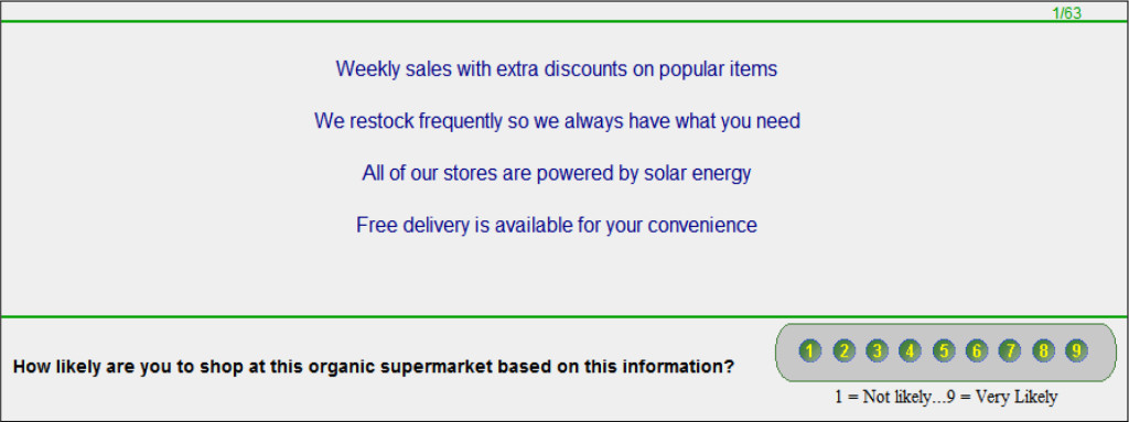
Figure 1. Shows an example of the vignette for a four-element vignette.

The vignette alone only provides information. It is the job of the researcher to focus the mind of the respondent on a specific issue. In this study the research focused on two issues. The first issue involves interest in shopping at the organic supermarket. The second issue involves the emotion that the respondent experiences. Emotions are becoming a key focus in consumer research [10, 11]. Mind Genomics deals with emotions by linking the emotions to the specific answers, the test messages. Figure 2 presents the two questions. The computer program constructed the vignette, and presented the respondent with the first question, likelihood to shop. The respondent answered the question. Immediately upon transmitting the rating, the Mind Genomics program changed the rating question but kept the vignette, allowing the respondent to rate the vignette on the second question, dealing with emotion.

NRFSJ 2018-103 - Howard Moskowitz USA - Revised Version_F2

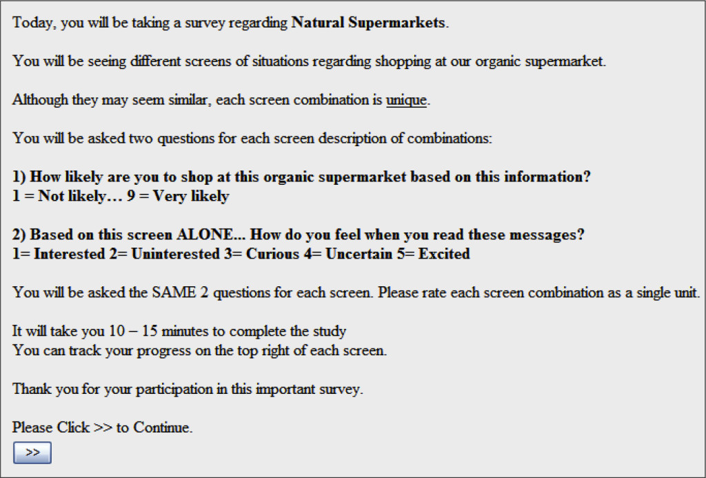
Figure 2. The orientation page.

The Classification Questionnaire

At the end of the on-line interview, the respondent completed a self-profiling questionnaire, dealing with WHO the respondent is, and HOW the respondent shops. This data allows us to look at subgroups defined by how the respondents describe themselves. With 51 studies, the classification questionnaire revealed that most subgroups were too small to analyze by themselves, other than males versus females, complementary subgroups that we will consider below.

Running the Study

The respondents were recruited from Amazon Mechanical Turk [12] Mechanical Turk represents a ready pool of respondents, who act as test subjects. They represent a good source of respondents for Mind Genomics studies because the focus of these studies is the discovery of basic mind-sets in the population, linked to a specific topic. A good analogy is the discovery of color primaries, red, yellow, and blue, which can be done from most colored objects, where the objects are multi-colored. One does not need a so-called representative sample to discover these color primaries, although one does need a representative sample to determine the distribution of these color primaries in population of interest. The same logic applies to the ‘primaries’ or mind-sets to be uncovered by Mind Genomics. It suffices for a so-called convenience sample to uncover the nature of these primaries, but not to estimate their distribution in a target population.

The respondents who agreed to participate clicked on a link embedded in the email invitation, and were taken to the first page, the orientation page, shown in Figure 2. The orientation page shows only the name of the study, and then what is expected from the respondent. The important things to notice are:

The only information provided about the topic is the name of the study. This paucity of information is deliberate because we want all the information about the natural supermarket to come from the vignettes that the respondents will evaluate. The words ‘natural supermarket’ is, however, included in every question, to remind the respondent about the context of the question.
The orientation page provides the respondent information relevant to the process. One of the most important sentences in the orientation page concerns the fact that all the vignettes differ from each other. It is a natural thing for respondents to feel that they have ‘seen these vignettes’ before in the evaluation, since the same messages or elements repeat. The sentences assuage this response, often an irritated response.
The orientation page then presents the two rating questions and the answers, but does not explain the meaning of the questions. The lack of explanation is deliberate, to prevent biasing the respondent by possibly leading with expected answers.
The last section tells the respondent the expected time for the interview. This is an important piece of information. Respondents do not like interviews which last a long time. It is better for a respondent to drop immediately when the respondent knows that the interview time is 15 minutes. When the respondent moves through the interview and then drops in the middle, the result is a very disgruntled panelist, who is less likely to participate in the future, in any interview, no matter how short. Telling the respondent that the study will last 15 minutes is simply good research policy in terms of the ongoing relationship with the respondent.

Data Analysis and Results for Question 1 (Likelihood of Shopping)

The fundamental analysis in Mind Genomics is uncovering the relation between the set of the 36 answers, the independent variables, and the rating assigned by the respondent.

First, a Binary transformation is necessary: For each tested vignette, the 9-point rating is replaced by either 0 (ratings 1-6) or 100 (ratings 7-9). This binary transformation traces its heritage to the world of consumer research. Most researchers do not know what the points on the scale mean. The reality in consumer research is that the focus on a simple response, either ‘no’ or ‘yes.’ Managers understand that. The only issue afterwards is to identify the region of the scale corresponding to the ‘no, ’ and complementary region of the scale corresponding to the ‘yes.’ Historically, we have divided the scale into these two specific regions, although on occasion, for countries and respondents who use the upper part of the scale very frequently, the practice may be to divide the scale into two parts as follows: 1-7 transformed to 0, 8-9 transformed to 1. That is not the case here.

A small random number is added to each transformed rating, with the number around 10-5. This random number ensures that the subsequent analysis by regression will not ‘crash, ’ even when the respondent limits the ratings to the low portion of the scale, 1-6, or limits the ratings to the high portion of the scale, 7-9. The random number does not materially affect the results.

The statistical method of OLS (Ordinary Least-Squares) regression is used, which relates the presence/absence of the 36 elements (coded as 1 when present, coded as 0 when absent), to the binary rating. The OLS regression is done at the respondent by respondent level. The OLS regression always ‘runs’ because the experimental design ensures that the 36 answers or elements, our independent variables, are statistically independent of each other, and because adding the small random number to every binary value ensures that there is the requisite variation in the dependent variable.

For each respondent an equation of the form:

Binary Value = k₀ + k₁(A1) + k2(A2) … k₃₆(F6) is generated.

The corresponding parameters are averaged, either across the total panel, or across the relevant respondents, which for our study will be, respectively, gender (male vs female), and three mind-set segments emerging from the clustering.

Table 2 presents the results for the total panel, and for males versus females. The 36 answers, the independent variables, are sorted in descending order by total.

Table 2. Parameters of the additive model for Natural Supermarket, for Total Panel, and Gender (Male versus Female). The numbers of in the body of the table are the average coefficients from the relevant individuals that the model comprises.

	Natural Supermarket	Total	Male	Female
	Base Size	51	22	29
	Additive constant	16	29	5
A5	We guarantee the lowest price or it’s free	34	39	29
B5	Free food samples so you can try before you buy	25	24	26
B6	We have a fresh juice stand so you can be hydrated while you shop	21	20	21
E6	We have a café that serves dishes made fresh from our products	19	14	23
A1	We have everyday low prices	18	12	22
B3	We have both organic and non-organic products available	17	14	20
B1	A wide range of fresh and high-quality products is available	17	6	25
B2	We restock frequently so we always have what you need	17	7	24
A4	We always have what you’re looking for in stock	15	11	18
C6	We’re open 24 hours a day and 7days a week	15	6	21
F6	We have been successful in the business for 50 years	14	8	20
E2	Free delivery is available for your convenience	14	13	15
F4	We are serious and efficient in our efforts to ensure quality and service to our customer	14	8	18
E1	Our staff is friendly and always ready to help	13	4	21
C3	All of our stores are powered by solar energy	13	8	17
D6	Monthly gifts are awarded based on how much you spent that month	12	6	17
A2	Weekly sales with extra discounts on popular items	11	7	13
F5	We have always passed our health inspections with high marks	11	6	14
F1	We support small businesses and local farms	10	2	17
F3	We handle mistakes and recalls in a professional manner	10	8	11
D3	Points earned from shopping never expire	9	5	11
C2	We’re always nearby and close to your home	8	7	9
E3	We have an easy and simple return/exchange policy	8	8	9
F2	We have a high overall customer service rating	8	-1	15
B4	Fresh produce is delivered daily	8	8	7
E4	Free parking is available for our customers	7	4	10
E5	Our staff is updated in nutritional and health benefits of our products	6	5	7
D2	We give exclusive discounts and coupons to members	6	12	2
A3	We offer a wide variety of items at competitive prices	6	-3	12
D5	We reward customers for using recyclable and non-plastic bags	4	5	4
D4	Points can be used for store credit based on out points to dollar system	4	2	6
A6	You can purchase gift cards as a gift for someone special in your life	3	-3	7
C5	We have special entrances and carts for the disabled	2	8	-3
C4	Special carts for children and toddlers are available	2	7	-2
D1	The membership to our rewards program is free	2	-1	4
C1	We have many destinations throughout the country	-4	-6	-2

The examination begins with the additive constant. The additive constant tells us the estimated percent of respondents who would rate a vignette 7-9 in the absence of elements, i.e., the 36 answers. Of course, all 48 vignettes comprised either three or four answers, by design. The additive constant is thus an estimated baseline. It is 16 for the total panel, meaning that only one out of six respondents might rate the basic idea of a natural supermarket 7-9. It is what the supermarket carries and does which makes the difference.

Continuing with the total panel, we see many of the answers or elements enjoying very high coefficients, several elements with coefficients of 15 or higher. Historically, these are extremely high, suggesting real interest in these features of the store. As we see below these very strong performers convey different types of messages, ranging from price to convenience to freshness. There is no single theme uniting the winning elements, but as we will see below, the themes emerge when we cluster the respondents on the basis of their response patterns. For right now, we need simply recognize that despite the low additive constant, it is the specifics which are important to drive interest in shopping. The simple notion of a natural market is not, by itself, compelling, and certainly not to women, as we will see.

We guarantee the lowest price or it’s free
Free food samples so you can try before you buy
We have a fresh juice stand so you can be hydrated while you shop
We have a café that serves dishes made fresh from our products
We have everyday low prices
We have both organic and non-organic products available
A wide range of fresh and high-quality products is available
We restock frequently so we always have what you need
We always have what you’re looking for in stock
We’re open 24 hours a day and 7 days a week

In many of these studies, we find few differences by gender, and the differences which emerge are minor. When we deal with the natural supermarket, however, we find dramatic differences between the genders, both in terms of the additive constant, and in terms of the particular answers or elements which perform well.

We begin our comparison with the additive constant. It is 5 for women, and 29 for men, a difference which tells us that for women there is no interest in the market without specification, whereas for the men there is some interest. Specification of the market features is far more important for women in order to interest them, and far less important for men. For women, the vignette which achieves a score off 70, for example, must comprise answers which add to 65 points, with the remaining 5 points contributed by the additive constant. Not so for men. The same score can be achieved by combining answers which add to 41 points, not 65.

Men and women show similar strong responses to two messages. The common message is ‘free’

We guarantee the lowest price or it’s free
Free food samples so you can try before you buy

One more element drives the men’s response. Women show a strong response to this element as well

We have a fresh juice stand so you can be hydrated while you shop

Women respond strongly to many more elements. There is no single theme among these very strong performing answers. The answers range from statements about price (we guarantee the lowest price or it’s free), to social consciousness (Our staff is friendly and always ready to help), to assortment (We always have what you’re looking for in stock), to ecology-minded (All of our stores ae powered by solar energy.)

We guarantee the lowest price or it’s free
Free food samples so you can try before you buy
A wide range of fresh and high-quality products is available
We restock frequently so we always have what you need
We have a café that serves dishes made fresh from our products
We have everyday low prices
We’re open 24 hours a day and 7days a week
Our staff is friendly and always ready to help
We have both organic and non-organic products available
We have been successful in the business for 50 years
We always have what you’re looking for in stock
We are serious and efficient in our efforts to ensure quality and service to our customer
All of our stores are powered by solar energy
Monthly gifts are awarded based on how much you spent that month
We support small businesses and local farms
Free delivery is available for your convenience
We have a high overall customer service rating

The patterns of coefficients differ dramatically across the genders. It’s not just that women begin with a lower additive constant, and show a constant increase in their coefficient versus the comparable coefficients emerging from the men’s data. Rather, the patterns are not correlated. What women find to be most important men may or may not find to be as important. The correlation between the two sets of 36 coefficients is only, lower than the correlation often observed when we compare the pattern of coefficients across genders.

Mind-Sets in the Population – The Contribution of Mind Genomics Thinking

We have seen that there are certainly differences among the elements based upon the data from the total panel, as well as substantial differences between genders on the same message. We also have seen that there is no single overriding description of what drives a strong positive coefficient. Rather, the data suggests a mélange of different answers, or different ideas.

The premise of Mind Genomics is that within any aspect of human experience we can dimensionalize the experience to define different aspects, which we call ‘questions.’ The aspects or questions (also called silos) tell a story. The task of Mind Genomics research is to provide reasonable answers to those questions, and then determine the degree to which each ‘answer’ drives the rating, doing so at the level of the individual respondent. We have seen how this approach generates estimates of the contribution of each answer, when we look at the total panel, as well as males versus females.

Mind Genomics makes its major contribution by identifying different groups of people, clustered together by the way they respond to these answers. That is, Mind Genomics uncovers possibly hitherto-unexpected groups of people, similar in the way they respond to a situation, rather than considered to be similar by the pattern of WHO THEY ARE, or by the pattern of WHAT THEY DO, or WHAT THEY BELIEVE. In a sense, the metaphor we use is mental genomes and mental alleles. Mind Genomics creates a world of mental genomes, each mental genome comprising alternative ways of responding to the same elements, i.e., mental alleles.

The process to uncover these mental genomes follows well-accepted statistical methods, encompassed by the methods know as clustering [13], and specifically k-means clustering [14]. The Mind Genomics philosophy to uncover the aforementioned clusters or mind-sets is presented as follows.

An array of 36 coefficients emerging from the modeling is created. Each respondent generates an equation with an additive constant (not considered), and 36 coefficients, one coefficient corresponding to each answer or element.

A measure of distance between pairs of respondents is defined. Clustering algorithms use many different measures of distance. Our selection is the quantity (1-Pearson R). The Pearson R assesses the degree of a linear relation between two sets of observations. The Pearson correlation varies from a high of 1 when there is a perfect linear relation between the two sets of observations. This highest correlation, +1, corresponds to a perfect relation, and thus to a 0 distance between the two respondents (1 – 1 = 0.)

The full set of respondents (here 51)is divided into two groups, with the property that the variability within the group is small, and the variability across groups is large. There are specific mathematical criteria for establishing the best division.

The mean coefficients for each group, or cluster are examined (here also referred to as mind-set) to determine:

Interpretability: Do the clusters tell; a coherent story, or does it seem that there are too many different ‘stories’ which define the cluster. Interpretability is a subjective criterion, left up to the researcher.

Parsimony: The fewer the number of clusters, the “better” the segmentation. It is always desirable to have a simpler solution with fewer groups than a more complex solution with more groups. However, parsimony must be considered along with interpretability.

The results of this study suggested that two clusters generated an unclear segmentation. The clusters seemed too diffuse. A three-cluster solution seemed far better, as shown in table 3. We show the clusters, i.e., mind-sets, sorted by the winning elements of each cluster.

Table 3. Parameters of the additive model for Natural Supermarket, for Total Panel, and the three Mind-Set segments. The numbers of in the body of the table are the average coefficients from the relevant individuals that the model comprises

Natural Supermarket	Total	Mind-set C1	Mind-set C2	Mind-set C3
Base Size	51	28	11	12
Constant	16	8	13	35
We guarantee the lowest price or it’s free	34	35	32	33
Mind-set 1 – It’s about the food
Free food samples so you can try before you buy	25	43	-5	11
We have a fresh juice stand so you can be hydrated while you shop	21	34	1	7
We have everyday low prices	18	22	4	19
We have both organic and non-organic products available	17	20	16	11
A wide range of fresh and high-quality products is available	17	20	26	2
We restock frequently so we always have what you need	17	19	15	13
We have a café that serves dishes made fresh from our products	19	19	33	8
All of our stores are powered by solar energy	13	18	5	10
Mind-set 2 – It’s about trust and customer focus
We are serious and efficient in our efforts to ensure quality and service to our customer	14	4	49	5
We have been successful in the business for 50 years	14	11	46	-6
We handle mistakes and recalls in a professional manner	10	11	35	-16
We support small businesses and local farms	10	5	34	0
Our staff is friendly and always ready to help	13	10	33	2
Monthly gifts are awarded based on how much you spent that month	12	8	31	5
Points can be used for store credit based on out points to dollar system	4	-5	27	5
Free parking is available for our customers	7	4	20	2
Points earned from shopping never expire	9	6	17	7
We have a high overall customer service rating	8	2	16	14
We’re always nearby and close to your home	8	7	15	5
Fresh produce is delivered daily	8	13	15	-12
We reward customers for using recyclable and non-plastic bags	4	-1	15	8
Mind-set 3 – It’s about convenience and sales
We have an easy and simple return/exchange policy	8	-3	9	33
We always have what you’re looking for in stock	15	12	9	29
Free delivery is available for your convenience	14	14	3	26
We’re open 24 hours a day and 7days a week	15	13	8	24
Weekly sales with extra discounts on popular items	11	6	8	24
You can purchase gift cards as a gift for someone special in your life	3	4	-13	17
Not very strong for any group
Our staff is updated in nutritional and health benefits of our products	6	8	-2	10
We offer a wide variety of items at competitive prices	6	7	-2	8
We have always passed our health inspections with high marks	11	12	13	5
The membership to our rewards program is free	2	1	0	4
We give exclusive discounts and coupons to members	6	6	9	4
We have special entrances and carts for the disabled	2	3	-2	4
Special carts for children and toddlers are available	2	13	-24	0
We have many destinations throughout the country	-4	4	-21	-5

Before we look in detail at the three mind-sets, we should note that one answer does extremely well among all mind-sets, ‘We guarantee the lowest price or it’s free.’ We have pulled that out of the segmentation. Mind-set C1 (It’s all about the food) responds to food, food freshness, and everyday low prices. Mind-set C1 is the largest mind-set, comprising more than half of the respondents (28 of 51), and shows the lowest additive constant (8). For Mind-set C1, it is the messages which do the work to drive interest.

Wants everyday low prices
Excited by free food samples and juice stands
Likes a selection of both organic and non-organic products
Don’t care about rewards and point systems
Not concerned with special services

Mind-set C2 (It’s all about customer focus), is much smaller, about one fifth of the respondents. This segment also shows a low additive constant (8). The coefficients for this mind-set are exceptionally large, six in the 30’s and 40’s. Those coefficients are some of the largest ever observed in a Mind Genomics study. It is not clear about the degree to which the study taps into the ‘hot topic’ of natural and shopping.

Wants efficient service
Professionalism is very important
Not concerned with child accessibility
Don’t care about multiple locations
Not interested in buying gift cards
Prefers small business tactics over large companies

Mind-Set C3 (It’s about convenience and sales), is also much slower, 12 of the 51 respondents. The additive constant for this mind-set is much large, 35, so that they are similar to typical shoppers. This group does not really respond to strongly to the special attractions of organic products, whether that be a café which serves the store’s products, or the selection. Mind-Set C3 seems to respond most strongly to price and convenience, as if they are shoppers in a hurry. For them, just make it easy.

Wants a clear simple return/exchange policy
Product availability for low prices is very important
Prefers convenient store hours and delivery
Not interested how mistakes are handled
Not concerned with fresh produce

The segments are not correlated at all as:

Pearson correlation Mind-set C1-C2 = -0.04
Pearson correlation Mind-set C1-C3 = +0.16
Pearson correlation Mind-set C2-C3 = -0.18

Linking Answers/Elements to Emotions

The experienced advertising professionals and consumer research professionals have recently discovered that beyond the messages themselves to which consumers respond, there are also emotions to be understood. Simply knowing that one of our answers appeals to a person, a gender, or a mind-set does not tell us the emotion which may be operating. Understanding the emotions and linking the emotions to the messages comprises one of the next big opportunities for sensory and consumer research.

Mind Genomics addresses the topic of emotion by instructing the respondent to select one of a limited number of feelings/emotions to describe the response to a vignette. Admittedly, the selection of 5-9 emotions is a limited number, compared the large number of emotions that have been enumerated in the literature [10, 11]. On the other hand, with 48 vignettes to evaluate, and the need to find a linkage between each emotion and each of the 36 answers/elements, it is prudent to reduce the number of feelings/emotions to a reasonable set. Five suffices to begin the process

Our objective here is to link each of the emotions to each of the messages. Following is presented our approach to establish the numerical value of the linkage.

Question 2 required the respondent to select one of the five emotions as appropriate for the particular vignette. A respondent had to select one of the emotions, and could not continue unless the selection was made. The five-point scale of emotion is not one of the typical numerical scales one encounters in research, but is an example of the so-called nominal scale, where each number corresponds to a (possibly) unrelated choice. There is no need for the five points to have any relation whatsoever. The single scale is expanded to five binary scales, one scale for each emotion. For the one emotion selected for the vignette, we put in the number ‘100’ plus a small random number (<10^-5). For the four emotions not selected for the vignette, we put in the number ‘0’ plus a small random number.

All of the data are then combined into one file. The data comprises the 36 independent variables, the five dependent variables, across 2448 cases, one per vignette (48 vignettes x 51 respondents = 2448). OLS (ordinary least-squares) regression is used to estimate the coefficients of the equation below. Each of the 36 answers or elements is an independent variable, which generates a coefficient. The equation does not have an additive constant. The assumption is that without any elements there is no emotion selected.

Emotion Selected = k₁(A1)+k₂(A2)…k₃₆(F6)

The coefficient shows the ‘linkage’ between the element and the selection of the emotion. Our norms suggest values around 10 as indicating a meaningful linkage.

Table 4 shows the elements sorted by linkage to the five emotions. For example, when we look at the feeling/emotion ‘curious’ we find the following strong linkages, and possible insights into the mind of the respondent that would not have emerged from the coefficients for interest (Question #1.) Although three of these seven answers/elements are the normal messages that a store might advertise (e.g., c, d, e), the other four are relatively unique.,

Fresh produce is delivered daily
We are serious and efficient in our efforts to ensure quality and service to our customer
Our staff is friendly and always ready to help
Free parking is available for our customers
The membership to our rewards program is free
We have a fresh juice stand so you can be hydrated while you shop
We have a café that serves dishes made fresh from our products

Table 4. Likage of the five feelings/emotions to the 36 answers/elements. Linkages of 10 or higher are considered to be strong and relevant.

		Interested	Uninterested	Curious	Uncertain	Excited
	Interested
A2	Weekly sales with extra discounts on popular items	13	4	3	3	4
B5	Free food samples so you can try before you buy	12	0	7	2	6
A1	We have everyday low prices	11	5	6	3	2
A5	We guarantee the lowest price or it’s free	11	-3	-3	8	16
D4	Points can be used for store credit based on out points to dollar system	11	2	10	3	1
A3	We offer a wide variety of items at competitive prices	10	6	5	4	4
C2	We’re always nearby and close to your home	10	6	3	4	2
	Disinterested
C1	We have many destinations throughout the country	3	17	6	1	0
A6	You can purchase gift cards as a gift for someone special in your life	2	14	4	4	3
F3	We handle mistakes and recalls in a professional manner	3	13	3	8	1
C4	Special carts for children and toddlers are available	1	11	6	8	-1
	Curious
B4	Fresh produce is delivered daily	6	2	16	2	0
F4	We are serious and efficient in our efforts to ensure quality and service to our customer	1	4	12	5	6
E1	Our staff is friendly and always ready to help	4	3	12	4	1
E4	Free parking is available for our customers	4	8	11	6	-2
D1	The membership to our rewards program is free	7	2	11	3	3
B6	We have a fresh juice stand so you can be hydrated while you shop	7	2	10	5	4
E6	We have a café that serves dishes made fresh from our products	3	0	10	5	7
	Excited
E2	Free delivery is available for your convenience	1	0	8	5	11
C6	We’re open 24 hours a day and 7days a week	8	0	2	5	10
	Answers not strongly linked to any emotion
D5	We reward customers for using recyclable and non-plastic bags	7	2	8	4	7
D6	Monthly gifts are awarded based on how much you spent that month	8	2	4	6	7
B3	We have both organic and non-organic products available	3	8	7	4	6
F1	We support small businesses and local farms	3	5	9	5	5
B2	We restock frequently so we always have what you need	6	4	7	5	5
E3	We have an easy and simple return/exchange policy	5	4	7	4	5
D3	Points earned from shopping never expire	9	3	7	2	5
C3	All of our stores are powered by solar energy	7	4	9	3	4
A4	We always have what you’re looking for in stock	7	1	8	6	4
F5	We have always passed our health inspections with high marks	8	8	4	3	4
B1	A wide range of fresh and high-quality products is available	7	5	8	4	3
D2	We give exclusive discounts and coupons to members	7	5	7	4	3
F2	We have a high overall customer service rating	9	8	3	5	3
F6	We have been successful in the business for 50 years	7	6	2	8	2
E5	Our staff is updated in nutritional and health benefits of our products	3	5	9	5	1
C5	We have special entrances and carts for the disabled	6	9	4	6	0

Further Use of the Obtained Knowledge

Similarly to many scientific fields, results of Mind Genomics studies are also ready to be used as the input data of prediction models. Prediction models are generally used in every scientific area to forecast unknown qualitative or quantitative information from some measured variables using a predefined model. In our case, the raw data of the presented study gives two important information:

The coefficients of the respondents
The known memberships of the respondents

These information enables us to create so-called classification models which need continuous data to classify (or predict) the segment membership of the participants. The presented data is used for model training, e.g. to create the classification model. This classification model defines the 6 most important elements, which differentiate the segments the most. The 6 key elements are defined by so-called distance measures and the highest between-group distances are calculated. The obtained 6 key elements are then collected and ordered under each other on a newly created webpage (Figure 3). New participants, who never took part in this test before, then are asked to answer one question about the six elements using a binary scale with tow endpoints named “not likely” and “very likely”. The obtained answers are then passed to the classification model which is able to predict the most likely segment membership of this new participant.

NRFSJ 2018-103 - Howard Moskowitz USA - Revised Version_F3

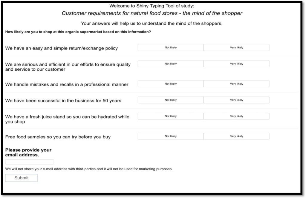
Figure 3. Personal viewpoint identification opening screen. Participants are forced to answer each six questions and need to add their e-mail addresses before submitting their answers.

Here, the personal viewpoint identification process can be divided. In our case, we use the segment membership as information presented to the respondent (Figure 4). However, the segment memberships can be also used to suggest personalized products, advertisements or services. Possible usage of this information is almost endless due to the vast opportunities of the World Wide Web.

NRFSJ 2018-103 - Howard Moskowitz USA - Revised Version_F4

Figure 4. Result screen of personal viewpoint identification. In this example, the segment membership (It’s all about the food) and a small description of it are presented to the participants.

Discussion and Conclusion

As we consider the results of this study, it’s clear that consumers place a premium value on price, which has been identified by other authors [15]. All factors being equal, freshness will be sacrificed for price – convenience will be sacrificed for price – and features like universal access, customer convenience, and even positive aspects of store service will be sacrificed for price. However, it has been shown that consumers usually prefer local food or food originated from a geographically closer country [16], our study raises the attention to the significant effect of price; hence our results are not surprising. It would be reasonable to expect that economic drivers would be a high priority, if not the highest priority, for a consumer. However, it’s the factors that came in under price that create the greatest opportunity for exploration. If price is equal – or at least comparable – then what consumers want is freshness, convenience, and rewards for consumer loyalty. A new study from Istanbul, Turkey reports that retailer innovativeness and perceived food healthiness positively affect both store prestige and store trust [17]. In a market, then, where stores like Whole Foods offer a nationally recognized brand, a wider distribution channel, and a sense of convenience (online ordering, consistency from store to store, and loyalty programs), those who are dedicated to healthful eating will likely look first for the best “deal” first – and then for other factors like freshness and national brand recognition, even if they are more inclined to tell others that they seek quality first.

For the same reason, CSAs and farmer’s markets exist more in the mindset of consumers as an opportunity that serves either a quaint or exotic space than they serve as legitimate competitors to groceries that offer healthful or local foods. Simply put, if a consumer can get their groceries (including reasonably healthful foods) in the same location as their other household supplies, they will choose first by overall pricing and value, even if that means foods that aren’t quite as fresh, or stores that aren’t specifically known for having a national presence.

The presented methodology is suitable to scale up the presented results. A newly developing app, called BimiLeap (needs a reference or a link !!), aims to bring the presented research methodology to every mobile phone user all around the world. Using BimiLeap, users will be able to create a series of studies all dealing with organic food acceptance. By collecting the results of numerous studies dealing with organic products, mapping of consumer minds about organic food products will be available in a short time.

Acknowledgement

AG thanks the support of Premium Postdoctoral Research Program of Hungarian Academy of Sciences.

References

Bustillos B, Sharkey JR, Anding J, McIntosh A (2009) Availability of more healthful food alternatives in traditional, convenience, and nontraditional types of food stores in two rural Texas counties. Journal of the American Dietetic Association 109: 883–889.
Halweil B (2002) Home grown: The case for local food in a global market. (T. Prugh, Ed.). Washington D.C.: Worldwatch Institute.
Green PE, Srinivasan V (1990) Conjoint Analysis in Marketing: New Developments with Implications for Research and Practice. Journal of Marketing 54: 3-19.
Gofman A, Moskowitz H (2010) Isomorphic Permuted Experimental Designs and their Application in Conjoint Analysis. Journal of Sensory Studies 25: 127-145.
Milutinovic V, Salom J (2016) Mind Genomics – A Guide to Data-Driven Marketing Strategy. Springer International Publishing.
Moskowitz HR, Gofman A, Itty B, Katz R, Manchaiah M, Ma Z (2001) Rapid, inexpensive, actionable concept generation and optimization: the use and promise of self-authoring conjoint analysis for the food service industry. Food Service Technology 1: 149-167.
Porretta S, Gere A, Radványi D, Moskowitz H (2018) Mind Genomics (Conjoint Analysis): The new concept research in the analysis of consumer behaviour and choice. Trends in Food Science and Technology, in press.
Bell GH, Ledolter J, Swersey AJ (2006) Experimental design on the front lines of marketing: Testing new ideas to increase direct mail sales. International Journal of Research in Marketing 23: 309-319.
Moskowitz HR, Gofman A, Beckley J, Ashman H (2006) Founding a New Science: Mind Genomics. Journal of Sensory Studies 21: 266-307.
King SC, Meiselman HL (2010) Development of a method to measure consumer emotions associated with foods. Food Quality and Preference 21: 168-177.
King SC, Meiselman HL, Carr BT (2013) Measuring emotions associated with foods: Important elements of questionnaire and test design. Food Quality and Preference, 28: 8-16.
Buhrmester M, Kwang T, Gosling SD (2011) Amazon’s Mechanical Turk: A New Source of Inexpensive, Yet High-Quality, Data? Perspect Psychol Sci 6: 3-5. [crossref]
Likas A, Vlassis N, Verbeek JJ (2003) The global k-means clustering algorithm. Pattern Recognition 36: 451-461.
Mucherino A, Papajorgji P, Pardalos PM (2009) A survey of data mining techniques applied to agriculture. Operational Research 9: 121-140.
Janssen M (2018) Determinants of organic food purchases: Evidence from household panel data. Food Quality and Preference 68: 19-28.
Pedersen S, Aschemann-Witzel J, Thøgersen J (2018) Consumers’ evaluation of imported organic food products: The role of geographical distance. Appetite 130: 134-145.
Konuk FA (2018) The impact of retailer innovativeness and food healthiness on store prestige, store trust and store loyalty. Food Research International.

Biomaterials for Periodontal Regeneration: A Comprehensive Discussion of its Merits and Demerits

Leave a reply

DOI: 10.31038/JDMR.2018121

Abstract

Treatment of periodontal diseases is becoming more prevalent and one of the treatment methods is to regenerate periodontal tissues. Over the period many biomaterials have been developed many of which are currently being used and more research is still in progress. Such a range of biomaterials choice makes it a challenging ordeal for Dentists to weigh the pros and cons of the popular biomaterials. This manuscript attempts to be a comprehensive document that discusses the merits and demerits of various biomaterials to aid in the decision making of biomaterial choice for periodontal disease treatments.

Key words

Dental Biomaterials, Periodontal Disease Biomaterials, Biomaterials for Intra-bony Defects.

Introduction

Periodontal diseases are one of the common dental problems among adults in the US population. According to the American Academy of Periodontology (AAP) it is defined as a chronic inflammatory disease that affects the gum tissue and bone supporting the teeth. 47.2% of adults aged 30 years and older have some form of periodontal disease and it increases with age, 70.1% of adults 65 years and older have periodontal disease [1]. It’s well known that if not treated, it will lead to dental (tooth loss due to alveolar bone destruction) and medical complications (heart diseases ,aggravate/worsen existing systemic conditions like diabetes by raising its Hba1c level due to entry of oral bacteria in to blood stream). So, it is inevitable to treat periodontal diseases and there are many treatment modalities available depending on the nature of bone destruction and symptoms of periodontal diseases. This paper will specifically explore the biomaterials emerging and being used to regenerate periodontal tissue as one of the treatment options.

Calcium Phosphate

Advantages of Calcium phosphate- it has a similar composition to bone mineral. It will promote cellular function and has a bioactivity meaning it will form the bone like material when used for regeneration. As CP has a high affinity for proteins, it will act as ideal carriers for peptides, bone growth factors etc. So, once it is bonded with circulating bone morphogenic proteins, it will promote osteo-induction [2]. Also has osteo-conductive property [3]. All these properties combined make this material more suitable for tissue regeneration and it could be used in gene therapy, cancer therapy and osteoporosis therapy. There are no known adverse effects associated with using material.

Hydroxyapatite (HA)

Advantages – Like calcium phosphate, HP also has a similar composition to natural bone mineral [4]. When it is implanted, it chemically bonds to bone [5]. The biocompatibility, tolerance and biologically active property of HA makes it ideal material for bone substitutes [6]. Disadvantages – it is long term outcome is not ideal as it has inconsistent cell reactions which limits its application in clinic [7]. A variant of HA called nano-HA has good biocompatibility, increases protein synthesis of PDL cells, improves alkaline phosphatase activity, induces cell differentiation, promotes periodontal tissue regeneration and forms new teeth attachments [8]. But the only disadvantage is limited bone regeneration (Li Shue, Biomaterials for periodontal regeneration: A review of ceramics and polymers, 2012) [3].

Tri Calcium Phosphate (TCP)

Advantages – It has been used for the past few years after thoroughly investigated as a bone substitute. The two crystallographic forms of TCP include; Alpha TCP, Beta TCP. Beta TCP shows the characteristics of good biocompatibility and osteo-conductivity [9]. When it comes to bone regeneration potential, β-TCP grafts have been shown to be like autogenous bone, FDBA, DFDBA and collagen sponge [10]. It can be used to repair periapical and marginal periodontal defects, as well as alveolar bony defects [10] however; some studies in the literature suggest that β-TCP could also be utilized for alveolar ridge augmentation in vertical and horizontal dimensions with variable results .Although it produces substantial clinical improvements in treating intra bony defects, it does not seem to regenerate cementum, PDL or bone (disadvantage) [11].

Calcium Polyphosphate (CPP)

Advantages – Calcium-Polyphosphate (CPP) is another good bone substitute as the mechanical properties are like trabecular bone. It has controlled degradability which is essential in tissue regeneration and El Sayegh et al. demonstrated that the degradation rate of CPP did not substantially affect the interactions of human gingival fibroblasts compared with titanium alloy substrates. CPP shows very good integration to host bone when implanted in vivo [12]. According to Nelson et al. CPP has a good bone regeneration potential after finding its ability to repair canine mandibular alveolar defects.

Brushite (Di Calcium Phosphate Dihydrate (DCPP))

Advantages – it has been shown that injectable brushite has the capability of regenerating bone. Potential applications of this material include vertical bone augmentation, buccal dehiscence defects. The only disadvantage associated with using brushite bone grafts is that after implantation, it will convert to HA which would limit its resorption rate. To overcome this advantage, a variant of Brushite called Monetite which will not convert to HA. By doing so, the resorption rate of Monetite is higher than Brushite [9].

Bioactive glass (BG)

Advantages – BG graft materials usually contain silicon dioxide, calcium oxide, sodium oxide, and phosphorus pentoxide. Studies have demonstrated that bioactive glass could induce bone formation as it enhances the expression of type I collagen, osteocalcin and alkaline phosphatase gene expression and osteocalcin protein [13]. Bioactive glass nanoparticles have been shown to induce cementoblasts to proliferate in an in vivo study [14]. BG grafts can be used as a supplement when the mount of the harvested autogenous grafts is not sufficient [15]. According to Mengel et all, BG produced a significant improvement in the parameters PD, CAL and distance from alveolar crest to defect base [16]. The disadvantage is that it has limited regenerative outcomes based on Nevins et all who conducted histological analysis [17].

Calcium Sulphate

Advantages – CS is used as a barrier material and it has greater compressive strength than cancellous bone and will resorb in 5-& 7weeks [18]. It inhibits the epithelial and connective tissue in-growth to produce a predictable regenerative response [19]. CS easily adapts and adheres to the root surface, including root concavities [20]. In addition, CS is readily available, it can be easily sterilized, inexpensive (economic alternative to collagen), completely resorbable, and biocompatible, and in the presence of bone and periosteum, it becomes osteogenic [21]. No specific disadvantages have been found when this material was used.

Enamel Matrix Protein

Enamel Matrix proteins consist of three primary proteins which are similar to amelogenin, enamelin and sheathaline respectively with two enzymes and it is derived from porcine teeth. A wide range of in vitro and in vivo studies have demonstrated that EMD and amelogenins stimulate growth of multiple mesenchymal cell types including fibroblasts, cementoblasts, osteoblasts, and stem cells [22]. In addition, it inhibits epithelial downgrowth. Although there are some controversies around using this EMP, some studies stated that it helps to repair bony defects in advanced intra bony defects. Recently, American Academy of Periodontology concluded that EMD is generally comparable with demineralized freeze-dried bone allograft and GTR in improving clinical parameters in the treatment of intra bony defects (Zeeshan Sheikh, Natural graft tissues and synthetic biomaterials for periodontal and alveolar bone reconstructive applications: a review, 2017) [9].

Platelet Rich Plasma and Platelet Rich fibrin

As these both (PRP & PRF) contains high platelets concentrate, these two play a role in augmentation of tissue healing, antimicrobial activity, modification of host defense mechanisms and immune reaction. The potential benefits of PRP is not consistent in the literature review because some authors reported significant improvements in tissue healing and bone formation using PRP [23, 24]. others failed to observe improvement [25, 26]. The technical and regenerative limitations of PRP restrict its applications. On the other hand, PRF has many advantages; completely autogenous, extended growth factor release for 7 days, simple and faster technique, in-expensive, no requirement of any additive constituent such as bovine thrombin, no biochemical handling involved no associated immune reactions and no associated infections [27]. The limitation of PRF is that a dried glass tube or glass coated plastic tube should be used. In addition, quantity and quality of PRF with aging, influence of systemic diseases such as thrombocytopenia, bleeding disorders etc, nutrition, blood profile, autoimmunity and genetic predisposition may influence the nature of PRF but not confirmed yet [27].

References

CDC (2015) Center for Disease Control and Prevention. Retrieved from What is Periodontal Disease?: https://www.cdc.gov/oralhealth/periodontal_disease/index.htm
Racquel Z, LeGeros JP (2006) Calcium Phosphate Biomaterials: An Update. International Journal of Oral Medicine and Science 4: 117–123.
Shue L, Yufeng Z, Mony U (2012) Biomaterials for periodontal regeneration: a review of ceramics and polymers. Biomatter 2: 271–277. [crossref]
Wang H, Li Y, Zuo Y, Li J, Ma S, et al. (2007) Biocompatibility and osteogenesis of biomimetic nano-hydroxyapatite/polyamide composite scaffolds for bone tissue engineering. Biomaterials 28: 3338–3348. [crossref]
Bagambisa FB, Joos U, Schilli W (1993) Mechanisms and structure of the bond between bone and hydroxyapatite ceramics. J Biomed Mater Res 27: 1047–1055. [crossref]
Sanjay Gupta, Vandana KL (2013) Evaluation of hydroxyapatite (Periobone-G) as a bone graft material and calcium sulfate barrier (Capset) in treatment of interproximal vertical defects: A clinical and radiologic study. Journal of Indian Society of Periodontology 17: 96–103.
Deligianni DD, Katsala ND, Koutsoukos PG, Missirlis YF (2001) Effect of surface roughness of hydroxyapatite on human bone marrow cell adhesion, proliferation, differentiation and detachment strength. Biomaterials 22: 87–96. [crossref]
Yancong Zhang, Hanwen Sun, Xinfeng Song, Xiangling Gu, Chunyan Sun (2015) Biomaterials for Periodontal Tissue Regeneration. Review of Advanced Materical Journal 209–214.
Sheikh Z, Hamdan N, Ikeda Y, Grynpas M, Ganss B, et al. (2017) Natural graft tissues and synthetic biomaterials for periodontal and alveolar bone reconstructive applications: a review. Biomaterials Research 21: 9. [crossref]
Nakajima Y, Fiorellini JP, Kim DM, Weber HP (2007) Regeneration of standardized mandibular bone defects using expanded polytetrafluoroethylene membrane and various bone fillers. International Journal of Periodontics and Restorative Dentistry 27: 151–159. [crossref]
Stavropoulos A, Windisch P, Szendröi-Kiss D, Peter R, Gera I, et al. (2010) Clinical and histologic evaluation of granular Beta-tricalcium phosphate for the treatment of human intrabony periodontal defects: a report on five cases. Journal of Periodontology 81: 325–332. [crossref]
Grynpas MD, Pilliar RM, Kandel RA, Renlund R, Filiaggi M, et al. (2002) Porous calcium polyphosphate scaffolds for bone substitute applications in vivo studies. Biomaterials Journal 23: 2063–2070. [crossref]
Varanasi VG, Owyoung JB, Saiz E, Marshall SJ, Marshall GW, et al. (2011) The ionic products of bioactive glass particle dissolution enhance periodontal ligament fibroblast osteocalcin expression and enhance early mineralized tissue development. J Biomed Mater Res A 98: 177–184. [crossref]
Carvalho SM, Oliveira AA, Jardim CA, Melo CB, Gomes DA, et al. (2012) Characterization and induction of cementoblast cell proliferation by bioactive glass nanoparticles. Journal of Tissue Engineering and Regenerative Medicine 6: 813–821. [crossref]
Yadav VS, Narula SC, Sharma RK, Tewari S, Yadav R (2011) Clinical evaluation of guided tissue regeneration combined with autogenous bone or autogenous bone mixed with bioactive glass in intrabony defects. J Oral Sci 53: 481–488. [crossref]
Mengel R, Soffner M, Flores-de-Jacoby L (2003) Bioabsorbable membrane and bioactive glass in the treatment of intrabony defects in patients with generalized aggressive periodontitis: results of a 12-month clinical and radiological study. Journal of Periodontology 74: 899–908. [crossref]
Nevins ML, Camelo M, Nevins M, King CJ, Oringer RJ, et al. (2000) Human histologic evaluation of bioactive ceramic in the treatment of periodontal osseous defects. The International Journal of Periodontics and Restorative Dentistry 20: 458–467. [crossref]
Sukumar S, Drízhal I, Paulusová V, Bukac J (2011) Surgical treatment of periodontal intrabony defects with calcium sulphate in combination with beta-tricalcium phosphate: clinical observations two years post-surgery. Acta Medica 54: 13–20. [crossref]
Sottosanti J (1992) Calcium sulfate: a biodegradable and biocompatible barrier for guided tissue regeneration. Compendium 13: 226–228. [crossref]
Anson D (1996) Calcium sulfate: a 4-year observation of its use as a resorbable barrier in guided tissue regeneration of periodontal defects. Compendium of Continuing Education in Dentistry 17: 895–899. [crossref]
Shilpa Budhiraja, Neeta Bhavsar, Santosh Kumar, Khushboo Desai, Sareen Duseja (2012) Evaluation of calcium sulphate barrier to collagen membrane in intrabony defects. Journal of Periodontal and Implant Science 42: 237–242.
Rathva VJ (2011) Enamel matrix protein derivatives: role in periodontal regeneration. Clinical Cosmetic and Investigational Dentistry 3: 79–92. [crossref]
Sánchez AR, Sheridan PJ, Kupp LI (2003) Is platelet-rich plasma the perfect enhancement factor? A current review. The International Journal of Oral and Maxillofacial Impants 18: 93–103. [crossref]
Ross R, Glomset J, Kariya B, Harker L (1974) A Platelet-Dependent Serum Factor That Stimulates the Proliferation of Arterial Smooth Muscle Cells In Vitro. Proceedings of the National Academy of Sciences of the United States of America 71: 1207–1210. [crossref]
Raghoebar GM, Schortinghuis J, Liem RS, Ruben JL, van der Wal JE, et al. (2005) Does platelet-rich plasma promote remodeling of autologous bone grafts used for augmentation of the maxillary sinus floor? Clinical Oral Implants Research 16: 349–356. [crossref]
Hamdan AA, Loty S, Isaac J, Bouchard P, Berdal A, et al. (2009) Platelet-poor plasma stimulates the proliferation but inhibits the differentiation of rat osteoblastic cells in vitro. Clin Oral Implants Res 20: 616–623. [crossref]
Muthukumaraswamy Arunachalam, Shaju JP, Nath Sonia (2016) Platelet Rich Fibrin in Periodontal Regeneration. Open Dent Jour 10 (Suppl 1- M4): 174–181.

About a Case of Aberrant Path of the Duplicity of the Cisternal Portion of the Trigeminal Nerve Revealed by Perceptive Deafness

Leave a reply

DOI: 10.31038/IMCI.2018112

Summary

Trigeminal nerve is a mixed nerve with a contingent of sensory fibers for integuments of the face, a contingent of driving fibers for the masticatory muscles and a contingent of autonomic fibers. Its nuclei are disseminated on the brainstem and it emerges from the middle of the pons, at the lateral surface of the brainstem by 2 driving and sensory roots that merge to the trigeminal ganglion.

We report an unilateral duplicity of the trigeminal nerve causing a sensorineural hearing loss caused by the conflict of the aberrant root and the vestibulocochlear nerve.

Keywords

Aberrant Emergency Nerve, MRI, Sensorineural Hearing Loss, Trigeminal nerve.

Introduction

The trigeminal nerve is the largest cranial nerve. It is a mixed nerve with a contingent of sensory fibers for integuments of the face, a contingent of driving fibers for the muscles of mastication and a contingent of autonomic fibers. Its nuclei are disseminated on the brainstem and it emerges from the middle of the pons, at the lateral surface of the brainstem by 2 driving and sensory roots that coalesce to form the trigeminal ganglion at the Meckel’s cave. Even if the variations of the path brain vessels are usual, the abnormalities of cranial nerves emergence are rare (Hypoglossal Nerve).

We report an unusual case of cisternal portion of trigeminal nerve duplicity, with aberrant emergency of one bundle responsible of a conflict with vestibulocochlear nerve.

Observation

Mr SD, 35, consulted for a unilateral left hearing loss since childhood without recent worsening. He does not feel tinnitus nor dizziness. The otoscopy is normal. The acoumetry is a unilateral left perception of hearing loss. The right ear is normal. Audiometric testing shows a sensorineural hearing loss of on average 60dB. The precocious Brainstem Auditory Evoked Potential (BAEPs) show a flat layout, without wave V, meaning a severe damage of cochlear nerve. A MRI (Siemens Avento 1,5Tesla) has already been realized with 3D Ciss, T1EG sequences with and without gadolinium injection and a TOF sequence. The MRI shows duplicity of cisternal portion of the left trigeminal with a upper bundle emerging from the middle of the pons, at the lateral surface of the brainstem. The lower bundle has an aberrant origin between pons and brainstem at the same level of the acousticofacial nerve bundle. Moreover, it compresse the cochleovestibular nerve from its origin, realising a nervous conflict (figure 1 and 2). TOF et 3DT1 weighted sequences after injection erase the vascular origin of this abnormalities
(figure 3). No vestibulocochlear nerve tumor was noted. The contralateral trigeminal nerve has a modal disposition. The signal of ear inner fluid and vestibular aqueduct fluid are normal.

Discussion

Variations of birth or cranial nerves directions are extremely rare anatomic situations. The trigeminal nerve is a mixte nerve with a sensory nucleus spreaded from the midbrain to the medulla in the general sensory column located laterally. Its motor nulei is located in the branchial motor column, which is shared with the other branchial motor nuclei in particular the VII [1]. In its modal position, the trigeminal nerve emerge from the antero-lateral side of pons at the upper and medium third junction by 2 roots: the largest sensory root and medium then lower one. The two roots cross the pontine cisterne in a vertical and lateral way to the Meckel’s cave [2,3]. There are aberrant or incidental radicels emerging separately from the main sensory root at the antero-lateral side of the pons in half cases [4]. This situation explains the persistence of sensitivity after rhizotomy of the main sensory root of trigeminal nerve [5]. Theses incidental radicels meet the sensory root in its first centimeter after its emergency in 90% cases. The driving root is composed by 7 to 8 radicels on average, born separately and that meets usually at 1 cm from the pons. Incidentals sensory fibers are closer to the sensory root than the motor root [4,5,6].

IRCI-102-Mbengue Ababacar_Africa_F1

Fig S1. 3D MRI Ciss, axial MinIP. Double emergence of the left trigeminal nerve.

The upper beam with normal emergence at the anterolateral side of the pons (a). The inferior beam with an aberrant origin at the level between the pons and the medulla, pushing back the vestibulocochlear nerve at his origin.

IRCI-102-Mbengue Ababacar_Africa_F2

Fig. S2. MRI 3D Ciss reconstruction coronal (a) and sagittal (b). Illustration of the 2 beams of the left trigeminal (double arrow). Modal anatomy of the right trigeminal (arrow).

IRCI-102-Mbengue Ababacar_Africa_F3

Fig. S3. IRM TOF MPR axial (a) and coronaleT1 (b) with injection eliminate vascular origin.

If duplicity of trigeminal nerve are reports in the anatomical study [4], they have never been described in imaging literature to our knowledge. The other particularity of our case is that aberrant emergency from of one bundles, at the same level of the acousticofacial nerve.

The aberrant bundle, probably the motor root of V, whose the original nucleus is located in the same column than the facial nerve (branchial motor column) explaining the emergency at the same level of the acousticofacial nerve bundle. The compression of cochlear nerve by motor fibers of the trijumeau would explain sensorineural hearing loss observed on the patient. Conflicts at cerebellopontine angle concern the most often Anterior Inferior Cerebellar Artery (AICA) and the acousticofacial nerve bundle or the trigeminal nerve. A conflict between two nervous structures is a rare situation. It very likely that the conflict is the cause of the hearing loss due to the presence of a mass effect on the vestibulocochlear nerve and the absence of other abnormalities that could explain the symptomatology.

Conclusion

Emergence anomalies of cranial nerves on the brainstem are rare. In our knowledge this would be the first case of trigeminal nerve duplicity described in the imaging literature.

References

Kahle W (2007) Anatomie, Tome 3 Système nerveux et organes des sens – Flammarion Médecine-Sciences: 423.
Wilson-Pawels, Akeson, Stewart. Cranial nerves: anatomy and clinical comments. Toronto, Philadephia: B.C. Decker Inc.; 1998.
Leblanc A. Encephalo-peripheral nervous system-vascularization, anatomy, imaging. Berlin, Heidelberg, New York: Springer-Verlag; 2001, 79–210, Trigeminal nerve.
Gudmundsson K, Rhoton AL Jr, Rushton JG (1971) Detailed anatomy of the intracranial portion of the trigeminal nerve. J Neurosurg 35: 592–600. [crossref]
Dandy WE (1929) An operation for the cure of tic douloureux: partial section of the sensory root at the pons. Arch Surg 18: 687–734.
Jannetta PJ, Rand RW (1966) Microanatomy of thetrigeminal nerve. Anat Rec 154: 362.

The Molecular Basis of Neural Memory. Part 10: The Sins and Redemption of Neurobiology

Leave a reply

DOI: 10.31038/JNNC.2018121

Abstract

Cajal, the “father” of neurobiology, used Golgi’s silver stain to visualize neurons, which he represented as extended, arborized cells with indirect, synaptic contacts to one another (1900–1914). But he represented the neuron as floating in space (“naked neuron”). By contrast, Golgi claimed a Perineural Net (PNN) around the neuron, which Cajal dismissed as a “staining artifact”. Notwithstanding, modern analytic and microscope techniques revealed an Extracellular Matrix (nECM) around the neurons, through which non-synaptic signals could pass.

Cajal also enunciated 4 principles of neural signaling. The neurobiologist Hebb [1] interpreted these as “Synaptic Plasticity” (SP). He ascribed the basis of learning and memory to the increased number and functionality of synaptic contacts. Subsequently, Arshavsky [2] accused Hebb of 7 sins”, of failing to address many issues critical to modeling neural memory. We note that Hebb and following generations of neurobiologists continued Cajal’s “original sin”, of ignoring the implications of neural shape, thereby overlooking the presence of nECM.

As unction to redeem these sins, we offer a tripartite mechanism whereby cognitive units of information (cuinfo) are encoded as metal-centered complexes within the nECM, the “memory material” around the neurons. Neurotransmitters (NTs) permit the “chemo-coding” of emotive states, not available to any other coding scheme (Baudot, Braille, binary, trinary, Morse, electronic).

One can no longer evade the inadequacies of the Cajal/Hebb model of exclusive synaptic signaling, which require a rethinking the canons of neurobiology. The novel tripartite mechanism, augments the concept of “synaptic plasticity” and provides a chemo-dynamic model of neural coding of memory.

Keywords

Cognitive information, Metal complexes, Emotions, Neurotransmitters

Background

“Memory is a mystery as deep as any that psychology can propound.”

– William Bateson

“It is obvious that nerve impulse is somehow converted into thought, and that thought can be converted into nerve impulse. And yet, all this throws no light on this strange conversion.”

– Roger Penfield

Modern neurobiologists posit that memory results from the cumulative performance of sets of synaptically connected neurons, predicated on the neural model first described by Cajal [1–10]. The terms “Synaptic Plasticity” (SP), “Long Term Potentiation” (LTP), “connectivity” and the like, are currently used to describe the ability to recall. However, such terms lack biochemical definition and do not suggest a coding system. To regain focus, we reexamine the origins of neurobiology.

History

Essentially, Cajal used Golgi’s silver stain method to visualize neurons. Cajal saw and drew the neuron as an arborized cell with indirect, synaptic contacts to others. But the neuron’s exquisite shape was presented as if it were floating in space, with nothing surrounding it (“naked neuron”). By contrast, Golgi claimed a Perineural Net (PNN) around the neuron, which Cajal dismissed as a “staining artifact”.

Technical aside: The chemistry of silver salt underlies its utility as a stain for neurons. It is based on the affinity of soluble Ag⁺ for the hydrophobic lipid bilayer of the neural membrane, where it is reduced to insoluble Ag, which oxidizes to form insoluble black Ag₂O [11, 12]. The stain thus reveals neural membrane shape at high b&w definition, effectively a photograph.

Silver Staining Equation

JNNC 2018-106 - Gerard Marx Israel_FC1

But as the silver stain does not react with polysaccharides of the nECM or most proteins, it did not reveal the nECM web enshrouding the neuron, which remained invisible and unconsidered.

Chemistry aside, Cajal did not infer the reality of the nECM from neural morphology. He did not recognize that the neural shape itself “spoke” about the cell’s intimate contact with its surroundings
(Figure 1A). It was as if he were a gardner who wanted to understand plant biology, but ignored the soil around the roots or the air around the leaves of the plant (Figure 1B).

JNNC 2018-106 - Gerard Marx Israel_F1

Figure 1. Reverse/ transpose panels A to B and B to A.

A. Cajal drawing (circa ~1911) of a neural net with dendrites extending into the surrounding area, many with no synaptic contact. The nECM is ignored (as “background”), with no function relating to signaling between neurons; hence “naked neurons”. B. Contrast-image

Consequently, Cajal ruled out non-synaptic signaling through the nECM. Based on his vision of neural connectivity, he proposed 4 principles of neural signaling.

Cajal’s 4 Principles [13]

The neuron is the elementary signaling unit of the nervous system.
The axon of the neuron communicates with other neurons only at specialized, non-contact regions, gaps called “synapses”.
A given neuron will only signal with some specific cells but not with others.
A neural signal travels in only one direction.

A schematic of Cajal’s idea of a neural net is provided in
Figure 2 A.

Based on Cajal’s principles, McCullogh and Pitts [14] mathematically described sets of synaptically connected neurons, uni-directionally signaling in binary modes (Equation 1).

Equation 1:

JNNC 2018-106 - Gerard Marx Israel_FC2

Pioneers of the “Information age”, von Neumann, Shanon and Schroedinger, attended McCullogh’s lecture at the 1948 Hixon Symposium [14, 15]. Ironically, this mathematical approach helped establish the theory and practice of electronic microprocessor memory at the core of modern computer chips. Though impressive, the equations did not throw much light on biological neuron mentation.

Continuing in the “Cajalian” vein, the neurobiologist Hebb [1] also ignored the nECM. He formulated a theory of “Synaptic Plasticity” (SP) wherein the basis of learning and memory was due to the increased number and functionality of neural synaptic contacts. An example of Hebb’s mathematical approach (Equation 2), reads:

Equation 2:

JNNC 2018-106 - Gerard Marx Israel_FC3

JNNC 2018-106 - Gerard Marx Israel_F2

Figure 2. A: Schematic of Cajal’s neural net composed of 4 cells in synaptic contact with one another. Note that the neural environment is ignored i.e. “naked” neurons. B. A corrected tripartite schematic of a neural net, enmeshed in a surrounding “neutrix” ( nECM + metals and neurotransmitters (NTs)), engaged in non-synaptic, as well as synaptic signaling.

The “Hebbian” model of memory [1, 15–20] ascribed to the following precepts:

Memory is represented by the joint activation of (sparse) groups of synaptically connected neurons.
Learning results from the strengthening (increased function) of neural synaptic connections, termed plasticity or Long Term Potentiation (LTP).

“Mechanisms of learning and memory reside not in the special properties of the neuron itself, but in the connections it receives and makes with the neural net.”

– Kandel [12]

But saying that synaptic connection between neurons are “strengthened” or “tagged” [18] does not describe the molecular details whereby they encode and store persistent memory in accessible form.

Consider the reality of the brain’s neural nets. Since the early 1960’s and onward,

Golgi’s PNN, now called nECM, was rediscovered, characterized by analytic techniques and visualized by Scanning and Transmission Electron Microscopy (SEM and TEM respectively) [20–26]. Today, all neurobiologists admit that neurons are encased in a 3D matrix. Thus, the reality of the nECM has been recognized, but not yet internalized as having functional significance for learning or memory.

Reservations have been raised about the Cajal/Hebb model of neural signaling [2, 26–31]. In particular, it was noted that there are non-synaptic signaling pathways through the ubiquitous extracellular matrix (nECM) around all neurons [32–34]. Still today, most neurobiologists attempt to correlate learning and memory simply with changes of synapse number and functionality, termed Long-Term Potentiation (LTP), and do not account for the non-synaptic dendrites.

Hebb’s 7 “Sins”

In the light of the inadequacies of the LTP model, Arashavsky accused Hebb of 7 “sins” [3], of failing to address many issues critical to modeling neural memory.

The synaptic plasticity hypothesis cannot explain the long-life persistence of memory.
The suggestion, that the same mechanism operates for memory storage and recall, is seriously flawed
Memory acquisition and storage have different localizations.
‘‘Synaptic’’ and ‘‘system’’ memory consolidations have different temporal characteristics.
Reconsolidation of memory is not ‘‘predicted by traditional theories of memory consolidation”. Persistent declarative memory, stored in the brain through structural modifications in synaptic connections, “is incompatible with the phenomenon of memory reconsolidation after retrieval”.
Neurogenesis occurs in the adult brain. Replacing old neurons with new neurons which still retain memory is puzzling; something basic in LPT must be missing.
The synaptic plasticity hypothesis does not explain the specific memory impairments present in Alzheimer’s disease.

We note other failings:

The neuron should be described as a polyvalent electro-chemical cell, not a binary (on/off) electrical devise.
Mathematical descriptions of neural code cannot encode emotions, the basis for mentation.

Doctrinal Guidelines

It is generally accepted that neural mental processing is governed by the laws of chemistry and rules of biology. In today’s dogma of neurobiology, Synaptic Plasticity (SP) enshrines the ideas of Cajal and Hebb and many other neurobiologists [35, 36]. But it is hard to devise a synaptic connectivity code that would persist beyond a few seconds and provide emotive context.

One asks: What can a scientist refer to when advocating a mechanism for coding an emotive event experienced by a neural net?

Just like “information”, “cognitive information” requires a physical embodiment to achieve persistence [36], not simply a dynamic connection between neurons. What is the physicality of the memory trace, the engram?

As we grope for enlightenment, we realize that we require a specific language to comprehend the linkage between the physiology of our bodies and the psychic talents of our brains. To that end, we do not enlist the equations of mathematics [38, 39] or the algorithms of the computer model, but the concepts and iconography of chemistry [40, 41], which has been successfully used to clarify many other, previously mysterious aspects of our biological being, like metabolism, breathing, (i.e. Krebs cycle, hemoglobin) [39], blood coagulation (i.e. cascades of Factors) [42, 43] and reproduction (i.e. DNA → RNA → protein) [44].

What are the doctrinal guidelines that a scientist can refer to when advocating a mechanism for a psychic state experienced by the neural net of any creature?

The 7 characteristics and traits that one needs to address include:

Process: A credible encoding mechanism for neural memory based on generally accepted biochemical principles, with components available to neurons in an aqueous milieu.
Kinetics: Molecular-scale encoding/decoding process, faster than the rate of neural firing (<100 ms).
Capacity: Large storage capacity for physically encoding cog-info.
Energy: Low energy requirements (<400 cal/day).
Storage: of cog-info for short and long durations.
Loss: Forgetting as a loss of memory code.
Universality: Applicable to all animals with neural circuitry.

Tripartite Mechanism of Memory

We propose that the neurons employ their surrounding nECM (Figure 1B) as a “memory material”. The diffusible metals and Neurotransmitters (NTs) perform as dopants to encode cognitive information (cog-info), at select addresses within the nECM to form “cognitive units of information” (cuinfo, (singular/ plural), metal-centered complexes represented as chemographic icons (Figure 3) detailed by Marx & Gilon [45, 46].

JNNC 2018-106 - Gerard Marx Israel_F3

Figure 3. Chemographic representation of the encoding of cog-info. An nECM address can react with a metal resulting in a cuinfo, which can be tagged. The cuinfo can form a ternary complex by binding NT to the metal, sunsequently crosslinked (route a), or the cuinfo can be derivatized by chemical reactions (route b). Both pathways add unique encoding tags. The NTs add psychic dimensions to the cuinfo; the cross-links ensure stability.

Monovalent metals form relatively unstable complexes; polyvalent metals are generally more stable. Some could also engage in redox (Fenton) reactions, with attendant covalent modifications involving new condensation or cross-linking reactions. Thus, these reactions provide the neuron with a large encoding repertoire. Such a system was contemplated by Fodor [47], but not detailed. We present a chemographic shorthand in Figure 3.

Feelings, Emotions and Memory

The terms “feeling” and “emotion” are often used interchangeably [46]. However, we employ them as distinct terms referring to different physiologic reactions and psychic states:

“Feelings” (often considered psychically [48]), actually relate to body sensations (light, sound, pain, balance, hunger, thirst, etc.) generated by specifc sensors to outside stimuli, which are accompanied by body reactions and corresponding psychic states. They are mediated with biologic modulators, called neurotransmitters (NTs) (Table 1) [49–52]. Astrocytes also release neuroactive molecules (gliotransmitters) to modulate neural signaling [52, 53].

The “meaning” of any stimulus set in memory, is based on its immediate “sensate value”, established by NTs. Any sensation (mild or acute) is “felt” physiologically and psychically, concomitant with the release of NTs during neural signaling (Table 1).

Table 1. Neurotransmitters (NTs), which effect both Physiologic reactions and Psychic States

Neurotransmitter (NT)

Physiologic Reactions*
(Sensation Feelings)

Psychic Effects!

Biogenic amines (8)

Amino acids (>10)

Neuropeptides (>70)

Acetylcholine (1)

NO (1)

Endocannabinoids (>10)

Breathing

Blinking

Blood Pressure

Cold

Contraction Muscles

Coughing

Crying

Dilation of Muscles

Dilation of Pupil

Drooling

Erection

Evacuation

Fever

Goose Bumps

Heart Beat

Heat

Hunger

Pain

Seeing

Smell

Thirst

Touch

Anxiety

Aggression

Awareness

Depression

Dreams

Fear

Hate

Joy

Love

Paranoia

Sadness

Sex Drive

Sociability

*No Memory required ! Emotions require memory

“Emotions” are remembered “feelings”, “chemo-coded” with neurotransmitters (NTs), as represented in Figure 3 and detailed elsewhere [45, 46]. NTs can attach to a cuinfo via a metal complexation bond and endow it with emotive (subjective) quality.

Accordingly, “feelings” do not require memory, whereas “emotions”, psychic states based on recalled feelings, do.

The “chemo-coding” options available to the neural net involve more than (>) 10 diffusible trace metals, >90 NTs and >5 endocannabinoids , collectively >100 “dopants” (Table 1), used by the neuron to encode/decode emotive cog-info within the nECM, with combinatorially explosive encoding options [49–55].

The formation of various sets of cuinfo of varying stability presented in equation 3, is the quantal basis for the engram, the trace of memory [56, 57].

Equation 3:

JNNC 2018-106 - Gerard Marx Israel_FC4

The 1^st formed, original unstable cuinfo are the templates, which are “transcribed” to various anatomic compartments of the brain, where they are established as stable forms, available for decoding and consolidating into long term, persistent memory.

Discussion

The concepts of “Synaptic Plasticity” (SP) and “long term potentiation” (LTP), have been developed on the basis of Cajal’s description of the neuron and its synaptic connections to other neurons. Cajal’s model was the basis for the mathematical treatments of neural signaling by McCullogh & Pitts and adopted by Hebbs in his LTP description of neural memory. These have been adopted by the community of neurobiologists and form the basis for most current research in memory. However, serious objections were raised, the Hebbian model was accused of the 7 “sins” enumerated above.

We take a wider view of Hebb’s transgressions which stemmed from the limitations of their staining technique. Cajal used Golgi’s silver stain, which however, could not stain the nECM around neurons (see above discussion). Thus, he drew “naked neurons”, suspended in empty space. Though later generations of neurobiologists (after 1960) could no longer deny the reality of the nECM [57], they still ignored it’s possible consequences for neural signaling, as well as the “message of neural shape” (Figure 1A). Most textbooks and current articles still present images of “naked neurons” without qualifying statements about the background. Thus, later generations of neurobiologists perpetuated Cajal’s “original sin”.

Without belaboring the point, we simply state that the neuron is neither mathematical nor “naked”. But it is emotional. We propose that memory is physically encoded as a collection of cuinfo within the nECM, the neuron’s “memory material” [59–60]. The NTs could be considered the molecular coding symbols for psychic states [15–19]. Equation 3 describes the formation of sets of cuinfo with different NTs, which permit the “chemo- coding” of emotive states not available to any other coding scheme (Baudot, Braille, binary, trinary, Morse). Nor can emotive states be simulated by binary-coded algorithms [61, 62]. We suggest that the earliest formed cuinfo become the templates for those formed later, which are transduced and stored in different anatomic compartments of the brain. The consolidation of these dispersed but entangled cuinfo into seamless memory is like the cloud computing of the internet. In the interest of space, we defer a more detailed discussion of the neural “read” / “write” mechanisms for another venue.

Paradigm Shift

The acquisition of a paradigm is a sign of maturity in the development of a scientific field [63]. And exchanging one paradigm for another with greater explanatory power, signals greater maturity. One can no longer evade the aforementioned anomalies of the Cajal’s and Hebb’s model of synaptic signaling, which require atonement, a rethinking of the canons of neurobiology.

The tripartite mechanism permits one to redeem the “sins” of Cajal and Hebb, by providing a molecular rationale with 7 virtues, as follows:

7 Virtues of the tripartite mechanism

Employs available physiologic components (neuron, nECM, metals, NTs).
Rapid, little energy requirements (< 400 cal/day human brain).
High (near limitless) capacity (combinatorials of Avogadro 10²³ number).
Permits the neural encoding of cog-info, with NTs as emotive signifiers.
Describes both short and long term memory in terms of chemical stability.
Reveals connection between memory, its loss, and inherited or drug-induced malfunctions.
Provides a chemographic representation of cognitive units of information (cuinfo), the basic “bits” from which memory is consolidated.

Essentially, we posit that memory is physically embodied by metal-centered complexes employed by the neuron to encode, store and recall cog-info in the nECM around the neurons. This mechanism permits neural function in regard to augmented learning and memory, interpreted as SP. The tripartite mechanism of neural memory provides a context in which SP is rendered operative as for example, the functioning of “engram neurons” [62].

Conclusion

It is said that God as well as the Devil are in the details. And so too for scientists who desire molecular-scaled details of mental processes. Modern neurobiologists can redeem their “guilt” over Cajal’s “original sin” and Hebb’s lapses, by confessing that the neuron’s shape and environment are relevant to its unique mentation talent, expressed as emotive memory, stored as engrams but without Ryle’s ghosts or Augustine’s spirits
[64–66].

Hebbs assigned increased learning/memory to the phrase “Synaptic Plasticity” (SP), the improved connectivity between two neurons in synaptic contact, which are consolidated by the neural net into coherent recall (learning and remembering). Recent literature also ascribes SP to connectivity between various anatomic compartments (i.e. hippocampus, thalamus, cortex, temporal lobe, etc.) of the brain. Thus, SP has anatomic aspects as well as neural network qualities. But underneath all, lies a molecular-scaled “chemo-coded” reality which must be confessed to atone the past “sins” of neurobiology, those of ignoring the nECM and the “message” of neural shape.

The tripartite mechanism complements the observed plasticity of neural nets that become modified as a result of learning. It adds molecular definition to the talent of neural recall. In addition to clarifying the underlying function of the extended neural shape (i.e. exposure to the nECM), it identifies a coding system for emotions in the form of NTs, molecules that elicit both physical reactions and psychic states from neural creatures (Table 1) that must learn and remember to survive.

We continue to mine the rich vein of published literature to cite works which support this tripartite mechanism of neural memory with emotive qualities. In following that vein, we employ the concepts and iconography of the chemist, to propose a chemo-coding process that underlies the most obscure qualities of our being, our ability to learn and to forget.

JNNC 2018-106 - Gerard Marx Israel_F4

Figure 4. Schematic representation of neuron surrounded by cog-info in the form of cuinfo ( JNNC 2018-106 - Gerard Marx Israel_FC5 ) with different colors representing different NTs) formed in the nECM .

Acknowledgement

(By GM). A memorium to my wife and fan, the artist Georgette Batlle (1940–2009), whose inspired my graphic approach to molecular reality. Thanks to friends, Lilly Rivlin (New York, N.Y.) and the late Bill Needle (Eastchester, N.Y.) for their early encouragement and financial support in the period 1980–1984. Thanks also to Karine Ahouva Leopold (Paris, Jerusalem) for many discussions on emotions and subjective states. Thanks to my brother Rabbi Dr. Tzvi Marx (Amsterdam, Jerusalem) for being a sounding board and for critical reading of the manuscript.

Conflict of Interest

GM is a founder of MX Biotech Ltd., with the commercial goal to develop new memory materials and devices.

CG is a professor emeritus of HUJI. He is active in inventing and developing of peptides and proteins-based drugs.

Not with standing, the ideas forwarded here are scientifically genuine and presented in good faith, without commercial clouding of the concepts expressed here.

References

Hebb DO (1949) The Organization of Behavior. Wiley, New York.
Costandi M (2017) Neuroplasticity. MIT Press, Massachusetts, USA
Arshavsky YI (2006) ‘The seven sins’’ of the Hebbian synapse: Can the hypothesis of synaptic plasticity explain long-term memory consolidation? Progress in Neurobiology 80: 99–113.
Willis WD Jr1 (2007) The somatosensory system, with emphasis on structures important for pain. Brain Res Rev 55: 297–313. [crossref]
Cajal SR, Swanson N, Swanson LW (1995) Histology of the nervous system of man and vertebrates. Oxford University Press, Oxford, United Kingdom ISBN: 9780195074017.
Vitellaro-Zuccarello L, De Biasi S, Spreafico R (1998) One hundred years of Golgi’s “perineuronal net”: history of a denied structure. Ital J Neurol Sci 19: 249–253. [crossref]
DeFelipe J (2006) Brain plasticity and mental processes: Cajal again. Nat Rev Neurosci 7: 811–817. [crossref]
Garcia-Lopez P, Garcia-Marin V, Freire M (2010) The histological slides and drawings of Cajal. Front Neuroanat 4: 9.
Jones EG (2011) Cajal’s debt to Golgi. Brain Res Rev 66: 83–91. [crossref]
Ferreira FR, Nogueira MI, Defelipe J (2014) The influence of James and Darwin on Cajal and his research into the neuron theory and evolution of the nervous system. Front Neuroanat 8: 1. [crossref]
Switzer RC (2000) Application of silver degeneration stains for neurotoxicity testing. Toxicol Pathol 28: 70–83. [crossref]
Bothun GD (2008) Hydrophobic silver nanoparticles trapped in lipid bilayers: Size distribution, bilayer phase behavior, and optical properties. J Nanobiotechnology 6: 13–20.
Kandel ER (2006) In Search of Memory. WW Norton & Co New York.
McCulloch WS, Pitts WH (1943) A logical calculus of the ideas immanent in nervous activity. Bulletin of Mathematical Biophysics 7: 115–133.
Jeffress LA (1951) Cerebral Mechanisms in Behavior. The Hixon 1947 Symposium. Wiley, New York.
Piccinini G (2006) Computational explanation in neuroscience. Synthese 153: 343–353.
Körding KP, König P (2000) Learning with two sites of synaptic integration. Network 11: 25–39. [crossref]
Frankland PW, Josselyn SA (2016) Neuroscience: In search of the memory molecule. Nature 535: 41–42. [crossref]
Josselyn SA, Köhler S, Frankland PW (2017) Heroes of the Engram. J Neurosci 37: 4647–4657. [crossref]
Stepanyants A, Hof PR, Chklovskii DB (2002) Geometry and structural plasticity of synaptic connectivity. Neuron 34: 275–288. [crossref]
Ruoslahti E (1996) Brain extracellular matrix. Glycobiology 6: 489–492. [crossref]
Dityatev A, Schachner M (2003) Extracellular matrix molecules and synaptic plasticity. Nat Rev Neurosci 4: 456–468. [crossref]
Barros CS, Franco SJ, Müller U (2011) Extracellular matrix: functions in the nervous system. Cold Spring Harb Perspect Biol 3: 005108. [crossref]
Kamali- Zare, Nicholson P (2013) Brain extracellular space: Geometry, matrix and physiological importance. Basic Clinical Neuroscience 4: 282–285.
Suttkus A, Morawski M, Arendt T (2016) Protective properties of neural extracellular matrix. Mol. Neurobiol. 53: 73–82.
Theocharis AD, Skandalis SS, Gialeli C, Karamanos NK (2016) Extracellular matrix structure. Adv Drug Deliv Rev 97: 4–27. [crossref]
Amit D (2013) Hebb vs Biochemistry: the Fundamentalist Viewpoint.
Bailey CH, Giustetto M, Huang YY, Hawkins RD, Kandel ER (2000) Is heterosynaptic modulation essential for stabilizing Hebbian plasticity and memory? Nature Reviews Neuroscience 1: 11–20.
Freeman WJ (1997) Three Centuries of Category Errors in Studies of the Neural Basis of Consciousness and Intentionality. Neural Netw 10: 1175–1183. [crossref]
Horn G (2004) Pathways of the past: the imprint of memory. Nat Rev Neurosci 5: 108–120. [crossref]
Gallistel CR, King AP (2009) Memory and the Computational Brain. Wiley Blackwell New York.
Anastassiou CA, Perin R, Markram H, Koch C (2011) Ephaptic coupling of cortical neurons. Nat Neurosci 14: 217–223. [crossref]
Vizi ES, Fekete A, Karoly R, Mike A (2010) Non-synaptic receptors and transporters involved in brain functions and targets of drug treatment. Br J Pharmacol 160: 785–809. [crossref]
Vizi ES (2013) Role of high-affinity receptors and membrane transporters in nonsynaptic communication and drug action in the central nervous system. Pharmacol Rev. 52: 63–89.
Kandel ER, Dudai Y, Mayford MR (2014) The molecular and systems biology of memory. Cell 157: 163–186. [crossref]
Carandini M (2012) From circuits to behavior: a bridge too far? Nat Neurosci 15: 507–509. [crossref]
Landauer R. 1991, 1996
Information is physical. Physics Today; May, p 93–29.
The physical nature of information. Physics Letters A 1996; 217: 188–193
Arbib MA (1987) Brains, Machines and Mathematics. (2ndedn). Springer Verlag, New York, USA.
Arbib MA (2000) Warren McCulloch’s search for the logic of the nervous system. Perspect Biol Med 43: 193–216. [crossref]
Shaik S (2003) Chemistry–a central pillar of human culture. Angew Chem Int Ed Engl 42: 3208–3215. [crossref]
Lehninger (2008) Principles of Biochemistry. (5thedn) W.H. Freeman, New York, USA.
Blomback M, Antovic J (2010) Essential Guide to Blood Coagulation. Wiley Blackwell, New York, USA.
Marx G (2014) Multiple modes of blood coagulation. J Bone Marrow Res 2: 141.
Watson J, Baker TA, Bell SA, Gann A, Levine M, et al 2013 Molecular Biology of the Gene. (7thend), ISBN-13: 978–0321762436
Marx G, Gilon C (2016) The molecular basis of neural memory. MBM Pt 6: Chemical coding of logical and emotive modes. Int J Neurology Res. 2: 259–268.
Marx G, Gilon C (2017) The molecular basis of neural memory. MBM Pt 7: Artificial intelligence (AI) versus neural intelligence (NI). AIMS Medical Science 4: 254–273
Fodor JA 1975 The Language of Thought. Harvard University Press, Cambridge, MA, USA.
Langer S (1967) Mind: An Essay on Human Feeling. Vol I, II. Johns Hopkins Press, Baltimore, USA.
Reith, M.E 2002 Neurotransmitter Transporters: Structure, Function, and Regulation. (2ndedn), Springer Science & Business Media, New York, USA.
Burbach JP (2010) Neuropeptides from concept to online database www.neuropeptides.nl. Eur J Pharmacol 626: 27–48. [crossref]
Roshchin VV (2010) Evolutionary considerations of neurotransmitters in microbial, plant, and animal cells. In: M. Lyte and P.P.E. Freestone (eds.), Microbial Endocrinology: Interkingdom Signaling in Infectious Disease and Health, Springer Science & Business Media Pg No: 17–37.
Grimmelikhuijzen CJ, Hauser F (2012) Mini-review: the evolution of neuropeptide signaling. Regul Pept 177: 6–9. [crossref]
Agulhon C, Fiacco TA, McCarthy KD (2010) Hippocampal short- and long-term plasticity are not modulated by astrocyte Ca2+ signaling. Science 327: 1250–1254. [crossref]
Lehn JM (1999) Dynamic combinatorial chemistry and virtual combinatorial libraries. Chem Eur J 5: 2455–2464.
Lehn JM (2012) Constitutional dynamic chemistry: Bridge from supramolecular chemistry to adaptive chemistry. Topics Curr Chem 322: 1–32
Schacter DL (2011) Forgotten Ideas, Neglected Pioneers: Richard Semon and the Story of Memory. Routlege, New York.
Dudai Y (2004) The neurobiology of consolidations, or, how stable is the engram? Annu Rev Psychol 55: 51–86. [crossref]
Kleene R, Schachner M (2004) Glycans and neural cell interactions. Nat Rev Neurosci 5: 195–208. [crossref]
Lin WP, Liu SJ, Gong T, Zhao Q, Huang W (2014) Polymer-based resistive memory materials and devices. Adv Mater 26: 570–606. [crossref]
Di Ventra M, Pershin YY (2011) Memory materials: A unifying description. Materialstoday 14: 584–591.
Boole G (1853) The Laws of Thought. The Mathematical Theories of Logic and Probabilities. Project Gutenberg . Released: 02/2005.
Turing A (1936) On Computable Numbers, with an application to the Entscheidungsproblem. Proc Lond Math Soc 42: 230–265.
Kuhn TS (1970) The Structure of Scientific Revolutions. (2ndedn), University of Chicago Press, Chicago, USA.
Tonegawa S, Liu X, Ramirez S, Redondo R (2015) Memory Engram Cells Have Come of Age. Neuron 87: 918–931. [crossref]
Ryle G (1949) The Concept of Mind. University of Chicago Press, United Kingdom.
Fredriksen P (2000) Augustine on God and memory. http://www.bu.edu/religion/files/pdf/Augustine-on-God-and-Memory.pdf

Very Rare a Coronary Anomaly: Anomalous Origin of the Right Coronary Artery from the Left Side of the Ascending Aorta

Leave a reply

DOI: 10.31038/IMCI.2018111

A 52-year female was admitted with a complaint of palpitation. On current admission to our hospital, she is mildly dyspneic, impaired heart sounds and blood pressure of 95/60 mmHg. Electrocardiography revealed atrial fibrillation with heart rate of 120/min. She did not have any chronic illness, such as diabetes mellitus, hypertension. Transthoracic echocardiography was performed and found normal. Transesophageal echocardiography was performed for electrical cardioversion and there was no thrombus in left atrial appendage.

The rhythm of atrial fibrillation returned to sinus rhythm after cardioversion. Coronary angiography was performed because of suspected ischemia. In coronary angiography, left anterior descending artery and circumflex artery was normal and Right Coronary Artery (RCA) arose from the ascending aorta with a high takeoff (approximately 5 cm above sinotubuler junction, Figure 1). RCA seemed such a saphenous graft (Figure 2).

IRCI-101-YahyaIslamoglu_Brazil_F1

Figure 1. Right Coronary Artery (RCA) arose from the ascending aorta with a high takeoff.

IRCI-101-YahyaIslamoglu_Brazil_F2

Figure 2. RCA seemed such a saphenous graft

In studies RCA origin abnormality, 0, 04-0, 46% frequency has been found [1, 2]. Ayalp et al found that frequency of occurrence of the anomalous RCA in the Turkish population is 0, 09% [3]. However, anomalous origin of the RCA from the left side of the ascending aorta is very more rare and only a few cases have been reported [4]. In our case, RCA was arising from the left side of the ascending aorta, approximately 5 cm above the sinotubuler junction.

In anomalous origin of the RCA might be compressed between the aorta and pulmonary trunk and may the reduction of coronary blood flow. As a result, cardiac arrhythmia and sudden death can be seen.

References

Cieslinski G, Rapprich B, Kober G (1993 ) Coronary anomalies: incidence and importance. Clin Cardiol 16: 711–715. [Crossref]
Garg N, Tewari S, Kapoor A, Gupta DK, Sinha N (2000) Primary congenital anomalies of the coronary arteries: a coronary arteriographic study. Int J Cardiol 12: 39–46.
Ayalp R, Mavi A, Sercelik A, Batyraliev T, Gumusburun E (2002) Frequency in the anomalous origin of the right coronary artery with angiography in a Turkish population. Int J Cardiol 82: 253–257. [Crossref]
Motamedi MH, Hemmat A, Kalani P, Rezaee MR, Safarnezhad S (2009) High take-off of right coronary artery: an extremely rare case of RCA anomaly. J Card Surg 24: 343-345. [Crossref]

Medical Marijuana Laws and Maternal Marijuana Use

Leave a reply

DOI: 10.31038/AWHC.2018121

Abstract

Objective: Marijuana is the most common illicit drug of abuse in the US among the general population as well as among pregnant women. Numerous states have passed various forms of marijuana laws while societal norms and current trends regarding marijuana use are becoming more relaxed. Evaluation of the potential association between living in a medical marijuana state and maternal marijuana use was lacking in the literature.

Methods: This was a secondary analysis of the 2014 National Survey on Drug Use and Health (NSDUH).

Results: The study revealed an increase of past month and past year use in medical marijuana states, but the observed increase was not significant. However, an increase of heavy users was observed in medical marijuana states (54% versus 37%).

Conclusion: This study will provide policy makers responsible for marijuana policy with useful evidence concerning the unintended consequence of increased maternal marijuana use in areas where medical marijuana is allowed.

Medical Marijuana Laws and Maternal Marijuana Use

Marijuana is the most common illicit drug of abuse in the United States among the general population as well as among pregnant women [1]. Nearly 4% of pregnant women between 2007 and 2012 used marijuana in the past 30 days according to the National Survey on Drug Use and Health [2]. Studies of prenatal marijuana exposure and neonatal outcomes including low birth weight, head circumference, birth length have not demonstrated consistent negative effects [3–5]. However, long term neurobehavioral studies of prenatal marijuana exposure have revealed a variety of negative consequences of prenatal marijuana exposure presenting in childhood and adolescence such as altered neural functioning, behavioral deficits, emotional deficits, low academic achievement, and increased risk of adolescent substance use initiation [6].

There exists a current trend in the United States of the adoption of various permutations of legislation permitting the use of medical and recreational marijuana [7]. California was the first state to pass a medical marijuana law in 1996 and 10 other states followed their lead over the next 10 years [8]. In 2014, Colorado implemented the most relaxed statewide marijuana policy to date allowing full commercialization and recreational use of marijuana [9]. Over the following 3 years, almost every state in the United States had introduced some version of marijuana law relaxation for consideration [10]. Specifically, during the 2014 NSDUH survey year, 19 states plus the District of Columbia had introduced medical marijuana laws, with three additional states approving medical marijuana during the 2014 survey year.

The potential association between residing in a state with a medial marijuana law and maternal marijuana use has not been reported in the literature to the best of my knowledge. The purpose of this study was twofold. First, using the responses from the 2014 NSDUH, the prevalence of past-month and past-year maternal marijuana use in states that have and do not have medical marijuana laws was conducted controlling for age, household income, race/ethnicity, educational level, and marital status. Second, the association of the level of past-year maternal marijuana use (light use compared to heavy use) in states that allow and do not allow medical marijuana was evaluated.

Methods

Study population

The 2014 NSDUH public access data was used for this study. The NSDUH, a nationwide survey of drug use patterns, is carried out periodically by the Substance Abuse and Mental Health Services Administration (SAMHSA) selecting people ages 12 years and older residing in civilian, non-institutional, settings [11]. The NSDUH utilized a complex multidimensional stratification strategy to ensure adequate representation of the national population [11]. The NSDUH provides de-identified data free to the public through internet download for secondary analysis without requiring further IRB approval. This study was limited to those who completed the 2014 NSDUH and were pregnant at the time of their interview. The participants self-reported their pregnancy status with their response to the question, “Are you currently pregnant?” Respondents were included in this study if they provided a response of “Yes.”

Data analysis

Maternal marijuana use was measured using the response to the question, “How long has it been since you last used marijuana or hashish?” for those that had answered yes to ever using marijuana or hashish. The responses recorded from the original question were recoded to past month use and past year use. Frequency of use was measured with the response to the question, “During the past year, on how many days did you use marijuana or hashish?” This variable was recoded into light use (less than 100 days) and heavy use (100 or more days). The presence of a medical marijuana law of the respondent’s state of primary residence was recorded at the time of the interview. The variable was recorded as either, “In state where marijuana is approved for medical use before interview” or “Not in state where marijuana is approved for medical use by interview date.”

The respondent’s self-reported age was recorded and categorized as 15–17 years old, 18–25 years old, 26–44 years old, and otherwise. Due to the low number of 15–17 years old and otherwise respondents, maternal age was recoded to 14–25 years old and 26–44 years old. The race/ethnicity of the participant was recorded as non-Hispanic White, non-Hispanic Black/African American, non-Hispanic American/Alaskan Native, non-Hispanic Native Hawaiian/Other Pacific Islander, non-Hispanic Asian, non-Hispanic more than one race, and Hispanic. Race/ethnicity was further aggregated to non-Hispanic White, non-Hispanic other, and Hispanic. The education level of the participant was recorded as less than high school, High school graduate, some college, and college graduate. The income of the household that the participant resides in was recorded as less than $20,000, $20,000 – 49,999, $50,000 – 74,999, and $75,000 or more. The marital status of the respondent was recorded as married, widowed, divorced or separated, and never been married. Due to the low number of widowed and divorced or separated respondents, the marital status category was aggregated to married and unmarried.

Differences in the proportion of pregnant women that self-reported past month or past year marijuana use living in states with medical marijuana laws compared to those residing in states that do not allow medical marijuana was assessed using χ² analysis. Multiple logistic regressions were used to examine relationships between the proportion of pregnant women that self-reported past month or past year marijuana use living in states with and without medical marijuana laws while controlling for age, household income, educational level, race/ethnicity, and marital status. Frequency of use was categorized into light use (< 100 days use in the past year) and heavy use (≥ 100 days use in the past year). Chi-square analysis was used to evaluate differences in the proportion of pregnant women’s self-reported frequency of use in states that allow medical marijuana compared to states that do not allow medical marijuana.

Results

The 2014 NSDUH surveyed 758 women who indicated that they were pregnant at the time of interview. Among these pregnant women, 306 (40.4%) women lived in states that allowed medical marijuana while 452 (59.6%) did not. The analysis revealed 48 (6.3%) pregnant women that self-reported marijuana use within the past 30 days and 122 (16.1%) pregnant women that self-reported marijuana use during the past year. Selected demographic characteristics of the 758 pregnant women are listed in (Table 1) and overall drug use frequencies percentages are listed in (Table 2).

Table 1. Core Demographic Frequencies and Percentages of Pregnant Women Respondents of the 2014 NSDUH (N = 758).

	n	%
Age Group
15–17	20	2.6
18–25	390	51.5
26–44	345	45.5
Otherwise	3	0.4
Family Income
Less than $20,000	210	27.7
$20,000-$49,999	244	32.2
$50,000 – $74,999	124	16.4
$75,000 or more	180	23.7
Education Level
Did not finish high school	117	15.4
High School Graduate	215	28.4
Some College	190	25.1
College Graduate	213	28.1
Race Ethnicity
Non-Hispanic White	414	54.6
Non-Hispanic Black	108	14.2
Non-Hispanic Native Am/AK	20	2.6
Non-Hispanic HI/Other Pac Island	10	1.3
Non-Hispanic Asian	34	4.5
Multiracial	25	3.3
Hispanic	147	19.4
Marital Status
Married	391	51.6
Divorced/Separated	43	5.7
Never Married	321	42.3
State Marijuana Law Status
Medical Marijuana Allowed	306	40.4
Medical Marijuana Not Allowed	452	59.6

Table 2. Frequencies and Percentages of Marijuana Use for Pregnant Women Respondents of the 2014 NSDUH (N = 758).

	n	%
Used Marijuana
Past Month	48	6.3
Past Year	122	16.1
Number of Days Used Past Year
Did Not Use	636	83.9
1–11 Days	30	4.0
12–49 Days	22	2.9
50–99 Days	16	2.1
100–299	41	5.4
300–365	13	1.7

There were 26 (5.8%) pregnant women living in states that did not have a medical marijuana law that self-reported marijuana use in the month prior to the interview (Table 3). States where medical marijuana was allowed had 22 (7.2%) pregnant women self-reporting past-month marijuana use (χ² = 0.636, p = 0.425). With regard to past year marijuana use, 68 (15%) pregnant women living in states without a medical marijuana law self-reported use and 54 (17.6%) pregnant women living in states that allowed medical marijuana self-reported use (χ² = 0.915, p = 0.339).

Table 3. Prevalence of Past Month and Past Year Marijuana Use for Pregnant Women Respondents of the 2014 NSDUH (N = 758) in States that Allow Medical Marijuana and States that do not Allow Medical Marijuana.

	Medical Marijuana
	Allowed (%)	Not Allowed (%)	p value	Φ
Past Month Use	7.2	5.8	0.425	–0.029
Past Year Use	17.6	15.0	0.339	–0.035

Logistic regression was used to evaluate the potential influence of the presence of a medical marijuana law on past-month and past-year self-reported use while controlling for age, household income, race/ethnicity, education, and marital status. The model summary suggested that this evaluation was significant (χ²(11) = 59.556; p < 0.001). The odds ratios, P-values, and 95% confidence intervals are listed in (Tables 4 (past month) and 5 (past year)). Interaction between terms was investigated but none were observed.

Table 4. Past Month use Reported by Pregnant Respondents of the 2014 NSDUH (N = 758).

	β	SE	Odds Ratio	p	Confidence Intervals
Medical Marijuana
Not Allowed	ref	ref	ref	ref	ref
Allowed	0.424	0.320	1.52	0.185	0.816–2.859
Age Group
14–25	1.271	0.484	3.565	0.009	1.379–9.213
26–44	ref	ref	ref	ref	ref
Family Income
Less than $20,000	0.129	0.571	1.138	0.821	0.372–3.482
$20,000–$49,999	0.359	0.549	1.433	0.513	0.488–4.203
$50,000–$74,999	–0.157	0.718	0.855	0.827	0.209–3.490
$75,000 or more	ref	ref	ref	ref	ref
Education Level
Did not finish high school	0.619	0.739	1.858	0.402	0.437–7.901
High School Graduate	–0.007	0.736	0.993	0.992	0.235–4.202
Some College	0.597	0.705	1.817	0.397	0.456–7.239
College Graduate	ref	ref	ref	ref	ref
Race Ethnicity
Non-Hispanic White	ref	ref	ref	ref	ref
Non-Hispanic Other	–0.122	0.359	0.886	0.735	0.438–1.789
Hispanic	–0.885	0.460	0.413	0.054	0.168–1.017
Marital Status
Married	ref	ref	ref	ref	ref
Not Married	1.918	0.769	6.810	<0.001	2.485–18.661

Table 5. Past Year use Reported by Pregnant Respondents of the 2014 NSDUH (N = 758).

	β	SE	Odds Ratio	p	Confidence Intervals
Medical Marijuana
Not Allowed	ref	ref	ref	ref	ref
Allowed	0.375	0.215	1.456	0.081	0.955–2.220
Age Group
14–25	0.782	0.267	2.185	0.003	1.294–3.689
26–44	ref	ref	ref	ref	ref
Family Income
Less than $20,000	0.238	0.362	1.269	0.511	0.624–2.580
$20,000–$49,999	0.139	0.341	1.149	0.684	0.589–2.243
$50,000–$74,999	0.265	0.388	1.304	0.494	0.610–2.790
$75,000 or more	ref	ref	ref	ref	ref
Education Level
Did not finish high school	0.005	0.397	1.005	0.989	0.462–2.190
High School Graduate	–0.587	0.388	0.556	0.130	0.260–1.188
Some College	–0.121	0.360	0.886	0.736	0.438–1.792
College Graduate	ref	ref	ref	ref	ref
Race Ethnicity
Non-Hispanic White	ref	ref	ref	ref	ref
Non-Hispanic Other	–0.229	0.248	0.796	0.357	0.489–1.294
Hispanic	–0.781	0.304	0.458	0.010	0.252–0.831
Marital Status
Married	ref	ref	ref	ref	ref
Not Married	1.537	0.335	4.650	> 0.001	2.713–7.971

The frequency of self-reported past year use was transformed into light use (< 100 days) and heavy use (≥100 days). In states where medical marijuana was not allowed, 36.8% (n = 68) pregnant women who reported past year marijuana use were categorized as heavy users. In the medical marijuana states, the proportion of pregnant heavy users increased to 53.7% (n = 54; χ² = 3.501, p = 0.060).

Discussion

The 2014 NSDUH revealed that 6.8% of women pregnant at the time of interview self-reported past-month marijuana use and 16.1% self-reported past-year marijuana use. Further evaluation with regard to residing in a state with or without a medical marijuana law showed that a higher proportion of pregnant women self-reported past-month marijuana use (χ² = 0.636, p = 0.425) and past-year marijuana use (χ² = 0.915, p = 0.339). Although both observations showed increased proportions in the expected direction, the differences were not statistically significant.

Other studies have specifically reviewed adolescent marijuana use using NSDUH data with mixed results. Wall et al studied adolescent marijuana use between 2002 and 2008 in states where medical marijuana was and was not allowed [12]. On average adolescent marijuana use was higher in medical marijuana states than non-medical marijuana states (8.68% compared to 6.94%). The study was a cross-sectional design and therefore could not infer cause and effect.

Isolation of potential time influences of medical marijuana laws was attempted using a more complex design [13]. An increase in adolescent marijuana use in states with medical marijuana laws observed by Wall et al [12] was confirmed by Harper et al [13]. However, their more complex difference in differences approach suggested that the passage of medical marijuana laws represented no significant affect (β = -0.53; 95% CI: -1.0, 0.0).

Multiple logistic regressions was used to investigate the differences of past month and past year maternal marijuana use in states that allow and do not allow medical marijuana use while controlling for age, family income, educational level, race/ethnicity, and marital status. These demographic elements did not significantly affect the influence of state medical marijuana laws on self-reported past month maternal marijuana use (β = 0.424; p = 0.185) and past year maternal marijuana use (β = 0.375; p = 0.081). Additionally, family income level or educational level did not demonstrate statistically significant influence. However, an association between maternal marijuana use and age, marital status, and race/ethnicity was statistically significant which is a similar observation seen in studies of other populations.

Young pregnant mothers (ages of 14–25 years old) self-reported more past month use (OR = 3.565; 95% CI: 1.379, 9.213; p = 0.009) and past year use (OR = 2.185; 95% CI: 1.294, 3.689; p = 0.003). Unmarried women’s odds ratio was 6.81 times higher for marijuana use during the month prior to interview than married women (95% CI: 2.485, 18.661; p < 0.001) and 4.650 times higher for marijuana use during the past year use (95% CI: 2.713, 7.971; p < 0.001). Being a pregnant Hispanic, however, seemed to provide a degree of protection, where the odds ratio was 0.413 past month use (p = 0.054; 95% CI: 0.168, 1.017) and 0.458 for past year marijuana use (p = 0.010; 95% CI: 0.252, 0.831) when compared to the reference group, non-Hispanic Whites.

Similar trends by age in the general population were reported by National Epidemiologic Survey on Alcohol and Related Conditions [14]. Among 18–29 year olds, 10.5% reported past-year marijuana use compared to the next highest age group (30–34 years old) only reporting 4.1% in the NESARC Wave I in 2001–2002 [14]. NESARC Wave II (2012–2013) showed past year marijuana use of 18–29 year olds at 21.2% compared to 30–34 year olds at 10.1%. Ko et al [2] showed in their study of the NSDUH (2007–2012) that over half of the pregnant mothers reporting past month marijuana use were between the ages of 18–25 years old (66.7%), which was similar to their findings among non-pregnant females ages 18–25 years old (54.8%). These findings are consistent and showed that young people, whether pregnant or simply part of the general population, were at higher risk to self-report marijuana use.

Marital status has also been a consistent predictor of self-reported marijuana use. The 2012–2013 Wave II of the NESARC showed that unmarried people (21.0%) were much more inclined to report past year marijuana use than widowed/separated people (8.3%) or married individuals (5.5%; Hasin et al, 2015 [14]). The NSDUH (2007–2012) data showed that 70.4% of pregnant women that reported past month marijuana use were never married [2]. This trend was also observed in a French national study which showed that the odds of women that did not cohabitate with the child’s father were 1.69 times higher (95% CI: 1.01, 2.82; p < 0.05) to report marijuana use during pregnancy than pregnant women cohabitating with their partner [15].

Race/ethnicity provided an interesting comparison, in which Hispanics tended to self-report less marijuana use than Non-Hispanics. In the NESARC Wave II in 2012 and 2013, Hasin et al observed in the general population a prevalence of past year marijuana use of 8.4% while non-Hispanic Whites and Blacks reported use at much higher rates (9.4% and 12.7%, respectively; Hasin et al, 2015 [14]). Previous studies using the NSDUH (2007–2012) demonstrated that pregnant Hispanic women were less likely to self-report past year marijuana use (OR = 0.6; 95% CI: 0.4, 0.8) when compared to Non-Hispanic Whites [2].

The final question of this study was to evaluate a potential increase in heavy marijuana use among pregnant women in states that allow medical marijuana use compared to pregnant women who lived in states that do not allow medical marijuana use. Light marijuana use was defined as using 99 days or less per year while heavy use was defined as using 100 or more days per year. Of the pregnant women that reported past year marijuana use living in a state that does not allow medical marijuana use, 37% self-reported as heavy users. In states that allowed medical marijuana use, 54% were categorized as heavy users. This was a large increase in the direction that was hypothesized and the finding approached statistical significance (p = 0.061).

This finding is consistent with a recent report evaluating concentrations of marijuana metabolite (THCA) in newborn meconium before and after legalization of recreational marijuana use in Colorado [16]. Meconium, the first fecal material excreted by the newborn soon after birth, is a complex material that has accumulated in the large intestine of the neonate during the second and third trimesters [17]. Meconium has been considered as the gold standard specimen type to monitor prenatal drug exposure due to its lengthy window of detection, near universal availability, and noninvasive collection procedure [17].

Chasnoff [16] reported data that indicated a significant increase in the prevalence of positive meconium specimens was not observed following the initiation of Colorado’s recreational marijuana law in 2012. There was, however, a significant increase in the levels of marijuana metabolite (THCA) found in newborn meconium (213 ± 230 ng/g compared to 361 ± 420 ng/g; p = 0.013). Chasnoff [16] inferred that this was due to an increase in heavy marijuana use among those that chose to use which is a similar conclusion to the study presented here.

Using the NSDUH presents two distinct advantages, the number of respondents and inclusion of the new question about the presence of medical marijuana law at the time of inquiry. The 2014 NSDUH surveyed nearly 60,000 respondents of which 758 were pregnant women. The NSDUH used a sophisticated sampling strategy to ensure an accurate representation of the national demographic. Inclusion of the new questionnaire item noting the presence of state medical marijuana laws at the time of interview allowed for simple categorization of the dependent variable.

The most significant limitation to this study was its reliance on self-report of drug use behavior. The prevalence and extent of marijuana use was expected to be under-reported due to reasons of self-incrimination and stigma. McDonald [18] concluded that individuals in general answer questions in a manner that is more socially acceptable. The survey attempted to mitigate these concerns by conducting the interview in a private area away from others and by the use of a computer assisted protocol. The NSDUH does not include institutionalized, incarcerated, or homeless individuals in their survey. These populations are at high risk for substance use and abuse which may affect the outcome of this study [19]. Lastly, this survey did not capture information regarding the participants residing in a state that adopted a recreational marijuana law. The influence of a state recreational marijuana law may not be equivalent to that of a state medical marijuana law thus affecting the outcome of this study. Future directions of this study include replication with subsequent waves of NSDUH [20], the inclusion of marijuana questions in the Pregnancy Risk Assessment Monitoring System general core questions, and inclusion of an appropriate biomarker in epidemiological studies of newborns in various geographical areas.

An association exists between in utero exposure to marijuana and long-term neurobehavioral deficits and these marijuana induced deficits are 100% preventable. The results of this study confirm previous reports in that marijuana use in jurisdictions that allow medical marijuana, while statistically insignificant, are higher than in jurisdictions that do not allow for medical marijuana. Furthermore, among those that reside in states that allow medical marijuana and that choose to use during pregnancy, use more frequently than their counterparts in states that do not allow medical marijuana. This study also aligns with previous reports stating that younger and unmarried women are at higher risk of maternal marijuana use than other women. These findings along with increasing permissive views of marijuana use among adolescents and an increase in the number of states that allow medical marijuana use demand that policymakers direct prevention efforts to these higher risk group.

The increase of permissive views of marijuana use among adolescents presents a compounded set of public health issues. An association between age of substance use initiation and higher substance dependency later in life exists. Additionally, the adolescent demographic are entering into the reproductive age range. Policymakers in all jurisdictions but especially in those jurisdictions that either allow medical marijuana or are considering the allowance of medical marijuana should focus substance use prevention resources to their adolescent constituents including information concerning the long term neurobehavioral deficits associated with maternal marijuana use.

Policymakers in all states but especially in states that allow medical marijuana or states considering the allowance of medical marijuana should provide additional resources for substance use prevention for young unmarried women. This study was consistent with previous reports showing that these two characteristics are at a statistically significant increased risk over other demographics studied. Additionally, young, unmarried women are more apt to not have adequate healthcare coverage which may present a barrier to prenatal treatment and a conduit for substance use prevention efforts. Access to accurate information regarding the question of negative long term health consequences of prenatal marijuana exposure was disappointing Jarlenski et al. [21]. The findings of Jarlenski and colleagues [21] along with the outcome of this study point to a public health opportunity for jurisdictions considering or adopting relaxed marijuana policies to make sure that quality information concerning prenatal marijuana exposure is readily available especially for young unmarried pregnant mothers-to-be.

References

Martin CE, Longinaker N, Mark K, Chisolm MS, Terplan M (2015) Recent Trends in Treatment Admissions for Marijuana Use During Pregnancy. Journal of Addiction Medicine 9: 99–104.
Ko JY, Farr SL, Tong VT, Creanga AA, Callaghan WM (2015) Prevalence and patterns of marijuana use among pregnant and nonpregnant women of reproductive age. Am J Obstet Gynecol 213: 201. [crossref]
Hingson, R, Zuckerman B, Amaro H, Frank Da, Kayne H, et al. (1986) Maternal marijuana use and neonatal outcome: Uncertainty posed by self-reports. American Journal of Public Health 76: 667–669.
Zuckerman B, Frank DA, Hingson R, Amaro H, Levenson SM, et al. (1989) Effects of maternal marijuana and cocaine use on fetal growth. N Engl J Med 320: 762–768. [crossref]
Conner SN, Carter EB, Tuuli MG, Macones Ga, Cahill AG (2015) Maternal marijuana use and neonatal morbidity. American Journal of Obstetrics and Gynecology 213: 422–422.
Minnes S, Lang A, Singer L (2011) Prenatal tobacco, marijuana, stimulant, and opiate exposure: outcomes and practice implications. Addiction Science & Clinical Practice 6: 57–70.
Pacula RL, Powell D, Heaton P, Sevigny EL (2015) Assessing the effects of medical marijuana laws on marijuana use: the devil is in the details. J Policy Anal Manage 34: 7–31. [crossref]
Morris RG, TenEyck M, Barnes JC, Kovandzic TV (2014) The effect of medical marijuana laws on crime: evidence from state panel data, 1990–2006. PLoS One 9: 92816. [crossref]
Hawken A, Caulkins J, Kilmer B, Kleiman M (2013) Quasi-legal cannabis in Colorado and Washington: local and national implications. Addiction 108: 837–838.
National Alliance for Model State Drug Laws. Controlled Substances and Prescription Drugs Maps: Marijuana Maps. Available at: http: //www.namsdl.org/marijuana-maps.cfm. Accessed March 05, 2016.
Center for Behavioral Health Statistics and Quality (2015) 2014 National Survey on Drug Use and Health: Methodological summary and definitions. Rockville, MD: Substance Abuse and Mental health Services Administration, USA.
Wall M, Poh E, Cerda M, Keyes K, Galea S, et al. (2011) Adolescent marijuana use from 2002 to 2008: higher in states with medical marijuana laws, cause still unclear. Annals of Epidemiology 21: 714–716.
Harper S, Strumpf EC, Kaufman JS (2012) Do medical marijuana laws increase marijuana use? Replication study and extension. Ann Epidemiol 22: 207–212. [crossref]
Hasin DS, Saha TD, Kerridge BT, Goldstein RB, Chou SP, et al. (2015) Prevalence of Marijuana Use Disorders in the United States Between 2001–2002 and 2012–2013. JAMA Psychiatry 72: 1235–1242. [crossref]
Saurel-Cubizolles MJ, Prunet C, Blondel B (2014) Cannabis use during pregnancy in France in 2010. BJOG 121: 971–977. [crossref]
Chasnoff IJ (2017) Medical marijuana laws and pregnancy: Implications for public health policy. American Journal of Obstetrics and Gynecology 216: 27–30.
Gareri J, Klein J, Koren G (2006) Drugs of abuse testing in meconium. Clin Chim Acta 366: 101–111. [crossref]
McDonald JD (2008) Measuring personality constructs: The advantages and disadvantages of self-reports, informant reports and behavioral assessments. Enquire 1: 1–19.
Mumola CJ, Karberg JC (2006) Drug use and dependence, state and federal prisoners, 2004. Bureau of Justice Statistics Special Report. Washington DC, USA.
U.S. Department of Housing and Urban Development (2016) HUD 2016 Continuum of Care Homeless Assistance Programs Homeless Populations and Subpopulations Full Summary Report (All States, Territories, Puerto Rico, and District of Columbia) Summary by household type reported: Summary of persons in each household.
Jarlenski M, Tarr JA, Holland CL, Farrell D, Chang JC (2016) Pregnant Women’s Access to Information About Perinatal Marijuana Use: A Qualitative Study. Women’s Health Issues 26: 452–459.

Invited Commentary Proposing Potential New Treatment Strategies to Combat Breast Cancer Based on our Recently Published Manuscripts

Leave a reply

DOI: 10.31038/AWHC.2018114

Most human breast cancers are hormone-dependent; as such they express estrogen and progesterone receptors (ER, PR). Such tumors respond more readily to chemotherapy than tumors that are hormone receptor negative. Women suffering from hormone receptor positive breast cancer are routinely treated with chemotherapeutic drugs such as tamoxifen and aromatase inhibitors, which either block the binding of estrogen to its receptor, or inhibit its synthesis.

Hormone-dependent breast cancer cells frequently express an inactive mutant form of tumor suppressor p53 protein (mtp53). In its wild-type form, p53 promotes apoptosis and cell cycle arrest and inhibits vascular-endothelial growth factor (VEGF)-dependent angiogenesis (formation of new blood vessels), thereby disrupting tumor development. Mtp53 however lacks these functions, resulting in tumor cell survival and metastasis. Conversion of mtp53 to wtp3, with consequent restoration of wild-type tumor suppressor functions occurs when tumors are exposed to the small molecule drug PRIMA-1 (p53 reactivation and induction of massive apoptosis). Using APR-246, a structural analog of PRIMA-1 which likewise restores wtp53 activity, together with an antibody (2aG4) that disrupts tumor vasculature by targeting phosphatidylserine residues on tumor blood vessels, we reduced the viability of BT-474 and T47-D human breast cancer cells, and also suppressed the in vivo growth of tumor xenografts in a mouse model of breast cancer [1].

Incubation of BT-474 cells with APR-246 resulted in significantly higher levels of wtp53, reduced VEGF expression and increased expression of genes related to apoptosis. Furthermore, flow cytometry studies showed that APR-246 dose-dependently induced apoptosis and cell death in cultured BT-474 cells. For in vivo studies, BT-474 tumor xenografts were grown in nude mice and allowed to develop to a volume of approximately 100 – 125 mm³whereupon treatment with APR-246 and/or 2aG4 commenced. Tumor volume was monitored for 40 days. Compared with control animals, mice in all three treatment groups (APR-246, 2aG4 and a combination of the two) exhibited significantly smaller tumors. In animals treated with a combination of APR-246 and 2aG4 tumor volumes were reduced by approximately 65-70% compared with controls, and in some animals tumors were completely eradicated. We observed a similar effect on xenografts derived from T-47D cells, indicating that APR-246 and 2aG4 exert their effects against different human breast cancer cell lines [1]. No signs of toxicity were observed in any of the experimental animals, suggesting that the two agents might be used safely in human subjects afflicted with hormone-dependent breast cancer.

Although the majority of human breast cancers are hormone-dependent, a significant number (approximately 15-20%) are described as triple-negative breast cancer (TNBC). Because they do not express ER and PR, and also lack Her-2-neu, a member of the epidermal growth factor receptor family, TNBCs are distinct from those that are hormone-dependent. By lacking these common chemotherapeutic targets, such cancers are extremely difficult to treat and women afflicted with TNBC often succumb to the disease following metastasis throughout the body. It is therefore imperative that we develop new treatments for this particularly aggressive and deadly form of breast cancer.

A hallmark of TNBC is the presence of mtp53 (in 80% of tumors) and cancer stem-cell like cells which frequently metastasize. While TNBCs are devoid of targetable receptors, expression of mtp53, the inactive form of tumor suppressor, provides a target through which we might treat TNBC. We therefore propose that APR-246 and 2aG4, as well as being effective against hormone-responsive breast cancer, might also be used therapeutically against metastatic TNBC. We will determine whether APR-246 activates mtp53 in TNBC cells and measure its capacity in vitro to modulate specific markers of stem cells. We will also carry out studies to ascertain whether migration of TNBC cells is disrupted by APR-246, which would indicate possible suppression of metastasis. Initial observations using an animal model are promising; APR-246 and 2aG4, administered alone or in combination, inhibited metastasis of TNBC and also reduced the number of metastatic colonies formed in the lungs.

During our earlier efforts to determine the mechanism through which PRIMA-1 reduces breast cancer cell viability [2], we serendipitously discovered that inhibition of cholesterol biosynthesis may be an effective means of suppressing breast cancer growth, leading us to investigate another line of research [3]. Based on clinical trials, there is overwhelming evidence that hormone replacement therapy (HRT) in post-menopausal women increases the risk of breast cancer. HRT regimens may contain estrogen alone, or a combination of estrogen and progesterone, and women undergoing combination therapy are more likely to develop breast cancer than those taking only estrogen.

Using an animal model of progestin-dependent breast cancer, we showed that medroxyprogesterone acetate (MPA), a synthetic progestin widely used in HRT, accelerates development of breast cancer [4]. Studies in vitro using cultured T47-D and BT-474 cells showed that MPA elevates levels of CD44 protein, increases ALDH activity and promotes the formation of mammospheres, all hallmarks of cancer stem cells (CSCs) [5]. Because millions of post-menopausal women worldwide take HRT and are therefore susceptible to the potentially deleterious and often fatal effects of progestins, we conducted studies using an inhibitor of cholesterol synthesis, in an attempt to counter such effects.

RO 48-8071 (RO), inhibits 2, 3-oxidosqualene cyclase (OSC), a critical enzyme in the biosynthetic pathway leading to cholesterol production. RO significantly reduced the MPA-induced expression of CD44, lowered levels of PR which were elevated in response to MPA and abolished mammosphere formation [5, 6]. The latter observation suggests that RO interferes with progestin-dependent enrichment of CSCs. By lowering PR levels, RO may affect the growth of tumors in a number of ways; by reducing expression of 1) VEGF, which is extremely angiogenic and promotes breast cancer cell proliferation and tumor development, and 2) CD44, which exists primarily as two variants that play important roles in cell-to-cell communication, cell adhesion and cell migration.

Since cholesterol biosynthesis is essential for cell growth, we will also determine whether RO might be effective against TNBC. Based on our studies to date we are confident that both APR-246 and RO have the potential to be used therapeutically against metastatic breast cancer. Future clinical trials will determine whether these findings can be translated into effective therapies to combat a variety of aggressive breast cancers and thereby alleviate the suffering of millions of women worldwide.

Acknowledgement

We would like to thank a number of colleagues, collaborators, and students who contributed towards this research. These studies were supported financially by the NIH, Dept. of Defense Breast Cancer Program, APREA AB, and COR awards from the College of Veterinary Medicine, University of Missouri.

References

Liang Y, Mafuvadze B, Besch-Williford C, Hyder SM (2018) A combination of p53-activating APR-246 and phosphatidylserine-targeting antibody potently inhibits tumor development in hormone-dependent mutant p53-expressing breast cancer xenografts. Breast Cancer: Targets and Therap 10: 53–67.
Grinter SZ, Liang Y, Huang SY, Hyder SM, Zou X (2011) An inverse docking approach for identifying new potential anti-cancer targets. J Mol Graph Model 29: 795–799. [crossref]
Liang Y, Besch-Williford C, Aebi JD, Mafuvadze B, Cook MT, et al. (2014) Cholesterol biosynthesis inhibitors as potent novel anti-cancer agents: suppression of hormone-dependent breast cancer by the oxidosqualene cyclase inhibitor RO 48-8071. Breast Cancer Res. Treat 146: 51–62. [crossref]
Liang Y, Besch-Williford C, Brekken RA, Hyder SM (2007) Progestin-dependent progression of human breast tumor xenografts: a novel model for evaluating anti-tumor therapeutics. Cancer Res 67: 9929–9936.
Goyette S, Liang Y, Mafuvadze B, Cook MT, Munir M, et al. (2017) Natural and synthetic progestins enrich cancer stem cell-like cells in hormone-responsive human breast cancer cell populations in vitro. Breast Cancer: Targets and Therapy 9: 347–357. [crossref]
Liang Y, Goyette S, Hyder SM (2017) Cholesterol biosynthesis inhibitor RO 48-8071 reduces progesterone receptor expression and inhibits progestin-dependent stem cell-like cell growth in hormone-dependent human breast cancer cells. Breast Cancer: Targets and Therapy 9: 487–494.

Proficiency Monitoring of Allergen Specific IgE macELISA–2018

Leave a reply

DOI: 10.31038/IJVB.2018234

Abstract

The purpose of this study was to evaluate the reproducibility of results yielded using a macELISA for detection of allergen specific IgE in dogs and cats when run by nine different individuals in seven separate affiliated laboratories. Samples of 21 different sera were independently evaluated in each laboratory by differing operators in a single blinded fashion. For evaluations completed by multiple operators, the average inter-operator variance was calculated to be 5.2% (range = 2.0%-9.4%). The average intra-assay variance among reactive assay calibrators in all laboratories was 4.4% (range = 1.5–9.4%). The overall inter-assay inter-laboratory variance evident with reactive calibrators was consistent among laboratories and averaged 6.9% (range 4.9 – 8.8%). All laboratories yielded similar profiles and magnitudes of responses for replicate unknown samples; dose response profiles observed in each of the laboratories were indistinguishable. Correlation of EAU observed for individual allergens between and among all laboratories was strong (r > 0.90, p < 0.001). Collectively, the results demonstrated that ELISA for measuring allergen specific IgE is reproducible, and documents that consistency of results can be achieved not only in an individual laboratory, but among different operators and between laboratories using the same ELISA.

Keywords

IgE, ELISA, Proficiency, Atopy, Allergy, Immunotherapy,

Introduction

Stallergenes Greer maintains a proficiency monitoring program for laboratories that routinely run a monoclonal antibody cocktail based Enzyme-Linked Immunosorbent Assay (macELISA) for evaluation of allergen specific IgE in serum samples [1–4]. The foundation for this program is based in the desire for inter-laboratory standardization and quality control measures that ensure the uniformity, consistency, and reproducibility of results among laboratories that perform the assays. This program is designed to periodically evaluate the proficiency of laboratories and ensures that individual operators yield consistent and reproducible results. The inaugural proficiency evaluations, initiated in 2009 and repeated in 2010, in six different laboratories documents that inter-laboratory standardization and quality control measures in the veterinary arena are on the immediate forefront and that uniformity, consistency, and reproducibility of results between laboratories is achievable [2]. Similarly, reproducibility of results among ten different laboratories was documented in the subsequent proficiency evaluations completed in 2013 and 2016 [3,4]. The results presented herein summarize the comparative results observed in the affiliate laboratories for the most recent proficiency evaluations that were completed in August 2018.

Materials and Methods

All serum samples, buffers, coated wells, calibrator solutions, and other assay components were aliquants of the respective lots of materials manufactured at Stallergenes Greer’s production facilities (located in Lenoir, NC, USA) and supplied as complete kits to the participating laboratories along with the exact instructions for completing the evaluations.

Participating Laboratories

Seven independent Veterinary Reference Laboratories (VRLs) participated in the 2018 proficiency evaluation of macELISA. Participating laboratories included three separate IDEXX laboratories located in Memphis, Tennessee, Ludwigsburg, Germany, and Markham, Ontario Canada. Other affiliated European laboratories that participated in this evaluation included Agrolabo (Scarmagno, Italy), Laboratorios LETI (Barcelona, Spain), and Ceva Biovac (Beaucouzé, France). Stallergenes Greer Laboratories (Lenoir, NC) served as the prototype for evaluation of macELISA; the 2018 evaluations included results reported by three separate and independent operators. Because the performance characteristics of macELISA in Stallergenes Greer’s VRL have been well documented for use over an extended period [1–4], all results observed in the other participating laboratories were compared directly with the results observed in Stallergenes Greer’s reference laboratory.

Serum Samples

Separate pollen and mite reactive serum pools or non-reactive sera pools were prepared from cat and dog serum samples that previously had been evaluated using the macELISA for detection of allergen specific IgE in dogs and cats. The allergen specific reactivity of each sera pool ranged from nonreactive to multiple pollen or mite reactivity’s. These sera pools and admixtures of the pools were used to construct a specific group of samples that exhibited varying reactivity to the allergens included in the evaluation panel. Eighteen samples were included in the blinded evaluation conducted by each laboratory. Two known pollen reactive control samples and one non-reactive control sample were also included; replicates of these identical samples were included as unknown blinded samples. Also included in the array of samples was a five tube three-fold serial dilution of a highly pollen-reactive pool, diluted into non-reactive sera, which served to document the dose response evident within the assay. The sera samples used for the current evaluation were identical to those evaluated during the 2016 proficiency testing [4]; all samples were stored at -20 °C for the interim between testing.

Calibrators

Grass pollen reactive calibrator solutions of predetermined reactivity in the macELISA were prepared as three-fold serial dilutions of a sera pool highly reactive to most pollen allergens. Replicates of each were evaluated in each assay run and served as a standard response curve for normalizing results observed with the various samples. All results were expressed as ELISA Absorbance Units (EAU) which is background-corrected observed responses expressed as milli absorbance.

Buffers

The buffers used throughout have been previously described [1–4], and included: a) well coating buffer: 0.05 M sodium carbonate bicarbonate buffer, pH 9.6; b) wash buffer: Phosphate Buffered Saline (PBS), pH 7.4, containing 0.05% Tween 20, and 0.05% sodium azide; c) serum and reagent diluent buffer: PBS, pH 7.4, containing 1% fish gelatin, 0.05% Tween 20 and 0.05% sodium azide.

Allergen Panel

The allergen panel was a 24 allergen composite derived from the array of allergens that are included in the specific panels routinely evaluated in the various laboratories; the composite allergen panel consisted of 4 grasses, 6 weeds, 6 trees, 5 mites, and 3 fungi. The protocol for coating and storage of wells has been previously described [1–4].

Sample Evaluations – macELISA

The operational characteristics and procedures for the macELISAs have been previously described [1–4]. Following incubation of allergen coated wells with an appropriately diluted serum sample, allergen specific IgE is detected using a secondary antibody mixture of biotinylated monoclonal anti-IgE antibodies, streptavidin alkaline phosphatase as the enzyme conjugate, and p-nitrophenylphosphate (pNPP) as substrate reagent. Specific IgE reactivity to the allergens is then estimated by determining the absorbance of each well measured at 405 nM using an automated plate reader. All results are expressed as ELISA Absorbance Units (EAU) which are background-corrected observed responses expressed as milli absorbance [1].

Statistics

A coefficient of variation was calculated as the ratio of standard deviation and means of the responses observed for the calibrator solutions within different runs in multiple laboratories. Pearson’s correlation statistic was used for inter-laboratory comparison among individual allergens.

Results

The assay variance (% CV) observed with the calibrator solutions in the different laboratories are presented in Table 1 and are representative of the assay reproducibility in the various laboratories. The average intra-assay % CV among positive calibrators (#1–4) was 4.4% (range = 1.5–9.4%); differences among laboratories or between assays and within assay runs were not detected. No substantial differences in results among various operators were revealed. The average inter-operator variance documented for Stallergenes Greer technicians was calculated to be 5.2% (range = 2.0%-9.4%). The average inter-assay variance (% CV) observed in Stallergenes Greer’s laboratory with the positive calibrators from multiple runs over a one year period has been documented at 8.9% (range 7.1%–9.7%), and the inter-laboratory % CV among reactive calibrators also remained relatively constant (average 12.1%; range 11.2 – 13.4%)[1–3]. The results of the current evaluation (Table 1) are consistent with these published findings; the inter-assay variance among positive calibrators for all laboratories included in this evaluation was calculated to be 6.9% (range = 4.9–8.8%). Similar to these previously published studies, the intra-assay variability was higher with negative calibrator #5 (average 3.9%; range 2.4 – 8.9%), and a similar increased intra-assay variability was evident with the background ODs (average 11.2%; range 3.9–36.2%).

To evaluate the strength of association with the magnitude of EAU results observed for each allergen among the different laboratories a Pearson’s correlation coefficient was determined (Microsoft Excel 2016) for each laboratory pair. Because the macELISA is designed to yield comparable responses in dog and cat samples, comparison of results among affiliate laboratories included both cat and dog sample as a single population of sera samples. These results
(Table 2) demonstrate that very high inter-laboratory correlation (r > 0.90; p < 0.001) is evident between the results observed in Stallergenes Greer’s laboratory and those observed in six affiliate laboratories for all mites and pollen allergens. The correlation (Pearson’s) of results observed with the fungal allergens within or between any of the testing laboratories was also substantial. However, the majority of results for the fungal allergens fell within the lower range of reactivity or within the negative range of the response curve ( < 150 EAU). Consequently, the correlation of results among laboratories for the fungal allergens was somewhat less than the correlation evident with the mite and pollen allergens. The overall correlation of results observed in the various laboratories is summarized in Table 3; a very strong correlation was demonstrated between and among the results of the participating laboratories.

Table 1. Calculated variance of macELISA calibrator solutions observed with different laboratory runs by multiple operators during the 2018 Proficiency evaluation.

IJVB 2018-109 - Kenlee USA_F1

^*Calibrator #1 is prepared as a dilution of a sera pool which is highly reactive to grass pollen allergens;
Calibrator #5 is a dilution of a negative sera pool.
Calibrators #2 – #4 are prepared as a serial 3-fold dilution of calibrator #1.
^†Background responses observed with diluent in place of serum sample.

Because the sera samples included in the 2016 proficiency evaluation were identical to the samples included in the current proficiency evaluation (2018), the results observed for the 2016 proficiency evaluation in all laboratories were compared to the results observed within the 2018 proficiency evaluation. The results presented in Table 4 demonstrate strong intra-laboratory correlation among mite and pollen allergens. Consistent with the correlation of fungi responses within each of the proficiency evaluations, the correlation of the two proficiency evaluation comparison of fungi responses was somewhat reduced. Overall, a strong inter-laboratory correlation of results ( > 0.90) is also evident among the participating laboratories (Table 5) that completed the two proficiency evaluations.

There is no compelling evidence that the level of allergen specific IgE correlates with severity of clinical disease [5–8]. However, an evaluation that purports to measure allergen specific IgE should have a reduction in signal that is directly proportional to the dilution factor of the test ligand [9]. For an evaluation of the dose response in this ELISA, a five tube three-fold serial dilution of a highly pollen-reactive dog sera pool was included as unknown independent samples. To be expected, the magnitude of responses observed in each laboratory was reduced in direct proportion to dilution and the profile of response for each allergen was indistinguishable from the results presented for the previous proficiency evaluation completed in 2016 [4] (data not shown). Results from the final tube in the dilution scheme yielded results that were indistinguishable from negative responses, indicating a dilution extinction of detectable response.

Discussion

The results of the present study demonstrate that the variability between and among the affiliate laboratories and technicians are indistinguishable from the results evident within and between runs completed in the laboratory of Stallergenes Greer. The intra-assay variance observed with the positive calibrators evident among the various runs within each of the laboratories remains relatively low and indistinguishable among the various laboratories. Likewise, the inter-assay variance within each laboratory remained relatively constant and the results from all laboratories were demonstrably similar and the CV of the positive responses was relatively constant across the entire range of reactivity tested. Thus, we conclude that any and all laboratories and technicians are equally proficient in providing consistent results for all allergens tested and the results are well within the acceptable variance limits (± 20%) established for this assay [1].

Comparison of results from the current proficiency evaluation (2018) with the results from the previous evaluation (2016), which evaluated identical samples, demonstrates multiple performance characteristic of the assay. The intra-assay comparison of the results for the two assays runs (Table 4) documents that comparable responses are yielded for mites and pollens in the two separate runs in each of the participating laboratories. The correlation of the two proficiency evaluation comparison of fungi responses was somewhat reduced. This less than stellar correlation is probably a result of the majority of the fungal responses falling within the negative range ( < 150 EAU). The overall correlation of results within the inter-laboratory comparison (Table 5) demonstrates the likelihood that the reported results for a specific sample between any two or among any and all laboratories will be indistinguishable. Further, similar results will be yielded with any specific sample that has been stored (- 20 °C) for a period in excess of three years, indicating that the allergen specific IgE present in serum remains stable for at least this time period. The sera samples are the only component within the two assays runs that were from the identical manufacture lot; the coated wells and assay reagents used in the 2016 proficiency evaluation were from separate manufacture lots of the respective components used in the 2018 evaluations. Consequently, the results presented herein not only demonstrate stability of sera samples stored over an extended period ( > 3 years), but that consistent results can be attained when differing lots of the interchangeable assay components are used. Indirectly, these results also substantiate that an adequate quality assurance/quality control program has been established for the manufacture of the components and reagents included in this ELISA.

The lack of a regulatory mandated quality assurance program for serum allergen-specific IgE testing in companion animals, that independently monitors performance of all laboratories and assay formats, prompts Stallergenes Greer to accept the responsibility for continued evaluation of laboratories that routinely use the company’s assays. Information presented herein documents the continued commitment of Stallergenes Greer and its affiliate laboratories to providing a stream of information relating these results to the veterinary community.

Table 2. Inter-laboratory correlation of macELISA results observed with individual allergens in Stallergenes Greer Laboratory and the results observed in the individual affiliate laboratories.

IJVB 2018-109 - Kenlee USA_F2

^*Pearson Correlation Coefficient (r); Good Correlation (r > 0.8, p < 0.001)

Table 3. Inter-laboratory correlation of macELISA results observed among individual affiliate laboratories.

IJVB 2018-109 - Kenlee USA_F3

^*Pearson Correlation Coefficient (r); Good Correlation (r > 0.8, p < 0.001)

Table 4. Intra-laboratory correlation of macELISA results observed among individual laboratories for evaluations completed in 2016 and 2018.

IJVB 2018-109 - Kenlee USA_F4

^*Pearson Correlation Coefficient (r); Good Correlation (r > 0.9, p < 0.001)

Table 5. Inter-laboratory correlation of macELISA results observed among individual laboratories for evaluations completed in 2016 and 2018.

IJVB 2018-109 - Kenlee USA_F5

^*Pearson Correlation Coefficient (r); Good Correlation (r > 0.9, p < 0.001)

Authors Contributions

Kenneth Lee contributed to the conception and design of the study; contributed to the acquisition, analysis, and interpretation of data; and drafted the manuscript. Karen Blankenship and Brennan McKinney manufactured all components used throughout the evaluation and contributed to acquisition of the data. Gerhard Kern, Elizabeth Roth, Janice Greenwood, Santiago Cerrato, Laurent Drouet, and Cecilia Tambone contributed to acquisition of the data. All authors gave final approval and agree to be accountable for all aspects of the work in ensuring that questions relating to the accuracy or integrity of any part of the work are appropriately investigated and resolved.

Declaration of conflicting interests

All authors from Stallergenes Greer are employees at Stallergenes Greer; other authors are employees of the affiliate laboratories.

Funding

Funding for this study was provided by Stallergenes Greer.

References

Lee KW, Blankenship KD, McCurry ZM, et al. (2009) Performance characteristics of a monoclonal antibody cocktail-based ELISA for detection of allergen-specific IgE in dogs and comparison with a high affinity IgE receptor-based ELISA. Vet Dermatol 20: 157–64. [crossref]
Lee KW, Blankenship KD, McCurry ZM, et al. 2012, Reproducibility of a Monoclonal Antibody Cocktail Based ELISA for Detection of Allergen Specific IgE in Dogs: Proficiency Monitoring of macELISA in Six US and European Laboratories. Vet. Immunol Immunopathol 148: 267–275.
Lee KW, Blankenship K, McKinney B, Kern G, Buch J, et al. (2015) Proficiency monitoring of monoclonal antibody cocktail–based enzyme-linked immunosorbent assay for detection of allergen-specific immunoglobulin E in dogs. Journal of Veterinary Diagnostic Investigation 27: 461–469.
Lee K, Blankenship K, McKinney B, Kern G, Roth E, et al. (2017) Continued Proficiency Monitoring Of Monoclonal Antibody Cocktail-Based Enzyme-Linked Immunosorbent Assay for Detection of Allergen Specific Immunoglobulin E in Dogs – 2016. Integr J Vet Biosci 1: 1–10.
DeBoer DJ, Hillier A (2001) The ACVD task force on canine atopic dermatitis (XVI): laboratory evaluation of dogs with atopic dermatitis with serum-based “allergy” tests. Vet Immunol Immunopathol 81: 277–87.
Gorman NT, Halliwell REW (1989) Atopic Diseases. In: Halliwell REW, Gorman NT (eds.). Veterinary Clinical Immunology. WB Saunders, Philadelphia, USA Pg No: 232–52.
Griffin CE, DeBoer DJ (2001) The ACVD task force on canine atopic
dermatitis (XIV): clinical manifestation of canine atopic dermatitis. Vet Immunol Immunopathology 81: 255–69.
Griffin CE, Hillier A. (2001) The ACVD task force on canine atopic dermatitis (XXIV): allergen-specific immunotherapy. Vet Immunol Immunopathol 81: 363–83.
Tijssen P (1993) Processing of data and reporting of results of enzyme immunoassays. In: Burdon, RH, van Knippenberg PH (eds.). Practice and Theory of Enzyme Immunoassays. Elsevier, Amsterdam, Netherlands Pg No: 385–421.

The Challenge of Measuring Caries Disease in Populations

Leave a reply

DOI: 10.31038/JDMR.2018115

Abstract

Introduction: There are so many methods for measuring caries disease in populations that it is a great challenge for researchers and epidemiologists to choose which one is most appropriate for their research or surveys.

Objective: to make a discussion about the difficulties in measuring caries disease in populations using scientific articles that contributed to the reflection on the subject.

Conclusion: Due to the importance of the issue a careful analysis of the literature is necessary to decide which method should be used to measure caries disease in the populations.

Keywords

DMF index, caries dental; health surveys.

Caries is a chronic disease worldwide and, according to the World Health Organization (WHO), affects 60–90% of school-age children and 100% of adults in various regions [1], with considerable variations between countries. In 2010, untreated caries lesions on permanent teeth were the most prevalent condition worldwide, affecting 2.4 billion people, with potential impact on the global economy [2]. Despite the importance of this disease, there is no consensus as to the most appropriate method for the detection of caries in populations, so there are numerous methods described in the literature [3–10]. Due to many options that currently exist researchers and epidemiologists need to be aware of several aspects when choosing a method to detect caries in populations. Before choosing a method, it is recommended that the researcher analyze several questions to determine which method is most appropriate to the objectives of his research or his epidemiological survey. These questions will be addressed here, while a comparison will be made between three methods that stood out in the literature, being validated and used internationally [11–13]: The Caries Assessment Spectrum and Treatment (CAST) [14], the International Caries Detection and Assessment System (ICDAS) [8] and the DMF (Decayed, Missing and Filled)[15].

The first question is:- What diagnostic threshold will be used to detect caries lesions? This threshold can vary from enamel lesions visualized after we dried the enamel until extensive dentin lesions have reached the pulp and caused an odontogenic infection. DMF has traditionally measured caries from dentin lesions (D3), leaving lesions in enamel (D1) sub registered. The CAST measures from non-cavitary enamel lesions that do not need to be dried to be detected, not using compressed air. The ICDAS measures from the first clinical sign of caries that are non-cavitated enamel lesions that need to be dried for 5 seconds to be seen [16]. The CAST and the ICDAS decrease the underestimation of caries when diagnosing these diseases from enamel lesions.

The second question is:- Which unit of measurement we will use? Can the individual unit be chosen when we detect how many individuals are sick in a community, for example, in 100 individuals who have lesions of caries? When we use teeth unit in a group of 100 people how many of its 3200 teeth have been affected? We can use the surface unit and, if so, how many of the 1,4800 surfaces examined have been affected by caries? In each one, caries can reach different levels of severity, from a reversible enamel lesion to total surface/tooth destruction.

A third important question relates to the choice of unit of measure we will include in calculating the prevalence of caries disease. The number of people with caries lesions? Alternatively, the number of teeth or surfaces affected by caries? [15]

With DMF and ICDAS the tooth or surface unit has been used. However, this makes it difficult to communicate with other areas of health and with planners and decision-makers, since generally the prevalence is calculated using the individual unit of measure. The prevalence of a disease is the proportion of a population that has a disease at a specific level at a point in time [17]. In epidemiology, a patient has one or more diseases, while the rest of the population is healthy. The sick individuals correspond to the number of cases [18].

In Dentistry, however, this principle is generally not followed, and therefore there is a specific approach to the tooth. It means that will be checked whether each tooth is diseased or not, by adding the tooth that has the disease at the time of examination (caries lesions) with the teeth that have been affected by it in the past and have been extracted or restored. However, it may be misleading to consider the teeth restored and absent as experience of caries because the teeth may have been restored or extracted for other reasons [18].

The CAST uses the individual unit to calculate the prevalence of caries without considering the extracted or restored teeth [19], which is more in agreement with the classical concept of prevalence because it detects the disease present at the moment of the examination per individual, thus identifying the individuals who need dental treatment at the time of the examination. When individuals receive this treatment, they are excluded from the disease prevalence this allows communicating more quickly to health planners the results of interventions in a given community.

A fourth and final question is: – We will evaluate the activity of the lesion? That is, once the lesion is detected, we must consider as active or inactive through its appearance?

The usefulness of measuring caries activity is questionable because when some authors [20, 21] used this indicator no significant change was identified. These authors argue that treating all non-cavitated lesions, as if they were all with active caries, instead of evaluating the caries activity, would be better cost-effective in the long term. CAST and DMF do not include caries activity. However, ICDAS has been proposed to be used in conjunction with methods that evaluate this activity (Nyvad System [6], Lesion Activity Assessment – LAA [22], and LA from the International Caries Classification and Management System – ICCMS [23] ).

According to Frencken [24], for an epidemiological index, it is not advantageous to include assessment of caries activity, as this would only make the index more complicated. However, for Nyvad [6], the evaluation of the lesion activity is essential for the determination of the need for treatment, since the active lesions require intervention (operative or non-operative), while inactive lesions require only the daily use of fluoride toothpaste.

The registry of non-cavitated enamel lesions aims to provide a more comprehensive epidemiological picture of the distribution of the disease in the population; however, to include these lesions, it is necessary that the teeth be dry, requiring more calibration time for examiners and a more detailed examination [1]. The choice of a particular method should take into account the purpose of the study, the human resources, and the materials available. Epidemiological surveys conducted in underdeveloped or developing countries have scarce resources, and therefore epidemiologists have chosen DMF because it is a quick and inexpensive index.

Limits and deficiencies of DMF have been reported in the literature, some authors point out the need to use new methods that measure caries disease in populations in a way that is more in agreement with new concepts of cariology and epidemiology, including non-cavitated enamel lesions and using an individual unit of measure [18, 25]. Given the importance of measuring caries in populations, studies are needed to assist researchers in the choices among the various methods. Castro et al. [26] compared to CAST, ICDAS, and DMF. After this study the authors arrived at the following conclusions:

Advantages and disadvantages of DMF

The DMF uses the unit of measure tooth or surface and offers as advantages: ease of use; speed of application; simplicity of analysis; does not require the use of compressed air; is recommended by WHO and MS; is comparable with international data collected since the 1940s. As for disadvantages of DMF, the authors cite: the use of the DMF mean that considers very different clinical conditions, implying the need to decompose the index in the lost and restored caries components, to verify how much each one is present in the population; traditionally, does not include lesions on enamel. The DMF includes decayed, restored and lost teeth, so it is an irreversible index; the prevalence calculated through it will never decrease in the same group over time; therefore, measures the prevalence of the disease cumulatively. That is, individuals who are no longer with the disease at the time of the examination can be included in the prevalence of the disease; also, some teeth may have been extracted or restored for reasons other than caries, overestimating the presence of the disease.

Advantages and disadvantages of ICDAS

As advantages of the ICDAS, it includes the caries lesions from its most initial clinical stage, when it is only possible to visualize the lesion through surface drying. This system is used in association with other methods that evaluate caries activity (Nyvad System, LAA, LA) [6, 22, 23].

It is a validated method used in several countries; its data are capable of being transformed into an average DMF; is an appropriate system for clinical use and for monitoring the evolution of individual caries lesions. The disadvantages of the ICDAS are based on the fact that for this method to record enamel lesions, it is necessary to use compressed air to dry each surface for 5 seconds, but in many places, it is not possible to use this equipment. By using many codes and two digits, the analysis becomes complex and overly detailed to be used at the collective level [27].

Advantages and disadvantages of CAST

The CAST can use the individual, tooth or surface unit measure, has the benefits of detecting enamel lesions that can be visualized without the use of a compressed air syringe, to lesions that caused fistula and abscess. Don´t need compressed air; it is a simple, fast method; was validated and used internationally; its criteria are arranged hierarchically, easy to apply and analyze; data can be transformed into an average DMF [14, 26].

The cited disadvantages of CAST were: it was not tested for clinic use [28]; does not measure enamel lesions that can only be seen after tooth drying. Not including this type of lesion is part of the characteristics that make this method more suitable for use in epidemiological surveys. The lack of knowledge about new methods to measure caries in the populations influences the decision on which index to use, as shown in the study by CASTRO et al. [29] most of the people interviewed said they were dissatisfied with DMF, but they did not use new methods because they could not compare the data later. However, both the CAST and the ICDAS had their data converted to the DMF mean in several studies, with results very similar to those found with the last index [26]. Therefore, the perception that there would be a loss of comparability of results, using other methods, is questionable, since data obtained through the ICDAS and CAST can be converted and compared to data previously registered with the DMF [26].

Conclusions

Due to the importance of the subject and the number of methods proposed, a careful analysis of the literature is necessary to decide which method should be used to measure caries disease in the populations because all of them have advantages and disadvantages. More studies should be done on the subject until a consensus is established.

Authors’ contributions

ALSC drafted the manuscript; ALSC, CMCM, and MIPV reviewed the original draft as well as read and approved the final manuscript.

References

Antunes JLF, Peres MA, Crivello Júnior O (2006) Epidemiology of oral health. In: Fundamentals of Dentistry. Guanabara Koogan pg: 441–442.
Kassebaum NJ, Bernabé E, Dahiya M, Bhandari B, Murray CJ, et al. (2015) Global burden of untreated caries: a systematic review and metaregression. J Dent Res 94: 650–658. [crossref]
Mount GJ, Hume WR (1997) A revised classification of carious lesions by site and size. Quintessence Int 28: 301–303. [crossref]
Fisher J, Glick M, Committee FWDFS (2012) A new model for caries classification and management: the FDI World Dental Federation caries matrix. Elsevier pg: 546–551.
de Souza AL, Leal SC, Bronkhorst EM, Frencken JE (2014) Assessing caries status according to the CAST instrument and WHO criterion in epidemiological studies. BMC Oral Health 14: 119. [crossref]
Nyvad B (2004) Diagnosis versus detection of caries. Caries Res 38: 192–198. [crossref]
Castro ALS, Vianna MIP, Reis SR de A (1999) A new index for measuring dental caries: a reversible index of dental caries-IRCD. Rev Fac Odontol Univ Fed Bahia 19: 35–40.
Ismail AI, Sohn W, Tellez M, Amaya A, Sen A, et al. (2007) The International Caries Detection and Assessment System (ICDAS): an integrated system for measuring dental caries. Community Dent Oral Epidemiol 35: 170–178.
Sheiham A, Maizels J, Maizels A (1987) New composite indicators of dental health. Community Dent Health 4: 407–414. [crossref]
Monse B, Heinrich-Weltzien R, Benzian H, Holmgren C, van Palenstein Helderman W (2010) PUFA–An index of clinical consequences of untreated dental caries. Community Dent Oral Epidemiol 38: 77–82.
de Souza AL, Bronkhorst EM, Creugers NH, Leal SC, Frencken JE (2014) The caries assessment spectrum and treatment (CAST) instrument: its reproducibility in clinical studies. Int Dent J 64: 187–194. [crossref]
Frencken JE1, de Souza AL, van der Sanden WJ, Bronkhorst EM, Leal SC (2013) The Caries Assessment and Treatment (CAST) instrument. Community Dent Oral Epidemiol 41: 71–77. [crossref]
Braun A, Guiraud LMJC, Frankenberger R (2017) Histological validation of ICDAS II and radiological assessment of occlusal carious lesions in permanent teeth. Odontology 105: 46–53.
Frencken JE, de Amorim RG, Faber J, Leal SC (2011) The Caries Assessment Spectrum and Treatment (CAST) index: rational and development. Int Dent J 61: 117–123. [crossref]
Klein H, Palmer CE (1938) Dental caries in American Indian children. US Govern. Print Off.
Frencken JE (2016) Dental Caries and Caries Epidemiology. In: Evidence-Based Caries Prevention. Springer pg: 1–11.
Rothman KJ (1998) Precision and validity in epidemiologic studies. Mod Epidemiol.
Larmas M, Mäkinen KK (2014) Insufficiency of currently used dental indices in epidemiology. Br J Med Med Res 4: 2058.
Ribeiro APD, Maciel IP, de Souza Hilgert AL, Bronkhorst EM, et al. (2018) Caries assessment spectrum treatment: the severity score. Int Dent J 68: 84–90. [crossref]
Brown JP, Amaechi BT, Bader JD, Shugars D, Vollmer WM, et al. (2015) The dynamic behavior of the early dental caries lesion in caries-active adults and implications. Community Dent Oral Epidemiol 43: 208–216.
Piovesan C, Ardenghi TM, Guedes RS, Ekstrand KR, Braga MM, et al. (2013) Activity assessment has little impact on caries parameters reduction in epidemiological surveys with preschool children. Community Dent Oral Epidemiol 41: 204–211.
Ekstrand KR, Martignon S, Ricketts DJN, Qvist V (2007) Detection and activity assessment of primary coronal caries lesions: a methodologic study. Oper Dent 32: 225–235.
Pitts NB, Ekstrand KR (2013) International Caries Detection and Assessment System (ICDAS) and its International Caries Classification and Management System (ICCMS)–methods for staging of the caries process and enabling dentists to manage caries. Community Dent Oral Epidemiol 41: 41–52.
Frencken JE, de Souza AL, van der Sanden WJ, Bronkhorst EM, Leal SC (2013) The Caries Assessment and Treatment (CAST) instrument. Community Dent Oral Epidemiol 41: e71–77. [crossref]
Ismail A1 (2004) Diagnostic levels in dental public health planning. Caries Res 38: 199–203. [crossref]
Castro ALS, Vianna MIP, Mendes CMC (2018) Comparison of caries lesion detection methods in epidemiological surveys: CAST, ICDAS and DMF. BMC Oral Health 18: 122.
de Amorim RG, Figueiredo MJ, Leal SC, Mulder J, Frencken JE (2012) Caries experience in a child population in a deprived area of Brazil, using ICDAS II. Clin Oral Investig 16: 513–520. [crossref]
Leal SC, Ribeiro APD, Frencken JE (2017) Caries Assessment Spectrum and Treatment (CAST): A Novel Epidemiological Instrument. Caries Res 51: 500–506.
Castro ALS, Vianna MIP, Mendes CMC (2018) The knowledge and use of population-based methods for caries detection. BMC Oral Health 18: 153. [crossref]

Dental Age Estimation: A Review

Leave a reply

DOI: 10.31038/JDMR.2018114

Abstract

Age is one of the essential factors in establishing the identity of the person. It plays an important role in forensic medicine, clinical dentistry and archaeology. Age estimation is crucial in medico legal cases and importance in forensic medicine, not only for identifying deceased victims but also in connection with crimes and accidents. Age estimation of unknown human bodies is very important in the setting of a crime investigation as well as mass disaster. The age for the individual can be assessed as skeletal, morphological, secondary sex character and dental age.This paper reviews various dental age estimation methods that have been used by the scientist in order to help the identification of remains.

Keywords

Age Estimation, Identification, Forensic Dentistry

Introduction

Age is one of the important biological profiles in the individuals. Thus far many anthropologists have studied the age systems, where age is often a major organizing principle. Age systems include formal age classes of individuals of similar numerical age, age grades or developmental stages based on social and biological development, and relative ages of individuals [1].

In many cases, chronological age and biological age may not be the same, due to the developmental variations. Hence, different parameters such as dental age, bone age, mental age, and other factors such as menarche, voice change, height, and weight are considered as the proxy indicator for biological age and body development [2]. Dental development is more reliable as an indicator of biological maturity in children. Dental maturity is more relevant as it is less affected by nutritional and endocrine status [2].

Over the past 100 years, forensic dentistry has become a part of forensic sciences that utilizes dental or orofacial findings in the legalistic system. The fundamental role of forensic dentistry in identification of human remains has been proved by many researchers in their studies [3]. There has been strong relationship between the growth rate of bone and teeth, which can be utilized for age identification of an individual. Tooth formation is used often to assess maturity and predict age. Within clinical dentistry, this information aids in diagnosis and treatment planning [4].

Various factors are considered for determination of age, out of which teeth are the most durable structures in the human body which are better preserved even in the acidic soil. Human teeth are the hardest substances in the human body and depending upon ambient conditions, characteristics associated with the teeth may provide an important and effective method to identify a person. Dental tissues are among the most durable tissues of the human body resistant to different external influence, as well as to mechanical, thermal and chemical irritations [5]. Thus, this reviewed paper was performed to determine various dental age estimation methods that have been used by the scientist in order to help the identification of individuals.

Methods of Age Determination

Many literatures describe various methods or techniques that address dental age estimation in human. The methods can be classified as follows:

1. Based on Tooth Development

Age estimation using tooth can be classified into two periods of time in human life. The first period is when the teeth are developing in the jaws up to 20 years of age. The second period when all teeth are fully formed [6].

1.1. Age estimation of individuals below 20 years of age

Most scientific studies have been developed developmental tables for the different stages of tooth formation [6]. These methods based upon developmental stages, are more accurate than age estimation based on the stages of eruption of teeth [6]. In these age periods, in many cases the statistical scientific tables have been used due to its stronger evidence and more accurate technique than visual age assessment [6].

However, the dental development may be decelerated by severe and long lasting diseases such as congenital syndromes and also nutritional deficiencies. On the other hand, only rare hormonal hyper secretion may accelerate the development [6]. Severe dental diseases and tooth extraction may also influence the dental development [6]. For a most accurate assessment of the age it is necessary to assess these factors and take them into consideration.

For an example, study had done by Solheim and Vonen, they used at least two different age estimation techniques in cases of age estimation in individual below 20 years of age. Generally they use tables from Finland of Haavikko [7] and from Canada by Anderson et al [8].

1.2. Age estimation of individuals above 20 years of age

For this group, age estimation relies upon regressive age changes such as attrition, loss of periodontal attachment and secondary dentin formation. In this case the visual assessment may be almost as accurate as the calculated age according to a specific technique. A visual assessment may thus be an important supplement to scientific methods [6].

The pioneer scientist who had been created the technique for age estimation was Gustafson [9]. In this method, longitudinal sections of teeth cut through the central area was examined. The age-related biological changes such as attrition, periodontal ligament retraction, cementum apposition, secondary dentin formation, root resorption and transparency of the root were scored from 0 to 3. The scores were added and a regression analysiswas performed. The formulae based upon regression analysis e.g multiple regressions with age as dependent variable and the different age related changes as independent variables [9]. However, this method was modified due to ethics involvement extract teeth in living person. Thus other techniques such as Radiographic methods is one can be used. It is based on the size of the pulp in the relation to the whole tooth and gives a measure of the secondary dentin formation [10].

The other morphologic technique in living person is methods by Solheim. This technique is based only upon attrition, colour and recession of the periodontal attachment. All these variables can be assessed in a living person [11].

2. Based on Dentition

2.1. Pre natal, neonatal and post natal

Age estimation in this group of individuals can be very accurate. Histological methods are used to assess the stage of tooth development during the pre-mineralization period. Mineralization of deciduous dentition commences from two or four months in-utero [12]. Some of the histological methods can detect early mineralization 12 weeks before being detectable in the radiographs. Before the mineralization of tooth germs starts, the tooth germs may be visible as radiolucent areas on the radiograph; the subsequent radiographs of the mandible will depict the deciduous teeth in various stages of mineralization as per the pre-natal age of the fetus [12].

2.2. Children and adolescents

In this stage, the age estimation is based on the time of emergence of the tooth in the oral cavity and the tooth calcification. The radiographic analysis of developing dentition, especially when there is no clinical evidence available (2.5–6 years) as well as the clinical tooth emergence in various phases will help in age determination. Schour and Massler’s chart was the first attempt to study dental age estimation [12]. This chart permits direct comparisons with radiographs. Demirjian et al developed an age estimation method that made use of a scoring system. In this method, seven mandibular teeth on the left side were divided into 8 stages and maturity score was evaluated [13]. Age estimation also can be measured using mandibular third molars in which formed part of root were digitized but the precision of the age estimation was slightly inferior compared with the standard method [14].

2.3. Adults

Most of the methods used in adults use various regressive changes of hard and soft tissues of the teeth [3,5,9–11]. Gustafson (1950) studied the changes occurring in individual teeth and succeeded in estimating the age with some accuracy. He used 6 dental changes connected with aging namely, attrition, apical migration of periodontal ligament, deposition of secondary dentin, cemental opposition, root resorption and transparency of the root dentin. Age was estimated using the formula. It was found that an increase in the total score corresponds to an increase in age [9].

3. Based on The Methods

3.1. Morphological methods

Morphological methods are based on assessment of teeth (ex-vivo). Hence, these methods require extracted teeth for microscopic preparation [9]. However, these methods may not be acceptable due to ethical, religious, cultural, or scientific reasons. Gustafson (1950), Dalitz (1962), Bang and Ramm (1970), Johanson (1971), Maples (1978), Solheim (1993) are few scientist that use morphological methods [15].

3.2. Biochemical

The biochemical methods are based on the racemization of amino acids. The racemization of amino acids is a reversible first-order reaction and is relatively rapid in living tissues in which metabolism are slow. Aspartic acid has been reported to have the highest racemization rate of all amino acids and to be stored during aging. In particular, L-aspartic acids are converted to D-aspartic acids and thus the levels of D-aspartic acid in human enamel, dentine, and cementum increase with age. Assessment of age using this method was first described by Helfman and Bada in 1975 [15].

3.3. Radiographic

Radiographic plays an important role in the human age determination. Radiographic images are utilized in the process of age estimation, which is one of the essential tools in identification in forensic science [3,10–12,16]. The assessment of age with this method is simple, non-invasive procedure and reproducible that can be employed both, on living and unknown dead. [10,12,16].

Various radiographic techniques that can be used in age identification are intraoral periapical radiographs, lateral oblique radiographs, cephalometric radiographs, panoramic radiographs, digital imaging and advanced imaging technologies [10,12,16].

Conclusion

Age estimation in human provides a comprehensive issue. Consequently, needs considerable experience in recognizing significant changes and allowing for their variability within any particular population. Human teeth are particularly helpful in age estimation because can display a number of observable ages related variables. Teeth also tend to remain intact under circumstances compare other parts in the human body which might alter or obliterate the rest of the skeleton.

References

Smith T, Brownless L (2011) Age assessment Practices: A Literature Review & Annotated Bibiliography. New York: United Nations Children’s Fund (UNICEF).
McKenna CJ, James H, Taylor JA, Townsend GC (2002) Tooth development standards for South Australia. Aust Dent J 47: 223–227. [crossref]
Limdiwala PG, Shah JS (2013) Age estimation by using dental radiographs. J Forensic Dent Sci 5: 118–122. [crossref]
Briffa K, Dougall NB, Galea J, Mifsud D, Camilleri S (2005) Chronologic and Dental Ages of Maltese Schoolchildren – A pilot Study. Malta Medical Journal 17: 31–35.
Gupta P, Kaur H, Shankari G S M, Jawanda MK, Sahi N (2014) Human age estimation from tooth cementum and dentin. J Clin Diagn Res 8: ZC07-10. [crossref]
Solheim T, Vonen A (2006) Dental Age Estimation – Quality Assurance and Age Estimation of Asylum Seekers in Norway. Forensic Science International 4747: 56–60.
Haavikko K (1970) The formation and the alveolar and clinical eruption of the permanent teeth. An orthopantomographic study. Suom Hammaslaak Toim 66: 103–170. [crossref]
Anderson DL, Thompson GW, Popovich F (1976) Age of attainment of mineralization stages of the permanent dentition. J Forensic Sci 21: 191–200. [crossref]
GUSTAFSON G (1950) Age determination on teeth. J Am Dent Assoc 41: 45–54. [crossref]
Kvaal SI, Kolltveit KM, Thomsen IO, Solheim T (1995) Age estimation of adults from dental radiographs. Forensic Sci Int 74: 175–185. [crossref]
Solheim T (1993) A new method for dental age estimation in adults. Forensic Sci Int 59: 137–147. [crossref]
Panchbhai AS (2011) Dental Radiographic Indicators, A Key to Age Estimation. DentoMaxillofacial Radiology 40: 199–212.
Willems G, Van Olmen A, Spiessens B, Carels C (2001) Dental age estimation in Belgian children: Demirjian’s technique revisited. J Forensic Sci 46: 893–895. [crossref]
Wedl JS, Friedrich RE (2005) [Measuring the distance of the wisdom teeth from the occlusal plane as forensic-odontological method for chronological age determination]. Arch Kriminol 215: 77–84. [crossref]
Priyadarshini C, Puranik MP, Uma SR (2015) Dental age Estimation Methods: A Review International Journal of Advanced Health Sciences 1(12).
Karaarslan B, Karaarslan ES, Ozsevik AO, Ertas E (2010) Age estimation for Dental Patients Using Orthopantomographs. European Journal of Dentistry 4: 389–394.