DOI: 10.31038/JPPR.2022532
Introduction
Cancer is one of the most major public health concerns with 1,658,370 new cases and 583,430 cancer-related deaths in 2015 in the United States [1]. Although the effort to the development in anticancer agents has made substantial progress on improving the survival and life quality in several cancer patient populations, side effects and cancer recurrence are the commonly rapid developed clinical problem in most of existing treatments [2-4]. Moreover, drug resistance is another frequently occurring issue, causing the slowing down of curability [5]. Thus, there is an urgent need to develop small molecules with novelty in both chemical structures and targeted proteins [6]. Recent studies have demonstrated that isophthalonitrile derivatives have been widely developed as anti-cancer [7-9], anti- HIV-1 [8], anti-inflammatory [10] and fungicidal agents [11]. We noticed that halogens, particular chlorine atom, are very interesting bioactive moiety for developing new chemical entity in treating various diseases [12-14]. These studies confirmed that chlorine atom displays a dramatic effect on enhancing the cytotoxic effects. Consistent with these observations, we showed that diphenylamine derivatives display a profound bioactivity with the most favorable structures of multiple-chlorine atoms in phenyl ring, indicating that chlorine atom exerts a significant effect on enhancement of the bioactivities of diphenylamine compounds [15]. Furthermore, the increased anti- cancer activity has been observed in structures with multiple-chlorine atoms in diarylamine derivatives with novel strobilurin-pyrimidine structures in another previous study as well [16]. However, the role of multiple chlorines of diarylamines on anticancer activities has not been specifically studied. In present study, we hypothesized that diarylamines substituted with multiple halogens, particularly chlorine atoms would have more potent anticancer activities. We reported the design, synthesis and evaluation of these title compounds with different substituent for comparison. One of the highest anticancer compound 23 was extensively studies to investigate its anticancer spectrum, the underlying molecular mechanism was explored and proposed. Furthermore, plasma protein binding, permeability and microsomal intrinsic clearance of compound 23 were determined to predict its properties of absorption, distribution, metabolism and excretion.
Results and Discussion
Chemistry
A series of multiple-halo isophthalonitriles containing substituted phenylamine were synthesized via the straightforward reaction of chlorothalonil and different substituted phenylamines in the presence of K2CO3 and DMF. These compounds have a diversity of various substituents which allow us to probe the effect of different substituents on anti-cancer activities. The synthetic route to these compounds is illustrated in Scheme 1. The information about their physical properties and chemical structure characterizations of total 29 compounds are listed in Experimental Section.
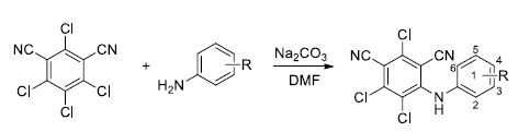
Scheme 1: Synthesis of titled compounds
Anti-proliferative Activity In Vitro and Structure-Activity Relationship
The vitro anticancer activities were assessed against lung cancer cell line A549 and colon cancer cell line HT29. The IC50 data (µM) (the concentration to achieve 50% proliferative inhibition) of the assessed compounds for these two cell lines are listed in Table 1.
Table 1: IC50 (μM) of compounds
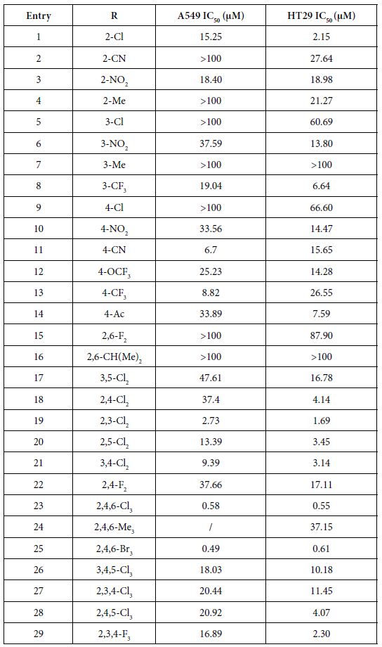
As presented in Table 1, these novel synthesized compounds showed various levels of anti-proliferative activities, indicating that substituents in phenyl ring exert important effect on anti-cancer activities. Generally, alkyl groups including methyl and isopropyl decreased the antiproliferative activities of title compounds which we can find the lowest antiproliferative activities (IC50 larger than 100 µM against both cancer cell lines) in compounds 4, 7, 16 and 24, except that compounds 4 and 24 have a moderate antiproliferative activity against HT29 with 21.27 and 37.15 µM IC50 respectively and no data on compound 24 against A549 yet. Nitro group is any interesting and important pharmacore group. Both clinical and preclinical results have demonstrated that compounds with nitro group hold great potential on enhancing anticancer properties. All prepared nitro compounds 3, 6 and 10 have moderate anticancer activities against both A549 and HT29 with 18.40, 18.98; 37.50, 13.80; and 33.56, 14.47 µM IC50 respectively, indicating that the position of nitro group at phenyl group (2-,3-,4- position of 3, 6, 10 respectively) does not cause any significant alteration of anticancer activities of these nitro compounds. Cyanide group does not have any positive sign on enhancing the anticancer activities as we see >100, 27.64; 6.7, 15.65 µM IC50 of compounds 2 and 11 against A549 and HT29 respectively although compound 11 with cyanide group located at 4 position in phenyl ring in has better anticancer activity than compound 2 with cyanide group located at 2 position in phenyl ring. Usually, compound with fluorine atom exhibits better bioactivities if the position is optimized [17]. In the present study, we prepared total six fluorine-containing compounds. Unexpectedly, all anticancer activities of them are not in the top levels. Compounds 22, 15 and 29 with fluorine alone as 2, 4-F2, 2, 6-F2, and 2, 3, 4-F3 respectively exhibited moderate activities as 37.66, 17.11; >100, 87.90; 16.89, 2.30 µM IC50 against A549 and HT29. Compounds 8 with trifluoromethyl group at 3-position of phenyl ring has a comparable but moderate anticancer activity with compound 13 with trifluoromethyl group at 4-position with 19.04, 6.64; 8.82, 26.55 µM IC50 against A549 and HT29 respectively. Furthermore, compound 12 with trifluoromethoxy group at 4-position of phenyl ring has a moderate anticancer activity as well with 25.23 and 14.28 μM IC50 against A549 and HT29 respectively.
The effect of chlorine atom on anticancer activities is our main focus on the present study. When compounds containing one chlorine atom at different positions of phenyl ring show moderate anticancer activities, compound 1 with 2-position chlorine has better activities than compounds 5 and 9 with 3-position and 4-position chlorine. Their IC50 are 15.25, 2.15; 100, 60.69; 100, 66.60 µM against A549 and HT29 respectively. Addition of one more chlorine to obtain di-chlorine compounds in phenyl ring slightly enhanced anticancer activities as we see in compounds 17, 18, 19, 20, 21, compared with compounds 1, 5, 9. The former IC50 are 47.61, 16.78; 37.4, 4.14; 2.73, 1.69; 13.39, 3.45; 9.39, 3.14 µM against A549 and HT29 respectively. Again, compounds with 2-position chlorine including compounds 18, 19, 20 have better activities than compounds with other position chlorine in phenyl ring. For compounds 23, 26, 27, 28 with three chlorines in phenyl ring, we see that compound 23 is the best one although others have moderate anticancer activities. Their IC50 are 0.58, 0.55; 18.03, 10.18; 20.44, 11.45 and 20.92, 4.07 µM against A549 and HT29 respectively. In contrast, comparing the trend of anticancer activities with three different halogens such as chlorine, bromine and fluorine would be very interesting to find the most important ones. Apparently, among compounds 23, 25 and 29, compounds 23 and 25 with either chlorine or bromine are the most active in all of prepared compounds in present study whereas compound 29 has moderate activity. Although there is no significant difference between compounds 23 and 25, compound 23 (chlorine atom) has better atom economy than compound 25 (bromine atom). Thus, compound 23 has the better potential to warrant further investigation.
Anti-proliferative Activity In Vitro of Compound 23 with Broad Spectrum
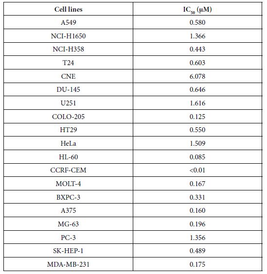
To further explore the anticancer activities of the most potent one, compound 23 in vitro, we screened its anticancer spectrum with total 19 cancer cell lines. As shown in Table 2, IC50 range is between 1.616 and ﹤0.01 µM with the most resistant one U251 and the most sensitive one CCRF-CEM. Except CCRF-CEM, HL-60, another non- solid tumor cell line showed the second most sensitivity to compound 23, indicating that compound 23 has strong activity to kill non-solid tumor cells. In contrast, brain tumor cells U251, cervical cancer cells HeLa and NIH-H1650 non small cancer lung cancer cells are in the most resistant cell lines with 1.616, 1.509 and 1.366 µM IC50 respectively.
Table 2: IC50 (μM) of compound 23 on 19 cancer cell lines
Exploration of Potential Molecular Mechanisms
To clarify the potential molecular mechanisms, we detected the expression of several critical proteins in three representative cells, T24, H520 and A549. As shown in Figures 1 and 2, compound 23 dramatically increases the expression of p-Akt, p-Erk and p21 in T24 cancer cells in both dose and time dependent patterns. In contrast, compound 23 profoundly decreases the expression of p-Akt but moderately increases the expression of p-Erk in H520 cells. Moreover, in A549 cells, compound 23 decreases the expression of both p-Erk and p-21, shown in Figures 3 and 4. However, compound 23 decreases the expression of p-Akt in low concentration but expression of p-Akt is increased in high concentration in Figure 5. Taken together, all evidence collected indicates that compound 23-induced alteration of p-Akt and p-Erk is in cell specific fashion. However, compound 23 broadly induced the decrease of p-Stat3 expression in all three cancer lines showed in Figures 1-5. These important results imply that decreasing p-Stat3 may be the major mechanism of compound 23 in inhibiting cancer cell growth although further detailed studies are needed to warrant this conclusion.
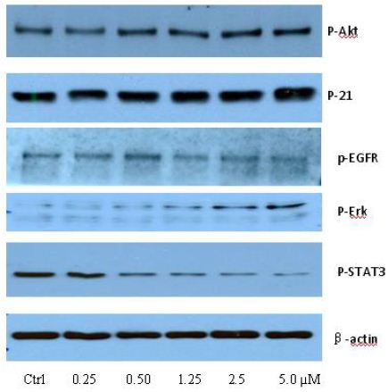
Figure 1: T24
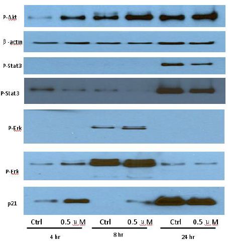
Figure 2: T24
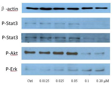
Figure 3: H520
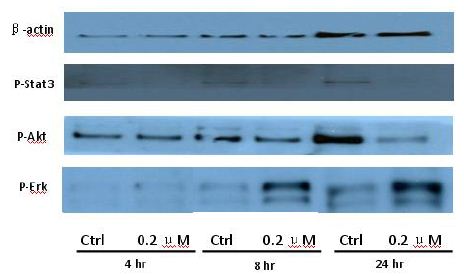
Figure 4: H520
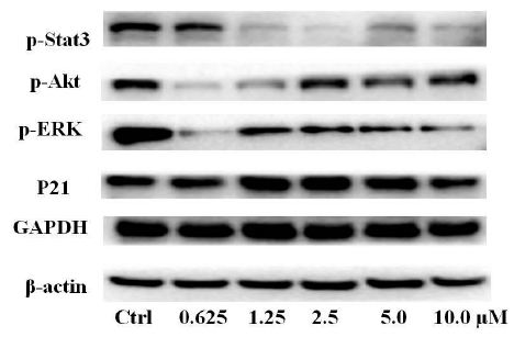
Figure 5: A549
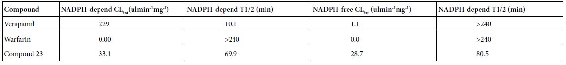
Microsomal Intrinsic Clearance
As shown in Table 3, the results of microsomal intrinsic clearance of compound 23 indicate that compound 23 has 33.1 and 28.7 uL min-1mg-1 under NADPH dependent and NADPH free conditions, indicating that NADPH has not an important effect to compound 23 on microsomal metabolism. Verapamil and warfarin were used as high-metabolized and low-metabolized controls respectively. Thus, CYP enzymes may have no important effect on microsomal intrinsic clearance.
Table 3: Microsomal Intrinsic Clearance
Caco-2 Permeability
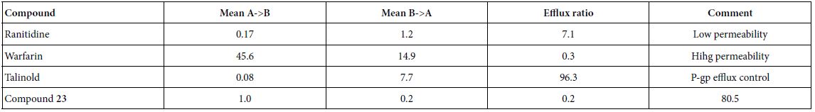
As shown in Table 4, compound 23 has relative low permeability with mean A → B Papp is higher than mean B → A Papp. Thus, this data implies that oral administration route is not proper way to clinically treat the patients. In this assay, we used ranitidine, warfarin and talinolol are controls.
Table 4: Caco-2 permeability
Plasma Protein Binding
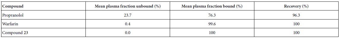
As shown in Table 5, compound 23 has 100% plasma protein binding ratio. Therefore, both oral and intravenous infusion administration routes may not be an efficient way to treat patients. In this assay, propranolol and warfarin were used as binding controls.
In summary, we prepared a series of novel compounds and tested their anticancer activities. The most potent compound 23 was found. Furthermore, novel mechanism of inhibiting Stat3 phosphorylation of compound 23 was explored. Also, brief ADME properties of compound 23 was determined and low potential to conventional drug administration routes was recommended.
Table 5: Plasma protein binding
Experimental Section
General Procedure for the Synthesis of Titled Compounds
Reagents were used without further purification unless otherwise specified. Solvents were dried and redistilled prior to use in the usual way. Analytical TLC was performed using silica gel HF254. To a solution of chlorothalonil (1 mmol) in dry DMF (20 ml), substituted aniline (1 mmol) and anhydrous sodium carbonate (1.5 mmol) were added at room temperature and the reaction mixture was stirred for 2 h at 60°C. The mixture was quenched by addition of ice water (100 ml). Then, the reaction mixture was filtered to afford the polyhalo isophthalonitriles compounds.
Physical and Spectral Information of Titled Compounds
2,4,5-Trichloro-6-((2-Chlorophenyl)Amino)Isophthalonitrile (1)
Yellow solid; Yield 69.6 %; mp: 208-210°C; 1H-NMR (300 M Hz, CDCl3): δ 7.03(s, 1H, NH), 7.27-7.38 (m, 3H, Ph-3,5,6-3H), 7.49-7.55 (m, 1H, Ph-4-H).
2,4,5-Trichloro-6-((2-Cyanophenyl)Amino)Isophthalonitrile (2)
Brown solid; Yield 67.5%; mp: 258-260°C. 1H-NMR (300 M Hz, CDCl3): δ 7.12 (s, 1H, NH), 7.24 (d, 1H, Ph-6-H, J=7.5 Hz), 7.47 (t,1H, Ph-4-H, J=7.2 Hz), 7.68 (t, 1H, Ph-5-H, J=7.5 Hz), 7.78 (d, 1H, Ph-3-H, J=7.8 Hz).
2,4,5-Trichloro-6-(o-Tolylamino)Isophthalonitrile (3)
Brown solid; Yield 74.1%; mp: 258-260°C.1H-NMR (300 M Hz, CDCl3): δ 9.48 (s, 1H, NH), 7.44 (d, 1H, Ph-6-H, J=7.5 Hz), 7.68 (t,1H, Ph-4-H, J=7.2 Hz), 7.60(t, 1H, Ph-5-H, J=7.5 Hz), 8.2 (d, 1H, Ph-3-H, J=7.8 Hz). HRMS (ESI): calcd for C14H5C13N4O2Na [M + Na]+ ; 390.5700; found 389.9411.
2,4,5-Trichloro-6-(o-Tolylamino)Isophthalonitrile (4)
Gray red solid; Yield 73.2%; mp: 212-214°C; 1H-NMR (300 M Hz, CDCl3): δ (s, 3H, CH3), 7.00 (s, 1H, NH), 7.15 (d, H, Ph-6-H, J=7.5 Hz), 7.28-7.34 (m, 3H, Ph-3,4,5-3H). HRMS (ESI): calcd for C15H8Cl3N3Na [M + Na]+; 359.6000; found 359.9659.
2,4,5-Trichloro-6-((3-Chlorophenyl)Amino)Isophthalonitrile (5)
Brown solid; Yield 68.4%; mp: 228-230°C. 1H-NMR (300 M Hz, CDCl3): δ 7.04 (br, 1H, NH), 7.09 (d, J=7.5 Hz, 1H, Ph-6-1H), 7.20 (s, 1H, Ph-2-1H), 7.33-7.39 (m, 2H, Ph-4,5-2H). HRMS (ESI): calcd for C14H5Cl4N3Na [M + Na]+ ; 380.0150; found 380.9136.
2,4,5-Trichloro-6-((3-Nitrophenyl)Amino)Isophthalonitrile (6)
Gray solid; Yield 69.6%; mp: 250-252°C. 1H-NMR (300 M Hz, DMSO): 7.54-7.64 (m, 2H, Ph-5,6-2H), 7.94-8.00 (m, 2H, Ph-2,4- 2H),9.86 (br, 1H, NH). HRMS (ESI): calcd for C14H5C13N4O2Na [M + Na]+; 390.5700; found 389.9411.
2,4,5-Trichloro-6-(m-Tolylamino)Isophthalonitrile(7)
Brown solid; Yield 69.6%; mp: 248-25°C. 1H-NMR (300 M Hz, CDCl ): 2.40(s,3H, Ph-3-CH ), 7.02 (br, 1H, NH),7.12-7.36 (m, 4H, Ph-2,3,4,6-4H). HRMS (ESI): calcd for C15H8Cl3N3Na [M + Na]+ ; 359.6000; found 359.9659.
2,4,5-Trichloro-6-((3-(Trifluoromethyl)Phenyl)Amino) Isophthalonitrile (8)
Yellow solid; Yield 69.6%; mp: 236-238°C. 1H-NMR (300 M Hz, CDCl3): 7.12 (s, 1H, NH), 7.28-7.40 (m, 1H, Ph-6-H), 7.41-7.52 (m, 2H, Ph-2,4-2H), 7.54-7.62 (m, 1H, Ph-5-H).
2,4,5-Trichloro-6-((4-Chlorophenyl)Amino)Isophthalonitrile (9)
Yellow Yield 74.2%; mp: 259-261°C; 1H-NMR (300 M Hz, CDCl3): 7.00 (s, 1H, NH), 7.17 (d, 2H, Ph-2,6-2H, J=8.4 Hz), 7.42 (d, 2H, Ph-3,5-2H, J=8.7 Hz).
2,4,5-Trichloro-6-((4-Nitrophenyl)Amino)Isophthalonitrile (10)
Yellow Yield 69.3%; mp: 256-258°C; 1H-NMR (300 M Hz, CDCl3): 7.00 (s, 1H, NH), 7.17 (d, 2H, Ph-2,6-2H, J=8.3 Hz), 7.42 (d, 2H, Ph-3,5-2H, J=9.5 Hz).
2,4,5-Trichloro-6-((4-Cyanophenyl)Amino)Isophthalonitrile (11)
Yellow Yield 69.6%; mp: 259-261°C; 1H-NMR (300 M Hz, CDCl3): 7.00 (s, 1H, NH), 7.17 (d, 2H, Ph-2,6-2H, J=8.7 Hz), 7.42 (d, 2H, Ph-3,5-2H, J=9.0 Hz).
2,4,5-Trichloro-6-((3-(Trifluoromethoxy)Phenyl)Amino) Isophthalonitrile (12)
Gray Yield 75.3.%; mp: 204-206°C; 1H-NMR (300 M Hz, CDCl3): 7.09 (s, 1H, NH), 7.22-7.32 (m, 4H, Ph-2,3,5,6-4H).
2,4,5-Trichloro-6-((4-(Trifluoromethyl)Phenyl)Amino) Isophthalonitrile (13)
Yellow Yield 74.2.%; mp: 186-187°C; 1H-NMR (300 M Hz, CDCl3): 6.06 (br, 1H, NH), 6.51(d, J=5.7 Hz,2H, Ph-2,6-2H), 7.52(d, J=5.7 Hz,2H, Ph-3,5-2H).
4-((2,3,5-Trichloro-4,6-Dicyanophenyl)Amino)Phenyl Acetate (14)
Gray Yield 74.2.%; mp: 246-248°C; 1H-NMR (300 M Hz, CDCl3): 2.29 (s, 3H, COOCH3), 7.08 (s, 1H, NH), 7.17 (d, 2H, Ph-3,5-2H, J=8.7 Hz), 8.10 (d, 2H, Ph-2,6-2H, J=8.7 Hz).
2,4,5-Trichloro-6-((2,6-Difluorophenyl)Amino)Isophthalonitrile (15)
Gray Yield 74.2.%; mp: 218-220°C; 1H-NMR (300 M Hz, CDCl3): 7.03 (s, 1H, NH), 7.13 (dd, 1H, Ph-6-H, 3J=8.1 Hz, 4J=0.9 Hz), 7.28 (t, 1H, Ph-5-H, J=8.1 Hz), 7.47 (dd, 1H, Ph-4-H, 3J=8.1 Hz, 4J=0.9 Hz). HRMS (ESI): calcd for C14H4CI3F2N3Na [M + Na]+ ; 381.5538; found 381.9346.
(2,4,5-Trichloro-6-((2,6-Diisopropylphenyl)Amino) Isophthalonitrile (16)
Gray Yield 69.3%; mp: 216-218°C; 1H-NMR (300 M Hz, CDCl3): δ 7.12 (d, J=8.1 Hz, 2H), 6.98 (dd, J=8.3, 6.9 Hz, 1H), 5.87 (d, J=2H), 3.02 (p, J=6.8 Hz, 2H), 1.29 (d, J=6.9 Hz, 12H).
2,4,5-Trichloro-6-((3,5-Dichlorophenyl)Amino)Isophthalonitrile (17)
White solid; Yield 56.7%; mp: 238-242°C; 1H-NMR (300 M Hz, CDCl3): 6.95 (s, 1H, NH), 7.05 (d, 2H, Ph-2,6-2H, J=1.8 Hz), 7.32 (d, 1H, Ph-4-H, J=1.5 Hz). HRMS (ESI): calcd for C14H4C15N3Na [M + Na]+; 414.4570; found 413.8757.
2,4,5-Trichloro-6-((2,4-Dichlorophenyl)Amino)Isophthalonitrile (18)
Brown Black solid; Yield 59.6%; mp: 209-212°C; 1H-NMR (300 M Hz, CDCl3): 6.95 (s, 1H, NH), 7.20 (d, 1H, Ph-6-H, J=8.1 Hz), 7.36 (dd, 1H, Ph-5-H, 3J=8.7 Hz, 4J=2.7 Hz), 7.54 (d, 1H, Ph-3-H, J=2.4 Hz). HRMS (ESI): calcd for C14H4C15N3Na [M + Na]+; 414.4570; found 413.8757.
2,4,5-Trichloro-6-((2,3-Dichlorophenyl)Amino)Isophthalonitrile (19)
Gray White solid; Yield 58.6%; mp: 218-220°C; 1H-NMR (300 M Hz, CDCl3): 7.03 (s, 1H, NH), 7.13 (dd, 1H, Ph-6-H, 3J=8.1 Hz, 4J=0.9 Hz), 7.28 (t, 1H, Ph-5-H, J=8.1 Hz), 7.47 (dd, 1H, Ph-4-H, 3J=8.1 Hz, 4J=0.9 Hz). HRMS (ESI): calcd for C14H4C15N3Na [M + Na]+; 414.4570; found 413.8757.
2,4,5-Trichloro-6-((3,4-Dichlorophenyl)Amino)Isophthalonitrile (20)
Gray white solid; Yield 57.6%; mp: 220-222°C; 1H-NMR (300 M Hz, CDCl3): δ 7.45 (d, J=8.6 Hz, 1H), 7.32 – 7.25 (m, 2H), 7.21 (d, J=2.4 Hz, 1H), 6.96 (s, 1H).
2,4,5-Trichloro-6-((3,4-Dichlorophenyl)Amino)Isophthalonitrile (21)
Brown solid; Yield 58.9%; mp: 230-232°C; 1H-NMR (300 M Hz, DMSO): 7.13 (dd, J=8.4 Hz,J=2.1 Hz,1H,Ph-4-1H), 7.39(d, J=2.1 Hz,1H,Ph-6-1H), 7.51(d, J=8.4 Hz,1H,Ph-3-1H),9.62(br, 1H, NH).
2,4,5-Trichloro-6-((2,4-Difluorophenyl)Amino)Isophthalonitrile (22)
Gray solid; Yield 67.5%; mp: 206-208°C; 1H-NMR (300 M Hz, CDCl3): 6.88 (s, 1H, NH), 6.99 (t, 2H, Ph-5,6-2H, J=8.1 Hz), 7.32 (d, 1H, Ph-3-H, J=2.4 Hz).
2,4,5-Trichloro-6-((2,4,6-Trichlorophenyl)Amino) Isophthalonitrile (23)
Brown solid; Yield 67.5%; mp: 241-243°C; 1H-NMR (300 M Hz, CDCl3): 6.86 (S, 1H, NH),7.48(s, 2H,Ph-3,5-2H).
2,4,5-Trichloro-6-(Mesitylamino)Isophthalonitrile (24)
Brown solid; Yield 67.5%; mp: 199-201°C; 1H-NMR (300 M Hz, CDCl3): 2.17(s,6H,Ph-2,6-2CH3),2.34(s,3H,Ph-4-CH3) 6.81(br, 1H, NH),6.97(s, 2H,Ph-3,5-2H). HRMS (ESI): calcd for C17H11CI3N3 [M-H]+ ; 387.6540; found 386.0040.
2,4,5-Trichloro-6-((2,4,6-Tribromophenyl)Amino) Isophthalonitrile (25)
Brown solid; Yield 67.5%; mp: 251-253°C 1H-NMR (300 M Hz, CDCl3) δ 7.82 (s, 2H), 6.93 (s, 1H).
2,4,5-Trichloro-6-((3,4,5-Trichlorophenyl)Amino) Isophthalonitrile(26)
Yellow solid; Yield 59.3%; mp: 264-266°C; 1H-NMR (300 M Hz, DMSO): 7.53 (s, 2H,Ph-2,6-2H),8.98(br, 1H, NH).
2,4,5-Trichloro-6-((2,3,4-Trichlorophenyl)Amino) Isophthalonitrile(27)
Gray solid; Yield 59.3%; mp: 198-200°C; 1H-NMR (300 M Hz, CDCl3): 6.98(br, 1H, NH), 7.08(d, J=9.0 Hz, 1H, Ph-6-1H), 7.46 (d, J=9.0 Hz, 1H, Ph-5-1H).
2,4,5-Trichloro-6-((2,4,5-Trichlorophenyl)Amino) Isophthalonitrile (28)
Yellow solid; Yield 78.5%; mp: 253-255°C; 1H-NMR (300 M Hz, CDCl3): 6.88 (br, 1H, NH), 7.33 (s,1H,Ph-6-1H),7.96 (s,1H,Ph-5-1H).
2,4,5-Trichloro-6-((2,3,4-Trifluorophenyl)Amino) Isophthalonitrile (29)
Gray solid; Yield 69.6%; mp: 182-184°C; 1H-NMR (300 M Hz, CDCl3): 6.87 (s, 1H, NH), 7.05-7.09 (m, 2H, Ph-5,6-2H).
Cell Lines and Culture Conditions
All human cancer cell lines were purchased from Cell Resource Center, Institute of Life Sciences, Chinese Academy of Sciences (Shanghai, China) and cultured in either DMEM (Hyclone, Logan, UT, USA) or RPMI-1640 (Hyclone, Logan, UT, USA) supplemented with 10% of FBS (Hyclone, Logan, UT, USA) and 1% of penicillin- streptomycin at 37°C, in humidified air containing 5% of CO2.
Cell Viability Assay
Cell viability was assessed using a tetrazolium based assay using microplate reader (Biotek, SYNERGY HTX, Vermont, USA). IC50 values were determined through the dose-response curves. Cells were seeded at 6×10³ per well in 96-well culture plates and incubated in medium containing 10% FBS. Different seeding densities were optimized at the beginning of the experiments. After 24h, cells were treated with different concentrations of titled compounds with various concentrations for 48 hours in incubator. 50μl of MTT tetrazolium salt (Sigma) dissolved in Hank’s balanced solution at a concentration of 2 mg/ml was added to each well with indicated treatment and incubated in CO2 incubator for 5 h. Finally, the medium was aspirated from each well and 150μl of DMSO (Sigma) was added to dissolve formazan crystals and the absorbance of each well was obtained using a Dynatech MR5000 plate reader at a test wavelength of 490 nm with a reference wavelength of 630 nm.
Protein Characterization
Western blot assessment was performed using regular procedure. Primary antibody was added in BSA and allowed to incubate overnight at 4°C, washed with TBS/0.05% Tween-20 for 5 times (10min per time) before the secondary antibody was added and then incubated for an additional hour at room temperature. The membrane was again washed 3 times before adding Pierce Super Signal chemiluminescent substrate (Rockford, IL, USA) and then immediately imaged on Chemi Doc (Bio-Rad, Hercules, CA, USA). The films were scanned using EPSON PERFECTION V500 PHOTO and quantified by Image J (NIH, Bethesda, MD, USA).
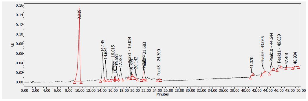
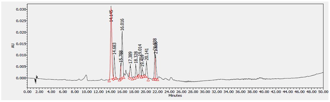
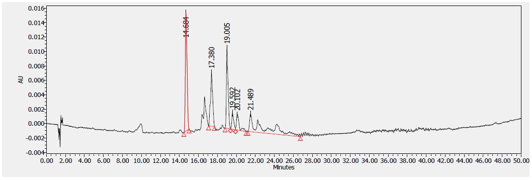
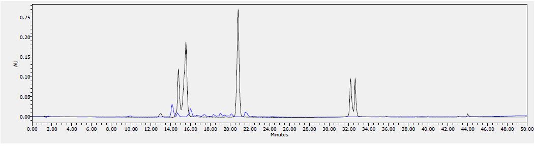
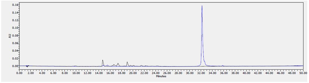
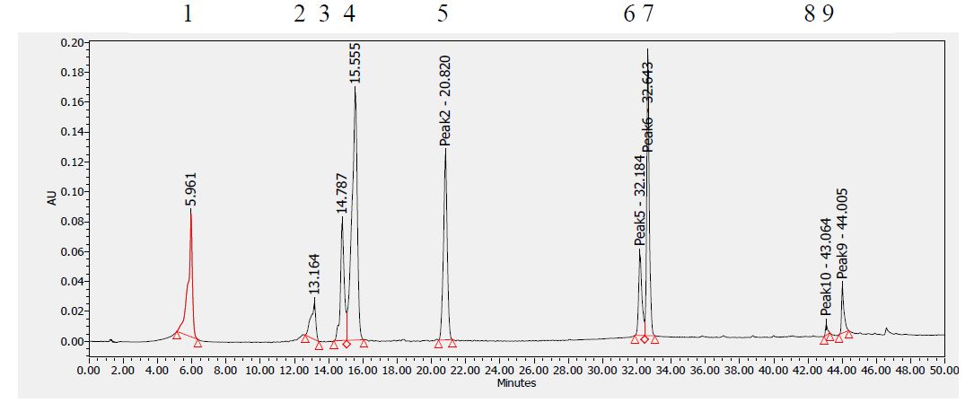
Analytical Method Development for compound 23
The signal was optimized for each compound by ESI positive or negative ionization mode. An MS2 scan or a SIM scan was used to optimize the fragmenter voltage and a product ion analysis was used to identify the best fragment for analysis, and the collision energy was optimized using a product ion or MRM scan. An ionization ranking was assigned indicating the compound’s ease of ionization.
Analytical Method Development for ADME
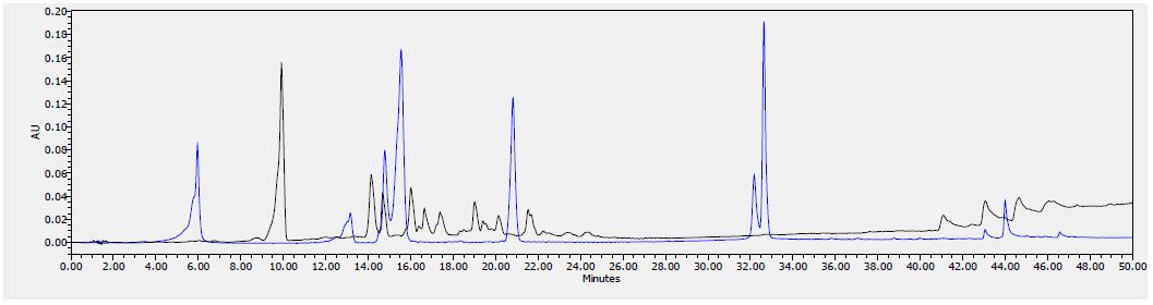
Samples were analyzed by LC/MS/MS using an Agilent 6410 mass spectrometer coupled with an Agilent 1200 HPLC and a CTC PAL chilled autosampler, all controlled by MassHunter software (Agilent). After separation on a C18 reverse phase HPLC column (Agilent, Waters, or equivalent) using an acetonitrile-water gradient system, peaks were analyzed by mass spectrometry (MS) using ESI ionization in MRM mode.
Microsomal Stability Assay
The test agent is incubated in duplicate with microsomes at 37°C. The reaction contains microsomal protein in 100 mM potassium phosphate, 2 mM NADPH, 3 mM MgCl2, at pH 7.4. A control reaction is performed for each test agent omitting NADPH (to detect NADPH- free degradation). At indicated times, an aliquot is removed from each experimental and control reaction and mixed with an equal volume of ice-cold Stop Solution (methanol, containing haloperidol, diclofenac, or other internal standard). Stopped reactions are incubated at least ten minutes at -20°C, and an additional volume of water is added. The samples are centrifuged to remove precipitated protein, and the supernatants are analyzed by LC/MS/MS to quantitate the remaining parent. Data are converted to % remaining by dividing by the time zero concentration value. Data are fit to a first-order decay model to determine half-life. Intrinsic clearance is calculated from the half-life and the protein concentrations:
CLint=ln(2) /(T1/2 [microsomal protein])
Verapamil (high metabolized) and warfarin (low metabolized) were used as reference controls.
Caco-2 cells grown in tissue culture flasks are trypsinized, suspended in medium, and the suspensions were applied to wells of a Millipore 96 well Caco-2 plate. The cells are allowed to grow and differentiate for three weeks, feeding at 2-day intervals. For Apical to Basolateral (A → B) permeability, the test agent is added to the apical (A) side and amount of permeation is determined on the basolateral (B) side; for Basolateral to Apical (B → A) permeability, the test agent is added to the B side and the amount of permeation is determine on the A The A-side buffer contains 100 μM Lucifer yellow dye, in Transport Buffer (1.98 g/L glucose in 10 mM HEPES, 1x Hank’s Balanced Salt Solution) pH 6.5, and the B-side buffer is Transport Buffer, pH 7.4. Caco-2 cells are incubated with these buffers for 2 hr, and the receiver side buffer is removed for analysis by LC/MS/MS. To verify the Caco-2 cell monolayers are properly formed, aliquots of the cell buffers are analyzed by fluorescence to determine the transport of the impermeable dye Lucifer Yellow. Any deviations from control values are reported.
Data are expressed as permeability (Papp): AC dt dQ Papp 0 = where dQ/dt is the rate of permeation, C0 is the initial concentration of test agent, and A is the area of the monolayer.
In bidirectional permeability studies, the Efflux Ratio (RE) is also calculated: ( ) ( R e BA P A B P app app →→ =
An RE > 2 indicates a potential substrate for P-gp or other active transporters.
Plasma Protein Binding
Test agent is added to plasma. This mixture is dialyzed in a RED Device (Pierce) per the manufacturers’ instructions against PBS and incubated on an orbital shaker. After the end of the incubation, aliquots from both plasma and PBS sides are collected, an equal amount of PBS is added to the plasma sample, and an equal volume of plasma is added to the PBS sample. Methanol (three volumes) containing internal standard is added to precipitate the proteins and release the test agents. After centrifugation, the supernatant is transferred to a new plate and analyzed by LC/MS/MS.
References
- Cancer Facts & Figures (2015) American Cancer
- Domingo-Musibay E, Galanis E (2015) What next for newly diagnosed glioblastoma? Future Oncol 11: 3273-3283. [crossref]
- Oberstein PE, Olive KP (2013) Pancreatic cancer: why is it so hard to treat? Ther Ad Gastroenterol 6: 321-337. [crossref]
- Lemjabbar-Alaoui H, Hassan OUI, Yang YW, Buchanan P (2015) Lung cancer: Biology and treatment Biochim Biophys Acta 1856: 189-210. [crossref]
- Holohan C, Van Schaeybroeck S, Longley DB, Johnston PG (2013) Cancer drug resistance: an evolving Nat Rev Cancer 13: 714-726. [crossref]
- O’Connor R (2009) A review of mechanisms of circumvention and modulation of chemotherapeutic drug Curr Cancer Drug Targets 9: 273-280. [crossref]
- Yan SJ, Huang, ; Zeng, X. H.; Huang, R.; Lin, J. (2010) Solvent-free, microwave assisted synthesis of polyhalo heterocyclic ketene aminals as novel anti-cancer agents. Bioorg Med Chem Lett 20: 48-51. [crossref]
- Huang C, Yan SJ, Zeng XH, Dai XY, Zhang Y, et (2011) Biological evaluation of polyhalo 1,3-diazaheterocycle fused isoquinolin-1(2H)-imine derivatives. Eur J Med Chem 46: 1172-1180. [crossref]
- Yan SJ, Zhen H, Huang C, Yan YY, Lin J, et (2010) Synthesis of highly functionalized 2,4-diaminoquinazolines as anticancer and anti-HIV agents. Bioorg Med Chem Lett 2: 4432-4435. [crossref]
- Heilman WP, Battershell RD, Pyne WJ, Goble PH, Magee TA, et (1978) Synthesis and antiinflammatory evaluation of substituted isophthalonitriles, trimesonitriles, benzonitriles, and terephthalonitriles. J Med Chem 21: 906-913. [crossref]
- Guan AY, Liu CL, Huang G, Li HC, Hao SL, et (2013) Design, synthesis, and structure-activity relationship of novel aniline derivatives of chlorothalonil. J Agric Food Chem 61: 11929-11936. [crossref]
- Kadayat TM, Song C, Kwon Y, Lee, S. (2015) Modified 2,4-diaryl-5H-indeno[1,2-b] pyridines with hydroxyl and chlorine moiety: synthesis, anticancer activity, and structure-activity relationship study. Bioorg Chem 62: 30-40. [crossref]
- Kadayat TM, Park S, Jun KY, Magar TB, Bist G, et (2016) Effect of chlorine substituent on cytotoxic activities: design and synthesis of systematically modified 2,4-diphenyl-5H-indeno[1,2-b]pyridines. Bioorg Med Chem Lett 7: 1726-1731. [crossref]
- Beck DE, Lv W, Abdelmalak M, Plescia CB, Agama K, Marchand C, Pommier Y, Cushman M (2016) Synthesis and biological evaluation of new fluorinated and chlorinated indenoisoquinoline topoisomerase I poisons. Bioorg Med Chem 7: 1469-1479.
- Li HC, Guan AY, Huang G, Liu CL, Li ZN, et (2016) Design, synthesis and structure-activity relationship of novel diphenylamine derivatives. Bioorg Med Chem 3: 453-461. [crossref]
- Chai BS, Wang SY, Yu WQ, Li HC, Song CJ, et (2013) Synthesis of novel strobilurin- pyrimidine derivatives and their antiproliferative activity against human cancer cell lines. Bioorg Med Chem Lett 23: 3505-3510. [crossref]
- Wang J, Sánchez-Roselló M, Aceña JL, del Pozo C, Sorochinsky AE, et (2014) Fluorine in pharmaceutical industry: fluorine-containing drugs introduced to the market in the last decade (2001-2011). Chem Rev 4: 2432-2506. [crossref]