DOI: 10.31038/NAMS.2022521

Abstract

The paper begins with a review of known diffusion models of the literature, in terms of the mass fraction and the chemical potential. Next the  thermodynamic consistency of the pertinent schemes is investigated and it follows that the recourse to the chemical potential is justified in two different ways. The alternative recourse to the balance equations, through a linearization procedure, is suggested as a check of consistency. Finally it is pointed out that, thanks to the correspondence probability-concentration, the classical models of diffusion can be extended to the quantum context.

Keywords

Diffusion models, Thermodynamic consistency, Concentration, Chemical potential

Introduction

The purpose of this paper is to review standard models of diffusion and to clarify the physical bases leading to the different differential equations. To understand the basic starting point and to establish the required notation we start with addressing attention to a mixture of n fluid constituents.

In essence, let ρ_α , v_α be the mass density and the velocity of the α th constituent,

α = 1, …, n. We let

be the mass density of the mixture and the mass fraction (or concentration) of the α th constituent; the sum on α is understood from 1 to n. As we prove in a moment ω_α is subject to the differential equation

where h_α is the mass flux,  ∇ is the gradient operator and then ∇ is the divergence, and the superposed dot denotes the (total) time derivative.

Within the theory of mixtures h_α is clearly defined and shown to satisfy a differential equation [1,2]. As we emphasize in this paper, h_α is regarded as an unknown vector to be determined through mathematical assumptions associated with physical properties of the mixture. The original Fick’s model is based on the assumption

where D_α is the diffusivity. Next other models and their generalizations have been developed in terms of the chemical potential.

In this paper we first review known diffusion models in terms of the mass fraction ω_α and the chemical potential µ_α. Next we investigate the thermodynamic consistency of the pertinent schemes and find that the recourse to the chemical potential is justified in two different ways. Next we examine the alternative recourse to the balance equations through a linearization procedure. Further, we point out that the ideas about the correspondence probability-concentration is applied to modelling diffusion in the quantum context.

Balance Equations for Fluid Mixtures

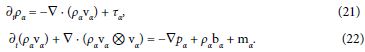
Consider a mixture of n fluid constituents (see, e.g., [1]). The suffices α, β = 1, 2, …, n label the quantities related to the α th, β th constituent. Hence ρ_α is the mass density and v_α the velocity of the α th constituent. The continuity equation of the α th constituent comprises the mass supply τ_α, per unit volume and unit time, so that

The conservation of mass of the whole mixture implies

Hereafter  is  a  shorthand for  The mass supply τ_α is nonzero in chemical reactions and phase transformations or generally whenever a constituent may gain or lose mass in favor of the other constituents.

The mass density ρ and the (barycentric) velocity v of the mixture are defined by

The ratio

is the mass fraction (or concentration) of the α th constituent and u_α = v_α − v

is the diffusion velocity. The definition of v implies that

The sum of (1) with the constraint (2) results in

∂_t ρ + ∇ · (ρv) = 0,                                              (3)

which is the continuity equation for the whole mixture.

We now investigate the evolution equation for ω_α. Replace ρ_α with ρω_α and v_α with

v + u_α in (1). In view of (3) we find

ρ(∂_tω_α + v · ∇ω_α) + ∇ · (ρ_αu_α) = τ_α.

Observe that ∂_tω_α   + v.  ∇ω_α  is the derivative with respect to the barycentric observer. As with any function it is denoted by a superposed dot. The vector

h_α:= ρ_α u_α

is the α th diffusion flux representing the flux of the α th constituent relative to the barycentric observer. Hence we can write

The mass fraction ω_α, in the barycentric reference, evolves according to (4). This equation is operative once τ_α and h_α are given in terms of  , possibly parameterized by temperature and pressure.

The equation of motion of the α th constituent can be written in the form

∂_t (ρ_αv_α) + ∇· (ρ_αv_α ⊗ v_α) − ∇ · T_α − ρ_αb_α = m_α,

where T_α is the Cauchy stress tensor, b_α is the body force, and m_α is the growth of the linear momentum, that is the force on the α th constituent due to other constituents of the mixture. The growths {m_α} are subject to the constraint

Modelling of Diffusion Fluxes and Diffusion Equations

The physical modelling of diffusion is most often restricted to non-reacting mixtures, τ_α = 0, and is based on the view that diffusion is governed by (4) with appropriate models for h_α.

The simplest and best known model of diffusion traces back to Fick [3] and is based on an assumption on h_α that is motivated by the analogy with the Fourier model of heat conduction. First the total derivative  is replaced with the partial derivative ∂_t ω_α; this means that diffusion is examined in the barycentric frame. Moreover, Fick’s law assumes the diffusion flux h_α is antiparallel to ω_α, i.e. h_α = κ_α ω_α, where κ_α > 0 may depend on the constituent. Hence divide eq. (4) by ρ to obtain

where ζ_α = τ_α /ρ. If κ_α is constant then the evolution equation for ω_α takes the form

the quantity D_α = κ_α /ρ is called diffusivity.

Diffusion in solids is often modelled by letting ([4], ch. 17) h_α = −D_α ∇ N_α,

where N_α is the concentration in the form

 being the number of atoms per unit volume.

Other diffusion equations are based on the following two main assumptions. Let ψ_α be the α th Helmholtz free energy and define

The assumption is h_α = −κ_α ∇ µ_α.

For definiteness we consider ψ_α in the form [5]

If λ_α is constant then it follows

and eq. (4) takes the form

Equation (8) is usually referred to as the Cahn-Hilliard equation [6,7]. It is a fourth-order partial differential equation. If the dependence on ∇ ω_α is ignored then the Cahn-Hilliard equation reduces to the second-order parabolic equation (6).

Alternatively it is assumed that the evolution of ω_α is in fact a relaxation toward equilibrium governed by [8]

Hence, letting ψ_α be given again by the Landau-Ginzburg function (7) we obtain

Equation (9) is a second-order partial differential equation  when ψ_α depends on ∇ω_α ; it is referred to as the Ginzburg-Landau equation or the Allen-Cahn equation. While eq. (6) is based on Fick’s law h_α = −κ_α ∇ ω_α , eqs (8) and (9) are based on the assumptions

The function    is often regarded as the chemical potential. As   we see in a moment differs from the standard (correct) expression of the chemical potential. Moreover even simple thermodynamic considerations would justify the use of the chemical potential.

Thermodynamic Test of (10)

The balances of energy and entropy are stated by considering the mixture as a whole body. The balance of energy is taken in the form

where ε is the internal energy density, per unit mass, D is the stretching tensor, q is the heat flux vector, and r is the external heat supply. Let θ > 0 be the absolute temperature. The second law of thermodynamics is stated as follows: the entropy density η and the entropy flux j satisfy the inequality

For every admissible process that is every set of constitutive functions compatible with the balance equtaions.

For formal conveneince let

k being the extra-entropy flux to be determined. Substituting ρr-∇.q from eq. (11)

Let ψ = ε-θη be the Helmholtz free energy of the mixture. The second law inequality can be written as

To determine thermodynamic consequences of the second law we now consider

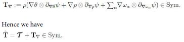
as the set of independent variables. Moreover we specialize T in the form

with T = O(D) as D→0. Compute ψ˙ and substitute in the Clausius- Duhem inequality (12). The arbitrariness and linearity of ω¨_α , ρ¨, D¨ , θ¨ reduces the possible dependencies of ψ

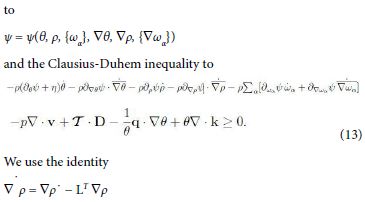
and the analogue for ∇ θ and ∇ ω_α. Now, divide (13) by θ and consider the identities

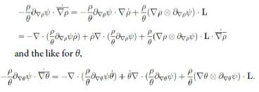
Moreover we have

Hence upon some rearrangements we can write inequality (13)  in the form

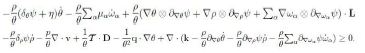
Since L = D+W, with W ∈ skw the spin tensor, then the arbitrariness of W implies that

Now,   D =  D₀ being the deviator of D. This in turn implies that T_∇ embodies an isotropic part to contribute to the pressure. For simplicity we let p be free of tr T_∇ . Consequently, since ρ˙ = −ρ∇ · v it follows that the inequality takes the form

the dots denoting the other terms of the inequality. Hence we let p = ρ²δ_pψ.

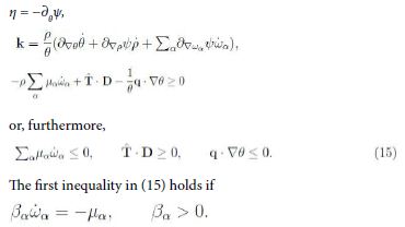
Consequently we are left with the inequality

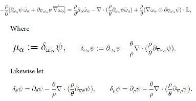
Thermodynamic Restriction on 

Sufficient conditions for inequality (14) are

It is suggestive that this thermodynamic condition has the form of (10)₂. Yet we have to check whether   Now, from the theory of mixtures we have

to within kinetic terms. If we let each ψ_α depend on the corresponding mass density

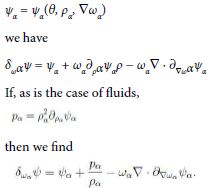
Hence  we  conclude  that,  to  within  the standard chemical potential is

Thermodynamic Restriction on h_α

Back to inequality (14) we let again η = −δ_θ ψ. Next we observe that  is given by (1). Substitution of  from (1) results in

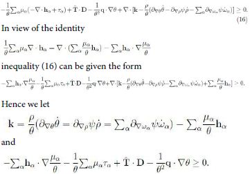
This inequality holds if each term has the required sign; in particular

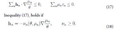
Hence, owing to the neglect of kinetic terms in ψ, by the second law inequality it follows that the diffusion flux h_α is determined by the gradient of µ_α /θ, and not merely of µ_α. This is a direct thermodynamic requirement without any need of a-priori rescaling [9].

Inequality (17)₂ governs the evolution of a possible reaction. For a binary mixture the inequality reduces to

the reaction proceeds toward the constituent with higher values of the chemical potential.

Diffusion of Electrically Charged Constituents

Equation (4) is a basic reference in the modelling of diffusion.

Indeed, for non-reacting mixtures the basic equation is written in the form

∂_tω_α = −∇ · h_α , (19)

the occurrence of ρ, though non-constant,  being  ignored;  in  the literature the notation is frequently c_i and J_i for ω_α and h_α. For definiteness, look at the motion of a charged constituent in a fluid medium.

The diffusion flux is viewed as the sum of three terms [10]: a diffusion term D_α ∇ ω_α as in Fick’s law, an advective term ω_αv viewed as the transport of the constituent via the motion of the fluid, the diffusivity times the electric force (electromigration). The advective term may be ignored by selecting a frame at rest with the fluid.

An extensive approach in the literature is based on eq. (18) and on h_α = −D_α ∇ ω_α

in the simplest model. Borrowing from the properties of the ideal gas we take the chemical potential µ_α in the form

to within inessential additive terms independent of ω_α. Hence we observe that, at constant temperature,

Now the chemical potential is an energy per unit mass. Assume the αth constituent consists of ions with electric charge z_αe, where e is (the absolute value of) the electron charge. The force per unit mass is

φ being the potential and m_α the ion mass. Moreover

where F is the Faraday constant, i.e. the charge of a mole, and M_α is the molar mass. Hence we write the whole chemical potential, or electrostatic-chemical potential, in the form

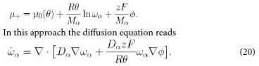
This is a form of the Nernst-Planck equation [11].

Kirkendall Effect

The Kirkendall effect involves a property of diffusion associated with different diffusivities of the constituents. The property was found experimentally by Smiglskas and Kirkendall. In essence, molibdenum markers are located at the boundary between the inner CuZn block and the outer copper covering. Upon heating, the markers are observed to move inward. To explain the experiment, we observe that within the block Cu and Zn atoms have the same density N; since  the atomic weights are almost the same (Cu 63.5, Zn 65.4) the equal density N means equal concentration ω. The Zn atoms have a higher diffusivity coefficient and hence the outward flux of Zn is not exactly compensated by the inward flux of Cu atoms. Thus the mass of matter in the block decreases and this results in the movement of the copper- brass interface(markers) toward the inner block.

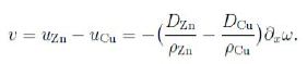
We now ask for the velocity of the markers. We have

ρ_Znu_Zn = h_Zn = −D_Zn∇ω, ρ_Cuu_Cu= h_Cu = −D_Cu ∇ω;

really we should account also for a inward flux of vacancies (from the material with the higher diffusion coefficient). In one dimension we obtain the velocity v of the markers as follows,

Dynamic Diffusion Equation

Models of diffusion are usually based on the balance equation (4) for the mass fraction ω_α and a constitutive equation for the mass flux h_α. Hence the resulting differential equation for ω_α is strongly affected by the constitutive assumption. It seems of interest to look  at the evolution problem via the balance equations for the unknown densities ρ_α.

Restrict attention to mixtures of inviscid fluids and hence T_α = p_α1. Consider the balance of mass and linear momentum in the local form,

Partial time differentiation of the first equation, divergence of the second one, and substitution of ∇ · ∂_t(ρ_αv_α) yield

∂2ρ_α = ∇ · [∇ · (ρ_αv_α ⊗ v_α)] − ∇ · (∇ · T_α) −  ∇· (ρ_αb_α) − ∇ · m_α + ∂_tτ_α.

If the constituent is regarded as an inviscid fluid, T_α = −p_α1, it follows

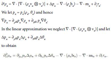
If, further, the temperature is assumed to be uniform, ∇ θ_α = 0, then

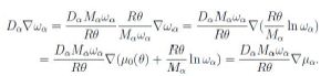
Equation (23) is the αth equation of a system where ∇. m_α and ∂_tτ_α account for possible coupling terms. Since ρ_α = ρω_α, if ρ is assumed to be constant then we have

If the αth constituent is electrically charged then

where e is (the absolute value of) the electronic charge, z_αe is the ionic charge, and m_α

is the ionic mass. In terms of molar quantities we have

where M_α is the molar mass and F is the Faraday constant, i.e. the charge of a mole. Hence, if E is uniform then we can write the equation for ω_α in the form

Quantum Diffusion Models

If a quantum particle moves in space under a force with potential U then the wavefunction

ψ evolves in time according to the Schr¨odinger equation

where m is the mass of the particle. Since ψ is complex valued then we can write

where ρ and S are functions of the position x and time t. The relation

ascribes to ρ(x, t) the probability density, per unit volume, of finding the particle at the point x at time t. Computing ∂tψ, ∆ψ and substituting in (24) we obtain

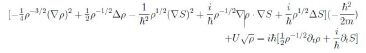
Equating the imaginary parts and observing that ∇ρ · ∇S + ρ∆S = ∇·(ρ∇ S) we have

This equation has an immediate physical interpretation. If we let ρ be the analogue of the classical mass density then if we let

we can write (25) in the form

which is formally the continuity equation in continuum mechanics. This result indicates a close analogy between quantum and classical schemes which are extended to diffusion.

We now look for the possible meaning of the relation coming from equating the real parts. Upon some rearrangements we find

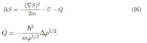
The quantity Q has the role of a potential, like U , and is often referred to as Bohm quantum potential [12]. Furthermore apply the gradient to (26) and assume S has continuous second-order derivatives to have

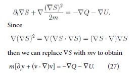
Equation (27) is formally the equation of motion with the Lagrangian (total) time derivative in the left-hand side, as it has to be. Consequently Q may also be viewed as a pressure term.

Diffusion is modelled by having in mind the parabolic character of the classical diffusion equation. Let P be the probability density of Brownian particles with mass m. Form the equation of motion we ascribe to P the equation

p being the opposite of the pressure. Then we let p = kBθP , where kB is the Boltzmann constant. In the high friction limit [13] it follows the parabolic equation

When quantum diffusion is described within a continuum mechanics approach the governing equation is taken in a Fick-like form. As an example [14], in the quantum diffusion of H atoms in solid molecular hydrogen films, the H atom concentration, n, is described by a differential equation in the form

Conclusions

Well-known diffusion equations are considered for the concentration (mass fraction) ω_α = ρ_α/ρ. In addition to the classical parabolic equation (6) we have reviewed the Cahn-Hilliard equation (8) and the Ginzburg-Landau equation (9). The rather general approach to the modelling of diffusion processes is based on the view that the diffusion flux, here h_α, has to be determined by a constitutive equation and that a safe rule is to let h_α be proportional to the gradient of the chemical potential µ_α. As a remarkable example we have shown how the approach via chemical potentials, for charged constituents, leads to the Nernst-Planck equation. Diffusion in the quantum domain is still based on the classical Fick’s law.

While h_α in terms of ω_α is inherited from the historical Fick’s model, the recourse to the chemical potential is found to be thermodynamically consistent in two cases, just those leading to the Cahn-Hilliard and Ginzburg-Landau equations. In the present thermodynamic analysis the αth chemical potential is derived from the Helmholtz free energy

instead of from ψ_α(ω_α).

The developments of this paper show that the constitutive equations for the mass flux hα are in fact approximations; the involved equation for h_α [1] justifies the recourse to approximations. However, the investigation of approximated  diffusion  equations  indicates  that a privileged role should be ascribed to the dynamic differential equations, based on the (exact) balance equations (21), (22). The difference in having recourse to the dynamic equations is exemplified with the analogue of Nernst-Planck equation.

Acknowledgments

This research has been developed under the auspices of INDAMCNR.

References

1. Müller I (1975). Thermodynamics of mixtures of J. M´ecan. 14: 267-303.
2. Morro A (2014). Balance and constitutive equations for diffusion in mixtures of fluids, Meccanica 49: 2109-2123.
3. Fick A (1855). Ueber Ann. Phys. 170: 59-86.
4. Kittel C (1976). Introduction to Solid State Wiley.
5. Landau LD, Khalatnikov IM (1965). On the theory of Oxford.
6. Cahn JW (1961). Spinodal Acta Metall. 9: 795-801.
7. Cahn JW, Hilliard JE (1971). Spinodal decomposition: a Acta Metall. 19: 151- 161.
8. Gurtin ME (1996). Generalized Ginzburg-Landau an Cahn-Hilliard equations based on a microforce Physica D. 92: 178-192.
9. Brokate M, Sprekels J (1996). Hysteresis and Phase Springer.
10. Kirby BJ (2010). Micro- and Nabnoscale Fluid Mechanics: Transport in Microfluidic Devices, Cambridge University Press.
11. Bockris JO’M, Reddy AKN (1970) Modern Plenum Press.
12. Bohm D (1952). A suggested interpretation of the quantum theory in terms of “hidden” I. Phys. Rev. 85: 166-179 (1952).
13. Tsekov R (2009). Thermo-quantum Int. J. Theor. Phys. 48: 630-636.
14. Sheludiakov S, Lee DM, Khmelenko VV, J¨arvinen J, Ahokas J et al. (2021) Purely spatial quantum diffusion of H atoms in solid H2 at temperatures below 1 K, Phys. Rev. Lett. 126: 195301.