Monthly Archives: December 2018

Burroughs Wellcome: The Seminal Link between Academia and the Pharmaceutical Industry

Abstract

This article reviews the research carried out by outstanding scientists to underscore the significant role played by Burroughs Wellcome Research Laboratories in erasing the differences in the objectives of scientists in academia and those in industry. These enlightened policies not only markedly advanced our fund of scientific knowledge in the biomedical sciences but led to the production of drugs that were of major benefit to mankind.

Introduction

Henry S. Wellcome (1853–1936) was an American-British entrepreneur who established the Burroughs Wellcome pharmaceutical conglomerate in London with his partner Silas Burroughs in the late 1880’s. Four years later, Wellcome formed a research component, which he named The Wellcome Physiological Research Laboratories. The creation of laboratories to conduct research was quite unusual in the late 1800’s, especially in association with a pharmaceutical enterprise [1–3]. When Henry Wellcome passed away in 1936, he left two legacies, his pharmaceutical company, The Wellcome Foundation and The Wellcome Trust, which distributed the financial resources for biomedical research [4].

This article will convey the company’s long time commitment to research by the fact that the staff scientists highlighted herein won a share of five Nobel Prizes (see below). At the same time, as a result of its long term involvement in basic research, Burroughs Wellcome became a major factor in bridging the gap that existed between academia and the pharmaceutical industry.

Sir Henry Hallett Dale (1875–1968)

Henry Dale (Figure 1), the renowned pioneer and leader in the discipline of Physiology/ Pharmacology, was the first major recruit to join Henry Wellcome’s new research initiative when he reluctantly accepted a research position at The Wellcome Research Laboratories in 1904 [5]. In those days it was unusual for a researcher at a university to give up his academic freedom to work in industry, and several colleagues advised him to decline the offer. However, Wellcome convinced Dale that he would be able to conduct basic research without concern for the business side of the organization.

Although Dale was free to select his own topics of research to investigate, Wellcome requested that Dale undertake the problem of ergot, which was marketed by the company as an abortifacient. Wellcome’s interest in ergot was in part commercially driven by the fact that Parke Davis was also marketing an ergot preparation for use in obstetrics. This competition prompted Henry Wellcome to also recruit a chemist, George Barger, whom he also encouraged to investigate ergot. Dale did not plan on ergot studies occupying a major portion of his time; however, his initial investigations into ergot properties proved to be unexpected and exciting and led him on a path that would ultimately provide the foundation for understanding the pharmacology of autonomic drugs and culminate in the awarding of the Nobel Prize.

IMROJ 2018-108 - Ronald Rubin USA_F1

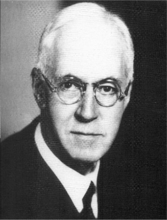
Figure 1. Sir Henry Hallett Dale (1875–1968)

In 1906, Dale provided the first example of an adrenergic blocking agent by demonstrating that a substance obtained from ergot called ergotoxine reversed the hypertensive effect of sympathetic nerve stimulation and epinephrine (adrenaline) [6]. The sympatholytic action of ergotoxine prompted Dale to interpret his own studies in the light of recent work by Thomas Elliott, who in 1905 observed that the action of exogenous epinephrine mimicked the effects of sympathetic nerve stimulation [7]. Thus, ergotoxine became important in medical history because Dale’s observation that it inhibited sympathetic activity eventually led to the discovery of chemical synaptic transmission. In 1910, Dale also published a detailed account of the sympathomimetic actions of a number of biogenic amines synthesized by George Barger [8]. Unfortunately, Dale chose to exclude the epinephrine (adrenaline) series of sympathomimetics and overlooked the most physiologically relevant derivative – norepinephrine (noradrenaline) – and thus delayed for several more decades the discovery of norepinephrine as a physiological neurotransmitter.

Ergot yielded additional constituents, including histamine in 1907 and acetylcholine in 1913, although neither provided any results that could be marketed for sale. A few years later, an accidental observation made with a particular extract of ergot prompted Dale’s interest in the possible existence of chemical transmission across neuronal synapses. A conventional dose of this extract caused a profound inhibition of heart rate, and was later identified as the labile substance, acetylcholine. In a paper published in 1914, Dale identified a nicotinic and muscarine-like substance in ergot as acetylcholine [9]. In this article, Dale summarizes his work by noting that “acetylcholine occurs occasionally in ergot, but its instability renders it improbable that its occurrence has any therapeutic significance [10].” Nevertheless, such findings set the stage for the classical experiments of Otto Loewi in 1921 and beyond, which provided direct evidence in favor of the theory of chemical synaptic transmission.

Thus, because of Dale’s commitment to deciphering the puzzling effects of ergot, much of our knowledge of the action of autonomic drugs on the physiological components of the autonomic nervous system stems directly from the work of Henry Dale carried out at Burroughs Wellcome Research Laboratories. The quality of Dale’s work was recognized by his academic peers and had much to do with reducing the prevailing negative opinion of the scientific mission of pharmaceutical companies. Dale was subsequently elected to the Royal Society and later served as President of the Royal Society of Medicine. He was knighted in 1932, and shared the Nobel Prize with Otto Loewi for a discovery of fundamental physiological significance that had its origins in a drug company interested in the pharmacological properties of ergot.

Dale spent 10 years at the Burroughs Wellcome Research Laboratories at Brockwell Park, where a great deal of his most productive work was carried out. Although Dale was appointed the first Director of the Medical Research Council at the National Institute for Medical Research in 1928, his link to Burroughs Wellcome was not at an end. In 1936, he became associated with the Trust which had been created by the will of Henry Wellcome. He first served as a Trustee, then as Chairman from 1938 to 1960. He spent the last eight years of his life as its scientific advisor [11]. In addition, a special Henry Dale Fellowship sponsored by the Wellcome Trust provides funds for biomedical research. The basic research fostered by Henry Wellcome and implemented by Henry Dale was not only profoundly significant in its day, but it led Burroughs Wellcome to become a dominant force in biomedical research. And, it was Sir Henry Dale who set the landscape for those who were to follow.

Sir John Robert Vane (1927–2004)

John Vane (Figure 2) was considered one of Britain’s most eminent pharmacologists [12]. He began working with Joshua Harold Burn at Oxford in 1946, where he learned to utilize bioassays. At the time, chemical methods were generally unavailable and bioassays, which detected and measured sensitivity of tissue strips to biologically active substances, required laborious procedures. As a graduate student, I myself toiled at a bath containing aortic strips to measure catecholamines by bioassay, and my task was made much easier when I learned the fluorometric method of assaying adrenomedullary catecholamines at Burroughs Wellcome.

IMROJ 2018-108 - Ronald Rubin USA_F2

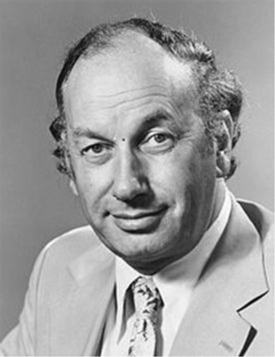
Figure 2. Sir John Vane

After graduating in Pharmacology and obtaining additional experience in the United States at Yale University, Vane returned to the United Kingdom where he was offered a position in The Department of Pharmacology at the University of London, which was headed by Sir William Paton. During those years, Vane, striving to move beyond outdated methodologies and antiquated concepts, further developed the blood-bathed organ bioassay system. By slowly perfusing mammalian blood over a series of isolated tissues in a cascade, Vane was able to measure the release of biologically active substances in a manner that simulated release in vivo. One of the first major biochemical processes to be discovered using the blood-bathed organ system was the conversion of angiotensin I to angiotensin II in the pulmonary vasculature. This finding led to the development of Angiotensin Converting Enzyme Inhibitors, which at the time revolutionized the treatment of hypertension. But, it was at the College of Surgeons that John Vane made an indelible mark on the scientific world by elucidating the mechanism of action of aspirin [13].

Vane left the Chair at the Royal College of Physicians in 1973, and followed the example of Henry Dale by joining The Wellcome Research Laboratories in the UK [14]. Vane, like Henry Dale, found that friends and colleagues were dubious about his accepting the offer to enter the industrial realm. Nevertheless, Vane was impressed by the fact that some seventy years before, Henry Dale had accepted a position at Burroughs Wellcome after experiencing academic life. Understanding that good science was not limited to academia, Vane undertook his new role as Director of Research and Development for a major pharmaceutical company.

The fact that he was able to take a number of his research team with him was a major factor in his final decision, and Vane never expressed any regrets about this move. The colleagues he recruited from the Royal College of Surgeons, included Salvador Moncada, Richard Gryglewski, and Rod Flower [15].This research group composed of very talented individuals of diverse ethnic origins, backgrounds, and traditions worked together in a highly competitive research environment. Vane’s laboratory became known as the Prostaglandin Research Group and served as a venue where basic pharmacological research could be carried out without being limited by outdated and narrow approaches to biomedical research. An example of the rewards that could be achieved by this philosophy was the other watershed in Vane’s storied history, the discovery of prostacyclin.

The years spent at Burroughs Wellcome was a challenging period for John Vane since he assumed a new set of managerial responsibilities, as well as research goals. Imbuing colleagues with the concept that it was possible to carry out quality science in an industrial setting, Vane advised them to follow their instincts with regard to drug discovery. This concept soon reaped rewards when in 1976 the Prostaglandin Research Group under the leadership of Salvador Moncada discovered prostacyclin and elucidated its pharmacological properties by utilizing the bioassay of extracts from platelets and vascular tissues [16]. Capitalizing on the versatility of the bioassay cascade, prostacyclin was found to be the main product of arachidonic acid metabolism in arteries and veins and its major effect was to inhibit platelet aggregation by stimulating adenylate cyclase.

John Vane presided over an environment in which there was a strong interaction with academia and the pharmaceutical industry. He, like Henry Dale, clearly demonstrated how it was possible to conduct quality scientific research in an industrial setting. During those years, Vane was awarded several honors, including Fellowship in the Royal Society, The Lasker Prize, and in 1982 the Nobel Prize for Medicine [17]. Salvador Moncada, who was also involved in the discovery of nitric oxide, was considered by some as deserving of a share of the Nobel Prize [18].

The work carried out by John Vane and his associates at the Wellcome Foundation spawned important research around the world that provided additional insights into the key factors that regulate blood circulation. In 1993, after much more information was accumulated about prostacyclin, Vane eventually reached the conclusion that the endothelium occupied a key role in regulating blood circulation and that prostacyclin, as well as nitric oxide, was responsible for defending against atherosclerotic angiopathies [19].

One of Vane’s other major contributions was to promote the link between scientists at academic institutions with those in the pharmaceutical industry, and he did a great deal to blur the boundaries that had separated these two groups of research scientists. In 1985, Vane returned to academia by establishing the William Harvey Research Institute at the Medical College of St. Bartholomew’s Hospital, where his research group focused its attention on cyclooxygenase-2 inhibitors and the interplay between nitric oxide and endothelin in the regulation of vascular function [20].

Sir James Whyte Black (1924- 2010)

The Nobelist, James Black (Figure 3), was one of the first scientists who utilized “rational design” for discovering new drugs [21,22]. Much of Black’s early work was carried out at the now defunct Imperial Chemical Industries (ICI Pharmaceuticals) in the United Kingdom from 1958–1964. Becoming aware of the importance of a balance between experimental research and drug development, Black and coworkers developed propranolol, the first clinically effective beta-adrenergic antagonist. The development of this drug not only represented a marked advance in the pharmacotherapy of hypertension, angina pectoris, and arrhythmias, but it also initiated further studies on the physiological role of beta adrenergic receptors by subsequently dividing them into beta-1 and beta-2 subtypes. At Black’s next position at Smith Kline and French (now GlaxoSmithKline), he introduced a new concept in the treatment of gastric ulcers by producing a drug that blocks histamine (H2) receptors.

IMROJ 2018-108 - Ronald Rubin USA_F3

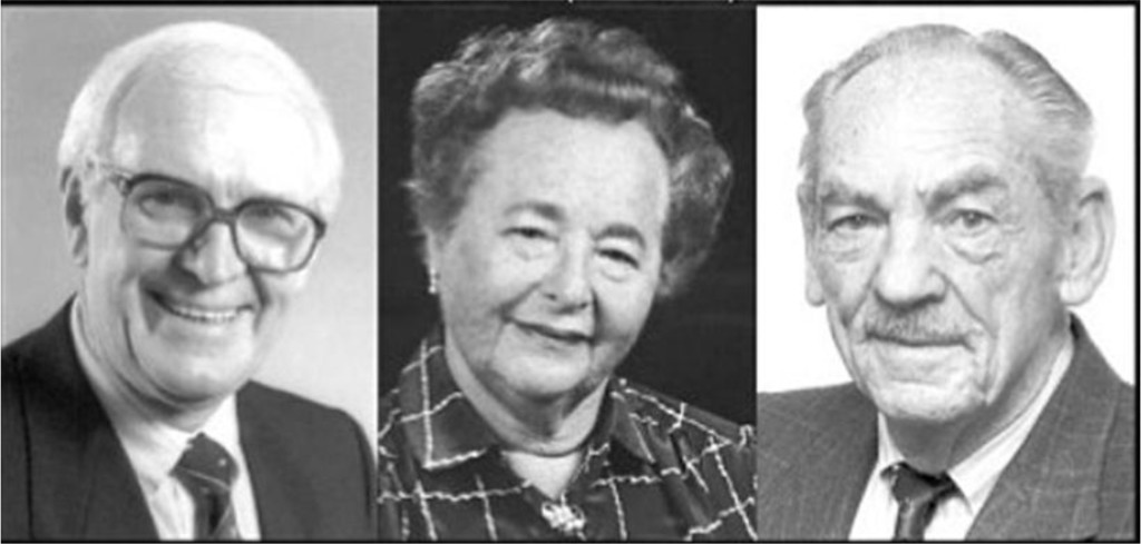
Figure 3. Sir James Black (left), Gertrude Elion (middle), and George Hitchings (right)

Black wanted to escape from commercial constraints in order to have the freedom to pursue his research interests, so he returned to academia by accepting a Chair in Pharmacology at University College London. But, it was not long before John Vane invited Black to join him at Burroughs Wellcome in the United Kingdom in 1977. Black accepted the offer to serve as Director of Therapeutic Research in order to implement ideas he held about the reasons for the success and failure of industrial projects.

During the next six years at Burroughs Wellcome, Black failed to make much progress in his managerial role, but his research, now involving analytical pharmacology, produced a major advance in the description of the functional effects of drugs and their therapeutic potential. A collaboration with Paul Leff, which compared pharmacological data to quantitative models, developed a new framework for categorizing and analyzing drug actions. The most significant tool employed was the operational model, in which the quantitation of agonist activity in one test system enabled the prediction of activity in another system [23]. The principles of this analytical approach have since been employed in drug classification and the mechanisms of drug action [24].

However, despite the fact that Burroughs Wellcome enjoyed an impeccable reputation with regard to its research activity, Black spent seven years dealing with what he felt were traditional and conservative attitudes. For Black, the interplay between corporate commercial needs and personal scientific aspirations provided an ongoing dilemma. The perceived counterproductive policies were resolved when a small independent research unit in King’s College, London was established for him in 1984 and financially supported by Burroughs Wellcome. It had modern facilities, and together with talented researchers and doctoral students, Black was able to carry out non-profit research with complete independence. Black received his Nobel Prize there in 1988, together with George Hitchings and Gertrude Elion (Figure 3), and remained at Kings College as Professor of Analytical Pharmacology until 1993 when he became Professor Emeritus. In 1988, Black also established the James Black Foundation in the United Kingdom to promote his own vision of pharmacological research [25].

As a fulltime employee of pharmaceutical companies, including Burroughs Wellcome, Black was provided with the independence and resources to be successful. In this way, he was able to offer benefit to both his company and for the good of mankind. Although he derived little personal gain from his discoveries, his strong sense of independence, combined with his dislike for large institutions, caused him to frequently abandon positions whenever he felt the short-sightedness of corporations was obstructing progress in his research. Black’s outstanding quality as a researcher can best be described as being able to discover drugs by meticulous structural design based upon known agonists, rather than by random screening.

George Herbert Hitchings (1905–1998) and Gertrude Belle Elion (1918–1999)

George Hitchings and Gertrude Elion (Figure 3) were the only Nobel Laureates who spent their entire careers at Burroughs Wellcome, even when the company moved from Tuckahoe, New York to North Carolina during a period of sustained research activity. Their investigations covered a span of nearly 40 years and were previously chronicled in some detail [26].

Hitchings received his doctoral degree in Biochemistry from Harvard in 1933, where he studied analytical methods used in physiological studies of purines at a time when little was known about nucleic acid metabolism. After working at several colleges for ten years, Hitchings was hired in 1942 as the only scientist in the Biochemistry Department at Burroughs Wellcome at the Tuckahoe New York facility. Two years later, he recruited Gertrude Elion, a chemist by training, to join his small research group. Elion was then able to leave a rather tedious job of food analyst to join Hitchings when World War II made research positions available for women.

Although up to that time women had difficulty finding jobs in scientific research, Hitchings had no trouble working with women or men from different ethnic backgrounds or religious beliefs, and he encouraged Elion to learn as rapidly and as much as she could. Because she never felt constrained to restrict herself to the subject of chemistry, Elion, who possessed only a Bachelor’s and a Master’s degree, greatly expanded her scope of knowledge in biochemistry, pharmacology, immunology and virology. As a result, Elion began to take on more and more responsibility by concentrating almost exclusively on purines. Because of residency requirements at Brooklyn Polytechnic University, which would take her away from Burroughs Wellcome, Elion never obtained a formal doctorate. However, she was later awarded an honorary PhD degree from Polytechnic University in 1989 and an honorary SD degree from Harvard in 1998.

As previously noted, drug development had historically been a consequence of random trial and error, as in the case of sulfa drugs for example [27]. Because of the legacy provided by the vision of Henry Wellcome, Hitchings and Elion, like James Black, were free to diverge from this approach by using what then was called “rational drug design [28].” It was based upon the supposition that the understanding of basic biochemical and physiological processes formed the basis for the design and development of drugs. Because their research was based upon the premise that drugs could be designed which were based upon differences in nucleic acid metabolism in normal and abnormal cells, Elion and Hitchings employed specifically designed chemicals to form atypical DNA in abnormal cells which did not affect normal cells. By blocking nucleic acid synthesis, the growth of the abnormal cells would be inhibited. Thus, for example, Hitchings postulated that folic acid deficiency would lead to alterations in the synthesis of purines and pyrimidines and thus DNA.

By 1950, this line of research reaped major dividends when Hitchings and Elion synthesized two antimetabolites, diaminopurine and thioguanine. These substances proved to be effective in the treatment of leukemia. In 1957, further alterations in chemical structure led to the production of azathioprine (AZT). This immunosupressant is now used to prevent the rejection of transplanted organs and to treat rheumatoid arthritis and other autoimmune disorders. However, in the 1980’s, because AZT was the primary treatment for AIDS, the United States government allowed Burroughs Wellcome to apply for full patent rights to the drug. As a result, Burroughs Wellcome was able to charge an exorbitant price for AZT to patients with AIDS, despite the fact that the majority of the company was owned by a charitable Foundation, the Wellcome Trust [29,30]. Thus, there was an aspect of the policies of Burroughs Wellcome that dimmed the luster of its legacy.

In 1967 Hitchings became Vice President in charge of research at Burroughs Wellcome, which virtually terminated his involvement in research and redirected his attention to philanthropy. Elion took over his position as Head of the Department of Experimental Therapy. In 1970, the group headed by Hitchings and Elion moved to Research Triangle Park, North Carolina, where they developed the first antiviral drug acyclovir, as well as allopurinol, which is used in the treatment of gout.

Although Henry Wellcome had always been resolute in his commitment to unencumbered biomedical research, Hitchings and Elion did not always find that their efforts were totally supported by management. Hitchings and Elion were subjected to interference by the Head of the Tuckahoe laboratories, William Creasy, who tried to persuade the chemists to work on projects that he favored. Eventually, Creasy relented, realizing that the successes achieved by Hitchings and Elion made it unwise to interfere with their work [31]. In marked contrast, Hitchings and his elite group had key collaboration from the Sloan-Kettering Institute to examine whether purines/pyrimidines possessed anti-neoplastic activity. Moreover, the financial support afforded by Sloan- Kettering enabled Burroughs Wellcome to expand and eventually become self-sustaining [32]. Thus, the ability of Hitchings and Elion to test their theories without interference by commercial considerations led to discoveries of important principles for drug treatment resulting in the development of new approaches to pharmacotherapy.

Hitchings and Elion were initially overlooked by the Nobel Committee. One reason perhaps had to do with the fact that the Nobel Prize Committee rarely honors the work of scientists who develop new drugs. However, in 1988 they were awarded the Nobel Prize, some 30 years after most of their major discoveries. Gertrude Elion underscored the profound significance of her work in a review published in Science in 1989, “…chemotherapeutic agents are not only ends in themselves but also serve as tools for unlocking doors and probing Nature’s mysteries [33].” When Hitchings retired in 1975, and Elion followed eight years later, another memorable chapter in the history of Burroughs Wellcome came to an end.

John J. Burns (1920–2007) and Allan H. Conney (1930–2013)

During the same period that Hitchings and Elion were making their invaluable drug discoveries in the Biochemistry Department, John Burns (Figure 4) joined Burroughs Wellcome as Vice-President and Director of Research in 1960. Prior to his arrival at the Tuckahoe New York facility, Burns had worked at the NIH and had provided valuable information about the biosynthesis and metabolism of Vitamin C (ascorbic acid) and the etiology of scurvy [34]. At Burroughs Wellcome, his seminal investigations demonstrated the clinical importance of microsomal enzyme induction. In particular, Burns demonstrated that phenylbutazone is converted in man to two major metabolites, one with anti-rheumatic activity, the other possessing uricosuric actions [35]. The importance of this basic research was underscored by the fact that during the 1960’s, the NIH provided financial support for the research being conducted at the Tuckahoe facility.

IMROJ 2018-108 - Ronald Rubin USA_F4

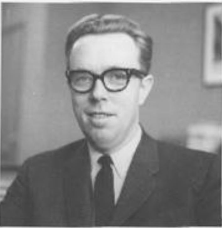
Figure 4. John J. Burns. Courtesy of ASPET)

Coincident with the advent of John Burns, a talented research group was formed in the Department of Biochemistry that included Allan Conney, Ronald Kuntzman, and Richard Welch. Providing fundamental knowledge concerning drug metabolism and its clinical implications, this group was the first to demonstrate the clinical significance of microsomal enzyme induction by showing that chronic administration of several drugs to animals stimulated their metabolism and decreased their toxicity [36]. Also by employing selective inhibitors, they were able to determine whether a drug possessed intrinsic pharmacological activity or owed its activity to a metabolite. This work was of considerable significance in the field of drug metabolism and led to early studies on individual differences in the metabolism of drugs in humans.

John Burns wore many hats as a scientist. While at Burroughs Wellcome, he was also an advisor to a number of biotech companies, a member and officer in a large number of national and international scientific committees, and served as a Visiting Professor of Pharmacology at Albert Einstein College of Medicine. In his capacity as an adjunct faculty member, Burns became thesis advisor to a graduate student, Louis Lemberger. Alfred Gilman, the Chairman of the Pharmacology Department was not enamored of the fact that Lemberger had graduated from a Pharmacy School. Nevertheless, Gilman allowed Lemberger to carry out his doctoral thesis with John Burns. At the time, I was a graduate student at Albert Einstein, and because of the prevailing views I was surprised that one of my fellow students had been allowed to carry out his research at an industrial setting.

Despite the vestiges of prejudice that still existed in academia about drug companies at the time, the legacy generated by Henry Wellcome endured. Subsequently, John Burns encouraged Lemberger to obtain his MD degree and gain further clinical training; and so, Lemberger went on to an outstanding career as Director of Clinical Pharmacology at Eli Lilly in Indianapolis Indiana and as Professor of Pharmacology Medicine and Psychiatry at the Indiana School of Medicine [37]. He was involved in the development of several centrally acting drugs, including Prozac, a commonly prescribed anti-depressant.

John Burns subsequently left Burroughs Wellcome in 1968 to serve as Vice President of Research & Development at Hoffmann LaRoche, where he helped to develop the famed Roche Institute of Molecular Biology. Adhering to the view that basic research would lead to practical results, Burns supported basic research as much as any pharmaceutical executive. The extensive research conducted by Burns and his colleagues on the metabolic fate and the mechanism of action of drugs provided a fundamental basis for discovering new drugs and improving their therapeutic use. After Dr. Burns retired from Hoffman LaRoche, he served as Adjunct Professor of Pharmacology at Weill Medical College and was scientific advisor to many biotech companies and a member of the National Academy of Sciences. However, his work at Burroughs Wellcome proved to be seminal.

The Biochemistry group led by Allan Conney (Figure 5) was also involved in investigating other areas of drug metabolism, including cytochrome P-450, a family of enzymes responsible for the biotransformation of many medications, toxic substances, and environmental chemicals [38,39]. Conney’s work provided the molecular basis for understanding how drugs induce tolerance and environmental chemicals produce mutagenesis and carcinogenesis.

Much of Conney’s career was spent in the pharmaceutical industry, first at Burroughs Wellcome and then at Hoffman-LaRoche, where he rejoined John Burns. Further recognition of Conney’s work came from a prestigious faculty appointment at Rutgers University in 1987, where he established the Department of Chemical Biology and founded the Laboratory for Cancer Research. At Rutgers University, Conney continued to carry out research mainly on cancer prevention [40]. His contributions were recognized by his election to the National Academy of Sciences in 1982, and as President of the American Society for Pharmacology and Experimental Therapeutics (ASPET) (1983–1984). During the years 1965–1978, Dr. Conney was among the 40 most cited scientists in the field of pharmacology.

IMROJ 2018-108 - Ronald Rubin USA_F5

Figure 5. Allan Conney

It was fitting that we end this article by recounting the work of Allan Conney, because it defines a gifted scientist who readily bridged the gap between industry and academia. The now entrenched alliances between academia and industry provided another important advance in mankind’s search for more effective medications. Once again, it took some time, but the overall lesson learned by scientists is that forward thinking and cooperation will always trump unfounded biases.

Epilogue

The research laboratories that Henry Wellcome set up first in the United Kingdom in 1880 and then throughout the world employed elite researchers who performed rational and outstanding biomedical research. As a result, the company set the stage for the advent of Pharmacology as an established biomedical discipline. Although the Burroughs Wellcome Research Institute is no longer a functional entity, having been assimilated by Smith/Kline/Glaxo in the 1980’s, the research arm of the company provided the path for academicians to join forces with industrial companies to produce medications that have extended human life and reduced human suffering.

References

  1. Church R, Tansey EM (2007) Burroughs Wellcome and Company: Knowledge, Trust, Profit and the Transformation of the British Pharmaceutical Industry  Crucible Books, Lancaster UK, Pg No :1880–1940
  2. Bailey P (2008) The birth and growth of Burroughs-Wellcome & Co. The Wellcome Trust, 2008.
  3. James RR. Henry Wellcome (1994) Hodder & Stoughton, London, United Kingdom.
  4. Bailey P (2008) Henry Wellcome’s Physiological and Chemical Research Laboratories. Wellcome Trust. 2008. http//www.wellcome.ac.uk./About-us/History/WTX052313.htm.
  5. Dale HH (1938) An autobiographical sketch. Perspec. Biol. Med. 1938; 1: 128–130. See also Dale HH. Introduction; In: Adventures in Physiology. London. Pergamon Press. pp x-xvi.
  6. Dale HH (1906) On some physiological actions of ergot. J Physiol 34: 163–206. [crossref]
  7. Elliott TR (1905) The action of adrenalin. J Physiol 32: 401–467. [crossref]
  8. Barger G, Dale HH (1910) Chemical structure and sympathomimetic action of amines. J Physiol 41: 19–59. [crossref]
  9. Dale HH (1914) The action of certain esters and ethers of choline, and their relation to muscarine. J. Pharmacol. Exp. Ther. 6: 147–190.
  10. Dale HH. (op cit. Ref 7). pg. 189.
  11. Sánchez García P (2010) [The neurotransmision from the other side]. An R Acad Nac Med (Madr) 127: 257–268. [crossref]
  12. Moncada S (2006) Sir John Robert Vane: 29 March 1927 – 19 November 2004. Biogr Mem Fellows R Soc 52: 401–411. [crossref]
  13. Vane JR (1971) Inhibition of prostaglandin synthesis as a mechanism of action for aspirin-like drugs. Nat New Biol 231: 232–235. [crossref]
  14. John R. Vane- Biographical. Nobelprize.org. Nobel Media AB 2014. Web. 7 Apr 2016.
  15. Flower R (2006) John Vane. A Biographical Sketch. In Memory of Sir John Vane. (Nistico, G. McGiff J & Born G. Editors); 2006; Roma; Exorma. pp. 53–55.
  16. Moncada S (1982) Eighth Gaddum Memorial Lecture. Biological importance of prostacyclin. Br. J. Pharmacol. 76: 3–31.
  17. Obituary (2004) Sir John Vane. The Telegraph.
  18. Howlett R (1998) Nobel award stirs up debate on nitric oxide breakthrough. Nature 395: 625–626. [crossref]
  19. Vane JR (1994) The Croonian Lecture, 1993. The endothelium: maestro of the blood circulation. Philos Trans R Soc Lond B Biol Sci 343: 225–246. [crossref]
  20. Moncada S (2006) Sir John Robert Vane: 29 March 1927 – 19 November 2004. Biogr Mem Fellows R Soc 52: 401–411. [crossref]
  21. Braunwald E (2010) Sir James W. Black MD, FRS. In Memoriam. Circ. Res. 107: 3–5.
  22. Black’s autobiographical sketch can be found in: Les Prix Nobel. The Nobel Prizes 1988; Editor Tore Frangsmyr. (Nobel Foundation) 1989. Stockholm.
  23. Black JW, Leff P (1983) Operational models of pharmacological agonism. Proc R Soc Lond B Biol Sci 220: 141–162. [crossref]
  24. Kenakin T, Christopoulos A (2011) Analytical pharmacology: the impact of numbers on pharmacology. Trends Pharmacol Sci 32: 189–196. [crossref]
  25. Wright P (2010) Sir James Black obituary: Nobel prizewinning pharmacologist who invented new drugs such as beta-blockers. The Guardian.
  26. Rubin RP. A brief history of great discoveries in pharmacology. Pharmacol. Rev. 2007; 59: pp. 311–314.
  27. Rubin RP (op. cit. Ref. 23). pp. 315–318.
  28. Turney J (2009) Rational drug design: Gertrude Elion and George Hitchings. Wellcome Trust. London, England.
  29. http://www.nytimes.com/1989/08/28/opinion/azt-s-inhuman-cost.html
  30. Emmons WM (1991) Burroughs Wellcome and AZT. (A): Faculty & Research. Harvard Business School Case 792–004.
  31. Turney J. (op. cit. Ref. 25).
  32. George H. Hitchings- Biographical. The Nobel Prize in Physiology or Medicine 1988. From Les Prix Nobel; The Nobel Prize 1988. Editor Tore Frangsmyr [Nobel Foundation]. Stockholm.1988.
  33. Elion G The purine path to chemotherapy. Science. 1989; 244: pg. 46.
  34. Kuntzman R and Conney A (2008) Dr. John J. Burns. 1920–2007. Obituary. Neuropsychopharmacology. 33: 458–459.
  35. Kuntzman R and Conney A. (op. cit. Ref. 34). pg. 458.
  36. Burns JJ (1964) Editorial. Implications of enzyme induction for drug therapy. Amer. J. Med. 37: 327–331.
  37. Albert Einstein College of Medicine (1989) Alumni. Louis Lemberger M.D, PH.D. Distinguished Alumnus.
  38. Conney AH (1967) Pharmacological implications of microsomal enzyme induction. Pharmacol. Rev. 19: 317–366.
  39. Conney AH (2003) Induction of drug-metabolizing enzymes: a path to the discovery of multiple cytochromes P450. Annu Rev Pharmacol Toxicol 43: 1–30. [crossref]
  40. Yang CS Suh N Stoner G, Dong, Z and Surh Y-J. Allan H (2013) Conney: In Memoriam (1930–2013). Cancer Prev. Res. 6: 1376–1377.

Kinematic Investigation, of a New Flexible Orthopedic Screw (FlexyScrew) for Repairing the Torn Scapholunate Ligament, with the Use of 3D-CT/Scan-Covariant Method and Demonstration on a 3D-Printed Model

DOI: 10.31038/IJOT.2018114

Abstract

Kinematic analysis with the use of 3D-CT/scan-reconstruction and covariant analysis gives the ability to have a detail kinematic prescription of the Scaphoid and Lunate bones and further of the Scapholunate joint when the wrist gets the extreme positions. This analysis can be used in the design criteria for the development of a new type screw FlexyScrew.

Data obtained from the 3D-CT/scan-reconstruction and the use of covariant analysis give a detail kinematic analysis of the Scaphoid and lunate bones. This data was used as the technical guidelines for constructing the FlexyScrew. Further a 3D-printed model of the Scapholunate joint which is based on the above analysis simulate the conditions in which the FlexyScrew can operate.

It was verified, that insertion of the FlexyScrew in the appropriate position does not disturb the 3D joint movement between the Scaphoid and Lunate bones. Moreover the spring of the Flexyscrew allows the relative motion, translation and rotation, of Scaphoid and Lunate bones and generally can follow in a satisfactory way the movements of the joint.

The insertion of the FlexyScrew seems to offer a good alternative method for the difficult and problematic carpal Scapholunate surgeries. This simple kinesiological method of analysis with the appropriate flexible screw can be applied also to other unstable joints, caused by ligamentous injuries, for example replacing the torn Anterior Cruciate Ligament in the knee joint.

Keywords

FlexyScrew, Orthopaedic, CT/scan, Scapholunate, Spring, Ligament

Introduction

The Scapholunate (Sc-L) joint is of major importance to the kinematics of the wrist, the injury of which can lead to radiocarpal dislocations or fractures- dislocations [1] and subsequently to the dissociation of the SL ligament and the instability of the carpus [2].

Various surgical methods which use autografts (tendons, articular capsules etc) have been proposed for the rehabilitation of the Sc-L joint instability and prevention of SLAC. Except for these methods, several types of implants, that are currently available, are used in procedures similar to RASL procedure [3] and various types of orthopaedic screws have been developed for Sc-L instability. Herbert Whipple screw (Herbert/Whipple, 2008) which is placed through scaphoid and lunate bone was developed [4] for the treatment from Sc-L ligament injury [5], SLIC screw joining scaphoid and lunate, was also proposed [6] and a prototype screw with helical coil cut design using solid screw from Zimmer® was developed by Helical Products Company Inc [7].

In previous work, we have already presented a new orthopaedic screw [8–11] named FlexyScrew (FS), because of its unique characteristic flexible middle spring portion. The FS is intended to repair the Sc-L unstable joint with a simple surgical technique for insertion and novel removal [12]. FS is based on a general biomechanical concept and potentially could be used on a number of other unstable joints with torn ligaments, like the anterior cruciate knee ligament, with the appropriate design modifications.

The insertion of the FS in the S-L joint should ideally substitute the function of the torn ligaments and restore fully the dynamics and kinematics of the joint. We have already studied the biomechanical forces of the Sc-L ligament complex [13] for the spring stiffness constant specifications of the FS. In addition to the stability that it must provide to the Sc-L joint, the FS must also cover the kinematics in the extreme positions of the wrist, flexion-extension and radio-ulnar deviation.

This work aims at studying the behavior of the FS via the kinematic analysis of the Sc-L joint, demonstrating the effectiveness and the functionality of the screw, in a 3D-printed model replicating the exact anatomic characteristics of the bones and the screwed joint.

In the present analysis we adopted the matrix method for the kinematic representation, considered as better applied in voxelized bone-data. We performed kinematic analysis in the neutral and all four extreme positions of the wrist using CT/scan and 3D/reconstruction of the scaphoid and lunate bones. By using co-variant analysis on bone data, we obtained the centroids and three principal axes for the Sc and L in the neutral and the four extreme positions of the wrist.

Methods and Materials

The healthy wrist of one of the authors, a male of 50 years old, was offered to be subjected to a CT/scan, with a General Electric, model Optima CT/660 tomograph. The scan was performed in four extreme positions of the wrist figure 2 flexion-extension, radio-ulnar deviation and in neutral as a reference position.

Sc-L Kinematic

The tomographic data (dicom file), from the CT scan, was analyzed with the help of the open code (3D Slicer), and the stereolithographic (STL) files obtained from the voxelized volume of Sc and L, were isolated with the method of Region of Interest (ROI) as shown in figure 3.

Suitable code was also developed, based on the open source code Octave@, for reading the STL bone files and for obtaining the centroid and the principal axis system for each bone using covariant matrix transformations. Principal axis directions and the centroid coordinates are characteristic and unique for each bone mass distribution in the 3D-space Figure 1 and therefore can be used to follow the motion of the bones.

IJOT 18 - 104_F1

Figure 1. Lunate with the 1st principal axis (yellow) with respect the fixed coordinate system X (red arrow), Y (green arrow), Z (blue arrow-direction of the CT-tomograph). Left-neutral position. Right-wrist extension.

IJOT 18 - 104_F2

Figure 2. Wrist in flexion position (Left). Wrist in extension position. A special silicon base for the wrist (right)

IJOT 18 - 104_F3

Figure 3. 3D reconstruction of the wrist. Hand in the neutral position. Sc and L are depicted also in extension (magenta). Frontal-palmar view, Z axis is the scanner table Axis (Left). Bone pairs of Sc and L in neutral (grey) to extension (magenta). View the capitate cavity. X-Y plane of the CT scanner coil (Right).

Thus the exact kinematic parameters of: a) the translation of the centroid, and b) the rotation of the principal axes system from the neutral and each of the extreme positions of the Sc and L bones are displayed in table 1.

Table 1. Covariant analysis (Eigenvector, principal axes) for Sc & L in each position of the wrist.

Sc in N p

Sc in E p

Sc in F p

Sc in RD p

Sc in UD p

1st PA EVect.

X

Y

Z

X

Y

Z

X

Y

Z

X

Y

Z

X

Y

Z

-0.474

0.718

0.509

-0.568

0.015

0.822

-0.400

0.916

-0.021

-0.503

0.815

0.285

-0.349

0.634

0.689

2nd PA EVect.

0.100

-0.531

0.841

0.193

-0.969

0.151

0.008

-0.019

-0.999

0.264

0.460

-0.847

0.176

-0.678

0.713

3d PA EVect.

0.874

0.449

0.179

0.799

0.244

0.548

-0.916

-0.400

-0.001

-0.822

-0.351

-0.477

0.920

0.371

0.125

L in N p

L in E p

L in F p

L in RD p

L in UD p

1st PA EVect.

X

Y

Z

X

Y

Z

X

Y

Z

X

Y

Z

X

Y

Z

-0.542

0.767

0.341

-0.610

0.639

0.467

-0.604

0.795

-0.039

-0.476

0.879

-0.014

-0.435

0.650

0.622

2nd PA EVect.

-0.701

-0.637

0.319

-0.715

-0.698

0.019

-0.706

-0.512

0.487

-0.863

-0.464

0.198

0.642

0.708

-0.291

3d PA EVect.

0.462

-0.066

-0.884

0.338

-0.323

0.883

0.367

0.322

0.872

0.168

0.106

0.980

-0.630

0.272

-0.726

Abbreviations: PA = Principal Axis, Sc = Scaphoid bone, L = Lunate bone, EVect. = Eigenvector, N = Neutral, E = Extension, F = Flexion, RD = Radial Deviation of wrist, UD = Ulnar Deviation of wrist, p = position.

Relative rotations of the principal axis within an error of ±1° and relative distances of the centroids within an error of ± 0.5 mm were calculated and are displayed in table 2.

Table 2a. Kinematic Study (relative solid angle) of the 1st Principal Axis in flexion, extension, radial & ulnar deviation with respect to the initial neutral position of the wrist.

1st principal axis in the initial-neutral position

2nd Principal axis in the initial-neutral position

3rd Principal axis in the initial-neutral position

1st principal axis of the Sc in Extension

46°

49°

25°

1st principal axis of the L in Extension

11°

18°

16°

1st principal axis of the Sc in Flexion

33°

146°

169°

1st principal axis of the L in Flexion

22°

12°

23°

1st principal axis of the Sc in radial deviation

14°

159°

63°

1st principal axis of the L in radial deviation

22°

15°

20°

1st principal axis of the Sc in ulnar deviation

13°

12°

1st principal axis of the L in ulnar deviation

19°

175°

162°

Table 2b. Centroid distances in different wrist positions.

Distances between the centroids of the Sc and L bones (+- 0.5mm)

neutral

17.9

flexion

16.9

extension

19.5

radial deviation

19.4

neutral

17.9

For practical anatomic reasons and in order for the data to become more easily available to the radiologist and hand surgeon, additional information of the major principal axis for Sc and L bones is given with respect to the global fixed (X, Y, Z) reference system in table 3a.

Table 3a. Angles of the Major, 1st Principal Axis, for Sc & L bone with respect to the global or reference axis X.Y, Z. Z is the longitudinal axis of the CT scanner table. (N.=Neutral, Flex.=Flexion, Ext.=Extension, Rad. D=Radial Deviation, Uln. D=Ulnar Deviation).

Angle of 1st Principal Axis

with x-Axis

Angle of 1st Principal Axis

with y-Axis

Angle of 1st Principal Axis

with z-Axis

N.

Flex.

Ext.

Rad. D.

Uln. D.

N.

Flex.

Ext.

Rad. D

Uln. D

N.

Flex.

Ext.

Rad. D.

Uln. D.

Scaphoid

118°

114°

125°

120°

111°

44°

24°

89°

35°

51°

1.5°

91°

35°

73°

46°

Lunate

123°

127°

128°

119°

116°

40°

37°

50°

28°

49°

70°

92°

62°

91°

52°

Table 3b. Angles between shafts AB and CD and spring elongation of the FS in the extreme positions of the wrist.

Angle AB-CD in neutral (degrees)

Angle

AB-CD in flexion

(degrees)

Angle AB-CD

in ext.

(degrees)

Angle AB-CD in radial D. (degrees)

Angle AB-CD in ulnar D.

(degrees)

Spring Elongation in neutral

(mm)

Spring Elongation in flexion

(± 0.5 mm)

Spring Elongation in extension

(± 0.5 mm)

Spring Elongation in radial D.

(± 0.5 mm)

Spring Elongation in ulnar D.

(± 0.5 mm)

0

35

23

33.5

53.5

0

0.03

0.03

1.68

– 0.24

The screw

The FS Figure 4, was constructed from stainless steel 316, with 7.7mm outer diameter , threaded step 1.3 mm, core diameter 4.5mm, total length 20 mm, spring length 3.2 mm, spring coil length and outer diameter 0.8mm and 6.5 mm respectively. The specifications kinematic data for extension and rotation of the flexible part of the screw are given in Tables 2–3.

IJOT 18 - 104_F4

Figure 4. The Flexible screw (FS). AB and CD the solid screwed part of the FS. Note that the midportion BC (the spring) is without any deformation (left). A k-wire has inserted through the cannulated FS in order to depict the flexibility (middle). FS in detail-Hexagonal cross section of the core for the insertion of the guide wire & the screw driver (right).

The screw is surgically designed to be inserted in the neutral position in a predetermined path, along a straight line ABCD Figure 4, opened with guide drilling.

The AB and CD segment of the screw is inside the Sc and the L bone mass respectively. Obviously BC represents the flexible spring portion of the FS Figure 5, which lies in the mid joint space.

IJOT 18 - 104_F5

Figure 5. The Flexyscrew and the spring in the Sc-L midjoint space in the neutral position from STL files processed (left). Detail of the Flexyscrew and the spring in the Sc-L midjoint in neutral position: from the capitate cavity (right).

As the Sc-L joint moves from the neutral to each of the extreme positions the middle spring of the FS deforms and flexes, following the motion of the bones.

The STL files were prepared for 3D printing with freeCad. Holes were opened on the bone volumes files, for the FS insertion and the 1st principal axis table 1. Subsequently the Sc and L bone STL files, were printed with ABS plastic material in a Zortax M200 3D printer. A k-wire was inserted through the 1st principal axis hole (see black arrow Figure 6a). Then the FS was screwed through the already opened hole (see red arrow Figure 6a).

IJOT 18 - 104_F6

Figure 6. (a)Hand posture in neutral position. Yellow: Z-axis of the CT/table, red: X-axis, blue: Y-axis. Black arrow: 1st principal axis of the Sc, red arrow: axis of the FS in neutral position. Detail (b) the 1st principal axis with y-axis at 44o (see Table 3a). (c) The spring can deform and flex over 180–110=700 degrees easily attainable in all directions. Therefore can satisfy all the calculated values of the Table 3b.

Results

Biometric data from covariant analysis

Eigenvectors for each of the three principal axes, of the Sc and L obtained from the covariant analysis are given in Table 1.

Translation of the bones

The centroids in radial and extension have maximum displacement of almost 19mm but generally we don’t have big centroid displacements from the initial neutral position which is approximately 17.9mm.

Rotation of the bones (relative & absolute)

In order to describe and analyze the actual kinesiology of the two bones in the extreme positions of the wrist, specifically for the rotation of the bones, the relative solid angles of the 1st principal axis, with respect to the neutral position, are presented in Table 2a. The 2nd and 3d principal axes are perpendicular-orthogonal to the 1st principal axis and thus omitted for simplicity reasons.

Concerning the absolute rotations of the bones the 1st principal axis with respect to XYZ global reference system angles are presented in Table 3a.

The Sc-L 3D printed model complex was placed in the XYZ fixed wire system, (Z is the axis of the CT/table). The 1st principal axis in 44° angle with the Y axis, and the z-axis (axis of the CT/scan table) is almost collinear (1.5°) with the 1st principal axis in neutral position being depicted in Figure 6b.

The FS

The FS is inserted in a straight line (ABCD) Figure 4, entering from the Sc entry point to the L bone as defined from the guide k-wire. Our kinematic analysis gives the transformation CD solid part into the L in relation to AB solid screw part into the Sc. Maximum angles between the solid parts of the FS were found to be 53.5° and 33.5° (see Table 3b) for ulnar and radial deviation and 35° and 23° for flexion and extension, respectively.

Maximum displacements of the spring BC is 1.68mm Table 3b in radial deviation. Small compression of the spring in ulnar deviation is -0.24mm. For extension and flexion the spring dimension does not alter significantly within experimental error.

The 3D-printed model

The 3D-printed model of the Sc-L joint with the screw embodied (Figure 6) was studied by visual inspection with the help of a protractor. In the extreme 4 positions of the wrist, flexion, extension, radial and ulnar deviation, the corresponding FS solid parts AB and CD are displaced and rotated following the kinematics of the Sc and L bones. It is obvious from Figure 6c that the FS makes an easy rotation of 70°, a value which is well over the maximum deflection of 53.5° for ulnar deviation as obtained in Table 3b.

Discussion

Various kinematic methods are offered in literature for the description of the scaphoid and lunate, such as a) coordinate Measuring Machine b) simple radiologic study with x-rays [14] c) markers in wrist cadavers recorded by stereoradiography [15] d) CT/scan tomography [16]. Other investigators exploit principal axis registration method and Helical Axis Motion parameters (HAM) [17]. Recent literature studied carpal kinematics using 3D-CT/scan. Snel, J.G et al [18] used the Finite Helical Axis (FHA) and registration techniques for the kinematics of the wrist and give data for the capitate bone. In the present work, we use covariant analysis for obtaining the principal axis of individual bones which is more practical for voxelized solids.

Sc-L kinematics

Short et al [19] in 24 cases, found that when the wrist extends 30°, the scaphoid extends approximately 20°. In the same position the lunate extends about 12°. During wrist 50° flexion, the scaphoid flexes about 35° and the lunate flexes about 25°. The relative motion between these two bones was about 8° to 10°.

In another study [20], during maximum flexion of the wrist the scaphoid extends about 28.2° and the lunate extends about 17.6° for the same position.

 Litchman stated that scaphoid and lunate “bind the proximal row into a unit of rotational stability”. Thus in radial and ulnar deviation the amount of intercarpal rotation allowed by the system is approximately 4° at the scapholunate joint. However in flexion and extension, there can be as much as 30° at the scapholunate joint” [21].

Julio [22–23] stated that “from neutral to dorsiflexion, the lunate rotates approximately 28° and the scaphoid 30°. From neutral to complete volarflexion the lunate rotates 30° and the scaphoid 60°. From these studies, it is understood that the rotation between the bones, relative to each other, is maximum 30°. Therefore, for their design implants criteria, relative rotation of the leading edge and trailing edge was set to 30° maximum.

On average the scaphoid extends about 50° and flexes about 58°, supinates about 6° and deviates about 4° in radial direction from start to finish. The lunate extends about 38°, pronates 5° and deviates 3° when the wrist moves from the neutral position. During radial deviation, the lunate flexes about 11°, radially deviates about 8.6° and pronates about 6°. During ulnar deviation of the wrist, the lunate extends 32°, ulnarly deviates about 16° and supinates about 5° [24].

For clinical purposes, estimation of physiological limits of Sc and L movements and positions is mainly based on 2D x-ray analysis, as a more empirical and convenient method for practical reasons. The Lunate during flexion of the wrist flexes and demonstrates an angle of 50° with the axis of the radius. During extension the L also extends and forms an angle of 35° [25]. The average Sc-L angle in full flexion is 76° and decreases in 35° in full extension [26].

Ruby et al [27] finds that from full radial to full ulnar deviation the Sc rotates 51° and the L rotates 35° in contrast with Horri et al who could not find such differences among the two bones and gives an average of 36°, 38° for the Sc and L respectively.

Normal carpal bone motion with respect to the radius, is also measured by means of biplanar radiographic apparatus and gives in HAM representation, angles for the Sc 55°, 56.1°, 12.8°,22,7° from neutral to flexion, extension, radial deviation and ulnar deviation respectively. For the L 45.1°, 31.2°, 13°, 25.4° from neutral to flexion, extension, radial deviation and ulnar deviation respectively [28]. Kobayashi,[15] gives for the carpal bone motion relative to the radius, for the Sc 40°, 52°, 4°, 17° and for the L 23°, 30° , 2°, 22° mean values for flexion, extension, radio-ulnar deviation respectively. The Sc and L bones are rotating around an axis which coincides with the dorsal portion of the Sc-L ligament assumed as the axis of Sc-L joint rotation forming a Sc-L angle 62° and 27° for flexion and extension of the wrist respectively [29].

Upal gives a rotation for the Sc 51.1° in a mixed flexed position (with supination) and 89.9 ° for a mixed extended position (with pronation) and for the L 52 ° and 81.3 ° respectively.

Since the different investigators do not use the same kinematic frames of reference and analyses, it is difficult to make an effective comparison between their respective studies. Furthermore, the meaning of individual matrix elements may be obvious but it is often difficult to visualize body attitude when all matrix elements are applied.

Concerning the classic literature’s Sc-L angle in one dimension radiographic plane, our result for this angle is 35° Table 3b for flexion and 23° in extension of the wrist and as already mentioned this angle represents also the angle between the axes through the two solid parts of the flexyscrew AB-CD.

The Sc also rotates more than the L in flexion and extension as seen from the 1st principal axis angles Table 2a.

On the other hand in radial and ulnar deviation, the L performs larger rotation than the Sc. Rotations of the bones for extension and flexion are found to be larger than those of the two deviations.

The large differences observed among all investigators can be explained by the fact that the motion of the bones in the 3D-space differs from the 2D projection on the radiographic plate. Radiographic images are normal projections of the 3D positions of the bones. In addition radiographic data is obtained by drawing lines from anatomic landmarks of the external surface of the bones and not axes passing through the centroids as in our 3D analysis. Our reported angles, as expected, are larger than those obtained from the radiographic data, since our values refer to the epicenter and are not inscribed angles.

Length of the Flexible section

In an intact wrist, the average distance between scaphoid and lunate is approximately 1.6 mm in maximum flexion and 1.2 mm in maximum ulnar deviation [30]. The max elongation of the FS spring as shown in Table 3b is 1.68 mm in radial deviation and there is a small compression -0.24 mm in ulnar deviation. Otherwise minimal elongations of the spring are observed in flexion and extension.

As a general comment from Table 2b we can infer that the bones do not translate a lot, but instead rotate almost perfectly about their centroids as is expected from a well functional joint with minimal friction.

3D-printed and FS-model

By visual inspection of the 3D printed Sc-L model, the joint was not found to be obstructed by the flexible spring part of the FS. Also the maximum reported angle between the two solid parts of the screw AB-CD were found to be 53.5°, a value that is easily attainable from the FS as shown in Figure 6. The maximum spring extension of ±2 mm due to centroid displacements of the Sc and L were found to be technically possible in the construction of the FS.

Finally, the main pearls of the FS could be summarized as:

  1. FS is not disturbing the Sc-L joint movement.
  2. The spring allows the relative motion, translation and rotation of Sc and L closer to the physiological motive.
  3. The insertion technique is simple for the hand surgeons since uniaxial insertion can replace the cumbersome and problematic difficult operations for Sc-L instability.

Concerning our kinematic method could be extended and easily applied to any other joint in order to provide technical specifications for custom made FS.

References

  1. Apergis M (2013) Fractures-dislocations of the wrist. (1stedn), Springer-Verlag, Italy Pg No: 223–295.
  2. Cooney PW, Linscheid LR, Dobyns HJ (1998) The Wrist: Diagnosis and Operative Treatment. In: Cooney PW, Linscheid LR, Dobyns HJ (eds.). (1stedn), Mosby Publisher, Missouri, USA Pg No: 501–524.
  3. Rosenwasser MP, Miyasajsa KC, Strauch RJ (1997) The RASL procedure: reduction and association of the scaphoid and lunate using the Herbert screw. Tech Hand Up Extrem Surg 1: 263–272. [crossref]
  4. Budoff JE (2008) Treatment of acute lunate and perilunate dislocations. J Hand Surg Am 33: 1424–1432. [crossref]
  5. Acumed – Acutrak 2® Standard. Available from: http://www.acumed.net/product/19. Accessed January 11th 2008.
  6. Sucec MC, Tuller TC (2006) Bone Connector with Pivotable Joint. United States Patent US 20060271054.
  7. Kabir S (2008) Flexible Screw Design for Bone Implant Application [Thesis]. Virginia Commonwealth University.
  8. Nikolopoulos F, Kefalas V (2013) Orthopedic Screw. Greece Patent GR 1008012.
  9. Nikolopoulos F, Kefalas V (2015) Orthopedic Screw. Greece Patent GR 1008431.
  10. Nikolopoulos F, Kefalas V (2018) Orthopedic Screw with tool of insertion. Greece Patent GR 1009280.
  11. Nikolopoulos F, Kefalas V (2017) Kinematic Analysis of a Flexible Orthopedic Screw (FlexyScrew) with the Use of CT/scan 3D Reconstruction and Technique Demonstration for Repairing the Scapholunate Rupture of the Wrist. 28th Annual Meeting of the European Society for Biomaterials. Megaron Athens International Conference, Athens, Greece.
  12. Nikolopoulos F, Poulilios A, Vidalis G, Kefalas V (2015) A New Screw and Technique for the Treatment of Ruptured Multiaxial Joint Ligaments: A Preliminary Study on the Scapholunate Dissociation of the Wrist. PeerJ PrePrints 3: 810v1.
  13. Nikolopoulos F, Apergis E, Kefalas V, et al (2011) Biomechanical Properties of the Scapholunate Ligament and the Importance of its Portions in the Capitate Intrusion Injury. Clinical Biomechanics 26: 819–823.
  14. Schernberg F (1990) Roentgenographic examination of the wrist: a systematic study of the normal, lax and injured wrist. Part 1: The standard and positional views. J Hand Surg Br 15: 210–219. [crossref]
  15. Kobayashi M, Berger RA, Nagy L, et al (1997) Normal kinematics of Carpal Bones: A Three Dimensional Analysis of Carpal Bone Motion Relative to the Radius. J Biomech 30: 787–793.
  16. Crisco JJ, McGovern RD (1998) Efficient Calculation of Mass Moments of Inertia for Segmented Homogenous Three-dimensional Objects. J Biomech 31: 97–101.
  17. Upal MA (2003) Carpal Bone Kinematics on Combined Wrist Joint Motions May Differ From the Bone Kinematics During Simple Wrist Motions. Biomed Sci Instrum 29: 272–277.
  18. Snel JG, Venema HW, Moojen TM, Ritt JP, Grimbergen CA, et al (2000) Quantitive in Vivo Analysis of the Kinematics of Carpal Bones from Three-Dimensional CT Images Using a Deformable Surface Model and a Three-Dimensional Matching Technique. Med Phys 27: 2037–2047.
  19. Short WH, Werner FW, Fortino MD, Mann KA (1997) Analysis of the kinematics of the scaphoid and lunate in the intact wrist joint. Hand Clin 13: 93–108. [crossref]
  20. Werner FW, Short WH, Green JK (2005) Changes in Patterns of Scaphoid and Lunate Motion During Functional Arcs of Wrist Motion Induced by Ligament Division. J Hand Surg 30: 1156–1160
  21. Lichtman DM (1988) The Wrist and its Disorder. Philadelphia: W.B. Saunders Company Pg No:14–45.
  22. Taleisnik J (1985) The Wrist. New York: Churchill Livingstone Pg No: 3–25.
  23. Walsh JJ, Berger RA, Cooney WP (2002) Current Status of Scapholunate Interosseous Ligament Injuries. Journal of the American Academy of Orthopaedic Surgeons 10: 32–42.
  24. Cooney PW, Linscheid LR, Dobyns HJ (1998) The Wrist: Diagnosis and Operative Treatment. In: Cooney PW, Linscheid LR, Dobyns HJ (eds.). (1stedn), Mosby Publisher, Missouri, USA Pg No: 501–526.
  25. Schmidt HM, Lanz U (2004) Surgical Anatomy of the Hand. (1stedn), New York: Thieme Pg No: 76.
  26. Cooney PW, Linscheid LR, Dobyns HJ (1998) The Wrist: Diagnosis and Operative Treatment. In: Cooney PW, Linscheid LR, Dobyns HJ (eds.). (1stedn), Mosby Publisher, Missouri, USA Pg No: 212.
  27. Ruby LK, Cooney WP 3rd, An KN, Linscheid RL, Chao EY (1988) Relative Motion of Selected Carpal Bones: A Kinematic Analysis of the Normal Wrist. J Hand Surg 13: 1–10.
  28. Horii E, Garcia-Elias M, An KN, et al (1991) A kinematic study of luno-triquetral dissociation. J Hand Surg 16: 355–362.
  29. Ritt MJ, Linscheid RL, Cooney WP, Berger RA, An KN (1998) The Lunotriquetral Joint: Kinematic Effects of Sequential Ligament Sectioning, Ligament Repair, and Arthrodesis. J Hand Surg Am 23: 423–445.
  30. Short WH, Werner FW, Green JK, Masaoka S (2002) Biomechanical evaluation of ligamentous stabilizers of the scaphoid and lunate. J Hand Surg Am 27: 991–1002. [crossref]

Oral Glucose Tolerance Test with Cooked Rhizomes of Zingiber Officinale (Ginger)

DOI: 10.31038/EDMJ.2019311

Abstract

Rhizomes of Zingiber officinale (ginger) are used as a spice in many culinary dishes of Bangladesh. Since a number of scientific reports are present on the beneficial effects of raw ginger in Type 2 diabetes mellitus, it was of interest to determine the anti-hyperglycemic efficacy of cooked (boiled) ginger through oral glucose tolerance test (OGTT) in mice. The OGTT results showed that when administered at doses of 50, 100, 200 and 400 mg per kg body weight, methanolic extract of cooked ginger (MEZOC) reduced blood glucose in glucose-loaded mice by 8.0, 20.3, 29.2, and 32.0%, respectively. By comparison, a standard antihyperglycemic drug, glibenclamide, when administered at a dose of 10 mg per kg, reduced blood glucose levels by 48.8%. The results suggest that cooked ginger retains efficiency in lowering blood glucose. Since cooking causes ginger to be less pungent, partaking of ginger in such a manner may prove to be more acceptable to diabetic patients and help control their blood glucose concentrations.

Key words

diabetes, ginger, OGTT, Zingiber officinale, Zingiberaceae

Introduction

The prevalence of diabetes and particularly Type 2 diabetes is increasing throughout the world. [1] The disease is characterized by high blood glucose levels (hyperglycemia) and cannot be completely cured with allopathic or traditional medicines, although drugs are available to reduce elevated blood glucose levels. Left unchecked, hyperglycemia can lead to both microvascular and macrovascular complications. [2] Since blood glucose and any other associated complications arising from diabetes needs continuous monitoring and may necessitate visits to doctors and taking of costly drugs, treatment is costly and on the most part unaffordable and unavailable to the rural population and particularly the poorer sections of the rural people of Bangladesh. As such, the rural people of Bangladesh and indeed many other countries are dependent on traditional medicinal practitioners, who mostly use plant-based medicines for lowering elevated blood glucose [3].

The rhizomes of Zingiber officinale Roscoe (Zingiberaceae), otherwise known as ginger have found use in ethnomedicine for treatment of diabetes. [4] Different scientific studies have also shown that ginger can reduce hyperglycemia and ameliorate diabetes-induced complications. [4–6] However, in the various scientific studies conducted thus far on humans or animals, either raw ginger or dried ginger powder or various solvent extracts of raw or dried ginger were used. Ginger is a very popular spice in Bangladesh and used in a number of culinary dishes. People also drink hot tea in which raw ginger slices have been steeped to alleviate coughs, cold and sore throat. Raw ginger is pungent in taste and is often disliked. On the other hand cooked or boiled ginger loses the pungency and can be consumed without any possible dislikes. It was therefore of interest to determine whether cooked (boiled) rhizome slices of Z. officinale retains its antihyperglycemic property as determined through oral glucose tolerance test (OGTT). The objective of the present study was to evaluate the oral glucose tolerance efficacy of methanol extracts of cooked rhizomes of Z. officinale (MEZOC).

Methods and Materials

Plant material collection

Rhizomes of Z. officinale were collected from a vegetable market in Dhaka city. The rhizomes were identified by a competent botanist at the University of Development Alternative.

Preparation of methanolic extract of cooked Z. Officinale rhizomes (MEZOC)

For preparation of methanol extract of cooked rhizomes of Z. officinale, rhizomes were sliced and cooked (boiled) in water for 30 minutes. 50g of the powder was extracted with 250 ml methanol over 48 hours. Methanol was evaporated at 40oC and the extract was dissolved in Tween 20 prior to administration to mice by gavaging. The final weight of the extract was 2.17g.

Chemicals and Drugs

Glibenclamide and glucose were obtained from Square Pharmaceuticals Ltd., Bangladesh. All other chemicals were of analytical grade. Glucometer and strips were purchased from Lazz Pharma, Bangladesh.

Animals

Swiss albino mice were used in the present study. The animals were of both sexes and weighed between 18–20g. Mice were obtained from the International Centre for Diarrhoeal Disease Research, Bangladesh (ICDDR,B). The animals were acclimatized for three days prior to actual experiments. During this time, the animals were fed with mice chow (supplied by ICDDR,B) and water ad libitum. The study was conducted following approval by the Institutional Animal Ethical Committee of University of Development Alternative, Dhaka, Bangladesh. Care was taken that the animals did not suffer from any unnecessary pain during the acclimatization or experimental period.

Oral Glucose Tolerance Tests For Evaluation Of Antihyperglycemic Activity

Oral glucose tolerance test (OGTT) was carried out as per the procedure previously described by Joy and Kuttan [7] with slight modification. Mice fasted for 12 hours were grouped into six groups of five mice each. The various groups received different treatments like Group 1 received vehicle (1% Tween 20 in water, 10 ml/kg body weight) and served as control, Group 2 received standard drug (glibenclamide, 10 mg/kg body weight). Groups 3–6 received, respectively, MEZOC at doses of 50, 100, 200 and 400 mg per kg body weight. The amount of Tween 20 administered was same in both control and experimental mice. Following a period of one hour as described earlier, all mice were orally administered 4g glucose per kg of body weight. Blood samples were collected 120 minutes after the glucose administration through puncturing heart following previously published procedures. Blood glucose levels were measured with a glucometer. The percent lowering of blood glucose levels were calculated according to the formula described below.

Percent lowering of blood glucose level = (1 – We/Wc) × 100,

where We and Wc represents the blood glucose concentration in glibenclamide or MEZOC administered mice (Groups 2-6), and control mice (Group 1), respectively [8].

Statistical analysis

Experimental values are expressed as mean ± SEM. Independent Sample t-test was carried out for statistical comparison. Statistical significance was considered to be indicated by a p value < 0.05 in all cases [8].

Results

When administered at doses of 50, 100, 200 and 400 mg per kg body weight, methanolic extract of cooked ginger (MEZOC) reduced blood glucose in glucose-loaded mice by 8.0, 20.3, 29.2, and 32.0%, respectively. By comparison, a standard antihyperglycemic drug, glibenclamide, when administered at a dose of 10 mg per kg, reduced blood glucose levels by 48.8%. The results suggest that even after boiling, Z. officinale rhizomes can be effective in their antihyperglycemic or blood glucose reducing capacities. The results are shown in (Table 1).

Table 1. Lowering action of MEZOC on blood glucose level in hyperglycemic mice following 120 minutes of glucose loading.

Treatment

Dose (mg/kg body weight)

Blood glucose level (mmol/l)

% lowering of blood glucose level

Control

10 ml

6.70 ± 0.14

Glibenclamide

10 mg

3.42 ± 0.10

48.8*

(MEZOC)

50 mg

6.16 ± 0.11

8.0*

(MEZOC)

100 mg

5.34 ± 0.19

20.3*

(MEZOC)

200 mg

4.74 ± 0.18

29.2*

(MEZOC)

400 mg

4.22 ± 0.12

37.0*

All administrations were made orally. Values represented as mean ± SEM (standard error of mean), (n=5); *P < 0.05; significant compared to hyperglycemic control animals.

Discussion

The active component of ginger for its glucose lowering effect has been attributed to 6-gingerol.[9] The compound has not been described to be a volatile compound, but rather produced through thermal degradation of gingerols or shogaols.[10] This can explain the finding that cooked or boiled ginger can retain its blood glucose lowering effect. Overall, the results suggest that boiled ginger can be consumed by diabetic persons to lower their blood glucose, but the amounts to be consumed need to be scientifically studied.

Authorship

All authors contributed to the design and actual conducting of the experiment. The corresponding author wrote the manuscript, which was read and approved by all authors.

Acknowledgment

The authors are grateful to Mr. Sohel for assistance during the experiment and to the University of Development Alternative for providing space for maintaining mice and conducting the experiment. The work was funded by the authors.

References

  1. Kalra S, Kumar A, Jarhyan P, Unnikrishnan AG (2015) Endemic or epidemic? Measuring the endemicity index of diabetes. Indian J Endocrinol Metab 19: 5–7. [crossref]
  2. Fowler MJ (2016) Microvascular and macrovascular complications in diabetes mellitus: Distinct or continuum. Indian J Endocrinol Metab 29: 116–122.
  3. Ocvirk S, Kistler M, Khan S, Talukder SH (2013) Traditional medicinal plants used for the treatment of diabetes in rural and urban areas of Dhaka, Bangladesh–an ethnobotanical survey. J Ethnobiol Ethnomed 9: 43.
  4. Wang J, Ke W, Bao R, Hu X (2017) Beneficial effects of ginger Zingiber officinale Roscoe on obesity and metabolic syndrome: a review. Ann N Y Acad Sci 1398: 83–98.
  5. Shidfar F, Rajab A, Rahideh T, Khandouzi N, Hosseini S, et al. (2015) The effect of ginger (Zingiber officinale) on glycemic markers in patients with type 2 diabetes. J Complement Integr Med 12: 165–170. [crossref]
  6. Akhani SP, Vishwakarma SL, Goyal RK (2004) Anti-diabetic activity of Zingiber officinale in streptozotocin-induced type I diabetic rats. J Pharm Pharmacol 56: 101–105.
  7. Joy KL, Kuttan R (1999) Anti-diabetic activity of Picrorrhiza kurroa extract. J Ethnopharmacol 67: 143–148. [crossref]
  8. Hossain AI, Faisal M, Rahman S, Jahan R (2014) A preliminary evaluation of antihyperglycemic and analgesic activity of Alternanthera sessilis aerial parts. BMC Complement Alternat Med 14: 169–173.
  9. Chakraborty D, Mukherjee A, Sikdar S, Paul A (2012) [6]-gingerol isolated from ginger attenuates sodium arsenite induced oxidative stress and plays a corrective role in improving insulin signaling in mice. Toxicol Lett 210: 34–43.
  10. Zhan K, Wang C, Xu K, Yin H (2008) [Analysis of volatile and non-volatile compositions in ginger oleoresin by gas chromatography-mass spectrometry]. Se Pu 26: 692–696. [crossref]

Genotypes and Biotypes Variation of Bovine Viral Diarrhea Virus from Persistently Infected Dairy Cattle in Java, Indonesia

DOI: 10.31038/IJVB.2018235

Abstract

The objective of this research was to study the genotype and biotype of BVDV variability among PI dairy cattle in Java, Indonesia between 2016 and 2017. Two hundred isolated buffy coat from dairy cattles that had low reproductive performance and never been vaccinated in Java were used in this studies. Using antigen capture Elisa, 12 out of 200 dairy cattles were positive for the presence of protein Erns BVDV (6.0%). The PI status was confirmed by multiple sequential viral molecular detection. Through phylogenetic and nucleotide sequence analysis of the 5’-Untranslated Region (5’UTR) of the samples investigated, it was determined that all the 12 field positive samples had the BVDV-1 genotype. Three IP-BVDV positive samples (2282-15, 0610-14 and 0813-2) sharing highest similarity (99% homology) with subgenotype BVDV-1c AY763030-1 and KF896608 isolates from Australia. Using Immuno Peroxidase Monolayer Assay (IPMA) the biotype of all the samples were identified as noncytopathic-BVDV. All of the informations would be necessary for designing the diagnostic tool and/or vaccine that match the circulating BVDV subgenotype.

Keywords

Bovine Viral Diarrhea Virus, Genotype, Biotype, 5’-Untranslated Region, Immuno Peroxidase Monolayer Assay

Introduction

Bovine Viral Diarrhea Virus (BVDV), a pestivirus belong to Flaviridae family, is an infectious pathogen affecting cattle in most part of the world [1]. In infected animals, the clinical manifestations caused by BVDV are mainly related to reproductive inefficiency such as poor conception rate, lengthened of calving intervals, congenital malformations, abortions, birth of weak calves and reduction in milk yield resulting significant economic losses to cattle industry worldwide [2, 3]. However, the most devastating consequences is the birth of Persistently Infected (PI) calf which occur when the cows infected by noncytopathic BVDV virus between 30 and 125 days of gestation. Persistently infected calves are immunotolerant and the main source of BVDV transmission in the herd since they shed large amount of the virus throughout their entire lives. Identification of persistent infected calves among cattle population is one of the most important but challenging strategy to control the disease from spreading [4]. Since the persistently infected animals are often born normal and can reach adulthood without any specific clinical signs [1, 5].

Genetically, BVDV is a positive sense single stranded RNA virus of approximately 12.3 kb in length with one Open Reading Frame (ORF) and is flanked on both sides by 5’ and 3’ untranslated regions [6]. Serologically and molecularly, BVDV has been differentiated into two genotypes BVDV-1 and BVDV-2 [7, 8] . Each genotype can be divided into two biotypes, cytopathic (CP) and non-cytopathic based on their cytopathogenecity on cell culture [1, 9] . To date there are many reports on genetic variations of BVDV from many countries [8, 10, 11, 12] but BVDV-1 remains the dominant genotype that has spreading worldwide. The genetic diversity that occur among BVDV isolates is mainly related to the nature characteristic for RNA viruses. According to [13] neither biotype nor genotype are not clinical sign specific. Eventhough the presence of genetic variations of BVDV-1 have not been accepted by the International Committee on Taxonomy of Viruses yet, but they are widely used in molecular epidemiology since the knowledge about the diversity has practical implications to control the occurance of BVDV new variants and to design effective vaccine against the BVDV present in a country [14, 15].

The objective of this study was to study the variation of the genotype and biotype of the BVDV isolated from persistently infected dairy cattle in Java, Indonesia, during 2016–2017, based upon the 5’ untranslated regions. That information is needed for designing the diagnostic tool and/or vaccine that match to the circulating BVDV in Indonesia.

Methods and Materials

Samples

A total of 200 dairy cattle that have low reproductive performance and never been vaccinated were used in this study. The whole blood was withdrawn through coccygeal vein using EDTA-vacutainer tube (Beckton Dickensen) and buffy coat were isolated according to [16]. The presence of the BVDV in the herd was analyzed using antigen capture ELISA (ACE) technique.

Antigen Capture Elisa (ACE)

The presence of protein Erns in the buffy coat were tested individually using Antigen Capture ELISA (IDEXX herdcheck BVDV Antigen Test Kit) as described by the manufacture. Fifty microliters (50 µl) of detection antibodies were dropped into each microwell. Fifty microliters of positive control, negative control and buffy coat samples were added into appropriate well, mixed the content of each well by gently tapping the microplate and incubated for 120 minutes at room temperature. After incubation, empty the liquid in each well followed by washing using 300 µl washed buffer/well for three to five times. One hundred microliters of anti-bovine HRP conjugated were then added into each well and incubated for another 30 minutes at room temperature. After incubation, excess conjugate were removed from microwell by washing the plate three to five times using washed buffer as previously described. One hundred microliters of substrat solution containing 3, 3’, 5, 5’ Tetramethylbenzidine (TMB) were added into each well and the plate was incubated for 10 minutes in the dark at room temperature for color development. The reaction was terminated by adding 100 µl of stop solution into each well. The absorbance of the controls and the samples were measured and recorded at 450 nm in absorbance microplate reader (Bio-Rad Model 680. 2000 Alfred Nobel Drive, Hercules, CA 94547) [17]. The blood samples from the cattles that positive based on ACE test were re-taken 4 weeks later to confirm the persistency of BVDV infection.

RNA Extraction and RT-PCR

The Viral RNA from 200 µl buffy coat suspensions and positive control isolate were extracted using Viral Nucleic Acid Extraction Kit II (Geneaid) as described by the manufacturer instruction. The extracted RNA was subjected to reverse transcription and PCR amplification in one-step reactions using MyTaqTM One-Step RT-PCR Kit (Bioline) according to manufacturer’s specification, in Personal Combi Thermocycler Biometra (37079 Goettingen Germany). Pairs of specific primers for 5’UTR regions of the BVDV genome [18]
(Table 1) were used for amplification of BVDV in the buffy coat. Thermal conditions were as follows: 62°C for 30 min of reverse transcription, 94°C for 2 min of initial denaturing followed by 40 cycles of 94°C for 1 min, 62°C for 1 min, 65°C for 1 min and then final elongation at 65°C for 10 min.

Table 1. Oligonucleotide primers used in this study

Primers

Genotype

Sequence (5’-3’)

Product

References

Forward

BVDV

5’ TAG CCA TGC CCT TAG TAG GAC 3’

288 bp

[18]

Reverse

5’ ACT CCA TGT GCC ATG TAC AGC 3’

The BVDV genotyping was done using a nested PCR. In the first cycle of RT-PCR amplification, MyTaqTM One-Step RT-PCR Kit (Bioline) and primer set A (Table 2) was used. The PCR mixtures were then amplified under the following cycling condition: 42°C for 1 h of reverse transcription, 94°C for 3 min of initial denaturing followed by 30 cycles of 94°C for 30 s, 50°C for 45 s, 72°C for 1 min and then one cycle of final elongation at 72°C for 10 min. In the PCR second amplification, a 198 bp DNA product from the first amplication was used as a template for the second round RT-nested PCR. The PCR reaction was prepared similarly to the first amplification but without RT enzyme and primer set B (Table 2). Thermal conditions for the second amplification were as follows: 94°C for 2 min of initial denaturing followed by 30 cycles of 94°C for 30 s, 50°C for 45 s and 72°C for 1 min followed by final elongation at 72°C for 7 min.

Table 2. Oligonucleotide primers for genotyping used in this study

Primers

Genotype

Sequence (5’-3’)

Product

References

Sense Set A

BVDV-1 and/or BVDV-2

5’ GTA GTC GTC AGT GGT TCG 3’

198 bp

[19]

Antisense Set A

5’ GCC ATG TAC AGC AGA GAT 3’

Sense Set B

5’ CGA CAC TCC ATT AGT TGA GG 3’

105 bp

Antisense Set B

5’ GTC CAT AAC GCC ACG AAT AG 3’

All the PCR products were separated on a 1.5% agarose gel, stained after electrophoresis with ethidium bromide and visualised using ultraviolet transillumination. Two isolates contain Singer strain and 890 strain were respectively used as BVDV type 1 and BVDV type 2 control.

For sequencing, PCR products were purified using High Pure PCR Product Purification Kit (Roche Life Science, Mannheim, Germany). Forward and reverse 5’-UTR sequences for each sampel were aligned and used in phylogenetic analysis. The sequences were compared to other previously publlished sequences. The sequence identities of nucleotide, as well as the estimation of the evolutionary divergence between sequences were analysed using DNA-Baser and Mega7 software, respectively [20]. The same tool was used to perform Neighbor-Joining analysis.

Immunoperoxidase Monolayer Assay (IPMA)

Immuno peroxidase monolayer assay were used for determination of BVDV biotype. Microtitration flat bottom plate wells were seeded with 100, 000 cells/ml Madin-Darby bovine kidney (MDBK) cells and incubated at 37°C in 5% CO2 atmosphere. After 24 hours, MDBK cells in every well were inoculated with 50 µl of the positive isolates. For non-infected control, the MDBK cells in the microtitration plate well was added with 50 µl distilled water. The MDBK infected and non-infected cells were incubated for another 72-hours at 37°C in 5% CO2 atmosphere. After incubation, the microtitration plates were drained, rinsed three times with wash buffer, and fixed with fixing buffer containing 35% acetone in phosphate-buffered saline (PBS, pH 7, 4) and 0, 02% bovine serum albumin for 10 minutes at room temperature. After fixation the cells were then incubated with 50 µl blocking serum solution for 10 minutes. After the incubation, the remnant of blocking serum solution left on the well was drained off. Fifty microliters monoclonal antibody anti BVDV 15c5 (1: 100 dilution) were added onto infected and non-infected MDBK cells and incubated for 60 minutes at room temperature. After incubation, the microtitration plate was drained and then rinsed 3 times with wash buffer (PBS solution containing 0.05% Tween 20) of 2 minutes each and drained off. Into each well was then added 50 µl with a secondary antibody solution-labeled with biotin and incubated for 10 minutes at room temperature. After incubation, the microtitration plate was drained and then rinsed 3 times with wash buffer 2 minutes each and drained off. Fifty microliters of streptavidin peroxidase conjugated solution were added into each microtitration well followed by another incubation step for 15 minutes. Following the incubation, the microtitration plate was drained and then rinsed 2 times 1 minute each with wash buffer. Fifty microliters of the mixed-substrate (H2O2) chromogen (3.3’-diaminobenzidine) solution were added into each well and left to react with the cells for 1 hour. The enzymatic reaction was stopped by rinsing the microtitration plate with tap water, drained off and followed by counterstaining the cells with hematoxylin for 3 minutes. The cells were then examined under light microscope [21].

Results

In this study, using antigen capture Elisa, 12 out of 200 dairy cattles were positive for the presence of protein Erns BVDV (6.0%). For confirming the virus persistence, blood samples from BVDV positive animals were re-taken and re-tested one month apart using RT-PCR technique. The results show specific product at 288 bp visible on the 1.5% agarose gel (Figure 1).

IJVB 2018-110 - Hastari Indonesia_F1

Figure 1. PI-BVDV detection by RT-PCR conventional technique. (Lane 1: negative control, lane 2: DNA marker 100 bp, lane 3: positive control, lane 4 – 7 PI-BVDV positive from field samples).

Using the oligonucleotide primers pairs listed in Table 2, after the first amplification, the DNA bands from all field samples and positive control either BVDV-1 and BVDV-2 were clearly visible at 198 bp (Figure 2). After the second amplification, the BVDV genotype 1 were no longer visible but BVDV genotype 2 should be clearly seen at 105 bp. In this study, however, only 890 strain (BVDV-2 positive control) showed positive result (Figure 3). Based on the sequence analysis, all of the positive samples in this study were clustered within the BVDV-1 genotype and no evidence for the presence of BVDV genotype 2.

IJVB 2018-110 - Hastari Indonesia_F2

Figure 2. First PCR amplification of RNA extracted from positive PI-BVDV samples. (Lane 1: negative control, lane 2: DNA marker 50 bp, lane 3: Singer strain BVDV-1 positive control, lane 4–7: BVDV-1 positive from field samples).

IJVB 2018-110 - Hastari Indonesia_F3

Figure 3. First PCR amplification of RNA extracted from positive PI-BVDV samples. (Lane 1: DNA marker 50 bp, lane 2: negative control, lane 3: Singer strain BVDV-1 positive control, lane 4, 5, 7, 8: BVDV-1 positive field samples, lane 6: 890 strain BVDV-2 positive control).

Discussion

Of the 200 animals tested 12 (6%) were positive for persistently infected BVDV (PI- BVDV). Regardless of their prevalence, PI-BVDV animals are the main source of infection within the herd [22]. The generation of persistently infected animals is more often when BVDV infection occur in-utero between 45 to 130 days of gestation period. Many PI-BVDV animals can be clinically healthy, although their life expectancy is low (< 2 years). However, according to [23]. PI-BVDV animals that can live beyond the age of 2 years were possibly related to the nonpathogenecity of the virus. The age range of the positive PI-BVDV animals in this study is between 2 weeks – 36 months. According to [16] and [24] in close confinement housing operation a PI animal can infect up 90% of the herd regardless of their prevalence. Results of this study have verified how well the persitently infected animals in a dairy herd with no BVDV vaccination had infected cattle in the same herd and confirm the magnitude of the infection in concentrate cattle production system.

The genetic variations of the PI-BVDV field positive samples in this study was done by determining the nucleotide sequences of the 5’UTR region that are highly conserved among all of the pestiviruses. High conservation permits rapid and accurate acquisition of the sequence data but may not be good target for interfering phylogeny [25, 26]. Based on the result, the genetic typing of viral RNA revealed that among PI-BVDV positive animals all were BVDV genotype 1 (BVDV-1). The result is in agreement with previous research finding done by [27] and [28]. BVDV-1 is distributed more widely throughout the world compared to BVDV-2 [26]. BVDV-2 was first reported in the USA but later has been described in European and Asian countries at lower rate than BVDV-1 [29, 30, 31].

Based on the phylogenetic analysis (Figure 4, Table 3), 9 of the samples clustered within the BVDV-1a subgenotype whereas 3 other samples belong to the BVDV-1c subgenotype. The result showed that the majority of BVDV subgenotype identified since 2015 in dairy cattle in Java is BVDV-1a [28]. Further result revealed that isolates number 2282–15, 0610–14 and 0813–2 sharing high similarity (98% homology) with the representative subgenotype BVDV-1c Genebank accession number AY763030–1 and KF896608 from Australia. The result is logic since the majority of dairy cattle used in this study were historically coming from Australia in which the BVDV-1c sub-genotype is predominant [32]. Using different genomic regions (NS5B) and larger samples (588) tested for genotyping of BVDV, [27] had found 4 BVDV-1 subgenotypes (1a, 1b, 1c, 1d) in cattle in Java. BVDV variability were generally analyzed using different genomic regions such as 5’UTR [33], NPRO [34], E2 [35], NS2–3 [36] and NS5B [37] and the result is not comparable to each other. Time periods for sampling also has an effect on the result of BVDV subgenotyping [28].Factor that influence the spread of the BVDV sub genotypes is unclear and do not appear to be affected by vaccine used but rather in part reflect the antigen diversity between strains [38]. According to [29], the genetic variation of the BVDV in a given geographic area has been largely influenced by animal movement within countries and/or introduction from other countries.

IJVB 2018-110 - Hastari Indonesia_F4

Figure 4. Phylogenetic tree of the 5’ untranslated regions (UTR) of BVDV strains and isolates. The tree was generated from comparative alignment of sequences from 288bp of the 5’UTR of the BVDV genome,

Table 3. Summary of genomic form of BVDV isolated from persistently infected dairy cattle in this study

No.

Isolate #

BVDV Biotype

BVDV Genotype

BVDV subgenotype

1.

JT-2282–15

NCP**

Type 1

1-c

2.

JT-0610–14

NCP

Type 1

1-c

3.

0813–2

NCP

Type 1

1-c

4.

0903–16

NCP

Type 1

1-a

5.

0783–16

NCP

Type 1

1-a

6.

0745–16

NCP

Type 1

1-a

7.

0805–14

NCP

Type 1

1-a

8.

5090–16

NCP

Type 1

1-a

9.

5069–17

NCP

Type 1

1-a

10.

5025–17

NCP

Type 1

1-a

11.

5031–17

NCP

Type 1

1-a

12.

0951–2

NCP

Type 1

1-a

**NCP=non-cytopathic

In this study, staining using IPMA technique was performed on MDBK cells that had infected with BVDV isolates obtained from cows with persistent BVDV infections. Positive results were characterized by brownish precipitates in single-layer cells (Figure 5). In the cells culture, within 24–48 hours after inoculation the virus did not cause vacuolization in the cytoplasm and / or cell damage. This suggests that the biotype of IP-BVDV in this study was non-cytopathic (NCP-BVDV) and proved that PI animals only have NCP-BVDV biotype. The NCP biotype is mostly occur in virus that transmitted vertically and is considered as a marker for persistentcy of BVDV in the herd [39]. Cytopathology in tissue culture does not correlate with virulence of the virus in vivo. In another word biotype is not clinical manifestation specific [13, 40]. Based on epidemiologic studies, NCP-BVDV is a more common biotype than BVDV cytopathic [39] .

IJVB 2018-110 - Hastari Indonesia_F5

Figure 5. Immunoperoxidase monolayer assay (IPMA) in Madin Darby Bovine Kidney (MDBK) immune cells infected with serum that does not contain BVD virus (negative control).

IJVB 2018-110 - Hastari Indonesia_F6

Figure 6. Biocytes of MDBK cells infected with non-cytopathic BVDV field isolates for 72 hours. Using IPMA cell-positive staining infected with BVDV appears brownish in the cytoplasm and nucleus.

The results of the study confirm the presence of the persistently- infected BVDV dairy cattles and provide information about BVDV biotypes and subgenotypes that are dominant among PI-BVDV positive dairy catttles, in Java, Indonesia between 2016 and 2017. All of the informations will be necessary for designing the diagnostic tool and/or a vaccine that match the circulating BVDV subgenotype in Indonesia in the future.

Author’s contribution

Sugiyono played a valuable role in blood sampling and preparing the buffy-coat from the whole blood for further analyses. Raden Wasito had responsibility in doing the IPMA. Hastari Wuryastuti had role in doing the RNA extraction, PCR analysis and sequencing. All researchers participated equally in preparing the manuscripts for journal publication.

Acknowledgment

The authors greatly acknowledge to the Direktorat Riset dan Pengabdian Masyarakat Direktorat Jenderal Penguatan Riset dan Pengembangan, Kementrian Riset, Teknologi, dan Pendidikan Tinggi and Gadjah Mada University for financial support through Penelitian Dasar Unggulan Perguruan Tinggi, Gadjah Mada University No.195/UN1/DITLIT/DIT-LIT/LT/2018 Tanggal 5 Maret, 2018. The authors are deeply grateful for the thoughtful advice given by Prof. Dr. Roger K. Maes, Michigan State University, East Lansing, MI, USA during the preparation of this manuscript.

References

  1. Brodersen BW (2014) Bovine Viral Diarrhea Virus infections: Manifestations of infection and recent advances in understanding pathogenesis and control. Vet Pathol 51: 453–464.
  2. Heuer C, Healy A, Zerbini C (2007) Economic effects of exposure to bovine viral diarrhea virus on dairy herds in New Zealand. J Dairy Sci 90: 5428–5438. [crossref]
  3. Richter V, Lebl K, Baumgartner W, Obritzhauser W, Kasbohrer A, Pinior B, et al (2017) A systematic worldwide review of the direct monetary losses in cattle due to bovine viral diarrhea virus infection. Vet J 220: 80–87.
  4. Stalder H, Hug C, Zanoni R, Vogt HR, Peterhans E, Schweizer M, Bachofen C, et al (2016) A nationwide database linking information on the hosts with sequence data of their virus strains: A useful tool for the eradication of bovine viral diarrhea (bvd) in Switzerland. Virus Res 218: 49–56.
  5. Thomann B, Tschopp A, Magouras I, Meylan M, Schupbach-Regula G, Hasler B, et al (2017) Economic evaluation of the eradication program for bovine viral diarrhea in the Swiss dairy sector. Prev Vet Med 145: 1–6.
  6. Meyers G, Thiel HJ (1996) Molecular characterization of pestiviruses. Adv Virus Res 47: 53–118. [crossref]
  7. Ridpath JF (2003) BVDV genotypes and biotypes: practical implications for diagnosis and control. Biologicals 31: 127–131. [crossref]
  8. Yesilbag K, Alpay G, Becher P, et al (2017) Variability and global distribution of subgenotypes of bovine viral diarrhea virus. Viruses 9: 128–146.
  9. Ammari M, McCarthy FM, Nanduri B, et al (2012) Understanding the pathogenesis of cytopathic and noncytopathic bovine viral diarrhea virus infection using proteomics. In: Heazlewood J (Ed.). Proteomics Application in Biology. In Tech Pg No: 53–66.
  10. Vilcek S, Paton DJ, Durkovic B, Strojny L, Ibata G, et al (2001) Bovine viral diarrhoea virus genotype 1 can be separated into at leasteleven genetic groups. Arch Virol 146: 99–115.
  11. Zhang J-J, Ma C, Li X-Z, Liu Y-X, Huang K, et al (2013) Genetic diversity of bovine viral diarrhoea virus in beijing region, China from 2009 to 2010. Afr J Microbiol Res 7: 4934–4939.
  12. Bazzucchi M, Bertolotti L, Giammarioli M, Casciari C, Rossi E, Rosati S, DeMia MG, et al (2017) Complete genome sequence of a bovine viral diarrhea virus subgenotype 1h strain isolated in Italy. Am Soc Microbiol 5: 1697–1716.
  13. Ahn BC, Walz PH, Kennedy GA, Kapil S, et al (2005) Biotype, genotype, and clinical presentation associated with bovine viral diarrhea virus (BVDV) isolates from cattle. Intern. J Appl Res Vet Med 3: 319–325.
  14. Simmonds P, Becher P, Collett MS, Gould EA, Heinz FX, et al (2012) Family Flaviridae. In: King, A.M.Q., Adams MJ, Carston EB, Lefkowitz EJ (Eds.). Virus Taxonomy Ninth Report of the International Committee on Taxonomy of Viruses. Elsevier Academic Press, Amsterdam, Boston, Heidelberg Pg No: 1003–1020.
  15. Moennig V, and Becher P (2018) Control of bovine viral diarrhea. Pathogens 7: 29–40.
  16. Peddireddi L, Foster KA, Poulsen EG, An B, Hoang QH, et al (2018) Molecular detection and characterization of transient bovine viral diarrhea virus (BVDV) infections in cattle commingled with ten BVDV persistently infected cattle. J Ve. Diag Invest : 1–10.
  17. Wuryastuti H, Putro PP, Wasito R, et al (2014) Identifikasi, isolasi dan propagasi virus penyebab infeksi persisten bovine viral diarrhea pada sapi untuk produksi isolat lokal unggulan. Laporan Penelitian Unggulan Perguruan Tinggi.Tahun Pertama. Universitas Gadjah Mada 2014.
  18. Weinstock D, Bhudevi B, Castro AE, et al (2001) Single-tube single-enzyme reverse transcriptase PCR assay for detection of bovine viral diarrhea virus in pooled bovine serum. J Clin Microbiol 39: 343–346.
  19. El-Kholy AA, Bolin SR, Ridpath JF, Arab RMH, Abou-Zeid AA, et al (1998) Use of polymerase chain reaction to simultaneously detect and type bovine viral diarrhea viruses isolated from clinical specimens. Rev Sci Tech Off Int Epiz 17: 733–742.
  20. Kumar S, Stetcher G. Tamura K, et al (2016) Mega7: Molecular evolutionary genetics analysis version 7.0 for bigger datasets. Mol Biol Evol 3: 1870–4.
  21. Wuryastuti H, and Wasito R. Application of the immunoperoxidase monolayer assay to characterize non-cytopathic bovine viral diarrhea virus of Indonesian samples. Indon J Biotech. 1997: 154–158.
  22. Fulton RW (2015) Impact of species and subgenotypes of bovine viral diarrhea virus on control by vaccination. Anim Health Res Rev 16: 40–54. [crossref]
  23. El-Bogoury GF, El-Nahas EM, Khadr KA, Ali NM, et al (2014) Isolation and genotyping of bovine viral diarrhea virus: Field isolates from infected cattle in Kaluobia during 2011. BVMJ 23: 6–10.
  24. Houe H (1999) Epidemiological features and economical importance of bovine viral diarrhea virus (BVDV) infections. Vet Microbiol 64: 89–107.
  25. Bedekovic T, Lojkic I, Lemo N, CAC Z, Cvetnic Z et al (2012) Genetic typing of Croation bovine viral diarrhea virus isolates. Vet Archiv 82: 449–462.
  26. Soltan MA, Wilkes RP, Elsheery MN, Elhaig MM, Riley MC, et al (2015) Circulation of bovine viral diarrhea virus-1 (BVDV-1) in dairy cattle and buffalo farms in Ismailia Province, Egypt. J Infec Dev Ctries 9: 1331–1337.
  27. Saepulloh M, and Sendow I (2015) Identification and characterization of bovine viral diarrhea virus from Indonesian cattle. J Vet 16: 1–7.
  28. Wuryastuti H, Putro PP, Wasito R, Maes, RK, et al (2015) Genetic variability of Bovine Viral Diarrhea Virus in persistently infected cattle in Central Java, Indonesia. Merit Res J Microbiol Biol Sci 3: 031–036.
  29. Luzzago C, Lauzi S, Ebranati E, Giammarioli M, Moreno A, et al (2014) Extended genetic diversity of bovine viral diarrhea virus and frequency of genotypes and subtypes in cattle in Italy between 1995 and 2013. Bio Med Res Pg No: 147–151.
  30. Fulton RW, Whitley EM, Johnson BJ, Ridpath JF, Kapil S, et al (2006) Prevalence of bovine viral diarrhea virus (BVDV) in persistently infected cattle and BVDV subtypes in affected catle in beef herds in south central United States. Can. J. Vet Res 73: 283–291.
  31. Jackova A, Novackova M, Pelletier C, Audeval C, Gueneau E, et al (2008) The extended genetic diversity of BVDV-1: typing of BVDV isolates from France. Vet Res Commun 32: 7–11. [crossref]
  32. Hay KE, Ambrose RC, Morton JM, Horwood PF, Gravel JL, et al (2016) Effects of exposure to bovine viral diarrhea virus 1 on risk of bovine respiratory disease in Australian feedlot cattle. Prev Vet Med 126: 159–169.
  33. Abe Y, Tamura T, Torii S, Wakamori S, Nagai M, et al (2016) Genetic and antigenic characterization of bovine viral diarrhea viruses isolated from cattle in Hokkaido, Japan. J Vet Med Sci 781: 61–70.
  34. Ridpath JF, Fulton RW, Kirkland P, Neil JD, et al (2010) Prevalence and antigenic differences observed between bovine viral diarrhea virus subgenotypes isolated from cattle in Australia and feedlots in southwestern United States. J Vet Diagn Invest 22: 184–191.
  35. Silveira S, Weber MN, Mosena AC, daSilva MS, Streck AF, et al (2015) Genetic diversity of Brazilian Bovine Pestivirus detected between 1995 and 2014. Transbound Emerg Dis 64: 613–623.
  36. Xia H, Liu L, Wahlberg N, Baule C, Belak S, et al (2007) Molecular phylogenetic analysis of bovine viral diarrhea virus, a Bayesian approach. Virus Res 130: 53–62.
  37. Mishra N, Dubey R, Rajukumar K, Tosh C, Tiwari A, et al (2007) Genetic and antigenic characterization of bovine viral diarrhea virus type 2 isolated from Indian goats (Capra hircus). Vet Microbiol 124: 340–347.
  38. Ambrose RK, Gravel JL, Commins MA, Fowler EV, Mahony TJ (2018) In Vivo Characterisation of Five Strains of Bovine Viral Diarrhoea Virus 1 (Subgenotype 1c). Pathogens 7: E12 [crossref]
  39. Bazid AI, Nayel MA, Elsify AM, Zaghloul AH, Khalil SA, et al (2015) Molecular diagnosis and genotyping of Bovine viral diarrhea virus. Minufiya Vet J 9: 1–13.
  40. Ridpath JF (2005) Practical significance of heterogeneity among BVDV strains: Impact of biotype and genotype on U.S. control programs. Prev Vet Med 72: 17–30.

On the Threshold: What Concerns Healthy People about the Prospect of Cancer?

DOI: 10.31038/CST.2018345

Abstract

The paper introduces a case study aiming to answer the question of what concerns healthy people about the prospect of cancer? The results suggest two distinct mind-sets. The mind-set is Life-Quality Pursuers, who are concerned the result is temporary and think cancer is chronic disease. The second mind-set is Outcome-Worriers, who fear the outcome, and worry about no recovery. The Outcome-Worriers are concerned a lot about physical pains and symptoms like nausea and joint pain. Incorporating the results of Mind Genomics and the mind-sets into a short, online personal viewpoint identifier, permits the use of these scientific results to assign a new patient to one of the two mind-sets. The benefit is the ability to better communicate information and instructions to the patients, based on the nature of the messages to which they are like to be most receptive.

Keywords

Mind Genomics; segmentation; regression analysis; hospitalization; hospital services

Introduction

Fields of services have been quickly adopting personalization, recognizing the power behind personal messages. Hospital services offer a great possibility to personalize patient experience, in turn increasing hospital satisfaction and personal experience. Mapping patients’ needs and finding the best messages for different groups (or mind-sets) might seem a complex and difficult task, but has been made much simpler and quicker through a technology, Mind Genomics, originally designed for consumer products and services. Mind Genomics uses experimental design of ideas to map the mind of a given population and identify profoundly different mind-sets, requiring different messaging and person-to-person interactions.

The patient experience is becoming a focus of medical science [1]. The world of evidence-based research is a fact of life, but the medical establishment is beginning to acknowledge what individual practitioners have known from time immemorial. That knowing the patient’s value, preferences, emotional pre-disposition (i.e. mind-set) are important for patient collaboration leading to improved clinical outcomes [2, 3].

Interacting with patients in today’s medical environment presents challenges to both well- seasoned and inexperienced physicians. Unlike the previous generation, there exists a new paradigm of the patient-physician relationship which involves parties that very often have not established a history with each other. For the most part, the days of “knowing” your patient intimately have passed. Physicians in the primary care environment have limited time resources to interact with their patients. In the usual 15 minute time slot the practitioner must address the patients concerns, which may turn out to be different and even more important than why the visit was scheduled in the first place. The practitioner needs to become a negotiator, prioritizing the issues and making sure that issues the patient values are addressed, not only to meet the patient’s expectations but also to integrate the relationship paradigm within the comfort zone of the physician’s practice philosophy.

Unlike other chronic health concerns, the issues surrounding receiving a diagnosis of cancer compound the physician/patient interaction and bring it to the highest level, involving both the emotional and technical aspects of medicine. No physician wants to deliver the news that their patient has cancer. As mentioned above, the construct of today’s environment adds to the stress on both sides of the issue. In the historic, Marcus Welby, model of care the physician intimately knows his patient and has the advantage of knowing how they may react to the news. They may know how to break the news in a personalized way. In today’s more impersonal medicine, the interaction may be taking place between relative strangers.

The Contribution of Mind Genomics

One of the emerging issues is to understand the mind of the patient. Beyond this understanding of the patient who has the disease is to understand the mind of a patient anticipating a disease, or anticipating a new treatment. What do people think about when they are entering a course of treatment, or when they are contemplating the results of a test, or even of a doctor’s visit? Can science help understand the mind of patients and what to say and what not to say to the patient?

Mind Genomics, addresses how a particular mindset thinks thereby adding finesse to the situation. The doctor may not know his patient very well, but he now has a glimpse into how that patient thinks, into what is important to that patient and into what the patient fears from. Bad news can now be broken to the patient in a tailored manner allowing a balanced presentation that addresses biological concerns and psychosocial concerns.

Recent developments using principles of experimental psychology and marketing science suggest that one ought to consider approaches that are used to understand how people make decisions. Decision making in life consists of looking at a composition of messages, a compound message, and from this compound identify what is important, and respond to that which is important [4]. In other words, the newly emerging science posits that the traditional scientific method of isolating one variable, and exploring that one variable, simply will not work. The person exposed to this one-at-a-time test can change the response criterion, either in a conscious way to be politically correct, or in an unconscious way to avoid painful or embarrassing responses.

The results reported here are part of a larger effort to understand how to communicate with individuals, either before they become cancer patients, while they are patients, or after they have been patients. The research effort is modeled after the method of experimental design of ideas, so-called Mind Genomics. The ingoing premise is that one can understand the mind of the patient, and avoid politically correct ratings, by presenting the patients with combinations of messages, doing so quickly in order to prevent the respondent from responding in a considered, so-called rational fashion, but a fashion which may have little or nothing to do with the honest feelings. The Nobel Laureate in economics, Daniel Kahneman of Princeton University calls the intuitive approach ‘System 1 Thinking,’ to be distinguished from the more rational, more analytical way of thinking, which he calls ‘System 2 Thinking’ [5].

Cancer has long inspired fear as it is viewed as an unpredictable and external threat [6]. Despite advances in early diagnosis and treatment a third to half of the general population in the United States and United Kingdom say they fear cancer more than they fear any other disease [7]. Many people report experiencing significant cancer worry [8]. In a British study, participants worried about the threat to life and the emotional upset that a diagnosis would cause. Half of participants would worry about surgery, radiotherapy, chemotherapy, and loss of control over life. Worries about the social consequences were less common but about a half thought they would worry about financial problems or their social roles, and a quarter would be worried about effects on identity, important relationships, gender role, and sexuality. Women and younger people reported they would be more worried about the emotional, physical, and social consequences of a cancer diagnosis [9]. Cancer fears related to perceptions of proximity; strategies to keep the enemy at bay; the emotional, physical, and social implications of disease; and dying [10]. Thus, cancer fear consists of various interrelated fears. Cancer illness may be perceived as incapacitation and death resulting in different fears of cancer.

To date, there is no comprehensive understanding of the various fears and which messages to use with people when diagnosed with cancer. This study is in response to calls to understand what evokes fear of cancer in order to measure cancer fear, to allay counterproductive fears, or to encourage adaptive behaviors in those who may be deterred by their fears [10]

Usually researchers design a single question type of survey when collecting respondent’s point of view about a certain problem. This traditional scientific method of isolating one variable, and exploring that one variable, may not give us the right results, particularly when studying attitudes towards cancer.

The underlying rationale of Mind Genomics is based on conjoint analysis. Conjoint analysis enjoys a history with cancer studies, and so the world-view of testing compound messages should not be strange in research. The reader is referred to previously work using conjoint measurement to study responses to cancer: [11–20].

Mind-Genomics is based in part upon the notion that it is better to use the type of information presented to people in their daily lives. This information comprises a compound, incorporating many different types of messages which communicate different, but related information about a topic. Mind Genomics works with these ‘compound messages.’ These compound messages, also called vignettes, can be thought of as comprising a series of answers to unwritten but guiding questions. When used properly by researchers and even by younger students, the Mind Genomics exercise becomes, in turn, an extremely powerful way to teach critical thinking.

Mind Genomics features a number of statistical properties which allow it to uncover the mind of people in an efficient manner, hard-to-fake. The experimental design ensures that the elements appear in a manner making them statistically independent of each other. The independence of the components of the vignette, the individual messages or elements, allows for the deconstruction of the responses by statistical methods such as ordinary least-squares regression. Regression uncovers the contributory power of each element. Each test stimulus comprises a number of different messages, with the test stimulus, the vignette, presenting stimuli that must be reacted to at an ‘emotional and ‘intuitive’ level. It is simply impossible to ‘select the correct answer’ since so many parts of the vignette are varying simultaneously.

The experimental design used by Mind Genomics comprises a basic or ‘kernel’ design. The structure of the design is fixed. The underlying mathematical structure of the experimental design is maintained from respondent to respondent. The only thing which changes is the particular combination that the respondent evaluated. The change is effected by a permutation scheme, a method which allows the different sets of vignettes to cover a very wide range of combinations [18, 19]

Our goal is to collect responses to vignettes, with the responses reflecting their feelings about the problem in question. The design of Mind Genomics studies focuses on both feeling and thinking, incorporating the ways we process information [5]. Feeling, the real focus of Mind Genomics, is part of what Kahnemann calls System 1 (brain’s fast, automatic, intuitive approach) that is influential, guiding and steering System 2 (mind slower, analytical mode where reason dominates).

Method

The study was designed as a preliminary evaluation of the types of messages which might be relevant to, or appeal to, people who had not yet been diagnosed with a disease, but people who were aware of the disease. We used the Mind Genomics to quantify the impact of each element, and to test the possibility that there would exist different mind-sets about the disease within a group of randomly chosen individuals, not necessarily suffering from a disease. This approach differs from the more conventional research method, which works with targeted populations, those who already suffer from the condition or disease. We were trying to look at the general population ahead of such a situation.

Mind Genomics works by presenting respondents with different messages. The messages are simple, easy-to-understand combinations of words, painting a word picture. Mind Genomics begins by creating the raw material, silos or questions, which are general categories of messages dealing with different aspects of the patient, the lifestyle, the disease, and the treatment, respectively. In this study we created six such silos, or six questions which ‘tell a story.’ Each silo or question then requires six alternative answers or ‘elements,’ which paint a word picture. Table 1 presents the six different silos (questions), and the six elements (answers, messages) for each silo. [4, 19]

Table 1. The six silos (questions) and the six elements (answers) for each silo.

Silo (Question) A – What aspect of daily living do you worry that you will lose?

A1

Be able to perform daily routine physical activity… walking…sleeping…eating…

A2

Be able to cook for yourself and family

A3

Be able to take the moderate physical work

A4

Be able to spend time with family and friends

A5

Be able to play and enjoy physical activity… gardening…bicycling…

A6

Be able to fall to sleep fast

Silo (Question) B – What aspects of your social life do you worry that you will lose?

B1

Enjoy cultural activity…sharing ideas…maintain social life.

B2

Enjoy the time interacting with friends

B3

Keep the sense of well-being

B4

Perceived self-independence in daily life

B5

Feel emotional balance…

B6

Perceived autonomy in daily life…go shopping without assistance…

Silo (Question) C – What physical aspect of yourself do you want to maintain?

C1

Your hair keeps same amount as before intaking the medicine

C2

Your skin looks flushing

C3

Your weight is in the balanced range

C4

Your finger nails color looks better

C5

Your new hair starts to come back

C6

Special tattoo marked survival…

Silo (Question) D – What health issues do you think about or worry about?

D1

Worry about no recovery

D2

Expect full recovery

D3

Remission might happen

D4

Feel you are borrowing time by taking the medicine

D5

Knowing the result is temporary

D6

Thinking cancer is a chronic disease…

Silo (Question) E – What discomforts do you think about or worry about?

E1

Experience HEADACHE after intaking the medicine and treatment

E2

Experience NAUSEA after intaking the medicine and treatment

E3

Experience FATIGUE after intaking the medicine and treatment

E4

Experience JOINT PAIN after intaking the medicine and treatment

E5

Experience STOMACH ACHE after intaking the medicine and treatment

E6

Experience MUSCLE PAIN after intaking the medicine and treatment

Silo (Question) F – What aspects do you think about with respect to your family?

F1

Bring the Sadness to family

F2

Fear of the outcome

F3

Seek Compassion from family members

F4

Seek Empathy from family members

F5

Ask family members’ help with chores, such as cooking… cleaning…shopping… yard work…

F6

Attached to family emotional support

The actual experiment takes place with the respondent interacting with a computer screen. The screen introduces the topic, and instructs to read the each of 48 screens, and rate the screen as a totality on a rating scale shown below the screen. The 48 screens comprise different combinations of the elements, combined according to an experimental design. The design specifies the combinations, ensuring that the elements are statistically independent of each other, and that each element appears five times in the set of 48, and is absent 43 times. The experimental design creates 36 combinations, vignettes, comprising four elements from different silos, and 12 combinations comprising three elements from different silos. A silo could either be absent from a vignette, by design, or contribute at most one element. Finally, each respondent evaluated a unique set of 48 vignettes, allowing the set of elements to cover a wide ‘space’ (space-filling) in the set of alternative combinations. Figure 1 presents an example of a 4-element vignette.

CST 2018-118 - Howard USA_F1

Figure 1. An example of a 4-element vignette. The respondent was instructed to read the entire vignette or combination of elements as a single entity, and rate the combination as a single entity.

The study was conducted with Amazon’s Turk, a service which allows respondents to participate, and keeps the cost of the research low [13, 20]. Amazon Turk has been used extensively for research of this type, where there is no physical intervention.

The respondents who agreed to participate clicked the embedded link in their invitation email. The respondent was the led to the experiment, which begin with the following text on their screen:

Being diagnosed with cancer will most likely have an effect, physically and emotionally. We understand these challenges, and are dedicated to providing a holis tic treatment to help people who face cancer. We need you help to understand what concerns you during your cancer experiences.

You will be presented with short descriptions of things which might happen during the cancer treatment, and will be asked to rate the description on the basis of your concern:

1 = Not at all … 9 = Very much

Each description is unique, although it may appear similar to another one. Just rate each one and move on to the next. After you complete rating the descriptions, you will be asked questions for analysis purposes. Your answers are confidential, and they will not identify you in any way. They will not be used for any purpose or shared.

Thank you for participating in our study of cancer treatment. Your answers will help us better understand your physical and emotional concerns. Your answers are anonymous, and will not be used for any other purpose.

Analysis of the ratings

The data from the study comprises 41 sets of 48 rows of numbers. Each set of 48 rows, one set of 48 per respondent, comprises the respondent’s identification number, then 36 columns corresponding to the coding of the 36 elements as either absent (the number 0 in the cell), or present (the number 1 in the cell). The final column is the rating assigned by the respondent to the particular vignette or combination of elements.

Managers have a difficult time understanding the ‘meaning’ of a rating scale, often asking ‘where on the scale is the most important region?’ In order to accommodate their concerns for understanding, we transform the ratings, with ratings of 1–6 transformed to the number ‘0’ and ratings of 7–9 transformed to the number ‘100.’ This transformation loses some of the granular information, but in the end, the transformation of the 9-point Likert scale into a binary scale makes the interpretation of the results far easier for the user, and thus promotes the use of structured experiments to answer problems. The final transformation simply adds a very small random number (<10–5) to the transformed numbers, so that the binary scale of 0/100 is really a distribution of numbers near 0 and 100, respectively. This transformation has no effect on the results after modeling, but ensures that the OLS (ordinary least-squares) regression will always work.

We run OLS regressions for each respondent. We can do that because the up-front experimental design created the combinations or vignettes for each respondent. The data can be analyzed at the level of each respondent. Furthermore, the systematic permutation of the basic design ensure that we are not simply testing the same set of 48 combinations, but really taking different ‘snapshots’ from various angles. The appropriate simile here is the different ‘pictures’ taken by the MRI.

The model generated by OLS regression is expressed by the simple linear equation:

Binary Response = k0 + k1(A1) + k2(A2)…k36(F6)

The additive constant, k0, tells us the conditional probability of the respondent being concerned (rating the vignette 7–9) in the absence of elements. By the ingoing design, all the vignettes comprised 3–4 elements. The additive constant is an estimated value. It gives us a sense of the probability that a respondent would be concerned about cancer, even in the absence of elements.

Each element has a coefficient. The coefficient tells us the additive probability value that a combination would enjoy were the element to be inserted into the combination or vignette. The coefficient adds to the additive constant to produce a sum. Thus, a coefficient of +7 tells us that when the element is inserted into a vignette, the vignette will enjoy an additional 7% of the respondents rating it 7–9. Thus, were we to begin with the additive constant of 35 (35% probability of worrying), and then insert an element with a coefficient of +5 (e.g., Be able to perform daily routine physical activity… walking…sleeping…eating...), we would expect the percent of respondents who worry to increase from 35% to 40% (35 + 5). We can add or in some cases subtract with negative coefficients, for a total of four unrelated elements in a vignette.

Table 2 shows the data for the total panel sorted by the coefficient. Respondents clearly show a range of concerns.

Table 2. Performance of the 36 elements by total panel. The elements are ranked in terms of the size of the coefficient.

Total Sample

Base size

41

Additive constant

35

D1

Worry about no recovery

16

E2

Experience NAUSEA after intaking the medicine and treatment

15

F2

Fear of the outcome

14

F5

Ask family members’ help with chores, such as cooking… cleaning…shopping… yard work…

13

D5

Knowing the result is temporary

11

D4

Feel you are borrowing time by taking the medicine

11

F1

Bring the Sadness to family

10

E1

Experience HEADACHE after intaking the medicine and treatment

10

E4

Experience JOINT PAIN after intaking the medicine and treatment

8

E6

Experience MUSCLE PAIN after intaking the medicine and treatment

8

D6

Thinking cancer is a chronic disease…

7

E3

Experience FATIGUE after intaking the medicine and treatment

7

F3

Seek Compassion from family members

6

E5

Experience STOMACH ACHE after intaking the medicine and treatment

5

D2

Expect full recovery

5

A1

Be able to perform daily routine physical activity… walking…sleeping…eating…

5

F6

Attached to family emotional support

5

B2

Enjoy the time interacting with friends

4

C5

Your new hair starts to come back

4

C2

Your skin looks flushing

4

B1

Enjoy cultural activity…sharing ideas…maintain social life.

3

C1

Your hair keeps same amount as before intaking the medicine

3

D3

Remission might happen

3

A2

Be able to cook for yourself and family

2

C4

Your finger nails color looks better

2

A4

Be able to spend time with family and friends

2

B5

Feel emotional balance…

1

B6

Perceive autonomy in daily life…go shopping without assistance…

1

A5

Be able to play and enjoy physical activity… gardening…bicycling…

0

B3

Keep the sense of well-being

0

B4

Perceived self-Independence in daily life

0

F4

Seek Empathy from family members

–1

A3

Be able to take the moderate physical work

–1

C3

Your weight is in the balanced range

–1

A6

Be able to fall to sleep fast

–3

C6

Special tattoo marked survival…

–3

  1. The additive constant is 35. This means that in the absence of specific elements which add ‘meaning’ to the vignette, the likelihood is about a 1/3 of the respondents will say that they are concerned. In fact, simply saying the word ‘cancer’ does not immediately result in ‘concern.’ It is the specifics which drive the rating beyond the low starting value of 35.
  2. The nature of the issue, i.e., the ‘meaning’ of the message is what is important.
  3. The most dramatic issue, understandably, is that the respondent feels that there will be no recovery.
  4. The other key fears involve nausea (dealing with one’s own discomfort), having to ask the family to help (dealing with one’s independence, and being at the mercy of others.)
  5. Phrasing the concerns in terms of specifics (e.g. asking family members’ help with chores..) is more anxiety provoking in terms of concerns than phrasing the same concern, but without painting a ‘word picture’ (e.g., seek empathy from family members.)
  6. We conclude that it is both topic and language. We further conclude that it is specifics rather than generalities. Painting a word picture is more effective in driving concern than using general language. This is an important result to keep in mind when working with patients, to understand and to ameliorate their concerns.

Mind-sets

Table 2 reveals that some elements are more effective in driving concern, whereas other elements are less effective in driving concern. Table 2 also reveals that even among the strong-performing elements, there are differences in the nature of the elements which drive concern, namely those elements with high coefficients, e.g., +10 or higher. Previous efforts using Mind Genomics to study responses to meaningful issues suggest that across a wide spectrum of issues those elements with coefficients around 10 or more are likely to correspond to relevant aspects of one’s actual experiences. This value 10 is not fixed in stone, but rather a region of coefficients which covary with other measured behaviors. In some other studies, the region of important may begin with coefficients around 8 or higher.

One of the tenets of Mind Genomics is that there exist in the population different groups of ideas which are held by individuals. These are equivalent, at least metaphorically, to gene alleles. The ideas move together, and are held by a single individual. Through experiments such as the one reported here, we can get a sense of which ideas co-vary. Furthermore, a person is likely to have one set of ideas, or one mind genome, and not have another.

The mind genomes, here called mind-sets, are extracted from the array of data using the standard statistical methods known as cluster analysis. Each respondent generates 36 coefficients, one coefficient for each of the 36 elements. We estimate these 36 coefficients because the 48 combinations, the vignettes for each respondent, were created according to an experimental design, allowing us to the estimate the individual coefficients.

Keep in mind that the clustering is a heuristic. There are many variants of clustering, and no ‘right answer.’ Rather, the objective is to divide a set of objects into two or more groups which are more homogeneous than the original complete set. Our criteria for arriving at the final group of mind-sets for a single data source is to extract as few clusters or mind-sets as possible (parsimony), while at the same time making sure that the strongest performing elements in each cluster or mind-set ‘tell a story’ (interpretability.)

The clustering algorithm defines a distance between each pair of respondents, (1 – Pearson R). The Pearson R or correlation coefficient varies from a high of +1 when two variables are perfectly related (and thus distance = 0), to a low of -1 when two variables are perfectly, but inversely related (and thus the distance = 2.)

The clustering suggested that we need only two mind-sets, i.e., two clusters, to account for the strong performing elements. Table 3 shows these strong performers for each group, and the elements which fail to perform well, i.e., are of no concern to either mind-set.

Table 3. Performance of the elements for mind-sets 1 (Life-Quality Pursuer) and mind-set 2 (Outcome-Worrier).

Total Sample

Life- Quality Pursuer

Outcome-Worrier

Base size

41

22

19

Additive constant

35

37

33

Mind-Set 1 – Life-Quality Pursuer

D5

Knowing the result is temporary

11

13

8

F1

Bring the Sadness to family

10

13

8

D6

Thinking cancer is a chronic disease…

7

11

4

B2

Enjoy the time interacting with friends

4

10

–3

F2

Fear of the outcome

14

10

18

F5

Ask family members’ help with chores, such as cooking… cleaning…shopping… yard work…

13

10

16

Mind-Set 2 – Outcome Worrier

D1

Worry about no recovery

16

9

25

E2

Experience NAUSEA after intaking the medicine and treatment

15

8

24

E4

Experience JOINT PAIN after intaking the medicine and treatment

8

–2

20

F2

Fear of the outcome

14

10

18

F5

Ask family members’ help with chores, such as cooking… cleaning…shopping… yard work…

13

10

16

E1

Experience HEADACHE after intaking the medicine and treatment

10

5

17

E3

Experience FATIGUE after intaking the medicine and treatment

7

–2

17

E6

Experience MUSCLE PAIN after intaking the medicine and treatment

8

2

14

D4

Feel you are borrowing time by taking the medicine

11

9

13

E5

Experience STOMACH ACHE after intaking the medicine and treatment

5

–1

11

Not strong for either mind-set

F3

Seek Compassion from family members

6

5

7

D2

Expect full recovery

5

1

8

A1

Be able to perform daily routine physical activity… walking…sleeping…eating…

5

4

5

F6

Attached to family emotional support

5

6

3

C5

Your new hair starts to come back

4

1

8

C2

Your skin looks flushing

4

6

2

B1

Enjoy cultural activity…sharing ideas…maintain social life.

3

5

1

C1

Your hair keeps same amount as before intaking the medicine

3

4

1

D3

Remission might happen

3

6

–1

A2

Be able to cook for yourself and family

2

1

3

C4

Your finger nails color looks better

2

2

2

A4

Be able to spend time with family and friends

2

2

1

B5

Feel emotional balance…

1

2

–1

B6

Perceive autonomy in daily life…go shopping without assistance…

1

7

–5

A5

Be able to play and enjoy physical activity… gardening…bicycling…

0

2

–4

B3

Keep the sense of well-being

0

4

–5

B4

Perceive self-Independence in daily life

0

4

–5

F4

Seek Empathy from family members

–1

2

–4

A3

Be able to take the moderate physical work

–1

1

–4

C3

Your weight is in the balanced range

–1

3

–5

A6

Be able to fall to sleep fast

–3

–1

–4

C6

Special tattoo marked survival…

–3

0

–6

Mind Set 1 – Life-Quality Pursuer: They are concerned the result is temporary, and think cancer is chronic disease. They care about their family’s feelings and worry about bringing sadness to their family. More important is that with the understanding cancer is a chronic disease, they still want to preserve quality of life in the long-term treatment process. They are concerned about being able to maintain the sense of well-being, and the ability to enjoy the time with friends. To perceive autonomy in daily life is still important to them; they want to be able to go shopping without assistance. They care whether they are betrayed by appearance; e.g., their faces look flushed. They are less concerned about the pains and other symptoms during the treatment.

Mind-Set 2 – Outcome-Worrier: They worry about no recovery and fear the outcome. They are concerned a lot about physical pains and symptoms like nausea and joint pain. They also have some concerns of coping with family when ask for help. But they care less about perceived autonomy in daily life. They do not care about appearance and self-independence. It is not their concern whether or not they are still able to preserve the quality of life and keep the sense of well-being when they take the cancer treatment

Understanding the ‘new patient’ – Personal Viewpoint Identification

The foregoing material establishes the science. We now imagine the very common situation of a person presenting symptoms, who is diagnosed with cancer. How might the communication be improved beyond the sterile clinical information, and perhaps beyond the standard information conveyed to patients about what might be expected? We might imagine that were we to know the mind-set to which the presenting patient belongs, the communications can be fine-tuned in light of what we believe to most concern the person. The person who can be identified as to membership in a mind-set can receive the information to allay the fears.

One way to use the information about mind-sets creates a personal viewpoint identifier, a short questionnaire, perhaps comprising 4–8 simple questions, answered with an easy-to-use scale (disagree versus agree.) The pattern of responses to this short questionnaire can be scored to assign the person to one of the two mind-sets. The scoring can be done quickly at the time of the initial testing, or can be done as part of an annual patient checkup, by a doctor or a health plan / health insurer.

The rest of this section shows the application of the PVI, the personal viewpoint identifier.

The obtained coefficients express the extent of concerns with an element. This information enables us to find the most discriminating elements, e.g. those which differ the most between the mind-sets. After transforming the difference between the coefficients to a binary scale (e.g. not concerned and very concerned), we created a short, online-based system in order assign new respondents to one of the two mind-sets previously discovered.

Note:      The PVI for this study is available online at the following link http://162.243.165.37:3838/TT01/

The welcome screen introduces the project, and the task, furthermore any kind of identification option can also be inserted (Figure 2). In order to avoid order effect, the order of the questions is randomly assigned for each participant. In this given case, e-mail address is used but any other identification number, code or character string can also be used depending on the institution using the system. After answering all five question, the classification is done by pressing the Submit button.

CST 2018-118 - Howard USA_F2

Figure 2. Welcome screen of the 5-question personal viewpoint identification tool. Participants are instructed to answer the binary questions and to add their e-mail address.

In the next step (Figures 3A and 3B), the medical staff and/or participants see a result screen, showing their mind-set membership and a short introduction of the given mind-set. This screen can also be changed, e.g. mind-set membership may be presented only to the doctor, with the participant simply receiving a thank-you message. The system records the chosen options and final mind-set membership. Applying the PVI to patients in the hospital or to health group members reveals the nature of memberships in the general population, and can be correlated with outcomes and with patient ratings of their experience.

CST 2018-118 - Howard USA_F3

Figure 3A. Result screen of the personal viewpoint identification for a respondent whose ratings on the PVI assign the respondent to the Outcome-Worrier mind-set.

CST 2018-118 - Howard USA_F4

Figure 3B. Result screen of the personal viewpoint identification for a respondent whose ratings on the PVI assign the respondent to the Life-Quality-Pursuer mind-set.

Discussion

In this study we introduced a case study aiming to answer the question of what healthy people fear about the prospect of cancer? We used the conjoint based science of Mind-Genomics to identify psychographic mindsets. We uncovered two distinct mind-sets. One mindset comprises life-quality pursuers, who are concerned the consequences of cancer are temporary, they perceive cancer as a chronic disease. The second mindset comprises outcome-worriers who worry about no recovery and fear the outcome of death. They are concerned with physical pains and symptoms like nausea and joint pain.

Findings answer a lingering question regarding fears of cancer which to date was conceptualized as consisting of various interrelated fears. This study contributes to closing this gap by establishing an understanding of various fears by mindset segments, and outlining messages clinicians may use while communicating with people in each segment throughout the diagnosis process or when diagnosed with cancer.

The ‘bottom-line’ is that Mind Genomics allows clinicians to target the right messages with each person concerned regarding cancer by person’s belonging to one of the mindsets. Knowing the right psychographic messages before saying a word gives an undoubtedly huge advantage to doctors shaping effective communication and improving outcomes and well-being [3, 21]

Conclusions

Effective communication enhances patient collaboration, enhances patient adherence and promotes outcomes, life quality and well-being. Using the right communicative behavior, clinicians may be able to deter patient fears, build trust and encourage adaptive behaviors throughout the treatment process. Our findings may assist oncologists to easily provide patients with a balanced presentation that addresses both the System 1 concerns and the System 2 concerns garnered from the information gathered from the patient’s Viewpoint Identifier (VPI).

Acknowledgements

Author Attila Gere thanks the support of the Premium Postdoctoral Research Program of the Hungarian Academy of Sciences

References

  1. Ryan M, Kinghorn P, Entwistle VA, *Francis JJ (2014) Valuing patients’ experiences of healthcare processes: towards broader applications of existing methods. Social Science & Medicine 106: 194–203.
  2. Gabay G (2015) Perceived control over health, communication and patient-physician trust. Patient Educ Couns . S0738-3991: 30007–0 [crossref]
  3. Arbuthnott A, Sharpe D (2009) The effect of physician–patient collaboration on patient adherence in non-psychiatric medicine. Patient Education and Counseling 77: 60–67.
  4. Gabay G, Moskowitz HR, Silcher M, Galanter E (2017) Mind Genomics: The New Novum Organum: Policy, Perceptions and Emotions in Health. Pardes Academic Publishing
  5. Kahneman D (2011) Thinking, Fast and Slow. Macmillan. ISBN 978-1-4299-6935-2
  6. Vrinten C, McGregor LM, Heinrich M, von Wagner C, Waller J, et al. (2017) What do people fear about cancer? A systematic review and meta-synthesis of cancer fears in the general population. Psychooncology 26: 1070–1079. [crossref]
  7. Vrinten C, McGregor LM, Heinrich M, von Wagner C, Waller J, et al. (2017) What do people fear about cancer? A systematic review and meta-synthesis of cancer fears in the general population. Psycho-oncology 2016: 1070–1079.
  8. Vrinten C, Waller J, von Wagner C, Wardle J (2015) Cancer fear: facilitator and deterrent to participation in colorectal cancer screening. Cancer Epidemiol Biomarkers Prev 24: 400–405.
  9. Moser RP, McCaul K, Peters E, Nelson W, Marcus SE (2007) Associations of perceived risk and worry with cancer health-protective actions: data from the Health Information National Trends Survey (HINTS). J Health Psychol 12: 53–65. [crossref]
  10. Murphy PJ, Marlow LAV, Waller J, Vrinten C (2018) What is it about a cancer diagnosis that would worry people? A population-based survey of adults in England. BMC Cancer 18: 86. [crossref]
  11. Bridges JF, Mohamed AF, Finnern HW, Woehl A, Hauber AB (2012) Patients’ preferences for treatment outcomes for advanced non-small cell lung cancer: A conjoint analysis. Lung Cancer 77: 224–231.
  12. Bridges JF, Hauber AB, Marshall D, Lloyd A, Prosser LA, et al. (2011) Conjoint analysis applications in health—a checklist: a report of the ISPOR Good Research Practices for Conjoint Analysis Task Force. Value in Health 14: 403–413.
  13. Buhrmester M, Kwang T, Gosling SD (2011) Amazon’s Mechanical Turk: A New Source of Inexpensive, Yet High-Quality, Data? Perspect Psychol Sci 6: 3–5. [crossref]
  14. Marshall D, Bridges JF, Hauber B, Cameron R, Donnalley, et al. (2010) Conjoint analysis applications in health—how are studies being designed and reported? The Patient: Patient-Centered Outcomes Research , 3: 249–256.
  15. Pignone, Michael P, Brenner AT, Sarah Hawley, Stacey L, et al. (2012) Conjoint analysis versus rating and ranking for values elicitation and clarification in colorectal cancer screening. Journal of general internal medicine 27: 45–50.
  16. Ryan M (1999) Using conjoint analysis to take account of patient preferences and go beyond health outcomes: an application to in vitro fertilisation. Social science & medicine 48: 535–546.
  17. Ryan M, Farrar S (2000) Using conjoint analysis to elicit preferences for health care. BMJ 320: 1530–1533. [crossref]
  18. Gabay G, Moskowitz HR (2012) The algebra of health concerns: implications of consumer perception of health loss, illness and the breakdown of the health system on anxiety. Inter j of cons studies 36: 635–646.
  19. Gofman A, Moskowitz H (2010) Isomorphic permuted experimental designs and their application in conjoint analysis. Journal of Sensory Studies 25: 127–145.
  20. Beusterien K, Grinspan J, Kuchuk I, Mazzarello S, Clemons M, et al. (2014) Use of conjoint analysis to assess breast cancer patient preferences for chemotherapy side effects. The Ocologist 19: 127–134.
  21. Gabay G (2016) Exploring perceived control and self-rated health in re-admissions among younger adults: A retrospective study. Patient Education and Counseling 99: 800–806.
  22. Costa MLV, Ribeiro KDCB, Machado MAC, Costa ACLV, Montagnini AL (2006) Prognostic score in gastric cancer: the importance of a conjoint analysis of clinical, pathologic, and therapeutic factors. Annals of surgical oncology 13: 843–850.

Increasing Vigilance by Second Observer during Colonoscopy Improves Adenoma Detection Rate

DOI: 10.31038/CST.2018344

Abstract

Colon cancer is the third most common diagnosed cancer for men and women in the United States. Colonoscopy remains the best diagnostic tool for the detection of colon cancer as well as adenomatous polyps. Adenoma Detection Reate has been directly linked to prep quality, colonoscopy withdrawal time and physician feedback on competency. Recently several endoscopic devices, endoscopes and techniques have been introduced to increase individual ADR. Endoscopes that increase mucosal visualization include wide-angle colonoscopes, multiple lense colonoscopes and short turn radius colonoscopes. Accessory devices include transparent caps, endocuff, and endorings among others. Finally, these products can be augmented by having a trained technician acting as a second observer during colonoscopy. Aim: To determine if a trained technician can augment polyp detection rates as a second observer. Methods: A prospective, non-randomized, pilot study was conducted on 1681 patients undergoing surveillance colonoscopy of patients with prior history of colon polyps. Consecutive patients were performed by Standard Colonoscopy; n = 765 (m = 317, f = 448) Group I, followed by Observer Augment Colonoscopy; n = 916 (m = 392, f = 524) Group II. Data collected included prep quality (Boston Criteria), withdrawal time (WT), ADR, number of Adenomas/patient, polyp location, polyp size and advanced polyp histology. Results: ADR rates was significantly higher in Observer Augmented Colonoscopy compared to Standard Colonoscopy (41.8% vs. 37.6%, p = 0.008). Average number of polyps per patient detected by Observer Augmented Colonoscopy was 2.32/patient compared to 1.85/patient in the Standard Colonoscopy group (p = 0.001). Seventy-eight % of the augmented polyps removed were flat and 5mm or less and 42% were found in the sigmoid colon. Absolute benefit increase and Relative benefit increase was 4.2% and 11.2% respectively. No differences in prep quality or withdrawal time were observed. Conclusion: Observer Augmented Colonoscopy results in significantly higher ADR compared to Standard Colonoscopy. It also results in greater average number polyps found per individual patient most often observed in the sigmoid colon. We strongly recommend training assistants to be vigilant observers during colonoscopy. A prospective, multi-centered, randomized study is currently underway.

Keywords

Colonoscopy, Colon Cancer, Polyp, Colon Cancer Screening, Adenoma Detection Rate (ADR)

Background

Cancer is the second leading cause of death after heart diseases [1]. Colonoscopy is a widely used gold standard tool for colorectal screening and can help detect both standard and advanced colonic neoplasms in asymptomatic adults [2–6]. Several studies have demonstrated that experienced gastroenterologists miss up to 11% of advanced adenomas and 26% of all adenomas [7]. Interval colon cancer is increasingly being reported, predominately as a result of missed polyps on prior colonoscopy and reflects strongly on quality of the exam.

Removal of adenoma is considered the most effective method in reducing the incidence of mortality of CRC and warrants the success of colonoscopy as a screening procedure [3, 4, 8]. One of the benchmarks of quality colonoscopy is Adenoma Detection Rates (ADR). The ADR and Polyp Detection Rate (PDR), defined as the proportion of colonoscopies in which one or more adenomas (or polyp) are detected, are both considered as an outcomes measure for colonoscopy [5, 9]. Factors that improve polyp and adenoma detection include prolonged colonoscopy withdrawal time, improved quality of the bowel preparation, and instrument accessories such as the application of a cap-assisted colonoscopy, and the third eye retro-scope [10–14]. Recent advances have shown improved polyp detection when additional trained individuals are monitoring for polyps by concentrating on the screen throughout length of the exam [15–17]. A study done on 844 patients in Korea by Lee et al.[18] in 2011 demonstrated that endoscopy nurse participation increased ADR, however, the benefit was exclusively with inexperienced endoscopists and nurses with ≥ 2 years endoscopy experience. A randomized prospective study done at Yale University including 502 patients showed a trend toward improved overall ADR with endoscopy nurse observation during colonoscopy [19]. Nurses in this study by
Aslanian et al. 2013 had ≥ 1.5 years of prior endoscopy experience. A meta-analysis by Y.S Oh et al [20] concluded that involvement of a fellow during colonoscopy did not affect adenoma and polyp detection rates. Our aim was to further determine if observer augmented colonoscopy by an experienced endoscopy technician improves ADR versus standard colonoscopy.

Materials and Methods

We conducted a prospective, non-randomized feasibility study to determine the merits of a large scale prospective study the study was approved by institutional review board. Written informed consent for the study was obtained from all patients. A total of 1681 patients undergoing surveillance colonoscopy of patients with prior history of colon polyps were included in the study. This included 765 consecutive patients with standard colonoscopy followed by 916 patients using augmented vigilance. Those with a diagnosis of colon cancer were excluded from analysis. Bowel preparation quality, withdrawal time, ADR, number of adenomas per patient, polyp location, size and polyp histology were prospectively recorded by the endoscopist. Endoscopy technicians at each site were educated to detect polyps by monitoring the endoscopy screen throughout the exam insertion and withdrawal. Each technician had a minimum of 3 years’ experience assisting in colonoscopy. A minimum requirement for bowel preparation was Boston score of 6, with each segment having a minimal score of 2. Polyps overlooked by the endoscopist and noted by the technician were removed and the procedure was flagged for final interpretation. A missed polyp by the endoscopist was credited to the endoscopy technician upon withdrawal if no attempt was made to stop the colonoscopy to target for removal.

Results

Figure 1 shows a flow diagram of the study. In total 1681 patients were included in the study. Patients were randomized to Standard Colonoscopy (ST) n = 765 (male = 317, female = 448) Group 1, or to Observer Augmented Colonoscopy (OAC) n = 916 (male = 392, female = 524 ) Group 2.

CST 2018-119 - Wazir USA_F1

Figure 1. Schematic Diagram showing layout of the study conducted with assortment of total number of patients (n = 1681) into 2 groups. Group 1: Standard Colonoscopy (n = 765) and Group 2: Observer Augmented Colonoscopy (n = 916) and subsequent analysis.

There was no significant difference in the baseline characteristics between the two groups. 42 percent were male and 58 percent were female.

A significant difference was found in the ADR rates between the 2 groups, 41.8% in Group 2 vs 37.6% in Group 1, p = 0.008, (Table 1). Average number of polyp per patient detected by Observer Augmented Colonoscopy was 2.32/patient compared to 1.85/ patient in standard colonoscopy group (p = 0.001). Absolute Benefit Increase (ABI) was 4.2% and Relative Benefit Increase (RBI) was 11.2% with Number Needed to Treat by OAC to find one additional patient with adenoma was 23.8. Polyps less than or equal to 5 mm were found to be 73.3% in group 1 (ST) and 78% in group 2 (OAC). Polyps sized 6–9mm and equal to or more than 10 mm were 9.8% and 16.9% in group 1 and 6.4% and 15.6% in group 2 respectively. Right sided and left sided polyps were 43.7% and 56.3% in group 1 versus 35.9% and64.1% in group 2. High grade dysplasia was evident in 2.4% polyps in group 1 versus 3.9% in group 2. Cancer was detected in 0.75 and 0.79% in group 1 and group 2 respectively.

Table 1. Detection Rates of colon polyps and mean number of polyps detected per subject with percentage of polyps according the size and location

Group 1(n = 765)

Group 2 (n = 916)

p value

ADR Polyps/Pt

Polyps/pt

ABI

RBI

NNT

TOTAL POLYPS

Polyp size

1. ≤ 5mm

2. 6–9mm

3. ≥ 10mm

Polyp location

Right colon

Left colon


High grade dysplasia polyps

Cancer

 37.6%

 1.85

533

391 polyps (73.3%)

52 polyps (9.8%)

90 polyps (16.9%)

233 (43.7%)

300 (56.3%)


13 (2.4%)

04 (0.75%)

 41.8%

 2.32

889

693 polyps (78%)

57 polyps (6.4%)

139 polyps (15.6%)

319 polyps (35.9%)

570 polyps (64.1%)


35 (3.9%)

07 (0.79%)

 <0.001

 4.2%

 11.2%

 23.8

Table illustrating detection rates of colon polyps and mean number of polyps detected per subject with percentage of polyps according to side and location. Polyp/patient was higher in Group 2 at 41.8% (Observer Augmented Colonoscopy) versus 37.6% in Group 1 (Standard Colonoscopy) . Absolute Benefit Increase (ABI) was 4.2% and Relative Benefit Increase (RBI) was 11.2% with Number Needed to Treat by OAC to find one additional patient with adenoma was 23.8. Right and left sided polyps in standard colonoscopy group were 43.7% and 56.3% respectively versus 35.9% and 64.1% in augmented colonoscopy group.

Discussion

Higher ADR decreases the risk of development of colorectal cancer by finding and removing precursor lesions [5]. The recommended minimum goal of ADR is >20% in women and >30% in men [21] This may vary depending on patient population, risk factors including patient age and family history. ADR’s also are dependent on screening versus surveillance colonoscopy. As in previous studies our results show that OAC resulted in higher ADR compared to standard colonoscopy. Furthermore data showed that the average number of polyps per patient in OAC was also higher compared to standard colonoscopy and the results were statistically significant. Two previous retrospective studies have evaluated the impact of a fellow involvement during colonoscopy [16, 22].A retrospective study by Rogart et al. reported 14% improvement in the ADR by including fellows as second observers. Our results demonstrated that 82% of the augmented polyps removed were flat and 5 mm or less. In a study by Rogart et al. the adenomas detected when fellows participated were also smaller (4.4mm vs 5.8 mm, p = 0.05) from these findings it is suggested that visual scanning might be efficient when two sets of eyes are involved. In this regard our study demonstrates that trained endoscopy technician participation increases ADR significantly. Our study showed that 58% of the polyps were found in the sigmoid colon. A multicenter study [18] showed no significant difference in the anatomical location or shape of polyps.

There can be several reasons that can lead to a polyp being missed. Failure to bring the polyp into view can result in missed lesions [17]. Several potential reasons for missing adenomas during a colonoscopy include the following [23]: (a) The polyp was not detected. (b) The polyp may not be visible in field of endoscopic view due to the anatomical location. (c) The polyp was in the field of view but not recognizable. (d) The endoscopist may have been distracted. (e) The polyp was recognizable but not detected. The latter indicates that some polyps are within the field of view. The current study suggests that better recognition may be achieved by adding a second observer to improve detection of recognizable, but missed polyps. The observer can be a technician rather than a fellow or nurse. The level of fellowship training and experience also increases ADR [16]. Study by Almansa C et al. shows a relationship between visual gaze patterns (VGP) and ADR and endoscopist with higher ADR spend more time concentrating on the center of the screen [17]. By having a second set of eyes focusing on the screen it can help improve ADR by addressing potential polyp detection limitations c-e above. This essentially has the same effect as decreasing withdrawal time, more area scanned in less time. Phenomenon’s like “change blindness” when changes are missed during eye movements and interruptions in visual scanning and “inattentional blindness” when we fail to visualize something when our attention is focused elsewhere [24, 25] can be a reason for endoscopist not perceiving the presence of adenomas. In OAC some of these deficiencies can be attenuated. It is evident from our prospective study in which the ADR is 41.8% in observer augmented colonoscopy vs 37.6% in standard colonoscopy, p<0.001

Experienced endoscopy staff usually focus on performing their responsibilities, such as administering sedation under physician supervision, patient monitoring, polypectomy assistance, and other technical aspects of the procedure. All aspects of the endoscopic procedure may be facilitated by an experienced nurse and or technician. A previous retrospective study showed that an experienced nurse increased the PDR versus an inexperienced nurse [26]. In a single-center retrospective study conducted by the same investigators endoscopy nurse inexperience was associated with increased odds for immediate complications, decreased cecal intubation rates and prolonged procedure times [27]. The endoscopy nurse/technician can help improve the quality of screening colonoscopy as an additional observer. We also believe that methods for maximizing polyp detection should be a part of endoscopy nurse and technician training programs. Endoscopy technicians in our study were educated to detect polyps in the observer augmented group which they performed along with their routine responsibilities during colonoscopy. Furthermore they had a minimum of 3 years’ experience in assisting with colonoscopy and polypectomy.

Colonoscopy rarely misses polyps that are equal to or greater than 10 mm, but the miss rate increases significantly in smaller sized polyps [28, 29]. Nonpolypoid depressed adenomas are more difficult to identify during a screening colonoscopy, but they carry a greater risk for developing into high-grade dysplasia or sub mucosal invasive cancer [30, 31]. Our results showed that most of the polyps identified in dual observation group were flat and 5mm or less and more than half of them were found in the sigmoid colon. There is no record whether the endoscopy technician or the endoscopist found the polyps. Our study mirrors the study by Lee et al. [18] who reported that only 7 (7/408, 1.7%) nonpolypoid depressed adenomas were found in the dual-observation group, but they did not record whether the nurse or endoscopist found the lesions. Increasing the detection of sessile polyps has been recognized as an important factor in improving the efficacy of colonoscopy particularly in the prevention of right-sided colon cancers [32]. A study by Sawhney MS et al [33] stated that adenomas with high grade dysplasia are more likely to be flat and in the proximal colon. Total colonic dye-spray enhances the detection of small adenomas in the proximal colon and patients with multiple adenomas [34]. A randomized controlled trial also concluded that chromoendoscopy improves the total number of adenomas detected and enhances the detection of diminutive and flat lesions [35].These technologies are time-consuming and not standard of care.

Our technicians were educated to inspect the mucosa for polyps during insertion and withdrawal phases. Studies by Aslanian [19], Lee [18] and Kim [36] inspected the colonic mucosa during withdrawal phase but did not report the phase in which the inspection occurred.

Recent randomized trials with High Defination (HD) colonoscopy have reported a high ADR, ranging from 48.4% to 57% in patients with indication screening [37, 38]. High-definition chromo colonoscopy marginally increased overall adenoma detection, and yielded a modest increase in flat adenoma and small adenoma detection, compared with high-definition white light colonoscopy [38]. The high adenoma detection rates observed in this study may be due to the high-definition technology used in both groups and the fact that these were colonoscopy surveillance patients. Further prospective investigations need to be performed in this regard.

Our study had certain limitations. It was not randomized but rather a consecutive enrollment of patients, first with standard colonoscopy and subsequently with augmented colonoscopy a better study would have been randomized study using a computer to alternate colonoscopy methods. Furthermore the study was not blinded, the endoscopist knew the procedure was augmented or not and could have added bias to the results. Nonetheless our study confirms that of others that visual augmentation can uncover previously overlooked polyps. It also shows that technicians can perform as well as endoscopy nurses and or GI fellows based on previous study results.

Nurses and or technicians appear to be ideal second observers given their experience and integral involvement in procedures. The implementation of routine observation by endoscopy staff should not require a significant increase in resource utilization. Therefore we recommend that both nurses and technicians be vigilant observers during colonoscopy while refraining from other responsibilities particularly during the withdrawal phase of the colonoscopy.

References

  1. Jemal A, Siegel R, Ward E, Hao Y, Xu J, et al. (2008) Cancer statistics, 2008. CA Cancer J Clin 58: 71–96. [crossref]
  2. Lieberman DA, Weiss DG, Bond JH, Ahnen DJ, Garewal H, et al. Use of colonoscopy to screen asymptomatic adults for colorectal cancer. New England Journal of Medicine 343: 162–168.
  3. Zauber A G, Winawer SJ, O’Brien MJ (2012) “Colonoscopic polypectomy and long-term prevention of colorectal-cancer deaths,” The New England Journal of Medicine 366: 687–696.
  4. Winawer SJ, Zauber AG, Ho MN, O’Brien MJ, Gottlieb LS, et al. (1993) Prevention of colorectal cancer by colonoscopic polypectomy. The National Polyp Study Workgroup. N Engl J Med 329: 1977–1981. [crossref]
  5. Kaminski MF, Regula J, Kraszewska E et al. (2010) “Quality indicators for colonoscopy and the risk of interval cancer,” The New England Journal of Medicine 362: 1795–1803.
  6. Davila RE, Rajan E, Baron TH (2006) ASGE guideline: colorectal cancer screening and surveillance. Gastrointest Endosc 63: 546–557.
  7. Heresbach D, Barrioz T, Lapalus MG (2008) Miss rate for colorectal neoplastic polyps: a prospective multicenter study of back-to-back video colonoscopies. Endoscopy 40: 284–290.
  8. Atkin WS, Morson BC, Cuzick J (1992) Long-term risk of colorectal cancer after excision of rectosigmoid adenomas. New England Journal of Medicine 326: 658–662.
  9. Williams JE, Holub JL, Faigel DO (2012) Polypectomy rate is a valid quality measure for colonoscopy: results from a national endoscopy database. Gastrointestinal endoscopy 75: 576–582.
  10. Leufkens AM, DeMarco DC, Rastogi A (2011) “Effect of a retrograde-viewing device on adenoma detection rate during colonoscopy: the TERRACE study,” Gastrointestinal Endoscopy 73: 480–489.
  11. S. C. Ng, K. K. F. Tsoi, H. W. Hirai (2012) “The efficacy of cap-assisted colonoscopy in polyp detection and cecal intubation: a meta-analysis of randomized controlled trials,” The American Journal of Gastroenterology 107: 1165–1173.
  12. Anderson JC, Shaw RD (2014) “Update on colon cancer screening: recent advances and observations in colorectal cancer screening,” Current Gastroenterology Reports 16: 403.
  13. Overholt BF, Brooks-Belli L, Grace M, Rankin K, Harrell R, et al (2010) Withdrawal times and associated factors in colonoscopy: a quality assurance multicenter assessment. Journal of clinical gastroenterology 44: 80–86.
  14. Rex DK (2006) Maximizing detection of adenomas and cancers during colonoscopy. Am J Gastroenterol 101: 2866–2877. [crossref]
  15. Xu L, Zhang Y, Song H, Wang W, Zhang S, et al. (2016) Nurse Participation in Colonoscopy Observation versus the Colonoscopist Alone for Polyp and Adenoma Detection: A Meta-Analysis of Randomized, Controlled Trials. Gastroenterology Research and Practice 2016: 1–7.
  16. Peters SL, Hasan AG, Jacobson NB, Austin GL (2010) “Level of fellowship training increases adenoma detection rates,” Clinical Gastroenterology and Hepatology 8: 439–442.
  17. Almansa C, Shahid MW, Heckman MG, Preissler S, Wallace MB (2011) Association between visual gaze patterns and adenoma detection rate during colonoscopy: a preliminary investigation. The American journal of gastroenterology 106: 1070.
  18. Lee CK, Park DI, Lee SH, Hwangbo Y, Eun CS, et al (2011) Participation by experienced endoscopy nurses increases the detection rate of colon polyps during a screening colonoscopy: a multicenter, prospective, randomized study. Gastrointestinal endoscopy 74: 1094–1102.
  19. Aslanian HR, Shieh FK, Chan FW, Ciarleglio MM, Deng Y, et al. (2013) Nurse observation during colonoscopy increases polyp detection: a randomized prospective study. Am J Gastroenterol 108: 166–172.
  20. Oh YS, Collins CL, Virani S, Kim MS, Slicker JA, et al. (2013) “Lack of impact on polyp detection by fellow involvement during colonoscopy: a meta-analysis,” Digestive Diseases and Sciences 58: 3413–3421.
  21. Rex DK, Schoenfeld PS, Cohen J, Pike IM, Adler DG, et al. (2015) Quality indicators for colonoscopy. Gastrointestinal endoscopy 81: 31–53
  22. Rogart JN, Siddiqui UD, Jamidar PA, Aslanian HR (2008) Fellow involvement may increase adenoma detection rates during colonoscopy. The American journal of gastroenterology 103: 2841.
  23. Wallace MB (2007) Improving colorectal adenoma detection: technology or technique?. Gastroenterology 132: 1221–1223.
  24. Wolfe JM, Reinecke A, Brawn P (2006) Why don’t we see changes? The role of attentional bottlenecks and limited visual memory. Visual Cognition 14: 749–780.
  25. Simons DJ, Chabris CF (1999) Gorillas in our midst: Sustained inattentional blindness for dynamic events. Perception. 28: 1059–1074.
  26. Dellon ES, Lippmann QK, Sandler RS, Shaheen NJ (2008) Gastrointestinal endoscopy nurse experience and polyp detection during screening colonoscopy. Clin Gastroenterol Hepatol 6: 1342–1347.
  27. Dellon ES, Lippmann QK, Galanko JA, Sandler RS, Shaheen NJ (2009) Effect of GI endoscopy nurse experience on screening colonoscopy outcomes. Gastrointestinal endoscopy 70: 331–343.
  28. van Rijn JC, Reitsma JB, Stoker J, Bossuyt PM, van Deventer SJ, et al. (2006) Polyp miss rate determined by tandem colonoscopy: a systematic review. Am J Gastroenterol 101: 343–350. [crossref]
  29. Ahn SB, Han DS, Bae JH, Byun TJ, Kim JP, et al. (2012) The Miss Rate for Colorectal Adenoma Determined by Quality-Adjusted, Back-to-Back Colonoscopies. Gut Liver 6: 64–70. [crossref]
  30. Kudo SE, Lambert R, Allen JI (2008) “Nonpolypoid neoplastic lesions of the colorectal mucosa,” Gastrointestinal Endoscopy 68: 3–47.
  31. Matsuda T, Saito Y, Hotta K, Sano Y, Fujii T (2010) “Prevalence and clinicopathological features of nonpolypoid colorectal neoplasms: should we pay more attention to identifying flat and depressed lesions?” Digestive Endoscopy 22: 57–62.
  32. Hewett DG, Rex DK (2011) Miss rate of right-sided colon examination during colonoscopy defined by retroflexion: an observational study. Gastrointest Endosc74: 246–252.
  33. Sawhney MS, Dickstein J, LeClair J, Lembo C, Yee E (2015) Adenomas with high-grade dysplasia and early adenocarcinoma are more likely to be sessile in the proximal colon. Colorectal Dis 17: 682–688. [crossref]
  34. Brooker JC, Saunders BP, Shah SG, Thapar CJ, Thomas HJ, et al (2002) Total colonic dye-spray increases the detection of diminutive adenomas during routine colonoscopy: a randomized controlled trial. Gastrointestinal endoscopy 56: 333–338.
  35. Hurlstone DP, Cross SS, Slater R, Sanders DS, Brown S. Detecting diminutive colorectal lesions at colonoscopy: a randomised controlled trial of pan-colonic versus targeted chromoscopy. Gut. 53: 376–380.
  36. Kim TS, Park DI, Lee DY (2012) “Endoscopy nurse participation may increase the polyp detection rate by second-year fellows during screening colonoscopies,” Gut and Liver 6: 344–348.
  37. Rex DK, Helbig CC (2007) High yields of small and flat adenomas with high-definition colonoscopes using either white light or narrow band imaging. Gastroenterology 133: 42–47.
  38. Kahi CJ, Anderson JC, Waxman I, Kessler WR, Imperiale TF, et al (2010) High-definition chromocolonoscopy vs. high-definition white light colonoscopy for average-risk colorectal cancer screening. The American journal of gastroenterology 105: 1301.

Effect of Perilla Oil on Reducing Arteriosclerosis Risk: A Randomized Controlled Cross-Over Study

DOI: 10.31038/JCRM.2018144

Abstract

The risk of arteriosclerosis may be reduced by increasing the levels of α-linolenic acid (ALA), a omega-3 polyunsaturated fatty acid. Perilla oil contains abundant ALA. This randomized crossover clinical study of perilla oil investigated its safety and effects on the levels of ALA and lipid profile in 10 subjects. Half of the subjects took 1 tablespoon of perilla oil (ALA content = approximately 9.4 g) and the remaining half took 1 tablespoon of olive oil (ALA content = approximately 0.09 g) daily for 1 week. After a 28-day washout period, each group switched and took the other oil for 1 week. Variables were measured before and after each week of oil ingestion. The ratio of low density lipoprotein cholesterol to high density lipoprotein cholesterol significantly decreased after ingestion of perilla oil (2.7 ± 0.6 vs. 2.6 ± 0.6, P = 0.037). The levels of ALA significantly increased after ingestion of perilla oil (31.6 ± 10.32 vs. 67.93 ± 24.35 µg/mL, P = 0.001). There were no adverse effects related to perilla oil. Therefore, as a dietary supplement, perilla oil has beneficial effects on the levels of ALA and lipid profile, suggesting that it contributes to a reduction in the risk of arteriosclerosis.

Keywords

Perilla oil, Olive oil, Arteriosclerosis, Vascular endothelial function, Reactive hyperemia index

Introduction

Arteriosclerosis leads to heart and cerebrovascular diseases and is the leading cause of death worldwide. Risk factors for arteriosclerosis are diabetes (DM), hypertension, dyslipidemia, obesity, and smoking [1]. Omega – 3 polyunsaturated fatty acids have attracted attention for their prophylactic effect against various disorders, including atherosclerosis, coronary artery disease, and inflammatory diseases [2, 3]. There are reports indicating that a high intake of α-linolenic acid (ALA), a plant-derived omega – 3 polyunsaturated fatty acid, is associated with a reduced risk of arteriosclerosis [4, 5]. Perilla oil contains 50%–60% of ALA. This oil can easily be used as a daily dietary supplement. In the human body, ALA synthesizes eicosapentaenoic acid (EPA) [6]. It has been reported that EPA and docosahexaenoic acid (DHA), both omega – 3 polyunsaturated fatty acids contained in fish oil, exhibit antithrombotic and lipid-lowering actions [7, 8]. There have been few studies of perilla oil and its hypothetical effect on reducing arteriosclerosis.

ALA inhibits arteriosclerosis-associated inflammation and reduces oxidative stress, which contributes to improve vascular endothelial function [9, 10]. Reactive hyperemia index (RHI) has been reported to be useful for evaluating vascular endothelial function. Moreover, it is a good predictor of cardiovascular disease [11, 12]. Previous studies have suggested that ALA reduces diastolic blood pressure and increase serum triacylglycerol concentration [13]. Salonen, J.T et al. showed that estimated dietary intake of linolenic acid has an inverse correlation with mean resting blood pressure [14]. However, it must be noted that overdoses of ALA, EPA, and DHA may cause blood coagulation [15].

We conducted a randomized crossover clinical trial of perilla oil to evaluate its safety and effects on the levels of ALA, lipid profile and endothelial function as markers of atherosclerotic risk.

Materials and Methods

Test diets. Perilla oil, extracted from perilla seeds, was used as the study oil. A commercially available olive oil was used as a placebo control. The ALA content of the perilla oil was 62.9 g/100 g, while that of the olive oil was 0.6 g/100 g. The ALA content was measured at the Japan Food Research Laboratories (Tokyo, Japan). Both oils were given in a dose size of 1 tablespoon as a daily supplement at breakfast for 1 week. The estimated content of ALA in each dose was approximately 9.4 g in the perilla oil and 0.09 g in the olive oil.

Subjects. Ten untreated individuals (4 male and 6 female) who had at least two risk factors for arteriosclerosis (aging, first-degree hypertension, dyslipidemia, DM, obesity, and smoking) were enrolled [16]. For the purposes of this study, hypertension was defined as a systolic blood pressure of 140 to 159 mmHg or a diastolic blood pressure of 90 to 99 mmHg. Dyslipidemia was defined as a low-density lipoprotein cholesterol (LDL-C) ≧ 140 mg/dL. Diabetes was defined as a fasting blood glucose concentration ≧ 126 mg/dL, or a hemoglobin A1c (HbA1c) ≧ 6.37%. Obesity was defined as a body mass index (BMI) ≧ 25 kg/m2. Smoking was recorded as a risk factor regardless of whether it was past or present. The definition of aging was 45 years or older men and postmenopausal women. Table 1 shows the subjects’ characteristics. The study was approved by the Ethics Committee of Nanpuh Hospital, Kagoshima Kyosaikai, Public Interest Inc. Association, Japan. Clinical examinations were performed according to the principles of the Declaration of Helsinki. Written informed consent was obtained from all individuals.

Table 1. Characteristics of subjects taking perilla oil or olive oil supplements

No

Age

Sex

hypertension

dyslipidemia

diabetes

obesity

Smoking

1

55

Male

No

Yes

No

No

No

2

56

Female

No

Yes

No

No

No

3

44

Male

No

Yes

No

No

Yes

4

57

Female

Yes

Yes

No

No

No

5

59

Female

No

Yes

No

No

No

6

47

Male

No

No

No

Yes

Yes

7

50

Female

Yes

Yes

No

No

No

8

56

Female

No

No

No

Yes

No

9

42

Male

Yes

Yes

No

Yes

Yes

10

56

Female

Yes

Yes

No

Yes

No

Study design. This study was designed as a crossover method. The 10 subjects were randomly divided into two groups of 5, the first group took perilla oil daily for 1 week and the second group took olive oil. After a 28-day washout period, the groups were reversed, with the first group took olive oil daily for 1 week and the second group took perilla oil (Table 2).

Table 2. Protocol of clinical study design

1st period

WO 3 term

2nd period

Day 1

Day 2–7

Day 8

Day 9–35

Day 36

Day 37–42

Day 43

Examination

BMI 1

Blood pressure

Blood test

RHI 2

Intake

1 Body mass index (kg/m2), 2 Reactive hyperemia index (-), 3 Washout

Variables were measured before and after each 1-week period of oil ingestion. All measurements at the beginning of each period were completed on the first day of the period before the supplement was given. The measurements after each period were taken the next day of the last oil supplement.

Physical parameters were measured including blood pressure, BMI, RHI, and blood examinations. RHI, a measure of peripheral endothelial function, was assessed using peripheral arterial tonometry (EndoPAT 2000; Itamar Medical, Caesarea, Israel) according to the manufacturer’s instructions. Serum levels of aspartate and alanine aminotransferase, total protein, γ-glutamyl transferase, and C-reactive protein were determined by latex agglutination using a BM6050 analyzer (Kyowa-Medex Co., Ltd., Tokyo, Japan). Serum levels of uric acid, blood urea nitrogen, glucose, triglycerides, high density lipoprotein cholesterol (HDL-C), LDL-C, and HbA1c were measured using a BioMajesty JCA-BM6050 analyzer (JEOL Ltd., Tokyo, Japan). The white blood cell (WBC), red blood cell (RBC), and platelet counts were measured with an XE-5000 Hematology Analyzer (Sysmex, Co., Hyogo, Japan). Plasma fatty acids (lauric, myristic, myristoleic, myristoleic, palmitic, palmitoleic, stearic, oleic, linoleic, γ-linolenic, α-linolenic, arachidic, eicosenoic, eicosadienoic, 5–8-11 eicosatrienoic, dihomo-γ-linolenic, arachidonic, eicosapentaenoic, behenic, erucic, docosatetraenoic, docosapentaenoic, lignoceric, docosahexaenoic, and nervonic acids) were measured by SRL Inc (Tokyo, Japan).

Subjects were interviewed regarding their intake of the test oils and any symptoms they experienced during the study.

Statistical analysis. Measured values are expressed as means ± standard deviation. The data were assessed using a paired t-test to compare results before and after ingestion of each oil. Data were analyzed using SPSS Version 25 (IBM Co., Armonk, NY, USA). A value of P <0.05 was considered statistically significant.

Results

Physical parameters. There were no significant differences in blood pressure, BMI, or RHI before and after the week-long interventions with perilla oil or olive oil (Table 3).

Table 3. Physical parameters in subjects taking perilla oil or olive oil

Test oils

Before

After

P-value

Systolic blood pressure (mmHg)

Perilla oil

138.6 ± 17.2

139.4 ± 19.0

0.739

Olive oil

138.5 ± 12.0

135.5 ± 12.5

0.380

Diastolic blood pressure (mmHg)

Perilla oil

87.7 ± 12.6

85.4 ± 14.0

0.090

Olive oil

84.8 ± 10.7

84.0 ± 7.9

0.658

Body Mass Index (kg/m2)

Perilla oil

23.5 ± 2.7

23.6 ± 2.8

0.711

Olive oil

23.5 ± 2.9

23.4 ± 2.9

0.136

Reactive hyperemia index (-)

Perilla oil

1.59 ± 0.41

1.68 ± 0.50

0.571

Olive oil

1.57 ± 0.32

1.76 ± 0.58

0.100

Values are presented as mean ± standard deviation; n = 10.

Biochemical markers. After a week of perilla oil, the LDL-C/HDL-C ratio decreased significantly from 2.7 ± 0.6 to 2.6 ± 0.6
(P = 0.037, Fig. 1A). There was no statistically significant difference in the LDL-C / HDL-C ratio after subjects ingested olive oil (2.9 ± 0.8 before vs. 2.8 ± 0.7 after, P = 0.314, Fig. 1B). Perilla oil thus improved the LDL-C / HDL-C ratio.

PowerPoint プレゼンテーション

Figure 1. Ratios of low density lipoprotein cholesterol (LDL-C) to high density lipoprotein cholesterol (HDL-C) before and after 1 week of intake of perilla oil (A) or olive oil (B). Values are presented as mean ± standard deviation; n = 10.

With the exception of significant decrease of the platelet count after a week of olive oil, none of the other biochemical or hematologic markers differed significantly before and after either perilla oil or olive oil (Table 4).

Fatty acids. We compared the levels of ALA before and after test oil intake. Fig. 2 shows the result of the levels of ALA before and after 1 week of intake of perilla oil or olive oil, respectively. The levels of ALA increased significantly after intake of perilla oil (31.60 ± 10.32 vs. 67.93 ± 24.35 μg/mL, P = 0.001, Fig. 2A), while the levels did not change after intake of olive oil (30.52 ± 10.34 vs. 32.74 ± 21.26 μg/mL, P = 0.702, Fig. 2B).

PowerPoint プレゼンテーション

Figure 2. Levels of α-linolenic acid before and after 1 week of intake of perilla oil (A) or olive oil (B). Values are presented as mean ± standard deviation; n = 10.

The levels of EPA also increased significantly after perilla oil but not after olive oil (perilla oil: 46.88 ± 16.40 vs. 64.43 ± 31.32 μg/mL, P = 0.023, Fig. 3A; olive oil: 60.44 ± 44.62 vs. 53.90 ± 28.36 μg/mL, P = 0.598, Fig. 3B).

PowerPoint プレゼンテーション

Figure 3. Levels of Eicosapentaenoic acid before and after 1 week of intake of perilla oil (A) or olive oil (B). Values are presented as mean ± standard deviation; n = 10.

Table 4. Biochemical and hematology markers before and after ingesting perilla oil or olive oil for 1 week

Group

Before

After

P

Aspartate aminotransferase (IU/L)

Perilla oil

22.0 ± 6.5

24.0 ± 7.2

0.219

Olive oil

21.6 ± 4.9

22.5 ± 6.2

0.235

Alanine aminotransferase (IU/L)

Perilla oil

26.2 ± 15.4

27.8 ± 15.8

0.437

Olive oil

26.4 ± 15.8

26.5 ± 17.6

0.968

Total protein (g/dL)

Perilla oil

7.0 ± 0.3

7.0 ± 0.4

0.763

Olive oil

7.1 ± 0.3

7.0 ± 0. 3

0.273

γ- glutamyl transferase (IU/L)

Perilla oil

42.8 ± 31.1

42.6 ± 30.6

0.937

Olive oil

48.0 ± 38.5

47.1 ± 38.2

0.780

Uric acid (mg/dL)

Perilla oil

5.6 ± 1.7

5.6 ± 1.6

0.825

Olive oil

5.8 ± 1.6

5.9 ± 1.5

0.672

Blood urea nitrogen (mg/dL)

Perilla oil

13.3 ± 2.6

12.0 ± 1.6

0.229

Olive oil

12.6 ± 2.9

13.7 ± 3.6

0.390

Triglyceride (mg/dL)

Perilla oil

129.2 ± 71.8

137.3 ± 70.0

0.585

Olive oil

122.6 ±59.0

150.9 ± 108.7

0.306

High density lipoprotein cholesterol (HDL-C) (mg/dL)

Perilla oil

64.4 ± 12.8

65.6 ± 14.7

0.549

Olive oil

64.1 ± 14.0

62.8 ± 12.2

0.593

Low-density lipoprotein cholesterol (LDL-C) (mg/dL)

Perilla oil

171.0 ± 31.5

165.0 ± 30.5

0.400

Olive oil

174.4 ± 27.7

168.3 ± 32.8

0.147

C-reactive protein (mg/dL)

Perilla oil

0.2 ± 0.2

0.3 ± 0.6

0.569

Olive oil

0.1 ± 0.1

0.1 ± 0.1

0.835

White blood cell count (10^2/μL)

Perilla oil

55.2 ± 8.3

54.4 ± 10.8

0.741

Olive oil

53.3 ± 9.7

59.2 ± 6.8

0.050

Red blood cell count (104/μL)

Perilla oil

445.5 ± 44.9

444.4 ± 40.0

0.828

Olive oil

448.4 ± 42.1

446.7 ± 37.6

0.564

Platelet count (104/μL)

Perilla oil

26.0 ± 9.8

26.1 ± 10.1

0.628

Olive oil

27.5 ±10.7

26.3 ± 11.0

0.008*

Blood sugar (mg/dL)

Perilla oil

100.5 ± 10.5

98.5 ± 5.5

0.363

Olive oil

99.8 ± 9.3

101.1 ± 11.0

0.537

Hemoglobin A1c (%)

Perilla oil

5.4 ± 0.4

5.3 ± 0.4

0.394

Olive oil

5.3 ± 0.4

5.4 ± 0.4

0.096

Values are presented as mean ± standard deviation; n = 10.
*Significant difference in values analyzed with a paired t-test.

None of the other fatty acids differed significantly before and after intake of either oil (Table 5).

Table 5. Levels of Fatty acid before and after ingestion of perilla oil or olive oil for 1 week

Group

Before

After

P

Lauric acid (μg/mL)

Perilla oil

1.96 ± 1.21

2.37 ± 1.19

0.156

Olive oil

2.83 ± 2.18

2.80 ± 1.56

0.974

Myristic acid (μg/mL)

Perilla oil

25.65 ± 11.17

29.55 ± 14.12

0.160

Olive oil

28.21 ± 10.11

31.96 ± 18.92

0.504

Myristoleic acid (μg/mL)

Perilla oil

1.45 ± 0.68

2.04 ± 1.59

0.147

Olive oil

1.50 ± 0.62

2.48 ± 2.32

0.223

Myristoleic acid (%)

Perilla oil

0.04 ± 0.02

0.05 ± 0.04

0.153

Olive oil

0.04 ± 0.01

0.06 ± 0.06

0.283

Palmitic acid (μg/mL)

Perilla oil

806.65 ± 179.01

840.05 ± 199.55

0.271

Olive oil

817.21 ± 168.76

862.76 ± 261.01

0.522

Palmitoleic acid (μg/mL)

Perilla oil

64.77 ± 25.50

73.94 ± 39.24

0.247

Olive oil

65.75 ± 37.47

73.91 ± 33.71

0.445

Stearic acid (μg/mL)

Perilla oil

260.59 ± 41.50

274.05 ± 45.73

0.106

Olive oil

262.54 ± 43.77

276.61 ± 57.94

0.346

Oleic acid (μg/mL)

Perilla oil

740.99 ± 233.84

776.63 ± 258.10

0.503

Olive oil

718.07 ± 198.32

831.36 ± 306.45

0.219

Linoleic acid (μg/mL)

Perilla oil

1166.83 ± 146.40

1155.99 ± 115.14

0.654

Olive oil

1154.53±119.03

1169.50 ± 216.89

0.799

γ-linolenic acid (μg/mL)

Perilla oil

13.84 ± 5.74

12.25 ± 3.03

0.394

Olive oil

14.07 ± 3.57

14.31 ± 3.87

0.891

Arachidic acid (μg/mL)

Perilla oil

9.37 ± 1.53

9.59 ± 1.57

0.340

Olive oil

9.38±1.54

9.55 ± 1.57

0.623

Eicosenoic acid (μg/mL)

Perilla oil

5.35 ± 2.05

5.17±1.88

0.515

Olive oil

4.76 ± 1.32

5.78 ± 3.33

0.276

Eicosadienoic acid (μg/mL)

Perilla oil

8.89 ± 2.30

8.63 ± 2.43

0.562

Olive oil

8.48 ± 1.85

8.94±3.35

0.604

5–8–11 eicosatrienoic acid (μg/mL)

Perilla oil

3.18±0.82

2.9 ± 1.31

0.410

Olive oil

2.96 ± 1.04

3.26 ± 1.18

0.387

Dihomo-γ-linolenic acid (μg/mL)

Perilla oil

47.76 ± 9.52

44.83 ± 13.35

0.242

Olive oil

51.63 ± 21.62

51.38 ± 16.84

0.945

Arachidonic acid (μg/mL)

Perilla oil

261.62 ± 42.74

253.67 ± 50.44

0.261

Olive oil

267.28 ± 45.99

258.96 ± 44.81

0.226

Behenic acid (μg/mL)

Perilla oil

25.2 ± 5.21

25.59 ± 5.14

0.607

Olive oil

25.83 ± 4.67

25.64 ± 5.00

0.785

Erucic acid (μg/mL)

Perilla oil

1.04 ± 0.07

1.12±0.14

0.121

Olive oil

1.09 ± 0.12

1.14 ± 0.21

0.475

Docosatetraenoic acid (μg/mL)

Perilla oil

6.82 ± 1.36

6.67 ± 1.80

0.726

Olive oil

6.77 ± 1.53

7.04 ± 2.02

0.666

Docosapentaenoic acid (μg/mL)

Perilla oil

19.82 ± 5.39

22.67 ± 8.14

0.126

Olive oil

20.24 ± 5.70

19.5 ± 6.72

0.505

Lignoceric acid (μg/mL)

Perilla oil

22.14 ± 3.74

22.57 ± 4.06

0.580

Olive oil

22.68 ± 2.91

22.52 ± 3.93

0.778

Docosahexaenoic acid (μg/mL)

Perilla oil

139.94 ± 42.19

142.82 ± 48.54

0.644

Olive oil

152 ± 51.35

140.64 ± 42.32

0.134

Nervonic acid (μg/mL)

Perilla oil

42.39 ± 7.28

41.71 ± 5.64

0.641

Olive oil

43.76 ± 6.12

42.04 ± 5.86

0.197

Values are presented as mean ± standard deviation; n = 10.

Safety. There were no serious adverse events related to the intervention. There were also no significant changes in WBC, RBC, and platelet counts after ingestion of perilla oil.

Discussion

Prevention of arteriosclerosis which leads to cardiovascular disease is very important [17]. Given its apparent preventing effects, we focused our experiments on ALA and confirmed that a week’s daily intake of perilla oil significantly increased the plasma levels of ALA and EPA. It has been reported that 11% to 19% of ALA ingested from a meal is converted to EPA or DHA through an in vivo chain extension process [18]. In this study, ALA and EPA increased significantly after intake of perilla oil.. The levels of LDL-C and HDL-C were not changed after intake of perilla oil, while the LDL-C/HDL-C ratio was significantly improve. Recently, the LDL-C/HDL-C ratio has been regarded as an important index of arteriosclerosis. Even in the presence of normal levels of LDL-C, myocardial infarction may occur with low levels of HDL-C. Prevention of arteriosclerosis thus necessitates balancing the levels of LDL-C and HDL-C, which supports the concept of the LDL-C/HDL-C ratio as an important index [19, 20]. Previous study has been reported that Omega – 3 polyunsaturated fatty acids treatments reduced serum total cholesterol and LDL-C and increased HDL-C [21]. Improving of HDL-C / LDL-C ratio is important for prevention of arteriosclerosis [22]. Improving the ratio would be important to reduce arteriosclerosis risk.

No other significant differences except the changes in the LDL-C/HDL-C ratio and levels of ALA and EPA after ingestion of perilla oils were found in any of the variables we measured. There were no changes in blood pressure or BMI. Overdoses of ALA, EPA, and DHA may affect blood coagulation [15]. However, the platelet counts in our subjects did not change significantly before and after ingestion of perilla oil, and no adverse events related to blood clotting were occurred. No adverse events occurred. Therefore, the daily ingestion of perilla oil for 1 week appears to be safe.

RHI evaluates the vasodilator functions of vascular endothelium-derived vasodilators [23]. In this study, RHI was measured as an indicator of vascular endothelial function. Long-term treatment with EPA has been reported to improve impaired endothelium-dependent relaxations of atherosclerotic blood vessels [24]. In this study, we expected that the RHI might improve by perilla oil-induced increases in ALA, but there was no significant difference in the RHI before and after perilla oil.

Because ours was a short-term study with ingestion of perilla oil occurring for only 1 week and involving a small number of subjects, the study may have been underpowered to detect a significant difference in the RHI. Future studies in large numbers of individuals with long-term intake of perilla oil are needed.

Conclusion

We confirmed significant increases in the plasma levels of ALA and improvement in the LDL-C/HDL-C ratio induced by intake of perilla oil. To the extent that improvement of those markers may have a preventive effect against arteriosclerosis, our study suggests that ingestion of perilla oil may be of value in decreasing or preventing arteriosclerosis. Confirming this hypothesis will require long-term administration of perilla oil supplementation and adequate numbers of subjects so that cardiovascular outcomes can be assessed.

Acknowledgments

We are grateful to J. Saito and M. Kamiaraiso and the staff of the Department of Clinical Laboratory, Nanpuh Hospital for their tireless efforts in the carrying out this study. We also thank the study subjects for their participation.

Conflict of Interest

No potential conflicts of interest were disclosed.

References

  1. Amraoui M.E, Hjira, N. (2018) [Atypical and revelatory livedo reticularis!?]. Pan Afr Med J 29, 91.[Crossref]
  2. Connor W.E. (2000) Importance of n-3 fatty acids in health and disease. Am J Clin Nutr 71, 171S-5S. [Crossref]
  3. Takeuchi H, Sakurai C, Noda R, Sekine, S, et al. (2007) Antihypertensive effect and safety of dietary alpha-linolenic acid in subjects with high-normal blood pressure and mild hypertension. J Oleo Sci 56, 347–360. [Crossref]
  4. Lanzmann-Petithory D.(2001) Alpha-linolenic acid and cardiovascular diseases. J Nutr Health Aging 5, 179–183. [Crossref]
  5. Hu FB, Stampfer MJ, Manson JE, Rimm, EB, et al. (1999) Dietary intake of alpha-linolenic acid and risk of fatal ischemic heart disease among women. Am J Clin Nutr 69, 890–897. [Crossref]
  6. Burdge GC, Calder PC. (2005) Conversion of alpha-linolenic acid to longer-chain polyunsaturated fatty acids in human adults. Reprod Nutr Dev 45, 581–597. [Crossref]
  7. Dyerberg J, Bang H.O, Stoffersen E, Moncada S, et al. (1978) Eicosapentaenoic acid and prevention of thrombosis and atherosclerosis? Lancet 2, 117–119. [Crossref]
  8. Bonaa K.H, Bjerve K.S, Nordoy A. (1992) Habitual fish consumption, plasma phospholipid fatty acids, and serum lipids: the Tromso study. Am J Clin Nutr 55, 1126–1134. [Crossref]
  9. Han H, Yan, P, Chen L, Luo, C, et al. (2015) Flaxseed Oil Containing alpha -Linolenic Acid Ester of Plant Sterol Improved Atherosclerosis in ApoE Deficient Mice. Oxid Med Cell Longev 958217.
  10. Hong S.H, Kim M, Noh J.S, Song Y.O. (2016) Perilla Oil Reduces Fatty Streak Formation at Aortic Sinus via Attenuation of Plasma Lipids and Regulation of Nitric Oxide Synthase in ApoE KO Mice. Lipids 51, 1161–1170. [Crossref]
  11. Mudau M, Genis A, Lochner A, Strijdom H. (2012) Endothelial dysfunction: the early predictor of atherosclerosis. Cardiovasc J Afr 23, 222–231. [Crossref]
  12. Moncada S, Palmer RM, Higgs EA. (1988) The discovery of nitric oxide as the endogenous nitrovasodilator. Hypertension 12, 365–372. [Crossref]
  13. Bemelmans W.J, Muskiet F.A, Feskens E.J, Vries J.H, et al. (2000) Associations of alpha-linolenic acid and linoleic acid with risk factors for coronary heart disease. Eur J Clin Nutr 54, 865–871. [Crossref]
  14. Salonen J.T, Salonen R, Ihanainen M, Parviainen, M, et al. (1987) Vitamin C deficiency and low linolenate intake associated with elevated blood pressure: the Kuopio Ischaemic Heart Disease Risk Factor Study. J Hypertens Suppl 5, S521–4. [Crossref]
  15. von Houwelingen R, Nordoy, A, van, der Beek E, Houtsmuller U, et al. (1987) Effect of a moderate fish intake on blood pressure, bleeding time, hematology, and clinical chemistry in healthy males. Am J Clin Nutr 46, 424–436. [Crossref]
  16. Scheuner M.T. (2003) Genetic evaluation for coronary artery disease. Genet Med 5, 269–285. [Crossref]
  17. Wang Y.Z, Yang L, Li C.F. (2018) Protective effect of atorvastatin meditated by HMGCR gene on diabetic rats with atherosclerosis: An in vivo and in vitro study. Biomed Pharmacother 104, 240–251. [Crossref]
  18. Emken E.A, Adlof R.O, Gulley R.M. (1994) Dietary linoleic acid influences desaturation and acylation of deuterium-labeled linoleic and linolenic acids in young adult males. Biochim Biophys Acta 1213, 277–288. [Crossref]
  19. Yokokawa H, Yasumura S, Tanno K, Ohsawa, M, et al. (2011) Serum low-density lipoprotein to high-density lipoprotein ratio as a predictor of future acute myocardial infarction among men in a 2.7-year cohort study of a Japanese northern rural population. J Atheroscler Thromb 18, 89–98. [Crossref]
  20. Tomosugi N, Yamamoto S, Takeuchi M, Yonekura, H, et al. (2017) Effect of Collagen Tripeptide on Atherosclerosis in Healthy Humans. J Atheroscler Thromb 24, 530–538. [Crossref]
  21. Shen T, Xing G, Zhu J, Zhang, S, et al. (2017) Effects of 12-week supplementation of marine Omega-3 PUFA-based formulation Omega3Q10 in older adults with prehypertension and/or elevated blood cholesterol. Lipids Health Dis 16, 253. [Crossref]
  22. Kanaoka T, Takahashi J, Wakamatsu Y, Ishii, K, et al. (2012) Lowered postoperative ldl-c/hdl-C ratio reduces later cardiovascular events after abdominal aortic aneurysm surgery. Ann Vasc Dis 5, 36–44. [Crossref]
  23. Axtell A.L, Gomari F.A, Cooke J.P. (2010) Assessing endothelial vasodilator function with the Endo-PAT 2000. J Vis Exp. [Crossref]
  24. Tagawa H, Shimokawa H, Tagawa T, Kuroiwa-Matsumoto M, Hirooka Y, et al. (1999) Long-term treatment with eicosapentaenoic acid augments both nitric oxide-mediated and non-nitric oxide-mediated endothelium-dependent forearm vasodilatation in patients with coronary artery disease. J Cardiovasc Pharmacol 33, 633–640. [Crossref]

Construct Validity Screening Biometrics. Construct validity of the BARABAZ-scan to screen biometrics in employees

DOI: 10.31038/JCRM.2018143

Abstract

Objective Preventive screenings and services to assess and monitor health-status in employees give valuable insights for individuals and increase health-consciousness. This may influence health-related behaviour. The BARABAZ-scan is a non-invasive test that is used to screen physiological measures. This study describes the construct validity of the signals from the BARABAZ-scan compared to signals from a golden standard instrument for the variables galvanic skin response, oxygen saturation of the blood and heath rate variability.

Methods: In the spring of 2018 three consecutive measurements per subject were conducted in a private practice. The room where measurements took place was decorated quietly and calming music was played.

Results: Of all 75 participants, 56 were female. The median age of the participants was 50 (21–82) 34 years of age. GSR-scores varied between the BARABAZ-scan and Shimmer and showed a median (range) of respectively µS = 50 (19–60) and µS = 32 (3–80). A strong correlation was found on GSR- scores between both devices ρ = 0.75 (p < 0.001). Oxygen saturation showed a mode of SpO2 = 99 and ranged from SpO2 = 95 to 99 on both instruments. The correlation between the measurements was strong with a ρ = 0.97 (p < 0.001). HRV gave a median (range) score for the RR-intervals from the BARABAZ-scan and Mobi 8 of respectively 0.867 (0>618–1.163) and 0.877 (0.651–1.052) seconds, the RMSSD was calculated at 28 ± 10.8 and 28 ± 9.4. The agreement was found at ICC = 0.98.

Conclusions: Based on this research, strong correlations were found between signals from the BARABAZ-scan and the golden standard references. The measurements from the BARABAZ-scan are useful to gain insight into physiological measures within a working age population.

Keywords

physiology, biometry, employment

Background

Good health of employees is a precondition for sustainable engagement. Preventive screenings and services to assess and monitor health-status in employees give valuable insights for individuals and increase health-consciousness. This may influence health-related behaviour. When risk factors can be identified an early intervention may be prominent to prevent negative health outcomes.

The BARABAZ-scan is a non-invasive test that is used to screen body functions related to personal capacity and stress resilience criteria. Physiological measures like the electrical resistance of the skin also referred to as galvanic skin response (GSR), oxygen saturation of the blood and heart rate variability (HRV). These measures will be explained in the next paragraphs.

The Galvanic Skin Response (GSR) is defined as a change in the electrical properties of the skin as a parameter of the sweat gland function. The signal can be used to describe the function of the autonomous nervous system [1]. The electrical properties of the skin are influenced by emotions and stress. As a result of an emotional stress reaction, there is a small change in the activity of the sweat glands in the skin. As the sweat glands release sweat, small changes of the skin’s moisture change the skin and tissue conductance, which is measured by the GSR-sensor.

Recent studies show that GSR provides diagnostic information of autonomic dysfunction as well as small somatosensory nerves [2,3]. This information is particularly of interest for diabetics, patients with metabolic syndrome, and patients with micro-vascular complications [4–6]. Sudomotor dysfunction is associated with significant peripheral artery disease, vascular inflammation, and impaired glycaemic status [4–6]. Finally, an autonomic dysfunction can be used as an early detection of neuropathy in high- risk populations like diabetics. The clinical importance of GSR measurement now became ever greater, due to the diagnostic value that such a measurement can have.

Oxygen saturation (SpO2) in the blood is monitored by pulse oximetry. A pulse oximeter shines red and infrared light through a part of the body that is relatively translucent and has good arterial pulsed blood flow. The ratio of wavelengths of the red to infrared light that passes through the body part and is received by the oximeter’s detector depends on the percentage of oxygenated versus deoxygenated hemoglobin through which the light passes. The percentage of oxygen saturation thus calculated is normally greater than 95%.

This noninvasive method offers useful insights in a range of patient groups. Pulse oximetry is used for diagnosis in case of acute respiratory failure in patients with chronic obstructive pulmonary disease [7]. Furthermore, low oxygen saturation is associated with a higher risk of cognitive impairment in elderly adults [8]. Finally, pulse oximetry is commonly used in detecting sleep disorders such as apnea and hypopnea [9].

The heart rate variability (HRV) describes the changes in the time intervals between successive heartbeats. Therefore, the accurate detection of heartbeats’ timing is of crucial importance for the HRV analysis. This detection is, generally, accomplished using the ECG signal. An alternative method of measuring HRV is using blood volume pulse (BVP) signals, which seems to be a promising alternative [10]. Detecting beat-to-beat intervals (RR-intervals) using BVP is based on a principle called photopletysmography which consists of measuring the changes in volume using an optical method [11]. Changes in blood volume are caused by the change in blood pressure following every pulse. Compared with an ECG sensor, the BVP sensor can be considered more ‘user-friendly’ and less obtrusive.

The HRV is an indirect measure of the activity of the autonomous nervous system and especially the short-term measurements are suitable for ambulatory care and patient monitoring providing immediate test results [12]. A low HRV is a strong indicator of compromised health in the general population. Reduced regulatory capacity may contribute to functional gastrointestinal disorders, inflammation, and hypertension [13]. Furthermore, low HRV contributes to the prediction of all-cause mortality in prognostic modelling [14,15].

To determine the construct validity, every signal from these physiological measures retrieved from the BARABAZ-scan is compared with a golden standard measurement device. This study aims to under scribe the use of the BARABAZ-scan in daily use answering the following research question: What is the construct validity of the signals from the BARABAZ-scan compared to signals from a golden standard instrument for the variables galvanic skin response, oxygen saturation of the blood and heath rate variability?

Methods

In the spring of 2018 healthy volunteers between 18 and 67 years of age were recruited in a network of joint companies in the south of The Netherlands were invited for the study by email. One week after receiving the invitation people were called to ask for their willingness to participate. Participants were planned on one of five measurement days until a maximum of 75 study subjects was achieved. Exclusion criteria for participation were cardiovascular diseases, a pacemaker, significant skin damage, excessive sweating; metal prostheses in the fingers or limbs; pregnancy; use of medication that can affect the heartbeat. This study was approved by the Ethics Committee in Maasstad Hospital under protocol 2018–20.

Instruments

The bio-impedance sensor of the Barabaz-scan measures electrodermal activity. Besides that, the Barabaz-scan has two sensors placed on the participants’ forehead, which allows the device to measure GSR over different circuits1. A golden standard for this measure was the Shimmer 3 GSR+ which was placed on proximal part of the index- and middle finger. Measurements were taken simultaneously. This instrument was found valid in multiple research situations [16–18].

Signals from the digital pulse oximeter in the Barabaz-scan (Contec CMS 50H) are compared to the measures taken with the Onyx Vantage 9590 oximeter by Nonin. A medical device validated for clinical use and scientific research [19]. Arterial blood gas measurements, obtained by arterial puncture, remain the gold standard for measurement of oxygen saturation [20]. However, this device is able to accurately measure in challenging conditions like when people move, have dark skin pigmentation or poor peripheral blood circulation [21]. The device uses pulse-by-pulse filtering to provide precise oximetry measurements. A good accuracy (difference  < 1.5%) was shown during rest and exercise [21]. Measurements were taken straight after each other on the same index finger.

A 3-lead ECG from a TMSi Mobi 8 was used to collect data on the HRV of the participants and compare these signals with the Barabaz-scan on the RR-intervals and RMSSD. ECG sensors were placed on both clavicula and a ground electrode on the hand. The same oximeter was used on the index finger. To evaluate the correlation between the HRV parameters computed from BVP and ECG signals measures were acquired simultaneously. The ECG directly detects the R-peek, the BVP needs to be converted into a heart signal [13]. For further analysis of the ECG signal the Pan- Tompkins QRS algorithm was applied for QRS detection.

Procedure

Participants were asked not to drink alcohol or train intensively a day before the measurements, not to eat an hour before the measurements but drink sufficiently. All tests were conducted in a controlled environment following a standardized protocol. The protocol was pilot-tested and trained by all testers prior to data collection. Prior to the measurements, the study protocol was explained, and Participants subjects gave their informed consent. Measurements took place in a private practice in a quietly decorated room where calming music was played. Three consecutive measurements were conducted to secure a useful dataset. Measurements lasted two minutes, the participants didn’t speak during the measurements to minimize the chance of artifacts.

Statistical Analysis

The first dataset is being used, unless there is missing data due to possible artifacts, it that case the second or third dataset was used. Descriptive statistics are used to present baseline characteristics and collected measures. The Kolmogorov-Smirnov test showed that data is not normally distributed. Hence, Spearman’s correlation coefficient is used to test the association between instruments for GSR and oxygen saturation. The HRV was compared using intra class correlation (acceptable, 0.75- 0.89, excellent ≥ 0.9) [22]. A sample size calculation according to Bonett and Wright (2000) was performed and showed a minimum required number of 62 subjects [23]. The correlation was classified as poor (0.00 to  ± 0.25), fair ( ± 0.25 to  ± 0.50), moderate ( ± 0.50 to  ± 0.75), or strong ( ± 0.75 to  ± 1.00) [22]. All statistical analyses were performed using SPSS 24 for Windows.

Results

Of all 75 participants, 56 were female. The median age of the participants was 50 (21–82) years of age. GSR-scores varied between the BARABAZ-scan and Shimmer and showed a median (range) of respectively μS = 50 (19–60) and μS = 32 (3–80). A strong correlation was found on GSR-scores between both devices ρ = 0.75 (p < 0.001). Oxygen saturation showed a mode of SpO2 = 99 and ranged from SpO2 = 95 to 99 on both instruments. The correlation between the measurements was strong with a ρ = 0.97 (p < 0.001). HRV gave a median (range) score for the RR-intervals from the BARABAZ-scan and Mobi 8 of respectively 0.867 (0.618–1.163) and 0.877 (0.651–1.052) seconds, the RMSSD was calculated at 28 ± 10.8 and 28 ± 9.4. The agreement was found at ICC = 0.98.

Discussion

Based on this research, strong correlations were found between signals from both the BARABAZ- scan and the golden standard references. The measurements from the BARABAZ-scan are valid and therefore useful to gain insight in physiological measures within a working age population. These measures are relating to personal health status which could be a valuable way to increase sustainable engagement for organizations.

Acknowledgements

The authors of this paper would like to thank C. Posthumus en C. Gunther for their help with data collection and clinical assessment.

References

  1. Medvedev S, Belozerov A, Kluchnikov S. (2017) R&D – Clinical Evaluation Report Multiscan PRO, Model BC-OBP.
  2. Boger MS, Hulgan T, Haas DW, Mitchell V, Smith AG, Singleton JR et al (2012) Measures of small-fiber neuropathy in HIV infection. Auton Neurosci 169: 56–61. [Crossref]
  3. Thaisetthawatkul P, Fernandes JA, Herrmann DN (2013) Contribution of QSART to the diagnosis of small fiber neuropathy. Muscle Nerve 48: 883–888. [Crossref]
  4. Chahal S, Vohra K, Syngle A. (2017) Association of sudomotor function with peripheral artery disease in type 2 diabetes. Neurol Sci. 38(1): 151–156. doi: 10.1007/s10072-016-2742-3. [Crossref]
  5. Gandecka A, Araszkiewicz A, Piłaciński S, Wierusz-Wysocka B, Zozulińska-Ziółkiewicz D. (2017) Evaluation of sudomotor function in adult patients with long lasting type 1 diabetes. Polish Arch Intern Med. 127(1): 16-24. doi: 10.20452/pamw.3884. [Crossref]
  6. Zhu L, Zhao X, Zeng P, et al. (2016) Study on autonomic dysfunction and metabolic syndrome in Chinese patients. J Diabetes Investig. 7(6): 901–907. doi: 10.1111/jdi.12524. [Crossref]
  7. Amalakanti S, Pentakota MR. (2016) Pulse Oximetry Overestimates Oxygen Saturation in COPD. Respir Care. 201661(4): 423–427. doi: 10.4187/respcare.04435. [Crossref]
  8. Su LQ, Yin ZX, Xu N, Lyu YB, Luo JS, Shi XM. (2016) Association between oxygen saturation and cognitive function in older adults from longevity areas in China. Zhonghua Yu Fang Yi Xue Za Zhi. 50(7): 600–604. doi: 10.3760/CMA.J.ISSN.0253-9624.2016.07.007. [Crossref]
  9. Ricci PA, Costa FSM, Júnior ADO, et al. (2016) Journal of Respiratory and CardioVascular Physical Therapy. Vol 4. Journal of Respiratory & Cardiovascular Physical Therapy; https://periodicos.ufrn.br/ revistadefisioterapia/article/view/7933. Accessed February 19, 2018.
  10. E. Peper, R. Harvey, M. I-Mei Lin, H. Tylova, e D. Moss, (2007 )“Is There More to Blood Volume Pulse Than Heart Rate Variability, Respiratory Sinus Arrhythmia, and Cardiorespiratory Synchrony?,” Biofeedback, vol. 35, pp. 54–61.
  11. R. Haahr, 2006 “Reflectance Pulse Oximetry Sensor for the Electronic Patch,” Technical University of Denmark.
  12. Voss A, Schroeder R, Heitmann A, Peters A, Perz S. 2015 Short-term heart rate variability – Influence of gender and age in healthy subjects. PLoS One. 10(3): 1–33. doi: 10.1371/journal.pone.0118308. [Crossref]
  13. Shaffer F, McCraty R, Zerr CL. (2014) A healthy heart is not a metronome: an integrative review of the heart’s anatomy and heart rate variability. Front Psychol. 5(September): 1–19. doi: 10.3389/fpsyg.2014.01040. [Crossref]
  14. Dekker JM, Schouten EG, Klootwijk P, Pool J, Swenne CA, Kromhout D. (1997) Heart Rate Variability from Short Electrocardiographic Recordings Predicts Mortality from All Causes in Middle-aged and Elderly Men: The Zutphen Study. Am J Epidemiol. 145(10): 899–908. doi: 10.1093/oxfordjournals.aje.a009049. [Crossref]
  15. Tsuji H, Venditti FJ, Manders ES, et al. (1994) Reduced heart rate variability and mortality risk in an elderly cohort. The Framingham Heart Study. Circulation. 90(2): 878–883. doi: 10.1161/01.CIR.90.2.878. [Crossref]
  16. Chen B-R. Objective Method for Pain Detection/Diagnosis.; 2013. http://www.dtic.mil/dtic/tr/fulltext/u2/ a617259.pdf. Accessed February 9, 2018.
  17. Burns A, Doheny EP, Greene BR, et al. (2010) SHIMMERTM: An extensible platform for physiological signal capture. In: Annual International Conference of the IEEE Engineering in Medicine and Biology. IEEE; 2010: 3759–3762. doi: 10.1109/IEMBS.2010.5627535. [Crossref]
  18. Udovičić G, Ðerek J, Russo M, Sikora M. (2017) Wearable Emotion Recognition System based on GSR and PPG Signals. In: Proceedings of the 2nd International Workshop on Multimedia for Personal Health and Health Care – MMHealth ’17. New York, New York, USA: ACM Press; 53–59. doi: 10.1145/3132635.3132641.
  19. Tan A, A Citation Tan JY, Tan X, Heng J, Chua K, Foo J. (2015) Title Bench to Bed: Researchers’ Limited Awareness of Regulatory Requirements to Market Medical. Proc Int Conf Comput Electron Biomed Eng. 49–59. http://hdl.handle.net/10220/40564 http://sdiwc.net/conferences/iccebe2015/]. Accessed February 9, 2018.
  20. National Health Service (UK) Center for Evidence-based Purchasing. 2009. Project initiation document: Pulse oximeters.
  21. Lapier J, Chatellier M. (2017) Optimizing Portable Pulse Oximeter Measurement Accuracy and Consistency During Exercise. Megan J Acute Care Phys Ther. 8(3): 96–105. doi: 10.1097/JAT.0000000000000056.
  22. Portney LG, Watkins MP, Portney G WP. (2009) Foundations of Clinical Research: Applications to Practice.; doi: 10.1016/S0039-6257(02)00362-4.
  23. Bonett DG, Wright TA. (2000) Sample size requirements for estimating pearson, kendall and spearman correlations. Psychometrika. 65(1): 23–28. doi: 10.1007/BF02294183.

Clinical diversity of Low Carbohydrate Diet (LCD)

DOI: 10.31038/JCRM.2018142

Commentary

When observing the medical and health situation in the world, diabetes, obesity and metabolic syndrome have been crucial social problems in developed and also developing countries [1]. Especially, the diet therapy would be indispensable which can be continued for long years such as low carbohydrate diet (LCD) and Calorie restriction (CR). LCD was originally begun by Atkins and Bernstein before, and it has been known and popular until now. [2, 3].

After that, there was a meaningful report from Dietary Intervention Randomized Controlled Trial (DIRECT) Group that showed the predominance compared with Mediterranean and Low-Fat Diet for 2 years [4]. Successively, DIRECT group reported the results for 4 years [5]. Thus, several researchers reported the predominance of LCD for weight reduction or HbA1c value [6].

 In contrast, authors and colleagues have introduced and developed LCD in Japan for long years [7]. We have continued practice and research of LCD and activities of Japan LCD promotion association, including educational seminars, medical journals / books and presenting in medical society [8].

There has been lots of discussion about LCD and CR for years. LCD has rather superiority to CR diets and low-fat foods in the light of weight control and blood glucose variety in short period [4]. For more than 1 year or more, continuing discussion has found concerning the comparison of LCD and CR [9]. Some reports showed beneficial effect of LCD and others revealed unremarkable difference between them [6, 10, 11].

There is a prospective randomized controlled trial (RCT) that LCD of 130g /day for 6 months reduced HbA1c and BMI more than CR [12]. However, the benefit for LCD after intensive intervention has not always maintained in the light of HbA1c and BMI between LCD and CR. This study was continued and summarized one year after regarding the comparison between LCD and CR. The result showed the beneficial efficacy for the LCD on reduction of HbA1c and BMI, but improved levels did not persist compared with that of CR. However, when combined the data of both groups, HbA1c and BMI values were significantly decreased from the baseline. The superiority of LCD seemed to disappear 1 year after, but those results would suggest the comparative efficacy to improve HbA1c value at least 1 year [12].

As described above, the discussion of the clinical effect for LCD and CR has been continued for long years. However, we cannot induce the final conclusion which is superior. They are various factors involved in the evaluation and measurement of the both methods. The research has been not in vitro research or in vivo study of the same feeds to rat every day, but clinical meal study for human in their ordinary daily life.

In the primary care setting, general efficacy of LCD has been understood rather widely. On the other hand, a problem has been known about whether the LCD continuation is possible, or whether the effect of weight reduction is possible during rather long period. After a while, some patients return to their previous meal style [13]. There are some reports that the effect of LCD can be sustained rather long term [14]. Since there are various influential factors, it will be necessary to investigate related influence into detail analysis [15].

 A recent report was found that revealed several results against the previous clinical effect for LCD. There has been the Atherosclerosis Risk in Communities (ARIC) Study which has continued its research development for some decades [16]. The ARIC study has many subjects more than 430 thousand for 25 years [17]. According to the results of ARIC cohort study, they have reported a U-shaped association between the percentage of energy of carbohydrate (mean 48·9%, SD 9·4) and mortality, after calculating for multivariable adjustment. Furthermore, they calculated and compared the total carbohydrate ratio of the diet. As a result, daily meal including high (>70%) percentage or low (<40%) percentage of energy from carbohydrates were observed, in association with elevated mortality rate, and with minimal risk found between carbohydrate content ratio in 50–55% [17].

In order to evaluate the optimal intake amount of carbohydrate for the guidance recommendations associated with certain medical evidence, the protocol included the population-based study of overall carbohydrate consumption [17]. Especially, it investigated the association of carbohydrate intake amount in accordance with mortality and residual lifespan levels. As a daily meal method, LCD was applied for reducing body weight and decreasing the cardiovascular and metabolic risk. At the same time, they recommended to replace of carbohydrate food with other proteins and plant-based fats. This procedure can give the subjects practical approach for daily healthy life in the light of anti-aging medicine [17].

In the practice and research on diabetes, how should we think about the relationship between clinical matters and the Evidence-Based Medicine (EBM)? [18] EBM has not only critically examined evidence, but also considered practicality, reality and individual tastes and situations. Short-term LCD has been effective by conventional reports and may increase the motivation feeling for progressive cure and care for the patients [19]. However, on the other hand, for long-term LCD, we have to consider the required daily calorie and also carbohydrate intake amount. Based on this situation, we would like to aim for Taylor-made diet therapy according to each patient, taking account of feasibility, continuity and safety [20, 21].

 In summary, the discussion on the comparison of LCD and CR has been continued for years. The main point would be the clinical efficacy for rather long term. Each report includes each definition of LCD such as the different amount or ratio of carbohydrate in the food. Consequently, further accumulation of the data would be expected for future practice and research development.

Key words: low carbohydrate diet (LCD), Calorie restriction (CR), Dietary Intervention Randomized Controlled Trial (DIRECT), Atherosclerosis Risk in Communities (ARIC), Japanese LCD Promotion Association (JLCDPA)

References

  1. Bando H (2018) Recent problems for the elderly life – diabetes, dementia, frailty. J Diabetes Metab Disord Control. 5(5): 167‒169. DOI: 10.15406/jdmdc.2018.05.00158.
  2. Atkins RC (1981) Dr. Atkins’ diet revolution. Bantam Books, New York. ISBN-10: 0553271571, ISBN-13: 978-0553271577.
  3. Bernstein RK (1997) Dr. Bernstein’s Diabetes Solution. Little, Brown and company, New York. ISBN 10: 0316093440, ISBN 13: 9780316093446.
  4. Shai I, Schwarzfuchs D, Henkin Y, et al. (2008) Dietary Intervention Randomized Controlled Trial (DIRECT) Group. Weight Loss with a Low-Carbohydrate, Mediterranean, or Low-Fat Diet. N Engl J Med. 359: 229–241. [Crossref]
  5. Schwarzfuchs D, Golan R, Shai I (2012) Four-year follow-up after two-year dietary interventions. N Engl J Med 367: 1373–1374. doi: 10.1056/NEJMc1204792. [Crossref]
  6. Meng Y, Bai H, Wang S, Li Z, Wang Q, Chen L (2017) Efficacy of low carbohydrate diet for type 2 diabetes mellitus management: A systematic review and meta-analysis of randomized controlled trials. Diabetes Res Clin Pract. 131: 124–131. doi: 10.1016/j.diabres.2017.07.006. [Crossref]
  7. Ebe K, Ebe Y, Yokota S, Matsumoto T, Hashimoto M, Sakai Y, et al. (2004) Low Carbohydrate diet (LCD) treated for three cases as diabetic diet therapy. Kyoto Medical Association Journal 51: 125–129.
  8. Bando H, Ebe K, Muneta T, Bando M, Yonei Y (2017) Effect of low carbohydrate diet on type 2 diabetic patients and usefulness of M-value. Diabetes Res Open J. 2017; 3(1): 9–16. doi: 10.17140/DROJ-3-130.
  9. Sato J, Kanazawa A, Hatae C, Makita S, Komiya K, Shimizu T, et al. (2017) One year follow-up after a randomized controlled trial of a 130 g/day low-carbohydrate diet in patients with type 2 diabetes mellitus and poor glycemic control. PLoS One. 12 (12): e0188892. doi: 10.1371/journal.pone.0188892. eCollection 2017. [Crossref]
  10. Tay J, Luscombe-Marsh ND, Thompson CH, et al. (2015) Comparison of low- and high-carbohydrate diets for type 2 diabetes management: a randomized trial. Am J Clin Nutr 102: 780–790. [Crossref]
  11. Snorgaard O, Poulsen GM, Andersen HK, Astrup A. (2017) Systematic review and meta-analysis of dietary carbohydrate restriction in patients with type 2 diabetes. BMJ Open Diabetes Res Care 5: e000354.
  12. Sato J, Kanazawa A, Makita S, et al. (2017) A randomized controlled trial of 130 g/day low-carbohydrate diet in type 2 diabetes with poor glycemic control. Clin Nutr 36: 992–1000. [Crossref]
  13. MacLeod J, Franz MJ, Handu D, et al. (2017) Academy of Nutrition and Dietetics Nutrition Practice Guideline for Type 1 and Type 2 Diabetes in Adults: Nutrition Intervention Evidence Reviews and Recommendations. J Acad Nutr Diet 117: 1637–1658. [Crossref]
  14. Lennerz BS, Barton A, Bernstein RK, et al. (2018) Management of Type 1 Diabetes With a Very Low-Carbohydrate Diet. Pediatrics 141.
  15. Sanada M, Kabe C, Hata H, et al. (2018) Efficacy of a Moderately Low Carbohydrate Diet in a 36-Month Observational Study of Japanese Patients with Type 2 Diabetes. Nutrients 10. [Crossref]
  16. The ARIC investigators (1989) The Atherosclerosis Risk in Communities (ARIC) Study: design and objectives. American Journal of Epidemiology, 129(4), 687–702. doi: 10.1093/oxfordjournals.aje.a115184. [Crossref]
  17. Seidelmann SB, Claggett B, Cheng S, Henglin M, Shah A, et al. (2018) Dietary carbohydrate intake and mortality: a prospective cohort study and meta-analysis. Lancet Public Health. 3(9): e419-e428. doi: 10.1016/S2468-2667(18)30135-X.
  18. American Diabetes Association (2018) Lifestyle Management: Standards of Medical Care in Diabetes-2018. Diabetes Care 41: S38-S50. [Crossref]
  19. Van Horn L (2014) A diet by any other name is still about energy. JAMA 312: 900–901.
  20. Noto H, Goto A, Tsujimoto T, Noda M (2013) Low-carbohydrate diets and all-cause mortality: a systematic review and meta-analysis of observational studies. PLoS One 8: e55030. [Crossref]
  21. Dehghan M, Mente A, Zhang X, et al. (2017) Associations of fats and carbohydrate intake with cardiovascular disease and mortality in 18 countries from five continents (PURE): a prospective cohort study. Lancet 390: 2050–2062. [Crossref]

Resident and Faculty Concordance in Screening Mammography: Impact of Experience and Opportunities for Focused Instruction

DOI: 10.31038/IMCI.2018113

Abstract

Purpose: To evaluate the frequency of and reasons for patient callback from offline screening mammography, comparing residents and breast imaging faculty.

Methods: Residents and MQSA-approved fellowship-trained breast imaging faculty independently recorded prospective interpretations of a subset of bilateral clinical screening mammograms performed over a 1-year period at our NCI-designated cancer site utilizing Computer-Assisted Diagnosis (CAD). BI-RADS 1, 2, or 0 were allowed at screen interpretation. IRB-approved retrospective review compared callback performance in both groups. Descriptive statistics and multivariate logistic regression were performed.

Results: 1317 consecutive bilateral screening mammograms were reviewed. Residents recommended callback for 123/1317 (9.3%) and faculty for 110/1317 (8.4%) women (p<.0001). Overall agreement was moderate (k=0.50) with lower agreement between faculty and novices (experience < 4 weeks) (k=0.39) than between faculty and senior residents (experience > 8 weeks) (k=0.63). Agreement varied with findings: calcifications (k=0.66), mass (k=0.52), focal asymmetry (k=0.45), asymmetry (k=0.33). In multivariate regression, all four finding types were predictors of discordance: calcifications (OR 10.4, 95% CI 3.4, 33.1, p<.0001); mass (OR 19.2, 95% CI 7.7, 48.0, p<.0001); focal asymmetry (OR 21.3, 95% CI 9.9, 45.7, p<.0001); asymmetry (OR 40.1, 95% CI 21.4, 75.2, p<.0001). Odds of discordance declined by 6% with each week of resident experience (OR 0.94, 95% CI 0.89, 0.99, p=.02). Breast density was not a significant predictor.

Conclusions: Resident and faculty callback agreement was moderate but improved with resident experience. Novices often detected calcifications and masses but missed focal asymmetry and asymmetry, suggesting educational efforts should focus on the perception of asymmetry.

Introduction

Breast cancer has the second highest mortality rate of all cancers in women, and mammography is the only known screening method shown to decrease disease-related mortality [1]. Robust diagnostic performance of screening mammography is essential to this public health impact, with a delicate balance between detecting clinically significant cancers and avoiding excessive callback rates. This level of accuracy is the intended result of specialty training and years of experience in breast imaging, but the first phase is residency training [2, 3].

To meet the requirements of the Mammography Quality Standards Act (MQSA) for training in breast imaging, radiology residents spend at least 12 weeks of their 4 year training in breast imaging clinical rotations [4]. Resident evaluations are based on faculty observation of interpretative skills and procedures, patient interactions, and dictated reports. This style of individualized instruction has the potential to provide residents with personalized training. However, given the time constraints often present at busy academic centers, there is a further need for objective metrics and data that can be used to assess the performance and tailor the education of trainees in breast imaging.

As residency training is integral to mammography expertise, many previous efforts have focused on improving the training process. Previous efforts have addressed the need for varied difficulty of cases based on self- and expert-assessments to maximize the effect of training on resident performance [5]. Mathematical models have been developed in an effort to address the need for objective assessment metrics [6, 7], and some efforts have been made to identify image features predictive of error to improve the clinical utility of such models [8].

Outside of breast imaging, concordance of resident and faculty interpretation is high [9, 10]. That is not the case in breast imaging. The goal of the current study is to evaluate the frequency and morphologic reason for trainee callbacks from screening mammography and to compare them to faculty breast imager callbacks. We hypothesize that the callback rates of radiology residents will be within the national benchmarks of 8–12% but higher than those of experienced breast imaging faculty.

Materials and Methods

All cases interpreted were 2D digital four view screening mammograms obtained on GE Senographe Essential Mammography equipment (Buc, France) at one of six screening locations within one academic health system. Residents and faculty had individual workstations to view the digital studies with hard copy images available for review as desired.

Anonymized screening mammography data sheets, including resident, and faculty interpretations, were routinely recorded for Quality Assessment (QA) and educational purposes from July 1, 2014, to June 30, 2015. All the radiology residents who rotated in breast imaging took part in this process. It has been shown that trainee interpretation of screening mammography influences faculty interpretation [2]. Thus, we asked residents and faculty to fill out an initial written assessment form independently, stating whether they would recall the mammography patient for additional screening or interpret the mammogram as negative. Faculty interpretation was the reference standard for purposes of this study. Subsequent Institutional Review Board (IRBMED) approval for retrospective reviews of the data waived the need for patient consent. Data included resident weeks of training, resident observations (calcifications, mass, focal asymmetry, asymmetry), location, recommendations for a callback for additional diagnostic imaging as well as faculty observations, location, recommendation, and assessment of breast density. All eleven faculties in the breast imaging section, with nine to thirty years of experience after fellowship, were included.

The hard copy data were subsequently entered into an electronic spreadsheet by a medical student blinded to clinical outcomes (Microsoft Excel, Redmond, WA). Resident interpretation was considered concordant with faculty interpretation when the decision and reason for callback matched that of the faculty, for one breast in per breast analysis or both breasts for per patient analysis. Descriptive statistics were performed to identify data trends and distribution. Continuous variables were evaluated with means and compared using t-tests or non-parametric tests where appropriate, while categorical variables were expressed as counts or percentages and compared using chi-square tests and measures of agreement.  Kappa agreement was considered slight if <.20, fair if 0.21–0.40, moderate if 0.41–0.60, substantial if 0.61–0.80, and almost perfect if 0.81–0.99.  Logistic regression analysis was performed to evaluate predictors of resident-faculty discordance.  A stepwise forward selection algorithm was used to select covariates for multivariate logistic regression.  All statistical procedures considered p<.05 as the standard for statistical significance and were performed using SAS 9.4 (SAS Institute, Cary, NC).

Results

Data sheets were reviewed for 1,345 consecutive bilateral screening mammograms; 28 of these were excluded from further analysis because the data sheets were incomplete (n=27), or the patient had clinical symptoms that would warrant a diagnostic exam regardless of screening mammographic findings (n=1), leaving 1,317 cases. Residents recommended that 123/1,317 (9.34%) women be called back for additional imaging, while faculty recommended callbacks for 110/1,317 (8.35%) women (p<.0001). Resident and faculty callback recommendations at the per-patient level were concordant in 1208/1,317 (91.72%) cases. Residents and faculty agreed on 62 callbacks, while residents would have called back 61 women who were not called back by faculty, and faculty called back 48 women who would not have been called back by residents. Among the 62 cases of apparently concordant callbacks, the sidedness of the resident and faculty’s reasons for callback differed in 5/62 (8.07%) cases. Therefore, the true proportion of concordant interpretations on the per-patient level was 91.34%, and the remaining analysis was performed on a per-breast basis with a total sample size of 2,634.

Regarding each breast as an individual observation, the residents recommended callback in 139/2634 (5.28%) cases and the faculty in 123/2634 (4.67%) cases (p<.0001). Overall agreement between residents and faculty was moderate (k=0.50, p<.0001). Recommendations were negative concordant (no call back) in 2441/2634 (92.67%) cases, positive concordant (both call back) in 69/2634 (2.63%), resident positive/faculty negative in 70/2634 (2.66%) and resident negative/faculty positive in 54/2634 (2.05%). Types and locations of findings prompting callbacks are illustrated in Figures 1 and 2. Resident and faculty agreement were highest for calcifications (k=0.66) and lowest for asymmetry (k=0.33), presented in table 1. Agreement for location was moderate (k=0.45).

IRCI 18 - 103_F1

Figure 1. M. ammographic findings prompting recommendation for callbacks among residents and faculty, on a per breast basis.

IRCI 18 - 103_F2

Figure 2. Location of findings prompting recommendation for callbacks among residents and faculty, on a per breast basis

Table 1. Agreement between residents and faculty on type and location of findings prompting recommendation for callback from screening mammography, on a per breast basis. P-values < .05 indicate the presence of a non-zero correlation between faculty and trainee interpretations of each feature.

Cohen’s kappa

p value

 Calcifications

0.66

<.0001

 Mass

0.52

<.0001

 Focal asymmetry

0.45

<.0001

 Asymmetry

0.33

<.0001

 Location

0.45

<.0001

Breast composition was classified by faculty in 2035 cases, by ACR BI-RADS v.5 (ACR 2013). 322/2035 (15.82%) were almost entirely fatty (A); 961/2035 (47.22%) had scattered areas of fibro glandular density (B); 690/2035 (33.90%) were heterogeneously dense (C); and 62/2035 (3.06%) were extremely dense (D).

1054/2634 (40.02%) of cases were read by a first-year radiology resident, 542/2634 (20.58%) by a second-year resident, 30/2634 (1.14%) by a third-year resident, and 1008/2634 (38.27%) by a fourth-year resident. Residents had 0–15 weeks (mean 6.11 ± 3.96 weeks) of prior experience in breast imaging.

Univariate logistic regression analysis was performed to evaluate whether any of the following features was a significant predictor of resident-faculty discordance: any of the four major types of findings (as judged by faculty), the presence of moderately (Classifications C+D vs. A+B) or extremely (Classification D vs. A+B+C) dense breasts, or the duration of the resident’s breast imaging experience. These results are presented in table 2.

Table 2. Parameter estimates from univariate logistic regression predicting resident-faculty callback discordance.

Outcome: Discordance

Odds ratio

95% CI

p value

Calcifications

6.94

2.21, 21.83

<.001

Mass

13.24

5.38, 32.59

<.0001

Focal asymmetry

14.05

6.66, 29.65

<.0001

Asymmetry

28.55

15.56, 52.40

<.0001

Moderately dense breasts

1.45

1.00, 2.11

0.05

Extremely dense breasts

0.67

0.16, 2.77

0.58

Resident experience (unit = 1 week)

0.96

0.91, 1.00

0.09

Multivariate logistic regression of all factors was performed using stepwise forward selection, and all four types of findings, as well as resident experience, were retained as significant predictors. The purpose of multivariate regression is to control for other factors that may alter the odds ratio estimates of each parameter. Parameter estimates are presented in Table 3.

Discussion

Our retrospective analysis of resident and faculty callbacks in 1345 screening mammograms demonstrated moderate agreement (k=0.50) between residents and faculty. Residents recommended callback more frequently than faculty (9.34% vs. 8.35% of women, p<.0001). Radiology residents are aware of the national benchmark for screening breast mammography callbacks, which could explain the low rate. Agreement improved with resident experience so that the odds of discordance dropped by 6% for every week of resident experience in multivariate analysis. All four major types of findings prompting callbacks were associated with discordance. The Kappa agreement was highest for the presence of calcifications (k=0.66) and lowest for asymmetry (k=0.33) with the higher concordance for the presence of calcifications possibly related to presence of coronary artery disease. Likewise, the odds ratios for discordance ranged from 10.39 (95% CI 3.27, 33.08, p<.0001) for calcifications to 40.10 (95% CI 21.38, 75.21, p<.0001) for asymmetry. Breast density was not a significant predictor of discordance.

Table 3. Parameter estimates from multivariate logistic regression predicting resident-faculty discordance.

Outcome: Discordance

Odds ratio

95% CI

p value

Calcifications

10.39

3.27, 33.08

<.0001

Mass

19.23

7.71, 47.96

<.0001

Focal asymmetry

21.31

9.92, 45.74

<.0001

Asymmetry

40.10

21.38, 75.21

<.0001

Resident weeks of experience (unit = 1week)

0.94

0.89, 0.99

0.02

C statistic

0.70

Benchmark Comparison

In the highly regulated and monitored world of screening mammography, recall rate is a performance metric that has been included in most accreditation guidelines. It is easy to obtain and has been used to assess institutional and personal professional quality. In our study, recall rate is defined as the number of screening studies with a final recommendation of BI-RADS 0 (Incomplete: needs additional imaging evaluation) out of the entire screening pool.

The 2017 update to the Breast Cancer Surveillance Consortium (BCSC) benchmarks for screening mammography is essential because it reflects modern technology and practice methods. In this study, only 59% of the radiologists studied fell within the national benchmark recall range of 5–12% with a trend towards higher recall rates [11]. The National Mammography Database (NMD) is a mammography data registry also providing performance metrics for clinical practice [12] that reported a mean recall rate of 10% from the NMD with a range of 8–11.4% based on practice location and type (using comparable BI-RADS 4 recall inclusion definition). The mean recall rate in an academic setting was 9.8%.

Our data show that the recall rates for the faculty (8.35%) and residents (9.34%) both fall within the benchmark ranges by national and academic center standards. As a QA measure, this is important and timely as this is a potential metric proposed by the Physician Quality Reporting System (PQRS) by the Centers for Medicare and Medicaid Services to determine payment for services [12]. [13] performed a reader study to assess the accuracy of interpretation of screening mammograms, concluding that diagnostic volume was not the only contributor to performance. Instead, they posited a multifactorial process that they could not yet fully define. Thus, the difference in recall rate between faculty and residents in the current study is unlikely to arise from differences in interpretation volume alone.

Discordancy Rates

In the literature, interest in the concordance of radiology resident image interpretation compared to faculty interpretation has focused on residents’ on-call interpretations.

Discordance has been shown to vary depending on the complexity of imaging. MRI cases, followed by CT, are the most common sources of discordant resident interpretations. Next, plain radiographs are the third most likely image type to be associated with discordance, followed by ultrasound, a modality where residents may be helped by experienced technologists [10, 14].

Discordance on call has been shown to decrease as residents progress in their training, presumably because resident knowledge and skill improve with clinical experience and didactics [14]. However, it has been shown that subspecialist breast imagers detect more cancers (and more early-stage cancers) and have lower recall rates than general radiologists [15]. Towards the end of their training, radiology residents are largely comparable to novice general radiologists. In agreement with Lewis et al, we found that residents with more breast imaging experience were more concordant with breast imaging subspecialty faculty [7] It is likely that the subtler finding of mammographic asymmetry, which was associated with the largest odds of discordance, requires more experience for reliable detection than a discrete finding like calcifications.

Limitations

This retrospective study is subject to several limitations. First, the data collection method does not allow for the identification of the resident or faculty, so it is not possible to control for the intrinsic correlation between multiple readings by the same person. Instead, each mammographic interpretation is treated as an independent observation, which could impact both confidence intervals and overall statistical inference. Otherwise stated, a specific radiologist’s tendency to overcall or under call may be a more powerful predictor than his or her level of training or the patient’s breast density, but we are unable to test for this. Second, patient age was not included on the data sheets but could have been a factor affecting clinical interpretations either consciously or unconsciously. Third, the experience level of the faculty was not noted on the data collection sheets, but given that all of the faculty involved were at least nine years out of training, this is considered to be a minor issue. Finally, the anonymized data collection method does not enable linkage of the screening mammogram to the results of any subsequent diagnostic workup, so the clinical significance of any resident-faculty discordance remains unknown.

Conclusion

We compared frequency and rationale for callbacks from offline screening mammography between residents and breast imaging faculty and found that while resident and faculty callback agreement was only moderate, it improved with resident experience. While novices often detected calcifications and masses, concordance was low for the more subtle findings of asymmetry, suggesting educational efforts should increase emphasis on the perception of asymmetry.

References

  1. U.S. Department of Health and Human Services, Centers for Disease Control and Prevention (CDC) and the National Cancer Institute (NCI) (2015) 1999–2013 Cancer Incidence and Mortality Data. Available from: https://nccd.cdc.gov/uscs/.
  2. Hawley JR, Taylor CR, Cubbison AM, Erdal BS, Yildiz VO, et al. (2016) Influences of Radiology Trainees on Screening Mammography Interpretation. J Am Coll Radiol 13: 554–561. [crossref]
  3. Poot JD, Chetlen AL (2016) A Simulation Screening Mammography Module Created for Instruction and Assessment: Radiology Residents vs National Benchmarks. Acad Radiol. 23: 1454–1462.
  4. Sickles EA, Philpotts LE, Parkinson BT, Monticciolo DL, Lvoff NM, Ikeda DM, et al. (2006) American College Of Radiology/Society of Breast Imaging curriculum for resident and fellow education in breast imaging. J Am Coll Radiol. 3: 879–884.
  5. Grimm LJ, Kuzmiak CM, Ghate SV, Yoon SC, Mazurowski MA (2014) Radiology resident mammography training: interpretation difficulty and error-making patterns. Acad Radiol. 21: 888–892.
  6. Wang M, Wang M, Grimm LJ, Mazurowski MA (2016) A computer vision-based algorithm to predict false positive errors in radiology trainees when interpreting digital breast tomosynthesis cases. Expert Systems with Applications 64: 490–499.
  7. Lewis PJ1, Rooney TB2, Frazee TE2, Poplack SP3 (2018) Assessing Resident Performance in Screening Mammography: Development of a Quantitative Algorithm. Acad Radiol 25: 659–664. [crossref]
  8. Grimm LJ, Ghate SV, Yoon SC, Kuzmiak CM, Kim C, et al. (2014) Predicting error in detecting mammographic masses among radiology trainees using statistical models based on BI-RADS features. Med Phys 41: 031909. [crossref]
  9. Xiong L, Trout AT, Bailey JE, Brown RKJ, Kelly AM (2011) Comparison of Discrepancy Rates in Resident and Faculty Interpretations of On-Call PE CT and V/Q Scans: Is One Study More Reliable During Off Hours? Journal of the American College of Radiology 8: 415–421.
  10. Ruma J, Klein KA, Chong S, Wesolowski J, Kazerooni EA, et al (2011) Cross-sectional examination interpretation discrepancies between on-call diagnostic radiology residents and subspecialty faculty radiologists: analysis by imaging modality and subspecialty. J Am Coll Radiol 8: 409–414.
  11. Lehman CD, Arao RF, Sprague BL, Lee JM, Buist DS, Kerlikowske K, et al (2017) National Performance Benchmarks for Modern Screening Digital Mammography: Update from the Breast Cancer Surveillance Consortium. Radiology 283: 49–58.
  12. Lee CS, Bhargavan-Chatfield M, Burnside ES, Nagy P, Sickles EA (2016) the National Mammography Database: Preliminary Data. AJR Am J Roentgenol 206: 883–890. [crossref]
  13. Beam CA, Conant EF, Sickles EA (2003) Association of volume and volume-independent factors with accuracy in screening mammogram interpretation. J Natl Cancer Inst 95: 282–290. [crossref]
  14. Weinberg BD, Richter MD, Champine JG, Morriss MC, Browning T (2015) Radiology resident preliminary reporting in an independent call environment: multiyear assessment of volume, timeliness, and accuracy. J Am Coll Radiol 12: 95–100.
  15. Sickles EA, Wolverton DE, Dee KE (2002) Performance parameters for screening and diagnostic mammography: specialist and general radiologists. Radiology 224: 861–869. [crossref]

Appendix

Location_____________ Radiology Residency Year_______________ No. week’s experience__________

Screener

Resident  negative

Resident Callback

1=Ca++

2=Mass

3=Focal Asymmetry

4=Asymmetry

5=Diagnostic

Location


1=UOQ

2=LOQ

3=UIQ

4=LIQ

5=RetroA

6=DNK

Faculty negative

Faculty Callback

1=Ca++

2=Mass

3=Focal Asymmetry

4=Asymmetry

5=Diagnostic

Location


1=UOQ

2=LOQ

3=UIQ

4=LIQ

5=RetroA

6=DNK

IF BOTH CALLBACK WAS IT FOR THE SAME REASON?

Density


1=Fatty

2=Scattered

3=Hetero-

Dense

4=Extreme

Dense

1    R

      L

2    R

      L

3    R

      L

4    R

      L

5    R

      L

Comments_______________________________________________________________________________________

LOCATION

NUMBER

Upper outer Quadrant

1

Upper Inner Quadrant

2

Lower Outer Quadrant

3

Lower Inner Quadrant

4

Retroareolar

5

*DNK

6

*Do Not Know because only seen on one view

CALL BACK REASON

NUMBER

Ca++

1

Mass

2

Focal Asymmetry

3

Asymmetry

4

Architectural Distortion

5

Diagnostic Reason

6