Monthly Archives: July 2026

Attempt to Interpret the Exceptional Element Enrichment and Distribution in Pegmatites Related to the Variscan Tin Deposits at the Example of Ehrenfriedersdorf, Germany

DOI: 10.31038/GEMS.2026834

Abstract

Pegmatite quard from the Variscan tin deposit of Ehrenfriedersdorf (Germany) preserves exceptional records of melt–fluid interaction near the critical point of a pseudo binary silicate melt–water system. Based on more than four decades of melt and fluid-inclusion studies, this work demonstrates that major and trace elements exhibit systematic enrichment maxima at the solvus crest, commonly expressed as Lorendian concentration distributions. These distributions reflect critical state behavior characterized by vanishing phase boundaries, enhanced diffusion, and maximum solubility. Extreme enrichments of elements such as Sn, Be, P, Li, B, Nb, and Ta, as well as the formation of rare phosphate minerals including arrojadite, are interpreted as products of transient supercritical melt–water conditions, locally influenced by mantle derived supercritical fluids or melts.

Keywords

Pegmatite, Melt inclusions, Supercritical melt–fluid system, Critical point (solvus), Lorentzian element enrichment, Tin mineralization, Phosphorus enrichment, Variscan Erzgebirge

Introduction

Pegmatite quartz from the tin deposit Ehrenfriedersdorf [1] contains key information on the formation of this tin-rich region. Over more than 40 years, the author studied samples from different locations there (Greifenstein granite, Sauberg mine, and others) and, with different coauthors, developed methods for the adequate study of present-day fluids, melts, and mineral inclusions. Very important steps were the development of methods to homogenize the unusually frequent melt inclusions under pressure to prevent decrepitation and water loss by diffusion. That was also an important step and a prerequisite for developing adequate analytical methods to study tiny inclusions with diameters of 10-20 µm and up to 100-200 µm. The first important samples I collected at that time were in the Sauberg mine near Ehrenfriedersdorf [2]. A stronger impulse for this work resulted from another mine exploration in 1984 in the same mine on the occasion of the completion of the joint project “Isotopic and element-geochemical as well as radio-geochronological investigations of the Ehrenfriedersdorf tin deposit” [3]. Gerhard Strauch from ZfI Leipzig call me attention to a pegmatite body in the deposit. I take a couple of samples with me to study the fluid and melt inclusions. To my surprise, the sample was extremely rich in melt inclusions (I called the sample Qu8). At that time, the necessary tools for a successful study of volatile-rich melt inclusions had not yet been developed [4]. Together with many coauthors, the author of this contribution developed analytical and experimental methods using the target-sample Qu8 [5-14]. An important methodological step was first the construction of solvus curves: water concentration in melt inclusions versus the trapping temperature [15], and later the correlating of main and trace elements in the melt inclusions with their water content, starting with the work on Be-daughter minerals in fluid and melt inclusions [16]. Later, we demonstrate that for pegmatite-derived solvus curves (in the coordinates water concentration in the melt versus the trapping temperature), about 20 different elements also correlate directly, mostly in the form of Lorentzian curves [17,18]. The number of such elements is probably open. The Lorentzian distribution of important elements as a function of melt water content was a novelty in geochemistry. We interpreted this correlation as resulting from the interaction of mantle-derived supercritical fluids (SCF) or supercritical melts (SCM) with crustal rocks, because we found in the affected minerals often high-pressure and high-temperature relicts (diamond, lonsdaleite, moissanite, coesite, orthorhombic cassiterite, and others [4,19,20]. Note: The involvement of SCF/SCM phases should therefore be interpreted as a consistent and plausible mechanism, not as a uniquely demonstrated source. Also, the Lorentzian distributions should therefore be regarded here as strong indicators of near-critical behavior rather than as standalone proof. Further studies show that isotopes of elements (e.g., boron, carbon, hydrogen-deuterium), which have in part a strong relationship with water, are highly prone to strong fractionation [21,22].

Key Observation

Starting with the water determination using Raman spectroscopy of melt inclusions in granites and pegmatites [15,23-25], it must be emphasized that the early-stage solvus curves for pegmatites are of fundamental significance for subsequent studies, as they have also been demonstrated for boron [26].

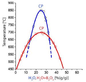
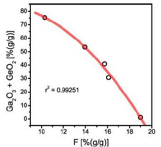
At this time, trace element data from the corresponding melt inclusions were relatively rare and yielded only unsatisfactory correlations. Therefore, an important step was the developing of analytical tools for the determination of elements and trace elements of the corresponding melt inclusions. At the beginning, only the microprobes SX50 and SX100 at the GFZ Potsdam and the SIMS in Woods Hole are available. After careful calibration of the microprobes by Dieter Rhede (GFZ Potsdam), we were able, besides the standard element, to determine boron and beryllium in the melt inclusions. Important was also the development of Raman spectroscopy for qualitative and quantitative analytical purposes, especially for the determination of water in melt inclusions – even under the sample surface [10]. At this time, we also began using the SYXRF-microprobe at DESY Hamburg (Thomas et al. 1995) [27] intensively, which was further improved by Rickerts et al. (2006) [10]. With this broad instrumentarium, we could, year after year, obtain a large amount of analytical data on melt inclusions in granites and pegmatites. An important result is the correlation between the re­homogenization temperature and the bulk water concentration in the melt inclusions. The first nearby complete solvus curve was already published by Thomas et al. (1999) [24]. An important prerequisite for the construction of such solvus curves was obtained from work on melt inclusions using the Stokes-Einstein equation to determine the viscosity and water content of melt inclusions at the homogenization temperature [28]. To produce reproducible values over 25 years, a constant homogenization time of 20 hours was generally used. Longer times for the re-homogenization of melt inclusions lead to significant diffusion losses of water and fluorine [24]. Figure 1 shows such a simplified solvus curve for pegmatites of the Ehrenfriedersdorf region. If we add boron oxide (B2O3) to water in the melt inclusion, the critical point shifts to 27.7% (H2O + B2O3). From that, a significant improvement results: an increase in the R2 value from 0.98995 to 0.99985 and the standard deviation from 9.44 to 2.19. It is also possible that some further element affects the solvus curve of the Ehrenfriedersdorf pegmatite. These are, for example, Rb and Sb [28].
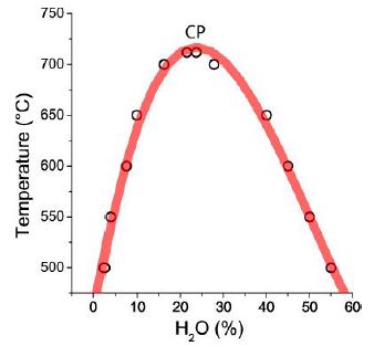
Figure 1: Solvus curve (polynom of third degree) for the Ehrenfriedersdorf pegmatite (simplified). Each point is the mean of more than 100 measurements. CP is the critical point (23.6 % H2O, 712°C). r2 is 0.98995, and the standard-deviation is 9.4.

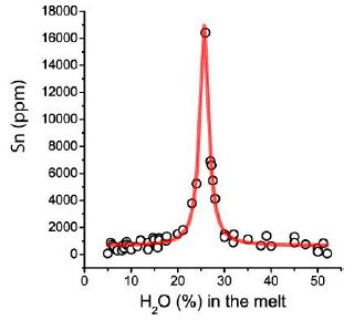
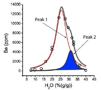
The solvus curve is the basis for further relationships with other elements. Starting with the distribution of tin versus the water concentration (Figure 2), beryllium shows, in contrast to Sn, a more complex Lorentzian distribution, composed of two overlapping Lorentzian components established by two different Be-species: beryllonite [NaBePO4] and hambergite [ Be2BO3(OH, F)] – see Thomas et al., 2022) [18]. That is also a clear hint that the solvus curve near the solvus crest is relatively flat and not a single point, but a small range. A distribution similar to that of tin is also observed for phosphorus (Figure 3).
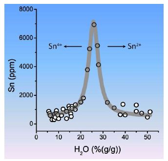
Figure 2: Lorentzian distribution of tin versus the water concentration of the corresponding solvus curve. The arrows indicate the tendency of Sn speciation.
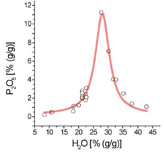
Figure 3: Lorentzian distribution of phosphorus versus the solvus water content.

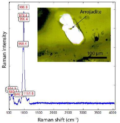
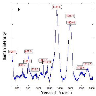
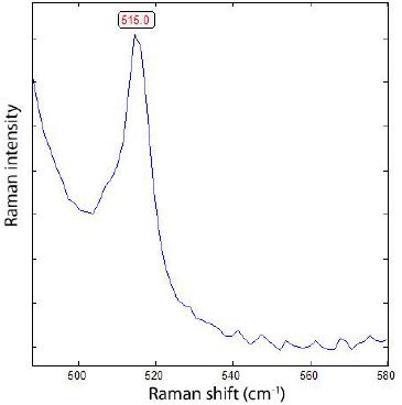
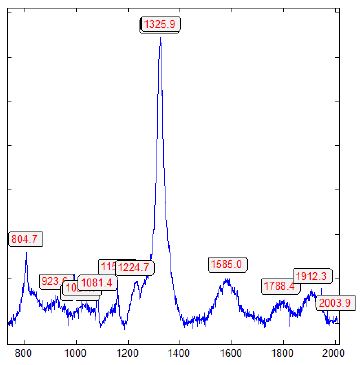
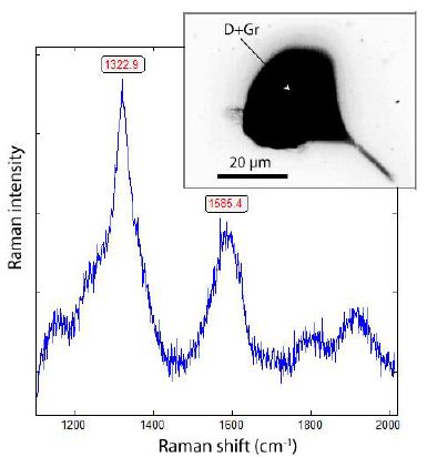
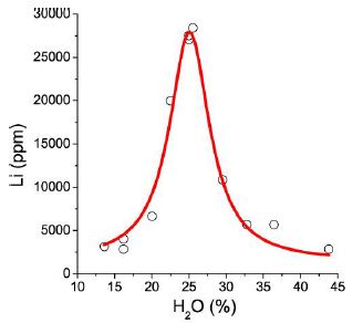
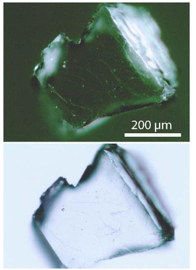
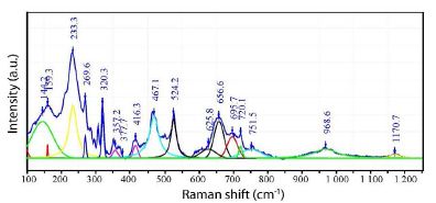
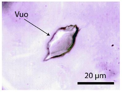
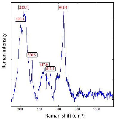
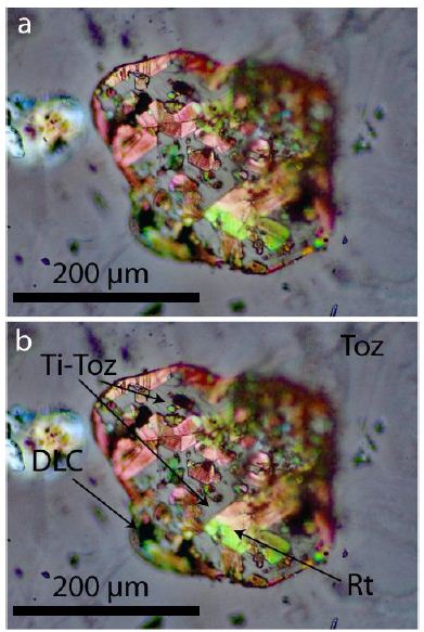
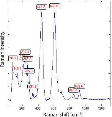
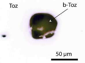
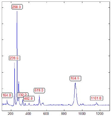
Similar distribution curves result for about 11 elements (Table 1), so, for example, for a typical main element, phosphorus of the Variscan Ehrenfriedersdorf tin deposit. Besides high P concentration in melt inclusions in the pegmatite quartz, there are also many different P-rich minerals as inclusions, often as needles. As examples, we call here arrojadite, berlinite, herderite (with 11.65 % F), and hydroxylherderite. Arrojadite (see Figure 4a and b) has never been reported from the Variscan Ehrenfriedersdorf tin deposit to date, although this mineral is not rare there. Here, we will give a picture of such a crystal and a Raman spectrum.

Table 1: Fitting parameters for element distributions in the range of the critical point of the pseudo-binary melt-water (solvus) system.

Element/compound

Distribution Area ppm2 Center [% H2O] Width [% H2O] Offset [ppm] Height [ppm]
Li Lorentzian 273330 25.1 6.5 1363

26,660

Be

Lorentzian 131560 26.5 10.1 132 11,600
B Lorentzian 217240 30.0 3.5 9993

39,718

Zn

Gaussian 217240 26.7 2.4 390 43,220
Sn Lorentzian 54207 25.6 4.8 503

6,865

Cs

Lorentzian 266000 26.0 5.6 1300 28,000
Ta Lorentzian 50148 27.4 9.9 86

3,236

WO3

Gaussian 73258 26.8 7.5 558 47,626
P Lorentzian 560320 28.5 5.8 1300

61,000

Cl

Lorentzian 147040 26.4 4.0 116 16,800
As Lorentzian 46433 30.1 3.2 520

9,464

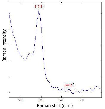
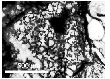
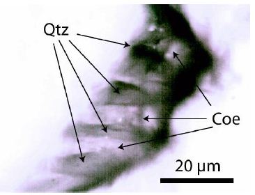
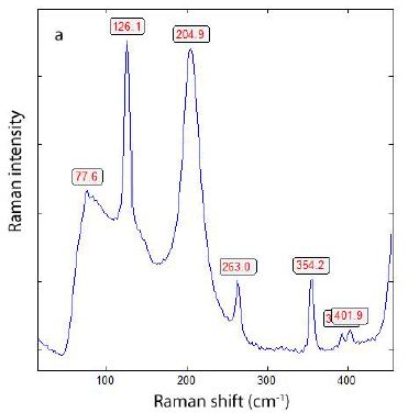
Figure 4a: Arrojadite in pegmatite quartz (Qu8) – Raman spectrum and micro-photograph.

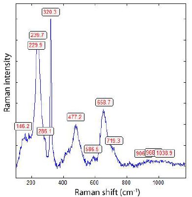
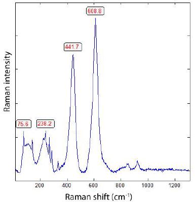
Figure 4b shows another Raman spectrum of arrojadite [KNa4Ca(Fe2+, Mn2+)14Al(PO4)12(OH)2] in the same sample. According to Anthony et al. (2000) [29], arrojadite is a high-temperature (~800°C) primary mineral in granite pegmatite. Opposite to many small (Königshain) or large (Volyn) pegmatites, the pegmatite from the Sauberg mine near Ehrenfriedersdorf shows a very large number of different melt inclusions with different, sometimes exotic daughter minerals (forming a solvus curve) and countless small mineral inclusions from which only a small number are identified by microprobe or Raman spectroscopy. To the so-called system-relevant minerals of the tin deposit, HT-HP minerals are brought by supercritical fluids (SCF) or supercritical melts (SCM) from mantle depths, indicating that supercritical phases make a non-negligible contribution. In addition, such HT-HP minerals also formed on the spot under strong reducing conditions (whiskers of graphite, diamond, lonsdaleite, moissanite) – see, for example, (Thomas 2026) [20] or by shock events.
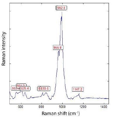
Figure 4b: Another Raman spectrum of arrojadite in pegmatite quartz (Qu8) from the Sauberg mine (Ehrenfriedersdorf).

Phosphorus is present in melt inclusions in pegmatite quartz from the Variscan tin mineralization of Ehrenfriedersdorf and is also well Lorentzian-distributed (Figure 4). Berlinite is often a daughter mineral in large melt inclusions [5]. The P2O5 content reaches about 7 % in melt inclusions, although the P-content in paragenetic feldspar is not higher than 1 %. Phosphorus is a relatively common element in melt inclusions and solid mineral inclusions in pegmatite quartz. In the sample Qu8, we found a remarkable, extremely P-rich inclusion with 50.7 ± 3.5 % P2O5 [5]. The components SiO2 (10.5 ± 2.2 %), Al2O3 (36.2 ± 1.6 %), and FeO (0.24 ± 0.06 %) are mainly contained in the Si-Al-glass phase, which means that the central “bubble” consist from nearly pure P2O5, which is an absolute novum and under normal geochemical conditions unthinkable in nature. Also, the small bubbles consist mainly of P2O5. The composition was determined with the microprobe SX50 at the GFZ Potsdam. During the acquisition of trace element data with SIMS in Woods Hole (J.D. Webster), the sample was destroyed during cleaning with distilled water. Here, the important point is that, for the formation of nearly pure P2O5 in a complex natural melt-water system, unusual conditions must be present (Figure 5).
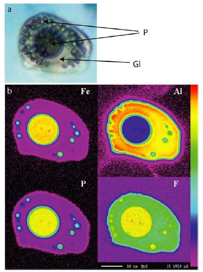
Figure 5: Phosphorus-rich melt inclusion in pegmatite quartz (Qu8). The figure a) shows the inclusion after rehomogenization (P – P2O5 globules, Gl – silicate glass), and plate b) shows the distribution of Fe, Al, P, and F presented. Al is mainly distributed in the silicate melt, while Fe, P, and F are distributed in the bubble-like part.

The most extreme melt inclusion compositions, such as near-pure P2O5 domains, represent rare boundary cases rather than modal system behavior. These inclusions define the upper solubility envelope attainable near the critical window, but they do not characterize average melt compositions. Such distributions (Figure 2, 3, 8, and data in Table 1) can be integrated into a standardized diagram using reduced coordinates (Figure 6) for all studied elements.

In Thomas et al. (2019 [17] and 2022 [18], some important elements are tabulated for the Ehrenfriedersdorf pegmatite system (besides many other pegmatites) and used to build Figure 6 and the shortened Table 1 for the Ehrenfriedersdorf case.
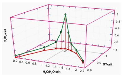
Figure 6: Combined and generalized solvus and Lorentzian curves in the reduced coordinates: X: water concentration divided by the water concentration at the critical point CP; Y: element concentration divided by the corresponding concentration at the critical point; Z: reduced temperature (temperature divided by the critical temperature CP (see also Thomas and Rericha, 2024) [30].

Table 1 shows the fitting parameters for the corresponding elements (including new ones) for the Ehrenfriedersdorf case.

The mean (center) of all 11 elements is 27.2 ± 1.6% H2O. That means at least the solvus crest is not a point, but a small range in reality. Table 1 shows two cases (Zn, WO3) where the data are Gaussian distributed (Zn and WO3). Maybe the data number is too small. Figure 7 shows a melt inclusion in pegmatite quartz Qu8 (partially homogenized) with a large sphalerite daughter crystal. Such inclusions are not rare.

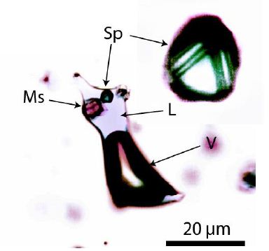
Figure 7 shows a typical melt inclusion (with an attached fluid inclusion) containing a relatively large brown sphalerite crystal (Sp) with more than 60,000 ppm Zn and about 30,000 ppm S (see Roedder (1984 [31]), Figure 4-1), which would transform the Gaussian into a Lorentzian distribution. Furthermore, for sulfur, a similar distribution is to be expected (i.e., increasing the number of elements follows the Lorenzian distribution). From Figure 6, followed clearly that the Lorentzian element distribution curves are related to the corresponding solvus curve – they (solvus and Lorentzian curves) are not independent, they are together related. That is an important result of the longstanding studies on silicate melt inclusions in mostly pegmatite quartz from the Ehrenfriedersdorf region. An important question arises: Is the three-dimensional representation (Figure 6) real? Or can these presentation simplificated into the two coordinates water content versus temperature, and can the element concentration at the solvus crest be transformed into temperature values? However, that temperature is, in general, the maximum solubility of the element and cannot be determined exactly, because many measurements at melt inclusions representing the critical point are necessary.
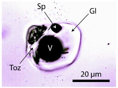
Figure 7: Melt inclusion in pegmatite quartz with a sphalerite daughter crystal (Sp). Gl – silicate glass, Toz – topaz, V – vapor phase.

Interpretation

The Meaning of the Critical Point (CP) at the Solvus Crest

At the critical point of a pseudo-binary solvus, the following statements are crucial:

  • The silicate melt and the aqueous fluid become compositionally
  • The system approaches a supercritical melt-water
  • The density contrast and the interfacial tension approach
  • The diffusion coefficients increase to extremely high
  • The dynamic viscosity goes to extremely low

In other words, the system temporarily loses the sharp boundary between “melt” and “fluid”.

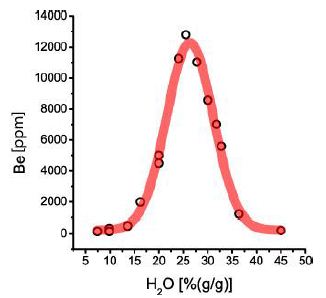
Far from the critical point, the element partition is different between the melt and the fluid. And the solubility is limited by phase boundaries and surface energy. Near the critical point, the element partition coefficients approach unity. Elements that normally prefer either a melt or a fluid can occupy the same continuous phase. The solubility maxima are reached. A typical example is Be (Figure 8).
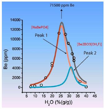
Figure 8: Distribution of Be in melt inclusions in pegmatite quartz from Ehrenfriedersdorf (see further above). It is here that at the solvus crest with the shown maximum at about 12,840 ppm Be is topped by a large daughter crystal of beryllonite [NaBePO4] in such a melt inclusion of the same sample corresponding to 71,500 ppm Be.

If we look at Table 1, it is striking that the solvus crest moves in very small limits: 27.2 ± 1.6 % H2O. In summary, element concentrations are highest at the critical point of a pseudo-binary melt-water solvus because phase boundaries vanish, solubility and diffusion reach maxima, and critical thermodynamic fluctuations allow extreme but transient enrichment that can be preserved upon quenching.

Small changes in temperature or composition can cause large changes in density, creating strong local concentration fluctuations. Elements with complexation tendencies (Be, Li, B, Sn, Nb, Ta, REE, etc.) are especially affected. Pegmatites are essentially the natural geological expression of what happens when a granite melt-water system (with extra input of water or water-rich melts by SCFs or SCMs) parks near the critical point of a pseudo-binary solvus for a prolonged time.

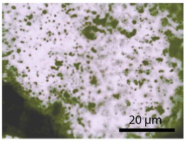
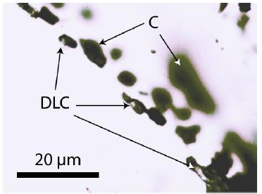
A key observation from pegmatite melt inclusions is that near the critical point, Lorentzian curves may degenerate into near-vertical lines (see Figure 8), controlled by the maximum solubility of the element (here Be) in the supercritical melt-water system. A nice example of a slightly different origin is the existence of graphite-like globules in silicate melt inclusions (Figure 9).
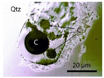
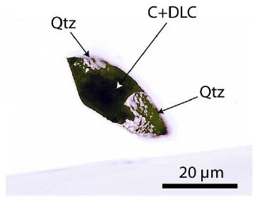
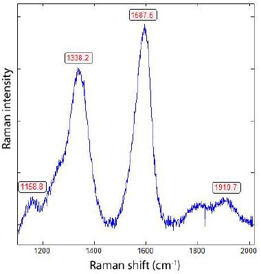
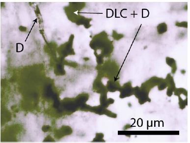
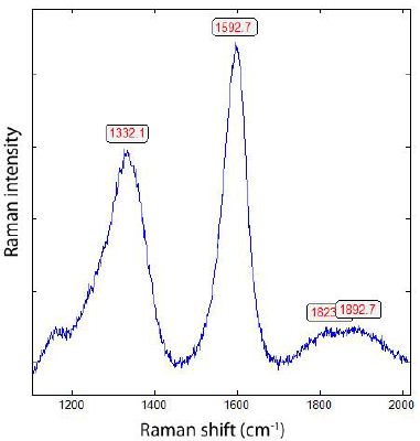
Figure 9: Carbon and graphite-like carbon (C) in a melt inclusion in pegmatite quartz (Qtz) from the Sauberg mine (sample Qu8). All black points are carbon. The larger ones contain nanodiamonds or diamond-like carbon (DLC).

That example is the trapping of micro-crystals suspended in the supercritical melt phase (SCM). The carbon and DLC here are not formed at the trapping site. A similar case shows Figure 10.
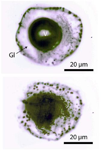
Figure 10: Melt inclusion in pegmatite quartz with suspended small carbon globules (black). Gl – silicate glass, V – vapor phase. The under photomicrograph shows a deeper look into the inclusion and significant mor carbon globules. The vapor phase is methane and hydrocarbon-rich.

Figures 9 and 10 clearly demonstrate that supercritical melts (SCM) from the deep mantle intrude into the pegmatite-forming melt and add water and water-rich melts, as well as carbon and DLC. According to Thomas (2026), the SCF and/or SCM may be responsible for the initial formation of larger pegmatite bodies within the Variscan tin deposit.

Why are most elements in melt inclusions at the critical point Lorentzian distributed, and why are Lorentzian peaks centered on the solvus crest (see Figure 6)?

  • Element concentration maxima align precisely with the solvus crest.
  • The offset of the Lorentzian curve corresponds to equilibrium (Clarke-level) concentration.
  • The height and width measure the strength and duration of critical enrichment.

This tight geometric coupling between solvus geometry and Lorentzian statistics has been documented repeatedly in pegmatites [17,18,31]. Importantly, Lorentzian distributions are not mathematical conveniences. The encode real physics. The Lorentzian feature has, in our case, the following physical meaning:

  • Sharp central peak –                     near-equilibrium background
  • Heavy tails –                                   critical enrichment
  • Divergent variance –                     scale-free
  • Vertical asymptote –                     maximum solubility

Lorentzian element distributions are typical near criticality because diverging correlation lengths, flattened chemical-potential landscapes, and transport-dominated non-equilibrium behavior produce scale-free, heavy-tailed concentration fluctuations that Gaussian statistics cannot describe.

Melts far from criticality (normal melts, equilibrium systems) are characterized by

  • Fluctuations are small, local, and independent.
  • Many random contributions add up.
  • The central limit theorem applies

Therefore, the Gaussian distribution dominates. However, near criticality, the situation is different:

  • Fluctuations become large, long-range, and correlated.
  • There is no characteristic length or time scale.
  • Rare but extreme events dominate the statisctics.

Therefore, the Lorentzian (heavy-tailed) distribution emerges. Meaning, the correlation length goes to infinity, composition, density, and speciation fluctuations extend over large volumes, and local chemical environments are no longer independent. As a result, the variance formally diverges, the system no longer has a well-defined “mean + small noise”, and the Gaussian statistics become invalid.

Lorentzian element distributions are typical near criticality because diverging correlation lengths, flattened chemical-potential landscape, and transport-dominated non-equilibrium behavior produce scale-free, heavy-tailed concentration fluctuations that Gaussian statistics cannot describe.

What Happens with the Supercritical System at Further Cooling?

Upon further cooling below the solvus crest, the supercritical melt–water system becomes thermodynamically unstable and separates into a two-phase assemblage consisting of a silicate melt and an aqueous fluid. The disappearance of the supercritical state is accompanied by the rapid re-establishment of density contrast, interfacial tension, and sharply reduced diffusion coefficients. As a result, melt–fluid immiscibility sets in abruptly. Elements that were homogenized in the supercritical state – where partition coefficients approach unity – are forced to repartition between melt and fluid as cooling proceeds. Because cooling in pegmatitic systems commonly outpaces diffusive re-equilibration, extreme and transient element enrichments generated near the critical point cannot fully relax to equilibrium. Instead, they become preserved by quenching, crystallization, and the entrapment of melt and fluid inclusions. This process effectively “freezes in” the chemical signature of criticality. Maximum solubilities attained at the solvus crest are converted into discrete mineral phases or highly enriched residual melts, explaining the coexistence of extreme element concentrations in melt inclusions and abundant rare-element minerals in pegmatites. Farther from the critical point, the system returns to normal magmatic–hydrothermal behavior characterized by Gaussian statistics and equilibrium partitioning.

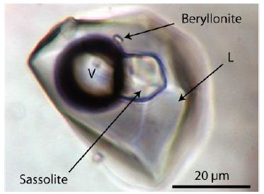
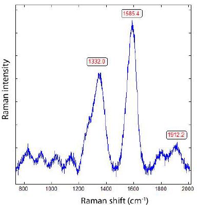
Pegmatites thus represent the geological record of granite melt–water systems that hovered near the solvus crest and then cooled just fast enough to preserve critical-state chemistry. Further cooling transforms the supercritical melt–water system into a two-phase melt + fluid system, triggers rapid immiscibility, and locks in extreme, transient enrichments through quenching and crystallization. Pegmatites thus represent the geological record of systems that hovered near the solvus crest and then cooled just fast enough to preserve critical-state chemistry. The high number of small minerals, mostly trapped in quartz, demonstrates that at the transition from the supercritical to the undercritical state, we have local oversaturation of elements that form the basis for the crystallization of many, often very rare, however system-relevant, minerals, such as arrojadite, berlinite, beryllonite, hambergite, herderite, sassolite, and many others. So, the Sauberg pegmatite is a Cockaigne for mineral hunters. Besides such minerals, we have often observed untypical HT-HP minerals, such as diamond, lonsdaleite, coesite, orthorhombic cassiterite, and others, which demonstrate that they are added by supercritical fluids (SCF) or supercritical melts (SCM) from mantle depths [20,32]. However, graphite is a common mineral in the Variscan tin deposit Ehrenfriedersdorf. Obviously, we have four types of graphite-like stuff: (i) introduced by SCF or SCM, (ii) formed on the spot by strongly reducing conditions [33], forming whiskers of graphite, diamond-like carbon (DLC), and moissanite in quartz and beryl [20,34-36] or (iii) formed via a natural chemical vapor (CVD) process, and (iv) by a shock event.

Conclusion and Outlook

The recognition that pegmatites record prolonged residence near the critical point of granite–water systems has implications well beyond the Ehrenfriedersdorf case. It provides a unifying physical framework linking pegmatite textures, extreme trace-element enrichments, and the formation of rare-element minerals to critical-state melt–fluid behavior rather than to purely fractional crystallization or late hydrothermal overprinting. Lorentzian enrichment patterns emerge as diagnostic fingerprints of criticality, providing a transferable criterion for identifying supercritical processes in other granitic, pegmatitic, and even magmatic–hydrothermal systems worldwide. More broadly, these findings emphasize the importance of transient, non-equilibrium states in crustal differentiation, suggesting that critical phenomena play a fundamental role in concentrating economically and mineralogically significant elements during the evolution of continental crust. Future work should focus on strengthening the quantitative and comparative framework of critical-state interpretations in pegmatite systems. A priority is the systematic application of model-comparison statistics (e.g., Gaussian vs. Lorentzian vs. Voigt fits – see Thomas and Rericha, 2026) [28] to larger datasets, allowing the statistical robustness of heavy-tailed distributions to be assessed independently of visual inspection. Equally important is the extension of the reduced-coordinate approach to other granite-pegmatite provinces. Demonstrating that solvus-centered Lorentzian enrichment is reproducible across different tectonic settings, melt compositions, and volatile regimes would decisively establish critical-state behavior as a general process rather than a local peculiarity of the Ehrenfriedersdorf system. From a process perspective, coupling melt inclusion observations with diffusion kinetic and cooling rate constraints would further clarify how extreme enrichments generated near the critical window are preserved during rapid immiscibility and crystallization. Even order-of-magnitude kinetic estimates would significantly narrow the range of permissible evolutionary paths. Finally, the recognition of Lorentzian enrichment patterns as signatures of transient non-equilibrium states opens new perspectives for economic geology. If critical windows systematically maximize element solubility and mobility, they may represent a fundamental control on rare-metal fertility in granitic systems. Future studies integrating melt inclusions, mineral chemistry, and isotopic tracers may therefore transform critical-state analysis into a predictive tool for pegmatite- and granite-related mineralization.

Acknowledgment

This paper is dedicated to my teachers at the Mining Academy Freiberg in mineralogy, geochemistry, and ore deposits, Prof. Hans Jürgen Rösler (1920-2009) and Prof. Ludwig Baumann (1929-2008), as well as Prof. James D. Webster from the AMNH in New York, for his strong interest in the genesis of the tin deposit Ehrenfriedersdorf.

References

  1. Hösel G (1994) Das Zinnerz-Lagerst ättengebiet Ehrenfriedersdorf/Erzgebirge. Pg: 195.
  2. Thomas R, Baumann L (1980) Ergebnisse von thermometrischen und kryometrischen Untersuchungen an Kassiteriten des Zeitschrift für geologische Wissenschaften 8: 1281-1299.
  3. Schütze H, Stiehl G, Wetzel K, Beuge P, Haberlandt R, et (1983) Isotopen-und elementgeochemische sowie radiogeochronologische Untersuchungen an der Zinnlagerstätte Ehrenfriedersdorf. Akademie der Wissenschaften der DDR, Zentralinstitut für Isotopen- und Strahlenforschung Leipzig, ZfI-Mitteilungen, Nr. 76: 232-271.
  4. Thomas R (2024a) Vom Schmelzeinschluss zum superkritischen Fluid – Ergebnisse und Folgen der Befahrung der Grube Sauberg bei Ehrenfriedersdorf. Veröffentlichungen Museums für Naturkunde Chemnitz 47: 59-66.
  5. Thomas R, Webster JD, Rhede D (1998) Strong phosphorus enrichment in a pegmatite-forming Acta Universitatis Carolinae – Geologica 42: 150-164.
  6. Webster JD, Thomas R, Veksler I, Rhede D, Seltmann R, Förster H-J (1998) Late-stage processes in P- or F-rich granitic magmas. Acta Universitatis Carolinae – Geologica 42: 181-188.
  7. Veksler, IV, Thomas R (2002) An experimental study of B-, P- and F-rich synthetic granite pegmatite at 1 and 0.2 GPa. Contribution Mineral Petrol 143: 673-683.
  8. Veksler IV, Thomas R, Wirth R (2003) Crystallization of AlPO4-SiO2 solid solutions from granitic melt and implications for P-rich melt inclusions in pegmatitic quartz. American Mineralogist 88: 1724-1730.
  9. Thomas R, Förster H-J, Heinrich W (2003) The behaviour of boron in a peraluminous granite-pegmatite system and associated hydrothermal solutions: a melt and fluid-inclusion study. Contrib Mineral Petrol 144: 457-472.
  10. Rickers K, Thomas R, Heinrich W (2006) The behavior of trace elements during the chemical evolution of the H2O-, B-, and F-rich granite-pegmatite-hydtothermal system at Ehrenfriedersdorf, Germany: a SXRF study of melt and fluid Mineralium deposita 41: 229-245.
  11. Thomas R, Kamenetsky VS, Davidson P (2006) Laser Raman spectroscopic measurements of water in unexposed glass inclusions (2006). American Mineralogist 91: 467-470.
  12. Romer RL, Thomas R, Stein HJ, Rhede D (2007) Dating multiple overprinting Sn-mineralized granites – examples from the Erzgebirge, Mineral Deposita 42: 337-359.
  13. Borisova AY, Thomas R, Salvi S, Candaudap F, Lanzanova A, Chmeleff J (2012) Tin and associated metal and metalloid geochemistry by femtosecond LA-ICP-QMS microanalysis of pegmatite-leucogranite melt and fluid inclusions: new evidence for melt-melt-fluid Mineralogical Magazine 76: 91-113.
  14. Hurai V, Huraiová M, Slobodník M, Thomas R (2015) Geofluids – Development in Microthermometry, Spectroscopy, Thermodynamics, and Stable Isotopes. Elsevier. Pg:489.
  15. Thomas R (2000) Determination of water contents of granite melt inclusions by confocal laser Raman microprobe American Mineralogist 85: 868-872.
  16. Thomas R, Webster JD, Davidson P (2011) Be-daughter minerals in fluid and melt inclusions: implications for the enrichment of Be in granite-pegmatite Contrib Mineral Petrol 161: 483-495.
  17. Thomas R, Davidson P, Appel K (2019) The enhanced element enrichment in the supercritical states of granite-pegmatite systems. Acta Geoichim 38: 335-349.
  18. Thomas R, Davidson P, Rericha A, Voznyak DK (2022) Water-rich melt inclusions as “frozen” samples of the supercritical state in granites and pegmatites reveal extreme element enrichment resulting under non-equilibrium Mineralogical Journal (Ukraine) 44: 3-15.
  19. Thomas R (2024b) The CaCl2-to-rutile phase transition in SnO2 from high to low pressure in Geol Earth Mar Sci 6: 1-4.
  20. Thomas R (2026) Precede high-pressure, high-temperature mineralization in the Variscan tin deposit Ehrenfriedersdorf/Germany. Geol Earth Mar Sci 8: 1-6.
  21. Thomas R (2024c) 13C-rich diamond in a pegmatite from Rønne, Bornholm Island: Proofs for the interaction between mantle and crust. Geol Earth Mar Sci 6: 1-3.
  22. Thomas R (2025) Raman spectroscopy of boroc acid daughter crystals with different B-isotopes: H3 11BO3 and H3 10BO3 , and different hydrogen and deuterium concentrations. Geol Earth Mar Sci 7: 1-3.
  23. Thomas R, Davidson P (2012) The application of Raman spectroscopy in the study of fluid and melt inclusions. Z. dt. Ges.. Geowiss 163: 113-126.
  24. Thomas R, Webster JD, Heinrich W (1999) Melt inclusions in pegmatite quartz: Complete miscibility between silicate melts and hydrous fluids?. Terra Nostra 99: 305-307.
  25. Thomas R, Webster JD, Rhede D, Seifert W, Rickers K, Förster H-J, Heinrich W, Davidson P (2006) The transition from peraluminous to peralkaline granitic melts: Evidence from melt inclusions and accessory minerals. Lithos 91: 137-146.
  26. Thomas R (2002) Determination of the H3BO3 concentration in fluid and melt inclusions in granite pegmatites by laser Raman microprobe American Mineralogist 87: 56-68.
  27. Thomas R, Klemm W, Haller M, Knöchel A, Radtke M (1995) First results on melt inclusions in geological samples using SYXRF-microprobe. Hamburger Synchrotronstrahlungslabor HASYLAB am Deutschen Elektronen-Synchrotron Jahresbericht II 961-962.
  28. Thomas R, Rericha A (2026) From the granite-pegmatite solvus curves to extreme element enrichment indicated by Gaussian, Lorentzian, and Voigt Geol Earth Mar Sci 8: 1-6.
  29. Anthony JW, Bideaux RA, Bledh KW, Nichols MC (2000) Handbook of Mineralogy, Volume IV – Arsenate, Phosphates, Tucson, Arizona. Pg: 680.
  30. Thomas R, Rericha A (2024) Meaning of supercritical fluids in pegmatite formation and critical-element Geol Earth Mar Sci 6: 1-5.
  31. Thomas R (2025) Interpretation of the Lorentzian distribution of tin in the Variscan Ehrenfriedersdorf deposit/Germany. Geol Earth Sci 7: 1-5.
  32. Thomas R, Davidson P, Rericha A, Recknagel U (2023a) Ultrahigh-pressure mineral inclusions in a crustal granite: Evidence for a novel Transcrustal transport Geoscience 13: 1-13.
  33. Thomas R, Webster JD (2000) String tin enrichment in a pegmatite-forming Mineralium Deposita 35: 570-582.
  34. Thomas R, Recknagel U, Rericha (2023b) A moissanite-diamond-graphite paragenesis in a small beryl-quartz vein related to the Variscan tin-mineralization of the Ehrenfriedersdorf deposit, Germany. Geosciences 13: 1-13.
  35. Thomas R (1994) Estimation of the viscosity and the water content of silicate melts from melt inclusion Eur J Mineral 6: 511-535.
  36. Thomas R, Webster JD, Heinrich W (2000) Melt inclusions in pegmatite quartz: complete miscibility between silicate melts and hydrous fluids at low Contrib Mineral Petrol 139: 394-401.
Characterisation of Contaminant Plumes Using Integrated Geophysical and Physico-chemical Methods

DOI: 10.31038/GEMS.2026832

Abstract

Rainfall precipitation on dumpsite dissolves organic and inorganic constituents, forming toxic chemicals thereby leaching into groundwater bodies resulting to generation of high biological oxygen demand (BOD), and thus contaminating the groundwater system and thereby resulting into the death of aquatic life. The impact is not limited to biodiversity as odour and vermin from dumpsites makes disease becomes an issue with other adverse concomitant health challenges. Effort to save the environment from further degradation necessitated this research. Geophysical and physico-chemical investigations were carried out across the dumpsite located at Kubwa, F.C.T. North-central Nigeria. The aim of the research is to delineate areas of possible contamination plume, its migration path and the vadose zones. For this purpose, Electrical resistivity tomography (ERT) data were acquired along eight traverses and results were inverted using RES2DINV Software likewise fifteen VES were equally acquired and results corroborate the ERT results. Water samples from boreholes, hand dug well and river channel were obtained and were analyzed. Distinct low resistivity zones that we adjudged to represent the contamination plumes were obtained from the ERT results. The water analysis revealed that the, total dissolved solid (TDS) were in the ranges of (2.30 x 101 to 8.20 x 101) μScm-1as against NSDWQ values of 1×10³ μScm-1. Biochemical oxygen demand (BOD), chemical oxygen demand (COD) and dissolved oxygen (DO), were in the ranges of 1-10, <2 to <98 and 0.01-0.12 mg/L respectively. The water samples also had detectable levels of Cu, Cd, Ni, Mn, Pb and Zn contents which are far below the permissible limits. The water samples microbiologically revealed presence of faecal contamination with bacteria pathogens such as Coliform, and Escherichia coli are above permissible limit, while the mould yeast and total aerobic are below the limit likewise. Ultimately, our findings showed that the investigated dumpsite constitutes a serious threat to groundwater body in the area. The efficacy of combined geophysical and physico-chemical approaches for groundwater contaminant studies has been demonstrated in this study.
Keywords

Leachate, Vadose zone, Contaminant Plumes, Physico-chemical, North Central Nigeria

Introduction

Dump materials are generated regularly as a result of human activities. The ferocity of these human activities has led to the growing amount of dump materials globally despite the level of worldwide advancement in technology. Ganiyu et al., (2016) [1] asserts that dumpsites serve as the ultimate recipient of municipal solid waste. Environments get Polluted when by-product of chemical substances infuse into natural habitats; and thus immensely alter nature’s ability to dispense these pollutants. Pollutants are materials which impose danger on the health of humans, causes discomfort and damages the environment. Sabahi et al., (2009) reports that air, soil, water, nuclear and oil pollution characterises major types of pollution. Huge amount of dumped materials from urban, municipal and industrial sectors are generated globally. According to Rukah and Al-Kofahi,(2001) [2], dumpsites have over many decades been used as harbours for varied dump materials. According to Vinai et al., (2015), dumpsites are either situated above the ground or located within quarries or pits. Poovarasan et al., (2018) throw more light on how physical, chemical and biological processes interact simultaneously to bring about the overall decomposition of wastes. Afangideh et al., (2015) described the end-products of all waste mechanisms as chemically laden leachates. Misra and Mani, (1991) attributed Leachates generated from dumpsites as sources of groundwater and soil pollutions. Leachate is characterised by high ion concentrations while the rock hosting them depicts low resistivity compared to surrounding rocks. Employing the geoelectrical techniques in mapping of the leachate has become necessary (Ganiyu et al., 2015) [3]. For example, Chen et al. (2020) [4] used a novel approach to assess the complexity of contaminant plume transportation in the aquifer based on Hausdorff Fractal Dimension. Furthermore, Chen, et al., (2019) [5]. Carried out the assessment of shallow groundwater contamination resulting from a municipal solid waste landfill-a case study in Lianyungang, China. Electrical Resistivity Tomography (ERT) studies on dumpsites were conducted by varied researchers to delineate leachate, contaminant plumes on the land and its effect on aquifer system. In this research work, the use of 2D resistivity Imaging and Vertical Electrical Sounding (VES) were employed to characterise the depth to the groundwater table, identify and characterise the extent of contaminant leachate plume and its migration flow paths at subsurface within and around dumpsite and the results were corroborated by physico-chemical analysis for robust research’s outcome.

Location Description and Geological Setting

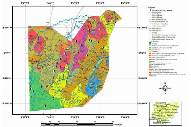
The study area, F01 Kubwa refuse dumpsite (Figure 2.1) is located within Abuja F.C.T metropolis in Bwari Area Council and lies within longitudes E007°22.650¹n to E007°22.591¹ and latitudes N0910.079¹ to N0910.080¹ north-central Nigeria. It was in operation before 2011 and still in use till date (Figure 1).

Figure 1: Geological Map of Abuja showing the Study Area (modified after NGSA 2004).

Geology of Abuja

Offodile (1992) described the geology and geomorphology of Abuja to have been underlain by crystalline basement rocks and it consists of rock types which contain different textures of granites, coarse to fine, consisting essentially of biotite, feldspars and quartz. In most cases, the rocks have weathered into reddish micaceous sandy-clay to clay materials capped by laterites [6]. Generally, only small amount of water can be obtained in the freshly unfractured bedrock below the weathered layers. Groundwater is found mainly in the variable weathered/transition zone which consist of fractures, joints and cracks of the crystalline basement [6]. Clark (1985) described fissure systems in Nigeria as rarely extends beyond 50m, as proven by the available drilling data. The local water table depth is controlled by textural and compositional changes within the regolith vertical profile and the bedrock topography according to David and Ofrey (1989) [7].

Methodology

Data Description, Acquisition and Processing

Electrical resistivity methods were adopted using Vertical Electrical Sounding (VES) and Electrical Resistivity Tomography (ERT) which are very much successful in delineating vertical variation and lateral of subsurface geology respectively. Comprehensive Geophysical studies using electrical resistivity were conducted with DC resistivity meter (Omega Allied). Omega Allied is an improved Digital resistivity meter with multi ingenious functional attributes inbuilt in its design and is known for its high quality data acquisition capability as well as for its field worthiness. It is a very close-packed, sophisticated and well grounded equipment, which is used for resistivity investigations. Omega Allied resistivity meter is made up of two units (i) Current unit (C unit), and (ii) Potential unit (P unit). This unit has the provision for measuring the potential difference across the potential electrode as well as the resistance values which provide direct display over digital panel metre. The current units provide the purpose of sending the required output of constant current, whereas the potential unit provides an accurate measurement and display. The depth of penetration is dependent on increase of electrode spacing, so that apparent resistivity measured at various depths is used to construct a vertical contoured section, displaying the resistivity contrast both laterally and vertically over the section. The 2D electrical resistivity pseudosection study was used in different locations in order to characterise the geology of various subsurface lithological, structural and hydrological conditions [8].

Wenner Arrangement

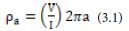
A simple method of determining the resistivity of the ground using four electrodes was discussed by Wenner (1916) otherwise called Horizontal Profiling (HP), when four electrodes are placed in a traverse line, and a known current is injected through the two extreme electrodes, the potential difference measured between the two inner electrodes gives a measure of the resistivity of the ground. The value of resistivity (ρ) is computed by the formula:

where, V is the potential in volts measured between the two inner electrodes, and I is the current in amperes passed into the ground, (a) is the distance between the successive electrodes and 2π, a constant. Since V/I = R, the resistance (Ω), the formula may be expressed as

In the above electrode arrangement, the two current electrodes are usually designated as C1 and C2, while the two inner electrodes, which pick up the potentials in the ground, are designated as P1 and P2, the potential electrodes or the measuring electrodes.

Schlumberger Array

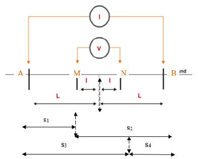
In the Schlumberger array, letters A and B denoted the current electrodes while M and N represented potential electrodes. The distance between M and N may be represented by l, while the distance AB/2 is represented by L. During field layout, the current electrodes AB are placed as outer electrodes, while the two potential electrodes M and N as inner electrodes as shown in Figure 3.2. The Schlumberger array has major advantage in depth soundings in that, long current carrying cables may not be necessary. However, the ground consists of two or more layers with different resistivity contrast, and the electrode separation ‘a’ is less than the thickness of the first layer, then the measured resistivity value (Q1) will pertain to the first layer; on increasing the separation to, say (2a), thus the second layer having a different resistivity will make itself felt in the apparent resistivity measured. Therefore, by successively increasing the electrode separation about a central point, deeper depth of investigations of the earth may be measured. The apparent resistivity values obtained by expanding the electrode intervals are plotted against the respective electrode separations. In depth soundings using the Schlumberger array, the potential electrodes represented by M and N are kept fixed but the current electrodes A and B are moved farther away on either side, i.e., increasing the distance L, i.e. (AB/2) in successive steps and obtaining the resistivity values for a series of such increases for one setting of MN with interval of l. With this arrangement, deep investigation can be made in two or more settings, increasing also the spacing of the potential electrodes and then moving out the current electrodes. When the readings are completed for a particular spacing of the potential electrodes MN, the spacing of the latter is increased; whenever such a shift of MN is made, a duplicate reading is obtained while the current electrodes are still in the old setting this serve as to validate the integrity of the acquired data. Thereafter, only the current electrodes are shifted for the next set of observations. The resistivity curves obtained in depth soundings readily indicate the numbers of layers involved in the sounding depending on AB/2 spread length and number of geologic layer in the study area. But, if the ground under investigation is homogeneous and isotropic, the generated values of Q will be the true resistivity. Such ideal conditions rarely exist in the ground since earth is inhomogeneous, and the value of Q is usually affected by the variations in the lateral and vertical dimensions, particularly layered medium. Some various electrode arrays for the measurement of resistivity of the ground will be dealt with in this work (Figure 2).

Figure 2: Schlumberger Array Layout.

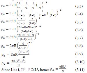
Below equations below are generated from first principle.

Given that;

s1= (L – 1); s2= (L + 1); s3= (L + 1); s4= (L – 1)

in computing the geometric factor, we have ;

Physico-Chemical Analysis

A physico-chemical was carried out on the water sample from a borehole, an open hand dug well and river channel were considered.

Results and Discussion

Data Presentation and Interpretations

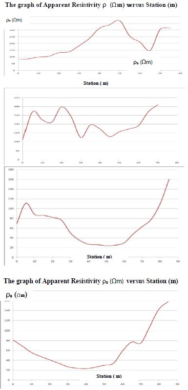
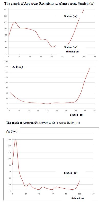
The Electrical Resistivity data using Horizontal Profiling (HP) were acquired along eight traverses and curves are presented in Figures 4.1-4.4 as 1D curves were generated using Microsoft excel showing characteristically low resistivity anomalies which coincide with dumpsite position while stations showing high anomalies are off the refuge positions, this was actually used as reconnaissance survey (Figure 3).

Figure 3: 1D Horizontal Profiling Curve for traverses 7 and 8.

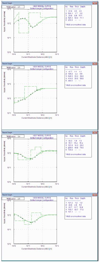
Thereafter, 2D Electrical Resistivity Tomography (ERT) was employed along eight traverses, 2D Pseudosection models were generated using RES2DINV Software as shown in figures 4.9-4.16. Isoresistivity and Isopach maps in Figures 4.32-4.40 were equally generated from Vertical Electrical Sounding (VES) model curves in Figures 4.9-4.13. The data of wenner Array (HP) and VES model curve are presented. The VES model curves were generated from acquired data which were interpreted using qualitative and quantitative approach so as to classify the model curves according to the type of the curve, which are as follow; VES1, VES9, VES10, VES11 and VES12 depict KHA type curves: ρ12345 VES2; ρ12345 depicts HKH type curve, VES3and VES7: ρ12345 depict HAK type curves, VES4, VES5 and VES8: ρ12345 depict QHK type curves, VES6: ρ12345 depicts AKA type curve, VES13 and VES14: ρ12345 depict KHA type curves while VES15: ρ12345.

Generated Isoresistivity maps, Isopach maps and Geoelectric section are presented as 2D images to further characterise subsurface geologic parameters. Subsequently geoelectric sections were as well produced as shown in figures 4.41-4.45. The anomalies observed on wenner array (HP) coincide with the area of low electrical resistivity as revealed by electrical tomography as indicated by 2D pseudosections (Figures 4-7).

Note: The high rms values recorded by the RES2DINV software is attributed to complexity of the dumpsite which pose challenge on electrode’s penetration into the ground through garbage materials as such several iterations were made and these seems to be the lowest rms values.

Interpreted Results of 2D Resistivity Pseudosection Models

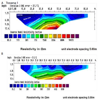
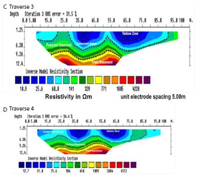
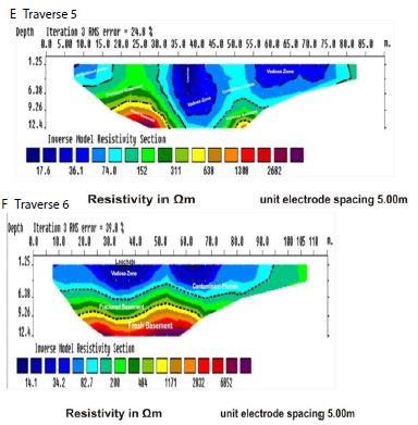
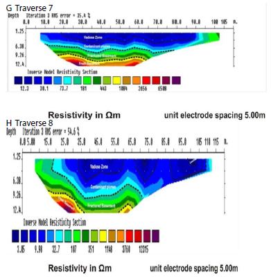
The generated 2D pseudosections of the subsurface resistivity arrangement obtained from 2D inversion process are shown in Figures 4.9-4.16 were generated from acquired wenner data, these resistivity peudosections along traverses 1-8 reveals the distributional extend over the leachate plume across horizontal direction with distance of 7.5-90 m in the East-West direction which depicts resistivity reading of about 3.09 Ωm, which is attributed to presence of leachate plume summing up to 22 m depth below the earth surface and believed to have infiltrated into the groundwater table thereby polluting it, this was measured to be varying from 10-15 m as confirmed by the observable insitu samples from the borehole and open well due to joints, cracks and faulting system as result of deformation the subsurface rocks must have suffered, thus making the weathered and fractured basement below the basin-like structure leached easily. Infiltration of contaminant plumes within some of the traverse lines originate from the western end of the traverse where it infiltrates into subsurface. Figure 4.11 shows pseudosection model along third traverse with low resistivity contrasts below 17.6 Ωm attributed to leachate or contaminant plume’s migration which occur at horizontal distances 7.5-45.0 and 50-75.0 m along the traverse. Traverse 4 showing in Figure 4.12 indicates that the leachate, vadose zone and contaminant plumes region fall within the resistivity range of 10.5-120 Ωm and with the estimated depth of 1.25-7.6 m which overlaid fractured and fresh basement which have resistivity range of 125-6552 Ωm. Figure 4.13 and 4.14 showing psudosection model along traverse 5showingresistivity anomalies as low as 20 Ωm and below, this low resistivity values further indicate presence of leachate across the horizontal distance of 10.0–50.0 m and 55.0-82.0 m. The general resistivity values across the study area as shown in the 2D pseudosections were mostly less than 100.0 Ωm which coincides with the leachate, vadose zones and contaminant plumes regions at the surface. Traverse 6 pseudosection shows low resistivity ranges from 10.9-60 Ωm attributed to leachate portion along traverse 6, which covered the distance of 30-70 m which has depth of 9.26 m. Traverse 7 pseudosection model in Figure 4.14 shows a resistivity anomaly of 14.1-82.1 Ωm which is interpreted as leachate, vadose zone and contaminant plume region which covered distance of 7.5-95 m and the depth of 9 m deep. The traverses 7 and 8 where run north-south perpendicular to traverses 2-6 while traverse 1 was actually used as control since it was located some distance away from dumpsite. Contaminant plumes thus infiltrated weathered layer at depth 10-17 m with resistivity values ranging from 12-100 Ωm showing characteristics of possible infiltration of leachate thereby contaminating the groundwater at greater depth at the under study dumpsite. Relatively low resistivity anomaly of resistivity values 3.05-12.3 Ωm to a depth of about 7.26 m occurs at the near surface indicating presence of sandy-clay mixed with indestructible garbage. The resistivity displayed by the pseudosection models across traverses 1-6 are shown in Figures 4.9-4.14. From these 2D sections, low resistivity inconsistencies were observed across traverse 1-8 within the study area. This observed low resistivity anomalies along the major traverses showed characteristics of uniform movement of contaminant plumes from western to eastern direction and downward infiltration up to about 17 m depth at subsurface. This is underlain by fractured basement rock with resistivity values ranging between 100 and 550 Ωm. The 2D resistivity inversion model sections of the subsurface resistivity distribution derived from 2D inversion models depict that the study area structurally controlled considering 2D resistivity inversion models of traverses 3-8 presented in figures 4.11-4.16 showed major resistivity low which could be attributed to possible fractured zones.

Figure 4(a & b): 2D Resistivity Pseudosection Model for traverses 1 and 2.

Figure 5(c &d): 2D Resistivity Pseudosection Model for traverses 3 and 4.

Figure 6(e & f): 2D Resistivity Pseudosection Model for traverses 5 and 6.

Figure 7(g &h): 2D Resistivity Pseudosection Model for traverses 7 and 8.

The resistivity pseudosection results along traverse 7 and 8 depicts general trend of uniform spreading of the contaminant plume from horizontal distance of 8-82 m along the North-South direction showing resistivity values 10 Ωm and below, this is an indication of leachate plume building up to the depth of about 12.4 m at the subsurface. It is obviously showing the 2D pseudosections that leachate plume formation migrate uniformly along both horizontal and vertical directions within the dumpsite. The low resistivity contrast of the upper stratum indicates that the underlying layer has higher resistivity values ranging between 140 and 300 Ωm indicating weathered or fractured basement across traverse1-8 in the study area. The central part of traverses showing in figures 4.11-4.16 the 2D pseudosection models with characteristics of low resistivity anomaly were observed between the positions 10-60 m with resistivity values ranges between 14 and 60 Ωm, this is an indicative of contaminant plumes at depth of about 12.4 m below the surface. The subsurface low resistivity was not quite obvious between 7.5 and 22 m along the traverse 1. A relatively high resistivity anomalies with resistivity values between 100 and 1097 Ωm attributed to fractured basements were observed at depth above 12.4m. The last layer of the pseudosections reveals an undulating fresh basement across traverses 1-8 with relatively high resistivity values between 1097 and 14173 Ωm. The 2D pseudosection models of traverses3-8in figures 4.11-4.16 show two major low resistivity anomalies situated at 7.5-90 m in the eastern and central portion across the traverses respectively with resistivity values below 50 Ωm, which further characterize the dumpsite into leachate, vadose zones and contaminant plume (Figures 8-12 and Tabes 1-15).

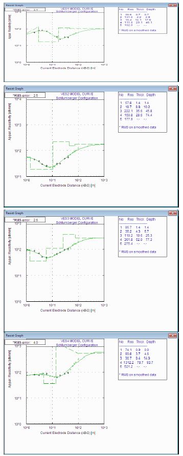
Figure 8: VES1-3 Model Curve along traverses 1.

Figure 9: VES4-6 Model Curves along traverses 2.

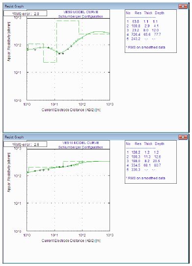
Figure 10: VES7-9 Model Curves along traverse 3.

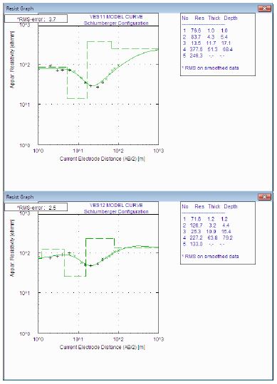
Figure 11: VES10-12 Model Curve along traverse 4.

Isoresistivity and Isopach Maps of the First to Fourth Layers

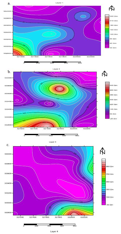
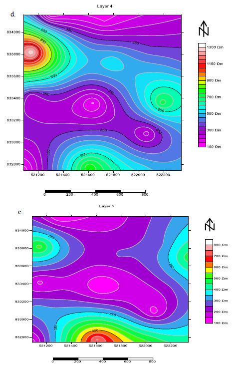
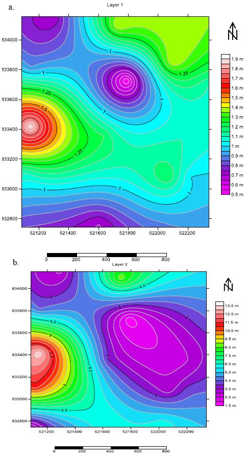
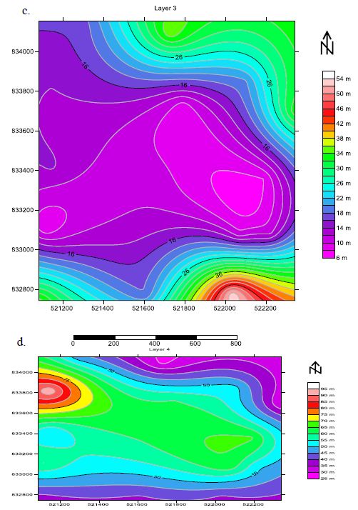
The Isoresistivity and Isopach maps of the first layer to fourth layer generated from VES1-VES 15 interpreted data were presented in Figure 4.32-4.40. The Isopach map for layer 1 indicates thickness ranging from 0.5-1.9 m. The map shows thickness in the south-Eastern part of the study area with thickness up to 1.3m which shows characteristics of leachate, while the Isoresistivity map indicates a resistivity range of 30.0-240.0 Ωm. The isoresistivity map and Isopach maps of layer 2 depict 20-580 Ωm and 1.5-13.5 m respectively which show an average thickness of about 6m which could be attributed to vadose zone. The third layer indicates the thickest thickness 6.0-54.0 m and its Isoresistivity map ranges from 50-950 Ωm. These three layers consist of resistivity low as indicated in 2D maps of both isoresistivity and isopach which thus attributed the contaminant leachate, vadose zone and plume zone respectively within the study area. The higher resistivity values were identified towards the southwestern, southeastern and central parts of the area up to 1300 Ωm and lowest resistivity values were identified in the Northern part of the study area ≤100 Ωm with the thickness values range from 25-95 m. This layer depicts competent geologic materials which is referred to as fractured basement layer which is underlain by fresh basement with the resistivity ranges from 100-800 Ωm. Very low resistivity suggests sandy-clay materials. Thus, water saturated materials, often infiltrated by leachate. The depth of the aquifer units range between 20 m and 30 m in the area which probably have been contaminated as a result of hydraulic communication through joints, crack and faulting which was further proved by the physico-chemical and microbiological analysis results. The Geochemical analysis further corroborate the geophysical interpretation by given insight to dissolve trace elements presence in water samples from borehole, hand dug well as well as stream water sample (Figures 13 and 14).

Figure 13(a-e): Isoresistivity map for layer 1-5.

Figure 14(a-d): Showing Isopach map for layer 1-4.

2D Geoelectric Sections of the First to Fifth Layers

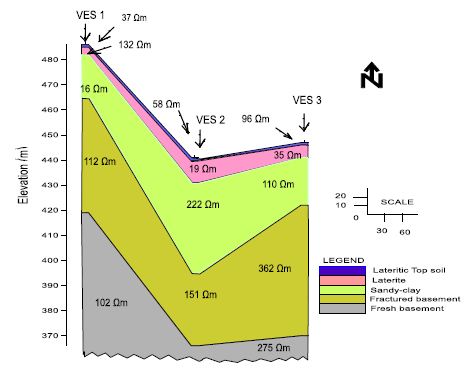
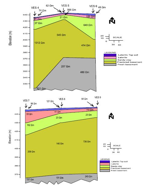
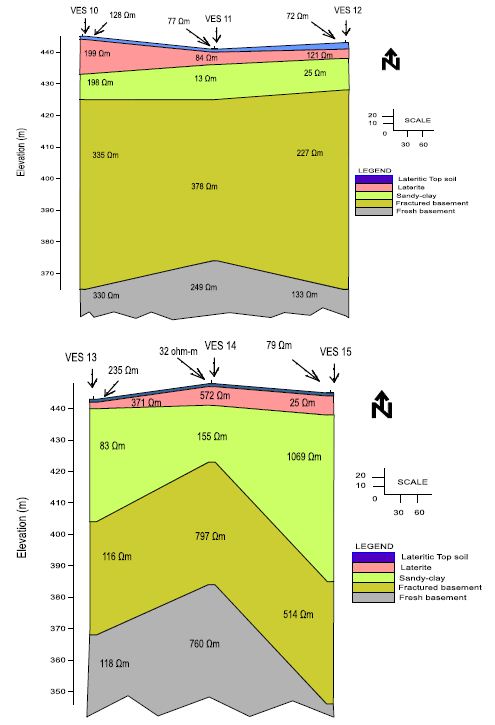
The interpreted VES1-VES15 results from Table 1-15 were equally used to generate 2D geo-electric sections (Figures 4.32-4.37). The geo-electric sections revealed five geo-electric sections of subsurface images based on layers comprising the lateritic topsoil(resistivity varies from 32.7-235.3Ωm and thickness range from 0.5 to 1.9 m); second layer laterite horizon (resistivity varies from 40.6 to 566.1 Ωm and thickness range from 2.2 to 11.3m); third layer sandy – clay ( resistivity varies from 12.5-36.7 Ωm and thickness range from 8.0 to 34.8 m; fourth layer fractured basement (resistivity varies from 111.6-1312.2 Ωm and thickness range from 28.9 to 79.7) m the resistivity value of the fifth layer fresh basement range from 101.1-759.1Ωm (Figures 15-17).

Table 1: VES1 interpreted result.

S/N

Resistivity(Wm) Thickness (m) Depth (m)

Lithological equivalence

1

36.6 0.7

0.7

Lateritic topsoil

2

131.6 2.2

2.9

Laterite

3

16.4 14.1

17.0

Sandy-clay

4

111.6 29.1

46.1

Fractured basement

5

102.0 ………..

…….

Fresh basement

Table 2: VES2 interpreted result.

S/N

Resistivity(Wm) Thickness (m) Depth (m)

Lithological equivalence

1

57.8 1.4

1.4

Lateritic topsoil

2

18.7 8.8

10.2

Sandy-clay

3

222.1 35.6

45.8

Fractured Basement

4

150.8 28.9

74.4

Fractured basement

5

177.9 ………..

……….

Fresh basement

Table 3: VES3 interpreted result.

S/N

Resistivity (Wm) Thickness (m) Depth (m)

Lithological equivalence

1

95.7 1.4

1.4

Lateritic topsoil

2

35.2 4.3

6.7

Sandy-clay

3

110.2 19.6

25.3

Fractured Basement

4

361.8 52.0

77.3

Fractured basement

5

275.4 ………..

……

Fresh basement

Table 4: VES4 interpreted result.

S/N

Resistivity(Wm) Thickness (m) Depth (m)

Lithological equivalence

1

74.1 0.9

0.9

Lateritic topsoil

2

90.8 3.7

4.5

Laterite

3

36.7 9.4

14.0

Sandy-clay

4

1312.2 79.7

93.7

Fractured basement

5

521.2 ………..

……….

Fresh basement

Table 5: VES5 interpreted result.

S/N

Resistivity(Wm) Thickness (m) Depth (m)

Lithological equivalence

1

61.6 0.5

0.5

Lateritic topsoil

2

566.1 1.7

2.2

Laterite

3

20.9 8.9

11.1

Sandy-clay

4

545.3 60.0

71.1

Fractured basement

5

256.9 ………..

…….

Fresh basement

Table 6: VES6 interpreted result.

S/N

Resistivity(Wm) Thickness (m) Depth (m)

Lithological equivalence

1

47.7 1.1

1.1

Lateritic topsoil

2

105.2 4.4

5.5

Laterite

3

649.3 33.2

38.8

Fractured Basement

4

414.0 30.0

68.8

Fractured basement

5

480.5 ………..

…….

Fresh basement

Table 7: VES7 interpreted result.

S/N

Resistivity(Wm) Thickness (m) Depth (m)

Lithological equivalence

1

96.3 1.9

1.9

Lateritic topsoil

2

33.1 13.4

15.4

Sandy-clay

3

161.9 14.3

29.6

Saprolite/weathered basement

4

259.0 49.8

79.5

Fractured basement

5

136.8 ………..

…….

Fresh basement

Table 8: VES8 interpreted result.

S/N

Resistivity (Wm) Thickness (m) Depth (m)

Lithological equivalence

1

121.2 1.2

1.2

Lateritic topsoil

2

40.6 4.0

5.2

Laterite

3

22.7 11.7

16.9

Sandy-clay

4

140.7 60.7

77.6

Fractured basement

5

101.1 ………..

……

Fresh basement

Table 9: VES9 interpreted result.

S/N

Resistivity(Wm) Thickness (m) Depth (m)

Lithological equivalence

1

63.8 1.1

1.1

Lateritic topsoil

2

109.8 2.9

4.1

Laterite

3

23.2 8.0

12.0

Sandy-clay

4

726.4 65.6

77.6

Fractured basement

5

243.2 ………..

……

Fresh basement

Table 10: VES10 interpreted result.

S/N

Resistivity(Wm) Thickness (m) Depth (m)

Lithological equivalence

1

128.2 1.1

1.1

Lateritic topsoil

2

199.3 11.3

12.5

Laterite

3

198.0 8.2

20.6

Sandy-clay

4

334.5 60.1

80.7

Fractured basement

5

330.3 ………..

……

Fresh basement

Table 11: VES11 interpreted result.

S/N

Resistivity (Wm) Thickness (m) Depth (m)

Lithological equivalence

1

76.6 1.0

1.0

Lateritic topsoil

2

83.7 4.3

5.4

Laterite

3

12.5 11.7

17.1

Sandy-clay

4

377.6 51.3

68.4

Fractured basement

5

249.3 ………..

……….

Fresh basement

Table 12: VES12 interpreted result.

S/N

Resistivity (Wm) Thickness (m) Depth (m)

Lithological equivalence

1

71.8 1.2

1.2

Lateritic topsoil

2

120.7 3.2

4.4

Laterite

3

25.3 10.7

15.4

Sandy-clay

4

227.2 63.8

79.2

Fractured basement

5

133.0 ………..

…….

Fresh basement

Table 13: VES13 interpreted result.

S/N

Resistivity(Wm) Thickness (m) Depth (m)

Lithological equivalence

1

235.3 0.8

0.8

Lateritic topsoil

2

370.7 2.4

3.2

Laterite

3

82.8 34.8

37.9

Sandy-clay/weathered basement

4

116.3 36.2

74.1

Fractured basement

5

118.0 ………..

…….

Fresh basement

Table 14: VES14 interpreted result.

S/N

Resistivity(Wm) Thickness (m) Depth (m)

Lithological equivalence

1

32.7 0.7

0.7

Lateritic topsoil

2

571.6 6.4

7.1

Laterite

3

154.5 18.2

25.3

Sandy-clay/Weathered basement

4

796.9 39.2

64.5

Fractured basement

5

759.1 ………..

……….

Fresh basement

Table 15: VES 15 interpreted result.

S/N

Resistivity(Wm) Thickness (m) Depth (m)

Lithological equivalence

1

78.6 0.9

0.9

Lateritic topsoil

2

24.6 6.3

7.2

Sandy-clay

3

1069.0 53.6

60.9

Fractured basement

4

514.4 38.9

100.8

Fractured basement

5

484.8 ……….

…….

Fresh basement

Figure 15: Showing Geoelectric section along traverse 1.

Figure 16: Showing Geoelectric section along traverse 2 and 3.

Figure 17: Showing Geoelectric section along traverse 4 and 5.

Evaluation of Leachate on Groundwater Quality

Leachate is generated by the degradation of waste and the process of water coming into contact with and infiltrate through, waste materials [9]. Generated Leachate varies in its chemical constituents from dumpsite to dumpsite and also depends upon numerous factors such as waste composition, ambient temperatures and rainfall or precipitation characteristics. However, leachate may have increased concentrations of numerous organic and inorganic pollutants [10]. The following metals were equally analyed in this study which include cadmium (Cd), Chromium, iron (Fe), lead, Magnesium Mg) and (Pb). Generally, the concentrations of the metals (except Fe which ranges from 0.01-0.20 mg L⁻¹) were not detected at F01 Kubwa leachate. This is due to the fact that the landfills received mainly municipal solid waste and very low quantities of industrial waste including batteries, radios and other Electronic gadgets.

Analysis of the Effects of Leachate and Contaminant Plume on Groundwater Quality

The importance of determining adverse effects of various elements that reach groundwater through leachate upon human health has gained momentum during the past decade [9]. The different approaches presume that, a sound scientific data base exists to defining the maximum exposure levels for a specific chemical compound. In this study, the pollutant indicators results obtained from groundwater monitoring program of the observation borehole, open well and River channel around F01 Kubwa dumpsite was used to study the effects of leachate formed from dumpsite on groundwater system.

Interpreted Results of Water Samples from Borehole, Open Well and River Channel

The low Electrical Conductivity (EC) measurements values in the water samples near the dumpsites give indications of its effect on groundwater. The EC values at the dump sites were below the NSDWQ suggested levels (1000 μs cm⁻¹). According to Abu Rukah and Al-Kofahi, (2001) [2] water conductivity within 1000 μs cm⁻¹ is suitable for irrigation purpose. It is important to note that the electric conductivity of the groundwater under F01 Kubwa dumpsite is lower of water conductivity of (230-460 μs cm⁻¹) as shown in tables. The followings are major anions tested in this study which are Chloride (Cl⁻), Nitrate (NO3-2) and sulphate (SO4-2).Faust and Aly, (1983) illustrated that Chloride in reasonable concentration is not harmful, but it aids corrosion in concentrations above 250 mg L⁻¹, while about 400 mg L⁻¹ of Chloride causes a salty taste in water Tamer et al (2011) [9]. Chloride concentration was measured and the range is not acceptable according to those permissible by NIGERIA INDUSTRIAL STANDARD (NIS)” 977: 2017 for potable water as shown in table 4.16-4.20 respectively. The geochemical investigation concluded that the water samples are physico-chemically and microbiologically unsatisfactory base on the parameters as shown in the tables 4.16-4.21 which were generated from physico-chemical analysis shown in appendix C, which thus corroborate the geophysical findings (Tables 16-21).

Table 16: Physico-chemical analysis for borehole sample.

Physio-Chemical parameter

Result of Sample

NSDWQ

PH

7.10

6.5 – 8.5

Conductivity, μs cm-1

2.30 x 10²

1 x 10³

Total alkalinity, mg L-1

57

100

P. Alkalinity, mg L-1

Nill

100

M. Alkalinity, mg L-1

57

100

TDS, ppm

115

500

Free Chlorine

Nill

0.1

Freely dissolved CO2, mg L-1

21

50

Total Chloride, mg L-1

18

200

Total Hardness, mg L-1

73

150

Nitrite, mg L-1

0.00

0.02

Nitrate, mg L-1

0.00

10

Lead, mg L-1

0.00

0.01

Cadmium, mg L-1

0.00

0.003

Chromium, mg L-1

0.00

0.01

Arsenic, mg L-1

0.00

0.01

BOD, mg L-1

1

1-3

COD, mg L-1

<2

TOC, mg L-1

0.01

0.5

Iron,mg L-1

0.01

0.3

Sulphate, mg L-1

0

200

Table 17: Microbiological analysis for borehole sample.

TEST

COUNT

LIMIT

Total aerobic bacteria plate count cfu/ml

1.1 x 101

1 x 10²

Mould/Yeast, cfu/ml

2.0 x 100

1 x 10²

Coliform, MPN/100 ml

11

0

E. coli, MPN/100 ml

0

0

Table 18: Physico-chemical analysis for open well.

Physio-Chemical parameter

Result of Sample

NSDWQ

PH

7.40

6.5 – 8.5

Conductivity, μs cm-1

8.20 x 10²

1 x 10³

Total alkalinity, mg L-1

87

100

P. Alkalinity, mg L-1

Nill

100

M. Alkalinity, mg L-1

87

100

TDS, ppm

410

500

Free Chlorine

Nill

0.1

Freely dissolved CO2, mg L-1

35

50

Total Chloride, mg L-1

18

200

Total Hardness, mg L-1

89

150

Nitrite, mg L-1

0.01

0.02

Nitrate, mg L-1

0.09

10

Lead, mg L-1

0.00

0.01

Cadmium, mg L-1

0.00

0.003

Chromium, mg L-1

0.00

0.01

Arsenic, mg L-1

0.00

0.01

BOD, mg L-1

3

1-3

COD, mg L-1

<8

TOC, mg L-1

0.12

0.5

Iron,mg L-1

0.09

0.3

Sulphate, mg L-1

0

200

Table 19: Microbiological analysis for open well.

TEST

COUNT

LIMIT

Total aerobic bacteria plate count cfu/ml

8.1 x 101

1 x 10²

Mould/Yeast, cfu/ml

2.1 x 101

1 x 10²

Coliform, MPN/100 ml

240

0

E. coli, MPN/100 ml

21

0

Table 20: Physico-chemical analysis for river channel.

Physio-Chemical parameter

Result of Sample

NSDWQ

PH

7.20

6.5 – 8.5

Conductivity, μs cm-1

4.60 x 10²

1 x 10³

Total alkalinity, mg L-1

65

100

P. Alkalinity, mg L-1

Nill

100

M. Alkalinity, mg L-1

65

100

TDS, ppm

230

500

Free Chlorine

Nill

0.1

Freely dissolved CO2, mg L-1

21

50

Total Chloride, mg L-1

14

200

Total Hardness, mg L-1

64

150

Nitrite, mg L-1

0.02

0.02

Nitrate, mg L-1

1.00

10

Lead, mg L-1

0.00

0.01

Cadmium, mg L-1

0.00

0.003

Chromium, mg L-1

0.00

0.01

Arsenic, mg L-1

0.00

0.01

BOD, mg L-1

10

1-3

COD, mg L-1

<98

TOC, mg L-1

0.01

0.5

Iron,mg L-1

0.20

0.3

Sulphate, mg L-1

0

200

Table 21: Microbiological analysis for river channel.

TEST

COUNT

LIMIT

Total aerobic bacteria plate count cfu/ml

4.3 x 101

1 x 10²

Mould/Yeast, cfu/ml

1.1 x 101

1 x 10²

Coliform, MPN/100 ml

53

0

E. coli, MPN/100 ml

13

0

Conclusion

Electrical resistivity tomography (ERT) method and Physico­chemical analysis approach were employed to investigate active dumpsite at F01, Kubwa Extension, Abuja F.C.T North-central Nigeria. The 2D resistivity image of subsurface structure delineated the contaminant plume, leachate and thus further characterise the dumpsite based on subsurface resistivity apportionment of vadose zones, contaminant plumes and the hydrogeological conditions underneath the study area. 1D curves were interpreted both qualitatively and quantitatively to detect leachate, vadose zones and possible extent of pollution infiltrating groundwater system. The results of fifteen VES curves further classified the curve types of study area into five layers as shown in the model curves in figures 4.17-4.31 and tables 4.1-4.15 which classified as follows: VES1, VES9, VES10, VES11 and VES12 depict KHA type curves: ρ12345 VES2; ρ12345 depicts HKH type curve, VES3 and VES7: ρ12345 depict HAK type curves, VES4, VES5 and VES8: ρ12345 depict QHK type curves, VES6: ρ12345 depicts AKA type curve, VES13 and VES14: ρ12345 depict KHA type curves while VES15: ρ12345.

Isoresistivity maps, Isopachmaps and Geoelectric section were equally generated from VES1-15 and presented as 2D images to further characterise subsurface geologic parameters. The anomalies observed on wenner array (HP) coincide with the area of low electrical resistivity as revealed by electrical resistivity tomography (ERT) as indicated by 2D pseudosection models; the results further conclude that the study area is structurally controlled.

Physico-chemical analysis revealed possible elemental contaminants within groundwater system. Leachate from dumpsite is a major pollutant contaminating groundwater body. The situation is currently bad and is expected to become worse in the near future Tamer et al (2011) [9]. The analysed results of physico-chemical parameters of the water samples corroborate the georesistivity interpretations, thus the physico-chemical results revealed that analysed sample fall below NSDWQ (2007) [11-43]. as shown in appendix C specification limits for portable water purpose. Therefore, effect of leachate infiltrating the dumpsite’s surrounding or agricultural run-off and fertilizer application might have raised ion concentrations of some parameters on open well, and river channel respectively. There is possible adulteration of shallow groundwater body around the central region of the dumpsite as results of strong manifestation of leachate movement and degree of infiltrating soil around the dumpsite as a result of possible structural geologic deformations the study area might have suffered.

Analyses of samples of F01 Kubwa showed that the total dissolved solid (TDS) were in the ranges of (2.30 x 10¹-8.20 x 10¹) μScm⁻¹ as against NSDWQ values of 1×10³μScm⁻¹; Total alkalinity, TDS, freely dissolved CO2, total chloride, total hardness (TH) and sulphate were 57-87, 115-410, 21-35, 14-18, 64-89mg/Land 0 respectively.

Biochemical oxygen demand (BOD), chemical oxygen demand (COD) and dissolved oxygen (DO), were in the ranges of 1-10, <2-<98 and 0.01-0.12mgL⁻¹ respectively. The water samples had detectable levels of Cu, Cd, Ni, Mn, Pb and Zn, but all the samples have metal contents far below the permissible limits, except for the Cd content which was above in some of the water samples. Also the ranges of pH recorded were 7.0-7.4. Results equally indicate that nitrate and iron in the water samples were in the ranges 0.00-1.00 and 0.01-0.2mgL⁻¹, respectively.

For robust results, multiple tube fermentation technique was deployed, the water samples microbiologically revealed presence of faecal contamination with bacteria pathogens such as Coliform, and Escherichia coli are above permissible limit while mould yeast and total aerobic are below the limit. Obviously, physico-chemical results presented above showed that dumpsite constitutes a serious danger to groundwater systems because of presence of contaminant constituents usually associated with dumpsite region. Geophysical interpreted results corroborate both the physic-chemical and geo-microbiological results.

Recommendations

  • Government should enact laws against indiscriminate waste disposal.
  • Government at all tiers should also improvise for incinerators for proper waste treatment.
  • Leachates should be properly treated before infiltrating into the ground.
  • General public should be educated on impending killer diseases associated with menace of leachate contaminating groundwater system.
  • Scholars and researchers should focus more attention to carrying out further research in this field subsequently.
  • There should be funding for research work.

References

  1. Ganiyu SA, Badmus BS, Olagundoye MA, Aizebeokhai AP, OzeboVC, et al. (2016) Assessment of groundwater contamination around active dumpsite in Ibadan southwestern Nigeria using integrated electrical resistivity and hydrochemical Environ Earth Sci 75.
  2. Abu-Rukah, Y, Al-Kofahi O (2001) The assessment of the effect of landfill leachate on ground-water quality — a case study’, El-Akader Landfill Site — North Arid Environ 49: 615-630.
  3. Ganiyu et al (2015) Delineation of Leachate Plume Migration Using Electrical Resistivity Imaging on Lapite Dumpsite in Ibadan, Southwestern Nigeria.
  4. Chen G, Sun Y, Xu Z (2020) A Novel Approach to Assess the Complexity of Contaminant Plume Transportation in the Aquifer Based on Hausdorff Fractal Water, Air, & Soil Pollution 231.
  5. Chen G, Sun Y, Xu Z, Shan X (2019) Assessment of shallow groundwater contamination resulting from a municipal solid waste landfill-a case study in Lianyungang, Water 11.
  6. Offodile ME (1992) An Approach to Groundwater Study and Development in Nigeria, Mecon Services Jos. Pg: 224-227.
  7. David LM, Ofrey O (1989) An in direct method of estimating groundwater Level on Basement complex regoliths.
  8. Akinde AS, Adepelumi AA, Dikedi PN (2019) Ifewara Mylonite: Identifying Neotectonic Overprint Using Integrated Geophysical J Geol Geophys 8.
  9. Tamer M. Alslaibi, Yunes K. Mogheir and Samir Afifi (2011) Assessment of Groundwater Quality Due to Municipal Solid Waste Landfills Journal of Environ Sci and Tech 4: 419-436.
  10. Jaber A, Nassar A (2007) Assessment of Solid Waste Dumpsites in Gaza Japanese International Cooperation Agency, Gaza.
  11. NSDWQ (2007) Nigerian standard for drinking water quality. Nigeria Industrial Standard, NIS Standard Organization of Nigeria, Lagos. Pg: 30.
  12. Adepelumi AA, Ako BD, Ajayi TR, Afolabi O, Omotosho (2008) Delineation of Saltwater Intrusion into the freshwater Aquifer of lekkiPennisula, Lagos, Environ Geol 56: 927-933.
  13. Adeyemi O, Oloyede OB, Oladiji AT (2007) Physicochemical and microbial characteristics of leachate- contaminated Asian J Biochem 2: 343-348.
  14. Afolayan OS, Ogundele FO, Odewumi (2012) Hydrological implication of solid waste disposal on groundwater quality in urbanized area of Lagos state, Int J Appl Sci Tech 2: 74-82.
  15. Andrea TU, Vagner RE, Giulliana M, Lazaro VZ, Heraldo (2012) Case study: a 3D resistivity and Induced polarization imaging from downstream in waste disposal site in Environ Earth Sci 66: 763-772.
  16. Ariyo SO, Enikanoselu EM (2007) Integrated use of geoelectrical Imaging and geochemical analysis in the environmental impact assessment of Egbe dumpsite in Ijebu-Igbo area, southwestern Cont J Earth Sci 1: 11-17.
  17. Armah FA, Luginaah I, Ason B (2012). Water quality index in the Takwa gold mining area in J TransdisciplEnv Stud 11: 1-15.
  18. Assmuth TW, Strandberg T (1993) Groundwater contamination at Finnish Water Air Soil Pollut 69: 163-175.
  19. Badejo AA, Taiwo AO, Bada BS, Adekunle AA (2013) Groundwater quality assessment around municipal solid waste dumpsite in Abeokuta, southwestern, Pac J Sci Tech 14: 593-603.
  20. Bayowa OG, Olayiwola NS (2015) Electrical resistivity investigation for topsoil thickness, competence and corrosivity evaluation: a case study from Ladoke Akintola University of Technology, Ogbomoso, Nigeria. 2nd international conference on geological and civil engineering. IPCBEE/ACSIT Press, Singapore, 80. Pg: 52–56.
  21. Benson R, Glaccum R, Noel M (1983) Geophysical techniques for sensing buried waste and waste Environ monitor systlab off Res Develop. Us Environ Protect Ag, Las Vegas, NV, Rep. 68-03-3050.
  22. Clark, L (1985): Groundwater abstraction from the basement complex area of Q.J. Engineering Geology London 18: 25-34.
  23. Dare Omolayo and Fatoba JT, (2014) 2D electrical imaging surveys for leachate plume migration at an old dump site in Ibadan South Western Nigeria: a case study.
  24. Ikem et al (2002) Evaluation of groundwater quality characteristics near two waste sites in Ibadan and Lagos, Water Air Solid Pollut 140: 307-333.
  25. Jagloo K (2002) Groundwater risk analysis in the vicinity of a landfill, a case study in M.Sc. Thesis, Royal Institute of Technology, Stockholm.
  26. Kayabali K, Yuksel FA, Yeken T (1998) Integrated use of hydrochemistry and resistivity methods in groundwater contamination caused by a recently closed solid waste Environ Geol 36: 227–234.
  27. Keller GV (1966) In Handbook of Physical Pg: 553-577. Geol Soc Am.
  28. leachate on ground-water quality-a case El-Akader landfill site-North Jordan. J Arid Environ 49: 615-630.
  29. Matias MS, Marques da Silva M, Ferreira P, Ramalho E (1994). Ageophysical and hydrogeological study of aquifers contamination by a J Appl Geophys 32: 155-162.
  30. Mondelli G, Giacheti HL, Howie JA (2010).Interpretation of Resistivity piezocone tests in a contaminated municipal solid waste disposal site. Geotech Test J 33: 1-14.
  31. Nouri J, Mahvi AH, Babaei AA, Jahed GR, Ahmadpour E (2006) Investigation of heavy metals in Pak J Biol Sci 9: 377-384.
  32. NGSA (2004) Modified Geological map of Abuja, from Nigerian Geological Survey Agency, 2004.
  33. Ogbonna DN, Igbenijie M, Isirimah NO (2006) Studies on the inorganic chemicals and microbial contaminants of health importance in groundwater resources in Port J Applied Sci 6: 2257-2262.
  34. Qrenawi I (2006) Environmental and health risk assessment of Al-akaider M.Sc. Thesis, Jordan University of Science and Technology.
  35. Shahidullah, M., M.A. Hakim, M.S. Alam and A.T.M. Shamsuddoha, (2000) Assessment of groundwater quality in a selected area of Bangladesh. Pak J Biol Sci 3: 246-249.
  36. Soltani, , E. Safari, A. Baghvand and M. Ali Abduli, (2007). Selection of bottom liner for land disposal of industrial waste containing lead-case study: Tabriz petrochemical complex. J Applied Sci 7: 4053-4056.
  37. Soupios, et al (2007) Use of engineering geophysics to investigate a site for a building J Geophys Eng 4: 94-103.
  38. Tijani MN, Onibalusi SO, Olatunji AS (2002) Hydrochemical and environmental impact assessment of Orita Aperin waste dumpsite, Ibadan, southwestern, Nigeria. Water Resour 13: 78-84.
  39. Ustra AT, Elis VR, Mondelli G, Zuquette LV, Giacheti HL (2012) Case study: a 3D resistivity and induced polarization imaging from downstream a waste disposal site in Environ Earth Sci 66: 763-772.
  40. Water Resources – Journal of Nigeria Association of 1: 61-164.
  41. WHO (2007) Water for pharmaceutical use in quality assurance of pharmaceuticals. A compendium of Guidelines and Relatedmaterials,2nd edn. World Health Organization, Pg: 170-187.
  42. WHO (2011). Guidelines for Drinking Water 4. Geneva: World Health Organization.
  43. Zohdy AAR, Eaton GP, Mabey DR (1974) Application of Surface Geophysics to Groundwater Investigation. U. S. G. S. Techniques of Water-Resource Investigation, Book 2.

Precede High-pressure, High-Temperature Mineralization in the Variscan Tin Deposit Ehrenfriedersdorf/Germany

DOI: 10.31038/GEMS.2026824

Abstract

This study documents the occurrence of diamond like carbon (DLC) and coesite remnants within pegmatite quard from the Variscan tin deposit at Ehrenfriedersdorf, Germany. Raman spectroscopic and microscopic analyses reveal both isolated DLC aggregates and a centimetre-scale carbon–quard network within the root zone of quard crystals. Quard within this network preserves spectral features indicative of former coesite, while associated carbon phases show broadened Raman bands characteristic of lonsdaleite-like and metastable diamond-like carbon formed under high-pressure, high-temperature conditions. The textures and mineral associations suggest rapid quenching and a primary origin, rather than secondary contamination. Transport by deep-sourced supercritical fluids is proposed as a mechanism for introducing ultrahigh-pressure material into the evolving pegmatite system, providing new evidence for transcrustal transport during Variscan magmatic and ore-forming processes.

Keywords

Diamond like carbon (DLC), Lonsdaleite like carbon, Coesite remnants, High pressure–high temperature (HP-HT) mineralization, Pegmatite quartz, Variscan tin deposit, Raman spectroscopy, Supercritical fluids, Ultrahigh pressure minerals, Trans crustal transport

Introduction

Recent studies have documented the occurrence of ultrahigh-pressure (UHP) mineral phases within crustal granitoids and associated ore systems, challenging conventional models of purely crustal magmatic evolution (see the discussion by Schütze et al., 1983 [1], which first suggested the involvement of components derived from depths of up to ~115 km, corresponding to pressures of ~60 GPa). In particular, the identification of diamond, diamond-like carbon (DLC), and related high-pressure carbon phases in the Variscan tin deposit of Ehrenfriedersdorf (Germany) has provided compelling evidence for a transient interaction between shallow magmatic systems and deep-seated, high-pressure environments [2,3]. These observations imply the operation of previously underappreciated transport mechanisms capable of transferring UHP material across large crustal depth intervals within geologically short timescales. Building on earlier reports of moissanite–diamond–graphite parageneses and isolated DLC inclusions in quartz and accessory minerals from Ehrenfriedersdorf, continued investigation of archival sample material has revealed additional, more systematic evidence for high-pressure carbon phases [4]. Most previously described DLC occurrences consist of small, isolated aggregates randomly distributed within low-quartz, topaz, fluorite, cassiterite, or beryl. In these host minerals, the presence of such phases is highly unexpected under normal crustal pressure–temperature conditions, raising fundamental questions concerning their origin, timing, and mode of incorporation. These observations extend beyond interpretations involving shock-related nanodiamond formation or whisker growth (e.g., moissanite or diamond) via natural chemical vapor deposition (CVD) processes driven by reduced CH4–H2–H2O–CO2 supercritical fluids [4]. During renewed, particularly careful microscopic screening of pegmatite quartz from the well-studied sample Qu8, special attention was paid to crystal root zones, which are commonly neglected due to their high inclusion density and analytical complexity. This approach led to the discovery of a centimetre-scale carbon–quartz assemblage forming an irregular, network-like structure within the root zone of a quartz crystal. Unlike previously reported isolated DLC grains, this network contains abundant carbon phases spatially associated with quartz that preserves Raman spectroscopic signatures indicative of former coesite. The coexistence of coesite remnants with lonsdaleite-like and diamond-like carbon implies formation under high-pressure, high-temperature (HP–HT) conditions, followed by rapid quenching. The present contribution documents the textural relationships, Raman spectroscopic characteristics, and mineralogical context of this carbon–quartz network. By contrasting these features with those of isolated DLC occurrences, this study aims to demonstrate that high-pressure carbon phases in the Ehrenfriedersdorf pegmatite system are not merely sporadic contaminants but may represent a primary feature of an early evolutionary stage of pegmatite formation. Transport by deep-sourced supercritical fluids is discussed as a plausible mechanism for introducing UHP material into the developing pegmatite system, providing further evidence for transcrustal transport processes operating during Variscan magmatic and ore-forming events.

Sample and Methods

Sample Description

The pegmatite quartz sample most frequently investigated in this study, designated Qu8, has been described in detail by Thomas et al. (1998) [5] and Thomas and Webster (2000) [6]. The sample originates from a large, granular-to-disc-shaped pegmatite body measuring approximately 2 × 10 × 10 m, exposed in the granite endocontact at the fifth gallery near the main shaft of the Sauberg mine, Ehrenfriedersdorf, Germany. The material was collected in 1987. The studied quartz crystals are mostly water-clear and exhibit well-developed prismatic morphologies and internal growth zoning. The host pegmatite contains a diverse mineral assemblage, including orthoclase (locally enriched in P2O5 up to 1.3 wt%), albite, beryl, topaz, cassiterite, fluorite, and numerous phosphate minerals such as apatite, amblygonite, berlinite, and isocite. Previous investigations of sample Qu8 primarily employed electron microprobe techniques with deposited carbon coatings. As a consequence, indigenous carbon phases—particularly diamond-like carbon (DLC)—were commonly overlooked. In addition, the root zones of quartz crystals were rarely examined because of their high inclusion density and analytical complexity. These zones, however, are shown here to be critical for recognizing high-pressure carbon–silica assemblages.

Analytical Methods

The analytical approach applied in this study follows established methodologies previously described in detail by Thomas et al. (1998) [5], Rickers et al. (2006) [7], Thomas and Davidson (2012) [8], and Borisova et al. (2012) [9]. Sample Qu8, with its exceptionally high abundance of melt, fluid, and mineral inclusions, has long served as a reference material for the development and application of microanalytical techniques. In the present contribution, emphasis is placed on optical microscopy and Raman spectroscopy, which together serve as essential preliminary tools for identifying diamond-like carbon, lonsdaleite-like carbon, and coesite remnants prior to further analytical work.

Optical Microscopy

Petrographic investigations were carried out using a Zeiss JENALAB POL polarization microscope in both transmitted and reflected light modes. This instrument was used to identify diamond-like crystals hosted in quartz, associated paragenetic minerals, and characteristic textural relationships.

Selected areas were subsequently examined using an Olympus BX43 microscope coupled to a Raman spectrometer. The system is equipped for both transmitted and reflected polarized-light microscopy and includes rotating and X–Y stages, allowing precise positioning and orientation of inclusions and microstructures within the quartz crystals.

Raman Spectroscopy

Raman spectroscopy was performed to identify carbon phases and silica polymorphs. Between 1992 and 2020, several Raman systems were employed (Raman Probe MRL1000; Dilor XY Laser Raman Triple 800 mm; LabRAM UV HR 800), using excitation wavelengths of 633, 514, 488, and 325 nm. The data presented here were acquired using an EnSpectr Raman microscope (RamMics R532).

Measurements covered the spectral range from 0 to 4000 cm⁻¹ and were conducted with a single-mode 532 nm laser operating at a maximum output of 50mW. Analytical settings included a 20 µm entrance aperture, a holographic grating of 1800 g mm⁻¹, and a spectral resolution of approximately 4 cm⁻¹. For most analyses of diamond-like carbon, a long-working-distance Olympus LMPlanFL 100× objective was used. Laser power at the sample surface was continuously adjustable down to 0.02 mW. Because elevated laser energies can induce partial or complete transformation of microdiamonds into carbon, analytical measurements were performed at laser powers ≤ 5 mW. Higher powers (up to 30 mW) were applied only for overview scans and sample mapping.

Raman band positions were calibrated before and after each measurement series using the Si band of a semiconductor-grade single-crystal silicon chip. Based on 20 repeated measurements, run-to-run reproducibility was ± 0.3 cm⁻¹ for silicon (520.4 ± 0.3 cm⁻¹) and ± 0.5 cm⁻¹ for diamond (1332.3 ± 0.5 cm⁻¹) over the spectral range from 50 to 2000 cm⁻¹. The full width at half maximum (FWHM) of the diamond reference peak was 4.8 ± 0.1 cm⁻¹. A water-clear natural diamond crystal from Brazil served as an external reference standard. An additional advantage of the Raman system used is its reliable, straightforward zero-point calibration.

Methodological Focus

The combined use of high-resolution optical microscopy and carefully controlled Raman spectroscopy proved essential for identifying rare, optically camouflaged high-pressure phases within inclusion-rich pegmatite quartz. Particular attention was paid to quartz root zones, which are commonly excluded from routine studies but are shown here to preserve critical evidence for high-pressure–high-temperature processes.

Key Observations

The pegmatite quartz contains many fluid and melt inclusions and, for a pegmatite, typical mineral inclusions. Table 1 presents a selection of daughter mineral phases, mostly found in pegmatite quartz.

Table 1: Some typical daughter mineral phases in fluid and melt inclusions in granite and pegmatite minerals from the Variscan Erzgebirge, mostly determined with Raman spectroscopy (mainly after Thomas and Davidson, 2012) [8]. Inclusion type: F = fluid inclusion, M = melt inclusion. Localities: 1 = Ehrenfriedersdorf (Sauberg, Greifenstein), 2 = Eibenstocker granite, 3 = Podlesi granite, 4 = Zinnwald, Altenberg. (Rb,Cs,K)-Zn-tetrachloride is a new mineral phase in fluid inclusions in the pegmatite quartz from Ehrenfriedersdorf, identified using Raman spectroscopy, SYRFA, and Laser ICP microanalysis; however not proposed to the IMA – it is a variety of the mineral flinteite [K2(ZnCl)4].

Mineral

Formula Locality

Inclusion type

Graphite

C

1

F, M

Diamond

C

1

F

Sulfur

S

4

F

Arsenic

As

1

F

Arsenolite

As2O3

3

F

Sassolite

H3BO3

1,2,3,4

F, M

Metaboric acid I

HBO2

1

F

Cristobalite

SiO2

1

F

Cristobalite-X-I

SiO2

1

F

Coesite

SiO2

1

F

Cassiterite

SnO2

1,2,3,4

F, M

Orthorhombic cassiterite

o-SnO2

1,2,4

F, M

Hematite

Fe2O3

1,2,4

F

Sphalerite

ZnS

1

F

Bromargyrite Br: Cl~1: 1)

Ag(Br,Cl)

1

F

Halite

NaCl

1,2,3,4

F

Sylvite KCl

1,2,3,4

F

Cryolite Na3AlF6

1,2,4

F

Elpasolite K2NaAlF6

1,4

F

Cryolithionite Na3Li3Al2F12

1,2,4

F

Hieratite K2SiF6

4

F

Avogadrite (K,Cs)BF4

1,2,4

F

Rb-Flinteite (K,Rb,Cs)2ZnCl4

1

F

SnF2 (no mineral name) SnF2

4

F

Nahcolite NaHCO3

1,2,3,4

F, M

Zabuyelite Li2CO3

1,2,4

F, M

Dawsonite NaAl(CO3)(OH)2

1

F, M

Ramanite-(Cs) Cs2B3O8 . 4H2O

1,2

F, M

Beryllonite NaBePO4

1

F

Hambergite Be2BO3(OH,F)

1

F, M

OH-Herderite CaBePO4(F,OH)

1

F

Berlinite AlPO4

1

M

Muscovite KAl4Si5Al2O20(OH,F)4

1,2,3,4

F, M

One part of the shown daughter mineral phases also appears as solid mineral inclusions in quartz. Rare examples include berlinite and boric acid (sassolite); the latter was found between cassiterite crystals in sample Sn70 [10]. The great variety of inclusions and minerals in the quartz sample masks the presence of small and rare DLCs. Figures 1 and 2 show two typical fluid inclusions in the pegmatite quartz Qu8, of this size and frequency, ideal for camouflaging unusual inclusions.

Figure 1: Fluid inclusion in pegmatite quartz (Qu8) from the Sauberg mine near Ehrenfriedersdorf/Germany. Daughter minerals are beryllonite [NaBePO4], and sassoline [H3BO3], L – solution, V – vapor.

Figure 2 shows another fluid inclusion type with a relatively large sphalerite daughter crystal beside muscovite in a NaCl-KCl-H3BO3-rich solution. This sphalerite daughter crystal is nearly water-clear, similar to the sphalerite in beryl [3]. Ore-forming sphalerite is present in the deposit; however, mostly jet-black, as the so-called christophite.

Figure 2: Vapor-rich fluid inclusion in pegmatite quartz, Qu8, with a Fe-poor nearby colorless sphalerite crystal (Sp). An enlargement of this crystal is right at the top. L – NaCl-KCl-H3BO3-rich solution, Ms – muscovite, V – CO2-CH4-rich vapor phase.

Such inclusions demonstrate the importance of daughter mineral phases for the estimation of the composition of ore-forming fluids. However, they mask rare and distinct minerals we normally do not encounter. Such a small aggregate is the leaf-like carbon with a whisker-like stalk [4]. Another type is an isolated quartz-carbon aggregate shown in Figure 3a. The quartz of this inclusion is very different to his low-quartz host – fine-grained and surrounded by a thin carbon film. The quartz contains indications of coesite (Figure 3b).

Figure 3a: Isolated foreign aggregate of carbon and quartz (Qtz) – formerly coesite – in transparent pegmatite low-quartz Qu8 from Ehrenfriedersdorf.

Figure 3b shows the remnant of the primary present coesite band at 517.5 cm⁻¹. Other lines are also present; however, in most cases, they are weak: 74.5 (vs), 202 (w), 355 (w), 784.7 ± 2.6 (m) – all in cm⁻¹ [11]. The letters in brackets mean the Raman intensity: vs – very strong, m – medium, w – weak.

Figure 3b: Main band of coesite of the quartz part of the inclusion in Figure 3a.

The carbon part of the inclusion (Figure 3a) contains many micrometer-large lonsdaleite-like carbon crystals (Table 2).

Table 2: High-pressure quenched lonsdaleite/diamond-like carbon in the foreign quartz-carbon aggregate (Figure 3) in pegmatite quartz (see also Table 1 in Thomas, 2026) [4].

Lonsdaleite-like carbon (cm⁻¹)

FWHM (cm⁻¹) G-band (cm⁻¹) FWHM (cm⁻¹)

n

1326.8 ± 1.7

54.6 ± 18.8 1570.4 ± 2.6 71.8 ± 8.0 12
1324.5 ±1.6 21.4 ± 4.2

14

n – number of measured points. Laser power on sample: 4.3 mW.

The lonsdaleite-like carbon in the second row shows practically no G-band (only a background). At least the observation of more or less isolated DLC aggregates “swimming” in the pegmatite quartz is, up to now, the state of knowledge. By careful screening of the root zone of a quartz crystal from the sample collective Qu8, we found a remarkable “network” of carbon (Figure 4) and formerly coesite (now only visible by Raman, with some typical coesite bands).

Figure 4a: Carbon-quartz network with coesite remnants in between in the root zone of the pegmatite quartz Qu8.

Figure 4b: Quartz (Qtz)-coesite (Coe)-carbon lamella in Figure 4a. The black part is carbon-rich.

The quartz shows, as a rule (see Hemley, 1987) [11], an adjacent linear, low-intensity background between 50 and 450 cm⁻¹. Quartz with remnants of coesite, on the other hand, shows, between 50 and 300 cm⁻¹, a strong increase and drop in intensity (see Figure 5a). Somtimes is the intensity of the Raman band at about 75 cm⁻¹ equeal or higher than the quartz main band at 464 cm⁻¹.

Figure 5a: Raman spectrum of coesite-like quartz in the carbon “network” – low frequency range without the very strong quartz band at 464 cm⁻¹. The band at 77.6 cm⁻¹ is often very strong, with an intensity comparable to that of the quartz main band at 464 cm⁻¹.

Figure 5b: Raman spectrum of coesite-like quartz and DLC in the “network” – high frequency range without the very strong quartz band at 464 cm⁻¹, taken at 10 mW. The position of the DLC band at 1338 cm⁻¹ may result from heating caused by the higher laser power (see Zaitsev, 2001) [12] and the black surroundings.

Using a small Raman window from 490 to 580 cm⁻¹ for the measurement of the coesite main line, a value of 516.0 ± 2.3 cm⁻¹ (n= 13) is obtained. Figure 6 shows such Raman spectra (Figures 6-9).

Figure 6: Coesite main band (515 cm⁻¹) in quartz of the “ carbon network”, similar to Figure 3b.

Figure 7: Quartz and coesite remnants inside the carbon “network” containing many small black carbon and DLC crystals.

Figure 8: Carbon (C) in pegmatite quartz (Qu8) with small DLC crystallites.

Figure 9: DLC in pegmatite quartz-carbon network (about 65 µm under the sample surface).

Table 3 summarizes the Raman measurements on DLC in the “network” part of the root zone of a quartz crystal; the data around 1323 cm-1 corresponds to lonsdaleite-like diamond. The FWHM values are the opposite of those of well-crystallized diamond, generally very large: >25 cm⁻¹ vs 4 cm⁻¹.

Table 3: High-pressure quenched DLC in the quartz-carbon “network” (Figure 4) in the root zone of the pegmatite quartz (see also Table 1 in Thomas, 2026). Laser power: 4.3 mW.

DLC (cm⁻¹)

FWHM (cm⁻¹) G-band (cm⁻¹) FWHM (cm⁻¹) n
1335.8 ± 2.9 67.2 ± 15.6 1577.5 ± 5.7 71.4 ± 10.1

12

1332.0 ± 2.8

81.8 ± 3.9 1588.3 ± 8.9 77.6 ± 1.0 9
1323.8 ± 2.1 25.6 ± 8.8 1572.3 ± 4.7 67.4 ± 8.8

27

1323.5 ± 0.2

76.7 ± 1.8 1486.9 ± 1.4* 40.8 ± 3.4

9

*According to Zaitzev (2001) [12] that is a quenchable metastable carbon phase consisting of an amorphous mixture of four-fold coordinated diamond and three-fold coordinated graphitic carbon. n – number of measured crystals.

Interpretation

Up to now, all found DLC crystals are generally rare, statistical distributed small aggregates. The found carbon-quartz “network” at the root zone of a quartz crystal is irregularly formed and measures about 2 x 0.5 cm. Transport via supercritical fluid (SCF) is conceivable at an early stage in the formation of the pegmatite chamber. Is maybe the embryonic stage of this chamber. Due to the high velocity of the SCF, larger rock fragments from greater depths (at pressures and temperatures of 4 to 6 GPa and 1000 to 1500°C) can also be transported. The SCF can, of course, come from greater depths.

Discussion

The observations presented in this contribution extend earlier reports of ultrahigh-pressure (UHP) mineral phases associated with the Variscan tin mineralization at Ehrenfriedersdorf and provide new textural evidence for their primary incorporation into pegmatite quartz. In contrast to previously described isolated diamond-like carbon (DLC) aggregates, the discovery of a centimetre-scale carbon–quartz “network” in the root zone of a quartz crystal indicates that high-pressure carbon phases were not merely sporadic contaminants but may represent a more systematic feature of an early evolutionary stage of the pegmatite system. Raman spectroscopic data demonstrate that quartz within this network preserves remnants of coesite, as evidenced by characteristic low-frequency bands and a main band near 515–517 cm⁻¹. These spectral features clearly distinguish the network quartz from the surrounding low-quartz host and indicate a former stability field well outside normal crustal conditions. The coexistence of coesite remnants with lonsdaleite-like and diamond-like carbon, characterized by broadened Raman bands and large FWHM values, is consistent with rapid quenching from high-pressure, high-temperature conditions. Such spectral characteristics suggest structurally disordered or metastable carbon phases rather than well-crystallized diamond. Textural relationships further support a primary origin of the carbon–quartz assemblage. The fine-grained quartz enclosed by carbon films and lamellae contrasts sharply with the optically homogeneous pegmatite quartz host, implying mechanical or chemical isolation prior to final crystallization. The network-like geometry, rather than discrete inclusions, argues against late-stage infiltration or secondary carbon precipitation and instead points to syn- or pre-pegmatitic incorporation. Transport by a supercritical fluid (SCF) offers a plausible mechanism for introducing such exotic assemblages into the upper crust. An SCF capable of operating at pressures of several GPa and temperatures exceeding 1000 °C could entrain fragments of deeper material, including coesite-bearing silica and high-pressure carbon phases, and deliver them rapidly into a developing pegmatite chamber. The observed preservation of coesite remnants and metastable carbon phases is consistent with rapid ascent and cooling, limiting complete back-transformation to low-pressure polymorphs. Overall, the data support a model in which the Ehrenfriedersdorf pegmatite system records an early, transient interaction with deep-seated, high-pressure materials. The carbon–quartz network documented here represents a rare snapshot of this process and strengthens the case for transcrustal transport mechanisms operating during Variscan magmatic and ore-forming events. Further systematic screening of quartz root zones may reveal that such features are more common than previously recognized, but commonly overlooked due to their optical camouflage within inclusion-rich pegmatite quartz.

Acknowledgment

The author thanks colleagues and collaborators for longstanding discussions on high-pressure mineral phases and the application of Raman spectroscopy to fluid and mineral inclusions. Access to archival sample material from the Ehrenfriedersdorf pegmatite system, collected during earlier underground work at the Sauberg mine, is gratefully acknowledged. Constructive comments from reviewers and editors, which helped to improve the clarity and focus of this contribution, are also appreciated.

References

  1. Schütze H, Stiehl G, Wetzel K, Beuge P, Haberlandt R, et (1983) Isotopen-und elementgeochemische sowie radiogeochronologische Untersuchungen an der Zinnlagerstätte Ehrenfriedersdorf. Akademie der Wissenschaften der DDR, Zentralinstitut für Isotopen- und Strahlenforschung Leipzig, ZfI-Mitteilungen, Nr. 76: 232-271.
  2. Thomas R, Davidson P, Rericha A, Recknagel U (2023a) Ultrahigh-pressure mineral inclusions in a crustal granite: Evidence for a novel Transcrustal transport mechanism. Geoscience 13: 1-13.
  3. Thomas R, Recknagel U, Rericha (2023b) A moissanite-diamond-graphite paragenesis in a small beryl-quartz vein related to the Variscan tin-mineralization of the Ehrenfriedersdorf deposit, Germany. Geosciences 13: 1-13.
  4. Thomas R (2026) Finding of lonsdaleite-like carbon in pegmatite quartz from the Sauberg mine near Ehrenfriedersdorf/Germany. Geology, Earth and Marine Sciences 8: 1-5.
  5. Thomas R, Webster JD, Rhede D (1998) Strong phosphorus enrichment in a pegmatite-forming Acta Universitatis Carolinae Geologica 42: 150-164.
  6. Thomas R, Webster JD (2000) Strong tin enrichment in a pegmatite-forming Mineral Deposita 35: 570-582.
  7. Rickers K, Thomas R, Heinrich W (2006) The behavior of trace elements during the chemical evolution of the H2O-, B-, and F-rich granite-pegmatite-hydtothermal system at Ehrenfriedersdorf, Germany: a SXRF study of melt and fluid inclusions. Mineralium Deposita 41: 229-245.
  8. Thomas R, Davidson P (2012) The application of Raman spectroscopy in the study of fluid and melt Z. dt. Ges Geowiss 163: 113-126.
  9. Borisova AY, Thomas R, Salvi S, Candaudap F, Lanzanova A, Chmeleff J (2012) Tin and associated metal and metalloid geochemistry by femtosecond LA-ICP-QMS microanalysis of pegmatite-leucogranite melt and fluid inclusions: new evidence for melt-melt-fluid immiscibility. Moneralogical Magazine 76: 91-113.
  10. Thomas R (2024) The CaCl2 -to-rutile phase transition in SnO2 from high to low pressure in nature. Geol Earth Mar Sci 6: 1-4.
  11. Hemley RJ (1987) Pressure dependence of Raman spectra of SiO2 polymorphs: a-quartz, coesite, and In: High-pressure Research in Mineral Physics, eds. By MH Manghnani and Y Syono. Pg: 347-359.
  12. Zaitsev AM (2001) Optical properties of A data handbook. Springer. Pg: 502.
  13. Thomas R (2002) Determination of the H3BO3 concentration in fluid and melt inclusions in granite pegmatites by laser Raman microprobe American Mineralogist 87: 56-68.
  14. Thomas R, Baumann L (1980) Ergebnisse von thermometrischen und kryometrischen Untersuchungen an Kassiteriten des Zeitschrift für geologische Wissenschaften. 8(10): 1281-1299.
  15. Thomas R (2000) Determination of water contents of granite melt inclusions by confocal laser Raman microprobe spectroscopy. American Mineralogist 85: 868-872.

From the Granite-Pegmatite Solvus Curves to Extreme Element Enrichment Indicated by Gaussian, Lorentzian, and Voigt Distributions

DOI: 10.31038/GEMS.2026821

Abstract

The Variscan Ehrenfriedersdorf tin deposit (Germany) is a classic example of extreme enrichment of Sn and associated elements in granite–pegmatite systems. This study investigates the statistical distributions of major and trace elements derived from melt and fluid inclusion data, with particular emphasis on Gaussian, Lorendian, Voigt, and idealized Dirac-like distributions. These distributions provide quantitative insight into the physicochemical processes governing ore formation. A key result is the identification of weakly asymmetric pseudobinary solvus curves in the silicate melt–H2O (±B2O3) system, defined by water concentration versus temperature. Both granite- and pegmatite-related solvus curves exhibit closely similar critical points (≈25–30 % H₂O), despite differences in bulk composition. The region around these critical points coincides with pronounced enrichment of economically important elements, whose concentrations follow characteristic Gaussian, Lorendian, or mixed (Voigt) distributions when plotted against water content of the melt inclusion glass. Gaussian distributions reflect relatively well-mixed systems governed by multiple small-scale processes, whereas Lorendian distributions indicate rare but powerful enrichment events driven by lifetime-limited, interaction-based processes. The frequent occurrence of Lorendian behavior for elements such as Sn, Li, Be, Ta, and W points to episodic supercritical fluid or melt pulses. Extremely high, δ-like “runaway” concentrations are interpreted as the result of trapping stoichiometric daughter minerals during the transition from supercritical to undercritical conditions. These observations demonstrate that solvus geometry, element distribution functions, and critical phenomena are fundamentally linked. The data provide compelling evidence that supercritical, water-rich melts and fluids—likely derived from mantle–crust interaction—play a decisive role in redistributing elements and forming ore in the Ehrenfriedersdorf deposit and comparable Variscan systems.

Introduction

In recently published papers [1,2], in part results from melt and fluid inclusions were used to explain the formation of Sn, Ta, Nb deposits by extraction at the magmatic stages in porphyry deposits, the formation of pegmatites, and the growth of gems from extremely hard fluids (Li, Be, and B). This author and coauthors use a very different model to explain the formation of mineral deposits in general. According to the first author’s research in the last 30 years, especially after the development of a method for the determination of water in glasses and melt inclusions [3], an idea about the extreme element enrichment near the solvus crest of the pseudo binary silicate melt–water system in the form of Gaussian, Lorentzian, and Voigt element distributions was born. The Gaussian, Lorentzian, and Voigt distributions are key to understanding the behavior of silicate melts during ore-forming processes in the famous tin deposit of Ehrenfriedersdorf, Germany. Basic results are in Thomas et al. 2019 [4] and 2022 [5]. Figure 1 shows the generalized pseudobinary solvus curves for the Ehrenfriedersdorf granites and pegmatites. The solvus of the granites (blue curve) of the Ehrenfriedersdorf area is remarkably small due to high concentrations of fluorine, phosphorus, and alkalies (Li, Na, K, Rb, Cs). This curve shows some similarity to the phase diagram of the haplogranite-H2O system according to Bureau and Keppler (1999) [6], due to the strong deviation of the actual composition from the haplogranite system, resulting in significantly lower pressure (see also Sowerby and Keppler, 2002) [7]. The water content at the critical points (CP) of both curves (850°C, 25 % H2O and 712°C, 27.7 % (H2O+B2O3) is nearly identical.

Figure 1: Pseudobinary solvus curves of evolved granites (blue) and pegmatites (red) for the Ehrenfriedersdorf tin deposit. CP – critical point. The critical point for the F-rich granites is 850°C and 25% H2O, and for the pegmatites, the CP is 712°C and 27.7% (H2O + B2O3).

The solvus curves of the granites and pegmatites determine the main processes for the enrichment of ore-forming and rare elements. As we will show below, the region around the critical point is where the crucial processes occur. To discuss the processes, we will first briefly define the relevant element distribution types in our case, including the Diracian distribution used by Vigneresse (2026) [2].

Gaussian, Lorentzian, Voigt, and Diracian distributions (see Linford, 2014 [8], and References in it)

Gaussian Distribution – “Normal Distribution” Natural Variability

The Geochemical meaning of a Gaussian (normal) distribution indicates that many small, random, additive processes produce element variability. That is the most common pattern in geochemistry. This kind of distribution results from measurement noise and multiple small-scale processes adding up (Central Limit Theorem). A Gaussian pattern suggests the system was relatively well-mixed and governed by many equal, independent factors – not dominated by rare or extreme processes. The standard Gaussian frequency distribution (distribution of an element) will not be considered here. We consider, in the following, the frequency distribution relative to another reference of the same sample (melt inclusion), for example, water (H2O) or (H2O+B2O3), which holds for the Lorentzian distribution (see further below). All points forming the corresponding curves are Gaussian distributed, which results from instrumental noise, sample heterogeneity, and counting statistics. In our case, the peak center corresponds to the sulvus crest, the water concentration at the critical point of the solvus curve. The area under the curve is proportional to the element concentration – giving us, in our case, information on the deviation from the corresponding Clarke concentration (see Rösler and Lange, 1975) [9].

Lorentzian Distribution — Presence of Outliers or Resonant Processes

A Lorentzian distribution has fatter tails than a Gaussian. That indicates occasional large excursions (outliers) and processes dominated by a few strong influences rather than many small ones. Typical causes are supercritical pulses that strongly enrich a trace element, forming a sharp element anomaly. For Lorentzian processes, “lifetime” effects (analogous to Lorentzian broadening in spectroscopy) are characteristic. A Lorentzian pattern implies that rare but powerful events influenced the chemical system. The “heavy tails” correspond to unusually high concentrations due to supercritical pulses. A Lorentzian distribution of an element indicates lifetime-limited or interaction-driven processes. It is important to note that, in our case, the Lorentzian curve is not a classic peak but a curve over another element concentration. Typical causes of the Lorentzian distribution are pressure- or collision-broadening and strong matrix or chemical interactions. The “peak” height becomes unreliable, but the area under the curve remains proportional to concentration.

Voigt Distribution

A Voigt profile is a convolution of Gaussian and Lorentzian effects, meaning both random noise and physical broadening mechanisms are important. The Voigt distribution, as a realistic concentration model, provides information about the instrumental noise (Gaussian component) and the physical or chemical broadening (Lorentzian component).

Dirac (δ) Distribution — Highly Uniform or Idealized Single-Value Concentrations

A Dirac delta distribution represents all values concentrated at one exact number – a perfect spike or an idealized, infinitely sharp line. That is, in our case, not attainable. In reality, this almost never occurs, but it is used conceptually to represent single transition energies or states in analog physical systems (e.g., δ-like spectral lines in the absence of broadening). A Dirac-like pattern suggests a geochemical reservoir with practically no heterogeneity, a mineral phase with stoichiometric composition, and an element controlled by a single dominant process (supercritical process) with negligible variability. An example is the appearance of ideal stoichiometric, however unusual, minerals in melt and fluid inclusions. In natural datasets, a δ distribution rarely occurs; it is more of a reference ideal. We call this distribution here because Vigeresse (2026) [2] used it for his very schematic interpretation.

Typical Examples of Distributions Obtained from Melt Inclusions in Quartz of Pegmatite and Pegmatite-Like Rocks from the Ehrenfriedersdorf Sn Deposit

It is important here that we correlate the distribution of trace and major elements with the water content of the melt inclusions, determined by micro-Raman spectroscopy [3]. The trace and major elements were determined using different analytical methods (microprobe, SIMS, LA-ICP-QMS, synchrotron radiation XRF, and Raman spectroscopy) – see Borisova et al. (2012) [10] and Thomas et al. (2019, 2022) [4,5]. First, we show the Rb vs. H2O distributions for a pegmatite from the Sauberg mine near Ehrenfriedersdorf, Central Erzgebirge, Germany. We see a distribution of Rb vs. H2O in melt and fluid inclusions, forming a solvus-like curve in the silicate-water range (up to about 50% H2O), and a distribution of Rb in the fluid phase at high water concentration (filled triangles).

A similar relationship holds for the B2O3-H2O and F-H2O systems of the Ehrenfriedersdorf pegmatite [11]; Thomas and Rericha, 2023). That means at least that the solvus curve obtained for the pegmatites related to the Variscan granites of the Ehrenfriedersdorf region is determined primarily by H2O, B2O3, Rb as well as by F. We will see that at least all elements forming Gaussian and Lorentzian curves over the water concentration take part in the formation of the characteristic solvus curves, because this refrains from the region around the critical point, the fringes fit well with the solvus curves. A similar plot result for antimony (Sb) vs. water. The Sb data for this plot were obtained using the Synchrotron radiation XRF technique with Monte Carlo-based quantification [12,13]. This plot clearly shows that trace elements like Sb also follow the solvus crest of the pegmatite-H2O system. In the fluid part of the system, even 700-900 ppm Sb is possible [10], obviously related to chlorine complexes.

We will later see that, around the critical point of the solvus, Gaussian and Lorentzian element distribution curves are sitting. That means the solvus, the Gaussian, and the Lorentzian curves are not independent. Figures 2 and 3 clearly show that, generally, on the right side of the solvus curves, a fluid phase coexists with the corresponding curve [14]. That means the coexistence of two melt inclusion types (A- and B-type MI) with fluid phases containing different daughter phases, often Al- and Si-bearing (topaz, muscovite). Now we will show a Gaussian distribution curve. As an example of such a Gaussian element distribution, see Figure 4: the distribution of Be versus water content in the measured melt inclusions.

Figure 2: Plot of the Rb concentration in melt and fluid inclusions versus the water content. Black points represent the so-called A-type melt inclusions, and half-filled points represent the water-rich B-type melt inclusions, and the black triangles stand for fluid inclusions. The isotherms are drawn in for both melt inclusion types.

Figure 3: Distribution of antimony (Sb) in melt (red) and fluid (grey line) inclusions.

Figure 4: Gaussian distribution of Be versus the water content of melt inclusions in pegmatite quartz from Ehrenfriedersdorf (beryl-quartz vein in the Sauberg mine). The center is at 26.4% H2O, the half-maximum distance is at 9.5% water, the maximum of the Gaussian curve is at 12075 ppm Be, and the offset corresponds to 214 ppm Be. The offset represents the regional enrichment of Be for the given mineralization.

Gaussian curves are rare in Ehrenfriedersdorf Sn deposits. Most of the studied elements follow a Lorentzian distribution, as shown in Figure 5. The relationship between the solvus curve of pegmatite-like mineralizations is presented by Thomas and Rericha (2024) [15]. In this paper, the authors also establish a clear relationship between the solvus curve and the Lorentzian distribution of Sn, as well as a generalization of the Lorentzian distribution using normalized element concentrations CA/CA-crit versus the normalized water concentration of the solvus H2O/H2O-crit. This correlation enables the estimation of the Lorentzian distribution of any element from only a couple of measurements (Table 1).

Figure 5: The figure shows the Lorentzian distribution of Sn vs. H2O, and in Table 1 are the resulting fitting data summarized. The center (25.7 % H2O) is the position of the peak’s center, which corresponds to the critical point of the solvus curve and the maximum (height) of the Sn concentration (here, 16400 ppm Sn). Width is the half-width at half-maximum (HWHM). The offset refers to the displacement of the Lorentzian curve from its original position along the x-axis (H2O concentration) corresponding to 644 ppm.

Table 1: Lorentzian fit of Sn, determined in silicate melt inclusions from the pegmatite system of the Sauberg mine near Ehrenfriedersdorf (46 measuring points). Each point is the mean of 5 to 10 single measurements. The values in the second data row are calculated (see Thomas 2025a).

Area Center Width Offset Height R2
A xc w yo Io
Measured 57799 ppm2 25.7% H2O 2.3% H2O 644 ppm Sn 16295 ppm Sn 0.9843
Calculated 58871 ppm2 25.7% H2O 2.3% H2O (603 ppm Sn) 16295 ppm Sn 1.0000

Thomas (2025a) [16] also discusses the Lorentzian distribution in more detail. In this contribution, the Lorentzian data for the 10 elements Be, B, P, Cl, Zn, As, Cs, Sn, Ta, and W are tabulated. More elements of other mineralizations are in Thomas et al. 2019, 2022. Here, we will include the results of another element, which is of great economic significance at the time: Li.

Table 2 summarizes the Lorentzian data for Li shown in Figure 6. According to Rösler and Lange (1975) [9], the mean of granitic rocks is 40 ppm.

Table 2: Lorentzian fit of Li, determined in silicate melt inclusions from the pegmatite system of the Sauberg mine near Ehrenfriedersdorf.

Area Center Width Offset Height R2
A xc w yo Io
273330 ppm2 25.1% H2O 6.53% H2O 1363 ppm Li 26660 ppm Li 0.9821

Figure 6: Lorentzian distribution of Li versus the water content in melt inclusions in pegmatite quartz from the Sauberg mine, Ehrenfriedersdorf/Germany.

In contrast to Sn, the width of Li is almost three times as large, and the value at the center (water content at the critical point) is 666.5 times that of the normal granite. The large width of the Li curve is a hint for the participation of Li in the formation of the solvus curve. Sometimes we also observe overlapping Lorentzian curves for a single element, as shown here for Be (Figure 7 and Table 3) [5].

Figure 7: Distribution of Be in some melt inclusions in pegmatite quartz from Ehrenfriedersdorf (sample Qu8). The sum curve (grey) results from the overlapping of two Lorentzian components caused by different Be species in the melt inclusions. Peak 1 is representative of beryllonite [NaBePO4], and peak 2 (blue) is for hambergite [Be2BO3(OH,F)] as a daughter mineral.

Table 3: Lorentzian fit parameters for both Be curves.

Center Width Height
Peak 1 25.5% H2O 7.5% H2O 12840 ppm Be
Peak 2 31.0% H2O 4.8% H2O 4280 ppm Be

In a single-melt inclusion, we found up to 71500 ppm Be as a large daughter crystal of beryllonite. That would, after the classic idea, be a (however real!) runaway value. This observation is typical for Lorentzian element distribution curves: peak height becomes unreliable. We see that the positions of the second Lorentzian Be peaks shift to higher H2O values with increasing bulk volatile concentration. This observation confirms the term “critical range.”

The fourth distribution, the Diracian distribution, is characterized by a signal that represents an idealized, infinitely sharp line. We often found extremely high concentrations at the centers of the Lorentzian distributions (mostly at the solvus crest). Such behavior is very typical for the Ehrenfriedersdorf case and does not approach the pure Lorentzian distribution. The distribution of tin (Figure 5) already suggests such a distribution. Also, the high Be value of 71500 ppm Be in the case of the first peak form, at least a so-called runaway value, which cannot be ignored. In the past, we often encountered so-called runaway data during our analytical work, which irritated us and others because it was mostly uncorrelated with other elements. See the extended discussion of our data by London and Evensen (2002) [17]. The first such example we found during the development of the first SYXRF-microprobe spectrometer at DESY/Hamburg in 1995, Thomas et al. (1995) [18], on a melt inclusion in quartz from the Sauberg mine near Ehrenfridersdorf. In the first studied melt inclusion, we found high Rb and Cs concentrations and extremely high Sn values, which could be traced to a cassiterite daughter mineral phase, as indicated by microscopic studies.

The so-called “Runaway-Points” can be explained very simply: At the transition of a supercritical fluid to the undercritical state, insoluble cassiterite microcrystalls form, are suspended in the melt, and are trapped by the change. A similar process can also be observed in the case of Be distribution, where different large beryllonite daughter crystals are trapped quite by chance. A completely different case is the sporadic occurrence of diamond crystals in the typical greisen rock of the Ehrenfriedersdorf tin deposits. The appearance of spherical diamonds (Raman peak at 1326 ± 9.8 cm-1, n = 13 different crystals) in such a typical crustal rock is clear proof of interaction with supercritical fluids coming from the Earth’s mantle. Another or additional explanation for the presence of diamonds in crustal rocks is the formation of extreme shock-like pressure at the transition of a supercritical fluid or melt into the undercritical state (see the whisker-like diamond needles in quartz crystals from Zinnwald, Thomas (2025b) [19]. Another surprising discovery is the presence of graphite and diamond aggregates or crystals (see Figure 8) in quartz, characterized by numerous melt and fluid inclusions, as the second explanation underline (Table 4).

Figure 8: Raman spectrum of diamond (D)-containing graphite (Gr) in pegmatite quartz (Qu8) from the Sauberg mine near Ehrenfriedersdorf. The leaf-like graphite (right at the top) is 80 µm deep from the sample surface. The FWHM is 77 cm-1 (FWHM is Full Width at Half Maximum).

Table 4: Results of the Raman spectroscopic determination of diamond in pegmatite quartz (Qu8) from the Saubach mine near Ehrenfriedersdorf, Central-Erzgebirge/ Germany.

Sample Mean 1s FWHM 1s n
leaf-like graphite 1324.4 2.9 75.9 5.0 10

1s: Standard Deviation, FWHM: Full Width at Half Maximum, n: Measured Points (at different points of the leaf; see Figure 8).

Discussion

In this contribution, we show, using the well-studied example from Ehrenfriedersdorf/Germany, that melt inclusions provide important information about element distribution. During the determination of water by Raman spectroscopy [3], a natural example of a solvus curve (water versus temperature) is identified for the first time. Further studies on the same example (Ehrenfriedersdorf) brought more information about the behavior of a couple of elements. Important ore-deposit-forming elements exhibit characteristic distributions that are Gaussian, Lorentzian, or mixed, such as the Voigt distribution. Very important points are the critical ones. It is remarkable that this point ± coincidence with all solvus, Gaussian, Lorentzian, and Voigt curves. Why is that so?. It is well known that, above the critical point, the matter is in the supercritical state. The presence of a Gaussian and/ or Lorentzian distribution indicates that we have not only a sharp peak but also a relatively large temperature range, from about 850 to 600°C (see Figure 1). Unusual physicochemical properties characterize this range: extremely low viscosity and extremely high diffusivity (see Thomas et al., 2019 [4], 2022 [5], 2023 [20]). These conditions enable the extreme enrichment of normally rare elements. By the transition of the supercritical fluid or extremely water-rich melt from the mantle region into under-critical conditions at the crustal level, a first crystallization of ore-forming minerals occurs – the trapping of such minerals (e.g., cassiterite, beryllonite, hambergite, and others with stochiometric composition) follows the Lorentzian distribution. A single dominant process with negligible variability controls such minerals. Similar processes also occur during a high-temperature hydrothermal stage (see Borisova et al. 2012) [10]: the trapping of Zn-rich minerals (88, 121, and 46,049 ppm) in two fluid inclusions, only some micrometers apart, in pegmatite quartz. The trapped mineral phase, according to Raman (room temperature), is a daughter crystal of K2[ZnCl4] (flinteite) in both fluid inclusions in pegmatite quartz (Qu8) from the Ehrenfriedersdorf tin deposit, with high Rb, Cs, and Br concentrations in the flinteite formula.

The finding of co-trapped high-pressure minerals, including diamond, moissanite, coesite, lonsdaleite, kumdykolite, reidite, as well as high-pressure orthorhombic cassiterite, in nearly all parts of the Ehrenfriedersdorf deposit (diamonds and BN also in the greisen part), underscores the significance of the supercritical state and the decisive role of supercritical fluids or extreme water-rich melts (see e.g. Thomas and Trinkler, 2024) [21]. First hints of such a scenario were discussed by Schütze et al. 1983 [22]. These authors, based on their studies, conclude that the inducing processes are subduction- or subfluence-related and involve older ocean crust. Our studies provide evidence that supercritical, water-rich melts and/or fluids have a significant influence on the entire Variscan ore mineralization in the Central Erzgebirge and elsewhere. The often-cited evidence that, for example, a large part of the tin is transported as orthorhombic cassiterite underscores the active interaction between mantle and crust. By the existence of orthorhombic cassiterite crystals in the supercritical fluid, it is plausible that this fluid is also saturated in Sn. That is compatible with the new discussion that a lot of water is concentrated in the deep Earth (see, for example, Mohn et al., 2025) [23-25] and may move episodically from the mantle deeps into the crust (see also Thomas et al., 2025a) [15].

Acknowledgments

We thank Jean-Louis Vigneresse for initiating this contribution, which will address some differences in his viewing and our understanding of the meaning of melt inclusions for ore-forming processes.

References

  1. Vigneresse J-L, Poddar A, Chattaraj PK (2025) Felsic trans-porphyry deposits and associated ore (Sn, Ta, Nb, pegmatites) viewed from physics, chemistry (cDFT) and geologic Lithos 514-515: 1-15.
  2. Vigneresse J-L (2026). Specificity of ore generation (tin, pegmatites, and gems) in trans-porphyry deposits. Minerals 16: 1-32.
  3. Thomas R (2000) Determination of water contents of granitic melt inclusions by confocal laser Raman microprobe American Mineralogist 85: 868-887.
  4. Thomas R, Davidson P, Appel K (2019) The enhanced element enrichment in the supercritical states of granite-pegmatite systems. Acta Geochim 38: 335-349.
  5. Thomas R, Davidson P, Rericha A, Voznyak DK (2022) Water-rich melt inclusions as “frozen” samples of the supercritical state in granites and pegmatites reveal extreme element enrichment resulting under non-equilibrium Mineralogical Journal (Ukraine) 44: 3-15.
  6. Bureau H, Keppler H (1999) Complete miscibility between silicate melts and hydrous fluids in the upper mantle: experimental evidence and geochemical Earth and Planetary Science Letters 165: 187-196.
  7. Sowerby JR, Keppler H (2002) The effect of fluorine, boron and excess sodium on the critical curve in the albite-H2O Contrib Mineral Retrol 143: 32-37.
  8. Linford MR (2014) The Gaussian-Lorentzian sum, product, and convolution (Voigt) functions used in peak fitting XPS narrow scans, and an introduction to the impulse Vacuum Technology & Coating 8(2): 1–6.
  9. Rösler HJ, Lange H (1975) Geochemische VEB Deutscher Verlag für Grundstoffindustrie. Leipzig 675 Pg.
  10. Borisova AY, Thomas R, Salvi S, Candaudap F, Lanzanova A, Chmeleff J (2012) Tin and associated metal and metalloid geochemistry by femtosecond LA-ICP-QMS microanalysis of pegmatite-leucogranite melt and fluid inclusions: new evidence for melt-melt-fluid Mineralogical Magazine 76: 91-113.
  11. Thomas R, Förster HJ, Heinrich W (2003) The behaviour of boron in a peraluminous granite-pegmatite system and associated hydrothermal solutions: a melt and fluid-inclusion study. Contrib Mineral Petrol 144: 457-472.
  12. Rickers K, Thomas R, Heinrich W (2004) Trace-element analysis of individual synthetic and natural fluid inclusions with synchrotron radiation XRF using Monte Carlo simulation for Eur J Mineral 16: 23-35.
  13. Rickers K, Thomas R, Heinrich W (2006) The behavior of trace elements during the chemical evolution of the H2O-, B-, and F-rich granite-pegmatite-hydrothermal system at Ehrenfriedersdorf, Germany: a SXRF study of melt and fluid Miner Deposita. 41: 229-245.
  14. Vogel R (1959) Die heterogenen Leipzig. Pg: 728.
  15. Thomas R, Rericha A (2024) Meaning of supercritical fluids in pegmatite formation and critical-element Geol Earth Mar Sci 6: 1-5.
  16. Thomas R (2025a) Interpretation of the Lorentzian distribution of tin in the Variscan Ehrenfriedersdorf deposit/Germany. Geol Earth Mar Sci 7: 1-5.
  17. London D, Evensen JM (2002) Beryllium in silicic magmas and the origin of beryl-bearing Reviews in Mineralogy & Geochemistry 50: 445-486.
  18. Thomas R, Klemm W, Haller M, Knöchel A, Radtke M (1995) First results on melt inclusions in geological samples using SYXRF-microprobe. Hamburger Synchrotronstrahlungslabor HASYLAB am Deutschen Elektronen-Synchrotron Jahresbericht II, 961-962.
  19. Thomas R (2025b) The change from supercritical fluid-melt system into the under­critical stage: The Zinnwald Geol Earth Mar Sci 7: 1-9.
  20. Thomas R, Davidson P, Rericha A, Recknagel U (2023) Ultrahigh-pressure mineral inclusions in a crustal granite: Evidence for a novel transcrustal transport mechanism. Geoscience 94: 1-13.
  21. Thomas R, Trinkler M (2024) Monocrystalline lonsdaleite in REE-rich fluorite from Sadisdorf and Zinnwald/E-Erzgebirge, Germany. Geol Earth Mar Sci 6: 1-5.
  22. Schütze H, Stiehl G, Wetzel K, Beuge P, Haberland R, et al. (1983) Isotopen-undelementgeochemische sowie radiogeochronologische Aussagen zur Herkunft des Ehrenfriedersdorfer Granits-Ableitung erster ZFI-Mitteilungen 76: 232-254.
  23. Mohn CE, Caracas R, Conrad CP (2025) Lower mantle water distribution from ab initio proton diffusivity in Earth Planet Sci Lett 649: 1-10.
  24. Thomas R, Brümmer G, Scheiblauer K (2025) Paradigm change of pegmatite formation – Where does the water come from?. Geol Earth Mar Sci 7: 1-7.
  25. Thomas R, Webster JD, Davidson P (2011) Be-daughter minerals in fluid and melt inclusions: implications for the enrichment of Be in granite-pegmatite systems. Contrib Mineral Petrol 161: 483-495.

A Nanoplatform for Hypoxia-Responsive Co-delivery of an NQO1 Enzyme-responsive Pterostilbene Prodrug and Phenanthriplatin for Multi-Mechanistic Cervical Cancer Therapy

DOI: 10.31038/CST.20261112

Abstract

This commentary discusses a recent study that developed a hypoxia-responsive nanoplatform PAP 3.5/Phen-Pt/PTS-433 for co-delivering phenanthriplatin (Phen-Pt) and an NQO1-activated prodrug of pterostilbene (PTS-433) in cervical cancer. The system exploits tumor hypoxia and NQO1 overexpression to achieve targeted drug release, enhance platinum-induced DNA damage, and restore natural killer (NK) cell activity. This commentary highlights the dual-responsive design, the immunological benefits, and the translational potential, while also discussing limitations such as NQO1 expression heterogeneity and the need for more advanced hypoxia models.

Keywords

Cervical cancer, Hypoxia-responsive nanoplatform, NQO1 prodrug, Phen-Pt, Pterostilbene, Immunotherapy

Introduction

Platinum-based chemotherapy remains a cornerstone for treating advanced cervical cancer, but its efficacy is severely limited by tumor hypoxia and acquired resistance [1]. In a recent article published in BBA-Molecular Cell Research, we present an elegant nanoplatform that addresses these challenges through a triple-action design: a hypoxia-sensitive size-switchable dendrimer (PAP 3.5) co-delivers the monofunctional platinum agent Phen-Pt together with a novel quinone-locked PTS-433, which is selectively activated by NQO1 overexpressed in cervical cancer cells [2]. We demonstrate that released pterostilbene acts as a histone deacetylase inhibitor (HDACi) to sensitize cancer cells to Phen-Pt, while also reversing the hypoxic immunosuppression of NK cells. This commentary evaluates the study’s strengths, potential limitations, and implications for future nanomedicine and immune-oncology.

Summary of Key Findings

We synthesized PTS-433 by modifying the phenolic hydroxyl of pterostilbene with a trimethyl-locked Quinone Propionic Acid (QPA) moiety, which is cleaved by NQO1. PTS-433 showed negligible toxicity in normal cells (low NQO1) but potent activity in HeLa and SiHa cells (high NQO1), with IC₅₀ values around 30 μM. The combination of PTS-433 and Phen-Pt produced strong synergistic effects (combination index < 0.2 at optimal ratios), increased histone acetylation, enhanced γ-H2AX phosphorylation, and induced apoptosis [2].

The PAP 3.5 nanocarrier (PAMAM-AZO-PEG) was 97 nm in normoxia but shrank to 10 nm under hypoxic conditions (Na₂S₂O₄ treatment), due to azobenzene (AZO) reduction and PEG detachment. This size switch promoted cellular uptake and tumor accumulation. Drug release was strictly dependent on both acidic pH (6.8) and hypoxia, achieving 80-90% release within 90 min. Importantly, PTS-433 upregulated major histocompatibility complex class I chain-related gene A and B (MICA/B) on cervical cancer cells (via PI3K/ AKT) and downregulated NRP-1, TGF-β, and IDO, thereby restoring NKG2D expression and NK cell cytotoxicity in co-culture models. In a HeLa xenograft model, PAP 3.5/Phen-Pt/PTS-433 achieved a 3.26-fold higher tumor inhibition than the negative control, with no significant body weight loss [2].

Strengths and Novelty

The study has several noteworthy strengths. First, the dual stimuli-responsiveness (hypoxia and acidic pH) ensures that the cytotoxic payloads are released preferentially in the tumor microenvironment (TME), minimising premature drug leakage. The hypoxia-triggered size reduction from 97 nm to 10 nm is a clever design that combines the EPR effect (via PEG shielding) with deep tumour penetration after size collapse. Second, the NQO1-activated prodrug strategy adds a second layer of selectivity: PTS is released only in cancer cells that overexpress NQO1, sparing normal tissues. This is particularly important because PTS acts as an HDACi, which could otherwise cause Zuoping Li (2026). A Nanoplatform for Hypoxia-Responsive Co-delivery of an NQO1 Enzyme-responsive Pterostilbene Prodrug and Phenanthriplatin for Multi-Mechanistic Cervical Cancer Therapy unwanted epigenetic changes. Third, the immunomodulatory function of PTS-433 distinguishes this platform from conventional platinum nanotherapies. By upregulating MICA/B and downregulating TGF-β/ IDO, it counteracts the immunosuppressive TME and restores NK cell activity-a feature that could synergise with immune checkpoint inhibitors [3].

Limitations and Open Questions

Despite these advances, some limitations warrant discussion. NQO1 expression heterogeneity-while high in many cervical cancers, NQO1 levels vary considerably among patients and even within tumour regions [4]. We used HeLa and SiHa cells as NQO1-high models, but clinical translation would require patient stratification or a theranostic approach to confirm prodrug activation. Second, the hypoxia model relied on Na₂S₂O₄ as a chemical reducing agent, which does not fully replicate the complex, chronic hypoxia in solid tumours (e.g., gradients of O₂, nutrient deprivation, and acidic metabolites). Future studies should validate the system in more physiological hypoxic cultures (e.g., 1% O₂ incubators for extended periods) and in orthotopic or patient-derived xenograft models. Third, while the nanoplatform showed excellent biocompatibility in the short term, long-term toxicity and biodistribution studies (e.g., accumulation in the reticuloendothelial system) are needed before clinical consideration. Finally, the combination of Phen-Pt and PTS produced strong synergy (CI = 0.14-0.20), but the optimal dosing ratio and scheduling in vivo require further refinement, especially because PTS-433 release kinetics differ from those of Phen-Pt.

Conclusion

We have developed a sophisticated nanoplatform that leverages two tumor-specific cues (hypoxia and NQO1) to deliver a synergistic combination of Phen-Pt and a PTS-433. The work convincingly demonstrates enhanced cytotoxicity, apoptosis, and NK cell activity in vitro, along with superior tumor inhibition in a xenograft model. Although certain gaps remain, this study provides a strong proof-of-concept for multi-mechanistic, microenvironment-responsive drug delivery in cervical cancer. Future refinement of the carrier design and more rigorous immune evaluation will determine its potential for clinical adoption.

Acknowledgment

The school-level scientific research fund project of Xinjiang University of Science and Technology, with the project number of 2026-KYRC21?

References

  1. Park GY, Wilson JJ, Song Y, Lippard SJ (2012) Phenanthriplatin, a monofunctional DNA-binding platinum anticancer drug candidate with unusual potency and cellular activity Proc Natl Acad Sci USA. [crossref]
  2. Li Z, Zhao Z, Zhang Y, Xie Z, Zhang J, Jin X, et (2026) A nanoplatform for hypoxia-responsive co-delivery of an NQO1 enzyme-responsive pterostilbene prodrug and phenanthriplatin for multi-mechanistic cervical cancer therapy. Biochim Biophys Acta Mol Cell Res. [crossref]
  3. Gutierrez-Hoya A, Soto-Cruz I (2021) NK cell regulation in cervical cancer and strategies for Cells. [crossref]
  4. Srivenugopal KS, Arutla V, Punganuru SR, Khan A (2024) Application of a specific and sensitive NQO1 turn-on near-infrared fluorescence probe for live cancer cell and xenografted tumor Methods Mol Biol. [crossref]

Geophysical Vectoring of Structurally Controlled Barite–Galena Mineralisation in a Precambrian Basement Terrain: Evidence from Integrated Magnetic and Electromagnetic Investigations, South-Eastern Nigeria

DOI: 10.31038/GEMS.2026852

Abstract

Barite–galena mineralization constitutes an important component of Nigeria’s industrial mineral and base metal resource potential. This study presents an integrated geophysical investigation of structurally controlled mineralization within the Precambrian basement terrain of Iyamitet, Obubra Local Government Area, south-eastern Nigeria. This deployment of ground magnetic and Very Low Frequency Electromagnetic (VLF-EM) methods produced robust interpretation of concise data for delineating Barite–Galena mineralisation within the Iyamitet area. Residual Magnetic Intensity, Analytical Signal, 3-D Euler Solution, and Q-Factor maps were generated to identify conductive sulphide-bearing structures, lithological contacts, hydrothermal alteration zones, and fracture-controlled mineralized pathways. The magnetic maps revealed pronounced low magnetic anomalies associated with hydrothermal alteration and sulphide mineralisation, while the Analytical Signal and Euler Solution maps delineated dominant NE–SW and NW–SE structural trends interpreted as faults, fractures, and vein systems favourable for hydrothermal fluid migration and ore emplacement. The Q-Factor map derived from VLF-EM filtering revealed conductive linear anomalies corresponding to sulphide-rich fracture zones spatially associated with magnetic lows and clustered Euler depth solutions. The mineralisation potential zonation further identified moderate to high prospective zones characterized by structurally controlled conductive and resistive signatures indicative of hydrothermal Pb–Zn–Barite mineralisation. The continuity and spatial distribution of these anomalies suggest significant economic potential for Barite–Galena deposit development within the area.

The integrated interpretation confirms that the Iyamitet area is highly prospective for structurally controlled hydrothermal Barite–Galena mineralisation. The results demonstrate the effectiveness of integrated geophysical techniques for mineral exploration in structurally complex basement terrains and provide a scientific framework for targeted drilling and sustainable mineral resource development in southeastern Nigeria.

Keywords

Barite–galena, Basement mineralization, Magnetic survey, VLF-EM, Structural controls, Nigeria

Introduction

Barite (BaSO₄) is a high-density industrial mineral widely used in petroleum drilling, chemical industries, and radiation shielding applications, while galena (PbS) remains the principal ore of lead globally. In Nigeria, barite–galena mineralization is commonly associated with hydrothermal vein systems controlled by tectonic structures within basement and sedimentary terrains. Oladapo et al. (2011) [1], Ezekwesili et al. (2012) [2] and Obaje et al. (2009) [3], the aforementioned carried out related studies on Galena and Barite deposit in different location within Nigeria. The workdone by Akinde et al. 2019 [4] recommended the use of multiple geophysical techniques to uncover the presence of Barite – Galena Mineralisation since the results of Vertical Electrical Sounding alone could not properly delineate the presence of Barite-Galena mineralisation. Recently, Akinde et al 2026b [5] adopted magnetotelluric to delineate structural traps hosting groundwater bodies, the work focussed on the important roles played by structural traps which is also relevant in hydrothermal mineral flows. Despite early documentation of barite occurrences, many deposits remain poorly characterized geophysically, limiting effective exploration and resource development. In the Iyamitet area, artisanal mining has revealed occurrences of barite–galena assemblages within quartz-schist host rocks. This study thus integrates the deployment of ground magnetic and Very Low Frequency VLF geophysical methods to characterize structural controls, delineate mineralized zones, and evaluate Iyamitet’s Barite-Galena mineralistion deposit (Figures 1 and 2).

Figure 1: Geological Exploration Base Map of the Iyamitet Prospect Area Showing Hydrographic Network, Exploration Access Routes, Vegetated Terrain and Dominant NE-SW Trending Mineralised Structural Lineament Interpreted to Control Subsurface Mineralisation.

Figure 2: Elevation and 3-D Elevation Map of the Study Area.

Geological Setting

The study area lies within the southeastern Nigerian Precambrian basement complex, comprising schists, phyllites, gneisses, and granitic intrusions. Regionally, the Oban Massif forms part of a tectonically reworked crustal block influenced by Pan-African orogeny. Hydrothermal mineralization is structurally controlled and typically occurs along fracture-filling systems within metamorphic lithologies. Oden et al. (2012) [6] carried out comparative analysis of fracture lineaments in Oban and Obudu areas, SE Nigeria.

Materials and Methods

Magnetic Survey

Ground magnetic data were collected along 21 traverses with 20 m station spacing. Data enhancement techniques included:

  • Reduction to magnetic equator (RTE).
  • Upward continuation filtering.
  • Pseudo-gravity transformation.
  • Analytical signal analysis.
  • Spectral depth estimation.
  • 3-D Euler deconvolution.

Electromagnetic Survey

VLF-EM data were acquired using ABEM WADI equipment along established grid lines. Filtered real (Q-factor) anomalies were used to map conductive structures interpreted as fracture systems associated with mineralization (Figures 3.1-3.3).

Figure 3.1: Magnetic Intensity Map of Iyamitet Obtained from Ground Magnetic Data.

Figure 3.2: Ground Magnetic Intensity Map of Iyamitet (Upward Continued to 20 m.

Figure 3.3: Reduction to the Equator Map of Iyamitet

Results

  1. Integrated geophysical interpretation revealed: A dominant NE–SW-trending structural corridor controlling mineralization.
  2. Low magnetic intensity zones coinciding with high pseudo-gravity anomalies.
  3. Conductive zones delineated by VLF-EM corresponding to fracture systems.
  4. Depth estimates indicating shallow (<10 m) to intermediate (~50 m) mineralized bodies.
  5. Analytical signal and Euler solutions confirmed structural controls on mineral emplacement (Figures 4.1-4.7).

Figure 4.1: Residual Ground Magnetic Intensity Map of Iyamitet.

Figure 4.2: Analytical Signal Map of the Study Area.

Figure 4.3: 3-D Euler Solution Map of Iyamitet (SI = 0).

Figure 4.4: 3-D Euler Solution Map of Iyamitet (SI = 0.5).

Figure 4.5: Radially Averaged Spectrum Map of Iyamitet.

Figure 4.6: Raw Real Component Map of Iyamitet.

Figure 4.7: Q-Factor Map of Iyamitet Obtained from Filtering of the Raw Real Data.

Discussion

The VLF-EM and ground magnetic maps of the Iyamitet area reveal significant subsurface structural and lithological characteristics that strongly favour the occurrence of structurally controlled barite–galena mineralisation. The integration of the Residual Magnetic Intensity Map, Analytical Signal Map, Euler Depth Solutions, and Q-Factor filtering maps provides convincing evidence for fracture-controlled hydrothermal mineral deposition within the study area. The Residual Ground Magnetic Intensity Map (Figure 4.1) shows pronounced magnetic contrasts characterized by alternating zones of high and low magnetic intensities. The dominant low magnetic closures (blue to cyan colours) observed particularly within the central and northeastern portions of the study area are interpreted as zones of hydrothermal alteration, demagnetization, and structural weaknesses. These low magnetic signatures are typical of sulphide-bearing mineralized zones because galena (PbS) and barite (BaSO₄) are essentially non-magnetic minerals and are commonly associated with altered host rocks that have undergone destruction of magnetic minerals such as magnetite during hydrothermal fluid circulation. Conversely, the moderate to high magnetic anomalies (yellow, red, and purple zones) surrounding the low magnetic corridors likely represent relatively fresh basement rocks or ferruginized lithologies which acted as competent host rocks and structural traps for mineralizing fluids. The sharp magnetic gradients observed between magnetic highs and lows indicate lithological contacts and faulted boundaries that served as migration pathways for hydrothermal solutions responsible for barite–galena emplacement. The Analytical Signal Map (Figure 3.5) further enhances the delineation of structural contacts and subsurface discontinuities independent of magnetization direction. The strong analytical signal amplitudes trending predominantly NE–SW and NW–SE suggest the presence of deep-seated fracture systems and fault intersections. These structural trends are highly significant because barite–galena mineralisation within the Benue Trough and adjoining basement terrains of Nigeria is commonly controlled by fault systems, shear zones, and fracture networks. The analytical signal closures around the central part of the map indicate concentrated subsurface structural disturbances which may represent mineralized veins or hydrothermal conduits. The clustering of anomalies around these lineaments strongly suggests structurally localized sulphide mineralisation. The intersection zones of the lineaments are especially important because they usually provide enhanced permeability for ascending hydrothermal fluids and consequently form favourable sites for barite and galena deposition.

The 3-D Euler Solution Maps (Figures 4.3 and 4.4) provide depth estimations and geometric characterization of the causative bodies. The Euler solutions with Structural Index (SI = 0) are indicative of contact-type geological structures such as faults, lithological boundaries, and vein systems. The clustering of Euler depth solutions along elongated trends suggests the presence of continuous structural corridors. These corridors are interpreted as fracture-controlled mineralized zones favourable for epigenetic barite–galena deposition. Similarly, the Euler solutions with SI = 0.5 indicate dyke-like or vein-like bodies occurring at shallow to intermediate depths. The concentration of these solutions within the central and southern parts of the study area strongly supports the existence of vein-controlled mineralisation. Barite and galena deposits in Nigeria are commonly emplaced as hydrothermal veins along fault planes and fractures; therefore, the observed Euler signatures strongly favour this style of mineral occurrence. The depth estimates ranging approximately from near-surface to moderate depths further increase the economic significance of the mineralization because shallow hydrothermal sulphide systems are generally more accessible for exploration and possible exploitation. The Q-Factor Map (Figure 4.7), derived from filtering of the VLF-EM real component data, provides one of the strongest evidences for conductive mineralized structures within the area. The map reveals several conductive zones represented by anomalous closures and linear conductive trends. These conductive anomalies are interpreted as sulphide-rich fracture zones because galena exhibits relatively high electrical conductivity compared to surrounding country rocks. The conductive linear features identified on the Q-Factor map correspond spatially with the structural trends mapped from the magnetic interpretation. This correlation strongly validates the interpretation of interconnected fracture-controlled mineralized systems. The conductive anomalies labelled around the central and western portions of the study area are particularly significant because they coincide with zones of magnetic lows and Euler structural clustering.

Such coincidence between:

  • conductive VLF-EM anomalies,
  • magnetic discontinuities,
  • analytical signal peaks,
  • And a clustered Euler depth solution is a classical geophysical signature of structurally controlled hydrothermal sulphide mineralisation.

The VLF-EM response also suggests that the mineralized fractures are likely steeply dipping and laterally extensive. This interpretation is consistent with hydrothermal barite–galena veins commonly associated with tectonic reactivation and fluid migration along regional fractures. Geologically, the integrated geophysical signatures suggest that the Iyamitet area experienced intense tectonic deformation that created interconnected fracture systems which later became conduits for hydrothermal fluids rich in barium, lead, zinc, and associated sulphides. The hydrothermal fluids precipitated barite and galena within structurally weak zones, especially along lithologic contacts, fractures, and fault intersections.

The spatial association of:

  • low magnetic anomalies,
  • conductive VLF-EM zones,
  • fracture-related Euler clusters,
  • and analytical signal lineaments therefore strongly favours the presence of structurally controlled barite–galena mineralisation within the Iyamitet area. The integrated interpretation of the VLF-EM and aeromagnetic and ground geophysical datasets confirms that the Iyamitet area possesses favourable subsurface structural architecture and hydrothermal conditions for economically viable barite–galena mineral deposition (Figure 4.8).

Figure 4.8(a-g): Maps Showing Synthesis of Results.

The synthesis maps (Figure 4.8 a–g) show the integrated interpretation of the geophysical datasets within the study area. Variations in colour patterns indicate contrasts in subsurface properties, structural features, and mineralisation potential. High-anomaly zones represented by red, pink, and purple colours suggest possible mineralised or conductive regions, while blue and green zones indicate relatively resistive formations.

The maps reveal structurally controlled anomalies associated with fractures, faults, and alteration zones that may have served as pathways for mineralising fluids. Concentrated and continuous anomalous zones observed in the central and lower sections are interpreted as favourable targets for mineralisation. Generally, the synthesis results indicate significant subsurface heterogeneity and delineate prospective zones suitable for further detailed exploration, trenching, and drilling activities [7-9] (Figure 5).

Figure 5: Mineralization Potential Zonation Map of Iyamitet.

Conclusions

The mineralisation potential zonation map of the Iyamitet area reveals well-defined anomalous zones characterized by structurally controlled conductive and resistive signatures favourable for Barite–Galena mineralisation. The distribution of the anomalous zones suggests hydrothermal fluid emplacement along fractures, faults, and lithological contacts within the subsurface. The moderate to high mineralisation potential zones identified on the map indicate significant concentration of sulphide-bearing minerals, particularly galena associated with barite veins. The continuity and spatial extent of the favourable zones further suggest that the Iyamitet area possesses appreciable economic potential for Barite–Galena deposit development. The integrated interpretation therefore confirms that the area is prospective for hydrothermal Pb–Zn–Barite mineralisation and justifies detailed exploration involving trenching, core drilling, geochemical sampling, and reserve estimation to delineate the ore body and evaluate its commercial viability.

Acknowledgement

The author acknowledges field support and geophysical data acquisition assistance from relevant technical teams, Contribution of late Mr Romanus E.J. to his blessed memory is well appreciated in this research work.

References

  1. Oladapo MI, Oladapo-Adeoye OO (2011) Geophysical Investigation of Barite Deposit in Tunga, Northeastern Nigeria. International Journal of the Physical Sciences 6: 4760-4774.
  2. Ezekwesili GE, Celestine OO, Chidozie IP (2012) Structural styles and economic potentials of some barite deposits in the Southern Benue Trough, Nigeria. Romanian Journal of Earth Sciences 86: 27-40.
  3. Obaje NG (2009) Geology and Mineral Resources of Nigeria, London. Springer Dordrecht. Pp 221.
  4. Akinde AS, Dikedi PN, Ogharandukun (2019) Adopting Geo-electric Approach in Mineral Characterisation of Iyamitet Settlement. Journal of Geology and Geophysics 8: 1-7.
  5. Akinde AS, Afuwai CG, Gata TB (2026b) Efficacy of Magnetotelluric Method in Delineating Structural Traps Hosting Groundwater Bodies. International Journal of Natural and Practical Sciences 8: 1-3.
  6. Oden MI, Okpamu TA, Amah EA (2012) Comparative analysis of fracture lineaments in oban and obudu areas, SE Journal of Geography and Geology. 4. ISSN 19169779. E-ISSN 1916-9787. Published by Canadian Center of Science and Education.
  7. Geosoft (2005) Quick start Tutorial and User guide applications (Electronic Version); Oasis Montaj data processing and analysis (DPA) system for Earth Science applications, Euro Technologies, 2007, Version.5.1.4, 242.
  8. Oyeniyi TO, Salami AA, Ojo SB (2016) Magnetic Surveying as an Aid to Geological Mapping: A Case Study from Obafemi Awolowo University Campus in Ile-Ife, Southwest Nigeria. Ife Journal of Science 18.
  9. Spector A, Grant FS (1970) Statistical Models for interpreting aeromagnetic data. Geophysics 35: 293-302.

A Further Example of a Striking Alkaline Premineralization in the Variscan Ehrenfriedersdorf Sauberg Tin Deposit, Central-Erzgebirge, Germany

DOI: 10.31038/GEMS.2026814

Abstract

In this short contribution, we show the complexity of mineral-forming processes using the example of the Variscan Ehrenfriedersdorf tin deposit and, by way of a further unexpected example, the occurrence of typical alkaline mineralization as an alkaline remnant of vuoriyarvite-K in fluorite in the tin paragenesis.

Keywords

Raman spectroscopy, Vuoriyarvite-K, Strong Alkalinity, Variscan Tin Mineralisation, Ehrenfriedersdorf

Introduction

The author and coauthors have previously shown that exceptional minerals are present in the classic tin deposit of Ehrenfriedersdorf. To these belong nepheline crystals (Figure 1), and the high-pressure minerals diamond, moissanite, orthorhombic cassiterite, and others [1]. In granite quartz, there are melt inclusions of peralkaline granitic composition [2]. That means, at last, that the famous and very rich tin deposits from the Variscan granites around Ehrenfriedersdorf are not the result of a single granite intrusion or a single mineral-forming process. Also, supercritical fluids and melts participate in mineral-forming processes. In Thomas and Rericha (2023) [3], a new microphotograph of nepheline (Figure 4) is presented, and the nepheline composition and that of the surrounding K-feldspar are tabulated. According to melt inclusion studies, there are generally two granite trends: the peraluminous and the peralkaline, as well as an alkaline mineralization, which are detectable to varying degrees and are roughly equal in abundance. In Figure 1, exemplarily shown are the nepheline aggregates in quartz from Ehrenfriedersdorf (Sauberg mine). The figure is from Thomas et al. (2006) [2] and serves as a reminder that nepheline is not typically present or possible in a granite environment; it is nevertheless present!

Furthermore, we will show that remnants of older mineral inclusions in younger ones demonstrate that multi-stage processes are responsible for the exceptional tin-rich deposit. One such example is the occurrence of vuoriyarvite-K [K2(Nb,Ti)2(Si4O12)(O,OH)2 · 4H2O]. Simple one-sided geochemical studies cannot solve the complex puzzle of mineral-forming processes.

Figure 1: Back-scattered electron images of nepheline inclusions in feldspar (a) and quartz (b) from the Ehrenfriedersdorf pegmatite. Nepheline shows kalsilite and aegirine exsolution lamellae. Ae – aegirine, Kfs- K-feldspar, Kls – kalisilite, Ne-nepheline, Qtz – quartz.

Methods and Samples

Raman Spectroscopy

Raman spectra were recorded with the EnSpectr Raman microscope RamMics R532 in the spectral range of 0 – 4000 cm-1 using a 50 mW single-mode 532 nm laser, an entrance aperture of 20 μm, a holographic grating of 1800 g/mm, and a spectral resolution of 4 cm-1. Depending on the grain size, we used microscope objectives with magnifications between 3.2x and 100x. As 100x objective, we used the long-distance LMPLFLN100x from Olympus. The laser energy on the sample can continuously be adjusted down to 0.02 mW. Generally, we used 30 mW on the sample for the present study. The positions of the Raman bands were controlled before and after each series of Si-band measurements using a single-crystal semiconductor-grade silicon chip. The run-to-run repeatability of the line position (from 20 measurements each) was ± 0.3 cm-1 for Si (520.4 ± 0.3 cm-1) and 0.5 cm-1 for diamond (1332.3 ± 0.5 cm-1 over the range 80 – 2000 cm-1), respectively. As a diamond reference, we used a water-clear natural diamond crystal (from Brazil). An essential advantage of the Raman spectrometer is the simple zero-point calibration. For the identification of minerals using Raman microspectroscopy, we used the RRUFF database and the Crystal Sleuth program [4].

Reference Sample

As a reference for our study, we used crystals of vuoriyarvite-K [K2(Nb,Ti)2(Si4O12)(O,OH)2 · 4H2O] from Pitkäranta (Lupikko shaft) on the northern shore of Lake Ladoga, Karelian SSR/Russia, which were proven with X-ray techniques (sample from Crystal-Treasure, Kassel).

Figure 2 shows an example of the nearby colorless reference vuoriyarvite-K material from Pitkäranta. The spectrum of reference vuoriyarvite-K is given in Figure 3. The RRUFF data file (RRUFF ID R070703 for a 532 nm laser) of vuoriyarvite-K is a little different, but similar. The sample is from another place: Kirov Mine, Kuukisvumchorr Mt. Khininy Massif, Kola Peninsula, Russia.

Figure 2: Reference crystals of vuoriyarvite-K from Pitkäranta/Lake Ladoga, Russia. The spectrum of reference vuoriyarvite-K is given in Figure 3.

Figure 3: Reference Raman spectrum of the vuoriyarvite-K [K2(Nb,Ti)2(Si4O12)(O,OH)2 4H2O] from Pitkäranta (Lupikko shaft) on the northern shore of Lake Ladoga, Karelian SSR/Russia, which was proven with X-ray techniques.

Sample

As a sample, we used a polished mostly green fluorite crystal from a cassiterite paragenesis (Sn-70 from the Prinzler ancillary vein) with a small violet rim at one end, measuring about 2.5 x 2.6 x 0.2 cm. Figure 4 shows the used sample.

Figure 4: Double-sided polished fluorite sample. The green part contains many remnants of vuoriyarvite-K (Vuo). In the fluorite part, the market with arrows contains a high concentration of this mineral.

Results – Key Observations

The Raman spectrum of the fluorite host is given in Figure 5. According to Chukanov and Vigasina (2020) [5], the fluorite is characterized by a single strong Raman band at about 322 cm1.

Figure 5: Raman spectrum of the fluorite host of vuoriyarvite-K. The lines beside the strong, sharp fluorite line at 320.7 cm-1  may be fluorescence lines.

The fluorit sample contains many small corroded crystal remnants of vuoriyarvite-K. By the refractive index (fluorite n = 1.44, vuoriyarvite-K = 1.73), the crystals under the microscope are well seen. During the study of the large fluorite crystal, unusual, corroded, and more or less colorless vuoriyarvite-K crystals were observed (Figures 6 and 7).

Figure 6: Vuoriyarvite-K (Vuo) remnant in the fluorite matrix.

Figure 7: A larger vuoriyarvite-K (Vuo) crystal in fluorite (CaF2) surrounded by dark, undefined material (product of decomposition – maybe oxides of Nb).

Figures 8 and 9 show the Raman spectra of the vuoriyarvite-K-like mineral.

Rastsvetaeva and Chukanov (2002) [6] reported that the labuntsovite group contains more than 20 minerals, with compositions that vary widely. For example, K2O can vary from 0 to 15%. From most minerals of this group, there are no Raman spectra. Therefore, the interpretation of the labuntsovite-group minerals by Raman and IR spectroscopy is very difficult.

Figure 8: Raman spectrum of vuoriyarvite-K-like mineral in fluorite from the Ehrenfriedersdorf tin deposit, Sauberg mine. The sharp line at 320.5 cm-1 is from the fluorite host.

Figure 9: Raman spectrum of a vuoriyarvite-K-like mineral. This spectrum corresponds well to the RRUFF ID R070703 (Lafuente et al., 2016). The 320.3 cm-1 Raman band comes from the fluorite host.

Discussion

The labuntsovite group minerals, with the here described vuoriyarvite-K, are typical of alkaline massifs of the Kola Peninsula and Greenland [6,7]. Here in the Variscan tin deposit of Ehrenfriedersdorf in the Central-Erzgebirge, Germany, are the occurrences of such minerals as nepheline, kalisilite, and vuoriyarvite-K-like minerals, at first sight untypical. However, they clearly demonstrate that the classic tin mineralization is not the result of a single enrichment process from the surrounding Sn-granite. The formation of the tin deposit results from multiple evolutionary stages, including alkaline stages and the interaction of supercritical fluids coming from Earth’s mantle. In such fluids, chromatographic processes of element enrichment and depletion can occur.

References

  1. Thomas R, Recknagel U, Rericha A (2023) A Moissanite-diamond-graphite paragenesis in a small beryl-quartz vein related to the Variscan tin-mineralization of the Ehrenfriedersdorf deposit, Geosciences. 13: 1-13.
  2. Thomas R, Webster JD, Rhede D, Seifert W, Rickers K, et al. (2006) The transition from peraluminous to peralkaline granitic melts: Evidence from melt inclusions and accessory Lithos 91: 137-149.
  3. Thomas R, Rericha A (2023) The function of supercritical fluids for the solvus formation and enrichment of critical Geol Earth Mar Sci. 5(8): 1-4.
  4. Lafuente B, Downs RT, Yang H, Stone N (2016) The power of database: The RRUFF In Highlights in Mineralogical Crystallography; Armbruster T, Danisi RM (Eds.). De Gruyter: Berlin, München, Boston. 1-30.
  5. Chukanov NV, Vigasina MF (2020) Vibrational (Infrared and Raman) spectra of minerals and related compounds. Springer Mineralogy. Pg: 1376.
  6. Rastsvetaeva PK, Chukanov NV (2002) X-ray diffraction and IR spectroscopy study of the labuntsovite-group Crystallography reports. 47: 939-945.
  7. Pekov IV (2000) Lovorzero Massif. Moscow. Pg: 480.

Diamond in Pycnite-Rock from Altenberg and in the Topaz from the Famous Schneckenstein Deposit

DOI: 10.31038/GEMS.2026851

Abstract

This study investigates topaz from Altenberg pycnite rock and the Schneckenstein deposit, with emphasis on fluorine variability and the occurrence of carbon phases. Raman spectroscopy was used to characterize topaz, determine fluorine contents, and identify inclusions. The results show that Altenberg pycnite is compositionally heterogeneous, containing both fluorine-rich and fluorine-poorer domains, whereas Schneckenstein topaz is associated with unusual Ti-rich topaz-rutile inclusions and small spheres of diamond-like carbon and diamond. The discovery of diamond and related carbon phases in both occurrences is interpreted as evidence that supercritical fluids and/or deeper melts participated in the formation of these rocks and minerals.

Keywords

Topaz, Pycnite, Altenberg, Schneckenstein, Raman spectroscopy, Fluorine, Diamond, Diamond-like carbon, Supercritical fluids, Mineral inclusions

Introduction

Topaz [Al2SiO4Fx(OH)2-x], normally an orthorhombic F-rich Generally, topaz is orthorhombic and has 2V axis angles of 50-68°. Especially the pycnite from Altenberg is a little bit unusual. The c-axis of the topaz crystals makes an angle of about 12° with mineral, is of mineralogical and genetic interest. The F-content is up to 20.65% F, and x=1.4-2.0. If we speak in%, we mean always [%(g/g)], because wt% is not a permitted unit since 1988 [1]. First, we will present some simple mineralogical characteristics. The F-content and the lattice angle 2V characterize mainly the topaz. Table 1 presents topaz data from a selection of crystals [2-4].

Table 1: Results of the X-ray determination of fluorine in topaz according to Thomas (1979 and 1982) [2-3] using the Ribbe and Rosenberg (1971) [5] method. The (200) peak of NaCl is the reference. Δ(021)=2ΘNaCl200 – 2ΘTopaz 021, the optical 2V-determination, and the Raman determination using equation (1) presented by Loges et al. 2025 [6].

Thomas (1979 and 1982) [2,3]

According to Loges et al. 2025, Equ. (1)
Sample Δ(021) F [%(g/g)] n 2V [°] F [%(g/g)]

n

San Luis Potosí, Mexico

3.909 ± 0.006

16.05 ± 0.21 23 50.6 ± 0.9 16.79 ± 0.35

11

Ehrenfriedersdorf, Sauberg mine: Top-5

3.845 ± 0.004

18.33 ± 0.14 7 60.1 ± 0.9

19.08 ± 0.35

10

Ehrenfriedersdorf, Sauberg mine: Top-4

3.839 ± 0.005

18.55 ± 0.18 8 61.0 ± 0.8 19.54 ± 0.35

10

Ehrenfriedersdorf, Sauberg mine: Top-2

3.825 ± 0.004

19.05 ± 0.14 11 63.1 ± 0.6 19.02 ± 0.23

11

Schneckenstein

3.822 ± 0.004

19.15 ± 0.14 11 63.5 ± 0.6 19.26 ± 0.74

10

Altenberg pycnite II

3.811 ± 0.005

19.55 ± 0.18 13 65.2 ± 0.8 19.44 ± 0.45

8

Zinnwald pycnite

3.814 ± 0.005

19.44 ± 0.18 9 64.7 ± 0.8 19.94 ± 0.68

10

Amerika bei Penig, Saxonia

3.811 ± 0.009

19.55 ± 0.32 9 65.2 ± 1.4 n.b.

Otani Jama, Japan

3.805 ± 0.005

19.76 ± 0.18 8 66.0 ± 0.8 n.b.

Altenberg, pycnite I

3.803 ± 0.005

19.83 ± 0.18 15 66.3 ± 0.8 n.b.

Ouro Preto, Brazil

3.802 ± 0.003

19.87 ± 0.11 10 66.5 ± 0.4

20.00 ± 0.45

 
Sadisdorf, pycnite

3.801 ± 0.007

19.90 ± 0.25 7 66.6 ± 1.0 19.98 ± 0.40

18

Topaz Mountain, Thomas Range, Utah, USA

3.800 ± 0.003

19.94 ± 0.11 10 66.8 ± 0.5 20.11 ± 1.00

14

Spitzkopje, Namibia

3.796 ± 0.007

20.08 ± 0.25 9 67.4 ± 1.0 20.19 ± 0.59

22

Tröstau, Fichtelgebirge

3.796 ± 0.006

20.08 ± 0.21 7 67.4 ± 0.9 n.b.

Epprechtstein, Fichtelgebirge

3.795 ± 0.008

20.12 ± 0.29 10 67.5 ± 1.2 20.14 ± 0.14

10

Note that in the original table (Thomas, 1979 and 1982) [2,3], the names of the topazes from San Luis Potosí, Mexico, and Ouro Preto, Brazil, are mixed up.
n.b. – means the samples are not present anymore.

Generally, topaz is orthorhombic and has 2V axis angles of 50-68°. Especially the pycnite from Altenberg is a little bit unusual. The c-axis of the topaz crystals makes an angle of about 12° with the a-b plane. Using conoscopic mode on a fine-grained fraction of topaz/pycnite cleavage lamellae reveals optical biaxial symmetry. However, that is not clear proof because many grains show unclear two axes, unlike the Schneckenstein topaz. In the same riddle fraction from Schneckenstein, most crystals show a clear biaxial behavior. According to Gatta et al. (2006) [7], topaz is the stable phase above 12 GPa and 1100°C. The Raman spectroscopic determination of F according to Loges et al. (2025) [6] and Thomas (2026a) [4] showed that the Altenberg topaz contain an relative high portion of topaz with lower fluorine content: F=15.66 ± 2.01% (n =11). Similar lower results were obtained for the black topaz inclusions in normal Topaz from Schneckenstein/W-Erzgebirge: F=16.52 ± 0.76% (n=10). However, we do not want to repeat the results reported in Thomas (2026a) [4] but rather present completely new results. That concerns the topaz and the not-so-rare diamond inclusions. The diamond is, of course, a little bit different from a perfect diamond because, on the long journey from the place of origin to the place of deposition via supercritical fluid (SCF), it undergoes extreme thermal and pressure stress. The spectren look, in a sense, like nanodiamonds.

Methods and Samples

Raman Spectroscopy

We used the Raman spectroscopy to identify the topaz-specific Raman bands and determine the fluorine concentration according to Loges et al. (2025) [6] and Thomas (2026a) [4]. Furthermore, Raman spectroscopy was very helpful in distinguishing the Ti-rich topaz from the wine-yellow Schneckenstein topaz. Another task is to provide clear proof of diamond and DLC (diamond-like carbon) in topaz from Altenberg and Scheckenstein. According to Zaitsev (2001) [8], the more correct term is “diamond-like materials.” The data presented here were acquired using an EnSpectr Raman microscope (RamMics R532). Measurements covered the spectral range from 0 to 4000 cm⁻¹ and were conducted with a single-mode 532 nm laser operating at a maximum output of 50 mW. Analytical settings included a 20 µm entrance aperture, a holographic grating of 1800 g mm⁻¹, and a spectral resolution of approximately 4 cm⁻¹ (generally for the whole range). For most analyses of different topaz crystals, a long-working-distance Olympus LMPlanFL 100× objective was used. Using lower magnifications introduces the problem of excitation of different F-bearing areas within the topaz crystal (lamellas). Laser power at the sample surface was continuously adjustable down to 0.02 mW. Higher powers (up to 50 mW) were applied only for overview measurements. Generally, for F-concentration measurements, we used 0.9 mW on the sample in the range from 75 to 900 cm⁻¹ to prevent local heating. For the measurement of the OH band of topaz, the 0-4000 cm⁻¹ range was used (which is not, however, the object of the present study). For OH-rich topazes transported via supercritical fluids, we have determined an XOH=0.83 ± 0.08 (at another place). Raman band positions were calibrated before and after each measurement series using the Si band of a semiconductor-grade single-crystal silicon chip. Based on 20 repeated measurements, run-to-run reproducibility was ± 0.2 cm⁻¹ for silicon (520.2 ± 0.2 cm⁻¹) in the measuring range 75 to 900 cm⁻¹.

Fluorine Determination

The Raman method for fluorite determination is described in detail by Thomas (2026a) [4] and is based on the method of Loges et al. (2025) [6].

Samples

A detailed description of the localities of the topaz crystals used is in both books: Topas (1997) [9] and the licensed edition topaz (2011) – [10]. A comprehensive description of the pycnite-bearing rock, including analyses, from Altenberg/E-Erzgebirge, Germany, is provided by Recknagel (1969), Weinhold (2002) [11], and Lausch (2024) [12]. For the preparation of the Altenberg samples, diamond was never used; for polishing, an alumina suspension (50 nm, pH 7-8, 200 g/l) was used. The topaz from the Schneckenstein dates from a visit to the Schneckenstein in October 1960, together with Peter Haupt. In the study, only centimeter-sized natural crystal cleavages perpendicular to the c-axis are generally used (Figure 1). A description of the occurrence of the “Schneckenstein” is given in Lahl (2012) [13].

Figure 1: Topaz crystal cleavage with Ti-rich topaz and DLC inclusions. The scale is 1 cm.

Results

New Results on Topaz (Pycnite) from Altenberg

The pycnite variety of topaz is not uniform in its F content. The main part has a F-concentration of 19.55 ± 0.18% (n=13), whereas in a smaller part the concentration is lower: F=15.66 ± 2.01% (n=11). By the mixture, the cleavage is not uniform. A 12° “inclination of the c-axis against the a–b plane” is a big red flag that what we are seeing is not a change from orthorhombic → monoclinic topaz, but rather an orientation/domain effect (misindexing, twinning, or internal lattice bending/mosaicity). However, as we will see, the high-pressure modifications (monocline system) are not absolutely impossible. However, the pressure should exceed 24 GPa. Another important new finding is the proof of diamond or DLC (diamond-like carbon).

New Results on Topaz from Schneckenstein

Normally, the topaz from Schneckenstein is yellow, water-clear, and contains only a small number of solid mineral inclusions (besides many fluid inclusions, which often contain sassolite daughter phases (see Gilg and Thomas in: Topaz, 2011) [10]. Later, we will see that the fluid inclusions are, as a rule, secondary, and that the F-concentration-temperature diagram (Figure 7 in Thomas 2026a) [4] has only a limited meaning. During the study of samples collected in 1960, we found that, in addition to black spherical topaz-like aggregates (which contain some graphite), topaz also contains small brown-orange spheres, which are topaz with significantly lower F-content. Striking inclusions in topaz (Figure 2) are composed of rutile and topaz; the relative amount of rutile in these inclusions is similar. So, the composition of this inclusion type is ± the same, suggesting a homogeneous formation. That means that this inclusion was at high temperature and high pressure, a single homogeneous mineral phase – in our case, a Ti-rich topaz, in analogy to the Ge- and Ga-rich analog of topaz, the krieselite (Spivak et al., 2021 [14] and Setkova et al., 2024) [15]. A further large surprise was the finding of small spheres (up to 10 µm in diameter) of diamond and DLC in the topaz host, as well as DLC in the old topaz-rutile inclusions in the same host. The finding of diamond spheres in both topaz types (pycnite from Altenberg, topaz from Schneckenstein) demonstrates that during the formation of the rock (pycnite-rock, topaz breccia), supercritical fluids (SCF) and/or supercritical melts (SCM) participated more or less strongly in the formation.

Figure 2: Inclusion in topaz (Toz) from Schneckenstein. The red and green minerals are mostly rutile, with a little anatase, and the grey parts are Ti-rich topaz (Ti-Toz). And the black crystals are DLC (diamond-like carbon).

Such quite unusual inclusions, if present, always have the same bulk composition. Of course, that is strictly speaking speculative; however, it looks like so. The substitution of Al by Ti4+ ions in the octahedral position is conceivable and, under HT and HP, realistic. The availability of titan is also important. There are well-formed topaz crystals that are very rich in ilmenite. Rutile and anatase are rare minerals and are (in the case of rutile) mostly arranged as a single small crystal in topaz. Anatase is absent in the matrix. The appearance of rutile and anatase clusters within topaz inclusions is remarkable. Figures 3 and 4 show examples of Raman spectra of the Ti-phases.

Figure 3: Raman spectrum of rutile in the inclusion (Figure 2, green crystal).

Figure 4: Raman spectrum of rutile in the inclusion (Figure 2, red crystal).

Figures 3 and 4 show the Raman spectra of rutile in the topaz inclusion in the matrix topaz crystal. Both spectra show remnants of TiO2-II [16], which means that rutile and TiO2-II coexisted at HP and HT (Figure 5). The black crystals in Figure 6 are DLC (diamond-like carbon) in the rutile-bearing topaz inclusion in topaz from Schneckenstein.

Figure 5: Raman spectrum of diamond-like carbon (DLC) in Figure 2.

The discovery of diamond-like carbon in the rutile-topaz inclusion in water-clear topaz prompted an intense search for diamonds in both studied topaz types. At first, we found diamond and DLC in pycnite-topaz quartz from Altenberg (Figure 6, and further down in Figure 8b).

Figure 6: DLC and diamond in pycnite-topaz from Altenberg.

Figure 7: Raman spectrum of diamond in pycnite-topaz from Altenberg (see Figure 6).

Figure 8a: Water-clear diamond (D) sphere in topaz (Toz) from Schneckenstein. The Raman spectrum is in Figure 8b.

Figure 8b: Typical first-order Raman spectrum of diamond in topaz from Schneckenstein.

Table 2 presents the Raman results for diamond and DLC in both samples (pycnite quartz, pycnite from Altenberg, and topaz from Schneckenstein.

Table 2: Results of the Raman measurement in the first-order range of diamond.

Diamond, DLC

FWHM G-band FWHM

n

Quartz from Altenberg (Thomas, 2025) [17]  

1324.2 ± 10.2 cm⁻¹

74.8 ± 18.0 cm⁻¹ 1585.8 ± 7.6 cm⁻¹ 57.0 ± 7.8 cm⁻¹

18

Topaz (Pycnite) from Altenberg

1330.2 ± 2.2 cm⁻¹

74.6 ± 21.4 cm⁻¹ 1574.7 ± 9.4 cm⁻¹ 64.3 ± 15.5 cm⁻¹ 13
1339.0 ± 3.6 cm⁻¹ 79.3 ± 6.0 cm⁻¹ 1593.3 ± 14.7 cm⁻¹ 64.9 ± 15.6 cm⁻¹

12

Topaz from Schneckenstein

1326.6 ± 4.2 cm⁻¹

41.6 ± 25.4 cm⁻¹ 1597.3 ± 2.8 cm⁻¹ 61.2 ± 3.5 cm⁻¹ 14
1304.2 ± 1.9 cm⁻¹ 22.7 ± 1.7 cm⁻¹ n.d. n.d.

7

DLC – Diamond-like carbon, FWHM – Full Width at Half Maximum. n – number of measured crystals. n.d. – not detected.
Note: The intensity of the second and third-order Raman bands (e.g., the 2666 cm⁻¹ and the 3825 cm⁻¹ peaks) of diamond is very weak and has a large FWHM, and at 2664 cm⁻¹, the topaz from Schneckenstein shows a relatively strong Raman background of the (OH)-band in this region.

The discovery of diamond in topaz supports the idea of the formation of Ti-rich diamond, because the interaction of supercritical phases (SCF, SCM) from mantle depths can yield 5 GPa pressures exceeding. At the crustal level, with low HP and HT values, the Ti-topaz phase is clearly unstable. The rutile concentration in the Ti-rich topaz (Figure 2) looks very high. However, if we take the analyses given by Setkova et al. (2024) [15] for Ga- and Ge-rich topaz, we obtain the following relationship.

The pure Ge-substituted topaz analog is krieselite, with the formula Al2(GeO4)F2, and the corresponding Ti-topaz analog is then Al2(TiO4)F2. Besides the remnants of Ti-topaz analog, some topaz crystals contain black, spherical, or rounded crystals that also exhibit the topaz Raman spectrum (Figure 10).

Figure 9: Sum of Ga2O3 and GeO2 versus fluorine in Ga, Ge-rich topaz according to Setkova et al. (2024).

Figure 10a: Black topaz (b-Toz)) in matrix topaz (Toz) from Schneckenstein.

Figure 10b: Raman spectrum of a black topaz inclusion in topaz from Schneckenstein.

Figure 10c: Raman spectrum of black Ti-rich topaz in the first-order carbon range.

The origin of the black color of the topaz is unclear. Possible materials are simple carbon, graphite, and DLC. More studies are necessary.

According to Beny and Piriou (1987) [18], all Raman lines are characteristic of topaz. Using long-time spectra in the narrow range of 50 to 200 and 400 to 900 cm⁻¹, three Raman lines appear, which are characteristic of anatase (145, 514, and 638 cm⁻¹). Obviously, that black Ti-rich topaz is on the verge of disintegrating into anatase and topaz. Additionally, several “anomalous” secondary O-H stretching bands can be seen in the region from 3200 to 3950 cm⁻¹ (see Beny and Piriou, 1987) [18]. The black coloring of the topaz is caused by DLC (see Figure 10c).

Interpretation

After the first proof of spherical diamonds in pycnite-topaz from Altenberg, we have found unusual rutile-(anatase)-rich topaz inclusions in topaz from Schneckenstein. The appearance of this type of inclusion suggests that the inclusion was primarily a homogeneous mineral phase – a very Ti-rich topaz. Because this inclusion is now present in the Schneckenstein topaz in the upper crust, we can assume that the primary homogeneous inclusion originated from greater depth. That is supported by the mostly spherical diamond crystals, which we interpret as evidence of the SCF and/or SCM originating from mantle depths [17,19]. This statement is supportedbynumerous studies over thepastfew years that have provided evidence of HP and HT minerals (cristobalite X-I, coesite, diamond, lonsdaleite, moissanite, orthorhombic cassiterite, stishovite, and others) in Variscan mineralization in the Lusatian Mts, the Saxon Granulite Mts., the Erzgebirge, Slavkovský les, and Thuringia [17, 19, 20-24]. At last, the ascent of SCF and SCM from the mantle into the crust is not a rare, insignificant event. Besides water and other volatiles (F, CO2, CH4, higher hydrocarbons), economic important elements like Sn (as orthorhombic cassiterite) and many others, as well as diamond, lonsdaleite, and moissanite, are evidence of the interaction between mantle and crust via SCF and SCM (e.g., Thomas and Rericha, 2025) [25-27]. Such phases from the mantle region must have left their traces not only as minerals but also in significant isotope shifts and trace element ratios.

Conclusions

In summary, Raman spectroscopy shows that topaz from Altenberg pycnite is compositionally heterogeneous and includes domains with distinctly lower fluorine contents, whereas topaz from Schneckenstein contains unusual Ti-rich topaz-rutile inclusions together with diamond-like carbon and diamond. The occurrence of these carbon phases in both localities, combined with evidence for high-pressure Ti-bearing inclusions, supports the interpretation that supercritical fluids and/or melts derived from greater depth contributed to the formation of the pycnite rock and Schneckenstein topaz. These results strengthen the view that mantle-derived components may have played a significant role in the evolution of Variscan mineralization in the Erzgebirge.

Acknowledgment

My interest in topaz began in October 1960 during a visit to the Schneckenstein crag with Peter Haupt, also an apprentice at the Zwickau coal mine, whose father participated in the drilling program by Prof. L. Baumann and S. Gorny.

References

  1. Ebel HF, Bliefert C, Russey WE (2004) The Art if Scientific Writing. Wiley-VCH. Pg:595.
  2. Thomas R (1979) Untersuchungen von Einschlüssen zur thermodynamischen aund physikochemischen Charakteristic lagerstättenbildender Lösungen und Prozesse im magmatischen und postmagmatischen Bergakademie Freiberg, Dissertation Pg: 245 + 83.
  3. Thomas R (1982) Ergebnisse der thermobarometrischen Untersuchungen an Flüssigkeitseinschlüssen in Mineralen der postmagmatischen Zinn-wolfram-mineralisation des Freiberger Forschungshefte (FFH). C370: 5-85 + I-XVI.
  4. Thomas R (2026a) Raman spectroscopic determination of fluorine in topaz. Geol Earth Mar Sci 8: 1-8.
  5. Ribbe PH, Rosenberg PE (1971) Optical and X-ray determinative method for fluorine in topaz. American Mineralogist 56: 1812-1821.
  6. Loges A, Qiao S, Zhong X, Fuller J, John T (2025) Determination of fluorine concentration in Topaz using Raman spectroscopy. American Mineralogist (Revision 2). Pg: 45.
  7. Gatta GD, Nestola F, Bromiley GD, Loose A (2006) New insight into crystal chemistry of topaz: A multi-methodological American Mineralogist 91: 1839-1846.
  8. Zaitsev AM (2001) Optical Properties of Diamond -A Data Handbook. Berlin, Heidelberg, New York, Springer. Pg: 502.
  9. Topas – Das prachtvolle Mineral, der lebhafte Edelstein (1997). Extra Lapis 13. Christian Weise Verlag München. Pg: 95.
  10. Topaz – Perfect Cleavage (2011). Licensed edition. Extra Lapis No. 14. Christian Weise Verlag München. Pg: 100.
  11. Weinhold G (2002) Die Zinnerz-Lagerstätte Altenberg/Osterzgebirge. Bergbaumonographie Band 9, Freiberg. Pg: 283.
  12. Lausch H (2024) (Editor) Geologie und Mineralien des Zwitterstocks zu Manuskripte zum Montanwesen um Altenberg und Zinnwald, Bergbaumuseum und Knappenverein Altenberg e.V. Heft 7/2024. Pg: 213.
  13. Lahl B (2012) Königliche Topase vom Chemnitzer Verlag. Pg: 142.
  14. Spivak AV, Setkova TV, Borovikova EY, Kvas PS, Balitsky VS, et (2021) Physical chemical properties of geomaterials. Experiment in Geosciences 27: 105-107.
  15. Setkova TV, Balitsky VS, Spivak AV, Kuzmin AV, Borovikova EY, et al. (2024) Crystal growth, composition, structure, and Raman spectroscopy of novel Ga,Ge-rich topaz. Journal of Crystal Growth 637-638: 1-10 inclusive, the Supporting Information: 1-18.
  16. Xie X, Gu X, Chen M (2023) The discovery of TiO2-II, the a-PbO2 -structured high-pressure polymorph of rutile, in the Suizhou L6 chondrite. Acta Geochim 42: 1-8.
  17. Thomas R (2025) The change from the supercritical fluid-melt system into the under-critical stage: The Zinnwald example. Geol Earth Mar Sci 7: 1-9.
  18. Beny JM, Piriou B (1987) Vibrational spectra of single-crystal Phys Chem Minerals 15: 148-154.
  19. Thomas R (2026b) Ultrahigh-pressure and -temperature mineral inclusions in more crustal mineralizations: The role of supercritical fluids. Geol Earth Mar Sci 5: 1-2.
  20. Thomas R (2024a) The CaCl2-to-rutile phase transition in SnO2 from high to low pressure in nature. Geol Earth Mar Sci 6: 1-4.
  21. Thomas R (2024b) Rhomboedric cassiterite as inclusions in tetragonal cassiterite from Slavkovský les – North Bohemia (Czech Republic). Geol Earth Mar Sci 6: 1-6.
  22. Thomas R, Recknagel U (2024) Lonsdaleite, diamond, and graphite in a lamprophyre: Minette from East-Thuringia/Germany. Geol Earth Mar Sci 6: 1-4.
  23. Thomas R, Trinkler M (2024) Monocrystalline lonsdaleite in REE-rich fluorite from Sadisdorf and Zinnwald/E-Erzgebirge, Germany. Geol Earth Mar Sci 6: 1-5.
  24. Thomas R, Davidson P, Rericha A, Recknagel U (2022) Discovery of stishovite in the prismatine-bearing granulite from Waldheim, Germany: A possible role of supercritical fluids of ultrahigh-pressure origin. Geosciences 12: 196: 1-13.
  25. Thomas R, Rericha A (2025) Extreme element enrichment by the interaction of supercritical fluids from the mantle with crustal rocks. Minerals 33: 1-10.
  26. Thomas R, Brümmer G, Scheiblauer K (2025) Paradigm change of pegmatite formation – Where does the water come from?
  27. Thomas R, Davidson P (2013) The missing link between granites and granitic Journal of Geosciences 58: 183-200.

Decolonising Medical Education in Low- and Middle- Income Countries: Reclaiming Social Accountability Beyond Commercial Metrics

DOI: 10.31038/JCRM.2026912

Introduction

Medical education in low- and middle-income countries (LMICs) is experiencing profound transformation. Expansion of private educational institutions, increasing global competition, international accreditation systems, and growing commercial influences have reshaped how medical schools define quality, excellence, and success. While these developments have contributed to educational expansion and international engagement, they have also intensified concerns regarding equity, social accountability, and the extent to which medical education remains responsive to local population health needs.

Recent evidence suggests that commercialisation and neo-colonial influences increasingly intersect within medical education systems. A qualitative evidence meta-synthesis examining studies from LMICs identified recurring patterns through which market incentives and external systems of legitimacy influence educational priorities, professional identity formation, and institutional decision-making [1]. Four interconnected mechanisms emerged: credential dependence linked to migration markets, market-driven educational recruitment, commercial influence on continuing professional development, and accreditation functioning as a market signal. Collectively, these mechanisms illustrate how commercial and neo-colonial forces can reshape institutional priorities, often privileging market value over social value.

These findings raise important questions regarding the purpose of medical education. Should educational success be defined primarily through international recognition, accreditation status, and graduate mobility, or through meaningful contributions to population health and health system strengthening? This commentary argues that the central challenge facing medical education in LMICs is not commercialisation itself, but the growing dominance of commercial and externally driven metrics over the social mission of medical education. Decolonising medical education therefore requires renewed commitment to social accountability, local relevance, and educational sovereignty.

Commercialism and the Reproduction of Dependency

Commercialisation and neo-colonialism are often treated as distinct phenomena, yet they frequently reinforce one another. Market forces increasingly shape educational priorities while simultaneously strengthening dependency on external standards, credentials, and systems of validation [1].

One of the most visible manifestations of this dynamic is credential dependence. Qualifications and examinations associated with high-income countries continue to function as markers of prestige, competence, and professional legitimacy. For many students, educational success is increasingly linked to opportunities for international mobility rather than service within local healthcare systems. Educational institutions may consequently adapt curricula, assessment systems, and strategic priorities to support these aspirations.

Such processes contribute to what Abimbola describes as the “foreign gaze,” whereby external actors and institutions exert disproportionate influence over how value and legitimacy are assigned [2]. Within medical education, this can result in the privileging of externally derived standards and knowledge systems while local expertise, contextual realities, and community priorities receive comparatively less attention.

Commercial pressures further intensify these dynamics. Competition for students, international partnerships, and institutional prestige may encourage medical schools to align themselves with globally recognised benchmarks. Although these efforts can enhance visibility and reputation, they may also redirect attention away from pressing local health needs. Educational quality becomes increasingly associated with external recognition rather than measurable contributions to healthcare delivery and population health.

The concern is therefore not that commercial investment or global engagement are inherently problematic. Rather, difficulties arise when market-oriented values become the dominant organising principle of educational systems and displace commitments to public service and social responsibility.

Accreditation, Regulation, and Educational Sovereignty

Accreditation has become one of the most influential forces shaping contemporary medical education. Ideally, accreditation promotes quality improvement, accountability, and transparency. However, accreditation systems do not operate in a political vacuum.

Rashid et al. argue that regulatory and accreditation processes must be examined through a decolonial lens because standards developed within particular educational, cultural, and economic contexts are frequently transferred across diverse settings with limited adaptation [3]. Consequently, accreditation may function not only as a mechanism for quality assurance but also as a vehicle through which external assumptions regarding educational excellence are reproduced.

The findings of Khan et al. [1] suggest that accreditation increasingly serves a dual purpose. While it continues to support quality improvement, it also functions as a form of market currency used for institutional branding, recruitment, and competitive positioning. Under such conditions, institutions may prioritise compliance with measurable indicators rather than meaningful educational transformation.

A decolonised approach to accreditation does not require rejecting standards or abandoning international collaboration. Rather, it requires recognising that educational quality cannot be reduced to technical compliance alone. Regulatory frameworks should support educational sovereignty by allowing institutions to respond to local health priorities while maintaining rigorous standards. Quality indicators should therefore include measures of social accountability, community engagement, workforce distribution, and responsiveness to national health needs.

Reclaiming Social Accountability

If commercialisation and neo-colonial influences risk distancing medical education from its social purpose, social accountability offers a framework through which that purpose can be reclaimed.

Boelen and Woollard argue that socially accountable institutions direct their education, research, and service activities towards addressing the priority health concerns of the populations they serve [4]. This perspective shifts evaluation away from purely institutional achievements and towards societal impact. Questions of educational quality become linked to workforce retention, health equity, community engagement, and contributions to health system strengthening.

This approach is particularly relevant in LMICs, where healthcare systems frequently face workforce shortages, uneven service distribution, and substantial disease burdens. In such settings, educational excellence should be measured not only by institutional prestige but also by the ability of graduates to address local health challenges and improve healthcare outcomes.

Importantly, social accountability does not imply isolation from global educational networks. Rather, it encourages forms of collaboration grounded in reciprocity rather than dependency. Abimbola highlights the importance of recognising LMIC institutions as producers of knowledge rather than passive recipients of expertise [2]. Decolonising medical education therefore requires creating space for local perspectives, local scholarship, and contextually relevant innovation within global educational conversations.

Recent guidance from Abdalla et al. further emphasises that social accountability should be embedded throughout the educational continuum rather than treated as an aspirational principle [5]. Curriculum design, assessment systems, institutional governance, and accreditation frameworks should all reflect commitments to community needs and health equity.

Towards a More Equitable Future

The future of medical education in LMICs will inevitably remain connected to global educational systems. The challenge is not whether institutions should engage internationally, but how such engagement can occur without undermining local relevance and social responsibility.

Several priorities emerge from current evidence. First, educational institutions should critically evaluate the influence of commercial incentives on decision-making processes and ensure that financial considerations do not supersede public health priorities. Second, accreditation and regulatory systems should incorporate measures of social accountability alongside traditional quality indicators. Third, greater investment is required in locally generated research, educational leadership, and scholarship to reduce dependence on externally defined models of excellence.

Most importantly, the definition of educational success must expand beyond accreditation status, rankings, and graduate mobility. Success should also be reflected in stronger health systems, improved health outcomes, reduced inequities, and meaningful contributions to the communities medical schools are intended to serve.

It is important to recognise that LMICs are not a homogeneous group, and the manifestations of commercialisation and neo-colonial influence may vary considerably across educational, regulatory, and health system contexts.

Conclusion

Commercialisation is not inherently detrimental to medical education. Investment, innovation, and international collaboration have contributed substantially to educational development across many LMICs. However, challenges emerge when market-oriented values become the dominant framework through which educational success is defined and evaluated.

Evidence from recent scholarship suggests that commercial and neo-colonial dynamics frequently reinforce one another, shaping educational priorities, professional aspirations, and institutional behaviour in ways that may distance medical education from its social mission [1]. Medical education exists not merely to produce internationally competitive graduates, but to strengthen health systems, advance health equity, and improve population health outcomes within the communities it serves.

Decolonising medical education therefore requires more than curricular reform. It demands a critical re-examination of the values that define educational excellence and a renewed commitment to social accountability as a guiding principle. The path forward does not lie in rejecting global engagement, but in ensuring that medical education remains accountable first and foremost to the populations it is intended to serve.

Declarations

Competing Interests

The author declares that there are no competing interests.

Funding Information

No external funding was received for this work.

Author Contribution

AFK conceptualised the commentary, conducted the literature review, drafted the manuscript, and approved the final version for submission.

Acknowledgements

The author would like to acknowledge the contributions of researchers whose work informed the development of this commentary.

Keywords

Medical education; Social accountability; Decolonisation; Commercialisation; Accreditation; Low- and middle-income countries

References

  1. Khan AF, Junaid A, Khan JS (2026) Commercialism in medical education in low- and middle-income countries through a neo-colonial lens: a qualitative evidence meta-synthesis (2015-2025). Pak J Med Sci 42: 1309-1317.
  2. Abimbola S (2019) The foreign gaze: authorship in academic global BMJ Glob Health 4: e002068.
  3. Rashid MA, Ali SM, Dharanipragada K (2023) Decolonising medical education regulation: a global BMJ Glob Health 8: e011622. [crossref]
  4. Boelen C, Woollard R (2009) Social accountability and accreditation: a new frontier for educational institutions. Med Educ 43: 887-894.
  5. Abdalla ME, Taha MH, Onchonga D, Preston R, Barber C, et (2024) Instilling social accountability into the health professions education curriculum with international case studies: AMEE Guide No. 175. Med Teach.