Author Archives: author

Anergy in COVID-19 Infected and COVID-19 vaccinee

DOI: 10.31038/JIPC.2022213

Abstract

Reduced immune reactivity RIR has been documented in some phases of sars-cov-2 infected and vaccinee. RIR attributed to; anergy, tolerance, exhaustion and hypo-activity. The present opinion was an at glance review of anergy in COVID-19 infected and COVID vaccinee. Anergy has gross organ system presentation and cellular basis. Lymphocyte anergy and lymphocyte exhaustion are associated with changes in genetic landscape, epigenetic control and metabolic reprograming. Anergic B cells are found of multiple phenotypes and some of which associated with COVID-19 vaccine boost anergy as that found in Indian health care workers. Both CD4+ and CD8+ T cells were associated with immune protection among COVID infected and vaccinee. CD4+ anergy and CD8+ exhaustion [Though some debate] were reported in covid vaccinee.

Keywords

Anergy, COVID-19, Exhaustion, Hypo-function, Infected, Vaccine

Introduction

The immune system ensemble in human being living in continuum with his own ecologic niche may express three immune-biological phases as; normogy, allergy and anergy [1-5]. This came in accordance with normal, abnormal and subnormal functioning immune system. Three descriptive concepts are known in evaluation of this subnormal functioning immune system. Though they are being not well demarcated. Exhausted, tolerant and anergic immune cells are actually allied but not identical and may be overlapping both in sense and use [2-6]. The present opinion stands as an attempt to visualize the immunobiology of lymphocyte anergy and to pinpoint the role of anergy in COVID-19 infection and COVID-19 vaccination.

Reduced Immune Reactivity

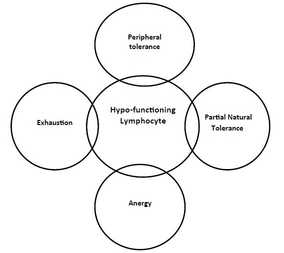
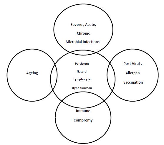
Normogy is a state of normal functioning human immune system. Allergy is a condition of hyper-functioning immune system towards certain exo- or endogenous materials, the allergens. While anergy is a state of reduced or hypo-functioning immune system in presence of certain antigens within the continuum of the immune cells niche. Anergy is one of the processes that induce tolerance and modify immune cells to in order to prevent self –destruction [1-6]. Allied to anergy are; clonal deletion, immune regulation and immune cell exhaustion, Figures 1 and 2. These allied reduced immune reactivity concepts can be delineated on the bases of three related, none-identical but overlapping senses which are identity, cause and function, the convergence strategy. Exhaustion can be defined on the bases of the aforementioned concepts, as that cells when exposed to chronic high, antigen exposure, are activated and proliferated before becoming dysfunctional. The first is that cell is evident in absence of effector response. Second is that cell that are produced in presence of a given cause like exposure to an antigen and the third is that cell presenting same molecular marker of death the programmed cell death protein-1 (PD-1) [2]. In this opinion reduced immune cell function was defined and anergic cells were visualized, their potential role played in COVID-19 was mapped.

fig 1

Figure 1: Effectors of lymphocyte hypo-function

fig 2

Figure 2: The Allied forms of lymphocyte Hypo-function

Cellular Basis of Anergy

Anergy in practice have two identifying facets. First, the reduced or absent gross clinical presentation and second the reduced or absent cellular functions. Herein, the study concerned with the cellular facets. The anergy is mainly tackled in lymphocytes [7-12] though there was report on anergy in basophils [13].

Mechanisms For Induction of Anergy In Lymphocytes

The target deletion in immune repose genes are associated with hyper-proliferation of T or B lymphocytes, frank autoimmune disease. These immune suppression genes represents the negative regulators that suppress self – reacting ability by enforcing negative selection in thymus for T cells and in bone marrow for B cells. The expression of these genes interferes with generation and/or function of regulatory T cells, altering signaling through T or B cells antigen receptors or promote apoptosis of peripheral T or B cells these two immune events outcomes with either T or B cell anergy. Such lymphocyte anergy might represent default genetic program, globally imposed on either mentioned lymphocyte types by low-level intracellular calcium influx occurring in response to recognition of self- antigen [6,8,13,14].

Mechanism of B cell Anergy

Yarkoni and associates [15] and Waterman and Cambier [12] have been thoroughly reviewing the multiple possible mechanisms for induction of B cell anergy. Going through these reviews, a hypothesis was arise from a collective viewing to the presented facts that may unify the mentioned mechanisms and was phrased as in the following;

  1. B cell face chronic antigen stimulation
  2. Surface immunoglobulin undergoes re –arrangement.
  3. Blockade of the second transducing signal.
  4. Notable Intracellular collective biochemical changes
  5. Activation of anergy specific gene circuit expression
  6. Genetic reprograming as a default genetic program
  7. Metabolic reprograming.

Mechanisms for Induction of Anergy In T cells

The induction of T cell anergy was based on the work of Valdor and Macian [7,16] and depicted in the following steps;

  1. Engagement of TCR and CD28.
  2. Free intracellular Ca influx.
  3. Activation of transcription factors
  4. NFAT form complex with AP1 with AP-1 inactivation
  5. NFAT direct the expression of anergy inducing genes.
  6. Expression of anergy inducing genes.

Mechanisms of induction of Exhaustion in T cells

Rha and Shin [17] were briefing the features of exhausted T cells which may in some way explained the mechanisms of induction of exhaustion in T cells, and were depicted in the followings

  1. Loss of effector function
  2. Sustained expression of inhibitory receptors
  3. Alteration in genetic and epigenetic landscape.
  4. Metabolic reprograming

B Cell Anergy

Anergic B cells are characterized by; Low surface IgM, normal surface IgD levels with reduction in their functional capacity. Reduced life span in absence of T cell help, inhibition of second signal transduction so that B cell does not release calcium as a critical pathway in activation of B cells. Anergic B cell undergoes change in migration patterns and distinctive recirculation fashion through lymphoid system as compared to normal functioning B cells. Normal B cells becomes anergic upon chronic exposure to self- antigen and reactivated to normal state by the expression to CD40 ligand in presence of IL4 (Table 1) [18].

Table 1: Comparative view to the immunobiologic features of anergic and exhausted lymphocytes as compared to normal

Features

Normal B cells Anergic B cell [10] Normal T cell Anergic T cell [7,8,14]

Exhausted T cell [17]

Origin and migration Bone marrow, peripheral lymphoid tissues Bone marrow, peripheral lymphoid tissue Bone Marrow, Thymus Bone Marrow, thymus Bone marrow, thymus
Developmental stage on migration for maturation Mature, bone marrow Mature, bone marrow Immature, thymus Immature, thymus Immature, Thymus
Surface Markers CD19, CD20, CD22, CD5, CD35, BCR, B7 IgD, CD10, CD24, CD36, CD9 TCR, CD2, CD3, CD28, CD5, CD7, CD45, CD4 or CD8 TCR and CD28 engagement CD28, CD5, CD2, CD3, CD5, CD7, CD45, CD8
Signaling Two signals Stimulatory Two signals Stimulatory Two signals
Anergy/phenotypic changes Down-regulation of IgM, antigen irresponsive Inhibition of cytokine production, Irresponsive to antigen
Exhaustion phenotypic changes PD-1, TIM-3, LAG-3, CTLA-4, TIGIT, Markers & Expression of exhaust associated genes
Reactivation BAFF, TLR, INF gamma, CD40L with IL4 Fas and Bcl-2 proteins In-vivo patient recovery

Auto-reactive B cells not controlled by receptor editing or clonal deletion may become anergic. Mature human B cell subsets that are naturally auto-reactive and controlled by the tolerizing mechanisms are those of functional anergy [9].

In healthy human IgMlo phenotypes are characterized by the absence of activation markersCD69,CD86and CD95,reduced expression of co-stimulatory molecules CD19 and CD21 with an evident inhibition levels of CD22. Therein the major fractions of mature B cell have a reversible anergic phenotypes determined impart by a down-regulation of sIgM that appears to determine a higher threshold for their activation through BCR [whether IgM or IgD] [10].

IgM but not IgD is down-regulated on auto-reactive B cells. IgD is less sensitive than IgM to endogenous antigens in-vivo. So the decision for the B cell developmental fate are shifted accordingly. The role of B cell surface IgD is in maintaining the quiescence of their auto-reactivity and restoring their differentiation into antibody secreting cells [11].

Clonal anergy was proposed as a way for inactivation of B cells stimulated early in their developmental phases when only auto-antigen would be present Anergic B cells are naïve-like B cells identified by the down-regulation of the complement -2 cell surface receptor (CD21) [10]. Though, the human anergic B cells are quite divergent and of multiple phenotypic forms [19].

There are about 2.5%-30% of human peripheral CD27- B cells are auto-reactive and anergic based on un-responsiveness to antigen-receptor BCR stimulation and auto-reactivity of cloned and expressed BCR. Human anergy is maintained by elevated expression of PTEN [a phosphatidylinositol 3 4 5 P-3- phosphatase],Reduction in expression of micro-RNA coding PTEN was associated with up-regulation PTEN and anergy in B cells (Table 1) [20].

Functions of Anergic B Cells

Rosenspire and Chen [6] deduced four main functions of anergic B lymphocytes in human welfare as:

  1. In healthy individuals it is found inactive and self -reactive.
  2. In autoimmune conditions, activated B cells found binding to self- antigenic epitopes.
  3. In state of infection with microbe bearing self- mimicking epitope, anergic cell found binding to cross-reacting epitope of the microbe.
  4. In fulminant Infection conditions, TLR signaling synergize with the anergic B cells allowing them to transition from the anergic cell pool, this in turn will lead to expression of active B cells which recognize host mimicking epitope on the pathogen as well as antigens on the host.

T Cell Anergy

Anergy in T cells is a state of growth arrest designed to reduce their proliferation during T cell immune responses. Failure of normal naïve T cell to establish the second signal transduction due to any cause will lead to T cell anergy state. The T cell anergy inducers are; peptide-MHc occupation, cross-link with concavalin A in absence of APC, binding with anti-CD3 mAb. Anergic T cells showed reduced IL2 to 25 to 50 folds lower than normal T cells and inhibition of CD40 ligand (Table 1) [21].

T cell anergy is a tolerance mechanism in which the lymphocyte is intrinsically functionally inactive following an antigen encounter but remain alive for an extended period of time in an hypo-responsive state. Two model explanations have been held for CD4 and CD8 T cells. First was the clonal anergy which principally growth arrest arise from an incomplete T cell activation. The second was the in-vivo anergy which represent more generalized inhibition of proliferation and effector function due to naïve T cell stimulated by deficient co-stimulation. Both of clonal anergy and in-vivo anergy are found in T reg. subsets [22].

T cell anergy is induced in previously activated T cells or cell clones by re-stimulation through T cell receptor TCR in absence of co-stimulating signal. Such anergic cells were found to be of reduced calcium flux, expression of protein enriched specifically by anergic program to induce T cell anergy. The induction ability of anergy in T cells depends on the intracellular assembly of E3 ubiquitin ligase activity [23].

Among a number of mechanisms that coevolved to control the adaptive immunity is the anergy. Which is the functional inactivation of T lymphocyte that responds to antigens in absence of inflammation. There found to be an intracellular protein in quiescent T cell that function to integrate signals for antigens co-stimulation and growth factor receptors. These factors ensure that all cells that fail to engage them from all the three pathways are shunted into alternative transcriptional program designed to dissuade them from participating in the subsequent immune response. Anergy is a combine result of factors that negatively regulate with a program of active transcriptional silencing that reinforced through epigenetic mechanisms [24].

One mechanism that is in place to control the activation of mature T cells that bears self- reactive antigen receptor is anergy, a long term state of hypo-responsiveness that establish T cell in response to sub-optimal antigen re-stimulation. T cell receive signals not only from antigen recognition and co-stimulation but also from other sources including cytokine receptor, inhibitory receptor or metabolic sensors. Under conditions that induce anergy, T cells activate program of gene expression that lead to the production of protein that block T cell receptor signaling and inhibit cytokine gene expression [8].

T cell anergy is already present in non-ventilated COVID-19 patients and strongly associated with virus persistence and reversible with clinical recovery [25].

Functions of T cell Anergy

T cell anergy may have the biological potentials to function in several immune conditions [7,14,25-28];

  1. Silence the auto-reactive T cells, so that in absence of such slience provoke marked autoimmune condition [7,14].
  2. Silence the allergenic reactions post-allergen vaccination [7,28]
  3. The developmental path of T cell anergy phases may serve potential target of pharmaceutical interventions [7].
  4. Serve as a pathognomic marker for viral persistence in severe viral infections including COVID-19 [25].
  5. Share part with T reg, functions in regulation of an aberrant immune responses [7].

Exhausted T Cells

It is a T cell that express hypo-functioning as well as reversible functional mode. Current information have develop a number of characteristics for this T cell functional form. Though its phenotype referred to as CD8+ T cells. Exhausted T cells have shown to be with; loss of effector function, alteration in the transcriptional and epigenetic landscape and metabolic reprograming. The presence of these cells in COVID-19 vaccine is contra-versial [17].

Anergy in Normal Human Being

Like the state of normal human being in whom there are percentages of auto-reactive cells and autoantibodies that represent the baseline levels of normal physiological autoimmune reactions [29-33]. There are normal levels of anergic immune cells like anergic B, anergic T and anergic myeloid cells [9].

Anergy in Sars-Cov-2 Human Infections

Both B and T cell immunity are involved in sars-cov-2 human infections. B cell produce Sars-cov-2 specific antibodies and T cells produce a spectrum of cytokines that take a role in the pathogenesis and immune-pathogenesis of sars-cov-2 infections. CD4 T cells helps B cells in production of antibodies. CD8+ T cells kills virus infected cells. T cells interferon gamma controls viral infection. Lymphopenia is evident in sars-cov-2 infection affecting CD4+,CD8+ and B cells. T cell responses in severe COVID infection forms may be over-activated, impaired or inappropriate. Post infection immunity yield memory B, memory CD4 and memory CD8 phenotypes [1]. Severe fatal sars-cov-2 infections in man showed a spectrum of immune responses that involve three phases; i-normal or hypo-immune, ii-hyper-activation and iii-Anergy [5]. COVID-19 infectious epidemic pneumonia is associated with; i-hyper-inflammation and ii- clear lymphocyte hypo-function that are mainly noted in hospitalized severe infection needing ventilation and associated with viral persistence [25]. Thus severe cod-19 infection is presenting both lymphopenia and lymphocyte hypo-function or anergy.

Anergy versus Antigens

Immune tolerance is either central genetic or peripheral, acquired. It can be of low or high dose tolerance depending on the toleragen dose, exposure frequency and continual coexistence facing the immune cells. On the absence of the antigen cells becomes reactive normal. Anergy need continual exposure of lymphocytes to the antigen which impacts the phenotypic, the migration behavior and the function. Regulatory T cell may function both in tolerance and anergy [26,27]. Vaccine for allergy in post-vaccination period may influence anergy in immune cells [28].

Anergy and Sars-Cov-2 Antigens

Sars cov-2 virus have an array of antigens; like spike, neucleo-capsed membranous as well as nonstructural protein [Grifoni et al. [29], Le Bert et al. [30]. This virus appeared to have super-antigen, super-antigen like and/or super-antigen trigger host cytokine storm, lymphocyte differentiation, lymphocyte apoptosis, anergy and autoimmunity [31].

The order of sars-cov-2 antigen exposure determine the nature of the immune response. Since it impacts the distribution between spike specific and non-spike specific responses. Thus the exposure history shapes phenotype and specificity of memory T cells [32].

Life Extreme and Vaccines

Life extremes are childhood and senescence. Ageing as life extreme impacts human immune system mainly as brook of immune tolerance, appearance of autoimmune reactions and reduction of other immune functions as; Decreased phagocytic activity, disturbed processing and presentation of antigens, decrease in functionality of innate and adaptive immune system, impaired responses to microbial vaccines in general and to sars-cov-2 vaccine. Low NK function, poor priming of T cells. B cell produces non-protective antibodies. These impacts may make aged subject vulnerable to respiratory infection and pneumonia [4].

Anergy versus COVID-19 Vaccines

In a population of 205 health care workers that were elected in Jan 2021. They were enrolled in a covisheild vaccine [same as ChAdOxl] vaccine. Vaccinated subjects were subjected to blood collection at the day14 and 28 after the first shot and three months after the second shot. Non-responder rate was 35:205 17% at the day 14 and 5;205 2% at the day 28. At the second dose all vaccinated were responders with 17 fold increase in anti-spike protein antibodies. Non-responder rates were higher in male and senior citizens. A 1.5 folds decrease in ASSA titers in the previously exposed. Thus, vaccination in non-exposed express prime-boost effects and in previously exposed express boost anergy effects [33,34]. Continual exposure to COVID vaccine induced anergy.

Vaccination after infection leads to expansion of spike specific T cell and differentiation of CCR-CD 4RA+ effector. In contrast Individuals after break through infection mount vigorous non-spike specific responses and diversify the T cell memory repertoire. Current vaccination protocols continue to expand and differentiate spike specific memory [32].

Conclusion

Reduction of immune reactivity of lymphocytes may be attributed to hypo-function, tolerance, exhaustion or anergy. Genetic versus epigenetic change, loss of function, identity, cause and function may be a helpful parameters for evaluation of these cell entities. Anergy influence change in phenotype, migration behavior and function of lymphocyte. Anergic lymphocytes were noted in; normal, chronic infected and vaccinated. Chronic viral infections and viral vaccination forms an insult for initiation of anergy. Post vaccination by viral vaccines and allegen vaccines can be terminate by anergic lymphocytes. Since continual antigen exposure to lymphocytes is one of the known ways for induction of anergic state in lymphocytes. One of the possible potentials of anergic cell is to silence auto-reactive cells and mediators. COVID-19 vaccination in exposed health care workers lead to boost anergy.

References

  1. Puddemann A, Aranson (2020) what is the role of T cells in covid-19 infection. why immunity is about more than antibodies. Oxford Covid-19 evidence team, Centre for evidence based medicine, Nuffield Department of Primary Care Health Sciences, University of Oxford. Oct.19.2020.
  2. Kaminski H, Lemone M, Paradeu T (2021) Immunological exhaustion; How to make a disparate concept operational? Plos Pathogen 17: e1009892. [crossref]
  3. Goldman M, Hermans C (2021) Thrombotic thrombocytopenia associated with covid-19 infection or vaccination; Possible to platelet factor 4 autoimmunity. Plos Medcine 18: 1003648. [crossref]
  4. Andryelkov BG, Besednova N (2021) Older adults: Panoramic view on covid-19 vaccination. Pub Hlth 8: 388-415. [crossref]
  5. Zhou X, Ye Q (2021) Cellular Immune responses to covid-19 and potential modulators. Front Immunol 12: 646333. [crossref]
  6. Rosenspire AJ, Chen K (2015) B cells precarious on call warriors at the nexus of autoimmunity and false flagged pathogens. Front Immunol 6: 580. [crossref]
  7. Valdor R, Macian F (2010) Mechanisms of Self inactivation in anergic T cells. Immunologia 29: 20-33.
  8. Valdor R, Macian F (2013) Induction and stability of anergic phenotype in T cells. Sem Immunol 25: 313-320. [crossref]
  9. Duty JA, Szodoray P, Zheng NY, Koelsch KA, Zhang Q, Swiatkowski M, et al. (2008) Functional anergy in subpopulation of naïve B cells from healthy human that express auto-reactive immunoglobulin receptor. J Exp Med 206: 139-151. [crossref]
  10. Quach TD (2010) human anergic B cells: IgMlo. PhD thesis. School of Medicine and Dentistry, University of Rochester, New York.
  11. Noviski M, Mueller JL, Satterwaite A, Sinha LAG, BromBacher F, et al. (2018) IgM and IgD B cell receptors functionally respond to endogenous antigen and control B cell fate. eLife 7: 35074. [crossref]
  12. Waterman PM, Cambier JC (2010) The conundrum of inhibitory signaling by ITAM containing immune-receptors: Potential molecular mechanisms. FEBS Letters 584: 4878-4882. [crossref]
  13. Ma A, Patil G, Lund K et al. (2012) Antigen induced anergy in human Basophils is not antigen specific. J Allergy Clin Immunol 129: AB123.
  14. Macian F, Im SH, Gavacia-Cozar FJ, et al. (2004) T cell anergy. Cur Opin Immunol 16: 209-216.
  15. Yarkoni Y, Getahun A, Cambier JC (2010) Molecular underpinning of B cell anergy. Immunol Rev 237: 249-253. [crossref]
  16. Belanti J A(ed) (2012) Immunology IV: Clinical application in health and disease, Distruption of co-stimulatory signal and anergy. Care Press. MD. Immunopedia.Org.Za.
  17. Rha MS, Shin EC (2021) Activation or exhaustion of CD8+ T cells in patients with covid-19. Cellular Mol Immunol 18: 2325-2333. [crossref]
  18. Tartinton DM (1998) Anergy B cells, Delves PJ, Roitt IM(ed.). Encyclopedia of Immunology 2nd London. Academic Press 105-108.
  19. Andrews SF, Wilson PC (2010) The anergic B cells. Blood 115: 4976-4977.
  20. Smith MJ, Ford MR, Rihanek M, Coleman BM, Getahun A, et al. (2019) Elevated PTEN expression maintain anergy in human B cells and reavels unexpectedly high repertoire autoreactivity. JCI Insight 4: 123384. [crossref]
  21. Shwartz RH (1998) Anergy T cells, Delves and Roitt IM eds. Encyclopedia of Immunology, 2nd London, Academic Press 109-111.
  22. Shwartz RH (2003) T cell anergy. Ann Rev Immunol 21: 305-334. [crossref]
  23. Fathman CG, Lineberry NB (2007) Molecular mechanisms of CD4+ T cell anergy. Nat Rev Immunol 7: 599-609. [crossref]
  24. Wells AD (2009) New insight into molecular basis of T cell anergy, factors, avoidance, sensors and epigenetic imprinting. J Immunol 182: 7331-7341. [crossref]
  25. Renner K, Schwittay T, Chaabane S (2021) Severe T cell hypoactivity in ventilated covid-19 patients correlate with roploged virus persistence and poor outcomes. Nat Immunol 12: 3006. [crossref]
  26. Tolar P, Sohn HW, Pierce SK (2005) The initiation of antigen induced B cell receptor signaling viewed in living cells by fluorescence resonance energy transfer. Nat Immunol 6: 1168-1176. [crossref]
  27. Gauld SB, Benschop RJ, Merrell KT, Cambier JC (2005) Maintainence of B cell anergy requires constant antigen receptor occupancy and signaling. Nat Immunol 6: 1160-1167. [crossref]
  28. Cao Y, Yang M, Luo Z, Monapatra SS (1997) Vaccination with multi-epitope recombinant allergen induce deviation via T cell anergy. Immunol 90: 46-51. [crossref]
  29. Grifoni A, Weiskopf D, Ramirez SI (2020) Target T cell responses to sars-cov-2 coronavirus in human with covid-19 disease unexposed individual. Cell 181: 1489-1501. [crossref]
  30. Lebert N, Tan AT, Kabasegaran K, Tham CYL, Hafezi M, et al. (2020) Sars-cov-2 T cell immunity in cases of covid-19 and sars and un-infected controls. Nature 484: 457-462. [crossref]
  31. Hamdy A, Leonardi A (2022) Superantigens and sars-cov-2. Pathogens 11: 390. [crossref]
  32. Minervina AA, Pogorely MV, Kirk AM, et al. (2022) Sars-co-2 antigen exposure history shape phenotypes and specificity of memory CD8+ T cells. Nat Immunol 597: 268-273.
  33. Shnawa IMS (2022) Post-infection-post-vaccination autoimmune neural long covid. J Pharmaceutical Res Inter 34: 1-7.
  34. Kannian P et al (2022) Booster and anergic effects of covishield vaccine among health care workers in south India. medRxiv. a license to display pre-print in perpetuating. It is made available under a CC-By4.0, international licensed.

Treatment of Hydrophobic Poly Aromatic Hydrocarbons and Toxicity Using GO-TiO2-Sr(OH)2/ SrCO3 Nanocomposite via Photocatalysis

DOI: 10.31038/NAMS.2022512

Abstract

The effects of increasing sun light irradiaiton time (30 min, 120 min, 240 and-360 min), increasing photocatalytic power (10 W, 50 and 100 W), increasing graphene oxide (GO) nanoparticle concentrations (2 mg/l, 4 and 8 mg/l), increasing titanium dioxide (TiO2) nanoparticle concentrations (1 mg/l, 3 mg/l, 6 and 9 mg/l), increasing GO-TiO2-Sr(OH)2/SrCO3 nanocomposite concentrations (1 mg/l, 2 and 4 mg/l) on the destructions of four hydrophobic polycyclic aromatic hydrocarbons (PAHs) in a real petrochemical industry wastewater in Izmir (Turkey) were investigated. The yields in more hydrophobic PAHs with high benzene rings [benzo[a]pyrene (BaP) and benzo[k]fluoranthene (BkF)] were as high as the less hydrophobic PAHs with lower benzene rings [acenaphthylene (ACL) and carbazole (CRB)] at pH = 7.0, at 22°C after 360 min sun light irradiation time. Maximum 97% ACL, 98%CRB, 98%BaP and 99%BkF PAHs removals was detected at 4 mg/l GO-TiO2-Sr(OH)2/SrCO3 nanocomposite concentration, under sun light intensity = 100 mW/cm2, at photocatalytic power = 100 W, at sun light irradiation time = 360 min, at pH = 7.0 and at 22°C, respectively. The effective PAHs concentrations caused 50% mortality in Daphnia magna cells increased from initial EC50 = 342.56 ng/ml to EC50 = 631.05 ng/ml, at pH = 7.0 and at 22°C after 360 min photocatalytic degradation time resulting in a maximum acute toxicity removal of 99.99% at GO-TiO2-Sr(OH)2/SrCO3 nanocompoasite concentration of 4 mg/l. The Daphnia magna acute toxicity was significantly reduced.

Keywords

Daphnia magna acute toxicity, Graphene oxide, GO-TiO2-Sr(OH)2/SrCO3 nanocomposite, Petrochemical industry wastewater, Photocatalytic degradation, Polycyclic aromatic hydrocarbons, titanium dioxide

Introduction

Polycyclic aromatic hydrocarbons (PAHs) are an important class of persistent organic pollutants (POPs), and have been ubiquitously found in the environment [1]. Besides the natural sources, PAHs are often from anthropogenic sources such as incomplete combustion of fossil fuels, and accidental spillages of crude and refined oils [2,3]. Due to their persistence and potential harmful impact on the ecosystem and human health, PAHs have been classified as priority pollutants by the United States Environmental Protection Agency (USEPA) [4].

Wastewater treatment plants, especially those serving industrial areas, consistently receive complex mixtures containing a wide variety of organic pollutants. Groups of compounds present in the petrochemical industries include polycyclic aromatic hydrocarbons (PAHs), which are listed as US-EPA and EU priority pollutants, and concentrations of these pollutants therefore need to be controlled in treated wastewater effluents [5]. PAHs are ubiquitous environmental pollutants with mutagenic properties, which have not been included in the Turkish guidelines for treated waste monitoring programs [6]. Several hydroxy-PAHs such as hydroxylated derivatives of Benzo[a]pyrene (BaP) and Chrysene (CHR) have been shown to possess estrogenic activity and cause damage to DNA leading to cancer and possibly other effects [7]. As a consequence of their strongly hydrophobic properties and their resistance to biodegradation, PAHs are not always quantitatively removed from wastewaters by activated sludge treatments, which very efficiently relocate them into treated effluents.

Titanium dioxide (TiO2) is the most used photocatalyst due to its environment friendliness, abundant supply and cost-effectiveness [8]. However, due to the wide bandgap (3.2 eV for anatase and 3.0 eV for rutile) [9], TiO2 can only be excited in the ultraviolet (UV) range, which accounts for only 4% of the solar radiation [10]. Therefore, various efforts have been attempted to extend the utilization of TiO2 to the visible light range (>40% of the solar energy), such as metal/non-metal doping, noble metal deposition, semiconductors coupling, and photosensitization [11,12].

Graphene is a flat monolayer of carbon atoms tightly packed into a two-dimensional honeycomb lattice. In recent years, graphene has attracted a great deal of attentions for its potential applications in many fields, such as nano-electronics, fuel-cell technology, supercapacitors, and catalysts [13,14]. Graphene oxide (GO) is one of the most important precursors of graphene, and thus, they share similar sheet structures and properties such as high stability and semiconducting characteristics [15]. GO can enhance the light absorption via expanding the photoresponsive range to visible light and suppress the charge recombination by serving as a photo-generated electron transmitter, when coupled with TiO2. To further enhance the conductivity and reduce the bandgap, noble metals (e.g., gold, palladium and platinum) are often incorporated to the GO-TiO2 nanocomposite by surface deposition [16].

Compared with noble metals, strontium (Sr), as an alkaline earth metal, has much wider and richer sources, and it is the 15th most abundant element in the Earth’s crust with an estimated abundance of nearly 360 mg/l [17]. Sr has been widely employed as a dopant for various semiconductors (e.g., TiO2, zinc oxide and germanium dioxide) to enhance the photocatalytic activities [18]. Moreover, the OH and carbonate forms of Sr (Sr(OH)2/SrCO3) have been reported to have high photocatalytic activity under visible-light irradiation [19-21].

The reactive oxygen species (ROS) formed during TiO2 photocatalysis include the hydroxyl radical (OH), superoxide anion radical (O2-●), hydroperoxyl radical (HO2), singlet oxygen (1O2), and their subsequent reactions with the target contaminants occur at or very near the TiO2 surface [22]. OH radicals, generated on the surface of the catalyst following oxidation of water from the positive holes of TiO2, are non-selective oxidizing species with strong oxidation potential (2.80 V) that rapidly react with most organic compounds with rate constants in the order of 106-1010 1/M.s [23]. Various studies have investigated the degradation of MC-LR in pure solutions or crude extracts with TiO2 photocatalysis to study the effect of specific water quality parameters [24-27] or the properties of the photocatalyst used [28-32]. Solar light activated materials have also been tested to reduce application cost [33]. Herein, sulfate radical generating oxidants were added as a way to reduce the energy requirements of the photocatalytic system for the removal of MC-LR as most of the light activated materials are not currently mass produced. Sulfate radicals (SO4-●) are among the strongest oxidants known for the abstraction of electrons [2.5-3.1 V] [34,35]. They are much stronger than OH radicals [1.89-2.72 V (Buxton et al., 1988)] and other commonly used in the drinking water industry oxidants, such as permanganate [E = 1.70 V] [36] and hypochlorous acid [E = 1.49 V] [37]. SO4-● radicals can be produced through homolytic dissociation of the oxidants through heat and radiation and e transfer mechanisms from Fenton-like reagents [38-40] reported that owing to their selectivity, SO4-● radicals are more efficient oxidants for the removal of organic compounds with unsaturated bonds and aromatic constituents than the OH radicals. Yet there are limited studies on SO4-● based AOPs (compared with OH) for the degradation of recalcitrant organic contaminants and especially cyanotoxins [41-43]. Even fewer studies have investigated the effect of coupling SO4-● radical generating oxidants with TiO2 on the removal of emerging contaminants with various light sources. Furthermore, simulated solar irradiation (SSI) has been used in the SSI/TiO2/PS treatment [44] and showed higher potential for the removal of the pesticide DEET compared with the SSI/TiO2/H2O2 system. PS was also coupled with TiO2 photocatalysts for the degradation of dyes under solar [45] and UV radiation [46].

The aim of this study was to determine the effects of increasing GO-TiO2-Sr(OH)2/SrCO3 concentrations (1 mg/l, 2 and 4 mg/l), increasing GO concentrations (2 mg/l, 4 and 8 mg/l), increasing TiO2 concentrations (1 mg/l, 3 mg/l, 6 and 9 mg/l), increasing photocatalytic powers (10 W, 50 and 100 W) and increasing sun light irradiation times (30 min, 120 min, 240 and 360 min) on the photocatalytic degradation of four hydrophobic PAHs namely ACL, CRB, BaP and BkF at pH = 7.0 and at 22°C, respectively. Furthermore, the effects of the operational conditions on the removal of acute toxicity were also determined using Daphnia magna.

Materials and Methods

Material Synthesis

GO was synthesized according to the modified Hummers method [47], and titanium dioxide nanoparticles (Nano-TiO2) were prepared following the approach reported in [48]. Supporting Information (SI) Text S1 provides detailed procedures for the preparation of GO and Nano-TiO2. The GO-TiO2 nanocomposite was then synthesized through the sono-chemical reaction of Nano-TiO2 in the presence of the GO. In brief, 3 g of the mixture of GO and Nano-TiO2 (mass ratio = 2:1) was added to 100 ml of distilled water, and stirred for 0.5 h at room temperature (22 ± 1°C). The suspension was then sonicated for 1 h. The resultant composite was recovered by filtration, rinsed with ethanol and then freeze-dried to yield the GO-TiO2 composites. Subsequently, dispersing known mass of GO-TiO2 (30 wt% of the final mass) in a 500 ml of sodium hydroxide (NaOH) solution (1 M), and a pre-determined amount of strontium chloride (SrCl, 0.5 M) was added dropwise to the dispersion at a rate of 2.0 ml/min using a Titronic Universal titrator (SCHOTT, Mainz, Germany). The resulting material, GO-TiO2-Sr(OH)2/SrCO3, was then filtered, washed with distilled water until no chloride was detected in the washing water, and then freeze-dried for 48 h. For comparison, a GO-Sr(OH)2/SrCO3 nanocomposite was also prepared by the similar procedure with 20 wt% GO but without TiO2.

Material Characterization

The X-ray diffraction (XRD) measurements were performed on a PW1820 X-ray diffractometer (Philips, Amsterdam, Netherlands) using Cu Kα radiation. Scanning electron microscopy (SEM) images were obtained with a JSM-840A electron microscope (JEOL, Tokyo, Japan) equipped with energy dispersive X-ray (EDX) micro-analytical system (EDAX, Mahwah, NJ, USA). The EDX analysis was performed at 263.15°C magnification to map the distribution of Sr and Ti on the nanocomposite surface. Fourier transform-infrared (FTIR) measurements were carried out with a Nicolet 560 FTIR spectrometer on KBr wafers (Thermo Fisher Scientific Inc., MA, USA). The spectra were recorded from 4000 to 400 1/cm at a resolution of 4 1/cm. Nitrogen (N2) adsorption-desorption isotherms were measured using AS1Win (Quantachrome Instruments, FL, USA) at the liquid N2 temperature of 196.15°C, from which Brunauer-Emmett-Teller (BET) specific surface area (SBET), micropore volume (Vmic), total pore volume (Vt), and pore size distribution (PSD) were derived. Potentiometric titration measurements were carried out with a T50 automatic titrator (Mettler Toledo, Columbia, MD, USA) and the total surface charge (Qsurf, mmol/g) of the nanocomposite was then calculated. Differential thermal gravimetric (DTG) analysis was conducted on an STA449F3 instrument (Netzsch, Selb, Germany). Reactive oxydizing agents such as potassium peroxymonosulfate (PMS, HSO5), potassium persulfate (PS, K2S2O8), and the quenching agent sodium thiosulfate (Na2S2O3) were purchased from Sigma-Aldrich (Poole, UK).

Photocatalytic Degradation

Simulated sun light was generated using a 94041A solar simulator (Newport Corporation, Irvine, CA). A cylindrical quartz tank reactor with a Pyrex pillar (80 × 70 mm) was fabricated as the photoreactor. The light intensity reached the reactor was 100 mW/cm2. The detailed information on the solar simulator and photoreactor has been reported elsewhere [49]. PAHs were purchased from Alfa Aesar (Ward Hill, MA, USA), and a stock solution of 2 g/l was prepared in methanol. Deionized (DI) water (Millipore Co., 18.2 MΩ·cm) was used in preparing all aqueous solutions. Typically, the photocatalytic degradation kinetic tests were conducted under the following conditions: solution volüme = 250 ml, initial PAHs concentration = 1 mg/l, 5 mg/l and 10 mg/l, catalyst dosage = 50 mg/l, pH = 7.0 ± 0.2, and T = 22 ± 1°C. The solution-photocatalyst mixture was first stirred in the dark for 2 h to allow PAHs adsorption to reach equilibrium. Subsequently, photodegradation was initiated by exposing the reactor to the simulated sun light.

Analytical Methods

UV-Visible spectra of solutions were obtained using an HP 8453 UV-Vis spectrophotometer (Agilent Technologies, Santa Clara, CA, USA). PAHs concentration was determined using an HP 1100 HPLC system (Agilent Technologies, Santa Clara, CA, USA) with a detection limit of 2.5 μg/l at the UV detection wavelength of 250 nm. Photodegradation intermediates were analyzed using an HP7890A/HP5975C gas chromatography-mass spectrometry (GC-MS) system (Agilent Technologies, Santa Clara, CA, USA).

The contributions of various reactive oxygen species (ROS) during the photocatalytic degradation process were investigated by adding scavengers to selectively quench radicals, i.e., potassium peroxymonosulfate (PMS, HSO5), potassium persulfate (PS, K2S2O8), and the quenching agent sodium thiosulfate (Na2S2O3) were used.

PAHs Measurements

For PAHs and some metabolites (hydroxy-benzoic acid, benzoic acid) analyses the samples were first filtered through a glass fiber filter (47 mm-diameter) to collect the particle-phase in series with a resin column (~10 g XAD-2) and to collect dissolved-phase polybrominated diphenyl ethers. Resin and water filters were ultrasonically extracted for 60 min with a mixture of 1/1 acetone: hexane. All extracts were analyzed for four PAHs (Table 1) gas chromatographically (Agilent 6890N GC) equipped with a mass selective detector (Agilent 5973 inert MSD). A capillary column (HP5-MS, 30 m, 0.25 mm, 0.25 µm) was used. The initial oven temperature was kept at 50°C for 1 min, then raised to 200°C at 25°C/min and from 200 to 300°C at 8°C/min, and then maintained for 5.5 min. High purity He(g) was used as the carrier gas at constant flow mode (1.5 ml/min, 45 cm/s linear velocity). PAHs and their metabolites were identified on the basis of their retention times, target and qualifier ions and were quantified using the internal standard calibration procedure. To determine the degradation intermediates, samples (10 ml each) were collected at 0 min, 30 min, 120 min, 240 min and 360 min. The hydrophobic PAHs (ACL, CRB, BaP and BkF) were performed using a HPLC (Agilent-1100) with a method developed by Lindsey and Tarr [50]. The chromatographic conditions for The hydrophobic PAHs (ACL, CRB, BaP and BkF) determination were as follows: C-18 reverse phase HPLC column (Ace 5C18; 25-cm x 4.6-mm, 5 μm, mobile phase: 50/50 (v/v) methanol/organic-free reagent water). pH, temperature, oxidation-reduction potential (ORP) were monitored following Standard Methods 2550, 2580 and 5220 D [51]. H2O2 was quantified with a colorimetric method following Standard Method 3550.

Table 1: Energy efficiency of photocatalysis with different sun light intensities at ambient conditions after 360 min sun light irradiation time (n=3, mean values, n: deionized water and petrochemical wastewater containing PAHs)

Energy efficiency of photocatalysis with different sun light intensities

Sun light intensity (W/cm2)

Power density (W/ml) Specific energy (kWh/kg COD-in influent)

COD removal efficiency (%)

17

0.12 8.29

47

38

0.91 8.90

59

24.03

1.34 9.26

68

39.09

1.71 9.91

77

46

1.97 10.83

80

52.3

2.38 12.42

86

Data Analysis

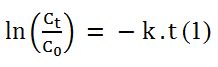
The pseudo-first-order kinetic model was employed to fit the kinetic data:

for 1

Where, Ct and C0 are the PAHs concentrations (μg/l) at the reaction time of t and 0 min, respectively, and k is the rate constant (1/min). The integration of UV-Vis absorbance of PAHs was achieved using the software OriginPro 8 (OriginLab Corporation, Northampton, MA, USA). The correlation fittings between the reaction rate constant and various water quality parameters were conducted by using OriginPro 8 or GraphPad Prism 6 (GraphPad Software, Inc., La Jolla, CA, USA). The fitting models included fourth-order polynomial and sigmoidal (Boltzmann and DoseResp functions) equations.

Daphnia magna Acute Toxicity Test

To test toxicity 24 h old Daphnia magna were used as described in Standard Methods. After preparing the test solution, experiments were carried out using 5 or 10 daphnids introduced into the test vessels. These vessels had 100 ml of effective volume at 7-8 pH, providing a minimum DO concentration of 6 mg/l at an ambient temperature of 20-25°C. Young Daphnia magna were used in the test (≤24 h old). A 24 h exposure is generally accepted as standard for a Daphnia acute toxicity test. The results were expressed as mortality percentage of the Daphnids. Immobile animals were reported as dead Daphnids.

All experiments were carried out three times and the results given as the means of triplicate samplings. Individual PAH concentrations are given as the mean with standard deviation (SD) values.

Statistical Analysis

The regression analysis between y (dependent) and x (independent) variables was carried out using Windows Excel data analysis. An ANOVA test was performed in order to determine the statistical significance between x and y variables.

Results and Discussion

Raw Wastewater

Characterization of raw petrochemical wastewater taken from the influent of the aeration unit of a petrochemical industry wastewater treatment plant was performed. The results are given as the mean value of triplicate sampling. The mean values for pH, ORP were recorded as 7.21 and 28.20 mV, respectively. The mean TSS and TVSS concentrations were measured as 310.3 and 250.6 mg/l, respectively. The mean DO, BOD5, CODtotal, CODdissolved concentrations were 1.78, 584, 1475 and 1127 mg/l while the Total-N, NH4-N, NO3-N, NO2-N, Total-P, PO4-P and oil concentrations were measured as 15.40, 2.20, 1.80, 0.05, 10.60, 6.80 and 206 mg/l, respectively. The less hydrophobic ACL and CRB concentrations were 124.2 ng/ml and 3.60 ng/ml while the more hydrophobic BaP and BkF concentrations were measured as 5.41 and 0.64 ng/ml, respectively, in the petrochemical industry wastewater. Physical and chemical properties of the PAHs studied in this work was shown at Table 2.

Table 2: Physical and chemical properties of the PAHs studied in this work

PAHs

CAS-No MF MW

(g/ mol)

TM

(°C)

TB

(°C)

Sw (25°C) (mg/l) VP (25°C) (mm Hg) H (25°C) (atm m3/mol) log KOA

(25°C)

log KOW

SORC

ACL

208-96-8

C12H8 152 93 280 16.1 6.68E-03 1.14E-04 6.34 3.94

23.56E+10

CRB

86-74-8

C12H9N 167 246 355 1.8 7.50E-07 1.16E-06 8.03 3.72

24.67E+10

BkF

207-08-9

C20H12 252 217 480 0.0008 9.70E-10 5.84E-08 11.37 6.11

0.45E+8

BaP

50-32-8

C20H12 252 177 495 0.00162 5.49E-09 4.57E-07 11.56 6.13

0.32 E+8

Acenaphthylene (ACL), Carbazole (CRB), Benzo[k]fluoranthene (BkF), Benzo[a]pyrene (BaP)
MF: Molecular Formula, MW: Molecular weight, TM: Melting point (°C), TB: Boiling point(°C), Sw: Solubility in water (mg/l), VP: Vapor pressure (mm Hg), H: Henry’s law constant (atm m3/mol), log KOA: Octanol-air coefficient, log KOW: Octanol-water coefficient, SORC: second-order reaction rate constants (ng/ml.s).

Characterization of Photocatalysts

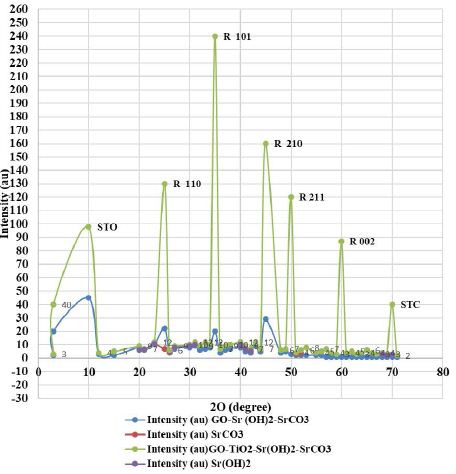
The XRD spectra of the prepared nanocomposites (GO-Sr(OH)2/SrCO3 and GO-TiO2-Sr(OH)2/SrCO3) (Figure 1). For both composite materials, the diffraction peak at about 10° is attributed to GO (Kyzas et al., 2014). For GO-Sr(OH)2/SrCO3, the broad peaks at 2θ = 25°, 28°, 36° and 43° are assigned to the crystalline phase of SrCO3 (JCPDS Card No. 005-0418), whereas weak peaks for Sr(OH)2, Sr(OH)2·. H2O and Sr (OH)2·. 8H2O were also observed as confirmed by JCPDS Cards Nos. 27- 0847, 28-1222, and 27-1438, respectively [52]. The XRD pattern of GOTiO2-Sr(OH)2/SrCO3 showed much sharper peaks than those of GO-Sr (OH)2/SrCO3, indicating well-developed crystalline phases. The peaks at 2θ = 25°, 28°, 36° and 43° are attributed to TiO2 belonging to the rutile phase (JCPDS Card No. 88-1175), while minor peaks from the anatase phase (JCPDS Card No. 84-1268) were also observed [53]. Besides, the peaks at 2θ = 24°, 32.7°, 40.1°, 46.6°, 57.8° and 67.9° can be attributed to the perovskite-type phase of cubic symmetry of SrTiO3 (STO) (JCPDS Card No. 86-0179) [54,55].

fig 1

Figure 1: XRD patterns of GO-Sr(OH)2/SrCO3 and GO-TiO2-Sr(OH)2/SrCO3 nanocomposites

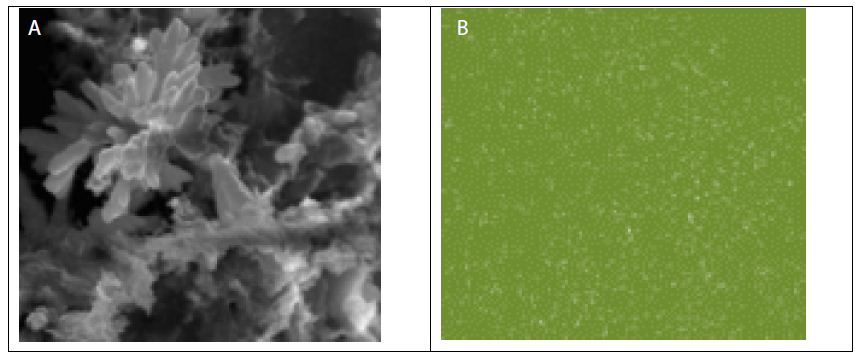
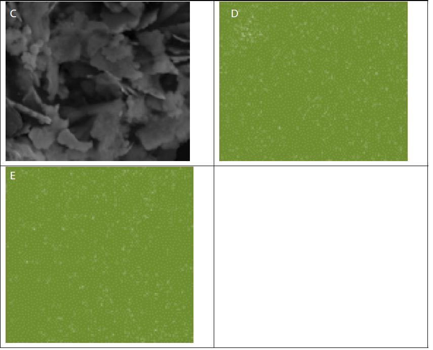
The SEM images along with the EDX maps of the elemental distribution (Figure 2) reveal that Sr and/or Ti are rather uniformly distributed in the GO-Sr(OH)2/SrCO3 and GO-TiO2-Sr(OH)2/SrCO3 nanocomposite matrices. The nano-rods in Figure (2a) are SrCO3, while the nanospheres on the GO surface in Figure (2c) are likely to be the aggregates of SrTiO3 nanoparticles with an average diameter of about 1 μm [56].

fig 2(1) fig 2(2)

Figure 2: SEM images of (a) GO-Sr(OH)2/SrCO3, (b) Sr distribution map with GO-Sr(OH)2/SrCO3, (c) GO-TiO2-Sr(OH)2/SrCO3, (d) Sr distribution map with GO-TiO2-Sr(OH)2/SrCO3 and (e) Ti distribution map

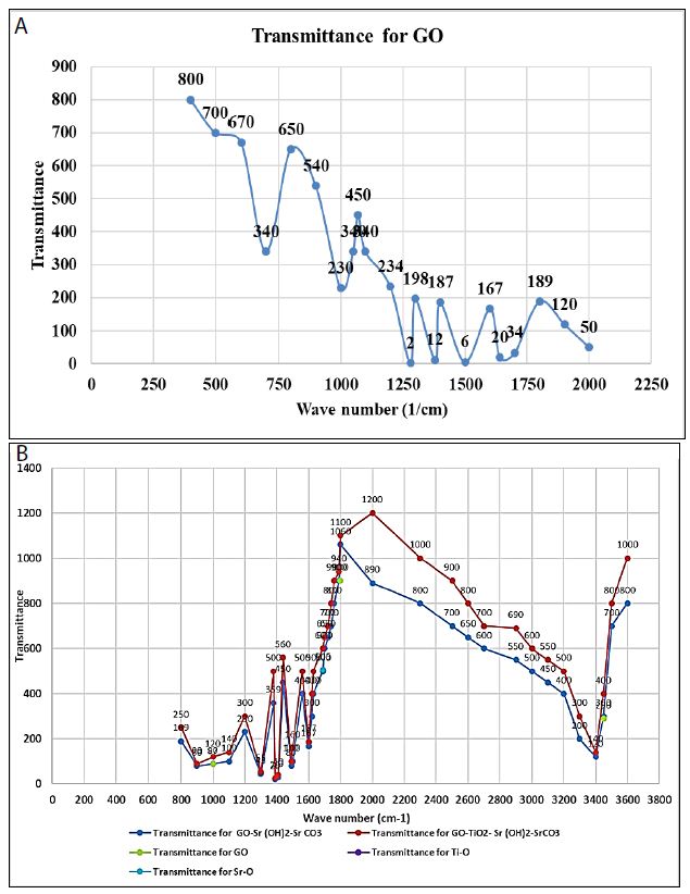
Figure (3a) shows the FTIR spectrum for GO. The characteristic bands are assigned as follows: carboxyl groups at 1070 and 1760 1/cm, C]C stretching vibration of the sp2 carbon skeletal network at 1600 1/cm, OeH groups at 1380 and 1000 1/cm, and epoxy groups at 900 1/cm [57]. The peak at 1240 1/cm can be attributed to the S]O asymmetric stretching vibrations arising from sulfones or sulfates that were formed upon graphite oxidation with H2SO4 (SI Text S1). Figure (3b) presents the FTIR spectra of the nanocomposite materials, i.e., GO-Sr (OH)2/SrCO3 and GO-TiO2-Sr(OH)2/SrCO3. The characteristic bands of GO are clearly seen in the spectra of both nanocomposites. For GO-Sr (OH)2/SrCO3, the bands at 1071 and 1760 1/cm are attributed to the asymmetric and symmetric stretching vibrations of the carboxylate groups. The band at 1446 1/cm is attributed to the asymmetric stretching vibration of carbonate anion (CO3 −2) in SrCO3 that has a D3h symmetry, while the bands at 860 and 600 1/cm are assigned to the vibrations of the carbonate anion due to bending out of plane and in plane, respectively (Alavi and Morsali, 2010). The bands at 3200, 1380 and 1000 1/cm are due to stretching mode of -OH groups and can be attributed to Sr(OH)2, Sr(OH)2·. H2O and Sr(OH)2·. 8H2O. For GO-TiO2-Sr(OH)2/SrCO3, a new broad peak was observed in the range of 550-780 1/cm, which can be ascribed to the TieO stretching. The bands at 1760 and 1384 1/cm for the carboxylate groups disappeared, indicating that these groups have been bounded to TiO2. The bands at 3200, 1384 and 1020 1/cm were diminished, indicating that less crystalline phases of Sr(OH)2, Sr(OH)2.H2O and/or Sr(OH)2·. 8H2O were formed (Alavi and Morsali, 2010).

fig 3

Figure 3: FTIR spectra of (a) GO and (b) GO-Sr(OH)2/SrCO3 versus GO-TiO2-Sr(OH)2/SrCO3 nanocomposites

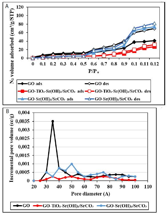
The textural features of the nanocomposites were investigated with the N2 adsorption-desorption isotherms and the results are shown in Figure 4a. According to the International Union of Pure and Applied Chemistry (IUPAC), the shape of the isotherm for the GO-Sr(OH)2/SrCO3 nanocomposite can be classified as a combination of Type II and Type III, indicating the coexistence of mesopores and macropores [58]. The deviation of the desorption isotherm from the adsorption isotherm (hysteresis) can be attributed to the presence of slit or bottle neck pores. The isotherm displayed a significant increase of N2 uptake at P/Po > 0.95, indicating the presence of external surface area and/or textural porosity. In contrast, the isotherm for GO-TiO2-Sr(OH)2/SrCO3 conforms to the Type II isotherm, which is characteristic of low-porosity materials or materials with large macropores. The decrease of the mesopores and macropores volume in GO-TiO2-Sr(OH)2/SrCO3 can be attributed to occupying part of the pores by TiO2 and SrTiO3 reaction products. The inset in Figure 4b presents the pore size distributions for GO, GO-Sr(OH)2/SrCO3 and GO-TiO2-Sr(OH)2/SrCO3 estimated by the density functional theory (DFT) calculations of the N2 adsorption data. The presence of mesopores and macropores is clearly evident in GO, which are then sharply diminished with the addition of Sr(OH)2/SrCO3 and TiO2. Moreover, the specific surface area of GO-TiO2-Sr(OH)2/SrCO3 (5.64 m2/g) was found 75% less than that of GO-Sr(OH)2/SrCO3 (21.47 m2/g), and the pore volume of GO-TiO2-Sr(OH)2/SrCO3 (0.0319 cm3/g) was 84% less than that of GO-Sr(OH)2/SrCO3 (0.1842 cm3/g).

fig 4

Figure 4: (a) Nitrogen adsorption-desorption isotherms and (b) pore size distribution of GO, GO-Sr (OH)2/SrCO3 and GO-TiO2-Sr(OH)2/SrCO3

Effect of Increasing GO Nanoparticle Concentrations during Hydrophobic PAHs Treatment with Photocatalytic Degradation Under Sun Light İrradiation

Preliminary studies showed that the optimum sun light intensity, irradiation time, pH, and temperature were 100 mW/cm2, 360 min, pH = 7.0 and at 22°C, respectively in the presence of 7 mg/l GO nanocomposite concentration (data not shown). The effects of increasing GO nanoparticle concentrations (2 mg/l, 4 mg/l and 8 mg/l) on the removals of PAHs [less hydrophobic (ACL, CRB) and more hydrophobic (BaP, BkF)] under a sun light intensity of 100 mW/cm2, at a sun light irradiation time of 360 min, at pH = 7.0 and at 22°C, respectively (Table 3; SET 1). The maximum removals of ACL, CRB, BaP and BkF hydrophobic PAHs were 87%, 87%, 85% and 84% at 8 mg/l GO nanoparticle concentration under a sun light intensity = 100 mW/cm2, at a photocatalytic powerof 100 W, at sun light irradiation time of 360 min, at a pHof 7.0 and at 22°C, respectively (Table 3; SET 1). The increasing GO nanoparticle concentrations were positively affect the photocatalytic degradation of hydrophobic PAHs (ACL, CRB, BaP and BkF) (Table 3; SET 1).

Table 3: Effect of increasing experimental parameters on photocatalytic degradation of hydrophobic PAHs in a petrochemical industry wastewater under sun light irradiaiton process, at sun light intensity=100 mW/cm2, at pH=7.0 and at 22°C, respectively (n=3, mean values)

Set

Parameters Hydrophobic PAHs removals (%)
Less hydrophobic

More hydrophobic

ACL

CRB BaP

BkF

1 GO nanoparticle concentrations (mg/l)
2

54

56 59

58

4

71

73 70

69

8

87

87 85

84

2 TiO2 nanoparticle concentrations (mg/l)
1

59

57 64

75

3

63

66 77

81

6

76

78 83

86

9

89

90 91

92

3 GO-TiO2-Sr(OH)2/SrCO3 nanocomposite concentrations (mg/l)
1

76

75 80

92

2

89

84 86

97

4

97

98 98

99

4 Sun light irradiation times (min)
30

56

61 60

65

120

65

68 65

66

240

74

76 72

79

360

81

80 84

84

2 Photocatalytic Powers (W)
10

56

62 67

69

50

69

70 78

74

100

84

86 88

89

Effect of Increasing TiO2 Nanoparticle Concentrations during Hydrophobic PAHs Treatment with Photocatalytic Degradation Under Sun Light Irradiation

The preliminary studies showed that the optimum removals for PAHs [less hydrophobic (ACL, CRB) and more hydrophobic (BaP, BkF)] were obtained at a TiO2 concentration of 8 mg/L under sun light intensity of 98 mW/cm2, at photocatalytic power of 95 W, at sun light irradiation time of 350 min, at pH = 7.1 and at a temperature of 22°C (data not shown). The effects of increasing TiO2 nanoparicle concentrations (1 mg/l, 3 mg/l, 6 mg/l and 9 mg/l) were measured to detect the PAHs yields [less hydrophobic (ACL, CRB) and more hydrophobic (BaP, BkF)] under a sun light intensity of 100 mW/cm2, at photocatalytic power = 100 W, at sun light irradiation time of 360 min, ata pH = 7.0 at 22°C (Table 3; SET 2). The removals of BaP, BkF, ACL and CRB PAHs increased from 75% up to 86% as the TiO2 nanoparticle concentrations was increased from 1 mg/l up to 6 mg/l, whereas 1-3 mg/l TiO2 nanoparicle concentrations dis not significantly contribute to the hydrophobic PAHs (ACL, CRB, BaP and BkF) removals (Table 3; SET 2). The maximum 89%ACL, 90%CRB, 91%BaP and 92%BkF hydrophobic PAHs removals were detected at 9 mg/l TiO2 nanopartilce concentration, under a sun light intensity = 100 mW/cm2, at a photocatalytic powerof 100 W, at sun light irradiation time of 360 min, at a pHof 7.0 and at 22°C, respectively (Table 3; SET 2). The increasing of TiO2 nanoparticle concentrations positively affected the photocatalytic degradation of hydrophobic PAHs (ACL, CRB, BaP and BkF) during sun light irradiation process (Table 3; SET 2).

Effect of Increasing GO-TiO2-Sr(OH)2/SrCO3 Nanocomposite Concentrations during Hydrophobic PAHs Treatment with Photocatalytic Degradation under Sun Light Irradiation

Based on the preliminary studies the optimum removals of some less hydrophobic (ACL, CRB) and more hydrophobic (BaP, BkF)] PAHs were researched at a sun light intensity of 100 mW/cm2, at photocatalytic power = 100 W, at sun light irradiation time = 360 min, at pH = 7.0 and at 22°C, respectively at a GO-TiO2-Sr(OH)2/SrCO3 concentrations of 3 mg/l (Table 3; SET 3). The removals in BaP, BkF, ACL and CRB increased from 92%, up to 99% as the GO-TiO2-Sr(OH)2/SrCO3 nanocomposite concentration was increased from 1 up to 4 mg/l, at a sun light intensity = 100 mW/cm2, at a photocatalytic power = 100 W, ata sun light irradiation time = 360 min, at 22°C (Table 3; SET 3). The maximum 97%ACL, 98%CRB, 98%BaP and 99%BkF hydrophobic PAHs removals were found at 4 mg/l GO-TiO2-Sr(OH)2/SrCO3 nanocomposite concentration under a sun light intensity = 100 mW/cm2, at a photocatalytic powerof 100 W, at sun light irradiation time of 360 min, at a pHof 7.0 and at 22°C, respectively. The increasing GO-TiO2-Sr(OH)2/SrCO3 nanocomposite concentrations were found to be positively affect for the photocatalytic degradation of hydrophobic PAHs (ACL, CRB, BaP and BkF) (Table 3; SET 3).

An optimum GO-TiO2-Sr(OH)2/SrCO3 nanocomposite concentration of 4 mg/l increase the ionic strength of the aqueous phase, driving the PAHs to the bulk-bubble interface in a photocatalytic reactor. This, increases the partitioning of the PAH species upon radical scavengers in a photocatalytic reactor. Beyond the partitioning enhancement, the presence of salt reduces the vapor pressure and increases the surface tension of the PAHs [59]. Therefore, the solubility of the solution decreases and the diffusion of solutes decreases from the bulk solution to the bubble-liquid interface with administration of decreasing GO-TiO2-Sr(OH)2/SrCO3 nanocomposite concentrations in the photocatalytic reactor [60]. The high PAH removals in raised GO-TiO2-Sr(OH)2/SrCO3 nanocomposite concentrations can be explained by the fact that a higher amount of GO-TiO2-Sr(OH)2/SrCO3 nanocomposite will create more salting out effect than the lower amount and thus increase the interfacial concentration of the PAHs. In our study, no contribution of GO-TiO2-Sr(OH)2/SrCO3 nanocomposite >4 mg/l to the PAH yields could be attributed to the sinergistic and antagonistic effects of the by-products and to the more hydrophobic (BaP, BkF) and less hydropholic (ACL, CRB) nature of PAHs present in petrochemical industry wastewaters (Table 3; SET 3).

Effect of Increasing Sun Light Irradiation Times during Hydrophobic PAHs Treatment with Photocatalytic Degradation Under Sun Light Irradiation

The effects of increasing sun light irraditiaon times (30 min, 120 min, 240 min and 360 min) were measured in PAHs [less hydrophobic (ACL, CRB) and more hydrophobic (BaP, BkF)] under sun light intensity = 100 mW/cm2, at photocatalytic power = 100 W, at pH = 7.0 at 22°C, respectively (Table 3; SET 4).

The removals of BaP, BkF, ACL and CRB increased from 56-65% up to 72-79% as the sun light irradiation times was increase from 30 min up to 240 min, whereas 30-120 min sun light irradiation times dis not significantly contribute to the hydrophobic PAHs (ACL, CRB, BaP and BkF) removals was not observed (Table 3; SET 4). The maximum 81%ACL, 80%CRB, 80%BaP and 84%BkF hydrophobic PAHs removals were indicated at 360 min sun light irradiaiton time, under sun light intensity = 100 mW/cm2, at photocatalytic power = 100 W, at pH = 7.0 and at 22°C, respectively (Table 3; SET 4). The increasing sun light irradiaiton times were affected positively effect for the photocatalytic degradation hydrophobic PAHs (ACL, CRB, BaP and BkF) during sun light irradiation process (Table 3; SET 4).

Effect of Increasing Photocatalytic Powers During Hydrophobic PAHs Treatment with Photocatalytic Degradation Under Sun Light Irradiation

The effects of increasing photocatalytic powers (10 W, 50 W and 100 W) were measured in PAHs [less hydrophobic (ACL, CRB) and more hydrophobic (BaP, BkF)] under sun light intensity = 100 mW/cm2, at sun light irradiation time = 360 min, at pH = 7.0 at 22°C, respectively (Table 3; SET 5).

The removals of BaP, BkF, ACL and CRB increased from 56-69% up to 69-78% as the photocatalytic powers was increase from 10 W up to 50 W, whereas 10-50 W photocatalytic powers dis not significantly contribute to the hydrophobic PAHs (ACL, CRB, BaP and BkF) removals was not obtained (Table 3; SET 5). The maximum 84%ACL, 86%CRB, 88%BaP and 89%BkF hydrophobic PAHs removals were indicated at 100 W photocatalytic power, under sun light intensity = 100 mW/cm2, at sun light irradiation time = 360 min, at pH = 7.0 and at 22°C, respectively (Table 3; SET 5). The increasing photocatalytic powers were affected positively effect for the photocatalytic degradation hydrophobic PAHs (ACL, CRB, BaP and BkF) during sun light irradiation process (Table 3; SET 5).

Photocatalytic Activity

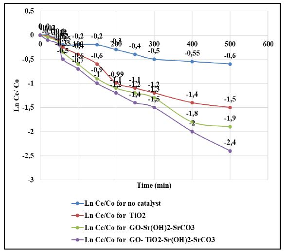
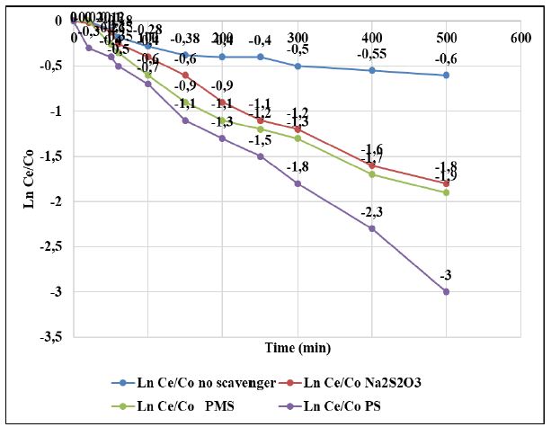
PAHs is resistant to photolysis under sun light [61]. The control tests showed that nearly 85% of PAHs still retained in the solution after 360 min sun irradiation time (Table 4 and Figure 5) and the pseudo-first-order rate constant was k = 0.0006 ± 0.0001 1/min. The addition of TiO2 nanoparticle enhanced the photodegradation rate by 3 folds (k = 0.0016 1/min) (Table 4 and Figure 5). The addition of GO increased the photodegradation yield (k = 0.0019 ± 0.0001 l/min) (Table 4 and Figure 5). The UV light in the sun light irradiation is the main driving energy for the photocatalytic activity of TiO2. The synthesized GO-Sr(OH)2/SrCO3 showed a slightly better photocatalytic activity (k = 0.0021 ± 0.0001 1/min) than TiO2 and GO nanoparticle (Table 4 and Figure 5). As expected, the GO-TiO2-Sr(OH)2/SrCO3 nanocomposite exhibited the highest photocatalytic activity and greatly accelerated the photocatalytic degradation rate. It was shown a synergistic interaction among the three nanocomponents, i.e., GO, TiO2 and Sr(OH)2/SrCO3, which can facilitate utilization of both UV and visible light energy in the sun light irradiation.

Table 4: The rate constants of GO, TiO2 and GO-TiO2-Sr(OH)2/SrCO3 after photocatyalytic degradation with sun light irradiation process

Sun light irradiaiton time (min)

k (1/min)
Control GO TiO2

GO-TiO2-Sr(OH)2/SrCO3

30

0.0001 ± 0.00001

0.0005 ± 0.0001 0.0004 ± 0.0001

0.0009 ± 0.0001

120 0.0003 ± 0.0001 0.0011 ± 0.0001 0.0009 ± 0.0001

0.0013 ± 0.0001

240

0.0005 ± 0.0001 0.0014 ± 0.0001 0.0012 ± 0.0001 0.0017 ± 0.0001
360 0.0006 ± 0.0001 0.0019 ± 0.0001 0.0016 ± 0.0001

0.0021 ± 0.0001

fig 5

Figure 5: Photocatalytic degradation of PAHs by various synthesized catalysts, at light intensity = 100 mW/cm2, at solution volume = 250 ml, at initial PAHs concentration = 1 mg/l, catalyst dosage = 50 mg/l, at sun light irradiation time = 360 min, at pH=7.0 and at 22°C

In the photocatalytic activity of GO-TiO2-Sr(OH)2/SrCO3 firstly, the hybridization of the two coupling semiconductors (TiO2 and Sr(OH)2/SrCO3) shifted the optical absorption to the higher wavelength region and impel the transfer of photo-excited electron and holes to opposite directions (data not shown) [62]. Secondly, the GO sheets can further promote the transport of the photo-excited electrons, and thus inhibit the recombination of electrons and holes. And thirdly, the reaction product SrTiO3 has high photocatalytic activity and can also contribute to the enhanced photodegradation of PAHs.

Contribution of Reactive Oxygen Species (ROS) on the Photocatalytic Yields of PAHs

In generally, photocatalytic oxidation processes, ROS (potassium peroxymonosulfate (PMS, HSO5), potassium persulfate (PS, K2S2O8) and the quenching agent sodium thiosulfate (Na2S2O3) generated during the photocatalytic reactions are mainly responsible for the degradation of organic pollutants [63]. Preliminary studies showed that among the concentrations studied with 1.1 mg/l PMS, 0.9 mg/l PS and 0.79 mg/l Na2S2O3 highest photooxidaton yields was detected.

PS and PMS can undergo homolytic dissociation of the peroxide bond from radiation or thermal activation and give SO4-● radicals, and sulfate and OH radicals, respectively (Equation 2 and Equation 3).

for 2,3

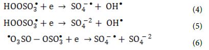
The oxidants can also act as electron acceptors of the photo-excited electron from the conduction band of the GO-TiO2-Sr(OH)2/SrCO3 and through electron transfer mechanisms to give additional sulfate and hydroxyl radicals based on the reactions listed below (Equation 4, Equation 5 and Equation 6) [64-66].

for 4,5,6

Heat activation of oxidants did not contributed on radical formation because of the temperature in the reactor and the relatively short treatment times compared to what was reported needed in the literature. On the other hand, homolytic dissociation of the peroxide bond of the oxidants through radiation seems to be a more probable mechanism. Even though, both oxidants have low absorption in the UVA range, the adsorption of PS at λ = 365 nm is four times the one of PMS, when measured in solutions of the same concentration of active species. This indicates that PS has a better ability to adsorb photons compared to PMS and therefore, more radicals can be formed. The remaining PMS and form peroxymonosulfate radicals (SO5-●) (Equation 7 and Equation 8) that have significantly reduced oxidation ability and higher selectivity (redox potential 1.1 V, at pH = 7.0) to SO4-● radicals (Table 5).

for 7,8

On the other hand, reaction of PS with a SO4-● radical will cause the formation of another SO4-● radical (Equation 9) which leaves the oxidative capacity of the system unaltered. The effects of (PMS, HSO5), (PS, K2S2O8) and Na2S2O3 on the photocatalytic degradation rates of the studied BkF PAH were tabulated (Table 5).

for 9

Table 5: Contributions of ROS to photocatalytic degradation of BkF PAH by GO-TiO2-Sr (OH)2/SrCO3 under simulated solar irradiation

Scavengers

Scavenging radicals

k (1/min)

None (Only GO-TiO2-Sr (OH)2/SrCO3)

0.0061

PMS

HSO5 –

0.0062

PS

K2S2O8

0.0067

Na2S2O3

SO4-2

0.0063

Photodegradation Pathway

At Table 6 and Figure 6 presents the reaction intermediates during the photocatalytic degradation of hydrophobic PAHs (ACL, CRB, BaP and BkF) by GO-TiO2-Sr(OH)2/SrCO3 under sun light irradiation process. It is noteworthy that the reaction rate and selectivity can be altered by the reaction matrix. For example, using dimethyl carbonate instead of water as the medium, the selectivity of TiO2 for the partial photooxidation of hydrophobic PAHs (ACL, CRB, BaP and BkF) was enhanced.

Table 6: By-products of BkF, BaP and ACL PAHs at sun light intensity = 100 mW/cm2, at solution volume= 250 ml, at initial PAHs concentration = 1 mg/l, at pH=7.0 ± 0.2, at 22°C, at 360 min sun light irradiaiton time, respectively (n=3, mean ± SD)

PAHs name

Initial PAH concentration (ng/ml)

Photocatalytic degradation metabolites (ng/ml)

BkF

0.804 ± 0.001

benzoic acid: 0.21 ± 0.002

FL: 0.59 ± 0.005

BaP 0.077 ± 0.003 benzoic acid: 0.028 ± 0.001

PY: 0.0040 ± 0.00014

ACL 53.42 ± 0.05 NAP: 44.13 ± 0.07

fig 6

Figure 6: Photocatalytic degradation of PAHs by GOTiO2-Sr(OH)2/SrCO3 in the various radical scavengers, at sun light intensity = 100 mW/cm2, at solution volume= 250 ml, at initial PAHs concentration = 1 mg/l, at catalyst dosage = 50 mg/l, at pH=7.0 ± 0.2, T=22 ± 1°C, at TBA dosage = 200 mg/l, at NaN3 dosage = 200 mg/l, at BQ dosage = 200 mg/l and at CAT dosage = 4000 U/ml, respectively

Determination of the Acute Toxicity of Studied PAHs on Daphnia magna before and after Treatment of Hydrophobic PAHs Under Photocatalytic Degradation at Different Experimental Conditions

The raw petrochemical industry wastewater samples induced 95% motility inhibition to Daphnia magna cells (Table 7). This inhibition could be attributed to the mixed reacalcitrant carcinogenic hydrophobic PAHs with high benzene rings and to the synergistic effects of the aforementioned more hydrophobic PAHs with less hydrophobic PAHs in petrochemical industry wastewaters. When Daphnia magnas were exposed to the effluent samples treated withonly photolysis without catalyst at 22°C for 360 min sun light irradiaiton time a significant reduction in inhibition (10.01%) was not observed (the inhibition decreased from initial 98% to 88%). In other words, photolysis alone was not sufficient to remove the toxicity of recalcitrant by-products from the petrochemical wastewater (Table 7). The maximum removals in inhibition were observed in photocatalytic degraded petrochemical wastewater containing 8 mg/l GO nanoparticle, 9 mg/l TiO2 nanoparticle and 4 mg/l GO-TiO2-Sr(OH)2/SrCO3 nanocomposite concentrations at a neutral pH = 7.0 after 360 min sun light irradiation time at 22°C. A decreasing toxicity trend due to long sun light irradiaiton time with catalyst can be explained by the formation of less toxic by-products over time. The petrochemical wastewater containing TiO2 nanoparticles >10 mg/l displayed toxicity to Daphnia magna after 360 min sun light irradiation time. Similarly, GO nanoparticle and GO-TiO2-Sr(OH)2/SrCO3 nanocomposite concentrations >10 mg/l and >6 mg/l caused inhibition to Daphnia magna motility after 360 min sun light irradiation time at 22°C. A significant corrrelation between Daphnia manga acute toxicity and TiO, GO and GO-TiO2-Sr(OH)2/SrCO3 nanocomposite concentrations was observed after 360 min sun light irradiation time according to multiple regression analysis (R2 = 0.87, F = 17.99. p = 0.001).

Table 7: Effect of sun light irradiaiton times during photocatalytic degradation process on the acute toxicity (EC50) removal efficiencies at different operational conditions at pH=7.0, at 22°C (n=3, mean values)

Sets

IAT

Operational conditions


PDA at 22 °C (Control)

GO TiO2

GO-TiO2-Sr(OH)2/SrCO3

EC50

t=0

ATRi SLIT a EC50


ATR GO b EC50

t=360

ATRe TiO2 c EC50 t=360 ATRe GO-TiO2-Sr(OH)2/SrCO3d EC50

t=360

ATRe

1

342.56

98 30 359.04 2.01 2 631.05 99.99 1 484.67 67 1 590.56 97.00
2 342.56 98 120 364.78 6.23 4 604.67 90.00 3 545.56 78 2 626.56

99.00

3

342.56 98 240 377.67 8.34 8 540.78 76.99 6 587.45 94 4 630.45 99.94
4 342.56 98 360 380.12 10.01 9 504.67 70
IAT: Initial acute toxicity; a: sun light irradiation times (min); b: GO concentration (mg/l); c: TiO2 nanoparticle concentrations (mg/l); d: GO-TiO2-Sr(OH)2/SrCO3 nanocomposite concentration (mg/l); PDA: Photocatalytic degradation alone without additives (Control); EC50 t=0 : Initial acute toxicity before photocatalytic degradation (ng/ml); ATRi: Initial inhibition percentage before photocatalytic degradation; EC50 : Acute toxicity after photocatalytic degradation in control versus sun light irradiation time (ng/ml); ATR: Acute toxicity removal (%) in control versus sun light irradiation time; ATRe: Acute toxicity removal (%) after 360 min sun light irradiation time; EC50 t=360 : acute toxicity after 360 min sun light irradiaiton time (ng/ml).

Toxicity results showed that both high concentrations of GO, TiO2 and GO-TiO2-Sr(OH)2/SrCO3 influence the toxicity of PAH mixtures which may interact with the PAHs and their degraded metabolites to form different by-products during photocatalytic degradation. These by-products exhibit synergistic and antagonistic toxicity effects on Daphnia magna as well. The effective PAH concentrations caused 50% mortality in Daphnia magna cells (EC50 value as ng/ml) increased from initial 342.56 ng/ml to EC50 = 631.05 ng/ml, at pH = 7.0 and at 22°C after 360 min sun light irradiation time resulting in a maximum acute toxicity removal of 99.99% at 1 mg/l GO-TiO2-Sr(OH)2/SrCO3 nanocompoasite concentration (Table 7; SET 1). The EC50 value increased from initial 342.56 ng/ml to EC50 = 587.45 ng/ml at a TiO2 concentration of 6 mg/l after 360 min sun light irradiation time, at pH = 7.0 and at 22°C resulting in a maximum acute toxicity removal of 94.00% (Table 7; SET 3). The EC50 value increased from initial 342.56 ng/ml to EC50 = 630.45 ng/ml at 8 mg/l GO nanopartilce concentration was measured to 99.94% maximum acute toxicity removal, at pH = 7.0, at 22°C after 360 min sun light irradiation time, respectively (Table 7; SET 3). In this acute toxicity reduction the EC50 value of petrochemical industry wastewater increased to EC50 = 631.05 ng/ml. Low acute toxicity removals found at high GO nanoparticle concentrations could be attributed to their detrimental effect on the Daphnia magna cells (Table 6; SET 1).

A strong significant correlation between EC50 values and PAH removals showed that the Daphnia magna acute toxicity test alone can be considered aa a reliable indicator of petrochemical wastewater toxicity (R2 = 0.87, F = 17.99. p = 0.001). Similarly, a strong linear correlation between threshold concentrations of GO, TiO2, GO-TiO2-Sr(OH)2/SrCO3 and decrease in inhibitions was observed (R2 = 0.91, F = 3.89, p = 0.001) while the correlation between the inhibition decrease and GO, TiO2 and GO-TiO2-Sr(OH)2/SrCO3 nanocomposite concentrations above the threshold values was weak and not significant (R2 = 0.38, F = 3.81, p = 0.001). In this study, the Daphnia magna acute toxicity test alone can be considered a reliable indicator of petrochemical industry wastewater toxicity.

Conclusion

The results of this study showed that the hydrophobic PAHs in a petrochemical industry wastewater with high benzene rings could be removed as successfully as the less hydrophobic PAHs (ACL and CRB) and more hydrophobic PAHs (BaP and BkF) with photocatalytic degradation under sun light irradiation process. The maximum removals of ACL, CRB, BaP and BkF hydrophobic PAHs were 87%, 87%, 85% and 84% at 8 mg/l GO nanoparticle concentration under a sun light intensity = 100 mW/cm2, at a photocatalytic powerof 100 W, at sun light irradiation time of 360 min, at a pHof 7.0 and at 22°, respectively. The maximum 89%ACL, 90%CRB, 91%BaP and 92%BkF hydrophobic PAHs removals were detected at 9 mg/l TiO2 nanopartilce concentration, under a sun light intensity = 100 mW/cm2, at a photocatalytic powerof 100 W, at sun light irradiation time of 360 min, at a pHof 7.0 and at 22°C, respectively. The maximum 97%ACL, 98%CRB, 98%BaP and 99%BkF hydrophobic PAHs removals were found at 4 mg/l GO-TiO2-Sr(OH)2/SrCO3 nanocomposite concentration under a sun light intensity = 100 mW/cm2, at a photocatalytic powerof 100 W, at sun light irradiation time of 360 min, at a pHof 7.0 and at 22°C, respectively.

The addition of TiO2 nanoparticle enhanced the photodegradation rate by 3 folds (k = 0.0016 1/min). The addition of GO increased the photodegradation yield (k = 0.0019 ± 0.0001 l/min). The synthesized GO-Sr(OH)2/SrCO3 showed a slightly better photocatalytic activity (k = 0.0021 ± 0.0001 1/min) than TiO2 and GO nanoparticle. As expected, the GO-TiO2-Sr(OH)2/SrCO3 nanocomposite exhibited the highest photocatalytic activity and greatly accelerated the photocatalytic degradation rate. It was shown a synergistic interaction among the three nanocomponents, i.e., GO, TiO2 and Sr(OH)2/SrCO3, which can facilitate utilization of both UV and visible light energy in the sun light irradiation. 1.1 mg/l PMS, 0.9 mg/l PS and 0.79 mg/l Na2S2O3 highest photooxidaton yields was detected.

The effective PAH concentrations caused 50% mortality in Daphnia magna cells (EC50 value as ng/ml) increased from initial 342.56 ng/ml to EC50 = 631.05 ng/ml, at pH = 7.0 and at 22°C after 360 min sun light irradiation time resulting in a maximum acute toxicity removal of 99.99% at 1 mg/l GO-TiO2-Sr(OH)2/SrCO3 nanocompoasite concentration. In sum, GO-TiO2-Sr(OH)2/SrCO3 nanocomposites holds the potential to serve as a highly effective and robust photocatalyst for energy-effective photodegradation of PAHs (and potentially other persistent organic pollutants) in complex water matrices, and the multiplicative model is a useful tool for predicting the photocatalytic performances under several experimental conditions.

Acknowledgements

This research study was undertaken in the Environmental Microbiology Laboratury at Dokuz Eylül University Engineering Faculty Environmental Engineering Department, Izmir-Turkey.

References

  1. Fu J, Sheng S, Wen T, Zhang Z-M, Wang Q, et al. (2011a) Polycyclic aromatic hydrocarbons in surface sediments of the Jialu River. Ecotoxicology 20: 940-950. [crossref]
  2. Fu J, Gong Y, Zhao X, O’Reilly SE, Zhao D (2014) Effects of oil and dispersant on formation of marine oil snow and transport of oil hydrocarbons. Environmental Science & Technology 48: 14392-14399. [crossref]
  3. Gong Y, Fu J, O’Reilly SE, Zhao D (2015) Effects of oil dispersants on photodegradation of pyrene in marine water. Journal of Hazardous Materials 287: 142-150. [crossref]
  4. Fu J, Ding Y-H, Li L, Sheng S, Wen T, et al. (2011b) Polycyclic aromatic hydrocarbons and ecotoxicological characterization of sediments from the Huaihe River, China, Journal of Environmental Monitoring and Assessment, 13: 597-604. [crossref]
  5. Banjoo DR and Nelson PK (2005) Improved ultrasonic extraction procedure for the determination of polycyclic aromatic hydrocarbons in sediments. Journal of Chromatography A, 1066: 9-18. [crossref]
  6. Sponza DT and Oztekin R (2010) Effect of sonication assisted by titanium dioxide and ferrous ions on Poly aromatic hydrocarbons (PAHs) and toxicity removals from a petrochemical industry wastewater in Turkey. Journal of Chemical Technology and Biotechnology 85: 913-925
  7. Quesada-Peñate I, Julcour-Lebigue C, Jáuregui-Haza U.-J, Wilhelm A-M, et al. (2009) Sonolysis of levodopa and paracetamol in aqueous solutions. Ultrasonics Sonochemistry 16: 610-616.
  8. Hoffmann MR, Martin ST, Choi W, Bahnemann DW(1995) Environmental applications of semiconductor photocatalysis. Chemical Reviews 95: 69-96.
  9. Sannino F, Pernice P, Imparato C, Aronne A, D’Errico G, et al. (2015) Hybrid TiO2-acetylacetonate amorphous gel-derived material with stably adsorbed superoxide radical active in oxidative degradation of organic pollutants. RSC Advances, 5: 93831-93839.
  10. Zeng P, Zhang Q, Zhang X, Peng T (2012) Graphite oxide-TiO2 nanocomposite and its efficient visible-light-driven photocatalytic hydrogen production. Journal of Alloys and Compounds 516: 85-90.
  11. Di Paola A, Garcia-López E, Ikeda S, Marcı G, Ohtani B. (2002) Photocatalytic degradation of organic compounds in aqueous systems by transition metal doped polycrystalline TiO2. Catalysis Today 75: 87-93.
  12. Zhao K, Zhao SL, Qi J, Yin HJ, Gao C, et al. (2016) Cu2O clusters grown on TiO2 nanoplates as efficient photocatalysts for hydrogen generation. Inorganic Chemistry Frontiers 3: 488-493.
  13. Qu L, Liu Y, Baek JB, Dai L (2010) Nitrogen-doped graphene as efficient metal-free electrocatalyst for oxygen reduction in fuel cells. ACS Nano 4: 1321-1326. [crossref]
  14. Liang Y, Li Y, Wang H, Zhou J, Wang J. (2011) Co3O4 nanocrystals on graphene as a synergistic catalyst for oxygen reduction reaction. Nature Materials 10: 780-786. [crossref]
  15. Guo J, Zhu S, Chen Z, Li Y, Yu Z (2011) Sonochemical synthesis of TiO2 nanoparticles on graphene for use as photocatalyst, Ultrasonics Sonochemistry.18: 1082-1090. [crossref]
  16. Stengl V, Henych J, Vomáčka P and Slušná M (2013) Doping of TiO2-GO and TiO2-rGO with noble metals: synthesis, characterization and photocatalytic performance for azo dye discoloration. Photochemistry and Photobiology 89: 1038-1046.
  17. Turekian KK, Wedepohl KH (1961) Distribution of the elements in some major units of the Earth’s crust. Geological Society of America Bulletin 72: 175.
  18. Yousefi R, Jamali-Sheini F, Cheraghizade M, Khosravi-Gandomani S, Sáaedi A, et al. (2015)Enhanced visible-light photocatalytic activity of strontium-doped zinc oxide nanoparticles. Materials Science in Semiconductor Processing 32: 152.
  19. Song L, Zhang S, Chen BA (2009) novel visible-light-sensitive strontium carbonate photocatalyst with high photocatalytic activity. Catalysis Communications 10: 1565-1568.
  20. Momenian HR, Gholamrezaei S, Salavati-Niasari M, Pedram B, Mozaffar F, et al. (2013) Sonochemical synthesis and photocatalytic properties of metal hydroxide and carbonate (M: Mg, Ca, Sr or Ba) nanoparticles. Journal of Cluster Science 24: 1031-1042.
  21. Márquezherrera A, Ovandomedina V, Castilloreyes B, Zapatatorres M, Meléndezlira, M, et al. (2016) J. Facile synthesis of SrCO3-Sr(OH)2/PPy nanocomposite with enhanced photocatalytic activity under visible light. Materials 9: 30. [crossref]
  22. Pichat PA (2007) brief overview of photocatalytic mechanisms and pathways in water. Water Science and Technology 55: 167-173. [crossref]
  23. Buxton GV, Greenstock CL, Helman WP, Ross AB (1988) Critical review of rate constants for reactions of hydrated electrons, hydrogen atoms and hydroxyl radicals in aqueous solution. Journal of Physical and Chemical Reference Data 17: 513-886.
  24. Robertson PKJ, Lawton LA, Münch B, Rouzade J (1997) Destruction of cyanobacterial toxins by semiconductor photocatalysis. Chemical Communications 393-394. [crossref]
  25. Feitz AJ, Waite TD, Jones GJ, Boyden BH, Orr PT (1999) Photocatalytic degradation of the blue green algal toxin microcystin-LR in a natural organic-aqueous matrix. Environmental Science and Technology 33: 243-249.
  26. Lawton LA, Robertson PKJ, Cornish BJPA, Marr IL, Jaspars M (2003) Processes influencing surface interaction and photocatalytic destruction of microcystins on titanium dioxide photocatalysts. Journal of Catalysis 213: 109-113 [crossref]
  27. Pelaez M, de la Cruz AA, O’Shea K, Falaras P, Dionysiou DD (2011) Effects of water parameters on the degradation of microcystin-LR under visible light-activated TiO 2 photocatalyst. Water Research 45: 3787-3796. [crossref]
  28. Choi H, Antoniou MG, Pelaez M, De La Cruz AA, Shoemaker JA, et al. (2007) Mesoporous nitrogen-doped TiO2 for the photocatalytic destruction of the cyanobacterial toxin microcystin-LR under visible light irradiation. Environmental Science and Technology 41: 7530-7535 [crossref]
  29. Pelaez M, Falaras P, Likodimos V, Kontos AG, de la Cruz AA, et al. (2010) Synthesis, structural characterization and evaluation of sol-gel-based NF-TiO2 films with visible lightphotoactivation for the removal of microcystin-LR. Applied Catalysis B: Environmental 99: 378- 387.
  30. Andersen J, Han C, O’Shea K, Dionysiou DD. (2014) Revealing the degradation intermediates and pathways of visible light-induced NF-TiO2 photocatalysis of microcystin-LR. Applied Catalysis B: Environmental 154-155: 259-266.
  31. Fotiou T, Triantis TM, Kaloudis T, Hiskia A (2015) Evaluation of the photocatalytic activity of TiO2 based catalysts for the degradation and mineralization of cyanobacterial toxins and water off-odor compounds under UV-A, solar and visible light. Chemical Engineering Journal 261: 17-26.
  32. Fotiou T, Triantis TM, Kaloudis T, O’Shea KE, Dionysiou DD, et al. (2016) Assessment of the roles of reactive oxygen species in the UV and visible light photocatalytic degradation of cyanotoxins and water taste and odor compounds using C-TiO2. Water Research 90: 52-61. [crossref]
  33. Pelaez M, Falaras P, Kontos AG, De la Cruz AA, O’shea K, et al. (2012) A comparative study on the removal of cylindrospermopsin and microcystins from water with NF-TiO 2-P25 composite films with visible and UV- vis light photocatalytic activity. Applied Catalysis B: Environmental 121-122: 30-39.
  34. Eberson L (1982) Electron-Transfer Reactions in Organic Chemistry, Advances in Physical Organic Chemistry 18: 79-185.
  35. Neta P, Huie RE, Ross AB (1988) Rate constants for reactions of inorganic radicals in aqueous solution. Journal of Physical and Chemical Reference Data 17: 1027-1284.
  36. Wang Y, Hong C (1999) Effect of hydrogen peroxide, periodate and persulfate on photocatalysis of 2- chlorobiphenyl in aqueous TiO2 suspensions. Water Research.33: 2031-2036.
  37. Legrini O, Oliveros E, Braun AM (1993) Photochemical processes for water treatment. Chemical Reviews 93: 671-698. [crossref]
  38. Anipsitakis GP, Dionysiou DD (2004) Transition metal/UV-based advanced oxidation technologies for water decontamination. Applied Catalysis B: Environmental 54: 155-163.
  39. Anipsitakis GP, Dionysiou DD, MA Gonzalez (2006) Cobalt-mediated activation of peroxymonosulfate and sulfate radical attack on phenolic compounds, Implications of chloride ions. Environmental Science and Technology 40: 1000-1007. [crossref]
  40. Antoniou MG, de la Cruz AA, Dionysiou DD (2010a) Degradation of microcystin-LR using sulfate radicals generated through photolysis, thermolysis and e- transfer mechanisms. Applied Catalysis B: Environmental 96: 290-298.
  41. Antoniou MG, De La Cruz AA, Dionysiou DD (2010b) Intermediates and reaction pathways from the degradation of microcystin-LR with sulfate radicals. Environmental Science and Technology.44: 7238-7244.
  42. He X, de la Cruz AA, O’Shea KE, Dionysiou DD (2014) Kinetics and mechanisms of cylindrospermopsin destruction by sulfate radical-based advanced oxidation processes. Water Research 63: 168-178
  43. He X, de la Cruz AA, Hiskia A, Kaloudis T, O’Shea K, et al. (2015) Destruction of microcystins (cyanotoxins) by UV-254 nm-based direct photolysis and advanced oxidation processes (AOPs): Influence of variable amino acids on the degradation kinetics and reaction mechanisms. Water Research.74: 227-238. [crossref]
  44. Antonopoulou M and Konstantinou IK (2014) Effect of oxidants in the photocatalytic degradation of DEET under simulated solar irradiation in aqueous TiO2 suspensions. Global NEST Journal 16: 507-515.
  45. Augugliaro V, Baiocchi C, Prevot AB, García-López E, Loddo V, et al. (2002) Azo-dyes photocatalytic degradation in aqueous suspension of TiO2 under solar irradiation. Chemosphere .49: 1223-1230. [crossref]
  46. Saquib M and Muneer M (2003) TiO2/mediated photocatalytic degradation of a triphenylmethane dye (gentian violet), in aqueous suspensions. Dyes and Pigments 56: 37-49.
  47. Hummers Jr WS and Offeman RE (1958) Preparation of graphitic oxide. Journal of the American Chemical Society 80: 1339.
  48. Xu Z, Li Q, Gao S, Shang JK (2010) As(III) removal by hydrous titanium dioxide prepared from one-step hydrolysis of aqueous TiCl4 solution. Water Research 44: 5713-5721. [crossref]
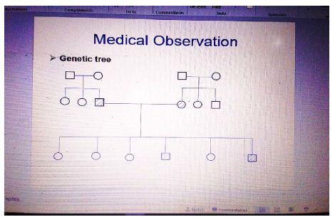
  49. Fu J, Gong Y, Cai Z, O’Reilly SE, Zhao D (2017) Mechanistic investigation into sunlight- facilitated photodegradation of pyrene in seawater with oil dispersants. Marine Pollution Bulletin 114: 751-758.
  50. Lindsey ME and Tarr MA (2000) Quantitation of hydroxyl radical during Fenton oxidation following a single addition of iron and peroxide. Chemosphere 41: 409-417. [crossref]
  51. Eaton AD, Clesceri LS, Rice EW, Greenberg AE, Franson MAH. (2005) Standard Methods for the Examination of Water and Wastewater’, Ed. by Franson MAH, (21th ed.), American Public Health Association (APHA), American Water Works Association (AWWA), Water Environment Federation (WEF), American Public Health Association (APHA)
  52. Alavi MA, Morsali A (2010) Syntheses and characterization of Sr(OH)2 and SrCO3 nanostructures by ultrasonic method. Ultrasonics Sonochemistry 17: 132-138. [crossref]
  53. Thamaphat K, Limsuwan P, Ngotawornchai B (2008) Phase characterization of TiO2 powder by XRD and TEM Kasetsart. Journal of Natural Sciences 42: 357-361.
  54. Huang S.-T, Lee WW, Chang J-L, Huang W-S, Chou S.-Y(2014) Hydrothermal synthesis of SrTiO3 nanocubes: characterization, photocatalytic activities, and degradation pathway. Journal of the Taiwan Institute of Chemical Engineers 45: 1927-1936.
  55. Wysmulek K, Sar J, Osewski P, Orlinski K, Kolodziejak K, et al. (2017) SrTiO3-TiO2 eutectic composite as a stable photoanode material for photoelectrochemical hydrogen production. Applied Catalysis B: Environmental 206: 538-546
  56. He Z, Sun X-Y, Gu X (2017) Electrospinning fabrication of SrTiO3: Er3+ nanofibers and their applications of upconversion properties. Ceramics International 43: 7378-7382.
  57. Kyzas GZ, Travlou NA, Deliyanni EA (2014) The role of chitosan as nanofiller of graphite oxide for the removal of toxic mercury ions. Colloids and Surfaces B: Biointerfaces113: 467-476.
  58. Lowell S (1979) Introduction to Powder Surface Area. John Wiley & Sons
  59. Chakinala AG, Gogate PR, Chand R, Bremner DH, Molina R, et al. (2008) Intensification of oxidation capacity using chloroalkanes as additives in hydrodynamic and acoustic cavitation reactors. Ultrasonics Sonochemistry 15: 164-170. [crossref]
  60. Fu J, Kyzasc GZ, Cai Z, Deliyanni EA, Liu W, et al. (2018) Photocatalytic degradation of phenanthrene by graphite oxide-TiO2-Sr (OH)2/SrCO3 nanocomposite under solar irradiation: Effects of water quality parameters and predictive modelling. Chemical Engineering Journal 335: 290-300.
  61. Chen J, Peijnenburg WJGM, Quan X, Chen S, Martens D, et al. (2001) Is it possible to develop a QSPR model for direct photolysis half-lives of PAHs under irradiation of sunlight? Environmental Pollution 114: 137-143. [crossref]
  62. Kanagaraj T and Thiripuranthagan S (2017) Photocatalytic activities of novel SrTiO3-BiOBr heterojunction catalysts towards the degradation of reactive dyes. Applied Catalysis B Environmental 207: 218-232.
  63. Cavalcante RP, Dantas RF, Bayarri B, González O, Giménez J, et al. (2016) Photocatalytic mechanism of metoprolol oxidation by photocatalysts TiO2 and TiO2 doped with 5% B: primary active species and intermediates. Applied Catalysis B: Environmental 194: 111-122.
  64. Anipsitakis GP and Dionysiou DD (2003) Degradation of organic contaminants in water with sulfate radicals generated by the conjunction of peroxymonosulfate with cobalt. Environmental Science and Technology 37: 4790-4797. [crossref]
  65. Konstantinou IK and Albanis TA (2004) TiO2-assisted photocatalytic degradation of azo dyes in aqueous solution: Kinetic and mechanistic investigations: A review. Applied Catalysis B Environmental 49: 1-14.
  66. Antoniou MG, Nicolaou PA, Shoemaker JA, de la Cruz AA, Dionysiou DD (2009) Impact of the morphological properties of thin TiO2 photocatalytic films on the detoxification of water contaminated with the cyanotoxin, microcystin-LR. Applied Catalysis B: Environmental 91: 165-173.

Wilyman Report on Vaccines: How do We Handle the Next Pandemic, Small, Large or ‘Predicted’?

DOI: 10.31038/IDT.2022321

Abstract

Censorship and active suppression of science and medicine exercised on scale during the COVID-19 pandemic has prevented the wide circulation of legitimate scientific inquiry, critical analysis and discussion. Together with the vaccination failure itself, as foreshadow by Judy Wilyman, the officially sanctioned censorship is now the No.1 issue of our time. It has involved the lockstep behaviour of BigPharma, the Main Stream Media, Big Tech, Governments, Peak Medical, Scientific and Public Health authorities. How did this happen? What are the well spring roots of this extraordinary co-ordinated active suppression of legitimate alternative viewpoints and data analysis in science and medicine?

Introduction – Origin and Global Spread COVID-19

My scientific colleagues and I have been tracking and endeavouring to understand, and thus explain, the space origins and global spread of COVID-19 since late 2019 – early 2020 [1]. We have had to vigorously confront this censorship head on in order to get our scientific message and narrative into the public square. We have tried many ‘publication’ routes to circumvent the pernicious influence of media-sanctioned censorship, both popular press and scientific press.

Our first attempt, an article for the general reader intended for publication in The Australian newspaper was spiked – despite prior back and forth telephone negotiated discussion with then Editor John Lehmann in the first week of February 2020 – by the newspaper’s Health Writer/Editor Natasha Robinson … “because on peer review with your epidemiology and infectious diseases colleagues in Australia, no one believes your explanation” [2]. Of course, that was not the point at all, and I warned both Robinson and Lehmann in prior email and telephone communications that we should not be ‘peer reviewed’ and gave my reason: – a balanced and supposedly fair newspaper like The Australian should have simply let our scientific story ventilate in the public mix of explanations irrespective of the story clashing with conventional received wisdom.

However, it is now clear to many of us that any deviation from the main-stream narrative that COVID-19 jumped from an infected bat or pangolin virus reservoir at a Wuhan wet market or from a Wuhan virus research laboratory could not be ventilated. Our coherent and evidence-based explanation on COVID-19 space origins and global spread by global prevailing wind systems, as well as our analysis of the subsequent vaccination failures and adverse reaction rates has been actively suppressed by continuous mainstream censorship. It is evident that powerful webs of official corruption, influence and collusion between the main stream media have included: Big Tech (Google, Facebook, etc particularly in Australia by Rupert Murdoch’s News Corp); BigPharma (pharmaceutical industry) pushing the vaccine rollouts around the world; National and Federal government endorsement of mandatory vaccinations by all political persuasions, and supported by administrators of our public health policies and pandemic responses. This was implemented through such government health administrative bodies which include: the TGA (Therapeutics Goods Administration, Australia), AMA (Australian Medical Association), ATAGI (Australian Technical Advisory Group on Immunisation), AHPRA (Australian Health Practitioners Regulatory Agency)- equivalent and similar bodies exist in most of the Western Democracies e.g. SAGE (Scientific Advisory Group for Emergencies, Gov. UK), FDA (Food and Drug Administration USA), CDC (Centers for Diseases Control USA).

The Wilyman PhD Thesis

My main motivation in reviewing Judy Wilyman’s 2015 PhD thesis has been to further ventilate her important research, scholarship and evidence-based analyses on how the present public health catastrophe in the response to the COVID-19 pandemic, has unfolded from an evidence-based historical perspective [3]. It has deep historical roots in the commercial profit-inspired modus operandi of the pharmaceutical industry producing vaccines for at least the past 35-40 years.

The issue of how effective the mandated political coercion and lack of informed consent has been in the COVID-19 vaccine roll-out, particularly in Australia and Great Britain, has also been exposed repeatedly and separately by the independent Australian researcher Elizabeth Hart.

See: Compulsory Vaccination and the Media – The Australian Experience, 12 May 2015 or https://davidhealy.org/compulsory-vaccination-and-the-media-the-australian-experience/ Censorship of comments re vaccination policy by The Conversation, 24 April 2016, or https://elizabethhart.files.wordpress.com/2019/05/gmail-censorship-of-comments-re-vaccination-policy-by-the-conversation.pdf; and see her website on investigating the gross over-use of vaccine products and conflicts of interest in vaccination policy vaccinationispolitical.net. Finally listen to her forthright interview on mandated vaccine coercion by Governments, Big Business, Bill and Melinda Gates Foundation, and BigPharma on TNT Radio “Politically Incorrect”, with Mike Tennessee & Richard (Dick) Carsson, Saturday 28 May 2022, https://tntradiolive.podbean.com/e/elizabeth-hart-on-politically-incorrect-28-may-2022/

Accordingly, in my review of the Wilyman thesis all relevant public domain papers and interviews are cited and listed with direct embedded URL links. These include references to: traditional peer-reviewed journal outlets; fast accelerated non-peer reviewed and thus non-censored outlets (Virology Current Research, Infectious Diseases and Therapeutics); URL links to actual interviews as Videos and /or Podcasts as important public records that can be cited legitimately and accessed on non-censored internet sites. These citation actions are because of the necessity for us to get our unfolding COVID-19 epidemiological and genetic data and analysis out into public domain, unfiltered, so other objective interested parties can then peer review our conclusions if they want to – nothing has been hidden or held back, including potential mistakes that will be revealed by further data and analyses in the fullness of time.

Recommended Wilyman Citations and Associated Key Published Papers

These are in Reference list but highlighted first here as a dot-point list:

The Wilyman thesis is in two main parts: First a detailed description of all the cohesive corruption pathways brought about by the pharmaceutical (BigPharma) industry’s commercial agenda in influencing government policy, university research funding (and thus the formal peer reviewed scientific literature), peak medical and regulatory bodies down to the medical coal-face of family doctors and medical specialists – who often get de-listed by the Australian Health Practitioners Regulatory Agency (AHPRA) if they question AMA/AHPRA directives on any of the COVID medical mandates (e.g. Queensland’s Dr Robert Brennan who interviews Specialist Gastroenterologist Dr Andrew McIntyre on TNT Radio https://tntradiolive.podbean.com/e/dr-andrew-mcintyre-on-an-hour-with-robert-brennan-11-may-2022/). This topic occupies content at great depth and length in Chapters 2 through 8 inclusive. This is to be expected in a PhD thesis – great depth of analysis at all crucial levels. I read most but skipped sections that to me were repetitive or obvious, as adjudged by my prior 50 years of lived experience of research funding and its administration in universities and biomedical research institutes. Second a detailed review of the recent science on the foundations of the origins of epidemics and pandemics small, large or ‘created’. This is reviewed and analysed in Chapters 9,10, particularly the roll out of the vaccines actually deployed in two succinct exemplar “created” or “low risk mortality” pandemics: Human Papilloma Virus (HPV) vaccines and protection against cervical cancer (Chapter 9) and the Swine Flu Pandemic 2009 (Chapter 10).

There is much overlap between these two themes and all chapters need to be read and understood to grasp the whole Wilyman achievement, particularly Chapter 2 first which introduces essential foundation concepts. On the issue of actual origins of genuine pandemics throughout history like the recent series of very familiar Influenza pandemics of the 20th Century – such as 1918-19 Spanish Flu and others such as Asian Flu 1957 and Hong Kong Flu 1968, including Swine Flu 2009 – Wilyman’s explanations understandably rely on the mainstream narrative as represented in Hays [7]. This story is familiar: the original viral or pathogen origins begin in an undetected animal reservoir (e.g., chickens, birds, swine, bats, monkeys, camels etc.) and then rapidly jumps to humans by an accumulation of discrete genetic mutations to become a human pathogen, and then rampant person-to-person spread (P-to-P). This traditional understanding of how pandemics emerge and spread in history is of course precisely what our recent work with COVID-19 challenges head on [1,8-10].) and is based, as indicated, on the prior ground breaking epidemiological analyses and historical examples of the 1979 book by astrophysicists and astrobiologists Fred Hoyle and N. Chandra Wickramasinghe now re-printed and updated [11,12].

The tendency of peak health authorities and infectious disease experts to prefix an animal name to the new emerging disease distorts our understanding of the real origins discussed by Hoyle and Wickramasinghe [11]. When a new pathogen comes in like this suddenly from space (protected in putative carbonaceous meteorite dust) some pathogen varieties may also equally infect animals and humans to varying degrees at the same time. That needs to be clearly understood. The full host-range and thus infectivity and spreadability (person-to-person) is unknown at that point. So on the emergence of genuine pandemics throughout history I would disagree with Judy’s mainstream origins assumptions (based on Hayes [7]), but agree with every other aspect of her analyses – on vaccine non-performance, high incidence of adverse events, undone science and the powerful forces of political and financial coercion she describes in clear detail. The problem is, as she clearly shows, that several of the more recent pandemics have been insignificant and of low risk to life no more serious than seasonal Flu mortality (Swine Flu 2009, Chapter 10), or literally ‘created’ as with the roll out of the HPV vaccine to ‘protect women against developing cervical cancer’ (Chapter 9). This led me to question the effectiveness, and thus relevance, of all our prior work on COVID-19’s space origin and subsequent spread by prevailing wind systems [1]. Even if our main recommendations are implemented on global near-Earth surveillance for incoming meteorite pathogens as well as the introduction of safe and effective oral-nasal vaccines for any future respiratory pathogen (cold or flu) the cohesive chains of BigPharma-controlled corruption would ensure all our work on understanding the origin and global spread of COVID-19 would come to naught.

This depressing thought means that pretty well all of Judy Wilyman’s research recommendations (and Elizabeth Hart’s independent analysis and conclusions) need implementation. This is the political challenge:  How do we break these causal corruption chains for the next really big global pandemic? e.g., globally dispersed like COVID-19, even though only a low risk ‘common cold’ virus in the present case [1,9]. The biggest casualty is public trust in our political and health care institutions. Many of us have experienced it directly in Australia, particularly in Victoria where the public health system has frayed or collapsed due to incompetent government pandemic control policies. The cohesive web of corruption revealed by Wilyman’s research is on a massive scale. Particularly all the fault lines revealed by the ‘undone science,’ yet sold as ‘settled science’ to a trusting public. To me the corruption chain is very clearly outlined and can be summarised in the bolded symbolic sequence:

BigPharma $$$<>Government/Politicians<>TGA/FDA, CDC<>AMA, AHPRA, ATAGI<>Research funding in Institutes and Universities<>Family doctors, specialists in hospitals at the medical frontline.

The excitation of fear among frontline doctors fearing de-listing by AHPRA has been staggering to witness by us all who have any medical condition requiring treatment. To be perfectly blunt all the authorities higher up the chain from the frontline have literally been ‘bought off’ so BigPharma can make huge profits. It is a gargantuan scandal, and the COVID-19 response has been a massive public health failure. So again, the question is – How do we break these causal corruption chains in order to handle the next really big genuinely lethal global pandemic, which will inevitable come to our shores?

The first requirement in Australia is that the TGA, the body the public trusts in approving new medicines and vaccines for human use must not receive any funds at all from the pharmaceutical industry– as is the case at present. It must be truly independent – and make the approval or rejection calls based on clear answers to questions like:

  • What is the undone science with this medicine or vaccine?
  • Does it protect human beings from the target disease or does it supply effective safe therapy for the disease or medical condition?
  • How safe is this drug, medicine or vaccine really in the short, medium and long term?

Water-tight unbiased decisions based on evidence must be performed by the TGA – which is clearly not the case at present with COVID-19 vaccines, which have not protected anyone anywhere in the world from catching COVID-19 as we have discussed [1,9,13,14]. Updates on the COVID-19 vaccine in-effectiveness on this issue by the current work of Judy Wilyman and associates can be viewed at People for Safe Vaccines  https://www.peopleforsafevaccines.org.

The entrenched corruption actually enfeebles us – and weakens us, and destroys our ability to act in the public interest in real medical emergencies. We have been lucky with COVID-19. The fact is that COVID-19 is ‘lethal’ – resulting in death – for only a very small faction of the unvaccinated population, perhaps 0.1% of all those exposed to COVID-19 (in the “Immune Defenceless Elderly Co-morbid” portion of the human population). Prior to the vaccine roll-outs this was clear [1,9] even by Dr Fauci and associates [15]. Indeed, all the indications from the publicly available Australian medical COVID-19 epidemiological data analysed by Wilyman and associate Sandy Barrett indicates the COVID-19 associated death rate actually increases (in linear regression) with increasing numbers of vaccine doses, implying a causal role for vaccination itself increasing the COVID-19 associated death rate [16]. This conclusion follows the Omicron strikes since mid- Dec 2021 [1] – the serial vaccinations and boosters are not only ineffective in protection against contracting COVID-19 but are actually causing COVID-19 associated death in vulnerable citizens – this is an appalling public health outcome on a mass scale as vaccination have been widely mandated by intense coercion in Australia to protect people against COVID-19 and stop them spreading the disease.

Precautionary Principle

So, the “Precautionary Principle” [5] which in medicine itself clearly advises “First do no Harm” has been misused, abused and violated by all BigPharma, Governments, Politicians, Public Servants, Public Health Officials and their main bodies in Australia such the AMA, TGA, AHPRA, ATAGI and others. To quote Wilyman [5]: “When the precautionary principle is reversed to put the burden of proof of harmlessness on the general public, instead of the pharmaceutical companies and governments then it can be used to protect the vested interests of industry in government vaccination policies and not the health of the general public.” It represents a massive scandal and betrayal of trust in scientific medicine. One cannot ‘gild the lily’ on this – a blunt confrontation with reality is required by all officials involved in Australia responsible for public health care provision and vaccine roll outs, which were mandated and unleashed on a trusting public – a putative and experimental new generation mRNA Spike protein expression-vector supposed protective medicine that is ineffective as it provides no protective benefit, and is positively dangerous with high adverse event rates, because it was not adequately safety tested that is, the “undone science” as put by Wilyman [3]. The first step is to publicly admit this massive failure and then a genuine honest reform process to begin, to ensure it never happens again in Australia or anywhere else in the world. Other biomedical scientists are making the same call [17,18].

Dangers of All Recent Vaccine Roll-Outs of the past 30-40 Years

The health of our children these past 25 or so years has been weakened and compromised by repeated vaccination early in life, with different antigen types and adjuvants. We have known this for at least 10 years. Thus, the real rise in infant mortality rates in the first year of life (Sudden Infant Death Syndrome, or SIDS) is causally related (linear regression) to the number of vaccine doses routinely given in the first year of life Miller and Goldman [6]. This is the tip of the iceberg disaster and violation of the Precautionary Principle. See Tables 1 and 2 present in Miller and Goldman study [6].

Even a casual observer will ask: What of all those newborn children who do not die suddenly before one year of age? How many will carry chronic debilitating developmental diseases into later life (e.g., allergies, autoimmune disorders, autism-spectrum disorders, through full blown autism)?  If vaccine-induced extreme outcome in the first year of life is death, the real rate of chronic maladies in survivors can only be imagined. The National Disability Insurance Scheme (NDIS) has been set up in Australia to handle the acknowledged rise in many debilitating chronic diseases over the past few decades – is there a connection between early life multiple and booster vaccinations (of all antigenic types) and the political need to introduce a NDIS program? (The question posed recently on TNT Radio by presenter Richard Carsson who made the connection live on air https://tntradiolive.podbean.com/e/professor-edward-j-steele-on-politically-incorrect-07-may-2022/).

Thus in 2009 a country with almost the lowest Rank in SIDS, Sweden with an Infant Mortality Rate (IMR) at 2.75 Deaths per 1000 births each child had a total number of childhood vaccine doses of 12 (covering the standard series Diptheria, Tetnus, Pertussis, Polio etc). In Australia and the United States (including Canada and Netherlands) the number of vaccine shots in the first year of life rises to 24-26 with an IMR per 1000 births of 4.73 – 6.22 (latter rate is for the USA).  If we assume that there are 10-20 times more living with chronic maladies this means at one extreme one 1 in 8 children in the United States may suffer a vaccine-induced chronic disease in later life. It is not surprising there has been a rise in chronic diseases in the generations born 20-30 years ago. This is a scandalous implication of the real world publicly available data published in 2011 by Miller and Goldman [6] and other data discussed and analysed by Judy Wilyman. This means that all vaccination of new born babies must cease immediately– if we are to retrospectively apply the Precautionary Principle as clearly articulated by Judy Wilyman [3,5] and the clear principle of seeking  Informed Consent from a patient prior to a medical intervention outlined by Elizabeth Hart (vaccinationispolitical.net).

Creation of a Public Health Pandemic by BigPharma for Low-Risk Diseases with much UNDONE Science

Wilyman [3] in Chapters 9 and 10 analyses examples of low risk-to-life, yet created and beat up, recent Pandemics (Chapter 9 Human Papilloma Virus and Cervical Cancer; Chapter 10 2009 Swine Flu Pandemic) The sequence is familiar: create fear of a serious pandemic real or imagined, then roll out the campaign by government and big business by mandated coercion for mass vaccination “to protect yourself, your family and the community” against catching the disease. This sounds like a familiar story. The most successful campaign in my mind prior to the COVID-19 mass vaccination effort was the campaign to vaccinate girls and women with “a vaccine to protect them from developing cervical cancer”.

Human Papilloma Virus (HPV) and Cervical Cancer

Human Papilloma Virus (HPV) is a sexually transmitted endemic disease across the developed and developing world.  In women the virus infects and grows in the mucosal epithelial surfaces of the genital tract. It can, as a result of sexual activity, flourish also in the oral-nasal mucosa and upper respiratory tract and can be transmitted via infected penile surfaces. It is not normally known to spread via the blood or lymph to other tissues. There are some 18-20 HPV variant strains in circulation and two dominate (#16, #18) in both the developed and developing world. However, the global strain composition differs between the developed and developing world – in the developing world many other minor strains are prominent in circulation frequency. HPV infection and exposure is a known necessary co-factor for the development of cervical cancer in later life which is the crux of how Big Pharm created the global pandemic, namely ‘exposure to HPV infection in the female genital tract causes cervical cancer later in life’ ergo ‘we need to immunise women and girls against HPV’. However, as Wilyman explains, while there is a precursor HPV association there are many other co-factors predisposing to cervical cancer such as general sanitation and public health measures, multiplicity of sexual partners, fresh water, nutrition and poverty, and general quality health care/surveillance (regular Pap smears). This precursor relationship is akin to UV light exposure in childhood tropical zones (particularly for the fair skinned) increasing the risk of suspicious skin moles in later life (in situ skin cancers) and thus leading eventually to malignant spreading melanoma if left untreated – all of which can be prevented by regular skin checks and excision of all suspicious moles. The same efficacy for early detection and removal of suspicious cervical growths applies to prevention of cervical cancer. In the developed world the incidence is very low perhaps 0.1% of all those HPV exposed and the regular Pap smear surveillance catches them early. The same applies to the developing world but all the other co-factors listed play a role in high incidence of both HPV strains and cervical cancer.

There is no doubt that systemic intramuscular (jab in the arm) vaccination, given over several shots can reduced the targeted strain incidence in the cervical mucosal [19] – thus systemic immunisation can induce both IgG and secretory IgA and thus purifying immunity at mucosal surfaces in the genital tract [20]. But does such elimination of dominant HPV strains decrease the incidence of cervical cancer later in life?  It is clear from Wilyman’s analysis there is no evidence for this second main claim which is the whole scientific basis of the HPV vaccine roll out since 2006. And that is the ‘necessary problem’ which BigPharma created by a massive fear campaign in young girls and woman “to get the jab” or “you will die of cervical cancer”. Given what has now happened with COVID-19 this sounds familiar. Front line doctors in the USA were co-opted in the education campaign and paid $4,200 to deliver ‘townhall’ public lectures on the necessity of women and girls “to get the HPV jab”, PowerPoint presentations and talking points provided by the vaccine manufacturers. Indeed, reading all the evidence laid out by Wilyman (Chapter 9) there is NO evidence that HPV vaccination has had any impact on cervical cancer incidence. There was no HPV-Cervical cancer pandemic. That had to be literally created by BigPharma. And it is clear that the massive vaccination roll out for the HPV vaccine was a controlled-for-profit BigPharm fraud operation on a truly global scale. And, of course, safety testing for adverse events and vaccine injury in later life has not been systematically undertaken in the vaccinated versus unvaccinated groups (and probably never will be now).

For me personally I now understand how the COVID-19 vaccine roll out in Australia was so successful. Thus, our now departed Health Minister Greg Hunt and our now departed former Prime Minister Scott Morrison were publicly declaring circa mid 2020 that “Australia would be a fully vaccinated country to begin in the second half 2021 and to be completed by December 2021” – in order to keep us all safe. The propaganda campaign in the mass media led by News Corp, the major TV networks and the taxpayer-funded ABC was at saturation – necessary in all propaganda campaigns as we all well know [4]. I was distracted with many other COVID-19 issues at that time (mid 2020) – but I now understand how and why the Morrison government was so confident in achieving success “in vaccinating the entire country” by Christmas 2021. Like the clear end-destinations known in advance when laying down new tram tracks or new railway tracks, teams of specialist workers swing into action and roll out the tracks in record time like a well-oiled machine of co-ordinated linesman and operators. At all levels in the cohesive chain of corruption set up by BigPharma the global vaccine operation was ruthlessly rolled out, as indicated earlier:-

BigPharma $$$<>Government/Politicians<>TGA/FDA, CDC<>AMA, AHPRA, ATAGI<>Research funding in Institutes and Universities<>Family doctors, specialists in hospitals at the medical frontline.

Thus, all the established corruption chains and pathways were in place and President Trump’s “Operation Warped Speed” just needed the greenlight. And given the association of the word “vaccine” in the trusting public mind with “safe protection against catching a deadly COVID infection that can kill you” most of the population complied with mandatory vaccination or forced tragically to comply or lose their employment.

The Swine Flu Pandemic of 2009 (Chapter 10)

A similar low death-risk seasonal Flu very much like COVID-19 emerged suddenly in parts of Mexico and then California in April 2009, and was hypothesized to have arisen first in domestic pigs then jumped to humans prior to P-to-P spread. The segmented Flu genome was a reassortment of derivatives of known bird, swine and human flu viruses combined further with a Eurasian pig flu virus- so it was a unique and complex segmented genome reassortment or shuffling of prior known genomic segments [21]. As it was also a variant of the H1N1 serotype, the same serotype as the Spanish Flu 1918-19, the WHO put the world on alert to further pandemic spread. And Swine Flu certainly did appear to infect many developed countries (incidence in Africa was low), but it was no more lethal than a seasonal influenza outbreak – the vulnerable patients very similar to the age and co-morbidity profile seen with COVID-19. The most vulnerable were the Immune Defenceless Elderly Co-morbids, the death rate being 0.1% of all those exposed to Swine flu 2009 (c.f. Steele, Gorczynski, Rebhan et al [9]). By August 2010 infection rates had subsided and then largely disappeared.

It is highly unlikely that the Swine Flu 2009 arose by mixed infections of pigs with multiple strains, then genomic segment shuffling at viral assembly during mixed cellular infections with the various precursor strains in the same infected cells. A direct experiment to test this origins hypothesis yielded negative results i.e., no fully assembled Swine Flu 2009 variant of H1N1 serotype emerged with the total combination of expected segments in any multiple infected test pigs [22].

In most flu seasons it is well known the vaccine protective efficacy is usually low and variable – one reason being that the vaccines are prepared for the variants in circulation in the previous season, thus during antigenically unmatched years [23]. There are other reasons, mainly the failure, as with all current ineffective COVID-19 intramuscular jab in the arm vaccines, to stimulate protective oral-nasal mucosal immunity involving secretory IgA and other aspects of cellular mucosal immunity including elevated Innate Immunity [1,14]. What then of the protective efficacy of the vaccination program roll out to protect against Swine Flu 2009 during that pandemic 2009-2010?  Indeed, in closely reading Wilyman’s summary of the machinations by the WHO and national governments in declaring a pandemic for this minor Flu illness in most infected people, it is not clear that the vaccine roll out in anyway contributed to protecting anyone against Swine flu 2009. A result strikingly similar to the lack of protective efficacy for the jab-in the-arm vaccine roll out against COVID-19 [13,14]. It was also clear from the global COVID-19 epidemiology and vaccination rate data that the pandemic as measured by the metric “% COVID-19 Associated death” was in steep decline via Natural Herd Immunity processes in 2020 and early 2021 well before the vaccine roll out had begun in many Northern Hemisphere infected zones [24]. It is hard to avoid Wilyman’s major conclusion that the Swine Flu 2009 pandemic “was created for profit” – although global in its infection reach, it was so minor in severity the only motivation for a massive vaccine roll out would be the profit motive by BigPharma producing millions of vaccine doses as requested by national governments.

Has Judy Wilyman’s Scholarship and Research been a Success?  A Deep Dive read of Judy Wilyman’s PhD Thesis (2015)

Apart from diligent PhD supervisors and commissioned academic peer-reviewers many of us do not have the time in our busy lives to actually read PhD theses -it can be heavy going. But this thesis was a clear exception.  I did read it through and I learnt a lot and had the scales lifted from my eyes. Wilyman’s work is the result of about 20 years research and analysis – it is extensive, systematic, scholarly, balanced, and thoroughly researched. In Wilyman’s own words “The aim of this thesis is to examine the complex relationship between policy development and scientific knowledge in order to assess the adequacy of the Australian government’s National Immunisation Program (NIP) in protecting public health.” This goal has been overwhelmingly achieved. It is pretty clear to me, as a biomedical scientist with 50 years’ experience trained in microbiology and immunology that Australia’s immunization program needs a complete re-think and overhaul at every level: scientific, medical, administrative and political. And this conclusion would apply to all comparable developed countries that Australia likes to compare itself. This will be one of the few books that will still be read hundreds of years hence. The other is on the origins of suddenly emergent pandemics throughout human history – the 1979 science masterpiece by Fred Hoyle and N Chandra Wickramasinghe “Diseases from Space” [11]. Arthur Koestler, the great expatriate Hungarian and British writer, war correspondent, philosopher, historian of science and staunch fighter against communist totalitarianism (particularly in Soviet Russia), often used to state “He was writing for the reader of the future perhaps 100 years hence” – that was his benchmark and I agree with him. Judy’s thesis will still be read and re-read hundreds of years from now, providing of course mankind does not self-destruct.

Two Final Thoughts

Immunology and protective vaccination programs need to return to their historical roots – mimic natural infection as much as possible, via portal of entry of vaccine and type: traditional defective whole virus or whole cell, attenuated fully safety tested vaccines. The elevation of local frontline mucosal Innate Immunity will assist all vaccine protective efficacy for those respiratory pathogens that enter first oral-nasally – current experimental data are very encouraging in this regard [25-27]. Professionals in Public Health at ALL levels, should not accept money at all from the pharmaceutical industry especially regulatory authorities such TGA, AMA, ATAGI, AHPRA and public health training Research Institutes and Universities with regard to the production and testing of medicines and vaccines. That would include such inducements as conference trips, public education lecture fees, and Research grants accepted with no strings attached to the pharmaceutical industry- BigPharma of course can do its own in-house research but has to be closely controlled and supervised in any financial support to universities and research institutes.

Acknowledgement

I thank Dr Judy Wilyman for comment on an earlier version of the manuscript.

References

  1. Steele EJ, Gorczynski RM, Lindley RA, Carnegie PR, Rebhran H, et al. (2022) Overview SARS-CoV-2 Pandemic as January-February 2022: Likely Cometary Origin, Global Spread, Prospects for Future Vaccine Efficacy. Infectious Diseases and Therapeutics 3: 1-16. DOI: 31038/IDT.2022311
  2. Wickramasinghe NC, Steele EJ (2020) The Coronavirus May Have Come from Space. At archive site viXra:2002.0118 and https://vixra.org/abs/2002.0118
  3. Wilyman J (2015). A critical analysis of the Australian government’s rationale for its vaccination policy, Doctor of Philosophy thesis, School of Humanities and Social Inquiry, University of Wollongong. https://ro.uow.edu.au/theses/4541
  4. Robinson, Piers (2021) Covid is a Global Propaganda Operation ASIA PACIFIC TODAY Published August 4, 2021 https://rumble.com/vkppo0-covid-is-a-global-propaganda-operation.html
  5. Wilyman J (2020) Misapplication of the Precautionary Principle has Misplaced the Burden of Proof of Vaccine Safety. Science, Public Health Policy, and The Law 2: 23-33. Ethics in Science and Technology The Misuse of the Precautionary Principle in Government Vaccination Policy (An Institute for Pure and Applied Knowledge (IPAK) Public Health Policy Initiative (PHPI) or https://www.semanticscholar.org/paper/Misapplication-of-the-Precautionary-Principle-has-Wilyman/ed068937c7275bc0e060139cc35e207bf390fede
  6. Miller NZ and Goldman S. (2011) Infant mortality rates regressed against number of vaccine doses routinely given: Is there a biochemical or synergistic toxicity? Human Experimental Toxicology, 30: 1420–1428. [crossref]
  7. Hays JN. (2000) The Burden of Disease: Epidemics and Human Response in Western History. New Brunswick, NJ: Rutgers University Press.
  8. Steele EJ, Gorczynski RM, Rebhan H, Carnegie P, Temple R, et al. (2020) Implications of haplotype switching for the origin and global spread of COVID-19 Virologl Current Research 4: 2. DOI: 37421/vcrh.2020.4.135
  9. Steele EJ, Gorczynski RM, Rebhan H, Tokoro G, Wallis DH, et al. (2021) Exploding Five COVID-19 Myths on the Origin, Global Spread and Immunity. Infectious Diseases and Therapeutics. 2: 1-15. DOI: 31038/IDT.2021223
  10. Steele EJ, Gorczynski RM, Lindley RA, Tokoro G, Temple R, et al. (2020) Origin of new emergent Coronavirus and Candida fungal diseases- Terrestrial or Cosmic? Advances in Genetics 106: 75-100. [crossref]
  11. Hoyle F, Wickramasinghe NC (1979) Diseases from Space JM Dent Ltd. London.
  12. Wickramasinghe C (2020) Diseases from Outer Space 2nd reprint edition “Diseases from Space” World Scientific Publishing Co, Singapore.
  13. Subramanian SV, Kumar A (2021) Increases in COVID-19 are unrelated to levels of vaccination across 68 countries and 2947 counties in the United States. European J Epidemioogyl 36: 1237-1240. https://doi.org/10.1007/s10654-021-00808-7
  14. Gorczynski RM, Lindley RA, Steele EJ, Wickramasinghe NC (2021) Nature of Acquired Immune Responses, Epitope Specificity and Resultant Protection from SARS-CoV-2. Pers. Med 11: 1253. [crossref] https://doi.org/10.3390/jpm11121253
  15. Fauci AS, Lane HC, Redfield RR (2020) Covid-19 — Navigating the Uncharted. New Engl J Medicine 382: 1268-1269. [crossref]
  16. Barrett S, Wilyman J (2022) People for Safe Vaccines at www.p4sv.org/our-work, a site that provides analysis of the raw number across all Australian states prepared from public domain data at https://ourworldindata.org/covid-vaccinations and https://www.peopleforsafevaccines.org/post/scorecard-on-national-plan“.
  17. Alexander, PE (2021) Twenty Steps to End the Madness. Brownstone Institute. https://brownstone.org/articles/twenty-steps-to-end-the-madness/
  18. Blaylock RL (2022) COVID UPDATE: What is the truth? Surgery Neurology International 13:167. [crossref] https://www.ncbi.nlm.nih.gov/pmc/articles/PMC9062939/ and https://www.ncbi.nlm.nih.gov/pmc/articles/PMC9062939/pdf/SNI-13-167.pdf?fbclid=IwAR2w8vecUhAo7Sny8OZXgnPUcR1VeKoh3KNBw4u8II1lOGdcAvVz3-uhJqs
  19. Garland SM, Hernandez-Avila M, Wheeler CM, Perez G, Harper DM, et al. (2007) Quadrivalent Vaccine against Human Papillomavirus to Prevent Anogenital Diseases. New Engl J Medicine 356: 1928–43. [crossref]
  20. Mestecky J, Russell MW (2019) Mucosal Immunity in Sexually Transmitted Infections. In: Diagnostics to Pathogenomics of Sexually Transmitted Infections, pp. 1-26, First Edition. Edited by Sunit K. Singh. © 2019 John Wiley & Sons Ltd. Published 2019 by John Wiley & Sons Ltd. https://complements.lavoisier.net/9781119380849_diagnostics-to-pathogenomics-of-sexually-transmitted-infections_Chapitre1.pdf
  21. Trifonov V, Khiabanian H, Rabadan R (July 2009). “Geographic dependence, surveillance, and origins of the 2009 influenza A (H1N1) virus”. New Engl J Medicine 361: 115–19. [crossref] (https://doi.org/10.1056%2FNEJMp0904572)
  22. Ma W, Liu Q, Qiao C, del Real G, García-Sastre A, et al. (2014) North American triple reassortant and Eurasian H1N1 swine influenza viruses do not readily reassort to generate a 2009 pandemic H1N1-like virus. mBio 5: e00919-13. [crossref]
  23. Osterholm MT, Kelley NS, Sommer A, Belongia EA (2012) Efficacy and effectiveness of influenza vaccines: a systematic review and meta-analysis. Lancet Infect Dis 12: 36–44. [crossref]
  24. Steele EJ, Gorczynski RM, Lindley RA, Tokoro G, Wallis DH, et al. (2021) An End of the COVID-19 Pandemic in Sight? Infectious Diseases and Therapeutics 2: 1-5. DOI:31038/IDT.2021222
  25. Oh JE, Song E, Moriyama M, Wong P, Zhang S, et al. (2021) Intranasal priming induces local lung-resident B cell populations that secrete protective mucosal antiviral IgA. Science Immunology 6: eabj5129. [crossref]
  26. Xiao Y, Lidsky PV, Shirogane Y, Aviner R, Wu CT, et al. (2021) A defective viral genome strategy elicits broad protective immunity against respiratory viruses. Cell 184: 6037-6051. [crossref]
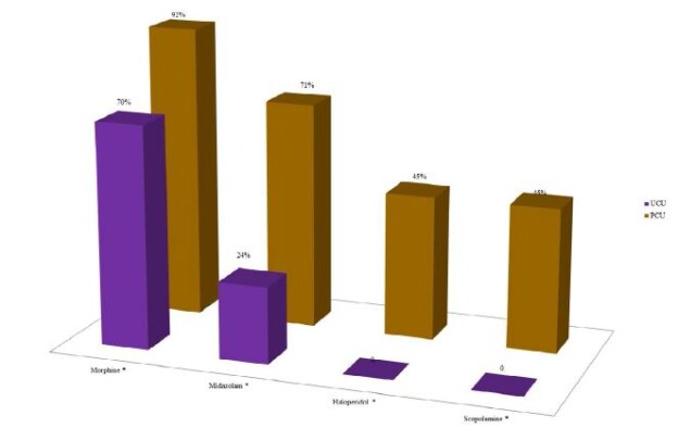
  27. Afkhami S, D’Agostino MR, Zhang A, Stacey HD, Marzok A, et al. (2022) Respiratory mucosal delivery of next-generation COVID-19 vaccine provides robust protection against both ancestral and variant strains of SARS-CoV-2. Cell 185: 896-915. https://doi.org/10.1016/j.cell.2022.02.005

Note in Proof

The scientific journey on vaccine efficacy and safety by the British clinical-biomedical scientist Dr Andrew Wakefield, has direct similarities to the scientific and academic journey on vaccine efficacy and safety of the Australian scholar Dr Judy Wilyman. Both their backgrounds are very different however, their conclusions are very similar, over similar time periods, and the cohesive corruption exerted by the BigPharma consortia as discussed above in both cases attempted to both destroy and smear them and the truthfulness of their scientific discoveries. The most recent interview June 9 2022 of Dr Andrew Wakefield can be found at https://rumble.com/v17xp5j-andrew-wakefield-interview.html

The Unvaccinated versus Vaccinated study mentioned by Dr Wakefield is : Hooker BS, Miller NZ. 2020. Analysis of health outcomes in vaccinated and unvaccinated children: Developmental delays, asthma, ear infections and gastrointestinal disorders. SAGE Open Med. 2020 May 27;8:2050312120925344. doi: 10.1177/2050312120925344. eCollection 2020. https://pubmed.ncbi.nlm.nih.gov/32537156/

The Dynamic Change in Philosophy in the Formation of the Dental Biofilm and the Rationale of Debridement: An Overview

DOI: 10.31038/JDMR.2022515

Abstract

The rationale for the treatment and management of periodontal disease has varied over the last three to four decades and as such the clinician should be aware of these changes to manage the condition effectively. For the example, the recognition that the modification and/or removal of the dental biofilm on the tooth surface is key to reducing the impact of the oral microflora on both the hard and soft tissues of the mouth rather than concentrate on the concept of the removal of ‘calculus removal and diseased cementum of the root to achieve success. The understanding of the role of the oral flora has also changed particularly with the emergence of the key pathogen hypothesis and this concept may have an impact on how the condition is managed. The improvement in instrumentation and surgical techniques together with the adjunctive use of antimicrobials in both non-surgical and surgical procedures has also impacted on our treatment philosophy. The aim of this paper, therefore, is to provide an overview on the dynamic changes in philosophy in the treatment and management of periodontal disease.

Keywords

Periodontitis, Dysbiosis, Dental biofilm, Key pathogen hypothesis, Antimicrobial therapy, Debridement

Introduction

Periodontitis is a chronic multifactorial inflammatory disease associated with a dysbiotic biofilm that results in loss of the periodontal attachment [1]. An aberrant immune response or exaggerated dysbiotic host inflammatory reaction can lead to the destruction of the periodontium [2]. This inflammatory condition is modified by genetics, lifestyle, and environmental factors [3]. Periodontitis is a disease affecting susceptible individuals to a greater extent [4] with its severest form affecting around 11.2% globally which is the sixth-most prevalent condition in the world [5]. According to Grazaini et al. [6], periodontal treatment aims to prevent disease progression, minimize symptoms of the disease, restore lost periodontal tissue, and facilitate patients to maintain healthy periodontium. Biofilm control has however, remained an important strategy to halt disease progression and restore periodontal health [7]. Successful periodontal treatment requires significant ecological changes throughout the oral cavity, leading to the conversion from dysbiosis to a homeostasis ecology. It has been highlighted that increasing the proportion of bacteria associated with health and reducing the level and proportion of bacteria associated with the disease is the key to achieving periodontal stability [8]. Recently, the new 2017 periodontal classification had been proposed which allows for a multidimensional diagnostic classification by providing more detail on the classification of periodontal disease [9,10]. Staging describes the severity of the disease and the anticipated complexity of treatment, whereas grading describes the rate of progression of periodontal disease, susceptibility to disease or case phenotype as well as the presence of risk factors [9].

The Dental Biofilm and Calculus Formation

The dental biofilm is a microbial community associated with a hard, non-shedding surface and enclosed in an extracellular polymeric substance matrix. Teeth in the oral cavity provide non-shedding surfaces and a moist environment which are essential requirements for bacterial colonization and the formation of dental biofilms [11]. Biofilm formation starts with the adsorption of a conditioning film (acquired pellicle) that is coated by biologically active proteins, phosphoproteins, and glycoproteins. Early bacterial colonizers (Streptococci species) have adhesins that allow them to attach with the receptors found on the acquired pellicle. Co-adhesion or attachment between the bacteria is promoted by Fusobacterium nucleatum since this specific species can co-adhere to most oral bacteria. Consequently, multiplication of the attached cells leads to an increase in biomass and synthesis of exopolymers forming a biofilm matrix. This matrix is more than just a scaffold for the biofilm since it can bind and retain molecules, including enzymes, and it could also retard the penetration of charged molecules thereby protecting bacteria in the biofilm. Detachment of the attached cells in the late stage allows the matured biofilm to colonize further elsewhere with more favorable environments [8]. The early colonizers (e.g., Streptococcus and Actinomyces spp.) consume oxygen and lower the redox potential of the environment, which favors the growth of anaerobic species. Several of the gram-positive early colonizers utilize sugars as their energy source. The bacteria that predominate in mature plaque are anaerobic and asaccharolytic (e.g., they do not break down sugars), and use amino acids and small peptides as their energy sources instead. Furthermore, it is recognized that while a pathogenic biofilm is a prerequisite for disease formation it does not in itself necessarily cause periodontal disease [3]. The overgrowth of commensal organisms rather than the acquisition of exogenous pathogens is supported as a key mechanism for developing periodontal disease [12]. Comparison between supragingival and subgingival biofilms showed a difference in several aspects due to the different habitats and environment(s). The “Keystone pathogen hypothesis” is a concept in which specific periodontal pathogens could evade the host response and remodel the microbial community promoting dysbiosis [13]. Keystone species are found in low abundance yet have a profound impact on the biofilm community. Their main function(s) in impairing the host defense are to inhibit IL-8 function, complement subversion, and TLR4 antagonism [14]. Consequently, the host-protective mechanisms are impaired, allowing the overgrowth of the entire community. P. gingivalis has been recognized as the main keystone pathogen since it contains lipopolysaccharide (LPS), gingipains, and fimbriae which allow them to interact with TLR, cleave complement, attach to a cell, and invade intracellularly [14,15].

Dental calculus is a mineralized biofilm composed primarily of calcium phosphate mineral salts and covered by an unmineralized bacterial layer [16]. Following the mineralization process, dental calculus loses its microbial virulence. Early studies revealed that autoclaved calculus did not elicit pronounced inflammation or abscess formation [17]. There is also evidence suggesting that a normal epithelial attachment can be formed on calculus previously treated with chlorhexidine [18]. However, dental calculus provides a roughened surface that harbors a living, nonmineralized biofilm. It increases the rate of biofilm formation, reduces the drainage of GCF, and serves as a secondary retentive site for toxic bacterial products. The rate of calculus formation may differ depending on location (e.g., proximity to a salivary gland), diet (alkaline foods), and salivary content (higher level of calcium, phosphate, and lower levels of potassium in heavy calculus formers) [19]. The mineralization process appears to be almost completed within 12 days, but half of the mineralization process occurs during the first two days [20].

There is a positive correlation between the presence of dental calculus and the prevalence of gingivitis, however; no cause-effect relationship between calculus and disease initiation and progression has been established. It has been demonstrated that signs of chronic inflammation were also observed when subgingival calculus was presented [21]. Furthermore, the intensity of inflammation was more intense with the presence of remnant dental calculus [22]. Mombelli et al. [23] compared a thoroughly root surface planing to only chipping off large calculus deposits during a surgical procedure. Clinical and microbiological parameters showed similar improvements one year after therapy. The conclusion was that the reduction of subgingival microorganisms was more critical for the success of the treatment than the removal of contaminated root cementum and mineralized deposits by root planing. The concept of intentional removal of cementum was therefore abandoned as this was considered unnecessary for successful treatment.

Non-surgical Periodontal Therapy

Non-surgical periodontal therapy together with self-performed plaque control aims to control the biofilm and level of inflammation and subsequently restore periodontal health. Previously, non-surgical periodontal therapy was considered only a preparatory measure for periodontal surgery and was not performed as a solo treatment. Results from studies from the Minnesota group [24], however, provided a better understanding of the role of non-surgical treatment. These findings provided a comparison between surgical and non-surgical approaches where it was shown that in pockets up to 6 mm, non-surgical treatment could provide a similar clinical outcome compared to surgical treatment. Nevertheless, in deep sites (>7 mm), additional surgical procedures could lead to an improvement in pocket reduction. From this point, scaling, and root planning as part of non-surgical periodontal treatment could be considered as a solo effective treatment for the treatment of mild to moderate periodontitis cases. Clinical studies attempting to assess clinical outcomes following non-surgical treatment indicated that significant improvement could be observed after one month following non-surgical treatment. This finding suggested that the need for periodontal surgery could not be properly assessed until the hygienic phase has been accomplished [25]. Non-surgical periodontal treatment is, therefore, considered to be a prerequisite and the fundamental step before any type of surgical periodontal therapy [7]. Furthermore, only deep pockets (>6 mm) in periodontal surgery procedures (open flap debridement) resulted in more PPD reduction and CAL gain, indicating that periodontal surgery appeared to be beneficial only in deep sites. In addition, the concept of ‘critical probing depth’ could also be applied to facilitate the decision-making process of when to treat specifically with non-surgical periodontal treatment or when additional surgical invention is required [26]. This concept demonstrated that only pockets more than 5.5 mm would benefit from periodontal surgery (Modified Widman flap) whereas in shallower pockets (≤5.5 mm), only non-surgical periodontal treatment could achieve a similar clinical outcome.

Recent Changes in the Diagnosis and Management of Periodontal Disease

According to the recent S3 level clinical guidelines for the treatment of stage I-III periodontitis [27], the first step in therapy focuses on guiding behavior change of the patient to control the supragingival biofilm and risk factors together with oral hygiene instruction, professional mechanical plaque removal (PMPR), smoking cessation, and improving diabetic control. For example, patients who managed to quit smoking showed improved outcomes of non-surgical treatment compared to oscillators or non-quitters [28].

The Role of Instrumentation in the Management of Periodontal Disease

Subgingival instrumentation is an accepted part of the cause-related therapy or the second step of therapy. This step aims to control the subgingival biofilm and calculus by various mechanical instruments and may additionally use chemical agents, host-modulating agents, or local and systemic antimicrobials as an adjunct. The second step is usually preceded by or delivery simultaneously with the first step in therapy, depending on the severity of the disease to prevent abscess formation. Subgingival instrumentation performed either by hand or ultrasonic instruments aim to alter the subgingival ecological environment by disrupting the dental biofilm and removing the hard deposits [29]. The first and second steps in therapy should be implemented for all periodontitis patients, emphasizing that non-surgical periodontal treatment must be completed before considering periodontal surgery as part of the third step of therapy [27].

Different approaches have been utilized for instrumentation, namely hand instruments, magneto-strictive ultrasonic scalers, and piezoelectric ultrasonic scalers. The advantages of hand instruments are due to their good tactile sensation and provide a smoother root surface after instrumentation [30]. The disadvantages of hand instruments are due to the 20-50% longer clinical time to match the similar clinical outcomes obtained by power scalers such as ultrasonic scalers. Furthermore, hand instruments may be considered an aggressive modality with a limited number of curette strokes before damaging the root cementum [31]. Hand instruments require sharpening every 5-20 stokes, which may not be practical for daily practice and could potentially damage the original contour of the instrument [32]. Magneto-strictive ultrasonic scalers operate by an elliptical movement with 18,000-45,000 cycles per second with amplitude of 10-100 microns. According to Krishna and De Stefano [30], linear vibratory movement with 25,000-50,000 cycles per second and amplitude of 12-72 microns were observed in Piezoelectric ultrasonic scalers. These ultrasonic instruments were showed to be less aggressive by removing less root surface and causing less soft tissue trauma compared to hand instruments [33]. Piezoelectric ultrasonic scalers also require less clinical time with a 37% reduction compared to hand instrumentation, thus reducing operator fatigue as well as being less dependent on the clinical skill of the operators [34]. The production of acoustic turbulence streaming, and cavitation promotes the enhancement of the disruption of the dental biofilm. In addition, slimline tip designs allow these devices to have an improved access in the furcation areas and deep vertical defects. The drawbacks of these ultrasonic instruments may be due to the rougher surfaces that may be created, as well as the production of a contaminated aerosol spray, and generation of pain/discomfort during treatment [35].

When comparing the clinical outcomes from using ultrasonic and hand instrumentation, it was evident from previous studies that both treatment modalities resulted in similar clinical and microbiological outcomes [36]. Furthermore, both modalities appeared to yield a similar degree of subgingival calculus removal and provided comparable healing responses. The major advantages of ultrasonic scalers are that they required less time as well as enhanced cleaning around the furcation areas and deeper pockets [37]. Wennström et al. [38] also showed that a higher efficiency as described with the number of minutes of instrumentation used to close one pocket was significantly higher in the ultrasonic groups compared to the hand instrumentation group. A more recent systematic review addressed the question on the efficacy of subgingival instrumentation compared with the different modalities. The systematic review only included randomized controlled trials with more than three months duration and observed no significant differences in terms of the clinical outcomes between sonic/ultrasonic and hand instrumentation [39]. It was also noted that a large heterogeneity was evident in terms of the instrument manufacturer, design, and technology employed across the different studies. In addition, clinicians often use both hand and power-drive instruments in their clinical practice.

The complete removal of dental calculus may be challenging and not straightforward. Several factors could affect the efficacy of calculus removal during instrumentation despite the different treatment modalities used. These factors are pocket depth, tooth type and surface, proper access, instruments designs, and operator experience. It was demonstrated from the observation of extracted teeth following subgingival scaling and root planning, that a deeper initial pocket depth resulted in more residual calculus [40]. Under scanning electron microscopy (SEM) of extracted teeth, it was also observed that the residual biofilm and calculus were detected primarily at the line angles, grooves, and depression of the root surfaces [41]. The detection of calculus after subgingival instrumentation had a high false-negative up to 77.4%, indicating difficulties in detecting the completeness of instrumentation [42]. Despite treated root surfaces that were judged as calculus-free after instrumentation under 3.5x magnification and assessed with a dental explorer. The remaining calculus was not uncommon and was shown as micro islands under a videoscope [43]. Dental calculus can bind directly to the hydroxyapatite structure of cementum in which its attachment is stronger than the cohesive strength that binds calculus together. Thus, a complete removal of calculus is difficult and residual micro islands often remain after instrumentation. Scaling and root planing with direct surgical access and with experienced operators was shown to be significant factors in achieving improved calculus removal in molars with furcation involvement. Caffesse et al. [44] demonstrated that periodontal flaps could provide better access for scaling and root planing resulting in an improved calculus free surface. Complete calculus removal in the furcation areas, however, was a rare outcome, possibly due to the tooth’s anatomical features and the conventional instruments used in that earlier study [45].

The Adjunctive Use of Systemic Antimicrobials in Non-surgical Periodontal Therapy

For the management of periodontitis, systemic antimicrobials can provide additional clinical benefits in specific cases. The main advantages of systemic antimicrobials are the ability to reach all oral surfaces and fluids, eliminating periodontal pathogen that invades the soft tissues. For instance, the eradication of Aggregatibacter actinomycetemcomitans (A.a) was reported to be difficult because of its ability to invade the periodontium. Systemic antimicrobials can also reach inaccessible areas such as concavities, furcation areas [6]. This modality can be delivered in cause-related therapy (the second step of therapy), and after the optimal control of the supragingival biofilm has been achieved [27]. Previously, the use of adjunctive use of systemic antimicrobials in non-surgical periodontal treatment was recommended in severe periodontitis cases (PPD > 6 mm) or aggressive form of periodontitis [29]. Guerrero and co-workers demonstrated that the administration of systemic amoxicillin and metronidazole in non-surgical treatment could significantly improve the clinical outcomes (PPD reduction, CAL gain) in patients with generalized aggressive periodontitis [46]. Despite the notion that the adjunctive benefit of antimicrobial may be greater in an aggressive form of periodontitis [47,48], the recent evidence, however, does not support any differences of the antimicrobial effect between aggressive and chronic periodontitis [49]. It was demonstrated that the patients with A.a did not receive any additional benefits from the use of systemic antimicrobials.

According to Teughel et al. [49] the evidence was consistent in confirming that the adjunctive use of systemic antibiotics could improve the clinical outcomes of non-surgical periodontal therapy The combination use of amoxicillin and metronidazole provided the most significant outcome in PPD reduction, a higher percentage of pocket closure, and a higher reduction in bleeding on probing (BoP) [49,50]. The additional effect of the use of antibiotics for PPD reduction and CAL gain were approximately 0.5 mm and 0.3-0.4 mm, respectively. The adjunctive effect was shown to be more pronounced in initially deep pockets with additional benefits in terms of the percentage of pocket closure was 14.5% and 12% at 6 and 12 months, respectively [49]. However, due to the awareness of the emergence of specific-drug-resistant and multidrug-resistant bacterial species that could potentially lead to serious socio-economic and health problems, the use of antibiotics should be limited to those patients who would experience a clinically relevant difference [51,52]. The clinical guidelines recommend that the routine use of systemic antibiotics as an adjunct to subgingival debridement in patients with periodontitis is not recommended. However, the adjunctive use of specific antibiotics may be considered for specific patient categories (e.g., generalised periodontitis Grade C in healthy young adults with good oral hygiene and a documented high rate of progression) [27,53].

The Adjunctive Use of Subgingival Locally Delivered Antimicrobials (LDAs) in Non-surgical Periodontal Therapy

In cases of localised residual pockets, locally delivered antimicrobials (LDAs) may be an alternative adjunct to non-surgical periodontal therapy. It provided a high level and sustained release of the active agent in GCF, providing fewer side effects, limits the development of microbial antibiotic resistance, and was independent of patient compliance [8]. Clinical indications for the use of LDAs included the management of non-responding sites or disease recurrence during supportive periodontal care, residual periodontal pockets in the esthetic zone where surgery may compromise esthetics, pocket disinfection prior to regenerative periodontal surgery, and the control of periodontal disease among patients with relative or absolute contraindications for surgery [8,54]. The previous recommendations from the American Academy of Periodontology (AAP) in 2006 stated that the use of LDAs can be considered when localised recurrent and/or residual PPDs > 5 mm with inflammation is still present following conventional therapies [55]. Whereas in the presence of multiple sites with PPD >5 mm in the same quadrant, or the presence of anatomical defects (e.g., intrabony defects), additional surgical therapies may be considered. Despite the difficulty to define an evidence-based protocol, the recent S3 level clinical guidelines have indicated that this type of antimicrobial intervention may be considered as an adjunct to subgingival instrumentation in patients with periodontitis as part of the second step of therapy [27].

A recent systematic review reported that statistically significant clinical differences in the adjunctive use of LDAs when compared with subgingival debridement alone or plus a placebo, providing addition short term (6-9 months) effect of 0.365 mm and 0.263 mm for PPD reduction and CAL gain, respectively. Minor improvements in additional PPD reduction (0.19 mm) in long-term studies with no statistically significant difference for CAL were also reported [56]. The largest reported clinical benefits were observed in doxycycline or tetracycline-based products such as Atridox, Actisite, and Ligosan.

The Adjunctive Use of Antiseptics in Non-surgical Periodontal Therapy

Adjunctive chemotherapeutics or antiseptics may be considered in periodontal therapy as adjuncts to mechanical debridement to manage the level of gingival inflammation in specific cases [27,57]. This personalized treatment approach would facilitate in controlling gingival inflammation among patients who were unable to effectively remove the supragingival biofilm by mechanical procedures alone. The adjunctive use of antiseptics may also slightly improve the clinical outcome of subgingival instrumentation in terms of PPD reduction during non-surgical periodontal therapy and may also be considered during supportive periodontal care to control inflammation [27,58]. Mouth rinses containing chlorhexidine or essential oils were shown to be the most effective in controlling gingival inflammation and the dental biofilm [58]. Chlorhexidine, for example, is a cationic agent of the bisbiguanide class that could provide an antimicrobial and plaque inhibitory effect as well as maintaining high substantively [8]. Nevertheless, the medical status of the patient, patient preference, the level of dexterity, economical costs, local anatomical factors, and unwanted adverse effects such as staining, and taste alteration may also be considered somewhat negative and unwanted, compared to the potential benefits of these agents. Also, due to the ability of these chemical agents to reduce gingivitis, it is essential that an adequate biofilm control has been established prior to considering the adjunctive use of antiseptics. The absence of gingival bleeding, following the use of these agents, may mislead the patient into thinking that their periodontal problem has been resolved and as such they may fail to consider the seriousness of the underlying periodontal disease if further professional treatment is not re-established [59].

Air-polishing Applications in Non-surgical Periodontal Therapy

Air polishing was introduced as a professional tooth cleaning method as an alternative to rubber cup instrumentation [60]. This cleaning method generates a mixture of pressurized air and abrasive particles [61]. Several studies have confirmed its effectiveness in removing the dental biofilm and stain with less operator fatigue time-efficient management [62,63]. Air polishing offers more comfort and patient acceptance compared to subgingival instrumentation with hand instruments or ultrasonic scalers [64]. Different powders are used in air-polishing procedures, for example, sodium bicarbonate, glycine, erythritol, and bioactive glasses powders. Glycine was reported to be safe effective in biofilm removal when applying on both dentine and root cementum, unlike sodium bicarbonate [61,65]. Air polishing using glycine powder resulted in less patient discomfort compared to hand instrumentation [66], as well as being safer to use on the periodontal tissues [67]. Erythritol is also safe to be applied subgingivally and could achieve similar clinical outcomes in periodontal treatment compared to ultrasonic debridement [68]. The introduction of a subgingival nozzle design also offered a safer approach for effective subgingival biofilm removal [69]. In fact, between maintenance visits, the dental biofilm may be relatively immature and unmineralized, and as such is easily removed thereby avoiding any unnecessary aggressive instrumentation that damages the tooth surfaces [70]. Several clinical studies have reported that the application of air-polishing was more efficient in removing the dental biofilm without any unnecessary discomfort compared to conventional modalities [64,68,71]. Air-polishing also offers a promising benefit as an alternative, more conservative procedure, for debridement during supportive periodontal care (SPC) a part of a professional mechanical plaque removal (PMPR) intervention [27]. Also, a recent clinical trial demonstrated that the adjunctive use of erythritol air-polishing in combination with a full-mouth disinfection protocol could result in greater pocket depth reduction in moderate and deep pockets and a higher percentage of pocket closure over 6 months when compared to conventional protocol [72].

Photodynamic Therapy in Non-surgical Periodontal Therapy

Antimicrobial photodynamic therapy (aPDT) is an adjunctive treatment modality in non-surgical periodontal therapy [7,73]. The combined use of a low-level light and a photosensitizer leads to the production of singlet oxygen energy and free radicals which are cytotoxic to microorganisms [74]. A local effect of this treatment is due to the inability of the generated cytotoxic oxygen species to migrate more than 0.02 μm [75]. This application aimed to reduce both the bacterial load and periodontal pathogens in the periodontal pockets [73]. A previously published systematic review reported on the limited clinical value of this treatment modality as either an independent or adjunctive treatment [76]. The clinical benefits were also shown to be minimal and provided only short-term benefits [77]. Despite some reported improvement in the published clinical studies, this treatment was shown to be inferior, compared to the use of systemic antibiotics [73,78]. The existing limited evidence also showed considerable heterogeneity among studies; therefore, no strong clinical recommendations could be recommended [77]. Furthermore, no conclusive evidence on the effect in reducing bacteria load and the level of inflammation could be drawn [74]. A recent systematic review confirmed that the adjunctive use of aPDT failed to achieve a statistically significant periodontal improvement in terms of PPD reduction [79]. Therefore, the recent guidelines would suggest that adjunctive aPDT should not be used for the treatment of patients with periodontitis [27].

Re-evaluation after Non-surgical Periodontal Therapy

After the recommended two steps of treatment, the periodontal condition should be allowed to heal sufficiently prior to any clinical re-evaluation. However, this evaluation should not be delayed too long since the subgingival microbial recolonization by pathogenic bacteria may occur [80]. Six to eight weeks after initial therapy has been suggested before reevaluating the periodontal condition following periodontal treatment [81,82]. This re-evaluation will be mainly assessing sites presenting with PPD >4 mm with BOP or having deep pockets (PPD >6 mm), which indicates that the endpoints of the therapy have not yet been achieved [83]. Patients who have not responded well from the initial stages will receive further treatment as part of the third step of therapy aiming to treat those non-responding sites. The treatment options at this point can be varied, ranging from repeated subgingival instrumentation with or without adjunctive therapies, access flap surgery, resective surgery, or regenerative surgery.

Wennström et al. [38] demonstrated that the percentage of closed pockets at three months after an initial round of subgingival instrumentation was 58-66%. Multilevel analysis indicated that the factors associated with an inferior outcome following non-surgical periodontal treatment was as follows: smoking, the presence of plaque at the tooth site, molars, and the initial pocket. In other words, smokers with deep pockets and the presence of plaque in molars sites were expected to have the poorest treatment response [84]. The evaluation of the efficacy of subgingival instrumentation has been shown to be an efficacious treatment in the reduction of gingival inflammation, probing pocket depth (PPD), and a number of disease sites [39]. The overall proportion of closed pockets (PD< 4 mm and absence of BOP), which is a relevant clinical outcome, was 74% at 6-8 months. Furthermore, a mean reduction of PPD 1.7 mm at 6-8 months and a greater PPD reduction of 2.6 mm in deep sites (> 6 mm) was observed. In terms of the reduction in gingival inflammation, a mean reduction of 62.7% in BOP scores was also observed. The findings from this systematic review indicated that subgingival instrumentation should be considered a key part of periodontal surgery to achieve infection control as it may also limit the need for additional therapy, which can be more expensive and cause further patient morbidity. The recent systematic review by Citterio et al. [85] also confirmed that non-surgical periodontal treatment was effective in reducing the number of periodontal pockets (between one-half and two-thirds of the depth of the pocket).

Adverse Effects following Non-surgical Periodontal Therapy

Non-surgical periodontal treatment often leads to significant clinical improvement and has remained the cornerstone in periodontal therapy [7]. Nevertheless, this treatment could potentially damage the periodontium as well. There are several adverse effects following non-surgical and surgical procedures that the clinician should be aware of. For example, sensitivity to hot and cold stimuli (dentine/root sensitivity), gingival trauma, inflammation (oedema, bleeding), infection (gingival or periapical abscess) following non-surgical procedures.

Pain and discomfort during regular scaling or instrumentation with an ultrasonic scaler may be an unpleasant experience that may deter a patient from attending for periodontal treatment [86]. Pain could be elicited by frictional forces and heat which are generated during treatment, as well as dentine hypersensitivity that is induced by cold irrigation from an ultrasonic scaler. The degree of post-operative discomfort may also be due to several factors such as 1) the length and complexity of the procedure, 2) poor tissue handling, 3) poor infection control and 4) experience and expertise of the operator [86,87]. Post-operative pain may also increase in intensity during the first few days following the procedure and then diminishes during the first week.

Dentine Hypersensitivity (Root Sensitivity)

The definition for dentine hypersensitivity (DH) is a “short, sharp pain arising from exposed dentin in response to stimuli typically thermal, evaporative, tactile, osmotic or chemical and which cannot be ascribed to any other form of dental defect or disease” [87]. The term root sensitivity is used to describe sensitivity associated with periodontal disease and therapy. It is estimated to occur in almost 50% of patients following periodontal treatment, and the intensity increases during the first week or so and then diminishes [88]. Dentine hypersensitivity after periodontal treatment has been showed to be transient in nature with associated mild to moderate pain [89]. Von Troil et al. [90] performed a systematic review to assess the prevalence of dentine hypersensitivity following periodontal therapy and reported that this condition occurred in approximately half of the patients following periodontal treatment. This high prevalence could be explained by the fact that instrumentation with various types of instruments led to cementum removal and loss of root structure, therefore increasing dentine permeability and sensitivity. This emphasizes that the patient should be informed of the potential risk of this complication following non-surgical periodontal treatment as the treatment may impact on the patient’s quality of life (QoL). A recent clinical study suggested that the use of warmed water (36°C) as an irrigation in conjunction with a piezoelectric scaler, which has its own reservoir of water, could reduce the pain perception during instrumentation and improve patient acceptance of the procedure [91]. Pristine plaque control following periodontal treatment was also suggested to help alleviate dentine hypersensitivity. This is possibly due to the promotion of mineral depositions around the dentinal tubules when root surfaces are kept free of a dental biofilm [92]. Moreover, all surgical procedures, particularly flap surgeries with osseous resection, have been shown to produce more dentine hypersensitivity than non-surgical periodontal therapy [93].

The management of dentine hypersensitivity is, therefore, to eliminate any predisposing factor that causes exposure of dentine and the opening of dentinal tubules [94]. Two main treatment approaches based on the hydrodynamic theory are tubule occlusion and nerve blocking by means of ionic diffusion. These agents can be classified according to their mode of action into a) over the counter (OTC) or b) In-office products. However, the existing evidence suggests that no desensitizing agent has been the ideal product for relieving the symptoms from dentine hypersensitivity [95]. Furthermore, the choices of professional, home use treatment, or the combination of both are mainly arbitrary depending on the practitioner’s understanding and experience of the problem [96]. Fluoride varnishes and gels, glutaraldehyde/2-hydroexethylmethacrylate (HEMA), potassium nitrates, and bonding agents are most often used to treat dentine hypersensitivity among dentists (97). Systematic reviews and meta-analysis suggest that there is sufficient evidence to support the use of potassium-, stannous fluoride-, potassium and stannous fluoride-, calcium sodium phospho-silicate-, and arginine-containing desensitizing toothpaste. Strontium-containing desensitizing toothpastes, however, were reported to have no statistically significant desensitizing effect [97,98].

Gingival Recession

Gingival recession is commonly observed among patients with a high standard of oral hygiene with overzealous toothbrushing but also identified in patients with poor oral hygiene [99]. Buccal gingival recession, especially in teeth or roots with a prominent position in the jaw, occurs frequently in those of high standard of oral hygiene and the severity tends to increase with age [100]. Once the root surface is left exposed to the oral cavity, the cementum can be lost and subsequently result in root sensitivity and root caries [96]. Incorrect tooth brushing methods, particularly excessive pressure while brushing, combined with a highly abrasive toothpaste can further contribute to the progression of the condition [101]. Patients should be informed that a good brushing technique rather than using an excessive force is crucial for good plaque control [94]. Several investigators have indicated that using a surgical root coverage procedure for patients complaining of dentine hypersensitivity showed a mean reduction of dentine hypersensitivity of 77.83%, following the procedure, however recent systematic review concluded that there was insufficient evidence to suggest that this surgical procedure predictably reduced dentine hypersensitivity [102]. Gingival recession together with a missing cemento-enamel junction (CEJ) due to tooth wear may also be observed. CEJ reconstruction can be performed using a resin composite prior to a surgical root coverage procedure with the aim of increasing the intimate contact and stability of the flap/graft as well as improving the final gingival margin contour which in turn may reduce dentine hypersensitivity by covering the previously exposed root surface [103,104].

Conclusions

Periodontitis is a multifactorial inflammatory disease affecting susceptible individuals. There has however been a fundamental shift in philosophy in the management of the condition due to an improvement in our understanding of the role and function of the oral flora indicating that the dysbiosis of the commensal microorganisms rather than any acquisition of exogenous pathogens are key in the development of any future disease progression. The control of the dental biofilm is therefore considered to be an important treatment strategy to halt the progression thereby achieving periodontal stability. Non-surgical and surgical periodontal debridement procedures together with self-performed biofilm control, therefore, is a prerequisite for managing inflammation and restoring periodontal health. Adjunctive treatment modalities as indicated in this overview may also be of benefit when incorporated into the management of the condition.

References

  1. Papapanou PN, Sanz M, Buduneli N, Dietrich T, Feres M, et al. (2018) Periodontitis: Consensus report of workgroup 2 of the 2017 World Workshop on the Classification of Periodontal and Peri‐Implant Diseases and Conditions. Journal of Periodontology. 89: 173-182. [crossref]

  2. Bartold PM, Van Dyke TE (2013) Periodontitis: a host‐mediated disruption of microbial homeostasis. Unlearning learned concepts. Periodontology 2000 62: 203-217. [crossref]
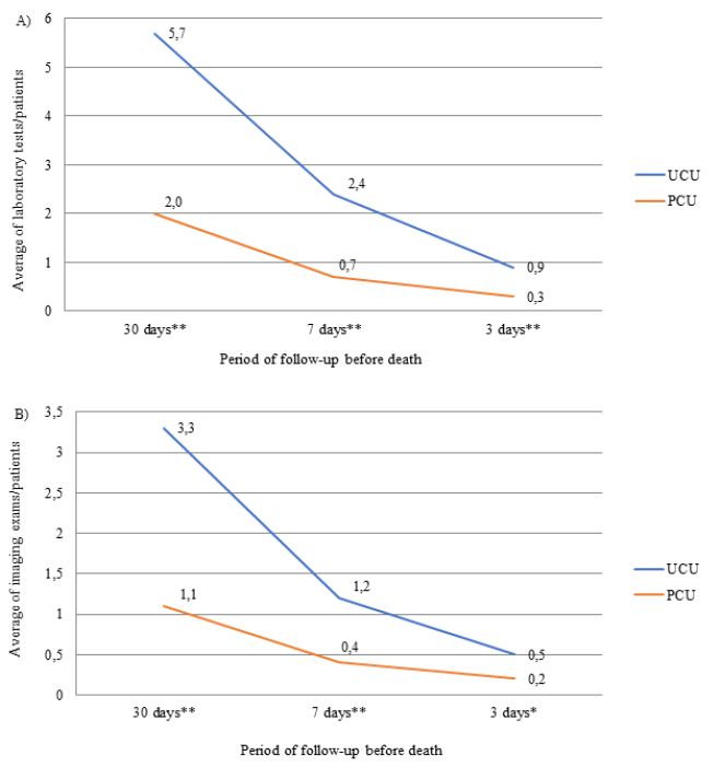
  3. Cekici A, Kantarci A, Hasturk H, Van Dyke TE (2014) Inflammatory and immune pathways in the pathogenesis of periodontal disease. Periodontology 2000 64: 57-80. [crossref]
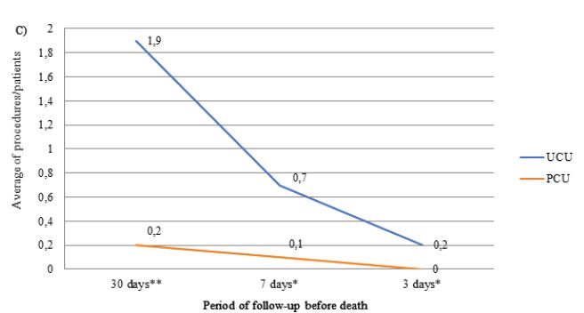
  4. Fine DH, Patil AG, Loos BG (2018) Classification and diagnosis of aggressive periodontitis. Journal of Clinical Periodontology 45: 95-111. [crossref]
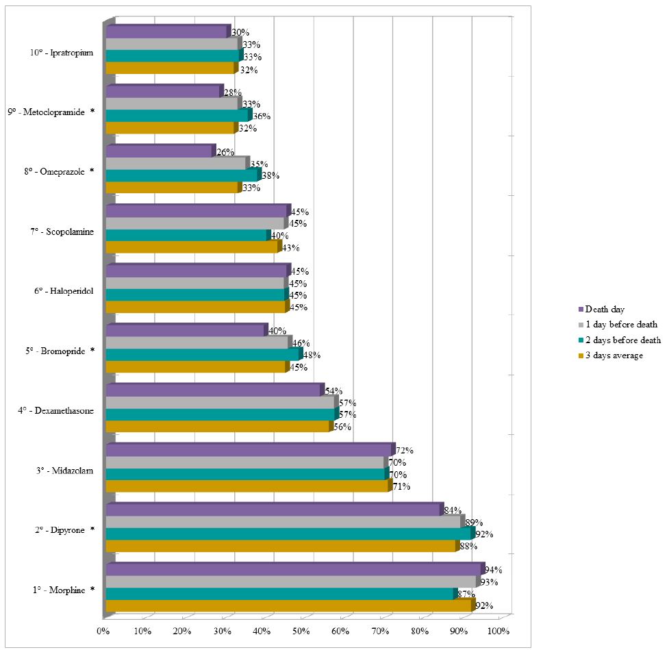
  5. Kassebaum N, Bernabé E, Dahiya M, Bhandari B, Murray C, et al. (2014) Global burden of severe periodontitis in 1990-2010: a systematic review and meta-regression. Journal of Dental Research 93: 1045-1053. [crossref]
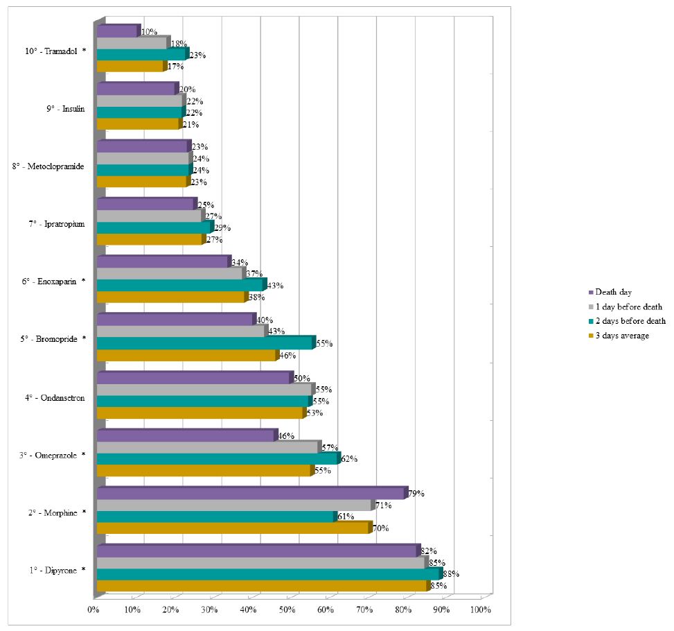
  6. Graziani F, Karapetsa D, Alonso B, Herrera D (2017) Nonsurgical and surgical treatment of periodontitis: how many options for one disease? Periodontology 2000 75: 152-188. [crossref]
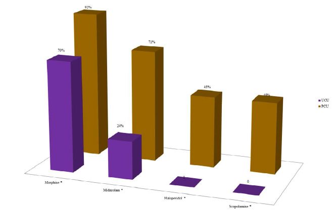
  7. Lang NP, Salvi GE, Sculean A (2019) Nonsurgical therapy for teeth and implants-When and why? Periodontol 2000 79: 15-21. [crossref]
  8. Berglundh T, Giannobile WV, Sanz M, Lang NP (2021) Lindhe’s Clinical Periodontology and Implant Dentistry: John Wiley & Sons.
  9. Tonetti MS, Greenwell H, Kornman KS (2018) Staging and grading of periodontitis: Framework and proposal of a new classification and case definition. Journal of Clinical Periodontology 45: 149-S61. [crossref]
  10. Caton JG, Armitage G, Berglundh T, Chapple IL, Jepsen S, Kornman KS, et al. (2018) A new classification scheme for periodontal and peri‐implant diseases and conditions–Introduction and key changes from the 1999 classification. Wiley Online Library 48: 1-8. [crossref]
  11. Marsh PD, Devine DA (2011) How is the development of dental biofilms influenced by the host? Journal of Clinical Periodontology 38: 28-35. [crossref]
  12. Curtis MA, Diaz PI, Van Dyke TE (2020) The role of the microbiota in periodontal disease. Periodontology 2000 83: 14-25. [crossref]
  13. Hajishengallis G, Darveau RP, Curtis MA (2012) The keystone-pathogen hypothesis. Nature Reviews Microbiology 10: 717-725. [crossref]
  14. Hajishengallis G (2014) Immunomicrobial pathogenesis of periodontitis: keystones, pathobionts, and host response. Trends in Immunology 35: 3-11. [crossref]
  15. Hajishengallis G, Lamont RJ (2012) Beyond the red complex and into more complexity: the polymicrobial synergy and dysbiosis (PSD) model of periodontal disease etiology. Molecular Oral Microbiology 27: 409-419. [crossref]
  16. Roberts-Harry E, Clerehugh V (2000) Subgingival calculus: where are we now? A comparative review. Journal of Dentistry. 28: 93-102. [crossref]
  17. Allen DL, Kerr DA (1965) Tissue response in the guinea pig to sterile and non‐sterile calculus. The Journal of Periodontology 36: 121-126. [crossref]
  18. Listgarten M, Ellegaard B (1973) Electron microscopic evidence of a cellular attachment between junctional epithelium and dental calculus. Journal of Periodontal Research 8: 143-150. [crossref]
  19. Jepsen S, Deschner J, Braun A, Schwarz F, Eberhard J (2011) Calculus removal and the prevention of its formation. Periodontology 2000. 55: 167-88. [crossref]
  20. Schroeder H (1963) Inorganic content and histology of early dental calculus in man. Helv Odont Acta 7: 17-30.
  21. Wilson Jr TG, Carnio J, Schenk R, Myers G (2008) Absence of histologic signs of chronic inflammation following closed subgingival scaling and root planing using the dental endoscope: Human biopsies–A pilot study. Journal of Periodontology 79: 2036-2041. [crossref]
  22. Fujikawa K, O’Leary TJ, Kafrawy AH (1988) The effect of retained subgingival calculus on healing after flap surgery. Journal of Periodontology 59: 170-175. [crossref]
  23. Mombelli A, Nyman S, Brägger U, Wennström J, Lang NP (1995) Clinical and microbiological changes associated with an altered subgingival environment induced by periodontal pocket reduction. Journal of Clinical Periodontology. 22: 780-7. [crossref]
  24. Pihlstrom BL, McHuon RB, Oliphant TH, Ortiz‐Campos C (1983) Comparison of surgical and nonsurgical treatment of periodontal disease A review of current studies and additional results after 6 1/2 years. Journal of Clinical Periodontology 10: 524-541. [crossref]
  25. Morrison E, Ramfjord S, Hill R (1980) Short‐term effects of initial, nonsurgical periodontal treatment (hygienic phase). Journal of Clinical Periodontology. 7: 199-211. [crossref]
  26. Lindhe J, Socransky S, Nyman S, Haffajee A, Westfelt E (1982) “Critical probing depths” in periodontal therapy. Journal of Clinical Periodontology. 9: 323-336. [crossref]
  27. Sanz M, Herrera D, Kebschull M, Chapple I, Jepsen S, Beglundh T, et al. (2020) Treatment of Stage I‐III Periodontitis–The EFP S3 Level Clinical Practice Guideline. Journal of Clinical Periodontology 47: 4-60. [crossref]
  28. Preshaw P, Heasman L, Stacey F, Steen N, McCracken G, Heasman P (2005) The effect of quitting smoking on chronic periodontitis. Journal of Clinical Periodontology. 32: 869-789. [crossref]
  29. Heitz‐Mayfield LJ, Lang NP (2013) Surgical and nonsurgical periodontal therapy. Learned and unlearned concepts. Periodontology 2000 62: 218-231. [crossref]
  30. Krishna R, De Stefano JA (2016) Ultrasonic vs. hand instrumentation in periodontal therapy: clinical outcomes. Periodontology 2000. 71:113-127. [crossref]
  31. Coldiron NB, Yukna RA, Weir J, Caudill RF (1990) A quantitative study of cementum removal with hand curettes. Journal of Periodontology. 61: 293-299. [crossref]
  32. Zappa U, Smith B, Simona C, Graf H, Case D, Kim W (1991) Root substance removal by scaling and root planing. Journal of Periodontology 62: 750-754. [crossref]
  33. Tunkel J, Heinecke A, Flemmig TF (2002) A systematic review of efficacy of machine‐driven and manual subgingival debridement in the treatment of chronic periodontitis. Journal of Clinical Periodontology. 29: 72-81. [crossref]
  34. Cobb CM (1996) Non‐surgical pocket therapy: Mechanical. Annals of Periodontology 1: 443-490. [crossref]
  35. Cobb CM (2002) Clinical significance of non‐surgical periodontal therapy: an evidence‐based perspective of scaling and root planing. Journal of Clinical Periodontology. 29: 22-32. [crossref]
  36. Badersten A, Nilveus R, Egelberg J (1984) Effect of nonsurgical periodontal therapy: II. Severely advanced periodontitis. Journal of Clinical Periodontology. 11: 63-76. [crossref]
  37. Claffey N, Polyzois I, Ziaka P (2004) An overview of nonsurgical and surgical therapy. Periodontology 2000. 36: 35-44. [crossref]
  38. Wennström JL, Tomasi C, Bertelle A, Dellasega E (2005) Full‐mouth ultrasonic debridement versus quadrant scaling and root planing as an initial approach in the treatment of chronic periodontitis. Journal of Clinical Periodontology. 32: 851-859. [crossref]
  39. Suvan J, Leira Y, Moreno Sancho FM, Graziani F, Derks J, Tomasi C (2020) Subgingival instrumentation for treatment of periodontitis. A systematic review. Journal of Clinical Periodontology. 47: 155-175. [crossref]
  40. Rabbani GM, Ash MM, Caffesse RG (1981) The effectiveness of subgingival scaling and root planing in calculus removal. Journal of Periodontology. 52: 119-123. [crossref]
  41. Rateitschak‐Plüss EM, Schwarz JP, Guggenheim R, Duggelin M, Rateitschak KH (1992) Non‐surgical periodontal treatment: Where are the limits? An SEM study. Journal of Clinical Periodontology. 19: 240-244. [crossref]
  42. Sherman P, Hutchens Jr L, Jewson L, Moriarty J, Greco G, McFall Jr W (1990) The effectiveness of subgingival scaling and root planing I. Clinical detection of residual calculus. Journal of Periodontology 61: 3-8. [crossref]
  43. Harrel SK, Wilson Jr TG, Tunnell JC, Stenberg WV (2020) Laser identification of residual microislands of calculus and their removal with chelation. Journal of Periodontology 91: 1562-1568. [crossref]
  44. Caffesse RG, Sweeney PL, Smith B (1986) Scaling and root planing with and without periodontal flap surgery. Journal of Clinical Periodontology 13: 205-210. [crossref]
  45. Fleischer HC, Mellonig JT, Brayer WK, Gray JL, Barnett JD (1989) Scaling and root planing efficacy in multirooted teeth. Journal of Periodontology 60: 402-409. [crossref]
  46. Guerrero A, Griffiths GS, Nibali L, Suvan J, Moles DR, Laurell L, et al. (2005) Adjunctive benefits of systemic amoxicillin and metronidazole in non‐surgical treatment of generalized aggressive periodontitis: a randomized placebo‐controlled clinical trial. Journal of Clinical Periodontology 32: 1096-107. [crossref]
  47. Herrera D, Sanz M, Jepsen S, Needleman I, Roldán S (2002) A systematic review on the effect of systemic antimicrobials as an adjunct to scaling and root planing in periodontitis patients. Journal of Clinical Periodontology. 29: 136-159. [crossref]
  48. Haffajee AD, Socransky SS, Gunsolley JC (2003) Systemic anti‐infective periodontal therapy. A systematic review. Annals of Periodontology 8: 115-181. [crossref]
  49. Teughels W, Feres M, Oud V, Martín C, Matesanz P, Herrera D (2020) Adjunctive effect of systemic antimicrobials in periodontitis therapy. A systematic review and meta‐ Journal of Clinical Periodontology. 47: 251-281. [crossref]
  50. Sgolastra F, Petrucci A, Gatto R, Monaco A (2012) Effectiveness of systemic amoxicillin/metronidazole as an adjunctive therapy to full‐mouth scaling and root planing in the treatment of aggressive periodontitis: A systematic review and meta‐ Journal of Periodontology 83: 731-743. [crossref]
  51. Elias C, Moja L, Mertz D, Loeb M, Forte G, Magrini N (2017) Guideline recommendations and antimicrobial resistance: the need for a change. BMJ open 7: 016264. [crossref]
  52. Mombelli A, Cionca N, Almaghlouth A (2011) Does adjunctive antimicrobial therapy reduce the perceived need for periodontal surgery? Periodontology 2000 55: 205-216. [crossref]
  53. Kebschull M, Chapple I (2020) Evidence-based, personalised and minimally invasive treatment for periodontitis patients-the new EFP S3-level clinical treatment guidelines. British Dental Journal 229: 443-449. [crossref]
  54. Tomasi C, Koutouzis T, Wennström JL (2008) Locally delivered doxycycline as an adjunct to mechanical debridement at retreatment of periodontal pockets. Journal of Periodontology 79: 431-439. [crossref]
  55. Periodontology AAo (2006) American Academy of Periodontology statement on local delivery of sustained or controlled release antimicrobials as adjunctive therapy in the treatment of periodontitis. J Periodontol 77: 1458. [crossref]
  56. Herrera D, Matesanz P, Martín C, Oud V, Feres M, Teughels W (2020) Adjunctive effect of locally delivered antimicrobials in periodontitis therapy: A systematic review and meta‐ Journal of Clinical Periodontology 47: 239-256. [crossref]
  57. Chapple IL, Van der Weijden F, Doerfer C, Herrera D, Shapira L, Polak D, et al. (2015) Primary prevention of periodontitis: managing gingivitis. Journal of Clinical Periodontology 42: 71-76. [crossref]
  58. Figuero E, Herrera D, Tobías A, Serrano J, Roldan S, Escribano M, et al. (2019) Efficacy of adjunctive anti‐plaque chemical agents in managing gingivitis: A systematic review and network meta‐ Journal of Clinical Periodontology. 46: 723-739. [crossref]
  59. Tonetti MS, Jepsen S, Jin L, Otomo‐Corgel J (2017) Impact of the global burden of periodontal diseases on health, nutrition and wellbeing of mankind: A call for global action. Journal of Clinical Periodontology 44: 456-462. [crossref]
  60. Willmann DE, Norling BK, Johnson WN (1980) A new prophylaxis instrument: effect on enamel alterations. The Journal of the American Dental Association 101: 923-925. [crossref]
  61. Petersilka GJ, Bell M, Mehl A, Hickel R, Flemmig TF (2003) Root defects following air polishing: An in vitro study on the effects of working parameters. Journal of Clinical Periodontology 30: 165-70. [crossref]
  62. Graumann SJ, Sensat ML, Stoltenberg JL (2013) Air polishing: a review of current literature. American Dental Hygienists’ Association. 87: 173-180. [crossref]
  63. Cobb CM, Daubert DM, Davis K, Deming J, Flemmig T, Pattison A, et al. (2017) Consensus conference findings on supragingival and subgingival air polishing. Compend Contin Educ Dent 38: 1-4. [crossref]
  64. Moene R, Decaillet F, Andersen E, Mombelli A (2010) Subgingival plaque removal using a new air-polishing device. J Periodontol 81: 79-88. [crossref]
  65. Petersilka GJ, Bell M, Häberlein I, Mehl A, Hickel R, Flemmig TF (2003) In vitro evaluation of novel low abrasive air polishing powders. Journal of Clinical Periodontology 30: 9-13. [crossref]
  66. Petersilka GJ, Steinmann D, Haberlein I, Heinecke A, Flemmig TF (2003) Subgingival plaque removal in buccal and lingual sites using a novel low abrasive air-polishing powder. J Clin Periodontol 30: 328-333. [crossref]
  67. Buhler J, Amato M, Weiger R, Walter C (2016) A systematic review on the effects of air polishing devices on oral tissues. Int J Dent Hyg. 14: 15-28. [crossref]
  68. Muller N, Moene R, Cancela JA, Mombelli A (2014) Subgingival air-polishing with erythritol during periodontal maintenance: randomized clinical trial of twelve months. J Clin Periodontol 41: 883-889. [crossref]
  69. Flemmig TF, Arushanov D, Daubert D, Rothen M, Mueller G, Leroux BG. Randomized controlled trial assessing efficacy and safety of glycine powder air polishing in moderate-to-deep periodontal pockets. J Periodontol. 2012;83(4):444-452. [crossref]
  70. Mombelli A (2019) Maintenance therapy for teeth and implants. Periodontol 2000 79: 190-199. [crossref]
  71. Wennstrom JL, Dahlen G, Ramberg P (2011) Subgingival debridement of periodontal pockets by air polishing in comparison with ultrasonic instrumentation during maintenance therapy. J Clin Periodontol 38: 820-827. [crossref]
  72. Stein JM, Yekta‐Michael SS, Schittenhelm F, Reichert S, Kupietz D, Dommisch H, et al. (2021) Comparison of three full‐mouth concepts for the non‐surgical treatment of stage III and IV periodontitis: A randomized controlled trial. Journal of Clinical Periodontology 48: 1516-1527. [crossref]
  73. Sculean A, Aoki A, Romanos G, Schwarz F, Miron RJ, Cosgarea R (2015) Is photodynamic therapy an effective treatment for periodontal and peri-implant infections? Dental Clinics 59: 831-858. [crossref]
  74. Cobb CM (2017) Lasers and the treatment of periodontitis: the essence and the noise. Periodontology 2000.;75(1):205-295. [crossref]
  75. Moan J, Berg K (1991) The photodegradation of porphyrins in cells can be used to estimate the lifetime of singlet oxygen. Photochemistry and photobiology. 53: 549-53. [crossref]
  76. Azarpazhooh A, Shah PS, Tenenbaum HC, Goldberg MB (2010) The effect of photodynamic therapy for periodontitis: A systematic review and meta‐ Journal of Periodontology 81: 4-14. [crossref]
  77. Sgolastra F, Petrucci A, Severino M, Graziani F, Gatto R, Monaco A (2013) Adjunctive photodynamic therapy to non‐surgical treatment of chronic periodontitis: a systematic review and meta‐ Journal of Clinical Periodontology 40: 514-526. [crossref]
  78. Arweiler NB, Pietruska M, Pietruski J, Skurska A, Dolińska E, Heumann C, et al. (2014) Six-month results following treatment of aggressive periodontitis with antimicrobial photodynamic therapy or amoxicillin and metronidazole. Clinical oral investigations 18: 2129-2135. [crossref]
  79. Salvi GE, Stähli A, Schmidt JC, Ramseier CA, Sculean A, Walter C (2020) Adjunctive laser or antimicrobial photodynamic therapy to non‐surgical mechanical instrumentation in patients with untreated periodontitis: A systematic review and meta‐ Journal of Clinical Periodontology 47: 176-198. [crossref]
  80. Magnusson I, Lindhe J, Yoneyama T, Liljenberg B (1984) Recolonization of a subgingival microbiota following scaling in deep pockets. Journal of Clinical Periodontology 11(3): 193-207. [crossref]
  81. Cobb CM, Sottosanti JS (2021) A re‐evaluation of scaling and root planing. Journal of Periodontology 92: 1370-1378. [crossref]
  82. Segelnick SL, Weinberg MA (2006) Reevaluation of initial therapy: when is the appropriate time? Journal of Periodontology 77: 1598-601. [crossref]
  83. Loos BG, Needleman I (2020) Endpoints of active periodontal therapy. Journal of Clinical Periodontology 47: 61-71. [crossref]
  84. Tomasi C, Leyland AH, Wennström JL (2007) Factors influencing the outcome of non‐surgical periodontal treatment: a multilevel approach. Journal of Clinical Periodontology 34: 682-690. [crossref]
  85. Citterio F, Gualini G, Chang M, Piccoli GM, Giraudi M, Manavella V, et al. (2022) Pocket closure and residual pockets after non‐surgical periodontal therapy: A systematic review and meta‐ Journal of Clinical Periodontology.;49(1): 2-14. [crossref]
  86. Matthews DC, McCulloch CA (1993) Evaluating patient perceptions as short‐term outcomes of periodontal treatment: A comparison of surgical and non‐surgical therapy. Journal of Periodontology 64: 990-997. [crossref]
  87. Canadian Advisory Board on Dentin H (2003) Consensus-based recommendations for the diagnosis and management of dentin hypersensitivity. J Can Dent Assoc 69: 221-226. [crossref]
  88. Sanz M, Addy M (2002) Group D summary. Journal of Clinical Periodontology 29: 195-196.
  89. Lin Y, Gillam D (2012) The prevalence of root sensitivity following periodontal therapy: a systematic review. International Journal of Dentistry 2012.
  90. Von Troil B, Needleman I, Sanz M (2002) A systematic review of the prevalence of root sensitivity following periodontal therapy. Journal of Clinical Periodontology. 29: 173-177. [crossref]
  91. Daly S, Newcombe RG, Claydon NC, Seong J, Davies M, West NX (2020) A randomised controlled trial to determine patient experience of a magnetostrictive stack scaler as compared to a piezoelectric scaler, in supportive periodontal therapy. Journal of Dentistry. 93: 103279. [crossref]
  92. Tammaro S, Wennström JL, Bergenholtz G (2000) Root‐dentin sensitivity following non‐surgical periodontal treatment. Journal of Clinical Periodontology. 27: 690-697. [crossref]
  93. Canakci CF, Canakci V (2007) Pain experienced by patients undergoing different periodontal therapies. The Journal of the American Dental Association. 138: 1563-1573. [crossref]
  94. Gillam DG, Chesters RK, Attrill DC, Brunton P, Slater M, Strand P, et al. (2013) Dentine hypersensitivity–guidelines for the management of a common oral health problem. Dental update 40: 514-524. [crossref]
  95. Gillam D, Orchardson R (2006) Advances in the treatment of root dentine sensitivity: mechanisms and treatment principles. Endodontic Topics. 13: 13-33.
  96. Dababneh R, Khouri A, Addy M (1999) Dentine hypersensitivity—An enigma? A review of terminology, mechanisms, aetiology and management. British Dental Journal 187: 606-611. [crossref]
  97. Cunha-Cruz J, Wataha JC, Zhou L, Manning W, Trantow M, Bettendorf MM, et al. (2010) Treating dentin hypersensitivity. The Journal of the American Dental Association. 141: 1097-1105.
  98. Bae JH, Kim YK, Myung SK (2015) Desensitizing toothpaste versus placebo for dentin hypersensitivity: a systematic review and meta‐ Journal of Clinical Periodontology 42: 131-141. [crossref]
  99. Löe H, Ånerud Å, Boysen H. (1992) The natural history of periodontal disease in man: prevalence, severity, and extent of gingival recession. Journal of Periodontology 63: 489-95. [crossref]
  100. Serino G, Wennström JL, Lindhe J, Eneroth L (1994) The prevalence and distribution of gingival recession in subjects with a high standard of oral hygiene. Journal of Clinical Periodontology. 21: 57-63. [crossref]
  101. West NX. (2008) Dentine hypersensitivity: preventive and therapeutic approaches to treatment. Periodontology 2000. 48: 31-41. [crossref]
  102. Douglas de Oliveira DW, Oliveira‐Ferreira F, Flecha OD, Gonçalves PF (2013) Is surgical root coverage effective for the treatment of cervical dentin hypersensitivity? A systematic review. Journal of Periodontology. 84: 295-306. [crossref]
  103. Santamaria MP, Silveira CA, Mathias IF, Neves FLdS, Dos Santos LM, Jardini MAN, et al. (2018) Treatment of single maxillary gingival recession associated with non‐carious cervical lesion: Randomized clinical trial comparing connective tissue graft alone to graft plus partial restoration. Journal of Clinical Periodontology 45: 968-976.
  104. Zucchelli G, Gori G, Mele M, Stefanini M, Mazzotti C, Marzadori M, et al. (2011) Non‐carious cervical lesions associated with gingival recessions: A decision‐making process. Journal of Periodontology 82: 1713-1724. [crossref]

Changing Patterns of Long-term Climatic Elements and Efficiency Levels of Adaptation Strategies Adopted by smallholder Farmers in Edo North, Nigeria

DOI: 10.31038/ESCC.2022311

Abstract

Understanding the long term patterns and trends in climatic variables in relations to their effects on farming operations and community-based adaptation techniques employed by smallholder farmers in minimizing the negative effects of climatic variability, is a perquisite towards achieving food security and key SDGs. Thus this study aimed to examine the long-term trends and patterns of agro-climatic variables in Edo north and efficient of existing climate change adaptation strategies employed by mainly smallholder farmers. Datasets used include minimum temperature (TMin), maximum temperature (TMax), rainfall, soil moisture (SM) and potential evapotranspiration (PET). The dataset were assembled on monthly basis and spanned across 119 years starting from January 1901 to December 2019 and 37 years starting from January 1982 to December 2018 for SM. These dataset were sourced from the University of East Anglia-Climatic Research Unit, the National Aeronautical and Space Administration Goddard Space Flight Center along with the University of Maryland. Primary data was collected from field survey through questionnaire and oral interviews. Results of long-term annual distribution of climatic variables revealed marked variations in TMin, TMax, and PET over time, while rainfall and SM showed no statistical significant changes. Of all the climatic variables investigated, only rainfall exhibited a rising trend. The study found that the three most adaptation strategies deployed by farmers were the use improved crop varieties (WMS = 4.51), application of early maturing plants (WMS = 4.49) and the use of intensive fertilizer and/or manure application for crop production (WMS = 4.48). The fact that other adaptation strategies are not widely employed in the study area, maybe attributed to low level of rural infrastructures, high poverty level and illiteracy etc. There therefore need for the formulation of climate change adaptation workable policy, programme development/implementation that is geared towards massive rural infrastructure transformations and access to extension services.

Keywords

Climate change, Agro-climatic variables adaptation strategies, Stallholder famers, Adaptation efficiency

Introduction

Nigeria has been adversely affected by climate change especially due to the high vulnerability of majority of her population, arising from poverty and low coping capacity. Increased temperature has been reported as one of the major indicator of climate change [1-10]. As temperature rises, crops will loss water rapidly through transpiration thereby increasing crop water need. High potential evapotranspiration (PET) is usually observed during high temperature condition [11]. Thus, higher value of PET, means increased moisture loss, leading to deficit water balance which is unfavourable to crops. When plant water deficit is not met on time, it causes contingent drought. Crops growing under low soil moisture, yield little and poor quality seeds. As reported by Obi [12], while increase in temperature is expected to elongate the growing season in temperate regions, such increase within the tropics is expected to decimate agricultural output by aggravating soil evaporation rate and invariably drought. Ayoade [13] has also noted that excessive heat destroys plant protoplasm and also decreases the reproductive capacities of animals. Increasing temperature weakens plants and their leaves wither easily hence poor photosynthesis [11]. Another study has established that rising temperature will result in reduced crop quantity and quality due to the reduced growth period following high levels of temperature rise; reduced sugar content, bad coloration, and reduced storage stability in fruits; increase of weeds, blights, and harmful insects in agricultural crops; reduced land fertility due to the accelerated decomposition of organic substances [14]. Furthermore, declining agricultural productivity in Nigeria arising from climate change has been implicated in food crisis and the ongoing farmers-herders’ crisis in Nigeria [15-23].

Fortunately, sustainable adaption measures to climate change hold potentials to reducing the negative impacts of climate change [24]. Climate change adaptation is the process of preparing for, and adjusting proactively to climate change-both negative impacts as well as potential opportunities [25]. It involves adjusting policies and actions because of observed or expected changes in climate [26]. Adaptation can be reactive, occurring in response to climate impacts, or anticipatory, occurring before impacts of climate change are observed [27]. In most circumstances, anticipatory adaptations will result in lower long-term costs and be more effective than reactive adaptations [27]. Studies have shown that farming operations and farming technologies in Nigeria have been changing in response to the effects of climate change [28-39]. While most of these authors focused on adaptation practices in other parts of the country, only few studies exist on climate change adaptation practices by farmers in Edo state, particularly Edo North. Oriakhi et al., [40] for example investigate perceived effect of climate change on crop production by farmers in Edo state, Nigeria, while Ufuoku [41] examined that determinants of adaptation to Climate change among arable Crop Farmers in Edo State, Nigeria and its Implications for Extension Service. These studies did not take into account the effectiveness and efficiency of existing adaptation measures in the northern part of the State. In addition, several climate adaptation practices exist; however, academic literature is scarce on the effectiveness, sustainability and contribution to resilience and sustainability of these adaptation practices, especially in Sub-Saharan Africa [42]. This two grounds justifies the need for the present study.

Materials and Methods

The study area is Edo North, and lies within Latitudes 6° 45′ 15.04” and 7° 34′ 31.31.23” North of the Equator while the longitudinal extent expands from Longitudes 5° 43′ 21.347” and 6° 41′ 46.579” East of the Greenwich (Figure 1). Edo North is bounded in the north by Kogi State, in the east by River Niger, in the south by Edo Central and Edo South and in the west by Ondo State. Edo North Agro Ecological Zone occupies an area of approximately 6169.56km2. Edo North is one of the Agro Ecological Zones in Edo State with a rapidly growing population. In 1991, the population of the six (6) local government areas (LGAs) namely: Akoko Edo, Etsako East, Etsako Central, Etsako West, Owan East and Owan West stood at 549,496 people. The population increased to about 955,791 in 2006 and projected to 1,494,815 in 2019 [43]. The people are presently distributed among three major sub-ethnic groups namely: Akoko Edo largely in the north, Etsako in the central and eastern parts and Owan in the western region of Edo North. Each sub-ethnic group is strongly connected by common tradition of origin, and they speak closely related dialects while at the same time exhibiting other numerous similar cultural traits.

fig 1

Figure 1: Study area showing Local Government Areas and Sampled Communities. Source: Compiled using Open Street Map Database (2019)

The climatic of Edo north fall within the warm-humid tropical climate region with distinct wet and dry seasons. The rainy season last for about seven months (May to October) and the dry season last for about five months (November to April). Rainfall is moderate between the months of March and May and heaviest between June and September with average rainfall between 1000 mm and 1500 mm and temperature as high as 36.7°C especially within the hottest period of February to April [44].

Dataset and Sources

Primary and secondary data were adopted for this study. The primary data was derived from field survey through the use of questionnaire and oral interviews with sampled crop farmers. The data derived through questionnaire focused on farmers’ adaptation strategies to climate change. The secondary data were the high-resolution time-series (TS) gridded climatic data of month-by-month variation in climate (version 4.04 from January 1980-December 2019) of minimum temperature, maximum temperature, rainfall, potential evapotranspiration (PET) and soil moisture (37 years). These dataset were retrieved from archives of the University of East Anglia-Climatic Research Unit, Harris and Jones (2019), while the time series of soil moisture data was downloaded from the Famine Early Warning Systems Network (FEWS NET) and famine Land Data Assimilation System (FLDAS) website. FLDAS is part of the mission of the United States of America (USA) National Aeronautical and Space Administration (NASA) Earth Science Division and archived and distributed by the Goddard Earth Sciences (GES) Data and Information Services Centre (DISC) (NASA GES DISC, 2019). This climatic dataset was selected based on their significance principally in farming as well as their influence in other socio-economic activities in Edo North. Ayoade [45] reported that these climatic parameters have been identified as the most important for crop growth and yield.

Sample Population and Determination of Sampling Size

The population of the study consists of farmers in the selected communities from the study area. However, to determine the sample size, [46] asserted that, it is not always possible to determine the size of most populations or to be certain that each element in the population has an equal chance of being included in the sample. Sample size is almost invariably controlled by cost and time [47]. Nevertheless, [48] provided a useful framework for determining an appropriate sample size. The required sample size is a function of population size and the desired accuracy (within 5%, 3%, or 1%) at the 95% confidence level. For instance, if a researcher is sampling from a population that consists of 10,000 respondents and wishes to be 95% confident that the outcome will be within 5% of the true percentage in the population, the researcher need to randomly sample 370 respondents” [48]. However, to obtain the study population, the 1991 census figures which was released at the community level was used due to the non-availability of same data in 2006 census. Given that population of any place is not static but dynamic, 1991 population of the area was projected to 2019 using 3.2 % annual Edo State growth rate. This gave a figure of 35,510 which therefore, formed the population for the study. Thus, [48] sampling framework was adopted to obtain the sample size from the sample population of 35,510 at 95% confidence level and 3% error margin. This also equals to 533 farmers which formed the sample size which was shared proportionally according to the population in each communities as shown in Table 1.

Table 1: Selected Settlements and Distribution of Respondents

S/No

Sampled Communities LGA Population Sample Size/No. of Questionnaires Number Retrieved
1991

2019

1. Makeke Akoko Edo

1861

4495 67

65

2. Aiyegunle Akoko Edo

1271

3070 46

43

3. Uzanu Etsako East

611

1476 22

22

4. Ekwoto Etsako East

1331

3215 48

46

5. Azukala Etsako Central

1803

4355 65

63

6. Anegbette Etsako Central

2762

6672 100

92

7. Odigie Etsako West

1995

4819 72

68

8. Ogbido Etsako West

802

1937 29

27

9. Ovbiomu Owan East

439

1060 16

15

10. Imafun Owan East

614

1483 23

23

11. Ukhuse-Oke Owan West

634

1532 24

24

12.

Atoruru-Ora Owan West

578

1396 21

21

Total

  14,701 35,510 533

509

Sampling Techniques

The study area is made up of six LGAs and purposive sampling was used in selecting two (2) communities each from the six LGAs. A total of 12 communities were purposively selected for this study. The purpose of using purposive sampling is based on their level of farming activities in the communities. Systematic random sampling was adopted in picking farmers in the communities. The working of this method is that, in each street, lane or layout in the community, the first house was picked and thereafter every third residential houses selected. In a case where there is no farmer in a particular house, the next residential house was chosen.

Data Analysis

Data on the of climate change in Edo North and challenges of existing adaptation strategies were evaluated using descriptive statistics, trend analysis as well as change in the time series climatic datasets. The descriptive statistics include mean, standard deviation, range, minimum, maximum, variance and coefficient of variation (CV). Based on Atedhor [49] the trend in the time series climatic datasets were analyzed using simple linear regression (SLR). Udofia [50] mathematically expressed the SLR model as:

Y = a + bx + ε (1)

Where:

Y: the dependent variable. These include each of the climatic datasets (minimum temperature, maximum temperature, rainfall, PET and soil moisture (O-40 cm) at annual bases.

x: the independent variable in this case time (Years, that is, 1980-2019),

a: the y intercept (that is where the regression line touches the y-axis.

b: the regression coefficient or slope.

e: the residual or random error term.

Similarly, IPCC [51] stated that “a change in the state of the climate could be established using statistical tests”. To evaluate the change in the time series climatic datasets, one-way analysis of variance (ANOVA) was used. However, before ANOVA was carried out, all the climatic datasets were partitioned into four climatic periods (1980-1989, 1990-1999, 2000-2009 and 2010-2020) based on [52]. The cardinal goal of partitioning the climatic data into six climatic periods was to facilitate easy decade-to-decade comparison with the view to establishing decadal change. Udofia [50] also expressed the ANOVA model as:

H0 : μ1 = μ2 = μ3 = … = μ½ (2)

Where: μ : group mean and; k: number of groups.

The mean squares are calculated by dividing each sum of squares by its degrees of freedom. The F ratios are the mean squares for each source divided by the within groups mean square. The significance level for the F is from the F distribution with the degree of freedom for the numerator and denominator mean squares. Besides, a post hoc test was further carried out on the ANOVA results to actually ascertain which particular decade changed or differed from another using Tukey’s Honestly Significant Difference Test (TUKEY) ([53,54]. The significance level of 0.01 and 0.05 was adopted. A five-point Likert’s scale was adopted to examine the extent of effects of socio-economic variables on the effectiveness of existing adaptation practices in the study area. The five-point Likert’s scale ranged from: Highly efficient (weight = 5), Efficient (weight = 4), Inefficient (weight = 3), highly efficient (weight = 2), Can’t tell (weight = 1).

Results and Discussion

The descriptive statistics of mean agro-climatic elements (1980-2020) of the study area are presented in Table 2. Mean minimum temperature (TMin) was 21.7°C, maximum temperature (TMax) 31.1°C, rainfall (1666 mm), soil moisture (SM 0-40 cm) 9.01 mm and potential evapo-transpiration (PET) 39.7 mm. Also, the standard deviation (SD) for TMin was 0.34°C, TMax (0.35°C), rainfall (175.3 mm), SM 0-40cm (0.12 mm) and PET (0.76 mm). The range for TMin was 1.6°C, TMax (1.9°C), rainfall (1164.2 mm) as compared to the temperature range of 5.14°C and rainfall range of 1013.08 mm between 1996-2014 in Akure, Ondo State reported by Olubanjo and Alade [55]. Also, the range of SM 0-40 cm was 0.53 mm and PET (4.5 mm).  In the period under investigation, minimum value for TMin was 20.9°C, TMax (30.1°C), rainfall (1189.6 mm), SM 0-40cm (8.73 mm) and PET (37.0 mm). On the other hand, maximum for TMin was 22.5°C, TMax (32°C), rainfall (2353.7 mm), SM 0-40 cm (9.25 mm) and PET (41.5 mm). In addition, the highest Coefficient of Variation (CV) of 10.52% was recorded for rainfall, 1.91% for PET, 1.33% for SM, 1.55% for TMin and 1.12% for TMax. The coefficient of variation (CV) is the ratio of the standard deviation to the mean and allows for comparison between distributions of values whose scales of measurement are not comparable [56]. Study has shown that low coefficient of variation associated with total annual, average annual, major and minor rains indicates high reliability and dependability of rainfall particularly for agricultural purpose [57]. Value of C.V for rainfall distribution in the study area show that rainfall was generally more irregular than other climatic elements in the study area and may be reliable for agricultural operations.

Table 2: Descriptive Statistics of Agro-Climatic Elements in Edo North


Statistics

Minimum Temperature Maximum Temperature Rainfall Soil Moisture

Potential Evapo-transpiration

Mean

21.682

31.073 1665.982 9.0451

39.683

Standard Deviation

0.3360

0.3476 175.2601 0.12068

0.7583

Range

1.6

1.9 1164.2 0.53

4.5

Minimum

20.9

30.1 1189.6 8.73

37.0

Maximum

22.5

32.0 2353.7 9.25

41.5

Variance

0.113

0.121 30716.12 0.015

0.575

Coefficient of Variation (CV)

1.55%

1.12% 10.52% 1.33%

1.91%

N (Years)

119

119 119 37

119

Results of patterns, trends and CV of TMin as presented in Figure 2. It can be seen that January and December are months with the lowest TMin of 21.2°C, whereas March the month of March recorded highest TMin, with the value of 23.2°C.

fig 2

Figure 2: Monthly Pattern of Minimum Temperature in Edo North

In Figure 3, the result of annual pattern and trend in TMin is presented. TMin exhibited a rising trend at 0.002°C per annum and 5.7% probability of persisting into the future in Edo North. In the 119 years. The years 1971 and 1975 emerged as the years with the lowest TMin of 20.9°C, while 2010 was the year with highest TMin of 20.5°C. A noticeable annual TMin decline was observed between 1970 and 1971 with a corresponding with another noticeable rise between 1929 and 1930.

fig 3

Figure 3: Annual trends and coefficient of variation of minimum temperature in Edo North (1901-2019)

In Figure 4, it can be seen that the month of August is the month with the lowest TMax of 27.8°C whereas February, with the value of 34.4°C recorded the highest TMax. As it could be seen in Figure 5, TMax exhibited an upward trend at 0.003°C per annum and 11.9% probability of the pattern reappearing in the future in Edo North. Similarly, the year 1976 emerged as the year with the lowest TMax of 30.1°C while 2016 was the year with highest TMax of 32°C (Figure 5). A noticeable rise in annual TMax could be observed in 1929/1930 with a corresponding decline between 1973 and 1974. The observed increase in temperature towards late 2000 may be associated to regional and global sea surface temperature (SST) changes. For example Bader, [58] reported that the sea surface temperatures (SSTs) of the tropical Indian Ocean has shown a pronounced warming since the 1950s and has impact of this warming on Sahelian environment. Other observational and model studies have associated the warming condition of the Sahel to warm SSTs in the tropical Atlantic and the Gulf of Guinea [59-63].  Lucas et al [64] on the other hand also attributed this increase to global warming caused by anthropogenic emission of greenhouse gasses and the gradual expansion of the tropics. Values of maximum and minimum temperatures were observed to be generally highest in northwest and southwest part of the basin which may be attributed to  nearest  to heat influx from the anomalous warming of the sea surface in the Guinea Gulf near the equator and  north Atlantic ocean SST.

fig 4

Figure 4: Monthly pattern of maximum temperature in Edo North

fig 5

Figure 5: Annual trends and coefficient of variation of maximum temperature in Edo North (1980-2019)

As seen in Figure 6, Edo North receives rainfall throughout the year with two obvious peaks. The first peak is in July with about 254.5mm while the second is September (289.1 mm) which also doubles as the month with highest rainfall. This seasonal rainfall pattern is typical of locations within humid tropical regions of Nigeria which is also known for a short dry season between the two peaks (August break).

fig 6

Figure 6: Monthly pattern of rainfall in Edo North

Annual pattern of rainfall distribution over the study area displayed marked variability between 1901 and 2019 and the simple linear regression showed a declining trend at annual rate of 0.1 mm (R2 = 0.000) (Figure 7). The year 1914 is seen to be the driest year in the climatic period with rainfall of 1189.6 mm, while the year 1901, with total rainfall of 2353.7 mm was the wettest year. Noticeable patterns in the distribution of annual rainfall is also easily discernible with a sharp rise of about 467.4 mm took place between 1946 and 1947 and 509.4 mm between 1956 and 1957 (10 years interval). A corresponding decline amounting to 644.8 mm was also observed between 1957 and 1958. This rainfall decline coupled with rising human population, urbanization and industrialization is capable of creating water security issues among individuals, firms and government as reported by Olubanjo [65].

fig 7

Figure 7: Annual trends and coefficient of Variation of rainfall in Edo North (1980-2019)

The fact that values of rainfall showed evidence of decline in the early 60s is an indication of pronounced rainfall anomaly in the basin which can be linked to global and regional large-scale sea-surface temperature anomaly (SSTA) which has become evident since 1950s. Model studies show that the increased Sahelian rainfall variability which became pronounced since 1970 onward is associated with SST anomaly patterns, including changes in the tropical Atlantic [59,60-63]  in the Pacific [64-67], in the Indian Ocean [68,69], and in the Mediterranean [70].  Numerical-modeling studies have also confirmed that Atlantic Ocean sectors exert significant impacts on West African precipitation anomalies [62,66,71-73]. Based on simulations by NSIPP1 (version 1 of the AGCM developed at NASA’s Goddard Space Flight Center) with the observed history of the twentieth century global SSTs, [74,75] proposed that the interdecadal and interannual variability of the Sahel rainfall is forced by warm waters surrounding the African continent, especially the Indian Ocean  SST.  A warm sea surface was observed to promote convection over the sea thereby reducing the penetration of the convergence band over the Sahel [76].

In Figure 8, monthly soil moisture pattern at the depth of 0-40cm for the study period (1982-2018) is presented. The figure revealed that the highest value of 0.85 m3/m3 was recorded in September and October while January and February were the months with the lowest value of 0.59 m3/m3. Similarly, annual pattern of soil moisture is presented in Figure 9. As it could be seen, the highest content was recorded in 1991 with the value of 9.3 m3/m3 whereas the lowest soil moisture content was recorded in 1983 with the value of 8.7 m3/m3.

fig 8

Figure 8: Monthly pattern of soil moisture (0 – 40 cm) in Edo North

Besides, an obvious increase in SM content observed in 1990/91 with the value of 0.3 m3/m3 while 1991/1992 experienced sharp decline in SM amounting to 0.4 m3/m3 in Edo North. In addition, soil moisture exhibited a rising trend in the climatic period with an increment of 0.003 m3/m3 per annum and 7.5% likelihood of the pattern and trend of SM observed to repeat itself in the future (Figure 9).

fig 9

Figure 9: Annual trends and coefficient of variation of soil moisture (0 – 40 cm) in Edo North (1982-2018)

Another ACE in Edo North that was investigated was potential evapotranspiration (PET). Findings from the 119 years climatic period (1901-2019) revealed various levels of variability and change in the trends and patterns of PET in the study area (Figure 10). As seen in Figure 9, there is no month in the year Edo North does not lose water in the form of moisture to the atmosphere. The lowest PET value of 2.5 mm each was observed in July and August while the highest PET value of 4.3 mm was noticed in February. Annual pattern of PET (Figure 11) displayed marked fluctuations in the 119 years’ climatic period with an outstanding peak of 41.5 mm) in 2015. Also, 1976 emerged as the year with lowest PET value of 37 mm. Appealing patterns in the oscillation of PET also displayed a sharp rise of about 2.9 mm between 1976 and 1977 and 2.9 mm and a corresponding decline amounting to 1.6 mm between 1998 and 1999. On the whole, PET showed a rising trend at annual rate of 0.001 mm (R2 = 0.006).

fig 10

Figure 10: Monthly pattern of potential evapotranspiration in Edo North

fig 11

Figure 11: Annual trends and coefficient of variation of potential evapotranspiration in Edo North (1901-2019)

In order to investigate the long term change of TMin, TMax, rainfall and PET from 1901 to 2019 and short term change in SM from 1982 to 2018 in Edo North, the 119 years and 37 years climatic periods (CP) were segmented into four distinct sub-periods. The long term change in TMin, TMax, rainfall and PET spanned 30 years each with the last sub-CP being 29 years (1901-1930, 1931-1960, 1961-1990 and 1991-2019). On the other hand, the short term change in SM each spanned10years with the last sub-CP being 7 years (1982-1991, 1992-2001, 2002-2011 and 2012-2018) as found in previous studies. Analysis of variance (ANOVA) was used to evaluate the differences in their means and the result is presented in Table 3. TMin recorded F-value of 6.900 Between Groups with p-value of 0.00 whereas TMax recorded F-value of 17.778 Between Groups with p-value of 0.00. Rainfall recorded F-value of 0.160 Between Groups with p-value of 0.923 whereas soil moisture (0-40 cm) recorded F-value of 1.684 Between Groups with p-value of 0.189. In addition, PET recorded F-value of 5.788, Between Groups with p-value of 0.001. To further identify the decades where the variation in ACE actually resided, TUKEY test was deployed. The result is presented in Table 4.

Table 3: ANOVA Results of Agro-Climatic Elements in the Edo North


Agro-Climatic Elements

Sum of Squares df Mean Square F

Sig.

Minimum Temperature Between Groups

2.032

3 0.677 6.900

0.000

Within Groups

11.291

115

0.098

Total

13.324

118

Maximum Temperature Between Groups

4.517

3 1.506 17.778

0.000

Within Groups

9.739

115

.085

Total

14.256

118

Rainfall Between Groups

15031.300

3 5010.43 0.160

0.923

Within Groups

3609469.284

115

31386.69

Total

3624500.584

118

Soil Moisture (0-40cm) Between Groups

0.070

3 0.023 1.684

0.189

Within Groups

0.455

33

0.014

Total

0.524

36

PET Between Groups

8.900

3 2.967 5.788

0.001

Within Groups

58.944

115

0.513

Total

67.843

118

Table 4: Tukey HSD Post Hoc Tests for Multiple Comparisons

Dependent Variable

Climatic Period (I) Climatic Period (J) Mean Difference (I-J) Standard Error Sig. 95% Confidence Interval
Lower Bound

Upper Bound

Minimum Temperature 1901-1930 1931-1960

-.1656

.0809 .177 -.376

.045

1961-1990

.0307

.0809 .981 -.180

.242

1991-2019

-.2943*

.0816 .003 -.507

-.082

1931-1960 1901-1930

.1656

.0809 .177 -.045

.376

1961-1990

.1963

.0809 .078 -.015

.407

1991-2019

-.1287

.0816 .396 -.341

.084

1961-1990 1901-1930

-.0307

.0809 .981 -.242

.180

1931-1960

-.1963

.0809 .078 -.407

.015

1991-2019

-.3250*

.0816 .001 -.538

-.112

1991-2019 1901-1930

.2943*

.0816 .003 .082

.507

1931-1960

.1287

.0816 .396 -.084

.341

1961-1990

.3250*

.0816 .001 .112

.538

Maximum Temperature 1901-1930 1931-1960

-.1710

.0751 .110 -.367

.025

1961-1990

.0429

.0751 .941 -.153

.239

1991-2019

-.4561*

.0758 .000 -.654

-.259

1931-1960 1901-1930

.1710

.0751 .110 -.025

.367

1961-1990

.2139*

.0751 .026 .018

.410

1991-2019

-.2851*

.0758 .002 -.483

-.088

1961-1990 1901-1930

-.0429

.0751 .941 -.239

.153

1931-1960

-.2139*

.0751 .026 -.410

-.018

1991-2019

-.4990*

.0758 .000 -.697

-.301

1991-2019 1901-1930

.4561*

.0758 .000 .259

.654

1931-1960

.2851*

.0758 .002 .088

.483

1961-1990

.4990*

.0758 .000 .301

.697

Rainfall 1901-1930 1931-1960

19.9001

45.74 .972 -99.352

139.153

1961-1990

21.6809

45.74 .965 -97.572

140.933

1991-2019

-3.1400

46.14 1.000 -123.416

117.136

1931-1960 1901-1930

-19.9001

45.74 .972 -139.153

99.352

1961-1990

1.7807

45.74 1.000 -117.472

121.033

1991-2019

-23.0402

46.13 .959 -143.316

97.236

1961-1990 1901-1930

-21.6809

45.74 .965 -140.933

97.572

1931-1960

-1.7807

45.74 1.000 -121.033

117.472

1991-2019

-24.8209

46.14 .950 -145.097

95.455

1991-2019 1901-1930

3.1400

46.14 1.000 -117.136

123.416

1931-1960

23.0402

46.14 .959 -97.236

143.316

1961-1990

24.8209

46.14 .950 -95.455

145.097

Soil Moisture (0-40cm) 1982-1991 1992-2001

-.04278

0.053 .847 -.1848

.0992

2002-2011

-.11655

0.053 .139 -.2585

.0254

2012-2018

-.05734

.0579 .755 -.2138

.0991

1992-2001 1982-1991

.04278

.053 .847 -.0992

.1848

2002-2011

-.07377

.053 .505 -.2158

.0682

2012-2018

-.01455

.058 .994 -.1710

.1419

2002-2011 1982-1991

.11655

.053 .139 -.0254

.2585

1992-2001

.07377

.053 .505 -.0682

.2158

2012-2018

.05921

.058 .737 -.0973

.2157

2012-2018 1982-1991

.05734

.058 .755 -.0991

.2138

1992-2001

.01455

.058 .994 -.1419

.1710

2002-2011

-.05921

.058 .737 -.2157

.0973

PET 1901-1930 1931-1960

-.3638

.1849 .206 -.846

.118

1961-1990

.2699

.1849 .465 -.212

.752

1991-2019

-.3907

.1864 .161 -.877

.095

1931-1960 1901-1930

.3638

.1849 .206 -.118

.846

1961-1990

.6337*

.1849 .005 .152

1.116

1991-2019

-.0269

.1864 .999 -.513

.459

1961-1990 1901-1930

-.2699

.1849 .465 -.752

.212

1931-1960

-.6337*

.1849 .005 -1.116

-.152

1991-2019

-.6606*

.1864 .003 -1.147

-.175

1991-2019 1901-1930

.3907

.1864 .161 -.095

.877

1931-1960

.0269

.1864 .999 -.459

.513

1961-1990

.6606*

.1864 .003 .175

1.147

*The mean difference is significant at the 0.05 level.

As it could be seen, the actual change in the long term mean of TMin resided between 1901-1930 and 1991-2019 with Mean Difference (I-J) of -0.2943 and standard error (SE) of 0.0816 and p-value of 0.003. Change in TMin also occurred between 1961-1990 and 1991-2019 with I-J of -0.3250, SE of 0.0816 and p-value of 0.001. Also, the actual change in the long term mean of TMax dwelled between 1901-1930 and 1991-2019 with I-J of -0.4561, SE of 0.0758 and p-value of 0.000. Change in TMax also occurred between 1931-1960 and 1961-1990 with I-J of 0.2139, SE of .0751 and p-value of 0.026 as well as between 1991-2019 with I-J of -0.2851, SE of 0.0758 and p-value of 0.002.

Similarly, the actual change in the long term mean of PET dwelled between 1931-1960 and 1961-1990 with I-J of 0.6337, SE of 0.1849 and p-value of 0.005. Change in PEt also occurred between 1931-1960 and 1961-1990 with I-J of -0.6337, SE of 0.1849 and p-value of 0.005 as well as between 1991-2019 with I-J of -0.6606, SE of 0.1864 and p-value of 0.003. In contrast, rainfall and soil moisture (0-40 cm) showed no statistically significant change since the p-values were greater than 0.05 significant level set for the analysis. Thus, at 95% level of confidence there was marked long term change in TMin, TMax, and PET with time in Edo North while rainfall and SM showed no statistical significant change. Farmers can explore the opportunities offered by the near normal pattern of rainfall and SM in Edo North in their planning farming operations to boost crop yield.

When households are negatively impacted by climate change, it is very common practice to deploy adaptation measures to boost resilience. In many instances, the extent of efficiency or workability of each adaptation strategies are unknown, hence this study also sought to unravel the climate change adaptation measure based on the farmers’ experience in the study area (Table 5). It can be seen from the table that using improved crop varieties as climate change adaptation strategy was highly efficient (HE) to 291 (57.2%), Efficient to 201 (39.4%) SCF, Inefficient to 4 (0.8%) SCF and highly inefficient (HIE) to 13 (2.5%). Fadina and Barjolle [77] showed that majority (38.3%) of the respondents in the Zou Department of South Benin Republic had attested to the efficiency of using improved crop varieties as climate change adaptation strategies (CCAS). Availability/access to improved crop varieties may have been the rationale for other respondents to state that it was Inefficient/HIE. Incidentally, this CCAS was ranked 1st in the continuum based on the weighted mean score (WMS) of 4.51.  The 2nd most deployed and efficient CCAS based on the WMS of 4.49 was using early maturing plants. This is based on the fact that 295 (57.9%) of the respondents considered it highly efficient while and 191 (37.5%) considered the measure to be efficient. This finding agree with earlier study by [78] who asserted that maize species with shorter growth period boosted overall yield in South-eastern USA. In contrast, [79] reported that the use of late-maturing hybrid species of maize was one of the HE CCAS in the Republic of Moldova.

Table 5: Climate Change Adaptation Strategies and Extent of Efficiency

Constraints

Extent of Efficiency WMS/Rank
Highly
efficient
Efficient Inefficient Highly Inefficient Can’t tell

Total

Using improved crop varieties Count (%)/

291 (57.2)

201 (39.4) 4 (0.8) 13 (2.5) 0 (0.0) 509 (100)

4.51

Weighted

1455

804 12 26 0 2297

1st

Using early maturing plants Count (%)/

295 (57.9)

191 (37.5) 2 (0.4) 20 (4.0) 1 (0.2) 509 (100)

4.49

Weighted

1475

764 6 40 1 2286

2nd

Using intensive fertilizer and/or manure application for crop production Count (%)/

291 (57.2)

195 (38.3) 2 (0.3) 17 (3.4) 4 (0.8) 509 (100)

4.48

Weighted

1455

780 6 34 4 2279

3rd

Mixed cropping Count (%)/

305 (60.0)

164 (32.2) 15 (3.0) 21 (4.2) 4 (0.6) 509 (100)

4.46

Weighted

1525

656 45 42 4 2272

4th

Practicing land and/or crop rotation Count (%)/

278 (54.5)

203 (39.8) 2 (0.4) 22 (4.4) 4 (0.8) 509 (100)

4.43

Weighted

1390

812 6 44 4 2256

5th

Change in planting/stocking time Count (%)/

271 (53.2)

197 (38.7) 14 (2.8) 27 (5.3) 0 (0.0) 509 (100)

4.4

Weighted

1355

788 42 54 0 2239

6th

Changing from production of agriculture to marketing Count (%)/

216 (42.5)

184 (36.1) 27 (5.4) 42 (8.2) 40 (7.8) 509 (100)

4.33

Weighted

1080

920 81 84 40 2205

7th

Planting deeper than the usual planting depth to prevent scorching Count (%)/

255 (50.2)

210 (41.3) 2 (0.4) 39 (7.6) 3 (0.5) 509 (100)

4.32

Weighted

1275

840 6 78 3 2202

8th

Using nursery for transplantable crops Count (%)/

254 (50.0)

190 (37.4) 28 (5.4) 27 (5.3) 10 (1.9) 509 (100)

4.28

Weighted

1270

760 84 54 10 2178

9th

Use of mulching materials for crops Count (%)/

255 (50.1)

192 (37.7) 9 (1.7) 49 (9.7) 4 (0.8) 509 (100)

4.27

Weighted

1275

768 27 98 4 2172

10th

Skipping storage but processing and marketing immediately after harvest Count (%)/

241 (47.3)

195 (38.4) 23 (4.5) 41 (8.1) 9 (1.7) 509 (100)

4.21

Weighted

1205

780 69 82 9 2145

11th

Change of harvesting date Count (%)/

237 (46.5)

204 (40.0) 17 (3.4) 30 (5.6) 21 (4.1) 509 (100)

4.19

Weighted

1185

816 51 60 21 2133

12th

Collection of runoff water in ditches for drought periods Count (%)/

225 (44.2)

179 (35.1) 50 (9.8) 43 (8.5) 12 (2.4) 509 (100)

4.1

Weighted

1125

716 150 86 12 2089

13th

Expansion of farming land Count (%)/

241 (47.3)

164 (32.3) 19 (3.8) 79 (15.5) 6 (1.1) 509 (100)

4.09

Weighted

1205

656 57 158 6 2082

14th

Raising walls with sand bags and/or blocks to divert flood water Count (%)/

234 (45.9)

182 (35.7) 17 (3.4) 50 (9.8) 26 (5.2) 509 (100)

4.08

Weighted

1170

728 51 100 26 2075

15th

Construction of drainage system or dam within farm/household Count (%)/

236 (46.4)

195(38.3) 16 (3.2) 57 (11.2) 5 (0.9) 509 (100)

4

Weighted

1088

780 48 114 5 2035

16th

Subsidizing of agricultural inputs by relevant authorities Count (%)/

206 (40.4)

190 (37.4) 41 (8.1) 39 (7.7) 33 (6.4) 509 (100)

3.98

Weighted

1030

760 123 78 33 2024

17th

Construction of foot bridges with wood, stones and sand bags Count (%)/

231 (45.3)

187 (36.8) 37 (7.3) 54 (10.6) 0 (0.0) 509 (100)

3.97

Weighted

1056

748 111 108 0 2023

18th

Sand filling water logged area to reclaim lost land Count (%)/

215 (42.4)

182 (35.7) 35 (6.9) 37 (7.2) 40 (7.8) 509 (100)

3.97

Weighted

1075

728 105 74 40 2022

18th

Giving the affected farmers financial support Count (%)/

227 (44.6)

161 (31.6) 29 (5.6) 61 (12.0) 31 (6.2) 509 (100)

3.96

Weighted

1135

644 87 122 31 2019

19th

Sinking of boreholes in farm to ensure water availability/artificial irrigation Count (%)/

195 (38.3)

171 (33.5) 54 (10.6) 63 (12.4) 26 (5.2) 509 (100)

3.88

Weighted

975

684 162 126 26 1973

20th

Resettlement of communities from hazard zones Count (%)/

176 (34.5)

159 (31.2) 28 (5.6) 67 (13.1) 79 (15.6) 509 (100)

3.56

Weighted

880

636 84 134 79 1813

21st

Setting up of housing programmes for displaced farmers Count (%)/

108 (21.2)

174 (34.3) 94 (18.4) 73 (14.3) 60 (11.8) 509 (100)

3.39

Weighted

540

696 282 146 60 1724

22nd

On the application of intensive fertilizer and/or manure application for crop production as CCAS, 291 (57.2%) of the respondents deem it highly efficient, while 195 (38.3%) considered it efficient. Despite the fact that 2 (0.3%) regard it as being inefficient, 17 (3.4%) believe it to be highly inefficient. Another 4 (0.8%) of the respondents can’t tell the extent of efficiency. The use of fertilizer and manure was considered 3rd most deployed measure based on the WMS of 4.48.  The insignificant percentage of respondents that considers the application intensive fertilizer and/or manure application for crop production inefficient or highly inefficient may have missed the timing of deployment of the adaptation measure, had little/no access to it or the fertilizer washed away by rainfall immediately after application. Amali and Namo [80] in a study of growth and yield of maize in Jos, Plateau State and Kartika et al. [81] on rice at Pemulutan District, South Sumatra, Indonesia reported that incorrect fertilizer application can lead to loss of valuable nutrients, fertilizer wastage as well as injuries to the crop subsequent reduction in the final yield.

About 60% of the respondents considered mixed cropping to be highly efficient, while 164 (32.2%) adjudged it efficient. This CCAS was however, the 4th most deployed measure based on the WMS of 4.46 notwithstanding the fact that 15 (3%) regard it as being inefficient and 21 (4.2%) highly inefficient. Mix cropping has been found to be very useful in boosting farmers’ resilience to CC impact owing to the discriminatory effects of CC on most arable, staple and perennial crops. Thornton et al., [82] reported that mixed cropping is the fulcrum of farming in sub-Saharan Africa based on its ability to guarantee secured and sustainable supply of foodstuff and employment opportunities to greater proportion of the population particularly in rural areas. The 5th most perceived and deployed CCAS based on the WMS of 4.43 was the practice of land and/or crop rotation. This stemmed from the responses of 278 (54.5%) of the respondents who adjudge it as highly efficient and 203 (39.8%) who regarded it as being effective. Only 2 (0.4%) and 22 (4.4%) of the sampled respondents believed that crop rotation was ineffective and highly efficient measure for climate change adaptation. When cultivated lands and left fallow for a period, soil regains its fertility status and during crop rotation, unutilized nutrients are made available to new the new cop thereby increasing yield. This finding agrees with that of Fadina and Barjolle [77] who reported land and/or crop rotation as the 2nd most efficient CCAS adopted by farmers (based on the response of 37% of the respondents) in Southern Benin Republic.

Change in planting/stocking time was considered highly efficient (53.2%), efficient (n = 197; 38.7%), inefficient (n = 14; 2.8%) and highly inefficient (n = 27; 5.3%). With WMS of 4.4 this adaptation strategy is ranked 6th in the continuum of CCAS in the study area. The change in planting/stocking time may not be unconnected the changeability in climatic element particularly rainfall. Crop farmers want to ensure that after cultivation, their seedling does not end up dying on soil or experience stunting due to unavailability of sufficient soil moisture. This finding consistent with previous study by Akinnagbe and Irohibe [83] who reported alteration of cultivation model and farming schedule as dependable antidotes to adverse effects of unreliable precipitation regime on agriculture. About 42.5% of the respondents rated changing from production of agriculture to marketing highly efficient, 184 (36.1%) ranked it as efficient, 27 (5.4%) adjudged it as inefficient, 42 (8.2%) regarded the strategy as being highly inefficient, while 40 (7.8%) can’t tell the extent of efficiency. Equally, changing from production of agriculture to marketing was ranked 7th based on the WMS of 4.33.

On the efficiency of planting deeper than the usual planting depth to prevent scorching, the sampled respondents rated it highly efficient by 255 (50.2%), efficient (n = 210; 41.3%), inefficient (n = 2; 0.4%), highly inefficient (n = 39; 7.6%) and can’t tell (n = 3; 0.5%).  The WMS of 4.32 placed this CCAS 8th in the order of efficiency and most utilized by the farmers. Using nursery for transplantable crops as CCAS was perceived highly efficient by 254 (50%), efficient (n = 190; 37.4%), inefficient (n = 28; 5.4%), HIE (n = 27; 5.3%) and can’t tell (n = 10; 1.9%).  The WMS of 4.28 placed this CCAS 9th in the order of efficiency and most utilized by the farmers. Application of mulching materials for crops as CCAS was considered highly efficient by 255 (50.1%), efficient (n = 192; 37.7%), inefficient (n = 9; 1.7%), HIE (n = 49; 9.7%) and can’t tell (n = 4; 0.8%).  The WMS of 4.27 placed this CCAS 10th in the order of efficiency and most utilized by the farmers.

The 11th most adopted and efficient CCAS based on the WMS of 4.21 was skipping storage but processing and marketing immediately after harvest. A total of 241 (47.3%) of the respondents considered this measure to be highly efficient, 195 (38.4%) considering it as efficient, 23 (4.5%) regarding it as being inefficient, 41 (8.1%) deeming it HIE and 9 (1.7%) can’t tell the extent of efficiency.

Similarly, the 12th most deployed and efficient CCAS based on the WMS of 4.19 was change of harvesting date. This is based on the assertion of 237 (46.5%) of the respondents who considered the strategy to be highly efficient and 204 (40%) as efficient, whereas 17 (3.4%) and 30 (5.6%) adjudged it to be inefficient and highly inefficient strategy respectively. The collection of runoff water in ditches for drought periods as CCAS, was considered highly efficient at 225 (44.2%) and 179 (35.1%) as efficient adaptation strategy for changing climate. On the expansion of farming land as CCAS, 241 (47.3%) of the respondents considered this measure to be highly efficient, while 164 (32.3%) adjudged it efficient. This CCAS was nevertheless, the 14th most deployed measure based on the WMS of 4.09 notwithstanding the fact that 19 (3.8%) regard it as being inefficient and 79 (15.5%) highly inefficient even as 6 (1.1%) SCF can’t tell the extent of efficiency. The inefficiency of this CCAS can be linked to the challenges on the existing land tenure and ownership system in the area. A situation where majority (55.9%) of the farmers owned about 1-5 hectares, expansion of learning,  practicing farming land as a measure to boost resilience to climate change effect becomes practically unfeasible. The 15th most perceived, deployed and efficient CCAS based on the WMS of 4.08 was raising walls with sand bags and/or blocks to divert flood water. This originated from the responses of 234 (45.9%) of the respondents who adjudge it as highly efficient and 182 (35.7%) who regarded it as being effective. Nevertheless, about 17 (3.4%) and 50 (9.8%) of the sampled respondents believed it to be ineffective and highly inefficient respectively while 26 (5.2%) can’t tell the extent of efficiency. With respect to construction of drainage system or dam within farm/household as CCAS, 236 (46.4%) respondents reported highly efficient, efficient (n = 195; 38.3%), inefficient (n = 16; 3.2%) and HIE (n = 57; 11.2%) while 5 (0.9%) can’t tell the extent of efficiency. The WMS of 4.0 placed the CCAS 16th in the continuum. Similarly, 206 (40.4%) of the respondents rated subsidizing of agricultural inputs by relevant authorities as CCAS highly efficient, 190 (37.4%) ranked it as efficient, 41 (8.1%) adjudged it as inefficient, 39 (7.7%) regard it as being HIE while 33 (6.4%) can’t tell the extent of efficiency. The CCAS was ranked 17th based on the WMS of 3.98.

The extent of efficiency of construction of foot bridges with wood, stones and sand bags as CCAS was rated highly efficient by 231 (45.3%), efficient (n = 187; 36.8%), inefficient (n = 37; 7.3%) and highly inefficient (n = 54; 10.6%).  Also, sand filling water logged area to reclaim lost land as CCAS was rated highly efficient by 215 (42.4%), efficient (n = 182; 35.7%), inefficient (n = 35; 6.9%), highly inefficient (n = 37; 7.2%) and can’t tell (n = 40; 7.8%). Interestingly, construction of foot bridges with wood, stones and sand bags and sand filling water logged area to reclaim lost land had the same WMS of 3.97 hence, ranked as the 18th most deployed and efficient CCAS in the study area. Furthermore, the extent of efficiency of giving the affected farmers financial support as CCAS was perceived as highly efficient by 227 (44.6%), efficient (n = 161; 31.6%), inefficient (n = 29; 5.6%), highly inefficient (n = 61; 12%) and can’t tell (n = 31; 6.2%).  The WMS of 3.96 placed this CCAS 19th on the table in the order of efficiency and most utilized by the farmers. Moreover, sinking of boreholes in farm to ensure water availability/artificial irrigation (WMS = 3.88) was ranked 20th, resettlement of communities from hazard zones (WMS = 3.56) ranked 21st even as setting up of housing programmes for displaced farmers (WMS = 3.39) became the 22nd most deployed CCAS in the study area.

Conclusion and Recommendations

This research was undertaken with the aim to changing partners of agro-climatic variables in relation to their effects on farming operations and efficiency of adaptation options in Edo North, Edo State.  Archival data for the 119years climatic period (1901-2019) and 37 years (1982-2018) depicted various degrees of variability with marked statistical significant change in minimum and maximum temperature as well as potential evapotranspiration. The upward trends in minimum and maximum temperature as well as potential evapotranspiration are indication that the study area is gradually getting warmer and drier than before in recent history as buttressed by sampled respondents. Out of the 24 adaptation strategies already in use in the study area, the use improved crop varieties (WMS = 4.51), application of early maturing plants (WMS = 4.49) and the use of intensive fertilizer and/or manure application for crop production (WMS = 4.48) were top three most adaptation strategies deployed by farmers. The fact that other adaptation strategies are not widely employed in the study area, maybe attributed to low level of rural infrastructures, high poverty level and illiteracy etc. There therefore need for the formulation of climate change adaptation workable policy, programme development/implementation that are geared towards massive rural infrastructure transformations and access to extension services. Furthermore, governments, NGOs and other stakeholders should make available climate change adaptation strategies at reduced or no cost to the farmers to boost their resilience.

References

  1. Omotosho DO (2007) Farmer’s perception of the impact of climate change on agricultural development in Edo State. Ph.D Project of the Department of Agriculture Economics, Michael Opkara University of Agriculture, Umudike
  2. Odjugo PA (2010) General Overview of Climate Change Impacts in Nigeria. Journal of Human Ecology 29: 47-55.
  3. Udenyi OG (2010) Impacts of Climate Change. Nigeria Social Network.
  4. Ebele NE, Emodi NV (2016) Climate change and its impact in Nigerian economy. Journal of Scientific Research & Reports 10: 1-13.
  5. Elisha I (2017) Evidence of climate change and adaptation strategies among grain farmers in Sokoto State, Nigeria. IOSR Journal of Environmental Science, Toxicology and Food Technology (IOSR-JESTFT) 11: 1-7.
  6. Adepoju AA (2019) Climate Change and Health in Nigeria. Nigerian Tribune.
  7. Ilevbare FM (2019) Investigating effects of climate change on health Risks in Nigeria. IntechOpen
  8. Haider H (2019) Climate change in Nigeria: Impacts and responses. K4D Helpdesk Report 675. Brighton, UK: Institute of Development Studies
  9. Butu AW, Emeribe CN (2019) Spatial patterns of climatic variability and water budget over Sudan Savannah Region of Nigeria. African Journal of Environmental Science and Technology 13: 464-480.
  10. Emeribe CN, Ezeh CU, Butu AW (2020a) Climatic Water Balance Over Two Climatic Periods and Effect on Consumptive Water Need of Selected Crops in the Chad Basin, Nigeria. Agric Res 10: 131-147.
  11. Audu EB, Audu HO, Binbol NL, Gana JN (2013) Climate Change and Its Implication on Agriculture in Nigeria. Abuja Journal of Geography and Development 3: 8-19.
  12. Obi CO (2010) Climate Change and Management of Degraded Soils for Sustainable Crop of Production. Tropical Built Environment Journal 1.
  13. Ayoade JO (2002) Introduction to agroclimatology. Vintage, Publisher, Ibadan.
  14. Kim C (2009) Strategies for Implementing Green Growth in Agricultural Sector.” in Proceedings in Green Korea 2009 – Green Growth and Cooperation. National Research Council for Economics, Humanities and Social Science.
  15. Abubakar AZ (2012) Effects of urbanization on land use/ land cover changes in Birnin Kebbi, Kebbi State, Nigeria. M.Sc Dissertation submitted to School of Post Graduate Studies, Ahmadu Bello University, Zaria, For The Award of Master of Science Degree in Remote Sensing and Geographic Information System, Department of Geography.
  16. Abugu SO, Onuba CO (2015) Climate change and pastoral conflicts in the middle belt and south-east Nigeria: Implication on human resource of the regions. Global Journal of Human Resource Management 3: 44-51.
  17. Fasona M, Omojola A (2005) Climate Change, Human Security and Communal Clashes in Nigeria (paper, International Workshop on Human Security and Climate Change, Asker, Oslo, June 21–23, 2005)
  18. Fabiyi M, Otunuga A (2016) Why The Fulani Herdsmen and Farmers Fight: How Climate Change and The Boko Haram Crisis Created The Crisis and Six (6) Evidence-Based Policy Recommendations For Its Resolution.
  19. Adeoye NO (2017) Land Use Conflict between Farmers and Herdsmen in parts of Kano, Yobe and Borno States of Nigeria: Nomads Viewpoint. Ghana Journal of Geography 9: 127-151.
  20. Odigbo JO (2019) Grazing Conundrum: Herdsmen–Farmers Conflict and Internal Security in Nigeria, in Internal Security Management in Nigeria: Perspectives, Challenges and Lessons, eds. Oshita O Oshita, Ikenna Mike Alumona and Freedom Chukwudi Onuoha (Berlin: Springer Nature, 2019), 99-12
  21. Adeniran AI (2020) Climatic Factors in Nigeria’s Farmer–Herder Conflict. Policy Briefing Climate Change and Migration May 202
  22. Abugu NA, Odele M, Ogah TA, Yero AB (2020) Analysis of Climate Variables and Resource Conflict in Benue State, Nigeria. WJIR 9.
  23. Abugu NA, Yero AB, Odele MO, Irene AM (2021) Reviewing the Links between Climate Change and Resource Conflict. Global Journal OF pure and Applied Sciences 27: 243-152.
  24. Mendelsohn R (2006) Climate change impacts on agriculture. In Evenson R & Pingali P (eds), Volume III: Handbook of Agricultural Economics: Agricultural Development Chapter 19.
  25. World Bank (2011) Guide to Climate Change Adaptation in Cities, The World Bank Group, Washington.
  26. Smith K, Barrett CB, Box PW (2000) Participatory risk mapping for targeting research and assistance: with an example from East African pastoralists. World Development 28: 1945-1959.
  27. Bryant CR, Smit B, Brklacich M, Johnston T, Smithers J, et al. (2000) Adaptation in Canadian agriculture to climatic variability and change. Clim Change 45: 181-201.
  28. Oyekale AS, Bolaji MB, Olowa OW (2009) The Effects of Climate Change on Cocoa Production and Vulnerability Assessment in Nigeria. Agricultural Journal 4: 77-80.
  29. Awotoye OO, Mathew OJ (2010) Effects of temporal changes in climate variables on crop production in tropical sub-humid South-western, Nigeria. African Journal of Environmental Science and Technology 4: 500-505.
  30. Oladipo E (2010) Towards Enhancing the Adaptive capacity of Nigeria: A Review of the Country’s Preparedness for Climate Change Adaptation, A Report Submitted to Heinrich Böll Foundation, Nigeria.
  31. Sayne A (2011) Climate change adaptation and conflict in Nigeria. Washington, DC: USIP.
  32. Adesina FA, Odekunle TO (2011) Climate change and adaptation in Nigeria: some background to Nigeria’s response – III. In: International conference on environmental and agriculture engineering IPCBEE, vol 15. IACSIT Press, Singapore
  33. Ozor N, Nnaji C (2011) The role of extension in agricultural adaptation to climate change in Enugu State, Nigeria. Journal of Agricultural Extension and Rural Development 3: 42-50.
  34. Adebayo K, Dauda TO, Rikko LS, George FOA, Fashola OS, et al. (2011) Emerging and indigenous technology for climate change adaptation in southwest Nigeria (ATPS Research Paper No. 10). Nairobi: African Technology Policy Studies Network
  35. Farauta BK, Idrisa YL, Egbule CL, Agu VC (2011) Farmers’ perceptions of climate change and adaptation strategies in Northern Nigeria: An empirical assessment’ African Technology Policy Studies Network Research Paper | No. 15
  36. Adebanjo OM (2013) The effects of climate change adaptation strategies on food crop production efficiency in Southwestern Nigeria. PhD thesis. Department of Agricultural Economics, University Of Nigeria.
  37. Atedhor GO (2015) Agricultural Adaptation Strategies to Climate Change in Sokoto State, Semi-Arid Region of Nigeria. Journal of the Environment 9: 25-41.
  38. Onyeneke RU, Mmagu CJ, Aligbe JO (2017) Crop farmers’ understanding of climate change and adaptation practices in Southeast Nigeria. World Rev Sci Technol Sustain Dev 13: 299-318.
  39. Adeagbo OA, Adeagbo TO, Ojo AA, Adetoro (2021) Understanding the determinants of climate change adaptation strategies among smallholder maize farmers in South-west, Nigeria. Heliyon 7: 06231.
  40. Oriakhi LO, Ekunwe PA, Erie GO, Ososogie DI (2017) Socio-economic Determinants of Farmers’ Adoption of Climate Change Adaptation Strategies in Edo State, Nigeria. Nigerian Journal of Agriculture, Food and Environment 13: 115-121.
  41. Ofuoku Albert (2011) Rural Farmers’ Perception of Climate Change in Central Agricultural Zone of Delta State, Nigeria. Indonesian Journal of Agricultural Science 12: 63.
  42. Remling E, Veitayaki J (2016) Community-based action in Fiji’s Gau Island: a model for the Pacific?. International Journal of Climate Change Strategies and Management 8: 375-398.
  43. National Population Commission (2010) National Population Commission. Report on the 2006 Census Result. Federal Republic of Nigeria Official Gazette, Abuja, B24.
  44. Banmeke TOA, Fakoya EO, Ayanda IF (2012) Agricultural Researchers’ Awareness of the Causes and Effects of Climate Change in Edo State, Nigeria. Journal of Agricultural Science 4: 233-238.
  45. Ayoade JO (2003) Tropical Hydrology and Water Resources. Ibadan Agbo Areo Publishers.
  46. Emaikwu, S.O. (2008). Fundamentals of educational research methods and statistics Kadunna: Deray Punts Ltd
  47. Ogundele OJK (2004) Wealth Creation through the Development of indigenous Technology, 12 national Conference Environments and Behavior of Association of Nigeria, University of Agriculture, Abeokuta, 24-26 November
  48. Mitchell ML, Jolley JM (2012) Research design explained (8th ed.). Belmon: Wadsworth Cengage Learning
  49. Atedhor GO (2016) Growing Season Rainfall Trends, Alterations and Drought Intensities in the Guinea Savanna Belt of Nigeria: Implications on Agriculture. Journal of Environment and Earth Science 6.
  50. Udofia EP (2011) Applied Statistic with Multivariate Methods. Enugu, IPL, 287 & 414.
  51. IPCC (2007) Annex B. Glossary of terms. Intergovernmental Panel on Climate Change.
  52. Ekpenyong RE (2015) An Sssessment of the Perceived Signs of Climate Change in Uyo Capital City-Akwa Ibom State, Nigeria. Asian Academic Research Journal of Social Sciences & Humanities 1: 166-181.
  53. Tukey JW (1977) Exploratory Data Analysis. Reading, MA: Addison-Wesley.
  54. Hoaglin DC, Mosteller F, Tukey JW (1983) Understanding Robust and Exploratory Data Analysis. New York: John Wiley and Sons.
  55. Olubanjo OO (2016) Evaluation of Quality of Rainwater Harvested from Different Roof
    Catchments Systems. Journal of Sustainable Technology 7: 14-20.
  56. Nyatuame M, Owusu-Gyimah V, Ampiaw F (2014) Statistical analysis of rainfall trend for Volta region in Ghana. J. Atmos. Sci. 2014: 1–11.
  57. Asare-Nuamah P, Botchway (2019) Understanding climate variability and change: analysis of temperature and rainfall across agroecological zones in Ghana. Heliyon 5: 02654.
  58. Bader (2003) The impact of decadal-scale Indian Ocean Sea surface temperature anomalies on Sahelian rainfall and the North Atlantic Oscillation. Geophysical Research Letters 30: 2169.
  59. Lamb PJ (1978a) Case studies of tropical Atlantic surface circulation patterns during recent sub-Saharan weather anomalies: 1967 and 1968. Wea. Rev 106: 482-491.
  60. Lamb PJ (1978b) Large-scale tropical Atlantic surface circulation patterns associated with sub-Saharan weather anomalies. Tellus 30: 240-251.
  61. Hastenrath S (1990) Decadal-scale changes of the circulation in the tropical Atlantic sector associated with Sahel drought. Int J Climatol 10: 459-472.
  62. Vizy EK, Cook KH (2001) Mechanisms by which Gulf of Guinea and eastern North Atlantic Sea surface temperature anomalies can influence African rainfall. J Clim 14: 795-821.
  63. Vizy EK, Cook KH (2002) Development and application of a mesoscale climate model for the tropics: influence of sea surface temperature anomalies on the West African monsoon. J Geophys Res 107: 4023.
  64. Lucas C, Timbal B, Nguyen H (2014) The expanding tropics: A critical assessment of the observational and modeling studies. Wiley Interdiscip. Rev. Clim. Chang 5: 89-112.
  65. Olubanjo OO, Alade AE (2018) Effect of Climate Variability on the Yield of Crops in Ondo State, Nigeria. International Journal of Water Resources and Environmental Engineering 10: 54-63.
  66. Janicot S, Moron V, Fontaine B (1996) Sahel drought and ENSO dynamics. Geophys Res Lett 23: 515-518.
  67. Rowell DP (2001) Teleconnection between the tropical Pacific and the Sahel. QJR Meteorol Soc 127: 1683-1706.
  68. Palmer TN (1986) Influence of the Atlantic, Pacific and Indian Oceans on Sahel rainfall. Nature 320: 251-253.
  69. Shinoda M, Kawamura R (1994) Tropical rainbelt, circulation, and sea surface temperatures associated with the Sahelian rainfall trend. J Metab Soc Jpn 72: 341-357.
  70. Rowell DP (2003) The impact of Mediterranean SSTs on the Sahelian rainfall season. J Clim 16: 849-862.
  71. Kucharski F, Bracco A, Yoo JH, Tompkins A, Feudale L, et al. (2009) A Gill-Matsun-type mechanism explains the Tropical Atlantic influence on African and Indian Monsoon Rainfall. J. R. Met. Soc 135: 569-579.
  72. Losada T, Rodriguez-Fonseca B, Janicot S, Gervois S, Chauvin F, et al. (2010a) A multimodel approach to the Atlantic equatorial mode. Impact on the West African monsoon. Dyn 35: 29-43.
  73. Losada T, Rodriguez-Fonseca B, Polo I, Janicot S, Gervois S, et al. (2010b) Tropical response to the Atlantic Equatorial mode: AGCM multimodel approach. Clim Dyn 35: 29-43.
  74. Giannini A, Saravanan R, Change P (2003) Ocean forcing of Sahel Rainfall on inter-annual to inter-decadal timescales. Science 302: 1027-1030.
  75. Giannini A, Biasutti M, Held IM, Sobel AH (2008) A global perspective on African climate. Climatic Change 90: 359-383.
  76. Giannini A, Saravanan R, Chang P (2005) Dynamics of the boreal summer African monsoon in the NSIPP1 atmospheric model. Clim Dyn 25: 517-535.
  77. Fadina AMR, Barjolle D (2018) Farmers’ Adaptation Strategies to Climate Change and Their Implications in the Zou Department of South Benin. Environments 5: 15.
  78. Alexandrov A, Hoogenboom G (2000) The impact of climate variability and change on crop yield in Bulgaria. Agricultural and Forest Meteorology 104: 315-327.
  79. Corobov R (2002) Estimations of climate change impacts on crop production in the Republic of Moldova. Geo Journal57: 195-202.
  80. Amali PE, Namo OAT (2015) Effect of time of Fertilizer Application on Growth and yield of Maize (Zea Mays L.) in Jos – Plateau Environment. Global Journal of Agricultural Sciences 14: 1-9.
  81. Kartika K, Lakitan B, Sanjaya N, Wijaya A, Kadir S, et al. (2018) Internal-edge row comparison in jajar legowo 4:1rice planting pattern at different frequency of fertilizer applications. Agrivita 40: xx-xx.
  82. Thornton PK, Jones PG, Owiyo T, Kruska RL, Herrero M, Kristjanson P, Notenbaert A, Bekele N, Omolo A with contributions from V. Orindi, B. Otiende,A. Ochieng, S. Bhadwal, K. Anantram, S. Nair, V. Kumar and U. Kulkar (2006) Mapping climate vulnerability and poverty in Africa. Report to the Department forInternational Development, ILRI, Nairobi, Kenya 171.
  83. Akinnagbe O, Irohibe I (2014) Agricultural Adaptation Strategies to Climate Change Impacts in Africa: A Review. Bangladesh Journal of Agricultural Research 39: 407-418.

Gender, Pain and Pandemic in the 21st Century

DOI: 10.31038/AWHC.2022523

Abstract

The objective of this work was to study the configuration of gender relations from the pandemic in 2020 and 2021, and its relationship with the uncertainty and pain of what was experienced when social scenarios were altered. The analysis of gender relations allowed us to understand what human beings felt and expressed when there are global problems such as a pandemic. The questions sought to be answered are: How were gender relations perceived in private spaces? How did gender relations develop? Why do they cause body pain? The methodology corresponded to the qualitative one; research techniques such as in-depth interviews were applied to both women and men of different gender identities. The findings of this research showed that the performative nature of domestic spaces favored power relations, for example, were found in the responses of the interviewees who stopped doing things they liked to please their children or the family, even if it causes them frustration. The frustration causing irritability, sadness and pain for giving up doing what several of them wanted. The women assumed without saying or giving an opinion about it, sometimes to avoid family conflicts, some and others because they did not feel heard or captured. Thus, both of them felt disconcerted with the relationships that were built with the confinement. Finally, the pandemic has disputed the roles of authority in gender relations, when men as well as women have questioned themselves about their contributions in daily life, mainly, women recognized frustration for the contributions they make and are the ones who receive a lower salary, an overload of work and have developed melancholy, sadness at not being able to change their situation, which translates into bodily pain or physical discomfort. Therefore, some of them have been led to consume medication, alcohol and drugs to overcome the frustration they suffer. Finally, the study of social and individual phenomena can lead to the development of public and institutional policies, as well as information that favors the construction of egalitarian gender relations in daily life.

Keywords

Women, Men, Pain, Pandemic, Health

Introduction

The objective of this work was the study of gender relations from the pandemic in 2020 and 2021, with the uncertainty and pain of what was experienced when social scenarios are altered. This work deals with the individual experiences of a group of men and women. The analysis of such relationships allows us to understand what human beings feel and express when there are global problems such as a pandemic. The patriarchal model that governs Western societies is ancient, which has perpetuated inequality between women and men throughout history. Men have enjoyed social prestige, a fact that gave them credibility in their undertakings [1] from early stages of history. The treatment of women has been abusive, domineering, and discriminatory. The patriarchal system generates illnesses in both men and women of different genders, which express themselves with pain, catastrophism, erotomania and the mythification of successful men; therefore, the confinement showed how gender relations are interwoven in the different dimensions of daily life. The questions sought to be answered are: How are gender relations perceived in private spaces? How did gender relations develop? Why do they cause body pain?

The qualitative methodology was utilized in this investigation and techniques applicated were in-depth interviews [2]. In addition to using interviews by electronic means and tracking of cases of complaints through social networks. Adult women were interviewed, who were asked if they wanted to participate in the non-profit research. The stories collected were from women who did domestic work, in addition to their professional activity as teachers, architects, engineers and accountants. All of them recognized that from isolation they developed feelings of sadness, melancholy, fear, and anger, as well as guilt in some cases; catastrophic ideas also arose accompanied by bodily pain. The interviews were applied by electronic means, and some in direct interview with due distance. In this way, it was shown that most of them have developed different manifestations of non-localized body pain, but felt as a physical and emotional discomfort; likewise, anxiety and catastrophic ideas were displayed.

Changes in Gender Relations

Accepting changes in moods as in daily interactions was difficult, because various discomforts could not be explained by women and men. Above all, for some women it was difficult to admit that throughout their lives they had experienced verbal violence and other times physical violence by their family and once they were adults by their partner.

The confinement caused what is done daily to be missed. During the pandemic, some tasks were reversed. For example, some men made purchases to stock the pantry. While they were away from home, the men could talk with friends with a feeling of freedom, but not the women who are mothers and had to be guiding their children during classes by electronic means without leaving home.

Accepting what bothered women or made them uncomfortable, made them feel “bad woman”, several of them recognized that before confinement, leaving home while going to work, school or shopping distracted them from their daily activities; however, with the pandemic, these spaces in solitude were no longer possible for some.

Realizing that the violence was accentuating in their lives caused several of them to fear for not being able to avoid what they felt and to recognize the tolerance towards the greater abuse of power by the couple, in addition to catastrophic ideas such as thinking that they were going to sick and contagious, a fact that in several of them and also the men, altered their moods and began to suffer body pain with a feeling of melancholy and sadness.

The pandemic led to the recognition of two important spaces for both men and women: the intimate space such as the house or home, and the workspace. In each one of them, emotions and feelings were experienced that led them to fear for the care of the home and, on the other hand, to keep their job. Although several of them recognized that they suffered different types of violence in both spaces.

In the house or home, the aggressions derived mainly from not covering the economic and social demands that were made of them. In this way, isolation exacerbated the idea of inability to solve problems, as well as a feeling of loneliness.

The loneliness experienced not only because of the isolation or the pandemic, but also because of what they were suffering, such as the recognition of their economic and emotional dependence, poverty, discrimination at work, which led them to suffer emotionally. Several women endured physical and verbal violence from their partners, sons and daughters, mainly adolescents, as well as family members who were in her care. In addition, they recognized that violence was not a new phenomenon in their personal lives, but that they had endured it since childhood. The home was not the safest place to shelter either, but the most demanding to fulfill a series of tasks, which, if not fulfilled, increased violence.

The men felt persecuted when being observed in daily life because they had the tendency to always be in communication with their jobs, they had the possibility of being absent when arguing some excuse for their employment, not so the women who felt limited by the assumed responsibilities. Thus, several couples came into conflict when the infidelities came to light when they realized the messages through electronic media.

The set of these emotions made several women think that they were entering severe depression and anxiety. Several of them were considered to have some mental illness. The reactions were diverse.

The other important space in which the violence took place was in the workplace, although several of them worked with some platform, they also felt relegated several times by their superiors. Loneliness, domestic violence, the recognition of working in a place with high levels of violence, in addition to salary reduction, or dismissal, favored irritability, therefore, they looked at life in a catastrophic way, which It manifested itself with the sensation of bodily pain, irritability and anxiety.

Not all women and men could remain sheltered because they had to work, and not all jobs considered the tasks to be carried out, so some could stay at home and others had to attend their work and risk getting infected. The attitudes of the bosses were diverse, the preferences for one and the other emerged, as well as the contradictions in the relationships, thus, reports were found that several women went to the office to work because they did not have children, or to take care of. Personal lives were also invaded. Social relationships can be explained from intersectionality, that is, how these ways of being, feeling and thinking are present in the subjectivity of humans.

The term intersectionality is part of the experience of black women, who emphasize how the different systems of inequality and domination intersect, not only is it enough to mention the oppressions of sexism, but also the set of emotions that emanate from them, such as the women’s irritability for being mothers, or for not being able to change their reality; on the other hand, it is necessary to mention the alterations of men. It is always believed that women at a certain age are more likely to suffer from mental illnesses, however, they also present a set of ailments little mentioned in academic research.

It is important to investigate the voyeuristic aspect that men developed with the pandemic and the consumption of images of women in erotic positions, as well as erotomania or the delusion of being loved, when men persecute women because they believe that one wants to establish a love relationship. Complaints against women as wives for their physical appearance due to being fat, ugly, old were also accentuated, according to what the interviewees referred to, thus unleashing pictures of domestic violence.

It is not necessarily about considering irritable moods as a pathology when the contexts show that a set of situations was being suffered that could not be controlled with personal desires, therefore, it must be understood that they are not necessarily chronic mental illnesses or rather, human reactions to uncertainty and disappointments about their lives, such as existing in a patriarchal system where cruelty can be present in everyday life, because it is learned [3], because for some men or women it is believed that with insults, aggression or any form of violence it is formative and only in this way is it possible to understand what is experienced.

The Transformation of Spaces with the Pandemic

Intimate spaces such as the home, work environments, and public spaces have been transformed by the pandemic. The transformation of virtual work environments helped the workplace to be the home. The children also stayed at home and established their school from a distance through electronic means. The house became the refuge and at the same time the spaces to stay working, studying and with a family life that seemed to protect the health of each of its members. However, statistics showed that domestic violence had increased worldwide and not only in poor countries [4].

The transformation of domestic environments was not necessarily protective for its members, it showed the intolerance and abuse of power of each of the family members, which brought with it domestic violence, which is that which is exercised by the couple and is the most common form in women’s lives, much more than assaults or rapes perpetrated by strangers or simple acquaintances [5]. In a study developed by the WHO (World Health Organization) in 2005, it was shown that this violence has repercussions on women’s health and is therefore a public health problem. In this way we can observe that on some occasions during the isolation the relationships within the house became violent and this violence was directed mainly towards women and girls.

The performative nature of domestic spaces favored the exacerbation of power relations at very low levels, for example, some women changed their entertainment habits with the use of television such as soap operas because the husband watched his television programs at that time and he didn’t want anyone to interrupt him; the teenage son liked to listen to music from the early hours of the morning with a very high volume; the teenage daughter wanted the boyfriend to stay home all afternoon until late at night. The women assumed without saying or giving an opinion about it. They could not complain to their sons and daughters because they immediately received verbal and even physical aggression.

Domestic Violence

The data revealed that domestic violence, understood as that which takes place within private spaces and is directed mainly towards women, increased. Women of different ages are the recipients of such violence, but especially those who manage money, the house and take care of others, both plants and pets. Almost all women within a family unit tend to suffer some type of violence, which falls on those who are the administrators, those who ration household products so that food is enough for each one of the members of the family unit. They are those who seek to maintain the harmony of the home without receiving a payment for it and do not feel satisfied either, but rather misunderstood, because they do not understand why the other members of the family do not understand them.

These models of women have been affected by contingency in dealing with loneliness and vulnerability. They were workers and employees, fired from their jobs due to the health crisis. Some other women said they did not have the same income for working independently, doing work as temporary employees.

Among the consequences that have been analyzed in this work are the alterations in interpersonal relationships that have become tense due to economic deprivation that leads to dissatisfaction of tastes and needs such as food, games, entertainment such as video games, which are important part of the distraction of young people within the home. By not satisfying these desires, the sons become violent towards the women. However, there are other women who have a job at home who have enough spaces for a comfortable life and who also suffered from catastrophism and bodily pain, which led us to think that the chances of suffering from some emotional disturbance could be developed by the violence experienced from their ideals built from childhood [6].

Other women presented feelings of guilt for finding themselves in attractive places such as a beach house, with all their problems solved; but with anxiety for not being able to leave their homes and do daily activities. The catastrophic ideas diminished when they started donating to social institutions or patronizing their workers or other people. The catastrophic feeling disappeared momentarily and gave them a certain satisfaction in their ways of acting. However, the pain did not disappear because it is felt and reflected in the body, this is due to the set of substances generated by the human body itself and the inflammation in the nerve terminals that alter the autonomic nervous system [7-32]. Isolation led several women to question their personal lives, which evidenced the fear of death and a set of dissatisfactions that they could not say due to the possibility of having conflicts with their partner or family.

The loneliness and feelings that women manifest was often experienced in private, without telling others how they felt because it led them to feel like bad women or transgressors of the models of being “good mothers” “good wives”. This situation most of the time led them to altered states due to the impotence of solving immediate problems.

The impossibility of solving problems many times turned them into irritable women, who yelled at, humiliated and abused others to express their impotence for not being able to resolve family demands as they used to. This is a form of violence made visible for some when they realized that several of them were bearing great responsibilities, but they did not recognize them since the departures or absences of the children or the husband at home made it easier for them to be distracted in other activities. The time spent at home while the children and the husband were away from home allowed women to distract themselves in the kitchen, in domestic work, or in work outside the home.

The consequences of violence against women are sometimes channeled towards others through small children, adolescents, older adults who are under their care. Faced with the impossibility of solving problems, most of them become absent, distracted, with little desire to talk and irritable, they almost always get caught up in interpersonal discussions that lead them to see a catastrophic scenario, thinking that things will get worse and they will not be resolved. Above all, in the economic aspect in which women often solve economic problems without consulting others.

The house is always thought of as a safe place for all members of a family (Buthler, 2019), but other appreciations regarding the home are neglected, such as, for example, it is the place where the most original patriarchal orders are reproduced, such as gender mandates accompanied by authoritarianism with shouts, inflexible orders, cruelty when speaking by men and sons, sometimes daughters also impose their mandates of authority.

The combination of time and work led women to inertia about the accepted normality of their lives, but verbal and physical violence made them reconsider the desire to remain with the lifestyle they were leading or wonder if it was a norm social or gender mandates that guided their behavior. Several of them recognized that their partners hindered them to carry out their life projects. They realized this when their spaces were invaded, then, the model of being women caregivers, administrators and doing everything possible to meet family needs led them to a catastrophic situation, realizing that the pandemic would not end overnight.

Final Considerations

Finally, catastrophism and pain play a fundamental role in this historical moment due to the pandemic, accompanied by fears due to not only economic, social, and labor uncertainty, but also due to interpersonal relationships that have been transformed by interacting in small spaces, that have acquired other functions: as a school or a workplace.

Catastrophism, with its manifestation of pain and confinement, become more acute when work is uncertain, the economic situation is precarious, and when many women have realized what they have contributed to their work at home and have received violence, indifference of the couple, mistreatment of children and even family members they care for. The care and tasks performed within the home are not considered as work, but as a set of obligations and commitments that must be fulfilled if they are women who have assumed a life as a couple with children and take care of each of them. The patriarchal system and the pandemic favor this catastrophism and the pain felt, manifest, not imagined, which is based on uncertainty. Work as a rare phenomenon and in other cases decadent; favor the triggering of pain pictures that cannot be explained only from a medical and psychological discipline, also from an analysis of culture and the way of meaning life.

The experiences recorded by the interviewees are closely associated with suffering, which not only corresponds to the moment of exploring an experience of aggression for more than six months in the workplace, but also these aggressions activate memories or experiences recorded in their childhood, in youth, in married life and in working life. All this contributes to the development of alterations in gender relations and social relations. The significance of work plays an important role for these women, because it not only nurtures self-esteem and identity, but also carries many illusions seeking attempts at autonomy and the desire to generate changes in personal lives and in work environments. Those ideals are shattered when faced with processes of prolonged aggression in the workplace. Once these are broken, women usually manifest bodily pain and a set of physical manifestations, mostly apparently psychosomatic, that even they themselves are sometimes unable to explain or define.

With this research, it has been possible to distinguish that the processes of prolonged suffering generate physical and emotional alterations, which are expressed with generalized bodily pain and that generate changes in all the contexts in which women operate. Culture plays an important role in how women and men can give meaning to their experience. In addition, it has been found that the meaning given to the different forms of violence and abuse in the workplace or at home has multiple and complex implications for the person who experiences or suffers it. For this reason, it is important that through scientific research it is shown that violent forms of coexistence can be modified when gender relations become affable and allow interaction without violence in daily life.

References

  1. Hernando, Almudena (2012) La fantasía de la individualidad. Sobre la construcción sociohistórica del sujeto moderno. Madrid: Katz Conocimiento.
  2. Tarrés M, Luisa (2018) Observar, escuchar y comprender sobre la tradición cualitativa en la investigación social, FLACSO, El Colegio de México, México.
  3. Segato Rita (2018) Contra-Pedagogías de la crueldad, Prometeo Libros, Argentina.
  4. ECLAC, (2020), The economic autonomy of women in a sustainable recovery with equality, Especial Report COVID 19 Response No. 9. UNITED NATIONS.
  5. OIT (Organización Internacional del Trabajo) (2016), Documentos de base para Reunión de expertos sobre la violencia contra las mujeres y los hombres en el mundo del trabajo, Ginebra: Organización Internacional del Trabajo.
  6. Meler Irene (2012) “Construcción de la subjetividad y actitudes ante el trabajo: diferencias y similitudes entre los géneros”. En, Subjetividad y Procesos Cognitivos, vol. 16, No. 2, pág. 70-94 ISSSN impreso: 1666-244X ISSSN electrónico: 1852-7310.
  7. Singla A (2018) ¿Por qué me duele? Reflexiones de un médico sobre el dolor. Penguin Random House Grupo Editorial, México.
  8. Agamben G, et al. (2020) Sopa de Wuhan, Editorial ASPO.
  9. Badinter Elizabeth (1981) ¿Existe el amor maternal? Historia del amor maternal. Siglos XVII al XX. Paidós, España.
  10. Butler, Judith, 2020, “El capitalismo tiene sus límites Butler (19 de marzo)”, en: Agamben, G., Zizek, S., Nancy, J. L., Berardi, F., López, S., Butler, J., Badiou, A., Harvey, D., Han, B., Zibechi, R., Galindo, M., Gabriel, M. Yañez, G., Manrique, P., Preciado, P., (Comps.), 2020 Sopa de Wuhan, editorial ASPO. Disponible en: Sopa de Wuhan: El libro completo y gratis para leer sobre el Coronavirus – El Extremo Sur (Consultado el 25 de septiembre de 2020).
  11. Chan JF, et al. (2020) “A familial cluster of pneumonia associated with the 2019 novel coronavirus indicating person-to-person transmission: a study of a family cluster”, en Lancet 395: 514-523.
  12. Centers for Disease Control and Prevention (CDC). Interim Considerations for Infection Prevention and Control of Coronavirus Disease 2019 (COVID-19) in Inpatient Obstetric Healthcare Settings. Disponible en: https://www.cdc.gov/coronavirus/2019-nCoV/hcp/infec tion-control.html. (Consultado el 2 de diciembre de 2020).
  13. Covid-19 México. Información General Nacional. Gobierno de México. Disponible en: https://coronavirus.gob.mx/datos/
  14. Ge H, Wang X, Yuan X, et al. (2020) “The epidemiology and clinical information about COVID-19.” Eur J Clin Microbiol Infect Dis 39: 1011-1019.
  15. Geertz, Clifford, (2001), La interpretación de las culturas, Gedisa Editorial, España.
  16. INEGI (2020) Encuesta Telefónica de Ocupación y Empleo (ETOE) Medidas Sanitarias, junio 2020, México.
  17. Lamas M (2021) Dolor y política Sentir, pensar y hablar desde el feminismo, Oceano, México.
  18. Le Breton D (1999) Antropología del dolor, Seix Barral, Barcelona.
  19. Lu L, Zhong W, Bian Z, et al. (2020) A comparison of mortality-related risk factors of COVID-19, SARS, and MERS: A systematic review and meta-analysis. J Infect 81: e18-e25.
  20. Phan LT , Nguyen TV, Luong QC, Nguyen TV, Nguyen HT, Le HQ, et al. (2020) Importation and Human-to-Human Transmission of a Novel Coronavirus in Vietnam. N Engl J Med 382: 872-874.
  21. Sojo Ana (2020) “Pandemia y/o pandemónium Encrucijadas de la salud pública latinoamericana en un mundo global,” Documentos de Trabajo 37/20, 2ª época, Fundación Carolina.
  22. Mc Phail E (2010) El tiempo libre como derecho humano. Políticas de comunicación. Disponible en Internet: http://www.razonypalabra.org.mx/anteriores/n8/elsie12.htm (Consultado el 11 mayo de 2010).
  23. Moruno Jorge (2018) No tengo tiempo geografías de la precariedad. España: Ediciones Akal.
  24. OMS (Organización Mundial de la Salud), (2002), Publicado en español por la Organización Panamericana de la Salud para la Organización Mundial de la Salud Washington, D.C.
  25. OPS (Organización Panamericana de la Salud), (2020) COVID-19: Recomendaciones para el cuidado integral de mujeres embarazadas y recién nacidos. Fecha: 27 de marzo de 2020.
  26. Royal College of Obstetrics and Gynecologists (2020) Coronavirus (COVID-19) Infection in Pregnancy. Information for healthcare professionals. Versión 6 Fecha: 3 de abril de 2020.
  27. Sánchez B, Ángeles (2009) “Reflexiones metodológicas para el estudio sociocultural de la maternidad,” en: Revista de Perinatología y Reproducción Humana 23: 237-246.
  28. Sánchez Asela (2009) Acoso escolar y convivencia en las aulas. Manual de prevención e intervención, Editorial Formación Alcalá, Andalucía.
  29. Schwartz D (2020) An Analysis of 38 Pregnant Women with COVID-19, Their Newborn Infants, and Maternal-Fetal Transmission of SARS-CoV-2: Maternal Coronavirus Infections and Pregnancy Outcomes. Archives of Pathology & Laboratory Medicine.
  30. Wang D, Hu B, Hu C, Zhu F, Liu X, Zhang J, et al. (2020) Clinical Characteristics of 138 Hospitalized Patients With 2019 Novel Coronavirus-Infected Pneumonia in Wuhan, China. JAMA 323: 1061-1069.
  31. Wearing HJ, Rohani P, Keeling MJ, (2005) Appropriate models for the management of infectious diseases. PLoS Med 2: e174.
  32. World Health Organization (WHO), (2020) Director-general’s statement on the emergency committee on novel coronavirus (2019-nCoV). Disponible en: https://www.who.int/dg/speeches/detail/who-director-general-s-statement-on-ihr-emergency committee-on-novel-coronavirus-(2019-ncov), (Consultado el 1 de diciembre de 2020).

Macrosomia: A Risk Factor of Childhood Obesity: A Case Report with Literature Review

DOI: 10.31038/PSC.2022211

Abstract

Childhood Obesity is a complex health issue caused by the abnormal accumulation or excessive fat in the body, threatening the life of the infant. We report the case of a 9 months old male infant who came in for a paediatric general consultation with complaints of left ocular reddishness and associated purulent discharge but was later on addressed to the endocrinologist consultation because was found to have a weight above normal on taking anthropometric parameters prior to consultation. After a complete medical observation, the diagnosis retained was communal obesity on the basis of a genetic predisposition (macrosomia at birth, a family history of obesity in both parents) and unhealthy life style habits (inappropriate nutrition). Through this case report with literature review, we wish to emphasize the facts that, although there are several aetiologies of obesity in children, the most common being communal obesity, include genetic predisposition which may serve as breeding ground to nutritional factors. Macrosomia appears to be a starting point, and so such babies should be followed up closely as they are at high risk of becoming obese later on in infancy. This with related complications. While the early diagnosis relies on routine assessment of anthropometric parameters, the effective management of communal obesity of childhood requires a multidisciplinary approach, with the parents being at the frontline.

Keywords

Macrosomia, Obesity, Anthropometric parameters, WHO-child growth curves

Introduction

Childhood Obesity is a challenging health issue caused by the abnormal accumulation or excessive fat in the body threatening the life of the infant through systemic involvement. The World Health Organization (WHO) defines obesity in children less than 5 years of age as a weight-for-height greater than 3 standard deviations above the WHO-Child Growth Standards median [1,2]. Many factors contribute to the onset of obesity in children such as non-modifiable factors including genetics and modifiable factors. Because anthropometric mensuration may suffice to pose the diagnosis, obesity is therefore a clinical diagnosis. It is worth mentioning that up to 39 million children under the age of 5 were overweight or obese in 2020 [1,2]. The fundamental cause of obesity is thought to be an energy imbalance between calories consumed and calories expended. Many factors might predispose to the onset of obesity in children. They can be classified as modifiable and non-modifiable risks factors with macrosomia and genetics being at the forefront, as it is often associated with a higher chance of obesity, premature death and disability in adulthood [3,4]. In addition to increased future risks, obese children experience breathing difficulties, hypertension, and early markers of cardiovascular disease, insulin resistance and psychological effects [3,4].

Case Report

We report the case of a 9 months old male infant who came in for a paediatric general consultation with complaints of left ocular reddishness and associated purulent discharge but was later on addressed to the endocrinologist consultation because was found to have a weight above normal on taking anthropometric parameters prior to consultation. The mother’s history revealed a notion of deliveries of big babies ˃ 3,5 kg. The pregnancy was uneventful without gestational diabetes, nor chronic diseases. The infant was born preterm at 36 weeks Gestational Age (GA) with a birth weight of 3600 g ˃ 95th percentile, with good extra uterine adaptation. Nutritional history permitted to note that the infant was exclusively breastfed up to 3 weeks of age, mixed feeding was then initiated till 6 months and thereafter, milk substitutes were stopped, while breast milk was continued thrice during the day and five times at night, in addition to meals that covered the day.

fig

The Genetic Tree of Family Obesity

During the systemic enquiry we noted rhinorrhoea. On Physical exam, the infant was obese with weight at 15.8 Kg (˃ 3 zscore) and height at 80 cm (height˃ 3 zscore) weight-for-height index was ˃ 3-zscore as well. A flu-like syndrome was found with cough, rhinorrhoea and fever. There was systemic inflammatory response syndrome with fever at 38,5°c, tachycardia with 120 beats per minute and also reddishness of the left sclera associated with purulent discharge. No dysmorphic signs were found. The diagnosis posed was a left bacterial conjunctivitis associated with rhinitis in a child with communal obesity. The management consisted of nasal wash with serum saline as frequent as possible (at least 6 times daily), antipyretic with paracetamol syrup: 15 mg/kg/6 h, Fucidin gel 1%: 1 eye drop twice daily as ocular antibiotic. Most essentially, was diet modification by reducing breastfeeding frequency during the night from 5 to 1 time? The mother was advised to complete breastfeeding with mineral water in case the baby cried for more. The number of meals per day was maintained at 3, but was automatically to include fruits and vegetables.

Discussion

Childhood obesity is one of the most serious public health challenges in the 21st century. The genetic factor accounts for less than 5 percent of cases [3,4]. Foetal macrosomia is associated with increased risk of obesity in children under 3 years, with estimated risk of 3,74 folds higher than that of babies with normal birth weight [3,4]. Results from a study conducted by Sonia Sparano et al. in 2013 showed that macrosomia was an independent determinant of obesity after the adjustment of confounders [4,5]. This was the case of our patient, who was born premature at 36 weeks GA, but with birth weight of 3600 g˃95th percentile for gestational age, which corresponded to macrosomia. This is a condition which requires effective perinatal and deep neonatal assessments, given potential complications. More so, there was maternal obstetrical history of big babies, which was predisposing to macrosomia as well, and a contributing finding [6-19].

The diagnosis of obesity is solely made on a clinical basis and varies according to age of the infant. For infants aged ≤ 5 years the diagnosis relies upon the use of weigh-for-height growth curves from which an index ˃ 3 z-score is indicative of obesity. This was the case of our patient weighing 15.8 Kg for 80 cm height which corresponded to this classification. On the other hand, it is worth mentioning that the diagnosis of obesity in children aged ≥ 5 years makes use of the body mass index-for-age curves when ˃ 2 z-score. This indicates a necessity for routine anthropometric assessment in paediatric consultations [20-22].

The known risk factors of childhood obesity can be classified into two groups, namely: modifiable risk factors and non-modifiable risk factors. The modifiable risk factors include maternal overweight or obesity, maternal smoking, gestational weight gain, sleeping, sedentary lifestyle, lack of breastfeeding, infant and young child feeding [23-27]. Whereas the non-modifiable risk factors are genetic or familial, and high birth weight. Our patient had family history of obesity, as well as history of macrosomia which oriented etiological hypotheses towards genetic determinism.

In effect, there are several aetiologies attributed to childhood obesity. They could have a genetic origin, especially when there is family history as it was the case in the patient we presented. Nevertheless, obesity could as well be of endocrinal cause with hypothyroidism, growth hormone deficiency and hypercortisolemia, in which case there is usually characteristic stunting with rapid onset obesity [20-22]. From a semiological standpoint, childhood obesity may be communal, when there is no other possible nor identifiable cause than genetic. Meanwhile, it is classified as syndromic when associated with a spectrum of other anomalies such as mental retardation, dysmorphism and/or visceral malformations, hypogonadism, just to name a few. This is the case with classical paediatric syndromes such as Prader Wilis or Bardet Biedl syndromes in which dysmorphism is often associated with obesity.

Oedemato-ascitic syndromes such as in heart failure, nephrotic syndrome, malnutrition, and anaphylactic reaction are sometimes evoked as differential diagnoses in the discussion of childhood obesity. However, they lack consistency with regards to context, evolution, duration, and physical exam findings. As a matter of facts, the positive diagnosis of obesity is clinical as we earlier mentioned, and anthropometric parameters are pathognomonic [20-22].

The management of childhood obesity relies upon a multidisciplinary approach and spans on a long term. Specialists involved in this procedure include the paediatrician and/or endocrinologist who coordinate and evaluate the process at regular intervals. The nutritionist-dietician enables to regulate quality and quantity feeding, while the sports coach helps to lose weight through age-appropriate physical exercises. The role of a psychologist is important and may be indispensable especially in adolescents, for whom the development of individual character may transit through constant opposition to established rules and recommendations, doubled with rebellion [28]. Furthermore, in this population group, self-esteem is paramount, being grounded in mirror image, peer, and peers’ opinion. Surgical intervention with liposuction or partial gastrectomy is experimental in paediatrics, but may be envisaged in extreme situations, just as in adults. However, the initial management in our patient consisted solely of dietetic measures given the young age. This comprised modification of breastfeeding frequency, meals with vegetables, and fruits [23-27].

When childhood obesity is not adequately managed, complications are numerous and multisystemic, occuring as time goes on. The basis of these complications stem from four factors, including: disorders of excess lipid metabolism, atherosclerosis, physical impact of plethora and conditioning. Cardiovascular complications include dyslipidemia, hypertension, blood coagulation disorders, chronic inflammation and endothelial dysfunction which are all due to accumulating lipids [20-22]. Neuropsychological complications may occur with pseudotumor cerebri with intracranial hypertension syndrome mimicry, while poor self-esteem, depression and eating disorders are related with non-acceptation or non-coping with the body image. Pulmonary manifestations are also frequent with physical exercise intolerance, asthma, sleep apnoea, and are aggravated by lung compliance disorders. This is due to the work load of mobilising relatively massif surrounding tissues to the respiratory system. Increased lipogenesis may give rise to gastrointestinal and urinary complications with gallstones, steatohepatitis and glomerulosclerosis. Affected by the impact of weight, the musculoskeletal system can manifest with fractures and arthrosis. Whereas, the metabolic syndrome might induce endocrinopathies such as type-2 diabetes, precocious puberty, polycystic ovary syndrome in girls and hypogonadism in boys [20-22].

Conclusion

We reported a case of communal obesity with fortuitous discovery, in an infant predisposed through macrosomia and family obesity, to which a nutritional factor was grafted. The diagnosis being purely clinical through anthropometric mensuration, a long course but simplified management was initiated by the child specialist. This process essentially relied on parental observation of recommendations over nutrition and dietetics, based on the child’s age. Another important aspect of this paper was the emphasis on the need for routine assessment of anthropometric parameters during children consultations. This is important for the early diagnosis and management of growth or nutritional disorders in children, in order to prevent complications.

References

  1. Obesity: preventing and managing the global epidemic. Report of a WHO consultation. World Health Organ Tech rep Ser. 2000;894:i-xii,1-253. PMID: 11234459
  2. World Health Organization. Obesity and Overweight. Fact sheet 2014 311.
  3. Sahoo K, Sahoo B, Choudhury AK, Sofi NY, Kumar R, et al. (2015) Childhood obesity causes and consequences. J Family Med Prim Care 4: 187-192. [crossref]
  4. Pan XF, Tang L, Lee AH, Binns C, Yang Y, et al. (2019) Association between fetal macrosomia and risk of obesity in children under 3 years of age in western china: a cohort study. World J Pediatr 15: 153-160. [crossref]
  5. Sparano S, Ahrens W, De Henauw S, Marild S, Molnar D, et al. (2013) Being macrosomic at birth is an independent predictor of overweihgt in children: results from the IDEFICS study. Matern Chirld Health J 17: 1373-1381. [crossref]
  6. Chiabi A, Kago DA, Moyo GPK, Obadeyi B (2019) Relevance and Applicability of the Apgar Score in Current Clinical Practice. EC Paediatrics 8: 01-07.
  7. Moyo GPK, Tetsiguia JRM (2020) Discussing the “First Cry” as an Initial Assessment for Neonates. Am J of Pediatr 6: 129-132.
  8. Moyo GPK, Sobguemezing D, Adjifack HT (2020) Neonatal Emergencies in Full-term Infants: A Seasonal Description in a Pediatric Referral Hospital of Yaoundé, Cameroon. Am J Pediatr 6: 87-90.
  9. Moyo GPK, Um SSN, Awa HDM, et al. (2022) The pathophysiology of neonatal jaundice in urosepsis is complex with mixed bilirubin!!! J Pediatr Neonatal Care 12: 68-70.
  10. Moyo GPK, Nguedjam M, Miaffo L (2020) Necrotizing Enterocolitis Complicating Sepsis in a Late Preterm Cameroonian Infant. Am J Pediatr 6: 83-86.
  11. Moyo GPK, Sap Ngo Um S, Awa HDM, Mbang TA, Virginie B, Makowa LK et al. (2022) An Atypical Case of Congenital and Neonatal Grave’s Disease. Annal Cas Rep Rev 2.
  12. Ngwanou DH, Ngantchet E, Moyo GPK (2020) Prune-Belly syndrome, a rare case presentation in neonatology: about one case in Yaounde, Cameroon. Pan Afr Med J 36: 120. [crossref]
  13. Tague DAT, Evelyn Mah, Félicitee Nguefack, Moyo GPK, Tcheyanou LLK, et al. (2020) Beckwith-Wiedemann Syndrome: A Case Report at the Gynaeco-Obstetric and Pediatric Hospital in Yaounde, Cameroon. Am J Pediatr 6: 433-436.
  14. Moyo GPK, Mendomo RM, Batibonack C, Mbang AT (2020) Neonatal Determinants of Mothers’ Affective Involvement in Newly Delivered Cameroonian Women. Journal of Family Medicine and Health Care 6: 125-128.
  15. Moyo GPK (2020) Epidemio-clinical Profile of the Baby Blues in Cameroonian Women. Journal of Family Medicine and Health Care 6: 20-23.
  16. Moyo GPK, Djoda N (2020) Relationship between the Baby Blues and Postpartum Depression: A Study among Cameroonian Women. American Journal of Psychiatry and Neuroscience 8: 26-29.
  17. Moyo GPK (2020) Perinatality and Childbirth as a Factor of Decompensation of Mental Illness: The Case of Depressive States in Newly Delivered Cameroonian Women ABEB 4: 000592.
  18. Moyo GPK, Djoda N (2020) The Emotional Impact of Mode of Delivery in Cameroonian Mothers: Comparing Vaginal Delivery and Caesarean Section. American Journal of Psychiatry and Neuroscience 8: 22-25.
  19. Foumane P, Olen JPK, Fouedjio JH, GPK Moyo, Nsahlai C, Mboudou E (2016) Int J Reprod Contracept Obstet Gynecol 5: 4424-4427.
  20. Moyo GPK, Djomkam IFK (2020) Epidemio-clinical Profile of Stunting in School Children of an Urban Community in Cameroon. Am J Pediatr 6: 94-97.
  21. Moyo GPK, Djomkam IFK (2020) Factors Associated with Stunting in School Children of an Urban Community in Cameroon. Am J Pediatr 6: 121-124.
  22. Moyo GPK, Ngapout OD, Makowa LK, Mbang AT, Binda V, Albane EA et al. (2022) Exogenous Cushing’s Syndrome with Secondary Adrenal Insufficiency in an Asthmatic Infant: “Healing Evil with Evil”. Arch Pediatr 7: 203.
  23. Hermann ND. Moyo GPK (2020) Neonatal Determinants of Inadequate Breastfeeding: A Survey among a Group of Neonate Infants in Yaounde, Cameroon. Open Access Library Journal 7: e6541.
  24. Hermann ND, Moyo GPK, Ejake L, Félicitée N, Evelyn M, et al. (2020) Determinants of Breastfeeding Initiation Among Newly Delivered Women in Yaounde, Cameroon: a Cross-Sectional Survey. Health Sci Dis 21: 20-24.
  25. Moyo GPK, Dany Hermann ND (2020) Clinical Characteristics of a Group of Cameroonian Neonates with Delayed Breastfeeding Initiation. Am J Pediatr 6: 292-295.
  26. Moyo GPK, Hermann ND (2020) The Psycho-Sociocultural Considerations of Breastfeeding in a Group of Cameroonian Women with Inadequate Practices. J Psychiatry Psychiatric Disord 4: 130-138.
  27. Moyo GPK, Ngwanou DH, Sap SNU, Nguefack F, Mah EM (2020) The Pattern of Breastfeeding among a Group of Neonates in Yaoundé, Cameroon. International Journal of Progressive Sciences and Technologies 22: 61-66
  28. Moyo GPK (2020) Children and Adolescents’ Violence: The Pattern and Determinants Beyond Psychological Theories. Am J Pediatr 6: 138-145.

Assistance to Patients with Terminal Cancer in the Last 30 Days Prior to Death: Differences in the Care of the Usual Health Care Units and a Palliative Care Unit

DOI: 10.31038/CST.2022731

Abstract

Objectives: To compare aspects related to the care of patients with terminal cancer during the 30 days prior to death between usual care units (UCUs) and a palliative care unit (PCU).

Methods: A retrospective cohort, for the last 30 days preceding the death of patients with terminal cancer, followed in UCUs and PCU. Demographic, clinical and nutritional (baseline) data were collected; also, performance of medical examinations and procedures, prescription of nutritional therapy (referring to 30, 7 and 3 days before death); and prescription of drugs and administration routes (relating to the last 3 days of life).

Results: We evaluated 239 patients, of which 131 (54.8%) have been assisted in UCUs and 108 (45.2%) in the PCU. Prescription of nutritional therapy, number of laboratory tests, imaging and procedures performed in the UCUs was higher than in the PCU. Regarding the four drugs considered essential for end-of-life care, we found that all were prescribed to patients in the PCU, while in the UCUs there was no prescription of haloperidol and scopolamine in any of the cases.

Conclusion: In the PCU, there was a better use of health resources, as clinical guidelines recommend limiting the use of disproportionate resources to the advancement of the disease in patients with limited life expectancy.

Keywords

Advanced cancer, Terminal cancer, Health care, Oncology, Usual care units, Palliative care unit

Introduction

The elaboration of the care plan for patients with terminal cancer must be based on a careful evaluation of clinical, bioethical and prognostic elements. The prognostic assessment can lead to the improvement of treatment strategies and support the planning of care and the efficient use of available resources, helping to minimize the risks of under treatment or excessive and futile treatments, especially in the phase close to death [1]. In the hospital setting, it is common for patients with terminal cancer to receive inadequate and ineffective care, with no provision for palliative care and pain relief. Even in a reality of scarce resources, there is an unnecessary use of invasive and high-tech methods, focused on trying to cure, which are unable to treat the most prevalent symptoms of the disease, prolonging suffering and pain [2].

Furthermore, the World Health Organization (WHO) [3] points out that palliative care with quality requires access to essential medicines (basic basket of medications) able to treat the most prevalent symptoms in terminal disease, rather than the use of measures and futile drugs. In 2013, a study published in the Journal of Palliative Medicine carried out through an international consensus of specialist physicians and practitioners in large Palliative Care centers described the relevance of four essential drugs (Morphine, Midazolam, Haloperidol and Scopolamine) for the relief of the most prevalent symptoms in patients with terminal cancer in the days before death. Therefore, physicians caring for patients with terminal cancer must be familiar with these medications to prescribe them and achieve their benefits [4].

In Brazil, the possibility of a patient with chronic illness in a terminal stage of disease, including oncological disease, not having access to basic medications to control symptoms and also remaining without access to the team and palliative care, is very large [5]. It is necessary to improve care for this group so that their real demands are met. In the end-of-life care (EOLC) phase, the patient may present different signs, symptoms and suffering that demand a reorganization of the therapeutic plan. Thus, this study proposes the comparison of aspects related to the care of patients with terminal cancer during the last 30 days prior to death between usual care units (UCUs) and a palliative care unit (PCU) of an oncological center of national reference.

Methods

This is a clinical, observational, retrospective cohort study, referring to the last 30 days of life of patients with terminal cancer, followed up in the different care units of an oncological center of national reference, located in Brazil. The study was approved by the Research Ethics Committee. The oncological center of national reference is composed UCU where treatments are carried out aimed at cytoreduction, whether by chemotherapy, surgery or radiotherapy. It also has the exclusive PCU, where patients from UCUs are referred to control symptoms and promote quality of life and death, at the end of the possibilities of treatment lines and failure to cure, disease progression during treatment or worsening of their clinical condition.

All patients who died of any reason in the period of interest defined in the research proposal (06/01/2019 to 07/31/2019) were identified through an electronic system and selected according to the criteria of inclusion, namely: ≥20 years of age; confirmed diagnosis of advanced-stage malignant tumor (locally advanced and/or with distant metastasis); having died between June and July 2019; having been enrolled at least 30 days before the date of death for follow-up at INCA; and having been admitted to INCA in at least one of the last three days of life. Patients with missing or inconsistent data on the date of death were considered losses.

Data Collection

The thirtieth day before death was considered the baseline and the day of death was the study deadline. The data were extracted from medical records and recorded in a specific form, as shown in Figure 1.

fig 1

Figure 1: Flowchart of data collection from patients with terminal cancer in the 30 days prior to death

Data Sociodemographic, Clinical, Nutritional and Performance Status (for the Baseline Study)

Age (<60 vs. ≥60 years old); gender (male vs. female); diagnosis [cancer of the gastrointestinal tract (GIT) vs. breast vs. head and neck vs. gynecological vs. lung vs. connective bone tissue vs. others]; disease progression (local vs. local + distance); Previous cancer treatment (yes vs. no)].

Information was collected on the Patient-Generated Subjective Global Assessment short form (PG-SGA SF) (©FD Ottery, 2005, 2006, 2015), available at pt-global.org. The tool is answered by the patient and allows for the assessment of: (1) change in body weight: the score can range from 0 to 5; (2) food intake: with a score from 0 to 4; (3) presence of symptoms of nutritional impact: scoring up to 24; and (4) functional capacity assessment: scoring from 0 to 3. At the end of the assessment, a numerical score is generated based on the sum of each of the items in the questionnaire. The higher the score, the worse the nutritional status. Patients with scores ≥9 were classified as being at nutritional risk [6,7].

The cachexia is defined by the modified Glasgow prognosis score (mGPS) at four different stages: not cachexia, malnutrition, pre-cachectic and refractory cachectic [8] (Table 1).

Table 1: Classification of cachexia using the modified Glasgow Prognostic Score

Biomarker

mGPS

Cachexia Stages

CRP (mg/L)

Albumin (g/dL)

0

<10 >3.5

Non cachectic

0

<10 <3.5

Malnourished

1

>10 >3.5

Pre-cachectic

2

>10 <3.5

Refratary cachectic

Note: mGPS= modified Glasgow Prognostic Score; CRP= C-reactive protein. Source: Douglas and McMillan (2014).

The performance status data obtained in the UCU refer to the Performance Status Eastern Cooperative Oncology Group (ECOG-PS) that ranges from 0 (normal activity) to 5 (death) [9]; while in the PCU was used the Karnofsky Performance Status (KPS) that ranging from 100 (normally active) to 0 (dead) [10]. These scales were converted and categorized as PS < 3 or KPS ≥ 40% (yes or no), as proposed by Ma et al. [11]

Laboratory Tests and Procedures (Referring to the Period of 30, 7 and 3 Days before Death)

Total number of laboratory tests performed; total number of full images of examinations and the most frequent types [e.g.: computed radiography (CR), computed tomography (CT), endoscopy, ultrasound and magnetic resonance image (MRI)]; and the total number of procedures performed and the most frequent types [e.g., chemotherapy (QT), radiotherapy, blood and platelet transfusion, biopsy, and gastrostomy].

Nutritional Therapy Prescription (Referring to the Period of 30, 7 and 3 Days before Death)

Prescription of oral (ONT), enteral (ENT) and parenteral (PNT) nutritional therapy.

Prescription and Administration Routes (Referring to the Period of 3 Days before Death)

Prescription of medications and routes of administration.

Statistical Analysis

Analyses were performed using Stata Data Analysis and Statistical Software (STATA) version 13.1 (Stata Corp., College Station, Texas, USA). To assess data, the Kolmogorov Smirnov test was applied. For continuous parametric data, averages, standard deviation, Student’s T test and ANOVA were used; for the categorical variables, number of observations and frequency were used, and the Chi-square test was used for proportions. The p-value <0.05 was considered statistically significant.

Results

The study included 239 patients who, in the majority, were >60 years old (63.2%), female (61.1%) and had the primary tumor site located in the breast (20.1%), followed by GIT (19.7%). The prevalence of nutritional risk was 70.3% and most patients were cachectic (35.4%) or refractory cachectic (46.9%). One hundred and thirty-one (54.8%) were assisted in the UCUs and 108 (45.2%) in the PCU (Table 2). In most patients, the reason for hospitalization was a decline in their general condition, with no statistically significant difference between the units (data not shown in tables).

Table 2: Sociodemographic, clinical and nutritional characterization of patients with terminal cancer according to health care units (N=239)

Variables

Total


N=239

UCU


N=131 (54.8%)

PCU


N=108 (45.2%)

p-valuea

Age (years)
 

<60


88 (36.8%)


54 (41.2%)


34 (31.5%)


0.120

>60

151 (63.2%) 77 (58.8%)

74 (68.5%)


Sex


Male


93 (38.9%)


52 (39.7%)


41 (38.0%)


0.785

Female

146 (61.1%) 79 (60.3%)

67 (62.0%)


Diagnostic

GITb

47 (19.7%) 21 (16.0%) 26 (24.3%) 0.062

Breast

48 (20.2%) 28 (21.4%)

20 (18.7%)

Head and neck

31 (13.0%) 13 (9.9%)

18 (16.8%)

Gynecologicalc

39 (16.4%) 27 (20.6%) 12 (11.2%)

Lung

25 (10.5%) 14 (10.7%)

11 (10.3%)

CBT

13 (5.5%) 5 (3.8%) 8 (7.5%)

Othersd

36 (14.7%) 23 (17.6%)

13 (11.2%)


Metastasis


Local


62 (26.0%)


39 (30.0%)


23 (21.3%)


0.311

Local + distant

177 (74.0%) 92 (70.0%)

85 (78.7%)


Previous cancer treatment

No (virgin)

41 (17.2%)

22 (16.9%) 19 (17.6%)

0.206

Note: UCU= Usual Care Units; PCU= Palliative Care Unit; N= number of observations; %= frequency; GIT= gastrointestinal tract; CBT= connective bone tissue; PG-SGA SF= Patient-Generated Subjective Global Assessment short form; PS= Performance Status; KPS= Karnofsky Performance Status.
ap-value refers to the chi-square test for proportions; bupper and lower GIT; ccutter, endometrium, ovary and vulva;
dcentral nervous system, kidney and urinary tract, male genitals, peritoneum, mediastinum, haematological and unknown primary; evariables with missing data.

The number of laboratory, imaging tests and procedure performed throughout the follow-up period was greater in patients assisted in the UCUs than in the PCU (Figure 2). The most frequently performed imaging tests were X-ray and CT, and the procedures were QT and blood/platelet transfusion. The frequencies of CT (UCU=4.6% vs. PCU=4.6%) and QT (UCU=0.9% vs. PCU=0) were only similar between units in the last three days of life. Patients followed in the PCU were less likely to prescribe ONT compared to those followed in the UCU during the entire evaluation period (p-value <0.001). The prescription of ENT was lower in the PCU only in the last 3 days before death (p-value <0.050) (Table 3).

fig 2(1)

fig 2(2)

Figure 2: Average number of prescriptions for laboratory tests (A), imaging tests (B) and procedures (C) in the last month of life by patients with terminal cancer according to health care units (N=239).
Note: N=number of observations; UCU=Usual Care Units; PCU= Palliative Care Unit; *p-value<0.050 and **p-value<0.001 of the Student t test.

Table 3: Types of imaging tests and most prescribed procedures in the last month of life for patients with advanced cancer according to health care units (N=239)

Period of follow up before death

Variables

30 days

7 days

3 days

Total UCU PCU Total UCU PCU Total UCU

PCU

Imaging exams

X-ray

135 (56.5%)

88 (67.2%) 47 (43.5%)** 78 (32.6%) 57 (53.5%) 21 (19.4%)** 50 (21.0%) 36 (27.5%)

14 (13.0%)*

CT

80 (33.5%)

54 (41.2%) 26 (24.0%)* 29 (12.1%) 22 (16.8%) 7 (6.5%)* 11 (4.6%) 6 (4.6%)

4 (4.6%)

Ecodoppler

15 (6.3%)

15 (11.4%) 0** 3 (1.3%) 3 (2.3%) 0 0 0

0

Endoscopy

10 (4.2%)

8 (6.1%) 2 (1.8%) 5 (2.1%) 5 (3.8%) 0 0 0

0

Ultrasonography

7 (2.9%)

7 (5.3%) 0 3 (1.3%) 3 (2.3%) 0 0 0

0

Outrosa

14 (5.8%)

12 (9.2%) 1 (0.9%)* 5 (2.1%) 2 (1.5%) 0 3 (1.3%) 3 (2.3%)

0

Procedure

Quimiotherapy

31 (13.0%)

29 (22.1%) 2 (1.8%)** 8 (3.3%) 7 (5.3%) 1 (0.9%)* 1 (0.4%) 1 (0.9%)

0

Transfusion

29 (12.1%)

29 (22.1%) 0** 19 (8.0%) 19 (14.5%) 0** 13 (5.4%) 13 (9.9%)

0*

Biopsy

16 (6.7%)

16 (12.2%) 0* 3 (1.3%) 3 (2.3%) 0 0 0

0

Radiotherapy

13 (6.4%)

11 (8.4%) 2 (1.8%)* 5 (2.1%) 5 (3.8%) 0 0 0

0

Note: UCU= Usual Care Units; PCU= Palliative Care Unit; CT=computed tomography; acystoscopy, colonoscopy, cholangio, resonance; bcatheter bi-implantation, lumbar puncture, thoracentesis, nephrostomy, arterial embolization, tracheostomy, gastrostomy, paracentesis, biliary and percutaneous drainage; *p-value<0.050 and **p-value<0.001 of the chi-square test.

Dipyrone remained as the drug with the highest proportion (average of 85%) of prescriptions in the last three days of life in the UCUs, followed by morphine (average of 70%). It should be noted that enoxaparin appeared in the sixth position (average of 38%) and insulin appeared in the ninth position (average of 21%) during the period (Figure 3). The three most prescribed medications in the last three days of life in the PCU were morphine (average of 92%), dipyrone (average of 88%), and midazolam (average of 71%) (Figure 4).

fig 3

Figure 3: Ranking of the ten most prescribed drugs in the Usual Care Units in the last three days of life of patients with terminal cancer (N=131).
Note: N=number of observations. *p-value<0.050 of the Chi-square test for proportions.

fig 4

Figure 4: Ranking of the ten most prescribed drugs in the Palliative Care Unit in the last three days of life of patients with terminal cancer (N=108).
Note: N=number of observations.*p-value<0.050 of the Chi-square test for proportions.

According to the analysis of the average frequency of prescription of the four essential drugs, in the last three days of life of patients with advanced cancer, according to the health care units, it was verified that in the UCU there was no prescription of haloperidol and scopolamine. Morphine and midazolam were prescribed in the UCUs, but in a much lower quantity than the PCU (p-value <0.050) (Figure 5).

fig 5

Figure 5: Analysis of the average frequency of prescription of the four essential drugs, according to Lindqvist et al. 2013, in the last three days of life of patients with terminal cancer according to the health care units (N=239).
Note: N=number of observations; UCU=Usual Care Units; PCU=Palliative Care Unit. *p-value<0.050 of the Chi-square test for proportions.

Discussion

The present study, about care provided to patients with terminal cancer in a national cancer treatment center, brings some main results. Patients followed-up in the last 30 days prior to death in the PCU underwent fewer laboratory, imaging and procedural tests, had fewer prescriptions for nutritional therapy and more prescriptions for essential drugs for end-of-life care, when compared to those in treatment in the UCUs. Therefore, as was to be expected, at PCU there was a limitation of the use of futile therapies and incapable of meeting the most relevant demands of terminally ill patients. This approach may be related to the fact that teams specialized in palliative care have greater technical knowledge about prognosis and a careful look at the management of symptoms, promotion of quality of life and death [12].

Even in follow-up at a national referral center for cancer treatment, most patients (54.8%) did not receive assistance from a team specialized in palliative care during the terminal process. World estimates by WHO5 indicate that more than 56.8 million people demand palliative care but only 12% of this need is met. Brazil has one of the worst offers of palliative care services, accessed by only about 0.3% of people who die annually in the country [13]. In addition to the incipient offer of this type of service, the referral of patients to exclusive palliative care is a difficult task that permeates different barriers, such as those related to health professionals, among which we can mention those related to oncologists. They find referring a patient with advanced cancer to exclusive palliative care a complex task, causing patients to be referred late or never be referred [14].

As expected, we found a high prevalence of nutritional impairment (nutritional risk: 70.3%; cachexia: 82.3%), regardless of the type of care unit. It is irrefutable that the impairment of nutritional status increases as cancer progresses [15]. Previous studies show that nutritional risk may be present in 71% to 100% [16,17] and cachexia in 13.8% to 53.9% of patients with advanced cancer [18].

The high prevalence of laboratory tests, imaging and procedures (chemotherapy and blood/platelet transfusion) performed in the UCUs reflect the therapeutic futility often present in care provided by professionals who are not specialized in palliative care for patients in the process of finitude. Receiving the last dose of chemotherapy within 14 days before death can be defined as an aggressive intervention [19]. Blood transfusion, in turn, involves the expenditure of a finite resource and requires careful evaluation for indication in patients with advanced cancer. However, scientific evidence has shown that patients with terminal cancer admitted to UCUs are likely to receive treatments with questionable benefits, such as chemotherapy and blood transfusion, towards the end of life, differently from those seen in PCUs [20,21].

The highest prevalence of ONT, ENT and PNT prescription occurred in UCUs. The decision to initiate and maintain Nutritional Therapy in patients with advanced cancer involves prognostic and bioethical issues, as an inadequate prescription can increase discomfort and suffering [22-24]. Kempf et al.20, in a study carried out in France, demonstrated that more than 15% of patients with advanced cancer received ENT and PNT in the last weeks of life, most of them (75.3%) in non-specialized hospitals. It is likely that palliative care providers are more conservative in their conduct related to Nutritional Therapy prescription in the last weeks of life, which may be related to the experience of patient-centered care [25,26].

The quantity and quality of medications used by patients with advanced cancer during their last days of life reflect the quality of care provided. In this context, we observed, for example, the presence of enoxaparin (advised in the institutional protocol for prevention of venous thromboembolism in prolonged hospitalization) and the absence of haloperidol (indicated in cases of hyperactive delirium) [27] among the 10 drugs. These data suggest the absence of medication reconciliation practice among non-palliative professionals, through the continuity of the prescription of futile medications [28,29].

Another relevant fact regarding the ranking of the 10 most prescribed drugs in UCUs is the absence of sedative drugs such as midazolam. We hypothesize that, this fact, linked to the prescription of morphine, and may indicate the use of opioids to sedate at the end of life, to the detriment of the use of appropriate sedatives, making it difficult to achieve safe sedation. Morphine is a strong opioid indicated for the treatment of pain and terminal dyspnea, which has a decreased level of consciousness as an adverse effect, characteristic of drug intoxication. Therefore, its use for the purpose of sedation is considered an inappropriate conduct [30]. In addition, the high prescription of omeprazole, ondansetron and bromopride found in UCUs may be related to the increase in symptoms of nausea and vomiting, common in intoxication conditions [31].

According to an international consensus of specialist physicians working in large Palliative Care centers, morphine, midazolam, haloperidol and scopolamine were considered the four essential drugs to control the symptoms prevalent in patients with terminal cancer, especially in the last 48 hours of life. Therefore, they must be available and prescribed in all care units for cancer patients. However, our results showed the absence of prescription of haloperidol and scopolamine and the reduced prescription of morphine and midazolam for patients followed in the UCUs during the last three days of life, when compared to those in the PCU.

Considering, therefore, the high prevalence of distressing symptoms at the end of life of cancer patients [32] and that appropriate drug interventions are essential to reduce suffering, we assume that terminal patients not assisted by a team specialized in palliative care are unlikely to receive adequate comfort for a good death. The development of institutional protocols for terminal patients, whether in the PCU or in the UCUs, could contribute to reversing this reality.

Despite all the evidence brought by this study, some methodological limitations need to be highlighted. Due to the retrospective design, it was not possible to assess the comfort and quality of life and death of the patients who made up the study group. Despite not having been the objective of the proposal, such an evaluation would enrich our findings. In addition, data collection from medical records can be a source of bias derived from potentially inadequate or insufficient records of information about the care provided to patients in the source document. It is necessary to develop further studies, with an appropriate design to assess other important variables such as symptom control based on the interventions performed.

Conclusion

The present study demonstrated that the use of health resources in the care of patients with terminal cancer differ between the assessed care units. The assistance provided at the PCU involved a better use of health resources, reflected in the limitation of the use of futile therapies in the context of limited life expectancy, as well as in the prescription of drugs potentially capable of contributing to reduce the burden of symptoms inherent in the terminal phase.

Funding

This research received no specific grant from any funding agency in the public, commercial, or not for profit sectors.

Declaration of Conflicts of Interest

The Authors declares that there is no conflict of interest

References

  1. Hui D, Mori M, Watanabe SM, et al. (2016) Referral criteria for outpatient specialty palliative cancer care: an international consensus. Lancet Oncol 17: 552-559. [crossref]
  2. Carvalho RCT, Parsons HA (2012) Academia Nacional de Cuidados Paliativos (ANCP). Manual de Cuidados Paliativos.
  3. World Health Organization (WHO) (2014) Global atlas of palliative care at the end of life.
  4. Lindqvist O, Lundquist G, Dickman A, et al. (2013) Four essential drugs needed for quality care of the dying: a Delphi-study based international expert consensus opinion. J Palliat Med 16: 38-43. [crossref]
  5. World Health Organization WHO (2020) WHO report on cancer: setting priorities, investing wisely and providing care for all.
  6. Vigano AL, Tomasso J, Kilgour RD, et al. (2014) The Abridged Patient-Generated Subjective Global Assessment Is a Useful Tool for Early Detection and Characterization of Cancer Cachexia. J Acad Nutr Diet 114: 1088-98. [crossref]
  7. Abbott J, Teleni L, McKavanagh D, et al. (2016) Patient-Generated Subjective Global Assessment Short Form (PG-SGA SF) is a valid screening tool in chemotherapy outpatients. Support Care Cancer 24: 3883-7. [crossref]
  8. Douglas E, McMillan DC (2014) Towards a simple objective framework for investigation and treatment of cancer cachexia: the Glasgow Prognostic Score. Cancer Treat Ver 40: 685-91. [crossref]
  9. Eastern Cooperative Oncology Group (ECOG-ACRIN) Cancer Research Group. ECOG Performance Status.
  10. Schag CC, Heinrich RL, Ganz PA (1984) Karnofsky performance status revisited: reliability, validity, and guidelines. J Clin Oncol 2: 187-193. [crossref]
  11. Ma C, Bandukwala S, Burman D, et al. (2010) Interconversion of three measures of performance status: An empirical analysis. Eur J Cancer 46: 3175-3183. [crossref]
  12. White N, Reid F, Vickerstaff V, et al. (2020) Specialist palliative medicine physicians and nurses accuracy at predicting imminent death (within 72 hours): a short report. BMJ Support Palliat Care 10: 209-212. [crossref]
  13. Academia Nacional De Cuidados Paliativos. Análise situacional e recomendações da ANCP para estruturação de programas de cuidados paliativos no Brasil. 2018. São Paulo: ANCP.
  14. Horlait M, Chambaere K, Pardon K, et al. (2016) What are the barriers faced by medical oncologists in initiating discussion of palliative care? A qualitative study in Flanders, Belgium. Support Care Cancer 24: 3873-81. [crossref]
  15. Fearon K, Strasser F, Anker SD, et al. (2011) Definition and classification of cancer cachexia: an international consensus. Lancet Oncol 12: 489-95. [crossref]
  16. Andrew IM, Waterfield K, Hildreth AJ, et al. (2009) Quantifying the impact of standardized assessment and symptom management tools on symptoms associated with cancer-induced anorexia cachexia syndrome. Palliat Med 23: 680-8. [crossref]
  17. Cunha MS, Wiegert EVM, Calixto-Lima L, et al. (2018) Relationship of nutritional status and inflammation with survival in patients with advanced cancer in palliative care. Nutrition 51: 98-103. [crossref]
  18. Wiegert EVM, Oliveira LC, Calixto-Lima L, et al. (2020) Cancer cachexia: Comparing diagnostic criteria in patients with incurable cancer. Nutrition 79-80.
  19. Cheung MC, Earle CC, Rangrej J, et al. (2015) Impact of aggressive management and palliative care on cancer costs in the final month of life. Cancer 121: 3307–15. [crossref]
  20. Kempf E, Tournigand C, Rochigneux PL, et al. (2017) Discrepancies in the use of chemotherapy and artificial nutrition near the end of life for hospitalised patients with metastatic gastric or oesophageal cancer. A countrywide, register-based study. Eur J Cancer 79: 31-40. [crossref]
  21. Wachtel TJ, Mor V (1985) The use of transfusion in terminal cancer patients. Hospice versus conventional care setting. Transfusion 25: 278-9. [crossref]
  22. Druml C, Ballmer PE, Druml W, et al. (2016) ESPEN guideline on ethical aspects of artificial nutrition and hydration. Clin Nutr 35: 545-56. [crossref]
  23. Bischoff SC, Austin P, Boeykens K, et al. (2020) ESPEN guideline on home enteral nutrition. Clin Nutr 39: 5-22. [crossref]
  24. Weimann A, Braga M, Carli F, et al. (2017) ESPEN guideline: Clinical nutrition in surgery. Clin Nutr 36: 623-50. [crossref]
  25. Masuda Y, Noguchi H, Kuzuya M, et al. (2006) Comparison of medical treatments for the dying in a hospice and a geriatric hospital in Japan. J Palliat Med 9: 152-60.
  26. Hickman SE, Tolle SW, Brummel-Smith K, et al. (2004) Use of the physician orders for life-sustaining treatment program in Oregon nursing facilities: beyond resuscitation status. J Am Geriatr Soc 52: 1424-9. [crossref]
  27. Friedlander MM, Brayman Y, Breitbart WS (2004) Delirium in palliative care. Oncology 18: 1541-53. [crossref]
  28. Saito AM, Landrum MB, Neville BA, et al. (2011) The effect on survival of continuing chemotherapy to near death. BMC Palliat Care 10: 1-11. [crossref]
  29. Marin H, Mayo P, Thai V, et al. (2020) The impact of palliative care consults on deprescribing in palliative cancer patients. Support Care Cancer 28: 4107–13.
  30. De Graeff A, Van Bommel JMP, Van Deijck RHPD (2010) Palliative care guidelines. Comprehensive cancer center the Netherlands (IKNL): Utrecht
  31. Pereira J, Bruera E (1997) Emerging neuropsychiatric toxicities of opioids. J Pharmaceut Care Pain Symptom Contr 5: 3-29
  32. Lichter I, Hunt E (1990) The last 48 hours of life. J Palliat Care 6: 7-15. [crossref]

Clinical Results of Kinetic Oscillation Stimulation (K.O.S.) in Non-Allergic Rhinitis

DOI: 10.31038/JCRM.2022532

Abstract

Introduction: Rhinitis is a condition associated with an inflammatory response. Non-Allergic Rhinitis (NAR) describes a syndrome of chronic symptoms of nasal congestion and rhinorrhea, unrelated to a specific allergen.

Objective: Our study is about a new method of rhinitis therapy with Kinetic Oscillation Stimulation (K.O.S.). The aim of the study is to evaluate the response after treatment with K.O.S. in the various groups of vasomotor rhinitis.

Methods: All the patients underwent K.O.S. treatment after a period of suspension from topical and systemic steroid therapy and any other kind of therapy for the rhinitis. The active treatment, K.O.S., consisted of vibrations created using an oscillation which stimulates and rebalances his autonomic nervous system.

Results: The data show an improvement in the overall quality of life in treated patients. The study of the nasal cells was found to be important to classify patients in the various forms of rhinitis, and to tailor the best treatment. Moreover, the stratification of SNOT-22 according to the various cell types has highlighted how the differences between the various cell types played an important role on determining good outcomes. In NARMA and NARNE patients the treatment results were not satisfactory and not statistical significative, while in the other forms they were optimal.

Conclusions: The K.O.S. treatment could be used as a successful and alternative treatment for vasomotor rhinitis. We believe that the study should continue to increase the number of cases available and better typing the various patients.

Keywords

Cytology, Rhinitis, Sympathetic Nervous system

Introduction

Rhinitis is a condition related to inflammatory responses as allergic rhinitis but can also occur in the absence of a specific cause such as in the “vasomotor” rhinitis. Allergic rhinitis is an Ig E mediated condition; it affects approximately 25% of the population of European countries and is characterized by nasal itching, sneezing, rhinorrhea, and congestion [1,2]. Non-Allergic Rhinitis (NAR) involves chronic sneezing, congested nose, drippy nose, unrelated to a specific allergen, in fact the term is used to describe rhinitis symptoms associated with nonallergic, non-infectious triggers It represents till 10 to 18 % of idiopathic rhinitis and affects children and adults [1,2]. A diagnosis of NAR is made after an allergic cause is ruled out and it may require allergy skin or blood tests and nasal citology. The diagnosis of the specific type of rhinitis can be tricky. The study of the nasal cells has been shown to be a useful and easy diagnostic tool in the study of rhinitis. We can detect and measure the cell population in the nasal mucosa at a certain instant to better discriminate different pathological conditions and to evaluate the effects of various stimuli [3]. NAR are divided into numerous different subtypes with vasomotor rhinitis being the most common type. When associated to an inflammatory cellular infiltration, NAR can be subclassified into Non allergic Rhinitis eosinophils (NARES), Non allergic rhinitis eosinophil mast cell (NARESMA), Non-Allergic Rhinitis Neutrophils (NARNE), Non allergic Rhinitis Mast cell (NARMA) due to different type of inflammatory cell [4]. In vasomotor rhinitis, especially for non-IgE mediated rhinitis, cytological diagnostics has become key. Based on the cell types present on the nasal mucosa, many of these specific forms have acquired a nosologically dignity. Therefore, based on the cytological pattern, it is possible to diagnose eosinophilic rhinitis (nonallergic rhinitis with eosinophils – NARES), neutrophils (NARNE), mast cells (NARMA), and eosinophil-mast cell forms (NARESMA) as reported in the ARIA classification. Among all cases of rhinitis, these forms have an incidence of 13%, and their appropriate diagnosis is important for prognostic and therapeutic purposes. These different types of cellular rhinitis can be diagnosed by a cytological exam of nasal cells. Examination that is carried out by taking cells at the level of the inferior turbinate. Material is affixed to a slide, fixed in the air, and colored with the May-Grunewald Geimsa method. The specimens are read under an optical microscope with a magnification of 100x. This method based on the cell type found at the sampling level allows to differentiate the various forms of rhinitis. The pathophysiology of nonallergic rhinitis is not a simple mechanism and must be discovered. An imbalance between parasympathetic and sympathetic inputs on the nasal mucosa can be the cause of the pathology. The etiology of vasomotor rhinitis is not well understood, it is probably associated with a dysregulation of sympathetic, parasympathetic, and nociceptive nerves innervating the nasal mucosa. This can increase vascular permeability and mucus secretion from the nasal glands. Mucous secretion is regulated by the parasympathetic nervous system, while the sympathetic nervous system controls vascular tone. To contribute to degranulate mast cell as well as the itching/sneezing reflexes the sensory neuropeptides and nociceptive type C fibers of the trigeminal nerve play an important role. The airflow is sensed by the nervous system. The nervous regulation by sympathetic and parasympathetic system is important to control all the function of the nose and the nasal cycle. An alteration of this control causes many functional alterations like a disfunction on the control of nasal flow, the temperature, the reflex, and so many cells can be recall in the alteration of this process: eosinophils, mast cell, neutrophil. These cells cause a cellular rhinitis in many patients [5]. The Kinetic Oscillation Stimulation (K.O.S.) treatment is based on kinetic oscillation (vibrations) and it works by stimulating the autonomic nervous system through its nerve endings in the mucosa of the nasal cavity. The underlying mechanism for this treatment effect is largely unknown, but an hypothesis is that it may be mediated through an alteration in autonomic balance (Juto & Hallin) [6]. The K.O.S. precise mechanism acting at the level of the mucosa is represented by the 50 Hz oscillation which regulates the nervous signal of the parasympathetic and sympathetic system operating at variable frequencies between 40 and 60 Hz. The alteration of these frequencies probably causes a dysfunction at the level of the nasal cycle.A particular catheter is inserted into one nasal cavity at time for 10 minutes to stimulate the nasal mucous membrane and the nervous system [6,7]. The idea behind the Kinetic Oscillation Stimulation (K.O.S.) treatment was that applying mechanical oscillations like naturally occurring turbulence would have a positive effect on the inflammatory condition on the mucosal surface layer [8,9].

Materials and Methods

A study was carried out and 90 patients evaluated in the centers of Varese, Pisa and Milan was enrolled. The average age of the patients is 39 years, 50 females and 32 males. All patients were evaluated before the procedure with an accurate medical history, a nasal endoscopy, a skin prick test, a nasal cytological examination, and compilation of SNOT-22.

It was used the SNOT-22 because it is the only validated tool that allows us to evaluate the quality of life of patients with chronic rhinosinusitis, which, considering the characteristics of vasomotor rhinitis, can be applied to this type of pathology. The patient’s symptoms began from a period of 10 years to 1 with an average of 3,27 years. All 90 patients underwent K.O.S. treatment, after a period of suspension of topical and systemically therapy for the rhinitis. The device was inserted into the nasal cavity, and it is inflated to 50mbar (0,05 atm). Active treatment, K.O.S., consisted of mechanical vibrations created using regular pressure oscillation (increased and decreased) at a frequency of 50 Hz. All patients underwent nasal cytological examination. This one allowed us to classify the various patients in the different forms of vasomotor rhinitis (Table 1). We submitted a questionnaire, in this case we use SNOT 22, to determinate the quality of life to all the patients, before, after one month and after three months, in order to assess whether the therapy was satisfactory. All the patients underwent many types of therapy before K.O.S. treatment and the therapy were stopped 7-10 days before the treatment. We excluded patients with an allergic pathogenesis, with important anatomical problems such as deviation of the nasal septum, patients with chronic polypoid rhinosinusitis, and patients with coagulation alterations and serious related diseases. All patients were asked to stop using topical nasal therapy of any kind (topical steroids, nasal decongestant) in the seven weeks prior to the procedure; even those suffering from medical rhinitis were asked to discontinue topical vasoconstrictor therapy.

The study was approved by the ethical committee with N. IAR2015112.

Table 1: Cytological Classification

NARES

NARESMA NARMA NARNE NANIPER

Meidcamentous rhinitis

Patients

31

10 4 5 16

16

All the patients are divided in the various form of Non allergic Rhinitis Eosinophils (NARES), Non allergic Rhinitis Eosinophil and mast cell (NARESMA), Non Allergic Rhinitis mast cell (NARMA), Non Allergic Rhinitis Neutrophils (NARNE), Non Allergic non infections perennial Rhinitis (NANIPER), and Medicaments Rhinitis.

Results

All patients completed the SNOT-22 questionnaire before treatment, after one month and after three months (Table 2). This cumulative data shows how there is an improvement in the overall quality of life in treated patients. The stratification of SNOT-22 (Table 3) according to the various cell types highlighted important differences between the various cell types. In NARMA and NARNE the result was not satisfactory, while in the other forms the results were optimal. A particular analysis must be done in the mast cell eosinophilic forms, NARESMA, where the result was only partial. Only 8 patients had no improvement on the nasal symptoms and exit from the follow up. The Table 4 analyzes the changing in the average of the symptoms, both dyspnea and rhinorrhea are decreased after the treatment, and the value is significative. The major results are on rhinorrhea. The cytological results show how the major result is the reduction of the value of eosinophils as reported in Table 5.

Table 2: Value of the SNOT 22 in all patients

Before-Treatment

After 1 month

After 3 months

Average

37,66

29,1

23,1

Snot 22: The value average of Snot 22 before the treatment and after one and three month shows how the improvement of quality of life of the patients.

Table 3: Snot 22 in all type of rhinitis before and post treatment

Rhinitis

Pre-treatment Post treatment (1 month) Post Treatment (3 month)

P value

NARES

32

21 18

<0.03

NARESMA

35

30 20

n.s.

NARMA

38

38 36

n.s.

NARNE

39

48 49

n.s.

NANIPER

41

18 15

<0.01

MEDICAMENTOUS

41

20 18

<0.01

Snot 22 by different type.
Data is statistical significative p<0.001.
Average of snot 22 before treatment and after one and three month from the end of the treatment.
The only data statistical significative are in the Naniper, medicaments and Nares.

Table 4: Value of dyspnea and rhinorrhea

Symptoms

pretreatment value 1 month value 3-months value

p

Dyspnea

4,15

0,9 0,4

p<0,001

Rhinorrhea

4,16

2,49 1,04

p<0,001

The first column is the value of the dyspnea pretreatment and after 3 month with a decrease of the grade, the second column is the rhinorrhea the decrease is more significative than dyspnea and statistical significative.
p < 0.001. The value of dyspnea and rhinorrhea is based on a VAS scale.

Table 5: Type of cells in nasal mucosa

Type of cells

Pre-treatment after 1 month after 3 months

p

Eosinophils

1,88

1,5 1

p<0.001

Mast cells

2

1,8 1,7

N.S.

Neutrophils

2,57

2 2

N.S.

The value of the eosinophils is the only type of cells decreased with a statistical significance.
p < 0.001. The value of the cells is based on the number of cells on the specimen.

Discussion

Rhinitis is a pathology involving the nose that represents an excessive reaction of normal defensive functions, and they are mediated by neural activity; some rhinitis symptoms are exclusively produced by nervous system. High responses to environmental or endogenous stimuli occur because of a highest neural activity due to a pathologic inflammatory nature. This phenomenon is known as neural hyperresponsiveness and probably due to a central role of the nervous system. The parasympathetic innervation of the nasal airways originates from the facial nucleus of the brain stem and the superior salivatory nucleus. Paraganglion fibers follow the greater superficial petrosal nerve and the vidian nerve to synapse in the sphenopalatine ganglion. The post ganglionic fibers are distributed through the branches of the posterior nasal nerve to the nasal mucosa [10]. The sympathetic input in the human nose originates from preganglionic fibers in the thoracolumbar region of the spinal cord and relays in the superior cervical ganglion. Sympathetic stimulation induces vasoconstriction and increases nasal airway patency. The sympathetic activity can induce airway secretion through stimulation of serous cells even through there is no evidence that the glands receive sympathetic innervation [6]. A central reflex is the sneezing which targets are various respiratory and laryngeal muscles. Vasodilation with consequent nasal vascular congestion and airflow limitation can also be generated through neural stimulation. The sensorineural stimulus would lead to decreased sympathetic outflow in combination with increased parasympathetic discharge [6]. Nasal congestion that alternates between nostrils can be explained by an exaggerated form of nasal cycle. The non-allergic rhinitis should be associated with abnormalities in the neural control of the nasal function. This condition can be due to nasal hyperresponsiveness to irritants and to changes in environmental condition. Another mechanism could be an overinterpretation by the central nervous system [11,12]. The K.O.S. method proved its effectiveness in the treatment of vasomotor rhinitis. In our study we staged patients by dividing them into groups based on the outcome of the cytological examination. In this way we were able to obtain more data based on the effectiveness of K.O.S. therapy. We were able to identify the groups that responded better to the treatment compared to those less responsive. In detail, the cellular rhinitis characterized by the presence of mast cells (NARMA), neutrophils (NARNE), did not respond to treatment, probably due to an inflammatory status of the mucosa. In fact, the data were not statistical significative; patients with this pathology are unlikely to have any improvements. The patients who received the best benefit were those with negative nasal cytology, with a rhinitis medicamentosa followed by those with a NARES and NARESMA. The patients with NARESMA had a poor result with the K.O.S. treatment probably due to the presence of mast cells. The cytological examination of the nasal mucus has shown the reduction in the number of eosinophils during follow up, especially in the eosinophilic forms such as NARES. This data is statistically significant; instead of neutrophils and mast cell which numbers were unvaried after the treatment. The cytological analyses can help us in the patient targeting to give more prospective of success. The mechanism has yet to be known. This treatment effect may be explained by the active stimulation of sensory nerves and, directly or indirectly, by the autonomic nervous system involved in the nasal cavity. Other mechanism of action could be a balanced change in each of parts of the autonomic nervous system, sympathetic and parasympathetic nerves or in the nerve signal transmission itself. Treatment is easy to do, well tolerate, and no side effects were observed during the procedure or in the immediate post-treatment.

Conclusion

The study of the cytology of the nasal mucosa cell in the diagnosis of vasomotor rhinitis was important to identify the different forms of rhinitis, and to submit them to the best possible treatment. The correct classification of the different patients into the groups made it possible to clarify the criteria for using K.O.S. Moreover, we consider nasal cytology as an indispensable procedure before treatment with K.O.S. We believe that the study should continue to increase the number of cases available for further typing the various patients but K.O.S. must be considered as an alternative treatment for the NAR rhinitis.

References

  1. Bousquet J, Fokkens W, Burney P, Durham SR, Bachert C, et al. (2008) Important research questions in allergy and related disease: non allergic rhinitis: a Ga2len paper. Allergy 63: 842-853. [crossref]
  2. Hellings PW, Klimek, Cingi C, Agache I, Akdis C, Bachert C, et al. (2017) Non allergic rhinitis: position paper of the European Academy of Allergy and Clinical Immunology. Allergy 72: 1657-1665. [crossref]
  3. Yan CH, Hwang PH (2018) Surgical Management of Nonallergic Rhinitis. Otolaryngol Clin North Am 51: 945-955. [crossref]
  4. Macchi A, Gelardi M (2017) Cellular rhinitis. The Rhinologist 4: 36.
  5. Bernstein JA (2013) Non allergic rhinitis: therapeutic options. Curr Opin Allergy Clin Immunol 13: 410-416. [crossref]
  6. Juto JE, Axelsson M (2014) Kinetic oscillation stimulation as treatment of non-allergic rhinitis: an RCT study. Acta Otolaryngol 134: 506-512. [crossref]
  7. Avdeeva KS, Reitsma S, Fokkens WJ (2012) The Effect of Kinetic Oscillation Stimulation on Symptoms of Non-allergic Rhinitis: A Per-protocol Analysis of a Randomized Controlled Trial Journal Otolaryngology Head & Neck Surgery 2012.
  8. Joe SA (2012) Non allergic rhinitis. Facial Plast Surg Clin North Am 20: 21-30. [crossref]
  9. Yıldız E, Axelsson M (2014) Non-Allergic Rhinitis, Inflammation. Acta Otolaryngology 134: 506-512.
  10. Ishman SL, Martin TJ, Hambrook DW, Smith T, Jaradeh S, et al. (2007) Autonomic nervous system evaluation in allergic rhinits. Otorlaryngology Head and Neck Surg 136: 51-56. [crossref]
  11. Sarin S, Undem B, Sanico A, Togias A (2006) The role of the nervous system in rhinitis. Molecular mechanism in allergy and clinical immunology 09: 13. [crossref]
  12. Tai CF, Baraniuk J (2002) Upper airways neurogenic mechanism. Curr opin Allergy Clin Immunol 2: 11-19. [crossref]

Structure and Properties of Barium and Strontium Cobaltites Synthesized in a Solar Furnace

DOI: 10.31038/NAMS.2022511

Abstract

Perovskite cobaltites of strontium SrCoO3-δ and barium BaCoO3-δ have been studied. It is shown that the technological route, which includes melting a stoichiometric mixture of cobalt oxide with barium or strontium carbonates in a solar furnace, quenching the melt into water, grinding the casting and molding, followed by sintering at 1100°C, makes it possible to obtain a material based on hexagonal barium and strontium cobaltites with a developed fine microstructure and semiconductor properties, the nature of the electrical conductivity.

Keywords

Barium cobaltites, Strontium, Solar furnace, Melting, Hardening, Sintering, Ceramics

Introduction

It is known that perovskite cobaltites of strontium SrCoO3-δ and barium BaCoO3-δ exhibit a wide range of electronic and magnetic characteristics and are of great interest. A feature of such compounds is the possibility of influencing their transport properties by varying the concentration of anionic vacancies [1]. At the same time, synthesis at high pressures makes it possible to obtain an ideal oxygen stoichiometry (δ = 0). For example, SrCoO3 obtained at 6 GPa [2,3] is a simple cubic perovskite structure.

When SrCoO3-δ oxides are produced at ambient pressure in air, they exhibit the approximate stoichiometry of Sr2Co2O5 (or SrCoO2.5). The observed high-temperature brownmillerite-like structures, the so-called “high-temperature phases”, and the hexagonal structures, called “low-temperature phases” are stabilized due to order-disorder transitions of oxygen vacancies. The complete ordering of vacancies with the formation of the brownmillerite phase is established within a few seconds during quenching after high-temperature (usually 1000°C) solid-phase synthesis [4,5].

Recently, more and more attention has been paid to barium cobaltite oxide due to its semiconductor characteristics [6-9]. Materials based on BaCoO3-δ doped with some other elements have low resistivity at low temperatures and can be used as thermistors.

Technological Approaches

In this work, we studied perovskite structures based on barium and strontium cobaltites obtained by melt synthesis in a solar furnace of the corresponding mixture of barium and/or strontium carbonates with cobalt oxide: BCO3 + Co2O3; SrCO3+Co2O3. From the mixture after grinding (63 μm) and molding by semi-dry pressing (P = 1t), samples were made in the form of a cylinder pie20 mm, which were installed on a water-cooled melting unit located on the focal plane of the solar furnace.

A concentrated flux of solar radiation with a density of the order of Q = 150 W/cm2 was directed to the sample. Such a value of the flux density according to the law of Stefan Boltzmann tq , where σ = 5.67 × 10⁻⁸ W/m2K is the Stefan Boltzmann constant, corresponded to the temperature of the heated body 1900°C. At this temperature, the sample melted. Melt droplets fell into water and cooled at a rate of 103 deg/s. Such cooling conditions made it possible to fix the high-temperature structural states of the material.

Drops of the melt loaded into water cracked into small glassy particles of arbitrary shape. To study such a material, it was ground to a fineness of 60 μm, dried at 400°C, and samples were molded in the form of cylinders pie8 mm and 15 mm high for firing at a temperature of 1000°C followed by arbitrary cooling.

The obtained samples were subjected to X-ray phase analysis using a DRON-3M setup with a copper anode with K-α radiation in the Bragg-Brentano reflection geometry with CuKα radiation (λ = 1.5418˚A). The data were obtained between 20 ≤ 2θ ≤ 60°. The slit system was chosen to ensure that the X-ray beam was completely within the sample over the entire 2θ range.

The temperature coefficient of thermal expansion was measured on a cathetometer in the temperature range 25-950°C. The electrical resistance was measured by the four-contact method in the temperature range 25-1000°. The density of the samples was determined pycnometrically ρef = m/Vef , the value of which was 4.87 g/cm3 for BaCoO3 and 4.64 g/cm3 for SrCoO3

Experimental Results and Their Discussion

Figure 1 shows X-ray patterns of barium and strontium perovskite cobaltites. The analysis of X-ray patterns showed that for the case of BaCoO3 the diffraction pattern is described by a hexagonal lattice of space group P63/mmc with lattice parameters a = 5.652 A, c = 4.763 A. In the case of strontium cobaltite SrCoO3, a hexagonal structure is also observed with lattice parameters a = 9.511 A, c = 12.287 A.

fig 1

Figure 1: X-ray patterns of perovskite structures of barium cobaltites BaCoO3 and strontium SrCoO3 obtained from a melt in a solar furnace

Figure 2 shows SEM micrographs of barium and strontium cobaltites obtained by melt quenchin. SEM analysis of BaCoO3-δ micrographs shows that the grains have a fine and uniform microstructure. The average ceramic grain size is 3 µm. The relative density of the samples was 94%. The dense microstructure made it possible to obtain good reproducibility of the electrical characteristics of the ceramic.

fig 2

Figure 2: SEM micrographs of barium (a) and strontium (b) cobaltites obtained by melt quenching in a solar furnace

The temperature coefficient of thermal expansion of the samples in the temperature range 25-950°C was α = 11.7 × 10⁻⁶ K–1 for SrCoO3 and α = 14.1 × 10⁻⁶ K–1 for BaCoO3.

The temperature dependence of resistivity (ρ) and samples are shown in Figure 3. As can be seen from Figure 3, the resistivity decreases exponentially with increasing temperature. Resistivity depends on temperature and can be expressed by the Arrhenius equation

formula 1

where ρ and ρ0 are electrical resistivity at a certain temperature and room temperature, respectively. Ea is the activation energy of electrical conductivity.

The analysis of the obtained results made it possible to determine the activation energy equal to 0.01 eV. The obtained results indicate that BaCoO3 and CaCoO3 cobaltites, demonstrating high electrical conductivity and low thermal expansion coefficient, can be used as a promising thermoelectric material [10].

fig 3

Figure 3: Temperature dependences of the electrical resistance of barium and strontium cobaltites in the temperature range 300-1200 K

Сonclusion

Thus, the technological route, which includes melting a stoichiometric mixture of cobalt oxide with barium or strontium carbonates in a solar furnace, quenching the melt into water, grinding the casting and molding, followed by sintering at 1100°C, makes it possible to obtain a material based on hexagonal barium and strontium cobaltites with a developed fine microstructure and semiconductor properties. the nature of the electrical conductivity. The materials, exhibiting high values of electrical conductivity and low coefficient of thermal expansion, can be used as a promising thermoelectric material.

References

  1. Grenier JG, Ghodbane S, Demazeau G, Pouchard M, Hagenmuller P (1979) ChemInform Abstract: Synthesis, Structural, Magnetic, and Electrical Study of BaSrCo2O5, a Highly Disordered Cubic Perovskite. Mat Res Bull 14: 831.
  2. Wang XL, Sakurai H, Takayama ME (2005) Synthesis, structures, and magnetic properties of novel Roddlesden–Popper homologous series Srn+1ConO3n+1 (n=1,2,3,4, and ∞) J Appl Phys 97,10M519.
  3. Deng ZQ, Yang WS, Liu W, Chen CS (2006) Oxygen-Vacancy-Related Structural Phase Transition of Ba8Sr0.2Co0.8Fe0.2O3-delta. J Solid State Chem 179: 362.
  4. Watanabe H, Takeda T (1970) Proc. Int. Conf. on Ferrites. p. 598.
  5. Wei Z, Ran Ra, Wanqin J. (2009) In situ templating synthesis of conic Ba5Sr 0.5Co0.8Fe0.2O3-δ perovskite at elevated temperature. Bulletin of Materials Science.
  6. Yao JC, Wang JH, Zhao Q,Chang AM.(2013). Int J Appl Ceram Technol 10: E106.
  7. Zhenhua H, Huimin Z, Junhua W (2017) Fabrication and thermosensitive characteristics of BaCoO3−δ ceramics for low temperature negative temperature coefficient thermistor. Journal of Materials Science: Materials in Electronics. 28: 8.
  8. Yamaura K, Zandbergen HW, Abe K, Cava RJ (1999) Synthesis and Properties of the Structurally One-Dimensional Cobalt Oxide Ba1-xSrxCoO3-d. J Sol St Chem 146:96.
  9. Felser C, Yamaura K, Cava RJ (1999) The Electronic Band Structure of BaCoO3. J Sol St Chem. 146: 411.
  10. Koumoto K, Terasaki I, Murayama N (2002) Oxide Thermoelectrics. Research Signpost.