Author Archives: author

Demographic and Clinicopathological Evaluation of Colorectal Adenocarcinoma in Bangladesh at a Tertiary Level Hospital

DOI: 10.31038/CST.2023811

Abstract

Background and aim: Colorectal Cancer (CRC) is the third leading cause of global cancer death in humans and its incidence is gradually rising in developing nations including Bangladesh. The study was carried out to unveil the demographic and clinicopathological profile of CRC cases in Bangladeshi patients.

Methods: A cross-sectional study was conducted among purposively selected 50 patients irrespective of age and sex with histologically proven colorectal cancer at a tertiary level hospital for a period of 2 years. Large bowel resection specimens of CRC made the samples. Demographic and clinical information were recorded in a pre-tested, structured case record. Relevant macroscopic and microscopic features of tumors were recorded during gross and microscopic examinations of the specimen.

Results: Mean age of the CRC patients was 48.60±14.6 years. Adult active males (35-54 years old) were significantly affected by CRCs (p=0.0001). Per rectal bleeding (38.7%) and generalized weakness and pallor (38.98%) were the most frequent findings in distal and proximal CRCs, respectively. Adenocarcinoma NOS was the most commonly observed histologic type. Occurrence of CRC and tumour grades were significantly (p=0.0001) related where Grade-II and Grade-III tumour occurred in 72% and 24% of cases, respectively. Majority of the cases were presented at stage pT3 (68%) and pN0 (48%). Tumors in adult active age showed a higher tendency to be presented at advanced stages.

Conclusions: Bangladeshi adult active males of 35-54 years old were predominantly affected by a locally advanced stage of CRC. Routine screening programs are proposed for early detection and treatment of the cases.

Keywords

Colon cancer; Bangladeshi patients; Clinical features; Demographic characteristics; Intestinal tumor

Introduction

Colorectal cancer is one of the most common cancers globally. It is the second most common malignancy among women and the third most common malignancy in men [1]. The global burden of colorectal cancer is expected to increase by 60% by 2030. Its incidence shows a 10-fold variation across the world [2]. The prevalence of colorectal cancer is lower in Asia than in Western countries. But the incidence has been alarmingly increasing in countries of the Asia-Pacific region during the last two decades due to the westernization of lifestyles [3]. In Bangladesh, 5-year prevalence of colon and rectal cancer are 3.28 and 3.1 per 100,000 population, respectively [4]. There are variations in risk factors, mode of disease presentation, sub-site distribution, tumor morphology, grade and stage at presentation. These tumors grow insidiously and remain undetected for long periods remaining potentially curable, premalignant lesions over several years. Therefore, screening procedures provide a unique opportunity for cancer prevention [5]. However, in the long run, the tumor cells metastasize to lymph nodes and in the other organs. The treatment, prognosis and survival rate largely depend on the stage of disease at diagnosis.

The development of both familial and sporadic colorectal cancers can be influenced by genetic factors [6]. Age is another major risk factor for sporadic CRC. The diagnosis is rare before the age of 40 years. The incidence starts to increase significantly between 40 to 50 years and the age-specific incidence rates raise in each succeeding decade thereafter [7]. Although patients over 50 years of age represent 90% of newly diagnosed cases [8], the trend is changing with the increasing incidence among the younger population who present in a more advanced stage [9]. In recent years, tumor location has also been suggested to be a valuable predictor, which has added to the difficulty of discussing its clinicopathological features and outcomes [10]. The majority of colorectal cancers belong to classical adenocarcinomas, with several histological variants associated with specific molecular characteristics  [11,12].  Understanding  these   features   could  guide the proper management and prognosis of the patient. But unfortunately, there is a scarcity of data regarding the demographic and clinicopathological patterns of colorectal cancers in Bangladeshi patients. Therefore, the present study was undertaken to understand the demographic and clinicopathological profiles of patients with colorectal carcinoma in Bangladesh.

Methods

Ethical Approval

This study was approved by the local Ethics Committee (Institutional Review Board) at Bangabandhu Sheikh Mujib Medical University (BSMMU) and informed consent was obtained from all participants.

Study Design, Period and Sample

This cross-sectional, descriptive, hospital based, study was conducted in the Department of Pathology, Bangabandhu Sheikh Mujib Medical University (BSMMU), Dhaka, Bangladesh during  the period of March 2019 to February 2021. Large bowel resection specimen histologically diagnosed as adenocarcinoma at the department of Pathology, BSMMU were included in this study. A total of 50 primary colorectal carcinoma cases irrespective of ages and sexes were included in the study. Clinically suspected colorectal carcinoma subsequently proved to be non-epithelial tumors of the colon were excluded from this study. Patients’ attendants were interviewed for demographic and clinical information, which were recorded in a performed questionnaire.

Gross and Microscopic Evaluation of Samples

During gross examination tumor site and macroscopic features of tumors were noted. Splenic flexure was taken as demarcating point of proximal and distal lesions. After that representative tissue blocks were submitted for routine processing and paraffin embedding. Standard protocol was maintained during tissue processing and staining. Microscopic examination of tissue sections stained with hematoxylin and eosin was carried out and relevant points were recorded. The tumors were classified following World Health Organization classification of tumor and grading of tumor was done by using AJCC specified four-tiered grading system. Staging was performed following TNM Classification of Colorectal Carcinoma American Joint Committee on Cancer (AJCC).

Statistical Analysis

Data was entered in MS Excel and analyzed by using SPSS software version 21. Categorical variables were expressed as percentages and analyzed using the Chi-square test or Fisher’s exact test. Continuous variables were expressed as mean or median and analyzed using the Mann-Whitney test. Demographic factors and clinical characteristics were summarized with percentages for categorical variables and median for continuous variables.

Results

A total of 50 patients with CRC were enrolled in this study. Age of the study population varied from 19-85 years with a mean of 48.60±14.6 (SD) years. All the 50 cases were categorized into four age groups where samples from patients belonging to 15-34 years, 35-54 years, 55-74 years and 75-94 years were considered as young, adult, elderly and old age groups, respectively. Figure 1 illustrates the distribution of CRC cases in different age groups.
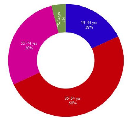
fig 1

Figure 1: Distribution of CRC cases in different age groups of Bangladeshi patients

As shown in Figure 1; half (50%) of the CRC cases belonged to adult active age group (35-54 years), followed by 28% cases in elderly (55-74 years), 18% cases in young (15-34 years) and 4% cases in  old age group (75-94 years). A chi-square test of independence was performed to examine the relationship  between  age  groups  and  the frequency of occurrence of CRCs. The relation between these variables was significant, X2 (3, N=50)=22.48, p=.0001 at α=0.05. The adult active age group (35-54 years) was more likely to be affected by colorectal carcinoma than the other groups.

Sex-wise distribution of CRC cases of this study revealed that almost two-thirds (64%) of the study cases were male while around one-third (36%) cases were female. The occurrence of male cases was numerically high in all age groups except the old age where the percentage of both cases was equal (Figure 2). The relation between the occurrence of CRS and sexes was weakly significant, [X2 (1, N=50)=3.92, p=.048 at α=0.05]. Males were more likely to be affected by colorectal carcinoma than females (Figure 2).
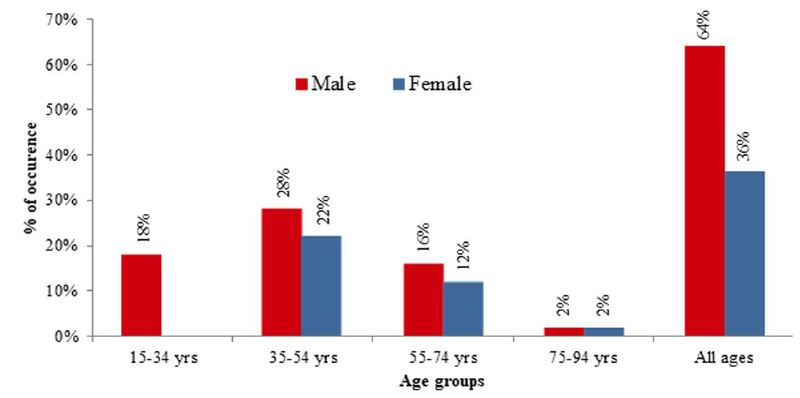
fig 2

Figure 2: Sex-wise distribution of CRC cases in different age groups of Bangladeshi patients

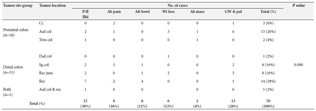
Per rectal bleeding was the most frequent clinical presentation  of CRC among the study population that was documented in 30% of cases followed by generalized weakness and pallor (26%), abdominal pain with or without features of obstruction (16%), altered bowel habit (12%), weight loss (12%) and abdominal mass (4%). Only one study case had a positive family history of colon cancer. None of the cases was presented with a history of extra-colonic malignancy. When the site of occurrence was considered, the tumor was located in the distal colon and proximal colon in 62% and 36% of cases, respectively. Only one (2%) of cases were recorded to have synchronous tumors involving both colons. However, no signification relation was observed between the tumor sites and the occurrence of CRC [X2 (1, N=50)=2.880, p=.090 at α=0.05]. The distribution of study cases based on tumor location along with presenting complaints is shown in Table 1.

Table 1: Distribution of study cases based on tumor location along with presenting complaints
ta 1

P/R Bld: Per rectal bleeding; Ab Pain: Abdominal pain; Alt bowl: Altered bowel habit; Wt loss: Weight loss; Ab mass: Abdominal mass; Gw & pal: Generalized weakness and pallor; Cc: Cecum; Asd. col: Ascending colon; Trns col: Transverse colon; Dsd col: Descending colon; Sg col: Sigmoid colon; Rec junc: Rectosigmoid junction; Rec: Rectum: Asd. col. & rec.: Ascending colon & rectum (synchronous)

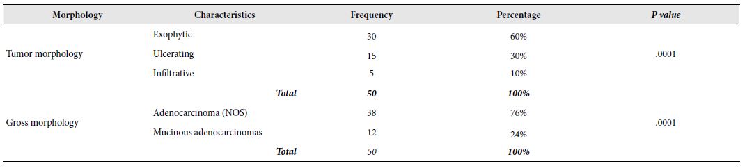
The exophytic pattern was the most common gross morphology which was observed in more than half (60%) of the cases, followed by ulcerating and infiltrative patterns, seen in 30% and 10% of the cases, respectively. In our study, the frequency of the Exophytic pattern was significantly higher than the other two patterns based on the chi- square test of independence, [X2 (2, N=50)=19.00, p=.0001 at α=0.05] indicating that Exophytic pattern was more likely to occur in CRC cases (Table 2).

Table 2: Distribution of study cases based on tumor morphologies
ta 2


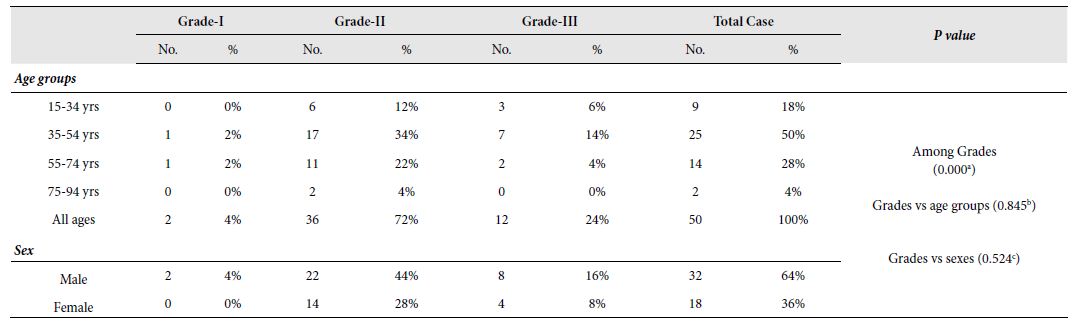
In this study, only two variants of adenocarcinoma were observed; the commonest one being adenocarcinoma (NOS) (76%) followed by  mucinous  adenocarcinomas  (24%).  The  frequency  of adenocarcinoma (NOS) in relation to CRC cases was highly significant [X2 (1, N=50)=13.52, p=.0001 at α=0.05] compared to mucinous adenocarcinoma. It seemed that adenocarcinoma (NOS) was the more frequent variant of CRC in Bangladeshi patients  (Table 2). Among the 50 selected cases, majority (72%) of the tumours belonged to grade II (moderately differentiated) tumors. Remaining 24% and 4% cases were categorized as grade III (poorly differentiated) and grade I (well differentiated) tumors, respectively. There was a highly significant relation between the occurrence of CRC the and grade of tumours [X2 (2, N=50)=36.640, p=0.000 at α=0.05]. However, no significant relationship was seen between the tumour grades and age groups [X2 (6, N=50)=2.702, p=0.845 at α=0.05] or sex [X2 (2, N=50)=1.292, p=0.524 at α=0.05]. It seemed that Grade-II CRCs were more likely to occur in case of colorectal carcinoma in Bangladeshi patients irrespective of age and sex. Figure 3 illustrates the graphical presentation of grades of tumours according to age groups and sexes whereas Table 3 summarizes the frequency of tumours according to grades, age groups and sexes with their relationship.
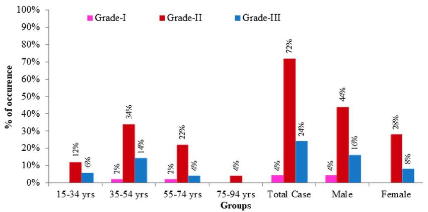
fig 3

Figure 3: Graphical presentation of grades of CRC cases according to age groups and sexes. Grade-I: well differentiated tumors; Grade-II: moderately differentiated tumours; Grade-III: poorly differentiated tumours.

Table 3: Frequency of tumours according to grades, age groups and sexes with their relationship
ta 3

No.: Number of occurrence; %: Percentage of occurrence;
a: X2 (2, N = 50) = 36.640, p = 0.000 at α = 0.05; b: X2 (6, N = 50) = 2.702, p = 0.845 at α = 0.05; c: X2 (2, N = 50) = 1.292, p = 0.524 at α = 0.05

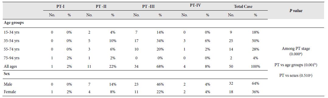
According to the pathological depth of invasion, studied CRC cases were ranked into 4 stages namely PT-I, PT-II, PT-III and PT- IV starting from lowest to highest invasion. Stage-3 (PT-III) was the most commonly recorded stage of tumour which was seen in 68% of the cases followed by PT-II, PT-IV and PT-I which were recorded in 22%, 8% and 2% cases, respectively. A highly significant relation was observed between the occurrence of CRC and the stage of tumours based on pathological invasion [X2 (2, N=50)=36.640, p=0.000 at α=0.05]. It seemed that PT-III is more likely to occur in Bangladeshi CRC cases. A highly significant relation was also observed between the pathological invasion of tumours and age groups [X2 (6, N=50)=2.702, p=0.845 at α=0.05] where adults are more likely to be affected by Stage-3 (PT-III) CRCs. However, no significant relationship was seen between the tumour stages and sex [X2 (2, N=50)=1.292, p=0.524 at α=0.05]. A graphical presentation of stage of tumours according to age groups and sexes has been depicted in Figure 4 and the summary of the frequency of tumours according to stages, age groups and sexes with their relationship is shown in Table 4.
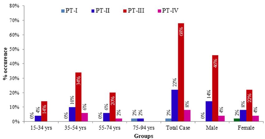
fig 4

Figure 4: Graphical presentation of stages of tumours according to age groups and sexes. PT-I: low pathological invasion; PT-II: moderate pathological invasion, PT-III: fair pathological invasion; PT-IV: high pathological invasion.

Table 4: Frequency of tumours according to stage of tumor based on the pathological depth of invasion. age groups and sexes with their relationship.
ta 4

PT-I; PT-II; PT-III; PT-IV; No.: Number of occurrence; %: Percentage of occurrence;
a: X2 (2, N = 50) = 36.640, p = 0.000 at α = 0.05; b: X2 (6, N = 50) = 2.702, p = 0.845 at α = 0.05; c: X2 (2, N = 50) = 1.292, p = 0.524 at α = 0.05

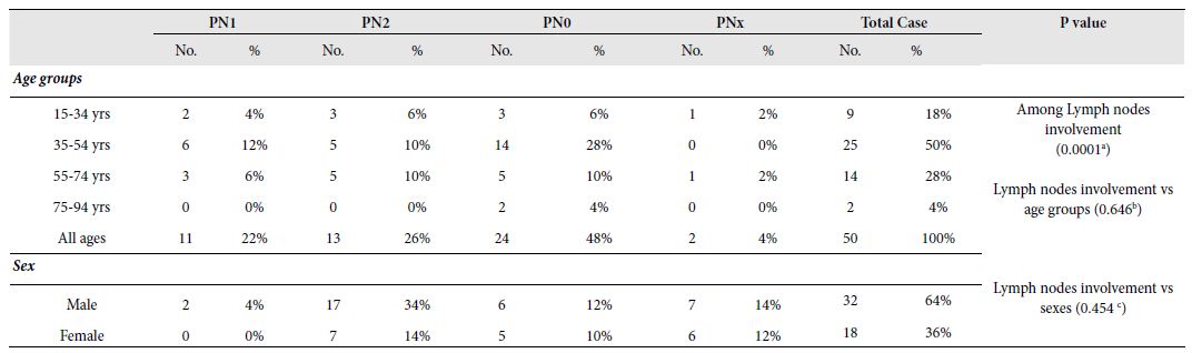
Studied CRC cases were further classified based on the involvement of regional lymph nodes by the tumor (PN) where cases with no lymph node involvement was grouped in PN0, metastasis in one to three regional lymph nodes in PN1, metastasis in four or more regional lymph nodes in PN2 and the cases where Lymph nodes could not be assessed was grouped in PNx. Almost half (48%) of the study cases was categorized in PN0 followed by PN2, PN1 and PNx in 26%, 22% and 4% cases, respectively. The involvement of regional lymph nodes was highly related to the occurrence of CRCs [X2 (3, N=50)=19.600, p=0.000 at α=0.05]. It is more likely that regional lymph nodes were not involved in CRC cases. However, no significant relationship was seen between the lymph node invasion and age groups [X2 (9, N=50)=6.915, p=0.646 at α=0.05] or sex [X2 (3, N=50)=2.620, p=0.454 at α=0.05]. Figure 5 illustrates the graphical presentation of different classes of CRC cases based on the involvement of regional lymph nodes according to age groups and sexes whereas Table 5 summarizes the frequency of different classes of CRC cases based on the involvement of regional lymph nodes according to stages, age groups and sexes with their relationship.
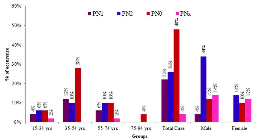
fig 5

Figure 5: Graphical presentation of different classes of tumours based on involvement of regional lymph nodes according to age groups and sexes. PNO: no lymph node involvement; PN1: metastasis in one to three regional lymph nodes; PN2: metastasis in four or more regional lymph nodes; PNx: lymph nodes could not be assessed.

Table 5: Frequency of tumours according to involvement of regional lymph nodes by the tumor, age groups and sexes with their relationship
ta 5

N1: ; N2: ; N3: ; N0: ; No.: Number of occurrence; %: Percentage of occurrence;
a: X2 (3, N = 50) = 19.600, p = 0.0001 at α = 0.05; b: X2 (9, N = 50) = 6.915, p = 0.646 at α = 0.05; c: X2 (3, N = 50) = 2.620, p = 0.454 at α = 0.05

Discussion

Although CRC is more likely to occur at old age, nowadays, younger patients are increasingly affected by different types of CRCs [13]. In this study, half (50%) of the cases belonged to the 35-54-years age group, with a mean of 48.60 ± 14.6 years which is lower than that reported age from the Western world [13-15]. Salminen, et al., 2005 recorded 59 years as the mean age of CRC in their study in the Finnish population and Turner, 2014 observed only 20% cases to occur below the age of 50 years [14,15]. However, Saha et al., 2016 and Raza et al., 2016 recorded the mean age as 50.77 years and 47 ± 14.8 years, respectively in Bangladeshi colorectal cancer patients [16,17], which are in good agreement with this study. The occurrence of CRCs specially in relatively young age group may be attributed  to the recent change in food habits of Bangladeshi active-aged people (35-54 years) who have shifted to western diets that ae well documented as a contributor to colon cancer. It has been reported that consumption of red or processed meats is associated with an increased risk of colon cancer [18]. Consumption of high fat containing foods like red or processed meats induces increased bile acids secretion that in turn results in altered microbial composition in gut [19, 20]. Such alternation in microbial community contributes to the production of different metabolites that might influence the development of colon cancer [20]. Moreover, geographical and environmental factors of the study population may have influenced the findings as well. However, the higher incidence of CRCs in the younger age group of Bangladeshi patients in comparison to western studies is alarming. This interesting finding necessitates the importance of cancer screening program and this report may be considered in future studies to evaluate predisposing and genetic factors for CRCs in this region.

In the current study, there was male preponderance (64%) with a male to female ratio 1.8:1. Studies conducted elsewhere also showed higher incidence of CRC among male patients [14,16,17]. Urbanization and changes in lifestyles might have contributed to the transformation in food habit from native to western diets rich in high fat which are known to trigger colon cancer. In association with altered food habit, higher incidence of smoking, alcohol consumption or genetic factors might be responsible for this male predominance.

Clinical presentations are different for proximal and distal CRC. In our study, per rectal bleeding was the most frequent finding (38.7%) in distal CRCs whereas, generalized weakness and pallor were the chief complaints of the patients with CRCs in proximal colon (38.98%). These features are consistent with the findings of reported elsewhere [5].

The most commonly observed location of CRC in this study is distal colon (62%). Rectum was most frequently observed site (28%). Other Bangladeshi studies conducted also found similar findings [17,21,22]. Occurrence of CRC in Bangladeshi population is higher in distal colon due to some unknown etiology which may be related to some genetic factors.

The exophytic pattern was the most common gross morphology observed in 60% cases followed by ulcerating (30%) and infiltrative pattern (10%). In this study, only two histological  types  of colorectal adenocarcinoma: adenocarcinoma (NOS) and mucinous adenocarcinoma were observed. Adenocarcinoma (NOS) comprises the majority (76%) of the total cases. These findings were consistent with the findings of other studies indicating common gross and histopathological feature of CRCs [17,21-23].

Among the 50 cases, 72% cases were Grade II tumours, 24% were Grade III and 4% were Grade I tumours. All of the mucinous adenocarcinoma was considered poorly differentiated (grade III). Several studies suggest that CRCs occuring in younger patients (less than 50 years of age) are less differentiated [24]. In the present study, 34% of Grade-II and 14% of Grade III tumours were observed in 35- 54 years of age whereas 22% Grade-II and 4% Grade III tumours were recorded in 55-74 years of age. Present study findings are in close agreement with previous findings that documented less differentiated CRCs are likely to occur within 50 years of age [23]. However, a statistically significant association between age group and tumor grade was not observed possibly due to a smaller sample size.

We also categorized study cases according to the PT and PN stage of the tumor. Our study revealed that PT3 (68%) and PN0 (48%) were the most commonly reported stages of tumor in CRC cases based on the depth of invasion and lymph node metastasis, respectively. Studies conducted elsewhere reported that colorectal cancers in young patients (<50 years of age) are biologically aggressive and present at advanced stage [9,25]. In our study, PT3 and PT4 stages were recorded in 34% and 6% cases, respectively in 35-54 years age group in comparison to 20% PT3 and 2% PT4 stages in 55-74 years age group. In the case of nodal staging, metastasis in one to three regional lymph nodes (PN1) was observed in 12% of cases in 35-54 years age group which was double of the observed cases (6%) in the 55-74 years age group. Our study findings for pathological invasion and metastasis in lymph nodes in CRC cases clearly support previous study reports that documented biological aggressiveness and advanced stage in colorectal cancers in patients under 50 years of age.  All  these  studies  suggest  that  patients  with colorectal adenocarcinomas usually present with advanced morphology in histopathology.

Conclusion

Present study findings on colon cancer were different from that described in the western countries. Active aged people (35-54 years old) were found to be significantly affected by CRC in our study. In majority of the cases, the tumour presented at a locally advanced stage. Quick urbanization, fast shifting to western food, lack of proper knowledge on CRC might account for some of these differences. Routine screening program is proposed for early detection and treatment of the cases to reduce the burden of morbidity and mortality. Genetic tests should also be carried out to unveil the cause of young age presentation of CRCs. However, this study had its own limitations. The study reflects to the findings of a specific geographical area with a small sample size. Therefore, further studies should be conducted all over the country with a larger sample size for a more comprehensive understanding on demographic and clinicopathological profiles of CRCs in Bangladesh.

Acknowledgements

The authors gratefully acknowledge the logistics and grant support to conduct the research activities from Bangabandhu Sheikh Mujib Medical University (BSMMU), Dhaka, Bangladesh.

Availability of Data and Materials

Raw data, supplemental data and materials are available on request.

Conflict of Interests

The authors declare that they have no conflict of interests in publishing the article.

Ethical Consideration

Written consent from individual patient/representative of patients was obtained for using the samples for research purposes. No personal data/information of patients was shared in public.

Author’s Contributions

SSUM planned, designed and performed the study. She also wrote the manuscript (MS). FB, MMR & AZ helped in planning & designing of the study and developing the research question. PR, TI, USS, UTN, SA and NA helped in data collection and processing. KBMS helped in study design, data screening and performed data analyses, interpretation and MS writing. All authors read and approved the final manuscript.

References

  1. GLOBOCAN 2020: New Global Cancer Data. [Online]; 2020. [crossref]
  2. Arnold M, Sierra MS, Laversanne M, Soerjomataram I, Jemal A, Bray 2017 Global patterns and trends in colorectal cancer incidence and mortality. Gut. 66(4): 683-691. [crossref]
  3. Wong MC, Ding H, Wang J, Chan PS, Huang J (2019) Prevalence and risk factors of colorectal cancer in Intestinal Research 17: 317-329. [crossref]
  4. Global Cancer Observatory. [Online].; 2020.
  5. Turner JR (2014) The Gastrointestinal In: Robbins and Cotran Pathologic Basis of Disease. 9th ed. Elsevier 749-819. [crossref]
  6. Valle L (2014) Valle Genetic predisposition to colorectal  cancer:  where  we  stand and future World Journal of Gastroenterology 20: 9828-9849. [crossref]
  7. Eddy DM. 1990 Screening for colorectal cancer. Annals of Internal Medicine 113: 373-84. [crossref]
  8. Paymaster JC (1964) Cancer and its distribution in India. Cancer 17: 1026-1034. [crossref]
  9. Mohandas M, Desai DC (1999) Epidemiology of digestive tract cancers in India large and small bowel. Indian Journal of Gastroenterology 18: 118-121. [crossref]
  10. Salem ME, Weinberg BA, Xiu J, El-Deiry WS, Hwang JJ, et (2017) Comparative molecular analyses of left-sided colon, right-sided colon, and rectal cancers. Oncotarget 8: 86356-86368. [crossref]
  11. Reynolds IS, Furney SJ, Kay EW, McNamara DA, Prehn JH, et al. (2019) Meta- analysis of the molecular associations of mucinous colorectal British Journal of Surgery. 106: 682-691. [crossref]
  12. Nguyen LH, Goel A, Chung DC (2020) Pathways of colorectal Gastroenterology 158: 291-302. [crossref]
  13. Nelson RL, Dollear T, Freels S, Persky 1997 The relation of age, race, and gender to the subsite location of colorectal carcinoma. Cancer 80: 193-197. [crossref]
  14. Salminen E, Palmu S, Vahlberg T, Roberts PJ, Söderström KO (2005) Increased proliferation activity measured by immunoreactive Ki67 is associated with survival improvement in rectal/recto sigmoid cancer. World Journal Gastroenterology 11: 3245-3249. [crossref]
  15. Turner The Gastrointestinal Tract. In: Kumar V, Abbas AK, Aster JC (2014) Robbins and Cotran Pathologic Basis of Disease. 9th ed. New Delhi: Reed Elsevier India Private Limited 810-814. [crossref]
  16. Saha M, Shil BC, Saha SK, Banik RK, Perveen I, et al. (2016) Study of Clinicopathological Profile of Sporadic Cases of Colorectal Euroasian Journal of Hepato-Gastroenterology 6: 134-136. [crossref]
  17. Raza AM, Kamal M, Begum F, Yusuf MA, Mohammad D, Begum M, et al. 2016 Clinico-demographic Characteristics of Colorectal Carcinoma in Bangladeshi Patients. Journal of Current and Advance Medical Research 3: 22-25. [crossref]
  18. Magalhaes B, Peleteiro B, Lunet N (2012) Dietary patterns and colorectal cancer: systematic review and meta-analysis. European Journal of Cancer Prevention 21: 15-23. [crossref]
  19. Islam B, Fukiya S, Hagio M, Fujii N, Ishizuka S, Ooka T, et (2011) Bile acid is a host factor that regulates the composition of the cecal microbiota in rats. Gastroenterology. 141: 1773-81. [crossref]
  20. Yokota A, Fukiya S, Islam KB, Ooka T, Ogura Y (2012) Is bile acid a determinant of the gut microbiota on a high-fat diet?. Gut Microbes 3: 455-459. [crossref]
  21. Rahman MM. Expression pattern of the proliferative marker Ki-67 and status of microsatellite instability in different histomorphological patterns of colorectal carcinoma. MD Thesis, Bangabandhu Sheikh Mujib Medical University (BSMMU), Dhaka, Bangladesh 2014.
  22. Hossain Clinicopathologic study of colorectal adenocarcinoma, MD Thesis, Bangabandhu Sheikh Mujib Medical University (BSMMU), Dhaka, Bangladesh 2014.
  23. Hashmi AA, Ali R, Hussain ZF, FN, Khan EY, Bakar SMA, et al. (2017) Mismatch repair deficiency screening in colorectal carcinoma by a four-antibody immunohistochemical panel in Pakistani population and its correlation with histopathological World Journal of Surgical Oncology 15: 116. [crossref]
  24. Chou CL, Chang SC, Lin TC, Chen WS, Jiang JK, et al. (2011) Differences in clinicopathological characteristics of colorectal cancer between younger and elderly patients: an analysis of 322 patients from a single institution. American Journal of Surgical Pathology 202: 574-582. [crossref]
  25. Mueller M, Schneider MA, Deplazes B, Cabalzar-Wond D, Rickenbacher A, et al. (2021) Colorectal cancer of the young displays distinct features of aggressive tumor biology: A single-center cohort World Journal of Gastrointestinal Surgery 13: 164-175. [crossref]
Bilateral Optic Neuropathy Induced by COVID-19

DOI: 10.31038/IMROJ.2023812

Abstract

Introduction: Bilateral optic neuropathy caused by the novel coronavirus SARS-CoV2 (COVID-19).

Case report: A 25 years old female COVID-19 (+) applied to our clinic with complaints of bilateral progressive visual loss. Two weeks prior to onset of eye and vision symptoms, she had tested positive for coronavirus disease (COVID-19) virus by nasopharyngeal polymerase chain reaction (PCR) after developing symptoms of shortness of breath and cough. One week prior to her admission, bilateral blurred and vision loss progresivvely. In her ophthalmological examination; right and left visual aquity were 10/200 with blurred vision and ocular tensions were 15 mmHg and 16 mmHg, right and left, respectively. Anterior segment in both eyes were natural, there were no active cells, however, there were optic disc edema and retinal edema in both eyes. The diffusion cranial MR was normal.

Discussion: Optic neuropathies is a clinical diagnosis based on the history and examination findings, generally. Because important findings on funduscopic examination help differentiate typical from atypical cases of optic neuritis, an ophthalmologic examination can be considered in the clinical evaluation. Our patient is believed to have acute bilateral optic neuropathies induced by COVID-19 infection. Ispite of optic neuropathies in young ages are usually associated with MS, our patient is an interesting and rare case induced by COVID-19 infection with bilateral optic neuropathies.

Keywords

The novel coronavirus SARS-CoV2 (COVID-19), Optic neuropathy

Introduction

Optic neuropathies in adults are usually unilateral and commonly linked to multiple sclerosis (MS). It usually occurs as sudden onset of visual loss associated with pain on eye movement and progress in its course to reach its maximum deficit in a week [1]. Diagnosis is usually clinical based on history and examination findings. Brain and orbital imaging such as magnetic resonance imaging (MRI) help in the diagnosis in most cases. After confirmation, treatment is usually standart. Bilateral acute optic neuropathies are seen rarely, particularly in individuals without known systemic inflammatory or autoimmune disorders.

Case Presentation

A 25 years old female COVID-19 (+) (the novel coronavirus SARS-CoV2) patient came to our clinic with bilateral vision loss in august 2021. Two weeks prior to onset of eye and vision symptoms, she had tested positive for coronavirus disease (COVID-19) virus by nasopharyngeal polymerase chain reaction (PCR) after developing symptoms of shortness of breath and cough. She was quarantined at her home and treated symptomatically with improvement; she never required hospitalization for his respiratory illness nor medications including hydroxychloroquine.

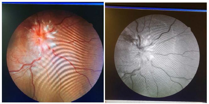
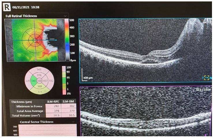
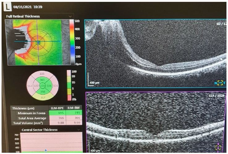
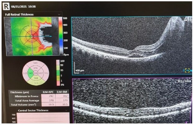
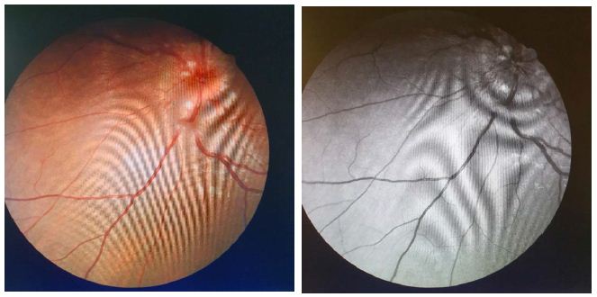
One week prior to her admission, bilateral blurred and vision loss progresivvely. She has no past medical history presented from clinic with bilateral eye pain and vision loss and family history of any neurological or immunological diseases. In her ophthalmological examination; right and left visual aquity were 10/200 with blurred vision and ocular tensions were 15 mmHg and 16 mmHg, right and left, respectively. Anterior segment in both eyes were natural, there were no active cells, however, there were optic disc edema and retinal edema in both eyes (Figures 1 and 2), and also seen in optic coherence tomography (OCT) (Figures 3 and 4). The diffusion cranial MR was normal.

fig 1

Figure 1: Right eye fundus photography

fig 2

Figure 2: Left eye fundus photography

fig 3

Figure 3: Optic coherence tomography of right eye

fig 4

Figure 4: Optic coherence tomography of left eye

Our patient was started on methylprednisolone 1 g every 24 hours for a total of 5 days/doses. Within 48 hours, his vision and eye pain had shown significant improvement. By day of discharge, our patient had complete restoration of vision in the left eye with remarkable but not complete vision recovery in the right eye. He was discharged on a tapering dose of prednisone over 4 weeks with planned follow-up with ophthalmology and neurology.

Discussion

Optic neuropathy is defined as a demyelinating, inflammatory condition that causes acute, usually monocular, visual loss. It is highly associated with MS, and it is the presenting feature in 15% to 20% of these patients and occurs in 50% of them at some time during their illness [2].

It is believed that the demyelination in optic neuropathies is immune-mediated, but the exact targeted antigens remain unknown [3].

Optic neuropathies is a clinical diagnosis based on the history and examination findings, generally. Because important findings on funduscopic examination help differentiate typical from atypical cases of optic neuritis, an ophthalmologic examination can be considered in the clinical evaluation. MRI of the brain and orbits with gadolinium contrast provide a better assessment of the diagnosis in most cases. Further diagnostic testing, such as lumbar puncture, is done to exclude other causes of visual loss in atypical cases. However, around 60% to 80% of patients with acute optic neuropathies have nonspecific findings in the CSF such as lymphocytes and elevated proteins [4].

Our patient is believed to have acute bilateral optic neuropathies induced by COVID-19 infection. Once the diagnosis of optic neuropathies is made, treatment is usually straightforward with intravenous methylprednisolone (typically 1 g per day for 3 days) often followed by oral prednisone (1 mg per kg per day for 11 days), with subsequent tapering over a period of 4 days [2]. Treatment is associated with a more rapid recovery of vision by 2 to 3 weeks with no impact on long-term visual function. Therefore, a follow-up with neurology and ophthalmology after discharge is recommended to reach a final diagnosis in cases like this.

Ispite of optic neuropathies in these young ages are usually associated with MS, our patient is an interesting and rare case induced by COVID-19 infection with bilateral optic neuropathies.

Conclusion

Our patient described in this clinical vignette has signs and symptoms typical of acute bilateral demyelinating optic neuritis on his presentation. His evaluation with brain and orbital MRI along with lumbar puncture to determine the possibility of MS or other autoimmune disease was negative as well as other laboratory assessment. Therefore, we believe his infection with COVID-19 virus has triggered his immune system to present these findings. COVID-19 virus infection is causing a huge impact in the world as pandemic; its extent as clinical disease is still poorly understood and explained.

Declaration of Interest

I have no declaration of interest.

References

  1. de la Cruz J, Kupersmith MJ (2006) Clinical profile of simultaneous bilateral optic neuritis in adults. Br J Ophthalmol 90: 551-554. [crossref]
  2. Balcer LJ (2006) Optic neuritis. N Engl J Med 354: 1273-1280. [crossref]
  3. Söderström M, Link H, Xu Z, Fredriksson S (1993) Optic neuritis and multiple sclerosis: anti-MBP and anti-MBP peptide antibody-secreting cells are accumulated in CSF. Neurology 43: 1215-1222. [crossref]
  4. Jacobs LD, Kaba SE, Miller CM, Priore RL, Brownscheidle CM (1997) Correlation of clinical, magnetic resonance imaging, and cerebrospinal fluid findings in optic neuritis. Ann Neurol 41: 392-398. [crossref]

Can Modern Medicine have Distorted Ideas?

DOI: 10.31038/IMROJ.2023811

Abstract

The reasons for the misconceptions that have arisen in modern ideas about the features of acute nonseptic inflammation of the lung tissue and the direction od necessary correction are considered.

Keywords

Acute pneumonia, Etiology, Pathogenesis, Disease doctrine

Acute inflammation of the lung tissue or acute pneumonia (AP) is one of the oldest medical nosologies, which has been and remains one of the  most serious diseases. Despite the severe nature of clinical manifestations, this disease has never had any reason to consider it dangerous from an epidemiological point of view.

For most of the history of the AP, the lack of sufficient scientific information about the features of the disease did not allow purposefully substantiating the most optimal means of medical care. Therefore, the search and selection of effective methods of treatment took place empirically, by trial and error. Nevertheless, such an intuitive search for medical care for these patients allowed ancient medicine to identify methods that were subsequently used with sufficient success for many centuries until the last decades. In this case, we are talking primarily about first aid methods, the timely use of which could bring relief to the patient and reduce the severity of the disease. In different regions of the world, to achieve this effect, preference was given to such methods of care as cupping therapy, bloodletting or short-term cooling of the patient’s body. The evaluation of the results was purely subjective on the part of both doctors and patients. Therefore, if these methods did not bring the expected satisfaction, they could hardly remain in demand for thousands of years. The situation in this field of medicine began to change dramatically after the discovery and the beginning of the clinical use of antibiotics in the middle of the last century. By this time, medical science had information and facts that created prerequisites for the distortion of scientific views on the problem of AP under the influence of a new type of therapy.

The development of microbiology made it possible to identify the pathogens of AP, among which Streptococcus pneumoniae, discovered in the 19th century and given its name in this regard, played a dominant role. At the same time, this circumstance did not change the indifferent view of the epidemiology of the disease due to the absence of cases of the spread of AP in contact with such patients. Pneumococcus continued to consistently dominate among the pathogens of AP, and its frequency on the eve of clinical use of antibiotics continued to reach 90-95% [1-3]. Nevertheless, these processes were fairly interpreted as acute nonspecific inflammation, which emphasized the polymicrobial nature of its etiology.

Continuing to consider AP as an inflammatory rather than an infectious process, medicine was initially aware of the fact that antibiotics are able to act only against the microbial factor and do not have a direct effect on the mechanisms of inflammatory tissue transformation. However, the initial results of the use of antibiotics created the illusion that a universal remedy for the treatment of inflammatory diseases has been found. At the same time, the fact was overlooked that the successful suppression of the pathogens of the process required the patient’s body to independently eliminate the pathological deviations that had arisen, not only morphological, but also functional. In the resulting atmosphere of euphoria, the centuries-old experience of medicine remained unclaimed as a relic of the past, and the standard treatment of AP after a short period of time began to appear under the term “antibiotics alone”. The revision of the principles of AP treatment has led to equally radical changes in the didactics of medical personnel training. Therefore, when the side effects of antibiotics began to intensify, requiring the correction of unforeseen situations, efforts were made in the hope of reviving the previous effect of antimicrobial therapy. By now, persistent attempts to revive the etiotropic principles of AP treatment have become a strategic goal of solving the problem, and the process of deformation of ideas about its essence has gone so far that many indisputable facts that contradict the currently dominant concept of the disease have ceased to be the subject of discussion. The generally recognized fact of the emergence of a large group of antibiotic-resistant strains and the loss by antibiotics of their role as the leading therapeutic agent in AP is just the tip of the iceberg.

In recent decades, many experts have expressed concern about the growing role of viruses in the etiology of lung inflammation, which accounted for almost half of all AP diseases in the world about two decades ago [4-6]. The former relatively stable list of AP pathogens began to differ by changing priorities with periodic change of leaders. The initial prevalence of pneumococcus in the etiology of the disease in recent years has decreased to 10.9% – 22.5% among the positive results of a bacteriological study [7]. It would seem that in the presence of these circumstances, there is an obligatory need for a radical revision of views on this problem and a change in therapeutic principles. However, the realization of these obvious needs has not been observed in recent decades, and even during the SARS-CoV-2 pandemic, antibiotics unable to suppress the coronavirus continued to be presented as the main method of treating COVID-19 pneumonia [8-10]. The fear of coronavirus that arose during the SARS-CoV-2 pandemic and the transition to strict epidemiological measures were dictated not only by the appearance of a pathogen that is not quite familiar to the human body, but, above all, by the lack of effective ways to provide assistance. At the same time, the statistics of this unexpected event convincingly show that 80% of the infected population safely endured this incident on an outpatient basis without any specific medical care, and 20% of them learned about the presence of infection only by the results of the tests carried out [11,12].

These data only confirm the ancient postulate that people get sick with pneumonia, not infected. Inflammation of the lung tissue, which is not a fatal inevitability even during the last coronavirus pandemic, further revealed pressing problems with the principles of its treatment when such patients began to concentrate in specialized departments, which had a strong psychological impact on medical personnel [13,14]. The loss of the former effectiveness of antibiotics every year more and more acutely required additional methods of treatment. The interpretation of the need for such care in patients with AP and the choice of additional methods were completely based on the “microbial” concept of lung inflammation, which was formed during the use of antibiotics and considers microbiological factors as the main cause of the disease and its consequences. As a result of such a narrow definition of the main difficulties in the treatment of AP, the disease itself has been classified as infectious in recent years, although the sanitary and epidemiological conditions have remained the same. In addition, in recent years, the number of cases with septic complications of AP has begun to grow, but, unlike sepsis in other localizations of inflammation, it is in this group of patients that the bacteriological blood test often turns out to be negative [15,16].

Such a selective discrepancy between the diagnosis and the criteria for its confirmation for this category of patients receives truly striking explanations as a consequence of preliminary antibacterial therapy [15,17,18]. In other words, in accordance with the dominant concept of the leading role of the etiology of the process, it is assumed that successful antibacterial therapy eliminates pathogenic microorganisms, but, at the same time, does not save (!?) from generalization of infection. In recent years, the process of diagnosing septic complications has also emerged solely on the basis of analogies and without any convincing arguments in the case of viral forms of inflammation [16,19,20]. Even more puzzling are the principles of septic shock diagnosis in patients with AP, in whom the presence of the pathogen in the bloodstream barely exceeds 10% and in fact does not differ from this indicator in sepsis [21], but the level of peripheral blood pressure continues to be one of the leading criteria for this assessment. At the same time, the fact that the primary focus of the disease damages the vessels of the small circulatory circle, which have diametrically opposite indicators with the periphery and have a regulating effect on the overall blood flow, is completely ignored [22-24].

The prevailing ideas about septic complications in patients with AP today suggest the use of additional treatment methods that were previously justified and tested for other localizations of inflammation. The basis of such assistance is infusion-bolus therapy, the effect of which is directly opposite to the methods of old medicine, since it is accompanied by an additional load on the blood vessels in the area of lung damage. And since the effectiveness of these efforts leaves much to be desired, modern recommendations provide in advance for the subsequent administration of vasopressors [16-19].

As a result, modern medicine cannot achieve noticeable success in the treatment of the most severe forms of AP, in which mortality in intensive care units remains unprecedentedly high, reaching, according to some data, 91% [25]. At the same time, only some authors publish frank confessions that the condition of many patients from this group continues to deteriorate after the start of inpatient treatment and despite this [19], and the overwhelming number of patients with septic shock did not have it during hospitalization (!) and it developed already during treatment [26]. The prevailing ideas about pneumonia today are the reason for the intensified search for etiotropic treatment of these diseases in the hope of a revival of success comparable to the beginning of the era of antibiotics. However, the nonspecific nature of this nosology, combined with the constant change of leading pathogens, as well as the accumulated experience and profound biological consequences of the use of antibiotics create real doubts about such a revival. At the same time, viral pneumonia does not have a special treatment, and studies at the cellular and molecular level, which are conducted in this direction, may be able to provide a detailed understanding of the mechanisms of the process and help in optimizing pathogenetic treatment methods. But so far this is only a prospect, not a reality. It should be added that the search for effective ways to help patients with AP over the past many years has not brought tangible success. A certain surge in the improvement of results was observed with the release of new antibacterial drugs, but their use was invariably accompanied by a tendency to decrease the achieved primary effect. At the same time, the former centuries-old experience of medicine remains forgotten and unexplored. A comparative evaluation of the effect of some of the ancient techniques mentioned above using objective tests has shown their amazing ability to bring a positive result. The rationale for new approaches to the treatment of this category of patients has been tested in the clinic and has demonstrated excellent results, fragments of which have been published in numerous articles in recent years and summarized in a monograph [27].

Today, medical science has much more opportunities for an objective assessment and selection of adequate methods of medical care than during the above-mentioned work. It is unlikely that for patients with AP, the old medical care options may be unacceptable if their use allows you to quickly and effectively eliminate the disease. To implement these projects, the results of which are urgently needed by millions of patients, it is necessary first of all to take a critical look at modern views on this problem, bringing the existing ideology of the disease in line with the facts of medical practice and the canons of science. Only after this step it will be possible to choose the optimal therapeutic methods – ancient or recently discovered.

References

  1. Heffron R (1939) Pneumonia, with special reference to pneumococcus lobar pneumonia. Cambridge: Harvard University Press.
  2. Small JT (1948) A short history of the pneumococcus with special reference to lobar pneumonia. Edinb Med J 55(3): 129-1. [crossref]
  3. Musher DM, Abers MS, Bartlett JG (2017) Evolving understanding of the causes of pneumonia in adults, with special attention to the role of pneumococcus. Clin Infect Dis 65(10): 1736-17. [crossref]
  4. WHO Revised global burden of disease 2002 estimates. 2004. http://www.who.int/healthinfo/global_burden_disease/estimates_regional_2002_revised/en/ (accessed Nov 5, 2010).
  5. Rudan I, Boschi-Pinto C, Biloglav Z, Mulholland K, Campbell H (2008) Epidemiology and etiology of childhood pneumonia. Bull World Health Organ 86: 408-416. [crossref]
  6. Ruuskanen O, Lahti E, Jennings LC, Murdoch DR (2011) “Viral pneumonia”. Lancet 377 (9773): 1264-1275.
  7. Cilloniz C, Martin-Loeches I, Garcia-Vidal C, San Jose A, Torres A (2016) Microbial Etiology of Pneumonia: Epidemiology, Diagnosis and Resistance Patterns. International journal of molecular sciences, 17(12), 2120. https://doi.org/10.3390/ijms17122120
  8. D. Huttner, G. Catho, J.R. Pano-Pardo, et al. (2020) COVID-19: don’t neglect antimicrobial stewardship principles. Clinical Microbiology and Infection, Vol 26, Issue 7, P808-810. [crossref]
  9. Beovic, M. Doušak, J. Ferreira-Coimbra, et al. (2020) Antibiotic use in patients with COVID-19: a ‘snapshot’ Infectious Diseases International Research Initiative (ID-IRI) survey. Journal of Antimicrobial Chemotherapy, dkaa 326.
  10. Lipman M, Chambers RC, Singer M, et al. (2020) SARS-CoV-2 pandemic: clinical picture of COVID-19 and implications for research. Thorax 75: 614-616. [crossref]
  11. Wu, J. M. McGoogan (2020) Characteristics of and Important Lessons from the Coronavirus Disease 2019 (COVID-19) Outbreak in China. Summary of a Report of 72 314 Cases from the Chinese Center for Disease Control and Prevention. JAMA 323(13): 1239-1242. [crossref]
  12. Zhou B, Kojima S, Kawamoto A, Fukushima M (2021) COVID‐19 pathogenesis, prognostic factors, and treatment strategy: Urgent recommendations. J Med Virol 1-11. [crossref]
  13. E. Leiter (2020) Reentry. NEJM, October 14, 2020.
  14. N. Rosenquist (2020) The Stress of Bayesian Medicine — Uncomfortable Uncertainty in the Face of Covid-19. NEJM, N Engl J Med 384: 7-9.
  15. Lin G L, McGinley JP, Drysdale SB, et al. (2018) Epidemiology and immune pathogenesis of viral sepsis. Front Immunol, 9: 2147. [crossref]
  16. Weiss, S.L, Peters, M.J, Alhazzani, W. et al. (2020) Surviving sepsis campaign international guidelines for the management of septic shock and sepsis-associated organ dysfunction in children.Pediat Intensive Care Med 46, 10-67. [crossref]
  17. Liapikou A, Ferrer M, Polverino E, et al. (2009) Severe Community-Acquired Pneumonia: Validation of the Infectious Diseases Society of America/American Thoracic Society Guidelines to Predict an Intensive Care Unit Admission. Clin Infect Dis 48: 377-385. [crossref]
  18. Restrepo MI, Mortensen EM, Rello J, et al. (2010) Late admission to the ICU in patients with community-acquired pneumonia is associated with higher mortality. Chest 137: 552-557. [crossref]
  19. Singer M, Deutschman CS, et al. (February 2016) “The Third International Consensus Definitions for Sepsis and Septic Shock (Sepsis-3)”. JAMA 315 (8): 801-810.
  20. Prescott HC, Girard TD (2020) Recovery From Severe COVID-19: Leveraging the Lessons of Survival From Sepsis. JAMA 324(8): 739-740.
  21. Garcia-Vidal C, Ardanuy C, Tubau F, et al. (2010) Pneumococcal pneumonia presenting with septic shock: host-and pathogen-related factors and outcomes. Thorax 65: 77-81. [crossref]
  22. Blood pressure. https://en.wikipedia.org/wiki/blood_pressure#pulmonary_pressure
  23. Schwiegk H (1935) Der Lungenentlastungsreflex. Pflügers Arch. Ges Physiol 236, 206-219.
  24. Olivia Vynn (2001) Cardiology secrets. Chapter 41, p. 210. Adair Edition: 2, illustrated Published by Elsevier Health Sciences, ISBN 1-56053-420-6, 978-1-56053-420.
  25. Rollas K, Ersan G, Zincircioglu, et al. (2021) Septic shock in patients admitted to intensive care unit with COVID-19 pneumonia. Eurasian J Pulmonol 23: 95-100. [crossref]
  26. Gattinoni L, Gattarello S, Steinberg I, et al. (2021) COVID-19 pneumonia: pathophysiology and management. Eur Respir Rev 30: 210138. [crossref]
  27. Klepikov I (2022) The Didactics of Acute Lung Inflammation. Cambridge Scholars Publishing, 2022, 320pp. ISBN: 1-5275-8810-6, ISBN13: 978-1-5275-8810-3.

Empowering Young People to become Researchers: What do People Think about the Different Factors Involved When Shopping for Food?

DOI: 10.31038/NRFSJ.2023612

Abstract

Two student researchers, one in middle school and the other in grade school, designed and executed an experiment to explore the different factors that other young people use when shopping for food for adults. Using a templated experimental design (BimiLeap), augmented with artificial intelligence, the researchers developed four questions and four answers (elements) to each question. The raw material for the study comprised the 16 elements combined by experimental design into 24 combinations, or 4950 vignettes tested across 100 respondents. The deconstruction of the responses by regression, followed by clustering, revealed two dramatically different mind-sets (focus on the experience of shopping versus focus on nutrition and healthfulness of the food). A third mind-set showed little polarization of responses. The study shows the potential of exploring topics of the everyday by students in grade and middle school, who bring a new perspective to a topic.

Introduction

The world of food selection and food consumption is replete with data, knowledge, insights, and practices. The reason for the abundance of knowledge is obvious; our very existence, and certainly our civilization is predicated on the smooth running of the world of food. And so a detailed review of the literature about food as an introduction to the topic of critical thinking about food ‘behavior’ is not necessary. What might well be a contribution is a study on how young people think about one or another ‘granular’ areas of food behavior. It is in that spirit that this paper focuses on ‘what do people think about the different factors involved when shopping for food?’

The literature on shopping suggests that children are 2-3 times more likely to be mentioned as the source of foods to be purchased in the store. Whether or not the child does the actual shopping, it is the child who exerts a great deal of influence. According to Kraak & Pelletier (1998) “Parents are two to three times more likely to name a child—- not themselves—-as the family expert for selection of fast food, snack food, restaurants, and new breakfast cereals. Market research reveals that children and teenage youth identify products more frequently by brand name rather than food category.”

Much of the information about shopping comes from questionnaires, with the information based upon one’s memory of who did what, and why. Gram (2010) points out that a great deal of what is assumed to be fact may not be as definitive as desired. There is little in the way of experimentation about shopping, and the experiments are often tied to a specific issue, done for a corporation, and stored in the corporate vaults until discarded. In Gram’s elegant questioning of what is presumed to be known “It is well documented that parents know that their children influence what they buy in supermarkets but it is also found that parents and children do not agree on just how much influence children have. Thus, a gap exists in the knowledge about what is actually happening in this grey zone of grocery shopping which seemingly cannot be solved through retrospective data collection. Family shopping is neither a completely rational nor conscious process, which makes the use of self-reported behaviour problematic.”

The origins of this come from separate roots. A literature search reveals that as far back as 2012, Bucknall (2012) published the results of a four-year practical effort to engage children in research. The volume is appropriately titled: Children as Researchers in Primary Schools: Choice, Voice and Participation. Bucknall presents the book as a challenge and a solution.

“How often do your primary school pupils have the opportunity to engage in open-ended, sustained pieces of work that offer them choice and control?

Do you find that the curriculum restricts openings to provide your pupils with real challenge? Is your school grappling with finding effective ways in which to elicit authentic pupil voice? ‘Children as Researchers in Primary Schools is an innovative and unique resource for practitioners supporting children to become ‘real world’ researchers in the primary classroom…. Children in primary schools are accustomed to being set short-term goals and are often unaware of long-term aims or of the connections between the concepts and skills they are learning. In contrast, this book demonstrates that children engaging in the research process have authentic opportunities to apply invaluable personal, learning and thinking skills while managing their own projects, making their ‘voices’ heard and experiencing increased levels of engagement and self-esteem.”

The origin of this paper comes from the ongoing efforts both to empower young people to become researchers by developing their faculty of critical thinking, and by using the opportunity to explore a topic from the point of view of a young person. That topic is what might a person think about when shopping for food. What makes the approach ever relevant is that we rarely explore topics of human thinking and behaving from the point of view of a young person. Even in those situations where we are interested in the response of young people, the process is bounded by the fact that the thinking going into the project is adult-driven. Adults choose the test stimuli. The young person provides data about topics relevant to being a young person, but with the test design by adults. Thus, to address the topic sentence of this paragraph, we are exploring the subject of food shopping, with test materials designed by a student in middle school (CLM, age 14), aided by a student in grade school (CIM, age 8) , and with respondents ages 13-24.

Mind Genomics

The research process is Mind Genomics (Moskowitz, 2012; Moskowitz & Hartmann, 2008). Mind Genomics is an emerging science, dealing with the perception of and decision about topics of the everyday. Mind Genomics emerged in the 1980s, its origin in the business world, where it was becoming increasingly important to create a science of decision-making. This science had to deal with the ordinary, the topics of which were and remain relevant to science. It was the sheer ordinariness, which was relevant, a relevance becoming increasingly important in the business world. The science of the day was and remains the study of decision-making, with, however, the surrounding features of the topic changed so that deep principles can emerge from the experiment. The reality of the situation had to be modified to reveal the underlying process of the way people think, and the way people make decisions. The foregoing paragraph can be summarized simply. That summary phrase is that every day is simply too complex, too unruly, to be of interest to experimental science.

With the inability of experimental science to deal with the complexities of the simple everyday, a different approach was necessary. Fortunately, the approach could be crafted by combining three different disciplines:

  1. Experimental psychology, with its emphasis on experimentation. The discipline of psychophysics is especially important. Psychophysics deals with developing relations between stimuli and responses. The foundation of psychophysics is the relation between physical stimuli and subjective responses (outer psychophysics in the words of S.S. Stevens, late professor of psychophysics at Harvard). Stevens occasionally stated wish (personal communication, 1967) was to rate the inner psychophysics, measuring ideas. And so Mind Genomics took that notion of inner psychophysics as one of its foundation stones.
  2. Statistics and its emphasis on experimental design. Experimental designs tell us how to order combinations of variables, i.e. creating mixtures. The experiment measures responses to these mixtures, and deconstructs the response to the components of the mixture. Experimental design is necessary because it is only mixtures that make sense to the person. The analogy is a food comprising several ingredients and processing variables. We can’t test a food with one ingredient alone. We have to make the combination, but in the combination, we don’t know what is happening. We can systematically vary the ingredients, test the combination, get ratings of tastiness, and identify how the different ingredients ‘drive’ tastiness.’ Mind Genomics does the same, but with combinations of ideas.
  3. Consumer research and its emphasis on measuring real things and events. Consumer researchers work in the world of business. They focus on how consumers make decisions about the everyday. Often the consumer researcher uses methods such as surveys to ask people what they do, or what to them is important versus what is unimportant. Of importance here is their focus on the ‘real and meaningful’, as well as their efforts to ‘measure’ the way people think. Consumer research does not, however, typically do experiments, except for the pioneering research efforts of the late Professor Paul Green and his associates at Wharton (Green & Srinivasan 1990). Green’s work used trade-off analysis (conjoint analysis) to identify the relative importance of different factors people used to make their everyday decisions for specific topics. Green’s work specifically, and the world of consumer research in general, are the immediate sources of much of the way Mind Genomics studies are conducted and analyzed.

Study Specifics

Mind Genomics studies are created using a templated system (www.BimiLeap.com). The system is set up to acquire the necessary information from the researcher, as well as to aid the researcher who needs guidance to provide the necessary inputs (questions, and answers).

Step 1 – Record the ‘Topic’

This portion is simply to give the study a name and to accept the terms of privacy.

Step 2 – Generate Four Questions

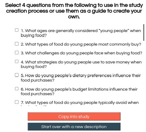
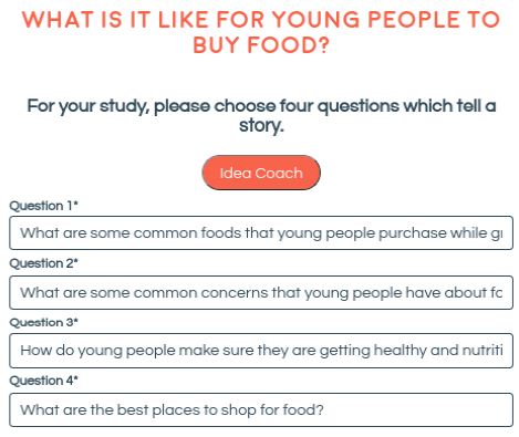
The questions will never be shown to the respondents who participate in a Mind Genomics study. The sole reason for the questions is to structure the vignettes so that the vignettes tell a story and to elicit from the researcher different answers to the questions. Figure 1 shows the request by the researcher for the embedded artificial intelligence, supplied by OpenAI (2023) to provide suggested questions. For researchers, the Idea Coach itself ends up being a teacher because the Idea Coach returns with up to 30 questions for each request. The researcher need only write a sentence or two in the specially designated ‘box’, with Idea Coach returning 30 new elements. Figure 1 shows some of the Idea Coach output for an iteration in Step 2. Figure 2 shows the four questions selected by the researcher from the Idea Coach offerings, and after slight editing by the researcher.

fig 1

Figure 1: Partial output from Idea Coach in response to the request ‘Tell me about young people and buying food’.

fig 2

Figure 2: The final four questions selected by the researcher

Step 3 – Develop Four Answers for Each Question

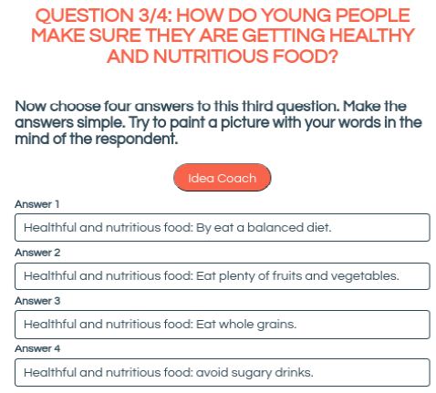
Most researchers using BimiLeap find that by the time they have developed the questions, they experience little difficulty answering each question. Nonetheless, Idea Coach provides about 15 candidate answers for each question. When the Idea Coach is instructed to provide new sets of 15 candidate answers for a question, it will return with a number of new answers. Idea Coach thus becomes a teaching aid for the researcher. Figure 3 shows a set of four answers to question #3. The answers emerged from Idea Coach, but the researcher changed the format of the answer by putting the aspect of the question (healthful and nutritious food), followed by a colon, and then the actual answer. The ability to combine the sourcing of the element by Idea Coach with the ability to edit the element to be appropriate for the question becomes an opportunity to reinforce critical thinking.

fig 3

Figure 3: The four answers provided by Idea Coach, after being edited by the researcher

Step 4: Finalize the Questions and the Answers (Elements)

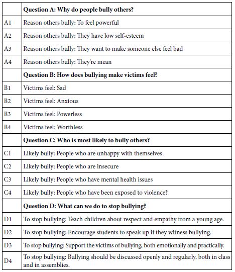
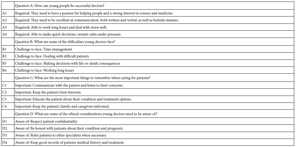
Table 1 shows the four questions and the four answers for each question. The researcher has edited the questions and answers (now called elements). Note that the answers have been edited for clarity. The original answers emerging from the Idea Coach had relevant information, but the structure of the phrases would not work in a Mind Genomics study, where the elements would be combined ‘as is’, with no polishing at all applied to make the combination easy to read. In light of the recognition that the elements have to ‘stand by themselves’, the researcher polishes the element, so that the first part of the element gives the idea, followed by a colon, and then the specific aspect. This editing did not do any violence to the element but ensured that the element would be meaningful when it would be presented.

Table 1: The questions and elements

tab 1

Step 5: Create the Introduction to the Respondent and the Rating Scale

In the actual Internet session with real people, the respondent will evaluate combinations of answers (viz., so-called vignettes). Step 4 instructs the respondents to read (the vignette), and assign a rating on an anchored 5-point scale. The rating question is kept deliberately vague, to let the elements themselves drive the response. In that way, the researcher can determine which elements do the ‘convincing.’

Step 6: Create the Self-profiling Classification Question(s)

The rationale here is that it is often of interest to do the analysis at a granular level. Consumer researchers especially focus on responses to questions, and how different types of people respond to the same question. Through the analysis of the same questions by different groups, consumer researchers often discover new patterns which do not emerge when all the data from all the respondents are combined. The self-profiling questionnaire requires the respondent to define age and gender (fixed for all studies), as well as answer the question below:

Preliminary question: Are young people responsible enough to buy food for older people?

Answers: 1=Yes, they are 2=No, they aren’t.

Step 7: Use the Built-in Experimental Design to Create the Vignette, and Test Them with Respondents

The objective of Mind Genomics is to determine the degree to which the individual elements drive the ratings. At the same time, the respondent evaluates more ‘natural’ combinations of elements, with these combinations constructed according to an underlying set of specifications, known as a permuted experimental design. The design specifies exactly 24 combinations, vignettes, for each respondent, some vignettes comprising two elements, some comprising three elements, and some comprising four elements. The vignettes follow a mathematical structure set up so that the data for each respondent who participates can be analyzed by regression to reveal the contribution of the individual elements.

  1. With 24 vignettes, each element appears five times in the 24 vignettes and is absent 19 times.
  2. A vignette can have at most one element or answer from a question
  3. The 16 elements, viz., the answers to the four questions are set up in the combinations, but with the 16 elements combined in different ways, and statistically independent of each other
  4. Each respondent ends up evaluating the 24 elements following the same mathematical structure, but with the combinations different for each respondent. The permutation scheme creates thousands of different vignettes, each set of 24 both ‘the same structurally, but different in terms of actual combinations’ (Gofman & Moskowitz, 2010).
  5. The foregoing preparation allows the results to be analyzed at the level of the group, or a level of the individual respondent.

Step 8: Work through an Online Aggregator of Respondents to Get 100 Respondents

The typical price for easy-to-find respondents may go from a low of US$2 when one provides one’s own respondents, e.g., students, to US$4 when one uses the services of Luc.Id, the aforementioned panel aggregator, to provide respondents It is not advisable to run important studies using one’s own students, simply because executing the study with one’s friends and neighbors can require a week or two when the students provide their own panelists. A more unique approach uses the online panel provider, which may be slightly more expensive but it moves the research as.

Initial Results – Frequency of Ratings

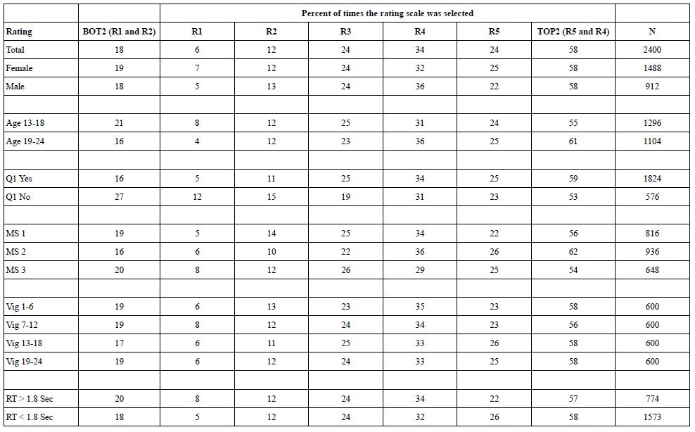
Mind Genomics produces a great deal of data, albeit with each of the test stimuli being unique, perhaps appearing one to three times across the 2400 vignettes generated by the 100 respondents. Our first analysis considers the frequency of assignment of each of the five ratings to the full set of vignettes. We begin by assuming that we know nothing about the meaning of each vignette. We look at the surface patterns emerging, specifically the relative frequency (percent) used by each of the groups that we can identify. These groups will be based on WHO the respondent is, how does the respondent THINK (mind-sets, to be discussed later), and two aspects of the test stimuli, namely the order of testing broken out into four equal positions, and then the speed of response for the assignment of ratings.

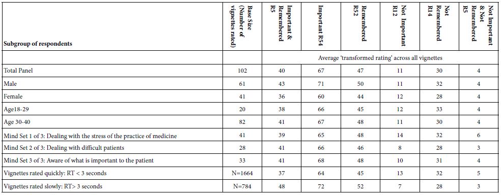
When we do this type of analysis, not knowing anything profoundly about the stimulus, we simulate what is often the case indeed what ends up being typical. Table 2 and 3 suggests that without knowing anything more than the information about the respondent, or some superficial information about the test stimulus (viz., position in the set of 24; the speed of response when rating the vignette) we will discover very little from simply deeply analyzing the superficialities of the stimulus [1-9].

Table 2: The rating question and the anchored 5-point rating scale

tab 2

Table 3: Percent of time respondents select each rating scale point, as well as percent of time respondents choose to say ‘makes no sense’ (BOT2) or ‘makes sense’ (TOP2).

tab 3

Creating a Database, and then Estimating Equations that Show How Elements ‘Drive’ Ratings

The underlying experimental design provides us with a number of benefits, the most important of which is that the researcher can easily determine the contribution of each element to the ratings. The respondents each evaluated unique sets of 24 vignettes, assigning a rating to the vignette. The data for each vignette was added to a simple database. The creation and properties of that database would be the key to deep understanding.

The database emerges from the following straightforward steps. One need only think of an Excel® worksheet to get an idea of what the database looks like. Here are the different sections of the database. Keep in mind that each respondent will generate 24 rows, one row for each vignette with a separate column assigned for each piece of information.

Section A: Row number. This section comprises a single number from 1 to 2400, to identify the record, and to allow the researcher to sort the file so it returns to the original order.

Section B: Information about the person, including a unique identifier for the respondent and separate columns for gender, age, and responses to the single-added classification question. Each person is different. The same information will be repeated a total of 24 times, once for each of the 24 vignettes that the respondent rated.

Section C: Order of the vignette for the respondent. Each respondent evaluates 24 unique vignettes. This column simply shows the order tested, from the start of the first vignette evaluated by the respondent (Order=1) to the last vignette evaluated by the respondent (Order=24). In the analysis, the order of testing will be augmented by a new variable, ‘Quarters’, with Quarters taking on the value ‘1’ for those vignettes tested in orders 1-6, the value ‘2’ for those vignettes tested in order 7-12, etc. This reduction will enable us to compare the response to the elements when the element was tested in different places, e.g., at the first part of the interview versus at the last part of the interview. Thus, the so-called ‘order effect’ can emerge and be measured.

Section D: 16 columns, one column reserved for each of the 16 elements. For any row (a vignette), the cell corresponding to a specific column is coded ‘0’ when the element is absent from the vignette and coded ‘1’ when the element is present in the vignette. The row will have 2-4 cells with the value ‘1’, and the remaining cells with the value ‘0’. This method is called ‘dummy variable coding’, denoting simply whether a variable is present or absent in a vignette. It will be this coding that allows the statistical analysis of the data.

Section E: The information recorded by the Mind Genomics program, www.BimiLeap.com, during the evaluation of the vignette. The program records both the rating and the response time (RT). RT is defined as the number of seconds to the nearest hundredth of a second elapsing between the presentation of the vignette on the screen and the rating.

Section F: Transformed ratings. Although it is easy to measure responses on a simple scale, such as the 5-point scale used here to assess ‘makes sense’, the reality is that the user of the data often has a difficult time working with the averages or distributions which emerge. The oft-heard question by the manager usually comes out as ‘please explain what this average value of 4.1 actually means, and what actions should I take when I see this average, versus when I see a smaller average such as 2.9?’. Managers who use the data find it easier to deal with yes/no information. To make the data more useful, the Mind Genomics program follows traditional paths previously done in consumer research, viz., recodes or transforms the data. There are two transformations:

TOP2 (Makes sense), ratings 5 and 4 transformed to 100, ratings 1,2,3 transformed to 0

BOT2 (Makes no sense), ratings 1, 2 transformed to 100, ratings 3,4,5 transformed to 0

To prepare the data for statistical analysis it is necessary that the newly created variables (TOP2, BOT2) exhibit some small variability, and not be the same for any individual respondent. To ensure this minimal variable, the BimiLeap program automatically adds a vanishingly small random number (< 10-5) to all newly created values of TOP2 and BOT2, respectively. The number will not measurably affect the results but will protect against ‘crashing’ the statistical analysis program (Regression Modeling).

Once the database is complete, the data are ready for analysis. The ‘workhorse’ procedure is known as dummy variable regression analysis, using OLS (ordinary least-squares) estimation. The analysis estimates the 17 parameters of the equation below:

Transformed Rating=k0 + k1(A1) + k2(A2) … k16(D4)

The early-stage effort to create vignettes according to an experimental design now creates benefits in the analysis. The foregoing equation can be created at the level of each respondent, using either TOP2 or BOT2 as the dependent variable. In turn, the equation can be estimated for any subgroup of respondents, or even any subset of ratings (e.g., for vignettes evaluated rapidly versus vignettes evaluated slowly; vignettes appearing in each of the four ‘quarters, viz., vignettes evaluated in positions 1-6 versus positions 7-12, and so forth).

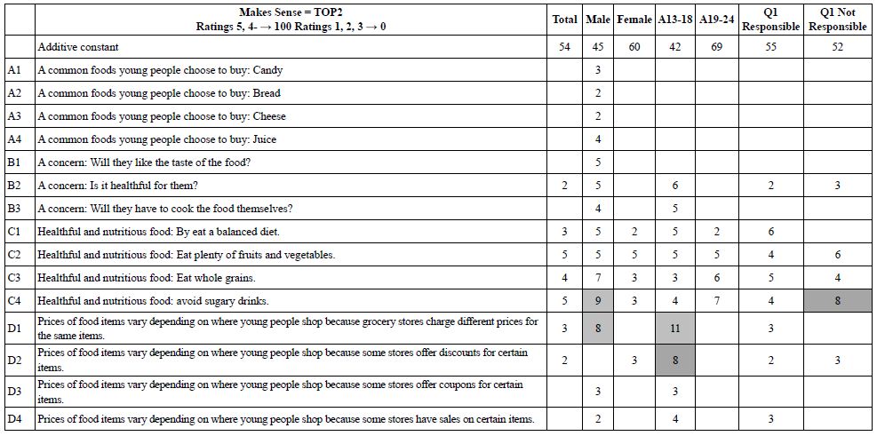
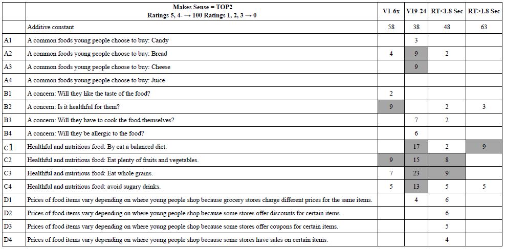
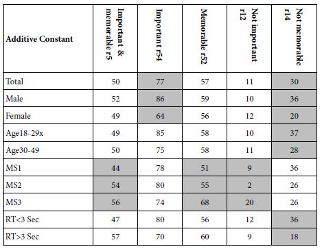
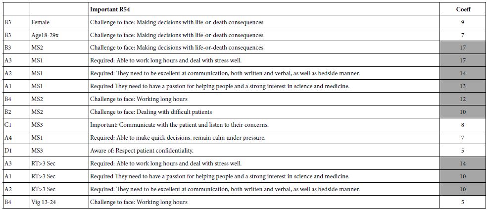
Parameters of equations for the total panel and for self-defined subgroups appear in Table 4. The table shows the additive constant (k0) and the coefficients for the 16 elements. The table shows only coefficients having a value of +2 or higher. Zero and negative coefficients do not necessarily mean that the elements ‘make no sense’, but rather mean that the element ‘does not clearly make sense.’ Eliminating the negative coefficients allows the patterns to emerge. Finally, strong performing elements, with coefficients of +8 or higher,’ are shown in shaded cells.

Table 4: Parameters of the equation for TOP2 for Total Panel and key self-defined subgroups

tab 4

Our first pass through the data focuses on the additive constant. The additive constant shows the likelihood to say that the vignette ‘makes sense’ in the absence of elements. Of course, the underlying experimental ensured that every vignette comprised 2-4 elements so that the additive constant is a computed parameter, one that we can use as a baseline. The data shows interesting patterns. The total panel shows an additive constant of 54, meaning that in the absence of elements we might expect 54% of the ratings to be 5 or 4, viz. TOP2. When we look at the genders, however, we see that males are less likely to say ‘makes sense’ (additive constant 45), whereas females are more likely to say ‘makes sense’ (additive constant 60). We see the same pattern emerging by age. The younger respondents show a much lower additive constant than the older respondent (additive constant 42 for ages 13-18 vs. 69 for ages 19-24). Finally, when the respondents are asked whether young people are sufficiently responsible to buy food for older people (Question #1), the additive constants are very close (55 versus 52).

It is in the elements that we see differences among the group. The first thing to keep in mind is that the elements are departures from the baseline. Thus, with a low baseline, there may be few positive elements or any positive elements. The reason is that with a low baseline, there may be a few strong-performing vignettes, but most perform poorly. With a high baseline, there are generally few strong-performing elements, moving beyond the already-high level. There may be many negative elements, but these will not appear because we are only looking at positive coefficients.

With the foregoing guidance, we see that males and respondents ages 13-18 show the largest number of positive coefficients, a pattern that is to be expected given their low additive constants.

There are a group of strong-performing elements

C1 Healthful and nutritious food: By eat a balanced diet.

C2 Healthful and nutritious food: Eat plenty of fruits and vegetables.

C3 Healthful and nutritious food: Eat whole grains.

C4 Healthful and nutritious food: avoid sugary drinks.

D1 Prices of food items vary depending on where young people shop because grocery stores charge different prices for the same items.

D2 Prices of food items vary depending on where young people shop because some stores offer discounts for certain items.

Our second pass through the results looks at the pattern of coefficients for elements appearing in vignettes at the start of the session (vignettes 1-6) versus elements appearing at the end of the session (vignettes 19-24), as well as elements appearing in vignettes evaluated quickly versus vignettes evaluated slowed (operationally different as response times >1.8 vs. response times >1.8 seconds). Table 5 shows the parameters. There are differences by groups. The only strong, consistent pattern to emerge is that the elements presenting ‘health and nutritious food’ makes much for sense at the end of the evaluation than at the beginning of the evaluation. It may be that these messages must be repeated, at which point they begin to make more sense.

C1        Healthful and nutritious food: By eat a balanced diet.

C2        Healthful and nutritious food: Eat plenty of fruits and vegetables.

C3        Healthful and nutritious food: Eat whole grains.

C4        Healthful and nutritious food: Avoid sugary drinks.

Table 5: Parameters of the equation for TOP2 for the first six versus the last six of the vignettes tested, as well as the vignettes rated quickly versus the vignettes rated slowly.

tab 5

The second set of columns shows the results for the vignettes rated quickly (RT<1.8 seconds) and the vignettes rated more slowly (RT>1.8 seconds). The additive constant for the more quickly rated vignettes is lower (48 for RT<1.8 vs. 63 for RT>1.8). This difference suggests that people may reject more quickly, versus accept more slowly. The rationale for this conjecture is that the lower additive constant for the vignettes rated quickly.

Of importance is that the strong performing elements are three of the four examples of nutritious foods.

C1          Healthful and nutritious food: By eat a balanced diet.

C2          Healthful and nutritious food: Eat plenty of fruits and vegetables.

C3          Healthful and nutritious food: Eat whole grains.

Our final pass through the TOP2 data for ‘makes sense’ involves the discovery of underlying groups of people who think differently about the same topic. These groups are called mind-sets. These mind-sets emerge when the researcher looks at the pattern of coefficients for a single topic, like the topic we investigate here, viz., making sense about buying food. The mind-sets emerge clearly when we use statistical methods to find these groups. The method is called ‘clustering.’ For the study, we use so-called k-means clustering to separate out the 100 respondents first into two groups, and then into three groups, based solely on the similarity of patterns of the 16 coefficients.

The clustering program looks for different groups by creating a measure of ‘distance’ between each pair of respondents. With 100 respondents we have 100×99/2 or 4950 pairs. The distance between two test respondents in this study is defined as the quantity (1-Pearson Correlation). The distance is 0 when the two respondents show exactly parallel patterns of coefficients. The distance e is 2 when the two respondents show exactly inverse patterns. The clustering program does not care about whether or not the clusters make sense. That is the researcher’s job. The clustering program is simply a mathematical tool (Likas, 2003).

The researcher’s job is to select the most meaningful cluster solution from the solutions generated by the clustering program. The two criteria are parsimony (few clusters are better than many clusters), and interpretability (the clusters must make sense, viz., tell a coherent story)

Table 6 suggests two strong clusters (Mind-Set 2 and Mind-set 3), and one weak cluster (Mind-Set 1). Mind-Set 2 focuses on the actual shopping behavior. Mind-Set 3 focuses on health. Mind-Set 1 might be folded into Mind-Set 3, but the responses of Mind-Set 1 are weak, suggesting an almost indifferent attitude.

Table 6: Parameters of the equation for TOP2 for the three mind-sets extracted by k-means clustering

tab 6

The additive constants for the mind-sets are quite different. Mind-Set 2 focusing on the shopping behavior shows the highest additive constant, 63, meaning that almost 2/3 of the time they are likely to say that the vignette makes sense. They do not seem to be particularly critical in the way they think. In contrast, Mind-Set 3 focusing on the healthfulness of the food shopped for shows the lowest additive constant, 39, meaning that only 40% of the time are these respondents likely to say that something makes sense.

Discussion and Conclusions

The study reported here demonstrates the ease with which students can investigate topics of everyday in a way that combines the joy of research and learning with the unbounded curiosity and enthusiasm of young people. One might consider the actual topic itself to be simple, not grounded in theory, and certainly not conducted with the gravitas of a ‘serious scientific experiment’, which often responds to so-called ‘question emerging from the literature’, or even more colloquially, research which fills a hole in the literature.

The topic of food choice is a serious topic, one relevant to well-being and to illness alike. Malnutrition is a worldwide problem, whether the poor nutrition comes from a lack of food, a lack of knowledge, or just bad eating habits. Many of the studies appearing in a rigorously scientific way address the topic, but in what ends up being an episodic, punctate fashion, each paper exquisitely analyzed in its own way, with a depth of information designed to demonstrate its inherent ‘scientificity’ (sic). The deeper information, the emergence of patterns leading to application, ends up being the job of the individuals doing ‘meta-research’, writing review papers, summarizing what is known, and then prescribing where appropriate.

These studies with Mind Genomics, augmented by artificial intelligence (REF) designed and executed by young researchers move science in a different, parallel direction, perhaps one reminiscent of the early days of science. It is the excitement of the unknown, the exploration of topics, the discovery of aspects of how people think, and the curiosity of youth that drive this new approach to science. And, there is the other side, the discipline in development, execution, and analysis of the data afforded by the Mind Genomics process, the remarkable simplicity, speed, and low cost of the approach, which when combined allow anyone in the world, or at least anyone with sufficient curiosity, to create a large-scale database of different aspects of a topic, such as food shopping. One can only imagine 100-200 studies of this type, with different sub-topics of food shopping, with different age people, in different regions of the world, at different times of the year. Such a dataset is simple to erect, and fun to do so, especially when the researchers are students from different schools, countries, and cultures, all cooperating on a platform design to make these types of Mind Genomics studies easy to do.

Acknowledgments

We gratefully acknowledge the sponsorship of our colleagues who support these studies to help students develop critical thinking, and thank our fellow students for the chance to discuss the topics with them.

References

  1. Bucknall S (2012) Children as Researchers in Primary Schools: Choice, Voice and Participation (1st ed.). Routledge. https://doi.org/10.4324/9780203116302
  2. Gofman A, Moskowitz H (2010) Isomorphic permuted experimental designs and their application in conjoint analysis. Journal of sensory studies 25: 127-145.
  3. Gram M (2010) Self‐reporting vs. observation: some cautionary examples from parent/child food shopping behaviour. International Journal of Consumer Studies 34: 394-399.
  4. Green PE, Srinivasan V (1990) Conjoint analysis in marketing: new developments with implications for research and practice. Journal of Marketing 54: 3-19.
  5. Kraak V, Pelletier DL (1998) The influence of commercialism on the food purchasing behavior of children and teenage youth. Family Economics and Nutrition Review 11: 15-24.
  6. Likas A, Vlassis N, Verbeek JJ (2003) The global k-means clustering algorithm. Pattern Recognition 36: 451-461.
  7. Moskowitz HR (2012) ‘Mind genomics’: The experimental, inductive science of the ordinary, and its application to aspects of food and feeding. Physiology & behavior 107: 606-613. [crossref]
  8. Moskowitz H, Hartmann J (2008) Consumer research: creating a solid base for innovative strategies. Trends in Food Science & Technology 19: 581-589.
  9. Open AI (2023) https://beta.openai.com/docs/models/gpt-3, accessed January 18, 2023.

The Experience of Disability in Cameroonian Families and the Contribution of EMDR Psychotherapy

DOI: 10.31038/PSYJ.2023523

Summary

In Cameroon, the number of people with disabilities is estimated at nearly two million nine hundred and ten thousand (2,910,000). Thus, a little over 5% of the population of Cameroon suffers from at least one disability [1]. These alarming figures lead us to consider the issue of children’s disability and its impact on the health of their parent(s). Certain types of disability cause more suffering to caregivers and relatives than to the disabled person. Within the framework of our activities in clinical psychology with associations of parents of children living with disabilities, through clinical interviews with parents of children with Down syndrome and autism, we have observed that many of these parents present various forms of psychopathology related to the disability of their children: affective disorders, depressive anxiety disorders, acute stress, behavioral disorders, PTSD, etc. We wondered how to deal with these suffering parents. To answer this question, we administered the SPRINT (a recent traumatic event assessment scale) to parents of children with disabilities whose discourse highlighted their experience with their different child as traumatic. This evaluation allowed us to set up therapeutic projects with EMDR (Eye Movement Desensitization Reprocessing). Through a reading of seven clinical cases followed in Yaoundé, Cameroon, we were able to verify that EMDR psychotherapy is a useful care tool for the management of parents of different children in pain. For most of the cases, the first EMDR session was very satisfactory. The results obtained were astonishing: 04 parents saw their VOC (truth scale) rise to 7 and their SUD (suffering scale) drop to 2 at the end of the first EMDR session. For the 03 other parents, the VOC rose progressively over the course of the sessions to reach 7 at the sixth session with an economic SUD at 1, due to their sometimes traumatic childhood experiences.

Keywords

Disability, Child with a disability, Psychopathology, EMDR, PTSD, SUD, VOC

Disability and Society

Society is a group of men and women who are united by nature or by laws. These laws differ from one sphere to another. Thus, what is seen as taboo in one society may be normal in another. However, there are common features between societies with regard to the concept of norm. This norm is applied to each individual who, for the most part, is subjected to it without any choice. Those who deviate from this pre-established norm are considered a problem, a social case. It is in this logic that the person living with a disability fits in. “Disability” is used here as an umbrella term for impairments, activity limitations and participation restrictions that represent the negative aspects of the interaction between a person (with a condition) and contextual factors (personal and environmental). Disability is neither a purely biological nor a purely social phenomenon” [2]. A person with a disability is therefore a person with physical, mental, or sensory incompetencies that affect their activities of daily living and limit their actions in society. The concept of disability can be defined in several ways depending on the culture and society. In so-called Western societies, disability is seen as incapacity, a lack. However, it should be noted that the concept of disability has evolved in these societies with the scientific progress of the 19th century because it was not always so. In African society, disability is still considered by most people as a curse to be got rid of. In most regions of Cameroon, disability is seen and understood as something mystical, supernatural. With the mixing of populations, a slight evolution of mentalities, the advent of ICTs, and access to education, this conception is changing. 5.4% of the population in Cameroon suffer from at least one type of disability. Sensory impairments (3.6%) are the most frequent, due to (2.2%) for visual impairments and (1.6%) for hearing impairments, followed by motor impairments (1.2%) which are mainly deformities of the lower or upper limbs [3]. According to the same survey, “the proportion of people with disabilities is higher in rural areas (6%) than in urban areas (4%) and “this proportion increases steadily with age, from just over 1% among children aged 0-4 years to 6% among people aged 25-49 years and reaches 19% among those aged 50 years or more.”

Disability and Its Manifestations

Disability is an impairment that limits the subject in the efficient performance of his or her actions. According to the WHO, “disability is universal”. According to the INS and ICF International survey, it is defined as “a disadvantage resulting from an impairment or disability, which limits or prevents the individual concerned from performing a role that is normal for him or her, taking into account age, gender, and social and cultural factors”. The number of people with disabilities is estimated to be over one billion people, including about 15% of the world’s population in general, and in turn, one in seven people [4].

Disability generates clinical manifestations that are often poorly understood. Whether sensory, motor, mental or social, disability always poses a societal problem. The lack of expression of positive emotions by parents towards their children with disabilities is a striking modality of the functioning of families with a child with a disability in Cameroon. Today, many families or parents want to give the maximum to their disabled child. Unfortunately, they face several difficulties or sufferings that can put them at a disadvantage; among others; the gaze of the other, the mourning of the idealized child, the fear of reliving the same experience and the inadequacy of our environment in terms of infrastructure. Whether it is sensory, motor, mental or social, disability almost always poses a problem of social integration. The emotional suffering of families with regard to their children with disabilities is a striking feature of the functioning of families with a child with a disability in Cameroon. In our different actions carried out with the parents of disabled people, we noticed that several parents had psychological illnesses linked to their child’s disability. We wondered if the non-acceptance of a child’s disability could lead to a psychological illness? What can be done to help them? What types of psychotherapies would best respond to their suffering? From these questions arise a series of hypotheses among which the following one. Following a high SPRINT score in these parents, we can use EMDR therapy to treat them and especially to control the impact of the suffering during therapy.

The term disability has several definitions depending on the model (medical and social). Medically, it is defined as an incapacity, a deficiency, a lack, whereas socially, it is defined as an inadequacy. It is for this reason that the WHO, taking into account these two models, defines a disabled person as “any person whose physical or mental integrity is temporarily or permanently impaired, either congenitally or as a result of age or accident, so that his or her autonomy, ability to attend school or to hold a job are compromised. The French law of February 11, 2005 [5] on equal rights and opportunities, participation and citizenship of people with disabilities provides a simpler definition of disability. According to this law, disability is “any limitation of activity or restriction of participation in society suffered in his or her environment by a person due to a substantial, lasting or permanent impairment of one or more physical, sensory, mental, cognitive or psychic functions, a multiple disability or a disabling health disorder. Disability is a social notion rather than a medical one because the person living with a disability needs to move in a society to consider himself as an important being. In short, the term disability refers to the difficulty that an individual encounters in interacting with his or her environment and that is caused by an impairment that results in a permanent or non-permanent inability to access, express, understand or apprehend.

In Cameroon, the population of people living with a disability is estimated at nearly 10% of the 18 million inhabitants [6], a percentage that has doubled in four years since the INS and ICF International survey. To understand the psychological situation of this part of the population, we must invoke the psychology of disability, which condenses the entirety of the psychological needs and experiences of the person with a disability as well as those around them, without ignoring the characteristics related to their life phases. It allows for a better understanding of the needs, adaptation problems and significant interference according to the types of disability situations (motor, sensory, psychological or mental). To make this field of investigation more concrete, let’s look at the role of a psychologist.

The Psychologist in Question

The psychologist is a health professional whose role is to offer the individual a place to listen, to speak, and to maintain confidentiality in order to identify conflicts. He is trained in the psychological analysis of the individual, but also in the analysis of factors internal or external to the individual that influence this psychological functioning. He is an expert in conscious and unconscious psychological functioning. His analysis allows him to understand what is going on in the individual at the cognitive, affective and behavioral levels, contextual and social. To perfect this, he has the appropriate methods, tools and techniques. His essential skills are: psychological evaluation (audits, diagnoses, counseling, training, orientation), clinical interviewing, psychological support, therapeutic management. In this panoply of skills, there is one that allows the specialist to work directly with the patient or individual with a mental health problem.

The clinical psychologist is the one who works at the bedside of the individual. He promotes mental health through prevention, care and reintegration or professional orientation. He/she assesses the people who make a request in order to determine the nature, causes and potential effects of the distress (emotional, physical, social) felt by the person or group. He intervenes in order to prevent, treat and address psychopathologies, emotional conflicts, and skill deficits at the root of the dysfunction. He therefore intervenes for the promotion of health. It is in this movement that the clinician is training in psychotherapy. One of these revolutionary therapies is called EMDR

What is EMDR?

EMDR psychotherapy is a fairly new therapeutic intervention that aims to provide relief to patients with post-traumatic stress disorder by helping them to let go of traumatic memories. EMDR (Eye Movement Desensitization and Reprocessing) is a therapy developed in the late 1980s by Francine Shapiro [7]. With the aim of reducing the emotional charge linked to traumatic events, EMDR thus becomes a powerful tool for “cognitive restructuring”. It is a therapy that is currently used to effectively treat a wide variety of psychological disorders resulting from traumatic memories, including anxiety disorders, depression, stress and trauma [8]. But especially in Post-Traumatic Stress Disorder (PTSD). Shapiro’s theory stipulates that the information linked to the trauma is stored in a fragmented manner (images, sounds, smells, places, events, etc.) in the brain and that these different fragments are not linked together, which prevents the integration of the trauma into the memory. It presents a specific information processing system, which deals with traumatic memories, called Adaptive Information Processing (AIT), so that during the course of our existence, certain information is not processed, and therefore not memorized, which means that it is constantly present in our memory. This dysfunctional information remains unresolved and constitutes dysfunctional memory networks; their voluntary or involuntary recall is unpleasant and painful, and the emotion can arise unexpectedly as soon as the environment recalls the circumstances of the traumatic event. They are the source of various disorders such as intrusive thoughts and images, nightmares, fears, untimely startles, phobias… The objective of the therapy is to promote the transfer of information between the emotional and cognitive brains in order to stop the disorders.

The EMDR Procedure

EMDR combines several methods already used by other approaches. In particular: CBT (cognitive and behavioral therapies), psychodynamic therapies and Ericksonian hypnosis. It consists of eight essential phases: the patient’s life history and treatment planning (collection of anamnestic data, the most distant or most recent memories), the preparation of the patient (targeting plan in agreement with the patient), the evaluation (preparation phase for cognitive associations for the TAI), thedesensitization (bilateral stimulation), settling (positive cognition reinforcement), body scanning, closing and re-evaluation.

When life episodes generate too much emotional disturbance, whether they are small traumas (being humiliated as a child, witnessing violent arguments from one’s parents, etc.), or large traumas (rape, accident, attack, earthquake…), the information processing system is blocked. This leads to the following consequences: post-traumatic stress disorder, depressive, anxiety or eating disorders, drug addiction, various physical disorders… EMDR is based on a neurological model in which the alternating stimulation of the cerebral hemispheres re-establishes a process of re-connecting the elements of information processing (emotional, cognitive, physical) disconnected by the traumatic event. In other words, the adaptive process of information processing could be reactivated by the bilateral stimulations. Once reactivated, this system would process the traumatic material in an accelerated manner. Thanks to this system, negative emotions are neutralized and adaptive information arises spontaneously. EMDR makes it possible to establish a connection between the memory network that contains the traumatic memory and the memory networks that carry the adaptive, incorporated experiences that have meaning for the individual and constitute psychological resources.

The Principle of EMDR Therapy

After having had an initial clinical interview with the patient, the therapist verifies the patient’s problematic using a scale of his or her choice, after which he or she must respect the above-mentioned steps. The patient identifies a representative image of the most disturbing dysfunctional target memory, gives the negative cognition of himself, finds a positive cognition of the same register with a verification scale, identifies the emotions linked to the target, the related body sensations, and above all situates the suffering, the disturbance linked to the event on a scale. The cognitive evaluation of the target dysfunctional memory is done on a subjective scale and the degree of distress in relation to the target memory is evaluated throughout the desensitization phase. During this desensitization phase, the patient returns to the image from the beginning by making a kind of cognitive association, while simultaneously making eye movements from left to right in order to follow the therapist’s hand movements, which act as a dual-action stimulus (either in front of the eyes, on the knees, on the shoulders or beside the ears). After each series of SBA (bilateral stimulation) the patient is asked to report the associative information that was elicited during the EMDR session, the instruction given to the patient is either to move the eyes from left to right, to listen to the sounds produced by the hand, to listen to the vibrations produced by the tapping… at a regular rhythm, while thinking of elements of a traumatic memory.

The EMDR Session

Each classic EMDR session lasts between 45 and 90 minutes. The EMDR treatment begins with a preparation. It is important for the therapist to diagnose the type of trauma (simple, psychic poisoning or complex). The therapist also helps the patient to develop resources, not only to improve his or her relationship with himself or herself and others, but also to facilitate the treatment of the trauma. EMDR allows the brain to reprocess the emotional information in order to remove the trauma from the nervous system. Before beginning the EMDR treatment, the therapist follows the above-mentioned steps. In this way, he/she offers the patient a safe therapeutic space that will allow him/her toto confront the origin of his suffering and especially to take refuge in a comfort zone in case of abreaction.

As Martine Gercault [9] puts it so well Once the foundations of the work have been established, the practitioner will help the patient to locate and represent as accurately as possible the origin of the target event, to feel in his or her body the perceptions, emotions and sensations that are linked to it. While the thoughts and affects surface, the psychotherapist sweeps his or her hand in front of the patient’s face and the patient follows rhythmically with his or her eyes”. The reprocessing of a trauma can take from one to several sessions. To reprocess a traumatic episode, the psychotherapist invites the patient to focus on his or her memory, by being in contact with its sensory elements (visual, auditory, olfactory, kinesthetic, gustatory…), with the beliefs and negative emotions generated. The therapist then initiates a series of alternating bilateral left and right stimulations (30 seconds to a few minutes) of eye movements, sounds or tactile stimulations. As free associations of ideas emerge, the patients reprocess the different information linked to the memory, integrating them into their memory network in a functional, adapted manner. Between each series, the therapist asks the patient to take a deep breath and to share what came to mind during the stimuli. These successive and quite brief series of bilateral movements continue until the emotions are neutralized and the emotional scars of the past are emptied of their traumatic charge. When the traumatic memory is thought of again without emotional discomfort and associated with positive thoughts, the therapist moves on to the next phase. The traumatic memories lose their negative emotional charge, thus ending the suffering and negative reactions. It may happen that during a session, the patient experiences strong emotions; it may also happen that between sessions such emotions resurface, as well as other memories, as in any form of psychotherapy. In the end, the patient experiences an improvement in the emotional disturbance related to the memory being treated, and a calming. Through this process, images, perceptions and memories that were negatively encoded in the emotional brain are reprocessed and lose their dramatic intensity. The past adversity is replaced by the uniqueness of the event.

Procedure for the Parent Survey

The first step taken was to contact the heads of the associations we had identified for our investigation (WellbeingAfrica, an association of parents of children with disabilities that works for the rights of vulnerable people), the Little Prince and the Moabi [P²M], an association of parents of children living with disabilities whose main mission is the empowerment of people with Down’s syndrome and other disabilities). Having obtained the various appointments, we organized ourselves for the meeting with the targeted parents. Once on site, after a detailed explanation of the object of our research, we were allowed to “arrange” an appointment with the parents concerned. On the day of the meeting, we first proceeded with a sort of interactive discussion with all the parents present. The purpose was to give them all the explanations related to the research and to the importance of their participation, especially for their well-being.

After this collective meeting phase, which lasted about 20 minutes, each parent was taken individually in a more private setting of the institution (consultation room or office set up on site). There, we would conduct a clinical interview with the parent to ensure that he or she met the inclusion criteria for our sample. As a reminder, these criteria were: being a parent (father or mother) since birth, having denial of their child’s disability, having a psychological disorder related to their child’s disability, and especially having a high SPRINT score, willingly agreeing to take an active part in therapy… Once these conditions were met, we asked the parent to ask any questions he or she might have about our study. After these preliminary steps we would then make a well-framed appointment for the preparation of the actual therapy.

Post-Traumatic Stress Disorder (PTSD) Clinic

Post-traumatic stress disorder (PTSD) affects people who have experienced trauma caused by violence, disability, accident, natural disaster or war, or degrading treatment. How society views the trauma. Lack of support or negative behaviours of those around them (criticism, blame, lack of understanding and empathy, or hostile, controlling, intrusive or stressful behaviours) aggravate the symptoms. Victims feel painfully judged by others. Support from others is very important. Trauma-related thoughts made by the victim herself.

A set of symptoms can develop in a person following a confrontation with an intense stressful event (loss of an object) that would involve serious injuries or a feeling of helplessness. Such situations sometimes trigger strong anxieties, chills, sweating, trembling; and psychic sides such as dreams, flashbacks and sometimes avoidance of similar situations. The positive symptoms are: reliving, avoidance, negative alterations, neurovegetative disorders. These symptoms cause significant suffering in the person, leading to an alteration in their social and professional functioning, and many other important areas. Thus, the patient’s entire functioning may be turned towards the trauma and its memory. Victims will tend to avoid thoughts and conversations that remind them of the traumatic event, as well as places, situations and people that may remind them of the original situation. Their interests and relationships gradually diminish.

Presentation of the Cases

Case PS

PS is a young married woman of 35 years old, of Catholic religion, of Bamileke ethnicity. Her schooling level is that of the 4th grade. She carries out an informal activity that is very common among women in Cameroon, known as “bayamselam,” which consists of buying food products in bulk at the end of the fields to transport them to the city markets and sell them in retail. She is the third of five siblings and her 15-year-old disabled child is schizophrenic. During the interview, she appeared very distressed. She was born in 2003 in Yaoundé, the first of five children of PS, including one girl and four boys.

Case M

M is a young Cameroonian woman, 42 years old, of Bulu ethnicity, with a BTS level of education and unemployed. She is the first of two girls. She is the mother of J who was born on May 31, 1997. He is the only child of M and suffers from an autistic spectrum disorder.

Case E

E was born 55 years ago to a Christian protestant family in the Sanaga Maritime. She has a CEPE. She is a housewife, married and mother of five children, herself the fifth of seven children. She is the mother of Y, born in 2007 in Yaoundé, the fourth of her five children. 02 girls and 03 boys, she attends a local special school, she has a mental retardation.

Case T

T is a 48 year old housewife. Of the Foulbé ethnic group, she is Muslim, without school education, she is married and mother of seven children. She is the sixth of nine children. She is the mother of J, born in 2007, who is the first of these 07 children, of which 03 are girls and 04 are boys. He has been in the special SIL for three consecutive years.

Case X

X was born 45 years ago and is of Douala ethnicity. Catholic, with a literary baccalaureate, he is a service provider. He is the first of three siblings, including two boys and a girl. X is the father of K who was born in 1998. He would suffer from an autism spectrum disorder.

Case P

P is a 30 year old Gabonese, of Fang ethnicity, catholic, he holds a BEPC, he is a military man by profession and single with two children, he is the second of three siblings. He is the father of B who was born in 2002 in Yaoundé, the first of 02 boys and he is being trained in a specialized school in the area. He has been suffering from schizophrenia for two years.

Case Z

Z is a 38 year old housewife, of Bulu ethnicity, from the evangelical church, with no school education. An only child, she is married and has three children. The disabled child is the third of 8 years old, autistic, and attends an inclusive school in the area.

Analysis of the Data Collected during EMDR Therapy

Seven parents were recruited on the basis of individualized clinical interviews among the parents of children with disabilities, including five (05) mothers and two (02) fathers from associations of parents of children with disabilities in Yaounde. Before starting the therapy, we made sure of the type of trauma that each parent might have, because the arrival of the disabled child could be just the trigger for the suffering. After each session, we administered a Stressful Event Rating Scale (SPRINT) to the parent to assess the effectiveness of EMDR therapy. By doing this, we were able to treat all seven parents according to their individual schedules, over a period of 2 months, with an average of 5 sessions of 60-90 minutes each (Table 1).

Table 1: Analysis of the data collected during EMDR therapy


Most Disturbing Image

Negative Cognition

Emotion

Body Sensations SSC

SUD

Positive Cognition

VOC

PS Haunting voice I am a bad mom Crying, sadness Pain in throat and heart palpitations 9 I am a good mom 3
M Vision of agressive child I am the worst of all Crying Headaches 10 I am among the best 2
E Sight of a normal child I am sick Sadness Jerky breathing 8 I am a human with limits 2
T The sight of an inhuman I am a monster Crying child Pain in the lower limbs 9 I am human 1
X A difficult delivery I am an incompetent father Sadness Tachycardia 7 I am a good father 3
P Nightmares I suck Crying Sweating 9 I am capable 1
Z A beautiful but hyperactive baby I am a bad mother  Sadness Sore throat 8 I am a good person 2

An insecure family context, a feeling of guilt related to a probable negligence during the pregnancy and the development of the disabled child, stereotypes, accusations and stigmatizations coming from the entourage, lack of projection in the future, feeling of devaluation, the look of others, the physical manifestations are the elements that emerge from the discourse of the different parents.

Clinical Case PS

For EMDR therapy, we need 08 phases: the life history of the subject, the assessment, the desensitization, the reinforcement of positive cognition, the body scan, the future scenario, the closure and the reassessment.

Clinical Aspects of the Test

The relationship with the clinician being well established, PS presents her apprehensions, suspects at the beginning of the manipulation as she declares “I trust you docta, even as I don’t know what I’m getting into, this doesn’t seem catholic to me, looking from left to right there scares me”. In spite of this, she lends herself to the game and respects all the instructions given for the good progress of the EMDR therapy.

The encounter with the therapy device immediately provokes a movement of surprise in PS. She smiles when I explain the course of the session. Regarding the eye movements, she said to me: “Docta, excuse me, but I am going to laugh”. This observation is recurrent with EMDR patients, because it is different from what they expect, not only do we not only do active listening or give them advice, but we also ask them to make eye movements, and to verbalize what comes to their mind during desensitization.

The Subject’s Life Story

PS is a young woman of 35 years old, of Catholic religion, of Bamiléké ethnicity. Her school level is that of the 4th grade. She is the third of five siblings and her 15-year-old disabled child has schizophrenia. Her score on the SPRINT test by Connor & Davidson 1997, translated by F. Mousnier – Lompré 2014 is 18. We made a targeting plan and listed 02 targets: The first is a conflict with her father because she never felt loved by him. The second is her child’s disability. With her permission, we started the therapy with the current situation, which is her child’s disabling illness.

Assessment of the Situation

The elements of the therapy are: the image which is the haunting voice of her daughter in crisis, the negative cognition “I am a bad mother”, the positive cognition “I am a good mother”, the VOC equals 2, the emotions are crying and sadness, the SUD equals 9 and as body sensation the pain in the throat and the heart palpitations.

Desensitization

This phase is marked by bilateral stimulations, breathing movements and especially by adaptive information processing (AIT). PS’s speech reveals an increased suffering following her daughter’s diagnosis. She revisits her childhood, her friends, her family, her marriage, in short, all the important elements of her life and notes a major fact that justifies her discomfort. Her behavior when she was young, she says in these terms: “I see myself with my brother making fun of people with a physical handicap, especially the neighbor’s son who had a limp”, “I can’t live with a handicap or put up with a person with a handicap”. As the therapy progressed, she understood that she did not have the right to decide for anyone, that life had its elements that she had to accept and deal with, that she had regained her values and, above all, that she had found meaning in all the efforts she had made since her daughter’s diagnosis, in all the appeals she had had to make for the child’s well-being, and, above all, that she had been a good mother because she had not abandoned her child in her situation of psychological illness. When the SUD drops to 1 economic, we move on to phase 5.

Reinforcement of Positive Cognition

We just check the positive cognition that she gave at the beginning namely “I am a good mother”, when the VOC goes up to 7, we go to phase 6.

The Body Scan

In a relaxing atmosphere, we go over all the parts of her body, always coming back to the disturbing image that we no longer name in this phase. We just say to him, thinking back to the starting image, and especially to the negative cognition that you stated at the beginning, we are going to do an examination of your whole body starting from the head, the neck… to the toes. The instruction is simple: every time she recently feels a knot, a pinch, a pain, an affect in any part of her body, she reports it to us and we desensitize. She has reported pain in her throat and neck and each time we ask her after the desensitization: “what came to mind”, until we get zero pain or manifestations in the body. Once the VOC is verified, we change phase.

The Closing

After having informed Mrs. PS that we will soon stop the session, we say to her: “you have worked well today, I encourage you to note down everything that appears in the meantime, you can report them to me at our next session”.

Reassessment

This session allows us to make a small evaluation of the previous one in order to desensitize the new elements if there are any. After six sessions, we have allowed Mrs. PS to have another look (admiring) on her child.

Results

The action of EMDR is based on the association of psychological and neurological processes. This technique allows the patient to revisit a traumatic event. This therapeutic action is understood as an information processing therapy during which the patient recounts the traumatic event by means of its cognitive, affective and physiological characteristics while concentrating visually, audibly on bilateral movements of an external stimulus until the psychological distress evoked by the traumatic memories diminishes or disappears (Shapiro, 2001).

We have experienced this in the seven parents who, after just two months of care, regained the smile they thought was lost forever. For most of the cases, the first EMDR session was very satisfactory for the parents because 4 of them saw their VOC rise to 7 and their SUD drop to 2. For the other 03 parents, the VOC rose progressively during the sessions to reach 7 at the sixth session with an economic SUD because of the sometimes traumatic experience of these parents.

Discussion

Contrary to other types of therapy which are all equally effective, EMDR has the particularity of not expecting patients to verbalize and perform precise tasks which will constitute the action of the treatment received. The effects of EMDR are less prolonged than cognitive and behavioral therapies, which facilitates the rapid recovery of parents who cannot feel good just by verbalizing their suffering. The main advantage of EMDR lies in the brevity of the application of this technique. Indeed, when properly indicated, it acts directly and shows positive effects in the first session. EMDR has been used in randomized controlled studies with a waiting list where placebo control groups show a definite therapeutic effect [10].

Conclusion

Our work highlights the action of EMDR therapy on the psychological problems of parents of disabled children. For these parents at the end of the therapies, each parent, who at the beginning felt a fair amount of suffering at the sight of his or her disabled child, found himself or herself satisfied with his or her life and, above all, found qualities to be amplified in order to consolidate each of his or her different child’s achievements. The results are very satisfactory.

The treatment is essentially psychosomatic and global. It would be interesting to verify the stability of the results in a few years by observing the parents concerned over the years. In the field of brief and effective therapies, EMDR is one more tool that seems promising.

We did this study in 2019, to check the sustainability of the therapy, we did an evaluation three months for each one after stopping the therapy and one year after. The advantage was that we stayed in contact with the parents in question.

References

  1. BUCREP (2010, April 22) Results presentation report.
  2. World Health Organization (2012) World report on disability. WHO. Disabilities and rehabilitation.
  3. Institut National de la Statistique & ICF International (2012) Cameroon Demographic and Health Survey and Multiple Indicators (EDS-MICS) 2011. INS and ICF International.
  4. World Health Organization (2016) WHO draft global disability action plan 2014-2021: better health for all people with disabilities. WHO.
  5. Vernet O (2006) Law for equal rights and opportunities, participation and citizenship of people with disabilities. La lettre de l’enfance et de l’adolescence 64(2): 105-110.
  6. Von Bernuth E, Gelfert L (2014) The social situation of the disabled person in Cameroon.https://vhandicap.net/La-situation-sociale-de-la.html
  7. Shapiro F (2001) Eye movement desensitization and reprocessing basics principlex, protocols and procedures. US Guilford press. [crossref]
  8. Lohr JM, Lilienfeld SO, Tolin DF, Herbert JD (1999) Eye movement desensitization and reprocessing: An analysis of specific versus nonspecific treatment factors. Journal of AnxietyDisorders 13(1-2): 185-207. [crossref]
  9. Gercault M (2014) My father away, Amazon.
  10. Bradley R, Greene J, Russ, E, Dutra L, Westen D (2005) A multidimensional meta-analysis of psychotherapy for PTSD. American journal of Psychiatry 162(2): 214-227. [crossref]

Impact of Differentially Synthesized Copper Oxide Nanoparticles on Haematological and Biochemical Changes of Common carp Cyprinus carpio

DOI: 10.31038/NAMS.2023612

Abstract

Metallic nanoparticles like iron, zinc, aluminium, copper, and nickel which are used in the removal of dyes and toxic materials from wastewater affect aquatic organisms including fishes. The present study deals with the impact of differentially synthesized copper oxide nanoparticles on haematological and biochemical changes of Common carp Cyprinus carpio. Hyptis suovelens leaf extract was used for the biological synthesis of copper oxide nanoparticles. Copper (II) sulphate pentahydrate is used as a precursor and starch as a capping agent for chemical synthesis. Characterized by using UV-Vis spectroscopy, Fourier transform infrared spectroscopy, Scanning electron microscopy, Energy dispersive X-ray analysis, and X-ray diffraction. Acute toxicity of biologically and chemically synthesized copper oxide nanoparticles was conducted for a period of 96 hrs. Based on the Probit value sub-acute concentrations of biologically and chemically synthesized copper oxide nanoparticles such as 0 (control), 0.23, 0.31, 0.46, 0.93 ppm and 0.018, 0.024, 0.036, 0.072 ppm respectively for a period of 14 days under static condition. Hematological (Red blood corpuscle, white blood corpuscle, Polymorph Neutrophils, lymphocytes, Eosinophils, Hemoglobin) and biochemical parameters (protein, carbohydrate, lipids) in gill, muscle and liver were estimated after exposing the fish for 7 and 14 days. One-way ANOVA was used for the analysis. The mortality was increased with increased concentration of differentially synthesized CuO Nps on Cyprinus carpio. Haematological and biochemical parameters decreased with increased concentration of differentially synthesized CuO NPs when compared to control. Results conclude that the biologically synthesized copper oxide nanoparticles are less toxic than chemically synthesized copper oxide nanoparticles on Cyprinus carpio.

Keywords

Biological, Chemical, Synthesis, Haematology, Biochemical, Cyprinus carpio

Introduction

Nanoparticles are very attractive materials for the manipulation, sensing and detection of biological structures and systems than bulk particles. The principal factors which make nanomaterials different from their bulk counterparts include an increase in their relative surface area and quantum effects, which affect their physical and chemical properties [1]. Nanoparticles are used in many economic sectors including consumer products, the metal industry, transportation, cosmetics, pharmaceuticals, antimicrobial agents and agriculture [2]. Large scale production and use of metal oxide nanoparticles lead to uncontrolled release into the environment. Nanoparticles present in the natural environment includes volcanic dust, glacial ice cores, clays, organic matter, iron oxides and other minerals which may also increase harmful effects to human health [3]. Nanoparticles and metal oxides present in solid wastes, direct or accidental spillages and industrial waste effluent water enter the aquatic ecosystem by rainwater runoff and the waste of nanoparticles synthesizing industry were dumped into landfills may also be washed off into the aquatic environment, because it is one of the final destinations of the released nanomaterials in the environment [4]. Among numerous metal oxide nanoparticles, copper oxide nanoparticles are often present in industrial wastewaters that may become extremely toxic for aquatic animals as their concentration in the water increase. Besides, it is toxic, harmful to organisms living in water, accumulate in the food chain and may affect humans too [5]. Among animal species, fishes are the inhabitants that cannot escape from the detrimental effect of these pollutants. The amount of protein, lipid and carbohydrate in fishes is used for the determination of their nutritive value in fish and haematological analysis of blood parameters are considered physiological indicators of the whole body and therefore are important in diagnosing the structural and functional status of fish exposed to nanoparticles. Haematological parameters such as hematocrit, haemoglobin, and red blood cells are used to assess the functional status of the oxygen-carrying capacity of the bloodstream and have been used as an indicator of metal pollution in the aquatic environment [6]. The biologically and chemically synthesized copper oxide nanoparticles have electrochemical properties, which can be used in the field of medicine, and fish farming. The present study is related to the impact of differentially synthesized copper oxide nanoparticles on haematological, and biochemical analysis of freshwater fish Common carp Cyprinus carpio.

Materials and Methods

For the biological synthesis of copper oxide nanoparticles methanol extracted Hyptis suovelens leaf extract and 1 mM of 100 ml of copper sulphate was used in the ratio of 1:1 under stirring vigorously in a magnetic stirrer for 2 minutes. After stirring the precipitation was achieved. The pH was observed at 7 and kept overnight. Then the CuO precipitate was centrifuged at 3500 rpm for 10 minutes. The centrifugal process continued with water and repeated the centrifuging process for purifying CuO. Then the precipitate was dried at room temperature. Finally, copper oxide nanoparticles were stored in dry tube containers. For chemical synthesis copper (II) sulphate pentahydrate (CuSO4.5H2O) was used as precursor and starch as capping agent. The synthesis preparation was started with the addition of 0.1 M CuSO4.5H2O solution into 120 ml of starch (1.2%) solution with constant stirring under a magnetic stirrer for about 30 min. Then 50 ml of 0.2 M ascorbic acid solution is added under continuous rapid stirring. Subsequently, 30 ml of 1 M sodium hydroxide solution was slowly added to the prepared solution with constant stirring and heating at 80°C for 2 hrs. The colour of the solution turned yellow to Ochre. After the completion of the reaction, the solution was taken from the heat and allowed to settle overnight and the supernatant solution was discarded. Then precipitates were separated by filtration and the filtrate was washed with deionised water and ethanol three times to remove the excess starch which is bound with nanoparticles. Ochre colour precipitates obtained was dried at room temperature. After drying, nanoparticles were obtained and stored in a glass vial for further studies.

For acute toxicity analysis (LC50) healthy fishes of Cyprinus carpio (weight of 7.8 ± 0.02 g and length 6.5 to 7.5 cm) were procured from AM fish farm, Madurai, Tamil Nadu, India and acclimatized to laboratory condition for about 15 days in the fish tank with 50 L aerated dechlorinated tap water. Feeding was given for one hour before the replacement of water. Water (one-third) was changed frequently to remove the excretory wastes. Feeding was stopped 24 hrs before the commencement of the experiment to keep the experimental animals more or less in the same metabolic state. The initial weight and length of the fish were measured. Fish were exposed to biologically and chemically synthesized CuO NPs for a period of 24, 48, 76 and 96 hrs, according to the OECD Test Guideline in static method (The water was not changed during the test). The carp were exposed to biologically and chemically synthesized CuO NPs in different concentrations such as 0 (control), 5, 10, 15, 20 and 25 ppm and 0.5,1, 1.5, 2 and 2.5 ppm respectively for a period of 96 hrs. All the experiments were conducted in a 20 L glass tank containing 10 fish in each concentration. During the experimental period, the mortality was absorbed and statistical Probit analyses using SPSS was carried out to find the LC50 of the CuO NPs.

For Sub-acute toxicity analysis glass tanks with 20 L capacity were taken and each glass tank was filled with 15 L of water. In each glass tank, 10 healthy fishes (weight of 7.8 ± 0.02 g and length 6.5 to 7.5 cm) were introduced and different concentrations of biologically synthesized CuO Nps (i.e. 0.23,0.31, 0.46, 0.93 ppm) was added and control was maintained without CuO. Chemically synthesized CuO Nps were exposed in each glass tank for different concentration (i.e.0.018, 0.024, 0.036, 0.072 ppm). The manifestation and survival time of fish was observed in each concentration for 14 days. After the experimental period, the fishes are sacrificed for the analysis of toxicological parameters.

Common carp were exposed to CuO NPs for 14 days. Blood samples were collected from fish in each exposure group and were subjected to complete blood profile analysis. Haematological parameters such as Red blood cells (RBC) (millions/cumm). White blood cells (WBC) (cells/cumm), Polymorph Neutrophils (%), lymphocytes (%), Eosinophils (%), and Hemoglobin (gm/dl).Total protein, carbohydrate and lipid in muscle, gill, liver of Cyprinus carpio was estimated after the 7th and 14th days (7-9]

Fish used in the present research was by the guidelines of the Committee for Control and Supervision of Experiments on Animals [CPCSEA, Ministry of Environment & Forests (Animal Division), Government of India] on the care and use of animals in scientific research and also approved by the Institutional Ethical Committee for Research on Human and Animal Subject (IECRHAS) from The Gandhigram Rural Institute – Deemed to be University, Govt. of India, Gandhigram, Tamil Nadu, India [7-9].

The experimental results are presented in the form of Tables and graphs using Microsoft Excel (Version 2007). One-way ANOVA was used for the analysis using SPSS (Version 2013). The data was input manually and computed. The output results obtained from the software indicate whether is there any differences between the treatments and days. Sum of Variability of sample means (MS), Critical probability value (F) and Probability (Prob.) are also obtained.

Results

The UV-Vis analysis of biologically and chemically synthesized CuO Nps are presented in Figure 1. The sharp bands were observed close to both 249 nm and 264 nm throughout the reaction that indicating the formation of CuO NPs. The FT-IR spectra of the Hyptis suveolens methanol extract were absorbed in different peaks (Figure 2). Several adsorption peaks at 3942.11, 3409.27, 2923.02, 1640.44 and 1055.63 cm-1, like as N-H stretch of amines O-H stretch of Carboxylic group, N-H bending of amines, C-N stretch of aliphatic amines. In biologically synthesized copper oxide nanoparticles, peak values at 3947.47, 3407.04, 2924.51, 1610.08, 1276.10, 1107.36, 817.95, and 616.56 cm-1 (Figure 2a) were observed. A peak at 616.56 cm-1 and 3947.47 cm-1 corresponds to O-H stretch phenolic compounds, N-H stretch of amines, O-H stretch of Carboxylic group, N-H bending of amines, C-H stretch of aliphatic amines, C-Cl stretch of alkaloids and C-H bending of alkanes. In chemical synthesis, copper oxide nanoparticles were carried out to identify the possible functional groups responsible for the reduction of the copper Oxide Nps (Figure 2b). The bands are observed in the sample at 608.07, 1027.54, 1375.48,1108.019, 1009.96, 1108.01, 1634.39, 617.07, 1018.60, 1411. 25, 1099.07, 1625.45 and 617.01 cm-1 were associated with C-O alcohol, N=O Nitro group, C=CO Carbonyl and C-CL alkaline Halide. The SEM images of biologically and chemically synthesized CuO Nps are presented in Figure 3a and 3b. It clearly shows that the particles are small and uniform in size, almost spherical which is free from agglomeration in the biologically synthesized copper oxide nanoparticles. The elemental composition of the biological and chemical synthesized CuO Nps are identified (Figure 4a and 4b) and were 82% and 67% by an Energy Dispersive X-ray Spectroscopy. XRD patterns of biologically and chemically synthesized CuO nanoparticles are presented in Figure 5. In biosynthesized CuO Nps (Figure 5a) a series of diffraction peaks at 2θ of 32.55˚, 35.56˚, 38.75˚, 48.75˚, 53.48˚, 58.34˚, 61.57˚, 65.43˚, 66.27˚, 72.40˚ and 75. 25˚ were assigned to (110), (111), (200), (−202), (020), (202), (−113), (-311), (022), (311) and (004) planes respectively, which are in good agreement with those of powder CuO Nps obtained from the International Centre of Diffraction Data card (JCPDS-80-1916). In chemical synthesized CuO Nps, the XRD diffraction peaks are indexed as 34.014˚ (002), 56.523˚ (111), 69.234˚ (204), 67.002˚ (202) and 68.393˚ (113) (Figure 5b). All diffraction peaks are indexed according to the hexagonal phase of copper oxide nanoparticles ((JCPDS-80-1916) and no characteristic peak impurity phase except copper oxide nanoparticles and revealed the good spherical shape of 65 nm.

fig 1

Figure 1: UV-VIS analysis of biologically and chemically synthesized CuO Nanoparticles

fig 2

Figure 2: FT-IR analysis of a) biologically and b) chemically synthesized CuO Nps

fig 3

Figure 3: SEM image of biologically (a) and chemically(b) synthesized CuO Nps

fig 4

Figure 4: EDAX of biologically (a) and chemically (b) synthesized CuO Nps

fig 5

Figure 5: XRD analysis of biologically (a) and chemically (b) synthesized CuO NPs

Acute toxicity tests for biologically and chemically synthesized CuO Nps are presented in Tables 1 and 2. No mortality was observed in the control group during the experiment. Fish mortality increased significantly when the concentration and the time of exposure were increased. Mortality was observed in biologically and chemically synthesized CuO Nps exposed to a dose of 5, 10, 15, 20 and 25 ppm and of 0.5,1, 1.5, 2 and 2.5 ppm for 96 hrs respectively. This indicates an increase in toxicity with exposure duration. Before death, fish exhibited rapid gill movement, nervous manifestations, erratic swimming, loss of equilibrium and inability to remain upright.

Table 1: Probit analysis of biosynthesized CuO NPs on Common carp Cyprinus carpio

Probit

95% Confidence Limits for concentration

95% Confidence Limits for log concentration

Estimate

Lower Bound

Upper Bound

Estimate

Lower Bound

Upper Bound

LC1

1.544

0.000

4.647

0.189

-6.854

-667

LC2

2.123

0.000

5.550

0.327

-5.727

-744

LC3

2.599

0.000

6.221

0.415

-5.012

-794

LC4

3.026

0.000

6.787

0.481

-4.475

-832

LC5

3.424

0.000

7.291

0.535

-4.038

-863

LC6

3.804

0.000

7.756

0.580

-3.667

-890

LC7

4.172

0.000

8.194

0.620

-3.342

-913

LC8

4.532

0.001

8.613

0.658

-3.051

-935

LC9

4.885

0.002

9.021

0.689

-2.787

-955

LC10

5.235

0.003

9.419

0.719

-2.544

-974

LC15

6.972

0.029

11.403

0.843

-1.543

1.057

LC20

8.755

0.174

13.640

0.942

-760

1.135

LC25

10.643

0.775

16.745

1.027

-111

1.224

LC30

12.684

2.639

22.652

1.103

421

1.355

LC35

14.922

6.272

39.246

1.174

797

1.594

LC40

17.411

10.015

94.151

1.241

1.001

1.974

LC45

20.213

12.830

269.507

1.306

1.108

2.431

LC50

23.411

15.090

823.141

1.369

1.179

2.915

Table 2: Probit analysis of chemically synthesized CuO NPs on Common carp Cyprinus carpio

Probit

95% Confidence Limits for concentration

95% Confidence Limits for log concentration

Estimate

Lower Bound

Upper Bound

Estimate

Lower Bound

Upper Bound

LC1

0.053

0.011

0.088

-1.278

-1.946

-1.054

LC10

0.092

0.035

0.131

-1.034

-1.458

-883

LC15

0.105

0.046

0.144

-977

-1.341

-840

LC20

0.0117

0.056

0.157

-931

-1.250

-805

.LC25

0.128

0.067

0.168

-892

-1.173

-774

LC30

0.139

0.078

0.180

-857

-1.105

-744

LC35

0.0150

0.090

0.193

-825

-1.044

-715

LC40

0.0161

0.103

0.206

-794

-988

-685

LC40

0.0172

0.116

0.222

-764

-936

-655

LC50

1.84

0.130

0.239

-735

-888

-621

Haematological parameters of Common carp exposed to differentially synthesized CuO Nanoparticles is presented in Table 3. All the parameters decreased with the increased concentration of differentially synthesized CuO nanoparticles. Impact of differentially synthesized CuO NPs on protein (µg/mg) of Common carp is presented in Figure 6a and 6b and is significant (P<0.05) (Table 4). As the concentration of biologically synthesized CuO, Nps was increased (0.23-0.93 ppm) with exposure periods (7-14 days) decreased protein level in muscle, gill, and liver was observed when compared to the control group. In chemically synthesized CuO Nps, with increased concentration (0.018-0.072 ppm) and exposure periods protein level in muscle, gill, liver decreased when compared to the control group. The impact of differentially synthesized copper oxide NPs on carbohydrate (µg/mg) in Common carp is presented in Figure 7a and 7b and is significant (P<0.05) (Table 4). As the concentration of biologically synthesized CuO Nps increased (0.23-0.93 ppm) for 7-14 days, there is a gradual decrease in the carbohydrate level in muscle, gill, and liver of Common carp. In chemically synthesized CuO Nps also the increase in the concentration (0.018-0.072 ppm) for 7-14 days, level of carbohydrate in muscle, gill and liver decreased when compared to control. The impact of differentially synthesized copper oxide NPs on lipid (µg/mg) in Cyprinus carpio is presented in Figure 8a and 8b and is significant (P<0.05) (Table 4). In biologically synthesized CuO Nps, when the concentration increased (0.23-0.93 ppm) with exposure periods from 7 to 14 days a decrease of lipid level in muscle, gill, and liver when compared to control.

Table 3: Hematological parameters of Common carp Cyprinus carpio exposed to biologically (a) and Chemically (b) synthesized CuO NPs.

Parameters

Treatments

a

b

Experimental Period (Days)

Experimental Period (Days)

7

14

7

14


Red Blood Cells (Million/cumm)

T0 (Control)

0.20

0.05

0.47

0.30

T1

0.17

0.01

0.25

0.19

T2

0.10

0.005

0.15

0,007

T3

0.07

0.005

0.05

0.04

T4

0.02

0.004

0.03

0.02


White Blood Cells (Cells/cumm)

T0 (Control)

10000

8100

9500

7100

T1

9200

7800

9000

6900

T2

8000

5100

7100

5000

T3

5200

3150

5200

2000

T4

3100

2000

4100

1200


Polymorphic Neutrophils (%)

T0 (Control)

60

35

52

48

T1

54

32

46

38

T2

32

30

42

25

T3

30

25

20

19

T4

20

18

10

7


Lymphocytes (%)

TO

65

42

49

38

T1

63

32

40

34

T2

45

30

24

20

T3

32

29

15

10

T4

19

18

05

02


Eosinophils (%)

T0

0.70

0.35

0.6

0.40

T1

0.60

0.29

0.41

0.30

T2

0.39

0.25

0.38

0.10

T3

0.31

0.24

0.12

0.05

T4

0.21

0.19

0.002

0.001


Haemoglobin(gm/dl)

To

0.7

0.50

0.47

0.31

T1

0.6

0.45

0.25

0.19

T2

0.5

0.30

0.15

0.07

T3

0.3

0.20

0.05

0.04

T4

0.26

0.19

0.03

0.02

Table 4: ANOVA of a) biologically and b) chemically synthesized CuO NPs on protein, carbohydrate and lipid in Muscle, Gill and Liver of Common carp Cyprinus carpio.

Biochemical Parameters


Source of variation

SS

Df

MS

F

PROB>F


Protein

a

Different concentration

Exposure period

Error

Total

600555

319371

66537.4

586464

4

6

24

34

150138.7

386561.9

27772.39

5.406043

13.91893

0.003002

8.79

 S

b

Different concentration

Exposure period

Error

Total

879498.7

2498362

643437.1

4021297

4

6

24

34

219874.7

416393.6

26809.88

8.201255

15.53135

0.000257

3.26

 s


Carbohydrate

a

Different concentration

Exposure period

Error

Total

24158.99

33680.29

16192.63

74031.92

4

6

24

34

6039.748

5613.382

674.6931

8.951846

8.319904

0.000143

6.13

 s

b

Different concentration

Exposure period

Error

Total

17890.6

26671.92

11201.2

55763.72

4

6

24

34

4472.651

4445.319

466.7166

2.776289

2.508189

0.000154

2.16

 s


Lipid

a

Different concentration

Exposure period

Error

Total

0.202657

32.19387

11.85176

44.24828

4

6

24

34

0.050664

5.365645

0.493823

0.102596

 10.86552

0.980507

7.41

 s

b

Different concentration

Exposure period

Error

Total

0.326944

32.19435

12.09109

44.61239

4

6

24

34

0.081736

5.365725

0.503796

0.16224

 10.6506

0.955403

8.74

 s

fig 6

Figure 6: Impact of a) biologically and b) chemically synthesized CuO NPs on protein of Common carp Cyprinus carpio

fig 7

Figure 7: Impact of a) biologically and b) Chemically synthesized CuO NPs on carbohydrate of Common carp Cyprinus carpio

fig 8

Figure 8: Impact of a) biologically and b) Chemically synthesized CuO NPs on lipids of Common carp Cyprinus carpio

Discussion

The UV-Vis analysis of biologically and chemically synthesized CuO Nps shows the sharp peaks at 249 nm and 264 nm, this peak indicates the formation of CuO NPs. Similarly, Sutradhar Prasanta et al. [10] reported that a strong absorption peak at 269 nm for CuO Nps synthesized by using tea leaf and coffee extraction and between 200-300 nm for CuO Nps synthesized from C. papaya leaves extract. Raja Naika et al. [11] reported that the synthesis of copper oxide nanoparticles (CuO Nps) using Gloriosa superba L. plant extract and UV-vis spectra, the formed CuO Nps dispersed in water exhibiting the maximum absorption peaks at about 380 nm. Jayalakshmi and Yogamoorthi [12] reported that the synthesized copper oxide particles are subjected to UV-spectroscopic analysis and obtained a single peak but broad at 263 nm indicating the presence of oxides of copper metal. Pulicherla Yugandhar et al. [13] reported the synthesis of copper oxide nanoparticles (CuO NPs) using fruit extract of Syzygium alternifolium, peak manifested at 285 nm in UV-Vis analysis confirms the synthesis of CuO NPs. In biologically and chemically synthesized copper oxide nanoparticles, FT-IR peaks correspond to O-H stretch phenolic compounds, N-H stretch of amines, O-H stretch of Carboxylic group, N-H bending of amines, C-H stretch of aliphatic amines, C-Cl stretch of alkaloids, C-H bending of alkanes and these peaks are similarly reported by Abbas Eslami et al. [14]. Vijay Kumar et al. [15] reported spectral peaks proposing the occurrence of bands relevant to amide NAH stretching (3444 cm-1), alkane CAH stretching (2926 cm-1) anhydride C-O bending (1880 cm-1) and C-O stretching (1087 cm-1). The SEM image of biologically and chemically synthesized CuO Nps clearly shows that the particles are small and uniform in size, almost spherical which is free from agglomeration that indicates the spherical and rectangular shape of synthesized copper oxide nanoparticles. Gultekin Demet Demirci et al. [16] reported that the copper nanoparticle was synthesized by using the water extract of Erzincan Cimini grape (Vitis vinifera). Nithya et al. [17] and Hemalatha and Maheshwari [18] reported the synthesis of CuO nanoparticles from Aloe barbadensis has a well-defined morphology and are nearly spherical. Saranyaadevi et al. [19] reported the synthesis of Cu NPs by the plant extract of Capparis zeylanica. Synthesized Cu Nps were obtained by Scanning Electron Microscopy (SEM) analysis and showed that the spherical and relatively uniform shape of the copper nanoparticles was confirmed in the range of 60-100 nm. Javad Karimi and Sasan Mohsenzadeh [20] reported that the formation of copper nanoparticles from the Aloe vera flowers extract as well as their morphological dimensions in the SEM study demonstrated that the average size was 40 nm and was spherical. Suresh et al. [21] reported that the SEM image of tea decoction stabilized copper nanoparticles prepared from copper sulfate salt and the image show clear spherical morphology with an average particle size around 5 nm. Mina Sorbiun et al. [22] reported the green synthesis of highly crystalline CuO nanoparticles (NPs) by oak fruit hull (Jaft) as a reducing and stabilizing agent and observed that most of the CuO nanoparticles are in nanometre scale and are mostly of quasi-spherical shape. The elemental composition of the biological and chemical synthesized CuO Nps was identified as spherical and sizes were 82% and 67% by an Energy Dispersive X-ray Spectroscopy. Alwin David et al. [23] reported the presence of copper and oxygen signal peaks in the EDX spectrum confirms CuO Nps which are synthesized by using Momordica charantia leaf extract. Vanathi et al. [24] also reported that Aloe barbadensis mediated copper oxide nanoparticles were spherical and elemental compositions were confirmed by EDX. Ayesha Khan et al. [25] reported that the synthesis of Cu NPs by chemical reduction method and ascorbic acid as reducing agents at low temperature (80°C). EDX spectroscopy is applied to quantify the elemental composition of the synthesized Cu nanoparticles in 83. 75%. Pulicherla Yugandhar et al., (2018) synthesized copper oxide nanoparticles (CuO NPs) using fruit extract of Syzygium alternifolium and the EDX analysis of nanoparticles showed 34.32 and 31.54% of copper oxide. The crystalline structure and size of biologically and chemically synthesized CuO nanoparticles were analyzed by using XRD analysis, a series of diffraction peaks and plane values showing hexagonal phase (JCPDS-80-1916) and 67 nm and 65 nm in size respectively. Similarly, Srivastava Sanjay et al. [26] reported that the lattice parameters of a unit cell of CuO are found as 4.691 Å, b=3.432 Å, c=5.138 Å and the peak positions with 2 theta values of 29.4, 36.8, 42.1, 61.9 and 77.6 are indexed with 110, 111, 200, 220 and 222 planes of biologically synthesized CuO NPs by using alga (Bifurcaria bifurcata) extract. Abboud et al. [27] reported that the CuO Nps synthesized by the hydrothermal method is indexed as monoclinic phased CuO NPs by comparison with a Joint committee on Powder Diffraction Standards (JCPDS) card files No. 80-1916. Abbas Eslami et al., reported that the XRD patterns of all the diffraction peaks are in good agreement with the standard diffraction data for CuO (JCPDS 45-0937), no characteristic peaks were observed for other oxides (such as Cu2O or Cu2O3) and the average crystallite size estimated by Debye-Scherer equation was about 71 nm.

Haematological parameters can be useful for the measurement of physiological disturbances in stressed fish and thus used as a reliable indicator for toxicological research, environmental monitoring and as indicators of disease and stress [28]. In this study, haematological parameters such as RBC, WBC, polymorphic, neutrophils, lymphocytes, eosinophil, and haemoglobin levels in Cyprinus carpio decreased significantly (P<0.05) with increasing concentration of biologically and chemically synthesized CuO NPs. Similar results were also reported in fish Cyprinus carpio exposed to sublethal concentration of ammonia for 35 days [29], in rainbow trout (Oncorhynchus mykiss) exposed to CuSO4 [30]. Mayilathal and Thamizhselvi [31] reported that the blood parameters like total RBC count, WBC count, haemoglobin content and hematocrit in the blood of C. carpio exposed to LC50 value of lead nitrate (4.45 ppt) are decreased with exposure periods. The decrease in RBC count, and Hb levels may act as indicators of acute anaemia. John et al. [32,33] suggested that in toxicological experiments the decrease in RBC count, Hb and Hct levels, lysing of RBC due to toxicant stress may also lead to a reduction in Hb values in the fish, it leads to alteration in the selective permeability of the membrane. Kori-Siakpere and Oghoghene [34] reported that an increase in the number of white blood cells is a normal reaction of fish to substances that alter their normal physiological processes. But in this present study, WBC count was significantly decreased with an increase in the concentration of CuO Nps, it may due to the toxic effect of nanoparticles and stress caused on the cell production activity of the spleen. Keerthika et al. [35] reported that the haematological parameters decreased with the increased concentration of iron oxide nanoparticles in Labeo rohita.

The protein, carbohydrate and lipid in muscle, gill, and liver of Cyprinus carpio decreased as the concentration of differentially synthesized CuO NPs when compared to the control group. Sevcikova et al. [36,37] reported a decreased total glycogen content of the fish tissues viz., gill, muscle when exposed to CuO and TiO2 Nps in Common carp and Zebrafish respectively. Mehibeen Javad and Nazurausmani [38] reported that the decreased total protein, albumin and globulin level when exposed to Cu NPs in Cyprinus carpio fish tissue viz., liver and muscle. Abdel-Tawwab Mohsen et al. [39] reported that the total protein and lipid decreased significantly by increasing Zinc NPs concentrations and exposure period. This decrease may be due to Zn exposure which causes significant alteration in the protein secondary structure by decreasing the α-helix and increasing the β-sheet content of the gill tissues of carp Rohu (Labeo rohita). Similarly, Rajeshwari and Sevarkodiyone [40] reported that the carbohydrate, lipids and protein content in Cyprinus carpio fish tissue viz., muscle and liver were exposed to sublethal concentrations of cadmium Nps for various exposure periods.

Conclusion

From the present study, it was concluded that the biologically synthesized copper oxide nanoparticles are less toxic than chemically synthesized copper oxide nanoparticles on Cyprinus carpio. This information may provide great benefit in the field of nanotechnology, biomedical and aquaculture industries.

Acknowledgment

The authors thank the Department of Biology, The Gandhigram Rural Institute – Deemed to be University, Dindigul, Tamil Nadu, India for giving laboratory facility.

Conflict of Interest

The authors declare no conflict of interest.

Authors Contribution

Muthuswami Ruby Rajan: The research work was formulated and the guidance was given to the second author for execution. Jayaram Mekala: Done experiments related to the biological and chemical synthesis of CuO nanoparticles, characterization using UV-Vis, FT-IR, SEM, EDX, and XRD, collection of fish, estimation of haematological, and biochemical parameters.

Abbreviations

ppm: Parts per million; mg: Milligram; mM: Milli Molar; cu mm: Cubic Millimeter; g/dl: Grams Per Decilitr; UV-Vis: Ultraviolet-Visible Spectroscopy; FTIR: Fourier Transform Infrared Spectroscopy; SEM: Scanning Electron microscopy; EDX: Energy Dispersive X-Ray Spectroscopy; XRD: X-Ray Diffraction; CuO: Copper oxide; NPs: Nanoparticles; ANOVA: Analysis of Variance;%: Percentage; SS: Sum of square Variation; df: Degree of Freedom; MS: Variability of Sample Mean; F: Critical Probability Value; Prob: Probability; S: Significant; Ө: Theta; JCPDS: Joint Committee on Powder Diffraction Standards; KeV: Kiloelectron Volts; LC50: Lethal concentration; WBC: White Blood Cell; RBC: Red Blood Cell; nm: nanometer; °C: Degree Celsius.

References

  1. Nel A, Xia T, Madler L, Li N (2006) Toxic Potential of Materials at the Nanolevel. Sci 311: 622-627. [crossref]
  2. Jovanović B, Palić D (2012) Immunotoxicology of non-functionalized engineered nanoparticles in aquatic organisms with special emphasis on fish-review of current knowledge, gap identification, and call for further research. Aqua Toxicol 118: 141-151. [crossref]
  3. Hasan K, Fatih A, Mert G, Sevdan Y, Mehmet A, et al. (2016) A comparative toxicity study between small and large size zinc oxide nanoparticles in tilapia (Oreochromis niloticus): Organ pathologies, osmoregulatory responses and immunological parameters. Chemosphere 144: 571-582. [crossref]
  4. Hamed GF, Halina BD, Hadi J, Soleiman H, Neda M, et al. (2017) The protective role of vitamin E on Oreochromis niloticus exposed to ZnO NP. Ecotoxicol Environ Saf 145: 1-7. [crossref]
  5. Pourkhabbaz A, Mohammad EK, Vahed K, Mohammad HH (2011) Effects of water hardness and Cu and Zn on LC50 in Gambusia holbrooki. J Chem Speci Bioavail 23: 224-228.
  6. Rajendra S, Ramrao P, Shivdas N (2014) Biochemical Analysis to Study the Nutritive Value of the Fish Catla Catla after Exposure to the Phytotoxin from Lasiosiphon Eriocephalus. Int Conf Trends in Econ Hum Manag 203-204.
  7. Lowry OH, Rosebrough NJ, Farr AL, Randall RJ (1951) Protein Measurement with the Folin Phenol Reagent. J Biol Chem 193: 265-275. [crossref]
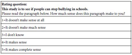
  8. Sadasivam S, Manickam (1991) Biochemical methods (Third edition), New Age International (P) limited , publishers.
  9. Folch J, Lees M, Stanley SGH (1957) A simple method for the isolation and purification of total lipids from animal tissues. J of Biochem 226: 497-509. [crossref]
  10. Sutradhar P, Mitali S, Debasish M (2014) Microwave synthesis of copper oxide nanoparticles using tea leaf and coffee powder extracts and its antibacterial activity. J Nanostru Chem 4: 1-6.
  11. Raja NH, Lingaraju K, Manjunath, Danith Kumar K, Nagaraju G, et al(2015) Green synthesis of CuO nanoparticles using Gloriosa superba extract and their antibacterial activity. J Taibah Uni for Sci 9: 7-12.
  12. Jayalakshmi, Yogamoorthi A (2014) Green synthesis of copper oxide nanoparticles using aqueous extract of flowers of Cassia alata and particles characterization. Int J Nanomat Biostruct 4: 66-71.
  13. Pulicherla Y, Thirumalanadhuni V, Yagani JR, Narasimha G, Savithramma N, et al. (2018) Cost Effective, Green Synthesis of Copper Oxide Nanoparticles Using Fruit Extract of Syzygium alternifolium (Wt.) Walp., Characterization and Evaluation of Antiviral Activity. J Cluster Sci 29: 743-755.
  14. Abbas E, Nafise MJ, Seyed GH, Maryam A (2017) Synthesis and Characterization of CuO Nanoparticles by the Chemical Liquid Deposition Method and Investigation of its Catalytic Effect on the Thermal Decomposition of Ammonium Perchlorate. Central Euro J Energetic Mater 14(1): 152-168.
  15. Vijay Kumar PPN, Shameem U, Pratap K, Kalyani RL, Pammi SVN (2015) Green synthesis of copper oxide nanoparticles using Aloe vera leaf extract and its antibacterial activity against fish bacterial pathogens. Bio Nano Sci 1-12.
  16. Gultekin DD, Hayrunnisa N, Azize AG, Nurhan HK (2017) Biosynthesis and characterization of copper oxide nanoparticles using cumin grape Vitis vinifera cv. Int J Sec Metabolite 4: 77-84.
  17. Nithya KP, Yuvasree N, Neelakandeswari N, Rajasekaran K, Uthayarani M, et al. (2014) Preparation and Characterization of Copper Oxide Nanoparticles. Int J Chemical Tech Res 6: 2220-2222
  18. Hemalatha S, Maheshwari M (2017) Green synthesis, characterization and antibacterial studies of CuO nanoparticles from Eichhornia crassipes. Rasayan J Chem10: 838-843.
  19. Saranyaadevi K, Subha V, Ernest Ravindran RS, Renganathan S (2014) Synthesis and characterization of copper nanoparticle using Capparis zeylanica leaf extract. Int J Chem Tech Res 6: 4533-4541
  20. Javad K, Sasan M. (2013) Rapid, green, and eco-friendly biosynthesis of copper nanoparticles using flower extract of Aloe vera. Nano-Metal Chem 45: 895-898.
  21. Suresh Y, Annapurna S, Singh AK, Bhikshamaiah G (2014) Green Synthesis and Characterization of Tea Decoction Stabilized Copper Nanoparticles. Int J Innovat Res Sci Engin Tech 3: 11265-11270.
  22. Mina S, Ebrahim SM, Ali R, Asemeh MM (2018) Biosynthesis of metallic nanoparticles using plant extracts and evaluation of their antibacterial properties. J Nanochem Res 3: 1-16.
  23. Alwin DS, Immanuel RS, Vignesh KS (2017) Biosynthesis of copper oxide nanoparticles using Momordica charantia leaf extract and their Nat Confer on Recent Innov in Sci Tech Engin pp. 333-340.
  24. Vanathi P, Rajiv P, Rajeshwari S. (2016) Synthesis and characterization of Eichhornia-mediated copper oxide nanoparticles and assessing their antifungal activity against plant pathogens. J Mat Sci 39: 1165-1170.
  25. Ayesha K, Audil R, Rafia Y, Ren C.(2016) A chemical reduction approach to the synthesis of copper nanoparticles. Int J Nano Let 6: 21-26.
  26. Srivastava S, Mahendra K, Arvind A, Sudhanshu KD (2013) Synthesis and Characterisation of Copper Oxide nanoparticles. IOSR J Appl Phy 5: 61-65.
  27. Abboud Y, Saffaj T, Chagraoui A, El Bouari A, Brouzi K, et al. (2014) Biosynthesis, characterization and antimicrobial activity of copper oxide nanoparticles (CuO NPs) produced using brown alga extract Bifurcaria bifurcata. Appl Nanosci 4: 571-576.
  28. Shaluei F, Hedayati A, Jahanbakhshi A, Kolangi H, Fotovat M (2013) Effect of subacute exposure to silver nanoparticle on some hematological and plasma biochemical indices in silver carp (Hypophthalmichthys molitrix) Human Experi Toxicol 32: 1-8. [crossref]
  29. Thangam Y, Perumayee M, Jayaprakash S, Umavathi S, Basheer SK (2014) Studies of ammonia toxicity on haematological parameters to freshwater fish Cyprinus carpio (Common carp) Int J Curr Microbiol Appl Sci 3: 535-542.
  30. Shaw JB, Genan AB, Richard DH (2012) Effects of waterborne copper nanoparticles and copper sulphate on rainbow trout, Oncorhynchus mykiss: Physiology and accumulation. Aqu Toxicol 117: 90-101. [crossref]
  31. Mayilathal K, Thamizhselvi N (2014) Impact of lead nitrate on haematological parameters of Cyprinus Carpio (Common Carp) Int JAdv Phar Bio Chem 3: 919-925.
  32. John R, Ahmad K, Gadgil, Sharma S (2007) Antioxidative response of Lemna polyrhiza L. to cadmium NPs stress. J Enviro Biol 28: 583-589. [crossref]
  33. Lavanya R, Veerappan N (2011) Antibacterial potential of six seaweeds collected from Gulf of Mannar of Southeast Coast of India. Adv Biol Res 5: 38-44.
  34. Kori-Siakpere O, Oghoghene UE (2008) Sublethal haematological effects of zinc on the freshwater fish, Heteroclarias sp. Osteichthyes: Clariidae. Afr J Biotech 7: 2068-2073.
  35. Keerthika V, Ramesh R, Rajan MR (2017) Toxicity assessment of iron oxide nanoparticles in Labeo rohita. Int J Fish Aqua Stu 5: 01-06.
  36. Sevcikova M, Modra H, Blahova J, Dobsikova R, Plhalova L, et al. (2016) Biochemical, haematological and oxidative stress responses of common carp (Cyprinus carpio ) after sub-chronic exposure to copper. Veterinarni Medicina 1: 35-50.
  37. Vutukuru SS, Sharada R, Kalpana Ba (2013)Acute exposure to nano Titanium dioxide causes biochemical and physiological alterations in the Zebrafish (Danio rerio)-A Case Study. Int J Chem Tech Res 5: 646-653.
  38. Mehibeen J, Nazura U (2015) Stress response of biomolecules (carbohydrate, protein, and lipid profiles) in fishes Channa punctatus inhabiting river polluted by thermal power plant effluent. Saudi J Biol Sci 22: 237-242.
  39. Abdel-Tawwab M, Mohamed NM, Mousaad, Khaled M, Sharafeldin, et al. (2013) Changes in growth and biochemical status of common carp, Cyprinus carpio exposed to water-born zinc toxicity for different periods. Int Aqu Res 5: 1-9.
  40. Rajeshwari S, Sevarkodiyone SP (2017) Biochemical parameters of Common Carp Cyprinus carpio exposed to Cadmium nanoparticles change to the leaf extract of Abutilon indicum. J Clin Micro Biochem Tech 3: 54-57.

A Reappraisal of Einstein’s Light-Quantum Hypothesis

DOI: 10.31038/NAMS.2023611

Abstract

Einstein published his light-quantum hypothesis (LH) 1905, suggesting that a light ray transmits discrete energy quanta h.fi, emitted at speed c from their source, where h refers to Planck’s constant – and fi to the frequency of a ray of light Lx in accordance with the wave equation  c=λi.fi – with λi  indicating the wavelength of Lx. Now, let fv and fr stand for the frequency of violet and red light, respectively, assuming that  fv=2.fr .  Following these premises, a source of light Qv emitting h.fv light-quanta would transmit an energy amounting to (h.fv.fv) per second, whereas a source Qr, releasing h.fr light-quanta would only emit an energy equivalent to (h.fr.fr). In other words: The LH implies that the energy a ray of light transports per time-unit corresponds to the square of its frequency. This stands at odds with the experimentally established view that the energy carried by different light-rays per time-unit is linearly proportional to their (respective) frequency.

Introduction

Einstein introduced 1905 the light-quantum-hypothesis (LH) in his paper «Über einen die Erzeugung und Verwandlung des Lichtes betreffenden heuristischen Gesichtspunkt» [On a heuristic point of view concerning the production and transformation of light]. With the help oft he LH he aimed to interpret the photoelectric effect – as well as other phenomena related to it – in a consistent, straightforward way.

In the present paper, I shall

  1. Consider the LH as a purely theoretical system, based on a number of explicit and implicit postulates;
  2. Check whether the postulates underlying the LH are self-consistent and mutually compatible;
  3. Analyse certain implications of the LH, and compare them with the generally accepted interpretation of the experimental findings.

*An earlier version of this paper was published in GALILEAN ELECTRODYNAMICS, Volume 30, Number 5, September/October 2019, p. 95-97.

Explicit and Implicit Postulates Underlying the LH

P1:          Let sources of light Qx emit homogenous, mono-frequent rays of light Lx.

P2: Let the wave-equation

(1) c=λi . fi

be valid for every light-ray Li emitted by a source Qi, with λi referring to the wavelength of a ray of light Li, and fi to the frequency of Li.

P3: Let Lv be of a higher frequency than Lr, i.e. fv > fr, with ‘v` standing for “violet“, ‘r’ for red.

P4: Let every source of light Qi which emits rays of light of a given frequency fi, emit these rays as bundles of light-quanta or photons Phi having the energy h.fi, i.e.

(2) Ei=h.fi,

where ‘h‘ refers to Planck’s constant (elementary quantum of action), and ‘fi’ to the frequency.

P5: Let the light-quanta (=energy quanta, photon) Phi, which are emitted by Qi, move through space as indivisible entities, and let them be absorbed as such by adequate targets.

P6: Let each light-quantum Phi move with speed c  in relation to its source Qi – if mutual conditions of rest are given between source, receiver, and medium (insofar a medium needs to be taken into account).

A short explanation of the foregoing postulates reads as follows:

Postulate P1 is seldom assumed explicitly. Einstein, in his introductory remarks, observed that he would consider the energy transmitted by a light-ray emitted by a «Lichtpunkt» (i.e. a very small source of light). With respect to the following analysis, I’ll assume the existence of « quasi-linear » rays of light, i.e. tiny bundles of light the cross-sections of which are so small that only one light-quantum per unit of time can hit and perforate an adequately placed perpendicular plane. Said in other terms, and in accordance with Einstein: I’ll consider rays of light in which light-quanta move in a linear row.

Postulate P2 is very rarely formulated explicitly. Nevertheless, it is implicitly taken for granted as soon as one:

(a) alludes to the frequency fi of a given light-ray, and distinguishes rays of light of different frequencies;

(b) introduces c as the constant speed of every light-ray Li in relation (i) to its source, (ii) to the medium (insofar a medium has to be considered), (iii) the receptor, and (iv) the « external observers » – albeit on the premises that source, medium, receptor, and « external observers » are at rest with respect to each other;

(c) assumes that the fronts of the rays of light – e.g. of violet and red light – proceed from their respective sources at equal speeds c.

Postulate P3 is generally accepted and needs no further comment.

Postulates P4 and P5 comprise the main, central, statements of Einstein’s LH [1]. Strictly speaking, P4 and P5 contain three separate assertions, concerning:

(i) the emission of light-quanta (see: P4);

(ii) the propagation through space of indivisible light-quanta (see: P5), and

(iii) the absorption of indivisible light-quanta (see: P5).

However, since I am dealing in the present paper only with the emission and the propagation of light-quanta, I have subsumed propagation and absorption to the same postulate P5.

Postulate P6 is seldom stated explicitly. In a configuration stating mutual rest of source, receiver, medium (insofar a medium needs to be considered), and observers – P6 is self-evident. Furthermore, P6 can be derived from P2 in conjunction with P4 and P5 [2-5].

Discussion of the LH

We shall start by considering the postulates P1 – P6 independently of one another: As far as I can see, there are no ambiguous demands being made, and nothing otherwise untenable can be discerned. Thus, every single postulate  P1 – P6, taken on its own, is free from contradictions [6,7].

We must now look at several combinations of these postulates:

(i) It follows from P3 and P4 that Lv-photons consist of a larger amount of energy than Lr-photons. In other terms:

(Ev=h.fv) > (Er=h.fr).

(ii) According to P4 in conjunction with P5, the light-quanta spread from their respective sources as indivisible entities, in their respective frequencies fv and fr – which is a constitutive factor of the light-rays we are considering.

(iii) With regard to P2, it follows that every frequency fi is univocally correlated to a corresponding wavelength λi, so that any kind of event belonging to Li (e.g. its wave-peaks) will be repeated with the corresponding frequency fi at any well-defined point along the path of Li that continues to move forth with speed c.

(iv) According to P4, source Qv emits light-quanta of energy h.fv, whereas a source Qr will release light-quanta of energy h.r.

(v) Now, following P3, ‘fv’ refers to the frequency of violet light-rays and ‘fr’ to the frequency of red light-rays, with fv > fr. On the basis of P2, we will then, reciprocally, have to infer that λv < λr.

This assertion implies that source Qv will not only emit light-quanta Phv which excel in energy the light-quanta Phr emitted by source Qr by the factor (fv – fr), but also that source Qv is due to propagate its light-quanta Phv with a frequency which surpasses the frequency with which source Qr releases its light-quanta Phr by the same factor (fv – fr).

In other words: On the basis of P1 – P6, we are compelled to deduce that if we – for instance – compare a ray of light Lv of wave-length λv=4000 nm with a ray of light Lr of wavelength λr=8000 nm, the former one (i.e. Lv) must transmit four times (and not twice) as much energy per unit of time than the latter (i.e. Lr).

It is hard to see, how this unexpected implication could be avoided: The frequency fi is a firmly bound variable of equation (1) [c=λi.fi]. – As soon as we use the symbol ‘fi‘ to point at the energy of a light-quant h.fi, we are forced to accept that these quanta are linked to equation (1) and are, therefore, emitted fi times per unit of time.

(vi) Einstein believed that the amount of energy contained in a single light-quantum  h.fi is linearly proportional to ist frequency, i.e. to the fi. However, on the basis of his premises – i.e. of his postulates P1 – P6 – we are logically compelled to infer that Einstein’s premises do not support what Einstein believed to be true, but -on the contrary – supported the erroneous assumption that the amount of energy contained in a single light-quantum h.fi is proportional to the square its frequency.

(vii) In 1916 [8]: Millikan pointed out: “The hypothesis [i.e. Einstein’s LH] was apparently made solely because it furnished a ready explanation that when an electron is thrown out of a metal by ultra-violet light or X-rays it is independent of the intensity of the light while it depends on its frequency .“ However, if one correctly argues – based on the experimental findings established by Millikan – that the amount of energy being transported by a ray of light Li per unit of time is linearly proportional to its frequency – one is compelled to dismiss as erroneous the core of Einstein’s theoretical premises and his reasonings based on them. In short: Einstein’s theoretical premises and his reasonings based on them stand at odds with his belief and with the experimental findings established by Millikan.

Conclusion

Einstein’s light quantum hypothesis (LH) prescribes that every ray of light Li transports and transmits discrete energy-light-quanta of magnitude h.fi.If every source of light Qi emitted discrete light-quanta of a specific, frequency-dependent magnitude h.fi, it would also have to release these energy-quanta with the corresponding frequency fi. This would, in turn, imply that the energy Qi emitted per unit of time with a ray of light Li, had to be proportional to the square of its frequency, i.e. the amount of the propagated and transmitted energy would have to be equivalent to fi.(h.fi) per unit of time.However, if we hold to the generally acknowledged – and by Millikan [9] experimentally established – view that every ray of light transports and transmits an amount of energy per unit of time which is linearly proportional to its frequency, Einstein’s premises and his reasonings cannot be maintained.

References

  1. Einstein A (1905) Über einen die Erzeugung und Verwandlung des Lichtes betreffenden heuristischen Gesichtspunkt. Annalen der Physik. 17: 132-148.
  2. Einstein A (1905) Ist die Trägheit eines Körpers von seinem Energieinhalt abhängig ? Annalen der Physik. 18: 639-641.
  3. Einstein A (1906) Zur Theorie der Lichterzeugung und Lichtabsorption. Annalen der Physik 20: 199- 206.
  4. Einstein A (1909) Zum gegenwärtigen Stand des Strahlungsproblems. Physikalische Zeitschrift 10: 185-193.
  5. Gut B (1996) Einstein’s Lightquantum Hypothesis. Analysis, Implications-and an Alternative. The Toth-Maatian Review 13: 5925-5929.
  6. Kaase H, Scrick F (2004) Optische Strahlung und ihre Messung. Bergmann, Schaefer. Lehrbuch der Experimentalphysik. De Gruyter 633-668.
  7. Kane JW, Sternheim MM (1988) Physics. John Wiley. 3rd ed.
  8. Millikan RA (1916) Quantenbeziehungen beim photoelektrischen Effekt. Physikalische Zeitschrift 17: 217-221.
  9. Millikan RA (1916) A direct photoelectric determination of Planck’s ‘h’. Physical Review 7: 355-388.

Empowering Critical Thinking among Young Students: Exploring Messaging about Bullying

DOI: 10.31038/PSYJ.2023522

Abstract

The study reported here investigates the response to ideas about bullying, these ideas emerging from the interaction of a young, eight-year old researcher with an artificial intelligence system (Idea Coach). The program permits the researcher to suggest the topic (bullying), uses the AI Idea Coach to create sets of 30 questions about bullying, requires to the research to select four questions, lets the AI suggest 15 answers to each question, requiring the researcher to select four of the answers for each question. The program then combined the answers (elements) into small combinations, comprising 2-4 elements, each respondent of the group (110 individuals, ages 15-26) evaluating a totally unique set of 24 combinations (vignettes). Deconstruction of the vignettes based upon the response ‘makes sense’ reveal three different mind-sets, focusing on WHO is a likely bully, How to STOP a likely bully and less clearly but still emerging, the reason WHY person is a bully, respectively. The approach shows the feasibility of AI as an enhancer of critical and creative thinking, empowering students as young as eight years able to begin doing high-level, original scientific research, in a systematized, programmed fashion.

Introduction

This paper is part of a series of research studies conducted by young students, enrolled in elementary and in middle school, with the dual goal of teaching students how to think critically while at the same time working with them as researchers to explore issues of social relevance. A glance at the literature reveals that virtually all research is executed by professionals, occasionally junior professionals such as graduate students, but far more often by young and middle-aged professionals, following the structure of academic research. Even when the topic involves the experience of young people, such experience is analyzed through the ‘trained’, perhaps biased eye of the professional, who brings along a career of studies. The study of the experience follows the time-hallowed practices of the scientific method, although the ‘immediacy’ of the experience cannot be tapped because the researcher is not a young person.

Almost 80 years ago, the radio and television personality Art Linkletter starred in a show called House Party, starting in 1945 and ending in 1969. As described by Wikipedia. The host would begin a conversation by posing a question about life topics to a child, who usually responds with their own innocent, often comedic perspectives on the various topics…. In the show’s first inception, it would sometimes flash back to the 1950s and 1960s show Art Linkletter’s House Party, with Cosby joined onstage by Art Linkletter, that show’s host, to introduce the vintage clips. It would show kids (of the time), their same comedic reactions to whatever Linkletter would ask or say to them…

The foregoing quote suggests that we may learn a great deal about the way children think about the world, although it is clear that a great deal of this learning is second-hand, with the researcher observing the behavior, and commenting on it. In recent years authors Deitel, Moskowitz and Rappaport have collaborated to create a system whereby anyone can be a researcher, at least for the type of research known as Mind Genomics. The idea behind Mind Genomics is that by showing people combinations of ideas and measuring their response, one can learn what specific aspects of these ideas drive the behavior, viz., the aspects to which people pay attention. Rather than asking people to say what is important to them about a topic (viz., open ended question), or ask people to rate importance of different ideas, one idea at a time, Mind Genomics assumes that people will find it more ‘natural’ to respond to combinations of ideas. The rationale for this assumption is that in the world of everyday experience people evaluate combinations of features, rather than one single feature at a time.

Bullying

The topic of bullying is becoming increasingly important [1-3]. It may be that the availability of video technology on smartphones to record one’s bullying efforts has become a stimuli to become a hero. Bullying on the internet has been shown to be responsible for teen and child suicides [4,5]. Those are just the most serious cases.

The emerging science of Mind Genomics may help us understand what young people think is important. The study reported here is unique because it was set up by young researchers, in elementary schools (3rd grade; Ciara) and in middle school (8th grade; Cledwin). The study objective was to explore aspects of bullying from the point of view of the younger researcher, using Mind Genomics augmented with AI, in the form of Idea Coach. Idea Coach helped the researcher both learn about the issues involved in bullying, and to take an active role providing new-to-the-world knowledge about these issues.

The Mind Genomics approach has been previously discussed in a variety of papers [6,7]. Three previous studies have appeared featuring the efforts of these young researchers [8,9]. The objective of the studies is to deal with a serious topic, framed not so much by an experienced adult researcher as is usually the case but rather a research effort framed by a young mind. Often the types of questions intriguing the young researcher may well differ from the questions intriguing an older researcher. We almost never heard from the young researcher, and from young respondents. The study reported here and its companion studies allow us a peek into the mind of the younger researcher, and the response to test stimuli by respondents of the appropriate age.

Method

Mind Genomics studies follow a now-standard approach, using templated inputs and automated, rapid analyses. The almost automated approach exemplifies the vision of author Moskowitz to create a system which allows anyone to become a researcher (democratization), coupled with the goal of accelerated knowledge development (efficiency), and with the vision of creating large-scale databases of aspects of ordinary life, doing so in a simple, inexpensive, iterative, and world-wide manner (industrial-scale knowledge development). The Mind Genomics program itself is called BimiLeap, short for Big Mind Learning App. The program can be accessed by anyone with access to the Internet, at www.BimiLeap.com.

Step 1 – Identify the Specific Topic

This sounds simple, and eventually is simple. The novice researcher often thinks in generalities, not in specifics.

Step 2 – Create Four Questions Regarding the Topic of the Study

The respondent is allowed to choose any questions, as long s the questions tell a story about the topic. It is at this point that Mind Genomics proceeds to structure the way the researcher approaches the problem. The first encounter with requiring the researcher to ask a question can be frightening, and certainly off-putting. Most novice researchers freeze up at this point, perhaps shocked by the directness of the question. The most common initial reaction at this point is a sense of discomfort, and in some cases that discomfort simply ends the effort, with the researcher.

For the researchers who cannot think of questions, there is the associated AI feature, Idea Coach. The researcher simply writes a short paragraph, really 1-3 sentences, and Idea Coach returns with 10-30 questions. Idea Coach can be invoked several times, either with the same paragraph or with different paragraphs. Each time Idea Coach will return with a set of somewhat different questions. Table 1 shows a run of Idea Coach, prompted by the researcher request ‘Help me create questions about bullying.’

Table 1: Thirty questions emerging from Idea Coach, based upon the request to ‘tell me some questions to ask about bullying in school’.

tab 1


Once the researcher selects the four questions, the next step requires the research to provide four answers to each question, specifically phrases which paint word pictures. Once again the researcher can either come up with answers, and/or work with the Idea Coach. For each ‘run’ of Idea Coach, comprising answers to a question, Idea Coach emerges with approximately 15 phrases which answer the question. This step in the process is much easier, simply because many people find it easier to answer questions than to pose questions. Answering questions relies on memory and experience. Posing questions relies more on critical thought because the researcher is going into a void, rather than filling the void under the direction of a question.

The process in Mind Genomics has been simplified, allowing the researcher to write the question to describe the topic, use Idea Coach to present 30 questions (and repeat as desired), select four questions, edit those questions when desired, and finally put in answers and have Idea Coach fill in the missing answers. In all cases the researcher is free to override the Idea Coach effort, whether overriding consists of editing the question/answer or even providing a new question/element based upon one’s insight.

Once the researcher has used Idea Coach to create questions, such as those shown in Table 1, the researcher select questions and/or adds in questions of one’s own. These questions are automatically inserted into the template. The researcher is then prompted to provide four answers to each question. The Idea Coach can provide answers to each question, providing 15 answers for each question for each ‘run’ of the Idea Coach. The researcher need only select four answers, or fewer answers, providing other answers as desired. The answers can be edited, as they were in this study, generally edited for simplicity, and recognizing the nature of the project. In this study the answers were edited by introducing the sub-topic, followed by a colon, and then followed by the text. In this way the element would end up ‘making sense’ in the format of Mind Genomics, wherein one element was presented atop another, not connected with each other, but part of the vignette.

Table 2 presents the four questions selected from the 30 questions at the start of the study. These questions may or may not have appeared in Table 1 for the simple reason that each iteration of Idea Coach produces different sets of questions. Table 2 also presents the four answers to each question.
 

Table 2: The four questions and the four answers to each question

tab 2
 

Once the questions and answers are selected, the Mind Genomics program creates combinations of elements. These combinations are called vignettes. A vignette comprises a minimum of two elements, and a maximum of four elements. The structure of the vignette is specified by a layout called an experimental design. The experimental design for Mind Genomics was created to ensure the following properties:

  1. Every respondent evaluates exactly 24 vignettes
  2. The 24 vignettes are set up so that each of the 16 elements appears exactly five times and is absent 19 times.
  3. A vignette has either two, or three or four elements.
  4. A vignette can have at most one element from a question, often has no elements from a question, and never has more than one element from a question. This property is important. It is a bookkeeping feature which ensures that a single vignette can never have two different pieces of information of the ‘same type’. The problem becomes obvious when instead of the elements selected here, the elements are prices and brands. In the latter case we want to ensure that a single vignette can have at most one price, not two prices, which would be self-contradictory.
  5. The underlying experimental design ensures that the 16 elements are statistically independent of each other. This statistical independence and the specific nature of the design allow the researcher to use statistical modeling (OLS, ordinary least-squares regression) to relate the presence/absence of the 16 elements to the dependent variable. Usually the dependent variable is the rating assigned, a simple transform of the assigned rating, or response time (the time elapsed between the presentation of the vignette to the respondent and the respondent’s rating, captured by the program).
  6. A special feature of the experimental design is that it is permuted [10,11]. The permutation means that the underlying mathematical structure is maintained, but each respondent evaluates different combinations. From the practical point of view, the permutation means that the research ends up covering a lot more of the underlying ‘design space’. Rather than having to have a good idea of the ‘right test stimuli’, viz., the right test combinations, and then test those ‘right combinations’, the permuted design tests many more combinations. The patterns in the data emerge more powerfully when the large design space is explored, rather than when one focuses on what ‘thinks’ to be a promising area.

Study Execution on the Internet

The actual study is run in a straightforward fashion, using the Mind Genomics program, www.BimiLeap.com. The program both guides the set-up of the study, as well as executes the study. Once the researcher has set up the study, the next step is to ‘order’ respondents. Traditionally, this process has been arduous, typically because over the past decades respondent participation has dropped. The simple reasons are that people are busy, but also one can scarcely do anything in the commercial world without a sweetly phrased request inquires whether the person would be willing to complete a short survey about the experience. One or two such requests are acceptable, but one can expect resistance, despite the motto of the Marketing Research Association that ‘Your Opinion Counts.’

To remedy the issue of difficulty in recruiting respondents, the BimiLeap program contains a built-in facility to both issue invitations (links to the study), or to pay for respondents, specifying these respondents by a set of screens showing qualifications. The paid request is immediately sent to the associated ‘on-line panel provider’, Luc.id, which aggregates respondents, and provides the necessary respondents in a short period of time, perhaps an hour or so for 100 qualified respondents. This speed means that the entire study can be set up in 30 minutes or less, and executed in 90 minutes or less for 100 easy-to-find respondents. The result is a study executed form start to finish within the space of two or two and a half hours.

The actual study begins with a short introduction about the project, a set of classificaiton questions (age and gender fixed, and then a no/yes question of having been bullied in school). The respondent then proceeds to the actual evaluation of the 24 vignettes. The orientation is short, providing almost no substantive information. The objective is for the orientation to simply introduce the topic. The actual information is presented in the vignettes, the combinations of the elements. Table 3 below presents the orientation sentence, the rating question, and the five answers comprising a Likert scale.

Table 3: The orientation sentence, the rating question and the five point rating scale

tab 3

Initial Analyses – Frequency of Selected Ratings by Groups of Respondents

Mind Genomics studies generate a great deal of data. We can approach the analyses in at least two different ways. The first way is to look for different patterns of responses, recognizing that we are dealing with different vignettes across all 110 respondents or 2680 vignettes, without the test stimuli having any cognitive meaning at all, other than being test stimuli, the responses to which are being measured.

Following the foregoing analysis, we can examine the frequency of ratings by groups. The first set of groups include the Total Panel, the genders, the ages, the groups who say they were bullied before versus not bullied before. The second set of groups is the mind-sets, individuals who think similarly to each other. We look at the 110 respondents divided into two mutually exclusive mind-sets and then three mutually exclusive mind-sets. Finally we look at the position of the vignette during the sequence of 24 vignettes (first to fourth quarter), and at the vignettes rated quickly (< 3 seconds) versus at the vignettes rated slowly (>= 3 seconds).

Table 4 shows the frequencies. There are occasional differences of 8% or more, especially for the ratings of ‘makes sense’ (5 and 4). There are a few differences for ‘makes no sense’ (1 and 2), and very few for ‘don’t know’. We conclude from Table 4 that there are differences in the measure ‘makes sense’, but beyond that deliberate overlooking of the cognitive meaning hampers our knowledge. It will be with the knowledge of what the elements ‘mean’ that we will make progress.

Table 4: Frequency of ratings assigned by the different, identifiable groups of respondents or vignettes. The numbers in the first three columns of each row should add to 100%.

tab 4

How Elements Drive Ratings of ‘Makes Sense’ and ‘Doesn’t Make Sense’

The previous section considering the frequency of ratings showed that simply measuring responses to test stimuli suggests some differences among groups, although one would be hard pressed to learn more about the process of decision making. Fortunately, the cognitive richness of the test stimuli, viz., the simple statement, can be used by the researcher to reveal what the respondent may ‘think’ about a topic, even when the respondent herself or himself cannot articulate the rules by which the respondent makes a simple decision. Indeed, quite often exit ‘comments’ by respondents participating in a Mind Genomics study end up with the respondent insisting that it was impossible to ‘find the right answer that was deemed appropriate’ and that much of the answering felt like ‘guessing’ rather than like a reasoned rating.

A deeper analysis of the ratings shows, time after time, that there is a clear set of rules that can be inferred by the pattern of ratings, but only when the ratings themselves can be related to the presence/absence of the specific messages in the vignettes. That is, the pattern of ratings themselves fail to provide information as Table 4 above suggests. Yet, as the remaining tables in this paper will reveal, there are clear, consistent, and interpretable patterns, especially when we bring to bear the combination of OLS (ordinary least squares) regression, coupled with cluster analysis to identify similar behaving groups in the population.

OLS regression, colloquially known as ‘curve fitting’, relates a dependent variable to one or more independent variables. For our study, the regression equation is written as:

Dependent variable = k0 +k1(A1) + k2(A2) … k16(D4)

In words, the expected value of the dependent variable (e.g., Makes Sense, Top2, Rating 54) is the sum of 17 numbers. The first number, k0, is the additive constant. It is the expected the top of the dependent variable (e.g., Top2, Makes Sense) in the absence of elements. Of course, all 24 vignettes evaluated by each respondent comprised a minimum of two elements and a maximum of four elements, so the case of a vignette without elements is hypothetical. Yet, the additive constant (also called the intercept by statisticians) is estimated, and is considered to be a correction factor. We can use it as a baseline, from which all elements either add or subtract. The additive constant is usually high when the dependent variable is ‘Top2, Makes Sense’, and usually low when the dependent variable is ‘Bot2, Does not make sense’.

The regression analysis returns with positive coefficients and with negative coefficients. For our analysis we will present only the positive coefficients of magnitude +2 or higher. The blank spaces in the tables of coefficients actually have numbers, negative or zero coefficients, but in the interest of discerning the pattern we are primarily interested in the positive coefficients. In actuality, presenting the positive and negative coefficients clouds the results.

The top portion of Table 5 presents the positive coefficients for the Top2, viz., for the Total panel, two genders, three ages, and the first six versus the last six vignettes in the set of 24 vignettes. The additive constants are all high, but the highest for the younger respondents, ages 15-18 (additive constant 83) and ages 19-21 (additive constant 78). This is noteworthy. It says something about the proclivity of younger respondents to agree with the statements about bullying, especially since respondents ages 22-26 show a much lower value (additive constant 61). It is important to recognize that this type of granular information could not have emerged from conventional research, and may not have been recognized without the use of OLS regression.

Table 5: Parameters of the models for ‘Make Sense’ (Top 2), and for ‘Does Not Make Sense’ for self-defined groups, and for first and last test orders.

tab 5

Moving now to the granular level of elements, we see many empty cells. These cells belong to elements which failed to drive a perception of agreement beyond the general proclivity to agree evidenced by the additive constant. What strikes us as noteworthy is that the majority of strong performing elements occur in the columns devoted to order of testing. There seem to be two types of elements, those which desensitize with exposure, and those which sensitize with exposure. The magnitude of the effect can be dramatic, especially when we see that the additive constants are virtually equal (63 for vignettes 1-6; 61 for vignettes 19-24).

Sensitizing elements (stronger tor vignettes 19-24, weaker for vignettes 1-6)

To stop bullying: Encourage students to speak up if they witness bullying.

To stop bullying: Bullying should be discussed openly and regularly, both in class and in assemblies.

Desensitizing elements (stronger for vignettes 1-6, weaker for vignettes 19-24)

Likely bully: People who are unhappy with themselves

Likely bully: People who are insecure

Likely bully: People who have mental health issues

When the analysis is reversed, focusing now on what does not make sense (BOT2), Table 5 suggests a different picture. As expected, the additive constants are quite low, hovering around 20. In turn, a low additive constant ends up allowing a variety of elements to emerge. Table 5 shows the greater number of low coefficients. Worthy of note are the three element responded to strongly by the youngest group of respondents, ages 15-18. Here are the elements which do not make sense to them:

Reason others bully: They want to make someone else feel bad

Reason others bully: They’re mean

Victims feel: Powerless

Table 5 gives us somewhat of a sense of the mind of the respondent. We find some messages to be strong, most messages to be weak. One hypothesis which emerges is that people may differ from each other in part of their life histories. For our study of bullying, a question which comes to mind is whether having been bullied (or at least answering YES on the up-front classification questionnaire) reveals itself in the pattern of responses to the elements.

Table 6 shows the parameters of the equations developed from the 38 respondents who said that they were bullied versus the parameters of the equation developed from the 72 respondents who said they were not bullied.

Table 6: Parameters of the models for ‘Make Sense’ (Top 2), and for ‘Does Not Make Sense’ for those who reported that were bullied versus not bullied.

tab 6

There are some differences, not in the additive constant (baseline), but in the elements. Those who said that they were bullied find more elements to ‘make sense’ than those who said that they were not bullied. In terms of not making sense, those who were not bullied find more elements not to make sense.

Mind-Sets

A foundational principle of Mind Genomics is that for the world of the everyday there are differences in the way that people make decisions. These differences emerge in the granular level of the everyday, not necessarily in a way which sets one person apart from others. Researchers might call these individual differences, often recognizing that they could end up being a vexatious source of variability, hindering the signal, but signifying nothing. In contrast, Mind Genomics processes this variability through clustering respondents on the patterns of their coefficients for their models. The clustering uses all 16 coefficients for the respondent, viz, positive coefficient, 0’s, and negative coefficients, the latter two coefficients not shown in the tables. The method k-means clustering, uses as a distance measure the value (1-Pearson correlation between the corresponding sets of 16 coefficients for two people [12]).

The k-means program extracted two mind-set and three mind-sets, using the coefficients relating the presence absence of the elements to the ratings of ‘make sense’ (viz., Top3) The 110 sets of coefficients were used for in the k-means, with the additive constant not included Table 6 presents the non-zero coefficients, first for TOP2 (Makes sense), and for BOT2 (makes no sense).

The two-mind set solution suggest one group one group focusing on WHO is a likely bully, and a second group focusing on HOW TO STOP a bully. The three mind-set solution distinguishes among WHO is a likely bully from How to STOP a likely bully, and less clearly but still emerging from the reason WHY person is a bully.

It is remarkable that in the face of such a complex task, respondents are able to focus on what is important to them. It is even more remarkable when we see that only with clustering the responses do these groups emerge clearly, in a way that could not possibly be biased (Table 7) [13].

Table 7: Parameters of the models for ‘Make Sense’ (Top 2), and for ‘Does Not Make Sense’ for two and three mind-sets extracted from the coefficients using k-means clustering.

tab 7

Discussion and Conclusions

The extensive literature on the topic of bullying has been created by adults, for adults, using the behavior of children towards each other. The inevitable effect of the research effort and the published result is to describe and explain the behavior of children as a combination of anthropology, sociology, and psychology. The researcher sits on the outside, observing the behavior, or talking to those involved in the behavior. Afterwards, the researcher translate the personal experience of the children into ‘adult, science-speak’, replete with statistics when relevant. Of course research ethics do not permit the researcher to induce bullying as part of an experiment, requiring observation and storytelling, rather than experimentation.

It is obvious that young researchers can construct simple questionnaires, and by administering these questions to the correct people the young researcher can learn a lot about the world from the point of view of other people. One need only look at the exercise of interviewing someone older about one or another life experience, the type of research that schools use to introduce students to the research process. Within that framework, the Mind Genomics study reported here presents the way people think about bullying. The data could be reported in that fashion.

The important activities of the Mind Genomics efforts occur at the start, when the study is designed and the questions/answer are developed, and at the end, when the results are analyzed. The Mind Genomics approach, modified by adding a coaching feature, enables the younger researcher to investigate topics in great depth, doing work which by virtue of the coaching and templating becomes valuable. When looking at the execution of the study, and the results, it would be hard to believe that the author of the study is a grade school student. That is precisely the point. The student has now done professional level research. The topics might be thought about initially by the mind of a grade school student, but quickly the execution and the results bring the student to a higher degree of understanding of the topic. It is the mind of the grade school student which frames the topic and selects the question. It is the research approach, the AI coaching, and finally the easy to read results emerging from powerful but ‘hidden’ analyses, which end up helping the student to get excited at the prospect of discovery, and accelerate the process of self-education.

References

  1. Bradshaw CP (2015) Translating research to practice in bullying prevention. American Psychologist 70: 322-332. [crossref]
  2. Dake JA, Price JH, Telljohann SK, Funk JB (2003) Teacher perceptions and practices regarding school bullying prevention. Journal of School Health 73: 347-355. [crossref]
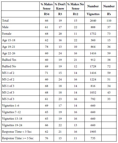
  3. Evans CB, Fraser MW, Cotter KL (2014) The effectiveness of school-based bullying prevention programs: A systematic review. Aggression and Violent Behavior 19: 532-544. [crossref]
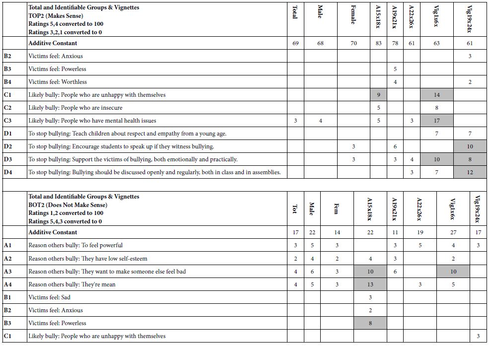
  4. Craig W, Boniel-Nissim M, King N, Walsh SD, Boer, M, et al. (2020) Social media use and cyber-bullying: A cross-national analysis of young people in 42 countries. Journal of Adolescent Health 66: S100-S108. [crossref]
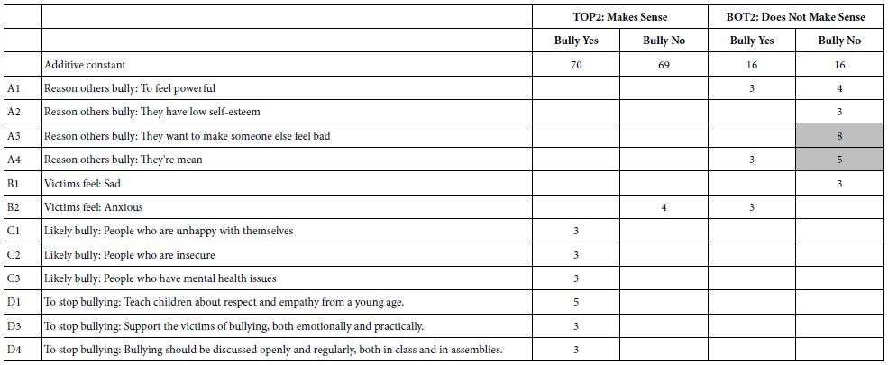
  5. Sedgwick R, Epstein S, Dutta R, Ougrin D (2019) Social media, internet use and suicide attempts in adolescents. Current Opinion in Psychiatry 32: 534. [crossref]
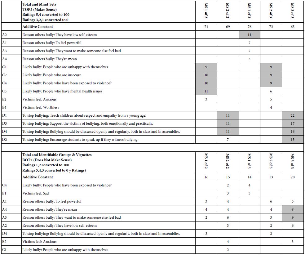
  6. Moskowitz HR, Gofman A, Beckley J, Ashman H (2006) Founding a new science: Mind Genomics. Journal of Sensory Studies 21: 266-307.
  7. Porretta S, Gere A, Radványi D, Moskowitz H (2019) Mind Genomics (Conjoint Analysis): The new concept research in the analysis of consumer behaviour and choice. Trends in Food Science & Technology 84: 29-33.
  8. Mendoza, CL, Mendoza CI, Rappaport S, Deitel J, Moskowitz HR (2023) Empowering Young Researchers: Understanding the mind of prospective aides regarding elderly clients.
  9. Mendoza CI, Mendoza CL, Rappaport S, Deitel J, Moskowitz HR (2023) Empowering Young Researchers: Exploring and understanding responses to the jobs of home aide for a young child.
  10. Mendoza CL, Mendoza CI, Rappaport S, Deitel J, Moskowitz HR (2023) Empowering young researchers to think critically: Exploring reactions to the ‘inspirational charge to the newly-minted physician.
  11. Gofman A, Moskowitz H (2010) Isomorphic permuted experimental designs and their application in conjoint analysis. Journal of Sensory Studies 25: 127-145.
  12. Likas A, Vlassis N, Verbeek JJ (2003) The global k-means clustering algorithm. Pattern Recognition 36: 451-461.
  13. Hardy MA (1993) Regression with Dummy Variables. Sage.

Communication Preferences of Obese Female Adolescents with Clinicians

DOI: 10.31038/AWHC.2022534

Abstract

This study tests the use of specific brief narrative messages that clinicians may use with obese female adolescents regarding body images. The sample comprised 102 obese adolescent females. Each respondent evaluated a unique set of 48 combinations (vignettes) of messages, created from a base size of 36 messages, each set vignettes evaluated by a respondent specified by an underlying experimental design. Regression analysis at the individual respondent level generated coefficients, which were clustered to real three interpretable groups of respondents (viz., three mindsets). These mindsets, limited to the granular topic of body image are: Known need of control (33%), Self-condemnation and shame (46%), Feeling ugly, panicky, and victimized (24%). A subsequent application created a predictive algorithm, a personal viewpoint identifier which is a six-question tool, based on mathematical clustering. The pattern of ratings assigned a new respondent to one of the three mindsets. Clinicians may use effective communication messages by mindset-belonging to influence body image and prevent eating problems in female adolescents.

Introduction

The term body image (BI, hereafter) describes one’s perceptions about one’s own body that develops throughout adolescence [1,2]. Body image entails a perceptual dimension referring to an individual’s self-perception of their appearance and an attitudinal dimension referring to four components: affective, cognitive, behavioural, and satisfaction. The affective component refers to the comprehension of feelings relating to one’s appearance. The cognitive component refers to knowledge about body image. The behavioural component considers body-checking behaviours and actions to avoid situations or objects that evoke body image concerns. The satisfaction component concerns a person’s appreciation over their body as a whole or to specific parts [3].

Female adolescents, more than males, associate higher and increasing Body Mass Index (BMI) with lower self-esteem, routinely evaluate their body, perceive their social worthiness as determined by their physical attractiveness, and tend to obsessively worry about their physical appearance [9,10]. DBI has been associated with low self-esteem, depression, anxiety, poor social functioning, poor health-related quality of life, and concerning unhealthy eating behaviours (i.e., fasting, vomiting, or laxative abuse) leading to malnutrition, noncommunicable diseases, obesity, diabetes, cardiovascular disease, cerebrovascular incidents and even cancer [4].

Female adolescents stated that DBI is a “touchy subject” [5]. Although clinicians are aware of the importance of communication to promote a positive BI in female adolescents, and 74% of clinicians in a study reported discussing DBI with adolescent patients, 85% of female adolescents reported that they wanted to talk about their DBI with their clinician, but never held such a conversation [2]. Clinicians acknowledge that they feel uncertainty and have no confidence to communicate with female adolescents on DBI [5,6]. Thus, while communication may mitigate the risk factors of DBI, research on how to discuss the topic in practice is scant [2,5]. This study begins to close the gap in the state-of-the-art, exploring preferences of female adolescents regarding clinician-adolescent communication on DBI [5,7,8]. This study seeks to identify and crystalize specific communication messages to support clinicians’ choices of the right messages in communication with adolescents on DBI.

Test Stimuli – Questions, Answers (Elements) and Vignettes

Mind Genomics works by presenting combinations of elements to the respondent, obtaining a rating of the combination, and then deconstructing the rating of the combination to the part-worth contribution of each element. The experimental design uncovers the preference for communication while inhibiting the social desirability bias of respondents as often occurs in surveys. The experimental design approach design has been used to understand preferences in different health contexts [9-11].

We begin with the raw materials, the elements. Mind Genomics comprises different structures, allowing a flexibility in the research process. The most popular version is the so-called 4×4 design, with four questions, and four answers (elements) for each question. A second popular version is a 6×6 design, entailing six questions, and six answers to each question. This second version, 6×6, was chosen for this study. Table 1 shows the six questions and the 36 elements.

  1. The independent variables are categories of communication based on previously used scales assessing perceptions regarding DBI [12-14].
  2. Perceived weight status was assessed with the question: “At this time do you feel that you are..”
  3. DBI was assessed with a modified version of the Body Shape Satisfaction Scale [15].
  4. Unhealthy and extreme weight control behaviours included: fasted, ate very little food, used a food substitute (powder or a special drink), and skipped meals [16].
  5. Binge eating was assessed with questions such as: “You eat so much food that you would feel embarrassed if others saw you” [17].
  6. Self-weighing was assessed by asking adolescents to indicate how strongly they agreed with the statement, “I weigh myself often.”

Table 1: The six questions (categories), and the six answers to each question

tab 1(1)

tab 1(2)

Mind Genomic then combines the elements in vignettes, which for the 6×6 design comprises 48 vignettes three or four elements, respectively. The combinations are not done randomly, but rather constructed according to an underlying experimental design. The design specifies the 48 combinations, ensuring that each element appears equally often, ensures that the 36 elements are statistically independent of each other, and that each respondent evaluates a unique, different set of combinations. This is called a permute experimental design [18]. The permutation allows the researcher to investigate a great of the underlying ‘design space’ of different combinations. Rather than having the researcher somewhat ‘know the promising combination’, the permuted design allows true exploration, even in the total absence of any knowledge. Mind Genomics thus differs from conventional research, sacrificing precision of measurement through replicated measurements of a few test vignettes to precision of understanding of the topic through exploration of much more of the design space. To give an example here, the Mind Genomics effort explored 4896 combinations in the design space rather than exploring 48 vignettes in the design space.

The underlying experimental design serves another purpose as well, specifically Bookkeeping. The experiment design is created so that mutually contradictory elements, viz., elements of the same type but conveying different messages, end up in the same category. The underlying experimental design ensures that a vignette has at most one element or answer from a viz., question. The happy outcome is that the vignettes never present directly contradictory elements to a respondent, at least when one considers a simple reading of the vignette. The elements themselves were relevant to the world of the clinician regarding DBI [19].

Executing the Study on the Internet

Respondents began with an orientation page, signed an informed consent for participation and publication, completed three demographic questions for classification, and finally rated the specific set of 48 combinations of messages corresponding to their own individual experimental design.

The 36 messages were presented in 48 combinations. Every respondent evaluated a unique, different set of 48 combinations [20]. The experimental design varies messages to create different combinations of messages, each combination comprising a minimum of three and a maximum of four messages. The experimental design is set up so that mutually contradictory messages cannot appear together in the same combination. The outcome variable was preferences of adolescent females regarding communication with clinicians on DBI.

It is important to note that the experimental design ensures that the elements will be statistically independent of each other, and the array of 36 elements will allow OLS (ordinary least-squares) regression to estimate the coefficients of the model created for each respondent separately. The rating question was “how important are these vignettes in communication with your clinician on BI?” Each respondent rated the 48 unique combinations using an anchored 9-point scale (1 = “I prefer not to talk about this in communication about my DBI”; 9 = “I would like to talk about this in communication about my DBI”).

After rating the 48 vignettes, the respondent completed a short socio-demographic questionnaire to define aspects of the respondent, without revealing any other personal information. The self-classification question recorded ethnicity and socio-economic status (e.g., higher education level of either parent; family eligibility for public assistance; eligibility for free or reduced-cost school meals, and parental employment status) [16,21].

Data Analysis

The 48 combinations created for each respondent, comprise a stand-alone experimental design for that respondent. Each of the 36 messages is statistically independent of the other 35 messages. The experimental design allows the analysis of the results using OLS (ordinary least-squares) regression, at either the individual respondent level (within-subjects analysis), or the analysis of groups of respondents (OLS) [22].

During the development of Mind Genomics from the 1990’s onwards, it has become a standard practice to convert the Likert Scale to a binary scale, to make the analysis and the interpretations more intuitive. Researchers and especially those who use the data for decisions encounter problems interpreting averages, often asking about the meaning of averages in everyday terms. To simplify the process the Mind Genomics process first transforms the ratings, to move the 9-point scale to a binary, 0/100 scale. By convention, ratings of 1-6 are transformed to 0, ratings of 7-9 are transformed to 100, and then for each newly transformed rating a vanishingly small random number (<10-5) is added.

The foregoing procedure now generates 102 sets of 48 rows each. Each row corresponds to one respondent, and one of the 48 vignettes evaluated by the respondent. The database is set up for OLS regression. The first set of columns record the respondent identification, the order of the vignette (1-48), and one column for each of the information questions asked in the self-profiling classification. The second set of 36 columns are reserved to code the presence of an element in a vignette (coded by the number ‘1’ for the column corresponding to an element), or the absence of an element in a vignette (coded by the number ‘0’). The final set of columns show the rating assigned by the respondent (viz, 1 to 9), and the transformed value of that rating (viz., 0 or 100).

For the OLS analysis, the independent variables are the 36 messages, coded 0 or 1 (absence/presence). The OLS model was formulated as Transformed Binary Rating = k0 + k1 (message A1) + k2 (message A2) … + k36 (message F6). For descriptive purposes, we will look at each of the 37 numbers as a measure of ‘describes me’. The Mind Genomics program computes the additive constant and all 36 coefficients, returning a great deal of data. To uncover patterns, we will present only the positive coefficient > 1. The smaller coefficients will not be shown, even though they were computed. The appropriate cell in the table will be left blank. Furthermore, for strong performing elements, those with coefficients of 8 or higher, the cell will be shaded to drawn attention to these elements.

The additive constant of the OLS model is a baseline, an estimated parameter, providing a measure of how likely it is for an adolescent to say ‘this describes the way I would like to talk to my clinician’, albeit in the absence of messages. Of course, the underlying experiment design ensures that every vignette comprises 3-4 elements, so the additive constant, is a baseline, a strictly estimated parameter.

The individual coefficients show the driving power of the messages. Continuing with the example but moving to the coefficient, a positive number of +8, means that when the message is incorporated into the combination, an additional 8% of the respondents are likely, on average, to say that they ‘this describes the way I would like to talk to my clinician.

People differ in their attitudes and perceptions, as well as their needs and wants. The self-profiling classification allows the creation of equations either for the Total Panel, or for any specified group. The OLS regression simply calculates the additive constant and the 36 coefficients based upon all the data appropriate to define that subgroup.

Finally, person-to-person variation may not necessarily depend on who the person is or what a person ‘believes’ for a specific situation. One’s perceptions and values may not clearly co-vary with who a person IS, or how a person THINKS about a general problem. There may be groups of people who are similar, not necessarily for all of the topics of their lives, but perhaps only for the granular topic being investigated. These are mindsets, groups of people who are similar in a specific topic area, based upon the similar of the pattern of their coefficients, in this case their 36 coefficients. To discover these groups, so-called ‘mindsets’, requires the use of a simple clustering method (viz., k-means). The clustering applied to the patterns of coefficient reveals new-to-the-world groups of individuals showing similar patterns of preferences in communications, a way to understand the different needs of the groups. [23].

Sample

Respondents were 102 obese female adolescents from the greater New York area, ages 13-19 years old. Respondents gave their informed consent for participation and publication. The size of the sample is consistent with the suggested sample size in conjoint analysis studies, particularly when aiming at stability of coefficients rather than stability of means [24]. Since DBI entails both a physiological indicator (BMI) and a subjective construct of BI, inclusion criteria for the study were a BMI of 30 and above and respondents’ self-definition of themselves as being overweight.

Relating the Presence/Absence of the Elements to the Binary Transformed Rating

The heart of the Mind Genomics analysis is the set of coefficients emerging from the regression analysis. Recall that the OLS regression deconstructs the response to the vignettes into the part-worth contribution of the 36 elements. Respondents cannot ‘game’ the system and give the correct analysis, simply because in the rapid process of stimulus/response, the typical evaluation time is about 3-4 seconds. There is simply no time for the respondent to try to ‘guess’ the right answer. It is simply impossible to do. Respondents report that they simply look at the vignette, and assign a value, often stating that they feel that they are guessing.

Table 2 presents the regression coefficients for the total panel and for the three mindsets as created by k-means clustering analysis. Messages are sorted by the strong performing coefficients for the three mindsets. The same message may appear twice when it is a strong performer. The total panel shows only two strong performing messages. These are “You eat until you are full and don’t pay attention to portion sizes”; and “You have erratic eating habits” reflecting erratic eating habits. It is when the data from the three mindsets are laid out that the patterns emerge.

Table 2: Coefficients for the messages by Total Panel and by the three emergent only positive coefficients greater than +1 are shown to allow patterns to emerge. The table shows strong performers for each mindset. (MS).

tab 2(1)

tab 2(2)

Table 2 suggests that a seemingly flat pattern of coefficients from the total panel may result from the combination of groups of adolescent females with different, often opposite, points of view. Groups of adolescents with similar response patterns emerge from the patterns in the data, patterns which are interpretable and parsimonious. What members of one mindset prefer to discuss in communication with clinicians on DBI may be irrelevant to adolescents in other mindsets. Furthermore, the coefficients for the mindsets are much higher, suggesting that the results from the total panel hide the underlying narratives by averaging dramatically different subgroups with different ways of thinking about their preferences. K-means clustering shows that there are distinct groups with different points of view regarding communication on DBI.

The Distribution of Mindsets across the Population

Table 3 shows that the three mindsets are distributed similarly across demographic attributes of the female adolescents, whether those are geo-demographics, parent’s education, or actual weight. There are some departures from random distribution, but there is no clear pattern and no explanations for the departures. Most of the adolescents are either Caucasian or African American. Mindset 2 seems to include more respondents who live in the suburbs. Mindset 3 comprises more African Americans and is over-represented by those with large families. Its members feel ugly, panicky, and a victim.

Table 3: Distribution of respondents into different groups, for Total Panel and for the three emergent min-sets

tab 3(1)

tab 3(2)

tab 3(3)

Assigning an Adolescent to a Mindset

This study reveals the existence of mindsets in the population of adolescent females and provides an organizing principle for clinicians by which to choose messages on DBI in communication with adolescents. For the data to become ‘actionable,’ it is necessary to develop an easy-to-use a predictive algorithm to rapidly assign an adolescent in the clinic to one of the three sample mindsets. Using a Monte-Carlo simulation process, we created a Personal Viewpoint Identifier (PVI) based on the mindsets data (Table 2). The PVI identifies a set of six original messages which can be scored on a two-point scale. Each of the 64 patterns of responses to messages assigns an adolescent to one of the three mindsets. The PVI presents the algorithm showing the six distinguishing messages taken from the data in Table 2. The pattern of response to those six messages assigns a female adolescent to a specific mindset, and may be linked to a video, to a website, or simply to the clinician.

Figure 1 presents the PVI which can be found at: https://www.pvi360.com/TypingToolPage.aspx?projectid=1266&userid=2008. The left panel shows the PVI instrument, and the completed answers from one person. The right panel shows the three mindsets. The shaded text presents the mindset to which the person is assigned. The tool is designed to be used in clinical work, as well as on the internet.

fig 1

Figure 1: The PVI which can be found

Discussion and Conclusions

This experimental design explored preferences of adolescent females regarding communication messages with clinicians on their DBI. The current study appears to be the first one to investigate preferences of adolescents regarding communication with clinicians on DBI. Within that framework, the study reveals the potential of tailoring, possibly enhancing the communication based upon the uncovered preference patterns of mindsets. The study revealed three mindsets, a finding which provides deeper insight to the minds of the adolescent.

Adolescents belonging to Mindset 1 (31%) seem to have an internal locus of control and prefer communication messages which accord with, and which encourage their internal locus of control [25]. They prefer to feel that they, not society nor their parents, have the control to change their thinking and behaviours, with the clinician by their side. They prefer communication which focuses on their responsibility and choices regarding DBI. For example, a potentially acceptable phrase might be: “You are independent and don’t get along with your family because you think they are too controlling”. Effective communication messages for members of Mindset 1 should focus on providing them with a higher sense of control through higher awareness of their feelings about their weight and behaviours due to their DBI, messages focusing on the possible reduction of their health-related quality of life [26].

Adolescents belonging to Mindset 2, comprising almost half of the population (45%), are female adolescents with low self-esteem and a negative BI increasing the risk for eating disorders [15]. Members of Mindset 2 prefer communication which encourages their reflective thinking:” Do you think that if you were thinner, you would be happier”; “Do you think that if you were thinner, you would be popular?” This finding confirms previous findings regarding adolescents’ expectations that the communication with clinicians will tap into mental and emotional aspects of DBI [34]. It also supports suggestions to convey genuine caring, active listening, and compassion to facilitate communication on DBI [27,28].

Adolescents belonging to Mindset 3, the smallest group (24%), appear to have a strong external locus of control. They feel they are victims of circumstances that are beyond their control [25]. They internalize the opinion of others, and in turn judge themselves [29]. This finding is in line with a study that contended that obesity should be communicated as driven by a psychological cause rather than a behavioural cause to mitigate prejudice and stigma [30]. Mindset 3 responds positively to the following communication messages: “You feel self-conscious about your appearance”; “You feel ugly in comparison to your friends”; “Your parent or caregiver does not cook healthy, balanced meals for you”; “When you go shopping, you buy clothes a size smaller than you really need, hoping that you will soon lose weight and they will fit you”; “You were born with big bones or a big frame”; “Your family has a history of health-related problems as the result of unhealthy eating lifestyles”. Communication with members of Mindset 3 should provide a sense of order, highlight dangers of unhealthy weight control behaviours, and enhance their internal locus of control [25,31]. Members of Mindset 3 respond when they sense that the communication with clinicians on DBI will be supportive, engaging, empathic, and authentic, indicating that the clinician cares about them as an individual [5].

This study has several contributions. Theoretically, the study extends the existent knowledge revealing preferences of obese female adolescents in sensitive communication with clinicians regarding their dissatisfaction with body image. The data suggest at least three mindsets of adolescents, showing the pattern of distinct preferences of adolescents in each mindset for specific communication messages of clinicians about DBI. Methodologically, the experimental design overcomes typical biases of survey questionnaires enabling to test many combinations of messages reflecting our complex reality [33].

In terms of practice contribution, this study developed a predictive algorithm enabling clinicians to quicky assign adolescent females in the clinic to a mindset in the sample, supporting clinicians in their communication on DBI with female adolescents in the clinic. Set-tailored communication messages may be helpful from a therapeutic standpoint to build trust of adolescents in the clinician, promoting adolescents’ perseverance throughout change processes [34]. Mindset-tailored communication may mitigate DBI among obese female adolescents, through trust in the clinician, perhaps preventing future disordered eating behaviours and extreme weight control behaviours [5]. Communication messages should correspond to the preferences of adolescents by mindset membership.

Currently, clinicians may discuss clinical issues with adolescent females (i.e., weight, growth, nutrition), but patient-centred communication on DBI requires clinicians to meet the communication preferences of the female adolescent and understand what troubles her. Currently, communication on DBI is sub-optimal as clinicians are not trained at patient-centred communication, facilitating trust, and open communication on DBI [5]. Female adolescents judge the communication with clinicians by the clinician’s communication skills, the extent of interest of the clinician in them as individuals, and the extent of sensitivity in discussing DBI [34,35]. Therefore, it may be helpful for if clinicians could customize the communication according to their mindset-membership. The creation of a predictive algorithm enables clinicians to better understand the adolescent and promote a positive BI through mindset-tailored communication messages. The ability of clinicians to tailor the communication to the mindset-belonging of an adolescent, almost at the start of the relationship, provides new opportunities for interactions which may improve trust in the communication on DBI and promote health, wellbeing, and life satisfaction. Last, our findings reaffirm the need to train clinicians to raise their awareness of differences among female adolescents on communication preferences and psychosocial issues associated with DBI [17]. Clinicians should set communication goals in mind (providing information, reducing distress, increasing adolescent satisfaction, and encouraging hope) while prioritizing efforts to reduce distress [36].

References

  1. Alharballeh S, Dodeen H (2021) Prevalence of body image dissatisfaction among youth in the United Arab Emirates: gender, age, and body mass index differences. Current Psychology 1-10. [crossref]
  2. Hartman-Munick SM, Gordon AR, Guss C (2020) Adolescent body image: influencing factors and the clinician’s role. Current Opinion in Paediatrics’ 32: 455-460. [crossref]
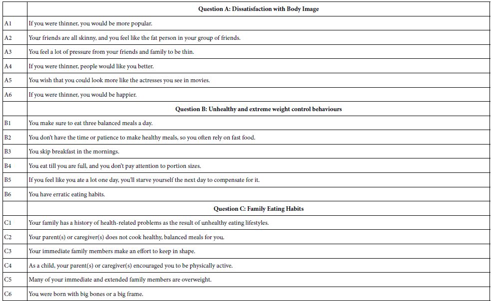
  3. Smolak L (2012) Appearance in childhood and adolescence. The Oxford handbook of the psychology of appearance 123-141.
  4. Duarte C, Gilbert P, Stalker C, Catarino F, Basran, J, et al. (2021) Effect of adding a compassion-focused intervention on emotion, eating and weight outcomes in a commercial weight management programme. Journal of health psychology 26: 1700-1715. [crossref]
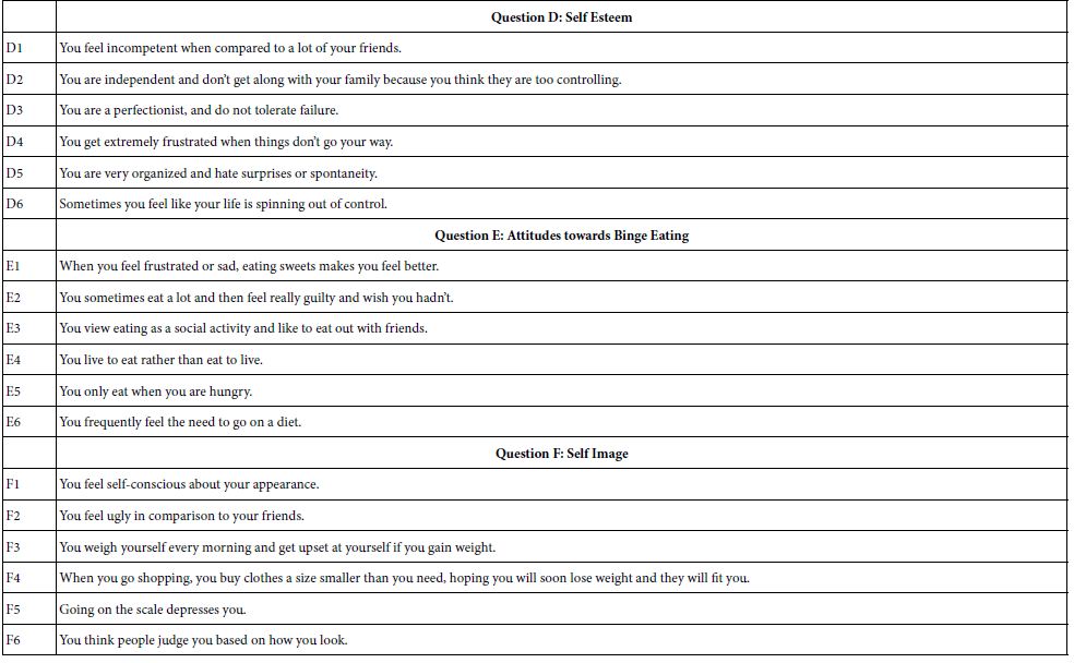
  5. Helms SW, Christon LM, Dellon EP, Prinstein MJ (2017) Patient and provider perspectives on communication about body image with adolescents and young adults with cystic fibrosis. Journal of Paediatric Psychology 42: 1040-1050. [crossref]
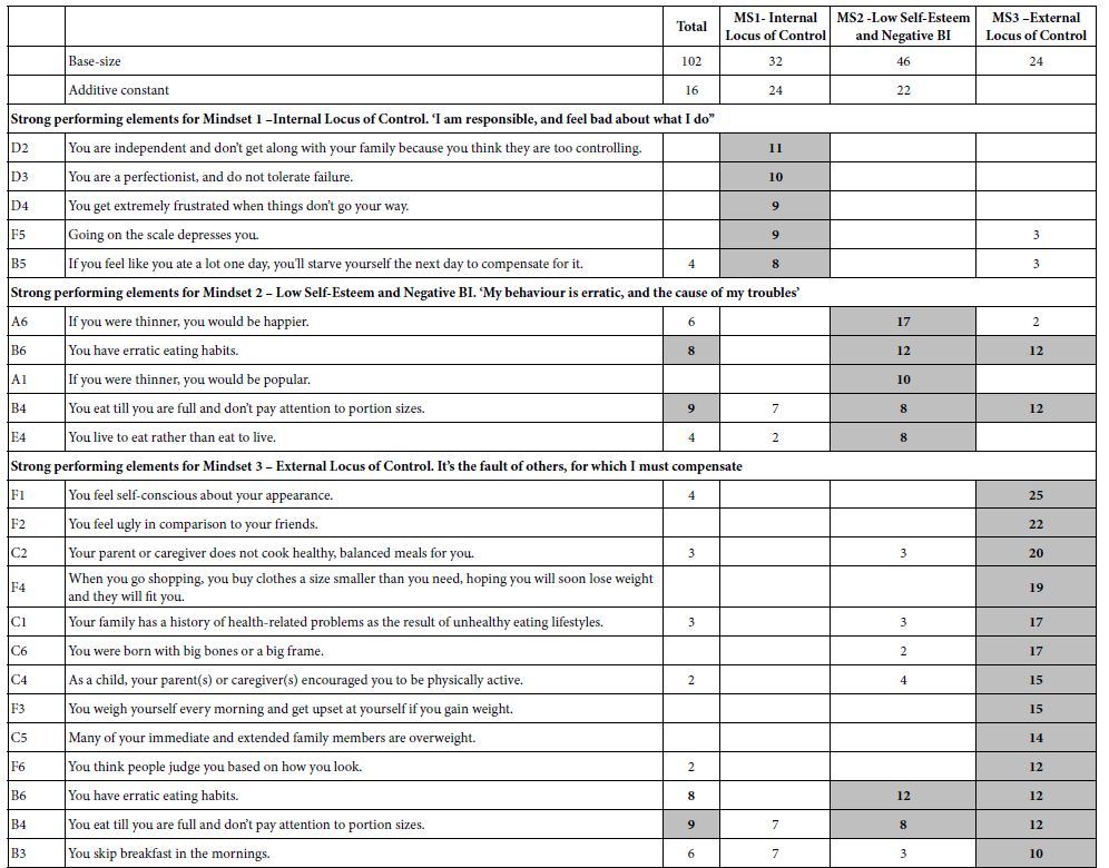
  6. Bodner ME, Bilheimer A, Gao X, Lyna P, Alexander SC, et al. (2017) Studying physician-adolescent patient communication in community-based practices: recruitment challenges and solutions. International Journal of Adolescent Medicine and Health 29. [crossref]
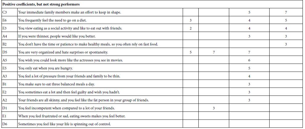
  7. Gabay G, Tarabeih M (2020) “A Bridge Over Troubled Water”: Nurses’ Leadership in Establishing Young Adults’ Trust Upon the Transition to Adult Renal-Care-A Dual-Perspective Qualitative Study. Journal of Pediatric Nursing 53: e41-e48. [crossref]
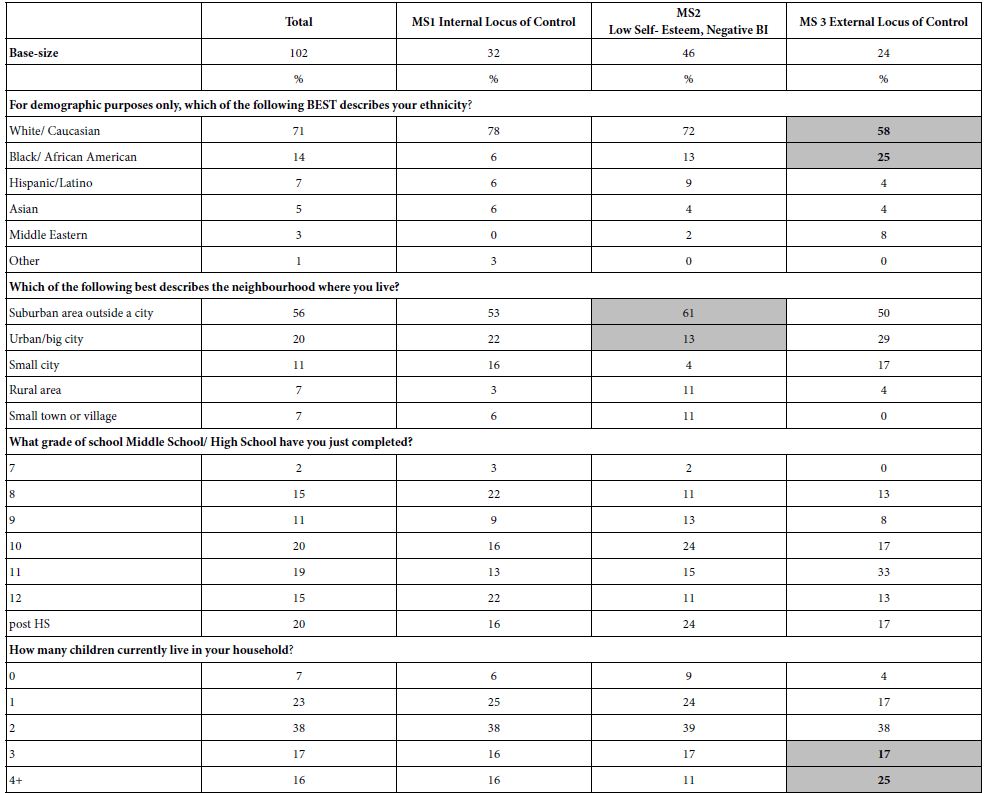
  8. Foti K, Lowry R (2010) Trends in perceived overweight status among overweight and non overweight adolescents. Archives of Pediatrics & Adolescent Medicine 164: 636-642. [crossref]
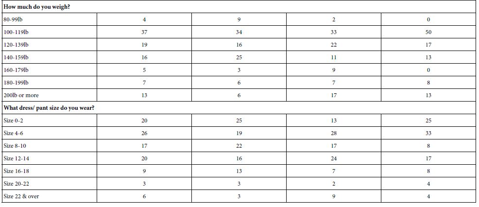
  9. Gabay G, Moskowitz H, Kochman M (2015) Market sensing, mind genomics and Health promotion. Business Expert Press 142-157.
  10. Gabay G, Moskowitz HR (2015) Mind genomics: what professional conduct enhances the emotional wellbeing of teens at the hospital? Journal of Psychological Abnormalities 4: 1000147.
  11. Gabay G, Ornoy H, Moskowitz H (2022) Patient-centered care in telemedicine–An experimental-design study. International Journal of Medical Informatics 159: 104672. [crossref]
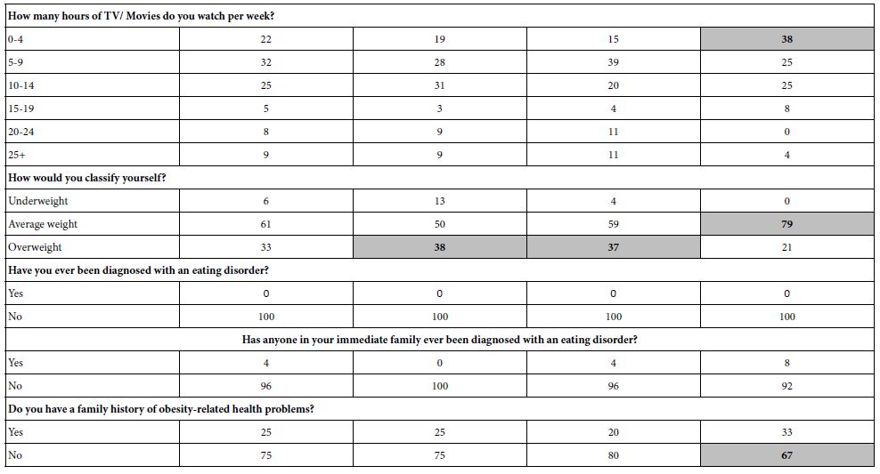
  12. Gunnard K, Krug I, Jiménez‐Murcia S, Penelo E, Granero R, et al. (2012) Relevance of social and self‐standards in eating disorders. European Eating Disorders Review 20: 271-278. [crossref]
  13. Bachar E, Gur E, Canetti L, Berry E, Stein D (2010) Selflessness and perfectionism as predictors of pathological eating attitudes and disorders: A longitudinal study. European Eating Disorders Review 18: 496-506. [crossref]
  14. Haines J, Kleinman KP, Rifas-Shiman SL, Field AE, Austin SB (2010) Examination of shared risk and protective factors for overweight and disordered eating among adolescents. Archives of Paediatrics & Adolescent Medicine 164: 336-343. [crossref]
  15. Pingitore R, Spring B, Garfieldt D (1997) Gender differences in body satisfaction. Obesity Research 5: 402-409. [crossref]
  16. Neumark-Sztainer D, Wall MM, Larson N, Story M, Fulkerson JA, et al. (2012) Secular trends in weight status and weight-related attitudes and behaviors in adolescents from 1999 to 2010. Preventive Medicine 54: 77-81. [crossref]
  17. Neumark-Sztainer D, Falkner N, Story M, Perry C, Hannan PJ, et al. (2002) Weight-teasing among adolescents: correlations with weight status and disordered eating behaviors. International Journal of Obesity 26: 123-131. [crossref]
  18. Gofman A, Moskowitz HR, Mets T (2010) Accelerating structured consumer‐driven package design. Journal of Consumer Marketing 27: 157-168.
  19. Moskowitz HR (2012) ‘Mind genomics’: The experimental, inductive science of the ordinary, and its application to aspects of food and feeding. Physiology & Behavior 107: 606-613. [crossref]
  20. Porretta S, Gere A, Radványi D, Moskowitz H (2019) Mind Genomics (Conjoint Analysis): The new concept research in the analysis of consumer behaviour and choice. Trends in Food Science & Technology 84: 29-33.
  21. Graybill FA, Iye HK (1994) Regression analysis: concepts and applications.
  22. Hastie T, Tibshirani R, Friedman J (2009) The elements of statistical learning: data mining, inference, and prediction. Springer series in statistics. Springer New York.
  23. Haxby JV, Gobbini MI, Furey ML, Ishai A, Schouten JL, et al. (2001) Distributed and overlapping representations of faces and objects in ventral temporal cortex. Science 293: 2425-2430. [crossref]
  24. Cattin P, Wittink DR (1982) Commercial use of conjoint analysis: A survey. Journal of Marketing 46: 44-53.
  25. Gabay G (2015) Perceived control over health, communication and patient–physician trust. Patient Education and Counselling 98: 1550-1557. [crossref]
  26. Chen G, He J, Zhang B, Fan X (2022) Body weight and body dissatisfaction among Chinese adolescents: Mediating and moderating roles of weight-related teasing. Current Psychology 41: 298-306.
  27. Zhou Y, Acevedo Callejas ML, Li Y, MacGeorge EL (2021) What Does Patient-Centred Communication Look Like? Linguistic Markers of Provider Compassionate Care and Shared Decision-Making and Their Impacts on Patient Outcomes. Health Communication 1-11. [crossref]
  28. Gorman JR, Drizin JH, Smith E, Flores-Sanchez Y, Harvey SM (2021) Patient-centered communication to address young adult breast cancer survivors’ reproductive and sexual health concerns. Health Communication 36: 1743-1758. [crossref]
  29. Volkmann NM, de Castro TG (2021) Body dissatisfaction, rumination and attentional disengagement toward computer-generated bodies. Current Psychology 1-9.
  30. Khan SS, Tarrant M, Weston D, Shah P, Farrow C (2018) Can raising awareness about the psychological causes of obesity reduce obesity stigma? Health Communication 33: 585-592. [crossref]
  31. Gabay G (2016) Exploring perceived control and self-rated health in re-admissions among younger adults: A retrospective study. Patient Education and Counselling 99: 800-806. [crossref]
  32. Zuair AA, Sopory P (2022) Effects of media health literacy school-based interventions on adolescents’ body image concerns, eating concerns, and thin-internalization attitudes: A systematic review and meta-analysis. Health Communication 37: 20-28. [crossref]
  33. Gustafsson A, Herrmann A, Huber F (2007) 1 Conjoint Analysis as an Instrument of Market. Conjoint Measurement: Methods and Applications, 1.
  34. Swedlund MP, Schumacher JB, Young HN, Cox ED (2012) Effect of communication style and physician–family relationships on satisfaction with pediatric chronic disease care. Health Communication 27: 498-505. [crossref]
  35. Aboueid S, Ahmed R, Jasinska M, Pouliot C, Hermosura BJ, et al. (2022) Weight Communication: How Do Health Professionals Communicate about Weight with Their Patients in Primary Care Settings? Health Communication 37: 561-567. [crossref]
  36. Hua J, Howell JL, Sweeny K, Andrews SE (2021) Outcomes of physicians’ communication goals during patient interactions. Health Communication 36: 847-855. [crossref]

Empowering Young Researchers to Think Critically: Exploring Reactions to the ‘Inspirational Charge to the Newly-Minted Physician’

DOI: 10.31038/PSYJ.2023521

Abstract

The study is part of a program set up to encourage young researchers (age < 18) to learn to think critically. The process shows the young researcher how to systematize aspects of daily life, create a database of specifics, and then explore the perception of these aspects by real people, using templated experimental designs and real ‘experiments’ on the web through a purpose-built application (www.BimiLeap.com). In this study respondents evaluated unique sets of 24 combinations (vignettes), each vignette presenting 2-4 statements which might have come from a ‘charge’ given to medical students and new doctors. Deconstruction of the response to these combinations at the level of individual respondents using regression analysis revealed which statements were perceived to be ‘important,’ which were perceived to be ‘memorable, which were both, etc. Cluster analysis of the individual coefficients from respondents revealed three mind-sets emerging, based upon the pattern of messages perceived to be important: MS1 – Dealing with the stress of the practice of medicine, MS2 – Dealing with difficult patients, MS3 – Aware of what is important to the patient.

Introduction

Empowering through Templated Experimental Design

This paper deals with the way a young researcher (Cledwin Mendoza) conceives of the way a medical school might inspire its students or give a ‘charge’ to a new doctor [1-4]. The topic of inspirational addresses given by senior professionals to newly-minted-professionals is of interest to middle school and high school students. It is their introduction to the world, a world about which they are curious, and excited to enter. The literature has publications on exhortations to the doctor, but virtually nothing from the vantage point of young people to whom the world of professionalism is both experienced but at the same time shrouded in mystery, the world of adulthood.

In this series of papers entitled ‘Empowering young researchers,’ we aim to look at the world of the everyday through the lens of the young researcher, in this case a junior high school student who is aware of the world, interested in the world, but whose sole experience is personal interactions with doctors, what he reads, and what he might see in the media. The research in this paper was designed and carried out using a new science, Mind Genomics. The objective of the research was to explore how ordinary people think medical students would react to inspirational and descriptive phrases regarding their teachings and ethical issues. The study is reported in the spirit of Mind Genomics, specifically a study of an everyday experience (the lecture or charge to a medical student), with the objective of learning what might be the inspiring messages and what might be the messages heard but soon forgotten.

Today’s computer technology allows people to do complex clerical tasks, often quite simply, by following a template. The template ensures that the person does the correct actions for each task, checks that the material is ready, and moves forward. As a consequence, the template ensures that the process will not run into a problem, at least in terms of the structure of the activity. Furthermore, what could be a complex, involved task might well become easy as the person filling out the template becomes conversant with the different steps. What could have been a boring, repetitive task may remain boring, but can be executed flawlessly over time. And, most of all, the learning to complete the template in general is fairly quick, although the material fitting into the template may itself be difficult.

Imagination about the Everyday

The history of science will show the increasing sophistication of the questions asked. From Aristotle who could only observe the world around and make conjectures, we move along to the world of experiments, where the notion was to understand how one variable ‘covaried’ with another variable, but more important, how one variable drove the other variable, viz., causation. As one readily recognizes today, the best experiments occur when the researcher is trying to understand how ‘nature’ works, searching doggedly in many cases for the rules of nature. At the same time there is the world of social science, the study of people, their social structures, motives, behaviors and so forth. Philosophers since Plato and Aristotle, and presumably many before them, were interested in why people behave the way they do. One never, however, feels that one can create a massive database about the many different aspects of people, at least in the social sciences.

Test Stimuli: Collaboration between the Researcher and AI (Idea Coach)

Mind Genomics works by creating a ‘bank’ of ideas (elements), presenting combinations of these elements to a respondent, having the respondent read and rate each combination on a fixed Likert scale, and then deconstructing the ratings to discover the contribution of each element. The process is mechanical once the elements are created. It is the creation of the elements which often stymies the researcher, leading to the abandonment of the project, or leading to an untenable delay in the project until ‘everything is just right’, everyone agrees with the choice of elements, etc. In the end, the task of creating the elements simply frightens many researchers, regardless of their experience or seniority.

The Mind Genomics template requires that the researcher select four questions which ‘tell a story’. For each question, the researcher is required to provide four answers. In the end, the raw material comprises the underlying story, knitting tighter the four specific questions, and the sixteen answers. Experience over three decades, since the early 1990’s, suggests that it is at this point in the process when many promising projects are simply abandoned by hopeful but frustrated researchers. The reasons for abandoning the project are not relevant, other than to say that there seems be a lowered tolerance for frustration in today’s researcher, and a belief that one should ‘know’ the answer, and select the ‘correct’ elements. Not being sure of ‘correct elements’ suffices to stop forward progress. Many researchers apparently suffer from “open-ended question anxiety.”

To remedy the problem, the Mind Genomics templated recently has been upgraded to incorporate Idea Coach, a user-friend tool based in OpenAI [5]. In the templated process, the researcher begins by providing the four questions. The researcher who would like ‘guidance’ chooses the Idea Coach button on the template form. The researcher then writes in a few sentences about the topic. Using that information, Idea Coach returns with up to 30 questions, from which the researcher can choose up to four. In the case where the questions do not all meet the researcher’s expectation, the researcher choose some, and repeats the Idea Coach effort, either with the same input (leading to a set of 30 questions, many of which are new), or with different input. The researcher ends up selecting four questions, some from AI, perhaps some from oneself, and can edit/polish before proceeding.

Table 1 shows the four questions. The Idea Coach was given the following background to the project:

Table 1: The four questions and the four answers (elements) for each question

tab 1

We created this study to see what important precautions young doctors need to face in the medical world. Also to help young doctors so they don’t make a serious mistake.

It is important to keep in mind that the formulation of the question comes from the mind of a young person, a middle-school student. The question is simple, direct, and not formulated in the typical manner that has become the pattern of today’s science. The question is one ‘about the world,’ in the naïve yet profound way that could only be asked by a young person. As the data will show, this type of questioning can lead to profound, powerful, and actionable results, as well as be a part of an easy-to-construct corpus of knowledge about the mind of people facing everyday life.

The quality of the questions shown in Table 1 come from the nature of the Open AI. The researcher’s task is made much easier. The task now morphs from trying to think about good questions to reading questions and selecting those which make sense for one’s project.

After the AI and researcher have collaborated to create/select the four questions, the BimiLeap templated system moves to acquiring four answers to each question. Once again the Idea Coach helps in this task, but requires the deeper involvement of the researcher. For the case of questions, Idea Coach required questions needing very little editing. Not so with the answers. Idea Coach returns with statements. These statements comprise the answers but the statements must be edited. For example, consider element A1. Idea Coach returned with the second part of the element, specifically ‘They need to have a passion for helping people and a strong interest in science and medicine.’ The BimiLeap program for Mind Genomics would be better when the sentence is given an ‘orientation’, such as the word ‘Required’. The authors changed the elements, inserting the orientation word(s), so that the elements were more meaningful. A good analogy to this is the placement of items in a menu under the proper headings (appetizer, main course, etc.,) rather than just having the food on the menu.

The second thing to note about the elements is that they are long, and well-crafted. Virtually all users of the BimiLeap program have commented on the fact that the questions, but more importantly the answers, move beyond what they might have generated had they been instructed to think about the elements, and do research to find elements. This up-front work, possibly taking hours and days, and often leading to frustration in the wake of progress seemingly out of one’s grasp, now takes approximately 20 to 30 minutes, with potentially far better results.

The final thing to note is that hitherto a long, arduous, and often frustrating effort to create questions literally from one’s mind is now replaced by a far more pleasant, intriguing learning experience. The researcher no longer has to feel alone in the effort to come up with questions and answers, but rather now engages in a focused experience of discovering and choosing. In some respects the creation of the elements evolves into its own learning experience, enjoyed by the researcher, with a motivating power to drive exploration of just-learned ideas. What was a difficult moment in the design of a Mind Genomics experiment now becomes perhaps the first learning experience. The Idea Coach, and AI, moves away from a simple aide to become a teacher who reveals new dimensions of a topic to a researcher deeply focused on the topic. Ideas that were not even in the ken of the researcher can now be explored in moments, as part of the research effort.

The History of Mind Genomics

Mind Genomics traces its history to three disciplines, psychophysics, statistics, and consumer research, respectively. Psychophysics is the oldest branch of experimental psychology, seeking to understand how to measure the internal perception of physical stimuli, such as the sweetness of sugar in a beverage. The origination of Mind Genomics can be traced to author Moskowitz’s studies as a graduate student in the Laboratory of Psychophysics in William James Hall, Harvard University, directed by the late Harvard professor, S.S. Stevens. During the latter part of Moskowitz’s tenure at Harvard, with a Ph.D. awarded for studies of taste mixture, it became obvious that the approach could be used to mix ideas, and obtain a measure of the mind in terms of responses to these ideas. The effort would have to wait until Moskowitz was safely ensconced as a scientist at the US Army Natick Laboratories, in Natick MA, where he could begin small scale studies of mixtures of ideas. The taste work would lead to the appreciation of human response mixtures as the relevant topic to explore, whether mixtures of ingredients, or mixtures of ideas [6,7].

Statistics, the second discipline, provides Mind Genomics with analytic tools. The history of science is often presented in terms of the researcher isolating all forms of extraneous noise, viz. unwanted variability, in order to study a phenomenon. We need only visit laboratories to see the apparatus used for these studies to get a sense of how proud the researcher is of the ability to study a phenomenon in ‘splendid isolation;, without the interfering noise. On the other hand, there are many effects where many variables interact with each other, and in the end produce a response. The traditional methods of isolating the variable and then studying the behavior of that variable simply cannot work. Rather, it is a matter of creating specific combinations, allowing the variables to interact, but at the same time allowing the researcher to measure the behavior of each variable, even though the variables are in a mixture. It is this discipline, statistics, specifically the area of experimental design, which constitutes the second foundation of Mind Genomics [8].

The third foundation of Mind Genomics is the world of consumer research, where the focus in on the complex, real-world stimulus, rather than on the artificially created world of the experimental psychologist. The consumer researcher focuses on what consumers are exposed to, how they react to situations which occur in everyday life. Consumer researchers are not attempting to understand the deep fundamentals of thinking and behaving, but rather interested in behavior in natural settings, dealing with responses to real test stimuli, or at least test stimuli which could be real.

The Test Stimuli

The foregoing history of Mind Genomics serves as an introduction to the nature of the test stimuli. The stimuli comprise combinations of elements, rather than single elements. The rationale is that only with combinations of elements can the test stimuli make sense, have ‘ecological validity.’ When we isolate the test elements, the 16 phrases shown in Table 1, instructing the respondent to rate each element, one at a time, we end up presenting the respondent with stimuli that are almost meaningless. Of course we are interested in the performance of each element, but it is very hard for the respondent to rate each element. It may be that the respondent and rate each element with the same mental rules, but more likely the respondent will end up shifting the mental criterion for the rating. That shift may be hard to imagine for these data, but easy to understand when we turn to elements which comprise brand name, price, nature of the product features, and location where the product is bought. When the rating sale is ‘interest in buying’, the respondent has a hard time using the same criterion. The data may look correct, but the reality is that during the course of evaluating the different types of elements the respondent may have shifted the criterion many time to be appropriate for the element.

To solve the foregoing problem, viz., of presenting ideas as simulating something real, Mind Genomics uses the power of experimental design to create combinations of elements. The experimental design for the 4×4 structure (four questions, four answers for each) comes up with 24 combinations. Within those 24 combinations, each of the 16 elements appears exactly five times, and is absent 19 times. A single vignette can have two, three, or four elements, but no more than one element from any question. The structure is set up so that the data from a single respondent can be analyzed by OLS (ordinary least squares regression), which as shown below, will reveal the individual level combination of every element to the response. Finally, the Mind Genomics design is set up so that each respondent sees different combinations. No respondents see the same combinations until the number of respondents exceeds 250. This property of different sets of 24 combinations created by the same mathematical scheme is called a permuted design structure.

The Orientation and Rating Scale

Mind Genomics studies are typically conducted with populations of respondents who are unfamiliar with the topic. They know that they will be reading and evaluating different combinations of messages, but have no idea that the combinations, also known as vignettes, will be created by experimental design. The respondent generally follows the instructions, doing what they are told. Thus, the simplest way to do the Mind Genomics experiment is to tell the respondent a little about the topic, viz., a sparse background, and then instruct the respondent to read the vignette and assign a rating using a defined rating scale.

Table 2 shows the instructions and the rating scale. The instructions are very simple. A principle of Mind Genomics is that it is more productive to provide a sparse orientation and let the individual elements in the vignette provide the necessary information about the topic. We follow this practice in our studies. Simplicity makes the task easy for a younger researcher because there needs to be very little deep knowledge behind the question.

Table 2: The orientation paragraph and the associated rating scale

tab 2

The rating scale in Table 2 merits more discussion. The rating scale actually encompasses two scales, one for important, and the other for remembering. Each point on the five point scale corresponds to one possible combination of thinking something is important and remembering the speech. Another thing to observe is that ‘remembering’ is first, and ‘important’ is second. In this way the scale is ‘broken up’ forcing the respondent to read the scale, rather than just remember a place on the scale, or at least that is the intention.

In order to prepare the data for analysis, it was first necessary to transform the scale. Users of data find it very hard to look at either the mean on the scale (which is meaningless for our broken up scale), or the distribution of ratings on the five-point scale. A simpler way to do things is to transform the scale values to binary (0 or 100). For simplicity, we abbreviate the word “Rating,” with “R” and the rating number. For example, “Rating 1” is abbreviated “R1,” etc. This study features two sets of transformations, one dealing with importance, and the other dealing with memorability.

1a. Important and Remembered (R5 only transformed to 100, rest of ratings transformed to 0)

1b. Not Important (viz., Not Necessary) and Not Remembered (R1 only transformed to 100, rest of ratings transformed to 0)

2a. Important (R5, R4 only transformed to 100, rest of ratings transformed to 0)

2b. Remembered (R5, R2 only transformed to 100, rest of ratings transformed to 0)

2c. Not Important (viz., Not Necessary) (R1, R2 only transformed to 100, rest of ratings transformed to 0)

2d. Not Remembered (R1, R4 only transformed to 100, rest of ratings transformed to 0)

With this transformation it becomes easier to discover patterns. The combination of rating scale points into those denoting ‘important’ vs. ‘not important’ allow us to isolate specific elements driving the perception of importance. Similarly, the combination of rating scale points into those denoting ‘remembered’ vs. ‘not remembered’ allow us the same power to isolate specific elements that the respondents feel will be ‘remembered’ by the medical students or young doctors. Keep in mind, however, that this experiment is done among the population of young people, ages 19-40. The same experiment could be done easily among medical students to discover whether they feel the same way.

Analysis 1

Do Different, Identifiable Groups of Respondent Score the Vignettes the Same Way?

In the foregoing introduction to Mind Genomics we made the point that each respondent in the study evaluated a unique set of 24 vignettes. This means that when we look at the distribution of ratings, we must keep in mind that we are not looking at the different groups of people evaluating the same stimuli, but rather evaluating different stimuli of the same type.

At this point it is worth pointing out that stopping here, just looking at the pattern of responses without any deeper analysis, would not be wrong. Indeed, the researcher who stops here, and supports her or his conclusions of similar patterns with conventional statistics, e.g., tests of statistical difference, would be lauded for defending the conclusion of ‘similar patterns’ using well-accepted statistics. Yet, as we will see below, when we move to the development of ‘mind-sets’, the researcher will be afforded the far deeper opportunity to understand the topic, one provided by the up-front efforts to create the test vignettes using experimental design.

Table 3 shows the average ratings for the six newly created dependent variables, for the key subgroups. Table 3 suggests similar patterns of response. Were we to stop here, we would not know anything beyond the observation that the patterns of transformed ratings seems to be similar across the different groups. As the subsequent analyses will reveal, our observation might seem correct on the surface, but is wrong. We would not, however, realize that there are deeper patterns, some of which are radically different from each other.

The groups shown in Table 3 are:

  1. Total
  2. Gender (male, female)
  3. Age (18-29 years old, 30-40 years old)
  4. Vignettes rated rapidly (response time < = 3 seconds) vs. rated slowly (response time > 3 seconds)
  5. Mind-Set emerging from clustering (Mind Set 1 of 3 Dealing with the stress of the practice of medicine; M2 of 3 Dealing with difficult patients; MS 3 of 3 Aware of what is important to the patient).

Table 3: Averages of six newly created transformed variables, by total panel and by key subgroups. The averages are computed based upon the original rating assigned to each of the vignettes seen by a member of the subgroup. The numbers can be treated like percentages.

tab 3

Building Models (Equations) Relating the Elements to the Newly Created Transformed Variables

We now move to the heart of Mind Genomics, creating equations which show how each of the 16 elements contributes to the newly created variables. Our analysis will focus on five of the six variables, as we see at the top of Table 4. We will look at the transformed variables corresponding to the highest level of performance (important and remembered), the transformed variables corresponding to ‘important’, the transformed variable corresponding to ‘remembered’, and then the complementary transformed variables of ‘not important’ and ‘not remembered’. The next set of tables will present the parameters of these five transformed variable for each identifiable subgroup previously presented in Table 3. The results will reveal a deeper, far more organized world, one emerging clearly due to the underlying experimental design.

Table 4: Values of the additive constant for five dependent variables (columns) and different groupings of respondents and vignettes, respectively

tab 4

The first step to build the equation is to create the database. The database can be thought of as a rectangular file, one row for each vignette. Recall that each respondent evaluated 24 vignettes, so this database comprises 24 rows for each respondent.

The columns of this database contain the relevant information:

Column 1 – The unique identification number for the respondent. It is sufficient to label the respondents with a sequential set of numbers, starting with 1, and continuing. The study comprises the data from 102 respondents.

Column 2 – Gender

Column 3 – Age

Up to now the data for a specific respondent has been repeated 24 times. We now turn to the data for a specific vignette.

Columns 4-19 correspond to the 16 elements, with each element having its own column. For example, column 4 is reserved for element A1, column 5 or element A2, and so forth. For a single row, each cell (4-19) will be given the value ‘0’ when the element is absent from that particular vignette, or given the value ‘1’ when the element is present in that particular vignette. Since the experimental design prescribe that each vignette will have 2-4 elements, and not more than one element from a question, the database will reflect the design by having the number ‘1’ in two, three, or four columns, and the number ‘0’ in the remaining columns. The rationale for this specific coding, so-called ‘dummy variable coding’ [9], is that the coding enables the regression program to estimate the contribution of each element when the element goes from ‘state =0’ to ‘state = 1’, viz., present.

Column 20 shows the order of presentation of the vignette for a respondent, with the value going from 1 (first vignette) to 24 (last vignette).

Column 21 shows the response time, defined as the number of seconds elapsing between the presentation of the vignette to the respondent and the response. The response time is measured to the nearest tenth of a second. The response time is an important measure in the world of consumer researcher, insofar as it may indicate the presence of different cognitive processes [10,11].

Column 22 shows the rating assigned to the specific vignette by the specific respondent.

Up to now, columns 1-22 were generated by the BimiLeap program, along with data acquired during the course of the experiment. The data can be used for analysis ‘as is’, but consumer researchers prefer to transform the data so that they can investigate different types of answers. There are five specific transformations of interest, focusing on five different aspects of the decision. Each one creates a new dependent variable that will be analyzed in depth.

  1. R5: ‘important’ and ‘memorable’. Ratings of ‘5’ are converted to 100. Ratings 1-4 are converted to 0.
  2. R54: ‘important’. Ratings ‘5’ and ‘4’ are converted to 100. Ratings 1-3 are converted to 0.
  3. R52: ‘memorable’. Ratings ‘5’ and ‘2’ are converted to 100. Ratings 1,3, and 4 are converted to 0.
  4. R12: ‘not important’. Ratings ‘1’ and ‘2’ are converted to 100. Ratings 3,4 and 5 are converted to 0.
  5. R14: ‘not memorable.’ Ratings ‘1’ and ‘4’ are converted to 100. Ratings 2,3 and 5 are converted to 0
  6. To prepare for the analysis by OLS (ordinary least-squares) regression the BimiLeap program adds a vanishingly small random number (<10-5) to each transformed value. The random number does not affect the coefficients of the regression equation, but ensures that the dependent variable will possess some minimal variation across the vignettes for each individual respondent. This variability is necessary for the statistical calculations.
  7. The equation or model is expressed by the simple formula: DV (dependent variable) = k0 + k1(A1) + k2(A2) … k16(D4)
  8. After the parameters of the OLS model for importance (R54) are calculated for each respondent and stored in a second database, that second database to be subsequently used by a clustering program. The clustering program [12], uses the 16 coefficients (k1-k16) as inputs to identify groups of respondents showing similar patterns of 16 coefficients The clustering program assigns each respondent to one of two clusters, based upon similar patterns, and then assigns each respondent to one of three clusters, again based upon similar patterns. The output is the assignment of each respondent to one of two ‘mind-sets’ or one of ‘three mind-sets.’ The assignment is done using strict mathematical criteria. However, the names assigned to the mind-sets or clusters are based upon the elements which are the strongest performers. This criterion is known as ‘interpretability.’
  9. Clustering generates groups of two and three mind-sets, with the name of each mind-set chosen based on the strongest performing elements in the mind-set, viz., the elements with the highest positive coefficients. Taking the three mind-set-solution as an example, Mind Set 1 of 3 is Dealing with the stress of the practice of medicine, Mind Set 2 of 3 is Dealing with difficult patients, and Mind Set 3 of 3 is Aware of what is important to the patient.

    1. Each respondent belongs to several different groups. The first group is Total Panel, viz., everyone. The second grouping divides into the respondent being a male or a female. The third grouping divides into the respondent into younger (ages 19-29) or older (ages 30-40). The fourth grouping divides the respondents by the mind-set to which they belong.
      1. Up to now, the vignettes were assigned to groups based upon the characteristic of the respondent, viz., a gender. We can also look at the vignettes, rather than at respondents to create groups. The fifth groups divides the vignettes by those that were evaluated quickly (operationally defined as response time, <= 3 seconds) versus those that were evaluated slowly (operationally defined as response time > 3 seconds). We can also look at the data focusing our attention on the speed of the response to the particular vignette.

      Steps 1-7 above create a database that is readily analyzed by standard regression methods. The approach here is OLS (ordinary least squares) regression. We begin with the additive constant, k0, shown above as part of Step 6. To review, the equation in Step 6 has 16 coefficients (k1-k16) and the additive constant. The additive constant is a ‘baseline’, defined as the expected transformed value were the vignettes to comprise no elements at all. The underlying experimental design ensures that all vignettes will comprise at lest two elements and at most four elements. The additive constant has no physical meaning other than as an adjustment factors. We can use the additive constant as a ‘baseline’, giving us a sense of the likely percent of responses to be obtained for a given dependent variable (e.g., R54), in the absence of elements.

      6. Table 4 shows the additive constant for each of the groups (rows), and for each of the five dependent variables (columns). For each group and for each dependent variable the additive constants have been shaded for those groups showing an 11 point or higher magnitude of difference between any two members of the group. The large magnitudes of differences in a group are most striking for the three mind-sets, viz., those groups create on the basis of different patterns of coefficients.

      We now turn to the important elements for the five transformed dependent variables, showing only those elements which generate a coefficient of +5 or higher. The standard error for Mind Genomics coefficients varies from 4-6 for most studies with a base size of 100. Furthermore, when elements with coefficients of 4-5 or higher are separately investigated, they often turn out to be relevant to the topic. Consequently, and in the interest of Mind Genomics studies as being early-stage explorations, the cut-off level is set to about 4-5. In this project the cut-off level was set at 5, to follow the conventional practice. In addition, the very strong performing elements are shown in shaded cells, specifically those elements with coefficients of +10 or higher. Finally, each table presents three sets of elements, each set sorted in descending order of coefficient value. The first portion of the table presents the results for relevant elements (coefficient = 5+) for the total panel, gender and age. The second portion of the table presents the results for relevant elements for the three mind-sets. Finally, the third portion of the table presents the results for relevant elements for vignette-based groups (response time, order of testing).

      Mind Genomics generates a great deal of data, much of which can be analyzed in depth for the simple reason that the elements themselves are ‘cognitively meaningful.’ That meaningfulness leads to the ability to discern general patterns, but then to evaluate the nuances of each element.

      7. If we were to summarize the results from the data in Tables 5-9 we would emerge with the conclusion that the strong results emerge from the mind-set, rather than from the self-profiled demographics of the respondents (viz., age and gender), and rather than from the non-cognitive nature of the stimulus (viz., speed of responses, order of testing (first half vs. second half)).

      Table 5: Strong performing elements (high coefficients) for ‘important and memorable, R5’

      tab 5

      Table 6: Strong performing elements (high coefficients) for ‘important (R54)

      tab 6

      Table 7: Strong performing elements (high coefficients) for ‘memorable’ (R52)

      tab 7

      Table 8: Strong performing elements (high coefficients) for ‘not important’ (R12)

      tab 8

      Table 9: Strong performing elements (high coefficients) for ‘not memorable’ (R14)

      tab 9

      Discussion and Conclusions

      Traditionally, the combination of young students and ‘science’ has been to repeat experiments that have been previously performed, experiments whose answers are known. The student’s task is to replicate the experiment in the proper manner, obtain the results, and present the process to the teacher. Success in such a case emerges from the combination of executing the study properly and getting the ‘right answer’. The approach has worked for decades, as generations of students went through the process, some emerging with the feeling that ‘science’ is for them, whereas others emerging with the feeling that this process is not at all for them. A century and more of scientific progress, and the emergence of the modern world with all its technology and ‘know-how’ testifies to the success of the traditional process to learn science.

      The world has changed. One can scarcely spend a day reading newspapers or now more frequently looking at the material flooding forth from the web, to get a sense that the traditional methods of teaching and exciting students no longer work very well. Perhaps it is the ‘tyranny of the small screen’, a phrase author Moskowitz coined to describe the everyday scene of people, young and old, glued to their smartphones. Perhaps the phones are smart, but the people seem to be less smart, or less educated, if one is to believe the ongoing reports in both the academic press and in the popular press, respectively.

      In this emerging world, how then can students be excited? The approach presented in this paper constitutes one way of exciting students through becoming researchers. Happily, there is very systematized thinking about the problems of the everyday, the world where ordinary people live, the world in which they experience the aspects of the quotidian, the daily, the routine. What then could happen if this daily world, so accessible to people, so very ordinary, could be magically transformed into a topic for true scientific investigation, research which not only teaches the student how to think, but actually creates a unique, valuable, indeed absolutely vital corpus of knowledge about the world. After all, the study just reported here, done in just a few hours, from beginning to end, produces unique to the world, valuable information. Most of all, this valuable information comes from the minds of young students, the senior researcher aged 13 (Cledwin), and the junior researcher aged 8 (Ciara), respectively. Their efforts, their curiosity, exploring the topic, produces unique to the world information, the beginning of a large corpus of knowledge on communications to students in the world of medicine.

      There is much to do, more than a billion students around the world, many of them that could be considered the ‘raw material’ of our civilization. Right now the issue continues to be concern about their learning, that they are not learning properly, that their motivation is lagging, that their attention is increasingly on the small screen. Perhaps it is because they are not involved in learning, that learning has become the ceaseless repetition of facts to be ingested, converted to bits of memory, and regurgitated at the proper time, somewhat like the cow chewing its cud. Expressed that way, learning is for the very motivated, and perhaps those who cannot escape this onerous task. But, and this is the important point, what would happen if the students could participate in world-wide projects which create separate topic-specific databases about the everyday, using templated experimental design, and using artificial intelligence. The escape would be into education, not away from education into mindless gaming. One could only imagine a world where thousands of students could collaborate and even compete as they jointly build large scale databases about the minds of people in society regarding the different aspects of daily living. An example might be a large scale database about different aspects of teaching and learning mathematics, across 192 countries, across the entire range from say 3rd grade to end of college, focusing on the many dozens different aspects of teaching and learning mathematics. This effort alone, with 192 countries x 10 aspects of learning mathematics creates a unique, valuable database. One could only imagine the pride of participation and learning for students world-wide who volunteer to participate in this effort. And, to finish, the opportunities are unlimited. Truly in this case ‘the appetite comes with the eating.’

      References

      1. Baruch JM (2017) Doctors as makers. Academic Medicine 92: 40-44. [crossref]
      2. Kassirer JP (2000) Patients, physicians, and the internet: Coming generations of doctors are ready to embrace new technology, but few incentives now exist to encourage their older peers to do likewise. Health Affairs 19: 115-123.
      3. Murtagh GM, Furber L, Thomas AL (2013) Patient-initiated questions: How can doctors encourage them and improve the consultation process? A qualitative study. BMJ Open 3: p.e003112.
      4. Swennen MH, van der Heijden GJ, Boeije HR, van Rheenen N, Verheul FJ et al (2013) Doctors’ perceptions and use of evidence-based medicine: a systematic review and thematic synthesis of qualitative studies. Academic Medicine 88: 1384-1396. [crossref]
      5. OpenAI (2023)
      6. Moskowitz HR, Gofman A, Beckley J, Ashman H (2006) Founding a new science: Mind Genomics. Journal of Sensory Studies 21: 266-307.
      7. Porretta, S, Gere A, Radványi D, Moskowitz H (2019) Mind Genomics (Conjoint Analysis): The new concept research in the analysis of consumer behaviour and choice. Trends in Food Science & Technology 84: 29-33.
      8. Gofman A, Moskowitz H (2010) Isomorphic permuted experimental designs and their application in conjoint analysis. Journal of sensory studies 25: 127-145.
      9. Suits DB (1957) Use of dummy variables in regression equations. Journal of the American Statistical Association 52: 548-551.
      10. Lenzner T, Kaczmirek L, Lenzner A (2010) Cognitive burden of survey questions and response times: A psycholinguistic experiment. Applied cognitive psychology 24: 1003-1020.
      11. Revilla M, Ochoa C (2015) What are the links in a web survey among response time, quality, and auto- evaluation of the efforts done? Social Science Computer Review 33: 97-114.
      12. Likas A, Vlassis N, Verbeek JJ (2003) The global k-means clustering algorithm. Pattern Recognition 36: 451-461.