Author Archives: author

Empowering Young Researchers through Mind Genomics: What Will Third Grade Mathematics Look Like in 10 Years?

DOI: 10.31038/PSYJ.2023533

Abstract

Using a templated Mind Genomics program coupled with artificial intelligence, school age students created an experiment to assess what ordinary people think will be the situation of the 3rd grade mathematics class. Artificial intelligence (Idea Coach) enabled the researchers to create four questions about the nature of the mathematics class, and for each question to create four answers. A total of 110 respondents of varying ages each evaluated systematically created, unique combinations of the answers, with the process enabling the researcher to create individual level equations (models) for each respondent, one model for ‘agreement’ based on direct ratings, the second model for ‘engagement’ based on response time. Two clear mind-sets of people emerged; MS1 focusing on the predicted technical accoutrements of the 3rd grade math class, MS2 focusing on the predicted education process of the 3rd grade math class. The templated Mind Genomics approach opens up a new vista of opportunities for educating students how to think about problems, as well as letting the curiosity of students produce insights into their daily lives from topics that are relevant to them.

Introduction

One can scarcely read stories about education without getting a sense that the K-12 education in the United States may be deteriorating [1], and that one of the most severe issues is the decline in the mathematical performance of young people [2]. Educators struggle with how to remedy this situation [3,4], as many simply throw up their hands in frustration. Going in a different direction, the authors have pioneered the use of research to understand the social issues of today as seen by young people [5]. We are so accustomed to reading research designed by professionals about topics relevant to education and similar ‘worlds of the young’ that we fail to realize that we might well learn a great deal by having the young people act as researchers, rather than having fully developed professionals do the research. Of course, the immediate reaction might be that only a professional knows how to ask the right question, use the appropriate scale, and interpret the results. Young students might be observed and talked to but are not typically considered to be able to do independent research about a topic, or if they are, the research is couched in a simplistic style deemed appropriate for the not-quite-intellectually-developed student researcher.

In a previous set of studies, the authors have begun to work with school age students as researchers, with these researchers familiar with the process, and using a template which guides them. The process is called Mind Genomics, an emerging science of everyday life, a science which allows people to create everyday scenarios of what reality might be like, and have real people respond to these scenarios [5,6]. Mind Genomics began as a branch of mathematical psychology [7], but within a decade its ability to uncover how people respond to mixtures of ideas or features brought it to the attention of consumer researchers at The Wharton School of The University of Pennsylvania. The outcome was the migration of the esoteric field of ‘conjoint measurement – a basic form of fundamental measurement’ into the world of applications of everyday life [8].

The Mind Genomics process proceeds in a step-wise manner, using a templated program, along with an artificial intelligence ‘Idea Coach’. The process is arranged in a fashion which encourages the young researcher, teaching the topic, as well as well as allowing the researcher to do the empirical testing of the stimuli, and receive a report in real time, and a full analysis with 30 minutes after the end of the study.

We present the results of a study designed by the senior author, a third-grade student in a local public school in the Bronx, New York, USA. It is important to note that when young students are the researchers, following a templated approach but at the same time with new material, they are experiencing the specifics, the discipline, and intellectual excitement and the professional development of a science. Finally, as we proceed into the method, it is important to realize that the structured approach embedded in the Mind Genomics process ends up producing results worthy of publishing, with such results giving information both about how a young person thinks about the world, and about the strength of that thinking in the minds of older people.

The Mind Genomics process follows a series of steps, from design to analysis. Figure 1 shows the process in simple summary. The six screen shots show the process from naming the study (Panel A), choosing the four questions (Panel B), choosing four answers to a question (Panel C), creating a self-profiling questionnaire (Panel D), introducing the topic to the respondent (Panel E), and presenting the rating question and the rating scale (Panel F). It is important to keep in mind that these panels prevent the templated system for Mind Genomics, and were completed, without any help, by an eight-year third grade student, who had previous experience with setting up Mind Genomics studies on the BimiLep platform. No effort was made to edit the setup, reflected in the language used by the research for the introduction to the topic and the rating scale.

FIG 1

Figure 1: The template for the BimiLeap project set up

During the three plus decades of the evolution of Mind Genomics, a continuing block has been the inability of researchers to think in a critical manner, developing questions and answers. Often, with practice, the individual becomes facile in developing a ‘story’ from a set of questions. The answers to the questions are easy, but it is the story, the questions, which are difficult, and often lead the prospective research to abandon the effort.

The recent efforts in artificial intelligence have created the possibility to develop questions and answers. Artificial intelligence is embedded in a query system, Idea Coach, itself now an integral part of the BimiLeap platform. Figure 2 shows the use of Idea Coach to describe the topic in a special ‘box’ (Panel A), after which the Idea Coach returns with up to 30 questions shown in part in Panel B. Scrolling down would reveal the additional questions which Idea Coach generated. The process can be repeated, either with the same text shown Panel A for a number of new questions along with dome old questions, or with new text. Panel C and D show the same process. The researcher has already selected the four questions. When it comes time to create four answers to each question, the researcher can either provide her or his answers, or use Idea Coach to suggest 15 answers to the question. The researcher can select several and return for another 15 answers.

The importance of an Idea Coach for young researchers cannot be overstated. The Idea Coach does exactly what it says it does, namely coaches the student in the process. Observations with the young students as researchers reveals that they begin by relying on the Idea Coach, but at some point, they ‘get it’, and begin to combine Idea Coach with their own ideas, and then stop using Idea Coach for certain types of issues and questions.

FIG 2

Figure 2: The Idea Coach process to develop questions based on the description of a topic (Panels A and B), and to develop answers based upon a specific question (Panels C and D).

Explicating the Mind Genomics Process: Case History of Mathematics I the 3rd grade

The best way to understand the emerging science of Mind Genomics is through case histories, studies of topics that might well be disregarded as being overly simple, almost trivial. Yet properly designed and executed, the studies reveal both the mind of the researcher and the mind of the respondent who is testing the stimuli developed by the researcher. Our study of the future of mathematics in the third grade is just such as example. It tells us the topics of interest to a young researcher, herself in the 3rd grade, and the reactions of people to her ideas. The actual study can be found in www.BimiLeap.com. The study itself can be easily replicated or modified, quickly and inexpensively. We present the results from one such study, designed in December 2022, run with five respondents, that part taking about 90 minutes, and then the completion of the study in February 2023, that part taking about 30 minutes.

Step 1

Give the study a name. Figure 1, panel A, shows the first screenshot, instructing the respondent to choose a name, select a language for the respondent-facing screens, and then agree not to ask for personal information that could identify the respondent. For those cases when the respondent is to be identified, there is an open-ended question where the respondent can provide identifying information, but only at the discretion of the respondent.

Step 2: Create/Select four Questions

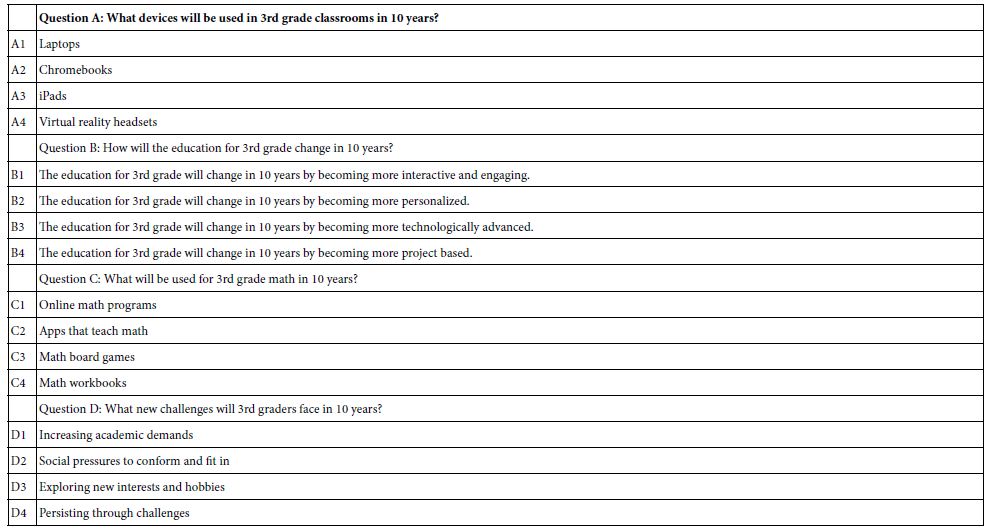
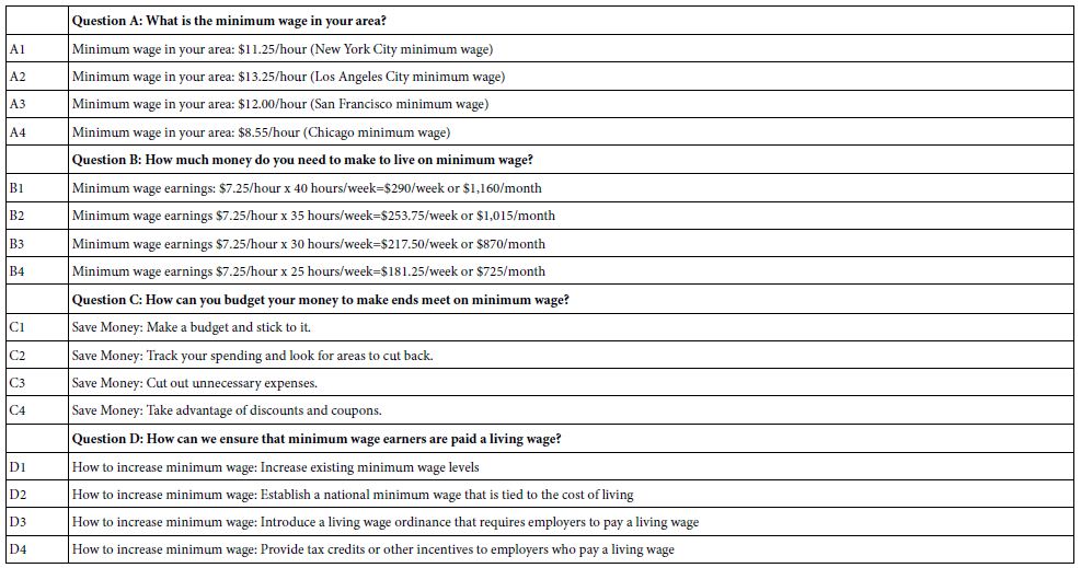
Figure 1, panel B, shows the next screenshot, instructing the researcher to provide questions which tell a story. At first, researchers reporting having a difficult time at first. It is at this stage that the researcher becomes nervous. Figure 2 screens A and B show the Idea Coach, which enables the researcher to type in a description of the study (Figure 2, Panel A, top). Idea Coach returns with up to 30 questions, and does so several times if desired. The researcher can use the same description or a different description each time in Figure 2, Panel A. Each time, whether the description is repeated is changed, Idea Coach will come back with a new set of 30 questions, some the same, many different. Figure 2, Panel B shows an example of the questions as returned from one run of the Idea Coach. Table 1 shows the four questions finally selected.

Table 1: The four questions and the four answers (elements) for each question. The questions and their answers were generated by the Idea Coach using artificial intelligence.

TAB 1

Step 3

Select/create four answers to each question. Creating answers to questions appears to be easier for researchers than creating questions, perhaps because of our education which stresses answering direct questions. Figure 1C shows the BimiLeap screen requesting four answers from question C: What will be used for 3rd grade math in 10 years? The researcher can either create four answers or use the Idea Coach to create answers that can be edited (see Figure 2C and 2D). The Idea Coach has been set up to use artificial intelligence to provide sets of 15 answers to each question. The Idea Coach can be interrogated several times to get a sense of the variety of answers available for the question. Thus the Idea Coach serves both as a facilitator of the research process, and as a way to help the researcher learn the topic by the traditional question/answer process, the Socratic method.

Step 4: Create a Set of Self-profiling Questions

The questions deal with WHO the respondent is (demographics), what the respondent DOES (behaviors), what the respondent BELIEVES (attitudes). The BimiLeap program is automatically set to ask for the respondent’s gender and age, leaving eight open questions, each with eight possible answers. Figure 1D shows the only classification question inserted by the researcher ‘Do you think the 3rd grade is going to change in 10 years?

Step 5: Create an Orientation Statement Which Introduces the Respondent to the Topic (Figure 1E)

The objective of Mind Genomics is to determine how the different elements or answers ‘drive’ the response. The standard strategy is to provide the respondents with as little up-front information as possible, indeed simply introducing the topic. For other uses, such as the law (REF), the respondent introduction might be far more detailed because of the necessity of ensuring that the background to the case is understood. That is not the issue for most research, however.

Step 6: Create a Rating Scale (Figure 1F)

The rating scale is typically a short category or Likert scale, as many as nine answers, but shorter scales as well, comprising seven or five scales. Other scales with other points can be used, but for the most part author HRM, with thirty years of experience, has found that shorter scales are easier for the respondent to use, and often can be labelled, as done here. Note once again that the labelling was done by the elementary school-age researcher, without any guidance. Thus the monotonicity of the scale is maintained, but the language is that of a third grade student.

Step 7: Instruct the Respondent to Answer an Open-ended Question

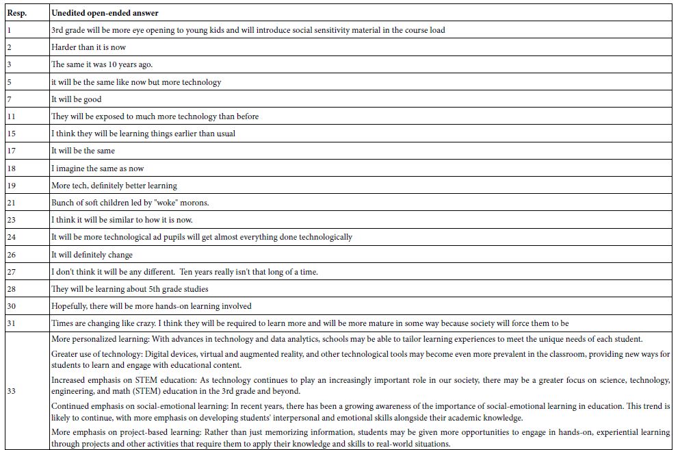
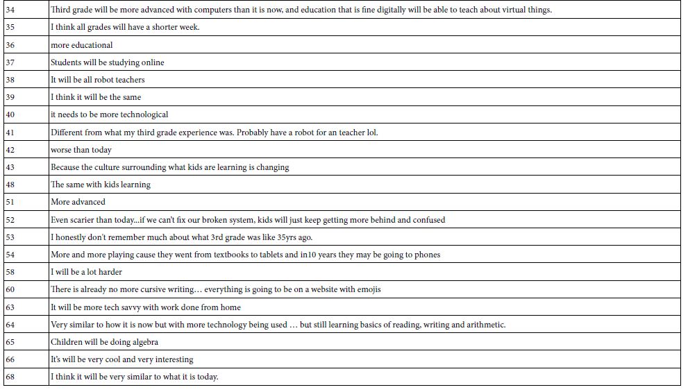
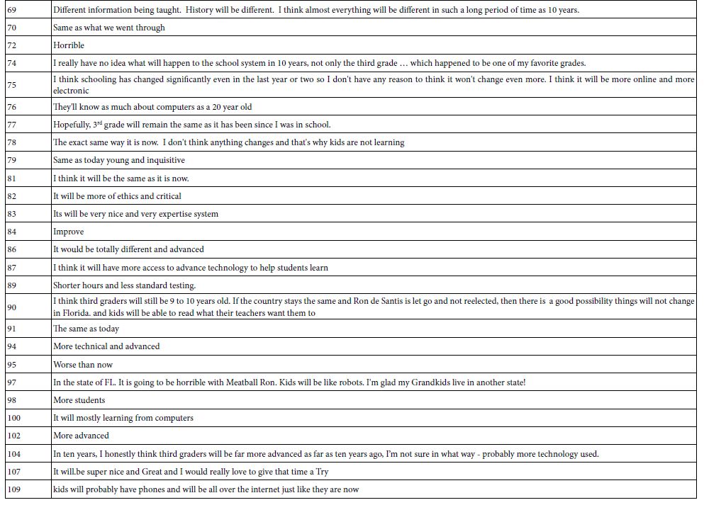
The open-ended question is ‘how will the 3rd grade be different in 10 years?’. The Appendix shows these answers.

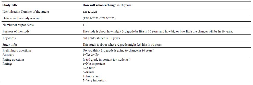
At this point, the study is set up. Table 2 shows the information for the study.

Table 2: Study information extracted from the set up

TAB 2

Step 8: Create 24 Unique Vignettes for Each Respondent, Using a Permutable Experimental Design

Mind Genomics works by presenting respondent with combinations of messages, so-called vignettes, comprising a minimum of two elements, and a maximum of four elements. Each question contributes at most one element (answer) to a vignette, but often contributes no element to the vignette. The composition of each vignette is dictated by an underlying experimental design, called a permutable design [9]. The design specifies the 24 combinations of elements, each element appearing exactly five times and absent 19 times. Each question contributes to 20 vignettes and does not contribute to four vignettes. Finally, the design is structured so that all 16 elements appear independently in a statistical sense, allowing the researcher (or, in our case, the BimiLeap program) to create an equation for each respondent, using statistical methods.

Each respondent evaluates a different set of 24 combinations, with a similar mathematical structure, but the composition of each of the vignettes for a respondent differs from the composition of each vignette, from every other respondent. In effect, the permutable design ends up with a similar, powerful design for each respondent, with the specific vignettes differing from one respondent. A good analogy is the MRI tool used in medicine, which takes pictures of the same tissue, the pictures from different angles. Each picture taken from a unique angle corresponds to a respondent. Eventually, one will be able to put the data together by regression to come up with a single coherent picture of the mind of the respondent.

Step 9: Execute the Study by Sending Out an Invitation to Respondents

The email invitation contains the link to the study. Figure 3 shows a screen shot of the page allowing the researcher to select the source of the respondent. Another set of screens allows the researcher to select the number of respondents, as well as the general qualifications of the respondents (country, gender, age, education, income, number of children). For more specific respondent qualifications the researcher has to go to a specialist panel provider.

FIG 3

Figure 3: Respondent ‘sourcing’ page

Step 10: Acquire the Rating and the Response Time and Create a Database for Analysis

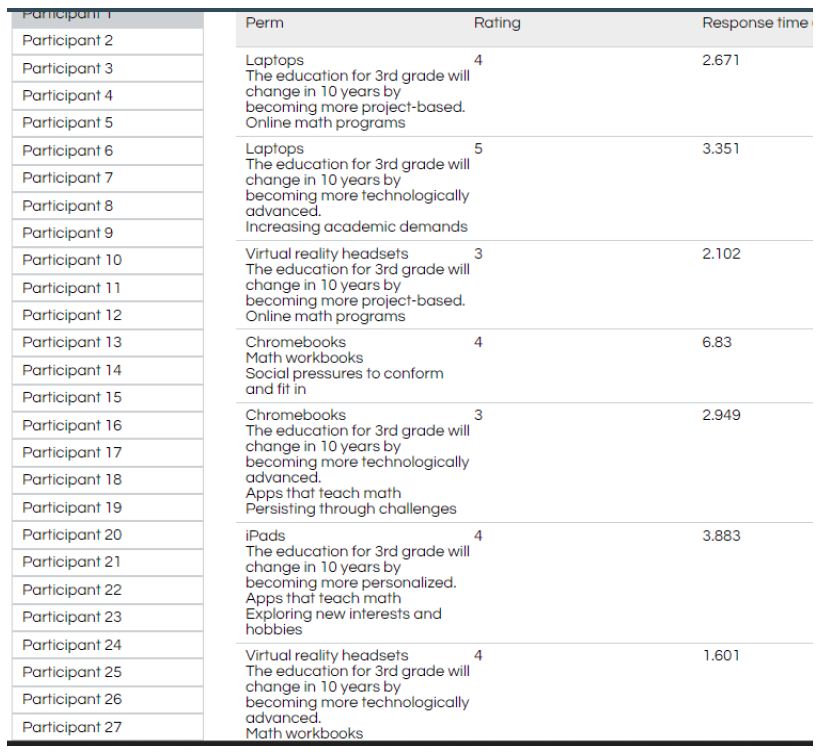
Each respondent evaluates 24 vignettes, and for each vignette assigns a rating on the 5-point scale. The BimiLeap program also records the response time, defined as the number of seconds elapsing between the moments that that the vignette appears on the respondent’s screen and the moment that the respondent assigns a rating. At that point, the screen automatically advances. Figure 4 shows a screen shot of the data available to the researcher.

FIG 4

Figure 4: Screen shot of the first seven vignettes of participant (respondent) #1, along with the rating, and the measured response time in seconds.

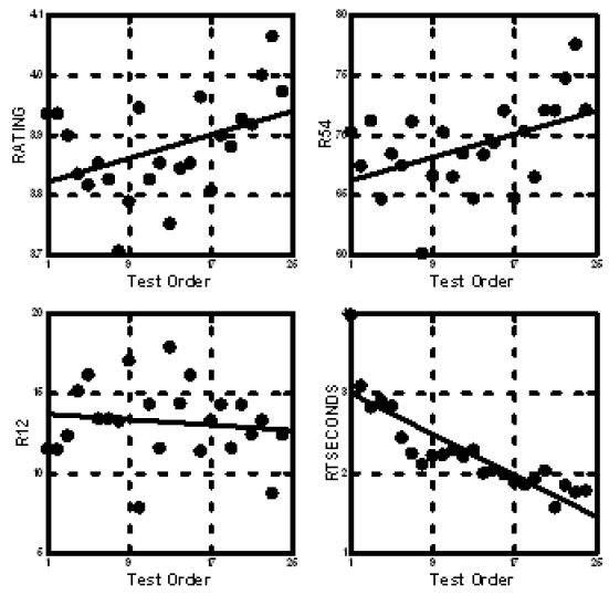
As the respondents proceed to evaluate the 24 vignettes, some changes in the criteria may emerge. Figure 5 shows the average rating by test position, for the raw rating on the 5-point scale, for the two binary transformation (R54=Agree; R12=Disagree), and for the response time. As respondents read the vignettes from first to last, they respond more quickly, and end up agreeing more with the description. It is for that reason that we look at the data across the entire set of 24 vignettes evaluated by a respondent. Presumably, the order bias will be dissipating by then.

FIG 5

Figure 5: Average rating, transformed rating, and response time across the 24 vignettes evaluated by each individual.

One of the ongoing complaints of respondents is that they feel ‘unsure’ that they assigned the ‘right answer.’ At first, hearing that respondents want to give the ‘right answer’ may sound encouraging, the actuality is that when respondents can intuit the right answer’ the researcher may end up with a flawed study, one wherein the judgments are driven by the what the respondent feels to be a researcher expectation or acceptance. Survey research is filled with these types of biases [10], with respondents taking a stand in terms of what is the ‘politically correct’ answer, one that would be socially acceptable. Fortunately, the Mind Genomics paradigm prevents this expectation bias from exerting a strong effect because the vignettes comprise mixtures, a ‘blooming, buzzing confusion,’ in the worlds of Harvard psychologist Wm James when describing the perceptual world of a baby.

Step 11: Prepare the Database for Analysis by Regression Modeling

The objective of Mind Genomics is to link the elements in the vignette to the rating, and to the response time, respectively. In order to do this linking, viz., deconstruct the response to the vignettes into the contribution of the different elements, it is important that the data be in the correct form for the statistical analysis. The experimental design already ensures that the responses to the test stimuli can be linked to the 16 individual elements, but the data are not in the correct format.

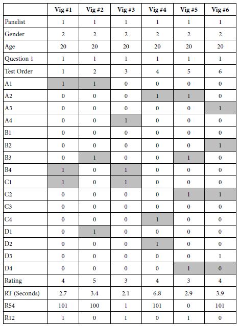
The BimiLeap program creates a file shown in ’90 degree’ rotated form in Table 3. The columns are actually rows, and the rows are actually columns. In Table 2 the columns correspond to the vignettes, the rows correspond to the information about each vignette, Table 2 shows the first six vignettes evaluated by respondent #1. Each respondent generates 24 columns of data. The rows have information about the study, the respondent number, the information about the respondent obtained from the self-classification (gender, age, feel about the 3rd grade in 10 years), then the design of the vignette, expressed in elements present/absent (1=present, shaded; 0=absent, unshaded). The final set of rows show the response time, the rating, and the binary transform of the rating to positive/agree (R54, 5 or 4 → 100, 1, 2 or 3 →0) or negative/disagree (R12, 1 or 2 → 100, 3, 4, or 5 →0). A vanishingly small random number is added to each binary transformed rating, in order that there will be some variation in the binary variable when it acts as a dependent variable in the regression analysis.

Table 3: Example of the part of the data set. The data set is shown rotated 90 degrees

TAB 3

Step: 12: Create Equations Relating the Elements to the Transformed Rating

The key to the analysis is using OLS (ordinary least-squares) regression, which deconstructs the transformed binary response to the presence/absence of the 16 elements. The equation can be written either as

R54=k0 + k1(A1) + k2(A2) … k16(D4) (abscissa of Figure 5) or as R4=k1(A1) + k2(A2) … k16(D4)

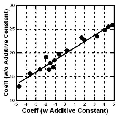
The former is estimated with an additive constant, the latter is estimated without an additive constant (Figure 6).

FIG 6

Figure 6: Scatterplot of coefficients for the total panel relating transformed binary variable R54 to the presence/absence of the 16 elements. The abscissa shows the coefficients estimated with an additive constant, the ordinate shows the coefficients for the same data estimated without an additive constant.

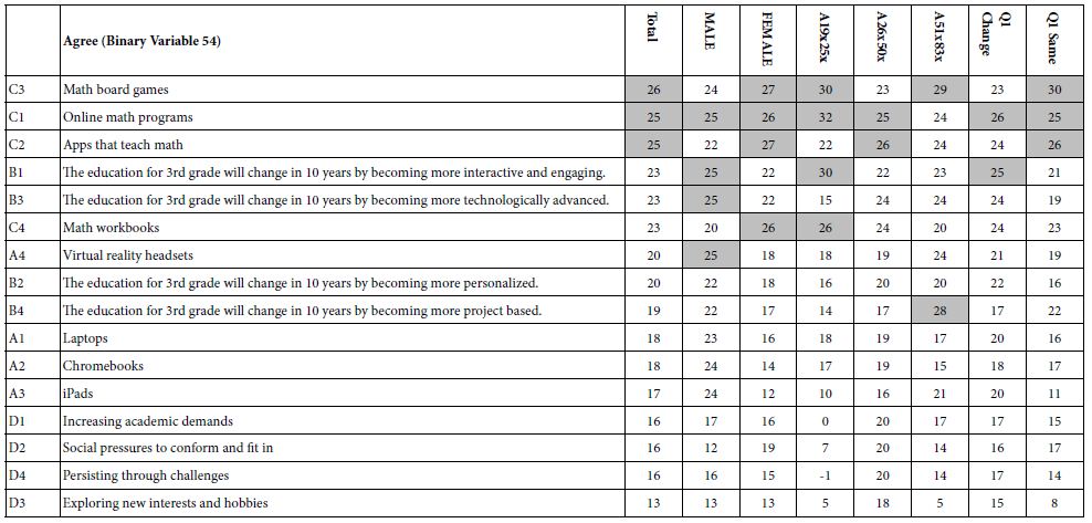
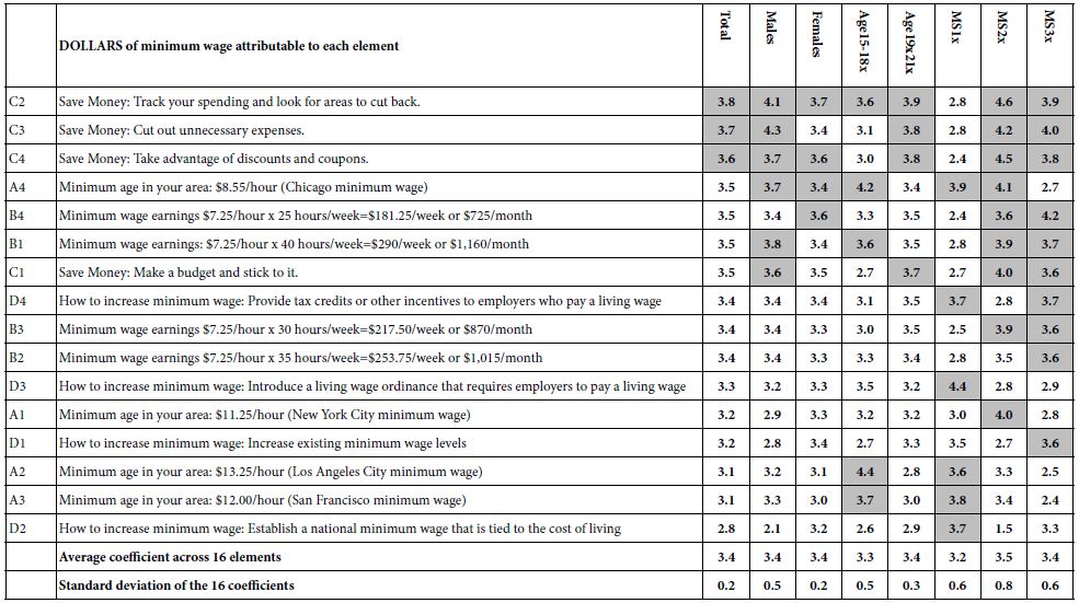
By transforming the five points on the Likert Scale to a binary scale we enable the user of the data to understand the results of the study more quickly. The reality of research is that whereas the Likert scale (viz., our 1-5 scale) is easy to create, it is hard to interpret. What exactly does a 3.5 mean. Managers who use the research are not accustomed to that type of thinking, and instead want a simple interpretation. Transforming the scale to a binary scale means that when we have a coefficient such as +26 for C3 (math board games, total pane) we can say that 26% of the time people will agree that this is likely to be the future of the 3rd grade mathematics class in 10 years. In contrast, the phrases which have little real meaning, but rather talk about challenges (D1-D4) end up generating the lowest coefficients for R54, what school will be like. Keep in mind that the respondents could not have ‘gamed’ the study

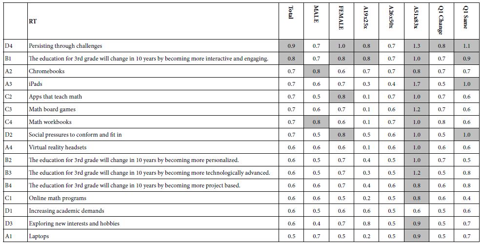
Table 4 shows the coefficients for the model relating R54 (Agree this will be the case in 10 years) to the elements. The columns show the different subgroups, viz., by gender, by age, and response to Question 1. Statements about problems (Question D) generated the lowest agreement, perhaps because they cannot be visualized.

Table 4: The coefficients for the 16 elements for Total Panel, and for each key self-defined subgroup

TAB 4

Step 13: Uncovering Mind-sets for the Granular Topic

A hallmark of Mind Genomics is the focus on the granular topics of the everyday, coupled with a search for different mind-sets, defined as groups of people who think in specific ways. In statistics, these mind-sets are called ‘clusters’ (REF). Clustering is usually reserved for bigger topics, especially in consumer research where the focus is on a ‘macro-level’ understanding of the differences among people in a big domain, such as ‘education in general.’ The notion of clustering people into mind-sets for the smaller, granular level issues of every day is not typically considered, usually because the effort to do the study and the large number of respondents required are prohibitive for the small-scale, local issues. The creation of Mind Genomics as an inexpensive, DIY (do-it-yourself) process, with rapid turnaround, allows Mind Genomics to approach the everyday problems with an eye towards how people make decisions, and the possible existence of different groups of mind-sets.

The process of uncovering mind-sets moves away from looking at people in terms of WJHO they are, and instead looks at people in terms of how they THINK, and more specifically how they think about a particular focused situation. Our study on what the mathematics class of the 3rd grade will look like typifies one of these granular=level examples.

The mathematics is very simple, following these well-accepted steps in clustering.

  1. Decide what the criterion will be. The criterion here is the pattern of values for the 16 coefficients relating the presence/absence of the element to the positive response R54.
  2. For each respondent, create an individual-level model relating the respondents rating of 54 to each of the 16 elements. The approach is simply regression but this time using only the data from one respondent, rather than the data from all respondents. We can use the data from one respondent because the underlying experimental design was used to construct the 24 vignettes evaluated by each respondent. Furthermore. We added a vanishingly small random number to the transformed rating (R54), whether the transformed value was 0 or 100,respectively. The small random number ensured that there would be some level of variability in the dependent variable, preventing the computer from crashing.
  3. The data file which emerges comprises 110 rows, one per respondent, and 16 columns, one per element The numbers in the rows are the coefficients of the equation for that individual: R54=k1(A1) + k2(A2) … k16(D4).
  4. The next analysis looks for common patterns across the 110 respondents, based upon the pattern of the coefficients. This analysis, clustering, is purely mathematical in nature. For the clustering used here, so-called k-means clustering [11], the computer program computed the ‘distance’ between every pair of respondents in the group of 110. The measure of distance is the quantity (1 – Pearson R) where the Pearson R is the linear correlation between two sets of numbers, here the two respondents each of whom is defined by 16 coefficients. When the correlation is perfectly linear (R=1), the distance is 0 (1 – 1=0). When the correlation is perfectly inverse (R=-1), the distance is 2 (1 – – 1=2).
  5. The k-means clustering program is purely objective, and has no input from the researcher. The program assigns each respondent first to one of two exhaustive and non-overlapping clusters, then to one of three exhaustive and non-overlapping clusters, etc. The assignment uses mathematical criteria.
  6. It is the task of the researcher to select the cluster and name it. The ideal is to use as few clusters as possible, but clusters which are clearly different and can be readily named.
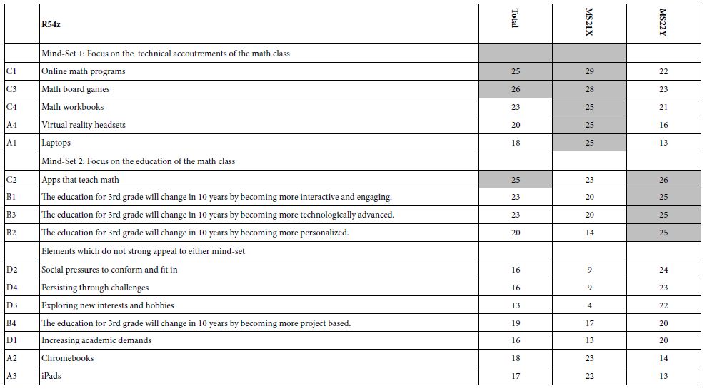
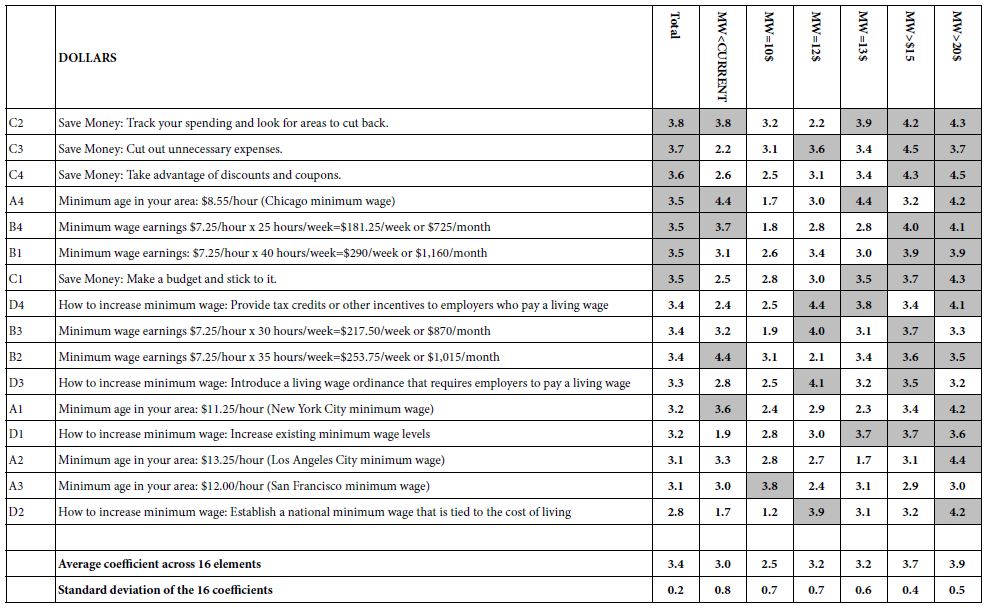
  7. For this study, two clearly different clusters emerged, and could be named. Mind-Set 1 focuses on accoutrements and technology. Mind-Set 2 focuses on the process of education.
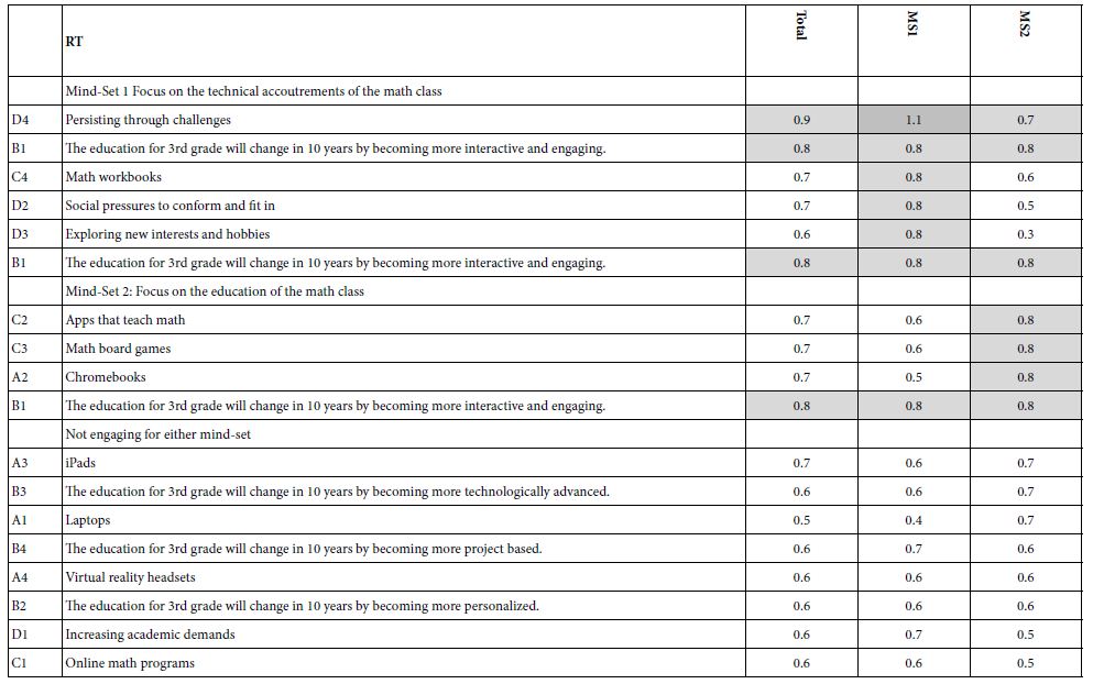
  8. Table 5 shows the mind-sets sorted by ‘strong’, for each mind-set, and then the elements which are not strong for either mind-set. Although the respondents may have thought that they were just guessing, the segmentation reveals clearly different, clearly meaningful mind-sets, based on the clustering.

Table 5: The coefficients for the 16 elements for Total Panel, and the two mind-sets

TAB 5

Step 14: Response Time and the Measurement of Engagement

In the history of experimental psychology and then later in the world of psychology in general, the notion of response time or reaction time has been considered to represent underlying, often non-conscious activities, such as engagement with the material [12,13] or active blocking of content [14]. In the world of consumer research a great deal of interest has been expended at various times to use the non-conscious measures as a perhaps a less cognitively biased measure of how a person feels. Whether these behaviors outside of conscious control are anything more than interesting measures is not relevant to this paper. What is relevant is that we know what the stimuli mean because they are phrases, we know how they drive agreement because we measure agreement, and we can estimate how much time they take to process because we measure response time to vignettes of known composition.

The equation relating the measured response time to a vignette (RT), versus the presence/absence of the elements is the same equation that we have used above: RT=k1(A1) + k2(A2) .. k16(D4).

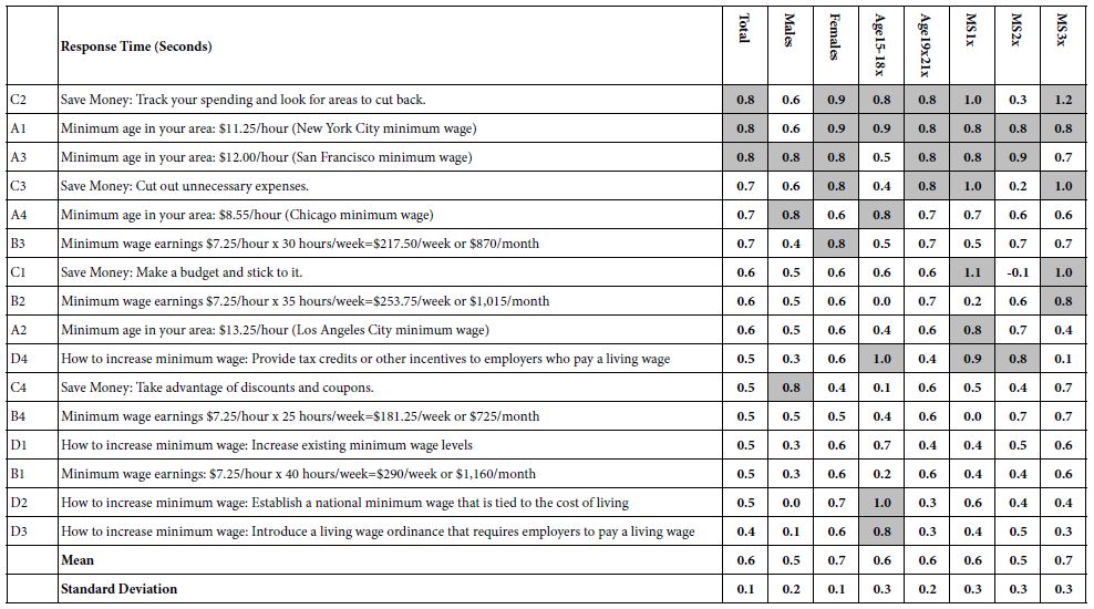
Table 6 presents the coefficients for the response time for the total panel and for the key self-defined subgroups, gender, age, and prediction about the change in the third grade ten years out. To identify patterns, we select long response times, considering these long response times to represent engaging statements. ‘Long’ response time has been set arbitrarily at 0.8 seconds. With that in mind, Table 6 suggests two elements which are engaging, but perhaps for different reasons:

Table 6: Response times for the 16 elements, for Total Panel and for key self-defined subgroups

TAB 6

An element which paints a word picture, forcing one to think about that word picture because it describes a universally meaningful situation and presumably summons to consciousness meaningful experience: D4 Persisting through challenges.

An element which is simple, real, and meaningful. B1: The education for 3rd grade will change in 10 years by becoming more interactive and engaging.

Table 6 also reveals that the typical response time for older respondents (age 51-83) is far longer than the response time of the younger respondents. Even among the older respondents, however, some element are far more engaging than others:

A3         iPads

D4         Persisting through challenges.

C3         Math board games

B3         The education for 3rd grade will change in 10 years by becoming more technologically advanced.

Table 7 presents the response-time coefficients for the two emergent mind-sets. What is remarkable is the seeming inverse relation.

Table 7: Response times for the 16 elements, for Total Panel and for the two emergent mind-sets

TAB 7

Mind-Set 1 (MS1), who appear to be focused on the technology (accoutrements of the math class) show the longest response time for elements dealing with the process and experience of education.

Mind-Set 2 (MS2), who appear to be focused on the process of education show the longest response times for elements dealing with technology.

We may have in Table 7 interesting evidence for underlying cognitive processes, namely that in an important social topic like education, people take the task seriously, and ‘figuratively’ are having difficulty processing elements with which they do not perceive to be part of the future of education.

Step 15: Uncovering Pairwise Interactions through Systematics Using Scenario Analysis

We end these steps of the Mind Genomics process by searching for hitherto unknown, often unexpected pairwise interactions between elements. Conventional research designs do not enable the research to uncover interactions unless these interactions are inserted into the study as defined test stimuli, the reaction to which can be assessed as being statistically significant or not. The key here is that that researcher must ‘know’ what pair or pairs of elements are expected to synergize with each other, or to suppress each other. The implication is that the researcher should know a great amount of topic in order to build in the interactions that can be measured.

A key benefit of the Mind Genomics process is that each respondent evaluates different combinations of elements. That means that across the 110 respondents it is likely that 90% of the combinations are different from each other. The reason for that feature is the permutation scheme, which ends up producing these different combinations. The researcher can benefit from this larger set of different combinations by selecting one specific question (e.g., Question D), and sorting the database into five groups or strata of vignettes. Each stratum of the five comprises one of the five answers to Question D (D=no answer, D1-D4=the four different answers).

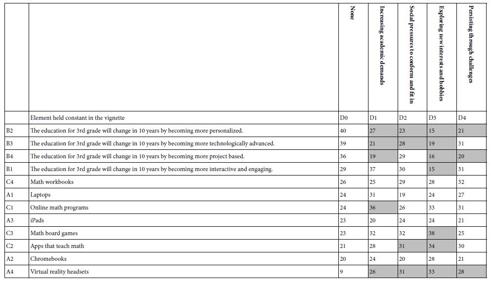
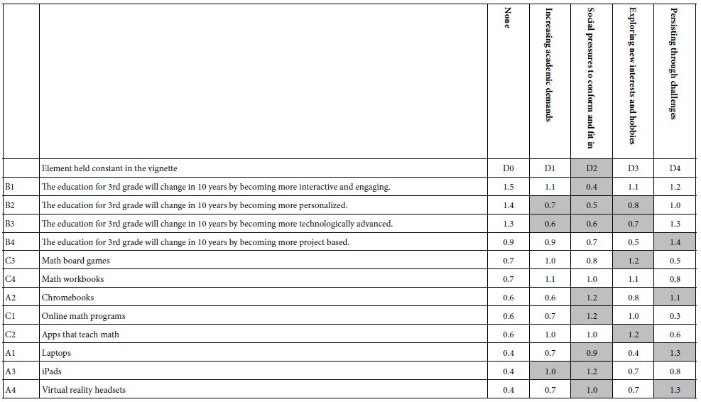
Once the five strata are defined, one can create an equation for each stratum. Within a stratum the element or answer from Question D is fixed, so the independent variables are the 12 elements, A1-C4. The equation is of the same form as before: Dependent Variable=k1(A1) + k2(A2) … k12(C4). There are five such equations, whose parameters are shown in Table 8 for the dependent variable being R54 (agree), and in Table 9 for the dependent variable being RT (response time).

Table 8: Scenario analysis showing the interactive effect of the column element (difficulty) with the row element as a driver of agreement (R54).

TAB 8

Our analysis focuses on differences due to interactions. The column elements are the difficulties that might be faced in 10 years in the 3rd grade. The column labelled D=0 corresponds to the values of the 12 elements in the absence of any element from Question D. We are searching for any element from Question D which generates more than a 10 point or greater change in either direction. The 10 points correspond to a major change.

  1. Agreement (R54) What is most striking is the interaction between the changes to be expected (Question B) and the difficulties to be encountered (columns). The agreement with the changes drops as one introduces the difficulties (Table 8).
  2. Response time (RT). A similar pattern emerges with response time. The response time gets shorter with the introduction of difficulties. It may be that to understand and comprehend difficulties takes away the attention from the other elements, such as change to be expected (Table 9).

Table 9: Scenario analysis showing the interactive effect of the column element (difficulty) with the row element as a driver of response time (RT).

TAB 9

Discussion and Conclusions

The literature on education is filled with studies of students and mathematics, how they learn [15,16], how to work with challenged students, and so forth [17]. These studies are done from the point of view of adults, whether those interested in the psychology of the child as the child grows (REF), or those interested in the process of education [18]. Some topics deal with the child, others with the curriculum, and best practices [19-21].

What may be missing, however, is the experimental analysis of the world according to the student. There are papers reporting observations of the student [22-25] and interviews with students [26] but few books or papers wherein the student is allowed to formulate questions as a researcher [27]. The formulation of the questions itself provides insight into the student. Just as important is the evaluation of these questions by other people, and the insights about the education from the mind of the student, as evaluated either by adults (done here), or by other students (not done here) (Table 10).

Table 10: Appendix – Responses to open-ended question about what the 3rd grade will be like in 10 years

TAB 10(1)

TAB 10(2)

TAB 10(3)

References

  1. García E, Weiss E (2019) US Schools Struggle to Hire and Retain Teachers. The Second Report in” The Perfect Storm in the Teacher Labor Market” Series. Economic Policy Institute.
  2. Freeman B, Marginson S, Tytler R (2019) An international view of STEM education. In: STEM Education 2.0, Brill 350-363.
  3. Rege M, Hanselman P, Solli IF, Dweck CS, Ludvigsen S (2021) How can we inspire nations of learners? An investigation of growth mindset and challenge-seeking in two countries. American Psychologist 76: 755-767. [crossref]
  4. Mendoza C, Mendoza C, Rappaport S, Deitel J, Moskowitz H (2023) Empowering young researchers to think critically: Exploring reactions to the ‘Inspirational Charge to the Newly-Minted Physician’. Psychology Journal, Research Open 5: 1-9.
  5. Moskowitz HR, Gofman A, Beckley J, Ashman H (2006) Founding a new science: Mind genomics. Journal of Sensory Studies 21: 266-307.
  6. Porretta S, Gere A, Radványi D, Moskowitz H (2019) Mind Genomics (Conjoint Analysis): The new concept research in the analysis of consumer behaviour and choice. Trends in Food Science & Technology 84: 29-33.
  7. Green PE, Srinivasan V (1990) Conjoint analysis in marketing: new developments with implications for research and practice. Journal of Marketing 54: 3-19.
  8. Gofman A, Moskowitz H (2010) Isomorphic permuted experimental designs and their application in conjoint analysis. Journal of Sensory Studies 25: 127-145.
  9. Suchman EA (1962) An analysis of “bias” in survey research. Public Opinion Quarterly 26: 102-111.
  10. Likas A, Vlassis N, Verbeek JJ (2003) The global k-means clustering algorithm. Pattern recognition 36: 451-461.
  11. Bassili JN, Fletcher JF (1991) Response-time measurement in survey research a method for CATI and a new look at nonattitudes. Public Opinion Quarterly 55: 331-346.
  12. Read B, Wolters L, Berinsky AJ (2022) Racing the clock: Using response time as a proxy for attentiveness on self-administered surveys. Political Analysis 30: 550-569.
  13. Solarz AK (1960) Latency of instrumental responses as a function of compatibility with the meaning of eliciting verbal signs. Journal of Experimental Psychology 59: 239-245. [crossref]
  14. Blanton M, Stephens A, Knuth E, Gardiner AM, Isler I, et al. (2015) The development of children’s algebraic thinking: The impact of a comprehensive early algebra intervention in third grade. Journal for Research in Mathematics Education 46: 39-87.
  15. Campos IS, Almeida LS, Ferreira AI, Martinez LF, Ramalho G (2013) Cognitive processes and math performance: A study with children at third grade of basic education. European Journal of Psychology of Education 28: 421-436.
  16. Zeleke S (2004) Differences in self‐concept among children with mathematics disabilities and their average and high achieving peers. International Journal of Disability, Development and Education 51: 253-269.
  17. Gardner H (2006) The Development and Education of Mind. Taylor & Francis Limited.
  18. Akerson V, Nargund-Joshi V, Weiland I, Pongsanon K, Avsar B (2014) What third-grade students of differing ability levels learn about the nature of science after a year of instruction. International Journal of Science Education 36: 244-276.
  19. Hanich LB, Jordan NC (2004) Achievement-related beliefs of third-grade children with mathematics and reading difficulties. The Journal of Educational Research 97: 227-234.
  20. Steffe LP, Gale J (1995) Constructivism in Education (1st ed) Routledge.
  21. Corno L, Mandinach E (1983) The role of cognitive engagement in classroom learning and motivation, Educational Psychologist 18: 88-108.
  22. Fredricks JA, Blumenfeld P, Friedel J, Paris A (2005) School Engagement. In: Moore, K.A., Lippman, L.H (eds) What Do Children Need to Flourish? The Search Institute Series on Developmentally Attentive Community and Society, Springer.
  23. Meece J, Blumenfeld PC, Hoyle RH (1988) Students’ goal orientation and cognitive ngagement in classroom activities. Journal of Educational Psychology 80: 514-523.
  24. Skinner E, Belmont MJ (1993) Motivation in the classroom: Reciprocal effect of teacher behavior and student engagement across the school year. Journal of Educational Psychology 85: 571-581.
  25. Gill P, Stewart K, Treasure E, Chadwick B (2008) Conducting qualitative interviews with school children in dental research. British Dental Journal 204: 371-374.[crossref]
  26. Kellett, Mary (2005) How to Develop Children as Researchers: A Step by Step Guide to Teaching the Research Process Sage Publications Ltd.
  27. Luce RD, Tukey JW (1964) Simultaneous conjoint measurement: A new type of fundamental measurement. Journal of Mathematical Psychology 1: 1-27.

Gender Differences on Indigenized Personal Resource Inventory (Pakistan)

DOI: 10.31038/PSYJ.2023532

Abstract

The main objective of the study was to find out the gender differences on the reliable and valid indigenized measure of Personal Resource Inventory measuring optimism, resilience, hope and self-efficacy in Pakistani population. Data was collected using purposive random sampling from 451 employees working in private, semi-government and government organizations. Out of which 62.3% were males and 37.7% were females. The sample mean age was (M=28.19) (SD=6.8); minimum age is 17 and maximum 57; highest percentage of educational level achieved as Graduation i.e. 32.6% (f=147). Results show that females received slightly higher mean score than males on Personal Resource variable in the study sample which had been non-significant for gender in the sample, t (449)=-0.42, p=0.67. This study has implications for gender based programs in Pakistan and opening new avenues for gender empowerment.

Keywords

Personal resource, Gender, Psychological well-being, Indigenized, Psychometric properties, Optimism, Resilience, Hope, Self-efficacy and psychological capital

Introduction

Gender role may play its’ role in exhibiting differences seen in various psychological capacities. Feminists’ movement may adapt according to indigenous needs [1,2]. Youssef and Luthans [3] suggest incorporating study of demographic differences with respect to gender on Psychological Capital (PsyCap). Some of studies from Pakistan, India and China have shown that differences are seen on the variable of Psychological Capital (PsyCap) in culturally shared geographic region. For example the finding of flood victims from Pakistan showed that male victims show higher positive Psychological Capital (PsyCap) than female victims0. Also, the study results of 200 students from Punjab University Patiala, India showed that female students tend to score higher on Psychological Capital (PsyCap) than male students [4,5]. Similarly, in another study in India on 100 telecom employees New Dehli, males tends to score higher on the sub-dimension of resilience; females tend to score higher on sub-dimension of optimism; differences found between the two genders on the sub-dimension of hope were not significant and both genders scored non-significantly equal of the sub-dimension of self-efficacy [4-6]. Moreover, a study carried out on 362 Chinese employees showed masculinity and femininity play different roles in mediating the relationship of Psychological Capital (PsyCap) with job satisfaction. In Pakistan Aziz, Saeed and Chaudhary [7] studied the motivational factors for better job satisfaction of teachers. Study result showed that job stress was a major factor affecting motivation of employees.

Some of the studies in West have also demonstrated gender difference on the variable of Psychological Capital (PsyCap). For example, the study results of 227 students from South African University showed that white females show higher levels of psychological strengths of hope, gratitude and life satisfaction [8]. Independent sample t-test showed that males are higher than females on Psychological Capital (PsyCap) and all of its’ subscales namely optimism, resilience, hope and self-efficacy [9].

There exists no significant gender difference on Psychological Capital (PsyCap) [10,11] study findings suggest that the measure of Psychological Capital (PsyCap) stand equivalent for both genders. Barmola [12] found no significant gender difference on Psychological Capital (PsyCap) and its three dimensions of optimism, resilience and self-efficacy. Whereas significant gender differences were found on hope sub-dimension in the sample. Luthans and Youssef [13] state that in looking for antecedents to Psychological Capital (PsyCap) the demographics are often controlled. Even if not controlled gender is rarely related and tends to exhibit weaker relationship with Psychological Capital (PsyCap).

As seen from the literature reviews it is obvious that there is reasonable variation in gender differences exhibited on the psychological construct of Psychological Capital (PsyCap) in different cultures. Mixed kind of data is seen from various sources in this regard. This could be due to the sociological and cultural differences in socialization of both genders. However, gender differences are still to be looked on the construct of Psychological Capital (PsyCap) with respect to Pakistani society. No research on gender differences on the study variable is found so far. Therefore, this research aims to find out gender differences on Psychological Capital (PsyCap) as measured by a reliable and valid measure of Personal Resource Inventory measuring four dimensions of optimism, resilience, hope and self-efficacy. The four dimensions of Personal Resources also called as Psychological Capital are defined as: “having confidence to take on and put in the necessary effort to succeed at challenging tasks (self-efficacy); making a positive attribution about succeeding now and in the future (optimism); persevering toward goals, and when necessary, redirecting paths to goals in order to succeed (hope); and when beset by problems and adversity, sustaining and bouncing back and even beyond (resiliency) to attain success.

Method

Participants

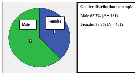
Sample comprised of 451 employees working in private, semi-government and government organizations. Out of which 62.3% were males and 37.7% were females. The sample mean age was (M=28.19) (SD=6.8); minimum age is 17 and maximum 57; highest percentage of educational level achieved as Graduation i.e. 32.6% (f=147). Figure also shows the statistics of the sample as total (N=451) out of which 62.3% were males and 37.7% were females.

FIG 1

Figure 1: Pie chart of Gender wise distribution of sample (N = 451)

Instrument

Personal Resource Inventory Urdu (PRI). It is a 36 item scale measuring optimism, resilience, hope and self-efficacy, with Alpha reliability coefficient of 0.89 in Urdu Language for the Pakistani population. Responses are scored on six point Likert scale ranging from “absolutely applies on me (5)”, “Moderately applies on me (4)”, Mostly applies to me (3)”, “Not really applies to me (2)”, “No hardly applies to me (1)”, “Not at all applies to me” (1). The mean score on the total scale of PRI is M=130.38 with SD=24.90.

Procedure

The data was collected by distributing the newly constructed 36 items Personal Resource Inventory (PRI). Firstly, the participants were assured of the confidentiality and the purpose of the research. They were requested to read the instructions carefully and ask any query. They were to select from the given options, the option which is most accurately describing them for the particular statement.

Ethical Considerations

Ethical issues were besides taken into attention, by abiding by to the ethical principles specified by the Ethical Principles of Psychologists and Code of Conduct (2002) [14]. It includes guaranteeing that participation was voluntary and that privacy was retained.

Results

Gender is a dichotomous variable. The two independent categories of gender are the male and female. The scoring was done following established standard scoring procedure. For this purpose “Independent samples” t-test was computed. Table summarizes the independent sample t-test result.

Results of the independent sample t-test indicated that there is non-significant difference on Personal Resource for gender, t (449)=-0.42, p=0.67, with females receiving slightly higher mean score than males in the study sample.

Table 1: Demographics (Gender wise distribution) of the study sample on the Personal Resource Inventory Urdu (PRI Urdu) (N = 451).

Gender (M / F)

Frequency (n)

Percent %

Male (M)

281

62.3 %

Female (F)

170

37.7 %

Table 2: Means, Standard Deviations and t-values on Personal Resource Inventory (PRI) with regard to Gender (N = 451).

Scale

Male

Female

n = 281

n = 170

M

SD

M

SD

t.


PRI


130

25.841

131.02

23.35

-.42

df = 449.  p = n.s.

Discussion

The purpose of this present study was to find out gender differences on the variable of Personal Resource in Pakistani sample. It was seen that in Pakistani sample females received non-significantly slightly higher mean score than males on Personal Resource comprising of Optimism, Resilience, Hope and Self-efficacy. In South Asia especially India beneficial steps have been taken over the past years to improve the role of females in chief aspects [15]. Whereas, Pakistan in 21st century has also made considerable advances in recognizing the role of females in achieving country’s political, economic, educational, health and sustainable development goals [16-18]. Bridging gender gap in Pakistani society is one of the goal from the seventeen sustainable development goals of the United Nation [19]. Dr Aisha Ghaus Pasha, Provisional Minister Finance, stated that government of Pakistan in line to global strategy towards gender equality has also integrated both gender equal opportunities in preparing, designing, implementing, monitoring and evaluating various policies, regulatory measures and spending programs [20]. The Global Gender Gap World report 2017 embraces 144 countries on their progress towards gender equality in economic participation, educational achievement, health opportunities and politics [21]. Shabir [22] study results highlights the steps to defend the Pakistani women’s right by the government. Similar research on gender difference on other variables of interest shows that at place of work differences on gender gets minimized with both being dominating in the role of boss and accommodating when in the role of sub-ordinates [23].

Implications, Limitations and Future Recommendations

Therefore, gender discrimination and inequality based on gender may not override any intervention, school of thought, organizational packages, educational opportunities and policies at government or private level. Otherwise, as the research result shows that the gender, if discriminated, may not be benefitted adequately despite being enriched with adequate resources at personal level.

Conclusion

No significant gender difference on the variables of Personal Resource measuring optimism, resilience hope and self-efficacy is seen whereas females received non-significantly higher mean score on the variable of Personal Resource comprising of Optimism, Resilience, Hope and Self-efficacy in Pakistani sample. Therefore, gender segregation is inappropriate and dis-advantaging women due to their weaker competency is baseless as now the research supported by data shows that women of Pakistan are more resilient, hopeful, optimistic and self-efficacious than males. This makes them a useful and psychologically resourceful fragment of Pakistani population in every walk of life whether domestic or workplace.

Findings

Differences on the gender variable on the role of Positive Personality characteristics measured through the indigenously designed “Personal Resource Inventory (Based on optimism, resilience, hope and self-efficacy) reveals to be non-significant. This study has implications for gender based programs in Pakistan.

References

  1. Ngo H Y, Foley S, Ji MS, Loi R (2014) Linking gender role orientation to subjective career success: The mediating role of psychological capital. Journal of Career Assessment 22: 290-303.
  2. Ain Q (2016) Feminist Movements Leading towards Emancipation or Alienation: Case Study of Pakistan. Pakistan Journal of Social and Clinical Psychology 14: 26-32.
  3. Youssef CM, Luthans F (2012) Psychological Capital: Meaning, findings and future directions. Oxford University Press.
  4. Riaz H, Riaz M,Batool N (2014) Positive Psychological Capital as predictor of internalizing psychological problems among flood victims. Journal of Indian Academy of Applied Psychology 40: 102-112.
  5. Jagpreet K, Sandhu, & Kaur K (2016) Psychological Capital in relation to stress among university students. Indian Journal of Health and Wellbeing 7: 323-326.
  6. Parthi K, Gupta R (2016) A study of Psychological Capital, job satisfaction and organizational climate in Telecom sector: A gender perspective. Diviner 13: 1.
  7. Aziz A, Saeed M, Chaudhary F S (2014) An exploratory study of teachers ‘motivation and job satisfaction in special education, Lahore, Pakistan. Biannual Research Journal: Social and Science Review 2: 21-38.
  8. Jackson LTB, van de Vijver FJR, Fouché R (2014) Psychological strengths and subjective well-being in South African white students. Journal of Psychology in Africa 24: 299-307.
  9. Lehoczky MH (2013) The socio-demographic correlation s of Psychological Capital. European Scientific Journal 9: 26-42.
  10. Hidayat A E (2010) Individual differences in Psychological Capital.
  11. Caza A, Bagozzi RP, Woolley L, Levy L,Caza BB (2010) Psychological capital and authentic leadership: Measurement, gender, and cultural extension. Asia-Pacific Journal of Business Administration 2: 53-70.
  12. Barmola KC (2013) Gender and Psychological Capital of adolescents. Indian Journal of Applied Research 3: 1-3.
  13. Luthans F, Avey JB, Avolio BJ, Norman SM, Combs GM (2006) Psychological Capital development: toward a micro-intervention. Journal of Organizational Behavior 27: 387-393.
  14. Anastasi A, Urbina S (2003) Psychological Testing.
  15. Ranjha N, Alam MT, Muqqadas K (2010) A Study the Planning and Organizational Skills of Head Teachers at Elementary Level in Distt. Attock. Biannual Journal of Gender and Social Issues 9: 2.
  16. United Nations Development Program (2017) Gender equality: Women empowerment.
  17. United Nations (2017) United Nations: Sustainable Development Goals.
  18. Pakistan Horizon (2014) Aurat Foundation: Dr Masuma Hasan’s speech on International Women day.
  19. United Nations (2017) United Nations: Pakistan’s challenges: Sustainable Development Goals.
  20. Pakistan Today (2017) Gender equality and economic opportunities for women our priority: Aisha Ghaus.
  21. World Economic Forum (2017) World Economic Forum: The Global Gender Gap Report 2017.
  22. Shabir S (2009) The Role of Various Movement and Organization to Defend the Pakistani Women’s Right and Measures adopted by the Government. Biannual Journal of Gender and Social Issues 8: 2.
  23. Didar S, Amjad N (2017) Gender Differences in Conflict Resolution Styles (CRS) in Different Roles: A Systematic Review. Pakistan Journal of Social and Clinical Psychology 15: 37-41.

Palygorskite, Chlorite and Illite Minerals in the Dukhan Sabkha Deposits, Qatar

DOI: 10.31038/GEMS.2023512

Abstract

The clay samples were studied using X-ray diffraction. The range of the run was between 2°and 40° and the run was 1.2°/min. Electronic Microscope also used in the study by using great magnification range from X20 up to 1000,000 to allow to examination the surfaces of fine grains and to takes photographs with great focus. Chemical analyses also carried out under the SEM, using energy-dispersive X-ray spectrometry to define their dominant elements. From the study, it emerged that the dominant clay minerals in the samples are palygorskite, followed by chlorite and illite. Based on the peak area measurements, the mean percentage of palygorskite in the clay deposits included dolomite and anhydrite is 59% (approximate percentage is 34%-79%). It is 23% for chlorite (approximate percentage is 7%-40%) and 9% for illite (approximate percentage is 4%-13%). After excluded dolomite and anhydrite from the samples, it is 65% for palygorskite (approximate percentage is 47%-85%), 25% for chlorite (approximate percentage is 8%-40%) and 10% for illite (approximate percentage is 6%-15%). Through EDX analyses of the palygorskite needles it was inferred that the P is the dominant element, followed by Si, Mg, Al, Ca, and K. Phosphate nodules of a globular shape (spherulites) in various sizes (1-<2 μ) also occur in most of the clay samples, especially that rich in palygorskite. In some samples, the phosphate nodules were present in small groups connected together as bunches.

The main conclusion of this study are:

(1) In Dukhan Sabkha, clay-rich deposits are mainly found beside the edges of the Sabkha, especially where the Sabkha is supplied with surface drainage. Later the wind contributes in distribution part of these sediments within the Sabkha. The thickness of clay-rich layers in such as these locations is between 0.5 and 1.5 cm.

(2) Palygorskite is mainly authigenic, formed inside the Dukhan Sabkha. This is because the conditions of formation this mineral within the Sabkha are widely available. Part of palygorskite is definitely detrital being, derived from shales of the Lower and Upper Dammam Formation of the Eocene age that exposed on the surface of Qatar. A small proportion of this mineral could also reach to inside Dukhan Sabkha after carried to Qatar as dust by the northern wind or by water currents from the neighboring areas, especially from the eastern part of the Arabian Peninsula.

(3) Chlorite and illite minerals are not form locally inside the Dukhan Sabkha; both of them are from pre-existing sedimentary rocks from outside the Sabkha. The main source of these two minerals is a detrital rocks derived from shales of the Tertiary of the Lower Dammam Formation and Rus Formation of Eocene age in addition to Dam Formation of Miocene age in Qatar and part of these minerals may reached to inside the Sabkha from outside Qatar.

(4) This work can be used as model for the study the possibility of formation palygorskite within the Sabkhas areas in Qatar and in the Arabian Gulf areas.

Introduction

Sabkhas are one of the important features of the Qatar Peninsula, covering about 7% of its surface area. They can be divided into coastal and inland Sabkhas. There are 42 coastal Sabkhas, covering about 590 km2 and 78 inland Sabkhas, covering about 205 km2. The surface of the Sabkhas in Qatar is mainly flat and nearly horizontal, with gradients usually less than 1:250°. Most of the Sabkhas are located at or within 1.5 m above sea level. Their interior margins, however, may be 2 or 3 m higher than sea level [1]. The study of clay minerals in the Sabkha areas of Qatar and Arabian Gulf countries are limited in number. Most studies focus on evaporite deposits. They only mention clays in the marine and Sabkha areas as fine deposits, dominant in the intertidal zone of the Sabkha and also where microbial mats and algae are found [2-8]. Further information about clay minerals in Qatar formations can be found in: Cavelier [9,10] and Cavelier [11-18].

This is the first study of clay minerals in large, famous Holocene inland Dukhan Sabkha in Qatar. The aim of the study is to identify the type, the amount and the origin of clay minerals in the Sabkha sediments, in addition to the dominant natural conditions that caused formation of these minerals in the Sabkha. Important series of science questions are answered in the study such as:

  1. What is the types of clay minerals that dominant in the Dukhan Sabkha.
  2. What is the source and the proportion of the clay minerals in the Sabkha sediments?
  3. What is the factors that affecting the formation of the clay in the Dukhan Sabkha?
  4. Is Palygorskite formed inside Dukhan Sabkha or it is detrital mineral comes from outside the Sabkha?

General Setting of the Study Area

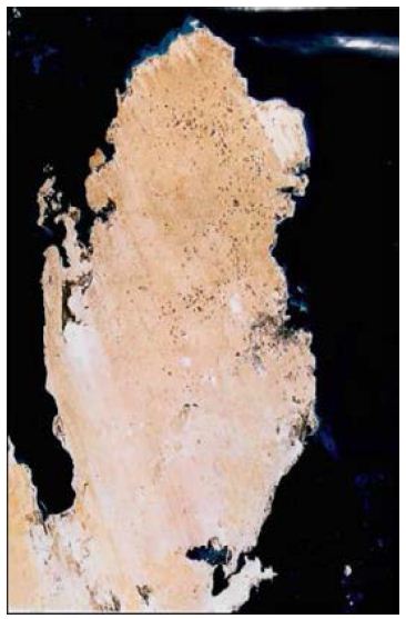
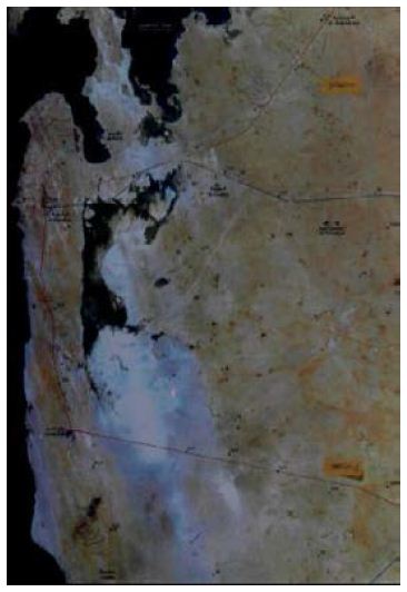
Dukhan Sabkha is the largest inland Sabkha in the Qatar Peninsula, located in the west adjacent to the Jabal Dukhan hill and covers about 73 km2. It is situated in a depression shaped like an inverted L, one of its arms extends north-south and the second one northeast-southwest (Figures 1 and 2). The western side of the Sabkha is straighter than the other side, as it is constrained by the Dukhan anticline [1]. The surface of the Sabkha is flat, about one meter below sea level, except near the edges, is more than 1 m above sea level due to the development of nebkhas (plants trapping sand). The lowest part of the Sabkha is in the south (25° 20 E, 50° 50 N), where it reaches-6 m below sea level [19]. The deposits of the Sabkha consists of a compact, dry crust of halite (3 mm-2 cm thick), above brown or grey sand deposits, or brown sand intercalated with white and light grey gypsum-rich layers. Anhydrite and halite minerals are mainly dominant in the northeastern part of the Sabkha at shallow depth, about 20 cm. Accumulation of sand sheets and small sand dunes are found in the south and southeastern part of the Sabkha. Recent eolian sand sheets are also present in various positions in the western part of the Sabkha. Recent deposits of white salt (covering about 4.5 km2) is present in the northeastern part of the Sabkha. Limonite is found as thin subsurface beds beside the eastern edges of the Sabkha and at the surface in the northern part of the Sabkha [20]. Small areas of the Sabkha, especially around the margins, are covered by mud. Typically, mud cracks appears in different locations due to desiccation. Deposits of sand, clay and silt are present at the edges of the Sabkha [21]. The groundwater level in Dukhan Sabkha is shallow (between a few centimeters and 120 cm). The sources of groundwater in the Sabkha include: sea water, rainwater and the freshwater of the main northern aquifer [20].

fig 1

Figure 1: Landsat image mosaic showing the general location of Dukhan Sabkha, in the western part of Qatar. (Produced by the Environmental Research in Statue of Michigan. Ann Arbor Michigan. Scan date 30-Jan. 1987, scale 1:200 km.

fig 2

Figure 2: Landsat image mosaic of Dukhan Sabkha. (Produced by the Central for GIS-State of Qatar with Geomatics Canada. Scan date 25-Jan. 1995, scale 1:200,000).

Methodology

Field Study and Sample Collection

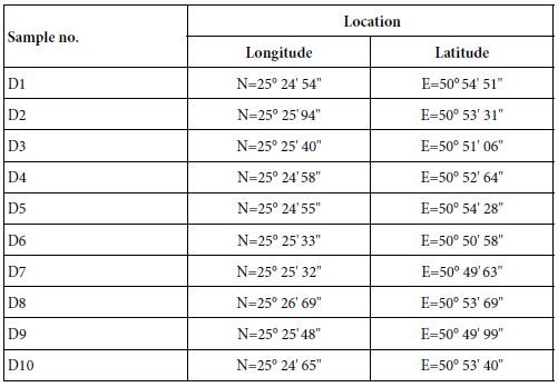
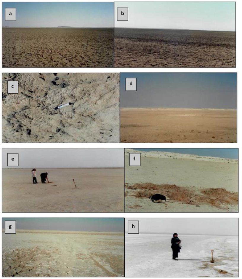
Field studies were carried out in Dukhan Sabkha during February and March 2020. Throughout fieldwork, observations were made for clay on the surface and at shallow depths in the sediments of the Sabkha. Information about type and size of the sediments, microbial mats dominant in the Sabkha were recorded. Sediment samples (10 samples) rich in clay were collected from different locations within the Sabkha: along the margins of the Sabkha, beside the northwestern edge, from northeastern part, from the middle of the northern part and from a surficial channels within the Sabkha (Table 1). Photographs for the common characteristics and for locations rich in clay, and fine deposits in the northern parts of the Sabkha were taken in the field (Figure 3).

Table 1: Names and locations of the studied samples in Dukhan Sabkha

tab 1


fig 3

Figure 3: General view of Dukhan Sabkha: a and b showing the compact surface crust in the northern part of the Sabkha, c is thick light gray crust in the northeastern part, d is patches of sands neair the  nothewestern edge of the Sabkha. Figures e and f is collection samples from northern and northwestern part of the Sabkha, g and h halite mixed with mud and anhydrite in the northeastern part. (note that mud occures as minor facies on the surface in fig. e, sand dominant beside the northwestern edge of the Sabkha in fig. f, whereas halite and anhydrite are dominent on the surface of the northeastern part in fig. g and h).

Sample Preparation

The clay samples from different locations within the Sabkha were studied using X-ray diffraction First the samples were treated with acetic acid (10%) to remove all the CaCO3 in the sediment. There was variation in the reactions in the samples and after all reaction had ceased any residual acid was washed from the samples, using tap water. Tap water was later added to each sample (4 cm) in a small beaker with sodium hexametaphosphate (calgon-1 ml of 10 % per 100 ml) to disperse the clay. The samples were shaken well and left in an ultrasonic tank for about 15 minutes. Then the samples were allowed to settle, using Stokes Law (3 hours for 4 cm for the <2 µ fractions), as per Galehouse [22] and Hardy and Tucker [23,24]. The fractions of each sample were collected in a small beaker and saturated with about 5 ml of MgCl2. Then, the samples were centrifuged 3 times, and each one was carefully washed, using tap water. Finally, three smear slides were made from the paste of each sample using a spatula. One of these was left (untreated) in the laboratory to dry and then it was run as an air-dried trace. This slide was then, heated to 375°C to collapse the smectite and illite/smectite, leaving the other clays unaffected. The second slide was left in ethylene glycol (vapour) for about 24 hours at 60°C. This was to distinguish the smectite, illite/smectite and chlorite-smectite from the chlorite and illite/smectite where overlaps occurred. The third slide was heated in a furnace to a temperature of 550°C to expel the interlayer water molecules in the smectite, and this caused a contraction in the basal spacing.

X-ray Diffraction

X-ray diffractometry was carried out on the clay fractions (<2 μ) separated from a total of 10 samples of clay-rich sediments. The weight of each sample from which clay was separated was about 40 g and the percentage of clay in the samples was approximately between 25% and 40%. The range of the run was between 2° and 40° and the run was 1.2°/min. The percentage of each clay mineral was calculated by dividing the area of its main peak by the total of the main peaks of the clay minerals of the same sample and multiplying by 100.

Scanning Electronic Microscopic Study and Chemical Analyses

The clay samples were studied by using the scanning electron microscope to determine their fine compositions. The great magnification range of SEM, range from X20 up to 1000,000 is allow to examination the surfaces of fine grains and to takes photographs with great focus. For study, the samples were placed sided sticky tape fixed on surface of stub (stage) and thin coated with gold as a conductive layer. The samples were positioned in the SEM, viewed, studied and photographed by the scanning electron microscope. Chemical analyses were also carried out under the SEM, using energy-dispersive X-ray (EDX) spectrometry to define their dominant elements. Some photographs of the palygorskite and other important features present in the samples were taken.

Result of the Study

Field Study

Most the Surface of the Sabkha is covered by compact crust of fine deposits of sand, silt, clay mud, halite and very fine grains of gypsum of various color between white and beige to light gray. The crust is compact and dry, and mostly between 1 to 3 cm thick (a, b and c in Figure 3). The thickness and dominance of the crust in the northern part of the Sabkha is more than in the southern part. Sand and silt are dominant in the deposits. They found on the surface or mixed with other deposits at different depths. The type of the sediments at the edges of the Sabkha is different from those in other parts of the Sabkha and mainly consists of sand, clay and silt (d, e and f in Figure 3). Mud occurs as a minor facies in selected stations. It is generally silty in nature, some with fine sand. It is dominantly siliciclastic in composition, more rarely calcareous, and commonly contains some evaporite precipitation. It is generally structure less, sometimes with desiccation cracks at the surface. Clay is mainly present on the surface and at shallow depths (few centimeters from the surface). Clays are not as common as sand, but found in limited positions on the surface and at shallow depths. In the Sabkha, clay-rich deposits are mainly found beside the edges of the Sabkha, especially where the Sabkha is supplied by surface drainage. The thickness of clay-rich layers in locations such as these is between 0.5 and 1.5 cm. The clay deposits are also, present inside small number of elongated, narrow, shallow-dry surface channels, extending from the land inside the Sabkha. In general, the proportion of clays in the Sabkha decreases towards the center of the Sabkha and it increases at the edges of the Sabkha and, where microbial mats are present. Anhydrite presents at shallow depth (about 20 cm) as nodules and as fine grains (similar to gruel) mixed with halite, mud, silt and dark black and grey deposits of microbial mats (g, and h in Figure 3). Anhydrite and halite are mainly dominant in the northeastern part of the Sabkha. The texture of most of the clay samples in this part of the Sabkha are like soft plastic (or rubber). Accumulation of sand sheets and small sand dunes found in the south and southeastern part of the Sabkha. Recent eolian sand sheets are also present in various positions in the western part of the Sabkha. Gypsum crystals and halite decrease in abundance near the edges. Limonite founds as thin subsurface beds beside the eastern edges of the Sabkha and at the surface in the northern part of the Sabkha.

Laboratory Study

X-ray Diffraction

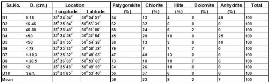
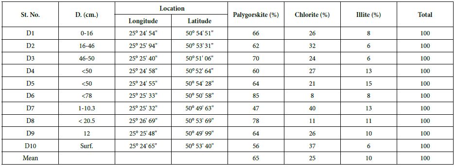
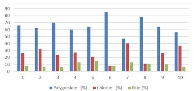
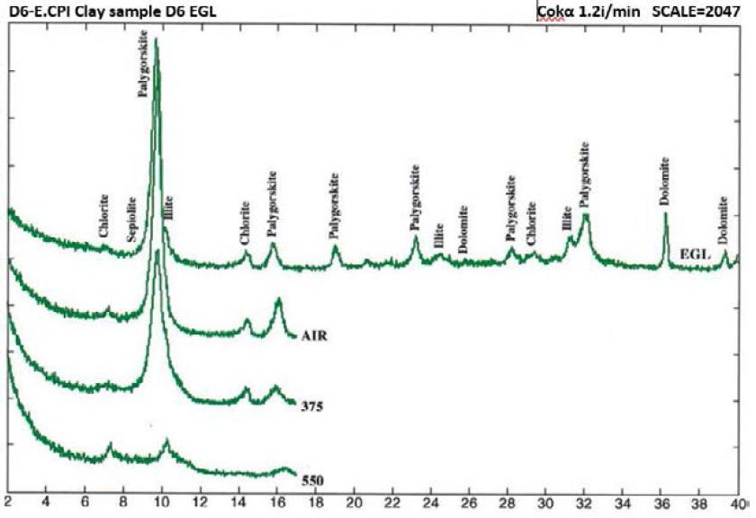
From X-ray study, it emerged that the clay minerals that are dominant in the samples are palygorskite, chlorite and illite (Tables 2 and 3, and Figures 4-8). Some samples included small amount of dolomite (Samples No. 3, 6 and 8 in Table 2) and other samples included anhydrite (Samples No. 1, 4 and 5 in Table 2). Based on the peak area measurements, the mean percentage of dolomite in the samples is 2% (approximate percentage is 2%-7%) and it is 7% for anhydrite (approximate percentage is 25% -49%) as shown in Table 2. The mean percentage of palygorskite in the clay deposits included dolomite and anhydrite is 59% (approximate percentage is 34%-79%) and it is 65% after excluded dolomite and anhydrite from the samples (approximate percentage is 47%-85%). The mean of the percentage of the total of the chlorite and illite minerals in the samples included dolomite and anhydrite is 23% and 9% respectively (approximate percentage is 7%-40% for chlorite and 4%-13% for illite). It is 25% for chlorite and 10% for illite (approximate percentage is 8%-40% for chlorite and 6%-15% for illite) after excluded dolomite and anhydrite from the samples (Tables 2 and 3). The main peak of chlorite is at 14.2 A° and tends not to be sharp, but slightly more rounded shape (Figures 5-8).

Table 2: Approximate percentages and mean of XRD peak areas for clay minerals in Dukhan Sabkha deposits (included dolomite and anhydrite).

tab 2

Table 3: Approximate percentage and mean of XRD peak areas for clay minerals in Dukhan Sabkha deposits (excluded dolomite and anhydrite).

tab 3

fig 4

Figure 4: Mean total percentage of clay minerals (peak areas) dominant in Dukhan Sabkha

fig 5

Figure 5: Clay mineral peaks, Dukhan Sabkha, Sample D6 (XRD analyses)

fig 6

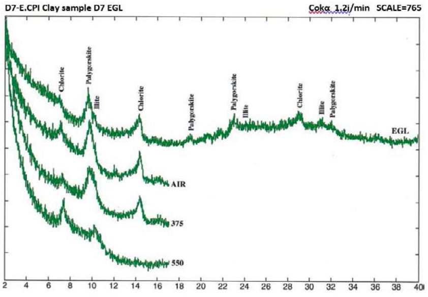
Figure 6: Clay mineral peaks, Dukhan Sabkha, Sample D7 (XRD analyses)

fig 7

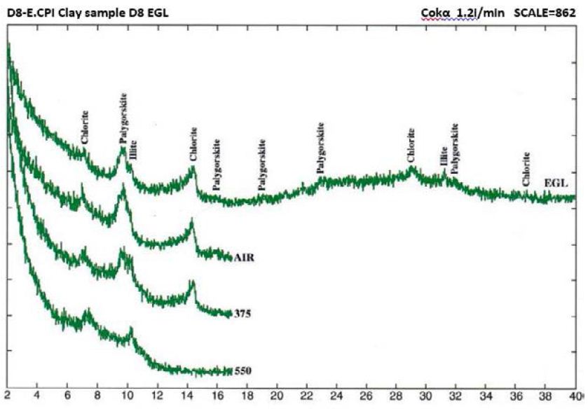
Figure 7: Clay mineral peaks, Dukhan Sabkha, Sample D8 (XRD analyses)

fig 8

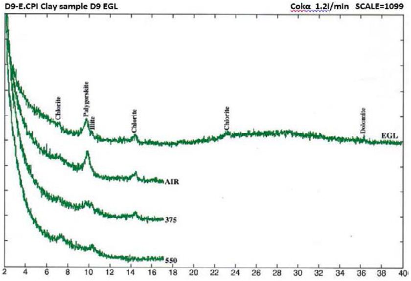
Figure 8: Clay mineral peaks, Dukhan Sabkha, Sample D9 (XRD analyses)

EDX Analyses

The EDX analyses of the palygorskite needles shows that the Si is the dominant element, followed by P, Mg, Al, Ca, and K (Figures 9 and 10). Because the size of phosphate nodules is extremely minute (<2 μm) and the spot used in the analyses is 2-3 μm diameter area and 2-3 μm deep, the X-ray beam covers the surrounding clays in addition to the phosphate nodule. P is the main peak and then Si, Mg, Ca, Al and K in that order.

fig 9

Figure 9: EDX analyses of clay sample (D6) from Dukhan Sabkha (See Figure 11). Au: from the gold coating

fig 10

Figure 10: EDX analyses of main elements in minute sphere plus surrounding area, Sample D6 from Dukhan Sabkha (see Figure 11). Note the size of the phosphorous peak in the clay sample D6 above.

SEM Survey

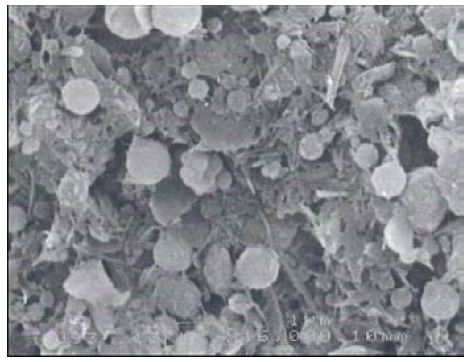
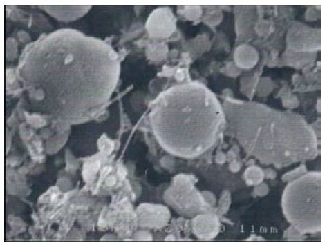
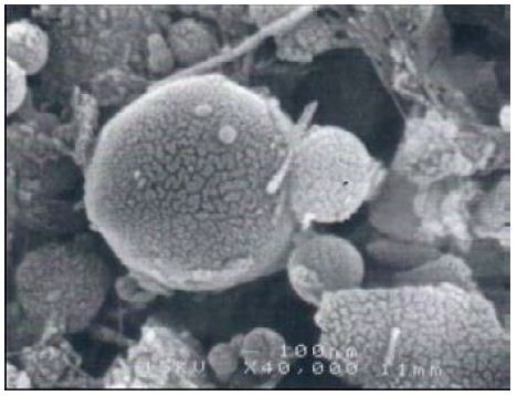
The SEM study of the clay samples from Dukhan Sabkha shows various proportions of long, fibrous palygorskite crystals (Figures 11-14). Phosphate nodules of a globular shape (spherulites) in various sizes (1-<2 μ) also occur in most of the clay samples (Figures 11-14). Some of the samples include a high proportion of extremely minute phosphate nodules of spherical shape and less than 2 μm diameter. A small protuberance appears on one side of some of the relatively large spheres (Figures 13 and 14). In some samples, the phosphate nodules were present in small groups connected together as bunches (Figures 1 and 2).

fig 11

Figure 11: Palygorskite fibers in various sizes. (1-<2 μm), Dukhan Sabkha, sample D6

fig 12

Figure 12: Palygorskite fibers and illite with minute spheres of phosphate (1 μm), Dukhan Sabkha, sample D6

fig 13

Figure 13: Minute spheres of phosphate with some palygorskite and illite, Dukhan Sabkha, sample D8

fig 14

Figure 14: Minute spheres of phosphate, Dukhan Sabkha, D8

Discussions

Sabkha Sediments

Most of the surface of the Dukhan Sabkha is covered with compact firm crust of sand, silt, clay mud, halite and fine grains of gypsum with fine carbonate sediments. The thickness of the crust is mostly between 1 to 3 cm thick. It dominant in the northern part of the Sabkha than in the southern part and not presents at the edges of the Sabkha. There are several natural factors prevailing in the area have played a major role in formed such as this crust within the Sabkha. The first important factor is the surface of the Sabkha is flat, about one meter below sea level and this leads to feeding Sabkha basin by great rate of groundwater. This water reaches to the Sabkha through subsurface water drainage that feed Sabkha with seawater, mainly from the western coast of the Qatar Peninsula. Because of the hot, dry climate, prevailing in Qatar during of the year seasons the water exposed to high evaporation process within the Sabkha, accordingly the previous compact crust formed. The second factor is the groundwater level in the northern part of the Sabkha is shallower than that in the southern part and this is why the crust is dominant in the northern part of the Sabkha than in the southern part. This reason also helped in increase the thickness of crust in the northern part of the Sabkha more than in the southern part. The third factor is the accumulation of sand by the prevalent northern and northwestern winds worked to prevent the formation of the crust at the edges of the Sabkha. The dominant sediment facies in the Dukhan Sabkha are sands with variable amounts of evaporite precipitates. Of secondary importance are sandy silts, muds and algal/microbial mat deposits. Mud occurs as a minor facies in selected areas. It is generally silty in nature, some with fine sand. It is dominantly siliciclastic in composition, more rarely calcareous, and commonly contains some evaporite precipitation. It is generally structureless, sometimes with desiccation cracks at the surface. The main types are mud with evaporite, mud with little or no evaporite and mud with phosphate nodules. On the other hand, the proportion of clay and silt in the sediments is high. The silt and clay facies increase in abundance towards the Sabkha margins, particularly along the eastern and northwestern edges. The surface deposits of these edges are different from those in the other parts of the Sabkha; the amount of gypsum and halite decreases, while the proportion of silt and clay increases. This is probably because the presence of surface water drainage brings rainwater and fine sediment to inside the Sabkha from outside especially during the rainy period. We cannot ignore the presence of another source supply the Sabkha with clay deposits. Probably the clays and shales of the exposed deposits of Midra (and Sila) shale of the Lower Dammam Formation and the Lower beds of the Simsima Member of the Upper Dammam Formation in Qatar forms a secondary source. In the northeastern part of the Sabkha, the clay is mainly present on the surface and at shallow depths (few centimeters from the surface). The texture of most of the clay samples is like soft plastic (or rubber). Undoubtedly there are more than factor worked in combined to give this texture for clay in this part of the Sabkha, such as the porosity and permeability of the deposits, percentage of silica, pressure on the sediments and percentage of the salinity of water. Al- Yousef [20] found that the TDS of the brine in the northeastern part of Dukhan Sabkha is 112.8 ppt and it increases from east to west. She believed that this is because the eastern part of the Sabkha is receiving amount of fresh groundwater as drainage from the main northern aquifer and from small ground lenses located to the east, whereas the western part of the Sabkha is more affecting by seawater. However, this recent study believed that such as this type of clay (soft plastic) is need special, independent study, especially it has not previously been studied or referred to in the previous studies of the clay minerals of the geological formations of the State of Qatar.

Palygorskite (Attapulgite)

Palygorskite is an aluminum-Magnesian silicate (2MgO3 SiO2. 4H2O-Al2O3 5SiO2. 6H2O) [25], in which the ratio of Mg: Al is varies from approximately 3:1 to 1:3 [26]. Palygorskite is not common in most clay-rich deposits, but does form authigenically in arid-region soils rich in Mg and Si, in alkaline lakes and in hypersaline sediments such as Sabkhas. It is well known throughout the Arabian Peninsula region, and occurs as a windblown component of sediments in the Arabian Gulf and Indian Ocean. It can also form authigenically in volcanic sediments and in calcareous soils. Waver [27] and Isphording [28]. It can transported by rivers as a detrital mineral and as windblown dust to other continental or marine environments [29]. There is no studies give details about the palygorskite in the deposits of the formations in Qatar or even about its presence in the Sabkhas deposits of Qatar. All the studies that dealt with clay deposits indicated only the presence of this mineral without gave details about it. Cavelier [9,10] observed that the Midra (and Saila) Shales Member of the Lower Dammam Formation mainly consist of fibrous clays of the attapulgite family. The shales have varying proportions of carbonate (calcite and dolomite) with numerous lenticular or nodule of phosphates and secondary black iron oxide. Cavelier [10] also stated that the deposits at the bottom (over 5 m) of the Simsima Member (lower part of the Upper Dammam Formation) in Qatar included marls and attapulgite shales (palygorskite) of red color, quite rich in marine fossils overlain by reddish granular limestone. Alkuwari [16] from her study of the Miocene argillaceous rocks in the southwestern part of Qatar found that the clay minerals are illite, kaolinite, Ca, Mg-montmorillonite and attapulgite. Aba-Husayn and Sayegh [30], from their mineralogical study of Al-Hasa desert soil in Saudi Arabia (20 soil horizons and beds of adjacent outcrops) found that it includes palygorskite (between 37% and 65%). They also found that palygorskite not only occurs in Al-Hasa, but also widely distributed throughout the Arabian Peninsula.

This recent study shows that palygorskite is the dominant clay mineral in the Dukhan Sabkha sediments. From XRD analyses, it appeared that the mean percentage of this mineral in the clay deposits included and excluded dolomite and anhydrite from the deposits is 59% and 65% respectively and the approximate percentage is between 34%-79% and 47%-85% respectively (Tables 2 and 3, and Figures 4-8). The EDX analyses of the palygorskite needles showed that the Si is the dominant element, followed by P, Mg, Al, Ca, and K (Figures 9 and 10). In indeed, P is more dominant than S, but because the size of the phosphate nodules extremely minute (<2 μm) and the analyses spot is 2-3 μm diameter area and 2-3 μm deep, the X-ray beam covers the surrounding clays in addition to the phosphate nodules, and this is why S appeared more dominant than P. Phosphate nodules of a globular shape (spherulites) in various sizes (1-<2 μm) also occur in most of the clay samples that rich in palygorskite (Figures 11-14). In some samples, the phosphate nodules were present in small groups connected together as bunches (Figure 12). With the presence of this high percentage of palygorskite in all the analyzed samples, the most likely the origin of palygorskite in the Dukhan Sabkha sediments is authigenic. This interpretation supported by the following: 1). the suitability of the Sabkha environment for palygorskite formation. It is an inland Sabkha, situated in flat depression of about one meter below sea level, feeding by subsurface seawater of shallow level, includes various types of deposits (evaporite, silica and carbonates), and chemical reaction within the Sabkha is active due to the hot climate conditions. These conditions probably provide the appropriate proportions for the elements for formation palygorskite mineral in the Sabkha. This saying can be supported by the results that reached by many of researchers. Al-Yousef [20] from XRD analyses of 36 sediment samples from Dukhan Sabkha found the mean percentage of gypsum and halite after excluded carbonate and clastic minerals from the samples is 46.1% and 46.8% respectively. With carbonate and clastic minerals, the main percentage of gypsum is 22% and it is 15.6% for halite. The mean percentage of dolomite in the samples is 10.4% and 17.2% included and excluded evaporite from the calculation respectively. She also found there is a good relationship between TDS and Mg2+, R2= 0.98 and good relationship between TDS with Mg2+/Ca2+; R2= 0.7. From XRF study of geochemical composition she found that the major elements oxides in the sediments is SiO2 and it various from trace amount to 75% and its respective mean value is 37%. The next most common major oxides present are MgO and AL2O3. The mean values for MgO is between 4.93% and 7.34% and it is between 2.228-3.04% for Al2O3. The overall mean percentage of CaO is 15.51% and reach to 20.08% in the northeastern part of the Sabkha.

Al-Youssef, 2015 [31] from her study of 22 shallow brine samples from various locations in Dukhan Sabkha at depth between 25-120 cm (temperature range for the brine was 21°C-23°C) found that the main of pH is 6.8 (range between 6.4 and 7.3). The mean for Na+ is 38.6 ppt, 62.1 ppt for Cl and 3.8 ppt for Mg2+. Khademi and Mermut [28] in their study of the source of palygorskite in gypsiferous aridisols and associated sediments from central Iran mentioned that palygorskite probably formed after the initial precipitation of gypsum that created a high pH and Mg/Ca ratio. Hassouba and Shaw [33] mentioned that the formation of gypsum rise the Mg/Ca ratio of the water which could in turn encourage palygorskite formation. Maurice, E. Tucker [29] believed that shallow saline lakes during the Tertiary were chemically favorable for the formation of fibrous silicate clays. This is because formation of gypsum increase the Mg/Ca ratio, which under an evaporative environment brought about the authigenic formation of large amount of palygorskite. He believed that palygorskite could precipitated directly from water or pore water in surficial sediments in Mg rich alkaline lake. Khormali and Abtahl [35] in their study of origin and distribution of clay minerals in calcareous arid and semi-arid soils of Fars Province, southern Iran found that the percentage of palygorskite in soils, significantly related to the gypsum content and P/ETº of the soils. Singer [36] believed that an increase in gypsum or decrease in the P/ETº, or increase in aridity would lead to higher levels of palygorskite in soils. He add that the presence of shallow saline and alkaline groundwater could also have favor formation of palygorskite from soil solution and under such conditions palygorskite may form from smectite. Callen [26] mentioned that Shallow hyper-saline water bodies appear to have been chemically suitable for formation of palygorskite and sepiolite. No doubt that all of these are good indications for the possibility of the formation of palygorskite mineral inside Dukhan Sabkha. 2). the clear complete sharp and delicate needle-like crystalline structure observed by SEM, this gives good evidence that the needle crystals of palygorskite not carried from outside the Sabkha and if it is, they will broke. 3). the clear sharp peak present on all x-ray diffraction traces. 4). there is no smectite mineral recording in the samples and this is may be because the elements of this mineral utilized in forming the palygorskite mineral within the Sabkha. 5). scientifically it is proven that palygorskite can forms authigenically in arid-region soils rich in Mg and Si, in alkaline lakes and in hypersaline sediments as the condition in the Dukhan Sabkha.

However, in this study, we cannot ignore the sediments that transport to inside the Sabkha by the wind or by the surface water discharges, they inevitably forming second source for this mineral inside the Sabkha. This is because palygorskite is present in the shales of Midra (and Sila) shale of the Lower Dammam Formation and in the Lower beds of the Simsima Member of the Upper Dammam Formation that exposed in different locations on the surface of Qatar. A small proportion of palygorskite could be also, carried to Qatar as dust by the northern wind or by water currents from the neighboring areas, especially from the eastern part of the Arabian Peninsula. With regard to phosphate nodules in Sabkha deposits, there is several reasons may have played a role in formed these nodules such as: Microorganisms in the Sabkha; limestone sediments within the Sabkha deposits (by replace the element of preexisting limestone rock). It possible also some of these nodules came with the clay sediments from outside the Sabkha by wind and by surface drainage during heavy rains.

Chlorite

Chlorite is a second clay mineral dominant in the Dukhan Sabkha sediments. Chlorites (Mg, Fe, Al)6 (Si, Al)4 O10 (OH)8 are a group of hydrous silicates of magnesium, aluminum and iron in widely varying proportions. The main source of chlorites is metamorphic rocks, but many of them appear to be either authigenic or diagenetic [37]. Chlorites are less common in igneous rocks, but very common in shales and muddy sandstones. Most of the chlorite in sediments is detrital in origin from metamorphic rocks or from pre-existing sedimentary rocks [33]. Weaver [37] observed that Mg-rich chlorites are found in evaporite deposits, such as dolomite and halite. Under evaporitic alkaline conditions, Mg concentrations and Mg/Ca are high and Mg-chlorite is stable. Maurice [34] mentioned that chlorite forms during intermediate stages of leaching in temperate soils but it is more easily oxidized and so occurs preferentially in acid soils. It also forms in soils of arid regions, both high and low latitude where chemical processes are minimal. Weaver [37] believed that chlorite is form by-product of the conversion of smectite to illite. He add that the chlorite packets consist of interstratified 7 Å and 14 Å layers. The 14 Å  phase has the following structural formula: (Al1.5 Fe3.1 Mg1.1 (Si2.8Al1.2) O10 (OH)8. The 7 Å chlorite is normally a low-temperature phase that converts to the 14 Å polymorph at higher temperatures. Khormali and Abtahl [35] mentioned that, the transformation of chlorite into smectite was rarely been reported in contrast to many reports about illite to smectite transformation, which seems rather more likely. Chester et al., [39] considered that the high concentration of chlorite in the sediments of the northern Arabian Sea and the Gulf of Oman are carried to the area as dust by the northeast monsoon during the winter from the adjacent arid landmasses. They found that in all seven of the eolian dust the average is approximately 30%. Wilson [40] and Khormali and Abtahl [35] mentioned that chlorite and illite are the major clay minerals of both the parent rocks and soils of southern Iran. Venkatarathnam, et al. [41] reported chlorite values in the sediments of the northern Arabian Sea and the Gulf of Oman as all being greater than or approximately equal to 30% with general decrease westwards towards the Indian coast. The authors postulated that the source may be an eolian one and that an input of atmospheric dust from the surrounding arid regions of Iran-Makran, the Arabian Peninsula and Somalia might be significant source of chlorite in the northwest Arabian Sea.

In Qatar, chlorite is widespread as a detrital clay mineral both in the more clay-rich sedimentary rocks and in soil samples [5, 10, 30, 42]. Unfortunately, there is no detailed studies of chlorite minerals in the sediments of Qatar. All the previous studies that dealt with the geological formations and sediments of Qatar only referred the presence of this mineral within the clay minerals of Qatar without give any details. In the present study, the X-ray analyses of clay samples showed that the proportions of chlorite in the samples is smaller than the amount of palygorskite (Figure 4).

Based on the peak area measurements, the main percentage of chlorite in the samples, included dolomite and anhydrite is 23% and the range is between 7%-40%. After excluded dolomite and anhydrite minerals from the samples, the mean percentage is 25% and the range is between 8%-40%. The main peak of chlorite is 14.2 Å and tends not to be sharp, but a slightly more rounded shape (Tables 2 and 3, and Figures 5-8). For several important reasons this study is exclude the formation of chlorite minerals within the Dukhan Sabkha. The most consideration of these reasons are: 1). the providers suitable conditions for formation chlorite minerals in the Dukhan Sabkha are not appeared in this study. Such as suitable conditions for transformation, presence of metals that usually contain this mineral like schist, fillet or silicate minerals containing aluminum, iron, and magnesium as: pyroxenes, amphiboles, biotite, garnet, and or even hot solutions. 2). the pattern of the main peak of chlorite mineral is not sharp as appeared in Figures 5-8.

This pattern is commensurate with a detrital origin either as windblown dust or by floods. 3). no evidence was record in this study indicate that there is changes was happened to the chlorite that would affect its percentage in the deposits. For example there is no smectite minerals found in the samples to say there is part of the chlorite transformed to smectite. In addition to that, we did not recorded any present of kaolinite to say there is replacement process happened and affected on the formation of chlorite minerals in Dukhan Sabkha deposits. 4). even though, chlorite usually common in shales and muddy sandstones, we found in Dukhan Sabkha it is not form a main clay mineral in the Sabkha sediments. Because of the previous conditions of formation of chlorite, this study strongly believed that the chlorite mineral in the Dukhan Sabkha is detrital in origin from pre-existing sedimentary rocks outside the Sabkha area, especially detrital rocks derived from shales of the Tertiary (Dammam, Dam and Rus Formations) in Qatar. Some of the chlorite may reached to inside the Sabkha from outside Qatar by sea currents and blown winds after mixed with the sediments of Qatar. Accordingly, the study can confirm that the chlorite minerals does not form within the Dukhan Sabkha.

Illite

Illite is a hydrous potassium dominant-silicate. It consists of K0.8-0.9 (Al, Fe, Mg)2 (Si, Al)4 O10 (OH2). The mineral has two tetrahedral and one octahedral layer, with an interlayer ion of potassium holding the layers together [25]. Half or more of the clay minerals in the earth crust is illite. Illite can be formed in the oceans or on the continents. At the present time more illite appears to be formed on the land from the weathering of K-feldspar than in the oceans [38]. Deer and others [43] mentioned that illite is formed where silica is abundant and potassium is present. It is usually formed from igneous and metamorphic rocks, also by weathering of feldspar in cool climate. Weaver [37] mentioned that the presence of excess Na, Ca or Mg in solution may have inhibited Al3+ uptake from solution. In nature, illite might form by either solid-state reorganization or dissolution- re-precipitation. Weaver believed that the acid conditions created by the CO2 is increase the solubility of K-feldspar and facilitate the growth of illite layers and variations in the organic content could have an effect on the rate of conversion of smectite to illite. Maurice [34] mentioned, where the degree of leaching is limited, as with many soils in temperate areas, then illite is the typical clay mineral formed. Weaver [37] mentioned that, in the Gulf Coast where smectite and illite coexist in direct contact, as individual phases and over a wide range of temperature, smectite + illite cannot be an equilibrium assemblage. The degree of the reaction of smectite to illite must be controlled by kinetic factors, such as: temperature, time, activities of chemical components and rock/water ratio. Khormali and Abtahl [35] from their study of clay minerals of Fars Province, southern Iran found there is simple transformation of illite to other clay minerals (mainly smectite). They mentioned that this might play a major role in the decrease in illite content with the depth. Kolla et al. [44] mentioned that illite is the dominant clay mineral (>40-50%) in most sediments of the western Arabian Sea, including Gulf of Oman and Murray ridge off the Iran-Makran region and the Owen Basin and Owen Ridge of the Arabian Peninsula. They postulated that the source may be an eolian one, and that an input of atmospheric dust from the surrounding arid regions of Iran-Makran, Arabian Peninsula and Somalia might be significant in the northwest Arabian Sea. Chester, R. et al. [39] found in all seven of the eolian dusts, illite is the dominant clay mineral in the sediments of the northern Arabian Sea and the Gulf of Oman, with an average of greater or approximately equal to 50%. Hilmy et al [16,17] mentioned that that the Precambrian rocks in western Saudi Arabia represented the only possible source for the detrital fraction of the Miocene argillaceous rocks. Consequently, it is most probable that the illite originated from feldspars and alumino-silicates in these rocks under mild to strongly acidic conditions and favorable potassium equilibrium. These conditions involved considerable leaching with the subsequent removal of Na+ and the divalent cations as Ca2+, Mg2+ and Fe2+. Ecclestone et al., [42] found that the deposits of the depressions in Qatar contain 40% illite and 10% illite-smectite. Alkuwari [16] from the study of the Miocene argillaceous rocks in the southwestern part of Qatar stated that illite and kaolinite are present in nearly all the rocks. Cavelier [11] from his analyses of 11 clay samples of the Lower Dam Formation from near Abu Samra in the southwestern part of Qatar found that they included illite. Abu-Zeid and Alkuwari [15] mentioned that the clay mineral composition of argillaceous rocks of Dam Formation of Miocene stratigraphic sequences, located in western and southwestern Qatar are consist of illite, kaolinite, attapulgite and Ca, Mg-montmorillonite. They found illite mineral is present in the oldest rocks while, it disappears in the overlying younger sediments. They believed that illite and kaolinite formed by detrital inheritance from weathering horizons and / or soils on the Precambrian rocks in western Saudi Arabia and transported by freshwater and/or wind to the basin of deposition in Qatar. They add that the suitable condition for formed this mineral is not found in Qatar, such as deep burial involving high temperatures and pressures. Aba-Husayn and Sayegh [30] from X-ray study of Al-Hasa desert soil found that it included 6% to 31% illite. The Attapulgite and illite are the most abundant and common clay minerals in the soils and strata, but are most pronounced in the strata. Sander [45] mentioned that the surface Eocene rocks in Qatar Peninsula are a part of the Al-Hasa Group. The Eocene rocks cover more than 80% of the surface of Qatar Peninsula [46].

In this recent study, it appeared that illite is a third clay mineral dominant in the Dukhan Sabkha sediments (Tables 2 and 3, and Figures 5-8). It forms around 10% in all analyzed samples for this study, with a somewhat ragged peak occurring at 10 Å. Based on the peak area measurements, the main percentage of illite in the samples included dolomite and anhydrite is 9% (range between 4%-13%( and it is 10% after excluded dolomite and anhydrite minerals from the samples (range between 6%-15%). This study excluded the possibility of formation illite mineral in the Dukhan Sabkha sediments for several reasons, which are: 1). the suitable conditions for formation illite mineral are not dominant in the Dukhan Sabkha such as present of feldspars, acidic conditions, the divalent cations as Ca2+, Mg2+ and Fe2+, high temperatures, and suitable pressure. 2). the study did not record any smectite minerals in the studied samples to say that the source of this small amount of illite formed because of alteration smectite to illite. 3). the study also, did not record any presence of kaolinite to say that there is replacement process happened and affected the amount and process of formation illite mineral in the Dukhan Sabkha deposits. 4). no igneous or metamorphic rocks in the Dukhan Sabkha deposits, even within its original rocks at great depths, which also reinforces the statement that the possibility of formation this mineral inside the Sabkha is excluded. Logically the illite mineral carried to inside Dukhan Sabkha from its inheritance formations parent rocks that containing this metal, whether from inside or outside Qatar.

Conclusion

Dukhan Sabkha is the largest inland Sabkha located in the western part of Qatar, covers about 73 Km2 and occupies a synclinal area. The surface of the Sabkha is flat, about one meter below sea level, except near the edges is more than 1 m above sea level because the accumulation of blown sand by Nebkhas (plants trapping sand). The lowest part of the Sabkha is 6 m below sea level and found in the south (25° 20 E, 50° 50 N). Most of the Surface of the Sabkha is covered by crust of fine deposits of sand, clay, silt, mud, halite and very fine grains of gypsum of various color between white and beige to light gray. The crust is compact and dry, and mostly between 1 to 3 cm thick. The thickness and dominance of the crust in the northern part of the Sabkha is more than in the southern part. Sand and silt are dominant in the deposits. They found on the surface or mixed with other deposits at different depths. Mud occurs as a minor facies and it is generally silty in nature, some with fine sand. It is dominantly siliciclastic in composition, more rarely calcareous, and commonly contains some evaporite precipitation. Clays are found in limited positions on the surface and at shallow depths (few centimeters from the surface). The proportion of clays decreases towards the center of the Sabkha and increases at the edges, especially where the Sabkha is supplied by surface drainage, and where microbial mats are present. It also, presents inside small number of elongated, narrow and shallow surface channels, extending from the land to inside the Sabkha. The thickness of clay-rich layers in locations such as these is between 0.5 and 1.5 cm. X-ray diffractometric was carried out for 10 clay samples, collected from the northern part of the Sabkha. The weight of each sample is about 40 g and the percentage of clay is between 25% and 40%. The range of the run was between 20 and 400 and the run was 1.20/min. The percentage of each clay mineral was calculated by dividing the area of its main peak by the total of the main peaks of the clay minerals of the same sample and multiplying by 100.

Scanning electron microscope were used to study the clay samples and to determine their fine compositions (the range of SEM is from X20 to 1000,000). Chemical analyses were also, carried out under the SEM, using energy-dispersive X-ray (EDX) spectrometry to define their dominant elements. Photographs were taken for the palygorskite and other important features present in the samples. From the study, it emerged that the dominant clay minerals in the samples are palygorskite, chlorite and illite. Based on the peak area measurements, the mean percentage of palygorskite in the clay deposits included dolomite and anhydrite is 59% (approximate percentage is 34%-79%) and it is 23% for chlorite (approximate percentage is 7%-40%), and 9% for illite (approximate percentage is 4%-13%). After excluded dolomite and anhydrite from the samples, it is 65% for palygorskite (approximate percentage is 47%-85%), 25% for chlorite (approximate percentage is 8%-40%) and 10% for illite (approximate percentage is 6%-15%). The main peak of chlorite is at 14.2 Å and tends not to be sharp, but slightly more rounded shape. Phosphate nodules of a globular shape (spherulites) in various sizes (1-<2 m) also occur in most of the clay samples, in some cases grouped into bunches. The analysis of the palygorskite needles showed that the Si is the dominant element, followed by P, Mg, Al, Ca, and K. This is because the size of phosphate nodules is extremely minute (<2 μm) and the spot used in the analyses is 2-3 μm diameter area and 2-3 μm deep, the X-ray beam covers the surrounding clays in addition to the phosphate nodule. In indeed, P is the main peak and then Si, Mg, Ca, Al and K in that order.

Most likely, the origin of palygorskite in the Dukhan Sabkha sediments is authigenic. This is because: 1). the suitability of the Sabkha environment for palygorskite formation. It is an inland Sabkha, situated in flat depression of about one meter below sea level, feeding by subsurface seawater and the chemical reaction within the Sabkha is active due to hot climate conditions. These conditions probably provide appropriate proportions for elements for formation palygorskite mineral in the Sabkha. Palygorskite can does form authigenically in arid-region soils rich in Mg and Si, in alkaline lakes and in hypersaline sediments (such as Sabkhas). In addition, formation of gypsum rise the Mg/Ca ratio of the water, which could in turn encourage palygorskite formation. 2). the clear complete sharp delicate needle-like crystalline structure observed by SEM, this gives good evidence that the needle crystals of palygorskite not carried from outside the Sabkha and if it is, they will broke. 3). the clear sharp peak of palygorskite, present on all x-ray diffraction traces. 4). there is no smectite mineral recording in the samples and this is may be because the elements of this mineral utilized in forming the palygorskite mineral within the Sabkha. 5). scientifically it is proven that palygorskite can forms authigenically in arid-region soils rich in Mg and Si, in alkaline lakes and in hypersaline sediments as the condition in the Dukhan Sabkha. Definitely, the sediments that transport to inside the Sabkha by the wind or by the surface water discharges are forming a second source for palygorskite inside the Sabkha. This is because palygorskite is present in the shales of Midra (and Sila) shale of the Lower Dammam Formation and in the Lower beds of the Simsima Member of the Upper Dammam Formation that exposed in different locations on the surface of Qatar. A small proportion of palygorskite could also reach to inside Dukhan Sabkha after carried to Qatar as dust by the northern wind or by water currents from the neighboring areas, especially from the eastern part of the Arabian Peninsula. Regard to the phosphate nodules in the Sabkha deposits, there is several reasons for formed these nodules such as: 1). Microorganisms in the Sabkha deposits. 2). Replacement the elements of preexisting limestone rock within the Sabkha deposits. 3). Some of these nodules came with the clay sediments from outside the Sabkha (specially Midra and Saila shales in Qatar) by wind and by surface drainage during heavy rains. However, a separate study is inevitably required to verify this. Chlorite and illite minerals both are interpreted as detrital in origin probably from within Qatar and possibly part of them are bring by windblown from Arabian Peninsula. This is based on several evidences such as: 1). the suitable conditions for formation these two minerals are not dominant in the Dukhan Sabkha such as: presence of metals that usually contain these minerals, suitable pressure, high temperatures and hot solutions for transformation. 2). There is no any evidences was recorded by this recent study for formation chlorite and illite within the Sabkha sediments or any proof indicate that there is changes was happened to the chlorite or illite that would affect their percentage in the deposits. 3). the study also, did not recorded any evidence for replacement process happened in the Sabkha and affected the amount and formation of these two minerals in the Sabkha deposits. 4). the pattern of the main peak of chlorite mineral is not sharp it is commensurate with a detrital origin either as windblown dust or by floods. 5). no igneous or metamorphic rocks in the Dukhan Sabkha deposits, even within its original rocks at great depths, which also reinforces the statement that the possibility of formation these mineral inside the Sabkha. According to the previous results, this study confirm that both of chlorite and illite minerals in the Dukhan Sabkha is detrital in origin from pre-existing sedimentary rocks outside the Sabkha area; especially detrital rocks derived from shales of the Tertiary (Dammam, Dam and Rus Formations) in Qatar. Some of these minerals may reached to inside the Sabkha from outside Qatar by sea currents and blown winds after mixed with the sediments of Qatar.

Recommendation

  1. This study has highlighted the necessity for further research to address many specific questions and gaps in our knowledge to the origin and formation of clay minerals in Dukhan Sabkha soils, in addition to do further study of the chemical characteristics and nature of the clay minerals in the geological formations deposits of Qatar. There is an urgent need also, to make detailed study and comparison for the types, percentages and chemical properties of clay minerals in the sediments of depressions (Rawdat) in addition to the deposits of the other Sabkhas areas in Qatar.
  2. A wide-ranging study to identify the reasons of formation and dominant of palygorskite within Dukhan Sabkha sediments is need to be undertaken. In addition to that, the formation of phosphate nodules of a globular shape and various sizes (1-<2 μ), also need more study to focus on the main reason for formation and dominance of these nodules, especially in the locations where palygorskite prevalent.
  3. Focus study need to be make on the clay that distinguished by plastic (or rubber) texture that dominant in the northeastern part of the Sabkha.

References

  1. Ashour MM, Abdul Mogeath MS, Metwelly AA, Al-Ghzally AJ, Abdul Gaor AS, et al. (1991) El-Sabkhat in Qatar Peninsual (geomorpholgical study-vitality-geological). Humanities and Documentation research centre, University of Qatar- Doha. Pg: 514 (in Arabic).
  2. Illing LV, Wells AJ, Taylor JCM (1965) Pencontemporary dolomite in the Persian Gulf. In Dolomitization and Limestone Diagenesis. Symposium. Edited by Pray, L. C. and Murray, R.C. Society of Economic Paleontologists and Mineralogists. Special Publication. No. 13. Tulsa, Oklahoma, U.S.A., pg: 89-111.
  3. Kinsman DJJ (1966a) Gypsum and anhydrite of recent age, TrucialCoast, Persian Gulf. Reprinted from second syymposium on salt. 1: 302-326. Northern Ohio Geological Society Cleveland, Ohio.
  4. Wood GV, Wolfe MJ (1969) Sabkha cycles in the Arab/Darb Formation of the Trucial coast of Arabia. Sedimentology 12: 165-191.
  5. FAO (1973) Reconnaissance soil survey and land classification. Hydro-Agricultural resources survey, Qatar. AGL: DP/Qat./71/501, technical report No.1, UNDP/FAO, Rome, 52 pp.
  6. Warren JK (1989) Evaporite sedimentology. Importance in hydrocarbon accumulation. Prentice Hall, Englewood Cliffs, New Jersey 07632.
  7. Al-Hargan AAK (1997) Creation of coastal zone information system for Qatar using remote sensing and GIS. Ph.D thesies. Centre for Environmental Sciences. Faculty of Science. Pg: 268.
  8. Al-Saafin Adly KH (1996) The characterization of sabkhas in the eastern part of Saudi Arabia and its implications for engineering. PhD. thesis. University of London, Queen Mary and Westfield College, Department of Engineering, pg: 300.
  9. Cavelier (1970a) Geological description of the Qatar Peninsula. Department of Petroleum Affairs. Bureau de Recherches Geologiques et Minieres, Paris, France, pg: 39.
  10. Cavelier C (1970b) Geological survey and mineral substances exploration in Qatar, Arabian Gulf. Government of Qatar, Department of Petroleum Affairs, pg: 100.
  11. Cavelier C (1975) Lexique Stratigraphique International Tertiary in Qatar Peninsula Asie, tome III, fasc. 10 b 3, (CNRS), Paris, pg: 90-120.
  12. FAO (1974) Water resources and use. Report prepared for the Government of Qatar. Hydro-Agricultural Resources Survey. United Nations Development Programme, p g: 9-122. Goldberg ED and Griffin JJ (1970) The sediments of the Northern Indian Ocean: deep sea research,17: 513-537.
  13. Seltrus Engineering Ltd (1979) Investigation of the development potential of mineral occurrences in Qatar. Final report. Vol. 7. Building and ornamental stone. Industrial Developments, Qatar. (Unpublished report).
  14. Abu-Zeid MM, Khalifa H (1983) Sedimentological and Paleoenvironmental aspects of the Miocene succession in Gebel Al-Nikhsh, Qatar, Arabian Gulf. N Jb Geo Palaont Mh. Pg: 385-399.
  15. Abu-Zeid MM, Alkuwari AJ (1989) Distribution, genesis and thermal behavior of clay minerals in the Miocene argillaceous rocks in Qatar, Arabian Gulf. Qatar Univ. Pg: 245-264.
  16. Hilmy ME, Abu-Zeid MM, Alkuwari AJ (1987) Petrography and sedimentology of the Miocene argillaceous rocks in Qatar, Arabian Gulf. M.E.R.C. Ain Shams University. Earth Sci Ser 1: 169-179.
  17. Al-Hitmy HH (1987) Geological, mineralogical and geochemical studies on the Sabkha deposits of Umm Said Area, east of Qatar. M.Sc. theses. Department of Geology, Faculty of Science, Ain Shams University, Cairo, Egypt, pg: 135.
  18. Al-Kuwari AJ (1987) Petrological, mineralogical and geochemical studies on the Miocene argillaceous rocks in Qatar, Arabian Gulf. M.Sc. thesis, Geology Dept, Faculty of Science, Ain Shams University, Cairo, Egypt, pg: 339.
  19. Batanouny KH (1980) Ecology and flora of Qatar. Alden Press, Oxford, U.K., Centre for Scientific and Applied Research, University of Qatar, Qatar, pg: 245.
  20. Al-Youself MM (2003) Mineralogy, geochemistry and origin of Quaternary Sabkhas in the Qatar Peninsula, Arabian Gulf. PhD. thesis. University of Southampton, School of Ocean and Earth Science, Faculty of Science. UK. Pg: 437.
  21. Perthuisot JP (1977) La sebkha de Doukane, Qatar et la transformation: gypse = anhydrite + eau, Bull. Geol. Soc. France, 7 (XIX,5), pg: 1145-1149.
  22. Galehouse JS (1971) Sedimentation analysis. In: procedures in sedimentary petrology (Ed. By R. E. Carver), Pg: 65-94. Wiley-Interscience, New York.
  23. Hardy R, Tucker M (1988) X-ray powder diffraction of sediments. In Techniques in sedimentology. Edited by Tucker, M. Blackwell Scientific Publications. Oxford, pg: 191-228.
  24. Tucker ME (1981) Sedimentary Petrology. An introduction to the Origin of Sedimentary Rocks. Second edition. Oxford, Blackwell Scientific Publications. London, pg: 260.
  25. Velde B (1995) Origin and mineralogy of clays. Clays and the environment. Springer. Borlin Heidelberg, pg: 334.
  26. Brindley GW (1980) Quantitative X-ray mineral analysis of clays. In Crystal structures of clay minerals and their X-ray identification. Edited by Brindley GW and Brown G. Mineralogy Society Monograph 5: 411-438.
  27. Waver CE (1984) Origin and geologic implications of the palygorskite deposits of S.E. United States. Pg: 39-58. In Singer A and Galan E (1984) Palygorskite-Sepiolite Occurrences, Genesis and Uses. Developments in Sedimentology, Elsevier 37.
  28. Isphording WC (1984) The clays of Yucatan, Mexico: a contrast in genesis. Pg: 59-73. In: Singer A and Galan E (1984). Developments in Sedimentology, Palygorskite-Sepiolite Occurrences, Genesis and Uses. Elsevier 37.
  29. Callen RA (1984) Clays of the palygorskite-sepiolite group: depositional environment, age and distribution. Pg: 1-37.
  30. Aba-Husayn MM, Sayegh AH (1975) Mineralogy of Al-Hasa desert soils in Saudi Arabia. Clays and clay minerals. Vol. 25: 138-147. Pergamon Press: Oxford New York, Paris, and Frankfort.
  31. Al-Youself MM (2015) Gypsum crystals formation and habits, Dukhan Sabkha, Qatar. Journal of Earth Science and Climatic Change 6: 1-12.
  32. Khaddmi H, Mermut AR (1998) Source of palygorskite in gypsiferous aridisols and associated sediments from central Iran. Clay Minerals 33: 561-575.
  33. Hassouba H, Shaw HF (1980) The occurrence of palygorskite in Quaternary sediments of the coastal plain of northwest Egypt. Clay Minerals 15: 77- 83.
  34. Maurice E Tucker (2009) Sedimentary Petrology, Anintroduction to the origin of sedimentary rocks (second edition). Blackwell Scientific Publications, London, Edinburgh Boston, Melbourne Paris Berlin Vienna.
  35. Khormali F, Abtahl A (2003) Origin and distribution of clay minerals in calcareous arid and semi-arid soils of Fars Province, southern Iran. Clay Minerals 38: 511-527.
  36. Singer A (1989) Palygorskite and sepiolite group minerals. Pg: 829-872. In: Minerals in Soil Environment, eds: Dixon JB, Weed SB. Soil Science Society of America. Madison, Wisconsin, USA.
  37. Weaver CE (1989) Clays, muds and shales. Developments in Sedimentology No. 44. Elsevier, Oxford, pg: 819.
  38. Weaver C, Pollard L (1973) The Chemistry of Clay Minerals. Developments in Sedimentology, 15, Elsevier Scientific Publishing Company. Amesterdam, Oxford and New York, pg: 213.
  39. Chester R, Sharples EJ, Sanders GS (1985) The concentrations of particulate aluminum and clay minerals in aerosols from the northern Arabian Sea. J Sed Petrol 55: 37-41.
  40. Wilson MJ (1999)The origin and formation of clay minerals in soils: past, present and future perspectives. Macaulay Land Use Research Institute, Craigiebuckler, Aberdeen AB15 8QH, UK (Received 23 September 1997; revised 15 January 1998.Clay Minerals (1999) 34: 7-25.
  41. Venkatarathnam K, Kostecki JA, Robinson F, Biso PE (1981) Distributions and origins of clay minerals and quartz surface sediments of the Arabian Sea. Jour Sed Petrology 51: 563-569.
  42. Eccleston B, Pick I, Harhash I (1981) The water resources of Qatar and their development. Technical note, Vol.1, no. 5, Doha Qatar, Ministry of Industry and Agriculture, Water Resources and Agricultural Development Project, Doha Qatar, 1981: 390.
  43. Deer WA, Howie RA, Zussman J (1975) An introduction to rock-forming minerals: Longman Group Ltd., London, 528.
  44. Kolla Venkatarthnam JA, Kostecki F, Biscaye PE (1981) Distribution and origins of clay minerals and quartz in surface sediments of the Arabian Sea. Journal of sedimentary petrology 51: 0563-o569.
  45. Sander NJ (1962) Apercu, Paleontologique et strattigraphique de Paleogene en Arabic Secudite orientale. Rev de Micro-Pleontologic 5: 3-40
  46. Hewaidy A, Al-Saad H (1993) Surface Eocene Stratigraphy of Qatar Peninsula. Al-Azhar Bull Sci 4: 165-193.

Origin of Life in the Water of the Earth

DOI: 10.31038/GEMS.2023511

Abstract

The origin of life can be explained by the intermolecular interactions among molecules via a spiral structure of water. DNA is composed of D-type saccharides, and proteins are composed of L-type amino acids in most organisms on Earth, production of biomolecules is controlled by two types of chirality. The homochirality of biomolecules is evidence of the existence of a spiral structure of water. The chirality of molecules affects the selective chaining of L-type amino acid in protein. The main components of the cell membranes of living organisms today are C 16 H 34 (melting point 18°C, boiling point 287°C) and C18H38 (melting point 28~30°C, boiling point 317°C). There was a time when the H+ of the solar wind collided with CO2, the main component of the primordial Earth’s atmosphere, at 500 km/sec to produce hydrocarbon molecules, and the long-chain molecules of C16H34 and C18H38 floated as a membrane on the surface of the waters. When a spiral structure is formed on the surface of the water, homochiral molecules are selectively incorporated into vacant channels of the helix. With the oil film as the surface, the spiral structure group are aligned in water, and rearranged by thermal motion. Lipid molecules invade the vacant channel of the helix and are arranged perpendicular to the membrane surface by hydrophobic interactions, thus forming a cell membrane. The three-dimensional structure of amino acid molecules and water molecules interact to form a structure adapted to amino acids. DNA was created for storing amino acids sequences of proteins in a double spiral structure with intermolecular bonds in the middle part of the protein replication region. By converting long-lived DNA into short-lived RNA, RNA modified by amino acids becomes m-RNA that stores amino acid sequences and t-RNA that selectively carries molecules of other RNA amino acids. After a protein detached by formation of a ribbon, the same amino acids can be attached to the remained RNA. The genetic code (codon) corresponds to one amino acid in three sets of four bases, and all organisms on Earth have codons in common. The genetic code (codon) is nothing but a label of molecular structure that is a key-lock relationship between m-RNA and t-RNA. Thus, origin of life depended upon the movement of water molecules and spiral structures.

Keywords

Intermolecular bond, Spiral structure, Homochirality, Protein, DNA, RNA, Codon

Introduction

It is highly likely that life in the universe exists only on Earth [1] 2014. Theories of how life first originated from nonliving matter are classified into two categories: replicator first and metabolism first [2] 2007. Wherever something is produced, the producer and the resulting product must exist at the same time. Nucleosides, which are the building blocks of DNA, and amino acids which are the basic blocks of proteins, must exist at the same time to establish a relationship between them. Therefore, replicator and metabolism are necessary concurrently. Hunding et al. discussed that life began as a prebiotic ecology of co-evolving populations of macro-molecular aggregates [3] 2006. However, they ignored the origin of homochirality of biomolecules and the origin of the genetic code. F. Crick and J. Watson described the double helix structure of DNA which is composed solely of D-type sugars [4] 1953. This paper puts forward the hypothesis that water molecules form spiral structures. When liquid oil is dropped into liquid water, the hydrophobic hydrocarbon molecules gather on the surface of the water to form an oil film. Water molecules become organized in a “spiral structure (α-quartz lattice structure [5] 1974.) under the influence of the oil film. Although hydrocarbon molecules pass through vacant channel, lipid molecules insert into the vacant channels of the helix of water, and the hydrophobic molecules align vertically to the surface, and the membrane of a cell has formed. After a while, carbohydrates are produced on the surface of hydrocarbons floating on the surface of the water. The left-handed L-type amino acid and the left-handed D-type glycans that make up nucleic acids are concurrently generated in the living creatures of the Earth. The three-dimensional structure of water molecules around both regions interact to form an adapted structure where the three-dimensional structure of molecules characterized by individual amino acids is formed in contact with amino acids and t-RNA, but these two structures do not coalesce due to different chirality. Evolution is achieved by partial improvement during activities of the life to prolong its life. Each living creature was formed by individual organization of itself. Leveraging formed tissues is not a random process. Approximately 3.5~4 billion years ago, the intermolecular interaction of water molecules caused the structures of molecules to influence each other, and the DNA gene system was established.

Spiral Structure of Water Molecules

Evidence that Indicates a Spiral Structure of Water Molecules in Carbonated Water

Liquid water contributes to the building and repairing of cellular membranes, as well as relaying mechanical and chemical messages. Eisenberg and Kauzmann describe the structure and properties of water in detail [6] 1969. However, the dynamic properties of water such as organized movements of atoms in liquid water for metabolism remain unclear. The microscopic structure of liquid water changes every 10-12 s. Such instantaneous change of state is difficult to observe using modern technologies.

Figure 1 indicates the activation energy of water. calculated from temperature characteristics of water vapor pressure on ice (Kaye and Laby), and water: by Wagner and Pruss) [7] p.421. The melting heat of ice is 1.4 kcal/mol which is one 3.7th of the hydrogen bond formation energy. The small energy difference is caused by clusters of hydrogen bonds in the liquid water. When carbonated water is slowly frozen, CO2 forms spikes of bubbles within the ice which are similar in appearance to the spikes of sea urchins (Figure 2). This is the evidence that CO2 forms cocoon like molecule of surrounded by water molecules. Figure 3 shows the vacant channel of a helix, in which pairs of hydrogen atoms of a water molecule shown in yellow are lined up toward the vacant channel. A linear molecule of CO2, in which the electron cloud of the carbon atom is covered by the electron clouds of the oxygen atoms, fits in the vacant channel.

fig 1

Figure 1: The small energy difference between ice and water

fig 2

Figure 2: Elongated bundle of CO2 bubbles in the ice of carbonated water

fig 3

Figure 3: Structure of through-holes in liquid helix structure Blue allows indicate electric dipole moment Oxygen atom: blue, Hydrogen atom: yellow.

The spiral structure of α-quartz has the smallest size and lowest energy among various SiO2 crystal structures. The spiral structure of liquid water would be similar to that of α-quartz. At β- quartz to α-quartz phase transition, a systematic movement takes place as shown in Figure 5.There are vacant channels along the rotational axes of the spiral structure (Figures 4 and 5).

Figure 5 shows a model in which tetrahedral of H2O molecules in a helix make systematic thermal motions. Alternate vibration of rotation θ on each electric axis (± δ θ) involves extension and contraction, enable the entire molecular structure to generate movements that are reminiscent of respiration. If the vibration changes to one-way rotation, the systematic thermal movement of the spiral structure of liquid water molecules makes neighboring two way of streams. These streams can support the replication of protein. One stream is for protein and the other is for a m-RNA.

fig 4

Figure 4: Formation of α-quartz spiral structure (This illustration was reproduced from Ref. [5])

fig 5

Figure 5: Movement of water molecules in spiral white triangle indicates upward movement, and black triangle indicates downward movement.

Thermal Motion of H2O in a Spiral Structure Formed in the Vicinity of the Membrane of CO2 Bubbles

The downsize of helix and the energy decreases at the phase transition from β-quartz structure to α-quartz structure as shown Figure 4, the coupling angle of the connection points of the tetrahedron intermittently.

The downsize ratio depends on the rotational angle (θ). Contraction ratio for the optical axis (γ) is expressed by Eq. (1)

γz= (cos θ).                                                                          (1)

The contraction ratio for the electrical axis is expressed by Eq. (2)

γxy={(1+31/2cos θ)/(1+31/2)}.                                                (2)

The rotation of θ results a large temperature-dependence of α-quartz typed phase as shown in Figure 6.

fig 6

Figure 6: Temperature-dependence on the size of α-quartz1 (from Carpenter et.al. [8] 1998)

Structure of Spirally Arranged Water Molecules

Observations of Bubbles in Carbonated Water and Systematic Movements of Molecules

Karasawa reported how the acidity of carbonated water varied with the addition of iron powder [9] 2014. Metabolic reaction takes place in the material of intermolecular bond. As an example, material of intermolecular bonds was observed by mixing iron powder with carbonated water. Bubbles made of carbonated water and iron atom are always formed by intermolecular interactions at the boundary conditions between liquids and gases. So, even if the bubbles begin to crack, the defects are quickly repaired through the bubble formation mechanism. Adding changes to the bubbles from the outside helps with metabolism and thus prolongs the life of the membrane (https://youtu.be/GCL6Sv3WvOI). The intermolecular reaction is expressed by Fe(OH)2 + 2(CO2) ⇆ Fe(HCO3)2. This material generates the membrane of bubble that exhibits a metabolism.(https://youtu.be/M6n9kURDNg8). But the bubbles are disappeared, and only Fe2O3 remained.

The systematic movement of liquid water can be observed by the behavior of bubbles generated when thawing ice of carbonated water as shown in (https://youtu.be/BbaMVCgKrA8). We observed occasional phenomena such as CO2 bubbles that moved suddenly, coalescence of moving bubbles, and a moving bubble taken into the intermediate region of paired bubbles. This is evidence of the connection of liquid water by small size and low energy. When sudden movements of bubbles were observed, these occurred when the flow of oxidized carbon through the vacant channel of the spiral structure underwent a continuous swirling motion. Observed activities are difficult to explain without by spiral structure of molecules of low energy downsize structure formed from the plane of the membrane. When carbonated water is frozen, CO2 bubbles form and appears like spikes on sea urchins. This is evidence that CO2 molecules form linear molecules surrounded by water molecules as shown in Figure 7. The systematic movement of water molecules can be observed from the behavior of CO2 bubbles generated when thawing ice with carbonated water as shown in previous section. In the final state of thawing the ice of carbonated water, clusters of water like grapes are observed as is the coalescence of bubble of CO2 and the movement of bubbles in pair. If a stream of CO2 takes place in the helical structure, the alternate thermal vibration changes to rotation. White triangle indicates upward movement, and black triangle indicates downward movement. The movements of neighboring opposite stream of up-word and down-word are necessary for replication of protein as shown in Figure 5.

fig 7

Figure 7: An illustration of thermal motion of molecules in helix structure of a carbonated water

Liquid water becomes the lowest-energy structure (α-quartz type lattice) in which tetrahedral molecules are arranged in a spiral shape, and phase transition takes place. The spiral structure of water has channels perpendicular to the X-Y plane, and the molecules inner wall exposes hydrogen atom pairs to be rotated three times symmetry, and the molecules in the channels move up and down by the thermal rotational vibration of the hydrogen pairs. The systematic thermal motion of the spirally arranged water molecules synthesized the homochiral molecule. Most of biochemical reactions are carried out by the network of reactions in which adjacent atoms and molecules are exchanged by the thermal motion, so the amount of consumption on energy and nutrients are small.

Evidence that Surface Water Molecules form a Planar Structure

Reflected light has polarization that oscillates almost parallel to the reflective surface. When observing the surface of water with a slight wind blowing, the surface of the water appears to sparkle because the light polarized horizontally from the surface of the water enters the human eye. This is evidence that the water molecules on the surface of the water form a planar structure. Liquid water is a large molecular structure that frequently changes its three-dimensional structure by changing partner of hydrogen bonds. In the cell, all molecules cooperate and easily move by thermal vibration. Since three-dimensional structure of water molecules contains a spiral structure, the biomolecules that make up the organisms that inhabit the entire Earth are homochiral. Sunlight irradiates the primordial Earth, but there is no material that changes chirality in outer space along the way. The homochirality of biomolecules is evidence of the existence of a spiral structure of water. The generated homochiral biomolecules induce the formation of spiral structures in water to support biochemical reactions. That is, chiral molecules selectively combine to form large chiral molecules due to the helical structure of water. While hydrothermal vents as the origin of life are local areas and cannot be diffused to other regions.

The Oldest Organic Molecules in the Primitive Earth

There was a time when CO2 was the main component in the atmosphere of the primitive Earth. Researchers at UCLA and the University of Wisconsin–Madison have confirmed that microscopic fossils discovered in a nearly 3.5-billion-year-old piece of rock in Western Australia are the oldest fossils ever found and the earliest direct evidence of life on Earth [10] 2017. Tice, M. M., and Low were discovered in South Africa in large quantities of carbonaceous mud produced 3.4 billion years ago. [11] 1999. The cell membranes of current organisms have a structure in which C16 H34 or C18H38 are aligned vertically on the water surface. These molecules were synthesized in the atmosphere. That is, H+ at a high speed of 500 km/sec of the solar wind synthesized organic molecules in the upper atmosphere due to the collision of the H+ of the solar wind [12] 2022. The small hydrocarbon molecules produced remain in the atmosphere and undergo repeated synthesis reactions. C16H34 and C18H38 are hydrophobic long-chain molecules with a melting point of 20°C and a boiling point of 300°C, which float as an oil film on the surface of water [13] 2022. There are systematic thermal movements in which spiral structures line up in water based on the oil film surface. Under the hypothesis of spiral structured liquid water, formation of biological cell membrane will understand as follows. There are vacant channels surrounded by a tetrahedron of water molecules as shown in Figure 5 facilitates uptake of a long-chain alkane CnH2n+2, because such molecules have an elongated shape and are covered with hydrogen atoms [14] p.52, 2017. The hexadecane (C16H34) and octadecane (C18H38) are involved in transport of hydrocarbons through cell membranes.

How Cell Membranes are Constructed?

The cell membrane is one of the most important for the creature. Dyson came up with the world theory of “garbage bags”, in which many “garbage bags” containing miscellaneous molecules were formed in the primordial ocean [15] 1999. However, he did not describe the process of how cell membrane had formed. Figure 8 shows an illustration of a cell membrane.

fig 8

Figure 8: An illustration of a cell membrane

Origin of the Mechanism of Protein Production

Biomolecules are Homochiral because They are Produced by the Information Stored in DNA

The control system consists of two factors that are activated at the same time. The controller makes action to the object one directionally. The replication of protein is carried out where L-type of amino acids and D-type of sugars exist. The different chirality of DNA makes possible to control the production of proteins. Here, L-type of amino acid chain and D-type of sugar chains precede in the opposite direction similarly the positive screw and the reverse screw precede in the opposite direction with the same rotation. If working tools of D-type of sugar chains at first, the products of L-type of amino acid chain are controlled at a selected portion by difference of the chirality. In DNA, the region connecting the rows of two main chains is an intermolecular bond and can be separated. Since the base pair in the region of DNA where the amino acid is released has a key-lock relationship between amino acids, the same amino acids as the separated amino acids can be bonded. Under the helical movement of water molecules, the cell membrane syntheses proteins by systematic thermal motions of spiral structure. Proteins produced by peptide-bonding between L-type amino acids are released like ribbons. The protein linked with water molecules to form various three-dimensional structures.

Different Chirality of D-type of Sugar Controls Production of Protein

It is possible that carbohydrates (Cx(H2O)y) are produced on the surface of hydrocarbons floating on the surface of the water. So, there exist long-chain polymeric carbohydrates composed of monosaccharide units bound together by glycosidic linkages. A region of D-type sugar is added to surround the invading amino acids to form a tissue of helical sugar molecules modified with amino acids. The rotation meshed by the rotation of the gear is combined with the L-type amino acid sequence and D-type helix glycan. That is, direction of progress of L-type amino acid sequence is opposed to that of D-type helix glycan sequence. D-type helical sugar becomes the more stable molecular region through dehydration bonding, and the DNA is formed (Figure 9) [16].

fig 9

Figure 9: The symmetry of sense chain against antisense chain in the double layered structured DNA are as follows, L-type adenine for D-type thymine, L-cytosine for D-guanine, L-guanine for D-cytosine, and L-thymine for D-adenine.

Processes of Protein Replication by DNA

All living things on Earth have a DNA code with a common design is used. Until the period when living organisms evolved to the level where they had common DNA, the evolutionary process was carried out by intermolecular interactions in water.

The process to establish DNA gene system can be explained as follows:

  1. When a L-type amino acid invades a cell membrane, and the next L-type of amino acid makes a peptide bond form a ribbon shaped L-type of If D-type sugar is added to surround amino acid, the shift of stem on D-type helix sugar sequence is opposed to that of the protein.
  2. A D-type helix sugar region for one amino acid forms a region of t-RNA which is used for transporting of an amino acid to m-RNA.
  3. Progression of L-type amino acid sequence will form a series of D-type of t-RNA. The series of D-type of t-RNA will be surrounded by L-type of sugars, and one L-type of m-RNA will be formed. So, each step of L-helix and D-helix proceed in opposite directions as amino acid unit step.
  4. L-type of m-RNA is changed to a stable double helix of DNA, and it is kept for the replication of protein.

Codon as the Label that Identifies the Type of Amino Acid

Amino acids and DNA that are active in the vicinity at the same time of day influence each other and incorporate the features of the three-dimensional structure of amino acids into the structure of the region of the molecular row of the double helix of DNA. However, the information of the intermolecular sequence that is intermolecular bound is not changed from the outside due to facing the inside of the molecular row of DNA. Therefore, even after the double strands are separated individually, the same pair can be made by the relationship between the pair of locks and keys in the base sequence. Since it is easier to manipulate DNA in the case of proteins with a small number of amino acids, DNA was made with fewer amino acids in the early stages.

Molecules of water move via hydrogen bonds, and those molecules in contact with organic molecules also move via replacing neighboring molecules due to the thermal motion of molecules. Therefore, proteins are replicated in amino acid units by RNA equipped with a backbone region modified with amino acids. RNA and amino acids are connected by intermolecular bonds and have weak bonding force, and L-type amino acid selectively bond with L-type amino acid. Since it is peptide bonded, the protein becomes like a ribbon and is separated from the RNA. RNA that has released amino acids can bind the same amino acid back to the trace where the amino acid was taken away by intermolecular bonds. Genetic code (codon) is used as the label that identifies the type of amino acid. There are 64 species of codons and 20 types of amino acids. If amino acids are directly related to messenger RNA (which indicates the sequence of amino acids), amino acids bind selfishly to messenger RNA and accurate replication is not possible. Therefore, the relationship between t-RNA, (which carries amino acid) and m-RNA is checked by the genetic code that is not related to amino acids, and the amino acid sequence is determined through t-RNA only when the matching conditions are satisfied.

Production of Protein by DNA

The pairs of complementary base sequences of DNA are bounded by weak intermolecular bond. Since the regions of protein and that of DNA must be interacted at each amino acid, modification of amino acid units is carried out in t-RNA. But the pair of complementary bases are placed inward so that it does not change due to external influences. Since one of DNA is disappeared by generation of L-type of m-RNA and D-type of t-RNA, the double helix of DNA is unwound to form two lines of single-stranded DNA. Each single strand of DNA is used as the template to incorporate and replicate complement.

The process on a protein replication is described as follows and it is shown in Figure 9:

  1. One of DNA is used to produce D-type t-RNA and L-type m-RNA.
  2. The D-type t-RNA adhered with L-type of amino acid move to at the position assigned L-type m-RNA.
  3. Progression of L-type amino acid sequence by peptide bonds will form L-type protein (Figure 10).

fig 10

Figure 10: Role of chirality in protein replication. L-type of amino acid joins D-type of t-RNA, and the D-type of t-RNA bond with L-type of m-RNA. The proceed of right screw and left screw are reversed in case of the same rotation. So, L-type m-RNA proceeds in opposite directions to D-type of t-RNA as the unit of amino acid [17] “Molecular Biology of the Gene”, Fig. 8.11, 2004.

The base sequence is used as a label to distinguish the type of amino acid and the genetic code (codon). There are 64 types of  codons by combining 3 elements with 4 elements. Any of them corresponds to 20 kinds of amino acids used in living organisms. If amino acid molecules are directly related to m-RNA, amino acids bind as one pleases to m-RNA. Then, the accurate replication is not possible. The genetic code of m-RNA must not physical relationship with amino acids.

The Mechanism of Cell-division is Incorporated into the Cell Cycle

The double spiral structure separates the original and copied DNA in different directions at the replication. There are many separations of double spiral structures. Those separations can be performed simultaneously at the copying DNA. When paired DNA double helix structures are separated in different directions, the central region of the cell that divides in two becomes concave, then the central cell membrane contracts and closes, eventually dividing into two cells. Cell division is built into the cycle of organisms that continue to react without rest [17,18] “Molecular Biology of the Cell”, Chap.13, 1989. Due to the rotation of the Earth, the environment changes in a one-day cycle. With these changes, a cycle of biochemical reactions of cells occurs naturally. Each DNA corresponding to various proteins is replicated. As the DNA that controls biochemical reactions in cells evolves, there will be longer ones. The mechanism of chaining cell activities one after another and circulating those activities has evolved into life activities (Figure 11).

fig 11

Figure 11: Cycle of intracellular biochemical reactions

Conclusions

This study elucidated how the spiral structure of water led to the evolution of biomolecules, DNA, and, ultimately, life on Earth. It is known that the life of the structure of liquid water is about the minus 12 power of 10 seconds, and it cannot be directly observed. However, there are many phenomena those indicate that the molecules of liquid water have a systematic thermal motion. The fact that most biomolecules in living organisms are homochiral is the evidence that water molecules work together to construct spiral structures. Adjacent molecules in liquid water are exchanged in an intermolecular bonded system. If a spiral-type thermal motion of water molecules works together to create organized motion, we can explain formation of cell membranes, protein production, and protein replication by DNA, which are crucial to the origin of life. The sense and antisense strands in a DNA are connected by inter-molecular bonds and t-RNA is modified by the molecular structure of the region around amino acids at the time of generation. The complementary symmetry of sense chain against antisense chain is formed via mechanism of left-hand type spiral and that of right-hand type spiral. Therefore, even after the double strands are separated individually, the same pair can be made again by locks-and-keys relationship in the base sequence. The structure of DNA indicates how to synthesize protein that carries out activity of life. The primitive biochemical reactions are carried out with small energy consumption. After years of trial and error, the evolution of creature reached the level of DNA. By using mechanisms of DNA acquired, If the species’ evolution fits the environment, they thrive. If it is not suitable to the environment, they become extinct. The evolution of specie is adapted to the environment.

Acknowledgment

I thank Edanz (https://jp.edanz.com/ac) for editing a draft of this manuscript.

References

  1. Cady Lawrence P, André Brack, Jorge EBP, Charles Cockell, Gerda Horneck, et al. (2014) Aastrobiology editorial board opinions “Where do we go from here?” Astrobiology Editorial Office, Portland, Oregon, USA.
  2. Shapiro R (2007) A simpler origin for l Scientific American 296: 46-53.
  3. Hunding A, Kepes F, Lancet D, Minsky A, Norris V, et al. (2006) Compositional complementarity and prebiotic ecology in the origin of life. Bio Essays 28: 399-412, Wiley Periodicals, Inc. [crossref]
  4. Watson JD, Crick FHC (1953) A Structure for Deoxyribose Nucleic Acid. Nature 171: 737-738.
  5. Karasawa S (1974) Origin of Piezoelectricity in an α-Quartz. Japanese Journal of Applied Physics 13: 799-803.
  6. Eisenberg E, Kauzmann W (1969) The structure and properties of water. Pg: 73. Oxford Univ Press.
  7. Chronological Scientific Tables (2020) pg 421, pg: 872, (On ice: by Kaye and Laby), (on water: by Wagner and Pruss) p.421. Maruzen-Pub. Co. Jpn. 2019.
  8. Carpenter MA, Salje EKH, Graeme-Barber A, Wruck B, Dove MT, et al. (1998) Calibration of excess thermodynamic properties and elastic constant variations associated with the α↔β phase transition in quartz. American Mineralogist 83: 2-22.
  9. Karasawa S (2014) Prebiotic reactions in the bubble that was formed in carbonated water by iron atoms. Viva Origino 42: 12-17.
  10. Schopf JW, Valley JW, “https://news.wisc.edu/oldest-fossils-found-show-life-began-before-3-5-billion-years-ago/” Proceeding of National Academy of Science, 18, 2017.
  11. Tice MM, Lowe DR (2004) Photosynthesis microbial mats in the 3.416-Myr-old ocean. Nature 431: 549-552.
  12. Karasawa S (2022) Effects of Solar Wind on Earth’s Climate. Geology, Earth & Marine Sciences 4: 1-5.
  13. Karasawa S (2022) Earliest BIF and life produced via submarine volcanism in carbonated seawater. Geology, Earth & Marine Sciences 4: 1-5.
  14. Nelson D L, Cox MM (2017) Lehninger Principles of biology. 7th p.52, W. H. Freeman and Company.
  15. Dyson F (1999) Origins of Life. 2nd Ed. Cambridge University Press, Cambridge.
  16. McKee T, McKee JR, (2016) Biochemistry – The molecular bases of life. 6th Fig.1.13, Oxford Univ. Press.
  17. Watson JD, Baker TA, Bell SP, Gann A, Levine M, et al. (2004) Molecular Biology of the Gene. 5th Ed, Replication fork, Fig.8.11, Benjamin Cummings.
  18. Alberts B, Bray D, Lewis J, Raff M, Roberts K, Watson JD (1989) Molecular Biology of the Cell. 2th Ed, Chap: 13, Garland Publishing.

Foreign Body (Giant Radish) in the Colon

DOI: 10.31038/SRR.2023512

Abstract

Colonic foreign bodies are a selective case of gastrointestinal foreign bodies. A feature of clinical importance is the passage of large foreign bodies through the rectum to the sigmoid and descending colon. In this case, the development of intestinal obstruction, direct damage or the formation of bedsores of the intestinal wall with subsequent perforation and the development of fecal peritonitis is dangerous. In the vast majority of cases described in the clinical literature, foreign bodies were introduced voluntarily, about 10% of cases had a violent origin [1]. Often, out of shame, patients point to the “accidental entry” of an object into  the  rectum  as  the  reason.  Among  the  previously  described  in  the  literature,  we  find  a  variety  of  extraneous  rectal objects by type and size: an apple [2], a carrot [3], a rubber ball [4,5], a glass container [6], a plastic cover for a toothbrush [7] vase [8]. Methods of removal in each case are individual: from manual to laparotomy, depending on the depth of penetration and technical capabilities. We present our own observation of a patient with a giant radish of the colon that got through the anal canal.

Purpose: Indicate a rare case of a foreign body (giant radish) that entered the descending colon through the anus and was removed without laparotomy through the anal canal without the use of auxiliary instruments.

Keywords

Rectum, Colon, Giant foreign body of the colon

Main Part

Patient R., 62 years old, was admitted on November 16, 2021.   at 3 p.m. 50 min. to the surgical department with complaints about the presence of a foreign body in the rectum – «a stick carved from a radish».

It is known from the anamnesis: the mentioned complaints, according to the patient, appeared today, November 16, 2021, around 8:00 a.m. in the morning, after the patient himself stuffed a «radish stick, about 20 cm long» into his anus for the purpose of «massaging the prostate.» When the patient, according to him, felt that «the stick fell deeper into the intestine», he called the emergency room, which took him to the surgical department.

Objectively: the general condition is closer to relatively satisfactory. Consciously, emotionally labile. Hypersthenic, hypertrophic. Excess body weight 2 st. Tongue wet, clean. The abdomen is enlarged due to the patient’s obesity, inflated, participates in the act of breathing evenly, soft, sensitive on the left flank. There are no symptoms of peritoneal irritation. Gases are not passing well, there was no stool today.

Rectal (local status): at a height of 8-10 cm, the lower end of a solid foreign body with a smooth surface with a diameter of about 3 cm is palpated (balloted), the upper end of the foreign object is out of reach. No horizontal fluid levels were detected on the X-ray examination of Kloiberg’s cups, and no signs of a foreign body were detected. General analysis of blood, urine without special features.

The patient was taken to the operating room, where the anus   was devolved under intravenous anesthesia. The foreign body of the colon, by pressing on its proximal end (which was palpated after relaxation of the abdominal wall of the patient under anesthesia in the left hypochondrium), was sufficiently lowered to the middle ampullary part of the rectum, after which it was possible to grasp it with the fingers by the distal end and remove it (an attempt to remove with a window clamp was ineffective due to the object slipping out of the clamp branch). Removal of the foreign body from the patient was complicated by the difference between the external atmospheric pressure of 760 mm Hg. and significantly lower intra-abdominal pressure (normally 0-5 mm Hg), which caused a «suction effect»  and advancement of the object in the proximal direction during attempts to extract it. The foreign object turned out to be a cylindrical shaped shaved giant radish 25 cm long, with a maximum diameter  of 6.5 cm, with a condom stretched over it. On the foreign object are traces of feces mixed with minor impurities of dark blood. Bleeding during removal was not observed. The ampoule of the rectum and the perianal area are sanitized with antiseptics. Aseptic bandage.

The postoperative period was uneventful. The next day, the patient’s condition is satisfactory, the abdomen is soft, painless, physiological functions are not disturbed, the patient was discharged under the surgeon’s outpatient observation at his own insistence. Examined after 2 months: no intestinal disorders are noted [1-8].

Conclusions

The given case is interesting due to the deep penetration of a large foreign body through the rectum to the descending colon and its successful removal through the natural opening without laparotomy and the use of instruments that were useless in this situation.

References

  1. Cohen JS, Sackier JM (1996) Management of colorectal foreign bodies. J Roy Coll Surg Edin 41: 312-315. [crossref]
  2. Glaser J, Hack T, Rubsam M (1997) Unusual rectum foreign body: Treatment using argon-beam In: Endoscopy 29: 230-231. [crossref]
  3. Vashist MG (1997) Screwing a carrot out of the rectum. Indian J Gastroenterol 16: 120.
  4. Coulson CJ, Brammer RD, Stonelake PS (2005) Extraction of a rectal foreign body using an Int J Colorectal Dis 20: 194-195. [crossref]
  5. Nivatvongs S (2006) A simple technique to remove a large object from the In: J Am Coll Surg 203: 132-133. [crossref]
  6. Yaman M (1993) Foreign bodies in the Can J Surg 36: 1993: 173-177.
  7. Busch DB, Starling JR (1986) Rectal foreign bodies: Case Reports and a Comprehensive Review of the World’s Surgery 100: 512-519. [crossref]
  8. Couch CJ (1986) Rectal foreign Med J Aust 144: 512-515.

The impact of expedited third trimester viral load testing on the proportion of vaginal deliveries in HIVpositive pregnant women in the Dominican Republic

DOI: 10.31038/IGOJ.2023611

Abstract

Objective: Advances in HIV treatment have led to a significant decrease in vertical transmission. Lack of adequate viral load testing capabilities inhibited the ability to follow national and international guidelines for obstetric care in the Dominican Republic (DR). The objective of this study was to determine if expedited third trimester viral load testing in HIV-positive pregnant women led to an increase in vaginal deliveries at a clinic in the DR, thus demonstrating the ability to follow national guidelines for obstetric delivery of HIV-positive women on antiretroviral therapy (ART).

Study Design: This study enrolled pregnant HIV-positive patients at a clinic in the DR October 2014-July 2015. Viral load testing was performed 34-36-weeks gestation and results were available within 48 hours. Demographic information, clinical factors, and obstetric outcomes were collected and compared to patients in a retrospective cohort, who delivered January 2012-December 2012 when expedited viral load testing was unavailable.

Results: Of the 20 women in the study, 17 (85%) had viral loads <1000 and seven women (35%) delivered vaginally. In the comparison retrospective cohort, of 41 women, three women (7%) had vaginal deliveries. Comparing the two groups, there was a statistically significant increase in vaginal deliveries from 7% to 35% (p=0.02) after expedited viral load testing was made available. All infants born in the study were HIV-negative.

Conclusion: The study with expedited viral load testing available had an increased number of vaginal deliveries of HIV-positive women on ART. The majority of these patients were on ART with HIV viral loads <1000, and access to viral load results allowed for providers and patients to plan for vaginal deliveries as indicated by national guidelines. These results reinforce the importance of access to timely viral load testing for pregnant women with HIV and support previous research demonstrating no increase in vertical transmission from mother to infant during vaginal delivery.

Keywords

HIV, Vertical Transmission, Viral Load, Dominican Republic, Caribbean

Introduction

The Caribbean region has the second-highest prevalence of human immunodeficiency virus (HIV) in the world after sub-Saharan Africa, with the Dominican Republic (DR) and Haiti accounting for nearly two-thirds of all new HIV cases in this area [1]. Currently, approximately 72,000 individuals are living with HIV in the DR, yielding a prevalence of 0.9% in adults [2]. Although much progress has been made, mother-to-child (i.e., vertical) transmission of HIV remains significant, with approximately 1,300 children below the age of 15 living with HIV in the DR [2,3].

Advances in HIV treatment and monitoring are changing the landscape of vertical transmission of this disease. Current guidelines from the United States and DR recommend that women infected  with HIV receive antiretroviral therapy (ART) during pregnancy, because ART significantly decreases vertical transmission rates [4,5]. Before ART, Cesarean sections (C-section) were recommended for all HIV-positive women to decrease the risk of HIV transmission to the infant during delivery [6]. However, C-section carries significant risks including wound infection, infant respiratory problems, and a higher rate of maternal complications with future pregnancies (e.g., uterine rupture, placenta previa, placenta accreta, and bowel and bladder injury) [7]. As access to ART became widespread, studies demonstrated that pregnant patients on ART achieve a viral load  low enough to decrease the risk of vertical transmission such that C-section and vaginal delivery carry the same vertical transmission rate [4]. Additionally, the DR has one of the highest maternal mortality rates in the region and the second highest C-section rate   in Latin America [8,9]. International and Dominican guidelines now recommend that HIV-positive pregnant women who are on ART by the third trimester and meet certain criteria (e.g., HIV viral load less than 1000; negative syphilis, Hepatitis B, and Hepatitis C testing; fewer than two prior C-sections; no C-section in the past two years) should consider vaginal delivery in consultation with their obstetrician [4,5].

At the time of the study described herein, the DR had one viral load analyzer serving the entire country’s population and was unable to support the testing demands. Thus, most HIV patients were either not monitored for viral load every six months, as recommended, or had their results returned months after testing, thereby decreasing clinical utility.

Located in the town of La Romana in the south-eastern region of the DR, Clínica de Familia La Romana (CFLR) is a non-profit primary care clinic that provides ambulatory services and houses an HIV clinic, in addition to providing care to HIV-positive pregnant women and their infants through a vertical transmission program.  At the  time this study was initiated, all HIV-positive pregnant women receiving care at CFLR were scheduled for delivery via C-section at 38 weeks gestation. Although national and international guidelines recommend considering vaginal delivery for women on ART with viral loads under 1000 at 34-36 weeks gestation, providers at CFLR were unable to follow these guidelines, because the in-country viral load testing program could not provide the required results in a timely fashion.

This study aimed to determine whether expedited viral load testing would be associated with an increase in planned vaginal deliveries in HIV-positive pregnant women in a vertical transmission program in the south-eastern DR (i.e., at CFLR).

Methods

This pilot study of HIV-positive pregnant women enrolled in a vertical transmission program at a primary care clinic, CFLR, and at    its affiliated adolescent reproductive health clinic in La Romana in the south-eastern DR was performed from October 2014 through July 2015. All HIV-positive pregnant patients who were less than 36 weeks gestation and who were enrolled in CFLR’s vertical transmission program were recruited and enrolled after providing written informed consent.

Demographic, clinical, and laboratory data were collected from patient medical records including the date of HIV diagnosis, current ART treatment and adherence, obstetric clinical history, expected date of delivery, planned and actual mode of delivery, maternal and infant outcomes, infant treatment regimen, maternal CD4 count, maternal complete blood count, and infant HIV PCR results at six weeks    and six months post-partum. The mode of delivery was categorized as emergency C-section, elective C-section, or vaginal. Prior to initiation of the study, clinic physicians and staff were already aware of national guidelines for delivery options for HIV-positive pregnant women, so no additional education on these topics was necessary.

Whole blood specimens were collected from patients at 34-36 weeks gestation by trained CFLR phlebotomists. The samples were prepared and shipped overnight via FedEx to the New York Presbyterian/Columbia University Medical Center (CUMC) Clinical Microbiology Laboratory in accordance with specifications for the COBAS® TaqMan® HIV-1 Test, v2.0 and United States Category B infectious shipping regulations. Viral load testing was performed using the COBAS® TaqMan® HIV-1 Test, v2.0 in the CUMC Clinical Microbiology Laboratory and the results were uploaded within 48 hours from receiving the sample at CUMC onto a secure server for remote viewing by research staff at CFLR. Research personnel were available for questions and comments from staff and patients throughout the duration of the study. Research staff provided the HIV viral load results to the patient’s medical team at CFLR, who independently utilized the results in the patient’s care management and delivery planning and included the results in the referral paperwork that each patient brought with them to the hospital at  the time of delivery. The obstetricians at CFLR were often the same providers performing the deliveries at the hospital. Data on the mode of delivery and maternal and infant outcomes were later extracted from the patient’s medical record.

The mode of delivery and maternal and infant outcomes were compared to a historical cohort comprised of the clinic’s vertical transmission program patients from a prior year during which timely viral load testing was not available. The historical cohort included obstetric HIV-positive patients cared for at CFLR and who delivered between January 1 and December 31, 2012 for whom HIV viral load results were not available during late pregnancy. Of the 55 patients who delivered in this time period, six patients were excluded due to insufficient recorded data and eight were excluded due to diagnosis with HIV at the time of their delivery.

The study protocol was approved by the Institutional Review Board of CUMC and by the “Consejo Nacional de Bioética en Salud” (CONABIOS), the ethical review board in the Dominican Republic.

Statistical Analysis

Analysis of the retrospective cohort data from 2012 was used to calculate a clinically meaningful vaginal delivery difference for the pilot group. Since the retrospective data from 2012 did not contain sufficient information (i.e. third trimester HIV viral load) to posit which women would have met clinical criteria for a vaginal delivery, we estimated that 41% of women in the retrospective cohort would have met clinical criteria for a vaginal delivery, given that they were

(1) receiving appropriate suppressive ART (and would thus likely have a viral load less than 1000) and (2) had a parity < 2 (as a proxy for those who were less likely to have had a previous C-section, given a 50% C-section rate in the DR and since C-sections are the major exclusion criteria for vaginal deliveries). Given variability in patient and provider preference of delivery mode, we determined that a proportion of vaginal deliveries of 25% in the pilot study cohort (relative to 7% in the retrospective cohort) would reflect a clinically meaningful difference.

Descriptive statistics were used to characterize baseline characteristics, HIV viral load testing, mode of delivery, and infant HIV PCR test results. Fisher’s exact test was performed to test for differences in the mode of delivery between the pilot study cohort and the retrospective cohort. All analyses employed two-tailed testing with a threshold of p<0.05 considered statistically significant. Data were analyzed using OpenEpi.

Results

Twenty women were recruited into the pilot study cohort during the nine-month study period in 2014-2015 and 41 women were included in the retrospective (2012) cohort. Mean (SD) age of women was 21.2 (4.0) years in the pilot cohort and 25.7 (6.3) years in the retrospective cohort (Table 1). HIV viral load testing was successfully completed at CUMC on all 20 patients in the pilot cohort at 34-36 weeks gestation, whereas in the retrospective cohort, one patient had an HIV viral load performed at 34-36 weeks gestation (Table 1).

Table 1: Baseline characteristics, HIV viral load testing, mode of delivery, and infant HIV PCR test results for participants in the 2012 retrospective cohort and 2014 pilot cohort of HIV-positive pregnant women.


2012 Retrospective cohort (n=41)

2014 Pilot study cohort (n=20)

Maternal characteristics

Mean (SD)


Age (years)

25.7 (6.3)

21.2 (4.0)


N (%)


HIV viral load testing performed at 34 to 36 weeks gestation

1 (2%)

20 (100%)

Mode of delivery


Vaginal

3 (7%)

7 (35%)

Cesarean section

38 (93%)

13 (65%)

Infant Characteristics    

HIV PCR result at 6 weeks of agea


Negative

39 (97.5%)

21 (100%)

Positive

0 (0%)

0 (0%)

Indeterminate

1 (2.5%)

0 (0%)

HIV PCR result at 6 months of ageb


Negative

7 (87.5%)

20 (100%)

Positive

1 (12.5%)

0 (0%)

Indeterminate

0 (0%)

0 (0%)

aAt six weeks, there were N=21 infants in the pilot study cohort (one set of twins) and there were N=40 infants in the retrospective cohort due to loss to follow-up.
bAt six months, there were N=20 infants in the pilot study cohort (one infant passed away due to unknown reasons) and N=8 infants in the retrospective cohort (the remainder did not have 6-month HIV PCR results recorded in their clinical charts).

Of the women in the pilot cohort, seven (35%) delivered vaginally and 13 (65%) delivered by C-section. In the retrospective cohort, three (7%) delivered vaginally and 38 (93%) delivered by C-section. In the pilot cohort, 17 (85%) had viral loads less than 1000 copies per mL (meeting viral load criteria for a vaginal delivery), and of those 17 women, six (35%) delivered vaginally (Table 2). Of the three women with elevated HIV viral loads, two had C-sections and the third woman arrived at the hospital in labor with a precipitous vaginal delivery. The deliveries were otherwise uncomplicated.

Table 2: 2014 pilot study cohort viral load testing and mode of delivery (N=20)


HIV viral load <1000 copies/ml N=17 (85%)

HIV viral load ≥1000 copies/ml N=3 (15%)


N (%)

 
Vaginal delivery

6 (35%)

1 (33%)

Cesarean section

11 (65%)

2 (67%)

Compared to the retrospective cohort, the pilot study cohort where viral load testing and results were made available prior to     38 weeks gestation had a significantly higher proportion of vaginal deliveries (7% vs. 35%, p=0.02). The observed proportion of vaginal deliveries in the pilot study cohort (35%) was higher than the predicted proportion (25%) from pre-study calculated parameters. Although target enrollment was not achieved, the post-hoc power calculation using 20 participants revealed a power of 81%.

At six weeks of age, all 21 infants in the pilot study cohort (including one set of twins)  had  negative  PCR  HIV  testing  and 20 infants had negative PCR testing at six months of  age  (one infant passed away due to unknown reasons before the six-month time point) (Table 1). In the retrospective cohort, at six weeks of  age, 39 infants had negative PCR HIV testing, one infant had an indeterminate result, and one infant did not have a result due to loss to follow-up. There are limited data available for the retrospective cohort infants at six months of age; however, the infant with the initial indeterminate result had a positive result at six months of age. This infant was born via C-section to a mother who was diagnosed with HIV during pregnancy and started on antiretroviral therapy at the 28-weeks gestation.

Discussion

Overall, the availability of expedited viral load testing and access to results was associated with an increased likelihood of vaginal deliveries in this vertical transmission program in the DR. Additionally, there was no associated increase in vertical transmission of HIV, which is consistent with findings of other studies [10].

Nonetheless, our study had several limitations. As discussed previously, in the power calculation, there was difficulty determining the expected proportion of vaginal deliveries in the pilot study cohort given limited data from the retrospective cohort. The sample size for the pilot study cohort (N=20) was significantly smaller than the prior cohort (N=41) due to the implementation of a prenatal vertical transmission program at the local public hospital, where many women deliver their infants, absorbing much of CFLR’s patient load during the time the study was completed. Additionally, study time was decreased from 12 months to 9 months due to personnel limitations. Chart abstraction did not provide clear data on indications for C-section at the hospital, as hospital notes were not available. Due to patient loss to follow up and limitations in chart abstraction, there was missing data for infant HIV PCR results at six months of age. Finally, the statistical analysis performed to test for differences in delivery mode between the retrospective and pilot study cohort did not control for any additional variables that might have differed between the groups, due to limitations in data abstracted from the clinical charts.

Despite these limitations, having viral load testing performed and the results available in an expedited fashion provided women and their care team with the option of a vaginal delivery, in keeping with national and World Health Organization guidelines for HIV vertical transmission programs. Although the model used in this study (i.e., expedited shipping to an academic medical center in the United States) is expensive, findings from this study demonstrate the benefits of improved access to viral load testing equipment to evaluate HIV-positive patients, especially when it can dramatically alter management and avoid unnecessary abdominal surgery. In December of 2016, CFLR received a donation of a GeneXpert instrument for HIV viral load testing, in part, as a result of these study results. The clinic is now able to provide viral load testing on site, greatly reducing the time it takes to get results, both for pregnant women and for other HIV-positive patients. Although CFLR now has these capabilities, much of the DR still does not have access to timely viral load testing. As demonstrated by this study, increased access to and more efficient HIV viral load testing, analysis, and distribution of results could help to reduce the number of unnecessary C-sections in pregnant women with HIV in the DR.

Acknowledgements

We thank Jane Netterwald for expert technical assistance. Funding  was  provided  by  New  York Presbyterian/Columbia University Medical Center (CUMC) Clinical Microbiology Laboratory.

References

  1. Joint United Nations Programme on HIV/AIDS. Global AIDS Update 2018: Miles to go: The response to HIV in the Geneva: UNAIDS; 2018. [Crossref]
  2. Joint United Nations Programme on HIV/AIDS. Country Fact Sheets: Dominican Republic 2019. Geneva: UNAIDS; 2020.: [Crossref]
  3. Lorenzo O, Beck-Sagué CM,  Bautista-Soriano  C,  Halpern  M,  Roman-Poueriet J, Henderson N, et al. Progress towards elimination of HIV mother-to-child transmission in the Dominican Republic from 1999 to 2011. Infect Dis Obstet Gynecol. 2012;2012:543916.
  4. Panel on Treatment of Pregnant Women with HIV Infection and Prevention of Perinatal Transmission. Recommendations for Use of Antiretroviral Drugs in Transmission in the United Washington, D.C.: U.S. Department of Health and Human Services; 2020. Available from: [Crossref].
  5. Ministerio de Salud Pública. “Guía Práctica Clínica de las Infecciones de Transmisión Sexual,” Dominican Republic, 2013.
  6. Azria E, Kane A, Tsatsaris V, Schmitz T, Launay O, Goffinet Term labor management and outcomes in treated HIV-infected women without contraindications to vaginal delivery and matched controls. Int J Gynaecol Obstet. 2010;111(2):161-164. doi:10.1016/j.ijgo.2010.05.023.
  7. American College of Obstetricians and Gynecologists (ACOG) Committee on Obstetric Practice. ACOG Committee Opinion Number 559: Cesarean Delivery on Maternal Request. Obstet Gynecol. 2013 Apr;121(4):904-7. doi: 10.1097/01. AOG.0000428647.67925.d3.
  8. Gibbons L, Belizán JM, Lauer JA, Betrán AP, Merialdi M, Althabe World Health Report: The Global Numbers and Costs of Additionally Needed and Unnecessary Caesarean Sections Performed per Year: Overuse as a Barrier to Universal Coverage, Background Paper, 30. Geneva: World Health Organization; 2010. Available from: https://www.researchgate.net/publication/265064468_The_Global_Numbers_ and_Costs_of_Additionally_Needed_and_Unnecessary_Caesarean_Sections_ Performed_per_Year_Overuse_as_a_Barrier_to_Universal_Coverage_HEALTH_ SYSTEMS_FINANCING.
  9. World “Maternal mortality ratio (modeled estimate, per 100,000 live births),” Washington, D.C.: World Bank; 2010. Available from: https://data.worldbank. org/indicator/SH.STA.MMRT?order=wbapi_data_value_2010+wbapi_data_ value+wbapi_data_value-first&sort=asc.
  10. Garcia PM, Kalish LA, Pitt J, Minkoff H, Quinn TC, Burchett SK, et al(. Maternal levels of plasma human immunodeficiency virus type 1 RNA and the risk of perinatal transmission. Women and Infants Transmission Study N Engl J Med. 1999 Aug 5;341:6:394-402.

Plant-Based Proteins and Mind-Sets Underlying Concerns

DOI: 10.31038/NRFSJ.2023614

Abstract

Respondents rated degree of agreement/disagreement with combinations of phrases describing the environmental and social impacts of vegetable-based meats, following the Mind Genomics paradigm. The template comprised four questions dealing with different aspects of the topic (climate change, local benefits, land/energy, values), and four phrases providing specifics of each aspect. Each of 87 randomly selected respondents from the United States rated a set of 24 unique combinations, arrayed according to an experimental design. Two clearly different mind-sets emerged. Mind-Set 1 focused on the person and on the effects of human behavior. Mind-Set 2 focused on the external environment, not on people. The study shows the efficiency of Mind Genomics to address a topic at the level of granularity, doing so quickly, affordably, and with the ability to iterate repeatedly to create a large encompassing database of information about the topic.

Introduction

Today’s world has increasingly come to focus on the environment, on warming, on gases, and the deleterious effects of human agriculture and industry. It seems almost impossible to escape the issue and of course the associated rhetoric. The topic of our changing environment is clearly a cause for concern, but a concern which morphs beyond the disagreements in the popular press, to affecting the world of science. As of February 2023, Google(r) reported 1.6 million hits on the topic of ‘food and climate change.’ The topics in the scientific literature are striking, but modulated, disciplined, and subject to validation. The popular literature, however, expands the scientific range, moving into rhetoric, conflict about the meaning of the scientific findings, to alarmist literature about the road to extinction [1], and finally to business-based decisions, such as insurance policies based upon the proximity to the sea, and the weather [2].

In the middle of all of this has emerged the world of PBM, plant-based meat, meat analogs grown from plants, made into products which are advertised as tasty as beef. What before were simply non-meat analogs of meat, without the taste and certainly without the marketing pizzaz, has given way to visibility, competition, venture capital funding, and the appearance of stories about adoption, success, and financial performance [3], although during these early days of 2023 the ‘bloom may be off the rose,’ with some issues in the ongoing consumption of plant-based proteins [4].

It is to this world of emotion in the mind of people, and specifically emotion tied to agriculture, food, environment, and human welfare that we turn. A review of the literature suggests well-thought-out topics involving human coping with the environment as affecting food [5]. In this paper we move into the emotions involved in messaging, these emotions studied using disciplined experimentation implemented by the emerging science of Mind Genomics [6].

The Mind Genomics Paradigm

Traditionally, consumer researchers as well as political pollsters and others interested in public issues have attempted to understand what people think about either through discussion (so-called qualitative methods) or through questionnaires (so-called quantitative methods). With the advent of the internet, and the ability to track a person’s behavior, it is increasingly possible to link what people say to what people do. It should come as no surprise that there is a plethora of research on many topics simply because the methods available have burgeoned in number, and have become easier to use, and far more affordable.

What these methods often lack, however, is the ability to penetrate deep within the mind of the respondent. There are those involved in qualitative research as well as in observational anthropological research who believe that their methods allow the researcher insight into the mind of the respondents, simply because the matrix of material from which to study is so rich, and because the researcher is somehow attuned to such insights, a sort of ‘Listening with the Third Ear’ metaphor by psychoanalyst Theodor Reik [7]. For ordinary researchers one must assume that to a great degree the tools are too blunt to dive deeply below the surface to generate deep insights about a granular topic.

An opportunity to probe deeply into the mind of a person is hinted at by the study of memory, discovered almost a century and a half ago by experimenting psychologists. These researchers discovered that it is easier to let a respondent ‘recognize’, rather than to reproduce. The approach just mentioned, recognition vs reproduction, comes from research on memory. The researcher presents the test subject with material, waits a measured length of time, and either instructs the person to reproduce what the person remembers (so-called reproduction memory), or presents the respondent with different stimuli, some of which were presented, others not, instructing the respondent to identify out that which had been previously presented (so-called recognition memory) [8].

Coming from the world of experimental psychology, Mind Genomics combines experimental design with an approach inspired by recognition memory. The underlying notion of Mind Genomics is that people respond most naturally to stories. The stories, really combinations of messages, need not be polished, with correct tenses, connectives, and so forth. Rather, the stories comprise messages which paint a ‘word picture.’ There is no ‘recommended way’ nor ‘best practice’, other than to keep the size of the word picture within reason, so that the respondent can ’graze’, take in the information, digest it, and then generate a response. We embed the information into a matrix that can be quickly ingested and acted upon, not something which requires detailed reading and thinking. The researcher presents the stimulus, measures the response, and looks for patterns.

The typical Mind Genomics study work with a limited set of elements, combines them by an experimental design, presents the combinations (vignettes) to the respondent, obtains ratings, deconstructs the ratings to the contribution of the element, and arrives at the performance of the elements. Or in other words, and in a much simpler way, present mixtures of ideas, and measure the driving power of each idea. It is the idea of ‘recognition’ which emerges as the leitmotif of the process.

Mind Genomics: The Applications and the Paradigm Explicated by a Case Study

Over the past three decades, since the early 1990’s, Mind Genomics has found use in understanding how people make decisions about food. The number of papers and books is growing. One need only look at the three books on Mind Genomics for food concepts [9], package design [10] and general application [6] to get a sense of its power and promise. Beyond those books lie many dozens of papers dealing with specific topics. The topic of non-meat foods has been dealt with through Mind Genomics (with the papers part of a series of papers on different aspects of the newly emerging world of plant-based meat [11]. The paper presented here is one of those studies, presented in further detail.

Mind Genomics studies are best understood following the templated sequence of design, field implementation, and analysis. The actual research process of Mind Genomics has been embedded in a template which allows anyone, expert down to novice researcher, to explore the mind of people in almost any topic where human judgment is relevant.

Step 1: Choose the Topic

This step seems quite simple, but the simplicity is deceptive. For a Mind Genomics study to ‘work’ the topic must be at once large enough to generate interesting information about human beings and decision processes, but sufficiently delimited, so that the specific messages, the elements, possess granularity, immediacy, and a sense of the real world. We may talk about topics in general, but it is granularity which is important. The topic here is environmental issues and moral/social points of view regarding plant-based meats.

Step 2: Choose the Raw Material, Comprising Four Questions and Four Answers to Each Question

The Mind Genomics paradigm forces the researcher to deconstruct the problem or topic into a set of questions, each of which has different answers (also called elements). It is Step 2, the systematization of thinking at the up-front stage, which is problematic for many scientists. The researcher must stand back, and treat the topic in a dispassionate manner, looking at the topic as comprising four steps. The discovery of the four steps is the most difficult part of Mind Genomics. Recently, however, the Mind Genomics program (www.BimiLeap) has been augmented with artificial intelligence to help the researcher discover the relevant questions. The AI augmentation, Idea Coach, has only recently been embedded in the BimiLeap program, as was not available at the time of this study, run in 2019.

Table 1 presents the four questions (really aspects). For each of the four questions, the researcher is instructed to create four answers, generating a total of 16 answers. It will be these answers but without the questions, combined into small vignettes in Step 3 which will become the material to which the respondent will be exposed with instructions to rate the vignette as a total idea.

Table 1: The four questions and the four answers to each question
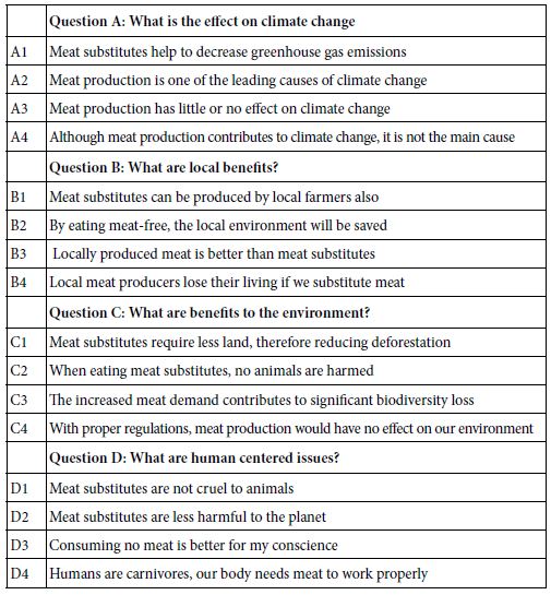
tab 1

Step 3: Create the Actual Test Stimuli, the Vignettes, and the Rating Scale

The Mind Genomics experience for the respondent is that the stimuli should comprise mixtures, combinations of elements or messages, simulating the combinations of stimuli one encounters in the environment. The respondent is presented with different combinations (the vignettes), along with a question and a rating scale. The respondent selects a rating from the scale for the specific vignette. The respondent evaluates different vignettes, rating each vignette on the same scale. The approach is radically different from the more conventional approach of ‘isolate and explore.’ The rationale is that through the evaluation of vignettes the researcher is reproducing the type of world of information which confronts the respondent every day. Mind Genomics simply takes that metaphor of combinations and converts the metaphor into a test reality by combining messages (answers) from Step 2. Note that the questions are never presented to the respondent. The respondent only sees combinations of answers. The questions are there to help the researcher create the answers.

The raw material comprises 16 elements, the four answers from each of the four questions. An underlying scheme, the permuted experimental design, creates a basic set of 24 vignettes, specifying the composition of each vignette. The 16 elements each appear five times across the 24 vignettes and are thus absent 19 times. A single vignette may have as many as four elements, or as few as two elements. No vignette contains more than one element from a question, but often a question does not contribute an element to the vignette. Finally, each respondent evaluates unique sets of 24 vignettes. The underly mathematical structures of the 24 vignettes are the same, but the actual combinations differ. This is known as a permuted design [12].

The precautions taken in the creation of the permuted design create three benefits:

  1. The vignettes cover many combinations, not just one combination. Compared to traditional methods studying the combinations, the Mind Genomics study evaluates a greater proportion of the design space, the possible vignettes. The researcher need not worry about having selected the proper set of 24 vignettes to test, which selection would mean that the research somehow ‘knew’ what combinations would be most fruitful to test. In practice the researcher need not know anything. It will the research which will reveal what is important, based upon the pattern of responses from the individuals who participate in the study.
  2. The Mind Genomics process builds in replication. Instead of measuring the response to the stimulus one time, the researcher measures the response to the stimulus five times, albeit in the presence of other elements.
  3. It is impossible to game the system. It is impossible for a normal person to figure out the underlying experimental design in the ‘heat of the moment,’ when reading 24 vignettes, one after another, each one taking about 1-5 seconds to read and evaluate.
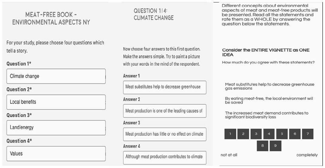
fig 1

Figure 1: Three of the set-up screens for the Mind Genomics template. Each study is templated in the same way, with screens leading the researcher through the steps.

Figure 1 presents the three major screens in the Mind Genomics program (www.BimiLeap.com)

  1. The left screen requests the researcher to type in the four questions. The questions are shown as simple phrases, as an aid to the researcher. Thus Figure 1 shows simple phrases such as ‘climate changes,’ sufficient to help the researcher create the element, viz., the answer.
  2. The middle panel shows the four questions. The researcher reads the first question or phrases (climate change) and is prompted to put in the four answers. The answers are shown as full phrases. The emphasis to the researcher is to create element which create word pictures, not just simply one or two word answers.
  3. The right panel shows an example of the introduction at the top, a vignette in the middle, and the scale at the bottom.

Different concepts about environmental aspects of meat and meat-free products will be presented. Read all the statements and rate them as a WHOLE by answering the question below the statement.

Agree: 1=Not at all … 9=Completely.

Step 4: Launch the Study, Invite the Respondents, Specifying Country, Market, Age/gender if Desired, and Other Specifics

The study was run in the United States in 2019. The issue at that time was both to understand the topic of plant-based foods from a variety of viewpoints, as well as to determine whether there would be differences in responses between two parts of the country, California vs. New York.

The study called for 50 respondents in New York, and 50 respondents in California, about equally distributed by gender and by age. The cost of the study (4$ per respondent, complete, including the fee for the respondent invitation and participation) reflects the fact that the Mind Genomics platform was created as a service to the world of education, society, health, and business. The low cost makes it possible for anyone to become a researcher.

At the start of the evaluation the respondent recorded gender, age, and answer the preliminary question regarding their behavior and attitude towards meat and the environment

Preliminary question: Which of the following describes you the best?

1=I eat meat and do care about the environment

2=I eat meat and don’t care about the environment

3=I don’t eat meat and do care about the environment

4=I don’t eat meat and don’t care about the environment

5=Not applicable

The Mind Genomics program assembles the 24 different vignettes prescribed for the specific respondent and presents them in a specific order to the respondent. Previous studies suggested that the respondent should be given a practice vignette. The practice vignette is vignette #24. The vignette is presented to the respondent, but the rating is not recorded. The vignette will be presented again, as the last vignette, and then the rating recorded.

Preliminary inspection of the ratings showed that out of 102 respondents who ended up participating 15 respondents showed ratings either of 1-2, 8-9, or one rating across all 24 vignettes, respectively. These 15 respondents were removed from the data set, based upon the belief that the respondents were either not paying attention, or were agreeing or disagreeing with everything, and thus showing no ability to discriminate.

Step 5: Modeling to Relate the Presence/absence of the Elements to the Ratings

The essence of Mind Genomics is the effort to relate the presence or absence of the elements to the ratings. Most users of research accept Likert scales, such as the 9-point scale presented here, but feel uncomfortable interpreting the individual scale values. One way to help them is to anchor the ends of the scales, another way to help them labels each scale point, as was done in the introductory, self-profiling questionnaire, wherein the respondent classified herself/himself with respect to meat-consumption and feelings about the environment. For this study, the rating scale was simply anchored at both extremes, with no attempt to label the intermediate points.

The Mind Genomics system uses a Likert scale to quantify the response, since it is simple for the respondent. The subsequent analysis, after the data collection, transforms the scale into a binary scale, vs 100, a transformation which makes the data more understandable. The 9-point scale was divided into two sections, based upon a criterion which makes sense. for this study. Ratings 9 and 8 were assumed to denote ‘agreement’ and were transformed to 100, with a vanishingly small random number added. Ratings 1-7 were assumed to reflect either no agreement or an uncertain mix of agreement and disagreement. These later ratings were transformed to 0, again with a vanishingly small random number added.

The small random number added to the transformation ensured that the transformed ratings from one respondent would not either be 100 for all or 0 for all. The addition of the vanishingly small random number prevents the OLS (ordinary least squares) regression from crashing, which would occur when all transformed ratings are 0, or in the other case when all transformed ratings are 100.

Step 6: Surface Analysis of the Ratings

The first analysis focuses on the degree to which the ratings change while evaluating the 24 vignettes. For our study no two vignettes were the same, making it impossible to compare the average ratings by position for the same stimulus. Each vignette only appears once. However, it makes sense to average the ratings of all the vignettes appear in position 1 (first vignette tested out of the 24), position 2, and onward to position 24.

Figure 2 shows the average transformed rating (8,9 –>100) for all vignettes in position 1, position 2 … position 24. A line fitted to the data slopes upwards but very slightly. The reality from inspecting Figure 2 is that the pattern is random.
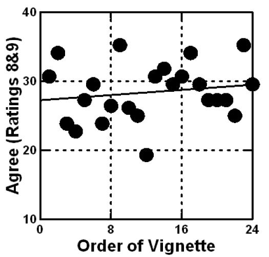
fig 2

Figure 2: Average percent of ratings ‘agree’ (ratings 9 and 8 transformed to 100) shown on the ordinate, vs each of the 24 positions in which a vignette could appear.

Step 7: Relate the Presence/absence of Elements to the Ratings and Uncover Mind-sets

The heart of Mind Genomics is the discovery of how elements ‘drive’ responses. The analysis is straightforward, made so by the judicious application of the permuted experimental design used in the construction of each respondent’s 24 vignettes. The analysis embedded in the BimiLeap program creates a database for all the data, 24 rows for each respondent. Each row corresponds to one of the 24 vignettes evaluated by that respondent.

The first set of columns in the each database record shows the respondent identification number, and the order of testing. The second set of 16 columns codes the composition of the vignette. Each of the 16 columns corresponds to one of the 16 elements, ranging from A1 to D4. When the when the element is present in a vignette, the number in the column (for that row) is ‘1’. When the element is absent from that vignette, the number in the column is 0.

The third set of columns shows the original rating, then the rating transformed to 0/100 (100 corresponds to 8,9; 0 corresponds to the remaining seven ratings 1-7), and the response time (RT) defined as number of seconds elapsing from the time the vignette was presented on the screen to the time that the rating was assigned, captured to the nearest tenth of a second.

The fourth set of columns shows the set of three classifications, gender, age, and behavior regarding eating meat and concern for the environment, respectively.

The matrix is immediately and automatically created at the end of the respondent’s evaluations. All the information is available from the study. Once the matrix is created and at any time the data can be totally analyzed since each respondent provides complete data, including the appropriate combinations of elements which allow the researcher to create an individual-level equation for the respondent.

The initial analysis creates 87 individual-level equations, each expressed as: Binary Response (Top2) = k1A1 + k2A2 … k16D4

Note that in this study the additive constant was not estimated. Continuing evaluation of the Mind Genomics methods suggest that the coefficients estimated without the additive constant correlate highly with the coefficients for the same study, this time estimated along with the additive constant. Thus, the patterns would be similar. The key difference is that the coefficients are larger when there is no additive constant. ‘Strong performing’ is here defined as a coefficient of +12 or higher, rather than +8 or higher (the value used when the additive constant is estimated).

The foregoing equation without the additive constant provides a measure of the ability of each element to drive the response. It will be the pattern of coefficients across all 87 individuals which will give us a sense of the nature of two or more groups, separated from each other based on the pattern of the coefficients. Such separation is accomplished by clustering, a way to separate ‘objects’ into non-overlapping groups based upon the patterns of their properties. The 87 rows x 16 columns were subject to a k-means clustering, to divide the respondents (rows) by the pattern of the coefficients [13]. The k-means clustering program works only on the mathematical properties of the dataset, attempting to split the respondents into two groups, and then three groups, so that the centroids of the groups on the 16 elements are as different (distant) as possible, whereas the individuals within a group are similar (close) as close as possible. The measure of distance between people, and between centroids was defined operationally as (1-Pearson R). The Pearson R, or the correlation, takes on the value +1 when two patterns are identical; the distance between them is 1-1, viz., 0. The Pearson R takes on the value of -1 when two patterns are identical; the distance between them is 1- -1, viz., 2.

The values for the coefficients based upon the Top2 (Ratings 9,8 –>100) appear in Table 2. The table shows the elements sorted based upon the values of the two emergent mind-sets, discussed below. The important thing to notice in Table 2 are those elements with coefficients of +12 or higher. Statistical analysis using OLS (ordinary least squares) regression, suggests that coefficients of this magnitude become statistically significant as well as ‘meaningful’ in a real-world sense when the equation is estimated without an additive constant.

Table 2: Coefficients for models relating the presence/absence of the elements to the level of ‘strong agreement’ (rating 9, 8 converted to 100). Strong coefficients (+12 or higher) appear in shaded cells. Coefficients of 5 and below are not shown.
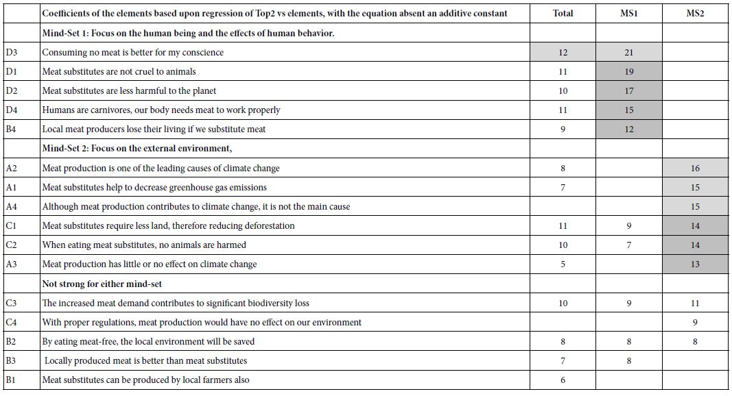
tab 2

The importance in a Mind Genomics study is not the magnitude of a single element nor its difference from 0, but rather the pattern of coefficients for a single group. When we look at the first data column, corresponding to Total Panel, we fail to see truly strong elements emerging, viz., elements which generate a coefficient of +12 or more. This is not surprising, given the ability of Mind Genomics to uncover groups of individuals with different patterns of coefficients, suggesting different ways of thinking about the same topic. Putting together these different mind-sets into one database ends up attenuating the strong patterns of each.

Table 2 shows the results from the clustering. The two-cluster solution, shown in the second and third data columns, suggests two clearly different mind-sets, groups of individuals who, faced with the same material, think in different ways. Mind-Set 1 focuses on the human being, and the effects of human behavior. Mind-Set 2 focuses on the external environment. Note that in the interest of allowing the patterns to emerge, the table shows coefficients of 12 or higher in shaded cells. There might well be more mind-sets, but for the purposes of this exploratory research two mind-sets suffice to demonstrate the radically different patterns. Extracting the third mind-set did not reveal a new group with a demonstrably new pattern of coefficients.

Table 3 shows the self-profiled classification of the respondents in the two mind-sets. The base sizes do not always add to 87 because in some cases the respondents left out the answer to one of the classification questions.

Table 3: Classification of the respondents by gender, market, meat-eating, and concern with the environment
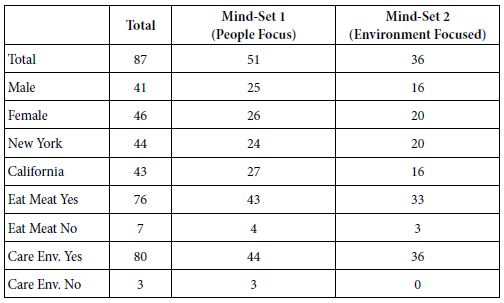
tab 3

Step 8: Measure Engagement with the Messages Using Response Time

Today’s concern with the environment continues to generate controversy, and emotion. The notion that our omnivore habits are the cause for climate change through animal farming continues to emerge, again and again, both in the popular press and in academic literature [14,15]. With the attention paid to climate, and with the importance of food and the increasing focus on vegetable-based meat, we have an opportunity to investigate the degree to which messages grab the attention of people, engaging them, not through a conscious probe of what they ‘feel’, but rather in the amount of time the person gives to reading, digesting, and then responding to the messages.

The Mind Genomics platform provides a measure of engagement through the response time. Response time is defined as the time elapsing from the moment the stimulus is presented until the moment the respondent. A small prophylactic measure moves all response times of 8 seconds or longer either to 8 seconds (done here) or removes the data point from analysis (not done here). The rationale for this prophylactic measure is that the respondents may be multi-tasking, which would produce a false measure of response time for the vignette.

The model for response time is the same as the model for the transformed rating, viz no additive constant. The 16 coefficients show the number of seconds that can be ascribed to each element, including reading and judging. Table 4 shows these coefficients for the total panel, and for both mind-sets.

Table 4: Response times in seconds attributed to each of the elements, by total panel and two mind-sets. The numbers in the body of the table are the number of seconds attributable to the element.
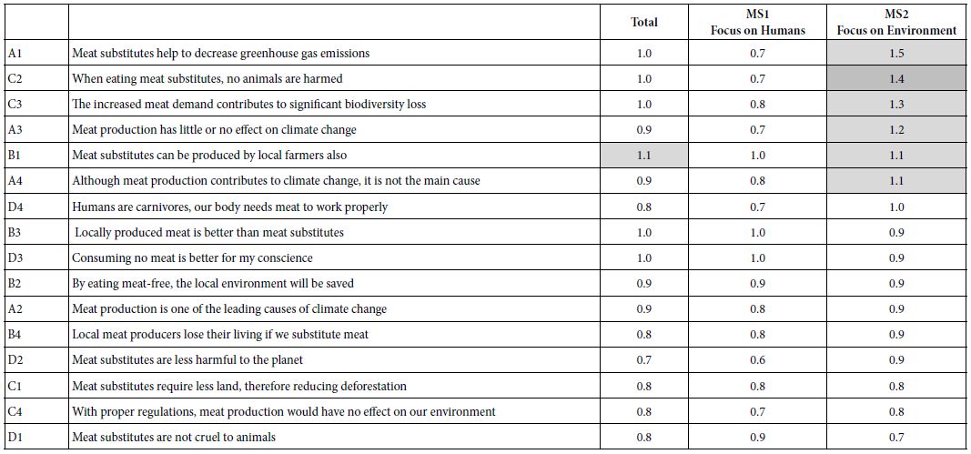
tab 4

The response times suggest dramatically different patterns of attention. Those respondents in Mind-Set 1, focusing on people and the human aspects, pay little attention to the elements. The only element to which they pay attention is B1, Meat substitutes can be produced by local farmers also (RT coefficient = 1.0). In contrast, those respondents in Mind Set 2, responding to the environment, pay more attention to certain elements, viz., those elements focusing on the environment.

A1           Meat substitutes help to decrease greenhouse gas emissions                                   1.5

C2              When eating meat substitutes, no animals are harmed                                       1.4

C3              The increased meat demand contributes to significant biodiversity loss             1.3

A3              Meat production has little or no effect on climate change                                    1.2

Step 9: How Mind-sets Process Interactions between Pairs of Elements

Our previous analysis focused on the performance of individual elements, showing clear differences between elements according to the two clearly different mind-sets. We saw two radically different mind-sets emerge, differing both in the elements which drive their agreement, as well as the speed at which they process information. These mind-sets focus on topics, but also represent different types of individuals. It would appear from informal observation that people who focus on the climate (Mind-Set 2) seem to be more outwardly verbal about the topic. In contrast, people who focus on the behavior of other individuals (Mind-Set 1) seem to be quiet.

Do these two mind-sets differ in the way they process information? That is, when we provide the respondents with combinations of the same type of elements versus different types of elements, how do they respond to the combination? Do the elements synergize, or suppress each other? Our strategy to assess interactions is called scenario analysis [6]. Scenario analysis follows these steps:

a. Select one question which will define the five different strata. This will be Question B, pertaining to ‘local benefits.’ Two of the four elements from Question B focus on people (B2 Meat substitutes can be produced by local farmers also; B4 Locally produced meat is better than meat substitutes). The remaining two elements from Question B focus on the environment (B1 although meat production contributes to climate change, it is not the main cause; B3 By eating meat-free, the local environment will be saved).

b. Working with the entire database of 87 respondents x 24 rows/respondent, divide the database into five groups or strata, each stratum determined by the specific element from question B. The first stratum comprises all vignettes containing element B1. The second stratum comprise all vignettes containing element B2 and on to the fifth stratum, which contains no element from question B. We will not consider the fifth stratum, those vignettes lacking an element from Question B.

c. We create four equations, one per stratum, relating the presence/absence of the remaining 12 elements to the transformed rating, the dependent variable (DV). The equation is: expressed as: DV=k1(A1) +k2(A2) +k3(A3) +k4(A4) +k5(C1) +k6(C2) + k7(C3) +k8(C4) +k9(D1) +k10(D2) +k11(D3) +k12(D4)

d. Table 5 presents the strong performing coefficients, defined operationally for this table only as a coefficient of +20 or higher. These very strong performing coefficients are presented in shaded cells. The remaining coefficients are suppressed, allowing the patterns to emerge.

Table 5: Scenario Analysis. The coefficients of elements from Questions A, C and D for different ‘strata’ defined by a fixed element from Question B.
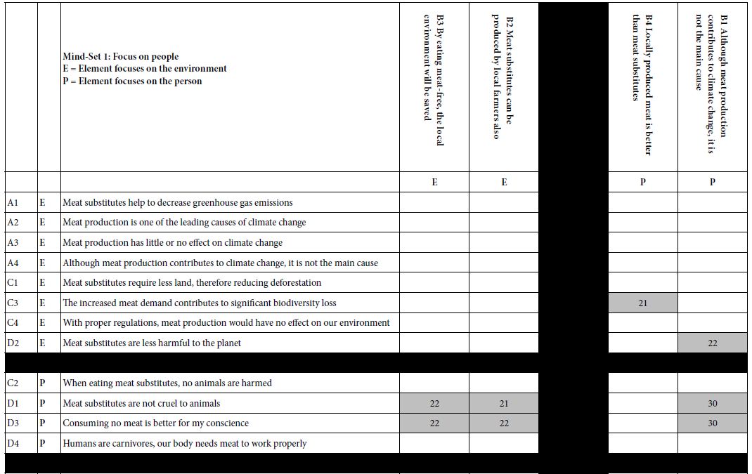
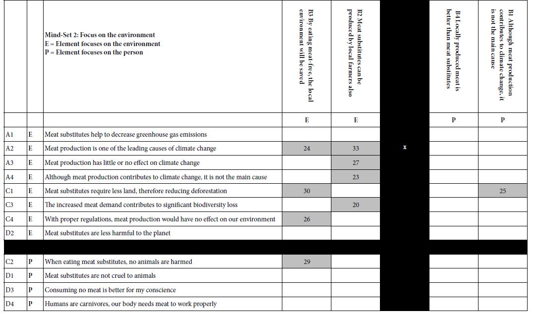
tab 5(1)

tab 5(2)

e. For Mind-Set 1 (focus on people), synergisms among elements occur when elements about the person are combined either with other elements about the person, or with elements about the environment. In fact, Mind-Set 1 shows six strong interactions out of 24 possible interactions between pairs of elements, one about environment, the other about the person. Mind-Set 1 seems to be able to take in all the information in the vignette to assign the rating. We do not get a sense of overly-focused perception on the topic of food and the environment.

f. Mind-Set 2 (focus on the environment) thinks differently, showing only two strong interactions out of 24 possible interactions. We get a sense of people in Mind-Set 2 thinking in a more focused manner, looking primarily at the messaging about the environment, not focusing on any other type of message.

Discussion and Conclusions

We can barely listen to the ever-updated business reports without hearing of the successes and now troubles or even failures of companies in this new food ‘space.’ Furthermore, the ability of concerned individuals to invoke issues of great emotionality such as the environment increases the intensity of the noise as it does the intensity of the signal [16].

The Mind Genomics exploration of the intersection of the environment and plant-based meats provides a way for the researcher to understand topics where there may be as much ‘noise’ as there is ‘signal. Mind Genomics studies are run in what might be called a ‘sterile’ fashion, without leading questions, but with test stimuli which may run the gamut from simple factual statements to statements designed to appeal to the emotions, with or without supporting facts. By testing the elements of all types in ever-changing combinations, it becomes possible for the researcher to assess the strengths and weaknesses of these statements as the consumer respondent see them, while preventing the respondent from ‘gaming’ the system. No matter what the mind-set of the respondent may be, the ever-changing combinations mean that the respondent ends up assigning honest ratings, even if the respondent feels that the rating is a ‘guess.’ The data in Tables 2, 4 and 5 reveal a great deal of consistency.

The complexity of thinking around the emotional and ethical response to the topic of ‘plant-based meat’ is staggering. A Google search of the topic of plant-based meat reveals 2.85 million hits, during early February 2023. Going more deeply into the topics of environment versus effect on people, the same topic of ‘plant-based meat’ combined with ‘effect on people’ generates 1.61 million hits. In turn, ‘plant-based meat’ combined with ‘effect on the environment generates 2.06 million hits. One must read a great deal about the topic to begin to intuit the existence of the two mind-sets. In contrast, almost immediately, the Mind Genomics exercise provides a sense of how people organize the topic. From the practical point of view, Mind Genomics provides a path to selecting the information appropriate to present to the audience, once it can be determined the mind-set to which the person belongs. If that capability is not available, then the next strategy is to explore different messages with individuals of known mind-sets, selecting an array of messages likely to appeal to each mind-set, while not alienating the other mind-set.

A search through the published literature confirms what was found in this study, namely that there are at least two different directions of thinking about the topic. On the one hand, there are those papers focusing on people and their intersection with the world of plant-based foods, viz. our Mind-Set 1 [15,17-19]. In contrast, there are those papers which deal with the issues of food and the environment, viz., our Mind-Set 2 [20,21]. What is missing from these papers, however, is the way people think, the nature of how they incorporate information, and how they combine similar types of information versus dissimilar types of information about the topic. It is as if the Mind Genomics approach might provide ‘informational mortar’, to help the other data provide deeper insights [22].

As it is worthwhile finishing this paper with some observations about the role of Mind Genomics in the ‘Project of Science. People are not accustomed to ‘design thinking.’ Most of the ideas which people proffer appear to emerge fully developed, or perhaps seem to require slight modification. There is the mystique that creating a new idea occurs during the almost impossible-to-describe ‘creative leap of faith.’ The likelihood of successfully bringing this leap of faith to business is thought to be by better ‘insights.’ Such insights believed to likely emerge when one uses by focus groups, in-depth interview, ‘creative exercises,’ or gives over the task to people who are deemed to be ‘creatives’, the latter either because of their corporation position or because they score well on a test presumed to measure ‘creativity.’ Creativity is elevated to an art, one which is special, but can be learned.

The elevation of the creative act into almost mystical moments, achievable of course by everyone, means that the mystique must be preserved. It is the thinking, the ‘aha’ experience, which is important. It is the idea, emerging like Venus, almost fully formed, with some need of polishing, which is important. Consequently, much of the research conducted today with consumers is commissioned to validate or falsify a hypothesis, a test of the consumer acceptance of one’s idea in business. It should come as no surprise then that the Russian wisdom is touted again and again; measure nine times cut once. It is at the point of cutting, of making a yes/no decision about the object created that the research effort is executed.

The Mind Genomics approach differs. Mind Genomics can be considered a cartography, an exercise in mapping terrain, terrain which is new, or terrain that has been well trodden but needs new measurement for one or another reason. The implementation of this of mapping exercise occurs in a straightforward manner; present different stimuli to the respondent, measure the reactions to these stimuli, and from the pattern of those reactions identify the driving power of each of the elements to ‘drive; the response. The approach is akin to creating the blueprints of a system, showing through experimentation how the different parts work together to drive the response. The steps are simple, iterative, and powerful in that they deal directly with the relevant stimuli, without having to force interpretation. It is likely that, when implemented in simple, small, affordable experiments like the one reported here, design thinking will prove its value, showing how the system ‘works’, identifying ‘what to do’, and then ‘what to communicate about what one has done.’

References

  1. Araújo MB, Whittaker RJ, Ladle RJ, Erhard M (2005) Reducing uncertainty in projections of extinction risk from climate change. Global ecology and Biogeography 14: 529-538.
  2. Bush DM, Neal WJ, Young RS, Pilkey OH (1999) Utilization of geoindicators for rapid assessment of coastal-hazard risk and mitigation. Ocean & Coastal Management 42: 647-670.
  3. Bonny SP, Gardner GE, Pethick DW, Hocquette JF (2017) Artificial meat and the future of the meat industry. Animal Production Science 57: 2216-2223.
  4. Demartini E, Vecchiato D, Finos L, Mattavelli S, Gaviglio A (2022) Would you buy vegan meatballs? The policy issues around vegan and meat-sounding labelling of plant-based meat alternatives. Food Policy 111.
  5. Van Vliet S, Kronberg L, Provenza FD (2020) Plant-based meats, human health, and climate change. Frontiers in Sustainable Food Systems 128.
  6. Moskowitz HR, Gofman A (2007) Selling Blue Elephants: How to Make Great Products that People Want Before They Even Know They Want Them. Pearson Education.
  7. Grotjahn M (1950) About The “Third Ear” In Psychoanalysis: A Review and Critical Evaluation of: Theodor Reik’s “Listening with the Third Ear; The. Psychoanalytic Review 37: 56-65. [crossref]
  8. Jacoby LL, Wahlheim CN, Coane JH (2010) Test-enhanced learning of natural concepts: effects on recognition memory, classification, and metacognition. Journal of Experimental Psychology: Learning, Memory, and Cognition 36: 1441-1451. [crossref]
  9. Moskowitz HR, Porretta S, Silcher M (2008) Concept research in food product design and development. John Wiley & Sons.
  10. Moskowitz HR, Reisner M, Lawlor JB, Deliza R (2009) Packaging research in food product design and development. John Wiley & Sons.
  11. Gere A, Harizi A, Bellissimo N, Roberts D, Moskowit H (2020) Creating a Genomics wiki for non-meat analogs. Sustainability.
  12. Gofman A, Moskowitz H (2010) Isomorphic permuted experimental designs and their application in conjoint analysis. Journal of Sensory Studies 25: 127-145.
  13. Likas A, Vlassis N, Verbeek JJ (2003) The global k-means clustering algorithm. Pattern Recognition 36: 451-461.
  14. Djekic I (2015) Environmental impact of meat industry – current status and future perspectives. Procedia Food Science 5: 61-64. Djekic I (2015) Environmental impact of meat industry – current status and future perspectives. Procedia Food Science 5: 61-64.
  15. Pimentel D, Pimentel M (2003) Sustainability of meat-based and plant-based diets and the environment. The American journal of clinical nutrition 78: 660S-663S. [crossref]
  16. Macdiarmid JI, Douglas F, Campbell J (2016) Eating like there’s no tomorrow: Public awareness of the environmental impact of food and reluctance to eat less meat as part of a sustainable diet. Appetite 96: 487-493. [crossref]
  17. Broad GM (2020) Making meat better: The metaphors of plant-based and cell-based meat innovation. Environmental Communication 14: 919-932.
  18. Curtain F, Grafenaue S (2019) Plant-based meat substitutes in the flexitarian age: An audit of products on supermarket shelves. Nutrients 11: 2603. [crossref]
  19. Slade P (2018) If you build it, will they eat it? Consumer preferences for plant-based and cultured meat burgers. Appetite 125: 428-437.
  20. Joshi VK, Kumar S (2015) Meat Analogues: Plant based alternatives to meat products-A review. International Journal of Food and Fermentation Technology 5: 107-119.
  21. Siegrist M, Hartmann C (2019) Impact of sustainability perception on consumption of organic meat and meat substitutes. Appetite 132: 196-202. [crossref]
  22. Saulo AA, Moskowitz HR (2011) Uncovering the mind-sets of consumers towards food safety messages. Food quality and preference 22: 422-432.
Empowering Young Researchers: Cognitive Economics and the Features Associated with Minimum Wage

DOI: 10.31038/ASMHS.2023713

Abstract

Respondents evaluated unique combinations of messages dealing both with the levels of minimum wage, and reasons for minimum wage, selecting one of five minimum wages that would fit each combination, respectively. The underlying experimental design ensured that each respondent had the appropriate set of vignettes so that it would be possible to create an equation showing the ‘dollar value’ of each of the messages. Regression modeling and clustering analysis revealed three emergent mind-sets, (Government should do the work; Individual should save money; Individual should suffer). The most effective messages to generate higher ratings of minimum wage were those suggesting what the person might do in order to economize, and live within their means. The least effective messages were those talking about what the government should do regarding minimum wages. Respondents paid attention to dollar values of minimum wage primarily for messages which presented additional information, such as the specific state where that minimum wage was the law. The paper shows the potential for creating a new learning and research paradigm for students, incorporating artificial intelligence to suggest questions and answers about a topic (learning phase), coupled with a templated program to acquire the responses to real people to the information provided by AI (experiential learning through research).

Introduction

The topic of minimal wage, often called minimal living wage, continues to draw attention, year after year [1]. Whether the issue is considered from the vantage point of economics [2,3], consumer research (e.g., [4]), or as part of the corpus of topics focused in by social planners and government economists [5], the topic never ceases to draw attention. Indeed, major treatises have been developed by economists relating minimal wage to a variety of other issues in society, both structural and behavior (e.g., [6]). And, of course, the sheer relevance of minimum wage continues to be the topic of numerous popular articles, and op ed letters (e.g., [7])

This paper emerged from the efforts of a student researcher in middle school in the Bronx, New York, the first author, Cledwin Mendoza. The topic was part of the senior author Mendoza’s effort to use Mind Genomics to explore the topic of minimum wage, from the point of view of a student looking at the world of adults, a world that he would soon enter. The underlying strategy was that to better understand the topic of minimum wage, one might explore some aspect of the topic from the point of view of a middle school student, using a combination of artificial intelligence to help frame questions and answers, along with one’s own experience to modify the output of artificial intelligence. The next step would be to understand how other young people would respond to these ideas. The strategy combines learning through questioning with artificial intelligence, and then evaluating what is learned by experiments with real people. The effort is called Mind Genomics, the computer program is BimiLeap, and the effort may be best understood as experimental analysis of topics of the everyday.

The study focuses on the ability of different messages about minimum wage to ‘drive’ estimated dollar values of the minimum wage. That is, the desire was to learn whether there were any types of messages which convinced people to increase the minimum wage that a worker might receive, and to the contrary, what types of messages convinced people to actually lower the minimum wage that a worker might receive.

Mind Genomics and ‘Cognitive Economics’

The approach used in this study is known as Mind Genomics, with a specific variant, known as Cognitive Economics. Mind Genomics is an emerging science focusing on the way we make decisions about the topics of the everyday [8,9]. Mind Genomics was founded on the belief that a strong way to understand people’s decisions is to present them with combinations of features relevant to the decision making (so -called vignette, which combine together elements), instruct the respondent to make a decision (e.g., assign a rating to the vignette), and then after having presented the respondent with an appropriate set of such vignettes, obtain the ratings, and deconstruct the pattern of rating into the contribution or driving power of each message, each element. In other words, combine elements, present combinations, get ratings, deconstruct the response, and create the knowledge base. The paper will explain each of these.

Method

The Mind Genomics approach followed a choreographed process, the steps set up to prepare the data for statistical analysis using OLS (ordinary least-squares) regression. The objective of the analysis is to generate a model, viz., an equation, relating the presence/absence of the raw materials (messages about minimum wage) to a dependent variable. For the study reported here, the dependent variable is a selection of an appropriate minimum wage, based upon how the respondent interprets the messages about minimum wage.

Step 1: Define the Topic, and then Create Both Questions and Answers (Messages) Which Present Information about Minimum Wage

The Mind Genomics process is an exploration, so the researcher need not know anything about the topic of minimum wage to do an experiment and discover how ‘people think about minimum wage.’

This approach of beginning with questions and answers, even in the almost total absence of knowledge, stands in stark contrast to the conventional method which assumes that the research is grounded to answer a specific problem existing in the state of knowledge. The latter is called the hypothetico-deductive system, positing that research should enable one to confirm or to falsify a hypothesis, a hypothesis grounded in one’s knowledge of the topic.

From the beginning researchers may know very little about the topic and need guidance. The Mind Genomics program, www.BimiLeap.com, provides a coaching system, Idea Coach, in which the researcher types in a sentence about the topic, with Idea Coach powered by artificial intelligence (Open AI) returns with 30 questions.

Table 1 presents the query, and two sets of 30 questions about minimum wage returned by the Idea Coach. The important things to note are that the Idea Coach can be used to investigate the topic and/or to select specific questions to use for BimiLeap, thus playing both a teaching role and a direct coaching role for the study. For this study the student researchers used Idea Coach as a teaching aid, and then formulated the questions and answers afterward.

Table 1: Example of two sets of questions about minimum wage generated by Idea Coach

tab 1(1)

tab 1(2)

tab 1(3)

Table 2 shows the four questions and the four answers to each question. The Idea Coach presented these elements as answers to the four questions that the senior author selected. Once again, it is important to note that the questions were not immediately provided by Idea Coach and its AI substructure, but rather emerged after the senior research (Cledwin Mendoza) ‘learned about the topic’ using Idea Coach as an interactive tool to explore different aspects of the topic.

Table 2: The raw material, comprising four questions and four answers to each question

tab 2

Step 2 – Create Test Vignettes, viz., Combinations of Elements

In a Mind Genomics study, the respondent is instructed to rate combinations of elements, these combinations describing a situation or an offer. The strategy of testing combinations rather than single elements allows Mind Genomics to simulate what might be encountered in the ‘real world,’ which virtually always presents a person with mixtures of features to which the person must react. The notion of isolating the features and then instructing the respondent to evaluate each feature, one feature at a time, comes from the traditional world of science, where isolating a variable allows a deeper study of that variable. With a person, however, presenting a single idea out of context may end up making that single idea meaningless, as is the case for elements A1-A4, and B1-B4 in Table 1. These elements are simple ‘facts’, devoid of deeper meaning when presented alone.

To study these elements Mind Genomics mixes the elements into small combinations, the aforementioned ‘vignettes. A vignette is simply a collection of elements, one element at top of the other, without any effort to connect the elements into a grammatically correct whole. By presenting the vignette as the disconnected combination of elements in this austere format, the researcher ends up making the task easy, because the respondent can ‘graze’ through the elements and make a decision.

The actual design comprises 24 vignettes, each vignette containing two, three, or four elements, respectively. In any vignette, only one element (answer) from a question may appear, preventing a vignette from presenting two elements which may directly contradict each other. Across the 24 vignettes, each element appears five times, and is absent 19 times. Each set of 24 vignettes ensures that the 16 elements are statistically independent of each other, and thus the data from one set of 24 vignettes can be subject to regression analysis. Finally, each respondent evaluates a totally unique set of 24 vignettes. No two respondents evaluate the same set of vignettes, nor even the same vignette. These powerful features allow the researcher to evaluate a great number of combinations, permitting anyone to explore and learn about the topic in an iterative fashion. The approach is called permuted experimental designs [10].

Step 3 – Create Self-profiling Classifications, Introduction to the Study for the Respondent, the Rating Question, and the Rating Scale

Step 3 requires the researcher to think about the type of information she or he wants from the respondent. The self-profiling questionnaire allows the researcher to identify WHO the respondent is, and how the respondent THINKS, both of which can be answered directly by the respondent. The researcher describes the topic of the study, presents a rating question. The researcher creates a rating scale, that scale used by the respondent to describe her or his reaction to the vignette. The rating scale or some transformation of the scale will be used in the analysis to link the elements of the vignette to the respondent’s ‘feeling.’

In this study the researchers used a numerical scale, requiring the respondent to select the most appropriate estimate of a minimum wage after reading a vignette (Table 3). The objective was to see how the different elements would drive the dollar value of the minimum wage. This approach, instructing the respondent to estimate the dollar value of an object or experience, has been previously used in a variety of Mind Genomics studies [11,12], and has been given the name ‘Cognitive Economics’ [13,14]. Cognitive economics deals with the responses framed in money, rather than in emotion, a contrast between homo economicus versus homo emotionalis.

Table 3: Questions which the respondents answer to define who the respondent IS, and how the respondent FEELS about the different vignettes presented in the evaluation.

tab 3

Step 4: Execute the Study on the Internet

The Mind Genomics procedure is templated, allowing the researcher to follow a series of steps from the creation of the study to its actual implementation. Once the study has been set up in the template, the BimiLeap program requests the researcher to specify the nature of the respondents, including age, gender, education, geography, and so forth. With today’s reach of the Internet finding respondents is straightforward, and in the interests of time preferable to getting volunteers from one’s pool of acquaintances. The study reported here requested 100 respondents, half males, half females, ages 15-21, provided by Luc.id. The 100 respondents were reduced to 78, based upon incomplete data or incorrect qualifications provided by the respondents. The 22 respondents who did not fit were eliminated at the start of the analysis, before any effort was made to analyze the results. It is important to note that a second wave of respondents could have been recruited, but the objective was met with 78 respondents. Finally, the entire effort to set up the study, including Idea Coach, required about 45 minutes, and the field effort took about 2.5 hours from launch to completion. It is this speed and simplicity of process which makes working with an online panel supplier so attractive for both the student researcher and the professional researcher alike.

The field execution required approximately 3-5 minutes for a respondent, from the time the respondent agreed to participate, pressed the link and began, to the time that the session completed. The respondents were members of various online panels in the United State, the country chosen for the study. The respondents were selected to be no older than 21 years. Qualifying respondents were sent an email invitation, the invitation containing the link.

Those respondents who agreed to participate were asked to complete the self-profiling questionnaire, then read the orientation, and finally evaluated the 24 vignettes. The rating scale was a set of dollar values corresponding to the hourly minimum wage. The five wages were set up in increasing order, although in other studies it is often the case that the five rating values (viz., minimum wages here) might be presented in random order. In any case, the respondent had no trouble completing the study in approximately 3-5 minutes.

The BimiLeap program recorded the information about the respondent from the self-profiling questionnaire, the order of evaluation of the vignette (from 01-24), the composition of the vignette in a set of 16 columns coded 1 if element were present, 0 if absent, and then the final two columns recording the dollar rating assigned along with the response time. The response time was defined as the number of tenths of seconds elapsing between the time that the vignette appeared on the respondent’s screen and the time that the respondent pressed the appropriate key for the rating. The foregoing format of the data record ensured that the database emerging from the 78 respondents, each evaluating 24 vignettes, was immediately ready for statistical analysis.

Step 5: Create Equations (models) Relating the Presence/Absence of the 16 Elements to the Dollar Value of the Rating Scale

The equation is expressed as Dollar Value = k1(A1) + k2(A2) … k16(D4). The equation does not contain an additive constant, under the assumption that in the absence of elements there is no minimum wage. The foregoing equation is created at both a group level for all individuals in the specific group (e.g., age group, gender, etc.), and at the level of the individual respondent.

Once the data are ready for regression analysis, a further analysis created 78 individual level models relating the presence/absence of the elements and the dollar rating. These 78 models were then submitted to cluster analysis [15], to generate two and then the different groups, clusters or ‘mind-sets’ in the language of Mind Genomics. These mind-sets were defined as groups of individuals who were most similar to each other, based upon the pattern of their coefficients. The cluster program created the index for dissimilarity (1-Pearson Correlation across corresponding elements), and then attempt to minimize the index of dissimilarity within a cluster or mind-set and maximize the same index across the centroids of the two or three mind-sets. The three mind-set-solution was selected because the data seemed to be more interpretable than the data from the two-mind-set solution.

Finally, the BimiLeap program measures the response time, and created an equation relating the presence/absence of the elements to the measured response time. Once again, the equation was estimated without the additive constant, gain for the same reason; without any elements in the vignette, there would be no response. The equation is now stated as: Response Time = k1(A1) + k2(A2)… k16(D4).

Results

The first analysis looks at the data without considering that the elements themselves have cognitive meaning. For this first analysis we compute the average dollar value assigned by each respondent to the set of 24 vignettes, as well as the standard deviation of these t dollar ratings. Figure 1 shows the distribution of the averages and standard deviations across the 78 respondents. For most of the respondents the average dollar value lies between 10$/hour and $15/hour. Of more interest is the standard deviation for the 24 ratings. Low standard deviations suggest that the respondent does not change her or his selection of a minimum wage. These would be the group with standard deviations between 0 and 1, respectively. Moderate to high standard deviations suggest that the respondent is swayed by what she or he reads. There is a small cohort of respondents with standard deviations of 3 or higher.

fig 1

Figure 1: Average rating and standard deviation of ratings for each respondent across the 24 vignettes evaluated by each respondent

Figure 1 represents the type of data that are often obtained in studies. The data themselves are simply points, each point having little ‘cognitive meaning’. The points are responses. The measures, average and standard deviation, tell us something about the respondent, viz., proclivity to assign high versus low dollar values to minimum wage, or likelihood to be swayed by information. Beyond that, however, we know little.

A deeper understanding emerges when the data are subject to OLS regression, to determine the contribution of each of the 16 elements to the dollar value selected for the minimum wage. Each regression analysis incorporates only the data from the relevant group of respondents. The regression analysis provides a deeper understanding of how the respondents integrate the information they read into a selection of minimum. The respondent is presented with 24 vignettes and responds almost ‘automatically’ to each vignette.

Table 4 shows the coefficients for the total panel, gender, age, and then the three mind-sets emerging from the clustering. These coefficients are dollar values. The average coefficient and the standard deviation of the 16 coefficients are shown at the bottom of the table. The table of 16 coefficients is sorted by the value for the Total panel, viz. the estimated coefficient (viz., part-worth dollar value) from the equation for the Total panel, viz., the equation using all 24 vignettes rated by the 78 respondents. All coefficients of 3.6 or higher are shown in shaded cells to call attention to them. These coefficients suggest that the elements are perceived to ‘drive’ a higher minimum wage. The coefficient (viz., part-worth dollar value) of 3.6 was chosen as an arbitrary cutoff-off.

Table 4: Dollar Values of minimum wage attributable to elements in the vignette for subgroups of respondents based upon WHO they are, and their emergent mind-sets from clustering

tab 4

Table 4 suggests a variety of interesting patterns:

  1. For total panel, the two high coefficients feature recommendations to save money.
  2. Save Money: Track your spending and look for areas to cut back.

    Save Money: Track your spending and look for areas to cut back.

  3. Males react more strongly than do females, meaning that they choose higher dollar values. Males respond far more strongly to this element, with a coefficient denoting 90 cents more: Save Money: Cut out unnecessary expenses.
  4. Younger respondents (ages 15-18) respond strongly to statements about money. In contrast, older respondents respond strongly to statements about how to save money. This is an important emergent finding, suggesting different ways of processing information.
  5. Three mind-sets emerged based upon similar patterns of coefficients. Mind Genomics studies again and again show that the greatest differences among comparable groups emerge from clustering people based on their responses to a granular topic. Thus, we should expect to see the largest group to group differences across the three mind-sets, which we do.

Mind=Set 1 feels that the government should do the work, and feels empowered to assign high minimum wages when they read about these wages being actually paid out in Los Angeles and in San Francisco.

How to increase minimum wage: Introduce a living wage ordinance that requires employers to pay a living wage

How to increase minimum wage: Provide tax credits or other incentives to employers who pay a living

How to increase minimum wage: Establish a national minimum wage that is tied to the cost of living wage

Minimum age in your area: $13.25/hour (Los Angeles City minimum wage)

Minimum age in your area: $12.00/hour (San Francisco minimum wage)

Mind-Set 2 feels that it is the job of the individual to make the best of the situation by saving money.

Save Money: Track your spending and look for areas to cut back.

Save Money: Cut out unnecessary expenses.

Save Money: Take advantage of discounts and coupons.

Mind-Set 3 appears to be what one might call penurious and judgmental.

Save Money: Cut out unnecessary expenses.

Minimum wage earnings $7.25/hour x 25 hours/week = $181.25/week or $725/month.

The self-profiling questionnaire at the start of the interview required the respondent to choose an appropriate minimum wage, with eight options, six of which comprised more than 10 respondents, and are thus shown (Table 5). Table 5 shows that the respondents who said that they wanted a higher minimum wage in self-profiling classification ended up generating higher part-worth coefficients for the minimum wage across the different vignettes. The coefficients for this group appear in the right-most column of Table 5. The average estimated dollar value across all 16 elements was $3.90, higher than the average of all the remaining groups.

Table 5: Dollar Values of minimum wage attributable to elements in the vignette for subgroups of respondents based upon their self-stated choice of the minimum wage

tab 5

Response Time as a Measure

The literature of experimental psychology is replete with papers on response time (RT). RT is assumed to reflect underlying psychological processes, with shorter RT’s representing fewer ongoing cognitive processes, and in contrast, longer RT’s representing more ongoing processes [16,17]. The BimiLeap program measures the RT by measuring the time elapsed between the presentation of the vignette and the response to the vignette. The BimiLeap program ‘assumes’ that a reasonable maximum RT for a native English-speaking respondent should be no longer than 9 seconds, and truncates at RT’s so that 9 seconds ends up as the maximum RT.

Table 6 shows the RT for the elements based on respondents as defined by WHO they are, and their mind-sets. Table 7 shows the RT for the elements based upon respondents as they select the appropriate minimum wage through the self-profiling questionnaire. In both tables the elements are sorted by the RT for the total panel. RT’s of 0.8 seconds or higher is shown by shaded cells. These are elements to which the respondent ‘pays more attention’, whether for reasons of interest, difficulty in understanding and so forth. The response time of 0.8 seconds was chosen as a representatively long response time, based upon the experience of author HRM.

Table 6: Estimated response time for each element (row), and each key subgroup (total, gender, age, emergent mindset (column)

tab 6

Table 7: Estimated response time for each element (row), and each key subgroup self-defining the appropriate minimum wage (column)

TAB 7

Table 6 shows that the longest response times are those which tell the respondent what to do, as well as information about the minimum wage in New York and in San Francisco.

Save Money: Track your spending and look for areas to cut back.

Minimum age in your area: $11.25/hour (New York City minimum wage)

Minimum age in your area: $12.00/hour (San Francisco minimum wage)

The shortest response time, not surprisingly, comes from an element which might be considered a ‘throw-away,’ viz., and element which seems to convey nothing but a platitude:

How to increase minimum wage: Introduce a living wage ordinance that requires employers to pay a living wage.

In terms of gender, females show longer RT’s than do males for almost all elements, and thus end up with an average response time of 0.2 seconds longer. Females appear to take the time to read the vignettes more slowly, and presumably more carefully.

The two age groups respond similarly as do the three mind-sets. There are differences between and among the groups, but the differences do not create a meaningful pattern that one can interpret.

When we turn to Table 7, the groups defined by the minimum wage that they self-define at the start of the study, we find no elements which generate consistently long response times.

Discussion and Conclusions

The study originated with the question about minimum wage, specifically whether giving minimum wage information was more persuasive than talking about minimum wage in a discursive manner. The study was designed to determine whether the selected value of the minimum wage could be traced to the specific elements. The underlying experimental design allowed the research to deconstruct the selection of a minimum wage into the contributions of each of four types of information; dollar value of minimum wage in four markets, dollar value of four levels of minimum wage; how to survive on the minimum wage; and what the government should do, respectively.

The important observations are quite simple:

  1. Some messages reach the emotions of the respondent, triggering the selection of a higher minimum wage. These are most likely to be messages about what to do, not informational messages about what is:
  2. Save Money: Track your spending and look for areas to cut back.

    Save Money: Cut out unnecessary expenses.

  3. People pay more attention to the meaning of messages rather than to the amount of money stated in the message. We see first and indirectly when we end up with similar dollar values for two ‘parallel’ statements about minimum wages:
  4. Minimum wage earnings $7.25/hour x 25 hours/week = $181.25/week or $725/month

    Minimum wage earnings: $7.25/hour x 40 hours/week = $290/week or $1,160/month

  5. If there is a pattern between dollar value from the coefficient and stated dollar value in the vignette, then the messages most likely also contains a cognitively meaningful and relevant message. The data below suggest that when we provide information to accompany the dollar value (viz., city) a pattern does emerge. Thus the element presenting Chicago ($8.55 minimum wage) generates the highest coefficient (contribution to minimum wage). The coefficient is 3.5. In contrast, the elements presenting Los Angeles and San Francisco (minimum wages stated as $13.25 and $12.00) end up having the lowest value in the group, coefficients of 3.1 for each.

Minimum age in your area: $8.55/hour (Chicago minimum wage) 3.5

Minimum age in your area: $11.25/hour (New York City minimum wage) 3.2

Minimum age in your area: $13.25/hour (Los Angeles City minimum wage) 3.1

Minimum age in your area: $12.00/hour (San Francisco minimum wage) 3.1

Beyond the specifics of the study is, perhaps, the most important finding of the research effort is the creation of a simple process which makes it easy for students to explore topics of social importance from their point of view, and contribute in a meaningful, serious way to knowledge. The templated Mind Genomics system, featuring Idea Coach empowered by artificial intelligence to help formulate questions and answers, provides a game-like introduction to the world of serious research. Just as important is the ability to ‘test’ the answers through consumer research. Even while having fun and learning, the student can do serious work, and emerge with important results.

There is a structural benefit to the above, the benefit of educating a generation fast, more deeply, at far less cost, and engaging the student by making the student an expert in the topic which is of interest. Rather than requiring years of understanding a topic before one is permitted to do ‘serious research’, the BimiLeap program teaches the student about the topic, allowing the student to use artificial intelligence in order to suggest questions, and provide answers, with answers that can be further explored with real people. At the same time that the student learns about the topic by interacting with artificial intelligence in Idea Coach, the student is encouraged to take an active role, to use the information in an experiment, and by so doing provide new-to-the-world knowledge, and often discoveries. It may be the best of all worlds, a source of learning through Idea Coach, and a template for involved, experiential learning and discovery, with the real opportunity to major, new-to-the-world contributions to a topic as one learns about that topic.

References

  1. Waltman JL (2000) The Politics of the Minimum Wage. University of Illinois Press.
  2. Frank RH, Cartwright E (2010) Microeconomics and behavior (Vol. 8). New York, McGraw-Hill.
  3. Sauer R (2018) The macroeconomics of the minimum wage. Journal of Macroeconomics 56: 89-112.
  4. Palazzolo M, Pattabhiramaiah A (2021) The minimum wage and consumer nutrition. Journal of Marketing Research 58: 845-869.
  5. McCurdy, Thomas (2015) How effective is the minimum wage at supporting the poor? Journal of Political Economy 123: 497-545.
  6. Kaufman BE (2010) Institutional economics and the minimum wage: broadening the theoretical and policy debate. ILR Review 63: 427-453.
  7. Gertner J (2006) What is a living wage? New York Times Magazine, January 15, 2006.
  8. Moskowitz HR (2012) ‘Mind Genomics’: The experimental, inductive science of the ordinary, and its application to aspects of food and feeding. Physiology & behavior 107: 606-613. [crossref]
  9. Porretta S, Gere A, Radványi D, Moskowitz H (2019) Mind Genomics (Conjoint Analysis): The new concept research in the analysis of consumer behaviour and choice. Trends in Food Science & Technology 84: 29-33.
  10. Gofman A, Moskowitz H (2010) Isomorphic permuted experimental designs and their application in conjoint analysis. Journal of Sensory Studies 25: 127-145.
  11. Galanter E, Moskowitz H, Silcher M (2011) People, Preferences and Prices: Sequencing the Economic Genome of the Consumer Mind. Bentham Science Publishers.
  12. Saulo A, Moskowitz V, Gere A, Papajorgji P, Ettinger Lieberman L, et al. (2019) Linking food endorsement labels & messaging to perceived price and emotions. A Mind Genomics® Exploration. Advances in Nutrition and Food Science 5.
  13. Moskowitz H, Moskowitz D (2022) Systematics of communication: Conjoint measurement, Emotions, cognitive economics, and Consumer Mind-sets. Product Innovation Toolbox: A Field Guide to Consumer Understanding and Research 198-244.
  14. Moskowitz H, Rappaport S, Moskowitz D, Porretta S, Velema B, et al. (2017) Product design for bread through mind genomics and cognitive economics. In: Developing New Functional Food and Nutraceutical Products 249-278, Academic Press.
  15. Likas A, Vlassis N, Verbeek JJ (2003) The global k-means clustering algorithm. Pattern Recognition 36: 451-461.
  16. Bassili JN, Fletcher JF (1991) Response-time measurement in survey research a method for CATI and a new look at nonattitudes. Public Opinion Quarterly 55: 331-346.
  17. Yan T, Tourangeau R (2008) Fast times and easy questions: The effects of age, experience and question complexity on web survey response times. Applied Cognitive Psychology 22: 51-68.

Cremaster Myogenenis in the Mouse Gubernaculum and the Effect of Androgen

DOI: 10.31038/PSC.2023311

Abstract

Background/Aim: Cremaster muscle is a specialized skeletal muscle, and its differentiation into mature skeletal muscle is normally delayed until after gubernacular migration to the scrotum. The molecular cues regulating its morphology remain elusive. We examined gene expression and immunofluorescence of known markers expressed in cremaster muscle to determine the effect of androgen blockade.

Methods: Gubernacular cells from wild-type (WT) and androgen receptor knock-out (ARKO) mice were cultured at E17, D0 and D3 (n=3 animals/group/day) and qPCR performed for b-Catenin; Desmin; Myogenin; Ki67; Pax 7; PPAR-g; Myh3; and Androgen receptor (AR). The same age groups were also processed for fluorescent immunohistochemistry, and visualized by confocal microscopy.

Results: Β-Catenin expression at D3 was increased in ARKO compared to control animals, and β-Catenin immunofluorescence demonstrated increased cytoplasmic staining in D3 ARKO animals and displaced in the banding pattern of mature skeletal muscle. Desmin, Myogenin and Ki67 expression were all increased in D3 ARKO compared to control animals.

Conclusions: Blockade of androgen in mice demonstrates increased expression of myogenic proteins at D3. This is consistent with premature maturation of cremaster muscle, which is associated with failed elongation of the gubernaculum, incomplete testicular migration to the scrotum, leading to cryptorchidism.

Keywords

Cryptorchidism, Beta-catenin, Testes, Cremaster muscle

Highlights

  1. What is currently known about this topic?
  2. Androgen controls the second stage of testicular descent. As the testes descend, the cremaster muscle is formed within the gubernacular mesenchyme. Cremaster myogenesis is known to involve the expression of β-Catenin; Desmin; Myogenin; Ki67; Pax 7; PPAR-g; and Myh3.

    1. What new information is contained in this article?

    Androgen seems to delay maturation of cremaster muscle allowing elongation of the gubernaculum and migration of the testis. Androgen receptor knockout animals express markers of muscle maturation earlier than control animals, consistent with premature maturation of the cremaster muscle.

    Introduction

    Testicular descent is vital for fertility and prevention of testicular malignancy. Failed testicular descent is one of the most common genital anomalies, affecting 2-4% of newborn males. The gubernaculum, or genitoinguinal ligament, controls testicular descent and subsequent cremaster formation within it in both rodents and humans. Androgen is the primary hormone that regulates the second stage of testicular descent, the inguinoscrotal phase, where the gubernaculum migrates across the pubic bone to reach the scrotum. This migration phase involves gubernacular remodelling and cremaster muscle formation; however the exact molecular mechanisms controlling this remain unknown [1-5].

    The gubernacular mesenchyme differentiates into the cremaster muscle, which is a specialized skeletal muscle with specialized properties that differ to other skeletal muscles. The most distal portion of the rodent gubernaculum containing more myoblasts than the proximal end, so the gubernaculum can elongate like an embryonic limb bud from a distal growth centre with cremaster development more advanced proximally [6,7]. Gubernacular eversion is an integral part of testicular descent in rodents. Rats treated with the anti-androgen (flutamide) demonstrated smaller cremaster muscle mass and a reduction in the size of the growth centre in the gubernaculum. Androgen receptor knockout (ARKO) mice demonstrate failed gubernacular eversion, and increase in gubernacular cord length with age between E17-D4 [8,9]. Androgen insensitivity in humans also leads to failed gubernacular migration and cremaster development. Although the timing of cremaster muscle development differs between rodents and humans, the basic process is similar and this makes the mouse/rat a suitable model for cremaster myogenesis in humans.

    The aim of this study was to determine if androgen blockade caused altered expression of myogenic markers at e17, d0 and d3 in gubernacular fibroblasts, which form the developing cremaster muscle. In response to androgen, the Wnt pathway is known to control multiple target genes to oversee cell proliferation, differentiation and mesenchymal cell migration, so we tested a number of markers in both wild type and ARKO males, which represent different aspects of cremaster myogenesis. Firstly Ki67, which is known to label proliferating cells. β-catenin and PPAR-γ which have been linked to the canonical Wnt pathway, and Myh3 (embryonic heavy chain skeletal myosin) which is expressed in developing muscle fibres. Desmin is one of the earliest protein markers expressed in somites, initially expressed at low levels and increases in expression as cells near terminal differentiation into myoblasts [10]. Myogenin is expressed in skeletal muscle in late myogenesis. It is a skeletal muscle transcription factor, and is known to turn myoblasts into myotubes [11].

    Materials and Methods

    Animals

    Androgen Receptor Knockout (ARKO) mice (Austin Health, Melbourne, Australia). Genetic modification of the third exon of the androgen receptor gene containing the DNA-binding domain was targeted by the Cre/loxP system to remove 1114bp, rendering the animal completely insensitive to androgens [12]. All experiments were performed with approval from Murdoch Children’s Research Institute animal ethics committee (AEC no. A854). Mice were fed normal chow and housed in an enriched, temperature-controlled environment of 23°C and 44% humidity, with a 14-hour-light and 10-hour-dark cycle. Mice were genotyped (refer to supplementary methods section 1.1) and their sex determined before experimental breeding and down-stream analysis.

    Experimental ARKO Mice

    Females with one copy of the mutation on the AR gene on the X chromosomes (het) were bred with wild-type (WT) males to produce litters containing ARKO males. Pregnant dams were sacrificed and fetuses collected via hysterectomy (n=3 animals/group/day litter matched) at embryonic day 17.5 (vaginal plug=day 0.5), pups at day of birth (D0) and postnatal day 3 (D3). Embryos were removed from the uterus and placed on ice for 15-20 minutes before decapitation, and then the gubernaculum was collected from the embryo and cultured in DMEM media. Gubernacular cells were isolated using trypsin for 30mins, incubated at 37°C and cultured in DMEM as single cell fibroblasts for two weeks until they were 90% confluent. These cells were used for downstream analysis. A further n=3 animals/group/day were collected at e17.5, D0 and D3 and processed for histology and immunohistochemistry.

    Standard Histology

    Pelvis from a fetus/pups (n=3 animals/group/day) were collected at e17.5, D0 and D3 fixed in 4% paraformaldehyde (PFA) at 4°C overnight before being processed through graded alcohols and xylene and embedded in paraffin. Samples were sectioned in the sagittal plane at 5µm and floated on silane-coated slides. Slides were stored at room temperature (RT) for minimum 24 hours before being stained.

    Immunofluorescence

    Specimens were sectioned (5μm) and prepared for immunohistochemistry according a previously described protocol [13]. Antibodies selecting specific stages of differentiation were used, β-Catenin; Desmin; Myogenin; Ki67. Single and double labelling of gubernacular sections occurred with the antibodies described in Table 1.

    Table 1: Primary and secondary antibodies. DAPI: *4’6-Diamidino-2-phenylindole (labels nuclei of all cells)

    Company/Catalogue number

    Raised in/clonality

    Working Con. (vol/vol)

    Primary Antibody
    Anti-PPARg BioVision, 3585BP-50 Mouse/polyclonal

    1/200

    Anti-bCatenin Abcam, ab2365 Rabbit/polyclonal

    1/200

     Myogenin Abcam, ab1835 Mouse/monoclonal

    1/200

     Myh3 DSHB, BF-G6 Mouse/monoclonal

    1/200

     Desmin CST, D93F5 Rabbit/monoclonal

    1/500

     Ki67 Abcam, AB16667 Rabbit/monoclonal

    1/300

     Pax 7 Abcam, 34360 Rabbit/polyclonal

    1/500

    Secondary antibody
     Alexa 488 Life Tech, A21202 Lot #898250 Donkey/mouse

    1/1000

     Alexa FluorÒ 488 Invit/a21206 Lot#93b2 Donkey/rabbit

    1/1000

     Alexa 568 Mol Prob, A-11019 Goat/mouse

    1/1000

     DAPI 454 Invitrogen, D3571 N/A

    1/1000

    Confocal Imaging

    Sections of the mouse pelvis were imaged on the Dragonfly spinning disc confocal microscope and images acquired via the Fusion Software (version 2.0, Andor, Northern Ireland). Primary antibodies along with secondary antibodies (Table 1) and DAPI (4, 6-diamidinophenylindole, 1:5000 in PBS) were used to label all nuclei. Confocal images were captured at 40x and 60x magnification. Laser at 488mm, 637 mm excited the DAPI and Alexa 568, respectively to create merged images, which were edited with Fiji Image J software (version 1.50; LOC1, University of Wisconsin-Madison, Madison, Wisconsin, USA) for colour, brightness, contrast correction and scale-bar inserted.

    Real-Time qPCR

    Total RNA was extracted from the cultured gubernacular fibroblasts of 3 independent ARKO and wild-type males at E17.5, D0 and D3 using the RNeasy mini column (Qiagen, Cat:74104). RNA was treated with DNase I (Qiagen, Cat: 79254) and the concentration was determined using NanoDrop spectrophotometer. Gene expression was measured using 10ng/µl of cDNA by GoTaq qPCR (Promega, Cat: A6001) for real time quantitative polymerase chain reaction (RT-qPCR). Nucleotide sequences (Table 2) were used and the expression was normalised to Rpl32. Rpl32 is a housekeeping gene which enables normalisation for heterogeneity in clinical samples, as well as for variability introduced during RNA extraction and cDNA synthesis [14].
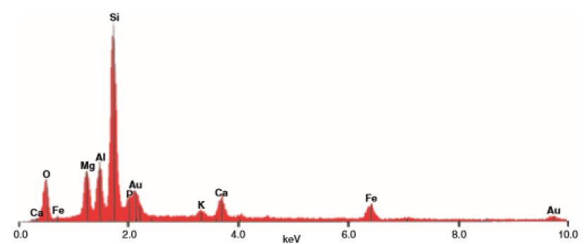
    Statistical analysis was performed using Student’s t-test or ANOVA, as appropriate using GraphPad Prism version 7.04 for Windows (GraphPad Software, San Diego, California USA, www.graphpad.com). Error bars on the graphs are presented as standard error of the mean (SEM). A P-value of <0.05 was considered statistically significant.

    Table 2: Mouse primer sequences

    Gene

    Forward Primer Sequence 5’

    Reverse primer Sequence 5’

    Rpl32

    GAGGTGCTGCTGATGTGC

    GGCGTTGGGATTGGTGACT
    β-catenin

    ACCTTTCAGATGCAGCGACT

    TGGCACACCATCATCTTGTT

    Desmin

    GTGGATGCAGCCACTCTAGC

    TTAGCCGCGATGGTCTCATA

    Mhy3

    ATGGTGGATGTGGAAAGAGC

    CCGTTTCACGGTTTCAAGTT

    Myogenin

    ACTCCCTTACGTCCATCGTG

    CAGGACAGCCCCACTTAAAA

    PPAR-γ

    GTCACACTCTGACAGGAGCC

    TCACCGCTTCTTTCAAATCT

    Ki67

    GACAGCTTCCAAAGCTCACC

    TGTGTCCTTAGCTGCCTCCT

    Pax 7

    GGAAAACCAGTGTGCCATCT

    CCTTGTCTTTGGCACCATTT

    Results

    β-Catenin Expression in ARKO and Control Animals

    In the cultured gubernacular fibroblasts, β-catenin expression was not significantly altered in e17.5 and D0 ARKO animals compared to WT. By contrast, β-catenin expression was upregulated in D3 ARKO fibroblasts, compared to the WT male counterpart (P=0.0003) (Figure 1A).

    β-Catenin Immunoreactivity in D3 ARKO and Control Animals

    Immunofluorescence of the gubernaculum in D3 ARKO and control animals showed differing patterns of staining (Figure 2A). Control animals showed staining throughout the cell cytoplasm, with cell membrane staining as well. ARKO animals showed staining throughout the cytoplasm with displacement into bands, consistent with myotube formation.

    Desmin, Myogenin and Ki67 Expression and Immunoreactivity in ARKO and Control Animals

    In the cultured gubernaculum; Mhy3 expression was upregulated in D0 ARKO animals, compared to the WT male counterpart (P < 0.0001) (Figure 1B). Immunofluorescence at D0 confirmed this, with decreased fluorescence in the wild type animal compared to the ARKO (Figure 2B). PPAR-γ expression was upregulated in ARKO males at D0 compared to WT male counterpart (p=0.022) (Figure 1C). Immunofluorescence at D0 confirmed this (results not shown). Desmin expression was upregulated in D0 ARKO and D3 ARKO animals, compared to the WT male counterpart (P=0.0242, P=0.05) (Figure 1D). Immunofluorescence at D3 confirmed this (results not shown). Myogenin expression was upregulated in ARKO males at D3, compared to WT male (P=0.05) (Figure 1E). Immunofluorescence at D3 confirmed this, with less fluorescence in wild type animals compared to ARKO (Figure 2C). Ki67 expression was upregulated in D3 ARKO animals, compared to the WT male counterpart (P=0.05) (Figure 1F). Immunofluorescence at D3 confirmed this, with less fluorescence in wild type animals compared to ARKO animals (Figure 2D).

    fig 1

    Figure 1: Real-Time qPCR was used to demonstrate gene expression changes in WT (black bar) and ARKO (grey bar) animals at e17.5, birth (day 0), and day 3 postnatal. (A) βCatenin expression (B) Mhy3 expression (C) Ppary expression (D) Desmin expression (E) Myogenin expression (F) Ki67 expression.

    fig 2

    Figure 2: Immunofluorescent labelling in the gubernaculum of wild-type and ARKO animals, blue is DAPI. Scale bar equals 100 mm (imaged with 60x oil magnification). (A) β-Catenin (green) at day 3 in the wild type and ARKO animals. (B) Mhy3 (green) at day 0 wild type and ARKO. (C) Myogenin (green) at day 3 (D) Ki67 (green) at day 3 in wild-type and ARKO animals.

    Discussion

    The results of this study indicate that fibroblasts cultured from the developing mouse cremaster muscle express more β-catenin at D3 in androgen receptor blockaded animals, and the pattern of immunoreactivity in ARKO animals is different from WT. ARKO animals demonstrated ‘banding’, presumably from myotubes developing skeletal muscle striation and displacing cytoplasm. ARKO animals also demonstrate increased expression of Mhy3 and PPAR-γ at D0, and Desmin, Myogenin and Ki67 at D3 compared to WT animals.

    At the onset of rodent inguinoscrotal testicular descent, the gubernaculum is a solid pyramidal structure of mesenchyme which everts from the abdominal cavity through the nascent inguinal canal to form a hollow cone lined by the future processus vaginalis mesothelium [6]. The solid mesenchymatous gubernacular tip is an undifferentiated ‘growth centre’ which has similar properties to an embryonic limb bud [15]. As the gubernaculum elongates to the scrotum the primitive fibroblasts differentiate into myoblasts and then eventually to mature muscle [16,17].

    These results suggest that androgen signalling is critical in allowing the cremaster differentiation to be delayed long enough to allow gubernacular eversion, as mature skeletal muscle may be too stiff to permit the radical remodelling required. The increased β-catenin expression by D3 is consistent with more mature muscle formation in the ARKO gubernaculum, and the situation seen in the cytoplasm shows what appears to be much more advanced development of skeletal cremaster muscle. By contrast, in the WT gubernaculum, there is no striated pattern of β-catenin, consistent with less advanced cremaster skeletal muscle differentiation, until migration is complete.

    The increased expression of Myh3 at D0, as well as PPAR-γ and desmin on D0, also suggest early differentiation into skeletal in the ARKO gubernaculum when in WT animals expression of these early markers of muscle development are much lower. The significant increase in myogenin expression at D3, a marker of later muscle development, is consistent with rapid differentiation of fibroblasts into mature cremaster muscle without androgen signalling, which is prevented in the WT mouse. The increased expression of Ki67 in D3 ARKO gubernacular fibroblasts is of uncertain significance, as in vivo the gubernaculum fails to migrate and remains bulky with persistence of hydrophilic extracellular matrix, and eventually undergoes metaplasia into adipose tissue [18]. These findings indicate the cremaster muscle behaves differently from other sexually dimorphic skeletal muscle in which AR signalling accelerates differentiation [19].

    The cremaster is a specialised skeletal muscle that has some properties alike cardiac and smooth muscle. The cremaster is not under conscious control, and responds to temperature and touch, as in the cremaster reflex. It’s different response to androgen stimulation is consistent with its different formation and physiological properties. Cremaster muscle myogenesis has been examined in the human fetus and is thought to have some smooth muscle characteristics [20].

    Historically, the cremaster muscle was thought to form passively by the gubernaculum collecting fibres from the internal oblique muscle as the testis descended past the internal inguinal ring. We now know androgen actively governs gubernacular growth and cremasteric development, during the window of androgen sensitivity, between E15-E19 of the rat embryo [21]. Androgen acts both directly and indirectly on the gubernaculum [22]; indirectly by causing the genitofemoral nerve (GFN) to release calcitonin gene-related peptide (CGRP), a known neuropeptide, which regulates gubernacular migration; and later directly by androgen receptors in the gubernaculum itself. We know that gubernacular eversion is a key aspect of testicular descent in rodents, and gubernacular eversion fails in androgen blockaded/ or knock out models. Despite the relative anatomical simplicity which occurs during gubernacular eversion, the effect of androgen on the linked molecular pathways remains complex.

    Androgen stimulation during inguinoscrotal descent has been linked to the canonical Wnt pathway and beta-catenin (β-catenin). β-catenin either binds to the androgen receptor and moves into the cell nucleus where it acts as a potent co-activator of the androgen receptor/ androgen receptor-positive genes; or it binds to the T-cell factor to promote activation of the Wnt-responsive genes [23]. In rats, it has been hypothesized that the interaction between androgen and β-catenin may be a necessary step in the digestion of collagen by androgen receptor-positive cells, assisting with cell migration from the core of the gubernaculum and enabling gubernacular eversion [24]. With androgen interacting with Wnt proteins, allowing nuclear translocation of β-catenin, androgen blockade leads to β-catenin accumulating in the cytoplasm and reduced myogenic proteins, thus myogenic gene transcription is necessary before gubernacular eversion and migration towards the scrotum. A conditional knockdown of β-catenin caused failure of CM myogenesis resulting in an intrabdominal testis [25]. Research using microarray analysis has suggested that Wnt signalling, working in conjunction with androgen receptor, may contribute to CM formation and testicular descent, as a defect in the Wnt signalling pathway and AR both produced intra-abdominal testis, which is a phenotype commonly associated with patients presenting with complete androgen insensitivity syndrome [26].

    Peroxisome proliferator-activated receptors (PPAR) also have been linked to the canonical Wnt pathway. PPAR’s are nuclear receptors that belong to the nuclear hormone superfamily and they share similar structural features with other nuclear receptors, such as androgen receptors (AR). PPAR-γ expression is critical for differentiation of rat skeletal muscle in vivo [27], and has also been linked to slow twitch skeletal muscle fibres known to be present in cremaster muscle. PPARs act as ligand-activated transcription factors which regulate gene expression by binding onto the Retinoid X Receptor (RXR), and specific regions of DNA sequence elements termed PPAR Elements (PPARE) in promoter regions of target genes, to modulate transcription. While the full range of PPAR ligands is not yet known, they are usually fatty acids or their derivatives. PPAR-γ may also interact with Beta (β)-catenin, a cytokine which has already been linked to testicular descent and cremaster development. b-catenin is thought to enhance PPAR-γ activity, leading to specific target gene activity. PPAR-γ has not been linked to cremaster myogenesis and the gubernaculum previously.

    The appropriateness of the mouse gubernaculum model to investigate cremaster development in humans is debated. Certainly, the anatomy of the cremaster muscle is different, with the rodent muscle forming a bi-laminar sac around the process vaginalis, while in the human it is just a strip [28]. However in both rodents and humans remodelling of the gubernacular mesenchyme is similar, except for timing, and cremaster develops within the gubernaculum itself. In both species androgen resistance prevents gubernacular migration and normal cremaster muscle development. We propose that once the difference in timing and cremaster development are taken into account, we can then extrapolate the results of this to suggest that, not only in the rodent but also in the human, androgen blockade may trigger premature differentiation of embryonic myoblasts in the gubernaculum, which may interfere with gubernacular eversion and/or elongation. Maintaining the cremaster myoblasts in a less differentiated state may allow the gubernaculum to elongate and migrate from the external inguinal ring to the scrotum in both species. Once terminal differentiation into mature muscle fibres has occurred, further elongation of the cremaster muscle within the gubernaculum is likely to be impaired. These alterations in muscle-related genes have also been detected in rat strains with inherited cryptorchidism and in anti-androgen-treated rats [29]. This is consistent with morphological changes showing disorganised abnormal striated cremaster muscle in cryptorchid rodents.

    The main limitation of this work is the small number of animals used, and that only 3 time points were studied. However, the consistency between the immunofluorescence and the gene expression results suggest that these limitations were not critical.

    Conclusion

    Testicular descent requires delayed development of cremasteric muscle; allowing migration of the testis into the scrotum. In the absence of AR, gubernacular mesenchymal cells prematurely develop into myoblasts prior to cremaster muscle differentiation.

    This study suggests that in the wild-type mouse, cremaster muscle maturation is usually delayed at the myoblast stage allowing eversion of the gubernaculum around D0 and then elongation to the scrotum. This study is consistent with AR blockade producing premature maturation which would inhibit eversion and gubernacular migration. We propose that undescended testes could be due to the premature maturation of cremaster muscle in AR-blockaded animals which prematurely halts the eversion and movement of the gubernaculum towards the scrotum. It is possible that defects in the response to androgen stimulation in the Wnt, b-catenin and PPAR signalling pathways may lead to cryptorchidism in boys without androgen resistance. These intracellular signalling systems should be included in future searches for the causes of cryptorchidism using modern genetic analysis.

    Funding

    NHMRC grant APP1144752.
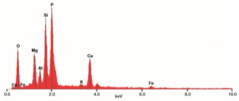
    Disclosures and Declaration of Interests

    None

    Human Ethical Approval

    Murdoch Children’s Research Institute Animal Ethics Committee AEC no. A854.
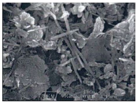
    References

      1. Hutson JM, Balic A, Nation T, Southwell B (2010) Cryptorchidism. Seminars in Pediatric Surgery 19: 215-24.
      2. Hutson JM, Hasthorpe S, Heyns CF (1997) Anatomical and functional aspects of testicular descent and cryptorchidism. Endocrine Reviews 18: 259-80. [crossref]
      3. Hutson JM (1985) A biphasic model for the hormonal control of testicular descent. Lancet 2: 419-21. [crossref]
      4. Favorito LA, Costa SF, Julio-Junior HR, Sampaio FJ (2014) The importance of the gubernaculum in testicular migration during the human fetal period. International Braz J Urol: Official Journal of the Brazilian Society of Urology 40: 722-9. [crossref]
      5. Costa WS, Sampaio FJ, Favorito LA, Cardoso LE (2002) Testicular migration: remodeling of connective tissue and muscle cells in human gubernaculum testis. J Urol 167: 2171-6. [crossref]
      6. Harnaen EJ, Na AF, Shenker NS, et al. (2007) The anatomy of the cremaster muscle during inguinoscrotal testicular descent in the rat. Journal of Pediatric Surgery 42: 1982-7
      7. Churchill JA, Buraundi S, Farmer PJ, et al. (2011) Gubernaculum as icebreaker: do matrix metalloproteinases in rodent gubernaculum and inguinal fat pad permit testicular descent? Journal of Pediatric Surgery 46: 2353-7
      8. Nation TR, Buraundi S, Balic A, et al. (2011) The effect of flutamide on expression of androgen and estrogen receptors in the gubernaculum and surrounding structures during testicular descent. Journal of Pediatric Surgery 46: 2358-62. [crossref]
      9. Perera N, Szarek M, Vannitamby A, et al. (2018) An immunohistochemical analysis of the effects of androgen receptor knock out on gubernacular differentiation in the mouse. Journal of Pediatric Surgery 53: 1776-80. [crossref]
      10. Li Z, Marchand P, Humbert J, Babinet C, Paulin D (1993) Desmin sequence elements regulating skeletal muscle-specific expression in transgenic mice. Development (Cambridge, England) 117: 947-59. [crossref]
      11. Faralli H, Dilworth FJ (2012) Turning on myogenin in muscle: a paradigm for understanding mechanisms of tissue-specific gene expression. Comparative and Functional Genomics 2012: 836374. [crossref]
      12. Notini AJ, Davey RA, McManus JF, Bate KL, Zajac JD (2005) Genomic actions of the androgen receptor are required for normal male sexual differentiation in a mouse model. Journal of Molecular Endocrinology 35: 547-55.
      13. Vikraman J, Sarila G, O’Conner L, Menheniott T, Hutson JM (2022) BDNF is upregulated by androgen in the inguinal fat pad of immature mice and may regulate inguinoscrotal testicular descent. Pediatric Research 91: 846-52. [crossref]
      14. Kriegova E, Arakelyan A, Fillerova R, et al. (2008) PSMB2 and RPL32 are suitable denominators to normalize gene expression profiles in bronchoalveolar cells. BMC Molecular Biology 9: 69.
      15. Sanders N, Buraundi S, Balic A, Southwell BR, Hutson JM (2011) Cremaster muscle myogenesis in the tip of the rat gubernaculum supports active gubernacular elongation during inguinoscrotal testicular descent. J Urol 186: 1606-13. [crossref]
      16. Lie G, Hutson JM (2011) The role of cremaster muscle in testicular descent in humans and animal models. Pediatric Surgery International 27: 1255-65. [crossref]
      17. Szarek M, Li R, Vikraman J, Southwell B, Hutson JM (2014) Molecular signals governing cremaster muscle development: clues for cryptorchidism. Journal of Pediatric Surgery 49: 312-6.
      18. Griffiths AL, Momose Y, Hutson JM (1993) The gubernaculum in adult female, adult male and TFM male mice. International Journal of Andrology 16: 380-4. [crossref]
      19. Lee DK (2002) Androgen receptor enhances myogenin expression and accelerates differentiation. Biochemical and Biophysical Research Communications 294: 408-13. [crossref]
      20. Tanyel FC, Talim B, Atilla P, Müftüoğlu S, Kale G (2005) Myogenesis within the human gubernaculum: histological and immunohistochemical evaluation. European Journal of Pediatric Surgery: Official Journal of Austrian Association of Pediatric Surgery 15: 175-9.
      21. Welsh M, Saunders PT, Fisken M, et al. (2008) Identification in rats of a programming window for reproductive tract masculinization, disruption of which leads to hypospadias and cryptorchidism. The Journal of Clinical Investigation 118: 1479-90. [crossref]
      22. Schwindt B, Farmer PJ, Watts LM, Hrabovszky Z, Hutson JM (1999) Localization of calcitonin gene-related peptide within the genitofemoral nerve in immature rats. Journal of Pediatric Surgery 34: 986-91. [crossref]
      23. Sarila G, Hutson JM, Vikraman J (2022) Testicular descent: A review of a complex, multistaged process to identify potential hidden causes of UDT. Journal of Pediatric Surgery 57: 479-87. [crossref]
      24. Choi HY, Lim JE, Hong JH (2010) Curcumin interrupts the interaction between the androgen receptor and Wnt/β-catenin signaling pathway in LNCaP prostate cancer cells. Prostate Cancer and Prostatic Diseases 13: 343-9.
      25. Kaftanovskaya EM, Feng S, Huang Z, et al. (2011) Suppression of insulin-like3 receptor reveals the role of β-catenin and Notch signaling in gubernaculum development. Molecular Endocrinology (Baltimore, Md) 25: 170-83. [crossref]
      26. Hughes IA, Davies JD, Bunch TI, Pasterski V, Mastroyannopoulou K et al. (2012) Androgen insensitivity syndrome. Lancet 380: 1419-28.
      27. Singh J, Verma NK, Kansagra SM, Kate BN, Dey CS (2007) Altered PPARgamma expression inhibits myogenic differentiation in C2C12 skeletal muscle cells. Molecular and Cellular Biochemistry 294: 163-71. [crossref]
      28. Hutson JM, Baskin LS, Risbridger G, Cunha GR (2014) The power and perils of animal models with urogenital anomalies: handle with care. Journal of Pediatric Urology 10: 699-705. [crossref]
      29. Barthold JS, McCahan SM, Singh AV, et al. (2008) Altered expression of muscle- and cytoskeleton-related genes in a rat strain with inherited cryptorchidism. Journal of Andrology 29: 352-66. [crossref]

Therapeutic Effect and Safety of Rectal Ozone Therapy in Mild and Moderate Symptomatic SARS CoV-2 Positive Patients

DOI: 10.31038/JNNC.2022514

Abstract

Background: COVID-19 an infectious disease caused by severe acute respiratory syndrome coronavirus 2 (SARS-CoV-2). Ozone therapy would be a therapeutic option for COVID- 19. Objective: To explore therapeutic effect and safety of rectal ozone therapy in mild and moderate symptomatic SARSCoV-2 positive patients, is the purpose of this study.

Methods: An exploratory, controlled, open and monocentric study was carried out in 32 patients, distributed at random in two groups of 16 patients each. The first group received rectal ozone therapy (ROT) with Standard treatment (ST) and the second one only ST. ROT were applied every 12 h for 10 days. Patients aged 19-80 years were included, after signing the informed consent, with positive SARS-CoV 2 symptomatic. RT-PCR and clinical signs evolution were primary efficacy variables. Ferritin, C-reactive protein, oxidative stress biomarkers, inflammatory cellular indicators, and biochemical and hematological variables.

Results: Patients (81%) had negative RT-PCR after ROT tenth application, with significant differences to ST group (43%). ROT significantly increases Glutation (GSH) levels compared to ST group, but not other REDOX markers as SOD, MDA, ON and AOPP. Catalase activity increased in both groups.

Conclusion: This study demonstrates the efficacy and safety of ROT in both mild and moderate symptomatic SARS-CoV 2 positive patients.

Keywords

COVID 19, SARS CoV-2, Rectal Ozonetherapy, REDOX Balance, Superoxide dismutase, Glutation

Introduction

COVID-19 is the third known zoonotic coronavirus disease after Acute Respiratory Response Syndrome (SARS) and Middle Eastern Respiratory Syndrome (MERS-CoV), which also originates from the β cluster –coronavirus [1].

Among the complexities of the pathophysiological process of this viral infection, the so-called “storm of decompensated cytokines” stands out, which damage the vascular system, causing activation of the coagulation system, the consequent formation of thrombosis, which prevents perfusion into the tissues, causes multiple organ failure and death of patients [2].

The generation of free radicals is one of the pathogenic mechanisms of viruses, to cause inflammation and tissue damage. Oxidative stress is induced after the virus enters the host cell to facilitate its replication [3]. This suggests that the use of immunomodulatory and stimulatory therapeutic forms of the endogenous antioxidant response, such as ozone therapy, could counteract the pathophysiological development of COVID 19.

Several therapeutic effects justify the use of ozone in COVID-19 patients [4]. Ozone therapy stimulates Nrf2 [5,6], that would be an important physiological mechanism to blocked virus (SARS CoV 2) replication endogenously, preventing receptor contact to the virus, by reducing the expression of ACE2 and TMPRSS2, inactivating the virus replication ability [7]. The rebalancing of REDOX state achieved with ozone therapy is also important to cytokine synthesis induction by monocytes and lymphocytes, heme-oxygenase (HO-1) and shock proteins release, which are powerful activators of the immune system [8,9].

The immunomodulatory action of inflammatory response mediated by pro-inflammatory cytokines and increase in endogenous antioxidant activity, accompanied by the increase in nuclear transcription factor Nrf2 (5), by ozone therapy, was demonstrated in both preclinical [10-14] and clinical chronic pathological processes [15,16].

The rectal ozone therapy efficacy and safety was studied in 12 clinical trials, including chronic pathologies (angiopathy, chronic inflammation, immune imbalances, chronic rheumatological inflammation, among others), reaching improvement in both clinical and biochemical parameters, without adverse effects, only in one clinical trial mild irritation was evidenced in two patients [17].

Recently, the ozone therapy benefits applied by MAHT as adjuvant treatment in severe patients with COVID-19 have been demonstrated in different countries such as China [18], Italy [19,20] and Spain [21]. On the other hand, rectal ozone therapy insufflation also demonstrated its benefits in severe COVID 19 patients [22,23].

Due to all these antecedents of ozone therapy and the eminent need to provide a therapeutic solution to this COVID- 19 disease, the objective is to explore the therapeutic effect and safety of rectal ozone therapy in both mild and moderate symptomatic SARS-CoV 2 positive patients.

Materials and Methods

Study Design

The study was conducted following the ethical principles reflected in the 2013 Helsinki declarations and WHO recommendations. The exploratory study was an open-label and randomized trial. The study was conducted from May to August 2020 and the Hospital Health Care Ethics Committee authorized the study and ozone treatment. Positive confirmed COVID 19 patients, hospitalized in “Salvador Allende” Hospital, La Habana, Cuba were recruited for the study. Eligibility criteria for the study were the age and positively tested COVID 19 at least for 48 h later. The institutional review board of the hospital, Cuban Ministry of Public Health (MINSAP) and the Cuban Regulatory Agency (CECMED) approved this study and registered in the clinical trials public register with the number: RPCEC 0000320.

Inclusion Criteria

Adults of age 19 to 80 from both sex with positive reverse transcription-polymerase chain reaction (RT-PCR) from the nasopharyngeal swab test result, presenting mild to moderate clinical signs and willing were included in the study. All hospitalized patients included were informed of the procedures and potential risks and gave written informed consent.

Exclusion Criteria

1) Pregnancy or lactation; 2) G-6PD (glucose 6-phosphate dehydrogenase) deficiency (favism); 3) Patients with uncontrolled hyperthyroidism, 4) patients with abnormal coagulation, thrombocytopenic and active bleeding. 5) Allergic or intolerance to ozone. 6) Patients that use immunosuppressive medication. 7) Patients participating in another clinical trial. 8) Patients with psychiatric diseases. 9) Patients suffering from uncontrolled chronic disease.

Groups

We screened 32 patients positive SARS-CoV 2, confirmed by RT-PCR and hospitalized in the “Salvador Allende Hospital”. Patients were randomly assigned to two groups of 16 patients each. Randomized treatment was open-label. Patients were assigned to a serial number by the study coordinator. Each serial number is linked to a computer-generated randomization list assigning the treatment regimens. The first group received rectal ozone therapy combined with standard treatment (Ozone + standard treatment (ST) and the second group with ST, where the patients were provided with conventional care as recommended in clinical management protocol for COVID 19 advocated by MINSAP.

Ozone Rectal insufflation

Medical Ozone obtained by Ozomed Plus®, (Ozone Generator) National Centre for Scientific Research, BioCubaFarma, Habana, Cuba. For rectal administration, the patients were placed in lateral decubitus position with lower limbs flexed and then lubricated rectal catheter was introduced rectally with patient’s collaboration. A hemostatic clamp was placed on the catheter before the gas was insufflated. Ozone from the generator and immediately insufflated through the catheter, after removing the hemostat clamp. The insufflation time will be a few minutes, at an administration rate of 1 ml/s. The Ozone therapy rectal insuflation schedule was the following described in TS1.

Standard Treatment (ST) Approved by MINSAP Protocol for COVID-19, Version 1.4

-Kaletra ® (Capsules 200 mg lopinavir + 50 mg ritonavir) Medsol, Havana, Cuba.

-Chloroquine (Tablets 250 mg), one every 12 h, for 10 days.

-Heberferon® (Interferon α-2b human recombinant + interferon-gamma human recombinant 3,5 M UI Ampoule (lyophilized)) according to the National Formulary, IM, three times a week. Heber Biotec, S.A. Havana, Cuba

-Ceftriaxone one bulb every 12 h during 10 days, in the cases with pulmonary infection diagnostic.

Analysis of Primary Efficacy Parameters

The primary endpoint in this study was the patient’s percentage having negative RT-PCR test for SARS-CoV-2 in nasopharyngeal swab samples on 5th and 10th treatments. A global response was considered too, where RT-PCR and clinical signs are classified into the complete response if RT-PCR test was negative and clinical signs disappear; partial response if RT-PCR was negative and clinical symptoms presented at inclusion time did not worsen or disappear at least two of them and non-response, if RT-PCR was still positive, regardless of clinical signs.

Secondary variables are C-reactive protein (CRP), neutrophil/lymphocytes ratio and redox parameters. The secondary variables were determined at the initial and after the 5th day of treatment. A high percentage of patients have a negative PCR on the fifth day and were discharged, for that reason most of the evaluations were made on the fifth day and not on the tenth day.

All redox parameters were determined in serum by spectrophotometric methods using Zuzi Spectrophotometer (Japan). Serum reduced glutathiones (GSH) concentrations were measured by kinetics assay using the glutathione reductase reaction [24]. Malondialdehyde (MDA) concentrations were analyzed with the LPO-586 kit obtained from Calbiochem (La Jolla, C.A., USA) [25]. Superoxide dismutase (SOD) activities were assayed by a modified pyrogallol autoxidation method [26]. Catalase (CAT) activity was measured according to the method of Claiborne [27]. Serum advanced oxidation protein products (AOPP) was measured according to the methods of Witko-Sarsat et al, 1998 [28]. Nitrates and nitrites relation (NO) levels were measured according to Griess methods described by Granger et al 1996 [29].

Blood parameters such as hematocrit, hemoglobin, and erythrocyte sedimentation rate, were screened by Hematological counter MICROS 60. Others as triglycerides, creatinine, cholesterol and alanine aminotransferase activity were performed by standard procedures in HITACHI analyzer 912. As an efficacy response, the values of hemoglobin, hematocrit, erythrocytes, leukocytes, platelets and differential of leukocytes (lymphocytes, monocytes, basophils, neutrophils and eosinophils), erythrocyte sedimentation were considered to normalize. Also as an efficacy response, the values of albumin, lactate dehydrogenase (LDH), alanine aminotransferase (ALT), aspartate aminotransferase (AST), creatinine (Cr), gamma-glutamyl transferase (GGT), glucose, creatinine, bilirubin, uric acid (AU), cholesterol, triglyceride, and high-density lipoproteins (HDL) were considered to remain within their normal values. The safety and tolerability were evaluated through complementary variables (hemogram and blood chemistry). Analysis of adverse reactions occurrence was included too. In addition, a subjective assessment of tolerability was performed, according to following categories: Very good (no adverse events-AE), Good (mild and transient AE), Fair (moderate AE), Poor (severe AE) [30-53].

Statistical Analysis

For the evaluation of the response, the proportions of response by groups were estimated for the main variables (a negative RT-PCR test and the evolution of the clinical signs). The groups were compared using Fisher’s exact test. This analysis was carried out for the variable “global response” according to the success criteria defined in the protocol. For the secondary variables (laboratory variables) were compared at times 5 and 10 days with respect to baseline using the paired t-test (before-after) or the Wilcoxon signed-rank test, as appropriate.

Results

With respect to baseline characteristics of the 32 patients included in the study there were no statistical differences, between the groups according to demographics, gender and age of patients (p˃0.05), except for comorbidities risk which was high in the Ozone group (87%) in comparison to 68,8% for the control group (p=0.0021). Regarding clinical symptoms classification (mild and moderate), the ozone group had 50% for both mild and moderate symptoms, however, the control group had 69% mild symptoms patients and 31% with moderate symptoms, which showed significant differences between both groups (p=0.0236).

After the fifth day of ozone therapy treatment, 81% of patients had a negative RT-PCR, with significant differences (p=0.01) compared to the control group (43%). After 10 days of treatment, 93.8% of patients showed a negative RT-PCR in the ozone group, with significant differences (p=0.01) with regards to the control group (62.5%) (Table 1).

Table 1: RT-PCR SARS CoV 2 analysis in swab samples from each group

Immunological response

RT-PCR

Ozone

Control

5th day Negative

13 (81.3%)

7 (43.8%)**

Positive

3 (18.8%)

9 (56.3%)

10th day Negative

15 (93.8%)

10 (62.5%)**

Positive

1 (6.3%)

6 (37.5%)

**Pearson’s chi-squared test

The severity of clinical symptoms and signs improved significantly after 5 days of treatment in ozone group, compared to control group (p<0.05), without differences at 10 days of treatment (Table 2). Regarding global response, there were significant differences for total, partial and non-response between groups. In the ozone group, the percentage of patients who had a total response (25%) increased significantly (p˂0.05) compared to the control group (0%) after 5 days of treatment. Furthermore, 56. 3% of patients from control group had non-response on the fifth day, compared to ozone group (18.8%) (p<0.05). After 10 days, the results were similar, in ozone group increased significantly (p<0.05) the patient percentage (37.5%) with a total response with regards to control group (12.5%) (Table 2).

Table 2: Disease evolution according to clinical symptoms and signs and global response to treatments


5th day

10th day


Ozone

Control

Ozone

Control

Disease evolution according to clinical symptoms and signs+, n patients (%)
Improved severity of the disease

7 (43.8%)

1 (6.3%)*

7 (43.8%)

3 (18.8%)

Global Response to treatments, n patients (%)
Total

4 (25.0%)

0 (0%)*

6 (37.5%)

2 (12.5%)*

Partial

9 (56.3%)

7 (43.8%)

10 (62.5%)

9 (56.3%)

Non-reponse

3 (18.8%)

9 (56.3%)*

0 (0.0%)

5 (31.3%)*

+Symptoms and signs: fever, headache, fatigue, sore throat and dry cough. *p˂0.05 comparing both groups Fisher exact test.

Ozone and control, showed a reduction in the levels of C reactive proteins after 5 days of treatment, but only was significant (p<0.05) for the control group. Regarding related indicators, such as neutrophil/lymphocyte ratio (N/L R), both groups experience a reduction of N/L R on the 5th day of treatment. However, only the ozone group achieved a statistically significant reduction (p<0.05) from 2.5 to 1.5 mg/L (Table 3).

Table 3: Inflammation variables

Groups

Baseline

5th day

C reactive protein mg/L (reference < 6)
Ozone

17.8 ± 22.7

 9.0 ± 11.4

Control

10.7 ± 16.2

 5.1 ± 6.6**

N/L R
Ozone

2.5 ± 1.5

1.5 ± 0.9**

Control

2.3 ± 1.4

1.6 ± 1.0

**Comparison within groups (before and after) Wilcoxon signed-rank test.
N/L R: neutrophil /lymphocytes ratio.

The behavior of the Redox state, shown by the values of antioxidant indicators (levels of glutathione and activity of CAT and SOD) and pro-oxidants (AOPP, MDA and NO), are shown in Table 4, for each group, at the beginning (baseline) and at 5 days after starting the treatments. Both groups began the study with similar GSH values, without significant differences between them. The group of patients that received treatment with rectal ozone showed a significant increase (p=0.025) in GSH levels on the fifth day of treatment. However, the control group did not experience significant changes on the fifth day with regards to the initial value. On the other hand, both groups show significant differences (p=0.009) between them on the fifth day after starting the study. Regarding CAT activity, both groups show significant increase (p=0.001) on the fifth day of treatment in comparison to the baseline value, without significant differences between the groups. SOD activity did not reveal significant changes between groups. The pro-oxidant indicators (AOPP, NO and MDA) did not reach significant changes in any of the study groups.

Table 4: The behavior of the REDOX indicators for each of the groups

Variables

Ozone

Control

Baseline

5th day

Baseline

5th day

GSH (mmol/mg Hb)

448.1 ± 105.2

511.7 ± 58.3*+

424.0 ± 72.2

398.6 ± 68.7

CAT (U/mg Hb min)

266.4 ± 47.6

302.2 ± 47.8*

223.4 ± 35.6

257.6 ± 39.3*

SOD ((U/mg Hb min )

3.01 ± 0.6

3.23 ± 0.4

2.27 ± 0.4

2.77 ± 0.4

AOPP (µM/cloramina T

20.6 ± 1.8

20.7 ± 2.7

21.66 ± 1.5

21.88 ± 2.7

NO ([NO2] μM)

31.3 ± 4.8

31.7 ± 7.4

33.3 ± 9.4

40.7 ± 19.0

MDA (mmol/mg Hb)

3.3 ± 0.6

3.2 ± 0.6

3.0 ± 0.4

2.9 ± 0.5

SD: standard deviation, CAT: catalase, SOD: superoxide dismutase, MDA: malondialdehyde, GSH: glutathione, AOPP: advanced oxidation protein product. +Compare between groups and *p<0.05 differences between the baseline and the 5th day, by t student test or Wilcoxon test.

The hematological indicators evaluated did not show differences between groups at the evaluation times (baseline and the fifth day) except for the percentage of neutrophils and lymphocytes, where in both groups, neutrophils were significantly reduced at the fifth day of treatment (after the 10th application of ozone treatment) compared to baseline. Furthermore, the lymphocytes percentage increased in both groups, but only with a significant (p<0.05) difference in the control group. Both figures of neutrophils and lymphocytes (baseline and 5th day) were within the reference values.

The biochemical behavior in blood serum in terms of triglyceride values, there was a significant increase for both groups on the fifth day regarding the baseline values, being the value in the control group within the range of normal values. Cholesterol values were significantly reduced in the control group in comparison with the baseline value. In the group of patients treated with rectal ozone therapy on the fifth day, a significant reduction in ALT levels was observed in the ozone group in comparison with the baseline. During all the biochemical analyzes carried out on the blood, it was found that, despite observing some significant differences in some indicators at the fifth day of treatment in comparison with the baseline value, none of these are outside the values of references reported as normal.

With respect to adverse events, there are no significant differences among the study groups. In 12 patients presented AE for 75%, and only 4 patients did not present AE (25%). In the group of control patients, 9 of them (56.3%) who presented AE were registered, and 7 (43.8%) who did not present AE. There were no significant differences between the two groups. The intensity of the side effects was considered mild and moderate for both groups.

The adverse events associated with rectal ozone application were feeling of full intestines, tenesmus, colics and intestinal peristaltic movements. Adverse events were recorded daily.

No deaths or serious AE were reported during the study. These patients have their general condition compromised, which together with the adverse reactions generated by the conventional drugs (Heberferon, kaletra, chloroquine) that they are taking, mask the real response to the tolerability of ozone therapy.

The physical safety indicators evaluated showed a significant reduction in the bodyweight of the patients after the fifth day of treatment in both groups (Table 5). On the other hand, a significant reduction in respiratory rate was evidenced in the control group on the fifth day, but despite reaching statistical significance, is considered not relevant within the analysis of the general condition of the patient, since none of these worsened their clinical symptoms.

No deaths or serious AE were reported during the study.

Discussion

This exploratory clinical trial results showed negative RT-PCR in the 81% of patients treated with conventional treatment plus ozone rectal insufflation every 12 h after 10 applications of ozone therapy, with significant differences with regards to the control group (conventional treatment) where only 43% of the patients obtained negative RT-PCR in the same time. Regarding the percentage of negative RT-PCR on the 10th day (20 applications of ozone therapy), the significant differences in favor of ozone therapy are maintained. This result, is considered the first evidence on the effect of rectal ozone therapy on the PCR result in COVID 19 positive patients with mild and moderate symptoms. Similar results were reported in a clinical trial in COVID-19 positive patients with mild and moderate symptoms, who were treated with the combination of rectal ozone therapy and minor autohemotherapy (minor AHT). The scheme used was rectal ozone therapy twice daily (150 mL of ozone volume with a concentration of 40 mg/L) and minor AHT less than 25 mg/L of ozone concentration, once a day. The results confirm that 77% of the patients had a negative RT-PCR at day 5, compared to 43% in the control group. After the 10th day, 100% of the cases showed negative RT-PCR in the ozone therapy group, which was significantly higher compared to 70% in the control group [30].

On the other hand, it is important to point out that the negative RT-PCR in patients with rectal ozone therapy was accompanied by a significant improvement in clinical symptoms on the 5th day, compared to the control group. Regarding the evaluation of the treatment’s global response, it was identified that rectal ozone therapy favored significantly the total response (negative RT-PCR and disappearance of clinical symptoms) compared to the control group, both in the analysis to 5 days. Similar results are reported in the clinical trial [30], where the cough and dyspnea, improved on the 5th and 10th day of treatment with rectal ozone therapy and minor AHT, compared to the control group.

In a recent study, the effectiveness of rectal ozone therapy was reported on the clinical symptoms of COVID-19. This study was carried out in four patients with severe pneumonia [23]. It describes that after 10 and 39 days with failed evolution under conventional treatment (retroviral drugs, IL6 and IL1 inhibitors, antibiotics and methylprednisolone), rectal ozone therapy was applied compassionately, five applications of 100 mL volume with a 35 mg/L ozone concentration, which resulted in a significant improvement dyspnea, respiratory rate, and oxygen saturation.

Other studies report the success of ozone therapy, applied by major autohemotherapy (M-AHT), in patients with COVID 19 in critical condition, hospitalized in intensive care units (ICU), in which the efficacy of the treatment was reported in terms of the improvement of the patient’s health status, or condition in a much shorter time than in conventional treatment [21]. A percentage of 53% of SARS-CoV 2 positive patients, treated with ozone therapy via M-AHT, significantly improved clinical symptoms compared to the control group [31].

C-reactive protein (CRP) is synthesized in the liver and is an acute reactive phase protein that is increased in the blood in a wide range of inflammatory diseases. This protein is increased in 73-93% of patients infected with COVID-19, particularly in the severe phase of the disease [32]. All the COVID-19 patients included in this trial, characterized by mild and moderate symptoms, presented mean values of CRP higher than those reported as normal (<6 mg / L). Both, ozone therapy group and conventional treatment reduced CRP levels on the 5th day of evolution, with percentages of changes of 49.4% and 52.3%, respectively. This reduction was only statistically significant in the control group. Although the ozone group did not show statistical significance, the possibility that this result is influenced by the fact that the number of patients was low and there was a high standard deviation should be considered. As reported in other studies, rectal ozone therapy reduces CRP in patients with COVID-19 (mild and moderate) [32] and also in severe patients treated with ozone therapy via MAHT [24]. Other inflammatory and thromboembolic markers such as IL-6 and Dimer-D were reduced by MAHT ozone therapy in COVID-19 patients hospitalized in intensive care units. In addition, ozone improved the respiratory function indicators, such as oxygen saturation percentage (Sat O2) and the arterial pressure index of oxygen/fraction of inspired oxygen (PaO2 / FiO2) [19].

Regarding the analysis of the cellular indicators of the inflammatory response, a significant reduction in N/L ratio was observed in the group treated with ozone after 5 days of treatment, which corresponds to the increase in the lymphocyte count in this group. Although in the control group there were no statistically significant differences regarding this indicator, a tendency to decrease was observed after 5 days of treatment. The N/L ratio index is a predictive prognostic factor for the risk of death in hospitalized SARS CoV 2 positive patients undergoing endotracheal intubation with prognostic values of N/L > 4.94 reported by Tatum D. et al. (2020) [33]. In this study, the patients presented baseline N/L values of 2.5 and 2.3 in the ozone and control group, respectively, decreasing to 1.5 and 1.6 in each group after 5 days of treatment, which is consistent with the improvement of patients and favors the prognosis of the disease.

On the other hand, considering the oxidative stress indicators evaluated in the study is analyzed was verified that pro-oxidant indicators (MDA, PAOP and NO) do not suffer significant changes in the patient group treated with rectal ozone therapy. Some results support the association between oxidative stress, inflammation, and the pathogenesis of SARS-COV infection [34]. In the preclinical setting, it is evidenced that the overproduction of Reactive Oxygen Species (ROS) and a deprived system of antioxidants play a major role in the pathogenesis of SARS-CoV infection, as well as in the progression and severity of the respiratory disease. Experimental animal models of severe acute respiratory syndrome have shown increased ROS levels and impaired antioxidant defense during SARS-CoV infection [35]. Some authors suggest that the appearance of a severe lung injury in patients infected by SARS-CoV depends on the activation of oxidative stress that is coupled with innate immunity and activates transcription factors, such as NF-kB, resulting in a response proinflammatory in the host in an exacerbated form [36].

In this study, it is highlighted that rectal ozone therapy significantly increased the GSH content on the fifth day of treatment, in comparison with the basal content and with the value of the control group on the fifth day [36]. These results correspond to those achieved in other trials carried out in chronic diseases (rheumatoid arthritis) [37], heart failure [38], multiple sclerosis [39] and coronary artery disease [40], among others, where demonstrates the stimulating action of ozone therapy on endogenous antioxidant systems. On the other hand, both treatments experienced an increase in CAT activity, without differences between them. The pro-oxidant indicators analyzed (MDA, PAOP) did not show significant changes on the fifth day of treatment.

Several studies indicate that higher glutathione levels can improve an individual’s responsiveness to viral infections. It protects the host’s immune cells through its antioxidant mechanism and is also responsible for the optimal functioning of a variety of cells that are part of the immune system. Glutathione inhibits the replication of various viruses at different stages of the viral life cycle, and this antiviral property of GSH appears to prevent the increase in viral load and the subsequent massive release of inflammatory cells in the lung (“cytokine storm”). Endogenous glutathione deficiency appears to be a crucial factor that increases the oxidative damage of the lung induced by SARS-CoV-2 and, as a result, leads to severe manifestations such as acute respiratory distress syndrome, multiple organ failure and death in patients with COVID-19 [41].

The nuclear transcription factor Nrf2 is the main regulator of the antioxidant response element (ARE) that directs the expression of cytoprotective proteins. Nrf2 confers protection against these pulmonary disorders [42], stimulates the innate immune system, eliminating numerous pathogenic bacteria and viruses [43]. Recently, a study in 40 patients showed that COVID-19 severity was directly related to the age and inflammatory response intensity was inversely associated with Nrf2 expression [44]. Patients with COVID-19 showed suppression of Nrf2 pathway, however, the pharmacological inducers of Nrf2 inhibited the replication of SARS-CoV2 and decreased the levels of inflammatory response [47]. Nrf2 agonists induce interferon (IFN)-independent antiviral program that is widely effective in limiting virus replication and suppressing pro-inflammatory responses of human pathogenic viruses, including SARS-CoV-2 [45].

It is well known that ozone therapy stimulates endogenous antioxidant systems through the expression of Nrf2 [5], which was confirmed in a clinical trial of multiple sclerosis, where rectal ozone therapy modulated the inflammatory response mediated by cytokines and increased antioxidant activity, accompanied by increased expression of Nrf2 [46]. There are several studies where have been well demonstrated that ozone therapy increases the level of Nrf2, with an improvement of the antioxidant defense system [47,48].

Although the physical examination of the patients showed a significant reduction in the weight of the patients 5 days after starting the treatment, for both groups, this indicator did not constitute a parameter of non-safety of the treatments, since it considers the influence of other aspects, such as the change of diet, the hospitalization of the patient and the general clinical symptoms that he presented, which prevented him from eating properly and therefore maintaining his body weight. Furthermore, no significant changes were observed in terms of hematological and blood chemistry indicators. The rest of the variables remained within the ranges of normal values.

Both treatments were tolerable. Within the tolerability classification, the highest percentage was regular for both treatments, both with high percentages, ozone therapy 60% and control 50%. The tolerability obtained for ozone therapy in this study is contradictory, as previous studies have shown that rectal ozone therapy has been very well tolerated [49]. This result could be subject to the fact that these patients, unlike those in other clinical trials, despite presenting mild and moderate symptoms of COVID-19, have implications for the general intake of their status, which together with adverse reactions generated by conventional drugs (Heberferon, Kaletra, chloroquine), mask the real response to the tolerability of ozone therapy. On the other hand, if we consider that ozone therapy significantly reduced the clinical symptoms of the patients compared to the control, we could confirm that this classification was influenced by the general deterioration of the patients as they were under so many adverse effects caused by the conventional medications.

AE occurred in 75% of the patients in the group that received treatment with rectal ozone therapy and in 56% of the patients in the control group. This difference between the groups with respect to this indicator was not statistically significant. These results were not as expected, since, according to experience and reports in the literature on clinical trials with rectal ozone therapy, this procedure, in general, does not cause AE in this sense, only very few and of mild intensity have been reported [50-52].

But, in this trial for the first time, rectal ozone therapy is being used in patients with COVID-19 in conjunction with conventional treatment (retroviral and others) who have adverse reactions. For example, in the study performed in COVID-19 convalescent patients treated with rectal ozone therapy, 80% (28/36) of the patients reported the feeling of fullness of the intestines, without other reports, that disappeared rapidly and in no case, treatment was required [53]. In addition, a high index of well-being was observed in the group of patients who received ozone and the safety in the use of this technique confirmed its therapeutic usefulness.

The compliance with the treatments by the ozone therapy group should be highlighted, in which no patient interrupted the treatment for any reason. However, in the control group 6 patients (37.5%) did not comply with the administration of Kaletra and chloroquine and 3 (18.8%) received incomplete treatment, which could be the reason why the analysis of the presentation of AE, had an increasing trend in the group that received rectal ozone therapy, although this was not statistically significant in comparison with the control group.

In conclusion, the results of this exploratory clinical trial show that rectal ozone therapy applied at the doses and therapeutic scheme described was effective and safe as an adjunctive treatment in positive patients for COVID-19. Ozone therapy significantly achieved a negative RT-PCR in 81 % of patients and reduced clinical signs after five days of treatment. This primary efficacy result was accompanied by an increase in the glutathione content and the activity of CAT in the serum of the patients, improving the endogenous antioxidant response. This exploratory study demonstrates the efficacy and safety of rectal ozone therapy in both mild and moderate symptomatic SARS-CoV 2 positive patients. The combined treatment showed superior efficacy to conventional treatment by reducing the time in which patients improve clinical symptoms and obtain a negative RT-PCR. In both groups, oxidative stress indicators and cellular markers of inflammation improve, and the treatments are safe and well-tolerated. As it is an exploratory study, the number of patients included limits the scope of these conclusions, so future Phase III studies should confirm the results found.

Acknowledgments

The authors give specials thanks to the Cuban Ministry of Public Health, especially to the head of Natural and Traditional Medicine Department, Dr. Johan Pedomo. Specials thanks to all hospital staff involved in the study, the administrative staff and patients who voluntarily agreed to be part of the research. This research was supported by National Center for Scientific Research, BioCubaFarma, Cuba, Cuban Ministry of Public Health.

References

  1. Zhu N, Zhang D, Wang W, X Li, B Yang, et al. (2020) China Novel Coronavirus Investigating and Research Team. N Engl J Med 382: 727-733. [crossref]
  2. Fara A, Mitrev Z, Rosalia RA, Assas BM (2020) Cytokine storm and COVID-19: a chronicle of pro inflammatory cytokines. Open Biol 10: 200160. [crossref]
  3. Paracha UZ, Fatima K, Alqahtani M, Chaudhary A, Abuzenadah A, et al. (2013) Oxidative stress and hepatitis C virus. Virol J 10: 251.
  4. Menendez CS, Marques MJA, Hernández MA, Hidalgo TFJ, Baeza NJ (2020) Therapeutic Effects of Ozone Therapy that Justifies Its Use for the Treatment of COVID-19. Journal of Neurology and Neurocritical Care 3: 1-6.
  5. Re L, Martínez-Sanchez G, Bordicchia M, Malcangi G, Pocognoli A, et al. (2014) Is ozone pre-conditioning effect linked to Nrf2/EpRE activation pathway in vivo? A preliminary result. J. Pharmacol 742: 158-162. [crossref]
  6. Pecorelli A, Bocci V, Acquaviva A, Belmonte G, Gardi C, et al. (2013) NRF2 activation is involved in ozonated human serum upregulation of HO-1 in endothelial cells. Toxicol Appl Pharacol 267: 30-40. [crossref]
  7. Hassan SM, Jawad MJ, Ahjel SW, Singh RB, Singh J, et al. (2020) The NrF2 activator (DMF) and Covid- 19: Is there a possible role? Med Arch 74: 134-138. [crossref]
  8. Bocci V, Zanordi I, Valachi G, Carraro F, Valachi G (2015) Validity of Oxygen-Ozone Therapy as integrated medication from in chronic inflammatory diseases. Cardiovasc Hematol Disord Drug Targets 55: 127-138. [crossref]
  9. Bocci V, Aldinucci C, Mosci F, Borrelli E, Valler Travaglil (2007) Ozonation of human blood induces a remarkable upregulation of heme oxygenase-1 and heat stress proteins- 70. Mediators Inflamm 26785. [crossref]
  10. Bette M, Nusing RM, Mutters R, Zamora ZB, Menendez S, et al. (2006) Efficiency of tazobactam/piperacilin in lethal peritonitis is enhanced after preconditioning of rats with O3/O2 pneumoperitoneum. Shock 25: 23-29. [crossref]
  11. Zamora RZ, Guanche A, Alvarez RG, Rosales FH, Alonso Y, et al. (2009) Preconditioning with ozone/oxygen mixture induces reversion of some indicators of oxidative stress and prevents organic damage in rats with fecal peritonitis. Inflamm Res 58: 371-375. [crossref]
  12. Guanche D, Zamora Z, Hernández F, Mena K, Alonso Y, et al. (2010) Effect of ozone/oxygen mixture on systemic oxidative stress and organic damage. Toxicol Mech Methods 20: 25-30. [crossref]
  13. Zamora RZ, Guanche D, Alvarez RG, Martinez Y, Alonso Y, et al. (20110 Effects of ozone oxidative preconditioning on different hepatic biomarkers of oxidative stress in endotoxic shock in mice. Toxicol Mech Methods 21: 236-240. [crossref]
  14. Calunga JL, Menendez S, Zamora Z (2019) Ozonetheray on rats submitted to subtotal nephrectomy: role of interleukin 6 and antioxiden System. Revista Cubana de Investigaciones Biomedicas 38.
  15. León OS, Takon GO, López GC, Serrano EI, García FE (2020) Gamma Glutamil transferasa, un marcador de la eficacia clínica del ozono médico y su rol patológico en artritis reumatoide y la osteoartritis de rodilla. Rev Cuba Reumatol 22: e104.
  16. Wilkins I, Delgado RL, Barrios J M, Popoco GBF (2015) Rectal insufflation of ozone attenuates chronic oxidative stress in elderly patients with cardiovascular diseases. Oxid Antioxid Med Sci 4: 23-27.
  17. Viebahn HR, León FOS, Fahmy Z (2012) Ozone in Medicine: The Low-Dose Ozone Concept-Guidelines and Treatment Strategies. Ozone Science & Engeneering 34: 408-424.
  18. Zheng Z, Dong M, Hu K (2020) A preliminary evaluation on the efficacy of ozone therapy in the treatment of COVID-19. Journal of Medical Virology 92: 2348-2350. [crossref]
  19. Franzini M, Valdenass L, Ricevuti G, Chirumbolo S, Depfenhart M, et al. (2020) Oxygen-ozone (O2-O3) immunoceutical therapy for patients with COVID-19. Preliminary evidence reported. International Immunopharmacology 88: 106879. [crossref]
  20. Ricevuti G, Franzini M, Valdenassi L (2020) Oxygen-ozone immunoceutical therapy in COVID-19 outbreak: facts and figures. Ozone Therapy 5.
  21. Hernández A, Viñals M, Isidoro T, Vilas F (2020) Potential role of Oxygen-Ozone therapy in treatment of COVID.19 Pneumonia. Am J Case Rep 17-21: e925849. [crossref]
  22. Peña-Lora D, Albaladejo-Florin MJ, Fernández-Cuadros ME (2020) Uso de Ozonoterapia en paciente anciana con neumon´ıa grave por COVID-19. Rev Esp Geriatr Gerontol. 55: 362-364.
  23. Fernández CE, Albaladejo FMJ, Álava RS, Usandizaga EI, Martinez QDJ, et al. (2020) Effect of Rectal Ozone (O3) in Severe COVID-19 Pneumonia: Preliminary Results. SN Compr Clin Med 2: 1328-1336. [Crossref]
  24. Motchnik P, Frei B, Ames B (1994) Measurement of antioxidants in human blood plasma. Methods in Enzymology 234: 269-279.
  25. Erdelmeier I, Gerard D, Yadan J, Chaudiere J (1998) Reactions of N methyl-2-phenyl-indole with malondialdehyde and 4-hydroxialkenals. Mechanistic aspects of the colorimetric assay of lipid peroxidation. Chem Res Toxicol 11: 1176-1183. [crossref]
  26. Marklund S, Marklund G (1974) Involvement of the superoxide anion radical in the autooxidation of pyrogallol and a convenient assay form superoxide dismutase. Eur J Biochem 47: 469-74.
  27. Clairborne A (1986) Catalase activity. In: Green-Wald R, editor. Handbook of Methods for Oxygen Radical Research. Boca Ratón: CRC Press, 283-284.
  28. Witko-Sarsat V, Friedlander M, Capeillere-Blandin C, Nguyen A, Zingraff J, et al. (1998) Advanced oxidation protein product as novel mediators of inflammation and monocytes activation in chronic renal failure. J Immunol 161: 2524-2532. [crossref]
  29. Granger DL, Taintor RR, Boockvar KS, Hibbs JBJr (1996) Determination of nitrate and nitrite in biological samples using bacterial nitrate reductase coupled with the Griess reaction. Methods Companion. Meth Enzymol 268: 142-151.
  30. Shah M, Captain J, Vaidya V, Kulkarni A, Valsanghkar K, et al. (2021) Safety and efficacy of ozone therapy in mild to moderate COVID 19 patients: A phase I/II randomized control trial (SEOT study). Int Immunopharmacol 91: 107301. [crossref]
  31. Tascini C, Sermann G, Pagotto A, Sozio E, De Carlo C, Giacinta A, et al. 2021 Blood ozonization in patients with mild to moderate COVID-19 pneumonia: a single centre experience. Intern Emerg Med. 16: 669-675. [crossref]
  32. Lippi G, Plebani M (2020) The critical role of laboratory medicine during coronavirus disease 2019 (COVID-19) and other viral outbreaks. Clin Chem Lab Med 19. [crossref]
  33. Tatum D, Taghavi S, Houghton A, Stover J, Toraih E, et al. (2020) Neutrophil-to-Lymphocyte Ratio and Outcomes in Louisiana COVID-19 Patients Multicenter Study. Shock 54: 652-658. [crossref]
  34. Shao H, Lan D, Duan Z, Liu Z, Min J, et al. (2006) Upregulation of mitochondrial gene expression in PBMC from convalescent SARS patients. J Clin Immunol 26: 546-54. [crossref]
  35. van den Brand JMA, Haagmans BL, van Riel D, Osterhaus ADME, Kuiken T, et al. (2014) The pathology and pathogenesis of experimental severe acute respiratory síndrome and influenza in animal models. J Comp Pathol 151: 83-112. [crossref]
  36. Smith JT, Willey NJ, Hancock JT (2012) Low dose ionizing radiation produces too few reactive oxygen species to directly affect antioxidant concentrations in cells. Biol Lett 8: 594-597.
  37. Fernández OSL, Viebahn-Haensler R, Cabreja GL, Espinosa IS, Matos YH, et al. (2016) Medical ozone increases methotrexate clinical response and improves cellular redox balance in patients with rheumatoid arthritis. J. Pharmacol 789: 313-318. [crossref]
  38. Buyuklu M, Kandemir FM, Set T, Bakırcı EM, Degirmenci H, et al. (2017) Beneficial effects of ozone therapy on oxidative stress, cardiac functions and clinical findings in patients with heart failure reduced ejection fraction. Toxicol 17: 426-433. [crossref]
  39. Delgado L, Romo MR, Mesta F, Matos YH, Barrios J, et al. (2017) Medical Ozone Promotes Nrf2 Phosphorylation Reducing Oxidative Stress and Pro-Inflammatory Cytokines in Multiple Sclerosis Patients. European Journal of Pharmacology. 811:148-154. [crossref]
  40. Martínez SG, Delgado RL, Díaz BA, Pérez DG, Re L (2012) Effects of ozone therapy on haemostatic and oxidative stress index in coronary artery disease. J. Pharmacol 691: 156-162. [crossref]
  41. Polonikov A (2020) Endogenous Deficiency of Glutathione as the Most Likely Cause of Serious Manifestations and Death in COVID-19 Patients. ACS Infect Dis. 6:1558-1562. [crossref]
  42. Liu Q, Gao Y, Ci X (2019) Role of Nrf2 and its activators in respiratory diseases. Oxid Med Cell Longev 7090534. [crossref]
  43. Battino M, Giampieri F, Pistollato F, Sureda A, de Oliveira MR, Pittalà V, et al. (2018) Nrf2 as a regulator of innate immunity: A molecular Swiss army knife!. Biotechnol. Adv 36: 358-370. [crossref]
  44. McCord JM, Hybertson BM, Cota-Gomez A, Gao B (2020) Nrf2 Activator PB125®asPotential TherapeuticAgent Against COVID-19. BioRxiv 12: 518.
  45. Olagnier D, Farahani E, Thyrsted J, Cadanet J, Herengt A, et al. (2020) Identification of SARS-CoV2-mediated suppression of NRF2 signaling reveals a potentantiviral and anti-inflammatory activity of 4-octyl-itaconate and dimethyl fumarate. Nature Communications 11: 4938. [crossref]
  46. Delgado RL, Mesta F (2020) Oxidative Stress as Key Player in Severe Acute Respiratory Syndrome Coronavirus (SARS-CoV) Infection. Arch Med Res 51: 384-387. [crossref]
  47. Pecorelli A, Bocci V, Acquaviva A, Belmonte G, Gardi C, et al. (2013) Nrf2 activation is involved in ozonated human serum upregulation of HO-1 in endothelial cells. Toxicol Appl Pharmacol 267: 30-40. [crossref]
  48. Meng W, Xu Y, Li D, Zhu E, Deng L, et al. (2017) Ozone protects rat heart against ischemia-reperfusion injury: A role for oxidative preconditioning in attenuating mitochondrial injury. Biomed Pharmacother 88: 1090-1097. [crossref]
  49. Viebahn RR, Leon OS, Fahmy Z (2016) Ozone in medicine: Clinical evaluation and evidence classification of the systemic ozone application, major Autohemotherapy and rectal insufflation, according to the requirements for evidence-based medicine. Ozone science & Engineering 38: 322-345.
  50. Razzaq HA, Al-Hmadi HB, Al-Silaykhee WM (2020) Use of ozone as an adjuvant therapy for patients with COVID-19 in Iraq. A Comparison study with studies from other countries. J Crit Rev 7: 2033-2038.
  51. Marini S, Maggiorotti M, Dardes N, Bonetti M, Martinelli M, et al. (2020) Oxygen-ozone therapy as adjuvant in the current emergency in SARS-COV-2 infection: A clinical study. J Biol Regul Homeost Agents 34: 757-766. [crossref]
  52. Zheng Z, Dong M, Hu K (2020) A preliminary evaluation on the efficacy of ozone therapy in the treatment of COVID19. J Med Virol 92: 2348-2350. [crossref]
  53. Gil del Valle L, López FOE, Sánchez MJA, Zamora RZ, Carballo RAL, et al. (2020) Amelioration of symptoms and oxidative stress in hospitalized convalescent post SARS-COV-2 patients treated with rectal ozonetherapy and nutritional supplementation. IJMPR 4: 94-107.