DOI: 10.31038/EDMJ.2023734
Abstract
101 older female respondents evaluated different sets of messages (vignettes) dealing with diabetes, obesity, and how to deal with them. Regression analysis related the ratings to the presence/absence of the messages. Most messages were perceived as appropriate to the respondent, suggesting a positive blandness and ineffectiveness of messaging. Clustering the respondents by the pattern of coefficients revealed three different mind-sets of approximately equal size, respectively; Focus on medical indicators, Focus on lifestyle, and Focus on drinking water. A mind-set assigner comprising six questions was developed to identify new people, who can then be messaged more convincingly based upon the mind-set to which they are assigned.
Introduction
It is clear that the rampant increase in the obesity followed by diabetes is becoming the most threatening problem to world health. Our lifestyle, the foods that we eat, the reduction in exercise, and the more sedentary behavior has changed affected our health. Overweight is rampant world-wide, and diabetes is not far behind. Both the popular press and the scientific literature abound with material on the spread of obesity [1-3].
There are drugs on the market which reduce intake [4], and a whole industry of dieticians who, for fee, can personally monitor a person, suggesting what to do in order for the person to be heathier. For those who can afford it, both financially and physically, there are retreats [5], dietetic coaches [6], new ways of reducing weight such as the buddy system for dieting [7], and of course bariatric surgery [8]. It may be possible to reduce the deleterious effects of being overweight through the judicious application of the arsenal of tools.
The issue addressed by this paper is whether it might be possible to enhance the messaging to those who are diabetic using the newly emerging technology of AI, artificial intelligence, coupled with a traditional research approach, conjoint measurement. The objective of the effort is to see what can be done in the space of 24 hours, using available technologies, with the goal of creating a systematized, industrial-sale system which teaches how to communicate health issues with people.
The origins of this paper come from three different sources.
- The use of personal computers and the internet to make consumer research fast, easy, and inexpensive. The approach used here, Mind Genomics, traces its history over a 30+ year period from the early 1990’s. The goal was to take a well-accepted research techniques in consumer science, conjoint measurement, and port it over to a DIY, do-it-yourself system. Summarizing Mind Genomics, one can think of presenting combinations of messages, elements, to a person, getting the person to react to these combinations, and then determining what specific feature or element drives the rating. The objective here is to simulate nature, which presents people with combinations, scenarios, to which the person reacts. Responding to mixtures is more nature, more ‘ecologically valid’ than responding to single ideas.
- The desire to create better messaging for the world of medicine. Messaging is the way that people can be encouraged to comply. Messaging is the way that the doctor can tell the patient what the problem is, and what may need to be done, as well as the specific words to say it. One might think that with the advances of medicine the messaging will take care of itself, but the reality is that often messaging is the ‘last mile,’ and fails the patient. The messaging may be relevant but motivating to the respondent. Or, the messaging may be incorrect, or even both. Years of experience can fine tune the messaging, but what happens when the person is a new graduate, and dozen have years.
- The ongoing effort to create a ‘wiki of the mind’, a systematized database of how people respond to the different aspects of everyday life. The idea is to explore the world of the everyday in a systematized manner, almost in the manner of a cartographer of the mind. The approach, called grounded research theory (REF), stands in contrast to the more popular method of hypothetical deductive reasoning, which posits how the world works, sets up a study to confirm or disconfirm, and then proceeds to implementing the experiment. The systematized exploration of the everyday experience does not lend itself to an explanation of how the world works; but rather just ‘what’s actually going on.’
Beyond Simple Questionnaires to Probing the Mind with Mind Genomics
The conventional way of understanding people’s thinking is through simple questionnaires. We are inundated with questionnaires, the modern era suffused with the desire to gain feedback on every interaction with a person and a service provider. Whereas previously questionnaires were often long documents with the respondent asked to score different facets of life, or an experience, today’s questionnaires are short, limited to a topic of one’s experience. Whether one works with a short questionnaire after an interaction, or with a long A&U (attitude and usage) questionnaire, the objective is the same, namely understand at an intellectual level how a person feels about a topic. These questionnaires parse the experience or topic into different, cleanly and surgically divided sections, instructing the respondent to think of each topic or each question, one topic at a time, and in isolated thought rate aspects of that topic. Along with the effort to administer these questionnaires there is an accompanying cadre of analytics, mainly summarizations of the data, data reduction principal component factor analysis [9], and clustering [10], to paint a picture.
The Evolution and Contribution of Mind Genomics to the Issue of Understanding and Messaging
The emerging science of Mind Genomics can be summarized as an experimenting science which understands how people respond to the ordinary world, such understanding promoted by the evaluation of systematically created vignettes of daily life, and the deconstruction of responses to those vignettes into the ‘driving power’ of the components of the vignettes, the ‘elements’. The description of Mind Genomics in this way hints at Mind Genomics as an experimenting science, rather than an observational science. It is the experimentation with features of the ‘ordinary’ which enables the Mind Genomics researcher to craft a new understanding of how people think when they are exposed to the world of ordinary life. In a Mind Genomics study there is no need to alter reality to establish a principle. Rather, the altered realities are simply combinations of features of the everyday, recombined into simple combinations that are evaluated, the pattern of responses showing how ‘nature is working’.
Mind Genomics plays a role in understanding the messaging about weight and diabetes because the messages are relevant to the topic. As will be shown below, the different combinations of messages end up judged in different ways by a person. The carefully created set of combinations of messages, the vignettes, put together through experimental design, present slightly different ‘realities’ to the respondent. It is the pattern of response to these different realities which allows for an immediate understanding of how people react to the messaging. A key benefit of the Mind Genomics approach is its ability to prevent a respondent from ‘gaming’ the system. Thus, Mind Genomics avoids biases which plague many survey methods, especially those dealing with sensitive topics [11,12].
The original work of Mind Genomics dealt with commercial products [13]. These studies were inspired by the pioneering work of the late Professor Paul Green of the Wharton School, University of Pennsylvania [14]. It was Green and his colleagues, especially Yoram Wind, who took the rather esoteric method of conjoint measurement, and, simplifying the notion of understanding ideas by studies of mixtures, brought conjoint measurement into common use. Mind Genomics made the system even simpler and more robust by having the respondents each evaluate different sets of combinations of ideas, each set created to allow for subsequent statistical analysis at the level of the individual [15]. The approach evolved to a DIY (do it yourself) system, with automated analysis and reporting [16,17]. The approach presented here is an example of that latest evolution. A history of Mind Genomics can be found in a variety of published papers [13,18].
Applying Mind Genomics to the Study of How to Communicate Weight Control
The remainder of this paper is devoted to an explication of the Mind Genomics approach to uncovering what to say to people to encourage weight control. The Mind Genomics approach follows a series of templated steps, so that the discoveries presented in this paper end up being simply empirically ‘fleshed out’ data tables and figures. That is, standardized approach to Mind Genomics studies provides the researcher with a tool that can be applied quickly and usually productively to a problem.
Step 1 – Create a name for the study, or really for the experiment. This first step may seem obvious, but the reality of research is that the novice researcher often fails to crystallize the reason for the study, and the topic. Rather, the novice attempts to put into the title the entire research project, rather than separating out the general topic from the specific method. The study here was simply called Diabetes Weight, a name which allowed the researchers to focus on different ways to think about the topic.
Step 2 – Develop four questions pertaining to the topic. The actual test stimuli for Mind Genomics comprise four sets of four phrases each. In turn, each set of four phrases represent four alterative ‘ideas’, or messages about the topic. The structure of four questions allows the researcher to answer each question. It will be the answers to the questions which constitute the test material that the respondent will evaluate. Thus, the structure of the question/answer is a way to focus the mind of the researcher, with the questions serving as an aid to thinking, and as a bookkeeping device.
It is at the stage of creating four questions that many prospective researcher find the task to be difficult. Our education does not teach people to think critically, focusing as it does on answering questions rather than developing them. It should come as no surprise that at this early stage in the Mind Genomics process many prospective researchers become frustrated and give up. It is a tribute to grade school and high students that they find this challenge to be fun, rather than frustrating, and proceed to come up with questions far more readily than do older people, and even far more readily than professionals.
In order to address the long-standing issue of ‘creating the raw material’, viz., questions but also answers, recent versions of the Mind Genomics platform have incorporated artificial intelligence, AI, as a TACT, Technical Aide to Creative Thought. That term was first used almost 60 years ago by the late Professors Anthony Gervin Oettinger at Harvard University, but it is appropriate here. The researcher need not come up with the actual questions, but instead must come up with a ‘squib’ or short paragraph about the topic. It is that ‘squib’ which will become the prompt for embedded AI, GPT3.5 [19].
Figure 1 shows screenshots which allow the researcher either to put in her or his questions, or to request that the AI embedded in “Idea Coach” suggest questions. Not surprising is the observation that having a ‘coach’ to help with the questions changes the set-up, so that it becomes intriguing and fun, rather than frightening. Panel A shows the set of four placeholders in which the researcher is to type a question. Panel A is stark, forbidding, a tabula rasa, a blank sheet, with little to support the researcher. The researcher who wants to use AI need only press the Idea Coach button, and be quickly guided away to a safer place, the box in Panel B. Of course, the researcher must talk about the project, but as we will see, the Idea Coach is forgiving, letting the researcher iterate.
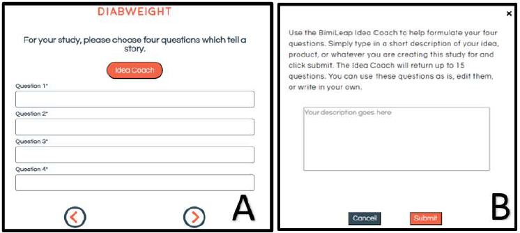
Figure 1: The completed set of four questions, after being edited and polished by the researcher
Once the researcher has composed the squib and put it into Figure 1, Panel B, the Idea Coach returns with a proposed set of questions. Each iteration of the Idea Coach generates 15 different questions. The researcher can iterate as many times as desired, changing the squib or keeping the squib the same. The AI will return a number of new questions each time, and occasionally repeat a question. At the end of the iteration the research will have developed four questions and can edit them. Figure 2 shows the completed set of four questions after they have been developed by Idea Coach, and ‘edited’ in preparation for the answers.
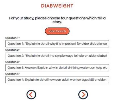
Figure 2: The completed set of four questions, after being edited and polished by the researcher
After the squib is constructed and put into Figure 1, Panel B, Idea Coach creates a set of 15 questions from a squib in approximately 10-20 seconds. The researcher can select a question or several questions, dropping them into the study, and editing them. When the researcher does not find a question to drop into the study it is easy to re-run the Idea Coach, either with the same squib or with a revised squib. The process can go on several times, until the researcher has uncovered four questions, using Idea Coach and/or developing the question(s) oneself. Idea Coach truly becomes a coaching tool after the researcher gains experience.
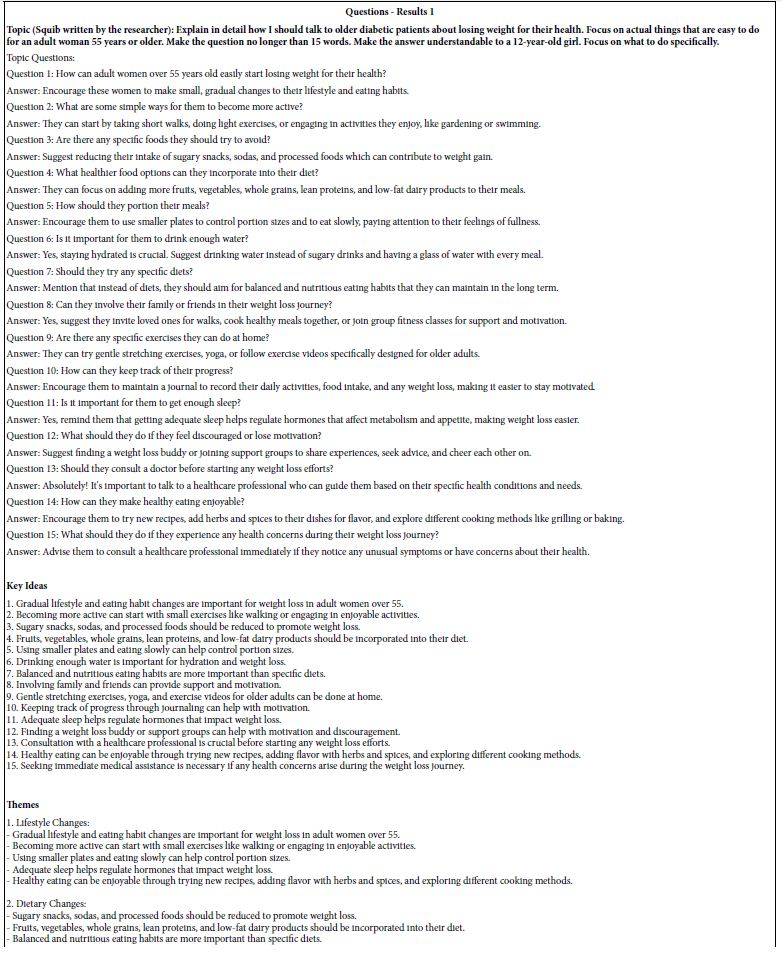
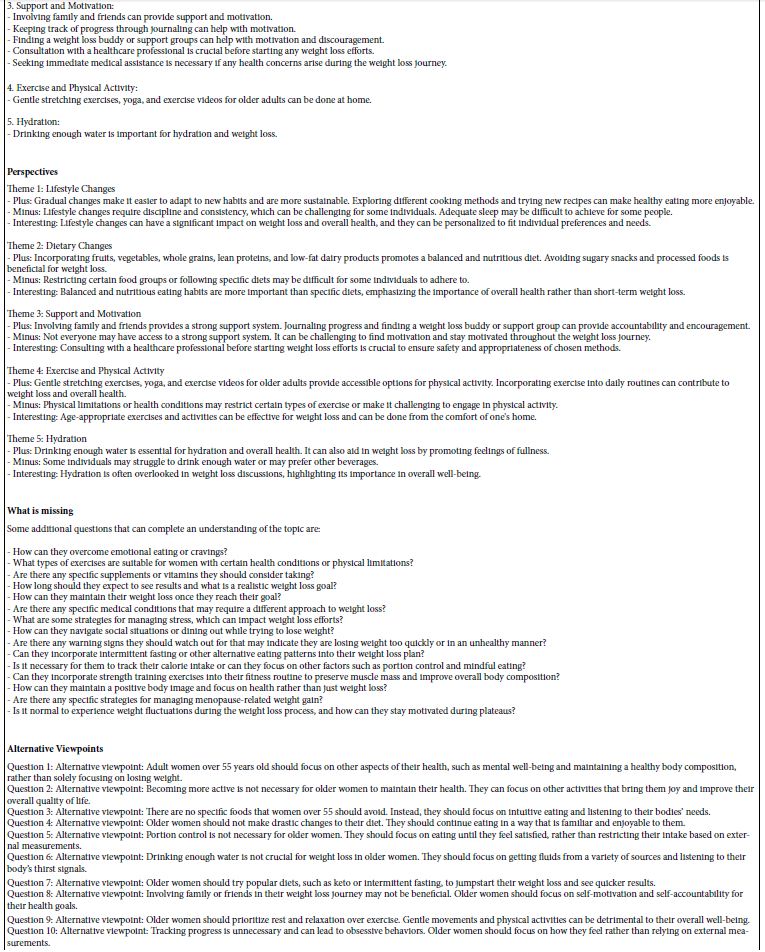
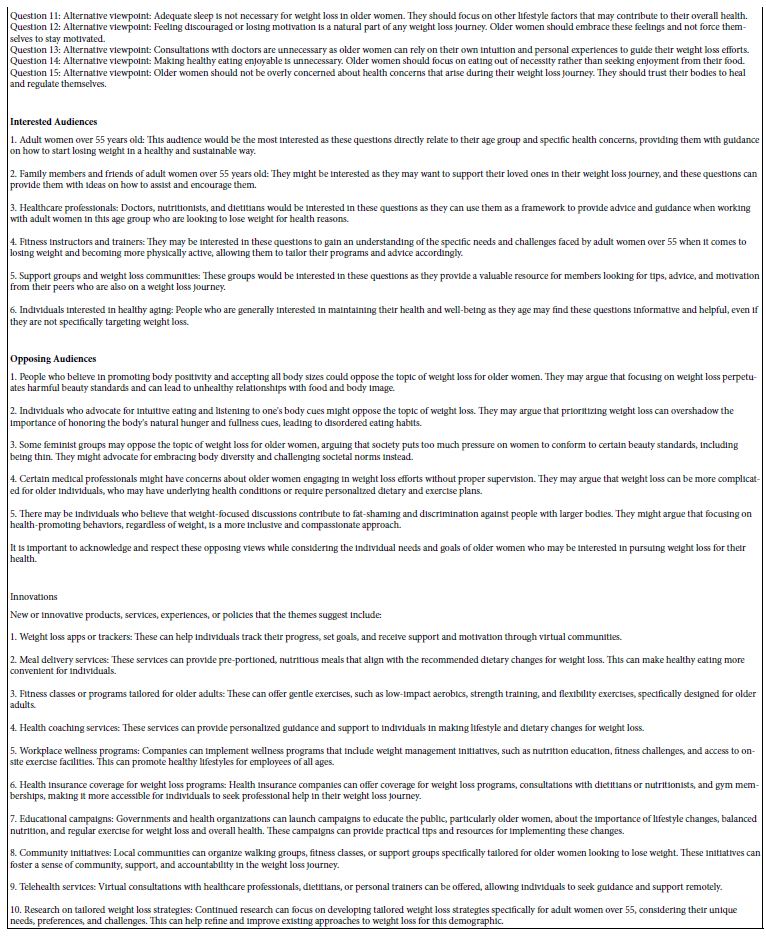
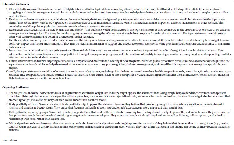
At the end of the development of questions, and later of answers, the Mind Genomics platform stores each of the iterations of 15 questions (and 15 answers) on a separate Excel tabulation. As the study is being closed, the platform subjects each set of 15 questions (or answers) to an extensive summarization, using AI, with specific prompts. Table 1 presents the AI summarization of the first set of 15 questions.
Table 1: First results from the AI-powered Idea Coach, attempting to develop questions from the squib
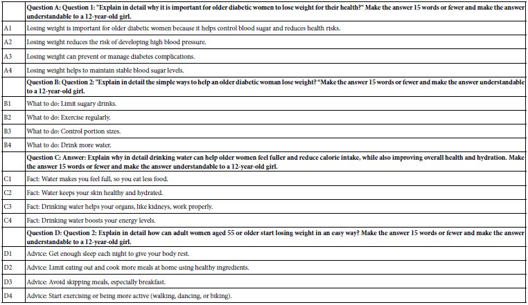
Once the researcher has completed the set-up of the questions, the next step is to set up the four answers to each question. In this case the researcher must edit the questions in order to ensure that the answers are short and understandable. Such editing occurs as the researcher completes the creation of the four questions. It becomes a simple matter to add a phrase to the question as part of the prompt to the AI-driven Idea Coach, that prompt guiding the style of the answer provided. Table 2 shows the first set of 15 answers to Question #1 after the question has been edited by the researcher.
Table 2: First results from the AI-powered Idea Coach, attempting to develop 15 answers from the first question, that question edited to direct the style and comprehension level of the answers.

As we finish this section of the set-up it is well to keep in mind that the incorporation of the AI into the creation of questions and answers ends up producing an ‘Idea Book.’ This Excel file becomes a rich source of information about the topic, summarized by key issues and questions. The Idea Book moves from the list of questions, itself valuable for the researcher, onto issues of points of view, suggestions of what’s missing, and even suggestions about innovations. As noted above, the entire process of creating each logical page should be no more than a minute, with the creation of a 20-page book on the topic requiring less than 20 minutes.
Table 3 shows the final set of questions and answers. The answers have been edited by the researcher in order to be more readable when they are presented to the respondents in various combinations of answers. Henceforth, the answers will be referred to as ‘elements.’ The questions themselves will not play any role in the actual evaluation by respondents, nor in the analysis of the results. Rather, the questions are simply used to allow the researcher or Idea Coach to create a set of related but different ‘elements’, viz., different answers.
Table 3: The final questions and elements (answers to the question), after editing by the researcher
Setting Up the Mind Genomics Study
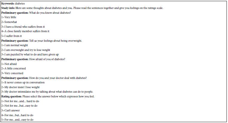
Mind Genomics studies comprise several parts, all templated. Table 4 shows these parts. Table 4 is provided as a standard output of every Mind Genomics project:
- Key words selected by the researcher in order to make searching for the study results easier in the database of Mind Genomics studies.
- Respondent orientation
- Self-profiling questions. Gender and age are standard questions in every study, and so are not shown in Table 4.
- The rating question and the different answers.
Table 4: Study information
The Respondent Experience in the Mind Genomics Study
Once the study set up has been completed it is the task of the researcher to provide respondents. With the advent of the Internet, it has become increasingly easy to obtain respondents, although at a slight cost to the researcher. It is the business of companies in the market research ‘space’ to provide motivated respondents for the many hundreds of thousands, perhaps millions or dozens of millions of studies on the internet. Across the entire world there have emerged companies which, for a fee, offer their members the chance to participate in on-line studies. It is from one of these companies, Luc.id Inc., in Louisiana, that the respondents are obtained, with the respondents satisfying specific criteria: Age 45 or older, Lives in one of three states: New York, New Jersey or Connecticut.
Luc.id Inc. is set up to provide these individuals, doing so with the actual experience taking approximately five minutes for a respondent. The respondents are recompensed by Luc.id, ad are totally anonymized. The respondent opts in to participate in the particular study. In turn, the research guarantees not t accept any specific identifying information during the course of the study, In situations where the researcher wants specific information, that information is requested in the ‘open ended’ questions, with a disclaimer that the information offered is entirely optional and left to the respondent.
Luc.id sent out email invitations to the prospective respondents, doing so in ‘waves’ until the quota of 101 respondents was filled. The quota comprised females, ages 45-70, living in New York, New Jersey or Connecticut, respectively. For easy to find respondents, such as those participating in this Mind Genomics study, the quota of 101 individuals is typically filled within 90 minutes. The Mind Genomics platform orients the respondents, presents the test materials, acquires the ratings, creates a database, performs the relevant analysis, and then creates the report along with AI summarization, generally within 15-30 minutes after the completion of the field work.
The actual Mind Genomics experiment begins with a short ‘hello’, and proceeds to the self-profiling classification shown in Figure 3, Panel A. The self-profiling classificaiton presents a clean screen to the respondent. The alternative answers to each question appear when the respondent reaches that question. The happy consequence of this pull-down screen is that the respondent is made to feel comfortable, rather than being confronted by a wall of words.
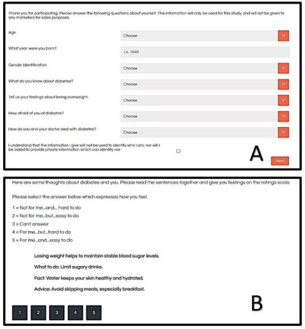
Figure 3: The respondent experience in the Mind Genomics experiment. Panel A shows the pull-down menu for the self-profiling classification. Panel B shows an example of a vignette, accompanied by a short introduction and the rating scale, both at the top.
Afterwards, the respondent is exposed to 24 different vignettes, similar to that shown in Figure 3, Panel B. The vignettes are shown one vignette after another. The respondent is told simply to rate the combination. Exit interviews with respondents over the years as well as observations of colleagues participating in the Mind Genomics interview continue to point to the fact that professionals try to ‘outsmart’ the system, whereas ordinary respondents simply fall into a relaxed mode, and end up saying that they ‘guess.’ The results below will show that the respondents are performing quite well, and that despite their statement that the feel they are ‘guessing’, the opposite is true. The typical respondent, the non-professional, ends up realizing that it is impossible to ‘game the system’, and settle for a relaxed experience. This relaxed, almost non-involved evaluation is felt to more validly represent the real judgment of the respondent, the judgment made when no one seems to be looking.
Creating the Database and Transforming the Ratings for Subsequent Statistical Analyses
The Mind Genomics study presents vignettes to the respondent, and acquires both the rating on the two-sided scale, as well as the response time. The response time is defined as the elapsed time between the presentation of the vignette and the respondent’s selection of the rating, Figure 4 shows the three vignettes from respondent (participant) #27. As one might surmise, there are 2424 vignettes in total, each vignette different in composition from every other vignette, accompanied by the rating and the response time. When the response time was longer than 9 seconds, BimiLeap automatically made the response time 9 seconds. The reason for this seemingly arbitrary rule is that the respondents were unsupervised and might have been doing other things. Thus, it is important to truncate the range of response times in order to avoid accepting response times of say 36 seconds. Clearly that response time reflects other behaviors besides the respondent participation in the study.
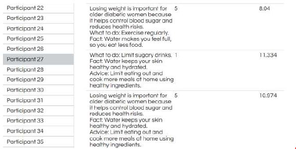
Figure 4: Example of input information to the database showing the respondent, the text of the vignette, the rating assigned to the vignette, and the number of seconds elapsing between the presentation of the vignette and the assignment of a rating.
Relating the Presence/Absence of the Elements
The essence of Mind Genomics is relating the presence/absence of the elements in the vignettes to the ratings. The vignettes themselves vary from respondent to respondent, and in actuality are only vehicles in which to embed the 16 elements. It is the elements which convey the actual information. In turn, the rating scale is the device by which the respondent can communicate feelings. Both the vignettes and the rating scale, however, need to be translated into a set of variables that can be analyzed by statistics.
Figure 5 shows the part of the database prepared for the subsequent statistical analysis. Figure 5 divides into three distinct panels.
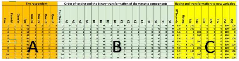
Figure 5: The database for vignettes 1-11 presented to and rated by Panelist (respondent) #1
Panel A shows the row number of the database, and then information about the respondent, as provided by the respondent.
Panel B shows the order of testing (1-24) for the specific vignette, and then the deconstruction of the composition of the vignette into a series of 1’ and 0’s. Recall that the vignettes comprise combinations of elements, done so according to an experimental design. The particular design used here, the permuted experimental design, uses one basic structure, but changes the specific combinations through a permutation scheme [15]. The benefit is that each respondent’s data can be analyzed as either part of a group, or analyzed separately, one respondent at a time. The transformation of the experimental design is done by so-called ‘dummy variable’ coding [20]. The coding creates 16 columns, one for each element. When the element is present tin the vignette the cell has the value ‘1’. When the cell is absent from the vignette the cell has the value ‘0’. The 1’s and 0’s are called dummy variables because nothing is known about these variables other than presence or absence. Any analysis with these dummy variables simply shows the contribution to a criterion variable which occurs when the element is placed into the vignette. The ‘why’ is unknown. Only the ‘what’ is known Panel C shows the response time (time elapsed between the appearance of the vignette on the screen and the response), as well as the five-point rating assigned to the vignette. The remaining columns show the transformations of the ratings into the five single responses, the key being R5x (For me, Easy to do), and then two ‘combined’ responses R54 (For me), R52 (Easy to do).
R54x=100 when the rating is either 5 or 4, R54=0 when the rating is 3, 2 or 1
R52x=100 when the rating is either 5 or 2, R52=0 when the rating is 5,3 or 1
Once the database has been constructed, the Mind Genomics platform creates a set of simple linear equations, viz., linear models, first for the total panel, and then for each self-defined subgroup, self-defined age grouping, and finally gender. The analysis is called linear regression [21], with the variables taking on only one of two levels, 0 for absent, 1 for present, so-called dummy variables.
The equation for each binary variable is expressed schematically as: Binary Dependent variable=k1(A1) + k2(A2) … k16(D4). The equation just presented shows how each of the 16 elements ‘drives’ the binary rating. Typically, the standard error is about 7-8 for these studies, suggesting that coefficients around 16 or higher should be significant in a statistical sense.
The Mind Genomics platform ends up providing a great deal of data, almost a ‘wall of numbers.’ In order to identify underlying patterns, the convention is to shade the so-called ‘strong performer.’ ‘Strong’ means meaningful, based upon insights gleaned from previous Mind Genomics experiments. We move beyond the conventional criterion of ‘statistically significant’ to the following:
For the binary transformed variable, R54, typically the key ‘evaluative variable, such as ‘for me’ or ‘I will buy’, we shade coefficients of 21 or higher.
For all other binary transformed variables, e.g., R52, R5, etc., we shade coefficients of 16 or higher.
For RT, response time, we shade coefficients of 1.5 or higher, the foregoing criteria are not ‘fixed in stone.’ Rather, they reflect simple heuristics which allow the researcher to identify emergent themes. Indeed, the search for themes is so important in Mind Genomics that an alternative heuristic might be considered, namely deleting all coefficients which are lower than the cut-off criterion. That alternative ends up typically creating a sparse table, since in conventional Mind Genomics the coefficients are usually far lower than what we see here.
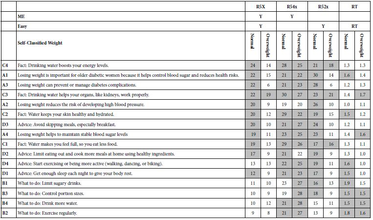
Table 5 shows the coefficients for the linear equations relating the presence/absence of the 16 elements to the binary transformed variables of R5x, R54x, and R52x, respectively, along with the coefficients for the RT (response time) equation. Ordinarily, R5x (For me and Easy) would not appear in the table. Rather, R54 (For Me) would become the focus of the analysis. Table 5 shows the surprising finding that for this study on obesity and diabetes virtually all of the elements (15 of 16) are strong performers, with coefficients of 21 or higher. In light of this remarkably strong performance of virtually all elements we move the key evaluative variable to R5x, (For me and Easy), which shows the more typical pattern observed in the results for other topics, not medical ones but rather products and services.
Despite the strong performance of many elements, Table 5 does not give up secrets about the underlying patterns of strong performing elements. For example, three of the four strongest performing elements for R5x deal with water and drinking, but drinking water must be associated with a reason, not just be present by itself. When present by itself, without any outcome, however, drinking water performs poorly.
Table 5: Coefficients for important transformed binary variables, and for response time. The elements are sorted in descending order by the coefficient for R5x.
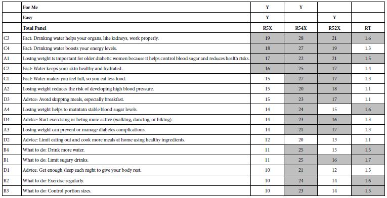
Fact: Drinking water helps your organs, like kidneys, work properly.
Fact: Drinking water boosts your energy levels.
Losing weight is important for older diabetic women because it helps control blood sugar and reduces health risks.
Fact: Water keeps your skin healthy and hydrated.
In a similar fashion patterns for R52X (Easy to do) and RT (response time) are elusive. No clear pattern emerges. We see differences in two variables when we deal with respondents who declare themselves normal weight versus those who declare themselves as overweight. Table 6 shows the dramatic differences between these groups, attributable to the rating of ‘easy’. Those who declare themselves overweight find most of the elements to refer to themselves (high coefficients for ME) but harder to do (lower coefficients for R52X, corresponding to easy). These results suggest the promising use of ‘Easy” as a key variable to consider.
Table 6: Coefficients for important transformed binary variables, and for response time, shown for two self-defined groups, Normal Weight versus Overweight.
Mind-Sets: Uncovering Deep Differences among People in Order to Drive Effective Messages
A continuing theme in Mind Genomics is the emergence of mind-sets, clusters of people who perceived the world in clearly different ways, in ways which make sense and point to divergence what these clusters to feel to be important. Table 6 gives us a sense that when it comes to ‘Hard vs Easy’, those who declare themselves to be overweight find many statements to be not quite as easy as those who declare themselves to be normal weight. This difference in people makes sense but does not satisfy. The differences are there, but do not strike us as a compelling story.
One way to identify these possibly more profound differences is by statistics alone, by considering the pattern of the 16 coefficients and searching for different patterns. The search is not based on the self- definition of the respondent, nor based on the meaning of the elements. Rather, the search is based purely on the mathematical structure of the 16 coefficients. If the mathematics reveals clearly different, easy to interpret mind-sets, the research will have provided a powerful tool to identify what to communicate, and to whom.
The method used to create these clusters is called k-means clustering [22]. The objective is to put the different objects, our 101 respondents, into groups based upon an objective criterion. The criterion is that the ‘distance’ between pairs of people in a cluster should be ‘small’, but the distances between the centroid (average) of the 16 coefficients should be large. The k-means clustering is not exact but tries to satisfy these conditions.
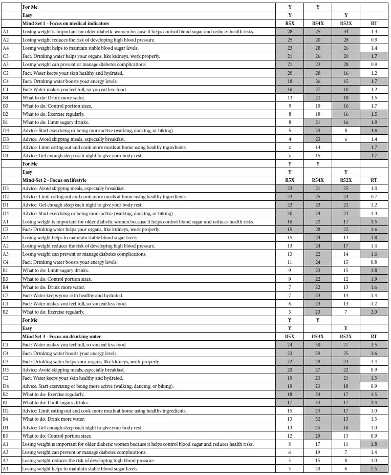
The study uses the coefficient for R5X (ME and Easy to do) as the variable on which to do the clustering exercise. We can imagine 101 rows of coefficients, one row for each respondent, and in turn 16 columns of coefficients. Table 7 shows the strongest performing elements for each mind-set or cluster, respectively Mind-Set 1 (focus on medical indicators), Mind-Set 2 (Focus on Lifestyle), and Mind-Set 3 (Focus on drinking water). Each table is sorted by the coefficients for R5X (For ME and Easy). Each mind-set is clearly different, and interpretable, remarkable in view of the actual ‘difficulty’ of doing the study on the part of the respondent. Recall that each respondent had evaluated 24 different vignettes, with 2-4 elements, seemingly randomly put together. Despite what one might think, the respondents actually perform quite well.
Table 7: Coefficients for important transformed binary variables, and for response time. The elements are sorted in descending order by the coefficient for R5x, for each of the three emergent mind-sets.
In Their Own Words
Our three mind-sets suggest radically different words to which they are sensitive. Do these mind-sets transcend the simple statistical analyses which brought them to our attention? In other words, beyond statistics which tell a ‘nice story’ can we find anything else. One way is to look at how they describe their experience with diabetes, whether their own, their family experience, or just their knowledge.
Each respondent was instructed to write bout diabetes from their own point of view, doing this exercise AFTER having done the evaluation of the 24 unique vignettes. An AI ‘summarizer’, QuillBot [23], took the open-ended answers, and summarized them. Table 8 shows three rather different summaries, suggesting that these mind-sets do actually think about diabetes in different ways. The objective of showing the summarizations is to give a sense of the different ‘morphologies’ or structures in the way people of mind-sets write about their experience, what they say, how they say it.
Table 8: AI summarization of open-ended answers about experience with diabetes from the three emergent mind-sets
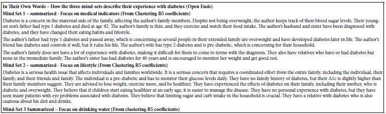
Diabetes is a terrible disease that can lead to limb loss and death. It is not a common issue in the family, but it is a serious concern that should be addressed by children. The author believes that children should be more proactive in preventing and helping others who are aware of the disease. They also mention that their family is concerned about obesity and is aware of sugar complications. The author believes that children can learn from their grandparents’ experiences and be more proactive in preventing diabetes. They also mention their own family members who have had diabetes and have lost limbs. They all try to maintain healthy lifestyles and avoid complications. Despite not having children, the author believes that everyone should prevent diabetes and help others.
Identifying the Mind-sets in the Population
An important outcome of dividing people into mind-sets is the ability to tailor the proper message to each person. By understanding the different messages to which people are sensitive, there is the possibility of increasing the overall health of a population. Proper messaging has been shown to substantially reduce the number of within-30-day hospital readmissions after discharge for patients with congestive heart failure [24], as well as double the number of colorectal cancer screenings in an underserved area in the Philadelphia area [25].
How then do we assign a given person to one of the mind-sets? Once the person is properly assigned to a mind-set it becomes much simpler to identify the set of messages likely to communicate properly and effect the appropriate behavior response. The traditional approach has been to look at easy-to-measure factors, such as gender, age, and superficial cultural cues. The experienced physician may attend to more cues, as would an experienced salesperson. But what about the situation wherein one cannot involve an experienced professional. Is there any way that the staff at the ‘front desk’ might be able to assign a patient to a mind-set in a perhaps a minute or less, and attach that information to the patient chart, along with the relevant material to communicate, as well as well as what to avoid.
During the past decade author Moskowitz and colleagues have worked on an identification system, a mind-type assigner or personal viewpoint identifier [16,17]. The objective is to create a short set of questions such as that shown in Figure 6. With such a tool, it becomes possible to have a patient fill out the form in a minute or two. Panel A shows the background information that the patient fills out. Panel B shows the six questions, taken from the study, and answered with a two-point scale. The pattern of responses to the six questions ends up assigning the patient to the most appropriate mind-set.
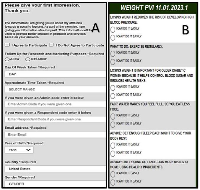
Figure 6: The first two portion of the mind-set assigner. Panel A shows the background information. Panel B shows the six questions, which are presented in randomized order for each respondent.
Table 9 shows set-up for the ‘assigner’ tool’, including the name of the mind-set, and the feedback given either to the patient and/or t the medical professional. The mind-set assigner further provides the ability to send the respondent to a website with a video.
Table 9: Set up information for the mind-set assigner
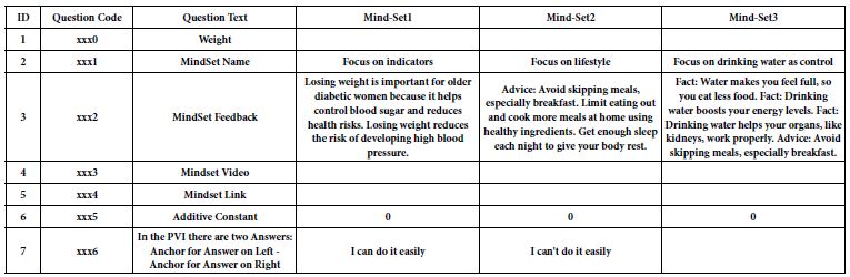
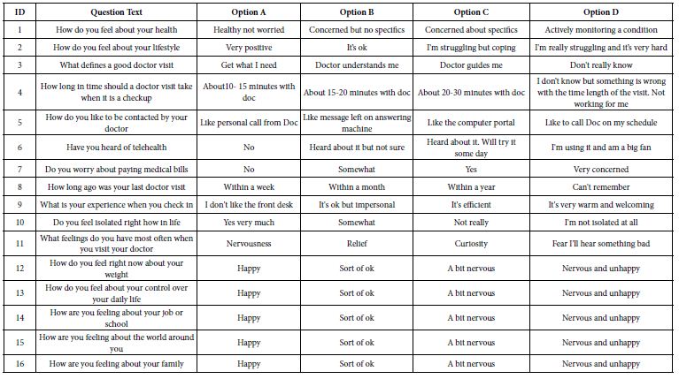
The final feature of the mind-set assigner is the ability to ask a set of 16 different questions, each with 2-4 answers. Table 10 shows the set of 16 questions for this study. The mind-set assigner with its set of 16 questions enables the researcher to work with many new respondents, both assigning each respondent to a mind-set, and obtaining more data about the respondent. In this way the research into mind-sets moves beyond simply understanding the person in terms of the particular situation, but actually allows the researcher to deepen knowledge of the person and the covariation of that knowledge with mind-type membership.
Table 10: The 16 questions and their associated answers. The Questions and Answers constitute the third ‘leg’ of the mind-set assigner.
Discussion and Conclusions
The study on diabetes and obesity presented here constitutes the second of a planned series of studies on the communication between the doctor and the patient, using the emerging science of Mind Genomics. Several searches through the published literature and a discussion with young medical professionals revealed again and again that there is a well-established clinical literature on many medical topics, but very little on the words that doctors should say to patients, and the meanings of what patients say to doctors. The oft-given reason, perhaps excuse, is that this sensitivity to the patient can come only with experience, and that the doctor must learn to listen [26].
As the medical world becomes increasingly subject to the financial structures of capitalism, the time that a doctor spends with a patient necessarily decreases. It is the doctor’s time which ‘costs’, and the goal of a business such as the business of health care is to reduce these topline costs. It may be possible to optimize the throughput of diagnostics, and increase the efficiencies in hospital stays, especially surgery, but what about the ability of the doctor or other medical professional to communicate with the patient. If it takes years to educate someone to become an actor as well as years to become a doctor. Where then is the time to become a listener, and an empathic conveyor of news, often bad news. It is the attention to this topic, empathic information exchange, to which this new effort of Mind Genomics is dedicated, and in which spirit this early experiment and paper in that effort have been done and written. The discovery that there are really three mind-sets, not just one general mind-set with the ‘most right messaging’ becomes the important discovery here, one which, if not addressed, can become an ongoing issue in mammography, perhaps getting worse as the medical system becomes increasingly driven to efficiency by driving out the human component.
References
- Boles A, Kandimalla R, Reddy PH (2017) Dynamics of diabetes and obesity: Epidemiological perspective. Biochimica et Biophysica Acta (BBA)-Molecular Basis of Disease 1863: 1026-1036. [crossref]
- Mokdad AH, Ford ES, Bowman BA, Dietz WH, Vinicor F, et al. (2003) Prevalence of obesity, diabetes, and obesity-related health risk factors, 2001. JAMA 289: 76-79. [crossref]
- Mozaffarian D (2016) Dietary and policy priorities for cardiovascular disease, diabetes, and obesity: a comprehensive review. Circulation 133: 187-225. [crossref]
- Ling H, Lenz, TL, Burns, TL, Hilleman, DE (2013) Reducing the risk of obesity: defining the role of weight loss drugs. Pharmacotherapy: The Journal of Human Pharmacology and Drug Therapy 33: 1308-1321. [crossref]
- Cohen MM Fiona Elliott, Liza Oates, Adrian Schembri, Nitin Mantri (2017) Do wellness tourists get well? An observational study of multiple dimensions of health and well-being after a week-long retreat. The Journal of Alternative and Complementary Medicine 17: 140-148. [crossref]
- Nagy A, McMahon A, Tapsell L, Deane F, Arenson D (2018) Therapeutic alliance in dietetic practice for weight loss: Insights from health coaching. Nutrition & Dietetics 75: 250-255. [crossref]
- Incollingo Rodriguez AC, Rodriguez A, Callahan LC, Saxbe D, Tomiyama, AJ (2019) The buddy system: A randomized controlled experiment of the benefits and costs of dieting in pairs. Journal of Health Psychology 24: 1945-1954. [crossref]
- Elder KA, Wolfe BM (2007) Bariatric surgery: a review of procedures and outcomes. Gastroenterology 132: 2253-2271. [crossref]
- Greenacre M, Groenen PJ, Hastie T, d’Enza AI, Markos A, et al. (2022) Principal component analysis. Nature Reviews Methods Primers 2: 100.
- Omran MG, Engelbrecht AP, Salman A (2007) An overview of clustering methods. Intelligent Data Analysis 11: 583-605.
- Grimm P (2010) Social desirability bias. Wiley International Encyclopedia of Marketing.
- Krumpal I (2013) Determinants of social desirability bias in sensitive surveys: a literature review. Quality & Quantity 47: 2025-2047.
- Moskowitz HR, Gofman A, Beckley J, Ashman H (2006) Founding a new science: Mind Genomics. Journal of Sensory Studies 21: 266-307.
- Green PE, Krieger AM, Wind Y (2001) Thirty years of conjoint analysis: Reflections and prospects. Interfaces 31: S56-S73.
- Gofman A, Moskowitz H (2010) Isomorphic permuted experimental designs and their application in conjoint analysis. Journal of Sensory Studies 25: 127-145.
- Porretta S (2021) The changed paradigm of consumer science: from focus group to mind genomics. In Consumer-based New Product Development for the Food Industry. The Royal Society of Chemistry 21-39.
- Porretta S, Gere A, Radványi D, Moskowitz H (2019) Mind Genomics (Conjoint Analysis): The new concept research in the analysis of consumer behaviour and choice. Trends in Food Science & Technology 84: 29-33.
- Moskowitz HR (2012) ‘Mind Genomics’: The experimental, inductive science of the ordinary, and its application to aspects of food and feeding. Physiology & Behavior 107: 606-613. [crossref]
- Cropley D (2023) Is artificial intelligence more creative than humans?: ChatGPT and the Divergent Association Task. Learning Letters 2: 13-13.
- Hardy MA (1993) Regression with dummy variables (Vol. 93). SAGE.
- Burton AL (2021) OLS (Linear) regression. The Encyclopedia of Research Methods in Criminology and Criminal Justice 2: 509-514.
- Likas A, Vlassis N, Verbeek JJ (2003) The global k-means clustering algorithm. Pattern Recognition 36: 451-461.
- Fitria TN (2021) QuillBot as an online tool: Students’ alternative in paraphrasing and rewriting of English writing. Englisia: Journal of Language, Education, and Humanities 9: 183-196.
- Gabay G, Moskowitz HR (2019) “Are we there yet?” Mind-Genomics and data-driven personalized health plans. The Cross-Disciplinary Perspectives of Management: Challenges and Opportunities 7-28.
- Oyalowo A, Forde KA, Lamann A, Kochman ML (2022) Effect of patient-directed messaging on colorectal cancer screening: A randomized clinical trial. JAMA Network Open 5: e224529-e224529. [crossref]
- Bombak AE, Riediger ND, Bensley J, Ankomah S, Mudryj A (2020) A systematic search and critical thematic, narrative review of lifestyle interventions for the prevention and management of diabetes. Critical Public Health 30: 103-114.