Author Archives: author

Age Structure and Growth Rate of Rutilus frisii kutum (Kamensky, 1901) Population in Vali Abad River (Southern Caspian Sea), Iran

DOI: 10.31038/AFS.2022422

Abstract

This study was conducted to determine the age and growth of Caspian kutum (Rutilus frisii kutum) in Vali Abad River, Mazandaran Province during 2020-2021. In this experiment, 100 fish were caught using a gill net with a mesh size of 5 mm. Kutum age was determined based on the scales. The results showed that the maximum age of males and females of the study area was 5+ and 6+ years, respectively. In males, the fish were 3+ years old (57.14%) and for females, 4+ years old (35.71%) had the highest frequency among age groups. The highest instantaneous growth rate was recorded in both sexes between 2+ and 3+ years, and this parameter has decreased significantly with increasing age. The relationship between total length and weight was calculated for males TL=3.23W-12.95 (R2=0.92, n=50) and for females TL=3.01W-11.61 (R2=0.85, n=50). Based on Powell’s formula, the growth pattern was isometric for both sexes.

Keywords

Age and growth, Caspian Sea, Mazandaran, Rutilus frisii kutum, Vali Abad River

Introduction

Age is one of the most important biological aspects of fish, and the lack of accurate information on the age of many fish species leads to inappropriate management policies [1]. Growth phenomenon is also one of the most key biological aspects of fish in the population, which exhibits the type of adaptation to environmental conditions [2]. The kutum in the Caspian Sea (Rutilus frisii kutum) belong to the Cyprinidae family [3]. This species can be found all along the southern coast of the Caspian Sea from the river Atrak to the Kora. Vali Abad River, one of the tributaries of Cheshmeh Kileh River, flows in the southeast of Tonekabon city center. It is rain-fed and flows from west to east. The river has a length of 14 km, an average bed slope of 0.7% and flows in bicarbonate and bicarbonate sulfate areas [4]. Many kutums migrate to the Shiroud, Vali Abad, Hawiq, Lemir, Anzali, Sefidrood, Tajan, Babolrood and Gorganrood Rivers to reproduce in the coasts of Iran [5]. Terms of catch and extraction, kutums is one of the most valuable fisheries in the Caspian Sea and contributes more than half of the total catch of bony fish [6]. Overall, 90% of its resources comes from Iran [7]. This fish with its high economic value in the southern shores of the Caspian Sea which depends on conservation [8].

There are numerous studies on the age structure and growth of kutum in the southern part of the Caspian Sea [6,9-14]. In view of the vital role of kutum, especially for northern Iran, and the policy pursued by the Iranian Fisheries Department to conserve this species by artificial reproduction, which takes place every year at the mouths of rivers, it would seem that the Caspian kutum must be examined annually. The objective of this study was to determine the age and growth parameters of the Caspian kutum in the Vali Abad River to take more effective management measures.

Materials and Methods

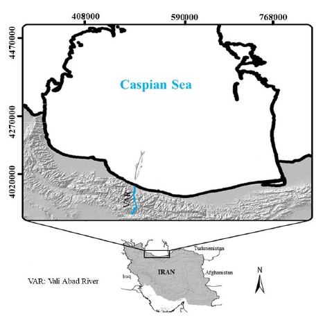
The study was conducted in 2020-2021 (from March 11 to May 4) on Vali Abad River in Mazandaran province (Figure 1).

fig 1

Figure 1: Map of the Iranian waters of the Caspian Sea, showing the fishing area

In this study, 100 fish samples (50 males, 50 females) were caught using a gill net with a 5 mm mesh size. At the same time, these fish were caught for reproduction, to be released and restore reservoirs. Total body weight was measured using a digital scale with 15 gr accuracy, and total body length was measured using a biometric board with 1 mm accuracy. To determine age, six scales were removed from the beginning of the dorsal fin and lateral line. They were first washed with a soap solution between two fingers to remove the epidermal layer. The scales were then placed dry between two slides and fixed with adhesive tape [15]. The annual rings were determined under a mirrored loop with a magnification of 10 to 40. The average length, weight, and composition of the different age groups as well as the length classes frequencies were evaluated in Excel.

Length-weight Relationship

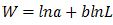
The relationship between length and weight in fish was an exponential relationship of 1 that was converted to a linear relationship by logarithm 2. Where W: weight of the fish (gr), L: total length (mm), a: constant coefficient, b: the slope of the curve resulting from length and weight [16].
Condition Factor

The condition factor is calculated by from the Whitely equation [17]. 3 where K: Condition factor, W: Total body weight (gr), L: Total body length (mm).
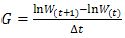
Instantaneous Growth Rate

Instantaneous growth rate is calculated by the presented formula [17]. 4 Where G is instantaneous growth coefficient, lnW (t) is normal logarithm of (t) yearly weight (gr), lnW (t + 1) is normal logarithm of weight of (t + 1) (gr), Δt is difference between (t + 1) age and yearly (t).

Growth Pattern

Growth pattern was determined by Pauli test [18] including: 5 Where SdlnL is standard deviation of the natural logarithm of length (mm), SdlnW is standard deviation of the natural logarithm of weight (g), b is slope of the curve resulting from the relationship between length and weight, r2 is regression coefficient between length and weight, and n is the number of samples.
The graphs and calculations were made with the programs Excel (2019) and SPSS (26) software.

Results

Average Length-Weight, and Frequency Percentage at Different Ages

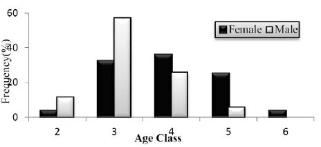
The results showed that the length of females and males ranged from 372.82 ± 2.13 to 447.28 ± 8.99 mm and from 369.90 ± 5.18 to 403.00 ± 5.70 mm, respectively. Their weight varied between 517.57 ± 5.27 and 894.19 ± 81.26 g, and between 486.41 ± 25.30 and 615.42 ± 42.00 g for the female and male fish, respectively (Table 1). Five and four age classes were observed between females and males, respectively. Females had the highest frequency in age group 4+ (35.71%) and the lowest frequency in age group 6+ (3.57%). While for males, the highest and lowest frequencies in age groups were recorded in 3+ (57.14%) and 5+ (5.72%) (Figure 2).

Table 1: Average length (mm), weight (gr) in different age groups of female and male kutum in the Vali Abad River

Age groups

Sex

2+

3+ 4+ 5+

6+

Female TL(mm)

372.82±2.13

412.17±16.83 430.30±5.96 438.32±14.71

447.28±8.99

W(gr)

517.57±5.27

684.10±33.90 819.45±67.18 842.24±21.38

894.19±81.26

Male Tl(mm)

369.90±5.18

383.19±8.82 387.16±7.39 403.00±5.70

W(gr)

486.41±25.30

549.99±44.18 571.94±38.10 615.42±42.00

fig 2

Figure 2: Kutum age frequency in the Vali Abad River

Frequency of Length Classes

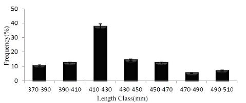
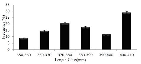
The most frequent length classes were recorded for female 430-410 mm (37.5%) (Figure 3) and male 410-400 mm (28.57%) (Figure 4).

fig 3

Figure 3: Percentage of length frequency of female kutum in the Vali Abad River

fig 4

Figure 4: Percentage of length frequency of male kutum in the Vali Abad River

Length-Weight Relationship

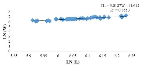
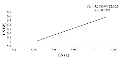
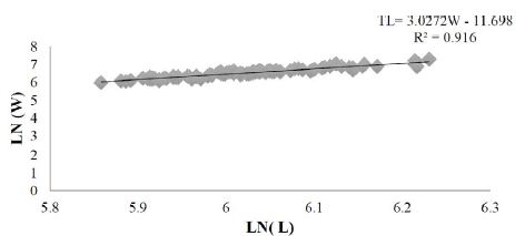
Relationship between length and weight in female fish TL=3.01W-11.61 (R2=0.85, n=50) (Figure 5), male fish TL=3.23W-12.95 (R2=0.92, n=50) (Figure 6) and total fish TL=3.02W-11.69 (R2=0.91, n=100) (Figure 7). Computational t was obtained for females, males, and total fish at 0.96, 1.39, and 1.04, respectively, which were compared with the t-table with n-2 degrees of freedom at the level 0.95, It is smaller than the t-table, so the growth pattern of all three groups is isometric.

fig 5

Figure 5: Length-weight relationship of female kutum in the Vali Abad River

fig 6

Figure 6: Length-weight relationship of male kutum in the Vali Abad River

fig 7

Figure 7: Length-weight relationship of total kutum in the Vali Abad River

Instantaneous Growth Rate (G)

The highest instantaneous growth rate was attributed to the two age groups 2+ to 3+ compared with other age groups (Table 2).

Table 2: Instantaneous growth coefficient (G) in different age groups of kutum in the Vali Abad River

Age

2+ – 3+ 3+ – 4+ 4+ – 5+

5+ – 6+

Female

 0.279

0.180  0.028 0.06
Male

0.122

0.039 0.074
Total

0.206

0.119 0.058

0.06

Condition Factor (K)

The results of the six groups age condition factor in females, males, and total fish showed that female fish in age group 2+ (1.065), male fish in age group 3+ (0.985), and total fish in age group 4+ (1.004) were condition factor better than other groups (Table 3).

Table 3: Condition coefficient (K) in different ages of kutum in the Vali Abad River

 Age

2+ 3+ 4+ 5+

6+

Female

1.065

0.977 0.996 0.746  1.001
Male

0.963

0.985 0.971 0.936

Total

0.977

0.981 1.004 0.996

1.001

Discussion

Population structure influences the number of age groups and maximum observed ages between populations [19]. The maximum age observed in this study was 5+ for male fish and 6+ for female fish. According to Afraei Bandpei et al. (2010), the maximum age for males and females in Shirood Tonekabon River was 7+ and 9+, respectively [13]. Gorjian Arabi et al. (2012) found that the observed maximum age for males was 4+ and for females was 5+ in Tajan River in Sari [12].

With respect to the average length and weight in the study area among the age groups, in male fish, length group 3+ (383.88 ± 19.52 mm) and weight group 4+ (571 ± 100.94 g) showed the highest standard deviation, while in female fish, the same parameter was observed in length and weight groups 5+ (438.32 ± 14.71 mm) and (842.246 ± 21.38 g), respectively. The high standard deviation in each of the above length and weight groups at different ages indicates the heterogeneity in length or weight at these ages, which may be attributed to the artificial reproduction of kutum in this river. Afraei Bandpei et al. (2010) studied fork length and weight of females of age classes 1+ to 9+ and reported that the highest fork length and weight were assigned to age class 9+ (580 mm and 2450 g) [13]. In addition, they examined males of age groups 1+ to 7+ and reported that age group 7+ (500 mm and 1689 g) had the highest values of the corresponding traits.

As for length frequency, the greatest in males was 416-400 mm (28.57%), while females’ length class in this river was 430-410 mm (37.5%). As for the growth pattern, the females (t=0.96), males (t=1.39) and total fish (t=1.04) were isometric. Growth patterns may vary depending on some biological and non-biological factors such as water temperature, food availability, and habitat type [20]. Isometric growth may be explained by seasonal variation and some biological parameters such as sex, maturity age, food quantity, etc. [15]. Similarly, Afraei Bandpei et al. (2010) found an isometric growth pattern for both sexes [13]. In contrast, Golshahi and Moradnejad (2009) claimed that growth pattern is allometric in both males and females [14]. Moreover, Forouhar Vajargah et al. (2020) demonstrated a negative allometric growth pattern for males and females is isometric [10]. The condition factor in male and female fish, as well as total fish was close to one. This factor is an indicator of the proportionality or relative condition factor of fish, that its increasing value indicates higher fish weight [17]. Farabi et al. (2008) stated the condition factor for female and male whitefish breeders in Mazandaran province as 1.42 and 1.38 respectively [21]. Forouhar Vajargah et al. (2020) determined condition coefficients for male, female and total fish of 1.10, 1.01 and 1.07, respectively [10]. Generally, weight of fish and other animals increases under the influence of body length, so it can be assumed that height and growth are related in a species. As for the correlation between length and weight, male fish (r2=0.92) showed a higher correlation than female fish (r2=0.85). Moreover, Golshahi and Moradnejad (2009) reported correlation coefficients for male fish (r2=0.976) and for female fish (r2=0.921) [14]. Regarding the instantaneous growth coefficient, the 3+ to 2+ age groups were the first age class, showed the highest instantaneous growth coefficient. Field and laboratory studies have shown that the change in growth rate is more dependent on the frequency and accessibility of food. [22] studied the instantaneous growth rate between age classes of both sexes and concluded that this coefficient does not follow the general rule of decreasing with age, which is consistent with our results.

Conclusion

Overall, the nutritional value of Caspian whitefish makes it necessary to take measures to prevent overfishing, especially during the reproductive season, in addition to artificial reproduction, to protect the region’s reserves and allow continuous fishing. Furthermore, proper management of dams on rivers leading to the Caspian Sea and water flow during the reproductive season in estuaries can allow migratory fish from the sea to enter the rivers to spawn, so that nature can find its way.

References

  1. Gelsleichter J, Piercy A, Musick JA (1998) Evaluation of copper, iron and lead substitution techniques in elasmobranch age determination. Journal of Fish Biology 53: 465-470.
  2. Mann RH, Growth and Production. In I.J (1991) Winfield and J.S. Nelson (EDS), Cyprinid Fishes. Systematic, Biology and Exploitation. Chapman and Hall, London, 446-481.
  3. Vossoughi GH, Mostajeer B (2006) Freshwater Fish. Tehran University Press, 317.
  4. National Geographical Organization of IRAN (2003) The gazetteer of rivers in the I.R of Iran, Caspian Sea watershed (Volume II). National Geographical Organization Publication, Tehran, 312.
  5. Naderi M, Abdoli A (2004) Fish Species Atlas of South Caspian Sea Basin (Iranian Waters). Iranian Fisheries Research Organization, Teheran, 2004, 112.
  6. Abdolmaleki SH, Hashemi A, Nahror R (2007) Fishing status and population structure of Caspian kutum, Rutilus frisii kutum in the Iranian Coastal Waters of Caspian Sea. Journal of Marine Science and Technology 6: 51-62.
  7. Razavi Sayad B. Kutum fish (1995) Iranian Fisheries Research Organization (IFRO). Tehran, 165.
  8. Abdoli A, Naderi M (2009) Biodiversity of Fishes of the Southern Basin of the Caspian Sea. Abzian Scientific Publication, Tehran, 237.
  9. Shahifar R, Patimar R, Fazli H, Raeisi H, Gholizadeh M, et al. (2020) Growth and mortality parameters of Caspian kutum, Rutilus kutum, in Southern Caspian Sea. International Journal of Aquatic Biology 8: 56-65.
  10. Forouhar Vajargah M, Sattari M, Imanpur J, Bibak M (2020) Length-weight relationship and‎ some growth parameters of‎ Rutilus kutum (Kaminski 1901) in‎ the South Caspian Sea. Experimental animal Biology 9: 11-20.
  11. Forouhar Vajargah M, Sattari M, Imanpur J, Bibak M (2020) Length-weight, length-length relationships and condition factor of Rutilus kutum (Actinopterygii: Cyprinidae) from the southern Caspian Sea, Iran. Journal of Animal Diversity 2: 56-61.
  12. Gojian Arabi MH, Sedaghat S, Hoseini SA, Fakhri A (2012) Age and Growth of Kutum, Rutilus frisii kutum (Kamenskii 1901) in Tajan River (Southern Caspian Sea to Iran). Global Veterinaria 9: 211-214.
  13. Afraei Bandpei MA, Mansor M, Abdolmalaki S, Keymaram F, Isa MM, et al. (2012) Age and growth of kutum (Rutilus frisii kutum, Kamensky, 1901) in Southern Caspian Sea. International Aquatic Research 2: 25-33.
  14. Golshahi K, Moradnezhad HR (2009) Investigation of migration and propagation of Rutilus frisii kutum in Goharbaran River (Mazandaran province). Journal of Fisheries 2: 78-88.
  15. Bagenal TB, Tesch FW (1978) Eggs and early life history. In; Bagenal. T.B. Methods for assessment of fish production in freshwater. 3rd edition. Blackwell scientific publication, London 165-201.
  16. Wooton RJ. Ecology of Teieost fishes (1990) Chapman and Hall Ltd, 1990, 404.
  17. Biswas SP (1993) Manual of Methods in Fish Biology. South Asian Publication Ltd. New Delhi, India 157.
  18. Froese R, Binohlan C (2000) Empirical relationships to estimate asymptotic length, length at first maturity and length at maximum yield per recruit in fishes, with a simple method to evaluate length frequency data. Journal of fish biology 56: 758-773.
  19. Goldspink CR (1979) The population density, growth rate and production of roach Rutilus rutilus (L.) in Tjeukemeer, The Netherlands. Journal of Fish Biology 15: 473-498.
  20. Wootton RJ (1992) Fish ecology. Blackwell, Glasgow 203.
  21. Patimar R, Hosseini SH, Azimi A, Hajidun HA (2007) Age structure of migrant Kutum (Rutilus frisii kutum kamensky, 1901) into the Tonekabon River. Journal of Fisheries 1: 9-18.
  22. Farabi SMV, Khoshbavar Rostami H, Ghaneei Tehrani M, Ghiasi M, Azari A, et al. (2004) The investigation of status brood stocks and releasing fingerlings of Rutilus frisii kutum (Kaminski, 1901) in the South of Caspian Sea (Mazandaran province, 2004). Journal of Pajouhesh Sazandegi 74: 156-166.

Factors Influencing Blood Loss in Orthognathic Surgery – A Retrospective Study

DOI: 10.31038/JDMR.2022511

Abstract

Objective: Severalatient-, and operator related factors have been confirmed to be of importance for blood loss in orthognathic surgery, e.g., type of surgical intervention and operative time. However, the surgeon´s impact has been studied only to a limited extent. Thus, the primary aim of this study was to evaluate the surgeon´s impact on intraoperative blood loss.

Methods: Clinical data was gathered retrospectively for all osteotomies performed by three different experienced surgeons between January 1, 2013 to December 31, 2016 at a regional centre for orthognathic surgery at the Sahlgrenska University hospital, Gothenburg, Sweden.

Results: A total of 179 patients (92 women and 87 men) who underwent Le Fort I osteotomy, Bilateral Sagittal Split osteotomy, or Bi-maxillary osteotomy were included. No statistically significant difference was seen between the three surgeons for intraoperative blood loss. Conclusions: Intraoperative blood loss during orthognathic surgery is not operator dependent when experienced surgeons are compared.

Keywords

Bimaxillary surgery, Bilateral sagittal split osteotomy, Le Fort I

Introduction

Orthognathic surgical procedures are used to correct a wide range of malocclusions and maxillofacial deformities. Novel standardised planning modalities and surgical methods are generally safe and severe complications are rare but can be substantial if encountered [1]. Bleeding, intra-, and/or postoperatively is among the most recognised complication in conjunction with orthognathic surgery and is frequently documented in both operator and nursing reports [2].

During Le Fort I (LFI) osteotomy, i.e., down-fracturing and mobilising of the maxillary segment of the viscerocranium, bleeding can occur by rupture of the maxillary artery and its collateral branches (descending palatine artery, sphenopalatine artery) or by damage to vessels in the pterygoid venous plexus [3,4]. The maxillary artery along with its terminal branches are commonly damaged in LFI osteotomy, especially during separation of the pterygomaxillary junction [5]. In contrast, haemorrhages associated with mandibular osteotomies, e.g., intra-, or extraoral vertical ramus osteotomy, or bilateral sagittal split osteotomy (BSSO), occur less frequently [3]. Nevertheless, once they ensue the haemorrhages are likely to originate from the maxillary artery or vessels in its dispersed vascular network [3].

There are several patient-, and operator related factors that are of importance for blood loss. However, in previous studies a direct correlation between the complexity of the surgical interventions and intraoperative blood loss has been demonstrated. Patients who are treated with Bi-maxillary osteotomy (LFI + BSSO) have a significantly higher blood loss compared to those who receive LFI or BSSO [2,6]. Other studies have promoted that intraoperative blood loss differs with the operative time [3,7-9]. It has further been speculated, but only investigated to a lesser extent whether the surgeon has an impact on the intra operative blood loss during the aforementioned surgical procedures.

Thus, the primary aim of this study was to evaluate the surgeon´s impact on intraoperative blood loss. Secondary aims were to evaluate the difference in blood loss between surgical procedures, and operative time (OT) for each surgical procedure.

Methods

Study Design

This study was a retrospective review of medical charts and databases at the Department of Oral and Maxillofacial Surgery, a regional centre for orthognathic surgery at the Sahlgrenska University hospital, Gothenburg, Sweden. We retrospectively analysed the patient records of all orthognathic surgery cases between January 1, 2013 to December 31, 2016, employing Melior (Siemens Healthineers AG, Erlangen, Germany), a digital record and documentation system used by healthcare facilities in Sweden today. The surgical procedures were carried out by three independent maxillofacial surgeons (A, B, C) with ≥ 15 years of experience in orthognathic surgery. As part of the clinical routines established for orthognathic surgery at our unit, one gram of Tranexamic acid solution was administered intravenously at start of the operation.

Study Population

Patients in the data base included in this study were: a) ≥ 18 years of age; b) had been treated with LFI, BSSO, or LFI + BSSO; c) the procedure had been carried out under hypotensive anaesthesia, defined as 20-30% reduction of mean arterial pressure (MAP). Patients were excluded: a) if the osteotomies were performed with additional genioplasty; or b) if the osteotomies were carried out for trauma, tumours, or cyst removals; c) smokers.

Data Collection

All the procedures in this retrospective study were conducted at the Department of Oral and Maxillofacial Surgery by the two investigators (MH, KW). The search strategy of the investigators had been previously calibrated to efficiently extract information, limit missing data and thus maintain standardisation in the study design. Specific information contained in the medical charts and databases for each patient included: i) gender, age; ii) medications prescribed which could potentially affect bleeding time; iii) surgical procedures (LFI, BSSO, LFI + BSSO); iv) principal surgeon; v) irrigation (sodium chloride 0.9%) and the total volume of blood collected in the suction unit, vi) OT, defined as the time from first incision to complete wound closure. The information obtained under paragraph v) was subsequently used to calculate the intraoperative blood loss, defined as estimated blood loss (EBL) in millilitre (mL) [2].

Objectives

The primary objective was:

(i) To evaluate the surgeon´s impact on EBL, for the procedures combined (EBL-total) and for each surgical procedure separately (EBL-LFI; EBL-BSSO; EBL-LFI + BSSO).

The secondary objectives were:

(ii-a) To investigate the difference in EBL between LFI, BSSO, LFI + BSSO.

(ii-b) To investigate the OT for LFI, BSSO, and LFI + BSSO, respectively.

Statistical Analysis

A power analysis (a priori) was performed for sample size estimation, based on data from a previous study [2] with similar measures. The effect size in this study was means (x̄ = 271 mL); standard deviations (SD = 149 mL). With an α-significance level = 0.05 and power = 0.8, the projected sample size needed with this effect size was n = 179 (G*power version 3.1.9.4; University of Düsseldorf, Germany).

Normality assumption was controlled using the Shapiro-Wilk test and a Gaussian distribution was confirmed for the tested variables. Descriptive data was presented with means (x̄) and standard deviations (SD). The primary, and secondary objectives were analysed using one‐way analysis of variance (ANOVA) followed by a Tukey correction for multiple comparisons. A p-value ≤ 0.05 was considered statistically significant. The analyses were employed using the IBM SPSS Statistics software package (IBM SPSS Statistics version 25, IBM Corp., Armonk, NY).
Ethical Considerations

All the procedures in this study including research on identifiable human data were performed in accordance with the ethical principles established in the WMA Declaration of Helsinki (Fortaleza, October 2013). The study was also reviewed and approved by the clinical lead at the Department Oral and Maxillofacial Surgery, The Sahlgrenska Academy, University of Gothenburg, Gothenburg, Sweden. An ethical approval by the Swedish Ethical Review Authority itself was not requested since this was a coded data base study. Identification numbers of all patients were encrypted and transformed using a random number sequence.

Results

In total, 208 case records of patients treated with orthognathic surgery were identified during this study, of whom 208 patients met the inclusion criteria. Following a systematic evaluation of the collected records, 29 out of the 208 included patients were excluded, and the remaining 179 patients were carried forward for the statistical analyses. The foremost reason for exclusion was osteotomy with additional genioplasty surgery, 59% (n = 17/29). Other reasons for exclusion were osteotomy carried out to for trauma, tumours, or cysts, which together made up the remaining 41% (n = 12/29) of the excluded patients.
Among the 179 included patients 51% (n = 92/179) were women and 49% (n = 87/179) were men. The vast majority of the patients (91%; n = 163/179) consumed no medications that were of significant importance from a bleeding point of view whereas 9% (n = 16/179) were found to expend drugs that could affect the patient’s bleeding time. These drugs were non-steroidal anti-inflammatory drugs or oral contraceptives.
Bi-maxillary osteotomy, i.e., LFI + BSSO accounted for the highest proportion ofosteotomies (40%), followed by LFI (35%) and BSSO (25%), respectively. Table 1 provides a summary of the patient characteristics, osteotomies, and distribution of osteotomies among the three surgeons.

Table 1: Summary of patient characteristics, osteotomies, and distribution of osteotomies among the three surgeons

Patient characteristics
Age

[years]

23 ±

 8

Gender

[F:M]

92 :

 87

51

%

 49

Medications

[Y:N]

16 :

163

 9

%

 91

Osteotomies:
LFI

[Freq]

 62 %

 35

BSSO

[Freq]

 44 %

 25

LFI + BSSO

[Freq]

 73 %

 40

Total

[Freq]

179 %

100

Osteotomies/surgeon:
Surgeon A:
LFI

[Freq]

21 %

 34

BSSO

[Freq]

 5 %

 11

LFI + BSSO

[Freq]

25 %

 34

Total

[Freq]

51 %

 28

Surgeon B:
LFI

[Freq]

17 %

 27

BSSO

[Freq]

24 %

 55

LFI + BSSO

[Freq]

34 %

 47

Total

[Freq]

75 %

 42

Surgeon C:
LFI

[Freq]

24 %

 39

BSSO

[Freq]

15 %

 34

LFI + BSSO

[Freq]

14 %

 19

Total

[Freq]

53 %

 30

LFI Le Fort I; BSSO Bilateral Sagittal Split Osteotomy; F Female; M Male; Freq Frequency. Y Yes; N No

When the volume of irrigation was subtracted from the total volume of blood collected in the suction unit, mean EBL-total for the entire study population was 354 ± 258 mL. Nevertheless, it varied considerably ranging from 20-1500 mL per operation. For the majority of all patients 75% (n = 135/179), an EBL between 100-500 mL was registered. The corresponding figures for the remaining 25% (n = 44/179) of the patients were as follows: 4% (8/179) < 100 mL; 15% (n = 26/179) 501-899 mL; and 6% (n = 10/179) ≥ 900 mL (Table 2).

Table 2: Distribution of estimated blood loss among the entire study population, including all three types of osteotomies

Estimated blood loss (mL)
< 100

[Freq]

 8 %

 4

100-500

[Freq]

135 %

 75

501-899

[Freq]

 26 %

 15

≥ 900

[Freq]

 10 %

 6

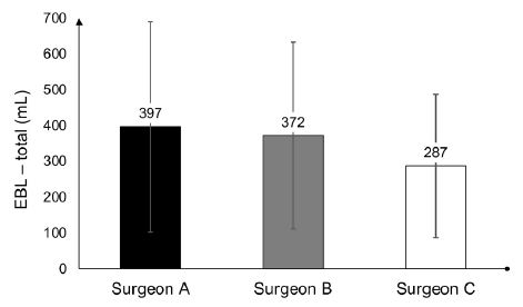
The surgeon´s impact on EBL-total (mL; x̄ ± SD) revealed the following numbers for surgeon A (397 ± 294); B (372 ± 261); and C (287 ± 200). However, no statistically significant difference was seen for EBL-total between the three surgeons (Figure 1). A similar outcome was observed when the corresponding comparison was carried out to compare the three surgeons for EBL-LFI; EBL-BSSO; and EBL-LFI + BSSO (Table 3).

fig 1

Figure 1: The surgeon´s impact on EBL – total. Datasets are presented as mean ± SD

Table 3: Analysis of the surgeons’ impact on EBL-LFI; EBL-BSSO; and EBL-LFI + BSSO. Datasets are presented as mean ± SD. A p-value ≤ 0.05 was considered statistically significant

Surgical procedures

Estimated blood loss (mL)

pvalues

Surgeon A

Surgeon B

Surgeon C

LFI

330 ± 202

388 ± 268 307 ± 195

Ns

BSSO

220 ± 244

213 ± 120 161 ± 80

Ns

LFI + BSSO

489 ± 342

477 ± 280 389 ± 236

Ns

LFI Le Fort I; BSSO Bilateral Sagittal Split Osteotomy; EBL Estimated Blood Loss; Ns Not significant

Furthermore, when mean EBL was calculated and subsequently compared between the three surgical procedures, the following figures were obtained (mL; x̄ ± SD): LFI (337 ± 218); BSSO (196 ± 126); and LFI + BSSO (464 ± 294). The ANOVA showed a statistically significant difference in mean EBL for all comparisons, i.e., [LFI] and [BSSO] (p = 0.008); [LFI] and [LFI + BSSO] (p = 0.006); and [BSSO] and [LFI + BSSO] (p < 0.001) (Table 4).

Table 4: The impact of the three surgical procedures, LFI; BSSO; and LFI + BSSO on EBL. Datasets are presented as mean ± SD. A p-value ≤ 0.05 was considered statistically significant

Comparisons of the surgical procedures

Mean difference in EBL (mL)

pvalues

LFI

BSSO  141

 0.008

337

± 218 LFI + BSSO -127

 0.006

BSSO

LFI -141

 0.008

196

± 126 LFI + BSSO -268

< 0.001

LFI + BSSO

LFI 127

 0.006

464

± 294 BSSO 268

< 0.001

LFI Le Fort I; BSSO Bilateral Sagittal Split Osteotomy; EBL Estimated blood loss

Ultimately, when OT was calculated for the three surgeons [A-C] individually, for each of the surgical procedures (LFI; BSSO, LFI + BSSO), the following figures were obtained (min; x̄ ± SD): LFI-[A]129 ± 58, [B] 103 ± 41, [C] 117 ± 30; BSSO-[A]104 ± 18, [B] 81 ± 18, [C] 109 ± 17; and LFI + BSSO-[A] 202 ± 71, [B] 172 ± 46, [C] 191 ± 24. A statistically significant difference was reached when OT was compared for BSSO between surgeon B and A (p = 0.031) as well as surgeon B and C (p < 0.001) (Table 5).

Table 5: Operative time for the three surgeons for each surgical procedure. Datasets are presented as mean ± SD. A p-value ≤ 0.05 was considered statistically significant

Surgical procedures

Operative time (min)

pvalues

Surgeon A

Surgeon B

Surgeon C

LFI

129 ± 58

103 ± 41 117 ± 30

Ns

BSSO

104 ± 18

81 ± 18 109 ± 17

0.031X and < 0.001Y

LFI + BSSO

202 ± 71

172 ± 46 191 ± 24

Ns

LFI Le Fort I; BSSO Bilateral Sagittal Split Osteotomy; Ns Not significant; [X] significant difference between surgeon B and A; [Y]significant difference between surgeon B and C

Discussion

The maxillofacial region is highly vascularised and even minor disruptions of the vessels in conjunctions with orthognathic surgery can jeopardise the blood supply to the actual region. Hence, seriously hamper the post-operative medical rehabilitation of the patient. In fact, severely damaged vessels constitute such a risk which may lead to a potentially fatal condition [10]. Over the past decades, a number of studies have been published investigating the potential association between patient-, or operator related factors and intraoperative blood loss [8,11]. Surprisingly, the impact of the surgeon on intraoperative blood loss has been studied only to a limited extent and needs to be further elucidated. This was the rationale for the conducting this four-year retrospective study.

The ANOVA showed no statistically significant difference between the three surgeons for EBL-total or for any of the surgical procedures separately. This was anticipated as the three surgeons were experienced and well-practised on the procedures performed in this study. However, it is worth mentioning that even if differences exist between operators with regards to EBL, it may be difficult to quantify. This for several reasons. First, extensive bleeding seldom occurs in conjunction with orthognathic surgery [10]. In fact, it has been shown that intraoperative blood loss is comparably low even when surgical residents are compared to experienced surgeons [11]. Second, all patients were given tranexamic acid prior to the surgical interventions, which is well-known to reduce the risk for bleeding [12,13] and improve the quality of the surgical field [13-15]. Third, the number of osteotomies were unequally distributed among the operators which may have influenced the outcome of this study. The latter however can be explained by the nature of retrospective studies where uneven cohorts may be encountered. Prospective, randomized studies where the number of patients and procedures are equally distributed among the operators is therefore warranted.

When the secondary objective (ii-a) was analysed, a statistically significant difference was found for EBL between all the surgical procedures. The maxillary osteotomies were bleeding significantly more as compared to the mandibular counterparts. This can be attributed to the fact that the maxilla encompasses a higher vascular density. Hence, entails a greater risk for bleeding [2]. In addition, some maxillary osteotomies were reported to bleed excessively, mainly due to aberrant anatomy, which had resulted in perforation of larger vessels. Some cases also reported a significant bleeding from the nasal mucosa during down fracturing-, or posterior repositioning of the maxilla. Bi-maxillary osteotomy as a group showed the highest EBL of the three surgical interventions, which is not surprising since it is the sum of both procedures. Taken together our findings seem reasonable and they are in accordance with previously published studies [2,6].

As for the secondary objective (ii-b), a statistically significant difference was seen when OT was compared for BSSO between surgeon B and A as well as surgeon B and C. However, although a statistically significant was observed, the clinical relevance remains questionable. Most likely, the additional time of approximately 25 min for operator A and C as compared to B will not lead to an increased EBL in clinical settings. This is supported by a study in which surgical residents required longer OT for their osteotomies as compared to the experienced surgeons, yet the EBL did not vary significantly [11].

Conclusions

Intraoperative blood loss during orthognathic surgery is not operator dependent when comparing experienced surgeons. However, both surgical procedure per se and operative time seem to be of relevance.

References

  1. Silva I, Suska F, Cardemil C, Rasmusson L (2013) Stability after maxillary segmentation for correction of anterior open bite: a cohort study of 33 cases. Journal of Cranio-maxillo-facial surgery: Official Publication of the European Association for Cranio-Maxillo-Facial Surgery 41: 154-8. [crossref]
  2. Salma RG, Al-Shammari FM, Al-Garni BA, Al-Qarzaee MA (2017) Operative time, blood loss, hemoglobin drop, blood transfusion, and hospital stay in orthognathic surgery. Oral and Maxillofacial Surgery 21: 259-266. [crossref]
  3. Pineiro-Aguilar A, Somoza-Martin M, Gandara-Rey JM, Garcia-Garcia A (2011) Blood loss in orthognathic surgery: a systematic review. J Oral Maxillofac Surg 69: 885-892. [crossref]
  4. Choi BK, Yang EJ, Oh KS, Lo LJ (2013) Assessment of blood loss and need for transfusion during bimaxillary surgery with or without maxillary setback. J Oral Maxillofac Surg 71: 358-365. [crossref]
  5. Apinhasmit W, Methathrathip D, Ploytubtim S, Chompoopong S, Ariyawatkul T (2004) Anatomical study of the maxillary artery at the pterygomaxillary fissure in a Thai population: its relationship to maxillary osteotomy. Journal of the Medical Association of Thailand 87:1212-1217. [crossref]
  6. Moenning JE, Bussard DA, Lapp TH, Garrison BT (1995) Average blood loss and the risk of requiring perioperative blood transfusion in 506 orthognathic surgical procedures. J Oral Maxillofac Surg 53: 880-883. [crossref]
  7. Yu CN, Chow TK, Kwan AS, Wong SL, Fung SC (2000) Intra-operative blood loss and operating time in orthognathic surgery using induced hypotensive general anaesthesia: prospective study. Hong Kong medical journal 6: 307-311. [crossref]
  8. Rummasak D, Apipan B, Kaewpradup P (2011) Factors that determine intraoperative blood loss in bimaxillary osteotomies and the need for preoperative blood preparation. J Oral Maxillofac Surg 69: 456-60. [crossref]
  9. Shetty V, Sriram SG (20150 Effectiveness of intravenous haemocoagulase on haemorrhage control in bi-maxillary orthognathic surgery-A prospective, randomised, controlled, double-blind study. Journal of Cranio-maxillo-facial surgery: Official Publication of the European Association for Cranio-Maxillo-Facial Surgery 43: 2000-2003. [crossref]
  10. Thastum M, Andersen K, Rude K, Norholt SE, Blomlof J (2016) Factors influencing intraoperative blood loss in orthognathic surgery. International Journal of Oral and Maxillofacial Surgery 45: 1070-1073. [crossref]
  11. Kretschmer W, Koster U, Dietz K, Zoder W, Wangerin K (2008) Factors for intraoperative blood loss in bimaxillary osteotomies. J Oral Maxillofac Surg 66: 1399-1403. [crossref]
  12. Zellin G, Rasmusson L, Pålsson J, Kahnberg KE (2004) Evaluation of hemorrhage depressors on blood loss during orthognathic surgery: a retrospective study. Journal of Oral and Maxillofacial Surgery 62: 662-666. [crossref]
  13. Lin S, McKenna SJ, Yao CF, Chen YR, Chen C (2017) Effects of Hypotensive Anesthesia on Reducing Intraoperative Blood Loss, Duration of Operation, and Quality of Surgical Field During Orthognathic Surgery: A Systematic Review and Meta-Analysis of Randomized Controlled Trials. J Oral Maxillofac Surg 75: 73-86. [crossref]
  14. Barak M, Yoav L, Abu el-Naaj I (2015) Hypotensive anesthesia versus normotensive anesthesia during major maxillofacial surgery: a review of the literature. The Scientific World Journal 2015: 1-7. [crossref]
  15. Ervens J, Marks C, Hechler M, Plath T, Hansen D, (2010) Effect of induced hypotensive anaesthesia vs isovolaemic haemodilution on blood loss and transfusion requirements in orthognathic surgery: a prospective, single-blinded, randomized, controlled clinical study. International Journal of Oral and Maxillofacial Surgery 39: 1168-74. [crossref]

Standardized Precipitation Index Valuation of Climate Change in Bamenda

DOI: 10.31038/GEMS.2022414

Abstract

Evidence of climate change in the tropics is often depicted by declining rainfall patterns, as mean tropical temperatures are high. A 12-month Standardized Precipitation Index was used in assessing drought recurrence as an indicator to evaluate climate change in Bamenda from 1963-2019. Results showed that the mean annual rainfall is 182.52 mm, with a Standard Deviation of 29.16 and a Coefficient of Variation of 15.96%, while rainfall has reduced by 2.07 mm. This deficit matches with a declining mean annual rainfall trend. The mean Standardized Precipitation Index is -0.17 (mild dryness), with 16 episodes of mild dryness, 4 moderate dryness, 3 severe dryness and 3 extreme dryness incidents. There is a need for the population to engage in water-saving activities to adapt to rainfall deficits.

Keywords

Climate index, Drought, Rainfall

Introduction

Rainfall events across the earth’s surface, for varied reasons, are unevenly distributed. Such variation is reflective of the availability of water for human use and the cycles of activities like agriculture [1]. In this era of global environmental changes, a sound knowledge of the climate of human-populated territories is indispensable, considering the current phenomenon of climate change [2]. Rainfall variability, which refers to changes in the amount of rain received in a specified geographic space within a defined period, can be daily, monthly, seasonal or annual. Precipitation change averaged over global land areas is low before 1951 and medium afterwards because of insufficient data, particularly in the earlier periods of the records [3]. The long-term mean rainfall for a month, season or year does not often indicate the regularity with which given amounts of rainfall can be expected, especially in the low latitudes where rainfall is known to be highly variable in its incidence from one year to another [1]. In the tropics, rainfall tends to be more variable seasonally than annually. Rainfall variability is a measure of the degree of likelihood that the mean amount of rainfall may be repeated each year, season or month depending on the period under consideration [4-6]. The paper bridges some methodological gaps in previous studies on climate variability in Cameroon. Ngakfumbe [7] analysed rainfall probability and reliability over Cameroon, using Standard Deviation (SD) and Coefficient of Variation (CV), with no other climatic index. Molua and Lambi [8] made a descriptive analysis of rainfall variability and its impact on water resources over Cameroon, to note that mean annual rainfall decreases inversely to latitude, without specifying the indices that show regional variations. Tume [9-11] assessed the susceptibility of water resources to climate variability on the Bui Plateau, using the Rainfall Seasonality Index (SI) and Standardized Precipitation Index (SPI), which failed to reveal regional disparities at a mesoscale. Meteorological drought has different impacts on groundwater, reservoir storage, soil moisture and streamflow and as such, McKee, Doesken and Kleist [12] develop the SPI in 1993 in which precipitation is the only required input parameter that is used in analyzing wet and dry cycles. Data sets required to compute SPI require 90% or even 85% complete records. The SPI was designed to quantify precipitation deficits for multiple timescales that best reflect drought impact on the availability of water resources. Moisture responds to precipitation anomalies on a relatively short scale. McKee [12] originally calculated the SPI for 3-, 6-, 12-, 24- and 48-month timescales. Positive SPI values indicate greater than median precipitation and negative values indicate less than median precipitation. Since the SPI is normalized, wetter and drier climates can be represented in the same way. The recurrence of meteorological, hydrological and agricultural droughts indicate that that climate is changing. This is critical in a tropical location like Bamenda where livelihood sources are rain-fed, such as agriculture and recharge of surface and groundwater resources.

Study Area

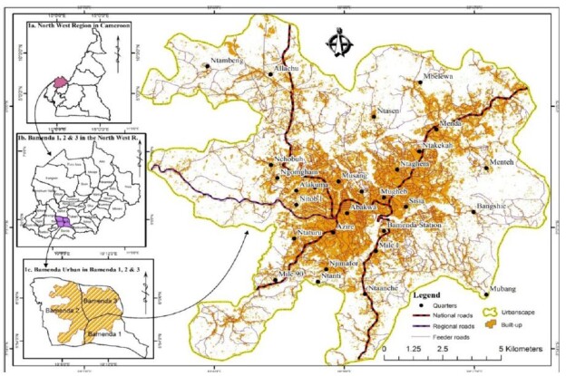
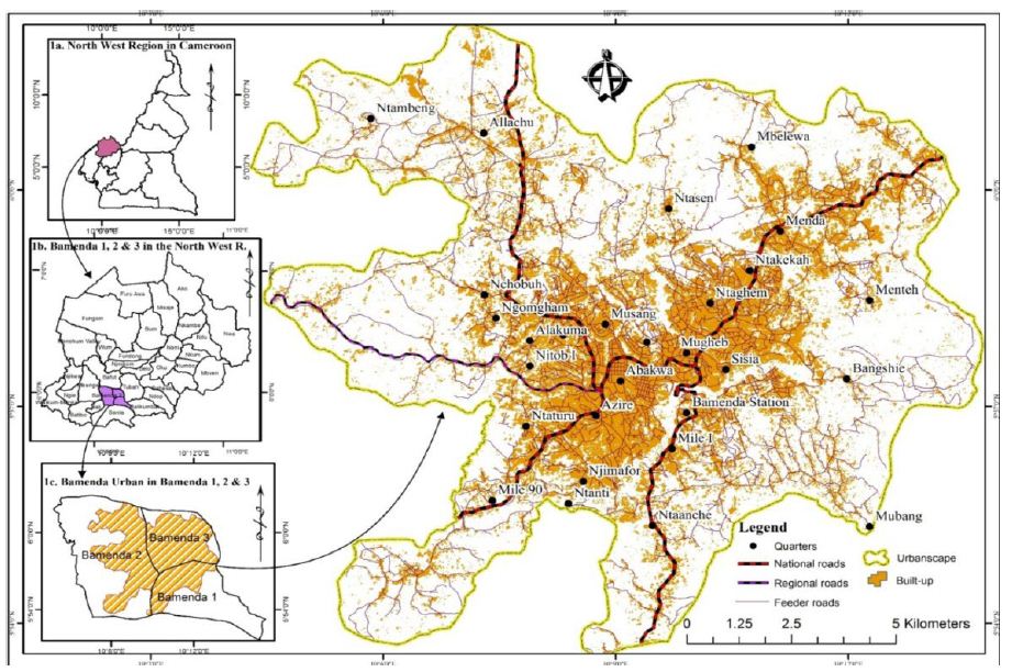
Bamenda is the headquarters of the North West Region and the socio-economic nerve wire of the region. Bamenda is a primate city considering her situation which is gradually merging with satellite towns like Bambui, Bambili, Bafut, Mbengwi, Bali, Bafut and Santa. The study area covers three Sub-Divisional Councils (Bamenda I, Bamenda II, Bamenda III). It is located between longitudes 10o09″ and 10o11″E of the Greenwich Meridian and between latitudes 5o56″N and 5o 58″N (Figure 1).

FIG 1

Figure 1: Location of Bamenda

Bamenda has a tropical climate, with a rainy and dry season. The dry season sets in from November till April, while the rainy season runs from April to November. It has been observed that the dry season has been prolonged over time. Even when the wet season sets in April, it is often characterised by recurrent dry spells that linger on till June [11]. Such dry spells are detrimental to agriculture and water resources as rainfall is often below a threshold to sustain tender crops and recharge surface and groundwater resources. These are shreds of evidence of agricultural, meteorological and hydrological droughts [13].

Data Collection and Analysis

Rainfall data were collected from the Regional Meteorological Service at the Northwest Delegation of Transport for a period of 56 years (1963-2019). Standardized Precipitation Index (SPI) is a tool that was developed primarily for defining and monitoring drought. It allows an analyst to determine the rarity of a drought at a given time scale of interest for any rainfall station with historic data. It can also be used to determine periods of anomalously wet events. Conceptually, SPI is the number of standard deviations by which the precipitation values recorded for a location would differ from the mean over certain periods. In statistical terms, the SPI is equivalent to the Z-score. It is calculated thus:

equ 1

Where: Z-score expresses the x score’s distance from the mean (µ) in standard deviation (δ) units.

The SPI is the cumulative probability of a given rainfall event occurring at a geographic location (Table 1).

Table 1: Drought probability of recurrence

SPI Value

Category Probability Freq. in 100 years

Severity of event

>2.00 Extreme wet

2.3

100

1 in 1 year
1.5 to 1.99 Severely wet

4.4

70

1 in 1.1 years
1.00 to 1.49 Moderately wet

9.2

50

1 in 1.3 years
0 to 0.99 Mildly Wet

34.1

45

1 in 1.5 years
-0.1 to -0.99 Mild dryness

34.1

33

1 in 3 years
-1.00 to -1.49 Moderate dryness

9.2

10

1 in 10 years
-1.50 to -1.99 Severe dryness

4.4

5

1 in 20 years
<-2 Extreme dryness

2.3

2.5

1 in 50 years

Source: McKee et al., (1993, 1995); World Meteorological Organization (2012) [13]

A 12-month SPI time series was used to assess the recurrence of meteorological, agricultural and hydrological droughts. All anomaly graphs generated were fitted with trend lines and linear equations. The trend lines indicate an increase or decrease. Rainfall reliability was assessed using the Coefficient of Variation (CV). CV is calculated thus:

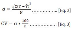
equ 2 3

Where: Ῡ = mean, N = sample size.

Results

The results are divided into mean monthly and annual rainfall patterns, and SPI valuation of climate change.

Mean Monthly and Annual Rainfall Pattern

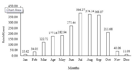
Rainfall in Bamenda increases from the onset of the wet season to a peak in July to September and gradually drops as the dry season sets in Figure 2.

fig 2

Figure 2: Mean monthly rainfall for Bamenda

The lowest rainfall is recorded from December to March. To assess how much rainfall has changed, the data were grouped into 3-month segments (Table 2).

Table 2: Rainfall change over Bamenda (1963-2019)


Months

Decadal mean rainfall (mm)
1963-1972 1973-1982 1983-1992 1993-2002 2003-2012

2013-2019

DJF

25.07

19.85 16.5 9.7 17.71

24.5

MAM

184.17

161.78 158.82 149.1 138.9

178.01

JJA

387.6

361.9 364.2 356.4 325.9

235.06

SON

238.81

240.9 202.5 210.9 195.97

126.5

Mean

208.91

196.11 185.51 181.53 169.62

141.02

Change

26.39

13.59 2.98 -1.00 -12.90

-41.50

DJF: December, January, February; MAM: March, April, May, JJA: June, July, August, SON: September, October, November

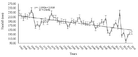
From 1963-1972, rainfall had an excess of 26.39 mm and has been declining over time. Between 1973-1982, the rainfall had dropped by 13.59 mm and 2.98 mm from 1983-1992. Since 1993, Bamenda has witnessed rainfall deficits (-1 mm from 1993-2002, -12.9 mm from 2003-2012 and -41.5 mm from 2013-2019). The average rainfall decline from 1963-2019 is -2.07 mm. This proves that the climate is changing and is affirmed by the declining inter-annual rainfall trend (Figure 3).

fig 3

Figure 3: Inter-annual rainfall for Bamenda (1963-2019)

The mean annual rainfall for Bamenda is 182.52 mm, with a Standard Deviation (SD) of 29.16 and a Coefficient of Variation (CV) of 15.96% (reliable).

Standardized Precipitation Index Valuation of Climate Change

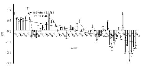
The climatic index used in assessing climate variability and change for this study is SPI. The SPI inter-annual pattern is the same as the inter-annual rainfall, with the same Coefficient of Determination (R2) of 0.4548 (45.48%) (Figure 4).

fig 4

Figure 4: Inter-annual Standardized Precipitation Index for Bamenda (1963-2019)

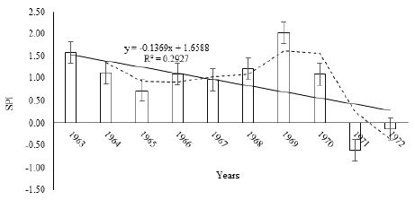
More insights into rainfall change over Bamenda are presented through decadal SPI trends. From 1963-1972, the SPI trend decreased above the average (Figure 5).

fig 5

Figure 5: Standardized Precipitation Index for Bamenda (1963-1972)

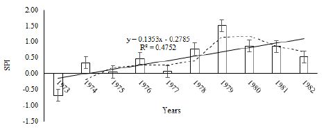
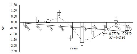
The SPI episodes were 1963 (1.57-moderately wet), 1964 (1.12-moderately wet), 1965 (0.73-mildly wet), 1966 (1.09-moderately wet), 1967 (0.96-mildly wet), 1968 (1.21 (moderately wet), 1969 (2.02-extreme wet), 1970 (1.09-moderately wet), 1971 (-0.6-mild dryness) and 1972 (-0.13-mild dryness). Eight out of the ten years of this decade were wet years, except 1971 and 1972. The dry years continued till 1973. The decade 1973-1982 experienced an increasing SPI trend, with nine wet years out of the ten (Figure 6).

fig 6

Figure 6: Standardized Precipitation Index for Bamenda (1973-1982)

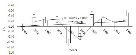
The SPI episodes were, 1973 (-0.69-mild dryness), 1974 (0.32-mildly wet), 1975 (0.04-mildy wet), 1976 (0.46-mildly wet), 1977 (0.06-mildly wet), 1978 (0.75-mildly wet), 1979 (1.51-moderately wet), 1980 (0.86-mildly wet), 1981 (0.84-mildly wet) and 1982 (0.51-mildly wet). The SPI trend increased above the average from 1983 to 1992 (Figure 7).

fig 7

Figure 7: Standardized Precipitation Index for Bamenda (1983-1992)

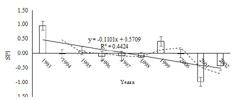
In 1983, the SPI value was (-0.01-mild dryness), 1984 (0.33-mildly wet), 1985 (0.24-mildly wet), 1986 (0.26-mildly wet), 1987 (-0.63-mild dryness), 1988 (-0.39-mild dryness), 1989 (0.45-mildly wet), 1990 (0.27-mildly wet), 1991 (0-mildly wet) and 1992 (0.51-mildly wet). The 1993 to 2002 period can be seen as a dry decade, with a decreasing SPI trend and seven years of negative SPI (Figure 8).

fig 8

Figure 8: Standardized Precipitation Index for Bamenda (1993-2002)

The SPI episodes were 0.95 (mildly wet) in 1993, 1994 (-0.03-mild dryness), 1995 (0.09-mildly wet), 1996 (-0.10-mild dryness), 1997 (-0.10-mild dryness), 1998 (-0.14-mild dryness), 1999 (0.4-mildly wet), 2000 (-0.01-mild dryness), 2001 (-0.99-mild dryness) and 2002 (-0.43-mild dryness). The 2003 to 2012 period was also another dry decade, with a decreasing SPI below the average (Figure 9).

fig 9

Figure 9: Standardized Precipitation Index for Bamenda (2003-2012)

The SPI values were, 2003 (-0.26-mild dryness), 2004 (0.21-mildly dry), 2005 (-0.01-mild dryness), 2006 (0.82-mildly wet), 2007 (-1.38-moderate dryness), 2008 (-1.75-severe dryness), 2009 (-1.01-moderate dryness), 2010 (-0.50-mild dryness), 2011 (0.14-mild dryness and 2012 (-0.69-mild dryness). From 2013 to 2019, the SPI continued to decline below the average (Figure 10). It is also another dry decade.

fig 10

Figure 10: Standardized Precipitation Index for Bamenda (2013-2019)

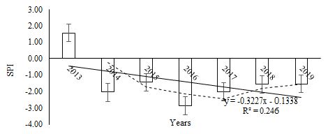
The SPI incidents were, 2013 (1.57-severely wet), 2014 (-2.06-extreme dryness), 2015 (-1.46-moderate dryness), 2016 (-2.86-extreme dryness), 2017 (-2.03-extreme dryness), 2018 (-1.58-severe dryness) and 2019 (-1.56-severe dryness). Rainfall and SPI characteristics for Bamenda can be summarized (Table 3).

Table 3: Summary of rainfall characteristics and SPI

Period

MAR (mm) CV (%) Mean SPI SPI class Trend

Reliability

1963-1972

208.92

10.69

0.91

Mildly wet Decreasing Reliable
1973-1982

196.1

8.84

0.47

Mildly wet Increasing Reliable
1983-1992

185.52

5.78

0.1

Mildly wet Increasing Reliable
1993-2002

181.51

8.05

-0.03

Mild dryness Decreasing Reliable
2003-2012

169.62

13.49

-0.44

Mild dryness Decreasing Reliable
2013-2019

141

29.04

-1.42

Severe dryness Decreasing Unreliable
Mean

180.445

15.96

-0.07

Mild dryness  Decreasing Reliable

MAR: Mean Annual Rainfall, CV: Coefficient of Variation

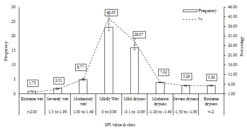
Rainfall was reliable from 1963 to 2012. Since 2013, dry episodes have been recurrent with a mean SPI of -1.42 and an unreliable CV of 29.04%. These characteristics show that rainfall has been deficient, thereby resulting to water scarcity. In all, the 1963-2019 period was characterised by 1 episode of extreme wet conditions (1969), 2 severely wet (1963, 2003), 5 moderately wet (1964, 1966, 1968, 1970, 1979), 23 mildly wet (1965, 1967, 1974, 1975, 1976, 1977, 1978, 1980, 1981, 1982, 1984, 1985,1986, 1989, 1990, 1991, 1992, 1993, 1995, 1999, 2004, 2006, 2011), 16 mild dryness (1971, 1972, 1983, 1987, 1988, 1994, 1996, 1997, 1998, 2000, 2001, 2002, 2003, 2005, 2010, 2012), 4 moderate dryness (1973, 2007, 2009, 2015), 3 severe dryness (2008, 2018, 2019) and 3 extreme dryness (2014, 2016, 2017) (Figure 11).

fig 11

Figure 11: Standardized Precipitation frequency

The overall mean SPI for the period under study is -0.07 (mild dryness) and a mean CV of 15.96% (reliable). It is worth noting that all the classes of SPI have been recorded in Bamenda from 1963-2019, distributed as: extreme wet, 1 (1.75%), severely wet, 2 (3.51%), moderately wet, 5 (8.77%), mildly wet, 23 (40.35%), mild dryness, 16 (28.07%), moderate dryness, 4 (7.02%), severe dryness, 3 (5.26%) and extreme dryness, 3(5.26%). Although the study period had more wet episodes than dry incidents, rainfall has continued reducing since 2014.

Discussion

Precipitation is projected to decrease over the tropics and sub-tropics (Inter-governmental Panel on Climate Change-IPCC, 2021) [14] as indicated by the rainfall trend in Bamenda that has decreased by 2.07 mm from 1963-2019 [9]. Several climatic indices have been developed from simple indices such as percentage of normal precipitation and precipitation percentiles to more complicated indices such as the Palmer Drought Severity Index (PDSI) (World Meteorological Organization (2012). Precipitation is the only required input parameter for the SPI. It is effective in analyzing wet and dry cycles with changes in latitude. It is more likely that data sets would only have 90% or even 85% complete records. Many users of SPI do not have this luxury and may have to settle for less (75-85% complete data sets) unless they look for estimation techniques to fill in the gaps in the record. Long and pristine data records are neither practical nor typical in many cases, so the user needs to be aware of the statistical shortcomings of extreme events when dealing with shorter periods of records for various locations [15]. Depending on the confidence and method of calculation, the use of estimated data is acceptable to show climate variability and change. Naturally, the fewer estimated data used the more reliable the results (World Meteorological Organization, 2012). The SPI is a good indicator of precipitation change over time. Its flexibility permits precipitation change to be calculated over different time scales like 3-, 6-, 12-, 24- and 48-months. Rainfall deficits assessment using SPI are recorded within a threshold of zero because a drought sets in when SPI values fall below the zero thresholds. The climate of Bamenda broadly falls under tropical climates per the Köppen classification (Aw tropical savannah climate). Tropics show seasonal precipitation changes [16,17] due to the influence of continentality (Rohli and Vega, 2018). Assuming that all other factors are equal, the interiors of continents like Bamenda have severe dry seasons due to their long distance from the sea [17]. In addition, the onset of the wet seasons is delayed significantly over continents due to the overriding effect of harmattan winds [2]. The Aw climatic regime is directly influenced by the Inter-Tropical Convergence Zone (ITCZ). The dominant prevailing winds during the wet season are the warm-moist SE from the Atlantic Ocean that pushes the ITCZ northwards with the onset of the wet season. As a zone of convergence of SE and NE trade winds, tropical rainfall is largely influenced by the position of the ITCZ. From late October to November, the NE trade winds have a dominating influence and the ITCZ is pushed to the south so that dry weather conditions prevail because of harmattan. From March to April, the SE trade winds have an urge over the NE trade winds, such that the ITCZ is gradually moved northwards, announcing the start of the wet season [2,6,12,18,19].

Conclusion

A 12-month SPI time series analysis showed that rainfall has been decreasing in Bamenda from 1963-2019, with 45.6% of dry episodes. These include 16 episodes of mild dryness (28.07%), 4 periods moderate dryness (7.02%), 3 events of severe dryness (5.26%) and 3 incidents of extreme dryness (5.26%). Rainfall deficits have been recorded since 2014. Inter-annual rainfall is not always a good measure of rainfall variability, because decreasing rainfall can still be reliable while increasing rainfall can be unreliable. That is why the inter-annual CV for Bamenda is 15.96%, (reliable). The overall SPI from 1963-2019 is -0.17 (mildly dryness), while rainfall has decreased by 2.07 mm. The characteristics show that Bamenda is getting drier, although rainfall is still reliable. Spatio-temporal variations of SPI have implications for agriculture, water resources and other aspects of the man-environment relationship such as subsistence agriculture and other agro-pastoral ventures. Water resources occur mostly in perched aquifers of volcanic origin and are recharged by seasonal rainfall. The Bamenda highlands have suffered severe highland montane forest loss as a result of deforestation for subsistence agriculture, settlement and the conversion of patches of natural vegetation into eucalyptus plantations. As such, the population must engage in water-saving activities as an adaptation to rainfall deficits.

References

  1. Ayoade JO (1998) Introduction to Climatology for the Tropics. Fourth edition, Spectrum Books Ltd., Ibadan, pg: 125-139.
  2. Ahrens CD, Henson R (2019) Meteorology Today: An Introduction to Weather, Climate and the Environment, Twelfth Edition. Cengage Learning, New York pg: 479-486.
  3. Strangeways I (2006) Precipitation: Theory, Measurement and Distribution. Cambridge University Press, Cambridge, pg: 1-15.
  4. World Meteorological Organization (2008) Guide to Meteorological Instruments and: Methods of Observation. Seventh edition, Geneva, WMO, 8: 5-16.
  5. World Meteorological Organization (2011) Guide to Climatological Practices. WMO (100) Geneva pg: 6-19.
  6. Barry RG, Chorley RJ (2003) Atmosphere, Weather and Climate, Eighth Edition: Routledge, Taylor and Francis Group, London pg: 262-230.
  7. Ngakfumbe SN (2001) Rainfall Probability and Reliability: The case of Cameroon: Readings in Geography, Unique Printers, Bamenda pg: 156-175.
  8. Molua EL, Lambi CM (2006) Climate, Hydrology and Water Resources in Cameroon. CEEPA Discussion Papers, Special Series on Climate and Agriculture in Africa, Centre for Environment and Policy in Africa, University of Pretoria pg: 1-37.
  9. Tume SJP (2019) Standardized Precipitation Valuation of Water Resources Vulnerability to Climate Variability on the Bui Plateau, Northwest Cameroon. Environment and Ecology Researc, 7: 83-92.
  10. Tume SJP (2021a) Impact of Climate Change on Domestic Water Accessibility in: Bamenda III Sub-Division, North West Region, Cameroon. Journal of the Cameroon Academy of Sciences 17: 131-145.
  11. Tume SJP (2021b) Rainfall Seasonality and Standardized Precipitation Valuation of: Water: Resources Susceptibility to Climate Variability on the Bui Plateau, Northwest Region, Cameroon. Advances in Hydrology & Meteorology 1: 1-20.
  12. McKee TB, Doesken NJ, Kleist J (1993) The Relationship of Drought Frequency and Duration to Time Scales. Proceedings of the Eighth Conference on Applied Climatology. American Meteorological Society Boston 179-184.
  13. World Meteorological Organization (2012) Standardized Precipitation Index User Guide. WMO (1090) Geneva, 50.
  14. Intergovernmental Panel on Climate Change-IPCC, (2021) Summary for Policymakers. In: Climate Change 2021: The Physical Science Basis. Contribution of Working Group I to the Sixth Assessment Report of the Intergovernmental Panel on Climate Change. Cambridge University Press, 41.
  15. Guttman NB (1999) Accepting the Standardized Precipitation Index: A Calculation: Algorithm. Journal of the American Water Resources Association 35: 311-322.
  16. Patt AG, Winkler J (2007) Applying Climate Information in Africa: An Assessment of Current Knowledge. University of Boston, 19.
  17. Rohli RV, Vega AJ (2018) Climatology, Fourth Edition. Jones and Bartlett Learning, Wall Street, Burlington, 25-33.
  18. Strahler A (2013) Introducing Physical Geography, Sixth Edition. John Wiley and Sons, London pg: 235-239.
  19. Dashew S, Dashew L (1999) Mariner’s Weather Handbook: A Guide to Forecasting and Tactics. First edition, Beowulf, Inc., Tucson, Arizona pg: 35-53.

Petrology of the Eocene Igneous Rocks of the Centennial and Henry’s Mountains, Idaho and Montana, USA

DOI: 10.31038/GEMS.2022411

Abstract

In the Centennial and Henry’s Mountains of Idaho and Montana north of Island Park, at least 40 km3 (maximum thickness >350 m) of Eocene shoshonite aa lava flows overlie local Paleozoic strata. The volcanic features, petrography, composition, and ages of these flows vary little throughout the section. Compositions of these rocks are uniformly shoshonitic, silica-oversaturated, magnesian, and calc-alkalic—and indicate that the original magmas are more like the mafic rocks of the Absaroka Volcanic Field that lies to the east and less like equivalent compositions from the Challis Volcanic Field that lies to the northwest. Variations in major and trace element compositions indicate that the magma that produced these flows evolved by fractional crystallization and mixing from primitive magma containing a subduction zone compositional component.

Introduction

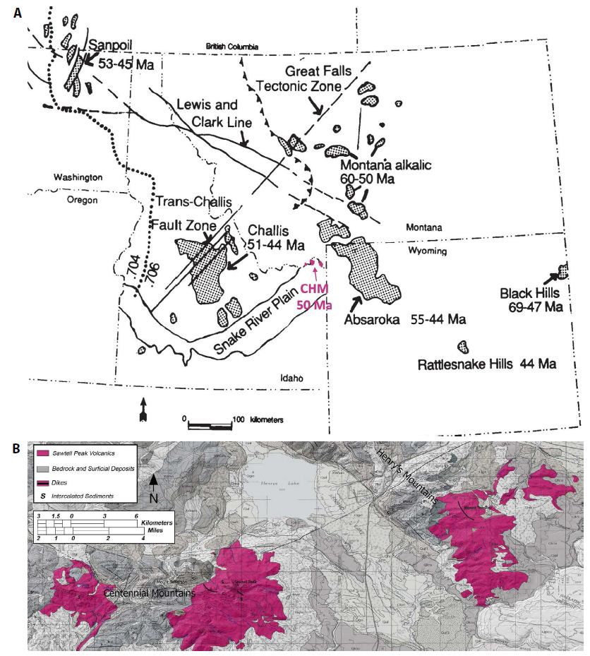
The Centennial and Henry’s Mountains lie on the Idaho-Montana border and are, respectively, east-west- and north-south-trending ranges located inside the Yellowstone tectonic parabola near the eastern margin of the Basin and Range Province (Figure 1A). The Eocene igneous rocks exposed in these ranges represent a small, deeply eroded Eocene volcanic field that we refer to as the Centennial-Henry’s Mountains volcanic field (CHM). Today, the CHM is exposed in three areas, from west to east: in the Centennial Mountains west of Mount Jefferson and at Sawtell Peak and in the Henry’s Mountains near Mount Two Top (Figure 1). During the Eocene, this area lay just south of the Madison-Gravelly Arch, a north-south trending topographic high [1]. The CHM lies between two of the largest Eocene volcanic fields in North America—the Absaroka and Challis Volcanic Fields, located 80 km to the east and 120 km to the west, respectively. The Absaroka volcanic field was dominated by composite volcanoes, was primarily active 55-44 Ma, and records compositions typical of subduction settings [2-10]. The Challis volcanic field, which is part of the Challis-Kamloops volcanic belt, contains remnants of composite volcanoes and calderas, was active 51-44 Ma, and records compositions interpreted to represent the opening of a window in the underlying subducted slab [3,6,10-16]. This study reports the field relations, petrography, and compositions of the CHM, evaluates the affinity of the CHM to nearby volcanic fields, and assesses the source and compositional evolution of CHM magma.

fig 1

Figure 1: Geographic reference map (A [23]) and geologic map (B [24]) for the Centennial-Henry’s Mountains volcanic field (CHM) showing the distribution of Eocene volcanic rocks and related features

Field Relations and Petrography

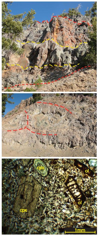
Standard 1:24,000 scale geologic mapping and petrographic work indicates that the volcanic features and petrography of CHM rocks are remarkably uniform—consisting almost exclusively of sequences of shoshonite aa flows that are one to ten meters thick (Figure 2A). Where slopes are steep, the cross sections of individual flow lobes are exposed (Figure 2B). CHM flows are crystal rich, contain euhedral clinopyroxene (cpx) phenocrysts and subhedral olivine (ol) phenocrysts that are commonly altered to iddingsite, include microlites of plagioclase and Fe-Ti oxides, and are sometime vesicular or amygdaloidal (Figure 2C). Modal proportions are 61-69% groundmass, 22-34% cpx, and 5-12% ol, and rocks with more cpx contain less ol. Three units contain minor phlogopite. No pyroclastic rocks or lahar deposits were observed. In very few locations (Figure 1B) there are small deposits of locally derived volcanic sediments between lava flows. CHM lava flows are cut by northwest-southeast trending vertical feeder dikes that are typically one to five meters thick. Some dikes have chilled margins, while others are surrounded by zones of hydrothermal alteration. Surface exposures of the large dikes are up to 100 m long. The absence of a clear eruptive center and scarcity of large dikes suggest that the eruptive center for CHM is no longer exposed. The orientations of CHM flows suggest that the eruptive center may lie north of Sawtell Peak (Figure 1B). 40/39Ar ages (of the oldest exposed flow exposed at the base of Sawtell Peak and of the youngest flows from there and exposures to the west; Figure 1B) are unable to resolve a difference between the initiation and cessation of volcanism in the Sawtell Peak volcanic field—suggesting the flows erupted in a short period at 50 Ma, in the early Eocene [16-25]. Field relations support rapid accumulation of lava flows. For example, the sequence of flows commonly preserves easily eroded flow tops and records no significant disconformities.

fig 2

Figure 2: A) Photo of a typical CHM aa flow showing a thin lower rubble zone, a dense interior, and thick upper rubble zone. B) Photo of several lava flow lobes. Outlines lie in the flow breccia carapaces surrounding dense flow interiors. C) Thin section photomicrograph of a CHM shoshonite showing phenocrysts of clinopyroxene (cpx) and olivine (ol) in a groundmass containing microlites of plagioclase and Fe-Ti oxides.

Composition, Affinity, and Source

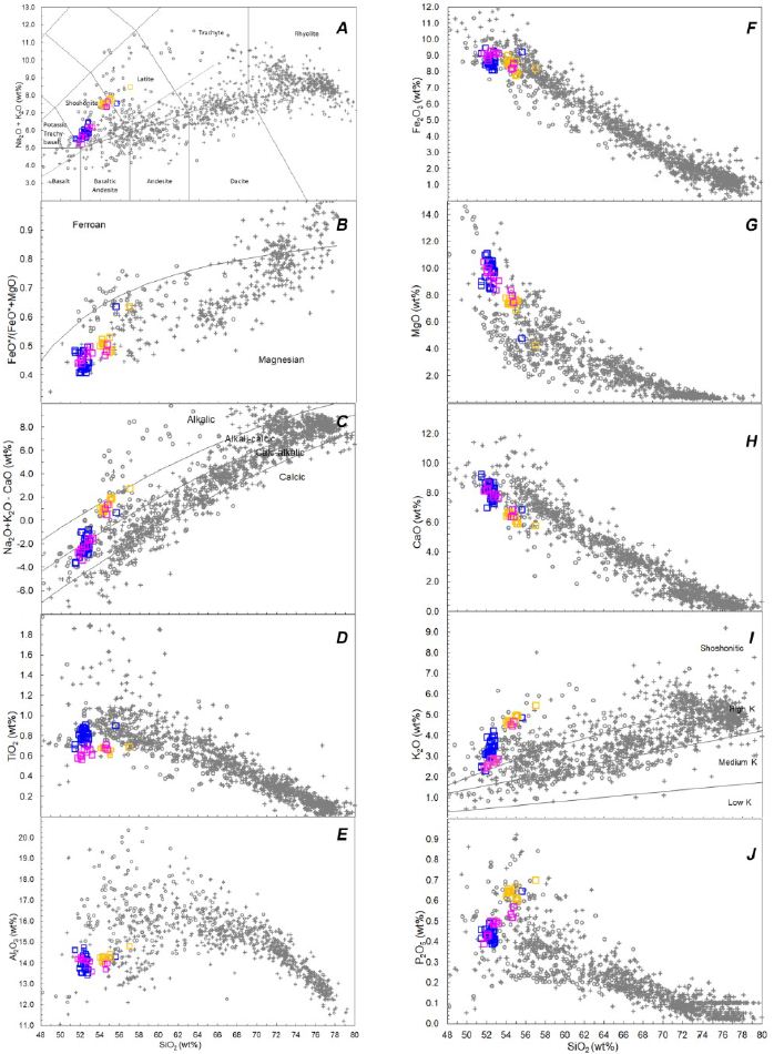
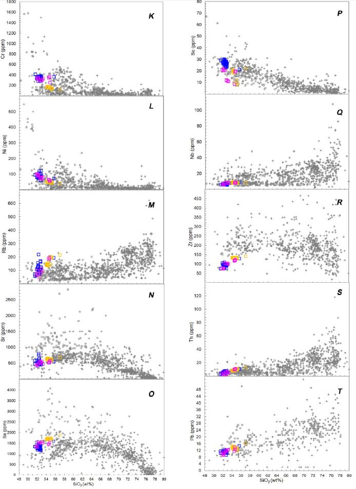
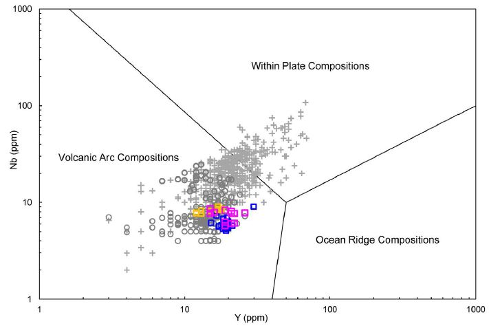
Whole-rock major- and trace-element analyses were obtained by wavelength dispersive X-ray fluorescence spectrometry at Brigham Young University, Provo following standard techniques (described at www.geology.byu.edu/faculty/ehc under the heading ‘resources’). The complete dataset is reposited in the EarthChem database (earthchem.org). Figure 3 plots CHM compositions relative to those from the Absaroka and Challis volcanic fields. CHM rocks are shoshonites and latites, shoshonitic (K2O 2-5%), silica-oversaturated, magnesian, and calc-alkalic to alkali-calcic (Figure 3A-C, I). Sundell [17] identified three magmatic groups from the Absaroka volcanic field, and Bray [4] argued for the combination of two of Sundell’s groups—resulting in two groups, the Sunlight and Washburn—Thorofare Creek groups. Although CHM compositions share compositional characteristics with Challis and both Absaroka groups, CHM lava flows are most like the Absaroka Sunlight group. Comparing Y and Nb compositions (Figure 4) emphasize the similarity of CHM and Absaroka compositions, which uniformly plot in the ‘volcanic arc’. In contrast, the Challis compositions display an early subduction component in the mantle source that disappears through time. We interpret compositional data to indicate that the CHM is part of the Absaroka volcanic field and resulted from partial melting from a mantle source with a subduction zone compositional component.

fig 3(1)

fig 3(2)

fig 3(3)

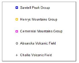
Figure 3: Classification and Harker variation diagrams for major and trace element compositions of CHM samples plotted relative to the compositions the Absaroka Volcanic Field [4, 7, 8, 10, 13]. A) IUGS classification diagram based on total alkalis (Na2O + K2O) versus SiO2 [21]. B) The SiO2 versus FeOtotal/(FeOtotal + MgO) classification diagram of Frost [20], using the dividing line of Miyashiro [22]. C) Modified alkali-lime versus SiO2 diagram of Frost [20]. I) K2O versus SiO2 using the classification lines of Ewart [19].


fig 4

Figure 4: Y versus Nb tectonic discrimination diagram of Pearce (1984) showing that CHM and Absaroka rocks have volcanic arc compositions, while Challis rocks plot in both the volcanic arc (for early magmatism) and intraplate (for late magmatism) fields.

Magmatic Evolution

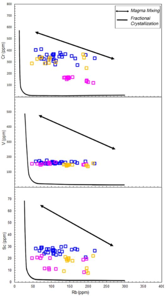
Major- and trace-element trends on Harker variation diagrams (Figure 3) suggest mineral control in the evolution of CHM magma but are too incoherent to be explained by evolution along a single line of descent. Trace-element modeling of fractional crystallization used a primitive Absaroka composition as the starting point. Figure 5 shows the fractional crystallization model, was applied to all trace elements with similar results, for Rb, Sc, V, and Cr compositions. It also shows a magma mixing line that connects primitive and evolved compositions. Together, these models define an envelope of magma mixing and fractional crystallization that is consistent with the compositional differentiation of CHM magma. he role of assimilation of crustal material can be assessed most effectively with isotopic data; however, the variability of incompatible trace elements (and their ratios) can be a reasonably good indicator of open-system processes. The variations of these elements suggest that assimilation did not play an important role in the development of CHM magma. In short, we propose that fractional crystallization and magma mixing controlled the evolution of CHM magma.

fig 5

Figure 5: Petrogenetic modeling diagrams for Rb, Sc, V, and Cr showing a fractional crystallization model and a magma mixing line that connects primitive and evolved compositions. The model suggests that CHM magma evolved by magma mixing and fractional crystallization. The Rayleigh fractional model employed the following mineral mode and partition coefficients were used: Ol = 6.7%; Cpx = 24.1%; Plag = 2.8%; Other = 0.2%; DRb bulk=0.013; DSc bulk=5.322; DCr bulk=2.172; DV bulk=0.316.

References

  1. Chetel LM., Janecke SU, Carroll AR, Beard BL, Johnson CM., et al. (2011) Paleogeographic reconstruction of the Eocene Idaho River, North American Cordillera. Geological Society of America Bulletin. 123: 71-88.
  2. Armstrong RL (1991) Evolving geographic patterns of Cenozoic magmatism in the North American Cordillera: the temporal and spatial association of magmatism and metamorphic core complexes. Journal of Geophysical Research 96: 13201-13244.
  3. Luedke RG (1994) Miscellaneous Investigations Series – U. S. Geological Survey Maps showing distribution, composition, and age of early and middle Cenozoic volcanic centers in Idaho, Montana, west-central South Dakota, and Wyoming, U.S. Geological Survey Map I-2291-C.
  4. Bray EL (1999) Geochemical and Isotopic Variations in the Absaroka Volcanic Supergroup, Wyoming – Implications on Petrogenesis and Magma Sources [M.Sc. Thesis]. Provo, Brigham Young University, pg: 133.
  5. Hiza MM (1999) The geochemistry and geochronology of the Eocene Absaroka volcanic province, northern Wyoming and Southwest Montana, USA [Ph.D. Thesis]. Eugene, University of Oregon pg: 262.
  6. Feeley TC, Cosca MA, Lindsay CR (2002) Petrogenesis and implications of calc-alkaline cryptic hybrid magmas from Washburn Volcano, Absaroka Volcanic Province, USA. Journal of Petrology 43: 663-703.
  7. Feeley (2003) Origin and tectonic implications of across-strike geochemical variations in the Eocene Absaroka volcanic province, United States. Journal of Geology 111: 329-346.
  8. Feeley TC, Cosca MA (2003) Time vs. composition trends of magmatism at Sunlight Volcano, Absaroka volcanic province, Wyoming. Geological Society of America Bulletin 115: 714-728.
  9. Lindsay CR, Feeley TC (2003) Magmagenesis at the Eocene Electric Peak-Sepulcher Mountain Complex, Absaroka volcanic province, USA. Lithos 67: 53-76.
  10. Chandler MR (2006) The Provenance of Eocene Tuff Beds in the Fossil Butte Member of the Green River Formation, Wyoming: Relation to the Absaroka and Challis Volcanic Fields [M.Sc. Thesis]. Provo, Brigham Young University, pg: 89.
  11. Ekren EB (1985) Eocene cauldron-related volcanic events in the Challis Quadrangle, in Symposium on the geology and mineral deposits of the Challis. USGS 1: 43-58.
  12. Lewis RS, Kiilsgaard TH (1991) Eocene plutonic rocks in south central Idaho. Journal of Geophysical Research 96: 13295-13311.
  13. Norman MD, Mertzman SA (1991) Petrogenesis of Challis Volcanics from central and southwestern Idaho: trace element and Pb isotopic evidence. Journal of Geophysical Research 96.
  14. Jellinek AM (1994) The Twin Peaks Caldera, Challis, Idaho: a unique window into the emplacement and evolution of a caldera-filling ignimbrite [M.Sc. Thesis]: Moscow, University of Idaho, pg: 202 .
  15. MacDonald WD, Palmer HC, Hayatsu A (1998) Structural rotation and volcanic source implications of magnetic data from Eocene volcanic rocks, SW Idaho. Earth and Planetary Science Letters 156: 225-237.
  16. Breitsprecher K, Thorkelson DJ, Groome WG, Dostal J (2003) Geochemical confirmation of the Kula-Farallon slab window beneath the Pacific Northwest in Eocene time. Geology 31: 351-354.
  17. Turrin B (2011) personal communication, Rutgers University.
  18. Sundell KA (1993) A geologic overview of the Absaroka volcanic province. Geological Survey of Wyoming Memoir 5: 480-506.
  19. Ewart A (1982) The mineralogy and petrology of Tertiary-Recent orogenic volcanic rocks with special reference to the andesitic-basaltic compositional range, in Thorpe, R.S., ed., Orogenic Andesites and Related Rocks. John Wiley and Sons pg: 25-95.
  20. Frost BR (2001) A geochemical classification for granitic rocks. Journal of Petrology 42: 2033-2048.
  21. Le Bas MJ (1991) The IUGS systematics of igneous rocks. Journal of the Geological Society of London 148: 825-833.
  22. Miyashiro A (1974) Volcanic rock series in island arcs and active continental margins. American Journal of Science 274: 321-355.
  23. Moye FJ, Hackett WR, Blakley JD, Snider LG, Link PK (1988) Regional geologic setting and volcanic stratigraphy of the Challis volcanic field, central Idaho, Guidebook to the geology of central and southern Idaho. Idaho Geological Survey Bulletin pg: 87-97.
  24. O’Neill JM, Christiansen RL (2004) Geologic map of the Hebgen Lake Quadrangle, Beaverhead, Madison, and Gallatin Counties, Montana; Park and Teton Counties, Wyoming; and Clark and Fremont Counties, Idaho. U. S. Geological Survey Map 2816.
  25. Pearce JA, Harris NBW, Tindle AG (1984) Trace element discrimination diagrams for the tectonic interpretation of granitic rocks. Journal of Petrology 25: 956-983.

Uncovering Richness of Price and of Emotion Mind- Sets in the Shopping Experience: A Mind Genomics Cartography across 30 Products

DOI: 10.31038/AWHC.2022522

Abstract

The paper presents a deep reanalysis of the response by consumers to pricing and emotion messages from 30 parallel studies of non-perishable products. The nine pricing and the nine emotion messages were approximate the same across the 30 products. Considering the results from 3656 respondents for pricing, and separately for emotion, revealed the exists about 2-3 new mind-sets, appearing across each of the 30 products. The ability to study judgments of pricing statements separately from judgments of emotion statements provides an increased power of research to more deeply understand the thoughts and feelings of ordinary people in ordinary situations. The implementation demonstrated successfully by the project, ‘Buy It!’ using Mind Genomics suggests the simplicity of creating a database of the mind across products, genders, ages, even cultures, and times, with the data easy to acquire, analyze, and apply.

Introduction

The topic of shopping consumes the attention of researchers, especially market researchers, consumer psychologists, economists, and occasionally occupies clinicians who are called in to deal with dysfunctional behavior involving shopping, especially compulsive shopping [1]. A great deal of the work is from the top down, looking at behavior, tabulating what people like about shopping, about products, and so forth. For the most part, the research focuses on the product, primarily because it is the focus of the marketer of products to sell the product. Whatever can be culled about the shopping situation is of interest to the product marketer, especially when that specific information helps ‘move product.’

Shopping as a behavior attracts a number of disciplines because it represents a fundamental set of behaviors necessary for survival, and an integral part of civilized life. The literature of shopping spans disciplines ranging from focus on the unconscious motives of people [2], to the behavioral economics involved in price [3-6], to the art and science of advertising, and onto the design of the shopping environment, and the observation of people shopping from the point of view of anthropology [2,7-11].

The consumer researcher working in an applied setting is not to be left out of this world. Companies which manufacture products and which offer services are interested in the process of shopping, to understand the way people think, or in today’s parlance the ‘shopper’s journey.’ One need only look at conferences today, many of them sponsored by organizations involved in for-profit consumer researcher, to discover the way companies use different research methods to provide so-called ‘shopper insights [12]. One will come across virtual shopping, a technology going back more than three decades [13], where the store can be set up. One will come across shop-by’s, wherein a researcher will accompany the shopper, asking questions at strategic points. Or one might well encounter eye tracking devices, which measure where on the shelf the shopper’s eyes alight [14,15].

At the most general levels are questionnaires, surveys about the shopping experience. These questionnaires can be of the most general kind, instructing respondents to rate the importance of different aspects of shopping, although such approaches seem to be quite general, and hard to deal with in an abstract situation. If questionnaires and surveys seem too abstract one need only wait, visit a store or a restaurant, to be bombarded later by questionnaire about how was the experience, as stores restaurants, even hospitals and physician’ office attempt to become smarter about the ‘purchaser.’

The Contribution of Experimental Design and Mind Genomics to the Understanding of Shopping

A key issue in research is what is important to the shopper. The question sounds easy, but deceptively so. When one talks about ‘what is important,’ one is requiring the respondent to abstract from a lifetime of experience to provide one number. The typical answers for ‘what is important to you’ are such generalities as price, assortment, product quality, product price, product reliability, convenience of shopping, and so forth.

The reality is that such questions as ‘what is important’ are hard to answer. The difficulties come from different sources. The first source is that it is hard to abstract an experience and rate it. It’s one thing to ask, ‘how much do you like oranges,’ or some other food product. That is pretty easy to answer, although the reality is that the respondent has to call up into memory the orange, and the last time the respondent ate the orange. Once the respondent has eaten an orange and remembers it, the rest is easy. The difficulty occurs when we move from a simple situation, remembering an orange, to the more amorphous situation of shopping for something. Shopping for an item is not like eating the item, in the most direct 1:1 comparison. For example, it may be straightforward to ask, ‘how much do you like eating an orange?’ It is much more difficult, and involves many more subtleties when the question is ‘how much do you like shopping for oranges?’. Furthermore, it’s fairly straightforward to ask a person about the degree to which a person likes or dislikes different aspects of oranges (or a specific orange), such as appearance, aroma, taste/flavor mouthfeel, etc. It’s far harder to answer that question about liking the different parts of the shopping journey for an orange.

The published data, but even more so the private data in the hands of companies, tell us a lot about the shopping experience. Most of the information can be categorized as ‘outside-in.’ That is, we ask the respondent to tell us what is important, or we infer importance by observing behavior. Occasionally, we may ask the respondent to describe the experience in his or her words, exercises which produce so-called ‘verbatims’, or records of the experience of shopping from the mind of the shopper, ask to describe what is happening during the experience. Often this is the richest kind of data because it gives a sense of what the respondent is thinking.

As a prelude to this paper, and the approach discussed in detail, let us begin with the some of the data that the study provides. We do so by putting the study in perspective. The respondent who began did so by selecting a product from a set of 30 products. We thus know that the respondent was interested in the product at some level. The respondent evaluated 60 different vignettes about the shopping experience. Afterwards, the respondent completed a self-profiling vignette. Question #8 presented the respondents with 26 factors, such as appearance, price, et al. The respondent was to check off three of the 26 elements which were deemed most important in the shopping experience.

Table 1 shows the distribution the 12 most aspects of shopping to the respondent. What is important about the numbers in Table 1 is that they allow us a sense of what the respondent feels to be important. What is troubling, however, is the lack of psychological depth, a lack of meaning, other than the most general. There is nothing to connect the term with the shopping experience. It is for that reason that we present an analysis of both shopping and emotional responses to the shopping experience, and determine how these more contextualized, elaborated phases, apply to the shopping experience.

Table 1: Factors that are deemed important to shopper, overall, by gender, and by age. The product data are arranged in descending order by appearance.

table 1(1)

table 1(2)

A good analogy is the difference between the plot of a novel or play, and the way evocative language brings the plot to life, engaging the reader. It is this ‘bringing the plot to life’ or the letter the mind ‘talk a bit’ in richer language that is the objective of Mind Genomics. The results are both a database and a richer comprehension of the inside of the mind revealed by the pattern of a person’s thought through Mind Genomics cartography, a simple experiment.

Mind Genomics, What it is, Where it Comes from, and How it Evolved to the It! Studies

The original research efforts upon which this reanalysis and paper is based came from pioneering research efforts using Mind Genomics experiments (cartographies) to study how people responded to what makes a shopping experience ideal for them. The project was funded by the University of Indiana. The goal was to create a way to understand the inner mind of a shopper, using experimental design and the (then) newly emerging research approach, first known as RDE (rule developing experimentation) [16], and then known as Idea Map, and finally as Mind Genomics.

The guiding rationale for Mind Genomics is that people respond best to contextualized combinations of ideas, and not to single ideas alone. We are dealing with people, and their evaluation of different representation of ideas that they would encounter in their daily life. Thus, in the world-view of Mind Genomics, the optimum research approach is to combine ideas into vignettes, so that the respondent evaluates a description closer to everyday reality. It seemed quite appropriate to study the mind of shoppers using this method. The key issue was what the stimuli would be to uncover the shopper mind, or more correctly to define what should be measured to uncover the shopper mind.

Mind Genomics creates combinations of messages, combinations of elements, and these elements telling somewhat of a story. The elements are phrases which describe the product or the service. The combinations are called vignettes. Typically, in a Mind Genomics study, the topic is first chosen, and then a set of questions posed. These questions ‘tell a story,’ or at least attempt to give different facets of the topic. Each question becomes the impetus to generate answers, these answers providing specific information about the shopping experience. It is the structured analysis of this type of data which allows Mind Genomics to generate a description of what might be going on in the mind of the shopper.

The next sections below will present the Buy It! project in more detail. Right now, it important to understand the world view of Mind Genomics, its history, and its modification to create the It! studies. These It! studies were developed in a pioneering effort to understand the world of consumer decision making, here for the shopping experience.

The emerging science of Mind Genomics as founded in the 1990’s, combining statistical design of ideas and consumer research, inspired by the pioneering effort of Wharton professors, Paul Green and Yoram (Jerry) Wind. The scientific power and practical applicability of conjoint measurement were to demonstrate themselves in those who used the conjoint methods to study shopping behavior [17].

Looking back a 50-year history, it is abundantly clear that most of the studies ended up being ‘one-off’, half the published paper discussing method, half the study discussing the actual topic results and implications. The studies themselves ranged across many aspects of human behavior, from products to services to even beliefs. The fascination with understanding human decision making through these tools was obvious, but left behind was the untapped potential of creating a database of the mind, using conjoint measurement.

During the early years of the 21st century, author Moskowitz and colleagues at the Understanding and Insight Group, Inc., became interested in creating a large-scale database on topics, using Mind Genomics [18]. It was to address the opportunity of a larger-scale data of the mind which prompted the creation of an approach known as the It! Studies. The approach, developed by the late Hollis Ashman and Jacqueline Beckley of the Understanding and Insight Group, together with author Howard Moskowitz, would put together a group of related studies, studies with similar underlying structure. The major difference among the studies would be the topic. The minor differences would be the specific wording pertaining to the topic.

In the specific studies, each respondent evaluated a unique set of combinations, the vignettes, the messages created by experimental design. Each respondent would rate a unique set of 60 vignettes, rating each vignette on a common scale for the entire set of studies, and all the vignettes. The rating scale would be something: How well does this vignette describe your ideal shopping experience, 1=Not at all … 9=perfectly. In other studies, such as dealing with emotional stressful issues (Deal With It!), the rating scale might be something like ‘How do you feel about this? 1=Can deal with it … 9=Cannot deal with it.’ These are not the actual words, but they give a flavor of the way the rating scale was designed.

The focus of the rating scale was on the degree to which the vignette described something in the mind of the respondent. The assumption was that the respondent may not be able to describe what she or he feels or is thinking, but can recognize it when presented. Psychologists have often reported that recognition memory is easier than reproduction memory [19].

Thus far we are dealing with a new form of test stimulus, a systematically varied set of combinations of answers to questions. Each respondent evaluates a different set of combinations, so that the Mind Genomic experiment covers more of the possible ‘space’ than would any conventional approach. It is with this approach then that the researcher can explore the way people make decisions in the world of the normal, the quotidian, the everyday, such as shopping.

The Buy It! Studies

The It! study reported here deal with the mind of the shopper, for durables, viz., non-perishable items. Figure 1 shows the 30 topics. The goal was to understand how people react both to the product, and to the nature of the store. It is the latter topic, which is of interest here, specifically how people respond to the store based upon what it announces about its pricing, and the shopping experience to be expected.

fig 1

Figure 1: The 30 products, shown as a wall to the respondents, who would choose the product of interest to them.

Step 1 – Select the 30 Products

Figure 1 shows the 30 different products that were studied, each product the subject of a separate Mind Genomics cartography, in which the respondent would evaluate different vignettes (combinations of statements about the store, for a specific product). Figure 1 is called the ‘wall’. The respondents who agreed to participate were able to choose a product that interested them. When the ‘quota’ for the product was filled the product ‘disappeared’ from the wall. Once again, the purpose was not to present a method, nor to study one topic in depth (viz. one product), but rather to create an integrated database across many respondents and non-perishable products.

Step 2 – Choose the Raw Materials (Elements) that would be Later Incorporated into the Study

The objective of the It! studies was to create a database whose elements could be compared to each other. The strategy to create the raw materials begins with asking questions, here four questions, and providing nine answers to each question. This so-called 4×9 design was the one use for all It! studies, generating36 elements.

The elements had to be particularized for the specific product. For example, many of the elements for ‘candles’ would not be appropriate for ‘sandals’ nor for ‘cars. Yet the form of the element could be maintained. Figure 2 shows the nature of the four questions. Table 2 presents the full set of answers in shortened form, both for Question 2 and for Question 3, respectively. The elements in Question 2 (Service, pricing scheme) and Question 3 (emotional benefits) were most similar across the 30 products, and did not need particularization. It will be the results from Question 2 and Question 3 which will constitute the data from which the analyses in this paper are drawn.

fig 2

Figure 2: The structure of the four questions, and the nature of the answers to the questions.

Table 2: The topics of the Questions B (Price) and C (Emotion).

table 2

Step 3 – Combine the Element (Answers) from the Four Questions into Small, Easy to Read Vignettes

The objective of the Mind Genomics effort is to identify the degree to which each of the 36 elements drives the feeling that the element contributes to the person’s ideal shopping experience. Rather than asking the respondent to check off different words or simple, colorless phrases as being important, Mind Genomics deduces the importance of richer, more evocative phrases, but does it in a more subtle, more ecologically meaningful way. A potentially more productive way combines phrases such as the answers from Questions 1-4, creating vignettes, combinations. The respondent is present with combinations, one combination at a time, rating how well the experience described by the combination of phrases (elements) in the vignette matches the person’s ideal shopping experience. People are accustomed to combinations of features in life, not to single ideas. The task becomes simply to match scale values to compound sets of messages.

The task may seem hard, but once the respondent gets accustomed to the fact that the vignette comprises disconnected phrases, the respondent seems to have no problem rating the combination. Of course, when asked the respondent will say that she or he did not know the ‘right answer,’ was just guessing. Yet the results will show clearly that the respondent was paying attention to the individual features. The story, the vignette, the combination was just there to present something that was realistic in its moderate complexity, preventing the respondent form gaming the system.

The actual combinations of the elements are prescribed by an underlying experimental design, a recipe book of combinations. Although the combinations may be thought of, and even described as random, nothing could be further from the truth. The 60 vignettes prescribed by the design allow each of the 36 elements to appear equally often, and ensure that the 36 elements are statistically independent of each other. The design prescribes combinations comprising 2-4 elements, at most one element or answers from each question, but often no element from either one or from two of the four questions. It is this particular arrangement which allows the researcher to estimate the relation between the presence/absence of each of the 36 elements and the rating (or more correctly the transformed rating). The method for estimation, OLS (ordinary least-squares regression) is perfectly adapted to work with experimental designs.

One more feature of the design is worth noting and emphasizing, the permuted design [20]. The family of permuted designs comprises designs which are mathematically the same, but whose combinations differ. Permuted designs, pioneered by the author and Alex Gofman, in the late 1990’s) ensures that there could be 200 or so different sets of combinations. The researcher using Mind Genomics need not be ‘right’ in the selection of the 60 vignettes, a frequently-encountered problem in conventional research. Rather, the Mind Genomics approach allows exploration of many different combinations. With 100 respondents, the Mind Genomics design ends up testing 100×60 or 6000 different vignettes, 6000 different combinations. Even when there is a great deal of ‘noise’ around each of the 6000 combinations, the pattern underlying the data is generally well-revealed by working with the 6000. Thus, Mind Genomics sacrifices the standard practice of narrowing vision but increased precision within that vision, abandoning that approach to the heretical but ultimate more success approach of broad view, less precision at any point, but ultimately far more precision when the grand pattern is encountered.

Figure 3 shows an example of a vignette the way the respondent would see it. The elements or answers are placed one atop the other, centered, with the rating scale on the bottom. The result is a format easy for the respondent to inspect and visually graze. The respondent may find this strange at first, but eventually the respondent looks at the vignettes, and almost automatically assigns a rating. The respondent generally does not pay much attention to the task, nor is the respondent asked to do so. It suffices that the respondent moves through the evaluation. One can always test for randomness at the level of the individual respondent by computing the goodness of fit of the individual models to the data [18].

Step 4 – Acquire the Ratings, Transform the Ratings to a Binary Scale, and Create the Equations on a Respondent by Respondent Basis

Step 4 constitutes the heart of the data preparation. The Mind Genomics program creates the combinations for each respondent as prescribed by the specific permuted variation of the experimental design, presents the combination on the screen, acquires the rating, and then moves to the next screen. The process is quick, allowing the respondent to rate a vignette almost every 3-4 seconds. The respondent rates each of the 60 vignettes on a 9-point rating scale, shown in at the bottom of Figure 3.

fig 3

Figure 3: Example of a three element vignette for exercise equipment. This vignette would be presented to one of the respondents choosing the Buy It! study dealing with exercise equipment. It is quite likely in the order of things that this vignette would be presented to only one respondent.

As attractive as the Likert scale of nine (or fewer points) may be, most users of research data do not find it straightforward to interpret the meaning of the scale. The attractiveness of research is greater when the user can see a story. Most users of research prefer answers couched in the ‘yes/no’ mode, viz., that the answer suggests one group (yes) or another group (no), what the topic may be. That binary thinking should be reflected in the data. To do so the Mind Genomics convention for 9-point scales converts ratings of 1-6 to 0 to denote no/low, and ratings of 7-9 to 100, to denote yes/high. To each converted rating is added a vanishingly small random number (< 10-5), which ensures some minimal variation in the ratings. That minimal variation will prevent statistical issues in the regression analysis, but will not affect the data in any material fashion. The benefit will be results far easier to understand and to interpret.

Step 4 Generates a Database of Data, Comprising these Specifics

a. Each row in the database corresponds to one vignette rate by a respondent. Therefore, by design each respondent generates 60 rows of data.

b. The first few set of columns provides the name of the product being studied, the unique identification number of the respondent, and the order of evaluation (from 1 to 60)

c. The second set of columns, totaling 36, corresponds to the 36 elements. Each of the 36 elements is associated with a column. When the element is present in the vignette, the cell is given the value 1. When the element is absent from the vignette, the cell is given the value 0.

d. The third set of two columns corresponds to the rating assigned by the respondent, and the transformed rating. As noted above, ratings of 1-6 are transformed to 0, ratings of 7-9 are transformed to 100, and a vanishingly small random number is added to the transformed number.

e. The remaining columns are given over to a set of self-profiling classification questions, comprising questions about WHO the respondent is, how the respondent FEELS about shopping, and so forth, what are the CRITICAL ASPECTS of the product, etc.

f. The OLS (ordinary regression analysis) is conducted at the level of the individual respondent. At the start, the data base comprised 3967 respondents. The database was reduced to 3656 individual respondents who showed some variation across the 60 vignettes, with at least three vignettes assigned 100 when the rest were assigned 0, or vice versa. The equation for each respondent is: TOP3 = k0 + k1(A1) + k2(A2) … k36(D9). The OLS equation can be done in a straightforward fashion because the set of 36 vignettes were created for each respondent according to the basic experimental design (4×9), which was then permuted to change the specific combinations.

g. The final database for subsequent analyses comprised the set-up information (respondent identification number, product covered by the study, a column for the additive constant and 36 columns for the elements, followed by the columns of classification information, based upon the answers provided by the respondents in the self-profiling classification questionnaire. The respondent completed that questionnaire after finishing the evaluation of the 60 vignettes. The self-profiling classification questionnaire was identical across all 30 products, and all 3656 respondents.

Step 5: Focus on the Two Silos, Question B (price), and Question C (emotion), as well the Self-profiling Classification

The analysis focuses only on the elements which are applicable to the shopping experience recognizing that some of the elements were slightly modified to make ‘sense’ in the context of a vignette. The relevant results appear in Table 2 (nine elements focusing on price), and Table 3 (nine elements focusing on emotions).

Table 3: Performance of the nine elements for Price (Top) and Emotion (Bottom).

table 3

A Mind Genomics cartography produces an extraordinary, occasionally overwhelming amount of data. Fortunately, there are no hypotheses to be discussed, nor detailed implications based on the limited set of data. Rather, with 30 studies, we are looking for emergent, easy-to-visualize results, and in the words of the market researcher of today as of this writing (winter 2022), ‘data which tell a story.’

Step 6: Look for Patterns

Our basic data are the coefficients in aforementioned regression analysis, done for each respondent separately. We are not going to focus on the additive constant, but rather focus only the magnitude of the 36 elements. These 36 coefficients tell us the degree to which the individual element drives the response to the similarity of the description to one’s the ideal shopping experience (rating 7-9). Thus, one can assume that each of the 36 regression coefficients shows the degree to which the specific element ‘drives’ the response toward describing the ideal shopping experience, presumably for that product.

The regression analysis is done on a respondent by respondent basis. Our first step in the search for patterns is to replace all coefficients less than+ 10 by a blank in the database. The coefficient +10 corresponds to a statistically significant coefficient in the OLS regression. From other studies, coefficients around +10 or higher suggest that the element is an important element.

Having now eliminated all coefficients lower than +10, we replace the remaining coefficients with the number ‘1’, simply to denote that for the element and for the respondent, the element is statistically significant. Now it is time to prepare the data in a way that will make it easy to discern patterns. We work according to the groups, the groups being defined by the total panel, by self-stated demographics, beliefs, and behaviors, as well as by the study. The strategy is to count the number of individuals who generate a coefficient of +10 or higher for a specific element, and then divide that number of individuals by the total number of individuals in the group.

Table 3 shows two sets of data, for the total panel, the top set corresponding to the percent of times across the total panel of 3656 that the element generated a coefficient of +10 or higher for the pricing elements (Elements B1-B9, in ranked order by total). The bottom set, in contrast shows the percent of times that the element generated a coefficient of +10 or higher for the emotion elements C1-C9, in ranked order by total). To review before the details, the percentages in Table 3 are obtained by dividing the number of coefficients of +10 or higher by 3656, corresponding the number of respondents in the group labelled ‘Total’. To help the pattern emerge more clearly, we have shaded all percentages of 40% or higher. This strategy allows the pattern to jump out at us.

Price: Three key elements drive strong positive reactions

B1 the right place

B4 Extras: Great deal on suggested retail price

B2 Self-serve

Emotion: Only one key element drives strong positive reactions

C3 Come in anxious, leave happy… even though you may have spent a lot of money.

The paucity of strong performing elements may mean either that these elements are not critical, especially ‘emotion’ elements, or that the differences among the groups are more likely to emerge from the individual groups.

Step 7 – The Surprising Similarity of Self-defined Subgroups

One of the continuing findings in Mind Genomics is the similarity of patterns of response across subgroups, these subgroups being defined by the respondent. The subgroups may comprise individuals who are of the same gender, age, education, income. The subgroups may comprise individuals who describe their behaviors in the same way, e.g., the number of people with whom they shop. Or the subgroups may comprise individuals holding different values, such as what is important to them.

In the Buy It! study with the 30 products the respondent completed an extensive self-profiling classification questionnaire, covering geo-demographics, beliefs, and behaviors. Sometimes this is called an A&U study (short for attitude and usage), or a habits and practices study. Do these groups differ in the patterns of elements that they find important? Once again our focus is on the percent of respondents in a group who find the element to be important, viz., the coefficient for the element is +10 or higher for the individual respondent.

Table 4 presents the percent of respondents showing strong coefficients (+10 or higher) for each of the nine price elements, for each defined group, based upon the self-profiling classification. Table 4 is the first of the two tables showing the relation of self-defined groups to responses emerging out of the Mind Genomics experiment Table 4 need not be dissected any further than a quick note to observe that for the most part, three of the nine elements account for a vast majority of the strong performing elements.

Table 4: Percent of respondents in self defined groups who generate strong coefficients for each of the nine PRICE elements (B1-B9). The nine elements are sorted by the percentage shown for the total panel.

table 4(1)

table 4(2)

B1 The right price

B4 Extras: Great deal on suggested retail price

B2 Self-serve

There are some outliers, such as element B7 Extras: Inexpensive extras, for the couch. refrigerator, and washer, respectively.

Table 5 presents the same analysis, this time for the nine elements (C1-C9) talking about emotions experienced during shopping. Only one element show strength:

C3 Come in anxious, leave happy… even though you may have spent a lot of money

Table 5: Percent of respondents in self defined groups who generate strong coefficients for each of the nine EMOTION elements (C1-C9). The nine elements are sorted by the percentage shown by the total panel.

table 5(1)

table 5(2)

Step 8 – Uncover Mind-sets for Price and for Emotion, respectively

Previous analyses of Mind Genomics data focused on the entire set of elements tested, rather than focusing on the elements of one silo. The regression analysis would be done on all of the elements, and the reporting would be done on the analysis emerging from all of the coefficients.

The It! studies make such a grand approach difficult. The elements for Questions A and D have been so ‘particularized’ for the product being studied that it makes little sense to work with the coefficients AFTER the regression analysis has been done on all 36 elements. That is, it makes statistical sense to incorporate A1-A9 and D1-D9 into the analyses, estimate their values, as well as estimating the values of B1-B9, and C1-C9, respectively. Afterwards, however, when A1-A9 and D1-D9 have served their purpose in the estimation of values of the 36 coefficients and the additive constant, it makes sense to discard them.

The focus for last new analysis is on two separate sets of data, coefficients B1-B9 on price, and then coefficients C1-C0 on emotion. This last analysis will work with the two data sets separately, for all respondents, and for each data set generate three new mind-sets, using k-means clustering [21-23].

Clustering in Mind Genomics is a way to divide the respondents into groups based upon the pattern of numbers generated by each respondent, using as a basic a metric of ‘distance’ between pairs of respondents based upon these numbers. For this study, and for each clustering exercise (price, emotion, respectively), the distance between all pairs of the 3656 people was computed based upon the Pearson Correlation. Each respondent generated nine coefficients, say for Price. The ‘distance’ between every pair of respondents was operationally defined as (1-Pearson correlated, based on the 9 pairs of coefficients). The distance measure used a well know statistic, the Pearson correlation or Pearson R. When two patterns are identical, the Pearson R is +1. The distance should be zero, because they show the same pattern. (1-1 = 0). When the patterns are exactly opposite the Pearson correlation, Pearson R, becomes -1, and the distance becomes (1 – – 1), or 2 based on the magnitudes of the nine corresponding coefficients. The measure of distance is defined as D = 1 – Pearson Correlation. The Pearson Correlation, R, takes on the value +1 when two sets of items are perfectly related to each other. When R is 1, the distance is 1-R, 1-1, or 0. The Pearson Correlation r takes on the value blue -1 when wo sets of items are perfectly inversely related. The distance is now 1- -1 or 0.

The story for pricing, Question B, is quite different when we move from the total panel to the three mind-sets. (Note that the number of mind-sets is left to the discretion of the researcher). We choose three mind-sets as a number which often proves to the few numbers of mind-sets to reveal interest and interpretable patterns (Table 6).

Table 6: The performance of elements emerging three mind-sets based upon price (Question B, Silo B).

table 6

Mind-Set MSB1 – Fast, easy buying, no price concerns

B2: Self Service; B1: The right price; B4: Extras: Great deal on suggested retail price.

Mind-Set MSB3 – Wants to be pampered, presented with good products, and will pay for it;

B9: Personalized service: Helpful staff; B8: Higher quality brands and services: Designed brands; B1 The right price.

Mind-Set MSB2 – Nothing stands out, almost indifferent to everything.

The story for emotion, Question C (Silo C), is also quite different when we move the total panel to the three mind-sets. We see differences among the three mind-sets based elements C1-C9 (Table 7).

Table 7: The performance of elements emerging from three mind-sets based upon emotion (Question C, Silo C).

table 7

Mind-Set MSC1: Simply interested in hassle-free shopping

C2 Lets you get your shopping done quickly

C3 Come in anxious, leave happy… even though you may have spent a lot of money

Mind-Set MSC3: Hassle-free (like MSC1) but also a bit of a seduction for repeat shopping

C2 Lets you get your shopping done quickly

C3 Come in anxious, leave happy… even though you may have spent a lot of money

C5 Such a good experience you will come back for more

Mind-Set MSC3: Shopping is therapy

C7 When you are down, shopping lifts you up

Table 8 presents the performance of these strong performing elements in mind-set by key subgroup. What becomes quite striking in Table 8 is the strength of these emergent mind-sets to perform well across all the smaller subgroups into which respondents fall, based upon their own self-profiling. That is, the emergent mind-sets based upon the pattern of the individual coefficients suggest the reality and strength of these mind-sets. Table 8 suggests that these elements perform well across all the groups. What is not show is the poor performance of these elements in the mind-sets in which the element does not resonate.

Table 8: Strong The performance of key elements in each mind-set (columns) across the different self-defined groups of respondents (rows).

table 8(1)

table 8(2)

table 8(3)

table 8(4)

table 8(5)

Discussion and Conclusions

The topic of shopping occupies a great deal of attention because of its importance in economies powered by consumer demand. The focus of the effort is on nature of the shopping venue, the way the products are presented, priced, and the nature of the sales effort. This is the world of ‘retail,’ with increasing of the focus which pleases the customer and increases sales. It should come as no surprise that there is a plethora of information on the nature of the sales process for people, this information making interesting reading in the popular press, as well as the to-be-expected abundance of individuals and organizations ready to teach, coach, team-build, all for a fee, of course.

What is lacking, however, is a sense of the inside out, viz., what do shoppers feel to be important, not in the rarified language of science and research, but in the language of feeling. When we talk about the sales situation, what is deemed to be important by respondents? As noted in the introduction, the typical research study focuses on the outside, for example the importance of something general. The description is sterile, the response is considered, the analysis is statistical, and the results are tabulations. The Mind Genomics approach works within these somewhat sterile confines. What is new, however, is the use of evocative phrases, and the effort to get people to match numbers to descriptions in an effort to ‘flesh out’ the inner experience.

The Mind Genomics efforts are labelled cartographies because they ‘map’ a domain, that domain being the mind of the person. In this case, the results of the analysis were remarkable, not so much in the richness of the shopping experience, but just the opposite. For the total panel, the shopping experience appears to be functional, and not emotional, more elements performing well in Question B on price, fewer on Question C on emotion. The results become far richer, however, when we move from the total data across the four questions or silos to each silo, specifically silo B on price, and silo C on emotions. We generate the entire model across 36 elements for each respondent, but then divide the data into the two ‘soft’ sections, statements about price and statements about emotion, respectively. It is then, in this ‘posterior, micro-analysis’ of the silos and the elements where the rich substructure of the mind of the shopper can begin to emerge.

Acknowledgements

The authors wish the acknowledge the support of the University of Indiana which funded the study in 2002, and acknowledge the guidance and friendship of Professor Thomas Hustad.

The creation of the study was directed by Jacquelyn Beckley and by the late Hollis Ashman, then of the Understanding and Insight Group, Inc., of New Jersey

Attila Gere gratefully acknowledges the support of Premium Postdoctoral Research Program of the Hungarian Academy of Sciences.

References

  1. Valence G, d’Astous A, Fortier L (1988) Compulsive buying: Concept and measurement. Journal of Consumer Policy 11: 419-433.
  2. Bargh JA (2002) Losing consciousness: Automatic influences on consumer judgment, behavior, and motivation. Journal of Consumer Research 29: 280-285.
  3. Ackerman D, Tellis G (2001) Can culture affect prices? A cross-cultural study of shopping and retail prices. Journal of retailing 77: 57-82.
  4. Lichtenstein DR, Ridgway NM, Netemeyer RG (1993) Price perceptions and consumer shopping behavior: a field study. Journal of Marketing Research 30: 234-245.
  5. Stassen RE, Mittelstaedt JD, Mittelstaedt RA (1999) Assortment overlap: its effect on shopping patterns in a retail market when the distributions of prices and goods are known. Journal of Retailing 75: 371-386.
  6. Tang CS, Bell DR, Ho TH (2001) Store choice and shopping behavior: how price format works. California Management Review 43: 56-74.
  7. Darden WR, Dorsch MJ (1990) An action strategy approach to examining shopping behavior. Journal of Business Research 21: 289-308.
  8. Goldsmith RE, Flynn LR, Clark RA (2011) Materialism and brand engagement as shopping motivations. Journal of Retailing and Consumer Services 18: 278-284.
  9. Miller D (1998) A Theory of Shopping. Cornell University Press.
  10. Suher J, Sorensen H (2010) The power of atlas: Why in-store shopping behavior matters. Journal of Advertising Research 50: 21-29.
  11. Turley LW, Milliman RE (2000) Atmospheric effects on shopping behavior: a review of the experimental evidence. Journal of Business Research 49: 193-211.
  12. Silveira PD, Marreiros C (2014) Shopper marketing: A literature review. International Review of Management and Marketing 4: 90-97.
  13. Burke RR (1997) Do you see what I see? The future of virtual shopping. Journal of the Academy of Marketing Science 25: 352-360.
  14. Pfeiffer J, Pfeiffer T, Meißner M, Weiß E (2020) Eye-tracking-based classification of information search behavior using machine learning: evidence from experiments in physical shops and virtual reality shopping environments. Information Systems Research 31: 675-691.
  15. Pizzi G, Scarpi D, Pichierri M, Vannucci V (2019) Virtual reality, real reactions?: Comparing consumers’ perceptions and shopping orientation across physical and virtual-reality retail stores. Computers in Human Behavior 96: 1-12.
  16. Moskowitz HR, Gofman A (2007) Selling Blue Elephants: How to Make Great Products that People Want Before They Even Know They Want Them: Pearson Education.
  17. Oppewal H, Timmermans HJ, Louviere JJ (1997) Modelling the effects of shopping centre size and store variety on consumer choice behaviour. Environment and Planning A 29: 1073-1090.
  18. Moskowitz HR, Silcher M (2006) The applications of conjoint analysis and their possible uses in Sensometrics. Food Quality and Preference 17: 145-165.
  19. Cohen RL, Granström K (1970) Reproduction and recognition in short-term visual memory. Quarterly Journal of Experimental Psychology 22: 450-457.
  20. Moskowitz HR, Gofman A, Lieberman LE, Ray I, Onufrey SR (2011) Sequencing the genome of the customer mind by RDE and intervention testing. Journal of Academic and Business Ethics 3: 1.
  21. Likas A, Vlassis N, Verbeek JJ (2003) The global k-means clustering algorithm. Pattern Recognition 36: 451-461.
  22. Gofman A, Moskowitz H (2010) Isomorphic permuted experimental designs and their application in conjoint analysis. Journal of Sensory Studies 25: 127-145.
  23. Moskowitz MR, Ashman H, Minkus-McKenna D, Rabino S, Beckley JH (2006) Databasing the shopper’s mind: approaches to a ‘mind genomics’. Journal of Database Marketing & Customer Strategy Management 13: 144-155.

Promoting Larval Source Management in Urban and Arid Communities as a Vital Supplementary Intervention, Zambia

DOI: 10.31038/JCRM.2022513

Abstract

Objective: To show the capabilities of Larval Source Management (LSM) as a tool that can significantly contribute to malaria elimination agenda.

Methods: Reviewed both published and unpublished literature for LSM of varying periods from (1929-2019), learning lessons from the mines in Zambia, Sri Lanka, Kenya, India, Greece, Philippines, Rwanda and Tanzania.

Cluster-Randomized Control Trials undertaken in Sri-Lanka, larviciding of abandoned mines, streams, irrigation ditches and rice paddies reduced malaria incidence by three-quarters compared to control (RR 0.26, 95% CI 0.22 to 0.31,20,124 participants, two trials, moderate quality assurance evidence). In three controlled, before- and trials in urban and rural India and rural Kenya, results were inconsistent (98,233 participants, three trials, very low-quality of evidence). I none trial in urban India, the removal of domestic water containers, weekly larviciding of canals and stagnant pools reduced malaria incidence that was higher at baseline intervention areas than in controls.

One cluster-RCT from Sri Lanka, larviciding reduced parasite prevalence by almost 90% (RR 0.11, 95% CI 0.05 to 0.22, 2,963 participants, one trial, and moderate quality evidence). In five controlled, before-and after trails in Greece, India, Philippines and Tanzania, an average reduction in parasite prevalence of two-thirds (RR 0.32, 95% CI 0.19 to 0.55,8041 participants, five trials, moderate quality evidence) resulted. The interventions in these five trials included dam construction to reduce larval habitats, flushing of streams, removal of domestic water containers, and larviciding. In randomized cross-over trial in the flood plains of Gambia River, larviciding by ground teams insignificantly reduced parasite prevalence (2,039) participants, one trial). So, there is strong evidence that LSM is associated with 69% of reduction in incidence (95% CI, 58-77% (in six studies) and a 75% reduction in prevalence of parasitemia (95% CI 49-88%, six studies).

In the first half of the 20th century, Zambia in the copper mines used LSM that resulted in a 97% reduction of malaria incidence from 514/1000 in 1929/1930 to 16/1000 in 1949/50; mortality fell by 88% from 32/1000/ year to 4/1000/year.

Conclusion: LSM is another policy option for Zambia to consider, alongside the primary interventions to reduce malaria morbidity and mortality in targeted breeding sites that are few, fixed, discrete and easily identifiable.

Keywords

Targeted management, Mosquito Breeding sites, Promoting larval source management, Zambia

Background

The global malaria control strategy of the 21st century aims at protecting individuals and the general public using Long Lasting Treated bed nets (LLINs), Indoor Residual Spraying (IRS) with prompt and effective measures of clinical malaria [1,2]. Notably, malaria still remains a major public health concern in Zambia and its elimination agenda strives for universal coverage of utilizing these global vector control tools. These two vector control interventions, complement each other for universal coverage for the population, as having either full coverage of LLINs or IRS within a household (NMESP, 2017-2021).

This momentum has to be maintained for further malaria reductions, supported by supplementary vector control tools needed to be added to the present arsenal [3-8]. The suppression of the transmission could be achieved by targeting the aquatic stages by reducing vector larval habitats. Larval Source Management (LSM) must be particularly important in those areas targeted for malaria elimination where malaria foci or “hot spots” persist [9-15]. LSM has been one of the oldest tools in the fight against malaria and has been largely forgotten and more often dismissed as malaria control intervention by non-vector control professionals [16].

Importantly, Zambia has to leverage the unrealized potential of LSM, that could help as the main focus for mosquito control program through lessons learnt for decades, in the developed countries like; America and other African countries [17,18]. LSM potentially aids in combating both mosquito physiology and behavioral resistance. Because LSM is primarily a complementary intervention, its impact needs to be evaluated in terms of the additive effect and cost-effective on top of primary interventions. The concept of “species sanitation” must be applied for malaria elimination. This means that attention must be directed primarily to local anopheline mosquitoes being the principal transmitters of malaria (WHO, 1982).

However, very little or no attention on financing has been given to LSM by government in Zambia. The objective of this paper was to appraise relevant literature on the global perspective, the success stories and feasible capabilities of LSM being an important tool that would contribute to the attainment of the current malaria elimination agenda for Zambia.

Justification on What Mosquito Larval Source Management is All about

Vector control has been proven to successfully reduce or interrupt malaria transmission when coverage is sufficiently high. Indoor Residual Spraying and Long-Lasting Insecticide Treated Bed nets target host-seeking adult mosquitoes while larval source management attempts to reduce malaria transmission by decreasing the number of mosquitoes that reach adult hood. However, there has been some noted chemical resistance to the two primary interventions. The mosquito larval source management is the management of water bodies (aquatic habitats) that are known to be potentially breeding sites for mosquitoes in order to prevent the completion of immature development.

Challenges of Existing Primary Malaria Interventions (LLINs and IRS) (Derue et al. 2019)

1)            Wide Spread Chemical Resistance Observed in Vector Control

The insecticides used in vector control need monitoring and understanding of their trend. Malaria vector control currently in most parts of Africa relies on the use of insecticides through IRS and Plinth has proven to be effective in the last Plinth emergence and spread of insecticide resistance is threatening the susceptibility of this approach posing further enormous logistics challenges.

Monitoring and understanding the dynamics in relation to some environmental elements such as climate, physicochemical properties are key to addressing the challenges. Mosquito resistance to chemical insecticides has been identified as a global threat. According to the World Health Organization urgent action is required to prevent the further development of resistance and to maintain the effectiveness of existing vector control interventions.

2)            Behavioral Modification of Target Species

Indoor mosquito species adapt to the use of LLINs and IRS through spatial avoidance and by altering the timing of their aggressiveness (changing feeding periods to earlier or later in the day).

3)            Limited Outdoor Application

The dynamics of mosquito control within a confined indoor space are fundamentally different than mosquito control outdoors. Insecticide-infused nets and surface sprays have little value for controlling adult vectors that prefer outdoor spaces where disease vectors pose a significant threat to human health (beyond just malaria).

4)            Negative Impact on Non-target Organisms

Depending on the product and the application, chemical interventions might have (or might be perceived as having) a negative impact on non-target organisms such as birds, bees, fish, and people.

5)            Progress on Malaria Reduction has Slowed

According to the World Malaria Report 2018, only modest progress was made on global malaria reduction from 2015-2017.

LSM has been classified into:1) habitat modification, 2) habitat manipulation 3) biological control and 4) larviciding [19-22]. Habitat modification is a permanent change of land and water including landscaping drainage of surface water, land reclamation and filling but also coverage of large water storage containers, wetlands and other potential breeding sites. In addition, habitat manipulation is a recurrent activity, such as water-level manipulation, which includes measures like flushing, drain clearance, shading or exposing habitats to the sun depending on the ecology of the local vector.

Further, the biological control is the introduction of natural enemies (predators) into aquatic habitats; these are predatory fish or invertebrates, parasites or disease organisms. The use of larvicides has been the regular application of biological or chemical insecticides to water bodies for the control of mosquitoes. However, it has to be noted that the insecticides used for LSM have different modes of action including the: (1) surface films like mineral oils and alcohol or silicon based surface products that suffocate larvae and pupae, (2) synthetic organic chemicals such as organophosphate (e.g.) that interfere with the nervous system of immature stages, (3) microbial such Bacillus Thuringiesis Israelis is (BTI), and Bacillus Spharerians (BS) that kill larvae with toxins that are ingested and lead to lysis of the insect`s gut and (4) insect growth regulators such as pyriproxyfen, methoprene and diflubenzuron that interferes with metamorphoses of the insect and prevent adult emergence from the pupae stage.

Historically, by Garis Green (Copper acetoarsenite), an arsenical compound, was extensively used for anopheline larval control and the application of BTI, akatoreite, draining, and the introduction of fishes (Flinger and Lindslay, 2011) proved to be a success. http://www.malariajurnal.com/content).

Related Benefits of Larviciding as Part of an Integrated Vector Management (IVM) Approach

1)            Larvicides Extend the Useful Life of Chemical Adulticides

By reducing the size of the population being selected for resistance. Biological mosquito larvicides promote the effects of chemical adulticide interventions when such applications are warranted.

2)            Larvae Cannot Change Their Behavior

Unlike adult mosquitoes; larvae cannot change their behavior to avoid interventions. Once habitats have been identified and targeted interventions are highly successful because larvae are concentrated, immobile, and accessible.

3)            Larviciding Works For Indoor and Outdoor Species

Larviciding is an effective intervention against both outdoor and indoor vector species. Advancements in wide area larvicide application strategies have demonstrated that larvicides can be delivered to cryptic habitats in both urban and rural settings, providing excellent reduction data for adult mosquitoes.

4)            Bacterial Larvicides are Highly Specific in Their Activity

The activity of the larvicides Bacillus Thuringiensis spp. israelensis (BTI) and Bacillus Sphericus (BS) are based on highly specific protein toxins that only break down in the gut of mosquitoes and other select dipterans larvae. Excellent safety data exists for these products and their low impact on non-targets, such as birds, bees, fish, and people, all unaffected by these beneficial bacteria.

5)            Data clearly Shows the Positive Effects

There is increasing adoption and a growing amount of empirical data on the impact and value of bacterial larviciding as part of an IVM program in developing countries.

Materials and Methods

We reviewed both published and unpublished literature for LSM of varying periods from (1929-2019). Zambia and other countries such as Rwanda and Tanzania LSM were reviewed bearing in mind that it is an additional intervention to the current National Malaria Elimination strategies. The reviews also addressed perceived challenges to larviciding, and heralded the research and development work that has expanded the capacity of larviciding and research cites mounting evidence that clearly demonstrates the value of larviciding in a broader integrated vector management strategy. Tanzania and Rwanda point to their empirical data demonstrating the value of a change towards a new set of interventions that includes an intensified focus on larval source management rather than only focusing on adult mosquitoes.

Discussion

This paper challenges the notion that larval source management cannot successfully be used for malaria elimination in Zambian transmission settings by highlighting historical and recent successes. It discusses LSM potential in an IVM approach working towards malaria elimination and critically reviews the common arguments that have been used against the adoption of larval source management. In addition, the paper does not aim to control advantages and disadvantages for LSM with the first line critical interventions (IRS and LLINs) which could be found everywhere [23,24] but rather aims to highlight its potential benefits as a neglected vector control tool.

The literature review addresses high demand LSM prospect, its role, efficiency and the maximum impact it can offer as well as the national neglect and underutilization in Zambia for malaria elimination, despite past success stories the interventions have contributed in some countries to control and eliminate malaria. By targeting the larval stages, mosquitoes larvae are killed “whole sale” before they disperse to human habitations. Mosquito’s larvae, unlike adults cannot change their habitat to avoid control activities [7].

Eliminating aquatic habitats close to human habitations by modification and manipulation of the environment, where possible could provide long-term and cost-effective solutions [8]. The drainage of aquatic habitats can be incorporated in the “Keep Zambia Clean, Green and Healthy Campaign Concept”. The cost for this exercise can be paid outside the health sector budget. In places where habitats cannot be eliminated, larvicides can be applied. The available formulations are very effective formulations that have been developed for anopheline control [10].

These larvicides are environmentally acceptable with minimal or no effect at all on the non-target invertebrate populations, aquatic insects such as fish, birds and mammals including human beings. LSM has been found to require no substantial change in human behavior or the management of key resources such as water, land and skills for larviciding that are similar to those requirements for IRS [11]. When LSM is appropriately and effectively used can contribute to reducing the numbers of both out-door and indoor house biting mosquitoes for malaria elimination.

LSM is a useful tool to reduce mosquito population more especially in “hot spots” and can reduce on overdependence on chemicals that at times face mosquito’s resistance. The intervention needs to be tailored to local environmental conditions. LSM can be a fordable on a small scale with pilot chemicals and then building capacity and appearance. LSM requires more than the current findings and political support needed for strategic planning and long-term funding.

The local authority and small communities with few resources but with high intervention to eliminate malaria such as in places where ITNS and IRS has not been deployed can implement LSM through heavy community strengthened engagement efforts. The interested parties outside the health sector can contribute support to LSM through major projects such as roads and buildings construction including infrastructure development in large areas and private schemes and as the mines and agriculture operations can implement LSM independent of but in collaboration with NMEP activities using corporate or local resources [6].

According to Griffin and colleagues (90) recently persecuted strong evidence that out-door biting defines the limit of what is achievable with IRS and LLINS. The only available solution to this is LSM being one of the few strategies effective against outdoor biting vectors. Locally appropriate implementation systems need to be developed on an individual basis taking local structures and administration systems into account and adapted to local epidemics ……. conditions (73). For sustainability’s sake, LSM program need time for implementation staff and institutions to develop, pilot refine and stabilize locally-appropriate, effective and sustainable procedures and institution structure (77). LSM is applied at in scale depending upon the local ecology, institutional structures including financial support.

Evidence of Efficacy of Vector Control Interventions

LSM advantage is that it abates the general mosquito’s population rather than anopheline control alone. The local population must generate more support for the program and at the same time produce infrastructure and reinforcement for the control of the adult mosquitoes especially the other viruses that have the potential for public health problems. It has to be known that interventions against malaria are typically evaluated by measuring a decline in malaria morbidity and mortality.

However, a decision making frame work must be considered before embarking on the project. The Insecticide Resistance Management and Monitoring Committee (IRMMP), the Technical Advisory Committee (TAC) must assist in decision making. The Framework to would be implementers must look at the Roll Back Malaria Structure: What is LSM? Evidence of efficacy, Economics of LSM, Minimum requirements before and embarking on LSM, where to do LSM and when not to, when to start LSM and when to stop, what`s needed for implementation? What`s needed for monitoring? Role of LSM in IVM (RBM-LSM Work stream, 2012).

Urban and Peri-urban Larval Source Management Implementation

In towns and cities, larval habitats have been found largely man-made and become relatively easy to identify and treat, as seen in the Zambian cities. Cities like Lusaka, IRS is deemed not feasible in the urban malaria vector control. LSM is very similar to that of IRS where the main evidence of efficacy is also on historical accounts and where there are few high -quality trials to measure their impact (97).

Several authors have convincingly shown that the limitations of LLINs/ITNs and IRS are largely defined by mosquitoes avoiding them by feeding or resting outdoors and/or at earlier hours and developing insecticide resistance (83,85). The concerns could be reduced if LSM is combined with indoor vector control tools. However, recent research suggests that LSM does not reduce the number of adult vectors.

It has been argued by many that LSM was not feasible in African setting due to the high number of temporary and small larval habitats for Agamidae that are difficult to find and treat promptly that the delivery of larvicide to very small habitats for example cattle hoof prints has been difficult and environmental management targets primarily larger, permanent water bodies, that are not typically anopheline habitats and therefore contribute little to malaria elimination [17]. However, recent studies show that these assertions have been found to be incorrect in many areas of the sub-Saharan Africa with stable malaria transmission. Importantly, the widely feared small and temporal habitats contribute little to the overall production of larvae and adults throughout the years (112).

Utilization of state-of-the-art tools for mapping like geographical positioning systems, geographical Information Systems with a remotely sensed imaginary, combined with modern communication tools increases the operational efficiency of disease control interventions. These interventions are successfully used for mosquito vector surveillance for example in Rwanda (126).

LSM Contributing Factors for Its Success for Malaria Elimination

There is a need for community engagement, acceptance, responsiveness, involvement, empowerment and support for LSM. The LSM interventions must strive towards community engagement of the locals in the targeted areas so that larval habitats can be increased and either treated with a larvicide or modified. The community needs have to be taken into consideration when the interventions are well planned, for example the local population livelihood might depend on some of the aquatic habitats such as sugar cane, rice and irrigation channels, pits and wells.

Therefore, capacity building programs need to be implemented to the technocrats and the community to be involved in connecting LSM as in other countries like Rwanda and Tanzania [6]. For LSM activities, information is needed for effective leadership, good arrangement and clarity of objectives. The health workforce at all levels of the implementation system and must relieve the LSM as an important industry with a tough support of the community.

Management capacity development is key to a successful LSM program. Importantly, the ability to quickly guarantee, collate, report the meaningful monotone of dates in reality, inadequate framing and management of staff and the LSM activity could lead to the limitation of LSM program, strengthening the promotion of multi-sectoral collaboration. There are key partners for LSM in Zambia such as: the Government of Republic Zambia (GRZ) sectors: Ministry of Local Government, Ministry of Agriculture, Ministry of Mining and Minerals Development, the community, local community, local business community, local parastatals, the mediators and NGOs including the Faith -Based Organizations in community mobilization.

When collaboration is well coordinated with other sectors, good practice is observed in for good infrastructure development and housing (Road construction, block making or house construction) do not create or build up new habitats for the larva [6]. Building enhanced surveillance system: strengthened surveillance system is quite important through continuous entomological monitoring. This approach has been crucial to ensure that habitat or the larva is being well handled. The epidemiological enhanced surveillance has been found to be quite vital to monitor the LSM program impact. In addition, technological innovations have also been found to make larviciding strategy viable in many parts of the world [8].

Management, Cost-effectiveness and Rate of Application of Larvicides for Malaria Elimination

Again, recent analysis from three LSM programs of various sizes and ecological settings in Africa showed the cost per person protected each year ranged from u$ LLINs U$0.94 to U$2.50 [25-50]. This compares favorably with IRS (Range from various African settings U$0.88-4.94 [47] or LLINs range costing U$5 and assumed to last three years U$1.48-2.60 [51], suggesting that LSM presents a viable and cost-effective malaria control tool that can complement existing malaria control methods. With the current agenda for the movements towards malaria elimination, there has been a need to scale-up use of additional LSM cost-effective tools to reach the elimination goal.

In order to be effective, larviciding must be specifically adapted to each locality and be carried out thoroughly and selectively. The current strategy of LSM with larvicides has been to treat all available larval habitats [24]. Many people argue for more spatially targeted approach [36] to apply larvicides only at the most productive habitats [19]. In fact, to date no published evidence exists that shows that accurately, determining where malaria vectors will develop is possible [20].

However, several models have been developed recently to predict mosquito larval habitats, location and productive potential. Still, in future it might well be possible to target interventions more effectively [22]. Any benefit of targeting larval habitats at specific times of the year needs to be proven but may work well when LSM has been part of the IVM package of intervention [14].

The other concern of LSM is the application frequency. For frequency, it must be considered for the elimination agenda with or without other interventions in the communities, where the breeding sites are few, fixable and findable [41]. The application of larvicides to potential breeding sites could be cost-effective more especially in urban communities. The LSM strategy is to treat all available larval habitats [42]. In some cases, whilst some types of habitats have been more likely than others to have aquatic stages 25, this has not been sufficiently refined for spray teams to be able to identify and target only these high-risk habitats.

However, the application frequency of larvicides is another concern; where microbial larvicides are generally applied weekly to all potential sites [4]. Whilst the larvicides with greater residual activity would benefit for treating permanent habitat [49]. It is important also to note that they are not necessarily the panacea. They might appear to be, since during periods of rain new potential mosquito larval habitats can appear and larvae can develop into adults before the next round of application becomes simpler, because the people who apply the larvicide become familiar with their treatment community area and weekly cycle of activity.

Consequently, the overall targeting interventions in space and time as well as the utilization of more residual larvicides will only reduce costs if proven to be equally effective, than blanket application and if the increased management effort for decision making does not outweigh the larvicides costs [13]. Further, the substantial reductions in long term costs might be made, if larviciding is combined with environmental management. In some country studies, like the study in Tanzania-Dar-es-Salaam, indicated that simply by improving the drainage in drains would reduce larval breeding by 40% [9].

Larval Source Management Feasible Capacity for Malaria Elimination

Generally speaking, Africa has renewed interest in LSM and is often called the heartland of malaria, with LSM application as a complementary intervention to Indoor Residual Spraying and Long-lasting Insecticide Treated nets [18]. As can be expected, LSM could perform better especially where outdoor biting by malaria vectors has been problematic or where there has been resistance to the insecticides used for IRS or LLINs [18]. In certain eco-epidemiological settings, where larval habitats have been fixable, few and findable for example in Asia and Africa have shown that larviciding can reduce adult vectors density and consequently morbidity and mortality due to malaria [6].

Major Findings

There are several lessons learnt, success factors and best practices on the effects of larval source management:

Effects of Bacterial Larvicides

It has been found that at low rates, bacterial larvicides cause: a reduction in larval density, vector density, vector biting, reduction in disease transmission in most tested areas [8]. Further, according to Cochrane data base of systemic reviews [5], they also concluded 13 studies; four cluster-RCTs, eight controlled before-and-after trials, and one randomized cross-over trial. The included studies evaluated habitat modification (one study), habitat modification with larviciding (two studies), habitat manipulation (one study), habitat manipulation plus larviciding (two studies), and larviciding alone (seven studies) all together) in a wide variety of habitats and countries.

Evidence of Effects of LSM on Malaria Incidence

Another cluster-RCTs undertaken in Sri-Lanka, larviciding of abandoned mines, streams, irrigation ditches and rice paddies reduced malaria incidence by around three-quarters compared to control (RR 0.26,95% CI 0.22 to 0.31,20,124 participants, two trials, moderate quality assurance evidence). In three controlled, before- and trials in urban and rural India and rural Kenya, results were inconsistent (98,233 participants, three trials, very low-quality of evidence). In one trial in urban India, the removal of domestic water containers together with weekly larviciding of canals and stagnant pools reduced malaria incidence that was higher at baseline intervention areas than in controls.

Further, dam construction in India and larviciding of streams and swamps in Kenya reduced malaria incidence to levels similar to the control areas. In addition, randomized cross-over trials in the flood plains of the Gambia river, where larval habitats were extensive and ill-river, where by ground teams did not result in a statistically significant reduction in malaria incidence (2039 participants, one trial).

Evidence of Effects on Parasite Prevalence

A further study, in one cluster-RCT from Sri Lanka, larviciding reduced parasite prevalence by almost 90% (RR 0.11, 95% CI 0.05 to 0.22, 2,963 participants, one trial, and moderate quality evidence). In five controlled before-and after trails in Greece, India, the Philippines and Tanzania, LSM resulted in an average reduction in parasite prevalence of around two-thirds (RR 0.32, 95% CI 0.19 to 0.55,8041 participants, five trials, moderate quality evidence). The interventions in these five trials included dam construction to reduce larval habitats, flushing of streams, removal of domestic water containers, and larviciding. In randomized cross-over trial in the flood plains of the Gambia River, larviciding by ground teams did not significantly reduce parasite prevalence (2,039) participants, one trial). So, there is strong evidence that LSM is associated with 69% of reduction in incidence (95% CI, 58-77% (in six studies) and a 75% reduction in prevalence of parasitemia (95% CI 49-88%, six studies).

In the first half of the 20th century, Zambia by then had a major threat of malaria to the economic success of the copper mines. Andes can arose to implement integrated malaria vector control program primarily based on attacking the larval stages of malaria vectors by use of environmental management 39], that resulted in a 97% reduction of annual malaria incidence from 514/1000 in 1929/1930 to 16/1000 in 1949/50 similarly, overall mortality fell by 88% from 32/1000/ year to 4/1000/year.

Recent evidence under research showed that; (I) hand – applied larviciding reduced transmission by 70-90% where the majority of aquatic mosquito larval habitats were defined and aquatic surface areas not too extensive [50], that the addition of larviciding with LLINs resulted in greater gains than could be achieved by using LLINs alone. Hard drive application of larvicides was not effective in areas with very extensive water bodies such as the floods -plains of larger river systems [33].

In the meantime, the mines on the Copper belt and Zambia Sugar field efficacy trials have been conducted for various strains of larvicides to ascertain LSM effectiveness as well as its feasibility capabilities to reduce malaria vector population density. The trial results revealed that larvicides performed extremely well and provided effective anopheles control for 30 days [31]. A further 2nd field trial study conducted by the NMEP in Nigeria on mosquitocidal strains of Bacillus Thuringiesis Var Israelensis (BTI) and Bacillus Sphaerians (BS) in 1 Kene Local Government Authority of Ogun State, revealed that the biological larvicides were highly effective against all strains of anopheline culicines and aedes mosquitoes [40].

Again, another 3rd trial was conducted in Nigeria on another formulation of BTI serotype H-14 (Bactive) and Bacillus Sphaerians strain 2362 (Griseleaf). In conclusion, the effectiveness of the residual efficacy of bactivec and Griseleaf biolarvicides were proven for the control of anopheles and other species present such as the culex quinequefasciatus. The selected 1, 2 and 4 sites a stable and significant reduction was observed from the first 24hrs to the 30th day in at least 3 of the 4 treated sites within ranges of 80.3% to 100%.

Currently, there are 734 named mosquitos’ abatement districts in countries/continents like the US, all deploying LSM, which is the primary and preferred method of mosquito control in the States. In states like California and Florida, LSM has been found to provide dual benefits of not only reducing numbers of house entering mosquitoes but, importantly, also those that bite outdoors. The large scale of LSM was a highly effective tool for malaria control in the first half of the twentieth century, but was largely disbanded in favor of IRS with DDT [40].

Further, it has been noted that currently many countries in Africa lack the capacity of local entomologists [12]. The few scientists available are very well qualified but their professional decisions are usually at the peril of the financiers` negative influence on the scientific decisions made by these scientists on the LSM programs. Yet the lack of capacity can be increased as available human resource need to be improved to ensure that any improved control could be sustained [37].

There is need for skills adaptation for empowering communities. It has been observed that LSM has several aspects that are significantly more sustainable than IRS and LLINs, since highly effective tools other than larvicides can be applied by local communities with dependency of high recurrent costs. Importantly, there is need for local adaptation and skills must be seen as an important opportunity for creating self-empowerment for malaria elimination.

Clearly, larval source management must build upon local initiatives with collaboration of existing stake holders and advocates. All mosquito species must be targeted to reduce nuisance biting “pest mosquitoes” and maintain community support. Community expectations must be met based on their perceptions of the impact to which the relationship between malaria, mosquito species and habitats are usually poorly understood, by local communities that are often more motivated by mosquito biting nuisance than malaria or any other pathogens they transmit [44].

However, there is a key challenge for mosquito control programs, focusing on larvicides in urban areas is to have full regular access to all open spaces potential for accommodating aquatic habitats where mosquito proliferation takes place. This includes all fenced plots and other areas within restricted access for the public. This has been found to require substantive and open collaboration between residents and stakeholders. Community involvement in both the recruitment process of the individuals and implementation of the intervention has been found to be essential to program performance [14].

In order to achieve wide -scale community-based implementation through a decentralized vertical management structure is by utilization of the hierarchical gradient of implementation strategies and partner roles across all the necessary spatial scales. Such centralized coordination is essential to enable institutionalization of strengthened management and planning, improved community mobilization capability and the capacity to exploit national, private and business community funding systems [43].

Data Utilization for Larval Source Management

Equally important has been the management of a successful larviciding program that requires a scientific approach with knowledge and data capture and analysis on: mosquito physiology [mosquito feeding strategy, age of larvae, and density of larvae] Temperature [Humidity, water depth and water turbidity], water organic content [Presence of vegetation, location of habitats, access to habitats]. Data shows that these skills and competencies can be managed effectively by a team, and that knowledge base created by this process offers additional benefits with positive impacts, on other areas of the program including such fundamental objectives as reduced vector densities, reduction in vector biting and reduction in disease transmission [43].

All things considered, effective mechanisms for communication and feedback to the community of monitoring data within days, weeks or months, rather than years are essential for LSM of mosquitoes that can develop from egg to an adult within a day and weeks. This calls for continuous and thorough monitoring because success and failure occur on the remarkable fine spatial (<1 KM2) and temporal scales (<1 Week) that match to the retreatment cycles and geographical division of responsibility to individual staff [43].

There is need for intensified surveillance for larvae mosquito populations in order to assess the effectiveness of the larvicide application, and the performance of individual personnel. This approach is essential for internal monitoring functions and external quality assurance of the activities, as well as monitoring and evaluation of impact on adult mosquitoes. However, malaria risk should be separately conducted by institutionally independent partners by reporting directly to program management to avoid conflicts of interest that inevitably arise from self-assessment [38].

In other words, proven systems for rigorous and timely monitoring of LSM remain to be fully developed, and take many years to slowly evolve to address the high standards required to ensure rapid identification of implementation failures at sufficiently fine spatial and temporal scales. LSM programs must therefore start small, through a manageable pilot scales and then progressively build and institutionalize implementers capacity and experience. Training and development cost must therefore be included in the budgets. These must be strategically planned and consistently supported over the long term so that locally-adapted LSM program and their supporting institutions have sufficient time to learn, consolidate and stabilize [44].

Ultimately, the effectiveness of LSM program relies upon monitoring and managing at very fine spatial and temporal scales. There must be the ability to collate, synthesize and report simple but reliable monitoring of data in the shortest time possible is essential. Furthermore, maintenance and management of a stable funding base, as well as an effective collaboration between the partner institutions responsible for the diverse and distinct functions of an LSM program that is paramount to the long-term success. Capacity to manage logistics, human resources, institutional partnerships and funding support are most limiting, far more so at this juncture than the technical entomology skills [38].

Conclusion

The pace of urbanization poses a number of public health problems including increases in malaria morbidity and mortality. Urban malaria control has to heavily rely upon larviciding and strengthened community implemented environmental management such as drainage and habitat filling. This provides vital LSM effectiveness, affordability and sustainable vector control for malaria elimination. In addition, participatory planning is equally essential to enhance local capacities and ensures community ownership. To achieve the required results, there is need for central coordination role of urban LSM by the local authorities, enabled institutionalization of strengthened management and planning, improved community mobilization capability and capacity to exploit planning for improved communities. In Zambia, LSM is another policy option to consider, alongside LLINs and IRS in order to reduce malaria morbidity and mortality in both urban and rural areas, where sufficient proportions of larval habitats can be targeted and where malaria breeding sites are fixed, discrete and easily identifiable. Therefore, in some settings LSM may complement other methods of vector control in malaria elimination programs. In such communities, there is need for high degree of LSM program ownership by the city councils, coupled with catalytic generated funding and technical support from the expertise from MOH for the establishment of a sustainable LSM program.

Acknowledgement

Part of the contents of this publication is based on the several results of the meetings of the Technical Working Groups (TWGs), Technical Advisory Committees (TACs) and Open Forum discussion on LSM over several years. I would like to thank all those who gave me time to discuss with over LSM prospects and arrived at crafting this article to spearhead the implementation of LSM as a critical supplementary Vector Control Intervention to LLINs & IRS.

References

  1. Becker N, et al (2003) Mosquitoes and their Control. New York.
  2. Blair J, et al (2008) Integrated Vector Management for malaria control.
  3. Carlson B (2006) Source reduction in Florida`s salt marshes: Management to reduce pesticide use and enhance the resource. J Am Mosq Control Assoc 22: 534-537. [crossref]
  4. Castro MC, Tsurutu A, Kanamoris S, Kamadu K, Mkude S Community-Based Environmental Management for malaria control: Evidence from a small -scale intervention in Dar-es- Salaam, Tanzania.
  5. Cochrane Data Base of Systematic Reviews (2013). cochranelibrary.com
  6. Cochrane Reviews (2012) WHO Documents, Country documents, private sector documents, LSM pilots and case studies.
  7. Cohen JM, Mooned B, Snow RW, Smith DL (2010) How absolute is Zero? An evaluation of historical and current definitions of malaria elimination.
  8. Derue, et al. (2019) Challenges of existing primary malaria interventions (LLINs and IRS).
  9. Dongus S, P Feither C, MettaE, Mbuyita S, Obrist B (2010) Building multi–layered resilience in a malaria control program in Dar -es-Salam, Tanzania.
  10. Elsen L, Eisen RJ (2011) Using Geographical Information Systems (GIS) and decision support systems for the prediction, prevention and control of vector borne diseases. Annu Rev Entomol 56: 41-61. [crossref]
  11. Ernst KC, Adoka SO, Kowuor DO, Wilson ML, John CC (2006) Malaria hotspot areas in a high land Kenya Sites are consistent in epidemic and non-epidemic years and are associated with ecological factors. Malar J 5: 78. [crossref]
  12. Ferguson HM, Dorn haust A, Beeche A, Borgemeister C, Gottlieb M, et al. (2007) Ecology: a prerequisite for malaria elimination and eradication. Plos Med 7: e1000303. [crossref]
  13. Flinger U, Lindslay SW (2011) Larval Source Management for malaria control in Africa: myths and reality. Malar J 10: 353. [crossref]
  14. Flinger U, Ndenga B, Githeko A, Lindslay SW (2009) Integrated Malaria Vector Control with microbial larvicides and Insecticide Treatednets in Western Kenya: a controlled trial. Bull World Health Organ 87: 655-665. [crossref]
  15. Flinger U, Sombroek H, Megampere S, Van Loon E, Takken W, et al. (2009) Identifying the most productive breeding sites for malaria mosquitoes. Malar J 8: 62. [crossref]
  16. Floore TG (2006) Mosquito Larval Control Practices: Past and Present. J Am Mosq Control Assoc 22: 527-533. [crossref]
  17. Gadawski R (1989) Annual Report on mosquito surveillance and control in Godowsky control Branch, Parks & Recreation Dept.
  18. Griffin JT, et al. (2010) Reducing Plasmodium Falciparum malaria transmission in Africa: a model -based evaluation of intervention strategies.
  19. Gu W, Novak R (2005) Habitat -Based Modelling of impacts of mosquito larval interventions on entomological inoculation rates, incidence and prevalence of malaria.
  20. Killen GF, Tanner M, Mukabana WR, Kalongolela MS, Kannady K, et al. (2006) Habitat targeting for controlling aquatic stages of malaria vectors in Africa. Am J Trop Med Hyg 74: 517-518. [crossref]
  21. Lee County Mosquito Control district website. http://www.Icmd.org/I
  22. LI L, Bian L, Yakob L, Zhou G, Yan G (2011) Analysing the generality of spatially predictive mosquito habitats models. Acta Trop 119: 30-37. [crossref]
  23. National Malaria Elimination Strategic Plan (2017-2021)
  24. Majambere S, Pinder M, Fillinger U, Ameh D, Conway DJ, et al. (2010) Is the mosquito larval source management appropriate for reducing malaria in areas of extensive flood in the Gambia? A cross-over intervention trial. Am J Trop Med Hyg 82: 176-184. [crossref]
  25. Malaria Vector Control in Africa (2001) Strategies and Challenges; Report from a symposium held at the American Association for the advancement of science annual meeting.
  26. Minakawa N, Sonye G, Yan G (2005) Relations between the occurrence of Anopheles Gambiae S.L (Diptera, Culicidae) and size and stability of larval habitats. J Med Entomol 42: 295-300. [crossref]
  27. NajeraJ A, Zaim M (2002) Malaria Vector Control-Decision making criteria and procedures for judicious use of insecticides. WHO Pesticide Evaluation Scheme (WHOPES).
  28. National Malaria Control Strategic Plan (2012-17)
  29. Pluess B, Tauser FC, Lengeler Sharp B (2010) Indoor Residual Spraying for Preventing Malaria (Review). Cochrane Review 2010: CD006657. [crossref]
  30. RBM: Global Malaria Action Plan. Roll Back Malaria Partnership (2008)
  31. Rezendaal JA (1997) Vector Control: Methods for use by individuals and communities. WHO.
  32. Riehle M, Guelbeogo WM, Gneme A, Eiglmeier K, Holm I, et al. (2011) A cryptic subgroup of Anopheles Gambiae is highly susceptible to human malaria parasites. Science 331: 596-598. [crossref]
  33. Roll Back Malaria -Larval Source Management (2012).
  34. Russell TL, Govella NJ, AZIZIS, Drakeley C, Kachurs P, Killen GF (2011) Increased proportion of outdoor feeding a mong residual malaria vector populations following increased use of ITNs in rural Tanzania.
  35. Smith D, Dushoff J, Snow RW, Hay SI, et al. (2005) The Entomological Inoculation Rate (EIR) and Plasmodium Falciparum infection in African children. Nature 438: 492-495. [crossref]
  36. Smith McKenzie FE, Snow RW, Hays (2007) Revisiting the basic reproductive number for malaria and its implications for malaria control. Plos Biol 5: e42. [crossref]
  37. Townson H, Nathan MB, ZAIM M, Gullet P, Manga L, et al (2005) Exploiting the potential of vector control for disease prevention. Bull World Health Organ 83: 942-947. [crossref]
  38. TustingL S, Thwing J, Sinclair D, Fillinger U, Gimnig J, et al. (2013) Mosquito Larval Source Management for controlling malaria (Review). Cochrane Database Syst Rev 2013: CD008923. [crossref]
  39. Utizinger J TozamY, Singer BH (2001) Efficacy and cost effectiveness of environmental management for malaria control. Trop Med Int Health 6: 677-687. [crossref]
  40. Walker K, Lynch M (2007) Contributions of Anopheles Larval Control to malaria suppression in Tropical Africa: Review of achievements and potential. Med Vet Entomol 21: 2-21. [crossref]
  41. WHO (2007).Malaria Elimination; Afield Manual for low and moderate endemic countries.
  42. WHO (2010). Hand book on integrated Vector Management (IVM) Geneva.
  43. WHO (2012). Related benefits of larviciding as part IVM Approach
  44. WHO (2013).A supplementary measure for malaria vector control. An Operational Manual.
  45. WHO Expert Committee on malaria Geneva: World Health Organization
  46. Wool House M, Dye C, Etard JF, Smith T, Charlwood JD, et al. (1997) Heterogeneities in the Transmission of Infectious agents: Implications for the design of control programs. Proc Natl Acad Sci USA. 94: 338-342. [crossref]
  47. E, Conor, Thomson M (2008) Improving the cost-effectiveness of IRS with climate informed health surveillance systems. Malar J 7: 263. [crossref]
  48. World Health Organization (1982) WHO Expert Committee on malaria, Geneva
  49. World Malaria Report (2018).
  50. Worrall E, Fillinger U (2011) Large scale use of mosquito larval source management for malaria control in Africa: A cost analysis. Malar J 10: 338. [crossref]
  51. Yelich Jedis Flagler C (2007) Operations, costs and cost-effectiveness of five insecticide-treated nets programs (treated) and two Indoor Residual Mozambique. Spraying Programs (Kwa Zulu Natal).

The Role and Impact of Female Health Workers on the Well-Being of Global South Communities: A Call for Gender-Transformative Action

DOI: 10.31038/AWHC.2022521

Abstract

One of the cornerstones of a sustainable health system is the presence of a strong primary health care sector; it is important to recognize the central role that universal health coverage has in achieving the Sustainable Development Goals. The 2030 Agenda for Sustainable Development has set its vision to ‘leave no one behind’. In particular, Sustainable Development Goal No. 3 and its targets (intended to ensure healthy lives and promote well-being for all people of all ages) will advance through substantial strategic investments in the global health workforce. There is, therefore, a need to address issues related to both the shortage and maldistribution of the health workforce and performance challenges in order to promote universal health care and improve all health-related goals. Many countries have adopted the concept of ‘task-shifting’, through the involvement of lay and community health workers as a rational strategy for addressing the shortage in human resources, impeding the roll-out of primary care programs in these countries. Anchored on the models of task-shifting and task-sharing, this paper explores the role and impact of female Community Health Workers (CHWs) to the well-being of communities in the ‘Global South’ (a term generally used to identify regions of Latin America, Asia, Africa, and Oceania. Findings revealed the well-known gaps that affect gender-transformative action for women, including occupational segregation, harassment, the gender pay-gap and leadership challenges in the health and social workforce, yet programmatic focus on maternal and newborn health and wellness in Global South communities are the most highly impacted by female CHWs.

Keywords

Women, Health workers, Developing countries

Introduction

In 1969, progressive social activist, Carl Oglesby, coined the term ‘Global South’, a broad term often referring to poor and/or socio-economically marginalized parts of the world and is generally understood to mean developing countries, underdeveloped countries, low-income economies or, the least-favored term, Third-World countries. It would include formerly colonized countries in Africa and Latin America, as well as the in the Middle East, Brazil, India, and parts of Asia.

The 2030 Agenda for Sustainable Development has set its vision to ‘leave no one behind’. In particular, Sustainable Development Goal No. 3 and its targets (intended to ensure healthy lives and promote well-being for all people of all ages) will be advanced through substantial strategic investments in the global health workforce. To ensure a diverse mix of sustainable skillsets, interprofessional primary care teams of health workers would be trained and deployed as part of greater efforts to strengthen primary health care, supported by strong health systems that enable and empower the health workforce to deliver safe and high-quality care for all [1]. The WHO’s General Director, Tedros Adhanom Ghebreyesus, emphasizes the “triple billion” targets of the new five-year strategic plan, which include: one billion more people benefiting from universal health coverage; one billion more people better protected from health emergencies; and one billion more people enjoying better health and well-being [2].

Strengthening Primary Health in Universal Health Care

A strong primary health care sector is one of the cornerstones of a sustainable health system; it is important to recognize the vital role of universal health coverage as part of achieving the Sustainable Development Goals. The 2008 Alma-Ata Declaration on Primary Health Care (PHC) had eight essential components, including (a) health education, focusing on the prevailing health problems and methods of preventing and controlling them; (b) nutritional promotion, including food supply; (c) supplying adequate safe water and sanitation; (d) maternal and child health care; (e) immunization against major infectious diseases; (f) prevention and control of locally endemic diseases; (g) appropriate treatment for common diseases and injuries; and (h) provision of essential drugs [3]. Community Health Workers (CHWs) in primary care settings are integral to building strong, resilient, and safe primary health care systems that contribute to the achievement of the interrelated Sustainable Development Goals and targets that include: nutrition (SDG 2), health (SDG 3), education (SDG 4), gender equality (SDG 5), employment (SDG 8), and reducing inequalities (SDG 10) [4].

There is, therefore, a need to address issues related to the shortage and maldistribution of the health workforce and performance challenges in order to promote universal health care and improve all health-related goals. The Global Strategy on Human Resources for Health: Workforce 2030 passed a resolution (WHA69.19) in 2016 identifying the opportunity to boost the performance, quality, and impact of CHWs for the achievement of universal health coverage and sustainable development goals [5]. Furthermore, many countries have adopted the concept of ‘task-shifting’, through the involvement of lay and community health workers as a rational strategy for addressing the shortage in human resources, impeding the roll-out of primary care programs in these countries [6]. Task-shifting makes use of already available human resources by delegating tasks requiring high skills to health workers with lower qualifications.

During the UN General Assembly in September 2015, the four pillars of the Decent Work Agenda – employment creation, social protection, rights at work, and social dialogue – became integral elements of the new 2030 Agenda for Sustainable Development [7,8]. The United Nations High-Level Commission on Health Employment and Economic Growth recognized the potential of the health sector to create opportunities for qualified employment, through job creation, that contributes to the economic development agenda [9]. This was reaffirmed in 2017 by the resolution on human resources for health (WHA70.6), which called to “stimulate investments in creating decent health and social jobs with the right skills, in the right numbers and in the right places, particularly in countries facing the greatest challenges in attaining universal health coverage.” In 2018, the World Health Organization adopted the evidence-based Guideline on health policy and system support to optimize community health worker programs [10]. In 2019, the World Health Assembly passed a landmark resolution on CHWs (WHA72.3), highlighting their role “to assure that universal health coverage and comprehensive health services reach difficult-to-access areas and vulnerable populations” and their role in “advancing equitable access to safe, comprehensive health services [11].

Community Health Worker Programmes

By the year 2030, it is projected that there will be a global shortage of almost 18 million health workers [2]. Demographic changes and rising health care demands are expected to drive the creation of 40 million new jobs by 2030 in the global health and social sectors [7]. The key to reversing this trend and promoting health efforts is to invest in female CHWs through education, training, and employment [12]. However, before investing public resources in activities such as curriculum development and certification, documentation of the effectiveness of these workers making an impact on important health concerns is required [13,14]. CHWs are comprised of various community health aides who are not trained health professionals, albeit trusted and respected, and able to provide a link between people’s homes and formal government Primary Health Care (PHC) clinics, thereby engaging in task-shifting and task-sharing [15,16]. These CHWs are usually trained to deliver basic health-related interventions and services within their own community; it is difficult to generalize one universal title for all CHWs, as their specific job responsibilities within their local cultures and health systems vary (e.g., traditional birth attendant, lay health advisor, community care coordinator, community health volunteer, lactation consultant, family service worker, barangay [village] health worker, village doctors, health advocates, promotor de salud [health promoter], consejera/animadora [counselor/organizer], maternal/infant health outreach specialist, patient navigator, peer educator, public health aide, neighborhood health advisor, shasthya shebika, etc.) [17-19]. The efficacy of CHWs in reducing the burden of care in under-staffed and under-resourced health systems remains a point of dialogue, with varying perceptions regarding their value.

National CHW programs comprise the foundational component for achieving universal access to primary healthcare [6]. In 2014, a group of experts produced a guide for developing and strengthening CHW programs, at scale, that drew heavily on previous experiences with CHW programs [20]. In 2017, this same group of experts produced 13 case studies of national CHW programs [21]. The compendium Health for the People: National Community Health Worker Programs from Afghanistan to Zimbabwe updated and broadened the 2017 case studies of national CHW programs to include the following 29 countries: Afghanistan, Bangladesh, Brazil, Ethiopia, Ghana, Guatemala, India, Indonesia, Iran, Kenya, Liberia, Madagascar, Malawi, Mozambique, Myanmar, Nepal, Niger, Nigeria, Pakistan, Rwanda, Sierra Leone, South Africa, Tanzania, Thailand, Uganda, Zambia, and Zimbabwe. Each case study has at least one author who has personal in-country experience with the program being described [22].

This expanding list of countries, with large-scale and stable CHW programs, provides growing evidence of the effectiveness of CHWs in achieving specific health outcomes and a renewed global confidence in CHWs [23-25]. A number of significant international consensus statements have recommended that CHW programs be integrated into health systems, increasingly linking these to the concept of Universal Health Coverage (UHC) [26-28].

CHWs and CHW programs encompass a broad concept and umbrella of practices that are driven by different imperatives to deliver a diverse array of programmatic priorities, roles, and forms of community involvement in health and healthcare delivery. CHW initiatives have taken a variety of regional- and country-specific forms. Some, such as the Brazilian Programa Saúde da Famiília [6,25,29], Ethiopia’s health extension workers [16,30] and the Behvarzs of Iran [31], the BRAC’s Shasthya Shebika Program of Bangladesh [16,19,32], the Lady Health Workers of Pakistan [33,34] and the Community Health Assistants of Liberia [20,22] have been part of broader social, political, and health sector changes, established in response to the public health challenge of high maternal, neonatal, and under-five mortality. The overwhelming care and social needs in southern African countries afflicted with HIV engendered home-based care and support that emerged organically through local community and non-governmental organizations. In other African countries, Global Health Initiatives and partnerships focused on malaria and childhood diseases.

There are several models for governance in CHW programmes, which may be either 1) integrated, 2) networked, or 3) detached from the formal health systems; each has its implications on how programmes obtain funding, select and train CHWs, support and supervise CHWs, pay CHWs, and how the programs involve communities.

The Brazil Programa Saúde da Família [PSF] and the Health Extension Worker [HEW] programmes in Ethiopia are integrated with the formal health system and obtain support from within the system. India’s Accredited Social Health Activists [ASHA] CHW program and the Building Resources Across Communities (BRAC) CHW program in Bangladesh do not belong to any formal facility-based health system, however, they have networked structures that link to the system. Non-governmental organizations (NGOs) run the CHW programs in South Africa and are centrally driven within established parameters at the national level but are run through separate structures.

Female CHW at the Forefront in the Global South

The ‘Shasthya Shebika’ Program of Bangladesh

Bangladesh traces a long history of productive collaboration between the government and NGOs on CHW programs, and a strong community engagement in development programs. The Building Resources Across Communities (BRAC) CHW program, of national scope, consists of two cadres of female CHWs (Shasthya Shebikas [SSs] and Shasthya Kormis [SKs]) that complement the government’s three CHW cadres, i.e., the Family Welfare Assistants, the Health Assistants, and the Community Health Care Providers.

The BRAC’s Shasthya Shebika Program has been an integral part of the country’s healthcare system for more than three decades and is widely seen as having made key contributions to Bangladesh’s remarkable achievements in reducing maternal and child mortality and controlling tuberculosis [19]. During monthly household visits, SSs provide health promotion sessions, educating families on safe delivery, family planning, immunizations, hygiene, and water and sanitation. A referral system to government facilities or BRAC clinics has been established for patients with illnesses that the CHW cannot manage. Over 110 million people in Bangladesh have benefited from BRAC community-based integrated programs.

Bangladesh’s experience is exemplary because of its record two-thirds decline between 1990 and 2015 in the mortality of children younger than five years of age. It has achieved a significantly high contraceptive prevalence rate of 62% and a fertility rate of only 2.1 births per woman, to which female CHWs have made major contributions. Home visits by female CHWs have, likewise, improved the distribution of Micronutrient Powder (MNP) within communities [32].

The Brazil Programa Saúde da Família

Officially launched in 1994, the Brazil Programa Saúde da Família (Family Health Program, now called the Family Health Strategy and abbreviated as PSF), builds upon several decades of experience in rural underserved areas with Community Health Agents (CHAs). CHAs are full-time government employees who engage in monthly home visits for health promotion, surveillance, and linkage to the facility-based health system. CHAs form Family Health Teams together with other CHAs, nurses, and a physician based at a nearby health center [22]. By 2002, CHAs were officially recognized as professionals by Law No. 10.507 [29].

Brazil’s health status is one of the best in the world, and it is one of the few countries in the world that has eliminated socioeconomic disparities in the nutritional status of children that result in childhood stunting. Expanded access to services has also resulted in marked reductions in maternal, infant, and child mortality [22]. The country’s CHAs are seen as critical to this achievement through their promotion of maternal and child health by educating families on appropriate household behaviors (including good nutrition) and linking families to needed health services [6].

The Community Health Extension Program of Ethiopia

Ethiopia began its current CHW program (HEP) in 2003, although the country’s experimentation with CHW models dates back to the 1950s. Its dual cadre CHW program consists of professionalized Health Extension Workers (HEWs) and the Women’s Health Development Army (HDA) volunteers. HEWs undergo twelve-month training before they are deployed as salaried government employees, with benefits, and serve a catchment of approximately 2,500 people. The HDA volunteers, on the other hand, each serve five to ten households and form health development teams (HDTs) that comprise up to thirty households residing in the same neighborhood. More than 42,000 government-salaried female HEWs are deployed in the country to provide key health services through outreach activities. They are expected to spend 25% of their working time conducting home visits and outreach activities, and the remaining 25% at health posts providing basic curative, promotive, and preventive services [22].

Ethiopia’s advances in reproductive, maternal, and child health have been outstanding since the implementation of the HEP. Ethiopia’s CHWs have been the foundation for these advances, leading to a rapid rise in the contraceptive prevalence rate from only 5% (when the HEWs were first introduced) to 40% at present. Ethiopia’s CHWs impacted a two-thirds decline in the mortality of children younger than five years of age between 1990 and 2015. Ethiopia is also remarkable for the role of HEWs and HDA volunteers in the control of HIV/AIDS, malaria, and tuberculosis, all of which have improved remarkably since the introduction of HEWs [30].

The ASHA Programme in India

India’s Accredited Social Health Activist (ASHA) programme was launched by the National Health Mission (NHM) in 2005 [formerly known as the National Rural Health Mission (NRHM)], in line with its policy of community engagement to ensure people’s participation in health, especially among the marginalized communities. Women between 25 and 45 years are preferentially recruited as ASHAs, based on leadership and communication skills. Each ASHA functions as a ‘health care facilitator, service provider, and health activist’ and is deployed and expected to conduct health promotion activities for at least 1,000 people in a village [35].

ASHAs’ activities in Reproductive, Maternal, Neonatal, and Child Health (RMNCH) include maintaining pregnancy registration records, holding village-level health meetings, motivating and escorting women to access Antenatal Care (ANC) and facility-based delivery, providing post-natal care, promoting and facilitating the use of birth spacing methods, immunizations, and counseling about pregnancy-related issues, including anemia management, and distributing iron tablets, sanitary napkins, contraceptives, and pregnancy kits. The ASHAs’ efforts were strongly correlated with the utilization of maternity services, specifically with the improved utilization of at least one antenatal care visit, skilled birth attendance, and giving birth in a health facility [36].

The Female CHW of Afghanistan

The Village Health Council (VHC), or Health Shu’ara, nominates the Community Health Workers (CHWs) in Afghanistan as part of the country’s national health care system. They make up the majority of the health workforce in the remote areas of this country and are often the first point of contact for most of the basic health needs of the communities. The Basic Package of Health Services for the Afghanistan (BPHS) initiative only requires the CHWs to undergo highly targeted, multi-phase training for a minimum period of eight weeks to learn about the management of basic illnesses [37]. Because of limited female mobility in Afghanistan, due to cultural and religious norms, the BPHS initiative employs CHW couples/partner groups, whereby female CHWs are often accompanied by a Mahram – usually their husband, brother, or father who acts as a male religious guardian, in order to ensure that health services are delivered efficiently [38].

The Lady Health Workers of Pakistan

The Pakistan Lady Health Worker (LHW) programme (The Pakistan National Program for Family Planning and Primary Health Care), was started in 1994 with a staff of nearly 30,000 women. Over the years, it has expanded to more than 125,000 employees, deployed in all districts of the country. Patriarchal normative proscriptions of seclusion forbid women’s access to health care facilities, hence the LHWs need to provide door-step reproductive health services in a context where socio-cultural factors such as gendered norms and extended family relationships and biradari/caste-based hierarchies impact rural women’s mobility patterns and LHWs’ home-visit rates. Lady Health Workers have, likewise, successfully provided cognitive-behavioral interventions for postpartum depression. Approximately 60-70% of rural areas and urban slum populations are benefited by the programme [33,34].

Female Community Health Volunteers of Nepal

Some 53,000 female community health volunteer workers (FCHV), serving 125 households, comprise the Female Community Health Volunteers of Nepal since the commencement of the programme in 1988. The foci of their tasks are safe motherhood, child health, family planning and immunization. Their basic training course usually lasts for 18 days. After completion of training, FCHVs are provided a certificate from the Ministry of Health, and a medicine kit that includes oral rehydration solution packets and oral supplements such as vitamin A and iron. They are provided an identity card and a register with 30 to 40 indicators to be recorded, including maternal, infant, and child deaths, and details of vertical programmes in their areas [7,39].

The Community Health Workers in South Africa

In 2011, the South African (SA) National Department of Health (NDOH) launched ‘The Re-engineering of Primary Health Care’ policy, which relies heavily on CHWs, to reduce maternal and child mortality and improve access to health care [39,40]. Local communities and Non-Governmental Organizations (NGOs) responded to overwhelming care and social needs in the HIV-affected countries of southern Africa and provided home-based care and support that emerged organically. Global Health Initiatives and partnerships in other African countries, focused on malaria and the promotion of integrated Community Case Management (iCCM) of childhood illness. CHWs and CHW programmes in South Africa are, thus, a broad umbrella concept and practice under which a diverse array of programmatic priorities, roles, and forms of community involvement in health and health care delivery exist. The Philani Plus (+) Intervention Program builds upon the original Philani CHW home-visiting intervention program for maternal and child nutrition by integrating content and activities to address HIV, alcohol, and mental health [41].

The Barangay Health Workers in the Philippines

The Philippines was an early adopter of the CHW model for the delivery of PHC, launching the Barangay (village) Health Worker (BHW) programme in the early 1980s. Operating at the level of barangays or villages, the smallest unit of governance in the Philippines, volunteer Barangay Health Workers (BHWs) has evolved to become an essential component of the nation’s healthcare workforce. In 1995, the Philippine Congress passed Republic Act 7883 (The BHWs’ Benefits and Incentives Act) aimed to empower BHWs to self-organize, strengthen, and systematize their services to communities, and create a forum for sharing experiences and recommending policies and guidelines. In most areas of the country, BHWs are often exclusively female. This points to yet another symbolic factor that impacts and limits wider participation in the BHW programme, i.e., the persistent effect of cultural patriarchy on women’s labor force participation in the Philippines. Despite the country’s world-leading performance on several key indicators of gender equality, the most recent figures for 2019 indicate that just under half of all Filipinas above 15 years of age are actively employed, placing the Philippines in the bottom third of over 180 nations [18].

The Impact of Women in the Health Care Workforce

Women comprise a large part of the community healthcare workforce, with approximately 67% of the health workforce in 104 countries being female. Gender distribution by occupation across all regions exhibits systematic professional differences, with males comprising the majority of physicians, dentists, and pharmacists, while females comprise the majority in the nursing and midwifery workforce [42]. This is confirmed by the report “Delivered by women, led by men: A gender and equity analysis of the global health and social workforce,” that female health workers are relegated to a lower status, with lower pay or, often, into unpaid roles, while facing harsh realities of gender bias and harassment [7].

For World Patient Safety Day, 17 September 2021, the WHO urged all stakeholders to “act now for safe and respectful childbirth!” with the theme “Safe maternal and newborn care” [43]. Approximately 810 women die every day from preventable causes related to pregnancy and childbirth. Aligned with this thrust are the programmatic foci on maternal and newborn health and wellness in communities that are the most highly impacted by female CHWs [1,44]. These include birth preparedness and distribution of misoprostol to prevent postpartum hemorrhage among mothers who deliver at home [45], postnatal home visiting, umbilical cord care, thermal care, promotion of exclusive breastfeeding, and prevention of neonatal sepsis through prompt treatment of neonatal infection [46-69] and support to mothers and infants for the prevention of mother to child transmission of HIV [50,51]. Promotion of child health, including uptake of immunization [52] nutrition, including breastfeeding, micronutrient supplementation and supplemental feeding [53], community management of malnutrition [54], and early childhood development [55]. The Integrated Community Case Management (iCCM) of childhood illness combines the diagnosis and treatment of malaria with Artemisinin Combination Therapy (ACT), pneumonia with oral antibiotics, and diarrhea with zinc and Oral Rehydration Salts (ORS) [56].

Gender-transformative Action for Female CHWs

There is no doubt about the role and significance of women in society. On the 8th of March, every year, the United Nations celebrates Women’s Day around the world to honor the achievements of women in all areas of life-social, economic, and cultural. The main purpose of the day is to honor the accomplishments of women while also raising awareness about gender bias. Recognized gaps that affect gender-transformative action for women include occupational segregation, harassment, the gender pay gap, and leadership challenges in the health and social workforce.

Systemic issues in the health workforce workplace include: gender biases, discrimination, and inequities leading to occupational segregation by gender [7,42]. In many organizations, female health workers are not allowed maternity leave, because they expect women to fit into systems designed for male life patterns and gender roles. Many countries still lack legal and social protection for women on issues that underpin gender equality at work, such as gender discrimination, sexual harassment, and equal pay [12]. The theme for the 2022 United Nations International Women’s Day is: “’Break the Bias’ – #BreakTheBias”-calling for ‘gender equality today for a sustainable tomorrow’.

The stigma and fear of retaliation inhibit female health workers from reporting workplace violence and sexual harassment. Violence and harassment – often from male colleagues, male patients, and even random members of the community – harm women physically and psychologically, cause attrition, low morale, and their ill-health impacts their ability to deliver the quality of care necessary for caring for others [38].

Occupational segregation drives a gender pay gap that is larger than in many other economic sectors, thus robbing women of decent work [8]. Women in the health care sector earn, on average, 28% less than men, with occupational segregation alone driving a 10% pay gap. When multiplied over a lifetime, this pay gap translates into poverty for many women during their older years. It is estimated that women in the health care workforce contribute 5% to the global Gross Domestic Product (GDP) – approximating US$ 3 trillion – annually, out of which almost 50% is unrecognized and unpaid. It is an unsettling fact that health systems are currently subsidized by the unpaid work done by women CHWs delivering care to families and others in their communities.

Occupational segregation by gender also means that health systems fail to take advantage of female talent and perspectives in particular specializations and in leadership. A significant challenge to gender-transformative change in the health workforce is women’s relative absence from decision-making and leadership positions. Representation of women in decision-making positions in global health organizations remains low, with only 25% having gender parity at senior management levels and 20% of organizations having gender parity in their governing bodies [57,58]. Health systems are stronger when the women who deliver healthcare have an equal say in the design and delivery of the systems they know best. Investments in the health workforce lead to the economic empowerment of women with a projected 9:1 return on investments [5]. Highlighting the impact that girls and women, worldwide, have in their roles as healthcare workers, caregivers, innovators, and community organizers during the COVID-19 pandemic, the 2021 United Nations theme for International Women’s Day was “Women in leadership: Achieving an equal future in a COVID-19 world” [59]. According to the International Labor Organization, or ILO’s Decent Work Agenda, the four pillars of decent work are: promoting jobs and enterprise, guaranteeing rights at work, extending social protection and promoting social dialogue. Indeed, much still needs to be done to advocate for gender equity in the health workforce and advance the cause for Decent Work among female community health workers in the Global South.

References

  1. Campbell J, Admasu K, Soucat A, Tlou S (2015) Maximizing the impact of community-based practitioners in the quest for universal health coverage. Bull World Health Organ 93: 590A. [crossref]
  2. Ghebreyesus TA (2019) Female Health Workers Drive Global Health. World Heal Organ [Internet] 1.
  3. Somocurcio Vílchez JG (2013) Alma-Ata Declaration on Primary Health Care. Vol. 30, Revista Peruana de Medicina Experimental y Salud Publica 171-172.
  4. Sacks E, Schleiff M, Were M, Chowdhury AM, Perry HB (2020) Communities, universal health coverage and primary health care. Bull World Health Organ 98: 773-780. [crossref]
  5. World Organization Health (2016) Global strategy on human resources for health: Workforce 2030. Who [Internet] 64.
  6. Schneider H, Okello D, Lehmann U (2016) The global pendulum swing towards community health workers in low- and middle-income countries: A scoping review of trends, geographical distribution and programmatic orientations, 2005 to 2014. Hum Resour Health [Internet] 14: 1-12. [crossref]
  7. World Health Organization (2019) Delivered by women, led by men: a gender and equity analysis of the global health and social workforce [Internet]. Human Resources for Health Observer 60.
  8. Aye B, Goss J, Lappin K, Whaites M, Barria S, Montufar V. Decent work for Community Health Workers in South Asia: A Path to Gender Equality and Sustainable Development.
  9. Shamian J, Tulenko K, MacDonald-Rencz S (2017) The UN High-Level Commission on Health Employment and Economic Growth: The Opportunity for Communities and their Primary Health Systems. World Health Popul 17: 11-17. [crossref]
  10. Cometto G, Ford N, Pfaffman-Zambruni J, Akl EA, Lehmann U, et al. (2018) Health policy and system support to optimise community health worker programmes: an abridged WHO guideline. Lancet Glob Heal [Internet] 6: e1397-404. [crossref]
  11. WHO (2019) Community health workers delivering primary health care: opportunities and challenges. World Heal Assem 114th Sess [Internet] 2018: EB144.R4.
  12. Betron M, Bourgeault I, Manzoor M, Paulino E, Steege R, et al. (2019) Time for gender-transformative change in the health workforce. Lancet [Internet] 393: e25-26. [crossref]
  13. Swider SM (2002) Outcome Effectiveness of community health workers 19: 11-20. [crossref]
  14. Perry HB (2017) Engaging Communities for Improving Mothers’ and Children’s Health; Reviewing the Evidence in Resouce-Constrained Settings 223.
  15. Guilbert JJ (2006) The World Health Report 2006: Working together for health [1]. Educ Heal Chang Learn Pract 19: 385-387. [crossref]
  16. Schleiff MJ, Aitken I, Alam MA, Damtew ZA, Perry HB (2021) Community health workers at the dawn of a new era: 6. Recruitment, training, and continuing education. Heal Res Policy Syst [Internet] 19: 1-29. [crossref]
  17. Olaniran A, Smith H, Unkels R, Bar-Zeev S, van den Broek N (2017) Who is a community health worker? – A systematic review of definitions. Glob Health Action 10: 1272223. [crossref]
  18. Mallari E, Lasco G, Sayman DJ, Amit AML, Balabanova D, et al. (2020) Connecting communities to primary care: A qualitative study on the roles, motivations and lived experiences of community health workers in the Philippines. BMC Health Serv Res 20: 1-10. [crossref]
  19. Javadi D, Gergen J (2014) The BRAC Shasthya Shebika Community Health Worker in Bangladesh. CHW Cent [Internet] 1-10.
  20. Perry H (2013) Developing and Strengthening Community Health Worker Programs at Scale: A Reference Guide for Program Managers and Policy Makers. Usaid 1-386.
  21. Aitken I (2017) Case Studies of Large-Scale Community Health Worker Programs.
  22. KaShelleytharine, Frumence G, Amalberga K (2020) Health for the People: National Community Health Worker Programs from Afghanistan to Zimbabwe 381-394.
  23. Lipp A (2011) Lay health workers in primary and community health care for maternal and child health and the management of infectious diseases: A review synopsis. Vol. 28, Public Health Nursing 243-245.
  24. Mutamba BB, Van Ginneken N, Smith Paintain L, Wandiembe S, Schellenberg D (2013) Roles and effectiveness of lay community health workers in the prevention of mental, neurological and substance use disorders in low and middle income countries: A systematic review. BMC Health Serv Res 13: 412. [crossref]
  25. Perry HB, Zulliger R, Rogers MM (2014) Community health workers in low-, middle-, and high-income countries: An overview of their history, recent evolution, and current effectiveness Annual Review of Public Health 35: 399-421. [crossref]
  26. Afzal MM, Pariyo GW, Lassi ZS, Perry HB (2021) Community health workers at the dawn of a new era: 2. Planning, coordination, and partnerships. Heal Res Policy Syst [Internet] 19: 1-18. [crossref]
  27. Tulenko K, Møgedal S, Afzal MM, Frymus D, Oshin A, et al. (2013) Community health workers for universal health-care coverage: from fragmenta…: Bull World Heal Organ [Internet] 91: 847-852. [crossref]
  28. Kluge H, Kelley E, Swaminathan S, Yamamoto N, Fisseha S, et al. (2018) After Astana: building the economic case for increased investment in primary health care The Lancet 392: 2147-2152. [crossref]
  29. Jurberg C, Humphreys G (2010) Brazil’s march towards universal coverage. Bull World Health Organ 88: 646-647. [crossref]
  30. Assefa Y, Gelaw YA, Hill PS, Taye BW, Van Damme W (2019) Community health extension program of Ethiopia, 2003-2018: Successes and challenges toward universal coverage for primary healthcare services. Global Health 15: 1-11. [crossref]
  31. Madadi Z, Pishgar F, Ghasemi E, Khajavi A, Moghaddam S, et al. (2021) Human resources for health density and its associations with child and maternal mortality in the Islamic Republic of Iran. East Mediterr Heal J [Internet] 27: 16-20. [crossref]
  32. Sarma H, Mbuya MNN, Tariqujjaman M, Rahman M, Askari S, et al. (2021) Role of home visits by volunteer community health workers: To improve the coverage of micronutrient powders in rural Bangladesh Public Health Nutrition 24: S48-58. [crossref]
  33. Ahmed KA, Grundy J, Shah MA, Banskota HK. An analysis of the Gender and Social Determinants of Health in Urban Poor Areas of the Most Populated Cities of Pakistan 1-11.
  34. Mumtaz Z, Salway S, Nykiforuk C, Bhatti A, Ataullahjan A, et al. (2013) The role of social geography on Lady Health Workers’ mobility and effectiveness in Pakistan. Soc Sci Med [Internet] 91: 48-57. [crossref]
  35. Agarwal S, Curtis SL, Angeles G, Speizer IS, Singh K, Thomas JC (2019) The impact of India’s accredited social health activist (ASHA) program on the utilization of maternity services: A nationally representative longitudinal modelling study. Hum Resour Health 17: 1-13.
  36. Sarin E, Lunsford SS (2017) How female community health workers navigate work challenges and why there are still gaps in their performance: A look at female community health workers in maternal and child health in two Indian districts through a reciprocal determinism framework. Hum Resour Health 15: 1-10. [crossref]
  37. MOPH Afghanistan (2010) A Basic Package of Health Services for Afghanistan – 2010/1389. Heal San Fr [Internet] 1-90.
  38. Parray AA, Dash S, Ullah MIK, Inam ZM, Kaufman S (2021) Female Community Health Workers and Health System Navigation in a Conflict Zone: The Case of Afghanistan. Front Public Heal 9: 1-7. [crossref]
  39. Le Roux KW, Almirol E, Rezvan PH, Le Roux IM, Mbewu N, et al. (2020) Community health workers impact on maternal and child health outcomes in rural South Africa – a non-randomized two-group comparison study. BMC Public Health 20: 1-14.
  40. Schneider H (2020) Ward-Based Primary Health Care Outreach Teams in South Africa Health for the People : National Community Health Worker Programs from Afghanistan to Zimbabwe.
  41. Rahman A, Malik A, Sikander S, Roberts C, Creed F (2008) Cognitive behaviour therapy-based intervention by community health workers for mothers with depression and their infants in rural Pakistan: a cluster-randomised controlled trial. The Lancet 372: 902-909. [crossref]
  42. Boniol M, McIsaac M, Xu L, Wuliji T, Diallo K, et al. (2019) Gender equity in the health workforce: Analysis of 104 countries. World Heal Organ [Internet] 1-8.
  43. Balsarkar G (2021) World Patient Safety Day 2021: “Safe Maternal and New Born Care.” J Obstet Gynecol India [Internet] 71: 465-467.
  44. Gilmore B, McAuliffe E (2013) Effectiveness of community health workers delivering preventive interventions for maternal and child health in low- and middle-income countries: A systematic review. BMC Public Health 13: 847. [crossref]
  45. Morrison J, Tumbahangphe KM, Budhathoki B, Neupane R, Sen A, et al. (2011) Community mobilisation and health management committee strengthening to increase birth attendance by trained health workers in rural Makwanpur, Nepal: Study protocol for a cluster randomised controlled trial. Trials 12: 128. [crossref]
  46. Wilford A, Phakathi S, Haskins L, Jama NA, Mntambo N, Horwood C (2018) Exploring the care provided to mothers and children by community health workers in South Africa: Missed opportunities to provide comprehensive care. BMC Public Health 18: 1-10.
  47. Rotheram-Borus MJ, Roux IM le, Tomlinson M, Mbewu N, Comulada WS, et al. (2011) Philani Plus (+): A Mentor Mother Community Health Worker Home Visiting Program to Improve Maternal and Infants’ Outcomes. Prev Sci [Internet] 12: 372-388. [crossref]
  48. Rotheram-Borus MJ, Tomlinson M, Le Roux IM, Harwood JM, Comulada S, O’Connor MJ, et al. (2014) A cluster randomised controlled effectiveness trial evaluating perinatal home visiting among South African mothers/infants PLoS ONE 9: e105934. [crossref]
  49. Waiswa P, Peterson SS, Namazzi G, Ekirapa EK, Naikoba S, et al. (2012) The Uganda Newborn Study (UNEST): An effectiveness study on improving newborn health and survival in rural Uganda through a community-based intervention linked to health facilities – study protocol for a cluster randomized controlled trial. Trials 13: 1-16.
  50. Barron P, Pillay Y, Doherty T, Sherman G, Jackson D, Bhardwaj S, et al. (2013) Cómo eliminar la transmisión del VIH de la madre al niño en Sudáfrica. Bull World Health Organ 91: 70-74. [Crossref]
  51. Kim MH, Ahmed S, Preidis GA, Abrams EJ, Hosseinipour MC, et al. (2013) Low Rates of Mother-to-Child HIV Transmission in a Routine Programmatic Setting in Lilongwe, Malawi. PLoS One 8.
  52. Glenton C, Scheel IB, Lewin S, Swingler GH (2011) Can lay health workers increase the uptake of childhood immunisation? Systematic review and typology. Trop Med Int Heal 16: 1044-1053. [crossref]
  53. Jilcott SB, Ickes SB, Ammerman AS, Myhre JA (2010) Iterative Design, Implementation and Evaluation of a Supplemental Feeding Program for Underweight Children Ages 6-59 Months in Western Uganda. Matern Child Health J 14: 299-306. [crossref]
  54. Kimani-Murage EW, Kyobutungi C, Ezeh AC, Wekesah F, Wanjohi M, et al. (2013) Effectiveness of personalised, home-based nutritional counselling on infant feeding practices, morbidity and nutritional outcomes among infants in Nairobi slums: Study protocol for a cluster randomised controlled trial. Trials 14: 1-11. [crossref]
  55. Rahman A, Iqbal Z, Roberts C, Husain N (2009) Cluster randomized trial of a parent-based intervention to support early development of children in a low-income country. Child Care Health Dev 35: 56-62. [crossref]
  56. Yousafzai AK, Rasheed MA, Rizvi A, Armstrong R, Bhutta ZA (2014) Effect of integrated responsive stimulation and nutrition interventions in the Lady Health Worker programme in Pakistan on child development, growth, and health outcomes: A cluster-randomised factorial effectiveness trial. Lancet 384: 1282-1293.
  57. Zeinali Z, Muraya K, Molyneux S, Morgan R (2021) The Use of Intersectional Analysis in Assessing Women’s Leadership Progress in the Health Workforce in LMICs: A Review. Int J Heal Policy Manag 1-12. [crossref]
  58. Vong S, Ros B, Morgan R, Theobald S (2019) Why are fewer women rising to the top? A life history gender analysis of Cambodia’s health workforce. BMC Health Serv Res 19: 1-9. [crossref]
  59. Awori M, Lukyamuzi S, Acan WJ (2021) “Being a Community Development Promoter ( Cdp ) Has Made Me a Role Model and Reference Point for Any Production, Markets, Nutrition and Health Information Needs By Fellow Farmers”.

COVID-19 “MN” Virus (Multiple Nucleons Virus) Energy Immunodeficiency’s Virus Hyper Intelligent-Hypo Detectable Virus

DOI: 10.31038/PSYJ.2022421

Introduction

The “MN” (Multiple Nucleons) or (COVID-19) bulbs cause the atmospheric molecules to expand and the protective radioactive ions to explode, which causes viral contamination. In order to carry out close health control, always remember that the virus primarily role is to affect the blood and massively destroy the cells while intoxicating them; “MN” (Multiple Nucleons) or (COVID-19) is activated from a negative atmospheric energy, its interference with the organism accentuates the operational deficiency of the cellular rhythm in normal state and procreates a second law of the body gravity compared to the atmospheric deficiency which plays a primordial role in the Organ failure or Severe Gravity Syndrome by causing Immune failure at the level of: Muscular System, Blood System, Auditory and Ocular System, Lymphatic System and Brain. It is an atmospheric-air born virus, shaped as atmospheric gas bulbs that cause an expansion of the molecules composing the tissues of the ozone layer and a bursting of the protective radioactive ions against the ultraviolet rays of the sun, which causes a very dense and contaminated gas at the level of the earth atmosphere layer which is held by the electric current of the force of the waters and the force of attraction of the earth collects by the orbit speed of the planet Jupiter/side East/and the massive ejection of the planet Mars by pressure on the western ozone layer. Currently very low resistance of the ozone layer: (0.0174691 CL O2) [1].

“MN” (Multiple Nucleons) or (COVID-19) Theory

“It is an atmospheric virus cell of approximately 1 million 224,000 < normal cell detected by infrared ray = 128 billion 236, 000, 0000 < electromagnetic ray. The ionic components of this cell are made on a very regular field and absorb the substantial energy of the organism based on the agent Iron which is formed from bulbs in the form of resistant gas in the walls of the blood vessels, the oxygenation of the organism is activated: The bulbs of “MN” (Multiple Nucleons) or (COVID-19) cause an expansion at the level of the atmospheric molecules and an explosion of the protective radioactive ions that causes viral contamination. It is the virus of the century which affects the atmosphere, as a result: the bulbs of gas cause an expansion of the molecules composing the tissues of the ozone layer and a bursting of the protective radioactive ions against the ultraviolet rays of the sun, which causes a very dense and contaminated moisture at the level of the atmospheric layer which is held from the electric current of the force of the waters and the force of attraction of the earth collects by the speed of orbit of the planet Jupiter/East side/and the massive ejection of the planet Mars by pressure on the West ozone layer. Currently very low resistance of the ozone layer: (0.0174691 CL O2)”.

Mechanism of the Organism’s Immunity

The body encompasses three (3) energies well divided and balanced in the organism; this system creates the Immunity which is sourced from the Central immune neuron.

Energy → Cognition

It is a substantial energy; it acts on the level of the blood circulation by allowing it to renew itself. The component cells circulate at a steady rate at the heart rate and react according to the intensity of the body’s magnetic energy. It is the level crossing of the blood system, it deteriorates the infectious level of blood while proceeding to the multiplication of red and white blood cells, the functional ion of this energy are located at the level of the central axis of the liver. This explains that the rejection of toxins at the level of the lymph acts on the protection of the body of any destructive energy. The atmospheric energetic molecular mass reacts directly on the blood system with the interference of the electromagnetic field of the interplanetary resistance related to the enigmatic network of Saturn and Jupiter at the bottom of the simple chemical equation composed of two essential agents which are oxygen and carbon. Oxygen plays the role of versatility between the cells constituting the neurons and traces itself on a trajectory symmetrical to the field of homogeneous mixing of hydrogen molecules in the atmosphere. A homogeneous and simple set to replace the body energy formula whatever its intensity. The human body encompasses 1 billion 69,000 nerves. The nerves are enveloped by a very fine texture while varying the temperature of the blood by stabilizing it and protecting the blood against the radiation and toxins.

Energy B → Body

It is a functional energy of the body, the rejection of toxins at the level of the lymph acts on the protection of the body from all destructive energy at the moment when the radioactive rays act directly on the vision of the producing cells. The atmospheric energetic molecular mass reacts directly on the lymphatic circuit which is of a very high functional competence. The reaction of the energies at the level of the organism depends on the lymphatic resistance which is the crossing field of any foreign agent at the level of the body connected to the lymphatic circuit which serves as a stream comprising the elements necessary for the organism and the toxins rejected by the blood.

Energy C → Brain

It is an impulsive energy that allows the elimination of any toxic body accessing the envelopment of neurons that are made of a very thin but very strong connective and protective tissue acting on the lymph. Its texture is formed from chromosomes very rich in proteins and iron, it mainly participates in the constitution of embryonic cells, this element projects rays that act directly on the gray matter fighting in this way any radioactive or viral agent. The Atmospheric energetic molecular mass reacts directly on gray matter. The bulbs of this agent tend towards a gaseous mixture integrity that qualifies as sulfuric. At the bottom of the proportional equation, the phenomenon reacts on the cellular intersection and goes as far as the growth of the milky condensation of the spinal fluid. Gray matter is the only essence of the bone mechanism. This liquid contains 1 billion 175,000 active cells, each cell contains a neuron, each neuron contains all of an oxygen atom + an iron atom + a magnesium atom, each atom is enveloped by a thin wall containing a charge electricity of 127.566 KW/mill micron, this load represents the life of the organism.

Relativity

The three (3) energies’ relativity creates the central neuron field shaped as a triangle providing an intensive force which is an electrical intensity that expands the circuits feeding the gray matter; this pressure causes a force on the cells composing the tissues and proceeds to the electric charge of the chromosomes, which creates the Body Gravity: The functional energy which defines the relativity in the body energy circuit and manipulate any offensive viral attack to the body, called immunity. The three angles are shaped as follow: The Substantial energy has some cellular fragments of the lymph and it is at this level that the nerve of the senses is located which is the motor of the brain. The root is located at the spine L5/S1 which is the most important region because it is the center of gravity and is the source of any organic failure. The gray matter is the only essence of the bone mechanism. This liquid contains 1 billion 175,000 active cells, each cell contains a neuron, each neuron comprises the set of: an atom of oxygen + an atom of iron + a volume of magnesium ,each atom is enveloped by a thin wall containing an electric charge this charge represents the life of the body. The Impulsive energy propagates very powerful and undetectable rays that act on the gray matter and cause heat that is distributed at the body level and expands as a function of the body’s magnetic field, these rays are propagated by solar energy. It acts on the circulatory rotation of the neurons, which accentuates the operational deficiency of the cellular rhythm in a normal state; the calcium reacts on the bone circuit and indirectly on the cardiac rhythm thing which controls the law of the gravity of the organism compared to atmospheric deficiency. The Virus “MN”’s (Multiple Nucleons) or (COVID-19) Impact (Figures 1 and 2):

fig 1 new

Figure 1: Interplanetary solar system

fig 2 new

Figure 2: Body energetic circuit

The Shape

The shape of the”MN” (Multiple Nucleons) or (COVID-19) is rounded and carries 1 rectangular cavity at the ends which have the function of absorbing the element oxygen which allows it to multiply at a speed equal to 278 minutes in 21 other balls things which determines the speed of its expansion. The center of is active from the electric charge of 1 billion 165,000 particles surrounding the nucleus.

Impact

The ions of the “MN” (Multiple Nucleons) or (COVID-19) viral cell are made on a very regular field and absorbing the organism’s energy, based on the agent iron which is formed from bulbs in the form of gas residing in the walls of the blood vessels; Iron agent activates the oxygenation of the organism. In a parallel position, viral radioactivity is shown to reveal itself at the level of the bone system and destroys the resistance of cells while causing dilation at the level of the atoms forming bone tissue. The virus shows itself to leak at the bone level and destroy the resistance of the cells while causing dilation at the level of the atoms forming the bone tissues. The radioactive activity of the virus is very resistant at the level of the cardiac system, although the rhythm seems very little variable, the energy activating the arterial cells is compensated at the blood level. The blood feeds from the organic cell wall which projects a viscous substance that feeds on food substances in the lymphatic circuit which serves as a stream containing the elements necessary for the body and the toxins released by the blood. The excess of carbon is attributed to immune weakness in the antibodies and subsequently in the nervous system which becomes compressed by the continuous surge of blood pressure = muscle failure. The radioactive intensity will only be operational if the radioactive ion only becomes operational if it feeds on oxygen, which will only be possible with the intersection of the hydrogen molecule. Bulbs of the virus cause the O2 molecules to expand and the protective atmospheric radioactive ions to explode which causes viral contamination. The radioactive activity of the virus affects the gray matter and the blood causing multiple inflammations in the body. It is very resistant at the level of the cardiac system, although the rhythm seems very little variable, the energy activating the arterial cells at the blood level is blocked by a failure of the potassium agent which appears in the form of energetic sparks in the blood form of compression and decompression of the body. The Impact acts on the organism’s energy and the organism’s cell. The organism’s energy is slackened as soon as toxins coil up with carbon, the agent that weakens the activity of the O2 agent, and deflects the body into iron deficiency. The “MN” (Multiple Nucleons) or (COVID-19) viral cell is shown to leak at the bone level and destroy the resistance of the cells while causing dilation at the level of the atoms forming the bone tissue. The radioactive activity of the “MN” (Multiple Nucleons) or (COVID-19) viral cell is very resistant at the level of the cardiac system, although the rhythm seems very little variable, the energy activating the arterial cells is compensated for in the blood and blocked by a failure of the potassium agent which presents itself In the form of energetic sparks in the form of a compressing and decompressing body it is the energy B which is the essence of the cardiac mechanism. This failure causes relaxation of vital tissues at the level of the blood speed which becomes greater than the magnetic pressure of the arterial pump of the blood circuit. When oxygenation to this nerve is blocked, it causes dysfunction in the blood, which causes failure in the respiratory system. The organism’s cell multiplication is well organized and takes place constantly as long as the body energies are operational correctly. The “MN” (Multiple Nucleons) or (COVID-19) viral cell interference, a failure occurs laterally with increasing blood velocity with each uncontrolled pulse. The organs’ failure at the starting point of the “MN” (Multiple Nucleons) or (COVID-19) viral cell is located in the respiratory organs. . In a parallel position, it attacks the bone system and destroys the resistance of the cells while causing dilation at the level of the atoms forming the bone tissues. The blood feeds from this wall which projects a viscous substance feeding on food substances of the lymphatic circuit which serves as a stream containing the elements necessary for the body and the toxins released by the blood. The excess of carbon is attributed to immune weakness in the antibodies and subsequently in the nervous system which becomes compressed by the continuous surge of blood pressure and affects the muscle system. The deficiency takes place as does the total shutdown of certain organs. An energy deficit causes a counterbalance and goes as far as destroying the bone balance by eliminating the magnetic energy of the human body. “MN” (Multiple Nucleons) or (COVID-19) viral cell is rich in the atmospheric radioactive agent which when combined with the agent Sulfur becomes infectious in the blood.

The Effects

Its active effect at the level of the organism will not allow any shock of the defensive cells at the level of the organism that is why the viral radioactive load reacts directly on the gray matter and its detection will not be positive that if the organism is really depleted in Iron, the agent Iron acts on the heart and cell rhythm and goes as far as the radiation of neurons. This failure causes relaxation of vital tissues at the level of the blood speed which becomes greater than the magnetic pressure of the arterial pump of the blood circuit. The ions of the viral cell are produced on a very regular field and absorb the body’s energy. Organic failure takes place as well as the total shutdown of some organs. An energy deficit causes a counterweight and goes as far as destroying the bone balance by eliminating the magnetic energy of the human body. The virus is rich in Mercury, with its combination with the agent Carbon, becomes infectious in the blood. The body’s energy fails as soon as the toxins accumulate carbon, which weakens the activity of the oxygen agent, which leads to an imbalance in the level of iron in the body. Methane is shown to leak at the bone level and destroy the resistance of the cells while causing dilation at the level of the atoms forming the bone tissue. The excess of carbon attributes to an immune weakness at the level of the antibodies and subsequently at the level of the nervous system which becomes compressed by the continuous surge of blood pressure provoking a muscle failure.

The Symptoms

The symptoms listed below are concluded from the effects of the components of the virus. The toxicity of the virus dissolves in plasma, blood and hemoglobin. Lowers the level of oxygen in the blood; rapid breathing and pulse, slight muscle in coordination; Emotional disturbances, abnormal exhaustion, difficulty breathing; Nausea, vomiting, loss of motor skills, collapse and possible loss of consciousness; Convulsions, shortness of breath, pulmonary collapse; Damage likely to affect all organs and the central nervous system and the brain; Tissue damage Methemoglobinemia which in turn produces oxidation of ferrous iron to ferric iron. In normal hemoglobin, the nucleus will bind a ferrous iron (Fe2+) which will bind oxygen. In the case of methemoglobinemia, the nucleus will bind a ferric iron (3+) which is unable to bind oxygen; Discoloration of the skin and mucous membranes, headache, dizziness, Irritations; Irritation of the eyes, throat, painful cough, shortness of breath, and effusion of fluid in the lungs; Fatigue, loss of appetite, headache, memory loss and dizziness, loss of smell; Irritation of the respiratory system; Paralysis of the diaphragm from the first inhalation, rapid asphyxiation; Rapid loss of consciousness, cessation of breathing and death.

Conclusion

The Mechanism of viral transmission starts with an atmospheric Stage: Crash of the virus of the atmosphere in the aquatic energy network while enveloping itself in walls which allow it to resist the aquatic environment and to make its crossing in the aquatic energy to the EST which is point the start-up of the viral Path crash point. Followed by an aquatic stage: the virus sneaks into the depths thanks to its energetic molecular composition rich in Hydrogen, the low temperature favors its survival, the necessary time to capture its adopted nest of a marine animal Candidate that has a favorable morphology and environment and finally the Land stage: this stage includes an expansion segment: The Pandemic occurs by transfer of the virus from the atmospheric path to the Land path through the aquatic path. This theory shows relativity in the pandemic trajectory made it and still making it continuous and progressive in its expansion.

Keywords

COVID-19, Pandemic, Solar system, Gravity

References

  1. Gravity Syndrome https://www.morebooks.de/store/gb/book/gravity-syndrome/isbn/978-613-8-80089-7.
  2. The Theory of Relativity and Other Essays, Secaucus, N.J.: Carol Pub. Group, 1996,©1950, 75 Pages (Einstein, Albert, 1879-1955)
  3. Web: https://www.cdc.gov/mmwr/preview/mmwrhtml/mm5313a2.htm
  4. Article : Influenza Activity — United States, 2003–04 Season
  5. CDC/https://www.cdc.gov/NASA https://cneos.jpl.nasa.gov/news/news146.html
  6. Article: Near-Earth Asteroid 2004 MN4 Reaches Highest Score To Date On Hazard Scale.
  7. Wikipedia : https://fr.wikipedia.org/wiki/(99942)_Apophis
  8. Article: (99942) Apophis
  9. Gravity Syndrome https://www.morebooks.de/store/gb/book/gravity-syndrome/isbn/978-613-8-80089-7

Ivermectin and Zuranolone: A Double Standard in the Literature

DOI: 10.31038/JNNC.2022511


Three recent publications illustrate the ongoing double standard concerning the effectiveness of ivermectin for treatment of early outpatient cases of COVID-19 infection. It seems to be true that ivermectin has no beneficial effect for seriously ill hospitalized patients – its potential utility is for reducing the frequency of transition from early mild outpatient cases to severely ill hospitalized cases. Lack of effectiveness inside hospitals does not prove a lack of effectiveness in outpatient populations.

Zuranolone: A New Antidepressant

A recent report by the manufacturers of zuranolone [1] concluded that, “Study supports the potential of zuranolone, when combined with standard of care, to accelerate the benefit of depression treatment compared to treatment with [antidepressants] alone.” This conclusion was affirmed by an article in the American Psychiatric Association’s Psychiatric Times [2]. The study involved 215 participants who received standard care with antidepressants and 210 for whom zuranolone was added to their standard care. Initial scores on the 17-item Hamilton Rating Scale for Depression (HAM-D) were 26.8 (SD 2.5) for the zuranolone group and 26.2 (SD 2.6) for the standard care group. The score range for the HAM-D is 0-50 (8 items are scored 0-4 and 9 are scored 0-2), and scores above 22 are regarded as indicating severe depression.

HAM-D score reductions at different time points in the 15-day study were:

Zuranolone Group

Standard Care Group

p value

Day 3

-8.9

-7.0

.0004

Day 8

-11.3

-9.2

.0012

Day 12

-12.8

-11.4

.0381

Day 15

-13.7

-12.9

.2477

At all points in the study the difference between the two groups on the HAM-D was less than 4%. This is a clinically meaningless difference, even though it was statistically significant at days 3, 8 and 12. By day 15, the difference was no longer statistically significant. Nevertheless, the drug likely will be prescribed by many psychiatrists: the Psychiatric Times article stated that, “Study examining zuranolone treatment in patients with major depressive disorder (MDD) demonstrated a rapid and statistically significant reduction in depressive symptoms at day 3 and over the 2-week treatment period” [2]. The Psychiatric Times article skimmed over the fact that there was no difference between the groups at the end of the study. This is how things work in psychiatry: tiny effects of medications are hailed as advances in the field because they are statistically significant. Pharmaceutical companies sell many billions of dollars of psychiatric drugs per year, whereas ivermectin is a cheap generic medication.

A Negative Study of Ivermectin

When it comes to ivermectin, the situation is reversed. Highly clinically significant benefits are cited as evidence that ivermectin does not work for COVID-19 because the results were not statistically significant. In a recent study [3], ivermectin was added to standard care for 241 participants while standard care was provided to 249 participants. The authors concluded that, “The study findings do not support the use of ivermectin for patients with COVID-19.” What were the results of the study? Mechanical ventilation was required in 1.7% of the ivermectin cases and 4.0% of the standard care cases (relative risk 0.41); ICU admissions were required in 2.4% of ivermectin cases and 3.2% of standard care cases (relative risk 0.78); and 28-day in-hospital deaths occurred in 1.2% of ivermectin cases and 4.0% of standard care cases (relative risk 0.31). Ivermectin reduced the frequency of 28-day in-hospitals deaths by 69%. The results of this study indicate that if ivermectin had been prescribed routinely to outpatients early in their course of infection, throughout the pandemic, hundreds of thousands of lives could have been saved worldwide.

Concluding Thoughts

Unscientific hostility toward ivermectin [4] as an outpatient treatment for COVID-19 continues in 2022. Physicians who recommend ivermectin are attacked, ostracized, fired from their jobs, canceled from social media, and threatened with board sanctions. Physicians who hail zuranolone as a significant step forward in the treatment of depression, on the other hand, get a round of applause from drug companies and their colleagues. They do not get accused of being anti-scientific, of being conspiracy theorists, or of spreading disinformation. It is unclear what financial or professional forces could ever change this pattern.

References

  1. Sage Therapeutics and Biogen announce the phase 3 CORAL Study met its primary and key secondary endpoints. BioSpace. News release. February 16, 2022. https://www.biospace.com/article/sage-therapeutics-and-biogen-announce-the-phase-3-coral-study-met-its-primary-and-key-secondary-endpoints/.
  2. Kuntz L (2022) Improving depression symptoms: study meets endpoints. Psychiatric Times, February 16. https://www.psychiatrictimes.com/view/improving-depression-symptoms-study-meets-endpoints.
  3. Lim SC, Hor CP, Tay KH, Jelani AM, Tan WH, et al. (2022) Efficacy of ivermectin treatment on disease progression among adults with mild to moderate Covid-19 and comorbidities. The I-TECH randomized clinical trial. JAMA Internal Medicine doi:1001/jamainternmed.2022.0189.
  4. Ross CA (2021) Thoughts on the Politics of COVID-19. Journal of Neurology and Neurocritical Care 4: 1-3.

Recent Approaches in the Treatment of Polycystic Ovary Syndrome: An Update

DOI: 10.31038/AWHC.2022514

Abstract

Polycystic Ovary Syndrome (PCOS) is a dominant and complex endocrine disorder present in women worldwide. The characteristic features include anovulation, polycystic ovaries, insulin resistance, menstrual irregularities, and hyperandrogenism-related difficulties. Medical treatment of PCOS focus on symptoms, and several drugs, natural products, and herbal plants are applicable to reduce PCOS-associated symptoms. This review discussed the treatment options for PCOS women, including lifestyle changes, bariatric surgery, and therapy for anovulation, insulin resistance, menstrual dysfunction, and hyperandrogenism-related symptoms. Furthermore, it provides the chemical structure of drugs and natural products exhibiting effectiveness in PCOS treatment.

We anticipate that the information provided in this review is beneficial to scientists globally associated with the discovery and development of PCOS treatment in the pharmaceutical industry and academia.

Keywords

Polycystic ovary syndrome (PCOS), Anovulation, Insulin resistance, Menstrual dysfunction, Acne, Alopecia

Introduction

Polycystic Ovary Syndrome (PCOS) is a common endocrine condition of hormonal imbalance in women, and it is affecting at least 5% to 10% of women of reproductive age [1]. Stein and Leventhal first described PCOS in 1953. It is a complicated ovarian disorder characterized by the clinical and biochemical manifestation of hyperandrogenism, ovulatory dysfunction (menstrual disturbances), and polycystic ovaries and one of the most common endocrinopathies in reproductive-age women of the developed world [2]. The main characters of PCOS include excess production of male hormone androgen by the ovaries resulting in anovulatory infertility. Fundamentally, this happens because of the unbalanced release of Luteinizing Hormone (LH) and Follicle-Stimulating Hormone (FSH) from the pituitary gland. The FSH is accountable for follicular development, and increasing the level of the female hormone estrogen and therefore diminution of its level in the bloodstream results in the undeveloped follicles. Several immature follicles dissolve, and the rest of them remain as fluid-filled sac known as cysts, and the name PCOS is derived from these developed cysts in one or both ovaries (Figure 1).

fig 1

Figure 1: Polycystic Ovary Syndrome (PCOS) in women with cysts in the ovary

Furthermore, not all PCOS patients develop a cyst, and cyst formation might occur in women with no PCOS condition. PCOS patients mainly build insulin resistance resulting in an increased insulin level, and it is one of the significant symptoms and underlying physiopathological causes of PCOS [3]. High insulin and LH levels result in hyperandrogenemia, which involves excess production of the male hormone androgen in females. It is one of the main reasons for PCOS’s clinical complications, including anovulation, abnormal menstrual cycle, and infertility. Furthermore, hyperandrogenism can initiate hirsutism, acne, androgenic alopecia, and metabolic abnormalities such as obesity, insulin resistance, hyperinsulinemia, and dyslipidemia. In many PCOS women, lipid abnormalities, exceptionally high triglyceride, low high-density lipoprotein cholesterol levels, and impaired fibrinolysis have been observed.

PCOS and associated complications physically affect the female body, and the complicated connection between genetics, environment, and hormones instigates mental health problems [4]. Reports suggest that PCOS patients are three times presumably suffer from depression, stress, anxiety, and Obsessive-Compulsive Disorder (OCD), bipolar illness, and eating problems. In PCOS women, the depression could be biological or because of distress associated with infertility, abnormal menstrual cycles, acne, body shape, and appearance or external pressure, including demands related to marriage, children, societal attitudes, standards, and culture. In certain cultures, irregular menstrual cycles link to a reduced sense of feminine identity, and therefore women develop feelings of being incomplete. PCOS-related ovulatory dysfunction is responsible for 75 percent of all female infertility cases and severely impacts psychological well-being, including depression in infertile women. Nevertheless, depression scores were still higher in PCOS patients in trials that included only infertile women or omitted all infertile women.

Polycystic ovary syndrome is a metabolic, hormonal, and psychosocial disorder with distinct biopsychosocial aspects and causing severe impacts on the life of PCOS patients. Women must take PCOS symptoms seriously and consult a medical professional or a counselor about any distress they are experiencing, as well as any misconceptions they may have regarding PCOS. The medical practitioner and gynecologist can facilitate the diagnosis and offer proper treatment and advice to manage PCOS. It is advisable to take good care of one’s physiological and physical health during PCOS treatment. In this respect, the advice from mental health professionals and psychologists and the lifestyle change are beneficial. Comprehensive treatment of PCOS patients in the early stages will help them overcome emotional stress; a significant complication mostly overlooked in PCOS patients. Early diagnosis and long-term management of PCOS will reduce its associated long-term complications, including metabolic syndrome and cardiovascular diseases, and allow PCOS women to live healthy and happy, active lives [5]. This review article is within the context of our ongoing drug design and discovery research work [6-14]. Here we have compiled the inclusive information related to PCOS, including its symptoms, management, and treatment, focusing on approved drugs. This article is valuable to PCOS patients and doctors, scientists involved in PCOS-related treatment and research, and anyone interested in acquiring more information on PCOS.

Common Symptoms of PCOS

PCOS symptoms are present in different ways in women with variations in severity and can change at various stages of women’s life. Some women can have only a few symptoms, mild symptoms, or many symptoms with seriousness. In PCOS women, menstrual cycles mostly last more than 35 days, as opposed to the usual 25- to 35-day menstrual cycle duration, and many women have fewer than six periods per year [15]. The women’s irregular menstrual cycle leads to the disruption of the ovulation schedule because of the hormonal imbalance. The eggs located in the follicles do not mature and ovulate, resulting in cysts in the ovaries and periods or irregular periods.

Furthermore, because of the inconsistent ovulation or inability to ovulate, the female may have trouble getting pregnant. The bodily mechanisms of normal females are different from PCOS females [16]. The hormone insulin, mainly responsible for converting sugars and starches into energy, is not utilized adequately, resulting in high insulin concentration and insulin resistance in PCOS women. Higher insulin level causes more release of male hormone androgen (hyperandrogenism) that induces weight gain. Hyperandrogenism can result in hirsutism, androgenic alopecia, or female pattern hair loss, specifically from the top of the scalp and forehead. Androgen hormones also induce the sebaceous glands to expand and produce more sebum resulting in acne on the face and body. In addition, acanthosis nigricans is witness as one of the symptoms of PCOS. It is an unsightly harmless skin condition that involves the development of patches of dark or dense skin on particular parts of your body, particularly on the pelvic area, beneath the breasts, armpits, and nape (i.e., back of the neck) is witnesses as one of the symptoms of PCOS. Skin tags are one of the less frequent signs of PCOS, although they do happen. Tiny, flexible lumps or flaps of skin are known as skin tags. PCOS-related skin tags usually develop in the same places as dark skin patches. The long-term effects of PCOS in later life include type 2 diabetes, cardiovascular diseases, and sleep apnoea, a sleeping disorder where breathing is interrupted. For several years, if a woman didn’t have periods or had highly irregular periods of less than four periods in a year, they have a greater than usual chance of getting womb lining cancer (endometrial cancer). However, the risk of developing endometrial cancer is still low and reduced by taking period-controlling medications such as the contraceptive pill or an intrauterine system (IUS). The PCOS symptoms also impair women’s confidence and self-esteem, and they might experience sadness and mood fluctuation [17].

Treatment Options for PCOS Women

As such, there is no specific treatment for PCOS. However, its therapy involves symptoms suppression. PCOS treatment is symptom-based (Figure 2) and focused on the primary leading illness. Therefore, treatment plan varies from person to person based on the symptoms. Here in this section, we will discuss in detail the various approaches utilized in PCOS treatment.

fig 2

Figure 2: Most common PCOS-associated clinical symptoms

Lifestyle Changes

The primary treatment approaches for women with polycystic ovary syndrome include diet, weight loss, and exercise. Obesity is one of the major issues not only in women but in our society as well. It is responsible for abnormalities in the reproductive system and metabolism, particularly in PCOS women [18]. Around 40-80% of PCOS patients suffer from obesity-associated anovulation, miscarriage, and late pregnancy complications. Some reports suggest that hyperandrogenism in PCOS women can cause obesity with a high waist/hip ratio independent of the Body Mass Index (BMI) [19]. Weight loss is a first-line treatment in obese PCOS patients with infertility issues. However, it is only recommended in overweight PCOS patients with a BMI of 25-27 kg/m2. In obese PCOS women, it is observed that weight loss can improves the endocrine profile and circulating androgen and glucose level and increases the ovulation and pregnancy rates.

Additionally, in obese PCOS patients, it is recommended to follow a hypocaloric diet with low carbohydrate intake that can be easily tolerated and maintained [20]. A low-fat diet reduces hyperinsulinemia and improves metabolism. Integration of low glycemic index food in the diet has exhibited improved insulin sensitivity and ovarian function. PCOS women mainly have a higher level of inflammation; therefore, an anti-inflammatory diet is recommended for PCOS women. Regular exercise and a nutritious diet can help maintain the bodyweight of PCOS patients and, therefore, can decrease the risk of severe health conditions, particularly high blood pressure, stroke, sleep apnea, etc. [21]. In addition, exercise mainly improves glucose metabolism and regulates insulin level, lowering testosterone level and helping to battle testosterone-related symptoms such as acne, hair loss, and unusual hair growth on the face. Undoubtedly, exercise is essential for PCOS patients. Still, the exercise program must be designed with the best activity of adequate duration and frequency, based on the patient’s degree of obesity and baseline fitness.

Bariatric Surgery

Recently, bariatric surgery emerged as an alternative approach for weight loss in obese PCOS patients who cannot reduce weight with diet and exercise [22]. However, the perfect bariatric procedure for PCOS is unidentified; the most common approaches include restrictive and combined restrictive, malabsorptive practices, adjustable gastric banding, and the Roux-en-Y gastric bypass. Reports suggest that bariatric surgery in some PCOS women effectively improves ovulation, insulin resistance, hyperandrogenism, and hirsutism. In several obese PCOS patients, a regular menstrual cycle is restored after bariatric surgery [23]. Undoubtedly, bariatric surgery leads to weight loss and therefore results in resumed ovulation and pregnancy. However, they are at higher risk of nutritional deficiency affecting the fetus’s nutrition and pregnancy. Reports suggest that women who conceive after bariatric surgery are at more risk for mall-for-gestational-age babies and shorter pregnancies. Although bariatric surgery has its own short and long-term risks, considering its potential benefits, it can be included as part of the treatment in PCOS women.

Therapy for Anovulation (Infertility) in PCOS Women

Ovulation is a vigorous process that involves highly coordinated endocrine changes with the hypothalamus, pituitary, and ovaries. Anovulation is the lack of ovulation and the most common cause of infertility that affects around 30% of infertile women. PCOS condition is one of the most commonly encountered reasons for anovulation [24]. In PCOS women, anovulation is described by the better response of some follicles to FSH and LH, multiple follicle development, and the arrest of antral follicles related to the suppression of serum FSH. High levels of LH, androgens, and insulin play a significant part in the anovulation process, enhancing steroidogenesis and stopping follicular growth. Several fertility drugs and medications can normalize ovulation, and we have discussed them in this section.

Selective Estrogen Receptor Modulators

Selective Estrogen Receptor Modulators (SERMs) are antiestrogens having selectivity to stimulate or inhibit the estrogen receptor of different target tissues and show variation in the ratio of the estrogenic and antiestrogenic at other tissues [25]. Clomiphene (Figure 3) (brand name Clomid and Serophene) is a triphenylethylene-derived non-steroidal selective estrogen receptor modulator used as an ovulation-inducing drug for the last 40 years. It is the first-line treatment in an ovulating woman, including PCOS patients. Clomiphene functions by affecting the hypothalamus and pituitary gland and subsequently increasing GnRH, FSH, and LH secretion that leads to follicle (egg) development and ovulation [26]. The pregnancy rate with clomiphene is 30-40% despite a reasonable ovulation rate of 70-80%, credited to the anti-estrogenic effect of clomiphene on endometrium and cervix. The multiple pregnancy rates after conception with clomiphene is 7.8%, with most twins and triplet or less than 0.9%. With Clomiphene treatment, mainly pregnancy is observed within the first six ovulatory cycles, and the live birth rate ranges from 20 to 40%.

fig 3

Figure 3: Chemical structure of drugs for the treatment of anovulation in PCOS women

Starting dose for clomiphene is 50mg/day for five days and then increased to 50mg/day and a maximum of 150mg/day in subsequent cycles if the patient remains anovulatory. However, clomiphene usage is associated with side effects including bloating, stomach or pelvic pain, ovarian enlargement, dizziness or headaches, hot flashes, abnormal uterine bleeding, yellow eyes or skin, nervousness, and change in vision or loss in vision possibly because of anti-estrogenic effect in the hypothalamus [27].

Tamoxifen (Figure 3) is another non-steroidal selective estrogen receptor modulator with a triarylethylene skeleton, which is used as an oral ovulatory agent because of its antiestrogenic activity clomiphene. Tamoxifen pregnancy rate (30-50%) and ovulation rate (50-90%) is better than tamoxifen [28]. Tamoxifen without the involvement of hypothalamic-releasing factors stimulates the ovary and promotes folliculogenesis. Tamoxifen exhibits a minimal anti-estrogenic effect on the cervix and endometrium and enhanced functioning of the corpus luteum; therefore considered an appropriate alternative to Clomiphene in PCOS patients who fail to ovulate with clomiphene or show clomiphene resistance [29]. The side effects of tamoxifen treatment include bone pain, hot flashes, nausea, fatigue, mood swings, depression, headache, and hair thinning.

Aromatase Inhibitors

Aromatase inhibitors are competitive inhibitors of enzyme aromatase that play a crucial role in the final step of the estrogen biosynthetic pathway. Anastrozole and letrozole (Figure 3) are non-steroidal aromatase inhibitors with encouraging ovulation-inducing properties [30]. Anastrozole and letrozole are selective, reversible, and highly potent aromatase inhibitors with a half-life of around 45 hours, much better than clomiphene (half-life 5-7 days). Compared to anastrozole, letrozole is studied comprehensively and considered first-line therapy in PCOS women for ovulation induction. Letrozole functions by inhibiting estrogen production in the hypothalamus-pituitary axis leading to an upsurge in Gonadotropin-Releasing Hormone (GnRH) and FSH level and subsequently results in enhancing the mature follicle quantity, optimizing ovulation, and increasing the pregnancy rate in PCOS women. The letrozole offers several advantages as an ovulation-inducing agent, including oral administration, shorter half-life, minimal peripheral antiestrogenic effect on the endometrium, higher implantation rate, and stimulating mono follicular growth ovulation, therefore, reducing the rate of multiple pregnancies [31]. Compared to clomiphene, letrozole has exhibited a 50-60% live birth rate, lower multiple pregnancy rate, higher per cycle and cumulative ovulation rate, and better quality ovulation. Letrozole can effectively induce ovulation in women with the estrogen-sensitive disease, particularly breast cancer, and long-term letrozole treatment is safe and effective in postmenopausal women with early breast cancer. Letrozole in long-term use produces more mature follicles and successful pregnancies than its short-term usage [32]. The most common side effects of letrozole include hot flashes, headaches, dizziness, weakness, bone pain, muscle or joint pain, swelling, and weight gain.

Gonadotropins

Gonadotropins are hormones secreted from the anterior pituitary gland and act on the gonads to increase the production of sex hormones and stimulate ova production in females. The main gonadotropin hormones are Follicle-Stimulating Hormones (FSH) and Luteinizing Hormones (LH). Exogenous gonadotropins are used as a second-line treatment to induce ovulation in PCOS women who developed resistance to clomiphene [33]. Gonadotropins work by inducing ovulation, maintaining follicle growth, and attaining healthy follicles for fertilization with no peripheral anti- estrogenic effect. Gonadotropins in low doses offer a high ovulation rate, mono follicular development, and lower the risk of Ovarian Hyperstimulation Syndrome (OHSS) and multiple pregnancies [34]. Patients who are unsuccessful in ovulating after clomiphene treatment suffers from severe ovarian abnormality, requiring a higher threshold dose of exogenous FSH. Whereas the patients who are successful in ovulation but unable to conceive after clomiphene intake need a lower FSH threshold. Therefore, a lower dose of exogenous FSH can attain sufficient ovarian stimulation. The two most commonly used approaches for ovulation induction with gonadotropins in clinical practice are the low-dose step-up and the low-dose step-down protocols. The chronic low dose protocols will reduce the risk of multiple follicular developments and their associated perils, including multiple pregnancies and OHSS. Additionally, the gonadotropin treatment is quite expensive, time-consuming and requires continuous monitoring by expert [35].

Glucocorticoids

Glucocorticoids are a class of corticosteroids having steroidal skeleton and secreted from the adrenal glands in stress response and effective at reducing inflammation and suppressing the immune system [36]. Glucocorticoids such as prednisone and dexamethasone (Figure 3) have been utilized in the anovulation treatment. In PCOS patients resistant to clomiphene treatment and having normal androgen levels, the addition of dexamethasone in high dose and short duration to clomiphene displayed a favorable response for induction of ovulation with minimal anti-estrogenic effect on the endometrium and higher ovulation and pregnancy rates. In PCOS patients with elevated androgen levels, only the low dexamethasone dose was efficient in increasing ovulation and pregnancy rate. Additionally, in PCOS patients, the addition of glucocorticoids during induction of ovulation by letrozole showed substantial improvement in folliculogenesis, ovulation, and pregnancy. However, glucocorticoids usage is associated with potentially adverse effects on insulin sensitivity; hence, its prolonged use must be avoided [37].

Laparoscopic Ovarian Diathermy

Laparoscopic ovarian drilling with laser or diathermy is a surgical treatment used to destroy part of the ovary in PCOS patients with anovulation [38]. It is recommended as a second-line treatment in clomiphene-resistant PCOS women who cannot undergo gonadotropin treatment because of high cost and continuous monitoring. In clomiphene-resistant PCOS women undergoing LOD versus gonadotropin treatment, the pregnancy rate was lower, whereas no difference in ovulation or pregnancy, live birth, and miscarriage rate was observed. In addition, ovarian drilling was ineffective in improving metabolic abnormalities, and in some PCOS patients, it exhibited temporary fertility advantages and required adjuvant therapy after drilling with clomiphene. LOD was more effective in patients with high LH levels, and after surgery, a substantial decrease in LH and androgen levels was observed. Furthermore, in some women (63%-85%), LOD retained the menstrual cycle and caused a prolonged positive effect on the reproductive system [39].

In vitro Fertilization

In Vitro Fertilization (IVF) is an assistive reproductive technology that involves fertilizing an egg with sperm “in vitro.” After the fertilized egg experiences embryo culture, it is stored or implanted in the uterus for creating a successful pregnancy. The in vitro fertilization technique is primarily used in patients where other treatments, including clomiphene citrate, letrozole, gonadotropins, etc., were unsuccessful. It is one of the last options to attain pregnancy in PCOS women [40]. However, in some patients with concomitant diseases, IVF is the first option. IVF in PCOS women have displayed decent pregnancy and live birth rates with reduced risk of multiple pregnancies. Therefore it is one of the rational options to accomplish pregnancy in PCOS women. However, the IVF procedure is expensive with no guarantee of success and can take patients’ emotional/psychological toll. Additionally, other drawbacks of in vitro fertilization include higher chances of ovarian hyper-stimulation syndrome (OHSS), multiple pregnancies (around 20-30%), ectopic pregnancy, and risk of prematurity and low birth weight in babies [41].

Therapy for Insulin Resistance in PCOS Women

The occurrence of insulin resistance measured by compromised glucose tolerance and its incidence rate is much higher in PCOS women than women with no PCOS and the same age and weight. Insulin resistance is associated with diabetes, metabolic syndrome, and in later stages with cardiovascular issues [42]. The treatment of PCOS with diabetes needs proper lifestyle changes including, diet and exercise and proper medications. The most common medicine to improve insulin resistance in PCOS patients is metformin (Figure 4) [43]. Metformin is an oral antidiabetic drug that belongs to the biguanide class, sold under the brand name Glucophage to treat type 2 diabetes mellitus. It is used as a first-line drug for treating type 2 diabetes, particularly in obese patients; however, it works more effectively in non-obese PCOS women than obese PCOS patients. It is used as a second-line agent to treat infertility in patients suffering from polycystic ovary syndrome. It is related to an increase in the menstrual cycle, improvement in ovulation, and reduction in circulating androgen level. In addition, metformin can support weight loss by enhancing metabolic functions [44]. Metformin’s clinical role is to obstruct glucose production, reduce glucose uptake by the intestine and increase insulin sensitivity in peripheral tissues. In PCOS women, metformin improves ovulation induction by lowering insulin levels and varying the insulin effect on ovarian androgen biosynthesis, theca cell proliferation, and endometrial growth [45]. Moreover, it can inhibit ovarian gluconeogenesis and therefore lowering ovarian androgen production. Metformin’s safe profile makes it the most commonly used drug in treating glucose intolerance and elevated diabetes risk in PCOS women. Metformin is given in numerous routines with focus and monitoring on patient tolerance. The target dose for metformin is 1500-2550 mg/day, which is achieved slowly by beginning with 500mg/day metformin for one week followed by 1000mg/day for another week and then 1500mg/day. Primarily the metformin exhibits response at the dose of 1000mg/day only in some patients the dose reaches 1500 or 2000 mg/day. Metformin also works efficiently in combination with clomiphene and gonadotropins. Clomiphene can improve ovulation and pregnancy rate, whereas gonadotropins encourage mono ovulation and decrease the dosage and duration of gonadotropins and the risk of canceled cycles. The most common complications associated with metformin use are nausea, diarrhea, weakness, flatulence, myalgia, hypoglycemia, and abdominal pain. Thiazolidinediones (Figure 4), also known as glitazones, are another class of insulin-sensitizing drug that has displayed good ovulation and pregnancy rates [46]. These drugs improve insulin sensitivity by increasing the ovulation rate and glucose tolerance and reducing circulating androgen. Troglitazone, rosiglitazone, and pioglitazone molecules of the thiazolidinediones class have been studied extensively, however in animal studies; these molecules possess hepatotoxicity, cardiovascular risk, weight gain, and reproductive toxicity and therefore resulted in restricted use in PCOS women [47].

fig 4

Figure 4: Chemical structure of drugs for the treatment of insulin resistance in PCOS women

Therapy for Menstrual Dysfunction in PCOS Women

PCOS patients mainly suffer from abnormal menstrual patterns because of prolonged anovulation, and these menstrual irregularities usually have a history dating back to menarche [48]. Some PCOS women have oligomenorrhea, menstrual bleeding <9 menstrual periods per year, or secondary amenorrhea, which is the absence of menstruation for six months. In addition, other consequences of anovulatory menstrual cycles include dysfunctional uterine bleeding and infertility. Ongoing anovulation can increase the risk of endometrial hyperplasia and carcinoma. Therefore, it must be treated on time. The most common approach to treat menstrual abnormalities in PCOS women is oral contraceptives [49]. In PCOS women who do not wish for pregnancy, hormonal contraceptives are the first-line treatment for menstrual irregularities. PCOS women are administered using progestin such as medroxyprogesterone (Figure 4) or oral contraceptive with a combination of estrogen and progestin to reduce circulating androgens, maintain regular menstrual cycles, and reduce the risk of endometrial hyperplasia and cancer. Additionally, metformin is used to improve insulin resistance and menstrual irregularities in PCOS women who cannot take or tolerate hormonal contraceptives or lifestyle changes that have no positive effect on them. Metformin can reduce free testosterone levels, cure metabolic and glycemic abnormalities and maintain regular menstrual cycles.

Therapy for Hyperandrogenism Related Symptoms in PCOS Women

Hyperandrogenism is one of the principal features of PCOS and is clinically displayed as hirsutism, acne, and alopecia, etc. [50]. The hyperandrogenism symptoms vary from patient to patient, and subsequently, its treatment.

Hirsutism

Hirsutism is a condition in women that results in excessive terminal hair in androgen-dependent areas of the body. This disorder mainly occurs because of increased androgen action on hair follicles or upsurge circulating level of androgens or amplified sensitivity of hair follicles to normal levels of circulating androgens. Treatment options for hirsutism in women with PCOS or without PCOS are the same. They include therapies that aim to local expressions of hirsutism or target underlying causes using proper medications [51]. The effective therapies that target the local expressions of hirsutism include hair removal using physical means such as shaving, laser therapy, electrolysis, topical treatment, etc. Pharmacological treatment is focused on blocking the androgen action at hair follicles or restricting androgen production [52].

Medications under pharmacological treatment generally take around six months to show a significant effect on hair growth. Patients intolerant to medical therapy are treated with a combination of local measures and drug treatment. Several medicines have been studied for the treatment of hirsutism in PCOS patients, and the most effective drug options are oral contraceptives, antiandrogens, and topical cream. Low-dose Oral Contraceptive Pills (OCPs) are mainly used in women who do not wish to conceive. Birth control pills or oral contraceptives comprising estrogen and progestin are used to treat hirsutism caused by androgen production; however, the selection of oral contraceptives is substantial because some of the progestins also have an androgenic effect. The low-dose OCPs available in the market include ethinyl estradiol (Figure 5) in doses ranging from 15-35g. OCPs with less androgenic progestin such as norgestimate, gestodene, and desogestrel (Figure 5) are good options for hirsutism treatment [53]. Anti-androgens, a drug that blocks androgens from binding to the receptor, are prescribed after six months of ineffective oral contraceptive treatment. Response to antiandrogen in hirsutism treatment is prolonged and sometimes takes around 18 months, and the most commonly used antiandrogens are spironolactone (Aldactone) and flutamide (Eulexin) (Figure 5). Spironolactone is safe and low- cost drug that possesses moderate antiandrogenic effects when monitored in high doses (100-200 mg daily). It works as dose-dependent competitive inhibitors of the androgen receptor and demonstrates effectiveness on hirsutism treatment. Flutamide is non-steroidal, selective antiandrogen with no progestogenic effect and equally effective as spironolactone, but its application required hepatic function monitoring. In addition, estrogen-progestin combination therapy, including a combination of OCPs, effectively reduces terminal hair growth and acne formation in PCOS patients.

fig 5

Figure 5: Chemical structure of drugs for the treatment of hyperandrogenism-related symptoms in PCOS women

Moreover, topical cream naming Eflornithine (Vaniqa) (Figure 5) is a prescription cream that displayed effectiveness in slowing down the growth rate of excessive facial hair in women [54]. Eflornithine is ineffectual in completely removing the existing hair. Therefore, it is used in combination with laser therapy to enhance its response. Gonadotropin-releasing hormone agonist (Gn-RHa) including, leuprolide (Lupron), is effective in women with severe insulin resistance who are unresponsive to combination hormonal therapy or not able to tolerate oral contraceptive pills [55]. It works by suppressing pituitary hormones, reducing androgen and estradiol secretion, and subsequently reducing the severity of hirsutism; however, the Gn-RHa treatment is expensive, and its use is associated with long-term consequences as hot flushes, bone demineralization, atrophic vaginitis. In some PCOS women with elevated adrenal androgen levels, glucocorticoids suppress adrenal androgen secretion [56]. Glucocorticoids such as prednisone and dexamethasone have shown efficiency against hirsutism in patients with classic congenital adrenal hyperplasia and retained normal ovulatory cycles. In addition, insulin-lowering agents are beneficial in patients struggling with terminal hair growth. Metformin and thiazolidinediones have shown effectiveness in lowering ovarian androgen secretion by improving insulin sensitivity. Metformin therapy has shown improvement in clinical manifestations of hyperandrogenism [57].

Acne and Alopecia

For acne treatment, both oral contraceptive pills and antiandrogens have been used successfully, whereas for alopecia, there are no extensive trials, but oral contraceptive pills and antiandrogens are administered [58,59]. Oral contraceptive pills treatment has shown a reduction in inflammatory acne count around 30-60% and is very useful in patients with deep-seated nodules or relapsing on isotretinoin. For alopecia treatment, spironolactone has shown some effect in few studies similar to finasteride.

PCOS Treatment with Natural Products

Natural products have been in immense use throughout human evolution. Several natural products from plants are used to cure various types of diseases in humans. Correspondingly, the natural molecules affecting the various pathological aspects of PCOS play a significant role in overcoming PCOS-related symptoms [60].

Inositol

Inositol is a vitamin-like substance with a basic chemical formula similar to glucose (C6H12O6) and is present in many plants and animals. Inositol exists in different stereoisomers with Myo-inositol (Myo-Ins) and D-chiro-inositol (D-Chiro-Ins) (Figure 6) the most common [61]. Both the isomers are the second messenger of insulin. The Myo-Ins (expression of glucose transporters and cellular glucose uptake) and D-Chiro-Ins (glycogen synthesis and storage) are involved in different functions. Furthermore, physiologically the Myo-Ins is converted into D-Chiro-Ins through the activation of the insulin-dependent epimerase enzyme. PCOS women mostly exhibit compromised inositol metabolism and insulin resistance, causing a reduction in the intracellular conversion of Myo-Ins to D-Chiro-Ins inositol [62]. Several studies suggested that the dietary supplementation of Myo- Ins, alone in combination with D-Chiro-Ins, effectively improves metabolic and hormonal profile, reduces hyperandrogenism, refining oocyte quality, and maintains a regular menstrual cycle. Mainly, in obese patients, the 40:1 ratio of Myo-Ins and D-Chiro-Ins was most effective in restoring ovulation and normalizing the progesterone, LH, SHBG, estradiol, and testosterone level [63]. Inositol can efficiently regulate glucose metabolism, and therefore in PCOS treatment, it can utilize competently.

fig 6

Figure 6: The chemical structure of natural products is effective in the treatment of PCOS

Flavonoids

Naringenin (Figure 6) is a tasteless and colorless flavanone present primarily in grapefruit and in various fruits and herbs [64]. Studies with naringenin in PCOS women suggest that it can decrease the level of testosterone and estradiol and increase the concentration of enzymes involved in scavenging reactive oxygen specie. Additionally, naringenin exhibited positive cytoprotective and anti-inflammatory results in the animal model, inhibited PCOS-associated weight gain, and reduced serum glucose levels [64]. Another flavonoid that positively affects PCOS treatment is rutin (Figure 6), a plant pigment found in certain fruits and vegetables. In obese mice, rutin can control obesity and insulin resistance, and rutin treatment is significantly effective against hyperandrogenism and infertility.

Vitamins

Vitamin C (Figure 6), also called ascorbic acid, is a micronutrient essential for cells and tissues’ physiological and healthy growth. It is a water-soluble vitamin with antioxidant properties and can restore fat-soluble vitamin E (Figure 6) antioxidant nature. In PCOS rats, it was observed that vitamin C level was controlled throughout the menstrual cycle. It plays a significant role in regulating the menstrual cycle and ovarian functions [65]. Vitamin E, also known as tocopherol, is a fat-soluble vitamin with antioxidant properties, and it neutralizes free radicals and promotes cell renewal. Because of its anticoagulant and antioxidant properties, Vitamin E displays the ability to improve endometrial thickness in women with idiopathic infertility. It effectively reduced oxidative stress and subsequently reduced the exogenous human menopausal gonadotropin; however, its intake does not affect the pregnancy rate [66]. Vitamin D (Figure 6) a fat-soluble secosteroid essential for calcium homeostasis and bone mineralization. In humans, vitamin D3, known as cholecalciferol and vitamin D2, also called ergocalciferol, are the most common forms of Vitamin D. Recent reports suggest that vitamin D deficiency plays a part in insulin resistance and inflammation, dyslipidemia, and infertility in PCOS women. Therefore, Vitamin D as a supplement may reduce insulin resistance and hyperandrogenism in patients with PCOS [67]. In addition, it was observed that the average vitamin D level in women helps attain more endometrium thickness and, therefore, increases the chances of pregnancy. It is evident that vitamins affect the various pathological features of PCOS; therefore, further study is required to establish the positive impact of vitamins in PCOS treatment.

Omega-3 Fatty Acids

Omega-3 fatty acids are polyunsaturated fatty acids, and their three primary forms are Alpha- Linolenic Acid (ALA), Eicosapentaenoic Acid (EPA), and Docosahexaenoic Acid (DHA). The ALA is found in plant oil such as flaxseed, soya bean, and canola oil. The biologically active Eicosapentaenoic Acid (EPA) and Docosahexaenoic Acid (DHA) are common in fish and other seafood. Omega-3 fatty acids are notable for their antioxidant, anti-inflammatory, anti-obesity, and insulin-sensitizing activity. Reports suggest that omega 3- fatty acids control insulin resistance and maintain total cholesterol, triglyceride, and low-density lipoprotein. Though no confirmation data is available suggesting the direct effect of omega-3 fatty acids on BMI, fasting insulin and glucose, and HDL< FSH, LH, SHGB, and total testosterone. In PCOS women, Omega-3 fatty acid supplements may decrease inflammation because of a reduction in high-sensitivity C-reactive protein and an increase in adiponectin level [68]. It’s recommended to administer omega-3-fatty acids in PCOS women with inflammatory and cardiovascular-related symptoms [69]. The most common side effects of omega-3-fatty acids include mild gastrointestinal discomfort, intestinal gas, nausea, diarrhea, headache, and synergistic effects. It is not recommended during antiplatelet and anticoagulant treatment, and its use requires continuous monitoring in obese PCOS patients.

Herbal Plants in PCOS Treatment

At present, no perfect treatment is available for the PCOS symptoms. Therefore, herbal plants bearing active compounds are practical alternatives to available drugs and have attracted much attention in recent years [70]. The treatment of PCOS women with M. spicata (spearmint) tea twice a day exhibited a positive effect and decreased the level of free and total testosterone, increased the FSH and LH level, and subsequently decreased the hirsutism. The oral treatment with cinnamon (C. Zeylancam) can improve insulin sensitivity, and PCOS women can experience a significant decrease in insulin resistance. The Maitake mushroom (Hen-of-the-wood) extract co- treatment with clomiphene citrate significantly improved insulin sensitivity and supported ovulation in PCOS patients [71]. The O. Majorana (Sweet Marjoram) tea treatment can improve insulin sensitivity and act as an antiandrogen, subsequently decreasing fasting insulin levels and DHEA-S [72]. In combination with metformin, the fenugreek (T. foenum graceum) seeds also show insulin sensitivity, reduce polycystic ovaries, and improve menstrual cycles [73]. Additionally, the plant has a large amount of phytoestrogen, including raspberry, licorice, soya been, etc. are having antiandrogenic properties and are therefore effective in decreasing androgen levels in PCOS patients [74]. The plants having an antioxidant property such as C. Sinensis (Green tea), B. Vulgaria (bamboo), P. granatum I. (Pomegranate juice), etc. significantly improve serum level of sex hormone and reduce oxidative stress [75].

Conclusion

PCOS is a severe heterogeneous disorder found in women with no complete understanding of its pathophysiology. No permanent therapy is available for PCOS. However, its treatment is symptom-based. PCOS-associated symptoms include anovulation, insulin resistance, menstrual dysfunction, hirsutism, hyperandrogenism, acne, and alopecia. PCOS women are susceptible to obesity, diabetes, and adverse cardiotoxicity. The review article provides comprehensive information regarding the most common therapies advantageous in treating PCOS symptoms. Several approved drugs applicable in the treatment of various PCOS symptoms have been discussed in detail. In addition, the natural products and herbal plants exhibiting beneficial effects in the preliminary examination on PCOS women have been included in the article. Substantial work is required to understand the pathophysiology and genetics of PCOS syndrome to develop specific treatment and to delay the long-term effects of PCOS in women. Furthermore, extensive research is needed to investigate more drugs like chemical compounds and natural products to discover a suitable cure for improving PCOS symptoms. The information presented here is beneficial to researchers, clinicians, and the pharmaceutical industry and promotes finding and developing PCOS treatment.

References

  1. Ndefo UA, Eaton A, Green MR (2013) Polycystic ovary syndrome: a review of treatment options with a focus on pharmacological approaches. Physical Therapy 38: 336-355. [crossref]
  2. El Hayek S, Bitar L, Hamdar LH, Mirza FG, Daoud G (2016) Poly Cystic Ovarian Syndrome: An Updated Overview. Front Physiol 7: 124. [crossref]
  3. Gambineri A, Patton L, Altieri P, Pagotto U, Pizzi C, et al. (2012) Polycystic ovary syndrome is a risk factor for type 2 diabetes: results from a long-term prospective study. Diabetes 61: 2369-2374. [crossref]
  4. Kshetrimayum C, Sharma A, Mishra VV, Kumar S (2019) Polycystic ovarian syndrome: Environmental/occupational, lifestyle factors; an overview. J Turk Ger Gynecol Assoc 2: 255-263. [crossref]
  5. Wawrzkiewicz-Jałowiecka A, Kowalczyk K, Trybek P, Jarosz T, Radosz P, et al. (2020) In Search of New Therapeutics-Molecular Aspects of the PCOS Pathophysiology: Genetics, Hormones, Metabolism and Beyond. Int J Mol Sci 21: 7054. [crossref]
  6. Shagufta, Ahmad I (2021) The race to treat COVID-19: Potential therapeutic agents for the prevention and treatment of SARS-CoV-2. J. Med. Chem 213: 113-157. [crossref]
  7. Shagufta, Ahmad I, Mathew S, Rehman S (2020) Recent progress in selective estrogen receptor down regulators (SERDs) for the treatment of breast cancer. RSC Medicinal Chemistry 11: 438-454. [crossref]
  8. Shagufta, Ahmad I (2020) Transition metal complexes as proteasome inhibitors for cancer treatment. Inorganica Chimica Acta 506: 119-521.
  9. Shagufta, Ahmad I (2018) Tamoxifen a pioneering drug: An update on the therapeutic potential of tamoxifen derivatives. European Journal of Medicinal Chemistry 143: 515-531. [crossref]
  10. Shagufta, Ahmad I (2017) An insight into the therapeutic potential of quinazoline derivatives as anticancer agents. Med Chem Comm 8: 871-885. [crossref]
  11. Shagufta, Ahmad I, Panda G (2017) Quest for steroidomimetics: Amino acids derived steroidal and non-steroidal architectures. European Journal of Medicinal Chemistry 133: 139-151. [crossref]
  12. Shagufta, Ahmad I (2016) Recent insight into the biological activities of synthetic xanthone derivatives. European Journal of Medicinal Chemistry 116: 267-280. [crossref]
  13. Ahmad I, Shagufta (2015) Recent developments in steroidal and non-steroidal aromatase inhibitors for the chemoprevention of estrogen-dependent breast cancer. European Journal of Medicinal Chemistry 102: 375-386. [crossref]
  14. Ahmad I, Shagufta (2015) Sulfones: An important class of organic compounds with diverse biological activities. International Journal of Pharmacy and Pharmaceutical Sciences 7: 19-27.
  15. Harris HR, Titus LJ, Cramer DW, Terry KL (2017) Long and irregular menstrual cycles, polycystic ovary syndrome, and ovarian cancer risk in a population-based case-control study. Int J Cancer 140: 285-291. [crossref]
  16. Witchel SF, Oberfield SE, Peña AS (2019) Polycystic Ovary Syndrome: Pathophysiology, Presentation, and Treatment with Emphasis on Adolescent Girls. J Endocr Soc 3: 1545-1573. [crossref]
  17. Amini L, Valian K, Avvalshahr HS, Montaeri A (2014) Self-Confidence in Women with and without Polycystic Ovary Syndrome. J Family Reprod Health 8: 113-116. [crossref]
  18. Pasquali R, Pelusi C, Genghini S, Cacciari M, Gambineri A (2003) Obesity and reproductive disorders in women. Hum Reprod Update 9: 359-372. [crossref]
  19. Sam S (2007) Obesity and Polycystic Ovary Syndrome. Obes Manag 3: 69-73. [crossref]
  20. Zhang X, Zheng Y, Guo Y, Lai Z (2019) The Effect of Low Carbohydrate Diet on Polycystic Ovary Syndrome: A Meta-Analysis of Randomized Controlled Trials. Int J Endocrinol 2019: 4386401. [crossref]
  21. Harrison CL, Lombard CB, Moran LJ, Teede HJ (2011) Exercise therapy in polycystic ovary syndrome: a systematic review. Human Reproduction Update 17: 171-183. [crossref]
  22. Luo D, Yang Q, Zhou L, Wang H, Li F, et al. (2020) Comparative Effects of Three Kinds of Bariatric Surgery: A Randomized Case–Control Study in Obese Patients. Diabetes Therapy 11: 175-183. [crossref]
  23. Lee R, Mathew CJ, Jose MT, Elshaikh AO, Shah L, et al. (2020) A Review of the Impact of Bariatric Surgery in Women with Polycystic Ovary Syndrome. Cureus 12: e10811. [crossref]
  24. Franks S, Hardy K (2020) What causes anovulation in polycystic ovary syndrome? Current Opinion in Endocrine and Metabolic Research 12: 59-65.
  25. Xu XL, Deng SL, Lian ZX, Yu K (2021) Estrogen Receptors in Polycystic Ovary Syndrome. Cells 10: 459. [crossref]
  26. Legro RS, Barnhart HX, Schlaff WD, Carr BR, Diamond MP, et al. (2007) Clomiphene, metformin, or both for infertility in the polycystic ovary syndrome. N Engl J Med 356: 551-566. [crossref]
  27. Wang L, Wen X, Lv S, Zhao J, Yang T, et al. (2019) Comparison of endometrial receptivity of clomiphene citrate versus letrozole in women with polycystic ovary syndrome: A randomized controlled study. Gynecological Endocrinology 35: 862-865. [crossref]
  28. Kishk EA (2018) Comparison of tamoxifen and clomiphene citrate for induction of ovulation in cases with thin endometrium. Evidence Based Women’s Health Journal 8: 288-292.
  29. Aref NK, Ahmed WAS, Ahmed MR, Sedik WF (2019) A new look at low-dose aspirin: Co- administration with tamoxifen in ovulation induction in anovulatory PCOS women. Journal of Gynecology Obstetrics and Human Reproduction 48: 673-675. [crossref]
  30. Pavone ME, Bulun SE (2013) Clinical review: The use of aromatase inhibitors for ovulation induction and superovulation. J Clin Endocrinol Metab 98: 1838-1844. [crossref]
  31. Carroll N, Palmer JR (2001) A comparison of intrauterine versus intracervical insemination in fertile single women. Fertil Steril 75: 656-660. [crossref]
  32. El-Aziz MMA, Fouad MS, Ouf TF (2019) Short letrozole therapy vs extended (long) letrozole therapy for induction of ovulation in women with polycystic ovary syndrome. Egyptian Journal of Hospital Medicine 74: 1884-1890. [crossref]
  33. Sastre ME, Prat MO, Checa MA, Carreras RC (2009) Current trends in the treatment of polycystic ovary syndrome with desire for children. Ther Clin Risk Manag 5: 353-360. [crossref]
  34. Homburg R, Hendriks ML, Konig TE, Anderson RA, Balen AH, et al. (2012) Clomifene citrate or low-dose FSH for thefirst-line treatment of infertile women with anovulation associated with polycystic ovary syndrome: aprospective randomized multinational study. Hum Reprod 27: 468-473. [crossref]
  35. Ege S, Bademkıran MH, Peker N, Tahaoglu AE, Çaça FNH, et al. (2020) A comparison between a combination of letrozole and clomiphene citrate versus gonadotropins for ovulation induction in infertile patients with clomiphene citrate resistant polycystic ovary syndrome-A retrospective study. Ginekologia Polska 91: 185-188. [crossref]
  36. Elnashar A, Abdelmageed E, Fayed M, Sharaf M (2006) Clomiphene citrate and dexamethazone in treatment of clomiphene citrate-resistant polycystic ovary syndrome: a prospective placebo- controlled study. Hum Reprod 21: 1805-1808. [crossref]
  37. Suh S, Park MK (2017) Glucocorticoid-Induced Diabetes Mellitus: An Important but Overlooked Problem. Endocrinol Metab (Seoul) 32: 180-189. [crossref]
  38. Mitra S, Nayak PK, Agrawal S (2015) Laparoscopic ovarian drilling: An alternative but not the ultimate in the management of polycystic ovary syndrome. J Nat Sci Biol Med 6: 40-48. [crossref]
  39. Al-Fadhli R, Tulandi T (2004) Laparoscopic treatment of polycystic ovaries: is its place diminishing? Curr Opin Obstet Gynecol 16: 295-298. [crossref]
  40. Tang K, Wu L, Luo Y, Gong B (2021) In vitro fertilization outcomes in women with polycystic ovary syndrome: A meta-analysis. European Journal of Obstetrics and Gynecology and Reproductive Biology 259: 146-152. [crossref]
  41. Refaat B, Dalton E, Ledger WL (2015) Ectopic pregnancy secondary to in vitro fertilisation-embryo transfer: pathogenic mechanisms and management strategies. Reprod Biol Endocrinol 13: 30. [crossref]
  42. Ehrmann DA (2005) Polycystic ovary syndrome. N Engl J Med 352: 1223-1236.
  43. Onalan G, Goktolga U, Ceyhan T, Bagis T, Onalan R, et al. (2005) Predictive value of glucose-insulin ratio in PCOS and profile of women who will benefit from metformin therapy: obese, lean, hyper or normoinsulinemic? Eur J Obstet Gynecol Reprod Biol 123: 204-211. [crossref]
  44. Yerevanian A, Soukas AA (2019) Metformin: Mechanisms in Human Obesity and Weight Loss. Curr Obes Rep 8: 156-164. [crossref]
  45. Mahamed RR, Maganhin CC, Sasso GRS, de Jesus Simões M, Baracat MCP, et al. (2018) Metformin improves ovarian follicle dynamics by reducing theca cell proliferation and CYP-17 expression in an androgenized rat model. J Ovarian Res 11: 18. [crossref]
  46. Rouzi AA, Ardawi MS (2006) A randomized controlled trial of the efficacy of rosiglitazone and clomiphene citrateversus metformin and clomiphene citrate in women with clomiphene citrate- resistant polycystic ovarysyndrome. Fertility and sterility 85: 428-435. [crossref]
  47. Froment P, Touraine P (2006) Thiazolidinediones and Fertility in Polycystic Ovary Syndrome (PCOS). PPAR Res 2006: 73986. [crossref]
  48. Ezeh U, Ezeh C, Pisarska MD, Azziz R (2021) Menstrual dysfunction in polycystic ovary syndrome: association with dynamic state insulin resistance rather than hyperandrogenism. Fertil Steril 115: 1557-1568. [crossref]
  49. Shah D, Patil M (2018) National PCOS Working Group. Consensus Statement on the Use of Oral Contraceptive Pills in Polycystic Ovarian Syndrome Women in India. J Hum Reprod Sci 11: 96-118. [crossref]
  50. Baptiste CG, Battista MC, Trottier A, Baillargeon JP (2010) Insulin and hyperandrogenism in women with polycystic ovary syndrome. J Steroid Biochem Mol Biol 122: 42-52. [crossref]
  51. Spritzer PM, Barone CR, Oliveira FB (2016) Hirsutism in Polycystic Ovary Syndrome: Pathophysiology and Management. Curr Pharm Des 22: 5603-5613. [crossref]
  52. Calaf J, López E, Millet A, Alcañiz J, Fortuny A, et al. (2007) Long-term efficacy and tolerability of flutamide combined with oral contraception in moderate to severe hirsutism: a 12-month, double-blind, parallel clinical trial. J Clin Endocrinol Metab 92: 3446-3452. [crossref]
  53. Fraison E, Kostova E, Moran LJ, Bilal S, Ee CC, et al. (2020) Metformin versus the combined oral contraceptive pill for hirsutism, acne, and menstrual pattern in polycystic ovary syndrome. Cochrane Database Syst Rev 8: CD005552. [crossref]
  54. Kumar A, Naguib YW, Shi YC, Cui Z (2016) A method to improve the efficacy of topical eflornithine hydrochloride cream. Drug Deliv 23: 1495-1501. [crossref]
  55. Azziz R, Ochoa TM, Bradley EL, Potter HD, Boots LR (1995) Leuprolide and estrogen versus oral contraceptive pills for the treatment of hirsutism: a prospective randomized study. J Clin Endocrinol Metab 80: 3406-3411. [crossref]
  56. Azziz R, Black V, Hines GA, Fox LM, Boots LR (1998) Adrenal androgen excess in the polycystic ovary syndrome: sensitivity and responsively of the hypothalamic-pituitary-adrenal axis. J Clin Endocrinol Metab 83: 2317-2323. [crossref]
  57. Sanoee MF, Neghab N, Rabiee S, Amiri I (2011) Metformin therapy decreases hyperandrogenism and ovarian volume in women with polycystic ovary syndrome. Iran J Med Sci 36: 90-95. [crossref]
  58. Huber J, Walch K (2006) Treating acne with oral contraceptives: use of lower doses. Contraception 73: 23-29. [crossref]
  59. Shapiro J (2007) Clinical practice. Hair loss in women. N Engl J Med 357: 1620-1630. [crossref]
  60. Iervolino M, Lepore E, Forte G, Laganà AS, Buzzaccarini G, et al. (2021) Natural Molecules in the Management of Polycystic Ovary Syndrome (PCOS): An Analytical Review. Nutrients 13: 1677. [crossref]
  61. Unfer V, Facchinetti F, Orrù B, Giordani B, Nestler J (2017) Myo-inositol effects in women with PCOS: a meta-analysis of randomized controlled trials. Endocr Connect 6: 647-658. [crossref]
  62. Laganà AS, Garzon S, Casarin J, Franchi M, Ghezzi F (2018) Inositol in polycystic ovary syndrome: Restoring fertility through a pathophysiology-based approach. Trends Endocrinol Metab 29: 768-780. [crossref]
  63. Roseff S, Montenegro M (2020) Inositol treatment for PCOS should be science-based and not arbitrary. J. Endocrinol 2020: 6461254. [crossref]
  64. Kicinska A, Kampa RP, Daniluk J, Sek A, Jarmuszkiewicz W, et al. (2020) Regulation of the mitochondrial bk ca channel by the citrus flavonoid naringenin as a potential means of preventing cell damage. Molecules 25: 3010. [Crossref]
  65. Olaniyan OT, Femi A, Iliya G, Ayobami D, Godam E, et al. (2019) Vitamin C suppresses ovarian pathophysiology in experimental polycystic ovarian syndrome. Pathophysiology 26: 331-341. [Crossref]
  66. Chen J, Guo Q, Pei YH, Ren QL, Chi L, et al. (2020) Effect of a short-term vitamin E supplementation on oxidative stress in infertile PCOS women under ovulation induction: A retrospective cohort study. BMC Womens Health 20: 69. [Crossref]
  67. Miao CY, Fang XJ, Chen Y, Zhang Q (2020) Effect of vitamin D supplementation on polycystic ovary syndrome: A meta-analysis. Ther. Med 19: 2641-2649. [Crossref]
  68. Tosatti JAG, Alves MT, Cândido AL, Reis FM, Araújo VE, et al. (2021) Influence of n-3 fatty acid supplementation on inflammatory and oxidative stress markers in patients with polycystic ovary syndrome: A systematic review and meta-analysis. J. Nutr 125: 657-668. [Crossref]
  69. Wekker V, Van Dammen L, Koning A, Heida KY, Painter RC, et al. (2020) Long-term cardiometabolic disease risk in women with PCOS: A systematic review and meta-analysis. Hum Reprod 26: 942-960. [Crossref]
  70. Kwon CY, Cho IH, Park KS (2020) Therapeutic Effects and Mechanisms of Herbal Medicines for Treating Polycystic Ovary Syndrome: A Review. Front Pharmacol 11: 1192. [Crossref]
  71. Chen JT, Tominaga K, Sato Y, Anzai H, Matsuoka R (2010) Maitake mushroom (Grifola frondosa) extract induces ovulation in patients with polycystic ovary syndrome: a possible monotherapy and a combination therapy after failure with first-line clomiphene citrate. J Altern Complement Med 16: 1295-1299. [Crossref]
  72. Haj-Husein I, Tukan S, Alkazaleh F (2016) The effect of marjoram (Origanum majorana) tea on the hormonal profile of women with polycystic ovary syndrome: a randomised controlled pilot study. J Human Nutrition Dietetics 29: 105-111. [Crossref]
  73. Bashtian MH, Emami SA, Mousavifar N, Esmaily HA, Mahmoudi M, et al. (2013) Evaluation of Fenugreek (Trigonella foenum-graceum L.), Effects Seeds Extract on Insulin Resistance in Women with Polycystic Ovarian Syndrome. Iran J Pharm Res 12: 475-481. [Crossref]
  74. Rajan RK, M SS, Balaji B (2017) Soy isoflavones exert beneficial effects on letrozole-induced rat Polycystic Ovary Syndrome (PCOS) model through antiandrogenic mechanism. Pharm Biol 55: 242-251. [Crossref]
  75. Soumya V, Muzib YI, Venkatesh P (2016) A novel method of extraction of bamboo seed oil (Bambusa bambos Druce) and its promising effect on metabolic symptoms of experimentally induced polycystic ovarian disease. Indian J Pharmacol 48: 162-167. [Crossref]