Author Archives: author

Why Diversity Matters in Providing Geriatric Care – An Academic Perspective

DOI: 10.31038/ASMHS.2022631


The year of 2020 and the ensuing years of 2021 and 2022 have been very insightful to the health care status of our country and the capabilities of providing care within our dental profession in many ways. The early deaths of our elderly population at nursing homes and other assisted living facilities have shown us the deficiencies in caring for this population. More than 75.5% of the deaths that occurred during the pandemic were those patients in the age group of 65 and over. I am proposing a perspective that will encourage us to re-evaluate how we identify, train, and prepare a pool of health care providers to help alleviate this problem in the future.

According to the 2010 Census, the US population 65 and older was the largest in terms of size and percent of the population. The group grew at a faster rate than the total population between 2000 and 2010. The 2010 Census determined that there were 40.3 million people 65 and older on April 1, 2010, increasing by 5.3 million since the 2000 Census when this population numbered 35.0 million. The population of those 65 and older grew at 15.1 percent while the total population grew at 9.7 percent. More so according to the US Administration on Aging, the population of Americans older than 65 years is expected to double to about 71 million by 2040. (Speed 2015-quality Oral Health Care for the elderly population: an academic and patient awareness perspective-HSOA Journal of Gerontology and Geriatric medicine) [1].

As we move into another decade, we find the numbers of the US population 65 and older has increased significantly. In 2019 the population age 65 and over was 54 million, an increase of 14 million from the 2010 census. It expected that this number will reach 80 million by the year 2040 and 94 million by the year 2060. The population grew at a rate of 16% in 2019 compared to 15% in 2010. That rate is forecast to be an increase of 21.6% by 2040. The population of 85 and older is projected to more than double from 6.6 million in 2019 to 14.4 million in 2040 (a 118% increase). 2020 Profile of Older Americans May 2021 US Department of Health and Human Services [2].

Academic papers have noted that the dental needs of these patients have increased given that more individuals are keeping their teeth much longer with much more involved dental restorative needs. Thru conversation with peers, general dentists are seeing an increase in dental cosmetic, social and functional expectations of this population. In that it is not unusual for a 70-80-year-old patient to request comprehensive restorative treatment plans options with the expectation that they will need their teeth for many more years. While conversely, the population of dental professionals willing and skillful to provide this level of specialized dentistry is limited and at the very least the number of available dental providers to perform this work is unclear.

In fact, a recent review of dental specialists as identify by the US Dental School programs does not include Geriatric dentistry as a specialty. Paralleling this is the resultant workforce of available dentists trained for this consistently changing clinical and technical work. To provide quality oral care to the elderly population we must first identify them as a priority group that needs specialized oral health care. This declaration will lead to the establishment of guideposts for educational and practical outcomes generally and specifically for the establishment of dental training facilities designed to treat these patients.

Withstanding this formal identification of a population in need, a systematic academic and patient – awareness process of addressing this challenge should include dental school admissions programs establishing criteria that will help create a pool of applicants with a demonstrated commitment and thus more likely to work with the elderly population. The establishment of a Geriatric dentistry core curriculum that focus on didactic and chairside training of students must become a priority. As well as the proper training of current and future dental students, the dental profession must create selective and quality resources of continuing dental education training for the general dentistry professional. While the utilization of currently practicing general dentists to provide these needed dental services seems like a reasonable solution, the proper avenue to address this challenge is to develop appropriate and formal standards within our educational institutions. These programs should specifically be designed to train current students as well as be a reliable resource of training for all practicing general dentists to become clinically competent to serve these patients. These clinical standards should include not only upgraded clinical technique and procedures for establishing and maintaining a quality, functioning and healthy oral environment, restoring existing dental restorations or aggressive root caries treatment and management but also exploring progressive treatment plans that will properly serve these patients. These upgraded standards developed with the oversite of our National Dental Accreditation body should be embraced by organized dental organizations such as our national and local dental societies.

Racial and Ethnic Populations

There are several reasons we must consider why we must diversify our profession. The ethnic and racial makeup will increase significantly along with an increase in a population of elderly patients over 65. According to a report by the ADA Health Policy Institute in February 2021, the dentist workforce compared to the US population consists of (use Graph from Health Policy Institute paper) 18% Asian (US population 5.6%), Blacks 3.8 % (US population 12.4%), Hispanic 3.5% (18.4%), White 70% (60% US population) and other 2.2% (3.6%) [3].

Knowledge of the racial and ethnic make-up of the US population is critical to establishing our approach to providing dental care for these populations. It has been widely researched and referenced that minority patients are most likely to inquire and accept medical, dental and other health care from those of their racial and ethnic groups. Given that fact, we must understand that the populations of these racial and ethnic groups increased from 7.8 million in 2009 (20% of older Americans) to 12.9 million in 2019. This projection of racial and ethnic minority populations is predicted to increase to by 29% by 2040 which represents a 115% increase. African Americans and Hispanics are disproportionally in their numbers within the population compared to the numbers of dentists available to provide care for them. This is true in the medical area as well. The pandemic demonstrated that deaths among elderly populations were higher for those age 65 and over with a breakdown of 65-74 years (22.2% deaths), age 75-84 (26% deaths) and 85 and over (27.3% deaths. This represents more than 75.5% of all the deaths in the US from COVID 19. Many of these patients lived alone and had other underlining health issues. The minority populations need health care providers that are willing and dedicated to providing services for them) [4].

The Economic Factor

Even though a 65-year-old individual has an average life expectancy of more than an additional 19.6 years (20.8 for women and 18.2 years for men). The income of these individuals does not meet the standards for them to acquire adequate health care. Thus, many are placed in facilities that are lacking the staff and services which they need, leading to the crisis of 2020. The lack of Black and brown dentists, physicians, nurses, counselors and other clinical decision-makers and professional providers of care is a detrimental to patient care. Having health providers that are similar in cultural exchanges and capable of providing familiar modes of communication during this stage of their life will be immeasurable. The resultant medical and social impact will provide a greater quality of life for our elders at a time that is most precious to them. This is information is significantly important when statists from deaths of Black and brown populations were shown to be disproportionally higher than for whites for COVID 19 [5].

Process and Recommendations for Change

The process to increase the number of minority health care providers should began early in an individual’s life. Thus, we must identify individuals most likely to want to serve these patients, as dentists we should become more involved in those underserved communities to help inspire students of color to become interested in the health profession – this process may begin by volunteering in the schools and community centers wherein respectful and trusted relations can develop. Many of my white colleagues/dentists have received mentoring from family dentists’ members such as mothers, fathers, uncles, aunts, and other relatives as well. However most Black, Hispanic, Native Americans and Pacific Islanders do not have these role models and mentors in their lives.

Another process to increase the number of minority dentists is by dentists becoming more involved in the admissions process of the dental schools. Particularly, the public dental schools wherein we have a personal stake to ensure that these schools are meeting the requirements of providing services to all populations.

Community services events and organizations such as the Community Health Professions Academy within dental schools provides wonderful opportunities for dentists or health professionals to meet with young students and by example encourage them to consider the health field – specifically those areas of Geriatrics. Our elderly populations deserve nothing less than health professionals taking steps to ensure their access to care and quality of life is available to them when it is most needed. Our health system administrators, leaders and providers should closely review the literature and then evaluate the impact of a lack of health providers available in general and minority providers in particularly to care for our seniors during the years of 2020 and 2021. Without doing this work and taking active steps in creating a stream of individuals with a compassion to care for our elderly population we are most certain to see a repeat of lost of lives and at the very least the creation of a structure of less than the optimum health care. The resultant of which is a far distance from the care that we all seek and deserve.

References

  1. Speed HSQA Journal 2015.
  2. 2020 Profile of Older Americans May 2021 US Department of Health and Human Services.
  3. ADA Health Policy Institute 2021.
  4. CDC statists 2022.
  5. Race Equity and Health Policy.

Dinosaurs – Mystery of Growth and Extinction of Giant Animals

DOI: 10.31038/GEMS.2022422

Abstract

It has been considered that mass extinction of dinosaurs – a complex problem of geology – has happened due to impact of a huge stone on earth as suggested by the father and son team of Alvarez who in 1980 proposed the view. Despite some criticisms, the view of Alvarez and Alvarez has been overwhelmingly supported by a large section of geologists, including paleontologists and other branches of sciences. Here the author presents a substantially dissimilar view on extinction of dinosaurs for which it has been considered prerequisite to comprehend the cause of growth of the huge animals. From the extensive coal deposits of the Permian and Carboniferous era, it can be assumed that due to widespread photosynthesis of glossopteris-rich forests, oxygen content of the atmosphere of the Triassic period – that immediately followed – became significantly high. From this view possible reason for rapid growth of some animals can be assumed to be due to favorable oxygen-enriched environment with plenty of food material that prevailed during the Triassic period. In consequence, the animals that roamed in oxygen-enriched environment of that time where plenty of food was also available, naturally grew up to large size. Nevertheless, a completely contrasting situation prevailed during the K-T boundary stage when extensive volcanism took place in various parts of the globe for which oxygen content of the atmosphere was substantially reduced. This selectively caused extinction of the large animals which required higher amount of oxygen for sustenance, whereas the smaller animals remained unaffected.

Introduction

In “The Problems of Philosophy” Bertrand Russell [1] in his inimitable style expressed:

Is there any knowledge in the world which is so certain that no reasonable man could doubt it? When we have realized the obstacles inthe way for a straightforward and confident answer, we shall be well launched on the study of philosophy – for philosophy is merely the attempt to answer such ultimate questions, not carelessly and dogmatically as we do in ordinary life and even in the sciences, but critically after exploring all that makes such questions puzzling, and after realizing all the vagueness and confusion that underlies our ordinary ideas. …”. Regarding apparently unquestionable notions, Sir Bertrand further pointed out that “Yet, all these may be reasonably doubted and all of it requires much careful discussions before we can be sure that we have stated it in a form that is wholly true.”

The present author [2] has pointed out that many of our concepts and axioms which are extensively been applied in earth sciences for a long time have been considered to be authentic and of paramount importance, require sensible evaluation, modification, and revision and in certain cases total rejection in the interest of science. Meaningful and judicious upgrading and circumspective analysis of our previous thinking may compel us to unlearn many well-known concepts of earth sciences [1]. The author would be satisfied if he can utilize the rich scientific heritage developed through protracted studies by the scientists from all over the globe in an honest and meaningful manner avoiding fairy tale-like imagination and dogma.

Discussion

The subject matter of the article is dinosaurs – a creature of huge dimension and because of their sheer dimension they aroused much interest and enthusiasm to all, especially to the avid museum visitors. Dinosaurs are a varied group of vertebrate animals which also include birds and are usually bipedal and egg-laying. From fossil evidence more than 900 distinct genera of these extinct animals have been identified. A most intriguing subject to all scientists is the cause of sudden disappearance of these species which once ruled the earth. A large number of scientists have attempted to understand the cause of extinction of dinosaurs amongst them the work of Alverez and co-workers suggesting impact of meteorite has attracted wide attention, appreciation, as well, as criticism. Although the credit of developing the concept of mass extinction of dinosaurs due to impact of a huge stone on earth goes to the father and son team of Alvarez [3] who in 1980 suggested the view. In 1953 almost a similar view was suggested by Allan O. Kelly and Frank Dachille [4] who consider that due to impact of asteroids angular shift in axis of the planet occurred associated with features like global floods, atmospheric occlusion and termination of the dinosaurs. According to the theory put forward by Nobel Laurate physicist Luis Alvarez [3] along with his geologist son Walter Alvarez that mass extinction of dinosaurs and certain other fauna was caused due to impact of an enormous meteorite over the surface of the earth during the Cretaceous–Paleogene period. The theory has been supported by many including a team of scientists who consider that a giant meteorite of about 15 km thickness fell at Chicxulub in Mexico causing this unusual event. Alvarez and co-workers consider that such impact would inject about 60 times the object’s mass in to atmosphere as pulverized rock, a fraction of which would stay in the stratosphere for several years and distributed worldwide. The resulting darkness would suppress photosynthesis, and the expected biological consequences match quite closely with the extinctions observed in the paleontological record. The present author considers that in case of such event the following possibilities would have taken place:

  1. Almost all the flora and fauna would have faced extinction, possibly including large and robust animals.
  2. Some large and robust animals would have escaped extinction while small and relatively weaker animals would have perished.
  3. The view cannot explain the reason of selective extinction all dinosaurs during the K-T period.
  4. It is not clear how the pulverized rocks are distributed worldwide in the stratosphere defying the force of gravity.
  5. The theoretical concept that pulverized rocks would have stayed in atmosphere for several years cannot be considered as sacrosanct and beyond any doubt. In all probability owing to gravitational attraction such debris would soon fall over the surface of the earth and due to that many animals, especially, the smaller ones would have died while larger ones too would have either died or severely injured. Extra-iridium content in rocks on earth’s surface could have also been caused owing to igneous intrusion, especially like the event of Deccan volcanism. Earlier, Charles Officer and Jake Page [5] pointed out that instead of an impact crater of Cretaceous-Tertiary age Chicxulub structure is possibly the remnant of a volcano of late Cretaceous age. Officer and Page consider that iridium might have been ejected from volcanoes. They also opined that even if a meteoric impact occurred at K-T time causing interruption of sunlight, many species remained unaffected. One of the criticizers of the Alvarez hypothesis Gerta Keller [6] thinks that Deccan volcanism to be a possible cause of extinction of dinosaurs in a gradual manner.

Author’s View

The author presents here a substantially different view for the cause of extinction of dinosaurs for which, to start with, the cause of growth of the huge animals is vital to understand. The concept suggests that the Permian and Carboniferous era marked is by rich Gondwana coal deposits formed from glossopteris-rich forests of that era. These thick forests would cause extensive process of photosynthesis, thereby producing considerable amount of oxygen that would enrich the atmosphere. Hence it can be visualized that oxygen content of the atmosphere of Triassic period must be high compared to the earlier periods. In consequence it is seems that the animals of the Triassic period roamed in an oxygen-rich environment where plenty of food was also available. The fossil records point out that animals of that period became huge in size, which can, therefore, reasonably be related to the oxygen-rich environment associated with availability of food of that period. However, during K-T boundary stage a contrasting situation prevailed when widespread volcanism occurred in various parts of the globe for which oxygen content of the atmosphere substantially reduced. This led large animals which required larger quantum of oxygen for sustenance to face selective extinction whereas smaller animals were not affected. Hence, it seems in the pertinent geological ages the following events took place (Table 1).

Table 1: Pertinent geological ages

Period

Age (m. years) Main Event

Main Result

Cretaceous 65-130 Igneous Activity Dinosaur Extinction
Jurassic 130-165 Reign of Dinosaurs Dinosaur Supremacy
Triassic 165-230 Oxygen-rich-Globe Growth-of-Dinosaurs
Permian 230-265 Photosynthesis Oxygen Production
Carboniferous 265-355 Photosynthesis Oxygen Production

Conclusion

The author considers that cause of extinction of large sized animals of various types which also consist of birds, bipedal and quadrupedal animals of both herbivorous and carnivorous types, commonly termed as dinosaurs, was not due to impact of meteorites, but depletion of oxygen of the atmosphere. During the Triassic period oxygen content of the atmosphere was greatly enhanced owing widespread photosynthesis of the glossopteris forests. In such a congenial oxygen-enriched environment with plenty of foods, the animals grew up to large size. However, due to the incidences of igneous activities that occurred during the Cretaceous period oxygen content of the atmosphere was significantly depleted when the large-sized animals that required more oxygen selectively faced extinction while the smaller animals remained unaffected.

References

  1. Russell, Bertrand (1912), The Problems of Philosophy, Home University Library, Oxford University Press paperback, 1959 Reprinted, 1971-72.
  2. Sen, Subhasis (2007) Earth – The Planet Extraordinary, Allied Publisher, New Delhi, pg: 232.
  3. Alvarez LW, Alvarez W, Asaro F, Michel HV (1980) Extraterrestrial cause for the Cretaceous–Tertiary extinction. Science 208 (4448): 1095-1108.
  4. Kelly AO, Dachille F (1953) Target: Earth – The Role of Large Meteors in Earth Science. California, Pensacola Engraving Company.
  5. Charles B. Officer, Jake Page (1996) The Great Dinosaur Extinction Controversy, Addison-Wesley.
  6. Gerta K, Paula M, Jahnavi P, Hassan K, Brian G, et al. (2018) Environmental changes during the Cretaceous-Paleogene mass extinction and Paleocene-Eocene Thermal Maximum: Implications for the Anthropocene. Gondwana Research 56: 69-89.

Effects of Solar Wind on Earth’s Climate

DOI: 10.31038/GEMS.2022421

Abstract

The mechanism of climate in conventional explanations is caused by the Sun’s irradiation under daily rotation of Earth. However, the effects of solar wind have been ignored. The Earth’s climate depends on the wind. The daily weather moves along latitudes, spreading to the same latitude, and a wide range of weather travels in cycles of several days from west to east along longitude. In Conventional theory of heat convection of air cannot explain why the weather rotates faster than the Earth’s rotation. The solar wind collides with the Earth at an angle corresponding to the state of tilted Earth’s rotation axis. Although magnetic field caused by isolated moving charged particle decreases at the place far from the source, chained magnetic coupling of charged particles with solar wind exist at the surface of rotating Earth. The solar wind passing at high speeds through the east side of the Earth’s atmosphere move the weather from east to west because it has a greater acceleration effect than the western deceleration effect. These facts are the evidence that the solar wind has been affecting the Earth’s climate.

Keywords

Climate change, Solar wind, Trade wind, Westerlies

Introduction

Human-caused global warming is a current phenomenon [1]. The Holocene epoch [2], however, was superimposed on a naturally varying climate. Wind depends on the hourly atmospheric pressure arrangements. As the strike angle of solar wind depends on the tilt of the rotational axis of Earth, seasonal changes in wind not only depend on the irradiation angle of the Sun, but also on solar wind. Milankovitch cycles [3] describe the long-term effects of changes caused by Earth’s movements. These cycles depend on Earth’s orbital eccentricity, axial tilt, and precession. However, none had recognized the importance effects by the solar wind. In conventional terms, solar wind does not reach Earth’s surface owing to the geomagnetic field; this description on the geomagnetic field induces to misunderstand as “the solar wind does not affect the climate of the Earth.” Atmospheric molecules at upper boundary the Earth collide with the solar wind H+ to ionize, and there is a locally magnetic interaction among the motioning charged particles. So, the atmosphere links with the solar wind by magnetic coupling among moving charged particles. Solar wind has an escape velocity (Ve = 617.5 km/s) characterized by anti-clockwise motion (V = 1.89 km/s) due to the rotation of the Sun. When solar wind collides head-on near the equator, the momentum of V provides a driving force in the clockwise direction based on the gear mechanism on the daytime. Thus, solar wind collides with the atmosphere during the daytime and generates trade winds that flows from the east to the west. Atmospheric flow links with the H+ in solar wind via the magnetic coupling of moving charged particles traveling in parallel. Magnetic coupling occurs for parallel-running charged particles, but it causes a repulsive action for anti-parallel charged particles. Therefore, solar wind that passes through the eastern region of Earth accelerates atmospheric rotation. However, solar wind passing through the west side region of Earth slows atmospheric rotation. The magnetic interaction of solar wind causes a strong acceleration in parallel-running charged particles. So, solar wind drives the westerly wind. Many explanations exist based on the Coriolis effect which can be applied to the movement of rotating objects. As the Coriolis force is perpendicular to the axis of an object, it is zero at the equator. Conventional explanations did not explain the mechanism: “why does weather, characterized by a large quantity of air, rotate faster than Earth’s rotation?”

The Geomagnetic Field that Expands by Magnetic Coupling of Moving Charged Particles

The density peak of hydrogen in the atmosphere of Earth is 1013 m–3, and occurs at an altitude of approximately 80 km, while that of the oxygen atom is 1017 m–3 at an altitude of 100 km [4]. Although H+ escapes from Earth’s gravity, the peak density of H+ exists based on a continuous supply of H+ via solar wind.

The conventional “bow-shock” concept has frequently been mispresented as “solar wind exhibits a decreasing velocity owing to a repulsive force in the geomagnetic field.” The bow-shock concept results from the collision of particles with solar wind in the upper boundary of the atmosphere. The idea that the geomagnetic field prevents solar wind is incorrect. The magnetic field is the result of line integral from the electric current in a closed circle. Isolated moving electrons in a coil always change the direction. The isolated charged particle in motion affects the local motion of other moving charged particles. According to the Aharonov–Bohm effect [5], the magnetic field (B) is a mathematical entity for contiguously moving electrons and the vector potential (A) physically influences a moving isolated electron. In other words, the A–B effect states that a moving charged particle should be described by A instead of B.

Quantum theory uses the magnetic coupling energy among charged motioning particles via A (B = rot A). Equation (1) indicates that A caused by current j provides energy (Em) to another current (i). Em = –A・i        (1)

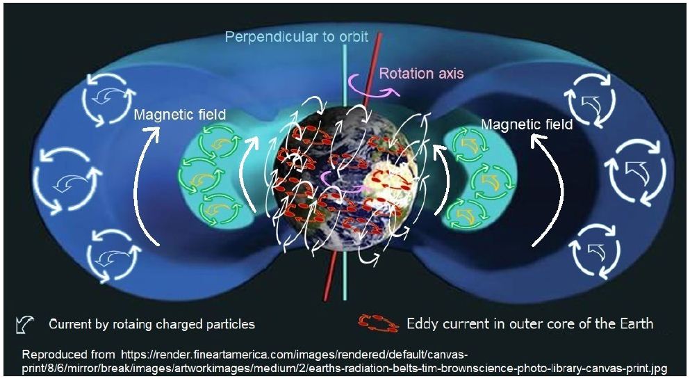
Although there is horizontal magnetic coupling on parallel traveling protons (H+), there is repulsive magnetic force between the parallel traveling H+ and electrons (e). This magnetic effect maintains the plasma state of solar wind. The movement of the scalar potential (V) generates vector potential A. The static potential V (E = grad V) and vector potential A have an identical form of distance dependency [6]. The magnetic field decreases at a location far from the source. The H+ in solar wind collides with an atom or a molecule in cosmic space; the ionized particles contribute to expansion of magnetic field by the chains of additions due to parallel-moving charged particles. So, the chain of coupled charged particles traveling in parallel expands the magnetosphere of the Planet (Figure 1).

fig 1

Figure 1: A model of Van Allen belt that is formed via chained magnetic coupling of moving charged particles

As shown in Figure 1, the inner van Allen belt is located at approximately 1.6 Re (Re = 6,378km; Earth radius). The Outer van Allen Belt is located at approximately 4.0 Re. There is a “gap” region between these belts at the distance of 2.2 Re [7]. The offset mechanism related to the magnetic coupling among charged particles causes this gap region.

Effects of Solar Wind on Planetary Wind

Comparison of the Wind on Planets

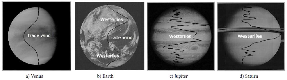
The sun emits high-speed H+ as solar wind. The rotational component of solar wind, i.e., 1.89 km/s, is perpendicular to a radiation velocity for several hundred kilometers. The charged particles emitted from the Sun travel over a long distance, eventually colliding with each other. Thus, the rotational component of the momentum of solar wind decreases owing to magnetic coupling. The charged particles of solar wind form a disk shape on a plane perpendicular to the Sun’s rotation axis via the magnetic coupling of parallel currents. Comparative planetology has revealed that solar wind drives the atmosphere of a planet. Solar wind passing at high speeds through the eastern region of Earth’s atmosphere pushes weather from the east to west because it has a greater acceleration effect than the western deceleration effect. Figure 2 shows the effects of solar wind on atmospheric flow on Venus, Earth, Jupiter, and Saturn. Mousis et al. describe atmospheric flow on the outer planets [8]. The wind flow on Saturn was overwritten by using illustrated data in [9].

fig 2

Figure 2: Atmospheric flow on Venus, Earth, Jupiter, and Saturn. Original images of each planet

Effects of Solar Wind on Super Rotation of Venus

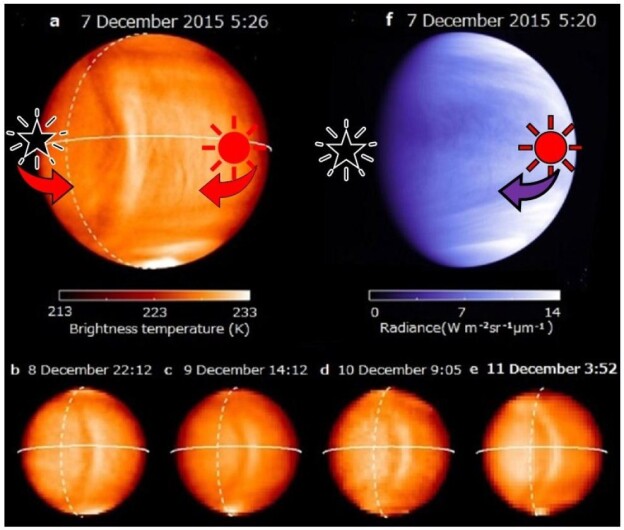
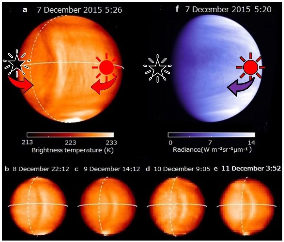
Venus rotates in a direction opposite to that of other planets. The rotational period is 243 days, the orbital period is 224.7 days, and the angle of orbital inclination is 3.39°. The rotational speed of Venus’s atmosphere reaches 100 m/s at an altitude of approximately 70 km. Super rotation does not occur by Venus’s rotation itself, because there is little angular momentum. The clockwise rotational velocity of the atmosphere of Venus is explained caused by the collisions of solar wind with anticlockwise rotational velocity of1.89 km/s. However, the atmosphere on the nightside of Venus receives solar wind from the direction opposite to that of the dayside. A large bow-like pattern was captured by the mid-infrared camera (LIR) onboard Akatsuki, the Venus climate orbiter, in December 2015 [10], as shown in Figure 3. This pattern remained in approximately the same place for more than four days. The dayside and nightside continued rotating for more than 100 days. So, the temperature on the dayside increased while that on the nightside decreased. Therefore, the high-temperature atmosphere of the dayside passes through the upper layer of the low-temperature atmosphere on the nightside at the boundary.

fig 3

Figure 3: Hot temperature atmosphere of dayside on Venus passes through at upper layer of low temperature atmosphere on nightside at the atmospheric boundary

Effects of Solar Wind on Earth’s Winds

Charged Particle in Earth’s Upper Atmosphere

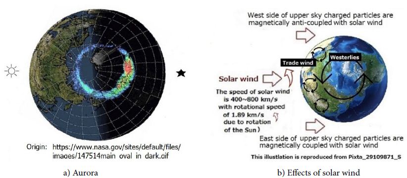
The charged particle density increases at noon owing to ultraviolet rays and light emitted by the Sun. As the mass of electrons is negligible compared with that of H+, H+ of solar wind moves in a counterclockwise direction, together with ions in the upper earth’s sky. The magnetism caused by the rotating charged particles combines with the geomagnetism caused by the inner core. Auroras occur at a latitude of 75–80° on the daytime side. However, auroras exist at a latitude of approximately 65–70° on the nightside. The difference in the latitudes of auroras between the dayside and night side is due to irradiation from the Sun (Figure 4).

As shown in Figure 4a, the increase in aurora luminescence shifts from the west side to the east side at night, but the decrease in aurora luminescence shifts from the dayside to the nightside. Auroras observed at night are not only caused by the effects of daylight but also by the neutralization of ions by free electrons. As shown in Figure 4b, the trade winds blowing from the east to the west shift the charged particles on the daytime side. The westerlies blow at high latitudes and on the nightside.

fig 4

Figure 4: Differences between the Sun-facing side and nightside, as observed from the North Pole

Weather in Equatorial Area Related to Solar Wind

Daily Changes in Weather in Equatorial Areas

During the daytime in equatorial areas, where solar irradiation occurs directly from the front, wind is characterized by a clockwise flow as solar wind enters the upper atmosphere. In contrast, solar wind drives the counterclockwise flow of the atmosphere at the nightside. Therefore, rain occurs in the evening along the equator. Madden–Julien oscillation (MJO) is a weather phenomenon in the equatorial region generated in the western Indian Ocean, wherein alternate wet and dry areas move eastward with a slow repetitive cycle of approximately 1~2 months [11]. Th slow speed at which weather migrates east over a wide area in the tropics can be understood as an effect of solar wind. The counterclockwise flow of the atmosphere at nighttime is offset by the effect of trade winds blowing from the east to west.

Mechanism of Typhoon

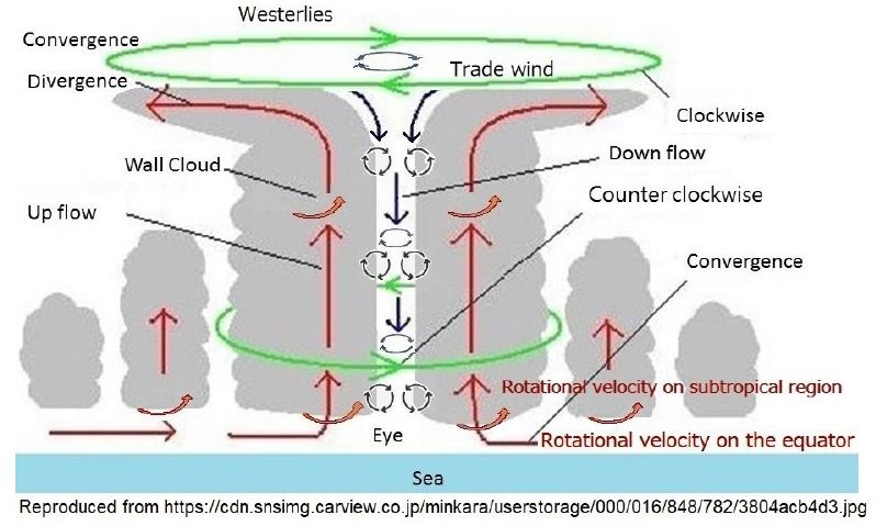
Typhoons occur in the Pacific Ocean during summer in the northern hemisphere. The most irradiated region during the summer solstice is around northern latitude of 23.4°. In this area, although trade winds blow in the daytime on end of June, westerlies of counterclockwise direction blow on both sides of the trade wind. Since the earth’s axis of rotation tilts at 23.4°, the solar wind has a moving component of north direction. So, when water vapor uprises at the southern region of the trade wind blows in the summer, that is the region where westerlies wind blows, the vapor of water moves northwest with counterclockwise rotation and collides with the trade wind of clock rotation. The collision forms an anticlockwise vortex. In the vortex, water vapor condenses, and rains, causes a tropical cyclone. This tropical cyclone moves northwest in a clockwise trade wind while develops into a typhoon. Then, the typhoon collides with the westerly winds of counterclockwise rotation and travels northeast direction. Figure 5 shows an illustration of the typhoon mechanism.

fig 5

Figure 5: Typhoon mechanism in the northern hemisphere during summer

Conclusion

Weather and climate rely on the winds blowing over a wide area affected by solar wind. The tilt of Earth causes seasonal changes in the wind owing to solar wind. The flows of atmosphere are linked to solar wind via magnetic coupling among moving charged particles.

This study described effects of solar wind on the weather and the climate of Earth. This will be helpful when discussing research in a wide range of fields such as global warming.

Acknowledgement

I would like to thank Editage (www.editage.com) for English language editing.

References

  1. Syvitski J, Colin NW, John D, John DM, Colin S, et al. (2020) Extraordinary human energy consumption and resultant geological impacts beginning around 1950 CE initiated the proposed Anthropocene Epoch. Communications Earth & Environment 1.
  2. Walker MJC, Berkelhammer M, Björck S, Cwynar LC, Fisher DA, et al. (2012) Formal subdivision of the Holocene Series/Epoch: a Discussion Paper by a Working Group of INTIMATE (Integration of ice-core, marine and terrestrial records) and the Subcommission on Quaternary Stratigraphy (International Commission on Stratigraphy). Journal of Quaternary Science 27: 649-659.
  3. Buis A (2020) Milankovitch (Orbital) Cycles and Their Role in Earth’s Climate. NASA’s Jet Propulsion Laboratory.
  4. CIRA, COSPAR international reference atmosphere 1972, Chronological Scientific Tables, 2020, pg: 872, 57, Marzen Publishing Co, Ltd. 2019.
  5. Aharonov Y, Bohm D (1959) Significance of Electromagnetic Potentials in the Quantum theory. Physical Review 115: 485-491.
  6. Feynman RP, Leighton RB, Sands M, Treiman SB (1964) “The Feynman lectures on physics. Physics Today 17: 45-46.
  7. NASA, The deadly van Allen Belts?
  8. Mousis O, David HA, Richard A, Sushil A, Don B, et al. (2021) In situ exploration of the giant planets. Experimental Astronomy.
  9. García-Melendo E, Pérez-Hoyos S, Sánchez-Lavega A, Hueso R (2011) Saturn’s zonal wind profile in 2004–2009 from Cassini ISS images and its long-term variability. Icarus. 215 (1): 62-74.
  10. Fukuhara T, Masahiko F, George LH, Takeshi H, Takeshi I, et al. (2017) Large stationary gravity wave in the atmosphere of Venus. Nature Geoscience 10 (2): 85-88.
  11. Wang B, Chen G, Liu F (2019) “Diversity of the Madden–Julian oscillation”, Science Advances 5.

Role of Alpha Fetoprotein in Hepatocellular Carcinoma

DOI: 10.31038/CST.2022723

Abstract

Hepatocellular carcinoma prevalence rate is higher in Pakistan due to HCV mortality rate, consumption of Alchol, and regular smoking, higher level of AFP progression normal liver cells into fatty liver cells, after inflammation it convert into HCC. In this study, we find the correlation between AFP and hepatocellular carcinoma. AFP involve in development of liver cancer, LFT’s test elevation and HCV also cause of cancer.

Keywords

Hepatocellular carcinoma, Alpha fetoprotein, Alanine amino transferases, Aspartate aminotransferases

Introduction

Hepatocellular carcinoma is the 4th most common malignancy in worldwide and it is leading cause of cancer like disease in liver, and it exceed more than 1 million deaths per year by 2030 [1]. Acute hepatitis and acute liver failure are the most serious medical condition that require early diagnosis by release of IL-6, TNF-α and elevated alanine amino transferases, aspartate aminotransferases, alkaline phosphatase and α-Fetoprotein that progress healthy liver in to fatty liver known as steatosis and then inflammation occur in this and leads to hepatocellular carcinoma [2]. Most cases of HCC due to the virus like HCV and HBV, Diabetic and obesity, alcohol related diseases, non-alcohol related diseases, carcinogens like aflatoxins compounds [3]. HCC is the most common cancer that have high mortality rate in cancers due to mortality of HCV and NLFD. In Pakistan HCC ratio high due to prevalence and mortality rate of HCV [4]. The major treatment of HCC is chemotherapy, radiotherapy, transplantation and surgery. Because the most cases diagnose at the late stage, surgery cannot be performed and drugs are the only treatment of HCC [5]. Most patients in HCC become more drug resistance drug resistance. Drug treatment is the best choice of patients who are not edible for surgery. HCC is usually resistance to chemotherapeutic drugs because it hinders liver cancer treatment. In recent years targeted drugs use as medication and immune checkpoint inhibitors are introduce for treatment [6].

In the previous research evidence indicates that alpha-fetoprotein has high false-positive rate in diagnosis of early stage of HCC. The EASL clinic practices shows that AFP as a biomarker for liver transplantation and drug indicator [7]. The AFP level increased in many patients’ ad its risk for progression of HCC. AFP, currently the only biomarker available for HCC drug treatment, function as immune suppressor and promote malignancy transformation in HCC [8].

HCC is resistant to traditional chemotherapeutic agents such as doxorubicin, tetrahydrofolate, oxaliplatin, cisplatin, and gemcitabine. Currently the recommended drugs include such as targeted therapeutics and immune checkpoint inhibitors [9].

AFP is a glycoprotein that secreted by endoderm embryonic tissue. The lower level of AFP in blood due to AFP is decrease in mature hepatocytes and that AFP gene expression is blocked. It is possible that AFP involved in HCC development and progression becomes an important factor affecting HCC diagnosis and treatment. AFP plays an important role in promoting cancer cell proliferation and, inhibition cancer cell apoptosis.

LFT’s test performed for liver injury, alanine aminotransferases, aspartate aminotransferases and alkaline phosphatase. These enzymes are commonly elevated in liver disease patients. Alkaline phosphatase and AFP play important role in the diagnosis of cancer.

Case Study

The patient name was sikandar, age 56 patient feel pain in their abdomen and sudden loss of weight. The patient has already hepatitis C infection and their PCR results were positive with high viral load. Due to serious illness it admitted in emergency ward 12, Nishter Hospital Multan. The doctor panel referred some test and kept in observations for better health condition.

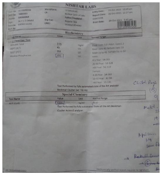
The total bilirubin level was 2.05 mg/dl in their blood and their normal values 0.6-1.2. The serum glutamate-pyruvate transaminase level is 43 U/L and normal values up to 40. Aspartate amino transferases and alkaline phosphatase level were high in blood respectively 151 U/L and 493 U/l show in Figure 1. It indicates liver injury and cirrhosis. The AFP test indicates correlation with Hepatocellular carcinoma. The AFP level in patient was 6101 ng/ml and normal values were 0.1 – 10. Higher level of AFP indicates that HCC have positive relation with AFP to proliferate cancer. The test formed by fully automated state of the Art analyzer Beckman Coulter 700 AIJ.

fig 1

Figure 1: Liver function and Alpha Feto Protein test in patient

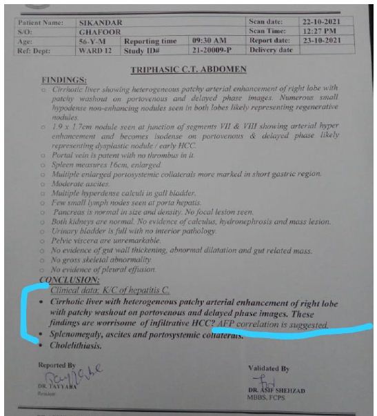
After blood reports, doctor suggest ultarosund Computrised Tomography whole abdominal view. In view, spleen size becomes enlarged 6 cm, calculi in gall bladder, heterogeneous patchy atrial enhancement of right lobe, and some nodules seen in both lobes of liver. The doctor finds the AFP correlation with HCC, splenomegaly, ascites, cholelithiasis and protosystematic collaterals (Figure 2).

fig 2

Figure 2: Ultrasound Computrised Tomography whole abdomen

The patient diagnosed with hepatocellular carcinoma at last stage, and doctor referred to liver transplantation in India. But after 4 weeks he cannot survive.

Conclusion

Hepatitis C was the major risk of hepatocellular carcinoma in Pakistan. Smoking and alcohol have big problem to influence HCC in humans. The case study shows that alpha fetoprotein has correlation with HCC. Higher Alkaline phosphatase and serum Bilirubin level enhance the liver carcinoma. AFP play role in cell proliferation, cancer cell differentiation and cell cycle arrest.

References

  1. Yang JD, Hainaut P, Gores GJ, Amadou A, Plymoth A, Roberts LR (2019) A global view of hepatocellular carcinoma: trends, risk, prevention and management. Nature Reviews Gastroenterology & Hepatology. 16: 589-604.[crossref]
  2. Effenberger M, Grander C, Grabherr F, Griesmacher A, Ploner T. et al. (2021) Systemic inflammation as fuel for acute liver injury in COVID-19. Digestive and Liver Disease. 53: 158-165.[crossref]
  3. Du J, Ma YY, Yu CH, Li YM (2014) Effects of pentoxifylline on nonalcoholic fatty liver disease: a meta-analysis. World Journal of Gastroenterology. 20: 569.[crossref]
  4. Ashtari S, Pourhoseingholi MA, Sharifian A, Zali MR (2015) Hepatocellular carcinoma in Asia: Prevention strategy and planning. World Journal of Hepatology. 7: 1708. [crossref]
  5. Daher S, Massarwa M, Benson AA, Khoury T (2018) Current and future treatment of hepatocellular carcinoma: an updated comprehensive review. Journal of Clinical and Translational Hepatology. 6: 69.
  6. Liu X, Qin S (2019) Immune checkpoint inhibitors in hepatocellular carcinoma: opportunities and challenges. The Oncologist. 24: S3-S10. [crossref]
  7. Wong RJ, Ahmed A, Gish RG (2015) Elevated alpha-fetoprotein: differential diagnosis-hepatocellular carcinoma and other disorders. Clinics in Liver Disease. 19: 309-323. [crossref]
  8. Trevisani F, Garuti F, Neri A (2019) Alpha-fetoprotein for diagnosis, prognosis, and transplant selection. Seminars in Liver Disease. [crossref]
  9. Galluzzi L, Senovilla L, Zitvogel L, Kroemer G (2012) The secret ally: immunostimulation by anticancer drugs. Nature Reviews Drug Discovery. 11: 215-233. [crossref]

COVID 19 Impact on Medical Students in Jordan, Cross-Sectional, Prospective Study

DOI: 10.31038/JCRM.2022514

Abstract

Introduction: COVID 19, the global pandemic that was first identified in December 2019 in Wuhan, China, caused by severe acute respiratory syndrome coronavirus 2 (SARS-CoV-2) and adversely affected global life style, was reported in Jordan in March 2020. Due to its high contagious dissemination, the rapid virus spread caused global lifestyle modifications. Medical schools in Jordan as other facilities were highly affected and had alterations related to education. Here we focus, discuss and conclude the final alterations impact according to students impressions to end up with recommendations for future pandemic education.

Methods: This cross sectional, prospective study explores the impact of COVID-19 pandemic on medical students’ academic performance in Jordan from their point of view. A survey questionnaire was developed to investigate the issue related to the study subject and to answer certain questions. Mainly we needed to find out if COVID-19 pandemic affected medical students’ academic performance in Jordan? In which aspects? And in what direction? Due to the nature of this study, and the circumstances during the study period, an online survey questionnaire was conducted through Google Forms and reflected the found outcome.

Results: The study population consists of approximately 6500 representing all medical students in each academic year from the six medical schools in Jordan. Appropriately found formula was used to determine the required sample size. Finalising that most but not all criteria used measures were negatively affected.

Conclusion: All the academic performance components -that we have assumed- have been affected negatively by the pandemic with the exception of medical knowledge. E-learning infrastructure and pre-experience in distance learning might have an improvement effect and may be better outcome than classical learning.

Introduction

COVID 19, the global pandemic that was first identified in December 2019 in Wuhan, China, caused by severe acute respiratory syndrome coronavirus 2 (SARS-CoV-2) and adversely affected global life style, was reported in Jordan in March 2020 [1]. Due to its high contagious dissemination and the variable symptoms from subclinical to severe lethal pneumonia [2,3], the rapid virus spread caused global lifestyle modifications. Most governments worldwide applied new regulations trying to flatten the escalating spread curves caused by the pandemic. Face masks wearing, strict hygiene, social distancing, travel restrictions, borders closing, and closing schools, colleges and Universities physically were all utilized. The higher educational institutions around the world have been fully or partially, closing their campuses to limit the rapid spread of COVID19 infection. All those alterations led to massive disrupt at all educational levels in general [4]. Therefore, such consequences forced the worldwide higher educational institutes to adopt distance learning mode. Taking in consideration that any unforeseen judgment would probably lead to massive derangement in the critical and civilian cervices [5].

Moreover, all students perspectives in general, were distorted due to the misbelief of expected curricula modification to fit for the new so-called remote learning. In addition, remote electronic exams (E-exams) were considered as the new mode of assessment. Distance learning, teaching, and assessment were never the fundamental one applied in Jordan schools of medicine. Lack of experience in both parties of electronic services created an unsecured atmosphere. The issue of having distance learning as being the solely one used in medical schools was growing over and over. Debate started to expand between experts whether distance learning decision was injudicious up to many where others considered it sapient [6].

Concerning students in medical schools in Jordan, there was an apprehension among them about that newly developed assessment mode [7]. The panic was higher between clinical years medical students as medicine studying depends in its majority on clinical, and practical part especially in the last three years. Their fear was understandable as the decision of distance learning was suddenly taken and not gradually as expected to be. Gradual transition was about to be justified especially if proper preparation and precautions were taken in consideration before the complete sudden distance education decision.

However, the unprepared technical infrastructure will always be an obstacle for distance learning indifferent of the educational level. Malfunctions, bugs, connection errors, inability to connect, sudden disconnection, or even video and audio technical problems are all challenges faced by best prepared networks. Dishonesty of either side whether students or lecturers was always considered an addressed issue and taken seriously due to its major and catastrophic consequences. Nevertheless, obscurant credence started to be a new challenge for medical schools to face. That belief of students and parents reached to the extent that many appealed for money refund. Accordingly, proving efficiency and ability to continue online without affecting the quality of learning was a new challenge for all educational institutions to take over. Hybridisation of conventional, as well as online educational programme was applied by many institutions as a way to keep the balance between safety during pandemic and high quality education [8]. For instance, all lectures and presentations which were considered theoretical were given online, while patient based practice sessions were in hospital module of learning, after taking all precautions as per ministry of health instructions.

Nevertheless, medical educational system continued to pursue its utmost efforts to facilitate the informations availability. Undergraduate medical student’s opinions about the modified system attitude were variable, and here we try to focus on their expression and to illustrate their point of view on the newly adopted distance learning era [9-13].

In this article, we have conducted a cross-sectional online survey study among all six years medical schools in Jordan to explore the above mentioned challenges, and the impact of COVID-19 pandemic on medical school students’ academic performance.

Materials and Methods

This cross sectional, prospective study explores the impact of COVID-19 pandemic on medical students’ academic performance in Jordan from their point of view. A survey questionnaire was developed to investigate the issue related to the study subject and to answer certain questions. Mainly we needed to find out if COVID-19 pandemic affected medical students’ academic performance in Jordan? In which aspects? And in what direction? Due to the nature of this study, and the circumstances during the study period, an online survey questionnaire was conducted through Google Forms. The form distributed to the study cohort could have been found at: https://docs.google.com/forms/d/1N0J8hiVVzYw7iV6zcPhvzRy_q_3NvdzxKlrovLVnqCg/prefill?skip_itp2_check=true. The targeted study population is the medical school students in Jordan indifferent in which year, meanwhile, basic and clinical years included. From all medical schools in Jordanian Universities, students were invited to participate in the study by completing the form online. The form was available through an invitation on known web platforms, sites and pages to students. Participation was voluntary and completely anonymous for the period from beginning of February till the end of it same year (2021). The study was approved by the ethical committee, and has IRB approval number 219/132/2020 from Jordan University of Science and Technology (JUST), Irbid, Jordan. The University of Jordan (UJ), Jordan University of Science and Technology (JUST), Mutah University (MU), The Hashemite University (HU), Al-Balqa Applied University (BAU), and Yarmouk University (YU) registered at study time students from medical schools were all eligible to participate in the study.

Variable Selection

The following variables are developed from literature reviews and serve as indicators of students’ academic performance:

1) Academic achievement which includes:

A. Medical knowledge.

B. Laboratory skills which applied for basic science years students only {first to third year}.

C. Clinical skills which applied for clinical science years students only {forth to sixth year}.

2) Attributes of studying which includes:

A. Studying hours

B. Sessions attendance

3) Seasonal grade.

4) Self-Assessment.

Based on the aforementioned variables, diagram 1 represent the operational definition of the impact of COVID-19 pandemic on students’ academic performance.

The reliability of Academic performance as indicated by the reliability coefficient (Cronbach’s Alpha=(0.723)). Indicates adequate reliability.

Hypothesis, test of hypothesis and sampling:

The hypotheses for this research are to test whether there is any significant impact of COVID-19 pandemic on students’ academic performance, and to test whether there is any association between specific demographic characteristics of the students and the impact of COVID-19 on their academic performance.

A. There is no impact of COVID-19 pandemic on students’ academic performance.

A1. There is no impact of COVID-19 pandemic on students’ academic achievement.

A1.1. There is no impact of COVID-19 pandemic on students’ medical knowledge.

A1.2. There is no impact of COVID-19 pandemic on students’ laboratory skills.

A1.3. There is no impact of COVID-19 pandemic on students’ clinical skills.

A2. There is no impact of COVID-19 pandemic on students’ attributes of studying.

A2.1. There is no impact of COVID-19 pandemic on students’ studying hours.

A2.2. There is no impact of COVID-19 pandemic on students’ attendance.

A3. There is no impact of COVID-19 pandemic on students’ grades.

A4. There is no impact of COVID-19 pandemic as self-assessed by students.

B1. There is no association between students’ Gender and the impact of COVID-19 pandemic on students’ academic performance.

B2. There is no association between students’ Academic year and the impact of COVID-19 pandemic on students’ academic performance.

B3. There is no association between students’ High school and the impact of COVID-19 pandemic on students’ academic performance.

B4. There is no association between students’ number of family members and the impact of COVID-19 pandemic on students’ academic performance.

B5. There is no association between students’ monthly family income and the impact of COVID-19 pandemic on students’ academic performance.

Due to the nature of this empirical study, an online survey questionnaire was conducted through Google Forms. The questionnaire was published through social media (multiple website, and platforms like Facebook groups for medical students in Jordan). The respondents were asked to evaluate the selected variables in a three point Likert scale, with 3=positively/increased, 2=neutral/not changed, 1=negatively/decreased.

One sample Student’s t-test is used to test hypotheses (A-A4). A t-test is a statistical hypothesis test in which the test statistic follows a Student’s t distribution if the null hypothesis is supported. It is most commonly applied when the test statistic would follow a normal distribution if the value of a scaling term in the test statistic is known. The one sample t-test requires that the dependent variable follow a normal distribution. When the number of subjects in the experimental group is 30 or more, the central limit theorem shows a normal distribution can be assumed. 95% of the t-Tests two tailed probability level was selected to signify the differences between preferences. The estimate value for testing hypotheses in this study is 2, which is neutral/not changed. It shows no differences in academic performance in the presence of the pandemic. A Pearson’s correlation test was run to test hypotheses (B1-B4). The respondents were asked to evaluate the selected variables in three points. One sample Student’s t-test is used to test hypotheses (A-A4). A t-test is a statistical hypothesis test in which the test statistic follows a Student’s t distribution if the null hypothesis is supported. It is most commonly applied when the test statistic would follow a normal distribution if the value of a scaling term in the test statistic is known. The one sample t-test requires that the dependent variable follow a normal distribution. When the number of subjects in the experimental group is 30 or more, the central limit theorem shows a normal distribution can be assumed. 95% of the t-Tests two tailed probability level was selected to signify the differences between preferences. The estimate value for testing hypotheses in this study is 2, which is neutral/not changed.

Results

Between Feb 2, 2021 and Feb 27, 2021. A total of 369 sixth year medical students in Jordan responded to the questionnaire, and of those who did, a number of 16 responses were excluded due to lack of accuracy-halo effect/since they answered a question not supposed to be answered. With 353 valid responses for analyses, representing 95% of the total was surveyed.

The study population consists of approximately 6500 representing all medical students in each academic year from the six medical schools in Jordan. The Slovin’s formula was used to determine the required sample size.

Sample Size=N/(1 + N*e22) where:  N=population size. e=margin of error.

Solving the formula using e=0.05, N=(6500) sample size of (364) was yielded.

Table 1 presents the distribution of the students according to specific Demographic characteristics:

Table 1: Demographic characteristics


Frequency

Percent

Gender Male

179

50.7

Female

174

49.3

Residence Central region

207

58.6

Northern region

97

27.5

Southern region

49

13.9

University Al-Balqaʼ Applied University (BAU)

119

33.7

Jordan University of Science and Technology (JUST)

59

16.7

Mutah University (MU)

39

11.0

The Hashemite University (HU)

43

12.2

The University of Jordan (UJ)

19

5.4

Yarmouk University (YU)

74

21.0

Academic year First year

48

13.6

Second year

83

23.5

Third year

47

13.3

Forth year

48

13.6

Fifth year

73

20.7

Sixth year

54

15.3

High school private school

191

54.1

public school

162

45.9

Number of Family members Small family

142

40.2

Medium family

188

53.3

Large family

23

6.5

Monthly family income Low income

125

35.4

Moderate income

112

31.7

High income

116

32.9

Table 2 presents the test results of One-Sample t-Test, with mean differences, t values, degrees of freedom, and two tailed significances of these tests.

Table 2: COVID-19 pandemic effect on medical students’ academic performance and its components

Test Value = 2

t*

df** P value

Mean Difference

95% Confidence Interval of the Difference

Lower

Upper

Academic performance

-8.020

352 .000 -.21211 -.2641

-.1601

Academic achievement

-7.725

352 .000 -.23654 -.2968

-.1763

Progress in medical knowledge

.274

352 .784 .01133 -.0699

.0926

Progress in laboratory skills

-8.910

177 .000 -.46629 -.5696

-.3630

Progress in clinical skills

-10.661

174 .000 -.50286 -.5960

-.4098

Attributes of studying

-7.604

352 .000 -.23229 -.2924

-.1722

Average daily studying hours

-2.796

352 .005 -.11898 -.2027

-.0353

Sessions attendance

-9.697

352 .000 -.34561 -.4157

-.2755

Seasonal grade

-2.306

352 .022 -.09632 -.1785

-.0142

Self-assessment

-7.289

352 .000 -.28329 -.3597

-.2069

*t value
**Degree of freedom

The mean for Academic performance score and all of its components – except medical knowledge- scores were statistically significantly lower than the neutral score of 2 (p<0.05). With progress in clinical skills having the highest mean difference of 0.49 and Seasonal grade having the lowest mean difference of -.10. Therefore, we can reject the null hypotheses (A, A1, A1.2, A1.3, A2, A2.1, A2.2, A3, and A4) and accept the alternative hypotheses. And accept the null hypothesis A.1.1.Thus the Academic performance and all of its components except medical knowledge is negatively affected by COVID-19 pandemic.

Table 3 presents the test results of Pearson’s correlation test between specific demographic characteristics and academic performance.

Table 3: Relationship between specific demographic characteristics and impact of COVID-19 pandemic on medical students’ academic performance


Gender

Residence University Academic year High school Family member groups

Monthly family income level

Academic performance

Pearson Correlation

-.071

.077 .030 .159** .049 -.001

-.026

p

.183

.150 .579 .003 .363 .983

.624

N

353

353 353 353 353 353

353

** Correlation is significant at the 0.01 level (2-tailed)
*. Correlation is significant at the 0.05 level (2-tailed)

There was a very weak, positive correlation between Academic year and Academic performance r=.159, N=353; the relationship was statistically significant (p=.003). However there were no statistically significant relationships between Academic performance and other demographic characteristics (p>.05). Therefore, we can reject the null hypothesis B2 and accept the alternative hypothesis. And accept the null hypotheses (B1, B3 and B4). According to the findings and statistics, the academic performance and all of its components except medical knowledge were negatively affected by COVID-19 pandemic.

Discussion

Since COVID 19 pandemic first appearance in Wuhan city in china, November 2019 and its spread over the world (9, 10, 11), it has been affecting almost all sectors of life and increasing efforts has been made to study that effect (12, 13), lock down have been held worldwide which led to a huge impact on economy, education and most importantly health regardless whether it was physical or mental health [14-17].

In this context, this study was conducted as to observe the impact of COVID 19 on the academic performance of medical students in Jordan Universities, and evaluate the effect on certain parameters like their medical knowledge, laboratory and clinical skills, their attendance, daily studying hours and their grades, and all that was viewed in regards to e-learning which was adopted as the learning method during the pandemic. This study was done on the 6 medical schools in Jordan and the sample was 353 medical students from all years.

Apparently, and according to our results illustrated; COVID19 pandemic has negative impact in all component measured by us of academic performance for medical students in Jordan (attributes of studying, average daily studying hours, sessions attendance, academic achievement, progression in laboratory and clinical skills, grades, and self-assessment) with the exception of medical knowledge progression as found in Tables 2 and 4.

Table 4: Components measured by us of academic performance for medical students in Jordan


Negative

Neutral

Positive

Total impact on academic performance Frequency

158

137

58

Percent

44.76

38.81

16.43

Average daily studying hours Frequency

136

123

94

Percent

38.53

34.84

26.63

Seasonal grade Frequency

127

133

93

Percent

35.98

37.68

26.35

Attendance Frequency

161.00

153.00

39.00

Percent

45.61

43.34

11.05

Progress in medical knowledge Frequency

104.00

141.00

108.00

Percent

29.46

39.94

30.59

Progress in laboratory skills for (1st – 3rd year) Frequency

104.00

53.00

21.00

Percent

58.43

29.78

11.80

Progress in clinical skills (for 4th-6th year) Frequency

100.00

63.00

12.00

Percent

57.14

36.00

6.86

The effect on daily studying hours and sessions attendance could be explained by the probability that students considered e-learning less serious and possibly there are difficulties in dealing with such kind of learning because it is an emerging one in medical schools in Jordan Universities. Moreover, resources limitation such as unavailability of proper internet connection in certain urban areas, and/or smart devices limited access by some students may have played a role and that could be indirectly observed through the participation in our study which is entirely dependant on digital platforms. Most of study participants are from central areas in Jordan (58.6%) where the most reliable internet is. On the contrary, contributors from northern and southern Universities where rural areas are, with unreliable internet connections represented 41.4% (27.5+13.9) as per (Table 1). Taking in consideration that students individual preferences, interests, vary from student to another [18].

Laboratory and clinical skills were the components that have been negatively most affected (mean difference=0.47, 0.5 respectively). We firmly believe that this effect is due to the fact that students have been away from the field of learning. Additionally, the suggested certainty related to the weaknesses of infrastructure in medical schools in Jordan to support appropriate e-learning which they believed it should have been far better that the existing [19]. Although some studies showed that laboratory skills can be acquired away from the lab by video feedback [20], the results we observed were against the results of those studies; and this can be explained by challenges found in Jordan Universities in supporting this kind of learning modality. Students in our study do believe that they substantially need to physically attend and participate in clinical rounds, take history and do physical examination to improve their clinical medical skills [21,22].

In contrast to other components, medical knowledge has shown no relation with the pandemic (p=0.784), we suggest that this is due to students ability to depend on self-studying from other resources outside the University premises. Books, slides, scientific papers, lectures, internet etc. participated to develop student’s medical knowledge. In addition, students platforms availability on the internet which facilitates knowledge sharing, and suggested sites between medical school students and their mentors again played distinguished part in improving faculty members and students medical knowledge [23].

Demographic characteristics in this study showed no relation (p>0.05) on the impact of COVID 19 pandemic on medical students academic performance with the exception of academic year (p=0.003). It showed only a weak positive effect (Pearson correlation=0.159) illustrated clearly in Table 3. The thing which can be explained by the fact that medical students autonomously progress in their years spent in medical schools. They perform more tests and sit for more evaluation exams, so more conjunction of knowledge and skills is met. Nevertheless, more development of cognition that makes them more independent in their self-developing [24]. Good example is that fourth year medical student is more likely to compensate the reduction in the quality and quantity than the second year medical student.

Alsoufi et al. found an accepted level of knowledge in medical students regarding e-learning in Libya in his study. In addition, they were concerned about how e-learning could be applied to provide clinical experience which depends heavily on bedside teaching [25].

Some other studies in other regions, specifically Kingdom of Saudi Arabia have shown acceptance in e-learning during COVID-19, showing better outcomes with promising potentials to prefer e-learning in medical education in the future [26]. As per experts, such findings could be related to better distance learning infrastructure and facilities.

The strength of this study is that it applied multiple measures (medical knowledge, laboratory and clinical skills, session attendance, daily studying hours, grades and self-assessment) to demonstrate and assess academic performance (Figure 1).

fig 1

Figure 1: Definition of the impact of COVID-19 pandemic on students’ academic performance

Certain limitations of this study could be addressed in future research are (low response, and absence of funding, limited number of studies on this topic).

More studies are still needed to evaluate the impact of distance learning under and free of the influence of certain pandemic.

Conclusion

All the academic performance components -that we have assumed- have been affected negatively by the pandemic with the exception of medical knowledge. E-learning infrastructure and pre-experience in distance learning might have an improvement effect and may be better outcome than classical learning.

References

  1. Al-Tammemi A (2020) The Battle Against COVID-19 in Jordan: An Early Overview of the Jordanian Experience. Front Public Health 8: 188. [crossref]
  2. Zhou F, Yu T, Du R, Fan G, Liu Y, et al. (2020) Clinical course and risk factors for mortality of adult inpatients with COVID-19 in Wuhan, China: a retrospective cohort study. Lancet 395: 1054-1062.
  3. Rothan HA, Byrareddy SN (2020) The epidemiology and pathogenesis of coronavirus disease (COVID-19) outbreak. J Autoimmun 109: 102433.
  4. Malee Bassett R, Arnhold N (2020) World Bank Blogs; COVID-19’s Immense Impact on Equity in Tertiary Education.
  5. Bergdahl, N, Nouri, J (2021) Covid-19 and Crisis-Prompted Distance Education in Sweden. Tech Know Learn 26: 443-459.
  6. Zalat M, Hamed M, Bolbol S (2021) The experiences, challenges, and acceptance of e-learning as a tool for teaching during the COVID-19 pandemic among university medical staff. Plos One 16: e0248578. [crossref]
  7. Birch E, de Wolf M (2020) A novel approach to medical school examinations during the COVID-19 pandemic. Med Educ Online 25: 1785680. [crossref]
  8. Mishra L, Gupta T, Shree A (2020) Online teaching-learning in higher education during lockdown period of COVID-19 pandemic. Int J Educ Res Open 1: 100012.
  9. Huang C, Wang Y, Li X, Ren L, Zhao J, et al. (2020) Clinical features of patients infected with 2019 novel coronavirus in Wuhan, China. Lancet 395: 497-506. [crossref]
  10. Chen N, Zhou M, Dong X, Qu J, Gong F, et al. (2020) Epidemiological and clinical characteristics of 99 cases of 2019 novel coronavirus pneumonia in Wuhan, China: a descriptive study. Lancet 395: 507-513. [crossref]
  11. Holshue ML, DeBolt C, Lindquist S, Lofy KH, Wiesman J, et al. (2020) First Case of 2019 Novel Coronavirus in the United States. N Engl J Med 382: 929-936. [crossref]
  12. Khoo Erwin J, Lantos John D (2020) Lessons learned from the COVID-19 pandemic. Acta Paediatrica 109: 1323-1325. [crossref]
  13. Haleem A, Javaid M, Vaishya R (2020) Effects of COVID-19 pandemic in daily life. Curr Med Res Pract 10: 78-79. [crossref]
  14. Prickett, Kate C, Fletcher Michael, Chapple Simon, Doan Nguyen, Smith Conal (2020) Life in lockdown: The economic and social effect of lockdown during Alert Level 4 in New Zealand.
  15. Kapasia, Nanigopal, Paul, Pintu, Roy, et al. (2020) Impact of lockdown on learning status of undergraduate and postgraduate students during COVID-19 pandemic in West Bengal, India. Children and Youth Services Review 116: 105194.
  16. Rajiv R, Ramachandran R, Surya J, Ramakrishnan R, Sivaprasad S, et al. (2021) Impact on health and provision of healthcare services during the COVID-19 lockdown in India: a multicentre cross-sectional study. BMJ open 11: e043590. [crossref]
  17. Adams-Prassl Abi, Boneva Teodora, Golin Marta, Rauh Christopher (2020) The impact of the coronavirus Lockdown on mental health: evidence from the US.
  18. Hamdan KM, Al-Bashaireh AM, Zahran Z, Al-Daghestani A, AL-Habashneh S, et al. (2021) “University students’ interaction, Internet self-efficacy, self-regulation and satisfaction with online education during pandemic crises of COVID-19 (SARS-CoV-2)”. International Journal of Educational Management 35: 713-725.
  19. Al-Balas Mahmoud, Al-Balas Hasan, Ibrahim Jaber, et al. (2020) Distance learning in clinical medical education amid COVID-19 pandemic in Jordan: current situation, challenges, and perspectives. BMC medical education 20: 1-7.
  20. Donkin Rebecca, Askew Elizabeth, Stevenson Hollie (2019) Video feedback and e-Learning enhances laboratory skills and engagement in medical laboratory science students. BMC medical education 19: 1-12. [crossref]
  21. Hassan Shahid (2007) How to develop a core curriculum in clinical skills for undergraduate medical teaching in the school of medical sciences at universiti sains malaysia?. The Malaysian journal of medical sciences: MJMS 14: 4-10. [crossref]
  22. Favarato, Maria Helena, Sarno, Murilo Moura, Peres, Lena Vania Carneiro et al. (2019) Teaching-learning process of clinical skills using simulations-report of experience. MedEdPublish 8.
  23. O’Doherty D, Lougheed J, Hannigan A, et al. (2019) Internet skills of medical faculty and students: is there a difference?. BMC Med Educ 19: 39.
  24. Reberti, Ademir Garcia, Monfredini, Nayme Hechem, Ferreira Filho, et al. (2020) Progress Test in Medical School: a Systematic Review of the Literature. Revista Brasileira de Educação Médica 44.
  25. Alsoufi Ahmed, Alsuyihili Ali, Msherghi Ahmed, Elhadi Ahmed, Atiyah Hana, et al. (2020) Impact of the COVID-19 pandemic on medical education: Medical students’ knowledge, attitudes, and practices regarding electronic learning. PloS one 15: e0242905. [crossref]
  26. Khalil R, Mansour AE, Fadda WA, et al. (2020) The sudden transition to synchronized online learning during the COVID-19 pandemic in Saudi Arabia: a qualitative study exploring medical students’ perspectives. BMC Med Educ 20: 285.

Cardiovascular Pathologies and Climate and Seasonal Variation: Prospective and Comparative Study between the Cold Season and the Hot Season 2016 at the Amirou Boubacar Diallo National Hospital (HNABD) about 258 Cases

DOI: 10.31038/JCCP.2022512

Abstract

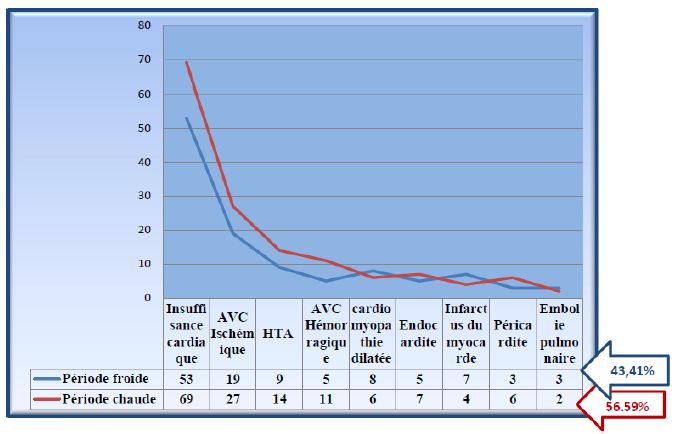
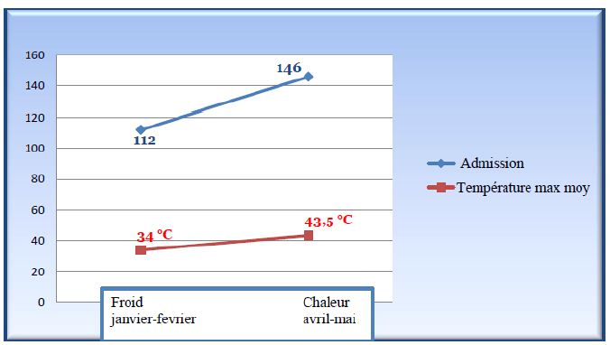
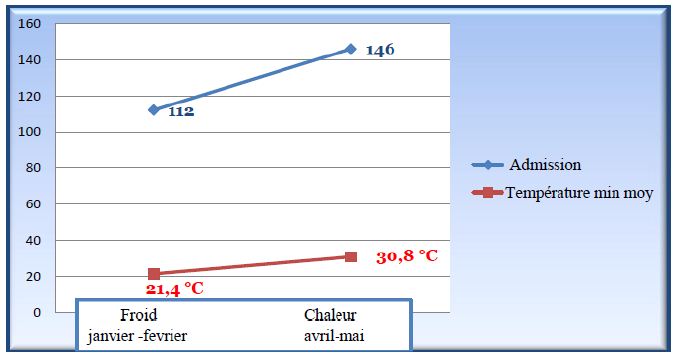
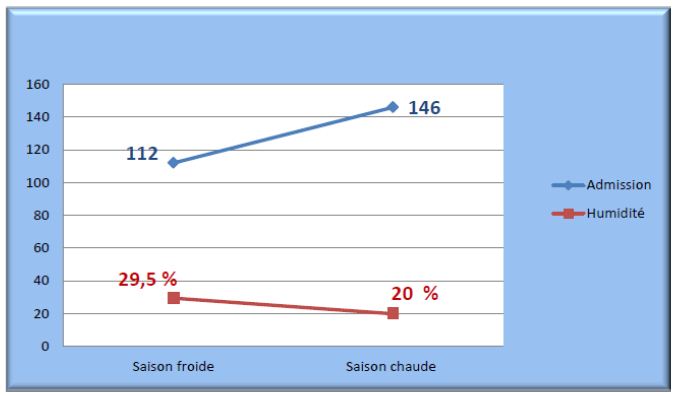
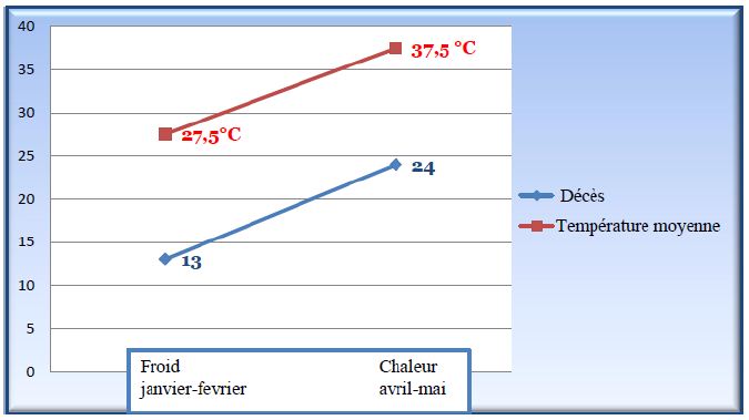
This is a prospective and comparative study over four months between the cold season (January-February) and the hot season (April-May) 2016. It involved 258 patients hospitalized in the department of cardiac medicine during this period in which the diagnosis of cardiovascular pathologies was made. Through this work, we studied the epidemiological, clinical, paraclinical, therapeutic and evolutionary aspects and finally the impact of climatic and seasonal variations on cardiovascular pathologies. Epidemiologically, cardiovascular disease accounts for 55.60% of admission to the service. There is a male predominance of 53.10% compared to 46.90% for females. The average age was 55.17 years. The age range greater than 60 years is the most affected with 54.25%. The admission rate for cardiovascular disease was 43.41% during the cold season compared with 56.59% during the heat season. Clinically, the most common diagnoses were heart failure, stroke and hypertension with 47.28%, respectively; 24.03%; and 8.91%. Therapeutically, the protocol used largely relies on diuretics, ACE inhibitors, antiplatelet agents. On an evolutionary level, 81.79% of the patients had a favorable outcome. The mortality rate is 14.34% with a peak of death during the warm season. Thus, 24 deaths were found, representing a mortality rate of 16.43% and 64.86% of total deaths in the warm season. Indeed, the elevations of temperature lead to an increase in the admissions but also of the mortality related to the cardiovascular diseases.

Keywords

Cardiovascular pathologies, Seasonal climatic variations, Prevalence, Morbimortality, National Hospital of Lamorde Niamey

Introduction

Cardiovascular disease (CVD) is a group of disorders affecting the heart and blood vessels. Nowadays, they pose an important public health problem because they constitute the first cause of death in the world [1]. CVD occurs in Africa in younger people compared to other regions of the world. Their increase is due to an increasing burden of their risk factors (RF) in the adult population [2]. CVD can largely be prevented by effective and efficient interventions directed against the major modifiable RIS [3]. However, apart from classic RFs, other factors influence cardiovascular pathologies, in particular climatic variations such as cold and heat. However, very few studies have been carried out in Niger to assess the impact of climate on cardiovascular pathologies. The aim of our work is to study the impact of seasonal climatic variations on cardiovascular pathologies at HNABD.

Patients and Methods

This was a prospective descriptive, analytical and comparative study over two climatic periods (cold season and hot season) in 2016. It took place over four months in the HNABD medicine-cardiology department. The study population consists of all patients hospitalized in the department during the period. All patients diagnosed with cardiovascular disease who agreed to participate in the study were included. The parameters studied were:

  • Epidemiological (frequency; age-sex; level of study; country of origin; provenance; standard of living)
  • Clinics (history, RDF, comorbidity, diagnosis)
  • Paraclinical (biology, chest x-ray, electrocardiogram (ECG), echocardiography, and brain scan).
  • Progressive (length of hospitalization, favorable=improvement of the clinical and/or paraclinical condition with discharge, death)
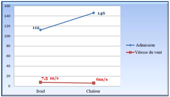
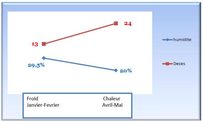
  • Climatic parameters (table 1) such as temperature, humidity, wind regime, were provided by the national meteorological service in Niamey in 2016. Temperature (in degrees Celsius, °C), humidity relative (in percentage,%) and wind speed in m/s. The season was defined from January to February for the cold and from April to May for the heat.

Table 1: Meteorological climatic parameters of the national meteorological service in Niamey in 2016

Climatic parameters

January Febuary April

May

Average temperature

26 °

29° 37°

38°

Average maximal temperature

32°

36° 43°

43°

Minimal temperature

20°

22° 31°

32°

Highest recorded temperature

39°

45° 47°

47°

Lowest recorded temperature

30°

37° 35°

36°

Wind Speed

29km/h

26km/h 22km/h

22km/h

Wind temperature

20°

22° 31°

32°

Average rainfall per day

0mm

0mm 1mm

1mm

One-day rainfall record

0mm

0mm 5mm

10mm

Humidity

36%

23% 22%

18%

Km/h: kilometer per hour, mm: millimeter

We proceeded by registering all of the patients hospitalized in the department as they progressed during the study period; The use of patient records as they are admitted. Data collection was manual, through an individual survey form. Data analysis and processing are carried out using the following software: Word 2010, EXCEL 2010, CSPro6.2, IBM SPSS 20. Consent of patients with participated in the study was obtained in advance as well as the approval of the ethics committee of the hospital.

Results

Epidemiological Aspects

A total of 464 patients were admitted during these periods of the study to the department, including 258 cases of cardiovascular disease, or 55.61% of all admissions. The admission rate for cardiovascular pathologies in the department was significantly higher during the hot season compared to the cold season, i.e. 146 patients (56.59%) vs. 112 patients (43.41%) (p=0.0027). Male sex was predominant at 53.10%, with a Sex ratio=1.13. The mean age of the patients was 55.17 years with extremes ranging from 10 to 99 years. The most affected age group is over 60 with 54.25%.

Clinical Aspects

The most common reasons for hospitalization were heart failure (HF) followed by stroke (32.17% and 24.03% respectively). The most common pathological antecedents were HF 37.60%; followed by high blood pressure (HBP) 34.49%; then stroke 9.30%. The most common risk factors were sedentary lifestyle in 62.79%, followed by hypertension in 37.60%. The comorbidities encountered were chronic obstructive pulmonary disease (COPD), human immunodeficiency virus (HIV) infection, tuberculosis, chronic renal failure (IRC), acute renal failure (ARI), hepatitis and cancer with respectively rates of 5.03; 4.26%; 3.12%; 2.71%; 2.32%; 1.94%; 1.16%. The most common functional signs were dyspnea and edema of the lower limbs, with 43.80% and 37.20% respectively. The most common physical signs were hypertension, 40.31% followed by tachycardia 33.72%, then fever 30.23%.

Paraclinical Aspects

Anemia was present in 34.11% of cases; inflammatory syndrome in 17.83% of cases; hyperlipidemia in 16.28% of cases; 15.11% fasting hyperglycemia and finally 8.91% cases of hyper creatinine. Chest x-ray revealed cardiomegaly and signs of acute pulmonary edema (APE) in 23.64% and 19.77%, respectively. ECG revealed 13.17% cases of atrial fibrillation (AF); 5.03% cases of atrioventricular block (AVB); 4.26% cases of myocardial infarction (MI); and 3.49% cases for the other signs. Cardiac ultrasound was performed in 95 patients (36.82%) including 52 cases (54.73%) normal, 14 cases (14.74%) of dilation of the cavities; 9 cases (9.49%) of pericardial effusion; 7 cases (7.36%) of valve disease, 13 cases (13.68%) for other signs. Brain CT was performed in 62 patients (24.03%) and revealed 46 cases (74.20%) ischemic stroke (DALY) and 16 cases (25.80%) hemorrhagic stroke (AVCH). We see that there are about 3 times more DALYs than AVCH. P=0.0012.

Strokes in general are much more frequent during the hot season with 38 cases against 24 cases during the cold season.

Diagnosis Aspect

The most frequent pathologies were HF, stroke, and hypertension, with a frequency of 47.28%, 24.03%, and 8.91%, respectively. However, 53 cases of HTA were associated with hypertension in 43.44% of cases and 28 cases of stroke had hypertension in 45.16% of cases. Of the 258 diagnoses relating to cardiovascular pathologies, 56.59% occur during the hot season vs. 43.41% during the cold season (p=). There is a predominance of cardiovascular pathologies during the hot season (Figure 1).

fig 1

Figure 1: Cardiovascular pathologies according to the period. Km/h: kilometer per hour, mm: millimeter

(Thus, out of the 122 cases of HF, 69 cases were admitted during the hot season vs. 53 cases in the cold season (p=0.04), 23 cases of hypertension, including 14 cases during the hot season vs. 9 cases during the cold season (p=0.14), of the 62 cases of stroke, 38 cases during the hot season against 24 cases in the cold season (p=0.012), of the 14 cases of dilated cardiomyopathy (DCM), 6 were admitted during the heat season against 8 cases in the cold season (p=0.11), 12 cases of endocarditis, of which 7 were admitted during the hot season against 5 cases in the cold season (p=0.41), 11 cases of myocardial infarction including 4 cases during the hot season against 7 cases in the cold season (p=0.20), 9 cases of pericardial effusion including 6 cases during the hot season against 3 cases in the cold season (p=0, 15), 5 cases of pulmonary embolism, including 2 cases during the hot season against 3 cases in the cold season (p=0.52).)

Therapeutical Aspects

Diuretics were administered in 70.93% of patients, antiplatelet agents in 69.37; CE inhibitors in 61.24%, beta blockers in 20.93%; calcium channel blockers in 20.15%; Anticoagulant in 8.60%; central antihypertensive drugs, in 6.58% of patients.

Evolutionary Aspects

An improvement was noted in 211 patients (81.79%) including 96 cases (45.50%) during the cold season vs. 115 cases (54.50%) in the heat season (0.064); 10 patients (3.87%) are transferred to other departments. 83 cases of death overall including 37 cases due to cardiovascular pathologies (44.58%) compared to 46 (55.42%) cases related to other pathologies (p=0.16). Thus among the 37 patients (14.34%) who died from cardiovascular causes, 64.87% had occurred in the heat season vs. 35.13% in the cold season (0.010). Regarding cardiovascular pathologies, a higher admission rate was recorded during the hot season with 146 patients or 56.59% of the sample against 112 patients (43.41%) during the cold season. Likewise, a higher mortality rate was recorded during this period with 24 deaths, i.e. 16.43% against 11.60% during the cold period (p=0.010).

Cardiovascular Pathologies and Climatic Variations

To better analyze the correlation between cardiovascular pathologies and seasonal climatic variations, we crossed the admission and death rate of patients with variation curves of climatic parameters (temperature, humidity, wind speed). Thus, Table 2 and Figures 2-7 summarize the variation in the number of admissions according to meteorological parameters.

Table 2: The number of admissions depending on the season

Clinical Parameters

Cold season

Number of deaths / admitted =13/112 patients (11,60%)

Hot season

Number of deaths / admitted =24/146 patients (16,43%)

Average Temperature

27,5° vs 33,8°

37,5° vs 33,8°

P=0,010

Highest average temperature

34° vs 38.6°

43.5° vs 38.6°

P=0.0027

Lowest average temperature

21.4° vs 27.3°

30.8°vs27.3°

Wind speed

7,5m/s vs 6.38m/s

6m/s vs 6.38m/s

Humidity

29.5 % vs 31.8%

20% vs 31.8%

fig 2

Figure 2: Average maximum temperature and number of inlets

fig 3

Figure 3: Average minimum temperature and number of inlets

fig 4

Figure 4: Average humidity and intake number

fig 5

Figure 5: Wind speed and intake number

fig 6

Figure 6: Evolution of the number of deaths and variation of the average temperature

fig 7

Figure 7: Evolution of the number of deaths and variation in average humidity

The peak intake was recorded during the hot season when the average maximum temperature is 43.5°C. The admission rate during the hot season was significantly higher than that in the cold season (146 vs. 112 cases, p=0.0027) for temperatures:

– respective maximum average of 43,5°C vs. 38,6°C vs. 34°C .

respective minimum average 30,8°C vs. 27,3°C vs. 21,4°C

A respective average humidity de 20% vs. 31,8% vs. 29,5%

-average wind speed of 6m/s vs. 6,38 m/s vs. 7,5 m/s

The number of deaths was significantly higher in the hot season than in the cold season (16,43% vs. 11,6% cases p=0,010 ) pour des

– respective maximum average temperature of 33,8°C vs. 37,5°C vs. 27,5°C.

-respective minimum average of 30,8°C vs. 27,3°C vs. 21,4°C

– average humidity of 20% vs. 31,8% vs. 29,5%,

– average wind speed of 6 m/s vs. 6,3 m/s vs. 7,5m/s

Comments and Discussions

We registered a total of 464 patients in the department, including 258 patients with cardiovascular disease. The application of chronobiology to the occurrence of cardiovascular pathologies allowed us to observe a fluctuation in the admission rates of these pathologies which were more predominant in the hot season than in the cold season (56.59% vs. 43.41%) with a peak of admission recorded during the hot season. Indeed, CVDs follow a seasonal pattern in many populations. Thus winter peaks and clusters of all broadly defined CVDs subtypes are consistently described after cold snap. Individuals living in colder climates may be more vulnerable to seasonality [4].

In our study these two periods were characterized that year, for the cold season, an average temperature (maximum and minimum), the average relative humidity lower than their annual averages, which proves the relatively cold and dry character of this period. For the hot season, the average temperature (maximum and minimum), average relative humidity were higher than their annual averages, which proves the hot and dry character of the period in Niger. The wind speed is equal to the annual average. Indeed, through the data of several studies, extreme temperatures seem to play a role on cardiovascular risk factors as well as on the risk of occurrence or decompensations of CVD.

Risk Factors for Cardiovascular Pathologies and Seasonal Variations

There are RFs that are the root cause of most CVD. In fact, we found that 85.25% of the patients in our sample had at least one FRD, the most frequent of which was sedentary lifestyle with 62.79%, followed by hypertension 37.60%. Our results are similar to those of Ben Ahmed and col, who have also found sedentary lifestyle as the most frequent RF (76.4%) [5]. However, FINDIBE and AL, found the existence of FDR in 89.3% of patients whose hypertension was the most frequent RF [6]. Just recently a study showed that there is a seasonal variation in risk factors, which found that the RFs studied tend to be higher in winter and lower in summer months. There is considerable evidence that the seasonality of variation in ambient temperature affects blood pressure (BP) levels and the incidence of cardiovascular events. The first evidence showing that ambient temperature is inversely associated with a change in arterial pressure (SBP and DBP) was published by Rose in 1961 [7]. Numerous studies have followed, showing that BP exhibits seasonal variations parallel to seasonal changes in ambient temperature, with lower BP levels at high temperatures and higher BP at lower temperatures [8]. Seasonal variation in BP appears to be a worldwide phenomenon with similar data reported for countries with varying climatic conditions, and affects both sexes, all age groups, normotensive individuals and hypertensive patients, untreated and treated [9]. In most people, the seasonality of the change in BP has no medical relevance. However, in the cases of hypertensive patients treated well controlled in winter, an excessive fall in BP could occur in summer, symptomatic requiring a down titration of drug therapy [10]. In contrast, hypertensive patients treated with controlled BP in summer may show a dramatic increase in BP above the recommended threshold in winter, requiring drug therapy upgrading. Similar fluctuations could occur in people traveling from cold to hot places, or vice versa, in such cases with severe hypotension, or with loss of BP control. In practice, the doctor should check the change in the BP level and should adjust the antihypertensive drug appropriately, aiming to achieve an optimal BP level without symptoms. A recent study showed that 13.5% of the 667 patients who visited a hypertension clinic saw their medication reduced in the summer with the highest drug reduction rate being for diuretics [11]. Due to the lower BP targets currently recommended by hypertension companies and the unusually high temperature recently observed in several studies in the summer, seasonal variation in BP is becoming a common concern in clinical practice. Exposure to cold may increase sympathetic nervous system activation and vasoconstriction, and reduce endothelial function which may contribute to increased BP [1]. Indeed, other factors have also been reported, such as increased plasma levels of fibrinogen, low density protein (LDL) cholesterol, vasoconstriction and blood viscosity, which may increase blood thrombogenicity and the risk of cardiovascular events [10]. Advanced age seems to correspond to an additional RF, although the scientific data in this area are sparse and sparse. For some authors, the impact of extreme winter temperatures appears over a longer term and seems less direct than high summer temperatures [11].

Cardiovascular Pathologies and Seasonal Variations

Extreme weather events can influence cardiovascular health in a number of ways. Too much heat or cold becomes stressful on the human body, especially if it is already stressed by the disease, and can worsen a person’s condition with heart disease. In addition to being a vulnerability factor, CVD can also be exacerbated over a period as short as a heat wave or a very cold period. For example, the loss of water and salt caused by sweat in a context of high heat increases the concentration of other components of the blood (globules, cholesterol, etc.) and thus increases its viscosity, which places l individual at risk of coronary or cerebral thrombosis. It is the same in a context of intense cold, which causes the shutdown of a large part of the blood supply to the skin, which overloads the central organs and increases the viscosity of the blood in the order of 20% [1]. In our study, we found a higher admission rate for cardiovascular pathologies during the hot season (56.59%), however our results are contrary to the literature which reports a higher admission rate in the cold season.

Heart Failure

In our series, HF is the most frequent cardiovascular disease with a frequency of 47.28% (122 cases) and this predominates in the hot season (56.55% vs. 43.45%). Our result is contrary to that of Gallerani et al. in Italia which found that hospitalization for HF is more frequent in winter (28.4%) and lower in summer (20.4%) and that there is a significant peak in January for all the groups [12] but the authors did not find any difference according to sex, age, severity, presence of hypertension, diabetes. In addition, the authors explain that the low admission may be related to the closure of beds in summer and the reduction in the population going on vacation. For hospitalization, there are similar variations with a difference of 30% (+10% in January and -20% in August).

In our study we found a high number of HF associated with hypertension (43.44%). Hirai in a recent work has also made this observation [13] and reports in its multivariate analysis, it is the absence of diuretics in such patients which is correlated with the increase in hospitalization in winter, explain the authors. Kaneko et al. by studying the characteristics of patients with heart failure hospitalized in winter, found that they are older and have a greater prevalence of hypertension and diabetes than patients hospitalized during these other seasons. Preserved ejection fraction (PEF) HFs are more common among patients hospitalized in winter [14].

Temperature variations throughout the day also seem to play a role as reported by Qiu et al. by studying daily weather results and hospitalizations for HF from 2000 to 2007 in Hong Kong. The authors find a peak in hospitalization for HF in winter, but above all they find that a large change in temperature during the day is associated with an increase in hospitalizations. They found that any temperature variation of 1°C increases the risk of hospitalization by 0.86%, especially during the cold season. The phenomenon is more marked among women and the elderly. Thus the others conclude that the large temperature changes in winter during the day are associated with an increase in hospitalizations for HF [15]. In Hong Kong, Winter is mild with average temperatures of 19.5°C. Residents may be more sensitive to temperature changes during the day. There is no heating in most homes. In contrast, during the hot season, people live with air conditioning and do less activity outdoors. They thus reduce the risk of significant temperature variation. This could explain the lack of impact of the temperature change in summer on the other hand in our countries the air conditioning is not accessible to all and that these periods are contemporaneous with power cuts, which means that patients have a longer exposure to heat. In addition, many of these patients continue to take diuretics at the same dose and rarely do blood tests. Exposure to heat and sweating can worsen the side effects of diuretics with ionic imbalances.

However recent studies show that the reality is more complex. Thus Zaoq et al. published in 2013 a study made in China. These authors find two peaks of hospitalization for HF: December (+40%) and August (+23%). In the multivariate study, the blood serum rate (95% CI: 2.132-2.144; p <0.036) is an independent risk factor for hospitalizations in August [16]. Recent publications show a seasonal variation with a peak also in summer Gostman et al. Yamamuto in Japan. Patients hospitalized in summer have a lower ejection fraction (EF), a greater need for dobutamine and die more [17,18].

MI

We recorded 11 cases of MI whose difference was not statistically significant between the two seasons, 4 cases during the hot season versus 7 cases in the cold (p=0.20). In fact, from 1985, Muller et al. showed a circadian variation in the frequency of MI with a peak at 6 a.m. until noon [19]. Twenty years later, Morabito et al. showed a relationship between weather and heart attack [20]. In fact, these authors show that the frequency of MI increases with the drop in temperature. A drop of 10°C during the day is associated with a 19% increase in heart attacks in patients over 65 years of age. Conversely, a high temperature for more than 9 hours also significantly increases the admission for infarction. The authors focus mainly on the notion of dyscomfort or severe discomfort caused by hot or cold climatic conditions rather than temperature. Recent studies find an increase in heart attacks in winter. Finally, in February 2015, Caussin et al. analyzed the association between a brief exposure (between 1 and 7 days) to environmental parameters and the appearance of a heart attack [21]. These authors found a 5% increase in risk of having a heart attack by 10°C drop in maximum temperature and 8.9% during a period of influenza epidemic after adjustment with weekends and days off. Thus the association between low temperatures and myocardial infarction (MI) is stronger during an influenza epidemic. Only the temperature drop is associated with the MI.

On the other hand, the authors do not find any effect of heat despite the fact that the period studied includes the years of heat wave (2003 and 2006). In the United States, an analysis of 259,891 cases of MI from the Second National Myocardial Infarction Registry demonstrated that there were 53% more cases of myocardial infarction (MI) in winter compared to the summer [22]. Udell, in a meta-analysis, shows that influenza vaccination is associated with a reduced risk of coronary heart disease, particularly for patients at risk [23]. The explanation put forward is the severe acute inflammation during influenza, responsible for plaque rupture and hypercoagulability. For the drop in temperature, it is evoked the sympathetic stimulation and the coagulation system. In fact, the cutaneous receptors of the skin stimulate the sympathetic system. Low temperature increases BP due to vasoconstriction. An increase in the sympathetic system will cause tachycardia, an increase in cardiac work, oxygen consumption and reduced coronary flow as well as a prothrombotic effect related to an increase in hematocrit, blood viscosity, blood pressure, fibrinogen, CRP (C-reactive protein) [23].

Stroke

In our series, 62 stroke cases were recorded including 38 cases during the hot season against 24 cases in the cold (p=0.012). Over the past decades, several studies from different countries have examined the seasonal variation of cerebrovascular disease and have led to results [24]. While some authors strongly doubt the existence of a true seasonal relationship, a series of studies suggest fluctuation with a peak during the cold season [24-26]. Recently published data also indicate a possible relationship with a typical winter peak for several factors of etiological relevance for the occurrence of stroke [27]. However, other studies report a peak summer stroke incidence, while others even suggest an inverse seasonal relationship between different types of stroke [28]. Indeed, a seasonal variation of stroke now seems to be widely accepted according to a study carried out in Athens, which included 1299 patients having suffered a stroke for the first time. The monthly distribution of all 1,299 stroke cases showed a decline in stroke admissions, starting in May and reaching its nadir in August, while an increase is seen in November. The stroke in this case remains at almost stable high levels during the cold season of the year (November to April). The authors would expect stroke cases to be evenly distributed over all 12 months of the year. However, the observed number of cases differs considerably from the expected number, indicating the existence of an annual variation in hospital admissions. August and September were the months with the least entries, while January and March were the most affected months. Dividing the year into 4 seasons as described above, we observed a significant drop in stroke incidence during the summer when most stroke cases were recorded, as expected during the cold season. They also examined the distribution of the different stroke subtypes over the 4 seasons of the year. The same seasonal pattern with the peak of incidence in the cold season and its nadir in summer has been identified for both CE and ICH [29].

Therapeutic and Evolving Aspects

Out of a total of 55.60% of patients with cardiovascular pathology, 70.93% had benefited from a diuretic, 69.37% antiplatelet agent, 61.24% CEI, 20.93% beta-blocker, 20.15% calcium channel blocker, 18.60% anticoagulant, and 6.58% central antihypertensive agent.

Evolutionarily, we saw 81.79% improvement over the study period. Thus, 63.56% of patients had a hospital stay of less than 10 days. The number of patients who died in the ward during the study was 83 cases, or 17.88% of all 464 patients hospitalized in the ward. Indeed, the mortality rate for cardiovascular pathologies is 14.34% (37 cases out of 258) and 44.58% of the total deaths.

The death rate from cardiovascular pathologies was higher in the hot season than in the cold season. It was 15.38% of total deaths and 64.86% of deaths due to cardiovascular pathologies.

Our results differ from data in the literature where we see a peak in death during the cold and a peak during the heat. The lack of mortality peak during the cold in Niger can be explained by the rarity of extreme lower temperatures.

Epidemiological studies have consistently shown an increased risk of cardiovascular disease in cold weather. For example, in England and Wales, the peak of winter and summer had 20,000 additional deaths per year [2].

In a time series analysis of 1,826,186 non-accidental deaths in 272 major cities in China, relative to temperature with the minimum mortality (22.8°C), 14.33% of non-accidental mortality was attributed to high temperatures. suboptimal, with moderate cold temperatures (−1.4°C to 22.8°C) for an attributable fraction of 10.49%, while moderate heat temperatures (22.8 to 29.0°C) accounted for an attributable fraction of only 2.08% [2]. In an analysis of 74,225,200 deaths at 384 locations in Australia, Brazil, Canada, China, Italy, Japan, South Korea, Spain, Sweden, Taiwan, Thailand, United Kingdom and United States, deaths attributable to non-hot temperatures. Optimal temperatures, defined as temperatures above or below the minimum mortality point, and extreme temperatures, defined using cutoffs at the 2.5th and 97.5th percentiles, were calculated. The results showed that the risk of death from cold temperatures (7.29%, 7.02-7.49) was higher than those from warm temperatures (0.42%, 0.39-0.44). Interestingly, extreme cold and high temperatures accounted for only 0.86% (0.84-0.87) of the total mortality [30]. Hemodynamic changes associated with cold temperature and increased thrombogenicity may explain both increased cardiovascular risk and seasonal mortality [31]. Exposure to cold induces endothelial dysfunction and increased BP, which may be the main contributors to the increased risk of mortality [6].

Recently, Marti-Soler et al. studied the monthly mortality of 19 countries out of approximately 54 million deaths [32]. The authors calculated the number of expected deaths without seasonal variation. All-cause mortality (cardiovascular and non-cardiovascular/non-cancer) shows a seasonal variation. In both hemispheres, the number of deaths is higher than expected in winter. In countries close to the equator, seasonal variations in all-cause mortality are smaller. For CV mortality, the difference between peak and nadir ranges from 0.185 to 0.466 in the northern hemisphere, from 0.087 to 0.108 near the equator, and from 0.219 to 0.409 in the southern hemisphere. Seasonal variation was not found for cancer mortality in most countries. Indeed, exposure to cold is recognized as one of the factors controlling the incidence and lethality of ischemic heart disease, sudden non-traumatic death. The highest rates of cardiovascular disease are found in the colder winter months as a Dutch study pointed out that mortality increases almost linearly as temperature decreases and is higher with strong winds (Kunst 2001) [33]. Cardiovascular and respiratory pathologies were the main causes of mortality identified in this study. Another study was conducted in the Netherlands between 1979 and 1997 by differentiating the causes of death (neoplasms, diseases and two age groups (0-64 years and over 65 years). During cold spells, excess mortality varies from 10,1 to 26.8%. It is defined as a period of at least 9 consecutive days during which the minimum temperature is below -5°C, or at least 6 consecutive days with a minimum temperature below -10°C. The effects can be more harmful the longer the period is (Huynen et al. 2001) [34]. A French study (Dijon) on daily mortality from 1968 to 1997 compared with the perceived temperature shows that cold spells are indeed associated with excess mortality over a period of about two weeks after the coldest day, with a delay of one to two days. However, the authors point out that because people are more exposed to indoor than outdoor temperatures, the excess mortality may be linked to infectious diseases rather than exposure to cold [35]. According to a Parisian study, scorching temperatures directly contribute to mortality from cardiovascular or respiratory diseases, in particular among the elderly. During the heatwave of summer 2003 in Europe, more than 70,000 additional deaths were recorded [36]. Very low winter temperatures and heat waves are associated with increased mortality, especially in the elderly population. In the elderly, the perception of cold and the performance of the vascular response are different compared to adults. The decompensation of chronic pathologies, more common in the elderly, makes them even more vulnerable to seasonal changes and extreme temperatures. A French study shows that rising temperatures are associated with a greater frequency of cardiovascular decompensations in people over 70 years old [37]. Also in the register of large studies, we must cite the study of Xu carried out in China on 626,950 patients using data from 32 hospitals in Beijing [38]. This study shows that hospitalized heart patients are older during the winter months, with a risk of mortality increasing by 30 to 50% (p <0.01) compared to those hospitalized in other months. This seasonal variation is not found in younger patients. The increase in winter deaths in elderly patients is associated with ischemic disease (RR: 1.22), pulmonary heart (RR: 1.42), arrhythmias (RR: 1.67), heart failure (RR: 1.30), stroke (RR: 1.3) and other brain diseases. Seasonal variability is found, whether the patient has lung disease or not.

In May 2015 in the EHJ, Yang studied seasonal variations in blood pressure and cardiovascular mortality in patients with a history of CV disease. They studied 23,000 people with CV backgrounds and recruited from around ten regions in China from 2004 to 2008. After 7 years of follow-up, 1,484 CV deaths occurred [38]. SBP is significantly higher in winter than in summer (145 vs. 136 mmHg; p <0.001). Below 5°C, each 10°C drop in outdoor temperature is associated with a rise of 6.2 mmHg. Furthermore, SBP predicts CV mortality: every 10 mmHg increase in SBP is associated with a 21% increased risk of CV mortality. The authors find an increase in mortality in winter (+41%) in these patients.

According to a study by SEDJAL [39] heart disease and stroke are two of the three main causes of death in Algeria. According to WHO statistics for 2008, cardiovascular disease was responsible for 29% of all deaths, or 69,648 deaths. In Algeria, cardiovascular disease is the leading cause of death, and is responsible for one in four deaths, according to WHO.

In industrialized countries, CVDs are responsible for 44% of deaths each year and 33% in France [40]. Higher rates are recorded during winter and this explains the increased mortality observed during this season. Approximately half of excess winter mortality is attributable to coronary thrombosis. The interval between a cold snap and the impact on cardiovascular mortality is 7 to 14 days. The heatwave of the summer of 2003 which affected a large part of Europe and the Maghreb countries is considered among the hottest of the last fifty years in France, while a 15-day heat wave killed 15,000 people, mostly elderly people with cardiorespiratory diseases. The analysis of the curves relating to the evolution of cardiac emergencies recorded and studied according to the meteorological parameters in the Wilaya of Oran during the year 2010, shows the existence of a relationship between the temperature drops and the significant peaks. heart problems. This analysis shows that cardiovascular disease is distinctly linked to temperature variations. The same observations have been observed in other studies carried out in Europe showing a correlation between CVD and the influence of temperature and more specifically during falls of the latter [39].

Conclusion

This prospective and comparative study on cardiovascular pathologies and seasonal climatic variations at the Amirou Boubacar Diallo National Hospital shows through the various results collected several observations on the subject and to draw conclusions such as the decompensation of cardiovascular pathologies in general is much more common in the hot season than in the cold season. That the mortality rate of these cardiovascular pathologies is higher during the hot season than during the cold season. Indeed, we see that the climate could play an important role in the morbidity and mortality of cardiovascular pathologies with seasonal variations.

Several studies in Africa and Europe have found the same findings. Likewise, within the service, other retrospective studies have found these findings. Further, more in-depth studies are needed on a larger scale to further confirm these findings.

References

  1. Sungha P, Kazuomi K, Yook-CC, Yuda T, Chen-H C, et al. (2019) The influence of the ambient temperature on blood pressure and how it will affect the epidemiology of hypertension in Asia. J Clin Hypertens 22: 438-448. [crossref]
  2. Chen R, Yin P, Wang L, et al. (2018) Association between ambient temperature and mortality risk and burden: time series study in 272 main Chinese cities. BMJ 363: 4306. [crossref]
  3. Gasparrini A, Guo Y, Hashizume M, et al. (2015) Mortality risk attributable to high and low ambient temperature: a multicountry observational study. Lancet 386: 369-375. [crossref]
  4. Discussions commentaires
  5. Simon S, Ashley KK, Adele R and John J. V. McMurray (2017) Seasonal variations in cardiovascular disease, CARDIOLOGY 658: 14. [crossref]
  6. H Ben Ahmed, M Allouche, B Zoghlami, M Shimi, R Razghallah, F Gloulou et al. (2014) Mort subite d’origine cardiaque au nord de la Tunisie: variation circadienne, hebdomadaire et saisonnière, Presse Med.
  7. FINDIBE D. et al. (2014) Morbidité et mortalité hospitalière des maladies cardiovasculaires en milieu tropicale: exemple du CHU de Lomé (Togo) The Pan African Medical Journal.
  8. Kuleshova VP, Pulinets SA, Sazanova EA, et al. (2001) Biotropic effects of geomagnetic storms and their seasonal variations. Biofizika 46: 930-934. [crossref]
  9. Gifford DK (1996) Monthly incidence of stroke in rural Kansas. Kans Nurse 71: 3-4.
  10. Biller J, Jones MP, Bruno A, et al. (1988) Seasonal variation of stroke—does it exist? Neuroepidemiology 7: 89-98. [crossref]
  11. Rosenthal T (2004) Seasonal variations in blood pressure. Am J Geriatr Cardiol 13: 267-272.
  12. Arakawa K, Ibaraki A, Kawamoto Y, Tominaga M, Tsuchihashi T (2019) Antihypertensive drug reduction for treated hypertensive patients during the summer. Clin Exp Hypertens 41:389-393. [crossref]
  13. Massimo Gallerani; Benedetta Boari; Fabio Manfredini; Roberto Manfredini (2011) Seasonal Variation in Heart Failure Hospitalization. Clin Cardiol 34: 389-394. [crossref]
  14. Hirai M, Kato M, Kinugasa Y, Sugihara S, Yanagihara Kyamada K, et al. (2015) Clinical scenario 1 is associated with winter onset of acute heart failure. Circ J 79: 129-135. [crossref]
  15. Qui H, Tak-Sun I, Ah Tse L, Tian L, Wang X, Wai Wong T (2013) Is greater temperature change within a day associated with increased emer- gency hospital admissions for heart failure. Circ Heart Failure 6:930-935. [crossref]
  16. Zhao Q, Yu S, Huang H, Cui H, Qin M, Kong B, et al. (2013) The seasonal variation in hospita- lizations due to chronic systolic heart failure correlates with blood sodium levels and cardiac function. Exp Clin Cardiol 18: 77-80. [crossref]
  17. Gostman I, Zwas D, Admon D, Lotan C, Keren A (2010) Seasonal variation in hospital admission in patients with failure and its effect on prog-nosis. Cardiology 117: 268-274. [crossref]
  18. Yamamoto Y, Shirakabe A, Hata N, Kobayashi N, Shinada T, Tomita K (2014) Seasonal variation in patients with acute heart failure: prognostic impact of admission in the summer. Heart Vessels 78: 911-921. [crossref]
  19. Muller JE, Stone PH, Turi ZG, Rutherford JD, Czeisler CA, et al. (1985) Circadian variation in the frequency of onset of acute myocardial infarction. N Engl J Med 313: 1315-1322. [crossref]
  20. Morabito M, Modesti PA, Cecchi L, Crisci A, Orlandini S, Maracchi G, et al. (2005) Relationships between weather and myocardial infarction: a biometeorological approach. Int J Cardiol 105:288-293. [crossref]
  21. Caussin C, Escolano S, Mustafic H, Bataille S, Tafflet M, et al. (2015) Short-term exposure to environmental parameters and onset of ST elevation myocardial infarction. The CARDIOARSIF registry. Int J Cardiol 183: 17-23. [crossref]
  22. Udell JA, Zawi R, Bhatt DL, Keshtkar6jah- romi M, Phrommintikul A, et al. (2013) Association between influenza vaccination and cardio- vascular outcomes in high-risk patients: a meta-analysis. JAMA 310: 1711-20. [crossref]
  23. Konstantinos S, Kostas NV, Georgios T, Andreas S, Nikolaos Z, et al. (2003) Journal of Stroke and Cerebrovascular Diseases 12: 93-96.
  24. Oberg AL, Ferguson JA, McIntyre LM, Horner RD (2000) Incidence of stroke and season of the year: evidence of an association. Am J Epidemiol 152: 558-564. [crossref]
  25. Kochanowicz J, Kulakowska A, Drozdowski W (1999) Seasonal variations in stroke incidence in North-Eastern Poland. Neurol Neurochir Pol 33: 1005-1013.
  26. Luong TH, Rand JH, Wu XX, Godbold JH, Gascon-Lema M, et al. (2002) Seasonal distribution of antiphospholipid antibodies. Stroke 32: 1707-1711. [crossref]
  27. McLaren M, Kirk G, Bolton-Smith C, Belch JJF (2000) Seasonal variation in plasma levels of endothelin-1 and nitric oxide. Int Angiol 19: 351-353.
  28. Woodhouse PR, Khaw KT, Plummer M, Foley A, Meade TW (1994) Seasonal variations of plasma fibrinogen and factor VII activity in the elderly: winter infections and death from cardiovascular disease. Lancet 343: 435-439. [crossref]
  29. Wang Q, Li C, Guo Y, Barnett AG, Tong S, et al. (2017) Environmental ambient temperature and blood pressure in adults: a systematic review and meta-analysis. Sci Total Environ 575: 276-286. [crossref]
  30. Gasparrini A, Guo Y, Hashizume M, Lavigne E, Zanobetti A, et al. (2015) Mortality risk attributable to high and low ambient temperature: a multicountry observational study. Lancet 386: 369-375. [crossref]
  31. Bhatnagar A (2017) Environmental Determinants of Cardiovascular Disease. Circ Res 121: 162-180. [crossref]
  32. Stergiou GS, Myrsilidi A, Kollias A, Destounis A, Roussias L, et al. (2015) Seasonal variation in meteorological parameters and office, ambulatory and home blood pressure: predicting factors and clinical implications. Hypertens Res 38: 869-875. [crossref]
  33. Kunst AE, Looman CW, Mackenbach JP (1993) Outdoor air temperature and mortality in The Netherlands: a time-series analysis. J. Epidemiol 137: 331-341. [crossref]
  34. Huynen M, Martens P, Schram D, Weijenberg MP, Kunst AE (2001) The Impact of Heat Waves ans Cold Spells on Mortality Rates in the Dutch Population. Environmental Health Perspectives 109: 463-470. [crossref]
  35. Groupe de travail météo France –laboratoire climat et santé ; faculté de médecine de Dijon,département santé environnement (DSE) de l’institut de veille sanitaire – cellules interrégionales d’épidémiologie (Cire).
  36. OMS, Deuxième conférence mondiale, Chaleur extrême ;Climat et santé, étude de cas, Paris, 7-8 juillet 2016 .
  37. NOURHASHEMI F (2008) Influence du climat sur les décompensations des personnes âgées. Service de Médecine Interne et de Gérontologie Clinique, CHU Toulouse.
  38. SEDJAL W, Paramètres météorologiques et les urgences cardiaques: Etude de cas à Oran 2010. Mémoire en science de l’environnement et climatologie.
  39. Bouhouita (2012) Mortalité cardiovasculaire. Journal El Watan 7.
  40. Mercer JB (2003) Cold-an underrated risk factor health. Environ Res.

Overview SARS-CoV-2 Pandemic as January-February 2022: Likely Cometary Origin, Global Spread, Prospects for Future Vaccine Efficacy

DOI: 10.31038/IDT.2022311

Abstract

As the SARS-CoV-2 pandemic is nearing its eventual end we focus on what we believe are two key omissions from the mainstream scientific literature and which have significant implications for how mankind manages the next global pandemic. We therefore review data, observations, analyses and conclusions from our series of papers published through 2020 and 2021 on its likely cometary origin and global spread. We also revisit our long held understanding of the superior effectiveness of intra-nasal vaccines against respiratory tract pathogens that involve induction of dimeric secretory IgA antibodies. While these two oversights seem disparate, together they provide us with new insights into our collective awareness of how we might view and address the next global pandemic. We begin with our hypothesis of the likely cometary origin of the SARS-CoV-2 virus via a bolide strike in the stratosphere on the night of October 11 2019 on the 40o N line over Jilin in NE China. Further global spread most likely occurred via prevailing wind systems transporting both the pristine cometary virus followed by continuing strikes from the same primary source as well as prior human-passaged virus transmitted by person to person spread and through contaminated dust in global wind systems. We also include a discussion of our prior work on data relating to vaccine protective efficacy. Finally we review the totality of evidence concerning the likely origin and global spread of the predominant variants of the virus ‘Omicron’ (+Delta mix?) from early to mid-December 2021 and extending into the first week January 2022. We describe the striking data showing the large numbers of infectious cases per day and outline the scale of what appears to be a global pandemic phenomenon, the causes of which are unclear and not completely understood. Firstly, these essentially simultaneous and sudden global-wide epidemic COVID-19 out breaks, appear to be largely correlated with events external to the Earth, probably causing globally correlated precipitation events. They appear related broadly to “Space Weather” events that render the Earth vulnerable to cosmic pandemic pathogen attack particularly during times of the minima of the Sunspot Solar Cycle which we are now currently passing through. Secondly, we argue that these sudden global-wide epidemic outbreaks of COVID-19 are specifically largely influenced by global wind transport and deposition mechanisms, the physics of which we need to further explore and comprehend. We conclude on an optimistic note for mankind. Given our prior knowledge of the effectiveness against respiratory tract pathogens of mucosal immunity involving induction of dimeric secretory IgA antibodies, we consider that the recently published intra-nasal vaccine data from laboratories based at the University of California, San Francisco and, independently at Yale University. These latter studies hold out great promise for the future development of both pan-specific and specific immunity against future pandemics caused by suddenly emergent respiratory pathogens, whether viral, bacterial or fungal.

Introduction

The authors encompass a multi-disciplinary team across the scientific disciplines of Biology, Medicine and Physics in the broadest meaning of those categories of scientific understanding. We follow in the footsteps of the prior foundation studies published in many key historical works on Astronomy, Astrophysics and Astrobiology incorporating references to many peer reviewed papers (many in the journal Nature) by Fred Hoyle and N. Chandra Wickramasinghe [1-8]. Many authors on the current list of co-authors have made significant contributions to recent publications on diverse related matters, with some of these presciently dating just prior to the emergence of the COVID-19 pandemic [9-13]. This previous experience has heightened our analytical ability to scientifically track and plausibly explain the cometary origin and global spread of COVID-19. A number of reviews of the relevant datasets and conclusions therefore have already been published through 2020 and 2021 [14-16], including a compendium of chapters on ‘Cosmic Genetic Evolution’ all of which places the COVID-19 pandemic in its appropriate cosmic perspective [17]. Thus, a number of papers published by us since February 14 2020 review the data supporting our first claims of COVID-19’s putative meteorite origins over China, following a cometary bolide strike on the 40o N Latitude line over Jilin, NE China on the night of October 11, 2019 [18]. We note here that the causative virus-carrying bolide may not have arrived at the top of the Earth’s atmosphere as a cohesive body, but as an aggregation of dust particles, with individual radii of the order of micrometres. It is well known that of the order of 100 tonnes of such material are incident on the upper atmosphere daily. Approximately two thirds of micron sized micrometeorites can plausibly be assumed to be of cometary origin. Modelling of their dynamics in the atmosphere shows that a significant fraction of these particles reach the surface of the Earth without experiencing destructive heating [19].

Our subsequent publications in the early weeks of the pandemic focused on the relative lack of evidence for person-to person transmission as the primary infection mechanism for COVID-19 [20]. Indeed, detailed analyses of the active region-wide epidemic episodes around the globe during 2020 and 2021 occurred initially (late 2019 to March through April 2020) mainly on the 30-50o N latitude band with limited outbreaks taking place outside this band [21]. We developed explanations of the unfolding data relating to the pandemic as it engulfed the world from the later months of 2019. In our modelling we took full account of genetic, immunologic and epidemiologic evidence, as well as the role of geophysical and atmospheric processes including a possible continuation of a space input of the virus.

In summary, our main analyses were as follows:

a. The genetic analysis of the SARS-CoV-2 viral genomes and the deaminase-mediated haplotype variation and adaptation strategy of the coronavirus as it navigated infections in different susceptible/vulnerable human hosts and genetic backgrounds first in China then Spain, France and New York with eventual infection documented in Australia from January through to September 2020 [15,18,20-23].

b. The immunologic analysis of the host-parasite relationship and vaccine efficacy of systemic versus mucosal-local antigen routes of immunization [22-24].

c. The epidemiologic analyses of both the temporal order of epidemics and their global location, including the role of prevailing winds systems, remote outpost strikes (O’Higgins Chilean Army outpost in Antarctica), sudden island strikes and strikes on ships at sea [15,16,25,26].

d. The geophysics and atmospheric physics of the major convection cells plus jet streams sweeping up and depositing virus-bearing dust, including human-passaged aerosol transferring them in the northern hemisphere with limited connection to the south [21,27-29]. Global connectivity is effective on the 10-day time-scale. The evidence of long-distance tropospheric transportation in the Northern Hemisphere is provided by the COVID-19 genomic sequence data from the Grand Princess cruise ship off San Francisco (engaged late February 2020) which displayed the exact same largely unmutated genomic sequence (Hu-1) as determined in China during December 2019 and January 2020 [16,22].

e. The role of human-passaged (and created) regional variants lofted or plumed attached to microdust particles into the troposphere and the global wind systems, in likely attenuated form [16,28,29] see also reference in these papers to the independent assessment of the role of global wind transportation systems in past influenza pandemics in [30] Hammond et al. 1989. “Thus these authors noted the large-scale eddy circulation as causing occasional lofting and patchy deposition of virus carriers. It saw survival of the influenza virus in the air and solar radiation as important, though did not know of survival against UV in clumps, or embedded in micro-dust particles.”

All of our prior analyses and conclusions and its relation to the wider scientific literature on SARS-CoV-2/COVID-19 can be found in our past publications, which can be accessed at https://www.academia.edu/50814212/ Papers and Summary Interviews on Origin and Global Spread of COVID 19 Wickramasinghe and colleagues. The URL links to all relevant video interviews involving N. Chandra Wickramasinghe and Edward J Steele can be found in this list and at The Cosmic Tusk website of George A. Howard. https://cosmictusk.com

We have also considered and refuted the main popular explanations that were spreading uncritically abroad in both the scientific and popular media, concerning the protective efficacy of all systemic-delivered vaccines and the putative origins of COVID-19, the latter as either a jump from a latent SARS-CoV-1 animal reservoir (bat, pangolin, cat) or as a human-engineered COVID-19 genome. In the latter case this infection, identical in genomic sequence to the original Hu-1 reference (isolated in China in December 2019, NC_045512.2), was postulated to have been released from a Chinese laboratory (Wuhan Institute of Virology) either accidently or deliberately. We show both these origin explanations are scientifically implausible or impossible on genetic grounds [15,29]. Indeed, the Wuhan Lab Leak and related narratives are clearly implausible and simply do not explain what was actually observed in the first month or two of the pandemic.

Against this backdrop, we have analysed a putative “Space Weather” and “solar-wind pulse” like event [10,11] which, although poorly understood at the present time, may well account for the manner in which the pandemic signature became evident globally. At the time of writing this review the pandemic appears to have waned in severity via the natural processes of natural Herd Immunity, attenuation of the human-passaged variants and viral decay in the environment [31,32]. From the Cases per Day Curves (Figures 1-8) we think these observations have been the major new phenomenon of the pandemic that has become manifest in the data from the middle of December 2021.
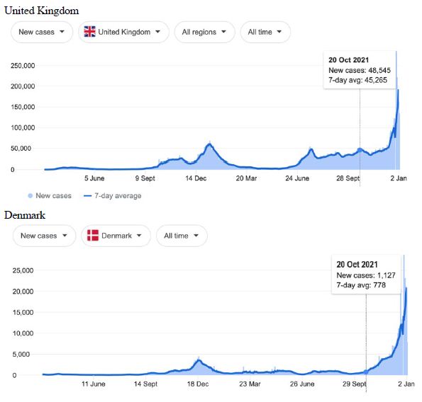
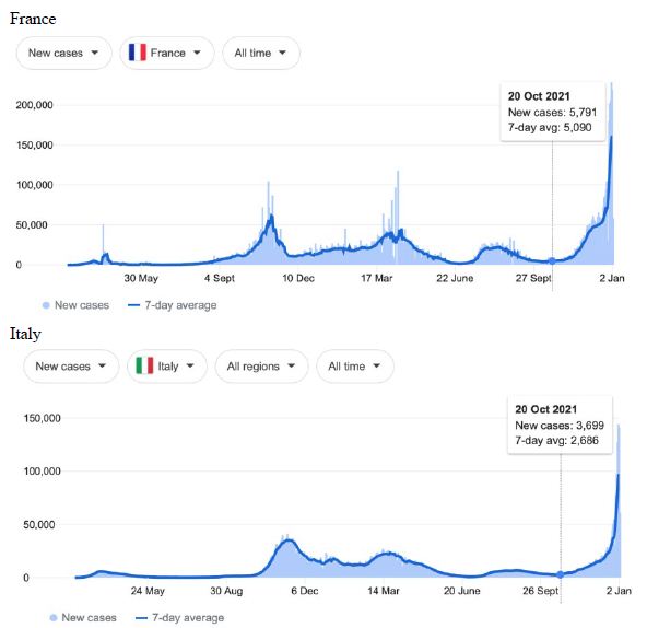
fig 1(1)

fig 1(2)

Figure 1: COVID-19 Case Rises in Selected Global Locations- Europe: United Kingdom, Denmark, France, Italy. Exponential rises in new COVID-19 cases per day as captured January 3 2022 from the Google searched site: “Coronavirus disease statistics”. The URL opens at the Australia dashboard but all countries and regions can be searched via the Cases and Deaths search Menus for that region. Click or copy and paste URL into your browser : shorturl.at/glwER
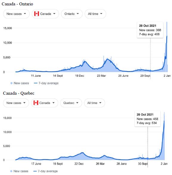
fig 2(1)

fig 2(2)

Figure 2: COVID-19 Case Rises in Selected Global Locations- Canada and USA: Ontario, Quebec, New York, Florida. Exponential rises in new COVID-19 cases per day as captured January 3 2022 from the Google searched site: “Coronavirus disease statistics”. The URL opens at the Australia dashboard but all countries and regions can be searched via the Cases and Deaths search Menus for that region. Click or copy and paste URL into your browser : shorturl.at/wQX69
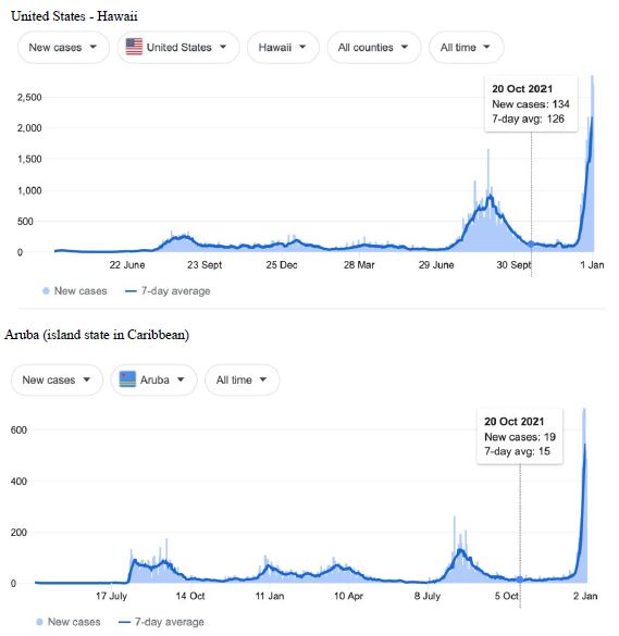
fig 3

Figure 3: COVID-19 Case Rises in Selected Global Locations- Hawaii and Aruba . Exponential rises in new COVID-19 cases per day as captured January 3 2022 from the Google searched site : “Coronavirus disease statistics”. The URL opens at the Australia dashboard but all countries and regions can be searched via the Cases and Deaths search Menus for that region. Click or copy and paste URL into your browser : shorturl.at/wINR0
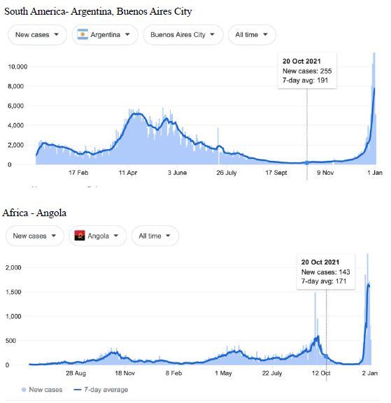
fig 4(1)

fig 4(2)

Figure 4: COVID-19 Case Rises in Selected Global Locations- South America and Africa: Buenos Aires, Angola, Kenya, Mozambique. Exponential rises in new COVID-19 cases per day as captured January 3 2022 from the Google searched site: “Coronavirus disease statistics”. The URL opens at the Australia dashboard but all countries and regions can be searched via the Cases and Deaths search Menus for that region. Click or copy and paste URL into your browser : shorturl.at/hsxGO
fig 5(1)

fig 5(2)

Figure 5: COVID-19 Case Rises in Selected Global Locations- Australia: South Australia, Victoria, New South Wales, Queensland . Exponential rises in new COVID-19 cases per day as captured January 3 2022 from the Google searched site: “Coronavirus disease statistics”. The URL opens at the Australia dashboard but all countries and regions can be searched via the Cases and Deaths search Menus for that region. Click or copy and paste URL into your browser : shorturl.at/lFIJ6
fig 6(1)

fig 6(2)

Figure 6: COVID-19 Case Rises in the whole Australia, and Western Australia, South Australia, Tasmania (similar right hand side shoulders observed for Northern Territory, Australian Capital Territory). Exponential rises in new COVID-19 cases per day as captured February 24 2022 from the Google searched site : “Coronavirus disease statistics”. The URL opens at the Australia dashboard but all countries and regions can be searched via the Cases and Deaths search Menus for that region. Click or copy and paste URL into your browser : shorturl.at/wDLTZ
fig 7(1)

fig 7(2)

Figure 7: COVID-19 Case Rises in Victoria, New South Wales, Queensland and New Zealand (similar rising ‘hockey stick’ cases per day graph seen for French Polynesia, and Chile). Exponential rises in new COVID-19 cases per day as captured February 24 2022 from the Google searched site: “Coronavirus disease statistics”. The URL opens at the Australia dashboard but all countries and regions can be searched via the Cases and Deaths search Menus for that region. Click or copy and paste URL into your browser: shorturl.at/ersIK
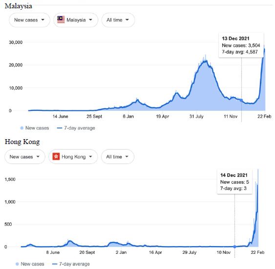
fig 8(1)

fig 8(2)

Figure 8: COVID-19 Case Rises in Indonesia, Singapore, Malaysia, Hong Kong (similar rising ‘hockey stick’ cases per day graph seen for Bhutan, Brunei, Thailand, Vietnam, Cambodia, Myanmar, South Korea, Mongolia possible shoulder in Japan). Exponential rises in new COVID-19 cases per day as captured February 24 2022 from the Google searched site: “Coronavirus disease statistics”. The URL opens at the Australia dashboard but all countries and regions can be searched via the Cases and Deaths search Menus for that region. Click or copy and paste URL into your browser : shorturl.at/lBP14

Omicron/Delta Outbreaks though December 2021 and January 2022 in Global Synchrony

Cases-per-day plots for selected locations (captured as screen shots on January 3 2022) are shown in Figures 1-5 to illustrate the extreme synchronous or simultaneous eruptions of COVID-19 epidemics (Omicron/Delta mix?) in the Northern Hemisphere regions Figures 1-3 (United Kingdom, Denmark, France, Italy, Ontario, Quebec, New York, Florida, Hawaii, Aruba), and in the Southern Hemisphere, Figures 4 and 5, embracing populated regions in South America, Africa and Australia (Buenos Aires, Angola, Kenya, Mozambique, and in Australia : South Australia, Victoria, New South Wales and Queensland). In Table 1 we list all regions of the world that display conformal exponentially rising cases per day curves over the same time interval as illustrated by the selected examples in Figures 1-5. Countries or regions with low or equivocal rises in case numbers are listed in Table 2. In some regions there was a clear peak of the presumed Omicron outbreak beginning about a week or two earlier with case numbers per day coming down in those regions (Table 3). However, many countries are ‘null zones’ with respect to this time period experiencing no rising epidemic profile (Table 4).

Table 1: Countries and Regions all showing clear Synchronous Epidemics as shown in Figures 1-5 as captured January 3 2022 (use URL Figures 1-5)

table 1


Table 2: Countries and Regions showing only a Low or Equivocal Synchronous Epidemics as shown in Figures 1-5 as captured January 3 2022 (use URL Figures 1-5)

table 2


Table 3: Countries and Regions all showing an explosive epidemic beginning a week or two earlier relative to those shown in Figures 1-5 as captured January 3 2022 (use URL Figures 1-5)

table 3


Table 4: Countries and Regions all showing no explosive epidemic or obvious begining a week or two earlier as Figures 1-5 as captured January 3 2022 (use URL Figures 1-5)

table 4


The reader can scrutinise the data at the URL site for ‘Coronavirus disease statistics’ shown in the legend to the figures. The predominant pandemic ‘strain’ evident in most regions of the world prior to these extraordinary explosive and temporally coordinated epidemic outbreaks was the ‘Delta’ strain (and related Indian-plumed strains) from the massive Indian epidemic of April-May 2021, which we hypothesized was released as a very large aerosol of many millions of trillions of virions into the troposphere for redistribution to globally distant regions via prevailing W-E, E-W and N-S wind systems [28]. The Omicron variant was found first in Botswana on November 2, 2021 and was widely assumed to have emerged first in South Africa. We discuss speculative causes of the emergence of the Omicron variant and the probable region of its origin in Section 3.

What plausible explanations can be provided for the data in Figures 1-5 and Table 1-4, and in particular the essentially simultaneous eruptions of region-specific epidemics of COVID-19 in so many different regions across the world? This is not a question that can be easily resolved. The strong indications are of a globally correlated phenomenon that we do not fully understand. One explanation could be connected to space weather events associated with the deep Sun-Spot minimum between Solar Cycles 24 and 25 [10,11]. Unseasonal weather that has been reported both in the Northern and Southern hemispheres (e.g.UK and Australia) during this time period may give a hint in this direction. The sheer numbers and global coverage of infection essentially eliminates Person-to-Person spread as the sole or main causative explanation.

A more plausible scientific explanation lies in massive region-wide in falls from the sky (the troposphere) of prior human-passaged then aerosol-plumed COVID-19 virions lofted into the troposphere and introduced into prevailing wind systems. Given current Omicron case densities, we tentatively assume a northern European origin followed by transport of viral aerosol-clouds across the Atlantic from an origin in the UK/North Europe (?), into the Pacific and Atlantic prevailing winds onto to Africa and thence to Australia.

We are still left with the conundrum of why now, and why at the same time all over the globe? The data in Figures 1-5 are but a small subset of the large number of global-wide regions in the Northern Hemisphere, Equatorial Regions, Island States, and Southern Hemisphere all struck like this at the same time (Tables 1 and 2). In addition, over this time period, many Atlantic cruise ships with double vaccinated and pre-screened passengers also became suddenly engaged with COVID-19 (assumed Omicron see [33,34]) including a fully vaccinated US Navy ship [35]. There was also the well-documented sudden outbreak from December 14 involving large numbers of fully vaccinated personnel at a remote Belgian Research Station in Antarctica thousands of miles from civilization [36]. This is indeed strikingly reminiscent of similar strikes on ships at sea and remote locations during the early phases of the pandemic in 2020 [15,16,25], including the sudden strike on the island of Sri Lanka Oct 4-5 2020 [26], and more recently on Taiwan presumed to have occurred as a result of Indian-plumed Delta virus which struck suddenly for first time from 14 May 2021 [28]. All indications are of a globally-correlated environmental trigger that we cannot fully understand at the present time.

One possible explanation is that globally dispersed viral aerosol-clouds (Omicron/Delta variant mix?) were released and lofted following human passage, and were widely distributed in the troposphere remaining viable although not immediately falling to Earth or ocean over many different regions of the world. A putative global trigger in mid-December 2021 might be postulated that brought such viral particles to earth virtually simultaneously around the world. This may have been ultimately facilitated by, but not been dependent upon, rain/precipitation [28,29]. The resulting virus-contaminated environments would then ignite outbreaks of mystery unlinked Omicron/Delta cases on a large scale giving the appearance of superfast infective spreading in a given populated contaminated region as we have previously discussed in detail for the outbreaks of mystery infections in Victoria, Australia [28,29]. This is a plausible explanation for the synchronous sudden rises of COVID-19 globally. The fact there are many “null” zones (Table 4) and ‘low’ or equivocal regions (Table 2) adds to the patchy cloud-like nature of the viral distribution in the troposphere prior to and coinciding with the solar cycle minimum. That is, it arises as deposition from the convection-driven upper troposphere which is patchy over a range of distance scales.

Another possibility, given the global nature of the present observations, and thus which cannot be ignored as a causative factor, is the known vulnerability of the Earth to pandemics during the minima of the sunspot Solar Cycle [10,11]. Thus it could be an ill-defined and poorly understood physical event broadly classed as a “Space Weather” event associated with the sunspot cycle minimum, particularly now between cycles 24 and 25, where we may be most vulnerable to “pathogen attack” from the outside the Earth: viz.

“..the Earth’s magnetosphere, and the interplanetary magnetic field in its vicinity, are modulated by the solar wind that in turn controls the flow of charged particles onto the Earth [4]. During times of sunspot minima, particularly deep sunspot minima, a general weakening of magnetic field occurs which would be accompanied by an increase in the flux of cosmic rays (GCR’s) and also of electrically charged interstellar and interplanetary dust particles”… bringing charged particles ( virus-laden dust particles) to earth. Wickramasinghe et al. 2019 [11].

Getting back to the original events in late 2019 we can advance another specific scenario on what actually happened across China which was initiated in the stratosphere over N-E China in late December 2019, and then in early January 2020 after the initial input of cometary virus-carrying dust. The virus became strongly amplified in humans across China until lock-down measures came into full force. Despite efforts to wash down the streets, the virus’s long lifetime and persistence in viable condition on dust particles enabled it to spread widely in the environment. When appropriate wind conditions arrived, the virus-carrying dust was readily swept up in tropospheric winds into the East-Asian subtropical jet stream, carrying it across the Pacific to southern USA and Western Europe. Precipitation into local wind systems thus caused infection on a state-wide and country-wide scale. In 2021 similar wind-borne viral-laden dust spread over the entire sub-continent of India causing sudden eruptions of COVID-19 infections (via PANGO variants Alpha, Kappa, and Delta at least). These country-wide sudden eruptions have been noted before although they have not been fully understood [14,16,28,29].

Finally, we should consider another putative “pulse-like” causative factor that contributed to the synchronous nature of the sudden outbreaks of Omicron/Delta infections around the world. This phenomenon was not previously explored except in the broadest of terms in our earlier publications [12,13]. It is most probably related to the fact that most viruses in their cell-to-cell infection cycle are transported as enveloped clusters of mature virions [37]. This may be important if an influence associated with “Space Weather” external to the Earth somehow triggered the liberation of smaller clusters of virions associated with tropospheric dust clouds over any given region. A dust particle of 2-3 microns could theoretically envelope 40-60 COVID-19 virions. If these were suddenly liberated to fall to ground as smaller clusters (doubletons or triplets) that would result in a ten-fold sudden increase in putative infective virion clusters floating down to contaminate a terrestrial environment. The nature of this virion liberation “trigger” is unknown (temp/pressure/radiation?) so this is still a highly speculative scenario that we present for further exploration.

However, we can now add further observations, as the manuscript was being prepared for final submission. This is again consistent with a series of “pulse-like” infection events enveloping a large fraction of the globe at the same time (prior 24-48 h). (This has been noted as January14 2022 from the “Coronavirus disease statistics” database.) The following countries appear to have been all engaged in an exponential sharp rise in COVID-19 new cases per day, a synchronous effect that was not evident in the earlier survey of January 3 2022. These countries are: Brazil, Bosnia Herzegovina, Costa Rica, Cuba, Djibouti, Egypt, French Guiana, Guatemala, Guinea-Bissau, Haiti, Hungary, Liechtenstein, Lithuania, Martinique, Maldives, Montserrat, Morocco, Monaco, North Macedonia, Norway, Pakistan, Poland, Slovenia, India, Nepal, Bhutan, Kyrgyzstan, Uzbekistan, Philippines, Japan, Romania, Sao Tome and Principe, Taiwan, Thailand, Trinidad and Tobago, Tunisia, Turks and Caicos Islands, Ukraine, Mongolia, and Venezuela. All these regions could be part of the same mid-December 2021 tropospheric in-fall process just described but show an apparent delay due to data reporting and database updating.

In addition, we surveyed plots of new cases per day from the same database as captured 24 February 2022. We detected a clear further set of global-wide synchronous eruptions of COVID-19 epidemics – presumed Omicron/Delta (mix) – in Oceania Figures 6 and 7 (all Australian states and territories, New Zealand, and French Polynesia, extending to Chile) and many countries throughout South East Asia and North East Asia (Figure 8). These synchronous eruptions we speculate have occurred by simultaneous tropospheric viral-cloud in-falls contaminating the environment of populated regions occurring most likely in early February 2022. All populated regions of Australia appear to have been struck like Western Australia (Figure 6) at the same time. WA stands out with a clear “hockey stick” infection curve as it came off a very low base. This is consistent with the evident shoulders and blips on the right hand sides of the curves for NSW, VIC, TAS, and QLD. A plausible explanation is this extended shoulder is due to this second synchronous in-fall but masked by the already high Cases per Day in these other Australian states. In a related survey of the database (captured 18-19 February 2022) we detected another set of synchronous epidemic eruptions beginning about January 10 2022 and peaking late January early February 2022, these include : Algeria, Armenia, Azerbaijan, Bangladesh, Czechia, Faroe Islands, Georgia, Iran, Iraq, Jordan, Kazakhstan, Kosovo, Latvia, Libya, Moldova, Nepal, New Caledonia, Oman, Palestine, Paraguay, Russia, Slovakia, Taiwan, Yemen.

Therefore since mid-December 2021 two further separate global-wide synchronous epidemic eruptions can be detected, from about Jan 10, then from early February 2022. We highlight in particular Western Australia in Figure 6 as that vast Australian region had never before experienced a genuine tropospheric COVID-19 epidemic strike until just recently (Figure 6) – yet that state of Australia was lock-downed repeatedly and isolated from the rest of Australia and the wider world by stringent enforced border and travel restrictions. In addition, mask mandates and social distancing regulations (crowd sizes sports events, movie theaters, churches and so on) were enforced outside homes and work places, including mandatory vaccinations for most WA workers during 2020 and 2021 despite very few if any COVID-19 cases being recorded in the state (mainly in travelers coming by road and airplane from other infected zones in Australia and from overseas who were immediately isolated and quarantined). The recent large Omicron/Delta (mix?) strike completely surprised the WA Department of Health and Medical authorities as they could not explain any of the suddenly emergent infection events recorded across the state by conventional person-to-person transmissions. The apparent ‘super spreading’ was particularly strange given the population was largely fully vaccinated.

Given these striking globally-coordinated cases per day events detected by data monitoring just COVID-19, we cannot rule out additional surprises. We speculate that other unknown dust-associated pathogens (viral, bacterial, eukaryotic spp) in the troposphere have also been brought to Earth by the same general Space Weather/Solar-pulse processes during the current Sun Spot minimum between solar cycles 24 and 25. We have laid out here a range of explanations, some over-lapping, because we are dealing with a “globally correlated phenomenon that we do not fully understand.” We have done so to ensure that as many plausible alternatives are available for further discussion and consideration in order that we may ultimately understand what happened.

Speculations How Omicron may have Arisen and Where?

All news reports in Australia, USA, South America, Africa and European countries, that are all engaged in the synchronous exponential eruptions, focus on Omicron as the main variant which is rapidly replacing Delta. From all available reports and early clinical experience, the respiratory disease severity of Omicron is less than Delta. This is consistent with death rate data (confirmed at URL links in Figures 1-5) that are consistently very low, and is approaching or remains below other estimates of death rates attributed to COVID-19 (whether Original Hu-1, Alpha, Delta and now Omicron). In approximately 0.1% of all COVID-19 exposed cases [29] death is the serious outcome mainly in the ‘Immune Defenseless Elderly Co-Morbid’ patient group. Highly vulnerable patients require administration of prompt respiratory therapies to navigate their respiratory crises that follow from the infection. Such patients often display clear deficits in innate immunity, often feeding into deficits in adaptive immunity and so are particularly at risk [38-44]. Other clinical studies [45] also show that patients in this subgroup specifically display deficits in Type I and type III interferon (IFN) inducible anti-viral immunity and thus appear ‘immune defenceless’ to coronavirus respiratory tract infections and so are at a very high risk for severe outcomes including death.

How could a human-passaged variant like Omicron arise? Omicron is clearly a derivative of “Delta” a PANGO lineage name of the L241f haplotype of the Steele-Lindley replicative-haplotype scheme (Steele and Lindley 2020) with many changes in the mRNA encoding the spike protein suggestive of mutation accrual via human passage (person to person spread, P-to-P). The analysis of how a single putative cloned variant we named “L241f.1vic” spread through aged care and nursing facilities in Melbourne, Australia beginning from about 10 May 2020 through June 2020 then erupting on scale in such facilities through July and August 2020 is very informative [23]. From the full-length genomic analysis of many thousands of publicly available SARS-Cov-2 genomes (>12,000 made available by the Victorian Dept of Health through The Peter Doherty Institute) we showed previously that there were two types of clearly identifiable patients. The first displayed unmutated versions of the virus over the entire 29903 nt genomic length. These types were particularly evident in the last two weeks of June 2020 through most of July 2020. It appeared very much like the virus was being amplified on scale in hosts that were unable to mutate the RNA virus genomes at APOBEC (cytosine to uracil) and ADAR (adenosine to inosine) deamination sites [22,23]. The second group of patients, clustering in a late August time window, displayed mutated versions of the virus, again largely at APOBEC and ADAR cytosine and adenosine deamination motifs. It was concluded thus [23] to quote conclusion directly:

The data reported herein are thus consistent with the following P-to-P infection model which is also the operational hypothesis under test: clusters of immune defenceless elderly co-morbid citizens in many aged care and nursing facilities were all systematically struck with devastating force (high infection rates and death rates), with a single unmutated (or lightly mutated) SARS-CoV-2 haplotype variant (L241f.1vic). Through late June, July, August and September in 2020, this putatively cloned variant must have been spread unimpeded by carriers who were asymptomatic or lightly symptomatic infected health- care professionals and carers working across multiple age care institutions [30-33]. The large-scale amplifications of the L241.1vic variant—instanced by the size of the multiple ‘New case’ spikes (shown in Figure 1), particularly through July 2020—could have produced many trillions of L241f.1vic virions in each location thus contaminating numerous surfaces (fomites, personal effects of all types) and could have contaminated or infected human carriers in each institution. This then fuelled the further putative quantitative dominant rapid spread of this apparently capricious L241f.1vic variant into the local community and particularly to other aged care facilities leading to further putative viral amplifications in elderly co-morbid subjects. If anything, the Victorian experience underlines why elderly co-morbid citizens require very special care, protection and therapies during cold and flu seasons [31,32].

It was then speculated that the putative highly contagious, yet clearly attenuated, “UK Mutant” (Alpha) that emerged in September in 2020 in parts of southern England was generated the same way. We also think Omicron arose by similar cycles of deaminase-mediated mutagenesis in healthy almost asymptomatic carriers, then became amplified (cloned unmutated) in Immune Defenseless Elderly Co-morbids – then after one or two more cycles via healthy intermediate ‘vectors’, infecting new cohorts of Immune Defenseless Elderly Co-Morbids where it was amplified and cloned. A plumed aerosol of literally millions on trillions of Omicron virions into the immediate troposphere and prevailing wind transportation could have easily distributed Omicron in the prevailing wind systems (e.g. from Northern Europe to South Africa where first detected). This model of alternating cycles of deaminase-mutagenesis and cloning amplification could have created a plume in a real high-density hotspot. Was it around or near UK where most Omicron have been recorded initially? At the present time we acknowledge these are speculations, but given the existence of detailed genomic records from the millions of genomes now sequenced and in computer databases, these speculations can, and will be tested in the fullness of time.

Future Vaccine Developments for Next Pandemic of Cold or Flu Respiratory Tract Pathogens?

There are many public health lessons to be learnt from the COVID-19 pandemic. Near-Earth balloon launches, stratospheric airplane and orbiting platform sampling of incoming meteorite dust have all been stressed as important early warning strategies on many previous occasions in other places (discussed recently in [9,16,29,46]. However a pandemic public health management strategy employing a more effective vaccination method needs urgent consideration. The aim should be quite different from the current very simplistic strategy of intramuscular “jab-in-the arm” vaccination (irrespective whether traditional antigens are used or the poorly safety tested mRNA expression vector vaccines). Public health vaccination which mimics natural ‘Herd’ immunity” is the desired outcome, whether to coronaviruses, influenza viruses and many other respiratory tract pathogens including bacterial ssp. that cause respiratory pneumonias and severe bronchitis.

Here we review how to optimize intranasal defective /attenuated live virus vaccination for all likely future types of pandemic respiratory viruses and finally discuss promising newly published experimental data which offers some hope for the future. We and many others have discussed the failure of the current jab in the arm intramuscular mRNA vaccines to protect against COVID-19 – yet they have been mandated by many governments and public health bureaucracies [24,29,47]. Further, the mRNA vaccines which also have high adverse effect rates are ineffective on first immunological principles because of the wrong route of delivery. The current ‘jab-in-the-arm’ route of immunization cannot possibly protect against COVID-19 infection gaining entry to and growing in mucosal cells of the respiratory tract. For that the mucosal secretory IgA antibody system needs local activation [23,24,29]. In a rush to bring COVID-19 vaccines to market, it seems that science and medicine neglected a large body of work already available on the nature of immunity and host resistance to respiratory viral infections, and how best to mimic this by vaccination, and instead became seduced by advances in 21st century molecular engineering principles into production of a vaccine whose utility and clinical efficacy even now remains unknown- more troubling is that any serious long-term sequalae are entirely unexplored. This is discussed graphically and underlined in recent interviews as well in https://youtu.be/Ijc4mjiIquk and in the Asia Pacific TV interview with Mike Ryan https://rumble.com/vmrmmq-the-origins-of-covid-19-and-why-the-vaccines-dont-work.html

Based on a wealth of scientific/immunologic data gleaned over decades, as well as experience in vaccination against respiratory viral disease, it is self-evident that protective vaccination needs to be via the oral-nasal route to activate the mucosal immune response, which is responsible for Natural Immunity and “Herd Immunity” in the population. The natural decline in the incidence of severe COVID-19 outcomes (COVID-19 associated death) was well underway before the vaccine roll out in European and USA Infection zones through 2020 and early 2021 [32]. This is brought about most effectively by effective ‘Herd Immunity’ which has been documented in a large longitudinal and population base study, conducted in Denmark through 2020 [31].

We have previously discussed the two most important forms of immunity to be activated in the mucosal cells and associated lymphoid cells of the respiratory lining. The first of these is Innate Immunity- a general elevation of these activities would strengthen the “Anti-Viral Wall” in all nasal cells and mucosal lining cells. This barrier is defective in ‘Immune Defenseless Elderly Co-Morbids’ which are the primary vulnerable group in the COVID-19 pandemic. Note that this group equates to < 1% of all infected patients see Netea et al. [41] and discussed elsewhere in detail [23] based on data from many clinical studies throughout 2020 [38-45]. In our analysis of the data >99% of the population handles COVID-19 effectively via natural immune mechanisms- to these patients it is just a “Common Cold”. Both Innate Immune Interferon Type I and III anti-viral barriers in all cells would be activated, and then adaptive acquired mucosal immunity.

Secondly, Adaptive Acquired Mucosal Immunity requires, as we discuss, the induction of dimeric secretory IgA antibodies – these antibodies are demonstrably highly avid (strong binding and thus neutralizing of toxins, viruses and adhesins preventing cell adherence and cell entry) that do not activate the Complement cascade thus do not add to “inflammatory cytokine storms.” Indeed, secretory IgA is expected to competitively block antigen binding and thus nullify the antibody-dependent enhancement (ADE) by the blood borne IgG and IgM complement fixing antibodies particularly in advanced COVID-19 infections of the elderly vulnerable group [23,24]. This sequelae of ADE pathology in vaccinated individuals who then go on to catch COVID-19 for first time is discussed more fully elsewhere [29].

To ensure that intranasal vaccination is effective it is desirable that activation of the innate immune response via the Toll receptors in addition to induction of secretory IgA against the virus. An agonist, INNA-51 of the Toll-2 receptor, was patented in 2018 (WO2018176099, Treatment of respiratory infection with a TLR2 agonist). It is currently being used in a Phase 2 trial of intranasal vaccination to prevent COVID-19 with the AstraZeneca antigen [48]. A better antigen could be an inactivated virus such as Sinovac as many more epitopes would be delivered than with AstraZeneca’s viral vector containing just the SARS-CoV-2 spike protein.

Two recent papers describing experiments in mice (a small mammal with an immune system similar to, but not identical to, humans in principle) involving intra-nasal vaccine development and assessment of efficacy in protection from disease, have now been published in December 2021. Xaio and associates [49] created a defective or harmless coronavirus that cannot replicate properly, and delivered it via the intra-nasal route so as to induce both Innate Immunity (to any other viral challenge oro-nasal) and Adaptive Immunity (that is antigen specific secretory IgA). In the other study Oh and associates [50] set up intranasal priming with influenza infection or with adjuvanted recombinant neuraminidase flu vaccine. This induced local lung-resident B cell populations that secrete protective mucosal antiviral secretory IgA. In these complimentary studies, using these different intra-nasal, mucosal lining activation strategies the workers induced both elevated pan-specific Innate Immunity as recommended by Netea and associates [41] protecting against many other unrelated respiratory track pathogens, but also the necessary dimeric secretory IgA adaptive specific immunity akin to more tradition vaccination strategies. Recent published work adds to this conclusion [51].

We would argue that studies such as these offer the hope that can now look forward to the production of easily delivered, safe and effective vaccines against many epidemic respiratory viruses, irrespective of variant or viral type, so we will be well armed in advance of the next pandemic of respiratory tract infections. This would represent a real scientific advance and a saving grace for humanity.

Acknowledgements

We thank Max Rocca, Heath Goddard, and Dayal T. Wickramasinghe for discussions and Brig Klyce also for bringing our attention to Afkhami et al 2022 [51].

Conflicts of Interest

None of the co-author team has a conflict of interest apart from understanding the scientific reasons for the origin, global spread and efficacy of human immunity to SARS-CoV-2.

Multi-author Contributions

Conceptualisation EJS, NCW, RGG, GAH: Draft writing: EJS, NCW, RMG Reading the primary clean draft: All co-authors. Active Contributions to primary draft via edits and additions: RAL, PRC, MW, SC, MKW Integration of all minor changes: EJS, NCW, RMG.

Multi-author Expertise

The areas of expertise of the multi-author team are:

Edward J. Steele: Biomedical science, Immunology, Ancestral Haplotypes, Mutagenesis, Biotechnology, Evolution, Panspermia, Cosmic Biology.

Reginald M. Gorczynski: Biomedical science, Medicine, Immunology, Evolution, Panspermia, Cosmic Biology.

Robyn A. Lindley: Biomedical science, Immunology, Biotechnology, Mutagenesis, Evolution, Panspermia, Cosmic Biology.

Patrick R. Carnegie: Biomedical science, Immunology, Biotechnology.

Herbert Rebhran: Biomedical science, Ancestral Haplotypes, Veterinary Surgeon, Cosmic Biology)

Shirwan Al-Mufti: Astronomy, Astrobiology, Astrophysics, Evolution, Panspermia, Cosmic Biology.

Daryl H. Wallis: Astronomy, Astrobiology, Scanning Electron microscopy, Meteorite Analysis, Evolution, Panspermia, Cosmic Biology.

Gensuke Tokoro: Biotechnology, Vaccines, Astroeconomics, Panspermia, Cosmic Biology.

Robert Temple: Evolution, History & Philosophy Science, Panspermia, Cosmic Biology.

Ananda Nimalasuriya: Medicine, Panspermia, Cosmic Biology.

George A Howard: Deep Earth Evolution, Archaeology, Ice Ages, Environment Restoration, Panspermia, Cosmic Biology.

Mark A. Gillman: Biomedical science, Neuropharmacology – Pain & Pleasure, Evolution, Panspermia, Cosmic Biology.

Milton Wainwright: Biomedical science, Microbiology, Balloon Loft Stratosphere Sampling, Evolution, Panspermia, Cosmic Biology.

Stephen Coulson: Astrobiology, Mathematics, Astrophysics, Panspermia, Cosmic Biology.

Predrag Slijepcevic: Biomedical science, Microbiology, Evolution, Panspermia, Cosmic Biology.

Max K. Wallis: Astrobiology, Geophysics, Space Science, Mathematics, Astrophysics, Panspermia, Cosmic Biology.

Alexander Kondakov: Astrobiology, Panspermia, Cosmic Biology.

N. Chandra Wickramasinghe: Astronomy, Astrobiology, Biomedical science, Mathematics, Astrophysics, Evolution, Panspermia, Cosmic Biology.

References

  1. Hoyle F, Wickramasinghe NC (1978) Life Cloud.M. Dent Ltd, London.
  2. Hoyle F, Wickramasinghe NC (1979) Diseases from Space. J.M. Dent Ltd, London.
  3. Hoyle F, Wickramasinghe NC (1981) Evolution from Space. J.M. Dent Ltd, London.
  4. Hoyle F, Wickramasinghe NC (1985) Living Comets. Univ. College, Cardiff Press, Cardiff.
  5. Hoyle F, Wickramasinghe NC (1991) The Theory of Cosmic Grains. Kluwer, Dordrecht.
  6. Hoyle F, Wickramasinghe NC (1993) Our Place in the Cosmos: the Unfinished Revolution. J.M. Dent Ltd, London.
  7. Hoyle F, Wickramasinghe NC (1999) Astronomical Origins of Life: Steps towards Panspermia. Reprints from Astrophys. Space Sci 268: 1-3. Kluwer Academic Publishers, Dordrecht, The Netherlands.
  8. Wickramasinghe C (2020) Diseases from Outer Space: Our Cosmic Destiny. 2nd Edition of Diseases from Space, World Scientific Publishing Company, Singapore.
  9. Wainwright M, Rose CE, Baker AJ, Wickramasinghe NC, Omairi T (2015) Biological Entities Isolated from Two Stratosphere Launches-Continued Evidence for a Space Origin. Astrobiol Outreach 3:2. https://www.walshmedicalmedia.com/archive/jao-volume-3-issue-2-year-2015.html
  10. Wickramasinghe NC, Steele EJ, Wainwright M, Tokoro G, Fernando M, et al. (2017) Sunspot Cycle Minima and Pandemics: The Case for Vigilance? J Astrobiol Outreach 5:2. https://www.walshmedicalmedia.com/open-access/sunspot-cycle-minima-and-pandemics-the-case-for-vigilance-2332-2519-1000159.pdf
  11. Wickramasinghe NC, Wickramsainghe DT, Senanayake S, Qu J, Tokoro G, et al. (2019) Space Weather and Pandemic Warnings? Sci 117: 1554. http://www.lifefromspace.com/resources/CurrentScience2020.pdf
  12. Steele EJ, Al-Mufti S, Augustyn KA, Chandrajith R, Coghlan JP, et al. (2018) Causes of Cambrian Explosion-Terrestrial or Cosmic? Biophys Mol Biol 136: 3-23. [crossref]
  13. Steele EJ, Gorczyski RM, Lindley RA, Liu Y, Temple R, et al. (2019 ) Lamarck and Panspermia-On the efficient spread of living systems throughout the cosmos. Prog Biophys. Mol. Biol 149: 10-32. [crossref]
  14. Steele EJ, Gorczynski RM, Lindley RA, Tokoro G, Temple R, et al. (2020) Origin of new emergent Coronavirus and Candida fungal diseases- Terrestrial or Cosmic? Genetics 106: 75-100. [crossref]
  15. Steele EJ, Gorczynski RM, Rebhan H, Carnegie P, Temple R, et al. (2020) Implications of haplotype switching for the origin and global spread of COVID-19. Virology: Current Research 4: 2020. DOI: 37421/Virol Curr Res.2020.4.115
  16. Steele EJ, Gorczynski RM, Lindley RA, Tokoro G, Wallis DH, et al. (2021) Cometary Origin of COVID-19 Infect Dis Ther 2: 1-4. https://researchopenworld.com/ cometary-origin-of-covid-19/ DOI: 31038/IDT.2021212
  17. Steele EJ, Wickramasinghe NC (2020) (Eds). Cosmic Genetic Evolution Academic Press-Elsevier: Advances in Genetics. Volume 106, Serial Editor Dhavendra Kumar, London and San Diego. https://www.elsevier.com/books/cosmic-genetic-evolution/steele/978-0-12-821518-0
  18. Wickramasinghe NC, Steele EJ, Gorczynski RM, Temple R, Tokoro G, et al. (2020) Comments on the Origin and Spread of the 2019 Coronavirus. Virology: Current Research 4: 1. DOI: 37421/vcrh.2020.4.109
  19. Coulson SG, Wickramasinghe NC. (2003) Frictional and radiation heating of micron-sized meteoroids in the Earth’s upper atmosphere. Not. Roy. Astron. Soc 343: 1123-1130.
  20. Wickramasinghe NC, Steele EJ, Gorczynski RM, Temple R, Tokoro G, et al. (2020) Growing Evidence against Global Infection-Driven b Person-to-Person Transfer of COVID-19. Virology Current Research 4:1. DOI: 37421/vcrh.2020.4.110
  21. Wickramasinghe NC, Steele EJ, Gorczynski RM, Temple R, Tokoro G, et al. (2020) Predicting the Future Trajectory of COVID. Virology Current Research 4:1. DOI: 37421/vcrh.2020.4.111
  22. Steele EJ, Lindley RA (2020) Analysis of APOBEC and ADAR deaminase-driven Riboswitch Haplotypes in COVID-19 RNA strain variants and the implications for vaccine design. Research Reports https://www.companyofscientists.com/index.php/rr
  23. Lindley RA, Steele EJ (2021) Analysis of SARS-CoV-2 haplotypes and genomic sequences during 2020 in Victoria, Australia, in the context of putative deficits in innate immune deaminase anti-viral responses. Scand J Immunol. https://doi.org/10.1111/sji.13100
  24. Gorczynski RM, Lindley RA, Steele EJ, Wickramasinghe NC (2021) Nature of Acquired Immune Responses, Epitope Specificity and Resultant Protection from SARS-CoV-2. Pers. Med 11: 1253. https://doi.org/10.3390/jpm11121253
  25. Howard GA, Wickramasinghe NC, Rebhan H, Steele EJ, Gorczynski RM, et al (2020) Mid-Ocean Outbreaks of COVID-19 with Tell-Tale Signs of Aerial Incidence. Virology Current Research 4:1. DOI: 37421/vcrh.2020.4.114
  26. Wickramasinghe NC, Steele EJ, Nimalasuriya A, Gorczynski RM, Tokoro G, et al. (2020) Seasonality of Respiratory Viruses Including SARS-CoV-2. Virology Current Research 4:2. DOI: 37421/vcrh.2020.4.117
  27. Wickramasinghe NC, Wallis MK, Coulson SG, Kondakov A, Steele EJ, et al. (2020) Intercontinental Spread of COVID-19 on Global Wind Systems. Virology Current Research 4:1. DOI: 37421/vcrh.2020.4.113
  28. Steele EJ, Gorczynski RM, Carnegie P, Tokoro G, Wallis DH, et al (2021) COVID-19 Sudden Outbreak of Mystery Case Transmissions in Victoria, Australia, May-June 2021: Strong Evidence of Tropospheric Transport of Human Passaged Infective Virions from the Indian Epidemic. Infect Dis Ther 2: 1-28. DOI: 31038/IDT.2021214
  29. Steele EJ, Gorczynski RM, Rebhan H, Tokoro G, Wallis DH, et al. (2021) Exploding Five COVID-19 Myths On the Origin, Global Spread and Immunity. Infect Dis Ther 2: 1-15. DOI: https://doi.org/10.31038/IDT.2021223
  30. Hammond GW, Raddatz RL, Gelskey DE (1989) Impact of atmospheric dispersion and transport of viral aerosols on the epidemiology of Influenza. Reviews of Infectious Disease 11: 494-497. [crossref]
  31. Hansen CH, Michlmayr D, Gubbels SM, Mølbak K, Ethelberg S (2021) Assessment of protection against reinfection with SARS-CoV-2 among 4 million PCR-tested individuals in Denmark in 2020: A population-level observational study. The Lancet 397: 1204-1212. DOI: https://doi.org/10.1016/S0140-6736(21)00575-4
  32. Steele EJ, Gorczynski RM, Lindley RA, Tokoro G, Wallis DH, et al. (2021) An End of the COVID-19 Pandemic in Sight? Infect Dis Ther 2: 1-5. DOI: 31038/IDT.2021222
  33. Lee H. (2021) CDC Investigates 86 Cruise Ships With COVID-19 Outbreaks Dec 28 2021. https://www.theepochtimes.com/cdc-investigates-86-cruise-ships-with-covid-19-outbreaks_4181845.html
  34. Khalip A, Pereira M (2021) COVID outbreak ends cruise for thousands on German ship in Lisbon https://www.reuters.com/world/europe/covid-outbreak-ends-cruise-thousands-german-ship-lisbon-2022-01-02/
  35. AP|Washington 2021 (Dec 25) US Navy pauses warship deployment to South America amid Covid-19 outbreak. https://www.business-standard.com/article/international/us-navy-pauses-warship-deployment-to-south-america-amid-covid-19-outbreak-121122500109_1.html
  36. BBC News Coronavirus Pandemic: Antarctic Outpost hit by Covid-19 outbreak. https://www.bbc.com/news/world-europe-59848160
  37. Combe M, Garijo R, Geller R, Cuevas JM, Sanjaun R (2015) Single-cell analysis of RNA virus infection identifies multiple genetically diverse viral genomes within single infectious units. Cell Host Microbe 18: 424-432. [crossref]
  38. Achary D, Liu G-Q, Gack MU (2020) Dysregulation of type I interferon responses in COVID-19. Rev Immunol 20: 397- 398. [crossref]
  39. Blanco-Melo D, Nilsson-Payant BE, Liu W-C, Uhl S, Hoagland D, et al. (2020) Imbalanced Host Response to SARS-CoV-2 Drives Development of COVID-19. Cell 181: 1036-1045. [crossref]
  40. Hadjadj J, Yatim N, Barnabei L, Corneau A, Boussier J, et al. (2020) Impaired type I interferon activity and exacerbated inflammatory responses in severe Covid-19 patients. Science 369: 718-724. DOI: 1126/science.abc6027
  41. Netea MG, Giamarellos-Bourboulis EJ, Domınguez-Andre’s J, Curtis N, Reinoutvan C, et al. (2020) Trained Immunity: A tool for reducing susceptibility to and the severity of SARS-CoV-2 infection. Cell 181: 969-977. [crossref]
  42. Zhang Q, Bastard P, Liu Z, Le Pen J, Moncada-Velez M, et al. (2020) Inborn errors of type I IFN immunity in patients with life-threatening COVID-19. Science 370: eabd4570. [crossref]
  43. Moderbacher CR, Ramirez SI, Dan JM, Grifron A, Hastie KM, et al. (2020) Antigen-specific adaptive immunity to SARS-CoV-2 in acute COVID-19 and associations with age and disease severity. Cell 183: 996-1012. [crossref]
  44. Sette A, Crotty S (2021) Adaptive immunity to SARS-CoV-2 and COVID-19. Cell 184: 861-880. [crossref]
  45. Lucas C, Wong P, Klein J, Castro TBR, Silva J, et al. (2020) Longitudinal analyses reveal immunological misfiring in severe COVID-19. Nature 584: 463-469. [crossref]
  46. Qu J, Wickramasinghe NC (2020) The world should establish an early warning system for new viral infectious diseases by space-weather monitoring. MedComm 1: 423 -426. [crossref]
  47. Subramanian SV, Kumar A. (2021) Increases in COVID-19 are unrelated to levels of vaccination across 68 countries and 2947 counties in the United States. Eur J Epidemiol 36: 1237-1240. https://doi.org/10.1007/s10654-021-00808-7
  48. Deliyannis G, Wong CY, McQuilten HA, Bachem A, Clarke M, et al. (2021) TLR2-mediated activation of innate responses in the upper airways confers antiviral protection of the lungs. JCI Insight 6: e140267. [crossref]
  49. Xiao Y, Lidsky PV, Shirogane Y, Aviner R, Wu CT, et al. (2021) A defective viral genome strategy elicits broad protective immunity against respiratory viruses. Cell 184: 6037-6051. [crossref]
  50. Oh JE, Song E, Moriyama M, Wong P, Zhang S, et al (2021) Intranasal priming induces local lung-resident B cell populations that secrete protective mucosal antiviral IgA. Science Immunology 6: eabj5129. [crossref]
  51. Afkhami S, D’Agostino MR, Zhang A, Stacey HD, Marzok A, et al. (2022) Respiratory mucosal delivery of next-generation COVID-19 vaccine provides robust protection against both ancestral and variant strains of SARS-CoV-2. Cell 185: 896–915. [crossref]
Utilisation of Cognitive Adaptation Strategies to Counteract Discrimination on Well-being

DOI: 10.31038/PSYJ.2022422

Introduction

Taylor’s theory of cognitive adaptation proposes that when the individual experiences threatened events, adjustment depends on the ability to search for meaning in the experiences, the ability to gain mastery over the event, and an effort to enhanced one’s self-esteem to feel good about oneself again despite the personal setback [1]. Cognitive adaptation views the individual as adaptable, self-protective, and functional in the face of adversities. Thus, cognitive adaptation deals with the utilization of various cognitive strategies to counteract negative distress on well-being. Cognitive adaptation theory has been broadly applied to threats to health, particularly with cancer patients [2,3] however, it has not been adequately used to understand the adaptation to social life challenges, such as the discrimination or exclusion. Crisp and Turner [4] propose that when people cognitively adapt to the experience of social and cultural diversity, there are cross-domain benefits these processes bring. Hence, cognitive adaptation theory may be particularly useful in predicting successful adjustment to the adaptation processes of individuals facing social exclusions and discrimination.

Cognitive Adaptation to the Experiences of Discrimination and Well-being

Several studies have shown that experiencing discrimination leads to a problem in psychological well-being (Blodorn et al., 2016; Jang et al., 2008; Suh et al., 2019). Despite this significant proportion of research on the negative implications of discrimination on health, there is a paucity of empirical research effectively distinguishes between individuals who adapt to discrimination versus those who are hugely affected. Similarly, there is a lack of clarity on how the individual adapts to a different environment. Early research in the discipline of health psychology focused on the causes and effects of poor psychological and ill-health. Over the last couple of decades, the field has moved from a diseased model to a personal strength model that delineates the psychological resources people adapt in dealing with threatening situations and adversity in their environment [5,6] opined that the theory of cognitive adaptation posits positivity biases in personally relevant information processing and memory which are significantly related to well-being. It has been well established that a positive outlook in the face of adversity is associated with psychological wellbeing. The phenomenon of cognitive adaptation is about selective information processing that yields positive outcomes. For example, within a social context, depressed individuals who are judged negatively worry more about critical appraisals whereas those free of depression erroneously conceived the critical appraisal positively [7].

Conclusions and Recommendations for Future Research

The adapted theory of cognitive adaptation incorporates the phenomenological tenets of the social strain model by assuming that perceived discrimination is a significant predictor of well-being, however, the association between perceived discrimination and well-being is dependent on the cognitive processes. Thus, an interesting question is if the individual develops cognitive adaptation strategies what happens when these cognitions are threatened by social strains such as discrimination? Cognitive adaptation is significantly associated with well-being among conjugal bereaved older women, aids in coping with adversity more effectively resolve any inaccurate and negative stereotypes of the local ethnic/cultural group that immigrants may hold and appears to be associated with improved physical health outcomes [8]. Other studies revealed that individuals on higher levels of cognitive responses (i.e. optimism, control, self-esteem) experience positive effects in response to a threatening event such as cancer, diabetes. Cognitive adaptation contends exhibiting unbridled optimism, a sense of meaning, and exaggerated perception of control to protect oneself from negative or threatening events [9]. Evidence from the above sources suggests that a positive view of the self, one’s control, and optimism may be apparent and adaptive in the face of adversity. One may speculate that similar phenomena may be instrumental in adjustment to perceived discrimination. Given this observation, the theory of cognitive adaptation may be germane to our understanding of adjustment to perceived discrimination. Cognitive adaptation theory, then, is proposed as an alternative model to the experiences of discrimination and well-being in adjusting to threatening events. To the best of my knowledge, there is as yet no detailed model of how the types of cognitive adaptation observed by victims of discrimination can occur or the conditions under which the utilization of the various cognitive strategies can help buffer the effect of discrimination on well-being. Granted, the challenge remains to ascertain whether the association between discrimination and well-being is realized over and above the contribution of idiosyncratic cognitive factors. Cognitive adaptation will offer a different view for our understanding of how people deal with discrimination. Essentially, I ask whether these components of cognitive adaptation theory can promote successful psychological well-being in the face of discrimination among a marginalised population.

References

  1. Taylor SE (1983) Adjustment to threatening events: A theory of cognitive adaptation. American Psychologist 8: 1161-1173.
  2. Helgeson VS, Reynolds KA, Siminerio LM, Becker DJ, Escobar O (2014) Cognitive adaptation theory as a predictor of adjustment to emerging adulthood for youth with and without type 1 diabetes. Journal of Psychosomatic Research 77: 484-491. [crossref]
  3. Stiegelis HE, Hagedoorn M, Sanderman R, Van der Zee KI, Buunk BP, Van den Bergh AC (2003) Cognitive adaptation: A comparison of cancer patients and healthy references. British Journal of Health Psychology 8: 303-318. [crossref]
  4. Crisp RJ, Turner RN (2011) Cognitive adaptation to the experience of social and cultural diversity. Psychological Bulletin 137: 242. [crossref]
  5. O’Rourke N (2004) Cognitive adaptation and women’s adjustment to conjugal bereavement. Journal of Women & Aging 16: 87-104.
  6. Zautra AJ, Reich JW (2011) Resilience: The meanings, methods, and measures of a fundamental characteristic of human adaptation. Oxford Library of Psychology 173-185.
  7. O’Rourke N (2005) Personality, cognitive adaptation, and marital satisfaction as predictors of well-being among older married adults. Canadian Journal on Aging 24: 211-224. [crossref]
  8. Taylor SE, Kemeny ME, Reed GM, Bower JE, Gruenewald TL (2000) Psychological resources, positive illusions, and health. American Psychologist 55: 99-109.
  9. Taylor SE, Brown JD (1999) Illusion and well-being: A social psychological perspective on mental health. [crossref]

Evaluation of Phytochemical Composition of Ginger Extracts

DOI: 10.31038/AFS.2022424

Abstract

This study involved the extraction of the bioactive phytochemicals from the ethanolic and water extract of ginger (Zingiber officinale). Further extractions were carried out using petroleum ether, ethanol and water. Phytochemical screening revealed the presence of phytochemicals except phlobatannins. A total of ten characterised compounds were isolated from ginger. In conclusion, the ethanolic extract of ginger showed higher extraction ability than water extract in alakloid, flavonoids, oxalate, phytate, phenols, and anthraquinone with the corresponding values of 9.02, 3.51, 1.27, 0.77, 1.81, 1nd 1.33 mg/g respectively. Therefore, ginger contains a wide range of bioactive which could be beneficial and possesses good inhibitory activities against varying diseases in aquaculture.

Keyword

Phytochemical, Ginger, Extracts, Composition

Introduction

Ginger (Zingiber officinale) belongs to Zingiberaceae family. The used part of the plant is rhizome. This plant produces an orchid like flower with greenish yellow petals streaked with purple color. Ginger is cultivated in areas characterized by abundant rainfall. Even though it is native to southern Asia, ginger is also cultivated in tropical areas such as Jamaica, China, Nigeria and Haiti and it is an important spice crop in India [1]. Ginger, Zingiber officinalis, is a perennial herbaceous plant that is a part of the Zingiberaceae family. Ginger is an important plant with several medicinal, ethno medicinal and nutritional values (Kumar et al., 2011). Ginger is the underground rhizome of the ginger plant with a firm, striated texture. Zingiber officinale R., commonly known as ginger belongs to family Zingiberaceae [1].

Ginger extracts contain polyphenol compounds (6-gingerol and its derivatives), which have a high antioxidant activity. Antioxidant activity is due to the presence of phytochemicals such as flavones, isoflavones, flavonoids, anthocyanin, coumarin, lignans, catechins and isocatechins [1]. Antioxidant property of ginger is an extremely significant activity which can be used as a preventive agent against a number of diseases. Many bioactive compounds in ginger have been identifified, such as phenolic and terpene compounds. The phenolic compounds are mainly gingerols, shogaols, and paradols, which account for the various bioactivities of ginger [3].

Ginger is abundant in active constituents, such as phenolic and terpene compounds [11]. The phenolic compounds in ginger are mainly gingerols, shogaols, and paradols. In fresh ginger, gingerols are the major polyphenols, such as 6-gingerol, 8-gingerol, and 10-gingerol. With heat treatment or long-time storage, gingerols can be transformed into corresponding shogaols. After hydrogenation, shogaols can be transformed into paradols [2]. There are also many other phenolic compounds in ginger, such as quercetin, zingerone, gingerenone-A, and 6-dehydrogingerdione [11]. Moreover, there are several terpene components in ginger, such as β-bisabolene, α-curcumene, zingiberene, α-farnesene, and β-sesquiphellandrene, which are considered to be the main constituents of ginger essential oils [11]. Besides these, polysaccharides, lipids, organic acids, and raw fibers are also present in ginger [11]. Therefore, the aim of this research study is to determine the phytoconstituent of ginger.

Materials and Methods

Study Site

The experiment was carried out in the laboratory of Biological Science Department, Gombe State University, Gombe, Gombe State. The university is located about 37 km from Gombe town of Gombe State. Gombe state university is located between latitudes 10° 18’ 00’’N to 10° 18’ 35’’N and longitudes 11° 10’ 10’’E to 11° 10’ 52’’E.

Collection and Processing of Ginger

Fresh gingers (Zingiber officinale) were purchased from a market in Gombe, Gombe State. They were prepared for the experiment by rinsing in distilled water.

Ginger

The rhizomes were purchased from Gombe main market. Washed with distilled water, sun-dried, and cleaned of its dirts by hand picking. The rhizomes size were reduced with pestle and mortar first, then air dried at ambient temperature before milling with hammer machine after which it was sieved using a sieving material (house hold siever 0.2 mm) and kept in polythene bag until when needed.

Phytochemical Screening of the Active Ingredients

The qualitative and quantitative phytochemicals present in Ginger rhizomes were analysed as follows:

Determination of Qualitative Phytochemical Analysis

The qualitative phytochemical analysis of active ingredients was carried out in the Department of Biochemistry, Gombe State University, Gombe, Gombe State. [7] method was used for the qualitative determination of the phytochemicals.

Alkaloids

A few drops of Wagner’s reagent were added to few ml of plant extract along the sides of test tube. A reddish-brown precipitate confirms the present of Alkaloids.

Flavonoids

0.5 g ginger was mixed with water in a test tube and shaken. Few drops of sodium hydroxide was added, formation of intense yellow colour which becomes colourless on further addition of dilute Hydrochloric acid indicate the presence of flavonoids.

Tannins

0.5 g of ginger powder was mixed with 20 ml of water in a test tube and heated. The mixture was filtered and 0.1% of ferric chloride was added. Appearance of brownish green colouration indicate the presence of tannins.

Saponins

0.5 g of ginger was mixed with water in a test tube and heat. Few drops of olive oil were added and shaken. Formation of soluble emulsion indicated the presence of Saponins.

Glycosides

Total of 100 mg of the extract was dissolved in 1 ml of glacial acetic acid containing one drop of ferric chloride solution ,it was then under layered with 1 ml of concentrated sulphuric acid, a brown ring obtained at the interface indicate the presence of de-oxysugar characteristic of cardenolides.

Steroid

Analytical method was used to determined 0.5 g of additives and was dissolved in 2 ml of Chloroform and few drops of Sulphuric acid was added to form a lower layer. A reddish brown color at the interface indicates the presence of steroid.

Anthraquinones

0.5 g of the extract was collected in a dry test tube and 5 ml of chloroform was added and shaken for 5 minutes it was then filtered and the filtrate was shaken with an equal volume of 100% ammonia solution. A pink violet or red colour in ammonia lower layer indicate the presence of free Anthraquinones.

Phenols

The extract (50 mg) was dissolved in 5 ml of distilled water and 2 ml of 1% solution of Gelatin containing 10% NaCl was added to it. White precipitate indicates the presence of phenol compounds.

Oxalates

5 ml of the extract was treated with 1 ml of concentrated sulphuric acid ,this was allowed to stand for an hour and two drops of potassium permanganate was added, the formation of steady red colour indicate the presence of oxalate.

Determination of Quantitative Phytochemical Composition

The fine powder of ginger was taken to the Analytical laboratory of Department of Biochemistry, Gombe State University. The quantitative phytochemical analysis was carried out in the laboratory.

Determination of Alkaloid

Determination of Alkaloid was carried out by the method described by [7]. The alkaloid content was determined gravimetrically. 5 g of the sample was dispersed in 10% acetic acid solution in ethanol to form a ratio of 1:10 (10%). The mixture was allowed to stand for 4 hours at 28°C and it was filtered using filter paper. The filtrate was concentrated to one quarter of its original volume by evaporation and treated with drops of additional of concentrated aqueous NH4OH until the Alkaloid is precipitated. The alkaloid precipitated in a weighed filter paper was washed with 1% ammonia solution, and dried in the oven at 80°C. Alkaloid content was calculated and expressed as a percentage of the weight sample analysed.

Determination of Flavonoids

This was determined according to the method outlined by [7]. 5 g of the sample was boiled in 50 mL of 2 mol/L HCl solution for 30 min under reflux. The content was allowed to cool and then filtered through a filter paper. A measured volume of the extract was treated with equal volume of ethyl acetate starting with a drop. The flavonoid precipitated was recovered by filtration using weighed filter paper. The resulting weight difference gave the weight of flavonoid in the sample.

Determination of Tannins

Tannin content of the flour samples was determined using the methods described by [7]. The sample (0.2 g) was measured in a 50-mL beaker, 20 ml of 50% methanol was added, covered with homogenizer, placed in a water bath at 77-80°C for 1 hour, and the contents stirred with a glass rod to prevent lumping. The mixture was filtered using a double-layered 1 filter paper into a 100-ml volumetric flask using 50% methanol rinse to made up the mark with distilled water and thoroughly mixed. One millilitre of the sample extract was homogenized into a 50-ml volumetric flask, and 20 ml distilled water, 2.5 ml Folin-Denis reagent, and 10 mL of 17% Na2CO3 were added, thoroughly mixed and allowed to stand for 20 min when a bluish-green coloration developed. Standard tannic acid solutions in the range of 0-10 ppm were treated similarly as the 1 mL sample above. The absorbances of the tannic acid standard solutions as well as samples were read after colour development on a Spectronic 21D spectrophotometer at a wave length of 760 nm. Percentage tannin was then calculated.

Determination of Saponins

The spectrophotometric method was used to determine Saponins as described by [7]. One gram of the flour sample was put into a 250-mL beaker and 100 mL iso-butyl alcohol was added. The mixture was shaken to ensure uniform mixing. The mixture was then filtered through filter paper into a 100-mL beaker and 20 mL of 40% saturated solution of magnesium carbonate was added. The mixture obtained was further filtered through a filter paper to obtain a clear colourless solution. One millilitre of the colourless solution was homogenized into a 50-mL volumetric flask and 2 mL of 5% FeCl3 solution was added and made up to mark with distilled water and allowed to stand for 30 min for blood red colour to develop. Standard Saponins solutions (0-10 ppm) was then prepared from Saponins stock solution and treated with 2 mL of 5% FeCl solution as done for experimental samples. The absorbance of the sample as well as standard Saponins solutions were read after colour development on a Spectronic 2lD spectrophotometer at a wavelength of 380 nm. The percentage of Saponins was calculated.

Determination of Steroids

Sample of fine powder of additives was weighed and transferred into 10 ml volumetric flasks. Sulphuric acid and iron (III) chloride were added, followed by potassium hexacyanoferrate (III) solution. The mixture was heated in a water-bath maintained at 70°C for 30 minutes with occasional shaking and diluted to the mark with distilled water. The absorbance was measured at 780 nm against the reagent blank [7].

Determination of Phenols

The sample (100 g) was extracted, by stirring with methanol 250 mL for 3 h. The extracted sample was then filtered through a filter paper, the residue was washed with 100 ml methanol, and the extract was allowed to cool. The extract was then allowed to evaporate to dryness under vacuum, using a rotary evaporator. The residue was dissolved with 10 ml of methanol and used for determination of total phenolic compounds. This determination was performed as gallic acid equivalents (mg/100 g), by using Folin-Ciocalteau phenol reagent. The diluted methanol extract (0.2 ml) was added, with 0.8 ml of Folin-Ciocalteau phenol reagent and 2.0 ml of sodium carbonate (7.5%), in the given order. The mixture was vigorously vortex-mixed and diluted to 7 mL of deionized water. The reaction was allowed to complete for 2 hours in the dark, at room temperature, prior to being centrifuged for 5 min at 125 g. The supernatant was measured at 756 nm on a spectrophotometer. Methanol was applied as a control, by replacing the sample. Gallic acid was used as a standard and the result was calculated as Gallic acid equivalents (mg/100 g) of the sample [7].

Determination of Phytates

An indirect colorimetric method of [7] was used in Phytate determination. This method depends on an iron to phosphorus ratio of 4:6. A quantity of 100 g of the test sample was extracted with 3% trichloroacetic acid. The solution was precipitated as ferric Phytate and converted to ferric hydroxide and soluble sodium Phytate by adding sodium hydroxide. The precipitate was dissolved in hot 3.2 N HNO and the colour read immediately at 480 nm. The standard solution was prepared from Fe (NO3)3 and the iron content was extrapolated from a Fe(NO3)3 standard curve. The Phytate concentration was calculated from the iron results assuming a 4:6 iron: phosphorus molecular ratio.

Determination of Oxalate

Oxalate was determined by [7] method. 100 g of the sample was weighed in a conical flask. Seventy-five millilitres of 3 mol/l H2SO4 was added and the solution was then stirred intermittently with a magnetic stirrer for about 1 h and then filtered with a filter paper. The sample filtrate (extract) (25 mL) was collected and titrated against hot (80-90°C) 0.1 N KMnO4 solution to the point when a faint pink colour appeared that persisted for at least 30 s. The concentration of oxalate in each sample was obtained from the calculation: 1 ml 0.1 permanganate = 0.006303 g oxalate.

Results

Phytochemical Screening of Ginger

Qualitative Phytochemicals

Table 1 presents the qualitative screening of ginger (Zingiber officinale). Similarly, Table 1 contained information on the screened from ginger. Alkaloid and flavonoid were in excess in ginger ethanol extract while in water extract there was no bioactive compound that was in excess. Phenol and phytate were moderate in ginger ethanol extract while flavonoid, saponin, and alkaloid were moderate in ginger water extract. Steroid, anthraquinone, tannin, and saponin were extracted in trace amount in ginger ethanol extract while phenol and tannin were in trace amount in ginger water extract. Glycosides were rare in ginger ethanol extract while glycosides, steroids, anthraquinone, phytate, and oxalate were rare in ginger water extract.

Table 1: Qualitative Phytochemical Screening of the Studied Herbs as Fish Feed Additives

Phytochemicals

Ginger Ethanol

Ginger Water

Alkaloid

+++

++

Flavonoid

+++

++

Tannins

+

+

Saponins

+

++

Glycosides

Steroid

+

Anthraquinone

+

Phenolics

++

+

Phytate

++

Oxalate

++

Keys: – Rare; + Trace; ++ Moderate; +++ Excess

Quantitative Phytochemicals of Studies Herbs as Bio-additives

Table 2 shows variations in the quantitative values of ginger phytochemicals analysed and that ethanol extracts recorded higher values than water extract. Alkaloid was highest in ginger ethanol extract with the value of 9.02 mg/g. Flavonoids was 3.5 mg/g as the highest value screened in ginger ethanol extract. Tannins shows 1.41 mg/g as higher in ginger water extract. Oxalates, phytate, phenols, and anthraquinone were higher in ginger ethanol extract than in ginger water extract and vice versa in ginger water extract for saponin, glycosides, and steroids with the value of 1.07 mg/g, 0.09 and 0.55 mg/g respectively.

Table 2: Quantitative Phytochemical Screening from Ginger

Phytochemcals (mg/g)

Ginger Ethanol

Ginger Water

Alkaloid

9.02a

6.52b

Flavonoid

3.51a

2.92b

Tannin

1.05bc

1.41b

Saponin

0.51d

1.07c

Glycoside

0.05d

0.09d

Oxalate

1.27b

0.09c

Phytate

0.77a

0.03c

Phenolics

1.81a

0.22b

Steroids

0.04e

0.55b

Anthraquinone

1.33b

0.99d

Means of data on the same row with different alphabets are significantly different (p<0.05)

Discussion

Phytochemical Screening of Ginger

These results on the potency of ethanol extract agreed with that of [8] who screened four medicinal plants as immune stimulants against bacterial infection using water and ethanol extracts but those extracts from ethanol showed presence of more phytochemicals. The quantitative analysis results on the potency of the ethanol and water extract corroborate the findings of [8]. It should be noted that the plants are rich in medicinal and immune-stimulating phytochemicals which will be beneficial to fish’s health.

Plants generally contain chemical compounds (such as saponins, tannins, oxalates, phytates, trypsin inhibitors, flavonoids and cyanogenic glycosides) known as secondary metabolites, which are biologically active [11]. Secondary metabolites may be applied in nutrition and as pharmacologically-active agents [11]. Plants are also known to have high amounts of essential nutrients, vitamins, minerals, fatty acids and fibre [11]. Flavonoids (quercetin) have inhibitory activity against disease-causing organisms in animals. Preliminary research indicates that flavonoids may modify allergens, viruses and carcinogens and so may be biological response modifiers. In vitro studies show that flavonoids also have anti allergic, anti-inflammatory, antimicrobial, anti-cancer and anti-diarrheal activities [10]. Tannins are plant polyphenols, which have ability to form complexes with metal ions and with macro-molecules such as proteins and polysaccharides [10]. Dietary tannins are said to reduce feed efficiency and weight gain in animal [11]. Environmental factors and the method of preparation of samples may influence the concentration of tannins present. Tannin presence influences protein utilization and build defense mechanism against micro-organism [10]. Saponins are glycosides, which include steroid saponins and triterpenoid saponins. High levels of saponins in feed affect feed intake and growth rate in animal [10]. Saponins, causes hypocholestrolaemia because it binds cholesterol making it unavailable for absorption (Soetan and Oyewole, 2009). Saponins also have haemolytic activity against red blood cell (RBC) [10]. Saponin-protein complex formation can reduce protein digestibility (Ogbe and Affiku, 2011). Saponins reduced cholesterol by preventing its reabsorption after it has been excreted in the bile. Proper food processing would reduce antinutrients [9].

The results obtained in this study showed the presence of alkaloids, cyanogenic glycosides, saponins, tannins, flavonoids etc. The concentrations of these metabolites in the additives were moderately available. Although, [10] described that these secondary metabolites were present in higher concentration. These variations can be explained by differences in agro-climatic conditions, age of plant, genotype, environmental factors, post-harvest treatments, the season of harvesting and maturation stage of the leaves have a strong influence on the phytochemical content of plants. [11] also ascribed the antimicrobial properties to the presence of flavonoid in onion bulb. [10] reported that the phytochemical screening of some medicinal plants revealed the presence of alkaloids, carbohydrates, flavonoids, saponnins and phenolic compounds which are associated with antimicrobial activities and curative properties against pathogen which are similar to the findings of this study.

Conclusion

In conclusion, the phytochemical assessment of ginger, ten known phytochemicals were discovered which are alkaloids, flavonoids, tannin, saponin, glycosides, oxalates, phytates, phenols, steroids, and anthraquinone. It has been found that ginger contains diverse bioactive compounds, such as gingerols, shogaols, and paradols, and possesses multiple bioactivities, such as antioxidant, anti-inflflammatory, and antimicrobial properties. Additionally, ginger has the potential to be the ingredient for functional foods or nutriceuticals in aquaculture (Tables 1 and 2).

Acknowledgement

This article is extracted from Ph.D. thesis in Fisheries and Aquaculture, Department of Fisheries, Modibbo Adma University, Yola, Nigeria. We would like to acknowledge Prof. Sogbesan O. Amos and Mr Jordan for their valuable assistance.

References

  1. Bajaj YPS (1989) Biotechnology in agriculture and forestry: medicinal and aromatic plants. Vol. Vl, Springer-Verlag, Berlin.
  2. Kumar NV, Murthy PS, Manjunatha JR, Bettadaiah BK (2014) Synthesis and quorum sensing inhibitory activity of key phenolic compounds of ginger and their derivatives. Food Chem 159: 451-457. [crossref]
  3. Stoner GD (2013) Ginger: Is it ready for prime time? Cancer Prev. Res 6: 257-262. [crossref]
  4. Prasad S, Tyagi AK (2015) Ginger and its constituents: role in prevention and treatment of gastrointestinal cancer. Res Pract 2015: 142979.[crossref]
  5. Ji K, Fang L, Zhao H, Li Q, Shi Y, et al. (2017) Ginger oleoresin alleviated gamma-ray irradiation-induced reactive oxygen species via the Nrf2 protective response in human mesenchymal stem cells. Med. Cell. Longev 2017: 1480294.
  6. Yeh H, Chuang C, Chen H, Wan C, Chen T, et al. (2014) Bioactive components analysis of two various gingers (Zingiber offiffifficinale Roscoe) and antioxidant effffect of ginger extracts. LWT-Food Sci. Technol 55: 329-334.
  7. Association of Official Analytical Chemists (2005). Official methods of chemical Analysis. 17th Edition, Washington, D.C., U.S.A.  37pg.
  8. Sogbesan OA, Ahmed YM, Ajijola KO (2011) Growth Performance, Nutrient Utilization, Somatic Indices and Cost Benefit Analyses of African Basil Leaf Additive Diets on Clarias gariepinus (Burchell, 1822) Fingerlings. Journal of Animal Resources and Nutrition 2: 10.
  9. Akinyeye AO, Kumar V, Makkar HPS, Angulo-Escalante MA, Becker K (2012) Jatropha platyphylla kernel meal as feed ingredient for Nile tilapia (Oreochromis niloticus L.): growth, nutrient utilization and blood parameters. Journal of Animal Physiology and Nutrition 96: 119-129. [crossref]
  10. Ajaiyeoba EO, Fadare DA (2006) Antimicrobial potential of extracts and fractions of the African walnut– Tetracarpidium conophorum. African Journal of Biotechnology 5: 2322-2325.
  11. Azu NC, Onyeagba RA (2007) Antimicrobial properties of extracts of Allium cepa (Onions) and Zingiber officinale (Ginger) on Escherichia coli, Salmonella typhi and Bacillus subtilis. The Internet Journal of Tropical Medicine 8: 1540-2681.

A Comparative Study and Quantitative Characterization of Hydrachna globosa, Hydryphantes dispar and Limnesia fulgida (Acari, Hydrachnidia) Species through Spectrophotometric Techniques

DOI: 10.31038/AFS.2022423

Abstract

This study has been so far the first attempt of biomolecular investigation on three water mite species, namely, Hydrachna globosa, Hydryphantes dispar and Limnesia fulgida. UV-Vis spectroscopy was used to determine vibration frequencies of different biomolecules, and FTIR spectrum ranges were used to characterize the functional groups of different biochemical substances. A comparative study was performed to understand similarities and/or differences between these three species, based on the qualitative and quantitative analyses of various biocompounds. Despite having similar functional groups in all of them, significant similarities between H. dispar and L. fulgida were found in terms of UV-Vis absorbance peaks, IR graphical patterns and absorption percentage (%). On the other hand, although these three species comprise distinctive morphological features, H. dispar and L. fulgida were observed to be closer considering their body lengths, whereas H. globosa was identified to be the largest among these mites. In addition to the noble findings, this investigation will contribute to the identification and characterization of other water mites too.

Short Summary

In this study, functional structural groups of three different water mite species were examined by spectrophotometric analysis method and these values were compared between species and their systematic similarities were discussed. This method is a new molecular systematic approach to controversial systematic problems in this group. It is clear that the results obtained in the study will contribute to classical taxonomy since they are species-specific.

Keywords

Acari, Hydracnidia, Hydrachna globosa, Hydryphantes dispar, Limnesia fulgida, UV-Vis spectroscopy, FTIR analysis

Introduction

Water mites composed of more than 6000 species, and are the most abundant, diverse inland water invertebrates which play a vital role in fresh water ecosystem [1]. The life cycle of water mites is very complex and their eggs can be found attached with many aquatic plants. Besides, throughout their larval phase, they co-habit with different insects, and live as the ectoparasites on the bodies and wings of these insects. Nymphs and adults have four pairs of legs while larvae have three. Adults also comprise oval or oblong or elliptical bodies with abdomen and a flattened dorsum [2]. However, depending on the type of habitats and mobility, water mites posses a wide range of morphological variations, such as variable shapes (from rounded to elongate), diverse external morphology with different colours etc. Different species of Hydrachnidia can be used as bioindicators to determine the ecological quality of freshwater habitation [3]. Therefore, genetical, biochemical and ecological analysis on water mites is very essential, since they signify the most essential level of life in fresh water ecosystem. On the other hand, most classical taxonomic techniques for studying water mites can often have many systematic problems due to insufficient in the detection and diagnosis [4]. Hence, biomolecular analysis could be a novel approach for the characterization of water mites.

Various spectrophotometric approaches have been utilized for evaluating different microorganisms, planktons, microalgae, mammals etc. [5-10]. In recent years, use of different spectrophotometric (e.g. UV, FTIR) techniques as a new molecular taxonomic method for studying invertebrates especially water mite species have gained huge attention since it is quite new aspect for characterization. For instance, [4] applied UV-Vis spectrophotometry for the structural analysis of six different water mite species (Acari, Hydrachnidia). In the Acaridae family, the IR technique was first used in a study [11] for isolating Rosefuran and Perillene derivatives of Tyrophagus neiswanderi (Acariformes, Acaridae). This study explained the structure of these natural compounds by using IR and other spectroscopic techniques and compared them with synthetic ones.

The primarily aim of this study was to determine the similarities and/or differences between three species of water mites, respectively Hydrachna globosa, Hydryphantes dispar, and Limnesia fulgida, based on the quantitative analyses of different biomolecules. Aiming this, UV-Vis spectrophotometry and Fourier-transform Infrared spectroscopy (FTIR) were applied on these water mites. Being so far the first attempt of biomolecular investigation on these species, this study will also open up new scopes in identification and characterization of other water mites.

Materials and Methods

The samples of this study were collected from the Lake Karamık in Afyonkarahisar province of Turkey, between May and August 2017. Based on species type, the samples were isolated from each other with the help of a microscope, and collected in different glass bottles. For photographing, the microscopic images were taken and transferred to the computer with the help of Nikon SMZ445 microscope and Argenit Kameram 12 CCD camera using the Kameram GEN3 program. The isolated samples were then washed several times by distilled water, and analyzed separately using UV (Ultraviolet) Spectrophotometer and FT-IR (Fourier Transform Infrared) Spectrophotometer techniques.

Preparation of PBS (Phosphate Buffered Saline) Solution

The PBS solution was prepared in desired amount for using in ultraviolet spectrophotometric analysis. For 1 L of 1X PBS, 800 mL of distilled water (dH2O) was filled into a sufficiently large glass flask and 8 g NaCl, 0.2 g KCl, 1.44 g Na2HPO4 and 0.24 g KH2PO4 salts were weighed using a precision balance (SHIMADZU ATX224), and added into the distilled water. The resulting solution was shaken well until homogeneous appearance. The pH was adjusted to 7.4 with HCl, and the solution was adjusted to 1 L with dH2O. Sterilization was then carried out in an autoclave (JEIO TECH ST-65G) at 121°C for 20 minutes, and stored in a 4°C for further experiments.

Ultraviolet (UV-VIS) Spectrophotometric Analysis

Species used in the study (Hydrachna globosa, Limnesia fulgida, Hydryphantes dispar) were weighed separately with a precision scales, and then, approximately 10 mg of each water tick sample was added into 0.5 mL of concentrated PBS (Phosphate Buffered Saline) solution, and dissolve properly with homogenator. The solutions were then taken into Eppendorf tubes and centrifuged (AWEL MF 20-R) for 20 minutes at 14000 rpm at 4°C. Afterward, the supernatant was removed with the help of micropipette into different eppendorf tubes, and 1 mL of PBS solution was added to form the dilute solution. The diluted solution was taken into micro quartz cuvette and UV (SHIMADZU UV-1700 Pharma) was measured against concentrated PBS solution. Freshly prepared PBS (Phosphate Buffered Saline) solution was used as blank.

FTIR (Fourier Transform Infrared) Spectrophotometric Analysis

The identified washed species were dried in sterile containers at room temperature. For each species (Hydrachna globosa, Limnesia fulgida and Hydryphantes dispar), 100 mg anhydrous KBr (Potassium Bromide) was added to a sample of about 5 mg of water tick by weighing with a precision balance. The mixture was taken into agate mortar and thoroughly crushed to obtain a homogeneous mixture. Afterwards, this powder mixture was pressed for 2 minutes to form a thin transparent disc like pellet which was used for FTIR analysis via FTIR (SHIMADZU IRAffinity-1S) spectrometer.

Results and Discussion

Three water mite species i.e., H. globosa, H. dispar and L. fulgida used in the study belong to the families Hydrachnidae, Hydryphantidae and Limnesiidae, respectively. Initially, a microscopic examination was conducted for imaging and observing the morphological features of these three water mites.

Adult Hydrachna globosa is reddish-brown in colour with rounded body and red paw placed at equal distances (Figure 1A). Males (2300 to 2110 μm) are smaller in size than females (2500 to 2250 μm) [12]. On the other hand, Hydryphantes dispar is a medium-sized dark red colored water mite with flat, thin and papilled body (Figure 1B). The body length of male H. dispar varies from 1368 to 1180 μm whereas females were found to be 1380 to 1250 μm [12,13]. Besides, Limnesia fulgida is a medium-sized blackish coloured mite with long, thick, bluish palps (Figure 1C). The body length ranges from 1370 to 1125 μm for meals and 1480 to 1200 μm for females [12].

fig 1

Figure 1: Microscopic dorsal views of Hydrachna globosa (A), Hydryphantes dispar (B), and Limnesia fulgida (C) at 500 µm scale

From this microscopic observation, Hydrachna globosa was identified to be the largest mites among all these three species. Besides, despite having differences in various morphological features i.e., body colour, palp length etc., Hydryphantes dispar and Limnesia fulgida were observed to be almost similar in their body lengths or size.

However, this study mainly focused on the UV-Vis spectrophotometric and Fourier-transform Infrared spectroscopic (FTIR) approaches for analyzing the chemical composition which can be used to compare these three Hydrachnidia species. This is due to the fact that, UV-Vis spectrophotometry and Fourier-transform Infrared spectroscopy (FTIR) are the most widely used methods applied for the qualitative and quantitative analyses of different biomolecules available in living organisms. In the UV-Vis spectrophotometry, ultraviolet and visible lights can transmit through a prepared dilution and determine the amount of light absorbed by that dilution by giving significant peaks. The higher contain of desirable agents in the dilution confirm the higher rate of absorption [4]. On the other hand, FTIR spectroscopy with a significant infrared region between 4000 – 670 cm-1 are utilized for determining and evaluating chemical information i.e., functional groups, side chains of different biomolecules such as nucleic acids, proteins, carbohydrates, lipids, and lipopolysaccharides [10].

Ultraviolet (UV-VIS) Spectrophotometric Analysis

The spectroscopic values of this study were calculated as absorbance versus wavelength graph. While the vertical axis in the graphs shows % absorbance, the horizontal axis shows the wavelength of the material in nm. The UV-vis spectrophotometric graphs of the studied species (Hydrachna globosa, Hydryphantes dispar and Limnesia fulgida) showed that the graphical values of each species are specific to that species. Moreover, the maximum wavelengths for both Hydryphantes dispar and Limnesia fulgida were 200 nm at the absorbance of 3.2 and 4.0, respectively (Figures 2-3). On the other hand, the third species, Hydrachna globosa confirmed the maximum wavelength of 230 nm at the absorbance of 3.9 (Figure 4). Based on the maximum wavelengths, Hydryphantes dispar and Limnesia fulgida were found to be very close to each other compared to Hydrachna globosa.

fig 2

Figure 2: UV spectrum of Hydryphantes dispar

fig 3

Figure 3: UV spectrum of Limnesia fulgida

fig 4

Figure 4: UV spectrum of Hydrachna globosa

A comparative study of water mites by using UV-Vis spectrophotometry analysis was conducted by [4]. In that study, the researchers performed UV-Vis analysis for Hydrodroma despiciens, Hydryphantes flexiosus, Eylais infundibulifera, Georgella helvatica, Torrenticola brevirostris and Hygrobates nigromacutlatus. According to the results, it was stated that all of these species are systematically very close to each other.

The optical properties as UV-vis spectra are able to provide quantitative information, like internal structure, abundance and chemical composition of microorganisms [14]. In a study, UV-Vis spectroscopy was applied on Bacillus globigii and Escherichia coli cell spores as model microbes to detect and identify microorganisms [14]. Furthermore, UV-Vis spectroscopy was utilized as a rapid method for identifying and quantifying some pathogenic protozoa in water, especially Cryptosporidium and Giardia responsible for causing serious waterborne diseases [15]. The outcomes of this study suggested that distinctive UV-vis spectra of these protozoa in the short wavelength region might be species specific for each protozoon, which can be applicable for water-control management.

FTIR (Fourier Transform Infrared) Spectrophotometric Analysis

The FTIR analysis was carried out for the three water mite species, and the result showed that the peaks of L. fulgida and H. dispar species were sharper and stronger, while the peaks of H. globosa species were weaker. Moreover, the graphical patterns as well as absorption percentage (%) of Hydryphantes dispar and Limnesia fulgida have strong resemblance in all aspects whereas Hydrachna globosa was slightly different from others regarding the infrared spectra at 3400-3200 cm-1 and 1200-1000 cm-1 (Figure 5). Thus, Infrared analysis also suggested that Hydryphantes dispar and Limnesia fulgida are closer to each other than Hydrachna globosa.

However, similar functional groups were observed in all species (Figure 5). The infrared spectra ranged from 3400 to 3200 cm-1 represent the intermolecular bonded alcohol (-OH) stretching and aliphatic primary amine (N-H) stretching. The IR absorbances from 2950 to 2800 cm-1 stand for various alkane and aldehyde based compounds (C-H stretching) which can be found in almost all organic compounds [16]. The graphs of this region are very similar in terms of the three species discussed in this study.

fig 5

Figure 5: FTIR Analysis of Limnesia fulgida, Hydryphantes dispar, Hydrachna globosa

Besides, the peaks from 1670 to 1550 cm-1 are the consequences of nitro compound (N-O stretching), trisubstituted and tetrasubstituted alkene (C=C stretching), imine / oxime (C=N stretching) and secondary amide (C=O Stretch). These bonds are found in amino acids, the building blocks of proteins. On the other hand, the spectra from 1450 to 700 cm-1 is also referred to as the fingerprint region. This region designate basic building blocks of both carbohydrates and proteins considering different bonds including methylated alkane group (C-H bending), carboxylic acid (O-H bending), sulfate, sulfonyl chloride, sulfonic acid (S=O stretching), fluoro compound (C-F stretching), aromatic amine (C-N stretching), aromatic ester (C-O stretching) and C-X stretching for halo compound [17,18].

Attenuated total reflection-fourier transform infrared spectroscopy (ATR-FTIR) was utilized in a study for a fast and non-destructive identification of species variation of maggots and the developmental stage of their larvae and adult samples as entomological evidences, which could be useful in forensic investigation [19]. Similarly, six species of flesh flies (Diptera: Sarcophagidae) native to Neotropical regions were categorized and differentiated by applying infra-red spectroscopy, i.e., ATR-FTIR, NIRS [20]. On the other hand, Infrared spectra are used to determine the origin of edible insect powder with the aim of quality control of food products. A rapid chemical fingerprinting of seven edible insect powders from different species, i.e., Locusta migratoria, Acheta domesticus, Gryllodes sigillatus, Alphitobius diaperinus, and Tenebrio molitor was prepared in study by applying ATR-FTIR spectroscopy [21].

Conclusion

This study has been so far the first attempt of biomolecular investigation by using UV-Vis spectrophotometry and Fourier-transform Infrared spectroscopy (FTIR) on three water mite species, respectively Hydrachna globosa, Hydryphantes dispar and Limnesia fulgida. The three water mite species have various distinctive morphological characteristics since they belong to three different families. However, the species H. dispar and L. fulgida only showed significant resemblance in their body length, while the species Hydrachna globosa was found to be larger. Nevertheless, it is interesting that spectrophotometric analyses ravelled considerable similarities between Hydryphantes dispar and Limnesia fulgida in terms of UV-Vis absorbance peaks, IR graphical patterns as well as absorption percentage (%). Furthermore, despite having similar functional groups in all species, the obtained differences indicate that the quantity of some biomolecules might be different in Hydrachna globosa. Therefore, it can be concluded that Hydryphantes dispar and Limnesia fulgida are closer than Hydrachna globosa, particularly regarding their chemical constitution.

On the other hand, most classical taxonomic techniques for studying water mites encountered many systemic problems since the conventional methods can often be insufficient for the detection and diagnosis of this group. However, the results obtained in this study will contribute to future studies, specifically in identification and classification of water mites by overcoming the existing problems. Moreover, the new molecular methods applied in this study could also be the novel protocols for characterization of any other species.

Disclosure Statement

The authors declare no conflicts of interest related to this study.

This research did not receive any specific funding

The data that support this study are available in the article and accompanying online supplementary material.

References

  1. Smith IM, Cook DR, Smith BP (2010) Water mites (Hydrachnidiae) and other Arachnids. In J. H. Thorp & A. P. Covich (Eds.), Ecology and Classification of North American Freshwater Invertebrates (pp. 485-586). London: Elsevier.
  2. Di Sabatino A, Smit H, Gerecke R, Goldschmidt T, Matsumoto N, et al. (2008) Global diversity of water mites (Acari, Hydrachnidia; Arachnida) in freshwater. Hydrobiologia 595: 303-315.
  3. Miccoli FP, Lombardo P, Cicolani B (2013) Indicator value of lotic water mites (Acari: Hydrachnidia) and their use in macroinvertebrate-based indices for water quality assessment purposes. Knowledge and Management of Aquatic Ecosystems 411: 08.
  4. Asci F, Akkus GU (2017) The application of ultraviolet spectrophotometry (UV) on some water mite species (Acari, Hydrachnidia). Advances in Bioscience and Biotechnology 08: 142-148.
  5. Alvarez AMF, Bouhy J, Dieu M, Charles C, Deparis O (2019) Animal species identification in parchments by light. Scientific Reports 9: 1825.
  6. Fasolato L, Andreani NA, De Nardi R, Nalotto G, Serva L, et al. (2018) Spectrophotometric techniques for the characterization of strains involved in the blue pigmentation of food: preliminary results. Italian Journal of Food Safety 7: 6928. [crossref]
  7. Lonni AASG, Scarminio IS, Silva LMC, Ferreira DT (2005) Numerical taxonomy characterization of Baccharis genus species by ultraviolet-visible spectrophotometry. Analytical Sciences 21: 235-239.
  8. Motrescu I, Oancea S, Rapa A, Airinei A (2006) Spectrophotometric analysis of the blood plasma for different mammals. Romanian Journal of Biophysics 16: 215-220.
  9. Santos-Ballardo DU, Rossi S, Hernández V, Gómez RV, del Carmen Rendón-Unceta M, et al. (2015) A simple spectrophotometric method for biomass measurement of important microalgae species in aquaculture. Aquaculture 448: 87-92.
  10. Vogt S, Löffler K, Dinkelacker AG, Bader B, Autenrieth IB, et al. (2019) Fourier-trransform infrared (FTIR) spectroscopy for typing of clinical Enterobacter cloacae complex isolates. Frontiers Microbiology 10: 2582.
  11. Leal WS, Kuwahara Y, Suzuki T, Nakao H (1989) Chemical taxonomy of economically important tyrophagus mites (Acariformes, Acaridae). Agricultural and Biological Chemistry 53: 3279-3284.
  12. Uysal G (2005) A Systematic Study on Karamik Lake Water Ticks (Acari; Hydrachnellae). Unpublished MSc thesis. Afyonkarahisar: Institute of Science, Afyon Kocatepe University.
  13. Erman O (1990) Systematic Examination of Elazig Water Ticks (Hydrachnellae, Acari). Unpublished Ph.D thesis. Erzurum: Institute of Science, Atatürk University.
  14. Alupoaei CE, García-Rubio LH (2005) An interpretation model for the UV-vis spectra of microorganisms. Chemical Engineering Communications 192: 198-218.
  15. Bacon CP, Rose JB, Patten K, Garcia-Rubio LH (1995) Quantitative classification of Cryptosporidium oocysts and Giardia cysts in water using UV/vis spectroscopy. In J. R. Lakowicz (Ed.), Advances in Fluorescence Sensing Technology II (pp. 471-480).
  16. Rohman A, Man YBC (2010) Fourier transform infrared (FTIR) spectroscopy for analysis of extra virgin olive oil adulterated with palm oil. Food Research International 43: 886-892.
  17. Jahan I, Erci F, Isildak I (2019) Microwave-assisted green synthesis of non-cytotoxic silver nanoparticles using the aqueous extract of Rosa santana (rose) petals and their antimicrobial activity. Analytical Letters 52: 1860-1873.
  18. Matwijczuk A, Oniszczuk T, Matwijczuk A, Chruściel E, Kocira A, Niemczynowicz A, et al. (2019) Use of FTIR spectroscopy and chemometrics with respect to storage conditions of moldavian dragonhead oil. Sustainability 11: 6414.
  19. Pickering CL, Hands JR, Fullwood LM, Smith JA, Baker MJ (2015) Rapid discrimination of maggots utilising ATR-FTIR spectroscopy. Forensic Science International 249: 189-196. [crossref]
  20. Barbosa TM, de Lima LAS, dos Santos MCD, Vasconcelos SD, Gama RA, et al. (2018) A novel use of infra-red spectroscopy (NIRS and ATR-FTIR) coupled with variable selection algorithms for the identification of insect species (Diptera: Sarcophagidae) of medico-legal relevance. Acta Tropica 185: 1-12.
  21. Mellado-Carretero J, García-Gutiérrez N, Ferrando M, Güell C, García-Gonzalo D, et al. (2020) Rapid discrimination and classification of edible insect powders using ATR-FTIR spectroscopy combined with multivariate analysis. Journal of Insects as Food and Feed 6: 141-148.