Author Archives: author

Synthesis of Novel Multiple-Chlorine Diarylamine Derivatives and their Antiproliferative Activity against Human Cancer Cell Lines

DOI: 10.31038/JPPR.2022532

Introduction

Cancer is one of the most major public health concerns with 1,658,370 new cases and 583,430 cancer-related deaths in 2015 in the United States [1]. Although the effort to the development in anticancer agents has made substantial progress on improving the survival and life quality in several cancer patient populations, side effects and cancer recurrence are the commonly rapid developed clinical problem in most of existing treatments [2-4]. Moreover, drug resistance is another frequently occurring issue, causing the slowing down of curability [5]. Thus, there is an urgent need to develop small molecules with novelty in both chemical structures and targeted proteins [6]. Recent studies have demonstrated that isophthalonitrile derivatives have been widely developed as anti-cancer [7-9], anti- HIV-1 [8], anti-inflammatory [10] and fungicidal agents [11]. We noticed that halogens, particular chlorine atom, are very interesting bioactive moiety for developing new chemical entity in treating various diseases [12-14]. These studies confirmed that chlorine atom displays a dramatic effect on enhancing the cytotoxic effects. Consistent with these observations, we showed that diphenylamine derivatives display a profound bioactivity with the most favorable structures of multiple-chlorine atoms in phenyl ring, indicating that chlorine atom exerts a significant effect on enhancement of the bioactivities of diphenylamine compounds [15]. Furthermore, the increased anti- cancer activity has been observed in structures with multiple-chlorine atoms in diarylamine derivatives with novel strobilurin-pyrimidine structures in another previous study as well [16]. However, the role of multiple chlorines of diarylamines on anticancer activities has not been specifically studied. In present study, we hypothesized that diarylamines substituted with multiple halogens, particularly chlorine atoms would have more potent anticancer activities. We reported the design, synthesis and evaluation of these title compounds with different substituent for comparison. One of the highest anticancer compound 23 was extensively studies to investigate its anticancer spectrum, the underlying molecular mechanism was explored and proposed. Furthermore, plasma protein binding, permeability and microsomal intrinsic clearance of compound 23 were determined to predict its properties of absorption, distribution, metabolism and excretion.

Results and Discussion

Chemistry

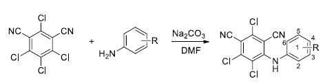
A series of multiple-halo isophthalonitriles containing substituted phenylamine were synthesized via the straightforward reaction of chlorothalonil and different substituted phenylamines in the presence of K2CO3 and DMF. These compounds have a diversity of various substituents which allow us to probe the effect of different substituents on anti-cancer activities. The synthetic route to these compounds is illustrated in Scheme 1. The information about their physical properties and chemical structure characterizations of total 29 compounds are listed in Experimental Section.

scheme 1

Scheme 1: Synthesis of titled compounds

Anti-proliferative Activity In Vitro and Structure-Activity Relationship

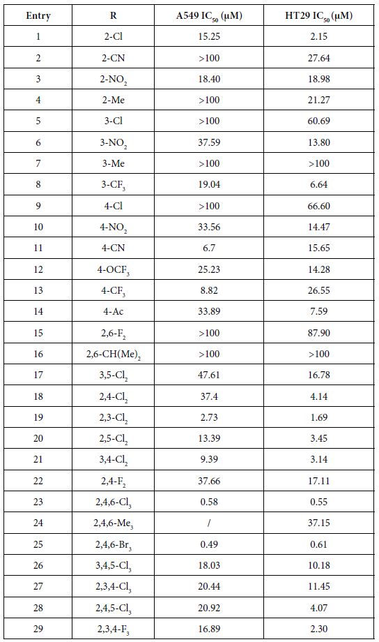
The vitro anticancer activities were assessed against lung cancer cell line A549 and colon cancer cell line HT29. The IC50 data (µM) (the concentration to achieve 50% proliferative inhibition) of the assessed compounds for these two cell lines are listed in Table 1.

Table 1: IC50 (μM) of compounds

tab 1

As presented in Table 1, these novel synthesized compounds showed various levels of anti-proliferative activities, indicating that substituents in phenyl ring exert important effect on anti-cancer activities. Generally, alkyl groups including methyl and isopropyl decreased the antiproliferative activities of title compounds which we can find the lowest antiproliferative activities (IC50 larger than 100 µM against both cancer cell lines) in compounds 4, 7, 16 and 24, except that compounds 4 and 24 have a moderate antiproliferative activity against HT29 with 21.27 and 37.15 µM IC50 respectively and no data on compound 24 against A549 yet. Nitro group is any interesting and important pharmacore group. Both clinical and preclinical results have demonstrated that compounds with nitro group hold great potential on enhancing anticancer properties. All prepared nitro compounds 3, 6 and 10 have moderate anticancer activities against both A549 and HT29 with 18.40, 18.98; 37.50, 13.80; and 33.56, 14.47 µM IC50 respectively, indicating that the position of nitro group at phenyl group (2-,3-,4- position of 3, 6, 10 respectively) does not cause any significant alteration of anticancer activities of these nitro compounds. Cyanide group does not have any positive sign on enhancing the anticancer activities as we see >100, 27.64; 6.7, 15.65 µM IC50 of compounds 2 and 11 against A549 and HT29 respectively although compound 11 with cyanide group located at 4 position in phenyl ring in has better anticancer activity than compound 2 with cyanide group located at 2 position in phenyl ring. Usually, compound with fluorine atom exhibits better bioactivities if the position is optimized [17]. In the present study, we prepared total six fluorine-containing compounds. Unexpectedly, all anticancer activities of them are not in the top levels. Compounds 22, 15 and 29 with fluorine alone as 2, 4-F2, 2, 6-F2, and 2, 3, 4-F3 respectively exhibited moderate activities as 37.66, 17.11; >100, 87.90; 16.89, 2.30 µM IC50 against A549 and HT29. Compounds 8 with trifluoromethyl group at 3-position of phenyl ring has a comparable but moderate anticancer activity with compound 13 with trifluoromethyl group at 4-position with 19.04, 6.64; 8.82, 26.55 µM IC50 against A549 and HT29 respectively. Furthermore, compound 12 with trifluoromethoxy group at 4-position of phenyl ring has a moderate anticancer activity as well with 25.23 and 14.28 μM IC50 against A549 and HT29 respectively.

The effect of chlorine atom on anticancer activities is our main focus on the present study. When compounds containing one chlorine atom at different positions of phenyl ring show moderate anticancer activities, compound 1 with 2-position chlorine has better activities than compounds 5 and 9 with 3-position and 4-position chlorine. Their IC50 are 15.25, 2.15; 100, 60.69; 100, 66.60 µM against A549 and HT29 respectively. Addition of one more chlorine to obtain  di-chlorine compounds in phenyl ring slightly enhanced anticancer activities as we see in compounds 17, 18, 19, 20, 21, compared with compounds 1, 5, 9. The former IC50 are 47.61, 16.78; 37.4, 4.14; 2.73, 1.69; 13.39, 3.45; 9.39, 3.14 µM against A549 and HT29 respectively. Again, compounds with 2-position chlorine including compounds 18, 19, 20 have better activities than compounds with other position chlorine in phenyl ring. For compounds 23, 26, 27, 28 with three chlorines in phenyl ring, we see that compound 23 is the best one although others have moderate anticancer activities. Their IC50 are 0.58, 0.55; 18.03, 10.18; 20.44, 11.45 and 20.92, 4.07 µM against A549 and HT29 respectively. In contrast, comparing the trend of anticancer activities with three different halogens such as chlorine, bromine and fluorine would be very interesting to find the most important ones. Apparently, among compounds 23, 25 and 29, compounds 23 and 25 with either chlorine or bromine are the most active in all of prepared compounds in present study whereas compound 29 has moderate activity. Although there is no significant difference between compounds 23 and 25, compound 23 (chlorine atom) has better atom economy than compound 25 (bromine atom). Thus, compound 23 has the better potential to warrant further investigation.

Anti-proliferative Activity In Vitro of Compound 23 with Broad Spectrum

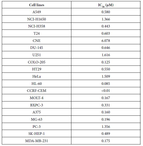
To further explore the anticancer activities of the most potent one, compound 23 in vitro, we screened its anticancer spectrum with total 19 cancer cell lines. As shown in Table 2, IC50 range is between 1.616 and ﹤0.01 µM with the most resistant one U251 and the most sensitive one CCRF-CEM. Except CCRF-CEM, HL-60, another non- solid tumor cell line showed the second most sensitivity to compound 23, indicating that compound 23 has strong activity to kill non-solid tumor cells. In contrast, brain tumor cells U251, cervical cancer cells HeLa and NIH-H1650 non small cancer lung cancer cells are in the most resistant cell lines with 1.616, 1.509 and 1.366 µM IC50 respectively.

Table 2: IC50 (μM) of compound 23 on 19 cancer cell lines

tab 2

Exploration of Potential Molecular Mechanisms

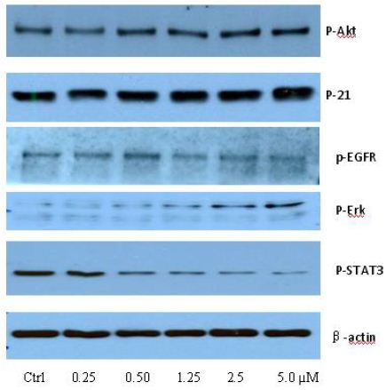
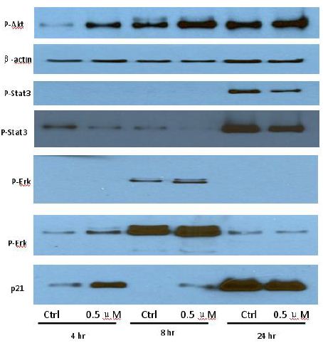
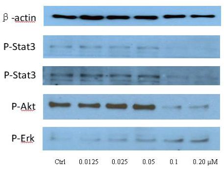
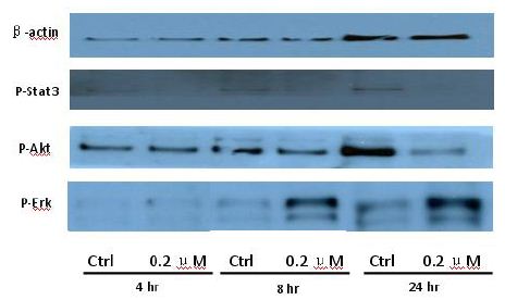
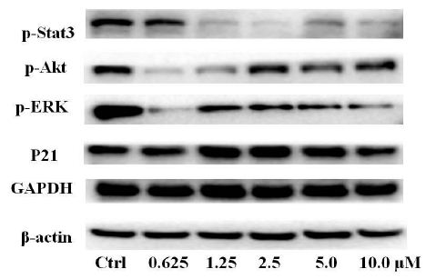
To clarify the potential molecular mechanisms, we detected the expression of several critical proteins in three representative cells, T24, H520 and A549. As shown in Figures 1 and 2, compound 23 dramatically increases the expression of p-Akt, p-Erk and p21 in T24 cancer cells in both dose and time dependent patterns. In contrast, compound 23 profoundly decreases the expression of p-Akt but moderately increases the expression of p-Erk in H520 cells. Moreover, in A549 cells, compound 23 decreases the expression of both p-Erk and p-21, shown in Figures 3 and 4. However, compound 23 decreases the expression of p-Akt in low concentration but expression of p-Akt is increased in high concentration in Figure 5. Taken together, all evidence collected indicates that compound 23-induced alteration of p-Akt and p-Erk is in cell specific fashion. However, compound 23 broadly induced the decrease of p-Stat3 expression in all three cancer lines showed in Figures 1-5. These important results imply that decreasing p-Stat3 may be the major mechanism of compound 23 in inhibiting cancer cell growth although further detailed studies are needed to warrant this conclusion.

fig 1

Figure 1: T24

fig 2

Figure 2: T24

fig 3

Figure 3: H520

fig 4

Figure 4: H520

fig 5

Figure 5: A549

Microsomal Intrinsic Clearance

As shown in Table 3, the results of microsomal intrinsic clearance of compound 23 indicate that compound 23 has 33.1 and 28.7 uL min-1mg-1 under NADPH dependent and NADPH free conditions, indicating that NADPH has not an important effect to compound 23 on microsomal metabolism. Verapamil and warfarin were used as high-metabolized and low-metabolized controls respectively. Thus, CYP enzymes may have no important effect on microsomal intrinsic clearance.

Table 3: Microsomal Intrinsic Clearance

tab 3

Caco-2 Permeability

As shown in Table 4, compound 23 has relative low permeability with mean A → B Papp is higher than mean B → A Papp. Thus, this data implies that oral administration route is not proper way to clinically treat the patients. In this assay, we used ranitidine, warfarin and talinolol are controls.

Table 4: Caco-2 permeability

tab 4

Plasma Protein Binding

As shown in Table 5, compound 23 has 100% plasma protein binding ratio. Therefore, both oral and intravenous infusion administration routes may not be an efficient way to treat patients. In this assay, propranolol and warfarin were used as binding controls.

In summary, we prepared a series of novel compounds and tested their anticancer activities. The most potent compound 23 was found. Furthermore, novel mechanism of inhibiting Stat3 phosphorylation of compound 23 was explored. Also, brief ADME properties of compound 23 was determined and low potential to conventional drug administration routes was recommended.

Table 5: Plasma protein binding

tab 5

Experimental Section

General Procedure for the Synthesis of Titled Compounds

Reagents were used without further purification unless otherwise specified. Solvents were dried and redistilled prior to use in the usual way. Analytical TLC was performed using silica gel HF254. To a solution of chlorothalonil (1 mmol) in dry DMF (20 ml), substituted aniline (1 mmol) and anhydrous sodium carbonate (1.5 mmol) were added at room temperature and the reaction mixture was stirred for 2 h at 60°C. The mixture was quenched by addition of ice water (100 ml). Then, the reaction mixture was filtered to afford the polyhalo isophthalonitriles compounds.

Physical and Spectral Information of Titled Compounds

2,4,5-Trichloro-6-((2-Chlorophenyl)Amino)Isophthalonitrile (1)

Yellow solid; Yield 69.6 %; mp: 208-210°C; 1H-NMR (300 M Hz, CDCl3): δ 7.03(s, 1H, NH), 7.27-7.38 (m, 3H, Ph-3,5,6-3H), 7.49-7.55 (m, 1H, Ph-4-H).

2,4,5-Trichloro-6-((2-Cyanophenyl)Amino)Isophthalonitrile  (2)

Brown solid; Yield 67.5%; mp: 258-260°C. 1H-NMR (300 M Hz, CDCl3): δ 7.12 (s, 1H, NH), 7.24 (d, 1H, Ph-6-H, J=7.5 Hz), 7.47 (t,1H, Ph-4-H, J=7.2 Hz), 7.68 (t, 1H, Ph-5-H, J=7.5 Hz), 7.78 (d, 1H, Ph-3-H, J=7.8 Hz).

2,4,5-Trichloro-6-(o-Tolylamino)Isophthalonitrile (3)

Brown solid; Yield 74.1%; mp: 258-260°C.1H-NMR (300 M Hz, CDCl3): δ 9.48 (s, 1H, NH), 7.44 (d, 1H, Ph-6-H, J=7.5 Hz), 7.68 (t,1H, Ph-4-H, J=7.2 Hz), 7.60(t, 1H, Ph-5-H, J=7.5 Hz), 8.2 (d, 1H, Ph-3-H, J=7.8 Hz). HRMS (ESI): calcd for C14H5C13N4O2Na [M + Na]+ ; 390.5700; found 389.9411.

2,4,5-Trichloro-6-(o-Tolylamino)Isophthalonitrile (4)

Gray red solid; Yield 73.2%; mp: 212-214°C; 1H-NMR (300 M Hz, CDCl3): δ (s, 3H, CH3), 7.00 (s, 1H, NH), 7.15 (d, H, Ph-6-H, J=7.5 Hz), 7.28-7.34 (m, 3H, Ph-3,4,5-3H). HRMS (ESI): calcd for C15H8Cl3N3Na [M + Na]+; 359.6000; found 359.9659.

2,4,5-Trichloro-6-((3-Chlorophenyl)Amino)Isophthalonitrile (5)

Brown solid; Yield 68.4%; mp: 228-230°C. 1H-NMR (300 M Hz, CDCl3): δ 7.04 (br, 1H, NH), 7.09 (d, J=7.5 Hz, 1H, Ph-6-1H), 7.20 (s, 1H, Ph-2-1H), 7.33-7.39 (m, 2H, Ph-4,5-2H). HRMS (ESI): calcd for C14H5Cl4N3Na [M + Na]+ ; 380.0150; found 380.9136.

2,4,5-Trichloro-6-((3-Nitrophenyl)Amino)Isophthalonitrile (6)

Gray solid; Yield 69.6%; mp: 250-252°C. 1H-NMR (300 M Hz, DMSO): 7.54-7.64 (m, 2H, Ph-5,6-2H), 7.94-8.00 (m, 2H, Ph-2,4- 2H),9.86 (br, 1H, NH). HRMS (ESI): calcd for C14H5C13N4O2Na [M + Na]+; 390.5700; found 389.9411.

2,4,5-Trichloro-6-(m-Tolylamino)Isophthalonitrile(7)

Brown solid; Yield 69.6%; mp: 248-25°C. 1H-NMR (300 M Hz, CDCl ): 2.40(s,3H, Ph-3-CH ), 7.02 (br, 1H, NH),7.12-7.36 (m, 4H, Ph-2,3,4,6-4H). HRMS (ESI): calcd for C15H8Cl3N3Na [M + Na]+ ; 359.6000; found 359.9659.

2,4,5-Trichloro-6-((3-(Trifluoromethyl)Phenyl)Amino) Isophthalonitrile (8)

Yellow solid; Yield 69.6%; mp: 236-238°C. 1H-NMR (300 M Hz, CDCl3): 7.12 (s, 1H, NH), 7.28-7.40 (m, 1H, Ph-6-H), 7.41-7.52 (m, 2H, Ph-2,4-2H), 7.54-7.62 (m, 1H, Ph-5-H).

2,4,5-Trichloro-6-((4-Chlorophenyl)Amino)Isophthalonitrile (9)

Yellow Yield 74.2%; mp: 259-261°C; 1H-NMR (300 M Hz, CDCl3): 7.00 (s, 1H, NH), 7.17 (d, 2H, Ph-2,6-2H, J=8.4 Hz), 7.42 (d, 2H, Ph-3,5-2H, J=8.7 Hz).

2,4,5-Trichloro-6-((4-Nitrophenyl)Amino)Isophthalonitrile (10)

Yellow Yield 69.3%; mp: 256-258°C; 1H-NMR (300 M Hz, CDCl3): 7.00 (s, 1H, NH), 7.17 (d, 2H, Ph-2,6-2H, J=8.3 Hz), 7.42 (d, 2H, Ph-3,5-2H, J=9.5 Hz).

2,4,5-Trichloro-6-((4-Cyanophenyl)Amino)Isophthalonitrile (11)

Yellow Yield 69.6%; mp: 259-261°C; 1H-NMR (300 M Hz, CDCl3): 7.00 (s, 1H, NH), 7.17 (d, 2H, Ph-2,6-2H, J=8.7 Hz), 7.42 (d, 2H, Ph-3,5-2H, J=9.0 Hz).

2,4,5-Trichloro-6-((3-(Trifluoromethoxy)Phenyl)Amino) Isophthalonitrile (12)

Gray Yield 75.3.%; mp: 204-206°C; 1H-NMR (300 M Hz, CDCl3): 7.09 (s, 1H, NH), 7.22-7.32 (m, 4H, Ph-2,3,5,6-4H).

2,4,5-Trichloro-6-((4-(Trifluoromethyl)Phenyl)Amino) Isophthalonitrile (13)

Yellow Yield 74.2.%; mp: 186-187°C; 1H-NMR (300 M Hz, CDCl3): 6.06 (br, 1H, NH), 6.51(d, J=5.7 Hz,2H, Ph-2,6-2H), 7.52(d, J=5.7 Hz,2H, Ph-3,5-2H).

4-((2,3,5-Trichloro-4,6-Dicyanophenyl)Amino)Phenyl Acetate (14)

Gray Yield 74.2.%; mp: 246-248°C; 1H-NMR (300 M Hz, CDCl3): 2.29 (s, 3H, COOCH3), 7.08 (s, 1H, NH), 7.17 (d, 2H, Ph-3,5-2H, J=8.7 Hz), 8.10 (d, 2H, Ph-2,6-2H, J=8.7 Hz).

2,4,5-Trichloro-6-((2,6-Difluorophenyl)Amino)Isophthalonitrile (15)

Gray Yield 74.2.%; mp: 218-220°C; 1H-NMR (300 M Hz, CDCl3): 7.03 (s, 1H, NH), 7.13 (dd, 1H, Ph-6-H, 3J=8.1 Hz, 4J=0.9 Hz), 7.28 (t, 1H, Ph-5-H, J=8.1 Hz), 7.47 (dd, 1H, Ph-4-H, 3J=8.1 Hz, 4J=0.9 Hz). HRMS (ESI): calcd for C14H4CI3F2N3Na [M + Na]+ ; 381.5538; found 381.9346.

(2,4,5-Trichloro-6-((2,6-Diisopropylphenyl)Amino) Isophthalonitrile (16)

Gray Yield 69.3%; mp: 216-218°C; 1H-NMR (300 M Hz, CDCl3): δ 7.12 (d, J=8.1 Hz, 2H), 6.98 (dd, J=8.3, 6.9 Hz, 1H), 5.87 (d, J=2H), 3.02 (p, J=6.8 Hz, 2H), 1.29 (d, J=6.9 Hz, 12H).

2,4,5-Trichloro-6-((3,5-Dichlorophenyl)Amino)Isophthalonitrile (17)

White solid; Yield 56.7%; mp: 238-242°C; 1H-NMR (300 M Hz, CDCl3): 6.95 (s, 1H, NH), 7.05 (d, 2H, Ph-2,6-2H, J=1.8 Hz), 7.32 (d, 1H, Ph-4-H, J=1.5 Hz). HRMS (ESI): calcd for C14H4C15N3Na [M + Na]+; 414.4570; found 413.8757.

2,4,5-Trichloro-6-((2,4-Dichlorophenyl)Amino)Isophthalonitrile (18)

Brown Black solid; Yield 59.6%; mp: 209-212°C; 1H-NMR (300 M Hz, CDCl3): 6.95 (s, 1H, NH), 7.20 (d, 1H, Ph-6-H, J=8.1 Hz), 7.36 (dd, 1H, Ph-5-H, 3J=8.7 Hz, 4J=2.7 Hz), 7.54 (d, 1H, Ph-3-H, J=2.4 Hz). HRMS (ESI): calcd for C14H4C15N3Na [M + Na]+; 414.4570; found 413.8757.

2,4,5-Trichloro-6-((2,3-Dichlorophenyl)Amino)Isophthalonitrile (19)

Gray White solid; Yield 58.6%; mp: 218-220°C; 1H-NMR (300 M Hz, CDCl3): 7.03 (s, 1H, NH), 7.13 (dd, 1H, Ph-6-H, 3J=8.1 Hz, 4J=0.9 Hz), 7.28 (t, 1H, Ph-5-H, J=8.1 Hz), 7.47 (dd, 1H, Ph-4-H, 3J=8.1 Hz, 4J=0.9 Hz). HRMS (ESI): calcd for C14H4C15N3Na [M + Na]+; 414.4570; found 413.8757.

2,4,5-Trichloro-6-((3,4-Dichlorophenyl)Amino)Isophthalonitrile (20)

Gray white solid; Yield 57.6%; mp: 220-222°C; 1H-NMR (300 M Hz, CDCl3): δ 7.45 (d, J=8.6 Hz, 1H), 7.32 – 7.25 (m, 2H), 7.21 (d, J=2.4 Hz, 1H), 6.96 (s, 1H).

2,4,5-Trichloro-6-((3,4-Dichlorophenyl)Amino)Isophthalonitrile (21)

Brown solid; Yield 58.9%; mp: 230-232°C; 1H-NMR (300 M Hz, DMSO): 7.13 (dd, J=8.4 Hz,J=2.1 Hz,1H,Ph-4-1H), 7.39(d, J=2.1 Hz,1H,Ph-6-1H), 7.51(d, J=8.4 Hz,1H,Ph-3-1H),9.62(br, 1H, NH).

2,4,5-Trichloro-6-((2,4-Difluorophenyl)Amino)Isophthalonitrile (22)

Gray solid; Yield 67.5%; mp: 206-208°C; 1H-NMR (300 M Hz, CDCl3): 6.88 (s, 1H, NH), 6.99 (t, 2H, Ph-5,6-2H, J=8.1 Hz), 7.32 (d, 1H, Ph-3-H, J=2.4 Hz).

2,4,5-Trichloro-6-((2,4,6-Trichlorophenyl)Amino) Isophthalonitrile (23)

Brown solid; Yield 67.5%; mp: 241-243°C; 1H-NMR (300 M Hz, CDCl3): 6.86 (S, 1H, NH),7.48(s, 2H,Ph-3,5-2H).

2,4,5-Trichloro-6-(Mesitylamino)Isophthalonitrile (24)

Brown solid; Yield 67.5%; mp: 199-201°C; 1H-NMR (300 M Hz, CDCl3): 2.17(s,6H,Ph-2,6-2CH3),2.34(s,3H,Ph-4-CH3) 6.81(br, 1H, NH),6.97(s, 2H,Ph-3,5-2H). HRMS (ESI): calcd for C17H11CI3N3 [M-H]+ ; 387.6540; found 386.0040.

2,4,5-Trichloro-6-((2,4,6-Tribromophenyl)Amino) Isophthalonitrile (25)

Brown solid; Yield 67.5%; mp: 251-253°C 1H-NMR (300 M Hz, CDCl3) δ 7.82 (s, 2H), 6.93 (s, 1H).

2,4,5-Trichloro-6-((3,4,5-Trichlorophenyl)Amino) Isophthalonitrile(26)

Yellow solid; Yield 59.3%; mp: 264-266°C; 1H-NMR (300 M Hz, DMSO): 7.53 (s, 2H,Ph-2,6-2H),8.98(br, 1H, NH).

2,4,5-Trichloro-6-((2,3,4-Trichlorophenyl)Amino) Isophthalonitrile(27)

Gray solid; Yield 59.3%; mp: 198-200°C; 1H-NMR (300 M Hz, CDCl3): 6.98(br, 1H, NH), 7.08(d, J=9.0 Hz, 1H, Ph-6-1H), 7.46 (d, J=9.0 Hz, 1H, Ph-5-1H).

2,4,5-Trichloro-6-((2,4,5-Trichlorophenyl)Amino) Isophthalonitrile (28)

Yellow solid; Yield 78.5%; mp: 253-255°C; 1H-NMR (300 M Hz, CDCl3): 6.88 (br, 1H, NH), 7.33 (s,1H,Ph-6-1H),7.96 (s,1H,Ph-5-1H).

2,4,5-Trichloro-6-((2,3,4-Trifluorophenyl)Amino) Isophthalonitrile (29)

Gray solid; Yield 69.6%; mp: 182-184°C; 1H-NMR (300 M Hz, CDCl3): 6.87 (s, 1H, NH), 7.05-7.09 (m, 2H, Ph-5,6-2H).

Cell Lines and Culture Conditions

All human cancer cell lines were purchased from Cell Resource Center, Institute of Life Sciences, Chinese Academy of Sciences (Shanghai, China) and cultured in either DMEM (Hyclone, Logan, UT, USA) or RPMI-1640 (Hyclone, Logan, UT, USA) supplemented with 10% of FBS (Hyclone, Logan, UT, USA) and 1% of penicillin- streptomycin at 37°C, in humidified air containing 5% of CO2.

Cell Viability Assay

Cell viability was assessed using a tetrazolium based assay using microplate reader (Biotek, SYNERGY HTX, Vermont, USA). IC50 values were determined through the dose-response curves. Cells were seeded at 6×10³ per well in 96-well culture plates and incubated in medium containing 10% FBS. Different seeding densities were optimized at the beginning of the experiments. After 24h, cells were treated with different concentrations of titled compounds with various concentrations for 48 hours in incubator. 50μl of MTT tetrazolium salt (Sigma) dissolved in Hank’s balanced solution at a concentration of 2 mg/ml was added to each well with indicated treatment and incubated in CO2 incubator for 5 h. Finally, the medium was aspirated from each well and 150μl of DMSO (Sigma) was added to dissolve formazan crystals and the absorbance of each well was obtained using a Dynatech MR5000 plate reader at a test wavelength of 490 nm with a reference wavelength of 630 nm.

Protein Characterization

Western blot assessment was performed using regular procedure. Primary antibody was added in BSA and allowed to incubate overnight at 4°C, washed with TBS/0.05% Tween-20 for 5 times (10min per time) before the secondary antibody was added and then incubated for an additional hour at room temperature. The membrane was again washed 3 times before adding Pierce Super Signal chemiluminescent substrate (Rockford, IL, USA) and then immediately imaged on Chemi Doc (Bio-Rad, Hercules, CA, USA). The films were scanned using EPSON PERFECTION V500 PHOTO and quantified by Image J (NIH, Bethesda, MD, USA).

Analytical Method Development for compound 23

The signal was optimized for each compound by ESI positive or negative ionization mode. An MS2 scan or a SIM scan was used to optimize the fragmenter voltage and a product ion analysis was used to identify the best fragment for analysis, and the collision energy was optimized using a product ion or MRM scan. An ionization ranking was assigned indicating the compound’s ease of ionization.

Analytical Method Development for ADME

Samples were analyzed by LC/MS/MS using an Agilent 6410 mass spectrometer coupled with an Agilent 1200 HPLC and a CTC PAL chilled autosampler, all controlled by MassHunter software (Agilent). After separation on a C18 reverse phase HPLC column (Agilent, Waters, or equivalent) using an acetonitrile-water gradient system, peaks were analyzed by mass spectrometry (MS) using ESI ionization in MRM mode.

Microsomal  Stability Assay

The test agent is incubated in duplicate with microsomes at 37°C. The reaction contains microsomal protein in 100 mM potassium phosphate, 2 mM NADPH, 3 mM MgCl2, at pH 7.4. A control reaction is performed for each test agent omitting NADPH (to detect NADPH- free degradation). At indicated times, an aliquot is removed from each experimental and control reaction and mixed with an equal volume of ice-cold Stop Solution (methanol, containing haloperidol, diclofenac, or other internal standard). Stopped reactions are incubated at least ten minutes at -20°C, and an additional volume of water is added. The samples are centrifuged to remove precipitated protein, and the supernatants are analyzed by LC/MS/MS to quantitate the remaining parent. Data are converted to % remaining by dividing by the time zero concentration value. Data are fit to a first-order decay model to determine half-life. Intrinsic clearance is calculated from the half-life and the protein concentrations:

CLint=ln(2) /(T1/2 [microsomal protein])

Verapamil (high metabolized) and warfarin (low metabolized) were used as reference controls.

Caco-2 cells grown in tissue culture flasks are trypsinized, suspended in medium, and the suspensions were applied to wells of a Millipore 96 well Caco-2 plate. The cells are allowed to grow and differentiate for three weeks, feeding at 2-day intervals. For Apical to Basolateral (A → B) permeability, the test agent is added to the apical (A) side and amount of permeation is determined on the basolateral (B) side; for Basolateral to Apical (B → A) permeability, the test agent is added to the B side and the amount of permeation is determine on the A The A-side buffer contains 100 μM Lucifer yellow dye, in Transport Buffer (1.98 g/L glucose in 10 mM HEPES, 1x Hank’s Balanced Salt Solution) pH 6.5, and the B-side buffer is Transport Buffer, pH 7.4. Caco-2 cells are incubated with these buffers for 2 hr, and the receiver side buffer is removed for analysis by LC/MS/MS. To verify the Caco-2 cell monolayers are properly formed, aliquots of the cell buffers are analyzed by fluorescence to determine the transport of the impermeable dye Lucifer Yellow. Any deviations from control values are reported.

Data are expressed as permeability (Papp): AC dt dQ Papp 0 = where dQ/dt is the rate of permeation, C0 is the initial concentration of test agent, and A is the area of the monolayer.

In bidirectional permeability studies, the Efflux Ratio (RE) is also calculated: ( ) ( R e BA P A B P app app →→ =

An RE > 2 indicates a potential substrate for P-gp or other active transporters.

Plasma Protein Binding

Test agent is added to plasma. This mixture is dialyzed in a RED Device (Pierce) per the manufacturers’ instructions against PBS and incubated on an orbital shaker. After the end of the incubation, aliquots from both plasma and PBS sides are collected, an equal amount of PBS is added to the plasma sample, and an equal volume of plasma is added to the PBS sample. Methanol (three volumes) containing internal standard is added to precipitate the proteins and release the test agents. After centrifugation, the supernatant is transferred to a new plate and analyzed by LC/MS/MS.

References

  1. Cancer Facts & Figures (2015) American Cancer
  2. Domingo-Musibay E, Galanis E (2015) What next for newly diagnosed glioblastoma? Future Oncol 11: 3273-3283. [crossref]
  3. Oberstein PE, Olive KP (2013) Pancreatic cancer: why is it so hard to treat? Ther Ad Gastroenterol 6: 321-337. [crossref]
  4. Lemjabbar-Alaoui H, Hassan OUI, Yang YW, Buchanan P (2015) Lung cancer: Biology and treatment Biochim Biophys Acta 1856: 189-210. [crossref]
  5. Holohan C, Van Schaeybroeck S, Longley DB, Johnston PG (2013) Cancer drug resistance: an evolving Nat Rev Cancer 13: 714-726. [crossref]
  6. O’Connor R (2009) A review of mechanisms of circumvention and modulation of chemotherapeutic drug Curr Cancer Drug Targets 9: 273-280. [crossref]
  7. Yan SJ, Huang, ; Zeng, X. H.; Huang, R.; Lin, J. (2010) Solvent-free, microwave assisted synthesis of polyhalo heterocyclic ketene aminals as novel anti-cancer agents. Bioorg Med Chem Lett 20: 48-51. [crossref]
  8. Huang C, Yan SJ, Zeng XH, Dai XY, Zhang Y, et (2011) Biological evaluation of polyhalo 1,3-diazaheterocycle fused isoquinolin-1(2H)-imine derivatives. Eur J Med Chem 46: 1172-1180. [crossref]
  9. Yan SJ, Zhen H, Huang C, Yan YY, Lin J, et (2010) Synthesis of highly functionalized 2,4-diaminoquinazolines as anticancer and anti-HIV agents. Bioorg Med Chem Lett 2: 4432-4435. [crossref]
  10. Heilman WP, Battershell RD, Pyne WJ, Goble PH, Magee TA, et (1978) Synthesis and antiinflammatory evaluation of substituted isophthalonitriles, trimesonitriles, benzonitriles, and terephthalonitriles. J Med Chem 21: 906-913. [crossref]
  11. Guan AY, Liu CL, Huang G, Li HC, Hao SL, et (2013) Design, synthesis, and structure-activity relationship of novel aniline derivatives of chlorothalonil. J Agric Food Chem 61: 11929-11936. [crossref]
  12. Kadayat TM, Song C, Kwon Y, Lee, S. (2015) Modified 2,4-diaryl-5H-indeno[1,2-b] pyridines with hydroxyl and chlorine moiety: synthesis, anticancer activity, and structure-activity relationship study. Bioorg Chem 62: 30-40. [crossref]
  13. Kadayat TM, Park S, Jun KY, Magar TB, Bist G, et (2016) Effect of chlorine substituent on cytotoxic activities: design and synthesis of systematically modified 2,4-diphenyl-5H-indeno[1,2-b]pyridines. Bioorg Med Chem Lett 7: 1726-1731. [crossref]
  14. Beck DE, Lv W, Abdelmalak M, Plescia CB, Agama K, Marchand C, Pommier Y, Cushman M (2016) Synthesis and biological evaluation of new fluorinated and chlorinated indenoisoquinoline topoisomerase I poisons. Bioorg Med Chem 7: 1469-1479.
  15. Li HC, Guan AY, Huang G, Liu CL, Li ZN, et (2016) Design, synthesis and structure-activity relationship of novel diphenylamine derivatives. Bioorg Med Chem 3: 453-461. [crossref]
  16. Chai BS, Wang SY, Yu WQ, Li HC, Song CJ, et (2013) Synthesis of novel strobilurin- pyrimidine derivatives and their antiproliferative activity against human cancer cell lines. Bioorg Med Chem Lett 23: 3505-3510. [crossref]
  17. Wang J, Sánchez-Roselló M, Aceña JL, del Pozo C, Sorochinsky AE, et (2014) Fluorine in pharmaceutical industry: fluorine-containing drugs introduced to the market in the last decade (2001-2011). Chem Rev 4: 2432-2506. [crossref]

A Clinical Study on Hypothyroidism and Early Pregnancy Loss

DOI: 10.31038/PSC.2022214

Abstract

Thyroid disorders are recognized associated factors for adverse pregnancy outcomes spontaneous miscarriages being an important entity. This study was conducted on 200 women who had early pregnancy losses and their thyroid profile was evaluated. Prevalence of overt and sub clinical hypothyroidism was calculated along with euthyroid women. The results obtained were statistically analysed. In conclusion, it was established that hypothyroidism, both overt and sub clinical, when untreated can lead to early pregnancy losses, therefore all antenatal women should be universally screened for thyroid dysfunction in their very first antenatal visit and treatment should be initiated at the earliest.

Keywords

Early pregnancy loss, Hypothyroidism, Overt hypothyroidism, Spontaneous miscarriage, Subclinical hypothyroidism, Thyroid dysfunction

Introduction

Thyroid dysfunction during pregnancy has been known to be associated with adverse pregnancy outcomes especially spontaneously miscarriages, being the most common early pregnancy complication. Though various causes of early pregnancy losses include genetic, anatomical factors, endocrine dysfunction, autoimmune disorders, thrombophillias, life style and environmental factors, maternal general diseases and infections, a large chunk of such cases are unexplained and also known as idiopathic early pregnancy losses. Thyroid dysfunction constitutes the most common endocrine disorder encountered in pregnancy sometimes recognized for the first time during antenatal check-ups. Pregnancy is characterized by profound physiological modifications in thyroid function regulation as a result of various factors e.g. increased Thyroid Binding Globulin (TBG) due to elevated Estrogen and human chorionic gonadotropin (HCG) levels, increased renal iodine losses due to increased Glomerular filtration rate (GFR), peripheral metabolism of maternal thyroid hormones modifications and physiological changes in the iodine transfer to the placenta [1-4].

It has been observed that antenatal women with thyroid dysfunction – both overt and subclinical types – are at higher risk for developing pregnancy-associated complications e.g. threatened miscarriage, pre-eclampsia, pre-term labour and pre term birth, abruption placentae and post-partum haemorrhage. Fetal complications are also associated with thyroid dysfunction in pregnancy e.g. spontaneous abortions in first trimester, pre term births, Intrauterine Growth Restriction (IUGR), low birth weight (LBW) babies, low APGAR scores, stillbirths and neonatal deaths, higher incidence of NICU admission because of neonatal hyper-bilirubinemia, neonatal hypothyroidism, and increased perinatal mortality rate [5]. Euthyroid status is defined as having normal TSH levels (0.1-2.5 mIU/L) in 1st trimester. Subclinical Hypothyroidism (SCH) is defined as TSH increase (>3.0 mIU/L) in the presence of normal Free T4 (0.8-2.0 ng/dL). Overt hypothyroidism (OH) has increased TSH (>3.0 mIU/L) and low Free T4 (<0.8 ng/dL). Subclinical hyperthyroidism is defined as low serum TSH (<0.2 mIU/L) and normal Free T4 (0.8-2.0 ng/dL). Overt hyperthyroidism has high free T4 (>2.0 ng/dL) and low TSH (<0.2 mIU/L). This study was conducted with the aim of determining the prevalence of hypothyroidism in patients presenting with early pregnancy loss.

Materials and Methods

  • Study type: Hospital based, cross-sectional study.
  • Study duration: 18 months.
  • Study population: Pregnant women presenting with Early pregnancy losses (EPL) (missed/incomplete/ complete miscarriages).
  • Sample size: 200.

This study was conducted in the department of Obstetrics and Gynaecology of a tertiary care medical college in rural Haryana, in North India.

All pregnant women presenting with EPL (missed/ incomplete/ complete miscarriages) were enrolled in this study after obtaining proper written informed consent. All these patients recruited had detailed history taken, followed by thorough clinical examination consisting of general physical, systematic and obstetric examinations and all the findings were entered in a pre-structured performa. History including socio-demographic parameters, age, parity, socio-economic status, menstrual history, obstetric history, medical or surgical history, date of her last menstrual period (LMP) were noted.

BMI was calculated based on pre-pregnancy body weight and height (BMI=wt in kg/height in sq.m).

Exclusion Criteria

  • Multiple gestation
  • Known Thyroid dysfunction
  • Known cases of DM/ Renal/ liver disease/ hypertension
  • Known cases of recurrent pregnancy losses ( RPL)

Blood samples were collected for Thyroid Function Test (TFT) Serum TSH and free T3 and T4. Thyroid status of the patient was established using the standard cut-off laboratory levels (Table 1).

Table 1: Interpretation of Thyroid Function Tests (TFT)

Status

TSH level (µIU/L)

Free T4 level (ng/L)

Euthyroid

0.1-2.5

Overt Hypothyroidism (OH)

> 3.0

<0.8 (decreased)

Subclinical Hypothyroidism (SCH)

>3.0

0.8-2.0 (normal)

Subclinical hyperthyroidism

<0.2 (decreased)

0.8-2.0 (normal)

Overt hyperthyroidism

<0.2(decreased)

>2.0 (raised)

Results and Observations

Total 200 patients with EPL were recruited in the study.

The results observed were as follows (Table 2-5):

Table 2: Age distribution of patients

Age (years)

Number (n)

Percentage (%)

19-24

115 57.50
25-29 51

25.50

30-34

26 13.00
≥35 8

4.00

Total

200

100.00

Table 3: Parity-wise distribution of patients

Parity

Number (n) Percentage (%)
≤1 99

49.50

2

49 24.50
3 28

14.00

≥4

24 12.00
Total 200

100.00

Most patients were primipara, were young (19-24 years of age),with low BMI

Table 4: Mean BMI of the patients

Thyroid status

BMI (kg/m2)

Euthyroid

22.1 ± 2.2

Hypothyroid

22.8 ± 3.6

Table 5: Comparison of age and BMI

Parameter

Mean age (years)

BMI (kg/m2)

Euthyroid women

22 ± 3.6

22.1 ± 2.2

Hypothyroid women

25 ± 2.3

22.8 ± 3.6

Discussion

This study was conducted on 200 antenatal women presenting with early pregnancy losses, showing that hypothyroidism is a significant contributor to miscarriages especially in the first trimester. In our study, 48 patients (24.0%) had hypothyroidism with 36 overt hypothyroidism (75.0%) and 12 with subclinical hypothyroidism (25.0%0). Our results are comparable with those from various studies from different geographical areas of the globe. In their study, Abalovich et al. reported that untreated hypothyroidism both SCH and OH at the time of conception, was associated with significantly higher rates of spontaneous miscarriages as compared to euthyroid women [6]. Ashoar et al. in their study reported statistically significant association between low serum thyroxine (FT4) in mothers in first trimester and early fetal loss in subclinical hypothyroid pregnant women [7]. Rao et al. from south India, determined the frequency of hypothyroidism in women with EPL in India, which they stated as 4.12%. Leduk et al. in their retrospective cohort study, concluded that patients with recurrent pregnancy losses in 1st trimester, 19.4% subclinical hypothyroidism SCH and 5.4% had overt hypothyroidism (OH). Salek et al. reported increased prevalence of hypothyroidism for twin gestation than singleton pregnancy at 6.42% and 5.32% respectively. Zhang et al. studied the relationship between SCH and risk of spontaneous miscarriage before 20 weeks of gestation and reported significantly increased chances. They also observed that SCH patients with thyroid autoimmunity had higher prevalence of spontaneous miscarriage as compared to euthyroid women [8-11].

Conclusion

From the present study, we reinforce the fact that hypothyroidism – both overt and subclinical – if untreated – leads to early pregnancy losses. It also causes recurrent pregnancy losses. Therefore all pregnant women should be universally screened for thyroid dysfunction so that replacement therapy can be initiated at the earliest so as to ensure the best maternal and fetal outcomes.

Conflict of Interest

Nil

Funding

None

Abbreviations

EPL: Early Pregnancy Loss; GFR: Glomerular Filtration Rate; IUGR: Intrauterine Growth Restriction; LBW: Low Birth Weight; NICU: Neonatal Intense Care Unit; OH: Overt Hypothyroidism; RPL: Recurrent Pregnancy Loss; SCH: Subclinical Hypothyroidism; TFT: Thyroid Function Test.

References

  1. Verma P, Roy D, et al. (2020) Hypothyroidism & early pregnancy losses: an overview. Int J Repod Contracept Obstet Gynecol 9: 5065-5067.
  2. Back KH, et al. (2007) Recurrent pregnancy Losses: The key potential mechanisms. Trends Mol Med 13: 310-317. [crossref]
  3. Abalovich M, et al. (2007) Management of thyroid dysfunction during pregnancy & post partum: An endocrine society clinical practice guideline Clin Endocrinol Meta 92: 1-47. [crossref]
  4. So L.B, et al. (2006) Thyroid disorders during pregnancy. Endocrinal Metab Clin North Am 35: 117-136. [crossref]
  5. Negro R, et al. (2006) L-thyroxine treatment in euthyroid pregnant women with autoimmune thyroid disease: Effects on obstetrical complications. Clin Endocrinol Meta 91: 2587-2591. [crossref]
  6. Abalovich M. (2002) Overt and SubClinical Hypothyroidism complicating pregnancy. Thyroid 12: 63-66. [crossref]
  7. Ashoor G, et al. (2010) Maternal Thyroid function at 11-13 weeks of gestation and subsequent fetal death. Thyroid 20: 989-993. [crossref]
  8. Leduk RG, Lewis M, et al. (2020) Prevalence of thyroid autoimmunity and effect of l-thyroxine treatment in patients with recurrent pregnancy losses. Reprod Bio med Online 40: 582-592. [crossref]
  9. Rao V.R, Lakshmi A.P. et al. (2018) Prevalence of hypothyroidism in recurrent pregnancy losses in 1st Ind J Med Sci 62: 357-361. [crossref]
  10. Salek T, Shaifalaha I, et al. (2019) The prevalence of maternal hypothyroidism in 1st trimester screening (11-14 weeks of gestation). Biomed Pap Med Fac Univ Palaky Czech Republic 63: 265-268. [crossref]
  11. Zhang Y, Wang H, et al. (2017) Patients with subclinical hypothyroidism before 20 weeks of pregnancy and miscarriages – A systematic review of meta-analysis. PLOS One 12: e0175708.

Diffusion Models of Continuum Physics

DOI: 10.31038/NAMS.2022521

Abstract

The paper begins with a review of known diffusion models of the literature, in terms of the mass fraction and the chemical potential. Next the  thermodynamic consistency of the pertinent schemes is investigated and it follows that the recourse to the chemical potential is justified in two different ways. The alternative recourse to the balance equations, through a linearization procedure, is suggested as a check of consistency. Finally it is pointed out that, thanks to the correspondence probability-concentration, the classical models of diffusion can be extended to the quantum context.

Keywords

Diffusion models, Thermodynamic consistency, Concentration, Chemical potential

Introduction

The purpose of this paper is to review standard models of diffusion and to clarify the physical bases leading to the different differential equations. To understand the basic starting point and to establish the required notation we start with addressing attention to a mixture of n fluid constituents.

In essence, let ρα , vα be the mass density and the velocity of the α th constituent,

α = 1, …, n. We let

in 1

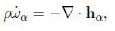
be the mass density of the mixture and the mass fraction (or concentration) of the α th constituent; the sum on α is understood from 1 to n. As we prove in a moment ωα is subject to the differential equation

in 2

where hα is the mass flux,  ∇ is the gradient operator and then ∇ is the divergence, and the superposed dot denotes the (total) time derivative.

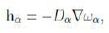
Within the theory of mixtures hα is clearly defined and shown to satisfy a differential equation [1,2]. As we emphasize in this paper, hα is regarded as an unknown vector to be determined through mathematical assumptions associated with physical properties of the mixture. The original Fick’s model is based on the assumption

in 3

where Dα is the diffusivity. Next other models and their generalizations have been developed in terms of the chemical potential.

In this paper we first review known diffusion models in terms of the mass fraction ωα and the chemical potential µα. Next we investigate the thermodynamic consistency of the pertinent schemes and find that the recourse to the chemical potential is justified in two different ways. Next we examine the alternative recourse to the balance equations through a linearization procedure. Further, we point out that the ideas about the correspondence probability-concentration is applied to modelling diffusion in the quantum context.

Balance Equations for Fluid Mixtures

Consider a mixture of n fluid constituents (see, e.g., [1]). The suffices α, β = 1, 2, …, n label the quantities related to the α th, β th constituent. Hence ρα is the mass density and vα the velocity of the α th constituent. The continuity equation of the α th constituent comprises the mass supply τα, per unit volume and unit time, so that

ba 1

The conservation of mass of the whole mixture implies

ba 2

Hereafter ba 3 is  a  shorthand for ba 4 The mass supply τα is nonzero in chemical reactions and phase transformations or generally whenever a constituent may gain or lose mass in favor of the other constituents.

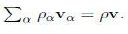
The mass density ρ and the (barycentric) velocity v of the mixture are defined by

ba 5

The ratio

ba 6

is the mass fraction (or concentration) of the α th constituent and uα = vα − v

is the diffusion velocity. The definition of v implies that

ba 7

The sum of (1) with the constraint (2) results in

ρ + ∇ · (ρv) = 0,                                              (3)

which is the continuity equation for the whole mixture.

We now investigate the evolution equation for ωα. Replace ρα with ρωα and vα with

v + uα in (1). In view of (3) we find

ρ(tωα + v · ∇ωα) + ∇ · (ραuα) = τα.

Observe that tωα   + v.  ∇ωα  is the derivative with respect to the barycentric observer. As with any function it is denoted by a superposed dot. The vector

hα:= ρα uα

is the α th diffusion flux representing the flux of the α th constituent relative to the barycentric observer. Hence we can write

ba 8

The mass fraction ωα, in the barycentric reference, evolves according to (4). This equation is operative once τα and hα are given in terms of ba 9 , possibly parameterized by temperature and pressure.

The equation of motion of the α th constituent can be written in the form

(ραvα) + ∇· (ραvα ⊗ vα) − ∇ · Tα ραbα = mα,

where Tα is the Cauchy stress tensor, bα is the body force, and mα is the growth of the linear momentum, that is the force on the α th constituent due to other constituents of the mixture. The growths {mα} are subject to the constraint

ba 10

Modelling of Diffusion Fluxes and Diffusion Equations

The physical modelling of diffusion is most often restricted to non-reacting mixtures, τα = 0, and is based on the view that diffusion is governed by (4) with appropriate models for hα.

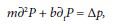
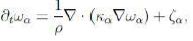
The simplest and best known model of diffusion traces back to Fick [3] and is based on an assumption on hα that is motivated by the analogy with the Fourier model of heat conduction. First the total derivative ba 9 is replaced with the partial derivative ωα; this means that diffusion is examined in the barycentric frame. Moreover, Fick’s law assumes the diffusion flux hα is antiparallel to ωα, i.e. hα = κα ωα, where κα > 0 may depend on the constituent. Hence divide eq. (4) by ρ to obtain

mo 1

where ζα = τα . If κα is constant then the evolution equation for ωα takes the form

mo 2

the quantity Dα = κα is called diffusivity.

Diffusion in solids is often modelled by letting ([4], ch. 17) hα = −Dα ∇ Nα,

where Nα is the concentration in the form

mo 3

mo 4 being the number of atoms per unit volume.

Other diffusion equations are based on the following two main assumptions. Let ψα be the α th Helmholtz free energy and define

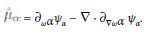
mo 5

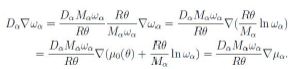
The assumption is hα = −κα ∇ µα.

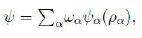
For definiteness we consider ψα in the form [5]

mo 6

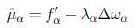
If λα is constant then it follows

mo 7

and eq. (4) takes the form

mo 8

Equation (8) is usually referred to as the Cahn-Hilliard equation [6,7]. It is a fourth-order partial differential equation. If the dependence on ∇ ωα is ignored then the Cahn-Hilliard equation reduces to the second-order parabolic equation (6).

Alternatively it is assumed that the evolution of ωα is in fact a relaxation toward equilibrium governed by [8]

mo 9

Hence, letting ψα be given again by the Landau-Ginzburg function (7) we obtain

mo 10

Equation (9) is a second-order partial differential equation  when ψα depends on ∇ωα ; it is referred to as the Ginzburg-Landau equation or the Allen-Cahn equation. While eq. (6) is based on Fick’s law hα = −κα ∇ ωα , eqs (8) and (9) are based on the assumptions

mo 11

The function   mo 12 is often regarded as the chemical potential. As   we see in a moment mo 12differs from the standard (correct) expression of the chemical potential. Moreover even simple thermodynamic considerations would justify the use of the chemical potential.

Thermodynamic Test of (10)

The balances of energy and entropy are stated by considering the mixture as a whole body. The balance of energy is taken in the form

th 1

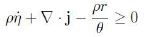
where ε is the internal energy density, per unit mass, D is the stretching tensor, q is the heat flux vector, and r is the external heat supply. Let θ > 0 be the absolute temperature. The second law of thermodynamics is stated as follows: the entropy density η and the entropy flux j satisfy the inequality

th 2

For every admissible process that is every set of constitutive functions compatible with the balance equtaions.

For formal conveneince let

th 3

k being the extra-entropy flux to be determined. Substituting ρr-∇.q from eq. (11)

th 4

Let ψ = ε-θη be the Helmholtz free energy of the mixture. The second law inequality can be written as

th 5

To determine thermodynamic consequences of the second law we now consider

th 6

as the set of independent variables. Moreover we specialize T in the form

th 7

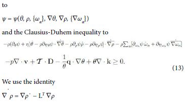
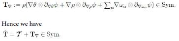
with T = O(D) as D→0. Compute ψ˙ and substitute in the Clausius- Duhem inequality (12). The arbitrariness and linearity of ω¨α , ρ¨, , θ¨ reduces the possible dependencies of ψ

th 11

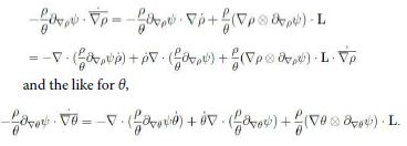
and the analogue for ∇ θ and ∇ ωα. Now, divide (13) by θ and consider the identities

th 12

Moreover we have

th 13

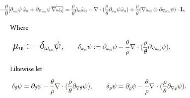
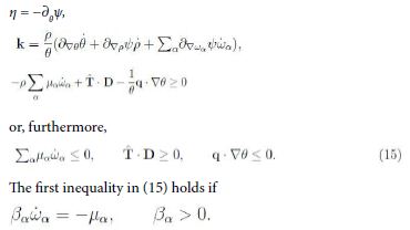
Hence upon some rearrangements we can write inequality (13)  in the form

th 14

Since L = D+W, with W ∈ skw the spin tensor, then the arbitrariness of W implies that

th 15

Now,   D = th 16 D0 being the deviator of D. This in turn implies that T embodies an isotropic part to contribute to the pressure. For simplicity we let p be free of tr T∇ . Consequently, since ρ˙ = −ρ∇ · v it follows that the inequality takes the form
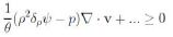

th 17

the dots denoting the other terms of the inequality. Hence we let p = ρ2δpψ.

Consequently we are left with the inequality

th 18

Thermodynamic Restriction on t 1

Sufficient conditions for inequality (14) are

t 2

It is suggestive that this thermodynamic condition has the form of (10)2. Yet we have to check whether t 4  Now, from the theory of mixtures we have

t 3

to within kinetic terms. If we let each ψα depend on the corresponding mass density

t 5

Hence  we  conclude  that,  to  within t 7 the standard chemical potential is

t 6

Thermodynamic Restriction on hα

Back to inequality (14) we let again η = −δθ ψ. Next we observe that tt 1 is given by (1). Substitution of tt 2 from (1) results in

tt 3

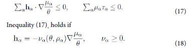
This inequality holds if each term has the required sign; in particular

tt 4

Hence, owing to the neglect of kinetic terms in ψ, by the second law inequality it follows that the diffusion flux hα is determined by the gradient of µα , and not merely of µα. This is a direct thermodynamic requirement without any need of a-priori rescaling [9].

Inequality (17)2 governs the evolution of a possible reaction. For a binary mixture the inequality reduces to

tt 5

the reaction proceeds toward the constituent with higher values of the chemical potential.

Diffusion of Electrically Charged Constituents

Equation (4) is a basic reference in the modelling of diffusion.

Indeed, for non-reacting mixtures the basic equation is written in the form

tωα = − · hα , (19)

the occurrence of ρ, though non-constant,  being  ignored;  in  the literature the notation is frequently ci and Ji for ωα and hα. For definiteness, look at the motion of a charged constituent in a fluid medium.

The diffusion flux is viewed as the sum of three terms [10]: a diffusion term Dα ∇ ωα as in Fick’s law, an advective term ωαv viewed as the transport of the constituent via the motion of the fluid, the diffusivity times the electric force (electromigration). The advective term may be ignored by selecting a frame at rest with the fluid.

An extensive approach in the literature is based on eq. (18) and on hα = −Dα ∇ ωα

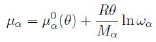
in the simplest model. Borrowing from the properties of the ideal gas we take the chemical potential µα in the form

d 1

to within inessential additive terms independent of ωα. Hence we observe that, at constant temperature,

d 2

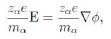
Now the chemical potential is an energy per unit mass. Assume the αth constituent consists of ions with electric charge zαe, where e is (the absolute value of) the electron charge. The force per unit mass is

d 3

φ being the potential and mα the ion mass. Moreover

d 4

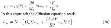
where F is the Faraday constant, i.e. the charge of a mole, and Mα is the molar mass. Hence we write the whole chemical potential, or electrostatic-chemical potential, in the form

d 5

This is a form of the Nernst-Planck equation [11].

Kirkendall Effect

The Kirkendall effect involves a property of diffusion associated with different diffusivities of the constituents. The property was found experimentally by Smiglskas and Kirkendall. In essence, molibdenum markers are located at the boundary between the inner CuZn block and the outer copper covering. Upon heating, the markers are observed to move inward. To explain the experiment, we observe that within the block Cu and Zn atoms have the same density N; since  the atomic weights are almost the same (Cu 63.5, Zn 65.4) the equal density N means equal concentration ω. The Zn atoms have a higher diffusivity coefficient and hence the outward flux of Zn is not exactly compensated by the inward flux of Cu atoms. Thus the mass of matter in the block decreases and this results in the movement of the copper- brass interface(markers) toward the inner block.
We now ask for the velocity of the markers. We have

ρZnuZn = hZn = −DZnω, ρCuuCu= hCu = −DCu ω;

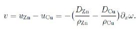
really we should account also for a inward flux of vacancies (from the material with the higher diffusion coefficient). In one dimension we obtain the velocity v of the markers as follows,

k 1

Dynamic Diffusion Equation

Models of diffusion are usually based on the balance equation (4) for the mass fraction ωα and a constitutive equation for the mass flux hα. Hence the resulting differential equation for ωα is strongly affected by the constitutive assumption. It seems of interest to look  at the evolution problem via the balance equations for the unknown densities ρα.

Restrict attention to mixtures of inviscid fluids and hence Tα = pα1. Consider the balance of mass and linear momentum in the local form,

21 22

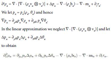
Partial time differentiation of the first equation, divergence of the second one, and substitution of · t(ραvα) yield

2ρα =  · [ · (ραvα ⊗ vα)] −  · ( · Tα) −  · (ραbα) − · mα + tτα.

If the constituent is regarded as an inviscid fluid, Tα = −pα1, it follows

21 22 down

If, further, the temperature is assumed to be uniform, ∇ θα = 0, then

23

Equation (23) is the αth equation of a system where ∇. mα and tτα account for possible coupling terms. Since ρα = ρωα, if ρ is assumed to be constant then we have

dy 1

If the αth constituent is electrically charged then

dy 2

where e is (the absolute value of) the electronic charge, zαe is the ionic charge, and mα

is the ionic mass. In terms of molar quantities we have

dy 3

where Mα is the molar mass and F is the Faraday constant, i.e. the charge of a mole. Hence, if E is uniform then we can write the equation for ωα in the form

dy 4

Quantum Diffusion Models

If a quantum particle moves in space under a force with potential U then the wavefunction

ψ evolves in time according to the Schr¨odinger equation

q 1

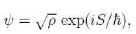
where m is the mass of the particle. Since ψ is complex valued then we can write

q 2

where ρ and S are functions of the position x and time t. The relation

q 3

ascribes to ρ(x, t) the probability density, per unit volume, of finding the particle at the point x at time t. Computing tψ, ψ and substituting in (24) we obtain

q 4

Equating the imaginary parts and observing that ∇ρ · ∇S + ρS = ∇·(ρ∇ S) we have

q 5

This equation has an immediate physical interpretation. If we let ρ be the analogue of the classical mass density then if we let

q 6

we can write (25) in the form

q 7

which is formally the continuity equation in continuum mechanics. This result indicates a close analogy between quantum and classical schemes which are extended to diffusion.

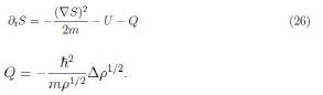
We now look for the possible meaning of the relation coming from equating the real parts. Upon some rearrangements we find

q 8

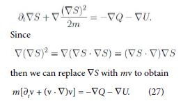
The quantity Q has the role of a potential, like U , and is often referred to as Bohm quantum potential [12]. Furthermore apply the gradient to (26) and assume S has continuous second-order derivatives to have

q 9

Equation (27) is formally the equation of motion with the Lagrangian (total) time derivative in the left-hand side, as it has to be. Consequently Q may also be viewed as a pressure term.

Diffusion is modelled by having in mind the parabolic character of the classical diffusion equation. Let P be the probability density of Brownian particles with mass m. Form the equation of motion we ascribe to P the equation

q 10

p being the opposite of the pressure. Then we let p = kBθP , where kB is the Boltzmann constant. In the high friction limit [13] it follows the parabolic equation

q 11

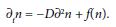
When quantum diffusion is described within a continuum mechanics approach the governing equation is taken in a Fick-like form. As an example [14], in the quantum diffusion of H atoms in solid molecular hydrogen films, the H atom concentration, n, is described by a differential equation in the form

q 12

Conclusions

Well-known diffusion equations are considered for the concentration (mass fraction) ωα = ρα. In addition to the classical parabolic equation (6) we have reviewed the Cahn-Hilliard equation (8) and the Ginzburg-Landau equation (9). The rather general approach to the modelling of diffusion processes is based on the view that the diffusion flux, here hα, has to be determined by a constitutive equation and that a safe rule is to let hα be proportional to the gradient of the chemical potential µα. As a remarkable example we have shown how the approach via chemical potentials, for charged constituents, leads to the Nernst-Planck equation. Diffusion in the quantum domain is still based on the classical Fick’s law.

While hα in terms of ωα is inherited from the historical Fick’s model, the recourse to the chemical potential is found to be thermodynamically consistent in two cases, just those leading to the Cahn-Hilliard and Ginzburg-Landau equations. In the present thermodynamic analysis the αth chemical potential is derived from the Helmholtz free energy

conclusion

instead of from ψα(ωα).

The developments of this paper show that the constitutive equations for the mass flux hα are in fact approximations; the involved equation for hα [1] justifies the recourse to approximations. However, the investigation of approximated  diffusion  equations  indicates  that a privileged role should be ascribed to the dynamic differential equations, based on the (exact) balance equations (21), (22). The difference in having recourse to the dynamic equations is exemplified with the analogue of Nernst-Planck equation.

Acknowledgments

This research has been developed under the auspices of INDAMCNR.

References

  1. Müller I (1975). Thermodynamics of mixtures of J. M´ecan. 14: 267-303.
  2. Morro A (2014). Balance and constitutive equations for diffusion in mixtures of fluids, Meccanica 49: 2109-2123.
  3. Fick A (1855). Ueber Ann. Phys. 170: 59-86.
  4. Kittel C (1976). Introduction to Solid State Wiley.
  5. Landau LD, Khalatnikov IM (1965). On the theory of Oxford.
  6. Cahn JW (1961). Spinodal Acta Metall. 9: 795-801.
  7. Cahn JW, Hilliard JE (1971). Spinodal decomposition: a Acta Metall. 19: 151- 161.
  8. Gurtin ME (1996). Generalized Ginzburg-Landau an Cahn-Hilliard equations based on a microforce Physica D. 92: 178-192.
  9. Brokate M, Sprekels J (1996). Hysteresis and Phase Springer.
  10. Kirby BJ (2010). Micro- and Nabnoscale Fluid Mechanics: Transport in Microfluidic Devices, Cambridge University Press.
  11. Bockris JO’M, Reddy AKN (1970) Modern Plenum Press.
  12. Bohm D (1952). A suggested interpretation of the quantum theory in terms of “hidden” I. Phys. Rev. 85: 166-179 (1952).
  13. Tsekov R (2009). Thermo-quantum Int. J. Theor. Phys. 48: 630-636.
  14. Sheludiakov S, Lee DM, Khmelenko VV, J¨arvinen J, Ahokas J et al. (2021) Purely spatial quantum diffusion of H atoms in solid H2 at temperatures below 1 K, Phys. Rev. Lett. 126: 195301.

Magnitude and Patterns of Female Genital Mutilation/ Cutting in Somaliland: The Case of Edna Adan University Hospital: A 17 Years’ Record Review

DOI: 10.31038/IGOJ.2022514

Abstract

Introduction: Female genital mutilation/cutting (FGM/C) involves partial or total removal of external female genitalia. The practice has no health benefits for girls and women. Somaliland is among the countries with the highest prevalence of FGM-C in the world.

Objective: To measure the magnitude and describe the trends of Female Genital Mutilation/Cutting among women attending Antenatal Care (ANC) and Delivery service at Edna Adan University Hospital, Hargeisa, Somaliland.

Methods: Edna Adan University Hospital, Hargeisa, Somaliland continuously records FGM/C status of pregnant mothers coming for ANC and delivery services since 2002. 13,320 antenatal and delivery cases were reviewed using a pre-determined checklist. Data were analyzed using IBM SPSS version 20, descriptive statistical analysis was performed. P-values less than 0.05 were considered statistically significant.

Results: Among the 13,320 reviewed charts, the overall prevalence of FGM/C was 96%. The reason for the majority (31.8%) of the FGM/C cases was traditional beliefs. Moreover, the majority (60.1%) of the FGM/C was performed by the traditional birth attendants (TBA). The median age that FGM/C is performed is 8 (IQR=3). The majority of girls are aged 7-10 when the procedure is performed. From 2002-2007, it was more common for an old woman to perform FGM; from 2007-2018, a traditional birth attendant conducted the procedure. Type III FGM/C (infibulation) appears to be the most commonly practiced type of FGM/C across the board.

Conclusion: The magnitude of FGM/C is high in Somaliland and is still practiced especially among women who are illiterate. The procedure is performed by traditional birth attendants for traditional reasons. Instigating interventions that would provide risk and benefit based health education to communities and promote girl-child education beyond the primary level could help end the practice.

Keywords

Edna Adan University Hospital, Female Genital Mutilation/Cutting, Somaliland, Traditional Birth Attendant

Introduction

Female genital mutilation (FGM) is defined by the World Health Organization (WHO) as all procedures that involve partial or total removal of the external female genitalia and/or injury to the female genital organs, whether for cultural or any other non-therapeutic reasons [1]. Globally, an estimated 200 million girls and women have undergone the cut, and approximately 70 million girls aged 0-14 years are at risk of being cut [2]. In a 2016 study, 25 communities living in the MaroodiJeex and Togdheer regions of Somaliland reported that the overall prevalence of FGM/C was 99%, with 80% having undergone infibulation [3].

The nomenclature for the practice varies across countries, ideological perspectives and research frames. According to the World Health Organization (WHO), female genital mutilation is classified into four major types:

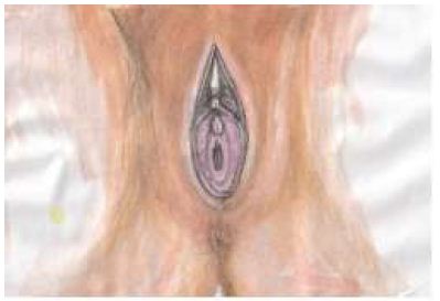
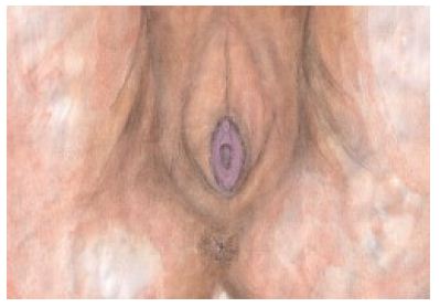
Type 1: Excision of the prepuce with or without excision of the clitoris (Figure 1).

fig 1

Figure 1: Type I of WHO classification of female genital mutilation/cutting

Type 2: Excision of the clitoris with partial or total excision of the labia minora (Figure 2).

fig 2

Figure 2: Type II of WHO classification of female genital mutilation/cutting

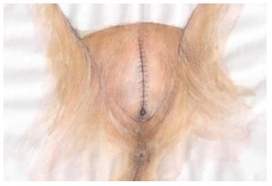
Type 3: Excision of part or all of the external genitalia and stitching together of the exposed walls of the labia majora, leaving only a small hole (typically less than 5cm) to permit the passage of urine and vaginal secretions. This hole may need extending at the time of the menarche and often before first intercourse (Figure 3).

fig 3

Figure 3: Type III of WHO classification of female genital mutilation/cutting

Type 4: This includes all other harmful procedures to the female genitalia for non-medical purposes (e.g. pricking, piercing, incising, scraping and cauterizing the genital area) [4].

Though FGM is practiced in more than 28 countries in Africa and a few scattered communities worldwide, its burden appears to be felt most heavily seen in Nigeria, Egypt, Mali, Eritrea, Sudan, Central African Republic (C.A.R.), and the northern part of Ghana where it has been an old traditional and cultural practice of various ethnic groups. The highest prevalence rates are found in Somalia, Somaliland, Djibouti and the Somali Region of Ethiopia where FGM is virtually universal [5].

Female genital mutilation/cutting (FGM/C) inflicts life-long injuries on women and their female children. It constitutes a violation of women’s fundamental human rights and threatens their bodily integrity. Historically performed by elderly women, or traditional birth attendants, FGM/C is a physically invasive procedure often associated with multiple adverse impacts [6]. FGM/C in Somalia and Somaliland is frequently performed on girls aged 5-9. This represents a shift in practice. Traditionally, FGM/C was performed in adolescence as an initiation into womanhood, but that is not true in Somali practices since FGM is performed in early ages [7]. Moreover, girls are one-third less likely to be cut than 30 years ago. According to the UNFPA-UNICEF joint program report on FGM/C,22 of the 30 of the countries involved where FGM is practiced and who are considered “least-developed” [8]. The health impacts associated with FGM/C that require interventions have been broadly categorized into the following categories: immediate, genito-urinary, gynecological, obstetric, sexual, and psycho-social consequences [9].

The reason why FGM is performed varies from one region to another as well as over time, and includes a mix of sociocultural factors within families and communities. In places where FGM is a social convention, strong motivations to perpetuate the practice of FGM include: the pressure to conform to what others have traditionally been doing, the need to be accepted socially, and the fear of being rejected by the community. Furthermore, FGM is often considered a necessary part of raising a girl, and a perceived requirement to prepare her for adulthood and marriage. In addition, FGM is often motivated by beliefs about what is considered acceptable sexual behavior. It aims to ensure premarital virginity and marital fidelity, by proving that her vulva has not been opened previously by any other man. Moreover, FGM is associated with cultural ideals of femininity and modesty, which include the notion that girls are clean and beautiful after removal of body parts that are considered unclean, unfeminine, or male [10].

In Somaliland, despite the continuous pledge to end female genital mutilation/cutting, this centuries-old practice still continues for non-medical reasons. Furthermore, the problem is not well-documented and reported. The majority of the studies about the prevalence and trends of FGM/C are based on reports from women attending health institutions. Moreover, community-based studies are expensive in nature. Information acquired from the woman’s own account has limitations since the woman might not easily understand the anatomy of her female genitalia nor be able to accurately classify the type of FGM/C that was performed on her. In order to overcome the limitations of such studies, reviewing hospital records and describing the magnitude and pattern of FGM/C must be appropriately verified by midwives and physicians. Moreover, understanding these phenomena could guide efforts to curb this harmful practice and reduce the morbidity and mortality of mothers and children. Furthermore, the investigators have developed the following research questions:

What is the overall prevalence of FGM/C in Somaliland?

What is the most prevalent type of FGM/C in Somaliland?

What does the trend of FGM/C look like since 2002?

What is the average age of practicing the FGM/C?

Is there association between FGM/C and educational status of the mother?

Method and Materials

Description of the Study Area and Study Setting

General Setting

According to the Somaliland Health and Demographic Survey 2020 (SLHDS, 2020) report, over 48 percent of Somaliland’s population is under the age of 15 years old, and 48 percent of the population is within the working age group (15-64 years old). The population of Somaliland has an average household size of six. Early marriage is common, particularly for women, as 23 percent aged 20 -24 interviewed were married by the time they turned 18 years old. FGM/Chas been practiced in Somaliland for several decades with insignificant declination. Furthermore, more than 70 percent of women indicated that the forms of domestic violence they are subject to by their husbands are physical assault, denial of education, forced marriage, rape, and sexual harassment. SLHDS noted that an overwhelming 67 percent of births were delivered at home. The death rate among reproductive age women is highest with 9.4 deaths per 1,000 populations, among women aged 30-34. This is also the age group in which childbearing hits its peak. Somaliland’s Maternal Mortality Rate (MMR) is 396 per 100,000 live births. Female Genital Mutilation/Cutting (FGM/C) is prevalent among 98% of women in their reproductive age [11].

Study Site

Edna Adan Ismail, a UK/US trained Somaliland certified nurse midwife, has been seeing patients with cases of FGM/C for the duration of her 50 years of midwifery experience, and has been engaged in a life-long struggle to put an end to this practice. With the establishment of her maternity hospital which is now a major teaching and referral general hospital, as well as with the still much-needed national services to combat FGM/C practices, it has become essential for the hospital to lead a campaign to tackle this tradition against women’s rights. The hospital is fast becoming a repository of all information relating to FGM/C in Somaliland and the region. The hospital has been registering mothers coming to the hospital for antenatal care (ANC) and delivery service since 2002. Though these were used as audit reports, these huge data sets have not been adequately analyzed. This research team has been established to conduct a detailed analysis and point out the important findings that would answer the above listed research questions and contribute for planning and interventions to end FGM/C by all stakeholders.

Study Design and Population

We conducted a 17 years’ retrospective hospital-based medical-record review in February 2022. After securing ethical clearance from the Edna Adan University Hospital Ethical Review Committee (ERC), we reviewed all 13,320 records of women who visited the antenatal clinic and who gave birth at Edna Adan University Hospital between the years 2002-2018. The female genital mutilation or cutting (FGM/C) data has been continuously recorded by the hospital starting from 2002 to 2018.

Data Extraction and Analysis

The data was extracted from the ANC and delivery charts using a predetermined English version data extraction checklist by 18 senior public health students and another two supervisors who were trained for three days on how to extract information from the ANC and delivery charts. Extracted data was cross-checked by the research assistants and all necessary modifications were made. Moreover, data entry, editing, coding and recoding, descriptive statistics, numerical summary measures, and analytic statistical tests such as Chi-square test and correlation tests were done using SPSS version 20 statistical software by the principal investigator and the research team. p-value and 95% confidence interval was used to determine if there was association among the variables or not. p-value less than 0.05 was considered a statistically significant association. In this study, classification of FGM/C was in accordance to the World Health Organization (WHO). After extraction of the required information, the charts were kept confidential and sent back to the hospital repository.

Variables

The following variables were extracted from the records: sociodemographic characteristics such as age, residence, educational status, and the year the data was collected; and FGM/C related variables such as FGM/C status, FGM/C type, reason for FGM/C, agent who performed the practice and place it was performed, age FGM/C was performed, as well as if FGM/C of daughter was performed and the reason for FGM/C.

Ethical Approval

Ethical clearance was solicited from the office of research and ethical committee of the Edna Adan University Hospital (ERC: EAUH/5973/22, dated 23 February, 2022) and confirmation of permission to access the data from the archives was secured from the hospital Director. The patient charts were properly handled ensuring the respect for the confidential nature of the survey during the data extraction and returning the charts to the repository of the hospital for storage.

Results

We reviewed and explored total of 13,320 ANC charts about the educational level of the clients, the reasons for performing FGM/C and the agent responsible for performing the procedure – we found that the overall prevalence of FGM/C in the patient population was 96%. The majority (60.2%) of the FGM/C were illiterate. And, the reason for the majority (31.8%) of the FGM/C cases was for traditional belief. Moreover, the majority (60.1%) of the FGM/C was performed by the traditional birth attendants (Table 1).

Table 1: Distribution of educational level, reasons for FGM/C and agent who performed the procedure, Hargeisa, Somaliland

table 1

NA* refers to Not Available

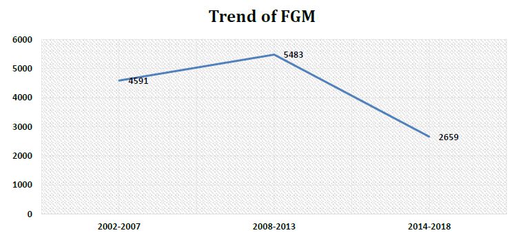
We have also run an analysis to look at the trend of the FGM/C and it depicts that there is a slight increase from 2002-2007 to 2008-2013, whereby the number of FGM/C procedures performed goes from 4591 (36%) to 5483 (43%). However, there is a steady decline of cases from 2008-2013 to 2014-2018 in which the cases reported was 2659 (21%) (Figure 4).

fig 4

Figure 4: A 17 years’ trends of Female Genital Mutilation in Hargeisa, Somaliland

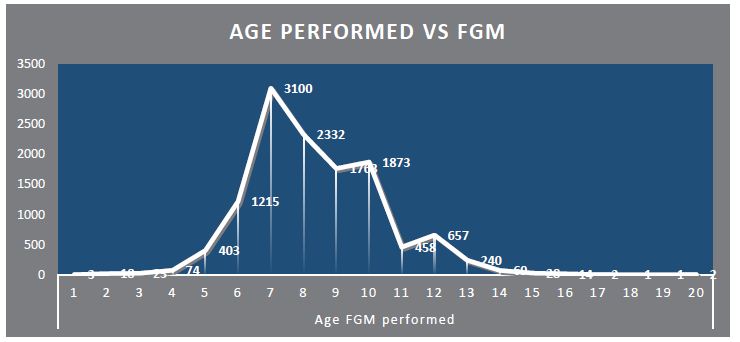
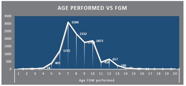
The following figure shows that the median age that FGM is performed is 8 (IQR= 3) years old. The majority of girls are aged 6-10 when FGM is performed. Moreover, FGM/C declines sharply after the age of 12 and almost insignificant before the age of 4 (Figure 5).

fig 5

Figure 5: Distribution of the age FGM/C is Performed, Hargeisa, Somaliland

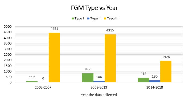
Even though there are fluctuations across the 17 years, it is observed that from 2002-2007 had the highest record rates of type III FGM/C 4451 (36%), as well as in 2008-2013 were the number of cases was 4315 (35%) though number of cases were declining 2014-2018, 1926 (16%). Type III FGM/C (infibulation) appears to be the most commonly practiced type of FGM/C across the board (Figure 6).

fig 6

Figure 6: Distribution of FGM type per year, Hargeisa, Somaliland

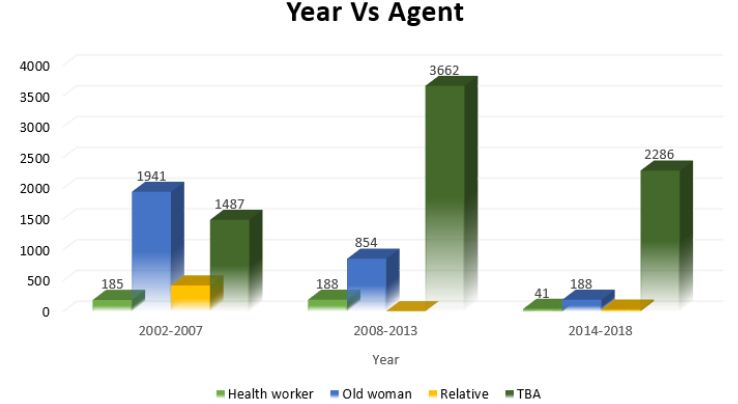
The following figure denotes that from 2002-2018, an old woman or traditional birth attendant were most commonly those that performed FGM/C. From 2002-2007, it was more common for an old woman to perform FGM, whereas from 2007-2018, a traditional birth attendant did the procedure (Figure 7).

fig 7

Figure 7: Distribution of the year and the agent who performed the FGM/C. Hargeisa, Somaliland

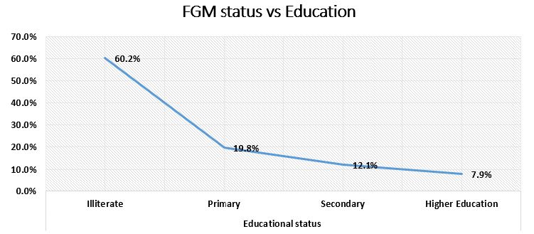
We used Chi-squared test statistic to assess whether education level and FGM/C status are associated, and we found that there is a statistically significant association (p-value=0.001). Moreover, we observed a sharp decrease in likelihood to perform the FGM/C procedure as education level rises. In addition, those that perform FGM/C on their daughters are most commonly illiterate (Figure 8).

fig 8

Figure 8: The pattern of FGM/C cases versus Educational Level, Hargeisa, Somaliland

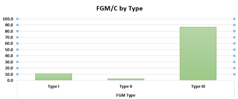
Type III FGM is found in almost 87 percent of the population we studied from 2002-2018, making it the most common type of FGM performed among those studied (Figure 9).

fig 9

Figure 9: Distribution of the Type of FGM/C, Hargeisa, Somaliland

Discussion

Somaliland continues to house a high prevalence of the phenomena known as female genital mutilation and cutting, compared to other countries in the horn of Africa and in Eastern Africa. This could be attributed to the fact that Edna Adan University Hospital is the only hospital in Eastern Africa that we know of that collects such data. As previously stated, the problem is not well-documented and reported; due to this, our research team set out to encapsulate the data of 13,320 women polled at the Edna Adan University Hospital in Hargeisa, Somaliland to fully grasp the magnitude and trends of FGM/C, based upon women’s reports taken during their antenatal appointments at our health institution. Their information was kept confidential throughout the entirety of the process and the patient files were returned to the repository in which they were stored upon completion of the analysis of the data presented.

The investigators developed the following research questions in order to fully understand the data gathered from 2002-2018: What is the overall prevalence of FGM/C in Somaliland? What is the most prevalent type of FGM/C in Somaliland? What has the trend of FGM/C looked like since 2002? What is the average age of those who had undergone FGM/C? Is there an association between FGM/C and educational status?

The current study reveals that the overall prevalence of FGM/C is 96% among the patients who attend Edna Adan University Hospital that may not give a true picture of the situation in Somaliland. However, this result goes beyond previous studies conducted in Tanzania, Nigeria, Yemen, Burkina Faso, Gambia, and Mauritania, where the prevalence of FGM/C was (45.2%, 45.9%, 48%, 68.1%, 75.6%, and 77%), respectively [12-17].

Moreover, the major findings associated with the research questions presented are as follows: it appears that there is a slight increase in the trend of FGM from 2002-2007 to 2008-2013, where the number of FGM/C procedures performed goes from 4591 (36%) documented cases to 5483 (43%) documented cases. There was a steady decline in cases from 2014-2018 which the case reported was 2659 (21%). Besides, our study is against when compared to a meta-analysis conducted in Ethiopia where the prevalence of FGM/C was higher from 2013-2017 (78.39%, 95% CI: 48.2, 108.5) [18].

A similar study conducted in Egypt to assess the prevalence of FGM among girls showed that the average age at which girls underwent FGM was 10.1 years, which is higher when compare to our findings that it is 8 years old [19]. Moreover, in our study, the majority of girls are aged 6-10 when FGM is performed.

Furthermore, it appears that in 2002-2007, record rates of type IIIFGM occurred, as well as in 2008-2013. Type III FGM seems to be the most common type of FGM performed across the span of the data in its entirety. Between 2002 and 2018, type III FGM was observed in 87 percent of the population studied. As a result, it is the most common type of FGM among those studied. This result ties well with a previous study conducted in Sudan, wherein type III FGM was the most common practice, while 66 percent of those who had undergone FGM had type III FGM [20].

Nevertheless, when it comes to agents who performed FGM, a study carried out in Burkina Faso explored that traditional practitioners performed the vast majority (82.4%) of FGM [15]. However, it is also a point of interest to note that the data suggests that an old woman or traditional birth attendant were most commonly those who performed FGM. From 2002-2007, it was more common for an old woman to perform FGM, whereas from 2008-2018, a traditional birth attendant performed the procedure.

Another study conducted in the United Arab Emirates to assess the association between educational status and FGM/C found that there is a statistically significant association between FGM status and educational level (p-value 0.001). Moreover, there was an inverse association between FGM status and literacy level: with increasing educational levels, there was a decrease in the proportion of women with FGM/C [21]. This result ties well with our data, which indicates that there is a sharp decrease in the likelihood of performing the FGM procedure as education level rises. Those that perform FGM on their daughters are most commonly illiterate. As the family’s education level rises, they are less likely to perform FGM on their daughter, suggesting there is a strong association between the education level of the family (the mother specifically) and the likelihood that she will organize the FGM/C procedure to be committed for her daughter (s) (p-value 0.001). We consider this to be the most important finding because if wide-spread education about the harms and tribulations of FGM/C and its long-term and short-term effects on those it is performed upon could target far-reaching communities as well as those in big cities, there may be a notable shift in the number of FGM/C cases seen in Hargeisa, Somaliland and other surrounding areas.

Alternatively, it is possible that the decrease in FGM/C cases is not solely attributable to the rise in education levels of the family. It could be possible that campaigns against the practice of FGM/C are also influencing attitudes towards FGM/C which are shifting ever so slightly with the younger population as they enter their reproductive years. Further studies to explore this variable would have to be conducted in order to be confirmed.

In regards to the type of FGM/C that is most commonly performed, it is possible that the data is not entirely accurate and can only be confirmed if a healthcare provider (nurse, midwife, or doctor) does a thorough exam of the patient’s genitals in order to confirm if it is indeed type I, II, or III FGM/C that was performed. It is highly likely that the women do not fully grasp the difference between the types of FGM or can accurately report the type that was done to them. During ANC, it is the nurse or midwife who physically examines the patient and who verifies the type of FGM/C seen in the patient.

There were limits to the study as well – the data for 2005, 2006 and 2019 appears to be incomplete and, due to very scarce data in 2019, it was omitted from the report. The data for 2020-2022 has not been documented during antenatal appointments, so our data is only up to date insofar as 2019.

Another limit is the amount of data made available to the research team-in order to fully encapsulate the prevalence of FGM/C in this area of Africa, other hospitals in Somaliland, as well as in neighboring countries, would have to be included in the study as a means of comparison. That extent of data was not made available to this research team, and further research would need to be done in order to accurately capture the desired results.

Conclusion

In this study, we documented and reported women’s sociodemographic characteristics such as age, residence, educational status, and the year the data was collected; and FGM/C related variables such as FGM/C status, FGM/C type, reason for FGM/C, agent who performed the practice and place it was performed, age at which FGM/C was performed, as well as if FGM/C of a daughter was performed and the reason for FGM/C. We chose these variables in the hope that trends in the data would appear. Most notably, there is an association between the education level of the mother and the likelihood that she will perform FGM/C on her daughter. There also appears to be a great likelihood that type III FGM/C will be performed on girls, the median age that FGM is performed is 8 years old, most commonly between the ages of 6 and 10, and that the procedure will be done either by a traditional birth attendant or an old woman in the community.

Overall, it appears that FGM/C is not decreasing in prevalence as the years go by. Further research into the prevalence for the years 2019-2022 should be conducted in order to accurately capture the number of FGM/C cases seen at Edna Adan University Hospital until now. Further data should have to be collected from the surrounding hospitals in order to conduct a comparative analysis.

Acknowledgement

We are pleased and thankful to Edna Adan University Hospital. We also acknowledge our data collectors for their tireless effort.

References

  1. Organization WH (1998) Female genital mutilation: an overview: World Health Organization.
  2. Shell-Duncan B, Naik R, Feldman-Jacobs C (2016) A state-of-the-art synthesis on female genital mutilation/cutting: What do we know now?
  3. Newell-Jones K (2016) Empowering communities to collectively abandon FGM/C in Somaliland. Action Aid. 2016.
  4. https://www.who.int/news-room/fact-sheets/detail/female-genital-mutilation [Internet].
  5. Okeke TC, Anyaehie U, Ezenyeaku C (2012) An overview of female genital mutilation in Nigeria. Annals of Medical and Health Sciences Research 2: 70-73. [crossref]
  6. Berg RC, Underland V (2014) Gynecological consequences of female genital mutilation/cutting (FGM/C): Nasjonalt kunnskapssenter for helsetjenesten. [crossref]
  7. UNFPA-UNICEF Joint Programme on Female Genital Mutilation, August 2018.
  8. Activities UNFfP (2015) Demographic perspectives on female genital mutilation: UNFPA.
  9. Berg RC, Underland V, Odgaard-Jensen J, Fretheim A, Vist GE (2014) Effects of female genital cutting on physical health outcomes: a systematic review and meta-analysis. BMJ Open 4: e006316. [crossref]
  10. World Health Organization (WHO) fact sheets, Female Genital Mutilation (FGM), 21 January 2022 [Internet].
  11. The Somaliland Health and Demographic Survey 2020 (SLSDH 2020).
  12. Klouman E, Manongi R, Klepp KI (2005) Self‐reported and observed female genital cutting in rural Tanzania: Associated demographic factors, HIV and sexually transmitted infections. Tropical Medicine & International Health 10: 105-115. [croosref]
  13. Snow RC, Slanger TE, Okonofua FE, Oronsaye F, Wacker J (2002) Female genital cutting in southern urban and peri‐urban Nigeria: self‐reported validity, social determinants and secular decline. Tropical Medicine & International Health 7: 91-100. [crossref]
  14. Alosaimi AN, Essén B, Riitta L, Nwaru BI, Mouniri H (2019) Factors associated with female genital cutting in Yemen and its policy implications. Midwifery 74: 99-106. [crossref]
  15. Inungu J, Tou Y (2013) Factors associated with female genital mutilation in Burkina Faso. Journal of Public Health and Epidemiology 5: 20-28.
  16. Kaplan A, Forbes M, Bonhoure I, Utzet M, Martín M, et al. (2013) Female genital mutilation/cutting in The Gambia: long-term health consequences and complications during delivery and for the newborn. International Journal of Women’s Health 5: 323. [crossref]
  17. Ouldzeidoune N, Keating J, Bertrand J, Rice J (2013) A description of female genital mutilation and force-feeding practices in Mauritania: implications for the protection of child rights and health. PLoS One 8: e60594. [crossref]
  18. Fite RO, Hanfore LK, Lake EA, Obsa MS (2020) Prevalence of female genital mutilation among women in Ethiopia: A systematic review and meta-analysis. Heliyon 6: e04403. [crossref]
  19. Tag-Eldin MA, Gadallah MA, Al-Tayeb MN, Abdel-Aty M, Mansour E, et al. (2008) Prevalence of female genital cutting among Egyptian girls. Bulletin of the World Health Organization 86: 269-274. [crossref]
  20. Satti A, Elmusharaf S, Bedri H, Idris T, Hashim MSK, et al. (2006) Prevalence and determinants of the practice of genital mutilation of girls in Khartoum, Sudan. Annals of Tropical Pediatrics 26: 303-310. [crossref]
  21. Al Awar S, Al-Jefout M, Osman N, Balayah Z, Al Kindi N, et al. (2020) Prevalence, knowledge, attitude and practices of female genital mutilation and cutting (FGM/C) among United Arab Emirates population. BMC Women’s Health 20: 1-12.

Ordinary People Thinking about What Emotional Issues Obesity Might Trigger: A Mind Genomics Cartography

DOI: 10.31038/EDMJ.2022613

Abstract

107 respondents each evaluated 60 unique vignettes (combinations of two, three or four messages), dealing with descriptions of how a person with obesity might feel. The respondent rated each vignette on degree to which the vignette would provoke a feeling of ‘cannot deal with it’ (viz., strong anxiety). Deconstruction of the responses to the full set of 36 messages on a respondent-respondent basis revealed that two specific messages provoked the highest degree of anxiety; you believe that the food industry will work to help you find the right foods to eat and you just can’t control the eating. Substantial differences emerged for age, and for the location where anxiety might be experienced (e.g., while listening to music.). Clustering the 107 respondents into mind-sets, groups with different points of view, revealed three radically different group, based on the elements which drive anxiety: MS1 – Anxiety about acceptance by others; MS 2 – Anxiety when thinking about professional help; MS3 – Anxiety about helplessness and being out of control.

Introduction

As the technology of agriculture and food production has become increasingly sophisticated, and the retailing of food has become embedded in our society, people have gained weight. Today, 2022, obesity) is considered a major health problem, both in developed and developing countries. We eat more than we need. The medical literature on obesity is rivaled by the popular literature, both dealing with the need to lose weight, the former for health reasons, the latter for social reasons.

Although obesity is moving into the realm of ‘disease’, rather than something about which one should feel shame, being overweight, fat, and so forth calls into play the confluence of emotions and health. Those who are fat feel inadequate because they fail to live up to society’s norms, even though increasing number of people can be classified as obese, many morbidly so.

The ‘literature’ about obesity divides into at least two areas, obesity in terms of medical issues, and obesity in terms of the personal/emotional/behavioral issues. Furthermore, the literature of obesity encompasses scholarly work of a scientific nature and an almost uncountable amount of information coming from the popular press. People are interested in how they look, how they feel, and often subscribe to various diets, fad and otherwise, to lose weight.

Most of the published studies about the mind of the obese person work with obese individuals, using directed interviews and group discussions on how they feel, looking at how these individuals respond on standardized scales of emotion all with the goal to understand the difference between the emotional responses of obese individuals and those of normal-weight individuals. For example, working with seven very obese women [1] used a ‘religious-history’ questionnaire. The questionnaire was content-analyzed, revealing feelings of helplessness and powerless, strong guilt feelings, and craving for love.

In a more directed study, but still one requiring the respondents to find language for their emotions [2] instructed adolescents to imagine eating each of 30 different foods, and to report their feelings. In this study the respondents used their own terms the focus, however, was not so much on the emotions themselves as it was on the differences between the normal weight and obese respondents in their emotions.

As one focuses in on emotions as a critical factor, it is easy to recognize the link between emotions and eating, especially when one deals with obesity. The key is to formalize that link, to understand it. A study [3] emphasized the variable nature of the emotion, recognizing that individual differences both in the food and in the emotions precipitating eating should be studied.

Our focus in this paper is on the ‘mind’ of the ordinary person when they think of obesity. If a person were obese, or were to think about being obese, how would the person feel about the ordinary aspects of daily life? What would bother them if they were obese, or at least what do they think would bother them? The approach taken in this paper comes from the world of consumer research, with the goal of understanding the mind of the consumer. If the person were to look at a description of a situation, that situation involving an obese person, how would the person, respondent, react? Would the respondent be indifferent? Or would the respondent feel a sense of anxiety, and panic?

Perhaps the paper which comes most close to the Mind Genomics efforts is [4]. In a qualitative study dealing with how people experience their own obesity, they described the impact of obesity on their self-identity using language such as “ugly”, “freak”, “hate”, “blob”, and “disgust” which reflected the pervasively negative impact of their weight…. Participants described the multitude of ways being obese impacted upon their self-identity and their lives in general. In particular they described how it had influenced their mood, their self-perception, a feeling of dissociation, and their health.”

As will be shown in the results section, the approach, Mind Genomics, applied to the emotions surrounding presumed obesity shows dramatic ways of thinking which pertain to everyday life. The ability to segment individuals into mind-sets, a hallmark feature of Mind Genomics, further provides a new approach to how people think about the obese individual, more from the vantage of everyday life than from the usual clinical perspective.

The Mind Genomics Approach

Mind Genomics evolved from a mixing of experimental psychology, statistics, and consumer research. The author has discussed the origins of Mind Genomics in a retrospective on more than a half a century of psychology research [5]. The three fields reflect different, complementary efforts to understand the world.

Psychophysics

Experimental psychology, and more specifically psychophysics, lies at the base of Mind Genomics. Rather than understanding the phenomena from the point of view of individual discussion, as the clinician might do, experimental psychology seeks to understand by varying antecedent conditions in a controlled fashion, measuring the response, determining the pattern of co-variation, and indeed at some level the pattern of causation. The key word is ‘experimentation,’ viz., the systematic alteration of conditions, measuring the reactions, and defining the underlying pattern. The contribution of psychophysics, the branch of experimental psychology best associated with Mind Genomics, is the desire to create a descriptive equation that can be used, respectively, to describe and to predict.

Statistics (Experimental Design, Regression Modeling and Clustering)

The actual stimuli in Mind Genomics studies are phrases which paint a word picture, these phrases combined in a systematic way, according to an underlying structure. Experimental design defines this systematic way. Experimental design is a branch of statistics which specifies certain combinations to be tested, with the design ensuring that the contribution of each component in the design can be individually estimated. Beyond the experimental design is the use of regression modeling to discover the linkage between the rating assign to the vignette (response) and the independent variable, viz., the stimuli tested (the individual elements that were combined in the vignettes in the vignettes).

Consumer Research

Consumer researchers generally work with meaningful test stimuli, rather than with stimuli artificial simplified and modified. Consumer researchers do not generally work with test situations isolating every variable but one, and modifying that variable. Such an approach is left to researchers who are working on theory, to validate or to disprove a theory. Consequently, the test stimuli used by Mind Genomics are words (or pictures), couched in ordinary consumer language, generally independent of theory. The goal for consumer researchers is often to understand how the consumer responds to stimuli which are meaningful in everyday life. Following that approach, the studies in Mind Genomics use phrases which paint word pictures that a normal person can understand without much effort.

Illustrating the Process with the Study on Obesity

Twenty years ago, around the beginning this 21st century, the author and colleagues implemented a long-discussed vision, viz., to create a database of the human mind, in terms of the way people make decisions. The goal was to move away from the artificial environment created by psychology experiments, these experiments design to confirm or disconfirm the theory (so-called hypothetico-deductive system). Rather than doing experiments within the confines of a theory, the idea was to study the way people reacted to information about a topic, doing so in a way which would create a database of the mind. The approach, Mind Genomics, emerged not from experimentation with people in a situation, but rather from studying the response of people to sets of messages [6,7].

The It! Studies were motivated by the development of an off-the-shelf version of Mind Genomics, then called ‘IdeaMap®’. The initial studies with IdeaMap® dealt with one-off issues, generally related to consumer goods. It was the recognition that one could generate a ‘signature’ of a product, in the language of consumers, which motivated the extension of IdeaMap®, first into the experience of buying products in stores, and then into the experience of anxiety provoked by common, realistic issues facing people. These studies have continued, and during the last twenty years the number of studies has increased dramatically. Topics ranged from the composition of products [8] to shopping for these products in the midst of the Covid-19 epidemic [9].

Moving beyond single studies to creating a database of the mind constituted the next step in the evolution of Mind Genomics. Rather than doing ‘one-off’ studies in different areas, the vision was to do a set of related studies, with the studies having the same underlying structure. The first set of related studies, funded by the McCormick & Company researcher department, was Crave It! The goal was to understand what aspects of food make us ‘crave’ the food. Shortly after there were sets of parallel studies on beverages (Drink If!), good for you foods (Healthy You), and the shopping experience for different household- products (Buy It!).

In 2003 the notion of expanding The It! studies to issues of anxiety emerged out of discussion among a group of researchers, viz., the author and colleagues [10,11]. The colleagues, Jacquelyn Beckley and Hollis Ashman of the Understanding and Insight Group in New Jersey drafted the first study, with its structure shown in Table 1 for obesity. Once the study had been constructed, it was straightforward to expand the topics to 14 other topics dealing with anxiety-provoking situations. Figure 1 shows the 15 studies, all ‘launched’ at the same time. The structure of the studies was maintained as much as possible, although as noted below, some of the elements had to be modified to accord with the study topic.

The remainder of this paper presents the study on obesity, was part of a set of 15 parallel studies called ‘Deal With It!’. We begin with the steps followed to set up the study, and move into a deep analysis of the results.

Table 1: The elements for the obesity ‘Deal With It!! Study. The left side shows the rationale for the element, the right side shows the specific language for the obesity study

table 1


fig 1

Figure 1: The 15 Deal with It! studies on a wall. The respondent chose the study she/he found interesting, and participated in that study

Step 1: Create the Elements to Describe One’s Personal Experience

The four sets of questions and nature of the answers were set up ahead of time. The structure on the left side of Table 1 was maintained for all 15 Deal With It! studies. The elements A1-A9, B1-B9, and some of the elements in Question 4 were different across the studies, to accord with the topic. The spirit of the answers were the same, but the specifics had to be modified to make sense. For the nine elements in Question C, the elements were far more similar to each other across studies, because there was no need to particularize the element to the topic.

The rationale for the elements was to make the language ‘vernacular,’ viz., informal. The motivation was to move away from a formal, possibly off-putting clinical presentation, and instead make the language informal, almost ‘folksy.’

Step 2: Create Vignettes – Mix Together Elements According to an Experimental Design

Mind Genomics differs profoundly in the way it measures the response to ideas, the messages shown in Table 1. Mind Genomics combines these messages in a systematized way to create vignettes, small, easy to read combinations of the messages. To the ordinary eye the combinations seen ‘haphazard,’ with the term ‘randomly put together’ often used to describe the 60 different combinations that would be evaluated by a single respondent. To that respondent, the combinations do seem random, but nothing could be further from the truth. The combinations are set up so that each combination or ‘’vignette’ comprises a minimum of two elements, a maximum of four elements, with all elements appearing an equal number of times across the 60 vignettes. Furthermore the 36 elements are statistically independent of each other, allowing the researcher to use programs like OLS (ordinary least-squares) regression to estimate how each element drives the ‘rating’ that the respondent is instructed to assign, after reading the vignette.

A further feature of the experimental design is that each respondent evaluates a unique set of 60 vignettes or combinations, so only in rare occasions do two respondents ever evaluate the same vignette. This novel approach, the so-called ‘permuted design’, acts metaphorically like the MRI, magnetic resonance imaging. With the MRI, the camera takes many X ray pictures of the underlying tissue, doing so from different angles, and afterwards combines them by computer to extract a 3-dimensional picture from a set of two-dimensional x-rays. Metaphorically, each respondent represents a different ‘angle’. The result is a deeper, more detailed view of the topic, because across the 107 respondents whose data are analyzed here, each respondent evaluating 60 different vignettes, we end up with 6420 different vignettes evaluated by the respondent. There is no need to ‘know the best combinations’ at the start of the study because the experimental design ensures that the researcher will sample a great deal of the underlying set of combinations [12].

It is important to emphasize that it is impossible to ‘game’ the Mind Genomics system. With a set of 60 vignettes, even the most dedicated effort will fail to uncover the pattern. As a consequence, the respondents stop trying to outwit the system, stop trying to give the ‘right answer’. Rather, they settle into an almost bored state, where they see something and they respond, pressing a key on the 9-point scale. As soon as the respondent pressed the rating scale the vignette disappeared, to be replaced by the next vignette. The rating scale, however, remained.

The instructions to the respondent were presented at the start of the study, the study executed on the computer. Figure 2 shows the standardized instructions, used for all 15 studies. The only thing which changed was the name of the study.

fig 2

Figure 2: The orientation page, showing the topic (black rectangle), the rating scale, the expected length of time, and the reassurance that all vignettes are different

The actual vignettes were presented one at a time. As soon as the respondent assigned a rating the next vignette appeared. The 9-point rating scaling was always present on the screen, or at least appeared so as the on-line ‘experiment’ proceeded. In actuality, each vignette was totally new. The vignette comprised the elements at the top (in centered format, but without connectives). At the bottom of the screen was the refreshed rating scale.

By 2003, the year of the study, people were already accustomed to doing surveys on the Internet. The interview was described as a ‘survey’ rather than the more correct description, ‘experiment.’ The rationale was that the term ‘experiment’ might be off-putting and frightening.

The actual vignettes are described as situation screens, to which the respondents are asked to judge how she or he would react. No effort was made to measure the degree to which the respondent felt that the screen actually described them. That is, the respondent was treated as a disinterested judge, evaluating a situation or a scenario. In this way the appearance of an objective evaluation was maintained, even though the only criteria used by the respondent were her or his own point of view.

Finally, it is important to note that the introduction for each of the 15 studies was exactly the same, except for the topic. Thus, the top of the page welcomes the respondent, and gives the name of the study), where the black rectangle appears. For the obesity study the word was ‘obesity.’ The respondents are further told how long to expect the ‘survey’ to take (15-20 minutes), and that all the vignettes (screens) are different. This reassurance that ‘no screen is exactly repeated’ comes from the experience of respondents saying that they were sure they saw repeat screens, which of course they could not by virtue of the underlying experimental design.

Analysis

The Mind Genomics ‘process’ begins by transforming the ratings, bifurcating the original 9-Point Likert Scale into two regions. The rationale for this is that most users of the data end up asking ‘what does a certain value mean?’ This question can be asked of the original scale values (e.g., what does a rating of 8 mean on the scale), or it can be asked of the average rating across groups. Most peoples, including professionals, really do not understand the meanings of the different scale points. As a consequence of the widespread failure to understand what scale values really mean in everyday life, consumer researchers as well as public opinion pollsters have moved away from using Likert value data in reporting to using percentages, making their presentations easier to understand.

Following the aforementioned issues eventuated in Mind Genomics dividing the 9-point scale, almost arbitrarily, into ratings 1-6, coded 0, and ratings 7-9 coded 100. A vanishingly small random number is added to each of the transformed numbers, so that the binary ratings exhibit some random variation. That random variation will be necessary to avoid statistical issues when we deal with the individual-level modeling (viz., fitting equations to the data). The random variation will be so small, however, that there will be no effect on the data, other than avoiding the problem of having no variation in the ratings (viz., when a respondent assigns all vignettes either ratings 1-6, or ratings 7-9, which end up producing all 0’s or all 100’s as transformed values). The subsequent regression analysis cannot then be ‘run,’ and the analysis ‘crashes.’

The second step in Mind Genomics analysis creates an individual-level equation relating the presence/absence of the 36 elements to the binary response, 0/100, respectively. The aforementioned addition of the random variation to the transformed variable ensures that the regression analysis will always deal with data for which the dependent variable has ‘variation. The regression analysis is estimated using OLS (ordinary least squares) regression, a standard statistical analysis procedure. The regression generates the following equation: Binary Response = k0 + k1 (A1) + k2 (A2)… k36 (D9).

The data from all respondents generate a database. A total of 120 respondents participated. The data from 13 respondents were eliminated because their responses showed no variation at all. That is, all their ratings from 60 vignettes lay either between 1 and 6 (transformed to 0), or 7-9 (transformed to 100). Little can be learned from their reaction. This left 107 respondents who clearly discriminated among the elements, in terms of some elements driving anxiety, and the other elements not driving anxiety.

Summarizing the Data in an Easier Format

The aforementioned binary response equation generates a set of coefficients which show the likelihood that the specific element would drive a positive anxiety response, manifested by the rating 7-9 (‘cannot deal with it’, in the vernacular language of the rating scale). Negative coefficients mean that the element does not drive anxiety. Negative coefficients do not mean, however, that the element reduces anxiety. Quite the contrary. Negative coefficients simply mean that the element does not drive anxiety. The element may do absolutely nothing, or may reduce anxiety. We do not know. Our focus will be solely on the positive coefficients.

In the light of the meaning of the coefficient, our final transform is done on the coefficients themselves. All estimated coefficients for the 36 elements for each respondent, viz., k1-k36, were themselves rescaled. Coefficients of 8 or higher, corresponding to ‘cannot deal with it’ were transformed to 100. Coefficients of 7. 99 or lower, including 0 and negative coefficients, corresponding to elements which do not drive strong anxiety, were transformed to 0. The choice of ‘8’ as the cutoff comes from analyses of the regression modeling, which suggests that coefficients of 8 or higher are ‘statistically significant’, viz., the t statistic approaches 2.0. Furthermore, with coefficients of 8 (or more typically 10) or higher, one begins to see external behavior which confirms that the element or message is relevant for behavior.

Table 2 shows an example of the 36 elements, (columns 1, 2), the coefficient emerging from the regression model (column 3), and the transformed coefficient (column 4). When we look at the data from total panel and key subgroups, this rescaling of coefficients will provide us with easy-to-understand averages, showing which elements drive anxiety and which do not.

Table 2: Example of the 36 estimated coefficients for two respondents (A, B, columns 3 and 4), their transformed value (columns 5 and 6). Coefficients of +8 or higher were transformed to 100. Coefficients lower than +8, whether positive, zero, or negative, were transformed to 0

table 2

What Drives Anxiety When Reading Vignettes about Obesity – Total Panel

Our first analysis (Table 3) presents the summary results for the total panel. The elements appear in column 1, with the element prefaced by an ‘X’ to remind us that the coefficients are transformed at the individual respondent level. Recall that a coefficient less than 8 is transformed to 0 at the level of the individual respondent, whereas a coefficient 8 or higher is transformed to 100.

Table 3: Average ‘transformed’ coefficients for the 36 elements. The transform replaced coefficients +8 or higher by 100, and coefficients less than +8 by 0. Note that the re-coded elements are prefaced by the letter X to signal the recoding the numbers represent the proportion of respondents who felt that they ‘could not deal’ with this situation described by the element, the proportion obtained by averaging the transformed coefficients

table 3

When we sort the 36 elements by the transformed coefficients, we see that 52% of the respondents will respond ‘I can’t deal with this’ when they are confronted with the statement that ‘You believe that the food industry will work to help you find the right foods to eat.’ Even though the phrase is stated in the positive, viz., that the food industry will help, the reality is that this statement is a negative. Slightly more than half of the respondents generate coefficients of +8 or higher.

Right below the panicked response to the stated ‘positive behavior of the food industry’ (!) are the statements ‘You just can’t control the eating…’ and ‘You believe a plastic surgeon will get you through this.’

It is important to reiterate that in a Mind Genomics study it is virtually impossible to ‘game’ the system. The elements are presented in different combinations, and each respondent evaluates what turns out to be most different combinations from everyone. Furthermore, the call on memory is so great that in these studies the respondents simply stop trying to be consistent, stop trying to outguess the researcher, and simply answer in a way that they feel is random, even though it is far from random. Thus the reactions we see in Table 3 represent the true feelings of the respondents, at least in 2003.

Delving Inside the Mind

After the respondent had completed the evaluation of the 60 vignettes, the respondent completed an extensive questionnaire about who the respondent was (gender, age, where live, income), the daily frequency that the respondent thought about ‘obesity’ (without any further explanation), how the respondent felt (select an emotion), where the respondent thought about the topic of obesity, and how the respondent was coping with the thought of obesity.

The next tables present partial, illustrative data, for several of these classification questions. Only data from subgroups of 10 or more respondents are shown, in the interest of both stability and cogency of analysis. The reality of a Mind Genomics study is the production of potentially hundred, sometimes thousands of data points. We present only strong coefficients, averages of 50 or higher. These are the elements to which at least 50% of the respondents react as driving an anxiety reaction (viz., rating of 7-9, cannot deal with it).

Time of Day When the Respondent Participated

The first classification question required the respondent to select the time of day that the respondent participated. The answers were presented as two-hour slots. The respondent selected the appropriate two-hour slot. The times were recoded to one of four periods during the day. The results are shown in Table 4.

Each cell in Table 4 tells us whether the element (row) covaries with anxiety (column), for at least 50% of the respondents. Empty cells in Table 4 correspond to elements and times wherein the average ‘transformed coefficient’ is less than 50.

Furthermore, in light of the 36 possible elements (rows), and the four times of day (columns), it is instructive to able to look at the elements from strongest to weakest as a driver of anxiety, and, in turn, look at the time of day as a driver of anxiety. Thus was born the strategy to sum up all the transformed coefficients (really sums of averages of transformed coefficients). Table 4 shows a row called ‘row sum’, and a column called ‘column sum’. These sums tell us which elements are the strongest across times of day (row sum), and which time of day is strongest across elements (column sum). We sort the table by row sum and column sum, presenting the data in descending order for both element (row sum), and for time of day (column sum).

Table 4: Average ‘transformed’ coefficients for the 36 elements, showing only strong performing elements for respondents based on the time of day in which they participated

table 4

The sorting reveals that night, with a column sum of 441, is the most frequently selected period for an anxiety attack. The row sums suggest two elements are most anxiety producing across time of day: You just can’t control the eating; you believe a plastic surgeon will help you get through this; you believe that the food industry will work to help you find the right foods to eat.

Presenting the data in this transformed fashion (coefficients transformed to 0/100 and average), and creating/sorting by ‘sum’ produces a simple, clear picture of the relation between obesity (the topic), time of day, and type of message which creates anxiety. We create almost a 3-dimensional sense of the mind with respect to the topic, with the elements providing a rich, evocative language which provokes the reaction. Respondents simply need to participate in the study.

Frequency of Thinking about Obesity

Table 5 shows the strong performing elements for those who think frequently about obesity (5x or more per day), versus those who report that they think less frequently about obesity (0-4x per day). Keep in mind that these the numbers in Table 5 are average coefficients, and that only elements with coefficients of 50 or higher are shown.

Table 5: Average ‘transformed’ coefficients for the 36 elements, showing only strong performing elements for respondents based on the daily frequency of thinking about obesity

table 5

Those who think frequently about obesity respond most strong to the messages of plastic surgery (average transformed coefficient of 59, viz, 59% of the 49 respondents are responsive to this element). The other elements are the food industry, and the inability to control one’s eating. For those who think less frequently about obesity, the anxiety drivers are the food industry, and the lack of control.

Who the Respondent is – Age

Moving the analysis to age (Table 6, again only for samples of 10+ respondents suggests that control is again a factor, but only for those age 41-60. For the younger respondents, ages 31-40, there are no elements which drive anxiety. For the older respondents, ages 41-60, control is again important. The two older age groups differ. Those age 41-50 respond to control. Those aged 51-60 respond to the mention of the plastic surgeon and the food industry, respectively. Furthermore, those aged 51-60 appear to be more attuned to themselves, and their behavior, acknowledging the fear.

Table 6: Average ‘transformed’ coefficients for the 36 elements, showing only strong performing elements for respondents based on 10-year age groups. Only respondent groups with at least 10 respondents in the group are shown

table 6

Who the Respondent is – Neighborhood

Researchers often think about issues of ‘geo-location’ as a key aspect to understand a person. Many studies ask the respondent to identify the city and state, or in some cases even ‘country’.’ The It! studies looked at location, but more in terms of the ‘neighborhood’ where the respondent lives, rather than the actual location.

When we perform this new analysis, with transformed coefficients we find that those respondents who say they live in ‘large suburban neighborhoods within city limits’ are the ones with the greatest anxiety, manifesting itself in the strong reaction to the elements. Table 7 shows the strong performing elements, this time cutting off the elements at 53 to make the table easier to read. There were a number of elements around 50, but the pattern did not ‘tell a story,’ and so they are omitted from the table.

Table 7: Average ‘transformed’ coefficients, showing only strong performing elements for respondents based on the type of neighborhood where the respondent lives

table 7

Emotion Experienced at the End of the Evaluation

As part of the classification, the respondent was instructed to select up to three emotions experienced at the end of the evaluation. These were not emotions necessarily linked with the vignettes, but simply the selection of overall emotions after the evaluation of the 60 vignettes. Again, only emotions selected by 10 or more respondent were analyzed.

Table 8 shows the seven most frequently selected emotions, some positive, some negative. A surprising pattern emerges. The strong emotions (top left) emerge when the respondent selects the term ‘optimistic’ (sum = 463) and when the respondent selects the term ‘relaxed’ (sum = 452). The lowest sum of transformed elements occurs when the respondent selects the term ‘depressed’ (sum = 62).

Table 8: Average ‘transformed’ coefficients for the 36 elements, showing only strong performing elements for respondents based on the emotion selected by the respondent to how she or he felt at the end of the evaluation. The elements are sort by sums of strong performing elements

table 8

The strongest performing elements are those found on top. These are

You believe a plastic surgeon will help you get through this

You just can’t control the eating.

You’ve added a lot of extra weight.

People around you are embarrassed.

The only new element to appear is B7 (people around you are embarrassed). This element drives anxiety for three different types of respondents; optimistic, restless, and stressed, respectively. This element may be anomalous.

Location Where Anxiety is Experienced

The respondent was given a set of venues and instructed to identify up to three venues where the anxiety was experienced. Table 9 shows the most frequently selected with ‘at home’ being far and away the most frequent. Yet, in terms of the degree of anxiety, shown by the transformed coefficients, it was the more relaxed situations which covered with the greatest level of anxiety, such as listening to music, or talking with friend.

Table 9: Average ‘transformed’ coefficients for the 36 elements, showing only strong performing elements for respondents based on the self-profiling classification question dealing with the venue where anxiety was experienced. The elements are sorted by the sum of the strong performing elements

table 9

Finally, two other results deserve a short mention;

Those who said that they experienced the anxiety at home were most responsive to controlling their eating.

The pattern of strong performing elements once again shows the unexpectedly strong anxiety with regard to the food industry.

How Respondent Say They Cope with Their Anxiety

The final ‘major’ question on the self-classification portion, after the evaluation, was the presentation of different ways that a person could cope with anxiety. Each method of coping was separately rated on a 4-point scale, from 4=frequent to 1=never. For each method of coping, the analysis looked only at the respondents who rated that coping ‘4’ or ‘3’. Some method of coping (e.g., drinking alcohol) had very few respondents who said they hoped that way.

Table 10 shows the most frequent methods of coping, once again arranged in order of the sums of the coefficients of 50 or higher. The most surprising result is the ability of thinking about the food industry and obesity to cause a strong anxiety reaction.

Table 10: Average ‘transformed’ coefficients for the 36 elements, showing only strong performing elements for respondents based on the way the respondent states she or he copes with anxiety

table 10

Uncovering Mind-sets

A hallmark of Mind Genomics is the ability to uncover different mind-sets in the population, these mind-sets defined by how they respond to the test stimuli. Rather than dividing people by who they say they are, or what they say they do, or even dividing them by what they do, Mind Genomics divides them by the patterns of how they think about specific topics, such as obesity.

Each of the 107 respondents generated an individual vector of 36 coefficients. The pattern of coefficients in a sense tells us how the respondent ‘thinks’ about the topic, obesity, or at least how the respondent reacts after reading these vignettes, and what specific elements drive anxiety (viz., cannot deal with it).

Statisticians use cluster analysis to divide groups of objects into mutually exclusive and exhaustive sets, based upon the pattern of these objects. We have 107 respondents, our ‘objects.’ The patterns emerge from the vectors of 36 elements. The method of k-means cluster analysis places objects, viz our 107 respondents, into a limited set of non-overlapping groups Individuals with different looking patterns are put into different groups. There are many different ways to cluster respondents the method used here is called k-means [13]. With k-means clustering, respondents with similar patterns of 36 coefficients sre put into the same cluster (or mind-set, in the language of Mind Genomics).

K-Means uses a measure of distance between pairs of people, based upon the 36 coefficients. That measure is the value (1-Pearson Correlation). The Pearson Correlation tells us the strength of the linear relation between two objects, based upon two sets of corresponding measures, one for each object. When the relation between the two sets of 36 (non-transformed) coefficient is perfectly the Pearson correlation if +1 and the distance is 0 (1-1 = 0). When the relation is inverse, the Pearson correlation is -1, and the distance is 2 (1 – – 1 = 2).

When we apply the clustering approach to the coefficients, extracting either two mind-sets or three mind-sets the results become startling. Table 11 shows the strong performing elements. This time, however, it becomes far easier to label the mind=sets. Keep in mind that the clustering is done with the goal of extracting as few mind-sets as possible (parsimony), and the mind-sets telling a coherent story (interpretability).

Table 11: Average ‘transformed’ coefficients for the 36 elements, showing only strong performing elements for respondents. The respondents are assigned to one of two clusters (mind-sets, MS21, MS22) or separately one of three clusters (mind-sets, MS31, MS32, and MS33) based on k-means clustering

table 11

Conclusion

The focus of this paper has been on the response of people instructed to think about their responses if they found themselves to be obese. That is, the spirit of the paper is to understand how people think an obese person might react to different messages. Like the other 14 studies in the Deal It! series, the Obesity project was done with the general population, who were instructed to think about their responses if they suddenly found themselves in the situation of being obese.

The project was done with the general population. A minimum of information was obtained about the respondent, information relevant to who the respondent IS (geo-demos), and how the respondent might react in terms of the nature of the anxiety. No effort was made to measure the actual degree of obesity. The measurement of one’s BMI, had it been taken, could have been used as another way to classify the respondent, with the analyses then looking at low vs normal vs high BMI.

It is important to note that the structure of investigation in this paper follows the approach that consumer researchers use to evaluate the response to product ideas or product concepts. The idea or concept is explained to the respondent, either alone in a paragraph, or with a picture. The respondent, having read the idea and taking from the description a ‘sense’ of the product (or service), is then questioned about the reactions to the product, the expected benefits, expected problems, usage patterns, and even economic aspects such as the expected dollar value of the product.

Mind Genomics studies typically show differences among groups, these groups being defined by who the respondent is, and so forth. The largest differences, and indeed the most important ones, emerge out of the clustering of respondents into different groups, mind-sets, based upon the pattern of their responses to the test stimuli. The data presented here confirms the continuing finding that it is mind-sets, differences in the way people respondent to the same information, which produce the most meaningful results. Although there are some striking differences between groups in terms of the elements which drive strong anxiety reactions (viz., can’t deal with it, ratings of 7-9), the strongest and clearest differences emerge when we create heretofore unexpected groups of respondents using clustering procedures. The groups are remarkably different and easy to describe.

The important outcome of this first effort is a new ability to get a sense of how people feel, not so much from what they say as from the pattern of reactions to messages. By presenting the respondents with the vignettes, by estimating the individual-level coefficients, and then by transforming these coefficients into a binary form, we are afforded a quick way to understand what the sensitivity points are. The keys are the unexpected but anxiety-driving force of mentioning the food industry and the issue of self-control. These may have been obvious, but the Mind Genomics approach provides a degree of quantification, and the ability to put elements into the proper perspective based upon their performance in different groups

As a methodological advancement in understanding the way people respond to external stimuli (messages), Mind Genomics may provide a new direction. Hitherto, much of the work was based on clinical analyses, and tests of differences between obese and non-obese. Mind Genomics may well help create a new focus, namely how obese vs. non-obese react to the vernacular world, the world of everyday language and easy to understand ideas. In turn, this focus may energize new ways to teach the science of being healthy [14].

References

  1. Hockley RE (1979) Toward an understanding of the obese person. J Relig Health 18:120-131. [crossref]
  2. Barthomeuf L, Droit-Volet S and Rousset S (2009) Obesity and emotions: differentiation in emotions felt towards food between obese, overweight, and normal-weight adolescents. Food Qual Prefer 20: 62-68. [crossref]
  3. Ganley RM (1989) Emotion and eating in obesity: A review of the literature. Int J Eat Disord 8: 343-361. [crossref]
  4. Ogden J and Clementi C (2010) “The experience of being obese and the many consequences of stigma”. J Obes. [crossref]
  5. Moskowitz HR (2022) The perfect is simply not good enough: Fifty years of innovating in the world of traditional foods. Food Control 138:109626. [crossref]
  6. Moskowitz HR (2012) ‘Mind genomics’: The experimental, inductive science of the ordinary, and its application to aspects of food and feeding. Physiol Behav 107: 606-613. [crossref]
  7. Moskowitz HR, Gofman A, Beckley J and Ashman H (2006(a)). Founding a new science: Mind Genomics. J Sens Stud 21: 266-307. [crossref]
  8. Porretta S (2021) The changed paradigm of consumer science: from focus group to mind genomics. In Consumer-based New Product Development for the Food Industry. R Soc Chem. Pp: 21-39. [crossref]
  9. Harizi A, Trebicka B, Tartaraj A and Moskowitz H (2020) A mind genomics cartography of shopping behavior for food products during the COVID-19 pandemic. Eur J Med Nat Sci 4: 25-33. [crossref]
  10. Moskowitz MR, Ashman H, Minkus-McKenna D, Rabino S & Beckley JH (2006(b)) Databasing the shopper’s mind: approaches to a ‘mind genomics’. J Database Mark Cust Strategy Manag 13: 144-155.
  11. Rabino S, Moskowitz H, Katz R, Maier A, Paulus K, Aarts P, Beckley J, Ashman H (2007). Creating databases from cross‐national comparisons of food mind‐ J Sens Stud 22: 550-586. [crossref]
  12. Gofman A and Moskowitz H (2010) Isomorphic permuted experimental designs and their application in conjoint analysis. J Sens Stud 25: 127-145. [crossref]
  13. Likas A, Vlassis N and Verbeek JJ (2003) The global k-means clustering algorithm. Pattern Recognit 36: 451-461. [crossref]
  14. Losavio J and Gollub E (2022) Application of mindsets to health education and behavior change Programs. Health 14: 407-417. [crossref]

The In vitro Effectiveness of Oxalate Based Desensitizing Products on Tubular Occlusion

DOI: 10.31038/JDMR.2022522

Abstract

Introduction: Dentine hypersensitivity (DH) is one of the most common clinically encountered conditions globally, affecting up to 74%. It has been described as a short, sharp pain resulting from changes in the fluid flow of exposed dentinal tubules, in response to physical and chemical stimuli.

Objective: To compare the effectiveness of oxalate containing desensitizing products in reducing both dentine permeability and tubular occlusion vs. a control product using a recognized in vitro model.

Methods: Three oxalate containing products were tested (Listerine® Advanced Defence Sensitive [LADS] mouth rinse, a 3% oxalate solution and an oxalate containing herbal toothpaste), vs. an artificial saliva control. The permeability of the acid-etched dentine discs was measured by hydraulic conductance (Lp). Dentine discs were examined using scanning electron microscopy and energy dispersive X-ray spectroscopy. After establishing the baseline permeability of the acid-etched dentine discs, discs (n=4) were randomly treated with the desensitizing products together with the addition of artificial saliva for 2 mins, followed by rinsing with distilled water (60 s). Permeability was measured at 30 s intervals for a total of 150 s. The occluded discs were acid challenged to assess tubular occlusion stability following the application of both the test and control products.

Results: The oxalate containing desensitizing products in combination with artificial saliva significantly occluded the dentinal tubules by up to 65%, in comparison to the artificial saliva control that occluded ≤21% of the dentinal tubules. The occlusion associated with the oxalate containing desensitizing agents was substantially more stable in resisting an acid challenge compared to the control as determined by hydraulic conductance. Furthermore, the SEM images of the oxalate containing desensitising agents and control were consistent with the hydraulic conductance data. Of interest was that the oxalate containing herbal toothpaste deposited more precipitation on the surface than inside the tubules. The EDX analysis confirmed the presence of oxalates, calcium, and other ingredients of toothpaste. The results from the present study are in broad agreement with those of a previous study in that an oxalate containing mouth rinse provided a more stable tubular occlusion which was more resistant to an acid challenge compared to the other test products.

Conclusion: Oxalate containing desensitizing agents were significantly more effective in occluding the dentinal tubules vs. an artificial saliva control. These results are of clinical significance as they demonstrate that oxalate containing desensitizing agents provide both significant and stable tubular occlusion of the open dentinal tubules following an acidic challenge.

Keywords

Oxalate based desensitizing products, Dentine hypersensitivity, Tubular occlusion, Hydraulic conductance

Introduction

Oxalate is a dianion with several derivatives including salts of oxalic acid, calcium oxalate, sodium oxalate and potassium oxalate and occurs naturally in plants, rhubarb, parsley, spinach, and cocoa. 2-3% potassium oxalate in the form of professionally applied products gels, sealants and whitening strips have become a widely accepted form of treatment for Dentine Hypersensitivity (DH) by practitioners in the USA [1-3]. The incorporation of oxalate products into dental products was based on in vitro studies that reported the dentine discs treated with oxalates showed significantly reduced hydraulic conductance [4- 7]. Other studies have been conducted both in vitro [8-12] and in vivo [13-17] using various oxalate products, with mixed results. However, most of the in vitro studies reported that oxalate products interacted with the exposed dentine tubules to form precipitates of calcium and phosphate, which in turn reduced hydraulic conductance through tubule occlusion. A systematic review comparing data achieved from studies on humans with DH, evaluating oxalate interventions vs. a placebo, concluded that a 3 monohydrogen-monopotassium oxalate treatment was effective against DH [18]. However, it was evident from this review that several studies did not provide a direct comparison between oxalate containing products and a suitable placebo. The mechanism of action of oxalates is not conclusive although, there is some evidence that promotes the theory of oxalate reacting with free calcium ions of saliva or dentine to form calcium oxalate crystals inside and on the surface of dentine tubules [19]. This reaction provides a sealing effect, occluding the tubules to reduce fluid flow within the dentinal tubules, and thus reducing DH. However, it has been shown that the effects of oxalate crystals diminish over time due to the removal of calcium oxalate by brushing or dietary acids [14,15]. Conversely, studies have shown that this can be improved by initially acid etching the dentine, to enhance the penetration of calcium oxalate crystals further within the tubules [20].

Recently, a novel desensitising mouthwash containing 1.4% potassium oxalate (Listerine Advanced Defence Sensitive) was produced as an improved form of delivery for desensitising products [21]. A randomised clinical trial evaluated the efficacy of this product compared to a positive control  (Sensodyne  Original  containing  5% potassium nitrate) and a negative control (Crest toothpaste containing sodium fluoride) over a 4-week period [22]. These investigators reported that the positive control significantly reduced DH compared to the negative control and in turn, the potassium oxalate containing mouthwash significantly reduced DH compared with the negative control. Sharma et al. [23] also demonstrated that multiple in vitro applications of potassium oxalate containing mouth rinses sequentially reduced hydraulic conductance of dentine. The question whether using oxalates in the form of mouth rinses, gels etc., as a long-term solution for treating DH, however, lacks supporting evidence since very few well controlled studies have been conducted. The present study aims to 1) evaluate the effectiveness of selected oxalate based desensitising products, in reducing fluid flow through dentine by tubular occlusion and 2) determine whether oxalates are more effective as a mouthwash or a toothpaste when immersed in artificial saliva.

Aim

The aim of the present study therefore, was to evaluate the ability of oxalate based desensitising products to occlude dentinal tubules and reduce dentine hypersensitivity (DH) by 1) measuring hydraulic conductance and fluid flow within the dentinal tubules using dentine discs following different treatments, 2) demonstrating occlusion of the dentinal tubules openings on the dentine disc sections using Scanning Electron Microscopy and 3) comparing the selected oxalate based desensitising products with other controlled or placebo products (Figures 1 and 2).

fig 1

Figure 1: Flow criteria for the selection of dentine discs

fig 2

Figure 2: Flow chart steps used to measure hydraulic conductance following treatment with different oxalate based desensitising products and artificial saliva

Material and Methods

Materials

Oxalate Base Desensitising Products

Three commonly used oxalate based desensitising products and one controlled product tested in this study are as follow

  1. Listerine advanced defence sensitive mouthwash
  2. Herbal toothpaste containing oxalates
  3. 3 % oxalic acid solution
  4. Artificial saliva as control

Methods

Preparation of Dentine Discs

  1. Cutting of dentine discs. Dentine discs were prepared from 29 extracted human molars and premolars teeth obtained from Royal London Dental Hospital, London after approval from the local Ethics Board/IRB (QMREC2011/99). The teeth were stored in sodium hypochlorite solution. A Struers Accutom-5 diamond cutting  was  used to cut the dentine discs. The teeth were moulded with impression compound (Kerr’s impression compound) and  placed  in  the  holder of the machine to make sure they were stable in the holder and in a direction perpendicular to the cutting  diamond  blade.  The  teeth were cut in mesio-distal directions to obtain dentine discs of 900 µm thickness. Discs from the mid coronal section of the crown with no visible defects were selected and stored in a 3 % ethanol solution.
  2. Sanding and Polishing of Discs. The selected discs were sand blasted on both sides with silicon carbide paper (Buehler-Met) of P1000 and P 2500 grit The discs were then polished using a polishing machine (Kemet 300L lapping Machine) to reduce the thickness of the discs and remove the smear layer. A micrometre gauge was used to measure the final thickness of the discs which were stored in ethanol for future use.

Preparation of Artificial saliva

All reagents were weighed in quantities as shown above (Table 1) on a digital weighing machine and were dissolved separately in small amount of deionised water (approximately 20 ml water per reagent) in clean beakers. 400 ml deionised water was boiled in a clean kettle, 400 ml room temperature deionised water was added into it to reduce the temperature, and overall, 800 ml mixed deionised water was placed on magnetic stirrer (Stuart SB 162-3 Hot plate stirrer). Reagents were dissolved separately and added one by one in small quantities until they mixed completely. Deionised water was added to make a 1 L solution and the pH of the artificial saliva was measured to be 5.5 using a pH meter (Oakten 11 series PH meter), the pH was adjusted to a pH of 6.5 by adding 0.5 M potassium hydroxide drop by drop and stored in a fridge at temperature of 2°C.

During the cutting of the dentine discs, a smear layer was created. To remove this smear layer and open the tubules, the discs were etched with a 6% citric acid solution for 180 seconds and then rinsed with deionised water for 60 seconds.

Table 1: Reagents used in the preparation of artificial saliva

table 1

Hydraulic Conductance

To obtain initial baseline values each disc was acid etched as indicated above and placed in a Pashley chamber sequentially and the flow rate of each disc was recorded using a modified hydraulic conductance machine (based on the original device by Pashley and co-workers) [4,6]. 27 discs were prepared from 29 human molar   and premolar teeth and 25 were  subsequently  deemed  suitable  after measuring the baseline fluid flow rates. Initially the hydraulic conductance system was examined to ensure that it was bubble free before introducing an air bubble via a syringe and the movement of the air bubble was measured at a 30 second interval for a period of 150 seconds (2.5 minutes).

The following criterion was used to select the dentine discs for SEM evaluation and Hydraulic conductance.

After measuring the baseline flow rates, 20 discs were suitable for treatment with the selected desensitising agents and five discs were also selected for SEM to assess the tubular occlusion following application of the products.

The following criteria were used to measure hydraulic conductance:

  • Twenty discs were used (with four discs per treatment group [n=5]) to determine the flow rate in dentinal tubules.
  • The discs remained in a Pashley cell during the measurements to ensure that the disc orientation was the same to prevent any changes in the fluid flow rate. An electric toothbrush (Oral B toothbrush) was used to brush the discs with the selected treatments.
  • The discs were then placed in 6% citric acid for 90 seconds to simulate an acid challenge, then rinsed with deionised water for 30 seconds prior to remeasuring the fluid flow rate to determine the impact of an acid challenge.

SEM Evaluation of the Dentine Discs

Initially, four discs were prepared for Scanning Electron microscopy to evaluate the occlusion of dentinal tubules due to the oxalate based desensitising products and control. The discs were sectioned into four parts using orthodontic pliers and the test and control treatments were applied as indicated (Figure 3).

fig 3

Figure 3: Sectioned dentine discs with the test and control products

EDX was also performed to analyse the elemental composition following the oxalate-based test and control treatments.

Statistical Analysis

The following formula and statistical tests were used to analyse the hydraulic conductance measurements.

Average Percentage Permeability Reduction for each Desensitising Agent

The average permeability reduction for each disc for a particular desensitising agent and control was measured and calculated using the formula below:

formula

Results

Hydraulic Conductance Results

The average value of permeability reduction for four discs per treatment is shown in Table 2 and a graphical representation of the data with standard deviations is shown in Figure 4 with the degree of resistance (remaining tubular occlusion) provided by both the test and control treatments (Figure 5).

Table 2: Average percentage reduction in permeability following treatment

table 2

A paired T test was also applied to the HC data following treatment and exposing the discs to an acid challenge, to compare pairs of desensitising agents to determine statistical significance. Values obtained are shown in Tables 3 and 4.

Table 3: P-values from a students T test on comparison of pairs of desensitising agents following treatment

table 3

Table 4: P-values from a students T-test on comparison of pairs of desensitising agents following an acid challenge

table 4

Paired student  T tests  were  also applied  to evaluate  the HC data  to statistically explore the relation between both the treated discs and immersing discs in 6% citric acid solution for each individual desensitising agent and the control. P-values obtained are shown in Table 5.

Table 5: p-values obtained on applying a paired students T-test on the treated discs before and after exposure to an acid challenge for each desensitising agent

table 5

Figures 6a-6d represent the hydraulic conductance data for one of the discs selected from the four discs tested. They compare the flow rates before treatment and after applying treatments.

SEM Imaging

Figures 7a-7e shows the images obtained after treating with different oxalate-based reagents and a control using SEM.

Energy Dispersive X-ray Analysis – EDX

The results of the EDX analysis of the oxalate-containing desensitising agents and the artificial saliva control are shown in Figures 8a-8d below. The high peaks of calcium carbon and oxygen were observed in almost all the desensitising agents, confirming the presence of oxalate(s) and that calcium was most likely originating from the addition of the artificial saliva as well as the available calcium already present within the dentinal tubules. EDX analysis of the discs treated with the herbal toothpaste showed small peaks of silicon phosphorous and silica, which confirmed that these were ingredients of the toothpaste. A small sodium peak was observed in the artificial saliva treated disc because of the addition of sodium chloride salt in the preparation stages of the artificial saliva.

Discussion

The hydrodynamic theory as proposed by Brännström [24,25] promotes two basic approaches for treating hypersensitive dentine, namely 1) occluding the patent (open) tubules and thereby reducing any stimulus-evoked fluid movements across dentine and 2) reduce the intradental nerve excitability, to prevent the nerves from responding to the stimulus-evoked fluid movements. Underpinning this mechanism is the importance of the presence of the open tubules and the size of their radius which is according to the Hagen-Poiseuille formula indicates is a direct function of fluid flow.  In other words,  if the radius of the dentinal orifice (opening) is reduced by tubular occlusion (following application of a desensitising agent) then the minute fluid flow movements within the tubules will be dramatically reduced to the power of r4 and a subsequent reduction in dentine hypersensitivity (DH) would be expected. Numerous desensitising products have  been  proposed  and  utilised  in  clinical  practice  and most of these products result in tubular occlusion except for potassium-based products where reduction of the response is by nerve desensitisation. Potassium oxalate may have a dual function of both tubular occlusion and nerve desensitisation although evidence for this is not forthcoming. There has however been some concern regarding the use of high concentrations of oxalates in the daily food intake as this can result in kidney stones [26]. It should be noted however those high concentrations of oxalates are often consumed as ingredients of food products as well as seeds and leafy plants such as spinach and rhubarb. For example, the concentration of oxalates in spinach is 794 mg/100 g and in chocolate, it is 60.4 mg/g [27]. The concentration of oxalate in the LADS mouthwash used by Sharma et al. [22,23] was 1.4%, which is, considerably less as compared to the concentration of oxalates found in spinach. One of the main aims of the present study was to determine the reduction in the rate of fluid flow using   a hydraulic conductance device following the application of several oxalate containing desensitising products onto an exposed dentine disc compared to a control. In the Sharma et al, [23] the investigators used a Listerine Advanced Defence Sensitive (LADS) mouthwash without the addition of artificial saliva, however in the present study the LADS mouthwash was used with and without the addition of artificial saliva. The rationale for this methodological change was that potassium oxalate would require a source of calcium to form the calcium oxalate precipitate. Since the dentine disc was treated with citric acid and washed in distilled water it can be postulated that most of the available of calcium rich fluid would have been removed from the disc surface. Consequently, the only calcium available to react with the oxalate was the calcium present within the dentine tubules which may explain the observation that tubule occlusion is often not seen at the surface with oxalates [5,8] The inclusion of immersing the dentine disks in AS, however provides a copious supply of Ca to react with the oxalate.

The results from the present study demonstrated than the application of the selected oxalate products resulted in a significant reduction in fluid flow rate for all the desensitising agents compared to a control as shown in Figures 4, 5 and Table 2. A 3% oxalate solution resulted in the highest average permeability reduction of 64.75%. These values of  permeability  reduction  were  calculated as an average of fluid flow rates for four treated discs against their flow rates calculated when the discs were only etched. One of the problems encountered with measuring fluid flow through dentine was the variation in the tubular orientation and density within each disc as can be observed with the standard deviations (Figures 4 and 5) which may impact on the results particularly in a relatively small sample size. An interesting observation from the results was the improvement in the flow rates when the samples were immersed in artificial saliva. For example, the LADS mouthwash with the addition of artificial saliva resulted in a greater average reduction in dentine permeability as compared to LADS mouthwash alone, 61.25% vs. 55% respectively Overall, the oxalate containing desensitising products 3% Oxalic Acid,, LADS mouthwash with or without AS and the Herbal toothpaste in combination with artificial saliva significantly occluded the dentinal tubules by up to 65%, in comparison to the artificial saliva control that occluded less than 21% of the dentinal tubules (Figures 4, 5, Table 2). The stability of tubule occlusion following an acid challenge demonstrated that while the flow rates increased for the oxalate containing products, indicating that there was some loss of the oxalate precipitate with a slight increase in the tubular radius, nevertheless the values were still favourable compared to the artificial saliva control (Figures 5 and 6a-6d).

fig 4

Figure 4: Average percentage reduction in permeability (fluid flow rate) following treatment

fig 5

Figure 5: The stability of tubule occlusion after an acid challenge for the selected oxalate containing desensitising agents and control (% occlusion and standard deviations)

fig 6

Figure 6a: Reduction in Hydraulic conductance following the application of a 3% oxalic acid solution

Figure 6b: Reduction in Hydraulic conductance after the application of LADS mouthwash and artificial saliva

Figure 6c: Reduction in Hydraulic conductance after application of the Herbal toothpaste and artificial saliva

Figure 6d: Reduction in Hydraulic conductance after application of the artificial saliva (control disc)

Statistically, there was a significant difference between all the oxalate containing desensitising agents and the artificial saliva control, in terms of the reduction in permeability (flow rate) following application of the oxalate containing desensitising agents and the acid challenge (Table 3 and 4; see also Figures 6a-6d). Significant differences were also observed the herbal toothpaste vs. the 3 % oxalic acid solution and the LADS mouthwash with artificial saliva where the p value was 0.03 and 0.01 respectively.

The application of oxalate containing desensitising agents with the addition of artificial saliva, therefore resulted in the enhanced formation of calcium oxalate precipitates which occluded the dentine tubules and surface and reduced the fluid flow rates. The calcium oxalate crystals formed by the oxalate containing desensitising agents were very stable to an acidic challenge and retained most of their occlusion compared to the control where all the crystals formed by the artificial saliva were completely washed away. The SEM images of the oxalate containing desensitising agents and control were consistent with the hydraulic conductance data (Figures 7a-7e). Of interest was the oxalate containing herbal toothpaste where more precipitation was evident on the surface rather than inside the tubules. EDX analysis confirmed the presence of oxalates, calcium, and other ingredients  of this toothpaste formulation. The results from the present study  are also in broad agreement with those of Sharma et al. [23] in that an oxalate containing mouth rinse provided a more stable tubular occlusion which was more resistant to an acid challenge compared to the other test products. However, it should be noted that the Sharma et al. study used multiple applications of the oxalate mouthwash to obtain a reduction in hydraulic conductance, whereas in the present study this effect was achieved using only one application of oxalate.

fig 7

Figure 7a: SEM images of a quartered dentine disc treated with Listerine Advanced Defence Sensitive mouthwash +Artificial Saliva: A) Etching-showing opening of dentine tubules. B) Treated with LADS+AS showing significant occlusion of tubules by calcium oxalate crystals. C) Acid Challenge: showing that the oxalate crystals are very stable to acid challenge due to their sustained tubular occluding properties D) The control: disc treated with Artificial Saliva showing relatively low levels tubular of occlusion and almost fully opened tubules.

Figure 7b: SEM images of a quartered dentine disc treated with toothpaste (TP) +Artificial Saliva. A) Etching showing the opening of dentine tubules. B) Treated with TP+AS showing significant numbers of oxalate crystals on the surface with partially occluded tubules. C) Acid Challenge showing that the oxalate crystals are very stable to an acid challenge due to their sustained tubular occluding properties D) The control disc treated with Artificial Saliva showing relatively low levels of tubular occlusion and almost fully opened tubules.

Figure 7c: SEM images of a quartered dentine disc treated with Oxalic Acid (OA) +Artificial Saliva. A) Etching: showing the opening of dentine tubules. B) Treatment with OA+AS showing significant occlusion of tubules by calcium oxalate crystals. C) Acid Challenge: showing oxalate crystals are very stable to acid challenge due to their sustained tubular occluding properties D) The control: disc treated with Artificial Saliva showing relatively low levels of tubular occlusion and almost fully open tubules.

Figure 7d: SEM images of a quartered dentine disc treated with LADS mouthwash alone (LADSMW). A) Etching: showing the opening of dentine tubules. B) Treatment with LADSMW showing significant occlusion of the tubules by calcium oxalate crystals. C) Acid Challenge after Artificial Saliva treatment: showing that immersion in artificial saliva does not improve the stability of the oxalate crystals against an acid challenge. The openings of the dentine tubules remained opened. D) The control: disc treated with Artificial Saliva showing relatively low levels of tubular occlusion and almost fully opened tubules.

Figure 7e: SEM images of the quartered dentine discs illustrating a comparison between the different treatments based on the occlusion of dentine tubules. A) Treatment with Mouthwash+ Artificial Saliva showed reasonable occlusion of the tubules. B) Treatment with Toothpaste +Artificial Saliva showed moderate occlusion of tubules with numerous crystals formed on the surface. C) Treatment with Oxalic Acid + Artificial Saliva showed significant occlusion of dentine tubules with relatively few crystals deposited on the surface. D) Treatment with Mouthwash alone showing only partial occlusion of the tubules.

fig 8

Figure 8a: EDX analysis of the LADS Mouthwash + Artificial Saliva treated disc

Figure 8b: EDX analysis of the Herbal Toothpaste + Artificial Saliva treated disc

Figure 8c: EDX analysis of the Artificial Saliva treated disc

Figure 8d: EDX analysis of the 3% Oxalic acid solution +Artificial Saliva treated disc

Conclusion

Within the limitations of the present in vitro study, it was observed that oxalate containing desensitizing agents were significantly more effective in occluding the dentinal tubules vs. an artificial saliva control. These results are of clinical significance as they demonstrate that oxalate containing desensitizing agents provide both significant and stable tubular occlusion of the open dentinal tubules following an acidic challenge.

References

  1. Cunha-Cruz J, Wataha J, Zhou L, et al. (2010) Dentin hypersensitivity: choice of treatments by dentists of the Northwest PRECEDENT network. J Am Dent Assoc 141: 1097-1105.
  2. Anderson CJ, Gerlach RW, Kugel G, et (2016) Use of Oxalate Strips in Dentistry: Overall Response and Case Studies with Recent and Longstanding Sensitivity. Compend Contin Educ Dent 37(1): e32-e37.
  3. Pejmon A, Melanie M, Paul Sage, et al. (2016) Comparative Effects of 1.5% Oxalate Strips Versus 5% Potassium Nitrate Dentifrice on Dentin Hypersensitivity. Compend Contin Educ Dent 37(1).
  4. Greenhill J and Pashley D (1981) The Effects of Desensitizing Agents on the Hydraulic Conductance of Human Dentin in vitro. J Dent Res 60(3): 686-698.
  5. Pashley D and Galloway S (1985) The effects of oxalate treatment on the smear layer of ground surfaces of human Arch Oral Biol 30(10): pp.731-737.
  6. Pashley D, Livingston MJ, Reeder OW et al. (1978) Effects of the degree of tubule occlusion on the permeability of human dentine in vitro. Arch Oral Biol 23(12): 1127- 1133.
  7. Pashley DH, Andringa HJ, Eicnmiller F (1991) Effects of ferric and aluminium oxalates on dentine J Am Dent Assoc 4(3): 123-126.
  8. Ling T, Gillam D, Barber P, et al. (1997) An investigation of potential desensitizing agents in the dentine disc model: a scanning electron microscopy J Oral Rehabil 24(3): pp.191-203.
  9. Zhang Y, Agee K, Pashley D et al. (1998) The effects of Pain-FreeR desensitizer on dentine permeability and tubule occlusion overtime, in vitro. J Clin Periodontol 25(11): 884-891.
  10. Pillon F, Romani I and Schmidt E (2004) Effect of a 3% Potassium Oxalate Topical Application on Dentinal Hypersensitivity after Subgingival Scaling and Root Planning. J Periodontol 75(11): 1461-1464.
  11. Sauro S, Gandolfi M, Prati C et al. (2006) Oxalate-containing phytocomplexes as dentine desensitisers: An in vitro Arch Oral Biol 51(8): pp.655-664.
  12. Pereira J, Segala A and Gillam D (2005) Effect of desensitizing agents on the hydraulic conductance of human dentin subjected to different surface pre-treatments-an in vitro Dent Mater 21(2): pp.129-138.
  13. Muzzin K and Johnson R (1989) Effects of Potassium Oxalate on Dentin Hypersensitivity in J Periodontol 60(3): pp.151-158.
  14. Kerns DG, Scheidt MJ, Pashley DH, Horner JA, Strong SL, Van Dyke TE. Dentinal tubule occlusion and root J Periodontol 1991 Jul;62(7): 421-8.
  15. Gillam D, Coventry J, Manning R, et (1997) Comparison of two desensitizing agents for the treatment of cervical dentine sensitivity. Dent Traumatol 13(1): pp.36-39.
  16. Morris MF, Davis RD, Richardson BW (1999) Clinical efficacy of two dentin desensitizing agents. Am J Dent 12(2): 72-6.
  17. Santiago S, Pereira J and Martineli A (2006) Effect of commercially available and experimental potassium oxalate-based dentin desensitizing agents in dentin sensitivity. Dent Traumatol 13(1): 36-39.
  18. Cunha-Cruz J, Stout J, Heaton L et al. (2010) Dentin Hypersensitivity and J Dent Res 90(3): pp.304-310.
  19. Orchardson R and Gillam D (2006) Managing dentin hypersensitivity. J Am Dent Assoc 137(7): 990-998.
  20. Hongpakmanoon W, Vongsavan N, Soo-Ampon M (1999) Topical application of warm oxalate to exposed human dentine in J Dent Res 78: 300.
  21. Mantzourani M and Sharma D (2013) Dentine sensitivity: Past, present, and J Dent 41: pp. S3-S17.
  22. Sharma D, McGuire J, Gallob et al. (2013) Randomised clinical efficacy trial of potassium oxalate mouth rinse in relieving dentinal sensitivity. J Dent 41: pp. S40-S48.
  23. Sharma D, Hong C and Heipp P (2013) A novel potassium oxalate-containing tooth- desensitising mouth rinse: A comparative in vitro J Dent 41: pp. S18-S27.
  24. Brannstrom M, Astrom A (1972) The hydrodynamics of the dentine; its possible relationship to dentinal Int Dent J 22: 219-227.
  25. Brannstrom M, Linden L and Astrom, A (1967) The Hydrodynamics of the Dental Tubule and of Pulp Caries Res 1(4): pp.310-317.
  26. Mitchell T, Kumar P, Reddy T, et (2019) Dietary oxalate and kidney stone formation. Am J Physiol Renal Physiol 316(3): F409-F413.
  27. Holmes RP, Kennedy M (2000) Estimation of the oxalate content of foods and daily oxalate intake. Kidney Int 57: 1662-1667.

Earliest BIF and Life Produced via Submarine Volcanism in Carbonated Seawater

DOI: 10.31038/GEMS.2022424

Abstract

The Isua Banded Iron Formation (BIF) formed just after Late Heavy Bombardment (3.8 Ga) and the first life produced through abiotic means appeared in a solution of essential elements on the early Earth. The volcanic layer in the Isua BIF contained no carbon, and the carbon present in the sedimentary layer contained more 12C than 13C. Iron-bearing lava was emitted intermittently into the primitive sea through volcanic eruptions. Bubbles were produced then Fe mixed with carbonated water, which may form through multiple chemical pathways. Hydrocarbon (CnH2n+2) was simultaneously produced via collisions between H+ from solar wind and early atmospheric CO2. Since long-chained molecule of CnH2n+2 is hydrophobic, they would have floated with membrane of Fe(HCO3)2 on the surface of the seawater. The carbonated water was neutralized by dissolved ions of Fe+2 and a floating solution of Fe(HCO3)2 developed in the presence of the BIF. Thus, the floating materials were gathered on the surface of the water. The intermolecular bonds in there floating materials exchanged neighboring atoms as the structure deformed, such that 12C was preferentially uptaken from carbon derived from the dissolution of CO2 molecules into the primitive sea at ~3.8 Ga. Given that Fe acts as a deoxidation agent, primitive photosynthesis was achieved in the CnH2n+2 and Fe(HCO3)2 via the chemical reaction of Fe(HCO3)2 in which the hydrophobic CnH2n+2 molecule was used as a scaffold for replication. Thus, the first life on Earth arose from abiotic processes due to metabolic intermolecular interactions.

Keywords

Isua Banded Iron Formation, Carbonated seawater, Origin of life, Iron(Ⅱ) hydrogen carbon, Metabolic intermolecular interaction, Primitive photosynthesis, Cyanobacteria

Introduction

In the 1970s, the world’s oldest stratum was explored via radiation dating. Although the oldest rock found on Earth to date is from the Acasta Gneiss Complex of northwest Canada [1], the oldest intact rock from the Isua sediment was of interest to many researchers as it showed signature of life. The Isua Banded Iron Formation (BIF) is classified as Algoma type that was formed 3.7~3.8 billion years ago, while BIF of Superior type first appeared around 3 billion years ago. A fundamental question remains about the oldest BIF that iron in BIF was oxidated by the oxygen that was absent throughout the early sea [2]. However, those previous studies focused on the ratio of 12C to 13C to verify the possibility that striped iron deposits were generated via photosynthesis by early organisms. Even though little is known about the earliest cyanobacteria, existing studies provide evidence that, unless some unknown abiotic process exists, which is able both to create such isotopically 12C rich and then selectively incorporate it into the grains, life on Earth emerged at least 3,8 billion years ago [3-5]. However, the isotope variations in nature cannot be uniquely ascribed to biology until nonbiological isotope effects are better understood [6]. A bubble has adaptability for external variation due to metabolic intermolecular interactions. Since the first life was produced abiotically, the definition of first life should be different from that used for today’s living creature. The strata in the Isua BIF included layers of lava and sediment layers that had piled up between the multiple lava layers [3]. Lava released from submarine volcanoes produced floating materials and dissolved Fe2+. The floating materials gather on the surface of water, and the energy from Sun’s irradiation triggers inorganic chemical reactions which produce iron dioxide from the floating materials. These materials ultimately form the Algoma-type striped iron deposit. Karasawa reported that mixing of iron powder with carbonated water creates bubbles and produces complex floating materials [7]. Metabolic intermolecular interactions within such bubbles gave rise to the earliest life. Thus, the environment in the early sea provided the conditions for abiotic process of the formation of the earliest BIF and that first life.

Material Formation Process Revealed by the Environment

Origin of Water on Earth

It is generally accepted that the Earth was formed by meteorite collisions. However, meteorites will be broken in pieces by a collision that cannot bind into one solid substance without external forces. Moreover, meteorites are produced by large celestial bodies. The Sun accounts for 99.87% of the total mass of the solar system, and the planets and other celestial objects accounts for the remaining 0.13%. The Sun as the center of gravity holds most of materials in the solar system except for the material orbiting the Sun. According to Kepler’s third law, the relationship between the orbit and the period of a celestial body orbiting the Sun does not depend on the mass of the orbiting material, i.e., the orbiting speed of every celestial material in the orbit with the same radius of orbit is the same. Thus, materials on the orbit stays around the Sun for a long period. Although the gravitational force of cosmic dust is very weak, their van der Waals force have a glue-like effect that hold together all the material in the celestial body. The celestial bodies aggregated by adsorbing fine cosmic dust particles. Although the traditional formation theory of the solar system explains that the formation of planets occurred after the nuclear fusion of the Sun [8], it is challenging for a small celestial body to grow under the environment of the solar wind. The Earth formed due to accumulation of celestial materials containing with ice (H2O) and dry ice (CO2). For example, about 80% of the comet’s core contains ice (H2O), and the remaining 20% contains dry ice (CO2) and dust like SiO2 grains. The surface of the Earth did not feature a high temperature during the growing period in the cold accretion phase and it is considered that the initial stage of planet is like to that of the Sun. Measurements using radioactive isotopes have shown that most of the meteorites were formed by 4.6~4.5 billion years ago. The phenomenon that able to emit meteorites cannot be considered except nuclear fusion. There are a lot of meteorites in asteroid belt. There is a possibility that asteroid belt had formed at the period of Late Heavy Bombardment (3.8 Ga) by a nuclear fusion of once existed a planet. (cf. https://www.youtube.com/watch?v=QY8C7XK6k7I). A considered that a part of the material collected in the Sun was released as the form of meteorites when nuclear fusion began in the Sun. The emitted material was collected again in the Sun and the process was repeated. Some of the materials released from the Sun reached to Earth’s gravitational sphere and fell to the Earth’s ground. Those materials increase the mass of the primitive Earth. The energy released during the collision transformed to thermal energy, which heated up the surface of the Earth. Due to the increase of temperature of the ground, a magma ocean formed on surface of the Earth at the end stage of the growing period. Thus, H2O and CO2 were degassed from inside of the Earth at the end stage of the growing. As the meteorite impacts subsided, the Earth’s surface gradually cooled down. Consequently, the degassed CO2 and H2O formed the primitive atmosphere. When the surface of the Earth cooled, H2O present in the form of water vapor in the atmosphere condensed and the rain fall on the surface of the Earth; thus, the early sea was formed.

Formation of Heat Source at the Center of the Earth

When the primitive Earth was growing by accumulation of powder-like materials, the planet was rather homogeneous. The pressure on the central area of celestial body increased with its size. Energy state is lowered by condensed state due to the high pressure. The change of state releases energy to surroundings. Additionally, radioactive elements emit heat radiation contributing to the temperature increase. As increasing the temperature of inner Earth, heavy metal such as iron were accumulated at the center of the Earth, and oxides such as SiO2 formed the outer layer of the Earth. The energy due to the gravity can be considered as the main factor driving the rise of temperatures at the Earth’s core, to level of 3,500 to 5,000°C. Half of the gravitational potential is converted into kinetic energy according to the Virial theorem (it is utilized as the equilibrium condition in the field of mechanics, statistical mechanics, astronomy, and atomic physics). Gravitational energy (W) stored in spherical uniformly dense objects with universal gravitational constants G, mass M, and radius R can be calculated using Eq.(1) [9] and the value obtained for Earth is shown using Eq.(2).

W= (3/5) (GM2/R)                (1)

(1/2) W=2.68 x 1031 [cal] = Δ4,500°C (cp =1, for Earth)               (2)

Assuming the specific heat of the Earth is Cp =1, the amount of heat is evaluated as increase of temperature Δ4,500℃. The heat source contributed to formation of the Isua BIF in carbonated sea water.

Characteristics of Sea Water under Atmosphere of CO2

When the surface of the Earth featured an ocean of magma heat convection became active at the surface layer of the Earth. Thus, there were mantle convections of upper layer and lower layers. Even though the heat released during meteorite collisions was large, temperature on the surface of Earth decreased as time progressed. However, mantle viscosity increases with a decrease in temperature, and consequently, the convection velocity slowed down. Thus, a layered structure comprising thin crust, thick silicate mantle, and iron core developed through prolonged convection. As discussed previously, water vapor fell to the surface of the Earth as rain when atmosphere cools down, However, when the surface of the Earth was still hot, the liquid water evaporate into the atmosphere. This repeated process and the thermal convections of water vapor contributed to the cooling down of the surface of the Earth. Gradually, an ocean was formed by the liquid water on the surface of the Earth, which comprised a SiO2 crust. However, the CO2 remained in the atmosphere until the temperature of the seawater cooled down to approximately 300℃; this is because CO2 does not dissolve in seawater at high temperatures. The CO2 in the sea water does not react with SiO2 on the seabed. The amount of the hydrogen ions in natural water can be determined by the reaction shown in Equation (3). Most of dissolved CO2 in the water stays as a molecule, while H+(aq) is produced as per the reactions outline in Equation (3) and (4).

CO2(aq) + H2O ⇔ H2CO3(aq) ; pKCO2 = 10-1.47 (3)

H2CO3(aq) ⇔ HCO3(aq)+ H+(aq) ; pKa1 = 10-6.35  (4)

HCO3(aq) ⇔ CO32-(aq) + H+(aq) ; pKa2 = 10-10.33 (5)

The equilibrium constants for the carbonate system are for fresh water at 25oC [10] p.221.

Floating Materials Formed by Intermolecular Bond of Fe(HCO3)2

Lava, released due to volcanic activity, supplied iron ions that neutralized carbonated water and produced HCO3- ions. The pH of water exposed to 100% CO2 atmosphere, soon decreases as pH< 7 [7]. However, when finely powdered iron is introduced to this carbonated water, the pH value slowly increases as pH>7. The speed with the pH changes depends on the surface state of iron powder [7] (Figure 1).

fig 1

Figure 1: Variation of density of carbonate species as a function of pH

The proposed model suggests that the Isua BIF was formed due to the accumulation of materials released during volcanic eruptions that broke through silicate crust at the seabed. The iron ions released during the volcanic eruption mixed in carbonated water, which neutralized the water and released HCO3 ions.

As shown in Figure 2, the arrangement of Fe2+ surrounded by hydrogen-bonded HCO3 is the same as that of 2-dimensional planes of [Fe(OH)2+2CO2]. Since a flexible plane of Fe(HCO3)2 is yielded by possibility of plural electronic states on the same atomic arrangement, it forms robust membranes and bubble [7] (Figure 2).

fig 2

Figure 2: Floating plane formed by resonating structure of intermolecular bonds of Fe(HCO3)2 = Fe(OH)2+2CO2 [6]

Figure 2 shows resonating structure of intermolecular bonds of Fe(HCO3)2=Fe(OH)2+2CO2. The resonating structure of intermolecular bonds of Fe(HCO3)2 leads to a plane structure of floating materials. Those floating materials gather on the surface of the water. The structure also forms the membrane of a bubble. The floating materials are gradually deposited on the seabed as chemical compounds through inorganic process including irradiated by ultraviolet rays of the Sun.

Observations

Bubbles formed in Carbonated Water by Mixing of Iron Powder

Mixing of powdered iron in carbonated water forms bubbles and complex floating materials as shown in Figure 3.

fig 3

Figure 3: Bubbled and floating materials generated after a mixture of powdered iron and carbonated water left undisturbed for several hours

The inorganic bubble responds to external changes due to internal metabolic intermolecular interactions. The bubble is always renewing and have adaptability for external changes. Even if a part of the bubble is cracked, it is repaired immediately through the formation process. (A video on inorganic bubble responds to external changes by a metabolism:

http://www.youtube.com/watch?v=7mLPULp-il8)

Deoxidation of Carbon Dioxide by Oxidation of Iron Atoms

The floating materials were oxidized taking many years of long time after mixing of powdered iron in carbonated water as shown in Figure 4.

fig 4

Figure 4: Floating materials were oxidized at a) floating state, and b) precipitate state

The Pauling electronegativity values of Fe, H, and C are 1.80, 2.30, and 2.54, respectively; thus, it is considered that the carbon particles in sediment of Isua BIF were generated through deoxidation of CO2 as shown in Eq. (6).

4Fe(HCO3)2→2Fe2O3 + 4H2O + C +7CO2                                   (6)

The oxidation of ultrafine iron powder exposed to solid state of carbon dioxide has been demonstrated previously (A Video on Oxidation of ultra-fine iron particles by solid state of carbon dioxide, https://www.youtube.com/watch?v=eyq3qbxFahw).

Electronic Configurations of Fe2+ and Fe3+

The electronic configurations of Fe2+ and Fe3+ are shown in Figure 5. When one electron of the 3d orbit in Fe2+ is emitted, the 3d orbit becomes a semi-closed shell and stabilizes. Although Fe3+ exists as a relatively stable ion, oxidation of Fe2+ to Fe3+ takes a long time. The flexibility of Fe3+ compound on structure decreases compared with that on Fe2+ compounds.

fig 5

Figure 5: Electronic configuration of Fe2+ and Fe3+

Early Photosynthesis via Metabolic Intermolecular Interactions in Floating Material

The ultrafine powder of iron acts as a reducing agent for CO2. Hence, it is considered that the earliest instance of photosynthesis will be carried out via oxidation of iron atom, as described in Equation (7),

As for anoxygenic photosynthesis at acidity of pH<6.3

3mCO2 + 3nH2O +4mFe → 3Cm (H2O)n +2mFe2O3↓                   (7)

In order to keep floating materials, there is a possible reaction as described Equation (8) occurred in the metabolic intermolecular interactions of Fe(HCO3)2 membrane with the hydrophobic CnH2n+2 molecule.

As for photosynthesis with producing oxygen in 6.3<pH<10.3,

Cn-1H2n + 4Fe(HCO3)2 → 2Fe2O3↓+ CnH2n+2 + 3H2O +7CO2 [O]                   (8)

Although the fossil evidence of photosynthesis can be tracked back to 3.5 billion years ago [11], It is estimated that the earliest life was produced soon after the development of oldest BIF.

Non-biological Origin of Organic Materials on Primitive Earth

Volcanic Origin of Carbon on Primitive Earth

The carbon particles of the Isua BIF are present as size of 2~5μm in thick layers that are sandwiched between thin layers formed by submarine volcanoes, and the biological origin carbon, of which 13C is about 2% less than non-biological origin, is included in these carbon particles. These carbon particles are included the max of 0.5% the clay layers, each of clay layers is several centimeters, the clay layers are sandwiched between thin volcanic layers of approximately several millimeters. The volcanic layers do not contain carbon [12] pp.123. In case of the pH value around volcanic rocks is much higher than 7, it I considered as FeCO3 precipitate without free carbons. Thus, the thin layers of iron oxide can be attributed to volcanic explosions, and it can be considered that carbon contained in the clay layer once floating materials and gradually deposited on the seabed with clay.

Atmospheric Origin of the Organic Carbon at Early Earth

Solar winds containing H+ influence the atmosphere on the Earth [13] (Figure 6).

H+ at approximately 500 km/s impacts atmospheric CO2. Hydrocarbons were synthesized in the collisions. Thus, floating materials contain atmospheric organic carbon of non-biological origin as shown in Figure 6.

fig 6

Figure 6: Proposed model to demonstrate the generation of atmospheric organic carbon of non-biological origin

Small hydrocarbon molecules such as CH4 and those involved in repetitive chemical reactions remained as gas molecules in the upper sky. However, the remaining carbon atoms bounded with hydrogen atoms to form long chain hydrocarbons without branches.

These hydrocarbon molecules formed floating materials that gathered on the surface of the early ocean.

Table 1 shows the melting and boiling points of various hydrophobic long chain hydrocarbons. In particular, the fatty acids possessing 16 or 18 pieces of carbon are of great importance as they are the main components of cell membranes.

Table 1: Temperature characteristics of hydrophobic long chain hydrocarbon molecules

Molecule

Melting point [] Boiling point []

Specific gravity [20]

Tetradecane; C14H30

4~6

253~257

0.76

Hexadecane; C16H34

18

287

0.773~0.776

Octadecane; C18H38

28~30

317

0.777

Eicosane; C20H42

36~38

343

0.7886

Individual Chickens are Formed from Individual Egg

These molecules shown in Table 1 remained in a liquid state for a prolonged period, which was made possible evolution of the molecules due to intermolecular bond. However, the same membrane must be reproduced without the mold, because the membrane that is adhered to peptide-bounded amino acids cannot be replicated using mirror symmetrical mold. Because the mold of the left-hand protein molecule cannot be copied from the right-hand protein molecule. The mechanism that able to reproduce protein cannot be considered except mechanism of the reproduction. Thus, the self-replication of primitive life is achieved by the memorization of the order of self-production. It will be possible via photosynthesis in the floating substance of hydrocarbon molecules containing metabolic intermolecular interactions of Fe(HCO3)2. Although it is reported that oldest fossils evidencing life were formed at 3.5 billion years ago, the developed floating materials may have initiated the processes necessary for early life to develop, shortly after the formation of the sea water on the surface of the Earth. However, many steps of evolutions are necessary for the development of a systematic cell system of replication such as use of RNA.

Conclusion

This paper describes the processes involved in the formation of the oldest BIF and earliest life on Earth based on evidence. The concept of the first life is different from that considered at the standard for today’s living creature, because the first life was produced abiotic process. The BIF in the Isua region was formed through abiogenic processes including intermittent volcanic explosions in a sea of carbonated water. Volcanic activity led to the formation of membranes or bubbles at the surface of the sea water; these membranes or bubbles are attributed to the 2-dimensional structure of Fe(HCO3)2, where Fe2+ is surrounded by four HCO3 ions linked to each other by hydrogen bonds. Such inorganic bubble responds to external changes via metabolic intermolecular interactions. The floating materials gather on the surface of water, following which, the neighboring atoms or ions in the materials were able to interchange positions via thermal motions. During this stage, the material became isotopically enriched in 12C. Since Fe atom acts as a reducing agent for CO2, the floating material that had participated in the reduction reaction dropped down to the seabed where it mixed with SiO2. Thus, the intermittent volcanic explosions and abiotic processes contributed to the layered structure of Isua BIF and the earliest life from an abiogenic perspective. The earliest instance of photosynthesis may have occurred in the membrane of Fe(HCO3)2 using hydrophobic CnH2n+2 molecule in floating materials as the catalyst and irradiation of the Sun as the energy. However, the development of the systematic cell replication system observed in living creature today require several steps of evolution and elucidating the metabolic intermolecular interactions of the floating materials is of great significance in improving our understanding of the life on the early Earth.

Acknowledgement

I would like to thank Editage (www.editage.com) for English language editing

References

  1. Bowring SA, Williams IS, Compston W (1989) 3.96 Ga gneisses from the Slave province, Northwest Territories, Canada. Geology 17: 971-975.
  2. Demoulin CF, Yannick JL, Luc C, Camille F, Denis B, et al. (2019) Cyanobacteria evolution: Insight from the fossil record. Free Radic Biol Med. 140: 206-223.
  3. Rosing MT (1999) 13C-Depleted Carbon Microparticles in >3700-Ma Sea-Floor Sedimentary Rocks from West Greenland. Science 283: 674-676. [crossref]
  4. Schidlowski M, Peter WUA, Rudolf E, Christian EJ, et al. (1979) Carbon isotope geochemistry of the 3.7×10⁹-yr-old Isua sediments, West Greenland: implications for the Archaean carbon and oxygen cycles. Geochimica et Cosmochimica Acta 43: 189-199.
  5. Mojzsis SJ, Arrhenius G, McKeegan KD, Harrison TM, Nutman AP, et al. (1996) Evidence for life on Earth before 3,800 million years ago. Nature 384: 55-59.
  6. Roe JE, Anbar AD, Barling J (2003) Nonbiological fractionation of Fe isotopes: Evidence of an equilibrium isotope effect. Chemical Geology 195: 69-85.
  7. Karasawa S (2014) Prebiotic reactions in the bubble that was formed in carbonated water by iron atoms. Viva Origino 42: 12-17.
  8. Hayashi C, Nakazawa K, Nakagawa Y (1985) Formation of the solar system, Protostars & planets Ⅱ, Arizona Press pg: 1100-1153.
  9. Maeder A (2009) Physics, Formation and Evolution of Rotating Stars, (Astronomy and Astrophysics Library) S1.2, The Potential Energy, Springer.
  10. White WM (2013) Geochemistry Chap 6, pg: 217-267, John Wiley & Sons, Ltd.
  11. Schopf JW (2011) The palaeobiological record of photosynthesis. Photosynth Res. 107: 87-101. [crossref]
  12. Rosing MT (2004) Search of the Earth’s oldest life, NHK special-Global Evolution-1, pg: 123, (written in Japanese).
  13. Karasawa S (2022) Effects of Solar Wind on Earth’s Climate. Geol Earth Mar Sci 4: 1-5.

Pattern of Head and Neck Cancer Presentation and Management in a Tertiary Hospital in Owerri, South- East Nigeria

DOI: 10.31038/SRR.2022511

Abstract

Background: Head and neck cancers are increasingly becoming a prominent part of oncological practice in Nigeria due to increasing awareness and advances in this area of practice. Tumours of the head and neck region make up about 5-30% of all tumours in the body and often constitute a burden that impacts their sufferers physically, socially, financially and psychologically. In addition, there has been enormous challenges in the management of these conditions in a developing setting such as ours. The study aimed at assessing the pattern of presentation and management of head and neck cancers cases that presented at Federal Medical Centre, Owerri, Nigeria.

Materials and methods: The study is a 5-year retrospective analysis of all head and neck cancer cases that presented to the ENT Department of Federal Medical Centre, Owerri, Nigeria between January 2015 and December 2019. Data was extracted from patients’ case files, sorted and analyzed with SPSS version 25.0.

Results: A total of sixty-eight (68) head and neck cancer cases were seen over the period, however fifteen (15) cases had incomplete records therefore only fifty-three (53) cases were analyzed. A M:F ratio of 1.3:1 was recorded with the mean age of the patients being 53.5±14.0 years. The mean duration of presenting complaints was 12.2±9.2months. The commonest site of cancer among the patients was the larynx (26.3%) while the commonest histological diagnosis was Squamous cell carcinoma (54.5%). Majority of patients (94.3%) presented with advanced disease (stages III and IV). \The commonest modalities of treatment were surgery alone (35.9%) and chemoradiation therapy (33.9%). Outcome of treatment at 3 months was satisfactory in 43.4%. About 15.1% of the patients did not attend follow up clinics after treatment while 3 patients (5.7%) died within 3 months of treatment.

Conclusion: The pattern of presentation and principles of management of head and neck cancers in Federal Medical Centre, Owerri over recent years are similar to those of contemporary facilities around the region and country. The challenges facing the management of these cases include late presentation, financial paucity, poor social support system and poor follow up culture.

Introduction

Head and neck cancers are increasingly becoming prominent in oncological practice in Nigeria owing to the attention given and the advances made in this area of clinical practice. Tumours of the head and neck make up 5-8% of all tumours in the human body in Europe and America. [1] In India, this figure can be as high as 30%. [2] The prevalence of head and neck cancers in Nigeria vary widely from 6.2% in southern Nigeria [3] to 30% in Northern Nigeria. [4] Worthy of note is that these figures were essentially derived from hospital-based studies and as such may represent only a tip of the iceberg of the real burden of disease. This observation notwithstanding, up to half a million cases of head and neck tumours are diagnosed yearly worldwide and a significant proportion of these are in developing countries. [5] The management of head and neck tumours in Africa and Nigeria in particular is still faced with many challenges due to relative paucity of treatment facilities and widespread ignorance of the nature of the disease among the population leading to late hospital presentation. The aim of this study was to assess the pattern of presentation and management of head and neck cancers that presented to a tertiary health centre, Federal Medical Centre, Owerri, Nigeria over a 5-year period (between January 2015 to December 2019).

Materials and Methods

The study was a retrospective analysis of all head and neck tumour cases that presented to the Ear, Nose and Throat/Head and Neck Department of Federal Medical Centre, Owerri in South-Eastern Nigeria between January 2015 and December 2019. A total of sixty-eight (68) head and neck cancer cases were seen over the period, however fifteen (15) cases had incomplete records and were excluded, therefore only fifty-three (53) cases were analyzed. The case files of all the patients were retrieved from the hospital records and data extracted and analyzed with SPSS software version 25.0. The data analyzed include the socio-demographic characteristics, presenting complaints, clinical and histological diagnoses, treatment and general outcome. The results are represented in tables and charts. Statistical significance was set at p < 0.05 (Tables 1-7).

Table 1: Sociodemographic characteristics of the patients


Male Female Total (%)

p-value

Age of patients (years)

<10

1 0 1 (1.9)

 p = 0.353

11-20

1 1 2 (3.8)
21-30 5 4

9 (16.9)

31-40

4 3 7 (13.2)
41-50 6 5 11 (20.8)

51-60

5 3 8 (15.1)
61-70 4 3

7 (13.2)

71-80

3 3 6 (11.3)

>80

1 1

2 (3.8)

  Total 30 23 53 (100.0)
Level of education

Primary

6 4 10 (18.9)

P = 0.671.

Secondary

12 6

18 (33.9)

Tertiary

10 11 21 (39.6)
None 2 2

4 (7.6)

Total

30 23

53 (100.0)

Occupation

Student

2 3 5 (9.4)

 p = 0.127

Unemployed

3 5 8 (15.1)
Business 19 7

26 (49.1)

Civil servant

6 8 14 (26.4)
Total 30 23

53 (100.0)

Table 2: Duration of complaints prior to presentation


Male

Female Total (%)

p-value

< 2 months

3

1 4 (7.6)

0.202

2-6 months

9

13

22 (41.4)

7-12 months

12

6

18 (33.9)

13-24 months

4

0

4 (7.6)

25-48 months

1

2

3 (5.7)

> 48 months

1

1

2 (3.8)

Total

30

23

53 (100.0)


The mean duration of presenting complaints prior to presentation was 12.2+/-9.2 months

Table 3: Primary sites of tumours among the patients


Male

Female Total (%)

p-value

Larynx

12

2 14 (26.3)

0.001

Sinonasal

6

5

11 (20.7)

Nasopharynx

7

1

8 (15.1)

Parotid gland

1

4

5 (9.4)

Hypopharynx

0

4

4 (7.6)

Oesophagus

2

1

3 (5.7)

Submandibular gland

2

2

4 (7.6)

Thyroid gland

0

2

2 (3.8)

Parapharynx

0

2

2 (3.8)

Total

30

23

53 (100.0)

Table 4: Histological diagnosis of the tumours


Male

Female Total (%)

p-value

Squamous cell carcinoma

24

5 29 (54.5)

0.001

Adenocarcinoma

0

5

5 (9.4)

Lymphoma

1

3

4 (7.6)

Sarcoma

1

1

2 (3.8)

Mucoepidermoid carcinoma

2

1

3 (5.7)

Adenoid cystic carcinoma

0

3

3 (5.7)

Acinic cell carcinoma

1

0

1 (1.9)

Verrucous carcinoma

0

3

3 (5.7)

Others

1

2

3 (5.7)

Total

30

23

53 (100.0)


Table 5: Stages of tumours among the patients


Male

Female

Total (%)

Stage I

0

0

0 (0.0)

Stage II

1

2

3 (5.7)

Stage III

11

7

18 (33.9)

Stage IV

14

18

32 (60.4)

Total

26

27

53 (100.0)

Table 6: Treatment modalities offered to the patients


Male

Female Total (%)

p-value

Surgery alone

12

7 19 (35.9)

0.210

Surgery & Radiotherapy

2

6

8 (15.1)

Chemotherapy and Radiotherapy

11

7

18 (33.9)

Surgery, Chemotherapy and Radiotherapy

5

3

8 (15.1)

Total

30

23

53 (100.0)


Table 7: Outcome of treatment 6 weeks after treatment


Male

Female Total (%)

p-value

Satisfactory

13

10 23 (43.4)

0.594

Persistent disease

3

2

5 (9.4)

Death

2

1

3 (5.7)

Lost to follow

9

5

14 (26.4)

No follow up

3

5

8 (15.1)

Total

30

23

53 (100.0)


Results

A total of 53 head and neck cancer cases were analyzed over the period (excluding ophthalmological, neurosurgical and oral tumours). This comprised 30 males and 23 females with a male to female ratio of 1.3:1. The ages of the patients studied ranged from 9 to 85 years with a mean age of 53.5±14.0 years. The largest proportion of the patients (39.6%) had tertiary level of education while 34.0% and 18.9% had secondary and primary levels of education respectively.

Discussion

Socio-demographic Characteristics

The study noted slight male predominance with a male to female ratio of 1.3:1. This difference was not statistically significant (p = 0.095). Similar pattern was recorded in similar studies notably by Forae et al, [6] Akinshipo et al [7] and Kanu et al. [8] A systematic review by da Lilly-Tariah et al also found M:F ratio ranging from 1.1:1 to 2.3:1 after reviewing 27 publications on the subject. [9] The reason for this pattern is not known however, it may partly be due to the overwhelming preponderance of the male gender in laryngeal cancers which have widely been reported to be among the commonest head and neck cancers in this part of the world. The mean age of patients in this study (53.5±14.0 years) was slightly higher than those found by other workers; Erinoso et al found 39.6±21.1 years, [10] Adeyemi et al found 43.8±19.6 years, [11] Fomete et al found 48.4±16.2 years [12] and Kodiya et al found 35.5±20.1 years. [13] This suggests that head and neck cancers is prevalent in the middle ages in our environment where life expectancy is not as high as in the developed world. Notably, some other similar studies recorded peak prevalence amongst patients between the 4th and 5th decades of life [14,15].

Presenting Features

The commonest presenting symptoms include hoarseness (34.0%), nasal obstruction (30.8%), epistaxis (28.3%), dysphagia (15.1%) and neck swelling (9.4%). This pattern is in keeping with patterns found by similar work where sinonasal and laryngeal malignancies were most predominant. [14,15] The mean duration between the onset of symptoms and presentation was 12.2±9.2 months with majority of the patients (33.9%) presenting after 7-12 months of having the symptoms. This relatively late pattern of presentation is not uncommon in our environment where self-medication with over-the-counter medication is often the first form of care. Only 17 (32.1%) of the patients had formal prior consultations by general practitioners before being referred for specialist attention. In majority of the cases, persistent and worsening symptoms prompted their eventual presentation, albeit in advanced stages. This delayed pattern of presentation was also reported in studies by Okwor et al and in the systematic review by da Lilly-Tariah et al. [9]

Tumour Sites/Clinical Diagnosis

Majority of the tumours were in the larynx (26.3%), Sinonasal region (20.7%) and the nasopharynx (15.1%) while the thyroid and the parapharyngeal area had the lowest proportions at 3.8% each. A systematic review of 27 similar studies found the nasopharynx to be the commonest site followed by the sinonasal region and the larynx.9 Identical pattern was recorded by Nwawolo et al, [14] in Lagos, south-west Nigeria however, about 300km northwards, Ologe et al in Ilorin, Nigeria found relatively low prevalence for the larynx (ranking 4th with 4.5%). [15] The reason for this discrepancy is not clear, however variation in social behaviours such as smoking and alcohol intake between these regions are thought to play a role. [16,17] Our study reveals significant male predominance among laryngeal cancer sufferers (M:F ratio of 6:1) with similar pattern widely reported in this part of the world and attributed largely to such social practices as smoking and alcohol intake which are commoner among men. [3,8,9,12] Similar trend applies for nasopharyngeal carcinoma with a M:F of 7:1 in this study.

Tumour Type/Histological Diagnosis

By far, the predominant cancer in this study was squamous cell carcinoma accounting for 54.5%. Less common types include adenocarcinoma (9.4%), lymphomas (7.6%), adenoid cystic carcinoma (5.7%), sarcomas (3.8%) and acinic cell carcinoma (1.9%). An overwhelming majority (82.9%) of head and neck cancers in this study are of epithelial origin which largely mirrors the pattern in several similar studies in Nigeria such as those by Nwawolo et al (carcinomas 91.0% and sarcomas 6.6%), [14] Forae et al (carcinomas 83.4%, lymphomas 7.7% and sarcomas 3.5%), [6] Akinshipo et al (carcinomas 70.0%, sarcomas 15.0% and sarcomas 15.0%) [7] and Ologe et al (carcinomas 70.8%, lymphomas 20.2% and blastomas 9.0%). [15] The predominance of epithelial cancers is understandable considering that majority of the surfaces of the upper aerodigestive tract where tumourigenesis generally occurs are lined by squamous cell and columnar epithelium. Furthermore, a Nigerian meta-analysis of head and neck cancers lends credence to the pattern. [9]

Tumour Stage

The cases were graded using the TNM group staging (UICC/AJCC) models. Stage III and IV tumours accounted for 33.9% and 60.4% of the tumours respectively and when combined, the two stages accounted for 94.3% of all cases. Similar results were obtained Okwor et al in Ibadan, southwest Nigeria (stages III and IV cancers accounted for 87.5% of all head and neck cancers) [16] and a systematic review of 27 studies by da Lilly-Tariah et al. [9] This underscores the rampant delayed presentation often experienced in the more deprived regions of sub-saharan/tropical Africa and brings to fore the challenges faced by clinicians managing head and neck cancers in this region of the world. Inadequate health knowledge and lack of efficient primary health care centres may be factors responsible for late presentation of head and neck cancers in Nigeria. More elaborate studies aimed at ascertaining these factors are desirable.

Treatment/Management

The modality of treatment adopted for each case was decided based on the nature/stage of the tumour and the available resources for treatment. Because of the lack of radiotherapy facility at the centre of study, patients who required radiation therapy were referred to centres where such facilities were available however, they were seen on follow up schedules at our centre, where feasible. Majority of the patients (35.9%) were treated with surgery alone while 33.9% had combined chemoradiation without surgery. Because majority of the patient presented with advanced disease, there was limited chance for complete surgical removal of the tumour in many patients who were then referred for chemoradiation therapy. This pattern of intervention described here have been reported by authors of similar works. [14,16] A systemic review by da Lilly-Tariah et al revealed that majority of all head and neck cancers in Nigeria presented late and only had palliative chemoradiation therapy. [9] The challenges precipitating this has been highlighted above.

Outcome

The outcome of head and neck cancers depend on a number of factors which include nature and stage of the disease as well as quality of intervention given. Beyond these factors are the peculiar considerations of financial paucity and poor social support systems among many patients such that even when appropriate treatment modalities are available, they are often unaffordable to many patients in our setting. The outcome of our treatment after 3 months was assessed in this study by comparing the symptoms and functionality of the patients pre- and post-management.

Eight patients (15.1%) did not show up for any follow up visits at the clinics in the initial 3 months after treatment while 26.4% were lost to follow up within 3 months (this group had only one follow up visit and defaulted on the next). Among these groups, the outcome of management could not be assessed. Of the patients seen on follow up, 9.4% were found to have features of persistent disease after treatment whereas 43.4% were deemed to have satisfactory outcome. Mortality was recorded in 3 patients (5.7%) within 3 months of follow up; all 3 had advanced cancer with metastasis. Accurate reports on outcome of head and neck cancers in Nigeria are few and far between as highlighted by da Lilly-Tariah et al in their systemic review. [9] A study by Okwor et al assessing the survivorship of head and neck cancer patients in University College Hospital, Ibadan, Nigeria found that the median survival duration after treatment was 7.8 years for stage 1 cancers and 1.9 years for stage 4 diseases. [16] In the same study, combined treatment modalities were found to increase survival rates significantly compared with single treatment modalities. [16] The dearth of advanced modalities for treatment of cancers in our region may account for relatively poorer outcomes when compared with figures from resource-rich climes even though our study did not follow up the patients for more than 3 months.

Follow up of head and neck cancers pose a big challenge to clinicians partly due to low socioeconomic status and poor enlightenment among the patients and their care givers in this part of the world. Many patients do not understand the impact of being seen at scheduled intervals following definitive treatment. Following the initial relief from symptoms it is not unusual for such patients to default check-ups thereby denying researchers the golden opportunity of measuring treatment outcome more accurately. Further researches, preferably prospective and multi-centre based are desirable to assess the survival and outcome of patients treated for head and neck cancers in our region.

Conclusion

To conclude, head and neck cancer patients have presented in significant numbers to Federal Medical Centre, Owerri in recent times and the case profiles mirror those of similar tertiary institutions. Although many of the patients presented with late diseases, concerted efforts were made at diagnosing, staging and treating the diseases. The challenges facing the management of these cases include late presentation, financial paucity, poor social support system and poor follow up culture.

References

  1. Tobias JS (1994) Cancers of the Head and Neck. BMJ 308: 961-966. [crossref]
  2. Sanghvi LD, Rao DN, Joshi S (1989) Epidemiology of Head and Neck Cancer. Semin Surg Oncol 5: 305-309.
  3. Lilly Tariah da OB, Nwana EJC, Okeowo PA (2000) Cancers of the Ear, Nose and Throat. Nig J Surg Sci 10: 52-56.
  4. Bhatia PL (1990) Head and Neck cancers in Plateau State, Nigeria. West Afr J Med 9: 304-310. [crossref]
  5. Goldenberg D, Lee J, Koch WM, et al. (2004) Habitual risk factors for Head and Neck cancers. Otolaryngol Head Neck Surg 131: 986-993. [crossref]
  6. Forae GD and Nwafor CC (2017) Pattern of occurrence of primary head and neck cancers presenting in Benin-City, Southern Nigeria. Saudi J Health Sci 6(1): 52-56. [crossref]
  7. Akinshipo AO, Taiwo AO, Abdullahi K, et al. (2017) Head and neck cancers: A histopathologic review of cases seen in three tertiary hospitals in Northwestern Nigeria. J Clin Sci 14(3): 113-118. [crossref]
  8. Kanu OO, Nnoli MA, Asoegwu CA (2015) Prevalence of head and neck tumours in Calabar, Southeastern Nigeria. Asian J Med Sci 7(1): 142-146. [crossref]
  9. Lilly Tariah da OB, Somefun OO, Adeyemo WL (2009) Current evidence on the burden of head and neck cancer in Nigeria. Head Neck Oncol 1: 14-17. [crossref]
  10. Erinoso OA, Okoturo E, Gbotolorun OM, et al. (2016) Emerging trends in the epidemiological pattern of Head and Neck Cancers in Lagos, Nigeria. Ann Med Health Sci Res 6(5): 301-307. [crossref]
  11. Adeyemi BF and Lawoyin JO (2008) Head and neck cancer – A clinicopathological study in a tertiary care centre. J Nat Med Assoc 100(6): 690-697. [crossref]
  12. Fomete B, Adeola DS (2017) An epidemiological study of 270 cases of carcinomas of head and neck region in Nigeria tertiary healthcare facility. Egypt J Ear Nose Throat Allied Sci 18(3): 251-255. [crossref]
  13. Kodiya AM, Adamu AI, Nggada HA, et al. (2016) Epidemiology of head and neck cancers in Maiduguri-Northeastern Nigeria. British J Med Med Res 11(5): 1-7. [crossref]
  14. Nwawolo CC, Ajekigbe AT, Oyeneyin JO, et al. (2001) Pattern of head and neck cancers among Nigerians in Lagos. West Afr Med 20(2): 111-116. [crossref]
  15. Ologe FE, Adeniji KA, Segun-Busari S (2005) Clinicopathological study of Head and Neck cancers in Ilorin, Nigeria. Trop Doct. 35(1): 2-4. [crossref]
  16. Okwor VC, Fagbamigbe AF, Fawole OI (2017) Survivorship of patients with head and neck cancer receiving care in a tertiary health facility in Nigeria. Cancer Man Res. 9(1): 331-338. [crossref]
  17. Adeloye D, Auta A, Fawibe A (2019) Current pattern of tobacco smoking in Nigeria: a systematic review and meta-analysis. BMC Pub Health. 19: 1719-1721. [crossref]

Older People Living with HIV and Antiretroviral Therapy: The Prevalence of Dysglycemia and Risk Factors

DOI: 10.31038/EDMJ.2022612

Abstract

Objective: To assess the prevalence and factors associated with dysglycemia (diabetes and prediabetes) in older people living with HIV infection.

Method: This was a cross-sectional, analytical study with 59 older people living with HIV and using antiretroviral therapy, recruited by convenience sampling in two HIV referral hospitals in Recife (PE), between May/2018 and February/2020. The prevalence and factors associated with dysglycemia were analyzed by Chi-square, Fisher Exact, Kruskal-Wallis and Mann-Whitney tests.

Results: The mean age of the 59 older people 64.3 years and 66.1% were male. The prevalence of diabetes and prediabetes was 20.3% and 35.6%, respectively, and the significant risk factors were physical activity, coronary disease, risk of cardiovascular disease in ten years, HDL cholesterol levels and glycemia.

Conclusion: A high prevalence of diabetes and prediabetes was observed in older people living with HIV. Interventions aimed at older people with HIV and the risk of diabetes and prediabetes are necessary, especially those with a sedentary life style, with a relevant cardiovascular risk and biochemical changes that participate in metabolic syndrome.

Keywords

Older people with HIV, Diabetes, Prediabetes, Cardiovascular disease, Physical activity, Premature Aging

Introduction

The control of human immunodeficiency virus (HIV) infection has enabled an increase in life expectancy and has progressively incorporated chronic non-communicable diseases (NCDs), especially dysglycemia (prediabetes (PD) and type 2 diabetes (T2DM) and their complications [1,2].

Dysglycemia represents a major worldwide concern, especially when it affects older people living with the human immunodeficiency virus (OPLHIV), for whom there are specific risks such as the duration of infection, the degree of immunosuppression, cumulative exposure to antiretroviral therapy (ART) and co-infection with hepatitis C [3,4]. On the other hand, conventional risk factors have increased their participation in the impaired glucose tolerance process in this group, such as senescence, obesity, sedentary lifestyle and family history [5].

Associations have been reported between HIV infection and T2DM, particularly with the use of ART, with variation over time, mirroring an unequal repercussion among the many antiretroviral drugs that have emerged. Thus, the careful choice of ART regimens in those individuals facing a higher risk of developing T2DM and the selection and monitoring of antidiabetic medications in older people living with HIV targeted in drug interactions and possible comorbidities are challenges that should be part of the practice of those who deal with OPLHIV [6].

Chronic non-communicable diseases are more prevalent in older people, and HIV infection is on the increase in this population resulting from both new cases and a higher survival rate due to ART [7]. The process of senescence in older people shares pathways in the aging process promoted by HIV [8]. This reality faces prejudice, stereotypes and particularly invisibility among health professionals and society. The complexity of this research is to work on two public health problems in people aged 60 years or older, who, in developing countries, are considered to be old.

Therefore, the diagnosis and management of dysglycemia require a thorough understanding and approach, although the true prevalence of this disorder in older people remains uncertain [9]. More sensitive diagnostic tools are essential for the prevention of T2DM complications, since these are people submitted to conditions that promote aging through many mechanisms, thereby emphasizing their vulnerability and hindering a successful aging process [10].

Methods

This was a cross-sectional, analytical study that assessed the prevalence and factors associated with dysglycemia (PD and T2DM) in older people living with HIV and being treated with ART, attended at two of the three main referral services in Recife (PE) for patients with HIV and AIDS infection, recruited by convenience sampling, from May/2018 to February/2020.

The inclusion criteria applied were: aged 60 years or over, attended at specialized outpatient clinics at the selected tertiary hospitals, with a confirmed diagnosis of HIV infection. Exclusion criteria were: impaired cognition and/or communication (the Mini Mental State Examination applied by the researcher), untreated syphilis and neurological sequelae (data obtained from medical records). Each participant was personally interviewed by the researcher to complete the research instrument and additional information was collected from a review of their medical records.

Variables investigated for the sociodemographic profile: a) personal: gender, chronological age, self-reported skin color, fixed partner, schooling, monthly income of the participant; b) life habits: physical activity [11], classifying the participant as sedentary (no) or active (yes), alcohol consumption [12], considering abstention (no) or drinker (yes), current smoking [13] (yes or no) and current cannabis user (yes or no). Health of the older people: a) comorbidities (hypertension, coronary artery disease and hepatitis C categorized as “yes” if participants had a documented diagnosis of these conditions or were taking medications or self-reporting); b) geriatric dimension (urinary and fecal incontinence, visual and auditory deficits, sleep, fall, polypharmacy. For the evaluation of functionality, the Barthel Index for basic activities of daily living (ADL) was used, composed of ten functions (feeding, bathing, grooming, dressing, bowel control, bladder control, toileting, chair transfer, ambulation, stair climbing), with a score ranging from zero to 100, whereby a total score equal to 100 was considered independent [14]. For the cognition analysis, the Mini Mental State Examination (MSE) was used, with 19 items distributed in the following domains: orientation (time and place), memory, attention and calculation, recall and language. Because it is influenced by schooling, different cutoff points were proposed to minimize this problem: 18 points for illiterate people, 21 points for individuals with 1 to 3 years of schooling, 24 points for those with 4 to 7 years of schooling and 26 for participants with more than 7 years of schooling [15]. The nutritional status was analyzed through the Mini Nutritional Assessment (MAN), the only instrument validated in Brazil for the older population. It is divided into 2 modules: the first focuses on questions A to F, and may be considered as screening, with 14 being the maximum score. At the end of this first module, if the score is equal to or greater than 12 points, it is not necessary to proceed, since the participant is considered nourished. If it is less than or equal to 11 points, the assessment moves on to the second module, which is composed of 12 questions (G to R), with 16 being the maximum score. If ≥ 24 points- normal; 17 to 23.5 points – risk of malnutrition; < 17 points: malnourished [16].

The estimate of biological age (BA) was calculated by the researcher by applying an artificial intelligence algorithm [17] that includes 19 laboratory tests taken from the patient’s medical records (albumin, glucose, urea, total cholesterol, total protein, sodium, creatinine, hemoglobin, total bilirubin, triglycerides, HDL, LDL, calcium, potassium, hematocrit, CHCM, VCM, platelets and erithrocytes), weight, height and smoking information. The BA is the result obtained from the following mathematical subtraction operation: chronological age (CA) minus the age predicted by artificial intelligence. If the result is negative (CA lower than expected), there is premature biological aging. On the other hand, if the result is positive (chronological age greater than expected), there is no premature biological aging. To assess adherence to ART, the Morisky scale of four questions was applied by the researcher [18].

Medical records were used in order to collect data on diagnosis (HIV-positive serology), the use of statins [19] (Silva16) and results of complementary tests (viral load: the current and highest load; CD4+ T lymphocyte count: current and nadir; the most recent biochemical and hematological dosages in relation to the interview), details on ART (start date, number and types of regimens used) and HIV/AIDS-related diseases (toxoplasmosis, syphilis, tuberculosis).

A cardiovascular risk at 10 years was estimated using the Framingham online risk calculator based on age, sex, total cholesterol, HDL cholesterol, LDL cholesterol, smoking, diabetes mellitus and blood pressure. Individuals at low risk present 10% or less risk of cardiovascular disease (CVD) in 10 years, with an intermediate risk of 10-20% and a high risk of 20% or more [20] (Latufo17).

Glucose homeostasis disorders were defined by the ADA 2020 [21] criteria as PD (fasting plasma glucose level of 100-125 mg/dl) and T2DM (fasting plasma glucose level of at least 126 mg/dl) [22].

The research is in accordance with Resolution No. 466/2012 and Resolution No. 510/2016. The research was approved by the Research Ethics Committee of the Center for Health Sciences at the Universidade Federal de Pernambuco, under Report Number: 2.545.05. All participants signed an informed consent form.

For data analysis, a spreadsheet database was produced and exported to a database validation program. To characterize patients with regard to their profile: personal, socioeconomic, life habits, metabolic condition, ART use, disease time and disease inventory, frequency distributions were constructed. To assess which of these factors were associated with the classification of blood glucose level, the contingency table was constructed and the Chi-square test for independence was applied. In cases where the assumptions of the Chi-square test were not satisfied, the Fisher Exact test was applied. In assessing the influence of the blood glucose classification on the clinical dimension, health indicators, viral load and medication use, the contingency table was constructed and the Chi-square test was applied for homogeneity. For laboratory measurements, normality was assessed and, in cases where normality was not indicated, the distribution of the measure between the groups was made by the Kruskal-Wallis test, for comparison between the three blood glucose classification groups. In the comparison of measurements between the blood glucose classification groups, two to two, the Mann-Whitney test was applied. All conclusions were drawn considering a significance level of 5%.

Results

This study included 59 older people aged between 60 and 77 years, of whom 39 (66.1%) were male. All participants were on ART and 26 (44.1%) received 3 or more regimens. Most had an undetectable viral load (91.5%) and a CD4 T lymphocyte count above 350 cells/mm3 (71.2%). Hepatitis C virus co-infection was present in 6 of the 59 participants (10.2%) and the adherence rate to ART was 62.7%. Around 10.2% of the older people had received no formal education and 67.8% had no partner. Most had a monthly income ≤1 minimum wage (76.8%) and a normal nutritional status (91.5%). With regard to the ART groups used throughout the follow-up, nucleoside analogue reverse transcriptase inhibitors (NRTI) were dispensed for 98.3% of the older people, non-nucleoside reverse transcriptase inhibitors (NNRTI) for 61% and protease inhibitors (PI) for 57.6%. A total of 39% of the participants presented with more than 10 years of infection.

Table 1 demonstartes that chronological and biological ages did not present significant results regarding the prevalence of dysglycemia, but we observed that chronological age behaved with a higher prevalence of T2DM for participants aged between 66 and 70 years. With regard to biological age, in the groups with premature aging (BA>CA) the dysglycemic state of PD predominated and in the group without premature aging there was a higher prevalence of T2DM. Physical activity presented a difference (p=0.01), with the same prevalence of T2DM and PD (25.6% for both) in the sedentary group, while in those physically active, PD prevailed (62.5%). The independence test was not significant for the other factors assessed: sex, skin color, having a steady partner, schooling, and monthly income of the participant, alcohol consumption, smoking and cannabis use.

Table 1: Distribution of blood glucose classification according to the sociodemographic profile and life habits of participants

table 1

¹Qui-square test p-value for independence. ²p-value of fisher’s exact test

Table 2 presents a higher prevalence of dysglycemia in the three groups of the calendar year of initiating ART, the sum of PD and T2DM (50.0%, 57.1% and 57.1%), in relation to normal, although the homogeneity test was not significant (p-value = 0.975). For the group of patients currently using statins, there was a higher prevalence of T2DM (60%). Despite the differences in blood glucose classification for the groups of participants with certain characteristics, the independence test was not significant.

Table 2: Distribution of blood glucose classification according to disease time, ART, adect and statin

table 2

Nota: Median (Interquartile Amplitude) .¹p-value of chi-square test for independence.²p-value of fisher’s exact test. Kruskal-Wallis test ³p-value

Table 3 presents the distribution of the blood glucose classification according to the disease inventory, viral load and CD4 T lymphocyte count of the participants. The majority had normal blood glucose levels except for those with coronary heart disease, where the prevalence of diabetes was 100.0%. In the group with a history of hepatitis C, PD was more prevalent (66.6%), but was not significant. The independence test was significant only for the coronary disease factor (p-value = 0.039).

Table 3: Distribution of glycemia classification, according to the inventory of diseases of the assessed patients, viral load and CD4 T lymphocyte count

table 3

¹p-value of the chi-square test for independence. ²p-value of Fisher’s exact test

Table 4 presents the scales and geriatric clinical dimension, the Framingham score and laboratory tests of the participants according to the blood glucose classification. The Framinghan score demonstrated a higher prevalence of high-risk CVD in the T2DM (91.7%) and PD (52.4%) groups of patients. For the normal group, the highest prevalence was intermediate risk (42.3%). The homogeneity test was significant for the classification of the Framingham score (p-value = 0.020), indicating that the risk of cardiovascular events differs between the glycemic groups, being higher for those with diabetes. For the metabolic measurements, there was a difference for HDL cholesterol (p-value = 0.038) and for the last blood glucose value (p-value < 0.001). When comparing the HDL cholesterol levels between the groups, two by two, there was a significant difference only in the comparison between the group with T2DM and the normal group (p-value = 0.038). When comparing the blood glucose distribution between the classification groups, two by two, there was a significant difference between all comparisons: diabetic x pre-diabetic, diabetic x normal and pre-diabetic x normal (all comparisons with p-value < 0.001).

Table 4: Geriatric scales, geriatric clinical dimension, Framingham score and laboratory tests of participants according to blood glucose classification

table 4

Note: Median (Interquartile Range) ¹p-value of Fisher’s exact test. ²p-value of the Kruskal-Wallis test. 3p-value of the chi-square test for homogeneity

Table 5 presents the distribution of the current ART regimen according to blood glucose classification. It appears that the most commonly used drugs by patients with diabetes are Efavirenz (NNRTI), Lavimudine (NRTI) and Zidovudine (NRTI). For the pre-diabetic groups of and normal participants, the most commonly used drugs were Lamivudine (NRTI), Ritonavir (IP) and Tenofovir (NRTI).

Table 5: Distribution of current ART regimen according to blood glucose classification

table 5

Table 6 presents the mean and standard deviation of the time (in months) of using ART according to the classification of glycemia. It was verified that in the group of participants with T2DM, the drugs that had been used for the longest mean period of time were Zidovudine (NRTI), Lamivudine (NRTI) and Ritonavir (PI). For the PD group, the drugs that had been used for the longest mean period of time were Saquinavir (PI), Ritonavir (PI) and Lamivudine (NRTI). In the normal group, the drugs that had been used for the longest mean period of time were Saquinavir (PI), Zidovudine (NRTI) and Indinavir (PI).

Table 6: Mean and standard deviation of time (in months) of using ART according to blood glucose classification

table 6

Note: Media ± standard deviation

Discussion

In this study, we evidenced a high prevalence of dysglycemia and a high risk of cardiovascular disease estimated by the Framingham score among older people living with HIV and receiving antiretroviral therapy. We observed an association between a sedentary lifestyle, coronary heart disease, HDL cholesterol levels and high current blood glucose in the T2DM and PD groups.

The prevalence of dysglycemia in older people living with HIV was 55.9%, 20.3% and 35.6% for T2DM and PD, respectively. Among adults with HIV in the US, a prevalence of diabetes was observed of 10.3%, with a higher incidence of younger individuals and no obesity [22]. Duncan, Golf et al. [23] recruited a group of ethnically diverse adults with HIV who were twice treated as outpatients in London in a cohort separated by ten years. T2DM prevalence in the initial cohort was 6.8% and 15.1% in the final cohort, with a higher risk of dysglycemia associated with time of infection, ART toxicity, increasing age and body mass index. In Africa, few studies have been conducted on the subject, with prevalences of 3.5 to 26.5% for T2DM and 20.2 to 43.5% for PD, among adults with HIV on ART [24]. In Sub-Saharan Africa, data on T2DM are scarce and the high prevalence of anemia compromises the usefulness of glycated hemoglobin in the diagnosis of dysglycemia [25]. The prevalence of T2DM and PD in our study was higher than that observed in the literature, probably because it is a sample with a CA equal to or greater than 60 years in which most presented premature aging [26]. (Pathai23).

Additionally, persistent inflammation in PLHIV (inflammaids) and senescence (inflammaging) also contribute to multiple diseases such as diabetes, CVD, kidney disease and others. Although the specific mechanisms of each process – HIV, aging, comorbidities – may be unique or shared, biomarkers of immune activation and inflammation (IL-6, CD14, CD163, D-dimer, Tumor Necrosis Factor) are known to be associated with the development and progression of pathologies in PLHIV. Inflammation is also linked to comorbidities in older people with no HIV [8,27]. A cohort assessed twice in a period separated by a peirod of 10 years, identified that the longer duration of HIV status and exposure to ART were determinants for dysglycemia [23]. In our research, the participants in the group with less biological aging and a greater frequency of T2DM had a longer period of time of a diagnosis of HIV infection and exposure to ART.

A sedentary lifestyle is a risk factor for the development of dysglycemia. In the sedentary participants of this study there was an equal prevalence of DT2 and PD, while in those physically active, the state of PD prevailed. Physical activity is linked to a reduction in the risk of diabetes in the general population, therefore, it is of express relevance for OPLHIV in view of the reduced practice of exercises observed in this population [19,23]. Segatto, Freitas et al. [28] demonstrated the protective effect of physical activity in the context of HIV, by verifying a lower incidence of lipodystrophy and an inverse relationship between physical activity and the concentration of central adiposity, which represent risk factors for the development of dysglycemia. Additionally, research conducted by Mutimura, Stewart et al. [29] reported that physically active individuals had higher CD4 levels. As in our study, Hoffmann et al. [30] assessing a cohort, concluded that there was a robust prevalence of coronary atherosclerosis in HIV patients and that glycemic levels were higher among those with atherosclerotic plaques and in the population with adequately controlled HIV, markers of immune activation were evidenced innate and arterial inflammation related to coronary artery disease (CAD). Endothelial dysfunction is the fundamental element of atherogenesis and represents the confluence of different processes. The endothelium is injured by the immunological, pharmacological release of particles secondary to the destruction of CD4+ T lymphocytes and an increased expression of adhesion molecules. Thus, an inflammatory cascade damages the vessel and promotes premature atherosclerosis. However, there are intricate specific viral mechanisms that promote sustained immunodeficiency, immune dysregulation/activation, and inflammation despite ART. Within this scenario, ART promotes a reduction of endothelial damage by controlling HIV infection, but harms this same endothelium through its involvement in glucose and lipid metabolism. Unquestionable conclusions on the role of ART in cardiovascular risk do not yet exist, since the regimens used make use of different class associations [31]. Currently, the recommendation for minimizing cardiovascular risk relies on the early initiation of ART and controlling traditional risk factors such as smoking, obesity, sedentary lifestyle, inadequate diet, among others [32].

The Framingham Risk Score is a widely used tool to estimate the absolute risk of developing cardiovascular disease over a 10-year period [33]. In this study, 91.7% of patients with T2DM and 52.4% of PD presented a high risk of CVD, according to the Framingham score, while most normal patients (42.3%) presented an intermediate risk. This finding is justified because it is a chronologically older population and with a prevalence of premature aging in 68.7% of the participants. While this score is easy to use, it may not be ideal for people with HIV because it does not include antiretroviral drugs, a fact that might generate a different risk. The duration of treatment and the large number of possible drug combinations make it difficult to assess the individual effects [34].

With regard to the metabolic measures, there was a difference for HDL cholesterol and blood glucose. Metabolic syndrome is an element of considerable importance in PLHIV, although estimates vary, partly due to the use of different diagnostic criteria and also due to the duration of the prescribed antiretroviral regimen and the differences between the populations studied. We observed a result with significance for two important components of the metabolic syndrome, with lower HDL and higher blood glucose in patients with T2DM followed by PD. Bezerra and Burgos [35], analyzing the lipid profile in PLHIV with coronary atherosclerosis, identified the protective role of HDL and its importance in preventing unfavorable early CAD outcomes, including death.

There are limitations to be observed in this study. The cross-sectional design is able to appreciate associations but frustrates the assessment of causality. The limited sample size associated with geographic restriction and male predominance generate results that cannot be extended to all OPLHIV. However, it provides a significant contribution because it is a chronologically older population, which is growing worldwide, bringing together people who are aging with HIV and those who are acquiring HIV infection from the age of 60. Another relevant point is the use of biological age estimated with the use of artificial intelligence, which confirms previous studies on premature aging in HIV carriers. Moreover, since the study was conducted at two university hospitals with a specialized HIV service, we observed a greater commitment of the participants to their treatment associated with the multiprofessional follow-up, which probably did not distort the sample and corroborated the functional and cognitive preservation of the group. In Brazil, there are few studies with national representation that indicate the prevalence of dysglycemia in older people with HIV. Thus, this work may generate perspectives on the issue.

Responding to the objectives of the study, we evidenced a high prevalence of dysglycemia among older people living with HIV infection and receiving antiretroviral therapy and the high risk of cardiovascular disease in 10 years estimated by the Framingham score. We also found differences in the variables of physical activity, coronary heart disease and levels of HDL cholesterol and blood glucose. Prospective studies are needed in order to clarify any associations, and assess the relevance of pharmacological actions and lifestyle changes to prevent the development of PD and its progression to T2DM. Faced with the great challenge of human aging, screening and preventive measures need to be created and applied to older people. Health professionals need to pay attention to the possibility of HIV in this age group, thus avoiding late diagnosis. Physicians should minimize drug interactions by understanding aspects of the geriatric prescription and the possible weaknesses of this age group.

References

  1. Guaraldi G, Orlando G, Zona S, et al. (2011) Premature Age-Related Comorbidities Among HIV-Infected Persons Compared With the General Clin Infect Dis. 53(11):1120-1126. [crossref]
  2. Kalra S, Kalra B, Agrawal N, et al. (2011) Understanding diabetes in patients with HIV/AIDS. Diabetol Metab Syndr. 3(1): 2. [crossref]
  3. Monroe AK, Glesby MJ and Brown TT (2015) Diagnosing and Managing Diabetes in HIV-Infected Patients: Current Concepts. Clin Infect Dis. 60(3):453-462. [crossref]
  4. Hulgan T (2018) Factors Associated with Insulin Resistance in Adults with HIV receiving Contemporary Antiretroviral Therapy: A Brief Update. Curr HIV/AIDS Rep. 15(3):223-232. [crossref]
  5. Samad F, Harris M, Puskas CM, et al. (2017) Incidence of diabetes mellitus and factors associated with its development in HIV-positive patients over the age of 50. BMJ Open Diabetes Res Care. 5(1): e000457. [crossref]
  6. Noubissi EC, Katte JC, Sobngwi E (2018) Diabetes and HIV. Curr Diab Rep. 18(11):1-8.
  7. Lopez-Otín C, Blasco MA, Partridge L, et al. (2013) The hallmarks of aging. Cell. 53(6):1194-1217. [crossref]
  8. Dalzini A, Petrara MR, Ballin G, et al. (2020). Biological Aging and Immune Senescence in Children with Perinatally Acquired HIV. J Immunol Res. 2020: 8041616. [crossref]
  9. Cunha GH, Franco KB, Galvão MTG, et al. (2020) Diabetes mellitus in people living with HIV/AIDS: prevalence and associated risk factors. AIDS Care. 32(5):600-607. [crossref]
  10. Coelho AR, Moreira FA, Santos AC, et al. (2018) Diabetes mellitus in HIV-infected patients: fasting glucose, A1c, or oral glucose tolerance test – which method to choose for the diagnosis?. BMC Infect Dis. 18(1):309. [crossref]
  11. Matsudo S, Araujo T, Matsudo V, et al. (2001) Questionario Internacional De Atividade Fisica (Ipaq): Estudo De Validade E Reprodutibilidade No Brasil. Rev Bras Atividade Física Saúde. 6(2): 5-18. [crossref]
  12. Defined DL. National Institute on Alcohol Abuse and Alcoholism (NIAAA). [crossref]
  13. Ariyothai N, Podhipak A, Akarasewi P, et al. (2004) Cigarette smoking and its relation to pulmonary tuberculosis in Southeast Asian J Trop Med Public Health. 35(1):219-227. [crossref]
  14. Mahoney FI and Barthel DW (1965) Functional evaluation: the barthel Md State Med J. 14: 61-65. [crossref]
  15. Folstein MF, Folstein SE and McHugh PR (1975) “Mini-mental state”: A practical method for grading the cognitive state of patients for the J Psychiatr Res. 12(3):189-198. [crossref]
  16. Vellas B, Guigoz Y, Garry PJ, et al. (1999) The Mini Nutritional Assessment (MNA) and its use in grading the nutritional state of elderly patients. Nutr Burbank Los Angel Cty Calif. 15(2):116-122. [crossref]
  17. Mamoshina P, Kochetov K, Putin E, et al. (2018) Population Specific Biomarkers of Human Aging: A Big Data Study Using South Korean, Canadian, and Eastern European Patient Populations. J Gerontol A Biol Sci Med Sci. 73(11):1482-1490. [crossref]
  18. Morisky DE, Green LW and Levine DM (1986) Concurrent and predictive validity of a self-reported measure of medication adherence. Med Care. 24(1):67-74. [crossref]
  19. Silva SP and Monteiro N (2016) Uso de estatinas e o risco de Diabetes Mellitus tipo 2: Revisão Baseada na Evidência. Rev Bras Med Fam Comunidade. 11(38): 1-8. [crossref]
  20. Lotufo PA (2008) O escore de risco de Framingham para doenças Rev Med. 87:232-237. [crossref]
  21. Association (2020) Standards of Medical Care in Diabetes-2020 Abridged for Primary Care Providers. Clin Diabetes. 38(1):10-38. [crossref]
  22. Hernandez-Romieu AC, Garg S, Rosenberg ES, et al. (2017) Is diabetes prevalence higher among HIV-infected individuals compared with the general population? Evidence from MMP and NHANES 2009-2010. BMJ Open Diabetes Res Care. 5(1):e000304. [crossref]
  23. Duncan AD, Goff LM, Peters BS (2018) Type 2 diabetes prevalence and its risk factors in HIV: A cross-sectional study. PloS One. 13(3):e0194199. [crossref]
  24. Rhee JY, Bahtila TD, Palmer D, et al. (2016) Prediabetes and diabetes among HIV‐infected adults in Cameroon. Diabetes Metab Res Rev. 32(6):544-549. [crossref]
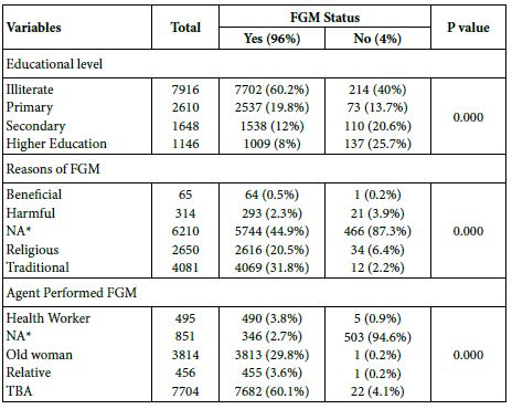
  25. Hodel NC, Hamad A, Reither K, et al. (2020) Assessment of diabetes and prediabetes prevalence and predictors by HbA1c in a population from sub-Saharan Africa with a high proportion of anemia: a prospective cross-sectional BMJ Open Diabetes Res Care. 8(1): e000939. [crossref]
  26. Pathai S, Lawn SD, Gilbert CE, et al. (2013) Accelerated biological ageing in HIV-infected individuals in South Africa: a case-control AIDS Lond Engl. 27(15):2375-2384. [crossref]
  27. Rinaldi S, Pallikkuth S, George VK, et al. (2017) Paradoxical aging in HIV: immune senescence of B Cells is most prominent in young age. Aging. 9(4):1307-1325. [crossref]
  28. Segatto AFM, Freitas Junior IF, Santos VR dos, et al. (2011) Lipodystrophy in HIV/AIDS patients with different levels of physical activity while on antiretroviral Rev Soc Bras Med Trop. 44(4): 420-424. [crossref]
  29. Mutimura E, Stewart A, Crowther NJ, et al. (2008) The Effects of Exercise Training on Quality of Life in HAART-Treated HIV-Positive Rwandan Subjects with Body Fat Redistribution. Qual Life Res. 17(3):377-385. [crossref]
  30. Hoffmann U, Lu MT, Foldyna B, et al. (2021) Assessment of Coronary Artery Disease With Computed Tomography Angiography and Inflammatory and Immune Activation Biomarkers Among Adults With HIV Eligible for Primary Cardiovascular JAMA Netw Open. 4(6):e2114923. [crossref]
  31. Carvalho A, Valente R, Almeida-Morais L, et al. (2017) VIH e doença coronária – quando a prevenção secundária é insuficiente. Rev Port Cardiol. 36: 569. [crossref]
  32. Kumar S and Samaras K (2018) The Impact of Weight Gain During HIV Treatment on Risk of Pre-diabetes, Diabetes Mellitus, Cardiovascular Disease, and Mortality. Front Endocrinol. 9:705. [crossref]
  33. Cesarino CB, Borges PP, Ribeiro R de CHM, et al. (2013) Avaliação do risco cardiovascular de pacientes renais crônicos segundo critérios de Framingham. Acta Paul Enferm. 26(1):101-107. [crossref]
  34. Friis-Møller N, Thiebaut R, Reiss P, et al. (2010) Predicting the risk of cardiovascular disease in HIV-infected patients: the data collection on adverse effects of anti-HIV drugs Eur J Cardiovasc Prev Rehabil. 17(5):491-501. [crossref]
  35. Bezerra LA and Burgos UMMC (2021) Analise do perfil lipídico de pacientes HIV- positivo com aterosclerose coronariana/ Analysis of the lipid profile in HIV- positive patients with coronary atherosclerosis. Braz J Health Rev. 4(2):9094-9102. [crossref]

A Living System

DOI: 10.31038/JCRM.2022541

Introduction

A living system is a structure that arises in order to solve the dissatisfaction of its elements – also living systems. It cannot arise over “inanimate” elements, only thanks to their properties it itself becomes a living structure.

In the course of modeling work on economic series, some properties were found that could be understood as properties of a living system. They were therefore verified on systems that were reasonably assumed to be live systems. It was about structural knowledge from the field of animal physiology (primarily human) and similar, albeit smaller, in the field of plant physiology. Using the “per analogiam” method, a common, systemic solution – the structure and principle of functioning of a living system – was found with a certain degree of objectivity.

For whom?

The basic question of every organizing system is – for whom it is built, who or what benefits from it. As detective lovers say – qui bono?

For man, it is completely conceivable and logical that, for example, society, as a living system, is created for man, to fulfill his interests. But for whom is a living system built an order lower, namely man himself? Who or what is its element?

The answer was usually the saying that for no one, that in short, evolutionarily asserted itself as the most successful. But for control theory this is not a sufficient answer. So what is its element?

Model works and the approach via analogies offer only one solution. The element of the so-called multicellular living systems is water! This is apparently not such a world-shattering statement, but it has its fundamental and world-shattering 😉 consequences.

The needs of water, its interests and dissatisfactions are therefore solved through it. And just as human society develops under the pressure of its elements, i.e. under the social pressure of man’s ideas and interests, other analogous living systems must also develop.

Dissatisfaction

The system evaluates the dissatisfaction of its elements for a simple reason – its existence rests on the elements, and if they become too dissatisfied, they will leave the system with all the resulting consequences. The system must be able to identify the dissatisfaction of the elements and must be able to respond to it adequately. The degree of satisfaction of all elements of a living system is the degree of its existence.

Elements

The whole scheme of a living system is based on the reason for which it arises. It is a solution to the dissatisfaction of the elements to an extent that is unattainable for the element itself.

The higher-level solution given by the new situation is given by the specialization ability of the elements. Specialized elements are involved in specialized production units. And these are divided from the point of view of the system into two basic groups: the production of food and the creation of suitable conditions for production and consumption.

Production units made of specialized elements – but extended by a more or less complex production structure (technique 😉) created in other production units – are companies in the case of human society and cells in the case of multicellular organisms. A cell is therefore not a living object, but only a productive, specialized unit.

The task of a living system simultaneously defines its two parts. Part of the regenerating, satisfying, not involved in the activity of the system of elements, and the part that creates the conditions for this regeneration, generally the solution of dissatisfaction. These two parts are in a constant process of overflowing. Each element “works” for some time, creates assumptions, but at the same time it is exhausted, its dissatisfaction changes and then it goes to the part for regeneration, where it consumes these created assumptions. The living system then has to ensure that the drawdown of the element during regeneration corresponds to the degree of its involvement and merit in the creation of assumptions.

In the text, the terms dissatisfaction and satisfaction will be used randomly, their meaning is identical – except for the sign.

Regeneration and Dark Matter

An element of a living system, having created common products within the framework of its specialization and received the corresponding remuneration (in society it is money), temporarily leaves these production units and relationships. It enters the “dark part, matter” – that is, a state where it cannot be seen from the living system. Only his activity aimed at solving his own dissatisfaction is observable. It restores its exhausted production possibilities and, as part of this regeneration, prepares to rejoin the system.

For regeneration, for some reason, it is necessary for the element to leave the system, to leave its specialized production relations, e.g. in a company or a cell. This part of the regeneration partly does not correspond to the terminology, it is not a restoration of a previously existing state. It is about the emergence of a new quality, especially in the area of finding new strategies for solving dissatisfaction. The element evaluates past experience and adjusts its past strategies to match possibly changing conditions. This specific part of regeneration – one could perhaps say sleep and its dream – is a completely irreplaceable part of regeneration.

In society, it is a person in the work process and a person in non-working time. In animals, it is the water that is active in the cells and the water that is in the cerebrospinal fluid and the lymphatic system, generally in the intercellular space. Similarly, in plants, it is water, when it is in living cells in an active process, regeneration occurs mainly in the vessels of plants (xylem).

In the case of the least studied – that is, astronomical systems – the essence of this division seems to be normal and dark matter.

In the following text, the term regeneration will be used in this broad, innovative sense. Like restoring elements not necessarily at the previous level.

Evaluation of the Element

In order for the element to subsequently and completely regenerate, it goes out of production. It is therefore necessary to somehow ensure in the system that it “takes away” indisputable information about its involvement in the creation of regeneration assumptions – some evaluation. For a person in a company it is money, for water in cells it is apparently some property in the distribution and dynamics of the charge of its package.

Production units generally operate independently. They have their own control mechanisms, evaluate the involvement of elements in production, solve their evaluation, etc. However, they are also under the influence of a system that moves their activity in the desired directions. In the case of the living system best known to us – human society – it is fiscal, monetary or economic policy.