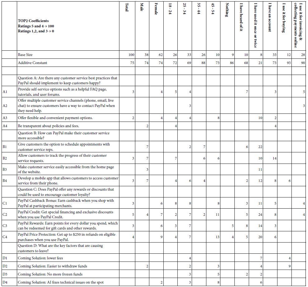
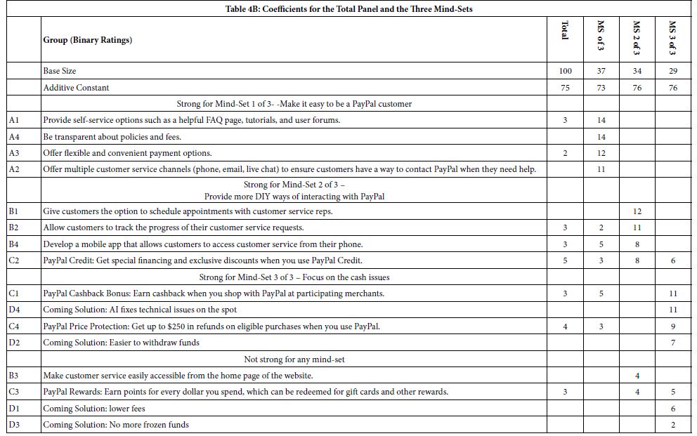
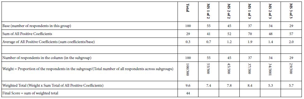
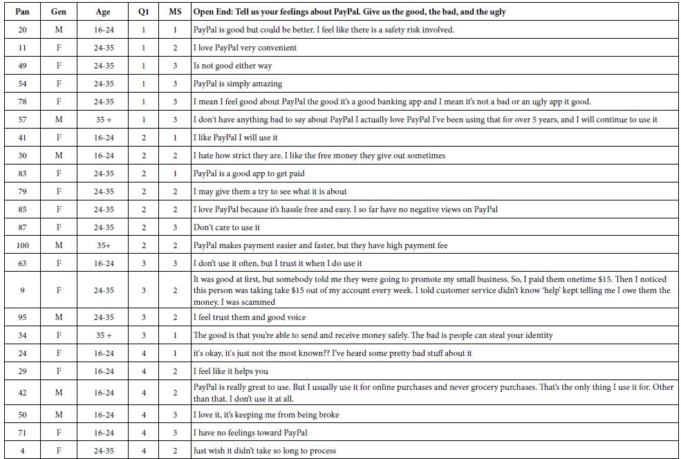
Author Archives: author

Review on Antimicrobial Susceptibility of Staphylococcus aureus from Raw Meat and Its Public Health Importance

DOI: 10.31038/MIP.2022334

Abstract

In the family Staphylococcaceae, Staphylococcus aureus is coagulase-positive, Gram-positive cocci. The bacteria are an opportunistic pathogen that frequently infects people without showing any symptoms. Although being mostly safe at these locations, it is possible for it to sometimes enter the body through skin breaches (such as abrasions, cuts, wounds, surgical incisions, or indwelling catheters) and injure both humans and animals. The ability of bacteria that cause foodborne poisoning to generate toxins after or during intoxication determines their pathogenesis. Staphylococcus aureus is one of the most common bacteria that cause these illnesses, and it is a major factor in gastroenteritis brought on by eating contaminated food. The ingestion of Staphylococcal enterotoxins produced in the food results in Staphylococcal food poisoning. The abrupt onset of nausea, vomiting, cramping in the abdomen and diarrhea are among its symptoms. Resistance to -lactam antibiotics and Vancomycin has mostly been attributed to plasmids and staphylococcal cassete chromosomes in particular. When bacteria are exposed to -lactam antibiotics, the extracellular enzyme -lactamase, which is encoded by blaZ, becomes active and confers penicillin resistance. The enzyme opens the -lactam ring by hydrolization to affect it. Globally as a result of the ongoing spread of bacterial strains that are resistant to antibiotics in the environment and the potential for food contamination, staphylococcal antimicrobial resistance is a serious issue for public health.

Keywords

Staphylococcus aureus, Antimicrobial susceptibility, Public health importance

Introduction

Staphylococcus aureus is a gram-positive, round (coccus) bacteria found in grape-like (staphylo) clusters; opportunistic colonies cause extreme harm. This bacterium is characterized by non-motile, non-spore forming and catalase positive which grow aerobically but which are capable to grow as facultative anaerobic [1]. Staphylococci are mostly occurs as harmless bacteria, that inhabiting the skin and soft tissue /nasal cavities of humans and animals. Among 31 species of staphylococci currently recognized, 15 are potentially pathogenic and It can causes a wide range of conditions in humans and animals, from mild skin infections to life-threatening bacteremia [2]. Staphylococcus aureus can also causes abscess in deep organs, by producing a toxin mediated diseases, self-limiting skin infections to life-threatening pneumonia, catheter-associated bacteremia, osteomyelitis, endocarditis, septicemia, Foodborne-illness and toxic shock syndrome (TSS) among other infections [3,4]. Meat is one of the animal product origins that contains high source of protein and vitamins for human being, again meat has high water content and rich in minerals and other nutrients which are suitable for the development of microorganisms. Due to its chemical composition and biological characteristics, meats are highly perishable foods providing a good source of nutrients for the growth of different microbial, that can leads infection in humans and also can lead to economic loss due to spoilage [5].

Staphylococcal food intoxication is happen due to the consumption of staphylococcal enterotoxins that preformed in the food. The main clinical manifestation of Staphylococcal food poisoning is vomiting, sudden onset of nausea, abdominal cramps and diarrhea. This condition is common in developing countries, because poor hygienic practices and low level of awareness. The staphylococcal enterotoxins are highly heat stable and are thought to be more heat resistant in food stuffs than in a laboratory culture medium. Due to this reason, even though we heating at normal cooking temperature, the bacteria may be killed but the toxins remain active. About half strains of staphylococcal strain are able to produce enterotoxins associated with food poisoning. Because of this condition enterotoxins producing Staphylococcus aureus are most dangerous and harmful for the human health [6]. Currently, Antimicrobial resistance is one of the most challenging situations to public health across the world. Even if different antimicrobial drugs are produced to treat S. aureus infections, the emergence and spread of antimicrobial resistant S. aureus can challenged for world to effectively treating and controlling of these. This is due to the high resistance percent could be traced to underuse or overuse of antibiotics due to poverty and ignorance, self-prescription, inappropriate prescription by physicians due to lack of effective antibiotic policies in our hospitals and other factors [7].

Staphylococci is one the most drug resistant bacteria, that develops resistance quickly and successfully to antimicrobial. This ways of defensive mechanism is due to consequence of the acquisition and transfer of antibiotic resistance plasmids and the possession of intrinsic resistance mechanisms [8] Currently, Methicillin-resistant Staphylococcus aureus (MRSA) strains are emerging wide spread to worldwide. Resistance to methicillin is mediated by different genes like, mec operon which is a part of the staphylococcal cassette chromosome mec (SCCmec). The mecA gene codes for an altered penicillin-binding protein, PBP2a, which has a minimum affinity for binding β-lactam antibiotics. The virulence of S. aureus was increased with existence of antibiotics resistance strains like Methicillin resistant S. aureus (MRSA) and Vancomycin resistance S. aureus [9].

Antibiotic resistance remains a major challenge in human and animal health. Resistance is increasingly being recognized in pathogens isolated from food. Food contamination with antibiotic-resistant bacteria can therefore be a major threat to public health, as the antibiotic resistance determinants can be transferred to other bacteria of human clinical significance. Furthermore, transfer of these resistant bacteria to humans has significant public health implications by increasing the number of food-borne illnesses and the potential for treatment failure. Food of animal origin could be contaminated from the farm, a situation which may be further compounded if the food is not properly handled during slaughtering and processing giving way for pathogens to multiply. Studies conducted in different countries to investigate the microbiological quality of food of animal origin reported the presence of potential human pathogens [10]. In general, S. aureus is one of the most common microbial, which causes diseases in both human and animals. Misuse of antibiotics in Livestock sector, Agriculture and in the treatment of human diseases, has contributed to the increase number of bacteria that are resistant to antimicrobial agents. Therefore, the main objective of this paper is to review the antimicrobial resistance in S. aureus from raw meat, virulence factors and focusing on the association between these characteristics and their implications for public and animal health.

Literature Review

Background of Staphylococcus aureus

Staphylococci family was first identified and isolated from the pus of surgical abscesses by the Scottish surgeon Sir Alexander Ogston in 1880 and he observed grape-like structure with circular in shape and he describe it staphylococcus. In 1881, Ogston found out that non-virulent staphylococci are also present on skin surfaces. Most staphylococcal strains from pyogenic lesions can produce golden yellow colonies, and the strains from normal skin, white colonies on solid media. In 1884, Friedrich Rosenbach name them Staphylococcus aureus (S. aureus) and S. albus respectively. Based on their characteristics and categorized them based on the production colonies color or pigments either golden or yellowish colonies. Later S. albus was renamed as S. epidermidis which were coagulase negative, mannitol non-fermenting and usually nonpathogenic strains.

The presence of Mobile genetic elements like bacteriophages, pathogenicity islands, plasmids, transposons, and staphylococcal cassette chromosomes enabled S. aureus to continually evolve and gain new traits. The genetic variation within the S. aureus species is approximately 22% of the S. aureus genome is non-coding and differ bacterium to bacterium, this is due to its reliance on heterogeneous infections. The different strains can secrete different enzymes/bring different antibiotic resistances to the group, increasing its pathogenic ability (https://en.wikipedia.org, 2021a).

Microbial Nomenclature

Staphylococcus aureus is a Gram-positive bacterium, which affects soft tissue and skin of host cell. The most common species of this pathogen that affects animal and human include S. aureus, S. intermedius, S. delphini, S. hyicus, S. schleiferi subsp. coagulans, S. pseudintermedius, S. equorum, S. xylosus, S. carnosus, S. simulans, S. saprophyticus, S. succinus, S. warneri, S. vitulinus, S. pasteuri, S. epidermidis, and S. lentus. One of these different species is S. aureus; so-named because of the color of the pigmented colonies (“aureus” means golden in Latin). Generally, S. aureus are opportunistic pathogens or commensals on host skin. However, they may act as pathogens if they gain entry into the host tissue through a trauma to the cutaneous barrier, inoculation by needles, the implantation of medical devices, or in cases in which the microbial community is disturbed or in immune compromised individuals [11,12].

Morphological and Biochemical Characteristics of Staphylococcus aureus

Morphologically, Staphylococcus aureus are characterized by spherical in shapes and after applying gram staining techniques, when examined under light electron microscope this bacteria can appeared as clusters resembling bunch of grapes with large round, golden-yellow colonies, often with hemolysis on blood agar Medias [13]. Additionally, S. aureus can produce an enzyme called coagulase. This enzyme reacts in the blood and produces a chemical called staphylothrombin. Staphylothrombin might make S. aureus even more difficult to kill by adding a layer of clotted protein to the bacterium membrane. Furthermore the S. aureus has a peptidoglycan membrane layer that would make it very hard for a bactericide drug to enter the cell and destroy it [14]. Biochemical test was one of the techniques that used to identify and differentiate S. aureus from other gram positive cocci microorganisms. Based on biochemical test, S. aureus is characterized by catalase-positive, which can be used to differentiate it from catalase-negative streptococci species and oxidase-negative. Staphylococci species can also be classified biochemically, S. aureus, which is coagulase-positive, produces a coagulase enzyme that agglutinates/clots blood or plasma while other medically important species of staphylococci, such as S. epidermidis and S. saprophyticus, are coagulase-negative. S. aureus can be distinguished from S. saprophyticus by novambicin susceptibility, while S. saprophyticus is novambicin-resistant.

Epidemiology of the Staphylococcus aureus

Staphylococcus aureus infections are found on the skin and mucous membranes. Human are the main reservoir for these organisms. Mostly, the S. aureus colonization up to 80% is common in health care workers, diabetics’ patient and intravenous drug users, hospitalized patients, and immunocompromised individuals [15]. The epidemiology of MRSA in particular has increased and distributed over the entire world. In general there are types of MRSA, this include community-associated MRSA, hospital-associated (HA-MRSA) and livestock-associated MRSA. Hospital-associated MRSA, the rise of novel strains of MRSA in the 1990s outside of the nosocomial environment will makes this pathogen to the recognition of “community-associated MRSA” (CA-MRSA), when compared to ancient hospital-associated (HA-MRSA) strains. In the mid-2000s, a third genre of MRSA was recognized, as colonization and infection of livestock and livestock workers and nominates it as livestock-associated MRSA (LA-MRSA) [16].

Distribution of S. aureus in Humans, Animals and Food of Animal Origin

Staphylococcus aureus is bacteria that normally reside in or on humans and does not usually cause infection. In 2019, Minnesota Department of health report on Staphylococcus aureus infectious disease, it stated that over 20% of their population almost always be colonized with S. aureus, while 60% of the population will be colonized with S. aureus either affected or not and the rest 20% are almost never colonized with S. aureus [17].

Meat is important food stuff and one of the main sources of protein, fats, minerals and vitamins. Meat contains high amount of water content and due to this reason most microorganism can growth easily, which leads to the food spoilage and foodborne infections to humans [18,19]. There are different mechanisms or factors that can initiate the growth of microorganism in meat. This factor includes; intrinsic factor and extrinsic (environmental factors), but the most common and efficient factors that contributes microbial to growth on meat are includes: – The temperatures in which meat can be storage, humidity and oxygen are the most important factors for microbial growth. Additionally, meat can be contaminated by these bacteria from the skin of animal during slaughtering at the abattoir and from different materials or equipment that are used for operation [20]. Currently, one of the most challenging problems in the world content is antibiotics resistance strains of S. aureus which pose a great risk in the food stuff. Of this meat of animal origin is one the most common sites at which drug residues can accumulate for a long period of time. Human being can gate this infection by eating contaminated meat [21-23]. Poor hygienic condition can cause meat to be contaminated by Staphylococcus aureus. When meat can contaminate by S. aureus; it can produce a toxin that activates disease. Even though, cooking destroys this pathogen, it will not destroy the toxin that produced by this pathogen, this is due to S. aureus can produce heat stable toxin [24]. Normally, S. aureus does not compete sufficiently with common microbial in raw foods; the contamination of food stuff with this pathogen is mostly associated with improper handling of foods, keeping of the food at which favorable for the growth of microorganism, which leads to multiplication of S. aureus and production of the enterotoxin [25].

Reservoirs and Sources of Infections

The primary ecological reservoir of Staphylococcus aureus causing infection in humans is the human nose, but a normal micro flora of the skin, hair, and mucous membranes may also be colonized. This pathogen can cause dermal infection if the cutaneous barrier is damaged. Any individuals that have been colonised by the bacteria are susceptible to any secondary infections, especially immune compromised people due to disease like HIV, type 1 diabetes and intravenous drug users, and patients undergoing hemodialysis, surgical patients are the most susceptible group for secondary infection. Additionally multiple sites in the body like, perineum, axillae, vagina, and gastrointestinal tract also were found to harbor this bacterium. Staphylococcus aureus in general have a commensal relationship with its host. The pathogen can causes disease in host tissue, when the skin of the host tissue can be damaged, inoculation by syringes, or by direct implantation with medical devices and leads infection in the host tissue. The main reservoirs of Staphylococcus aureus are infected mammary glands, ducts, and papillary lesions [26]. The primary reservoirs of S. aureus in affected countries are those animals in intensive systems like pigs, veal calves and broilers [27]. Normally S. aureus can be found in healthy cows, as carriers on the teat skin, nasal cavity, and rectum. But, the main reservoirs in a dairy cow are infected udders and teat skin [28]. From animal Pork is the main source of S. aureus reservoir host and human can gate this pathogen through consuming of the meat and causes foodborne illnesses. Staphylococcal foodborne infection is food poisoning disease that can occurs when human consume contaminated meat and the pathogen can induce staphylococcal enterotoxins expressed by enterotoxigenic strains of Staphylococcus species [29] S. aureus is an opportunistic pathogen that has capable to colonize a wide variety of host species, including birds and fish [30].

Modes of Transmission

Staphylococcus is the most common bacteria that cause mastitis in ruminants. The pathogen spread from one teat to another through the lining of the tea cups, milker’s hands, towels and fruit flies [31]. Staphylococcus including MRSA can be transmitted from animals to humans through direct contact especially from meat and also humans act as a reservoir for the transmission of S. aureus to vertebrate animals. Infections that can be present in both humans and animals and transmitted in both directions, such as S. aureus infections called as “amphixenoses. Different researcher can reported animal-to-human transmission of S. aureus in dairy sheep. S. aureus is usually transmitted by direct contact with colonised skin. Generally, Staphylococci can be transmitting from one species to another species or within the same species through direct or indirect contact with a patient who has a clinical infection of the respiratory or urinary tract and who is colonised with the bacterium. Contaminated surfaces and medical equipment are also used as a vehicle for transmission of MRSA (www.health.vic.gov.au).

Pathogenicity of Staphylococcus aureus

Virulence Factors

S. aureus possess different potential virulence factors that causes tissue damage: surface proteins that promote colonization of host tissues; invasions that promote bacterial spread in tissues (leukocidin, kinases, hyaluronidase); surface factors that inhibit phagocytic engulfment (capsule, Protein A); immunological disguises (Protein A, coagulase); membrane-damaging toxins that lyse eucaryotic cell membranes (hemolysins, leukotoxin, leukocidin and exotoxins that damage host tissues and leads disease [32]. S. aureus exotoxins, alpha-toxin, beta-toxin, delta-toxin and phenol soluble modulins are the cellular by products that activates the lysis of leukocytes (white blood cell), although α-toxin and phenol soluble modulins (PSMs) can also induces the formation of biofilms. Another surface-associated virulence factors like, protein A, fibronectin-binding antigen, and envelope associated proteins used to attaches and entrance of S. aureus to epithelial cells and initiates infection in the host cells [33]. S. aureus bacterial structures such as capsules, adhesins, extracellular products (enzymes) and toxins such as toxin α toxin β toxin leucocidin, enterotoxin, exfoliative toxin, and toxic shock syndrome toxin, contribute to different stages of infection [34]. Alpha toxin (α) is one of the vital virulence factors of S. aureus, that contains beta sheets which is water-soluble monomer targeting the red blood cells [35].

The formation of biofilms makes the pathogen to enter or live from the host cell, increasing their population within the host cell and protects the pathogen from environmental attack within the host cell. Enterotoxin is one of the dangerous toxins that mostly detect in the meat of animal origin due to S. aureus contamination and leads to gastroenteritis. S. aureus enterotoxin intoxication on consumers occurs through the establishment of contamination on food consumed. This enterotoxin is resistant to heat (heat stable), acid-resistant, and resistant to the effects of proteolytic enzymes like pepsin and trypsin [36]. Additionally biofilm formation is used the pathogen to attach to a living or non-living surface area which is used for grow and secrete several small molecules that attaches the microbial cells together [37]. Biofilms can cause antibiotics resistance, chronic disease and makes the host immune weak, because of it allows the pathogen to evade multiple clearance mechanisms [38]. S. aureus have capability to regulate the expression of virulence factors because of they have accessory regulatory gene (Agr) and the sigma factor (σB) and also this pathogen have ability adapt different microenvironments with environmental conditions, due to they generate the acquisition of genes like, bacteriophage, the staphylokinase gene and Panton-Valentine [39].

Mechanism of Disease Development

Although S. aureus is a normal flora of the skin and mucous membranes, any break in the skin or colonization of individuals with compromised immune systems can give an opportunity for this bacterium to invade and cause infection. The disease process can be mediated via two possible mechanisms; the production of toxins and the colonization that causes tissue invasion and destruction [40]. The pathogenicity of S. aureus is depends on the virulence factors that promote adhesion and evasion of the host immunologic responses. This organism can produce some toxins, that are causes diseases and a high mortality rate, of them toxic shock syndrome toxin (TSST) and Panton–Valentine leukocidin toxin, which causes necrotizing pneumonia and inducing leukocytosis and tissue necrosis [41]. Staphylococcus aureus can produce different kinds of virulence, which make to decrease in host’s immune system and causes diseases. Among S. aureus these virulence cytotoxins, nucleases, proteases, lipases, hyaluronidase, catalase, coagulase, collagenase, leucocidin, Toxic Shock syndrome (TSST-1), enterotoxins and exfoliative toxins are the most common virulence factors that S. aureus can produce in order to affect the host tissues. Other virulence factors are: – peptidoglycan, protein A, adhesion factors, teichoic acids, capsular polysaccharides and biofilms are the structural components that produce different toxin in the host cell (Figure 1) [42,43].

fig 1

Figure 1: The mechanism of Staphylococcus aureus infection cells (Zhou et al., 2018)

The mechanism of Staphylococcus aureus disease development has five stages; this includes colonization, localization, dissemination and metastatic infections. The colonization proceeds to infection under certain predisposing factors such as prolonged hospitalization, immune suppression, surgeries, use of invasive medical devices and chronic metabolic diseases. Localized skin abscess develop when the organism is inoculated into the skin from a site of carriage. This can further spread and results in various clinical manifestations of localized infections such as carbuncle, cellulitis, and wound infection. The organism can enter into blood and spread systemically to different organs causing sepsis [44].

Disease Caused by Staphylococcus aureus

S. aureus was a bacterial infection that affects humans and all warm blooded animals. These organisms are the causative agents of different human and animal diseases, like bacteremia, endocarditis, impetigo, folliculitis, furuncles, carbuncles, cellulitis, scalded skin syndrome, osteomyelitis, septic arthritis, prosthetic device infections, pulmonary infections, and gastroenteritis, meningitis, toxic shock syndrome, and urinary tract infections.

Disease in Humans

Staphylococcus aureus causes a different form of disease in humans. Human staphylococcal infections are frequent, but usually remain localized at the portal of entry by the normal host defenses and leads to superficial lesions such as inflammation (characterized by an elevated temperature at the site, swelling, the accumulation of pus, and necrosis of tissue). Around the inflamed area, the fibrin will clot and the bacteria will form abscess. Additional this pathogen can causes Localized infection of the bone, which is called osteomyelitis and at serious stages it will causes septicemia and bacteremia, when the bacteria invade the blood stream. Moreover, S. aureus can causes more serious infections like pneumonia, mastitis, phlebitis, meningitis, and urinary tract infections; osteomyelitis and endocarditis. S. aureus is a major cause of hospital acquired (nosocomial) infection of surgical wounds and infections associated with indwelling medical devices. S. aureus causes food poisoning by releasing enterotoxins into food, and toxic shock syndrome [45].

Staphylococcus aureus is the leading cause of bacterial disease that harboring the health of human being and it causes gastrointestinal, respiratory, skin and soft tissue, and blood stream infections. In human S. aureus can causes different diseases ranging from ranges from mild stage to life threatening issues and hence most common is the skin infections which are often caused by abscesses. The most common disease of S. aureus on human are includes: purulent skin infections such as boils, abscesses, impetigo and scalded skin syndrome, systemic infections such as bloodstream infections, pneumonia, osteomyelitis, endocarditis and deep abscesses, hospital-acquired (nosocomial) infection of surgical wounds or treatment lines, infections of prosthetic devices such as pacemakers, heart valves, joint replacements and other foreign bodies, including central venous catheters and peritoneal dialysis catheters and food poisoning by releasing toxins into food toxic shock syndrome by releasing toxins into the bloodstream. Occasionally, staphylococcal infections can cause disease condition such as Bloodstream infections, Endocarditis, Osteomyelitis and Lung Infection.

Disease in Animals

S. aureus infections in animals are the most common reported as a cause of abscesses, mastitis, pneumonia and meningitis. Additionally, this pathogen can cause Abortion and stillbirth in sheep and goat [46]. In dairy cow, S. aureus causes mastitis. S. aureus can cause both acute and chronic form of mastitis. Acute form of mastitis caused by S. aureus is characterized by severe clinical infection with visible changes to milk color. The second typical sign of S. aureus in dairy cow is chronic form of mastitis, which is characterized by subclinical and under this condition there is no any change of milk color [47]. Staphylococcus aureus is the leading pathogen causing the most dangerous mastitis in cattle and the most difficult dairy product in most countries. Staphylococcus aureus has emerged as superbug of dairy udder, compromising animal health and economy. Its virulence is due to its ability of producing wide array of virulence factors that enhances its attachment, colonization, longer persistence and escaping the immune response. S. aureus can causes different disease conditions in pigs with starts from skin infections to severe condition. The most common infection caused by S. aureus in pig includes, septicemia, mastitis, vaginitis, metritis, osteomyelitis, and endocarditi. In small ruminants, S. aureus is a major cause of mastitis and septicemia. In goats, staphylococcal infection can allows the secondary infection because of the host immunity was decreased due to S. aureus infection and among the secondary infection that affects shoat due to this pathogen was Para poxvirus infection, which causes chorioptic mange or contagious pustular dermatitis. Staphylococcus aureus was also affect pet animal like dog and it causes different types of disease condition including pyoderma, otitis media, and wound infections [48].

Prevalence of Staphylococcus aureus from Meat

Globally, the prevalence of S. aureus ranges from 23.3% to 73 and the prevalence rate of S. aureus in raw meat in African countries are 16.0% in Tunisia, 57.8% in Ethiopia and 52.0% in Egypt were reported (Table 1) [49].

Table 1: Prevalence of Staphylococcus aureus from meat in the world

Countries Prevalence Reference
Iran 26.31% Dehkordi et al., 2017
United state 27.8% Carrel et al., 2017
Colombia 6% Gutierrez et al., 2017
China 20.5% Li et al., 2019
Africa 24.5%, Thwala et al., 2021
Chile 47.6% Valeria et al., 2019
Indonesia 58.3% Wardhana et al., 2021

Prevalence of Staphylococcus aureus from Meat in the World

The prevalence of S. aureus in raw meat from different countries is varies, this is due to different reason like: – techniques of sample collection, season of the study, microbiologically examination methods, and meat handling methods [50]. In European countries, prevalence of Livestock Associated -MRSA ranging from 0 to 16% in broiler chickens, while the prevalence of chicken retail meat products ranges from 0 to 37% have been recorded. In general, the prevalence of Livestock Associated -MRSA in different countries are as follow: – In Hong-Kong, 6.8% of 455 chicken meat, from Quebec, Canada, and to characterize LA-MRSA isolates total of 309 retail chicken, MRSA was found in 4 samples out of the 309 retail chicken meat samples for an estimated prevalence of 1.3% (Table 2) [51].

Table 2: Prevalence of Staphylococcus aureus from meat in the Africa

Countries

Prevalence

Reference

Algeria 29.4% Chaalal et al., 2018
Ethiopia 34.3% Hassan et al., 2018
Morocco 40.38% Ed-Dra et al., 2018
Ghana 45% Effah et al., 2018
Egypt 15% Osman et al., 2015

Prevalence of Staphylococcus aureus from Meat in the Africa

The contamination of meat by S. aureus across the food chain is a complicated process. The contamination may originate from animals, as well as from humans. Improper hygiene at that level should be avoided to reduce the odds of meat contamination and food poisoning. The main factors that influence the level of contamination are the length at which animals are transported and the methods which are used to move animals from one place to another, holding conditions, geographic location, as well as climate changes (Table 3).

Table 3: Prevalence of Staphylococcus aureus from meat in the Ethiopia

City

Prevalence

Reference

Bahirdar 54.45% Bizuneh et al., 2020
Addis Ababa 29.17% Kibrom, 2017
Jigjig 32.22% Ayalew et al.,  2015
Mekelle 40% Gurmu et al., 2013
Debre-Zeit 36.5% Senait and Moorty, 2016

Prevalence of Staphylococcus aureus from Meat in the Ethiopia

In the above table there is difference between prevalence in the different years and cities, this may be due to the degree of meat contamination at food handling, level of environmental hygiene and the degree of awareness related to microbial contamination. The highest incidence of disease usually occurs in people with poor personal hygiene, people subject to overcrowding and children. The European Union estimated that the additional costs of MRSA infections are €380 million annually. In United States different research reported that increase in costs for treating a patient with a MRSA infection compared to a methicillin susceptible Staphylococcus aureus (MSSA) infection range from $3836 – $13,901 per patient per incident. Mortality rates for MRSA and MSSA disease are also increased [52].

Antimicrobial Resistance in Staphylococcus aureus from Meat

Staphylococcus aureus can develops antimicrobial resistance through mutation and horizontal transfer of resistance genes. The most mechanisms which are used to resist the action of antimicrobials include, the production of enzymes that inactivate or destroy the antimicrobial; a reduction of the bacterial cell wall permeability limiting the antimicrobial access into the cell; the development of alternative metabolic pathways to those inhibited by the antimicrobial; and active elimination of the antimicrobial from the bacterial cell or the target site. The new mec gene called which called mecD can confers resistance to all β-lactams antimicrobials, including anti-MRSA cephalosporins, ceftobiprole, and ceftaroline. The mecD gene was in an island of resistance associated with a site-specific integrase, which implies a risk of transmission by horizontal gene transfer to other species [53].

Mechanism of Antimicrobial Drug Resistance

Penicillin Resistance

Penicillin G was discovered in 1928 by Alexander Fleming and the drug was used in human as chemotherapeutic agent in 1941. This antimicrobial was the most common used to treat fatal Gram positive pathogens including Staphylococcal infections. Penicillin resistance of S. aureus is highly prevalent with up to 86% of clinical S. aureus isolates being resistant to the antibiotic in the US. Similar finding was made in Australia and recorded 80% of S. aureus isolates were resistant to penicillin. Staphylococci can produce penicillin resistance by inducing enzyme penicillinase or beta-lactamase encoded by the blaZ gene. This enzyme have ability breakdown the beta-lactam ring of penicillin which lead to inactivation of the antibiotic [54].

Methicillin Resistance

Methicillin Resistance which is also called penicillin’s-stable in S. aureus is characterized as resistance to all β-lactam antibiotics. Because of the presence of resistance gene (mecA) that can stops β-lactam antibiotics from inactivating enzymes. The mecA is a biomarker gene that is responsible for resistance to methicillin and other β-lactam antibiotics by expression of foreign antigens (PBP and PBP2a) that can bind to penicillin. The PBP and PBP2a are resistant to the action of methicillin. Synthesis of PBP2a is controlled and kept at low level, but the level of synthesis can be enhanced if mutations occur in the regulatory genes (https://en.wikipedia.org, 2021b). Additionally, MRSA has a mobile genetic element which called staphylococcal cassette chromosome (SCCmec). The SCCmec carries the mecA gene to encode altered PBP (PBP2a) these binding proteins decrease the ability of β-lactam antibiotics and the MRSA strains can survive in the presence of β-lactam antibiotics [55,56].

Vancomycin Resistance

Vancomycin-resistant S. aureus is a strain of S. aureus that has become resistant to the glycopeptides. This drug was primary observed from a microbial source which is called Streptomyces Orientalis in 1952 and approved for use in 1958. This drug is the first line drug of choice for MRSA infections. The first, reduced vancomycin susceptibility in S. aureus was reported in 1997 in Japan. This resistance mechanism can be occurred by inhibiting the transpeptidation of the peptidoglycan layer in the bacterial cell wall by binding to the C-terminal D-ala-D-ala of the peptidoglycan stem pentapeptide, which prevents the interaction between the penicillin binding proteins and their substrate [57]. The binding between Vancomycin and bacterial cell wall with D-alanyl-D-alanine can inhibits the elongation and cross-linking of bacterial cell wall peptidoglycans, although repressing cell wall synthesis and proceeds to bacterial death. Today, different researchers can divide vancomycin-resistant Staphylococcus aureus into three types: Vancomycin-resistant Staphylococcus aureus, vancomycin-intermediate Staphylococcus aureus and heterologous vancomycin resistant Staphylococcus aureus [58].

Macrolide Resistance

The mechanism of antibiotic resistance development in S. aureus to macrolide, lincosamides can happen when there is the occurrence of methylation at the receptor binding site on the ribosomes. However, this methylation can be catalyzed by a methylases enzyme that is encoded by ribosome methylationmthrough erythromycin methylases enzymes erm and mediated by an efux pump system encoded by mrsA.

Quinolone Resistance

Predominantly the mechanism of action of quinolones was act on DNA gyrase, which is an enzyme that relieves DNA supercoiling and topoisomerase. These antimicrobials can develop resistance due to marked by a gradual acquisition of chromosomal mutations. This action can take place at gyrase and ParC (GrlA in S. aureus) of topoisomerase [59].

Diagnosis and Treatment of S. aureus

The diagnosis of S. aureus pathogen was based on laboratory examination techniques, isolation and identification method. Among the bacteriological examination techniques, the common used for isolation and identification of this pathogen are includes: – Serological and biochemical tests such as catalase, DNase and coagulase tests are used to identify the strain of S. aureus. The most common samples or specimens collected for laboratory examination for this pathogen include: – Blood, sputum, tracheal aspirate, pus, and surface swab. During examined under microscope after employing Gram staining techniques, the organism presence with Gram-positive grape-like cocci in clusters, or pairs. Biochemical test is also the techniques that uses for isolation and identification of this pathogen. Mannitol salt agar is a selective medium that used to isolate S. aureus and S. aureus produces different types of haemolysis including beta-haemolysis, alpha haemolysis and gamma haemolysis on blood agar media (https://microbiologyclass.com/).

The treatment of the Staphylococcus aureus was based on the strain of the infection whether it is resistant to methicillin antibiotic (MRSA) or sensitive to methicillin antibiotics (MSSA). S. aureus infections must be treated with antibiotics, especially in elderly, young, and immune-compromised patients. Skin infections can be treated topically with antibiotic creams. Antibiotic that used for treatment of MRSA includes vancomycin, clindamycin and a combination of antimicrobials that are resistant for bacterial strains. Penicillin is used for non-resistant S. aureus infections (https://biologydictionary.net, 2020). Before treating the affected person as well as humans the physicians must be doing the antibiotic sensitivity test. The most common used antibiotics against this bacteria/pathogen are penicillin, tetracycline, streptomycin, novobiocin, sulfonamides, lincomycin, and spectinomycin. But currently most bacteria are resistant to penicillin and other variety of antibiotics. However, at this time Vancomycin most effective drug of choice against this pathogen.

Anti-virulence or anti–toxin compound is the best option used to treat S. aureus strain pathogen, especially those produce toxin because of this compound does not affect bacterial viability or growth. This anti virulence compound can inhibit bacterial virulence genes, and leads decreasing the ability of pathogen to colonize the host and inversely allow the host innate immunity/biomarkers to eradicate the attenuated pathogen [60]. According to the report from Cordeiro et al. Lysostaphin drug was the most effective than mupirocin in rat models, but there is no any trials are applied for human. Additionally, both thymol and carvacrol are the phenolic terpenoids that are effective antimicrobial activity against S. aureus [61]. Again Daptomycin, a cyclic lipopeptide molecule, is a novel antibiotic that used for vancomycin-unresponsive S. aureus disease. This drug can damages the cytoplasmic membrane of bacteria and leads the protein synthesization [62]. The pathogenic S. aureus is resistant to different antibiotics that previously used to treat this pathogen like; cephalosporins, vancomycin, methicillin, oxacillin and penicillins. Drainage of the fluids or pus in abscess caused by S. aureus can be employed in the management of pus-infections mediated by the pathogen. Treating food poisoning Staphylococcus aureus by fluid and electrolyte were used to boost the immune system of the patient (https://microbiologyclass.com).

Mupirocin is also another antibiotic that used to treat impetigo and nasal decolonization infection of S. aureus. Mupirocin can inhibit the protein synthesis. Fusidic acid is an antibiotic that binds to bacterial elongation factor G and leads to impaired translocation process and inhibition of protein synthesis. This antibiotic has potent activity against S. aureus and clinically used in treatment of mild to moderately severe skin and soft-tissue infections, for example, impetigo, folicullitis, erythrasma, furunculosis, abscesses and infected traumatic wounds. For treating S. aureus strain that develops the biofilm formation, not only antibiotic treatment is effective, in addition to antibiotics using alternative treatment like postsurgical antibiotics was effective. Novel treatments for S. aureus biofilm involving nano silver particles, bacteriophages, and plant derived antibiotic agents effects against S. aureus embedded in biofilms (https://en.wikipedia.org).

Prevention and Control

The control and prevention methods of staphylococcus aureus disease was based on the practice of proper hygienic and individual protection at abattoir and hospital areas. Currently, there is no vaccine available to prevent staphylococcal diseases or infections, due to this reason individuals and hospital institutions must be implement the individual and environmental hygienic practices like hand washing and proper disinfection. Teaching the societies regarding to the protection method of the pathogen such as contaminated foods should be avoided; and food handlers should always observe proper hygiene in the handling, processing, preparation and distribution of food in order to avoid the outbreak of food poisoning due to Staphylococcus aureus (https://microbiologyclass.com). Educate hospital staff based on how hand hygiene can be important in order to protect this bacterium. Narrow-spectrum antibiotics, is used to control decolonization in patients planned for high-risk surgical procedures. Affected group might be recommended antibiotics to eliminate the bacteria, like mupirocin (www.health.vic.gov.au).

Public Health Importance

S. aureus is a major pathogen of public health concern throughout the world, this is due the pathogen can produce Staphylococcal food poisoning. Meat and meat products of animal origin are one of the main sources of staphylococcal food poisoning. Symptoms of Staphylococcus poisoning which include diarrhea, abdominal cramps, vomiting, and nausea occur after consuming toxin-contaminated food. The emergence of antimicrobial resistance, especially the multidrug resistance strain of S. aureus becomes an emerging zoonotic issue for worldwide. Because the resistant organisms fail to respond to first-line treatment, hence, leading to high cost of treatment, prolonged illness and high risk of death with its concomitant financial burden and loss in man-hour to families and societies [63]. Multi Drug resistant staphylococci can affect the health care system by causing prolonged hospitalization, increases the costs of treatments and patient mortality.

Zoonotic bacteria or pathogen can transmit to human through direct contact with animals or indirectly through the food of animal origin. The most common population at risk with zoonotic pathogen are farmers, veterinarians, farm laborers and abattoir workers is greater risk of being colonized or even infected with zoonotic pathogen. Humans may represent an important source of new bacterial strains, which can cause disease in livestock and, as such, pose a potential threat to food security. According to the recent research, the epidemic S. aureus clones in human and animal hosts, Both LA-MRSA ST398 and S. aureus ST5 clone, can causes lameness in poultry, have been shown to originate from humans but have now adapted and diversified to spread in animal hosts [64]. According to different researcher the organisms can be transferred to animals, and re-transmitted from this source to humans (reverse transmission) [65]. Different researcher reports the presence of Methicillin-resistant S. aureus in chicken meats, because of contamination and is considered a source of human infections caused by consuming contaminated meat of animal origin [66] Administering of under dose drugs to food animals can leads the pathogen to carry antimicrobial resistance genes or plasmids, which makes the multiplication and transmission of those genes among strains. This means using low dosage of antibiotics can initiates the transmission of resistance between different hosts including humans, animals and the environment [67]. The incidence rate of S. aureus disease was highest among the people with poor personal hygiene, overcrowding and children. But, staphylococcal disease may affect all people and animals. Healthcare employees, football players, prison inmates, people in day-care centers, people in military quarters, homeless people, intravenous drug users and men who have sex with men are also among the most people at risk (www.health.vic.gov.au).

Economic Impact of S. aureus

In Europe, Asia and North America, there is an increasing level of MRSA due to epidemics of highly transmissible. Due to the increasing incidence rate of MSSA and MRSA diseases and it increase in load of bacteremia and costs for treatment. This will causes economic problems, especially for developing countries there is scarcity of effective drugs and failure of treatment due to inappropriate antimicrobials or lack of efficacy of anti-MRSA drugs, excess toxicity of will causes to increase the morbidity and mortality. Drug-resistant infections also affect patients’ social and economic status by increasing healthcare costs, mortality and morbidity, and decreasing productivity. Among countries where use has been successfully reduced, significant investments were necessary to improve biosafety and biosecurity on farms in order to enable intensive production systems without the use of antimicrobials. Similar measures could be implemented in newer facilities in LMICs but may be too expensive for small livestock operations that lack the necessary technical and financial resources. Regardless, the benefits of reducing national resistance rates are predicted to outweigh the costs of introducing such bans. One study predicted that a worldwide ban on antimicrobial growth promoters would lead to a decrease of 1% to 3% in global meat production and a loss in meat production value of US$ 13.5 to US$ 44.1 billion, compared to an estimated loss of US$ 35 billion per year in the United States alone due to healthcare costs and losses to productivity from AMR [68-85].

Conclusion and Recommendation

Staphylococcus aureus is a Gram-positive, facultative anaerobic bacterium which grows individually, in pairs, short chains or grape-like clusters. The bacterium is catalase and coagulase positive, oxidase-negative, non-motile microorganism that does not form spores. Staphylococcus aureus can causes different diseases such as abscess in deep organs, toxin mediated diseases, self-limiting skin infections to life-threatening pneumonia, osteomyelitis, endocarditis, septicemia, Foodborne-illness and toxic shock syndrome (TSS). Foods contaminated with S. aureus are a potential vehicle for the transmission of enterotoxigenic S. aureus to humans. Staphylococcus aureus is a foodborne pathogen which is responsible for contamination of different food products and results food spoilage, reduction of food safety and shelf life and cause foodborne poisoning via production of deadly enterotoxins. S. aureus is a very versatile human pathogen that readily adapts to changing environments and acquires antibiotic resistance genes through a number of different mechanisms. Antimicrobial resistance is a serious threat to public health across the globe. A wide variety of antimicrobial drugs are employed to treat S. aureus infections. However, emergence and spread of antimicrobial resistant S. aureus isolates constitute a global challenge for the effective treatment and control of these infections.

Therefore, based on the above conclusion, the following recommendations are forwarded:-In the future the researcher:

  • Should focus on developing a safe vaccine that contains secreted as well as cell wall-associated antigens that evoke a sustained protective response over a significant period of time.
  • Should utilize information on the variation, distribution and function of surface protein antigens amongst aureus lineages to ensure that cocktails of gene variants are included in the vaccine.
  • Should focus on the unraveling of the cellular immune responses directed against aureus.
  • proper handling of raw meat, adequate cleaning of hands, surfaces, equipment’s, disinfection of slaughter houses, vehicles and good personal hygiene can reduce spreading of Staphylococcus through meat.
  • The occurrence of multidrug resistance Staphylococcus particularly aureus should be under consideration during selection of antimicrobials for the treatment.
  • Multiple drug resistant Staphylococcus aureus have a wide distribution in different meat of animal origin and therefore care should be taken in to account during processing to destroy the micro-organisms to avoid the risk of human infection.

Acknowledgment

I would like to start by extending gratitude and praise to Almighty Allah, the kindest and most merciful, for keeping us well and bestowing upon us the unwavering resolve, bravery, strength, and endurance needed to complete this difficult endeavor. The person who controls the course of advancement is Dr. Daniel Shiferaw (DVM, MSC, Assist Prof), who is my advisor. Words can’t quite explain how grateful I am for his constant constructive criticism, diligent scientific advice, and untold hours spent editing this work. Last but not least, we would want to express how grateful we are to Haramaya University Faculty of Veterinary Medicine for providing the necessary facilities.

Abbreviations

Agr: Accessory Regulatory Gene; AMR: Antimicrobial Resistant; CA-MRSA: Community-Associated Multi Drug Resistant Staphylococcus aureus; DNA: Deoxy Nucleic Acid; HA-MRSA: Hospital-Associated Multi Drug Resistant Staphylococcus aureus; HIV: Human Immunodeficiency Virus; LA-MRSA: Livestock-Associated Multi Drug Resistant Staphylococcus aureus; MRSA: Multi Drug Resistant Staphylococcus aureus; PBP: Penicillin-Binding Protein; PSM: Phenol Soluble Moduli’s; SCCmec: Staphylococcal Cassette Chromosome mec; SCV: Small Colony Variant; TSS: Toxic Shock Syndrome; σB: Sigma Factor.

References

  1. Rasoul Y, Mashouf Seyed M, Hosseini Seyed M, Mousavi and Mohammad R, Arabestani (2014) Prevalence of Enterotoxin Genes and Antibacterial Susceptibility Pattern of Staphylococcus aureus Strains Isolated from Animal Originated Foods in West of Iran. Oman Medical Journal 30: 283. [crossref]
  2. Ronaq Zaman, Muhammad Inam, Zobia AF (2013) Sensitivity Pattern of Staphylococcus Aureus Isolates to Commonly Used Antibiotics. Pakistan Journal of Medicine and Health Science 7(3):651.
  3. U. Olugbue, V. O. Nwaugo, M. C. Korie, M. O. Okata, I. Oko and N. U. O (2018) Antimicrobial Susceptibility Profiles of Staphylococcus aureus Strains from Ear, Nose and Wound Swabs of Patients Attending Health Care Facilities, Ebonyi Sate, Nigeria. Microbiology Research Journal International. 3973123:1: 1.
  4. Frederick Adzitey, Rejoice Ekli and Martin Aduah. 2020. Incidence and antibiotic susceptibility of Staphylococcus aureus isolated from ready to eat meats in the environs of Bolgatanga Municipality of Ghana. Cogent Environmental Science 6: 1791463:
  5. Lika, E.; Puvaˇca, N.; Jeremi´c, D.; Stanojevi´c, S.; Shtylla Kika, T.; Cocoli, S.; de Llanos Frutos, R (2021) Antibiotic Susceptibility of Staphylococcus Species Isolated in Raw Chicken Meat from Retail Stores. Antibiotics 10: 904: 1-2. [crossref]
  6. Piyali Das, Pranab Behari M (2016) Prevalence of Staphylococcus in raw meat samples in Southern Assam, India. IOSR Journal of Agriculture and Veterinary Science 9(1):23.
  7. Bizuneh Tsehayneh, Taddesse Yayeh, Birhan Agmas and Semahegn Y (2021) Valuation of Bacterial Load and Antibiotic Resistance Pattern of Staphylococcus aureus from Ready-to-Eat Raw Beef in Bahir Dar City. International Journal of Microbiology 10(1155-5560596): 2-6. [crossref]
  8. Nwankwo Emmanuel Onwubiko andb Nasiru Magaji Sadiq.(2018) Antibiotic sensitivity pattern of Staphylococcus aureus from clinical isolates in a tertiary health institution in Kano, Northwestern Nigeria. The Pan African Medical Journal 8(4):2.
  9. Narin A Rasheed and Nawfal R H. 2021. Staphylococcus aureus: An Overview of
    Discovery, Characteristics, Epidemiology,Virulence Factors and Antimicrobial Sensitivity. European Journal of Molecular & Clinical Medicine 8(3): 1161-1169.
  10. Jhalka Kadariya, Tara C. Smith, and Dipendra Thapaliy (2014) Staphylococcus aureus and Staphylococcal Food-Borne Disease: An Ongoing Challenge in Public Health. Hindawi Publishing Corporation Biomedical Research International 827965: 6.
  11. Lesley Maurice Bilung, Ahmad Syatir Tahar, Rosdi Kira, Aina Ariffah Mohd Rozali,
    and Kasing Apun (2018) High Occurrence of Staphylococcus aureus Isolated from Fitness Equipment from Selected Gymnasiums. Hindawi Journal of Environmental and Public Health 2018: 4592830: 1. [crossref]
  12. Alexandra Fetsch and Sophia Johler (2018) Staphylococcus aureus as a Foodborne Pathogen. Current Clinical Microbiology Reports.
  13. Arumugam Gnanamani, Periasamy Hariharan and Maneesh Paul-Satyaseela (2017) Staphylococcus aureus: Overview of Bacteriology, Clinical Diseases, Epidemiology, Antibiotic Resistance and Therapeutic Approach.Staphylo coccus Aureus: Intech Open Access books 54154: 4-12.
  14. Biology dictionary.net Editors. Staphylococcus Aureus. Biology Dictionary 14 May 2020.Accessed on November 22, 2021.
  15. Tracey A. Taylor; Chandrasekhar G. Unakal (2021) Staphylococcus Aureus. NCBI Bookshelf. A service of the National Library of Medicine, National Institutes of Health 441868 (28722898): 2-3. [crossref]
  16. Christina J. Heaton, Gracen R. Gerbig, Lucas D. Sensius, Vishwash Patel and Tara C. Smith (2020) Staphylococcus aureus Epidemiology in Wildlife: A Systematic Review. Antibiotics 9: 1-2. [crossref]
  17. Uka, K.K, Oguoma, S.I, Chukwu, C.A. and Emele, C.I (2020) Adoption of Artificial Intelligence for Diagnosis and Treatment of Staphylococcus aureus Infections Disease on Humans. E-Health Telecommunication Systems and Networks 9: 1-4.
  18. Henok Ayalew Tegegne, Amare Berhanu, Yitbarek Getachew, Biresaw Serda, Dagmar Nölkes, Sissay Tilahun, Berhanu Sibhat (2019) Microbiological safety and hygienic quality of camel meat at abattoir and retail houses in Jigjiga city, The Journal of Infection in Developing countries 13;3: 189. [crossref]
  19. Matewos Kebede Kassa (2020) The Prevalence, Distribution of Staphylococcus and its Antimicrobial Susceptibility Status of the Isolates from Meat and Dairy Milks of Bishoftu, Ethiopia. International Journal of Advanced Research in Biological Sciences 7;3: 153.
  20. Matewos Kebede Kassa (2020) The Prevalence, Distribution of Staphylococcus and its Antimicrobial Susceptibility Status of the Isolates from Meat and Dairy Milks of Bishoftu, Ethiopia. International Journal of Advanced Research in Biological Sciences 7: 3: 153.
  21. Smith TC (2015) Livestock-Associated Staphylococcus aureus: The United States Experience. PLOS Pathogens 11(2):4.
  22. Andarge Zelalem, Mekonnen Sisay, Jessie L. Vipham, Kebede Abegaz, Ameha Kebede and Yitagele Terefe (2019) The prevalence and antimicrobial resistance profiles of bacterial isolates from meat and meat products in Ethiopia: a systematic review and meta-analysis. International Journal of Food Contamination 6(1): 2.
  23. Onuoha, S.C, Ani, T. P, Oko, F.N, Ovia, K.N (2020) Prevalence of antibiotic resistant staphylococcus aureus in raw meat samples intended for human consumption. International Journal of Biology, Pharmacy and Allied science 9(3): 345-346.
  24. Abunna F, Abriham T, Gizaw F, Beyene T, Feyisa A. 2016. Staphylococcus: Isolation, Identifcation and Antimicrobial Resistance in Dairy Cattle Farms, Municipal Abattoir and Personnel in and Around Asella, Ethiopia. Journal of Veterinary Science and Technology 7(6): 2.
  25. Shawish RR, Al-Humam NA (2016) Contamination of beef products with staphylococcal classical enterotoxins in Egypt and Saudi Arabia. GMS Hygiene and Infection Control 11(8):5. [crossref]
  26. Amjad Islam Aqib, Muhammad Ijaz, Muhammad Shoaib, Iqra Muzammil, Hafiz Iftikhar Hussain, Tean Zaheer, Rais Ahmed, Iqra Sarwar, Yasir Razzaq Khan and Muhammad Aamir Naseer, (2021) Staphylococcus aureus and Dairy Udder, Insights into Drug Resistance in Staphylococcus aureus, Amjad Aqib, IntechOpen.
  27. Crespo‑Piazuelo and Lawlor (2021) Livestock‑associated methicillin‑resistant Staphylococcus aureus (LA‑MRSA) prevalence in humans in close contact with animals and measures to reduce on farm colonization. Irish Veterinary Journal 74(21): 2-3. [crossref]
  28. Haag AF, Fitzgerald JR, Penadés JR (2019) Staphylococcus aureus in animals. Microbiol Spectrum 7(3): 5-6.
  29. Mulemba Tillika Samutela, Geoffrey Kwenda, Edgar Simulundu, Panji Nkhoma,
    Hideaki Higashi, Andrew Frey, Matthew Bates, Bernard M. H (2021) Pigs as a potential source of emerging livestock-associated Staphylococcus aureus in Africa: a systematic review. International Journal of Infectious Diseases 109:39. [crossref]
  30. Christina J. Heaton, Gracen R. Gerbig, Lucas D. Sensius, Vishwash Patel and Tara C. Smith (2020) Staphylococcus aureus Epidemiology in Wildlife: A Systematic Review. Antibiotics 9:89: 1-2. [crossref]
  31. Muhammad Farhab, Muhammad Tahir Aleem, Shakseema Shaukat, Ayesha Qadry, Muhammad Zeeshan Ul Haq, Fateh Ullah, Muhammad Jawad and Amjad Islam Aqib (2021) Staphylococcus aureus and the Veterinary Medicine, Insights into Drug Resistance in Staphylococcus aureus. Intech open.
  32. Maliha Gulza and Asima Zehra (2018) Staphylococcus aureus: A brief review. International Journal of Veterinary Science and Research.
  33. Peng Gaoa, Pak Leung Hoab, Bingpeng Yana, Kong Hung Szea, Julian Daviesc and Richard Yi Tsun K (2018) Suppression of Staphylococcus aureus virulence by a small molecule compound. PNAS 115(31): [crossref]
  34. Foster TJ, Geoghegan JA, Ganesh VK, Höök M (2014) Adhesion, invasion and evasion: The many functions of the surface proteins of Staphylococcus aureus. Nature Reviews Microbiology 12(1): 1-2. [crossref]
  35. Kavitha Shettigar and Thokur Sreepathy Mura (2020) Virulence factors and clonal diversity of Staphylococcus aureus in colonization and wound infection with emphasis on diabetic foot infection. European Journal of Clinical Microbiology and Infectious Diseases 39:2237. [crossref]
  36. Valeria Velasco, Mario Quezada-Aguiluz and Helia Bello-Toledo (2019) Staphylococcus aureus in the Meat Supply Chain: Detection Methods, Antimicrobial.
  37. Gordon Y. C. Cheung, Justin S.B and Michael (2021) Pathogenicity and virulence of Staphylococcus aureus. Virulence 12(1):556.
  38. Jelle Vlaeminck, Dina Raafat, Kristin Surmann, Leen Timbermont, Nicole Normann, Bret Sellman, Willem J. B. van Wamel and Surbhi Malhotra K (2020) Exploring Virulence Factors and Alternative Therapies against Staphylococcus aureus Toxins 12:721: 5. [crossref]
  39. Roberto Adame-Go´mez, Natividad Castro-Alarco´n, Amalia Vences-Vela´zquez,
    Jeiry Toribio-Jime´nez, Abigail Pe´rez-Valdespino, Marco- Antonio Leyva-Va´zquez, and Arturo Ram´ ırez-Peralta (2020) Genetic Diversity and Virulence Factors of aureus Isolated from Food, Humans, and Animals. Hindawi International Journal of Microbiology (2020)(1048097): 2.
  40. Yilmaz, E.S. and Aslantas, O (2017) Antimicrobial resistance and underlying mechanisms in Staphylococcus aureus Asian Pacific Journal of Tropical Medicine 10(11): 1059-1064. [crossref]
  41. Nadira Mourabit, Abdelhay Arakrak, Mohammed Bakkali, Zeineb Zian, Joaira Bakkach, and Amin Laglaoui (2021) Antimicrobial Resistance Trends.
  42. Zhou Kaixiang Chao Li Dongmei Chen Yuanhu Pan Yanfei Tao wei Qu Zhenli Liu Xiaofang wang Shuyu Xie (2018) A review on nanosystems as an effective approach against infections of Staphylococcus aureus. International Journal of Nano medicine 13:7335. [crossref]
  43. Alejandro De Jesús Cortés-Sánchez, Mayra Díaz-Ramírez, Ma. De la Paz Salgado-Cruz and Rocío G. HernandezNava (2020) Food Safety and Fish Production the Case of Staphylococcus aureus: A Review. Online Journal of Biological Sciences 20 4: 294-299.
  44. Liyun Shi, Huanhuan Wang and Zhe Lu. 2016. Staphylococcal Infection and Infertility, Genital Infections and Infertility. IntechOpen.
  45. Thwala, T.; Madoroba, E.; Basson, A.; Butaye, P (2021) Prevalence and Characteristics of Staphylococcus aureus Associated with Meat and Meat Products in African Countrie. Antibiotics 10:1108: 1-4. [crossref]
  46. Piva S, Mariella J, Cricca M, Federica Giacometti, Angelo Romano and Andrea Serraino (2021) Epidemiologic case investigation on the zoonotic transmission of Staphylococcus aureus infection from goat to veterinarians. Zoonoses Public Health 68:685. [crossref]
  47. Park S, Ronholm J (2021) Staphylococcus aureus in agriculture: lessons in evolution from a multispecies pathogen. Clinical Microbiology Reviews 34(2): 11-16. [crossref]
  48. Qekwana, Daniel Nenene; Oguttu, James Wabwire; and Odoi, Agricola (2019) “Geographic distribution of Staphylococcus spp. infections and antimicrobial resistance among dogs from Gauteng Province presented at a veterinary teaching hospital in South Africa. Faculty Publications and Other Works Biomedical and Diagnostic Sciences (https://trace.tennessee.edu/utk_compmedpubs/117) Accessed on December 12, 2021.
  49. Birhan Agmas ,Bizuneh Tsehayneh and Taddesse Yayeh (2020) Staphylococcus Aureus Health Risk from Ready-To-Eat Raw Beef Meat and Associated Risk Factors in North West Ethiopia. Scholarly Journal of Food and Nutrition 3(2): 348-350.
  50. Wardhana DK, Haskito AEP, Purnama MTE, Safitri DA, Annisa S (2021) Detection of microbial contamination in chicken meat from local markets in Surabaya, East Java, Indonesia. Veterinary World 14(12): 3138. [crossref]
  51. Bernier-Lachance J, Arsenault J, Usongo V, Parent E´, Labrie J, Jacques M, et al. (2020) Prevalence and characteristics of LivestockAssociated Methicillin-Resistant Staphylococcus aureus (LA-MRSA) isolated from chicken meat in the province of Quebec, Canada. PLoS ONE 15(1): 1-2. [crossref]
  52. Wanda Reygaert (2014) Antimicrobial resistance mechanisms of Staphylococcus aureus. Research Gate. C. Reygaert Department of Biomedical Sciences, Oakland University William Beaumont School of Medicine, Rochester, MI, USA (https://www.researchgate.net/publication/267695121). [crossref]
  53. Schwendener S, Cotting K, Perreten V (2017) Novel methicillin resistance gene mecD in clinical Macrococcus caseolyticus strains from bovine and canine sources. Scientific Reports 7:43797:2. [crossref]
  54. Jactty Chew, Suat-Cheng Peh and Teow Sin Yeang (2018) Non-microbial Natural Products That Inhibit Drug Resistant Staphylococcus aureus Chp1. Intechopen 10: 5772-74588.
  55. Zhu Li (2018) A Review of Staphylococcus aureus and the Emergence of Drug-Resistant Problem. Advances in Microbiology 8: 2165-3410.
  56. Anderson Clayton da Silva, Marjory Xavier Rodrigues and Nathália Cristina Cirone Silva (2019) Methicillin-resistant Staphylococcus aureus in food and the prevalence in Brazil: a review. Brazilian Journal of Microbiology 51:349. [crossref]
  57. Bitrus, A.A, O.M. Peter, M.A. Abbas and M.D. Goni (2018) Staphylococcus aureus: A Review of Antimicrobial Resistance Mechanisms. Journal of Veterinary Sciences: Research and Reviews 4(2): 47-58.
  58. Guo Y, Song G, Sun M, Wang J and Wang Y (2020) Prevalence and Therapies of Antibiotic-Resistance in Staphylococcus aureus. Frontiers in Cellular and Infection Microbiology 10:107.
  59. Irina Gheorghe, Marcela Popa and Luminiţa Gabriela M (2018) Molecular Features of Virulence and Resistance Mechanisms in Nosocomial and Community-Acquired Staphylococcus aureus. Intech Open.
  60. Daniela Bencardino, Giulia Amagliani, Giorgio Brandi (2021) Carriage of Staphylococcus aureus among food handlers: An ongoing challenge in public health. Food Control 130:108362: 7-8.
  61. Kong, C.; Neoh, H.M.; Nathan, S (2016) Targeting Staphylococcus aureus toxins: A potential form of anti-virulence therapy. Toxins 8:72:6.
  62. Mohini Bhattacharya, Daniel J Wozniak, Paul Stoodley, and Luanne HallStoodley (2016) Prevention and treatment of Staphylococcus aureus biofilms. Expert Review Anti Infection Therapeutics 13(12): 6.
  63. Mahendra Pal, Gemechu Berhanu Kerorsa, Lencho Megersa Marami, and Venkatara Kandi (2020) “Epidemiology, Pathogenicity, Animal Infections, Antibiotic Resistance, Public Health Significance, and Economic Impact of Staphylococcus Aureus: A Comprehensive Review.” American Journal of Public Health Research 8(1):15-19.
  64. Tracy Schmidt, Marleen M. Kock and Marthie M. Ehlers (2015) Antimicrobial Resistance in Staphylococci at the Human-Animal Interface IntechOpen 103-104.
  65. Spickler, Anna Rovid (2016) Methicillin Resistant Staphylococcus aureus (http://www.cfsph.iastate.edu/DiseaseInfo/factsheets).
  66. B. Kim, K. W. Seo, H. Y. Jeon, S.-K. Lim and Y. J. Le (2018) Characteristics of the antimicrobial resistance of Staphylococcus aureus isolated from chicken meat produced by different integrated broiler operations in Korea. Poultry Science Association Inc 97: 962.
  67. Verónica Karen Castro Péreza, Geraldo Márcio da Costaa, Alessandro Sá Guimarãesb, Marcos Bryan Heinemannc, Andrey Pereira Laged, Elaine Maria Seles Dorneles (2020) Relationship between virulence factors and antimicrobial resistance in Staphylococcus aureus from bovine mastitis. Journal of Global Antimicrobial Resistance 22: 793. [crossref]
  68. Laxminarayan R, Van Boeckel TP, Teillant A (2015) The Economic Costs Of Withdrawing Antimicrobial Growth Promoters From The Livestock Sector. OECD Food, Agriculture and Fisheries Papers 78: 33.
  69. Abunna F, Abriham T, Gizaw F, Beyene T, Feyisa A (2016) Staphylococcus: Isolation, Identifcation and Antimicrobial Resistance in Dairy Cattle Farms, Municipal Abattoir and Personnel in and Around Asella, Ethiopia. Journal of Veterinary Science and Technology 7(6): 2.
  70. Chaalal W, Chaalal N, Bouraf N, Kihal M, Diene SM and Rolain JM (2018) Characterization of Staphylococcus aureus isolated from food products in Western Algeria. Foodborne Pathogen Disease 15(6): 353. [crossref]
  71. Dehkordi FS, Gandomi H, Basti, AA, Misaghi A and Rahimi E (2017) Phenotypic and genotypic characterization of antibiotic resistance of methicillin-resistant Staphylococcus aureus isolated from hospital food. Antimicrob Resistant Infection Control 6 (1): 104. [crossref]
  72. Ed-Dra A, Filali, FR, Bouymajane A, Benhallam F, El Allaoui A, Chaiba, A and Giarratana, F (2018) Antibiotic susceptibility profile of Staphylococcus aureus isolated from sausages in Meknes, Morocco. Veterinary World 11(10): 1459.
  73. Endalle Gurmu and H. Gebretinsae (2013) Assessment of bacteriological quality of meat cutting surfaces in selected butcher shops of Mekelle city, Ethiopia,” Journal of Environmental and Occupational Science 2(2):61.
  74. Gutiérrez D, Fernández L, Martínez B, Ruas-Madiedo P, García P and Rodríguez A (2017) Real-Time Assessment of Staphylococcus aureus Biofilm Disruption by PhageDerived Proteins. Microbiology 8: 1632.
  75. Ayalew, A. Berhanu, B. Sibhat, and B. Serda, (2015) Microbiological assessment of meat contact surfaces at abattoir and retail houses in Jigjiga town, Somali National Regional State of Ethiopia,” ISABB Journal of Food and Agricultural Sciences 5(3): 21.
  76. Vic (Victoria Department of Health) (2015) Stapylococcal infection. Melbourne, Victoria: Department of Health.
  77. Kavitha Shettigar and Thokur Sreepathy Mura (2020) Virulence factors and clonal diversity of Staphylococcus aureus in colonization and wound infection with emphasis on diabetic foot infection. European Journal of Clinical Microbiology and Infectious Diseases 39:2237. [crossref]
  78. Margaret Carrel, Michihiko Goto, Marin L, Schweizer, Michael Z David, Daniel Livorsi, and Eli N. Perencevich (2017) Diffusion of clindamycin-resistant and erythromycin resistant methicillinsusceptible Staphylococcus aureus (MSSA), potential ST398, in United States. Veterans Health Administration Hospitals, (2003)-(2014) Antimicrobial Resistance and Infection Control 6: 55. [crossref]
  79. Microbiology Class (2020) Staphylococcus Aureus. Microbiology Bacteriology 103 (https://microbiologyclass.com).
  80. Nadira Mourabit, Abdelhay Arakrak, Mohammed Bakkali, Zeineb Zian, Joaira Bakkach, and Amin Laglaoui (2021) Antimicrobial Resistance Trends in Staphylococcus aureus Strains Carried by Poultry in North of Morocco: A Preliminary Analysis. Hindawi, Journal of Food Quality (2021) 8856004: 2.
  81. Osman KM, Amer AM, Badr JM and Saad AS (2015) Prevalence and antimicrobial resistance profile of Staphylococcus species in chicken and beef raw meat in Egypt journal of Foodborne Pathogen and Disease 12(5): 406. [crossref]
  82. Senait G and Moorty PA (2016) “Isolation and identification of Staphylococcus species from ready-to-eat meat products in and around Debre-Zeit, Ethiopia,” International Journal of Research 3(4): 6.
  83. Tracy Schmidt, Marleen M. Kock and Marthie M. Ehlers (2015) Antimicrobial Resistance in Staphylococci at the Human-Animal Interface IntechOpen 103-104.
  84. D. Karisma, N. Wiqoyah, S. Pusarawati (2021) Prevalence of Escherichia Coli, Salmonella Species, Staphylococcus Aureus Bacteria in Chicken Meat of Traditional Market
    Surabaya City. Jurnal Ilmu dan Teknologi Kesehatan 8(2): 195.

A Case Study and Review of the Literature Regarding Extradural Spinal Arachnoid Cyst

DOI: 10.31038/JNNC.2023611

Abstract

Arachnoid cysts are spaces containing cerebrospinal fluid partitioned into an arachnoid-formed sheath and are a rare cause of symptomatic spinal cord compression. This case study examined a patient with spastic paraparesis who underwent surgery to remove the cystic lesion and push back the marrow. Post-op control spinal MRI showed total excision of the cyst, and the patient has progressed well and has fully recovered from his deficit.

Nabors divides extradural arachnoid cysts into three types: type 1, type 2, and type 3. Type 1 is essentially thoracic, extending over several vertebrae with a peak of greater frequency around the eighth dorsal vertebra. Symptoms are generally slowly progressive, but rapid revelation or decompensation are possible. Treatment options include marsupialization, wide resection, and total excision. For symptomatic cases, total excision is the reference treatment. For painful cases, complete excision, tied off the intradural communication pedicle, and reshaping the dura is the primary surgical goal.

Keywords

Arachnoid cyst, Spastic paraparesis, Decompensation

Introduction

Arachnoid cysts are commonly defined as spaces containing cerebrospinal fluid partitioned into an arachnoid-formed sheath. Described for the first time by Magendie in 1843 [1]. However, they represent a rare cause of symptomatic spinal cord compression [2]. Their development would require the presence of a communication pathway with the subarachnoid spaces by means of a small opening. This opening could remain open, form an anti-reflux valve, or close completely and then give rise to true cysts. Communicating cysts are also called “arachnoid diverticula” [3]. We report the case of a symptomatic spinal arachnoid cyst that was operated on in our department.

Definition

Arachnoid cysts are arachnoid formations with arachnoid walls that don’t look different from the arachnoid tissue around them. They can develop wherever there is arachnoid tissue, with a tendency to localize in the cisterns, but spinal localization remains rare. These cysts contain CSF of the same composition as the neighboring CSF and communicate with the contiguous arachnoid lakes, allowing regular exchange of intracystic fluid.

Materials and Methods

We have collected a case of symptomatic extradural intraspinal arachnoid cysts that required complete excision with ligation of the intradural communication pedicle and dural plasty.

Case Study

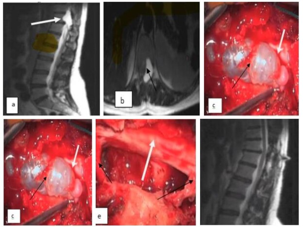
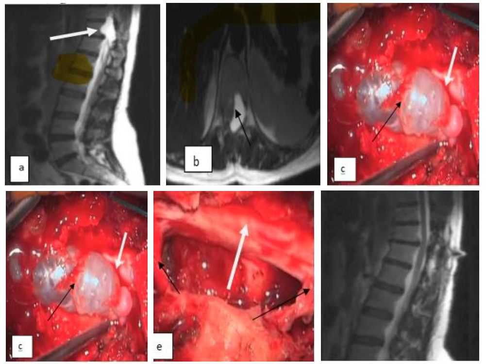
A young 36-year-old patient who has had spastic paraparesis for a few months, whose radiological exploration with a sagittal (a) and axial (b) T2 MRI showed a cystic lesion at the height of D10 D11 with the same signal as the lateralized extradural CSF on the left and driving back the spinal cord on the right.

The patient underwent surgery where a laminectomy was performed, removing this voluminous arachnoid cyst (black arrow) and pushing back the marrow on the right (white arrow). d: reduction of the cystic volume by puncture and coagulation of the cystic wall, which is made of a thick arachnoid. After complete excision of this cyst, we find good release of the marrow (white arrow) and the nerve roots (black arrows). A post-op control spinal MRI shows total excision of the arachnoid cyst; the patient has progressed well and has fully recovered from his deficit (Figure 1).

FIG 1

Figure 1: Radiological images sagittal (a) and axial (b) T2 MRI showed a cystic lesion (c), (d) reduction of the cystic volume by puncture and coagulation of the cystic wall. After cyst removal (e) good release of the marrow (white arrow) and the nerve roots (black arrows), (f) post-op control spinal MRI.

Discussion

The term “arachnoid cyst” is used to describe most types of cysts that involve the arachnoid. Nabors [4] has put them into groups based on where they are in relation to the nervous system in:

Type 1: An extradural cyst not comprising a nervous structure;

Type 2: Extradural cyst comprising nervous structures (Tarlov cyst);

Type 3: Intradural cyst.

Its topography is essentially thoracic, extending over several vertebrae with a peak of greater frequency around the eighth dorsal vertebra; our case sits at the level of D10 D11. Cervical or lumbosacral localization is very rare [5]. Dorsal locations are particularly frequent in the second decade of life given the narrowness of the canal at this level, and lumbosacral locations are observed later, between 30 and 50 years of age [6,7]. It is almost exclusively posterior, more rarely anterior or anterolateral [8,9].

In our case, the seat is posterolateral:

There is no sex ratio; the age of discovery can vary from 4 to 80 years, according to the cases listed in the literature [8]. Our patient was 36 years old; the symptoms are generally slowly progressive, but rapid revelation or decompensation is possible [10]; There is no relationship between the severity of the signs and their date of appearance. For thoracic cysts, the duration of the development of symptoms is shorter than for lumbar cysts due to the difference in the diameter of the spinal canal [11];

There are some particularities in terms of their clinical expression: The spinal syndrome and the radicular syndrome are very often in the foreground, frequently increased by the standing position (which may correspond to a tensioning of the cyst or its stretching) [12,13]; spinal deformities are the prerogative of old cysts; the sublesional syndrome, linked to the position of the cyst, is dominated by posterior cord involvement; sphincter disorders are more rare and moderate.

The etiopathogenesis remains hypothetical, and several theories have been presented. Extradural arachnoid cysts likely have a congenital origin, and they are the result of congenital dural diverticula or herniation of the arachnoid through congenital dural aplasia [14]. The nerve or the junction of the dural root and sheath are the most common sites of these defects, although less often the dorsal midline of the dural sac is also involved. The defect of the dura mater would be due to a structural anomaly of congenital origin, the consequence of a failure of the tightness of the collagen fibers. This failure leads to elongation and ectasia of the dura mater. Cases of spinal arachnoid cysts that do not clearly have a congenital origin have also been reported. The association of spinal arachnoid cysts with arachnoiditis   potential source of arachnoid septations), spinal surgery, and spinal cord trauma has prompted some authors to suggest that these cysts may result from acquired dural lesions [15]. Several surgical methods can be proposed, including marsupialization of the cyst which consists in opening the cyst and making its contents widely communicated with the spaces under perimedullary arachnoids, however, wide resection of the cyst is the method of choice. Since the goal is to stop the pressure difference between the cyst and the space under arachnoid.

For asymptomatic patients, it is recommended to observe conservative treatment with monitoring of the evolution of clinical symptoms and radiological controls regular.  Regarding symptomatic epidural arachnoid cysts, all authors agree on the indication for surgery. It is then recommended to carry out the complete excision of the cyst, and then the pedicle connecting the cyst to the subarachnoid space and the cyst is tied off. repair of the dural defect. This is the technique of choice to prevent the CSF reaccumulation and cyst recurrence. For our patient with a painful extradural arachnoid cyst, we removed the whole cyst, tied off the intradural communication pedicle, and reshaped the dura.

Conclusion

Extradural spinal arachnoid cysts are rare lesions, and treatment options should be considered carefully. In symptomatic cases, total excision of the cyst should be considered the reference treatment. We believe that closure of the dural defect should be the primary surgical goal to prevent recurrence. We offer laminoplasty for the treatment of extradural arachnoid cysts involving multiple segments to prevent postoperative kyphosis.

References

  1. Perret G, Green D, Keller J (1962) Diagnosis and treatment of intradural arachnoid cysts of the thoracic spine. Radiology 79: 425-429. [crossref]
  2. Lesoin F, L Eys D, Rousseaux M, Cama A, Jomin M, Petit H (1985) Spinal intradural arachnoid cysts. Acta Neurchir 76 : 125-128.
  3. Goyal RN, Russell NA, Benoit BG, Belanger JM (1987) Intraspinal cysts: a classification and literature review. Spine 12(3): 209-213. [crossref]
  4. Nabors MW, Pait TG, Byrd EB, Karim NO, Davis DO, et al. (1988) Updated assessment and current classification of spinal meningeal cysts. J Neurosurg 68(3): 366-377. [crossref]
  5. AJNSAfrican Journal of Neurological Sciences | » KYSTE ARACHNOÏDIEN EXTRADURAL RACHIDIEN AJNS 2009. 28(1).
  6. Paramore CG (2000) Dorsal arachnoid web with spinal cord compression: variant of an arachnoid cyst? Report of two cases. Journal of Neurosurgery: Spine 93(2): 287-290. [crossref]
  7. Rimmelin A, Clouet PL, Salatino S, Kehrli P, Maitrot D, et al. (1997) Imaging of thoracic and lumbar spinal extradural arachnoid cysts: report of two cases. Neuroradiology 39(3): 203-206. [crossref]
  8. LVISI C, ERISOLI M, IULIONI M, UERRA L (1987) Long term results of surgically treated congenital intradural spinal arachnoid cysts. J Neurosurg 67 : 333-335. [crossref]
  9. Kendall BE, Valentine AR, Keis B (1982) Spinal arachnoid cysts: clinical and radiological correlation with prognosis. Neuroradiology 22(5): 225-234. [crossref]
  10. Rousseaux M, Combelles G, Destée A (1983) Diverticules et kystes arachnoïdiens rachidiens intraduraux: 6 observations. Neurochirurgie 29: 279-284.
  11. Nabors MW, Pait TG, Byrd EB, Karim NO, Davis DO, et al. (1988) Updated assessment and current classification of spinal meningeal cysts. J Neurosurg 68(3): 366-377. [crossref]
  12. YS, RS, MS (1991) Spinal intradural arachnoid cysts. Neurochirurgia (Stuttg) 1 Juill. 34(4): 127-130. [crossref]
  13. Ar W, Jd L, Fc K (1975) Septum posticum cysts: an uncommon cause of chronic back pain. Pain 1(3): 271-275. [crossref]
  14. Neo M, Koyama T, Sakamoto T, Fujibayashi S, Nakamura T (2004) Detection of a dural defect by cinematic magnetic resonance imaging and its selective closure as a treatment for a spinal extradural arachnoid cyst. Spine 29(19): E426-430. [crossref]
  15. Saqui AE, Aggouri M, Benzagmout M, Chakour K, Chaoui ME (2017) Une cause rare de compression médullaire: kyste arachnoïdien épidural rachidien (à propos de 03 cas). The Pan African Medical Journal. [crossref]

Health Beauty Regimens, Inner Beauty, and Homo emotionalis versus Homo economicus

DOI: 10.31038/PSYJ.2023542

Abstract

Female respondents each evaluated sets of 48 unique vignettes, comprising messages about new regimens for ‘beauty from within’. The messages were sales and information messages that might likely appear in an advertisement. Respondents rated believability in the messages presented by the vignette, and from a set of different prices selected the price they would pay for the product described by each vignette. Deconstructing the rating assigned to a vignette into the contribution of the messages revealed three strong minds when the criterion was ‘believability; MSB1 – Make your inner self come alive and real; MSB2 – Appeal to authority and tradition; MSB3 – Reinforce the power for beauty within by hypnosis. Deconstructing the price rating revealed two strong mind-sets; MSP1 – Appeal to secret ‘formula’; MSP2 – Ease and convenience; and one weak mind-set. All six mind-sets show similar patterns of price would pay versus belief, even though each mind-set differed in the patterns of what it believed, or in the patterns of what it would pay. The approach, using Mind Genomics, shows how topics of everyday experience can become inputs for a science of ordinary human behavior.

Introduction

The pursuit of beauty is and has been a long-term affair in the history of humankind. Beauty, however defined, is always sought after. What makes the topic so interesting is that the search for beauty seems to be almost universal. People want to look good for themselves and to others. The exact methods by which this goal is accomplished depend on the historical eras, the available technology, the particular conception of what is beauty, and finally the ‘zeitgeist,’ and the ever-changing technology of the time.

One can scarcely open any media and successfully elude the barrage of stories and advertisements, all talking in an increasing babble about one or another aspect of ‘beauty.’ What was a simple world a century ago after World War I have morphed into a cacophony. Beauty is no longer ‘skin deep’ but has migrated to all parts of the body and the brain. One need only look at the stories in the paid advertisements to realize that beauty has migrated to the world of Estee Lauder three quarters of a century ago to the world of good living, meditation, hypnotism, and so forth. All are things, behaviors, ways of thinking to which beauty is attached, and which can enhance beauty.

In the 1980’s and 1990’s the author wrote two books on cosmetics and personal products [1,2]. The research in those books was based upon the emergent science of psychophysics, the study of the relation between physical stimulus and subjective responses. During the formative years of the author’s scientific career, 1969-1985, a great deal of the work with done with product developers, interested in the laboratory-level improvement of cosmetics, toiletries, and fragrances. Colleagues and clients such as Morton Pader would encourage this effort

During the later years of the 1980’s, the author began to work with the marketing departments of companies, with the focus on how to communicate the benefits of beauty. The intense competition among the major cosmetic companies, as well as those large companies marketing the world of products known as ‘personal care’ drove interest into studying the mind of the consumer. The focus moved from how to formulate to achieve optimal acceptance and support of a positioning through just what to say. It became increasingly clear that there were no real databases about the mind of the consumer, despite the seemingly massive amounts of corporate data residing in the corporate files. The information available was one-off, focused, often being the ‘verbatims’ reported from focus groups and depth interviews, but almost no quantitative data. Even companies like Procter & Gamble, Inc., in Cincinnati, bastion of standardized methods, could not or would not produce books about messaging, although they were able to produce books about standard research methods.

It was in the early to mid-1990’s that the approach used here, Mind Genomics, would emerge to create the necessary structured database about the mind. Mind Genomics is a science which studies through experiments the perception of the person’s everyday world [3,4]. It is the application of Mind Genomics to the new world of ‘beauty from within’ which will be the subject of this paper.

Method

Through a disciplined approach using statistical experimental design, Mind Genomics combines elements describing daily experience (messages), creating vignettes. The vignettes comprise simple combinations of these elements, one element atop the other in an easy-to-read format, viz., without connectives. The respondent scans the vignette, viz., this combination of elements, and assigns a rating on the scale(s) provided. The analysis deconstructs the response to the combinations, revealing the part-worth contribution of each element.

This seeming ‘round-about’ way to understand the strength of each element has several built-in positives.

Ecological Validity

In our normal lives we don’t evaluate one stimulus at a time in splendid isolation, even though that approach is taught as the epitome of good science. People experience the stimuli in combinations, ideas fighting each other for attention. Mind Genomics attempts to reproduce a world of ‘bustling confusion.,’ and within that world suffused with noise estimate how each element performs.

Reduction of Bias

Often respondents attempt to ‘guess’ what the researcher wants, and assign the desired answer, rather than the answer which truly reflects the way the individual respondent feels. All one has to do is ask people to describe their food shopping behaviors and their food pantries to end up with a description of what seems to be a healthy diet filled with the foods that are highly recommended. Closer inspection of the houses of such individuals often reveals a lot of junk food. Similarly, people who vote and then participate in an exit poll or a qualitative interview often do not give an honest answer when asked for whom they voted. The effort to appear politically correct may undercount some candidates who held publicly unpopular yet meaningful and attractive points of view about social situation. Former President Donald Trump provides an example. Votes for Trump were undercounted because the participants in the poll were often subtly positive but felt that the interviewer would feel negatively about them were they to state their positive feeling.

Ability at the Level of Each Individual to Understand How the Elements ‘Drive’ the Ratings

The Mind Genomics method works by creating experimental designs (combinations of elements into vignettes), and with the property that each individual respondent evaluates the precisely correct combination of elements in the 48 vignettes so that one can use statistical methods such as OLS (ordinary eat-squares) regression to relate the presence/absence of the 36 elements to the rating, or to a specified transformation of the rating [5]. In behavioral science the ability to do all of the analyses at the level of the individual (within-subjects design) means that the respondent ends up providing all of the relevant information. There is no immediate need to work with data beyond one person to understand the pattern of results generated by that one person.

Evaluation of More of the Design Space

Every respondent evaluates a unique set of combinations, allowing the research to explore a great deal of the so-called design space, the space of possible combinations. This set of individual sets of combinations means that in our study of 100 respondents, each of whom evaluated 48 different combinations, the study actually covered 4800 different combinations. The benefit of covering a lot of the design space is that the research becomes an exploration, a cartography of new to the world topic, rather than requiring the researcher to evaluate the most likely test combinations to prove or disprove a hypothesis. Mind Genomics becomes an exploratory tool for new knowledge, a tool which helps one understand the topic at a macro level. [6]

Explicating the Process with the Study on Hypnosis and Inner Beauty

With the foregoing in mind, we now proceed to the study of a new way of thinking about beauty, beauty from within. The actual study came from a discussion with Wendy Packer of Westchester, New York, around 2013. The issue was whether Mind Genomics could provide a way to quantify what was believable in some of the topics and claims, and for what was something for which respondent would pay. The author immediately offered to ‘try out’ the different messages, in a simple exploratory study, to see what would emerge. The paper is the result of that effort. What is important to keep in mind is that the templated version of Mind Genomics allows the researcher to setup the study, get the respondents, run the study, and receive the data almost automatically in an hour or two [7]

Step 1: Create the Raw Materials, Comprising Questions (Aspects) and Answers (Elements, Test Messages)

This first section is the hardest. Once the study is named, a step requiring the researcher to summarize the study in a word or two, the task becomes harder. The researcher has to develop a ‘story,’ within that story ask six questions which flow in reasonable order, and then for each question provide six answers. Table 1 shows the final set of six questions, and each question having six answers.

Table 1: ‘The final set of six questions and six answers (elements) for each question

tab 1

This initial exercise may seem easy to the reader, but the task is often daunting, mostly for beginning researchers, but occasionally for experienced researchers as well. The researcher must create a set of questions or topic statements which tell a story. The story need not have a plot. Rather the story will end up being a set of questions which seem plausible when stated. In turn each question requires six answers.

The above-mentioned task often drives the researcher to abort the study as it is being developed. Our education system is reasonably strong in teaching us how to answer questions. It is critical thinking necessary to formulate the questions in a way which becomes hard. We are accustomed to one at a time questions, the questions not being part of a story. Making the researcher produce a story can be frustrating for the researcher.

The act of developing the ‘proper’ questions and the array of possible answers (elements) for these questions often becomes the most important part of the learning process. One might think that the experiment itself with real respondents does most of the teaching. Three decades of working with Mind Genomics and its antecedent, IdeaMap® have continued to show them that much of the learning occurs in the up-front preparation, and that in effect the benefits of IdeaMap end up being the co-creation of insight by the research during the up-front set-up along with information gleaned from the respondent in the actual experiment.

Step 2: Create the Instructions and the Rating Questions

In this earlier version of Mind Genomics, the study ended up focusing on two aspects of the topic, believability, and value, respectively. The practical aspects of the topic led naturally to study these two issues as the core of what was needed for the practitioner to discover. The first issue was ‘would anyone believe this statement,’ which answer would emerge after the deconstruction of the rating of believability assigned to a vignette into the part-worth estimates of believability of the component elements. To the practitioner, having a statement which is believable is of paramount importance.

The second topic aspect was the expected price that the element could command. From the practitioner’s viewpoint it is always important to offer something which respondents are willing to purchase, rather than offering something for which they are not willing to open their pocketbook, expecting it to be free.

Table 2 shows the orientation scale, and the two rating questions. Each rating question was transformed into a format mor easily used by the computer in regression analysis. For the first rating question, believability, ratings 8-9 were transformed into the top part of a two-part scale, believable. For the same first rating scale, the ratings of 1-7 were transformed into the bottom of the two-part scale, not believableFor price; the selected price became the rating of value.

Table 2 also presents a set of self-profiling questions, completed by the respondent. The self-profiling questions enable the researcher to understand more about WHO the respondent is, what the respondent DOES, and what the respondent BELIEVES. This information can come only from the respondent or from a deep analysis of data available for sales, data that has to be combed through to create a partial profile of the respondent. It is far easier to ask the respondent to profile herself.

Table 2: Belief scale, price scale

tab 2

Step 3: Execute the Mind Genomics Experiment on the Internet

The standard approach is to recruit respondents who are pre-qualified, usually individuals who are members of an online panel. It is tempting to save money by recruiting individuals who one knows, and who can be persuaded to ‘volunteer.’ Although the use of unpaid respondents may seem to be a cost saving, rarely does it ever turn out to be so. The study may take at least 20-50 times longer to complete, as the researcher hunts for willing, qualified respondents. In light of this, the Mind Genomics system works with panel providers, companies which specialize in providing qualified respondents, doing so in a matter of hours, not weeks.

The respondents were recruited with the panel provider. Today’s studies are done with Luc.id Inc., a panel provider with the ability to source respondents from around the world. The study was done in 2012, a decade ago with an entirely different company. The study was completed in a matter of our hours, from launch to completion. The Mind Genomics system sends out the test elements and constructs them on the site. The respondent reads the introduction, is presented with each screen (48 screens altogether, each with 3-4 elements, according to the vignette), rates the vignette on the two questions, and then immediately proceeds to the next vignette

Step 4: Acquire the Data Format the Data for Analysis

Each respondent generates 48 rows, one row for each of 48 different vignettes that a respondent evaluates. The database comprises three sets of columns. The first set of columns defines the respondent, and the information provided by the respondent about herself from the self-profiling questionnaire. This first set of columns remains the same for all 48 rows, since it refers to the respondent, and not the vignette. The second set of columns contains one column showing the test order (1-48), and then 36 succeeding columns, one column assigned to each of the 36 elements in the design. For a specific column (the element) and a specific row (the vignette), the cell will either have a ‘0’ when the element is absent from that vignette, or a ‘1’ when the element is present in that vignette. This is called ‘dummy variable coding’ because the variable has almost no information except absent or present. The third set of columns shows the rating assigned to the vignette, the dollar value selected, and then two additional columns which are transformed values. The second to the final column is 100 when the rating was 9 or 8, denoting extremely or very believable, and 0 when the rating was 7 or lower, denoting modestly believable, or degrees of unbelief. The final column shows the actual dollar and cents value corresponding to the rating selected for the second question.

As preparation for the additional analysis, a vanishing small umber (<10-5) was added to every transformer rating for both belief (R98) or price. The vanishingly small number ensures that no matter what rating the respondent chooses, there is always variability associated with the rating, a requirement for regression analysis.

Step 5: Create a ‘Sneak Preview’ of the Data to Get a Sense of ‘How Well’ the Vignettes Performed

Even before we look at the strength of the individual elements, we can quickly assess how well we did. Figure 1 shows the distribution of ratings of believability (left panel) and the distribution of selected prices (right panel).

By itself, Figure 1 tells us little about the mind of the respondent. We could look more deeply into the data by a variety of different analyses, simply on the responses to the vignettes alone. Another analysis might be to look at the ratings at the beginning of the evaluation versus at the end of the analysis (viz., ratings assigned for test orders 1-3 vs ratings assigned for test orders 46-48). Do they differ, and if so, then how do they differ? Figure 2 shows this comparison. Figure 2 suggests a slight decrease in belief in the validity of what the vignette communicates, as well as a slight decrease in the price one would pay. What Figures 1 and 2 fail to do, however, is exploit the cognitive richness of the vignette embedded in the meaning of the elements, and then draw conclusions about the effect of order.

fig 1

Figure 1: Distribution of the ratings of believability and price for the full set of vignettes

fig 2

Figure 2: Distribution of the ratings of believability and price for the first four vignettes (order 1-4) versus the final four vignettes (order 45-48).

Step 6: Create an Equation Relating the Presence/Absence of the 36 Elements to the Transformed Rating

The equation is estimated by standard statistical techniques. The equation shows how each of the 36 elements ‘drives’ the transformed rating. The equation is developed for each respondent, respectively, as well as for groups. This ability to fit the equation, even at the level of the individual respondent, occurs because of the previously discussed process known as experimental design. The experimental design that we use in Mind Genomics is set up so that each individual respondent evaluates the precisely correct vignettes for a regression model.

The equation is expressed as: DV (dependent variable+ = k1A1 + k2A2…k36F6

The dependent variable is either the variable R98 denoting believable, or Price (the actual price chosen by the respondent).

We create this pair of equations for every subgroup of interest. The computer program (Systat, 2013) allows the researcher to input the variables (dependent, independents), to then select or not select the additive constant (we do not select), after which in less than 1-2 seconds, the statistical program has estimated and stored the parameters of the equation.

The key benefit of the analysis by OLS regression is that we now understand the data more deeply. Rather than treating each of our ratings as simply a ‘point’ and focusing on the general pattern created by those set of points, we can understand the ‘meaning’ of each point from knowing the text of each element. With that type of information, our questions about the data become more pointed, more realistic, and ultimately far more informative.

Table 3 shows the coefficients for the 36 elements. The left pairs of data columns show the elements sorted in descending order of believability, with the believability coefficient on the left, and the price coefficient to its right. The right pairs of data columns show the same elements, this time sorted by price, with price coefficient on the left, and the believability coefficient to its right.

Table 3: Self profiling questions and number of respondents choosing each answer

tab 3

Table 3 presents a great deal of data. To enable the pattern to emerge we show all elements of coefficient of 6 or higher for R98 or price would pay (for the element) of $5.00 or higher. Noteworthy in Table 3 is the low coefficients for R98 (viz., low belief in the validity of the messages), and the low price that would be paid. Figure 3 shows the approximately linear relation between the degree of believability and the price that would be paid, both coefficients from the regression models presented in Table 3. We conclude from Figure 3 that respondents feel willing to pay more for elements whose validity they believe, although the relation is ‘noisy.’ Despite the noisiness, the linear relation gives one confidence that the data are internally consistent.

fig 3

Figure 3: Scatterplot showing the relation between the coefficient for believability (abscissa) and the coefficient for dollars would pay (ordinate).

Step 7: Uncover Mind-sets Based Upon Coefficients for Believe, and Again Mid-sets Based on Coefficients for Price

A hallmark of Mind Genomics is the search for groups of like-minded respondents, the term ‘like-minded’ applied to similar patterns of responses to a granular topic. The world of consumer research is awash with different ways of dividing people, the most common being differences in who the people ARE [8], how the people THINK [9], and how the people BEHAVE [10]. The effort to create these different groups is significant so that the division of people into these groups, the process called segmentation, is reserved for the most important topics in the area, and becomes a seminal work generally not repeated because of effort and expense. The result is the macro-level segmentation of big topics and the efforts needed in turn to apply this macro-level segmentation to the world of the everyday, where it is most needed, and where ‘real life’ occurs.

The Mind Genomics approach works at the level of the granular, looking at simple-to-understand patterns of differences in responses to messages about a specific topic. Rather than working at the macro-level and trying to apply the general rules to the particular instance, Mind Genomics uses the pattern of responses to the specific topic to create the different groups, the segments, or in the language of Mind Genomics, the so-called ‘mind-sets.’

The segmentation into mind-set for our study proceeds in a simple manner [11].

  • Create 101 individual-level models or equation, of the same form that we created above. Do this creation twice, once for the equation relating the element to R98 (believable), and then for the equation relating the elements to price.
  • Beginning with the 101 individual level equations for believable, compute the ‘distance’ between each pair of the 101 respondents, using the formula Distance = (1-Pearson R). This distance will be 0 when the Pearson R (correlation) is 1.00, viz., the case where two respondents are perfectly aligned in their pattern of 36 coefficients. In contrast, this distance will be 2.0 when the Pearson correlation is -1, viz., when the two respondents are perfectly aligned in opposite directions.
  • Cluster the respondents into two, and then three groups, such that the distances between the people in a cluster are small, whereas the distances between pairs of centroids of different clusters are large. This strategy ends up assigning people to clusters or mind-sets in a purely quantitative fashion. There is no conscious effort for the clusters to make sense.
  • Invoke two rules, parsimony (fewer clusters are better than more clusters), and interpretability (the strong performing elements within a cluster should tell a coherent story).
  • For this project three clusters made more sense than two clusters, even though the two-cluster solution was more parsimonious.

Table 4 shows the three mind-sets emerging from clustering on the basis of belief in the validity of the information. Table 5 shows a different group of three mind-sets, emerging from the clustering the basis of price.

Table 4: Coefficients of the 36 elements for the Total Panel, across the two dependent variables (believable via R98; price would pay in actual dollars).

tab 4

Table 5: Coefficients for Mind-Sets based upon belief in validity (DV = 98). Only positive coefficients 4 or higher are shown.

tab 5

The segments are different. When we extract three mind-sets for each dependent variable, we find that the mind-sets emerging from the emotion reaction (R98; believe in validity) seem to the author be authentic and compelling. In contrast, the mind-sets based upon price seem to be more conventional. Furthermore, although we pull out three mind-sets for price, the reality is that there are probably two mind-sets, not three. The third mind-set (self-fulfillment) really only has one strong performing element.

Mind-Sets Based Upon Believe in Validity (R98)

MSB1 – Make your inner self come alive and real (N=47)

MSB2 – Appeal to authority and tradition (N=34)

MSB3 – Reinforce the power for beauty within by hypnosis (N=20)

Mind-Sets Based Upon Price

MSP1 – Appeal to secret ‘formula’ (N = 40)

MSP2 – Ease and convenience (N = 26)

MSP3 – Self Fulfillment (N=35)

Figure 3 shows a linear relation between coefficient of price (ordinate) and coefficient of believability (abscissa). Figure 4 shows the same plot, this time for the three mind-sets created by clustering coefficients for believability (MSB1, MSB2, MSB3), and for the three mind-sets created by clustering coefficients for price (MSP1, MSP2, MSP3). Surprisingly, the lines fit to the scatterplots are parallel to each other.

fig 4

Figure 4: Scatterplot for the six mind-sets extracted from the data. MSB1-MSB3 were extracted from the coefficients for believability. MSP1-MSP3 were extracted from the coefficients for price.

Discussion and Conclusions

The study presented in this paper was done around 2012, a decade ago, and resurrected after a discussion about alternative forms of beauty that are available. During the course of the conversation the author recalled the study, returned to it, looked at the topics, and ‘worked up’ the data for publication. The realization then once again dawned. Here was a way to do science, motivated by a simple problem (quest for beauty), a world view (holistic), and a set of techniques (hypnotism and auto-suggestion).

A search through the scientific literature using Google Scholar® revealed little published information about hypnosis combined with beauty, and virtually nothing dealing with the appropriate messaging about the topic. There were papers and books dealing with the general benefits of hypnosis for better living, including enhanced beauty [12]. It is as if the idea of hypnosis and beauty was left to the popular press, and not invited to be studied by serious researchers.

At this point, almost 11 years after the study was done, remains the realization of the value of the process. On the one hand, it was easy to do in 2011-2012. One simply needed to collaborate with a person involved in beauty and with another person working in the world of hypnosis and psychodynamics (e.g., psychotherapy). The was no need for expertise, but simply a set of questions, and then answers each question, as well as two additional scales (believe, price, respectively) The rest proceeded virtually automatically, creating what might be called a ‘database of the mind’ in this exceptionally circumscribed topic of beauty emerging from hypnosis. The other key observation is the value of data about messaging in a specific, circumscribed topic, value which lasts decade, and no doubt longer.

References

  1. Moskowitz HR (1984) Cosmetic Product Testing: A Modern Psychophysical Approach. Marcel Dekker.
  2. Moskowitz HR (1995) Consumer Testing and Evaluation of Personal Care Products. Marcel Dekker.
  3. Moskowitz HR, Gofman A, Beckley J, Ashman H (2006) Founding a new science: Mind Genomics. Journal of Sensory Studies 21: 266-307.
  4. Moskowitz HR, Gofman A (2007) Selling Blue Elephants: How to Make Great Products that People Want Before They Even Know They Want Them. Pearson Education.
  5. Hardy MA (1993) Regression with Dummy Variables. Sage.93
  6. Gofman A, Moskowitz H (2010) Isomorphic permuted experimental designs and their application in conjoint analysis. Journal of Sensory Studies 25: 127-145.
  7. Moskowitz H, Itty B (2003) Jumpstarting product development: Competitive analysis and conjoint measurement in the cosmetic industry. Journal of Advertising Research 43: 62-77.
  8. Rangan VK, Chu M, Petkoski D (2011) Segmenting the base of the pyramid. Harvard business review 89:113-117.
  9. Wells WD (1975) Psychographics: A critical review. Journal of Marketing Research 12: 196-213.
  10. Kameniduou IC, Mamalis SA, Pavlidis S, Bara EZ (2019) Segmenting Generation Z cohort university students based on sustainable food consumption behavior: A preliminary study. Sustainability 11: 837.
  11. Likas A, Vlassis N, Verbeek JJ (2003) The global k-means clustering algorithm. Pattern Recognition. 36: 451-461.
  12. Blair F (2007) Self-hypnosis Revolution: The Amazingly Simple Way to Use Self-hypnosis to Change Your Life. Sourcebooks, Inc.

The Ionic Liquid-Assisted Synthesis of a Novel Polyaniline/Graphitic Carbon Nitride/Zinc Tungstate (PANI/g-C3N4/ZnWO4) Ternary Nanocomposite: The Usage of Easy Double Electron Transfer Photocatalyst for Glyphosate Photocatalytic Degradation Process

DOI: 10.31038/NAMS.2023622

Abstract

In this study, a novel polyaniline/graphitic carbon nitride/zinc tungstate (PANI/g-C3N4/ZnWO4) (PGZ) ternary nanocomposites (NCs) as a heterostructure photocatalys was examined during photocatalytic degradation process in the efficient removal of glyphosate herbicide from a aqueous solution. Different pH values (3.0, 5.0, 7.0, 9.0 and 11.0), increasing glyphosate concentrations (5 mg/l, 10 mg/l, 15 mg/l and 20 mg/l), increasing PANI/g-C3N4/ZnWO4 ternary NCs concentrations (5 mg/l, 15 mg/l, 30 mg/l and 45 mg/l) and increasing recycle times (1., 2., 3., 4., 5., 6. and 7.) was operated during photocatalytic degradation process in the efficient removal of glyphosate in a aqueous solution. The characteristics of the synthesized nanoparticles (NPs) were assessed using X-Ray Difraction (XRD), Field Emission Scanning Electron Microscopy (FESEM), Energy-Dispersive X-Ray (EDX), Fourier Transform Infrared Spectroscopy (FTIR), Transmission Electron Microscopy (TEM), Diffuse reflectance UV-Vis spectra (DRS) and X-Ray Photoelectron Spectroscopy (XPS) analyses, respectively. The cyctotoxicity test was operated to the standard TBE (trypan blue dye exclusion) assay technique with Drosophila melanogaster (fruit fly). ANOVA statistical analysis was used for all experimental samples. The maximum 99% glyphosate removal efficiency was obtained during photocatalytic degradation process in aqueous solution, at 15 mg/l gylphosate, at 30 mg/l PANI/g-C3N4/ZnWO4 ternary NCs, at pH=11.0, at 150 W UV-vis light irradiation power, after 180 min photocatalytic degradation time and at 25°C, respectively. The maximum 99% cyctotoxicity removal was observed at untreated glyphosate samples, after 180 min photocatalytic degradation time, at 150 W UV-vis light irradiation power, at pH=7.0 and at 25°C, respectively. The maximum 99% cyctotoxicity removal was observed at 5 mg/l PANI/g-C3N4/ZnWO4 ternary NCs photocatalyst concentrations, after 180 min photocatalytic degradation time, at 150 W UV-vis light irradiation power, at pH=7.0 and at 25°C, respectively. The study revealed the excellent minimization of cytotoxicity of glyphosate after photocatalytic degradation process with the PANI/g-C3N4/ZnWO4 ternary NCs photocatalyst. As a result, the PANI/g-C3N4/ZnWO4 ternary NCs photocatalyst is found to be non-cytotoxic irrespective of its quantity used. Finally, the combination of a simple, easy operation preparation process, excellent performance and cost effective, makes this a novel PANI/g-C3N4/CoMoO4 ternary NCs heterostructure photocatalyst a promising option during photocatalytic degradation process in agricultural industry wastewater treatment.

Keywords

ANOVA statistical analysis, Cytotoxicity test, Diffuse reflectance UV-Vis spectra (DRS), Drosophila melanogaster (fruit fly), Electrochemical filtration process, Energy-dispersive X-ray (EDX), Field emission scanning electron microscopy (FESEM), Fourier transform infrared spectroscopy (FTIR), Gylphosate, Herbicites, Ionic liquid-assisted synthesis, Novel polyaniline/graphitic carbon nitride/zinc tungstate (PANI/g-C3N4/ZnWO4) ternary nanocomposites, Pesticides, Photocatalytic degradation, Transmission electron microscopy (TEM), X-ray difraction (XRD), X-ray photoelectron spectroscopy (XPS)

Introductıon

The intense populational growth and industrial expansion in the most diverse segments of society have led to a substantial increase in the demand for drinking water supply and large-scale food production [1]. Thus, to increase productivity at an economically profitable level, the employment of agrochemicals has been widely used to combat pests and weeds [2]. With the enhanced use of a new variety of anthropogenic compounds towards industrialization, water pollution has increased substantially [3]. Anthropogenic compounds like synthetic pesticides and herbicides are often used in agricultural fields to protect crops. However, pesticides are characterized by low biodegradability, high bioaccumulative capacity arising from their physicochemical properties, and a long half-life, of 5-15 years, increasing their toxicity to the environment and humans [4,5]. Thus, pesticide persistence in soil, wastewater, ground, and surface water has proved to be a considerable environmental problem, and may be compounded along the food chain, reaching concentrations toxic to human health [6]. Due to their high stability, these compounds can contaminate areas distant from pulverization through water volatilization and soil absorption. Studies have associated exposure to compounds with hormonal changes in the immune, neurological and cardiac systems, as well as with the development of neoplasms [7,8].

For this purpose, diverse techniques, such as adsorption and advanced oxidative processes (AOPs), which include Fenton, photo-fenton, heterogeneous photocatalysis and ozonation systems, have been explored for removing and degrading biopersistent organic compounds [9-11]. AOPs are based on the generation of free radicals, e.g., hydroxyl (OH) and superoxide (O2– ●) radicals, which have high oxidizing power in an aqueous solution and are able to degrade pollutants into lower molecular weight intermediates and inorganic precursors [12,13]. Heterogeneous photocatalysis is an advanced oxidative process that occurs through the photoactivation (by sunlight or artificial light) of a semiconductor, which uses water molecules and dissolved oxygen as reagents of oxi-reduction reactions [14]. This technique is very efficient and promising for the degradation of organic pollutants, including dyes, drugs and pesticides [15,16]. Among the materials used, metallic nanooxides (zinc oxide, ZnO and titanium dioxide, TiO2) have been largely employed due to their excellent properties, such as low toxicity, good availability, chemical stability, large surface area/porosity, and photocorrosion [17,18]. However, these conventional nanocatalysts are characterized by their high bandgap energy, which is the energy required to start photocatalytic reactions. Additionally, due to their high surface energy, they tend to agglomerate during the photocatalytic process. Therefore, the association of these nanocatalysts with a second, less active material (called catalytic support or matrix) can solve these drawbacks, even when the active material is dispersed in low concentrations (ca. 0.5-5 wt%) on the support [19]. Thus, combining the two materials results in a new material called NCs, in which the active substance is in the above-mentioned concentration range and this is named the reinforcement phase [20].

NCs are multiphase materials formed by a continuous and dispersed phase and have at least one dimension in the nanoscale [21]. The continuous phase (matrix) consists of a compound of polymeric, ceramic or metallic origin, while the dispersed phase (reinforcement) is commonly derived from fibrous materials [22-24]. NCs materials are synthesized to combine individual properties and reduce limitations, such as physicochemical and thermal instability, expanding the scope of applications. In parallel, at the nanoscale, the materials exhibit distinct behaviors to those found at the micrometer scale, such as volume/area relationship and increased reactivity [25]. Another technique widely used for pesticide removal from wastewater consists of adsorption, especially when using nanomaterials (adsorbents), due to its simplicity of operation, relatively low cost, and low energy requirements [26]. In addition, nanoadsorbents are characterized by their high specific surface area, chemical/thermal stability, and affinity for organic pollutants [27]. Although the efficiency of nanoadsorbents in the removal of organic compounds is remarkable, there are still limitations to conventional materials’ use, such as separation from the aqueous medium and the reuse of nanoadsorbents and nanocatalysts [28]. Recently, the development of nanocomposites as nanoadsorbents has been the subject of diverse research due to their increased surface area and physicochemical stability. Moreover, magnetic NCs have been used as a good alternative to improve the stability, textural properties, and reuse of nanoadsorbents [29]. The facilities separate material from the aqueous medium and considerably increase their reuse, resulting in high adsorptive capacity [30]. Additionally, the same behavior is observed for magnetic NCs as nanocatalysts. Using magnetic nanocatalysts allows the reuse of the material, increasing the cost-effectiveness and avoiding subsequent steps such as filtration and centrifugation [31].

Glyphosate {N-phosphomethyl[glycine] or (C3H8NO5P)}, is an organophosphorus compound with herbicide properties discovered in 1970. It is a competitive inhibitor of the 5-enolpyruvylshikimate-3-phosphate synthase, an enzyme involved in aromatic amino acid biosynthesis in plants and microorganisms [32]. Glyphosate is now the most used herbicide globally, and its usage keeps increasing with the emergence of weed resistance, from 16 million kg spread in the world in 1994 to 79 million kg spread in 2014, including 15% in the United States alone [33]. Once in the environment, glyphosate is metabolized by microorganisms into aminomethylphosphonic acid (AMPA; known as its most active metabolite) and methylphosphonic acid (MPA) (Figure 1) [34]. Glyphosate and its metabolite AMPA can be found in soils, water, plants, food, and animals [35-37]. Glyphosate is detected in human urine, blood, and maternal milk, with urinary levels of 0.26-73.5 μg/l in exposed workers and 0.16-7.6 μg/l in the general population [38,39]. Glyphosate most likely enters the body via the dermal, oral and pulmonary routes [40]. Even if the dermal route allows a poor absorption (≈2%), it is the main reported route of entry in exposed farmers [41]. Glyphosate then seems to accumulate principally in the kidneys, liver, colon, and small intestine and is eliminated in the feces (90%) and urine within 48 h. Because of this omnipresence, its safety is of grave concern. Glyphosate has long been regarded as harmless allegedly because it targets an enzyme inexistent in animals, is supposedly degraded into CO2, and its formulation contains misleadingly-called “inert” ingredients. Nevertheless, there is growing literature that describes the risks for glyphosate and glyphosate-based herbicides on human health [42]. After more than 40 years of global use, glyphosate has been classified as “probably carcinogenic” in humans by the International Agency for Research on Cancer (IARC). In March 2015, the World Health Organization’s IARC classified three organophosphates (glyphosate, malathion, and diazinon) as “probably carcinogenic for humans” (Category 2A) [43]. In contrast, in November 2015 the European Food Safety Agency determined glyphosate was “unlikely to pose a cancer risk for man” [44]. In 2018 the European Chemicals Agency, Risk Assessment Committee concluded that “the scientific evidence so far available does not satisfy the criteria for classifying glyphosate as carcinogenic, mutagenic or toxic for reproduction” [45]. In 2019, US federal health agency, the Agency for Toxic Substances and Disease Registry (ATSDR) [46], part of the Centers for Disease Control and Prevention [47], determined that both cancer and non-cancer hazards derive from exposure to glyphosate and glyphosate-based herbicides.

fig 1

Figure 1: Glyphosate and main glyphosate by-products; aminomethylphosphonic acid (AMPA), methylphosphonic acid (MPA) and glyoxylate, respectively.

In modern agriculture, especially in most intensive and large-scale crops, herbicides are used to eliminate weeds. Glyphosate is a non-selective, highly effective, broad-spectrum, and low toxicity herbicide, whose usage increases exponentially for the effective in eliminating weeds indiscriminately [48]. In recent years, the long half-life of glyphosate and its main metabolite AMPA causes the existence in the environment. The potential impact of glyphosate in the environment is an increasing concern around the world. In the recent past, a significant increase in the use of the glyphosate herbicide has been noticed which further increased after the introduction of glyphosate-tolerant crops [49,50]. According to a report, The United States saw a 14 times increase in glyphosate use between 1992 and 2015, where the majority was applied to soybean and corn crops [51]. Being a nonselective, mutagenic, and carcinogenic herbicide, their presence in atmosphere can cause severe health and environmental issues [52]. As a result, it poses a high environmental risk and requires prompt studies towards its elimination.

In recent years, photocatalytic studies have explored the fabrication of ternary heterojunctions as a preferred scientific and practical method to improve the migration of photogenerated charge carriers [53]. Towards this end, ternary type II heterojunctions have shown significant success with accelerated charge carrier production [54]. However, the repulsion between the photogenerated electrons and the formation of weaker redox potentials limit its photocatalytic activity [55]. Therefore, another promising photosystem known as a Z-scheme heterojunction was developed to overcome the aforementioned issues [56]. In the case of Z-scheme photosystems, the conduction band electrons with a lower energy of one semiconductor migrate towards the valence band holes with a higher energy of other semiconductors. This combination leads to the formation of highly reductive electrons as well as highly oxidative holes [57]. Additionally, Z-scheme photo-systems not only enhance the charge separation efficiency of semiconductor photocatalysts but also possess electrons and holes with strong redox potential for superior photocatalytic applications. Moreover, ternary heterojunctions with a double electron transfer Z-scheme have photogenerated charge carriers with a prolonged lifetime compared to binary systems which improves the scope of light-harvesting [58]. Some recent ternary heterojunctions with double electron transfer Z-scheme channelization are g-C3N4/ZnO/ZnWO4, polyaniline-BiOBr-GO, g-C3N4/Zn2SnO4N/ZnO [59-61].

The fabrication of NCs in ionic liquid (IL) media can provide a better scaling up approach for microscopic dispersion of particles and close interface contact between the individual components [62]. ILs as synthetic media provide unique advantages like negligible vapor pressure, thermal stability, and better conductivity than NCs. Additionally, the effect of “cation-π” and “π-π” interactions due to the presence of ionic liquids improve the nanoparticles (NPs) dispersion and stabilization which boosts the surface to volume ratio of NCs [63]. Recently, ionic liquids have been also employed for extensive polymerization and catalysis applications. Pahonik et al. [64] verified the oxidative polymerization of aniline with ammonium persulphate and the IL 1-butyl-3-methylimidazolium chloride (BMIMCl) under acidic conditions. More interestingly, IL-assisted NCs synthesis processes are relatively rapid, facile, greener, and more efficient without the requirement of any foreign stabilizer and surfactants [65]. The development of nanostructures and NCs with a simplified and greener IL-assisted in situ oxidative polymerization method is highly preferable method for photocatalytic degradation process of environmental pollutants.

Polyaniline (PANI) is a conducting polymer and organic semiconductor of the semi-flexible rod polymer family. PANI is one of the most studied conducting polymers [66,67]. To fabricate a ternary heterojunction, PANI can serve as the third active component of the photosystem. PANI has high demand as a low-cost and environment-friendly conjugated semiconductor for the fabrication of visible light harvesting photocatalysts [68]. It is a conducting polymer with an extensive conjugated π-system and high absorption coefficient towards visible light mediated charge carrier production. Furthermore, advantages like simple processing and high conductivity make it an emerging material for the synthesis of heterojunction materials. Recently, many efforts have been made to maximize the photo-harvesting efficiency of PANI-based composite materials. Researchers explored many positive hybrid effects arising from such systems due to the close contact of the interfaces of individual components leading to high separation efficiency of photogenerated electron-hole pairs [69].

The two-dimensional (2D) g-C3N4 semiconductor has a wide range of applications in the environmental and energy fields because of its visible-light activity, unique physicochemical properties, excellent chemical stability and low-cost [70,71]. Some important limitations of the photocatalytic activity of g-C3N4 are its low specific surface area, fast recombination of electrons and holes and poor visible light absorption [72-74]. To improve the above problems, the construction of a heterojunction with a suitable band gap semiconductor (co-catalyst) has been shown to be a good strategy to improve the photocatalytic performance of g-C3N4, such as g-C3N4-based conventional type II heterostructures, g-C3N4-based Z-scheme heterostructures, and g-C3N4-based p-n heterostructures, etc. The unique “Z” shape as the transport pathway of photogenerated charge carriers in Z-scheme photocatalytic systems is the most similar system to mimic natural photosynthesis in the many g-C3N4-based heterojunction photocatalysts. The construction of Z-scheme photocatalytic systems can promote visible light utilization and carrier separation, and maintain the strong reducibility and oxidizability of semiconductors [75-78]. There are many studies on g-C3N4-based Z-scheme heterojunction photocatalysts, such as ZnO/g-C3N4 [79-82], WO3/g-C3N4 [83], g-C3N4/ZnS, g-C3N4/NiFe2O4 [84], g-C3N4/graphene/NiFe2O4 [85], NiCo/ZnO/g-C3N4 [86] and Bi2Zr2O7/g-C3N4/Ag3PO4 [87], respectively. g-C3N4-based Z-scheme heterojunction photocatalysts have been made to improve the photocatalytic activity by combining with other semiconductor materials. Therefore, there are some problems with the single photocatalytic method, such as low adsorption ability, limited active sites and low removal efficiency. The integration of the adsorption and photocatalytic degradation of various organic pollutants is considered as a suitable and promising technology. On the other hand, it is still essential to fabricate photocatalysts with superior adsorption and degradation efficiencies.

g-C3N4 has been gaining great attention as a potential photocatalyst due to its stability and safety characteristics, as well as the fact that it can be facilely synthesized from low-cost raw materials. The low bandgap (~2.7 eV) can drive photo-oxidation reactions even under visible light [88-90]. However, the pure g-C3N4 has some drawbacks such as its low redox potential and high rate of recombination between photo-induced electrons and holes, which dramatically limits its photocatalytic efficiency. Several strategies have been investigated, including modification of the material’s size and structure [91], nonmetal and metal doping [92,93], and coupling with other photocatalysts [94-97]. For example, Liu et al. improved bulk g-C3N4’s performance in terms of Rhodamine B degradation from 30% to 100% by synthesizing mesoporous g-C3N4 nanorods through the nano-confined thermal condensation method. Dai et al. doped g-C3N4 with Cu through a thermal polymerization route and acquired a degradation rate of 90.5% with norfloxacin antibiotic. Nithya and Ayyappan, synthesized hybridized g-C3N4/ZnBi2O4 for reduction of 4-nitrophenol and reached an optimal removal efficiency of 79%. Among all, the construction of heterostructure photocatalysts by coupling g-C3N4 with other semiconductors seems to be an effective strategy to prevent electron and hole recombination, hence improving photocatalytic efficiency for contaminant treatment.

Zinc tungsten oxide or zinc tungstate (ZnWO4) has received wide attention owing to its high ultraviolet (UV) light response, tunable band edges, optical transparency, easy availability, chemical stability, and adequate strength [98]. The band edge tunning of ZnWO4-centered nanostructures can be organized through appropriate changes such as heterostructure construction, doped/combining with transition metal ions, and noble metals [99,100]. The alteration of electronic environment in ZnWO4 nanomaterials through such engineered modifications can lead to interesting catalytic properties. The relationship between their structures and properties should therefore be considered to progress extremely proficient solar light conserving photocatalysts for the removal of toxic contaminants [101]. In the case of heterogeneous photocatalysis such as ZnWO4, solid catalysts/semiconductors are utilized to remove organic pollutants under light irradiation due to redox reactions in photogenerated charge carriers. The mechanism is divided into three significant steps, generation of charge carrier pairs under irradiation, photogenerated charge carriers migrating on the surface of the catalyst, and initiation of the redox reaction by oxidative (OH) and superoxide (O2– ●) radicals [102]. For instance, Alshehri et al. [103] investigated that ZnWO4 was used as a photocatalyst to degrade MB dye, and they reported the formation of OH and O2– ● free radicals oxidized the dye molecules to form inorganic minerals. The organic molecules by the photogenerated electron holes can also occur while hydroperoxyl radicals (OOH) and H2O2 are produced by the subsequent reactions, which occur between O2– ● and H+. This heterogeneous photocatalytic process induces the mineralization of organic pollutants (CO2 and H2O). Depending on the process’s efficiency, the pollutant’s composition, and its structure, additional products such as acids and salts can be formed. Exploration into photocatalysis has shown how UV-light, visible light, and solar irradiation can be utilized effectively to reduce environmental pollution [104,105]. Electron-hole pairs are produced when photon energy more prominent than the band gap of the semiconductor used to illuminate the semiconductor; this then leads to the formation of electron-hole pairs. OH when the generated electrons and holes react with H2O and molecular oxygen on the surface of the crystal. With oxygen ions deposited around the tungsten, ZnWO4 forms an insulated [WO6] octahedron coordination with an asymmetric shape showing its local atomic structures with a monoclinic wolframite-type structure with the space group P2/c [106]. This is an essential inorganic ternary oxide material as it has been known to crystallize as a scheelite structure depending on the ionic radius [107]. However, W clusters form a network because they are more stable, which leads to forming the covalent nature of W-O bonds. In forming electron-hole pairs associated with a charge separation process and dipoles, the WO6 clusters act as electron receptors. Thus, the oxygen vacancies in the Zn/W clusters can transfer electrons to the tungsten cluster and thus form permanent dipoles [108]. The Zn and W vacancies act as hole traps because they are negatively charged [109]. During the UV irradiation of ZnWO4, the conduction band electrons generated are transferred to Ag nanocrystallite due to the Schottky barrier at Ag/ZnWO4, which aid the charge carrier separation [110,111]. Different researchers have provided detailed and in-depth information, including improving ZnWO4 as the next-generation catalysts for wastewater treatment. For instance, Gouveia et al. demonstrated that the overall performance of ZnWO4 NPs was linked to the exposed surfaces of materials, their functional properties, and morphological structures; however, the authors failed to explain the concept of binary and multiple doping effects of ZnWO4. According to the first-principle approach, the photocatalytic activity of ZnWO4 depends on the intrinsic atomic properties and the electronic structure of the incomplete surface clusters of the exposed surfaces of the morphology. The authors found that the surface clusters in the morphology controlled the intrinsic atomic properties of the metal oxide in question. Furthermore, Geetha et al. [112] prepared ZnWO4 nanoparticles via the co-precipitation method for the photocatalytic degradation of methylene blue (MB). The highest dye removal (81%) was observed for ZnWO4 NPs prepared with 30 cm3 distilled water. Also, the performance of ZnWO4 depended on the volume of the solvent (30-90 ml) and band gap energy (3.19 eV-3.16 eV), which was evidence of reduced interaction between metal and oxygen orbital. The members of the tungstate family have, over the years, been used for the mineralization of organic pollutants under UV [113] and sunlight [114] irradiation. However, the photocatalytic strength of ZnWO4 stand-alone is not strong enough (Rahmani and Sedaghat, 2019). The enhancement of the photocatalytic activity of semiconductor ZnWO4 for practical applications has deeply been considered for the degradation of contaminants. This has been the goal of many industries and scientists interested in environmental pollution control. However, a couple of approaches have been reported to further increase the properties of ZnWO4 NPs for wastewater treatment.

In this study, a novel PANI/g-C3N4/ZnWO4 ternary NCs as a heterostructure photocatalys was examined during photocatalytic degradation process in the efficient removal of glyphosate herbicide from a aqueous solution. Different pH values (3.0, 5.0, 7.0, 9.0 and 11.0), increasing glyphosate concentrations (5 mg/l, 10 mg/l, 15 mg/l and 20 mg/l), increasing PANI/g-C3N4/ZnWO4 ternary NCs concentrations (5 mg/l, 15 mg/l, 30 mg/l and 45 mg/l) and increasing recycle times (1., 2., 3., 4., 5., 6. and 7.) was operated during photocatalytic degradation process in the efficient removal of glyphosate in a aqueous solution. The characteristics of the synthesized NPs were assessed using XRD, FESEM, EDX, FTIR, TEM, DRS and XPS analyses, respectively. The cyctotoxicity test was operated to the standard TBE (trypan blue dye exclusion) assay technique with Drosophila melanogaster (fruit fly). ANOVA statistical analysis was used for all experimental samples.

Materıals and Methods

Preparation of Graphitic Carbon Nitride (g-C3N4) Nanoparticles

g-C3N4 nanoparticles (NPs) was prepared by calcination of melamine (C3H6N6) in a crucible with a lid at 550°C for 4 h. The obtained yellow powder was ground in an agate mortar after being cooled down to 25°C room temperature.

Preparation of Zinc Tungstate (ZnWO4) Nanoparticles

ZnWO4 NPs was prepared to sol-gel methods. Sol-gel method also called chemical solution deposition; it entails hydrolysis and polycondensation, gelation, aging, drying, densification, and crystallization. It is a highly effective method for synthesizing ZnWO4 NPs with modified surfaces. Grossin [115] describe this method as involving the hydrolysis of the precursor in acidic or basic mediums and the polycondensation of the hydrolyzed. Rahmani and Sedaghat studied the nature of the ZnWO4 NPs obtained from this study. The ZnWO4 NPs were synthesized by adding 30 ml ethanol and 3 ml HCl into a mixture of zinc acetate dropwise, while sodium tungstate in deionized water was added to 20 ml of ethanol in a dropwise form. Both solutions were mixed vigorously, after which urea was added to the zinc acetate and sodium tungstate mixture. The ZnWO4 NPs synthesized were characterized as well, where it was observed that the band gap energy was 3.20 eV. The ZnWO4 NPs synthesized had an average diameter of between 26-78 nm.

Preparation of A Novel PANI/g-C3N4/ZnWO4) (PGZ) Ternary Nanocomposites (NCs)

The novel PANI/g-C3N4/ZnWO4) (PGZ) ternary NCs was synthesized by adopting an ionic liquid-assisted in situ oxidative polymerization process. The process includes the 1-butyl-3-methylimidazolium chloride-assisted polymerization of aniline using (NH4)2S2O8 as an oxidant. Firstly, 0.5 ml, 1.0 ml and 2.0 ml of aniline was added to an aqueous solution of 1-butyl-3-methylimidazolium chloride to make three different PANI solutions. Afterward, to each PANI mixture, an appropriate amount of (NH4)2S2O8 was added in a (NH4)2S2O8 /aniline=1/1 molar ratio. In two other round bottom flasks, 0.20 g g-C3N4 and 0.20 g ZnWO4 were dispersed in 30 ml of 0.10 M HCl solution under ultra-sonication for 30 min. Subsequently, the particle mixtures were poured into the previously prepared PANI mixtures. The polymerization process was maintained for 12 h under mechanical stirring at 25°C room temperature. The products were separated by centrifugation and washed multiple times with ethanol to remove the residual IL media. The three composite mixtures obtained were dried in a vacuum oven at 70°C. The prepared samples are marked as xPGZ (0.5-PGZ, 1-PGZ, and 2-PGZ), where x denotes the amount of aniline added. For simplicity, sample 1-PGZ is referred to as PGZ throughout this study.

Photocatalytic Degradation Reactor

A 2 liter cylinder quartz glass reactor was used for the photodegradation experiments in the glyphosate aqueous solution at different operational conditions. 1000 ml glyphosate aqueous solution was filled for experimental studies and the photocatalyst were added to the cylinder quartz glass reactors. The UV-A lamps were placed to the outside of the photo-reactor with a distance of 3 mm. The photocatalytic reactor was operated with constant stirring (1.5 rpm) during the photocatalytic degradation process. 10 ml of the reacting solution were sampled and centrifugated (at 10000 rpm) at different time intervals. The UV irradiation treatments were created using one or three UV-A lamp emitting in the 350-400 nm range (λmax=368 nm; FWHM=17 nm; Actinic BL TL-D 18W, Philips). Three 50 W UV-A lamps (Total: 150 W UV-A lamps) were used during experimental conditions for this study.

Glyphosate Photocatalytic Degradation Experiments

The photocatalytic degradation efficiencies of PANI, g-C3N4 NCs, ZnWO4 NCs and PANI/g-C3N4/ZnWO4 ternary NCs were investigated with a cylinder quartz glass photocatalytic reactor under UV-vis light irradiation. The series of glyphosate degradation studies were performed in an aqueous solution. The temperature of the photocatalytic system was maintained using continuously circulating aqueous solution. Typically, 25 mg/l catalysts were used for the batch degradation study with 100 ml of 10 mg/l glyphosate under continuous magnetic stirring. The pH=7.0 ± 0.1 of the pollutant solutions was maintained throughout the degradation process by adding H2SO4 and NaOH solutions as necessary. Initially, the reaction mixtures were kept in dark to check the adsorption properties of glyphosate and to attain adsorption-desorption equilibrium. Next, the whole setup was exposed to UV-vis light for the photocatalytic degradation study. In 20 min time gap, a 4 ml aliquot of the pollutant solution was withdrawn and centrifuged to separate the NCs. The initial and final concentration supernatants were analyzed using a UV-vis spectrometer for detection of the intermediates and degradation products formed during the photocatalytic degradation process. The percentage degradation was calculated by the following Equation (1):

for 1

Determination of Glyphosate and Photodegradation by-Products

The quantification of glyphosate and glyphosate major photodegradation products was determined to a Gas Chromatography-Mass Spectrometry (GC-MS). These samples were performed with a gas chromatographya gas chromatographically (Agilent 6890N GC) equipped with a mass selective detector (Agilent 5973 inert MSD) (GC-MS) (Hewlett-Packard 6980/HP5973MSD). A capillary column (HP5-MS, 30 m, 0.25 mm, 0.25 m) was used. The initial oven temperature was kept at 50°C for 1 min, then raised to 200°C at 25°C/min and from 200°C to 300°C at 8°C/min, and then maintained for 5.5 min. High purity He(g) was used as the carrier gas at constant flow mode (1.5 ml/min, 45 cm/s linear velocity). The method involves the addition of 5% borate buffer to the aqueous sample to adjust the pH=9.0 and then mixing with 9-fluorenylmethyl chloroformate (FMOC) in acetonitrile prior to analysis. The derivatization process was continued for 16 h at 25°C and the process was stopped by drop-wise addition of 6 M HCl solution where the resulting pH was measured to be pH=1.5. Chromatographic separation was performed with a C18 column where the mobile phase was 5 mM HAc/NH4Ac (pH=4.8) acetonitrile. The acetonitrile percentage was changed from 75% (0-42 min) to 100% (42.1-45 min) to 5% (45.1-50 min). For each sample separation process was completed in 50 min. The degradation products were detected at 210 nm with a PDA detector. The same method was also applied for derivatization and analysis of glyphosate and glyphosate by-products; acetate, aminomethylphosphonic acid (AMPA), phosphate, sarcosine and glycine as standards.

Quantification of Major Oxygen Species

To quantify the reactive oxygen species (OH and O2– ●) production under light illumination, 1.2 g/l benzoic acid and 5×10⁻⁵ mol/l nitro blue tetrazolium dichloride (NBT) solutions were considered as molecular probes, respectively. 100 mg of PANI/g-C3N4/ZnWO4 ternary NCs was dispersed in 100 ml of the molecular probe solutions to evaluate the radical production efficiency. For every 10 min, 3 ml of sample was pipetted out for further analysis. The NBT sample was analyzed with a UV spectrometer (Shimadzu 2450) at 258 nm. The quantification of O2– ● was done by the NBT degradation method. The quantity of OH was measured by analyzing the amount of p-hydroxybenzoic acid in the sample with the same GC-MS method mentioned above. In this case, the mobile phase was acetonitrile/water (30/70) with a 1 ml/min flow rate.

Characterization

X-Ray Diffraction Analysis

Powder XRD patterns were recorded on a Shimadzu XRD-7000, Japan diffractometer using Cu Kα radiation (λ=1.5418 Å, 40 kV, 40 mA) at a scanning speed of 1°/min in the 10-80° 2θ range. Raman spectrum was collected with a Horiba Jobin Yvon-Labram HR UV-Visible NIR (200-1600 nm) Raman microscope spectrometer, using a laser with the wavelength of 512 nm. The spectrum was collected from 10 scans at a resolution of 2 /cm. The zeta potential was measured with a SurPASS Electrokinetic Analyzer (Austria) with a clamping cell at 300 mbar.

Field Emission Scanning Electron Microscopy (FESEM) and Energy Dispersive X-Ray (EDX) Spectroscopy Analysis

The morphological features and structure of the synthesized catalyst were investigated by FESEM (FESEM, Hitachi S-4700), equipped with an EDX spectrometry device (TESCAN Co., Model III MIRA) to investigate the composition of the elements present in the synthesized catalyst.

Fourier Transform Infrared Spectroscopy (FTIR) Analysis

The FTIR spectra of samples was recorded using the FT-NIR spectroscope (RAYLEIGH, WQF-510).

Transmission Electron Microscopy (TEM) Analysis

The structure of the samples were analysed TEM analysis. TEM analysis was recorded in a JEOL JEM 2100F, Japan under 200 kV accelerating voltage. Samples were prepared by applying one drop of the suspended material in ethanol onto a carbon-coated copper TEM grid, and allowing them to dry at 25°C room temperature.

Diffuse Reflectance UV-Vis Spectra (DRS) Analysis

DRS Analysis in the range of 200-800 nm were recorded on a Cary 5000 UV-Vis Spectrophotometer from Varian. DRS was used to monitor the glyphosate concentration in experimental samples.

X-Ray Photoelectron Spectroscopy (XPS) Analysis

The valence state of the biogenic palladium nanoparticles was investigated and was analyzed using XPS (ESCALAB 250Xi, England). XPS used an Al Ka source and surface chemical composition and reduction state analyses was done, with the core levels recorded using a pass energy of 30 eV (resolution ≈0.10 eV). The peak fitting of the individual core-levels was done using XPS-peak 41 software, achieving better fitting and component identification. All binding energies were calibrated to the C 1s peak originating from C-H or C-C groups at 284.6 eV.

Cytotoxicity Test

The standard TBE (trypan blue dye exclusion) assay technique was followed for to check the cytotoxicity of the photo-treated glyphosate solution and photocatalyst. Drosophila melanogaster (fruit fly) was considered as a model organism since 75% of its disease genome sequence is functionally homologous to that of humans [116]. Similar studies were also reported where Drosophila melanogaster was employed as a model research organism to study the toxic effects of various chemicals, drugs, medicines and NPs. The TBE assay has been studied for differentiating live and dead cells in the Drosophila melanogaster larval gut. Before the cytotoxicity study, glyphosate samples (untreated, 5 mg/l, 10 mg/l, 15 mg/l and 20 mg/l) were prepared. And, to analyze the cytotoxic effects of both the initial glyphosate solution and phototreated products, the TBE assay was implemented. Firstly, third instar larvae were taken and washed with 1× PBS to remove food particles that remained in the larval body. Then, the larvae were transferred to a Petri plate with 2% solidified agar to keep them hungry. After that, 10 3rd instar larvae were transferred to 1.5 ml eppendorf tubes each containing 500 μl of the glyphosate solutions, respectively. These larvae were kept for 30 min to feed on the chemical orally. After the incubation, the larvae were washed once with 1× PBS. Then, the larvae were transferred into a container with 0.5% TBE solution and kept for 45 min in a dark atmosphere at 25°C room temperature. After incubation, again the excess strain was washed twice with 1× PBS for 10 min each [117]. Then, further analysis was done with a USB stereomicroscope and digital images were taken to check any abnormality in the gut. A similar procedure was followed for different amounts of the PANI/g-C3N4/ZnWO4 ternary NCs samples (5 mg, 15 mg, 30 mg and 45 mg). Finally, the percentage of the defective Drosophila melanogaster larva is calculated as following Equation (2):

for 2

Statistical Analysis

ANOVA analysis of variance between experimental data was performed to detect F and P values. The ANOVA test was used to test the differences between dependent and independent groups [118]. Comparison between the actual variation of the experimental data averages and standard deviation is expressed in terms of F ratio. F is equal (found variation of the date averages/expected variation of the date averages). P reports the significance level, and d.f indicates the number of degrees of freedom. Regression analysis was applied to the experimental data in order to determine the regression coefficient R2 [119]. The aforementioned test was performed using Microsoft Excel Program.

All experiments were carried out three times and the results are given as the means of triplicate samplings. The data relevant to the individual pollutant parameters are given as the mean with standard deviation (SD) values.

Results and Discussions

A Novel PANI/g-C3N4/ZnWO4 Ternary NCs Characteristics

The Results of X-Ray Diffraction (XRD) Analysis

The results of XRD analysis was observed to pure g-C3N4 NPs, pure ZnWO4 NPs, pure PANI and PANI/g-C3N4/ZnWO4 ternary NCs, respectively, in aqueos solution with photocatalytic degradation process for glyphosate removal (Figure 2). The characterization peaks were observed at 2θ values of 12.71° and 28.84°, respectively, corresponding to the (100) and (002) planes of implying pure g-C3N4 NPs in aqueous solution with photocatalytic degradation process for glyphosate removal (Figure 2a). The characterization peaks were obtained at 2θ values of 17.10°, 19.52°, 14.70°, 15.01°, 30.17°, 37.28°, 39.11°, 42.34°, 44.41°, 46.53°, 49.20°, 50.65°, 53.42°, 54.41°, 61.36°, 65.22°, and 68.74°, respectively, corresponding to the (010), (100), (011), (110), (111), (021), (200), (121), (112), (211), (002), (220), (130), (202), (032), (311) and (041), respectively, implying pure ZnWO4 NPs in aqueous solution with photocatalytic degradation process for glyphosate removal (Figure 2b). The characterization peaks were found at 2θ values of 18.27°, 24.32°, 26.11°, 28.44°, 30.10°, 37.22°, 41.34°, 53.28°, 61.34° and 64.42°, respectively, corresponding to (100), (011), (110), (002), (111), (021), (200), (121), (202), (032) and (311), respectively, implying PANI in aqueous solution with photocatalytic degradation process for glyphosate removal (Figure 2c). The characterization peaks were observed at 2θ values of 28.39°, 30.17°, 37.63°, 41.20°, 54.33°, 61.20° and 64.60°, respectively, corresponding to (002), (111), (021), (121), (202), (033) and (312), respectively, implying PANI in aqueous solution with photocatalytic degradation process for glyphosate removal (Figure 2d).

fig 2

Figure 2: The XRD patterns of (a) pure g-C3N4 NPs, (b) pure ZnWO4 NPs, (c) PANI and (d) PANI/g-C3N4/ZnWO4 ternary NCs, respectively, in aqueous solution with photocatalytic degradation process for glyphosate removal.

The Results of Field Emission Scanning Electron Microscopy (FESEM) Analysis

The morphological features of pure g-C3N4 NPs, pure ZnWO4 NPs, PANI and PANI/g-C3N4/ZnWO4 ternary NCs were characterized through FE-SEM images (Figure 3). The FESEM images of pure g-C3N4 NPs were obtained in aqueous solution with photocatalytic degradation process for glyphosate removal (Figure 3a). The FESEM images of pure ZnWO4 NPs were observed in aqueous solution with photocatalytic degradation process for glyphosate removal (Figure 3b). The FESEM images of PANI were viewed in aqueous solution with photocatalytic degradation process for glyphosate removal (Figure 3c). The FESEM images of PANI/g-C3N4/ZnWO4 ternary NCs were characterized in aqueous solution with photocatalytic degradation process for glyphosate removal (Figure 3d).

fig 3

Figure 3: FESEM images of (a) pure g-C3N4 NPs, (b) pure ZnWO4 NPs, (c) PANI and (d) PANI/g-C3N4/ZnWO4 NCs, respectively, in aqueous solution with photocatalytic degradation process for glyphosate removal.

The Results of Energy Dispersive X-Ray (EDX) Spectroscopy Analysis

The EDX analysis was also performed to investigate the composition of pure g-C3N4 NPs (Figure 4a), pure ZnWO4 NPs (Figure 4b), PANI (Figure 4c) and PANI/g-C3N4/ZnWO4 NCs (Figure 4d), respectively, in aqueous solution with photocatalytic degradation process for glyphosate removal.

fig 4

Figure 4: EDX images of (a) pure g-C3N4 NPs, (b) pure ZnWO4 NPs, (c) PANI and (d) PANI/g-C3N4/ZnWO4 ternary NCs, respectively, in aqueous solution with photocatalytic degradation process for glyphosate removal.

The Results of Fourier Transform Infrared Spectroscopy (FTIR) Analysis

The FTIR spectrum of pure g-C3N4 NPs, pure ZnWO4 NPs, PANI and PANI/g-C3N4/ZnWO4 ternary NCs, respectively, were determined in aqueous solution with photocatalytic degradation process for glyphosate removal (Figure 5). The main peaks of FTIR spectrum for pure ZnWO4 NPs (black spectrum) was observed at 3421 1/cm, 1326 1/cm, 1015 1/cm and 678 1/cm wavenumber, respectively (Figure 5a). The main peaks of FTIR spectrum for pure g-C3N4 NPs (green spectrum) was obtained at 3348 1/cm, 1645 1/cm, 1410 1/cm, 1234 1/cm and 807 1/cm wavenumber, respectively (Figure 5b). The main peaks of FTIR spectrum for PANI (blue spectrum) was determined at 3151 1/cm, 1544 1/cm, 1408 1/cm, 1239 1/cm, 900 1/cm and 815 1/cm wavenumber, respectively (Figure 5c). The main peaks of FTIR spectrum for PANI/g-C3N4/ZnWO4 ternary NCs (red spectrum) was obtained at 3416 1/cm, 1638 1/cm, 1074 1/cm and 549 1/cm wavenumber, respectively (Figure 5d).

fig 5

Figure 5: FTIR spectrum of (a) pure ZnWO4 (black spectrum), (b) g-C3N4 NPs (green spectrum), (c) PANI (blue spectrum) and (d) PANI/g-C3N4/ZnWO4 ternary NCs (red spectrum), respectively, in aqueous solution with photocatalytic degradation process for glyphosate removal.

The Results of Transmission Electron Microscopy (TEM) Analysis

The TEM images of PANI/g-C3N4/ZnWO4 ternary NCs was observed in micromorphological structure level in aqueous solution with photocatalytic degradation process for glyphosate removal (Figure 6).

fig 6

Figure 6: TEM images of PANI/g-C3N4/ZnWO4 ternary NCs in micromorphological structure level in aqueous solution with photocatalytic degradation process for glyphosate removal.

The Results of Diffuse reflectance UV-Vis Spectra (DRS) Analysis

The absorption spectra of glyphosate was observed in DRS Analysis (Figure 7). First, the absorption spectra of glyphosate were obtained at a maximum concentration of 15 mg/l in the wavelength range from 300 nm to 800 nm using diffuse reflectance UV-Vis spectra (Figure 7). Absorption peaks were observed at wavelengths of 375 nm for pure g-C3N4 NPs (red pattern) (Figure 7a), 390 nm for pure ZnWO4 NPs (blue pattern) (Figure 7b), 370 nm for PANI (green patern) (Figure 7c) and 430 nm for PANI/g-C3N4/ZnWO4 NCs (black pattern) (Figure 7d), respectively, in aqueous solution with photocatalytic degradation process for glyphosate removal.

fig 7

Figure 7: The DRS patterns of (a) pure g-C3N4 NPs (red pattern) (b) pure ZnWO4 NPs (blue pattern), (c) PANI (green pattern) and (d) PANI/g-C3N4/ZnWO4 NCs (black pattern), respectively, in aqueous solution with photocatalytic degradation process for glyphosate removal.

The Results of X-Ray Photoelectron Spectroscopy (XPS) Analysis

The XPS analysis of pure g-C3N4 NPs, pure ZnWO4 NPs, PANI and PANI/g-C3N4/ZnWO4 ternary NCs, respectively, were perforned to investigate in aqueous solution with photocatalytic degradation process for glyphosate removal (Figure 8). Absorption peaks were observed at binding energy of 401.51 eV for pure g-C3N4 NPs (blue pattern) (Figure 8a), 399.63 eV for pure ZnWO4 NPs (green pattern) (Figure 8b), 398.12 eV for PANI (red patern) (Figure 8c) and 398.36 eV for PANI/g-C3N4/ZnWO4 NCs (black pattern) (Figure 8d), respectively, in aqueous solution with photocatalytic degradation process for glyphosate removal.

fig 8

Figure 8: The XPS spectra of (a) pure g-C3N4 NPs (blue pattern) (b) pure ZnWO4 NPs (green pattern), (c) PANI (red pattern) and (d) PANI/g-C3N4/ZnWO4 NCs (black pattern), respectively, in aqueous solution with photocatalytic degradation process for glyphosate removal.

The Reaction Kinetics of Glyphosate Herbicide

The reaction kinetics glyphosate were investigated using the Langmuir-Hinshelwood first-order kinetic model, expressed by Eddy et al. [119], as following Equation (3):

for 3

where; ro: denotes the initial photocatalytic degradation reaction rate (mg/l.min), and k: denotes the rate constant of a first-order reaction. At the beginning of the reaction, t=0, Ct=C0, the equation can be obtained after integration as following Equation (4):

for 4

where; C0 and C: are the initial and final concentration (mg/l) of glyphosate; the solution at t (min) and k (1/min) are the rate constant.

The pollutants photocatalytic degradation rate was found using a pseudo first-order reaction kinetic equation (Equation 5):

for 5

where; Kapp: is the apparent rate constant, C0: is the pollutant concentration before illumination and Ct: is the final concentration of the pollutant at time t.

The correlation coefficients had R2 values greater than 0.9, as a result, the first-order kinetic model fit the experimental data well. The first-order rate constants (k) were determined from the slope of the linear plots.

Photocatalytic Degradation Mechanisms

The possible photocatalytic reactions for glyphosate degradation over the PANI/g-C3N4/ZnWO4 ternary heterojunction (PGZ) can be expressed as following Equation (6), Equation (7), Equation (8), Equation (9), Equation (10), Equation (11), Equation (12) and Equation (13):

for 6-13

The photocatalytic degradation mechanism can be better understood when it is correlated to the kinetics of the degradation reaction. The rate constants were determined from the equation ln(Ct/C0)=Kappt, where Kapp is the apparent rate constant for the reaction, and C0 and Ct represent the initial and final (after time t) concentrations of glyphosate. The apparent rate constants were calculated from the experimental data. Linear fitting between the experimental data and pseudo-first order kinetic model suggested that the degradation process of glyphosate follows the pseudo-first-order kinetic model. The optimized results indicate the highest photo-degradation ability and kinetics for the PANI/g-C3N4/ZnWO4 ternary NCs, which may be due to its suitable composition and enhanced surface active sites as suggested by BET (Brunner-Emmett-Teller) analysis.

Effect of Increasing pH values for Glyphosate Removal in Aqueous Solution during Photocatalytic Degradation Process

Increasing pH values (pH=3.0, pH=5.0, pH=7.0, pH=9.0 and pH=11.0, respectively) was examined during photocatalytic degradation process in aqueous solution for glyphosate removal (Figure 9). 42%, 58%, 71% and 89% glyphosate removal efficiencies was measured at pH=3.0, pH=5.0, pH=7.0 and pH=9.0, respectively, at 150 W UV-vis light irradiation power, after 180 min photocatalytic degradation time, at 25°C (Figure 9). The maximum 99% glyphosate removal efficiency was obtained during photocatalytic degradation process in aqueous solution, at pH=11.0, at 150 W UV-vis light irradiation power, after 180 min photocatalytic degradation time and at 25°C, respectively (Figure 9).

fig 9

Figure 9: Effect of increasing pH values for glyphosate removal in aqueous solution during photocatalytic degradation process, at 150 W UV-vis light irradiation power, after 180 min photocatalytic degradation time and at 25°C, respectively.

Effect of Increasing Glyphosate Concentrations for Glyphosate Removal in Aqueous Solution during Photocatalytic Degradation Process

Increasing glyphosate concentrations (5 mg/l, 10 mg/l, 15 mg/l and 20 mg/l) were operated at 150 W UV-vis light irradiation power, after 180 min photocatalytic degradation time, at pH=11.0, at 25°C, respectively (Figure 10). 60%, 85% and 73% glyphosate removal efficiencies were obtained to 5 mg/l, 10 mg/l and 20 mg/l glyphosate concentrations, respectively, at 150 W UV-vis light irradiation power, after 180 min photocatalytic degradation time, at pH=11.0 and at 25°C (Figure 10). The maximum 99% glyphosate removal efficieny was found with photocatalytic degradation process in aqueous solution, at 15 mg/l glyphosate, at 150 W UV-vis light irradiation power, after 180 min photocatalytic degradation time, at pH=11.0 and at 25°C, respectively (Figure 10).

fig 10

Figure 10: Effect of increasing glyphosate concentrations for glyphosate removal in aqueous solution during photocatalytic degradation process, at 150 W UV-vis light irradiation power, after 180 min photocatalytic degradation time, at pH=11.0 and at 25°C, respectively.

Effect of Increasing PANI/g-C3N4/ZnWO4 Ternary NCs Concentrations for Glyphosate Removals in Aqueous Solution during Photocatalytic Degradation Process

Increasing PANI/g-C3N4/ZnWO4 ternary NCs concentrations (5 mg/l, 15 mg/l, 30 mg/l and 45 mg/l) were operated at 15 mg/l glyphosate, at 150 W UV-vis light irradiation power, after 180 min photocatalytic degradation time, at pH=11.0, at 25°C, respectively (Figure 11). 51%, 75% and 82% glyphosate removal efficiencies were obtained to 5 mg/l, 15 mg/l and 45 mg/l PANI/g-C3N4/ZnWO4 ternary NCs concentrations, respectively, at 15 mg/l glyphossate, at 150 W UV-vis light irradiation power, after 180 min photocatalytic degradation time, at pH=11.0, at 25°C, respectively (Figure 11). The maximum 99% glyphosate removal efficieny was measured to 30 mg/l PANI/g-C3N4/ZnWO4 ternary NCs with photocatalytic degradation process in aqueous solution, at 15 mg/l glyphosate, at 150 W UV-vis light irradiation power, after 180 min photocatalytic degradation time, at pH=11.0 and at 25°C, respectively (Figure 11).

fig 11

Figure 11: Effect of increasing PANI/g-C3N4/ZnWO4 ternary NCs concentrations for glyphosate removal in aqueous solution during photocatalytic degradation process, at 15 mg/l glyphosate, at 150 W UV-vis light irradiation power, after 180 min photocatalytic degradation time, at pH=11.0 and at 25°C, respectively.

The Results of Cytotoxicity Test

The cytotoxicity of PANI/g-C3N4/ZnWO4 ternary NCs photocatalyst and the glyphosate solutions were tested with the TBE assay analytical protocol and by considering with Drosophila melanogaster larvae before and after photocatalytic degradation process. Cytotoxicity test was performed with untreated glyphosate solution and after photodegradation process sample of different glyphosate concentrations (5 mg/l, 10 mg/l, 15 mg/l and 20 mg/l) and different PANI/g-C3N4/ZnWO4 ternary NCs concentrations (5 mg/l, 15 mg/l, 30 mg/l and 45 mg/l), at 25°C, at pH=7.0, respectively (Table 1).

98%, 95%, 90% and 80% cyctotoxicity removal efficiencies were obtained to 5 mg/l, 10 mg/l, 15 mg/l and 20 mg/l glyphosate concentrations, respectively, after 180 min photocatalytic degradation time, at 150 W UV-vis light irradiation power, at pH=7.0 and at 25°C, respectively (Table 1). The maximum 99% cyctotoxicity removal was observed at untreated glyphosate samples, after 180 min photocatalytic degradation time, at 150 W UV-vis light irradiation power, at pH=7.0 and at 25°C, respectively (Table 1).

96%, 82% and 74% cyctotoxicity removal efficiencies were measured to 15 mg/l, 30 mg/l and 45 mg/l PANI/g-C3N4/ZnWO4 ternary NCs photocatalyst concentrations, respectively, after 180 min photocatalytic degradation time, at 150 W UV-vis light irradiation power, at pH=7.0 and at 25°C, respectively (Table 1). The maximum 99% cyctotoxicity removal was observed at 5 mg/l PANI/g-C3N4/ZnWO4 ternary NCs photocatalyst concentrations, after 180 min photocatalytic degradation time, at 150 W UV-vis light irradiation power, at pH=7.0 and at 25°C, respectively (Table 1). The study revealed the excellent minimization of cytotoxicity of glyphosate after photocatalytic degradation process with the PANI/g-C3N4/ZnWO4 ternary NCs photocatalyst. Also, the PANI/g-C3N4/ZnWO4 ternary NCs photocatalyst is found to be non-cytotoxic irrespective of its quantity used.

Table 1: Effect of increasing glyphosate and PANI/g-C3N4/ZnWO4 ternary NCs concentrations on cyctotoxicity test in aqueous solution after photocatalytic degradation process, at 25°C, at pH=7.0, respectively.

tab 1

Effect of Different Recycle Times for Glyphosate Removals in Aqueous Solution during Photocatalytic Degradation Process

Different recycle times (1., 2., 3., 4., 5., 6. and 7.) were operated for glyphosate removals in aqueous solution during photocatalytic degradation process, at 15 mg/l glyphosate, 30 mg/l PANI/g-C3N4/ZnWO4 ternary NCs, at 150 W UV-vis light irradiation power, after 180 min photocatalytic degradation time, at pH=11.0 and at 25°C, respectively (Figure 12). 92%, 87%, 84%, 80%, 76% and 73% glyphosate removal efficiencies were measured after 2. recycle time, 3. recycle time, 4. recycle time, 5. recycle time, 6. recycle time and 7. recycle time, respectively, at 15 mg/l glyphosate, 30 mg/l PANI/g-C3N4/ZnWO4 ternary NCs, at 150 W UV-vis light irradiation power, after 180 min photocatalytic degradation time, at pH=11.0 and at 25°C, respectively (Figure 12). The maximum 99% glyphosate removal efficiency was measured in aqueous solution during photocatalytic degradation process, after 1. recycle time, at 15 mg/l glyphosate, 30 mg/l PANI/g-C3N4/ZnWO4 ternary NCs, at 150 W UV-vis light irradiation power, after 180 min photocatalytic degradation time, at pH=11.0 and at 25°C, respectively (Figure 12).

fig 12

Figure 12: Effect of recycle times for glyphosate removal in aqueous solution during photocatalytic degradation process, at 15 mg/l glyphosate, 30 mg/l PANI/g-C3N4/ZnWO4 ternary NCs, at 150 W UV-vis light irradiation power, after 180 min photocatalytic degradation time, at pH=11.0 and at 25°C, respectively.

Conclusıons

The maximum 99% glyphosate removal efficiency was obtained during photocatalytic degradation process in aqueous solution, at pH=11.0, at 150 W UV-vis light irradiation power, after 180 min photocatalytic degradation time and at 25°C, respectively.The maximum 99% glyphosate removal efficieny was found with photocatalytic degradation process in aqueous solution, at 15 mg/l glyphosate, at 150 W UV-vis light irradiation power, after 180 min photocatalytic degradation time, at pH=11.0 and at 25°C, respectively.The maximum 99% glyphosate removal efficieny was measured to 30 mg/l PANI/g-C3N4/ZnWO4 ternary NCs with photocatalytic degradation process in aqueous solution, at 15 mg/l glyphosate, at 150 W UV-vis light irradiation power, after 180 min photocatalytic degradation time, at pH=11.0 and at 25°C, respectively.The maximum 99% cyctotoxicity removal was observed at untreated glyphosate samples, after 180 min photocatalytic degradation time, at 150 W UV-vis light irradiation power, at pH=7.0 and at 25°C, respectively. The maximum 99% cyctotoxicity removal was observed at 5 mg/l PANI/g-C3N4/ZnWO4 ternary NCs photocatalyst concentrations, after 180 min photocatalytic degradation time, at 150 W UV-vis light irradiation power, at pH=7.0 and at 25°C, respectively. The study revealed the excellent minimization of cytotoxicity of glyphosate after photocatalytic degradation process with the PANI/g-C3N4/ZnWO4 ternary NCs photocatalyst. Also, the PANI/g-C3N4/ZnWO4 ternary NCs photocatalyst is found to be non-cytotoxic irrespective of its quantity used.

As a result, the a novel PANI/g-C3N4/CoMoO4 ternary NCs photocatalyst during photocatalytic degradation process in aqueous solution for glyphosate removal was stable in harsh environments such as acidic, alkaline, saline, and then was still effective process. When the amount of contaminant was increased, the a novel PANI/g-C3N4/CoMoO4 ternary NCs photocatalyst during photocatalytic degradation process performance was still considerable. The synthesis and optimization of a novel PANI/g-C3N4/CoMoO4 ternary NCs heterostructure photocatalyst provides insights into the effects of preparation conditions on the material’s characteristics and performance, as well as the application of the effectively designed photocatalyst in the removal of gylphosate herbicites, which can potentially be deployed for purifying wastewater, especially agricultural industry wastewater treatment. Finally, the combination of a simple, easy operation preparation process, excellent performance and cost effective, makes this a novel PANI/g-C3N4/CoMoO4 ternary NCs heterostructure photocatalyst a promising option during photocatalytic degradation process in agricultural industry wastewater treatment.

Acknowledgement

This research study was undertaken in the Environmental Microbiology Laboratories at Dokuz Eylül University Engineering Faculty Environmental Engineering Department, Izmir, Turkey. The authors would like to thank this body for providing financial support.

References

  1. Rout PR, Zhang TC, Bhunia P, Surampalli RY (2021) Treatment technologies for emerging contaminants in wastewater treatment plants: A review. Sci Total Environ 753: 141990. [crossref]
  2. Song B, Xu P, Chen M, Tang W, Zeng G, et al. (2019) Using nanomaterials to facilitate the phytoremediation of contaminated soil Crit Rev Environ Sci Tecnol 49: 791-824.
  3. Xiang H, Zhang Y, Atkinson D, Sekar R (2020) Effects of anthropogenic subsidy and glyphosate on macroinvertebrates in streams. Environ Sci Pollut Res 27: 21939-21952.[crossref]
  4. García-García CR, Parrón T, Requena M, Alarcón R, Tsatsakis AM, et al. (2016) Occupational pesticide exposure and adverse health effects at the clinical, hematological and biochemical level. Life Sci145: 274-283. [crossref]
  5. Saleh IA, Zouari N, Al-Ghouti MA (2020) Removal of pesticides from water and wastewater: Chemical, physical and biological treatment approaches. Environ Technol Innov 19: 101026.
  6. Sharma A, Kumar V, Shahzad B, Tanveer M, Sidhu GPS, et al. (2019) Worldwide pesticide usage and its impacts on ecosystem. Sn Appl Sci 11: 1446-1462.
  7. Mostafalou S, Abdollahi M (2013) Pesticides and human chronic diseases: Evidences, mechanisms, and perspectives. Toxicol Appl Pharmacol 268: 157-177.[crossref]
  8. Casida JE, Durkin KA (2017) Pesticide chemical research in toxicology: Lessons from nature. Chem Res Toxicol 30: 94-104. [crossref]
  9. Abdennouri M, Baâlala M, Galadi A, El Makhfouk M, Bensitel M, et al. (2016). Photocatalytic degradation of pesticides by titanium dioxide and titanium pillared purified clays. Arab J Chem 9: S313-S318.
  10. Liu G, Li L, Huang X, Zheng S, Xu X, et al. (2018) Adsorption and removal of organophosphorus pesticides from environmental water and soil samples by using magnetic multi-walled carbon nanotubes@ organic framework ZIF-8. J Mater Sci 53: 10772-10783.
  11. Pandiselvam R, Kaavya R, Jayanath Y, Veenuttranon K, Lueprasitsakul P, et al. (2020) Ozone as a novel emerging technology for the dissipation of pesticide residues in foods—A review. Trends Food Sci Technol 97: 38-54.
  12. Barka N, Qourzal S, Assabbane A, Nounah A, Ait-Ichou Y (2010) Photocatalytic degradation of an azo reactive dye, Reactive Yellow 84, in water using an industrial titanium dioxide coated media. Arab J Chem 3: 279-283.
  13. Dehghani MH, Karamitabar Y, Changani F, Heidarinejad Z (2019) High performance degradation of phenol from aqueous media using ozonation process and zinc oxide nanoparticles as a semiconductor photo catalyst in the presence of ultraviolet radiation. Desalin Water Treat 166: 105-114.
  14. Ibhadon AO, Fitzpatrick P (2013) Heterogeneous photocatalysis: Recent advances and applications. Catalysts 3: 189-218.
  15. Silva WL, Lansarin MA, Livotto PR, Santos JHZ (2015) Photocatalytic degradation of drugs by supported titania-based catalysts produced from petrochemical plant residue. Powder Technol 279: 166-172.
  16. Dariani RS, Esmaeili A, Mortezaali A, Dehghanpour S (2016) Photocatalytic reaction and degradation of methylene blue on TiO2 nano-sized particles. Optik 127: 7143-7154.
  17. Kamat PV (2012) TiO2 Nanostructures: Recent Physical Chemistry Advances. J Phys Chem C 116: 11849-11851.
  18. Hernández S, Hidalgo D, Sacco A, Chiodoni A, Lamberti A, et al. (2015). Comparison of photocatalytic and transport properties of TiO2 and ZnO nanostructures for solar-driven water splitting. Phys Chem Chem Phys 17: 7775-7786.[crossref]
  19. Das S, Srivastava VC (2017) Synthesis and characterization of ZnO/CuO nanocomposite by electrochemical method. Mater Sci Semicond Process 57: 173-177.
  20. Saravanan R, Karthikeyan S, Gupta VK, Sekaran G, Narayanan V, et al. (2013) Enhanced photocatalytic activity of ZnO/CuO nanocomposite for the degradation of textile dye on visible light illumination. Mater Sci Eng C 33: 91-98. [crossref]
  21. Da Silva Bruckmann F, Ledur CM, da Silva IZ, Dotto GL, Rhoden CRB (2022) A DFT theoretical and experimental study about tetracycline adsorption onto magnetic graphene oxide. J Mol Liq 353: 118837.
  22. Rane AV, Kanny K, Abitha VK, Thomas S (2018) Methods for synthesis of nanoparticles and fabrication of nanocomposites. In Synthesis of Inorganic Nanomaterials; Woodhead Publishing: Amsterdam 121-139.
  23. Omanovi´c-Mikliˇcanin E, Badnjevi´c A, Kazlagi´c A, Hajlovac M (2020) Nanocomposites: A brief review. Health Technol 10: 51-59.
  24. Nunes FB, Da Silva Bruckmann F, Da Rosa Salles T, Rhoden CBR (2022) Study of phenobarbital removal from the aqueous solutions employing magnetite-functionalized chitosan. Environ Sci Pollut Res 12: 908-931. [crossref]
  25. Khan I; Saeed K; Khan I (2019) Nanoparticles: Properties, applications and toxicities. Arab J Chem 12: 908-931.
  26. Yoldi M, Fuentes-Ordoñez E, Korili S, Gil A (2019) Zeolite synthesis from industrial wastes. Microporous Mesoporous Materials 287: 183-191.
  27. Mintova S, Jaber M, Valtchev V (2015) Nanosized microporous crystals: Emerging applications. Chem Soc Rev 44: 7207-7233.[crossref]
  28. Nguyen CH, Tran HN, Fu CC, Lu YT, Juang RS (2020) Roles of adsorption and photocatalysis in removing organic pollutants from water by activated carbon-supported titania composites: Kinetic aspects. J Taiwan Inst Chem Eng 109: 51-61.
  29. Bruckmann FS, Rossato Viana A, Tonel MZ, Fagan SB, Garcia WJS, et al. (2022) Influence of magnetite incorporation into chitosan on the adsorption of the methotrexate and in vitro cytotoxicity. Environ Sci Pollut Res 29: 70413-70434.[crossref]
  30. Rahimi B, Jafari N, Abdolahnejad A, Farrokhzadeh H, Ebrahimi A (2019) Application of efficient photocatalytic process using a novel BiVO/TiO2-NaY zeolite composite for removal of acid orange 10 dye in aqueous solutions: Modeling by response surface methodology (RSM) J Environ Chem Eng 7: 103253.
  31. Falyouna O, Eljamal O, Maamoun I, Tahara A, Sugihara Y (2020) Magnetic zeolite synthesis for efficient removal of cesium in a lab-scale continuous treatment system. J Colloid Interface Sci 571: 66-79.[crossref]
  32. Steinrucken H, Amrhein N (1984) 5-Enolpyruvylshikimate-3-phosphate syn- € thase of Klebsiella pneumoniae 2. Inhibition by glyphosate [N-(phosphonomethyl)glycine]. Eur J Biochem 143: 351-357.[crossref]
  33. Benbrook C (2016) Trends in glyphosate herbicide use in the United States and globally. Environ Sci Eur 28: Article number: 3.[crossref]
  34. Williams G, Kroes R, Munro I (2000) Safety evaluation and risk assessment of the herbicide Roundup and its active ingredient, glyphosate, for humans. Regul Toxicol Pharmacol 31: 117-165.[crossref]
  35. Alferness P, Iwata Y (2002) Determination of glyphosate and (aminomethyl)- phosphonic acid in soil, plant and animal matrixes, and water by capillary gas chromatography with mass-selective detection. Am Chem Soc 42: 2751-2759.
  36. Caloni F, Cortinovis C, Rivolta M, Davanzo F (2016) Suspected poisoning of domestic animals by pesticides. Sci Total Environ 539: 331-336.[crossref]
  37. El-Gendy K, Mosallam E, Ahmed N, Aly N (2018) Determination of glyphosate residues in Egyptian soil samples. Anal Biochem 557: 1-6.[crossref]
  38. Acquavella J, Alexander B, Mandel J, Gustin C, Baker B, et al. (2004) Glyphosate biomonitoring for farmers and their families: Results from the Farm Family Exposure Study. Environ Health Perspect 112: 321-326. [crossref]
  39. Gillezeau C, van Gerwen M, Shaffer R, Rana I, Zhang L, et al. (2019) The evidence of human exposure to glyphosate: A review. Environ Health 18: 2.
  40. Martinez T, Long W, Hiller, R (1990) Comparison of the toxicology of the herbicide Roundup by oral and pulmonary routes of exposure. Proc West Pharmacol Soc 33: 193-197.[crossref]
  41. Connolly A, Coggins M, Galea K, Jones K, Kenny L, et al. (2019) Evaluating glyphosate exposure routes and their contribution to total body burden: A study among amenity horticulturalists. Ann Work Expo Health 63: 133-147.[crossref]
  42. Vandenberg LN, Blumberg B, Antoniou MN, Benbrook CM, Carroll L, et al. (2017) Is it time to reassess current safety standards for glyphosate-based herbicides? J Epidemiol Community Health 71: 613-618.
  43. IARC (2015) Outdoor Air Pollution. IARC Monographs on the Evaluation of Carcinogenic Risks to Humans 109.
  44. EFSA (2016) The 2014 European Union Report on pesticide residues in food. EFSA J 14: e04611.
  45. ATSDR (2019) Toxicological Profile for Silica. Atlanta, GA: U.S. Department of Health and Human Services, Public Health Service.
  46. CDC (2009) Fourth National Report on Human Exposure to Environmental Chemicals. Atlanta (GA)
  47. Huang Y, Li Z, Yao K, Chen C, Deng C, et al. (2021) Suppressing toxic intermediates during photocatalytic degradation of glyphosate by controlling adsorption modes. Appli Catal B: Environ 299: 120671.
  48. Duke SO, Powles SB (2009) Glyphosate-resistant crops and weeds: now and in the future. AgBioForum 12: 346-357.
  49. Annett R, Habibi HR, Hontela A (2014) Impact of glyphosate and glyphosate-based herbicides on the freshwater environment. J Appl Toxicol 34: 458-479. [crossref]
  50. United States Geological Survey, Pesticide National Synthesis Project, 2014.
  51. Torretta V, Katsoyiannis IA, Viotti P, Rada EC (2018) Critical review of the effects of glyphosate exposure to the environment and humans through the food supply chain. Sustainability 10: 950.
  52. Wang H, Zhang L, Chen Z, Hu J, Li S, et al. (2014) Semiconductor heterojunction photocatalysts: design, construction, and photocatalytic performances. Chem Soc Rev 43: 5234-5244.
  53. Cai H, Wang B, Xiong L, Bi J, Yuan L, et al. (2019) Orienting the charge transfer path of type-II heterojunction for photocatalytic hydrogen evolution. Appl Catal B 256: 117853.
  54. Di T, Xu Q, Ho W, Tang H, Xiang Q, et al. (2019) Review on metal sulphide-based Z-scheme photocatalysts. ChemCatChem 11: 1394-1411.
  55. Low J, Jiang C, Chen B, Wageh S, Al-Ghamdi AA, et al. (2017) A review of direct Z-scheme photocatalysts. Small Methods 1: 1700080.
  56. Yang C, Xue Z, Qin J, Sawangphruk M, Rajendran S, et al. (2019) Visible-light driven photocatalytic H2 generation and mechanism insights on Bi2O2CO3/G-C3N4 Z-scheme photocatalyst. J Phys Chem C 123: 4795-4804.
  57. Liang C, Niu CG, Guo H, Huang DW, Wen XJ, et al. (2018) Combination of efficient charge separation with the assistance of novel dual Z-scheme system: self-assembly photocatalyst Ag@AgI/BiOI modified oxygen-doped carbon nitride nanosheet with enhanced photocatalytic performance. Catal Sci Technol 8: 1161-1175.
  58. Zhu L, Li H, Xu Q, Xiong D, Xia P (2020) High-efficient separation of photoinduced carriers on double Z-scheme heterojunction for superior photocatalytic CO2 J Colloid Interface Sci 564: 303-312.[crossref]
  59. Liu X, Cai L (2019) A novel double Z-scheme BiOBr-GO-polyaniline photocatalyst: Study on the excellent photocatalytic performance and photocatalytic mechanism. Appl Surf Sci 483: 875-887.
  60. Wang M, Tan G, Ren H, Xia A, Liu Y (2019) Direct double Z-scheme O-g-C3N4/Zn2SnO4N/ZnO ternary heterojunction photocatalyst with enhanced visible photocatalytic activity. Appl Surf Sci 492: 690-702.
  61. Ravula S, Zhang C, Essner JB, Robertson JD, Lin J, et al. (2017) Ionic Liquid-Assisted Synthesis of Nanoscale (MoS2)x(SnO2)1-x on Reduced Graphene Oxide for the Electrocatalytic Hydrogen Evolution Reaction. ACS Appl Mater Interfaces, 9: 8065-8074.[crossref]
  62. Barik B, Kumar A, Nayak PS, Achary LSK, Rout L, et al. (2020) Ionic liquid assisted mesoporous silica-graphene oxide nanocomposite synthesis and its application for removal of heavy metal ions from water. Materials Chemistry and Physics, 239: 122028.
  63. Pahovnik D, Žagar E, Vohlídal J, Žigon M (2010) Ionic liquid-induced formation of polyaniline nanostructures during the chemical polymerization of aniline in an acidic aqueous medium. Synthetic Metals 160: 1761-1766.
  64. Zhao S, Fang J, Wang Y, Zhang Y, Zhou Y (2019) Poly(ionic liquid)-assisted synthesis of open-ended carbon nitride tube for efficient photocatalytic hydrogen evolution under visible-light irradiation. ACS Sustainable Chem Eng 7: 10095-10104.
  65. Okamoto Y, Brenner W (1964) Organic Semiconductors. New York: Reinhold Publishing Corporation.
  66. Heeger, A (201) Nobel Lecture: Semiconducting and metallic polymers: The fourth generation of polymeric materials. Reviews of Modern Physics 73: 681-700.
  67. Chen S, Huang D, Zeng G, Xue W, Lei L, et al. (2020) In-situ synthesis of facet-dependent BiVO4/Ag3PO4/PANI photocatalyst with enhanced visible-light-induced photocatalytic degradation performance: Synergism of interfacial coupling and hole-transfer. Chem Eng Sci 382: 122840.
  68. Jiang J, Li H, Zhang L (2012) New insight into daylight photocatalysis of AgBr@Ag: synergistic effect between semiconductor photocatalysis and plasmonic photocatalysis. Chemistry A European Journal 18: 6360-6369.
  69. Fu J, Yu J, Jiang C, Cheng B (2018) g-C3N4-based heterostructured photocatalysts. Adv Energy Mater 8: 1701503.
  70. Ren Y, Zeng D, Ong WJ (2019) Interfacial engineering of graphitic carbon nitride (g-C3N4)-based metal sulfide heterojunction photocatalysts for energy conversion: A review, Chin J Catal 40: 289-319.
  71. Hao Q, Chen T, Wang R, Feng J, Chen D (2018a) A separation-free polyacrylamide/bentonite/graphitic carbon nitride hydrogel with excellent performance in water treatment. J Clean Prod 197: 1222-1230.
  72. Hao X, Zhou J, Cui Z, Wang Y, Wang Y, et al. (2018b) Zn-vacancy mediated electron-hole separation in ZnS/g-C3N4 heterojunction for efficient visible-light photocatalytic hydrogen production. Appl Catal B 229: 41-51.
  73. Mestre AS, Carvalho AP (2019) Photocatalytic degradation of pharmaceuticals carbamazepine, diclofenac, and sulfamethoxazole by semiconductor and carbon materials: a review, Molecules 24: 3702. [crossref]
  74. Chen Y, Fan ZX, Zhang ZC, Niu WX, Li CL, et al. (2018) Two-dimensional metal nanomaterials: synthesis, properties, and applications. Chem Rev 118: 6409-6455.
  75. Xu Q, Zhang L, Yu J, Wageh S, Al-Ghamdi AA, et al. (2018) Direct Z-scheme photocatalysts: Principles, synthesis, and applications. Mater Today 21: 1042-1063.
  76. Huang D, Chen S, Zeng G, Gong X, Zhou CY, et al. (2019) Artificial Z-scheme photocatalytic system: What have been done and where to go?, Coord Chem Rev, 385: 44-80.
  77. Zhang X, Lou S, Zeng Y (2020) Facile fabrication of a novel visible light active g-C3N4-CoMoO4 heterojunction with largely improved photocatalytic performance. Mater Lett 281: 128661.
  78. Yu W, Xu D, Peng T (2015) Enhanced photocatalytic activity of g-C3N4 for selective CO2 reduction to CH3OH via facile coupling of ZnO: a direct Z-scheme mechanism. J Mater Chem A 3: 19936-19947.
  79. Liu X, Pang F, He M, Ge J (2017a) Confined reaction inside nanotubes: New approach to mesoporous g-C3N4 Nano Res 10: 3638-3647.
  80. Liu D, Zhang M, Xie W, Sun L, Chen Y, et al. (2017b) Porous BN/TiO2 hybrid nanosheets as highly efficient visible-light-driven photocatalysts, Appl Catal B-Environ 207: 72-78.
  81. Liu S, Chen F, Li S, Peng X, Xiong Y (2017) Enhanced photocatalytic conversion of greenhouse gas CO2 into solar fuels over g-C3N4 nanotubes with decorated transparent ZIF-8 nanoclusters. Appl Catal B 211: 1-10.
  82. Cui L, Ding X, Wang Y, Shi H, Huang L, et al. (2017). Facile preparation of Z-scheme WO3/g-C3N4 composite photocatalyst with enhanced photocatalytic performance under visible light. Appl Surf Sci B 391: 202-210.
  83. Gebreslassie G, Bharali P, Chandra U, Sergawie A, Boruah PK, et al. (2019a) Novel g-C3N4/graphene/NiFe2O4 nanocomposites as magnetically separable visible light driven photocatalysts. J Photochem Photobiol A 382: 111960.
  84. Gebreslassie G, Bharali P, Chandra U, Sergawie A, Boruah PK, et al. (2019b) Hydrothermal synthesis of g-C3N4/NiFe2O4 nanocomposite and its enhanced photocatalytic activity. Appl Organomet Chem 33: e5002.
  85. Wu J, Hu J, Qian H, Li J, Yang R, et al. (2022) NiCo/ZnO/g-C3N4 Z-scheme heterojunction nanoparticles with enhanced photocatalytic degradation oxytetracycline. Diamond Relat Mater 121: 108738.
  86. Qu Z, Jing Z, Chen X, Wang Z, Ren H, et al. (2023) Preparation and photocatalytic performance study of dual Z-scheme Bi2Zr2O7/g-C3N4/Ag3PO4 for removal of antibiotics by visible-light. J Environ Sci 125: 349-361. [crossref]
  87. Zhao H, Yu H, Quan X, Chen S, Zhang Y., et al. (2014) Fabrication of atomic single layer graphitic C3N4 and its high performance of photocatalytic disinfection under visible light irradiation. Appl Catal B 152-153: 46-50.
  88. Mamba G. Mishra AK (2016) Graphitic carbon nitride (g-C3N4) nanocomposites: A new and exciting generation of visible light driven photocatalysts for environmental pollution remediation. Appl Catal B 198: 347-377.
  89. Zhang C, Li Y, Shuai D, Shen Y, Xiong W, et al. (2019) Graphitic carbon nitride (g-C3N4)-based photocatalysts for water disinfection and microbial control: A review, Chemosphere 214: 462-479.[crossref]
  90. Darkwah WK, Ao Y (2018) Mini review on the structure and properties (photocatalysis), and preparation techniques of graphitic carbon nitride nano-based particle, and its applications. Nanoscale Res Lett 13: 388. [crossref]
  91. Oh WD, Chang VWC, Hu ZT, Goei R, Lim TT (2017) Enhancing the catalytic activity of g-C3N4 through Me doping (Me = Cu, Co and Fe) for selective sulfathiazole degradation via redox-based advanced oxidation process Chem Eng J 323: 260-269.
  92. Dai Y, Gu Y, Bu Y (2020) Modulation of the photocatalytic performance of g-C3N4 by two-sites co-doping using variable valence metal. Appl Surf Sci 500: 144036.
  93. Ye L, Liu J, Jiang Z, Peng T, Zan L (2013) Facets coupling of BiOBr-g-C3N4 composite photocatalyst for enhanced visible-light-driven photocatalytic activity. Appl Catal B 142-143: 1-7.
  94. Tian N, Huang H, He Y, Guo Y, Zhang T, et al. (2015) Mediator-free direct Z-scheme photocatalytic system: BiVO4/g-C3N4 organic-inorganic hybrid photocatalyst with highly efficient visible-light-induced photocatalytic activity, Dalton Trans., 44: 4297-4307.[crossref]
  95. Nithya R, Ayyappan S (2020) Novel exfoliated graphitic C3N4 hybridised ZnBi2O4 (g-C3N4/ZnBi2O4) nanorods for catalytic reduction of 4-Nitrophenol and its antibacterial activity. J Photochem Photobiol Chem 398: 112591.
  96. Tian N, Huang H, Wang S, Zhang T, Du X, et al. (2020) Facet-charge-induced coupling dependent interfacial photocharge separation: A case of BiOI/g-C3N4 p-n junction. Appl Catal B 267: 118697.
  97. Reddy CV, Koutavarapu R, Reddy IN, Shim J (2021) Effect of a novel onedimensional zinc tungsten oxide nanorods anchored two-dimensional graphitic carbon nitride nanosheets for improved solar-light-driven photocatalytic removal of toxic pollutants and photoelectrochemical water splitting. J Mater Sci Mater Electron 32: 33-46.
  98. Ojha DP, Kim HJ (2020) Investigation of photocatalytic activity of ZnO promoted hydrothermally synthesized ZnWO4 nanorods in UV-visible light irradiation. Chem Eng Sci 212: 115338.
  99. Ke J, Younis MA, Kong Y, Zhou H, Liu J, et al. (2018) Nanostructured ternary metal tungstate-based photocatalysts for environmental purification and solar water splitting: a review. Nano-Micro Lett 10: 69.[crossref]
  100. Liu H, Huang J, Chen J, Zhong J, Li J, et al. (2019) Preparation and characterization of novel Ag/Ag2WO4/ZnWO4 heterojunctions with significantly enhanced sunlight-driven photocatalytic performance. Solid State Sci 95: 105923.
  101. Enesca A (2021) The influence of photocatalytic reactors design and operating parameters on the wastewater organic pollutants removal – a mini review. Catalysts 11: 556: 1-22.
  102. Alshehri SM, Ahmed J, Ahamad T, Alhokbany N, Arunachalam P., et al. (2018) Synthesis, characterization, multifunctional electrochemical (OGR/ ORR/SCs) and photodegradable activities of ZnWO4 J Sol Gel Sci Technol 87: 137-146.
  103. Zhang L, Wang Z, Wang L, Xing Y, Li X, et al. (2014a) Electrochemical performance of ZnWO4/CNTs composite as anode materials for lithium-ion battery. Appl Surf Sci 305: 179-185.
  104. Zhang C, Zhang H, Zhang K, Li X, Leng Q, et al. (2014b) Photocatalytic activity of ZnWO4: band structure, morphology and surface modification. ACS Appl Mater Interfaces 6: 14423-14432.
  105. He G, Fan H, Ma L, Wang K, Ding D, et al. (2016) Synthesis, characterization and optical properties of nanostructured ZnWO4. Mater Sci Semicond Process 41: 404-410.
  106. Chena G, Wanga F, Yu J, Zhang H, Zhang X (2017) Improved red emission by codoping Li+3 in ZnWO4: Eu+3 J Mol Struct 1128: 1-4.
  107. Gouveia AF, Assis M, Cavalcante LS, Gracia L, Longo E, et al. (2018) Reading at exposed surfaces: theoretical insights into photocatalytic activity of ZnWO4. Front Res Today 1: 1005.
  108. Zhai B, Yang L, Huang Y (2019) Intrinsic defect engineering in Eu+3 doped ZnWO4 for annealing temperature tunable photoluminescence. Nanomaterials 9: 99.
  109. Li M, Zhu Q, Li JG, Kim BN (2020a) Elongation of ZnWO4 nanocrystals for enhanced photocatalysis and the effects of Ag decoration. Appl Surf Sci 515: 146011.
  110. Li S, Chang L, Peng J, Gao J, Lu J, et al. (2020b) Bi0 nanoparticle loaded on Bi3þ-doped ZnWO4 nanorods with oxygen vacancies for enhanced photocatalytic NO removal. J Alloys Compd 818: 52837.
  111. Geetha GV, Keerthana SP, Madhuri K, Sivakumar R (2021) Effect of solvent volume on the properties of ZnWO4 nanoparticles and their photocatalytic activity for the degradation of cationic dye. Inorg Chem Commun 132: 108810.
  112. Rahmani M, Sedaghat T (2019) Nitrogen-doped ZnWO4 nanophotocatalyst: synthesis, characterization and photodegradation of methylene blue under visible light. Res Chem Intermed 45: 5111-5124.
  113. Paliki AK, Suresh P, Sailja VB (2016) Rapid visible light photocatalytic degradation of organic pollutants using ZnWO4 Int J Eng Appl Sci Technol 1: 183.
  114. Grossin D (2021) Encyclopedia of materials: technical ceramics and glasses. Phosphates 3: 567-574.
  115. Bergman P, Esfahani SS, Engström Y (2017) Drosophila as a model for human diseases-focus on innate immunity in barrier epithelia. In: Current Topics in Developmental Biology 121: 29-81.[crossref]
  116. Fernández Bedmar Z, Anter J, de La Cruz Ares S, Muñoz Serrano A, Alonso Moraga A, et al. (2011) Role of citrus juices and distinctive components in the modulation of degenerative processes: genotoxicity, antigenotoxicity, cytotoxicity, and longevity in Drosophila. J Toxicol Environ Health A 74: 1052-1066. [crossref]
  117. Zar JH (1984) Biostatistical analysis, Prentice-Hall, Englewood Cliffs.
  118. Statgraphics Centurion XV, sofware, StatPoint Inc, Statgraphics Centurion XV, Herndon, VA, USA, 2005.
  119. Eddy DR, Puri FN, Noviyanti AR (2015) Synthesis and photocatalytic activity of silica-based sand quartz as the supporting TiO2 Proced Chem 17: 55-58.

Accelerating and Widening Knowledge of the Everyday: Reducing Churn for a Financial Service What a Thousand Dollars Can Do that a Million Dollars Cannot

DOI: 10.31038/PSYJ.2023541

Abstract

This paper responds to a Linked In post by Matt Lerner, regarding efforts by PayPal, Inc. to segment the market, identify personas, and move towards more actionable marketing efforts. The reported disappointing results came after thousands of interviews, a period of one year to design the research, collect the data, and analyze the results, with an expenditure of 1mm dollars. Using the same challenge, to provide a company such as PayPal with powerful, actionable information, the study of 100 people using artificial intelligence embedded in Mind Genomics, generated results and insights presented here, doing so in approximately two hours from start to finish, at an out-of-pocket cost slightly above $400. The results are presented as an exemplar of easy-to-create databases of the human mind on topics that range from profound to quotidian events, the everyday situations that escape notice but could contribute to a deeper knowledge of people and society.

Introduction

In early March 2023, the following post appeared in Linked In, a social media site specializing in business connections. The tonality of the post coupled with the specific information provides an implicit challenge to today’s methods to build systematic knowledge databases. Lerner moved from the standard methods of developing personas in segmentation [1] to the important approach called JTDB (jobs to be done), a contribution by the late Harvard business professor, Clayton Christensen [2]. Figure 1 presents a screen shot of the first part of the Linked In post, leaving out the details about the JTDB.

fig 1

Figure 1: Screen shot of post by Matt Lerner regarding PayPal

The post by Lerner immediately generated a cluster of strong reactions, as perhaps it was meant to do. The most important reaction was the sense that here was an opportunity to demonstrate what could be done in an hour or two to solve the same problem, albeit with a different worldview (experimentation rather than hypothesis generation). We chose the road ‘less trodden,’ viz., describe and attempt to provide direct business solutions using a combination of simple thinking, direct experimentation, artificial intelligence, focusing almost on the basis of the business issue for PayPal, namely solving a problem (reducing impediments to customer usage and customer retention).

We offer this paper as an example of what can be done today (2023) in about 1-3 hours, at a cost of a few hundred dollars. This alternative approach involves thinking, reduces the cycle time for learning, demands far lower investments for the knowledge, and produces databases of knowledge, local, generally, in the moment, or over time to provide time-based, geography-based knowledge. Rather than providing a different approach to the specific problem, the authors present a general re-thinking of the issue as one of the ‘production of useful information’. The paper is not a solution as much as a stimulant for discussion. We present our approach to tackling the PayPal issue, this time using Mind Genomics. Mind Genomics is an experimenting science of decision making and behavior, tracing its origins to experimental psychology (psychophysics), statistics (experimental design), and public opinion and consumer research.

Psychophysics, the oldest branch of psychology, is the study of the relation between physical stimuli and subjective reactions to those stimuli. The objective is to measure the perception of the stimulus, viz, a subjective measurement, and then relate that measure to the nature and magnitude of the physical stimulus. Harvard Professor of Psychophysics, S.S Stevens, called this discipline the ‘outer psychophysics’. Mind Genomics focuses on what Stevens called the ‘inner psychophysics,’ the structure and measurement of relations between ideas [3].

Statistics provides a way of dealing with the world, analyzing the measures, finding relations, defining order of magnitude and the evidence of effects of one variable on another. Statistics also allow us to find ‘order’ in nature, and in some cases help us interpret the order. The discipline of experimental design allows us to create test combinations of stimuli, those stimuli being combinations of phrases or ingredient [4], or even combinations of other variables, such as combinations of pictures to study responses to a package [5]. Experimental design lets us understand relations between variables in a clear fashion, moving the world of ‘insights’ out from disciplined description to quasi-engineering. Finally, consumer research and opinion polling focus on the nature of what is being measured. Rather than looking for general principles of behavior, deep behaviors, often needing artificial situations in which these deep principles can be illustrated, consumer research works with the quotidian, the everyday, the granular in which life is lived and experienced [6]. The consumer researcher is interested in the reactions to the world of the everyday, as the world is constituted, rather than concentrating on unusual combination, structured in an unusual fashion to illustrate an effect. Our stated goal for the project was to see how quickly and how inexpensively we could ‘solve’ the problem, or at least contribute materially to the solution. The ‘real’ goal, however, was to create a series of templated steps to solve the problem and offer those steps to the world community as an ‘algorithm’ to approach the creation of new knowledge about decision making, assuming the effort to start with absolutely no knowledge at all. Rather than theorizing about the best steps, opining about what should be done and why, we began with the belief that the best approach would be simply ‘do it’, and see what happens. In this spirit, we offer the reader our templated approach, with results, and with the delight that the effort lasted about two hours, cost about $400 (but could have been less), and that that effort produced clear, understandable, testable results. The final delight is that had the initial effort been less successful there was another two-hour slot immediately afterwards to build on the partially successful first effort.

How Mind Genomics Works

Mind Genomics differs from the traditional questionnaire. In the traditional approach, the researcher presents the respondent with a phrase or other test stimulus and instructs the respondent to rate that single stimulus. The pattern of responses to many such stimuli provides the raw materials. Such a system might at first seem to be the very soul of good research, because the stimulus is isolated, and rated one at a time. In some cases that might be the case, but when we deal with real people we are faced with the ongoing desire for the respondent to ‘game’ the system, to provide what is believed to be the ‘right answer’, perhaps an answer that the respondent feels to be one that the researcher will more readily accept. The published literature recognizes these types of response biases, and has done for at least 60 years, and more like 80 years [7,8].

Mind Genomics operates differently. Mind Genomics works by combining phrases, presenting combinations of these phrases to respondents, obtaining a rating of the combination, and then deconstructing the response to the combination in order to understand how each phrase drives the response. In a Mind Genomics study the respondent evaluates different combinations, generally 24 different combinations of phrases. Each combination or ‘vignette’ in turn comprises 2-4 phrases (elements), with these elements appearing five times in the 24 vignettes evaluated by each respondent and absent 19 times in the 24 vignettes.

Often researchers who look at the Mind Genomics studies complain that it seems to be almost impossible to ‘do this study correctly.’ The inability to ‘guess’ the right answer because of the apparently random combinations of elements irritates many professionals, who feel that the respondent has to cope with a ‘blooming, buzzing confusion,’ the term that psychologist William James used to describe the perceptual world of the newborn child [9]. The reality, however, is that most respondents who think they are guessing actually do quite well, as they negotiate through the 24 vignettes. They pay attention to what is important to them. The result is a clear pattern, often a pattern which might surprise them by its correctness and clarity in the light of their experience with these combinations of messages that seemed so random.

The Mind Genomics Steps – from Chaos to Tentative Structure

We present the Steps in Mind Genomics, assuming that we start with virtually no knowledge at all about the issues involved with PayPal, other than possible customer issues which may or may not end up in ‘churn.’ The reality of the process is far deeper than one might imagine. Virtually all research conducted by author Moskowitz since first starting a career in 1969 has revealed that most researchers in the business community do not really profoundly understand how to solve specific problems, although with a bit of study many learn to discern the relevant aspects of a problem, and eventually move towards a solution, whether that solution be optimal or not. Thus, the need for an algorithmic approach to problem design and problem solution, a solution which can be implemented even by a young person (e.g., age 10 or so).

The authors of this paper are all reasonably senior or beyond. In order to keep to the vision of an algorithmic solution doable quickly and easily by anyone, we have limited all of the effort to working with artificial intelligence as a provider of substantive materials for questions and answers pertaining to PayPal and its issues.

Step 1: Choose a Name (Figure 2, Top Left Panel)

Naming requires that the researcher focus on what is to be studied. Choosing a name is generally simple, but not always. Even in this study there was a bit of hesitation about what to call the study. Such hesitation is revealing. It means that the researcher may have a general idea about the topic but must focus. That focus can be a bit discomforting at first, because it means deliberately limited the effort, almost hypothesizing at the start of the project about what is the real ‘goals’ Figure 2 (top left panel) shows the screen where the respondent names the study.

fig 2

Figure 2: Set-up screen shots. Top Row Left Panel = select a name for the study, Top Row Right panel = Idea Coach input to provide questions. Bottom Row Left panel = 7 of 30 questions generated by Idea Coach, Bottom Row Right Panel = The four questions finally chosen (screen shot shows partial text).

Step 2: Choose Four Questions Which ‘Tell a Story’

The objective here is to lay the groundwork for a set of test elements or messages that will be shown to the respondent in systematically varied combinations. Rather than simply drawing these test elements out of the ‘ether’ and having respondents rate each one, Mind Genomics instructs the research to create a story, beginning with questions flowing in a logical sequence. Those questions will be used to generate answers. A recurrent problem faced by researchers using Mind Genomics is that the ordinary, unskilled professional often gets lost at this early stage. It is daunting to think of questions. Answers are easy; we are accustomed to answering questions from our early and later education. It is the questions which are difficult. We are not accustomed to thinking of good questions, except when we debate in a competitive way, and have to hone down our answers, or perhaps when we begin higher education after college. Before then, college and earlier, our expertise is answering, not asking. It is no wonder that many would-be researchers attempting to follow the steps of Mind Genomics simply throw up their hands at this step.

Our ‘demo study’ on PayPal is a perfect example. We know the problem. But what are four relevant questions that we should ask? We are not accustomed to thinking about questions, and so we need an extra ‘hand’ to pass through this Step 2. The approach we use employs AI, artificial intelligence, embedded in the Idea Coach. The researcher describes the problem (Figure 2, top right panel), lets Idea Coach use the description to produce sets of 30 questions (Figure 2, bottom left), and across several uses of Idea Coach. The research will end up with four questions (Figure 2 bottom right).

The important thing to keep in mind is that the researcher can interact with the AI driven Idea Coach. The briefing given to Idea Coach (Figure 2 top right panel) can be run several times, each time with different questions emerging, along with repeat questions. The briefing can be changed, and the Idea Coach is re-run, again producing different sets of 30 questions. Finally, the questions which emerge from Idea Coach can themselves be changed by the user. Table 1 shows the four questions in their final text form, along with the four answers to each question.

Table 1: The four final questions, and the four answers to each question. Questions and answers emerged from Idea Coach, powered by AI.

tab 1

Step 3: Select Four Answers to Each Question

Once the researcher selects the questions, the BimiLeap program presents each question 2, with a request to provide four answers. Figure 3 shows this third step. The top left panel in Figure 3 shows the layout, presenting the first question for the researcher, and requesting four answers. Often researchers find this step easy. For those who want to use Idea Coach, the question is already selected, but can be edited, and then Idea Coach invoked (Figure 3, Top Row, Right screen). Each request to Idea Coach uses the question as Idea Coach currently finds it. As the researcher learns more about the topic from Idea Coach, the researcher can run many requests to get the four answers, or change the question, and rerun the Idea Coach. The Bottom Row (left panel) shows 7 of the 15 answers.

fig 3

Figure 3: Creating four answers for a single question, showing the contribution of Idea Coach

The Bottom Row (right panel) shows the four answers selected or written in. Once again, the answers can be used as Idea Coach provides them, or edited, or even some answers can be provided by the researcher without using Idea Coach. As the researcher becomes more familiar with the Mind Genomics templated process it becomes easier to skip the Idea Coach steps, at least when providing answers.

Step 4: Create an Orientation Page and a Rating Scale

Respondents in the Mind Genomics study will be presented with vignettes, viz., with combinations of messages. The respondent has to be instructed what to do. In most studies it suffices to instruct the respondent to read the vignette. Figure 4 (Top Left Panel) shows the orientation page, presented at the start of the study. Right below (Figure 4, Bottom Left Panel,) appear the instructions accompanying each test stimulus (vignette, described below), along with the set-up page to define the scale. The five-point scale used here is a simple Likert scale, with the middle scale point reserved for ‘don’t know.’ Respondents find this scale easy to use.

fig 4

Figure 4: Left panels show the orientation to the respondent (Left Panel, Top Row), and the rating scale to be used for each vignette (Left Panel, Bottom Row). Right panel Top Row shows the instructions for the open-end question regarding feelings about PayPal. Right Panel Bottom Row shows the instructions regarding the acquisition of respondents.

There is little guidance given to the respondent, the reason being that it is the elements which must convey the information, not the instruction. Only in situations where it is necessary for the respondent to understand the background facts more deeply, e.g., law cases, does the respondent orientation move beyond the basics of ‘read and rate.

Step 5: Launch the Study

Once the study is created, a process requiring about 30-40 minutes, the final task is to launch the study. In the interests of efficiency, the BimiLeap program provides the researchers with four builds in options, as shown in Figure 4 (Bottom Row, Right Panel). The standard approach is to use a built-in link to the panel provider (Luc.id), for easy-to-find respondents of specific gender, age, income, education, country, etc. This standard approach is made easy. All the research need do it select the top bar in the screen shot. The researcher ends up paying about $4.00/respondent for respondents in most geographies. Below are other options, such as a custom sample of respondents, a third-party provider of respondents (e.g., not Luc.id, Inc.), and finally the ability to source one’s own respondents at the fee of $2.00/respondent processed. In all cases but the first, with BimiLeap providing the respondent, it is the researcher who must assume the responsibility of finding respondents. For this study, the request was for n=100 respondents, males and females, ages 18-54.

The Mind Genomics process works best with respondents who are part of a panel. The panel comprises many hundreds of thousands, perhaps millions of individuals, whose qualifications are known, and who have agreed to participate in these types of studies. The field service (Luc.id Inc., for this study) sends out invitations to respondents who fit the criteria requested by the researcher. The entire mechanism is automated. In the interests of cost and efficiency, it is almost always better to work with standard respondents provided by BimiLeap. The time between launch and completion of Mind Genomics sessions, one per respondent, is generally 50-60 minutes for the respondents specified here.

In the end, Steps 1-5 required about a little less than two hours from start of the study with ‘no knowledge’. The results are returned by email, the detailed analysis along with summarization through AI contained in an Excel report.

Step 6: The Respondent Experience

The respondents receive an email invitation. Those who click on the embedded invitation link are led to the study. The first screens introduce the topic, obtain information about the respondent. The standard information is gender and age. The third self-profiling question was the respondent’s experience-with/opinion-of PayPal.

The actual experience comprises a set of 27 screens.

  1. Welcome.
  2. Self-profiling classification (gender, age, attitude/experience regarding PayPal. The self-profiling classification has room for a total of 10 questions, each question with 10 possible answers.
  3. Introduction to the issue.
  4. Presentation of 24 screens, each screen comprising 2-4 rows of elements, and the rating scale below.

The noteworthy thing to keep in mind about the experience is that each respondent evaluates a set of vignettes which comprise seemingly unconnected elements, as Figure 2 shows. To many respondents and to virtually all professionals who inspect the 24 vignettes, the array of 2-4 elements in vignette after vignette speaks of a ‘blooming, buzzing confusion’ in the words of the revered Harvard psychologist, William James, writing at the end of the 19th century. Nothing, however, could be further from the truth. The 24 vignettes are set up in an specific array, called an experimental design,, with the property that the 16 elements are presented an equal number of times, that they are statistically independent of each other, that the data emerging from any single set of 24 vignettes from one respondent can be analyzed by OLS (ordinary least squares) regression, and finally the coefficients have ratio scale properties. The design is called a permuted design.

Figure 5 shows the content of the three vignettes recorded after the evaluation, and just before deconstruction in to the record-by-record database used in the statistical analysis. The figure shows the respondent number, the order of the vignettes, the text of the vignette as presented to the respondent, followed by the rating scale and the response time. The rating scale is taken from Figure 4 (bottom left panel).

fig 5

Figure 5: Content of three vignettes, as recorded by the BimiLeap program, showing the respondent (participant), the text of the vignette, the rating, and the response time in thousands of a second.

The respondents are oriented with what ends up being very little information, but after the first evaluation the respondent find the evaluation easy to do. Figure 6 shows the average response time by each position of the 24 positions. By the time the third or really fourth vignette is evaluated, the respondent feels comfortable with the process, and settles down to a about 2-2.5 seconds per vignette. One of the unexpected implications of these results is that the initial set of responses may be unstable, at least in terms of the externally measured variable of response time. It may be that the decreasing response time is due to the time taken to develop an automatic point of view, one which may not change during the last 20 or so vignettes. If this is the case, then we might not want to look at the data from the first part of the study simply because the processing of the information has not reached ‘steady’ state.’ The implications call for a rethink of just how to measure attitudes when the ratings for the first few questions are labile as a point of view emerges and solidifies, unbeknownst to the respondent and to the researcher alike. This is an interesting finding, and reinforces the good research practice of randomizing the different test stimuli.

fig 6

Figure 6: How average response time to the vignettes varies with test order

Table 2 presents the final information recorded for the study, including name, number of respondents, etc. This table is presented for archival purposes in every report of the study returned to the researcher.

Table 2: Final specifics of the study, based upon the input for the researcher

tab 2

Step 7: Create the Database in Preparation for Statistical Analysis

All of the set up and research steps become preparations for a database that can be accessed by statistical analysis. The database is ‘flat,’ with all of the relevant information in one file. Thus, beyond the automatic analysis of the data to be done by the BimiLeap program, the raw data are available for further custom analysis by the researcher.

The database comprises one record or row for each vignette. Thus, 100 respondents, each of whom evaluate 24 different vignettes, generate a database of 100 x 24 or 2400 rows. The entries in the database are usually numbers ready for immediately statistical analyses, or easily converted to new variables for additional analysis.

First set of columns – correspond to the study name and the information about the respondent, including a respondent identification number unique for the Mind Genomics system, as well as a sequence number for the particular study. The data in this first set of columns correspond to information which remains the same across all 24 vignettes.

Second set of numbers – change according to the vignette. The first number is the order number, from 01 (first vignette in the set of 24) to 24 (the 24th vignette in the 24). The ‘actual first vignette’ is used as training, data not recorded. The actual first vignette is repeated to become the 24th of 24 vignettes whose data are recorded. The next set of 16 elements, 2nd to 17th, correspond to the 16 elements. For a specific row or vignette, the elements which appear in that vignette are coded ‘1’, the elements absent from that vignette are coded ‘0.

Third set of numbers – vary according to the 5-point rating assigned by the respondent, and then the response time in thousandths of a second elapsing between the time that the vignette appeared on the screen and the time that the respondent assigned a rating using the 5-point scale.

The fourth set of numbers is created by the program or by the researcher working with the raw data. This fourth set of numbers is called the binary transformed data. The objective of the binary transformation is to move from a scale to a yes/no measurement. The reason for doing so is pragmatic, based on the history of consumer research and public opinion polling. Those who use the scales, such as managers in companies find it difficult to understand how to interpret the average value of a scale, such as our 5-point scale. For example, just what does a 4.2 mean on the scale? Or a 2.1? And so forth. The question is not whether two scale values ‘differ’ from each other in a statistical sense, but rather just what does this mean tell the manager? Is it a good score? A bad score? How does on interpret the scale value, the average rating, and communicate its real meaning to others?

The consumer researcher and public opinion pollsters have realized that the ordinary person can easily deal with concepts such as ‘a lot of people were positive’ or the message convinced some of the people to change their attitude from mildly positive to deeply negative. To simplify the interpretation, these researchers and pollsters have transformed the 5-point scale (or other scales like in) into discrete scale, such as ‘positive to an idea’ versus ‘negative to an idea’. The typical transformation on a 5-point scale (5 = agree, 1 = disagree) is that the ratings of 4 and 5 are ‘agree with / positive to an idea, whereas the ratings of 1.2, and 3 agree ‘not agree with / positive to an idea’. Following this train of thought, the binary transformation would be ratings of 5 and 4 are transformed to 100, whereas ratings of 3,2 and 1 are transformed to 0 This transformation produces 100’s and 0’s. The transformation is called, not surprisingly, ‘TOP2’. In other studies, there might be several transformations, such as BOT2 (Ratings 1,2 → 100, Ratings 3,4,5 → 0). A vanishingly small random number (<10-5) is added to each transformed number, to ensure that the binary transformed variables exhibit some variation, a variation that will be necessary for analysis by OLS (ordinary least-squares) regression.

Step 8: Relate the Presence/Absence of Elements to the Binary Transformed Variable, TOP2

The underlying objective of Mind Genomics is to relate subjective feelings (responses) to the underlying messages. The entire thinking, preparation and field execution is devoted to the proper empirical steps needed to discover how the different ideas embodied in the elements drive the response.

The TOP2 variable is the positive response to PayPal selected after reading the vignette (Definitely/Probably use PayPal). How does each of our 16 elements ‘drive’ that feeling. And, what it the pattern across the different genders, ages and PayPal-related attitudes and self-described behaviors?

The analysis uses OLS (ordinary least-squares) regression analysis, colloquially known as curve fitting, although the model here is strictly linear, with no curvature [10]. We express the dependent variable, Binary Transformed Variable, TOP2 as a weight sum of the elements, or more correctly, the weights of ‘positive feeling’ (ratings 4 and 5) contributed by each of the 16 elements. Each element is going to contribute to the positive feeling when that element is present in the vignette, or perhaps take away from the positive feeling.. The real question is ‘how much weight or how big is the contribution’.

OLS uses the regression model to create the simple equation: TOP2 = k0 + k1(A1) + k2(A2)…k16(D4).

We interpret the model as follows:

Additive constant (k0) is the estimated percent of ratings of 5 and 4 (TOP2) in the absence of elements. Of course, the experimental design ensures that each respondent will evaluate vignettes with a minimum of two elements and a maximum of four elements. There is never a vignette actually experienced with no elements. Yet, the OLS regression estimates that value. The additive constant ends up being a ‘baseline’ value, the underlying likelihood of a TOP2 rating. The additive constant is high when most of the vignettes are rated 4 or 5, not 1 or 2 or 3. The additive constant is low when most of the vignettes are rated 1 or 2 or 3.

The coefficients k1-k16 show us the estimated percent of positive ratings (TOP2) when the element is incorporated into the vignette. Statisticians use inferential statistics to study the statistical significance of the coefficients. Typical standard errors of the coefficients are around 4-5 for base sizes of 100 respondents.

Mind Genomics returns with a great deal of data, almost a wall of numbers, such as that shown in Table 3. To allow the patterns to emerge we blank out all coefficients of +1 or lower and highlight through shading coefficients of +7 or higher.

Table 3 shows us high additive constants for all respondents except those who define themselves as having used PayPal once or twice. The 8 respondents generate an additive constant of 21, quite different from the high additive constants for the regular users.

Table 3 further shows a great number of positive coefficients, as well as very strong performing elements. Our goal here is not to describe the underlying rationales of what might be occurring, but rather in the spirit of an applied effort with limit budget and short time frames identify ‘what to do.’ The science exists and can be developed at one’s leisure.

Table 3: Parameters of the models for Total Panel and for panelist who identify themselves by gender, age, and experience/attitude regard PayPal.

tab 3

Step 9: Create Individual Level Models and Use Clustering to Discover Mind-sets

A hallmark analysis of Mind Genomics is to cluster the respondents on the basis of the pattern of their 16 element coefficients, in order to discover new to the world mind-sets, viz., patterns of reactions to the different elements. Underlying this strategy of clustering is the worldview of Mind-Genomics that it is the pattern of responses to the activities of the everyday which teach us a great deal.

A word of explanation is in order here. Researchers accept the fact that people differ from each other, and that the nature of these differences is important to understand, for either basic science of human behavior., or for applications. The conventional methods of dividing people fall into at least three different classes, namely WHO the person is, what the person THINKS/BELIEVES, and finally what the person DOES, viz., how the person behaves. These divisions are not considered to be hard and fast, but rather simple heuristics to divide people into meaningful groups. The studies leading to these groups in, these clusters, are generally large, expensive, and work at the higher level of abstraction. That is, the focus is on how people think in general about a topic. The topic of these ways of understanding people has been written about many times, in popular books, but also in scientific tomes [11-13].

A key problem of conventional division of people into the large groups is how to apply this group information to the world of the specific, granular, every day. Faced with a real-world problem, such as our PayPal issues, can we use these large-scale studies to illuminate the issue with what to do with PayPal. In other words, what are these issues when the topic is the whole world, but rather the quotidian, daily efforts of people in the world of ‘PayPal.

The Mind Genomics approach to the problem of individual differences is to work at the level of the granular, finding groups of respondents who show different patterns of responses to the same test stimuli, with these patterns of responses being both parsimonious (the fewer the better) and interpretable (the patterns must make sense). Generally, as the researcher extracts more groups of smaller size from the population the groups are increasingly interpretable, but at the same time the effort ends up with many groups, often too many to use in any application.

The approach used by Mind Genomics ends up being very simple, but often such simplicity generates powerful, actionable results. The researcher follows these steps:

  • Generate a model, viz., equation, for each individual respondent, following the same form as the equation for the total panel and each subgroup. It will be straightforward to create this model for each respondent because the vignettes, test combinations evaluated by the respondent, were created to follow an experimental deign at the level of the individual respondent. Furthermore, even when the respondent rates every one of the 24 vignettes similarly (e.g.,, ll rated 5 or 4, transformed to 100 for TOP2), the vanishingly small random number added to eh transformed value of TOP2 ends up ensuring sufficient variation I the dependent variable, in turn preventing the regression program from crashing.
  • The regression generates 100 models or equation one for each respondent, with 17 parameters (additive constant, 16 coefficients)
  • Using only the 16 coefficients, compute a correlate coefficient between each pair of respondents. The correlation coefficient measures how ‘linearly related’ are two individuals, based upon the measures of the 16 correlations. This is called the Pearson R, which varies from a high of +1 when the 16 pairs of coefficients line up perfectly, to a low of -1 when the 16 pairs of coefficients are perfectly but inversely related to each other.
  • Create a measure of ‘dissimilarity’ or ‘distance’, defined here as (1-Pearson R). The quantity (1-Pearson R) is one of many distance measures that could be used. (1-Pearson R) varies from of a low of 0 when two set of 16 coefficients correlate perfectly (1-R) becomes 0 because for perfect linear correlation R =1. In contrast, when two sets of 16 coefficients move in precise opposite direction (1-R) becomes 2 because R= -1
  • The k-means regression program [14] attempts to classify the respondent, first into two groups (clusters, mind-sets,) and then into three groups, using strictly mathematical criteria. The solution is approximately. The program does not use the meanings of the elements as an aid.
  • It remains the job of the researcher to choose the number of clusters and then to name the clusters. In keep with the orientation of Mind Genomics, namely, to find out how people think, the clusters emerging from the k-means clustering exercise are named Mind-Sets.
  • Once each respondent has been assigned by the clustering program to only one of two emergent mind-sets, or one of three emergent mind-sets, the researcher ca easily rerun the regression models, two times for the two mind-sets (once per mind-set) or three times for the three mind-sets, respectively.
  • Table 4 shows the data array in the form to which we have become accustomed. The rows are the elements, the columns are the respondents. The top of Table 4 (Table 4A) shows the results from the two mind-set-clustering. The bottom of Table 4 (Table 4B) shows the results from the three mind-set-clustering. As before, only positive coefficients are show. Negative coefficients and coefficients of 0 and 1 are also omitted. The stronger coefficients of 7 or higher are shown in shaded cells.
  • Table 4 shows the elements with positive coefficients and the strong performing elements. The names of the mind-sets are used as a mnemonic. The reality is that the respondents are identified by mind-sets for convenience only. It is the content of the message which is important/.

    Table 4: Parameters of the models for Total Panel and for panelist who identify themselves by gender, age, and experience/attitude regard PayPal.

    tab 4a

    tab 4b

    Step 10: How Well Did We Do, the Index of Divergent Thought (IDT)

    A continuing issue in research is the need to measure how ‘good’ the ideas are. Just because the researcher can quantify the ideas using experimental design and regression, the results can be useless. In consumer research one often hears about the quality of ‘insights’, and that it takes a seasoned professional to know what to do. The effort in consumer research and its sister disciplines such as sensory analysis is to follow a set of procedures, doing so meticulously. Yet, to reiterate, just how good are the results?

    S.S. Stevens, the aforementioned Professor of Psychophysics at Harvard University from the 1940’s to the early 1970’s, would often proclaim the truism that ‘validity is a matter of opinion.’ Stevens was actually ‘on to something.’ How does one know the validity of the data, the quality of insights.

    The notion of IDT, the Index of Divergent Thought, was created with the notion that ‘divergent’ is a qualitative number. Divergent means attractive to different groups, rather than divergent from 0. Low IDT values mean that the ideas are simply weak for people who think differently (viz., the mind-sets) High IDT values mean that the ideas are strong among people who think differently. The term ‘divergent’ refers to the nature of the ideas, the different that ideas can take.

    To answer this question, we present one bookkeeping approach shown in Table 5. The idea is to calculate the weighted sum of positive coefficients (1 or higher), based upon the results from the six clearly defined groups: Total, MS1 of 1, MS2 of 2, MS1 of 3, MS2 of 3, and MS3 of 3, respectively. Each group generates a sum of positive coefficients, emerging from the study. Each group has a defined base size from the study. The data in Table 4 suffice to create a weight sum of positive coefficients. The value of the IDT is 44. The IDT is only an indexed value. Other studies have shown IDT values both above and below. High IDT value corresponds to studies with high or even very high coefficients among a relatively sizeable subgroup in the study. These high coefficients belong to elements that respondents believe to be important, elements which should draw attention.

    Table 5: The Index of Divergent Thought (IDT)

    tab 5

    Step 11: Responses to the Open-ended Question

    Our final empirical section involves the open ends. Respondents were instructed to write about their feelings towards PayPal. Step 11 provides an edited version of the open ends, for those respondents who wrote a ‘reasonable’ answer. The open end response is accompanied by the respondent number, gender, age, Q1 (attitude about PayPal), and membership in one of the three mind-sets. Table 6 presents the open-ended responses. The open-ended questions are presented here as background to the analysis of open-ended questions by artificial intelligence, later on in Step xxxx.

    Table 6: Responses to the open-ended question

    tab 6(1)

    tab 6(2)

    tab 6(3)

    Bringing Generative AI into the World of Mind Genomics and Insights

    During the past year or two the idea of artificial intelligence as a critical aspect of intelligence gathering and insights development t seems to be at the tips of everyone’s tongue. From an esoteric approach wonderful to throw around at cocktail parties and business meetings to create an ‘image’, AI has burst on the scene to become a major player. Unlike some of the other hype technologies, ranging from Big Data to neuromarketing, AI seems to be able to deliver beyond its hype.

    As part of the evolution of Mind Genomics as a science and BimiLeap as a program, we have instituted artificial intelligence in the Idea Coach to provide ideas, questions, and answer. The approach works well, or at least seems to do when the task is to generate disparate questions and disparate answers to reasonably well formulated inputs, such as a specific description of a problem to generate questions, or a specific question to generate answer.

    The next step in the use of AI in Mind Genomics may be the interpretation of the winning element of defined subgroups. The elements tell what ideas rise to the topic, but don’t tell us a pattern. Can AI discern patterns, and report them without human guidance?

    The four final tables are more of a demonstration of the AI enhancements to Mind Genomics and placed in the appendix to this paper. It’s important to note that the BimiLeap software used by Mind Genomics instructs the AI using a defined set of pre-programmed templated prompts to learn about the mind-set segments, Total panel, subgroups, and questions and answers themselves generated by Idea Coach.. The prompts command the AI to write summaries that tell a story and aim for completeness in thinking. For example, the prompts ask for “what’s missing,” alternative points of view, and groups or audiences that might hold opposing views. In other words, the summarizer equips researchers not just with data interpretation but adds different perspectives and counterarguments that may be helpful in assessing their results, anticipating disagreements, or suggesting further research.

    Appendix 1 shows us the use of AI to understand the winning elements of each mind-set.

    Appendix 2 shows the use of AI to understand the open-end questions.

    Appendix 3 shows the use of AI to digest and summarize the output of Idea Coach during the creation of the 30 questions. Each separate query to generate 30 question using Idea Coach will produce its own page, to digest and to summarize that particular set of 30 questions generated by Idea Coach.

    Appendix 4 shows the use of AI to digest and summarize the 15 answers produced by Idea Coach for a single question.

    Appendices 3 and 4 show summaries by artificial intelligence of somewhat disconnected ideas, specifically ideas produced by a previous query to the artificial intelligence engine represent by Idea Coach.

    Discussion and Conclusions

    A Google Scholar® search of the combined terms ‘marketing research’ and ‘artificial intelligence’ generates 982,000 ‘hits’, most hits appearing during the past few years as the interest in artificial intelligence has exploded, and the potential applications have expanded due to the widespread availability of AI tools, such as Chat GPT4. A deeper look at these references shows that the term ‘marketing research’ really devolves down to marketing, not research. Indeed, it is hard to find good reference about the use of AI in marketing research as we know marketing research to be. A parallel can be drawn with the introduction of the ‘web’ into the world of the computer, and the interest, but not really ‘new’ applications for the capabilities of ‘on-line research’. There were issues about the ‘quality’ of data that would be obtained in this new and more rapid fashion, and many issues emerging about validating the interviews, but sadly, few truly new vistas emerging in market research. In both the emergence of the internet and the growth of artificial intelligence marketing research has focused primarily on data acquisition, rather than on vistas of a truly new nature [15-22].

    It is on the vision of ‘new’ to the world of marketing research, the world ‘new’ reserved for a new vision of what could be, not just simply a possibly threat of technology to the ‘best practices’ endorsed by the thought leads and the status quo. The focus of this paper has been on the use of a templated system to enhance insights and solutions about a problem, the specific problem here being the self-declared lack of information about solutions to a marketing problem. As the paper unfolds, however, it becomes increasingly clear that the paper moves away from the traditional approaches, best-practice, and wisdom of the consumer research and other insight-based communities, such as sensory evaluation in the world of food, cosmetics, and other consumer products. Rather, the paper moves towards a systemized approach which requires absolutely no knowledge about a topic, an approach easy to use even by school children as young as eight years old [23,24]. The focus is on a process which requires literally no expertise to master, a process which starts with questions and exports actionable answers. In other words, the vision of democratizing research, and liberating it from the bonds of best practices.

    References

    1. Howard TW (2015) Are personas really usable? Communication Design Quarterly Review 3: 20: 6.
    2. Christensen, Clayton M, Taddy Hall, Karen Dillon, David S. Duncan. (2016) Know your customers’ jobs to be done. Harvard Business Review 94: 54-62.
    3. Lubashevsky I (2019) Psychophysical laws as reflection of mental space properties. Physics of Life Reviews 31: 276: 303.
    4. Moskowitz HR, Gofman A (2007) Selling Blue Elephants: How to Make Great Products that People Want Before They Even Know They Want Them.
    5. Gofman A, Moskowitz H (2010) Isomorphic permuted experimental designs and their application in conjoint analysis. Journal of Sensory Studies 25: 27-145.
    6. Gofman A, Moskowitz HR, Mets T (2010) Accelerating structured consumer‐driven package design. Journal of Consumer Marketing27: 157-168.
    7. Suchman E (1962) An analysis of” bias” in survey research.” Public Opinion Quarterly 26: 102-111.
    8. Deming WE (1944) On errors in surveys. American Sociological Review 9: 359-369.
    9. James W (1892) H. Holt.
    10. Watson GS (1967) Linear least squares regression. The Annals of Mathematical Statistics 38: 1679-1699.
    11. Kahle LR (1986) The nine nations of North America and the value basis of geographic segmentation. Journal of Marketing 50: 37-47.
    12. Wells WD (1975) Psychographics: A critical review. Journal of Marketing Research 12: 196-213.
    13. Wells WD (ed) (2011) Life Style and Psychographics, Chapter 13: Life Style and Psychographics: Definitions, Uses, and Problems. Marketing Classics Press.
    14. Likas A, Vlassis N, Verbeek JJ (2003) The global k-means clustering algorithm. Pattern Recognition 36: 451-461.
    15. OpenAI (2023) Introducing ChatGPT, accessed March 25, 2023.
    16. Chintalapati S, Pandey SK (2022) Artificial intelligence in marketing: A systematic literature review. International Journal of Market Research 64: 38-68.
    17. De Bruyn A, Viswanathan V, Beh YS, Brock JKU, Von Wangenheim F (2020) Artificial intelligence and marketing: Pitfalls and opportunities. Journal of Interactive Marketing 51: 91-105.
    18. Feng CM, Park A, Pitt L, Kietzmann J, Northey G (2021) Artificial intelligence in marketing: A bibliographic perspective. Australasian Marketing Journal 29: 252-263.
    19. Huang MH, Rust RT (2021) A strategic framework for artificial intelligence in marketing. Journal of the Academy of Marketing Science 49: 30-50.
    20. Gkikas DC, Theodoridis PK (2019) (Artificial intelligence (AI) impact on digital marketing research. In Strategic Innovative Marketing and Tourism: 7th ICSIMAT, Athenian Riviera, Greece. 1251-1259.
    21. Wirth N (2018) “Hello marketing, what can artificial intelligence help you with?.” International Journal of Market Research 60: 435-438.
    22. Bowers DK (1998) The new research Tool. Marketing Research,10: 34-38
    23. Mendoza C, Mendoza C, Rappaport S, Deitel Y, Moskowitz HR (2023), Empowering young researchers: Cognitive economics and the features associated with minimum wage. Ageing Science Mental Health Studies 7: 1-9.
    24. Pitt C, Eriksson T, Cabirian A, Vella J (2018) “Elementary, my dear Watson: the use of artificial intelligence in marketing research: an abstract.” In Boundary Blurred: A Seamless Customer Experience in Virtual and Real Spaces: Proceedings of the 2018 Academy of Marketing Science (AMS) Annual Conference 46, 325-325. Springer International Publishing.

Fractures after Initiation of a Drug Holiday in a Real- Life Setting

DOI: 10.31038/EDMJ.2023712

Abstract

Purpose: We aimed to assess the fracture rate in patients who were placed on a drug holiday (DH) after minimum adequate therapy versus those who continued therapy (CT) in a real-life setting.

Methods: This is a retrospective cohort study conducted in a tertiary academic center. Inclusion criteria involved osteoporotic adults who received minimum adequate bisphosphonate therapy (≥ 3 years), otherwise, patients were excluded.

Results: Of 1,814 charts randomly selected and reviewed, 272 patients met the inclusion criteria. In our cohort, females were 90.9%, White 50.0%, and African American 40.5%. A DH was initiated in 119 patients (43.8%). In the CT versus DH cohorts, the mean duration of therapy was 6.0 ± 2.6 versus 5.7 ± 2.3 years, total duration of follow-up 6.9 ± 2.9 versus 7.8 ± 2.7 years, and fractures occurred in 11.7% versus 9.2% respectively, not statistically different. The mean duration of follow-up after starting DH was 2.5 ± 1.9 years. Upon risk stratification using FRAX scoring, in the high-risk cohort, fragility fractures occurred in 16.5% (n=22/133) of the CT group versus 13.5% (n=7/52) of the DH cohort (P=0.66). In the lower risk cohort based on FRAX scoring, fragility fractures occurred in 7.1% (n=10/131) of the CT group versus 6.0% (n=4/63) of the DH cohort (P=1.0).

Conclusion: In our cohort, continued drug therapy did not provide additional fracture protective benefits beyond the minimum adequate duration of therapy. A drug holiday after three to five years of treatment may be considered after review of risk factors for future fracture.

Keywords

Osteoporosis, Fracture, Fragility fracture, Drug holiday, Continuous therapy

Introduction

Osteoporosis (OP) is a silent disease that may initially present as a fragility fracture with subsequent high morbidity, mortality, and healthcare financial burden [1]. Screening patients using fracture risk assessment modalities is suggested for case detection and institution of appropriate preventative therapeutics to prevent fragility fractures [2]. Fracture risk assessment modalities include DXA scanning (Dual-Energy X-ray Absorptiometry), online risk assessment tools such as the FRAX algorithm, and determining the presence of prevalent or incident fragility fractures [3]. High-risk patients are candidates for treatment while intermediate-risk patients may be monitored more frequently versus initiating a moderate intensity therapy like zoledronate 5 mg every other year [4].

Several classes of effective OP medications are available that significantly decrease the risk of initial and subsequent fragility fractures [5]. The pharmacological therapies for osteoporosis at the time of this analysis were broadly classified as antiresorptive therapies (bisphosphonates, denosumab, hormonal therapy, selective estrogen receptor modulators [SERM]) and osteoanabolic therapies (teriparatide, abaloparatide). Bisphosphonates (BP) include alendronate, risedronate, ibandronate, and zoledronate (FDA approved 1995, 2000, 2005, and 2007, respectively).

The concept of a drug holiday (DH) was introduced in 2008 after several reports of rare severe side effects including osteonecrosis of the jaw and atypical femur fracture [6]. Accurate fracture risk assessment is critical for appropriate risk stratification in a variety of clinical settings inclusive of whether a patient should be initially started on medical therapy, when to consider a DH, and continued surveillance every 1-2 years while on a DH to determine when reinstitution of pharmacological therapy will be necessary [7]. It is important to note that a DH is presently considered for only bisphosphonate therapy, it should not apply to other classes of therapy due to the rapid loss of bone mineral density (BMD) and increased fracture risk associated with their withdrawal [8].

In this study, we aimed to retrospectively assess incidence rates of fractures between patients on continuous osteoporosis treatment versus patients placed on a DH after minimum adequate therapy in a tertiary academic center.

Methods

This is a retrospective cohort study. Data were collected by chart review of patients who were followed at a tertiary academic center from October 2007 to September 2016 for treatment of osteoporosis.

Definitions

  • Osteoporotic fracture: a fracture caused by an injury that would be insufficient to fracture a normal bone as a result of reduced compressive and/or torsional strength of bone [9]. Typical fractures in patients with osteoporosis include vertebral (spine), proximal femur (hip), distal forearm (wrist), and proximal humerus [9,10]. Osteoporotic fractures may involve any bone except the hand (distal to carpal bones), foot (distal to ankle), face, and skull [11]. Osteoporotic fractures are also termed fragility fractures in this study.
  • DXA scan: Dual-energy X-ray Absorptiometry
  • Drug holiday: A period when treatment is stopped after a patient has been on continuous treatment. However, the term ‘holiday’ implies the temporary withdrawal of treatment that may be restarted in the future [12]
  • FRAX score: An online validated tool for fracture risk assessment (https://www.shef.ac.uk/FRAX/tool.jsp), FRAX web version 4.0 was utilized in this study.

Risk Stratification

Risk Assessment was based on the recommendations of the National Osteoporosis Foundation (NOF) (USA) [13-16]:

  • High risk:
  • FRAX Score: Major Osteoporotic Fracture [MOF] risk ≥20% and/or Hip Fracture [HF] risk ≥3%
  • DXA scan findings: T-score ≤ -2.5 SD at the lumbar spine, femur neck, or total hip
  • Presence of a fragility fracture (sites as previously mentioned in the protocol)
  • Only one positive high risk categorical finding is enough to be classified as “high-risk”.
  • Intermediate risk:
  • FRAX Score: MOF risk 10-19% and/or HF risk 1.5-2.9%
  • Low risk:
  • FRAX Score: MOF risk <10% and/or HF risk <1.5%
  • Lower risk:
  • Patients in the low or intermediate-risk categories to facilitate their combined risk as compared to high-risk patients.

Medications for the treatment of osteoporosis [16]:

Bisphosphonates: Alendronate, ibandronate, risedronate, and zoledronate.

Inclusion and Exclusion Criteria

Inclusion criteria consisted of adults aged ≥18-year-old with a history of receiving continuous bisphosphonate therapy (alendronate, ibandronate, risedronate, zoledronate) for treatment of osteoporosis or patients at high risk of fracture. Continuous therapy was defined as a minimum of three years of continuous bisphosphonates therapy.

Exclusion criteria included adult patients who received a shorter duration of bisphosphonates therapy for treatment of osteoporosis or receiving other osteoporosis treatment medications solely; receiving treatment to manage hypercalcemia or osteolytic lesions related to malignancy or other medical conditions. Institutional Review Board (IRB) approval was obtained.

Aim, Data, and Analysis

We aimed to assess fracture incidence rates between patients on continuous treatment (CT) for osteoporosis versus patients placed on a drug holiday (DH) after minimum adequate therapy.

Descriptive analysis was performed to assess baseline patient demographics, clinical characteristics, duration of therapy, and fracture rates. Categorical variables were presented as frequencies, proportions, and percentages. Continuous variables were presented as means ± standard deviations. The χ2 test was used for the analysis of categorical variables and the t-test was used for continuous variables. Fracture-free survival analysis was performed using the Kaplan-Meier method, comparison and assessment of statistical difference were performed using Mantel-Cox analysis. SPSS (Statistical Package for the Social Sciences) ≥23 was used for all the statistical analyses.

To compare data between different proportions or means, a fixed-effects statistical model for meta-analysis was used [17]. The means, SD, and proportions were weighted based on the sample sizes of the different cohorts in each study. The confidence intervals for the variables were calculated for the p values of 0.05, 0.01, and 0.001. These were compared with corresponding means and proportions in the other cohort to determine the statistical significance [17].

Results

A total of 12,885 patients were identified based on the presence of at least one prescription for an osteoporosis medication in the electronic medical records from 2007 to 2016. The research group reviewed 1,814 randomly selected charts and 272 patients met the inclusion criteria as shown in Figure 1. The mean age of the cohort ( ± standard deviation) was 68.8 ± 10.7 years, females accounted for 90.9%. Most of the patients were Caucasian (50.0%) and African American (40.5%). A Drug holiday was initiated in 119 (43.8) patients. Table 1 summarizes the baseline clinical characteristics of the cohort and the medical specialty of the treating providers. Table 1 discloses the prevalence of comorbidities and risk factors for osteoporosis and fragility fractures in our cohort.

fig 1

Figure 1: Consort Table

Table 1: Clinical characteristics, and comorbidities and risk factors for osteoporosis and fractures

Age (years, mean ± SD)

68.8 ± 10.7

Female gender [n (%)]

248 (91.2%)

Race [n (%)]
Caucasian

135 (49.6%)

African American

111 (40.8%)

Hispanic

22 (8.1%)

Asian

3 (1.1%)

Unknown

1 (0.4%)

Treating Provider
PCP (IM)

132 (48.5%)

Rheumatologist

62 (22.6%)

PCP (FM)

34 (12.5%)

Endocrinology

19 (6.9%)

PCP (Geriatrics)

12 (4.4%)

Others

8 (2.9%)

Oncology

5 (1.8%)

Comorbidities and risk factors for osteoporosis and fractures
Falls

146 (53.7%)

Smoking

90 (33.1%)

Glucocorticoids

59 (21.7%)

Prednisone (or equivalent) ≥7.5mg

32/59 (54.2%)

Diabetes mellitus

53 (19.5%)

Rheumatoid arthritis

28 (10.3%)

Parent fractured hip

10 (3.7%)

Premature menopause

8 (2.9%)

Liver disease

7 (2.6%)

Hyperthyroidism

6 (2.2%)

Hypogonadism

4 (1.5%)

Alcohol abuse

1 (0.4%)

Osteogenesis imperfect

0 (0%)

Abbreviations: SD=Standard Deviation; DH=Drug Holiday; PCP=Primary Care Physician; IM=Internal Medicine; FM=Family Medicine.

The entire cohort received continued therapy beyond the minimum of three years and therefore, all the patients (n=272) were included in the analysis for the continued therapy (CT) group while they were receiving uninterrupted treatment. The mean duration of therapy in the CT group was 6.0 ± 2.6 years. A total of 119 patients were placed on a DH after a mean duration of prior bisphosphonate therapy of 5.7 ± 2.3 years. Any fragility fractures that occurred while receiving therapy and before initiating their DH were analyzed as being in the CT group. Fragility fractures that were present before starting anti-osteoporosis therapy were documented in 82 (29.9%) patients but were not included as occurring during therapy in the CT group. In the CT group, fragility fractures occurring during the initial three years of therapy were noted in 30/272 (11.0%) patients, as observed in Table 2 (fragility fractures within the first 3 years of therapy). These fractures were included in the calculation of each patient’s FRAX fracture risk assessment at the time of institution of their DH but were not considered a failure of therapy since these patients had not completed the predefined minimum adequate therapy of three years. A total of 159 patients received 5 or more years of continuous therapy.

Table 2: Continued therapy and drug holiday


Continued Therapy

Drug Holiday

P-Value

Number of patients

272

119

Duration of therapy (y; mean ± SD)

6.0 ± 2.6

5.7 ± 2.3

P>0.05

Follow-up duration (y; mean ± SD)

6.9 ± 2.9

7.8 ± 2.7

P=0.05

Fragility fractures within the first 3 years of therapy (%; n)
Total

11.0% (30/272)

13.4% (16/119)

P>0.05

During 1st year of Rx

3.3% (9/272)

3.4% (4/119)

P>0.05

During 2nd year of Rx

2.2% (6/272)

4.2% (5/119)

P>0.05

During 3rd year of Rx

5.5% (15/272)

5.9% (7/119)

P>0.05

Fragility fractures beyond the first 3 years of therapy (%; n)
Total

11.7% (32)

9.2% (11)

P>0.05

3-4.9y of therapy

6.3% (17/272)

14.0% (8/57)

P>0.05

≥5y of therapy

9.4% (15/159)

4.8% (3/62)

P>0.05

Fragility Fractures in the Continued Therapy versus Drug Holiday Cohorts

In the CT versus DH cohorts, mean duration of therapy was 6.0 ± 2.6 versus 5.7 ± 2.3 years (p>0.05) and total duration of follow-up was 6.9 ± 2.9 in CT group versus 7.8 ± 2.7 years in DH group (P=0.05). The mean duration of follow-up after starting DH was 2.5 ± 1.9 years. The mean duration of follow-up until the occurrence of first fracture (after a minimum of three years of therapy) or last follow-up if there were no fractures was 2.6 ± 2.3 years for the CT group and 2.3 ± 1.8 years for the DH group. As observed in Table 2, the total number of fragility fractures during the entire study period were 32/272 (11.8%) of the CT group versus 11/119 (9.2%) of the DH cohort (P=0.60). A total of 272 patients continued to receive therapy beyond three years and 159 patients received therapy for ≥5 years. Fragility fractures occurred in 17/272 (6.3%) patients on CT for 3-4.9 years and in 15/159 (9.4%) patients on CT for 5 or more years (p>0.05). Fragility fractures after initiation of a DH occurred in 8/57 (14.0%) patients who completed 3-4.9 years of prior bisphosphonate therapy and 3/62 (4.8%) patients who received ≥5 prior treatment, P>0.05. The mean duration for the occurrence of the first fragility fracture was 2.3 ± 2.7 years in the CT cohort versus 1.5 ± 1.2 years in the DH cohort (P<0.01). The fracture-free survival analysis for the whole cohort using Kaplan Meier analysis revealed no significant difference in fracture rates between the CT and DH groups (P = 0.74) as shown in Figure 2.

fig 2(1)

fig 2(2)

fig 2(3)

Figure 2: Fracture-free survival using Kaplan-Meier analysis.
Analysis for the whole cohort using continued therapy after a minimum of 3 years is presented in figure A. Analysis for the whole cohort using continued therapy after a minimum of 5 years is presented in figure B. Analysis based on risk assessment using FRAX scoring are presented in figures C (high risk with continued therapy ≥3 y), D (high risk with continued therapy ≥5 y), E (lower risk with continued therapy ≥3 y), and F (lower risk with continued therapy ≥5 y). High risk patients based on FRAX score were defined as having major osteoporotic fracture risk ≥20% and/or hip fracture risk ≥3. Censored data refers to incomplete data for patients like those who lost follow up or deceased before experiencing the primary outcome (fractures) and who could have otherwise experienced it if continued followed up [2]. Abbreviations: CT=Continued Therapy; DH=Drug Holiday; FRAX=An Online Fracture Risk Assessment Tool.

Fragility Fractures Using Different Risk Assessment Tools

Fragility fractures in the high risk versus lower-risk patients in the CT cohort based on FRAX high risk (HR) were 16.5% versus 7.1% (P=0.01). In the combined FRAX HR plus DXA HR groups, fragility fractures occurred in 13.2% of the high-risk group versus 9.0% in the lower-risk groups (P=0.20). Based on fragility fractures that occurred during the first three years of therapy, 0.0% in the higher risk group versus 13.2% in the lower risk group (P=0.02) respectively. Fragility fractures in the high-risk versus lower-risk patients in the DH cohort based on FRAX HR were 13.5% versus 6.0% (P=0.14). In the combined FRAX HR plus DXA HR group, fragility fractures occurred in 11.3% versus 6.3% in the lower risk group (P=0.28). Based on the presence of fragility fractures during the first three years of therapy, 14.3% were in the high risk versus 8.2% in the lower risk group (P=0.30).

Fragility Fractures in FRAX High Risk versus Lower Risk Patients and Drug Holiday

In the FRAX high-risk group of 133 patients, 87/133 (65.4%) continued therapy whereas 46/133 (34.6%) were placed on a drug holiday. For the high-risk cohort, the mean duration of follow-up until the time of the first fracture or last follow-up if no fractures occurred ( ± standard deviation) was 2.4 ± 2.0 years for the CT group (after 3 years of minimum therapy), and 2.1 ± 1.8 years for the DH group. Among the high-risk patients at initial FRAX risk stratification, fragility fractures occurred in 22/133 (16.5%) of the CT group versus 7/52 (13.5%) of the DH cohort (P=0.66). The mean duration for the occurrence of the first fragility fracture was 2.5 ± 3.1 years in the CT cohort after minimum adequate therapy versus 1.4 ± 1.4 years in the DH cohort.

In the 141 lower-risk patients, 68 (48.2%) continued therapy and 73 (51.8%) were placed on a DH. For the lower risk cohort, the mean duration of follow-up until the time of first fracture or last follow-up if no fractures occurred ( ± standard deviation) was 2.8 ± 2.6 years for the CT group (after 3 years of minimum therapy), and 2.4 ± 1.8 years for the DH group. Among the lower risk patients at initial FRAX risk stratification, fragility fractures occurred in 10/141 (7.1%) of the CT group versus 4/67 (6.0%) of the DH cohort (P=1.0). The mean duration for the occurrence of the first fragility fracture was 2.0 ± 1.9 years in the CT cohort after 3 years of therapy versus 1.6 ± 0.8 years in the DH cohort. The fracture-free survival analysis for the high-risk and low-risk cohorts using Kaplan Meier analysis revealed no significant difference in the fracture rates between the CT and DH groups (P = 0.87 and 0.88 respectively) as shown in Figure 2.

Five Years of Therapy

The rate of fractures was also assessed for patients who continued therapy for a minimum of five years. In FRAX high-risk patients on CT for 3-4.9 years versus ≥5 years of minimum therapy, fractures occurred in 11/63 (17.5%) versus 11/70 (15.7%) patients, respectively, P=0.88. In FRAX lower-risk patients on CT for 3-4.9 years versus ≥5 years of minimum therapy, fractures occurred in 6/52 (11.5%) versus 4/89 (4.5%) patients, respectively, P=0.34. Among the entire cohort, 159/272 patients continued therapy ≥5 years (mean 7.1 ± 2.5y) while the mean duration of therapy for the DH cohort (n=119) was 5.7 ± 2.3 years. Fracture rates were comparable between both groups as shown in Figure 2, P=0.61.

Discussion

The duration of osteoporosis therapy and when institution of a drug holiday should be considered is an under-researched area. There are differences in guidance regarding a DH among the osteoporosis-related societies [7,18-23]. At present, there are few prospective clinical trials or retrospective studies available to assess the risk of fracture while on continuous osteoporosis pharmacological therapy versus a drug holiday. The present consensus states that high-risk patients should continue therapy for no less than 5 years. Our goal was to assess the pattern of osteoporosis pharmacological treatment and fracture rates in a real-life setting in patients on continued therapy (CT) and a drug holiday (DH). Patients in the CT and DH subgroups were further stratified by FRAX scoring into high risk versus lower risk categories.

The first clinical trial to prospectively assess the concept of DH was the FLEX trial comparing continuing alendronate for a total of 10 years versus a DH after 5 years of therapy [24]. DH did not increase the risk of non-vertebral fractures or x-ray-detected vertebral fractures over the 5 years of follow-up, but the risk of clinically diagnosed vertebral fractures was significantly lower among CT 2.4% (16/662) versus DH cohort 5.3% (n=23/437); relative risk 0.45; 95% confidence interval 0.24–0.85). However, post hoc analysis of this data disclosed increased risk of fractures in the DH group was associated with lower baseline BMD and increased number of fractures prior to starting therapy. Significant limitations of the FLEX trial included the lack of assessing shorter duration of therapy (namely three years of treatment) and inability to utilize fracture risk assessment tools such as FRAX scoring (2008) [24]. The second clinical trial to prospectively assess CT versus DH was the Zoledronate HORIZON-Pivotal Fracture Trial, 3 years of therapy (Z3) versus placebo (P3) [25]. Two subsequent extension trials assessed CT versus DH, 6 years of CT (Z6) versus 3 years of therapy followed by a DH (Z3P3), followed by 9 years of CT (Z9) versus 6 years of therapy followed by a DH (Z6P3) [26,27]. In the first extension trial (Z6 versus Z3P3), there was no significant difference in non-vertebral or hip fractures, although patients who continued therapy had a lower rate of new vertebral fractures: 3.0% versus 6.2% (Odds ratio 0.51, 95% confidence interval [0.26, 0.95], P 0.035), and >60% of the patients in each cohort were at high risk of fractures. In the second extension trial (Z9 versus Z6P3), there was no significant difference in fracture rates between CT versus DH. Limitations of the HORIZON extension trials included the lack of risk stratification at either baseline or at the time of starting a drug holiday using a well-validated fracture risk assessment tool. In the study assessing Risedronate in osteoporosis, there was no DH comparator group but rather a comparison of 7 years of CT versus 5 years of placebo followed by 2 years of therapy [28]. DH after the use of denosumab was found to be associated with a rebound rapid increase in bone remodeling rates and a high risk of vertebral fragility fractures [29]. DH after teriparatide therapy is associated with loss of accrued bone mass and loss of the fracture protective effect of the drug and as such the general recommendation has been to follow osteoanabolic therapy with an antiresorptive therapy [19]. It should be noted that all the recommendations regarding drug holidays are primarily based on the alendronate and zoledronate clinical trials with the noted limitations of the trials and reliance on expert opinion.

Based on the previously mentioned two prospective placebo-controlled trials and their extensions, the general recommendation has been to consider a DH after 5 years of oral bisphosphonate therapy (FLEX Trial for alendronate) and 3 years for intravenous zoledronate. In our study, the statistical analysis was performed after a minimum of 3 years of therapy that is comparable to all bisphosphonate registration trials with assessment of fracture rates in both CT and DH groups. We performed our preliminary analysis after collecting data for 272 patients with the aim of re-estimating the power analysis and the number of patients to be reviewed afterward. Unexpectedly, the rate of fractures was not statistically different in CT as compared to DH. The absolute rate of fractures was numerically higher in the CT group, and therefore the study was terminated at that point.

In our study, the rate of fractures was assessed for the entire cohort and FRAX high and lower-risk patients. Comparison of the rate of fractures between CT and DH cohorts in each of these groups was performed at treatment thresholds of ≥3 and ≥5 years. The cut-off of 3 years was suggested to assess the efficacy after the use of 3 years of oral bisphosphonate therapy. The mean duration of therapy in patients who were placed on a drug holiday was 5.7 ± 2.3 years, and as most of the initial therapy was oral bisphosphonates, followed the general recommended guidelines of 5 years of oral therapy. Therefore, analysis of CT ≥5 years was necessary as well to avoid the bias of under-treatment using the cut-off of 3 years and having a falsely higher number of fractures in the CT cohort. Among the 6 comparison studies as shown in Figure 2, there was no significant difference between the patients on CT versus DH, independent of the risk status (high or lower FRAX risk) or duration of therapy (≥3 or ≥5 years).

The position statements of the American Society of Bone and Mineral Research, International Osteoporosis Foundation (IOF), AACE/ACE, FDA commentary, and the Endocrine Society guidelines agree that initial therapy with oral bisphosphonates of 5 years or 3 years of intravenous zoledronate should be considered standard of care [7,18-23]. In high-risk patients, these guidelines suggest the continuation of therapy with some advocating at least 10 years of oral therapy and 6 years of intravenous zoledronate. In low to intermediate-risk patients, it was suggested that clinicians consider a DH with frequent risk assessment every 2-4 years [7,18]. Although it is a reasonable approach to consider continuation of therapy and avoidance of fragility fractures in high fracture risk patients started on a premature DH after less than 5 years of therapy, there is little objective evidence to confirm this position. In our study, the rate of fractures was comparable between the high-risk patients who continued therapy as compared to those who were placed on a DH.

Our study is the first retrospective cohort study to perform an in-depth fracture risk assessment based on calculating FRAX scores and assessing fracture rates in different risk strata. The pre-treatment fracture rate in our cohort was 29.9% consistent with the inclusion of a significant number of high-risk patients comparable to several prospective studies and as such avoiding under-powering of the study. The mean duration of therapy, as well as post-drug holiday follow-up, is reasonable considering the introduction of electronic health records in 2007. There are some limitations of this study including the retrospective nature of the study, small number of patients, and relatively short duration of follow-up. Patients who had their bone density scans or received treatment at outside facilities were not available in the EMR via notes/charts, per verbal discussion with the provider, or through use of cross-EMR observations (Care Everywhere®) reference. Most of our patients received alendronate without sufficient information available in the EMR regarding medication compliance. Bone remodeling markers were rarely checked. Lastly, no significant episodes of ONJ or AFF were observed although outside medical records were not always available, and assessment of these rare complications was limited.

Conclusion

In our cohort study, continued drug therapy beyond 3 years did not provide additional protective benefit as compared to a drug holiday in high-risk patients. Future studies with larger cohorts and a longer duration of follow-up are needed to validate these findings. Although not uniformly performed in all patients of our cohort, annual reassessment of the response to pharmacological therapy and fracture risk assessment should be performed. The present common use of the term “Drug Holiday” in osteoporosis management should be replaced and endorsed by all societies as “Bisphosphonate Drug Holiday”.

References

  1. Johnell O, Kanis JA (2006) An estimate of the worldwide prevalence and disability associated with osteoporotic fractures. Osteoporos Int 17: 1726-1733. [crossref]
  2. Goel MK, Khanna P, Kishore J (2010) Understanding survival analysis: Kaplan-Meier estimate. Int J Ayurveda Res 1: 274-278. [crossref]
  3. Baim S (2011) Assessment of fracture risk. Rheumatic diseases clinics of North America 37: 453-470.
  4. Reid IR, Horne AM, Mihov B, Stewart A, Garratt E, et al. (2018) Fracture Prevention with Zoledronate in Older Women with Osteopenia. N Engl J Med 379: 2407-2416. [crossref]
  5. Tu KN, Lie JD, Wan CKV, Cameron M, Austel AG, et al. (2018) Osteoporosis: A Review of Treatment Options. PT 43: 92-104. [crossref]
  6. Sebba A (2008) Osteoporosis: how long should we treat? Curr Opin Endocrinol Diabetes Obes 15: 502-507. [crossref]
  7. Adler RA, El‐Hajj Fuleihan G, Bauer DC, Camacho PM, Clarke BL, et al. (2016) Managing osteoporosis in patients on long‐term bisphosphonate treatment: report of a task force of the American Society for Bone and Mineral Research. Journal of Bone and Mineral Research 31: 16-35. [crossref]
  8. Xu X-L, Gou W-L, Wang A-Y, Wang Y, Guo Q-Y, et al. (2013) Basic research and clinical applications of bisphosphonates in bone disease: what have we learned over the last 40 years? Journal of translational medicine 11: 303. [crossref]
  9. Bonjour JP, Ammann P, Rizzoli R (1999) Importance of preclinical studies in the development of drugs for treatment of osteoporosis: a review related to the 1998 WHO guidelines. Osteoporos Int 9: 379-393. [crossref]
  10. Brown JP, Josse RG, Scientific Advisory Council of the Osteoporosis Society of C (2002) 2002 Clinical practice guidelines for the diagnosis and management of osteoporosis in Canada. CMAJ 167: S1-34. [crossref]
  11. Seeley DG, Browner WS, Nevitt MC, Genant HK, Scott JC, et al. (1991) Which fractures are associated with low appendicular bone mass in elderly women? The Study of Osteoporotic Fractures Research Group. Ann Intern Med 115: 837-842. [crossref]
  12. Diab DL, Watts NB (2013) Bisphosphonate drug holiday: who, when and how long. In: SAGE Publications Sage UK: London, England. [crossref]
  13. Siris ES, Adler R, Bilezikian J, Bolognese M, Dawson-Hughes B, et al. (2014) The clinical diagnosis of osteoporosis: a position statement from the National Bone Health Alliance Working Group. Osteoporos Int 25: 1439-1443. [crossref]
  14. Watts NB, Lewiecki EM, Miller PD, Baim S (2008) National Osteoporosis Foundation 2008 Clinician’s Guide to Prevention and Treatment of Osteoporosis and the World Health Organization Fracture Risk Assessment Tool (FRAX): what they mean to the bone densitometrist and bone technologist. J Clin Densitom 11: 473-477. [crossref]
  15. Organization WH (2004) WHO scientific group on the assessment of osteoporosis at primary health care level. In: Summary meeting report 5-7.
  16. Cosman F, de Beur SJ, LeBoff MS, Lewiecki EM, Tanner B, et al. (2014) Clinician’s Guide to Prevention and Treatment of Osteoporosis. Osteoporos Int 25: 2359-2381. [crossref]
  17. Brownlee KA (1965) Statistical theory and methodology in science and engineering. Wiley New York.
  18. Camacho PM, Petak SM, Binkley N, Clarke BL, Harris ST, et al. (2016) American Association of Clinical Endocrinologists and American College of Endocrinology Clinical Practice guidelines for the diagnosis and treatment of postmenopausal osteoporosis. Endocrine Practice 22: 1-42. [crossref]
  19. Kaufman JM, Orwoll E, Goemaere S, San Martin J, Hossain A, et al. (2005) Teriparatide effects on vertebral fractures and bone mineral density in men with osteoporosis: treatment and discontinuation of therapy. Osteoporos Int 16: 510-516. [crossref]
  20. Silverman S, Adachi J, Dennison E (2016) Bisphosphonate drug holidays: we reap what we sow. In: Springer 27: 849-852. [crossref]
  21. Whitaker M, Guo J, Kehoe T, Benson G (2012) Bisphosphonates for osteoporosis-where do we go from here? New England Journal of Medicine 366: 2048-2051. [crossref]
  22. Eastell R, Rosen CJ, Black DM, Cheung AM, Murad M, et al. (2019) Pharmacological Management of Osteoporosis in Postmenopausal Women: An Endocrine Society Clinical Practice Guideline. The Journal of Clinical Endocrinology & Metabolism 104: 1595-1622. [crossref]
  23. Camacho PM, Petak SM, Binkley N, Diab DL, Eldeiry LS, et al. (2020) American Association of Clinical Endocrinologists/American College of Endocrinology Clinical Practice Guidelines for the Diagnosis and Treatment of Postmenopausal Osteoporosis. Endocrine Practice 26: 1-46. [crossref]
  24. Black DM, Schwartz AV, Ensrud KE, Cauley JA, Levis S, et al. (2006) Effects of continuing or stopping alendronate after 5 years of treatment: the Fracture Intervention Trial Long-term Extension (FLEX): a randomized trial. Jama 296: 2927-2938. [crossref]
  25. Black DM, Delmas PD, Eastell R, Reid IR, Boonen S, et al. (2007) Once-yearly zoledronic acid for treatment of postmenopausal osteoporosis. N Engl J Med 356: 1809-1822. [crossref]
  26. Black DM, Reid IR, Boonen S, Bucci-Rechtweg C, Cauley JA, et al. (2012) The effect of 3 versus 6 years of zoledronic acid treatment of osteoporosis: a randomized extension to the HORIZON-Pivotal Fracture Trial (PFT). J Bone Miner Res 27: 243-254. [crossref]
  27. Black DM, Reid IR, Cauley JA, Cosman F, Leung PC, et al. (2015) The effect of 6 versus 9 years of zoledronic acid treatment in osteoporosis: a randomized second extension to the HORIZON-Pivotal Fracture Trial (PFT). J Bone Miner Res 30: 934-944. [crossref]
  28. Mellstrom DD, Sorensen OH, Goemaere S, Roux C, Johnson TD, et al. (2004) Seven years of treatment with risedronate in women with postmenopausal osteoporosis. Calcif Tissue Int 75: 462-468. [crossref]
  29. Cummings SR, Ferrari S, Eastell R, Gilchrist N, Jensen JB, et al. (2018) Vertebral Fractures After Discontinuation of Denosumab: A Post Hoc Analysis of the Randomized Placebo-Controlled FREEDOM Trial and Its Extension. J Bone Miner Res 33: 190-198. [crossref]

Chronic Hepatitis B and Hepatocellular Carcinoma: Novel Therapeutic Concepts

DOI: 10.31038/IDT.2023411

Abstract

Hepatitis B virus (HBV) is a partially double-stranded hepatotropic DNA virus that currently infects about 4% of the population world-wide (ca. 296 million people) with the highest prevalence in Asia and Africa and more than half a million deaths annually. Clinically, HBV infection can be asymptomatic with normal or near normal aminotransferase levels or with elevated alanine aminotransferase levels, significant necroinflammation and eventually progression to advanced liver cirrhosis and hepatocellular carcinoma. Indications for treatment of chronic hepatitis B are HBV DNA levels >2000 IU per milliliter and liver cirrhosis. Different from the now available curative oral therapies of chronic hepatitis C by direct-acting antiviral agents (DAAs), to date there exists no curative therapeutic strategy for chronic hepatitis B. Therefore, multiple new investigational therapeutic antiviral concepts are currently explored.

Globally, HCC is the sixth most diagnosed cancer and the third leading cancer-related death in 2020. The management of HCC is complex and depends on the stage of the disease at the time of diagnosis. HCC is largely chemotherapy-resistant and no systemic treatments improved survival until recently. In the early 2000s HCC treatment was revolutionized by sorafenib, a modestly effective orally available tyrosine kinase inhibitor (TKI). In 2018 levantinib was also approved as first-line treatment, followed by several antiangiogenic agents, including among others regorafinib, ramucirumab, and cabozantinib as second-line treatments. Unfortunately, 5-year overall survival of advanced or metastatic disease is still <10%. Therefore, numerous clinical trials are ongoing, assessing immune checkpoint inhibitors (ICIs) in combination with each other or with targeted agents in the treatment of HCCs. Further, ICI incorporation into the treatment of very early-stage HCC by resection or ablation may lower recurrence rate or even cure these patients.

Abbreviations

CHB: Chronic Hepatitis B, HBV: Hepatitis B Virus, HCC: Hepatocellular Carcinoma, ICI: Immune Checkpoint Inhibitors, TKI: Tyrosine Kinase Inhibitor

Introduction

Hepatitis B is a major global public health problem. Hepatitis B virus (HBV) causes acute and chronic infection. The long-term consequences, i.e. liver cirrhosis and hepatocellular carcinoma (HCC) arising from chronic HBV infection carry a risk of premature death in 25% of individuals. The World Health Assembly adopted in 2016 the WHO Global Health Sector Strategy on Viral Hepatitis (WHO-GHSS) aiming at a 30% reduction of new hepatitis B infections and a 10% reduction of HBV-related deaths by 2020 and a 95% reduction of new HBV infections and a 6% reduction of HBV-related deaths by 2030, compared to the baseline year 2015 [1-4]. Vaccines, virus testing and antiviral therapies already exist to prevent HBV infection as well as HBV-related disease progression. While new cases of hepatitis B have been reduced by vaccination [1]. HBV-related deaths are expected to rise under the current pace of testing and the available treatment interventions. The same holds true for the early detection of advanced hepatocellular carcinoma and the medical treatment of advanced tumor stages.

In the following novel concepts for the medical treatment of chronic hepatitis B and of advanced HCC will be discussed.

Novel Antiviral Strategies against Chronic HBV Infection

HBV infects and replicates in hepatocytes after it binds to the cell surface via the pre-S glycoprotein and interacts with the hepatic bile acid transporter sodium taurocholate cotransporting polypeptide. The relaxed circular DNA genome is transported to the nucleus and converted to covalently closed circular DNA (cccDNA) that is transcribed into pregenomic RNA which serves as template for reverse transcription into HBV RNA and the translational template for the core protein and polymerase. After the partially double-stranded HBV DNA is enveloped, the virion is secreted or recycles back into the nucleus [2-4].

Therapy of chronic hepatitis B at present rests mostly on pegylated interferons alpha and nucleos(t)ide analogues, such as adefovir, entecavir, lamivudine, telbivudine, tenofovir disoproxil fumarate and tenofovir alafenamide. The nucleos(t)ide analogues result in a sustained viral suppression, improvement of ALT levels and ultimately in a decrease of liver cirrhosis and liver cancer [5,6]. However, even with clearance of serum HBV DNA and hepatitis B e antigen, HBsAg and cccDNA can persist, putting the patient at risk for relapse if therapy is stopped with a potentially severe or even fatal clinical course. To reduce the need for lifelong treatment, novel strategies are aimed at a functional or complete cure (Table 1). Numerous new anti-HBV compounds that are expected to fulfill these requirements have been or are presently evaluated in clinical studies [2-4].

Table 1: Therapeutic Antiviral Response

Liver cccDNA

Serum ALT

Serum HBV DNA

Serum HBsAg

Anti-HBs

Virologic + Variable

+

Biochemical + Normal

variable

+

Functional + * Normal

-/+

-/+

-/+

Cure – ** Normal

+

* Time-limited therapy, e.g. 1 yr
** Long-term therapy, yrs.

While none of the antivirals evaluated to date in clinical trials result in a functional or complete cure (Table 2), one can hope that innovative curative therapeutic concepts will be developed in the future. For the time being the major focus will be the worldwide implementation of HBV vaccination, the consequent clinical testing of individuals at risk and the antiviral treatment of those already infected. Given the seminal development of effective drugs against chronic hepatitis C [7], it is hoped that a similar success will eventually eradicate HBV infections and its associated morbidity and mortality.

Table 2: HBV antivirals in clinical studies

Drug

Mode of Action

Myrcludex B Entry inhibitor
Nitazoanide HBx target
CRV-431
GSK 3228836 RNA degradation
JNJ-3989
AB-729 RNAi
ALN-HBV (VIR-2218) RNA degradation
   
Vebicorvir Capsid Assembly Modulator
ABI-H3733
ABI-4334
Morphodiadin
JNJ-6379
EDP-514
RG7907
QL-007
ALGH-000184
AB-836
VNRX-9945
O7049839
RG7336 iRNA agent
JNJ-3989 “ [15]
AB7-29-001
VIR-22198
ALG-125755
Bepirovirsen Antisense oligo [16,17,18]
   
ALG-020572-401
Nivolumab Anti-PD-1
Cemiplimab

Novel Therapeutic Strategies for Advanced Hepatocellular Carcinoma

Hepatocellular carcinoma (HCC) is the most common primary liver malignancy, the sixth most frequent cancer and the third leading cause of cancer-related death worldwide [8]. HCC is an aggressive tumor that usually occurs in the setting of chronic liver diseases and cirrhosis [9]. A widely accepted treatment algorithm has been proposed by the Barcelona Clinic [10]. Depending on the stage of the HCC, treatment options are divided into surgical (resection, cryoablation, liver transplantation) and liver-directed non-surgical procedures (percutaneous ethanol or acetic acid injection, radiofrequency/microwave ablation, transarterial embolization, external beam radiation) and systemic treatment modalities (chemotherapy, molecularly targeted therapy and immunotherapy with immune checkpoint inhibitors (ICIs) [10].

Systemic treatment approaches for patients with advanced, unresectable HCCs in most cases are inappropriate for surgical or liver-directed non-surgical interventions, due the patient’s limited hepatic reserve. Unfortunately, in clinical practice >20% of HCCs are detected late, at already advanced stages. Further, HCCs are relatively chemotherapy-refractory tumors.

With a better understanding of the pathophysiology of HCCs, its hypervascularity and vascular abnormalities, the role of proangiogenic factors such as VEGF was identified in the early 2000s. With the development of the small molecule sorafenib, blocking the VEGFR, PDGFR, cRAF1, B-Raf, as orally available tyrosine kinase inhibitors (TKIs) or humanized monoclonal antibodies bevacizumab, cetuximab, e.g., VEGF, EGF, into clinical practice [11,12] this strategy gained momentum]. While the single-agent anti-programmed cell death (anti-PD-1) ICIs resulted in a modest response, the combination of atezolizumab (an anti-PFD-L1 ICI) with bevacizumab (an anti-VEGF antibody) was approved as first-line therapy in 2020. It showed a significant improvement in response rate, progression free survival and overall survival compared to sorafenib, the previous standard of care. This study established the combination of the antibody anti-PD-L1 atezolizumab with the VEGF-Inhibitor bevacizumab as first-line therapy for the advanced HCC [S]. While pembrolizumab and nivolumab were conditionally approved, a decision whether to keep or withdraw the approval is still pending [13, 14].

Despite these promising results of the combination of atezolizumab and bevacizumab for advanced HCC, several issues need to be carefully considered, especially the hepatic reserve and possibly the cause of liver disease. Further, a word of caution is in order, regarding the efficacy of multiple combination therapies. A recent study evaluating the combination of siRNA (JNJ-3989) with or without a CpAM (JNJ-6379) had the lowest rate of response compared with the 2 siRNA plus NA for comparison. This raises the possibility of an interaction between CpAM and siRNA and suggests that not all combinations will result in synergy.

Discussion and Conclusion

Chronic HBV infection results in chronic hepatitis with a life-time risk for progression to cirrhosis and HCC. Consequently, life-long monitoring is required to detect disease progression and surveillance is recommended to identify individuals at increased risk for HCC development. Current therapeutic options against chronic hepatitis B improve clinical outcome, but are not curative because they have no effect on cccDNA and integrated HBV DNA. While to date, none of the numerous therapeutic options (Table 2) have resulted in a functional or curative response. Given the global burden of disease there is an urgent need for more effective therapies, increased efforts to identify the patients already infected and to expand the vaccination programs with the aim to eliminate HBV infection worldwide.

With respect to the dismal prognosis of patients with advanced HCC at the time of diagnosis numerous clinical trials are assessing ICIs in combination with each other and with targeted agents. At the same time, major efforts are directed at the earlier detection of HCCs that are amenable to surgical and non-surgical liver-directed therapeutic strategies.

Conflict of Interest

No financial interest or conflict of interest exists.

References

  1. GBD 2019 Hepatitis B Collaborators (2022) Global, regional, and national burden of hepatitis B, 1990-2019: a systematic analysis for the Global Burden of Disease Study 2019. Lancet Gastroenterol Hepatol 7: 796-829. [crossref]
  2. Dusheiko G, Agarwal K, Maini MK (2023) New approaches to chronic hepatitis B. N Eng J Med 388: 55-69. [crossref]
  3. Naggie S, Lok AS (2020) New therapeutics for hepatitis B: the road to cure. Ann Rev Med 72: 93-105. [crossref]
  4. Yardeni D, Chang KM, Ghany MG (2023) Current best practice in hepatitis management and understanding long-term prospects for cure. Gastroenterology 164: 42-60. [crossref]
  5. Kim WR, Telep LE, Jump B, Lu M, Ramroth H, Flaherty J, et al. (2022) Risk of hepatocellular carcinoma in treatment-naive chronic hepatitis B patients receiving tenofovir disoproxil fumarate versus entecavir in the United States. Aliment Pharmacol Ther 55: 828-835. [crossref]
  6. Wong GL H, Hui VW K, Yip TC F, Liang LY, Zhang X, Tse YK, et al. (2022) Universal HBV vaccination dramatically reduces the prevalence of HBV infection, and incidence of hepatocellular carcinoma. Aliment Pharmacol Ther 56: 869-877. [crossref]
  7. Falade Nwuli O, Suarez Cuervo C, Nelson DR, Fried MW, Segal JB, Sulkowski MS (2017) Oral direct-acting agent therapy for hepatitis C virus infection. A systematic review. Ann Intern Med 166: 637-648. [crossref]
  8. Sung H, Ferlay J, Siegel RL, Laversanne M, Soerjomataram I, Jemal A, et al. (2021) Global cancer statistics 2020. GLOBOCAN estimates of incidence and mortality worldwide for 36 cancers in 185 countries. CA: Cancer J Clin 71: 209-249. [crossref]
  9. Gines P, Krag A, Abraldes JG, Sola E, Fabrellas N, Kamath PS (2021) Liver cirrhosis. Lancet 398: 1359-1376. [crossref]
  10. Forner A, Reig M, Bruix J (2018) Hepatocellular carcinoma. Lancet 391: 1301-1314. [crossref]
  11. Llovet JN, Ricci S, Mazzaferro V, Hilgard P, Gane RE, Blanc JG, et al. (2008) Sorafenib in advanced hepatocellular carcinoma. N Eng J Med 359: 378-390. [crossref]
  12. Spangenberg HC, Thimme R, Blum HE (2009) Targeted therapy for hepatocellular carcinoma. Nat Rev Gastroenterol Hepatol 6: 423-432. [crossref]
  13. Sperqandio RC, Pestana RC, Miyamura BV, Kaseb AO (2022) Hepatocellular carcinoma immunotherapy. Annu Rev Med 73: 267-278. [crossref]
  14. Cheng A-L, Quin S, Ikeda M, Galle PR, Kim T-Y, Ducreux M (2022) Updated efficacy and safety data from Mbrave 150: Atezolizumab plus bevacizumab vs. sorafenib for unresectable HCC. J Hepatol 76: 862-873. [crossref]
  15. Yuen MF, Locarnini S, Lim TH Strasser SI, Sievert W, Cheng W, et al. (2022) Combination treatments including the small interfering RNA JNJ-3989 induce rapid and sometimes prolonged viral responses in patients with CHB. J Hepatol 77: 1287-1298. [crossref]
  16. Yen MF, Heo J, Jang J-W, Yoon J-H, Kweon Y-O, Park S-J, et al. (2021) Safety, tolerability and antiviral activity of the antisense oligonucleotide bepirovirsen in patients with chronic hepatitis B: A phase 2 randomized controlled trial. Nat Med 27: 1725-1734. [crossref]
  17. Yuen M-F, Lim S-G, Plesniak R, Tsuji K, Janssen HLA, Pojoga C, et al. (2022) Efficacy and safety of Bepirovirsen in chronic hepatitis B virus infection. N Engl J Med 387: 1957-1968. [crossref]
  18. Hoofnagle JH (2022) A modern therapy for an ancient disease. N Engl J Med 387: 1996-1998. [crossref]

The Decision-Making Process for Percutaneous Endoscopic Gastrostomy in People with Amyotrophic Lateral Sclerosis

DOI: 10.31038/ASMHS.2023714

Abstract

Percutaneous endoscopic gastrostomy (PEG) insertion is recommended for people with amyotrophic lateral sclerosis (PALS) who are experiencing dysphagia resulting in diminished food and oral intake. Unintended weight loss and malnutrition are negative prognostic factors in PALS. Insertion of a PEG tube provides reliable access for nutrition, hydration, and medication, and can diminish the risk for aspiration pneumonia, choking, weight loss and fatigue. PEG use can significantly increase survival time for PALS; however, less than half of PALS who meet the criteria for PEG tube placement undergo the procedure. The factors influencing PALS in making this decision have not been extensively explored. This qualitative case study investigated the decision-making process in accepting a PEG as an alternative means of feeding. A purposive sample of 5 participants utilizing a PEG tube was recruited. Data was collected using in-depth semi structured interviews consisting of open-ended questions. Interviews were completed face to face through Zoom, a virtual platform. A thematic analysis was conducted to understand the unified subjective experiences of the participants. The analysis revealed four themes: (1) Survival; (2) Scary and Anxiety Provoking Process; (3) Wanted to Live Longer; and (4) Not Alone in My Decision. Conclusions: The decision-making process for PALs is highly emotive and challenging. Lack of appropriate education and comprehensive discussions with health care providers were negative factors that influenced the decision making process. Social supports and the will to live were positive factors that facilitated autonomous decision-making and eased the angst in PALS during this very difficult process.

Keywords

Amyotrophic lateral sclerosis, Percutaneous endoscopic gastrostomy, Decision-Making, Feeding tube, Dysphagia

Introduction

Amyotrophic lateral sclerosis (ALS) is an uncurable, progressive, fatal neurodegenerative disorder that destroys motor neurons in the nervous system. Motor neurons are key in the transmission of impulses from the spinal cord to skeletal muscles, as they enable individuals to have direct control of all muscle movements. As such, this neurodegenerative disease ultimately leads to progressive muscle weakness and loss of voluntary muscle control [1]. ALS has an incidence of 5.2 per 100,000 people in the United States [2]. The average life expectancy for patients with this disease is 2-5 years post diagnosis, with most deaths resulting from respiratory failure, often precipitated by pneumonia [3]. Several subtypes of ALS exist, with the most common resulting in limb onset (70%) and bulbar onset (25%) [4]. Both subtypes are characterized by upper motor neuron (UMN) symptoms, including hyperreflexia, spasticity, and bradykinesia, and lower motor neuron (LMN) symptoms, including fasciculations, muscle weakness, and atrophy. Despite the decreased mobility of people with ALS (PALS), the metabolic demands increase secondary to continuous muscle spasms and fasciculations [5]. The decreased nutritional intake due to difficulty swallowing results in negative caloric balance, further exacerbating muscle wasting, reducing body mass index (BMI), and worsening functional status. Furthermore, weakness and atrophy of the tongue and muscles of mastication contribute to fatigue in chewing and increase the time required for feeding. Other serious complications such as aspiration pneumonia and acute episodes of choking, either of which can be life threatening, have also been observed. Similarly, progressive dysphagia diminishes patients’ respiratory reserve, which will become a crucial factor in recommending and evaluating for further intervention [4].

Although the progression of symptoms and the areas of the body affected vary by subtype, approximately 85% of all PALS develop dysphagia [6], or difficulty swallowing, over the course of the disease. PALS with bulbar onset have a greater incidence of dysphagia early in the progression of the disease, whereas those with spinal onset develop dysphagia in the late stages [7]. Statistics reflect that dysphagia in those with bulbar onset increased from an initial incidence of 95% to 98% and those with spinal onset from 35% to 73% over a 2-year period [8]. Depending on the severity and onset of dysphagia, many PALS need additional support for receiving proper nourishment. Negative prognostic factors in PALS includes weight loss and malnutrition. Guidelines for intervention for dysphagia include placement of an enteral gastrostomy tube [1]. There are different enteral tube procedures utilized for tube placement, with the two most common procedures being the percutaneous endoscopic gastrostomy (PEG) and the Radiologically Inserted Gastrostomy (RIG). The RIG is less desirable than PEG because it has been associated with increased rates of dislodgement, tube blockages, and infections [9,10]. Further, a meta-analysis [11], studied the technical success rates, complication rates, and mortality rates between PEG and RIG resulting in the PEG having an increased success rate, with complications and mortality comparable after placement. Similarly, a prospective study [12], found mortality and complication rates comparable involving 50 patients with ALS who underwent a PEG or RIG procedure. Another meta-analysis evaluated postoperative complications, procedural success rate, and survival outcomes. In contrast, the PEG procedure was associated with less post-operative pain, but again had a lower success rate without any differences in survival [13]. An important advantage of the RIG procedure is that it does not require general anesthesia which lessens the possibility of respiratory complications, especially in patients with a reduced forced vital capacity (FVC) less than 50%, as measured by spirometry [12-14].

Furthermore, feeding tubes require specialized care and maintenance which oftentimes causes considerable burden on PALS and their caregivers leading to significant emotional impact and decreased quality of life. Although medically necessary, there is a limited amount of qualitative literature on the factors that influence the patients’ decision-making process to undergo such a procedure. Current studies [15,16], have shown that PEG tube acceptance in patients with ALS varies across countries and that patients are often reluctant to undergo this procedure [17].

In a review, Bradly [18], evaluated changes (in terms of ALS management) established in the 1999 American Academy of Neurology ALS Practice Parameters publication and reported that only 46% of patients were recommended for a PEG tube and of those only 43% received one. This amounts to an overall 20% PEG insertion rate. The timely implementation of a PEG tube is important, as there is a limited window of opportunity to receive this type of treatment. Without a PEG tube, PALs nutritional intake is compromised and thus negatively impacts health.

Initial studies have failed to demonstrate the benefit of enteral feeding in survival duration in the ALS population. However, more recent research has shown a trend toward a positive effect, especially in studies following the most recent guidelines and larger sample sizes [7]. A retrospective study combined with a meta-analysis demonstrated that enteral feeding increased survival duration irrespective of ALS subtype and stabilized BMI. Furthermore, analysis determined that enteral tube placement in patients with an FVC greater than 50% had a better survival duration than those with a FVC less than 50%. This trend was magnified in patients with a FVC greater than 60% [19]. Lastly, the American Academy of Neurology (AAN) recommends a FVC of below 50% as a threshold where complication rates are increased [20]. However, other studies have proposed higher FVC, such as 60% to 70%, to improve outcomes [19,21,22].

Currently, there are no established criteria to determine the optimal timing of a tube placement. This may result in a delay in recommendations and patients missing a window of opportunity for the most beneficial outcomes and maximal risk reduction. To assist a patient in the decision-making process, it is important to understand the factors that influence and motivate an individual in choosing a course of action. Thus, the purpose of this study was to explore the decision-making process that contributed to the placement of a PEG feeding tube in people with ALS. The study also sought to highlight the influences and experiences, while obtaining such an invasive alternate feeding device.

Methods and Materials

Study Design

This research used qualitative case study methodology based on thematic analysis to conduct an in-depth exploration of the phenomena of the decision-making process among PALS who opted for PEG tube insertion. The question “how do PALS describe their decision-making process in obtaining a PEG “feeding tube”?” guided this study. Secondary questions included “how do people with ALS describe the experience of obtaining a PEG feeding tube?” and “what were the influences that impacted the decision to accept a feeding tube?”.

The number of participants recruited for this study was based on previous qualitative studies. The literature suggests a small sample size, which enables a more in-depth perspective on the phenomena (decision-making process). Specifically, a purposive sample of 5 participants would offer a more in-depth perspective on the decision-making process of these individuals [23].

Approval from Hofstra University’s Institutional Review Board (IRB) was obtained (HUIRB Approval Ref#: 20220727-OT-HPHS-CIA-1) prior to recruitment of participants.

Participants

A purposive sampling was used to recruit PALS who use PEG tube feedings. Recruitment occurred via ALS care teams in multidisciplinary clinics located in various areas of the northeast USA. Members of care teams were asked to inform PALS with PEGs of our study. Those PALS who were interested were contacted by the first author. Participation was voluntary and informed consent was obtained from all participants. Confidentiality and anonymity were assured as well as the right to withdraw from the study at any time.

Five participants, 3 male and 2 female, were interviewed for this study. The mean age of the participants was 55.4 (range=36-75 years old). The mean time from diagnosis to PEG insertion was 5.6 years (range=2-11 years). All participants had a diagnosis of ALS, and all were using PEG tube for nutrition and hydration. All participants attend specialized multi-disciplinary clinics for ALS located in the northeast of the United States. None of the participants held any form of paid or volunteer employment, all resided with family, and all utilized a power wheelchair to meet their mobility needs (Table 1).

Table 1: Study participants demographics and related information

Participant

Information

1 Diagnosed with ALS in 2014; PEG inserted in 2016; ventilator dependent, uses assistive technology devices for augmentative and alternative communication. Lives with spouse and dependent child.
2 Diagnosed with ALS in 2017; PEG inserted in 2021. Lives with spouse and adult children.
3 Diagnosed with ALS in 2008; PEG inserted in 2017; ventilator dependent. Lives with adult child.
4 Diagnosed with ALS in 2010; PEG inserted in 2021. Lives with spouse and adult children.
5 Diagnosed with ALS in 2019; a PEG inserted in 2022; uses assistive technology devices for augmentative and alternative communication. Lives with parents.

Data Collection

Participants were interviewed between August and September of 2023 by one of the researchers (GC) using a semi-structured interview format. Semi-structured interviews addressed the aims of this research and facilitated a deep understanding of the decision-making process, which was further appreciated by encouraging a bidirectional dialogue between researcher and participant. This is an inherent strength of interviews over questionnaires [24].

All interviews were conducted face-to-face using the online platform Zoom. Interviews were video and audio recorded. Participants reaffirmed consent verbally prior to the interviews. All interviews were scheduled at a time of the participant’s choosing. Interview duration ranged from 55 to 89 minutes, as is typical for a semi-structured interview [25]. Interview time was longer for participants who used augmentative and alternative communication. A personal zoom account through the University was used to allow for great control of privacy and security. A unique private meeting ID and passcode was created for each interview. Unique identifiers were applied to each participant for referencing purposes and to protect confidentiality.

Data collection consisted of participants responding to demographic questions and semi-structured questions developed prior to the interviews which focused on the decision-making experience of having a PEG placement. The use of open-ended questions in a semi-structured interview format permitted the participants to expound upon their experience while allowing the interviewer to obtain relevant data across the participant sample. Data collected provided researchers with descriptive and personal findings from each participant.

Data Analysis

All interviews were audio recorded, transcribed, and anonymized. Demographic information was recorded and included age, sex, social support, living arrangements, date of ALS diagnosis and the date of the PEG procedure. Additional informational data recorded was the time, date, and location of each interview. Two researchers (GG and IS) independently analyzed and coded the five transcripts for description and themes. [26] This process assisted in isolating common responses between participants to assist in theme development. Using this method built textural and structural description of the participants’ experiences [27]. Due to the qualitative design of this study, the information obtained is highly subjective. Participants had different reasons for agreeing to a PEG tube insertion and experiences surrounding the process. Several steps were implemented to enhance trustworthiness and increase the rigor within the study design. Trustworthiness was established through formulating structured questions in advance to minimize bias and increase consistency between questions asked. This uniformity prevented the use of “lead in” questions, which also tends to bias responses from research participants [28]. Data collection was completed through a consistent interview technique involving open-ended non-leading questions. All interviews were voice recorded with typed verbatim transcriptions for researchers to verify for accuracy.

To confirm the accuracy of the researchers’ interpretations, inductive thematic analysis was utilized to evaluate the data [29]. Researchers familiarized themselves with the data collected and initial construction of data was created, and hierarchies developed. This was then analyzed and aggregated to develop themes. Themes were further reviewed, defined, named, and refined by returning to the raw data for confirmation of an accurate representation of the participants’ experiences. A written summary on each theme was completed with participants’ responses linked to the themes that shared the essence of that theme. Results of their analysis were compared, and discrepancies discussed to enhance the credibility of the results and to minimize interpretation bias.

Results

Results of the thematic analysis illuminated the many challenges that impact the decision-making process of undergoing an invasive procedure as a PEG insertion. Analysis produced 4 themes and included the following: (1) survival; (2) scary and anxiety provoking process; (3) wanting to live longer; and (4) not alone in my decision.

Theme 1: Survival

As the disease progressed, participants described the ability to swallow becoming more difficult with various type of food consistencies. Participants reported starting with solid foods, then moving to solids cut into very small pieces and eventually progressing to puree. Besides the physiology intricacies of swallowing, the psychological fear of choking became apparent (Table 2).

Table 2: Participant responses related to survival

Participant

Exemplar Responses

1 I was having trouble swallowing solid foods; ALS, and that the expected progression, the next step would be that I wouldn’t be able to feed myself; Went from cut up food very small then to puree then to straining the food. You know we’d rather do it earlier then wait till it’s too late … I choked a couple of times, scared the hell out of me…It was an awful submission to come to.
2 “I knew it had to be done, do it now before it is too late”
4 I was having trouble swallowing solid foods so I thought that with ALS that was the expected progression, the next step I wouldn’t be able to feed myself.
5 I was losing weight and my ability for chewing and swallowing…and muscles in my mouth got weaker… I was having trouble swallowing solids- food…concerned I wouldn’t be able to feed myself to stay alive”

Theme 2: Scary and Anxiety Provoking Process

Participants experienced a range of emotions from being scared to having anxiety in the decision-making process to obtain a PEG. These feeling stemmed from the lack of education and misinformation from the medical team who conveyed the urgency for a PEG, although not necessarily needed at the time. Participants expressed that medical teams were overly assertive and too comfortable in recommending such an invasive procedure that would have a lasting impact in their lives. The fear of the procedure was only heightened when participants were told they would not be able to feed orally post PEG placement. These factors and inconsistencies contributed to the theme of scary and anxiety provoking process, which is reflected in the following statements (Table 3).

Table 3: Participant responses related to scary and anxiety provoking process

Participant

Exemplar Responses

1 It was awful!! It was scary. I saw the doctor and he wanted to PEG me right away even though my vital capacity was near 70……not the type of bedside manner I could handle ….Awful submission to come to.
2 “They wanted to do it preemptively….I did not want to stop eating. I was concerned that I could no longer eat my favorite food. I mean…you know…my gosh!”
3 The doctor decided, I went to the hospital because of pneumonia and ending up with a tracheostomy and a PEG inserted…It was very terrifying… I was misinformed by the doctors as I was still able to eat by mouth. At that time, no one believe in those guys (doctors)… I didn’t need this as I never had a swallowing issue…I don’t recall them (doctors) sorry about the issue. Not well informed.” “I was misinformed by the MDs, as they told me I need it (PEG) as I would not be able to eat…. I still eat by mouth. Either I get the tracheotomy and the feeding tube, or they (doctors) unhook me. It was terrible… It was terrible.
4 I had a bad experience… the anesthesiologist, she scared the heck out of me; she had no experience. We were told that it was going to be a very simple procedure, it’s a common procedure, it happens all the time, it’s not a big deal. And we had a very different experience. When the anesthesiologist wasn’t experienced with ALS patients, apparently, and said in a nutshell that I was going to have to be intubated in order to do this procedure, and there was a very strong possibility that I would have a tracheostomy for the rest of his life, after that procedure. There was discussion when we went to the ALS Clinic, that you should get a feeding tube before you need it, but at that time I was eating food just fine; Overall it was scary…I fear procedures.
5  “The ALS clinic very persistent (in PEG placement). ”I was told that there was a possibility that if I didn’t come out of anesthesia I would be put on a vent and they weren’t sure if it could be reversed”

Theme 3: Wanted to Live Longer

Although the participants ranged in age, the need to live longer was an overarching theme for different reasons. The decision to have a PEG insertion weighed heavily as participants wanted to spend time with their children and see them through the stages of their lives. Besides their own children, the thought of not meeting future grandchildren seemed apparent. Other participants wanted to be able to live longer to spend time with family (Table 4).

Table 4: Participant responses related to wanting to live longer

Participant

Exemplar Responses

1 I did it (PEG insertion) for my daughter, I wanted to be here longer for her. The practical reasons were lost on me. I just needed more time with my daughter.
2 “It was all steppingstones, I walked with the walker, then a scooter. I couldn’t drive my car anymore. So it’s like each step…O.k., this is real, I’m not getting better.
3 They (doctors)could do anything they want; I want to live…all I want was to live a few more years. That’s what I’m thinking about. The day I can’t eat or swallow is the day that I’ll lose all hope.
4 I want to be here to see my kids grow up, see my grandchildren…so it’s my driving force.
5 “losing weight, not being able to chew or swallow, not having enough nutrition, I want to go on”

Theme 4: Not Alone in My Decision

The decision-making process to have a PEG placement can be influenced by an individual’s immediate or extended family to a health care provider, having the knowledge of the outcomes of prior patients. In this study, participants cited that both family and healthcare team members were instrumental in the decision-making process. These influences in decision-making were reflected in participants’ statements (Table 5).

Table 5: Participant responses related to not alone in my decision

Participant

Exemplar Responses

1 I was bombarded by them, my family. My mom, spouse, siblings, mother-in-law who wanted me to live longer…There were just a lot of them… you should do it sooner, don’t wait too long… The person that helped me agree to it was my nurse practitioner working for my neurologist.. She had a nice bedside manner and explained the process.
2 My spouse and I…We talked about it; it was scary… My spouse, together we made the decision… We knew it had to be done. I started to cry…just another step further into the disease…We knew it was time…do it earlier than wait till it’s too late…My RN played a huge role in my decision. She knows everything, she’s really smart
4 My spouse and I made the decision… didn’t want to get it until I needed it…when I had difficulty that would be the time to get it.
5 ” Family, brothers, sister- in- laws, parents, aunts, uncles, cousins, all encouraged and supported that this would be the best thing before my lungs got worse”

Discussion and Conclusion

Participants of this study went through a myriad of feelings and emotions including fear and anxiety when faced with the decision to have a PEG tube inserted. The decision-making process was described as very difficult and layered, filled with an array of varying opinions, facts, and influences from family members, friends, and health care professionals. Participants described the support from family and friends and the need to survive and live on as greatly contributing to the decision-making process. Two participants identified the nurse or nurse practitioner at multidisciplinary clinics as being instrumental in the decision-making process because they took the time to explain and educate on what the procedure and what living with a PEG might be like.

Some participants expressed frustration and resentment over feeling pushed by into the decision even though they were not quite ready. These feelings were exacerbated by receiving differing or no information from healthcare professionals about the PEG procedure, the need for the PEG, and what to expect after the procedure. Additionally, participants described some healthcare professionals as being cavalier in their discussions with them, which left them feeling disrespected and not heard. The experience in decision making of our participants was found to be congruent with research reviewed. Shaghayegh (2016) found that inconsistent or poor patient involvement between the medical team and patients led to patients’ loss of autonomy and responsibility for their own care [30]. Similarly, Covvey et al. 2019, identified themes for barriers to shared decision making were uncertainty in the treatment decision, concern regarding adverse effects, and poor physician communication [31].

Research reflects that patients are often fearful to engage health professionals in discussions regarding medical issues beyond their understanding, placing patients in a negotiating position from fear and confusion, rather than knowledge and shared discussion, Berry (2017) refers to as “hostage bargaining syndrome” (HBS) [32]. This idea of HBS, where an imbalance of knowledge exist, will only further breakdown shared decision-making and lead to a sense of frustration, anger, or helplessness on part of the patient. The outcome of this study reflects some participants who were offered little options or medical justification for the PEG insertion, rather “since you’re here in the clinic already, you will need a PEG eventually”. This mindset left participants with increased anxiety and a loss of autonomy over their own care. Although participants were able to cope with these challenges, it was not without exerting a toll on their emotional well-being. The data also suggests collaborative decision-making can provide benefits in terms of a reduction of conflict between families and healthcare members to improve the overall decision-making process. Effective communication is a medical necessity for the delivery of quality professional care to PALS and their families, as vital decisions cannot be made lightly.

The study further shows that the decision-making process is multifaceted, from participants’ healthcare team, spouses, children, to extended family and friends. Participants highlighted that family played an integral role supporting them in the process. Although family may have not understood the process, through their eyes, it was an extension of life. Besides family, participants discussed their healthcare teams in both a positive and negative context. Some PALS found the nurses and nurse practitioners in the multidisciplinary ALS clinics that they attend, to be helpful. Some PALS perceived that some members of their health care team showed little compassion or that they treated the situation as “another day on the job”. All participants wished that they had received better education on PEG tubes from their health care teams. Patients with ALS face a difficult and multifaceted decision when it comes to accepting or refusing the placement of a permanent feeding tube. Interviewing these participants who decided to obtain a PEG tube allowed us to obtain first-hand information on the factors that went into their decision-making process. Beside researchers, healthcare teams may be better equipped in meeting patients’ needs in preplacement stages to reduce overall stress and anxiety. Ultimately, the study shed light on the reasons that participants choose to receive a feeding tube despite the procedure’s implications. Given that patient participation results in improved health outcomes, increased quality of life, and provision of more client-centered interventions, patients need to be involved in the shared decision making process [33-35]. Based on the information widely available through current technology, patients need to be regarded as equal partners in the discussion of their own health care process, to better make more informed decisions.

Finally, we note that the results of this study cannot be generalized to the rest of the ALS population. Findings are not intended to speak for the experiences of other PALS who made the decision to receive a feeding tube. However, the study collected meaningful, individualized data, allowing participants the opportunity to share their personal experiences and tell their stories. This will contribute to the knowledge base regarding PEG feeding and have the potential to help other PALS, caregivers, and healthcare professionals. There are several limitations to this study. There are a small number of participants, all attending multidisciplinary ALS clinics, and all living in the same region of the United States. As such, these factors may limit the generalizability to PALS living in other geographical locations.

Acknowledgments

The authors thank Erin Callahan, OTS, Sara Long, OTS, and Samantha Sewell, OTS, (Hofstra University) for assisting with this research study.

References

  1. Masrori P, Van Damme P (2020) Amyotrophic lateral sclerosis: a clinical review. European Journal of Neurology. [crossref]
  2. Mehta P, Kaye W, Raymond J, Wu Ruoming, et al. (2020) Prevalence of amyotrophic lateral sclerosis—United States, 2014. Morbidity and Mortality Weekly Report. [crossref]
  3. Brown RH, Al-Chalabi A (2017) Amyotrophic lateral sclerosis. New England Journal of Medicine. [crossref]
  4. Zarei S, Carr K, Reiley L, Diaz K, et al. (2015) A comprehensive review of amyotrophic lateral sclerosis. Surgical Neurology International. [crossref]
  5. Muscaritoli M, Kushta I, Molfino A, Inghilleri M, et al. (2012) Nutritional and metabolic support in patients with amyotrophic lateral sclerosis. Nutrition. [crossref]
  6. Epps D, Kwan JY, Russell JW, Thomas T, et al. (2020) Evaluation and management of dysphagia in amyotrophic lateral sclerosis: a survey of speech-language pathologists’ clinical practice. Journal of Clinical Neuromuscular Disease. [crossref]
  7. Castanheira AÉ, Swash M, De Carvalho M (2021) Percutaneous gastrostomy in amyotrophic lateral sclerosis: a review. Amyotrophic Lateral Sclerosis and Frontotemporal Degeneration.
  8. Onesti E, Schettino I, Gori M C, Frasca V, et al. (2017) Dysphagia in amyotrophic lateral sclerosis: impact on patient behavior, diet adaptation, and riluzole management. Frontiers in Neurology.
  9. Khan M A, Thompson N P, McGowan L (2021) P37 complication rates in first 30 days post peg and riginsertion: single tertiary centre experience. Gut.
  10. Pols J, Limburg, S (2016) A matter of taste? quality of life in day-to-day living with ALS and a feeding tube. Culture, Medicine, and Psychiatry. [crossref]
  11. Yuan T-wen, He Y, Wang S-bo, Kong P, et al. (2020) Technical success rate and safety of radiologically inserted gastrostomy versus percutaneous endoscopic gastrostomy in motor neuron disease patients undergoing: a systematic review and meta-analysis. Journal of the Neurological Sciences. [crossref]
  12. Desport JC, Mabrouk T, Bouillet P, Perna A, et al. (2012) Complications and survival following radiologically and endoscopically-guided gastrostomy in patients with amyotrophic lateral sclerosis. Amyotrophic Lateral Sclerosis. [crossref]
  13. Yang B, Shi X. 2017. Percutaneous endoscopic gastrostomy versus fluoroscopic gastrostomy in amyotrophic lateral sclerosis (ALS) sufferers with nutritional impairment: a meta-analysis of current studies. Oncotarget. [crossref]
  14. Thomas K, Schrager J, Neel R, Brook L. (2020). Percutaneous endoscopic gastrostomy tube placement in amyotrophic lateral sclerosis: a case series with a multidisciplinary, team-based approach. Annals of Gastroenterology. [crossref]
  15. Greenaway LP, Martin NH, Lawrence V, Janssen A, et al. (2015) Accepting or declining non-invasive ventilation or gastrostomy in amyotrophic lateral sclerosis: patients’ perspectives. Journal of Neurology. [crossref]
  16. Martin N H, Lawrence V, Murray J, Janssen A, et al. (2016) Decision making about gastrostomy andnoninvasive ventilation in amyotrophic lateral sclerosis. Qualitative Health Research. [crossref]
  17. Katzberg HD, Benatar M (2011) Enteral tube feeding for amyotrophic lateral sclerosis/motor neuron disease. Cochrane Database of Systematic Reviews. [crossref]
  18. Bradley W G, Anderson F, Gowda N, Miller R. G, et al. (2004). Changes in the management of ALS since the publication of the AAN ALS practice parameter 1999. Amyotrophic Lateral Sclerosis and Other Motor Neuron Disorders. [crossref]
  19. Bond L, Ganguly P, Khamankar N, Mallet N, et al. (2019) A comprehensive examination of percutaneous endoscopic gastrostomy and its association with amyotrophic lateral sclerosis patient outcomes. Brain Sciences. [crossref]
  20. Miller RG, Jackson CE, Kasarskis EJ, England JD, et al. (2009) Practice parameter update: the care of the patient with amyotrophic lateral sclerosis: drug, nutritional, and respiratory therapies (an evidence-based review). Report of the Quality Standards Subcommittee of the American Academy of Neurology. Neurology. [crossref]
  21. Chiò A, Finocchiaro E, Meineri P, Bottacchi E, et al. (1999) Safety and factors related to survival after percutaneous endoscopic gastrostomy in ALS. Neurology. [crossref]
  22. Pena M J, Ravasco P, Machado M, Pinto A, et al. (2012) What is the relevance of percutaneous endoscopic gastrostomy on the survival of patients with amyotrophic lateral sclerosis? Amyotrophic Lateral Sclerosis.
  23. Schoch K (2020) Case Study Research. Research Design and Methods: An Applied Guide for the Scholar-Practitioner. Thousand Oaks, CA: Sage Publishing 245-258. [crossref]
  24. Mashuri S, Sarib M, Alhabsyi F, Syam H, et al. (2022). Semi-structured interview: a methodological reflection on the development of a qualitative research instrument in educational studies. Journal of Research & Method in Education.
  25. Jamshed S (2014) Qualitative research method-interviewing and observation. Journal of Basic and Clinical Pharmacy.
  26. Creswell J, Poth C (2018) Qualitative Inquiry and Research Design: Choosing among Five Approaches. Thousand Oaks, CA: Sage Publishing 96-102.
  27. Creswell JW (1998) Qualitative Inquiry and Research Design: Choosing among Five Traditions. Thousand Oaks, CA: Sage Publishing 186-187.
  28. Moustakas C (1994) Phenomenological Research Methods. Thousand Oaks, CA: Sage Publishing 1994: 90-104.
  29. Nowell LS, Norris JM, White DE, Moules NJ (2020) Thematic analysis. International Journal of Qualitative Methods.
  30. ShaghayeghV, Hamzehgardeshi L, Hessam S, Hamzehgardeshi Z.(2014).Patient involvement in health care decision making: a review Iranian Red Crescent Medical Journal.
  31. Covvey JR, Kamal, KM, Gorse EE, Mehta Z, et al.(2019) Barriers and facilitators to shared decision- making in oncology; a systematic review of the literature. Supportive Care in Cancer.
  32. Barry LL, Danaher TS, Beckham D, Awdish LA. et al. (2017) When patients and their families feel like hostages to heath care. Mayo Clinic Proceedings.
  33. Hibbgard JH (2003) Engaging health care consumers to improve the quality of care. Medical Care.
  34. Gluyas H (2015) Patient-centered care: improving healthcare outcomes. Nursing Standard.
  35. Zizzo N, Bell E, Lafontaine AL, Racine E (2017) Examining chronic care patient preferences for involvement in health-care decision making: the case of Parkinson’s disease patients in a patient-centered clinic. Health Expectations. [crossref]

The Use of a Novel Graphitic Carbon Nitride/Cerium Dioxide (g-C3N4/CeO2) Nanocomposites for the Ofloxacin Removal by Photocatalytic Degradation in Pharmaceutical Industry Wastewaters and the Evaluation of Microtox (Aliivibrio fischeri) and Daphnia magna Acute Toxicity Assays

DOI: 10.31038/NAMS.2023621

Abstract

In this study, a novel graphitic carbon nitride/cobalt molybdate (g-C3N4/CeO2) nanocomposites (NCs) as a photocatalys was examined during photocatalytic degradation process in the efficient removal of Ofloxacin (OFX) from pharmaceutical industry wastewater plant, İzmir, Turkey. Different pH values (3.0, 4.0, 6.0, 7.0, 9.0 and 11.0), increasing OFX concentrations (5 mg/l, 10 mg/l, 20 mg/l and 40 mg/l), increasing g-C3N4/CeO2 NCs concentrations (1 mg/l, 2 mg/l, 4 mg/l, 6 mg/l, 8 mg/l and 10 mg/l), different g-C3N4/CeO2 NCs mass ratios (5/5, 6/4, 7/3, 8/2, 9/1, 1/9, 2/8, 3/7 and 4/6), increasing recycle times (1., 2., 3., 4., 5., 6. and 7.) was operated during photocatalytic degradation process in the efficient removal of OFX in pharmaceutical industry wastewater. The characteristics of the synthesized nanoparticles (NPs) were assessed using X-Ray Difraction (XRD), Field Emission Scanning Electron Microscopy (FESEM), Energy-Dispersive X-Ray (EDX), Fourier Transform Infrared Spectroscopy (FTIR), Transmission Electron Microscopy (TEM), and Diffuse reflectance UV-Vis spectra (DRS) analyses, respectively. The acute toxicity assays were operated with Microtox (Aliivibrio fischeri also called Vibrio fischeri) and Daphnia magna acute toxicity tests. The photocatalytic degradation mechanisms of g-C3N4/CeO2 NCs and the reaction kinetics of OFX were evaluated in pharmaceutical industry wastewater during photocatalytic degradation process. ANOVA statistical analysis was used for all experimental samples. The maximum 99% OFX removal efficiency was obtained during photocatalytic degradation process in pharmaceutical industry wastewater, at 300 W UV-vis light irradiation power, after 180 min photocatalytic degradation time, at pH=6.0 and at 25°C, respectively. The maximum 99% OFX removal efficieny was found with photocatalytic degradation process in pharmaceutical industry wastewater, at 20 mg/l OFX, at 300 W UV-vis light irradiation power, after 180 min, at pH=6.0 and at 25°C, respectively. The maximum 99% OFX removal efficieny was measured to 8 mg/l g-C3N4/CeO2 NCs with photocatalytic degradation process in pharmaceutical industry wastewater, at 20 mg/l OFX, at 300 W UV-vis light irradiation power, after 180 min, at pH=6.0 and at 25°C, respectively. The maximum 99% OFX removal efficiency was measured at 2/8wt g-C3N4/CeO2 NCs mass ratios at 20 mg/l OFX, at 300 W UV-vis light irradiation power, after 180 min, at pH=6.0 and at 25°C, respectively. The maximum 99% OFX removal efficiency was measured in pharmaceutical industry wastewater during photocatalytic degradation process, after 1. recycle time, at 20 mg/l OFX, 8 mg/l g-C3N4/CeO2 NCs, at 2/8wt g-C3N4/CeO2 NCs mass ratio, after 180 min, at pH=6.0 and at 25°C, respectively. 96.41% maximum Microtox (Aliivibrio fischeri) acute toxicity removal yield was found in OFX=20 mg/l after 180 min photocatalytic degradation time and at 60°C. It was observed an inhibition effect of OFX=40 mg/l to Microtox with Vibrio fischeri after 180 min and at 60°C. 92.38% maximum Daphnia magna acute toxicity removal was obtained in OFX=20 mg/l after 180 min photocatalytic degradation time and at 60°C, respectively. It was observed an inhibition effect of OFX=40 mg/l to Daphnia magna after 180 min and at 60°C. OFX concentrations > 20 mg/l decreased the acute toxicity removals by hindering the photocatalytic degradation process. Similarly, a significant contribution of increasing OFX concentrations to acute toxicity removal at 60°C after 180 min, was not observed. It can be concluded that the toxicity originating from the OFX is not significant and the real acute toxicity throughout photocatalytic degradation process was attributed to the pharmaceutical industry wastewater, to their metabolites and to the photocatalytic degradation process by-products. As a result, the a novel g-C3N4/CeO2 NCs photocatalyst during photocatalytic degradation process in pharmaceutical industry wastewater was stable in harsh environments such as acidic, alkaline, saline, and then was still effective process. When the amount of contaminant was increased, the a novel g-C3N4/CeO2 NCs photocatalys during photocatalytic degradation process performance was still considerable. The synthesis and optimization of g-C3N4/CeO2 heterostructure photocatalyst provides insights into the effects of preparation conditions on the material’s characteristics and performance, as well as the application of the effectively designed photocatalyst in the removal of antibiotics, which can potentially be deployed for purifying wastewater, especially pharmaceutical wastewater. Finally, the combination of a simple, easy operation preparation process, excellent performance and cost effective, makes this a novel g-C3N4/CeO2 NCs a promising option during photocatalytic degradation process in pharmaceutical industry wastewater treatment.

Keywords

ANOVA statistical analysis, Antibiotics, Coronavirus Disease-2019 (COVID-19), Cost analysis, Diffuse reflectance UV-Vis spectra (DRS), Electrochemical filtration process, Energy-dispersive X-ray (EDX), Field emission scanning electron microscopy (FESEM), Fourier transform infrared spectroscopy (FTIR), Hydrothermal-calcination method, Hydroxly (OH●) radicals, Microtox (Aliivibrio fischeri or Vibrio fischeri) and Daphnia magna acute toxicity tests, Nanoparticles (NPs), Novel graphitic carbon nitride/cerium dioxide nanocomposites (g-C3N4/CeO2 NCs), Ofloxacin (OFX), Pharmaceutical industry wastewater, Photocatalytic degradation mechanisms, Reaction kinetics, Sol–gel method, Transmission Electron Microscopy (TEM), Ultraviolet (UV), X-ray difraction (XRD)

Introductıon

Emerging contaminants (ECs), sometimes known as contaminants of emerging concern (CECs) can refer to a wide variety of artificial or naturally occurring chemicals or materials that are harmful to human health after long-term disclosure. ECs can be classified into several classes, including agricultural contaminants (pesticides and fertilizers), medicines and antidote drugs, industrial and consumer waste products, and personal care and household cleaning products [1,2]. Antibiotics are one of the ECs that have raised concerns in the previous two decades because they have been routinely and widely used in human and animal health care, resulting in widespread antibiotic residues discharged in surface, groundwater, and wastewater.

Antibiotics, which are widely utilized in medicine, poultry farming and food processing, have attracted considerable attention due to their abuse and their harmful effects on human health and the ecological environment. The misuse of antibiotics induces Deoxyribonucleic Acid (DNA) contamination and accelerates the generation of drug-resistant bacteria and super-bacteria thus, some diseases are more difficult to cure . A number of studies have revealed that the level of antibiotics in the soil, air and surface water, and even in potable water, is excessive in many areas, which will ultimately accumulate in the human body via drinking water and then damage the body’s nervous system, kidneys and blood system. Therefore, it is necessary to develop an efficient method to remove antibiotics present in pharmaceutical industry wastewater [3-13].

The uncontrolled, ever-growing accumulation of antibiotics and their residues in the environment is an acute modern problem. Their presence in water and soil is a potential hazard to the environment, humans, and other living beings. Many therapeutic agents are not completely metabolized, which leads to the penetration of active drug molecules into the biological environment, the emergence of new contamination sources, the wide spread of bacteria and microorganisms with multidrug resistance. Modern pharmaceutical wastewater facilities do not allow efficient removal of antibiotic residues from the environment, which leads to their accumulation in ecological systems . Global studies of river pollution with antibiotics have shown that 65% of surveyed rivers in 72 countries on 6 continents are contaminated with antibiotics. According to the World Health Organization (WHO), surface and groundwater, as well as partially treated water, containing antibiotics residue and other pharmaceuticals, typically at < 100 ng/l concentrations, whereas treated water has < 50 ng/l concentrations, respectively . However, the discovery of ECs in numerous natural freshwater sources worldwide is growing yearly. Several antibiotic residues have been reported to have been traced at concentrations greater than their ecotoxicity endpoints in the marine environment, specifically in Europe and Africa . Thus, the European Union’s Water Framework Directive enumerated certain antibiotics as priority contaminants. In some rivers, the concentrations were so high that they posed a real danger to both the ecosystem and human health. This matter, the development of effective approaches to the removal of antibiotics from the aquatic environment is of great importance [14-26].

The removal of antibiotics and their residues from water and wastewater prior to their final release into the environment is of particular concern. Modern purification methods can be roughly divided into the following three categories depending on the purification mechanism: biological treatment, chemical degradation, and physical removal. Each of these methods has its own advantages and disadvantages. For example, biological purification can remove most antibiotic residues, but the introduction of active organisms into the aquatic environment can upset the ecological balance. Various chemical approaches (ozonation, chlorination, and Fenton oxidation) cannot provide complete purification and, in some cases, lead to the death of beneficial microorganisms due to low selectivity. Photocatalysis is widely used in new environmental control strategies. However, this method has a number of key disadvantages, such as insufficient use of visible light, rapid annihilation of photogenerated carriers, and incomplete mineralization, which greatly limits its application [27-33].

Ofloxacin (OFX) is a quinolone antibiotic useful for the treatment of a number of bacterial infections . A quinolone antibiotic is a member of a large group of broad-spectrum bacteriocidals that share a bicyclic core structure related to the substance 4-quinolone . They are used in human and veterinary medicine to treat bacterial infections, as well as in animal husbandry, specifically poultry production . OFX is well-known for their antimicrobial and anti-inflammatory capabilities . OFX is used to treat pneumonia, skin and urinary tract infections . Severe acute respiratory syndrome (SARS)-CoV-2 (COVID-19) pandemic, which has killed and infected people in 216 countries/territories, has become the most significant pandemic of the century . OFX combined with other drugs, has been widely used to minimise COVID-19-induced inflammation in 2020.OFX is a typical fluoroquinolone antibiotic administered to both humans and animals, and after administration, approximately 78% of OFX is excreted. OFX pharmaceutical compounds enter water resources in various ways, such as human and animal excretions and inefficient industrial wastewater treatment. In the class of antibiotics, OFX is also recognised as highly refractory and persistent in aquatic water systems. As the biodegradation of OFX is difficult, sewage treatment plants (STPs) have a low removal rate, and the OFX concentrations in the STP effluents of Beijing, Hangzhou, and Vancouver have been determined to be between 6×10⁻⁷ and 1.405×10⁻³ mg/l [34-41].

Generally, the advanced oxidation processes (AOPs), such as the Fenton or Fenton-like reaction, ozonation or catalytic ozonation, photocatalytic oxidation, electrochemical oxidation, and ionizing radiation, have been widely used for antibiotics degradation in recent years . One of the most promising techniques applied for efficient degradation of antibiotics are Advanced Oxidation Processes (AOPs). Nowadays, particular attention is paid to photocatalytic reactions, in which highly oxidizing species responsible for mineralization of organic pollutants are formed in-situ in the reaction media by means of light and a photocatalyst . The photocatalytic activity is closely related to the physicochemical properties but also to the morphology and texture of the materials studied, for this reason the synthesis techniques are often of great importance. Photocatalysis, which occurs under exposure to UV light, is also a common method for the environmental pollutant elimination . The conventional photocatalysis utilizes mostly UV from sunlight, which accounts for only 4% of the solar energy. Therefore, through the introduction of catalysts, the utilization rate of sunlight can be effectively improved. To overcome the low-efficiency problem of the photocatalysis, the development of a more efficient catalyst system that would effectively improve the catalytic oxidation efficiency and overcome the existing limitations is important. The catalytic activity of the catalyst can be effectively improved by modulating its surface area, preparation method, and changing its properties and structures [42-57].

Numerous materials have been reported to have the potential and capacity to treat water or wastewater polluted with these antibiotics residue by applying the processes of adsorption and catalytic oxidation during the last few decades. The reported materials include mesoporous carbon beads, clay minerals, activated carbon, cellulose, and chitosan. As a result of engineering and science evolution, and in complement to the urgent need to increase the adsorption capability of antibiotic contaminants, more advanced materials such as carbon nanotube (CnT), nano-zero valent iron (nZVI), nanoporous carbons, porous graphene and graphene oxide (GO), to date have been analyzed and improved in their ability to remove these ECs from water [58-85].

Nanomaterials with a high specific surface area are a promising platform for the development and production of low-cost and highly efficient sorbents for various pollution molecules. For example, graphene-based nanomaterials were utilized to remove antibiotics, which are adsorbed on the material surfaces due to π-π-, electrostatic or hydrophobic interactions, as well as the formation of hydrogen bonds. Highly efficient antibiotic sorption was also observed when using highly porous, surface-active, and structurally stable silica-based materials, metal oxide NPs, and metal-organic frameworks. The photocatalysts, which mainly rely on the production of highly oxidizing species such as hydroxyl radical (OH) and superoxide anion radical (O2− ●), have been considered an effective approach for the degradation of antibiotics in water [86-103].

The two-dimensional (2D) g-C3N4 semiconductor has a wide range of applications in the environmental and energy fields because of its visible-light activity, unique physicochemical properties, excellent chemical stability and low-cost. Some important limitations of the photocatalytic activity of g-C3N4 are its low specific surface area, fast recombination of electrons and holes and poor visible light absorption. To improve the above problems, the construction of a heterojunction with a suitable band gap semiconductor (co-catalyst) has been shown to be a good strategy to improve the photocatalytic performance of g-C3N4, such as g-C3N4-based conventional type II heterostructures, g-C3N4-based Z-scheme heterostructures, and g-C3N4-based p–n heterostructures, etc. The unique “Z” shape as the transport pathway of photogenerated charge carriers in Z-scheme photocatalytic systems is the most similar system to mimic natural photosynthesis in the many g-C3N4-based heterojunction photocatalysts. The construction of Z-scheme photocatalytic systems can promote visible light utilization and carrier separation, and maintain the strong reducibility and oxidizability of semiconductors. There are many studies on g-C3N4-based Z-scheme heterojunction photocatalysts, such as ZnO/g-C3N4, WO3/g-C3N4, g-C3N4/ZnS,, g-C3N4/NiFe2O4, g-C3N4/graphene/NiFe2O4, NiCo/ZnO/g-C3N4 and Bi2Zr2O7/g-C3N4/Ag3PO4, respectively. g-C3N4-based Z-scheme heterojunction photocatalysts have been made to improve the photocatalytic activity by combining with other semiconductor materials. Therefore, there are some problems with the single photocatalytic method, such as low adsorption ability, limited active sites and low removal efficiency. The integration of the adsorption and photocatalytic degradation of various organic pollutants is considered as a suitable and promising technology. On the other hand, it is still essential to fabricate photocatalysts with superior adsorption and degradation efficiencies [104-121].

g-C3N4 has been gaining great attention as a potential photocatalyst due to its stability and safety characteristics, as well as the fact that it can be facilely synthesized from low-cost raw materials. The low bandgap (~2.7 eV) can drive photo-oxidation reactions even under visible light. However, the pure g-C3N4 has some drawbacks such as its low redox potential and high rate of recombination between photo-induced electrons and holes, which dramatically limits its photocatalytic efficiency. Several strategies have been investigated, including modification of the material’s size and structure, nonmetal and metal doping, and coupling with other photocatalysts. For example, Liu et al. improved bulk g-C3N4’s performance in terms of Rhodamine B degradation from 30% to 100% by synthesizing mesoporous g-C3N4 nanorods through the nano-confined thermal condensation method. Dai et al. doped g-C3N4 with Cu through a thermal polymerization route and acquired a degradation rate of 90.5% with norfloxacin antibiotic. Nithya and Ayyappan, synthesized hybridized g-C3N4/ZnBi2O4 for reduction of 4-nitrophenol and reached an optimal removal efficiency of 79%. Among all, the construction of heterostructure photocatalysts by coupling g-C3N4 with other semiconductors seems to be an effective strategy to prevent electron and hole recombination, hence improving photocatalytic efficiency for contaminant treatment [122-131].

CeO2 (Ceria or Cerium(IV) oxide) is a versatile, inert, and physically and chemically stable material with multiple and diverse applications. Due to its hardness (Mohs scale 7), it was initially used as an abrasive material, but today it is used (alone or in binary or complex mixtures) in the field of heterogeneous catalysis (oxidation of hydrocarbons) or in the field of sensors, energy, and fuels such as solid oxide fuel cells, but also in water-splitting processes or photocatalysis. CeO2 applications in the dermato-cosmetics industry and in the biomedical field (antibacterial effect) should also be mentioned here. CeO2 is also possible to combine two or more properties, for example, the infrared filtering properties with the photocatalytic ones, to optimize practical applications. CeO2 is semiconductor photocatalyst with various applications and similar properties to TiO2. However, its band gap is in the wide range of 2.6 to 3.4 eV, depending on the preparation method. Furthermore, CeO2 exhibits promising photocatalytic activity. Nonetheless, the position of CB and VB limits its application as an efficient photocatalyst utilizing solar energy, even though CeO2 can absorb a larger fraction of the solar spectrum than TiO2. The photocatalytic and photoelectrocatalytic activity of CeO2 in wastewater treatment can be improved by various modification techniques, including changes in morphology, doping with metal cation dopants and non-metal dopants, coupling with other semiconductors, combining it with carbon supporting materials, etc.. The main properties that make CeO2 significant as a photocatalyst and photoelectrode material applied in the degradation of various pollutants result from its high band gap energy, high refractive index, high optical transparency in the visible region, high oxygen storage capacity, and chemical reactivity. The other properties of CeO2 which should be mentioned include its high thermal stability, high hardness, oxygen ion conductivity, special redox features, and easy conversion between Ce+3 and Ce+4 oxidation states [132-156].

The conduction band (CB) of g-C3N4 is more negative than that of CeO2 (-1.24 eV and -0.44, respectively), while CeO2 possesses a relatively positive valance band (VB) (2.56 eV) compared to the conduction band of g-C3N4, would theoretically facilitate the electron transition within the coupled photocatalyst to prolong the electron-hole separation [157]. Particularly, under the illumination of visible light, g-C3N4 can be excited to generate electron-hole pairs. Cerium (Ce) has exciting catalytic characteristics because 4d and 5p electrons sufficiently defend the 4f orbitals. The photogenerated electrons in the conduction band of CeO2 tend to transfer and recombine with the photogenerated holes in the valence band of g-C3N4. Like this, the larger number of photogenerated electrons accumulated in the conduction band of g-C3N4 can reduce the adsorbed O2 to form more O2– ●. At the same time, the photogenerated holes left behind in the valence band of CeO2 can oxidize the adsorbed H2O to give OH. But, the photocatalytic activity of the g-C3N4/CeO2 system would be significantly increased, leading to the decomposition of organic compounds by O2– ● and OHreactive species.

In this study, a novel g-C3N4/CeO2 NCs as a photocatalys was examined during photocatalytic degradation process in the efficient removal of OFX from pharmaceutical industry wastewater plant, İzmir, Turkey. Different pH values (3.0, 4.0, 6.0, 7.0, 9.0 and 11.0), increasing OFX concentrations (5 mg/l, 10 mg/l, 20 mg/l and 40 mg/l), increasing g-C3N4/CeCO2 NCs concentrations (1 mg/l, 2 mg/l, 4 mg/l, 6 mg/l, 8 mg/l and 10 mg/l), different g-C3N4/CeO2 NCs mass ratios (5/5, 6/4, 7/3, 8/2, 9/1, 1/9, 2/8, 3/7 and 4/6), increasing recycle times (1., 2., 3., 4., 5., 6. and 7.) was operated during photocatalytic degradation process in the efficient removal of OFX in pharmaceutical industry wastewater. The characteristics of the synthesized NPs were XRD, FESEM, EDX, FTIR, TEM and DRS analyses, respectively. The acute toxicity assays were operated with Microtox (Aliivibrio fischeri also called Vibrio fischeri) and Daphnia magna acute toxicity tests. The photocatalytic degradation mechanisms of g-C3N4/CeO2 NCs and the reaction kinetics of OFX were evaluated in pharmaceutical industry wastewater during photocatalytic degradation process. ANOVA statistical analysis was used for all experimental samples.

Materıals and Methods

Characterization of Pharmaceutical Industry Wastewater

Characterization of the biological aerobic activated sludge proses from a pharmaceutical industry wastewater plant, İzmir, Turkey was performed. The results are given as the mean value of triplicate samplings (Table 1).

Table 1: Characterization of Pharmaceutical Industry Wastewater

Parameters

Unit

Concentrations

Chemical oxygen demand-total (CODtotal) (mg/l)

4000

Chemical oxygen demand-dissolved (CODdissolved) (mg/l)

3200

Biological oxygen demand-5 days (BOD5) (mg/l)

1500

BOD5/CODdissolved

0.5

Total organic carbons (TOC) (mg/l)

1800

Dissolved organic carbons (DOC) (mg/l)

1100

pH

8.3

Salinity as Electrical conductivity (EC) (mS/cm)

1552

Total alkalinity as CaCO3 (mg/l)

750

Total volatile acids (TVA) (mg/l)

380

Turbidity (Nephelometric Turbidity unit, NTU) NTU

7.2

Color 1/m

50

Total suspended solids (TSS) (mg/l)

250

Volatile suspended solids (VSS) (mg/l)

187

Total dissolved solids (TDS) (mg/l)

825

Nitride (NO2) (mg/l)

1.7

Nitrate (NO3) (mg/l)

1.91

Ammonium (NH4+) (mg/l)

2.3

Total Nitrogen (Total-N) (mg/l)

3.2

SO3-2 (mg/l)

21.4

SO4-2 (mg/l)

29.3

Chloride (Cl) (mg/l)

37.4

Bicarbonate (HCO3) (mg/l)

161

Phosphate (PO4-3) (mg/l)

16

Total Phosphorus (Total-P) (mg/l)

40

Total Phenols (mg/l)

70

Oil & Grease (mg/l)

220

Cobalt (Co+3) (mg/l)

0.2

Lead (Pb+2) (mg/l)

0.4

Potassium (K+) (mg/l)

17

Iron (Fe+2) (mg/l)

0.42

Chromium (Cr+2) (mg/l)

0.44

Mercury (Hg+2) (mg/l)

0.35

Zinc (Zn+2) (mg/l)

0.11

Preparation of Graphitic Carbon Nitride (g-C3N4) Nanoparticles

g-C3N4 was prepared by calcination of melamine (C3H6N6) in a crucible with a lid at 550°C for 4 h. The obtained yellow powder was ground in an agate mortar after being cooled down to 25°C room temperature.

Preparation of Cerium Dioxide (CeO2) Nanoparticles

CeO2 NPs were prepared by sol–gel method. Nano-sized CeO2 was also prepared by the sol–gel procedure using Cerium nitrate hexahydrate [Ce(NO3)3.6H2O] and 20 ml of Triethanolamine (C6H15NO3). Then, they were mixed together by a magnetic stirrer on a hot plate to insure that the cerium salt was dissolved in C6H15NO3. After that the solution was heated up to 90°C until the clear dark brown homogenous solution, sol, was observed. To prepare black colloidal solution (gel), it was kept in a digital furnace at 270°C for 2 h. As gel was produced, it was cooled to 25°C room temperature. In order to form the expected precipitate, the volume of the gel solution was adjusted to 100 ml by adding ethanol (C₂H₆O). Then, synthesized precipitate was separated by centrifugation and washed by deionized water and C₂H₆O. Finally, the produced CeO2 NPs was dried at 90°C and calcinated.

Preparation of A Novel Graphitic Carbon Nitride/Cerium Dioxide (g-C3N4/CeO2) Nanocomposites

The g-C3N4/CeO2 NCs was synthesized by the hydrothermal-calcination method. Firstly, 1 gram g-C3N4 NPs was added into distilled water and magnetically stirred for 30 min. Then, the portions of prepared g-C3N4 NPs were added to the mixtures to obtain the mass ratios of g-C3N4 to CeO2 of 5/5, 6/4, 7/3, 8/2, 9/1, 1/9, 2/8, 3/7 and 4/6, respectively, and kept being stirred for another 1 h. The final mixtures were transferred into a 100 ml autoclave and reacted at 180°C for different hydrothermal (HT) times of 2 h, 4 h and 6 h. The final samples were centrifuged and washed with distilled water and C₂H₆O for 2 times. Then, the samples were dried, and finally, the dried products were heated in a Muffle furnace at different calcination temperatures of 300°C, 400°C and 500°C for 4 h to get the target composites. The synthesis conditions and the corresponding sample names were summarized at Table 2.

Table 2: The optimization parameters of g-C3N4/CeO2 NCs samples


Sample Name

Mass Ratios of g-C3N4/CeO2 NCs

Calcination Temperature (°C)

in 240 min

Hydrothermal Time (min) at 180°C

HT-2h-Cal300

8/2

300°C

120

HT-2h-Cal400

8/2

400°C

120

HT-2h-Cal500

8/2

500°C

120

HT-4h-Cal300

8/2

300°C

240

HT-4h-Cal400

8/2

400°C

240

HT-4h-Cal500

8/2

500°C

240

HT-6h-Cal300

8/2

300°C

360

HT-6h-Cal400

8/2

400°C

360

HT-6h-Cal500

8/2

500°C

360

5/5 wt, g-C3N4/CeO2

5/5

500°C

360

6/4 wt, g-C3N4/CeO2

6/4

500°C

360

7/3 wt, g-C3N4/CeO2

7/3

500°C

360

8/2 wt, g-C3N4/CeO2

8/2

500°C

360

9/1 wt, g-C3N4/CeO2

9/1

500°C

360

1/9 wt, g-C3N4/CeO2

1/9

500°C

360

2/8 wt, g-C3N4/CeO2

2/8

500°C

360

3/7 wt, g-C3N4/CeO2

3/7

500°C

360

4/6 wt, g-C3N4/CeO2

4/6

500°C

360

Photocatalytic Degradation Reactor

A 2 liter cylinder quartz glass reactor was used for the photodegradation experiments in the pharmaceutical industry wastewater at different operational conditions. 1000 ml pharmaceutical industry wastewater was filled for experimental studies and the photocatalyst were added to the cylinder quartz glass reactors. The UV-A lamps were placed to the outside of the photo-reactor with a distance of 3 mm. The photocatalytic reactor was operated with constant stirring (1.5 rpm) during the photocatalytic degradation process. 10 ml of the reacting solution were sampled and centrifugated (at 10000 rpm) at different time intervals. The UV irradiation treatments were created using one or three UV-A lamp emitting in the 350–400 nm range (λmax = 368 nm; FWHM = 17 nm; Actinic BL TL-D 18W, Philips). Six 50 W UV-A lamps (Total: 300 W UV-A lamps) were used during experimental conditions for this study.

Characterization

X-Ray Diffraction Analysis

Powder XRD patterns were recorded on a Shimadzu XRD-7000, Japan diffractometer using Cu Kα radiation (λ = 1.5418 Å, 40 kV, 40 mA) at a scanning speed of 1°/min in the 10-80° 2θ range. Raman spectrum was collected with a Horiba Jobin Yvon-Labram HR UV-Visible NIR (200-1600 nm) Raman microscope spectrometer, using a laser with the wavelength of 512 nm. The spectrum was collected from 10 scans at a resolution of 2 /cm. The zeta potential was measured with a SurPASS Electrokinetic Analyzer (Austria) with a clamping cell at 300 mbar.

Field Emission Scanning Electron Microscopy (FESEM) and Energy Dispersive X-Ray (EDX) Spectroscopy Analysis

The morphological features and structure of the synthesized catalyst were investigated by FESEM (FESEM, Hitachi S-4700), equipped with an EDX spectrometry device (TESCAN Co., Model III MIRA) to investigate the composition of the elements present in the synthesized catalyst.

Fourier Transform Infrared Spectroscopy (FTIR) Analysis

The FTIR spectra of samples was recorded using the FT-NIR spectroscope (RAYLEIGH, WQF-510).

Transmission Electron Microscopy (TEM) Analysis

The structure of the samples were analysed TEM analysis. TEM analysis was recorded in a JEOL JEM 2100F, Japan under 200 kV accelerating voltage. Samples were prepared by applying one drop of the suspended material in ethanol onto a carbon-coated copper TEM grid, and allowing them to dry at 25°C room temperature.

Diffuse Reflectance UV-Vis Spectra (DRS) Analysis

DRS Analysis in the range of 200–800 nm were recorded on a Cary 5000 UV-Vis Spectrophotometer from Varian. DRS was used to monitor the OFX antibiotic concentration in experimental samples.

Analytical Procedures

Chemical oxygen demand-total (CODtotal), chemical oxygen demand-dissolved (CODdissolved), total phosphorus (Total-P), phosphate phosphorus (PO4-3-P), total nitrogen (Total-N), ammonium nitrogen (NH4+-N), nitrate nitrogen (NO3-N), nitrite nitrogen (NO2-N), biological oxygen demand 5-days (BOD5), pH, Temperature [(°C)], total suspended solids (TSS), total volatile suspended solids (TVSS), total organic carbon (TOC), Oil, Chloride (Cl), total phenol, total volatile acids (TVA), disolved organic carbon (DOC), total alkalinity, turbidity, total dissolved solid (TDS), color, sulfide (SO3-2), sulfate (SO4-2), bicarbonate (HCO3), salinity, cobalt (Co+3), lead (Pb+2), potassium (K+), iron (Fe+2), chromium (Cr+2), Mercury (Hg+2) and zinc (Zn+2) were measured according to the Standard Methods (2017) 5220B, 5220D, 4500-P, 4500-PO4-3, 4500-N, 4500-NH4+, 4500-NO3, 4500-NO2, 5210B, 4500-H+, 2320, 2540D, 2540E, 5310, 5520, 4500-Cl, 5530, 5560B, 5310B, 2320, 2130, 2540E, 2120, 4500-SO3-2, 4500-SO4-2, 5320, 2520, 3500-Co+3, 3500-Pb+2, 3500-K+, 3500-Fe+2, 3500-Cr+2, 3500-Hg+2, 3500-Zn+2, respectively [158].

Total-N, NH4+-N, NO3-N, NO2-N, Total-P, PO4-3-P, total phenol, Co+3, Pb+2, K+, Fe+2, Cr+2, Hg+2, Zn+2, SO3-2, and SO4-2 were measured with cell test spectroquant kits (Merck, Germany) at a spectroquant NOVA 60 (Merck, Germany) spectrophotometer (2003).

The measurement of color was carried out following the methods described by Olthof and Eckenfelder [159] and Eckenfelder [160]. According these methods, the color content was determined by measuring the absorbance at three wavelengths (445 nm, 540 nm and 660 nm), and taking the sum of the absorbances at these wavelengths. In order to identify the color in pharmaceutical industry wastewater (25 ml) was acidified at pH=2.0 with a few drops of 6 N HCl and extracted three times with 25 ml of ethyl acetate. The pooled organic phases were dehydrated on sodium sulphate, filtered and dried under vacuum. The residue was sylilated with bis(trimethylsylil)trifluoroacetamide (BSTFA) in dimethylformamide and analyzed by gas chromatography–mass spectrometry (GC-MS) and gas chromatograph (GC) (Agilent Technology model 6890N) equipped with a mass selective detector (Agilent 5973 inert MSD). Mass spectra were recorded using a VGTS 250 spectrometer equipped with a capillary SE 52 column (HP5-MS 30 m, 0.25 mm ID, 0.25 μm) at 220°C with an isothermal program for 10 min. The initial oven temperature was kept at 50°C for 1 min, then raised to 220°C at 25°C/min and from 200 to 300°C at 8°C/min, and was then maintained for 5.5 min. High purity He (g) was used as the carrier gas at constant flow mode (1.5 ml/min, 45 cm/s linear velocity).

The total phenol was monitored as follows: 40 ml of pharmaceutical industry wastewater was acidified to pH=2.0 by the addition of concentrated HCl. Total phenol was then extracted with ethyl acetate. The organic phase was concentrated at 40°C to about 1 ml and silylized by the addition of N,O-bis(trimethylsilyl) acetamide (BSA). The resulting trimethylsilyl derivatives were analysed by GC-MS (Hewlett-Packard 6980/HP5973MSD).

Methyl tertiary butyl ether (MTBE) was used to extract oil from the water and NPs. GC-MS analysis was performed on an Agilent gas chromatography (GC) system. Oil concentration was measured using a UV–vis spectroscopy fluorescence spectroscopy and a GC–MS (Hewlett-Packard 6980/HP5973MSD). UV–vis absorbance was measured on a UV–vis spectrophotometer and oil concentration was calculated using a calibration plot which was obtained with known oil concentration samples.

Acute Toxicity Assays

Microtox Acute Toxicity Test

Toxicity to the bioluminescent organism Aliivibrio fischeri (also called Vibrio fischeri or V. fischeri) was assayed using the Microtox measuring system according to DIN 38412L34, L341, (EPS 1/ RM/24 1992). Microtox testing was performed according to the standard procedure recommended by the manufacturer [161]. A specific strain of the marine bacterium, V. fischeri-Microtox LCK 491 kit was used for the Microtox acute toxicity assay. Dr. LANGE LUMIX-mini type luminometer was used for the microtox toxicity assay [162].

Daphnia magna Acute Toxicity Test

To test toxicity, 24-h born Daphnia magna were used as described in Standard Methods sections 8711A, 8711B, 8711C, 8711D and 8711E, respectively [163]. After preparing the test solution, experiments were carried out using 5 or 10 Daphnia magna introduced into the test vessels. These vessels had 100 ml of effective volume at 7.0– 8.0 pH, providing a minimum dissolved oxygen (DO) concentration of 6 mg/l at an ambient temperature of 20–25°C. Young Daphnia magna were used in the test (≤24 h old); 24–48 h exposure is generally accepted as standard for a Daphnia magna acute toxicity test. The results were expressed as mortality percentage of the Daphnia magna. Immobile animals were reported as dead Daphnia magna.

Statistical Analysis

ANOVA analysis of variance between experimental data was performed to detect F and P values. The ANOVA test was used to test the differences between dependent and independent groups, [164]. Comparison between the actual variation of the experimental data averages and standard deviation is expressed in terms of F ratio. F is equal (found variation of the date averages/expected variation of the date averages). P reports the significance level, and d.f indicates the number of degrees of freedom. Regression analysis was applied to the experimental data in order to determine the regression coefficient R2, [165]. The aforementioned test was performed using Microsoft Excel Program.

All experiments were carried out three times and the results are given as the means of triplicate samplings. The data relevant to the individual pollutant parameters are given as the mean with standard deviation (SD) values.

Results and Dıscussıons

A Novel g-C3N4/CeO2 NCs Characteristics

The Results of X-Ray Diffraction (XRD) Analysis

The results of XRD analysis was observed to pure g-C3N4 NPs, pure CeO2 NPs and g-C3N4/CeO2 NCs, respectively, in pharmaceutical industry wastewater with photocatalytic degradation process for OFX antibiotic removal (Figure 1). The characterization peaks were observed at 2θ values of 14.21°, 20.12° and 28.24°, respectively, implying pure g-C3N4 NPs in pharmaceutical industry wastewater with photocatalytic degradation process for OFX antibiotic removal (Figure 1a). The characterization peaks were obtained at 2θ values of 29.41°, 34.22°, 48.45°, 57.62°, 59.27°, 70.18°, 77.17° and 79.31°, respectively, implying pure CeO2 NPs in pharmaceutical industry wastewater with photocatalytic degradation process for OFX antibiotic removal (Figure 1b). The characterization peaks were found at 2θ values of 13.20°, 28.72°, 33.67°, 48.15°, 58.39°, 60.16°, 71.17°, 75.35° and 79.53°, respectively, and which can also be indexed as (100), (002), (111), (200), (220), (311), (222), (400), (331) and (420), respectively, implying g-C3N4/CeO2 NCs in pharmaceutical industry wastewater with photocatalytic degradation process for OFX antibiotic removal (Figure 1c).
fig 1

Figure 1: The XRD patterns of (a) pure g-C3N4 NPs (black pattern), (b) pure CeO2 NPs (blue pattern) and (c) g-C3N4/CeO2 NCs (red pattern), respectively, in pharmaceutical industry wastewater with photocatalytic degradation process for OFX antibiotic removal.
The Results of Diffuse Reflectance UV-Vis Spectra (DRS) Analysis

The absorption spectra of OFX was observed in DRS Analysis (Figure 2). First, the absorption spectra of OFX were obtained at a maximum concentration of 40 mg/l in the wavelength range from 250 nm to 800 nm using diffuse reflectance UV-Vis spectra (Figure 2). Absorption peaks were observed at wavelengths of 400 nm for pure g-C3N4 NPs (black pattern) (Figure 2a), 310 nm for pure CeO2 NPs (green pattern) (Figure 2b), and 340 nm for g-C3N4/CoMoO4 NCs (blue pattern) (Figure 2c), respectively, in pharmaceutical industry wastewater with photocatalytic degradation process for OFX antibiotic removal.

fig 2

Figure 2: The DRS patterns of (a) pure g-C3N4 NPs (black pattern) (b) pure CeO2 NPs (green pattern) and (c) g-C3N4/CeO2 NCs (blue pattern), respectively, in pharmaceutical industry wastewater with photocatalytic degradation process for OFX antibiotic removal.

The Results of Field Emission Scanning Electron Microscopy (FESEM) Analysis

The morphological features of pure g-C3N4 NPs, pure CeO2 NPs and g-C3N4/CeO2 NCs were characterized through FE-SEM images (Figure 3). The FESEM images of pure g-C3N4 NPs were obtained in in pharmaceutical industry wastewater with photocatalytic degradation process for OFX antibiotic removal (Figure 3a). The FESEM images of pure CeO2 NPs were observed in pharmaceutical industry wastewater with photocatalytic degradation process for OFX antibiotic removal (Figure 3b). The FESEM images of g-C3N4/CeO2 NCs were characterized in pharmaceutical industry wastewater with photocatalytic degradation process for OFX antibiotic removal (Figure 3c).
fig 3

Figure 3: FESEM images of (a) pure g-C3N4 NPs, (b) pure CeO2 NPs and (c) g-C3N4/CeO2 NCs, respectively, in pharmaceutical industry wastewater with photocatalytic degradation process for OFX antibiotic removal.
The Results of Energy Dispersive X-Ray (EDX) Spectroscopy Analysis

The EDX analysis was also performed to investigate the composition of g-C3N4/CeO2 NCs (Figure 4), respectively, in pharmaceutical industry wastewater with photocatalytic degradation process for OFX antibiotic removal.

fig 4

Figure 4: EDX spectrum of g-C3N4/CeO2 NCs, respectively, in pharmaceutical industry wastewater with photocatalytic degradation process for OFX antibiotic removal.

The Results of Fourier Transform Infrared Spectroscopy (FTIR) Analysis

The FTIR spectrum of pure g-C3N4 NPs (black spectrum), pure CeO2 NPs (blue spectrum) and g-C3N4/CeO2 NCs (red spectrum), respectively, in pharmaceutical industry wastewater with photocatalytic degradation process for OFX antibiotic removal (Figure 5). The main peaks of FTIR spectrum for pure g-C3N4 NPs (black spectrum) was observed at 1645 1/cm, 1564 1/cm, 1411 1/cm, 1321 1/cm, 1240 1/cm and 807 1/cm wavenumber, respectively (Figure 5a). The main peaks of FTIR spectrum for pure CeO2 NPs (blue spectrum) was obtained at 462 1/cm wavenumber, respectively (Figure 5b). The main peaks of FTIR spectrum for g-C3N4/CeO2 NCs (red spectrum) was determined at 462 1/cm wavenumber, respectively (Figure 5c).
fig 5

Figure 5: FTIR spectrum of (a) pure g-C3N4 NPs (black spectrum), (b) pure CeO2 NPs (blue spectrum) and (c) g-C3N4/CeO2 NCs (red spectrum), respectively, in pharmaceutical industry wastewater with photocatalytic degradation process for OFX antibiotic removal.

The Results of Transmission Electron Microscopy (TEM) Analysis

The TEM images of g-C3N4/CeO2 NCs was observed in micromorphological structure level in pharmaceutical industry wastewater with photocatalytic degradation process for OFX antibiotic removal (Figure 6).
fig 6

Figure 6: TEM images of g-C3N4/CeO2 NCs in micromorphological structure level in pharmaceutical industry wastewater with photocatalytic degradation process for OFX antibiotic removal.

The Reaction Kinetics of OFX Antibiotic

The reaction kinetics OFX were investigated using the Langmuir–Hinshelwood first-order kinetic model, expressed by Eddy et al. [166], as following Equation (1):
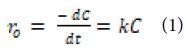
for 1

where; ro: denotes the initial photocatalytic degradation reaction rate (mg/l.min), and k: denotes the rate constant of a first-order reaction. At the beginning of the reaction, t = 0, Ct = C0, the equation can be obtained after integration as following Equation (2):
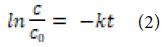
for 2

where; C0 and C : are the initial and final concentration (mg/l) of OFX; the solution at t (min) and k (1/min) are the rate constant.

The correlation coefficients had R2 values greater than 0.9, as a result, the first-order kinetic model fit the experimental data well. The first-order rate constants (k) were determined from the slope of the linear plots.

Photocatalytic Degradation Mechanisms

The photocatalytic performance of the catalyst in the degradation of OFX is determined by photons. The degradation mechanism of OFX by hydroxyl radicals (OH) radicals concerning g-C3N4/CeO2 NCs as following equations (Equation 3, Equation 4, Equation 5, Equation 6, Equation 7, Equation 8, Equation 9 and Equation 10):
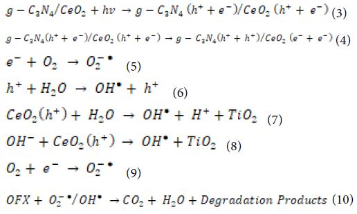
for 3-10

g-C3N4/CeO2 NCs absorbs photons with energies greater than the photocatalyst bandgap. As a result, the electron in the valence band (VB) jumps to the conduction band (CB), leaving a hole in the CB. The electrons present in the CB and VB will react with oxygen (O2) and water (H2O) molecules which are absorbed by the photocatalyst and lead to the formation of OH radicals which react with OFX. OH radicals are produced when the photocatalyst surface is illuminated with photons, and OH radicals are strong oxidising species, with an oxidation potential of approximately 2.8 V [as opposed to Normal hydrogen electrode (NHE)], which may increase total pollutant mineralisation. Normally, the higher the rate of formation of OH radicals, the greater the separation efficiency of electron-hole pairs. In this way, there is a correlation between the increased photocatalytic activity and the rate of formation of OHradicals. The OH radicals generation of g-C3N4/CeO2 NCs was extremely high, indicating that the sample has a high electron and hole separation rate.

CeO2 composites with g-C3N4 are also promising photocatalytic materials with a lower band gap energy [167-169] and significantly higher photocatalytic efficiency in degradation processes [170,171]. Considering the position of CB and VB in CeO2 and g-C3N4, the higher photocatalytic efficiency can be attributed to the transfer of photoexcited electrons and holes between CeO2 and g-C3N4, which suppresses the recombination of photogenerated h+/e pairs. During irradiation, photogenerated electrons on CB in g-C3N4 are transferred to CB in CeO2 and react with O2, while photogenerated holes on VB in CeO2 are transferred to VB in g-C3N4 and react with H2O according to the following reactions [172]:

The superoxide and hydroxyl radicals formed in the above-presented reactions take part in the degradation of pollutants. In the case of CeO2 composites with g-C3N4, two problems have still not been resolved. The first one is related to the lower rates of TOC or COD decrease in wastewater in comparison with the degradation rate of pollutants [173]. The second one is attributed to the immobilization of a composite photocatalyst, which could eliminate the post-treatment process of photocatalyst removal from the wastewater.

Effect of Increasing pH values for OFX Removal in Pharmaceutical Industry Wastewater during Photocatalytic Degradation Process

Increasing pH values (pH=3.0, pH=4.0, pH=6.0, pH=7.0, pH=9.0 and pH=11.0, respectively) was examined during photocatalytic degradation process in pharmaceutical industry wastewater for OFX removal (Figure 7). 67.2%, 85.7%, 96.4%, 56.5% and 44.8% OFX removal efficiencies was measured at pH=3.0, pH=4.0, pH=6.0, pH=7.0 and pH=11.0, respectively, at 300 W UV-vis light irradiation power, after 180 min photocatalytic degradation time, at 25°C (Figure 7). The maximum 99% OFX removal efficiency was obtained during photocatalytic degradation process in pharmaceutical industry wastewater, at 300 W UV-vis light irradiation power, after 180 min photocatalytic degradation time, at pH=6.0 and at 25°C, respectively (Figure 7).
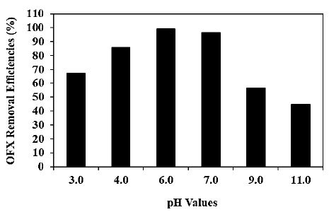
fig 7

Figure 7: Effect of increasing pH values for OFX removal in pharmaceutical industry wastewater during photocatalytic degradation process, at 300 W UV-vis light irradiation power, after 180 min photocatalytic degradation time, at pH=6.0 and at 25°C, respectively.

Effect of Increasing OFX Concentrations for OFX Removal in Pharmaceutical Industry Wastewater during Photocatalytic Degradation Process

Increasing OFX concentrations (5 mg/l, 10 mg/l, 20 mg/l and 40 mg/l) were operated at 300 W UV-vis irradiation power, after 180 min photocatalytic degradation time, at pH=6.0, at 25°C, respectively (Figure 8). 85.3%, 94.1% and 77.2% OFX removal efficiencies were obtained to 5 mg/l, 10 mg/l and 40 mg/l OFX concentrations, respectively, at pH=6.0 and at 25°C (Figure 8). The maximum 99% OFX removal efficieny was found with photocatalytic degradation process in pharmaceutical industry wastewater, at 20 mg/l OFX, at 300 W UV-vis light irradiation power, after 180 min photocatalytic degradation time, at pH=6.0 and at 25°C, respectively (Figure 8).

The percentage decrease (8%) in the concentration of OFX during the studies under the dark conditions was due to the contaminant adsorption onto the catalyst surface [174]. The formation of contaminant monolayer on the surface of the catalyst may have occupied all its active sites, and therefore no more adsorption was observed.
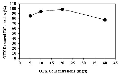
fig 8

Figure 8: Effect of increasing OFX concentrations for OFX removal in pharmaceutical industry wastewater during photocatalytic degradation process, at 300 W UV-vis light irradiation power, after 180 min photocatalytic degradation time, at pH=6.0 and at 25°C, respectively.

Effect of Increasing g-C3N4/CeO2 NCs Concentrations for OFX Removals in Pharmaceutical Industry Wastewater during Photocatalytic Degradation Process

Increasing g-C3N4/CeO2 NCs concentrations (1 mg/l, 2 mg/l, 4 mg/l, 6 mg/l, 8 mg/l and 10 mg/l) were operated at 20 mg/l OFX, at 150 W UV-vis light irradiation power, after 180 min photocatalytic degradation time, at pH=6.0, at 25°C, respectively (Figure 9). 54.5%, 68.1%, 75.8%, 87.3% and 92.1% OFX removal efficiencies were obtained to 1 mg/l, 2 mg/l, 4 mg/l, 6 mg/l and 10 mg/l g-C3N4/CeO2 NCs concentrations, respectively, at 20 mg/l OFX, at 300 W UV-vis light irradiation power, after 180 min photocatalytic degradation time, at pH=6.0, at 25°C, respectively (Figure 9). The maximum 99% OFX removal efficieny was measured to 8 mg/l g-C3N4/CeO2 NCs with photocatalytic degradation process in pharmaceutical industry wastewater, at 20 mg/l OFX, at 300 W UV-vis light irradiation power, after 180 min photocatalytic degradation time, at pH=6.0 and at 25°C, respectively (Figure 9).
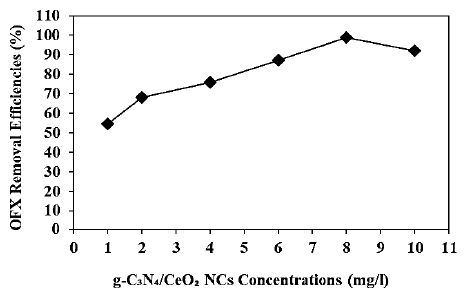
fig 9

Figure 9: Effect of increasing g-C3N4/CeO2 NCs concentrations for OFX removal in pharmaceutical industry wastewater during photocatalytic degradation process, at 20 mg/l OFX, at 300 W UV-vis light irradiation power, after 180 min photocatalytic degradation time, at pH=6.0 and at 25°C, respectively.

Effect of Different g-C3N4/CeO2 NCs Mass Ratios for OFX Removals in Pharmaceutical Industry Wastewater during Photocatalytic Degradation Process

Different g-C3N4/CeO2 mass ratios (5/5wt, 6/4wt, 7/3wt, 8/2wt, 9/1wt, 1/9wt, 2/8wt, 3/7wt and 4/6wt, respectively) were examined for OFX removal in pharmaceutical industry wastewater during photocatalytic degradation process, at 20 mg/l OFX, at 300 W UV-vis light irradiation power, after 180 min photocatalytic degradation time, at pH=6.0 and at 25°C, respectively (Figure 10). 80.3%, 84.6%, 77.9%, 62.1%, 48.4%, 55.2%, 64.0% and 79.7% OFX removal efficiencies were measured at 5/5wt, 6/4 wt, 7/3wt, 8/2wt, 9/1wt, 1/9wt, 3/7wt and 4/6wt g-C3N4/CeO2 NCs mass ratios, respectively, at 20 mg/l OFX after 180 min photocatalytic degradation time, at pH=6.0 and at 25°C, respectively (Figure 10). The maximum 99% OFX removal efficiency was measured at 2/8wt g-C3N4/CeO2 NCs mass ratios at 20 mg/l OFX, at 300 W UV-vis light irradiation power, after 180 min photocatalytic degradation time, at pH=6.0 and at 25°C, respectively (Figure 10).
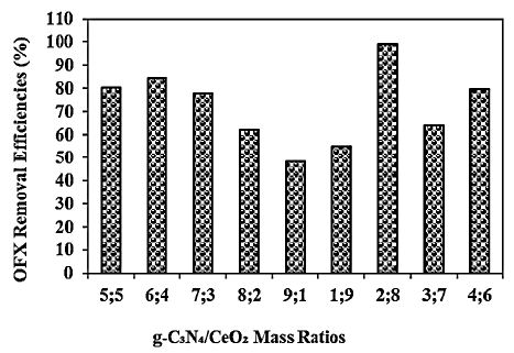
fig 10

Figure 10: Effect of different g-C3N4/CeO2 NCs mass ratios for OFX removal in pharmaceutical industry wastewater during photocatalytic degradation process, at 20 mg/l OFX, at 300 W UV-vis light irradiation power, after 180 min photocatalytic degradation time, at pH=6.0 and at 25°C, respectively.

Effect of Different Recycle Times for OFX Removals in Pharmaceutical Industry Wastewater during Photocatalytic Degradation Process

Different recycle times (1., 2., 3., 4., 5., 6. and 7.) were operated for OFX removals in pharmaceutical industry wastewater during photocatalytic degradation process, at 20 mg/l OFX, 8 mg/l g-C3N4/CeO2 NCs, at 2/8wt g-C3N4/CeO2 NCs mass ratio, after 180 min photocatalytic degradation time, at pH=6.0 and at 25°C, respectively (Figure 11). 97.5%, 96.2%, 94%, 93.8%, 89.2%, 86.2% and 80.1% OFX removal efficiencies were measured after 2. recycle time, 3. recycle time, 4. recycle time, 5. recycle time, 6. recycle time and 7. recycle time, respectively, at 20 mg/l OFX, 8 mg/l g-C3N4/CeO2 NCs, at 2/8wt g-C3N4/CeO2 NCs mass ratio, after 180 min photocatalytic degradation time, at pH=6.0 and at 25°C, respectively (Figure 11). The maximum 99% OFX removal efficiency was measured in pharmaceutical industry wastewater during photocatalytic degradation process, after 1. recycle time, at 20 mg/l OFX, 8 mg/l g-C3N4/CeO2 NCs, at 2/8wt g-C3N4/CeO2 NCs mass ratio, after 180 min photocatalytic degradation time, at pH=6.0 and at 25°C, respectively (Figure 11).
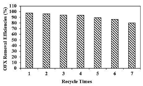
fig 11

Figure 11: Effect of recycle times for OFX removal in pharmaceutical industry wastewater during photocatalytic degradation process, at 20 mg/l OFX, 8 mg/l g-C3N4/CeO2 NCs, at 2/8wt g-C3N4/CeO2 NCs mass ratio, at 300 W UV-vis light irradiation power, after 180 min photocatalytic degradation time, at pH=6.0 and at 25°C, respectively.

Acute Toxicity Assays

Effect of Increasing OFX Concentrations on the Microtox (Aliivibrio fischeri or Vibrio fischeri) Acute Toxicity Removal Efficiencies in Pharmaceutical Industry Wastewater at Increasing Photocatalytic Degradation Time and Temperature

In Microtox with Aliivibrio fischeri (also called Vibrio fischeri) acute toxicity test, the initial EC90 values at pH=7.0 was found as 825 mg/l at 25°C (Table 3: SET 1). After 60 min, 120 min and 180 min photocatalytic degradation time, the EC90 values decreased to EC57=414 mg/l to EC22=236 mg/l and to EC12=165 mg/l in OFX=20 mg/l at 30°C (Table 3: SET 3). The Microtox (Aliivibrio fischeri) acute toxicity removal efficiencies were 40.86%, 79.75% and 90.86% after 60 min, 120 min and 180 min, respectively, in OFX=20 mg/l and at 30°C (Table 3: SET 3).

The EC90 values decreased to EC51, to EC16 and to EC6 after 60 min, 120 min and 180 min, respectively, in OFX=20 mg/l, at 60°C (Table 3: SET 3). The EC51, the EC11 and the EC7 values were measured as 550 mg/l, 540 mg/l and 500 mg/l, respectively, in OFX=20 mg/l at 60°C. The toxicity removal efficiencies were 46.41%, 85.30% and 96.41% after 60 min, 120 min and 180 min, respectively, in OFX=20 mg/l, at 60°C (Table 3: SET 3). 96.41% maximum Microtox (Aliivibrio fischeri) acute toxicity removal yield was found in OFX=20 mg/l after 180 min and at 60°C (Table 3: SET 3).

The EC90 values decreased to EC62=422 mg/l to EC21=241 mg/l and to EC17=168 mg/l after 60 min, 120 min and 180 min, respectively, in OFX=5 mg/l at 30°C (Table 3: SET 3). The EC90 values decreased to EC62=421 mg/l to EC27=239 mg/l and to EC11=167 mg/l after 60 min, 120 min and 180 min, respectively, in OFX=10 mg/l at 30°C. The EC90 values decreased to EC67=408 mg/l to EC32=230 mg/l and to EC22=162 mg/l after 60 min, 120 min and 180 min, respectively, in OFX=40 mg/l at 30°C. The Microtox (Aliivibrio fischeri or Vibrio fischeri) acute toxicity removals were 85.30%, 85.28% and 79.75% in 5 mg/l, 10 mg/l and 40 mg/l OFX, respectively, after 180 min, at 30°C. It was obtained an inhibition effect of OFX=40 mg/l to Vibrio fischeri after 180 min and at 30°C (Table 3: SET 3).

The EC90 values decreased to EC57=419 mg/l to EC22=266 mg/l and to EC12=150 mg/l after 60 min, 120 min and 180 min, respectively, in OFX=5 mg/l at 60°C (Table 3: SET 3). The EC90 values decreased to EC57=414 mg/l to EC22=232 mg/l and to EC12=161 mg/l after 60 min, 120 and 180 min, respectively, in OFX=10 mg/l at 60°C. The EC90 values decreased to EC62=403 mg/l to EC27=218 mg/l and to EC17=148 mg/l after 60 min, 120 and 180 min, respectively, in OFX=40 mg/l at 60°C. The Microtox (Aliivibrio fischeri or Vibrio fischeri) acute toxicity removals were 90.86%, 90.83% and 85.30% in 5 mg/l, 10 mg/l and 40 mg/l OFX, respectively, after 180 min, at 60°C. It was observed an inhibition effect of OFX=40 mg/l to Microtox with Vibrio fischeri after 180 min, and at 60°C (Table 3: SET 3).

Table 3: Effect of increasing OFX concentrations on Microtox (Aliivibrio fischeri) acute toxicity in pharmaceutical industry wastewater after photocatalytic degradation process, at 30°C and at 60°C, respectively.

No

Parameters

Microtox (Aliivibrio fischeri) Acute Toxicity Values, * EC (mg/l)

25°C

0 min

60 min

120 min

180 min

*EC90

*EC

*EC

*EC

1 Raw ww, Control

825

EC70=510

EC60=650

EC49=638

30°C

60°C

0. min

60 min

120. min

180. min

0 min

60 min

120 min

180 min

*EC90

*EC

*EC

*EC

*EC90

*EC

*EC

*EC

2 Raw ww, control

825

EC70=580

EC50=580

EC39=548

825

EC55=550

EC40=590

EC29=688

3 OFX=5 mg/l

825

EC62=422

EC27=242

EC17=168

825

EC57=419

EC22=266

EC12=150

OFX=10 mg/l

825

EC62=421

EC27=239

EC17=167

825

EC57=414

EC22=232

EC12=161

OFX=20 mg/l

825

EC57=414

EC22=236

EC12=165

825

EC52=550

EC17=540

EC7=500

OFX=40 mg/l

825

EC67=408

EC32=230

EC22=162

825

EC62=403

EC27=218

EC17=148

* EC values were calculated based on CODdis (mg/l).

Effect of Increasing OFX Concentrations on the Daphnia magna Acute Toxicity Removal Efficiencies in Pharmaceutical Industry Wastewater at Increasing Photocatalytic Degradation Time and Temperature

The initial EC50 values were observed as 850 mg/l at 25°C (Table 4: SET 1). After 60 min, 120 and 180 min photocatalytic degradation time, the EC50 values decreased to EC31=350 mg/l to EC17=240 mg/l and to EC12=90 mg/l in OFX=20 mg/l, at 30°C (Table 4: SET 3). The toxicity removal efficiencies were 42.96%, 72.87% and 82.65% after 60 min, 120 min and 180 min, respectively, in OFX=20 mg/l at 30°C (Table 4: SET 3).

The EC50 values decreased to EC27 to EC12 and to EC7 after 60 min, 120 min and 180 min, respectively, in OFX=20 mg/l at 60°C (Table 4: SET 3). The EC27, the EC12 and the EC7 values were measured as 150 mg/l, 60 mg/l and 375 mg/l, respectively, in OFX=20 mg/l at 60°C. The toxicity removal efficiencies were 52.94%, 82.62% and 92.36% after 60 min, 120 min and 180 min, respectively, in OFX=20 mg/l at 60°C (Table 4: SET 3). 92.38% maximum Daphnia magna acute toxicity removal was obtained in OFX=20 mg/l after 180 min and at 60°C, respectively (Table 4: SET 3).

The EC50 values decreased to EC37=450 mg/l to EC22=145 mg/l and to EC17=260 mg/l after 60 min, 120 min and 180 min, respectively, in OFX=5 mg/l at 30°C (Table 4: SET 3). The EC50 values decreased to EC37=450 mg/l to EC22=175 mg/l and to EC17=100 mg/l after 60 min, 120 min and 180 min, respectively, in OFX=10 mg/l and at 30°C. The EC50 values decreased to EC42=300 mg/l to EC27=170 mg/l and to EC22=52 mg/l after 60 min, 120 min and 180 min, respectively, in OFX=40 mg/l and at 30°C. The Daphnia magna acute toxicity removals were 72.22%, 72.56% and 63.21% in 5 mg/l, 10 mg/l and 40 mg/l OFX, respectively, after 180 min and at 30°C. It was observed an inhibition effect of OFX=40 mg/l to Daphnia magna after 180 min and at 30°C (Table 4: SET 3).

The EC50 values decreased to EC32=130 mg/l to EC17=425 mg/l and to EC12=340 mg/l after 60 min, 120 min and 180 min, respectively, in OFX=5 mg/l and at 60°C (Table 4: SET 3). The EC50 values decreased to EC32=425 mg/l to EC17=140 mg/l and to EC7=90 mg/l after 60 min, 120 min and 180 min, respectively, in OFX=10 mg/l and at 60°C. The EC50 values decreased to EC37=250 mg/l to EC22=110 mg/l and to EC17=10 mg/l after 60 min, 120 min and 180 min, respectively, in OFX=40 mg/l and at 60°C. The Daphnia magna acute toxicity removals were 83.06%, 92.65% and 73.11% in 5 mg/l, 10 mg/l and 40 mg/l OFX, respectively, after 180 min and at 60°C. It was observed an inhibition effect of OFX=40 mg/l to Daphnia magna after 180 min and at 60°C (Table 4: SET 3).

Increasing the OFX concentrations from 5 mg/l to 40 mg/l did not have a positive effect on the decrease of EC50 values as shown in Table 4 at SET 3. OFX concentrations > 20 mg/l decreased the acute toxicity removals by hindering the photocatalytic degradation process. Similarly, a significant contribution of increasing OFX concentration to acute toxicity removal at 60°C after 180 min of photocatalytic degradation time was not observed. Low toxicity removals found at high OFX concentrations could be attributed to their detrimental effect on the Daphnia magna (Table 4: SET 3).

Table 4: Effect of increasing OFX concentrations on Daphnia magna acute toxicity in pharmaceutical industry wastewater after photocatalytic degradation process, at 30°C and at 60°C.


No


Parameters

Daphnia magna Acute Toxicity Values, * EC (mg/l)

25°C

0. min

60. min

120. min

180. min

*EC50

*EC

*EC

*EC

1 Raw ww, control

850

EC45=625

EC40=370

EC29=153

30°C

60°C

0 min

60 min

120 min

180. min

0. min

60. min

120. min

180. min

*EC50

*EC

*EC

*EC

*EC50

*EC

*EC

*EC

2 Raw ww, control

850

EC39=468

EC34=228

EC23=111

850

EC34=373

EC29=210

EC18=71

3 OFX=5 mg/l

850

EC32=450

EC22=145

EC17=260

850

EC32=130

EC17=425

EC12=340

OFX=10 mg/l

850

EC37=450

EC22=175

EC17=100

850

EC32=425

EC17=140

EC7=90

OFX=20 mg/l

850

EC32=350

EC17=240

EC12=90

850

EC27=150

EC12=60

EC7=375

OFX=40 mg/l

850

EC42=300

EC27=170

EC22=52

850

EC37=250

EC22=110

EC17=11

* EC values were calculated based on CODdis (mg/l).

Direct Effects of OFX Concentrations on the Acute Toxicity of Microtox (Aliivibrio fischeri or Vibrio fischeri) and Daphnia magna without Pharmaceutical Industry Wastewater after Photocatalytic Degradation Process

The acute toxicity test was performed in the samples containing 5 mg/l, 10 mg/l, 20 mg/l and 40 mg/l OFX concentrations, at 25°C room temperature. In order to detect the direct responses of Microtox (Aliivibrio fischeri or Vibrio fischeri) and Daphnia magna to the increasing OFX concentrations the toxicity test were performed without pharmaceutical industry wastewater after photocatalytic degradation process, at 25°C room temperature. The initial EC values and the the EC50 values were measured in the samples containing increasing OFX concentrations after 180 min photocatalytic degradation time. Table 5 showed the responses of Microtox (Aliivibrio fischeri or Vibrio fischeri) and Daphnia magna to increasing OFX concentrations.

The acute toxicity originating only from 5 mg/l, 10 mg/l, 20 mg/l and 40 mg/l OFX were found to be low (Table 5). 5 mg/l OFX did not exhibited toxicity to Aliivibrio fischeri (or Vibrio fischeri) and Daphnia magna before and after 180 min photocatalytic degradation time. The toxicity atributed to the 10 mg/l, 20 mg/l and 40 mg/l OFX were found to be low in the samples without pharmaceutical industry wastewater after photocatalytic degradation process for the test organisms mentioned above. The acute toxicity originated from the OFX decreased significantly to EC2, EC4 and EC6 after 180 min photocatalytic degradation time. Therefore, it can be concluded that the toxicity originating from the OFX is not significant and the real acute toxicity throughout photocatalytic degradation process was attributed to the pharmaceutical industry wastewater, to their metabolites and to the photocatalytic degradation by-products (Table 5).

Table 5: The responses of Microtox (Aliivibrio fischeri or Vibrio fischeri) and Daphnia magna acute toxicity tests in addition of increasing OFX concentrations without phamaceutical industry wastewater during photocatalytic degradation process after 180 min photocatalytic degradation time, at 25°C room temperature.


OFX Conc. (mg/l)

Microtox (Aliivibrio fischeri or Vibrio fischeri)

Acute Toxicity Test

Daphnia magna

Acute Toxicity Test

Initial Acute Toxicity EC50 Value (mg/l)

Inhibitions after 180 min photocatalytic degradation time

EC Values (mg/l)

Initial Acute Toxicity EC50 Value (mg/l)

Inhibitions after 180 min photocatalytic degradation time

EC Values (mg/l)

5

EC10=24

EC10=39

10

EC15=79

3

EC2=3

EC20=99

5

EC3=5

20

EC20=149

5

EC4=6

EC30=199

6

EC6=11

40

EC25=219

7

EC6=9

EC40=299

9

EC8=15

The Comparison with Other Scientific Studies in the Literature

Comparison of our study “The use of a novel graphitic carbon nitride/cerium dioxide (g-C3N4/CeO2) nanocomposites for the ofloxacin removal by photocatalytic degradation in pharmaceutical industry wastewaters and the evaluation of microtox (Aliivibrio fischeri) and Daphnia magna acute toxicity assays” with other scientific studies in the literature is summaried at Table 6 [175-182].

Table 6: The Comparison with other Scientific Studies in the Literature

Photocatalyst

Experimental Conditions (for maximum removal efficiencies)

Experimental Results

References

a-Bi2O3/g-C3N4 [DOX]=10 mg/l, [Material]=500 mg/l, [H2O2]=10 mM, Unadjusted pH, Xe lamp (150 W). 79.1% DOX (30 min) (Liu et al., 2021a)
Ag/AgCl@ZIF-8/g-C3N4 150 W, Xe, λ > 420 nm, 50 mg/l, [LVFX]=10 mg/l, V=50 ml, 87.3% LVFX (60 min) (Zhou et al., 2019)
Ag@ZIF-8/g-C3N4 300 W, Xe, λ > 420 nm, [Ten antibiotics] =10 mg/l, V=50 ml 90% (60 min) (Guo et al., 2022)
Peroxymonosulfate/ZnFe2O4 Waters e2695 HPLC instrument (Milford, USA), UV-Vis detector λ=294 nm [OFX]=1000 mg/l, pH=6.0 80.9% OFX (30 min), pH 6.0 (Sun et al., 2021b)
Bi2WO6 and g-C3N4 nanosheets [CRO]=16.5-66 µM, KrCl excilamp, λ=222 nm, 23 W, incident irradiance 0.74 mW/cm2, 60 min 91% Ceftriaxone (60 min) (Sizykh et al., 2023)
Bi2WO6/g-C3N4 [CRO]=100 mg/l 300 W Xe lamp, 94.5% Ceftriaxone (120 min) (Zhao et al., 2018)
CeO2-ZnO hetero photocatalyst [TCN]=100 mg/l, 300 W Xenon lamp, 87.25% Tetracycline (60 min) (Ye et al., 2016)
g-C3N4/CeO2 core-shell structure Hydrothermal method, [DOX]=1000 mg/l, HCl=10 mg/l, H2O2=100 µl, 150 W Xe lamp (λ > 400 nm), g-C3N4=2.82 eV, CeO2=2.76 eV 66.7%g-C3N4, 71.7%CeO2,

84% g-C3N4/CeO2 (60 min)

(Liu et al., 2019)
CeO2/ATP/g-C3N4 ATP—attapulgite Electrostatic-induced self-assembly method, Dibenzothiophene (DBT), m(catal)/m(DBT)=1/10, SO₂=200 mg/l, 30% H2O2, 300 W Xe lamp (λ > 420 nm) Desulfurization 42% g-C3N4,

83% CeO2/g-C3N4, 98% CeO2/ATP/g-C3N4 (180 min)

(Li et al., 2017b)
g-C3N4/CeO2 NCs g-C3N4/CeO2 NCs was prepared to hydrothermal calcination method, CeO2 was prepared sol-gel method, g-C3N4 was prepared to calcination method, pH=6.0,

[OFX]=20 mg/l,

[g-C3N4/CeO2 NCs]=8 mg/l, g-C3N4/CeO2 mass ratio=2/8,

300 W UV-vis A lamp λ=350-400 nm range (λmax=368 nm; FWHM=17 nm; Actinic BL TL-D 18W, Philips)

Recycle time=7, at 25°C Microtox (Aliivibrio fischeri) and Daphnia magna acute toxicity assays

99% OFX (180 min, at 25°C)

96.41% maximum Microtox (Aliivibrio fischeri) acute toxicity removal (180 min, at 60°C)

92.38% maximum Daphnia magna acute toxicity removal (180 min, at 60°C),

99% OFX after 1. recycle time

This study
DOX: doxycycline; LVFX: Levofloxacin; CRO: ceftriaxone; TCN: Tetracycline; OFX: ofloxacin

Conclusıons

The maximum 99% OFX removal efficiency was obtained during photocatalytic degradation process in pharmaceutical industry wastewater, at 300 W UV-vis light irradiation power, after 180 min photocatalytic degradation time, at pH=6.0 and at 25°C, respectively.

The maximum 99% OFX removal efficieny was found with photocatalytic degradation process in pharmaceutical industry wastewater, at 20 mg/l OFX, at 300 W UV-vis light irradiation power, after 180 min photocatalytic degradation time, at pH=6.0 and at 25°C, respectively.

The maximum 99% OFX removal efficieny was measured to 8 mg/l g-C3N4/CeO2 NCs with photocatalytic degradation process in pharmaceutical industry wastewater, at 20 mg/l OFX, at 300 W UV-vis light irradiation power, after 180 min photocatalytic degradation time, at pH=6.0 and at 25°C, respectively.

The maximum 99% OFX removal efficiency was measured at 2/8wt g-C3N4/CeO2 NCs mass ratios at 20 mg/l OFX, at 300 W UV-vis light irradiation power, after 180 min photocatalytic degradation time, at pH=6.0 and at 25°C, respectively.

The maximum 99% OFX removal efficiency was measured in pharmaceutical industry wastewater during photocatalytic degradation process, after 1. recycle time, at 20 mg/l OFX, 8 mg/l g-C3N4/CeO2 NCs, at 2/8wt g-C3N4/CeO2 NCs mass ratio, after 180 min photocatalytic degradation time, at pH=6.0 and at 25°C, respectively.

96.41% maximum Microtox (Aliivibrio fischeri) acute toxicity removal yield was found in OFX=20 mg/l after 180 min and at 60°C. It was observed an inhibition effect of OFX=40 mg/l to Microtox with Vibrio fischeri after 180 min photocatalytic degradation time and at 60°C. 92.38% maximum Daphnia magna acute toxicity removal was obtained in OFX=20 mg/l after 180 min photocatalytic degradation time and at 60°C, respectively. It was observed an inhibition effect of OFX=40 mg/l to Daphnia magna after 180 min photocatalytic degradation time and at 60°C. OFX concentrations > 20 mg/l decreased the acute toxicity removals by hindering the photocatalytic degradation process. Similarly, a significant contribution of increasing OFX concentrations to acute toxicity removal at 60°C after 180 min photocatalytic degradation time was not observed. Finally, it can be concluded that the toxicity originating from the OFX is not significant and the real acute toxicity throughout photocatalytic degradation process was attributed to the pharmaceutical industry wastewater, to their metabolites and to the photocatalytic degradation process by-products.

As a result, the a novel g-C3N4/CeO2 NCs photocatalyst during photocatalytic degradation process in pharmaceutical industry wastewater was stable in harsh environments such as acidic, alkaline, saline, and then was still effective process. When the amount of contaminant was increased, the a novel g-C3N4/CeO2 NCs photocatalys during photocatalytic degradation process performance was still considerable. The synthesis and optimization of g-C3N4/CeO2 heterostructure photocatalyst provides insights into the effects of preparation conditions on the material’s characteristics and performance, as well as the application of the effectively designed photocatalyst in the removal of antibiotics, which can potentially be deployed for purifying wastewater, especially pharmaceutical wastewater. Finally, the combination of a simple, easy operation preparation process, excellent performance and cost effective, makes this a novel g-C3N4/CeO2 NCs a promising option during photocatalytic degradation process in pharmaceutical industry wastewater treatment.

Acknowledgement

This research study was undertaken in the Environmental Microbiology Laboratories at Dokuz Eylül University Engineering Faculty Environmental Engineering Department, Izmir, Turkey. The authors would like to thank this body for providing financial support.

References

  1. Idham MF, Abdullah B, Yusof KM (2017) Effects of two cycle heat treatment on the microstructure and hardness of ductile iron. Pertanika J Sci Technol 25: 99-106.
  2. Idham MF, Falyouna O, Eljamal O (2021) Effect of graphene oxide synthesis method on the adsorption performance of pharmaceutical contaminants. Proc Int Exch Innov Conf Eng Sci 7: 232-239.
  3. Arenas NE, Melo VM (2018) Producción pecuaria y emergencia de antibiótico resistencia en Colombia: Revisión sistemática. Infectio 22: 110-119.
  4. Pellerito A, Ameen SM, Micali M, Caruso G (2018) Antimicrobial substances for food packaging products: the current situation. J AOAC Int 101: 942-947. [crossref]
  5. Fridkin S, Baggs, J, Fagan R, Magill S, Pollack LA, et al. (2014) Vital signs: improving antibiotic use among hospitalized patients. MMWR-Morb Mortal Wkly Rep 63: 194-200. [crossref]
  6. Tamma PD, Avdic E, Li DX, Dzintars K, Cosgrove SE (2017) Association of adverse events with antibiotic use in hospitalized patients. JAMA Intern Med 177: 1308-1315. [crossref]
  7. Huo TI (2010) The first case of multidrug-resistant NDM−1-harboring Enterobacteriaceae in Taiwan: here comes the superbacteria! J Chin Med Assoc 73: 557-558. [crossref]
  8. Ferri M, Ranucci E, Romagnoli P, Giaccone V (2017) Antimicrobial resistance: A global emerging threat to public health systems. Crit Rev Food Sci 57: 2857-2876. [crossref]
  9. Tan L, Li LY, Ashbolt N, Wang XL, Cui YX, et al. (2018) Arctic antibiotic resistance gene contamination, a result of anthropogenic activities and natural origin. Sci Total Environ 621: 1176-1184. [crossref]
  10. Tong S, Pan J, Lu S, Tang J (2018) Patient compliance with antimicrobial drugs: a Chinese survey. Am J Infect Control 46: E25-E29. [crossref]
  11. Alygizakis NA, Gago-Ferrero P, Borova VL, Pavlidou A, Hatzianestis I, et al. (2016) Occurrence and spatial distribution of 158 pharmaceuticals, drugs of abuse and related metabolites in offshore seawater. Sci Total Environ 541: 1097-1105. [crossref]
  12. Casanova LM, Sobsey MD (2016) Antibiotic-resistant enteric bacteria in environmental waters. Water 8: 561-567.
  13. Zhang LH, He YW, Chen M, Gao M, Qiu TL, et al. (2016) Pollution characteristics of antibiotic resistant bacteria from atmospheric environment of animal feeding operations. Huan Jing Ke Xue 37: 4531-4537. [crossref]
  14. Jiménez TM, Ferreira IJ, da Silva DS, Guimarães Barrocas PR, Saggioro EM (2018) Removal of contaminants of emerging concern (CECs) and antibiotic resistant bacteria in urban wastewater using UVA/TiO2/H2O2 photocatalysis. Chemosphere 210: 449-457. [crossref]
  15. Kerrigan JF, Sandberg KD, Engstrom DR, LaPara TM, Arnold WA (2018) Small and large-scale distribution of four classes of antibiotics in sediment: association with metals and antibiotic resistance genes. Environ Sci Process Impacts 20: 1167-1179. [crossref]
  16. McConnell MM, Truelstrup HL, Jamieson RC, Neudorf KD, Yost CK, et al. (2018) Removal of antibiotic resistance genes in two tertiary level municipal wastewater treatment plants. Sci Total Environ643: 292-300. [crossref]
  17. Karthikeyan KG, Meyer MT (2006) Occurrence of antibiotics in wastewater treatment facilities in Wisconsin, USA, Sci Total Environ 361: 196-207. [crossref]
  18. Dinh QT, Moreau-Guigon E, Labadie P, Alliot F, Teil MJ, et al. (2017) Occurrence of antibiotics in rural catchments. Chemosphere 168: 483-490. [crossref]
  19. Dong D, Zhang L, Liu S, Guo Z, Hua X (2016) Antibiotics in water and sediments from Liao River in Jilin Province, China: occurrence, distribution, and risk assessment. Environ Earth Sci 75: 1202.
  20. Siedlewicz G, Białk-Bielinska A, Borecka M, Winogradow A, Stepnowski P, et al. (2018).Presence, concentrations and risk assessment of selected antibiotic residues in sediments and near-bottom waters collected from the Polish Coastal Zone in the Southern Baltic Sea-Summary of 3years of studies. Mar Pollut Bull 129: 787-801. [crossref]
  21. Barry S (2019) Dangerously high levels of antibiotics found in world’s major rivers, says study. World news global study 1: 1-10.
  22. Maycock DS, Watts CD (2011) Pharmaceuticals in drinking water. Encycl Environ Heal 472-484.
  23. Fekadu S, Alemayehu E, Dewil R, Van der Bruggen B (2019) Pharmaceuticals in freshwater aquatic environments: a comparison of the african and european challenge. Sci Total Environ 654: 324-337. [crossref]
  24. Wang J, Hao J, Liu D, Qin S, Chen C, et al. (2017a) Flower stamen-like porous boron carbon nitride nanoscrolls for water cleaning. Nanoscale 9: 9787-9791. [crossref]
  25. Wang X, Wang A, Lu M, Ma J (2017b) Synthesis of magnetically recoverable Fe0/graphene-TiO2 nanowires composite for both reduction and photocatalytic oxidation of metronidazole. Chem Eng J 337: 372–384.
  26. Wang W, Zhu Q, Dai Q, Wang X (2017c) Fe doped CeO2 nanosheets for catalytic oxidation of 1,2-dichloroethane: Effect of preparation method. Chem Eng J 307: 1037-1046.
  27. Yang X, Chen Z, Zhao W, Liu C, Qian X, et al. (2021) Recent advances in photodegradation of antibiotic residues in water. Chem Eng J 405: 126806. [crossref]
  28. Akyon B, McLaughlin M, Hernández F, Blotevogel J, Bibby K (2019) Characterization and biological removal of organic compounds from hydraulic fracturing produced water. Environ Sci Process 21: 279-290. [crossref]
  29. Zhang C, Li Y, Shuai D, Shen Y, Xiong W, et al. (2019) Graphitic carbon nitride (g-C3N4)-based photocatalysts for water disinfection and microbial control: A review. Chemosphere 214: 462-479. [crossref]
  30. de Souza Santos LV, Meireles AM, Lange LC (2015) Degradation of antibiotics norfloxacin by fenton, UV and UV/H2O2. J Environ Manag 154: 8-12. [crossref]
  31. Yang L, Zhu YJ, He G, Li H, Tao JC (2022) multifunctional photocatalytic filter paper based on ultralong nanowires of the calcium-alendronate complex for high-performance water purification. ACS Appl Mater Interfaces 14: 9464-9479. [crossref]
  32. Zhong Y, Han L, Yin X, Li H, Fang D, et al. (2018) Three dimensional functionalized carbon/tin(IV) sulfide biofoam for photocatalytical purification of chromium(VI)-containing wastewater. ACS Sustain Chem Eng 6: 10660-10667.
  33. Alagha O, Ouerfelli N, Kochkar H, Almessiere MA, Slimani Y, et al. (2021) Kinetic modeling for photo-assisted penicillin G degradation of (Mn0.5Zn0.5)[CdxFe2-x]O4 (x ≤ 0.05) nanospinel ferrites. Nanomaterials 11: 970-986. [crossref]
  34. The American Society of Health-System Pharmacists. Ofloxacin. Archived from the original on 28 December 2016.
  35. Andriole VT (1989) The Quinolones, Academic Press.
  36. Johnson JR, Murray AC, Gajewski A, Sullivan M, Snippes P, et al. (2003) Isolation and molecular characterization of nalidixic acid-resistant extraintestinal pathogenic escherichia coli from retail chicken products. Antimicrob Agents Chemother 47: 2161-2168.
  37. Kritas S, Ronconi G, Caraffa A, Gallenga C, Ross R, et al. (2020) Mast cells contribute to coronavirus-induced inflammation: new anti-inflammatory strategy. J Biol Regul Homeost Agents 34: 9-14. [crossref]
  38. Amini Z, Givianrad MH, Husain SW, Azar PA, Saber-Tehrani M (2020) Cu-S codoping TiO2/SiO2 and TiO2/SiO2/Fe3O4 core-shell nanocomposites as a novel purple LED illumination active photocatalyst for degradation of diclofenac: the effect of different scavenger agents and optimization. Chem Eng Commun. 207: 1536-1553.
  39. Sen Gupta PS, Rana MK (2020) Ivermectin, famotidine, and doxycycline: A suggested combinatorial therapeutic for the treatment of COVID-19. ACS Pharmaco Trans Sci3: 1037-1038. [crossref]
  40. Tong C, Zhuo X, Guo Y (2011) Occurrence and risk assessment of four typical fluoroquinolone antibiotics in raw and treated sewage and in receiving waters in Hangzhou, China. J Agric Food Chem 59: 7303-7309. [crossref]
  41. Xiao Y, Chang H, Jia A, Hu J (2008) Trace analysis of quinolone and fluoroquinolone antibiotics from wastewaters by liquid chromatography–electrospray tandem mass spectrometry. J Chromatogr A 1214: 100-108. [crossref]
  42. Anjali R, Shanthakumar S (2019) Insights on the current status of occurrence and removal of antibiotics in wastewater by advanced oxidation processes. J Environ Manage 246: 51-62. [crossref]
  43. Liu J, Yin ML, Xiao TF, Zhang CS, Tsang DCW, et al. (2020) Thallium isotopic fractionation in industrial process of pyrite smelting and environmental implications. J Hazard Mater 384: 121378. [crossref]
  44. Wang J, Zhuan R (2020) Degradation of antibiotics by advanced oxidation processes: An overview. Sci Total Environ 701: 135023. [crossref]
  45. Liu W, Li Z, Kang Q, Wen L (2021a) Efficient photocatalytic degradation of doxycycline by coupling α-Bi2O3/g-C3N4 composite and H2O2 under visible light. Environ Res 197: 110925. [crossref]
  46. Liu YP, Lv YT, Guan JF, Khoso FM, Jiang XY, et al. (2021b) Rational design of three-dimensional graphene/graphene oxide-based architectures for the efficient adsorption of contaminants from aqueous solutions. J Mol Liq 343: 117709.
  47. Homem V, Santos L (2011) Degradation and removal methods of antibiotics from aqueous matrices-A review. J Environ Manage 92: 2304-2347. [crossref]
  48. Bagheri S, TermehYousefi SA, Do TO (2017) Photocatalytic pathway toward degradation of environmental pharmaceutical pollutants: Structure, kinetics and mechanism approach. Catal Sci Technol 7: 4548-4569.
  49. Cuerda-Correa EM, Alexandre-Franco MF, Fernandez-Gonzalez C (2020) Advanced oxidation processes for the removal of antibiotics from water, an overview. Water 12: 102-153.
  50. Lima VB, Goulart LA, Rocha RS, Steter JR, Lanza MRV (2020) Degradation of antibiotic ciprofloxacin by different AOP systems using electrochemically generated hydrogen peroxide. Chemosphere 247: 125807.
  51. Biancullo F, Moreira NFF, Ribeiro AR, Manaia CM, Faria JL, et al. (2019) Heterogeneous photocatalysis using UVA-LEDs for the removal of antibiotics and antibiotic resistant bacteria from urban wastewater treatment plant effluents. Chem Eng J 367: 304-313.
  52. Wei Z, Liu J, Shangguan W (2020) A review on photocatalysis in antibiotic wastewater: Pollutant degradation and hydrogen production. Chinese J Catal 41: 1440-1450.
  53. Ahmed MM, Brienza M, Goetz V, Chiron S (2014) Solar photo-Fenton using peroxymonosulfate for organic micropollutants removal from domestic wastewater: Comparison with heterogeneous TiO2 Chemosphere 117: 256-261. [crossref]
  54. Wang Y, Sun H, Ang HM, Tade MO, Wang S (2014) Facile synthesis of hierarchically structured magnetic MnO2/ZnFe2O4 hybrid materials and their performance in heterogeneous activation of peroxymonosulfate. ACS Appl Mater Interfaces 6: 19914-19923. [crossref]
  55. Ren Y, Lin L, Ma J, Yang J, Feng J, et al. (2015) Sulfate radicals induced from peroxymonosulfate by magnetic ferrospinel MFe2O4 (M ¼ Co, Cu, Mn, and Zn) as heterogeneous catalysts in the water. Appl Catal B: Environ 165: 572-578.
  56. Mady AH, Baynosa ML, Tuma D, Shim JJ. (2019) Heterogeneous activation of peroxymonosulfate by a novel magnetic 3D gamma-MnO2@ZnFe2O4/rGO nanohybrid as a robust catalyst for phenol degradation. Applied Catalysis B: Environmental 244: 946-956.
  57. Zhu S, Xu Y, Zhu Z, Liu Z, Wang W (2020) Activation of peroxymonosulfate by magnetic Co-Fe/SiO2 layered catalyst derived from iron sludge for ciprofloxacin degradation. Chem Eng J 384: 123298.
  58. Ahammad NA, Zulkifli MA, Ahmad MA, Hameed BH, Mohd Din AT (2021) Desorption of chloramphenicol from ordered mesoporous carbonalginate beads: Effects of operating parameters, and isotherm, kinetics, and regeneration studies. J Environ Chem Eng 9: 105015.
  59. Jiang Q, Zhang Y, Jiang S, Wang Y, Li H, et al. (2020).Graphene-like carbon sheetsupported nZVI for efficient atrazine oxidation degradation by persulfate activation. Chem Eng J 403: 126309.
  60. Shirani Z, Song H, Bhatnagar A (2020) Efficient removal of diclofenac and cephalexin from aqueous solution using Anthriscus sylvestris-derived activated biochar. Sci Total Environ 745: 140789. [crossref]
  61. Ahmed MB, Zhou JL, Ngo HH, Guo W (2015) Adsorptive removal of antibiotics from water and wastewater: Progress and challenges. Sci Total Environ 532: 112-126. [crossref]
  62. Zhang X, Lou S, Zeng Y (2020a) Facile fabrication of a novel visible light active g-C3N4-CoMoO4 heterojunction with largely improved photocatalytic performance. Mater Lett 281: 128661.
  63. Zhang W, Mohamed AR, Ong WJ (2020b) Z-scheme photocatalytic systems for carbon dioxide reduction: where are we now? Angew Chem Int Ed 59: 22894-22915. [crossref]
  64. Avcu T, Üner O, Geçgel Ü (2021) Adsorptive removal of diclofenac sodium from aqueous solution onto sycamore ball activated carbon-isotherms, kinetics, and thermodynamic study. Surf Interfaces 24: 101097.
  65. Ji Y, Zhang C, Zhang XJ, Xie PF, Wu C (2022) A high adsorption capacity bamboo biochar for CO2 capture for low temperature heat utilization. Sep Purif Technol 293: 121131.
  66. Shahnaz T, Vishnu Priyan V, Pandian S, Narayanasamy S (2021) Use of nanocellulose extracted from grass for adsorption abatement of ciprofloxacin and diclofenac removal with phyto, and fish toxicity studies. Environ Pollut 268: 115494. [crossref]
  67. Wang Z, Song L, Wang Y, Zhang XF, Yao J (2021) Construction of a hybrid graphene oxide/nanofibrillated cellulose aerogel used for the efficient removal of methylene blue and tetracycline. J Phys Chem Solids 150: 109839.
  68. Cui G, Guo J, Zhang Y, Zhao Q, Fu S, et al. (2019) Chitosan oligosaccharide derivatives as green corrosion inhibitors for P110 steel in a carbon-dioxide-saturated chloride solution. Carbohydr Polym 203: 386-395. [crossref]
  69. Phasuphan W, Praphairaksit N, Imyim A (2019) Removal of ibuprofen, diclofenac, and naproxen from water using chitosan-modified waste tire crumb rubber. J Mol Liq 294: 111554.
  70. ALOthman ZA, Badjah AY, Alharbi OML, Ali I (2020) Synthesis of chitosan composite iron nanoparticles for removal of diclofenac sodium drug residue in water. Int J Biol Macromol 159: 870-876. [crossref]
  71. Yu F, Sun S, Han S, Zheng J, Ma J (2016) Adsorption removal of ciprofloxacin by multi-walled carbon nanotubes with different oxygen contents from aqueous solutions. Chem Eng J 285: 588-595.
  72. Zhao H, Liu X, Cao Z, Zhan Y, Shi X, et al. (2016) Adsorption behavior and mechanism of chloramphenicols, sulfonamides, and nonantibiotic pharmaceuticals on multi-walled carbon nanotubes. J Hazard Mater 310: 235-245. [crossref]
  73. Bellamkonda S, Thangavel N, Hafeez HY, Neppolian B, Ranga Rao G (2019) Highly active and stable multi-walled carbon nanotubes-graphene-TiO2 nanohybrid: An efficient non-noble metal photocatalyst for water splitting. Catal Today 321-322: 120-127.
  74. Rigueto CVT, Rosseto M, Nazari MT, Ostwald BEP, Alessandretti I, et al. (2021) Adsorption of diclofenac sodium by composite beads prepared from tannery wastesderived gelatin and carbon nanotubes. J Environ Chem Eng 9: 105030.
  75. Ahmed MB, Zhou JL, Ngo HH, Guo W, Johir MAH, et al. (2017) Nano-Fe0 immobilized onto functionalized biochar gaining excellent stability during sorption and reduction of chloramphenicol via transforming to reusable magnetic composite. Chem Eng J 322: 571-581.
  76. Zhao J, Yang X, Liang G, Wang Z, Li S, et al. (2020) Effective removal of two fluoroquinolone antibiotics by PEG-4000 stabilized nanoscale zerovalent iron supported onto zeolite (PZ-NZVI) Sci Total Environ 710: 136289. [crossref]
  77. Nguyen LT, Nguyen HT, Pham TD, Tran TD, Chu HT, et al. (2020) UV–visible light driven photocatalytic degradation of ciprofloxacin by N, S co-doped TiO2: the effect of operational parameters. Top Catal 63: 985-995.
  78. Nguyen CH, Tran ML, Van Tran TT, Juang RS (2021) Efficient removal of antibiotic oxytetracycline from water by Fenton-like reactions using reduced graphene oxide-supported bimetallic Pd/nZVI nanocomposites. J Taiwan Inst Chem Eng 119: 80-89.
  79. Falyouna O, Idham MF, Maamoun I, Bensaida K, Ashik UPM, et al. (2022a) Promotion of ciprofloxacin adsorption from contaminated solutions by oxalate modified nanoscale zerovalent iron particles. J Mol Liq 359: 119323.
  80. Falyouna O, Maamoun I, Bensaida K, Tahara A, Sugihara Y, et al. (2022b) Encapsulation of iron nanoparticles with magnesium hydroxide shell for remarkable removal of ciprofloxacin from contaminated water. J Colloid Interface Sci 605: 813-827. [crossref]
  81. Mokhati A, Benturki O, Bernardo M, Kecira Z, Matos I, et al. (2021) Nanoporous carbons prepared from argan nutshells as potential removal agents of diclofenac and paroxetine. J Mol Liq 326: 115368.
  82. Shan D, Deng S, Li J, Wang H, He Cet al. (2017) Preparation of porous graphene oxide by chemically intercalating a rigid molecule for enhanced removal of typical pharmaceuticals. Carbon N Y 119: 101-109.
  83. Khalil AME, Memon FA, Tabish TA, Salmon D, Zhang S, et al. (2020) Nanostructured porous graphene for efficient removal of emerging contaminants (pharmaceuticals) from water. Chem Eng J 398: 125440.
  84. Görmez F, Görmez Ö, Gözmen B, Kalderis D (2019) Degradation of chloramphenicol and metronidazole by electro-fenton process using graphene oxide Fe3O4 as heterogeneous catalyst. J Environ Chem Eng 7: 102990.
  85. Qiao D, Li Z, Duan J, He X (2020) Adsorption and photocatalytic degradation mechanism of magnetic graphene oxide/ZnO nanocomposites for tetracycline contaminants. Chem Eng J 400: 125952.
  86. Yadav S, Asthana A, Singh AK, Chakraborty R, Vidya SS, et al. (2021) Methionine-functionalized graphene oxide/sodium alginate bio-polymer nanocomposite hydrogel beads: synthesis, ısotherm and kinetic studies for an adsorptive removal of fluoroquinolone antibiotics. Nanomaterial,11: 568-593. [crossref]
  87. Liu WX, Song S, Ye ML, Zhu Y, Zhao YG, et al. (2022) Nanomaterials with excellent adsorption characteristics for sample pretreatment: a review. Nanomaterials 12: 1845. [crossref]
  88. Bao J, Zhu Y, Yuan S, Wang F, Tang H, et al.(2018) Adsorption of tetracycline with reduced graphene oxide decorated with MnFe2O4 Nanoscale Res Lett 13: 396-403. [crossref]
  89. Tang H, Li W, Jiang H, Lin R, Wang Z, et al. (2019) ZIF-8-derived hollow carbon for efficient adsorption of antibiotics. Nanomaterials 9: 117. [crossref]
  90. Wang ZT, Xu JL, Zhou H, Zhang X (2019a) Facile synthesis of Zn(II)-doped g-C3N4 and their enhanced photocatalytic activity under visible light irradiation. Rare Met 38: 459-467. [crossref]
  91. Wang B, Zhu B, Yun S, Zhang W, Xia C, et al. (2019b) Fast ionic conduction in semiconductor CeO2-δ electrolyte fuel cells. NPG Asia Mater 11: 51.
  92. Masoudi F, Kamranifar M, Safari F, Naghizadeh A (2019) Mechanism, kinetics and thermodynamic of Penicillin G antibiotic removal by silica nanoparticles from simulated hospital wastewater. Desalination Water Treat 169: 333-341.
  93. Zeidman AB, Rodriguez-Narvaez OM, Moon J, Bandala ER, et al. (2020) Removal of antibiotics in aqueous phase using silica-based ımmobilized nanomaterials: a review. Environ Technol Innov 20: 101030.
  94. Sturini M, Puscalau C, Guerra G, Maraschi F, Bruni G, et al. (2021) Combined layer-by-layer/hydrothermal synthesis of Fe3O4@MIL-100(Fe) for ofloxacin adsorption from environmental waters. Nanomaterial 11: 3275. [crossref]
  95. Li Y, Gutiérrez Moreno JJ, Song Z, Liu D, et al. (2022) Controlled synthesis of perforated oxide nanosheets with high density nanopores showing superior water purification performance. ACS Appl Mater Interfaces 14: 18513-18524. [crossref]
  96. Dehghan A, Mohammadi AA, Yousefi M, Najafpoor AA, Shams M etal (2019) Enhanced kinetic removal of ciprofloxacin onto metal-organic frameworks by sonication, process optimization and metal leaching study. Nanomaterials 9: 1422-1438. [crossref]
  97. Sun T, Fan R, Zhang J, Qin M, Chen W, et al. (2021a).Stimuli-Responsive metal–organic framework on a metal–organic framework heterostructure for efficient antibiotic detection and anticounterfeiting. ACS Appl Mater Interfaces 13: 35689-35699. [crossref]
  98. Sun L, Cao G, Xu M, Cheng G, Xia D, et al. (2021b) Visible-light-induced peroxymonosulfate activation over ZnFe2O4 fine nanoparticles for ofloxacin degradation. Elementa: Science of the Anthropocene 9: 1-10.
  99. Luo B, Xu D, Li D, Wu G, Wu Met al. Fabrication of a Ag/Bi3TaO7 plasmonic photocatalyst with enhanced photocatalytic activity for degradation of tetracycline. ACS Appl Mater Interfaces 7: 17061-17069. [crossref]
  100. Lu Y, Chu Y, Zheng W, Huo M, Huo H, et al. (2019) Significant tetracycline hydrochloride degradation and electricity generation in a visible-light-driven dual photoelectrode photocatalytic fuel cell using BiVO4/TiO2 NT photoanode and Cu2O/TiO2 NT photocathode. Electrochim Acta 320: 134617. [crossref]
  101. Lu ZY, Ma YL, Zhang JT, Fan NS, Huang BC (2020) A critical review of antibiotic removal strategies: Performance and mechanisms. J Water Process Eng 38: 101681.
  102. Yu H, Wang D, Zhao B, Lu Y, Wang X, et al. (2020) Enhanced photocatalytic degradation of tetracycline under visible light by using a ternary photocatalyst of Ag3PO4/AgBr/g-C3N4 with dual Z-scheme heterojunction. Separ Purif Tech 237: 116365.
  103. Chen Y, Yang J, Zeng L, Zhu M (2022) Recent progress on the removal of antibiotic pollutants using photocatalytic oxidation process. Crit Rev Environ Sci Technol 52: 1401-1448.
  104. Fu J, Yu J, Jiang C, Cheng B (2018) g-C3N4-based heterostructured photocatalysts. Adv Energy Mater 8: 1701503.
  105. Ren Y, Zeng D, Ong WJ (2019) Interfacial engineering of graphitic carbon nitride (g-C3N4)-based metal sulfide heterojunction photocatalysts for energy conversion: a review Chin J Catal 40: 289-319.
  106. Hao Q, Chen T, Wang R, Feng J, Chen D, et al. (2018a) A separation-free polyacrylamide/bentonite/graphitic carbon nitride hydrogel with excellent performance in water treatment. J Clean Prod 197: 1222-1230.
  107. Hao X, Zhou J, Cui Z, Wang Y, Zou, Z (2018b) Zn-vacancy mediated electron-hole separation in ZnS/g-C3N4 heterojunction for efficient visible-light photocatalytic hydrogen production. Appl Catal B 229: 41-51.
  108. Mestre AS, Carvalho AP (2019) Photocatalytic degradation of pharmaceuticals carbamazepine, diclofenac, and sulfamethoxazole by semiconductor and carbon materials: a review. Molecules 24: 3702. [crossref]
  109. Low J, Jiang C, Chen B, Wageh S, Al-Ghamdi AA, et al. (2017) A review of direct Z-scheme photocatalysts. Small Methods 1: 1700080.
  110. Chen Y, Fan ZX, Zhang ZC, Niu WX, Li CL, et al. (2018) Two-dimensional metal nanomaterials: synthesis, properties, and applications. Chem Rev 118: 6409-6455.
  111. Xu Q, Zhang L, Yu J, Wageh S, Al-Ghamdi AA, et al. (2018) Direct Z-scheme photocatalysts: principles, synthesis, and applications. Mater Today 21: 1042-1063.
  112. Huang D, Chen S, Zeng G, Gong X, Zhou CY, et al. (2019) Artificial Z-scheme photocatalytic system: What have been done and where to go? Coord Chem Rev 385: 44-80.
  113. Yu W, Xu D, Peng T (2015) Enhanced photocatalytic activity of g-C3N4 for selective CO2 reduction to CH3OH via facile coupling of ZnO: a direct Z-scheme mechanism. J Mater Chem A 3: 19936-19947.
  114. Liu X, Pang F, He M, Ge J (2017a) Confined reaction inside nanotubes: New approach to mesoporous g-C3N4 Nano Res 10: 3638-3647.
  115. Liu D, Zhang M, Xie W, Sun L, Chen Y, et al. (2017b) Porous BN/TiO2 hybrid nanosheets as highly efficient visible-light-driven photocatalysts. Appl Catal B-Environ 207: 72-78.
  116. Liu S, Chen F, Li S, Peng X, Xiong Y (2017c) Enhanced photocatalytic conversion of greenhouse gas CO2 into solar fuels over g-C3N4 nanotubes with decorated transparent ZIF-8 nanoclusters. Appl Catal B 211: 1-10.
  117. Cui L, Ding X, Wang Y, Shi H, Huang L, et al. (2017) Facile preparation of Z-scheme WO3/g-C3N4 composite photocatalyst with enhanced photocatalytic performance under visible light. Appl Surf Sci B 391: 202-210.
  118. Gebreslassie G, Bharali P, Chandra U, Sergawie A, Boruah PK, et al. (2019a/) Novel g-C3N4/graphene/NiFe2O4 nanocomposites as magnetically separable visible light driven photocatalysts. J Photochem Photobiol A: Chem 382: 111960.
  119. Gebreslassie G, Bharali P, Chandra U, Sergawie A, Boruah PK, et al. (2019b) Hydrothermal synthesis of g-C3N4/NiFe2O4 nanocomposite and its enhanced photocatalytic activity. Appl Organomet Chem 33: e5002.
  120. Wu J, Hu J, Qian H, Li J, Yang R, et al. NiCo/ZnO/g-C3N4 Z-scheme heterojunction nanoparticles with enhanced photocatalytic degradation oxytetracycline. Diamond Relat Mater 121: 108738.
  121. Qu Z, Jing Z, Chen X, Wang Z, Ren H, et al. (2023) Preparation and photocatalytic performance study of dual Z-scheme Bi2Zr2O7/g-C3N4/Ag3PO4 for removal of antibiotics by visible-light. J Environ Sci 125: 349-361. [crossref]
  122. Zhao H, Yu H, Quan X, Chen S, Zhang Y, et al. (2014) Fabrication of atomic single layer graphiticC3N4 and its high performance of photocatalytic disinfection under visible light irradiation. Appl Catal B 152-153: 46-50.
  123. Mamba G, Mishra AK (2016) Graphitic carbon nitride (gC3N4) nanocomposites: A new and exciting generation of visible light driven photocatalysts for environmental pollution remediation. Appl Catal B 198: 347-377.
  124. Darkwah WK, Ao Y (2018) Mini review on the structure and properties (photocatalysis), and preparation techniques of graphitic carbon nitride nano-based particle, and its applications. Nanoscale Res Lett 388: 1-15.
  125. Oh WD, Chang VWC, Hu ZT, Goei R, Lim TT.(2017) Enhancing the catalytic activity of g-C3N4 through Me doping (Me = Cu, Co and Fe) for selective sulfathiazole degradation via redox-based advanced oxidation process. Chem Eng J 323: 260-269.
  126. Dai Y, Gu Y, Bu Y (2020) Modulation of the photocatalytic performance of g-C3N4 by two-sites co-doping using variable valence metal. Appl Surf Sci 500: 144036.
  127. Ye L, Liu J, Jiang Z, Peng T, Zan L (2013) Facets coupling of BiOBr-g-C3N4 composite photocatalyst for enhanced visible-light-driven photocatalytic activity. Appl Catal B 142-143: 1-7.
  128. Tian N, Huang H, He Y, Guo Y, Zhang T, et al. (2015a) Mediator-free direct Z-scheme photocatalytic system: BiVO4/g-C3N4 organic–inorganic hybrid photocatalyst with highly efficient visible-light-induced photocatalytic activity. Dalton Trans 44: 4297-4307.
  129. Tian N, Huang H, Liu C, Dong F, Zhang T, et al. (2015b) In situ co-pyrolysis fabrication of CeO2/g-C3N4 n-n type heterojunction for synchronously promoting photo-induced oxidation and reduction properties. J Mater Chem A 3: 17120-17129.
  130. Nithya R, Ayyappan S.(2020) Novel exfoliated graphiticC3N4 hybridised ZnBi2O4 (g-C3N4/ZnBi2O4) nanorods for catalytic reduction of 4-Nitrophenol and its antibacterial activity J Photochem Photobiol Chem 398: 112591.
  131. Tian N, Huang H, Wang S, Zhang T, Du X, et al. (2020) Facet-charge-induced coupling dependent interfacial photocharge separation: A case of BiOI/g-C3N4 p-n junction. Appl Catal B 267: 118697
  132. Montini T, Melchionna M, Monai M, Fornasiero P (2016) Fundamentals and catalytic applications of CeO2-based materials. Chem Rev 116: 5987-6041. [crossref]
  133. Fauzi AA, Jalila AA, Hassan NS, Aziz FFA, Azami MS, et al. (2022) A critical review on relationship of CeO2-based photocatalyst towards mechanistic degradation of organic pollutant. Chemosphere 286: 131651. [crossref]
  134. Kashmery HA, El-Hout SI, Zak ZI (2022) Fast photocatalytic oxidation of ciprofloxacin over Co3O4@CeO2 heterojunctions under visible-light. J Taiwan Inst Chem Eng 140: 104563.
  135. Rajeshkumar S, Naik P (2018) Synthesis and biomedical applications of Cerium oxide nanoparticles-A Review. Biotechnol Rep 17: 1-5.
  136. Latif MM, Haq AU, Amin F, Ajaz-un-Nabi M, Khan I, et al. (2021) Synthesis and antimicrobial activities of manganese (Mn) and iron (Fe) co-doped cerium dioxide (CeO2) nanoparticles. Physica B Condens Matter 600: 412562.
  137. Parvathy S, Subramanian P, Karthick SA, Subbaiya R (2022) The structural, optical, antimicrobial and anticancer properties of biocompatible astaxanthin coated ZnO and CeO2 Mater Lett 312: 131669.
  138. Sharma D, Sastsangi VR, Shrivastav R, Waghmare UV, Dass S. (2016).Understanding the photoelectrochemical properties of nanostructured CeO2/CuO2 heterojunction photoanode for efficient photoelectrochemical water splitting. Int J Hydrog Energy 41: 18339-18350.
  139. Sharma D, Mehta BR (2018) Nanostructured TiO2 thin films sensitized by CeO2 as an inexpensive photoanode for enhanced photoactivity of water oxidation. J Alloys Compd 749: 329-335.
  140. Yin D, Zhao F, Zhang L, Zhang X, Liu Y, et al. (2016) Greatly enhanced photocatalytic activity of semiconductor CeO2 by integrating with upconversion nanocrystals and graphene. RSC Adv 6: 103795-103802.
  141. Li R, Li C, Yin S, Fu C, Satom T (2012) Synthesis of C-N Co-doped nano-CeO2 and dye degradation under compact fluorescent lamp irradiation. J Nanosci Nanotechnol 12: 2797-2801. [crossref]
  142. Channei D, Inceesungvorn B, Wetchakun N, Ukritnukun S, Nattestad A, et al. Photocatalytic degradation of methyl orange by CeO2 and Fe-doped CeO2 films under visible light irradiation. Sci Rep 4: 5757. [crossref]
  143. Huang K, Li YH, Liang C, Xu X, Zhou YF, et al. (2014) One-step synthesis of reduced graphene oxide-CeO2 nanocubes composites with enhanced catalytic activity. Mater Lett 124: 223-226.
  144. Qu X, Xie D, Gao L, Du F (2014) Synthesis and photocatalytic activity of TiO2 /CeO2 core-shell nanotubes. Mater Sci Semicond Process 26: 657-662.
  145. Saranya J, Ranjith KS, Saravanan P, Mangalaraj D, Kumar RTR (2014) Cobalt-doped cerium oxide nanoparticles: Enhanced photocatalytic activity under UV and visible light irradiation. Mater Sci Semicond Process 26: 218-224.
  146. Zhang C, Zhang X, Wang Y, Xie S, Liu Y, et al. (2014) Facile electrochemical synthesis of CeO2 hierarchical nanorods and nanowires with excellent photocatalytic activities. New J Chem 38: 2581-2586.
  147. Issarapanacheewin S, Wetchakun K, Phanichphant S, Kangwansupamokon W, Wetchakun N (2015) A novel CeO2 /Bi2WO6 composite with highly enhanced photocatalytic activity. Mater Lett 156: 28-31.
  148. Mittal M, Gupta A, Pandey OP (2018) Role of oxygen vacancies in Ag/Au doped CeO2 nanoparticles for fast photocatalysis. Sol Energy 165: 206-216.
  149. Xiu Z, Xing Z, Li Z, Wu X, Yan X, et al. (2018) Ti3+-TiO2 /Ce3+-CeO2 nanosheet heterojunctions as efficient visible-light-driven photocatalysts. Mater Res Bull 100: 191-197.
  150. Toro RG, Malandrino G, Fragala IL (2004) Relationship between the nanostructures and the optical properties of CeO2 thin films. J Phys Chem B 108: 16357-16364.
  151. Chen HI, Chang HY (2005) Synthesis and characterization of nanocrystalline cerium oxide powders by two-stage non-isothermal precipitation. Solid State Commun 133: 593-598.
  152. Avellaneda CO, Berton MAC, Bulhões LOS (2008) Optical and electrochemical properties of CeO2 thin film prepared by an alkoxide route. Sol Energy Mater Sol Cells 92: 240-244.
  153. Wongkaew A (2008) Effect of cerium oxide and zirconium oxide to activity of catalysts. Chiang Mai J Sci 35: 156-162.
  154. Zhang N, Zhang G, Chong S, Zhao H, Huang T, et al. (2018) Ultrasonic impregnation of MnO2/CeO2 and its application in catalytic sono-degradation of methyl orange J Environ Manag 205: 134-141. [crossref]
  155. Aboutaleb WA, El-Salamony RA (2019) Effect of Fe2O3 -CeO2 nanocomposite synthesis method on the Congo red dye photodegradation under visible light irradiation. Mater Chem Phys 236: 121724.
  156. Munoz-Batista MJ, Gomez-Cerezo MN, Kubacka A, Tudela D, Fernandez-Garcia M (2014) Role of interface contact in CeO2-TiO2 photocatalytic composite materials. ACS Catal 4: 63-72.
  157. Kusmierek E (2020) A CeO2 semiconductor as a photocatalytic and photoelectrocatalytic material for the remediation of pollutants in ındustrial wastewater: a review. Catalysts 10: 1435-1489.
  158. Baird RB, Eaton AD, Rice EW (2017) Standard Methods for the Examination of Water and Wastewater.
  159. Olthof M, Eckenfelder WW (1976) Coagulation of textile wastewater. Text Chem Color8 : 18-22.
  160. Eckenfelder WW (1989) Industrial Water Pollution Control (2nd ed), Signapore: McGraw-Hill Inc.
  161. Lange B (1994) LUMISmini, Operating Manual. Dusseldorf, Germany.
  162. Lange B (2010) Vibrio fischeri -Microtox LCK 491 kit. Germany.
  163. Lange B (1996) LUMIXmini type luminometer. Dusseldorf.
  164. Zar JH (1984) Biostatistical analysis, Prentice-Hall, Englewood Cliffs.
  165. Statgraphics Centurion XV, sofware, StatPoint Inc, Statgraphics Centurion XV, Herndon, VA, USA, 2005.
  166. Eddy DR, Puri FN, Noviyanti AR (2015) Synthesis and photocatalytic activity of silica-based sand quartz as the supporting TiO2 Proced Chem 17: 55-58.
  167. Li H, Hu J, Meng Y, Su J, Wang X (2017a) An investigation into the rapid removal of tetracycline using multilayered graphene-phase biochar derived from waste chicken feather. Sci Total Environ 603-604: 39-48. [crossref]
  168. Li X, Zhu W, Lu X, Zuo S, Yao C, et al. (2017b) Integrated nanostructures of CeO2 /attapulgite/g-C3N4 as efficient catalyst for photocatalytic desulfurization: Mechanism, kinetics and influencing factors. Chem Eng J 326: 87-98. [crossref]
  169. Vignesh S, Suganthi S, Sundar JK, Raj V (2019) Construction of α-Fe2O3/CeO2 decorated g-C3N4 nanosheets for magnetically separable efficient photocatalytic performance under visible light exposure and bacterial disinfection. Appl Surf Sci 488: 763-777.
  170. Huang L, Li Y, Xu H, Xu Y, Xia J, et al. (2013) Synthesis and characterization of CeO2/g-C3N4 composites with enhanced visible-light photocatalytic activity. RSC Adv 3: 22269-22279.
  171. Yuan Y, Huang GF, Hu WY, Xiong DN, Zhou BX, et al. (2017) Construction of g-C3N4 /CeO2/ZnO ternary photocatalysts with enhanced photocatalytic performance. J Phys Chem Solids 106: 1-9.
  172. Liu W, Zhou J, Hu Z (2019) Nano-sized g-C3N4 thin layer @ CeO2 sphere core-shell photocatalyst combined with H2O2 to degrade doxycycline in water under visible light irradiation. Sep Purif Technol 227: 115665.
  173. Murali A, Sarswat PK, Free ML (2010) Minimizing electron-hole pair recombination through band-gap engineering in novel ZnO-CeO2-rGO ternary nanocomposite for photoelectrochemical and photocatalytic applications. Environ Sci Pollut Res 27: 25042-25056.
  174. Dixit D, Verma A, Gupta S, Bansal P (2016) Assessment of solar photocatalytic degradation and mineralization of amoxicillin trihydrate (AMT) using slurry and fixed-bed batch reactor: efficacy of parabolic trough collector. RSC Adv 6: 36109-361017.
  175. Ferri M, Ranucci E, Romagnoli P, Giaccone V (2017) Antimicrobial resistance: A global emerging threat to public health systems. Crit Rev Food Sci 57: 2857-2876. [crossref]
  176. Guo X, He S, Meng Z, Wang Y, Peng Y (2022) Ag@ZIF-8/g-C3N4 Z-scheme photocatalyst for the enhanced removal of multiple classes of antibiotics by integrated adsorption and photocatalytic degradation under visible light irradiation. The Royal Society of Chemistry, RSC Adv 12: 17919-17931.
  177. Lei W, Zhang T, Gu L, Liu P, Rodriquez JA, et al. (2015) Surface-structure sensitivity of CeO2 nanocrystals in photocatalysis and enhancing the reactivity with nanogold. ACS Catal 5: 4385-4393.
  178. Pellerito A, Ameen SM, Micali M, Caruso G (2018) Antimicrobial substances for food packaging products: the current situation. J AOAC Int 101(4): 942-947.
  179. Sizykh M, Batoeva M, Matafonova G (2023) Enhanced catalyst-free degradation and mineralization of ceftriaxone by UV/H2O2 and UV/S2O82−processes using KrCl excilamp (222 nm) J Photochem Photobiol A Chem 436: 114357.
  180. Ye Z, Li J, Zhou M, Wang H, Ma Y, et al. (2016) Well-dispersed nebula-like ZnO/CeO2@HNTs heterostructure for efficient photocatalytic degradation of tetracycline. Chem Eng J 304: 917-933.
  181. Zhao Y, Liang X, Wang Y, Shi H, Liu E, et al. (2018) Degradation and removal of Ceftriaxone sodium in aquatic environment with Bi2WO6/g-C3N4 J Colloid Interface Sci 523: 7-17. [crossref]
  182. Zhou JB, Liu W, Cai WQ (2019) The synergistic effect of Ag/AgCl@ZIF-8 modified g-C3N4 composite and peroxymonosulfate for the enhanced visible-light photocatalytic degradation of levofloxacin. Sci Total Environ 696: 133962. [crossref]
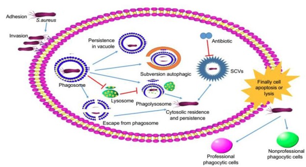
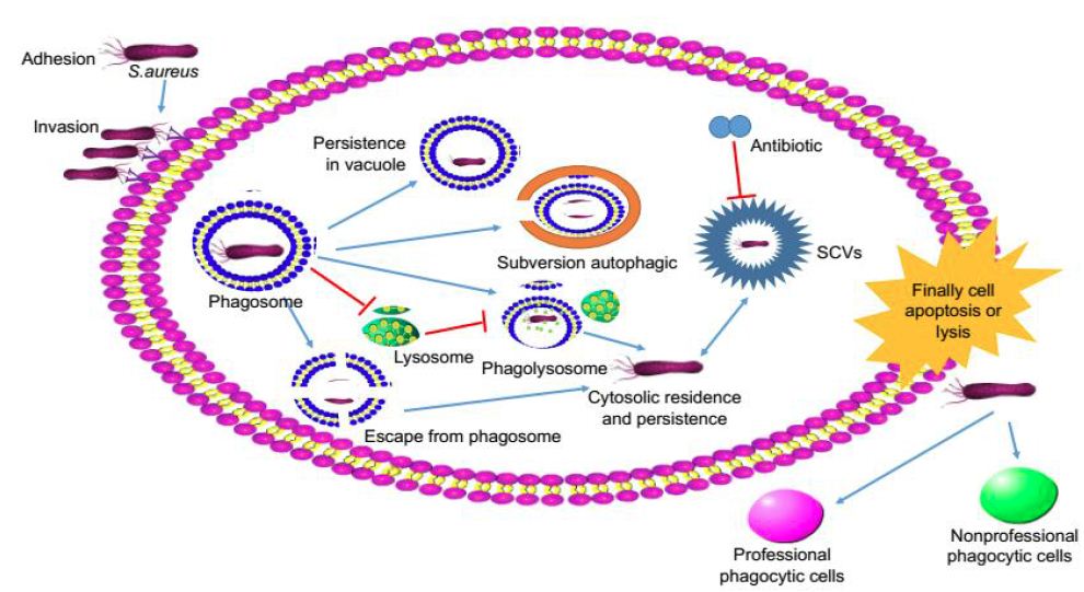
Stock Effect of Bio-Economic Indicators in an Over- exploited Fishery of the Gulf of Mexico

DOI: 10.31038/AFS.2023513

Abstract

The main bio-economic indicators of a pelagic fishery of the Northern Gulf of México (the Gulf Menhaden Brevoortia patronus Goode), was examined to understand their 8 performance as a result of simulated trials of the age of first catch and the fishing mortality. First, the validity of simulation was tested rebuilding numerically the performance of biological data and catch over time. A simple approach was made assigning economic value to the catch per-kg and the cost of fishing, so the output of biological variables could be linked to their corresponding economic performance, under the dynamics of the exploited stock, before adding value to the catch. As a part of results, the historical trend of a declining yield, suggests that the fishery has been over exploiting the juveniles, and even tough this condition has been sustained for more than forty years, this process produces nearly 400 thousand t, while it could yield more than one million t if it exploits only adult fish. On testing the economic indicators of the stock response as effect of the age of first catch, it is evident that the current yield is well below the Maximum Sustainable Yield, which might be higher if only adult fish are the targets of the fishery. The same occurs with the Maximum Economic Yield. The Benefit/Cost displays an inverse relationship with the Cost per t. It was found that the fishery could profit more than three hundred million USD if the age of first catch is re-addressed to get only adults as fisheries target. It is clear that this approach could be adopted as useful tool for decision-making and fisheries management.

Keywords

Stock assessment, Maximum sustainable yield, Maximum economic yield, Overexploited fishery, Gulf menhaden

Introduction

One of the problems of fisheries management deals with use of formal procedures of evaluation of exploited stocks in order to derive quantitative regulations able to foresee accurate consequences after the application of certain management actions [1-5]. However, a few years ago, it was stated that fisheries overexploitation and unsustainability are still not widely understood [6], despite cascade effects have been reported [7,8]. Fortunately, after twenty years, with much scientific research work done on this problem, it is much better understood. Therefore, there are multiple examples of mismanagement of fisheries resources, with regrettable consequences leading to the over exploitation of many fish resources and their consequences in their environment [9-12]. In the present paper, populations are evaluated by reconstructing the age structure of each of the years analyzed. The potential catch, benefits, direct jobs, and earnings per fisher can be estimated in several scenarios by changing the fishing mortality F, and the age of first catch, tc. In this way it is possible to test the response of the biologic and socio-economic variables of each fishery with reference to the maximum sustainable yield MSY, and the maximum economic yield MEY.

Many Fisheries at a worldwide level, have been declared chronically overexploited [13]. However, stock assessments and management regulations are usually addressed towards limitations of access, reduction of fishing seasons, reduction of fishing effort, establishment of closed areas, etc., but fisheries scientists as advisers and managers do not usually pay attention in the effects of mesh openings as means to control the age of first catch (tc), allowing to catch only adults of the fish stock and giving to juveniles usually caught, the opportunity to survive to the adult age and having the chance to breed at least only once in their lifetime. An examination of the population parameter values of several fisheries shows that tc value is at least one year lower than the age of first maturity ™. This is a circumstance that unavoidably leads these fisheries towards a condition of overexploitation, which in the case of the Gulf Menhaden and other cases, becomes a chronical condition that often leads to a biological and economic crisis. It is remarkable to find out that management regulations usually ignore the need to increase mesh openings to allow juvenile fish being released from the nets and capturing only adults [14].

Methods

The assessment of the Menhaden stock was made by using a simulation model [15,16]; is based on the general principles of the assessment of exploited fish stocks and is conducted with usually fifteen years of catch data. Thus, with the purpose of formulating better management options, a meta-analysis of data was conducted  to evaluate the performance of the fisheries with reference to the output of this model. In each of these options, catch data and the values of the population parameters are used, from the references    or estimated directly [17-20] and are indicated in Table 1. The associated costs and economic benefits of the fishery are taken as a reference for the bio-economic analysis. The model proposed allows testing of as many exploitation possibilities as fishing data allow, in a dynamic programming exercise that can provide answers to logical questions such as: What will happen to the biomass of the stock and the economic yield if the size of first capture is increased? What will be the biological and economic consequences if fishing effort is doubled? What is the maximum effort that the fishery can sustain and fail to deliver benefits of at least 10 percent above costs? And what are the economic expectations for the next season if the cost of fuel increases in a certain proportion? Population parameter values used as input of the simulation and the corresponding equations are in Table 1.

Table 1: Population parameter values, units, equations and source or comments used for the evaluation of the Gulf Menhaden fishery are indicated.

tab 1

Among the results obtained with the use of this model, the evaluations carried out indicate that for a combination of tc and F values, the estimated performance describes a dome-shaped response surface; if a single value of tc is taken and the response of the stock is observed, the yield is shown as a curve that at certain F level attains a maximum value and declines after this point. The output also describes the number of jobs as a function of F as a line with the same trend as that of potential capture; the benefit/cost ratio is a curve that declines as F increases. In general, the MSY level is at a higher value of F than in the case of the economic yield (MEY). In high-value fisheries, such as lobster, this value coincides with MSY at the same F. In addition, it is remarkable to find out that the cost of fishing increases with higher F intensity, making the activity unprofitable with higher values.

For the economic analysis of the resource, it is necessary to feed the model with data such as the number of fishing days that each season lasts on average, the number of boats and the number of fishers per boat. The total costs are obtained by multiplying the costs/ship/ day by the total number of ships in operation. Ideally, estimates of economic data are made after examining the fishing log from a trading trip [21]. The maximum social value can be determined in two ways, the first is the level of maximum employment (the maximum number of fishers). The second is the maximum profit per fisher. The economic and social values as input data were the value per kilogram landed and the number of fishers during the last fishing season. It is desirable to use a long series of economic data, but these variables though exist, they are not easily available nor collected in a systematic way like those of the catch and effort and for now the estimate that is made by the model roughly reconstructs the economic history of the fishery, with the risk of incurring in certain errors. This problem will cease when a diagnosis of the current situation be made as a basis for the rationale and future management of the resource.

Benefits are determined by subtracting total costs from the total value of the catch. Costs and value are linked to the catch and the other variables in the model. The populations are evaluated by reconstructing the age structure of each one during the series of years of the analyzed data. The potential catch, benefits, direct jobs, and profits per fisher are estimated under the scenarios sought, changing the F and the tc. In this way, it is possible to test the response of the socio-economic variables of the fishery with reference to MSY and MEY. In this context, benefits are obtained by subtracting total costs from the total value of the catch; costs and value are linked to the catch and the other variables in the model.

It is amazing to find out that more than six decades ago Beverton & Holt [22] stated the principle that yield tends to increase with higher values of the age of first catch and displayed this in the well-known figure of yield per recruit. In addition, with the advent of computers and profuse modelling, it is not understood why this problem has not been tackled by fisheries scientists in the following years after that paper. Therefore, this essay was written with the purpose of showing evidence that for any exploited stock, there is a MSY value which is the maximum catch that can be extracted from an exploited stock in the long term, as one of the many equilibrium values that any fishery can have. It is pertinent to mention that in some cases there are huge differences between the MSY and the optimum yield (OY), which is the maximum harvest producing the highest benefit indefinitely. OY is a particular case of the equilibrium MSY values, corresponding to the highest yield that an exploited stock can produce. In addition, when economic values are explicitly considered, it is possible to talk about the MEY, which is closely equivalent to the MSY, but values  of these variables do not coincide at the same F value. Fishing effort was not explicitly considered in this paper, based on the amount of noise usually implicit in it; instead, the spread sheet allowed that catch equation was fitted backwards and most of the significant amount of uncertainty disappeared in the stock assessment process.

The Gulf Menhaden

Despite the distribution range of the Gulf menhaden  spreads over the Gulf of Mexico, and beyond, the fishery takes place in the brackish-waters of the Mississippi river delta, where the coastal areas contain high Cla values, in contrast with the low Cla content along the southern Gulf, where there is much lower productivity (an order of magnitude lower than along the northern Gulf) [23], which does not allow the high stock biomass of this fish as along the vicinity of the Mississippi river delta.

It is pertinent to mention that the catch trend shows an even decline since 1987 (data after Gedar 03 2021) [24], with 640 thousand t in 1987 to 414 thousand t in 2020, as shown in Figure 1, which was drawn to display the fitting process of catch and reconstructed data as a part of the model calibration. No fishing effort data were used to avoid the noise implicit in its use. Population structure was rebuilt in the simulation by applying backwards the stock assessment equations.

fig 1

Figure 1: Model fitting of the catch and assessment of the biomass of the Gulf menhaden for the years 1977-2020

Once the population structure was rebuilt with the current parameters of the fishery, successive trials were applied to each age of first catch of the simulated stock, and this way the stock response could be measured. With the purpose of having an economic output, explicit consideration of the catch value before landing, the number of boats, the catch per trip, and the cost per trip were taken into consideration. The analysis presented in this paper deals within the scope of the so- called stock effect [25,26], it refers to the idea that unit operating costs are sensitive to the size of the exploited fish stocks; in other words, the analysis is referred to the performance of bio-economic indicators inside the fishery, before landing the catch.

With this information in the model, and by knowing the stock response as consequence of different values of the F, it was possible to determine the potential catch, the profits, the benefit/cost ratio,  the MSY, the MEY, the best tc, and other bio-economic variables useful for fisheries management,  produced  as  model  outputs.  As it was stated before, population parameter values were  obtained from FishBase, and Gedar 03 2021. Estimation of some population parameter values were obtained with the aid of Froese 2006; Froese & Binohlan 2000 [27].

Results

Profits and Benefit/Cost Ratio

Despite its declining trend, the Gulf menhaden is a very productive economic activity, displaying profits above 160 M USD in 1987 to around 70 M USD in the year 2020 (Figure 2). The same statement is valid for the Benefit/Cost, whose values (times the cost of fishing) range from 86 in 1986 to 47 in 2011. During the last five years of the series, the economic activity displayed a significant increase up to 116 in 2020 (Figure 2).

fig 2

Figure 2: Trend of profits, in USD and B/C ratio of the Gulf menhaden fishery since 1977

Optimum Yield

The MSY use to be the target of many fisheries; however, it is not usually mentioned that it is not a fixed parameter, it is a variable which depends on the age  of  first  catch  and  therefore  there  are as many MSY values as age groups are in a given stock, being the optimum that one which is at or near the oldest age class in the fishery; in this case it would be the catch of 3.3 M t at the age of eight years profiting 527 M USD at the same age. For obvious reasons, it would be no practical the application of tc = 8 years and the most convenient option could be choosing seven years instead. Any other values are sustainable and are maximum for each age class before the last one. Under the MSY (Figure 3A) and the MEY (Figure 3B), the stock responds the same way and both variables display in an analogous way as a function of tc.

fig 3

Figure 3: Maximum sustainable yield (MSY), 3A, and Maximum economic yield (MEY), 3B, of the Gulf menhaden fishery as a function of tc. In the first case the units are metric tons (t) and in the second case the units are Million USD.

Economic Variables

As a result of the analysis, it was found that there is an inverse relationship between the costs of exploitation and the B/C ratio (Figure 4). This is an evident condition, because it is logical to expect that the exploitation of the fishery is subject to higher costs when the stock is less abundant and vice versa.

fig 4

Figure 4: Relationship between the Benefit/Cost ratio (B/C) and the Costs of exploitation per t (C/t, USD) in the Gulf menhaden fishery. Each dot represents a tc value, being the first two overlapped on the right end of line trend, corresponding to tc ages of 1 and 2 years. The horizontal axis indicates the cost per t.

Under-Exploited or Over-Exploited?

The main reason why the consideration that the Gulf menhaden is overfished, as stated in the title of the present paper, is because from the viewpoint of the author, based on this and previous analysis, the stock is exploited as overexploited of recruits in a condition such that is shared by many fisheries around the world [28-32] and there are countless examples evidencing this problem. The analysis of this and other fisheries lead to the conclusion that the main reason for the over exploitation of recruits may be economic, because often occurs in pelagic stocks which are very productive and display high turnover rate. They are often linked to high economic value, product of high catch volumes, as it is the case of the Gulf menhaden; this fishery is very productive for its high landings and for its high profits. Then, it has been exploited for long time and the yield shows a declining trend to the point of capturing near 400 thousand t per season in the last few years, as compared to the landings of near one million t per season recorded in the middle eighties. It is amazing to realize that nobody has pointed this situation before, despite that the historical decline of catch is an evident fact and the teams in charge of evaluations refuse to accept this condition of the fishery, stating that “the Gulf of Mexico menhaden stock is not experiencing overfishing and is not overfished” (Gedar 03 2021). The authors of the present paper believe that the main reason why nobody has called the attention on the condition   of an overexploited fishery is because the menhaden has been very profitable for many decades, confirming what was stated above. Then if nobody pays attention on this problem, the condition will continue until the turnover rate of recruits becomes critical, the stock biomass to be not enough to replace the stock and the fishery to become unprofitable [33]. This is evidence confirming that the Gulf menhaden is under a condition of overexploitation of recruits [34], a problem common to many other fisheries [35-39].

As result of the analysis, it was found that a nearly four times higher catch could be obtained by applying F = 0.4, as shown in Figure 5, where the exploitation rate (E) and the F estimated for the years 1977-2020 are displayed. It is pertinent to mention that it is  not desirable to increase the F in an overexploited stock because the number of recruits would get exhausted in a few more fishing seasons and the whole fishery would fall into a collapse in brief time.

fig 5

Figure 5: Historic trend of the F (bars) and the E (dotted line) in the menhaden fishery for the period 1977 – 2020.

Numerical analysis and simulation of fisheries systems allow estimating potential yields, amongst other options; one of them deals with the possibility of doing a long-term forecast of the expected performance of the stock under different exploitation policies, with a very reasonable accuracy. In this case, after rebuilding the structure of the population, it is possible to estimate the expected potential yield by application as many feasible management options of F and the tc in a modern and flexible approach of the Beverton- Holt (1957) yield per recruit method. In this study case, three age classes, one, three- and five-years old fish were used as an example to demonstrate in first place, that the current fishery is overexploited of recruitment by applying a tc = 1, as shown in Figure 6. The trend line of each one of the three age classes selected here for demonstration display the outputs of the expected yield as a function of F. In the last few years of catch records, the F value estimated is F = 0.11 and the yield is Y = 414,730 t; then by looking at the expected potential yield by exploiting only adults (tc = 3 and tc = 5), would allow a much higher stock biomass to catch, and the F could be three times the current one being able to yield more than 1.1 M t, without the risk of depleting the fishery.

Horizontal lines showing the FMSY and the EMSY values are indicated as reference, showing that the fishery is exploited below the limit reference points since 1988. This is an apparent situation, because by increasing the F above the current values, the yield would decrease instead of increasing (Figure 6).

fig 6

Figure 6: A. Expected yield of the Gulf menhaden fishery under three scenarios, as a function of fishing mortality. The lowermost line corresponds to the current condition with tc=1, whose maximum yield could hardly produce 670 thousand t at the maximum at F=0.4. By contrast, after applying the same F, with tc=3, the fishery would yield 904 thousand t; with tc=5, the fishery would harvest 1.3 M t. In the last two cases, only adult fish would be exploited. B. Economic performance of the fishery by expressing the profits in Million USD as a dependent variable. In the current condition (tc=1) the maximum profit is $104 M. By applying the same F, with tc=3 the fishery would produce $142 M; with tc=5, the fishery would profit $218 M. Other variables are the same as in Figure 6A.

Discussion

By examining the causes of over exploitation of the most productive world fisheries, it is generally aknowledged that the most common problems of overexploitation of a fishery may occur after the application of excessive fishing effort, by overexploitation of recruits or both, leading to an excess of fishing capacity [40-43], despite clear recommendations and reference points are defined [44,45]. This is the case of the Gulf menhaden, exploited in the northern Gulf of Mexico, and whose huge biomass makes it one of the most productive fish stocks at world level (Myers & Worm 2003).

Production of the Gulf menhaden fishery was briefly examined because of the Deep-Sea Horizon oil spill in 2010 awakened the interest on it by the authors, but an impact of the oil spill on its stock biomass immediately after that event was not evident. A ban was temporarily imposed to the fishery during this disaster, but the fishery continued shortly afterwards. However, no evidence of depletion could be observed in the stock biomass if there was any, as it is not shown in Figure 1.

Overexploitation of fish stocks is a major concern in many world fisheries. It is the case for not just the Gulf menhaden, but it occurs in many others and it has been pointed as one of the reasons why   the world fisheries production display decreasing trends since more than fifty years ago [40,41], claiming for urgent rebuilding of stocks, Despite reference points and statements on the management have been provided (Caddy 1999; Caddy & Mahon 1995).

It has been stated that close to 90% of the world’s marine fish stocks are fully exploited, overexploited or depleted, threatening the chance of renewal of stock biomass, because the gradual reduction  of production capacity of the stocks to the point that a stock may be exhausted becoming incapable to restore its biomass as consequence of the lack of enough reproducers, compromising the sustainability of a fishery [42-44]. There are several causes leading fisheries to    an overexploited condition, like illegal fishing, subsidies, fishing overcapacity and degradation of environment, as the more common ones. The effects of overexploitation are often expressed as social and economic crises on the harbours and ports where the reduced catches are landed, and where much infrastructure and services stop being  in use leaving many people out of jobs. Contrary to what has been expressed in most of stock assessments [45], in this paper the use of fishing effort data was deliberately ignored, but once the model was fitted, it was possible to do an estimation of the number of fishing days, without the noise that is usually implicit in the current stock assessment procedures.

An undesirable perspective of the current condition of the Gulf menhaden, is maybe the worst case of a more general problem, biomass overexploitation not necessarily expresses the more critical consequence of this fishery, which has been gradually overexploiting its juveniles for decades. In this activity, the age groups caught by the fishery include since the age class of one year of age, but the stock reaches the age of sexual maturity at the age of two years; this implies that the fishing gears are catching all age classes. By consequence, the portion of the stock caught by the fishing gears include juveniles that otherwise would have the chance of reaching the adulthood   and contributing to replace the stock with the products of their reproduction. In the Gulf menhaden fishery, catch trend over time displays a slight but consistent decline, evidencing the effect of a gradual reduction of the population turnover rate, which as far as it persists without change, eventually would lead the fishing activity into a crisis, becoming unprofitable, because the cost of fishing would make the fishery unviable. A reduction of the stock biomass would lead to an increase of fishing because it will make the fishery more expensive, to the point of reaching the economic equilibrium limit, this is when the fishing stops being profitable.

In order to conclude this paper, it is considered that despite the Gulf menhaden still is a productive fishery, with profits near to one hundred million USD, it could profit more than three hundred million USD if the owners of the fishing fleet decide to open the meshes of fishing gears, and the age of first catch is re-addressed to get only adults as target of the fishery. Evidently, the adoption of this fishing strategy would imply some previous trials of selectivity using several mesh openings, and results could allow choosing the most suitable one [46-52]. However, in order to achieve the expected goals in the desired size-frequency of the new catch, the adoption of the new mesh size should be applied to the whole fishing fleet, so the new selectivity can have impact on the whole exploited stock; otherwise it would not have the expected effect. It is considered that the use of the new mesh sizes, may take a couple of years to achieve the expected results.

Author Credit Statement

EC and ACH developed the paper concept; EC created the draft and structure of the paper; both authors contributed to writing and editing.

Declaration of Competing Interest

The authors declare that they have not known competing financial interests or personal relationships that could have appeared to to influence the work reported in this paper.

References

  1. Hardin H (1968) Tragedy of the Science 162: 1243-1248.
  2. Lleonart J, Maynou F, Recasens L, Franquesa R (2003) A bioeconomic model for Mediterranean fisheries, the hake off Catalonia (western Mediterranean) as a case Sci Mar 67: 337-351.
  3. Myers RA, Worm B (2003) Rapid worldwide depletion of predatory fish Nature 423: 280-283. [crossref]
  4. Beddington JR, Agnew DJ, Clark CW (2007) Current problems in the management of marine Science 316: 1713-1716. [crossref]
  5. Demirel, N, Zengin M, Ulman A (2020) First Large-Scale Eastern Mediterranean and 428 Black Sea Stock Assessment Reveals a Dramatic Front Mar Sci 7: 103.
  6. Gréboval, D (comp.) (2002) Report and documentation of the International Workshop on Factors Contributing to Unsustainability and Overexploitation in Fisheries.
  7. Sala E, Boudouresque CF, Harmelin VM (1998) Fishing, trophic cascades, and the structure of algal assemblages: evaluation of an old but untested paradigm. Oikos 82: 425-439.
  8. Shears NT, Babcock RC (2003) Continuing trophic cascade effects after 25 years of 505 no-take marine reserve Marine Ecology Progress Series 246: 1-16.
  9. Hilborn R, Walters CJ (1992) Quantitative Fisheries Stock Assessment: Choice, dynamics and Uncertainty. Routledge.
  10. Pauly D, Christensen et al. (2002) Towards sustainability in world fisheries. Nature 418: 689-695. [crossref]
  11. Schijns R, Froese R, Hutchings JA, Pauly D, Raicevich S (2021) Five centuries of cod catches in Eastern ICES Journal of Marine Science.
  12. Rosenberg A (2003) Managing to the Margins: The Overexploitation of Frontiers in Ecology and the Environment 1: 102-106.
  13. Pauly D, Christenen V, Dalsgaard J, Froese R, Torres F (1998) Fishing Down Marine Food Science 279: 860-863.
  14. SEDAR (2018) SEDAR 63 – Gulf Menhaden Stock Assessment Report.
  15. Chávez Kruse G.H, Gallucci VF, Hay DE, Perry RI (2005) FISMO: A Generalized Fisheries Simulation Model. Fisheries assessment and management in data-limited situations. Alaska Sea Grant College Program, University of Alaska Fairbanks.
  16. Chávez-Ortiz EA (2014) Un modelo numérico para la administración sustentable de las pesquerías. CICIMAR Oceánides 29: 45-56.
  17. Jensen AL (1996) Beverton and Holt life history invariants result from optimal trade- off 469 of reproduction and survival. Canadian Journal of Fisheries and Aquatic Sciences 53: 820-822.
  18. Jensen AL (1997) Origin of relation between K and Linf and synthesis of relations among life history Canadian Journal of Fisheries and Aquatic Sciences 987-989.
  19. Froese R, Binohlan C (2000) Empirical relationships to estimate asymptotic length, 439 length at first maturity and length at maximum yield per recruit in fishes, with a simple method to evaluate length frequency Journal of Fish Biology 56: 758-773.
  20. Froese R, Pauly D (2021) www.fishbase.org.
  21. Mora C, Myers RA, Coll M, Libralato S, Pitcher TJ, et al. (2009) Management Effectiveness of the World’s Marine PLoS Biol 7: 6. [crossref]
  22. Beverton RJH, Holt SJ (1957) On the dynamics of exploited fish Fisheries Investigations, 19: 1-533.
  23. Chávez EA (2020) Maximum Sustainable Yield, Maximum Economic Yield and Sustainability.
  24. Gedar 03 (2021) Schueller, Amy, G D A R GULF DATA, ASSESSMENT, AND REVIEW GDAR 03 Gulf Menhaden Stock Assessment 2021 Update October 2021.
  25. Hannesson, R (1993) Bioeconomic analysis of Fishing News Books, 138 pp.
  26. Froese R (2006) Cube law, condition fator and weight-length relationships: history, meta-443 analysis and J Appl Ichthyol 22: 241-253.
  27. FAO (2020) The State of World Fisheries and Aquaculture Sustainability in action.
  28. Fiorentino F, Vitale S (2021) How Can We Reduce the Overexploitation of the Mediterranean Resources? Front Mar Sci 23.
  29. Fouzai N, Coll M, Palomera I, Santojanni A, Arneri E et al. (2012) Fishing management scenarios to rebuild exploited resources and ecosystems of the Northern-Central Adriatic (Mediterranean Sea) J Mar Syst 102: 39-51.
  30. Froese R, Winker H, Coro G, Demirel N, Tsikliras A et al. (2018) Status and rebuilding European Mar Policy 93: 159-170.
  31. Unctad (2017) A man tragedy: the Overexploitation of Fish Switzerland.
  32. Tsikliras AC, Froese R (2018) Maximum sustainable In: Reference Module in Earth Systems and Environmental Sciences.
  33. Jennings S, Kaiser M (1998) The effects of fishing on marine ecosystems. Adv Mar Biol 34: 201-352.
  34. Bellido JM, García RM, García JT, González AM, Carbonell QA (2017) Could the obligation to land undersized individuals increase the black market for juveniles: evidence from the Mediterranean?. Fish Fish 18: 185-194.
  35. Watson RA, Cheung WWL, Anticamara JA, Sumaila RU, Zeller et al. (2013) Global marine yield halved as fishing intensity redoubles. Fish Fish 14: 493-503.
  36. Worm B, Barbier EB, Beaumont J, Duffy E, Folke C. et al. (2006) Impacts of biodiversity loss on ocean ecosystem Science 314: 787-790. [crossref]
  37. Worm B, Hilborn R, Baum JK, Branch TA, Collie et al. (2009) Rebuilding global fisheries. Science, 325: 578-585.
  38. Zeller D, Cashion T, Palomares M, Pauly D (2018) Global marine fisheries discards: A synthesis of reconstructed Fish and Fisheries, 19: 30-39.
  39. Thurstan RH, Brockington S, Roberts CM (2010) The effects of 118 years of industrial fishing on UK bottom trawl Nature Communications 1: 1-6. [crossref]
  40. Hilborn R, Hilborn U (2019) Ocean Recovery: A sustainable future for global fisheries? Oxford U Press.
  41. Pauly D, Zeller D (2016) Catch reconstructions reveal that global marine fisheries 496 catches are higher than reported and Nat Commun 7: 1-9. [crossref]
  42. Perisi I, Bardi U, Asmar EI, Lavacchi A (2017) Dynamic patterns of overexploitation in fisheries Ecological Modelling 359: 285-292. [crossref]
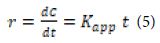
  43. Chávez EA, Chávez HA, Pérez LE (2020) Fisheries Potential of the Gulf of Mexico. Japan J Medical Science 1: 18-21.
  44. Maunder MN, Punt AE (2004) Standardizing catch and effort data: a review of recent approaches. Fisheries Research 70: 141-159.
  45. Mora C, Myers RA, Coll M, Libralato S, Pitcher TJ et al. (2009) Management Effectiveness of the World’s Marine PLoS Biol 7: e1000131. [crossref]
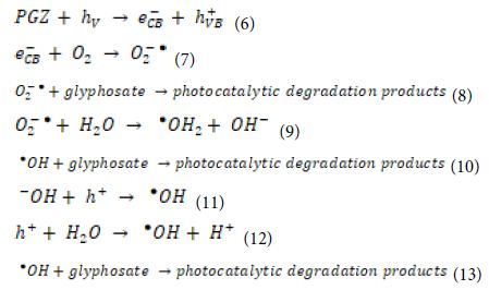
  46. Hilborn R, Amoroso RO, Anderson CM, Baum JK, Branch et al. (2020) Effective fisheries management instrumental in improving fish stock status Proceedings of the National Academy of Sciences, 117: 2218-2224.
  47. Kirkley JE, Squire D (1999) Measuring Capacity and Capacity Utilization in In: Gréboval, D (Ed) Managing Fishing Capacity: Selected Papers on Underlying Concepts and Issues. FAO Fisheries Technical Paper No 386: 75-200.
  48. Pascoe S, Gréboval D (2003) Measuring capacity in FAO Fish Tech Pap 445: 1-314.
  49. Bell J, Watson W, Ye Y (2017) Global fishing capacity and fishing effort from 1950 to 2012. Fish and Fisheries 18: 489-505.
  50. Colloca F, Scarcella G, Libralato S (2017) Recent Trends and Impacts of Fisheries Exploitation on Mediterranean Stocks and Front Mar Sci 4: 244.
  51. Caddy JF (1999) Fisheries management in the twenty-first century: will new paradigms apply? Rev Fish Biol Fish 9: 1-43.
  52. Caddy JF, Mahon R (1995) Reference Points for Fisheries FAO Fisheries Technical Paper.