Author Archives: author

Empowering Young Researchers: Searching for What to Say to Young People to Avoid Becoming Obese

DOI: 10.31038/EDMJ.2023713

Abstract

71 US respondents, ages 14-19, evaluated phrases about what to do to avoid overeating. The phrases were selected by two student researchers, one in middle school, one in elementary school, using artificial intelligence. The phrases were combined according an underlying experimental design, creating 24 vignettes, with each of the 71 respondents evaluating a unique set of vignettes, rating each vignette on ‘for me versus not for me’. Clustering reveal three clearly different mind-sets about what is most relevant to the respondent; Mind-Set 1 focuses on exercise, Mind-Set 2 focuses on eating healthfully, Mind-Set 3 focuses on parental responsibility. The three mind-sets emerged clearly and dramatically, even though the respondents evaluated combinations of messages, some relevant, some not relevant.

Introduction

Obesity and diabetes are serious problems around the world. With the increasing consumption of processed foods, with the decrease in exercise as part of the sedentary lifestyle, the inevitable result is an increase in diabetes. The literature is filled with information about the problem, albeit from the point of view of the clinician seeing the patient, and from the point of view of professionals involved with public health [1-4]. There are also numerous professional nutritionists and lifestyle counselors who specialize in eating disorders, along with the many psychologists and psychiatrists who provide acute treatment for the suffering patient [5]. Diabetes is so threatening that many medical professionals are recommending bariatric surgery as a way to deal with the problem [6]. One key is educating the children to eat properly, a topic becoming increasingly relevant over the years [2,7-10].

This paper emerged from a short conversation with a colleague in Israel about the issue of obesity in young people, and the potential of that obesity to evolve into juvenile diabetes. The issue was whether one could work with student-age researchers, rather than with professionals [11]. These researchers would design the study from their perspective, rather than from the perspective of a professional. The research itself might not be as polished, but the inputs to the research might be more genuine because the ages of the researchers (Cledwin, Age 14; Ciara Age 8). These two students have already collaborated on a variety of papers, providing the inputs needed to run the study. This newest collaborative was quite easy for them, requiring about two hours to set up, and two hours to execute.

The Mind Genomics Paradigm as a Way to Understand the Mind of People

The research process used in this study is Mind Genomics, an emerging science which focuses on the decision processes of everyday experience. Mind Genomics differs from traditional psychology in that it presents systematically created combinations of descriptions of descriptions about a specific experience, obtains ratings of the combinations, and deconstructs the ratings to the contribution of each component of the combination. One might at first think that this approach is ‘roundabout’ because the typical approach is to present the individual items, the components, one at a time, get respondent ratings to each component, and then report the average rating. The reality, however, is that this ‘one at a time’ approach allows the respondent to focus on each component separately. As a result, the respondent shifts his or her criterion to be appropriate to the nature of the component, as well as tempting the respondent to outguess the researcher, looking for the ‘right answers’. Presenting combinations prevents the respondent from gaming the system, forcing the respondent to maintain the same criterion through the set of evaluations [12,13].

Demonstrating the Mind Genomics Process and Results for the Topic of ‘Preventing Childhood Obesity’

The process begins with a topic, namely childhood obesity. In the traditional Mind Genomics process, before the introduction of artificial intelligence through Idea Coach, it was the researcher’s job to create four questions which tell a story. The researcher would be presented with an empty screen, similar to the left panel of Figure 1, no questions filled in. It would be at this point when that the inexperienced researcher would experience a psychological ‘wall’, one sufficiently high to discourage. Over time, of course, and with practice, one could become sufficiently facile to fill in four questions, but the learning curve was fairly flat and long, requiring 4-5 experiences with a Mind Genomics study. That barrier, requiring the research to think of questions, sufficed to slow the acceptance of the process, although over time many people ‘stayed the course’ and became facile.

fig 1

Figure 1: The request for four questions to begin the study (left panel), the Idea Coach input (middle panel) where the user describes the topic with artificial intelligence returning with up to 30 questions, and then the four selected questions (right panel).

With the advent of widely available artificial intelligence though such platforms as Open AI the researcher is afforded an opportunity to write about the topic (see Figure 1, middle panel). For each description of the topic written by the researcher, Idea Coach returns with up to 30 questions. One may even use the same query or modify it, and return with additional questions, as Table 1 shows. Indeed, it has become apparent that many uses of Mind Genomics, and especially Bimi Leap, use the embedded artificial intelligence to learn about the topic in a greater depth, doing so in a self-directed, enjoyable fashion, akin to exploring to follow one’s curiosity [14].

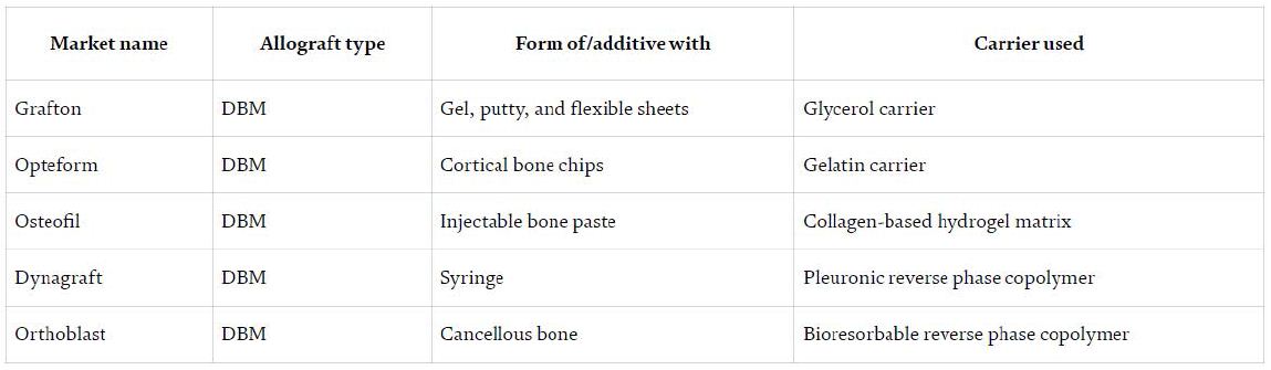
Table 1: The first set of 30 questions returned by Idea Coach on the first ‘run’, and set of 24 questions returned on the second ‘run’.

tab 1

Finally, the researcher selects the four questions from the list, provides some from the list, even editing them, and comes up with some of his or her own questions (Figure 1, right panel). Experience with Idea Coach suggests that after five or six times the researcher feels empowered by Idea Coach. It should be noted that for our student researchers who had had practice with Mind Genomics, this latest effort to create four questions ended up requiring less than 10 minutes.

Once the researcher has completed the selection of four questions, either from one’s own knowledge or using Idea Coach, or eventually some combination of the two, the BimiLeap program requests the researcher to provide four answers to each question selected, or a total of 16 answers. For each question, invoking Idea Coach generates 15 possible answers Once again, the researcher can invoke Idea Coach many times. Table 2 shows the output of Idea Coach.

Table 2: Example of 15 answers emerging from Idea Coach to address one of the four questions selected

tab 2

Before we move on to the next set up questions, it should be noted that the activity of creating questions and obtaining answers can end up as an activity itself. In the words of co-author Ciara Mendoza, the 8-year old student researcher, ‘this is so much fun…. Better than video games.’

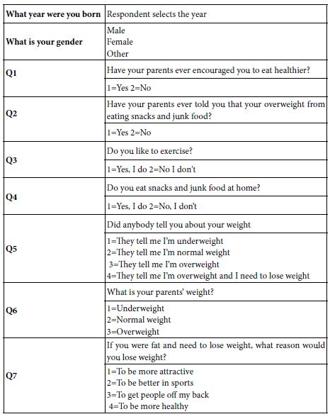
The next and optional step creates a set of classification questions. These questions provide additional information about the respondent. In the analysis below, we will look at the respondent’s gender and age, both obtained automatically in the BimiLeap program. In addition, the researcher is able to ask up to an additional eight questions, each question with up to eight different answers. For the study here, the researcher selected seven different question. Table 3 shows the actual questions and answers. Figure 2 shows the layout for the classification questionnaire. The appendix shows the distributions of the 71 participants across the self-profiling classification questions, as well as across the three emergent mind-sets.

Table 3: Self-profiling classification questions

tab 3
 
fig 2

Figure 2: An example of the self-profiling classification question. The BimiLeap program allow for eight such questions, each with up to eight possible answers.

As explained above, the strategy of Mind Genomics is to present the respondent with combination of elements. These combinations created according to an experimental design. The design used by Mind Genomics is known as a ‘permuted design’ [15]. The design has been created for a variety of numbers of elements. For this study, and indeed for most recent Mind Genomics studies, the design calls for four questions, each with four answers. Henceforth, these will be Questions and elements, with the word ‘element’ replacing ‘answer’ or in other renditions of experimental design, the word ‘element’ we use here will replace terms such as ‘option’ or ‘level’.

The underlying permuted design creates precisely 24 vignettes, viz., combinations, comprising either two, three, or four elements, at most one element from each question, but often no element from a question. Each of the 16 elements appears exactly five time in the 24 vignettes, and is absent from 19 of the vignettes. The experimental design is set up to create different sets of 24 vignettes for the respondents, so that for a reasonable size study (fewer than 500 people), it is quite likely that no two respondents will evaluate the same vignettes. In this way the Mind Genomics system allows anyone to explore a topic, with a high likelihood of discovering the promising aspects of the topic. This open-vision, this virtually unfettered exploration of the topic, stands in stark contrast to the hypothetico-deductive thinking of most of today’s research, where one must formulate a hypothesis, design the combinations of variables likely to be most important, and then do the study to confirm or disconfirm one’s hypothesis. This science subtly converts the study from exploration to discover into effort to confirm or falsify, a world-view which makes it important virtually to ‘know the answer’ before the doing the experiment. In the case of our student researchers, such subtle demands of ‘knowing the answer ahead of time’ may disenchant the student. The rigor of the hypothetico-deductive system may be exactly what can do the job of crushing the spirit of the novice.

Among the final steps in the creation of the experiment is respondent orientation, choice of a rating question, and actual rating scale, shown in Figure 3. The researcher types in the question, the number of scale points, and is free to label or not label the scale points.

fig 3

Figure 3: (Left panel) Respondent orientation to the study. (Right panel) The rating question, the selection of the number of scale points, and an optional anchor for each scale point.

The actual study is done on the Internet through a cooperating panel provider, Luc.id, Inc. Any panel provider who an access people can do equally well. Often the researcher wants to use his or her friends, or other individuals known to them. In such cases the BimiLeap program provides a link to be sent to the prospective respondents. A word of caution is due here. Although it is tempting to work within a limited group of friends or prospects one knows, the time to do the experiment can be become unduly long. The study reported here (actually two precisely parallel studies, one with males, one with females) took about 60 minutes to complete. That 60 minutes could turn into two or three weeks, and could end up without sufficient respondents as one’s friends, acquaintances, invited to participate, end up forgetting, deleting, or just ignoring the invitation.

Figure 4 shows an example of one of the 24 vignettes shown to a respondent. The vignette shows very little information, presents the requirement to think of the vignette as a single idea, presents the rating sale, and then the vignette. The respondent has no problem reading and evaluating 24 of these vignettes, with the entire process taking about 3-5 minutes. Most respondents to whom we have talked felt that they were ‘guessing’, but the exact opposite turned out to be the case, as their data revealed consistencies that would make the data appear to be valid.

fig 4

Figure 4: Example of a test vignette, showing the rating question and the rating scale

Acquiring Data, Transforming Ratings, and Creating Equations

The ratings for each respondent for each vignette are acquired as processed within moments. The basic information for the respondent (age, gender, answers to the seven self-profiling classification questions) are captured at the start of the respondent interview on the web, and remain constant for the 24 vignettes that the respondent evaluates. When the respondent evaluates a specific vignette, the database captures the structure of the vignette in terms of 16 numbers, one column for each number, each column corresponding to a specific element. The database also inserts the order of the rating, from 1 (tested as the first vignette) to 24 (tested as the 24th vignette). This information will make it possible to evaluate any effects due to order of testing. Then database then captures the rating on the 5-point scale, and the response time, defined as the number of seconds (to the nearest hundredth of a second elapsing between the time that the vignette appeared and the tie that the respondent rated the vignette.

The rating itself, a 5-point Likert scale is easy to create, but for everyday practice the meaning is often elusive. Managers simply do not know what to do when they get an average rating. As simple as that sounds, the reality is far more problematic. Most managers using these scales ask whether the effect is significant, meaningful, or more telling ‘now what should I do with these numbers?’ Research practices among consumer researchers and public opinion pollsters is to convert the Likert Scale to a yes/no scale. For our study we make two conversions.

TOP 2 – Positive response — Ratings of 5 and 4 are converted to 100, ratings of 1,2,3 are converted to 0, and a vanishingly small random number is added to the converted values so that the OLS regression will ‘not crash’, even when a respondent confines the rating either to 4 and 5, in which case the transformed rating for all 24 vignettes will become 100, or to 3,2,1 in which case the transformed ratings will all become 0.

BOT2 – Negative response – Ratings of 1 and 2 are converted to 100, rating 3,4,5 are converted to 0, with a different but vanishingly small rando number is add to the transformed rating.

Relating the Presence/absence of the 16 Elements to the Transformed Ratings

The objective of Mind Genomics is to link the elements to the ratings, and by so doing more profoundly understand the mind of the respondent. As emphasized above, the approach avoids the use of a simple survey wherein the respondent is presented with a series of ideas, one idea at a time, and instructed to rate the idea on a scale. Yet with the respondent presented what must seem like a proverbial ‘blooming, buzzing confusion’ in the worlds of Harvard psychologist William James how can the researcher ever disentangle the individual contributions of the distinguishable elements.

The answer to the foregoing lies in the underlying use of the permuted experimental design, used to create the 24 vignettes for each respondent. We know that the combinations were selected to ensure that we could estimate an equation for each respondent separately as well as a single equation for any defined group of respondents. Furthermore. We know that the individual models can be estimated without fear that the regression process will ‘crash’ because of either multicollinearity among the independent variables, or lack of variation in the dependent variable.

Our equation is: Dependent Variable = k0 + k1(A1) + k2(A2) … k16(D4)

The dependent variable can either be TOP2 or BOT2.

To relate response time (RT) to the presence/absence of the 16 elements we use the same equation but do not estimate the additive constant: RT = k1(A1) + k2(A2) …+ k16 (D4)

We estimate the equations quite easily once we know the members in the group viz., which specific respondents

Finally, the fact that we can estimate individual-level models, with the additive constant and the 16 coefficients, doing so for each respondent, and based only on the data from that respondent means that we can divide people b the pattern of their coefficients. These are the mind-sets, created from, individuals who show similar patterns of the 16 coefficients (k1 – k16). We do not use the additive constant. The method is called k-means clustering [16], with the measure of distance of dissimilarity defined as (1-Pearson correlation between the two respondents, computed on the basis of their 16 corresponding coefficients.

Results

The Mind Genomics process generates a great deal of data, the most relevant of which are the additive constants and the positive coefficients. The negative coefficients need not be considered. Negative coefficients are the ‘absence’ of a positive coefficient, either a true negative feeling (not for me), or perhaps a rating of ‘may/may not be for me’ (rating of 3). In any case for the most important data (Total Demographic groups and Mind-set, we look at both TOP2 and BOT2.

All data tables presenting results for TOP2 and BOT2 have been edited so that only coefficients of +2 or higher are shown. Furthermore, for those tables, strong performing elements with coefficients of +8 or higher are show in shaded cells. For response time all coefficients are shown.

For TOP2 and for BOT2 we interpret the results as follows:

  1. The additive constant is the baseline. The baseline is the estimated percent of the respondent rating the vignette 4 o 5 for TOP2, or 1 or 2 for BOT2. Of course, the underlying experimental design ensured that all vignettes would comprise a minimum, of two elements and a maximum of four elements. The additive constant, viz., intercept in regression terms, is simply an adjustment factor. We can use it to give us a sense of the baseline likelihood of the person responding fits me (TOP2) or doesn’t fit me (BOT2).
  2. The element coefficient shows the increased percent of respondents saying fits me (TOP2) or doesn’t fit me (BOT2), when the element is inserted into the vignette.
  3. The coefficient tells a lot of the story about what drives the respondent. Keep in mind that frequently the respondent cannot really explain why she or he responded in certain way to a vignette, although when asked directly the respondent searchers for a plausible answer. Yet, the coefficients reveal that criterion, sometimes clearly, sometimes strongly, occasionally however failing to find any criterion for the decision.

Who the Person ‘IS’ (Total, Gender, Age)

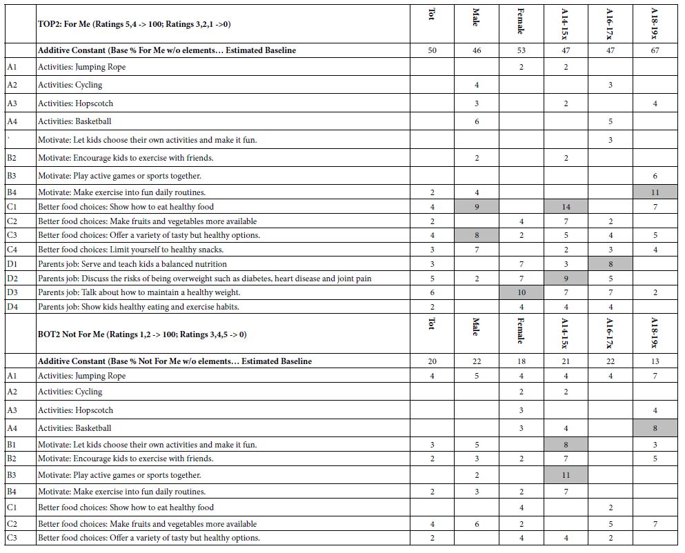
The first analysis (see Table 4, section for TOP2) shows the positive coefficients for Total Panel, gender, and age. There are clearly some elements which perform well, some which perform ‘very well.’ The additive constants hover around 50. The oldest groups of young people, age 18-19 are the exception, with an additive constant of 67, and a very strong element generating a coefficient of +11: Motivate: Make exercise into fun daily routines. When we look across all of the elements for these three groups, the story revolves around healthful living.

When we change the focus to the negative (see Table 4, second section, BOT2) we see far fewer elements which drive rejection, and thus the bottom of Table 4 is shorter. The elements which strongly drive rejection (not m) are those related to sports, and manifest themselves in the age groups.

Table 4: Positive coefficients for key demographic groups for TOP2 (For Me) and for BOT2 (Not For Me)

tab 4

How the Respondents Describe Their Eating History and Weight

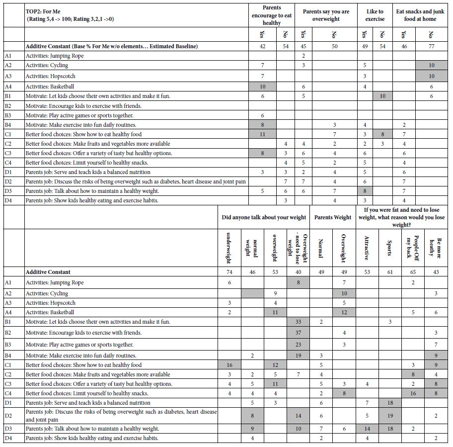
The respondents completed a self-profiling questionnaire, allowing the creation of new groups of respondents, based upon membership in each group. Depending upon the number of answers to the self-profiling question, each question generated a minimum of two mutually exclusive groups and a maximum of four mutually exclusive groups. In the interest of brevity, Table 5 presents only the data from TOP2 (For Me), again showing only the positive coefficients, and highlighting the strong performing coefficients with values of 8 or higher.

Table 5 shows a great many strong performing elements. The surface analysis of the results suggests that the data make sense. For example, for those respondents who say they don’t like to exercise, the strong performing element for the four exercise elements is B1 (Motivate: Let kids choose their own activities and make it fun), with a coefficient of +10. One could go through each of the cells in Table 5, because the results are ‘cognitively rich.’ That is, the Mind Genomics study deals with meaningful phrases as components of what is evaluated. Thus, any pattern which emerges comes with the advantage that the surface meanings of the components of the pattern are already known, and immediately accessible.

Table 5: Positive coefficients for key subgroups emerging from the self-profiling classification questionnaire

tab 5

Creating Mind-sets

One of the foundations of Mind Genomics is the proposition that people differ from each other in virtually every aspect of human behavior where conscious decisions are made. We already classify people by who they ARE, what they DO, what they say the BELIEVE, and so forth. The issue of person to person variability should not surprise us. In countless ways we are reminded daily of the wondrous variety of human differences, whether these be in foods, in leisure activities, and even in the way one wants to be treated in a medical situation. To this end, researchers have recognized different groups, which they call ‘psychographic’ groups, groups based upon the values people hold, and the way that they think [17]. For many of these ‘psychographic’ approaches the development time and costs are sufficient encumbrances which end up motivating the creator to ensure that the different psychographic groups cover as much as possible in terms of topics. Thus, a study on the psychographics of weight control might deal with many topics of weight control and healthy living, take months to design and execute, require the involvement of professionals for analysis, and finally require a way to translate the general findings to a specific issue of immediately, local, and relatively modest relevance to the entire topic.

Mind Genomics works in the opposite direction, creating mind-sets, psychographic group, not to understand the general topic as such as to profoundly understand the specific topic. Thus, in this study, the topic is not weight control in general, but rather what can one do in a local situation. The data which emerge end up telling the researcher about the mind-sets in the population for this specific topic, along with exactly what to say to the population, and finally, with the help of another program (www.pvi360.com; personal viewpoint identifier), a way to assign a new person to a mind-set by asking six questions. The sheer granularity of the mind-sets, ensured by the limited and precise focus of the study, ends up producing information which is both instructive and actionable.

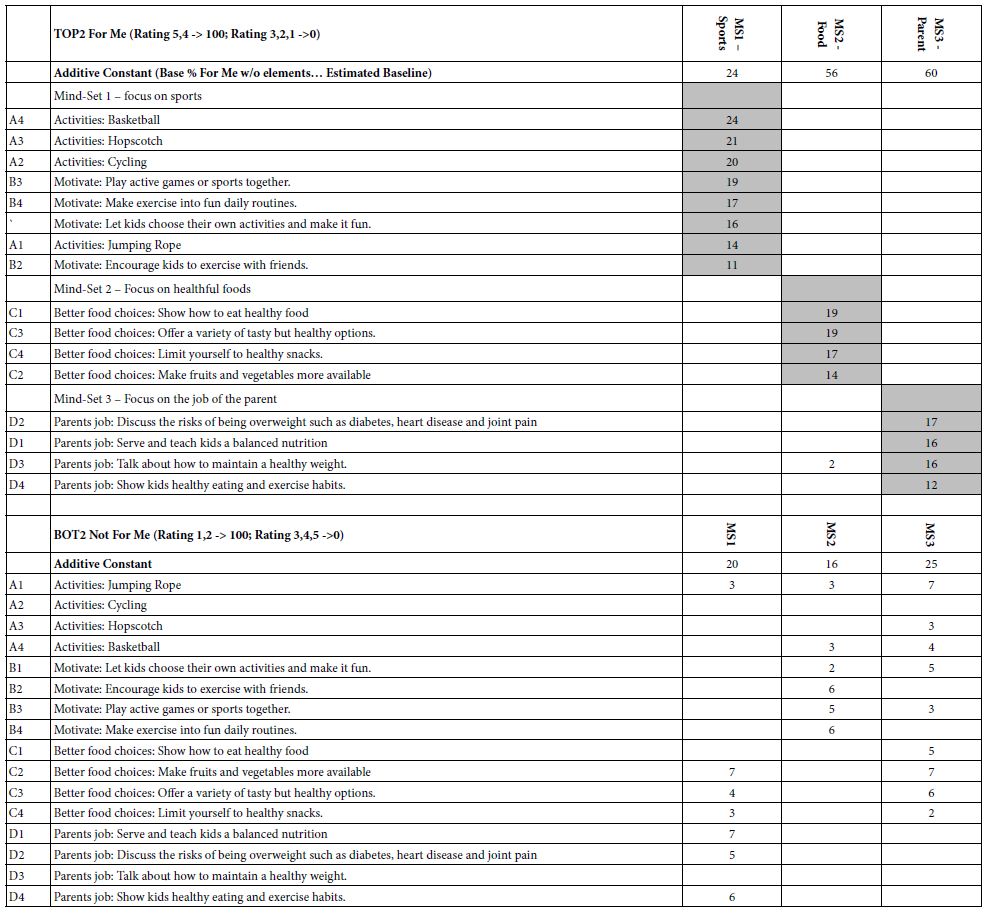
Table 6 shows the three mind-sets which emerge from the study. Recall that the respondents evaluated combinations, so that there was no way that any respondent could ‘game’ the study, and provide information that would be acceptable. The k-means clustering produces clearly defined groups, each group responding strongly to their own set of particularly convincing elements.

Table 6: Positive coefficients for thee emergent mind-sets for TOP2 (For Me) and for BOT2 (Not For Me)

tab 6

Mind-Set 1 (Sports) shows the lowest additive constant, 24. They are not ready to say ‘for me’ unless the topic is sports and exercise’. Nothing else interests them.

Mind-Set 2 (Food) shows a much higher additive constant, 56. They are ready to say ‘for me’, but the topic has to be food choice.

Mind-Set 3 (Parent) also shows a much higher additive constant, 60, with the focus on what parents should say.

Finally, when we look at the opposite, BOT2, Not For Me, we see an active but not very strong rejection of ideas other than those appealing to one’s mind-set. The preferences are clear and distinct.

Response Time as a Measure of Engagement with the Message

As part of the output of Mind Genomics effort, the BimiLeap program measures the response time to the vignette, operationally defined as the time in hundredths of seconds between the appearance of the vignette on the computer screen and the rating assigned by the respondent. The original assumption was that there might be some deeper ‘reality’ to be discovered when one moves from responses under ‘conscious control’ (willful responses, such as ratings), to responses not under ‘conscious control.’ There is a long history of response time in studies of behavior , giving a sense with the sense that some deep truth about the way we ‘think’ may emerge somehow when we measure non-conscious behavior instead of ‘considered’ actions [18].

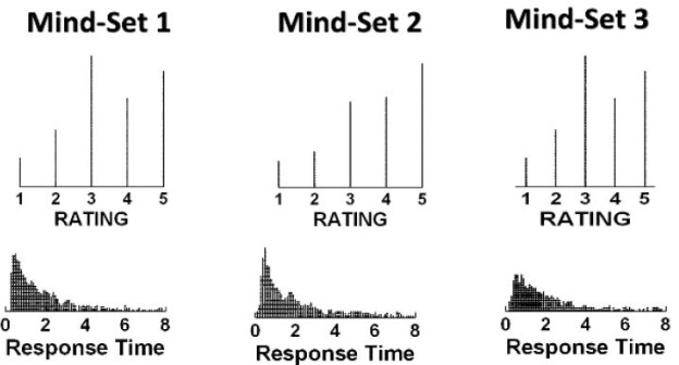
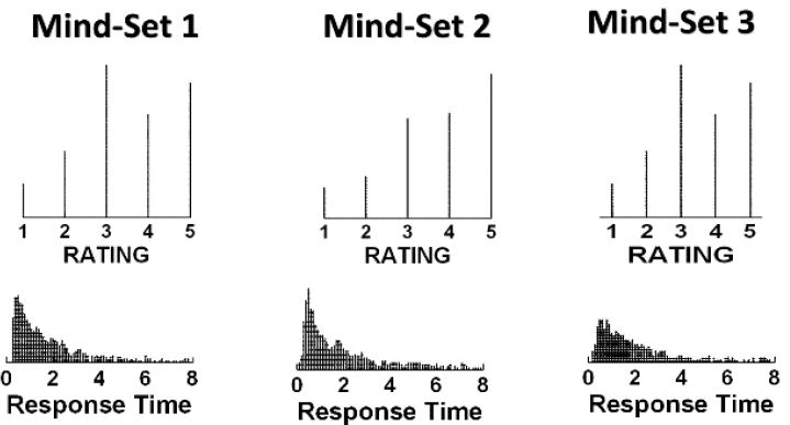
In the world of consumer research, investigators are perennially looking for the ‘next thing,’ something which can be measured reliably, something which can tell the research about what the respondent is ‘really thinking.’ There is a fantasy in the mind of the researcher that somehow these measures contain within them deep knowledge about the ‘mind of the respondent’, knowledge which simply needs to be decoded from these deeper measures, such as response time. Figure 5 shows the distribution of ratings for the vignettes rated by the three mind-sets, as well as the distribution of the response times (right side). The simple answer is that there are no clear ‘underlying’ patterns for the three mind-sets that we saw from Table 6, patterns which revealed clearly different and interpretable ways of looking at the same information. The clarity of differences in mind-sets emerging from Table 6 becomes clouded when we look either at the distribution of ratings, or the distribution of responses times it is only when we have cognitively meaningful test stimuli, systematically varied, that the difference emerges.

fig 5

Figure 5: Dot density plots of ratings on the 5-point scale (top) and response time in seconds (bottom). Each plot comprises the rating assigned to all vignettes, or the measured response time in tenths of seconds.

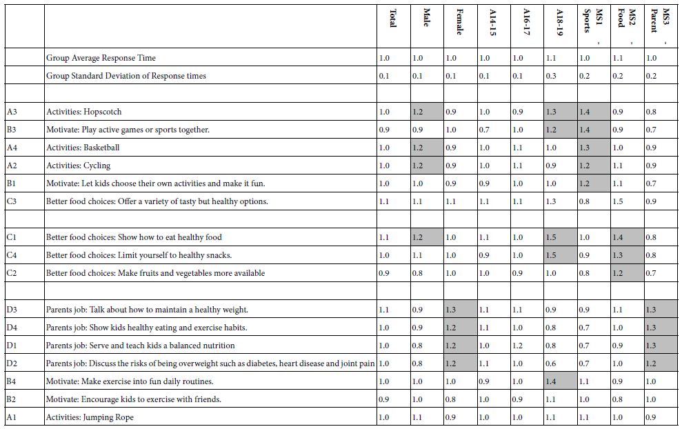
It may be that there is deep information awaiting us when we deconstruct the overall response times into the response times assignable to each of the 16 elements. Table 7 shows the coefficient for the response times attributable to each of the 16 elements by all key groups, viz., total, gender, age, and three mind-sets. All long response times, assumed to be elements which are engaging (or perhaps just difficult to read, are shown in shaded cells. Operationally, we chose 1.2 seconds or longer. Table 6 suggests that there are differences in strong performing elements among the groups, and even more interesting, the mind-sets spend longer time reading the elements with which they identify (viz., Top 2 in Table 6). Despite that, however, and perhaps sadly, there is no clear flash of deep insight emerging from the patterns of response times by elements by groups, whether self-defined groups or statistically created groups from cluster analysis.

Table 7: The estimated ‘time’ for each element, used for reading and processing the information, revealed by the deconstruction-by-regression of response times for reading individual vignettes.

tab 7

Discussion and Conclusions

Issues such as nutrition are almost always left to adults. It is the job of the child or teenager to do what is ‘best’, but that ‘best’ is usually established by adults and forced on the child or the teenager. The rationale for such a strategy is reasonable and obvious – it is the adults who know the potential outcomes of a healthful versus a non-healthful diet. Knowledge alone does not suffice. A responsible, loving adult is often necessary, albeit one who is knowledgeable [19-21].

What is often unknown is the mind of the person who is the subject of the nutrition effort. One can measure the physical variables associated with the person, the person’s nutritional status, even the daily behaviors. At the same time, however, what is the mind of the individual? And, to be more direct, not what is the assumed mind of the person based upon a short interview with the person or with the parent, but rather what is the psychological makeup of the individual, the messages to which the person will respond, this child or teen. Of course, one may invoke the common answer that to know such information is easy; one need only hire a psychologist to interview the person, to diagnose, to recommend language. But, in turn, what happens when we talk about tens of thousands, hundreds of thousands, or millions of children for whom we need to know the words.

The study presented here suggests that it may be profitable to include children as researchers, discuss topics which are everyday and ordinary, and move beyond the confines of a simple questionnaire which stresses intellectualization and ‘one at a time thinking.’ A more holistic approach might be called for, one which at first might offend those who have been educated in the world of the hypothetico-deductive, where questions emerge from the data, where the literature comprises a gap to be filled, where knowledge is the accretion of hypotheses that have succeeded in avoiding being ‘falsified’, in the true tradition of scientific exploration [22,23]. Rather, the study here suggests that it is the naïve questions posed by student researchers which can bring us a long way towards understanding thinking about food, bodyweight, obesity, and perhaps diabetes, although one might well like to work with students who have some familiarity with the concept of diabetes, and with respondents who are closer to the world of diabetes than our random 71 respondents studied here.

The paper closes with the caveat that the effort was done simply as an exploratory investigation to answer a quick question from a colleague. That humble origin of the study should not be held against the information gained from the research exercise. The study did not emerge as an answer to the ‘call from the literature,’ nor as an effort to ‘fill a hole or plug a gap in the literature.’ Rather, the study emerged as data-based practical answers to a question, the approach using the scientific method to create archival, relevant knowledge, giving a voice to prospective researchers with potential novel, valuable ingoing points of view.

References

  1. Felber JP, Golay A (2002) Pathways from obesity to diabetes. International Journal of Obesity 26: S39-S45. [crossref]
  2. King LA, Loss JH, Wilkenfeld RL, Pagnini DL, Booth ML, et al. (2007) Australian GPs’ perceptions about child and adolescent overweight and obesity the Weight of Opinion study. British Journal of General Practice 57: 124-129.[crossref]
  3. Kranjac AW, Wagmiller RL (2020) Decomposing Trends in Child Obesity. Population Research Policy Review 39: 375-388.
  4. Levin NZ, Cohen M, Phillip M, Tenenbaum A, Koren I, et al. (2022) Youth‐onset type 2 diabetes in Israel: A national cohort. Pediatric Diabetes 23: 649-659. [crossref]
  5. Helm KK (2007) Nutrition therapy: Advanced counseling skills. Lippincott Williams & Wilkins.
  6. Black JA, White B, Viner RM, Simmons RK (2013) Bariatric surgery for obese children and adolescents: a systematic review and meta‐analysis. Obesity Reviews 14: 634-644. [crossref]
  7. Boles DZ, DeSousa M, Turnwald BP, Horii RI, Duarte T, et al. (2021) Can Exercising and Eating Healthy Be Fun and Indulgent Instead of Boring and Depriving? Targeting Mindsets about the Process of Engaging in Healthy Behaviors. Frontiers in Psychology [crossref]
  8. Borra ST, Kelly L, Shirreffs MB, Neville K, Geiger CJ (2003) Developing health messages: qualitative studies with children, parents, and teachers help identify communications opportunities for healthful lifestyles and the prevention of obesity. Journal of the American Dietetic Association 103: 721-728. [crossref]
  9. Farrow CV, Haycraft E, Blissett JM (2015) Teaching our children when to eat: how parental feeding practices inform the development of emotional eating a longitudinal experimental design. The American Journal of Clinical Nutrition 101: 908-913. [crossref]
  10. Schwartz MB, Brownell KD (2007) Actions necessary to prevent childhood obesity: creating the climate for change. Journal of Law, Medicine & Ethics 35: 78-89. [crossref]
  11. Bucknall S (2012) Children as researchers in primary schools: Choice, voice and participation. Routledge.
  12. Moskowitz HR (2012) ‘Mind Genomics’: The experimental, inductive science of the ordinary, and its application to aspects of food and feeding. Physiology & Behavior 107: 606-613. [crossref]
  13. Pantzar M (1996) Rational choice of food: on the domain of the premises of the consumer choice theory. Journal of Consumer Studies & Home Economics 20: 1-20.
  14. Palanisamy P (2018) Hands-On Intelligent Agents with OpenAI Gym: Your guide to developing AI agents using deep reinforcement learning. Packt Publishing Ltd.
  15. Gofman A, Moskowitz H (2010) Isomorphic permuted experimental designs and their application in conjoint analysis. Journal of Sensory Studies 25: 127-145.
  16. Likas A, Vlassis N, Verbeek JJ (2003) The global k-means clustering algorithm. Pattern Recognition 36: 451-461. [crossref]
  17. Novak TP, MacEvoy B (1990) On comparing alternative segmentation schemes: the list of values (LOV) and values and life styles (VALS). Journal of consumer research 17: 105-109.
  18. McClelland JL (1979) On the time relations of mental processes: an examination of systems of processes in cascade. Psychological Review 86: 287-330.
  19. Seshadri SR, Ramakrishna J, Rao Seshadri S, Ramakrishna J (2018) What Do the Children Eat in Schools? Teachers’ Account. Nutritional Adequacy, Diversity and Choice among Primary School Children: Policy and Practice in India 125-141.
  20. Story M, Resnic MD (1986) Adolescents’ views on food and nutrition. Journal of Nutrition Education 18: 188-192.
  21. Thomas SL, Olds T, Pettigrew S, Randle M, Lewis S (2014) “Don’t eat that, you’ll get fat!” Exploring how parents and children conceptualise and frame messages about the causes and consequences of obesity. Soc Sci Med 119: 114-122. [crossref]
  22. Lawson AE (2000) The generality of hypothetico-deductive reasoning: Making scientific thinking explicit. The American Biology Teacher 62: 482-495.
  23. Schleider JL, Schroder HS, Lo SL, Fisher M, Danovitch JH, et al. (2016) Parents’ intelligence mindsets relate to child internalizing problems: Moderation through child gender. Journal of Child and Family Studies 25: 3627-3636.

Global Surface Temperature Variability and Trends and Data Based Attribution to Carbon Emissions

DOI: 10.31038/GEMS.2023523

Abstract

The patterns and trends of monthly time series of global atmospheric land based surface temperatures and oceanic surface temperatures, and the combination of the two, from 1850 to 2018, are presented and compared to the overall time series of fossil fuel burning which is shown to be highly correlated with atmospheric carbon dioxide concentrations. Considering only monthly temperature data time series dating back to 1850, and climate factor data in-kind, and by employing an empirical mathematical methodology, we decompose the non-linear, non-stationary, global time series and confirm patterns of frequency and amplitude modulated, discreet internal modes of variability. We find periods of warming and cooling on both the surfaces of the ocean and atmosphere over land with prominent seasonal, annual, inter-annual, multi-year, decadal, multi-decadal, and centennial modes, riding atop overall trends. Our calculated overall rates of global warming differ significantly from the estimates of the Intergovernmental Program on Climate Change (IPCC) 2007 findings, and also with the most recent, 2023 IPCC Report (https://www.ipcc.ch/ar6-syr/). Because the ocean has an enormous heat capacity relative to that of the atmosphere, we find the oceanic warming rate to be less than two-thirds of surface air over land, making the ocean a regulator, a heat capacitor, thus the dominant player in determining global surface temperatures. By employing an econometrics-based statistical formula, we establish a causal relationship between fossil fuel burning and global surface temperatures, which causally links the overall trends in planetary surface temperature rise, to the overall upward trend in fossil fuel burning. Our study also found that there is a 1-year phase lag of global temperatures to fossil fuel burning.

Keywords

Patterns of climate variability, Climate change, Global warming, Climate warming, Global surface atmospheric temperature anomalies, Sea and ocean surface temperature anomalies, Fossil fuel burning, Attribution of anthropogenic influence in climate change

Introduction

The Earth system absorbs the Sun’s incoming short-wave radiation and re-radiates, stores or exchanges it at different rates via natural processes. For a planetary condition of thermal equilibrium, the amount of total outgoing, long-wave radiation would equal the total amount of incoming, short-wave radiation. If outgoing radiation does not equal incoming radiation, then the planet’s global body temperature will vary both spatially and temporally; so, “climate variability”. Many studies have shown that the climate has been warming over the 20th and into the 21st Centuries, and they collectively attribute the warming climate to fossil fuel burning. Recent studies have suggested links between fossil fuel burning and climate warming [1-7]. Numerical model studies, such as Millar et al. [8] and Ekwurzel et al. [4], employed global energy-balance coupled climate-carbon-cycle models which attempted to assess global surface temperatures with the emissions of global carbon production. The relationships were visually correlated with causality assumed. However visual correlations of one curve to the next does not in and of itself establish true attribution, and thus “causality”. Herein, our study is based entirely data based, and employs only the global temperature time series and the fossil fuel burning time series. Attribution, by definition, links cause to effect.

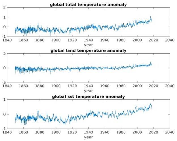
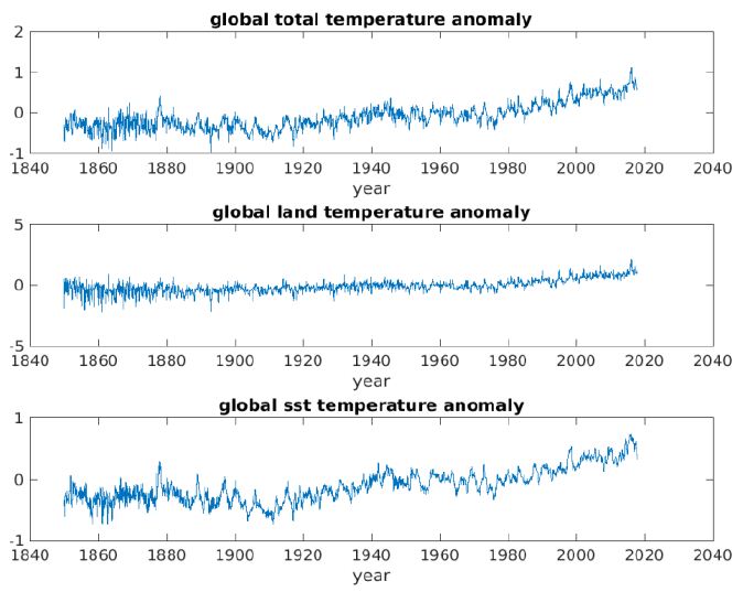
In this study, we address the global surface temperature anomalies (GSTA) of the global surface of the Earth, in the upper panel in Figure 1, the global atmosphere surface temperature anomalies above land (GLSTA), in the middle panel in Figure 1, and the global ocean surface temperature anomalies (GOSTA), in the lower panel in Figure 1, from 1850 through the first half of 2018. The reason we limit ourselves to 2018 is that the outbreak and spread of the Covid viral infection globally, may have effected fossil fuel consumption and we will only address more “normal” conditions of greenhouse gas loading of the oceans and atmosphere. We employ documented surface-temperature-anomaly-data. While much attention has focused on the global surface atmospheric temperature record, as greenhouse gases have built up in the atmosphere, far less attention has been paid to the global ocean surface temperature record in-kind. We address that fact. Data are from the Climatic Research Unit and the UK Meteorology Office, Hadley Centre: http://www.cru.uea.ac.uk/cru/info/.

fig 1

Figure 1: Monthly averaged time series of GSTA (top), GLSTA (middle), GOSTA (bottom) 01 01 1850-07 31 2018.

The climate system, as represented by surface temperature anomaly data, consists of non-linear (NL) and non-stationary (NS) processes, so we utilize an empirical, mathematical, data adaptive technique to decompose the data. Our mathematical decomposition methodology, the Ensemble Empirical Mode Decomposition (EEMD) first presented by Wu and Huang (2009) [1-10] produces internal, intrinsic modes of variability buried within the temperature data time series. We account for the patterns revealed by the internal modes of variability, relate them to naturally occurring physical phenomena and also compute the overall data time series “trends” which we find do not have a natural causal basis. However, we employ a statistical hypothesis test for determining whether one time series, such as fossil fuel burning, can be useful in forecasting another, specifically global surface temperatures, and thus to predict climate warming, past, present and future; thus establishing causality.

Background and Methodology

Wu and Huang (2009) developed EEMD based on the earlier work of Huang et al. [11-17], which employed the Hilbert Transform (the HT) [18,19], in the development of the Empirical Mode Decomposition (EMD) methodology. We employ EEMD in the decomposition of global surface temperature anomaly data time series. It is of note that a mode-mixing problem existed in the EMD decomposition in which successive IMFs were discovered to occasionally mix with or contaminate each other. To address this issue, Wu and Huang (2009) [9,10] added white noise to the various time series, created ensembles, and the mean IMFs were found to stay within the natural dyadic filter windows, preserving their dyadic properties, leading to stable decompositions of frequency and amplitude modulated internal modes of variability in the record length data. The decomposition reveals temporal internal modes of variability (referred to as Intrinsic Mode Functions or IMFs) which are frequency and amplitude modulated, and reveal non-linear (NL) and non-stationary (NS) signals in the data. The IMFs stack from higher to lower frequencies. We also produce data time series “trends”. In discussing the trend of any time series, we first need to consider the definitions and the methodologies of computing a trend. As such, no conventional simple averaging process can be utilized to reflect what information is buried in the multiple temperature time series as they are non-linear and non-stationary to the naked eye (see Figure 1, for example). This underscores the importance of clearly defining what constitutes a trend. Granger [20] presented an insightful definition of a trend as “a trend in mean comprises all frequency components whose wavelength exceeds the length of the observed time series”. For NL, NS datasets, none of these definitions is mathematically applicable leading to employment of the definition based on the EEMD methodology. With EEMD, the non-oscillation “residue”, which is left after the higher to lower frequency IMFs are removed from the time varying decomposition, becomes the trend of the time series.

Global Ocean and Land Based Atmospheric Temperature Anomaly Time Series

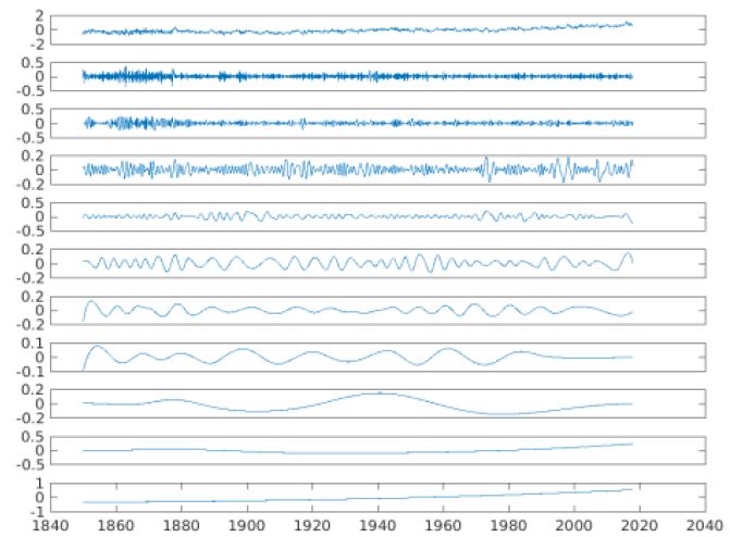
Figure 2 shows eleven IMF modes in the GSTA (also true of the GLSTA and GOSTA) with the 11th being the overall trends of the land-based atmosphere, the ocean surface and the combination of the two. The IMF modes have their respective physical bases. Mode 1 is several monthly variability. Mode 2 is seasonal variability. Mode 3 is the motion of the Earth on its axis of rotation. Mode 4 is the annual signal. Mode 5 is inter-annual variability. Mode 6 is the dominant signal of the El Nino Southern Oscillation (ENSO). Mode 7 is the quasi-Solar Cycle (10-12 years), centered about 11 years. Mode 8 reflects both the North Atlantic Oscillation (NAO) and of the 22-year Solar Cycle. Mode 9, 60-70 years is the Atlantic Meridional Overturning Circulation Belt (MOC), described by Cunningham et al. [21]. Mode 10, 105-110 years represents the Global Thermohaline Circulation Conveyor Belt [22,23]. Mode 11 is the gravest mode or overall trend of the 167-year time series of total data (Table 1).

fig 2

Figure 2: The EEMD Mode decomposition of the 1850-2017 time series of the GSTA (shown in the Top Panel.

Table 1: Intrinsic Mode Functions (IMFs) shown in Figure 2, in Months (M) or Years (Y)

IMF

1

2

3

4

5

6

7

8

9

10

11

GLSTA

GOSTA
GSTA

2 M

3 M

6 M

1 Y

2-3 Y

5-7 Y

10-12 Y

20-22 Y

60-70 Y

105-110 Y

167 Y Trend

We note in Figure 2, that for the GSTA, the IMF modes 2, 3 and 10 have amplitudes of 0.4°C, modes 4 and 6 have amplitudes of 0.3°C, modes 5, 7 and 9 have amplitudes of 0.2°C and mode 8 amplitude of 1°C. Mode 11 ranges between +/- 0.5°C. Thus, all the IMF modes contribute to the total time series in temperature amplitudes in a nominally equitable manner across the range of 0.1 to 0.4°C. This finding suggests that the Planet’s internal, natural modes of variability all contribute significantly to surface temperatures and thus cannot be ignored. Thus, periods of relative warming and or cooling occur naturally by the positive and negative disposition of the natural variability, all riding atop overall atmospheric and oceanic trends, and presented in the Table 1.

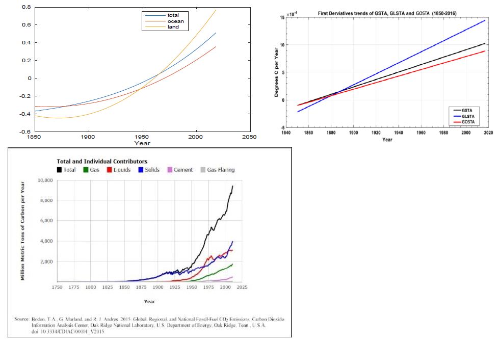
In Figure 3 (left panel), the trend of the GLSTA shows a record length total rise of 1.22°C and the GOSTA displays a rise of 0.67°C. The collective GSTA rises 0.88°C. The ocean surface temperature has risen at a much slower rate than the atmosphere over land. This is an excellent example of the power of the EEMD IMF decomposition. The full time series of the GOSTA displays an overall beginning to end of the series increase of 0.75°C, the GLSTA shows a rise of 2.91°C and the GSTA indicates an overall increase of 1.25°C. If connecting lines from start to end of the three time series had been drawn, the overall trends would have been greatly overestimated, demonstrating the failing of traditional methods (see IPCC, 2007) [24] of computing a trend, which are to create regression lines. Thus, the IPCC rates of rise of GSTA overestimate the actual rises in temperatures over land by 0.72°C and by a combined air-sea overestimate of 0.37°C. The IPCC straight-line, regression slope estimates are 0.05°C/decade over the full GSTA temperature record, 0.07°C/decade over the prior 100 years, 0.13°C/decade over the previous 50 years and 0.18°C/decade over the latter 25 years of the record.

fig 3

Figure 3: (left panel) The overall trends of the GSTA (blue), GOSTA (red) and GLSTA (yellow) time series. The GOSTA raw data are shown in Figure 2 and represents the GLSTA and the GSTA (both not shown). (center panel) The time rates of change or 1st derivatives, of the trends of the GLSTA, GOSTA and GSTA time series. (right panel) The fossil fuel burning curves. Atmospheric carbon dioxide concentrations also shown in far right panel Confirming sources are: T. Boden and R. Andres, The Carbon Dioxide Information Analysis Center, Oak Ridge National Laboratory, Oak Ridge, Tennessee 37831-6290, USA; and G. Marland, The Research Institute for Environment, Energy and Economics, Appalachian State University, Boone, North Carolina 28608-2131, USA.

In Figure 3 (left panel), we present the time rates of our trends and find that the rates of warming from 1850 through 2017 are 0.713°C/Century for the GLSTA, 0.427°C/Century for the GOSTA, and 0.529°C/Century for the combined GSTA. In the Figure 3 central panel, the 1st derivatives of the trend curves are all positive, and curving upward indicating that the rate of warming is accelerating. From 1955 to the present the overall warming trend of the GSTA (Figure 3) has been ~0.09°C/decade. Clearly, the rate of warming of air over land has globally been 167% greater than that of the surface of the global ocean. In the Figure 3 right panel, we present the fossil fuel burning time, Carbon Emissions (CE) series from 1751-2014, provided via <http://cdiac.ornl.gov/trends/emis/tre_glob.html>. From 1751 until 1850, global CO2 production was from 3 MMTs in 1751 to 54 MMTs in 1850. In the latter half of the 19th century, carbon emissions increased considerably, with a dramatic upsurge from 1949 to 2014, reaching a value of 950 MMTs and this resulted in the nonlinear rise of atmospheric carbon dioxide concentrations. The CE was essentially flat from 1751 through the mid latter half of the 19th century when the change of carbon burning began to be spiky. One could proceed here with cross correlations between the CE and GLSTA, GOSTA and/or the GSTA. However, although the temperature curves all display strong visual correlation with the fossil fuel burning curve, visual correlation does not prove a cause-and-effect relationship or attribution.

Granger Causality relating Carbon Burning to Global Surface Temperature Anomalies

We next employ the Granger Causality Test (GCT) [25] to obtain evidence for the strength of the causal relationship between the carbon burning and atmospheric carbon dioxide concentrations and atmospheric carbon dioxide concentrations and the globle temperature time series. GCT statistically tests for determining whether one time series is useful in forecasting another. Generally regressions reflect mere correlations, but Granger argued that by measuring the ability to predict the future values of a time series using prior values of another time series, causality in economics could be tested. A time series X is said to “Granger-cause” Y if it can be shown, through a series of t-tests and F-tests on lagged values of X (and with lagged values of Y also included), that those X values provide statistically significant information about future values of Y. The idea is that if series {xt} helps to cause series {yt}, then past values of {xt} should improve predictions of series {yt}. This type of causality is established by first modeling {yt} in terms of the past values of {yt} through an autoregressive (AR) process, then adding past values of series {xt} to create a second model. If the second model is statistically better than the first, then one has established causality in the Granger sense. Testing for Granger Causality in global temperatures has been considered by Attanasio et al. [26], Pasini et al. [27-29], amongst others. The above papers consider more time series than those considered here so they can for example separate out anthropogenic forcing and they also allow for non-stationarity in the temperature series. Our approach differs in that we consider only anomaly series {yt} and one emission series {xt}, and we find a stationary AR model for the anomalies after appropriately differencing the series and testing for white noise of the residuals?, which we justify our modeling by use of a time series goodness-of-fit test (see Fisher and Gallagher, 2012). One advantage of our methodology is that our final fitted model can be used to predict the impact of current (future) carbon emissions on temperature. We will approach this in a systematic process.

We first consider establishing a causal relationship between the carbon burning time series ({xt}) and the ocean surface temperature time series GOSTA ({yt}). Here we model on the monthly scale by taking the average temperature anomaly for each year as y and the average monthly carbon emission created by taking the yearly value divided by 12. Our first model relates GOSTA to past values of GOSTA. Using Akiake’s Information Criterion [30] we select the order of the auto regression to be three, meaning that each year’s GOSTA is related to the values from the last 3 years. The model is fitted using Gaussian maximum likelihood [31]. We use the goodness of fit test [32] to verify that the AR model adequately models the autocorrelation in the GOSTA series; the p-value of 0.9464 indicates that we have found an adequately fitting stationary model for GOSTA model given in Equation (1):

equ 1

The above model explains the dynamics of the observed series solely from past-observed values. However, to establish the (Granger) causal relationship we instead add the previous year CE value to the model. The resulting model is given by Equation (2):

equ 2

We can test for statistical significance of each fitted coefficient using the asymptotic normality of the Gaussian maximum likelihood estimators [31]. In particular, we conclude with a p-value of 0.00009 that the coefficient of xt-1 is non-zero. In other words, the predictive model for GOSTA is significantly statistically better if the previous year CE is included. Model (2) explains the changes in temperature through a combination of autocorrelation (AR) and the impact of CE. We have thus established causality in the Granger sense. In this analysis, we selected the data beginning in 1950, since the warming trend in the latter half of the 20th century is well established (cf. Figure 3, left panel). However, a similar analysis could be conducted starting at any point in the past. For example, the same analyses beginning each decade in the first half of the 20th, i.e., in years 1900, 1910, 1920, 1930, 1940, and 1950, resulted in p-values, 0.00005, 0.0002, 0.00002, 0.0002, 0.003, 0.009, for the coefficient of xt-1, respectively. In each case we conclude the model using the previous year CE is statistically better than the AR (3) model alone; the carbon emission series significantly improves predictions for GOSTA over the model based solely on past GOSTA values. Regardless of starting time, in the 20th century, one finds statistical evidence of a causal relationship between CE and GOSTA. The coefficient for xt-1 in model (2) is as follows. For each additional one-million metric tons of carbon emissions (CE), we estimate an increase in global ocean temperature (GOSTA) of 0.0007°C. The average increase in carbon emissions per year for years 1950 through 2014 is about 130 metric tons per year. Our model estimates an increase of 0.007+°C for each 10 metric ton increase in carbon emissions. The highly statistically significant coefficients of xt-1 for land based atmospheric temperatures and total global surface temperatures are 0.0117 and 0.0087, respectively.

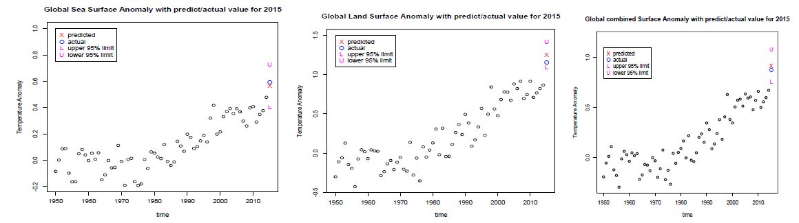
We next employ our fitted models to predict the global sea surface anomaly (GOSTA), the land atmosphere (GLSTA) and combined global surface temperature anomalies (GSTA) for 2015. Figure 4 shows the observed anomalies for years 1950 through 2014. The prognostic values are remarkably accurate. In the plots, we mark the predicted value from our fitted model, the upper and lower 95% prediction limits and the observed value for Year 2015. We conducted multiple-year lag experiments between CE and the surface temperature time series, beginning with 10 year down to 1 year lags (not shown except for the latter). We find that the model, which uses both past values of the anomaly series and the previous year’s carbon emission ( a 1-year lag), provides excellent predictions for the observed anomalies of the ocean surface, atmosphere on land and the combination therein for 2015. This provides further empirical evidence of Granger Causality relating previous year carbon emissions to sea surface, atmosphere on land and the combination temperatures on a global scale. We utilized the 2014 and 2015 data because 2014 is the last year for which we were able to obtain Fossil Fuel Burning data from the website provider at the time that this study was conducted. The results presented above provide a pathway and portend to future increases in global surface temperatures given anticipated increases in fossil fuel burning, GOSTA, GLSTA and GSTA as a function of CE. GOSTA is increasing at the rate of 0.0007°C/ Million Metric Tons of CE. GLSTA is increasing at the rate of 0.00117°C/Million Metric Tons of CE. Thus, the GSTA is increasing at the rate of 0.00087°C/Million Metric Tons of CE. Presently we are on a trajectory to reach 104 Million Metric Tons/year of CE by years 2020 to 2022. These numbers are less foreboding than the straight-line estimates of both the IPCC and NIPCC, but are nonetheless very noteworthy.

fig 4

Figure 4: Global Surface Temperature Anomalies from 1949-2014 with Granger Causality Predicted (X) versus Actual Temperatures (O) for 2015 and upper and lower 95% confidence limits. (left panel) is for the GOSTA. (middle panel) is for the GLSTA. (right panel) is for the GSTA.

Discussion and Conclusions

Mathematical relationships between fossil fuel burning and surface temperatures in the oceans and over land are presented. The statistical relationship curves reveal strongly that there is a one-year phase lag between global carbon loading via fossil fuel burning and planetary surface temperature rise, different from Ricke and Caldeira [33-41] who proposed that planetary temperatures changed about a decade after burning. In fact, robust relationships are presented between the GLSTA, GOSTA and GSTA, and their past time series, and the CE time series. Via Granger Causality, these surface temperatures are predicted very accurately from fossil fuel burning a year earlier. Thus, the conclusion we reach is that we have proven that there is “attribution” between fossil fuel burning and climate warming. In 2007, the IPCC was awarded a Nobel Prize for its comprehensive analyses of global climate change, including a visual-correlative-comparison of fossil fuel burning and temperature rise. However, a visual correlation does not prove “causality”. In 2003 C.W.J Granger was awarded a Nobel Prize for his work in econometrics theory and applications. We invoked “Granger Causality” to attribute the overall trends in global surface warming to fossil fuel burning and carbon emissions (https://en.wikipedia.org/wiki/Clive_Granger).

Acknowledgement

The authors thank Dr. Thomas S. Malone (former member of the U.S. National Academy of Sciences, now deceased), for having encouraged this study. He observed that cause and effect was necessary to prove attribution. The authors thank Coastal Carolina University for supporting this study.

References

  1. Allen MR, Frame DJ, Huntingford C, Jones CD, Lowe JA, et al. (2009) Warming caused by cumulative carbon emissions towards the trillionth tonne. Nature 458.
  2. Heede R (2014) Tracing anthropogenic carbon dioxide and methane emissions to fossil fuel and cement producers, 1854-2010. Climatic Change 122: 229-241.
  3. Stocker TF, Qin D, Plattner GK, Tignor M, Allen SK, et al. (2013) IPCC, 2013: Climate Change 2013: The Physical Science Basis. Contribution of Working Group I to the Fifth Assessment Report of the Intergovernmental Panel on Climate Change, pg: 1535. Cambridge Univ. Press, Cambridge, UK, and New York.
  4. Ekwurzel B, Boneham J, Dalton MW, Heede R, Mera RJ, et al. (2017) The rise in global atmospheric CO 2, surface temperature, and sea level from emissions traced to major carbon producers. Climatic Change 144: 579-590.
  5. Millar RJ, Fuglestvedt JS, Friedlingstein P, Rogelj J, Grubb MJ, et al. (2017) Emission budgets and pathways consistent with limiting warming to 1.5°C. Nature Geoscience 10: 741-747.
  6. Al‐Ghussain L (2019) Global warming: review on driving forces and mitigation. Environmental Progress & Sustainable Energy 38: 13-21.
  7. Smith CJ, Forster PM, Allen M, Fuglestvedt J, Millar RJ, et al. (2019) Current fossil fuel infrastructure does not yet commit us to 1.5°C warming. Nature Communications 10: 1-10.
  8. Millar R.J,. Nicholls ZR, Friedlingstein P, Allen MR (2016) A modified impulse-response representation of the global response to carbon dioxide emissions. Atmospheric chemistry and physics discussions.
  9. Wu Z, Huang NE (2009) Ensemble Empirical Mode Decomposition: a noise-assisted data analysis method. Advances in Adaptive Data Analysis 1: 1-41.
  10. Wu Z, Huang NE, Chen X (2009) Multi-Dimensional Empirical Mode Decomposition Based on Ensemble Empirical Mode Decomposition. Advances in Adaptive Data Analysis 1: 339-372.
  11. Huang NE, Shen Z, Long SR, Wu MC, Shih EH, et al. (1998) The empirical mode decomposition and the Hilbert spectrum for nonlinear and non-stationary time series analysis. Roy. Soc. Lond 454A: 903-993.
  12. Huang NE, Wu z, Long SR, Arnold KC, Chen X, Blank K (2009) On instantaneous frequency, Advances in Adaptive Data Analysis. 1: 177-229.
  13. Huang NE, Shen, Long SR (1999) A New View of Nonlinear Water Waves – The Hilbert Spectrum. Rev. Fluid Mech 31: 417-457.
  14. Huang NE, Wu ML, Long SR, Shen SS, Qu WD, et al. (2003) A confidence limit for the Empirical Mode Decomposition and Hilbert Spectral Analysis. Roy. Soc. London 459A: 2317-2345.
  15. Huang NE, Wu Z (2008) A review on Hilbert-Huang Transform: the method and its applications on geophysical studies. Geophys 46.
  16. Wu Z, Huang NE (2004) A study of the characteristics of white noise using the empirical mode decomposition method. Roy. Soc. London 460A: 1597-1611.
  17. Wu Z, Huang NE, Wallace JM, Smoliak BV, Chen X (2007) On the time-varying trend in global-mean surface temperature. Climate Dynamics 2011, 37.
  18. Gabor D (1946) Theory of communication. IEE 93: 429-457.
  19. Van der Pol B (1946) The fundamental principles of frequency modulation. IEE 93: 153-158.
  20. Granger CWJ (1966) The Typical Spectral Shape of an Economic Variable. Economtrica 34: 150-161.
  21. Cunningham SA, Rayner MO. Baringer WE, Johns J, Marotzke HR, et al. (2007) Temporal Variability of the Atlantic Meridional Overturning Circulation at 26.5°N. Science 317: 935-938. [crossref]
  22. Rahmstorf S (2003) The concept of the thermohaline circulation. Nature 421.
  23. Sabra K, Cornuelle B, Kuperman W (2016) The Rising Heat Content of the Earth’s Oceans. Physics Today 32.
  24. Bernstein L, Bosch P, Canziani O, Chen Z, Christ R, et al. (2008) IPCC, 2007: climate change 2007: synthesis report. IPCC.
  25. Granger CWJ (1980) Testing for causality: A personal viewpoint. Journal of Economic Dynamics and Control 2: 329-352.
  26. Attanasio A, Pasini A, Triacca U (2012) A contribution to attribution of recent global warming by out-of-sample Granger causality analysis. Atmospheric Science Letters 13: 67-72.
  27. Pasini A, Triacca U, Attanasio A (2012) Evidence of recent causal decoupling between solar radiation and global temperature. Environmental Research Letters 7.
  28. Attanasio A, Pasini A, Triacca U (2013) Granger causality analyses for climatic attribution. Atmospheric and Climate Sciences 3: 515-522.
  29. Triacca U, Attanasio A, Pasini A (2013) Anthropogenic global warming hypothesis: testing its robustness by Granger causality analysis. Environmetrics 24: 260-268.
  30. Akaike H (1974) A new look at the statistical model identification. IEEE Trans. Control 19: 716-723.
  31. Brockwell PR, Davis RA (1991) Time Series: Theory and Methods (2nd edn) New York: Springer-Verlag.
  32. Fisher TJ, Gallagher CM (2012) New Weighted Portmanteau Statistics for Time Series Goodness of Fit Testing, Journal of the American Statistical Association 107.
  33. Pietrafesa LJ, Gallagher C (2017) The Global Surface Temperature Anomaly Time Series and Relationships. Indian Journal of Applied Research. 7: 601-608.
  34. Ricke KL, Caldeira K (2014) Maximum warming occurs about one decade after a carbon dioxide emission. Environ Res Lett 9.
  35. Chatfield C (2003) The Analysis of Time Series, An Introduction. 6th Ed. Chapman & Hall.
  36. Cheng LKE, Trenberth J, Fasullo T, Boyer J, Abraham J, Zhu (2017) Improved Estimates of Ocean Heat Content 1960-2015. Science Advances 3, Number 3. Cunningham, S.A, T. Kanzow, D.
  37. Flandrin P, Rilling G, Gonçalves P (2004) Empirical mode decomposition as a filter-bank. IEEE Signal Proc Lett 11: 112-114.
  38. Hill C, DeLuca C, Balaji V, Suarez M, A. da Silva. (2004) The Architecture of the Earth System Modeling Framework. Computing in Science and Engineering 6: 18-28.
  39. James and James (1976) The Mathematical Dictionary. 4th Edition. D. Van Nostrand Com. Publisher.
  40. Ljung GM, Box GEP (1978) On a Measure of Lack of Fit in Time Series Models. Biometrika 65: 297-303.
  41. Shakespeare W, 1603. Hamlet, Quarto Ed.

Electrodeposition of In2S3 Layer for Solar Cells

DOI: 10.31038/NAMS.2023623

Abstract

The electrochemical deposition of In2S3 thin films was carried out from an aqueous solution of InCl3 and Na2S2O3. The effect of the potential of deposition was studied on the cell parameters of CZS based solar cells. The obtained films depending on the deposition potential and thickness exhibited complete substrate coverage. Maximum photoelectric conversion efficiency of 12.0% was obtained, limited mainly by a low fill factor (65%). Further process optimization is expected to lead to efficiencies comparable to CdZnS buffer layers.

Keywords

Indium sulfide; CZS solar cells; Electrodeposition

Introduction

Solar cells based on CdZnS (CZS) chalcopyrite absorbers have reached 20.0% conversion efficiencies at the laboratory scale, using high vacuum processes. However, due to the toxicity of cadmium and the possible gain in current associated with the use of a wider bandgap material, many works are carried out with the aim of developing alternative buffer layers. The In2S3-based material is among the most relevant alternatives. Several techniques, such as sputtering, atomic layer deposition (ALD), evaporation and chemical bath deposition (CBD) have been used to synthesize In2S3 thin films on CZS. However, it seems that soft chemical based deposition techniques such as CBD which do not damage the surface of the absorbers and can provide highly conformal coating are more suitable to get high efficiency Cd-free CZS solar cells. Electrodeposition is a soft technique widely used in industrial processes for large area coating, both in batch and inline systems. This method, more recently applied to semi-conductor synthesis, may allow to control the width of the bandgap and the doping level by monitoring solution composition, applied potential, pH and temperature. Moreover it provides conformal growth with controlled thickness layers. All these advantages yield the method attractive for the synthesis of the absorber, the buffer layers as well as the transparent conductive oxide layer in CIGSe-based solar cells. Even if important works have been done on the electrodeposition of the CZS-based absorbers, very few attempts have been carried out so far to electrodeposit In2S3 buffer layers [1-7].

Experimental Section

The electrodeposition of In-S based layers was carried out using an aqueous solution containing indium chloride (5 mM), sodium thiosulfate (20 mM) as sulfur source and potassium chloride as supporting electrolyte (0.1M). A standard three-electrode setup was used. The reference electrode was a saturated mercurous sulfate electrode (MSE, E°=0.64V/NHE) and platinum was used as the counter electrode. The deposition was carried out at 60°C. A preliminary investigation was carried out on molybdenum-coated glass substrates to determine the optimal deposition conditions. In-S layers were then deposited on CdZnS absorbers, Al and glass substrate provided by Würth Solar. The surface morphology of the samples was investigated by scanning electron microscopy (SEM) using a Leo Supra 35 field emission gun (FEG). The electrical properties of cells were characterized by current voltage measurements at 25°C under illumination (AM1.5 global spectrum). Absolute spectral response measurements were made with a monochromator under chopped illumination and a lock-in technique. Thermal annealing at 300°C for 10 min in air and light soaking for 60 minutes under AM 1.5 solar-type spectrum were typical post treatments.

Results and Discussion

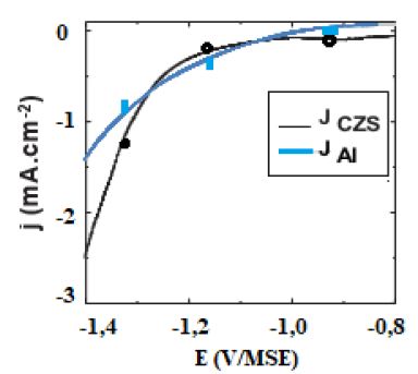
In order to define the optimal deposition potential range of the In-S thin films and the role of S, a voltammetric investigation was carried out both on Al and ITO glass substrates. Figure 1 shows cyclic voltammograms recorded at 60°C on Al and CZS substrates. As is observed on this figure, on both substrates, the deposition starts at potentials lower than -0.8V/MSE. the deposition process is more significantly inhibited on CZS absorber. On CZS a plateau is observed corresponding to a low current density between -0.8 and -1.2V, which might indicate that a different nucleation and/or deposition process occurs on this substrate compared to Al.

fig 1

Figure 1: Voltammetric curves recorded at 5 mVs-1, 60°C. for 0.1 M KCl, 5 mM InCl3 and 20 mM Na2S2O3 solution on Al and CZS substrates.

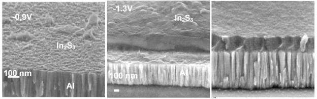
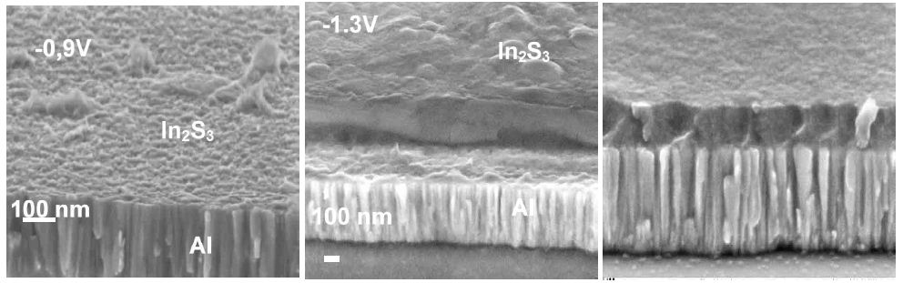
When sodium thiosulfate is added to the In(III) solution, a whitish colloid solution is formed. This is due to the formation of elemental sulfur which is favoured at low pH values where the Na2S2O3 is decomposed. For solutions with the mixture of sodium thiosulfate and In(III), no oxidation peak of the In-S layer on the reverse scan is observed, whatever the substrate used, indicating the formation of a passive layer during the oxidation process. Based on these observations, when InCl3 and Na2S2O3 are mixed in acidic solutions and for potential lower than – 0.9 V/MSE, In-S compound can be formed, thanks to In2S3 energy formation (DG°=-420 kJ mol-1). In-S layers were deposited at various potentials on Al and CZS substrates for different electrical charges between -1.0 and -1.3 V/MSE under potentiostatic conditions. The evolution of the film morphology is presented in Figure 2. SEM observations point out that the substrate nature has a marked influence on the morphology of the buffer layer.

fig 2

Figure 2: Effect of the potential of deposition on film morphology deposited on Al substrate The thickness of In2S3 on Al as function of potential are: -0,9 V: 16.5 nm, -1.1 V: 124 nm and -1.3 V: 178 nm.

For films deposited on an Al substrate (Figure 2 upper part) we can observe that, whatever the potential of deposition, films remain dense and homogenous and for the same deposition time, the electrical charge and the thickness of the buffer layer increase by decreasing the potential of deposition from -1.0V, to -1.3 V/MSE.

In parallel, In2S3 deposited films on CZS absorbers are dense, homogenous, and provide a conformal covering of the absorbers for films deposited at low potential <-1.1 V/MSE. However, as soon as the potential and the thickness of the layer increases, a transition in the morphology is observed and more or less disordered nanorods are growing (Figure 2).

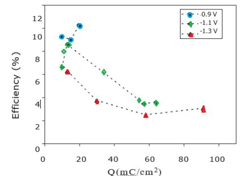
The global film stoichiometry can be estimated by correcting the total O % measured from a C/4 quantity corresponding to a classical ratio of O involved in the carbonaceous contaminant layer. The In/(S+O-C/4) ratios obtained are close to 0.7 for deposition at -1.3 V and -1.2 V and close to 1.0 when proceeding at -1.0 V. These values approach the one expected for an In2SxOy compound (with x+y=3), which is 0.66. This means that in our case, we probably do not deposit a pure In2S3 layer but a mixture of oxide, hydroxide and/or oxi-sulfide compound (In(S, O, OH)). Such a mixed structure was already observed for In2S3 buffer layers deposited by electrodpeosition. More studies are in progress to have a better understanding of the evolution of composition of our films. Cells with electrodeposited In2S3 layer at different deposition potentials were prepared using co-evaporated CZS absorbers. Finally, a post annealing of the completed cells in air at 200°C for 10 min and a light-soaking at room temperature for 1 h were made. Figure 3 shows the dependence of the efficiency of the CZS cells with In-S buffer layers prepared at different potential (-0.9V, -1.1V, -1.3V) and different electrical charges used for the buffer layer deposition.

fig 3

Figure 3: Efficiency of CZS/In2S3-based solar cell as a function of deposition potential and electrical quantity of  deposition measured under simulated AM1.5-100 mW/cm2 illumination.

As shown, for very low electrical charge values (<20 mQ/cm2) corresponding to low thickness of In2S3 buffer layers, similar conversion efficiencies are obtained for layers deposited between -1.0 and -1.3 V. However, the conversion efficiency for cells deposited at -1.2V decreases markedly when the electrical charge used for the buffer layer deposition increases. On the contrary, for buffer layers deposited at-0.9 V the efficiency of solar cells increases with the increase of electrical charge. Best results are obtained for a potential of -0.9 V and an electrical charge between 10 and 20 mQ/cm2 with a maximum efficiency of 12.0%.

Figure 4 shows the current voltage curve of one of the best cell prepared at -0.9 V compared to that with CdS (Figure 4b). An improvement of Jsc for cells with In2S3 buffer is observed compared to cells with CdS. For comparison the spectral responses of the cell obtained with In2S3 and that of a cell are shown in Figure 4b. The spectral response displays external quantum efficiencies of about 80% between 450 and 900 nm. Towards short wavelengths, for CdS buffer layers, the quantum efficiency drops from about 500 nm, while for In2S3 buffer layers the drop of the quantum efficiency occurs only at about 380 nm. Such a result confirms the higher value of the apparent bandgap of the In2S3 buffer layers. However for instance the Voc and FF of the solar cells remains lower than the one with CdS buffer layers indicating the non-optimized interface between CIGSe and the ED-In2S3.

fig 4

Figure 4: (a) Current-voltage curves for best CZS cells under simulated AM1.5-100 mWcm-2-illumination with a before (1) and after (2) HT (b) Spectral responses measured under short-circuit conditions before (1) and after (2).

Conclusion

Through a systematic study of the deposition parameters of In2S3 layers on Al and CZS solar cells as function of potential of deposition we have achieved a high efficiency of about 12.0%. We observed that, to obtain good efficiencies, the two key parameters are potential of deposition and the thickness of the films. The morphology of films are highly substrate dependent and for higher deposition potential (higher than – 1.1V) and low thicknesses films exhibited good substrate coverage. Solar cells with ED-In2S3 layers present very good photo current densities, but cell performance was limited by the low Voc and fill factor. The low values of the open-circuit voltage and the fill factor of the best cells show that the interface quality between CZS and In2S3 can be more improved.

References

  1. XH, Xu, et (2011) A novel one-step electrodeposition to prepare single-phase CuInS2 thin films for solar cells. Solar Energy Materials and Solar Cells 95: 791-796.
  2. Fiechter S (2008) On the homogeneity region, growth modes and optoelectronic properties of chalcopyrite-type CuInS2. Phys Stat Sol (b) 245: 1761-1771.
  3. Maier E, et (2011) CuInS2–Poly(3-(ethyl-4-butanoate) thiophene) nanocomposite solar cells: Preparation by an in situ formation route, performance and stability issues. Solar Energy Materials and Solar Cells 95: 1354-1361.
  4. Cui Yanfeng, et al. (2011) Synthesis and characterization of co-electroplated Cu2ZnSnS4 thin films as potential photovoltaic Solar Energy Materials and Solar Cell 95: 2136-2140.
  5. Sharma R, et (2009) Optimization of growth of ternary CuInS2 thin films by ionic reactions in alkaline chemical bath as n-type photoabsorber layer. Materials Chemistry and Physic 116: 28-33.
  6. Lee DY, Kim JH (2010) Characterization of sprayed CuInS2 films by XRD and Raman spectroscopy Thin Solid Films 518: 6537-6541.
  7. Merdes S, et (2011) Influence of precursor stacking on the absorber growth in Cu(In,Ga)S2 based solar cells prepared by a rapid thermal process. Thin Solid Films 519: 7189-7192.

Health of Stock of Commercially Exploited Non- Native Fish Species, Cyprinus carpio (Linnaeus, 1758) from the Tributary of the Ganga River, Central India

DOI: 10.31038/GEMS.2023514

Abstract

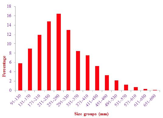
The human activities have strongly altered size, age, sex ratio, fecundity, feeding nature and biodiversity of fishes from the freshwater ecosystems over the world especially riverine division. During study period 548 specimens of Cyprinus carpio were collected from February 2019 to January 2020 in fish landing centre at Sirsa from the lower stretch of the Tons River at Prayagraj, Uttar Pradesh, India. The size of fishes varied from 97 to 687 mm (total length). The maximum size of fishes indicated that the stock of C. carpio in the Tons River was in healthy condition. The 251-290 mm size group was most dominated (16.42%) compared to 211-250 mm (14.78%) and 291-330 mm (12.96%) in total exploited stock. The lower size group was maximum exploited with 57.83% from the Tons River at Prayagraj. Higher size group contributed minute proportion with 4.74% in the exploited stock. The exploitation pattern was systematic in all size groups. Current exploitation pattern is systematic and healthy form with environmentally friendly sourcing of food.

Keywords

Size composition, Stock, Exploitation pattern, Ecosystem, Tons River, Cyprinus carpio

Introduction

Fish size composition is an essential component of river and stream ecosystem and represents an evident of structure, function, depth and health of stream/river [1-5]. Mostly large size and perennial rivers has large size of fishes in lotic water bodies [6-9]. The fish exploitation is an economic activity governed by social needs, food security and pressures [10-14]. Freshwater fishing is a chief foundation of income and protein for the riverine populations of most tropical regions [15-20]. Cyprinus carpio (Linnaeus, 1758) or Common carp is an omnivorous and bottom feeder fish species. It is distributed throughout countries in Asian countries as like India, Pakistan, Bangladesh, Burma and Nepal and also globally spread [21,22]. It is economically important fish species from the Tons River and also Ganga River system, and supports an important commercial fishery in rivers, reservoirs, lakes and even in culture ponds [23-25]. C. carpio is a non-native fish species for India. Non-native fishes are helping for homogenization of fish faunas, increasing of diversity and create pressure (example food, space, breeding ground, oxygen, infection and survival of organisms) for indigenous species or native species [26-30]. The fish are often key elements in the environmental planning [31-34]. The present study was thus undertaken to estimate size composition and health of the stock of C. carpio from the Tons River at Prayagraj, Uttar Pradesh, Central India. This study will help in formulating the fishery management policies of C. carpio from the Tons River and to update the knowledge in this field.

Material and Methods

Climate and Characteristics of the River

The climate of this region (Tons River basin) is marked by mild cold during winter and intensive heat during summer. The monsoon season is July to September month. Sometimes winter rainfall is also recorded. The Tons River is essentially a hilly stream arising in the Kaimur hills of the Vindhyan range, Madhya Pradesh, India. The Tons River drains the Bundelkhand geographic region of central India. Bundelkhand lies between the Indo-Gangetic Plain to the north and the Vindhya Range to the south. It is a tributary of the Ganga, which forms confluence at Sirsa near Meja in the Prayagraj district. Tons River lies between latitude 24° 0 to 25° 16 54 North and longitude 80° 26 45 to 82° 04 57 East. It banks are lined by deep ravines and the bed is rocky. Agriculture and human settlements were the major land use category in its catchment. During study period 548 specimens of Cyprinus carpio were collected from February 2019 to January 2020 in fish landing centre at Sirsa from the lower stretch of the Tons River at Prayagraj, Uttar Pradesh, India. Size composition (total length) varied from 97 to 687 mm. Drag net, cast net, gill net and hook and line were used by fishers/fishermen to catch the fishes in the river. A total of 548 fish samples (male and female) were collected and analyzed. The total length (mm) from the tip of snout to the end of caudal fin rays was measured by measuring scale. The obtained data from the river was classified into a series of size groups of 40 mm intervals. The number of samples calculated according to size group then converted into percentage.

Result and Discussion

Current exploitation pattern is systematic and healthy form with environmentally friendly sourcing of food. The size composition of C. carpio was varied from 97 mm to 687 mm of total length of fishes with majority between 251 to 290 mm from the lower stretch of the Tons River at Prayagraj, Uttar Pradesh, India (Figure 1). The large size of fishes also recorded in the Tons River in respect of river length. The maximum exploitation was recorded in 251 to 290 mm size group with 16.42%. Minimum exploitation was observed with 0.18% in 651-690 mm size group. Exploitation is an economic activity governed by social needs and pressures. Lower size groups 91-130 mm, 131-170 mm 171-210 mm, 211-250 mm and 251-290 mm were shared in exploited with 5.83%, 8.94%, 11.86%, 14.78% and 16.42%, respectively. Middle size groups 291-330 mm, 331-370 mm, 371-410, 411-450 mm and 451-490 mm were shared in exploitation 12.96%, 8.39%, 7.48%, 5.29% and 3.28%, respectively. Higher size groups 491-530 mm, 531-570 mm, 571-610 mm, 611-650 and 651-690 mm were contributed in exploitation with 2.19%, 1.28%, 0.73%, 0.36% and 0.18%, respectively (Figure 1). The lower size group was maximum exploited compared to middle and higher size groups from the lower stretch of the Tons River at Prayagraj. The experienced mature female fish stock was healthy in the river in monsoon season but very high fishing pressure we observed in this season. On the basis of data, it is observed that lower size group was maximum exploited with 57.83% at Prayagraj. Middle size group was exploited with 37.40%. Higher size group shared sizeable proportion with 4.74% in exploited population (Figure 2). The results also indicated that the exploitation was systematic in lower size group to higher size group. If exploitation is systematic then it is indication of healthy and heavy recruitment in near future. The over exploitation and non-targeted fishing is the biggest problem of riverine fishery [35-37]. The fishing pressure, mesh size, size of nets and fishing technique (example degree) are responsible for increasing or decreasing of total size of fishes and recruitment in the lotic ecosystems [14,38-42]. Fishing pressure changes the biodiversity, size composition, growth rate, age composition, sex ratio, income of fisher and maturation [43-45]. Non-native fishes are also changed selectivity of gear due to nature, dwelling behavior and ecological condition [28,46,47]. The growths of fishes are slightly checked by heavy metals accumulation in the body of fishes [48-50] (Insert Fig 1-2).

fig 1

Figure 1: Size composition and exploitation pattern of C. carpio from the Tons River at Prayagraj, Uttar Pradesh

fig 2

Figure 2: Exploitation pattern of C. carpio according to major group-wise from the Tons River at Prayagraj, Uttar Pradesh

Conclusion

It may be concluded that the present research work provides an important baseline study of this fish (Cyprinus carpio). Size composition indicated that the stock of C. carpio from the Tons River was in healthy condition and exploitation was also systematic form. Present condition was recorded due to sustainable exploitation of this species in the river. [20,51,52] stated that the when sustainably harvested or farmed, inland fish can be considered part of the green food movement for more environmentally friendly sourcing of food.

References

  1. Imran S, Thakur S, Jha DN, Dwivedi AC (2015). Size composition and exploitation pattern of Labeo calbasu (Hamilton 1822) from the lower stretch of the Yamuna River. Asian Journal of Bio Science 10: 162-164.
  2. Arlinghaus R, Lorenzen K, Johnson B M, Cooke S J and Cowx I (2015). Management of freshwater fisheries: addressing habitat, people and fishes. In: Freshwater fisheries ecology. edited by J. F. Craig. John Wiley & sons Ltd. 1st Ed., pg: 557- 579.
  3. Dwivedi A C, Mishra A S, Mayank P and Tiwari A (2016). Persistence and structure of the fish assemblage from the Ganga River (Kanpur to Varanasi section), Journal of Geography and Natural Disasters 6.
  4. Khan S, Dwivedi AC, Mayank P (2017). Size Composition and Exploitation Pattern of Cirrhinus mrigala (Hamilton, 1822) from the Ghaghara River, Journal of Scientific Achievements 2: 20-22.
  5. Mayank P, Mishra N, Dwivedi AC (2021). Invasive potential of Nile Tilapia, Oreochromis niloticus (Linnaeus, 1758) from the tributary of the Ganga River, Central India. Journal of Earth and Environmental Science Research.
  6. Dwivedi AC (2006). Age structure of some commercially exploited fish stocks of the Ganga river system (Banda-Mirzapur section). Thesis submitted to Department of Zoology, University of Allahabad, Prayagraj, (Uttar Pradesh), Pp. 138.
  7. Harting JH, Zarull MA, Ciborowski J, Gannon J, Wilke E, et al. (2009). Long-term ecosystem monitoring and assessment of the Detroit River and western lake Erie. Environ. Assess 158: 87-104.
  8. Mishra N, Dwivedi A C and Mayank P (2021) Invasion potential, impact and population structure of non-native fish species, Cyprinus carpio (Linnaeus, 1758) from the tributary of the Ganga River, Central India. Aquaculture and Fisheries Studies 3: 1-4.
  9. Hering D, Aroviita J, Baattrup, Pedersen A, Brabec K, et al. (2015) Contrasting the roles of section length and instream habitat enhancement for river restoration success: a field study of 20 European restoration projects. Appl. Ecol.
  10. Rizvi AF, Dwivedi AC, Singh KP (2010). Study on population dynamics of Labeo calbasu (Ham.), suggesting conservational methods for optimum yield. National Academy of Science Letter, 33: 247-253.
  11. Dwivedi A, Mayank P, Tripathi S (2011) Size composition, exploitation structure and sex ratio of catfish, Rita rita (Hamilton) in the lower stretch of the Yamuna River at Allahabad. Flora and Fauna 17: 295-300.
  12. Mayank P, Dwivedi AC (2015). Role of exotic carp, Cyprinus carpio and Oreochromis niloticus from the lower stretch of the Yamuna River. In: Advances in Biosciences and Technology In: Pandeya, AS. Mishra, RP Ojha and AK Singh published by NGB (DU), Allahabad, Pg: 93-97.
  13. Nautiyal P, Dwivedi AC (2020) Growth rate determination of the endangered Mahseer, Tor tor (Hamilton 1822) from the Bundelkhand region, central India. Journal of Fisheries Research, 4: 7-11.
  14. Gopesh A, Tripathi S, Joshi KD, Dwivedi AC (2021). Size composition, exploitation structure and sex ratio of Clupisoma garua (Hamilton) from middle stretch of the Ganga River at Allahabad, India. National Academy Science Letter 44: 309-311.
  15. Gozlan RE, Britton JR, Cowx I, Copp GH (2010). Current knowledge on non-native freshwater fish introductions. Journal of Fish Biology 76: 751-786.
  16. Jha DN, Joshi KD, Dwivedi AC, Mayank P, Kumar M, et al. (2015). Assessment of fish production potential of Chitrakoot district, Uttar Pradesh. Journal of the Kalash Science 3: 7-10.
  17. Dwivedi AC, Tiwari A, Mayank P (2018) Environmental pollution supports to constancy and invader potential of Cyprinus carpio and Oreochromis niloticus from the Ganga River, India. International Journal of Poultry and Fisheries Sciences 2: 1-7.
  18. Dwivedi AC, Nautiyal P (2010) Population dynamics of important fishes in the Vindhyan region, India. LAP LAMBERT Academic Publishing GmbH & Co. KG, Dudweiler Landstr. 99, 66123 Saarbrucken, Germany, Pg: 220.
  19. Mishra N, Dwivedi AC (2020) Environmental derivers supports to distribution, composition and biology of Cyprinus carpio (Linnaeus, 1758) in respect of time scale: A review. Journal of the Kalash Science 8: 91-102.
  20. Lynch A J, Cooke S J, Deines A M, Bower S D, Bunnell D B, et al. (2016) The social, economic and environmental importance of inland fish and fisheries. Rev.
  21. Dwivedi AC, Mayank P, Tiwari A (2016) The River as transformed by human activities: the rise of the invader potential of Cyprinus carpio and Oreochromis niloticus from the Yamuna River. Journal of Earth Science & Climatic Change 7.
  22. Tripathi S, Gopesh A, Dwivedi AC (2017). Framework and sustainable audit for the assessing of the Ganga River ecosystem health at Allahabad, India. Asian Journal of Environmental Science 12: 37-42.
  23. Zambrano L, Martinez-Meyer E, Menezes N, Peterson AT (2006) Invasive potential of common carp (Cyprinus carpio) and Nile tilapia Oreochromis niloticus in American freshwater systems. Canadian Journal of Fisheries Aquatic Sciences 63: 1903-1910.
  24. Dwivedi AC, Mishra N (2021) Age structure of non-native fish species, Cyprinus carpio (Linnaeus, 1758) from the tributary of the Ganga River, India. Journal of Aquaculture & Marine Biology 10: 76-79.
  25. Tripathi S, Gopesh A, Dwivedi AC (2017) Fish and fisheries in the Ganga River: current assessment of the fish community, threats and restoration. Journal of Experimental Zoology, India, 20: 907-912.
  26. Boll T, Levi EE, Bezirci G, Özuluğ M, Tavsanoğlu UN, et al. (2016) Fish assemblage and diversity in lakes of western and central Turkey: role of geo-climatic and other environmental variables. Hydrobiologia 771: 31-44.
  27. Dwivedi AC, Mayank P, Tripathi S, Tiwari A (2017) Biodiversity: the non-natives species versus the natives species and ecosystem functioning. Journal of Biodiversity, Bioprospecting and Development 4.
  28. Toussaint A, Beauchard O, Oberdorff T, Brosse S, Villeger S (2016) Worldwide freshwater fish homogenization is driven by a few widespread non-native species. Biological Invasions 18:1295-1304.
  29. Mishra N, Dwivedi AC (2021). Age and growth of commercially exploited fish species, Oreochromis niloticus (Linnaeus, 1758) from the tributary of the Ganga River, India. Poultry Fisheries & Wildlife Sciences 9.
  30. Lodge DM, Taylor CA, Holdich DM, Skurdal J (2000) Non indigenous crayfish threaten North America freshwater biodiversity: lessons from Europe. Fisheries 25: 7-20.
  31. Dwivedi AC, Nautiyal P (2021). Age and growth increment of Labeo calbasu (Hamilton 1822) from the Vindhyan region, Central India. International Journal of Aquaculture and Fishery Science 7: 010-013.
  32. Mayank P, Dwivedi AC, Mishra N (2021) Age pyramid of Common carp, Cyprinus carpio (Linnaeus, 1758) from the Tons River, India. Journal of the Kalash Science 9: 19-24.
  33. Mishra N, Dwivedi A C and Mayank P (2021) Study on stock health of non-native fish species, Cyprinus carpio (Linnaeus, 1758) through age pyramid from the tributary of the Ganga River, India. Journal of Aquaculture and Technical Development 4.
  34. Brown LR (2000) Fish communities and their associations with environmental variables, lower San Joaquin River drainage, California. Environmental Biology of Fishes 57: 251-269.
  35. Mayank P, Dwivedi AC (2016) Linking Cirrhinus mrigala (Hamilton, 1822) size composition and exploitation structure to their restoration in the Yamuna River, India. Asian Journal of Bio Science 11: 292-297.
  36. Khan S, Dwivedi AC, Mishra P (2007) Sex ratio and exploitation structure of Labeo calbasu (Hamilton) in the tributary of the Ganga River system (Ghaghara River). Bioved, 18: 7-12.
  37. Nautiyal P, Dwivedi AC (2019) Fishery in the tributaries of Yamuna River (Ken River, Paisuni Rivers) and Ganga River (Tons River). Journal of Mountain Research 14: 19-36.
  38. Dwivedi AC, Mayank P, Pathak RK (2016). Size composition and exploitation structure of Indian major carp, Cirrhinus mrigala (Hamilton, 1822) from the Ganga River, India. Journal of Fisheries and Life Science 1: 30-32.
  39. Dwivedi AC, Mayank P, Tiwari A (2017) Size selectivity of active fishing gear: changes in size, age and growth of Cirrhinus mrigala from the Ganga River, India. Fisheries and Aquaculture Journal 8.
  40. Mayank P, Rizvi AF, Dwivedi AC (2017) Population dynamics of Cirrhinus mrigala (Hamilton 1822) from the largest tributary of the Ganga River, India. International Journal of Fauna and Biological Studies 4: 42-47.
  41. Mayank P, Dwivedi AC, Pathak RK (2018) Age, growth and age pyramid of exotic fish species Oreochromis niloticus (Linnaeus 1758) from the lower stretch of the Yamuna River, India. National Academy Science Letter, 41: 345-348.
  42. Prakash S, Mayank P, Dwivedi AC, Mishra BK, Tiwari A, et al. (2019) Size structure and exploitation pattern of Rita rita (Hamilton 1822) in the Yamuna River at Prayagraj, Uttar Pradesh. Journal of the Kalash Science, 7: 21-24.
  43. Arlinghaus R, Mastsumura S, Dieckmann U (2010) The conservation and fishery benefits of protecting large pike (Exos lucius) by harvesting regulations in recreational fishing. Biological Conservation 143: 1444-1459.
  44. Dwivedi AC, Khan S, Mayank P (2017) Stressors altering the size and age of Cirrhinus mrigala (Hamilton, 1822) from the Ghaghara River, India. Oceanography Fish Open Access Journal 4.
  45. Dwivedi AC, Nautiyal P (2012). Stock assessment of fish species, Labeo rohita, Tor tor and Labeo calbasu in the rivers of Vindhyan region, India. Journal of Environmental Biology 33: 261-264.
  46. Mayank P, Dwivedi AC (2017) Resource use efficiency and invasive potential of non-native fish species, Oreochromis niloticus from the Paisuni River, India. Poultry Fisheries & Wildlife Sciences, 5.
  47. Dwivedi AC, Mishra AS, Mayank P, Tripathi S, Tiwari A (2019) Resource use competence and invader potential of Cyprinus carpio from the Paisuni River at Bundelkhand region, India. Journal of Nehru Gram Bharati University 8: 20-29.
  48. Tiwari A, Dwivedi AC (2014) Assessment of heavy metals bioaccumulation in alien fish species Cyprinus carpio from the Gomti River, India. European Journal of Experimental Biology 4: 112-117.
  49. Tiwari A, Dwivedi AC, Mayank P (2016) Time scale changes in the water quality of the Ganga River, India and estimation of suitability for exotic and hardy fishes. Hydrology Current Research 7.
  50. Dwivedi AC, Tiwari A, Mayank P (2015) Seasonal determination of heavy metals in muscle, gill and liver tissues of Nile tilapia, Oreochromis niloticus (Linnaeus, 1758) from the tributary of the Ganga River, India. Zoology and Ecology 25: 166-171.
  51. Dwivedi AC, Jha DN, Mayank P (2014) Food security, livelihood and non-native fish species: status, trends and future perspectives. Journal of the Kalash Science 2: 41-46.
  52. Neeti Mishra, Amitabh Chandra Dwivedi (2022). Reproductive properties and impacts of invasive alien species, Common carp (Cyprinus carpio Linnaeus, 1758) from the Tons River at Prayagraj, India. Journal of the Kalash Science 10: 5-11.

MMR Vaccine Provides Protective Immunity Severe SARS-coV-2 Infections

DOI: 10.31038/MIP.2023411

Abstract

The MMR (measles, mumps, and rubella) vaccine has been found to generate protective immunity against severe SARS-CoV-2 infections. Analysis of 21 countries that have had general MMR vaccination over the last few years has shown near-zero fatality rates due to COVID-19. This phenomenon could be related to the mild or no effects of COVID-19 in children who have received the MMR vaccine at birth. Our clinical study involving 200 adults, 100 of whom were vaccinated with MMR, demonstrated that the vaccine provides immunity against severe COVID-19 infection in a human challenge. There are several similarities between the SARS-CoV-2 virus and the measles, mumps, and rubella viruses, and the MMR vaccine behaves like a T-cell induced vaccine that can be effective against COVID-19. The MMR vaccine has been in use for many years without side effects, and its global use against COVID-19 could be a viable option as it provides immunity for several years, which is longer than the currently available COVID-19 vaccines.

Introduction

The present paper discusses the potential use of the measles-mumps-rubella (MMR) vaccine as a means of protecting humans against infection by the severe acute respiratory syndrome coronavirus 2 (SARS-CoV-2), which causes COVID-19. Since the outbreak of COVID-19 in late 2019, it has resulted in more than hundred million cases and many deaths globally. Coronaviruses are important human and animal pathogens, and the development of an effective treatment and vaccination strategy for COVID-19 cases will require a better understanding of the mechanisms by which the host immune system responds to the virus [8].

Recent studies have shown that patients who have recovered from COVID-19 possess specific acquired immunity based on both T and B cells. The spike or S protein of coronaviruses, including SARS-CoV-2, mediates the binding of virions to the host cell receptor, and it is the target of virus-neutralizing antibodies [1]. The S glycoprotein on the surface of SARS-CoV-2 is also the main site for antibodies to neutralize the virus, making it a potential target for vaccination [2]. In addition, COVID-19 has presented various paradoxes, including the fact that young children have immunity to severe COVID-19 [5], and 21 countries have COVID-19 fatality rates that are as low as 1% of the fatality rates of other countries. The authors theorize that the MMR vaccine may be responsible for these differences and suggest that the vaccine could be used as a means of protecting against COVID-19 [3].

The MMR vaccine contains the Edmonston strain of measles, the Jeryl Lynn (B-level) strain of mumps, and the Wistar RA 27/3 strain of rubella, and it elicits a protective immune response against severe COVID-19. The authors will discuss their clinical research on 200 adults, 100 of whom were vaccinated with MMR, which showed the vaccine’s efficacy against severe COVID-19 in a human challenge [4]. In summary, the paper will explore the potential use of the MMR vaccine as a means of protecting against SARS-CoV-2 and COVID-19, providing a comprehensive overview of the current state of research on this topic.

Summary of Paper

In summary, the paper discusses different strategies that scientists are pursuing to develop new therapeutics against SARS-CoV-2, including the development of antibodies and small protein fragments. The paper also presents a method of protecting humans against coronavirus infections, particularly SARS-CoV-2, using a MMR vaccine that includes at least one of the measles, mumps, or rubella vaccines or a combination of two or three of them. The paper explains that all coronaviruses trigger antibody and T cell responses, but antibody levels tend to wane faster than T cells [8-11]. The MMR vaccine is shown to have long-lasting effects, lasting for at least several years, which could potentially provide protection against COVID-19.

Detailed Description of Paper

The paper being referred to in this text is discussing the potential of a vaccine that includes mumps, measles, and rubella (MMR) as an immunogen to protect humans against serious coronavirus infections. The authors of the paper suggest that the MMR vaccine could be used to vaccinate people who are susceptible to coronavirus infections, particularly SARS-CoV-2. Vaccines work by training the body’s immune system to identify and attack viruses before they can infect healthy cells [6]. Vaccines typically contain key components of the virus, such as the envelope, spike, or membrane protein, which the immune system can use to recognize the virus and mount a defense against it [9]. The MMR vaccine is a pure preparation of viral proteins that can be injected into the body to give the immune system a preview of the virus, without causing disease. Developing vaccines based on viral proteins can be a complex process that can take years or even decades. Protein-based vaccines require mass production of viral proteins in facilities that can guarantee their purity. Growing the viruses and purifying the proteins at medically acceptable pharmaceutical scales can take years, and may not be possible for some recent epidemics.

The MMR vaccine, on the other hand, has already been developed and is widely available. According to the paper, it could be employed to vaccinate humans against coronavirus infections, or at least to prevent the severe clinical symptoms associated with such infections. MMR-based vaccines would provide protection against multiple coronaviruses, including SARS-CoV-2, and could even offer cross-species protection. The authors of the paper conducted a study to compare MMR titers to recent COVID-19 severity levels. They divided 200 people into two groups: one group consisted of 100 people who primarily had MMR antibodies from the MMR II vaccine, and a comparison group of 100 people who primarily had MMR antibodies from sources other than the MMR II vaccine, including prior measles, mumps, and/or rubella illnesses.

Discussion

The present study has explored the possible correlation between the measles-mumps-rubella (MMR) vaccine and COVID-19 severity. The study has found that individuals who had previously been vaccinated with MMR II, one of the most widely used MMR vaccines, exhibited lower severity of COVID-19 symptoms. This finding supports the theoretical association between the MMR vaccine and COVID-19 severity that some scientists have proposed. It is important to note that the study has some limitations, which should be considered in interpreting the results. Firstly, the sample size is relatively small, with only 200 participants divided into two groups. This may limit the generalizability of the findings, and further studies with larger samples are needed to confirm the results. Secondly, the study design was retrospective, and the information on the participants’ COVID-19 severity was obtained from their medical records, which may not have been comprehensive or accurate.

Despite these limitations, the present study has shed light on the potential of the MMR vaccine in protecting individuals against COVID-19. The MMR vaccine is known to elicit a robust immune response against measles, mumps, and rubella viruses, which are all members of the same family as the SARS-CoV-2 virus. This means that the immune system of individuals who have received the MMR vaccine may be better equipped to recognize and respond to the SARS-CoV-2 virus, thereby reducing the severity of COVID-19 symptoms. The potential of the MMR vaccine in protecting against COVID-19 is particularly relevant in the context of the global pandemic. The development of new vaccines against COVID-19 has been a major focus of the scientific community, with several vaccines receiving emergency use authorization from regulatory agencies. However, the mass production and distribution of these vaccines face significant logistical challenges, particularly in low-income countries where access to vaccines is limited. The MMR vaccine, on the other hand, is already widely available and has been used for several decades with a proven safety record.

It should be noted that the MMR vaccine is not a substitute for the currently authorized COVID-19 vaccines, and individuals are still encouraged to get vaccinated against COVID-19 as soon as they are eligible. However, the findings of the present study suggest that the MMR vaccine may provide an additional layer of protection against COVID-19, particularly in individuals who are at higher risk of severe disease. In conclusion, the present study provides preliminary evidence of a potential association between the MMR vaccine and COVID-19 severity. The findings highlight the importance of further research in this area, particularly larger, prospective studies that can confirm the results and shed more light on the mechanism behind the potential protective effect of the MMR vaccine. Nonetheless, the potential of the MMR vaccine in protecting against COVID-19 is a promising avenue for future research, particularly in the context of the ongoing global pandemic.

Conclusion

In conclusion, our study provides evidence that the MMR vaccine can elicit a protective immune response against severe SARS-CoV-2 infection that causes COVID-19. The results of our study support the hypothesis that the MMR vaccine may be responsible for the no-effect or mild-effect of COVID-19 in children and some adults. We found that IgG titers related to the MMR II vaccine are inversely correlated with the severity of COVID-19 in recovered patients who were previously vaccinated with the MMR II vaccine. This suggests that the MMR vaccine can provide cross-reactive protection against SARS-CoV-2 and other coronaviruses. The similarities of the spike protein in the MMR viruses and SARS-CoV-2 further support this hypothesis. Our study provides a potential strategy for preventing severe COVID-19 infections through the use of a MMR vaccine. The MMR vaccine is readily available, affordable, and has an established safety record. Therefore, it has the potential to be rapidly deployed for widespread vaccination against COVID-19. In summary, our results suggest that the MMR vaccine can be used to elicit a protective immune response against SARS-CoV-2 and other coronaviruses. Further research is needed to confirm these findings and to determine the optimal use of the MMR vaccine in preventing and controlling COVID-19.

References

  1. Gorbalenya AE, Baker SC, Baric RS (2020) Coronaviridae Study Group of the International Committee on Taxonomy of Viruses. The species severe acute respiratory syndrome-related coronavirus: classifying 2019-nCoV and naming itSARS-CoV-2. Nat Microbiol 5: 536-544.
  2. Zhou P, Yang X, Wang X, Hu B, Zhang L, et al. (2020) A pneumonia outbreak associated with a new coronavirus of probable batorigin. Nature 579: 270-273.
  3. Zhao J, Van Rooijen N, Perlman S (2009) Evasion by stealth: inefficient immune activation underlies poor T cell response and severe disease in SARS-CoV-infected mice. PLoS Pathog 5: 10.
  4. Brouwer PJM, Caniels TG, Van Der Straten K, Snitselaar JL, et al. (2020) Potent neutralizing antibodies from COVID-19 patients define multiple targets of vulnerability. Science 369: 6504: 643-650.
  5. Gold JE, Baumgart WH, Okyay R, Licht WE, Fidel Jr P, et al. (2020) Analysis of Measles-Mumps-Rubella (MMR) Titers of Recovered COVID-19 Patients. mBio.
  6. Farshi E (2021) Immunological Reason for Mild Affection of Children to COVID-19, A Key Factor for Novel Solution of Vaccination and Medications. Japanese J Gstro Hepato 8(2): 1-9.
  7. Farshi E (2020) Peptide-mRNFarshi Vaccine for SARS-Cov-2. J Vaccines Vaccin 11: 431.
  8. Farshi, E (2020). Simulation of Herd Immunity in Covid-19 Using Monte Carlo Method. Austin J Pulm Respir Med 1: 1066.
  9. Farshi, Esmaeil, Bahram Kasmapur, and Anya Arad (2021) Investigation of immune cells on elimination of pulmonary‐Infected COVID‐19 and important role of innate immunity, phagocytes. Reviews in Medical Virology 2: e2158.
  10. Farshi, Esmaeil. Cytokine storm response to COVID-19 vaccinations. J Cytokine Biol1000125 (2020): 2.
  11. Farshi E (2023) Peptide-Based mRNA Vaccines. J Gastro Hepato 9(16): 1-6.

Mechanism of Survival of Arthropods to Saline-Water Habitat, Osmoregulation Habit

DOI: 10.31038/GEMS.2023513

Abstract

Objectives: Insects arose in the terrestrial environment. Some species eventually evolved forms that could take advantage of freshwater habitats particularly in the larval stage. The numbers of species capable of surviving in saline is rare (about 5% of all known mosquito species). Most plants do not require sodium but animal however require sodium for some physiological function for example nervous activity. Salinity and certain ions such as sodium and sulphate challenges for insects are important. Other somatically active osmolytes occur in the blood of many insect. The evolutionary advantages of flight for mating and dispersal led more species to retain terrestrial or aerial adult stage. This creates substantial physiological problem for freshwater and terrestrial animals. The insects got around this problem by reducing the amount of sodium in the body to an essential minimum. From a water hardness/salinity perspective, arthropods occupy very soft water up to salt lakes twice as concentrated as seawater.

Materials and methods: To provide authentic information about this novel we use reliable data on academic resources such as Google Scholar, Scopus, Web of Science, Springer, Pro Quest, Wiley Online, Science Direct, Research Gate, PubMed, Sage, and SID.

Results: Only a limited number of species thrive in saline lakes, including some fairy shrimp (e.g., Artemia, Parartemia, and Phallocryptus) and brine and shore flies (Diptera, Ephyridae), such as Ephydra hians.

Discussion: Mechanisms of survival of Ephydra hians will provide a guideline for environmental and ecosphere creatures for environmental adaptation.

Keywords

Ephyda hians, Environment adaptation, Osmoregulation habit

Mini Review

Insects capable of surviving in saline water intensively studied are: Culicidae (mosquitoes) and Ephydridae (brine flies). Brine fly is classified in Phylum: Arthropoda, Class: Insecta, Order: Diptera, Family: Ephydridae, Genus: Ephydra, Species: Ephydra hians. Ephydra hians, commonly known as the alkali fly. Both salinity and desiccation lead to dehydration and osmotic stress, which is a critical problem at the cellular level [1-3]. Therefore, salinity and desiccation stress in insects trigger common physiological mechanisms, mainly aimed at increasing water content (e.g. drinking from the medium), avoiding its loss (e.g. control of cuticle permeability) and maintaining ionic homeostasis (e.g. activity of Malpighian tubules and specialized parts) [1,4-6]. Ecology of Brine fly: Among aquatic insects, members of the shore fly family Ephydridae are well-known for their tolerance of severe environmental conditions. High temperatures and salinities, acid and alkaline pH, anoxia and ephemeral waters are among the factors to which a variety of ephydrids have become adapted. Hot springs, tidal splash pools, salt evaporation ponds, hypersaline desert lakes, and even crude petroleum have been described as larval habitats Collection records for species in the genus Ephydra, which are common in saline waters, indicate a wide range in chemical composition and salinity is tolerated by this group, but that any one species tends to be restricted to a particular type of habitat water chemistry [1,7-10]. The adult flies live 3-5 days, during which they eat algae and lay eggs in the hypersaline water; (Figure 1) lays eggs in saline water (Figure 2). The larvae are important for their capacity to survive in highly saline water (Figure 3). Concretions of calcium carbonate in the Malpigian tubules make the larvae more dense and allow them to stay on the beneath of the water. The haemolymph had a total osmotic concentration of about 300 mOsm. The osmotic concentration of the lake was well over 1500 mOsm. It follows that the larvae must lose water across the cuticle. The larvae drink the external medium. The very high concentration sodium, carbonate and sulphate are present in the lake. The lime gland acts like a kidney, by removing carbonate ions from the blood. Inside the glands carbonate is mixed with calcium to form a limestone (Figures 4 and 5). Saline water larvae drink equal to about their body volume every 10 hours. Table 1 shows different ions in the heamolymph of larvae in comparison to Mono lake water. Eggs of the genus Ephydra are attached to an algae mat. The main food sources of adults and larvae are algae, some bacteria, and protozoa.

FIG 1

Figure 1: Adults of brine fly (Ephydra hians)

FIG 2

Figure 2: Egg of brine fly (Ephydra hians)

FIG 3

Figure 3: Larvae of brine fly (Ephydra hians)

FIG 4

Figure 4: Internal organs of the brine fly (Ephydra hians) with limestone

FIG 5

Figure 5: Lime gland of larvae

Table 1: Ionic concentration in the larval haemolymph of Ephydra hians

Ion

Concentration in larval haemolymph

Concentration in Mono lake water

Sodium

Potassium

Calcium

Magnesium

Chloride

Sulphate

135.7 ± 1

6.9  ± 0.4

5.6 ± .0.1

13.2  ± 0.5

120  ± 1.4

0.6 ±  0.1

1224

18

≤1

≤1

627

151

Larvae change to the pupae (Figure 6). Pupae are non-feeding, and sequestered from the aquatic environment, Pupae then to the adults. Adults emerge from water in a large population (Figure 7). Birds understand the time of adult emergence and reach the lake for catching them as a food. Many migrating birds stop at Lake during their trips to feed on the brine fly larvae in the lake water (Figure 8).

FIG 6

Figure 6: Pupae of brine fly (Ephydra hians)

FIG 7

Figure 7: Emerging of brine fly from saline water lake

FIG 8

Figure 8: Emerging of adult of brine flies as a good food source for immigrant birds

In a research conducted on the mosquitoes, they found that Aedes albopictus was the most tolerant species, followed by Anopheles coluzzii, Ae. aegypti, Culex. quinquefasciatus, and An. gambiae, in decreasing order. Cx. pipiens was the least tolerant species [11].

Conflict of Interest

The author declares that there is no conflict of interest.

Acknowledgments

This research is financially supported by Ministry of Health and Medical Education under code number of NIMAD 995633.

References

  1. Bradley T (2009) Animal Osmoregulation. New York: Oxford University Press.
  2. Cohen E (2012) Roles of aquaporins in osmoregulation, desiccation and cold hardiness in insects. Entomology, Ornithology and Herpetology 1: 1-17.
  3. Evans DH (2008) Osmotic and Ionic Regulation: Cells and Animals. Boca Ratón:CRC Press.
  4. Dow JAT, Davies SA (2006) The Malpighian tubule: rapid insights frompost–genomic biology. Journal of. Insect Physiology 52: 365-378. [crossref]
  5. Gibbs AG, Rajpurohit S (2010) Cuticular lipids and water balance. In Insect Hydrocarbons: Biology, Biochemistry, and Chemical Ecology (ed. G. J.Blomquist and A. G. Bagnères), pg: 100-120. Cambridge: Cambridge University Press.
  6. Larsen E.H, Deaton LE, Onken H, O’Donnell M, Grosell M, et al. (2014) Osmoregulation and Excretion. Comprative Physiology. 4: 405-573.
  7. Brock,TD, Brock ML (1968) Life in a hot-water basin. Natural History 77: 47-53.
  8. Brock ML, Wiegart RG, Brock TD (1969) Feeding by Paracoenia and Ephydra (Diptera: Ephydridae) on the microorganisms of hot springs. Ecology 50: 192–200.
  9. Foley C, White B (1989) Occurrence of Ephydra hians Say (Diptera: Ephydridae) in deep water in Mono Lake, California. Bulletin of South California Academic Science 88: 40-41.
  10. Herbst D (1988) Comparative population ecology of Ephydra hians Say (Diptera: Ephydridae) at Mono Lake (California) and Abert Lake (Oregon). Hydrobiologia 158: 145-166.
  11. Kengne P, Charmantier G, Blondeau‐Bidet E, Costantini C, Ayala D (2019) Tolerance of disease‐vector mosquitoes to brackish water and their osmoregulatory ability. Ecosphere 10: 1-14.

Formation of Terrestrial Planets from the Viewpoints of Astrophysics and Material Science – Formation of Planetesimals by Chemical Reactions at Contact Points between Solids

DOI: 10.31038/GEMS.2023522

Abstract

Where did the sea water originally come from? The water must have originated from interstellar mediums. Comets are born from lumps of dusts, mostly at the edge of the solar system. The lump consists of dust particles and ice (H2O) and moves toward the Sun due to the Sun’s gravitational force. However, in the asteroid belt between Mars and Jupiter exists a snow line. The water collected by comets does not reach the Earth because ice (H2O) sublimates into vapor around the snow line. It is considered that the sea water of the Earth would have been captured together with interstellar medium before the snow line appeared. The formation of the early Earth must have been in an environment before the nuclear fusion reactions in the Sun. A beginning of clump forms from through point bonds of dusts. The Coulomb force around interatomic distance is approximately 1036 times that of gravitational force. A fixed connection will be formed by short-range forces at the local contact point of solids in cold environment. According to experimental results, when solid CO2 (dry ice) is mixed with iron powder, the powder turns black. But the iron powder does not change by in a gas state of CO2. The results indicate that the surface of the fine iron powder is locally oxidized by the solid CO2 and CO2 is reduced to carbon. The first step of formation of celestial bodies occurred as a result of chemical characteristics of materials. When the Sun underwent gravitational collapse and nuclear fusion reactions began, the Earth was at the last stage of formation. The Earth’s seawater accumulated as ice with cosmic dust during the Earth’s formation. These initial situations of the solar system led to new scenarios differ from conventional theories. For example, a large planet had formed in the region near the snow line, but one nuclear fusion explosions formed an asteroid belt. The proto-Moon was born in the geostationary orbit of the Earth and once had come into touch slightly with the Earth, resulting in the tilt of the Earth’s rotational axis and the inclination of the Moon’s orbit. The new scenario of formation Moon-Earth system is characterized as “Little touch” instead of “Giant impact”.

Keywords

Accretion, Cosmic dust, Meteorite, Comet, Asteroid, Satellite, Planet

Introduction

Many models have been proposed to explain the origin of the solar system. Among them, the Hayashi (Kyoto)-model [1] is a representative example. Many models have attempted to describe the formations of planets [2-4]. The tradiational models tends to adhere to the viewpoint of physics. The physics is universal, but it is abstracted. The world of logic tends to estrange the real world. The real world includes various aspects. Theoreticians tend to dislike a bird’s-eye view, and sometimes they failed in “idols of the cave” [5]. The first step of traditional models in the formation of the Sun was the accumulation of hydrogen through gravitation. However, the gravitational force of the hydrogen atom is extremely weak. A planetesimal does not form due to the gravitational force. It was formed by local bonds of dusts. Although the London‐Van der Waals attractionis a weak bond, the short-range force is more thirty orders of magnitude stronger than the gravitational force. The short-range forces offsets within a short distance, whereas long range-forces are accumulated very wide range. The accretion models have been discussed [6], while the formation of a solar system from a viewpoint of chemical describes in this paper. When a celestial body becomes sufficiently large to hold hydrogen atoms via gravitation, the hydrogen rich environment increases the body’s growth rate at a fast pace. This will correspond to a “gravitational collapse”. Before nuclear fusion, the proto-Sun contained large amounts of solids. In this context, the iron currently contained in the Sun is 0.014% of the total mass. The mass of the Sun is about 333,000 times that of the Earth where the mass of iron in the Sun is 46.6 times that of the Earth. The large amount of material of core was released as meteorites by the nuclear fusion of the Sun. The meteorite is the most objects in the solar system. The Japanese Hayabusa 2 mission revealed the rubble-pile structure of asteroid 162173 Ryugu [7]. The gravity of this asteroid is extremely weak with an escape speed of 30 cm/sec. Such a small celestial body does not retain its structure by gravitational force, rather the lump of solid matter is formed into the relevant shape by short-range forces at points of attachment. 51 Pegasi b, is the first exoplanet and was discovered by M. Mayor, D. Queloz, in 1995 [8]. It is a massive planet with a mass approximately 149 times that of the Earth and an orbital period of 4.23 days at 7.8 million km from its host star, this is approximately only one-twentieth of the distance between the Sun and the Earth. This suggests that 51 Pegasi b had fairly formed in the environment before fusion reaction began in the host star. The proto-Earth would grow by accumulating solid forms of H2O (ice) and solid of CO2 (dry ice) via point contacts. Reconfiguration of solids occurs at the high-pressure and high-temperature environment of the inner celestial body. When the fusion reactions began in the Sun, the protoplanet of the solar system had become considerably large. This paper describes that the first step in the solar system is the accumulation of nebular dust through the intermolecular bonds of short-range forces [A Reference, https://www.youtube.com/watch?v=fiMgXpUz2GQ].

Adhesion among Fine Particles in a Cold Environment

The Model of Formation of the Solar System Based on Material Science

When an isolated H2O molecule collides with fine particles, the momentum of the gas molecules is low, and it bounces back. Thus, a chemical reaction does not occur in the gas state. Since the kinetic energy of the collision is concentrated at the contact points between ice and fine particles, a localized chemical reaction may take place. Planetesimals were formed by accretion of cosmic dust in a very cold environment. Formation of a celestial body by cold accretion requires lengthy periods of time. The traditional formation theory ignored the importance of non-uniform phenomena. If the celestial body grows to satellite level, the debris scattered by a meteorite impact will fall onto the original celestial body owing to its gravity. When the proto-Sun became able to maintain hydrogen gas by its gravity, its mass rapidly increased via the positive feedback between mass and gravity in the high-hydrogen-density environment. This is corresponded the “gravitational collapse” in the traditional model. The formation of planets began before the nuclear reactions of the Sun, as shown in Figure 1.

fig 1

Figure 1: Traditional model and proposing model for the formation of the solar system

The Sun exploded by nuclear fusion and released a large amount of core material into space. These materials fell onto planets as meteorites. The radial impacts of meteorites from the Sun had slightly changed its circular orbit of the planet. The traditional model on migration of planet and collision with planets is difficult to explain the nearly circular orbits of the planets. The large number of meteorite impacts caused the hot state of the crust to become a magma ocean, and the solid H2O and CO2 molecules entered into gas state. The degassed molecules formed the proto atmosphere of the Earth.

The Cold Accretion due to Chemical Reeactions at the Contact Points between Solids

The Coulomb force that binds atoms together at interatomic distances is equivalent to ~1036 times that of universal gravitation. When fine particles come into contact in the cold vacuum environment of the Universe, atoms near the point of contact may form intermolecular bonds. The interatomic bonds are much stronger forces than the gravitational force. One obstacle in lunar exploration for astronauts is the adhesion of lunar dusts [9]. The adhesion in the environment of the Moon is similar to the adhesion of cosmic dusts. It depends on surface energy, roughness, mechanical properties, and electronic properties. Electronic energy state of fine dust is high compared with that large-size particles. As the size of dust increases, the energy to surface ratio decreases, resulting in a low energy state. According to the Virial theorem, the total energy (E total) becomes minimum at equilibrium for a quantum state (pq=constant). Here, p represents the momentum, and q represents the distance. E total = Ep +Ek, where Ep and Ek denote the potential (Ep=-const/q) and kinetic energy [Ek=p2/(2m)] respectively. A downsized equilibrium state results in lower energy as shown in Figure 2. Therefore, the inner temperature of the planet increases. The compressed electronic state of a substance becomes a low energy state, as shown in Figure 3. As the lump of mass grows, the temperature around the gravitational center increases. The change from a chemical mixture into a chemical compound can be explained by the energy state of the core of a planet.

fig 2

Figure 2: Variation of energy vs. variation of size. The equilibrium state exists at the minimum energy

fig 3

Figure 3: Energy splitting inside of a planet. The interactions yield the lower energy level

Surface Oxidation of Iron Fine Particles by Mixing with Dry Ice (CO2)

The adhesion between solids depends not only on surface forces but also on surface roughness and the degree of ductility of the solids themselves [10]. A chemical reaction at a point on the surface indicates the possibility of localized chemical reactions. The following experiments were carried out to confirm the difference in the oxidation of iron particles with solid-state CO2 compared with gas-state CO2.

Mixtures of fine iron powder and dry ice were sealed and stored in a freezer at −18℃ to confirm the oxidation of iron powder by dry ice. Upon increasing in temperature above −79°C, dry ice sublimates. The iron powder used in the present experiments was reduced-iron produced by the Canadian Pharmaceutical Industry. Iron powder and dry ice were placed in a glass jar, mixed well, and the jar was closed with a cap. The jar was removed from the freezer after 29 h. Next, the processed powder was compared with the initial powder. As shown in Figure 4, black-colored ferrous monoxide (FeO) formed inside the glass jar, but brown-colored Fe2O3 on the jar wall. The SiO2 glass wall functions as a catalyst that extracts electrons from FeO. At the left side of Figure 5, iron powder that was not treated with dry ice is gray, whereas the right side of Figure 5 indicates surface oxidation by dry ice. The blackening was attributable to iron monoxide.

fig 4

Figure 4: Ion powder with dry ice in a bottle

fig 5

Figure 5: Left, iron powder without dry ice, right, iron powder oxidized after dry ice treatment

Oxidation of Ultrafine Iron Particles by Sprinkling on Dry Ice

Ultrafine Fe particles were obtained from (FeC2O4·2H2O) via heating at 200°C. Red light emissions were observed when the pyrophoric iron particles were sprinkled on dry ice, as shown in Figures 6 and 7.

fig 6

Figure 6: Sprinkling of pyrophoric iron on dry ice

fig 7

Figure 7: CO2 reacts with pyrophoric iron as an oxidizer

When the dry ice and pyrophoric iron metal were in contact, the iron particles were oxidized by the oxygen in the dry ice. The black-colored particles correspond to FeO, while the red particles indicate the state of oxidation. The relevant video demonstration has been up-loaded online [https://www.youtube.com/watch?v=eyq3qbxFahw].

Distribution of the Interstellar Medium in the Solar System

Distribution of Interstellar Medium Estimated from the Masses of Gas Planets

Figure 8 shows the relationship between the common logarithm of the value of (m planet/L Sun-planet vs. the distance from the Sun on the horizontal plane). Here, the data were obtained from chronological scientific tables [11]. Planet X* represents a hypothetical planet. As explained section 3.2, planet X* disappeared after a single nuclear explosion, leaving asteroids and meteorites in the asteroid belt. The relationship for the distribution of the interstellar medium is estimated from the relationship between the distance of gas planets from the Sun (L Sun-planet) and their mass (m planet). The gravitational potential energy of the planet by the Sun is defined by setting an infinity point for 0 and the change at the current position from the Sun. According to Newton’s mechanics, the gravitational potential energy of a planet is inversely proportional to its distance from the gravitational center (L Sun-planet). Therefore, the value of potential energy (Φ planet) on a planet, obtained by collecting the interstellar medium in the surrounding area is proportional to the mass of the planet (m planet) and inversely proportional to distance (L Sun-planet), as expressed by Eq. (1).

Φ planet = G (m planet)/(LSun-planet)        (1).                       (1). Where, G is the constant of gravitation.

fig 8

Figure 8: The gravitational potential collected by planets

For exoplanets (Jupiter, Saturn, and Uranus), the value of (m planet/L Sun-planet) decrease exponentially with respect to their distance from the Sun. This indicates that gas planets grew in a state where the interstellar medium was distributed exponentially with respect to the distance from the Sun. Optical data indicate the existence of comet clusters in the main asteroid belt [12]. This refers to the region where material accumulation was active due to the molecule are state of H2O that changes to the liquid or solid state around the snow line located almost in the center of the planetary belt. However, no large planets exist in this region, as shown in Figure 8. Where did the accumulated substances exist? Although several scenarios attempt to explain the behavior of planets through collisions among celestial bodies, it has been challenging to provide an orbit that has remained the same orbit for a long time at equilibrium.

A scenario of Formation of an Asteroid Belt

Once Existed Planet X* Leaved Debris in the Asteroid Belt by a Nuclear Explosion

The meteorites were created inside of a large planet. The gravitational force cannot shatter a large celestial body. The planet X* increased enormously in the snow line region rapidly collects hydrogen due to gravitational collapse. A scenario that the planet X* has grown to a size of approximately more than 10fold that of Jupiter, and 3.8 billion years ago, it exploded with deuterium nuclear fusion [13] was proposed. Material that scattered as a result of this explosion did not return to the original planet X*, and the explosion ended only once. The author proposed a scenario entitled as “Asteroid belt formed by debris of the planet that failed to become the second Sun”. The relevant video demonstration has been up-loaded online [https://www.youtube.com/watch?v=QY8C7XK6k7I].

[Time series of events for the formation of an asteroid belt]

  1. Rapid accumulation of materials takes place around the snow line.
  2. Rapid increase of planet X* takes place due to gravitational
  3. Nuclear explosion occurs in the rapidly grown planet X*.
  4. Planet X*’s core is shattered to pieces by a nuclear
  5. Most of the ejected fragments fall onto the
  6. The asteroid belt is formed by the debris in the orbit of the exploded planet X*.

The nuclear explosion of planet X* likely explains the late heavy bombardment of meteorites approximately 3.8 billion years ago. The fall of many meteorites on Earth heated the crust, followed by degassing of crustal H2O and CO2.

The Rotational Speed of Gas Planets Increases with Increasing Planet’s Mass

A planet grows by accumulating material orbiting around it. When a planet increases in size, its gravitational potential increases. The orbital speed of interstellar material that lands on the planet increases. Therefore, the rotation period shortens as planet grows large. Except for Mercury and Venus, the rotational period of planets is shortened as their mass increase, as shown in Figure 9.

fig 9

Figure 9: Relationship between the period of rotation and mass of planets [13]

The rotational period of the Sun is 25.38 days, and we consider that the slow rotation speed of the Sun is caused by the large amount of interstellar medium that had been collected without orbiting the Sun at the beginning of the formation.

How Galilean Satellites Formed

The interior structures of the four Galilean moons are shown in the animation at [https://www.esa.int/ESA_Multimedia/Videos/2021/07/Inside_the_Galilean_moons]. The internal materials in the Galilean moons are shown in Figure 10. These facts suggest the formation process.

fig 10

Figure 10: The internal structure of Galilean moons those suggests the process of satellite formation. The figure was reproduced from https://surrealsciencestuff.files.wordpress.com/2014/10/planets7.jpg.

The average density of the Galilean moons Io, Europa, Ganymede, and Callisto decreases with their distance from Jupiter, as presented in Table 1.

Table 1: Characteristics of Jupiter’s four Galilean moons { *[14], **[11] }

tab 1

The geostationary orbit is a region in which material accumulation by accretion thrives. The formation of a celestial body at a geostationary orbit shifts the gravitational center towards Jupiter. The geostationary orbit of Jupiter can be determined using Eq.(2). The radius of Jupiter’s geostationary orbit (L geostationary orbit) is short compared with the orbits of the Galilean moons.

L geostationary orbit= {G・m Jupiter (T/2π)2}1/3 =1.6×10⁸m (2)

Rotational period of all Galilean satellites is synchronized with the revolution. There exists a gravitational coupling between Jupiter and the Galilean moons those had born in the geostationary orbit. The rotational speed of Jupiter will be fast due to the increase in mass, as described in Section 3.2. The coupling due to gravitational force accelerates the orbital speed of the Galilean moons. Even if Jupiter’s rotation speed did not change, the speed at which satellites accelerate their orbit due to gravitational coupling will be faster speed for the moons away from Jupiter. The effect of magnetic couplings among parallel-running charged particles partially collided with solar wind also contributes to the Galilean moons moving away from Jupiter. According to Aharonov-Bohm effect, the conventional consideration that set the geomagnetic field first and describe the behavior of charged particles is incorrect [15]. The magnetic coupling energy (Um) between charged particles must be considered the vector potential (A) instead of the magnetic field (B). Um for a point charged particle (q) with velocity (v) is expressed in Eq. (3). Here, the negative sign is set to be low when v and A are parallel. The relationship between A and magnetic flux density (B) is defined by Eq. (4).

Um= ‐ (qv)・A.                          (3).

B = rot A.                               (4).

Φ=∫Bds= ∮A dx.                             (5).

Here, rot is an operation in which the orbital direction of A in a minute area around a circle is added. Eq. (5) is expressed as the magnetic flux (Φ) of the penetrating area and is given by a line integral of the point field of A around the penetrating area. The chain of magnetic coupling among charged particles forms a donut shape of rotating charged particles. The movement of charged particles above the Arctic and Antarctic regions shown at Aurora are slow owing to the slow rotational speed of charged particles inside planet. Assuming that the Galilean moons were born in the Jupiter’s geostationary orbit and migrated from Jupiter, the order of birth of the Galilean moons will be Callisto, Ganymede, Europa, and Ion.

How Today’s Moon-Earth system Formed

Migration of the Moon due to the Tidal Effect

The rotation period of the Moon is synchronized with the revolution of the Moon. The current distance from the Earth to the Moon is 380,000 km, and the Moon moves away at a rate of 3.8 cm per year. The assumptions that the Moon formed in the geostationary orbit of Earth, and if the velocity of migration due to the acceleration of the orbital speed of the Moon described in section 3.3 has been remained the same, today’s distance will require the time of 1010 years. Considering that the tidal effect is large when the Moon is close to the Earth, it is estimated that the Moon was born and formed near the Earth’s geostationary orbit. In the Giant Impact Theories, Lagrangian point (Ls) is one of candidate of place where the Moon formed [16]. However, Ls is 395 times of the current orbital radial of the Moon.

The Small Impact Model is Suitable to Explain the Current State of Moon-Earth system

The traditional model considered that the Moon formed by a large off-centered collision nearly at the end of the Earth’s formation [17]. Several simulations have dealt with the giant impact [18]. However, where did impactor originate from and where did it end. The giant impact model must result in a large migration of the orbits. Although far side of the Moon is thick and is composed of light material, shape of the current Moon is nearly spherical, a more accurate description is “slightly pear-shaped”. The highest point on the Moon is +10.75 km and the lowest point is -9.06 km, both at the far side form the Earth. Taking into account the rotation period of Moon is synchronized with the revolution, a scenario of formation of Moon-Earth system was proposed as follows. Proto-Moon was born near the geostationary orbit of the Earth as described in the section 3.3. The proto-Moon includes many voids. As the Moon grew in size, the distributed mass reorganized and the center of mass shifted to the side of the Earth. Thus, the orbital period of the Moon and the rotational period of the Moon coincided. A migration of Moon that caused the Moon was in contact with the Earth was triggered by the fall of materials released from the Sun’s core at the early nuclear explosion of the Sun. The Moon’s orbit was slightly accelerated by the contact with rotating Earth to form an elliptical orbit. After the contact, the distance from the Earth to the Moon has been expanding due to the tidal effect of the sea water of the Earth. Proposing scenario is suitable to explain the current Moon-Earth system. The new scenario is characterized as “Little touch” (Figure 11).

fig 11

Figure 11: The model describes that proto-Moon touches on the Earth,  marks the position of contact.

The proposed model according to which the proto-Moon lightly touched the Earth is the most suitable candidate to explain following facts. Inclination of the orbit of the Moon is 5.14°. Rotational axis of the Earth is tilted by 23.4° relative to the equatorial plane of the Sun. The tilt of the Earth shifts as a precession in a cycle of 26,000 years, with the direction of the Sun as the axis of the rotation.

Summary

The formation of the solar system was examined from viewpoint of astrophysics and material science. Although orbital motion is explained by Newtonian mechanics, a celestial body is formed by chemical bonds at contact points at first. Traditional studies tend to extrapolate from current facts using serial logics. Even though the correct calculation on the chemical bonds is hard, the assumption or preconditions for a study must be carefully set real facts as the base. This paper describes the protoplanet of the solar system had become considerably large, when the fusion reactions began in the Sun. The verifications based on different viewpoint will reveal new aspects of the world. It led to new scenario that differs from conventional scenarios. For example, the geostationary orbit is a region in which material accumulation by accretion thrives. The formation of a celestial body at a geostationary orbit shifts the gravitational center towards the gravitational center. There exists a gravitational coupling between the planet and satellites those had born in the geostationary orbit. Therefore, a rotation period of all Galilean satellites is synchronized with the revolution. Asteroid belt had formed by debris of the planet that failed to become second Sun. A model of “Little touch” instead of “Giant impact” of the proto-Moon with the Earth resulted in the tilt of Earth’s rotational axis and the inclination for Moon’s orbit. These results will contribute to present the preconditions for the study of or to the understanding of the solar system.

Acknowledgment

I would like to thank Editage (www.editage.com) for English language editing.

References

  1. Hayashi C, Nakazawa K, Nakagawa Y (1985) “Formation of the solar system”, Protostars & Planets II, The University of Arizona Press, p. 1100-1153.
  2. Montmerle T, Augereau J-C, Chaussidon M, Gounelle M, Marty B, et al. (2006) Solar system formation and early evolution: the first 100 million years. Earth, Moon, and Planets 98: 39-95.
  3. Ringwood AE (1966) Chemical evolution of the terrestrial planets. Geochimica et Cosmochimica Acta 30: 41-104.
  4. Hutchison R (1974) The formation of the Earth. Nature 250: 556-558.
  5. Magee B (1998) The history of philosophy. Dorling Kindersley Limited 77.
  6. Chambers JE (2004) Planetary accretion in the inner Solar System. Earth and Planetary Science Letters 223: 41-252.
  7. Miura H, Nakamura E, Kunihiro T (2022) The Asteroid 162173 Ryugu: a Cometary Origin. The Astrophysical Journal Letters 925-L15.
  8. Mayor M, Queloz D (1995) A Jupiter-mass companion to a solar-type star. Nature 378: 355-359.
  9. Dove A, Devaud G, Xu-Wang, Crowder M, Lawitzke A, et al. (2011) Mitigation of lunar dust adhesion by surface modification. Planetary and Space Science 59: 1784-1790.
  10. Tabor D (1977) Surface forces and surface interactions. Journal of Colloid and Interface Science 58: 2-13.
  11. Chronological Scientific Table, National Astronomical Observatory (ed) Maruzen Publishing Co. Ltd. 2012.
  12. Hsieh HH, Jewitt D (2006) Population of Comets in the Main Asteroid Belt. Science 312: 561-563.
  13. Chabrier G, Baraffe I (2000) Low-mass stars and substellar objects, Rev. Astron. Astrophys. 38: 337-377.
  14. Rees M (ed.) (2012) “Universe”, Dorling Kindersley Limited. London.
  15. Karasawa S (2022) “How rings of outer planets formed and why the rotating axis of icy planets tilted”, Academia Letters, Article 4996.
  16. Belbruno E, Richard Dott Ⅲ J (2005) “Where did the Moon come from?, The Astronomical Journal 129: 1724-1745.
  17. Canup RM, Asphaug E (2001) Origin of the Moon in a giant impact near the end of the Earth’s formation. Letters to Nature 412: 708-712.
  18. Hartman WK, Davis DR (1975) Satellite-sized planetesimals and lunar origin. Icarus 24: 504-515.

What Became of Horse Y?

DOI: 10.31038/GEMS.2023521


“For the accommodation of myself and my wife, the missionary of the American Baptist Mission, Mr. Priest, had kindly provided two horses of pure African breed. Mine was so small that my feet nearly touched the ground and it was with great difficulty, when I went down a steep place that I could keep from falling over his head on to mine. But this equine pigmy carried me seven miles with so much ease that at times he was even unruly. His strength and endurance were truly wonderful”.

What Happened To The Yoruba Horse? This is a veritable equestrian whodunit! [1]

This is a very interesting question. Yorubas had tamed the horse for centuries, nay millennia. Mounted terracotta Nok figures dating to 2,000 years ago have been unearthed.[2] At the 1886 peace treaty British officials recorded the presence of many horses and their “colourful trappings” [3]. So what happened to the Yoruba horse? Here the British government is to blame again. We have to understand that when Britain took Yorubaland in 1886, the motor car was in its infancy. Horse riding was the prerogative of the white upper class British and a symbol of colonialism. The British did not like the idea of black, colonized people cavorting on horses. Before British colonization there were two species of horses in Yorubaland. The homegrown Yoruba horse and the Arabian horse. The majority of Yorubas rode the homegrown Yoruba horse which was short compared to the Arabian horse which was taller [4]. The Yoruba elite [Yoruba kings, chiefs and military commanders] rode the Arabian type. Kurunmi of Ijaye and Ogunmola of Ibadan are recorded to have ridden Arabian horses. The Yoruba middle class rode the shorter Yoruba horse. The American Baptist missionary William H Clarke compared this horse breed to the American mustang which is a short horse. This horse was so short that when the six feet tall American missionary Richard Henry Stone rode one, he reported that his legs were nearly touching the ground! It is safe to say that this species of horse does not exist again today. At least not in its pristine form. A few years ago I took riding lessons at the Ibadan Polo club. I dropped out after a few weeks because I could no longer afford it. While I was there all the horses I saw at their stables were the tall Arabian types. Although I saw some I suspected were hybrids.

BADA

Before colonization, mounted Yoruba soldiers were called “Bada” [knights]. The British did not like the idea of Yoruba knights or Yoruba cavalry of any kind. I suspect that the same way the British collected Snider rifles, rockets and The Gatling gun from Ogedengbe and his soldiers in 1895 is the same way the British rounded up and shot all The Yoruba horses. I can’t put it past them. The British told The Yorubas they would now ride the railway. This was at best a half-truth because the railway was mostly used to transport raw materials. Only Yoruba kings were allowed to keep their [Arabian] horses. It will be a task for a future historian to investigate what exactly the British did to the Yoruba horse. SHAME ON BRITAIN! In the 1852 dictionary of the Yoruba language compiled by Bishop (then still Reverend) Ajayi Crowther “Bada” is defined as “a title” [page 51]. All references to the horse and militarism has been erased. This was just a year after Britain took Lagos. The British did not want Yorubas having any “funny” ideas. In the 1913 Dictionary of Yoruba printed by the Church Missionary Society the word “bada” is not featured at all. The British wanted Yorubas to forget about the horse.

References

  1. Richard Henry Stone, Page 19, In Afric’s Forest and Jungle or six years among The Yoruba, Fleming H. Revell Company, 1899, The Caxton Press, New York.
  2. Seun Ayoade (2019) The Nok Smoking Gun. Peer Re J Foren & Gen Sci 3 PRJFGS.MS.ID.000159.
  3. Mister Seun Ayoade (2021) A Tale of Two Empires: A Forensic Analysis of How and Why the Ethiopians Escaped Colonization but the Yorubas Did Not. Anthropol Ethnol Open Acc J 4.
  4. ©Seun Ayoade (2023) Page iv, How Britain Brought Poverty To The Yorubas 1886-1951, ISBN 978-978-58691-6-3, The 199 Palace.

Bone Graft Materials and Substitutes

DOI: 10.31038/IJOT.2023612

Abstract

There have been great advances in the bone-grafting field. Grafts to enhance porosity, mechanical strength, and compatibility are currently being created and studied. As has been stated in previous literature, porosity of a bone-grafting scaffold is essential for the infiltration of cells and nutrients; which will enhance the compatibility. Currently, most researchers are looking at the introduction of various calcium phosphates to scaffolds and the use of bioactive glass to enhance the mechanical integrity of the graft. Reviews on such bone grafts are described in this article (Figure 1).

fig 1

Figure 1: Classification of bone graft and substitute materials used in dentistry, broadly classified into five categories and showing their associated sub-categories [30].

Bone grafting is a surgical procedure that rebuilds bone by transplanting bone tissue. A dental bone graft is often required, if a patient has lost one or more adult teeth or has developed gum diseases as both problems can cause bone loss. After tooth loss, bone resorption is irreversible, leaving the area without adequate bone volume for successful dental procedures. Bone grafting is the only solution to reverse dental bone loss and is a well-accepted procedure. Bone grafts are used as pillar and scaffold over which regeneration and healing takes place. A dental graft adds volume and density to the jaw in areas where bone loss has occurred. Bone Grafting techniques have been used by specialists for more than 100 years. Many factors are involved in the successful incorporation of a graft material, including graft type, preparation site, vascularity, mechanical strength and pore size of the materials. These parameters make the use of bone substitutes challenging in terms of reliability and Predictability.1 Bone grafts are generally evaluated based on their osteogenic, osteoinductive or osteoconductive potential. Materials to be grafted can be obtained from the same person (autograft), from a different person of the same species (allografts), or from a different species (xenografts) (Table 1).

Table 1: Some of the common advantages and disadvantages associated with autograft [29]

tab 1

History

The use of bone grafts for reconstructing intra-osseous defects produced by periodontal disease dates back to Hegedus in 1923. It was then revived in 1965 by Nabers and O’Leary.Buebe and Silvers used boiled cow bone powder to successfully repair intra-bony defects in humans. Force berg used Ox purum in 11 human intra-bony defects. Melcher and Dent used an organic bone in bovine bone in bone defects, which showed sequestration and slow resorption militated against the use of organic bone. Scopp used Boplant bovine bone and reported pocket depth reduction at 6 months. Now, with the introduction of advanced bone grafting techniques, it is possible to increase the volume, width, and height of bone in deficient areas [1-5].

The biologic mechanisms that provide a rationale for bone grafting are osteoconduction, osteoinduction and osteogenesis [6].

Osteogenesis

Osteogenesis is the ability of the graft to produce new bone and this process is dependent on the presence of live bone cells in the graft i.e. It occurs when vital osteoblast, originating from bone graft material, contributes to the new Growth of new bone along with bone formation. Osteogenic graft material contain viable cells with the ability to form bone (osteoprogenitor cells) or the potential to differentiate into bone forming cells including Osteogenic precursor cells. Osteogenesis is a property found only in fresh autologous bone and in bone marrow cells.

Osteoconduction

It is a physical property of a bone graft material to serve as a scaffold for viable bone healing and new bone growth, which is perpetuated by the native bone. It allows for the growth of neovasculature and infiltration of osteogenic precursor cells into the graft site.Osteoconductive properties are found in cancellous bone autograft and allograft demineralized bone matrix, hydroxyapatite, collagen and calcium phosphate. Osteoblast forms the margin of defect that is being grafted, Utilizing the bone graft material as a framework upon which to spread and generate new bone. In the very least, a bone graft material should be osteoconductive.

Osteoinduction

Osteoinduction is the ability of graft material to induce stem cells to differentiate into mature bone cells.The process is typically associated with presence of bone growth factors within the graft material or a supplement to bone graft.It Involves stimulation of osteoprogenitor cells to differentiate into osteoblast and then begin formation of new bone. The most widely studied type of osteoinductive cell mediator is BMP.4 A bone graft material that is osteoconductive and Osteoinductive will not only serve as a scaffold for currently existing osteoblasts, but will also trigger formation of new osteoblasts promoting faster integration of the graft.

Osteo Promotion

It involves Enhancement of osteoinduction without possession of osteoinductive properties.For example, enamel matrix derivative enhances the osteoinductive effect of the demineralized freeze dried bone allograft (DFDBA) but will not stimulate bone graft alone (Figure 2).

fig 2

Figure 2: Schematic representation shows the process of bone graft substitutes [29]

Classification of Bone Graft [7]

Based on the type of graft used:

  • Particulate
  • Putty
  • Block.

These are available as large or small particles, a combination of porosities, and from specific locations of origin (e.g. cortical, cancellous).

Based on the source (Table 2):

  • Autograft
  • Allograft
  • Xenograft
  • Alloplast

Table 2: Common advantages and disadvantages associated with an allograft [29]

tab 2

Based on Bone Graft Substitutes (Laurencin):

  • Allograft based
  • Factor based
  • Cell based
  • Ceramic based
  • Polymer based.

Allograft based:

  • Allograft bone used alone or in combination
  • For example: allegro, orthoblast, graft-on
  • Action: osteoconductive, osteoinductive

Factor based:

  • Natural and recombinant growth factor used alone or in combination
  • For example: Transforming growth factor-beta, platelet-derived growth factor, fibroblast growth factor, BMP
  • Action: Osteoinductive, osteoinductive, and osteoconductive with carrier materials.

Cell based:

  • Cells used to generate new tissue alone or seeded onto a support matrix • For example: Mesenchymal stem cells
  • Action: osteogenic, both osteogenic and osteoconductive with carrier materials.

Ceramic based:

  • Includes calcium phosphates, calcium sulfate, and bioactive glass used alone or in combination
  • For example: Osteograft, osteoset, Novabone • Action: Osteoconductive, limited osteoinductive when mixed bone marrow.

Polymer based:

  • Includes degradable and nondegradable polymers used
  • For example: Cortoss, OPLA, Immix
  • Action: Osteoconductive, bioresorbable in the degradable polymer (Table 3).

Table 3: Bone graft and bone graft substitutes

tab 3

Indications of Bone Grafts

  1. Deep intraosseous defects-two-walled and three-walled defects
  2. Tooth retention
  3. Support for critical teeth-abutment tooth
  4. Bone defects associated with juvenile periodontitis
  5. Esthetics (shallow intraosseous defects)
  6. Furcation defects-Grade II, III furcation
  7. Ridge augmentation
  8. Sinus lifting procedure
  9. Regeneration around implants
  10. Filling donor site bone defects (Figure 3) [8].

fig 3

Figure 3: Use of structural scaffolds to restore bony defects. Diagram shows placement of a bone graft scaffold within a bony defect in alveolar bone following surgical generation of an access flap.

Ideal Requisites of Bone Grafts

  • Osteoinductive property
  • Non-toxic
  • Resistant to infection
  • No root resorption or ankylosis
  • Non-antigenic and biologic compatibility
  • Easily adaptable and available
  • Predictability
  • Strong and resilient
  • Require minimal surgical intervention
  • Rapid vascularization
  • Should stimulate new attachment and be able to trigger osteogenesis [9].

Bone Morphogenic Protein (BMP)

BMP’s are members of the family of transforming growth factors. 15 different bmp’s have been identified all having different degrees of cellular activity, including cartilage or bone inducing properties. Two recombinant proteins are available at present- recombinant human bone morphogenic protein (rhBMP-2) and (rhBMP-7). Two rhBMP associated carrier systems have received approval from the US Food and Drug Administration. 1) Osteogenic protein-1 (OP-1) consists of rhBMP-7 and bovine collagen (Stryker Biotech Hopkinton, Massachussetts) 2) InFuse System (Medtronic Sofamor Danek Warsaw, Indiana) consists of rhBMP-2 on an absorbable bovine type I collagen sponge carrier. BMP product is packaged as a lyophilized powder in a sterile vial which can be reconstituted with sterile water and applied to the carrier (Table 4) [10].

Table 4: Bone graft Substitutes [31]

tab 4

Platelet Rich Plasma (PRP)

PRP is a source of platelet derived growth factor (PGDF) and transforming growth factor beta (TGF-b) that is obtained by sequestering and concentrating platelets by a process of gradient density centrifugation [11].

Platelet Derived Growth Factor (PDGF)

PDGF, a glycoprotein has a molecular weight of approximately 30kd. It was first described in the alpha granules of platelets, but can also be synthesized and secreted by cells like macrophages and endothelium. There are approximately 0.06ng of PDGF per one million platelets, a fact that emphasizes this molecule’s great potency. Its mechanism is to activate cell membrane receptors on target cells, which results in the development of high-energy phosphate bonds on internal cytoplasmic signal proteins which then activate the signal proteins which initiate a specific activity within the target cell. The most specific activities of PDGF are mitogenesis, angiogenesis and macrophage activation [12,13].

TGF-b

The term transforming growth factor beta is applicable to the superfamily of growth and differentiating factors. Bone morphogenic protein (BMP) is a member of this family and contains at least 13 BMPs. TGF-b1 and TGF-b2 are proteins that have molecular weight of approximately 25kd [14]. Like PDGF, they are synthesized and found in macrophages as well as in other cell types. When released by platelet degranulation or actively secreted by macrophages, they act as paracrine growth factors and affect cells such as fibroblasts, marrow stem cells and preosteoblasts. Each of these target cells has the ability to synthesize and secrete its own TGF-b proteins. TGF-b therefore represents a mechanism for sustaining a long term healing process and even develops into a bone remodeling factor. The most important functions are chemotaxis and mitogenesis of osteoblast precursors. They also have the ability to stimulate osteoblast deposition of the collagen matrix of wound healing and bone. In addition TGF-b inhibits osteoclast formation thus favoring bone formation over resorption [15].

Biocompatible Bone Graft Material

Erbe developed a biocompatible bone graft material with a biocompatible, resorbable polymer and a biocompatible, resorbable inorganic material exhibiting macro, meso, and microporosites. This invention incorporates the benefits of inorganic shaped bodies having a macro, meso, and microporosity and polymers such as collagen. Different stoichiometric compositions of calcium phosphate such as hydroxyapatite (HaAP), tricalcium phosphate (TCP), tretacalcium phosphate (TTCP), and other calcium phosphate salts and minerals, have all been employed to match the biocompatibility, structure, and strength of natural bone. The role of pore size and porosity in promoting revascularization, healing, and remodeling of bone has been recognized as a critical property for bone grafting materials. To enhance porosity, this invention includes an oxidation- reduction product of at least one metal cation, at least one oxidizing agent, and at least one oxidization precursor anion. The reaction-product may be inorganic compositions comprising calcium phosphate, biphasic calcium phosphate, or beta tri-calcium phosphate (􀀁-TCP). The oxidationreduction product gives the present invention graft material macro, meso, and microporosity, which allow the graft material to have extraordinary absorption properties. The inclusion of a polymer, such as the structural protein collagen, lends to improved handling and flexibility. The porosity and large pore distribution (1 μm-1000μm) of these bone grafts increases their ability to imbibe fluids such as bone marrow aspirate, blood, or saline and cell loaded solutions (e.g. fibroblasts, mesenchymal, stromal, marrow and stem cells) for use in vivo. Applications of this property include the ability to incorporate growth factors such as BMP into the graft to enhance healing. The flexibility of the bone graft allows the graft to be shaped into any basic shape, including cylinder, blocks, strips, sheets, and wedges. This graft may also serve as a coating on any orthopaedic appliance. Further, unlike traditional bone graft substitutes, this invention is highly compressible and therefore can be packed to insure maximum contact with adjacent bone for beneficial healing of a bony defect [16-18].

Porous Ceramic Composite Bone Grafts

This porous ceramic composite developed by Smith incorporates biodegradable polymers (polycaprolactone) for use as a bone substitute in the field of orthopedics and dentistry or as a scaffold for tissue engineering applications. The biodegradable polymer allows for the passage and/or delivery of a variety of agents throughout the porous ceramic matrix and improves mechanical properties of the implant in vivo. A disadvantage of current commercially available bone grafts is their poor mechanical properties, which limits the use of these implants to non-load bearing applications. Therefore, the main focus of this particular bone graft is to enhance the mechanical properties through the use of a porous ceramic composite without the risk of articulating debris. The bone graft is a porous bone substitute that can limit fragmentation, and migration of debris during standard orthopedic fixation practice [19,20].

The graft, composed of a porous osteoinductive ceramic matrix and a biodegradable polymer, possesses optimum pore size, pore size distribution, porosity, and pore connectivity to promote the rapid in-growth of bone tissue upon implantation. In comparison to prior ceramic bone grafts, this graft has advantageous mechanical properties as a result of repeatedly coating the organic substrate with a mixture of thickening agents (slurries) varying in solid loading. The coated structure is heated to burn away the flexible organic foam and then sintered, thereby providing a fused, ceramic foam having many interconnected voids. When used as a biodegradable polymer coating, it helps to improve functional (mechanical) properties of the implant in vivo. In summary, the porous ceramic graft presented by Smith has numerous advantages and uses in the field of orthopedics and dentistry both in vitro and in vivo. As an implant, the graft can be used in both non-load bearing and load bearing applications [21,22].

Bioactive Bone Graft Substitute – Collagen Enhancement

Clineff proposed a biocompatible bone graft composed of resorbable calcium phosphate, resorbable collagen, and bioactive glass. The invention is a composite of biocompatible, resorbable, substantially homogeneous blend of calcium phosphate having maco-, meso-, and microporosity. The graft replicates the natural osteoactivity of native bone by the addition of a bioactive glass. Bioactive glasses explored in the invention include glass-ceramics, crystalline phase materials, and a combination of acrylic polymerizable species. The purpose of the bioactive glass is to react as it comes in contact with physiologic fluids including, but not limited to, blood and serum. The reaction of the bioactive glass and the surrounding fluid will lead to bone formation by forming an apatite layer on the surface of the graft. The bioactive glass can have a glass ceramic composition comprised of heterogeneous particles with an irregular morphology and regions of crystallinity. Similar to other biocompatible synthetics bone grafts, collagen is included to enhance the ability of the graft to be shaped or cut using various instruments such as scalpel and scissors. Some basic shapes may be a disk, semi-sphere, semi-tube, or torus. Collagen and bioactive glass is combined with calcium phosphate by blending the mixture to form a homogeneous mixture and a composite matrix of various shapes and sizes [23,24].

The proposed graft materials may act as both a barrier to prevent migration of other implants or graft materials and serve as an osteoconductive resorbable bone graft capable of promoting bone formation. The bone graft will reabsorb following delivery to the surgical site. The inclusion of a bioactive glass as an osteoinductive component is believed to be novel bone technology application [25].

Growth Factor Encapsulation System for Enhancing Bone Formation

Lu developed a bone technology, which enhances bone formation by releasing various growth factors and/or platelet-rich plasma (PRP) from a solid material. PRP is known to contain a number of autologous thombocyte growth factors that may aid in the acceleration of bone regeneration. These growth factors include platelet-derived growth factor (PDGF) and transforming growth factors (TGF-1); both are produced by platelets and released during granulation. PDGF stimulates mitogenesis of osteoblastic precursors while TGF-1 stimulates proliferation and collagen synthesis by osteoblasts and osteoblast precursors. PRP gel has most recently been used as an adhesive with cancellous bone particles in oral and maxillofacial surgery bone grafting procedures. The invention is comprised of a capsule of protein-permeable material having growth factor therein, releasable calcium alginate porous beads with encapsulated growth factors, a PRP gel, and a bone regeneration facilitating material [26].

The bone regeneration facilitating material is a solid material or scaffold, which serves as facilitator for the formation of new bone by bone-forming cells. Such materials include collagen, BioOss (calcium phosphate-based bone graft substitute), Pepgen P-15 (synthetic P-15 peptide bound to natural form of hydroxylapatite) and AlloGraft (demineralized bone matrix, allograft-based bone graft substitute). The bone graft is designed so that the contained growth factors can be released and delivered to a desired location site when implanted. The alginate porous beads having autologous PRP contained therein allows the growth factors to be released from the PRP and then released from the bead for delivery to the defect location. The controlled release of this invention is crucial to the enhancement of bone regeneration because the growth factors can be released at varying stages throughout the natural healing process. Chitosan beads are also explored and mentioned in this patent as a possible containment for growth factors/PRP. This novel hydrogel delivery system permits prolonged and modulated release of growth factors relevant to bone regeneration [27].

Polymeric Bone Defect Filler

Deslauriers propose bone defect filler for implantation in a bone defect of patients. The bone filler includes a particulate polymer distributed within a polymeric binder. The particulate polymer includes a plurality of particles, which may have the same materials as the polymeric binder. The particles within the particulate polymer may take on a variety of shapes and/or sizes to provide the bone defect filler with improved pore interconnectivity, materials expansion, and contamination characteristics. The proposed bone defect filler also maintains sufficient mechanical strength and handling characteristics for bone repair applications. The presented polymeric bone defect filler is advantageous to current synthetic nondegradable bone defect fillers that maintain their chemical and mechanical properties, such as titanium. Synthetic bone fillers may have poor tensile and shear properties. They also have poor adhesion properties and therefore can be washed out of the defect area before the in growth of new bone. Conventional bone grafting technologies such as the use of PMMA, are problematic because, as permanent bone fillers, they are not resorbable and/or cannot be molded and shaped for in situ curing. A similar bone technology to the proposed innovation is the use of particulate polymer mixed with biological fluids, but the particulate polymer and fluid mixtures tend to adhere poorly to the surround bone and also exhibit low initial structural properties, e.g. tensile and compressive, after implantation [28].

DBM possesses most of the biological properties of native bone that are important for successful bone grafting. The present bone morphogenic proteins in DBM signal stem cells to differentiate into osteoprogenitor cells to product new bone; making DBM osteoinductive. DBM is also osteoconductive in that it supports neovascularization and invasion of osteoblasts. The DBM can be made from the same species as the recipients or from a different species, with similar genetic alterations as the ATM [29]. The inventors of this bone technology are able to create ATM and DBM in multiple forms including fibers, particles, or threads. The final product or bone graft can be composed of any combinations of forms of ATM and any form of DBM (e.g. fibers of ATM and particles of DBM) and freeze dried for prolonged storage (Table 5).

This particular bone graft, held in place by sutures, can be wrapped around a bone that is damaged or that contains a defect, placed on a surface of a bone that is damaged or defected, or placed at a non-bony site to induce bone formation [30,31].

Table 5: The types of DBM bone graft substitute which is commercially available [29]

tab 5

Conclusion

Bone graft and substitute materials which are either in the form of particulate or blocks are mostly used in dentistry to regenerate the missing hard tissue structures. There is a high and growing demand for new and more efficient dental grafting materials. Current bone graft and substitute materials primarily serve as a structural framework for osteo-regenerative processes that only satisfy the osteoconductivity criteria. r understanding of these materials and the growth factors at the molecular level is growing, which allows us to better control and modify their structure, understand their surface properties, and tune the interaction with other materials or physiological environment. This progress will eventually allow us to design and develop more effective dental bone substitutes. Despite the progress highlighted in this review article more work is needed to develop dental biomaterials that have a porous structure, mechanically stability, controlled degradation, and remodeling ability which is comparable with the rate of new bone formation.

References

  1. Fetner AE, Low SB, Wilson J, Hench LL (1987) Conducted a study to evaluate the particulate form of bioglass periodontal defects.
  2. Hegedus Z (1923) The rebuilding of the alveolar process by bone transplantation. Dent Cosmos 65: 736.
  3. Nabers CL, O’leary TJ (1965) Autogenous bone transplants in the treatment of osseous defects. J Periodontol 36: 5-14. [crossref]
  4. Melcher AH, Dent HD (1962) The use of heterogenous anorganic bone as an implant material in oral procedures. Oral Surg Oral Med Oral Pathol 15: 996-1000.
  5. Scopp IW, Morgan FH, Dooner JJ, Fredrics HJ, Heyman RA (1966) Bovine bone (boplant) implants for infrabony oral lesions. Periodontics 4: 169-176.
  6. Baldwin P, Li DJ, Austin DA, Mir HS, Yoon RS, et al. (2019) Autograft allograft bone graft substitutes. Clinical evidence and indication for use in the setting of orthopedic traumatic surgery. J Orthop Trauma. [crossref]
  7. Mellonig JT (1992) Autogenous and allogeneic bone grafts in periodontal therapy. Crit Rev Oral Biol Med 3: 333-352.
  8. Borghetti A, Novakovitch G, Louise F, Simeone D, Fourel J (1993) Cryopreserved cancellous bone allograft in periodontal intraosseous defects. J Periodontol 64: 128-32. [crossref]
  9. Jangid MR, Rakhewar PS, Nayyar AS, Cholepatil A, Chhabra P (2016) Bone Grafts and bone graft substitutes in periodontal regeneration: A review. Int J Curr Res Med Sci 2: 1-7. [crossref]
  10. Piattelli M, Favero GA, Scarano A, Orsini G, Piattelli A (1999) Bone reactions to anorganic bovine bone (Bio-oss) used in sinus augmentation procedures: A histologic long-term report of 20 cases in humans. Int J Oral Maxillofac Implants 14: 835-40. [crosssref]
  11. Mahesh J, Mahesh R, John J (2012) Predictability of bone regeneration in periodontal surgery – A review. IOSR J Dent Med Sci 2: 46-50.
  12. Ashman A (1992) The use of synthetic bone materials in dentistry. Compendium 13: 1020.
  13. Gross JS (1997) Bone grafting materials for dental applications: A practical guide. Compend Contin Educ Dent 18: 1013-8, 1020-2. [crossref]
  14. Yagihashi K, Miyazawa K, Togari K, Goto S (2009) Demineralized dentin matrix acts as a scaffold for repair of articular cartilage defects. Calcif Tissue Int 84: 210-20. [crossref]
  15. Ritchie HH, Ritchie DG, Wang LH (1998) Six decades of dentinogenesis research. Historical and prospective views on phosphophoryn and dentin sialoprotein. Eur J Oral Sci 106: 211-20.
  16. Oonishi H, Kushitani S, Yasukawa E (1997) Particulate bioglass compared with hydroxyapatite as a bone graft substitute. Clin Orthop Relat Res 334: 316-25. [crossref]
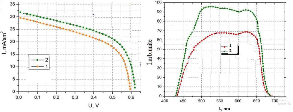
  17. Ten Huisen KS, Brown PW (1998) Formation of calcium-deficient hydroxyapatite from alpha tricalcium phosphate. Biomaterials 19: 2209-17. [crossref]
  18. Eppley BL, Pietrzak WS, Blanton MW (2995) Allograft and alloplastic bone substitutes: A review of science and technology for the craniomaxillofacial surgeon. J Craniofac Surg 16: 981-989. [crossref]
  19. Harris RJ (2004) Clinical evaluation of a composite bone graft with a calcium sulfate barrier. J Periodontol 75: 685-692. [crossref]
  20. Hench LL (2006) The story of bioglass. J Mater Sci Mater Med 17: 967-978. [crossref]
  21. Stavropoulos A, Geenen C, Nyengaard JR, Karring T, Sculean A (2007) Oily calcium hydroxide suspension (Osteoinductal) used as an adjunct to guided bone regeneration: An experimental study in rats. Clin Oral Implants Res 18: 761-767.
  22. Giannoudis PV, Dinopoulos H, Tsiridis E (2005) Bone substitutes: An update. Injury 36: S20-7.
  23. Louis PJ, Gutta R, Said-Al-Naief N, Bartolucci AA (2008) Reconstruction of the maxilla and mandible with particulate bone graft and titanium mesh for implant placement. J Oral Maxillofac Surg 66: 235-45.
  24. Soga lA, Tofe AJ (1999) Risk assessment of bovine spongiform encephalopathy transmission through bone graft material derived from bovine bone used for dental applications. J Periodontol 70: 1053-63. [crossref]
  25. Brunel G, Brocard D, Duffort JF, Jacquet E, Justumus P, et al. (2001) Bioabsorbable materials for guided bone regeneration priorto implant placement and 7-year follow-up: report of 14 cases. J Periodontal. 72: 257-64. [crossref]
  26. Pieri F, Corinaldesi G, Fini M, Aldini NN, Giardino R, et al. (2008) Alveolar ridge augmentation with titanium mesh and a combination of autogenous bone and anorganic bovine bone: A 2-year prospective study. J Periodontol 79: 2093-103. [crossref]
  27. Trombelli L, Farina R, Marzola A, Itro A, Calura G (2008) GBR and autogenous cortical bone particulate by bone scraper for alveolar ridge augmentation: A 2-case report. Int J Oral Maxillofac Implants 23: 111-6. [crossref]
  28. Blanco J, Alonso A, Sanz M (2005) Long-term results and survival rate of implants treated with guided bone regeneration: A 5-year case series prospective study. Clin Oral Implants Res 16: 294-301. [crossref]
  29. Application of Bone Substitutes and Its Future Prospective in Regenerative MedicineUjjwal Ranjan Dahiya, Sarita Mishra and Subia BanoSubmitted: August 29th, 2018 Reviewed: February 11th, 2019.
  30. Rusin Z, Ruijia Y, Paul R, Cooper, Zohaib K, et al. (2021) Bone Grafts and Substitutes in Dentistry: A Review of Current Trends and Developments. Molecules 26: 3007. [crossref]
  31. Donimukkala BR, Chandrasekharan N, Meghana G (2018) Bone Substitutes used in Implant Dentistry.

Clinical Presentations of Acute Leukemia in Children’s Cancer Units at Al-Kuwait Hospital, Sana’a City: A Cross-Sectional Study

DOI: 10.31038/JCRM.2023613

Abstract

Background and aims: Leukemia is a heterogeneous group of blood disorders consisting of several diverse and biologically distinct subgroups. Leukemia is the eleventh and tenth most common cause of cancer morbidity and mortality worldwide, respectively. There are insufficient data on clinical symptoms of acute leukemia in Yemen, particularly in the study area. Therefore, this cross-sectional study aimed to determine the clinical form of acute leukemia among children with leukemia in pediatric cancer units of Kuwait Hospital, Sana’a City.

Patients and method: A cross-sectional study was conducted on children with leukemia who were selectively treated in pediatric leukemia units at Kuwait Hospital in Sana’a. The mass diagnosis and histopathological prognosis in line with the French, American and British classifications of pediatric leukemia were formed in pediatric leukemia units, over a period of 7 years from 1 January 2015 to 31 December 2021. Factors associated with leukemia such as age, sex, clinical symptoms and outcome were studied.

Results: The mean ± SD age of all cases was 7.96 ± 3.93 years. Most of the cases were in the age group 6-10 years (67.8%), followed by the age group 11-15 years (25.1%). As for gender, slightly more of the cases were males (53.3%), VS 46.7% in females (ratio=1.14-1). The cure rate was 40.56% while the death rate was 20 cases (6.19%). The relapse rate was 2.2%. The rest of the cases were in maintenance therapy (31.6%), induction therapy (15.2%), and consolidation (post-remission therapy) for 4.33% of cases. Most cases were ALL (83.3%) while AML was only 16.7%. The most common symptom was fever (78.3%), followed by pallor (34.4%), bleeding disorders (31.9%), and abdominal pain/distention (26.9%). Hepatomegaly was recorded in 5.6%, splenomegaly in 12.1%, lymphadenopathy in 10.8%, and 18.6% of the total patients had enlargement of all three organs.

Conclusion: ALL is the most common type of leukemia. The male-to-female ratio is roughly equal, and young children between the ages of 6-10 are most affected by leukemia. More comprehensive investigations of relevant factors and predictors using more recent diagnostic methods and investigation of association factors with valuation of the treatment protocols currently in use are needed.

Keywords

Childhood leukemia, Clinical presentation, Acute leukemia, Children, Sana’a City, Yemen

Introduction

Acute leukemia (ALs) are one of the most common types of cancer with approximately 20,000 cancers diagnosed and more than 10,000 deaths annually in the United States [1]. Acute leukemia represents tumors of hematopoietic cell precursors that manifest as clonal expansion of myeloid and lymphoid hematopoiesis [2]. Acute leukemia can be broadly categorized into acute lymphocytic leukemia and acute myeloid leukemia depending on the type of cell line affected. Hematopoietic tissue in the bone marrow is characterized by an overproduction of immature lymphocytes (a type of white blood cell). Acute lymphoblastic leukemia (ALL) occurs at all ages, from birth to puberty, but the incidence peaks between 2 and 6 years of age [3,4]. Acute Lymphocytic Leukemia (ALL) is clinically and morphologically heterogeneous.1 morphologically, it is classified according to FAB (French, American and British) criteria into L-1, L-2 and L-3 sub-types, which is clinically reproducible. Acute Myelogenous Leukemia (AML) refers to a group of hematological malignancies that arise within bone marrow precursors of myeloid, monocyte, erythroid and megakaryotic cell lineages. FAB classification system divides Acute Myelogenous Leukemia into M-0 to M-7 sub-types [5]. Improvements in treatment resulted in marked gains in survival, estimated at 79 percent at 5 years. The AML score was poorer than for ALL, with a 5-year survival rate of 41 percent [3,4]. The precise cause of leukemia is not up till now obvious. Nevertheless a lot of factors, mainly genetics, genetic mutations, epigenetic lesions, ionizing radiation, other chemical and occupational contacts, curative drugs, smoking and some viral agents, have been concerned in the development of leukemia [5-13]. In developing countries, the impact of leukemia is attributed to premature death of children, loss of parents, failure of productivity due to disability, and prohibitive medical costs affecting the social, economic and health well-being of the population [14-16]. While leukemia is treated very well in the developed world, there is little evidence for the current status of the disease in Yemen in general and in the study area in particular. On the other hand, in Yemen as in most Arab countries, there are few specialized epidemiological registries dedicated to this field, which is why it is important to encourage, update, build and continue to provide studies on pediatric leukemia. The goal is to have a greater impact on public health, with early diagnosis and appropriate treatment aimed at enhancing survival and minimizing potential consequences. According to the limited Yemeni cancer studies, the most common types of cancers among Yemeni children and adults are leukemia (33.1%), lymphoma (31.5%), central nervous system tumors (7.2%), and bone tumors (5.2%) [17-22], while there are new published reports indicating an increased interest in communicable and non-communicable diseases that are closely linked to war, poverty, and the collapse of health systems in Yemen [23-30]. But there is insufficient data on the clinical symptoms of acute leukemia in Yemen, especially in the study area, so this cross-sectional study aimed to determine the clinical form of acute leukemia among children.

Patients and Method

A cross-sectional study was conducted on children with leukemia who were selectively treated in pediatric leukemia units at Kuwait Hospital, Sana’a. The mass diagnosis and histopathological diagnosis was formed in line with the French, American and British classifications of pediatric leukemia, over a period of 7 years from 1 January 2015 to 31 December 2021. Incidence-related factors were studied including ages, sex, clinical symptoms and outcomes.

Statistical Analysis

By using EPI Info statistical program version 6 (CDC, Atlanta, USA) the analysis of data was performed. Expressing the quantitative data as mean values, standard deviation (SD), when the data was normally distributed. Expressing the qualitative data as percentages; Chi square test was used for comparison of two variables to determine the P value.

Ethical Approval

Ethical approval was obtained from the Medical Research & Ethics Committee of the Faculty of Medicine and Health Sciences, Sana’a University. All data, including patient identification were kept confidential.

Results

The mean ± SD age of all cases was 7.96 ± 3.93 years. Most of the cases were in the age group 6-10 years (67.8%), followed by the age group 11-15 years (25.1%), while only 7.1% of the cases were in the age group 1-5 years. As for gender, slightly more of the cases were males (53.3%), while the percentage of females was 46.7% (male to female ratio=1.14-1). Most of the patients were from rural areas counting 68.7% while only 31.3% were from urban areas (Table 1). The cure rate was 40.56% while the death rate was 20 cases (6.19%); the relapse rate was 2.2%. The rest of the cases were in maintenance therapy (31.6%), induction therapy (15.2%), and consolidation (post-remission therapy) for 4.33% of cases (Table 2). Table 3 shows the prevalence of leukemia type among children with childhood leukemia in Sana’a, Yemen, and most cases were ALL (83.3%) while AML was only 16.7%. Table 4 shows the prevalence of clinical symptoms at the first visit among 323 children suffering from childhood leukemia. The most common symptom was fever counting 78.3%, followed by pallor (34.4%), bleeding disorders (31.9%), and abdominal pain/distention (26.9%) while less than 20% occurring for weakness (12.7%) and weight loss (10.5%). Table 5 shows the results of the physical examination at the first visit. Hepatomegaly was recorded in 5.6%, splenomegaly in 12.1%, lymphadenopathy in 10.8%, and 18.6% of the total patients had enlargement of all three organs, while 9.6% had hepatosplenomegaly and 4.3% had lymphadenopathy + H or S as well as 39% of all patients had no hyperplasia in the 3 organs (Table 5).

Table 1: Age and gender distribution of children with childhood leukemia in Sana’a, Yemen

Sex

Total

No

%

Male 172 53.3
Female 151 46.7
Age groups
1-5 years 23 7.1
6-10 years 219 67.8
11-15 years 81 25.1
Total 323 100
Mean age 7.96 years
SD 3.93 years
Median 8 years
Mode 6 years
Min 1 year
Max 15 years
Residency
Urban 101 31.3
Rural 222 68.7

Table 2: Leukemia outcomes among children suffering from childhood leukemia in Sana’a, Yemen

Outcomes

Frequency

No

%

Induction therapy 49 15.2
Consolidation (post-remission therapy) 14 4.33
Maintenance therapy 102 31.6
Relapse 7 2.2
*Cure 131 40.56
Died 20 6.19
Total 323 100

*Cure = 5-year survival rate = percentage of children who live at least 5 years after a diagnosis of leukemia

Table 3: Age and gender wise distribution of various types of leukemia’s among children suffering from childhood leukemia in Sana’a, Yemen.

Characters

Diagnosis

ALL

AML

Total

No

%

No

%

No

%

Gender
Male 141 52.4 31 57.4 172 53.3
Female 128 47.6 23 42.6 151 46.7
Age groups
1-5 years 18 6.7 5 9.2 23 7.1
6-10 years 178 66.2 41 75.9 219 67.8
11-15 years 73 27.1 8 14.8 81 25.1
Total 269 83.3 54 16.7 323 100

Table 4: The prevalence of clinical symptoms at the first visit among 323 children suffering from childhood leukemia in Sana’a, Yemen.

Symptoms

Frequency

No

%

Fever 253 78.3
Pallor 111 34.4
Bleeding disorders 103 31.9
Generalized body aches 89 27.6
Abdominal pain / distention 87 26.9
Weakness 41 12.7
Weight loss 34 10.5

Table 5: Findings of physical examination at the first visit among 323 children suffering from childhood leukemia in Sana’a, Yemen.

Signs

Frequency

No

%

Hepatomegaly 18 5.6
Splenomegaly 39 12.1
Lymphadenopathy 35 10.8
All 3 enlarged 60 18.6
Hepatosplenomegaly 31 9.6
Lymphadenopathy + H or S 14 4.3
No enlargement 126 39
Total 323 100
Total hepatomegaly 116 35.9
Total splenomegaly 137 42.4
Total lymphadenopathy 109 33.7

Discussion

Information about the prevalence of leukemia in the population may provide pathogenic hypotheses for disease control and assist in the effective management of leukemia and other hematological malignancies. In developing countries, especially in Yemen, there is little information about the burden and patterns of hematological malignancies, especially leukemia. In the current study, in relation to gender, the number of cases was slightly more male (53.3%), while the percentage of female was 46.7% (male to female ratio=1.14-1). This result is similar to that reported in Africa where the male-to-female ratio is approximately equal, although slightly dominated by females (1:1.06) [31], but differs from that reported in the United States where the Cancer Society estimates American Leukemia in 2021, about 5690 new cases, 3000 in males and 2690 in females [32] and of those previously reported from Yemen where most cases were males (66.7%) while females were 33.3% (male to female ratio=2: 1) [33]. The present findings of different gender-specific leukemia prevalence rates contradict the facts that leukemia prevalence should vary by sex due to biological factors [13,34-36].

Leukemia may appear at all ages, from newborns to the elderly, but the distinctive forms have different age distributions [37]. In the current study, the mean age of ± SD for all cases was 7.96 ± 3.93 years and most of the cases were in the age group 6-10 years (67.8%) (Table 1). This is roughly similar to what has been reported elsewhere for pediatric leukemia where the mean age of pediatric leukemia cases was 6.0 years with a peak incidence at 6-10 years [4,38,39]. This differs from the leukemia hypothesis with age in which older children may develop leukemia more frequently than younger children due to advancing age, as many environmental exposures to carcinogens, irradiation, and malignant mutations due to clonal expansion occur more often [40,41]. However, most of the younger children in the current study can be explained by the fact that prenatal and early life exposures are thought to be important determinants of pediatric leukemia. Several mechanisms have been identified through which exogenous and intrinsic factors can influence the risk of childhood leukemia. Exposure to a carcinogen or toxin early in a female’s life may cause permanent damage. Since no new eggs are formed after birth and begin to mature during pregnancy, exposures that occur during this critical time can be of great importance. During pregnancy, exposure to factors such as ionizing radiation may act directly while others may act indirectly by transferring the placenta. On the other hand, offspring may be exposed after birth to environmental exposure, either directly or indirectly [42]. Since most of the children are from rural areas (68.7%) (Table 1), they may have been exposed to various environmental exposures during their stay with their parents who are farmers. Environmental factors, even though not well articulated, influence the chance of developing leukemia. In Yemen, rural residents’ lifestyle is based on agricultural activities such as farming and plantations agriculture; especially Gat, fruits and vegetables plantation are the major practice around the study area, thus this may lead to the repeated use of chemicals such as pesticides, herbicides, and fertilizers for agricultural activities which will result in genetic mutations conferring leukemia [43]. In this study, acute lymphocytic leukemia was the most common, accounting for 83.3% of the total, while acute myelogenous leukemia counted 16.7% (Table 3). This result was consistent with results from Ethiopia, Nepal, and Pakistan [33,44], while it was contradictory with a study from Albania [45].

The clinical presentation of acute leukemia is vague and variable which makes it difficult to diagnose [46]. In this study, fever (78.3%), pallor (34.4%), bleeding disorders (31.9%), and abdominal pain/flatulence (26.9%) were found to be the most common complaints presented to patients at the first visit (Table 4). These are consistent results with Perveen et al. and Kakibuto et al. studies [47,48]. Zaki et al. [49] Shahab and Raziq [50] mentioned that fever, bleeding and pallor are the main symptoms of complaints. These findings may be explained by the mechanism of leukemia as maturation block and/or suppression of erythrocytes and polymorph nuclear cells by increased production of blastocytes resulting in decreased/disordered production of normal leukocytes/neutrophils (leading to fever), and erythrocytes ( leading to anemia/pallor) and platelets (leading to bleeding) [50]. Hepatomegaly was seen in 35.9% of patients, splenomegaly in 42.4% of patients and lymphadenopathy in 33.7% of patients. Enlargement of all three organs occurred in 18.6% of the total patients. Yasmeen et al. [51] and Shahab and Raziq [50] reported elevated hepatomegaly (71%, 67%), splenomegaly (58%, 66%) and lymphadenopathy (75%, 71%). These results are consistent with the idea that patients in our area are in hospitals when the disease reaches an advanced stage [51]. This increase in the number of organ enlargements can be attributed to the fact that the study population was children and their organs can be easily observed if the slight increase in size is compared with the organs of adults.

Limitation of the Study

There were a number of limitations in this study. It was a retrospective, hospital-based study. There was selection bias because all cases were those that presented to the hospital. The hospital-based study also does not take into account the number of similar cases within the community, and therefore, estimates of the relative prevalence of specific diseases cannot be generalized. Data were taken from patient records that were filled in by different doctors, and were therefore not standardized.

Conclusion

ALL is the most common type of leukemia. The male-to-female ratio is roughly equal, and young children between the ages of 6-10 are most affected by leukemia. More comprehensive investigations of relevant factors and predictors using more recent diagnostic methods and investigation of association factors with valuation of the treatment protocols currently in use are needed.

References

  1. Jemal A, Siegel R, Xu J, Ward E (2010) Cancer statistics. CA Cancer J Clin 60: 277-300.
  2. Kumar VD, Abbas AK, Fausto N, Mitchell RN (2010) Robbins basic pathology. 8th ed. Philadelphia: Saunders Company 421-477.
  3. Whitehead TP, Metayer C, Wiemels JL, Singer AW, Miller MD (2016) Childhood leukemia and primary prevention. Current Problems in Pediatric and Adolescent Health Care 46: 317-352. [crossref]
  4. American Cancer Society. Acute Myeloid Leukemia (AML) Subtypes and Prognostic Factors, American Cancer Society Inc., Atlanta, GA, USA, 2018.
  5. Namayandeh SM, Zaher Khazaei Z, Moslem Lari Najafi ML, Goodarzi E, Moslem A (2020) GLOBAL Leukemia in Children 0-14 Statistics 2018, Incidence and Mortality and Human Development Index (HDI): GLOBOCAN Sources and Methods. Asian Pac J Cancer Prev 21: 1487-1494. [crossref]
  6. Deschler B, Lübbert M (2006) Acute myeloid leukemia: epidemiology and etiology. Cancer 107: 2099-2107. [crossref]
  7. Pyatt D, Hays S (2010) A review of the potential association between childhood leukemia and benzene. Chemico-biological Interactions 184: 151-164. [crossref]
  8. Pyatt D (2004) Benzene and hematopoietic malignancies. Clinics in Occupational and Environmental Medicine 4: 529-555. [crossref]
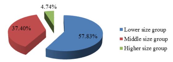
  9. Sandler DP, Shore DL, Anderson JR, Davey FR, Arthur D, et al. (1993) Cigarette smoking and risk of acute leukemia: associations with morphology and cytogenetic abnormalities in bone marrow. J Natl Cancer Inst 85: 1994-2003. [crossref]
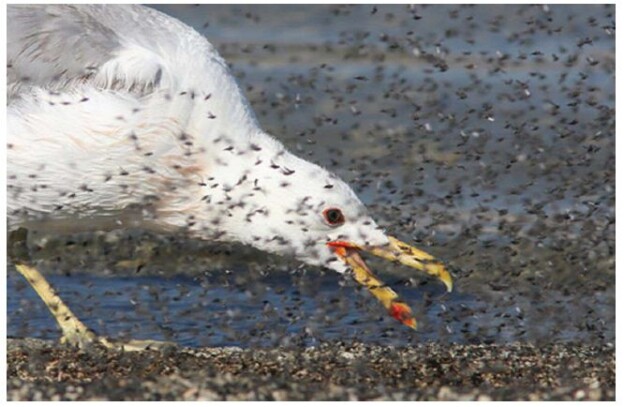
  10. Belson M, Kingsley B, Holmes A (2007) Risk factors for acute leukemia in children: a review [published correction appears in Environ Health Perspect. Environ Health Perspect 115: 138-145. [crossref]
  11. Bennett JM, Catovsky D, Daniel MT, Flandrin G, Galton DA, et al. (1976) Proposals for the classification of the acute leukaemias. French-American-British (FAB) co-operative group. Br J Haematol 33: 451-458. [crossref]
  12. Swerdlow SH, Campo E, Harris NL, et al. (2018) WHO Classification of Tumours of Haematopoietic and Lymphoid Tissues, IARC, Lyon, France.
  13. Eys JV, Pullen J, Head D, Boyett J, Crist W, et al. (1986) (e French-American-British (FAB) classification of leukemia. (e pediatric oncology group experience with lymphocytic leukemia. Cancer 57: 1046-1105. [crossref]
  14. Zeidan AM, Mahmoud D, Kucmin-Bemelmans IT, Alleman CJ, Hensen M, et al. (2016) Economic burden associated with acute myeloid leukemia treatment. Expert Review of Hematology 9: 79-89. [crossref]
  15. Mutuma J, Wakhungu J, Mutai C (2016) (e socio economic effect of cancer on patients’ livelihoods in Kenyan house holds. Bibechana 14: 37-47.
  16. American Cancer Society, 6e Global Economic Cost of Cancer, American Cancer Society, Atlanta, GA, USA, 2010.
  17. Cancer patients in Yemen face the – WHO EMRO. www.emro.who.int › yemen › news
  18. Ba-Saddik IA (2013) Childhood cancer in Aden, Yemen. Cancer Epidemiology 37: 803-806. [crossref]
  19. Bawazir AA (2018) Cancer incidence in Yemen from 1997 to 2011: a report from the Aden cancer registry. BMC Cancer 18: 540. [crossref]
  20. El-Zine MA, Alhadi AM, Ishak AA, Al-Shamahy HA (2021) Prevalence of Different Types of Leukemia and Associated Factors among Children with Leukemia in Children’s Cancer Units at Al-Kuwait Hospital, Sana’a City: A Cross- Sectional Study. Glob J of Ped & Neonatol Car 3.
  21. El-Zine MAY, Ali MAA, Al-Shamahy HA (2021) Prevalence of CNS tumors and histological recognition in the operated patients: 10 years experience in Yemen. Universal Journal of Pharmaceutical Research 6: 20-27.
  22. Okbah AA, Al-Shamahy HA, Al-Shamahi EH, Al-Ankoshy AAM (2022) Renal lesions: Differentiation of malignant and benign tumors, sex and age distribution and variables associated with renal cell carcinoma in Sana’a City, Yemen. Universal Journal of Pharmaceutical Research 7: 34-39.
  23. Abu-Hurub AS, Okbah AA, Al-Dweelah HMA, Al-Moyed KA, Al-Kholani AIM, et al. (2022) Prevalence of visceral leishmaniasis among adults in Sana’a city-Yemen. Universal Journal of Pharmaceutical Research 7: 21-26.
  24. Al-Anesi M, Hu Q, Al-Eryani E, Al-Amrani M, Al-Shamahy H (2017) The association of adult male and female infertility with celiac disease patients in Yemen. Universal J Pharm Res 2: 21-23.
  25. Alastot EM, Al-Shamahy HA (2018) Prevalence of leptospirosis amongst slaughterhouse workers and butchers in Sana’a city-Yemen. Universal J Pharm Res 3: 17-20.
  26. Al-Hrazi RMA, Al-Shamahy HA, Jaadan BM (2019) Determination of rifampicin mono-resistance Mycobacterium tuberculosis in the National tuberculosis control programme in Sana’a city-Yemen: A significant phenomenon in war region with high prevalence tubercloisis. Universal J Pharm Res 4: 1-6.
  27. Al-Shamahi EY, Muhsin NM, Al-Shamahi EH, Al-Shamahy HA (2022) Patterns of uveitis at a tertiary referral center in Yemen: One central retrospective study. Universal Journal of Pharmaceutical Research 7: 1-6.
  28. Alshamahi EYA, Al-Eryani SA, Al-Shamahy HA, et al. (2021) Prevalence and risk factors for Trachoma among primary school children in Sana’a city, Yemen. Universal J Pharm Res 6: 19-25.
  29. Ishak AA, Al-Shamahy HA (2022) Traveling Through Life with Arthritis Mutilans: Humanity Joins All Medical Practitioners in Treating and Supporting the Condition of Chronic Arthritis Mutilans Case. Ann Case Report 7: 729.
  30. Ishak AA, Al-Shamahy HA (2020) Trends and causes of morbidity in part of children in the city of Sana’a, Yemen 1978-2018: findings of single children’s health center. Universal J Pharm Res 5: 1-5.
  31. Woldeteklehaymanot Kassahun , Girum Tesfaye, Lealem Gedefaw Bimerew, et al. (2020) Prevalence of Leukemia and Associated Factors among Patients with Abnormal Hematological Parameters in Jimma Medical Center, Southwest Ethiopia: A Cross-Sectional Study. Hindawi, Advances in Hematology 152: 1-7.
  32. American Cancer Society. Cancer Facts & Figures 2021. Atlanta, Ga: American Cancer Society; 2021.
  33. Alhadi AM, El-Zine MAA, IshaK AA, Al-Shamahy HA (2021) Childhood Leukemia in Yemen: The Main Types of Childhood Leukemia, its Signs and Clinical Outcomes. EC Paediatrics 5.
  34. Solomon Tessema M, Mahlet Kifle H, Asefa M, et al. (2018) Estimates of Cancer Incidence in Ethiopia in 2015 Using Population-Based Registry Data, American Society of Clinical Oncology, Alexandria, VA, USA.
  35. Ireland National Cancer Registry, Cancer Trends; Leukaemia, National Cancer Registry Ireland, Dublin, Ireland, 2010.
  36. Hodgson CS (2016) Blood Cancer in Canada Facts and Statistics, Leukemia and Lymphoma Society of Canada, Toronto, Canada.
  37. Juliusson G, Hough R (2016) Leukemia. Progress in Tumor Research 43: 87-100. [crossref]
  38. Australia Cancer Society Leukaemia Statistics, Australia Cancer Society, 2017, https://leukaemia.canceraustralia.gov.au/statistics.
  39. American Cancer Society, Cancer Facts and Figures, American Cancer Society Inc., Atlanta, GA, USA, 2017.
  40. Konieczny J, Arranz L (2018) Updates on old and weary haematopoiesis. Int J Mol Sci 19: 2567. [crossref]
  41. Cagnetta A, Soncini D, Orecchioni S, Talarico G, Minetto P, et al. (2018) Depletion of SIRT6 enzymatic activity increases acute myeloid leukemia cells’ vulnerability to DNA-damaging agents. Haematologica 103: 80-90. [crossref]
  42. Lightfoot T (2005) Aetiology of childhood leukemia. Bioelectromagnetics 26: S5-s11. [crossref]
  43. Sinner PJ, Cerhan JR, Folsom AR, Ross JA (2005) Positive association of farm or rural residence with acute myeloid leukemia incidence in a cohort of older women. Cancer Epidemiology Biomarkers & Prevention 14: 2446-2448. [crossref]
  44. Khan A, Ahmad M, Khan S (2018) Analysis of clinic-epidemiological features of leukemia at a tertiary care facility in Peshawar. Journal of Medical Sciences 26: 41-45.
  45. Pepa E (2017) Prevalence of leukemia in Albania in the recent year. Inter-displinary Journal of Research and Development 4: 1-5.
  46. Piya MK, Acharya SC (2012) Oncology in Nepal. South Asian J Cancer 1: 5-8. [crossref]
  47. Perveen R, Yasmeen N, Hassan K (2010) Prognostic factors of acute lymphoblastic leukemia in children. Ann Pak Inst Med Sci 6: 24-7.
  48. Kakepoto GN, Burney IA, Zaki S, Adil SN, Khurshid M (2002) Long-term outcomes of acute myeloid leukemia in adults in Pakistan. J Pak Med Assoc 52: 482-486. [crossref]
  49. Zaki S, Burney IA, Khurshhed M (2002) Acute myeloid leukemia in children in Pakistan: an audit. JPMA 52: 247-249. [crossref]
  50. Shahab F, Raziq F (2014) Clinical Presentations of Acute Leukemia. Journal of the College of Physicians and Surgeons Pakistan 24: 472-476. [crossref]
  51. Yasmeen N, Ashraf S (2009) Childhood acute lymphoblastic leukemia; epidemiology and clinicopathological features. J Pak Med Assoc 59: 150-153. [crossref]