DOI: 10.31038/GEMS.2023523

Abstract

The patterns and trends of monthly time series of global atmospheric land based surface temperatures and oceanic surface temperatures, and the combination of the two, from 1850 to 2018, are presented and compared to the overall time series of fossil fuel burning which is shown to be highly correlated with atmospheric carbon dioxide concentrations. Considering only monthly temperature data time series dating back to 1850, and climate factor data in-kind, and by employing an empirical mathematical methodology, we decompose the non-linear, non-stationary, global time series and confirm patterns of frequency and amplitude modulated, discreet internal modes of variability. We find periods of warming and cooling on both the surfaces of the ocean and atmosphere over land with prominent seasonal, annual, inter-annual, multi-year, decadal, multi-decadal, and centennial modes, riding atop overall trends. Our calculated overall rates of global warming differ significantly from the estimates of the Intergovernmental Program on Climate Change (IPCC) 2007 findings, and also with the most recent, 2023 IPCC Report (https://www.ipcc.ch/ar6-syr/). Because the ocean has an enormous heat capacity relative to that of the atmosphere, we find the oceanic warming rate to be less than two-thirds of surface air over land, making the ocean a regulator, a heat capacitor, thus the dominant player in determining global surface temperatures. By employing an econometrics-based statistical formula, we establish a causal relationship between fossil fuel burning and global surface temperatures, which causally links the overall trends in planetary surface temperature rise, to the overall upward trend in fossil fuel burning. Our study also found that there is a 1-year phase lag of global temperatures to fossil fuel burning.

Keywords

Patterns of climate variability, Climate change, Global warming, Climate warming, Global surface atmospheric temperature anomalies, Sea and ocean surface temperature anomalies, Fossil fuel burning, Attribution of anthropogenic influence in climate change

Introduction

The Earth system absorbs the Sun’s incoming short-wave radiation and re-radiates, stores or exchanges it at different rates via natural processes. For a planetary condition of thermal equilibrium, the amount of total outgoing, long-wave radiation would equal the total amount of incoming, short-wave radiation. If outgoing radiation does not equal incoming radiation, then the planet’s global body temperature will vary both spatially and temporally; so, “climate variability”. Many studies have shown that the climate has been warming over the 20^th and into the 21^st Centuries, and they collectively attribute the warming climate to fossil fuel burning. Recent studies have suggested links between fossil fuel burning and climate warming [1-7]. Numerical model studies, such as Millar et al. [8] and Ekwurzel et al. [4], employed global energy-balance coupled climate-carbon-cycle models which attempted to assess global surface temperatures with the emissions of global carbon production. The relationships were visually correlated with causality assumed. However visual correlations of one curve to the next does not in and of itself establish true attribution, and thus “causality”. Herein, our study is based entirely data based, and employs only the global temperature time series and the fossil fuel burning time series. Attribution, by definition, links cause to effect.

In this study, we address the global surface temperature anomalies (GSTA) of the global surface of the Earth, in the upper panel in Figure 1, the global atmosphere surface temperature anomalies above land (GLSTA), in the middle panel in Figure 1, and the global ocean surface temperature anomalies (GOSTA), in the lower panel in Figure 1, from 1850 through the first half of 2018. The reason we limit ourselves to 2018 is that the outbreak and spread of the Covid viral infection globally, may have effected fossil fuel consumption and we will only address more “normal” conditions of greenhouse gas loading of the oceans and atmosphere. We employ documented surface-temperature-anomaly-data. While much attention has focused on the global surface atmospheric temperature record, as greenhouse gases have built up in the atmosphere, far less attention has been paid to the global ocean surface temperature record in-kind. We address that fact. Data are from the Climatic Research Unit and the UK Meteorology Office, Hadley Centre: http://www.cru.uea.ac.uk/cru/info/.

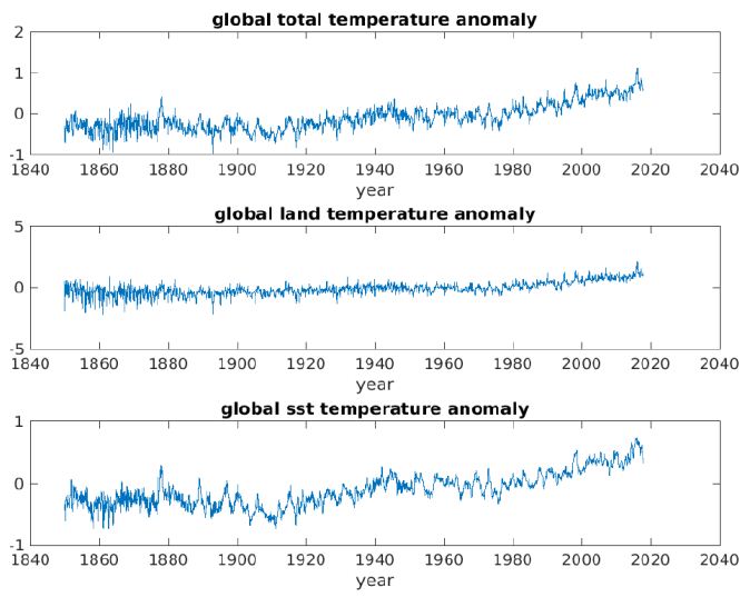
Figure 1: Monthly averaged time series of GSTA (top), GLSTA (middle), GOSTA (bottom) 01 01 1850-07 31 2018.

The climate system, as represented by surface temperature anomaly data, consists of non-linear (NL) and non-stationary (NS) processes, so we utilize an empirical, mathematical, data adaptive technique to decompose the data. Our mathematical decomposition methodology, the Ensemble Empirical Mode Decomposition (EEMD) first presented by Wu and Huang (2009) [1-10] produces internal, intrinsic modes of variability buried within the temperature data time series. We account for the patterns revealed by the internal modes of variability, relate them to naturally occurring physical phenomena and also compute the overall data time series “trends” which we find do not have a natural causal basis. However, we employ a statistical hypothesis test for determining whether one time series, such as fossil fuel burning, can be useful in forecasting another, specifically global surface temperatures, and thus to predict climate warming, past, present and future; thus establishing causality.

Background and Methodology

Wu and Huang (2009) developed EEMD based on the earlier work of Huang et al. [11-17], which employed the Hilbert Transform (the HT) [18,19], in the development of the Empirical Mode Decomposition (EMD) methodology. We employ EEMD in the decomposition of global surface temperature anomaly data time series. It is of note that a mode-mixing problem existed in the EMD decomposition in which successive IMFs were discovered to occasionally mix with or contaminate each other. To address this issue, Wu and Huang (2009) [9,10] added white noise to the various time series, created ensembles, and the mean IMFs were found to stay within the natural dyadic filter windows, preserving their dyadic properties, leading to stable decompositions of frequency and amplitude modulated internal modes of variability in the record length data. The decomposition reveals temporal internal modes of variability (referred to as Intrinsic Mode Functions or IMFs) which are frequency and amplitude modulated, and reveal non-linear (NL) and non-stationary (NS) signals in the data. The IMFs stack from higher to lower frequencies. We also produce data time series “trends”. In discussing the trend of any time series, we first need to consider the definitions and the methodologies of computing a trend. As such, no conventional simple averaging process can be utilized to reflect what information is buried in the multiple temperature time series as they are non-linear and non-stationary to the naked eye (see Figure 1, for example). This underscores the importance of clearly defining what constitutes a trend. Granger [20] presented an insightful definition of a trend as “a trend in mean comprises all frequency components whose wavelength exceeds the length of the observed time series”. For NL, NS datasets, none of these definitions is mathematically applicable leading to employment of the definition based on the EEMD methodology. With EEMD, the non-oscillation “residue”, which is left after the higher to lower frequency IMFs are removed from the time varying decomposition, becomes the trend of the time series.

Global Ocean and Land Based Atmospheric Temperature Anomaly Time Series

Figure 2 shows eleven IMF modes in the GSTA (also true of the GLSTA and GOSTA) with the 11^th being the overall trends of the land-based atmosphere, the ocean surface and the combination of the two. The IMF modes have their respective physical bases. Mode 1 is several monthly variability. Mode 2 is seasonal variability. Mode 3 is the motion of the Earth on its axis of rotation. Mode 4 is the annual signal. Mode 5 is inter-annual variability. Mode 6 is the dominant signal of the El Nino Southern Oscillation (ENSO). Mode 7 is the quasi-Solar Cycle (10-12 years), centered about 11 years. Mode 8 reflects both the North Atlantic Oscillation (NAO) and of the 22-year Solar Cycle. Mode 9, 60-70 years is the Atlantic Meridional Overturning Circulation Belt (MOC), described by Cunningham et al. [21]. Mode 10, 105-110 years represents the Global Thermohaline Circulation Conveyor Belt [22,23]. Mode 11 is the gravest mode or overall trend of the 167-year time series of total data (Table 1).

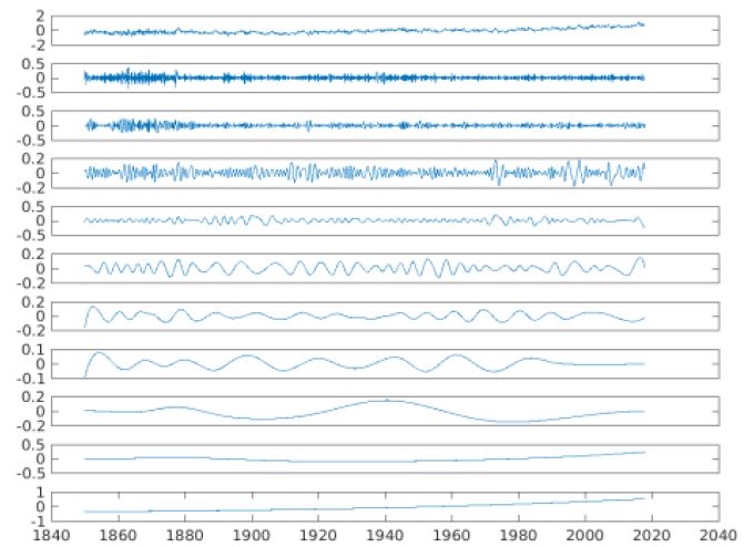
Figure 2: The EEMD Mode decomposition of the 1850-2017 time series of the GSTA (shown in the Top Panel.

Table 1: Intrinsic Mode Functions (IMFs) shown in Figure 2, in Months (M) or Years (Y)

IMF	1	2	3	4	5	6	7	8	9	10	11
GLSTA GOSTA GSTA	2 M	3 M	6 M	1 Y	2-3 Y	5-7 Y	10-12 Y	20-22 Y	60-70 Y	105-110 Y	167 Y Trend

We note in Figure 2, that for the GSTA, the IMF modes 2, 3 and 10 have amplitudes of 0.4°C, modes 4 and 6 have amplitudes of 0.3°C, modes 5, 7 and 9 have amplitudes of 0.2°C and mode 8 amplitude of 1°C. Mode 11 ranges between +/- 0.5°C. Thus, all the IMF modes contribute to the total time series in temperature amplitudes in a nominally equitable manner across the range of 0.1 to 0.4°C. This finding suggests that the Planet’s internal, natural modes of variability all contribute significantly to surface temperatures and thus cannot be ignored. Thus, periods of relative warming and or cooling occur naturally by the positive and negative disposition of the natural variability, all riding atop overall atmospheric and oceanic trends, and presented in the Table 1.

In Figure 3 (left panel), the trend of the GLSTA shows a record length total rise of 1.22°C and the GOSTA displays a rise of 0.67°C. The collective GSTA rises 0.88°C. The ocean surface temperature has risen at a much slower rate than the atmosphere over land. This is an excellent example of the power of the EEMD IMF decomposition. The full time series of the GOSTA displays an overall beginning to end of the series increase of 0.75°C, the GLSTA shows a rise of 2.91°C and the GSTA indicates an overall increase of 1.25°C. If connecting lines from start to end of the three time series had been drawn, the overall trends would have been greatly overestimated, demonstrating the failing of traditional methods (see IPCC, 2007) [24] of computing a trend, which are to create regression lines. Thus, the IPCC rates of rise of GSTA overestimate the actual rises in temperatures over land by 0.72°C and by a combined air-sea overestimate of 0.37°C. The IPCC straight-line, regression slope estimates are 0.05°C/decade over the full GSTA temperature record, 0.07°C/decade over the prior 100 years, 0.13°C/decade over the previous 50 years and 0.18°C/decade over the latter 25 years of the record.

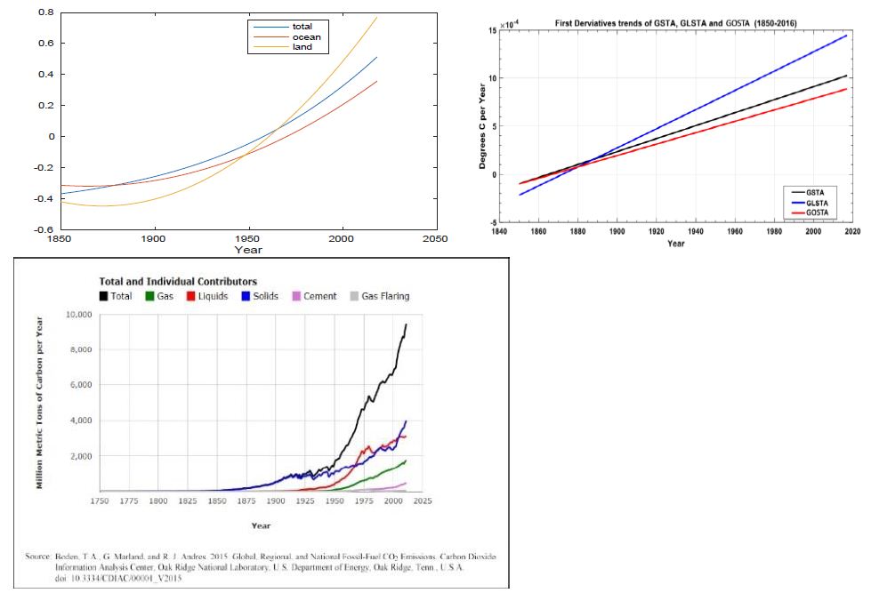
Figure 3: (left panel) The overall trends of the GSTA (blue), GOSTA (red) and GLSTA (yellow) time series. The GOSTA raw data are shown in Figure 2 and represents the GLSTA and the GSTA (both not shown). (center panel) The time rates of change or 1st derivatives, of the trends of the GLSTA, GOSTA and GSTA time series. (right panel) The fossil fuel burning curves. Atmospheric carbon dioxide concentrations also shown in far right panel Confirming sources are: T. Boden and R. Andres, The Carbon Dioxide Information Analysis Center, Oak Ridge National Laboratory, Oak Ridge, Tennessee 37831-6290, USA; and G. Marland, The Research Institute for Environment, Energy and Economics, Appalachian State University, Boone, North Carolina 28608-2131, USA.

In Figure 3 (left panel), we present the time rates of our trends and find that the rates of warming from 1850 through 2017 are 0.713°C/Century for the GLSTA, 0.427°C/Century for the GOSTA, and 0.529°C/Century for the combined GSTA. In the Figure 3 central panel, the 1^st derivatives of the trend curves are all positive, and curving upward indicating that the rate of warming is accelerating. From 1955 to the present the overall warming trend of the GSTA (Figure 3) has been ~0.09°C/decade. Clearly, the rate of warming of air over land has globally been 167% greater than that of the surface of the global ocean. In the Figure 3 right panel, we present the fossil fuel burning time, Carbon Emissions (CE) series from 1751-2014, provided via <http://cdiac.ornl.gov/trends/emis/tre_glob.html>. From 1751 until 1850, global CO2 production was from 3 MMTs in 1751 to 54 MMTs in 1850. In the latter half of the 19^th century, carbon emissions increased considerably, with a dramatic upsurge from 1949 to 2014, reaching a value of 950 MMTs and this resulted in the nonlinear rise of atmospheric carbon dioxide concentrations. The CE was essentially flat from 1751 through the mid latter half of the 19^th century when the change of carbon burning began to be spiky. One could proceed here with cross correlations between the CE and GLSTA, GOSTA and/or the GSTA. However, although the temperature curves all display strong visual correlation with the fossil fuel burning curve, visual correlation does not prove a cause-and-effect relationship or attribution.

Granger Causality relating Carbon Burning to Global Surface Temperature Anomalies

We next employ the Granger Causality Test (GCT) [25] to obtain evidence for the strength of the causal relationship between the carbon burning and atmospheric carbon dioxide concentrations and atmospheric carbon dioxide concentrations and the globle temperature time series. GCT statistically tests for determining whether one time series is useful in forecasting another. Generally regressions reflect mere correlations, but Granger argued that by measuring the ability to predict the future values of a time series using prior values of another time series, causality in economics could be tested. A time series X is said to “Granger-cause” Y if it can be shown, through a series of t-tests and F-tests on lagged values of X (and with lagged values of Y also included), that those X values provide statistically significant information about future values of Y. The idea is that if series {x_t} helps to cause series {y_t}, then past values of {x_t} should improve predictions of series {y_t}. This type of causality is established by first modeling {y_t} in terms of the past values of {y_t} through an autoregressive (AR) process, then adding past values of series {x_t} to create a second model. If the second model is statistically better than the first, then one has established causality in the Granger sense. Testing for Granger Causality in global temperatures has been considered by Attanasio et al. [26], Pasini et al. [27-29], amongst others. The above papers consider more time series than those considered here so they can for example separate out anthropogenic forcing and they also allow for non-stationarity in the temperature series. Our approach differs in that we consider only anomaly series {y_t} and one emission series {x_t}, and we find a stationary AR model for the anomalies after appropriately differencing the series and testing for white noise of the residuals?, which we justify our modeling by use of a time series goodness-of-fit test (see Fisher and Gallagher, 2012). One advantage of our methodology is that our final fitted model can be used to predict the impact of current (future) carbon emissions on temperature. We will approach this in a systematic process.

We first consider establishing a causal relationship between the carbon burning time series ({x_t}) and the ocean surface temperature time series GOSTA ({y_t}). Here we model on the monthly scale by taking the average temperature anomaly for each year as y and the average monthly carbon emission created by taking the yearly value divided by 12. Our first model relates GOSTA to past values of GOSTA. Using Akiake’s Information Criterion [30] we select the order of the auto regression to be three, meaning that each year’s GOSTA is related to the values from the last 3 years. The model is fitted using Gaussian maximum likelihood [31]. We use the goodness of fit test [32] to verify that the AR model adequately models the autocorrelation in the GOSTA series; the p-value of 0.9464 indicates that we have found an adequately fitting stationary model for GOSTA model given in Equation (1):

The above model explains the dynamics of the observed series solely from past-observed values. However, to establish the (Granger) causal relationship we instead add the previous year CE value to the model. The resulting model is given by Equation (2):

We can test for statistical significance of each fitted coefficient using the asymptotic normality of the Gaussian maximum likelihood estimators [31]. In particular, we conclude with a p-value of 0.00009 that the coefficient of x_t-1 is non-zero. In other words, the predictive model for GOSTA is significantly statistically better if the previous year CE is included. Model (2) explains the changes in temperature through a combination of autocorrelation (AR) and the impact of CE. We have thus established causality in the Granger sense. In this analysis, we selected the data beginning in 1950, since the warming trend in the latter half of the 20^th century is well established (cf. Figure 3, left panel). However, a similar analysis could be conducted starting at any point in the past. For example, the same analyses beginning each decade in the first half of the 20^th, i.e., in years 1900, 1910, 1920, 1930, 1940, and 1950, resulted in p-values, 0.00005, 0.0002, 0.00002, 0.0002, 0.003, 0.009, for the coefficient of x_t-1, respectively. In each case we conclude the model using the previous year CE is statistically better than the AR (3) model alone; the carbon emission series significantly improves predictions for GOSTA over the model based solely on past GOSTA values. Regardless of starting time, in the 20^th century, one finds statistical evidence of a causal relationship between CE and GOSTA. The coefficient for x_t-1 in model (2) is as follows. For each additional one-million metric tons of carbon emissions (CE), we estimate an increase in global ocean temperature (GOSTA) of 0.0007°C. The average increase in carbon emissions per year for years 1950 through 2014 is about 130 metric tons per year. Our model estimates an increase of 0.007+°C for each 10 metric ton increase in carbon emissions. The highly statistically significant coefficients of x_t-1 for land based atmospheric temperatures and total global surface temperatures are 0.0117 and 0.0087, respectively.

We next employ our fitted models to predict the global sea surface anomaly (GOSTA), the land atmosphere (GLSTA) and combined global surface temperature anomalies (GSTA) for 2015. Figure 4 shows the observed anomalies for years 1950 through 2014. The prognostic values are remarkably accurate. In the plots, we mark the predicted value from our fitted model, the upper and lower 95% prediction limits and the observed value for Year 2015. We conducted multiple-year lag experiments between CE and the surface temperature time series, beginning with 10 year down to 1 year lags (not shown except for the latter). We find that the model, which uses both past values of the anomaly series and the previous year’s carbon emission ( a 1-year lag), provides excellent predictions for the observed anomalies of the ocean surface, atmosphere on land and the combination therein for 2015. This provides further empirical evidence of Granger Causality relating previous year carbon emissions to sea surface, atmosphere on land and the combination temperatures on a global scale. We utilized the 2014 and 2015 data because 2014 is the last year for which we were able to obtain Fossil Fuel Burning data from the website provider at the time that this study was conducted. The results presented above provide a pathway and portend to future increases in global surface temperatures given anticipated increases in fossil fuel burning, GOSTA, GLSTA and GSTA as a function of CE. GOSTA is increasing at the rate of 0.0007°C/ Million Metric Tons of CE. GLSTA is increasing at the rate of 0.00117°C/Million Metric Tons of CE. Thus, the GSTA is increasing at the rate of 0.00087°C/Million Metric Tons of CE. Presently we are on a trajectory to reach 10⁴ Million Metric Tons/year of CE by years 2020 to 2022. These numbers are less foreboding than the straight-line estimates of both the IPCC and NIPCC, but are nonetheless very noteworthy.

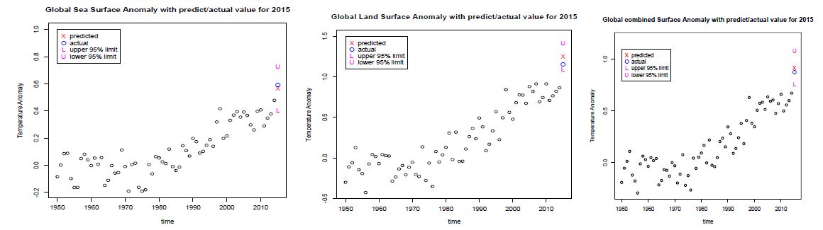
Figure 4: Global Surface Temperature Anomalies from 1949-2014 with Granger Causality Predicted (X) versus Actual Temperatures (O) for 2015 and upper and lower 95% confidence limits. (left panel) is for the GOSTA. (middle panel) is for the GLSTA. (right panel) is for the GSTA.

Discussion and Conclusions

Mathematical relationships between fossil fuel burning and surface temperatures in the oceans and over land are presented. The statistical relationship curves reveal strongly that there is a one-year phase lag between global carbon loading via fossil fuel burning and planetary surface temperature rise, different from Ricke and Caldeira [33-41] who proposed that planetary temperatures changed about a decade after burning. In fact, robust relationships are presented between the GLSTA, GOSTA and GSTA, and their past time series, and the CE time series. Via Granger Causality, these surface temperatures are predicted very accurately from fossil fuel burning a year earlier. Thus, the conclusion we reach is that we have proven that there is “attribution” between fossil fuel burning and climate warming. In 2007, the IPCC was awarded a Nobel Prize for its comprehensive analyses of global climate change, including a visual-correlative-comparison of fossil fuel burning and temperature rise. However, a visual correlation does not prove “causality”. In 2003 C.W.J Granger was awarded a Nobel Prize for his work in econometrics theory and applications. We invoked “Granger Causality” to attribute the overall trends in global surface warming to fossil fuel burning and carbon emissions (https://en.wikipedia.org/wiki/Clive_Granger).

Acknowledgement

The authors thank Dr. Thomas S. Malone (former member of the U.S. National Academy of Sciences, now deceased), for having encouraged this study. He observed that cause and effect was necessary to prove attribution. The authors thank Coastal Carolina University for supporting this study.

References

1. Allen MR, Frame DJ, Huntingford C, Jones CD, Lowe JA, et al. (2009) Warming caused by cumulative carbon emissions towards the trillionth tonne. Nature 458.
   
2. Heede R (2014) Tracing anthropogenic carbon dioxide and methane emissions to fossil fuel and cement producers, 1854-2010. Climatic Change 122: 229-241.
3. Stocker TF, Qin D, Plattner GK, Tignor M, Allen SK, et al. (2013) IPCC, 2013: Climate Change 2013: The Physical Science Basis. Contribution of Working Group I to the Fifth Assessment Report of the Intergovernmental Panel on Climate Change, pg: 1535. Cambridge Univ. Press, Cambridge, UK, and New York.
4. Ekwurzel B, Boneham J, Dalton MW, Heede R, Mera RJ, et al. (2017) The rise in global atmospheric CO 2, surface temperature, and sea level from emissions traced to major carbon producers. Climatic Change 144: 579-590.
5. Millar RJ, Fuglestvedt JS, Friedlingstein P, Rogelj J, Grubb MJ, et al. (2017) Emission budgets and pathways consistent with limiting warming to 1.5°C. Nature Geoscience 10: 741-747.
6. Al‐Ghussain L (2019) Global warming: review on driving forces and mitigation. Environmental Progress & Sustainable Energy 38: 13-21.
7. Smith CJ, Forster PM, Allen M, Fuglestvedt J, Millar RJ, et al. (2019) Current fossil fuel infrastructure does not yet commit us to 1.5°C warming. Nature Communications 10: 1-10.
8. Millar R.J,. Nicholls ZR, Friedlingstein P, Allen MR (2016) A modified impulse-response representation of the global response to carbon dioxide emissions. Atmospheric chemistry and physics discussions.
9. Wu Z, Huang NE (2009) Ensemble Empirical Mode Decomposition: a noise-assisted data analysis method. Advances in Adaptive Data Analysis 1: 1-41.
10. Wu Z, Huang NE, Chen X (2009) Multi-Dimensional Empirical Mode Decomposition Based on Ensemble Empirical Mode Decomposition. Advances in Adaptive Data Analysis 1: 339-372.
11. Huang NE, Shen Z, Long SR, Wu MC, Shih EH, et al. (1998) The empirical mode decomposition and the Hilbert spectrum for nonlinear and non-stationary time series analysis. Roy. Soc. Lond 454A: 903-993.
12. Huang NE, Wu z, Long SR, Arnold KC, Chen X, Blank K (2009) On instantaneous frequency, Advances in Adaptive Data Analysis. 1: 177-229.
13. Huang NE, Shen, Long SR (1999) A New View of Nonlinear Water Waves – The Hilbert Spectrum. Rev. Fluid Mech 31: 417-457.
14. Huang NE, Wu ML, Long SR, Shen SS, Qu WD, et al. (2003) A confidence limit for the Empirical Mode Decomposition and Hilbert Spectral Analysis. Roy. Soc. London 459A: 2317-2345.
15. Huang NE, Wu Z (2008) A review on Hilbert-Huang Transform: the method and its applications on geophysical studies. Geophys 46.
16. Wu Z, Huang NE (2004) A study of the characteristics of white noise using the empirical mode decomposition method. Roy. Soc. London 460A: 1597-1611.
17. Wu Z, Huang NE, Wallace JM, Smoliak BV, Chen X (2007) On the time-varying trend in global-mean surface temperature. Climate Dynamics 2011, 37.
18. Gabor D (1946) Theory of communication. IEE 93: 429-457.
19. Van der Pol B (1946) The fundamental principles of frequency modulation. IEE 93: 153-158.
20. Granger CWJ (1966) The Typical Spectral Shape of an Economic Variable. Economtrica 34: 150-161.
21. Cunningham SA, Rayner MO. Baringer WE, Johns J, Marotzke HR, et al. (2007) Temporal Variability of the Atlantic Meridional Overturning Circulation at 26.5°N. Science 317: 935-938. [crossref]
22. Rahmstorf S (2003) The concept of the thermohaline circulation. Nature 421.
    
23. Sabra K, Cornuelle B, Kuperman W (2016) The Rising Heat Content of the Earth’s Oceans. Physics Today 32.
    
24. Bernstein L, Bosch P, Canziani O, Chen Z, Christ R, et al. (2008) IPCC, 2007: climate change 2007: synthesis report. IPCC.
25. Granger CWJ (1980) Testing for causality: A personal viewpoint. Journal of Economic Dynamics and Control 2: 329-352.
26. Attanasio A, Pasini A, Triacca U (2012) A contribution to attribution of recent global warming by out-of-sample Granger causality analysis. Atmospheric Science Letters 13: 67-72.
27. Pasini A, Triacca U, Attanasio A (2012) Evidence of recent causal decoupling between solar radiation and global temperature. Environmental Research Letters 7.
    
28. Attanasio A, Pasini A, Triacca U (2013) Granger causality analyses for climatic attribution. Atmospheric and Climate Sciences 3: 515-522.
29. Triacca U, Attanasio A, Pasini A (2013) Anthropogenic global warming hypothesis: testing its robustness by Granger causality analysis. Environmetrics 24: 260-268.
30. Akaike H (1974) A new look at the statistical model identification. IEEE Trans. Control 19: 716-723.
31. Brockwell PR, Davis RA (1991) Time Series: Theory and Methods (2nd edn) New York: Springer-Verlag.
32. Fisher TJ, Gallagher CM (2012) New Weighted Portmanteau Statistics for Time Series Goodness of Fit Testing, Journal of the American Statistical Association 107.
    
33. Pietrafesa LJ, Gallagher C (2017) The Global Surface Temperature Anomaly Time Series and Relationships. Indian Journal of Applied Research. 7: 601-608.
34. Ricke KL, Caldeira K (2014) Maximum warming occurs about one decade after a carbon dioxide emission. Environ Res Lett 9.
    
35. Chatfield C (2003) The Analysis of Time Series, An Introduction. 6th Ed. Chapman & Hall.
36. Cheng LKE, Trenberth J, Fasullo T, Boyer J, Abraham J, Zhu (2017) Improved Estimates of Ocean Heat Content 1960-2015. Science Advances 3, Number 3. Cunningham, S.A, T. Kanzow, D.
37. Flandrin P, Rilling G, Gonçalves P (2004) Empirical mode decomposition as a filter-bank. IEEE Signal Proc Lett 11: 112-114.
38. Hill C, DeLuca C, Balaji V, Suarez M, A. da Silva. (2004) The Architecture of the Earth System Modeling Framework. Computing in Science and Engineering 6: 18-28.
39. James and James (1976) The Mathematical Dictionary. 4th Edition. D. Van Nostrand Com. Publisher.
40. Ljung GM, Box GEP (1978) On a Measure of Lack of Fit in Time Series Models. Biometrika 65: 297-303.
41. Shakespeare W, 1603. Hamlet, Quarto Ed.