Author Archives: author

Abstract

Background: Myelinated retinal nerve fibers (MRNFs) are usually unilateral and asymptomatic benign lesions associated with mild hypermetropia, emmetropia, or severe myopia. We describe herein an myopic patient with a syndrome of ipsilateral myelinated retinal nerve fibers associated with other pathological changes: epiretinal membrane with pseudohole, vitreomacular traction syndrome and bilateral lattice degeneration.

Methods: Extended ophthalmoscopy was used to evaluate retinal posterior segment. Infrared reflectance imaging helped in visualizing sub-retinal pathology. Detailed images from within the retina were obtained by using optical coherence tomography.

Results: Ophthalmologic examination revealed ipsilateral small temporal myopic conus with lattice degeneration temporally and inferotemporally. The area of myelinated nerve fiber extended into the pappilomacular bundle, but did not reach the fovea. At the fovea, an epiretinal membrane with clinically visible vitreomacular traction and some retinal elevation was found. In the peripheral fundus areas of lattice degeneration temporally and inferiorly was also noted. The OCT scans of the affected eye showed an incomplete posterior vitreous detachment with traction of a thickened posterior hyaloid base to the fovea. There was distortion of the foveal anatomy with a small amount of subfoveal fluid but a full-thickness macular hole could not be detected. Macular traction detachment of retina and epiretinal membrane with macular hole were treated surgically (S/P Repair Complex RD (25g, 20% SF6, membrane peel with gas endotamponade) and vitreomacular traction was released. Lattice degeneration was treated by laser (S/P Laser).

Conclusions: MRNF lesions were stable and although associated with other ocular pathology progression was not observed during follow-up.

Keywords: Myelinated – Myopia – Lattice degeneration – Vitreomacular traction – Coherence tomography

Introduction

Myelinated retinal nerve fibers (MRNFs) are usually unilateral and asymptomatic benign lesions of the retina around the optic disk [1–2]. but it could also be found in other parts of the retina and in fovea [3]. During embryonic development the retinal nerve fibers may retain the myelin coat resulting in abnormal intraocular myelination of the peripheral nerve anterior to the lamina cribrosa [4]. The MRNF may be inherited but early-age trauma to the eye damaging lamina cribrosa may let oligodendrocytes to pass to the retina causing myelination [5]. MRNF has been associated with mild hypermetropia, emmetropia, or severe myopia. The size and the location of opaque nerve fiber patch determine visual field defects in eyes with MRNF [2], [6]. Studying the correlation between the extend of myelinated nerve fibers and refraction anomalies Schmidt D. at al [7]. concluded that myopia only occurred in eyes with wide-spread myelinated nerve fibers but not in eyes with circumscribed myelinated nerve fibers.

Case report

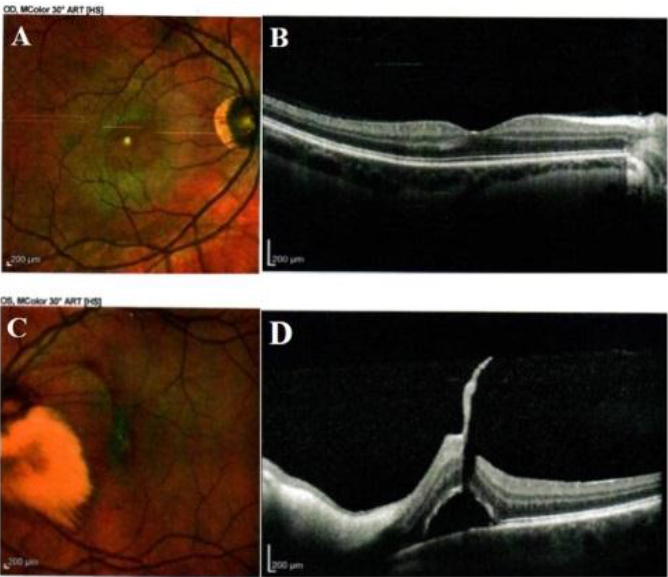
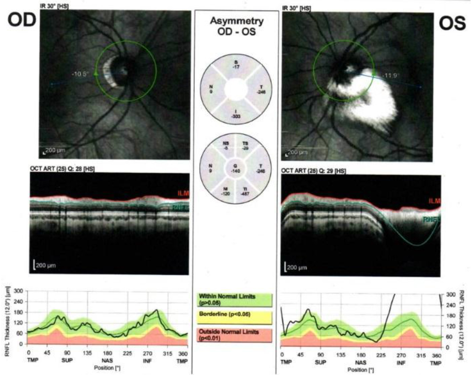
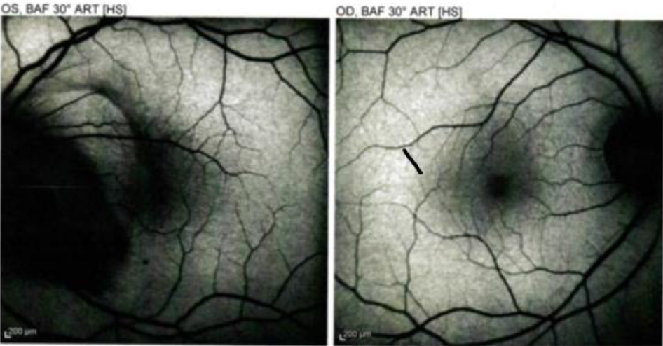
A 20-year-old man presented with severe left eye (OS) central blurred vision worsening during a period of one year. Reading and watching TV were affected activity. On the right eye (OR) he had gradual onset of blurred vision with mildly affected reading. The patient was noted to have an area of myelinated nerve fiber layer in his left eye a number of years ago, which remained stable over several years of follow-up. More recently change in visual acuity of the left eye was noted. The patient’s past ocular history was also notable for anisometropia, but he did not report a history of amblyopia. On examination visual acuity with correction at distance measured 20/25 OD and 20/80 OS. RO examination also revealed a small temporal myopic conus and lattice degeneration temporally – inferotemporally and a few additional areas inferiorly (Fig.1A). Optical Coherence Tomography (OCT) showed normal thickened retinal nerve fibers with an attached hyaloid (Fig.1B). Left eye fundus examination showed abnormal layer of blood vessels and circumferential areas of lattice degeneration temporally and inferotemporally (Fig.1C). The area of myelinated nerve fiber extended into the papillomacular bundle, but did not reach the fovea. At the fovea, an epiretinal membrane with clinically visible vitreomacular traction and some retinal elevation was noted. The OCT scans of the left eye showed an incomplete posterior vitreous detachment with traction of a thickened posterior hyaloid base to the fovea distorting foveal anatomy with a small amount of subfoveal fluid but a full-thickness macular hole could not be detected (Fig. 1D). Myelinated nerve fiber lesions showed hyperreflectibility (Fig. 2). Autofluorescence imaging revealed a dark area in the region of myelinated RNFL (Fig. 3). Macular traction detachment of retina and epiretinal membrane with macular hole were treated surgically (S/P Repair Complex RD (25g, 20% SF6, membrane peel with gas endotamponade) and vitreomacular traction was released. Lattice degeneration was treated by laser (S/P Laser). Initial ocular post-op medication was: Cyclogyl 2%, Gentacidin 0.3%, and Prednisolone Acetate 1%. Three days after surgery Timol (Maleate) 0.25% was added. Retinal examination found periphery laser scarring and lattice degeneration with atrophic hole with laser (inferotemporal). The patient was regularly followed up in order to monitor progression and one year after surgery no disk edema and pallor, no new holes or tears were found and retinal vessels had normal caliber.

JCRM 2019-113 - Dragan Jovanovic USA_F1

Figure 1. Optic disc imaging findings: A, OD color fundus photograph showing circumferential areas of lattice degeneration emporally – inferotemporally. B, OD OCT showing normal thickened retinal nerve fibers with an attached hyaloid . C, OS color fundus photograph showing a large area of MNFL extended into the papillomacular bundle without reaching the fovea. D, OS OCT showing an incomplete posterior vitreous detachment with traction of a thickened posterior hyaloid base to the fovea. Distorted foveal anatomy with a small amount of subvoveal subretinal fluid.

JCRM 2019-113 - Dragan Jovanovic USA_F2

Figure 2. OCT of the right and of the left eye showed hyperreflectivity of myelinated nerve fiber lesions in the left eye.

JCRM 2019-113 - Dragan Jovanovic USA_F3

Figure 3. Autofluorescence imaging reveals a dark area in the region of the myelinated RNFL in OS.

Discussion

MNFL represent an asymptomatic developmental anomaly in which myelin sheaths extend to retinal nerve fibers along their intraocular portion causing displacement of the axons toward the vitreous body causing decreased vessel density in MRNF areas [8]. In our patient MRNF lesions were stable and although associated with other ocular pathology progression was not observed during follow-up. Cases with regression of MRNF associated with inflammatory diseases and glaucoma were also reported in the literature [9], [10]. Our patients was myopic (OD – 10.25 and OS – 5.50) and ophthalmologic examination revealed a small temporal myopic conus in right eye. High myopia is one of the leading causes of low vision in the world. [11] Genetic and environmental factors play role in its development [12]. Physiological myopia is a common optical aberration [13], but in pathological shortness with irreversible conditions such as retinal detachment, and macular atrophy can lead to blindness. In the myopic eye excessive axial elongation can lead to mechanical stretching and thinning of the choroid and RPE. [14], [15]. Changes in peripheral retina of myopic are predisposing factors for retinal detachment and include lattice degeneration, white-without-pressure, pigmentary degenerations, and retinal tears and holes. Association of extensive myelinated nerve fibers and high degree myopia have been reported [16]. Ellis et al [17] found that 83% of patients with myelinated retinal nerve fibers had myopia greater than 6 diopters. It is not clear whether myelination of retinal nerve fibers is the reason for or the result of myopia. In patient with myelinated fibers retinal images may be blurred causing visual deprivation. This deprivation may contribute to myopia by including an axial enlargement. On the other hand, it is also possible that axial elongation predisposes to retinal nerve fiber myelination. Straatsma et al [18] found that 10% of patients with myelinated nerve fibers have myopia, ampliopia, and strabismus. Our patient had refractive error of -9.0 in OD and -5.5 in OS. In pathologic myopia progressive chorioretinal degeneration is often associated [19]. In our patient’s OS where MRNF lesions were found posterior cortical vitreous partially separated from the retina (epiretinal membrane) and some tractional areas remain adherent to portions of the macula causing Vitreomacular Traction Syndrome (VTS).

Compliance with ethical standards

Conflict of interest: The authors declare that they have no conflict of interest.

Ethical approval: All procedures performed in studies involving human participants were in accordance with the ethical standards of the institutional and/or national research committee and with the 1964 Helsinki Declaration and its later amendments or comparable ethical standards

Informed consent: Informed consent was obtained from patient’s parents to publish his photo and all other information

References

Straatsma BR, Foos RY, Heckenlively JR, Taylor GN. (1981) Myelinated retinal nerve fibers. Am J Ophthalmol. 91: 25–38.
Kodama T, Hayasaka S, Setogawa T. (1990) Myelinated retinal nerve fibers: Prevalence, location and effect on visual acuity. Ophthalmologica. 200: 77–83. [Crossref]
Serdar O, Mehmet YT. (2017) Ring-shaped myelinated retinal nerve fibers at fovea. Indian J Ophthalmol. 65(7): 630–632. [Crossref]
Darin RG. (2018) Atlas of Retinal OCT. Optical Coherence Tomography 2018, Elsevier;2018
Prakalapakorn SG, Buckley EG. (2012) Acquired bilateral myelinated retinal nerve fibers after unilateral optic nerve sheath fenestration in a child with idiopathic intracranial hypertension. J Pediatr Ophthalmol Strabismus. 16: 534–8. [Crossref]
Bradley R. Straatsma, John R. Heckenlively, Robert Y. Foos, and John K. (1979) Shahinian, Myelinated retinal nerve fibers with ipsilateral myopia, amblyopia, and strabismus. American Jopurnal of Opthalmology. 88: 506–510. [Crossref]
Smitdt D, Meyer JH, Brandi-Dohrn J. (1996–1997) Wide-spread myelinated nerve fibers of the optic disc: do they influence development of myopia? Int Ophthalmol. 20(5): 263–8. [Crossref]
Hollo G. (2016) Infuence of myelinated retinal nerve fibers on retinal vessels density measurement with AngioVue OCT angiography. Int Ophthalmol. 36(6): 915–919. [Crossref]
Sowkia JW, Nadeau MJ. (2013) Regresion of myelinated nerve fibers in a glaucomatous eye. Optom Vis Sci. 90(7): e2018-e220. [Crossref]
Chavis PS, Tabbara KF. (1998) Demyelinization of retinal myelinated nerve fibers in Behcet’s disease. Doc Opthalmol. 95: 157–64. [Crossref]
Hayashi K, Ohno-Matsui K, Shimada N, Moriyama M,Kojima A, Hayashi W, Yasuzumi K, Nagaoka N, Saka N, Yoshida T, Tokoro T, Mochizuki M. (2010) Long-term pattern of progression of myopic maculopathy: a natural history study. Ophthalmology 117: 1595–611. [Crossref]
Pan CW, Zheng YF, Wrong TY, et al. (2012) Variation in prevalence of myopia between generations of migrant Indians living in Singapore. Am J Ophthalmol 154: 376–81. [Crossref]
Baker BJ, Pruett R. (2004) Degenerative myopia. In: Yanoff M, Duker SJ. Ophthalmology: 2^nd ed. Spain : Mosby 934–7.
Grossniklaus HE, Green WR. (1992) Pathologic findings in pathologic myopia: Retina 12(2): 127– 133. [Crossref]
Rabb MF, Garoon I, LaFranco FP. (1981) Myopic macular degeneration. Int Ophthalmol Clin 21(3): 51– 69. [Crossref]
Elvan Yalcın, Ozlem Balcı, and Ziya Akıngol (2013 ) Indian J Ophthalmol. 61(10): 606–607;
Ellis GS Jr, Frey T, Gouterman RZ. (1987) Myelinated nerve fibers, axial myopia, and refractory amblyopia: An organic disease. J Pediatr Ophthalmol Strabismus 24: 111–9. [Crossref]
Straatsma BR, Heckenlively JR, Foos RY, Shahinian JK. (1979) Myelinated retinal nerve fibers associated with ipsilateral myopia, amblyopia, and strabismus. Am J Ophthalmol 88: 506–10). [Crossref]
Soubrane G, Coscas G.J. (2001) Choroidal neovascularization in degenerative myopia. In: Ryan SJed. Retina. 3^rd St Louis, Mo Mosby Inc 1136–1152.

What do we know about Food Cravings and Aversions during Pregnancy?

Leave a reply

DOI: 10.31038/IGOJ.2019234

Abstract

During pregnancy, it is very common for women to make changes in the choice of foods they eat and often experience cravings and aversions to certain foods. The purpose of this narrative review is to describe the current state of knowledge about the different hypotheses that try to explain the presence of food cravings and aversions during pregnancy and to know the occurrence of these phenomena in different geographical contexts.

The most studied hypothesis relates to food aversions to maternal-fetal protection mechanisms; others with less sustenance link them as preventive of the metabolic syndrome, as a consequence of shortage of resources or compensatory of placental growth. The hypotheses that explain the appearance of food cravings relate them as a consequence of a search for nutrients or active compounds present in the foods craved for, or as a consequence of the hormonal fluctuations that are special to pregnancy.

The prevalence with which cravings and aversions occur varies from 38 to 79%, being less frequent in European populations and more common in the African continent. In general terms, foods craved by pregnant women in Western cultures are chocolate, fruits and fruit juices, sweet foods and, to a lesser extent, meats and dairy products. In geographical contexts of socio-economic vulnerability, foods of animal origin such as meat, cheese and milk, followed to a lesser extent by vegetables, fruits and grains, emerge as usually cravings.

Protein-rich foods of animal origin are largely rejected by pregnant women in Western countries, while cereals and vegetables are frequently avoided by pregnant women in Africa and Asia.

Keywords

Pregnancy, Cravings, Aversions, Food Choice

Introduction

Pregnancy is a complex and vitally important period and its physiology is of great biological and nutritional importance since the contribution of nutrients must be adequate in quantity, quality and distribution so that both the process of embryogenesis and development of the fetus and health of the mother are adequate [1, 2].

It is common for pregnant women to make changes in the choice of foods they eat, which are the result of a complex set of biological and cultural interactions that have implications for maternal and child health [3–6]. Within these food variations appear phenomena that pregnant women frequently experience: cravings and aversions to certain foods. These phenomena, in which causes and consequences are little known, are usually considered as anecdotal and marginal [7].

Several conceptualizations and definitions have been used in relation to the terms “cravings” [4,6,8–11] and “aversions”[4,6,8,10–12], among them the one used by Weigel, who points out that they are phenomena with the following characteristics: sudden appearance, strong intensity and absence prior to pregnancy [11].

It is important to distinguish food cravings during the pregnancy from pica, a condition characterized by the persistent and compulsive consumption of non-nutritive substances such as earth and clay (geophagia), ice (pagophagia), among others [13, 14]. In the case of aversions, it is necessary to differentiate them from food taboos, in which certain foods are not culturally accepted as suitable for consumption in particular phases of the life cycle, such as pregnancy. Taboos in most cases seem to be meaningless since the characterizations of food vary from one population group to another [15, 16].

The important physiological changes of pregnancy, especially hormonal ones, could in part give an answer to understand the complex plot of possible causes that cause food cravings and aversions in the pregnant woman [17–20]. (Graph 1) outlines the hormonal interactions that could influence on the appearance of food cravings and aversions.

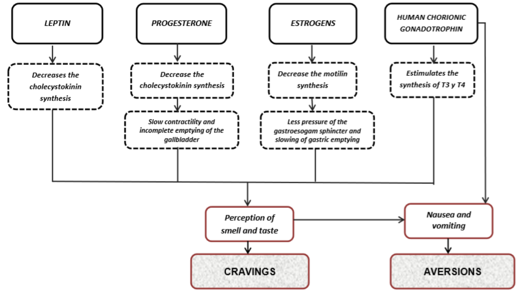
IGOJ 2019-112 - Laura Beatriz López Argentina_F1

Graph 1. Possible hormonal influence on food cravings and aversions.

The rabbi, physician and philosopher Maimonides (1138–1204) was one of the first to take into account changes in maternal physiology to describe food cravings, and proposed the theory that they were the result of an imbalance in body fluids, caused by the accumulation of “bad liquids” in the stomach folds of pregnant women, due to their inability to release menstrual blood during conception. When these liquids penetrated the stomach, a woman craved sour and spicy things until these unpleasant juices were eliminated by the vomit. As the pregnancy progressed and the growing fetus reduced the penetration of these fluids, women would be less susceptible to cravings and nausea [21].

Since then and until now, food cravings and aversions during pregnancy have been the focus of research and debate among anthropologists, nutritionists and public health professionals.

The present work consists of a narrative review that aims at describing the current state of knowledge about the different hypotheses that try to explain the presence of food cravings and aversions during pregnancy and to know the occurrence of these phenomena in different geographical contexts.

Hypothesis about the Presence of Food Aversions

Several hypotheses centered on a biological perspective have been postulated in order to understand why some pregnant women present food aversions; possibly the hypothesis of maternal-fetal protection has been the most studied. Other explanations with less bibliographic support link dietary aversions as preventive of the metabolic syndrome during pregnancy, or related to shortage of resources, or as a compensation mechanism for placental growth.

“Maternal-fetal protection hypothesis”

This theory is based on the fact that food aversions could protect the embryo or fetus against certain toxins at a moment of extreme vulnerability: organogenesis. Of the approximately 280 days that gestation lasts, embryonic tissues are more susceptible to teratogenic damage during certain well-defined critical periods, when cell division and differentiation and the morphogenesis of various systems and organs reach a simultaneous peak, produced between weeks 6 and 18. [10]. If the presence of food aversions occurs mostly during these periods, the pregnant woman could have developed different adaptive mechanisms to face the challenges of pregnancy.

This hypothesis is based on the year 1940, when Irving, in a study from Boston, observed that pregnant women with gravid hyperemesis had fewer spontaneous abortions than the usual expectation for that moment, postulating a possible association between nausea and vomiting with positive results during pregnancy [10, 22, 23].

Thirty-six years later, Ernest Hook resumed this observation and raised the “embryo protection hypothesis”, suggesting that in early pregnancy nausea, vomiting, food aversions, together with anatomical and sensory changes evolved as a complex set of symptoms that would make pregnant women avoid or expel foods with strong smells or flavors that could be potentially toxic and / or teratogenic. Their observations were based on the decrease in alcohol consumption, caffeine and the desire to smoke that women presented during pregnancy, which were explained by sensory changes and by nausea and vomiting, symptoms that could act as fetusprotectors [24].

Later in 1988, this hypothesis is extended by Margie Profet [25, 26], who proposes that nausea, vomiting and food aversions would be an evolutionary adaptation mediated by the modification of taste and olfactory sensibility to protect the embryo against the maternal ingestion of “toxins” present in some foods. Certain “toxic” plants that supposedly contain high levels of potentially abortive or teratogenic phytochemicals should be avoided. While humans commonly ingest phytochemicals naturally present in vegetables, and also selectively use phytochemicals in the preparation of food (spices), some of them could be potentially harmful during pregnancy, such as those present in bitter-tasting vegetables and spicy foods with strong flavor. Profet also suggests that the methods of cooking by frying, roasting or toasting would be the frequently aversive or avoided because their strong smells would indicate the presence of potentially mutagenic compounds, as well as decaying animal foods that emit suggestive smells due to the presence of parasites and / or bacteria that cause deterioration and produce toxins. On the other hand, it could be predicted that the best tolerated foods would be those that have mild smells and flavors and that do not decompose easily, such as breads, cereals and processed grains.

Later on, other authors deepened this hypothesis by renaming it “maternal-embryo protection hypothesis”, theorizing that pregnant women learn to avoid and / or expel through vomit potentially dangerous foods, not only for their embryos in development but also for themselves [8,11,12,27,28]. As part of this adaptation that evolved, in a coordinated way, the vomit would expel the noxious substance, while the nausea would be produced by an experience of aversion [27].

Hypothesis about “dietary aversions as preventive of the metabolic syndrome during pregnancy”

This proposal suggests that aversions during pregnancy may have evolved, in part, to motivate women to avoid eating foods that increase the risk of developing certain chronic non communicable diseases, particularly gestational diabetes mellitus [28–30].

Following this line of reasoning, dietary aversions would be an evolutionary tactic in populations without a long history of cereal cultivation to avoid the metabolic syndrome. This idea is based on evidences that come from populations in which, historically; the sugar necessary for fetal growth was not available due to a shortage of cereals, grains and starches or due to intense and regular cycles of hunger. In these cases, aversions to these carbohydrate-rich foods were possibly a mechanism to prevent the gestational metabolic syndrome [28, 29].

Hypothesis about “Scarcity of resources”

From the evolutionary biology, certain authors support that a decrease of the alimentary aversions during pregnancy in vulnerable populations could be predicted, with an important load of infectious diseases, with alimentary insecurity and anthropometric indexes that indicate a deficient maternal nutrition. However, studies in which all these associated factors were evaluated could not demonstrate their relationship with the food aversions of pregnant women [12, 31, 32].

Hypothesis about “Compensation of placental growth”

This hypothesis suggests that dietary aversions in the early stages of pregnancy would improve the growth of the placenta; thus, the fetus would exert a “manipulation” upon the maternal physiology, in such a way that mothers are motivated to avoid highly energetic meals. The restriction of maternal energy would benefit the fetus because, according to this hypothesis, mothers with restricted energy intake will prioritize the destiny of any resource that they have available for the development of the placenta and the embryo [28,33]. This position was based on observations of the severe hunger that affected the West of the Netherlands between the years 1944–1945 and its relationship with the weight of the placenta and neonate [28]. It was observed that when the period of maternal malnutrition occurs only during the first trimester, moment that coincides with the highest prevalence of food aversions, the neonates have weights within the normal range and greater weight of the placenta, effects that are not observed in undernourished mothers in the second half of pregnancy. This finding, which is also observed in animals, suggests that malnutrition in the first trimester would lead to a compensatory placental growth [33–35].

Hypothesis about the presence of food cravings

Different statements try to explain the reasons that could be responsible for the presence of cravings during pregnancy. The hypotheses found are: the search for nutrients or cravings in response to nutritional deficiencies; cravings in relation to the presence of active compounds in the desired foods and cravings as a result of hormonal fluctuations.

Hypothesis: “Cravings as a search for nutrients” or “In response to nutritional deficiencies”

From a biological perspective, it was postulated that cravings could serve to provide depleted nutrients in maternal diets, [9, 28]. This position considers craving as a mechanism to ensure adequate and balanced nutrition during pregnancy, which would motivate pregnant women to seek and consume foods rich in energy and micronutrients essential for fetal development.

Some authors consider that taking into account that the nutritional needs of the fetus increase as their development progresses, the intensity of the cravings should follow the same upward trajectory [9,28,36].

In 2002, the anthropologist Daniel Fessler, from an evolutionary perspective, also suggests that pregnant women may have a particular predisposition to seek through cravings, missing nutrients from their diets due to losses caused by aversions and vomiting; that is, there would be a functional link between cravings and food aversions [27]. These interactions were observed in pregnant women who had aversions to certain foods and they were more likely to have cravings compared to those who did not have food rejections [3]. However, this synergy between aversions and food cravings still remains a controversial issue that requires greater evidence from different geographical, social or cultural contexts [10].

Hypothesis: “Cravings are due to the presence of active compounds in the desired foods”

It is suggested that cravings could be due to the presence of active compounds (phytonutrients) in the desired foods [9]. The benefits of potentially bioactive ingredients are due to the possible ability to alleviate physical and perhaps psychological symptoms associated with pregnancy, such as fatigue, irritability and cramps, among others [9]. Chocolate being one of the foods most desired by pregnant women in some contexts, it is pointed out that women’s inclination to it could be cyclical and hormone dependent [9]. The biologically active components of chocolate such as methylxanthines, biogenic amines and cannabinoid-like fatty acids can trigger transient feelings of well-being during pregnancy [37]. However, this relationship is also questioned because the potentially active ingredients of chocolate are present in small quantities, which would make their potential benefits unlikely [9].

Hypothesis: “Cravings are due to hormonal fluctuations”

This hypothesis relates the presence of cravings with the sensory modifications resulting from the hormonal changes that occur during pregnancy. Several hormones such as estrogen, progesterone, leptin, ghrelin and neropeptide Y, among others, change significantly in this period affecting sensory perception with an increase in sensitivity to smells, taste and smell and indirectly being able to influence the selection pattern of the food. [9, 37, 39]. Despite these observations, there is an information gap that relates the exact nature of the link between hormonal fluctuations during pregnancy and food cravings [9].

(Table 1) summarizes the most relevant hypotheses and their foundations on the possible causes of the appearance of food aversions and cravings during pregnancy.

Table 1. Most relevant hypotheses and their foundations upon the possible causes of the appearance of food aversions and cravings during pregnancy.

Hypotheses	Authors, year (Reference)	Foundations
AVERSIONS
Maternal-fetal protection	Hook, 1978 (23) Profet, 1988 (24) Bayley, 2002 (8) Fessler, 2002 (26) Weigel, 2011 (11) Placek, 2015 (12) McKerracher, 2016 (27)	Nausea and vomiting work to protect the embryo by expelling dangerous chemicals transmitted by food and resulting in subsequent aversion. At first, the possible relationship between nausea, vomiting and aversions to alcohol, coffee and tobacco is explored. Then, this hypothesis is extended to certain “toxic” potentially abortive or teratogenic plants. After this, the presence of nausea and vomiting is linked to the development of food aversions and it is theorized that pregnant women learn to avoid and / or expel through vomit potentially dangerous foods not only for the developing embryo, but also for themselves.
Preventive of the metabolic syndrome during pregnancy	Haig, 1996 (44) McKerracher, 2016 (27)	The aversions during pregnancy may have evolved, in part, to motivate women to avoid eating foods that increase the risk of developing metabolic syndrome and / or gestational diabetes mellitus.
Scarcity of resources	Holland, 2003 (45) Placek, 2012 (12)	Food insecurity and anthropometric indices that indicate poor maternal nutritional status could predict a decrease in dietary aversions during pregnancy.
Compensation of placental growth	Huxley, 2000 (30). McKerracher, 2016 (27)	Malnutrition in the first trimester of pregnancy, a period that coincides with food aversions, would lead to compensatory placental growth.
CRAVINGS
Search for nutrients or in Response to nutritional deficiencies	Tierson, 1985 (33) Orloff, 2014(9) McKerracer, 2016 (27)	They consider craving as a mechanism to ensure adequate and balanced nutrition during pregnancy, in which women are motivated to seek and consume foods rich in energy and micronutrients essential for fetal development.
Presence of active compounds in the desired foods	Orloff, 2014 (9)	The pregnant woman, through cravings, consumes food with bioactives that produce a sensation of well-being.
Hormonal Fluctuations	Orloff, 2014 (9)	There is a relationship between hormonal changes and the frequency and intensity of cravings in pregnant women.

Although there may be a biological and evolutionary component in the development of these modifications in food preferences, food cravings or aversions do not escape the cultural food patterns that are also involved in the food choices of pregnant women [5]. There are civilizations that have a cultural model in which the cravings must be fulfilled by the pregnant woman, in some cases rituals are performed at the end of pregnancy to ensure that the wishes of the woman and the “fetus” have been fulfilled [9, 12]. However, in other cultural settings, pregnant women do not have a “special” treatment, so cravings are not very valued [12].

In such a way that from an anthropological and cultural perspective, interpreting the meanings behind the expressions of food cravings and aversions and unraveling the biocultural mechanisms of these food choices could be more complex than expected. In addition to evolutionary influences, experiences during an individual’s life can have significant impacts on the nature of food cravings and aversions. Both the context and social status as well as relative wealth can affect the choices of which foods are desired or avoided by the pregnant women [5].

Possible consequences postulated upon the presence of food cravings

Beyond the different theories that can cause food cravings, we have also tried to explain the possible consequences that such cravings could generate in the pregnant woman. A recent explanation suggests a possible association between cravings and the risk of excessive weight gain during pregnancy [9]. This association is based on the high frequency of cravings during pregnancy in North American women, and the increasing increment in the prevalence of pregnant women with greater weight gain than recommended [40–42]. This construction is based on the popular belief that cravings should be fulfilled by pregnant women. A possible explanation could be based on a model in which the cravings result from ambivalence or a tension between giving (please) or avoiding (effort to restrict consumption) the desired food. It is assumed that women, in general, try to resolve this ambivalence in favor of abstinence due to the cultural pattern of thinness, but this model also gives occasional permission to break the restriction, resulting in episodic consumption and potentially excessive of the desired foods [9]. This statement would be supported in part by recent studies [41, 43] that identify cravings during pregnancy as a possible predictor of excess of weight gain.

Another potential risk suggests that cravings for sweet foods are associated with an increased risk of abnormal glucose tolerance and the development of gestational diabetes mellitus [44, 45]. In some studies, women who developed gestational diabetes mellitus had a decreased perception of sweet taste and an increase in food cravings with that taste mainly during the third trimester, compared to healthy pregnant women. However, these associations are weak and other investigations fail to support this association between cravings for sweet-tasting foods and maternal blood glucose levels [45, 46].

Prevalence and characteristic of food cravings and aversions

The prevalence with which cravings occur varies from 40 to 79%, the lowest figure comes from Europe, while the highest prevalence corresponds to the African continent. With respect to food aversions, its occurrence varies from 38% in pregnant women in Asia to 78% in Africa.

The nature of the food desired and / or rejected also has special characteristics according to the geographical context in which they are studied, possibly shaped by cultural, ethnic and / or socio-economic influence. In general terms, foods craved for by pregnant women in Western cultures are chocolate, fruits and fruit juices, sweet foods such as ice cream and desserts and to a lesser extent different types of meat and dairy products. On the other hand, pregnant women in other geographic contexts of greater socioeconomic vulnerability experience cravings mainly for protein foods of animal origin such as meat, cheese and milk followed to a lesser extent by vegetables, fruits and grains.

On the other hand, meat and protein-rich foods such as dairy products are largely avoided by pregnant women from Western countries, followed by coffee, highly spicy foods and to a lesser extent vegetables. Cereals such as wheat, corn and rice and less strongly vegetables and meats are mostly avoided by pregnant women in other geographical areas such as Africa and Asia.

(Table 2) summarizes the prevalence and characterization of food cravings and aversions in different geographical contexts.

Table 2. Prevalence and characterization of food cravings and aversions in different parts of the world.

Author, year (reference)	Place (n)	Prevalence of cravings and foods mostly craved for	Prevalence of aversions and foods mostly aversive
Tsegaye, 1998 (3)	Africa, Etiophia (n:295)	72% Meat sauce, cheese and milk	65% Roasted wheat, coffee, wheat bread, meat sauce, kocho and injera.
Nyaruhucha, 2009 (47)	Africa, Tanzania (n: 204)	73% Meat, mango, yoghurt, orange, banana.	70% Rice, meat, fish, evo, legumes, tea.
Young, 2012 (5)	Africa, Kenya and Tanzania: (n:188)	56% Meat and milk.	78% Corn, millet, rice, buttermilk and blood. vegetables and fried foods.
Patil, 2012 (48)	Africa, Tanzania (n: 545)	79% Meat / fish, vegetables, fruits and grains.	63% Vegetables, meat, fish and grains.
Placek, 2015 (12)	Asia, India (n:149)	50% Sour foods (immature mango and tamarind), ethnic tasty and strong, vegetables and fruits, grains – starches and meat – sweets.	60% Fruits, tasty and strong ethnic foods, meat, vegetables and sweets, non-alcoholic beverages, starch-dairy products and ice cream.
Qureshi, 2015 (49)	Asia, Pakistan (n: 110)	78% Sweets, salty foods, spicy and fried food	38% Poultry products, sweets, tea, milk and rice and fried foods, legumes, spicy and vegetable foods.
Mc Kerracher, 2016 (27)	Oceania Fiji Islands, Yasawa (n: 70)	Bananas, mango, green leafy vegetables, fish and meat.	Fish, cassava, meat, non-fish aquatic foods, imported starches, locally grown starches and rarely spicy, sour or bitter-tasting vegetables.
Bayley, 2002 (8)	Europe, Great Britain (n: 99)	61% Fruits and fruit juices, sweet foods (sweets, chocolates, cookies).	54% Coffee, high-spiced foods, meats and protein-rich foods.
Hill, 2015 (43)	Europe, Great Britain (n: 1693)	39% Sweet foods (chocolate, sweets, ice cream, desserts), fruits and dairy products.	Not studied
Coronios Vargas, 1992 (4)	América, USA (n: 160)	dairy products, chocolate, tea vegetables, meats, sweets cereals, fermented fish, fruits ^a	Vegetables, meats and dairy products.
Weigel, 2011 (11)	América, Ecuador (n: 849)	69% Fruits and fruit juices (limes, apples, oranges, grapes, pineapple, tangerines, watermelons, mangoes and strawberries), meats, (poultry, fish, shellfish) eggs, foods rich in carbohydrates with starch.	74% Different types of meats (beef, pork, lamb, liver, other organs, sausages), poultry (chicken), fish (tilapia, sea bass, tuna), seafood (shrimp, prawns, squid) and chicken or quail eggs, “toxic vegetables” such as cabbage, cauliflower, broccoli, Brussels sprouts, onions, eggplants, tomatoes, turnips, potatoes and mellocos, an indigenous tuber similar to potatoes, white rice, wheat noodles, corn, barley and other foods with carbohydrates with starch.
Orloff, 2014 (9)	América, USA (n: 200)	Sweet foods (chocolate, candies), carbohydrates with high calories and flavors (pizza, chips) animal protein (meats, chicken), fruits, cheeses, creams, other carbohydrates, fast foods.	Not studied.
Orloff, 2016 (38)	América, USA (n: 83)	Sweet foods, as chocolate, cookies, ice creams and fast foods	Not studied.
Farland, 2015 (42)	América, USA (n: 2022)	45% Sweet foods (candies, desserts, cookies, fruit, fruit juices, cereals with sugar, ice cream, yogurt), salty (chips, fried potatoes, cheeses, fried foods, tasty (eggs, meats, mixed dishes, seafood), starches (bread, rice, pasta, potatoes).	Not studied.
Flaxman, 2000 (10)	Systematic review Cravings: 21 studies, n: 6239 Aversions: 20 studies, n: 5.432	67% Fruits and fruit juices, sweet foods, desserts and chocolate, followed by dairy products and cream ice cream and, to a lesser extent, meat.	65% Meat, fish, poultry and eggs, soft drinks and vegetables

^aVariations in the selection according to ethnic origin.

Conclusion

Cravings and food aversions are frequent phenomena that affect the selection of food during pregnancy; its etiology is still unclear. Numerous hypotheses focused on biological, cultural and anthropological approaches attempt to explain their occurrence. Although the description of food cravings and aversions during pregnancy has been studied by various authors, there is no uniformity of criteria in the modalities used for their characterization. Different types of questionnaires, the vast majority of which have not been validated, have been used to identify these phenomena. Having diagnostic tools specially designed to know the occurrence and describe the cravings and aversions during pregnancy is an important step to learn more about the relationship these changes may have in the selection of foods with nutritional status and maternal-fetal health.

Acknowledgement

This Word was supported by the University of Buenos Aires (UBACyT Code: 20020170100385BA).

References

Academy of Nutrition and Dietetics (2014) Position of the Academy of Nutrition and Dietetics: Nutrition and lifestyle for a healthy pregnancy outcome. J Acad Nutr Diet 114: 1099–1103.
Gernand AD, Schulze KJ, Stewart CP, West Jr KP, Parul C (2016) Micronutrient deficiencies in pregnancy worldwide: Health effects and prevention. Nat Rev Endocrinol 12: 274–289.
Tsegaye D, Muroki NM, Kogi-Makau W (1998) Food aversions and cravings during pregnancy: Prevalence and significance for maternal nutrition in Ethiopia. Food and Nutrition Bulletin 19: 85.
Coronios-Vargas M, Toma RB, Tuveson RV, Schutz IM (1992) Cultural influences on food cravings and aversions during pregnancy. Ecol Food Nutr 27: 43–49.
Young AG, Pike IL (2012) A Biocultural Framework for Examining Maternal Cravings and Aversions among Pastoral Women in East Africa. Ecol Food Nutr 51: 444–462.
Patil CL, Young SL (2012) Biocultural considerations of food cravings and aversions: an introduction. Ecol Food Nutr 51: 365–373. [crossref]
Mahaluf ZJ, Nader NA, Correa D, Vargas J, Arraztoa V, et al. (1991) El antojo en la embarazada definición inicial. Rev. Psiquiatr clín 28: 118–125.
Bayley TM, Dye L, Jones S, DeBono M, Hill AJ (2002) Food cravings and aversions during pregnancy: relationships with nausea and vomiting. Appetite 38: 45–51. [crossref]
Orloff NC1, Hormes JM (2014) Pickles and ice cream! Food cravings in pregnancy: hypotheses, preliminary evidence, and directions for future research. Front Psychol 5: 1076. [crossref]
Flaxman SM1, Sherman PW (2000) Morning sickness: a mechanism for protecting mother and embryo. Q Rev Biol 75: 113–148. [crossref]
Weigel MM, Coe K, Castro NP, Caiza ME, Tello N, et al. (2011) Food Aversions and Cravings during Early Pregnancy: Association with Nausea and Vomiting. Ecol Food Nutr 50: 197–214.
Placek CD1, Hagen EH (2015) Fetal Protection : The Roles of Social Learning and Innate Food Aversions in South India. Hum Nat 26: 255–276. [crossref]
López LB, Ortega Soler CR, Pita Martín de Portela ML (2004) La pica durante el embarazo: un trastorno frecuente subestimado. Arch Latinoam Nutr 54: 17–24.
Poy MS, Weisstaub A, Iglesias C, Fernández S, Portela ML, et al. (2012) [Pica diagnosis during pregnancy and micronutrient dificiency in Argentine women]. Nutr Hosp 27: 922–928. [crossref]
Meyer-Rochow VB (2009) Food taboos: their origins and purposes. J Ethnobiol Ethnomed 5: 18. [crossref]
Vasilevski V, Carolan-Olah M (2016) Food taboos and nutrition-related pregnancy concerns among Ethiopian women. J Clin Nurs 25: 3069–3075.
Carlin A, Alfirevic Z (2008) Physiological changes of pregnancy and monitoring. Best Pract Res Clin Obstet Gynaecol 22: 801–823. [crossref]
Purizica M (2010) Modificaciones fisiológicas en el embarazo. Rev PeR Ginecol obstet 56: 57–69.
Ojeda González J, Rodríguez Alvarez M, Estepa Pérez J, Piña Loyola, Cabeza Poblet B (2011) Cambios fisiológicos durante el embarazo. Su importancia para el anestesiólogo. Revista Electrónica de las Ciencias Médicas en Cienfuegos 9: 484–491.
Soma-Pillay P, Nelson-Piercy C, Tolppanen H, Mebazaa A (2016) Physiological changes in pregnancy. Cardiovasc J Afr 27: 89–94. [crossref]
Graves A (2010) Synapse. The Boston University Undergraduate Science magazine. http://www.bu.edu/synapse/2010/07/28/the-mystery-of-pregnancy-cravings/
Irving FC (1940) The treatment of pernicious vomiting of pregnancy. Virginia Medical Monthly 67: 717–724 https://archive.org/details/virginiamedicalm67unse/page/n775.
Flaxman SM, Sherman PW (2008) Morning sickness: adaptive cause or nonadaptive consequence of embryo viability? Am Nat 172: 54–62. [crossref]
Hook EB (1978) Dietary cravings and aversions during pregnancy. Am J Clin Nutr 31: 1355–1362. [crossref]
Profet M (1988) The evolution of pregnancy sickness as protection to the embryo against Pleistocene teratogens. The University of Chicago. Biology Department. Evolutionary theory 8: 177–190.
Profet M (1995) Pregnancy sickness as adaptation: a deterrent to maternal ingestion of teratogens. Adapt Mind 327–365.
Fessler DM (2002) Reproductive immunosupression and diet. An evolutionary perspective on pregnancy sickness and meat consumption. Curr Anthropol 43: 19–61.
McKerracher L, Collard M, Henrich J (2016) Food Aversions and Cravings during Pregnancy on Yasawa Island, Fiji. Hum Nat 27: 296–315.
Brown EA, Ruvolo M, Sabeti PC (2013) Many ways to die, one way to arrive: how selection acts through pregnancy. Trends Genet 29: 585–592. [crossref]
Drewnowski A (1997) Taste preferences and food intake. Annu Rev Nutr 17: 237–253. [crossref]
Haig D (1996) Altercation of generations: genetic conflicts of pregnancy. Am J Reprod Immunol 35: 226–232. [crossref]
Huxley RR (2000) Nausea and vomiting in early pregnancy: its role in placental development. Obstet Gynecol 95: 779–782.
Holland TD, O’Brien MJ (2003) On morning sickness and the Neolithic revolution. Current Anthrop 44: 707–711.
Lumey LH (1998) Compensatory placental growth after restricted maternal nutrition in early pregnancy. Placenta 19: 105–111.
Godfrey K, Robinson S, Barker DJ, Osmond C, Cox V (1996) Maternal nutrition in early and late pregnancy in relation to placental and fetal growth. BMJ 312: 410–414. [crossref]
Tierson FD, Olsen CL, Hook EB (1985) Influence of cravings and aversions on diet in pregnancy. Ecol Food Nutr 17: 117–129.
Räikkönen K, Pesonen AK, Järvenpää A-L, Strandberg TE (2004) Sweet babies: chocolate consumption during pregnancy and infant temperament at six months. Early Hum Dev 76: 139–145.
Nordin S, Broman DA, Olofsson JK, Wulff M (2004) A longitudinal descriptive study of self-reported abnormal smell and taste perception in pregnant women. Chem Senses 29: 391–402. [crossref]
Nordin S, Broman DA, Bringlöv E, Wulff M (2007) Intolerance to ambient odors at an early stage of pregnancy. Scand J Psychol 48: 339–343. [crossref]
Institute of Medicine (2009) Weight Gain During Pregnancy: Reexamining the Guidelines. Washington, D.C. National Academy Press.
Orloff NC, Flammer A, Hartnett J, Liquorman S, Samelson R, et al. (2016) Food cravings in pregnancy: Preliminary evidence for a role in excess gestational weight gain. Appetite 105: 259–265.
Academy of Nutrition and Dietetics (2016) Position of the Academy of Nutrition and Dietetics: Obesity, Reproduction, and Pregnancy Outcomes. J Acad Nutr Diet 116: 677–691.
Allison KC, Wrotniak BH, Pare E, Sarwer DB (2012) Psychosocial characteristics and gestational weight change among overweight, African-American pregnant women. Obstet Gynecol 2012: 878607.
Belzer LM, Smulian JC, Lu SE, Tepper BJ (2010) Food cravings and intake of sweet foods in healthy pregnancy and mild gestational diabetes mellitus. A prospective study. Appetite 55: 609–615.
Farland LV, Rifas-Shiman SL, Gillman MW (2015) Early Pregnancy Cravings, Dietary Intake, and Development of Abnormal Glucose Tolerance. J Acad Nutr Diet 115: 1958–1964.
Hill AJ, Cairnduff V, McCance DR (2016) Nutritional and clinical associations of food cravings in pregnancy. J Hum Nutr Diet 29: 281–289. [crossref]
Nyaruhucha CNM (2009) Food cravings, aversions and pica among pregnant women in Dar es Salaam, Tanzania. Tanzan J Health Res 11: 29–34.
Patil CL (2012) Appetite Sensations in Pregnancy among Agropastoral Women in Rural Tanzania. Ecol Food Nutr 51: 431–443.
Qureshi Z, Khan R (2015) Diet intake trends among pregnant women in rural area of Rawalpindi, Pakistan. J Ayub Med Coll Abbottabad 27: 684–688.

A rare case of distant metastasis of primary malign pericardial mesothelioma with 18F-FDG PET/CT

Leave a reply

DOI: 10.31038/JCRM.2019234

ABSTRACT

Primary pericardial mesothelioma is a rare malignant tumor derived from the pericardial mesothelial cell layers. 65-year-old man was admitted to hospital with dyspnea and chest pain. Pericardial effusion and pericardial tamponade were observed with transthoracic echocardiography. Contrast-enhanced computed tomography (CECT) demostrated pericardial effusion, diffuse pericardial thickening and pleural effusion in both hemithorax. The final diagnosis was proven as primary malignant pericardial mesothelioma with histopathological evaluation. Subsequently, F-18 FDG PET-CT scan demonstrated high FDG uptake in pericardial thickening areas. Additionally, increased FDG uptake was also seen in the hypodense lesions in the both adrenal gland lesions and in liver.

Keywords

PET-CT, echocardiography, primary malign pericardial mesothelioma, FDG

INTRODUCTION

Malignant mesothelioma (MPM) is a rare, aggressive malignant tumor derived from the mesothelial cells of serosal membranes. Malignant mesothelioma may occur most frequently from the pleura (90%), less frequently from the peritoneum (6–10%) and from the pericardium, and very rarely from the tunica vaginalis in the testis [1]. Primary pericardial mesotheliomas (PPM) very rare malignancy (incidence 0,0022 %). It represents 6% of all mesothelioma cases [2]. It usually provides nonspecific findings such as dyspnea, fever, cough and chest pain. It is more common in men. The mean age was 46 (19–76) years [3]. Mesotheliomas particularly metastasize to the intratorasic lymph nodes or lung, distant extrathorasic metastasis is very rarely observed [4]. Various imaging methods can be used for the diagnosis such as echocardiography (ECO), chest X-ray, chest CT, magnetic resonance imaging (MRI) and positron emission tomography-computed tomography (PET-CT) [5]. PET-CT imaging have an important role in staging, treatment response, recurrence detection and prognosis in pleural mesothelioma [6]. In contrast to pleural mesothelioma, a few case reports with PPM is described by FDG PET-CT [7].

CASE

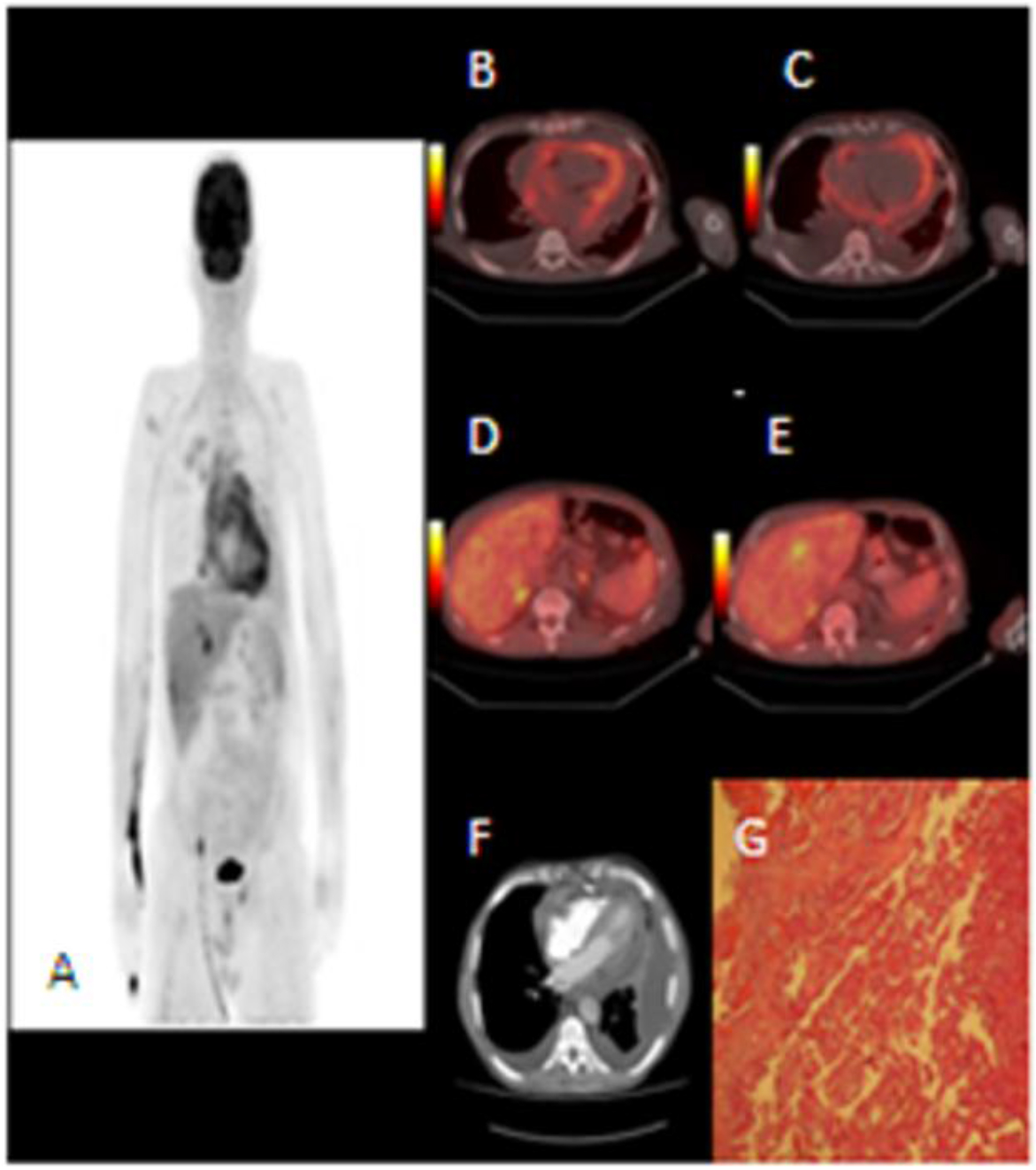
A 65-year-old male was admitted to the cardiology clinic with complaints of dyspnea and chest pain. He had no prior history of exposure to asbestos. Echocardiography showed pericardial effusion and tamponade findings. Diagnostic and therapeutic pericardiocentesis with pericardial drain was performed, all laboratory analyses showed normal results, cultivations and polymerasechain reaction (PCR) for tuberculosis were negative. Contrast-enhanced computed tomography (CECT) showed pericardial effusion, diffuse pericardial thickening and pleural effusion in both hemithorax (Figure 1-F).

JCRM 2019-112 - Tarik Sengoz Turkey_F1

Figure 1. A-MIP imaging of PET. B.C.D.E- Axial fusion imaging. B.C-Diffuse FDG uptake in pericardial thickining (SUVmax: 6,2). D- Focal FDG uptake in both adrenal glands (SUVinax: 3,l and 5,8). E-Focal FDG uptake in liver (SUVmax: 4,0). F-Axial CECT show diffuse pericardial thickining and effusion. G-liistopathological evaluation of malignant pericardial mesotheliomas (H&E).

F-18 FDG PET-CT scan demostrated intense uptake in diffuse pericardial thickening areas, with a maximum standardized uptake value (SUVmax) of 6.2 (Figure 1-A). Fused PET-CT images indicated the thickened pericardium with high FDG uptake (Figure 1-B,C). Furthermore, fused PET-CT images showed increased FDG uptake both in adrenal gland lesions (SUVmax: 3.1–5.8) (Figure 1-D) and in the hypodense lesion with a diameter of 1 cm in in liver segment 4A (SUVmax: 4.0) (Figure 1-E). Cytologic evaluation of pericardial effusion demonstrated with malignant pericardial mesothelioma. However, immunohistochemistry evaluation was not able to be performed. The case was evaluated as the PPM with liver and bilateral surrenal gland metastases. While the chemotherapy was planning, the patient had multiorgan insufficiency and emergency dialysis. Cardiac arrest developed two times during the dialysis and resulted in death.

DISCUSSION

PPM is a very rare malignant tumor of 6% of all mesotheliomas [8]. It can be seen in the form of mass formation or disseminated pericardial thickening. The effect of asbestos exposure is not as clear as pleural and peritoneal mesothelioma. The symptoms are usually nonspecific (fatigue, shortness of breath, chest pain, cough, etc.). It may indicate pericardial effusion, constrictive pericarditis, cardiac tamponade, and congestive heart failure in the clinic [9]. Imaging methods such as chest radiography, transthoracic echocardiography, CECT, MRI are used in the diagnosis.

In ECO and chest X-ray radiography, an enlarged heart silhouette and pericardial effusion are described, whereas the pericardial mass cannot be differentiated. In a review of 28 pericardial mesothelioma cases, mediastinel mass could be differentiated in only one of 24 cases with X-ray graph [3]. Although CECT is an effective examination to demonstrate tumor invasion and pericardial thickening, sometimes large pericardial effusion complicate the evaluation of the mass [10]. ECO and CECT have a low sensitivity (12–44%) in detecting pericardial mass (3). The use of MRI is limited, high signal intensity in T2-weighted image has been demonstrated in one patient [11].

FDG is a glucose analogue and offers metabolic information on the basis of increased glucose uptake due to the increased glucose requirement in cancer cells. PET-CT is frequently used in the diagnosis, staging and treatment response of many different cancers. Since the use of PET-CT in pleural mesothelioma has been well known [6], the knowledge in PPM is limited. There was no information about FDG PET-CT in the review of Thomson et al. with 27 PPM cases between 1972–1992 [3] and in the review of Nilsson et al. with 29 PPM cases between 1994–2008 [12]. After 2008, 5 PPM cases confirmed with PET-CT were found [13–17] . 3 of 5 cases were female and 2 of them were male. The average age is 52 (19–72). The characteristics of 5 cases are summarized in Table 1. In 3 of the patients, PET-CT showed no regional lymph nodes and distant metastases, while the other 2 cases had mediastinel lymph node metastasis [15,17]. In our case, liver and bilateral surrenal gland metastasis were detected. Thus, our case was the first case with liver and adrenal metastasis detected by PET-CT. Metastasis is seen in 25–45% of PPM cases. Generally, regional lymph nodes, lung and kidney metastases were detected [18]. Nilsson et al. study, metastasis was defined in 16 (55%) of 29 PPM cases (lymph nodes, liver and lung metastasis) [12]. Cytological examination of pericardial fluid in PPM does not always distinguish between reactive / malignant cells. Pericardial biopsy may be required for the final diagnosis [19]. Although the diagnosis was made after pericardiectomy in 5 cases in literature, our patient was diagnosed with pericardiocentesis (Table 1).

Table 1. Cases of pericardial mesothelioma with F-18 FDG PET/CT published in the literature

Case	Age	Sex	Symptom	Asbestos exposure	Radiological imaging	PET-CT	Pathology
Our case	65	M	Dyspnea, chest pain	none	USG: pericardial effusion CT: pericardial effusion, pericardial thickining	PPM (SUVmax:6.2), liver (SUVmax:4.0) and bilateral adrenal (SUVmax:3.1-5.8) met	pericardiosentesis
3	72	F	unspecified	none	CT: pericardial thickining	PPM (SUVmax not specified)	pericardial biopsy
4	58	F	Fewer, fatigue	unspecified	X-ray: enlarged cardiac silhouette USG: pericardial effusion without ventricul dilatation CT: pericardial mass	PPM (SUVmax:12.9) and dissemine pericardial spread	Subtotal pericardiectomy
5	19	F	Dyspnea, chest pain, low exercise capacity	unspecified	X-ray: enlarged cardiac silhouette USG: pericardial effusion without ventricul dilatation CT: pericardial thickining/effusion MR: pericardial mass	PPM (SUVmax:5.22) and mediastinel lymph node metastasis (SUVmax:1.6)	Partial pericardiectomy
7	54	M	Dyspnea	none	USG: pericardial effusion without ventricul dilatation CT: pericardial thickining/effusion	PPM (SUVmax:7.5)	pericardiectomy
8	57	M	Dyspnea, ankle edema	unspecified	USG: constrictive pericarditis	PPM (SUVmax:19.5) and mediastinel lymph node metastasis	pericardiectomy

M: male, F:female, USG: transthoracic echocardiography, CT: Computed tomography, MR: Magnetic resonance imaging, PET-CT: positron emission tomography- computed tomography, PPM: primary pericardial mesothelioma

Treatment is often palliative, curative treatment is not possible in PPM. Surgical resection, chemotherapy and radiotherapy are the treatment options. Average survival was reported as 10 months in one study [19]. Our patient was died 16 day after the diagnosis.

Consequently, PET-CT can change the management of patients with PPM by showing the distant metastasis. However, the shortness of survival and the palliative treatment are the factors that limit the effect of PET-CT on the treatment plan. Our case is differentiated due to liver and bilateral surrenal metastasis from PPM confirmed by PET-CT in the literature. In the future, it can be predicted that PET-CT have an important role for PPM like pleural mesothelioma.

REFERENCES

Adams VI, Unni KK, Muhm JR, et al. (1986) Diffuse malignant mesothelioma of pleura: Diagnosis and survival in 92 cases. Cancer 58: 1540–51. [Crossref]
Ohmori T, Arita N, Okada K, et al. (1995) Pericardial malignant mesothelioma: case report and discussion of immunohistochemical and histological findings. Pathol Int. 45: 622–625. [Crossref]
Thomason R, Schlegel W, Lucca M, et al. (1994) Primary malignant mesothelioma of the pericardium. Case report and literature review. Tex Heart Inst J 21: 170–174. [Crossref]
Silvestri F, Bussani R, Pavletic N, et al. (1997) Metastases of the hearth and pericardium. G Ital Cardiol. 27: 1252–1255.
Maisch B, Seferovic PM, Ristic AD, et al. (2004) Guidelines on diagnosis and management of pericardial diseases executive summary;The task force on the diagnosis and management of pericardial diseases of the European society of cardiology. Eur Hearth J. 25: 587–610. [Crossref]
Gerbaudo VH, Sugarbaker DJ, Britz-Cunningham S, et al. (2002) Assessment of malignant pleuralmesothelioma with (18)F-FDG dual-head gamma-camera coincidence imaging: comparison with histopathology. J Nucl Med. 9: 1144–1149. [Crossref]
Ceresoli GL, Chiti A, Zucali PA, et al. (2006) Early response evaluation in malignant pleural mesothelioma by positron emission tomography with [18F]fluorodeoxyglucose. J Clin Oncol. 24: 4587–4593. [Crossref]
Burke A, Virmani R. (1996) Malignant mesothelioma of the pericardium. In: Rosai J, Sobin LH, eds. Tumors of the Heart and Great Vessels. Atlas of Tumor Pathology, Third Series, Fascicle 16. Washington, DC: Armed Forces Institute of pathology; 181–194.
Eren NT, Akar AR. (2002) Primary pericardial mesothelioma. Curr Treat Options Oncol 3: 369–73. [Crossref]
Quinn DW, Qureshi F, Mitchel IM. (2000) Pericardial mesothelioma: the diagnostic dilemma of misleading images. Ann Thorac Surg. 69: 1926–1927.
Gössinger HD, Siostrzonek P, Zangeneh M, et al. (1988) Magnetic resonance imaging findings in a patient with pericardial mesothelioma. Am Heart J 115: 1321–2. [Crossref]
Nilsson A, Rasmuson T. (2009) Primary pericardial mesothelioma: Report of a patient and literature review. Case Rep Oncol 2: 125–132. [Crossref]
Sakuraba M, Tatsumori T, Hirama M, Ogura K.(2011) Malignant pericardial mesothelioma. European Journal of Cardio-thorasic Surgery 39: 420.
Aga F, Yamamoto Y, Norikane T, Nishiyama Y. (2012) A case of primary pericardial mesothelioma detected by ¹⁸F-FDG PET/CT. Clin Nucl Med 37: 522–523. [Crossref]
Ost P, Rottey S, Smeets P, et al. (2008) F-18 Fluorodeoxyglucose PET/CT scanning in the diagnostic work-up of a primary pericardial mesothelioma: a case report. J Thorac Imaging 23: 35–38. [Crossref]
Sivrikoz İA, Onner H, Dundar EK, et al. (2016) F-18 FDG PET/CT images of rare primer cardiac tumour: primary pericardial mesothelioma. Anatol J Cardiol 16: 635–638. [Crossref]
Edel JP, Balink H. (2018) ¹⁸F-FDG PET/CT revealing constrictive pericarditis as the only manifestation of malignant mesothelioma. Clin Nucl Med 00: 00 (accepted, but yet unpublished). [Crossref]
Karadzic R, Kostic-Banovic L, Antovic A, et al. (2005) Primary pericardial mesothelioma presenting as constrictive pericarditis. Arch Oncol 13: 150–152.
Kaul TK, Fields BJ, Kahn DR. (1994) Primary malignant pericardial mesothelioma: a case report and review. J Cardiovasc Surg. 35: 261–267. [Crossref]

Late Rise Human Chorionic Gonadotropin after Embryo Transfer: Causality and Significance! A mini review

Leave a reply

DOI: 10.31038/IGOJ.2019233

Abstract

The reliable detection of hCG in maternal blood usually coincides with the embryonic implantation phase which is around 7 days post fertilization. It is believed that hCG levels taken post embryo transfers have a diagnostic and prognostic value when it comes to reproductive outcomes. Very low initial hCG levels predict a higher risk of chemical pregnancies, miscarriages and ectopic pregnancies. A review of the literature was performed so as to understand the mechanisms leading to late hCG rises as well as significance of such findings.

Introduction

Human chorionic gonadotropin (hCG) is produced by the placental syncytio-trophoblasts as early as 7–8 blastomere stage of the embryonic development i.e. before actual implantation takes place (M.-L.Bonduelle et al. 1988). The reliable detection of hCG in maternal blood usually coincides with the embryonic implantation phase which is around 7 days post fertilization (Ahmed et al. 1983). While serial hCG levels aren’t usually monitored in spontaneous pregnancies, women undergoing assisted reproductive technologies (ART) treatments usually necessitate such an approach especially after embryo transfer (ET). It is believed that hCG levels taken post ET have a diagnostic and prognostic value when it comes to miscarriages, ectopic pregnancies, predicting multiple gestations as well as live births (Schmidt et al., 1994, McCoy et al. 2009).

Discussion

Despite the lack of consensus on the hCG cutoff values that correlate with the best ART outcomes, a bulk of the studies use a value of 70 mIU/ml on day 14 post ovum pickup as an acceptable reference value (Sung et al. 2016). Values equivalent to 5 mIU/mL or below are judged as negative pregnancy tests (Sung et al. 2016, Maslow et al. 2016). It is believed that the amount of hCG produced reflects the mass of the trophoblast tissue as well as it’s function (Porat et al. 2007). Despite the discrepancies in the literature, there is a certain agreement that very low initial hCG levels are associated with adverse pregnancy outcomes and intra-uterine growth restriction. This can be explained by the small placental mass with a suboptimal function thus preventing normal fetal growth (Haddad et al. 1999, Krantz et al. 2004, Porat et al. 2007). A possible explanation for the latter might be that some embryos have a division lag, thus a later or abnormal implantation due to variances in trophoblast differentiation (invasive/extravillous versus hCG-producing/ villous phenotype) in an endometrium of decreased receptivity (Bolton et al. 1989, Woodward et al. 1993, Smith et al. 2004, Morse et al. 2016). Jukic et al. found out that smoking status and age at menarche affected the time of implantation by almost 24 hours and thus a late hCG rise. Current active or passive smoking status was significantly associated with delayed implantation. Younger age at menarche (younger than 12 years of age) was also found to be associated with a slow initial hCG rise (Jukic et al.2011). On another note, low initial hCG levels from 1.0 to 5.0 mIU/mL might be due to a false negative result related to laboratory methodology used for the hCG titration (Maslow et al. 2016). It s worth mentioning that it’s not only the initial hCG value but the doubling time as well as the hCG- rise curve is more correlated with the pregnancy outcome (Shamonki et al. 2009, Maslow et al. 2016, Morse et al. 2016). A doubling time of 2 days has been set as the best predictor of live birth rate although an increase rate as low as 53% can also predict a viable pregnancy (Shamonki et al. 2009, Seeber et al. 2012). Initial hCG value post ET is important to diagnose a possible pregnancy, however it doesn’t correlate alone with the possibility of a live birth. Serial hCG levels are important especially when the initial values are lower than the cut-off value.

References

Ahmed, A. G., and A. Klopper. “Diagnosis of early pregnancy by assay of placental proteins.” BJOG: An International Journal of Obstetrics & Gynaecology 90.7 (1983): 604–611.
Bolton VN, Hawes SM, Taylor CT, Parsons JH. Development of spare human preimplantation embryos in vitro: an analysis of the correlations among gross morphology, cleavage rates, and development to the blastocyst. J In Vitro Fert Embryo Transf 1989; 6: 30–5
Bonduelle, M-L., et al. “Chorionic gonadotrophin-β mRNA, a trophoblast marker, is expressed in human 8-cell embryos derived from tripronucleate zygotes.” Human Reproduction 3.7 (1988): 909–914.
Haddad, Bassam, et al. “Predictive value of early human chorionic gonadotrophin serum profiles for fetal growth retardation.” Human Reproduction 14.11 (1999): 2872–2875.
Jukic, A. M. Z., et al. “The association of maternal factors with delayed implantation and the initial rise of urinary human chorionic gonadotrophin.” Human reproduction 26.4 (2011): 920–926.
Krantz, David, et al. “Association of extreme first-trimester free human chorionic gonadotropin-β, pregnancy-associated plasma protein A, and nuchal translucency with intrauterine growth restriction and other adverse pregnancy outcomes.” American Journal of Obstetrics & Gynecology 191.4 (2004): 1452–1458.
Maslow, Bat-Sheva L., et al. “Occult abnormal pregnancies after first post–embryo transfer serum beta-human chorionic gonadotropin levels of 1.0–5.0 mIU/mL.” Fertility and sterility 105.4 (2016): 938–945.
McCoy, Travis W., Steven T. Nakajima, and Henry CL Bohler. “Age and a single day-14 β-HCG can predict ongoing pregnancy following IVF.” Reproductive biomedicine online19.1 (2009): 114–120.
Morse, Christopher B., et al. “Association of the very early rise of human chorionic gonadotropin with adverse outcomes in singleton pregnancies after in vitro fertilization.” Fertility and sterility 105.5 (2016): 1208–1214
Porat, Shay, et al. “Early serum β-human chorionic gonadotropin in pregnancies after in vitro fertilization: contribution of treatment variables and prediction of long-term pregnancy outcome.” Fertility and sterility 88.1 (2007): 82–89.
Schmidt, Lila L., et al. “The predictive value of a single beta human chorionic gonadotropin in pregnancies achieved by assisted reproductive technology.” Fertility and sterility 62.2 (1994): 333–338.
Seeber, Beata E. “What serial hCG can tell you, and cannot tell you, about an early pregnancy.” Fertility and sterility 98.5 (2012): 1074–1077.
Shamonki, Mousa I., et al. “Logarithmic curves depicting initial level and rise of serum beta human chorionic gonadotropin and live delivery outcomes with in vitro fertilization: an analysis of 6021 pregnancies.” Fertility and sterility 91.5 (2009): 1760–1764.
Sung, Nayoung, et al. “Serum hCG-β levels of postovulatory day 12 and 14 with the sequential application of hCG-β fold change significantly increased predictability of pregnancy outcome after IVF-ET cycle.” Journal of assisted reproduction and genetics 33.9 (2016): 1185–1194.
Woodward BJ, Lenton EA, Turner K. Human chorionic gonadotrophin: embryonic secretion is a time-dependent phenomenon. Hum Reprod 1993;8: 1463–8.

Hydatid Disease and Pregnancy: A Short Note

Leave a reply

DOI: 10.31038/IGOJ.2019232

Short Commentary

Tapeworm is the common name of the cestode worm, Echinococcus granulosus, which is the causal agent of hydatid disease in humans. This helminth infection is also known as cystic echinococcosis and hydatidosis, and is included in the zoonoses group. According to WHO [1]: (i) more than 1 million people are affected with echinococcosis at any one time; (ii) infection is globally distributed and found in every continent except Antarctica; (iii) robust surveillance is fundamental in order to show burden of disease and to evaluate progress and success of control programmes. However, as for other neglected diseases which are focused in underserved populations and remote areas, data is especially scarce and will need more attention if control programmes are to be implemented and measured; (iv) ultrasonography imaging is the technique of choice for diagnosis of cystic echinococcosis; (v) cysts can be incidentally discovered by radiography. Specific antibodies are detected by different serological tests and can support the diagnosis. Biopsies and ultrasound-guided punctures may also be performed for differential diagnosis of cysts from tumors and abscesses; (vi) cystic echinococcosis are often expensive and completed to treat, sometimes requiring extensive surgery and/or prolonged drug therapy.

As to transmission: (i) a number of herbivorous and omnivorous animals act as intermediate hosts of E. granulosus. They become infected by ingesting the parasite eggs in contaminated food and water, and the parasite then develops into larval stages in the viscera; (ii) carnivores act as definitive hosts for the parasite, and host the mature tapeworm in their intestine. They are infected through the consumption of viscera of intermediate hosts that harbor the parasite; (iii) humans act as so- called accidental intermediate hosts in the sense that they acquire infection in the same way as other intermediate hosts, but are not involved in transmitting the infection to the definitive host; (iv) several distinct genotypes of E. granulosus are recognized some having distinct intermediate hosts preferences. Some genotypes are considered species distinct from E. granulosus. Not all genotypes cause infections in humans. The genotype causing the great majority of cystic echinococcosis infections in humans is principally maintened in a dog-sheep-dog cycle, yet several other domestic animals may also be involved, including goats, swine, cattle, camels and yaks; (v) human infection with E. granulosus leads to the development of one or more hydatid cysts located most often in the liver and lungs, and less frequently in the bones, kidney, spleen, muscles, central nervous system and eyes; (vi) abdominal pain, nauseas and vomiting are commonly seen when hydatids occur in the liver. If the lung is affected, clinical signs include chronic cough, chest pain and shortness of breath. Other signs depend on the location of the hydatid cysts and the pressure exerted on the surrounding tissues.

These results of the parasitism for tapeworms in humans show that it may have direct and indirect consequences in human health, in general. cause devastating morbidity with severe consequences in general and in female reproductive health. Here our objective is to alert medical practitioners of gynecology and obstetrics for hydatid cyst in pregnancy.

The authors: (2) report that “Incidence of hydatid disease in pregnancy ranges from 1 in 20,000 to 1 in30,000. The diagnosis of liver hydatid cyst is not difficult but management during pregnancy is problematic. Both medical and surgical treatments are available but there is no consensus and each case has to be individualized”; (3) report “we present a 32-years old multigravida at 25 weeks of pregnancy in whom splenic and liver cysts were diagnosed by ultrasonography and magnetic resonance imaging (MRI). The splenic cyst was removed and a healthy baby was delivered vaginally at term”; (4) report “Case report A 25-year-old, gravida 1, para 0 pregnant female with history of liver cyst was admitted to the obstetric outpatient clinic for checkup. Patient who did not have any complaints was redirected to the radiology clinic for a second trimester ultrasound scan. Abdominal ultrasound revealed lesions of type-1, hydatid cyst 84×67 mm in size at the right lobe fifth segment, and 67×64 mm in size at the seventh segment of the liver, with millimetric echogenic female cysts and well-defined thickwalls. In addition, a type-2 hydatid cyst with membrane dissociation, 55×52 mm in size, was observed at the caudate lobe. An intrauterine fetus with fetal heart rate was observed with a bipariental diameter concordant with 21 weeks of gestation. Besides, there was a cystic lesion with fine septations surrounding the uterus. The patient was admitted to the obstetric care service with hydatid cyst hydatidosis in the vicinity of the uterus; (5) report “A young, apparently healthy from a rural area in South Africa presented in the third trimester of pregnancy with a symptomatic abdominal mass between the uterine fundus and liver. The etiology was established to be an echinococcus cyst of the liver and medical treatment was initiated. The fetal outcome was good but the mother died 3 days postpartum due to an unusual but devastating complication of the hydatid cyst; (6) report the management of hydatid disease in pregnancy, and they write that “in this review, we have attempted to summarize the presentation and available management approaches to hydatid disease, and have suggested evidence-based guidelines for its management during pregnancy; (7) report 2 cases of hydatid disease of liver during pregnancy, and they also made a review of literature; (8) report “A huge primary hydatid cyst of uterus” and they made also a review of literature.

Final conclusion: 1 – we think that it was here demonstrated the importance of the hydatid cyst as an underlying cause of negative effects in pregnancy; 2 – surgery in patients with hydatid cysts needs special care before, during or after surgery. Effectively, opening of a hydatid cyst requires special care not to spill the contents into the peritoneal cavity or tissues, since this may result in an anaphylactic reaction to the spilt fluid or dissemination and implantation of the immature scolices contained in the “sand” in the fluid. Incomplete removal of viable germinal epithelium from the liming of a hydatid cyst results in the formation of multiple cysts: 3 – we are in agreement with the conclusions of the authors (9): E. granulosus can affect any organ in the body from head to toe, and high suspicion of this disease is justified in endemic regions.

Keywords

Helminths; Cestodes; Tapeworms; Echinococcus granulosus; Hydatid Disease; Pregnancy; Gynecology; Obstetrics.

References

WHO (18 February 2018) Echinococcosis Key facts.
Ghosh JK, Goyal SK, Behera MK, Dixit VK, Jain AK. 2014 Hydatid cyst of liver presented as obstructive jaundice in pregnancy; Managed by PAIR. Journal of Clinical and Experimental Hepatology, https://doi.org/10.1016/j.jceh.2014.11.002
Can D, Oztekin O, Oztekin O, Tinar S, Sanci M. Hepatic and splenic hydatid cyst during pregnancy: a case report. Archives of Gynecology and Obstetrics, August 2003, 268(3): 239–240.
Tekin AF, Yilmaz H, Kara T, Seçkin E, Aybay MN, Alkan E, Case report A very rare case hydaid bcyst surrounding uterus and magnetic resonance imaging findings in the pregnant patient, 2018 Available online at www.sciencedirect.com.
Robertson M, Geerts L, Gebhardt S. A case of hidatid cyst associated with postpartum maternal dead. Ultrasound Obstet Gynecol 2006; 27: 693–696.
Rodrigues G, Seetharam P. Management of hydatid disease (echinococcosis) in pregnancy. Obstet Gynecol Surv, 2008 Feb; 63 (2): 116–123.
Demirel E, Ekmekci E, Izmirkatip C., Keeckci S, Gencdal S. Hydatid disease of liver during pregnancy: Report of two cases and Review of literature. 2018, Jacobspublishers.com, email: erem.dr@hotmail.com
Slimane NN, Taieb M, Khiali R, Rabehi H, Bekhouuche R, et al. A huge primary hydatid cyst of uterus. A case report and review of literature. J Univer Surg 2018; 6(2): 12 (5pags)
Sachar S, Goyal S, Sangwan S. Uncommon locations and presentations of hydatid cyst. Ann Med Health Sci Res 2014; 4: 447–452.

Does Rider Weight have a Measurable Effect on the Horse’s Back Muscle Longissimus dorsi?

Leave a reply

DOI: 10.31038/IJVB.2019315

Abstract

The topic of rider weight in relation to a horse´s body weight, the so called Body Weight Ratio (BWR), has been discussed widely with regard to both health and performance by the equestrian community. However, direct measurements of the effects of a riders weight on the back muscle of horses is lacking. This study uses non-invasive multi-frequency bioimpedance (mfBIA) and Acoustic Myography (AMG) to measure the health and performance of m.Longissimus dorsi in 10 horses and with three groups of riders; Light-weight (BWR 17%), Medium (BWR 19%) and Heavy-weight (BWR 27%). mfBIA values obtained from the horses prior to being ridden at the walk and trot, revealed information about muscle mass, swelling, resting tension and metabolic activity. AMG values revealed not only the real-time efficiency/coordination of the muscle, but also it’s spatial- and temporal-summation during periods of physical activity. The results revealed no significant effect of rider weight on the mfBIA parameters of the horses in this study, and AMG values were likewise not significantly different across the three rider groups. It is tentatively concluded, that rider weight, within the limits of this study, does not appear to affect back muscle health or performance.

Introduction

Despite a lack of scientific basis for the introduction of prescribed loading capacities for horses, the Japanese Riding for the Disabled Association describes a loading capacity of between 16–17% of the body weight of the horse, whilst Hadrill in their volume entitled “Horse Healthcare”, suggests a limit of 33 to 50% of the horse´s body weight [1,2].

Interestingly, Matsuura and colleagues published findings that short and wide horses are better suited to riding with disabled individuals, so called therapeutic riding, although their gait may be disrupted when riders are too heavy [3]. It has also been reported that horses carrying loads of 25–30% of their body weight have both elevated heart rates and respiration rates [4].

Then recently, a study of 8 Icelandic horses confirmed the findings of Powell and colleagues [4], by showing that body-weight ratios of 20–35% result in an increase in heart rate, an elevated frequency of breathing as well as a rise in rectal temperature, all physiological changes that one might expect with an elevated level of physical exertion [5]. More interestingly though, and in keeping with the results of Matsuura and colleagues [3], this same research group subsequently published findings that show that the stride length of horses becomes significantly shorter and more frequent with increasing rider weight [6]. This is not altogether surprising, as anyone who has walked whilst carrying something heavy will have noticed that they do not walk with long strides, but rather short and frequent movements of their feet.

Whilst these and other studies investigating the influence of the rider on the horse have evaluated weight and riding technique [7–9], there is still a lack of direct methodology, evaluating the effect of loading on the back muscles of ridden horses.

This study has therefore chosen to measure the changes in the back muscle Longissimus dorsi of horses ridden by riders of different body-to-weight ratios (Light-weight, Medium and Heavy-weight) using the non-invasive techniques of multi-frequency bioimpedance (mfBIA), and Acoustic Myography (AMG). mfBIA as a method, can be used to directly assess changes in muscle tension, metabolic status and cellular health, whilst AMG enables the real-time assessment of muscle contraction (coordination, spatial summation, temporal summation) [10–12]. The hypothesis being, that rider weight per se, does not affect muscle health or performance.

Materials and Methods

Subjects

Ten healthy horses were used for data collection. The population consisted of 2 mares and 8 geldings, of which there was 1 Danish Warmblood, 1 Oldenburg, 4 Icelandic horses, 1 OX Arabian, 1 Appaloosa and 2 Fjord horses. The mean age of the horses was 10.4 ± 2.5 years. The body weights of the horses in this study ranged from 334–732 kg.

In order to investigate muscle health and function of the ten subjects, mfBIA measurements and AMG recordings were conducted on m. Longissimus dorsi. The measurements were carried out at the respective home of the subjects, in order to avoid any stress or environmental interference. Furthermore, the riders were recommended not to exercise their horse for between 24–48 hours before the recordings were due to be made, in order to achieve the best possible mfBIA and AMG results. These measurements, which were non-invasive, were taken with the full informed consent of the owners and riders.

Equipment and Measurements

Acoustic Myography

A gel pad was placed under the saddle (Acavallo Gel; Lonato del Garda, IT), with the AMG recording unit (CURO-diagnostics ApS, Bagsværd, DK) attached to the pad behind the saddle. CURO sensors (CURO-diagnostics ApS) were placed on both the left and right sides of the horse at the region of m. Longissimus dorsi. The muscle sites measured were prepared with acoustic gel (CURO-diagnostics ApS), which was thoroughly rubbed into the overlying hair to ensure a good connection with the skin above the muscle. Similarly, the two sensors were prepared with acoustic gel and attached to the horse using flexible self-adhesive bandage (Animal Polster, Snögg Industry AS, Kristiansand, NO). Smaller pieces of self-adhesive bandage were used to secure sensor cables to avoid errors caused by irritation of the horse and contact between the cables and sensors. The sensors were then connected to the CURO unit. Recordings were made to both an iPad in real-time, as well as directly to the CURO unit itself, in the form of a WAV file. Data collection was made during walk and trot on both left- and right-hand circles. The subjects were ridden by their usual riders and with their usual saddle and riding equipment. For further details see [10,12].

Multi-frequency bioimpedance

For mfBIA measurements, the horse was restrained in a calm standing position. The region of m. Longissimus dorsi of interest was prepared by the application of conductive paste (Ten20; Weaver and Company, Aurora, Colorado USA), followed by placement of four pure platinum electrodes (1 x 3cm; made by AH) on to the prepared muscle. The mfBIA unit (ImpediVET BIS 1, Pinkenba, AU) providing a current of 1000 μA, was subsequently attached to the electrodes. Recordings were carried out at 256 frequencies ranging from 3 kHz to 850 kHz and repeated six times with a one second interval. By repeating the recordings, it was possible to avoid any slight movement artifacts or changes in the R or Xc values due to cable movement or change in body stance (Elbrønd et al., 2015). Throughout the recordings, the R-, Xc- and the full Cole-Cole plot was assessed for normality, in order to validate the strength and accuracy of the recordings. For further details see [11].

AMG data processing and analysis

Recorded data, stored on the CURO, was analyzed for its efficiency (E-score), amplitude (S-score; spatial summation) and frequency (T-score; temporal summation), using the CURO System Software (CURO-diagnostics ApS, Bagsværd, DK). The analysis was carried out with a maximum frequency (max T) of 160 Hz and a maximum amplitude of 0,99 (max S) equivalent to approx. 1V. Analysis was carried out for both sides of m. Longissimus Dorsi while riding on both circles.

The E-, S- and T-values from the two sides of the muscle were pooled and the means ± standard deviations calculated for walk and trot within the groups; Light-weight, Medium and Heavy-weight.

mfBIA data processing and analysis

The mfBIA data were analyzed using the ImpediVET software. At the time of recording, the Cole-Cole plots were assessed for a normal distribution and the R and Xc values and plots were examined to ensure precise recordings. Subsequently, a detailed analysis was performed at 50 kHz, where the parameters Z, R, Xc, fc, Re, Mc and Ri were obtained for each subject. The Phase Angle (PA) was calculated as (arctan Xc/R). The mean ± standard deviation for each group; Light-weight, Medium and Heavy-weight were calculated.

Statistical analysis

AMG and mfBIA data were initially assessed for normal distribution using a D’Agostino & Pearson normality test in GraphPad Prism 7 for Windows (La Jolla, CA, USA). Due to the small sample size (n=10), the normality test had very little power to discriminate between normal and non-normal distributions. Nevertheless, the majority of the tested data turned out to be normally distributed.

Results

AMG results

The AMG data for the measured horses during both walking and trotting revealed a non-significant difference for the E-, S- and T-scores for all three weight groups; Light-weight (BWR = 17%; n=2), Medium (BWR = 19%; n=6) and Heavy-weight (BWR = 27%; n=2) (see Figs 1 & 2).

At the walk, a very similar E-score and T-score were found for all three rider groups, indicating an identical degree of muscular efficiency/coordination and temporal summation (approx. 75Hz). Moreover, despite an apparently higher S-score for the Light-weight and Heavy-weight groups compared with the Medium group, there was no significant difference between the values in terms of spatial summation. This serves to indicate that muscle function for all three groups was not statistically different at this gait.

IJVB 2019-107 - Adrian Denmark_F1

Figure 1. The mean ± SD of the E-, S- and T-scores recorded during walking for m. Longissimus Dorsi. Values obtained from both sides have been pooled within the three groups. Red = Heavy-weight (n=4; 2 horses x 2 muscles), Blue = Light-weight (n=4; 2 horses x 2 muscles), Black = Medium groups (n=12; 6 horses × 2 muscles).

IJVB 2019-107 - Adrian Denmark_F2

Figure 2. The mean ± SD of the E-, S- and T-scores recorded during trotting for m. Longissimus Dorsi. Values obtained from both sides have been pooled within the three groups. Red = Heavy-weight (n=4; 2 horses x 2 muscles), Blue = Light-weight (n=4; 2 horses × 2 muscles), Black = Medium groups (n=12; 6 horses × 2 muscles).

At the trot, a very similar E-score, S-score and T-score was found for all three rider groups, indicating an identical degree of efficiency/coordination, spatial summation and temporal summation (approx. 40Hz). This likewise serves to indicate that muscle function for all three groups was not statistically different at this gait.

However, when comparing the AMG data from the two gaits, the E- and S-scores were found to be consistently higher during the walk for all three groups, whereas the highest T-score values were found during trotting.

.mfBIA results

No consistent body-weight-ratio patterns were noted for either the Light-weight, Medium or Heavy-weight groups, nor were any significant differences noted. When the Light-weight mfBIA values were plotted against those obtained for the Heavy-weight group (see Fig 3), it was found that values for muscle mass (Z; PA) were comparable, as was the indicator of resting tension (fc). Likewise, there were no signs of dehydration or inflammation (R; Re) between the two extremes. There was an elevated value for (Ri), which has been shown to be correlated with VO₂-max at rest in the Heavy-weight cf Light-weight group, but this was not found to be significant.

IJVB 2019-107 - Adrian Denmark_F3

Figure 3. mfBIA values for the two extreme body weight groups, measured for m. Longissimus Dorsi. Red = Heavy-weight (n=2), and Blue = Light-weight groups (n=2). Values are mean ± SD.

Discussion

Whilst these findings represent a limited data set, they appear to suggest that the weight of the rider to the horse´s weight per se does not affect muscle function or muscle health, as documented by the AMG and mfBIA measurements.

In terms of possible confounding factors, it should be noted that whilst two horses from the Medium group had been competing in the days up to the study, a factor that might have influenced the accuracy of the measurements, this level of physical activity does not appear to have had any negative effect.

The mfBIA and AMG data reveal a very similar picture, that is one in which the back muscle Longissimus dorsi is quite relaxed (low fc value) and very comparable across the two extremes of Light-weight and Heavy-weight groups. The mfBIA data further reveals a very comparable muscle mass (Z, PA) for these two extreme groups, and there are no signs of swelling or inflammation (R, Re). Indeed, it can be concluded that this back muscle is fit and healthy for both extreme groups, as well as for the Medium group of riders, being comparable with previously published values [11].

The AMG data likewise, reveal fit and healthy scores for m. Longissimus dorsi. It is interesting to note a very similar E-score for the three groups, suggestive of a similar level of training and performance, as this value increases with highly trained horses, and falls with inactivity and convalescence. What is striking is that the T-score remains very consistent between the groups. One could have anticipated that some degree of muscle soreness was present in the Heavy-weight group of horses, and it is known that soreness/pain affects temporal summation, raising the firing frequency of afflicted muscles [13]. However, this was not observed either at the walk or the trot.

It is interesting though that the change in gait from walk to trot is reflected in the E,S,T-scores as has been reported previously in dogs [14]. It can be seen that there is a fall in the E-score as the muscle becomes more active with the change from walk to trot, contracting more of the time (E-score approx. 3 to 1–2). At the same time the S-score falls a little from 6–8 at the walk to approx. 5 at the trot, reflecting an increase in fibre recruitment (spatial summation). In contrast though, the T-score increases from approx. 5.5 at the walk (approx. 75Hz) to 7.5 at the trot (approx. 40Hz). This improvement in the T-score, which represents a drop in firing frequency, is very comparable with values for dogs and m.longissimus lumborum, as they change from walk to trot [14].

In conclusion, whilst these data do not reveal any suggestion that high rider-to-horse body weight ratios have an adverse effect on muscle health or function, as assessed by the non-invasive techniques of mfBIA and AMG, there is now a great need for a more detailed study in this field.

Acknowledgement

The authors are indebted to the horse owners for allowing us to measure them and their horses.

Conflicts of Interest

AH is in the process of forming a company with the aim of commercializing the AMG equipment.

Reference

Matsuura A, Sakuma S, Irimajiri M, Hodate K (2013) Maximum permissible load weight of a Taishuh pony at a trot. Journal of Animal Science 91: 3989–3996.
Hadrill D (2002) Horse Healthcare. 1^st Edition. ITDG Publishing, London.
Matsuura A, Ohta E, Ueda K, Nakatsuji H, Kondo, S (2008) Influence of equine conformation on rider oscillation and evaluation of horses for therapeutic riding. Journal of Equine Science 19: 9–18.
Powell DM, Bennett-Wimbush K, Peeples A, Duthie M (2008) Evaluation of indicators of weight-carrying ability of light riding horses. Journal of Equine Veterinary Science 28: 28–33.
Stefánsdóttir GJ, Gunnarsson V, Roepstorff L, Ragnarsson S, Jansson A (2017) The effect of rider weight and additional weight in Icelandic horses in tölt: part I. Physiological responses. Animal 11: 1558–1566.
Gunnarsson V, Stefánsdóttir GJ, Jansson A, Roepstorff L (2017) The effect of rider weight and additional weight in Icelandic horses in tölt: part II. Stride parameters responses. Animal 11: 1567–1572.
Clayton HM, Lanovaz JL, Schamhardt HC, Van Wessum R (1999) The effect of a rider´s mass on ground reaction forces and fetlock kinematics at the trot. Equine Veterinary Journal 30: 218–221.
Roepstorff L, Egenvall A, Rhodin M, Byström A, Johnston C, et al (2009) Kinetics and kinematics of the horse comparing left and right rising trot. Equine Veterinary Journal 41: 292–296.
De Cocq P, Duncker AM, Clayton HM, Bobbert MF, Muller M, et al (2010) Vertical forces on the horse´s back in sitting and rising trot. Journal of Biomechanics 43: 627–631.
Riis KH, Harrison AP, Riis-Olesen K (2013) Non-invasive assessment of equine muscular function: A case study. Open Veterinary Journal 3: 80–84.
Harrison AP, Elbrønd VS, Riis-Olesen K, Bartels EM (2015) Multi-frequency bioimpedance in equine muscle assessment. Physiological Measurements 36: 453–464.
Jensen A-M, Ahmed W, Elbrønd VS, Harrison AP (2018) The efficacy of intermittent long-term bell boot application for the correction of muscle asymmetry in equine subjects. Journal of Equine Veterinary Science 68: 73–80.
Graven-Nielsen T, Kendall SA, Henriksson KG, Bengtsson M, Sörensen J, et al (2000) Ketamine reduces muscle pain, temporal summation, and referred pain in fibromyalgia patients. Pain 85: 483–491.
Fenger C, Harrison AP (2017) The application of acoustic myography in canine muscle function and performance testing. SOJ Veterinary Science 3: 1–6.

Zinc Supplements – Any Benefit in Diabetes?

Leave a reply

DOI: 10.31038/EDMJ.2019342

Abstract

Zinc is a divalent cation mainly present intracellularly and exerts several indispensible effect therefore maintaining zinc homeostasis is essential. Zinc has a pivotal role in the insulin production, storage and pathways and in carbohydrate metabolism. Plays also an important function in the development of diabetes mellitus and diabetic complications as well. Based on preclinical and clinical studies here we present the most important contributions of zinc to diabetic state and briefly demonstrate why zinc supplementation is beneficial for diabetic patients.

Keywords

Zinc, Supplementation, Diabetes mellitus

Introduction

Zinc (Zn) is the third abundant bivalent cation in the human body, after calcium. Zn is found 99,8% intracellularly. It is part of several hundreds of enzymes and of ca. two thousand cofactors. Stored mainly in skeletal muscle and brain neurones. Zn plays very important role in cognitive functions and learning, in cell proliferation, in immun system, the physical development of infants and children, the skin, the metabolic processes, etc. Unfortunately, plasma zinc is insensitive to early zinc deficit and detection of hypozincemia is not a routin process. Zinc deficiency produce a myriad of symptoms but non of them is typical for the Zn deficit. However, as an ubiquitous trace elemet, zinc has a role in the carbohydrate metabolism and its regulation as well. Diabetes mellitus (DM) is a disease based on absolute or relative insulin deficiency with subsequent disturbances in carbohydrate metabolism. DM exists in two basic forms like type I and type II diabetes (T1DM and T2DM, respectively). Although the two types of diabetes are totally different from ethiology point of view there are numerous well defined and similar Zn effects in both T1DM and T2DM. Hypozincemia and hyperzincuria is part of the typical clinical symptoms of both DM forms therefore control of Zn deficiency in diabetic patients is necessary [1].

In the present compilation we briefly demonstrate some facts and rational considerations about use of zinc supplementation in diabetes patients.

1. Preclinical Experiences

Pancrease Beta-Cell Stimulation

Zinc exert a dual effect in beta-cells: via direct effect Zn is increasing of free insulin concentration near to beta cells besides it has an inhibitory effect on glucose stimulated insulin secretion. Transient elevation of se-glucose concentration increase free cytosolic Zn levels facilitating insulin storage, but chronic high intracellular zinc concentration resuling in beta cell dysfunction, in the extreme also cell death. Metabolic stress and hypoxia downregulate zinc-importer ZnT8 protein with subsequent decrease in the intracellular/intragranular* Zn concentration. Research group of Liu demonstrated that also ZnT6 and ZnT7 transporters are needed to defend insulin secretion in beta-cells and the insulin storage [2].

Zn in Insulin

Pancreatic beta cells have exceptionally high zinc content. Zinc is prerequisit for the hexamerization (ie. three dimer structure of insulin), which is the storage form of insulin (Fig 1.) in the beta-cell granules [3]. But Zn is also necessary to the transformation from proinsulin to insulin. Therefore to maintain normal function of the production and storage of insulin zinc is indispensible [4].

EDMJ _Telessy Istvan Hungary_F1

Figure 1. Insulin hexamer with stabilizer Zn⁺⁺ in the middle.

Insulin Mimetic Function

Among others also trace elements (eg. vanadium) may have insulin-like properties. In vitro (cell culture) zinc administration is able to activate insulin signaling pathway [5]. Several mechanisms of action were assumed, eg. rat experiments supported that insulin-mimetic actions of zinc are mediated via inhibition of glycogen synthase kinase 3beta. In vivo ZnO nanoparticles – in mice and rat model – improve glucose tolerance, decrease blood glucose levels, increase expression of DM related gens, eg. that of insulin and insulin receptors’, GLUT2 and glucokinase, furthermore elevate blood insulin concentration [6]. Zn also augment insulin-binding on insulin-receptors.

Modification of Carbohydrate Metabolism

Zinc hinders carbohydrate absorption by inhibiting alpha-glucosidase activiy (direct binding resulting in conformation-change) in the small intestine. The low zinc intake increases glucose utilization in rats [7]. It increases phosphofructokinase and pyruvate kinase enzymes thus support glycolysis and the subsequent lactate production. Zinc overcome the inactivation of pyruvate kinase by glucagon, too. This ion also enhances glucose transport in adipocytes and blocks glycogen synthesis by indirect enzyme inhibition [8]. Noteworthy, Zn improve lipogenesis and support expression of PPARgamma, one of the regulators of fatty acid storage and glucose metabolism, furthermore insulin sensitizer.

*ZnT8 transmembrane protein is essential component of plasma mambrane of insulin secretory granules of pancreatic beta-cells. Its imbalance basically influence beta cell function and may contribute to development of glucose intolerance.

Antioxidant Effect

In diabetes mitochondria produce more reactive free oxigen radicals which have direct (modification of insulin signaling) and indirect (diabetes-induced complications) effects [9,10]. This is one of the hypotheses why use of antioxidants in diabetes is recommended. Zinc exert antioxidant effect in various targets and normalize the in diabetes low levels of glutathion peroxidase, restore catalase and superoxide dismutase activity and activates antioxidant metallothionein sysnthesis [11].

Interactions among the Trace Elements

Copper administration in rats impairs body gain, diminishes the se-zinc and tissue zinc levels and worsened clinical chemical blood parameters like alkaline phophatase, lactic dehydrogenase and amylase in diabetes as well as in non-diabetes animals. Addition of high dose of zinc to food ameliorates the referred parameters [12]. High doses of zinc hinders absorption of copper. Presence of moderate amounts of iron and iron-fortificated food does not influence significantly the Zn-absorption. In contrast, zinc supplementation inprove iron uptake in the diabetic intestine [13]. Zn inhibit N-methyl-D-aspartase (NMDA) receptors therefore Zn deficit results in increased intracellular Ca-levels [14]. These and other examples demonstrate that the abovementioned bivalent cations are normally in balance and supplementation of the trace elements should be administered simultaneously.

2. Zinc Supplementation

The most natural way of zinc intake is food consumption. In general, fruits and vegetables are poor in zinc except potatoes and in less extent green beans and kale. Concentrated dairy products like cheese contains more Zn and one serving of nuts (cashew, almonds, pine nut) or seeds (especially hemp, flax or pumpkin-seed) is also containing the estimated average requirement of this cation. Best sources from this aspect are red meat (beef, in lower degree lamb, pork) and shellfish (oysters are paticularly high in Zn but, crab, shrimps, mussels are also very rich in zinc). Zinc content of some groups of food is presented in Table 1. Recommended Daily Allowance (US Institute of Medicine) for zinc is between 8 – 11 mg/day. It seems in case of zinc deficiency restoration of body zinc content by food intake is difficult.

Table 1. Zinc content of selected foods.

Food	Cereals (ready-to-eat)	Shellfish, mussels	Beef, meat	pumpkin seed	Lamb, chicken	Cheese	Fruits, fruit coctail	Milk, dairy	Mushrooms
Mg Zn/100g food	10–30	50–70	6–12	10	2–4	3–6	0,5–7	0,3–0,5	0,6–1,2

Various attempts have been made to improve Zn-content of staple foods. It seems high Zn-content of soil or Zn-spaying of plants during the growth (biofortification of food) may help in zinc-deficiency on population level.

Zinc absorption takes place mainly in the proximal jejunum and distal duodenum. Absorption from food ranges from 11 to 22% but absorbed proportion depends on the body Zn-content and the form of zinc as well as on the constituents of the specific food (enhancers and inhibitors) [15]. The high protein-content may rise the Zn-absorption and high Cu⁺⁺ hampers its absorption. These conditions may explain why zinc absorption from the US diet is estimated around 30% [16]. In contrast, high phytate content of food (phytate: zinc molar ratio >ca.14) can inhibit zinc intake [17]. The list of high phytate-containing foods are presented in Table 2. The aggregation of zinc deficiency in low-income developing countries supposedly due to regular consumption of high phytate-containing plant-based food [18]. Various pure chemical supplements, like zinc oxide, zinc sulfate, zinc citrate, zinc gluconate, demonstrated an absorption of 49,9 – 61,3% in human [19]. Constant cytosolic Zn concentration is maintained by SLC 30 and SLC39 gene families controlled zinc transporters , named ZnT-s with 10 members and ZIP-s with 14 members, respectively [20]. Zinc transporter gene SLC 30A1 plays a direct role in inorganic zinc (eg. ZnCl, ZnSO4) absorption. The absorption from Zn-gluconate is better than that from ZnO (C_max: 18,3% but not T_max) and also AUC was better by 8,1% [21]. The uptake of organic Zn-compounds (eg. Zn-glycine and Zn-methionine) is less dependent on this transporter-system [22].

Table 2. Phytates in foods.

Food	Phytate content (mg/100g)
kidney beans	610–2.380
peas	510–1.770
lentils	270–1510
mais	720–2.200
wheat (whole)	390–1.350
rice	60–1.080
peanuts	170–4.470
almonds	650–9.420
walnuts	200–6.690

Dietary supplements usually contain supraphysiologic doses (20–40 mg or more) of zinc in inorganic (oxide compound or chloride/sulphate salt), or recently rather in organic (eg. Zn-gluconate) form. Or just endogenous vehicles transport Zn better to the target, like in case of Zn-carnosine. Carnosine is a small, water-soluble endogenous peptide physiologically present in skeletal muscle, brain and nearly every organ. It is prone to form chelates of metals, inclusive Zn [23].

3. Clinical Experiences

Serum zinc is supposed to be low in diabetes patients [24, 25]. Moreover, the total blood zinc concentration gradually sink in T2DM patients in relation to the duration of diabetes [26]. However Skalnaya reported elevated se zinc level in type 2 diabetes patients in a cohort of 413 postmenopausal women [27]. Zinc concentration in cellular level needs a tight control in order to keep healthy functions. In diabetes even a sin healtly subjects, the Zn-transporters and metallothioneins basicly influence the cellular zinc homeostasis [28]. In a group of pre-diabetes youngsters (between 10–17years of age) se-zinc levels positively correlated with elevated protein intake and negatively correlated with higher carbohydrate intake [29]. The onset of diabetes however is not linked to the zinc levels as describes Park and coworkers based on the results of assesment of toenail-concentration of 3.960 american young population in a periode of 23 years [30].

Meta-analysis of Jayawardena demonstrate beneficial effet of zinc supplementation on glycaemic control [31].The systematic literature survey of de Carvallho demonstrated that plasma zinc levels negatively correlated with glycated hemoglobin percentage (HbA1c) and zinc supplementation tendentiously has ameliorated glycemic control of type 2 diabetes patients [25]. According to the available data zinc is beneficial only for patients having low serum-zinc levels [32]. From the prevention aspect Cochrane evaluation of 2015 conclude to neutral regarding zinc supplementation and insulin resistance (HOMA_IR) as well as major complications like cholesterol and triglyceride levels [33]. The cardiovascular complications are, according to the systematic review of Chu, also not clearly correlat with the zinc status of the T2DM patients [34]. The microvascular complications natheless seems to be Zn-concentration dependent [35]. This is partly due to the antioxidant effect of Zn as demonstrated Cruz in his summary [36].

Discussion

Scientific literature of zinc is rich enough however there are few evidences from clinical point of view, ie. randomized controlled studies supporting confident knowledge about the use of zinc supplementation in diabetes mellitus are scarce. Physiological zinc levels in somatic cells are very low but extremly constant. Therefore the presence of stored Zn and the concerted regulation seems to be essential. If zinc levels in blood were low, symptoms appear slowly and signs usually are aspecific, in this situation supplementation is recommended. In diabetes plasma zinc concentration should be kept within the normal range otherwise insulin-resistance as well as diabetes complications worsen. In case of hypozincemia zinc supplementation improves glycemic control. In prediabetes, when zinc levels are still normal or near normal, supplemental administration of zinc has no beneficial effect. Collectively: if diabetic patient had low zinc concentration, permanent zinc supplementation is needed and should be administered in supraphysiological doses. Contemporary formulations, especially nano-formulations are effective in normalization of zinc homeostasis and dysregulations of diabetes originate in hypozincemia can be corrected by Zn supplementation.

References

Anderson RA, Roussel AM, FridnD, et al (2001) Potential antioxidantm effects of zinc and chromium supplementation in people with type 2 diabetes mellitus. J Amer Coll Nutr 20: 212–218.
Liu Y, Batchuluun B, Ho L, et al (2015) Characterization of zinc influx transporters (ZIPs) in pancreatic betas cells. J Biol Chem 290: 18757–18769.
Fu Z, Gilbert ER, Liu D.(2014) Regulation of insulin synthesis and secretion in pancreatic beta cell dysfunction in diabetes. Curr Diabetes Rev 9: 25–53.
Fukunaka A, Fujitani Y (2018) Role of zinc homeostasis in the pathogenesis of diabetes and obesity. Int J Mol Sci 19: 467.
Norouzi S, Adulcikas J, Sohal SS, Myers S.(2018) Zinc stimulates glucose oxidation and glycemic control by modulating the insulin pathway in human and mouse skeletal muscle cell lines. PloS ONE 13: e0191727.
Alkaladi A, Adelazim AM, Afifi M (2014) Antidiabetic activity of zinc oxide and silver nanoparticles on streptozocin-induced diabetic rats. Int J Mol Sci 15: 2015–2023.
Kechrid Z, Demir N, Abdennour C, Bouzerna N (2002) Effect of low dietary zinc intake and experimental diabetes on the zinc and carbohydrate metabolism int he rats. Turk J Med Sci 32: 101–105.
Olechnowicz J, Tinkov A, Skalny A, Suliburska J (2018) Zinc status is associated with inflammation, oxidative stress, lipid, and glucose metabolism. J Physiol Sci 68: 19–31.
Ullah A, Khan A, Khan I ( 2015) Diabetes mellitus and oxidative stress – a concise review. Saudi Pharmaceut J 24: 547–553.
Gerber PA, Rutter GA (2017) The role of oxidative stress and hypoxia in pancreatic beta-cell dysfunction in diabetes. Antioxid Redox Signal 26: 501–518
Ranasinghe P, Pigera S, Galappathy P, Katulanda P (2015) Zinc and diabetes mellitus: understanding molecular mechanisms and clinical implications. DARU J Pharmaceut Sci 23: 44.
Derouiche S, Kechrid Z (2016) Zinc administration overcomes effects of copper on zinc status cstbohydrate metabolism and some enzyme activities in diabetic and non-diabetic rats. Can J Diabetes 40: 342–347.
Barman S, Shrinivasan K (2018) Enhanced intestinal absorption of micronutrients in streptozocin-induced diabetic rats maintained on zinc supplementation. J Trace Elem Med Biol 50: 182–187.
Oteiza PI (2012) Zinc and the modulation of redox homeostasis. Free Radic Biol Med 53: 1748–1759.
Roohani N, Hurrel R, Kelishadi R, Schulin R (2013) Zinc and its importance for human health: an integrative review. J Res Med Sci 18: 144–157.
Armah SM (2016) Fractional Zn absorption for men, women and adolescents is overestimated in the current Dietary Reference Intakes. J Nutr 146: 1276–1280.
Sandstead HH, Freeland-Graves J (2014) Dietary phytate, zinc and hidden zinc deficiency. J Trace Elem Med Biol 28: 414–417
Brown KH, Rivera JA, Bhutta Z, et al. (IZiNCG) (2004) Assessment of the risk of zinc deficiency in populations and option for its control. Food Nutr Bull 25: S99-S203.
Wegmüller R, Tay F, Zeder C, et al. (2014) Zinc absorption by young adults from supplemental zinc citrate is comparable with that from zinc gluconate and higher than from zinc oxide. J Nutr 144: 132–136.
Bafaro E, Liu Y, Xu Y, Dempski RE (2017) The emerging role of zinc transporters in cellular homeostasis and cancer. Signal Transduct Targeted Ther 2: 17029.
Siepmann M, Spank S, Kluge A, et al.( 2005) The pharmacokinetics of zinc from zinc gluconate: a comparison with zinc oxide in healthy men. Int J Clin Pharmacokinet Ther 43: 562–565.
Huang D, Zhuo Z, Fang S. et al. (2016) Different zinc sources have diverse impacts on gene expression of zinc absorption related transporters in intestinal porcine eipthelial cells. Biol Trace Elem Res 173: 325–332.
Kawahara M, Tanaka K, Kato-Negishi M (2018) Zinc, carnosine, and neurodegenerative diseases. Nutrients 10: 147.
Linn CC, Huang YL. (2015) Chromium, zinc and magnesium status in type 1 diabetes. Curr Opin Clin Nutr Metab Care 18: 588–592.
de Carvalho GB, Brandao-Lima PN, Maia CS et al. (2017) Zinc’s role in the glycemic control of patients with type 2 diabetes: a systematic review. Biometals 30829: 151–162.
Fernandez-Cao JC, Warthon-Medina M, Hall-Moran V et al. (2018) Dietary zinc intake and whole blood zinc concentration in subjects with type 2 diabetes versus healthy subjects: a systematic review, meta-analysis and meta-regression. J Trace Elem Med Biol 49: 241–251.
Skalnaya MG, Skalny AV, Tinkov AA. (2017) Serum copper, zinc, and iron levels, and markers of carbohydrate metabolism in postmenopausal women with prediabetes and type 2 diabetes mellitus. J Trace Elem Med Biol 43: 46–51.
Chu A, Foster M, Hancock D, et al. (2017) Interrelationship among mediators of cellular zinc homeostasis in healthy and type 2 diabetes mellitus population. Mol Nutr Food Res 61: 27957812
Ho M, Heath AM, Gow M, et al. (2016) Zinc intake, zinc bioavailability and plasma zinc in obese adolescentswith clinical insulin resistance following low energy diets. Ann Nutr Metab 69: 135–141.
Park JS, Xun P, Li J, et al. (2016) Longitudinal association between toenail zinc levels and the incidence of diabetes among American young adults: The CARDIA Trace Element Study. Sci Report 6: 23155.
Jayawardena R, Ranasinghe P, Galappatthy P et al. (2012) Effect of zinc supplementation on diabetes mellitus: a systematic review and meta-analysis. Diabetol Metabol Syndome 4: 13.
Ruz M, Carrasco F, Sanchez A, et al. (2016) Does zinc really „metal” with diabetes? The epidemiologic evidence. Curr Diab Rep 16: 111.
El Dib R, Gameiro OL, Ogata MS et al. (2015) Zinc supplementation for the prevention of type 2 diabetes mellitus in adults with insulin resistance. Cochrane Database Syst Rev 5: CD005525.
Chu A, Foster M, Summan S. (2016) Zinc status and risk of cardiovascular diseases and type 2 diabetes mellitus – a systematic review of prospective cohort studies. Nutrients 8: 707.
Luo YY, Zhao J, Han XY, et al. (2015) Relationship between serum zinc level and microvascular complications in patients with type 2 diabetes. Chin Med J 128: 3276–3282.
Cruz KJC, de Oliveira ARS, Marreiro DN (2015) Antioxdant role of zinc in diabetes mellitus. World J Diabetes 6: 333–337.

Analysing Three Decades of Land cover Change in Chilika Lake Ecosystem

Leave a reply

DOI: 10.31038/ESCC.2019115

Abstract

To understand how an area changed over time, change detection analysis using multi-decadal satellite remote sensing data can be quite useful. Out study here uses 30m Landsat data acquired at 30 years apart from 1987 to 2016 collected during the same time of the year (December) to understand the landscape dynamics in the Chilika Lake and neighbouring areas. ISODATA unsupervised classification technique is applied in ArcGIS 10.4.1 for our analysis. The Landsat images of our study area were categorized into bare ground, grass, shrubs, forests and surface water cover types. Our analysis showed that during the last thirty years, bare ground, grass and surface water cover decreased by 139 sqkm, 115 sqkm and 139 sqkm respectively while shrub and forest cover types increased by 180 sqkm and 217 sqkm respectively. The results from our study provides a baseline understanding of the changes happening in this key coastal ecosystem during the last three decades and thus provides information towards developing understanding of long-term coastal ecosystem change in the study area.

Keywords

Decadal Change, Change Detection, Ecosystem Change, Coastal Ecosystems, Landsat

Introduction

Land use and land-cover (LULC) change is in the mainstream of studying Global Change impacts. Land use and land cover are two separate terminologies often used interchangeably [1]. The changes in the physical characteristics of the earth’s surface e.g. deforestation, afforestation, distribution of water bodies, soil and types of vegetation as well as anthropogenic changes such as proliferation of manmade structures are captured in the term land use. The land use and land cover changes of a region is characteristic of the human use of the land and can also be representative of the economic activities. The patterns of these changes are normally a combination of natural and socio-economic drivers over time. Therefore, developing an understanding of the land use and land-cover changes of a region is important to develop management schemes to meet increasing stresses on the natural resources of a region.

Over the years, Land-change science established itself as the foundational ground for studying global environment change and overall sustainability of an ecosystem [2]. This field helps to better understand the human and environment dynamics leading to changes land uses and land covers. This takes care of the change happening in terms of their type, magnitude and location as well. This requires the integration of social, natural, and geographical information sciences. LULC is considered as one of the major concerns in global environmental change and hence overall sustainability of an ecosystem. The LULC driven by rapid urbanization and increasing economic activities put a lot of pressure on natural resources. This is especially true for a rapidly developing country such as India. The environmental degradation associated with LULC change has shown to impact various ecosystem good and services. Various studies have demonstrated that conversion of various land cover types to agriculture and urban landscapes have negative impacts on nutrient cycling, erosion control and climate regulation and water availability and soil fertility [3–7]. The direct consequences of these changes degrade various ecosystem goods and services provided to the human beings through various ecosystem functions. Thus it is important to understand the consequences of the LULC change and hence the overall impact it can have on a whole ecosystem using satellite based measurements over decades.

Remote sensing and GIS has taken a significant role in developing the LULC change science [8–10]. While remote sensing has made possible to study the changes of large areas with precision and over decade’s time-scale, GIS provided a platform for data analysis and updating of mapping products. With emergence of high resolution and long-term satellite programs such as Landsat combined with advanced GIS software, the LULC science has been able to provide routine services for monitoring and modelling of land use / cover patterns. The Landsat series of satellite data archive since 70s has provided one of the strongest resources for LULC science. The freely made available Landsat archive represents a huge information source for studying the changes and developing monitoring capabilities in our manmade and physical environments [11].

Coastal ecosystems are key ecosystems considering their importance in providing goods and services. In addition to the aesthetic and recreational value provided by the coastal ecosystems, economic benefits provided by them in supporting human livelihood via food and materials, nutrient cycling, waste processing and other essential goods and services are quite important. Millennium Ecosystem report of 2005 identifies coastal ecosystems as one of the most productive yet highly vulnerable ecosystems of the world. Coastal areas are vulnerable to climate change impacts due to factors such as: sea level rise, changes in storm surge and precipitation, increased coastal water temperature and ocean acidification. Additionally, factors such as increasing human habitats and technological advances also put additional pressures on coastal ecosystems and thus contribute to the exploitation of coastal resources. In recent times, there are evidences of dramatic declines in various types of coastal ecosystems such as coral reef, mangroves, estuaries, marshes, dunes, deltas, seagrass beds and kelp forests. In this study, an attempt has been made to develop a baseline understanding of changes happening in the Chilika and its neighbouring areas using long-term satellite data records.

Study Area

Our Study area is Chilika Lagoon and its neighbouring areas. Chilika Lagoon is the largest brackish water wetland of India and a Ramsar site. The highly productive eco-system, and its rich fishery resources provides livelihood for more than 0.2 million people who live in and around the lagoon. The lagoon was encountering serious ecological as well as anthropogenic problems leading to change in its ecological characters for which it was included in the Montreux record in 1993 by Ramsar Bureau. This serious threat to the lagoon eco-system had also adversely affected the biodiversity and livelihood of local communities. To restore this unique ecosystem the Government of Orissa created Chilika Development Authority. Rising to the occasion Chilika Development Authority initiated the restoration of the lagoon with ecosystem approach and active community participation. Our interest in the particular area is mainly due its dynamic ecological nature as a coastal area which also provides essential goods and services for a sizeable population and thus providing services for regional economy.

Methods

Two cloud-free Landsat scenes at 30m spatial resolution were selected in December, 1987 (Landsat-TM) and December, 2016 (Landsat-8) for the land use / cover analysis. The data was downloaded from the USGS Earthexplorer site (https://earthexplorer.usgs.gov). The datasets were pre-processed in open source software QGIS using Semi-Automatic Classification Plugin for QGIS (Ref). First, the raw DN data for individual bands were converted to radiance values and TOA reflectance. Then the TOA reflectance was converted to surface reflectance using the DOS1 correction. An area of interest (AOI) was created for the Chilika Lake and the adjoining areas and both the scenes were subset to the AOI. Following this, NDVI values were calculated using NIR and Red bands for respective sensors for both the dates. The Landsat data provided by USGS are already georegistered and orthorectified and hence these steps were not performed. As we calculated NDVI i.e. a standard spectral index, inter-sensor calibration was also not needed.

For our classification, we wanted to have a simple classification scheme for a few classes to have an understanding of how the landscape changed over three decades. Iso Cluster Unsupervised Classification analysis of the Spatial Analyst Extension in ESRI ArcGIS 10.4.1 software was used to classify the two NDVI images into five classes each. The number of classes that we wanted to have for our study was determined based on our estimation of broad land-use classes for the area after reviewing the NRSC LULC map. The Iso Cluster Unsupervised Classification analysis combines the functionalities of the Iso Cluster and Maximum Likelihood Classification tools and outputs to a classified raster. The algorithm automatically finds the clusters in an image and outputs a classified image and an optional signature file. We identified our broad classes as Bare ground, Grass, Shrub, Forrest and Water.

To perform change detection analysis for land use / cover change in the study area, a post classification detection analysis was employed. First a pixel-based comparison was used to identify change information for each of the classes and thus interpret changes using “-from, -to” information from 1987 to 2016. Then each of the raster images for each of the classes were converted to vector files and total areas for each of the classes was calculated for each of the years i.e. 1987 and 2016. This information was used to calculate gain or loss of the total area of each of the classes over three decades time period. These data were compiled and presented in table forms.

Results

The results from our analysis are shown below in Figs 2 – 8. Figure-1 Shows the study area and Table-1 summarize the results from the change detection analysis. The following paragraphs provide a brief account of the results obtained.

Table 1. Summary of Landcover change during 1987–2016

Land-cover Type	Area in 1987 (Sq. Km)	Area in 2016 (Sq. Km)	Area Change (Sq. Km)	% of total area in 1987	% of total area in 2016	% change
Bare ground	1893	1754	-139	30.9	28.6	-7.3
Grass	1302	1187	-115	21.2	19.4	-8.8
Shrub	866	1046	180	14.1	17.1	20.7
Forrest	1070	1287	217	17.4	21.0	20.2
Water	999	860	-139	16.3	14.0	-13.9

Our initial visual assessment of the study area using natural colour RGB images of Landsat images in December showed visible changes which is shown in Figure 1. Particularly, the northern sector of the lake showed some distinct visible changes in vegetation as marked with dotted circles in the figure. This was also visible from the LULC analysis as shown in Figure 2. Figures 3 – 7 are created by overlaying spatial distribution of the particular land cover type for 1987 and 2016 for all the (a) figures and overlaying the 2016 on top of 1987 for all the (b) figures. The purpose of these figures is to show the dynamics of each of the landcover types and how they lost and/or gained in spatial extension from 1987 to 2016. Figure 3 shows the increase in bare ground class from 1987 to 2016 (Fig 3a) and decrease in bare ground spatial class from 1987 to 2016 (Fig 3b). This reveals that bare ground coverage decreased by 7.3% of the total from 1987 to 2016 which is equal to an area of 139 Sq. Km.

ESCC 2019-105 - Santonu India_F1

Figure 1. The figure shows natural colour RGB images of Landsat in December of 1987, 1999, 2006 and 2013 for a subset of the study area. The image depicts some visible changes in vegetation change. The type of vegetation change was identified in consultation with the Chilika Development Authority and also in a recent field visit to the study area.

ESCC 2019-105 - Santonu India_F2

Figure 2. The figure shows the five classes in December, 1987 and December, 2016. The legend inside each figure marks the classes with respective colours.

ESCC 2019-105 - Santonu India_F3

Figure 3. Dynamics of bare ground change between 1987 and 2016. The lightly shaded areas in Fig 3a shows the bare ground extent gained in 2016 compared to 1987 while the dark shaded areas in Fig 3b shows the bare ground extent lost in 2016 compared to 1987. Overall, the bare ground coverage decreased by 7.3% of the total from 1987 to 2016 with an area of 139 Sq. Km.

ESCC 2019-105 - Santonu India_F4

Figure 4. Dynamics of grass change between 1987 and 2016. The dark shaded areas in Fig 4a shows the grass extent gained in 2016 compared to 1987 while the light shaded areas in Fig 4b shows the grass extent lost in 2016 compared to 1987. Overall, the grass coverage decreased by 8.8% of the total from 1987 to 2016 with an area of 115 Sq. Km.

ESCC 2019-105 - Santonu India_F5

Figure 5. Dynamics of shrub change between 1987 and 2016. The lightly shaded areas in Fig 5a shows the shrub extent gained in 2016 compared to 1987 while the dark shaded areas in Fig 5b shows the shrub extent lost in 2016 compared to 1987. Overall, the shrub coverage was increased by 20.7% of the total from 1987 to 2016 with an area of 180 Sq. Km.

ESCC 2019-105 - Santonu India_F6

Figure 6. Dynamics of forest change between 1987 and 2016. The dark shaded areas in Fig 6a shows the forest extent gained in 2016 compared to 1987 while the light shaded areas in Fig 3b shows the forest extent lost in 2016 compared to 1987. Overall, the forest coverage increased by 20.2% of the total from 1987 to 2016 with an area of 217 Sq. Km.

ESCC 2019-105 - Santonu India_F7

Figure 7. Dynamics of Surface Water change between 1987 and 2016. The red shaded areas in Fig 7a shows the surface water extent lost in 2016 compared to 1987 while the blue shaded areas in Fig 7b shows the surface water extent lost in 2016 compared to 1987. Overall, the surface water extent coverage decreased by 13.9% of the total from 1987 to 2016 with an area of 139 Sq. Km.

Similarly, figure 4 shows the change of cover type grass from 1987 to 2016. The figure depicts that this cover type decreased by 8.8% of the total from 1987 to 2016 with an area of 115 Sq. Km. For land cover type shrub shown in figure 5, the cover type has seen an overall increase by 20.7% of the total from 1987 to 2016 which equals to an area of 180 Sq. Km. Figure 6 depicts the change dynamics of the land cover type forest i.e. dense vegetation from 1987 to 2016. The figure reveals that this land cover type increased by 20.2% of the total from 1987 to 2016 with an area of 217 Sq. Km. The surface water land cover type change increased decreased by 13.9% of the total from 1987 to 2016 which equals an area of 139 Sq. Km.

Table 1 summarizes the analysis for the land use / cover type carried out on the Landsat data for December 1987 and December 2016. The total area in 1987 and 2016 and how much they changed are shown in sq.Km. Each of the land cover types in percent of the total area in 1987 and 2016 and how much they changed from 1987 to 2016 as a percentage are also shown in positive and negative changes.

Discussions and Conclusion

This study conducted near Chilika and its adjoining areas provided us the first glimpse of land cover change over three decades. The basic land cover types we chose helps us to have an baseline understanding of the changes happening in the area which is important while trying to develop long-term studies of change detection in finer spatial and temporal resolution. This study also shows us how we can exploit the long-term Landsat archive for ecosystem studies at a reasonably fine spatial resolution which is otherwise not available from any of the other satellites data archive. The results from our study reveal that bare ground, grass and water land cover types decreased from 1987 to 2016 while shrub and forest types increased from 1987 to 2016. We did our analysis on December Landsat data mainly due to better coverage because of less cloudy conditions. The timing of the season also has an impact on the land cover types we chose. For example, the bare ground included areas that are normally left barren after rice cultivation in December months in addition to open soils. Therefore, decreasing of bare ground from 1987 to 2016 probably means that less areas being cultivated in 2016 compared to 1987. The decrease of grass land cover types from 1987 to 2016 might mean that more naturally vegetated areas are being exploited for built-up areas. The shrub land cover type included shrubby vegetation which also included some of the weed infestation in Chilika area such as Phragmites Karka. Chilika Development Authority recognizes this as a major problem in Chilika area and also states the proliferation of this vegetation around Chilika over the last few decades. So, increase of shrub from 1987 to 2016 by about 180 sq.km probably captures the proliferation of this particular weed infestation problem that is happening in Chilika which is an interesting result. The forest land cover type included any dense vegetation including actual forests. The increase of forest type from 1987 to 2016 is mostly because of replantation that is happening in the area which was confirmed by the Chilika Development Authority. The decrease of surface water in the area by 139 sq km also complements the finding of increase of shrubs in the area which is actually proliferation of weeds in the chilika area. The decrease in surface water probably also depicts the degradation of coastal wetlands in the areas over three decades duration. Degradation of wetlands is a recognised problem in India and elsewhere and hence our finding provides us important baseline information for developing further studies. This finding needs further investigation with finer spatial and temporal resolution data and ground validation.

Acknowledgements

We would like to acknowledge support from the NRSC-NICES program to conduct this study as part of the Ecosystem Change and Climate Change research theme. We would also like to thank Chilika Development Authority, Govt. of Odisha for helpful feedback during our studies and also to interpret our results.

References

Dimyati MUH, Mizuno K, Kobayashi S, Kitamura T (1996) An analysis of land use/cover change in Indonesia. International Journal of Remote Sensing 17: 931–944.
Turner BL, Lambin EF, Reenberg A (2007) The emergence of land change science for global environmental change and sustainability. Proceedings of the National Academy of Sciences 104: 20666–20671.
Ahearn DS, Sheibley RW, Dahlgren RA, Anderson M, Johnson J et al (2005) Land use and land cover influence on water quality in the last free-flowing river draining the western Sierra Nevada, California. Journal of Hydrology 313: 234–247.
Leh M, Bajwa S, Chaubey I (2013) Impact of land use change on erosion risk: an integrated remote sensing, geographic information system and modeling methodology. Land Degradation & Development 24: 409–421.
Li S, Gu S, Liu W, Han H, Zhang Q (2008) Water quality in relation to land use and land cover in the upper Han River Basin, China. Catena 75: 216–222.
Xiong X, Grunwald S, Myers DB, Ross CW, Harris WG et al (2014) Interaction effects of climate and land use/land cover change on soil organic carbon sequestration. Science of the Total Environment 493: 974–982.
Gallo KP, Easterling DR, Peterson TC (1996) The influence of land use/land cover on climatological values of the diurnal temperature range. Journal of climate 9: 2941–2944.
Dewan AM, Yamaguchi Y (2009) Land use and land cover change in Greater Dhaka, Bangladesh: Using remote sensing to promote sustainable urbanization. Applied Geography 29: 390–401.
Basnyat P, Teeter LD, Lockaby BG, Flynn KM (2000) The use of remote sensing and GIS in watershed level analyses of non-point source pollution problems. Forest Ecology and Management 128: 65–73.
Gupta M, Srivastava PK (2010) Integrating GIS and remote sensing for identification of groundwater potential zones in the hilly terrain of Pavagarh, Gujarat, India. Water International 35: 233–245.
Chander G, Markham BL, Helder DL (2009) Summary of current radiometric calibration coefficients for Landsat MSS, TM, ETM+, and EO-1 ALI sensors. Remote sensing of environment 113: 893–903.

Understanding Ecosystem-Based Adaptation to Climate in Kenya’s Mt Elgon Forest Ecosystem: Definitions, Opportunities and Constraints

Leave a reply

DOI: 10.31038/ESCC.2019114

Abstract

A number of approaches have been employed across the world to address adaptation to climate change impacts. The role of ecosystems in adaptation to climate change impacts has been recognized at the international level more so upon the realization that conservation, sustainable management and the restoration of ecosystems can help people adapt to the impacts of climate change. This concept of using ecosystems for climate change adaptation otherwise known as Ecosystem based Adaptation (EbA) utilizes the premise that healthy, well managed ecosystems have climate change mitigation potential. The approach is gaining increasing attention as it is accessible to the rural poor in developing countries due to its cost-effectiveness and due to the fact that it uses infrastructure that is already established by nature. Research has it that the Mount Elgon ecosystem in the south-rift part of Kenya has EbA characteristics which can offer longer term solutions to adaptation to climate change impacts while providing a range of other benefits in terms of ecosystem goods and services. This paper seeks to profile Mt. Elgon ecosystem’s natural infrastructure in improving resilience of the forest adjacent community to the impacts of climate change. This was achieved by carrying out, a descriptive survey that involved 405 household and 51 civil servant and civil society respondent drawn from Saboti, Kiminini, Endebess, and Kwanza sub- counties, Transnzoia County in Kenya. Results show that residents of the study area grow maize (90.6%) being their staple food as compared with other crops such as beans (3.7%), vegetables (2.7%) and millet (1.5%).The household incomes centre around crop farming (47.4%) followed by formal employment (21.5%),family business (12.9%), casual employment in the agricultural sector (10.9%), while other sources accounted for 0.5%. This specialty economy exposes residents to the effects of climate. A major conclusion in this study is that beneficiary decentralized governance systems must seize opportunities presented by the Mt Elgon ecosystem to develop initiatives that improve the resilience of ecosystems and people to climate change impacts.

Keywords

Ecosystem based adaptation, opportunities, challenges, Mt. Elgon

1. Introduction

Ecosystem based adaptation is a nature-based approach, has the potential to increase adaptive capacity and social and ecological resilience to climate change in both developed and developing countries [1]. It provides a cost effective, economically beneficial, as well as longer term solutions, with a range of co-benefits in terms of the goods and services provided by ecosystems

Mount Elgon Forest Ecosystem is one of Kenya’s five major water towers and the second highest mountain in the country. It doubles up as an important biodiversity hotspot of global significance, supporting several endemic plant and animal species (CIFOR, 2017). This gazetted montane forest reserve was recognized as a Biosphere Reserve by UNESCO in 2003 due to its significance as a water tower and biodiversity reservoir [2]. The key values of Mt Elgon are presented in the form of natural heritage, biodiversity, water catchments, agricultural base, and tourism that support a poor human population in its landscape. This ecosystem is characterized by peasant farmers whose population density average at 600 people per km² near forest. This community depends on the forest for most of their subsistence needs. The bimodal pattern of rainfall with annual rainfall of 1,400 – 1,800 mm comes in March to May and September to November. The dry seasons run from June to August and from December to March. The reliable climatic conditions, coupled with other ecological services of this ecosystem supports the adjoining human population of about 2 million people, a majority of whose livelihoods and economic activities depend solely on the goods and services that they derive from this forest ecosystem.

As a key afro-montane ecosystem, the effectiveness of management policies and institutional arrangement has direct impacts on the livelihoods of the surrounding community and other support sectors across large watersheds in Kenya and Uganda (CIFOR, 2017). Improved understanding of the ecosystem health of this ecosystem, biodiversity status and its contribution to provision of ecosystem goods and services is a key step in developing a cost effective and economically viable policy strategy to increase community resilience to climate change impacts. In view of the foregoing, this paper seeks to profile Mt. Elgon ecosystem’s natural infrastructure in improving resilience of the forest adjacent community to the impacts of climate change.

1.1 Study area

The study area covers four sub-counties whose residents directly or indirectly interact and depend on the Mt. Elgon forest for their livelihoods (Figure 1).

ESCC 2019-104 - Jusper M. Omwenga USA_F1

Figure 1. Study area.

(Source: Moi University Geography Department GIS Lab, 2013.)

This landscape which consist of a forest reserve and a national park extend and border with the local communities who live adjacent to the forest and depend on its forest for their livelihood. The forest provides most of the goods and services, which form the basis of their subsistence. The rivers and many rivulets which emanate from this forest have for a long time influenced greatly the livelihoods of the immediate and downstream communities.

The rich agro-ecosystem that is supported by this afro-montane forest has recently experienced the impacts of climate change. This has manifested itself through increasing mean annual temperatures and shifting of precipitation means of the crucial agricultural calendar (figures 2 & 3)

ESCC 2019-104 - Jusper M. Omwenga USA_F2

Figure 2. Mean annual temperature changes in the Mt. Elgon ecosystem.

ESCC 2019-104 - Jusper M. Omwenga USA_F3

Figure 3. Rainfall variability in MAM and OND over the years (2009 -2018).

1.2 Methodology

A descriptive survey was used to collect data from fro 405 households who are residents of Saboti, Kiminini, Endebess, and Kwanza sub- counties (table 1).

Table 1. Sample size of households.

Sub-county	No of households	Number in sample
Kwanza	139,708
Endebess	53,811
Saboti	141,575
Kiminini	58,437
Total	393,531	405

Another set of 51 responds drawn from the civil servants and civil society organizations was selected using purposive sampling. The selection was based on their knowledge on Mt. Elgon ecosystem and climate change adaptation matters. The civil servant respondents were drawn from the County Government of Transnzoia, the national government ministries, departments and agencies. Civil society respondents were drawn from the private sector, local NGOs and CBOs. Information obtained from this category of respondents was correlated with existing secondary information.

2. Results and Discussion

2.1 Opportunities for Ecosystem based management in Mt. Elgon ecosystem

2.1.1. Ecosystem goods and services in enhancing resilience to climate change

There is a wide range of ecosystem goods and services that are obtained from the Mt. Elgon forest ecosystem (table 2). The community regards these as important in both directly and indirectly supporting their livelihoods.

Table 2. Goods and services obtained from the Mt. Elgon forest ecosystem.

HOUSEHOLD RESPONSES (N=405)				GOVERNMENT/CIVIL SOCIETY RESPONSE (N=41)
Goods/service	Trend	Freq	Percent	Goods/service	Trend	Freq	Percent
Food	Increase	111	27.4	Food	Increase	5	12.2
Food	Decrease	289	71.4	Food	Decrease	36	87.8
Fuel wood	Increasing	100	24.7	Fuel wood	Increasing	7	17.1
Fuel wood	Decreasing	304	75.1	Fuel wood	Decreasing	34	82.9
Fresh water	Increasing	78	19.3	Fresh water	Increasing	7	17.1
Fresh water	Decreasing	321	79.3	Fresh water	Decreasing	34	82.9
Medicinal plants	Increasing	65	16.0	Medicinal plants	Increasing	7	17.1
Medicinal plants	Decreasing	339	83.7	Medicinal plants	Decreasing	34	82.9
Air quality	Increasing	81	20.0	Air quality	Increasing	8	19.5
Air quality	Decreasing	321	79.3	Air quality	Decreasing	33	80.5
Natural hazard regulation	Increasing	142	35.1	Natural hazard regulation	Increasing	16	39.0
Natural hazard regulation	Decreasing	259	64.0	Natural hazard regulation	Decreasing	25	61.0
Water flow regulation	Increasing	127	31.4	Water flow regulation	Increasing	8	19.5
Water flow regulation	Decreasing	275	67.9	Water flow regulation	Decreasing	33	80.5
Cultural and spiritual	Increasing	99	24.4	Cultural and spiritual	Increasing	6	14.6
Cultural and spiritual	Decreasing	304	75.1	Cultural and spiritual	Decreasing	35	85.4
Biodiversity regulation	Increasing	118	29.1	Biodiversity regulation	Increasing	7	17.1
Biodiversity regulation	Decreasing	284	70.1	Biodiversity regulation	Decreasing	34	82.9

Explanation

Goods such as food, fiber, fuel wood, freshwater and medicinal plants are obtained from this forest ecosystem besides offering diverse ecosystem services. Generally, the benefits obtained from Mt. Elgon ecosystem can be grouped into four main categories. These are provisioning, regulating, supporting, cultural, and recreational services. They are all relevant in contributing to the reduction of vulnerability of the community to the effects of climate change.

A healthy, fully functioning Mt. Elgon ecosystem can enhance the provision of these much needed ecosystem goods and services. Further, a healthy ecosystem can be more resilient to stressors and thus better able to support adaptation to climate change impacts. Further, a healthy ecosystem implies a greater element of flexibility in adaptation response options. Strengthening and protecting this ecosystem is a sustainable investment that ensures an array of environmental, social and financial benefits especially under adverse climatic situations.

2.1.2 Eba in improving food security in Mt. Elgon Ecosystem

Table 3 shows the main crops grown by most households in the study area. They include maize (90.6%), beans (3.7%), vegetables (2.7%), millet (1.5%) and sugarcane (1.5%). The physiographic and edaphic factors are suitable for growing other crops such as millet, sunflower and sorghum (GoK, 2013) [2] but this opportunity has not been exploited.

Table 3. Main crops grown by respondents.

Crop type		Frequency	Percent	Valid Percent	Cumulative Percent
	Beans	15	3.7	3.7	3.7
	Vegetable	11	2.7	2.7	6.4
	Maize	367	90.6	90.6	97.0
	Millet	6	1.5	1.5	98.5
	Sugarcane	6	1.5	1.5	100.0
	Total	405	100.0	100.0

Source: (Author, 2015)

Maize farming is widely adopted in the study area with the size of land owned not being an obstacle to people growing maize (α = 0.05, p = 0.207). It is the most preferred irrespective of the size of land owned by a household (table 4).

Table 4. Relationship between sizes of land owned by respondent and the main crop grown.

Size of Land Owned by Respondent	Main crop
	Beans	Vegetable	Maize	Millet	Sugarcane	Total
< 0.5 Acre	3	4	126	2	3
0.5 – 1 Acre	6	4	47	0	0
2 – 4Acres	5	2	106	4	3
5 – 10 Acres	1	1	55	0	0
> 10 Acres	0	0	15	0	0
None	0	0	18	0	0
Total	15	11	367	6	6

Source: (Author, 2018)

Explanation

Owing to the food preferences, maize is a staple food in both the study area and in Kenya as a nation. The adequacy of this preferred crop determines how food secure the Mt. Elgon community is at any one given moment. In the event of a short supply occasioned by the effects of climate change, most households will have limited choices of other food stuffs and will be considered to be food insecure. This causes maize to be widely grown as compared to other crops. Its production is relies mainly on rain-fed agriculture, which is in turn influenced by the prevailing climatic conditions in the Mt. Elgon forest ecosystem. This climatic fluctuations that are characteristic of the area exposes Maize production to climate related uncertainties and may in turn affect the production pattern of this staple food. The major climatic uncertainties include precipitation variability, seasonal temperature change, extreme weather events such as; drought, floods, emergence of new crop pests and diseases, which may in turn increase the community’s vulnerability to climate change impacts.

Herrero [4] observes that overreliance on one staple food crop by a society may expose them to the impacts of climate change. This is especially so when the production systems rely on the prevailing climatic patterns of the area. The uncertainties associated with natural climatic patterns may strongly affect the stability of food supplies. This results to multiple effects that include the reduction of the society’s ability to access food at affordable prices besides leading to critical effects on food security. Seizing ecological opportunities that come with the Mt. Elgon’s ecosystem can diversify crop farming and thus broaden the variety of agricultural activities in the area. These favorable conditions can positively be used to increase resilience to impacts of climate change.

2.1.3 EbA in increasing income diversity in the Mt. Elgon ecosystem

Crop farming (47.4%) is the main source of family income followed by formal employment (21.5%). Other income sources include family business (12.9%), casual employment in the agricultural sector (10.9%), while other sources accounted for 0.5% (table 5).

Table 5. Common source of household income.

Family business		Common income Household income source						Total
Family business		Crop farming	Livestock farming	Formal employment	Casual employment	Other		Total
Age of the Respondent	Below 18	0	6	0	0	0	0	6
	18-25	7	17	3	7	7	0	41
	26-32	7	28	2	14	10	0	61
	33-38	24	49	4	26	14	1	118
	39 and Above	14	92	19	40	13	1	179
Total		52	192	28	87	44	2	405

Source: (Author, 2018)

Explanation

Agriculture, being the main economic activity has a strong ripple effect on the vibrancy of other sectors in the same region. This sector emerged as the single largest source of income supporting a majority of homesteads. It was established that even those in formal employment and are with a relatively stable income are actually working in agriculture-allied institutions. For instance, the Kenya Seed Company, Agricultural Development Corporation (ADC), Educational facilities, and flower farms in the study area have a workforce that receives a relatively regular income to supports their livelihoods. All these employees are categorized as working in the agriculture sector and its value chain facilities. This implies that the agricultural share of total labor force and associated income is big and largely influences the vulnerability to climate change narrative in the study area. This is largely due to the fact that agricultural activities practiced by the community in the area heavily rely on the natural climatic patterns.

Indeed the findings point out to lack of diversification in income sources in the study area. This narrow range of income streams is an important socio-economic exposure to the effects of climate change. Diversified income sources can help in cushioning households against the negative effects of climate change by providing alternatives should another fail. Herrero et al [4] observes that over-reliance on limited economic livelihood options is a strong predisposing factor to vulnerability to the effects of climate. Broadening of income-generating opportunities by vulnerable groups especially with the imminent threats of climate change and its impacts is urgent. This then calls for the need to avoid the overreliance on climate dependent agriculture and its income sources. Adger [5] too observes that dependency on income from agriculture is an important aspect of vulnerability and is caused by reliance on a narrow range of limited resources. Such dependency may often lead to social and economic stresses. He further points out that there are links between poverty and lack of diversification of livelihood activities by the farmers and thus leading to enhanced poverty.

The Mt. Elgon ecosystem which has diverse ecological niches can wistfully be utilized to broaden the economic base of the residents. This call on enhanced investment in research directed at birthing economic ventures that site match the different ecological niches presented by this ecosystem. Eco-tourism and commoditization guided by sustainable exploitation of some renewable natural resources such as water may provide additional avenues of income generation. Restoration of degraded ecosystems is an important aspect of EbA because it provides a mechanism for carbon sequestration and hence climate change mitigation, sources of employment and enhancement of resources to support livelihoods [6,7].

Payment for ecosystem services also known as payments for environmental services or benefits are other possible income streams in the Mt. Elgon ecosystem. It implies that incentives can be offered to farmers, landowners and natural resource conservancies in exchange for managing their land to provide some sort of ecological service [8]. The programs are voluntary and mutually beneficial contracts between the riparian consumers of environmental services and the suppliers of these services.

Challenges to Ecosystem based adaptation

3.1. Biodiversity loss

The Mt. Elgon ecosystem has lately suffered from a shrinking biodiversity resource base, a situation that has been attributed to over-abstraction of some species. Diminished biodiversity is a pointer of poor ecosystem health and consequently, reduced ability to buffer the community against the effects of climate changes. A publication by IUCN [2] points out that there has been a marked reduction in forest cover due to clearing of land for agricultural production (figure 4).

ESCC 2019-104 - Jusper M. Omwenga USA_F4

Figure 4. Land use and land cover changes in Mt. Elgon ecosystem (1973–2013)

Source: ACCCESS/IUCN, 2014

The use of land and natural resources in and around the Mt Elgon ecosystem has resulted to significant alteration of ecosystem structure, function and processes, including connectivity within and between ecosystems, a case that has also been observed by Western [9]. Ongugo (op cit) [10] observes that water streams emanating from the Mt. Elgon have in the recent past reduced significantly in terms of volumes and annual discharge due to anthropogenic factors. The soils too have lost their fertility due to poor soil management practices. Deterioration of these resources has in turn impacted negatively on the community livelihood resources, whose existence is closely linked to the ecosystem health. Modification of the Mt. Elgon ecosystem may reduce its health, productivity and resilience, and must be managed to ensure sustainable supply of ecosystem goods and services.

Over-abstraction of the ecosystem goods in the Mt. Elgon has been linked to people viewing the resources as free goods that are open to exploitation by all. IPCC (op cit) observes that, because many of the ecosystem goods and services have always been freely available, with no markets and no prices, their true long-term value is not included in society’s economic estimates. It calls for “hercynian” decision to value these goods and services in monetary terms. Further, promoting better governance, and strengthening the rules that help to protect this ecosystem is encouraged in order to enhance the ecosystem health, which culminates in enhanced EbA services.

3.2. Uncoordinated management of the ecosystem

Cumulatively, 77% of household are of the opinion that there is uncoordinated approach towards managing the ecosystem resources. This has led to the degradation of the individual natural resources and consequently affecting their livelihood sources (table 6).

Table 6. Respondent views on coordination the management of ecosystem resources.

There is poor coordination in the management of natural resources		Frequency	Percent	Valid Percent	Cumulative Percent
	Strongly Agree	160	39.5	39.5	39.5
	Agree	152	37.5	37.5	77.0
	Don’t know	35	8.6	8.6	85.7
	Disagree	46	11.4	11.4	97.0
	Strongly disagree	12	3.0	3.0	100.0
	Total	405	100.0	100.0

Source: (Author, 2018)

Responses indicate that 32% of households have not witnessed nor do they have knowledge these collaborative meetings while 26.7% have seen these meetings being held yearly (table 7).

Table 7. Household view on inter-sectoral ecosystem management meetings.

Frequency of inter-sectoral meetings		Frequency	Percent	Valid Percent	Cumulative Percent
	Weekly	6	1.5	1.5	1.5
	Monthly	43	10.6	10.6	12.1
	Bi-monthly	11	2.7	2.7	14.8
	Quarterly	107	26.4	26.4	41.2
	Yearly	108	26.7	26.7	67.9
	Never	130	32.1	32.1	100.0
	Total	405	100.0	100.0

Source: (Author, 2015)

A major pre-requisite for effective utilization of ecosystem-based adaptation to climate change is the presence of inter-agency collaborative management of the natural environment. Mt. Elgon ecosystem is not a homogenous landscape. It is made up of at least four discrete eco-climatic zones that support different plant and animal communities [11]. The situation calls for a management arrangement that reflect the ecological diversity and inter-connectedness of ecosystem processes. Contrary to this expectation, ecosystem restoration activities geared towards addressing ecosystem restoration, resource management and conservation in the Mt. Elgon ecosystem often take a sectoral approach. This is often associated with to an old age common practice in government in which departments are used to working sectorally while enjoying the benefits of selective mandate. In this kind of setup, the departments lobby and direct much effort to oppose any move towards holism and collaborative management. Under this arrangement, ecosystem restoration activities and natural resource management are often characterized by sector fragmentation with a number of government departments managing specific resources which focuses on specific uses.

There are consequences of fragmentation that may affect the ecosystem health of Mt. Elgon and by extension EbA. Mhlanga et al [12] observes that sectoral fragmentation of conservation efforts in a homogenous ecosystem can lead to some negative outcomes such as; lack of continuity caused by almost constant programmatic and structural change, loss of public confidence in both the processes of governance and government; and the rapid shift of natural resource management policies to community-based programs without adequate funding and other support. Mt. Elgon ecosystem risks the same consequences should this challenge of sectoral fragmentation fail to be addressed.

3.3. Duplication of conservation efforts

Fragmented management of strategic activities by different actors in one ecosystem is contributing significantly to ecosystem degradation. This poses a threat of interfering with institutional frameworks. There are possibilities of weak enforcement of polices and legislation at all levels of governance, right from the ecosystem to the national level. Morrison et al [13] notes that governments regularly restructure departments in the natural resource management and environmental arena, sometimes for the purpose of improved policy integration, but most frequently to meet ministerial and bureaucratic aspirations. He further observes that fragmentation of policies and their implementation seriously diminishes the overall effectiveness of natural resource management programs.

A major recommendation given in his study is the adoption of an integrated ecosystem management system which requires active but sustained involvement of all resource users and stakeholders on how the available financial and human resources are allocated and utilized. Conflicts mitigation is crucial too in order to encourage long-term supply of ecosystem goods and services for improved livelihoods.

Diversity of statutory instruments in the Mt. Elgon can make the management of an ecosystem’s resources very effective if properly coordinated. Such coordination can create synergies between and among various government departments which is necessary for sustainable production and utilization of ecosystem goods and services hence cushioning against the effects of climate change.

3.4. Natural resource governance challenges

Findings show that 73.2% of government and civil society respondents report that there exist inter-sectoral policy inconsistencies (table 8) and incoherencies as regards the management of Mt. Elgon ecosystem natural resources whereas a paltry 26.8% have not noticed any policy inconsistencies.

Table 8. Presence of inter-agency policy inconsistencies.

Presence of inter-sectoral conflicts		Frequency	Percent	Valid Percent	Cumulative Percent
	Yes	30	73.2	73.2	73.2
	No	11	26.8	26.8	100.0
	Total	41	100.0	100.0

Mt. Elgon Ecosystem offers a range of benefits and opportunities for local and national economic development, improved livelihoods and provision of environmental goods and services. This call for a good environmental policy that ensure that there is harmonized and integrated approach towards the management of natural resources to ensure that there is sustainable provision of goods and services to beneficiaries. In this manner there will be reduced vulnerability to effects of climate change by ecosystem goods and service dependent communities. Management of renewable natural resources in Mt. Elgon as separate entities becomes difficult because of the complexity of their interlinked social and ecological components.

The observed policy inconsistencies in managing natural resources found in the same ecosystem is a major factor that could determine the health of this ecosystem and its sustainable supply of livelihood goods and services. A good ecosystem plan and management policy should aim at maintaining an ecosystem in a healthy, productive and resilient condition so that it can meet human needs into the future [14]. The plan should embrace an all-inclusive approach to management that considers the entire ecosystem, including the various stakeholders.

Co-management, where management responsibility is shared between government and resource-users, may improve the suitability and perceived legitimacy of management rules when there is policy coherence. However, despite the potential for such arrangements to improve the resilience of natural resource systems, how co-management works in the face of the glaring policy inconsistencies remains poorly understood [14].

4. Conclusion and Recommendations

Conclusion

The study area is characterized by a specialty economy dominated by maize farming. The fact that it is basically supported by rain-fed agriculture, this specialty agricultural practice exposes the community to climate change impacts. Since the prevailing climate still favors agriculture, residents should be encouraged to adopt mixed farming which caters for both crop and livestock farming. This, coupled with complete value chains, will lead to diversified income sources.

For effective utilization of EbA, the decentralized governance system must make deliberate effort to enhance the ecosystem health of Mt Elgon through sustainable management, conservation and restoration of natural and agro-ecosystems, taking into account anticipated climate change impact trends to reduce the vulnerability and improve the resilience of ecosystems and people to climate change impacts.

References

IUCN (2016) Ecosystem-based adaptation: a win–win formula for sustainability in a warming world. Briefing 2016.
Muhweezi AB, Sikoyo GM, Chemonges M (2007) Introducing a Transboundary Ecosystem Management Approach in the Mount Elgon Region. Mountain Research and Development 27: 215–219.
Government of Kenya (2013). National Climate Change Action Plan 2013–2017. Executive Summary, Nairobi Kenya.
Herrero M, Ringler C, van de Steeg J, Thornton P, Zhu T, et al (2009) Climate variability and climate change and their impacts on Kenya’s agricultural sector. Nairobi, Kenya. ILRI.
Adger WN, S Agrawala, MM Q Mirza, C Conde, Karen L O’Brien, et al (2007) Climate Change 2007: Impacts, Adaptation, and Vulnerability. In: ML Parry, OF Canziani, JP Palutikof, PJ van der Linden, CE Hanson (eds.), the Fourth Assessment Report of the Intergovernmental Panel on Climate Change. Cambridge: Cambridge University Press Pg No: 717–743.
Wamsler C, Christopher Luederitz C, Brink E (2014). Local levers for change: Mainstreaming ecosystem-based adaptation into municipal planning to foster sustainability transitions. Global Environmental Change 29: 189–201.
Worldbank (2009) Convenient Solutions to an Inconvenient Truth: Ecosystem-based Approaches to Climate Change. The World Bank, 1818 H Street NW, Washington, DC 20433, USA.
Kagombe BN (2013) Determinants of auctioneers participation in auctioneering industry: A case of Nyanza / Western chapter of Kenya Auctioneers.
Western D (2001) Human-modified ecosystems and future evolution. Proceedings of the National Academy of Sciences 98: 5458–5465.
Ongugo PO, Langat D, Oeba VO, Kimondo JM, Owuor B, et al (2014). A review of Kenya’s national policies relevant to climate change adaptation and mitigation: Insights from Mount Elgon. Working Paper 155, Bogor, Indonesia: CIFOR.
KEFRI (2018) Kenya Forestry Research Institute (KEFRI).
Mhlanga L, Nyikahadzoi K, Haller T (2014) Fragmentation of Natural Resources Management: Experiences from Lake Kariba Volume 2 of Defragmenting African resource management 2: LIT Verlag Münster.
Morrison TH, Mcdonald GT, Lane MB (2004) Integrating Natural Resource Management for Better Environmental Outcomes, Australian Geographer 35: 243–258.
Plummer R, Fitzgibbon J (2004) Co-management of Natural Resources: A Proposed Framework. Environmental Management 33: 876–885.

Ecotoxicological Genetics: from Mussel Watch to Crop Watch

Leave a reply

DOI: 10.31038/ESCC.2019113

Commentary

A good researcher usually specializes and enjoys a specific area of study. For example, the researcher is passionate to spend and devotes most of his/her time in studies like biomonitoring, ecology, ecotoxicology, genetics and plant crop improvements. The aim of this paper is to review Ecotoxicological Genetic (EG) study by using marine mussel Perna viridis under the Mussel Watch program and to discuss the potential EG o be applied to crop plants as Crop Watch.

From worldwide scenario, the pace of knowledge increment on EG studies highly indicates that this area is not a new knowledge since it can be easily found in the literature (see Nevo et al., 1986 [1]). However, in Malaysia, the first (perhaps) paper on such topic was published by Yap et al. [2], which will be further discussed in the following paragraph.

Anthropogenic activities have created significant impacts on chemical levels in the coastal environment [3], including inorganic and organic (persistent and emerging) chemicals. The evaluation of EG study in Malaysia is based on the marine mussel P. viridis as a model in this review paper.

Firstly, the most detailed ecotoxicological and biomonitoring study on P. viridis was that reported by Yap et al. [4] which reported on four heavy metals. As found in the literature, heavy metal pollution in Malaysia is increasingly reported in the literature since early 2000 see Yap et al., [5,6]. Application of the biomonitoring data of heavy metals in the marine mussels from Malaysia has been assessed for human health risks [7].

Secondly, the first genetic structures of P. viridis were investigated by Yap et al. [8] by using electrophoretic allozyme study. The genetics differentiation/composition of P. viridis is heavily dependent on free-swimming larvae along the west coast of Peninsular Malaysia especially in Malacca (Al-Barwani et al., 2007) [9]besides the physical barrier (the Johore Causeway [10] and heavy metal contamination in the east part of the Causeway [11,12]. These causative agents should merits more studies in future.

Yap and Tan [13] has made a comprehensive review on the EG studies, based on P. viridis, in Malaysia. This emerging research perspective, perhaps, has started with the use of allozyme polymorphism of P. viridis in relation to heavy metal stress [14]. Preliminary studies on the EG studies on biomonitors in Malaysia have been focused on green-lipped mussels [2,15,16], horseshoe crabs [17] and guppy fish [18].

Perhaps, the earliest EG study was that on the heavy metal stress on allozyme polymorphisms in Malaysia by Yap et al. [19]. They found a positive relationship between allozyme polymorphisms and heavy metal levels in P. viridis sampled from contaminated and uncontaminated coastal waters. Following that, Yap and Tan [15] reported changes in the enzymes GOT, EST and ME in direct connection to Zn stress. This was explained by a lower rate of filtration in the gills and a decreased value of condition index. The above laboratory experiment was conducted by using P. viridis as a test organism. The significance finding of Yap and Tan [15] supported the previous study by Yap et al. [20] that allozymes of P. viridis could be influenced by heavy metal stress based field collected samples. Yap et al. [16] reported significant (P< 0.01) relationships between heavy metal levels and RAPD primers in the byssus and soft tissues of P. viridis. This implied that correlation analysis between a specific primer of RAPD marker and a particular metal could be employed for the identification of metal pollution in the mussels.

Following the above EG studies by using P. viridis as a model, heavy allozyme polymorphisms and heavy metal levels were investigated in female guppy populations collected from two contrasting sites, namely polluted and unpolluted ecosystems [17]. They reported that the levels of Fe and Cu were significantly (P< 0.05) higher in guppy population sampled from polluted drainage than those from unpolluted ecosystem. This finding was largely supported by the significantly (P< 0.05) higher levels of Fe and Cu in the surface sediments, showing contamination by Fe and Cu in the polluted drainage. Based on allozyme study, they found that the banding pattern of the unpolluted wild guppy population with monomorphic alleles which were similar and comparable to unpolluted domesticated guppy population bought from a pet shop. This confirmed that LDH in the guppy can be used as a good biomarker of Fe and Cu contamination. Almost similar ecotoxicological genetic approach was applied to horseshoe crab populations in Malaysia by Yap et al. [18]. They sampled populations of horseshoe crab (Carcinoscorpius rotundicauda) from contaminated and uncontaminated coastal areas of Peninsular Malaysia.

Future ecotoxicological genetic studies should focus on crop plants since they are the major food sources to the ever increasing world populations nowadays. Food crop such as oil palm is an important focus. This is due to the fact that oil palm (Elaeis guineensis Jacq.) has arisen as a key economic crop nourishing the world population nowadays [21]. For example, ecotoxicological monitoring study has been conducted in the oil palm by Yap et al. [22] while genetic studies on the oil palm by Wahid et al. [23] for the high-quality planting material through genetic improvements. However, the above two studies were conducted separately and interpretations were made based on ecotoxicology and genetics, respectively. Future studies should merge the two areas as EG study to make the our understanding in a more holistic ecologically and genetically. Other ecotoxicological monitoring study in crops such as papaya and bananas have been published by Yap et al. [24] and Yap et al. [25], respectively. However, the genetic studies on the above crops are lacking in the literature.

Therefore, Crop Watch is a new research approach incorporating ecotoxicology and genetics. This EG studies hold a great potential research in the future, not only in academia but also commercial industries.

In conclusion, the above literature review indicated Crop Watch by means of EG studies is a potential (although not a new) research area. Considering the importance and combination of knowledge on ecology, ecotoxicology and genetics would help to monitor the growth and yield besides human health risk assessment of the crop better. This Crop Watch approach is expected to continue in future, especially in Malaysia and other Asian countries.

References

Nevo E, Noy R, Lavie B, Beiles A, Muchtar S (1986) Genetic diversity dan resistance to marine pollution. Biol J Linn Soc 29: 139–144.
Yap CK, Ismail A, Tan SG and Rahim Ismail A (2004) Assessment of different soft tissues of the green-lipped mussel Perna viridis (Linnaeus) as biomonitoring agents of Pb: Field and laboratory studies. Wat AirSoil Pollut 153: 253–268.
Amin B, Ismail A, Arshad A, Yap CK and Kamarudin MS (2009) Anthropogenic impacts on heavy metal concentrations in the coastal sediments of Dumai, Indonesia. Environ Monitor Assess 148: 291–305.
Yap CK, Ismail A and Tan SG (2003) Background concentrations of Cd, Cu, Pb and Zn in the green-lipped mussel Perna viridis (Linnaeus) from Peninsular Malaysia. Mar Pollut Bull 46: 1043–1048.
Yap CK, Ismail A, Din Mohd A, Said ZB Tan S. and Siraj SS (2005) Heavy metal (Cd, Cu, Pb dan Zn) concentrations in the green-lipped mussel Perna viridis (L.) from artificial substrates at aquacultured farm of Sebatu. Malays Fisheries J 4: 81–87.
Yap CK, Yeow KL, Edward FB and Tan SG (2009) Revealing copper contamination at the penang industrial area by using Malaysian Mussel Watch Approach. Asian J Microbiol Biotechnol Environ Sci 11: 683–689.
Yap CK, Cheng WH, Karami A and Ismail A (2016) Health risk assessments of heavy metal exposure via consumption of marine mussels collected from anthropogenic sites. Sci Tot Environ 553: 285–296.
Yap CK, Tan SG, Ismail A and Omar H (2002) Genetic variation of green-lipped mussel Perna viridis (Linnaeus) from the west coast of Peninsular Malaysia. Zool Stud 41: 376–387.
Al-Barwani SM, Arshad A, Nurul Amin SM, Japar SB, Siraj SS, Yap CK (2007) Population dynamics of the green mussel Perna viridis from the high spat-fall coastal water of Malacca, Peninsular Malaysia. Fish Res 84: 147–152.
Yap CK, Cheng WH, Ong CC and Tan SG (2013) Heavy metal contamination and physical barrier are main causal agents for the genetic differentiation of Perna viridis populations in peninsular Malaysia. Sains Malays 42: 1557–1564.
Yap CK, Mohd Nasir S, Edward FB and Tan SG (2012a) Anthropogenic inputs of heavy metals in the east part of the Johore Straits as revealed by their concentrations in the different soft tissues of Perna viridis (L.). Pertanika J Trop Agric Sci 35: 827–834.
Yap CK, Shahbazi A and Zakaria MP (2012b) Concentrations of heavy metals (Cu, Cd, Zn and Ni) and PAHs in Perna viridis collected from seaport and non-seaport waters in the Straits of Johore. Bull Environ Contam Toxicol 89: 1205–1210.
Yap CK and Tan SG (2011) Ecotoxicological genetic studies on the green-lipped mussel Perna viridis in Malaysia. In: L.E. McGevin, ed., Mussels: Anatomy, habitat and environmental impact. Nova Science Publishers USA 221–244.
Tan SG, Yap CK (2006) Biochemical and molecular indicators in aquatic ecosystems: Current status and further applications in Malaysia. Aquat Ecosyst Health Manage 9: 227–236.
Yap CK, Tan SG (2007) Changes of allozymes (GOT, EST and ME) of Perna viridis subjected to zinc stress: A laboratory study. J Appl Sci 7: 3111–3114.
Yap CK, Chua BH, Teh CH, Tan SG, Ismail A (2007) Primers of RAPD markers and heavy metal concentrations in Perna viridis (L.), collected from metal-contaminated and uncontaminated coastal waters: Are they correlated with each other? Russian J. Genetics 43: 544–550.
Yap CK, Chong CM, Tan SG (2011a) Lactate dehydrogenase in the guppy fish (Poecilia reticulata) as a biomarker of heavy-metal pollution in freshwater ecosystems. J. Sust. Manage. 6(2): 240–246.
Yap CK, Chong CM, Tan SG (2011b) Allozyme polymorphism in the horseshoe crabs Carcinoscorpius rotundicauda collected from polluted intertidal area in Peninsular. Malaysia. Environ Monitor Assess 174: 389–400.
Yap CK, Ismail A, Tan SG, Rahim Ismail A (2004b) The impact of anthropogenic activities on heavy metal (Cd, Cu, Pb and Zn) pollution: Comparison of the metal levels in green-lipped mussel Perna viridis (Linnaeus) and in the sediment from a high activity site at Kg. Pasir Puteh and a relatively low activity site at Pasir Panjang. Pertanika J Trop Agric Sci 27: 73–78.
Yap CK, Tan SG, Ismail A, Omar H (2004c) Allozyme polymorphisms and heavy metal levels in the green-lipped mussel Perna viridis (Linnaeus) collected from contaminated and uncontaminated sites in Malaysia. Environ Int 30: 39–46.
Kushairi A, Soh KL, Azaman I, Elina H, Meilina-Ong A, et al.(2018) Oil palm economic performance in Malaysia and R & D progress in 2017. J Oil Palm Res 30: 163–195.
Yap CK, Nur Aishah H, Cheng WH, Zakaria MP, Al-Shami SA (2019a) Bioaccumulation of Cu and Pb in the different parts of oil palm (Elaeis guineensis) in comparison to their habitat topsoils. In: Soil Pollution: Sources, Management Strategies and Health Effects, Editor: Chee Kong Yap, Nova Science Publishers, New York, USA.
Wahid MB, Nor S, Abdullah A, Henson IE (2005) Oil Palm – achievements and Potential. Plant Prod Sci 8: 1–13.
Yap CK, Nur Sakinah MJ, Cheng WH, Omar H, Nulit R, et al (2019b) Distribution of Ni and its human health risk assessment in the Carica papaya from Peninsular Malaysia. In: Soil Pollution: Sources, Management Strategies and Health Effects, Editor: Chee Kong Yap, Nova Science Publishers, New York, USA.
Yap CK, Ahmad Zulfadhli T, Cheng WH, Sharifinia M, Ye F, et al (2019c) Health risks of heavy metals via consumption of Musa paradisiaca and the ecological risk assessment of heavy metals in the habitat topsoils. In: Soil Pollution: Sources, Management Strategies and Health Effects, Editor: Chee Kong Yap, Nova Science Publishers, New York, USA.