Author Archives: author

Messages for Giving to Education Causes: A Mind Genomics Cartography of Responses to Different Recipients

DOI: 10.31038/MGSPE.2022211

Abstract

In six parallel studies, selected as relevant for education from a total of 35 studies about ‘giving’ (Give It! project), respondents evaluated the appeal of messages for donations to education causes. These specific causes included, respectively, Importance of Reading, Education about Art, Technical Education, Art in Education, Alumni Efforts and University Scholarships. In each study, respondents recruited by an online panel recruited provide 70-80 respondents in each study. Each respondent selected the study of interest from a list and participated in the study they selected. Respondents each evaluated unique sets of 60 vignettes, created from 36 elements, presented in different combinations for each respondent, with the vignettes created according to an underlying design, permuted for each respondent. The pattern of results revealed three different mind-sets cutting across the six studies. These three mind sets were: MS1 (Commitment) Because I Care….it’s about what I can personally do to make the issue better; MS2 (Actions) Showing Support It takes more than just effort and good wishes to make things change… it takes money, time, items’; MS3 (Effect) It Makes a Difference….it’s about what can be done to help those affected by the issue. The discovery of mind-sets, and their presence in different proportions in the six studies, suggest that on a practical level communications seeking donations for the various education causes would be best served by mixing together strong performing and mutually compatible messages appealing to each mind-set.

Introduction

In 2002 author Moskowitz along with Jacquelyn Beckley and Hollis Ashman of the Understanding and Insight Group, Inc. created a set of studies called ‘Give It!’ The objective was to use the emerging science of Mind Genomics to create a database of patterns of response to messages about ‘charitable donations.’ The focus of these then-called ‘It!” studies was to explore the way people responded to these messages with the aim of uncovering basic mind-sets in the population. The previous studies in the It! series dealt with foods (Crave It!), beverages (Drink It!), and insurance (Protect It!), as well as anxiety (Deal With It!), and shopping (Buy It!). The Give It! studies, funded by the O’Grady Foundation, broke new ground in understanding the messages which would drive people to say that they were intrigued. The focus was not to drive giving, but rather to find out the messages that would put people into a positive frame of mind for a specific cause.

The rationale underlying the It! studies was the recognition that our knowledge of what drives donations is extensive, but piecemeal. In the words of a recently published paper [1]:

“Charities operate in a highly fragmented environment with many players competing for individuals’ support. The limited resources available for campaign development (creative, filming) and execution (media planning, on-air time) means that charity marketers need to use the most effective principles to ensure return on investment. Commercial marketers can use clear guidelines published on how to execute the brand to enhance advertising effectiveness and, more specifically, brand recall and recognition. Whether such guidelines are adhered to by charity marketers is unclear as no known research exists on this topic.”

A glance into the academic literature through Google Scholar® for the phrase charitable donation messaging reveals 21,200 as of this writing (Fall, 2021), with the academic literature focusing on general theory of why people give, and in turn, messaging which works. This focus on trying to understand the deeper WHY something works is admirable because it increases our understanding of the mind of people. Thus, it should come as no surprise that the academic literature focuses on the general types of messages used for different causes, the modes of donating e.g., Chen [2], and of course the nature of the giver. As in most academic studies of these social issues, the objective is to work from the top down, from general classes of ideas to the effectiveness of those ideas in particular uses [3]. Thus, one might see studies focusing on ‘guilt’ as a topic of the message, and its effectiveness. For example, consider crowd funding for a cause. Chen [4] reported that three types of messages work best: guilt, utilitarian products, and emotion messaging, respectively. Do we find this troika reflected in giving for causes?. Occasionally one might encounter papers dealing with specific phrasing, but the focus on the performance of such phrase is motivated by the fact that the phrase itself is unusual (e.g., even a penny will help; Shearman) [5].

Moving further, from the general to the particular, we find that in a great deal of the scientific literature there does not seem to be a systematic review of the power of specific messages, as a focus of the research, although one might speculate that such information is a staple of private databases used for seeking donations. It is there, in the world of the everyday specifics, the world of the granular, that Mind Genomics makes its mark, and its contribution.

The Mind Genomics Approach

To understand Mind Genomics and the large topic of ‘giving’ we first turn to the world of conventional research and specifically the types of experiments that are done. In the world of conventional research, a typical experiment to understand the mind of the ‘giver’ for creates an experiment with one or two conditions, often exaggerated changes of what might occur in everyday life, executes the experiment, and determines which antecedent method drives the greater amount of the criterion response. This traditional approach creates its knowledge base by aggregating together the results of such isolated experiments, establishing the pattern by a meta-analysis of these many findings. There may be a desire to create a library of practical information, ‘vetted’ by science, but the one-at-a-time process allows such library to emerge years, often decades after the data has been collected, the individual experiments reported, and then re-considered as a totality to create the library.

Mind Genomics differs from the conventional methods in worldview, execution, and types of data collected, and types of inferences made, respectively. Mind Genomics focuses on decision rules emerging from systematic experiments with many variables, doing so in ways which have become rapid, scalable, affordable, and amenable to iteration. Mind Genomics presents the respondent with many systematically varied messages, each respondent evaluating a different set of messages. It is the pattern of responses to the set of systematically varied combinations which provides the necessary data, but only after the pattern id deconstructed into the contribution of the individual messages. At a more global level, Mind Genomics looks for patterns across stimuli, and for emergent groups in the same topic area who show meaningfully different patterns of responses to the same set of stimuli. These are so-called mind-sets, appearing again and again across all topics explored by Mind Genomics, with the natures of the mind-sets driven by the topic itself [6-8]. These mind-sets vary in nature by category (nature of product, nature of service), and most important, clearly transcend most conventional ways of dividing people (viz., gender, age, country etc.). During the past 30 years, since 1993, Mind Genomics have evolved from a one-off system for research, based on conjoint analysis, to a templated system set up so that anyone can become a researcher. We present here the template adapted to the set of studies run in 2002 [9-11]. Note that processes which started out manual, such as combining files for the ‘reporting’ have become totally automated as of this writing.

The Mind Genomics Research Process Applied to the World of Giving

Step 1 – Select the Topics about ‘Giving’ to Explore

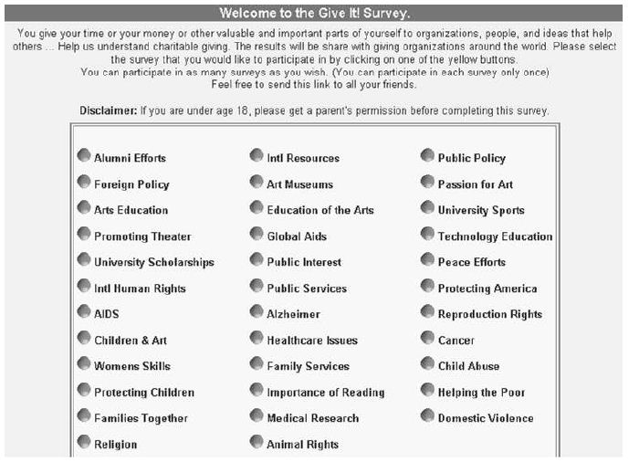
Figure 1 shows the 35 topics. At the time of the actual study the respondent would select the topic of interest, go to the study, and then participate. The topic would ‘disappear’ from the wall after a certain number of respondents completed the study. Unknown to the respondent, the ‘test material’ viz., the ‘elements, ‘ viz., phrases, full set of studies were almost mirror image of each other across the 35 different studies except for eight of 36 elements which were specific to the topic.

fig 1

Figure 1: The wall of 35 Give It! studies. The respondent selected the study and was led to the actual Mind Genomics experiment corresponding to the study

Step 2 – Create the Basic Structure of the Experiment, Comprising a Specific Number of ‘Questions, and a Specific Number of Answers’ for Each Question

The IT! studies conducted during the first five years 2001-2005 used four questions, each with nine answers, or in the language of today’s Mind Genomics, four questions, and nine elements (answers). The choice of this 4×9 experimental design was based upon the joint desire to acquire as much information as possible, and the popularity of Mind Genomics designs around 2003, the early phrase of the internet in consumer research.

The designs had to fall into the class of permuted experimental designs, which could be created in the hundreds, so that each respondent would evaluate answers (elements), albeit in different combinations. That structure, allowing for strong individual-level analysis, pre-determined the set of viable design structures. Table 1 presents the 36 different messages, groups into four categories, or in today’s usage, four questions. Each category (or question) comprises nine elements (or answers). It is critical that a group of related elements, viz., elements of the same type but which may carry different information, just appear in the same category or question. This requirement is a ‘bookkeeping device’ to ensure that two elements of the same type, but containing mutually contradictory information, can never appear together, since the vignette specifies as much. The elements or answers are direct statements, painting a word picture. As the vignettes will show below, simple one- or two-word answers to a question do not suffice to paint a word picture. The objective was to create answers or elements, which in combination, painted such a word picture without the need of a question to set the stage.

Table 1: The 4 questions or categories, and the 36 answers or elements, nine per question/category. The elements pertain to supporting alumni efforts.

Code What is the goal of giving?
A1 You can make a difference
A2X Sharing a love of your college/university with others
A3X Ensuring that students become productive citizens
A4 Your support ensures strong communities and strong families
A5X To provide tools for complete learning
A6X Because everyone knows that supporting schools is important
A7X To enhance the quality of life on campus
A8X To ensure the richness of culture
A9 Helping to maintain standards of excellence
How do you give?
B1 You can give by cash or check donations
B2 You can even use your credit card to donate
B3 Show your support by attending special events
B4 Having a gift matched by your employer
B5 Show your support through a pledge program
B6 Offer your support through regular attendance
B7 Support the organization by purchasing items they sell or need
B8 Volunteer!
B9X You support an individual trying to impact higher education
How do you and how do the recipient benefit?
C1 Gain an association with the organization
C2 Build a connection to other donors
C3 Get the benefits of a tax deduction
C4 Participate in group endeavor
C5 Encouraging yourself and others to participate in a worthwhile project
C6 Giving is a part of your family tradition
C7 Fulfilling a religious obligation to help others
C8 Realizing your personal belief
C9 Preserving the vitality and the future of the program
What are emotional and real outcomes?
D1 Because you want to “DO” good
D2 Be seen, be heard, be an active part!
D3 Be appreciated
D4 A great way to network
D5 Be associated with an organization you believe in
D6X Ensure that a strong interest in supporting alumni efforts remains a priority
D7 Because you want to honor a loved one
D8 Donating time, money and effort makes a difference
D9 Be with people who share your interests

It is important to keep in mind that any large-scale investigation of a vertical, such as donations with Give It!, must sacrifice a great deal of the specifics of a cause in the interests of comparability of causes. The objective of Mind Genomics applied to the vertical is to discover general patterns from sets of common elements. The alternative approach, doing individual studies for each topic, would provide deeper information, but the meta-analysis of the results might require a great deal more effort, and require involve luck at the end, rather than planning at the start. In Table 1, eight of the 36 elements have an ‘x’ added to their code. These are elements which are similar across the six different mind-sets, but also contain topic-specific language that was changed in a minor fashion from study to study.

Step 3 – Create Small, Easy to Read Vignettes, Using an Experimental Design

Step 3 creates the test stimuli, the combinations f messages. In the language of Mind Genomic, these combinations are called vignettes. Figure 2 shows an example of a vignette. The stimuli comprise 60 different combinations, all similar in format to Figure 2, except that some comprised two elements, some three elements, and some four elements. The spacing and design of the vignette is such that the respondent could easily read the vignette. Experience with Mind Genomics suggest that the combination of messages in a spare form, with open space allows the respondent to quickly ‘graze’ the information and make a rating. The design of the test stimulus in Figure 2 goes contrary to approaches, which present the respondent with a crafted paragraph. In the end, comments from respondents who, having been presented with these spare looking vignettes like that of Figure 2, concur that it is easier, less fatiguing, less frustrating to deal with form of design when rating many vignettes, rather than working one’s way through what a dense paragraph.

fig 2

Figure 2: Example of a vignette comprising four elements

The vignette is created according to an underlying experimental design [11]. The design prescribes the exact composition of each vignette, specifying which specific elements are combined. To the novice unfamiliar with the design structure, such as the respondent, the vignette looks as if the elements had been thrown together at random. The truth is precisely the opposite. The compositions are carefully crafted to ensure that each element appears equally often, that each element is statistically independent of every other element, and that there are sufficient of compositions or vignettes which lack one or two elements. The latter feature of the experimental design ensures the data can be used by OLS (ordinary least=squares ) regression to deconstruct the response into the contribution of the individual 36 elements. Furthermore, the built-in incompleteness of some vignettes prevents the statistical problem of multi-collinearity, which would eventuate in the crash of the statistical analysis for that data set. Finally, and most important, the coefficients emerging from the OLS regression have ratio-scale values, and are comparable from study to study, from period to period, and even across different individuals. Two other features of the experimental design are important to note. The first is that no question or category can contribute more than one element to a vignette. The rationale for this constraint is that quite often the question or category comprises elements which mutually contradict each other. Were these mutually contradictory elements to appear in the same vignette they would corrupt the response to the vignette. The second significant feature in the Mind Genomics system is the permutation of the basic design, so that the mathematical structure is identical, but the actual combinations differ from one another. The use of the permuted design at first seems to be merely a statistical enhancement, but the reality is that it is a frontal attack on some of the thinking of conventional science, and an alternative to the oft-quoted proverb ‘measure nine times and cut once.’ This permuted design (Gofman and Moskowitz) emerged out of a recognition that the standard research approaches are based on reducing statistical error by repeating the same experiment with dozens or hundreds of people. The implicit assumption of the conventional research procedure is that the ‘correct answer’ is known, and that the research is going to confirm or disconfirm that guess. Yet, the ‘reality on the ground’ is that no one really knows what messages will work, and what messages will fail to work. Thus, the choice of the messages and the combinations becomes one’s best guess. The permuted design avoids the need to select a limited set of vignettes, or test combinations at the start of the study. The key benefits of the permuted design used by Mind Genomics are ability to explore a wide number of alternative ideas (36 in this study), and at the same time explore a great deal of the underlying ‘design space’ of different combinations. Each respondent evaluated a unique set of 60 vignettes. Across the approximate 70-80 respondents, this means that for each topic (e.g., technical education), the Mind Genomics experiment investigated the response to many different vignettes, albeit each vignette evaluated just a few times The creation of a model relating the presence/absence of the elements to the ratings was stabilized because of the many different combination. Even if one or several, or several dozen were mis-judged, the weight of the approximate 60×75, viz. 4500 judgments of different combinations sufficed to ensure that no systematic error could affect the result. In contrast, conventional research testing the same 60 vignettes 75 times each might be well advised to make sure that the 60 vignettes are the correct vignettes. Choosing the wrong single vignette to test or having an aberrant reaction to that vignette is not quite as serous in Mind Genomics as it is for conventional research. To summarize this point, it should thus be kept in mind that the permutation of the combinations ensures a wide coverage of the possible combinations, producing a better experiment. It is simply very difficult to introduce a strong bias when the combinations change all the time. It is the underlying pattern, emerging for 4800+ vignettes which is critical.

Step 4: Invite the Respondent to Participate, Introduce the Respondent to the Subject, and Execute the Actual Interview

The It! studies were run with the Canadian on-line panel, Open Vue Ltd. Their panel comprised both USA respondent and Canadian respondents, among many others. The respondents were selected to be residents of the United States. Open Vue sent out email invitations to its panelists. Those who answered were led to the screen shown in Figure 1, where they selected a study of interest to them. During this early period of research with Mind Genomics and with the It! studies, it became obvious that an efficient way to do 35 studies with approximately similar numbers of respondents was to let the respondent choose the study. Once the study quota was filled, the study disappeared from the available choices. Figure 3 shows the orientation screen for the study. Most of the screen is taken up with bookkeeping details, about the length of the study, the fact that the screens (viz., the vignettes) differ, the rating question, and the expected time of the study. During this early period of internet research, the respondents were not yet saturated by requests to participate in simple studies or evaluations of their experience, and thus were more likely to donate 15 minutes of their time to the study. Nonetheless, it was important to incentivize the respondent with a monetary reward, a drawing for a prize. The three prizes were the incentive across all 35 studies. That is, all respondents across all studies were entered into the drawing, and three respondents were selected as winners.

fig 3

Figure 3: The orientation page for the Give It! studies. Each study was introduced by the same page, with the only difference being the specific topic.

Step 5- Transform the Rating to a Binary Dependent Variable and Create Individual-level Models

The respondent rated each vignette on the simple scale ‘How much does this giving situation appeal to you?’ Note that the respondent was not asked to state whether or not the respondent would donate, or how much, although those could have been legitimate questions to ask. Rather, the respondent was asked a question about feelings, about a sense of ‘appeal to me.’

The 9-point scale, a category or Likert Scale, can be easily analyzed. The problem with the scale, however, is how to interpret the scale. When managers receive data, they often ask the simple question ‘what do these ratings MEAN?’. To a manager, the fact that one can easily analyze the data with sophisticated statistics means very little when the results cannot be easily understood and acted upon. Thus, it has become standard procedure to transform these Likert scales, usually to a binary scale, yes/no. The manager using the data has no problem understanding yes/no. The transformation is straightforward. Standard practice has evolved to transforming the ratings of 1-6 to 0, and ratings of 7-9 to 100. This division of the scale makes thee interpretation easier. As a prophylactic measure, we add a vanishingly small, random number to every transformed variable to ensure that the transformed variable, viz., the newly created binary variable, has some minimal variation. If the respondent were to rate all 60 vignettes as 7-9, or as 1-6, respectively, then the transformation as just specified would create a set of 60 number, all 100, or all 0, respectively. The analysis of the data by OLS (ordinary least squares) regression would immediately crash. Adding a vanishingly small random number to the newly created binary value ensures that this unhappy event does not occur. Every vignette will have its own number, around 100 or around 0, respectively, depending upon the original rating assigned to the vignette. Once the data have been transformed the 60 rows of data from each respondent is subjected to an OLS (ordinary least squares) regression. The regression is called ‘dummy variable’, because each of the 36 element corresponds to an independent variable, and takes on only one of two values, 0 or 1, as follows: The element is either present in or absent from a vignette, so its corresponding independent variable is coded ‘1’ when present, or coded ‘0’ when absent.

The equation is: Binary (0/100) = k0 + k1(A1) + k2(A2) .. k36 (D9)

The regression analysis created 60 rows of input data for each respondent. Each row comprised 37 numbers, additive constant (k0) and the 36 coefficients, k1-k36. With 453 respondents participating, the regression analysis generated 453 rows of coefficients. It would be these 453 rows of coefficients that would be used to create mind-sets. The 453 rows, viz. the full data set, was subject to k-means clustering, the inputs for the clustering being the 36 coefficients k1-k36. The additive constant was not used for the clustering. To make the analysis easier, we extracted three clusters, a number usually found to reveal strong patterns, but not unwieldy to analyze. The clustering was done by the k-means method [12], which looks at the distance between each pair of respondents and tries to put respondents into a set of mutually exclusive groups so that the distance between the respondents in a cluster is small, while at the same time the distance between the centroids of the three clusters is large. The clustering does not take into account any of the ‘meaning’ of the elements, but simply tries to satisfy a mathematical criterion. Table 1 shows eight elements with the element code having an ‘x’ as the suffix. These were elements deemed too specific to the topic and were not included in the clustering. The rationale was that the clustering should comprise only those elements common in meaning to the six different topics of giving. These eight elements did not satisfy that criterion of being ‘topic-agnostic.’ They will, however, be presented in the results. Within any group, whether total, donation topic, mind-set or topic x mind-set, the corresponding additive constants and 36 coefficients were averaged to generate the results shown in the data tables. More recent approaches simply combine data together for the respondents in a defined group and rerun the regression model on the total data for the relevant group. The results are similar for both forms of analysis.

Results

Total Panel and the Six Different Topics

The Mind Genomics analysis generates a substantial amount of summary data. Our objective is to discover patterns and generalities, not to show all of the data, which would hide the patterns which exist. In order to make the discovery task simpler, we will eliminate from consideration all elements with coefficients of +7 or lower and report the element when it has a coefficient of +8 or higher. The element will not appear at all in the case that all of the coefficients for the key subgroups are lower than +8. This pruning action brings the really important elements into the foreground. Table 2 presents the results from the total panel, combining the six studies, and all of the respondents. The additive constant is 41, meaning that on average two of five responses to the vignettes will be rated as appealing (viz., rated 7-9 on the nine-point sale). The messages range from belief in the organization (D5) to affiliation (A2X), to focus on the recipient (A3X). These are the key messages that any organization seeking donations should incorporate.

Table 2: Strong performing elements from the total panel, combining all respondents across the six studies.


Total

  Additive Constant

41

D5 Be associated with an organization you believe in

9

A2X Sharing a love of your TOPIC with others

9

A3X Ensuring that TOPIC become productive citizens

8

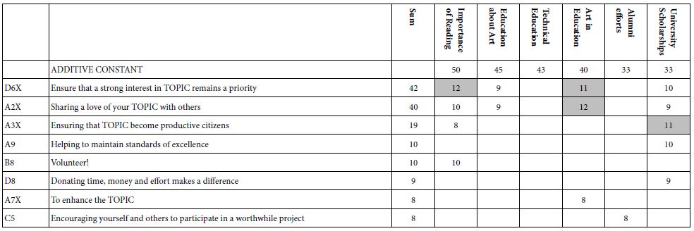
The array of strong performing elements increases when we move from combining all the data into one group (Total) and do the analysis on a topic-by-topic basis. The results appear in Table 3. Once again the table shows only those elements which generate at least one coefficient of +8 or higher. Thee first data column shows the sum of the strong performing coefficients and used to sort the elements from strongest performing elements to the weakest performing elements. In addition, the six studies are sorted by the magnitude of the additive coefficient, viz., the likelihood to find the vignette appealing in the absence of elements. Stated differently, the additive constant might be considered to represent the basic proclivity of the respondent towards the topic.

Table 3: Strong performing elements for each of the six giving topics.

table 3

The additive constants suggest that the most appealing topic is ‘importance of reading’, the least, but still strong being university connected topics, ‘alumni efforts’; and ‘university scholarships’, respectively. One of the properties of Mind Genomics is the fact that the coefficients have ratio scale properties. Thus, we can conclude that ‘importance of reading’ is 50% more appealing than the two university topics. Table 3 is characterized by a great number of blank spaces, suggesting that the strong performing elements do not transcend the different topics. No element drives strong appeal to more than three of the six topics The two strongest elements appear to focus on different directions, first a focus on the topic itself (D6X), and second a focus on the social aspects (A2X). There is a third focus, that of helping the person who is associated with the giving cause. These three directions suggest three different foci of appeal, directions which will emerge as mind-sets

D6X: Ensure that a strong interest in TOPIC remains a priority

A2X Sharing a love of your TOPIC with others

A3X: Ensuring that TOPIC become productive citizens

Moving from Total to Mind-sets

Table 3 hinted at the possibility that there might be different ways of evaluating the messages. Although at first glance we might consider the key factor to be the recipient of the donation so that certain topics are more attractive than another, there might be a far deeper factor at work, mind-sets. The hallmark of Mind Genomics is the discovery of these different patterns of response to messaging. The metaphor is white light, which seems to be colorless, but when the light is diffracted through a prism, the spectrum of colors emerges. We see white perhaps because the different colors interfere with each other. Mind Genomics posits that for virtually all conventional aspects of daily experience, there are different patterns of focus, of importance. What one person thinks to be important (viz., more is better) another person might as consider to be utterly irrelevant, even off-putting. The discovery of these groups, so-called mind-sets, it a matter of experiment. Furthermore, once these mind-sets are established through analysis, some of the data begins to make more sense. We may hypothesize about the possible mind-sets, but an easier way to establish these mind-sets is through a set of experiments, such as the experiments run here. The analysis to establish these mind-sets is simple OLS regression as we have done, followed by clustering to create groups of individuals with similar patterns of responses. The set of individual coefficients comprises raw material for the creation (or discovery) of these mind-sets, the permuted experimental design provides us with what we need to create the individual-level set of coefficients. As discussed above, the OLS regression analysis was straightforwardly able to create an individual level model for each of the 453respondents. The OLS regression estimated the additive constant and the value of each of the 36 coefficients, one coefficient for each element. Table 1 showed the expression of the elements for the topic of Alumni Efforts. Eight of the 36 elements appear to be specific to the topic and are marked with an ‘X’ in the element code. As noted above, these eight elements will not be used to establish the mind-sets by clustering, but then will be included in the later analyses after the mind-sets are created. The clustering method of k-means created two clusters for the 453 respondents, and then created three clusters for the same 454 respondents. The clustering procedures are a purely objective one, attempting to satisfy certain mathematical criteria. The criteria previously adopted for Mind Genomics studies for choosing the appropriate number of clusters (now called mind-sets) are not statistical, but rather qualitative. The two criteria are that there be as few clusters or mind-sets as possible (parsimony), and that each mind-set tells a story (interpretability). The criteria suggested a three-cluster solution, rather than a two-cluster solution. These clusters become the mind-sets. The clustering itself was done, as noted, on 28 of the 36 elements. Once each respondent was assigned to a cluster or mind-set, it was straightforward to estimate the additive constant and the value of the coefficient for each of the original 36 elements. That is, we resort to the 28 ‘general’ elements ONLY to create the clusters or mind-sets, and then revert back to the full set of data for further interpretation.

Three segments emerged, based on a qualitative ‘sense’ of what is communicated by the strong preforming elements. No element is strong across all six giving topics, so the interpretation of the meaning of the mind-sets become a simple heuristic with which to discuss the results. Furthermore, the clustering does not dramatically separate the three mind-sets. It’s a matter of emphasis. This is important. The dynamics of appealing to the heart of the donor become a matter of combining messages of different types, rather than focusing on one specific factor, such as EFFECT (viz., the benefit to the recipient).

MS1 (Commitment) Because I Care….it’s about what I can personally do to make the issue better.

MS2 (Actions) Showing Support It takes more than just effort and good wishes to make things change… it takes money, time, items,

MS3 (Effect) It Makes a Difference….it’s about what can be done to help those affected by the issue.

The Baseline Proclivity of the Mind-sets towards ‘What Appeals’

The additive constant tells us the estimated rating of 7-9 (appeal to me), in the absence of elements. Although the additive constant is a purely estimated parameter, it can be used to indicate the proclivity of the respondents to say ‘appeals to me’. Table 4 presents the additive constants estimated separately for the six different causes, and the three mind-sets that were developed for all the causes combined. The additive constants are sorted by average, first in descending order of cause by averaged across the three mind-sets, and then by mind-set averaged across causes. There are remarkable differences in the additive constant of the three mind-sets and in the six studies. The strongest ‘pull’ emerges from donations to help teach reading (average 50), and the weakest from alumni efforts (average 34) and university scholarship (32). This teaches us that the strongest pull, on average, is exerted by causes which pull toward young people, to give them an opportunity. Universities will have a more difficult time reaching the donors’ heartstring. In terms of the three mind-sets, we also see radical differences. Mind-Set 1 (commitment) shows the strongest proclivity to feel positive (additive constant 50), As the array is presented, there is also clear evidence for some interactions, specifically for reading. Mind-Set 2 (actions) finds its strongest pull with reading.

Table 4: Additive constants for the three mind-sets and the six donation ‘causes’, sorted by cause and by mind-set.

Additive Constant

MS1 (Commitment)

MS3 (Effect) MS2 (Actions)

 Average

Reading

49

41 60

50

Tech Education

58

45 34

46

Ed in Arts

51

40 44

45

Arts Ed

45

36 39

40

Alumni Efforts

47

41 13

34

University Scholarship

51

30 14

32

Average

50

39 34

What Elements ‘Drive’ Positive Feelings about Giving for the Three Mind-sets?

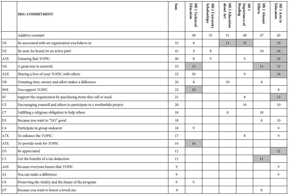
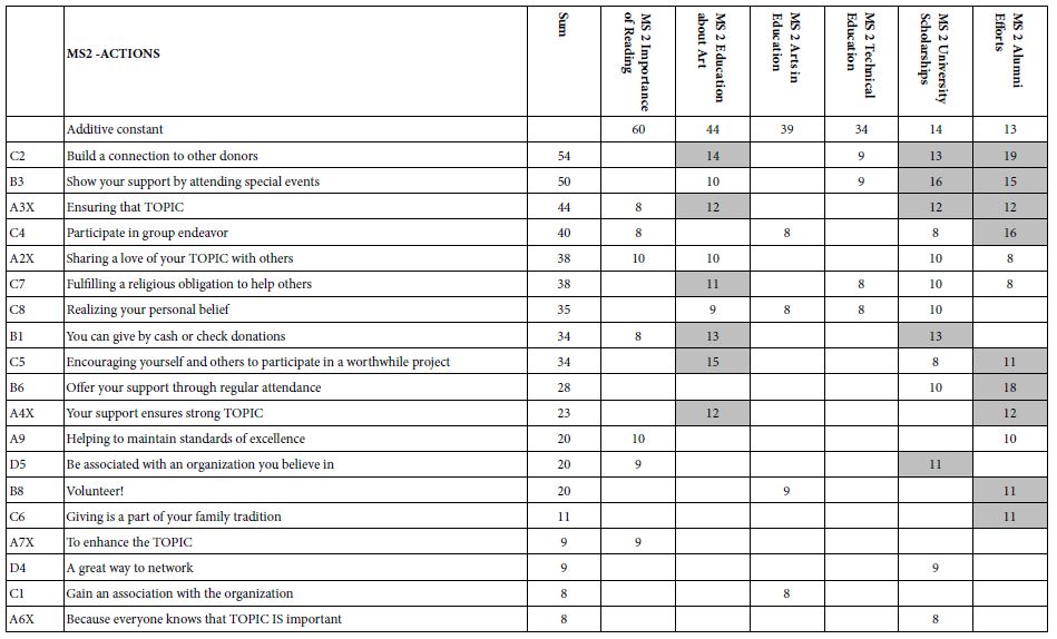
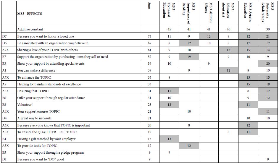
Tables 5-7 show the strong performing elements for each of the three mind-sets. Note again that the tables present only the strong performing elements for at least one of the three mind-sets, and that all elements were considered for inclusion. In the case of the eight elements which were topic-specific, the topic is replaced by the word ‘TOPIC.’ One gets a sense of the specific thrust of the communication by reading the complete element, even with the word ‘TOPIC’ replacing the actual topic.

Table 5: Mind-Set1: The table shows the strong performing elements for MS1, labelled ‘COMMITMENT’’.

table 5

Table 6: Mind-Set 2. The table shows the strong performing elements for MS1, labelled ‘ACTIONS’.

table 6

Table 7: Mind-Set 3 . The table shows the strong performing elements for MS3, labelled ‘EFFECTS’.

table 7

The Composition of the Three Mind-sets

A hallmark of conventional research is that WHO a person is often covaries with what a person does or what a person believes. It is for this reason that so many consumer researchers spend a great deal of time collecting so-called classification questions about the respondent. What attracts many conventional researchers is the possible covariation of the easy-to-measure-behavior with additional information about the respondent.

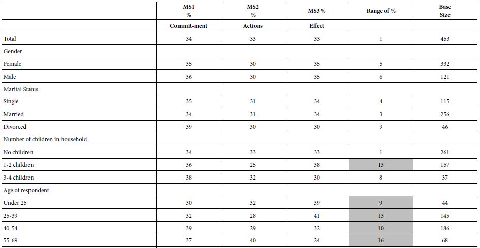
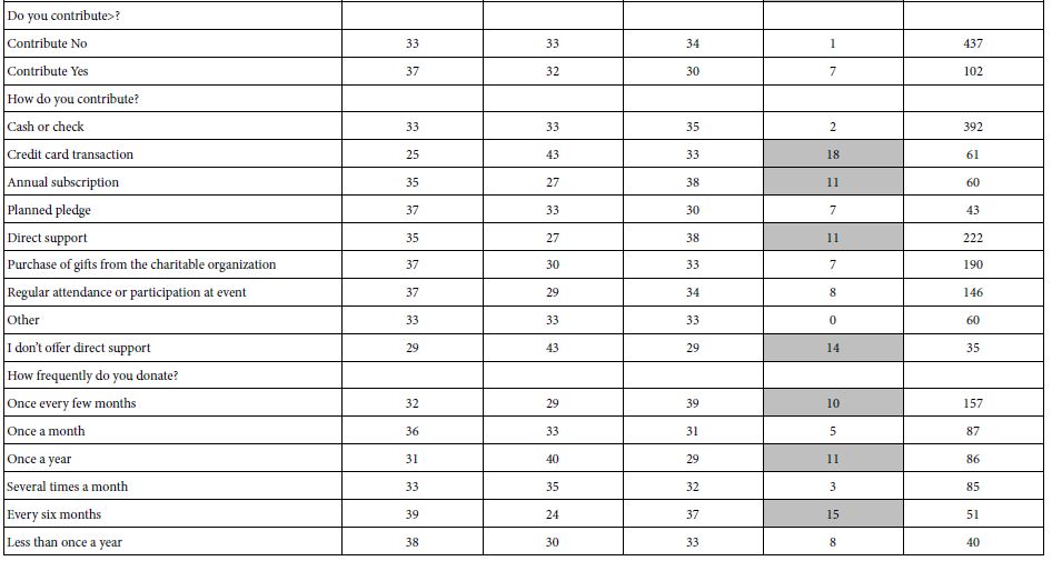
In the world of Mind Genomics, the focus is on a better understanding of the individual. Only secondarily is the focused on establishing the relation between who a person IS versus, what the person THINKS To a great degree the lack of focus on the covariation between mind-set and behavior is due to the belief that the most pressing task is to understand the mind-sets, rather than to link the scarcely understood mind-sets to other variables. The It! studies captured a great deal of individual level data regarding attitudes and behaviors involving ‘giving’. Some of the data appears in in Table 8. Table 8 shows the complicated relationship between the three mind-sets and both WHO the person is, as well as how the person BEHAVES with respect to donating to causes. There are many patterns emerging, depending upon the way the respondent self-classifies, but no simple pattern which can be said to be common to the mind-sets.

Table 8: The percent of respondents in each of the three mind-sets, the range of percentages across the three mind-sets, and the base size. Each row constitutes a classification variable in the self-profiling classification.

table 8(1)

table 8(2)

Discussion and Conclusions

The academic study of ‘giving’ typically focuses on higher level motive, looking at the individual material from either actual campaigns, or creating an experiment. The important thing to note is that these studies generate a certain kind of knowledge, understanding the general drivers of donations. That information is important to understand donating to causes in the context of theories about why people do what they do. Being able to put a person’s ‘giving’ behavior, or response to different appeals allows the academic to understand yet another part of the mind of the person, for the world of the everyday. The Mind Genomics approach presented here, with its focus on the specific messages, give us a different point of view. The goal of Mind Genomics is to work with the stimuli of the everyday, in this study the stimuli being ‘messages.’ Rather than look for underlying patterns to fit into a theory, the effort is to identify what really works, and then point to what might be happening. Mind Genomics is atheoretical, but systematized experimentation. There is no theory in which to place the response patterns of giving, or at least no theory which drives the effort. Rather, the objective of the study is to see ‘what works’, with the test material being the type of messages that would be used in actual campaigns. The important results from this study are simple to summarize, namely that most of the messages really don’t work very well in terms of the ratings by respondents, and that the nature of the mind-sets which emerge is not a case of ‘polarization’ but rather ‘emphases. It’s not that the mind-sets respond only to one type of message, but rather the mind-sets respond to the messages, the elements, but some messages are stronger for one mind-set, and still positive but weaker for another mind-set. There is a strong practical side to the data presented here. That side is the fact that the patterns emerging from messages can be used immediately. There is no need to translate the test messages used in the experiment to actual messages that might be useful in a practical situation. The messages from the Mind Genomics experiment come from actual campaigns, although edited to have general application. Finally, the finding emerges once again that although there are mind-sets that are clearly different, there do not seem to be any simple co-variation of the mind-sets with who the respondent IS, or the self-stated patterns of involvement with the world of giving. It is that finding, a continuing revelation, which continues to surprise. The practice has always been to stratify the efforts by dividing people by WHO they are, assuming that people who appear similar on the criteria of who they are or how they involve themselves with the world of giving will be similar in their response to messages about giving. It just not the case.

Acknowledgments

These studies were run under the aegis of It! Ventures, Inc. The authors acknowledge the contribution of the late Hollis Ashman, as well as the contribution of Jacquelyn Beckley of the Understanding and Insight Group, New Jersey, USA. The studies were sponsored by Kathleen O’Grady of the O’Grady Foundation.

References

  1. Nguyen C, Faulkner M (2020) In pursuit of effective charity advertising: Investigating the branding and messaging execution tactics used by charity marketers. Third Sector Review 26: 66-87.
  2. Chen W, Givens T (2013) Mobile donation in America. Mobile Media & Communication 1: 196-212.
  3. Duncan T (1995) Why mission marketing is more strategic and long-term than cause marketing. In: 1995 AMA Winter Educators Conference: Marketing Theory and Applications, Vol. 6, (eds: Stewart D, David W, Vilcassim N, Chicago: American Marketing Association) 469-75.
  4. Chen S, Thomas S, Kohli C (2016) What really makes a promotional campaign succeed on a crowdfunding platform?: Guilt, utilitarian products, emotional messaging, and fewer but meaningful rewards drive donations. Journal of Advertising Research 56: 81-94.
  5. Shearman SM, Yoo JH ( 2007) “Even a penny will help!”: Legitimization of paltry donation and social proof in soliciting donation to a charitable organization. Communication Research Reports 24: 271-282.
  6. Luckow T, Moskowitz HR, Beckley J, Hirsch J, Genchi S (2005) The four segments of yogurt consumers: preferences and mind-sets. Journal of Food Products Marketing 11: 1-22.
  7. Foley M, Beckley J, Ashman H, Moskowitz HR (2009) The mind-set of teens towards food communications revealed by conjoint measurement and multi-food databases. Appetite 52: 554-560.
  8. Rabino S, Moskowitz H, Katz R, Maier A, Paulus K, et al. (2007) Creating databases from cross‐national comparisons of food mind‐ Journal of Sensory Studies 22: 550-586.
  9. Moskowitz HR, Gofman A, (2007) Selling Blue Elephants: How to make Great Products that People Want Before They Even Know They Want Them. Pearson Education.
  10. Moskowitz, H.R., Gofman, A., Beckley, J. & Ashman, H., (2006) Founding a new science: Mind genomics. Journal of Sensory Studies 21: 266-307.
  11. Lundstedt T, Seifert E, Abramo L, Thelin B, Nyström Å, et al. (1998) Experimental design and optimization. Chemometrics and Intelligent Laboratory Systems 42: 3-40.
  12. Likas A, Vlassis N, Verbeek JJ (2003) The global k-means clustering algorithm. Pattern Recognition 36: 451-461.

Mind-Sets for Senior Dining: the Contrast between Homo ‘Emotionalis’ and Homo ‘Intellectualis’

DOI: 10.31038/NRFSJ.2021422

Abstract

Respondents rated vignettes (combinations of elements, viz., statements) describing the different features of senior communal dining. Each of 108 senior respondents (age 65+) rated unique sets of 50 vignettes, combinations of 2-5 elements created according to a permuted experimental design, ensuring that the 50 combinations differed for each respondent. Each vignette was rated on both importance of, and emotional response to, the combination of the specific elements presented in the vignette. Deconstruction based on ratings of importance revealed different mind-sets, focusing on food, service, and ambiance, respectively In terms of emotions, few elements were delighters. Most elements did not strongly drive either positive or negative emotions. The one consistently important message was ‘warm food out of the oven’, but it was not a delighter. The one element consistently driving negative emotions was ‘high noise level’. Groups of mind-sets emerged, showing different patterns of importance (Mind-Sets 1-3) and emotion (Mind-Sets 4-6). The mind-sets distribute across the population, suggesting simple knowledge of WHO the respondent is in terms of age, marital status, and so forth does not clearly predict what will be important to any specific senior diner.

Introduction

As the nation ages, there are an increasing number of group or community living facilities, designed for healthy, aging seniors [1]. These communities have group dining facilities. The issue becomes one of finding what is important to a senior. The obvious answer is food, companionship, and service [2]. But what exactly is entailed by each of these? And furthermore, are there differences in the importance of these three general factors?.

The usual approach to answering these questions is for the respondent to rate or rank these factors, either in the abstract, or after having experienced a certain community, so that the specific community is rated on satisfaction with respect to these three or more general factors. The rating or ranking factors requires that the respondent evaluate the general factors in isolation, and in general terms. Sometimes the researcher recognizes that the general factor, e.g., service, might be better assessed by first specifying the question in terms of defined behaviors, or food specified in terms of defined dishes and/or method of preparation.

As popular as the ‘one-at-a-time’ evaluation has been, it suffers from at least two defects which limit its usefulness. One is that the respondent may unconsciously adjust the judgment criterion when dealing with the different factors, when evaluating one element at a time. For example, the same rating scale for food versus service may mean different things. The researcher does not know that. Second, the one-at-a-time strategy fails to recognize that people rate things more readily and easily when what they are rating is less abstract, more concrete. It is more natural to rate combinations of ideas which represent a situation, a vignette, than to rate each idea separately.

This paper presents the results of a Mind Genomics cartography, an investigation of different ideas, so-called elements, which might be relevant to older adults eating in communual dining situations, such as retirement homes. The objective is understand senior communal dining from the ‘inside-out.’ The strategy maps out what might be important to the senior diner, doing so by presenting the respondent with different ‘vignettes’, viz., combinations of features describing a senior dining situation. Through the response to these vignettes, rated both as describing something important, and as eliciting an emotion, the researcher uncovers both what is important, and what produces an emotional response, respectively. The approach differs dramatically from the one-at-a-time approach, used to in conventional research [3,4].

The background of Mind Genomics can be found in the confluence of statistics (experimental design; [5], patterns emerging from the study of consumer opinions [6], and the change in focus from a sociological viewpoint (outside-in) to a psychological viewpoint (inside-out). The underlying world-view of Mind Genomics is the vision of the science as a tool to ‘map the mind’, focusing on the ordinary aspects of life, rather than setting up experiments configured to test a hypothesis. The Mind Genomics science comes from a history of psychophysics, with the objective to discover patterns, regularities in nature, rather than from the hypothetico-deductive system, which assumes the world works a certain way, and seeks to confirm or to disconfirm that assumption through experiment. Thus, the study reported here was done in the spirit of an exploration of the mind of what senior feel about the various aspects of communal dining.

Dining behavior is a well-explored areas of foodservice. Most studies of dining among adults focus on the choice of restaurant, and the dimensions of food and service, topics which are relevant in a situation where the diner eats and pays, even in the world of senior dining [7]. In contrast, there has been less focus on institutional communal dining, and much less on communal dining among seniors.

Focus on Emotions and Feelings

This study focused on the response of older, relatively healthy adults (age 65+) to different messages about senior communal dining. The objective was to identify which elements were important to them (viz., homo intellectualis) and which elements generated positive or negative feelings (viz., homo emotionalis). The latinized terms intellectualis and emotionalis were coined for this paper.

Rather than instructing the respondent to rate the importance of, and the emotional response to, single elements, Mind Genomics proceeds in another direction, one that might seem less direct, but one that cannot be gamed, and thus provides robust information. The respondent reads a set of messages or elements, created according to a specific recipe plan (experimental design). For this study, comprising 35 elements in 50 vignettes, the combinations primarily comprise vignettes containing 3-4 elements, but a few containing 2 elements, or 5 elements. Each element appeared five times, always in combination with other elements. The experimental design is set up so that no two respondents evaluate the same set of vignettes, allowing the Mind Genomics experiment assess many of the possible combinations [8]. This property makes Mind Genomics unusual because it directly measures many of the possible stimuli, rather than forcing the researcher to ‘know’ what will work before the experiment is done. The goal is to avoid the folk wisdom which prescribes the cautionary ‘measure nine times, cut once,’ a way of thinking which subtly transforms research to confirmation, rather than allowing research to explore the ‘new’.

Method

The Mind Genomics approach to knowledge follows a structured, formatted pattern, in recent years put into the form of a computer-aided process (see www.BimiLeap.com). The study reported here was done a few years before the automated system was developed, but the actual creation, presentation, of the vignettes, and analysis were reasonably automated, although not from beginning to end as they are as of this writing (Fall, 2021).

Step 1 – Select the Topic, Ask the Questions, and Provide Answers in the Form of Simple Declarative Sentences

Table 1 shows the five questions and the seven answers for each question. The underlying mathematics of Mind Genomics prescribes certain combinations of questions (or categories) and answers (or elments). The rationale for the five questions and seven answers is that it is a specific array which fits into the prescribed experimental designs of Mind Genomics. Those prescribed designs are important because they allow each respondent to test the same elments, but each respondent testing a different set of actual combinations. This is a permuted design, and will be discussed below [8].

It is important to note in Table 1 that the focus is on word pictures, on specifics, ratherr than general ideas. The underlying reason is that the Mind Genomics effort attempts to paint ‘word pictures’ about the situation (here adult communal dining). To paint these word pictures requires that the researcher move beyond simple, general statement, and focus on the particular, even if the particular is something ‘new’ to the respondent.

Table 1: The raw material comprising five questions, and seven answers for each question.

Question A: Describe the ambiance

A1 Adequate lighting at the table
A2 The overall volume of noise in the dining room is high
A3 Eating with a group of friends
A4 Eating by yourself
A5 Listening to music during a meal
A6 Lots of stimulating conversation during a meal
A7 Table settings (plates, silverware, tablecloth etc.) makes for an enjoyable meal

Question B: Describe the service

B1 Friendly waiters can really make for an enjoyable meal
B2 Waiters who are knowledgeable about the food help you select items from the menu
B3 Family style service with bowls of food to pass around the table
B4 Speedy service is important for your enjoyment
B5 Waiters let you substitute items such as sides and salads not included in the menu item description
B6 You are given the choice to sit anywhere in the dining room
B7 Waiters remember the type of food or drink you like

Question C: Describe the information provided on the menu regarding the items

C1 Nutritional information on the menu to help you make your selections
C2 Total calories for each item listed on the menu to help you make your selections
C3 The amount of sodium for each item listed on the menu will help you make a choice
C4 Listing the amount of fat in menu items helps you decide what to order
C5 Clear and simple wording on the menu makes it easy to decide what you will order
C6 You select menu items with exotic or foreign sounding descriptions
C7 Having the option for ordering smaller portions of the items on the menu
C8 You love fresh uncooked vegetables (salads for example) at every meal

Question D: Describe a specific food

D1 You enjoy vegetables that are thoroughly cooked
D2 Fresh fruit at every meal
D3 If it contains chicken, you will like it
D4 Red meat is your choice every time
D5 You can’t go wrong with a simply prepared fish dish
D6 You like large portions of food

Question E: Describe the sensory aspect of the food

E1 The aromas of herbs or spices you love
E2 Foods with soft textures are your preference
E3 You choose food with vibrant colors
E4 You prefer food that is under-salted
E5 Food is served hot out of the oven every time
E6 You prefer food that is served warm
E7 You enjoy hot and spicy flavors

Step 2 – Combine the Elements into Small, Easy to Read Vignettes Using an Underlying Experimental Design

This experimental design for this study (5×7) generated an experimental design or set of combinations totally 50 different combinations or vignettes, all but three vignettes comprising either three or four elements. The remaning three vignettes encompassed two elements or five elements. Each element appears five times in the 50 different combinations.

The important thing about the underlying 5×7 design, like others of its class, is that the experimental design is complete at the level of each respondent. This means that the 50 cases or observations from one respondent can be used to estimate the contribution of each element to the rating. Such analysis at the level of the individual respondent becomes important when we create equations for each individual and then combine individuals on the basis of similar patterns of individual-level coefficients to discover mind-sets.

It is at Step 2 where Mind Genomics departs radically from the conventional approaches, which are founded on the principle of ‘isolate and study’. The objective of conventional research is to quantify the basic dimensions, such as ambiance, service, information, food, and so forth. Conventional research looks for the general principles. It is usually the evaluation of elements one-at-a-time which allow the researcher to rank order the different general aspects. There are situations when the topic requires the combination of different aspects, but in those situations the actual combination itself is important, and treated as a ‘single’ element by itelf, even though it comprises a composition. That composition is fixed, and analyzed as a single item. The fact that the stimulus is a composition is not relevant for the analysis.

The ingoing approach of Mind Genomics is the opposite of the conventional approach. The basic interest remains the performance of the individual element, and from that performance the understanding of how the respondent, the older adult, makes a decision. The strategy is different, however, working with combinations, and from the response to these combinations estimating the performance of the individual elements, the messages.

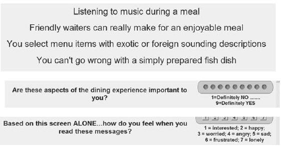
Figure 1 shows an example of the vignette. The vignette was shown twice, first instructing the respondent to assign a rating of importance, and second insructing the respondent to choose a feeling/emotion. To the respondent it appeared that the vignette did not change, only the insrtructioins did.

fig 1

Figure 1: Hows an example of a 4-element vignette, with the two rating scales.

There are at least three clear advantages emerging from a Mind Genomics study.

Ecological Validity

The combination of elements is ecologically more valid because it describes something that could be real. People are accustomed to reading combinations of ideas in everyday life, whether in advertisements, or hearing the description in a story told to them, etc. We call this ‘ecological validity’ because it is that to which they people are accustomed.

Inability to ‘game the experiment’

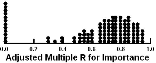
The continually changing combinations of elements make it virtually impossible for the respondent to find a ‘right answer.’ The vignettes appear to comprise elements put together in a haphazard order. Most respondents feel that the combinations are, in fact, random. When asked about their experience, many respondents said that they could not figure out the ‘correct answer’ from the pattern of vignettes, and simply ‘guessed.’ This ‘guessing’ is actually not the case, because otherwise the responses would not correlate with the ratings, which they do. Figure 2 show the adjusted multiple R (Pearson Correlation), a meaure of the goodness of fit of the 108 models, one per respondent, with the models predicting the response from the elements. Were the respondents actually ‘guessing’, the adjusted multiple R across the 108 respondents would cluster around 0 – 0.3. There are a number of respondents with adjusted multiple R values of 0. These respondents were no doubt guessing. The data from the other respondents can be said to be consistent.

fig 2

Figure 2: Distribution of adjusted multiple R statistic for 108 respondents. R values near 1.0 suggest a strong, consistent relation between the presence/absence of elements and the 9-point rating. R values near 0 suggest no relation between presence/absence of elements and the 9 point rating.

No need to ‘know’ the right test stimuli at the start of the session

Mind Genomics was created with the idea that one need not know the ‘correct combinations’ at the inception of the experiment. All- too-often the research preparation focuses on weaker than optimal efforts to narrow the range of possible combinations of ideas, such narrowing done by qualitative discussion. Only when the researcher feels that the correct combinations have been identified does the researcher then use the experment to ‘validate’ the guess about what elements are really important. This effort is self-defeating. Conventional research makes ‘the perfect the enemy of the good.’ It is better to have an inexpensive, rapid, iterative system which allows quick screening of messages, viz. in the form of vignettes, with the poor performers eliminated, and new performers inserted, for the next iteration.

Step 3 – Invite Respondents to Participate

Good practice dictates that the respondents be selected by a third party, based upon the research specifications. The increasingly popular use of the Internet as the reearch venue has spurred the growth of many providers who specialize in such online studies. The respondents in this study were recruited using a local US panel provider. The respondents were ‘double opt-in’, viz., agreed to participate in these types of studies. The identify of the respondents was never disclosed to the research team performing the study.

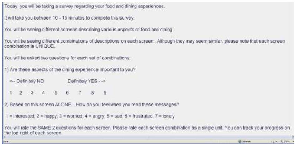
The panel provider sent a link to the respondents with the topic, doing so to adults 65 and older. The records kept by the provider ensured the age. The respondents who agreed to participate were introduced to the the study by the screen shown in Figure 3. The majority of the introduction is ‘bookkeeping’, informing the respondents about the topic, but spending more time about the nature of the vignettes, the approximate amount of time, and the rating questions. These instructions have been significantly shortened at the time of this writing (2021). The standard Mind Genomics study has been reduced in size from 35 messages in 50 combinations to 16 messages in 24 combinations.

fig 3

Figure 3: The orientation page to the communal dining study for seniors.

Analysis and Results

Converting the Data to Usable Formats

Each respondent evaluated 50 vignettes, rating every vignette on two scales, as noted above. The first scale was the Likert scale for importance, anchoared at 1 (Definitely NO) and 9 (Definitely YES). The second question is called a nominal scale. Each of the seven scale points corresponds to a feeling/emotion. The scale itself has no intrinsic numerical properties for analysis. The numbers are placeholders, corresponding to different words.

It is common in the world of consumer research and political polling to reduce the scales to a binary scale, yes/no. The binary scale makes it easy to communicate the findings. It is a matter of understanding what a number ‘means.’ ‘No’ versus ‘Yes’ is understandable. A rating of a 4 versus a 7 is less understandable, other than what was rated 7 had ‘more’ of the attribute than what was rated ‘4.’

The transformation was straightforward. TOP2 (Important) – Ratings of 1-7 were transformed to 0 to denote ‘not important.’ Ratings of 8-9 were transformed to 100 to denote ‘important.’ The usual transformation is 1-6 and 7-9, but the interest here was to identify the ‘really imporant’ messages. Thus, the range corresponding to ‘important’ was narrowed. This first transformation produced the necessary data for the subsequent analysis by OLS (ordinary least-squares) regression, which would relate the presence/absence of the 35 elements to the binary rating.

The second transformation creates two new binary variables, POS (positive emotion), and NEG (negative emotion), respectively. When the respondent selected either the feeling ‘interested’ or ‘happy,’ POS took on the value ‘100’, and NEG took on the vaue ‘0’. When the respondent selected any other feelings, POS took on the value ‘0’ and NEG took on the value ‘100.’ This second transformation also produced the necessary format of data for OLS regression.

One final transformation, or better prophylactic action was done to ensure that each dependent variable (TOP2, POS, NEG) was always different from 0, and that the different. A small random number (<10-5) was added to each transformed value, to create slight variation across the responses of a single respondent. This process ensured that the OLS regression would never encounter the situation that all observations for a dependent variable (viz., all TOP2, or POS or NEG) for a given respondent would be the same value. OLS (ordinary least squares) regression requires some vanishingly small variation in the dependent variable.

Mean Ratings

The simplest, most direct analysis involves computing the average rating assigned by the different groups of respondents. By different groups we refer to the total panel, to gender, age, married versus single, number of meals per day eaten by the respondent, order of testing the vignettes, and to three newly created groups of mind-sets, the criteria for which are presented below. For this first analysis the focus is on whether there are dramatic differences across the defined respondent subgroups in the averages of TOP2 (what is important), and the emotions selected (Positive, POS; Negative NEG).

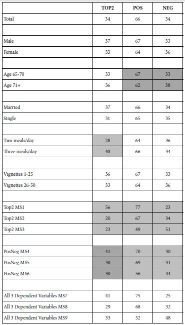
Table 2 shows us the averages ratings across all respondents which fall into a particular group. Thus the Total Panel comprises the averages of all 108×50 or 5,400 vignettes. We get a sense of the proclivity of the groups to consider vignettes important, respectively, as well as generating a positive feeling or a negative feeling.

Table 2: Averages for the four key dependent variables, by different groups of respondents or different orders of testing.

table 2

For the most part, the averages are similar across key subgroups. For groups of respondents defined by who they say they are, and by what they do, we see a few patterns which are interesting. There are more group to group differences when the respondent subgroups are created from the pattern of ratings (emergent mind-sets, discussed below).

The most notworthy differnence is the average rating of TOP2 (importance) for two groups defined by how frequently they eat. Those who eat two meals a day thought the vignettes to be far less important, on average, and those who eat three meals a day thought the vignettes to be more important (28 vs 40).

The second noteworthy difference is the emotional response by age. When rating the feeling after reading the vignette, the younger respondents chose the positive emotion slightly more frequently than did the the older respondents (67 versus 62).

Relating the Presence/Absence of the 35 Elements to the Three Newly-created Dependent Variables

Beyond simple averages and the discovery of some interesting differences lies the opportunity to link the elements and the ratings, and by so doing create a deeper undertanding because the elements themselves are ‘cognitively rich’. Table 2 showed us ‘averages,’ but Table 2 cannot tell us whether the patterns we see correspond to anything more deep. That deeper understanding will emerge from the linking exercise. We will more deeply understand the mind of the respondents because the strong performing elements, those with the deeper linkage, will have meaning in and of themselves.

The initial linking is done by regression modeling. The modeling creates an equation relating the presnece/absence of the 35 elements to the binary rating. The equation states simply that the binary dependent variable is the sum of an additive constant (baseline) and individual contribution of each element, respectively.

The equation is written as follows: Binary Dependent Variable = k0 + k1(A1) + k2(A2) … k35(E7)

The additive constant, k0, is the expected value of the binary dependent variable (e.g., TOP2 for important, POS for positive emotion, NEG for negative emotion), estimated in the absence of all 35 elements. The experimental design ensures that all vignettes comprise 2-5 elements, primarily 3-4 elements as noted above. Thus, the additive constant is a purely computed, theoretical parameter, an ‘adjustment factor.’ The additive constant is the baseline, the basic likelihood to choose a rating.

Table 3 shows the results from the first application of the modeling, result from the Total Panel. Table 3 is short, allowing us a sense of what really makes a difference. We present only those elements which have a TOP2 coefficient of +8 or more, or a POS or NEG coefficient of +10 or more. These cut-points are selected to focus our search for patterns on those elements which perform ‘strongly,’ viz., are statistically ‘significant’ (p<0.05), in the language of interential statistics.

Table 3: Strong performing elements for the Total Panel.

Total Panel


TOP2

Additive Constant

39

E5 Food is served hot out of the oven every time

10

POS

NEG

Additive Constant

74

26

E2 Foods with soft textures are your preference

10

E7 You enjoy hot and spicy flavors

12

D5 Red meat is your choice every time

12

A4 Eating by yourself

21

A2 The overall volume of noise in the dining room is high

27

Total Panel – Importance: 39% likehood of being saying something is important. Warm food is important.

Total Panel – Feelings: Strong basic positivity (74%), but no ‘delighters’. There are are strong negatives, however; eating by oneself and eating with noise, respectively.

Does More Information in the Vignette Affect the Coefficients?

The respondent population in this study was 65 years or older. It is very likely that most of the respondents would never have participated in an experiment quite like the Mind Genomics experiment presented in the previous data. One of the issues which continues to arise is just ‘how’ do the respondents actually form their judgments, and are the judgments affected by the complexity of the test stimulus? That is, most people are accustomed to answering questions one question at a time, with one topic, even though in the introduction we suggested that this one-at-a-time approach might lead to biased data because the respondent would attempt to provide what is believed to be ‘the correct answr’

The data collected here can address one issue, namely are we likely to see the patterns of coefficients change when we base our analysis only on the vignettees comprising three elements, versus only on the vignettes comprising four elements. Recall that in the set-up, most of the vignettes comprised either three or four elements. Only three of the vignettes comprised 2 or 5 elements, respectively.

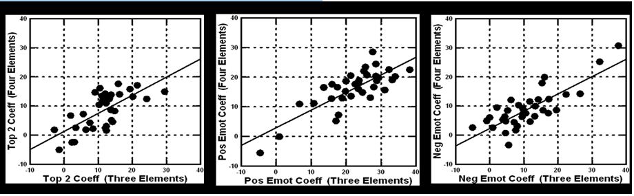
The robustness of the data from the total panel emerges from Figure 3. The data were divided into two strata, those vignettes comprising three elements, and those vignettes comprising four elements. These two data sets were analyzed in parallel, by computing a simple equation relating the presence;absence of the 35 elements to the response (Top2, Positive Emotion, Negative Emotion, respectively). To make the comparison easier, the euqations were estimated without an additive constant, so that one could directly compare the coefficients to each other.

The equation is written as: Dependent Variable = k1(A1) +k2(A2) … k35(E7)

Each anaysis generated 35 coefficients. Figure 4 shows three scatterplots. The abscissa shows the 35 coefficients estimated using only those vignettes comprising three elements. The ordinate shows the same 35 coefficients, this time estimated using only those vignettes comprising four coefficients. There are remarkably high correlations, even though at an element by element basis basis there might be some slight difference in the value of the oefficient for that element. The patterns and decisions would be the same, suggesting remarkable stability of judgment.

fig 4

Figure 4: Values of the coefficients estimated using only vignettes comprising three elements (abscissa) versus using only vignettes comprising four elements (ordinate).

Gender

Table 4 shows the strong performing elements by gender. The gender differences are clear.

Table 4: Strong performing elements for Males vs Females.


TOP2

Males

Additive Constant

41

E5 Food is served hot out of the oven every time

8

Females

Additive Constant

38

C7 Having the option for ordering smaller portions of the items on the menu

14

E5 Food is served hot out of the oven every time

12

C5 Clear and simple wording on the menu makes it easy to decide what you will order

11

B5 Waiters let you substitute items such as sides and salads not included in the menu item description

9

E1 The aromas of herbs or spices you love

9

B2 Waiters who are knowledgeable about the food help you select items from the menu

8


POS

NEG

Males

   
Additive Constant

74

26

D4 If it contains chicken you will like it

10

D5 Red meat is your choice every time

12

A4 Eating by yourself

19

A2 The overall volume of noise in the dining room is high

27

Females

   
Additive Constant

75

25

C7 Having the option for ordering smaller portions of the items on the menu

11

B5 Waiters let you substitute items such as sides and salads not included in the menu item description

10

D7 You like large portions of food

10

D6 You can’t go wrong with a simply prepared fish dish

12

E2 Foods with soft textures are your preference

14

D5 Red meat is your choice every time

14

E7 You enjoy hot and spicy flavors

19

A4 Eating by yourself

23

A2 The overall volume of noise in the dining room is high

26

In terms of what is important, for males it is only warm food, out of the oven. For females, there are five elements covering portion size, warmth, simplicity of ordering, flexibility, and sensory aspects (2).

In terms of positive emotions, delighters, no elements stand out for males. Two elements stand out as delighters for females:

Having the option for ordering smaller portions of the items on the menu

Waiters let you substitute items such as sides and salads not included in the menu item description

Age

Table 5 shows the strong performing elements by the two age groups.The two age groups are similar to each other. There are some differences, but in degree, and not very large.

Table 5: Strong performing elements for Males vs Females.


TOP2

Age 65-70
Additive Constant

38

E5 Food is served hot out of the oven every time

10

Age71+

Additive Constant

41

E5 Food is served hot out of the oven every time

11

POS

NEG

Age 65-70

Additive Constant

73

27

E7 You enjoy hot and spicy flavors

10

D4 If it contains chicken you will like it

10

D5 Red meat is your choice every time

13

A4 Eating by yourself

20

A2 The overall volume of noise in the dining room is high

26

Age 71+

Additive Constant

71

29

C7 Having the option for ordering smaller portions of the items on the menu

10

E4 You prefer food that is under-salted

10

D5 Red meat is your choice every time

11

E2 Foods with soft textures are your preference

12

A4 Eating by yourself

15

E7 You enjoy hot and spicy flavors

18

A2 The overall volume of noise in the dining room is high

26

Both ages want ‘Food is served hot out of the oven every time’. In terms of emotion, there is only one delighter, that for the older respondent: Having the option for ordering smaller portions of the items on the menu

Mind-sets Based on the Patterns for Importance, and the Patterns for Emotions

The foregoing analysis of the models suggests that there are modest differences between complementary groups, when these groups are self-defined. A fundamental principle of Mind Genomics is that people differ from each other in terms of patterns of judgment about the events of the everyday. Mind Genomics looks at inter-individual variation from the ‘bottom-up’, viz., for the particular topic [9].

When applied to the topic of senior communal dining, we can divide the respondents by either the pattern of what is important, the pattern of what drives positive and negative emotions, or a combination of both. The computational approach is the same; create individual level models relating the presence/absence of the elements to the dependent variable and then cluster the respondents on the basis of the patterns of the coefficients.

There are a few modifications to the modeling done to make the results simpler to work with.

  1. Begin with the data from importance (TOP2). Estimate the individual-level models without an additive constant. The coefficients correlate highly when the models are estimated with an additive constant versus without an additive constant.
  2. Using the coefficients for TOP2 (importance), cluster the 108 respondents into two groups, and then three groups, based upon the k-means algorithm [10]. Clustering simply divides the respondents (or other objects) into a set of non-overlapping groups, based upon the pattern of their coefficients. The two-cluster solution was hard to interpret. The three cluster solution was easier. These become the three mind-sets, MS1, MS2, and MS3, respectively
  3. Move to the emotion data (POS, NEG). For each repondent estimate the coefficients for POS and for NEG separately. Again, do not estimate the additive constant. Combine the two sets of 35 coefficientsm to create a set of 70 coefficients. Extract three clusters, or mind-sets; MS4, MS5, and M6 respectively.
  4. Combine the coefficients for TOP2 (#1) with the coefficients for emotion (#3), to create a set of 105 coefficients. For this third analysis, reduce the 105 coefficients to a set of 14 statistically independent variables using principle components factor analysis [11]. The analysis creates 14 new variables, the factors, with each respondent located on these newly created variables, according to the 14 factor scores for each respondent. Then cluster the 108 respondents on these 14 new variables, to create a third group of mind-sets (MS7, MS8, MS9).

The results from the clusteriong the mind-sets appear in Tables 6-8.

Mind-Sets Created on the Basis of Importance

We focus only on groups emerging for importance, to see how they differ. The first mind-set feels that many things are important. The additive constant is 58, showing that they believe that the topic of senior communal dining to be important. Fve of the elements are important, based upon the requirement that the coefficient be +8 or higher. These respondents feel that it is service (Table 6).

Table 6: Strong performing elements based upon the coefficients for mind-sets defined by different patterns of importance (TOP2).


TOP2

Mind-Set 1 – Service is important

 
Additive Constant

58

B5 Waiters let you substitute items such as sides and salads not included in the menu item description

13

E5 Food is served hot out of the oven every time

12

B7 Waiters remember the type of food or drink you like

10

B1 Friendly waiters can really make for an enjoyable meal

9

B4 Speedy service is important for your enjoyment

8

Mind-Set 2 – Make the meal simple – just warm out of the oven, and that’s all

Additive Constant

26

E5 Food is served hot out of the oven every time

10

Mind-Set 3 – The experience is importance

Additive Constant

27

A3 Eating with a group of friends

10

E5 Food is served hot out of the oven every time

9

C5 Clear and simple wording on the menu makes it easy to decide what you will order

9

A7 Table settings (plates, silverware, tablecloth etc.) makes for an enjoyable meal

9

C3 The amount of sodium for each item listed on the menu will help you make a choice

8

The second mind-set shows a much lower additive coefficient, 26. They are not likely to think of anything as really important, except the food be warm out of the oven. The third mind-set also shows a low additive constant, 27. The elements which are important revolve around the experience itself.

The one common element which is important is E5: Food is served hot out of the oven every time.

Mind-Sets Created on the Basis of Emotional Response

Table 7 show the strong performing elements for both POS and NEG. The three mind-sets which emerge show similar additive constants. As in the case of segmenting on importance, the mind-sets differ on the elements, but the picture is less clear.

Table 7: Strong performing elements based upon the coefficients for mind-sets defined by different patterns emotions (POS, NEG).


POS NEG

Mind-Set 4 – Picky eater, does not want to be alone

   
Additive Constant

75

25

D4 If it has chicken, you will like it

11

D5 Red meat is your choice every time

13

A4 Eating by yourself

33

A2 The overall volume of noise in the dining room is high

39

Mind-Set 5 – A good sensory experience engenders a warm feeling, but hold off on providing too much information

Additive Constant

73

27

E1 The aromas of herbs or spices you love

12

E5 Food is served hot out of the oven every time

12

C3 The amount of sodium for each item listed on the menu will help you make a choice

10

C4 Listing the amount of fat in menu items helps you decide what to order

10

C6 You select menu items with exotic or foreign sounding descriptions

14

D6 You can’t go wrong with a simply prepared fish dish

14

A2 The overall volume of noise in the dining room is high

18

Mind-Set 6 – Good service, good food, good company all make for a great meal, but don’t go into specifics about the food

Additive Constant

68

32

B5 Waiters let you substitute items such as sides and salads not included in the menu item description

11

B7 Waiters remember the type of food or drink you like

10

E4 You prefer food that is under-salted

10

E3 You choose food with vibrant colors

10

D5 Red meat is your choice every time

15

A4 Eating by yourself

16

A2 The overall volume of noise in the dining room is high

17

E6 You prefer food that is served warm

18

E2 Foods with soft textures are your preference

25

E7 You enjoy hot and spicy flavors

33

The one common element is A2, The overall volume of noise in the dining room is high’. This element consistently drives a negative emotion.

The three mind-sets do not share the same elements as delighters, viz., drive a strong positive emotional response.

Mind-Set 4 shows no delighters

Mind-Set 5 suggests delight with sensory experience

Mind-Set 6 suggests delight with good service

Avoid specifics.

It is important to emphasize that the segmentation by pattern of emotional response fails to reveal many delighters, at least among this age group. There are, however, many elements which drive a negative emotion.

Is there any Benefit to Segmenting by Both Intellectual and Emotional Responses at the Same Time?

We need not limit cluster anaoysis to one type of variable, e.g., importance or emotion, respectively. What happens when we create a profile for each, and do the analysis simultaneously? Table 7 shows the third set of three mindsets, created from considering importance and emotion jointly. Rather than providing a richer set of results, combining two measures, importance and emotion, ends up generating a demostrably more sparse set of results, harder to understand. There is nothing new which emerges. The same delighters emerge (viz., choice in what one orders). These results suggest it is better to work separately with intellectual dimensions (viz., importance) and with emotional dimensions, respectively.

Composition of the Mind-sets

An onpoing issue in consumer research is the whether there is a strong relation between standard demographics and other information gathered for a respodent and membership in a specific mind-set. One might expect there to be, but the data from 30+ years of Mind Genomics and its predecessor research suggest that the simple co-variation is not the case. Who a person IS does not covary in a simple way with how a person THINKS. One might be able to create a predictive model using statistics, but the model is usually descriptive, works in a limited way, and does not necessarily have any value other than ability to predict.

Table 8 shows once again that although one can readily create apparently meaningful mind-sets from the coefficients (viz., the underlying response patterns), but there is little in the way of covariation of these mind-sets with the different ways of dividing the respondent as the respondent identifies herself or himself; gender, age, marital status, eating patterns, or health issues (Table 9).

Table 8: Strong performing elements based upon the coefficients for both importance (TOP2) and emotional response (POS, NEG).

TOP2

Mind-Set 7 – Joint Mind-Set (Service and warm food)

Additive Constant

42

B1 Friendly waiters can really make for an enjoyable meal

12

E5 Food is served hot out of the oven every time

11

Mind-Set 8 – Joint Mind-Set (warm food)

Additive Constant

32

E5 Food is served hot out of the oven every time

15

Mind-Set 9 – Joint Mind-Set (Easy to decide and to customize)

Additive Constant

40

C5 Clear and simple wording on the menu makes it easy to decide what you will order

11

B5 Waiters let you substitute items such as sides and salads not included in the menu item description

9


POS

NEG
Mind-Set 7 – Joint Mind-Set (Service and warm food)


Additive Constant

81

19

B5 Waiters let you substitute items such as sides and salads not included in the menu item description

11

A2 The overall volume of noise in the dining room is high

34

A4 Eating by yourself

41

Mind-Set 8 – Joint Mind-Set (Warm food)

Additive Constant

72

28

E5 Food is served hot out of the oven every time

14

C7 Having the option for ordering smaller portions of the items on the menu

11

C1 Nutritional information on the menu to help you make your selections

11

A2 The overall volume of noise in the dining room is high

14

C6 You select menu items with exotic or foreign sounding descriptions

15

E7 You enjoy hot and spicy flavors

18

Mind-Set 9 – Joint Mind-Set (No delighters)

Additive Constant

61

39

A4 Eating by yourself

10

E7 You enjoy hot and spicy flavors

11

D2 You enjoy vegetables that are thoroughly cooked

14

D4 If it contains chicken, you will like it

15

D6 You can’t go wrong with a simply prepared fish dish

15

E2 Foods with soft textures are your preference

16

D7 You like large portions of food

18

D5 Red meat is your choice every time

27

A2 The overall volume of noise in the dining room is high

31

Table 9: Composition of the mind-sets based on how the respondent self-defines herself or himself.

Mind-Sets based on Importance

Mind-Sets based on POS NEG Emotions
 Base Sizes Total MS1 MS2 MS3 MS4 MS5

MS6

Total Panel

108

41 36 31 44 32

32

Gender
Male

66

29 22 15 26 22

18

Female

42

12 14 16 18 10

14

Age
Age 65-70

72

28 21 23 25 21

26

Age 71+

25

7 11 7 13 8

4

Marital Status
Married

66

27 24 15 27 17

22

Single

42

14 12 16 17 15

10

Frequency of Eating
Day/3 Meals

59

27 18 14 24 14

21

Day/2 Meals

43

13 15 15 18 15

10

Health Issues
Cholesterol

108

41 36 31 21 15

16

Blood Pressure

56

18 19 19 21 14

21

Heart Disease

20

3 7 10 7 5

8

Gastrointestinal discomfort

19

10 7 2 8 8

3

Discussion and Conclusions

As the population ages, more of the population may be expected to move to community facilities, where the respondents will be eating food prepared by a central kitchen. Unlike community feeding in schools, the communal meals of adults may be expected to be more difficult. Adults will have had a lifetime of experience choosing their own foods. Subtle issues of satisfaction may not revolve around the food at all, but around the ambiance.

The data suggest a panoply of individual differences. For most of the world of food service, individual differences in preference end up being an annoying factor, something which reduces the ability of the food service ‘system’ to satisfy and thus to achieve a high satisfaction score [12]. When it comes to satisfaction, however, it may well turn out that the key to satisfaction is to understand the specifics of what to do, rather than the general categories of what is done. For example, Cluskey (2001) suggested that three meals rather than two meals might increase satisfaction, a suggestion which is specific, and which finds confirmation in these data [13]. Undoubtedly, there are many more such suggestions that have been made, which are lying around dormant, but potentially game-changing.

The data in this study once again suggest the need for exploratory research, with ‘cognitively rich’ material as the stimuli. Asking respondents to rate stimuli which are not specific runs the risk of missing what is really important. The research process embodied in Mind Genomics can provide a database about elements, and what is important. When the respondents evaluate the combinations, they do so in a repeatable fashion, and appear to do so validly. Yet, and suprisingly, few people appear to ‘know’ what is really important, despite experience in community foodservce. The elements selected here were chosen on the basis of what was thought to be important, but surprisingly, the results suggest only a few elements stand out, not many delighters, and some but not many which are important.

As a closing note, it is worth noting that the Mind Genomics platform, as constituted as of this writing (Fall, 2021) makes it feasible, straightforward, easy and affordable to do dozens, if not hundreds of similar studies in a short period of time, to create a wiki of the mind for ‘senior communal feeding.’ The opportunity for such an effort is being recognized as the natural outgrowth of qualitative research, and quantitative research [14-16].

Acknowledgment

The data for this paper were first presented at the Pangborn Conference, Toronto, Canada, September, 2011, and then reanalyzed for this paper. The authors wish to acknowledge the original contributions of Christopher Loss of Cornell University, for the original work presented in 2011.

References

  1. Brecht SB, Fein S, Hollinger-Smith L (2009) Preparing for the future: Trends in continuing care Retirement Communities. Seniors Housing & Car Journal 17: 1.
  2. Seo S, Shanklin CW (2006) Important food and service quality attributes of dining service in continuing care retirement communities. Journal of Foodservice Business Research 8: 69-86.
  3. Moskowitz HR (2012) ‘Mind genomics’: The experimental, inductive science of the ordinary, and its application to aspects of food and feeding. Physiology & Behavior 107: 606-613. [crossref]
  4. Moskowitz HR, Gofman A, Beckley J, Ashman H (2006) Founding a new science: Mind genomics. Journal of Sensory Studies 21: 266-307.
  5. Hinkelmann K, Kempthorne O (2007) Design and analysis of experiments, volume 1: Introduction to experimental design. John Wiley & Sons.
  6. Becker-Suttle Cheri B, Pamela A Weaver, Simon Crawford-Welch (1994) A pilot study utilizing conjoint analysis in the comparison of age-based segmentation strategies in the full service restaurant market.” Journal of Restaurant & Foodservice Marketing 1: 71-91.
  7. Sun YHC, Morrison AM (2007) Senior citizens and their dining-out traits: Implications for restaurants. International Journal of Hospitality Management 26: 376-394.
  8. Gofman A, Moskowitz H (2010) Isomorphic permuted experimental designs and their application in conjoint analysis. Journal of Sensory Studies 25: 127-145.
  9. Saulo AA, Moskowitz HR (2011) Uncovering the mind-sets of consumers towards food safety messages. Food quality and preference 22: 422-432.
  10. Likas A, Vlassis N, Verbeek JJ (2003) The global k-means clustering algorithm. Pattern Recognition 36: 451-461.
  11. Ringnér M (2008) What is principal component analysis?. Nature Biotechnology 26: 303-304.
  12. Seo SH (2006) Perception of foodservice quality attributes of older adults: compared by lifestyle and dining frequency in continuing care retirement communities. Korean Journal of Community Nutrition 11: 261-270.
  13. Cluskey M (2001) Offering three-meal options in continuing care retirement communities may improve food intake of residents. Journal of Nutrition for the Elderly 20: 57-62.
  14. Porretta S (2021) The changed paradigm of consumer science: From focus group to Mind Genomics. In: Consumer-based New Product Development for the Food Industry, 21-39. Royal Society of Chemistry.
  15. Bakar AZA (2013) Dining at continuing care retirement communities: A social interaction view. Kansas State University. PhD thesis.
  16. Christine Sun YH (2008) Dining-in or dining-out: Influences on choice among an elderly population. Journal of Foodservice Business Research 11: 220-236.

Fast, Cheap, Objective: A Mind Genomics DIY (Do It Yourself) Cartography Using Third Parties to Evaluate Options in Business Negotiations

DOI: 10.31038/MGSPE.2021114

Abstract

As preparation for a negotiation involving the merger of two corporations through direct purchase, an experiment was conducted to determine whether the negotiations could be enhanced by understanding how ‘uninvolved third parties’ felt about the different aspects to be negotiated. These aspects were topics such as dividing shares of the merged company, and policy toward retaining employees and assets. The research effort was to assess the operational viability of a process which required about an hour from beginning to end to provide that ‘third party view of the issues. Aspects of the merger were surfaced and combined into vignettes comprising 2-4 element, and evaluated by an outside panel of respondents, unknown to the negotiating parties. The panel responses to the elements were deconstructed into the potential ability of each element to drive agreement (MERGE – YES) or disagreement (MERGE – NO). The process quickly revealed the elements on which there would probably be agreement, and elements over which there might be conflict. A segmentation of the test respondents showed two different mind-sets, uncovering types of sticking points for each mind-set.

Introduction

A great deal of the practice of the law involves negotiation and coming to an agreement. The negotiations may be left to the parties, to a professional negotiator/mediator, to the lawyers involved, and so forth. When there are opposing parties with different interests, how can negotiations be expedited, using knowledge, to reduce time, and reduce expense? Is there room for an application of the scientific method, which can provide a sense of what the parties can agree upon? Discussions with law professionals continue to suggest problems with ‘access to the law’ [1,2]. By access to the law is meant an easy, affordable, rapid way to get legal advice. Many lawyers are happy to give a free hour or so of consultation before they take on the case and request payment for their legal services. Despite this gesture, which is often welcome by businesspeople making deal as well as by parties seeking to sue another, the access to the law is not what it could be. The lawyer or the legal aid group must put time against the situation, understand it, and then decide whether there is a sufficient opportunity to monetize the time put against the effort. One unhappy consequence is that the ordinary small efforts are given short shrift. Sometimes the unhappy result is the oft-heard plaint ‘the only ones who made money from the situation were the lawyers.’ As denigrating as the statement might seem, it is hard to refute, especially when one tries to look at what the law provides for the small issues. The literature on negotiation, whether for business transactions or legal issues, continues to grow. The value of sensitivity in negotiation is obvious, and serves the negotiator well [3]. In fact, the importance of such sensitivity, and its practical application are subjects taught in law schools and business schools [4-6], as well as in the world of medicine. What then might be an appropriate technology or at least technique to introduce into the world of law to create a way to access the law? The approach might have to avoid taking up the time of a legal professional, because that defeats the purpose, especially when the case or situation is relative minor. The equivalent would be to find an approach to access knowledge in a set of printed material, without having to involve a librarian or even a legal assistant. In other words, the approach would have to rely on automatic computing, and analysis, to some people bordering or actually using ‘artificial intelligence.’ The idea of having technology assist in the negotiation process is not a new one. With the advent of computers and the recognition that there can be decision support systems of an electronic nature, interest has focused on the features of such a system [7-9].

The foregoing problem has been the focus of author HRM for 20 years, since 2001. The issues then, twenty years ago, were to understand how to evaluate the feelings of people presented with scenarios of a societal nature. The approach used by author HRM is called Mind Genomics [10]. Mind Genomics grew out of work beginning in 1980, trying to understand the patterns of preference of people towards foods, and the application of those patterns to the creation of commercial products [11]. The pioneering work, first with products eventually migrated into a variety of areas, some dealing with food, others dealing with social issues [12], and finally with the law [13], and with bigger issues in society [13]. The original efforts migrated to consulting projects in the legal and business areas, with work in different places around the world. It was clear from the projects that people from different countries often had markedly different styles of negotiating, an observation supported by published studies [14]. What was also interesting was the range of different responses to the same offers, suggesting the need to treat aspects of the negotiation process in a way which respects and understands these profound individual differences.

Demonstrating the Opportunity Through a Short Case History

During a meeting with lawyers in the Albany region of New York State, the opportunity emerged to demonstrate the approach. The topic was a merger of two companies. The opportunity was to identify how the owners of two companies could find an area of agreement. Separately from the private meeting with their lawyers negotiating the merger, the parties agreed to discuss the issues with author HRM, in an informal manner, and strictly for purposes of science. From the short, 10-minute background discussion, it become possible to ‘create’ a matrix of different issues, elaborating on the topics raised. At this point, the participants in the merger, here presented as Charles and Rebecca, respectively, returned to the meeting, after having given HRM permission to do a small demonstration ‘experiment’ using the material surfaced in the meeting. The relevant information was disguised where necessary.

Table 1 shows the set of four questions emerging from the discussion. The questions pertain to the topics of the merger. The 16 answers or elements present alternatives raised in the discussion, as well as several added by HRM afterward, based on the discussion, but not directly raised. The Mind Genomics process provides a template by which the researcher can quickly record the topic, the four questions, and the 16 answers, as shown in Table 1.

Table 1: The four questions and the four answers to each question, for the project pertaining to the merge of two companies.

table 1

Figure 1 shows three panels, each a screenshot from the actual project. The left panel shows the selection of the project name (business case Rebecca). The middle panel shows the four questions. The right panel shows the four answers to Question 1. The Mind Genomics program follows this right-hand panel with three additional panels (now shown), allowing for the remaining three sets of four answers each. It is important to note that the project can be set up ‘live,’ viz., in real time. The www.BimiLeap.com website is set up to guide and structure the thought processes, making the approach feasible in the middle of the meeting to gain quick feedback. The website can be freely accessed and easily used. Figure 1, as well as Figures 2 and 3, show the set-up of the experiment, requiring about 15-20 minutes at most.

fig 1

Figure 1: The set-up screens for the Mind Genomics project showing the selection of the name, the list of four questions, and the set of four answers to the first question.

fig 2

Figure 2: Screen shots showing communication to the respondent, including the third self-classification question (left panel), the rating scale and anchors (middle panel), and the short orientation which introduces the topic to the respondent.

fig 3

Figure 3: The final user screen (left), and the two respondent screens (middle, self-profiling classification; right, sample vignette to be rated).

The next set of screens shown in Figure 2 instruct the user first to add a question pertaining to the respondent (left panel), then the rating scale, and finally the orientation to the study that the respondent will read. The Mind Genomics project is entirely private, so that the respondent is only identifiable by age gender and the third question.

Have you negotiated in the last five years in business?

1=no 2=yes 3=no but occasionally give advice 4=Not applicable

The rating scale provides the opportunity for the respondent to voice her or his opinion about the merger (whether or not the offer for merger will be rejected (rating = 1) or accepted (rating = 9)). This scale is called the Likert Scale, showing the magnitude of feeling. More recent practice has been to use a shorter 5-point scale. The scale is anchored at both ends, serving as a tool to show the respondent’s opinion AFTER the respondent has read the vignette, the test stimulus, described below.

Low Anchor: Rating question                                                   1=reject offer

High Anchor: Rating question                                                 9=accept offer

The orientation provides the user with a way to tell the respondent about the project. Creating the orientation is easy, but the user should be sure to provide as little specific information as possible. It will be the vignettes, small combinations of 2-4 messages which will provide the necessary ‘real’ information about the communications pertaining to the proposed merger.

Rebecca and Charles are merging companies. Here are negotiation suggestions. Read each screen as a suggestion and rate whether it be accepted by both by both Rebecca and Charles

Figure 3 shows the final screen of the user’s set-up experience (left panel), and then the respondent’s experience (middle and right panels, respectively). The user is given a set of options, to declare the study a business study or an academic study, to define the number of respondents to participate, and then to define the sourcing of the respondents. The study here involved the selection of 25 respondents, a sufficient and affordable number of respondents to provide necessary information about the ‘case.’ The user specified recruiting from the preferred provider (Luc.id, Inc.), and did not choose any specifics about the respondent. The final step is either to review and edit, or to ‘launch’ the study, and pay with a credit card.

The respondents are selected by country, and by other criteria available through the Luc.id system of literally hundreds of user-specified criteria. The respondents are sent notifications, and within minutes, many of the respondents from the ‘blast email’ participate. The respondent goes through two major steps for this study. The first step is completion of a self-profiling questionnaire (middle panel), which asks for gender, age, and response to the classification question shown in Figure 2 (left panel. The second step is the evaluation of 24 vignettes, set up like the vignette shown in Figure 3 (right panel).

The right panel of Figure 3 shows all of the information that the respondent needs to decide, but using information presented in an unusual way. Every one of the 24 vignettes that the respondent will see is set up the same way:

a. Orientation about the topic

b. Reminder to consider the entire vignette (viz., all the elements) as one idea

c. The rating question/scale

d. Three elements put together seemingly ‘at random,’ left justified

e. The response scale and the anchors

The vignette itself comprises 2-4 elements, combined according to an experimental design. The combination may look random, but the combination(s) is set up according to a strict structure called an experimental design [15]. Each of the 24 screens has a defined number of elements, and a defined listing of the specific elements to be incorporated. As a consequence, each of the 16 elements appears exactly five times, and is absent from 19 vignettes. Each question or grouping of four elements is allowed to contribute either one or no elements, but never two or more elements. This design feature means that for bookkeeping purposes, one should put into the same question two, three or four elements which are mutually contradictory. Finally, the 16 elements are statistically independent of each other, allowing for regression analysis. The novel part of the design is that by the correct permutation each respondent can evaluate the same ‘structure’ of vignettes, but the combinations are different. One can liken this metaphorically to the MRI, magnetic resonance imaging, which takes many pictures of the same tissue, all from different angles, and during the processing phase recombines them to arrive at a single in-depth image with 25 respondents, each viewing 24 DIFFERENT combinations, we end with 600 pictures of the topic, and the associated rating of that vignette or ‘picture’. The study was launched approximately 20 minutes from the start, although the novice may require at first 30-40 minutes to set up, and then launch. The actual data collection and basis, automated analysis, required 30 minutes. The results were ready for discussion approximately 60 minutes from the start, and available in printed form (easy-to-read EXCEL booklet). The speed and cost of the process are worth emphasizing before we look at the data. If nothing else, the process actually helped the merger negotiation by surfacing issues and the responses to the issues.

The First Experience with the Data – Average Ratings by Total and by Key Subgroups

Mind Genomics experiments generate a great deal of information, much of it usable. Our first analysis looks at the averages. We will look at complementary groups, shown in Table 2. The averages are computed on four measures

a. Rating = average of the 1-9 rating (1=merger offer not accepted .. 9=merger offer accepted)

b. TOP3 = a new binary variable, showing either strong acceptance (ratings 7-9) or all else (1-6)

c. BOT3 = a new binary variable, showing either strong rejection (ratings 1-3) or all else (4-9)

d. Response time in seconds = The Mind Genomics program measured the time from the presentation of

Table 2: Average values for ratings, binary variables and response times for Total Panel and key subgroups.

table 2

The test vignette to the time when the respondent rated the vignette. The authors’ experiences in a variety of studies suggest most response times of approximately 1.5-4.5 seconds for a vignette. Typically, response times of 8 or more seconds suggest that the respondent was multi-tasking. These longer response times (about 1/5 of the data) were simply eliminated from all analyses, but the remainder of the data from the respondent was kept.

Based upon Table 2 we see a simple story emerging when we look data from the total panel.

a. An average rating of 4.9 on the anchored 9-point scale, suggesting neither MERGER-YES (higher averages) or MERGER-NO (lower averages).. This may be due to most of the ratings clustering in the middle, or the decisions about equally divided between TOP3 (YES to the merger), and BOT3 (NO to the merger). Table 1 shows that the responses are divided about equally among YES (27%), NO (32%) and the rest MAYBE (100% – 27% – 32% = 41%)

b. The response time is short, about 1.6 seconds. The information in this merger is not difficult to comprehend and does not require much thinking. The information appears to be more emotionally driven than fact driven.

The self-profiling questionnaire allows us to identify respondents by gender, by age group, and by involvement in negotiations. Further analysis to uncover mind-sets (groups of people who think alike) reveal two mind-sets. These two mind-sets will be further explicated below. For the current analyses, it suffices to measure the average ratings for each of these defined groups. Table 3 suggests some differences, such as the fact that the younger respondents (ages 14-29) are far more negative about the prospects for the merger (BOT3 = 48), almost beginning with a negative attitude), and read the vignettes on average twice as quickly than do the older respondents (1.0 vs 2.1 seconds). For those with experience in negotiating, the average is overwhelmingly positive, and the time to read the vignettes is shorter. The two mind-sets differ from each other and are explicated below in depth.

Table 3: How the elements drive a third-party group (respondents) to feel whether there will be a merger (TOP3) or there won’t be a merge (BOT3).

table 3

Beyond Averages to the Stability/Instability of the Averages across the 24 Vignettes

A continuing issue in attitude research concerns how stable the responses are over time, especially when the respondent is evaluating many test stimuli. Practitioners have discovered the so-called ‘tried first bias’ [16], which means that the stimulus evaluated first may score aberrantly higher or lower than it would score when tried in the middle of a set of similar stimuli. This bias, sufficient to affect the validity of the data, has led to different ‘best practices’ such as testing only stimulus per person (so-called pure monadic), evaluating many products and rotating the order of the products to minimize the ‘tried first bias.’ The Mind Genomics system ensures that the respondents each evaluate a different set of vignettes, so that there is no tried first bias. Yet, there is always the possibility that the vignette evaluated first is biased, even though we cannot measure the effect of that bias due to the different combinations. Figure 4 shows two panels. The left panel shows the average TOP3 (merger = YES), and average BOT3 (merger = NO). The right panel shows the average response time. The graph shows the change in the averages across the 24 positions. Figure 3 does not suggest a systematic bias in the ratings for TOP3 or BOT3, although one might make a case for the variation in averages being at the start of the evaluation. The effect of repeated evaluations is far clear when the dependent variable is average response time. Over time the response times become shorter, presumably because at some point the respondent both knows what to do and responds more quickly when recognizing those elements which are important. It might an interesting study to compare different sets of messages around the same topic of mergers, to see whether the pattern of decrease of response time with experience in rating time is affected by the type of message.

fig 4

Figure 4: The change in the average responses (TOP3 – merge; BOT3 – no merge; Response time) as a function of position in the 24 vignettes evaluated by the respondent.

Linking Elements to Response to Determine ‘What Messages’ Work

The most important aspect of the Mind Genomics effort is the ability to link together the elements and the responses, and by so doing discover what elements might be driving the response. The benefit of the Mind Genomics design is that cognitive richness of the test stimuli. Up to now we have simply looked at the pattern and surmised what might be happening. Up to now we had to be content with discovering that there are regularities in the data, such as the drop in the response time with increasing experience, or the difference in the average rating by key subgroup. For practical applications, such as study of the efficacy of messages, we must move beyond general patterns of responses, and into the specific elements themselves. The strategy of combining the messages by underlying experimental design ensures that that the combinations have some semblance of reality, and that the respondent cannot ‘game the system.’ The elements are combined in a way which precludes the respondent from changing the criterion of judgment. Such change of criterion may occur when the messages, the elements, are presented one at a time. The respondent might well adopt one criterion when the issue is division of ownership, and another criterion when the issue is which employees and assets to retain. By combining the elements into vignettes, Mind Genomics makes it virtually impossible for the respondent to adjust the judgment criterion. As explicated above, each respondent evaluated a unique 24 different vignettes, with the elements statistically independent of each other [17]. The underlying experimental design makes it feasible to use OLS (ordinary least-squares) regression to relate the presence/absence of the 16 elements to the newly created binary dependent variables, TOP3 and BOT3, respective, as well as Response Time. The equation deconstructs the newly created binary variables into the part-worth contribution of each element, as well as a baseline value the additive constant.

The equation is written as: Dependent Variable = k0 + k1(A1) + k2(A2).. k16(D4)

The additive constant, also called the intercept, shows the expected value of the dependent variable (e.g., TOP3) when all 16 elements are absent. Of course, the experimental design ensures that every vignette comprises a minimum of two and a maximum of four elements, at most one element from each question. Thus, the additive constant is strictly theoretical, but does provide a sense of the baseline. Table 3 shows that the additive constant for TOP3 is 40, and the additive constant for BOT3 is 38. We conclude from that the basic likelihood is equal for votes for (TOP3) versus against (BOT3) the merger. It is in the coefficients where matters become interesting, informative. A positive coefficient means that including the element in a vignette will increase the vote, either for the merger (TOP3) or against the merger (BOT3). A negative or a 0 coefficient men that including the element in a vignette will not increase the vote, either for the merger or against the merger. In the interest of making the study simple to report, and patterns easy to spot It has become customary in Mind Genomics studies to report only the positive coefficients, and to highlight the strong positive coefficients, viz., those around 8 or higher. The negative and 0 coefficients do not tell us much. For TOP3 they tell us the strength of failure to push for TOP3. When we are really interested in the elements which actively drive away agreement (Merger – NO), we are better served by looking at the coefficients for BOT3. Positive elements for BOT3 are those which actively drive away agreement. Table 3 presents the positive coefficients for TOP3 and for BOT3, respectively. When an element fails to have a positive coefficient for either TOP3 or BOT3 the element does not appear. In this way it becomes easier to see the patterns. The data suggest that the there is an equal proclivity for Merger and No Merger. The elements which push for a merger are those about the way the merger will combine the companies. The elements which push away from a merger are those about ownership. It becomes clear that control is a major issue, as perceived by an outside group of people evaluating the different propositions for merger. The data do not mean that these are the actual issues that will be discussed, but rather perceived to be potentially contentious.

Mind-Sets and Negotiations

If we were to stop at the results in Table 3, the effort to understand the ‘sticking points’ of the merger would have emerged, in a matter of 30 minutes, from a small group of 25 respondents acting as ‘consultants,’ albeit unknowingly since their job was to evaluate the likely outcome of a set of discussion points. We could stop here and have our job more or less compete. Yet, there is more to be learned. That ‘more’ is the discovery of different ways of looking at the same information and arriving at different decisions. These different way are called mind-sets. Mind-sets emerging from segmentation have been a hallmark of marketing for decade [18], and is now interesting, or even better carving out new areas of the practice of business and law. Even with as few as 25 respondents it is possible to discover meaningful mind-sets. The researcher creates individual-levels, two per respondent, one for TOP3 vs elements, and the other for BOT3 vs elements. The models do not have an additive constant. The database comprises 25 rows (one per respondent), with 32 columns (16 for TOP3; 16 for BOT3). The numbers in the body of the data matrix are coefficients. The researcher clusters the respondents into two groups, based upon pattern of the coefficients. Within each cluster or mind-set are respondents whose pattern of 32 coefficients are ‘similar to each other, and dissimilar to the patterns of the 32 coefficients generated by respondents in the other cluster or mind-set [19]. After all is done, Table 4 reveals two clear mind-sets. Both mind-sets are equal in their desire for a merger, with the additive constants of 37 and 40. It is the elements which are important. Mind-Set 1 wants equity in the division. Nothing really turns off Mind-Set 1, viz., there is nothing driving BOT3. In contrast, Mind-Set 2 wants a rational merger, and is turned off by either unequal division of stock, or loss of control. The important thing about Table 4 is a sense of the fine-grained needs of the different mind-sets, setting the agenda about what to discuss, and what to ‘take off the table.’

Table 4: Strong performing elements for the two emergent mind-sets, created the combination of the 16 TOP3 coefficients, and the 16 BOT3 coefficients.

table 4

A Shortened, Which is Both Inclusive (Participatory) and Objectively (Data Centric)

The analysis above suggests a rich database can be developed quickly, viz., in less than 60 minutes, from start to analysis. The nature of the Mind Genomics approach forces the use into a disciplined presentation of the ‘case.’ Some may consider the speed and the concomitant ‘structuralizing’ of the process as a negative, viz, that those involved may be forced to study the topic without having a chance to think deeply about the topic. This criticism is absolutely correct. The spirit of the Mind Genomics process is founded on the alluring combination of structure, speed, and depth. The very design, as a computer-based app, with almost automatic front-to-back effort, and an automated basic analysis, prevents deep thinking, at least at the time of the evaluation. The focus is on pulling out the salient ideas, putting them into a template, involving a third part as judges in a way which prevent judgment biases, and h nth return with structured data. What might be the way such a system could be used in the world of the everyday? The first use is a subtle one. The structure forces the people involved to think about alternatives or options facing them. The user must contribute the question and the four elements for each question. The thinking, therefore, is to support one’s position, but rather to focus on the different aspect of the topic. Ongoing work with Mind Genomics suggests that simply requiring the participants to offer ideas in a structured manner improves their thinking. There is a second benefit as well. That benefit is the ability to identify what specifics work, and whether there exist hitherto unknown or only suspected mind-sets of individuals having different points of view [20]. Such information is important to the people involved in the case because it demonstrates the very real possibility that there are different ways to approach the same topic. The disagreements between people become more explainable. Even more promising, however, is the possibility of finding ideas which are very acceptable to one mind-set and to another, or at least ideas which are acceptable to one mind-set, and do not turn off the other. There is a third benefit, perhaps the most important. That benefit is improved access to the law, something being regularly recognized as a major need. Howard [21-25]. With an opposing party threatening to sue, or at least to damage by driving up legal fees, there is a need for rapid, inexpensive DIY (do it yourself) methods. It is quite possible that Mind Genomics might be one of those methods, a simple DIY system, executed collaboratively by the different groups involved in the negotiation, leading to speedier, fruitful negotiations, filled with mutual understanding, less expensive, and ultimately being far more productive.

References

  1. Frandino J (2018) (Personal communication).
  2. Moskowitz H, Wren J, Papajorgji, P (2020) Mind Genomics and the Law. LAP Lambert Academic Publishing.
  3. Arunachalam, V, Dilla WN (1995) Judgment accuracy and outcomes in negotiation: A causal modeling analysis of decision-aiding effects. Organizational Behavior and Human Decision Processes 61: 289-304.
  4. Chetkow-Yanoov B (1996) Conflict-resolution skills can be taught. Peabody Journal of Education. 71: 12-28.
  5. Gettinger J, Koeszegi ST, Schoop M (2012) Shall we dance?—The effect of information presentations on negotiation processes and outcomes. Decision Support Systems 53: 161-174.
  6. Nadai E, Maeder C (2008) Negotiations at all points? Interaction and organization. In Forum Qualitative Research (online), 9: 1-19.
  7. Julian V, Sanchez-Anguix V, Heras S, Carrascosa C (2020) Agreement Technologies for Conflict Resolution. In Natural Language Processing: Concepts, Methodologies, Tools, and Applications pg: 464-484. IGI Global.
  8. Kersten GE, Lo G (2003) Aspire: an integrated negotiation support system and software agents for e-business negotiation. International Journal of Internet and Enterprise Management. 1: 293-315.
  9. Neijens P, Swaab R, Postmes T (2004) Negotiation support systems: communication and information as antecedents of negotiation settlement. International Negotiation 9: 59-78.
  10. Moskowitz HR, Gofman A, Beckley J, Ashman H (2006) Founding a new science: Mind genomics. Journal of Sensory Studies 21: 266-307.
  11. Gladwell M (2004) Choice, happiness and spaghetti sauce.
  12. Moskowitz HR, Gofman A (2007) Selling Blue Elephants: How to Make Great Products that People Want Before They Even Know They Want them. Pearson Education.
  13. Kover A, Moskowitz H, Papajorgji P (2020) Applying Mind Genomics to Social Sciences, Book submitted, In Review.
  14. Gabrielidis C, Stephan WG, Ybarra O, Dos Santos Pearson VM, Villareal L (1997) Preferred styles of conflict resolution: Mexico and the United States. Journal of Cross-Cultural Psychology 28: 661-677.
  15. Ryan TP, Morgan, JP, (2007) Modern experimental design. Journal of Statistical Theory and Practice 1 ; 501-506.
  16. Malhotra N (2008) Completion time and response order effects in web surveys. Public Opinion Quarterly 72: 914-934.
  17. .Gofman A, Moskowitz H (2010) Isomorphic permuted experimental designs and their application in conjoint analysis. Journal of Sensory Studies 25: 127-145.
  18. Wedel M, Kamakura WA (2012) Market segmentation: Conceptual and methodological foundations (Vol. 8). Springer Science & Business Media.
  19. Likas A, Vlassis N, Verbeek JJ (2003) The global k-means clustering algorithm. Pattern Recognition 36: 451-461.
  20. Sternberg RJ, Soriano LJ (1984). Styles of conflict resolution. Journal of Personality and Social Psychology 47: 115-126.
  21. Howard D (2001) The Law School Consortium Project: Law Schools Supporting Graduates to Increase Access to Justice for Low and Moderate-Income Individuals and Communities.” Fordham Urb. LJ 29 (2001): 1245.
  22. Nader L (1980) No Access to Law: Alternatives to the American Judicial System (pp. 64-67). New York: Academic Press.
  23. Trebilcock M, Duggan A, Sossin L (2018) Middle Income Access to Justice. University of Toronto Press.
  24. Ware SJ (2012) Is adjudication a public good: Overcrowded courts and the private sector alternative of arbitration. Cardozo Journal of Conflict Resolution 14.
  25. Wren J (2021) (Personal communication).

Convincing Prospects to Switch Mobile Phone Providers: A Mind Genomics Cartography of an Everyday Opportunity to Optimize Messaging

DOI: 10.31038/MGSPE.2021113

Abstract

In a rapid, affordable, and scalable experiment, 50 respondents each evaluated unique sets of 24 ‘messages’ dealing with ‘offers to switch mobile phone providers’. The focus of the study was to show what could be learned from a simple experiment dealing with an everyday topic. For each test vignette of 2-4 messages, the respondents rated both likely to switch, and selected an emotion. The analysis revealed the emotional signature of each element, showing the feeling(s) most associated with each element, as well as the degree to which the element or message was rated as driving the respondent to switch providers. In terms of convincing respondents to say that they would be likely to switch providers, no elements performed strongly for the total panel. Only after clustering the respondents into four mind-sets by the patterns of their responses to the elements did the opportunities emerge, corresponding to specific messages. The paper shows the power and contribution of Mind Genomics to understanding a person’s person’s decision criteria, as well as providing immediate guidance to solve a practical problem. The attractiveness of the approach comes from the combination of the power of the approach, combined with the practical benefits of simplicity, speed, and affordability.

Introduction

Today (2021) it would be no exaggeration to say that the smart phone is ubiquitous. The millennial generation has grown up with the smart phone. It is unimaginable to many that there could have been an era when the telephone was just that, a device into which people spoke to other people either on the next street, or more rarely in the next state, or even more remarkably (and with great expense) people living in a foreign country. Those who are old enough to marvel at the change in technology like to compare the technology of today’s smart phone with the available technology in 1969, when John Glenn went to the moon and back.

As a consequence of the accelerated acceptance of the smart phone, the phone itself has become a commodity. What attracted attention 30 years ago in the 1990’s is now a part of everyday life? And of course, with the ubiquity of the smartphone is the ubiquity of the provider. The smartphone is everyone’s entry point into today’s powerful technology. Virtually world-wide people can do things such as make video calls at low price, and with the abandon of something which is virtually free.

A search through today’s literature (Google Scholar®, done October 18, 20201) for the topic of ‘switching mobile phone providers’ showed an astonishing 57,800 hits, and changing the word from provider to carrier reduced the number of hits to 38,000. The numbers become even more remarkable when we break up to ‘hits’ for mobile phone providers, doing the analysis in by five-year periods, and then compute the approximate hits/month. Table 1 shows these statistics.

Table 1: Hits for ‘switching mobile phone providers’.

Period

Total Hits

Hits/Month

1990-1994

634 11
1995-1999 2450

41

2000-2004

6700 112
2005-2009 10,900

182

2010-2014

15,900 265
2015-2019 16,700

278

2020-2021

7,390

308

Clearly the academic literature reflects the interest in mobile telephony, and the services provided. What is just as interesting are the topics. What emerge from the literature search is what might be expected, namely studies of the topic in different countries, namely what are the important aspects to which people attend. Here are two representative titles of papers. The focus is on the general process of how people think about the issue of switching:

Switching behavior of mobile users: do users’ relational investments and demographics matter? [1]

Drivers of brand switching behavior in mobile telecommunications. [2]

The search through many of the Google Scholar® hits reveals two patterns. The first pattern is the academic effort to simplify the topic of switching into a set of actions, or need states, viz., the need to systematize understanding. The second pattern, far more frequent, is the analysis of switching behavior, along with motivations for doing so, in the many countries around the world. This second effort gives the reader an awed sense of the power, and the ubiquity of mobile telephony.

What is missing, however, is the practical understanding of the type of messaging which drives consumers to feel that they would switch mobile phone providers. The literature may contain some of these messages, but the focus is generally from the ‘outside in’, viz., looking at the patterns of behavior in the increasingly important world of mobile telephony. Like so many other areas, the focus ends up rarifying the specifics, the messages, which become ephemera, to be discarded in the search for lasting ‘truth’ or at least ‘general patterns.’

The focus on Mind Genomics is on these ephemera, specifically the messaging. The objective of Mind-Genomics, as emphasized below, is the understanding of the messaging, and by so doing, understanding the topic from the ‘inside-out’, from the mind of the customer faced with the array of messages, and the competing cacophonies of merchants hawking their wares, shouting their offers.

Faced with this topic, the experiment reported here, done 10 years ago, is still relevant. The technology may have changed, but as we will see, the minds of people then made sense. Nothing discovered a decade ago has not changed very much, nor surprises very much. In this paper we resurrect data a decade old to show how understanding the way the consumer mind works provides data which has a very long shelf-life. Underneath the technology is the benefit, the appreciation of that which does not change from year to year.

Ways to Solve the Problem

Better messaging to convince buyers is a hallmark topic of consumer research. The publications one sees in the scientific and business literature about the topic is dwarfed by the amount of information retained in the archives warehousing corporate research. It should come as no surprise that the proper messaging of a company’s offer is a key to attracting customers, at least new customers, who have almost no other opportunity to know what is available unless they are told.

The above being said, it is rare that a corporate executive will truly know the messages which appeal to customers. There may be some answers of an obvious nature, but the reality is that most of the corporate knowledge is based upon such things as ‘this is the way we have advertised before…. it works. …let’s not take a chance, let’s not change.’ Of course there are situations such as the recent Covid-19 pandemic which has changed the way people behave, but there is the seemingly eternal reticence to explore new ideas.

The typical approach to testing messages, so-called ‘promise testing’, evaluates the messages one at a time, looking for messages which either simply score well, or upon probing, appear to convey messages of the right tonality. It is often averred by the advertising agency and by marketing gurus that one requires a sensitive and developed ear and mind to ‘know’ what will succeed in the marketplace, and that simply testing many messages does not reveal the truly breakthrough idea. The result of such statements is the continuing fight between the artist who ‘knows’ what will work, and the researcher, who must test to know what will work. The artist feels that one or two of the ‘right talented’ individuals, like the copyrighter, can do the job. The researcher feels that it will require a representative group of target consumers to ensure that one is making the correct choice.

The Mind Genomics Process

The Mind Genomics process has evolved over the past thirty years, during which time is has evolved into the beginning of a science, with many published paper, and an increasing cadre of practitioners around the world [3-6].

The Mind Genomics process is a systematized, templated process, requiring the researcher to break up the problem into a series of small, easily managed steps. By so doing, Mind Genomics forces the researcher (really the user) to think in both a creative and a structure way, respectively. The steps below, moving from thinking to discovery, were done over a period of two days. Today, a decade later, the process would be reduced to about two hours.

Step 1 – Create Materials

Table 2 shows the set of four questions and six answers for each question. Mind Genomics forces the researcher to think a structured fashion, beginning with a topic, continuing with a set of questions, and then for each question a set of alternative answers. The Mind Genomics system comprises a variety of different experimental designs, layouts or sets of combinations comprising a specific number of ‘questions’ and for each question a set required number of ‘answers’. The array shown in Table 2 is called a 4×6 (four questions, each with six answers). Today’s practice has been reduced to the much easier and faster design, the 4×4 (four questions, each with four answers).

Table 2: The four questions and the six answers for each question. Brand names are disguised.

Question A: How do we allay your concerns about our support?

A1 Hundreds of technical support staff only a phone call away
A2 Check service problems online! Our online support staff can keep you updated on all service problems
A3 Connect with fellow network members via our online forums
A4 Stores everywhere to help you find the right phone
A5 Check your phone and voice your concerns at any of our retail stores
A6 Reasonably priced extended warranties for all of our phones

Question B: What are the ‘fun’ features of our phones?

B1 Most of our phones come with pre-installed cameras, games, and applications
B2 Buying applications for phones is simple, easy, and inexpensive
B3 Numerous applications ranging from calculators to puzzles and games
B4 All compatibility questions can be easily answered online on our website
B5 Applications can be purchased online and downloaded immediately to your phone
B6 Many different pricing options for applications -from monthly subscription to one-time fees

Question C: What prices do we feature?

C1 Individual plans start as low as $39.99 a month
C2 Family plans starting from $59.99
C3 Don’t want a plan… pre-paid service for only $2 a day
C4 A 2-gigabyte data plan for only $35 a month
C5 Inexpensive plan for international calls
C6 Mobile Broadband Plan enables you to use internet on your (Product 1) or any other  smartphone

Question 4: What are some other fun features?

D1 Various phones featuring slide out keyboards
D2 Don’t like too many buttons We also carry simple touch tone phones
D3 Buy one of our phones and immediately begin texting
D4 Star Wars lover… Our new (Product 2) has an awesome Star Wars theme
D5 Choose from our wide (Product 3) selection for web browsing and mobile apps
D6 Our amazing phone also features a slide out keyboard

The questions in Table 2 ‘tell a story’. There is no need for the researcher to deeply understand the topic in order to develop the questions and the answers to the questions. Rather than forcing the researcher to select the answers that will be best, thus delaying the process until everything is ‘just right,’ the Mind Genomics process has been designed to be simple, affordable, and iterative. The researcher is encouraged to ‘just do it,’ find the results, and ‘do it again, changing what didn’t work with new guesses. Thus, Table 1 presents a ‘first guess.’ With ‘n’ cycle time of 1-2 hours, the second iteration would see some new questions and answers replacing the ones which performed poorly, viz., simply ‘did not convince the respondents’.

As one might surmise, the hardest part of this first section is coming up with the four questions which ‘tell a story’. The questions require the researcher to think more deeply and critically about the topic. When presented with the notion about asking a question, most researchers begin with a question that can be answered yes or no, or with some specific one-word answer. It takes a while for the researcher to think in terms of questions which require a phrase as an answer, rather than a simple no/yes. In contrast, once the questions are asked, the answers in the form of a declarative phrase are easy to create. The questions provide the structure for the answer.

Step 2 – Creating an Experimental Design Which Mixes and Matches 2-4 Elements in Each Element

The hallmark of ‘field work’ in Mind Genomics is the evaluation of combinations of elements (so-called vignettes), with these vignettes systematically composed according to an underlying experimental design [7]. The design specifies the composition of each vignette. No effort is made to link together the elements of the vignette, an example of which appears in Figure 1.

fig 1

Figure 1: The orientation page to the Mind Genomics study on purchasing a mobile phone.

Each vignette comprises a specified number of 2-4 elements. Each respondent evaluates 48 vignettes. The mathematical structure of the 48 vignettes is the same from one respondent to another with the mathematical structure ensuring that the 24 elements are statistically independent of each other. The Mind Genomics system presents each respondent with a totally new set of combinations of the 24 elements but a set of combination following the SAME underlying structure. Although the structure remains the same, the actual combinations different. Rarely do respondents ever test the same combinations. That difference in combinations is a property of the underlying design [8].

Step 3 – Execute the Study, through a Third Part On-line Field Service

Since the early years of this century, on-line panel providers have made available respondents to participate in studies conducted on the internet. What was unusual in the late 1990’s is today the ‘norm.’ Most people have been invited to participate in a variety of ‘studies’, whether these studies deal with limited topics such as the satisfaction of their last transaction with a company, or the studies deal with longer, more involved topics conducted as polls. In contrast, the Mind-Genomics process can be thought of as an experiment conducted on the internet, but in the form of a simple set of answers to systematically varied stimuli.

The respondents received an invitation to participate in the study, which would last about 10-15 minutes. The respondents interested in the study pressed on the linked embedded in the email invitation, and were taken to the study. The study began with an orientation, which is shown in Figure 1. The orientation screen used at the time of the study in 2012 was substantially longer than the orientation screen used today. Of special interest is the effort to reassure respondents that they are evaluating different vignettes. This effort to communicate that all the vignettes are really different from each came from a few complaints from professional and students that the vignettes seemed all the same. The early efforts in Mind Genomics focused on establishing the usefulness of the approach, one way of doing so being an effort to anticipate problems and avoid them. Thus the effort to reassure the respondent that the vignettes all differ from each other. Another remnant of the early effort, still in force, is the reassurance that the evaluations will last 10-15 minutes. This effort comes from the complaint from some professionals (but not panel respondents) that the effort is ‘overly long’, and that ‘how much is left?’

The IdeaMap program presented the respondent with a set of 48 vignettes, each vignette to be rated on two scales. The first scale instructed the respondent to rate the vignette on likelihood to switch to the provider. The second scale instructed the respondent to select one of five emotions experienced after reading the vignette.

Figure 2 shows an example of the vignette, set up for Rating Scale #1 (how likely are you to switch to this mobile service provider?). The combinations of elements are dictated by the specific permuted design for the respondent. The program makes no effort to beautify the combination, viz., by providing connections between the elements. The elements are presented as centered phrases, in unadorned fashion. Despite the apparent starkness of the stimulus, few respondents complain. Rather, over the 40+ years that this format has been used (since 1980), many respondents have made the unsolicited comment that the format actually helped them to ‘scan’ the vignette, and make their decision.

fig 2

Figure 2: Example of a vignette set up for Rating Scale #1.

For each vignette, the respondent assigned two ratings, for the likelihood of switching, and then for the selection of emotion. The vignette remained the same. As soon as the respondent rated the vignette by selection the closest emotion to what was being experienced, the vignette closed, and the next vignette was immediately presented. At the end of the evaluation, the respondents provided answers to four classification questions, including gender, age, and two on patterns of usage.

From Vignette to Mind – The Templated Analyses of Mind Genomics

The focus of Mind Genomics moves to the elements. The vignettes are only a convenient way to ensure that the elements are presented in a more typical fashion, approximating the typical type of offer, rather than being presented one-at-a-time. Presenting vignettes, all differing from each other, makes it almost impossible for the respondent to be politically correct, to ‘game the system,’ and provide the answers that one might deem to be ‘the right answer.’

Given focus on individual elements, Mind Genomics moves from the combinations, the vignettes, to deconstructing the vignettes into the contributions of the individual elements. Recall that each respondent evaluated 48 different combinations, and that the elements appeared 2-4 times in the combinations. Furthermore, each element appeared an equal number of times, and the elements appeared in an uncorrelated fashion.

The analysis begins by creating a data matrix, each row corresponding to one vignette from one respondent. The matrix comprised a column to identify the respondent, 24 columns corresponding to the 24 element, and two final columns corresponding to the rating assigned on Rating Scale #1 and Rating Scale #2, respectively. The final four columns contained the answers to the self-profiling questions (age, gender, and two questions about phone use).

The data matrix comprising 1’s (element present in vignette) and 0’s (element absent from vignette) presents the 24 elements as so-called dummy variables, absent or present. There is no metric information about the dummy variables. The objective of the analysis is to determine the degree to which the element drives estimated switching (Rating Scale #1) or links with certain feelings/emotions (Rating Scale #2).

The actual data matrix comprises a set of 48 rows for each of the 50 respondents, or 2400 rows of data.

The 9-point rating for Rating Scale #1 (1=not likely to switch at all … 9=very likely) is converted to a binary scale, with ratings of 1-6 converted to 0, and ratings of 7-9 converted to 100. To each of the newly created binary numbers is added a very small random number (< 10-5).

The rationale for converting the 9-point scale to a binary scale is the proclivity of users of data to demand simple yes/no statements, viz., will the respondent switch or not switch, based upon the elements in the vignette? It is technically correct to say, ‘the data shows a rating of 7, closer to switch and further away from not likely to switch’. That answer is not useful in a business situation, where the answer should be all or none. The 9-point Likert scale could be replaced by a simple binary scale (no/yes) at the outset, but there is always interest in precision for other analyses that may be of interest.

The same type of transformation is done for the emotions, except that five new binary variables are created, one each for curious, interested, positive, hesitant, and uncomfortable, respectively. For each vignette, the emotion selected in Rating Scale #2 is given the value 100, and the four emotions not selected in Rating Scale #2 are each given the value 0. Again, and afterwards, each of the five newly created emotion variables has another vanishingly small random number added.

The rationale for adding a small random number to each newly created binary variable is ensure that the binary variables exhibits some small degree of variation each at the individual level. Were a single respondent to rate all the vignettes 1-6, for instance, or select the emotion ‘hesitant’, the conversion would transform all of the respondent’s ratings into the same value. The OLS (ordinary least-squares) regression would fail. Adding a the vanishingly small random number is a prophylactic step, not affecting the results, but protecting against a crash of the regression program used to relate the elements to the ratings.

Linking Emotions to Elements

Our first analysis focuses on the link, if any, between the element and the selection of an emotion. Recall that the respondent selected one feeling/emotion for each vignette. The analysis is straightforward, promoted by the foresight of creating the vignettes according to the permuted experimental design.

The analysis creates five OLS (ordinary least squares) regression equations, each expressed in the same way: Linkage (to an emotion) = k1 (A1) + k2 (A2) … k24 (D6)

The foregoing equation says that the linkage between the feeling/emotion and be expressed by a simple equation, which shows the linkage of each element to the emotion. Coefficients (k1 to k24) are estimated using OLS regression, without estimating the additive constant. Coefficients of about 10 or higher are statistically significant and relevant, based upon previous observations across many projects using Mind Genomics conjoined with ratings of emotion.

For our presentation here, and to allow the strong patterns to emerge, we show the data from the total panel, but show only those coefficients or linkages 10 or higher. Table 3 shows those strong linkages. The elements not appearing at all in the table are those which do not show a strong linkage to the feeling/emotion. nt.

Table 3: Linkage between elements and feelings/emotions. Only strong linkages of 10 or are shown.

Curious  
C4 A 2-gigabyte data plan for only $35 a month

10

Interested  
C4 A 2-gigabyte data plan for only $35 a month

13

C1 Individual plans start as low as $39.99 a month

10

Positive  
A2 Check service problems online! Our online support staff can keep you updated on all service problems

16

A4 Stores everywhere to help you find the right phone

14

D6 Our amazing phone also features a slide out keyboard

14

A1 Hundreds of technical support staff only a phone call away

12

A3 Connect with fellow network members via our online forums

12

A5 Check your phone and voice your concerns at any of our retail stores

12

B3 Numerous applications ranging from calculators to puzzles and games

12

C6 Mobile Broadband Plan enables you to use internet on your  (Product 1) or any other smartphone

11

D1 Various phones featuring slide out keyboards

11

C1 Individual plans start as low as $39.99 a month

11

B1 Most of our phones come with pre-installed cameras, games, and applications

11

A6 Reasonably priced extended warranties for all of our phones

10

  Hesitant  
A6 Reasonably priced extended warranties for all of our phones

18

B5 Applications can be purchased online and downloaded immediately to your phone

16

D3 Buy one of our phones and immediately begin texting

16

D4 Star Wars lover… Our new (Product 2) has an awesome Star Wars theme

15

C2 Family plans starting from $59.99

15

C3 Don’t want a plan… pre-paid service for only $2 a day

15

D6 Our amazing phone also features a slide out keyboard

15

D2 Don’t like too many buttons We also carry simple touch tone phones

14

C5 Inexpensive plan for international calls

14

B4 All compatibility questions can be easily answered online on our website

14

A4 Stores everywhere to help you find the right phone

13

A3 Connect with fellow network members via our online forums

12

D5 Choose from our wide (Product  3) selection for web browsing and mobile apps

11

B2 Buying applications for phones is simple, easy, and inexpensive

11

B6 Many different pricing options for applications -from monthly subscription to one-time fees

11

A2

Check service problems online! Our online support staff can keep you updated on all service problems

10

A1 Hundreds of technical support staff only a phone call away

10

B3 Numerous applications ranging from calculators to puzzles and games

10

C1 Individual plans start as low as $39.99 a month

10

Uncomfortable  
D4 Star Wars lover… Our new (Product 2) has an awesome Star Wars theme

 10

The important thing to note is that improvement in our understanding of the elements, simply by learning the linkage of emotions and elements. From the entire array of 50 x 48 or 2400 vignettes we see that despite the imagined difficulty of the task, the linkages exhibit face validity, making sense.

The elements which are interesting are pricing.

The elements which are strongly positive are first service, and then features.

Sometimes an element links to a positive element and to a slightly negative element (hesitant). For some people the element (Reasonably priced extended warranties for all of our phones) provokes the feeling of interested, for others the same element provokes the feeling of hesitant. There may be different mind-sets among the respondents, viz., and ways of thinking.

Finally, one message actually makes the respondent feel uncomfortable (Star Wars lover… Our new (Product 2) has an awesome Star Wars theme)

Linking the 24 Elements to the Likelihood of Switching

We now return to the original focus of the study, viz.., what messages, if any, are likely to get a person to consider switching mobile phone providers. Although the study focused on mobile phone providers, the question is universal in the world of business. The Mind Genomics process provides an approach to answer the question, doing so quantitatively and efficiently.

The analysis once again begins with a transformation, this time with ratings of 1-6 transformed to 0, rating 7-9 transformed to 100, and a vanishingly small random number added to each of the transformed ratings. There is not fixed about the criteria of transformation, but the bifurcation of 1-6 and 7-9 has been the standard one for decades. Sometimes the division is at 7 (1-7 transformed to 0; 8-9 transformed to 100). This is done for respondent populations which tend to up-rate vignettes, and corrects for the exceptionally large number of positive responses.

The analysis creates one OLS regression equation, of the form: Likely to switch = k0 + k1 (A1) + k2 (A2) … k24 (D6)

This time the equation has an additive constant. The additive constant, k0, is a measure of the likelihood to switch in the absence of elements. Of course, by design all the vignettes comprised 2-4 elements, so there are no vignettes without elements. Nonetheless, the additive constant gives a good sense of the likely reception of one’s offers, information valuable to have in a marketing campaign. Without a Mind Genomics experiment of this sort, one would have to ask a respondent directly, or mine the switching data of the respondent. With Mind Genomics the additive constant convenient provides this measure of proclivity to switch. The above-mentioned equation is calculated at the level of the group, with the group defined by total, by specific ages, and by gender, respectively.

When the topic is switching, the information emerging from the analysis suggests the following findings, information that would be useful both to the marketer facing the business problem, but also to the researcher trying to understand what motivates people. Table 4 shows the relevant elements of the model for five groups; total, two genders, two age groups, respectively. There are only 42 of the 50 respondents shown in the age groups. The remaining groups, younger and older, did not comprise a sufficient number of respondents to show.

We begin with the additive constant. As noted above, the additive constant is the estimates likelihood of switching providers in the absence of messages, and should be considered a baseline. Table 4 shows a basically low likelihood of switching in the absence of a compelling message, with the additive constant of 20 for the total panel. Females are more likely to switch than males are (constant 29 vs 21). The age groups are similar, although the older respondents are slightly less likely to switch.

At this point, the common criticism is the small base size. With larger base sizes the additive constant will remain the same, with the usual ‘variability’ encountered with subjective data. What is important is that a 3-4 hours excursion into an experiment suggests topics, messages, and even opporgtunities, perhaps even not hitherto expected or perhaps conjectured but not demonstrated.

The body of Table 4 shows only those elements which generate a coefficient of +6 or higher for any one of the five groups. Only four elements do so, with the male respondents being most positive. For the total panel and for females no elements generate strong performing coefficients.

The low additive constant and the lack of strong performing elements among the total panel and key demographic subgroups are not the results of a low base size. That is, increasing the number of respondents from 50 to 100 or even 200 or 500 is not likely to produce results too different from what we see in Table 4. We conclude, therefore, that there are simply no elements which really drive switching, and that the team must go back to create new messaging. It is better to find this information out in an hour or two than in a month or two.

Table 4: Additive constant and strong performing elements for total panel, gender, and age. Only elements showing a coefficient of +6 or higher are shown.

table 4

There is, however, another possibility, viz., that there are different ways of thinking about the offers, ways which do not emerge when we just know age and gender. This is known as mind-sets,

Clustering uncovers hitherto unexpected groups of people in the population, mind-sets in the language of Mind Genomics. Within a cluster the respondents see the world similarly, at least the world of offers regarding switching mobile phone providers. Clustering does not pretend that these mind-sets are actually fixed in stone. Rather, clustering is an analytic ‘heuristic’, trying to make sense out of variation which inevitable occurs in data concerning choices. The clustering provides insights which would otherwise not emerge

The mechanics of clustering is straightforward. There are different ways to cluster data, all of which are equally ‘correct,’ but simply a matter of decision. Clustering attempts to uncover groups in the data, not based on who the groups ARE but rather on how the groups perform.

The mechanics of clustering begins with the generation of the information on which the clustering will be done, such information obtained at the level of the individual respondent. The subsequent analysis creates the clusters or mind-sets. Recall that each respondent tested the same structure of 48 combination, prescribed according to by a single experimental design that was permuted to create new combinations evaluated by each respondent. . The design allows for the estimation of individual-level models or equations, just as we estimated the group model. Thus, the foregoing equation with the additive constant is created at a respondent-by-respondent level to provide a matrix of 50 rows, one per respondent, and 25 numbers in each row, the additive constant and the 24 coefficients. That data matrix is then analyzed by through clustering, using the 24 coefficients (but not the additive constant) to define first two clusters, then three clusters, then four clusters of respondents. A cluster comprises individuals whose patterns of coefficients are similar to each other, and quite dissimilar to the coefficients of the respondents in the other clusters [9].

Table 5 shows new opportunities for messaging when we break the respondents into mind-sets based upon the pattern of responses to the messages that a mobile provider would likely use With 50 people the objective is not to create the science of messaging for this topic, but rather at a tactical level to identify messages which seem to work. There are certainly no promising messages when we look at the Total Panel. When we move to two mind-sets we three elements emerging. When we move to three mind-sets we see seven elements emerging. When we move to four mind-sets, we also see the same seven elements emerging, and some very strong performances. The key group on which to focus is Mind-Set 4F, first because it is the largest mind-set (19 respondents), and second because it has the highest basic likelihood to switch, based on the additive constant of 29. Table 4 is sorted by Mind-Set 4F of the four mind-sets. These are the price-focused, and the serious users. The key messages are:

A2: Check service problems online! Our online support staff can keep you updated on all Service problems.

C1: Individual plans start as low as $39.99 a month

The offering can be improved by choosing a message which also appeals to Mind-Set 4G, those who like to explore, but are not technically adept (not ‘techy’)

A5: Check your phone and voice your concerns at any of our retail stores

Table 5: Additive constant and strong performing elements for total panel, two complementary mind-sets, three complementary mind-sets, and four complementary mind-sets, respectively. Only elements showing a coefficient of +6 or higher are shown.

table 5

Discussion and Conclusions

Everyday life is replete with opportunities to understand the way people make decisions. The common approach is to look at the problem from the ‘outside-in,’ searching for regularities, and patterns. This approach characterizes a great deal of what we know about consumers. The academic literature focuses on the pattern, the generalities, the so-called ‘nomothetic’, coined from the Greek word Nomos, pertaining to the general, the normative.

We can trace this focus of outside-in to the development of science, where the focus is on discovering patterns, and where there was no ‘mind’ to report the experience, other than the mind of the researcher. This attitude of searching for patterns is important in the world of science, where the focus is on discovering patterns in a nature which has no ‘communicating mind.’ The reality is that searching for patterns, running experiments and measuring results, are the only ways of making sense out of nature which is mute, but lawful.

The opportunity learns about patterns of thinking and patterns of behavior are much different when we work with people who can talk. Two different measures emerge. The first is what people say they will do, and second is what people actually do. Up to now the focus of ‘real science’ has been on measuring what people actually do. That measure is considered the ‘real’ information. What people say they do is cast off as attitudes, something to measure, but not necessarily something on which to establish a science. It is precisely the patterns of what people ‘say they will do’ with different stimuli and in varying situations which constitutes the basis of Mind Genomics.

At the practical level, the data just shown suggests a richness of understand to be had of the world of the everyday by doing the simple experiments prescribed by Mind Genomics. The data may well enhance business performance on the one hand, as it enhances our knowledge of people and motives on the other. Examples include studies on attendance at museum by teens [10], and the recognition that entire world of new knowledge awaits the Mind Genomics researcher [11,12].

Acknowledgment

The author wishes to thank Professor Martin Braun of Queens College, and Professor Sue Henderson of New Jersey City University, who were instrumental in the work at Queens College leading to these Mind Genomics studies. The studies were done by the Ms. Janna Kaminsky and the late Stephen Onufrey, in Math 110.

References

  1. Ranganathan C, Seo D, Babad Y (2006) Switching behavior of mobile users: Do users’ relational investments and demographics matter? European Journal of Information Systems 15: 269-276.
  2. Grigoriou N, Majumdar A, Lie L (2018) Drivers of brand switching behavior in mobile telecommunications. Athens Journal of Mass Media and Communications 4: 7-28.
  3. Moskowitz HR (2012) ‘Mind Genomics’: The experimental, inductive science of the ordinary, and its application to aspects of food and feeding. Physiology & behavior 107: 606-613. [crossref]
  4. Moskowitz HR, Gofman A, Beckley J, Ashman H (2006) Founding a new science: Mind genomics. Journal of Sensory Studies 21: 266-307.
  5. Porretta S (2021) The Changed Paradigm of Consumer Science: From Focus Group to Mind Genomics. In Consumer-based New Product Development for the Food Industry Royal Society of Chemistry 21-39.
  6. Porretta S, Gere A, Radványi D, Moskowitz H (2019) Mind Genomics (Conjoint Analysis): The new concept research in the analysis of consumer behaviour and choice. Trends in Food Science & Technology 84: 29-33.
  7. Lundstedt T, Seifert E, Abramo L, Thelin B, Nyström Å, et al. (1998) Experimental design and optimization. Chemometrics and Intelligent Laboratory Systems 42: 3-40.
  8. Gofman A, Moskowitz H (2010a) Isomorphic permuted experimental designs and their application in conjoint analysis. Journal of Sensory Studies 25: 127-145.
  9. Fraley C, Raferty AE (1998) How many clusters? Which clustering method? Answers via model-based cluster analysis. The Computer Journal 41: 578-588.
  10. Gofman A, Moskowitz HR (2010b) Improving customers targeting with short intervention testing. International Journal of Innovation Management 14: 435-448.
  11. Milutinovic V, Salom J (2016) Mind Genomics: A Guide to Data-Driven Marketing Strategy. Springer.
  12. Gofman A, Moskowitz HR, Mets T (2011) Marketing museums and exhibitions: What drives the interest of young people. Journal of Hospitality Marketing & Management 20: 601-618.

Integrated Molecular Breeding for Enhanced Genetic Improvement of Climate Smart and Insect Protected Hybrid Maize in Africa

DOI: 10.31038/MGJ.2021424

Abstract

Africa suffers from food deficits. Droughts along with associated insect pests have contributed to reduce crop yields, particularly maize, a major staple food crop for over 300 million people in Sub- Sahara Africa (SSA). While genetic improvements have gradually increased, albeit at low speed for genetic gains through classical breeding in Africa, mitigating the effects of climate change requires exploring innovative breeding approaches to accelerate yield response at an elevated pace. Two maize projects have explored integrated molecular breeding to improve genetic gains with new hybrid maize varieties released in Africa reaching 10 tons/ha from the abysmal low production potential of 2 tons/ha previously recorded for most open pollinated varieties (OPVs) grown by smallholder farmers. A combination of marker aided breeding and transgenesis may offer a very efficient means to rapidly transforming maize food system in Africa.

Introduction

Due to climate change, droughts have contributed to reduced crop yields [1], particularly maize, a major staple food crop for over 300 million people in SSA. The role of modern breeding in enhancing adaptation and resilience against abiotic stress and associated biotic stresses induced by climate change has been increasingly substantiated by science-based facts and evidence that supports the need for continuous investments in capacity for research and development in the developing world especially in Africa where food and nutrition is still a challenge. Until few years back, open pollinated varieties (OPV) maize were principally grown in Africa by smallholder farmers who substantially engaged in subsistence agriculture. The need to rapidly attain the UN SDGs [2] related to zero hunger, good health and well-being, and alleviation of poverty, means that Africa needs to transform to commercial agriculture that essentially requires increasing yield levels of maize that was for a long time just about 2 tons/ha and well below the average yields of approximately 5.5 tons/ha globally. The already dire yield levels in Africa, is unfortunately being threatened by climate change that necessitated an initiative to rapidly avail Africa, highly innovative platforms through public private partnerships (PPP) that offer the state-of-the- art modern breeding opportunities. This led to the commencement of the Water Efficient Maize for Africa (WEMA) initiative over a ten-year period that was immediately followed by TELA Maize Project currently in its 4th year of implementation. These projects, executed in a seamless stretch of continuity and gains, have explored novel technologies and strategies to rapidly develop climate smart and insect protected maize for Africa. The partnership comprises AATF, Monsanto (Bayer Crop Science), CIMMYT, and National Agricultural Research Systems (NARS) of Kenya, Uganda, Mozambique, Tanzania, and South Africa as first tier target countries and later with Ethiopia and Nigeria as second tier countries.

The Eastern and Southern African region (ESA) has a net deficit in maize. These projects have explored perhaps the most advanced modern breeding approaches on the continent that could help revolutionize agriculture for improved food and nutrition security. Both WEMA and TELA provide yet the biggest evidence of the importance of the roles of biotechnology in improving food systems and the need to invest further in research and development capacity based on modern breeding concepts. Some key significant results, lessons learnt, experience and implications for forward breeding and development of resilient crops are appraised in this paper for transformative approach to crop genetic improvement.

Enriched Pedigree-based Breeding Pipeline

Open pollinated maize has long been grown in the SSA borne out of the need to support or supplement farm family house food needs often requiring the re-use of grains as seeds. On the long run, yields are compromised with gradual decline in productivity overtime. The need to rejig African economy to fast track development and to stem increasing poverty and for modern African agriculture has justified the need for a shift from the use of OPVs to hybrid maize. Hybrid technology revolutionized maize breeding in 1920s in the Americas and has largely accounted for the phenomenal productivity levels observed for maize worldwide [3]. Africa research systems are rapidly evolving its hybrid maize breeding.

The WEMA project, to enhance capacity for hybrid maize breeding in Africa, accessed global maize germplasm through CIMMYT and over 700 germplasm elite lines from Monsanto (now Bayer Crop Science) breeding programs. CIMMYT’s germplasm offered rich genetic complementation for desirable traits for improved adaptation, good producibility, drought tolerance from Drought Tolerant Maize for Africa (DTMA) populations and other highly desirable traits, which were integrated through crosses with Monsanto lines having good genetics for yield enhancement and drought tolerance offered unique opportunities to improve maize germplasm for Africa. These materials have been with African national partners who explored the new enriched germplasm in classical breeding approaches to improve the genetic background of farmer-preferred maize germplasm to enhance maize performance under optimum and moderate stress conditions (24-49% moisture stress growing conditions) in Africa.

The enriched germplasm created good genetic base for the development of good populations for molecular breeding in attempts to strengthen forward breeding and rapid genetic gains. The improved germplasm provided strong power to explore biotechnology tools or platforms to track useful genetic variation and architecture critical to accelerated breeding. WEMA and TELA facilitated access to doubled haploids (DH) facilities of CIMMYT and Monsanto, which rapidly aided the development of thousands of improved inbred lines, and single-cross and three-way hybrids which have significantly improved productivity and genetic gain in maize in recent years [4]. Results indicate that superior DH lines outperformed top pedigree-based lines under both optimum-moisture and drought stress conditions. Yield range for DH lines under optimum-moisture conditions, for example, was between 3.5–4.7 tons/ha and were superior to pedigree-based lines with yield range of 2.2–3.4 tons/ha.  Similarly, under drought stress conditions, DH lines expressed yield levels of between 1.4 and 2.1 tons/ha compared to 0.06–1.2 tons/ha for pedigree-based lines.

Molecular Breeding Architecture for Fast-tracked Forward Breeding

Both WEMA and TELA projects used a stepwise approach that explored several molecular breeding paradigms which were arched as connected pipelines to strengthen, and drive accelerated improvement in genetic gains based on a complementary and highly synergistic system. Each segment of the breeding system adopted made a significant contribution to the whole process (Figure 1). The foundational basis for the molecular breeding architecture application adopted in the two projects, was the utilization of the enriched pedigree breeding populations used to further create bi-parental and multi-parental quantitative trait loci (QTL) mapping populations. These populations were used to identify useful genetic factors to dissect and better understand the complex underlying basis for drought tolerance and yield in maize. SNP markers were used for molecular studies by the project consortium to identify QTLs for the primary traits of focus (i.e., drought tolerance and productivity) which are mainly influenced by polygenic inheritance expectedly. MARS was used to identify QTLs of major and minor effects for improved performance under optimum-moisture and drought stress conditions.

fig 1

Figure 1: Integrated molecular breeding system of pipelines.

The ability to explore higher number of QTLs for trait improvement under marker assisted recurrent selection (MARS) efficiently helps to provide good measure of the phenotypic variance driving complex traits with better control than would be expected for marker assisted selection (MAS) that is more amenable to traits controlled by few genes. Both major and minor QTLs were mapped.  Over 180 QTLs were identified in trials for traits of adaptation and resilience mainly having phenotypic variance explained (PVE) of 1.2–13.1%. For traits like Maize Lethal Necrosis (MLN) disease, whose study were incorporated at the onset of the disease’s outbreak in 2012, three QTLs could explain up to 40–50% of the phenotypic variance [5]. Once QTLs are efficiently mapped, MARS as a molecular breeding (MB) approach, typically minimizes the frequency of phenotyping during breeding cycles when crosses are being made to develop best haplotype combinations and gene pyramiding to accelerate genetic gain. Genomic selection (GS), as further step was also subsequently used to advance genetic gain over MARS thus, integrating more genome coverage for additional genetic factors controlling crop performance both under optimum-moisture and drought stress conditions. Results indicate that MARS and GS increased genetic gains four times over pedigree selection in the project [6].

Hybrids developed through these conventional processes were released as DroughtTEGO® in the project target countries. In further progression towards improving the genetic gains of the drought tolerant hybrids developed, the inbred parental lines of the released best performing hybrids in the target countries were selected and used for trait integration for drought tolerance through genetic engineering in Bayer Crop Science facility. MON87460 (DroughtGard®, CspB gene) was used for the transgenesis. Pest build-up of stem borers (Busseola fusca, Chilo partellus, and Sesamia calamistis) on the fields are often associated with drought stress, so trait integration of MON 810 (Bt gene) for insect protection of maize was done as well and hybrids evaluated for efficacy and productivity effects. Meta analyses of field data from multiple years and several locations across countries for these trait integrations have revealed 17% yield increase for MON87460 efficacy and 43% increase in yield for MON810 efficacy (Figure 2). Further, results indicate that MON810 partially but significantly controlled the fall armyworm (Spodoptera frugiperda) insect pest in the studies.

fig 2

Figure 2: Efficacy of GM (Stacked MON810+MON84760) vs. Non-GM Genotypes and Commercial Checks.

Transgenic hybrid maize developed by the project has been released as TELA®, as its brand name. Thus far, TELA® hybrids have been released in South Africa while several other promising TELA® products are at advanced trial stages either for commercial release or deregulation in the other countries. Trait integration is still on-going with over 170 inbred lines traited already by the first quarter of 2021. A total of 128 maize hybrids have been released from these projects as at 2020 (Table 1) with five being TELA® within a short space of time through this PPP. Yields of the released hybrids are relatively at about 10 tons/ha under optimum-moisture conditions and nearly 5 tons/ha under drought stress conditions, exceeding current yields farmer grown varieties which were often 2 tons/ha or below when the initiatives started in 2008.

Table 1: Dissemination of Climate Smart Maize.

Year

Climate smart maize developed and released

2013

1

2014

22

2015

21

2016

55

2017

7

2018

11

2019

8

2020

3

Total

128

Impactive Integrated Breeding as Driver to Product Scaling

The integrated breeding strategy adopted by the projects encompassed extensive field trials to address the relevant diverse maize growing agroecologies of Africa to maximize scalability of the products in a rapid time and cost-efficient approach during scaling to other countries. WEMA wide trials were conducted first in the five first-tier target countries to assess and identify hybrids that were well suited/adapted to low-, mid- and high- altitude conditions in addition to selecting for early-, mid- and late- maturing varieties. They allowed the WEMA project to easily, based on hybrid descriptors, match DroughtTEGO® hybrids to different production zones outside the first-tier project target countries. Under the TELA project, with increased pedigree and genomic information, hybrid testing and selection of the best inbred lines and hybrids were efficiently deployed for testing in Ethiopia and Nigeria within few season trials with promising products advanced to national variety testing and then finally released within 2-3 years. In such a relatively short time, the DroughtTEGO® hybrids were availed for deployment to farmers in these second-tier target countries of the project. Product scaling to other countries is expected to progress through other initiatives for these products. The released DroughtTEGO® hybrids in both Nigeria and Ethiopia will be further traited for insect protection genes (MON810 and MON80934) and MON87460 for drought tolerance in collaborative engagement with the regulatory authorities of both countries.

Enabling Support System Needs of Africa

Molecular breeding requires efficient infrastructural support systems and good policies to drive implementation of product development with the best strategies as articulated above. While marker aided breeding does not have inhibitory laws holding its application, this is not the case for the genetically modified (GM)- based research where many countries in the Africa still have no regulatory frameworks to support its application. Where such systems are in place, cost are still prohibitory, making it more complicated to offer good entry for public-sector driven breeding initiative. A functional and easily facilitated regulatory systems are critical to building trust and confidence in the use of GM technologies and the expected products from such a process. AATF, working with its partnership has significantly improved the regulatory environment within Africa, getting its first GM food crop (Pod-borer Resistant [PBR] Cowpea) released for commercialization outside Republic of South Africa (RSA). It is hoped that TELA® hybrids will be released soon in the other countries outside RSA.

Although MAB has a friendlier environment, the lack of capacity and limited expertise in the application of this technology could hamper the effective use of the numerous strategies it offers for rapidly developing precise and improved products for farmer and consumer needs.  Increased investments in molecular breeding are, therefore, a key area requiring attention to maximize the benefits of modern breeding in Africa.

Conclusion

Biotechnology has evolved in the last few decades to address some severe limitations with classical breeding related to genetic variation, biological factors, speed, cost, and efficiency in responding to global needs of food and nutrition security as it relates to product development. The initiatives described above indicate that several molecular breeding approaches must be integrated to drive genetic gains and productivity to steer impact in huge proportions. Combining both classical breeding with molecular strategies result in better and robust products than if either strategy was used independently. The power of molecular breeding is largely dependent on the populations explored for genetic improvement as not every population is most suitable depending on the traits of focus. Given that breeding is often geared towards addressing several traits of different genetic basis (modes of inheritance and expression mechanisms), an integrated breeding approach is the most pragmatic way to addressing crop improvement needs of the 21st century. The breeding pipelines used in these studies will hopefully, lead to an array of drought tolerant hybrid maize several years to come in efforts to mitigate climate change impacts. With genome editing strategy coming on pace, it will no doubt further enrich the integrated breeding platform now evolving to modernize African agriculture.

References

  1. Meschede C (2020) The Sustainable Development Goals in Scientific Literature: A Bibliometric Overview at the Meta-Level. Sustainability 12: 4461.
  2. Voss-Fels KP, Stahl A and Hickey LT (2019) Q&A: modern crop breeding for future food security. BMC Biology 17: 18.
  3. Ray RL, Fase A, Rosch E (2018) Effects of Drought on Crop Production and Cropping Areas in Texas. Agric Environ Lett 3: 170037.
  4. Odiyo O, Njorogeb K, Chemining’wab G, Beyene Y (2014) Performance and adaptability of doubled haploid maize testcross hybrids under drought stress and non-stress Conditions. Int Res J Agric Sci Soil Sci 4: 150-158.
  5. Semagn K, Beyene Y, Babu R, Nair S, Gowda M, et al. (2015) QTL mapping and molecular breeding for developing stress resilient maize for sub-Saharan Africa. Crop Science 55: 1449-1459.
  6. Beyene Y, Semagn K, Mugo S, Tarekegne A, Babu R, et al. (2015) Genetic Gains in Grain Yield Through Genomic Selection in Eight Bi-parental Maize Populations under Drought Stress. Crop Science 55: 154-163.

Exploding Five COVID-19 Myths on its Origin, Global Spread and Immunity

DOI: 10.31038/IDT.2021223

Abstract

By critically analysing and exploding the key foundation myths that have arisen around the origin, mode of spread and immunity on COVID-19 we lay out the evidence and critical arguments supporting an immediate end to all COVID-19 justified lockdowns. These emergency laws, invoked by many previously free and democratic societies, involve social distancing, obligatory wearing of masks, limited crowd sizes and gatherings (funerals, weddings, religious gatherings, sporting fixtures etc), the closures of schools and many small and large businesses not deemed necessary to containing the virus, border closures, and thus free travel movements, domestic and international. The basic premise in all these dictums is that the primary mechanism of spread of COVID-19 is assumed via person-to-person contacts only. We show this premise to be false. Our recommendations are anchored in the key relevant evidence and observations of the past two years gathered by us and published in a series of papers through 2020 and 2021. Our analysis documents the plausible putative first cause to the arrival of COVID-19 from space in a carbonaceous meteorite bolide the in stratosphere over China on October 11 2019; and then its blanket China-wide viral-laden meteorite dust contamination through November-December 2019 followed by further global dispersal of these viral-laden meteorite dust clouds by prevailing stratospheric and tropospheric wind systems, including human passaged virus aerosol-plumes adding to lower level (tropospheric) viral laden clouds. We explain why all lockdowns of any type cannot possibly work in principle against viral dispersal and transportation of this type – emergence of new clusters of disease, with poor evidence of connectivity through contact, clearly does not support person-to-person infections as the primary cause of spread. The initiation of mass infective events (“Mystery Cases”) in each regional and localised COVID-19 epidemic is caused by unsuspecting victims most likely catching the virus by rubbing up against a virus contaminated environment. We also deal with the efficacy of current vaccination roll outs on population-wide scales. It is most unfortunate that currently available mRNA expression vector vaccines, delivered by the intramuscular route (“Jab in the Arm”), may not only be dangerous in inducing many putative adverse reactions as their human safety is untested, they also cannot protect in principle against common cold and other respiratory pathogen infections like COVID-19 that arrive via the oral-nasal route. That evidence is discussed along with our recommendations for mankind’s preparedness for future suddenly emerging pandemics of this type.

Introduction

We have published recent papers that review the evidence that the prevailing global wind systems are the primary distributors of COVID-19 viral-rich clouds [1-3] and a detailed summary of the analysis of a clear set of mystery outbreaks in Victoria, Australia May-June 2021 [4] which constitute unequivocal evidence of a non-person-to-person introduction of the virus. These airborne viral in-falls from the troposphere have resulted in significant region-wide environmental viral contaminations, both small and large scale across the globe, of meteorite-derived viral-laden dust clouds. These include sudden strikes of COVID-19 outbreaks on crew and passengers on ships at sea [5,6] islands such as Sri Lanka that had avoided the epidemics until Oct 6 2020 [7] and the remote Chilean O’Higgins Army Outpost in Antarctica where most of the personnel were struck down suddenly and simultaneously with COVID-19 in late Dec 2020 [3].

While some infections can theoretically be caught by victims from breathing in viral-laden dust particles in the air, the case Incidence maps which show the stability of an infected zone outbreak in carefully analysed specified regions (as an example, selected parts of the State of Victoria in Australia and State New South Wales, covering pre-Winter and Winter months May-Sept both 2020 and 2021) suggest alternate explanations. We surmise that most infections are caught by unsuspecting victims from contact with a virus-contaminated environment (e.g. contaminated fingers or contaminated face masks themselves) with subsequent transfer to portals of entry via oral-nasal passages, initiating an infection in the lining of the respiratory tract. Case Incidence maps for Victoria, Australia and the prevailing weather directions of rain visiting Victoria from Southern Ocean are shown in Figure 1a and 1b.

fig 1a

Figure 1a: Map of COVID-19 outbreaks (40-50% Mystery cases) in Victoria Winter 2021. Note the whole town of Shepparton 190 km north of Melbourne was a cluster of numerous and sudden mystery outbreaks (unlinked genomically in sequence to Melbourne ‘Delta’ outbreaks according to newspaper reports) as Melbourne was sealed off by a ‘ring of steel’ hard lock down with night time curfews, no movement in or out of Melbourne, no travel through country regions, and the border with New South Wales was sealed by police, army and surveillance drones.

fig 1b

Figure 1b: Infection arc of Figure 1a showing very similar to prevailing Winter weather into Victoria from the Southern Ocean. Notice that the East of the State (Figure 1a) is basically virus free. The same pattern was observed in 2020 (see Appendix A).

The viral-laden dust clouds would need to be brought down to ground by local precipitation (rain). This likely occurred through most of 2020 across the globe given the localised stability of regional outbreaks (USA, Europe, Pakistan, Japan, South Korea, South Africa and the Indian subcontinent), particularly through April-May 2020 on the 40° N Latitude band prior to the strike on New York City. Early outbreaks in South Korea and Japan were also centred on this latitude line [1]. On either side of this line, during this 2020 time interval, there were many countries which represented infection “null zones”, which soon became engaged north and south of the 40° N line (France, United Kingdom, most countries in Europe and Russia and Scandinavian countries). Subsequently we have suggested that the putative meteorite viral-laden dust clouds then washed down and entered the Southern Hemisphere over the Atlantic Ocean [2]. The viral clouds were then brought to Australia in 2020 along the 40° S latitude Line, via the W->E Roaring Forties prevailing winds to Victoria and to a far lesser extent into NSW, Australia (May-Sept 2020, and then again in 2021, including the significant out breaks in French Polynesia 2020-21 as well as small outbreaks in New Zealand [3]. In Australia in both winters Western Australia (Perth), South Australia (Adelaide), Tasmania (Hobart, Launceston), and Queensland (Brisbane) were all null zones, only suffering transient outbreaks via infected international passengers entering by jet planes. It is very important to understand such null zones, as they confirm the annual regularity of the prevailing wind and weather systems – the COVID-19 strikes in Australasia were clearly governed by these predictable weather systems.

Later in the year 2020, and into 2021, the main spreads and regional in-falls could well have been of human passaged COVID-19 rich viral dust clouds generated by the significant tropospheric plumes of viral aerosols above United Kingdom, India, South Africa, Brazil and other countries through the later months 2020 and through 2021 [4]. Other genomic and epidemiological evidence to be referred to here is an analysis of >12,000 full length COVID-19 genomes and associated epidemiology data publicly available from the 2nd Wave COVID-19 epidemic in Victoria, Australia June-Sept 2020 [8]. This analysis builds on the COVID-19 full length genome analysis in clear hotspot epidemics in [9]. Here we expose to critical scrutiny the unscientific myths in wide mainstream media circulation (and also actively promoted by the same media particularly the global News Ltd media) which has driven the global response of all governments and their health authorities.

What Actually Happened in China Late 2019 and Early 2020?

Before exposing the key circulating myths we must have a clear-eyed view of what actually transpired in China late 2019 through January 2020, and into the explosive exponential rise in COVID-19 case numbers per day in January 2020 [9]. The earliest confirmed cases in retrospect emerged from late October-early November [10]. The widely discussed data is based on the Wuhan epidemic in Hubei province central China but it is clear from all the data collected at the time from across China that a series of China-wide explosive epidemics occurred simultaneously (Figure 2). Any explanation has to manage this clear fact – tens to hundreds of millions of Chinese were exposed and succumbed to COVID-19 infections over a short time period, too fast for any type of person-to-person (P-to-P) spread as is commonly assumed by mainstream epidemiological theory and bat-human and most Lab leak conspiracy theories.

fig 2

Figure 2: This is Figure 7 discussed in depth in Ref [11], Steele EJ, Gorczynski RM, Lindley RA, Tokoro G, et al. (2020) Origin of new emergent Coronavirus and Candida fungal diseases- Terrestrial or Cosmic? Advances in Genetics 106, 75-100 https://doi.org/10.1016/bs.adgen.2020.04.002

Current Myth#1

The COVID-19 pandemic began with a sudden explosive animal – to – human jump on China-wide scale of the earlier SARS-CoV-1 now in a bat or pangolin reservoir in South East Asia.

Both we and mainstream viral molecular evolutionists (e.g. Professor Andrew Rambaut, University Edinburgh; Professor Ed Holmes, University of Sydney) agree such a jump is statistically impossible on the basis of all existing SARS-CoV-2 “like” sequences isolated from putative bat, pangolin or cat reservoirs. We discuss these data and calculate the odds of a “jump” giving a COVID-19 sequence match [6]. For the closest known bat sequence, 96.2% similar to COVID-19 across the full length 29903 nucleotide (nt) positions of the Wuhan or Hu-1 reference sequence, the probability of getting a match of a correct nucleotide substitution at approx. 1100 positions is of the order one successful trial in 10684 random trial jumps. If we are generous and assume there is a sequence of 99% similarity to COVID-19 lurking in some unknown bat or pangolin animal reservoir it is 10184. If the reader has difficulty grasping the essence of such astronomical numbers a good comparator number is 1084, the number of Hydrogen nuclei in the known Big Bang Universe (H atoms quantitatively dominate the known Universe). So getting a successful jump outstrips, by many orders of magnitude, the molecular and statistical resources of the known universe. To re-state the obvious conclusion: this infection did not come from an infected bat via wet market contact (supported also by all the early reports that exclude such ‘origin’ sources on other grounds [11-13].

Current Myth#2

The COVID-19 pandemic began with a sudden explosive release of a genetically engineered virus just like COVID-19 (the full length 29903 nt Hu-1 sequence) from the Wuhan Institute of Virology. This has been actively and strongly pushed by Professor Nikolai Petrovsky (Flinders University), Sharri Markson the lead investigative journalist in News Ltd in Australia, other writers in The Australian newspaper, many Fox News Channel (News Ltd) talking Heads eg Tucker Carlson Tonight and others on FNC) and many writers in The Wall street Journal (News Ltd) and The London Times (News Ltd, including Professor Luc Montagnier [14]). It is a fair assessment that the News Ltd media in particular has actively pushed this Cold War Conspiracy. Theory propaganda globally on a massive scale. Ex-president Trump also argued the same case with his ‘China Virus’ accusations in 2020, despite having been told this story was most likely false “in a big power telephone communication” on Feb 6 2020 with President Xi – see Appendix B, pages xviii-xix Bob Woodward’s book Rage: “It goes through the air,” Trump said. “That’s always tougher than the touch. You don’t have to touch things. Right? But the air, you just breathe the air and that’s how it’s passed. And so that’s a very tricky one. That’s a very delicate one.”

Notice that none of the material put out by those advocating a human-engineered cause (Petrovsky, Markson, Carlson, Montagnier et al ) ever attempts to grapple with a wealth of precise facts that need to be considered (see Figure 2). Our own explanation of a natural cosmic cause is plausible in terms both of timing and location, given the Oct 11 2019 meteorite strike over Nth East China [15,16], and all existing historical and recent knowledge on life bearing carbonaceous meteorites arriving in the stratosphere prior to COVID-19 [17-19]. Our analysis comes to grips with this explosive first strike (Figure 2) of putatively tens of millions of mystery infections imposed across a vast area of China (Dec 20219-Jan 2020) and the subsequent sequelae of epidemics (and genetics of the virus) on the ground in the first few months after Oct 11 2019, first in China, then elsewhere in South East Asia, Western Pacific, then Iran, Italy, Spain and New York City [1,6,9]. Of course, following a mystery infection (falling from the sky) there would then be person to person (P-to-P) spread to close contacts and to close uninfected family members (the genetic data from the Wuhan sequences suggest 1 or at most two P-to-P transfers, [9]). This we do not deny. Such a human passaged transmission would have begun immediately in China, resulting eventually in a rising aerosol plume of human passaged COVID-19 virions being lofted into the troposphere above China. The infective strikes on the cruise ships in the South China Sea and Sea of Japan (Diamond Princess, Westerdam), the USS Theodore Roosevelt aircraft carrier (May 2020, north Pacific Ocean) and the sudden strike in late February 2020 on the other side of the Pacific Ocean on the Grand Princess cruise ship, support lower level West -to-East global transport of the Wuhan human passaged viral plume cloud across the Pacific in this time interval [3]. This is consistent with the available genetic evidence viz. unmutated and lightly mutated Hu-1 sequences (L or in Pango, B) among infected passengers/crew on that ship [9].

The meteorite viral-laden dust cloud arising from a cometary strike over Jilin, North East China on the 40° N line on the night Oct 11 2019 was, we believe, the likely first deposit of viral-laden dust into the stratosphere above China – and its East to West stratospheric jet stream transport ensured global spread – coincident with a first ground strike by the direct faster fall of a fragment of the viral-laden meteorite cloud to ground blanketing China through November and December 2019, although still centred on Wuhan. The estimate of the earliest cases in November fit this explanation [10]. This explanation is consistent with all known facts about the early months as the pandemic ignited in China. It is far more plausible and parsimonious than the animal jump or Lab leak theories, and does not require multiple additional, and implausible, assumptions (further discussed below and Appendix C). The cause of the many genuine ‘mystery cases’ observed in Victoria (and NSW) in Australia in 2020 [8], and 2021 needs to be interpreted in the same way, but on a far smaller scale of infection numbers [4]. The stability of the infection arc over two winters in Victoria (Figure 1 and Appendix B for 2020) implies prevailing weather patterns. The null zones of Perth (Western Australia), Adelaide (South Australia), Hobart & Launceston (Tasmania), Brisbane (Queensland), despite all the political finger pointing in Australia, are most simply explained as arguing that all those other Australian states were lucky- they were not in the “teeth” of prevailing weather winds and in consequence they have avoided the political, social and economic mayhem which has followed the “conventional dogma explanations”.

Implausibility of Lab Leak Theories

We next turn attention to confront in detail and properly assess the “Lab Leak Conspiracy” theories that are gaining widespread apparent momentum and respectability in the public mind. As stated above these models require multiple additional, and in our view implausible, assumptions, which are discussed in depth in a series of numbered points (below and Appendix C). In exploring in detail the implications of the ‘Predictions’ of this theory, as we would for any scientific theory, which must be tested also for coherence and robustness, and here to, by necessity, we will limit the number of tacit and overt assumptions (and Appendix C). The advantage of the latest claims is we can examine the predictions. The claim now is that an engineered COVID-19 virus culture at very high titre and thus dose was somehow deposited in the stratosphere and thus entered into the global weather system over China. In our view this is a concocted and politically convenient cold war conspiracy fantasy (Sharri Markson Wed 15 Sept 2021 p.1 The Australian newspaper “Revealed: US failed to act on Covid-19 intelligence, says Wei Jingsheng”, the latter is a Chinese defector to the USA).

In exploring the implications and predictions of this assertion for coherence and scientific plausibility, readers must also stay aware of the scientific plausibility of the argument, critique any data put forward to support it, and ask themselves whether it even “makes sense” to imply a ‘human purpose’ and ‘motivation’ for a first strike stratospheric cause which fits the observed and sudden China-wide infection data (vide supra). We have already made clear that in our view all the available scientific data is consistent with the pandemic being a natural phenomenon – like that which occurred 100 years ago in an era before viruses were not fully characterised and a time when DNA/RNA genetic manipulation biotechnology did not exist. As we shall show the assumptions needed to defend a conspiracy alternative are ad hoc, without independent evidence, and so also are the number of additional concepts needed to reconcile with the available epidemiologic and genetic data

Points to Consider as Arguments in Favour of a “Lab Leak Conspiracy”

  1. A balloon launch or drone plane flight released a viral ‘bomb’ in the stratosphere over China. There is no reported evidence, from China, US or European satellites of a balloon launch, drone flight, or spy-plane which could be responsible, in Oct-Dec 2019. No coherent argument (political) has been suggested for who might have been responsible for such a strike, and why.
  2. If it was from outside China, one would expect the Chinese military to have neutralised it quickly and for there to have been political repercussions-it is hard not to expect repercussions detected by the rest of the world if a launch occurred from within China itself. The viral vector vehicle is postulated to harbour a pure culture of COVID-19 virions with an exact genomic sequence to the Hu-1 (Wuhan) reference sequence, and would need to be in the stratosphere on the 40° N line above China in the period Oct-Dec 2019 to fit the known subsequent global spread and time lines. Simultaneous infection of multiple Chinese cities, with the biggest dose over Hubei/Wuhan, has also to be explained-does this imply multiple deliberate releases?
  3. How and where was the exact COVID-19 29,903 nt sequence made? Was it at the Wuhan Institute of Virology, or the National Institutes of Health (NIH), Bethesda Maryland, where Dr. Fauci’s group are based, and are known collaborators with the Wuhan laboratory (according to Tucker Carlson and many other news outlets). Furthermore, if the infection source was a product of a bioweapon development program, why was a common cold coronavirus chosen, which has such low mortality effects, causing death in <1% of the exposed population (with deficits in Type I and III Interferon responses [21-26]? One could claim that this was a “trial run”, but that also brings up the question (if this really does represent a trial bioweapon) how is it planned that the designers of this agent would be protected?

This short summary shows that Sharri Markson, Luc Montagnier, Wei Jingsheng, Nikolai Petrovsky and all the other writers elsewhere and at News Ltd on the influential The Australian newspaper in particular (Nick Cater, Adam Creighton, Paul Monk) have not thought through the implications of these proposals. There must be, as was the case with the 9/11 strike on the World Trade Centre, a significant amount of discoverable ‘human-factor’ associated-evidence behind this stratospherically launched viral attack over China and thus the world in Oct-Dec 2019, if there is any credibility to this theory-none has been reported. Scientific analyses of data and observations and building of explanatory models works in a different way. Science sticks to known facts, plausible mechanisms, with an absolute minimum number of useful assumptions, to explain the observed facts in a coherent way. As soon as the tested theory starts to flounder without the introduction of an ongoing series of ad hoc assumptions, the theory is abandoned and new, testable, hypothesis considered. Our published explanation has, to date, consistently explained the myriad of global data, without any need for further modification.

Current Myth#3

COVID-19 is a very severe respiratory disease resulting in death in many people.

All the current evidence strongly suggests that a very small immune defenceless group of patients lacking type I and type III interferon innate immunity responses are vulnerable and at high risk of death to COVID-19 infection [20-25]. In longitudinal studies these innate immune deficits are revealed, as expected, very early in infection in patients with a poor prognosis [24] (Figure 2c in that paper). Therapies to quell the respiratory crisis clearly need to be implemented very early in the infection in order to prevent life threatening pneumonia and other respiratory compromise. Included amongst such conventional therapies are pulse steroids (including prednisone; inhaled budesonide; dexamethasone) along with anti-viral agents (remdesivir) and other more novel immunobiologic interventions (monoclonal antibodies). Ivermectin therapy, although controversial, has also been suggested as a novel treatment [26]. What proportion of the population falls into the “immune defenceless elderly co-morbid group”? In surveying Cases and Deaths world-wide for some 18 months, and applying reasonable correction factors for the Numerator and Denominators in different countries and an assessment of the coverage and reliability of the tests and death outcomes in different countries and regions an estimate of 0.1% of all Covid-19 exposures appear to result in severe outcome, viz. death by COVID-19. A concrete example illustrates the calculation on data released on September 12 2021 at the NSW Dept Health Website, https://www.nsw.gov.au/covid-19/find-the-facts-about-covid-19#nsw-covid-19-datasets

For all COVID-19 Cases to date (for 2020 -21) there have been 41,999 confirmed cases of COVID-19 (severity has not been appended or made public here). There have been 14,701,732 PCR tests in a population of about 7 million over 2020 -21 to Sept 12 2021. The number of lives lost 2020-21 is 226. The great bulk of the deaths (as in Victoria in 2020 [9]) would occur in the ≥ 60 yr group (≥97%) or ≥ 70 yr group (≥94%). Clearly COVID-19 infection caused by any variant (raw meteorite dust or human passaged plume dust) causes high mortality in a very small vulnerable subset of the elderly population, as was evident in Wuhan in Jan 2020 and New York City (Mar-April 2020). What is this fraction? In NSW the Death rate is 0.54% on the above numbers, if you correct the Numerator (x2) and Denominator (divide by 2) for undetected cases and those dying with COVID-19 you arrive at a proportion close to the global estimate mentioned already of 0.1% deaths of all COVID-19 exposed cases in New South Wales in 2020-21. In the USA the correction to the Denominator is obligatory as in April-May 2020 the White House Chief Medical Advisor Dr Deborah Birx made it clear on several occasions in public that all deaths in COVID-19 positive patients would be scored as “COVID-19 deaths”. This has catastrophic consequences for an accurate appraisal of all the data coming out of the USA- the data, as presented, simply is not reliable, and needs to be corrected the way it has been done above. Indeed, the same erroneous calculation has almost certainly been going on all over the world – and is clearly also evident in public information released by the Victorian and New South Wales Departments of Health, their Chief Health Officers and their Health Ministers. viz a sensational headline of young people dying of COVID-19, only to be revealed later or fine print of the same report that many of the patients had very severe comorbidities (a curated and backed up digital file of most newspaper reports of this type in Australia 2020-21 has been maintained by the authors and the assertions can be backed up by news reports).

We posit the inescapable conclusion that the COVID-19 pandemic is a pandemic of a (slightly more severe?) common coronavirus (influenza-like) infection which >99% of people shrug off as they have throughout previous cold and flu outbreaks in past years. This has been dealt with in the past without widespread isolation, wearing of masks, and being locked at home with businesses and schools closed down. Indeed in past Influenza seasons the mortality rates in geriatric, aged care /nursing home facilities have often been higher during influenza epidemics (Table 1, summarised from Melbourne’s Herald-Sun p.32 29 August 2021). A comparison with influenza in Australia 2019 prior to COVID-19 shows that the seasonal influenza outbreaks in that year took a greater toll in cases and similar numbers in deaths. The numbers are biased because of the situation in Victoria [8]. There was massive political incompetence and chaos in Victoria in 2020 (and into 2021) – a reflection of the poor government and health system incompetence. Also, all the aged carers (usually Asian women with families to feed on poor wages) worked across multiple aged care and nursing homes and were very efficient viral vectors- a veritable bonfire of the nursing and aged care homes, almost simultaneous ignitions on scale. It was mainly caused by the single clone the L241f.1vic haplotype identified which the health authorities tracked and released genomic sequences of – although they did not release the genomes of the approx. 40% of mystery genome sequences (>3500) where it is hard not to see those infections not playing a role in the aged care and nursing homes. This is covered in detail [8].

Table 1: INFLUENZA v COVID-19: By the numbers.

Australian Influenza Cases in 2019

NSW

112,841
Vic

66,015

Qld

66,407
WA

22,720

SA

22,754
ACT

3,952

TAS

2,937
NT

1,458

Source: National Notifiable Diseases Surveillance System, Oct 2019.

Australian COVID-19 Cases in 2020-21

NSW

20,466
Vic

21,618

Qld

1,972
WA

1,064

SA

870
ACT

300

TAS

235
NT

201

Source: covid19data.com.au, 25 Aug 2021.

Australian Influenza Deaths in 2019

NSW

334
Vic

138

Qld

264
WA

80

SA

119
ACT

10

TAS

0
NT

5

Source: NSW Health, Victorian Influenza Snapshot, Qld Health, SA Health, ACT Health NT Health.

Australian COVID-19 Deaths in 2020-21

NSW

129
Vic

820

Qld

7
WA

9

SA

4
ACT

3

TAS

13
NT

0

Source: covid19data.com.au, 25 Aug 2021.

However, we have deduced, no real viral cloud in-fall occurred in the other Australian states. More than 95% of COVID-19 infections were in Victoria in 2020. The other states had mainly infected travellers from overseas or interstate from Victoria. Mystery infections in Victoria in 2020 were about 40% of all cases (often publicly confirmed as unlinked by genomic sequencing to known nursing home clusters) – these 3500-4000 genomes have yet to be released into the public scientific domain by the Peter Doherty Institute despite repeated requests in writing by the authors. Very few deaths this year so far in both Victoria and NSW, and mystery cases when reported are running at least at 50% of all PCR positive cases. All the details are not being released by the health authorities. It is conceivable that in 2021 lessons have indeed been learnt and aged care facilities may well be applying immediate therapies to the infected elderly to quell the respiratory crisis (and prevented employees working across multiple facilities). The infection flare-ups discussed below (Figure 3) appear now in large migrant 3-generation families under one roof in West-North suburbs of Melbourne (but same infection arc as 2020), and South-West arc of infections in Sydney, NSW.

fig 3(1)

fig 3(2)

Figure 3: Cases per day plots in Victoria and NSW May-August 2021.

So COVID-19 is potentially dangerous for those with severe innate immune deficit in type I and III interferon responses [8] and references above. The target vulnerable group that requires special immediate therapeutic care are our elderly citizens in geriatric, aged care and nursing homes – as has always been the case in past cold and flu seasons in Australia. Indeed, in the early phases of this pandemic, the global argument for any restrictions (“lockdowns”) was to give time for health care systems everywhere to “get their ducks in order” so they were not overwhelmed and could be better prepared to deal with infections in those most at risk-that valid argument was rapidly forgotten, and people seemed to accept the early response strategy as a valid long-term one, without ever questioning why this viral infection should merit such long-term draconian responses. It is apparent with COVID-19 that elderly grandparents that still live with a wider three-generation family under one household roof are now especially vulnerable – as is typically the case for many recently arrived migrant families in the communities of western Sydney and western /northern Melbourne in Australia, in particular.

Current Myths#4

Nature of “Virulence’ with COVID-19? “Highly virulent rampaging and transmissible variants” (UK Mutant, South African mutant, Indian Delta etc).

Virulence is a term now widely and loosely used in the media and by political leaders and Chief Health Officers, without any good consensus as to its biologic meaning. In the current “Delta” outbreaks in Victoria and NSW the public is told that “Delta” seems to be “speeding through the community” indeed so fast it out runs the contact tracing teams, and it must therefore represent a highly virulent and transmissible variant, and thus a forebearer of a dangerous disease. When the sudden outbreaks in Shepparton, 190 km north of Melbourne began to appear from August 21 2021, one might have hoped for a pause for critical thinking by Victorian Premier Daniel Andrews and Chief Health Officer Brett Sutton. A “ring of steel” had been erected around Melbourne (from Aug 11) and hard stage 4 lock downs (and night curfews) had begun much earlier. This meant that no one from Melbourne could have travelled to/from Shepparton- and given the northern border with NSW was sealed (by police, army and drones) no one from the highly infected northern state of NSW could have come to Shepparton. We argue that only one infection route could and should have been considered……. “It must have come via an airborne route”. There is no public evidence that this explanation has been considered. At the time of preparing this paper, Sept 12-13 2021, the hard Stage 4 lockdown is still in place, cases per day are going up, 50-60% of all cases are genuine “mystery cases”, mandatory masks required inside and outside, QR tracking everywhere, hysterical headlines every day “to get tested” then “get jabbed”. Full night curfews are still in place. Only AFL Footballers (and NRL Footballers) seem to be able to move around. Many businesses have literally gone broke and many families will never recover. The number of bordered up businesses in the neighbourhood of EJS (Prahran, Toorak, Armadale, and South Yarra) is staggering. Long term social and health damage has been caused in Victoria, we are now in our 8th month of hard Stage 4 lock down.

However, we must be very clear, these lockdowns have had zero impact on the spread or apparent ‘virulence’ of the virus and course of the epidemics. The lockdown during the 2nd wave in Victoria in 2020 also had no effect, leaving us with the following conclusion [3]: “With respect to the symmetrical nature of the bell-shaped curves (Figure 4 below) describing the distributions of cases per day seen in such well documented epidemics such as the Victorian 2nd Wave an important deduction can be drawn about the impact of extreme ‘lockdown’ social distancing measures aimed at reducing viral reproduction rate Ro to less than 1. We have statistically analysed the Gaussian features of the Victorian 2nd Wave (which peaked on August 1-2, 2020). The best Gaussian fit with R2 gives 0.8999 which implies an almost perfect statistical fit to a symmetrical bell-shaped curve. Such a result would be consistent with the epidemic curve being overwhelmingly dominated by the growth and decay of a localised atmospheric in- fall event. The hard Stage 4 lockdown in Victoria came into effect on August 2, 2020. Given this perfect symmetry we conclude that the hard lock down measures had little impact, if any, on the course of the 2nd Wave COVID-19 epidemic in Victoria, Australia. This conclusion is consistent with the independent analyses of the impact of extreme lockdown measures on the course of the COVID-19 lockdowns introduced in a number of States in the USA during 2020 [27].”

fig 4

Figure 4: New SARS-CoV-2 cases per day recorded in Victoria, Australia, during 2020. These data can be accessed at https://www.dhhs.vic.gov.au/victorian-coronavirus-covid-19-data

Further Comment on COVID-19 Virulence

In our view the high virulence of a variant is an illusion caused by occurrence of multiple simultaneous ‘mystery cases’ occurring over a defined short time periods- a month or two via airborne region wide viral contamination. The impression of speed of transmission is created as unsuspecting victims catch CVOVID-19 via touching their contaminated environment. What then is the nature of the this suddenly emergent pandemic? Since COVID-19 first emerged in China in Dec 2019- Jan 2020 we have been trying to quell and eliminate a variant annual respiratory viral infection (similar to a common cold) – most (>99.9%) of all infected people handle the virus by Innate Immunity and Adaptive Immune Responses in the cells and tissues lining the mouth, nose, respiratory tract and lung- there is a vulnerable group about 0.1% of all infected people. The best response would have been to provide therapies and pro-active care of all Immune Defenceless Elderly Co-Morbid citizens through the respiratory crisis: Vulnerable age group for death by COVID-19 is ≥ 70 yrs and median is somewhere around 80-90 yr. COVID-19 is therefore basically a common seasonal respiratory virus, but if there is an Innate Immune Deficit that would result in uncontrolled replication and potential pneumonia [8].

Another Media Claim: Rampaging Virulent Variants?

Answer: No it just appears that way.

According to the main stream media and political leaders the human passaged COVID-19 variants currently engaging Australia and Northern Hemisphere infected zones (2021) such as the UK Mutant (alpha’), Indian Plume Mutants (‘Delta’, Kappa’) are apparently highly rampaging and virulent transmissible variants. This is not true. They have been spread and globally transported as viral-dust clouds first by prevailing tropospheric winds from the plumes of human passaged viral aerosols that arose in the original host country, and were then brought to ground by precipitation (rain) in defined regions. Figure 1 is illustrative: In Australia the prevailing weather systems have struck repeatedly in Victoria (South West-West- North arc of Melbourne into Northern regions (Shepparton, and maybe also further north east to ACT). The East of the State of Victoria has been virus free, 2020, 2021; in Sydney, NSW a similar defined arc Bondi-South West-West Sydney suburbs in 2021. Thus a viral-laden contaminated environment causing large numbers of effectively (in time) simultaneous “mystery cases “of community transmissions i.e. the variant(s) only appear as “Rampaging Virulent variants”.

However, they are dangerous in geriatric, aged care/nursing homes and in large three generation migrant families viz. closed clusters of Immune Defenceless elderly Co-morbid communities, where massive viral amplifications to trillions of virions contaminating all peoples and fomite surfaces in immediate environment. Thus carers, medical staff, family members and close associate who then all develop a flu-like illness (due to sheer viral dose loads at infection) are at risk of infection and likely to become PCR Positive. These are the ramping flare-ups in PCR Positive numbers per Day often seen in the published Cases Per Day Plots in both Victoria and NSW in 2021 (Figure 4) – and in the Victorian 2nd wave in 2020 (Figure 2). These striking features are NOT being discussed or mentioned in the mainstream media or press conferences. Such patients will be High PCR cycle number positives (i.e. very low numbers of virus or viral fragments in oral-nasal swab); and the primary infected amplifying elderly patients are expected to be very low PCR cycle number positive cases.

The other evidence against is that the “ UK Mutant” entered Australia by jet plane in Jan-Feb 2021 at multiple portals of entry (Perth, Adelaide, Brisbane, Melbourne etc) and also dispersed contacts to regional cities in Australia, with large numbers (hundreds) of putative contacts- hotel cleaners, drivers, departure and arrival lounges, trains, buses, kiosk workers at food counters, taxis etc: The UK mutant DID NOT spread person-to-person in Australia (but may well have amplified in communities of Immune Defenceless Elderly co-morbids if such an entry had happened, but it did not. So again the group that should be monitored and cared for are our elderly citizens. As we have discussed [8] these negative transmission data led the Australian epidemiologist at The Australian National University, Professor Peter Collignon, to release his considered opinion to The Australian newspaper [28]: “…In retrospect, the Melbourne lockdown was unnecessary… From my perspective, if you’ve got very little community transmission, I’m not sure that a short lockdown achieves much extra, if you’ve got good contact tracing and good testing,” he said. … “If I look at the lockdowns done in Adelaide, Brisbane, Perth, and now Melbourne, it didn’t turn up one more case than contact tracing did. … “The UK strain has not spread uncontrollably and wildly.” Further research is required to understand why the putative highly virulent “UK Mutant” did not spread when introduced via multiple entry points into Australia in the first few months of 2021.

Current Myths#5

Efficacy of current Jab in the Arm vaccines?

We have discussed [8, 29] why all “Jab in the Arm” vaccines, whilst stimulating systemic immunity in the blood stream (IgG and IgM complement fixing and other classes of serum antibodies and later potentially enduring cytotoxic T lymphocyte adaptive immunity) may not be the best antigen-delivery route for activating enduring mucosal immunity (non-complement fixing yet very avid neutralising secretory IgA including mucosal adaptive T cell responses). This can be expected based simply on current textbook knowledge and past experimental experiences. This explains why many examples are now emerging of a failure of twice vaccinated individuals to be protected against catching COVID-19 e.g. many high profile politicians, sportsmen, whole US baseball teams travelling on the road, and of course the current wide-spread infections in the State of Israel despite most of the population being double vaccinated. Further, the phenomenon of antibody dependent enhancement (ADE) means that such individuals are at additional risk to formation of complement fixing antigen-antibody complexes in lung capillary airways if they become subsequently COVID-19 infected compounding the severity of the pathogenic cytokine storms [30]. This unintended adverse consequence has been discussed at length by Professor Dolores Cahill in a recent May 21 2021 interview [31]. Indeed apart from all the other deep and genuine concerns widely held by scientists and in the community about the safety and adverse affects of these novel engineered mRNA expression vector vaccines [31], it is clear also to us, that the vaccine roll out has played little if any role at all in the clear decline of the severity of the pandemic in Northern Hemisphere infected zones [32]. Thus in exemplar countries, with a substantial vaccine roll out at time of writing, Sweden, Denmark, Netherlands, United Kingdom, France, Germany, Italy, and Israel it is clear the decline in respiratory disease severity as assessed by the metric “% COVIDI-19 associated Death” was well advanced and effectively over before the vaccine roll out began (Figure 5 for Denmark).

fig 5

Figure 5: Percent Deaths Among COVID-19 cases versus the timing of the Vaccination roll out (% population vaccinated) in Denmark.

In the case of Denmark there is clear supportive independent evidence that natural herd immunity induced by prior oral-nasal infections throughout 2020 prior to the vaccine roll out was the clear cause of the type of decline in COVID case severity curve typical of many countries in Figure 5. Thus, to directly quote from [8]: “Natural infections with SARS-CoV-2 (in recovered patients) would therefore be expected to induce protective dimeric sIgA mucosal immunity. Certainly the recent longitudinal population scale study in Denmark implies that prior infection with SARS-CoV-2 affords upwards of 80% protection in the population under 65yr against reinfection between the first and second major surges of SARS-CoV-2 in Denmark in 2020; with the protective rate in the re-infected elderly vulnerable group a half lower again at 47% [33]. These are encouraging findings suggesting, at the time of writing, that natural ‘herd immunity’ could be well underway in Denmark and similar Northern hemisphere infected zones in 2020 and into likely surges and waves of SARS-CoV-2 in 2021.” There is also reason to believe, given the failure of a typical ‘virulent’ mutant (UK Mutant) to spread widely and quickly by P-to-P spread in Australia that the human passaged variants are attenuating- typical during decline phases of all epidemics as the host v parasite interaction tempers the replicative efficacy of the pathogen.

Our Recommendations

Given that all the fundamental assumptions of all governments and all their chief health advisors and epidemiologists have been wrong about every aspect of the COVID-19 pandemic – from its origin, its global mode of spread and the best way to medically treat and induce vaccine-immunity against oral-nasal acquired cold and flu infection, we recommend the following:

  1. All lockdown measures to stop P-to-P be immediately lifted viz. social distancing, mask wearing, curfews, crowd controls, border closures, restrictions on business operations, school closures, church closures, sporting club closures, fitness centre closures etc.
  2. Abolish vaccination rollouts and stop vaccine mandates and passports: All government (and main stream media) propaganda about vaccines protecting individuals needs to cease; all vaccine mandates of all types cease (for work, business trading, travel domestic and international) be lifted.
  3. All State and International borders be immediately opened.
  4. Immediate financial compensation scheme by the Federal Government to help all Australian citizens affected by any of these clearly erroneous and wrong emergency power laws especially small business owners.
  5. An apology is in order for wrongful actions that have caused harm. From: Governments and their Chief Health Officers and associated organisations that implemented all lockdown and vaccine procedures. In Australia, The Therapeutic Goods Administration (TGA) including major scientific organisations that actually gave a scientific blessing to the Federal and State Governments justifying their actions (The Peter Doherty Institute, The Australian Academy of Science) all need to apologise.

As we have suggested on numerous occasions the world needs to accept that suddenly emerging diseases from space have been a regular feature of our history and the evolution of life on Earth. Thus, the need for early warning surveillance, via orbiting satellite platforms and sampling the meteorite and cosmic dust on the external surface of the International Space Station. This would seem a logical step now for mankind to take as a unified collective. Since many suddenly emergent pandemic diseases are often cold or flu viruses that target the respiratory tract it would be sensible to design all such future vaccines to mimic the natural infection portal of entry via nose and mouth. Vaccines designed to be delivered via the oral-nasal route would certainly induce acquired mucosal secretory IgA immunity which is the most likely population-wide identifiable immune factors responsible the currently observed population-scale ‘Herd Immunity’ [32,33].

References

  1. Wickramasinghe NC, Steele EJ, Gorczynski RM, Temple R, Tokoro G, et al. (2020) Predicting the Future Trajectory of COVID-19. Virology: Current Research 4:1. https://www.hilarispublisher.com/open-access/predicting-the-future-trajectory-of-covid19-44601.html
  2. Wickramasinghe NC, Wallis MK, Coulson SG, Kondakov A, Steele EJ, et al. (2020) Intercontinental Spread of COVID-19 on Global Wind Systems. Virology: Current Research 4:1. https://www.hilarispublisher.com/open-access/intercontinental-spread-of-covid19-on-global-wind-systems-45198.html
  3. Steele EJ, Gorczynski RM, Lindley RA, Tokoro G, Wallis DH, et al. (2021) Cometary Origin of COVID-19 (2021) Infect Dis Ther 2:1-4. https://researchopenworld.com/cometary-origin-of-covid-19/
  4. Steele EJ, Gorczynski RM, Carnegie P, Tokoro G, Wallis DH, et al. (2021) COVID-19 Sudden Outbreak of Mystery Case Transmissions in Victoria, Australia, May-June 2021: Strong Evidence of Tropospheric Transport of Human Passaged Infective Virions from the Indian Epidemic. Infect Dis Ther 2:1-28. https://researchopenworld.com/covid-19-sudden-outbreak-of-mystery-case-transmissions-in-victoria-australia-may-june-2021-strong-evidence-of-tropospheric-transport-of-human-passaged-infective-virions-from-the-indian-epidemic/
  5. Howard GA, Wickramasinghe NC, Rebhan H, Steele EJ, Gorczynski RM, et al. (2020) Mid-Ocean Outbreaks of COVID-19 with Tell-Tale Signs of Aerial Incidence Virology: Current Research 4:2. https://www.hilarispublisher.com/open-access/midocean-outbreaks-of-covid19-with-telltale-signs-of-aerial-incidence.pdf
  6. Steele EJ, Gorczynski RM, Rebhan H, Carnegie P, Temple R, et al. (2020) Implications of haplotype switching for the origin and global spread of COVID-19. Virology: Current Research 4:2. https://www.hilarispublisher.com/open-access/implications-of-haplotype-switching-for-the-origin-and-global-spread-of-covid19.pdf
  7. Wickramasinghe NC, Steele EJ, Nimalasuriya A, Gorczynki RM, Tokoro G, et al. (2020) Seasonality of Respiratory Viruses Including SARS-CoV-2. Virology: Current Research 4:2. https://www.hilarispublisher.com/open-access/seasonality-of-respiratory-viruses-including-sarscov2-51923.html
  8. Lindley RA, Steele EJ (2021) Analysis of SARS-CoV-2 haplotypes and genomic sequences during 2020 in Victoria, Australia, in the context of putative deficits in innate immune deaminase anti-viral responses. Scand J Immunol. 00:e13100 https://doi.org/10.1111/sji.13100
  9. Steele EJ, Lindley RA (2020) Analysis of APOBEC and ADAR deaminase-driven Riboswitch Haplotypes in COVID-19 RNA strain variants and the implications for vaccine design. Research Reports. doi:10.9777/rr.2020.10001 https://companyofscientists.com/index.php/rr.
  10. Pekar J, Worobey M, Moshiri N, Scheffler K, Wertheim JO (2021) Timing the SARS-CoV-2 index case in Hubei province. Science 372: 412-417. [crossref]
  11. Steele EJ, Gorczynski RM, Lindley RA, Tokoro G, Temple R, et al. (2020) Origin of new emergent Coronavirus and Candida fungal diseases-Terrestrial or Cosmic? Advances in Genetics 106: 75-100. https://doi.org/10.1016/bs.adgen.2020.04.002
  12. Huang C, Wang Y, Li X, Ren L, Zhao J, et al. (2020) Clinical Features of Patients Infected with 2019 Novel Coronavirus in Wuhan. Lancet 395: 497-506. [crossref]
  13. Cohen, J (2020) Wuhan seafood market may not be source of novel virus spreading globally. Science https://www.sciencemag.org/news/2020/01/wuhan-seafood-market-may-not-be-source-novel-virus-spreading-globally
  14. Luc Montagnier Gilmore Health https://www.gilmorehealth.com/chinese-coronavirus-is-a-man-made-virus-according-to-luc-montagnier-the-man-who-discovered-hiv/
  15. Wickramasinghe NC, Steele EJ, Gorczynski RM, Temple R, Tokoro G, et al. (2020) Comments on the Origin and Spread of the 2019 Coronavirus. Virology: Current Research 4: 1. https://www.hilarispublisher.com/open-access/comments-on-the-origin-and-spread-of-the-2019-coronavirus-33365.html
  16. Wickramasinghe NC, Steele EJ, Gorczynski RM, Temple R, Tokoro G, et al. (2020) Growing Evidence against Global Infection-Driven by Person-to-Person Transfer of COVID-19. Virology Current Research 4: 1. https://www.hilarispublisher.com/open-access/growing-evidence-against-global-infectiondriven-by-persontoperson-transfer-of-covid19.pdf
  17. Hoyle F, Wickramasinghe NC (1979) Diseases from Space JM Dent & Son London
  18. Steele EJ, Al Mufti S, Augustyn KA, Chandrajith R, Coghlan JP, et al (2018) Causes of Cambrian Explosion-Terrestrial or Cosmic? Biophys Mol Biol 136: 3-23. [crossref] https://doi.org/10.1016/j.pbiomolbio.2018.03.004
  19. Steele EJ, Gorczyski RM, Lindley RA, Liu Y, Temple R, et al (2019 ) Lamarck and Panspermia-On the efficient spread of living systems throughout the cosmos. Prog Biophys. Mol. Biol. 149: 10-32. [crossref] https://doi.org/10.1016/j.pbiomolbio.2019.08.010
  20. Acharya D, Liu G, Gack MU (2020) Dysregulation of type I interferon responses in COVID-19 Rev. Immunol 20: 397–98. [crossref]
  21. Blanco-Melo D, Nilsson-Payant BE, Liu WC, Uhl S, Hoagland D, et al. (2020) Imbalanced Host Response to SARS-CoV-2 Drives Development of COVID-19. Cell 181: 1036-1045. [crossref]
  22. Hadjadj J, Yatim N, Barnabei L, Corneau A, Boussier J, et al. (2020) Impaired type I interferon activity and exacerbated inflammatory responses in severe Covid-19 patients. Science 369: 718-724. [crossref]
  23. Sette A, Crotty S (2021) Adaptive immunity to SARS-CoV-2 and COVID-19. Cell 184: 861-880. [crossref]
  24. Lucas C, Wong P, Klein J, Castro TBR, Silva J, et al. (2020) Longitudinal analyses reveal immunological misfiring in severe COVID-19. Nature 584: 463-469. [crossref]
  25. Zhang Q, Bastard P, Liu Z, Le Pen J, Moncada-Velez M, et al. (2020) Inborn errors of type I IFN immunity in patients with life-threatening COVID-19. Science 370: eabd4570. [crossref]
  26. Bryant A, Lawrie TA, Dowswell T, Fordham EJ, Mitchell S, et al. (2021) Ivermectin for Prevention and Treatment of COVID-19 Infection: A Systematic Review, Meta-analysis, and Trial Sequential Analysis to Inform Clinical Guidelines. American Journal of Therapeutics 28: e434–e460. [crossref]
  27. Luskin DL (2020) The failed experiment of COVID-19 lockdowns. The Wall Street Journal. https://www.wsj.com/articles/the-failed-experiment-of-covid-lockdowns-11599000890
  28. Baxendale R, Robinson N (2021) Spread of UK coronavirus variant limited to close contacts. The Australian.
  29. Gorczynski RM, Lindley RA, Steele EJ, Wickramasinghe NC. 2021 Nature of acquired immune responses, epitope specificity and resultant protection from SARS-CoV-2. Under submission
  30. Lee WS, Wheatley AK, Kent SJ, DeKosky BJ (2020) Antibody-dependent enhancement and SARS-CoV-2 vaccines and therapies. Microbiol 5: 1185-1191. https://www.nature.com/articles/s41564-020-00789-5
  31. Professor Dolores Cahill in a recent May 21 2021 interview on Asia Pacific Today: https://rumble.com/vjhasl-professor-dolores-cahill-says-the-mrna-vaccines-cause-injury-and-death..html
  32. Steele EJ, Gorczynski RM, Lindley RA, Tokoro G, Wallis DH, et al. (2021) An End of the COVID-19 Pandemic in Sight? Infectious Diseases and Therapeutics 2: 1-5. https://researchopenworld.com/an-end-of-the-covid-19-pandemic-in-sight/
  33. Hansen CH, Michlmayr D, Gubbels SM, Mølbak K, Ethelberg S (2021) Assessment of protection against reinfection with SARS-CoV-2 among 4 million PCR-tested individuals in Denmark in 2020: a population-level observational study. The Lancet 397: 1204-1212.

Application of Hybrid CTC/2D-Attention End-to-End Model in Speech Recognition during the COVID-19 Pandemic

DOI: 10.31038/MGJ.2021423

Abstract

Recent research in the field of speech recognition has shown that end-to-end speech recognition frameworks have greater potential than traditional frameworks. Aiming at the problem of unstable decoding performance in end-to-end speech recognition, a hybrid end-to-end model of connectionist temporal classification (CTC) and multi-head attention is proposed. CTC criterion was introduced to constrain 2D-attention, and then the implicit constraint of CTC on 2D-attention distribution was realized by adjusting the weight ratio of the loss functions of the two criteria. On the 178h Aishell open source dataset, 7.237% word error rate was achieved. Experimental results show that the proposed end-to-end model has a higher recognition rate than the general end-to-end model, and has a certain advance in solving the problem of mandarin recognition.

Keywords

Speech recognition, 2-Dimensional multi-head attention, Connectionist temporal classification, COVID-19

Introduction

Speech recognition technology is one of the important research directions in the field of artificial intelligence and other emerging technologies. Its main function is to convert a speech signal directly into a corresponding text. Yu Dong et al. proposed deep neural network and hidden Markov model, which has achieved better recognition effect than GMM-HMM system in continuous speech recognition task [1-3]. Then, Based on Recurrent Neural Networks (RNN) [4,5] and Convolutional Neural Networks (CNN) [6-11], deep learning algorithms are gradually coming into the mainstream in speech recognition tasks. And in the actual task they have achieved a very good effect. Recent studies have shown that end-to-end speech recognition frameworks have greater potential than traditional frameworks. The first is the Connectionist Temporal Classification (CTC) [12], which enables us to learn each sequence directly from the end-to-end model in this way. It is unnecessary to label the mapping relationship between input sequence and output sequence in the training data in advance so that the end-to-end model can achieve better results in the sequential learning tasks such as speech recognition. The second is the encode-decoder model based on the attention mechanism. Transformer [13] is a common model based on the attention mechanism. Currently, many researchers are trying to apply Transformer to the ASR field. Linhao Dong et al. [14] introduced the Attention mechanism from both the time domain and frequency domain by applying 2D-attention, which converged with a small training cost and achieved a good effect. And Abdelrahman Mohamed [15] both used the characterization extracted from the convolutional network to replace the previous absolute position coding representation, thus making the feature length as close as possible to the target output length, thus saving calculation and alleviating the mismatch between the length of the feature sequence and the target sequence. Although the effect is not as good as the RNN model [16], the word error rate is the lowest in the method without language model. Shigeki Karita et al. [17] made a complete comparison between RNN and Transformer in multiple languages, and the performance of Transformer has certain advantages in every task. Yang Wei et al. [18] proposed that the hybrid architecture of CTC+attention has certain advancement in the task of Mandarin recognition with accent. In this paper, a hybrid end-to-end architecture model combining Transformer model and CTC is proposed. By adopting joint training and joint decoding, 2D-Attention mechanism is introduced from the perspectives of time domain and frequency domain, and the training process of Aishell dataset is studied in the shallow encoder-decoder network.

Hybrid CTC/Transformer Model

The overall structure of the hybrid CTC/Transformer model is shown in Figure 1. In the hybrid architecture, chained chronology and multi-head Attention are used in the process of training and grading, and CTC is used to restrain Attention and further improve the recognition rate.

fig 1

Figure 1: An encoder-decoder architecture based on Transformer and CTC.

In end-to-end speech recognition task, the goal is through a network, the input 𝑥 ㉠𝑥1,…,𝑥𝑇 , calculate all output tags sequence 𝑦 ㉠   𝑦1,…,𝑦𝑀               corresponding probability, usually 𝑀 ≤ 𝑇, 𝑦𝑚 ∈ 𝐿, 𝐿 is a finite character set, the final output is one of the biggest probability tags sequence, namely

𝑦* ㉠ argmax 𝑃i𝑦g𝑥s          (1)

𝑦

Connectionist Temporal Classification

Connectionist Temporal Classification structure as shown in Figure 2, in the training, can produce middle sequence 𝜋 ㉠ 𝜋1,…,𝜋𝑂 , in sequence 𝜋 allow duplicate labels, and introduce a blank label 𝑏𝑙𝑎𝑛𝑘: <−> have the effect of separation, namely 𝜋i ∈ 𝐿 𝖴 𝑏𝑙𝑎𝑛𝑘 . For example 𝑦 ㉠ wo,ai,ni,Zhong,guo ,

𝜋 ㉠ − ,wo, − , − ,ai,ai, − ,ni,ni, − ,zhong,guo, − ,

fig 2

Figure 2: Connectionist Temporal Classification.

𝑦’ ㉠ − ,wo, − ,ai, − ,ni, − ,zhong, − ,guo, − , this is equivalent to construct a many-to-one mapping 𝐵:𝐿’ → 𝐿≤𝑇 , The 𝐿≤𝑇 is a possible 𝜋 output set in the middle of the sequence, and then get the probability of final output tag:

𝑥   ㉠ ∑𝜋∈ 𝐵−1i𝑦’s 𝑃i𝜋g𝑥s (2)

Where, 𝑆 represents a mapping between the input sequence and the corresponding output label; 𝑞𝑡 represents label 𝜋𝑡 at time 𝑡 corresponding probability. All tags sequence in calculation through all the time, because of the need to 𝑁𝑇 iteration, 𝑁 said tag number, the total amount of calculation is too big. HMM algorithm can be used for reference here to improve the calculation speed:

𝑃𝑐𝑡𝑐𝑦 𝑥 ㉠ ∑𝑇𝑦’𝑢㉠1𝛼   𝛽𝑡i𝑢s𝑡𝜋𝑡                     (3)

Among them, the 𝛼𝑡 𝑢 𝛽𝑡i𝑢s respectively are forward probability and posterior probability of the -th label at the moment    to. Finally, from the intermediate sequence     to the output sequence, CTC will first recognize the repeated characters between the delimiters and delete them, and then remove the delimiter <−>.

Transformer Model for 2D-attention

Transformer model is used in this paper, which adopts a multi-layer encoder-decoder model based on multi-head attention. Each layer in the encoder should be composed of a 2-dimensional multi-head attention layer, a fully connected network, and layer normalization and residual connection. Each layer in the decoder is composed of a 2-dimensional multi-head attention layer that screens the information before the current moment, an attention layer that calculates the input of the encoder, a three-layer network that is fully connected, and a layer normalization and residual connection. The multi-head attention mechanism first initializes the three weight matrices.

𝑄Ǥ𝐾Ǥ𝑉 by means of linear transformation of the input sequence:

𝑄 ㉠ W𝑄X ; 𝐾 ㉠ W𝐾X ; 𝑉 ㉠ W𝑉X                (4)

Then the similarity between the matrix           and K is calculated by dot product:

ƒ 𝑄,𝐾 ㉠ 𝑄𝐾𝑇 (5)

In the process of decoder, requiring only calculated before the current time and time characteristics, the similarity between the information on subsequent moment for shielding, usually under the introduction of a triangle total of 0 and upper triangular total negative infinite matrix, then, the matrix calculated by Equation (5) is transformed into a lower triangular matrix by replacing the negative infinity in the final result with 0. Finally, Softmax function is used to normalize the output results, and weighted average calculation is carried out according to the distribution mechanism of attention:

𝐴𝑡𝑡𝑒𝑛𝑡i𝑜𝑛 𝑄,, ㉠ 𝑠𝑜ƒ𝑡𝑚𝑎𝑥 ƒ 𝑄,𝐾      𝑉             (6)

Multi-head attention mechanism actually is to multiple independent attention together, as an integrated effect, on the one hand, can learn more information from various angles, on the one hand, can prevent the fitting, according to the calculation of long attention, if the above results when the quotas for time calculation, then the final result stitching together, converted into a linear output:

𝑚𝑢𝑙𝑡i𝐻𝑒𝑎𝑑 𝑄,, ㉠ 𝑐𝑜𝑛𝑐𝑎𝑡 ℎ𝑒𝑎𝑑1,…,ℎ𝑒𝑎𝑑𝑛  W𝑂           (7)

2D – Attention

The Attention structure in Transformer only models the position correlation in the time domain. However, human beings rely on both time domain and frequency domain changes when listening to speech, so the 2D-Attention structure is applied here, as shown in Figure 3, that is, the position correlation in both time domain and frequency domain is modeled. It helps to enhance the invariance of the model in time domain and frequency domain.

fig 3

Figure 3: The structure of 2D-Attention.

Its calculation formula is as follows:

2𝐷 − 𝐴𝑡𝑡𝑒𝑛𝑡i𝑜𝑛 𝐼 ㉠ W𝑂 * 𝑐𝑜𝑛𝑐𝑎𝑡i𝑐ℎ𝑎𝑛𝑛𝑒𝑙ƒ,…,ℎ𝑎𝑛𝑛𝑒𝑙ƒ,

1              𝑐

𝑐ℎ𝑎𝑛𝑛 ,…,𝑐ℎ𝑎𝑛𝑛𝑒𝑙𝑡s           (8)

1              𝑐

𝑤ℎ𝑒𝑟𝑒 𝑐ℎ𝑎𝑛𝑛𝑒𝑙ƒ ㉠ 𝑎𝑡𝑡𝑒𝑛𝑡i𝑜𝑛i W𝑄 * 𝐼 𝑇, W𝐾 * 𝐼 𝑇, W𝑉 * 𝐼 𝑇s

i               i               i               i

𝑐ℎ𝑎𝑛𝑛𝑒𝑙𝑡 ㉠ 𝑎𝑡𝑡𝑒𝑛𝑡i𝑜𝑛i W𝑄 *  , W𝐾 * 𝐼 , W𝑉 * 𝐼 s

i               i               i               i

After calculating the 2-dimensional multi-head attention mechanism, a feed-forward neural network is required at each layer, including a fully connected layer and a linear layer. The activation function of the fully connected layer is ReLU:

𝐹𝐹𝑁 𝑥   ㉠ 𝑚𝑎𝑥 0,W1 + 𝑏1 W2 + 𝑏2               (9)

In order to prevent the gradient from disappearing, the residual connection mechanism should be introduced to transfer the input from the bottom layer directly to the upper layer without passing through the network, so as to slow down the loss of information and improve the training stability:

𝑥 + 𝑆𝑢𝑏𝐵𝑙𝑜𝑐𝑘i𝐿𝑎𝑦𝑒𝑟𝑁𝑜𝑟𝑚i𝑥ss         (10)

To sum up, the Transformer model with 2D-attention is shown in Figure 4. The speech features are first convolved by two operations, which on the one hand can improve the model’s ability to learn time-domain information. On the other hand, the time dimension of the feature can be reduced to close to the quotaslength of the target output, which can save calculation and alleviate the mismatch between the length of the feature sequence and the target sequence.

fig 4

Figure 4: Overall network architecture of Transformer model with 2D-Attention.

The loss function is constructed according to the principle of maximum likelihood estimation:

𝐿𝑎𝑡𝑡 ㉠− 𝑙𝑜𝑔𝑝 𝑦1,2,…,𝑦𝑇’ 𝑥1,𝑥2,…,𝑥𝑇

㉠ ∑𝑇’    𝑝i𝑦   g,,…,,s           (11)

𝑡’ ㉠1      𝑡’              1     2

𝑡’ −1

The final loss function consists of a linear combination of CTC and Transformer’s losses:

𝐿 ㉠ 𝜇𝐿𝐶𝑇𝐶 + 𝛾𝐿𝑎𝑡𝑡            (12)

FBANK Feature Extraction

The process of FBANK feature extraction is shown in Figure 5. In all experiments, the sampling frequency of 1.6KHz and the 40-dimensional FBANK feature vector are adopted for audio data, 25ms for each frame and 10ms for frame shift.

fig 5

Figure 5: Flowchart of FBANK feature extraction.

Speech Feature Enhancement

In computer vision, there is a feature enhancement method called “Cutout” [19]. Inspired by this method, this paper adopts time and frequency shielding mechanism to screen a continuous time step and MEL frequency channel respectively. Through this feature enhancement method, the purpose of overfitting can be avoided. The specific methods are as follows:

(1)    Frequency shielding: Shielding ƒ consecutive MEL frequency channels:

[ƒ0,ƒ0 + ƒs, replace them with 0. Where,        is from zero to custom frequency shielding parameters              randomly chosen from a uniform distribution, and ƒ0 is selected from                0, − ƒ randomly, 𝑣 is the number of MEL frequency channel.

(2)    Time shielding: Time step [𝑡0,𝑡0 + 𝑡s for shielding, use 0 for replacement, including             from zero to a custom time block parameters randomly chosen from a uniform distribution, 𝑡0 from [0,𝑟 − 𝑡s randomly selected. The speech characteristics of the original spectra and after time and frequency shield the spectrogram characteristic of language contrast as shown in Figure 6, to achieve the purpose of to strengthen characteristics.

fig 6

Figure 6: Feature enhancement contrast chart.

Label Smoothing

The learning direction of neural network is usually to maximize the gap between correct labels and wrong labels. However, when the training data is relatively small, it is difficult for the network to accurately represent all the sample characteristics, which will lead to overfitting. Label smoothing solves this problem by means of regularization. By introducing a noise mechanism, it alleviates the problem that the weight proportion of the real sample label category is too large in the calculation of loss function, and then plays a role in inhibiting overfitting. The true probability distribution after adding label smoothing becomes:

1, iƒii ㉠ 𝑦s

1 − s,   iƒii ㉠ 𝑦s

𝑃i ㉠0,  iƒii G 𝑦s 𝑃i ㉠s

𝐾−1, iƒii G 𝑦s

Where K represents the total number of categories of multiple classifications, and is a small hyperparameter.

Experiment

Experimental Model

The end-to-end model adopted in this paper is a hybrid model based on Linked Temporalism and Transformer based on 2-dimensional multi-head attention. Compare the end-to-end model based on RNN-T and the model based on multiple heads of attention. The experiment was carried out under the Pytorch framework, the GPU RTX 3080.

Data

This article uses Hill Shell’s open source Aishell dataset, which contains about 178 hours of open source data. The dataset contains almost 400 recorded voices from people with different accents from different regions. Recording was done in a relatively quiet indoor environment using three different devices: a high-fidelity microphone (44.1kHz, 16-bit); IOS mobile devices (16kHz, 16-bit); Android mobile device (16kHz, 16-bit) to record, and then by sampling down to 16kHz.

Network Structure and Parameters

The network in this paper uses four layers of multi-head attention, and the input attention dimension of each layer is 256, the input feature dimension of the forward full connection layer is 256, and the hidden feature dimension is 2048. The combined training parameter λ is 0.1, the rate of random loss of activated cells is 0.1, and the label smoothing is 0.1. The epoch times are 200.

Evaluation Index

In the evaluation of experimental results, word error rate (WER) was used as the evaluation index. Word error rate is identified primarily for the purpose of make can make between words and real words sequences of the same, the need for specific words, insert, substitute, or delete these insertion (I), substitution (S) or deletion (D) of the total number of words, divided by the real word sequence of all the percentage of the total number of words namely

W𝐸𝑅 ㉠ 100 × 𝐼 + 𝑆 + 𝐷 %

𝑁

Experimental Results and Analysis

Table 1 shows the comparison between the 2D-attention model without CTC and the 2D-attention model with CTC. Compared with the ordinary model, the performance of the model with CTC is improved by 6.52%-10.98%, and the word error rate of the end-to-end model with RNN-T is reduced by 4.26%. Performance improved by 37.07%.

Table 1: Comparison of model word error rate.

Model

Test-WER/%

RNN-T

11.50

4Enc+3Dec

9.320

4Enc+4Dec

9.165

4Enc+4Dec+0.1CTC

8.567

6Enc+3Dec

8.130

6Enc+3Dec+0.1CTC

7.237

Figure 7 shows the comparison of the loss functions of the two models (2D-attention model without CTC and 2D-attention model with CTC). Compared with the ordinary model, the loss of the constrained model with CTC can reach a smaller value.

fig 7

Figure 7: Contrast chart of loss changes.

Conclusion

In this paper, we propose a hybrid architecture model of Transformer using CTC and 2-dimensional Multi-head Attention to apply to Mandarin speech recognition. Compared with the traditional speech recognition model, it does not need to separate the acoustic model and the language model to train, only needs to train a single model, from the time domain and frequency domain two perspectives to learn the speech information, can achieve advanced model recognition rate. It is found that compared with the end-to-end model of RNN-T, the performance of Transformer model is better, and the increase in the depth of the encoder can better learn the information contained in the speech, which can significantly improve the performance of the model for Mandarin recognition, while the increase in the depth of the decoder has little effect on the overall performance of speech recognition. At the same time, by introducing a link of sequence alignment is improved, the model makes the model to achieve the best effect, but on some professional vocabulary is not accurate, the subsequent research by increasing solution of language model, at the same time, in view of the very deep network training speed slow problem, to improve and upgrade.

Acknowledgement

This work was supported by the Philosophical and Social Sciences Research Project of Hubei Education Department (19Y049), and the Staring Research Foundation for the Ph.D. of Hubei University of Technology (BSQD 2019054), Hubei Province, China.

References

  1. Yu D, Deng L, YU Kai et al. (2016) Analytical Deep Learning: Practice of Speech Recognition [M]. Beijing: Publishing House of Electronics Industry.
  2. Dahl GE, Yu D, Deng L, Acero A (2012) Context-dependent pre-train deep neural networks for large vocabulary speech recognition. Audio, Speech, and Language Processing. IEEE Transactions 20: 30-42.
  3. Hinton G, Deng L, Yu D, Dahl G, Mohamed A, et al. Deep Neural Networks for Acoustic Modeling in Speech Recognition: The Shar Views of Four Research Groups. Signal Processing Magazine, IEEE 29: 82-97.
  4. Hochreiter S, Schmidhuber J (1997) Long Short-term Neural Computation 9: 1735-1780.
  5. Zhang Y, Chen GG, Yu D, Yao K, Khudanpur S, et al. (2016) Highway Long Short-term Memory RNNS for Distant Speech Recognition[C]. IEEE International Conference on Acoustics, Speech and Signal Processing, March 20-25 Shanghai, China. Piscataway: IEEE Press.
  6. Lecun Y, Bengio Y (1995) Convolutional Networks for Images, Speech and Time-series. Cambridge: MIT Press.
  7. Abdel-Hamid O, Moham AR, Jiang H, Penn G (2012) Applying Convolutional Neural Networks Concepts to Hybrid NN-HMM model for Speech IEEE International Conference on Acoustics, Speech and Signal Processing, March 20, 2012, Kyoto, Japan. Piscataway: IEEE Press: 4277-4280.
  8. Abdel-Hamid O, Moham AR, Jiang H, Deng L, Penn G, et al. (2014) Convolutional Neural Networks for Speech IEEE/ACM Transactions on Audio Speech & Language Processing 22: 1533-1545.
  9. Abdel-Hamid O, Deng L, Yu D (2013) Exploring Convolutional Neural Network Structures and Optimization Techniques for Speech Recognition. Interspeech 58: 1173-1175.
  10. Sainath T N, Moham A R, Kingsbury B, Ramabhadran B (2013) Deep Convolutional Neural Networks for IEEE International Conference on Acoustics, Speech and Signal Processing, May 26-30: Vancouver, BC, Canada. Piscataway: IEEE Press: 8614-8618.
  11. Sainath T N, Vinyals O, Senior A, Sak H (2015) Convolutional, Long Short-term Memory, Fully Connect Deep Neural Networks. IEEE International Conference on Acoustics, Speech and Signal Processing, April 19-24, Brisbane, QLD, Australia. Piscataway: IEEE Press: 4580-4584.
  12. Graves A, Fernández S, Gomez F, Scmidhuber J (2006) Connectionist Temporal Classification: Labelling Unsegmented Sequence Data with Recurrent Neural Networks. Proceedings of the 23rd international conference on Machine learning 369-376.
  13. Vaswani A, Shazeer N, Pamar N, Uszkoreit J, Jones L, et al. (2017) Attention is All You Need. Advances in Neural Information Processing Systems 6000-6010.
  14. Dong L, Xu S, Xu B (2018) Speech-Transformer: A No-Recurrence Sequence-to-Sequence Model for Speech Recognition. IEEE International Conference on Acoustics, Speech and Signal Processing (ICASSP).
  15. Abdelrahman M, Dmytro O, Luke Z (2019) Transformers with Convolutional Context for ASR. arXiv 1904: 11660.
  16. Kyu J H, Akshay C, Jungsuk K, and Ian L (2017) The Capio 2017 Conversational Speech Recognition System. arXiv 1801: 00059.
  17. Karita S, Wang X, Watanabe S, Yoshimura T, Zhang W, et al. (2019) A Comparative Study on Transformer vs RNN in Speech Applications. IEEE Automatic Speech Recognition and Understanding Workshop (ASRU).
  18. Yang W, Hu Y (2021) End-to-end Accent Putonghua Recognition Based on Hybrid CTC/ Attention Application Research of Computers 38: 755-759.
  19. Pham NQ, Nguyen TS, Niehues J, et al. (2019) Very Deep Self-attention Networks for End-to-end Speech Recognition[EB/OL]. arXiv 13377: 1904.
  20. Ekin D C, Barret Z, Dandelion M, Vijay V, Quoc V (2018) Autoaugment: Learning Augmentation Policies from arXiv 09501: 1805.

Comparative Transcriptomic Analysis for Wheat Etiolated and Green Seedlings during Vernalization

DOI: 10.31038/MGJ.2021422

Abstract

Light can promote the growth and development of wheat seedling during vernalization. However, the mechanism has not been sufficiently explored. In this study, transcriptomic analysis was performed on wheat etiolated seedlings and green seedlings vernalized in dark and light, respectively. Results showed that light could promote photo morphogenesis and photosynthesis of wheat seedlings and increase fresh weigh of seedlings, including root biomass and leaf area. The number of differentially expressed genes (DEGs) between etiolated and green seedlings increased with vernalization time increasing, and the maximum value occurred on vernalization 40 d. GO and KEGG enrichment analysis showed that the main DEGs on vernalization 40 d were significantly different from those on 10, 20 and 30 d in functions. Top GO and KEGG enrichment related to photosynthesis, such as chloroplast, thylakoid, photosynthesis and oxidoreductase activities, were identified on vernalization 40 d. Then a series of candidate genes were identified, 15 of which were confirmed by qRT-PCR. The above findings provide valuable information for understanding the molecular mechanism of light on wheat seedlings during vernalization.

Keywords

Winter wheat, Vernalization, Seedlings, Light, Photosynthesis

Introduction

Wheat (Triticum aestivum L.) is one of the most widely cultivated crops in the world. Its growth and development are determined by complex genetic and environmental factors, in which genes related to vernalization and photoperiod sensitivity play more important roles [1,2].

Winter wheat is sensitive to vernalization and requires a period of continuous cold temperature for its transition from vegetative to reproductive growth [3]. The vernalization response is also integrated with the environmental cue of light. VRN3 is an integrator of the vernalization and photoperiod pathways in temperate cereals, the role of which has been well documented [1,4]. Plants have a sophisticated network to decipher the information of light-temperature integration. The sensation can be defined as a process in which a sensory receptor changes its activity as a result of a stimulus. The photoreceptors phyB and phot have been identified as temperature sensors [5-7].

Light is one of the major environmental factors that regulate seedling growth and development. After seed germination under the soil, dark-grown seedlings usually grow heterotrophically from seed reserves and accumulate protochlorophyllide (Pchlide) via a process referred to as skotomorphogenesis (etiolation; [8]. Upon exposure to light, Pchlide is rapidly converted into chlorophyll to initiate photoautotrophic growth, resulting in large-scale genes expression of photomorphogenesis (greening) [9]. Photomorphogenesis is marked by chlorophyll biosynthesis, differentiation of protoplastids into chloroplasts, initiation of carbon assimilation, elongation and thickening of hypocotyl, and the activation of shoot apical meristem leading to the development [10,11]. There is a comprehensive regulatory network that corresponds to specific morphological aspects in seedling skotomorphogenesis and photomorphogenesis [12-14].

The vernalization in light can promote winter and semi-winter wheat varieties flowering earlier than in dark for [15-17], when plants are stimulated by two external signals, light and low temperature. Some vernalization-responsive genes or proteins have been identified during wheat vernalization by high-throughput transcriptomics and proteomics [18,19]. However, the extent to which genes contribute to wheat seedling development during vernalization remains unclear.

In this study, we conducted RNA-seq analysis to determine the effect of light on transcriptomic changes of wheat seedlings during vernalization. Further, the hypothetical molecular mechanisms of several genes responding to vernalization of wheat in light were discussed.

Materials and Methods

Plant Materials and Vernalization

The uniform seeds of winter wheat Liangxing 99 (vrn-A1/vrn-B1/vrn-D1) were selected and cultivated on plates supplied with moist vermiculite at 25°C in dark, 30 seeds per plate. After 3 d, the developed seedlings were vernalized in dark or in continuous light (25 µmol m-2 s-1) in a growth cabinet at 6°C. The light was provided by cool white fluorescent lamp. At each timepoint of vernalization 0, 10, 20, 30 and 40 d, the fresh weight of single plant, fresh weight of seedling leaves, fresh weight of roots, and the longest root length were all measured. Three biological replicates were conducted. SPSS19.0 and Sigmaplot 12.0 were performed to analyze the difference between etiolated and green seedlings.

RNA-seq Sample Preparation and Sequencing

At each investigation timepoint, about 500 mg samples of shoots and leaves per treatment were collected from 5-15 seedlings for total RNA isolation (Figure 1a and 1b). When sampling, the collected leaves and shoots were immediately frozen in liquid nitrogen and then stored at -80°C. Total RNA was extracted with TRIzol™ Reagent (ThermoFisher, USA) following manufacturer’s instructions and confirmed using the 2100 Bioanalyzer (Agilent Technologies). mRNA was purified and then constructed into sequencing library using TruSeq RNA Sample Preparation Kit v2 (#RS-122-2001, Illumina, USA) following manufacturer’s recommendations. The obtained libraries were adjusted and pooled at a concentration of 20 nmol. Sequencing was performed with 300-400 bp, paired-end reads on the NextSeq 500 (Illumina). Each treatment had two biological replicates.

fig 1a

fig 1b

Figure 1: Etiolated and green wheat seedlings used for generating transcriptome, which were vernalized in dark and in light respectively. On each panel, seedlings from left to right were vernalized for 0, 10, 20, 30, and 40 d, respectively.

Data Processing, De-novo Transcriptome Assembly, Differential Expression Gene Analysis

Clean reads with Q-score>20 was further analyzed by removing the adapters and filtering low Q-score reads from raw reads. Reference genome index was constructed using Bowtie2 Software (http://bowtie-bio.sourceforge.net/bowtie2/index.shtml) based on the data in Ensembl (http://www.ensembl.org/). The clean reads were aligned to the reference genome by Tophat2 (http://tophat.cbcb.umd.edu/). The original expression level of corresponding gene was considered to be the alignment value (read count) and was analyzed by HTSeq0.6.1p2 (http://wwwhuber.embl.de/users/anders/HTSeq). The read count was normalized with reads per kilobases per million mapped (RPKM), with >1 as gene expressing threshold. Furthermore, the differential expression genes (DEGs) were analyzed by DESeq with |fold change| >2, P-value <0.05, and false discovery rate (FDR) <0.05.

Functional Analysis on DEGs

Gene ontology (GO, http://geneontology.org/) terms with corrected P-value of less than 0.05 were considered to be significantly enriched. KEGG (Kyoto Encyclopedia of Genes and Genomes, http://www.kegg.jp/) enrichment pathways of DEGs were confirmed with P-value<0.05. The DEGs related to photosynthesis and having a minimum 3-fold change were further analyzed.

Evaluation of RNA-Seq by qRT-PCR

To verify the reliability and accuracy of our transcriptomic data, 15 DEGs associated with photosynthesis, signaling interaction, amino acids metabolism, fatty acid metabolism, etc. were selected and evaluated by qRT-PCR. The primers designed with Primer 5.0 Software (PREMIER Biosoft, USA) are detailed in Table S1. Actin was used as an internal control [20]. Using the identical RNA samples for RNA-seq, qRT-PCR was performed on a C1000 Thermal Cycler (CFX96 Real-Time System, Bio-Rad, USA) using a Quant One Step RT-PCR (SYBR Green) Kit (TianGen, China) following manufacturer’s instructions. Three independent biological replicates and three technical replicates per biological replicate were conducted. The PCR efficiency of target and reference genes were determined by generating standard curves and the relative expression values were calculated using the 2–∆∆CT method [21]. With the expression level value on 0 d set as 1, each DEG expression level was recorded and its significance was analyzed by the independent t-test at P-value <0.05. In addition, the relative expression levels of DEGs were analyzed based on RNA-Seq and qRT-PCR, respectively.

Results

Performance of Wheat Seedlings Vernalized in Dark and in Light Conditions

At the beginning, the seedlings for vernalization treatments were exactly the same. On vernalization 10 d, etiolated seedlings, which was vernalized in dark, showed significantly higher fresh weight (including single plant fresh weight, shoot fresh weight and root fresh weight) and root length than green seedlings (Figure 1). However, with the initiation of the photosynthesis and photomorphogenesis, the fresh weight of green seedlings (vernalized in light) were gradually increased and became more than that of etiolated seedlings from vernalization 20 d (Figure 2A). Although green seedlings had less shoot fresh weight compared with etiolated seedlings on vernalization 40 d (Figure 2B), their root fresh weight and length were both significantly more than etiolated seedlings. This indicated that light promoted the growth of wheat seedlings during vernalization (Figure 2C and 2D).

fig 2A,2B

figure 2c, 2d

Figure 2: Performance of wheat seedlings development at five timepoints (0, 10, 20, 30, and 40 d) under dark and light vernalization treatments. A: fresh weight of single plant; B: fresh weight of shoots; C: fresh weight of roots; D: length of the longest root. *, data are mean ± SD of three replicates, P-value <0.05.

Identification of Differential Expressed Genes

The expression level of the DEGs was calculated and normalized to FPKM (fragments per kilobase million), and then DEGs between etiolated and green seedlings were screened with fold change >2 and P-value <0.05. The number of DEGs between etiolated and green seedlings on vernalization 0, 10, 20, 30 and 40 d were 0, 6131, 6971, 7249, and 11807, respectively (Table 1). The maximum was on vernalization 40 d, indicating that more metabolic activities had occurred in green seedlings.

Table 1: Primers for quantitative real-time PCR (qRT-PCR).

Gene ID

Forward primer (5’−3′)

Reverse primer (5’−3′)

TRIAE_CS42_4AL_TGACv1_289136_AA0965610

TGCGCGGACAATATATCTCA GTGCAGGATCAAACACATCG
TRIAE_CS42_7BL_TGACv1_579174_AA1904930 AGTGGTATGCCTGCGAGTGC

CTGCTGCTTGTTGATGATTGC

TRIAE_CS42_5DL_TGACv1_432937_AA1395210

CGATGCCAACAGCGACAA CGCCATTGATACCCGTCTT
TRIAE_CS42_3AL_TGACv1_195180_AA0645990 GCTACGCACTTTACGGTATCACA

ACCTTCGCCAACTCCTTCTC

TRIAE_CS42_2DS_TGACv1_179360_AA0606510

CATCATTGGAGGGAGAAACCG CCGCATACTTGGCAAACCTG
TRIAE_CS42_3B_TGACv1_237526_AA0832830 GGAGCTGGTCGAGTTGAAGA

GAACCAAGCCGCTATCTGGT

TRIAE_CS42_1BS_TGACv1_052086_AA0181320

ACCTGGTGTTGCCGATAGAAT CGTTGGGTCGTCAAACTCATAC
TRIAE_CS42_2BL_TGACv1_727308_AA2170970 ACTATCACCCATCGCATCACA

ACACGCCTTCCATTCTCCC

TRIAE_CS42_3AL_TGACv1_195180_AA0645980

CGGGCCTCGCAATTTACA AGTCCTCGCCAACTCGGTCT
TRIAE_CS42_5DL_TGACv1_433817_AA1422930 ACCGCCAAACAAACCCAA

GCAGTCACGAAACCCACCAT

TRIAE_CS42_6AS_TGACv1_486935_AA1566680

ACAGCACCAACTACTGCATCC GGAAGAAGACGACCATCTCCA
TRIAE_CS42_6BS_TGACv1_514208_AA1656980 TCGAGGGGTACTGCATTGTC

CTTGATCTCCTTCACCTTGAGC

TRIAE_CS42_7BS_TGACv1_594457_AA1957650

TACCGACTTCTGCTTCCACTCA ACCCCAGTAATCATCAATACATCC
TRIAE_CS42_5DL_TGACv1_433244_AA1406760 GTTCTACACGCCGGACAAGA

GGTAGCGGTGGATAGGGTTT

TRIAE_CS42_6BL_TGACv1_505061_AA1629060

CGGACTGGTTCAGGAAGGAC CACGTGATGTGAGGGTAGGC
Actin GAAGCTGCAGGTATCCATGAGACC

AGGCAGTGATCTCCTTGCTCATC

Evaluation of RNA-Seq Data by qRT-PCR

To verify the RNA-seq results, 15 DEGs on vernalization 40 d were further analyzed by qRT-PCR. The expression level of every DEG in etiolated seedlings was set as 1. Then their expression level in green seedlings were recorded. qRT-PCR and t-test analysis showed that each of the 15 DEGs showed significantly different expression levels between etiolated and green seedlings, which was consistent with the result from transcriptome sequencing. Also, their expression patterns correlated well (R2 =0.8123) with those obtained from RNA-seq analysis (Figure 3). Therefore, the transcriptome changes obtained by RNA-seq were accurate.

fig 3a, 3b

fig 3c, 3d

Figure 3: Correlation analysis of the 15 differentially expressed genes (DEGs)’ expression levels revealed by RNA-seq and qRT-PCR, respectively. The plots indicate the log2 (Fold change) in RNA-seq and qRT-PCR.

GO Enrichment Analysis of DEGs

The functions of DEGs were annotated by GO enrichment analysis (P-value <0.05) and then they were divided into three terms: biological process, cellular component and molecular function. The topGO enrichment results for DEGs on 10, 20 and 30 d were almost the same. The biological processes of DEGs were mainly involved in cell wall macromolecule catabolic process, aminoglycan catabolic process, chitin catabolic process and oxidation-reduction process (Figures S1-S3); the cellular components were mainly extracellular region, cytoplasmic region, endoplasmic reticulum, photosystem and membrane part (Figures S4-S6); the molecular functions were mainly involved in oxidoreductase activity, chitinase activity, catalytic activity, heme binding, iron ion binding and tetrapyrrole binding (Figures S7-S9).

On vernalization 40 d, a total of 2180 DEGs between etiolated and green wheat seedlings were annotated by GO enrichment analysis (P<0.05). The biological process was mainly involved in photosynthesis, chloroplast organization, cellular ketone biosynthesis process (Figure S10), the cell components were associated with chloroplast, plastid, thylakoid (Figure S11), and the molecular function was associated with chlorophyll binding, fructose-bisphosphatase activity, catalytic activity (Figure S12). This result indicated that the DEGs between etiolated and green seedlings on vernalization 40 d were mainly related to photosynthesis.

KEGG Pathway Analysis of DEGs

KEGG enrichment pathways were selected by DESeq with |fold change| > 2, P-value <0.05, and false discovery rate (FDR) <0.05. The top KEGG pathway of DEGs on vernalization 10, 20 and 30 d were nearly the same. They were involved in amino acids metabolism, fatty acid metabolism, metabolism of cytochrome P450, photosynthesis, environmental adaptation, etc. (Figure 4a-4c). While on vernalization 40 d, the top KEGG enrichment pathways were mainly involved in photosynthesis (photosynthesis-antenna proteins, porphyrin and chlorophyll metabolism, photosynthesis, photosynthetic biological nitrogen fixation, carbon fixation in photosynthetic organisms, etc.), secondary metabolism(including synthesis of flavonoid, anthocyanin, ubiquinone and terpenoid-quinone biosynthesis, indole alkaloid, phenylpropanoid, riboflavin, etc.), nitrogen and carbon metabolism (including vitamins, amino acids, carbon, methane, glyoxylate and dicarboxylate, etc.) and environmental adaptation (circadian rhythm, longevity regulating pathway, and estrogen signal transduction, etc.) (Figure 4d).

DEGs Related to Photosynthesis during Wheat Vernalization

To further understand the effect of light on photosynthesis during vernalization, we focused on the DEGs with a minimum three-fold change in expression between etiolated and green seedlings at V40 d according to KEGG enrichment analysis. Compared with etiolated seedlings, the up-regulated genes in green seedlings were related to chloroplast component, nitrogen and carbon synthesis, while the down-regulated genes were related to catalase, dehydrogenase, ubiquitin, phosphate dikinase and glutamine synthetase.

Discussion

The effect of light on the morphological development of seedlings is achieved through regulating the expression levels of a series of genes [22]. In this study, we used whole-transcriptome sequencing to analyze the seedlings vernalized in dark and in light conditions to identify their molecular changes at different times of vernalization. The results showed that light can regulate a series of genes related to skotomorphogenesis and photomorphogenesis, which is consistent with previous studies [11,12,22,23].

Usually, either triggering photosynthesis or initiating flowering is the acting mode of light on plants. The former is the energy source of plant, while the latter is the developmental key from vegetative growth to reproductive development [24,25]. Interestingly, the results in this paper indicated that light can significantly increase the length and fresh weight of roots but inhibit the growth of above ground part of seedlings. Previously, it has been proved that light influence root development and plasticity through complex signaling pathways [26]. Generally, the roots of dark-grown seedlings are much shorter and have a much thinner diameter than those of light-grown seedlings [27,28]. In speed breeding, green plant vernalization can promote winter wheat flowering earlier in the subsequent development process [16,17]. Therefore, during vernalization process, supplementation of light may be conducive to promoting the morphological development of roots and leaves, as well as indirectly promoting later flowering development.

In our study, GO and KEGG enrichment analysis shows that the significantly DEGs between seedlings vernalized in dark and in light are mainly involved in photosynthesis with the elongation of wheat vernalization. Chlorophyll is essential for harvesting light energy during photosynthesis. It is proved that the complex integration of intracellular chloroplast retrograde redox signaling combined with intercellular, and vascular-mediated signaling pathways during vernalization process enhance both photosynthetic capacity and plant biomass production in cold-grown winter cereals.

In this experiment, the level of chloroplast, photosystem II 10 kDa polypeptide, fructose 1,6-bisphosphatase, pyruvate, phosphate dikinase (PPDK) was higher in green seedlings than in etiolated seedlings. Chlorophyll is essential for light harvesting and energy transduction during photosynthesis. Leaf color results from the processes of chlorophylls accumulation in leaf, which is related to chloroplast development and division, biosynthesis [29]. Photosystem II (PSII) is a multisubunit protein-pigment complex embedded in the thylakoid membrane that harnesses light energy to split water into oxygen, protons, and electrons [30]. Fructose 1,6-bisphosphatase is required for optimum regulation of photosynthetic carbon metabolism. Fructose 6-phosphate (F6P) is the branch point for metabolites leaving the Calvin cycle and moving into starch biosynthesis through the conversion into glucose 6-phosphate (G6P) [31]. Pyruvate, phosphate dikinase (PPDK), a key role in the C4 photosynthetic pathway, proposed first functionally seated in C3 plants as an ancillary glycolytic enzyme [32]. In intact spinach chloroplasts, light-induced dephosphorylation of C(3) PPDK was shown to be dependent on photosystem II activity but independent of electron transfer from photosystem I [33-35].

Therefore, the above up-regulation genes associated with photosynthesis and Calvin cycle improves the biomass of seedlings under light. Meanwhile, the developing seedlings under dark could reduce their light-harvesting capacity and components of photosynthetic apparatus.

Conclusions

The analysis of DEGs between seedlings vernalized in dark and in light indicates that light influences plant growth and development by triggering photosynthesis and feeding plants energy. Thus, the supplementation of light during wheat vernalization can directly improve the biomass of seedlings, as well as indirectly promote the later reproductive development.

References

  1. Distelfeld A, Li C, Dubcovsky J (2009) Regulation of flowering in temperate cereals. Current Opinion in Plant Biology 12: 178-184. [crossref]
  2. Dennis E S, Peacock W J (2009) Vernalization in cereals. Journal of Biology 8: 57.
  3. Trevaskis B (2010) The central role of the VERNALIZATION1 gene in the vernalization response of cereals. Function Plant Biology 37: 479-487.
  4. Yan L, Fu D, Li C, Blechl A, Tranquilli G, et al. (2006) The wheat and barley vernalization gene VRN3 is an orthologue of FT. PNAS 103: 19581-19586. [crossref]
  5. Jung JH, Domijan M, Klose C, Biswas S, Ezer D, et al. (2016) Phytochromes function as thermosensors in Arabidopsis. Science 354: 886-889. [crossref]
  6. Legris M, Klose C, Burgie ES, Costigliolo RC, Neme M, et al. (2016) Phytochrome B integrates light and temperature signals in Arabidopsis. Science 354: 897-900. [crossref]
  7. Fujii Y, Tanaka H, Konno N, Ogasawara Y, Hamashima N, et al. (2017) Phytotropin perceives temperature based on the lifetime of its photoactivated state. Proceedings of the National Academy Sciences of the United States of America 114: 9206-9211.
  8. Von Arnim A, Deng XW (1996) Light control of seedling development. Ann Rev Plant Physiol Plant Mol Biol 47: 215-243. [crossref]
  9. Shi H, Lyu MH, Luo YW, Liu SC, Li Y, et al. (2018) Genome-wide regulation of light-controlled seedling morphogenesis by three families of transcription factors. PNAS 115: 6482-6487. [crossref]
  10. Seo HS, Yang JY, Ishikawa M, Bolle C, Ballesteros ML, et al. (2003) LAF1 ubiquitination by COP1 controls photomorphogenesis and is stimulated by SPA1. Nature 423: 995-999.
  11. Fox SE, Geniza M, Hanumappa M, Naithani S, Sullivan C, et al. (2014) Denovo transcriptome assembly and analyses of gene expression during photomorphogenesis in diploid wheat Triticum monococcum. PLoS One 9: 96855. [crossref]
  12. Xiong B, Ye S, Qiu X, Liao L, Sun GC, et al. (2017) Transcriptome analyses of two citrus cultivars (Shiranuhi and Huangguogan) in seedling etiolation. Scientific Reports 7: 46245.
  13. Xie F, Yuan JL, Li YX, Wang CJ, Tang HY, et al. (2018) Transcriptome analysis reveals candidate genes associated with leaf etiolation of a cytoplasmic male sterility line in Chinese cabbage (Brassica Rapa L. ssp. Pekinensis). Int J Mol Sci 19: 922. [crossref]
  14. Armarego-Marriott T, Sandoval-Ibañez O, Kowalewska Ł (2020) Beyond the darkness: recent lessons from etiolation and de-etiolation studies. J Exp Bot 71: 1215-1225.
  15. Mukade K, Kamio M, Hosoda K (1975) Development of new procedures for accelerating generation advancement in breeding rust resistant wheat. Bulletin of the Tohoku National Agricultural Experiment Station 1: 1-5.
  16. Lu WZ, Zhou YK, Zou ML, Feng XT (1982) A preliminary study on the green-vernalization in wheat. Scientia Agricultura Sinica 2: 20-23.
  17. Wang HB, Xie XL, Sun GZ, Zhang YQ, Zhao H, et al. (2000) Fast breeding technique to achieve many generations a year in plants. Patent CN 1262031A, Hebei, China.
  18. Greenup AG, Sasani S, Oliver SN, Walford SA, Millar AA, et al. (2011) Transcriptome analysis of the vernalization response in barley (Hordeum vulgare) seedlings. PLoS ONE 6: 17900. [crossref]
  19. Feng YL, Kong BB, Zhang J, Chen XN, Yuan JL, et al. (2018) Proteomic analysis of vernalization responsive proteins in winter wheat Jing841. Protein and Peptide Letters 25: 260-274. [crossref]
  20. Simonetti E, Veronico P, Melillo MT, Delibes Á, Andrés M F, et al. (2009) Analysis of class III peroxidase genes expressed in roots of resistant and susceptible wheat lines infected by Heteroderaavenae. Molecular Plant-Microbe Interactions 22: 1081-1092. [crossref]
  21. Livak KJ, Schmittgen TD (2001) Analysis of relative gene expression data using real-time quantitative PCR and the 2−ΔΔCT method. Methods 25: 402-408. [crossref]
  22. Montgomery BL (2016) Spatiotemporal phytochrome signaling during photomorphogenesis: from physiology to molecular mechanisms and back. Frontiers in Plant Science 7: 480. [crossref]
  23. Kami C, Lorrain S, Hornitschek P, Fankhauser C (2010) Light-regulated plant growth and development. Current Topics in Development Biology 91: 29-66. [crossref]
  24. Cerdan PD, Chory J (2003) Regulation of flowering time by light quality. Nature 423: 881-885. [crossref]
  25. Renger T, Müh F (2013) Understanding photosynthetic light-harvesting: A bottom up theoretical approach. Physical Chemistry Chemical Physics 15: 3348-3371.
  26. Gelderen K V, Kang C, Pierik R (2018) Light signaling, root development and plasticity. Plant Physiology 176: 1049-1060. [crossref]
  27. Laxmi A, Pan JW, Morsy M, Chen RJ (2008) Light plays an essential role in intracellular distribution of auxin efflux carrier PIN2 in Arabidopsis thaliana. PLoS One 3: 1510. [crossref]
  28. Dyachok J, Zhu L, Liao FQ, He J, Huq E, et al. (2011) SCAR mediates light-induced root elongation in Arabidopsis through photoreceptors and proteasomes. The Plant Cell 23: 3610-3626. [crossref]
  29. Yang Y, Chen X, Xu B, Li Y, Ma Y, et al. (2015) Phenotype and transcriptome analysis reveal chloroplast development and pigment biosynthesis together influenced the leaf color formation in mutants of Anthurium andraeanum ‘Sonate’. Front Plant Sci 6: 139. [crossref]
  30. Crepin A, Santabarbara S, Caffarri S (2016) Biochemical and spectroscopic characterization of highly stable photosystem II supercomplexes from arabidopsis. J Biol Chem 291: 19157-19171. [crossref]
  31. Tamoi M, Nagaoka M, Miyagawa Y, Shigeoka S (2006) Contribution of fructose-1,6-bisphosphatase and sedoheptulose-1,7-bisphosphatase to the photosynthetic rate and carbon flow in the Calvin cycle in transgenic plants. Plant & Cell Physiology 47: 380-390. [crossref]
  32. Chastain CJ, Failing CJ,  Manandhar L, Zimmerman MA, Lakner MM, et al. (2011) Functional evolution of C4 pyruvate, orthophosphate dikinase. J Exp Bot 62: 3083-3091.
  33. Chastain CJ, Fries JP, Vogel JA, Randklev CL, Vossen AP, et al. (2002) Pyruvate, orthophosphate dikinase in leaves and chloroplasts of C (3) plants undergoes light-/dark-induced reversible phosphorylation. Plant Physiol 128: 1368-1378. [crossref]
  34. Dalal VK, Tripathy BC (2018) Water-stress induced downsizing of light-harvesting antenna complex protects developing rice seedlings from photo-oxidative damage. Sci Rep 8: 5955. [crossref]
  35. Kohzuma K, Froehlich JE, Davis GA, Temple JA, Minhas D, et al. (2017) The role of light-dark regulation of the chloroplast ATP Synthase. Frontiers in Plant Science 8: 1248. [crossref]

How the Medical Profession Contributes to COVID-19 Vaccine Hesitancy

DOI: 10.31038/JNNC.2021434


Hopefully the pandemic will be over within another year. In the meantime, the medical profession and public health officials continue to denigrate and sanction ‘anti-maskers’ and ‘anti-vaxxers’, as discussed in previous papers [1-6]. This behavior inflames the people characterized as anti-vaxxers and anti-maskers, increases polarization, and breeds distrust in the medical profession. These effects of the denigration and sanctions can do nothing but increase vaccine hesitancy. The medical profession should stop putting all blame for vaccine hesitancy on a misinformed public, and instead should examine its own contributions to vaccine hesitancy. I am double vaccinated. There are a number of topics that illustrate the unhelpful attitudes and unscientific statements of doctors and public health officials during the pandemic. These are reviewed below.

Ivermectin

Ivermectin for COVID-19 has been attacked aggressively in the courts, the media and the medical literature as being ineffective. It has been referred to as a ‘horse worm drug’ even though it has long been approved by the FDA for use in humans. The main study cited to justify the banning of ivermectin from clinical practice randomized 238 patients with mild-moderate COVID-19 to ivermectin and 238 to placebo [7]. The authors reported adverse events occurring in 77% of participants receiving ivermectin and 81.3% of those on placebo, indicating both that ivermectin is safe compared to placebo, and a high nocebo effect rate in both groups. Both groups received a 5-day course of ivermectin or placebo. There was an escalation of care to a higher level in 4 participants receiving ivermectin and 6 receiving placebo. The median time to resolution of symptoms was 10 days on ivermectin and 12 on placebo. There were no statistically significant differences between groups on any outcome measures. However, ivermectin resulted in a 17% reduction in time to symptom resolution. The authors cited four randomized controlled trials of ivermectin that had not yet been published, all with positive results, including one with substantial differences between ivermectin and placebo on a range of clinical measures [8].

Although the reduction in time to symptom resolution was not statistically significant in the JAMA study [7], a 17% reduction in duration of symptoms would result in a very large reduction in personal suffering across a large sample. If ivermectin also reduced hospitalizations and deaths by 17% in a future randomized controlled trial, that would be very helpful. Normally, in medicine, a study like this would not be used to support a ban on using the medication in hospitals or clinics. Rather, there would be a call for further research, and prescribing the medication would be regarded as a legitimate off-label use of the medication in clinical settings, given that it is generic, cheap and safe, especially if there were no more effective medications available. Although there is a posture of science and protecting patients in mainstream medicine, the behavior of the medical profession with regards to ivermectin has been starkly different from standard practice. In standard practice, the existence of a trial showing a reduction in time to symptoms resolution of 17%, plus a set of unpublished trials showing a positive effect, would never result in the aggressive dismissal of that medication. This is disturbing because such deviations from standard medicine could happen regarding any disease or treatment in the future, if politics over-ride standard practice. It doesn’t matter if ivermectin proves not to be useful in properly designed future trials. The problem is the unscientific hostility towards a cheap, generic, safe and potentially useful medication. The standard mantra – “there is no evidence that ivermectin works” – is not scientifically true. That is an attitude, not a scientific statement.

Lockdown Mandates

The justifications for lockdowns at the height of a pandemic are clear and valid, but there has been an over-use and over-reaction in government lockdown mandates. For example, as a former resident of the Northwest Territories in Canada, I was interested to read that the level of lockdown there has just been increased by the top public health physician. Why? In a population of 44,991 people [9], throughout the entire pandemic there have been 2 COVID-19 deaths [10] and 918 confirmed infections as of September 24, 2021. This is a death rate of 2/44,991 = 0.00004 and an infection rate of 0.02. As percentages, these are an infection rate of 2% and a death rate of 0.004%. How do those numbers justify an increased lockdown? Similarly, in the Canadian province of New Brunswick, levels of lockdown have been increased recently [11]. The province of 781,315 people has recorded 49 deaths (49/781,315 = 0.0006, or a death rate of 0.06%): the increased lockdown level is justified by one additional recent death. These lockdowns in response to those levels of threat do not make sense. This does not mean that one should be ‘anti-lockdown’, but it calls into question the judgment of public health officials. Excessive lockdowns will breed distrust in the medical profession and public health officials and fuel vaccine hesitancy.

The Wuhan Lab Leak Theory

It is possible that the COVID-19 pandemic started with a lab leak at the Wuhan Institute of Virology [6]. It is also possible that it did not. A serious problem in the medical profession has been the vitriol and condemnation directed at anyone who supported the Wuhan lab leak theory, at least for the first year of the pandemic. This vitriol was justified by a letter in The Lancet on March 7, 2020 [12] in which the authors stated that: “We stand together to strongly condemn conspiracy theories suggesting that COVID-19 does not have a natural origin. . . Conspiracy theories do nothing but create fear, rumours, and prejudice that jeopardise our global collaboration in the fight against this virus. We support the call from the Director-General of WHO to promote scientific evidence and unity over misinformation and conjecture.”

The problem with this letter [12] was the major conflicts of interest that the authors did not disclose [13]. Rather, they represented themselves as objective scientists. Of the 27 authors of the letter, 26 had direct connections with the Wuhan Institute of Virology. For example: Peter Daszak and five other authors were affiliated with EcoHealth Alliance, which funded gain of function research on coronaviruses at the Wuhan Institute of Virology; three authors were affiliated with Britain’s Welcome Trust which funded research at the Wuhan Institute of Virology; and five were coauthors of Dr. Ralph Baric, who is an author on papers from the Wuhan Institute of Virology. The Lancet letter was designed to shut down any suggestion that the pandemic could have started with a leak from the Wuhan Institute of Virology. This is not objective science. It is using an appearance of science for politics and self-protection. This kind of posturing by leading figures in virology and public health carries the risk of blowback once it is exposed for what it is, which in turn can do nothing but undermine confidence in public health and the medical profession.

Treating the Unvaccinated as Untouchables

There is nothing wrong with trying to motivate people to get vaccinated for COVID-19. It seems clear that the risk for severe illness, hospitalization and death all drop substantially with vaccination. However, it is less clear that vaccination by itself reduces the rate of viral transmission in public when social distancing is in place. We know that vaccinated individuals can have break-through infections. Regardless, unvaccinated people are now being shunned, denigrated, and financially punished: they are becoming untouchables. For example, the New York Metropolitan Transportation Authority recently changed its policy to continue a $500,000.00 death benefit for the families of employees who die of COVID-19, but canceled the benefit for families of unvaccinated employees [14]. Similarly, Southwest Airlines withheld an award of an extra 16 hours of pay from unvaccinated workers while also cutting sick pay for unvaccinated workers [15]. In New York, the Governor is considering bringing in out-of-state health care workers and declaring a state of emergency due to the number of health care workers refusing to get vaccinated [16]; recent legislation prevents them from coming to work. Bringing in out-of-state health care workers would compound staff shortages and burnout in other states. In addition, the New York state labor department issued guidance that people who lose their jobs due to vaccine refusal will not be eligible for unemployment benefits. These government actions will cause ‘anti-vaxxers’ to regard their own actions as morally justified civil unrest, which will in turn reinforce their behavior and increase the dividedness and hostility in the United States.

The motive of encouraging people to get vaccinated is fine, but these methods are not. They create two classes of citizens and punish one class financially for exercising what, up till now, has been a right. Why do we not punish smokers and the morbidly obese for occupying hospital beds and imposing costs on society, including increased insurance premiums? Such punishment would be widely regarded as a human rights violation. The difference is that unvaccinated people increase the risk of infection for others. However, smoking can increase the health risks for other people due to second-hand exposure, yet no one punishes smokers or their families financially. No-smoking areas are designed to protect people, not to punish smokers, who experience only a minor inconvenience from not being able to smoke indoors. The problem here is not the fact that vaccination rates are lower than is desirable. The problem is that public health and medicine are becoming tools for punitive social control. If unchecked, this could escalate in a dangerous direction. The medical profession has been contributing to the creation of a class of untouchables, the unvaccinated. This has been done through nasty condemnation, threats to withhold medical services, and government financial penalties. More people have died from drug overdoses in the twenty-first century than from coronaviruses. There are negative attitudes towards ‘addicts’ in both the general public and the medical profession, but the pandemic ramps such attitudes up because of the fear it generates. These negative attitudes push people away from the medical profession. There are two forces at work: doctors driving anti-maskers and anti-vaxxers further away into isolation and extremism, and extremists pulling them in that direction. Rather than attacking the attractive force, the medical profession should reduce the repulsive force.

Face Masks

There are no randomized controlled trials that demonstrate a reduction in viral transmission in public from wearing face masks, and there are multiple trials demonstrating no effect [2,4]. A year and a half into the pandemic, the negative trials are still not referenced by doctors, the CDC, public health officials and governments who strongly recommend or mandate face masks. This is an example of politics over-riding science. Two recent studies reported by the CDC [16,17] that are characterized as providing strong evidence in favor of face masks do not actually do so. In one study [16], the authors surveyed 3142 counties but included only 16.5% of them in their final analysis, which rules out the results being representative or valid. In the other study [17], the authors surveyed 999 schools and divided them into 210 schools that adopted masking early in the study time period, 309 that adopted masks late, and 480 that never adopted a mask mandate. They reported the percentage of schools experiencing a COVID-19 outbreak during the study period, but they never defined an ‘outbreak’. Whether an outbreak could be one case, or required some minimum number of cases was not stated. Thus, the no-mask schools, in principle, could have had fewer total cases than the masked schools because they had a smaller number of cases per outbreak. The authors concluded that, “this was an ecologic study, and causation cannot be inferred.” In their text [17,18], the percentages of schools with outbreaks were: early mask 8.4%; late mask 32.5%; and no mask 59.2%. However, in their table the percentages were: early mask 8.0%; late mask 20.0%; and no mask 24%. The numbers in the table suggest that there was no difference between late masking and no masks – the lower percentage in the early mask schools could have been due to the virus not being as widespread in the early part of the study period, rather than a mask effect. Why doctors, public health authorities and governments recommend mask mandates remains a mystery. Mask mandates are a risky strategy because once the public catches on that face masks do not work for reducing viral transmission in public, the medical profession could experience blowback and there could be increased vaccine hesitancy.

Concluding Thoughts

The problem outlined here is not with ivermectin, face masks, the Wuhan lab leak, or mandates as such. The problem is the misinformation being provided by doctors, governments and public health authorities during the pandemic. This misinformation can do nothing but increase distrust in the medical profession and vaccine hesitancy. Physicians have contributed to the creation of a social class of untouchables – the ‘anti-maskers’ and ‘anti-vaxxers’ – who are denigrated and accused of spreading misinformation, which they often do. But the social ostracism of this class, which includes a significant number of medical workers, is compounding the problem of vaccine hesitancy, not solving it. The medical profession should take a look at its own misinformation rather than attacking members of the public. Attacking is different from educating. This does not mean that vaccine hesitancy is entirely the medical profession’s fault – but medicine should examine its own role in vaccine hesitancy and any unintended consequences of its attitudes, behavior and recommendations.

References

  1. Ross CA (2020) Thoughts on COVID-19. Journal of Neurology and Neurocritical Care 3: 1-3.
  2. Ross CA (2020) Facemasks are not effective for preventing transmission of the coronavirus. Journal of Neurology and Neurocritical Care 3: 1-2.
  3. Ross CA (2020) Differences in evaluation of hydroxychloroquine and face masks for SARS-CoV-2. Journal of Neurology and Neurocritical Care 3: 1-3.
  4. Ross CA (2020) How misinformation that facemasks are effective for reducing COVID-19 is transmitted. Journal of Neurology Neurocritical Care 3: 1-2.
  5. Ross CA (2021) mRNA vaccines for SARS-CoV-2 are “95% effective”: What does that mean? Journal of Neurology and Neurocritical Care 3: 1-1.
  6. Ross CA (2021) Misinformation concerning face masks and the Wuhan lab leak. Journal of Neurology and Neurocritical Care 4: 1-3.
  7. Lopez-Medina E, Lopez P, Hurtado IC, Dávalos DM, Ramirez O, et al. (2021) Effect of ivermectin on time to resolution of symptoms among adults with mild COVID-19. A randomized controlled trial. JAMA 325: 1426-1435. [crossref]
  8. Elgazzar A, Hany B, Youssef SA, Hafez M, Moussa H, et al. (2020) Efficacy and safety of ivermectin for treatment and prophylaxis of COVID-19 pandemic. Research Square. DOI: https://doi.org/10.21203/rs.3.rs-100956/v2
  9. NWT Bureau of Statistics (2021) Northwest Territories population, April 2021. https://www.statsnwt.ca/population/population-estimates/PopEst_Apr2021.pdf.
  10. Government of the Northwest Territories (2021) COVID-19 in NWT. https://www.gov.nt.ca/cov.
  11. Author (2021) N.B. COVID-19 roundup: Record 76 new cases and another death reported as new measures take place. CBC. https://ca.yahoo.com/news/n-b-covid-19-roundup-135336077.html.
  12. Calisher C, Carroll D, Colwell R, Corley RB, Daszak P, et al (2020). Statement in support of the scientists, public health officials, and medical professionals of China combatting COVID-19. Lancet 395: E42-43. [crossref]
  13. Knapton S (2021) It’s already ‘too late’, but that doesn’t make it pointless. Daily Skeptic, https://niqnaq.wordpress.com/2021/09/14/its-already-too-late-but-that-doesnt-make-it-pointless/.
  14. Martinez J (2021) MTS yanks $500K COVID death benefit from unvaccinated transit workers. The City, https://www.thecity.nyc/2021/9/12/22667777/no-covid-death-benefit-for-unvaccinated-mta-bus-subway-workers.
  15. Dean G (2021) Southwest Airlines is giving fully vaccinated staff 16 hours extra pay – and cutting sick pay for unvaccinated workers who catch COVID-19. Business Insider, https://www.businessinsider.com/southwest-airlines-covid-vaccine-incentive-pay-unvaccinated-staff-mandate-2021-9.
  16. Hayes C, Bacon J (2021) Yens of thousands of New York health care workers could lose jobs as soon as today over vaccine: covid-19 updates. https://ca.yahoo.com/news/massachusetts-troopers-quit-over-vaccine-080021866.html.
  17. Budzyn SE, Panaggio MJ, Parks SE, Papazian M, Magid J, et al. (2021) Pediatric COVID- 19 cases in counties with and without school mask requirements – United States, July 1-September 4, 2021. Morbidity and Mortality Weekly Report Report (MMWR) 70: 1377-1378.
  18. Jehn M, McCullough JM, Dale AP, Gue M, Eller B, et al. (2021) Association between K-12 school mask policies and school-associated COVID-19 outbreaks – Maricopa and Pima counties, Arizona, July-August 2021. Morbidity and Mortality Weekly Report (MMWR) 70: 1372-1373.

Study of Epidemiology and Human Papilloma Virus Prevalence in Oral Cavity Cancers

DOI: 10.31038/MGJ.2021421

Abstract

Oral cavity cancers (OCC) are the most common malignancies in the subcategory of head and neck cancers, and represent the 6th most common cancer in the world. These cancers have become more frequent in individuals without a history of alcohol-tobacco abuse, which are the major risk factors. Other factors have been suggested, such as viral infections, but especially genetic alterations. This work establishes the epidemiological profile and researches the presence of viral DNA in OCCs. The epidemiology was highlighted with 105 patients using the Epi Info software. HPV DNA was sought in 50 samples of diseased tissue and blood by attempting to amplify its L1 region by PCR. At the epidemiological level, the results show a mean age of 53.2 years, a sex ratio of 0.8 and a low consumption of tobacco (16.2%) and alcohol (4.8%). HPV was not detected in any of the samples. Thus, the epidemiological profile of OCCs in Senegal is different from that in other countries, and HPV is not associated with its occurrence.

Keywords

Cancer, Oral cavity, HPV, Epidemiology

Introduction

The epidemiology of cancers of the oral cavity is part of the more general framework of cancers of the upper aerodigestive tract (UADT) [1]. They account for approximately 25 to 30% of UADT cancers [2]. In general, they appear from the sixth decade of life [3] with alcohol and tobacco being identified as the main risk factors. They are ranked as the 6th most common cancer worldwide, and 3rd in developing countries [4]. Globally, they had 354,864 new cases in 2018, or 2% of all cancers, and approximately 177,384 cases of deaths, or 1.9% of cancer deaths [5]. Men account for 69.4% of cases, with a higher cumulative risk of dying before age 75. Age-standardized incidence rates are lower in West Africa, with little difference between men and women at 1.2 and 1.1 cases per 100,000 persons/year, respectively [5,6]. The five most affected countries are India (77,003 cases), the United States (26,064 cases), China (21,413 cases), Pakistan (12,761 cases), and Bangladesh (10,550 cases) [7]. Reports have shown that the global incidence is higher in more developed regions, but mortality is higher in less developed regions, which reflects social inequality [8].

According to GLOBOCAN [9], it is the 16th most common cancer in Senegal, with 130 new cases during the last 5 years and 111 deaths. The average age is about 52 years and the female sex predominates, with the majority being non-alcoholic-tobacco users [10,11]. In Africa in general and in Senegal in particular, data on cancers of the oral cavity are scarce and besides that the epidemiology differs from other countries.

Based on epidemiologic and clinicopathologic evidence, it has been proposed that Human Papillomavirus (HPV) infection is linked to the development of oral cancer [12]. HPV is one of the most common sexually transmitted infections and belongs to a large family of viruses, the papovaviridae. They are small (about 55 nm in diameter) and epitheliotropic. Their genome is composed of 7,200 to 8,000 base pairs with molecular weights of 5.2 x 10⁶ daltons. They have a double-stranded circular DNA with a capsule of 72 capsomers of icosahedral structures, without a lipoprotein envelope [13]. Numerous papillomaviruses are known, with over 150 types; however, not all genotypes are considered carcinogenic [14]. Based on their potential oncogenic activity, HPV subtypes have been divided into high-risk (HPV-HR) and low-risk (HPV-LR) viruses. HPV-HR are associated with cancer development and are called viral “oncogenes” [15]. The prevalence of HPV in normal oral mucosa (latent infection) and its relationship to oral cancer have generated conflicting opinions. Most of the published studies have included several head and neck subsites, which have prevented specific analysis of HPV involvement in oral carcinogenesis [16]. In addition, the frequency of HPV infection in oral cavity cancer shows a lot of variation between studies around the world [17]. To support the implication of HPV in oral tumors, few studies have been conducted to determine the frequency of HPV DNA exclusively in squamous cell carcinoma of the oral cavity, particularly in Senegal. Hence, this study aims to update the epidemiological profile of oral cavity cancers and to detect the presence of HPV in them.

Methodology

This study was approved by the Research Ethics Committee of Cheikh Anta Diop University (Reference: Protocol 0272/2018/CER/UCAD). One hundred and five (105) patients diagnosed with OCCs between March 2017 and October 2020, at the Department of Stomatology and Maxillofacial Surgery of the Hospital Center University Aristide Le Dantec in Dakar were the subject of this study. Demographic, clinico-pathological, and etiological data were collected from the patients’ clinical records and then entered with Microsoft Excel 2016 spreadsheet for statistical analyzes, thereby allowing the description of the epidemiological profile of OCC in Senegal. Epi Info software version 7.2.4.0 enabled these analyses to be carried out by providing, among other things, the number of patients, the frequency, and the 95% confidence interval for each parameter studied. For statistical tests, a p value <0.05 is considered significant.

DNA extraction was performed from blood and tissue using the Zymo research kit and the Purelink viral RNA/DNA kit according to the manufacturer’s conditions. In order to test for the presence of viral DNA in the OCCs, the L1 gene was amplified using the primer pair (MY09/11). PCR was performed using 25 µl of master mix, 1 µl of forward primer, 1 µl of reverse primer, 1 µl of MgCl2, 20 µl of ultrapure water and 2 µl of DNA. The following conditions were used: 94°C for 5 min; 35 cycles (94°C for 30 s, 55°C for 30 s, 72°C for 1 min); 72°C for 15 min. A positive control (PC) for cervical cancer was used.

Results

Characteristics of the Population

The clinical parameters of the one hundred and five (105) patients enrolled in this study are listed in Table 1. More than half (55.4%) come from the different regions of Senegal. Age at diagnosis ranged from 22 to 90 years, with 38.1% of patients aged between 50 and 64 years old. There was a slight predominance of women, with a sex ratio of 0.8, and they were older than men (55.7 years vs. 49.9 years) with a non-significant p-value of 0.12. Histologically, 93.3% of cases are squamous cell carcinomas, and are generally well differentiated (64.8% of cases). Different structures of the mouth are affected: the gum (30.5% of cases), the tongue (17.1%) and the inner face of the cheek (15.2%) are the most affected. Among the patients whose tumor size was reported, the majority (23 cases) were larger than 4 cm in size. The presence of lymphadenopathy (s) was noted in 21.9% of patients, and 48.6% were at an advanced stage (stage III or IV). The rate of alcohol and tobacco use was low, with only 16.2% of smokers and 4.8% of alcohol users. Note that 21.9% of cases have poor oral hygiene.

Table 1: Epidemiological and clinical characteristics of patients.

Characteristics

Minimum Maximum

Average

Age (year)

Overall age

22 90 53.2
Men 22 78

49.9

Women

25 90

55.7

Number

Frequency (%)

CI (95%)

Gender

Male

46 43.8 34.1-53.8
Female 59 56.2

46.2-65.9

Sex ratio

0.8

Age groups

Under 35 years

19 18.1 11.3-26.8
35 years – 49 years 19 18.1

11.3-26.8

50 years – 64 years

40 38.1 28.8-48.1
65 years and older 27 25.7

17.7-35.2

Origin

Dakar

41 39 29.7-49.1
Other regions 55 52.4

42.4-62.2

Neighboring countries

9 8.6

4-15.6

Histopathology

Squamous cell carcinoma

98 93.3 86.7-97.3
Adenoid carcinoma 1 1

0-5.2

Verrucous carcinoma

1 1 0-5.2
Sarcoma 4 3.8

1-9.5

Lymphoma

1 1

0-5.2

Differentiation

Good

68 64.8 54.8-73.8
Average 15 14.3

8.2-22.5

Weak

8 7.6 3.3-14.5
NP 14 13.3

7.5-21.4

Tumor site

Gum

32 30.5 21.9-40.2
Tongue 18 17.1

10.5-25.7

Cheek

16 15.2 9-23.6
Lip 8 7.6

3.3-14.5

Palate

6 5.7 2.1-12
Floor 2 1.9

0.2-6.7

Facial mass

9 8.6 4-15.6
Mixed 14 13.3

7.5-21.4

Tumor size (cm)

T ≤ 2

3 2.9 0.6-8.1
2 ˂ T ≤ 4 18 17.1

10.5-25.7

T ˃ 4

23 21.9 14.4-31
Large extension 18 17.1

10.5-25.7

NA

43 41

31.5-51

Lymphadenopathy

Positive

23 21.9 14.4-31
Negative 82 78.1

69-85.6


Stage

Early (stage I + stage II)

13 12.4 6.8-20.2
Advanced (stage III + stage IV) 51 48.6

38.7-58.5

NA

41 39

29.7-49.1

Common risk factors

Tobacco

17 16.2 9.7-24.7
Alcohol 5 4.8

1.6-10.8

No Alcohol-smoking

66 62.8 52.9-72.1
NA 17 16.2

9.7-24.7

Oral hygiene

Poor

23 21.9 14.4-31
Good/NA 82 78.1

69-85.6

TOTAL

105

100

Table 2 shows the distribution of age groups in relation to gender. For all age groups, the incidence is higher in women except those under 35 years of age.

Table 2: Distribution of the different age groups in relation to gender.

Men Women
Age groups Number Frequency (%) Number Frequency (%)

Total

Under 35 years

13

68.4 6 31.6

19

35-49 years

8

42.1 11 57.9

19

50-64 years

14

35 26 65

40

65 years and older

11

40.8 16 59.2

27

P-value=0.11

Amplification Reactions of the HPV L1 Region

The result of this PCR for 10 cancerous tissue and one positif control is shown in figure 1. The latter shows the absence of viral DNA for our samples, except for the positive control which shows a band, of about 450 bp. The result is the same for all samples (tissue and blood).

fig 1

Figure 1: Electrophoretic migration profile of PCR products from the L1 region.
MW:molecular weight; TC = Cancerous tissue PC: positive control; TN: negative control.

Discussion

One of the first activities of this study was to collect tumor samples as well as clinical data from patients with OCC at the Department of Stomatology and Maxillofacial Surgery of the Hospital Center University Aristide Le Dantec. Of the 105 cases, 59 (56.2%) were women as opposed to 46 (43.8%) men. This shows that in Senegal, there is a slight predominance of women in the incidence of OCC, with a sex ratio of 0.8. This sex ratio is identical to that found in Senegal by Dieng et al. [11], and not far from the result of Millogo et al. [18] in Burkina with a sex ratio of 0.85. In this study, the hypothesis is supported according to which the aesthetic concern would lead women of our societies to consult more often than men as soon as a significant anomaly is noticed in the oro-maxillo-facial sphere. However, oral cancer is considered worldwide as a male pathology and especially in the most affected countries like India [7]. Indeed, in India, a study by Singh et al. [19] identified 84.8% of men as opposed to 15.2% of women.

Cancer is a disease whose risk increases with age. In Europe and America, the average age of patients with OCC is estimated to be around 60 years old [3]. In Africa, the average age range is from 47.8 years in Côte d’Ivoire to 49.15 years in Burkina [18]. In our study, the modal class 50 – 64 years represents 38.1% of the cases (40 patients), with a mean age of 53.2 years for the entire study population. This result is close to those found by Touré et al. [10] and Dieng et al. [11] with 52.6 and 52.9 years of mean age, respectively. This age difference with developed countries could be explained by the difference in standard of living and therefore easier access to medical care, disfavoring for example poor oral hygiene for these populations [2,18]. Indeed, poor oral hygiene is thought to play a direct role in the occurrence of OCCs [20] and it may play a non-negligible role in Senegal [21]. It was often poor in the study by Touré et al. [10], and for the study of Millogo et al. [18], all patients experienced poor oral hygiene. In our case, these represent 21.9% of the study population, but with missing data.

Despite the fact that older people are more exposed, our results show that young people are also not spared from the disease, especially among men. In fact, in our results, 38 patients were not yet in their fifties and 19 of them were under 35 years of age, 68.42% of whom were men. Touré et al. [10] had observed in their cohort that 38% of patients were under 50 years of age. In many countries of the world, there has been an alarming increase in the incidence of oral cancer, especially among young men [3]. This could be explained by earlier exposure to common risk factors such as tobacco use [7] as is the case in India or Pakistan. In these regions, the average age of patients is between 41 and 50 years and one-third of the population aged 15 years uses tobacco in any form [22]. However, the consumption of these substances (tobacco and alcohol) is not common among patients with OCC in Senegal [10,11]. Our results confirm this with only 17 smokers (16.2% of cases), and 5 alcoholics (4.8%). The low alcohol consumption is explained by the fact that 95% of the population is Muslim [21].

The fact that 93.3% of the cases in our study were squamous cell carcinomas is not surprising, since it is well known that they account for more than 90% of all oral cancers [23]. Most studies have confirmed the predominance of squamous cell carcinomas, but with different frequencies. They were the predominant histological type for: Singh et al. [19] for all cases (100%), Dieng et al. [11] with 98% of cases, and 55.9% for Millogo et al. [18]. The latter support the hypothesis that the predominance of squamous epithelial tissue in the mucosa is the cause of this high frequency of squamous cell carcinomas.

The tongue is one of the most common sites in OCCs with 40% of cases [8] especially in Western countries due to excessive smoking and alcohol consumption [22]. In 2005, according to Touré et al. [10], the mandible (24.8%), tongue (21.9%) and maxilla (15.2%) represented the majority sites. The gum (30.5% of cases), tongue (17.1%) and inner face of the cheek (15.2%) are the most affected sites in our study. The fact that the maxillary and mandibular gingiva are grouped together may have caused this high rate for the gingiva. This distribution of tumor sites could be explained by poor dental hygiene: either non-healing after dental extraction, creating an open wound in the gum area; or decayed teeth, traumatizing the cheek or tongue, especially for the latter.

More than half of OCCs were diagnosed at stage III or IV [20]. This was the case in Senegal based on previous studies with an average of 86% of cases diagnosed at advanced stages [10,11]. For 48.6% of the cases in our study, the disease was at an advanced stage (stage III or IV), with the presence of lymphadenopathy in 23 cases (21.9%). However, a lot of data are missing to make an estimate of the stage of the disease in our study population. The diagnosis at an advanced stage shows an irregularity or a late consultation of our population at the level of oral care structures, which can be explained by a weakness at the financial level or by the ignorance for example of the early signs of the disease. Other authors such as Millogo et al. [18] point to the omnipresence of traditional medicine as perhaps the first resort in our societies

This epidemiological study has certain limitations, such as the large number of unspecified data for a few parameters, or the failure to take into account other parameters such as occupation. The existence of a register or database of oral cancers, which compiles data from all hospital services receiving patients with this pathology, would allow us to know a little more about this disease and its incidence in Senegal.

Searching for HPV DNA was also one of the objectives of the study. It was done by gene amplification of its L1 region on 50 extracts of cancerous tissue and 50 extracts of blood, and none revealed the presence of this virus. This suggests that there is no significant association between OCCs and HPV infection. Ndiaye et al. [21] found only 3.4% HPV-positive cases in a study conducted in Senegal on head and neck cancers (HNC). This study, in addition to our own, shows that the prevalence of HPV in HNCs in Senegal is low. This is more or less the same observation that has been made in some African countries. For example, HPV was found in 6.3% of HNC cases in a study in South Africa; [24] 0.74% in Central Africa for Kofi et al. [25]; and like our case, it could not be detected in studies in Mozambique [26] and Nigeria [27]. These results are different from what has been reported in other parts of the world. In a systematic review by Kreimer et al. [28] compiling data from 60 studies, the overall HPV positivity was 25.9%; and North American countries were more representative than Europe or Asia. Ndiaye et al. [29] reported a positivity of 31.5% when compiling 148 studies. Ndiaye et al. [21] argue that there are ethnic disparities regarding the prevalence of the virus in these cancers, with less of it being found to affect the black race. Indeed, studies in the US have shown this to be the case [30,31]. For example Settle et al. [30] found 34% positivity in whites as opposed to 4% in blacks. This racial difference would be explained by risky sexual practices, especially oral sex, which is believed to be more prevalent among whites; but also by genetic differences between the two groups, impacting host immunity or viral integration [27]. It also appears that smoking, besides being an independent risk factor in developed countries, makes infections more likely to persist, thus increasing the risk of developing HPV-related diseases [32].

Furthermore, it is recognized that the highest prevalences of HPV infection in HNCs are found in the oropharynx (45.8%) including the tonsils (53.9%), compared to 24.2% for the oral cavity [29]. Thus, the oral cavity is not the preferred site for HPV in HNCs.

Conclusion

As a result of the heterogeneous etiology and lack of definite prognosis of oral cavity cancers, this study aimed to contribute to a better understanding of the epidemiological and molecular profile of patients with OCC in Senegal. An epidemiological profile different from that of Western or Asian countries was found. Indeed, it is that of a relatively young individual, often of a female gender, nonalcoholic-smoker. Added to this is the absence of HPV in patients with OCC in Senegal. Thus, the risk factors are not yet clearly identified, and this opens the way to the search for other factors such as those related to the environment, lifestyle or diet, but especially genetic events.

References

  1. Barthélémy I, Sannajust JP, Revol P, Mondié JM (2005) Cancers of the oral cavity. Preamble, epidemiology, clinical study. EMC-Oral Maxillofac Surg 1.
  2. Bissa H, Darre T, Pegbessou PE, Amana P, et al. (2014) Histo-epidemiological profile of cancers of the oral cavity, about 66 cases observed in Togo. Rev Col Odonto-Stomatol Afr Chir Maxillo-fac 21: 5-9.
  3. Adeola DS, Obiadazie AC (2006) Oro-facial carcinoma in Kaduna. Niger J Surg Res 8: 144-147.
  4. Patil NN, Wadhwan V, Chaudhary M, Nayyar AS (2016) KAI-1 and P53 Expression in oral squamous cell carcinomas: Markers of significance in future diagnostics and possibly therapeutics. J Oral Maxillofac Pathol 20: 384-389.
  5. Bray F, Ferlay J, Soerjomataram I, Siegel RL, Torre LA, et al. (2018) Global Cancer Statistics 2018: GLOBOCAN Estimates of Incidence and Mortality Worldwide for 36 Cancers in 185 Countries. CA: Cancer J Clin 68: 394-424. [crossref]
  6. Ferlay J, Colombet M, Soerjomataram I, Mathers C, Parkin DM, et al. (2019) Estimating the global cancer incidence and mortality in 2018: GLOBOCAN sources and methods. Int J Cancer 144: 1941-1953. [crossref]
  7. Salehiniya H, Raei M (2020) Oral cavity and lip cancer in the world: An epidemiological review. Biomed Res Ther 7: 3898-3905.
  8. Rivera C (2015) Essentials of oral cancer. Int J Clin Exp Pathol 8: 11884-11894. [crossref]
  9. Global Cancer Observatory (GLOBOCAN)/2018 data. Cancer Today. International Agency for Research on Cancer/OMS.
  10. Toure S, Sonko L, Diallo BK, Diop R, et al. (2005) Epidemiological profile of oral cavity cancers in Senegal. J Stomatol Maxillofac Surg 106: 68-71.
  11. Dieng MM, Dem A, Gaye PM, Diouf D, Toure S, et al. (2012) Cancers of the oral cavity: about 145 cases at the Joliot-Curie Institute in Dakar. Cancer/Radiother 16: 547.
  12. Betiol J, Villa LL, Sichero L (2013) Impact of HPV infection on the development of head and neck cancer Brazilian. J Med Biol Res 46: 217-226.
  13. Alvarenga GC, Sá EMM, Passos MRL, Pinheiro VMS (2000) Human papillomavirus and cervical carcinogenesis. J Bras Doenças Sex Transm 12: 28-38.
  14. Wagner S, Sharma SJ, Wuerdemann N, Knuth J, Reder H, et al. (2017) Human papillomavirus-related head and neck cancer. Oncol Res Treat 40: 334-340. [crossref]
  15. Lafaurie GI, Perdomo SJ, Buenahora MR, Amaya S (2018) Human papilloma virus: An etiological and prognostic factor for oral cancer? J Investig Clin Dent 9: 11.
  16. Paolini F, Rizzo C, Sperduti I, Pichi B, Mafera B, et al. (2013) Both mucosal and cutaneous papillomaviruses are in the oral cavity but only alpha genus seems to be associated with cancer. J Clin Virol 56: 72-76. [crossref]
  17. Abreu PMD, Gregório AC, Pedro Leite Azevedo PL, Valle IBd, Oleiviera KGD, et al. (2018) Frequency of HPV in oral cavity squamous cell carcinoma. BMC cancer 18: 324. [crossref]
  18. Millogo M, Bambara TA, Ouédraogo RWL, Konsem T, et al. (2019) Oro-maxillo-facial cancers at the Yalgado Ouédraogo University Hospital Center in Ouagadougou. Rev Col Odonto-Stomatol Afr Chir Maxillo-fac 26: 42-47.
  19. Singh RD, Patel KR, Patel PS (2016) P53 mutation spectrum and its role in prognosis of oral cancer patients: a study from Gujarat, west India. Mutat Res 783: 15-26. [crossref]
  20. Bambara AT, Millogo M, Konsem T, Bambara HA, et al. (2015) Cancers of the oral cavity: predominantly female disease in Ouagadougou. Med Buccale Chir Buccale 21: 61-66.
  21. Ndiaye C, Alemany L, Diop Y, Ndiaye N, Dieme MJ, et al. (2013) The role of human papillomavirus in head and neck cancer in Senegal. Infect Agents Cance 8: 14.
  22. Anwar N, Pervez S, Chundriger Q, Awan S, Moatter T, et al. (2020) Oral cancer: Clinicopathological features and associated risk factors in a high-risk population presenting to a major tertiary care center in Pakistan. PLoS One 15: 0236359.
  23. Bagan J, Sarrion G, Jimenez Y (2010) Oral Cancer: Clinical Features. Oral Oncol 46: 414 ‑ 417.
  24. Sekee TR, Burt FJ, Goedhals D, Goedhals J, Munsamy Y, et al. (2018) Human papillomavirus in head and neck squamous cell carcinomas in a South African cohort. Papillomavirus Res 6: 58-62. [crossref]
  25. Kofi B, Mossoro-Kpinde CD, Mboumba Bouassa RSM, Péré H, Robin L, et al. (2019) Infrequent detection of human papillomavirus infection in head and neck cancers in the Central African Republic: A retrospective study. Infect Agents Cancer 14: 9. [crossref]
  26. Blumberg J, Monjane L, Prasad M, Carrilho C, Judson BL, et al. (2015) Investigation of the presence of HPV related oropharyngeal and oral tongue squamous cell carcinoma in Mozambique. Cancer Epidemiol 39: 1000-1005. [crossref]
  27. Oga EA, Schumaker LM, Alabi BS, Obaseki D, Umana A, et al. (2016) Paucity of HPV-related head and neck cancers (HNC) in Nigeria. PLoS One 11: e0152828. [crossref]
  28. Kreimer AR, Clifford GM, Boyle P, Franceschi S (2005) Human papillomavirus types in head and neck squamous cell carcinomas worldwide: a systematic review. Cancer Epidemiol Biomarkers Prev 14: 467-475. [crossref]
  29. Ndiaye C, Mena M, Alemany L, Arbyn M, Castellsague S, et al. (2014) HPV DNA, E6/E7 mRNA, and P16INK4a detection in head and neck cancers: a systematic review and meta-analysis. Lancet Oncol 15: 1319-1331. [crossref]
  30. Settle K, Posner MR, Schumaker LM, Tan M, Suntharalingam M, et al. (2009) Racial survival disparity in head and neck cancer results from low prevalence of human papillomavirus infection in black oropharyngeal cancer patients. Cancer Prev Res. (Phila) 2: 776-781. [crossref]
  31. Weinberger PM, Merkley MA, Khichi SS, Lee JL, Psyrri A, et al. (2010) Human papillomavirus-active head and neck cancer and ethnic health disparities. Laryngoscope 120: 1531-1537. [crossref]
  32. Hübbers CU, Akgül B (2015) HPV and Cancer of the Oral Cavity. Virulence 6: 244-248. [crossref]