Author Archives: author

Dual Arginine and Glutamic Amino Acids Delivery Effectiveness of Injectable Chitosan-Poloxamer P407 towards Wound Healing Application

DOI: 10.31038/JPPR.2021435

Abstract

The development of bioactive hydrogels has received much attention in the field of tissue regeneration. In the study, we utilized an injectable and biocompatible chitosan-Poloxamer P407 (CS-P407) hydrogel to deliver dual amino acids: glutamic and arginine. The amphiphilic CS-P407 copolymer structure was identified by 1H-NMR and FITR. The obtained copolymer solution shows the sol-gel transition point at body temperature (35-37°C), which is suitable for wound healing application. Through SEM imaging, this hydrogel presented a well-defined three-dimensional microporous network. In addition, CS-P407 exposed excellent bio-compatibility, with 90% fibroblast cell survival. The encapsulation of Arg and/or Glu did not induce any change to sol-gel transition behavior of CS-P407 as well as their biodegradation. The release of Arg and Glu from CS-P407 performed a sustainable profile following the non-Fickian kinetic model. The bioactive hydrogel may provide great potential for future clinical chronic wound management.

Keywords

Arginine, Chitosan, Glutamic, Hydrogel, Poloxamer P407, Wound healing

Introduction

Currently, the engineered bio-materials have significantly contributed to the field of tissue regeneration [1]. Specifically, engineered biomaterials, can control, regulate or mimic the natural regeneration process of tissue or organ. During this process, engineered biomaterials provide the framework structure to promote the migration and the proliferation of the target cells resulting in the promotion of the re-programming tissue [1,2]. In terms of mimicking extracellular matrix, the hydrogel is known as the best candidate in tissue engineering [2,3]. Hydrogels have a 3D network structure of hydrophilic polymeric with a controllable mechanical property as well as the ability to release growth factors sustainably; consequently, supporting the healing of damaged tissues [2-4]. More recently, hydrogel response to changing temperature through physical cross-linking has attracted extensive studies [5]. The outstanding advantages of the temperature-responsive hydrogel are of relative ease and do not require exogenous agents that may induce immune responses inside the body [5]. Additionally, the sol-gel transition behavior of thermal-sensitive hydrogel provides an injectable platform with minimal invasion compares to surgical delivery [4,5].

In the modern concept of tissue engineering, hydrogel-based natural materials such as chitosan, alginate, gelatin, or collagen have been fabricated [1-3]. Among them, chitosan is of great significance for tissue regeneration [5]. Chitosan has good biocompatibility, low toxicity, and rapid biodegradability. Various studies proposed the great pharmaceutical application of chitosan, including anti-bacteria, anti-inflammation, hemostasis, etc. [6,7]. Furthermore, chitosan contains abundant functional groups on its backbone; therefore, it is easy to modify or fabricate to optimize the hydrogel structure [6-8]. For example, chitosan could be co-polymerization with pluronic F127 to form the thermal sensitive hydrogel [6,8]. The system was considered an effective platform for drug delivery and tissue regeneration [5-7]. Poloxamer, an amphiphilic, thermo-sensitive, and FDA-approved Triblock copolymer of poly (ethylene oxide) and poly (propylene oxide), is one of the most studied platforms for the preparation of highly efficient hydrogels [5,6,8]. Chitosan-grafted poloxamer is widely exploited in cartilage regeneration, wound healing, burn healing, and anti-cancer drug delivery [7,9-13].

L-Arginine (Arg) is an essential amino acid that helps to prevent and treat circulatory diseases, alleviate fatigue, and stimulate the immune system. Arg is also known as endothelial nitric oxide synthase enzyme (eNOS) substrate [14], responsible for Nitric Oxide (NO) synthesis [15]. NO creates the signal for macrophage activation leading to the migration of fibroblast cells in wound healing process [14]. Along with Arg, L-Glutamic acid (Glu) is a necessary amino acid in the body, a precursor for collagen synthesis [15]. Collagen is a crucial protein for skin and tissue regeneration. It has been shown that the rate of collagen synthesis in tissues was completely dependent on the concentration of Arg and Glu in the micro-environment [16,17]. Therefore, Arg and Glu supplements into the hydrogel are necessary to ensure treatment outcomes of wounded areas. In this study, we develop a thermo-sensitive system of chitosan-poloxamer (CS-P407) hydrogel with Arg and Glu dual loading. The thermal-responsive behavior of the multifunctional hydrogel was evaluated by inverted tube method. The release profile with the kinetic model of Arg and Glu was also exanimated. Furthermore, the degradation of this system was investigated in the physiological medium. It is expected that CS-P407 in the combination with two amino acids could be used as a promising functional wound dressing in the future clinical treatment of chronic wounds.

Materials and Methods

Chemicals

Chitosan (CS) low molecular weight 85% deacetylated was supplied from Sigma. L-Arginine (Arg), L-Glutamic (Glu) and FMOC chloride (FMOC-Cl) were purchased from Sigma-Aldrich (USA). The cellulose dialysis membranes (molecular weight cut-off of 12-14 and 3.5 kDa) obtaining from Repligen were used to purify products. Mononitrophenyl formate-activated Poloxamer (NPC-P407-OH) was prepared in our previous studies at the Institute for Applied Materials Science as described [12,13]. All other chemicals were purchased from Thermo Fisher Scientific (Waltham, MA) or Fisher (USA) or of the analytical grade.

Synthesis of Poloxamer P407-Conjugated Chitosan Copolymers (CS-P407)

CS-P407 was prepared by the combination of Poloxamer P407 activated by mononitrophenyl formate with CS solution in acidic media (pH 4-5) followed by our previous report [9]. Briefly, NPC-P407-OH 10°C was added dropwise into CS solution (mass ratio of CS: NPC-P407-OH was 1:15). After 24 h, CS-P407 was dialyzed against distilled water using a cellulose membrane (MWCO = 12-14 kDa) in 5 days and then lyophilized to obtain the final product. 1H-NMR and Fourier Transform Infrared Spectroscopy (FTIR) measurements were used to identify the chemical structure of copolymers.

Characterizations of CS-P407 Hydrogels

Preparation of the CS-P407 Hydrogels and Bioactive Hydrogels

The grafted copolymer CS-P407 was dissolved in DI water (PBS, DMEM) contained vials (5, 8, 10, 12, 15, and 20% w/v) at 4°C. The temperature-responsive behavior of copolymer was investigated by sol-gel transition observation with a temperature range from 15 to 50°C, each measurement is spaced 5°C. The temperature of the incubator was stabilized in 5 min before dipping the test tube. At each investigated temperature, the test tube was kept in the incubator for 10 min to observe the gel-sol transition behavior [16,17]. The sol-gel transition of the bioactive hydrogels was conducted in the same method. The three-dimensional microporous network of the hydrogel was observed by SEM.

Adhesion Testing of the CS-P407 Hydrogel

The pigskin was cleaned of fat and cut into 2 squares with dimensions of 2.5 x 3 cm then soaked in 1X PBS solution (pH 7.4) for 2 h at 37°C. The pigskin was then fixed on the glass slide (25.4 x 76.2 cm) and left to stabilize for about 1 hour. The hydrogel (0.5 g) was drenched in cold water to evenly coat the pork skin. The remaining pigskin is then placed on top of the hydrogel-coated skin. The sample was stabilized at 37°C then pulled with a universal tester (Portable Tension Tester MTT 1500) at 10 mm/min until the piece of skin is separated. The value of the adhesive strength is calculated as the tensile strength at the point of the separated skin divided by the contact area of the skin. The unit of adhesive strength is measured in N/mm2, then converted to KPa (1 N/mm2 = 1000 KPa). The experiment was repeated thrice.

Cytocompatibility Test of the Hydrogels

Human fibroblasts cells (BJ (ATCC® CRL-2522™) were used in this study. The percentage of viable cells was determined by Sulforhodamine B (SRB) assay. The process was based on the guidance of Abcam. CS-P407 hydrogel was dissolved in distilled water then irradiated with a dose of 25 kJ for sterilization. The copolymer solution (100 µL) was evenly seeded in the culture disks with the dense of 104 cells/mL, then the culture media DMEM with the supplement of 10% FBS and 1% Penicillin Streptomycin was added to reach 0.5 mL. The untreated cells incubating with completed DMEM only was used as the control while the cell culture with 10 µL water was considered as the negative control and the cell culture with 10 µL Camptothecin (CPT) solution at the determined concentration (0.2 µg/mL) was considered as the positive control. The cells were incubated at 37°C, 90% humidity, 5% CO2 condition. At the designed time (4h, 24h, 72h, and 96h), the SRB kit was applied to each well. The results were recorded by ELISA at 570 nm. The percentage of viable cells was determined by the ratio of OD value of the treated cells to untreated cells. All the experiments were repeated thrice each case with 3 replications.

Release Profile and Release Kinetics of Amino Acid

CS-P407 Hydrogel Containing Amino Acid

The fabrication of Glu/Arg loaded CS-P407 hydrogel. CS-P407 (4.5 g) was dissolved in 20.5 mL DI containing Glu/Arg at 10°C. Copolymer solution with predetermined Glu/Arg concentration was lyophilized for further use in Glu/Arg content evaluation and in vitro release behavior. Since it is difficult to determine the content of Glu/Arg loaded CS-P407 hydrogels, a mediated-reagent (FMOC-Cl) was used to quantify different amino acids via reactions between amino acids and FMOC-Cl [18-20]. Pure Glu/Arg was dissolved in H2O with various concentrations (in the range from 1 to 10 ppm). The other stock solutions were prepared by dissolving 1.237 g H3BO3 in 100 mL H2O with pH was adjusted to 9 by NaOH 0.1 M and 100 ppm FMOC-Cl in acetonitrile. A mixture containing 3 stock solutions as follows Glu/Arg: H3BO3 : FMOC-Cl = 1:1:2 (v/v) was stirred at 30°C in 2h. The residual FMOC-Cl and FMOC-OH were eliminated by diethyl ether (5×5 mL). The remaining solution was diluted to 10 mL. UV-Vis spectra (Agilent 8453 UV-Vis Spectrophotometer) were used to determine each amino acid content at the absorb wavelength of 265 nm. The release profiles of loading agents from the hydrogels in vitro were characterized by self-diffusive method of Glu/Arg-loaded hydrogel contained in a cellulose membrane (MCWO = 3.5 kDa). Samples (2 mL hydrogel 18%) was immersed in the phosphate-buffered saline (PBS) pH 7.4 (20 mL) and shaken (100 rpm) at 37 ± 1°C. At predetermined intervals (0h, 1h, 3h, 5h, 7h, 9h, 12h, 24h, 36h, 48h), the released PBS was collected and replaced by fresh PBS. The number of released agents was measured using UV-vis spectrophotometer as mentioned. The experiments were repeated 3 times. The percentage of released Glu/Arg was calculated as follows:

formula 2

Where Cn is the concentration of Glu/Arg in the sample, Cn-1 is the concentration of Glu/Arg released at time t, Vs is the volume of incubation medium, and Vt is the volume of medium replaced at time t [21].

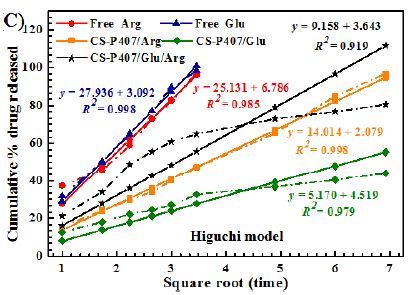
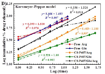
The release profiles of Glu/Arg were found to be suitable for zero and first-degree equations, Higuchi, and Korsmeyer [22,23]. The mean dissolving time (MDT) value was calculated from release kinetic data using equation (Mockel and Lippold) [24].

formula 3

Where n and k are the release exponent and the release rate constant from the Korsmeyer equation, respectively.

Degradation Profiles

Approximately 2 mL hydrogels (Mi) were fabricated in vials subsequently incubated at 37°C. The samples were prepared in distilled water and then diluted in 5 mL buffer PBS pH 7.4 or DMEM. After every 2 days incubation, the liquid was consecutively replaced by 5 mL culture media until the hydrogels had completely disintegrated. The weight of the remaining hydrogel is recorded by an electronic balance. The data profiles were expressed as the average of three measurements. The percentage weight loss is calculated as follows:

formula 1

Mi: initial gel mass (g); Mt: the remaining gel mass (g) and after the degraded time.

Results and Discussions

Characterizations of the Amphiphilic CS-P407 Copolymers

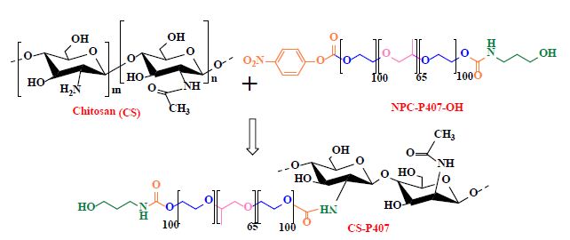
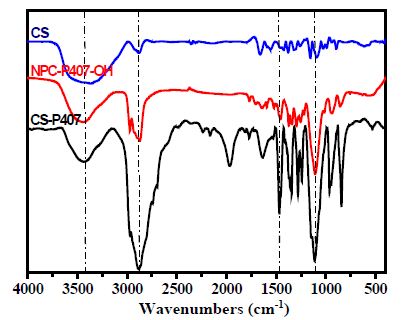
CS-P407 is synthesized based on the carbamate group synthesis reaction through a covalent bond between the carbonate group (NPC-P407-OH) and amino group (-NH2) of CS (Figure 1). The 1H-NMR spectroscopy of CS-P407 copolymer has been mentioned in our previous research [25,26]. Overall, the resonance signal of Poloxamer protons and methyl, methylene and methine group exist in 3.41 – 4.03 ppm and 1.10 ppm (-CH3 of PPO unit). The max resonance was achieved at δ = 1.97 ppm, δ = 2.90 ppm, and δ = 4.64 ppm for protons in glucosamine of CS backbone, which confirmed the structure of co-conjugated compound CS-P407. The FTIR result (Figure 2) describes the spectroscopic features of standard CS in 3368.02 cm-1 wavenumber due to oscillation of O-H bond, 1558.89cm-1 is the oscillation of N-H bond. The NPC-P407-OH spectroscopy shows that the peak in 2885.96cm-1 belongs to the C-H bond in the PEO fraction of Poloxamer P407. The peak at 1111.03cm-1 is caused by a specific C-O linkage of Poloxamer P407. These signals also occurred in CS-P407 spectroscopy at 2890.07cm-1 is a peak of C-H linkage. The stretched oscillation of the C-O bond shows a signal at 1111.88cm-1. The peak at 1571.05cm-1 indicates the -NH deforming signal of the amine group in CS, even though this signal doesn’t exist in CS-P407 spectroscopy due to the amine group has formed a bond with P407 and create an amide I group with a wavenumber at around 1650.04cm-1 [27]. To sum up, the FTIR spectroscopy data shows that the peaks observed are suitable with the expected functional groups in the compound structure of conjugated copolymer.

fig 1

Figure 1: Synthesis of thermosensitive copolymer CS-P407

fig 2

Figure 2: The FTIR spectra of P407, NPC-P407-OH, and CS-P407.

Characterizations of CS-P407 Hydrogels

The CS-P407 hydrogel was coated with a thin layer of approximately 2 mm on the glass slide and the samples were allowed to dry naturally. The sample was then measured by SEM to observe the hydrogel surface structure.

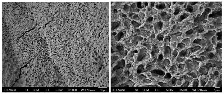
SEM imaging results of Figure 3 show that the CS-P407 hydrogel has an abundant-porous structure (1-2µm) formed by the overlapping network of CS-P407 copolymers. This is the most important characteristic of the hydrogel system (scaffold) since it is not only able to absorb the fluid exudate and maintain certain water content in the wound but also allows the fibroblasts to divide and migrate. The interconnected porous structure has an impact on the supply of nutrient and gas exchange in order to maintain cellular ingrowth and retain a high amount of water, and also it offers ideal material for the Glu/Arg delivery carrier system [10].

fig 3

Figure 3: C-P407 hydrogel surface structure (x1000 image on the left) and (x5000 image on the right)

Thermal Sensitivity of CS-P407 Solution

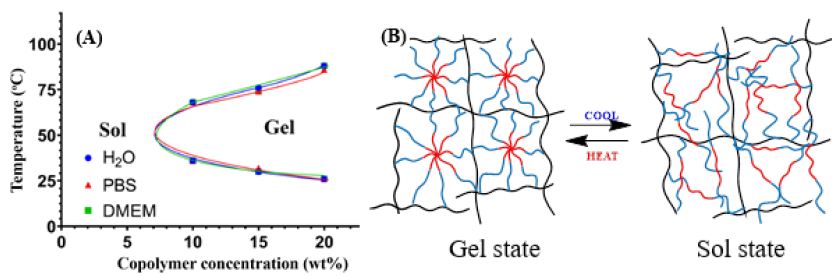
Obtained results of sol-gel transition investigation show that CS-P407 solution can create gel at a relatively low copolymer concentration (above 10% wt/v) at 32-37°C (Figure 4A). When replacing water with PBS buffer and DMEM cell culture media, the transition temperature is unaffected significantly. The thermosensitive hydrogel was formed via hydrophobic interaction of hydrophobic PPO domains in the CS-P407 as seen in Figure 4B. The phenomenon was reported in several studies [5,7,9,10].

fig 4

Figure 4: The phase diagram of the sol-gel transition (A); illustration of the sol-gel transition of the CS-P407 solution (B).

Adhesion of the Hydrogel Scaffolds

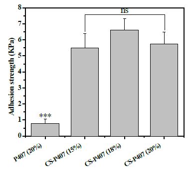
The cohesive ability of hydrogel material to the skin surface is a critical factor in creating material for wound healing. The cohesion process will suppress plasma leakage, prevent bacterial infection, maintain gaseous exchange and provide better access to bioactive compounds in the hydrogel. The tissue adhesive experiment was conducted in porcine skin. As shown in Figure 5, the adhesivity of CS-P407 hydrogels at 15%Wt, 18%Wt, and 20%Wt are 5.51 ± 0.88 KPa, 6.62 ± 0.7 KPa and 5.74 ± 0.74 KPa, respectively. This result was similar to Ji Hyun Ryu’s research in 2011 (The value in this study are about 5.3±2.6 KPa) [28]. At the same condition, P407 hydrogel exhibits a very low tissue adhesion, at which the value is 0.79 ± 0.26 KPa that is similar to a previous study (0.72±0.32 KPa) [29].

fig 5

Figure 5: Adhesion strength (KPa) of the material to the pigskin surface.

The experiment was repeated three times independently (n=3), and the errors are presented in S.E. Statistical significance of p < 0.001 is indicated by ***. Non-statistical insignificance of p ≥ 0.05 is indicated by ns.

This adhesive feature is formed by the positively charged amine groups in the CS backbone interact with the collagen matrix of porcine skin. It depends on chitosan, a polymer with strong adhesivity through its -NH2 groups. As a result, when attaching to the skin surface, CS-P407 can interact with the surface through hydrogen bonds, electrostatic bonds, hydrophobic interaction that make CS-P407 have better adhesive intensity.

Cytotoxicity of Hydrogel CS-P407

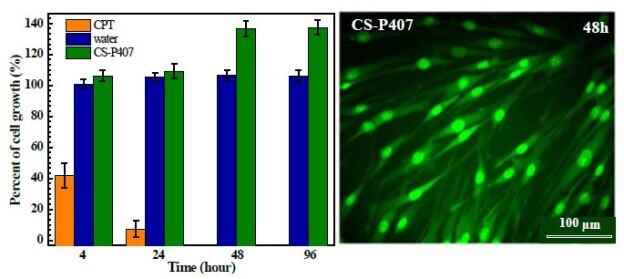
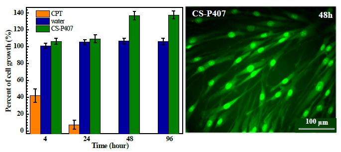
In biomedical material, biocompatibility, or the fitness and harmlessness of the material with the human body and related physiological activities, is the primary criteria to decide its possibility for application. Fibroblasts are vital for wound regeneration, especially in the division, differentiation, and migration stage of fibrocytes at the wound surface. These cells synthesize and secrete extracellular proteins, mainly collagen, to reconstruct the extracellular matrix of connective tissue. In this research, a preliminary cytotoxicity assessment was conducted on fibroblast cell lines from human skin. According to the results in Figure 6, CS-P407 hydrogel is non-toxic for fibroblast. CPT was used at 3 µg/mL, the fibroblast growing rate decreased 42.02 ± 8.05% after 4h of exposure and go down to 7.21 ± 5.38% after 24 hours with total cell death was observed after 48 hours. The number of cells on CS-P407 increase from 106.07 ± 3.52% after 4 hours to 136.8 ± 5.07% after 48 hours. This proves that besides its non-toxicity, CS-P407 can improve cell growth for fibroblasts.

fig 6

Figure 6: Percentage of BJ fibroblasts growth incubated in 0.1 mL of CS-P407, water (negative control) and CPT (positive controls).

In Vitro Amino Acid Release Profile and Release Kinetic Models

In this study, we investigated the proliferative capacity of human fibroblasts (ATCC® CRL-2522™) of free Arg and Glu. Tested concentrations of Arg and Glu from 0-250 µM and 0-500 µM respectively. Figure S.1 showed that the increasing concentration of active ingredients leads to cell proliferation, proving that both Arg and Glu support cell growth and increase wound healing. Arg’s support was significantly impactful on proliferation. Specially, 50 µM for Arg (number of cells = 9 x 10⁴) and 250 µM for Glu (number of cells = 8 x 10⁴) are the optimal concentration for cell proliferation. On the other hand, the excessive use of Arg and Glu also reduces cell growth. This inhibition of cell growth can be seen above 200 µM for Arg and above 450 µM. Based on obtained data, we selected the optimal carry concentrations of Arg and Glu are 50 µM and 250 µM, respectively, into CS-P407. These primary results are the premise to develop a hydrogel system CS-P407 to support treatment and wound healing, show great applications in medicine in general and tissue regeneration in particular.

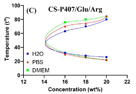
The gelation temperature range was determined from the minimum temperature of gel formation Tgel to the temperature at which the gel begins to melt Tm. In Figure 7, from the measured results, it can be seen that the Tgel gelation temperature of CS-P407 carrying amino acids when mixed with distilled water is higher than that of PBS night medium and physiological DMEM medium at the same concentration. Gel forming temperature range in an aqueous medium is mostly narrower, the results are similar to that of CS-P407 hydrogel. The influence of the medium on the gelation of the hydrogel can be seen. It is understood that in the medium PBS and DMEM gel has higher mechanical properties, more stable. The above results show that the gel is effective in carrying amino acids, without losing the inherent mechanical properties of the system. The CS-P407 polymer system creates a gel at 30-35°C and the gel melting point is above 50°C, so it is very suitable for biomedical applications, especially wound treatment gels.

fig 7

Figure 7: The phase diagram of the sol-gel transition of CS-P407/Arg (A); CS-P407/Glu (B) và CS-P407/Glu/Arg (C)

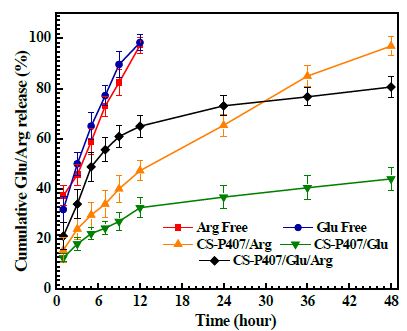
Figure 8 represents the release rate of free Glu and Arg after 12 hours achieve 100% when CS-P407/Glu, CS-P407/Arg, and CS-P407/Glu/Arg rates are 32.53%, 47.28%, and 65.02%. After 48 hours, the release rate at CS-P407/Glu and CS-P407/Arg reach 43.97% and 96.83%, respectively. The Arg release profile of CS-P407 was faster compared to Glu. This difference is according to the carboxylated form of the 2 -COOH group in Glu at pH=7.4 has electrostatic interaction with the positively charged structure of CS-P407, which leads to a slower release rate. When both amino acids were captured in the hydrogel, their release rate reaches 80.59% after 48 hours. Thus, CS-P407 hydrogel helps decelerate the release rate of amino acids, increases their absorptivity at wounded tissue

fig 8

Figure 8: Release profile of amino acid (Glu/Arg) from the hydrogel CS-P407

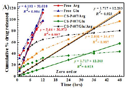
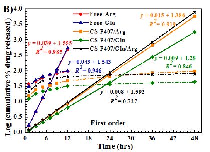
Among all formulas investigated, the Korsmeyer-Peppas regression model has the greatest fitness (R2= 0.9155-9.8874) (Table 1 and Figure 9). With this model, the transport exponent (n) belongs to the (0.3078-0.5218) interval, indicating that the release mechanism of free amino acid and CS-P407/Glu are Fickian diffusions. With free amino acid, it is the passive diffusion, for CS-P407/Glu is due to the CS-P407 gel barrier interaction with Glu. On the other hand, with CS-P407/Arg and CS-P407/Glu/Arg, the release mechanism is non-Fickian, influenced by diffusion and swelling. The rate of diffusion and swelling are the same. The rearrangement of polymer chains happens in slow progress, while the diffusion triggers some abnormal effects over time [30,31].

Table 1: Amino acid release parameters of CS-P407/Glu, CS-P407/Arg, and CS-P407/Glu/Arg hydrogel were obtained to four different mathematical models of drug release kinetics.

Formulation

Mathematical models for drug-release kinetics
Zero order First order Higuchi

Power law

k0

R2 k1 R2 kH R2 K n

R2

Glu Free

0.0981

0.9836 0.5243 0.9459 0.2911 0.9980 0.3179 0.4122

0.9972

Arg Free

0.0935

0.9972 0.5182 0.9854 0.2771 0.9846 0.3339 0.3760

0.9760

CS-P407/Glu

0.0121

0.9231 0.1560 0.8463 0.0799 0.9790 0.1364 0.3078

0.9920

CS-P407/Arg

0.0238

0.9875 0.1805 0.9188 0.1369 0.9982 0.1422 0.4719

0.9974

CS-P407/Glu/Arg

0.0233

0.8275 0.1869 0.7269 0.1611 0.9195 0.2032 0.5218

0.9155

fig 9a

fig 9b

fig 9c

fig 9d

Figure 9: Release kinetics of Glu/Arg from CS-P407 fitted to four kinetic models: (A) zero-order kinetic model, (B) first-order kinetic model, (C) Higuchi model, and (D) Korsmeyer-Peppas model.

Table 2 shows that the MDT value of hydrogel is much higher than free amino acid, which means that amino acids have been entrapped inside the hydrogel matrix. This improves the usage efficiency of the bioactive compound with a short half-life. Thus, CS-P407 hydrogel has prominent potential in the drug distribution process in wound treatment.

Table 2: The fit kinetic model and the MDT value of the modulation formulas.

Formulation

Order of release t25% (hours) t50% (hours) t75% (hours) t90% (hours)

MDT (hours)

Glu Free

Fickian

0.5583 3.0000 8.0223 12.4849

4.7056

Arg Free

Fickian

0.4631 2.9265 8.6043 13.9741

5.0533

CS-P407/Glu

Fickian

7.1578 68.0652 254.1572 459.6082

152.3172

CS-P407/Arg

Non-Fickian

3.3073 14.3690 33.9318 49.9357

20.0140

CS-P407/Glu/Arg

Non-Fickian

1.4878 5.6165 12.2164 17.3257

7.2699

Degradation Profiles

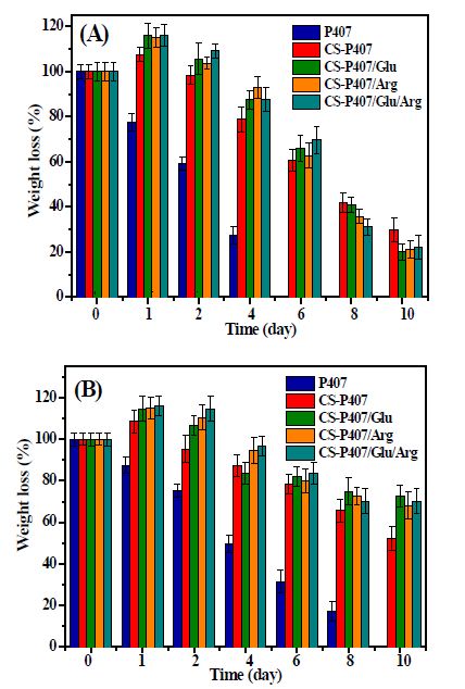
The hydrogel degradability was evaluated by gravimetric analysis of CS-P407 in PBS (pH 7.4) or DMEM solution until the hydrogel was completely degraded. Figure 10 shows that CS-P407 hydrogel had a degradation time of 10 days in PBS buffer with pH 7.4, which was 1.7 times longer than the P407 hydrogel sample. This shows that the combination of Poloxamer P407 with CS (which is a bio-adhesive agent) has increased the stability of the hydrogel system. The results can be explained as the interweaving of the branched copolymer chains is increased by CS, leading to increase hydrogel stability during decomposition. Comparing degradation time in two physiological media, PBS medium pH 7.4 degraded more rapidly, when all samples have been downgraded after 12 days. DMEM medium has a longer degradation time, as the hydrogel sample remains after 16 days of investigation. Loading arginine and glutamic resulted in prolonging degradation of the bioactive hydrogels. This could be contributed by hydrogen bonding formation of amino acids and chitosan chains leading to increase the stability of the hydrogel matrix.

fig 10

Figure 10: Degradation profile of hydrogel samples in PBS pH 7.4(A) and DMEM (B).

Conclusion

The bioactive hydrogel loading glutamic and arginine amino acid was developed. CS-P407 18 wt/wt% copolymer solution strongly forms hydrogel at body temperature. The system exhibits a porous structure, high tissue adhesion, and cytocompatibility which is injectable for applying minimal invasion surgery. The optimum concentrations of Arg and Glu used in the CS-P407 system to increase cell proliferation are 50 µM and 250 µM, respectively. The CS-P407 hydrogel performed a suitable platform for controlling the delivery of these amino acids. The release behavior is affected by concentration diffusion and the swelling of the gel system. Arginine and glutamic encapsulation resulted in the prolonged degradation of bioactive hydrogels. The preliminary results could pave the way to apply the bioactive hydrogel in would healing.

Acknowledgements

This work was supported by the Ho Chi Minh Department of Science and Technology (number of contract 47/2019/HĐ-QPTKHCN)

References

  1. Pramanik S, Pingguan-Murphy B, and Osman NAA (2012) Progress of key strategies in development of electrospun scaffolds: bone tissue. Science and Technology of Advanced Materials 13: 043002.
  2. Wang K, Hao Y, Wang Y, Chen J, Mao L, et al. (2019) Functional hydrogels and their application in drug delivery, biosensors, and tissue engineering. International Journal of Polymer Science.
  3. Le PN, Huynh CK, Tran NQ (2018) Advances in thermosensitive polymer-grafted platforms for biomedical applications. Materials Science and Engineering: C 92: 1016-1030. [crossref]
  4. Bhattarai N, Gunn J, Zhang M (2010) Chitosan-based hydrogels for controlled, localized drug delivery. Advanced drug delivery reviews 62: 83-99.
  5. Choi JH, Joung YK, Bae JW, Choi JW, Quyen T, et al. (2011) Self-assembled nanogel of pluronic-conjugated heparin as a versatile drug nanocarrier. Macromolecular research 19: 180-188.
  6. Antoniraj MG, Kumar CS, Kandasamy R (2016) Synthesis and characterization of poly (N-isopropylacrylamide)-g-carboxymethyl chitosan copolymer-based doxorubicin-loaded polymeric nanoparticles for thermoresponsive drug release. Colloid and Polymer Science 294: 527-535.
  7. Huynh NT, Dang LH, Pham NO, Nguyen CT, Vu MT, et al. (2019) Injectable nanocurcumin-dispersed gelatin–pluronic nanocomposite hydrogel platform for burn wound treatment. Bulletin of Materials Science, 42: 1-10.
  8. Nguyen TTC, Nguyen CK, Nguyen TH, Tran NQ (2017) Highly lipophilic pluronics-conjugated polyamidoamine dendrimer nanocarriers as potential delivery system for hydrophobic drugs. Materials Science and Engineering: C 70: 992-999.
  9. Dang LH, Nguyen TH, Tran HLB, Doan VN, Tran NQ (2018) Injectable nanocurcumin-formulated chitosan-g-pluronic hydrogel exhibiting a great potential for burn treatment. Journal of healthcare engineering. [crossref]
  10. Pham L, Dang LH, Truong DM, Nguyen TH, Le L, et al. (2019) A dual synergistic of curcumin and gelatin on thermal-responsive hydrogel based on Chitosan-P123 in wound healing application. Biomedicine & Pharmacotherapy 117: 109183.
  11. Park KM, Lee SY, Joung YK, Na JS, Lee MC, et al. (2009) Thermosensitive chitosan–Pluronic hydrogel as an injectable cell delivery carrier for cartilage regeneration. Acta biomaterialia 5: 1956-1965. [crossref]
  12. Hosseinzadeh H, Atyabi F, Dinarvand R, Ostad SN (2012) Chitosan–Pluronic nanoparticles as oral delivery of anticancer gemcitabine: preparation and in vitro study. International journal of nanomedicine 7: 1851-63. [crossref]
  13. Nguyen VT, Nguyen TH, Dang LH, Vu-Quang H, Tran NQ (2019) Folate-conjugated chitosan-pluronic P123 nanogels: synthesis and characterizations towards dual drug delivery. Journal of Nanomaterials.
  14. Fujiwara T, Kanazawa S, Ichibori R, Tanigawa T, Magome T, et al. (2014) L-arginine stimulates fibroblast proliferation through the GPRC6A-ERK1/2 and PI3K/Akt pathway. Plos one 9: e92168.
  15. Aalto M, Lampiaho K, Pikkarainen J, Kulonen E (1973) Amino acid metabolism of experimental granulation tissue in vitro. Biochemical Journal 132: 663-671. [crossref]
  16. Szekalska M, Puciłowska A, Szymańska E, Ciosek P, Winnicka K (2016) Alginate: current use and future perspectives in pharmaceutical and biomedical applications. International Journal of Polymer Science.
  17. An D, Ji Y, Chiu A, Lu YC, Song W, et al. (2015) Developing robust, hydrogel-based, nanofiber-enabled encapsulation devices (NEEDs) for cell therapies. Biomaterials 37: 40-48. [crossref]
  18. Armstrong DW, Gasper M, Lee SH, Zukowski J, Ercal N (1993) D‐amino acid levels in human physiological fluids. Chirality 5: 375-378. [crossref]
  19. Nguyen CT, Dang LH, Nguyen DT, Tran KP, Giang BL, et al. (2019) Effect of GA3 and Gly plant growth regulators on productivity and sugar content of sugarcane. Agriculture 9: 136.
  20. Zhou W, Zhanga XY, Duana GL (2011) Liquid‐Chromatography Quantitative Analysis of 20 Amino Acids after Derivatization with FMOC‐Cl and Its Application to Different Origin Radix isatidis. Journal of the Chinese Chemical Society 58: 509-515.
  21. Nguyen TD, Nguyen TN, Nguyen TT, Ivanov IA, Nguyen KC, et al. (2019) Nanoencapsulation enhances anticoagulant activity of adenosine and dipeptide IleTrp. Nanomaterials 9: 1191.
  22. Kuksal A, Tiwary AK, Jain NK, Jain S (2006) Formulation and in vitro, in vivo evaluation of extended-release matrix tablet of zidovudine: influence of combination of hydrophilic and hydrophobic matrix formers. AAPS pharmscitech 7: E1-E9. [crossref]
  23. Sahu A, Kasoju N, Goswami P, Bora U (2011) Encapsulation of curcumin in Pluronic block copolymer micelles for drug delivery applications. Journal of biomaterials applications 25: 619-639. [crossref]
  24. Roni MA, Kibria G, Jalil RU (2009) In vitro studies of controlled release alfuzosin matrix tablets prepared with ethylcellulose and hydroxypropyl methylcellulose. Iranian Journal of Pharmaceutical Sciences.
  25. Dang LH, Vu MT, Chen J, Nguyen CK, Bach LG, et al. (2019) Effect of ultrasonication on self-assembled nanostructures formed by amphiphilic positive-charged copolymers and negative-charged drug. ACS Omega 4: 4540-4552.
  26. Nguyen DH, Nguyen VT, Nguyen CK, Nguyen TH (2016) Green processing of thermosensitive nanocurcumin-encapsulated chitosan hydrogel towards biomedical application.
  27. Nguyen TBT, Dang LH, Nguyen TT, Tran DL, Nguyen DH, et al. (2016) Green processing of thermosensitive nanocurcumin-encapsulated chitosan hydrogel towards biomedical application. Green Processing and synthesis 5: 511-520.
  28. Ryu JH, Lee Y, Kong WH, Kim TG, Park TG et al. (2011) Catechol-functionalized chitosan/pluronic hydrogels for tissue adhesives and hemostatic materials. Biomacromolecules 12: 2653-2659. [crossref]
  29. Lee Y, Chung HJ, Yeo S, Ahn CH, Lee H, et al. (2010) Thermo-sensitive, injectable, and tissue adhesive sol–gel transition hyaluronic acid/pluronic composite hydrogels prepared from bio-inspired catechol-thiol reaction. Soft Matter 6: 977-983.
  30. Mircioiu C, Voicu V, Anuta V, Tudose A, Celia C, et al. (2019) Mathematical modeling of release kinetics from supramolecular drug delivery systems. Pharmaceutics 11: 140. [crossref]
  31. Shaikh HK, Kshirsagar RV, Patil SG (2015) Mathematical models for drug release characterization: a review. World J. Pharm. Pharm. Sci 4: 324-338.

Resource Optimization through Group, Pooling, Tests, Testing in the Detection of Asymptomatic People with COVID-19

DOI: 10.31038/MIP.2021221

Abstract

The current ongoing coronavirus disease 2019 (COVID-19 SARS2 and detection and isolation of infected people with the virus is crucial. Real-time polymerase chain reaction (RtPCR) test has proven to be most useful  in  viral  detection.  The  objective  of  this  work  is  to  determine  the  benefit  of  group testing for resource optimization and be able to expand the number of individuals who are screened to find healthy COVID-19 carriers. Groups from 2 to 27 of a total of 2,100 people were included. RT-PCR was done with Seegene kits for mRNA extraction and reagents in Biorad RT-PCR machine. Results: groups of between 4 to 6 people have been the ones with the best optimization results with 64 to 67%, this means that with 1 test it is possible to cover the same number of people and detect more quickly those who must be isolated and follow their contacts. Conclusion: Grouping tests can optimize resources up to 67%.

Background

The current ongoing coronavirus disease 2019 (COVID-19 SARS2) pandemic with mainly severe acute respiratory syndrome, is a serious global public health problem. The detection and  isolation  of infected people with the virus is crucial. Hitherto, the real-time polymerase chain reaction (RT-PCR) test has proven to be most useful in viral detection when performed using nasal and oropharyngeal exudate samples. Due to the global and rapidly progressive nature of the pandemic, the tests have been limited in supply with a high cost; therefore, their optimization is important. The Many millions of tests have been performed almost exclusively on an individual basis and are many millions of tests [1]. To date, the United Kingdom has performed the highest number of tests globally, with 486 billion tested inhabitants [2]. In the open population, the first positivity reported by South Korea, who had performed the greatest number of tests, the statistic of positives was 1.7% in the open population, and later in May 2020 they performed 10 million tests and only had 300 positives (positivity rate of 0.9% of positivity) between 1,553,5523.. In the United States of America, the positivity rate in the suspected sample population was 19.8% and 9.6% in the general population of 32,009,840 by July 25, 20204. Based on this percentage, the negativity rate in the general  population  is expected to be high. It is known that a person infected by COVID-19 (SARS- CoV-2) who is asymptomatic, has an approximate viral load of 6.76 x 10⁶ viral copies in the first five days of infection [3-9]. Subsequently, the viral load decreases from day 6, to 3.44 x 10 viral copies. In addition, it has been described that the viral load is not detectable by day 28 in up to 39.93% of infected people. On the other hand, patients with symptoms can present a viral load of up to 7.11 x 10⁸ viral copies [5-9]. Taking these findings into account, it was found feasible to do group tests (pooling), the first published antecedent for COVID-19 is from Yelin and collaborators [10] in which they make groups of 35 people. In later publications, theoretical calculations are made on the number of people to include in the groups and with automated equipment [11-13], finding savings and optimization of resources of 69% [13].

Objective

Determine the benefit of group testing for resource optimization and be able to expand the number of individuals who are screened  to find healthy COVID-19 carriers. In our laboratory to assess this observation at the beginning, we carried out a preliminary test with 19 people including technicians, doctors, administrative and cleaning staff, all asymptomatic, a sample was taken from each person and the pilot group was carried out, gathering aliquot of 19 people in a pool, performing a single RT-RCR test for COVID-19, obtaining a negative result. None developed any symptoms of COVID-19 in the next 2 months. Additionally, the same  procedure  was  performed  adding to that pool with an already known positive sample, obtaining the positive result in the pool sample.

Material and Methods

An observational, cross-sectional and descriptive study was carried out.

Selection and Inclusion Criteria

Open population with asymptomatic individuals who are considered healthy, including asymptomatic carriers, which is the objective of this study. Selection of people and groups: a call was made to individuals and companies of various types, who were named as suppliers: 1) Family group: people who live in the same home; 2) Work group: people who work in the same place; 3) Health group: health workers with or without direct contact with patients. The selection of the groups was initially proposed in groups selected by each supplier, without exceeding 30 people. People were recruited between May  21 and August 5, 2020. Exclusion criteria: People with respiratory symptoms of any type and degree and with fever were ruled out. Taking samples: It was carried out either in the laboratory or at the work sites. In both cases with the safety measures by the sampling personnel according to the WHO recommended. The transport was carried out with triple packaging. A nasopharyngeal sample was taken from each individual and placed in a tube with 2.0 ml of transport medium, from which an aliquot of 0.10 ml was taken from each individual to form the pool of that group, a single mRNA extraction was performed in each group. The samples were kept refrigerated for the first 24 hours and after that time they were kept frozen at -20°C until processing.

Sample Processing

Extraction of viral DNA/RNA, using Invisorb® Spin universal kit reagents Invitek Molecular Gmbh Berlin. In a 2 ml Safe lock tube, place 200 µl of the sample, with 200 µl HTL buffer, 20 µl of carrier DNA and 20 µl of Proteinase K, mix in vortex for 10 seconds, place the tube in thermomix and incubate with constant shaking x 10 minutes at 65°C and then 10 minutes at 95°C. Binding Add 260 µl of binding solution to the sample lysate and mix by pipetting up and down or vortex. The sample is incubated for 5 minutes at room temperature. The sample is transferred to the RTA Spin filter with the receiving RTA tube. The tube is closed and centrifuged for 1 minute at 11.1100 g. Discard the RTA Receiver with the filtrate and fit a new receiver tube. The samples are centrifuged at -20°C. Separately, the following reagents are prepared: 1) 5 µl of 2019-nCoV MOM reagent (Seegene®); 2) 5 µl of RNase-free water; 3) 5 μl of Buffer 5X Real-time One-Step (Seegene®), and 4) 2 μl of Real-time One-Step enzyme (Seegene®). The mixture is centrifuged briefly and 17 μl of One-step RT-PCR Mastermix (Seegene®) will be added.

8 μl of the group of samples, 2019-nCoV PC and RNAs-free distilled water will be added to the previous solution. Afterwards, the samples will be centrifuged and they will be placed in the equipment for RT-PCR. (2) The AllplexTM 2019-nCoV kit (Cat. No. RP10243X; Seegene®) will be used for the qualitative detection of SARS-CoV-2 (COVID-19). The kit evaluates the E, RdRP and N genes of SARS- CoV-2. (3) Polymerase chain reaction with reverse transcriptase. The samples will be placed in the equipment for RT-PCR (CFX96TM, BioRad®), with the following parameters: Cycle 1) Temperature 50°C, duration 20 minutes; Cycle 2) Temperature 95°C, duration 15 minutes; Cycles 3-44) Temperature 94°C, duration 15 seconds each; Cycle 45) Temperature 58°C, duration 30  seconds.  The  cycling  determined to evaluate the positivity of the sample is 45 cycles according to the manufacturer’s protocol.

Data Interpretation

The data obtained from the RT-PCR process will be automatically analyzed in the CFX96 ManagerTM program included in the BioRad® kit. The cut-off point to establish a sample as positive is the value of Ct ≤40.

Statistical Analysis

Frequencies and percentages were determined, Pearson’s correlation test was applied. The data analysis was carried out with the SPSSv23 program. A p value <0.05 was considered as statistical significance. Ethical and biosafety aspects: The protocol was approved by the research department of the General Hospital of Mexico Eduardo Liceaga of CDMX with number DI / 20/405103150.

Results

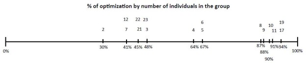
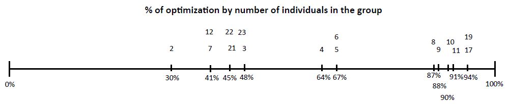
2,100 participants were included, 60% (1,260 people) were men and 40% (840 people) were women. The average age was 35 years, with a range of 18 to 65 years. The participants were gathered into 536 groups, which meant performing the same  number  of  tests. The groups consisted of a minimum of 2 people and a maximum     of 23 people and were selected by the suppliers (Table 1), 17.35% (93 groups) were positive with a total of 131 positive people, which means 6.2% of positive people out of the 2,100 included in the study. To detect positive people in each group, 372 additional tests were required, optimization of the test resource in total groups between    2 to 27 people was 56.76%, this figure was obtained in relation to the total number of people included that would be equivalent to the tests performed individually (n 2,100, 100%) and the number of tests actually performed, obtained from the sum of the number of groups (n 536) plus the number of additional tests, of each positive group individual tests were performed in groups. The additional tests where done in the positive groups as follows: from 2 to 7 people individually and in those from 8 to 27 in subgroups of 2 or 3 and of them the positive ones individually, obtaining a total of 372 additional tests, which added to the initial ones were 908, the % optimization in relation to the Initial theoretical of 2,100 tests and the performed test 908 equivalent to 56.76% (100-(908 * 100/2100). Table 1 shows the % optimization for each group, the small % was 2 people and the better between 4, 5 and 6 people. There were between 1 and 2 groups of 8, 9 and 11 to 23 people who were carried out very early in the study (May- June) that had a very high % optimization (87 to 94) and it should  be considered that at the beginning of the pandemic there were very few infected people. The number of members of each group had a low positive correlation with the number of additional tests performed (rho=0.13, p=0.009), while the number of additional tests performed had a high positive correlation with the number of tests that resulted positive for COVID-19 (rho=0.99, p=0.0001) (Figure 1) [14].

Table 1: Optimization% for each group.

People per group

Total no. of people in the groups n of groups Positive no. of groups no. of positive People Additional tests Total of Tests performed Theoretically individual tests % Optimization
2 482 241 48 49 96 337 482

30.08

3

132 44 8 8 24 68 132 48.48
4 220 55 6 11 24 79 220

64.09

5

580 116 15 32 75 191 580 67.07
6 294 49 8 12 48 97 294

67.01

7

63 9 4 8 28 37 63 41.27
8 16 2 0 0 0 2 16

87.50

9

9 1 0 0 0 1 9 88.89
10 50 5 0 0 0 5 50

90.00

11

22 2 0 0 0 2 22 90.91
12 24 2 1 1 12 14 24

41.67

17

17 1 0 0 0 1 17 94.12
19 19 1 0 0 0 1 19

94.74

20

40 2 1 2 20 22 40 45.00
21 42 2 0 0 0 2 42

95.24

22

44 2 1 7 22 24 44 45.45
23 46 2 1 1 23 25 46

45.65

Total

2100 536 93 131 372 908 2100

56.76

fig 1

Figure 1: From Left to Right % of optimization below the line. In top of line number of individuals in each group.

Discussion

The SARS COVID-19 pandemic persists till the end of 2020 and probably the first half of 2021, and in the absence of a specific drug and only treatments for the effects of the virus on the coagulation and inflammatory process, the isolation strategy and follow-up of contacts with real-time PCR tests should be followed. The Vaccines probably will modify the number of positive people, but still will be important, given the cost of the tests to be able to optimize resources and group or pool tests is an effective method to do it. Groups of between 4 to  6 people have been the ones with the best optimization results with 64 to 67%, this means that with 1 test it is possible to cover the same number of people and detect more quickly those who must be isolated and follow their contacts. The groups of two are not adequate since an initial test is required and if positive result requires 2 additional tests and this means to carry out for two people three tests. Positive groups of more than 10 people require performing individual tests   in subgroups of 2 or 3 and positive ones in individual tests, which is not practical since it takes at least two or three additional days to perform them and although the optimization obtained was of up to 94%, in time and at present time with the expected increase in the number of cases it would not be practical. We found groups of 4 to 6 people are optimal. 3 groups with false positives were detected, these show to start positive above cycle 33 of the 45 cycles of the Rt-PCR programming and the individual tests were always negative. In the groups with cycles less than 31, the positive person or persons were always detected. Two different brands of reagents were used to verify the results in the 3 false positive groups with the same results.

Conclusion

Carrying out group tests in asymptomatic people of open population for any reason, whether it is resuming activities or detecting cases of healthy carriers, is very effective and is optimal in groups 4, 5 and 6 people, this allows more tests to be carried out at a lower cost.

References

  1. Huipeng Ge, Xiufen Wang, Xiangning Yuan, Gong Xiao, Chengzhi Wang et (2020) The epidemiology and clinical information about COVID-19. European Journal of Clinical Microbiology & Infectious Diseases 39: 1011-1019. [crossref]
  2. Consultada 21 de octubre 2020
  3. http://ncov.mohw.go.kr/en/ Tests in Suth Corea updated 1 july 2020
  4. Ultimo acceso 1 de Agosto 2020
  5. Chen Y, Liu Q, Guo D (2020) Coronaviruses: genome structure, replication, and pathogenesis Deyin Guo ORCID.
  6. Zou L, Ruan F, Huang M, Liang L, Huang H et al (2020) SARS-CoV-2 Viral Load in Upper Respiratory Specimens of Infected Patients. N engl j med 382: 1171-1179. [crossref]
  7. Enfermedad por coronavirus, COVID-19 Ministerio de Sanidad España Centro de coordinación de alertas y emergencia sanitaria actualización 4 de abril 2020
  8. Tapiwa G, Cécile K, Dongxuan Ch, Andrea T (2020) Estimating the generation interval for COVID-19 based on symptom onset medRxiv
  9. Wölfel R, Corman VM, Guggemos W, Seilmaier M, Zange S (2020) Virological assessment of hospitalized patients with COVID-2019. Nature 581: 465-469. [crossref]
  10. Idan Yelin, Noga Aharony,  Einat Shaer Tamar,  Amir Argoetti, Esther Messer, et  (2020) Evaluation of COVID-19 RT-qPCR test in multi-sample pool. medRxiv preprint
  11. Roni Ben-Ami, Agnes Klochendler, Matan Seidel, Tal Sido, Ori Gurel-Gurevich, et (2020) Large-scale implementation of pooled RNA extraction and RT-PCR for SARS- CoV-2 detection. Clinical Microbiology and Infection PII: S1198-743X(20)30349-9.
  12. Michael G Becker, Tracy Taylor, Sandra Kiazyk, Dana R Cabiles, Adrienne FA Meyers, et al. (2020) Recommendations for sample pooling on the Cepheid 1 GeneXpert® system using the Cepheid Xpert® Xpress SARS-2 CoV-2 bioRxiv preprint
  13. Abdalhamid B, Bilder CR, McCutchen EL, Hinrichs SH, Koepsell SA, etal. (2020) Assessment of Specimen Pooling to Conserve SARS CoV-2 Testing Am J Clin Pathol 153: 715-718. [crossref]
  14. Ola Brynildsrud (2020) COVID-19 prevalence estimation  by  random  sampling in population – optimal sample pooling under varying assumptions about true prevalence BMC Med Res Methodol 20: 196.

Soybean Phosphatidylcholine-based Nanovesicular Topical Formulation for Non-invasive Treatment of Localized Obesity

DOI: 10.31038/JPPR.2021434

Abstract

A novel non-invasive approach for treatment of localized obesity is introduced utilizing carbopol gel containing soybean phosphatidylcholine based nanovesicular system for topical application. The tested systems are designed to combine the absence of side effects of the multi-injection system used in mesotherapy and the ease of application. Nanovesicles such as transfersomes and transethosomes were prepared using soybean phosphatidylcholine, tween 80, sodium deoxycholate, cremophor, and oleic acid in different concentrations determined according to 3D-optimal mixture experimental design. The prepared vesicles were evaluated and incorporated into carbopol gel. The stability of the prepared nanovesicles and gel was examined after storage for six months at 4˚C. In-vivo and In-vitro studies were performed using male albino rats. Performed experiments on rats showed that the three formulations of choice (F4e, F11e and Et11) succeeded to reduce body weight, percentage dorsal fat and total lipid content significantly (P<0.05) without appearance of any sign of skin irritation compared to PC marketed injections (Adipoforte®) used in mesotherapy. PC nanovesicular gel, containing transethosomes (F4e, F11e & Et11), can be significantly considered as effective noninvasive treatment for localized obesity as an alternative to multi-injections for mesotherapy.

Keywords

Phosphatidylcholine, HPLC-Determination, Experimental Design, Nanovesicles, Mesotherapy.

Introduction

Obesity is recognized as one of the most important public health problems facing the world[1]. Up to 30% of the western adults are obese[1]. In Middle East and North Africa, obesity prevalence reaches about 19% of whole population while it reaches 33% in Egypt [2]. Mesotherapy is a controversial cosmetic procedure for localized fat accumulations reduction. Subcutaneous Phosphatidylcholine(PC) injection has been performed effectively as nonsurgical treatment of localized fat deposits in abdomen, neck, arms and thighs [3]. PC has first a lipocyte-destroying effect and then a lipolytic action, which is active over 8weeks [4]. Despite being minimally invasive alternatives to liposuction, it causes localized and systemic side effects that usually appear 2-5days after application and include allergic reactions, tissue necrosis and body surface irregularities [5]. Nanotechnology-based delivery systems can protect drugs from degradation, reduce dose regimen, and enhance drug solubility. Vesicular system offers controlled drug delivery and increased drugs permeation through skin [6]. Transfersomes are metastable vesicles, sufficiently deformable to penetrate pores much smaller than their own size. They consist of phospholipids and one or more edge-activator [7]. Transethosomes are elastic ultra-deformable lipid vesicles containing high concentration of ethanol and edge-activators causing destabilization of the lipid bilayer and increases its flexibility [8]. Accordingly, this work aims to introduce non-invasive dosage form of high patient compliance for efficient, safer treatment of localized obesity instead of the applied multi-injection regimen through application of nanotechnology in drug targeting.

Materials and Methods

Materials

Soybean PC, SDC, cremophorA25, cholesterol, chloroform and methanol HPLC grade were purchased from Sigma-Aldrich (Darmstadt, Germany). Potassium hydroxide, oleic Acid, tween 80, and ethanol were purchased from El-Nasr Pharmaceutical Chemicals (Cairo, Egypt). Trichloroacetic acid was purchased from Carl-Roth Company (Karlsruhe, Germany). Carbopol 934 was purchased from Arabic laboratory equipment (Cairo, Egypt).

Animals

Male Albino rats (50±5gm) were purchased from National Research Center, Giza, Egypt. The study protocol was conducted in accordance with the ethical procedures and policies approved by the Animal Care and Use Committee of Faculty of Pharmacy-German University in Cairo. All rats were maintained in the animal facility at 25±5ºC,12hours dark and 12hours light cycle.

Methods

Quantitative analysis of PC

A modified method was applied for PC determination. A Spectrasystem High performance liquid chromatography (HPLC) consisting of Spectrasystem pump P2000 and detector UV-3000 connected to Thermo C8 reverse-phase analytical column (250mm lengthx4.6mm internal diameter and particle size 5μm) (Thermofisher, UK). The mobile phase consists of acidified water at pH3.5 and methanol [9]. Gradient elution was performed at a flow rate of 1.5ml/min from 80% to 100% methanol in 40min (as shown in Table1). Invitro calibration curve was constructed using concentration range (7.5-62.5µg/ml) of PC standard solution in ultrapure water. 50µl of prepared solution was injected into the HPLC. The flow rate was adjusted at 1.5ml/min at 20˚C and detection was carried at 205nm [10]. The assay procedures were validated in terms of linearity, precision, and accuracy (R=0.9981, LOD=2.5ng/ml;LOQ=6.5ng/ml; interday and intraday assay RSD<10%, accuracy≈99%). PC concentrations in the withdrawn samples were calculated with reference to the calibration curve of area under the curve of peak corresponding to PC concentrations (Insert Table 1).

Table 1: Gradient elution of PC using methanol and acidified water

Time (min)

Acidified Water (%) Methanol (%)
0 20

80

40

0 100
45 0

100

46

20 80
55 20

80

Preparation of Phosphatidylcholine Vesicles

Preparation of Transfersomes

Transfersomes were prepared using the thin film hydration method. PC and surfactants were solubilized in chloroform-methanol (2:1respectively) [11]. The organic solvent was evaporated leaving a dry thin film using a rotary evaporator (Buchi, Switzerland) at 55˚C, 80rpm and 471bars. The film was hydrated with 5ml ultrapure water previously heated at 55˚C. The hydrated vesicles were then rotated using rotary evaporator at 80rpm and 55˚C for 1hour at normal atmospheric pressure [12]. The prepared vesicles were left at room temperature for 2hours for swelling then kept at 4˚C [13]. The aforementioned prepared vesicles were labeled(F).

Preparation of Transethosomes Hydrated with 20%Ethanol

Transethosomes were prepared using the thin film hydration method similar to that used for preparation of transfersomes. However, the hydration step was performed with 5ml of 20%ethanol. These vesicles were labeled (Fe).

Preparation of Transethosomes

Transethosomes were prepared using the solvent dispersion method. PC and surfactants were solubilized in 1.5ml of 20%ethanol [14] under vigorous stirring in tightly covered round bottom flask in a water bath at 30˚C. An aliquot of 3.5ml ultrapure water [15] was added slowly under continuous stirring. The nanosuspension was left at room temperature for 30min under continuous stirring. The prepared formulations were left at room temperature for 2hours then kept in at 4˚C[13]. They were then labeled (Et).

D-Optimal Mixture Design Model

In order to investigate the different effects of the used ingredients for preparing the vesicles which are composed of PC together with a blend of surfactants, a D-optimal mixture design was conducted using the Design-Expert 7.0software [16]. The demonstrated independent variables were: the individual amounts of each of Cremophor, Sodium deoxycholate (SDC), Tween 80 and Oleic acid. The responses were: the particle size, polydispersity index and the %yield. Values of the dependent variables; particle size (P.S), polydispersity index (PDI) and yield percentage (%yield), were fed into the utilized software and equations linking the dependent and independent variables were produced. The composition of the prepared formulations for the full experimental design is shown in Table2. Three Models were conducted; P.S, PDI and %yield respectively (Insert Table 2).

Table 2: Composition of the prepared nanovesicles (mg)

Formula

PC (mg) CHOL (mg) Tween80 (mg) Sodium deoxycholate (mg) Cremophor (mg) Oleic acid (mg)
Transfersomes prepared by thin film hydration method Transethosomes prepared by thin film hydration method

Transethosomes prepared by solvent dispersion method

F 1

F 1e Et 1 80 0 10 10 0 0
F 2 F 2e Et 2 80 0 0 10 0

10

F 3

F 3e Et 3 80 0 0 0 20 0
F 4 F 4e Et 4 80 0 2.5 12.5 2.5

2.5

F 5

F 5e Et 5 80 0 10 0 0 10
F 6 F 6e Et 6 80 0 0 20 0

0

F 7

F 7e Et 7 80 0 0 20 0 0
F 8 F 8e Et 8 80 0 0 0 0

20

F 9

F 9e Et 9 80 0 20 0 0 0
F 10 F 10e Et 10 80 0 10 0 10

0

F 11

F 11e Et 11 80 0 12.5 2.5 2.5 2.5
F 12 F 12e Et 12 80 0 0 0 0

20

F 13

F 13e Et 13 80 0 0 0 20 0
F 14 F 14e Et 14 80 0 0 10 10

0

F 15

F 15e Et 15 80 0 5 5 5 5
F 16 F 16e Et 16 80 0 0 0 10

10

F 17

F 17e Et 17 100 0 0 0 0 0
F 18 F 18e Et 18 80 20 0 0 0

0

Et 19

80 0 0 0 20 0
Et 20 80 0 3 1 13

3

Et 21

80 0 1 5 13 1
Et 22 80 0 2 2 14

2

Et 23

80 0 1 1 17 1

Et 24

80 0 2.5 0 15

2.5

Et 25

80 0 6 8 4 2
Et 26 80 0 3 14 2

1

Characterizations of the Prepared Vesicles

Determination of Phosphatidylcholine %yield. PC %yield was determined using the ultracentrifugation method using cooling centrifuge (Hermle, Germany) where 1ml sample of each formulation was placed in a 1.5ml eppendorf [17] and centrifuged at 4˚C at a speed of 14000rpm for 2hours [18]. The supernatant was collected. The vesicles were washed with 0.5ml ultrapure water and recentrifuged for 2hours. The supernatant was separated and its total volume was detected. An aliquot of 50µl of the total supernatant was diluted and peak area was measured using HPLC at λmax=205nm. The concentration was calculated according to the established calibration curve. Each sample was measured in triplicates and mean value was reported. %Yield was calculated as follows:

equation 1

Particle Size, Polydispersity index and Zeta Potential (ZP) Measurement

An aliquot of a 1ml sample of the prepared formulation was ultra-centrifuged at 4˚C and 14000rpm for 2hours. Consequently, the supernatant was removed. The vesicles were washed with 0.5ml ultrapure water and recentrifuged for 2hours. The supernatant was removed and the vesicles were redispersed by vortexing for 10seconds. Afterwards, 0.35ml of the vesicles was diluted to 5ml with ultrapure water. P.S and surface charges of the nanovesicles were measured using Zeta-Sizer Nano-ZEN3600. The measurements were executed in triplicates for each sample and the average values were calculated [14;19].

Transmission Electron Microscopy (TEM)

The morphology of a dilute stock of selected nanovesicles was examined using electron transmission microscope TECNAI-G2 S-Twin (Netherlands) at 80KV after being stained with phosphotungstic acid [1].

Elasticity Test

The selected vesicles elasticity test was performed using the extrusion method[20] where the nanosuspension was extruded through Micropore cellulose membrane filter of 0.22µm at a constant flow of 115L/min. Deformability was reported as the deformability index (DI) calculated by following equation [21]:

DI=j×(rv/rp)2   (Equation2)

Where, j is the suspension flow rate, rv the vesicle size and rp the membrane pore size [20].

Stability testing of the prepared nanovesicles

Stability tests were performed for the selected formulae stored at 4˚C for 6months. The stability was assessed by measuring %yield, ZP, P.S and PDI. Measurements were executed in triplicates for each sample and the mean values were calculated [22].

Preparation of the nano-phosphatidylcholine vesicular gel:

The selected nanovesicles were centrifuged at 4ºC, 14000rpm for 2hours. The supernatant was removed and samples were redispersed using 0.5ml ultrapure water. Nanovesicular gel with 2%carbopol 934 was prepared using triethanolamine, methyl and propyl parabens [23]. The prepared gel was stored at 4˚C.

Characterizations of the nanovesicular gel:

Physical examination

The developed gel was tested for color, transparency, homogeneity by visual inspection [24].

pH measurement

The pH of 1%aqueous solutions of the prepared gels was measured using pH-meter (Jenway, UK) [25].

Viscosity Studies

The gel apparent viscosity was measured using Visco-star plus Viscometer (Fungilab, Barcelona) at room temperature. Readings were taken after 5min. Measurements were executed in triplicates [25].

Spreadability Test

Spreadability was assayed by pressing 0.5gm of gel between two glass slides till no more spreading occurs. Four diameters, for each of the formed circle, were measured and the average diameter was calculated. The mean of triplicates of each formulation was used as comparative values for spreadability [26].

Drug content determination

Drug content of the gel was quantified. 250mg of the prepared gel was mixed with 10ml water thoroughly. The produced solution was centrifuged for 30min at 6000rpm using Hermle centrifuge (Wehingen, Germany). The supernatant was then filtered, 0.5ml of supernatant was diluted. Drug content was determined using HPLC. The concentration was obtained using the established calibration curve at a λmax of 205nm [27].

Stability of the nanovesicular gel

Stability was studied after storage of the prepared gel at 4˚C for total periods of 3and 6months. The stability was assessed through measuring viscosity, pH and drug content. The measurements were executed in triplicate for each sample. Average values were obtained [22].

In-vivo studies on rats

Induction of obesity

Rats were randomly assigned to one of the two groups, the model group(n=42) or the control group(n=6). They were allowed free access to regular rat chow (the formula of low-fat diet) and tap water for 1week. The rats of control group were fed with rat chow. Other groups were fed with high-fat diet containing 70%lard. Meal administration continued for 4months. The criterion of successful induction of obesity was reaching 450±5gm body weight. Successful rats were divided into 4main groups (GpII to GpV). After obesity induction and during treatment period, all groups were fed with low-fat diet while model group was still fed with high-fat diet [28].

Treatment Groups

Adult male rats (50g±5) were divided into 5groups:

Group I: Control group (Allowed to low-fat diet without drug administration) and consists of 6rats

Group II: Model group (Allowed to high-fat diet without drug administration) and consists of 6rats.

Group III: Low-fat diet group (Allowed to high-fat diet and treated with low-fat diet without drug administration) and consists of 6rats.

Group IV: Market Treatment group (Allowed to high-fat diet and treated with low-fat diet & PC-market injection (Adipoforte®)) and consists of 6rats.

Group V: Introduced dosage form Treatment Group (Allowed to high-fat diet and treated with low-fat diet & PC new topical dosage form) and consists of 24rats. It was divided into 4subgroups (Group Va, Vb, Vc and Vd) for each formulation of the 4different selected formulations (F4e, F11e, Et11 and Et20) respectively. Each subgroup consists of 6rats.

Treatment and drug delivery

According to Lu,2014 [1], the abdominal hair was shaved and then intervened by drug application. Animals in the model group (GrpII) were massaged with the same amount of water on the abdomen in a clockwise direction. Animals in (GrpIII) were not treated with any massage or drug administration. The rats in the market treatment group (GrpIV) were injected subcutaneously with Adipoforte® at a dose of 0.85mg/day [29] for 8weeks. GrpV received PC new topical formulation at a dose equivalent to 0.85mgPC/day. Treatment was administered at the morning for 8weeks [30, 31]. Rats were weighed 2times/week before drug administration using electronic balance TE-612 (Sartorius AG, Germany) [1].

Skin irritation test

For skin irritation test, 36rats were divided into 3groups:

Group I: Control Group and consists of 6rats

Group IV: Market Treatment Group and consist of 6rats.

Group V: Introduced dosage form Treatment Group and consists of 24rats. It was divided into 4subgroups (Group Va, Vb, Vc and Vd) for each of the four different selected formulations (F4e, F11e, Et11 and Et20) respectively. Each subgroup consists of 6rats. Amount of gel equivalent to 0.85mg PC was applied to shaved area of group V (n=6 for each formula of prepared PC vesicular gel); same way control gel was applied to group I for the determination of irritation characteristics and hypersensitivity reaction on the skin. Group IV was injected with market PC injection (Adipoforte®). The visual observation was carried out at regular interval of 10, 24 and 48hours [24]. The erythema and edema were scored as follows: none=0, slight=1, well defined=2, moderate=3, and 4 for severe erythema, edema and scar formation [32].

Dorsal fat percentage and total lipid content analysis

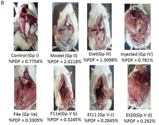
At the end of treatment, rats were weighed and sacrificed. Dorsal adipose tissues were removed and weighed (wet weight of dorsal fats) after excess blood and tissue fluids were dried by filter paper. Dorsal fat percentage (PDF) was calculated[1].

equation 3

The dorsal adipose tissue was digested in hot 30%KOH using homogenizer (Wiggenhauser, Germany) and then acidified. The produced homogenate was centrifuged for 2hours at 6000rpm. Total Lipid content was extracted with chloroform-methanol (2:1respectively) where organic phase was isolated and evaporated to dryness using rotary evaporator (Buchi, Switzerland). The total remaining lipid content was weighed [33].

Statistical Analysis

Data statistical analysis was performed with nonparametric one-way ANOVA test. Results were expressed as mean ±SD. All statistical tests were two-sided.

Results

%Yield Model for transfersomes (formulations code starting with F)

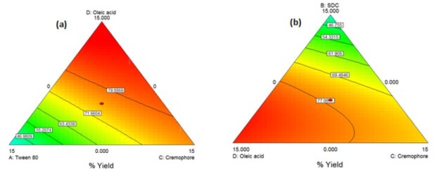
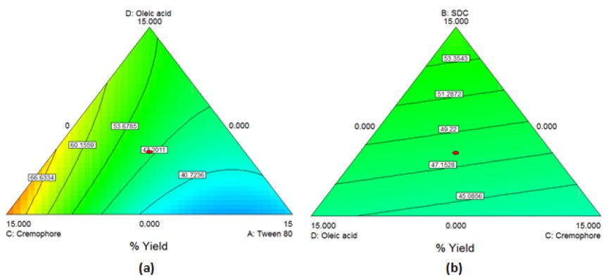
The obtained model was a quadratic one. By applying ANOVA test, it was nonsignificant(P=0.04) though with a desired nonsignificant lack of fit. All the linear mixture components: A, B and D were significant while C and other quadratic terms: AB, AC, AD, BC, BD and CD were nonsignificant. Accordingly, model reduction was carried out and ANOVA was reconducted. A significant model was obtained with a desired nonsignificant lack of fit. The results modeling showed r2 of 0.700, adjusted r2 of 0.55 and a predicted r2 of 0.44. The predicted r2 is in a reasonable agreement with the adjusted r2 (Difference between them<0.2). The Box-Cox plot for power transforms demonstrated the approximate coincident of the current lambda (1) with the best lambda (1.14) lying within the confidence intervals (-0.17to2.99) [34]. The obtained contour plots are shown in Figure1 (Insert Figure 1).

fig 1

Figure 1: Contour Plot demonstrating the effect of (a)Oleic acid, cremophor and Tween 80 (b)Oleic acid, cremophor and SDC on the %yield of PC-transfersomes

The obtained Model Equation obtained was:

%Yield=2.502*Tween80+2.451*SDC+3.486*Cremophor+4.387*Oleicacid (Equation4)

%Yield Model for transethosomes (formulations code starting with Fe)

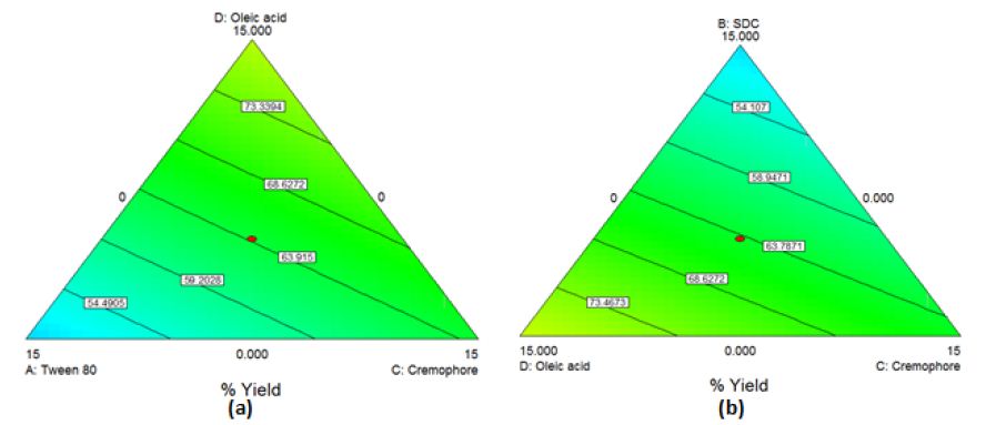
The obtained model was a quadratic one. By applying ANOVA test, it was significant(P<0.0001) with a desired nonsignificant lack of fit. All the linear mixture components: A, B, C and D besides the terms AB, AC, AD, BC and BD were significant. The CD quadratic term was nonsignificant. Accordingly, model reduction was carried out and ANOVA was reconducted. A significant model was obtained with a desired nonsignificant lack of fit. The results modeling was successful as demonstrated by the values of r2 (0.98), adjusted r2 (0.96) and predicted r2 (0.76). The predicted r2 is in a reasonable agreement with the adjusted r2. The Box-Cox plot for power transforms demonstrated the approximate coincident of the current lambda (1) with the best lambda (1.32) lying within the confidence intervals (0.41to2.61). The obtained contour plots are shown in Figure2 (Insert Fig 2).

fig 2

Figure 2: Contour Plot demonstrating the effect of (a)Oleic acid, cremophor and Tween 80 (b)Oleic acid, cremophor and SDC on the %yield of PC-transethosomes prepared by thin film hydration

The obtained Model Equation obtained was:

call equation 5

%Yield Model for transethosomes (formulations code starting with Et)

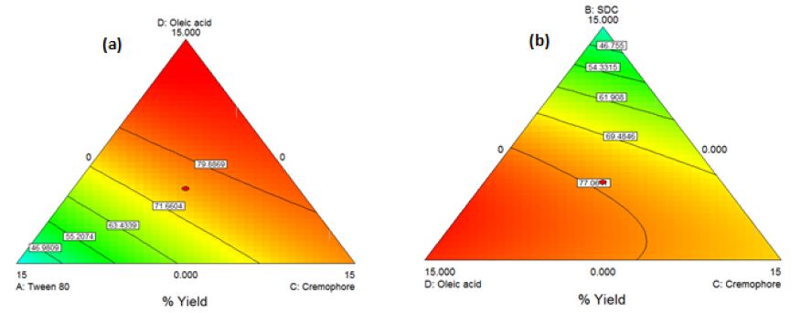
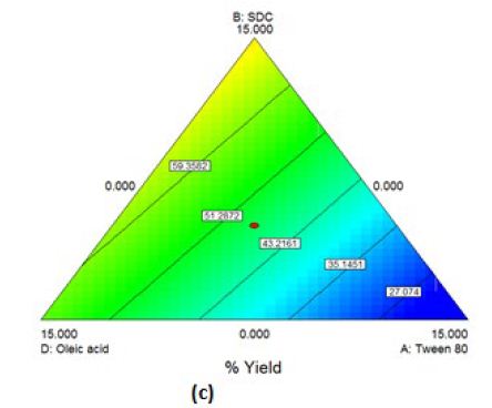
The obtained model was a quadratic one. By applying ANOVA test, it was significant(P=0.0056) but with a non-desired significant lack of fit. All the linear mixture components: A, B, C and D besides the term AC were significant. The other quadratic terms: AB, AD, BC, BD and CD were nonsignificant. Accordingly, model reduction was performed. This time a significant model was obtained with a higher p-value for lack of fit but still significant. The modeling of the results was successful as demonstrated by the values of r2 (0.81), adjusted r2 (0.74) though the predicted r2 was low (0.31). The Box-Cox plot for power transforms demonstrated the approximate coincident of the current lambda (1) with the best lambda (1.33) lying within the confidence intervals (-0.15to2.96). The obtained contour plots are shown in Figure3.

fig 3a,b

fig 3c

Figure 3: Contour Plot demonstrating the effect of (a)Oleic acid, cremophor and Tween 80 (b)Oleic acid, cremophor and SDC (c)Oleic acid, Tween 80 and SDC on the % yield of PC-transethosomes prepared by solvent dispersion

The model equation obtained was:

%Yield=1.396*Tween80+3.229*SDC+3.798*Cremophore+2.567*Oleicacid0.279*Tween80*Cremophore            (Equation6)

Validation of experimental design

Eight new formulations (Et19-Et26) were chosen. The actual %yield, P.S and PDI were compared with the predicted values. For %yield model, the obtained values were comparable to the predicted counterparts, these results ensured the validity of the %yield model with a mean %bias of 7.4%. For P.S and PDI models, the overall mean was considered a better predictor of the response than the obtained models due to the obtained negative predicted r2. Thus, these models are not reliable [35] and were considered as reported values.

Zeta Potential

ZP give indication about surface charge type and magnitude [36] which can affect both vesicular stability and skin-vesicle interactions[8;37]. Vesicles showed highly negative charges ranging from -31 to -72.5mV for the prepared transfersomes (F), -24.8 to -53mV for the prepared transethosomes (Et) and ranging from -23.2 to -64.2mV for the prepared transethosomes (Fe). For the transethosomal formulations (Et21 to Et26), no significance difference was observed in their ZP(P>0.05).

Selection of the formula of choice

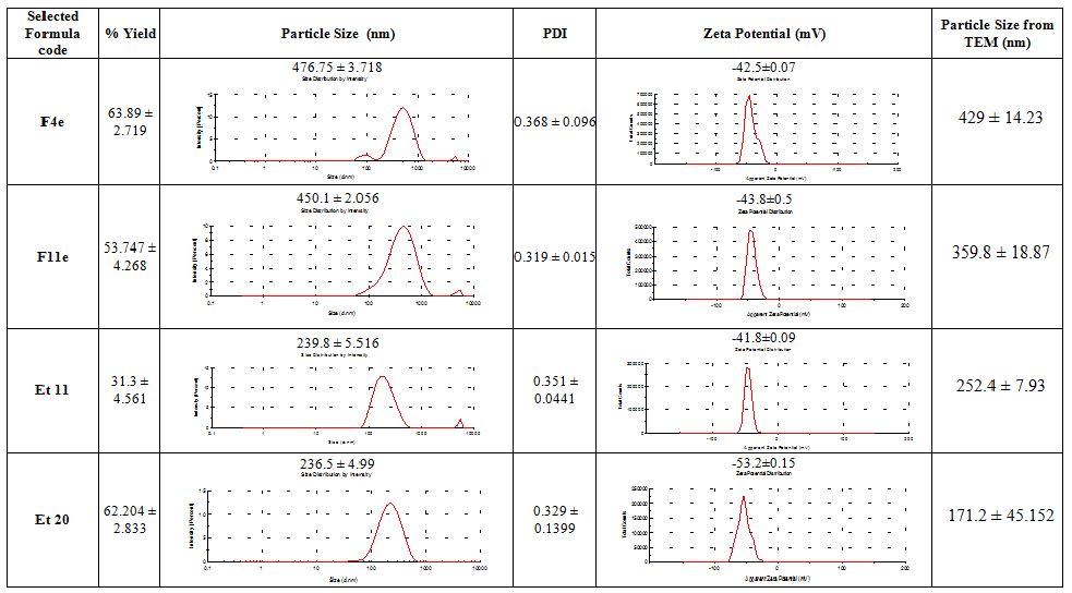
From the data shown in Table3, it was found that transethosomes (F4e, F11e, Et11 & Et20) showed SD<10% of the mean of the evaluated parameters indicating their reproducibility. Their P.S ranged from 200 to 480nm, so they can reach the skin subcutaneous layer and become entrapped. Besides, their ZP range is between -41.8mV and -53.2mV ensuring particle stability with reduced mutual aggregation. Moreover, they have PDI around 0.3 ensuring low variability. Their %yield ranged between 31.3% to 63.89%, on which the dose will be calculated. Consequently, F4e, F11e, Et11 & Et20 were selected as formulations of choice on which further studies were done.

Elasticity Test

The elasticity results are shown in Table4. The chosen formulations showed a high deformability index ranging from 70.8976±4.29 to 137.1707±6.14 (Insert Table 3 & 4).

Table 3: Characteristics of the selected vesicles

table 3

Table 4: Particle size and Deformability Index of the selected vesicles before and after extrusion

Formula Code

Particle Size (nm)

Deformability Index (DI) Average DI ± SD
Before Extrusion

After Extrusion

F4e

476.8 ± 3.72

176.73 74.2118 70.8976 ± 4.29
174.6

72.43

166.73

66.051

F11e

450.1 ± 2.06

235.6 131.887 137.1707 ± 6.14
239

135.72

246.13

143.905

Et11

239.8 ± 5.52

188.3

84.25

88.4467 ± 4.26

197.6

92.77

192.8

88.32

Et20

236.5 ± 4.99

189.6 85.41

84.26133± 2.72

Transmission Electron Microscopy

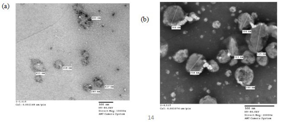
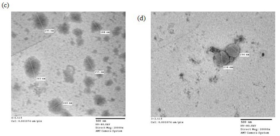
The morphology of the four selected formulations is shown in Figure4. The imaging analysis showed unilamellar vesicles possessing a thin lipid layer that is hydrated forming enclosed vesicular structure whose shape ranges from spherical to oval with some irregular shapes and black precipitates (Insert Fig 4).

fig 4a,b

fig 4c,d

Figure 4: TEM micrographs of formulation (a)F4e, (b)F11e, (c)Et11, (d)Et20

Stability test

The stability of the selected formulae was evaluated by macroscopic inspection and by measuring their P.S, PDI and %yield monthly and ZP every 3months for 6months storage at 4˚C. At room temperature, fungal growth appeared after the first month. An adequate stability of the selected transethosomes (F4e, F11e, and Et11) was observed with nonsignificant change regarding their P.S, PDI, %yield and ZP through the 6months of storage at 4˚C(P-value>0.05). Transethosome formula (Et20) showed nonsignificant differences regarding PDI, %yield and ZP throughout the 6months (P-value=0.4279, 0.4344, 0.4291, 0.4225, 0.4287 & 0.4247) but showed a highly significant change in P.S compared to P.S of original samples throughout the 6months (P-value=0.0009, 0.0002, 0.0091, 0.0077, 0.0068 & 0.0091).

Characterizations of nanovesicular gel

All prepared gels were translucent, smooth, and consistent in appearance with pleasant acceptable odor and without appearance of any clumps nor phase separation.

pH Measurement

The pH of all prepared gels was found to range from 8.24±0.36 to 8.78±0.14.

Viscosity Studies

The prepared gel viscosity ranged from 71254±4cps to 77183±3cps ensuring the successful preparation of the gel structure.

Spreadability Test

The prepared gel spreadability was measured in terms of average diameter of the spread circle. The longer the diameter, the better the spreadability [26]. Measurements lie between 3.43±0.14cm and 3.75±0.13cm indicating good spreadability properties.

Drug content determination

Drug content of PC was found to be 94.53±0.02%, 95.476±0.1%, 95.43±0.35%, and 96.875±0.1% for F4e, F11e, Et11 and Et20 gels respectively.

Stability Studies of gel

Nanovesicular gel color, consistency, pH, drug content and viscosity were evaluated after 3and 6months of storage at 4˚C [24]. The prepared gels were consistent with no signs of phase separation or deterioration.

In-vivo studies on rats

Invivo studies of PC-vesicular gel formulations containing F4e, F11e, Et11 and Et20 were performed and results are presented in Table (5,6) and Figure (5–8).

Induction of obesity

As shown in Table5 & Figure 6(a), the body weights were similar among all groups before initiation of high-fat diet(P>0.05). At the end of 4months on high-fat diet, the body weight of obese rats (GpII-V) significantly increased compared to control group (GpI)(P<0.0001).

Table 5: Rats body weight changes before and after treatment

Rat Group

Initial body weight Body weight before high fat diet Body weight after high fat diet Body weight after treatment %weight loss
Control 51.3 ± 2.43 74.1233 ± 5.437 227.016 ± 5.937

297.08 ± 27.648

Model

50.92 ± 3.64 76.0775 ± 7.0175 451.865 ± 3.4027 462.917 ± 24.076
Diet only 451.95 ± 2.3036 418.833 ± 51.219

7.328

Injected

449.417 ± 3.11

397.33 ± 38.867

11.59

F4e

452.03 ± 3.1123 356.667 ± 62.67

21.097

F11e

451.383 ± 3.517 394.33 ± 23.157 12.64
Et 11 450.433 ± 4.9066 379.833 ± 34.649

15.6

Et 20

450.817 ± 3.414 394.5 ± 29.751

12.4

Skin irritation test

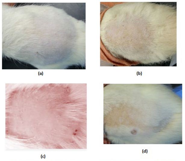
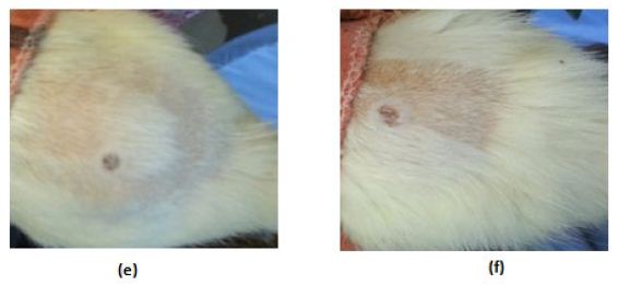
In the control (GpI) and treated (GpVa to Vd) groups, the erythema score was 0 and no irritation signs appear through the total examination period (Figure5(a) and (b) respectively). In grpIV, that was injected with Adipoforte®, slight erythema with score 1 appear after 24hours in 50% of the group (Figure5(c)). After 48hours, a hard scar appeared with erythema score of 4 ((Figure5(d), (e) and (f)) forming hard nodules or lesion that disappeared after 3days (Insert Figure 5).

fig 5a,b,c,d

fig 5e,f

Figure 5: Irritation score zero in (a)control group (Gp I), (b)treated groups (GpVa-Vd), (c)Irritation score 1 in injected group (Gp IV) after 24hours, (d,e,f)Irritation score 4 in injected group (Gp IV) after 48hours

Treatment and drug delivery

As shown in Table5 & Figure6, the body weight of obese rats (GpVa) after obesity treatment showed nonsignificant difference compared to the control group (P=0.1647). In comparison to the model group (GpII), the body weight of the treated groups (i.e. GpVa and Vc) was reduced significantly (P<0.05) with %weight loss of 21.097% and 15.6% respectively. On the other hand, there was nonsignificant difference in weight reduction between the model group (GpII) and the group treated with diet only (GpIII)(P=0.5142) whose body weight decreases by 7.328%. There was nonsignificant difference in weight reduction between the model group (GpII) and the group treated with injection (GpIV)(P=0.0932). There was nonsignificant difference in weight reduction between the model group (GpII) and the group treated with prepared topical formulations containing F11e, Et20 (GpVb and Vd) (P=0.0686 & P=0.0698 respectively) whose body weight decreases by 12.64% and 12.4% respectively. There was nonsignificant difference between the diet group (GpIII) and treated groups (GpV)(P>0.05) (Insert Table 5& Fig 6).

fig 6a

fig 6b

Figure 6: ** P value ≤ 0.01 indicating significant difference
*** P value ≤ 0.001 indicating highly significant difference
**** P value ≤ 0.0001 indicating an extremely significant difference
(a)Body weight changes among treatment groups, (b)%weight loss changes among different treatment groups after end of treatment

Dorsal Fat Percentage and total lipid content

According to %PDF, a highly significant difference between the control group and other groups (P<0.0001) appeared as shown in Table6, and Figure7. The %PDF of the injected obese rats (GpIV) was nearly equal to that of the control group by the end of treatment (P>0.9999). On comparing model group (GpII) with the treated groups, the %PDF of the treated groups (GpIV and V) reduced significantly(P<0.0001). As shown in Table6 and Figure8, the total Lipid content of the treated groups (GpIII, IV and V) reduced significantly (P<0.0001) compared to model group. Meanwhile, there was a highly significant difference between the control group (GpI) and the model, diet and injected groups (GpII, III, and IV) (P<0.0001). Interestingly, the total lipid content of the control group (GpI) compared to the treated group with PC vesicular gel (GpV) showed nonsignificant difference (P>0.05). Total lipid content in rat group treated with diet only (GpIII)(4.834±0.403g) decreased to half that of the model group (GpII)(9.05±0.7319g). On comparing model group (GpII) with injected group (GpIV) and invented new dosage form group (GpV), total lipid content decreased in group IV and group V by 67.96% and 88.398% respectively reaching in the latter group a comparable value as that of control group (GpI) (Insert Table 6& Fig 7-8).

Table 6: Comparison of obesity parameters among groups

Rat Group

Rat weight (gm) Fat tissue wet weight (gm) %PDF Total Lipid content weight (gm)
Control 297.08 ± 27.648 2.286 ± 0.2034 0.7754 ± 0.1029

1.552 ± 0.266

Model

462.917 ± 24.076 9.366 ± 0.6992 2.0218 ± 0.074 9.05 ± 0.7319
Diet only 418.833 ± 51.219 5.387 ± 0.707 1.3098 ± 0.2772

4.834 ± 0.403

Injected

397.33 ± 38.867 3.1 ± 0.4406 0.781 ± 0.0893 2.9 ± 0.5168
F4e 356.667 ± 62.67 1.218 ± 0.604 0.3305 ± 0.1151

1.103 ± 0.488

F11e

394.33 ± 23.157 1.294 ± 0.486 0.3245 ± 0.1104 1.102 ± 0.4028
Et 11 379.833 ± 34.649 1.099 ± 0.346 0.2845 ± 0.0693

1.019 ± 0.3044

Et 20

394.5 ± 29.751 1.169 ± 0.3592 0.292 ± 0.0708

1.094 ± 0.307

fig 7a

fig 7b

Figure 7: ns P value > 0.05 indicating no significant difference
**** P value ≤ 0.0001 indicating an extremely significant difference
(a) Changes in %PDF among different groups, (b)%PDF obtained for all treatment groups

fig 8

Figure 8: ns P value > 0.05 indicating no significant difference
**** P value ≤ 0.0001 indicating an extremely significant difference
Changes in total lipid content among different treatment groups

Discussion

The contour plots obtained confirm the interaction effects of the used oils and edge-activators in increasing the %yield of the prepared transfersomes and transethosomes. For the three types of prepared vesicles, the area of high %yield lies between oleic acid and cremophor which indicates that by increasing their percentage, the %yield increases. Increasing the percentage of Tween 80 decreases the %yield demonstrated by the blue area close to its apex. For transfersomes and transethosomes prepared by thin film hydration method, increasing SDC decreases %yield demonstrated by the blue area close to its apex where increasing tween 80 and SDC causes lipid layer destabilization leading to reduced %yield [22, 38]. Also, increasing the concentration of some edge-activators beyond certain threshold leads to formation of micelles instead of vesicles causing solubilization of the phospholipids [19, 39]. This can be attributed to cremophor bulky structure which provides rigidity to the vesicles leading to higher P.S increasing %yield [40]. According to literature, increasing HLB value as in the case of cremophor [41] increases the P.S which can in turn increase %yield by increasing hydrophilicity, enhancing surface free energy[39]. Increasing SDC, in transethosomes prepared by solvent dispersion method, increases %yield demonstrated by the yellow area close to its apex where SDC increases the whole lipid bilayer volume increasing P.S causing increase in %yield [42]. For good physical stability [43], ZP should not be less than -30 or +30mV [37] and on approaching -60mV [44], vesicles obtain an excellent physical stability through shelf life preventing aggregation [45]. This means that all formulations are stable except (F1e, F10e, F13e, Et3, Et10, Et13 and Et14). This can be attributed to the presence of edge-activators [8]; tween 80 was reported to cause decrease in ZP, although it is a nonionic surfactant [46] due to its oxyethylene part[47]. Oleic acid was reported to produce negative ZP [6;48]. Using SDC produces high negatively charged vesicles due to the presence of cholate anions [47]. Although PC is zwitterionic compound with an isoelectric point (6-7), PC carried a net negative charge under experimental conditions of pH7.4 [12;39] due to the negatively charged phosphate group[43;49]. For transethosomes, ethanol produces negative charges on vesicles [14;45]. These negatively charged vesicles enhances skin permeation of drugs [12]. Lipid bilayer elasticity affects permeation enhancing skin penetration[47]. The edge-activator chemical structure affects vesicles deformability where flexible non-bulky carbon chain gives more fluidity to the membrane bilayer compared to bulky cyclic edge-activators [39]. Transethosomal formula (F11e) show the highest DI followed by Et11 then Et20 and finally F4e showing the least DI. This can be attributed to the high concentration (12.5%) of tween 80 with its highly flexible and non-bulky hydrocarbon chains [20] which aid in their squeezing along the stratum corneum and localization at high concentration in the deepest skin layers [47, 50]. Although Et11 and F11e have the same percentage of Tween 80, F11e has a higher ethanol volume (5ml) than Et11 (1.5ml) where increasing ethanol content increases lipid bilayer elasticity [8, 51]. Et20 showed lower DI compared to F11e due to high concentration of cremophor (12.5%) with its bulkier structure compared to Tween 80[40]. F4e showed the lowest DI with the highest percentage of P.S change comparing P.S before (476.75±3.718nm) and after extrusion (172.69±5.27nm) whereas %P.S change increases, DI decreases. This can also be due to high concentration of SDC (12.5%) with its steroid-like structure [52]. The use of oleic acid and ethanol provides high elasticity [51]. The TEM micrographs show a highly recognized vesicles in the nanometer range which agreed with the size data obtained using dynamic light scattering (DLS) and ensures vesicle formation at the used concentrations of ethanol and edge-activators [8]. Deviation of particle shape from spherical form is due to lipid modification during sample drying for imaging [45] and being highly deformable [43, 47]. The slight change in size can be attributed to the samples drying prior imaging [53]. The appearance of black precipitates may be due to precipitation of phosphotungstic acid in hydrophilic core [53, 54]. The selected transethosomes (F4e, F11e, and Et11) adequate stability can be due to their high ZP [44, 45]. Transethosome formula (Et20) shows a highly significant change in P.S compared to freshly prepared samples throughout the 6months (P-value=0.0009, 0.0002, 0.0091, 0.0077, 0.0068 & 0.0091), however, it is still in the size range targeting skin subcutaneous layer (185-460nm) [1]. It was reported that high cremophor concentration causes physical instability [55] due to enhanced water penetration into vesicle increasing P.S upon storage [56]. The pH of the prepared gel lies in the physiologically accepted range of 5-9 [57, 58]. Gel viscosity affects the extrudability, drug release [27] and vesicles delivery onto or across the skin [45]. The prepared gel high viscosity, due to the presence of lipid vesicles [39], facilitates the retention of gel on the skin for better skin penetration. The prepared gel spreadability indicates that the gel is easily spread by low shear[24] with uniform spreadability [26, 32]. Drug content results show homogenous dispersion of vesicles in gel[39] indicating the suitability of method used for gel preparation [27, 59]. On comparing the original results and those obtained after storing gel for 3and 6months, nonsignificant change was observed in the above mentioned parameters (P-value>0.05) ensuring stability over 6months [59]. Average body weights after high-fat diet, shown in Table5 column4, shows about 50% increase compared to the normal control group (GpI) indicating the successful establishment of obesity model by feeding the animals with high-fat chow containing 70%lard [1]. In comparison to the model group (GpII), the body weight of the treated groups (GpVa and Vc) was reduced significantly (P<0.05) with %weight loss of 21.097% and 15.6% respectively indicating their ability to reduce body weight. On the other hand, there was nonsignificant difference in weight reduction between the model group (GpII) and the group treated with diet only (GpIII)(P=0.5142) whose body weight was decreased by 7.328% which is in coordinance with previous studies which stated that diet regimens failed to act on localized obesity [5]. Skin irritation test was conducted to assess the potential irritant effect of PC vesicular gel formulations [22]. The appearance of hard scar in rats injected with PC-market injection, confirms lack of patient compliance of injection lipolysis for treatment of localized obesity which is in accordance with previous experiments which reported that localized adverse effects were described as “very mild’(18.4%) or “mild”(39.2%) [60]. According to observed changes in body weight, %PDF and total lipid content observed, the topical application of PC vesicular gel, revealed the ability of newly prepared gel containing transethosomes (F4e, F11e, Et11 & Et20) to significantly decrease localized fat. This confirms the successful penetration of vesicles into the skin subcutaneous layer that can be attributed to the solvent action of ethanol, used in preparation of transethosomes on stratum corneum, in addition to the high deformability and malleability of these vesicles. This aids in their squeezing along the stratum corneum and localizing at high concentrations in subcutaneous layer producing their lipolysis effect[15].

Conclusion

PC nanovesicular gel, containing transethosomes (F4e, F11e & Et11), can be used as effective non-invasive treatment for localized obesity as an alternative to multi-injections for mesotherapy.

Conflict of Interest

No conflict of interest associated with this publication and there has been no significant financial support for this work that could have influenced its outcome.

References

  1. Lu K, Xie S, Han S, Zhang J, Chang X, et al. (2014) Preparation of a nano emodin transfersome and study on its anti-obesity mechanism in adipose tissue of diet-induced obese rats. Journal of translational medicine 12 : 1-14. [crossref]
  2. Nikoloski Z, Williams G (2016) Obesity in Middle East. In Metabolic Syndrome. Switzerlands: Springer.
  3. Rittes PG, Rittes JNC, Amary MFC (2006) Injection of phosphatidylcholine in fat tissue: experimental study of local action in rabbits. Aesthetic plastic surgery 30 : 474-478. [crossref]
  4. Hasengschwandtner F (2005) Phosphatidylcholine treatment to induce lipolysis. Journal of Cosmetic Dermatology 4 : 308-313. [crossref]
  5. Abel MR (2012) Evaluation of the Efficacy of Injection Lipolysis using Phosphatidylcholine/Deoxycholate Versus Deoxycholate Alone in Treatment of Localized Fat Deposits. Journal of Clinical & Experimental Dermatology Research 3 : 1-9.
  6. Shilakari G, Singh D, Asthana A (2013) Novel vesicular carriers for topical drug delivery and their applications. International Journal of Pharmaceutical Sciences Review and Research 21 : 77-86.
  7. Uchechi O, Ogbonna JD, Attama AA (2014) Nanoparticles for dermal and transdermal drug delivery. Sezer, AD eds; pg : 193-235.
  8. Shaji J, Garude S (2014) Transethosomes and Ethosomes for Enhanced Transdermal Delivery of Ketorolac Tromethamine: A Comparative Assessment. International Journal of Current Pharmaceutical Research 6 : 88-93.
  9. Descalzo AM, Insani EM, Pensel NA (2003) Light-scattering detection of phospholipids resolved by HPLC. Lipids 38 : 999-1003. [crossref]
  10. Jangle RD, Galge RV, Patil VV, Thorat BN (2013) Selective HPLC method development for soy phosphatidylcholine fatty acids and its mass spectrometry. Indian journal of pharmaceutical sciences 75 : 339-345. [crossref]
  11. Abdel-Hafez SM, Hathout RM, Sammour OA (2018) Curcumin-loaded ultradeformable nanovesicles as a potential delivery system for breast cancer therapy. Colloids and Surfaces B: Biointerfaces 167 : 63-72. [crossref]
  12. Shaji J, Lai Maria (2014) Preparation, Optimization and evaluation of transferosomal formulation for enhanced transdermal delivery of a COX-2 Inhibitor. Int J Pharm Pharm Sci 6 : 467-477.
  13. Pal R, Pandey M (2015) Transferosomes: A Novel Carrier For Enhanced Dermal Delivery of Drug. World Journal oof Pharmacy and Pharmaceutical Sciences 4 : 1816-1832.
  14. Kaur A, Jain SK, Pandey RS (2012) Aceclofenac Encapsulated Ethanolic Nano-Vesicles for Effective Treatment of Osteoarthritis. International Journal of Pharmaceutical Sciences and Research 3 : 2562-2567.
  15. Bragagni M, Mennini N, Maestrelli F, Cirri M, Mura P (2012) Comparative study of liposomes, transfersomes and ethosomes as carriers for improving topical delivery of celecoxib. Drug delivery 19 : 354-361. [crossref]
  16. Safwat S, Hathout RM, Ishak R, Mortada N (2016) Augmented simvastatin cytotoxicity using optimized lipid nanocapsules: a potential for breast cancer treatment. Journal of liposome research 27 : 1-10. [crossref]
  17. Abdallah MH (2013) Transfersomes as a Transdermal Drug Delivery System for Enhancement the Antifungal Activity of Nystatin. Int J Pharm Pharm Sci 5 : 560-567.
  18. Argan N, Harikumar SL (2012) Topical Liposomal Gel: A Novel Drug Delivery System. International Journal of Research in Pharmacy and Chemistry 2 : 383-400.
  19. Chaudhary H, Kohli K, Kumar V (2013) Nano-transfersomes as a novel carrier for transdermal delivery. International journal of pharmaceutics 454 : 367-380. [crossref]
  20. Elazreg R, Soliman M, Mansour S, El Shamy A (2015) Preparation and evaluation of mucoadhesive gellan gum in-situ gels for the ocular delivery of carbonic anhydrase inhibitor nanovesicles. International Journal of Pharmaceutical Sciences and Research 6.
  21. Naguib SS, Hathout RM, Mansour S (2017) Optimizing novel penetration enhancing hybridized vesicles for augmenting the in-vivo effect of an anti-glaucoma drug. Drug delivery 24 : 99-108. [crossref]
  22. Tsai MJ, Huang YB, Fang JW, Fu YS, Wu PC (2015) Preparation and Characterization of Naringenin-Loaded Elastic Liposomes for Topical Application. PloS one 10 : 1-12.
  23. RAJESH B, Saumya D, Dharmajit P, PAVANI M (2014) Formulation Design and Optimization of Herbal Gel containing Albizia Lebbeck Bark Extract. International Journal of Pharmacy and Pharmaceutical Sciences 6 :111-114.
  24. SINGH A, Vengurlekar P, Rathod S (2014) Design, Development and Characterization of Liposomal Neem Gel. International Journal of Pharma Sciences and Research 5 : 140-148.
  25. Shankar NB, Kumar RP, Kumar NU, Brata BB (2010) Development and characterization of bioadhesive gel of microencapsulated metronidazole for vaginal use. Iranian journal of pharmaceutical research: IJPR 9 : 209-219. [crossref]
  26. Soliman SM, Malak NA, El-Gazayerly ON, Rehim AA (2010) Formulation of microemulsion gel systems for transdermal delivery of celecoxib: In vitro permeation, anti-inflammatory activity and skin irritation tests. Drug Discov Ther 4 : 459-471. [crossref]
  27. Rajan R, Vasudevan DT (2012) Effect of permeation enhancers on the penetration mechanism of transfersomal gel of ketoconazole. Journal of advanced pharmaceutical technology & research 3 : 112-116. [crossref]
  28. Wilkes JJ, Bonen A, Bell RC (1998) A modified high-fat diet induces insulin resistance in rat skeletal muscle but not adipocytes. American Journal of Physiology-Endocrinology And Metabolism 275 : E679-E686. [crossref]
  29. Rittes P (2001) The use of phosphatidylcholine for correction of lower lid bulging due to prominent fat pads. Dermatologic surgery 27 : 391-392. [crossref]
  30. Co A, Abad-Casintahan M, Espinoza-Thaebtharm A (2007) Submental fat reduction by mesotherapy using phosphatidylcholine alone vs. phosphatidylcholine and organic silicium: a pilot study. Journal of Cosmetic Dermatology 6 : 250-257. [crossref]
  31. Karl G (2005) Efficacy of injections of phosphatidylcholine into fat deposits-a non-surgical alternative to liposuction in body-contouring. Indian Journal of Plastic Surgery 38.
  32. Shetty PK, Venuvanka V, Jagani HV, Chethan GH, Ligade VS, et al. (2015) Development and evaluation of sunscreen creams containing morin-encapsulated nanoparticles for enhanced UV radiation protection and antioxidant activity. International journal of nanomedicine 10 : 6477-6491. [crossref]
  33. Couturier K, Servais S, Koubi H, Sempore B, Sornay-Mayet M, et al. (2002) Metabolic Characteristics and Body Composition in a Model of Anti-Obese Rats (Lou/C). Obesity Research 10 :188-194. [crossref]
  34. Abdel-Hafez SM, Hathout RM, Sammour OA (2014) Towards better modeling of chitosan nanoparticles production: screening different factors and comparing two experimental designs. International journal of biological macromolecules 64 : 334-340. [crossref]
  35. Rai A, Mohanty B, Bhargava R (2015) Modeling and response surface analysis of supercritical extraction of watermelon seed oil using carbon dioxide. Separation and Purification Technology 141 : 354-365.
  36. Honary S, Zahir F (2013) Effect of zeta potential on the properties of nano-drug delivery systems-a review (Part 1). Tropical Journal of Pharmaceutical Research 12 : 255-264.
  37. Neves A, Lucio M, Martins S, Lima J, Reis S (2013) Novel resveratrol nanodelivery systems based on lipid nanoparticles to enhance its oral bioavailability. International journal of nanomedicine 8 : 177-187. [crossref]
  38. Al-mahallawi AM, Khowessah OM, Shoukri RA (2014) Nano-transfersomal ciprofloxacin loaded vesicles for non-invasive trans-tympanic ototopical delivery: In-vitro optimization, ex-vivo permeation studies, and in-vivo assessment. International journal of pharmaceutics 472 : 304-314. [crossref]
  39. Yusuf M, Sharma V, Pathak K (2014) Nanovesicles for transdermal delivery of felodipine: Development, characterization, and pharmacokinetics. International journal of pharmaceutical investigation 4 : 119-130. [crossref]
  40. Patel K, Sarma V, Vavia P (2013) Design and evaluation of Lumefantrine – Oleic acid self nanoemulsifying ionic complex for enhanced dissolution. DARU Journal of Pharmaceutical Sciences 21. [crossref]
  41. Matsaridou I, Barmpalexis P, Salis A, Nikolakakis I (2012) The influence of surfactant HLB and oil/surfactant ratio on the formation and properties of self-emulsifying pellets and microemulsion reconstitution. AAPS PharmSciTech 13 : 1319-1330. [crossref]
  42. Liu D, Hu H, Lin Z, Chen D, Zhu Y, et al. (2013) Quercetin deformable liposome: preparation and efficacy against ultraviolet B induced skin damages in vitro and in vivo. Journal of Photochemistry and Photobiology B: Biology 127 : 8-17. [crossref]
  43. Ascenso A, Raoso S, Batista C, Cardoso P, Mendes T, et al. (2015) Development, characterization, and skin delivery studies of related ultradeformable vesicles: transfersomes, ethosomes, and transethosomes. International journal of nanomedicine 10 : 5837-5851. [crossref]
  44. Caddeo C, Sales O, Valenti D, Sauri A, Fadda A, et al. (2013) Inhibition of skin inflammation in mice by diclofenac in vesicular carriers: liposomes, ethosomes and PEVs. International journal of pharmaceutics 443 : 128-136. [crossref]
  45. Uprit S, Sahu RK, Roy A, Pare A (2013) Preparation and characterization of minoxidil loaded nanostructured lipid carrier gel for effective treatment of alopecia. Saudi Pharmaceutical Journal 21 : 379-385. [crossref]
  46. Uchino T, Lefeber F, Gooris G, Bouwstra J (2014) Characterization and skin permeation of ketoprofen-loaded vesicular systems. European Journal of Pharmaceutics and Biopharmaceutics 86 : 156-166. [crossref]
  47. Alomrani A, Shazly G, Amara A, Badran M (2014) Itraconazole-hydroxypropyl-cyclodextrin loaded deformable liposomes: In vitro skin penetration studies and antifungal efficacyusing Candida albicans as model . Colloids and Surfaces B: Biointerfaces 121:74-81. [crossref]
  48. Caddeo C, Manconi M, Fadda AM, Lai F, Lampis S, et al. (2013) Nanocarriers for antioxidant resveratrol: formulation approach, vesicle self-assembly and stability evaluation. Colloids and Surfaces B: Biointerfaces 111:327-332. [crossref]
  49. Manca M, Castangia I, Zaru M, Nacher A, Valenti D, et al. (2015) Development of curcumin loaded sodium hyaluronate immobilized vesicles (hyalurosomes) and their potential on skin inflammation and wound restoring. Biomaterials 71:100-109. [crossref]
  50. Kakkar S, Kaur I (2011) Spanlastics – A novel nanovesicular carrier system for ocular delivery. International journal of pharmaceutics 413 : 202-210.
  51. Song CK, Balakrishnan P, Shim CK, Chung SJ, Chong S, et al. (2012) A novel vesicular carrier, transethosome, for enhanced skin delivery of voriconazole: characterization and in vitro/in vivo evaluation. Colloids and Surfaces B: Biointerfaces 92 : 299-304. [crossref]
  52. Salama HA, Mahmoud AA, Kamel AO, Abdel Hady M, Awad GA (2012) Brain delivery of olanzapine by intranasal administration of transfersomal vesicles. Journal of liposome research 22 : 336-345. [crossref]
  53. Zhu Z, Li Y, Li X, Li R, Jia Z, et al. (2010) Paclitaxel-loaded poly(N-vinylpyrrolidone)-b-poly(epsilon-caprolactone) nanoparticles: preparation and antitumor activity in vivo. Journal of Controlled Release 142 : 438-446. [crossref]
  54. Hathout RM, Mansour S, Mortada ND, Guinedi AS (2007) Liposomes as an ocular delivery system for acetazolamide: in vitro and in vivo studies. AAPS PharmSciTech 8 : E1-E12. [crossref]
  55. Mognetti B, Barberis A, Marino S, Berta G, De Francia S, et al. (2012) In vitro enhancement of anticancer activity of paclitaxel by a Cremophor free cyclodextrin-based nanosponge formulation. Journal of Inclusion Phenomena and Macrocyclic Chemistry; 74 : 201-210.
  56. Dixit AR, Rajput SJ, Patel SG (2010) Preparation and bioavailability assessment of SMEDDS containing valsartan. AAPS PharmSciTech 11 : 314-321. [crossref]
  57. Jana S, Manna S, Nayak AK, Sen KK, Basu SK (2014) Carbopol gel containing chitosan-egg albumin nanoparticles for transdermal aceclofenac delivery. Colloids and Surfaces B: Biointerfaces 114 : 36-44. [crossref]
  58. Mahajan Suvarnalata S, Chaudhari R (2016) Transdermal gel: As a novel drug delivery system. International Journal of Pharmacy and Life Sciences 1 : 4864-4871.
  59. Rai VK, Yadav NP, Sinha P, Mishra N, Luqman S, et al. (2014) Development of cellulosic polymer based gel of novel ternary mixture of miconazole nitrate for buccal delivery. Carbohydrate polymers 103 : 126-133. [crossref]
  60. Palmer M, Curran J, Bowler P (2006) Clinical experience and safety using phosphatidylcholine injections for the localized reduction of subcutaneous fat: a multicentre, retrospective UK study. Journal of Cosmetic Dermatology 5 : 218-226. [crossref]

Creating Micro Mind-Sets for Healthful Pasta: A Mind Genomics Cartography

DOI: 10.31038/MGSPE.2021111

Abstract

Respondents evaluated systematically varied combinations of messages (vignettes) about healthful pasta. Each respondent evaluated a unique set of 48 vignettes constructed from 36 messages about different aspects of health carbs, rating it both on purchase intent and selecting the price willing to pay. Each respondents rated each vignette on both purchase intent and price would pay. Two sets of three mind-sets emerge, one based on purchase intent, one based on price would pay. Three patterns of mind-sets emerge; focus on cognitive (Brain) performance, focus on a healthier/more enjoyable life (Life), and focus on taste and sensory pleasure (Comfort Food). These mind-sets exhibit different patterns of what is important to them when making a judgment.  The paper shows the ability of the emerging science of Mind Genomics to probe deeply into what seems at first to be a simple topic, healthful pasta, and the ability to reveal profound differences in the way people think about this supposedly simple, limited topic.

Introduction

During the past sixty-plus years, the notion that people ‘differ’ from each other in predictable ways has gained increasing popularity in the world of consumer research. The ever-present variation among people, observed by authors, philosophers, social scientists, biologists, not to mention governments and their politicians, no longer represents a source of irritating variability in the world of ‘nomos’, of laws which apply the same to all people. Rather, the person-to-person variations, the world of ‘idio’, is falling increasing under the scrutinizing lens of the researcher, who is searching for rules explicating that person-to-person variability.

More than sixty years ago, famed consumer researcher William D. Wells suggested that it might be possible to divide people not so much by who they ARE, but rather by how they THINK. This was the auspicious beginnings of the field of Psychographics [1], which eventuated into classifications such as PRIZM by Claritas [2], with its 68 different personas. The number of personas might seem unusually high in light of the normal desire of people to simplify the world, but the objective of PRIZM and such types of classifications is to deal with the remarkable diversity of the minds of people, doing so in a way, which makes the diversity tractable.

The move in business and research is find many mind-sets for a topic, and in so doing account for the substantial variability across people. Mind-sets, the search for ‘basic groups’, moves the reality of variability from merely an irritating fact-of-life to a front-and-center position as a signal that there are fundamental groups in the population to be discovered.  The only issue is the desire to account for the variability by find ever more ‘basic factors’ in an attempt to explain as much of the variation as possible. The aforementioned system, PRIZM, is just such an example.  The general focus, then, is to take a subject with a large number of aspects, like the way one thinks about life, or health, and break it down to simplistic groups. The key words are wide range, many groups, account for as much variability as possible

This paper moves in the opposite direction, looking at a topic that might be considered ‘narrow’ at the very outset, healthful pasta, and trying to divide this narrow topic even further. The objective, therefore, is to work with a narrow world that people might already consider to be ‘hard to segment because of its specificity’, and uncover even deeper-lying mind-sets.

Mind Genomics and the study of psychological granularity

We approach the topic of micro-segmentation looking at one product, healthful pasta. Pasta itself is a very large category around the world, historically important during the past centuries [3][4], and a source of continuing innovation. We are accustomed to pasta as being the carrier for a flavor-imparting and mouthfeel-imparting product, most generally that product being a sauce. Pasta can also be a carrier for vegetables, for meats, and even eaten without anything, except perhaps with a bit of melted butter to add flavor.

Our focus, micro-segmentation, means that we want to look at the different ways that a person can perceive pasta.  One might ask the respondent to talk about pasta, and the different aspects of pasta, but it’s not clear that this in-depth interview or focus group interview will be able to uncover the micro-segments or realize their existence and nature when the research happens upon them.  Conventional consumer research, whether interviews, surveys, and so forth, simply are instruments which, in the end, are just too dull to work.  The issue is just how many ways can one talk about pasta, and what kind of questions can one ask, and then just recognize when something really new emerges.

Mind Genomics works in a variety of fashions radically different from the approaches used by consumer research. The approaches of Mind Genomics have been explicated in a number of earlier publications [5][6][7]

Experiment, not survey

Mind Genomics comprises experiments, not surveys, not discussions. Mind Genomics mixes together statements about the topic, pasta, these statements (or elements) having been combined by an underlying menu (experimental design) which dictates the combinations. For our case history with helpful pasta, we have to limit ourselves to the specific number required by the underlying experimental design. The Mind Genomics design requires six questions and six answers to each question (aka elements, messages) Table 1 shows the six questions, and the six answers to each question, or a total of 36 elements. These elements will be the raw material of the study.

One of the important aspects of Table 1 is the depth of information, the granularity of the statements. The granularity matches the type of information presented to people in every-day life, the type of information which makes the stimulus more real. People do not live in a world of abstractions, a world where the detail is sacrificed to a general phrase which is so general as to not to relate very much to the actual experience. For example, in Table 1 we might use the phrase ‘good carbohydrates’ to give the reader a sense of the stress on good for the mind, good for the body, good for everyday life. Yet, the term ‘good carbohydrates,’ pales in in comparison to the phrases in Table 1, which add color, texture, and a sense of reality.

Table 1

Question A: How can whole gran fortified pasta be presented as a ‘brain food’?
A1 Fortified whole-grain pasta contains complex carbohydrates – the “good carbs” which are essential to healthy brain function…boosts your brainpower … keeps you mentally sharp
A2 Brain friendly complex carbohydrates in fortified whole-grain pasta … low in Glycemic Index… increase mental alertness by releasing glucose
A3 Iron-fortified whole-grain pasta improves memory and attention…many of us don’t get enough iron in our diet
A4 Fuels the brain through the day…complex carbohydrates are digested slowly…steady glucose supply to the brain cells
A5 Vitamins and anti-oxidants in fortified whole-grain pasta improve brain power & thinking… reduce risk of cognitive impairment
A6 The carbohydrates in fortified whole-grain pasta supply your body with glucose… favored fuel for your central nervous system
Question B: How can whole grain pasta be presented as a food which improves health & performance?
B1 Look good & feel great at any age with a whole-grain fortified pasta diet… delivers plenty of energy & lifelong weight control
B2 That surge of energy running through our body every time we eat whole-grain fortified pasta boosts self-confidence … so we love who we are
B3 Eat your way to happiness with whole-grain fortified pasta …look & feel attractive!
B4 Put radiance back into your skin with whole-grain fortified pasta, which helps you sleep better and stop night-time problems
B5 Make your pasta whole-grain fortified, providing plenty of fiber …feel full and stay in a positive frame of mind all day!
B6 Stop feeling tired, eat whole grain fortified pasta for extra stamina … no need to cancel your evening plans anymore!
Question C: How can one associate feelings with whole grain pasta (moods, emotions)?
C1 A filling whole grain fortified pasta serving…stops that regretful feeling after eating
C2 Double pleasure without the guilt: whole grain lasagna is not only heavenly delicious, but  healthy and nutritious too!
C3 After a hearty whole grain fortified lasagna…no need to worry about weight gain
C4 A whole grain fortified pasta meal comforts and soothes… exactly what you need to manage stress
C5 Feel more self-assured and positive- a whole grain fortified pasta meal fills you up & satiates!
C6 Prepare a whole grain fortified pasta meal…reward yourself after a hard day’s work!
Question D: How can the purchase behavior be described?
D1 No time for ponderous decision-making? Buy whole grain fortified pasta on autopilot…just grab and go!
D2 No need to fret over nutritional content on the label / package… it’s all there…with whole grain fortified pasta
D3 Buy a ready-to-mix sauce…pre-selected for you… to complement your whole grain fortified pasta purchase
D4 Go online: check our healthy & delicious whole grain fortified pasta recipes
D5 On our packaging .. be on the lookout for healthier & easy to prepare recipes for whole grain fortified pasta
D6 Manufacturer offers smaller pack sizes – ingrain that healthy habit … go ahead, try whole grain fortified pasta varieties…economically!
Question E: What are the features?
E1 Whole grain fortified pasta is not always the most palatable taste & texture… a bit grainy
E2 Robust, whole-grain flavor of fortified pasta…MINUS the bloating
E3 Hearty, grain flavored fortified spaghetti…. made from the finest ingredients
E4 Whole grain fortified pasta …a great vehicle for toppings … featuring a mild, neutral taste
E5 Whole grain fortified pasta … not too dark… with that little hint of an earthy/ wheaty tone
E6 Whole grain pasta…a new better taste… but may not go with your traditional tomato sauce!
Question F: Describe the personality of the whole grain pasta eater
F1 Pretty convincing…. for a confirmed whole-grain fortified pasta skeptic
F2 Not particularly convincing… for a confirmed whole-grain fortified pasta skeptic
F3 Love social interactions? Tend to be enthusiastic, verbal, and assertive? Whole-grain fortified pasta boosts YOUR sociability
F4 Like interacting with people and offering your opinions freely? Whole-grain fortified pasta keeps YOU going
F5 Prefer activities that you can do alone or with a close friend, such as reading, reflecting? Whole grain fortified pasta calms you … a positive effect on YOUR mood
F6 Find social gatherings draining after some time? Whole grain fortified pasta reduces daily stress & irritability

If there is any single aspect of Mind Genomics which can be said to be of major import to the world of knowledge development, that aspect might just be the study using granular messages, rather than the study using generalities, hollowed-out messages, presenting a general idea, but one without a sense of experience, richness and evocative meaning. In other words, the building blocks of Mind Genomics, are ‘cognitively rich.’

Vignettes, combinations of elements as the test stimulus

The respondent reacts to the combinations. The stimulus is presented in simple format, with no attempt to create a coherent picture, and a pleasant reading experience (See Figures 1,2). The Mind Genomics experiment comprises the presentation of disparate pieces of information, pieces which may be joined in the mind of the respondent, pieces which may be concordant or discordant. All the respondent has to do is read and rate the combination, on either one rating scale (Figure 1; Purchase Intent) or on two rating scales (Figure 1 for Purchase Intent; Figure 2 for Price.  The typical commissioning professional of the research , the market researcher or the marketer, or product developer, often expresses a desire for fully formed, polished concepts, and just one or two of them, one to be selected as the ‘better’ and presumably (but not directly stated), the ‘best’ of that could be. The Mind Genomics approach flies in the face of that conventional system, presenting combinations of factoids. It is the task of the respondent to roam through the information and assign the rating.
fig 1

Figure 1: Example of a test combination of elements (vignette) rated on purchase interest

fig 2

Figure 2: Example of the same test combination of elements, rated on price would pay

Experimental Design of test stimuli

The vignettes are constructed according to an experimental design [8]. The experimental design specifies the combinations to be created for each individual, so-called vignettes. For this study of 6 questions, 6 answers per question, comes to a set of 60 vignettes. The vignettes comprise as few as two elements, and as many as four elements, designed in such a way that each element appears equally often, that the 36 elements are statistically independent of each other, and the number of 2-element, 3-element and 4-element vignettes are always the same across respondents. A permutation scheme [9] changes the specific combinations, on a respondent-by-respondent basis. The combinations for each respondent are different from each other, allowing the Mind-Genomics system to test many of the possible combinations at least once, sometimes twice. This approach differs at its core from the conventional approach in research which selects a limited number of combinations, testing that limited set of combinations many times in to reduce the variability, viz., by averaging.

Both approaches, the Mind Genomics evaluation of many combinations and the conventional many-replicate approaches focus on the same objective – to identify how each element drives the response, doing so by reducing noise. The conventional approach averages out the noise but limits the number of vignettes to what turns out to be very few. The conventional approach assumes that the combinations selected truly provide a ‘good sample’ of the full set of data. I contrast, the Mind Genomics approach allows for a noisy measurement of each point, because each point has only one measurement. However, across many respondents the Mind Genomics study evaluates many of the possible combinations, allowing the pattern to emerge. A good metaphor for the Mind Genomics approach is the ‘MRI of the mind.’

The respondent experience

The respondent is oriented in the evaluation through a simple description, provided more as a formality than as a deep introduction to the topic (Figure 3). The respondent reads the vignette and rates the vignette on two scales, purchase intent and price would pay, defined as shares of stock (Table 2). The respondent rates the vignette on the first, and then the second scale appears. The respondent rates the vignette on the second scale and then next vignette appears. Respondents have no problem sifting through any size vignette, reading what is presented, and making their judgment. Indeed, to the respondent, there is no sense of complete versus incomplete. The vignette is simply a collection of elements to be read as a unity and then rated.
fig 3

Figure 3: The orientation page, instructing the respondent what to do.

Table 2: The rating scales

1. How likely would you be to buy this new product, as described in THIS VIGNETTE
1= Not at all likely to buy… 9= Very likely to buy
2. If a company were to make this NEW product and you had a chance to buy shares in the company, at a special one-time deal of $5.00- a share, how many shares would you purchase, after reading THIS vignette?  
1= 0 SHARES  2= 10 SHARES  3= 30 SHARES 4= 50 SHARES  5= 70 SHARES  6= 80 SHARES  7= 100 SHARES

Prepare data for analysis

Each respondent evaluates 48 vignettes, created from the 36 elements. All elements appear an equal number of times across the48 vignettes. The respondent’s rating is assigned according to a Likert Scale (Rating Scale 1) or in terms of different dollar values (Rating Scale 2).  For each respondent and each vignette, the rating scales are transformed prior to analysis by OLS (ordinary least-squares) regression.

a. For rating scale #1 (purchase), the first transformation (TOP3) shows the likelihood of the response ‘I’ll buy this product as described by the vignette.’ The 9-point Likert Scale is transformed to a binary scale, with ratings of 1-6 transformed to 0 to denote either ‘not buy’ or ‘may buy / may not buy.’  Ratings of 7-9 are transform to 100 to denote ‘will probably or definitely buy.’ The transform from a category or Likert scale to a binary scale follows the approach of consumer researchers and public opinion pollsters who find that it is easier for their audiences to understand no/yes, rather than the meaning of say a 6.3 on a 9-point scale.

b. For rating scale #1 (purchase), the second transformation (BOT3) shows the likelihood of the response ‘I will not buy this product as described by the vignette.’ The 9-point Likert Scale is transformed to a binary scale, but ratings of 1-3 are transformed to 100 denoting ‘not buy’ and ratings of 4-9 are transformed to 100, denoting ‘may/may not buy or probably/definitely buy. We will be interested in the elements which drive a respondent away from buying, towards actively rejecting the product. The best way to discover the ‘drivers’ of rejection is to look at the part of the underlying rating scale dealing with active rejection.

c. For rating scale #2 (price), we transform the rating value to the dollars selected. This gives us a sense of how much people are willing to pay.

When we look at the actual data from our 151 respondents, each of whom evaluated the 48 vignettes, we see a distribution in each of these dependent variables.  We see that the respondents distribute their ratings on the 9-point scale, and that there quite a number of vignettes which score well, assigned a rating of 7-9 (see Figure 4, left panel). We also see that despite the high ratings of purchase intent, the respondents do not feel that the shares of stock in the company making the product are worth very much (Figure 4, middle panel). Finally, when we plot price of the share on the ordinate versus purchase intent on the abscissa, two measures of acceptance, on involving behavior, the other invoking economics, we see the expected relation between purchase intent (‘I like it more’) and price willing to pay (Figure 4, right panel).

Figure 4 gives a sense of the general type of information provided by data in which the test stimuli have little or no cognitive richness, but are rather test stimuli, the responses to which are measured and summarized.  There is little to be gained from an in-depth analysis of the data at this point because the data has little cognitive richness. We can say that the patterns appear to follow one or another structure, but we cannot actually feel that we are entering into the ‘mind’ of the respondent. The researcher could develop a picture of some aspect of the mind of the respondent by looking at the patterns of purchase intent vs price for different groups, such as males versus females, and so forth. The researcher would then learn that for a specific group (to be named after analysis), the respondents in that group are likely to say that they would pay a fair bit MORE for the product as the purchase rating goes from level A to level B, whereas a complementary group would not pay a fair bit more for the same change in purchase rating, from Level A to Level B. As long as one can measure purchase intent and price on many stimuli one can create these graphs for the total panel, for any subgroup, and in turn show differences in pattern, and then hypothesize about what might be responsible for those group-to-group differences in the patterns of the data.
fig 4

Figure 4: Distribution of ratings for purchase, of price willing to pay, and the ‘smoothed and summarized’ relation between price willing to pay and purchase intent. The data come from the full group of 151 respondents, each of whom evaluated 48 unique vignettes.

The Mind Genomics ‘project’ moves in a deeper direction, putting numbers on the individual elements which constituted the building blocks of the vignettes. The deep goal of Mind Genomics is to put numbers onto these elements, numbers which are meaningful to the respondent and the researcher alike, numbers which tell a story, and shed light on the decision-making process. The cognitively rich array of elements in Table 1 provides the matrix of messages. The nature of the respondent’s mind can be understood a bit more deeply when these different elements have numbers attached to them. When these numbers attached to the elements emerge from behavior rather than from direct evaluation of the elements in a survey, the insight into the mind is even deeper. When the elements compete with each other, the resulting numbers show the ‘drawing power’ of each element.

Transform the data to prepare for regression modeling

The experimental design, creating as it does 48 vignettes for each person, allows for a statistical analysis which relates the presence/absence of the elements to the dependent variable. The data matrix is set up as a set of rows, specifically 48 rows for each respondent, each row corresponding to one of the 48 vignettes. The elements are the columns, 36 columns altogether, one column for each element. For each vignette, a column can either show the value ‘0’ when the element is absent from the vignette, or a ‘1’ when the element is present in the vignette.  The next two columns correspond to the actual rating assigned by the respondent. The final three columns correspond to transformed data. The first of the final three columns is labelled TOP3, taking on the value 0 when the rating was 1-6 (viz., not buy or may/may not buy), and taking on the value 100 when the rating was 7-9 (probably/definitely buy). The second of the final three columns is labelled BOT3, taking on the value 100 when the rating was 1-3 (definitely Not buy/probably Not buy), and taking on the value 0 when the rating was 4-9 (might/might not buy, probably/definitely buy). The third and last of the final three columns is labelled PRICE corresponding to the price defined by the number shares x dollars/share.  Table 3 shows a portion of the data table, rotated for the sake of space, with the data in the table ready for analysis by OLS (ordinary least-squares.)

The data are now ready for analysis by OLS (ordinary least-squares) regression. The objective is to create a mathematical equation of the form below, the equation showing how each of the 36 elements drives the response. The 36 elements will be the independent variables, the three newly created variables (TOP3, BOT3, Dollar Price) will be the dependent variables. The matrix show in Table 3 is ready for analysis, both at the level of each of the 151 respondents, and at the level of all of the respondents, or some defined subset of the responses.

Table 3: Example of data from the study, along with the transformation, and ready for OLS (ordinary least-squares) analysis

Vignette

V1

V2 V3 V4 V5

V6

A1

0

0 1 0 1

0

A2

0

0 0 0 0

0

A3

0

1 0 0 0

0

A4

0

0 0 1 0

1

A5

0

0 0 0 0

0

A6

0

0 0 0 0

0

B1

1

0 0 0 0

1

B2

0

0 0 0 0

0

…….
F2

1

0 0 0 0

0

F3

0

0 0 0 0

0

F4

0

0 1 0 0

0

F5

0

0 0 0 0

0

F6

0

0 0 0 0

0

Original Rating
Purchase Int

3

3 5 3 6

3

Shares (Select)

2

2 2 2 4

1

Transformed Variables
TOP3

0

0 0 0 0

0

BOT3

100

100 0 100 0

100

Dollar Price

10

10 10 10 50

0

Create individual level models for TOP3, BOT3, and Price, respectively, generating three sets of 151 models or equations, each set comprising 36 coefficients

Each model is an equation of the form: Transformed Rating = k1(A1) + k2(A2) … k36(F36)

The equation is absent the additive constant, viz., goes through the origin. This form of the equation makes it easier to compare coefficients for TOP3 and BOT3.  The equation shows us the number of transformed rating points attributed to each element, when that element is included in the vignette. Thus, when the coefficient is + 11, we interpret this to mean that 11 transformed rating points are added to the rating. For the case of TOP3, a +11 means that when the element is incorporated into the vignette, an additional 11% of the respondents will assign the vignette the rating of 7-9. For the case of BOT3, a+11 means that when the element is incorporated into the vignette, an additional 11% of the respondents will assign the vignette the rating of 1-3.  Finally, for PRICE, when the coefficient is +11, the incorporation of the element into the vignette will increase the number of dollars by 11.

Create the three models (equations) for the Total Panel

Table 4 shows the coefficients for the 36 elements, sorted by the coefficients for TOP3, interest in purchasing the pasta product. The important thing to observe about Table 4 is the sense of ‘knowing the mind of the respondent,’ simply by knowing the text of the elements. The modeling provides the numbers. It is the numbers which allow us to sort the data and to get a sense of which elements most likely will drive purchase, which elements will prevent purchase, as well as which elements are most valuable versus least valuable.  Note that the Mind Genomics output presents what could be an overwhelming volume of numbers. In order to let patterns emerge, Table 4 presents only coefficients of 7 or higher for TOP3 and for BOT3.

Table 4: Coefficients for the three models (TOP3, BOT3, PRICE) for the total panel

Coefficients for the Total Panel

Model has no additive constant

TOP3

BOT3

PRICE

A1 Fortified whole-grain pasta contains complex carbohydrates – the “good carbs” which are essential to healthy brain function … boosts your brainpower … keeps you mentally sharp

12

10

A2 Brain friendly complex carbohydrates in fortified whole-grain pasta … low in Glycemic Index. increase mental alertness by releasing glucose

10

9

A3 Iron-fortified whole-grain pasta improves memory and attention…many of us don’t get enough iron in our diet

8

A4 Fuels the brain through the day…complex carbohydrates are digested slowly…steady glucose supply to the brain cells

11

7

8

A5 Vitamins and anti-oxidants in fortified whole-grain pasta improve brain power & thinking… reduce risk of cognitive impairment

12

10

A6 The carbohydrates in fortified whole-grain pasta supply your body with glucose… favored fuel for your central nervous system

10

7

8

B1 Look good & feel great at any age with a whole-grain fortified pasta diet… delivers plenty of energy & lifelong weight control

13

4

11

B2 That surge of energy running through our body every time we eat whole-grain fortified pasta boosts self-confidence … so we love who we are

10

8

B3 Eat your way to happiness with whole-grain fortified pasta…look & feel attractive!

11

9

B4 Put radiance back into your skin with whole-grain fortified pasta, which helps you sleep better and stop night-time problems

13

7

9

B5 Make your pasta whole-grain fortified, providing plenty of fiber …feel full and stay in a positive frame of mind all day!

10

9

B6 Stop feeling tired, eat whole grain fortified pasta for extra stamina …no need to cancel your evening plans anymore!

12

10

C1 A filling whole grain fortified pasta serving…stops that regretful feeling after eating

10

7

C2 Double pleasure without the guilt: whole grain lasagna is not only heavenly delicious, but healthy and nutritious too!

12

10

C3 After a hearty whole grain fortified lasagna.no need to worry about weight gain

12

10

C4 A whole grain fortified pasta meal comforts and soothes. exactly what you need to manage stress

11

9

C5 Feel more self-assured and positive- a whole grain fortified pasta meal fills you up & satiates!

11

9

C6 Prepare a whole grain fortified pasta meal… reward yourself after a hard day’s work!

8

D1 No time for ponderous decision-making? Buy whole grain fortified pasta on autopilot…just grab and go!

7

7

D2 No need to fret over nutritional content on the label / package. it’s all there…with whole grain fortified pasta

7

D4 Go online: check our healthy & delicious whole grain fortified pasta recipes

11

8

D5 On our packaging … be on the lookout for healthier & easy to prepare recipes for whole grain fortified pasta

7

D6 Manufacturer offers smaller pack sizes – ingrain that healthy habit … go ahead, try whole grain fortified pasta varieties…economically!

8

E2 Robust, whole-grain flavor of fortified pasta…MINUS the bloating

8

6

6

E3 Hearty, grain flavored fortified spaghetti… made from the finest ingredients

11

8

F1 Pretty convincing…. for a confirmed whole-grain fortified pasta skeptic

8

7

F4 Like interacting with people and offering your opinions freely? Whole-grain fortified pasta keeps YOU going

10

7

8

F5 Prefer activities that you can do alone or with a close friend, such as reading, reflecting? Whole grain fortified pasta calms you …a positive effect on YOUR mood

8

10

6

F6 Find social gatherings draining after some time? Whole grain fortified pasta reduces daily stress & irritability

9

7

D3 Buy a ready-to-mix sauce.pre-selected for you… to complement your whole grain fortified pasta purchase

8

7

6

E4 Whole grain fortified pasta .a great vehicle for toppings … featuring a mild, neutral taste

7

8

6

E5 Whole grain fortified pasta ..not too dark…with that little hint of an earthy/ wheaty tone

7

8

6

F3 Love social interactions? Tend to be enthusiastic, verbal, and assertive? Whole-grain fortified pasta boosts YOUR sociability

12

5

E6 Whole grain pasta…a new better taste. but may not go with your traditional tomato sauce!

14

2

F2 Not particularly convincing… for a confirmed whole-grain fortified pasta skeptic

14

2

E1 Whole grain fortified pasta is not always the most palatable taste & texture… a bit grainy

23

Highest TOP3: Look good & feel great at any age with a whole-grain fortified pasta diet… delivers plenty of energy & lifelong weight control

Highest BOT3: Whole grain fortified pasta is not always the most palatable taste & texture… a bit grainy

Highest PRICE: Look good & feel great at any age with a whole-grain fortified pasta diet… delivers plenty of energy & lifelong weight control

As we read through the data in Table 4 it is no necessary to accept or reject hypotheses. Mind Genomics presents us with a list of the different elements, and their scores. There is no necessity to begin with any hypothesis that must be falsified. There may be absolutely no prior knowledge at all about healthful pastas, in which case these would be the results from the pioneering efforts. The real thinking can now begin, to look at the winner versus the losers, and create grounded hypotheses, results from simple experiments. Furthermore, the experiment will provide a great deal of additional knowledge and insight, as we soon will see in the subsequent sections.

Divide the 151 respondents into three complementary mind-sets, based upon the pattern of coefficients for a dependent variable

The division into three mind-sets was done in order to compare the nature of mind-sets for TOP3, BOT3, and PRICE, respectively. The three sets of coefficients give us a sense of how the 36 elements drive positive interest in purchase (TOP3), drive negative interest in purchase (BOT3), and drive price that would be paid (PRICE).

Quite often there is an assumption that people differ in what they like, and so the respondents are divided by convenient geo-demographic data such as gender, age, where the respondent lives, and so forth. Occasionally the respondents are divided by what they say they feel to be important (e.g., taste versus price versus convenience versus health), such information obtained by an additional questionnaire administered at the time of the evaluation. A third and equally common way to divide the respondents is by what they say they have done, either in consumption or in purchase.  All three ways of dividing people end up showing differences in the pattern of responses to the elements, but the patterns are quite noisy, and the underlying ‘story’ is hard to discern.  It is not clear whether the variation is noise, or a weakly attenuated signal. What is clear, however, is that WHO A PERSON IS DOES NOT PREDICT HOW A PERSON RESPONDS TO SPECIFIC MESSAGES.

Once the coefficients are created for a variable, e.g., TOP3, we use clustering to divide the 151 respondents into exactly three groups. The choice of three groups is done by fiat, to divide the respondents into ‘fine grained groups,’ not too many and not too few.  The clustering is done by minimizing the ‘distance’ between pairs of respondents within a cluster, based upon a measure of distance (D = (1-Pearson Correlation)), with the distance based upon the coefficients.  Two respondents whose 36 coefficients show the same exact pattern of responses to the messages, generate a Pearson Correlation of +1, and a distance between then of 0 (D = 1-1 = 0). In contrast, two respondents whose 36 coefficients show precisely opposite patterns of responses generate a Pearson Correlation of -1, and a distance between them of 2 (D = 1 – – 1 = 2).

We run the separate k-means clustering program separately for each of the three sets of coefficients [10]. These three separate analyses each generates its own group of three mind-set. The three mind-sets for each of the three dependent measures (TOP3, BOT3, PRICE) need no necessary relation to each other. For example, two respondents falling into the same mind-set for one dependent variable (e.g. TOP3) need not fall into the same mind-set for the other dependent variables (e.g. BOT3 and PRICE, respectively).

Once we define the mind-sets for each dependent variable, we then run three regressions, again without the additive constant, one regression equation for all the data from Mind-Set1, a second regression for all the data from Mind-Set2, and finally a third regression for all the data from Mind-Set3.

Themes of the mind-sets.  Our first analysis of the mind-sets considers the themes. There are really three themes:  Brain function, Life performance, and Pasta as food, respectively. Each general theme is positive for some mind-sets and negative for others. The elements were all written as positive descriptors, so the negatives come from people’s dislike of the content of the message, not from the structure of the message.

Brain function

TOP3 Mind Set 1 – Good brain function

PRICE Mind-Set 2 – Values pasta for better brain function

Life performance

TOP3 Mind Set 2 – Good product for energy, socializing, good thinking, better overall life.

PRICE Mind-Set 3 -Better looking, better life, better performance

PRICE Mind-Set 1 – Values strength, health, positive outlook, no weight gain

BOT3 Mind-Set 1 – Turned off by pasta seen as a functional fuel for behavior

BOT3 Mind-Set 3 – Turned off by pasta for mood

Comfort food

TOP3 Mind-Set 3 – Pasta as comfort food

BOT3 Mind Set 2 – Turned off by novel taste, wheaty

Strong performing elements in the three mind-sets

Mind Genomics studies generate a great deal of data, results which are interesting in and of themselves because the test stimuli are meaningful. In the interests of clarity and space, the mind-set data will be reduced to show only the strong performing elements for the specific mind-set, and the performance of those strong performing elements for the Total Panel as well. In the interests of simplicity, we now present only those elements with coefficients of +10 or higher.

The data appear in Table 5 (TOP3), Table 6 (BOT3), and Table 7 (PRICE), respectively. The strong performing elements are shown in shaded cells.  It is not necessary to go through each table, but rather simply look at the name assigned to the mind-set to get a sense of the commonality. The names themselves, however, are not what is important. Rather, it is the membership of the individuals in the mind-set and the nature of the commonality in the mind-set, which commonality may or may not be simple to discover.  The fact that the study focused on what might be considered a ’micro-topic,’ healthful pasta may be the cause both of richness of information about the micro-topic, but also harder-to-name subsets of this micro-topic, which is quite unified to begin with.

Table 5: Coefficients for TOP3 by mind-set and total panel. Only the strong performing elements for the mind-sets are shown
table 5

Table 6: Coefficients for BOT3 by mind-set and total panel. Only the strong performing elements for the mind-sets are shown.
table 6

Table 7: Coefficients for PRICE by mind-set and total panel. Only the strong performing elements for the mind-sets are shown.
table 7

The surprising resilience of cognitive economics patterns – price vs purchase (TOP3)

Figure 4 above suggests a monotonic increasing function of PRICE versus rated purchase intent on the 9-point scale. The underlying data is a scattergram from all of the respondents. The curve shows the smoothed relation, estimated by the smoothing function of the Systat statistical analysis program [11].  The pattern makes intuitive sense; for healthful pasta people say that they would pay more for a product that they like.

The same analysis can be done for the data from the three groups of mind-sets, derived in term from TOP3, from BOT3, and from PRICE, respectively. Figure 5 shows these nine smoothed curves. Again, Purchase Intent refers to the 9-point rating scale, Price refers to the dollars, and the data contain all the vignettes for the relevant mind-set. What is remarkable about Figure 5 is the dramatic similarity of the patterns, no matter how the respondents are divided. There may be slight variation, but the patterns are almost identical.
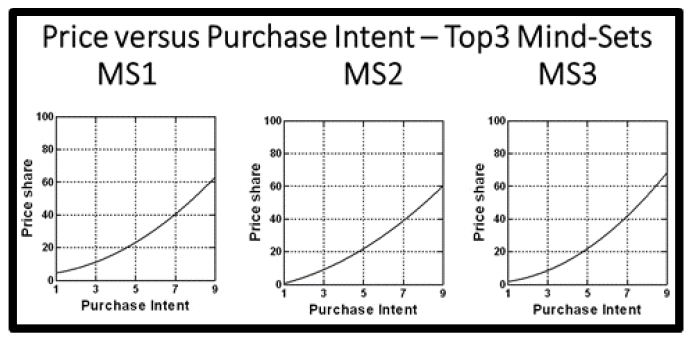
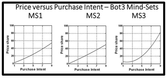
fig 5

fig 5(1)

fig 5(2)

Figure 5: Relation between Price willing to pay (ordinate) and 9-point rating of purchase (abscissa), for three dependent variables (TOP3, BOT3, PRICE), each generating three mind-sets. The curves emerge from smoothing the raw data to show the underlying pattern.

Finding these mind-sets in the population

One of the hallmarks of Mind Genomics is that the mind-sets distribute in apparently random ways through the population, a fact which disturbs the traditional researcher searching for a co-variation between HOW THE PERSON THINKS ABOUT A TOPIC (the mind-set) and WHO THE PERSON IS, OR WHAT THE PERSON DOES, OR EVEN THE PERSON’S GENERAL ATTITUDES (GENERAL PSYCHOGRAPHICS.) In only very rare cases do we find strong co-variation between the mind-sets and other factors about a person. We should not be surprised at this lack of co-variation. The old adage ‘birds of a feather flock together’ does not seem to hold true when we focus on the deep variation between people on a topic, even people living in the same household. People may share some general attitudes, but it is rare, if ever, to find two people who agree completely on the granular aspects of any topic.

Table 8 shows the distribution of the three mind-sets for each dependent variable in terms of total, gender, age, and where the person lives.  Table 9 shows the cross-tabulation of the mind-sets. Any value greater than 40% of the total panel is darkened. For example, there are 68 males. We would expect an equal 1/3 distribution, of 23,23,23 for the three mind-sets. We have chosen the 40% cut-off as worthy of note. Thus, for 68 respondents, 40% means more than 27.2 respondents. We round to the lower whole number (27). It Is clear from both tables that knowing a person’s membership in either a geo-demographic subgroup (Table 8) or in a mind-set (Table 9) does not allow us to easily predict the person’s membership in any other type of mind-set.

Table 8: Cross-tabulation of membership in gender, age, and residence by respondents in the total panel, and in the three groups of three mind-sets each. There is no clear pattern.
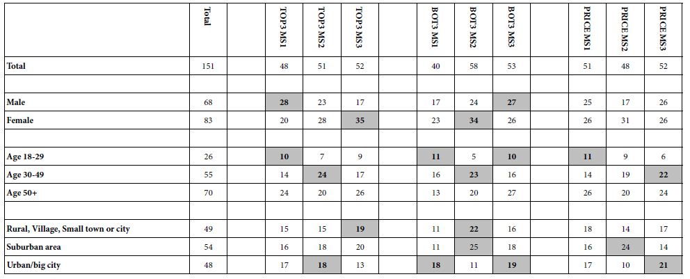
table 8

Table 9: Cross-tabulation of membership in the three groups of three mind-sets each. There is no clear organizing pattern allowing prediction of mind-set membership from knowledge of other mind-set membership.
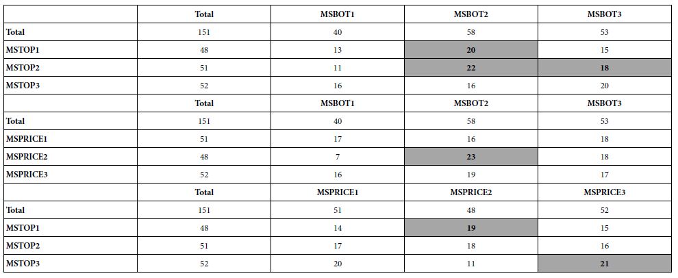
table 9

Predicting the profile of mind-set memberships using the PVI (personal viewpoint identifier)

During the past four years it has become increasingly obvious to authors Moskowitz and Gere that the practical applications of Mind Genomics would increase in number and scope when one could move beyond the limited number of respondents and apply the mind-set ‘clustering’ or ‘segmentation’ to the world at large.

Initial observations of how researchers were using segmentation revealed that the segments emerging from typical studies were very large, very general, and lacking the granularity. The typical segmentation appeared to emerge from the top down, so that one could divide people into general personas. The division would be made on the basis of questionnaires about general topics, leading to a limited number of personas, general groups of people [2][12][13]

The segmentation made interesting reading, the personas were described in detail, but there was no clear way to link these personas to the specific topic, especially when the topic is so granular as healthful pasta, and more so when the topic does not yet even exist.

Traditional segmentation is interesting, but really inactionable at the granular level simply because the segmentation is created with general propositions in mind, not with respect to a specific product. In a deep philosophical sense, one might say that traditional segmentation is imbued with sociology, organizing the world at large, the ‘nomothetic,’. In contrast, Mind Genomics segmentation is imbued with psychology, organizing the response to a granular topic, focusing on the individual, the ‘idiographic’.

In order to make the Mind Genomics segmentation more usable the analogy used is that Mind Genomics segmentation discovers groups of ‘mental primaries’, and not groups of people. The research would reveal these primaries, combinations of ideas, as shown by the three groups of mind-sets. Those mind-sets would be primaries, like color primaries. One needs a tool, a mental colorimeter, as it were, to assign a new person to one of these three primaries. With three sets of mind-sets, one for each dependent variable, the tool would have to assign a new person to one mind-set for each dependent variable.

The approach to create these assignments uses Monte Carlo simulation of the data, with 20,000 iterations. In the actual study, there were three such PVI’s created, one for each of the three dependent variables. The objective was t create a six-question tool for each dependent variable. The six questions are taken from the 36 elements used to create the mind-set segmentation for the dependent variable.  The six questions are answered on an anchored, two-point scale. With six questions and a two-point scale, the PVI questionnaire generates exactly 64 combinations. Each combination links with one of the relevant three mind-sets.

Figure 6 shows the introduction to the PVI. The respondent simply presses a link, and is taken to the introduction, which requests participation and then background information.  The information will be stored in a database for later use.

fig 6

fig 6(1)

Figure 6: Introduction to the PVI, showing the request for permission and for background information. As of this writing (Summer, 2020) the link is:
https://www.pvi360.com/TypingToolPage.aspx?projectid=215&userid=2018

Figure 7 shows the actual PVI, with three sets of six questions. Each respondent will receive the same PVI, but the order of PVI’s will be randomize across respondents, as will the order of questions within each PVI.  With three PVI’s, one per dependent variable, there are six orders of the PVI’).  Second, within each PVI, the order of the questions will be randomized. For each PVI there are 6! Orders of questions, i.e., 6x5x4x3x2x1 or 720 orders
fig 7

Figure 7: The actual PVI, for the three dependent variables.

Finally, Table 10 shows an example of feedback for a respondent, who completed the three PVI’s. The segment membership and the feedback are shown by the shaded cells. The researcher has the option to provide no feedback at all, to provide mind-set membership, or provide mind-set membership, feedback as well as information about the segments to which the respondent does not belong!

Table 10: Feedback for one respondent based upon pattern of answers to the three PVI’s. The shaded cells show the mind-set to which the respondent belongs, and the feedback for that mind-set.
table 10

Discussion and conclusions

When the topic of healthful pasta was first proposed some years ago and the study run (late 2012), the notion of Mind Genomics as a cartography was in its infancy. The research objective at the time was to determine what specific messages pertaining to pasta would prove to be most compelling. The effort at that time, only nine years ago, was to explore messaging, with the objective that here was a tool, Mind Genomics, which could provide a great deal of deal on many alternative messages. Up to then, the conventional wisdom was either to test single messages (so-called promise testing) or test fully formed concepts, polished, dense paragraphs, presenting a few ideas in a well-executed, almost seamless package. The idea was novel — discover through systematic experimental design powerful albeit mind-set specific messages.

When one looks at the richness of the data, the first question which emerges is ‘what do these data tell us about good carbs, or healthy pasta?’ This first question is the scientific aspect. The second question is ‘how do I use these data to help people enjoy a healthier diet’. The third question is ‘how do I used these data for commercial purposes.’  There are other questions of a research nature, such as ‘why do people fall into the mind-sets they do,’ ‘why is the price-purchase intent curve so similar across mind-sets,’ and the ever-recurring question ‘are these mind-sets stable, and does a person person’s mind-set ever change?’

What do these data tell us about good carbs?

This first question is answered by an abundance of data. The elements below are the strong performing elements. Rather than working with one theme at a time, and either saying that theme (e.g., brain power) is important or not important, Mind Genomics works with many themes. Thus, the information which emerges is far richer, a landscape of information rather than a single image, a single idea. The notion of the cartography, the landscape, is dramatically different from the more traditional, focused, hypothetico-deductive system, which considered one hypothesis or theme at a time, and through experiment attempting to falsify it [14] In Mind Genomics, the effort is to explore a broad landscape, not investigate each location off the landscape in a sequence of seemingly disconnected experiments, only later put together by a met-analysis

In terms of specifics, here are promising messages.

Look good & feel great at any age with a whole-grain fortified pasta diet… delivers plenty of energy & lifelong weight control

Put radiance back into your skin with whole-grain fortified pasta, which helps you sleep better and stop night-time problems

Stop feeling tired, eat whole grain fortified pasta for extra stamina …no need to cancel your evening plans anymore!

Vitamins and anti-oxidants in fortified whole-grain pasta improve brain power & thinking… reduce risk of cognitive impairment

Fortified whole-grain pasta contains complex carbohydrates – the “good carbs” which are essential to healthy brain function … boosts your brainpower … keeps you mentally sharp

Double pleasure without the guilt: whole grain lasagna is not only heavenly delicious, but healthy and nutritious too!

After a hearty whole grain fortified lasagna.no need to worry about weight gain

How do I use these data to help people enjoy a more healthful diet?

A growing issue in today’s world is the unhealthiness of the diet, the growing issue of obesity, and the need to create a better way to eat so that obesity and diet-related diseases such as diabetes do not ravage our society.  The discovery of strong performing messages allows those who communicate about healthful living to discover ‘what to say’ and ‘what not to say.’  One might surmise that any nutrition professional would know what to say, and that the information shown. Nutrition professionals know the science behind the food but may not know what messages convince. Indeed, as Table 11 shows, what appeals to the total panel may appeal strongly to only some of the respondents, and not to others.  It is here that the PVI, the personal viewpoint identifier, emerges with the power to assign a new person to a mind-set, and thus know at the start of the relationship with that new person the kinds of messages that will resonate.

Table 11: Strong performing messages may appeal to the total without appealing to all mind-sets or may appeal strongly to only one mind-set.

table 11

Are there ‘rules’ about how many mind-sets exist, and does a person’s mind-set change over time?

As Mind Genomics experiences increasing application, with more studies and more situations, questions of the number of mind-sets emerge, as well as the invariance of a mind-set. There is no fixed n umber of mind-sets. Each topic can be investigated in depth, to generate an array of different mind-sets. Unlike basic colors, of which there are only three (red, yellow, blue), mind-sets emerge for virtually any topic where decisions are made on the basis of information.  This study on good pasta shows one can take one topic and ‘drill down’ to create at least three mind-sets. There are smaller topics within good pasta, such as brain function, which themselves can generate mind-sets.   As for the invariance of mind-sets over time for a single person, that question remains a topic for the next generation of investigators.

Acknowledgement

Attila Gere thanks the support of the Premium Postdoctoral Researcher Program of the Hungarian Academy of Sciences

Reference

  1. Barry J, Weinstein A (2009) Business psychographics revisited: from segmentation theory to successful marketing practice. Journal of Marketing Management25: 315-340.
  2. Brower M (2018) Claritas (formerly Nielsen) Segmentation and Market Solutions. The Charleston Advisor. 18: 15-20.
  3. Shelke K (2016) Pasta and Noodles: A Global History. Reaktion Books.
  4. Webb D (2019) Pasta’s history and role in healthful diets. Nutrition Today. 54: 213-220
  5. Moskowitz HR (2012) ‘Mind genomics’: The experimental, inductive science of the ordinary, and its application to aspects of food and feeding. Physiology & behavior107: 606-613. [crossref]
  6. Moskowitz HR, GofmanA Beckley J, Ashman H (2006) Founding a new science: Mind genomics. Journal of sensory studies. 21: 266-307.
  7. Moskowitz HR, Gofman A (2007) Selling Blue Elephants: How to Make Great Products that People Want Before They Even Know They Want Them. Pearson Education
  8. Box GE, Hunter JS (1961) The 2 k—p fractional factorial designs. Technometrics. 3: 311-351
  9. Gofman A, Moskowitz H (2010) Isomorphic permuted experimental designs and their application in conjoint analysis. Journal of sensory studies. 25: 127-145.
  10. Jain AK, Murty MN, Flynn PJ (1999) Data clustering: a review. ACM computing surveys (CSUR). 31: 264-323.
  11. Wilkinson L (2010) Systat. Wiley Interdisciplinary Reviews: Computational Statistics. 2: 256-257.
  12. Kahle LR (1986) The nine nations of North America and the value basis of geographic segmentation. Journal of Marketing 50: 37-47.
  13. Wells WD (1975) Psychographics: A critical review. Journal of marketing research12: 196-213.
  14. Lakatos I (1976) Falsification and the methodology of scientific research programmes. In Can theories be refuted? (pp. 205-259). Springer, Dordrecht.
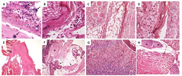
Mind Genomics & Perception of the Restaurant: Homo Emotionalis vs Homo Economicus

DOI: 10.31038/PSYJ.2021334

Abstract

Three experiments explored the perception of the situation in a restaurant from the point of view of an observer. The first experiment, focusing on the projected feelings of a server in a situation, revealed the ease with which respondents were able to project the emotions of the server, as well as exhibiting two easy-to-uncover mind-sets. The second and third experiments focused on the expected price of the meal, expressed relative to the normal amount they would expect to pay. In these two experiments, The results were harder to interpret and did not tell a convincing story, either for the total panel, or for mind-sets extracted.  We posit that the psychological mechanism for judging feelings, easily available when judging a situation, are different from the psychological mechanisms for judging the economic aspects of the same situation, when what is being judged is behavior, rather than a specific product..

Introduction

With the proliferation of the catering and restaurant industries, there is a wealth of knowledge emerging about the different aspects of food service, from the point of view of food, but also the point of view of service. Indeed, there is the Food Service Division in US-based Institute of Food Technologists, headquartered in Chicago, USA. There are similar divisions in other food-based organizations, such as the Research Chefs of America. Beyond these organizations are journals devoted to food service, such as Food Service Research.  Furthermore, the importance of out-of-home-eating has sparked the growth of restaurants of all sorts, with the interest in how to make a restaurant succeed. Success is not only measured by momentary popularity, but by long-term customers, low staff turn-over, and the ability to focus on the restaurant, and not on the ancillary staff issues. Ideally, the restaurant should run smoothly, the service and food should be good, and the décor should make the restaurant a welcome place for repeat visits.

With the importance of food service, the authors began to consider the potential of understanding how outside people feel about the restaurant, when different aspects of the restaurant are described to them. The emerging science of Mind Genomics suggested itself as a way to get into the ‘mind’ of the prospective customer, based upon a description of the restaurant. The key difference for our Mind Genomics effort was the desire to look into the aspect of describing the restaurant ‘situation’ as it actually ‘is’,  from the point of view of a restaurant professional (author Mazzio). The issue was whether it would be possible to understand the emotions of the situation (dubbed homo emotionalis), and whether it would be possible to understand responses to the situation manifesting themselves in monetary terms (dubbed homo economicus).  These studies thus reflect a new avenue for Mind Genomics, studies of emotions and of responses expressed in term of money, rather than responses expressed in terms of feelings.

Comparing the ‘outside in’ vs the ‘inside out’ – Anthropology and Sociology vs Mind Genomics

Our approach uses a new way to explore social and psychological factors driving judgments, specifically going in depth from the’ inside out,’ rather than from the ‘outside in.’  Our approach merges sociology, anthropology, and psychology, to create a systematized approach to investigate the topic.

The sociologist investigates the social structure of a situation, the roles people play, and attempts to formulate the structure based upon behavior. There is rarely a focus on the individual in other than a part of this situation. The sociologist adopts the nomothetic approach, searching for general rules of structure of the group. The sociologist might use observation of groups, coupled with questionnaires, surveys, and so forth. The sociologist might even move to big data, large arrays of compiled statistics. When applied to the restaurant, and specifically to the quick server ‘local diner,’ the sociologist eventually uncovers the structure people, positions, and activities regarding what goes on in a restaurant, the nature of cultural norms, and so forth. There is little in the way of focus on the mind of the individual person in the restaurant, what the person feels, thinks, and so forth, except as part of the nomos, the general description of the typical day, and ordinary behavior [1-5].

When we move from sociology to anthropology, we move more deeply into the behavior which occurs [6]. The anthropologist produces a much finer description of what happens in a situation, such as a restaurant, albeit with the focus on a specific restaurant, rather than a summary of restaurants in general. Thus, an anthropological study of the behavior in a local neighborhood diner would focus on a deeper description of the behavior in one or a few restaurants (see as examples; [1, 7-9]. With today’s tools, including the Internet for range of situations, video and video-coding of behaviors, the anthropologist can produce a much deeper understanding of what actually occurs in the restaurant.  It is no wonder that many consumer researchers are moving towards quantitative methods combined with qualitative methods. Today’s Internet technology makes it possible to acquire vast amounts of information, by automating the acquisition of behavior, and then the classification of the behavior by coding methods [10].

Delving into the mind through consumer psychology and Mind Genomics

Sociology and anthropology allow us to understand the situation in a restaurant, but do not let us delve deeply into the mind of the customer. Indeed, it is not the mind of the customer that is of interest, but rather the restaurant situation, in which the person and the person’s feelings and behaviors are simply a part.  Sociology and anthropology stop at the deep understanding of the mind of the customer, leaving that to psychology, and especially consumer psychology.

Consumer psychologists want to know more from the patron and the server than can be obtained from sociological and anthropological study. Consumer psychologists want to know how patrons and servers think about situations, what they really look for, what they find wonderful, and just as important, what they find horrid. The tools used are primarily discussions with patrons and servers, whether in-depth discussions with one or two people, or group discussions with several individuals, led by a moderator who follows a ‘script’ to discuss a variety of topics. These discussions are called qualitative research, to distinguish them from researching using surveys, called quantitative research. The differences are not relevant for this paper. What is important, however, is that the discussions and the surveys invoke the ‘rational’ part of the individual’s brain. Whether the individual is describing her or his feelings or experiences, either to an interviewer or to a group, the individual is attempting to present a rational, coherent story. IN the same way, when the individual is participating in a survey, the individual typically tried to be coherent, so that the individual will feel that the answers are meaningful, and thus the individual is a worthy person for answering honestly. The information presented in a focus group or in a survey may or may not be accurate, because of many biases [11]. Nonetheless, these are the major ways used by consumer researchers to understand the topic.

With relatively few respondents in these expensive studies, the likelihood is high that we would rediscover a lot of what we know, and perhaps discover a few new nuggets. Our changes of discovery would rest upon the talent of the interviewer to elicit the information, and the ability of the interviewee to verbalize the situation, if that is possible. People are not necessarily articulate, especially in a situation where there is little emotional involvement. Eating in a diner or quick serve restaurant does not typically bring with it deep emotional involvement when one is the guest. When one is staff, such as wait- staff, the emotions may be far deeper, especially when connected with receiving a gratuity.

The emerging science of Mind Genomics represents an approach to understand the way people make decisions, especially about the situations of the everyday. Mind Genomics has been in development for the past 40 years, since 1980, but came into its own during the early part of the 21st Century [12-15].

The science of Mind Genomics can be traced to three major sources, psychophysics, statistical design, and consumer research. Psychophysics, the study of the relation between sensory perception and physical stimulus, is a branch of experimental psychology, which stresses the search for a metric of sensory experience. In turn, Mind Genomics searches for a metric of ideas. Statistical  experimental design is a branch of statistics whose focus is the proper combination of independent variables (e.g., ideas), the evaluation by people of those combinations, and the estimation of the contribution of the individual ideas to the mixture. Experimental design is the key tool by which the researcher can set up the appropriate test stimuli, specifically combination of messages. Consumer research focuses on regularities of the everyday, the quotidian, the ordinary.

These three sources of Mind Genomics allow the us to explore the mind of the restaurant patron or the restaurant staff. Rather than observing the situation or conducting a survey, the researcher more directly selects a topic, creating four questions which are relevant to the topic, and then creating four answers to each question, viz., 16 answers.  These 16 answers are combined into small, easy-to-read vignettes about a restaurant. An underlying system, the built-in experimental design, prescribes each vignette. The respondent rates each vignette on a scale. It is impossible to ‘game the system’ because the vignettes comprise 2-4 different answers or ‘elements,’ which paint a ‘picture’.  Respondents find this task easy to do, viz., read a set of vignettes dealing with a topic relevant to a restaurant, and then rate the particular vignette on a defined scale.

The entire process from the point of view of the respondent lasts 3-5 minutes. Each respondent rates a totally unique set of 24 vignettes, allowing the study to proceed with virtually zero knowledge. The researcher need not select the ‘appropriate’ vignettes, which would imply some level of knowledge at the start of the study. The Mind Genomics process is so efficient that with 20-30 respondents, one can get a good idea of the mind(s) of the consumer, based upon the pattern of responses to many elements of the study. Furthermore, the experimental design works at the level of each individual respondent who participates, even though every respondent tested different combinations (vignettes.)

Over the past decade, the system for Mind Genomics has been templated, to allow rapid input of ideas, followed by rapid field work, and virtually instantaneous analysis. As a result, any topic where judgment is relevant can be studied in small, easy, affordable increments. One need not ‘be right’ at the start. The benefit to the researcher is the ability to understand the ‘mind’ of the respondent from the ‘inside out’. That is, the respondent need not have any conscious idea of WHAT she or he feels, or WHY.  The reasons emerge from the pattern of responses to meaningful stimuli.

The Mind Genomics Template used in this set of three studies

The research template follows these steps, which can be accomplished in a matter of an hour or two, from start to finish (type in the elements to inspect the analyzed data).

  1. Select a topic
  2. Identify four aspects of the topic just chosen. The four aspects can be thought of as four ‘questions.
  3. For each aspect, provide four specifics. These are ‘answers or ‘elements, expressed in simple, single-minded phrases, in declarative format. The 16 elements provide the richness of description since they can be particularized to paint a word picture.
  4. Using experimental design (built into the Mind Genomics program, BimiLeap.com), create vignettes (combinations) comprising these elements (answers). The underlying experimental design specifies the precise set of 2-4 elements, ensuring that only one element from a question ever appears in a vignette.
  5. Each respondent evaluated 24 vignettes, with the vignettes being unique, viz., different from one respondent to another. Each set of 24 vignettes presents each element 5x, so that the element is present in five of the 24 vignettes, and absent from 19 of the vignettes.
  6. The underlying view behind this approach is modeled on the MRI, which takes many pictures of the same tissue, albeit from different vantage points, and combines the view into a 3-dimensional picture.
  7. This uniqueness is important .It means that each respondent evaluates a different set of descriptions, rather than having each respondent evaluate the same set of descriptions. One need not know the ‘correct’ set of elements ahead of time, with the empirical portion of the study measuring how well the limited, pre-selected combinations perform. The ‘underlying picture’ emerge, even though each measurement point is ‘noisy’ and possibly slightly wrong. The pattern will emerge, even from noisy data [16].
  8. We can estimate the models for the total panel, simply by putting all the data into the datafile, and running one regression equation, with the method being OLS, ordinary least-squares regression. The independent variables are the 16 elements, taking on the value 0 when absent from a vignette, and taking on the value 1 when present in the vignette. The 16 elements, A1-D4, constitute the independent variables.
  9. Each individual respondent evaluated a unique set of 24 vignettes. Thus, we can estimate the coefficients at the level of the individual respondent. For any set of data, we end up with a data set comprising sets of 24 rows of data, each set corresponding to a respondent.
  10. For Study #1 (5-point Likert scale, 1=Hate … 5=Love), we convert the ratings of 4 and 5 to 100, the ratings of 1,2 and 3 to 0. This created the binary variable TOP to which we added a very small random number, useful to prevent crashes of the regression program. We also converted the ratings of 1 and 2 to 100, and ratings 3,4 and 5 to 0, to create the variable BOT, again modified slightly by a small random number to prevent crashes of the regression program.
  11. For Studies #2 and #3 we converted the ratings to relative dollar value, and again added the very small random number.
  12. To prepare for clustering in each study, we calculated a regression equation for each respondent. We did not estimate an additive constant for the individual-level model estimated in all three studies.
  13. We then used k-means clustering separately in each study [17] to divide the group of respondents into two complementary groups for that study, these groups showing different patterns of coefficients. In each study, the respondents for that study were assigned to one of the groups, based upon the similarity of the pattern to the average of the group. These groups are ‘mind-sets’, groups of individuals who react similarly to the information about the restaurant.

Study 1 – How the server would feel about the customer

In study 1 the respondents evaluated 24 descriptions of the behavior of the customer. The respondents comprised 30 random respondents from the Luc.id list of respondents who had signed up to participate in these studies. The respondent rated each vignette on a 5-point scale. The ratings were transformed to Top (ratings 4-5 transformed to 100, ratings 1-3 transformed to 0), then transformed to Bot (ratings 1-2 transformed to 100, ratings 3-5 transformed to 0). Finally, individual-level models were created relating the presence/absence of elements to TOP (positive server reaction). The 30 sets of 16 coefficients each, but not the additive constant, were used in a k-means clustering to generate two different mind-sets. The standard distance metric for Mind Genomics was used to calculate distances between pairs of respondents. The distance is D = (1-Pearson R, calculated between two respondents, based on the 16 elements). Thus the clustering put together individuals with similar response patterns.

Table 1 shows the results, in three separate parts of the Table. PART A of  1 shows the additive constant and non-zero coefficients. These are elements which drive satisfaction with the customer (viz., a rating of 4-5 for the vignette.) PART B of Table 1 shows the additive constant and non-zero coefficients when we begin by looking at the elements which drive dissatisfaction’ (viz., a rating of 1-2 for the vignette). Finally, PART C of Table 1 shows the estimated response times for the different elements. The Mind Genomics program was able to deconstruct the response time (time between stimulus presentation on the screen and response) into the different response times ascribable to each element.  In Parts A and B, only the positive coefficients are shown, in order to allow the patterns to emerge more clearly. In Part C, only the response times of 1.0 seconds or longer for an element are shown, again to allow the patterns to emerge more clearly.

When we look at the ratings of liking the customer (PART A), we begin with the additive constant. We interpret the additive constant to represent the degree of positivity of the server towards the guest, estimated as if there were no elements present in the vignette. Of course, by the underlying design, all vignettes comprised at least two elements, and at most four. Thus, the additive constant is an estimated parameter. The additive constant for liking the customer is about 50. In the absence of elements, the respondent feels that the server is likely to be positive towards the customer, but not very positive. Very positive feelings would be shown by additive constants around 70.

For the total panel, we see no elements strongly driving the server to ‘like’ the customer. That is, there are no strong performing elements (Part A). When we move to drivers of disliking the customer (PART B of Table 1), we see that the total panel less likely to begin with dislikes the customer (additive constant 28, versus additive 51 for liking the customer).   The only element which drives disliking for the total panel is element A4: customer says, :  we’re in a big hurry.

The division of the 30 respondents into the two mind-sets changes the picture entirely. Mind-set 1, comprising 12 of the 30 respondents, can be characterized as simply wishing as little interaction with the customer. Mind-set 2, comprising 18 of the 30 respondents can be characterized as wanting to help the customer.  These patterns emerge from Table 1, Part A.

Table 1: Mind Genomics investigation of how the respondent feels about the customer as a function of their interaction.

fig 1

fig 1(1)

fig 1(11)

fig 1(111)

Positive drivers of liking – Mind-Set 1 (little interaction desired)

End of meal: rudely asks for the check, and hurries off

Negative drivers of liking – Mind-Set 1

Customer says, :  we’re in a big hurry. 

Customer says, : I’m in a big hurry. 

Customer demeanor : seems to be in a big rush

Customer says, : can I give you my order?

Placing order: unhappy with discrepancy of prices for similar menu items

Customer says. : Hello, how are you today? 

Positive drivers of liking – Mind-Set 2 (likes helping the customer)

Customer says. : Hello, how are you today? 

Customer says, :  we’re in a big hurry. 

Placing order:  unclear, hesitant, changes mind a lot

Customer says, : I’m in a big hurry. 

Negative drivers of liking – Mind-Set 2

None

One of the unexplored areas of consumer research is the amount of attention paid to the different messages. Researchers can ask a respondent to guess how much attention the respondent pays to information. The answer may or may not make sense, but most certainly the respondent will try to give a sensible answer, not so much based on real attention or engagement time, but on a guess. The Mind Genomics program measures the total time of engagement with each screen, viz., each combination of messages, and then deconstructs the response time to the estimated number of seconds that can be attributed to each element. The model or equation used to fit the data is absent an additive constant, the rationale being that in the absence of elements, the response time should be 0.

With this introduction in mind, let us look at the coefficients in PART C of Table 1. We show only response times of 1.0 seconds or longer. These are the elements which ‘engage’ the respondent. Mind-Sets 1 and 2 spend the longest times looking at the description of the customer saying that she or he is in a big rush, and then reading the end of the meal.

The data from this first study suggests that asking the respondent to rate the emotional reaction of the server is likely to result in patterns which make sense or at least do not appear to be radically contradictory. We conclude from this first study that using emotion-based ratings unleashes f homo emotionalis, with the ratings telling a story, making sense, and dividing the two mind-sets from each other, at least in a basic way.

Homo economicus – letting the respondent judge in terms of money

The first study, summarized in Table 1, suggests that the respondent can vicariously estimate the feelings of the server in a diner type restaurant. The assignment of ratings to denote feelings appears to be straightforward, at least judged by the outcome that the data make sense, viz., ‘tell a story.’   We now change the dependent variable to money. Rather than having the respondent rate the expected feeling (hate to love), we instruct the respondent to read the vignette and estimate the relative amount of money to change hands during the transaction, from a low of 25% less than expected to a high of 25% more than expected. The scale is anchored at the bottom (1=25% lower) and at the top (9=25% higher).

The 9-point scale was divided into nine equal values, starting with 75 (corresponding to 25% lower), through 100 (corresponding to same), and 125 (corresponding to 25% higher). The respondent simply assigned a number. It was at the analysis stage that these nine numbers were assigned their corresponding percent values (75% of what is expected to 125% of what is expected).

The data for the two studies appear in Table 2 (Size of check vs described staff behavior and problem resolution), and Table 3 (Size of check vs described behavior with the customer). The coefficients for dollars are the expected percent of the check that can be ascribed to the element. The response time is the number of seconds estimated for reading and processing the element.

Study 2, expected size of the check as a function of described staff behavior and problem resolution, suggests two mind-sets (Table 2).

Table 2: Study 2 – Expected size of the check as a function of described staff behavior and problem resolution

table 2

Mind-Set 1 expects to have a higher check for the meal when the staff is described as more attentive. Respondents read with more attention, and thus engagement, messages about problem resolution.

Mind-Set 2 expects to have a higher check for the meal when the staff is described as unprofessional, fighting with each other or kidding around with each other. Respondents read with more attention, and thus engagement, messages about the staff interaction with each other.

The elements which engage the respondents are staff interaction and problem resolution, neither group having any significant affect on the expected size of the check for the meal.  These elements are almost stories about ‘human behavior’, interesting in and of themselves, as topics that people would discuss with each other.

Study 3, the expected size of the check as a function of described staff-customer interaction, also suggests two mind-sets (Table 3).

Table 3: Study 3 – Expected size of the check as a function of described staff-customer interaction

table 3

Mind-Set 1 expects a higher check for the meal when the wait staff is indifferent, walking around. Mind-Set 1 is engaged by messages talking about the competence of the wait staff, in terms of taking order.

Mind-Set 2 expected a higher check for the meal when the wait staff is a measured number of second late, noticing the waiting customer. There is no clear pattern to the elements which engage Mind-Set 2.

Discussion

Our goal in this paper is to apply a newly emerging branch of psychological science, Mind Genomics, to the mundane, virtually every-day topic of the quick serve restaurant or diner. The objective is to move beyond the surface research, the efforts of sociology and anthropology, and beyond business practices and issues as dealt with by the HR department, human resources. The objective is to dig deeply into the mind of the customer, faced with different situations in a restaurant, and understand attitudes towards those situations, using Mind Genomics as the structure for investigation, and using first emotional attributes as the rating scale (Study 1), and then ‘financial outcomes’ (e.g. estimated check price) as the rating scale (Studies 2-3). To our knowledge, this paper is among the early papers to probe the mind of the respondent using monetary scales rather than emotional scales (viz., rating using the mind as homo economicus versus the mind more ordinarily used in the form of homo emotionalis).

During the four-decades experience developing Mind Genomics, a number of studies were executed wherein the elements, the messages, were either features of the product, or numerical aspects, such as weight of the product. The ratings used were evaluative, such as interest or value for the money, both emotional. In the different studies, once the part-worths of the elements were estimated by OLS regression, as in Study 1, it was straightforward to plot the coefficient for the element (e.g., part-worth estimate for value for the money) versus the element, where the element presented a numerical attribute. In almost all cases the coefficients for judgment emerging from the ratings show high correlation with the numerical information about the product, e.g., the weight.  These results suggest the usefulness of Mind Genomics to quantify the perceived value of an aspect of the product [12-15, 18].
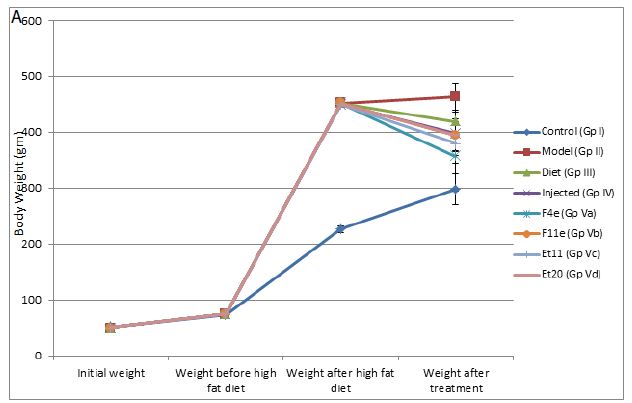
The issue now emerges regarding the success of Mind Genomics in the use of numbers to measure emotions generated by the description of situations (Study 1), but the seeming failure of the use of numbers described as money to measure emotions generate by the description of situations (Study 2 and Study 3, respectively). We know from everyday experience that we can estimate the ‘fair value,’ but it is generally the ‘fair value’ of something tangible, whether that be a physical object or an experience such as the value of a recording of an opera or the value of a ticket to the opera.  What then is the difference? It may be that we have not yet found the appropriate way to measure the ‘dollar value’ of emotions tied to the description of an experience. That is, it is not a question of the utility of the experience, but simply that the effort may be difficult, and even perhaps impossible to use dollar value scaling to describe an experience without a tangible outcome of utilitarian nature.

Conclusion

The results from these three studies suggest that Mind Genomics will find more success using measures of good/bad than measures of money as the dependent variable. Money (viz., the price of an item or a service) may well be a strong performing element, driving feelings of like/dislike, or good/bad.  Money as a response, viz., the use of money as a rating scale may well work when the stimulus messages are about items, but it does not appear from this study that money as a rating scale can be used easily to rate situations or behaviors, at least not in foodservice.

At a deeper level, the notion that it is difficult for respondents to rate the expected size of a check based upon description of staff behavior calls up the need to think about the ‘meaning’ of assigning monetary damages to situations where the damages cannot easily be quantified, viz., damage to the psyche human being. That corollary to this study deserves its own set of studies, viz., homo economicus and the law.

References

  1. Butler S, Skipper Jr JK (1981) Working for tips: An examination of trust and reciprocity in a secondary relationship of the restaurant organization. Sociological Quarterly2: 15-27.
  2. Haghighi M, Dorosti A, Rahnama A, Hoseinpour A (2012) Evaluation of factors affecting customer loyalty in the restaurant industry. African Journal of Business Management6: 5039-5046.
  3. Heung VC, Gu T (2012) Influence of restaurant atmospherics on patron satisfaction and behavioral intentions. International Journal of Hospitality Management31: 1167-1177.
  4. Madanoglu M (2006) Validating restaurant service quality dimensions. Journal of Foodservice Business Research7: 127-147.
  5. Ryu K, Han H (2011) New or repeat customers: How does physical environment influence their restaurant experience? International Journal of Hospitality Management30: 599-611.
  6. Mariampolski H (2006) Ethnography for Marketers: A guide to Consumer Immersion. Sage.
  7. Gueguen N, De Gail MA (2003) The effect of smiling on helping behavior: Smiling and good Samaritan behavior. Communication Reports16: 133-140.
  8. Gueguen N, Jacob C (2014) Clothing color and tipping: Gentlemen patrons give more tips to waitresses with red clothes. Journal of Hospitality & Tourism Research38: 275-280.
  9. Leodoro G, Lynn M (2007) The effect of server posture on the tips of whites and blacks. Journal of Applied Social Psychology37: 201-209.
  10. Porretta S (2021) The Changed Paradigm of Consumer Science: From focus group to Mind Genomics. In Consumer-based New Product Development for the Food Industry. Royal Society of Chemistry 21-39.
  11. Downey B (2015) The looking glass self and deliberation bias in qualitative interviews. Sociological Spectrum35: 534-551.
  12. Moskowitz D, Moskowitz H (2012) Conjoint analysis plus (cross category, emotions, pricing and beyond). Product Innovation Toolbox: A Field Guide to Consumer Understanding and Research 192-223.
  13. Moskowitz HR, Silcher M (2006) The applications of conjoint analysis and their possible uses in Sensometrics. Food Quality and Preference17: 145-165.
  14. Moskowitz HR, Gofman A, Beckley J, Ashman H (2006) Founding a new science: Mind genomics. Journal of Sensory Studies21: 266-307.
  15. Moskowitz MR, Ashman H, Minkus-McKenna D, Rabino S, Beckley JH (2006) Databasing the shopper’s mind: Approaches to a ‘mind genomics’. Journal of Database Marketing & Customer Strategy Management13: 144-155.
  16. Gofman A, Moskowitz H (2010) Isomorphic permuted experimental designs and their application in conjoint analysis. Journal of Sensory Studies25: 127-145.
  17. Likas A, Vlassis N, Verbeek JJ (2003) The global k-means clustering algorithm. Pattern Recognition36: 451-461.
  18. Moskowitz HR (2012) ‘Mind genomics’: The experimental, inductive science of the ordinary, and its application to aspects of food and feeding. Physiology & behavior107: 606-613. [crossref]

Neoadjuvant Chemotherapy with S-1 and Oxaliplatin followed by Laparoscopic D2 Gastrectomy for Clinical Stage III Gastric Cancer: Primary Results of Phase II nacG-SOX130 Study

DOI: 10.31038/CST.2021634

Abstract

Background: In spite of modern multimodal strategies, the prognosis of Stage III gastric cancer is still insufficient. We conducted a phase II study to evaluate the safety and efficacy of neoadjuvant chemotherapy with S-1 and oxaliplatin for clinical Stage III gastric cancer.
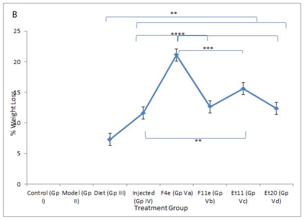
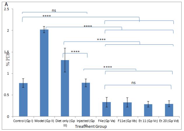
Methods: Patients with clinical Stage III gastric adenocarcinoma were treated with two-cycles of nacG-SOX130 (S-1 80 mg/m2 daily for 2 weeks, oxaliplatin 130 mg/m2 on day 1, every 3 weeks), followed by laparoscopic D2 gastrectomy. The primary endpoint was the clinical response rate. The planned enrollment was 36, which was calculated based on an expected response rate of 70% and a threshold response rate of 56%, with a one-sided alpha of 5% and a power of 90%.

Results: Between January 2016 and February 2019, 36 patients were enrolled, of whom 34 were assessed for efficacy. R0 resection rate was 97.1% (33/34). The clinical response rate was 73.5% (25/34, 95%CI 58.70-88.36, p=0.025) and the pathological response rate was 58.8% (20/34). The most common toxicities during neoadjuvant chemotherapy were grade 1/2 neutropenia (58.8%) and grade 1/2 peripheral sensory neuropathy (52.9%). The grade 3 surgical morbidity was 8.8% (3/34). Treatment-related death and operative mortality were not observed.

Conclusions: nacG-SOX130 was feasible and resulted in encouraging response rates without compromising surgery. nacG-SOX130 would be a promising option of neoadjuvant chemotherapy for clinical Stage III gastric cancer.

Mini-Abstract

Phase II nacG-SOX130 study showed favorable safety and efficacy of neoadjuvant chemotherapy with S-1 and oxaliplatin followed by laparoscopic D2 gastrectomy for clinical Stage III gastric cancer.

Keywords

Neoadjuvant chemotherapy, Laparoscopic surgery, SOX, Gastric cancer

Introduction

Over the past decade, multimodal treatments have improved the prognosis of resectable gastric cancer. High quality surgery, which should be precise in lymph node dissections and, at the same time, less invasive for quality of life, is also critical for better survival [1]. However, gastric cancer is still one of the leading causes of cancer-related deaths worldwide, and there is an unmet need for a newer strategy [2]. Radical surgery is an essential step of the treatment. In Asian countries, it is followed by adjuvant chemotherapy according to the pathological status of the tumor. 1-year S-1 monotherapy or 6-month oxaliplatin-combined doublet therapy is widely used in Stage II/III gastric cancer [3,4]. Even with these established strategies, prognosis still remains poor in some patients with high-risk features of recurrence, i.e. Stage III. In the ACTS-GC study, which tested adjuvant S-1 [5], the 5-year overall survival (OS) in Stage II patients was 84.2% (hazard ratio (HR) 0.509, 95% confidence interval (CI): 0.338-0.765). In contrast, in Stage IIIA and IIIB, the 5-year OS were 67.1% (HR 0.708, 95%CI: 0.510-0.983) and 50.2% (HR 0.791, 95%CI: 0.520-1.205), respectively, which could not be satisfactory as compared with the results of Stage II patients. In the CLASSIC trial, which tested adjuvant capecitabine plus oxaliplatin [6], the 5-year OS in Stage II, IIIA and IIIB were 88% (HR 0.54, 95%CI: 0.34-0.87), 70% (HR 0.75, 95%CI: 0.52-1.10) and 66% (HR 0.67, 95%CI: 0.39-1.13), respectively, which showed the similar trend of OS reduction as seen in the ACTS-GC study. Even with a newer adjuvant regimen of S-1 plus docetaxel in Stage III gastric cancer in the JACCRO GC-07 trial, similar reduction of relapse-free survival was observed as the cancer stage progressed, and more than half of stage IIIC patients recurred after surgery [7]. Poor compliance in a post-operative phase is one of the reasons for worse outcomes. Not only the surgical complications, but eating disorders and subsequent body weight loss might have substantial impacts on continuity of every treatment [8]. From this standpoint, chemotherapy before surgery, namely neoadjuvant chemotherapy, is a promising option, especially when more intensive and therefore more toxic combined regimens including platinum compounds are considered. Although relative advantages of a preoperative time period are now well understood, some clinical hesitations for neoadjuvant chemotherapy still remain. The positive results of two pivotal studies in perioperative settings, the MAGIC trial [9] and the ACCORD07/FFCD 9703 trial [10], could not be translated into the current clinical situations because surgical procedures in these studies were not reached to the today’s standards of curative intent D2 gastrectomy. Furthermore, it is a well-known fact that racial and ethnic disparities widely exist in the world of gastric cancer [11]. Therefore, in the planning of a new neoadjuvant study in gastric cancer, we should set up a planning with the latest, non-invasive radical D2 gastrectomy, and arrange the experimental regimen suitable for each country. In this phase II study, we evaluated the efficacy and toxicity of neoadjuvant chemotherapy with S-1 plus oxaliplatin for clinical Stage III gastric cancer patients who underwent laparoscopic radical D2 gastrectomy.

Methods

Study Design

nacG-SOX130 study was planned as a prospective, single-institution, investigator-initiated phase II trial at Kyoto Katsura Hospital, Kyoto, Japan and was conducted in accordance with the Declaration of Helsinki as well as the Japanese Ethical Guidelines for Clinical Studies. The study was approved by the Institutional Review Board and was registered in the University Hospital Medical Information Network Clinical Trials Registry (https://www.umin.ac.jp/ctr/) as UMIN000036139.

Eligibility Criteria

The eligibility criteria were; (1) histologically proven and clinically resectable gastric adenocarcinoma; (2) clinical T3-4/N1-3M0 disease: T and N stages were determined by computed tomography (CT) based on the 7th UICC/AJCC TNM classification. Positive lymph node was defined as that with a long axis diameter > 8 mm or a short axis diameter ≥ 6 mm; (3) an age of over 20; (4) an Eastern Cooperative Oncology Group performance status 0-1; (5) no history of prior chemotherapy, radiotherapy, or surgery for gastric cancer; (6) an adequate oral intake without intestinal obstruction; (7) adequate hepatic, renal, cardio-respiratory and bone marrow functions; (8) a written informed consent. The exclusion criteria were; (1) synchronous or metachronous (within 5 years) malignancy other than carcinoma in situ; (2) pulmonary fibrosis, interstitial pneumonitis, bowel obstruction; (3) pregnant or breastfeeding women; (4) active infections; (5) severe mental disease. Before entry in this study, staging laparoscopy was required to exclude peritoneal dissemination. Chest radiography, contrast-enhanced thoracic/abdominal/pelvic CT and upper gastrointestinal tract endoscopy were conducted as a pretreatment workup.

Treatment Schedule

Patients were treated with two-cycles of neoadjuvant chemotherapy (nacG-SOX130: S-1 80 mg/m2 daily for 2 weeks, oxaliplatin 130 mg/m2 on day 1, every 3 weeks), followed by surgery. Surgery was planned 4-6 weeks after the end of neoadjuvant chemotherapy. Toxicity was assessed according to the Common Terminology Criteria for Adverse Events, version 4.0. The subsequent chemotherapy cycle was delayed until patient recovery for those with severe adverse events. After the second cycle of nacG-SOX130, efficacy was evaluated on the basis of CT findings, tumor marker levels and the upper gastrointestinal endoscopic examination.

Surgery

Patients underwent surgery between 4 and 6 weeks after the last administration of S-1 if R0 resection was considered possible on the findings of imaging studies and laboratory data. All patients underwent gastrectomy laparoscopically. After placing laparoscopic ports, intraperitoneal washing cytology specimens were sampled first of all to investigate peritoneal dissemination. If cytology was negative, R0 resection was attempted by distal or total laparoscopic gastrectomy with D2 lymphadenectomy according to the Japanese Gastric Cancer Treatment Guideline 2014 (ver. 4) [12]. Involved adjacent organs, if any, were removed to achieve R0 resection. If R0 resection was considered impossible, the protocol treatment was terminated.

Endpoints

The primary endpoint of this trial was the clinical response rate (cRR), which was calculated by a sum of uni-dimensional measurements of short axis of positive lymph nodes: complete response (CR), disappearance of positive lymph nodes; partial response (PR), at least a 30% decrease; progressive disease (PD), at least a 20% increase or appearance of new lesions; stable disease (SD), non-PR and non-PD. Objective responses were evaluated by two experienced physicians who were not informed of the results of each treatment. Concordance between two physicians was evaluated with contingency tables and by Cohen’s kappa coefficient. The average value was generated as a representative one for response. The secondary endpoints were R0 resection rate, pathological response rate (pRR), dose intensity of neoadjuvant chemotherapy, toxicities, 3-year relapse-free survival (RFS) and overall survival (OS) from the registration. The pathological response was graded by the institutional pathologists according to the Japanese classification of gastric carcinoma [13]: grade 1a, the degeneration area was less than one-third of the tumor; grade 1b, more than one-third and less than two-thirds; grade 2a, more than two-thirds but <90%; grade 2b, more than 90% but <100%; grade 3, no residual tumor. In this study, the pathological response was defined as grade 1b to grade 3 responses. All enrolled patients were followed for 5 years. Physical and blood examinations were conducted every 3 months for the first 3 years and every 6 months for the last 2 years. Abdominal CT was performed at least every 6 months.

Statistical Considerations

S-1 plus cisplatin (SP) is a standard treatment for advanced/recurrent gastric cancer. The cRR of SP was 54% (95% CI: 46–62) in the SPIRITS study. On the other hand, the cRR of S-1 plus oxaliplatin was 55.7% (95% CI: 50–62) in the G-SOX phase III study. Based on the results of these two studies, the threshold response rate in this trial was set at 56%. The expected response rate was set at 70%. Assuming that a one-tailed score test was performed with an α of 0.05, 33 patients were needed to ensure a statistical power of 90%. Planned enrollment was 36 subjects.

Postoperative Chemotherapy

S-1 monotherapy was started within 42 days after surgery if R0 resection was achieved pathologically. A 6-week cycle consisting of 4 weeks of oral administration of S-1 at a dosage of 40 mg/m2 twice daily followed by 2 weeks rest was repeated during the first postoperative year. If S-1 therapy was not started within 3 months after surgery for any reason, the protocol treatment was terminated. The protocol treatment was completed when a patient finished postoperative chemotherapy. After completion of the protocol, no further treatment was given until tumor recurrence.

Results

Patient Characteristics

From January 2016 to February 2019, staging laparoscopy was performed in 43 consecutive candidates, and seven patients were excluded; three with macroscopic peritoneal disseminations and four with positive cytology. Finally, 36 patients were enrolled, of whom two patients were excluded; one with emergency surgery for inguinal herniation, and the other with patient’s withdrawal. Accordingly, 34 patients were assessed for efficacy (Figure 1). There were 28 males and 6 females with a median age of 71.5 years (Table 1).

fig 1

Figure 1: Patient flow chart. Staging laparoscopy was performed in 43 candidates, and seven patients were excluded. Finally 36 patients were enrolled, of whom 34 were assessed for efficacy. Completion rate of protocol treatment was 61.8% (21/34).


Table 1: Patient and tumor characteristics (n=34)

Values
Age (years)a

71.5

(40-80)

Sex Male 28 (82%)
Female 6 (18%)
ECOG PS 0 34 (100%)
1 0 (0%)
Tumor location EGJ or cardia 4 (12%)
Body 4 (12%)
Antrum, Pylorus 19 (56%)
Diffuse or multiple 7 (21%)
Histology Differentiated 19 (56%)
Undifferentiated 15 (44%)
Macroscopic type 1 0 (0%)
2 17 (50%)
3 10 (29%)
4 3 (9%)
5 4 (12%)
Tumor depth cT0 0 (0%)
cT1a, cT1b 0 (0%)
cT2 0 (0%)
cT3 12 (35%)
cT4a, cT4b 22 (65%)
Lymph node metastasis cN0 0 (0%)
cN1 1 (35%)
cN2 19 (56%)
cN3a, cN3b 10 (29%)
M category cM0 34 (100%)
cM1 0 (0%)

TNM categories are based on 14th Japanese classification of gastric carcinoma (corresponding to the third English edition)
ECOG Eastern Cooperative Oncology Group
a The median is given, with the range in parentheses

Neoadjuvant Chemotherapy and Toxicities

The completion rate of two cycles of nacG-SOX130 was 100%. Relative dose intensity was 89.1% in S-1 (95%CI: 85.0-93.2) and 97.3% in oxaliplatin (95%CI: 95.2-99.4). The most frequent hematological and non-hematological toxicities were neutropenia (Grade1; 35.3%, Grade2; 23.5%, Grade3; 0%) and peripheral sensory neuropathy (Grade1; 50%, Grade2; 2.9%, Grade3; 0%), respectively. No treatment-related death was observed (Table 2).

Table 2: Adverse events during chemotherapy (n=34)

Any Gradea

(%) Grade 1 (%) Grade 2 (%)

Grade 3


Hematological toxicity

Leukopenia

8

(23.5) 4 (11.8) 4 (11.8)

0

Neutropenia

20

(58.8) 12 (35.3) 8 (23.5)

0

Anemia

27

(79.4) 21 (61.8) 6 (17.6)

0

Thrombocytopenia

14

(41.2) 13 (38.2) 1 (2.9)

0


Non-hematological toxicity

Peripheral neuropathy

18

(52.9) 17 (50) 1 (2.9)

0

General malaise

2

(5.9) 2 (5.9) 0 (0)

0

Fever

2

(5.9) 2 (5.9) 0 (0)

0

Diarrhea

2

(5.9)

1 (2.9) 1

(2.9)

0

Anorexia

6

(17.6) 6 (17.6) 0 (0)

0

Constipation

2

(5.9) 2 (5.9) 0 (0)

0

Eczema

2

(5.9) 2 (5.9) 0 (0)

0

Dry eye

1

(2.9) 1 (2.9) 0 (0)

0

a National Cancer Institute Common Terminology Criteria for Adverse Events version 4.0 (CTCAE ver. 4.0)

Clinical and Pathological Responses

In terms of interobserver agreement on clinical responses, substantial concordance was shown by Cohen’s kappa coefficient of 0.582 (95%CI: 0.2934–0.8706, p<0.001). There were no complete responses, partial responses in 25 patients (73.5%) and stable disease in 9 patients (26.5%). No progressive disease was observed (Table 3). The cRR was 73.5% (95%CI: 58.70-88.36), and the null hypothesis was rejected (one-sided p=0.025). The pRR was 58.8% (20/34), including 3 pathological complete response cases (8.8%). 17 patients were revealed as ypN0 status (50%) (Table 4). In case of applying 10% as a cutoff for residual tumor (Grade 2b/3), this conditional pRR was 26.4% (9/34).

Table 3: Clinical response (n=34)

Response

Values

% (95% CI)

CR

0

0

PR

25

73.5

SD

9

26.5

PD

0

0

Overall response rate (CR+ PR)

25

73.5 (58.70-88.36)

Disease control rate (CR+PR+SD)

34

100

CR complete response, PR partial response, SD stable disease, PD progressive disease

Table 4: Pathological findings (n=34)

Values

%

(95%CI)


Tumor depth

ypT0

3

8.8

ypT1a, ypT1b

2

5.9

ypT2

6

17.6

ypT3

16

47.1

ypT4a, ypT4b

7

20.6

Lymph node metastasis
ypN0

17

50

ypN1

9

26.5

ypN2

4

11.8

ypN3a, ypN3b

4

11.8

Resection
R0

33

97.1

R1

1

2.9

Pathological response
Grade 0

4

11.8

Grade 1a

10

29.4

Grade 1b

3

8.8

Grade 2a

8

23.5

Grade 2b

6

17.6

Grade 3

3

8.8

Pathological response rate (grade 1b, 2a, 2b, 3)

20

58.8

(42.3-75.3 )

Surgical Findings

34 patients underwent D2 gastrectomy (100%). No patients had peritoneal dissemination at the planned operation. Concomitant splenectomy was performed in one patient. R0 resection rate was 97.1% (33/34) with one R1 case who had a positive proximal margin. 31 patients had no postoperative complication more than G1 (91.2%). 3 patients had G3 complications (8.8%); one with postoperative bleeding and two with intra-abdominal abscess. No operative mortality was observed (Table 5).

Table 5: Surgical complications (n=34)

Morbidity

Grade 1a Grade 2 Grade 3a Grade 3b

% Grade 3a/b

Anastomotic leakage

0

0 0 0

0

Pancreatic fistula

0

0 0 0

0

Pneumonia

0

0 0 0

0

ileus

0

0 0 0

0

Pleural disorder

0

0 0 0

0

Emptying disorder

0

0 0 0

0

Post-operative bleeding

0

0 0 1

2.9

Abdominal infection

0

0 2 0

5.9

a National Cancer Institute Common Terminology Criteria for Adverse Events version 4.0 (CTCAE ver. 4.0)

Postoperative Chemotherapy

Of 34 patients, 32 subsequently began postoperative chemotherapy as a protocol treatment (94.1%). Postoperative chemotherapy was not started in the remaining 2 patients due to renal dysfunction and postoperative anastomotic stenosis, respectively. Of the 32 patients who started postoperative chemotherapy, 21 completed postoperative S-1 therapy for 1 year (65.6%). Therefore, the completion rate of the protocol treatment comprising neoadjuvant nac-GSOX130, surgical resection, and postoperative S1 was 61.8% (21/34).

Survival after Resection

RFS and OS were assessed for 34 patients. After a median follow-up of 38.05 months, the 3-year RFS rate was 65.7% (38.23% of RFS events, 95% CI: 46.5% to 79.5) and the 3-year OS rate was 64.3% (35.29% of OS events, 95% CI: 44.6% to 78.6) (Figure 2).

fig 2

Figure 2: (a) 3 year RFS rate was 65.7%. (b) 3 year OS rate was 64.3%. RFS relapse free survival, OS overall survival, 95 CI 95% confidence interval.

Discussion

In this phase II study, we demonstrated that neoadjuvant chemotherapy with nacG-SOX130 had a significantly better cRR with acceptable safety and feasibility for clinical Stage III gastric cancer (73.5%, 95%CI: 58.70-88.36, p=0.025). Secondary endpoints also showed favorable results, in which pRR was 58.8% (20/34), including 3 pathological complete response cases (8.8%) and the 3-year RFS rate was 65.7% (95% CI: 46.5% to 79.5) and the 3-year OS rate was 64.3% (95% CI: 44.6% to 78.6). These results were encouraging for selecting the next candidate of neoadjuvant treatment in multimodal strategy for clinical Stage III gastric cancer.

Although surgery is the main-stay of treatment of gastric cancer, multimodal strategy is needed to further improve the prognosis, especially in the high-risk patients of recurrence, i.e. Stage III [14]. However, in the situation where surgery is very precise with D2 gastrectomy, there are still arguments about necessity of neoadjuvant treatment, because high quality lymphadenectomy might marginalize the contribution of neoadjuvant chemotherapy, which would be otherwise hazardous for subsequent surgery owing to fibrosis and edema induced by chemo-drugs. Furthermore, several negative results of Japan Clinical Oncology Group (JCOG) studies for preoperative chemotherapy using cisplatin for advanced gastric cancer complicated an interpretation whether the regimens using platinum compound were effective or not in the neoadjuvant setting compared to the unresectable, metastatic setting, although these JCOG studies did not exactly target the pure neoadjuvant population, i.e. Stage II/III patients [15-17]. On the other hand, the proof of principle that other platinum, i.e. oxaliplatin, would bring a different outcome from cisplatin has already been shown in pre-clinical and clinical models in gastric cancer. Tan et. al analyzed gene expression profiles for gastric cancer cell lines and identified the intrinsic subtypes which had a favorable response to oxaliplatin instead of cisplatin [18]. In the clinical setting, the AIO-FLOT4 study demonstrated that the replacement of cisplatin to oxaliplatin in combination with epirubicin to docetaxel, did show a higher rate of curative resection (84% versus77%, p=0.01), and prolonged OS [HR 0.77 (0.63-0.94), p=0.012] [19]. More recently, oxaliplatin-specific signatures based on tumor biology are rigorously sought after in gastric cancer [20]. In order to clarify these confusing understandings about neoadjuvant chemotherapy for resectable gastric cancer, it is necessary to plan a new study targeting the pure neoadjuvant population of Stage III patients with a regimen containing oxaliplatin instead of cisplatin, and also with the latest non-invasive radical D2 surgery.

In the recruitment of candidates in neoadjuvant treatment, exact evaluations of cancer staging should be done before treatment. Nonetheless, there is no explicit consensus for the size criteria for lymph node metastasis. Generally, metastatic lymph nodes are considered to be large. However, metastatic lymph nodes are not necessarily large in size [21], and even more, the majority of metastatic lymph nodes are smaller than 10mm [22]. With the technological improvement of diagnostic performance, current CT scanners already have the ability to detect lymph nodes less than 5 mm in diameter. In the setting of a cut-off value, we should lower the threshold and increase sensitivity to recruit as many patients who need neoadjuvant treatment. Thus, it is still challenging to establish the optimal size criteria for clinical N status with the trade-off balance of sensitivity and specificity.

The cRR, which we used as a primary endpoint in this study, is expected as an on-treatment marker for personalized treatment [23]. It would be a next challenge to monitor on-treatment efficacy and arrange the scheduled treatment to promote the personalized medicine in neoadjuvant chemotherapy for gastric cancer. The pRR, which was one of the secondary endpoints, was 58.8% (95%CI: 76.8-99.6), and was favorable compared to those in previous studies (48-51%) [17,24,25]. In addition, the conditional pRR of 26.4% by the threshold of 10% of the residual tumor was also favorable compared to those of previous study (15.4-19.4%) [26]. Another thing that we want to highlight here is the high rate of ypN0 status (17/34, 50%). Pathological N0 status is reported to be more linked to better survival than pRR. Achieving ypN0 status was shown as an important hallmark demonstrating the effectiveness of neoadjuvant therapy in gastric cancer [27]. In this context, our result of ypN0 is promising in the future analysis of survival.

The chemotherapy-related adverse events are also critical in the neoadjuvant setting because the safety for subsequent surgery should be warranted. In this study, grade 3 or higher adverse events were not observed both in hematological and non-hematological categories (Table 3). The minimal number of treatment cycles for enough tumor control, which we think to be 2 cycles, might have contributed to the reduction of adverse events. As for peripheral sensory neuropathy induced by oxaliplatin, 94.4% of the toxicities were Grade 1 (17/18), and only one patient had Grade 2 neuropathy. It is important to note that oxaliplatin has cumulative toxicity, and here again, 2 cycles of oxaliplatin might have resulted in a relatively low rate and grade of neuropathy. So far, treatment duration of neoadjuvant chemotherapy has not been established yet. However, looking at the balance of treatment effects and adverse events demonstrated in this study, it seems to be not always necessary to increase the treatment cycles more than 2, which was also suggested in COMPASS trial [28]. In addition, considering that the median age of patients in this study was relatively high at 71.5 years, safety and tolerability of nacG-SOX130 might be further suggested.

Surgical morbidities were two cases of abdominal infection and one case of postoperative bleeding only (5.9% and 2.9%, respectively). Anastomotic leakage and pancreatic fistula, which were the most serious complications in gastric cancer surgery, were not observed in this study, suggesting the quality procedures of noninvasive laparoscopic D2 gastrectomy in this study. Since neoadjuvant chemotherapy is premised on surgery, it must always be evaluated in the context of surgical outcomes, and this study demonstrated feasibility of nacG-SOX130 for the subsequent radical surgery.

There are some limitations in this study. First, this trial had a single-arm, phase II design conducted in a single institution with a limited number of patients. Secondly, only the short-term results were analyzed. After the follow-up period will be completed, the efficacy of nacG-SOX130 should be reevaluated in terms of survival.

Conclusion

In conclusion, nacG-SOX130 in clinical Stage III gastric cancer was feasible and the efficacy results of clinical and pathological responses were encouraging in this high-risk population without impairing curative intent laparoscopic D2 gastrectomy. nacG-SOX130 would be a promising candidate of neoadjuvant treatment for Stage III gastric cancer. With a high rate of ypN0, the future analysis of survival will be expected.

Acknowledgements

We thank all the patients and families who participated in this trial.

Compliance with Ethical Standards

Conflict of Interest

The authors declare that they have no conflict of interest.

Human Rights Statement and Informed Consent

All procedures followed were in accordance with the ethical standards of the responsible committee on human experimentation (institutional and national) and with the Helsinki Declaration of 1964 and later versions. Informed consent or substitute for it was obtained from all patients for being included in the study.

References

  1. Aggelis V, Cunningham D, Lordick F, Smyth EC (2018) Peri-operative therapy for operable gastroesophageal adenocarcinoma: past, present and future. Annals of Oncology 29: 1377-1385. [crossref]
  2. Ferlay J, Colombet M, Soerjomataram I, Mathers C, D M Parkin, et al. (2019) Estimating the global cancer incidence and mortality in 2018. GLOBOCAN sources and methods. International journal of cancer 144: 1941-1953. [crossref]
  3. Japanese Gastric Cancer Association jgca@ koto. kpu-m. ac. Jp. (2020) Japanese gastric cancer treatment guidelines 2018. Gastric Cancer 1-21.
  4. Group DW, Panel R (2019) Guideline Committee of the Korean Gastric Cancer Association. Korean practice guideline for gastric cancer 2018: an evidence-based, multi-disciplinary approach. Journal of gastric cancer 19: 1. [crossref]
  5. Sasako M, Sakuramoto S, Katai H, Kinoshita T, Hiroshi Furukawa, et al. (2011) Five-year outcomes of a randomized phase III trial comparing adjuvant chemotherapy with S-1 versus surgery alone in stage II or III gastric cancer. J clin oncol 29: 4387-4393. [crossref]
  6. Noh SH, Park SR, Yang HK, Chung HC, Ik-Joo Chung, et al. (2014) Adjuvant capecitabine plus oxaliplatin for gastric cancer after D2 gastrectomy (CLASSIC): 5-year follow-up of an open-label, randomised phase 3 trial. The Lancet Oncology 15: 1389-1396. [crossref]
  7. Yoshida K, Kodera Y, Kochi M, Ichikawa W, et al. (2019) Addition of docetaxel to oral fluoropyrimidine improves efficacy in patients with stage III gastric cancer: interim analysis of JACCRO GC-07, a randomized controlled trial. Journal of Clinical Oncology 37: 1296.
  8. Kanazawa Y, Yamada T, Kakinuma D, Matsuno K, Fumihiko Ando, et al. (2020) Skeletal Muscle Mass Depletion After Gastrectomy Negatively Affects the Prognosis of Patients With Gastric Cancer. Anticancer Research 40: 4271-4279. [crossref]
  9. Cunningham D, Allum WH, Stenning SP, Thompson JN, Marianne Nicolson, et al. (2006) Perioperative chemotherapy versus surgery alone for resectable gastroesophageal cancer. New England Journal of Medicine 355: 11-20. [crossref]
  10. Boige V, Pignon J, Saint-Aubert B, Lasser P, et al. (2007) Final results of a randomized trial comparing preoperative 5-fluorouracil (F)/cisplatin (P) to surgery alone in adenocarcinoma of stomach and lower esophagus (ASLE): FNLCC ACCORD07-FFCD 9703 trial. Journal of Clinical oncology 25: 4510-4510.
  11. Merchant SJ, Li L, Kim J (2014) Racial and ethnic disparities in gastric cancer outcomes: more important than surgical technique? World Journal of Gastroenterology 20: 11546. [crossref]
  12. Japanese Gastric Cancer Association, et al. (2017) Japanese gastric cancer treatment guidelines 2014 (ver. 4). Gastric cancer 20: 1-19. [crossref]
  13. Japanese Gastric Cancer Association jgca@ koto. kpu-m. ac. jp. (2011) Japanese classification of gastric carcinoma: 3rd English edition. Gastric cancer 14: 101-112. [crossref]
  14. Smyth EC, Nilsson M, Grabsch HI, van Grieken NC, et al. (2020) Gastric cancer. The Lancet 396: 635-648.
  15. Yoshikawa T (2007) A phase II study of preoperative chemotherapy with irinotecan and cisplatin followed by gastrectomy with D3 dissection for gastric cancer with extensive lymph node metastasis: Final results of JCOG0001. In Proc Am Soc Clin Oncol 40.
  16. Ito S, Sano T, Mizusawa J, Takahari D, et al. (2017) A phase II study of preoperative chemotherapy with docetaxel, cisplatin, and S-1 followed by gastrectomy with D2 plus para-aortic lymph node dissection for gastric cancer with extensive lymph node metastasis: JCOG1002. Gastric Cancer 20: 322-331.
  17. Iwasaki Y, Terashima M, Mizusawa J, Katayama H, et al. (2020) Gastrectomy with or without neoadjuvant S-1 plus cisplatin for type 4 or large type 3 gastric cancer (JCOG0501): an open-label, phase 3, randomized controlled trial. Gastric Cancer 1-11. [crossref]
  18. Tan IB, Ivanova T, Lim KH, Ong CW, et al. (2011) Intrinsic subtypes of gastric cancer, based on gene expression pattern, predict survival and respond differently to chemotherapy. Gastroenterology 141: 476-485. [crossref]
  19. Al-Batran SE, Homann N, Schmalenberg H, Kopp HG, et al. (2017) Perioperative chemotherapy with docetaxel, oxaliplatin, and fluorouracil/leucovorin (FLOT) versus epirubicin, cisplatin, and fluorouracil or capecitabine (ECF/ECX) for resectable gastric or gastroesophageal junction (GEJ) adenocarcinoma (FLOT4-AIO): A multicenter, randomized phase 3 trial. Journal of clinical oncology 4004. [crossref]
  20. Wang Q, Liu X, Chen C, Chen J, et al. (2021) A predictive signature for oxaliplatin and 5-fluorouracil based chemotherapy in locally advanced gastric cancer. Translational oncology 14: 100901.
  21. Noda N, Sasako M, Yamaguchi N, Nakanishi Y (1998) Ignoring small lymph nodes can be a major cause of staging error in gastric cancer. British journal of surgery 85: 831-834.
  22. Kim DJ, Kim W (2018) Is lymph node size a reliable factor for estimating lymph node metastasis in early gastric cancer? Journal of gastric cancer 18: 208-208. [crossref]
  23. Tarhini A, Kudchadkar RR (2018) Predictive and on-treatment monitoring biomarkers in advanced melanoma: Moving toward personalized medicine. Cancer treatment reviews 71: 8-18. [crossref]
  24. Kawashima Y (2008) Phase II study of preoperative neoadjuvant chemotherapy (CX) with S-1 plus cisplatin for gastric cancer (GC) with bulky and/or para-aortic lymph node metastases: A Japan Clinical Oncology Group Study (JCOG0405). In ASCO GI symposium abstract 2008.
  25. Iwasaki Y, Sasako M, Yamamoto S, Nakamura K, et al. (2013) Phase II study of preoperative chemotherapy with S‐1 and cisplatin followed by gastrectomy for clinically resectable type 4 and large type 3 gastric cancers (JCOG0210). Journal of surgical oncology 107: 741-745. [crossref]
  26. Aoyama T, Nishikawa K, Fujitani K, Ito S, et al. (2017) Early results of a randomized two-by-two factorial phase II trial comparing neoadjuvant chemotherapy with two and four courses of cisplatin/S-1 and docetaxel/cisplatin/S-1 as neoadjuvant chemotherapy for locally advanced gastric cancer. Annals of Oncology 28: 1876-1881. [crossref]
  27. Ikoma N, Estrella JS, Hofstetter W, Das P, et al. (2018) Nodal downstaging in gastric cancer patients: promising survival if ypN0 is achieved. Annals of surgical oncology 25: 2012-2017. [crossref]
  28. Yoshikawa T, Tanabe K, Nishikawa K, Ito Y, et al. (2014) Induction of a pathological complete response by four courses of neoadjuvant chemotherapy for gastric cancer: early results of the randomized phase II COMPASS trial. Annals of surgical oncology 21: 213-219. [crossref]

A Retrospective Single Center Study Investigating the Clinical Significance of Grade in Triple Negative Breast Cancer

DOI: 10.31038/CST.2021633

Abstract

The purpose of this study was to investigate the predictive value of histological grade in triple negative breast cancer (TNBC). We retrospectively analyzed 305 TNBC patient charts from 2004-2017 at Windsor Regional Cancer Center with triple negative defined as estrogen (ER), progesterone (PR), and HER-2 negative. The significance of grade with respect to demographic and treatment variables as well as patient outcomes was determined. There were found to be 10, 45, and 250 patients with tumor grades 1, 2, 3, respectively. The overall survival rates were 90.12%, 64.4%, and 77.2%, for patients with grade 1, 2 and 3 tumors respectively (p=0.019). Overall relapse rates were 70%, 55.6%, and 75.6%, respectively for patients with tumor grades 1, 2, and 3 (p=0.04) Comparing between grade 2 and grade 3, we determined that patients with grade 2 tumors had a 5.5-fold increased risk of death (HR=5.513; 95% CI 1.2-25.6) and shorter time to relapse (HR=1.9; 95% CI 1.1-3.2) at five years from time of diagnosis. In this retrospective review, grade was shown to have positive predictive value in determining relapse. This finding has the potential to impact patients and their clinicians, and as well, suggests a unique focus on this patient group in future research is recommended.

Keywords

Triple negative, Breast cancer, Grade

Introduction

Triple-negative breast cancer (TNBC) is heterogeneous cancer type, which lacks the receptors for estrogen, progesterone, and human epidermal growth factor receptor-2 proteins [1]. Clinical features associated with TNBC in comparison to other breast cancer subtypes include younger age, less than 50 years, positive breast cancer gene (BRCA 1/2) status, and a family history of breast cancer [2,3].

TNBC cancer sub-type makes up 10-20% of invasive breast cancer subtypes, and most patients present with significantly larger tumor masses exhibiting rapid growth [4,5]. TNBC has an aggressive clinical course, often with lymph node involvement early on at diagnosis, a higher rate of early recurrence, poor short-term prognosis, and increased 5-year risk of mortality [6-8]. The current therapeutic management is primarily chemotherapy and surgical resection of localized tumors [9,10], followed by radiotherapy. Despite advances in novel immunotherapies and the discovery of additional biomarkers serving as therapeutic targets, TNBC remains clinically challenging to treat [11,12]. A distant recurrence rate of 33.9% has been found in TNBC patients compared to a 20.4% rate amongst patients with non-TNBC [7].

WHO classifies TNBC tumors in histopathological grades from 1 to 3 [13]. Many TNBC disease prognosis and outcome clinical research studies on focused on tumor stage or the extent of cancer spread whereby patients presenting with localized, early-stage cancers have better outcomes than those presenting at a later stage [14]. Tumor size, molecular profiles, and nodal status have also been studied in relation to disease outcome, yet there remains limited information on the histological grade’s predictive significance in TNBC outcome [15,16]. The new American Joint Committee on Cancer (AJCC) Staging System 8 has incorporated grade into the overall prognostic scoring system for breast cancer [17]. On a similar note, a review of the Surveillance, Epidemiology, and End Results (SEER) database found that the tumor grade remains a prognostic factor in breast cancer despite lymph node burden or tumor size [18]. In both systems, grade 3 remains a higher risk for recurrence than grade 2.

A key marker for defining the biological character of a tumor is the grade or tumor differentiation status. The most widely used grading system is Scarff, Bloom, Richardson, updated by the Nottingham group [19]. This grade for a tumor is determined by assessing morphologic features such as tubule formation, nuclear pleomorphism, and calibrated mitotic count. Grade 3 tumors have the highest unfavorable score [17]. Therefore, of interest are the unique results of non-pre-planned subgroup analysis from a recent trial that noted that the smaller group of patients with grade 2 tumors demonstrated a non-statistically significant increase in relapse than patients with grade 3 tumors [20].

Considering this increased recurrence trend and already limited chemotherapy options available to TNBC patients, we must identify TNBC-specific predictive factors influencing patient outcomes. This study investigates the predictive value of grade in TNBC from the Windsor Regional Cancer Program database of 1734 breast cancer patients from 2004-2017.

Materials and Methods

Study Patients

Following research ethics board approvals, a previously compiled TNBC database was updated with new patients from 2011-2012 and a cohort of triple negative patients treated with carboplatin as part of Speedy (Spy)1 clinical trials from 2013-2017 [21]. The final database consisted of 305 triple negative breast cancer patients treated at the Windsor Regional Cancer Centre (WRCC) from 2004-2017. Research Ethics Approval was obtained from the Joint REB of Windsor Regional Hospital and University of Windsor #35666.

Inclusion Criteria

In this study, triple negative breast cancer was defined as less than or equal to 10% ER, PR, HER-2 expression or greater than 10% for HER-2 considered equivocal and confirmed negative by FISH testing. Tumor grade was recorded in all cases as grade 1, 2, or 3 as listed in patient records or as a grade 3 when reported as ‘high grade’.

Exclusion Criteria

Any patients with a diagnosis prior to 1994 with recurrence after 2004 and/or missing oncological information and patients with cancer types such as Ductal Carcinoma in Situ were excluded due to limited involvement of physiological breast tissue.

Database Variables

Database variables included the following demographics pertaining to the patient (age, BRCA1/2 status), tumor (ER/PR/HER-2 status, size, grade), cancer (pathology type, AJCC-7 stage, lymph node status, both side cancer), and treatments (surgery, radiation, chemotherapy, and hormone therapy).

Outcomes

The relapse-free and overall survival (OS) was assessed from date of diagnosis to date of last follow-up or death. Relapse free and overall survival data was updated through reviewing newspaper obituaries, Windsor Regional Hospital electronic medical record, and south-west Ontario wide Clinical Connect electronic records as proxy for continued use of health care services.

Statistical Analysis

Statistical comparisons (t-test or chi square) were carried out among the three grade groups with respect to the relevant demographic and clinical factors. In order to identify pairwise differences between grades, a multiple comparison test was performed. Kaplan-Meier survival analysis was done for survival time and time to relapse but due to a crossing of the curves, a weighted version with higher statistical power, known as Fleming-Harrington test was used instead of the usual Log-Rank Test. Due to the crossing, a COX PH stepwise regression compared overall survival and time to relapse between grades 2 and 3, with time stratified by 5-year cut point.

Results

Association between Grade and Clinical Variables

This study examined a total 305 TNBC cases. 82% patients were grade 3 (n=250), 15% were grade 2 (n=45) and 3% were grade 1(n=10). The median patient age at diagnosis was 56 years however grade 3 tumors were frequently observed in women younger by 3-7 years as compared with grades 1, 2 patients (P=0.007). Results of BRCA testing are available for 50 patients. Seventy per cent of those tested were positive for BRCA1 or BRCA2.

Infiltrating ductal cancer was the predominant histological subtype (91%). Other histological subtypes were squamous metaplasia, mucinous, papillary, cystic adenoid and atypical medullary. The majority of patients (87.2%) had tumor size less than 5 cm and fewer (12.8%) had a tumor size more than 5 cm. There were no statistically significant differences in tumor size between grade 1, 2, and 3 patients. Positive or non-zero ER immunostaining was found in 7.9% of the cases and PR positivity in 9.5% cases.

For chemotherapy, 17.4% of the patients received anthracycline based regimens (Adriamycin/Cyclophosphamide (AC) or 5Florouracil/Epirubicin/Cyclophosphamide (FEC)). Meanwhile, 30% of patients received an anthracycline/taxane regimen (AC paclitaxel (ACT) or FEC paclitaxel (FECT). Almost thirty per cent (27.9%) received carboplatin (ACT+ Carboplatin) and 3.3% received other chemotherapy types. Eighteen per cent of the patients did not receive any chemotherapy.

The results were statistically insignificant among three tumor grade patient groups for all tested variables except for chemotherapy administration with fewer grade 1 patients receiving chemotherapy (P=0.008). The small sample size of grade 1 patients (n=10) and a significant portion of these individuals or 50 % were not treated with any chemotherapy which may explain the skewed statistical significance of chemotherapy with grade.

There was also a marginally significantly difference in ER status and hormone therapy distribution (P=0.097). The majority of patients (92%) in the study already had a zero % ER status and 95% did not receive hormone therapy. A higher percentage of grade 2 patients had some ER positivity, but this did not affect outcomes by multivariate analysis (Table 1).

Table 1: Analysis of Grade with Clinical Variables.


Grade

Variable Grade 1 (N=10) Grade 2 (N=45) Grade 3 (N=250) Total (N=305)

p value

Age

        0.007

   Mean (SD)

58.400 (12.580) 61.067 (12.646) 54.512 (13.196)

55.607 (13.271)

   Range 43-78 37-86 25-89

25-89

Stage (AJCC-7)


0.498

   IA

3 (30.0%) 17 (37.8%) 60 (24.0%)

80 (26.2%)

   IIA,B

6 (60.0%) 19 (42.2%) 136 (54.4%) 161 (52.8%)
   IIIA,B,C 1 (10.0%) 9 (20.0%) 50 (20.0%)

60 (19.7%)

   IV

0 (0.0%) 0 (0.0%) 4 (1.6%) 4 (1.3%)
Tumor Size (cm)        

0.487

   0-1.9

4 (40.0%) 18 (40.0%) 73 (29.2%) 95 (31.1%)
   2-4.9 5 (50.0%) 20 (44.4%) 146 (58.4%)

171 (56.1%)

   >5

1 (10.0%) 7 (15.6%) 31 (12.4%) 39 (12.8%)
Chemotherapy        

0.008

   AC/CEF/FEC

1 (10.0%) 7 (15.6%) 45 (18.0%) 53 (17.4%)
   ACT/FECT 4 (40.0%) 14 (31.1%) 84 (33.6%)

102 (33.4%)

   ACT+ Carbo

0 (0.0%) 7 (15.6%) 78 (31.2%) 85 (27.9%)
   Other (TC, CMF, FEC+FUC) 0 (0.0%) 3 (6.7%) 7 (2.8%)

10 (3.3%)

   None

5 (50.0%) 14 (31.1%) 36 (14.4%) 55 (18.0%)
ER Status        

0.086

   0%

10(100.0%) 38 (84.4%) 233 (93.2%) 281 (92.1%)
   Rest 0 (0.0%) 7 (15.6%) 17 (6.8%)

24 (7.9%)

PR Status

        0.565
   0% 10(100.0%) 41 (91.1%) 225 (90.0%)

276 (90.5%)

   Rest

0 (0.0%) 4 (8.9%) 25 (10.0%) 29 (9.5%)
Pathology Type        

0.833

   Infiltrating

9 (90.0%) 40 (88.9%) 229 (91.6%) 278 (91.1%)
   Other (squamous metaplasia, mucinous, papillary, cystic adenoid, atypical medullary) 1 (10.0%) 5 (11.1%) 21 (8.4%)

27 (8.9%)

BRCA 1/2 Status

0.734
Negative 1 (10.0%) 3 (6.7%) 31 (12.4%)

35 (11.5%)


Positive

0 (0.0%) 3 (6.7%) 12 (4.8%) 15 (4.9%)  
N/A (Not Tested) 9 (90.0%) 39 (86.7%) 207 (82.8%)

255 (83.6%)


Radiation Site

0.681
   None 2 (20.0%) 17 (37.8%) 70 (28.0%)

89 (29.2%)

   Breast

6 (60.0%) 21 (46.7%) 130 (52.0%) 157 (51.5%)
   Chest Wall 2 (20.0%) 7 (15.6%) 50 (20.0%)

59 (19.3%)

Surgery Type

        0.926
None 0(0.0%) 0 (0.0%) 1 (0.4%)

1 (0.3%)

Mastectomy (M)

0 (0.0%) 3 (6.7%) 21 (8.4%) 24 (7.9%)
M + Axillary LN 3 (30.0%) 14 (31.1%) 74 (29.7%)

91 (29.9%)

M + Sentinel LN

1 (10.0%) 2 (4.4%) 17 (6.8%) 20 (6.6%)
Lumpectomy (L) 0 (0.0%) 1 (2.2%) 4 (1.6%)

5 (1.6%)

L + Axillary LN

3 (30.0%) 15 (33.3%) 62 (24.9%) 80 (26.3%)
L + Sentinel LN 3 (30.0%) 6 (13.3%) 59 (23.7%)

68 (22.4%)

Other (Multiple)

0 (0.0%) 4 (8.9%) 11 (4.4%) 15 (4.9%)
N/A 0 0 1

1

Hormone Therapy

        0.097
   None 10(100.0%) 40 (88.9%) 240 (96.0%)

290 (95.1%)

   Received

0 (0.0%) 5 (11.1%) 10 (4.0%) 15 (4.9%)
Number of LN Positive        

0.543

   Mean (SD)

2.200 (4.392) 2.089 (4.502) 1.484 (3.647) 1.597 (3.802)
   Range 0.000-13.000 0.000-21.000 0.000-24.000

0.000-24.000

*The p-value is calculated by ANOVA for numerical covariates and chi-square test for categorical covariates.

The Role of Radiation Therapy in TNBC

The factors that appeared to be significantly associated with a shorter time to relapse included late stages, chemotherapy and radiation site. The time-independent analysis yielded factors associated with death risk and found that radiation site to a targeted area of breast tissue was deemed statistically preferable than the chest wall.

Comparison of Disease-Free and Overall Survival Times among the Three Tumor Grades

Effect of Grade on Time to Relapse

Time from diagnosis of breast cancer to relapse was determined in each patient and analyzed by grade. In this analysis, grade 2 patients had an inferior relapse-free survival than both grade 1 and grade 3 patients. Overall, the relapse-free survival rates were 70, 55.6 and 75.6%, respectively for the three groups (grade 1, 2 and 3 respectively) with a 16-year follow-up. The mean disease-free survival time was 6.8, 8.7, and 8.9 years, respectively by grade 1, 2, and 3. Over the maximal 16-year follow-up, grade 3 patients faired significantly better than grade 2 in terms of disease-free survival (P=0.04) (Figure 1).

fig 1

Figure 1: Relapse-free survival estimate by grade. The relapse-free rate by grade, of 305 TNBC patients that were followed for a 16-year maximal follow-up time. Time to relapse (years) was depicted using Kaplan-Meier curves. Overall, the relapse-free survival rates were 70, 55.6 and 75.6%, respectively for the three groups. The mean relapse-free survival times for the three groups were, 6.8, 8.7 and 8.9 years, respectively for Grades 1, 2 and 3 (p=0.04).

Effect of Grade on Overall Survival

Time from diagnosis to death or last follow-up was analyzed from all 305 patients to determine overall survival (OS) times for the patient subgroups stratified by grade 1, 2 and 3 tumors. Among the 3 grades, grade 2 patients had poorest OS at 64.4% while survival rates for grade 1 and grade 3 were 90.12% and 77.2% (p=0.019), respectively at 5 years.

We observed that grade 2 patients had better OS during the first three years of treatment followed by worse OS than the other 2 groups in the following years, with a maximum follow-up time of 16 years. This is apparent from the Kaplan-Meyer curves for grades 2 and 3 crossing each other at about three years from date of diagnosis (Figure 2). Due to this crossing, the usual log-rank test suffered from low statistical power and therefore we employed a weighted version, known as Fleming-Harrington test. This method placed more emphases on the differences in survival between the groups after the curves crossed which was 3 years from the time of the diagnosis to maximum follow-up.

fig 2

Figure 2: Survival estimate by grade and time of diagnosis. The OS rates, by grade, of 305 TNBC patients that were followed for a 16-year maximal follow-up time. Survival (years) was depicted using Kaplan-Meier survival estimates. Overall, the survival rates were 90.12% and 64.4% and 77.2%, respectively for Grades 1, 2, and 3 (p=0.019).

The overall results showed that grade 2 patients had a 5.9-fold increased risk of death after the first five years from diagnosis, while before five years, the difference was not statistically significant (HR=5.930; 95% CI 1.2-27.3). Additionally, grade 2 patients were shown to have a 2-fold sooner time to relapse (HR=1.888, 95% CI 1.1-3.2).

The OS rates, by grade, of 305 TNBC patients that were followed for a 16 year maximal follow-up time. Survival (years) was depicted using Kaplan-Meier survival estimates and Fleming-Harrington weighted testing due to the curves’ crossing. A statistically significant difference was then found among the three groups in terms of overall survival by grade (P=0.019). We followed this up with a statistical multiple comparison test to determine any pairwise differences among the three groups. The analysis found a statistically significant difference between grades 1 and 2, 2 and 3, but not 1 and 3.

Statistical Considerations Regarding the Survival Analyses

To elucidate the significance of grade 2 patients standing out from other grades during the pairwise testing, we stratified these cohorts of patients by time using five years as a cut point. As can be seen from the crossing of the Kaplan-Meyer curves (Figures 1 and 2), one can infer that after about 3 years from time of diagnosis, grade 2 patients did worse than grade 3. A conservative assumption is that the curves depart from each other after 5 years. In this way, the stratification helped detect a significant grade effect on survival after the initial five years. A limitation of this approach is ad hoc time cut off at 5 years. There are no established statistical methods to better determine the time cut off.

It is important to note here that attention was restricted to comparing the differences between grade 2 and grade 3 only. The small sample size of grade 1 as well as lack of pairwise statistical significance between grade 1 and 2, did not lend itself in further delineating and uncovering the significance of grade in this study.

We did a model selection using stepwise regression and found that the factors that appeared to be significantly associated with the risk of death-independent of the time interval – were stage, the chemotherapy, and radiation site (Table 1). Specifically, patients with late stage cancers (IV), those who did not receive chemotherapy, and ones who received radiation to the chest wall as opposed to the breast, had worse outcomes. As to the outcomes associated with specific chemotherapy subtype such as ACT vs. Carboplatin, the results were not found to be statistically significant at this time.

Discussion

TNBC can be divided into six different subtypes by microarray [22,23]. The pivotal report by Perou re-defined TNBC into five subtypes and illustrated significant heterogeneity of TNBC. Research to identify more readily available prognostic characteristics in this patient group is ongoing since micro-array analyses are not available in the majority of clinical settings [24-26]. Recent reports have identified different low-grade histologies that are triple-negative [27,28] In our study, 89% of those in our study were invasive ductal carcinomas. Kwon et al demonstrated that the modified Nottingham Prognostic Index, which includes tumor size, nodal status, and grade as the most critical factor in determining outcome in a patient with TNBC [29]. Chollet et al. also demonstrated this importance of grade showing that grade was the only significant factor for survival in patients treated in the neoadjuvant fashion [30].

The importance of grade in ER-positive tumors has been examined previously [31-33]. A recommendation from the 2009 St. Gallen International Expert Consensus on the ‘Primary Therapy of Early Breast Cancer’ suggested that grade 1 and grade 3 be taken into consideration to assess indications of adjuvant chemotherapy in ER-positive patients [31]. Grade 2 was regarded similar to other parameters of intermediate-risk significance: however, there was no comment on the importance of grade in the TNBC patient population. Two retrospective database reviews from SEER underlined the importance of grade in breast cancer patients’ outcomes. However, neither study examined the TNBC patient population as a separate sub-group and TNBC patients were included in the analysis without stratification [18,32]. Another study presented at the St. Gallen’s meeting examined ER-positive patients but only in determining the importance of grade in breast cancer patient outcomes [34].

In our study, 82% of TNBC patients had grade 3 tumors, and 18% had grade 1 and 2 tumors. This is similar to the findings of other reports in which grade 3 patients make up the majority of patient set [26,29,35]. However, here we present an important and unique feature of grade in TNBC with the surprising finding that patients with grade 2 tumors have worse long-term outcomes compared with grade 3 tumors.

Interestingly, we found that patients with grade 2 tumors experienced better progression-free and overall survival for the first three-five years, followed by a significant decline in PFS and OS and a 5.9-fold increased risk of death compared with grade 3 tumor patients. It was interesting to note that the grade 2 patients had pairwise, significant differences with both counterparts: grade 1 and 3; but the grades 1 and 3 did not have any significant differences with each other. There may be unknown genomic and molecular mechanisms at play between high and low-grade lesions thus necessitating a closer look into histological subtyping, molecular subtyping and cell biology of TNBC tumors [24,36,37].

The definition of ER/PR negativity at < 10% in this study is a weakness. Although this was a historically accepted, newer guidelines restrict HR negativity to 0% [38]. The marginal significance of ER status and hormone therapy can be explained; only 8% of patients had 1-9% ER positivity, and 9.5% had PR positivity. Only 5% received any hormone therapy. In grade 2 patients, 15.6% had 1-9% ER positivity versus 6.8% in the grade 3 patient population. In the grade 2 population, 8.8% had 0-9% PR positivity and 10% of the grade 3 had 0-9 PR positivity. Although a higher percentage of patients with grade 2 tumors had 1-9% HR positivity, this did not predict for relapse in this patient population.

A closer look into TNBC patient population is necessary in examining the importance of grade in patient. Curiously, the grade 2 patients fared better for the first three years, but then lose this advantage. Molecular profiling, such as utilizing miRNA changes and examination of the tumor at the time of relapse, may help determine the reasons behind this relapse pattern as the grade 2 tumors may change more often than the grade 3 tumors [39-41].

The increased number of HR+ patients in this group (27 out of 305) also supports the likelihood of a unique molecular profile in this patient population. Additional studies are underway to investigate this finding while ongoing research is focusing on changes in HR/HER-2 expression at relapse in TNBC with implications in adjusting chemotherapy options for better patient outcomes [42]. Subsequent molecular profiling at relapse can also determine differential expression of biomarkers such as programmed cell death ligand (PD-1/PD-L1) or cell proliferation protein speedy (Spy1) [43], by grade [44]. This may open up novel targets for triple-negative breast cancer treatment by introducing Cyclin inhibitors’ potential in future neoadjuvant clinical trials [45].

This study used the AJCC 7 staging however, the new 2018 AJCC 8 staging guidelines have incorporated grade into the staging system of a breast cancer patient. In our study, a T2N0M0 grade 3 breast cancer patient is staged as IIA; however, with AJCC 8, the system would upstage this patient to IIB. Our findings question that grade 3 might be favorable and downstage the patient, whereas a grade 2 tumor may upstage the patient.

Although there is increasing information about low-grade TNBC, this study offers clinical outcomes for those diagnosed with grade 2 invasive ductal carcinoma. This report has all of the limitations of a retrospective study but has intriguing findings of worse outcomes in grade 2 TNBC. Incorporating grade into the stratification of analysis for future TNBC cases would clarify the importance of grade in TNBC overall survival.

Limitations of this analysis include the retrospective nature of the analysis. As well, the inclusion of the 1-9% HR positivity in the analysis may have influenced the outcomes of our analysis, and stricter criteria of HR positivity may influence these results.

Conclusion

In this retrospective review, we found that Grade 2 in TNBC was shown to have a negative prognostic value in determining progression-free survival and overall survival. This is paradoxical to non-TNBC where grade 3 has worse long-term outcomes than grade 2. Long term follow-up of TNBC patients is necessary to elucidate this phenomenon as we noted a difference in outcome in shorter follow up versus longer follow-up. TNBC patients with grade 2 tumors experienced inferior disease-free survival and overall survival with long term follow-up, with a six-fold increased risk of death. We are currently planning collaborative research using a stricter definition of ER PR status to expand this data set to further investigate the issue of grade in triple negative breast cancer. If this finding is confirmed, it would have significant and easily translatable prognostic information for patients and clinicians alike in the triple negative breast cancer population.

Funding

This research received funding from the South Western Ontario Research Program, Western University, and the University of Windsor.

Institutional Review Board Statement

Research Ethics Approval was obtained from the Joint REB of Windsor Regional Hospital and University of Windsor #35666.The study was conducted according to the guidelines of the Declaration of Helsinki, and approved by the Institutional Review Board (or Ethics Committee) of Windsor Regional Hospital and the University of Windsor (protocol code 35666, Feb 27, 2019)

Informed Consent Statement

Patient consent was waived, per institutional guidelines. No patient identifiable data was used in this research. All patient information was de-identified prior to analysis and report development.

Data Availability Statement

Data available on request due to restrictions in privacy or ethical reasons. The data presented in this study are available on request from the corresponding author. The data are not publicly available as this data set is based on hospital-based data.

Acknowledgments

We acknowledge Windsor Regional Hospital for their support in facilitating this research.

References

  1. Foulkes WD, Smith IE, Reis-Filho JS (2010) Triple-negative breast cancer. N Engl J Med 363: 1938-1948.
  2. Gierach GL, Burke A, Anderson WF (2010) Epidemiology of triple negative breast cancers. Breast Dis 32: 5-24. [crossref]
  3. Yeh J, Chun J, Schwartz S, Wang A, Kern E, et al. (2017) Clinical Characteristics in Patients with Triple Negative Breast Cancer. International Journal of Breast Cancer 2017: 1796145. [crossref]
  4. Boyle P (2012) Triple-negative breast cancer: epidemiological considerations and recommendations. Annals of Oncology 23: 7-12. [crossref]
  5. Plasilova ML, Hayse B, Killelea BK, Horowitz NR, Chagpar AB, et al. (2016) Features of triple-negative breast cancer: Analysis of 38,813 cases from the national cancer database. Medicine (Baltimore) 95: 4614. [crossref]
  6. Dawson SJ, Provenzano E, Caldas C (2009) Triple negative breast cancers: clinical and prognostic implications. Eur J Cancer 45: 27-40. [crossref]
  7. Dent R, Trudeau M, Pritchard KI, Hanna WM, Kahn HK, et al. (2007) Triple-Negative Breast Cancer: Clinical Features and Patterns of Recurrence. Clinical Cancer Research 13: 4429-4434. [crossref]
  8. Lin NU, Vanderplas A, Hughes ME, Theriault RL, Edge SB, et al. (2012) Clinicopathologic features, patterns of recurrence, and survival among women with triple-negative breast cancer in the National Comprehensive Cancer Network. Cancer 118: 5463-5472. [crossref]
  9. Li CH, Karantza V, Aktan G, Lala M (2019) Current treatment landscape for patients with locally recurrent inoperable or metastatic triple-negative breast cancer: a systematic literature review. Breast Cancer Research 21: 143. [crossref]
  10. Schmadeka R, Harmon BE, Singh M (2014) Triple-Negative Breast Carcinoma: Current and Emerging Concepts. American Journal of Clinical Pathology 141: 462-477. [crossref]
  11. Bianchini G, Balko JM, Mayer IA, Sanders ME, Gianni L (2016) Triple-negative breast cancer: challenges and opportunities of a heterogeneous disease. Nat Rev Clin Oncol 13: 674-690. [crossref]
  12. Park JH, Ahn JH, Kim SB (2018) How shall we treat early triple-negative breast cancer (TNBC): from the current standard to upcoming immuno-molecular strategies. ESMO Open 3: 000357.
  13. World Health Organization. Regional Office for the Eastern, M. Guidelines for management of breast cancer. 2006.
  14. Hamm C, Kulkarni S, Gupta R, Kay A, Mathews J, et al. (2016) Early Stage Triple Negative Breast Cancer Has Significantly Better Outcomes than More Advanced Disease: A Single Centre Retrospective Review. Journal of Cancer Therapy 7: 665-674.
  15. Elnashar AT, Ali ESM, Gaber A (2012) The prognostic value of triple negative in stage II/III breast cancer. Journal of Oncology Pharmacy Practice 18: 68-75. [crossref]
  16. Ovcaricek T, Frkovic SG, Matos E, Mozina B, Borstnar S (2011) Triple negative breast cancer -prognostic factors and survival. Radiol Oncol 45: 46-52. [crossref]
  17. Badve S, Beitsch P, Bose S, Byrd D, Chen V, et al. (2018) Cancer Staging Manual Eighth Edition.
  18. Schwartz AM, Henson DE, Chen D, Rajamarthandan S (2014) Histologic grade remains a prognostic factor for breast cancer regardless of the number of positive lymph nodes and tumor size: a study of 161 708 cases of breast cancer from the SEER Program. Arch Pathol Lab Med 138: 1048-1052. [crossref]
  19. Elston C, Ellis I, Elston CW, Ellis IO (2002) The value of histological grade in breast cancer: experience from a large study with long term follow up. Histopathology 19: 403-410.
  20. Hamm C. A Prospective Adjuvant Trial of Carboplatin based treatment in Triple Negative Breast Cancer.
  21. Trials, C.C. Spy 1.
  22. Perou CM, Sorlie T, Eisen MB, van de Rijn M, Jeffrey SS, et al. (2000) Molecular portraits of human breast tumours. Nature 406: 747-752. [crossref]
  23. Santonja A, Sánchez-Muñoz A, Lluch A, Chica-Parrado MR, Albanell J, et al. (2018) Triple negative breast cancer subtypes and pathologic complete response rate to neoadjuvant chemotherapy. Oncotarget 9: 26406-26416. [crossref]
  24. Penault-Llorca F, Viale G (2012) Pathological and molecular diagnosis of triple-negative breast cancer: a clinical perspective. Ann Oncol 23: 19-22. [crossref]
  25. Eden P, Ritz C, Rose C, Ferno M, Peterson C (2004) “Good Old” clinical markers have similar power in breast cancer prognosis as microarray gene expression profilers. Eur J Cancer 40: 1837-1841. [crossref]
  26. Alsaleem MA, Ball G, Toss MS, Raafat S, Aleskandarany M, et al. (2020) A novel prognostic two-gene signature for triple negative breast cancer. Mod Pathol 33: 2208-2220.
  27. Ginter P, Zhiyan Fu, Shin S (2020) Low-grade variants of triple negative breast carcinoma: a review. Diagnostic Histopatholgy 26: 51-60.
  28. Geyer FC, Pareja F, Weigelt B, Rakha E, Ellis IO, et al. (2017) The Spectrum of Triple-Negative Breast Disease: High-and Low-Grade Lesions. Am J Pathol 187: 2139-2151. [crossref]
  29. Kwon J, Eom KY, Koo TR, Kim BH, Kang E, et al. (2017) A Prognostic Model for Patients with Triple-Negative Breast Cancer: Importance of the Modified Nottingham Prognostic Index and Age. J Breast Cancer 20: 65-73. [crossref]
  30. Chollet P, Amat S, Belembaogo E, Cure H, de Latour M, et al. (2003) Is Nottingham prognostic index useful after induction chemotherapy in operable breast cancer? Br J Cancer 89: 1185-1191. [crossref]
  31. Goldhirsch A, Ingle JN, Gelber RD, Coates AS, Thürlimann B, et al. (2009) Thresholds for therapies: highlights of the St Gallen International Expert Consensus on the primary therapy of early breast cancer 2009. Ann Oncol 20: 1319-1329. [crossref]
  32. Henson DE, Ries L, Freedman LS, Carriaga M (1991) Relationship among outcome, stage of disease, and histologic grade for 22,616 cases of breast cancer. The basis for a prognostic index. Cancer 68: 2142-2149. [crossref]
  33. Rakha EA, Reis-Filho JS, Baehner F, Dabbs DJ, Decker T, et al. (2010) Breast cancer prognostic classification in the molecular era: the role of histological grade. Breast Cancer Research 12: 20. [crossref]
  34. Ehinger A, Malmström P, Bendahl PO, Elston CW, Falck AK, et al. (2017) Histological grade provides significant prognostic information in addition to breast cancer subtypes defined according to St Gallen 2013. Acta Oncol 56: 68-74. [crossref]
  35. Abdul Aziz AA, Md Salleh MS, Ankathil R (2020) Clinicopathological and Prognostic Characteristics of Malaysian Triple Negative Breast Cancer Patients Undergoing TAC Chemotherapy Regimen. Int J Breast Cancer 2020: 8424365.
  36. Geyer FC, Pareja F, Weigelt B, Rakha E, Ellis IO, et al. (2017) The Spectrum of Triple-Negative Breast Disease: High-and Low-Grade Lesions. The American Journal of Pathology 187: 2139-2151. [crossref]
  37. Jung K, Gupta N, Wang P, Lewis JT, Gopal K, et al. (2015) Triple negative breast cancers comprise a highly tumorigenic cell subpopulation detectable by its high responsiveness to a Sox2 regulatory region 2 (SRR2) reporter. Oncotarget 6: 10366-10373. [crossref]
  38. Hammond ME, Hayes DF, Dowsett M, Allred DC, Hagerty KL, et al. (2010) American Society of Clinical Oncology/College Of American Pathologists guideline recommendations for immunohistochemical testing of estrogen and progesterone receptors in breast cancer. J Clin Oncol 28: 2784-2795.
  39. Fu F, Xiao X, Zhang T, Zou Q, Chen Z, et al. (2016) Expression of receptor protein tyrosine phosphatase [zeta] is a risk factor for triple negative breast cancer relapse. Biomedical Reports 4: 167-172.
  40. Kleivi Sahlberg K, Bottai G, Naume B, Burwinkel B, Calin GA, et al. (2015) Serum MicroRNA Signature Predicts Tumor Relapse and Survival in Triple-Negative Breast Cancer Patients. Clinical Cancer Research 21: 1207-1214. [crossref]
  41. Nishimura R, Osako T, Okumura Y, Tashima R, Toyozumi Y, et al. (2011) Changes in the ER, PgR, HER2, p53 and Ki-67 biological markers between primary and recurrent breast cancer: discordance rates and prognosis. World J Surg Oncol 9: 131.
  42. Porter, L. 2019.
  43. Ferraiuolo RM, Tubman J, Sinha I, Hamm C, Porter LA (2017) The cyclin-like protein, SPY1, regulates the ERalpha and ERK1/2 pathways promoting tamoxifen resistance. Oncotarget 8: 23337-23352. [crossref]
  44. Ferraiuolo RM, Tubman J, Sinha I, Hamm C, Porter LA (2017) The cyclin-like protein, SPY1, regulates the ERα and ERK1/2 pathways promoting tamoxifen resistance. Oncotarget 8: 23337-23352. [crossref]
  45. Garrido-Castro AC, Lin NU, Polyak K (2019) Insights into Molecular Classifications of Triple-Negative Breast Cancer: Improving Patient Selection for Treatment. Cancer Discovery 9: 176.

Three-Dimensional (3D) Ultrasound and Doppler Angiography Imaging in the Prenatal Assessment on Normal and Abnormal Fetal Cardiac Anatomy

DOI: 10.31038/IGOJ.2021434

Abstract

Objective: To highlight the value of 3D volume ultrasound in the prenatal assessment on normal and abnormal fetal cardiac anatomy.

Methods: A retrospective offline analysis of volume datasets of 160 pregnant women carrying fetuses with normal cardiac anatomy and 40 pregnant carrying fetuses with cardiac malformations was conducted.

Results: 45 cardiac malformations were diagnosed. Isolated cardiovascular malformations were detected in 27 fetuses, of which 4 had trisomy21 and 1 had trisomy 18 one fetus exhibited 22q11 microdeletion (DiGeorge syndrome). Extracardiac abnormalities were identified in 13 fetuses.

Conclusion: 3D ultrasound offers a high-resolution volume rendering image that provides excellent delineation of fetal cardiac anatomy and add significantly to understanding of the normal and abnormal cardiovascular anatomy, an axiomatic element, to understand cardiovascular anomalies, moreover, these high-quality images clarifying fetal cardiac anatomy may be effective in teaching basic fetal echocardiography.

Keywords

Fetal echocardiography, Power doppler imaging, Prenatal diagnosis, 3D ultrasound, 4D ultrasound, Cardiovascular malformations, Ultrasound, Congenital Heart Disease (CHD)

Introduction

Congenital Heart Disease (CHD) are structural abnormalities of the heart or intra-thoracic great vessels arising before birth [1,2]. They are the most common congenital malformations and the most frequently overlooked during prenatal ultrasonographic scanning with an estimated prevalence of 8 in 1000 live births [3,4].

It is an axiomatic fact that recognition of abnormality from fetal heart require  an in-depth understanding of the normal fetal cardiovascular anatomy. This knowledge is necessary to fully understand different types of congenital heart defects. Echocardiography remains the preferred modality for assessment of the fetal heart for congenital heart disease [5].

We conducted this study on 160 pregnant women carrying fetuses with normal cardiac anatomy and 40 pregnant women carrying fetuses with cardiac malformations. Examinations were performed via Voluson 730 Pro (General Electric, Milwaukee, WI, USA) with a volumetric abdominal transducer (4-8 MHz). The examination, rendering and display of stored cardiovascular volumes datasets were performed by one independent examiner who was not blinded to the previous diagnoses of cardiac anomalies per 2D ultrasound.

Sonography from patients with suspected cardiac anomalies was then sent via the internet to a prenatal diagnosis reference center (Caen Teaching Hospital, France), and the initial diagnosis was confirmed or revised. A multidisciplinary team including a pediatric cardiologist, a neonatologist, and a pediatric cardiac surgeon provided comprehensive prenatal counseling to each expectant mother. Neonatal echocardiography was used to confirm the prenatal diagnosis in surviving fetuses. Autopsy findings from terminated pregnancies were compared to fetal echocardiograms.

Results

In total, 160 pregnant women carrying fetuses with normal cardiac anatomy and 40 pregnant women carrying fetuses with 45 cardiac malformations were evaluated (Table 1). Mean gestational age at diagnosis was 26 weeks (range, 20-34 weeks). In the second group, isolated cardiovascular malformations were detected in 27 fetuses, extracardiac abnormalities were identified in 13 fetuses, 4 fetuses had trisomy21 and 1 had trisomy 18. One fetus exhibited 22q11 microdeletion (DiGeorge syndrome). The 2D ultrasound diagnosis was revised after offline analysis of cardiovascular volumes for 4 cases: transposition of the great arteries was revised to double outlet right ventricle; in which atrioventricular canal defect was revised to persistent left superior vena cava interventricular septal defect was revised to atrioventricular canal defect; cardiomegaly was revised to extrahepatic umbilical vein (6L). A misdiagnosis of aortic coarctation was made via 3D ultrasonography in 1 case; however, this was rectified after reanalysis of cardiac volume.

Table 1: Cardiac malformations diagnosed.

Cardiac anomaly

No. Associated cardiac anomalies Extracardiac anomalies

Chromosomal anomalies

Situs inversus

3

Situs ambiguus or heterotaxy

10

10 (7 cases of interruption of IVC with azygos continuation) 7

Dextrocardia

2

1

Tetralogy of Fallot

1

1

Transposition of the great arteries

2

Pulmonary valve stenosis/pulmonary valve atresia

2

2

DiGeorge syndrome (n=1)

Single ventricle

4

3

Aortic coarctation

2

Atrioventricular canal defect

5

3 2

Trisomy 21 (n=3)

Persistent left superior vena cava

3

1 1

Aneurysm of foramen ovale

2

Double outlet right ventricle

2

Hypoplastic aortic arch

1

1 1

Trisomy 18 (n=1)

Extrahepatic umbilical vein

2

1

Abnormal course of left hepatic vein

2

2

Right aortic arch

Total anomalous pulmonary venous return (TAPVR)

1

1


Total

45

20 16

4

Grayscale largely facilitated the diagnosis of situs (Figures 1-5). Power Doppler imaging contributed primarily to prenatal diagnosis of vascular anomalies, and it was extremely beneficial in detecting situs (Figure 6A, 6B and 6E). Dextrocardia was diagnosed by Doppler imaging following localization of the apex of the heart and axis of the left hepatic vein on opposite sides (Figure 6E and 6F). By moving through an acquired volumetric datasets of fetus’s normal hearts and with fetuses with Congenital Heart Disease (CHD), we have been able to display normal and abnormal fetal cardiac anatomy, to obtain realistic anatomic image with no mental reconstruction of spatial relationships thus enhancing our understanding of anatomic relationships. Despite the use of an ultrasound machine that does not have STIC technology, we have been able to display images, especially fetal cardiac valves, to our knowledge, not yet obtained with devices having recent technology like STIC, FINE, highlighting the inherent capacity of 3DUS which has not been fully exploited. In our previous work, we have shown the added value of 3D volume in delineation of the gastrointestinal tract aberrant anatomy of intestinal malrotation caused by Ladd’s bands [6].

fig 1(1)

fig 1(2)

Figure 1: Grey-scale volume-rendered images. Situs determination.
(A) Levocardia. the heart is mainly situated in the left hemithorax, with the apex pointing to the left and stomach are on the left; the gallbladder is on the right.
(B) Dextrocardia, heart in the right chest, apex pointing rightward.
(C) Dextrorotation: the base of the heart is in the normal position, but the apex has rotated rightwards.
(D) Dextroposition, rightward displacement of the heart with apex (A) pointing leftward, in (left-sided diaphragmatic hernia).
(E) Levoposition: The heart is mainly located in the left chest due to (CCAM) Congenital Cystic Adenomatoid Malformation – confirmed by fetopathological examination; cardiac apex is to the left (same side as stomach).
(F) Mesocardia, the heart is positioned in the middle of the chest, with the apex pointing to the midline.
Abbreviations: A: apex of the heart Stomach; VB: gallbladder; VCI: inferior vena cava. CCAM: Congenital cystic adenomatoid malformation. UV: umbilical vein. H: heart. UB: urinary bladder. Li: liver.

fig 2(1)

fig 2(2)

Figure 2: Normal and abnormal Four-chamber view.
A,B,C,D and E: Four-chamber view in a normal fetus showing
• Foramen ovale pointing to the left.
• Apical displacement of the tricuspid valve septal leaflet insertion when compared with septal insertion of the mitral valve(asterisks)
• Septal leaflet of the Tricuspid valve. (White arrow).
• Interventricular Septum (IVS).
• Interatrial Septum (IAS).
>SVC >> IVC Green arrows IAS
(F) Atrial septal aneurysm (Aneurysm of the foramen ovale).
(G) A dilated azygos vein (Az) posterior to the descending aorta (Ao) “Double vessel sign.”
(H) Distended esophagus (arrowhead). Esophageal duplication cyst that can be confound with a dilated Azygos vein, color doppler easily differentiate between them.
(I, J) Ebstein’s anomaly. Note the apical displacement of the tricuspid valve and “atrialization” of the base of the RV. > denotes septal leaflet of the TV ,>> denotes anteropr leaflet of the TV.

fig 3

Figure 3: Atrioventricular valves.
A,B-Volume-rendered image showing the Tricuspid Valve (TV) that consists of 3 leaflets, with the characteriatic septal leaflet (S), the mitral valve has 2 leaflets with no attachments to the septum.
C-Membranous part of the IVS, papillary mucle(PM) and the chordae tendineae (*) of the mitral valve
D, E,F- Mitral valve, the MV (left atrioventricular or bicuspid) is so named because of its resemblance to a cardinal’s hat, known as a mitre.
H- Volume-rendered image showing the mitral the leaflets valve (MV) Note that anterior leaflet is longer than the posterior leaflet. 1, antero-lateral papillary muscle; 2,PMPM, postero-medial papillary muscle.IA, interatrial septum,IV, interventricular septum.

fig 4

Figure 4: Normal and abnormal aortic arche.
(A,B)Normal aortic arch.Asterisk denotes arterial canal.
(C,D,E) Aortic coarctation, note the presence of coarctation shelf (Asterisk).
(F) Right aortic arch with aberrant left subclavian artery arising from a diverticulum of Kommerell.
(G) Right aortic arch, Trachea (T) is located between paralleled pulmonary artery and aorta.
(H) Sagittal image demonstrating the dilated azygos vein and azygos arch connecting to the superior vena cava (*). Care should be taken not to confound it with aortic arch.
Abbreviations: LCCA, left common carotid artery; LSA, left subclavian artery;; left brachiocephalic trunk (BT).
KD; Kommerell diverticulum Pulmonary artery AO; Aorta HV; Hepatic vein DV; Ductus venous
EV; Eustachian Valve VC; superior vena cava. Dao; Descending aorta0.

fig 5

Figure 5: Aortic and pulmonary valves.
(A,B) Right Ventricular Outflow Tract (RVOT) showing Trisuspid Valve (TV) and pulmonary valve).
(C) Left Ventricular Outflow Tract (LVOT) showing aortic valve (3 cuspids),
(D,E) Aortic valve , Astricks* denotes mitral leaflet of the aortic valve,arrowhead denotes septal leaflet of the tricuspid valve.
>> denotes the membranous septum
N: denotes the noncoronary cusp of the aortic valve.
Astricks*: Mitral leaflet of the aortic valve
Ao: aorta; MPA: Main Pulmonary Artery; PV: Pulmonary Valve; RA: Right Atrium; RPA: Right Pulmonary Artery; RV: Right Ventricle; TV: Tricuspid Ventricle.

fig 6

Figure 6: Glass body rendred volume.
A. Parasagittal view in a normal fetus showing abdominal vessels of the heart, the apex of the heart, and the left hepatic vein are on the same side, stomach (St) is on left side.
B. Parasagittal view in a fetus with left isomerism and interrupted inferior vena cava. The inferior vena cava is not identified (location marked by the “*” sign).
C. A diagram showing abdominal vessels of the heart, the apex of the heart, and the left hepatic vein are on the same side, stomach (St) is on left side.
D. The heart is turned 180 c, i.e. dextrocardia, note that the apex of the heart, and the LHV are on opposite sides (dextrocardia), stomach (St) is on left side. (This is not a real anatomic photo).
E. 3D power Doppler ultrasound showing dextrocardia, the apex of the heart, and the spine are on opposite sides, cardiac apex is toward the spine, cardiac apex and LHV are on opposite side.
F. Persistent left superior vena cava draining into the dilated coronary sinus and to the right atrium, the coronary sinus is aneurysmal
G. Pulmonary atresia with an intact ventricular septum (PA-IVS), Asterisk denotes cameral fistula , abnormal communication between right coronary artery and right ventricle.
H. Doppler angiography showing total anomalous pulmonary venous connection with two left and two right pulmonary veins draining into a common vertical vein (V) which drains into
infradiaphragmatic inferior vena cava.
I. Normal crisscrossing of the great vessels a Left Persistent Superior Vena Caves (LPSVC).
J. Normal crisscrossing of the great vessels with small pulmonary artery diameter, a case of Tetralogy of Fallot (TOF).
K. Transposition of great arteries, arrow head denotes a ventricular septal defect
L. Extrahepatic umbilical vein draining directly into LA.

Discussion

3D volume is like clay can be moulded into different shapes, the only difference is that the 3D volume can be shaped into predetermined shapes, i.e. anatomy; it is up to the operator to retrieve anatomic components of the fetal heart from these volume datasets. To better understand this concept, we refer the reader to our work in which D-TGV was diagnosed by off-line analysis from only one stored 3D volume of 4-chamber view [7].

3D volume datasets are static by nature as they only acquire spatial information which contains an infinite number of adjacent 2D with no regard to temporal or spatial motion [8,9].

For example, in the 4-chamber view the anatomy of the heart and great vessels at the moment of acquisition i.e., according to the phase of the cardiac cycle, is contained and stored in volume datasets, the main value of 3D volume is the ability unveil the anatomical information contained i.e., reconstruct 3D spatial images standard planes on a 2D screen in a process called rendering [10]. To obtain volume database during a complete cardiac cycle, temporal dimension information that is present during acquisition has to be incorporated, Spatio-Temporal Image Correlation (STIC) is a new a software modality that unites the spatial and temporal domains resulting in a volume of a complete fetal cardiac cycle displayed in motion by means of a sequence of 3D cineloop that consists of a high number of 2D frames, one behind the other [11,12]. However, extracting and displaying meaningful information from volume datasets is highly expertise-dependent,  difficult to perform and require a sound knowledge of fetal anatomy [12]. It has recently been shown that applying “intelligent navigation” technology to STIC the FINE method can automatically generates and displays eight to nine standard fetal echocardiography views [13]. For a more in-depth description of the various techniques, readers are directed to the original references. The availability of several display modes and standardized examinations permits the demonstration of both the normal and abnormal fetal anatomy in controlled planes and rendered images from different angles [14].

Three- and four-dimensional (3D/4D) ultrasound in offers several distinct advantages to fetal echocardiography [15]. To assess cardiac situs, it is essential to determine which the right is and left side of the fetus [16], to determine fetal visceral situs, fetal head and spine must be checked and compared with maternal spine [17]. However, this approach can be inherently difficult and affected by fetal position or movements; in addition, this method is not reliable if there is a malposition of an indicator organ [18].

Our current experience shows that grayscale offer great advantages in the diagnosis of situs (Figure 1-3). 3D rendered images clearly showed the position of heart in the thorax, the direction apex of the heart with regard to stomach without the need to reconstruct the spatial relations between the fetus and the mother. Power Doppler imaging contributed primarily to prenatal diagnosis of vascular anomalies, and it was extremely beneficial in detecting situs (Figure 4A and 4B).

Because the definition of dextrocardia has generated a lot of controversy [19] in this article we adopt the definition of dextrocardia as the heart being in the right hemithorax, and the apex is oriented to the right (Figure 1 B) [20,21]. Dextroposition, the heart is shifted into right hemithorax the right chest as a result of extracardiac abnormalities, with cardiac apex pointing to the left while (Figure 1D) [22]. Dextrorotation (Figure 1C), the base of the heart is in the normal position, but the cardiac apex points to the right [23]. Mesocardia, the heart is positioned in the middle of the chest; the apex is in a midline position (Figure 1F) [21]. Dextrocardia was diagnosed by doppler imaging following localization of the apex of the heart and axis of the left hepatic vein (Figure 4B).

From our experience [21-23], both Left Hepatic Vein (LHV) and the apex of the heart are in the same side and point to the same direction i.e., downwards, the cardiac apex points to an opposite direction with respect to the spine i.e., away from the spine (Figure 6A-6E) [20].

Any deviation from this relationship , using either Glass body mode or Doppler angiography would necessities further evaluation, for example, (Figure 6D and 6E) the cardiac apex and the LHV are in opposite directions and the cardiac apex points toward the spine, denoting an abnormal cardiac axis (Dextrocardia). Fetal parasagittal view (Figure A, B, C, D) showing this relation is easy to obtain and interpret, offer a realistic anatomic image, needs no mental reconstruction of spatial relationships and is very beneficial mainly in detecting the situs and offers a novel technique for the diagnosis of normal and abnormal fetal situs and an added tool for the diagnosis of other anomalies and we recommended to obtain this view, if not routinely, in all cases suspected of situs anomalies using either doppler angiography with or without glass body mode.

With Grayscale we have been able to interactively unveil and display the anatomy fetal cardiac valves. Figure 3 illustrate mitral valve anatomy (left atrioventricular or bicuspid) so named because of its resemblance to a cardinal’s hat, known as a mitre. Photo of the Pope that appears on the Vatican Web site [24].

The anatomy of the tricuspid valve (Figure 3) with its apical displacement, septal leaflet in both normal and abnormal (Ebstein’s) hearts. The three cusps of both pulmonary and aortic valves (Figure 5) are displayed with mitral leaflet of the AV valve of clearly demonstrated. Moreover, with 3D Power Doppler we have been able to demonstrate A Persistent Left Superior Vena Cava (PLSVC) draining through a dilated coronary sinus into the right atrium with presence of right SVC (Figure 6F and 6I).

With both volumes rendered datasets and doppler angiography we obtained a high-quality image of “contraductal shelf” in a case the aortic coarctation (Figure 4C-4E). In addition, in Figure 6G, four- chamber view showed coronary cameral fistula involving the right coronary artery and right ventricle in a case of pulmonary atresia with an intact ventricular septum (PA-IVS), to our knowledge, this is the first article to illustrate cameral fistula using 3D Power Doppler.

Despite the use of an ultrasound machine that does not have STIC technology, we have been able to display images, especially fetal cardiac valves, to our knowledge, not yet obtained with devices having a more recent technology like STIC, FINE, highlighting the inherent capacity of 3DUS which, in our opinion, has not been fully exploited. By moving through an acquired volumetric dataset of fetuses with normal hearts and with fetuses with Congenital Heart Disease (CHD), we have been able to display normal and abnormal fetal cardiac anatomy, to obtain realistic anatomic image with no mental reconstruction of spatial relationships thus enhancing our understanding of anatomic relationships.

Conclusion

3D ultrasound offers a high-resolution volume rendering image that provides excellent delineation of cardiac anatomy and add significantly to understanding of the normal and abnormal cardiovascular anatomy, an axiomatic element, to understand cardiovascular anomalies, moreover, these high-quality images clarifying fetal cardiac anatomy may be effective in in-depth understanding and teaching basic echocardiography. Offline analysis of cardiovascular anomalies conferred significant diagnostic advantages over standard 2D and represents an invaluable tool for the prenatal diagnosis and optimal management of fetuses with congenital heart diseases. This technology enabling worldwide remote diagnosis especially underserved area not having access to facilities and represents an invaluable tool for a better understanding and interpretation of normal and abnormal fetal cardiac anatomy.

References

  1. Saxena A (2018) Congenital heart disease in India: A status report. Indian Pediatr 55: 1075-1082. [crossref]
  2. Ossa Galvis MM, Bhakta RT, Tarmahomed A, et al. Cyanotic Heart Disease. [Updated 2021 Jul 22]. In: StatPearls [Internet]. Treasure Island (FL): Stat Pearls Publishing; 2021 Jan.
  3. Suluba E, Shuwei L, Xia Q, et al (2020) Congenital heart diseases: genetics, non-inherited risk factors, and signaling pathways. Egypt J Med Hum Genet 21: 11.
  4. Morris SA, Lopez KN (2021) Deep learning for detecting congenital heart disease in the fetus. Nat Med 27: 764-765. [crossref]
  5. Afari HA, Davis EF, Sarma AA (2021) Echocardiography for the Pregnant Heart. Curr Treat Options Cardiovasc Med 23: 55. [crossref]
  6. Wael El Guindi, Michel Dreyfus, Gabriel Carle, Nidal Alassas (2020) The Additional Diagnostic Value of the Three-dimensional 3D ultrasound and Doppler angiography imaging in the prenatal diagnosis of left isomerism. Journal of Clinical Case reports and Images 2: 9-21.
  7. El Guindi W, Dreyfus M, Carles G, Alassas N (2020) Can we build a House From one Brick? : Diagnosis of TGV Diagnosis from a Single Stored Heart Volume. Int J Cardiovasc Dis Diagn 28; 5: 047-053.
  8. Yagel, Simcha & Cohen, Sarah & Shapiro, I & Valsky, Dan (2007) 3D and 4D ultrasound in fetal cardiac scanning: A new look at the fetal heart. Ultrasound in obstetrics & gynecology 29: 81-95. [crossref]
  9. Viñals F (2011) Current experience and prospect of internet consultation in fetal cardiac ultrasound. Fetal Diagn Ther 30: 83-87. [crossref]
  10. Chaoui R, Abuhamad A, Martins J, Heling K, (2020) Recent Development in Three and Four Dimension Fetal Echocardiography. Fetal Diagn Ther 47: 345-353. [crossref]
  11. Karmegaraj B, Kumar S, Srimurugan B, Sudhakar A, Simpson JM, et al. (2021) 3D/4D Spatiotemporal Image Correlation (STIC) fetal echocardiography provides incremental benefit over 2D fetal echocardiography in predicting postnatal surgical approach in double-outlet right ventricle. Ultrasound Obstet Gynecol 57: 423-430. [crossref]
  12. Spiridon Pepes, Fragiskos Parthenakis, Antonis Makrigiannakis, Ioannis Germanakis (2020) Electronic versus conventional Spatiotemporal Image Correlation (STIC) fetal echocardiography: a direct comparison The Journal of Maternal-Fetal & Neonatal Medicine 15: 1-8. [crossref]
  13. Hu WY, Zhou JH, Tao XY, Li SY, Wang B, et al. (2020) Novel foetal echocardiographic image processing software (5D Heart) improves the display of key diagnostic elements in foetal echocardiography. BMC Med Imaging 20: 33. [crossref]
  14. Eberhard M, Sonila P (2017) “Advantages of 3D ultrasound in the assessment of fetal abnormalities:” Journal of Perinatal Medicine 45: 643-650. [crossref]
  15. Chaoui R, Abuhamad A, Martins J, Heling KS, (2020) Recent Development in Three and Four Dimension Fetal Echocardiography. Fetal Diagn Ther 47: 345-353. [crossref]
  16. Allan JL, Chaoui R, Copel J, DeVore G, Hecher K, et al. (2013) ISUOG Practice Guidelines (updated): sonographic screening examination of the fetal heart. Ultrasound Obstet Gynecol 41: 348-359.
  17. Neel Patel, Evan Narasimhan, Anne Kennedy (2017) Fetal Cardiac US: Techniques and Normal Anatomy Correlated with Adult CT and MR Imaging. Radio Graphics 37: 1290-1303. [crossref]
  18. Dursun S, Aktoz F (2020) A novel technique for determining the axis of the fetal heart: Clock position method. J Turk Ger Gynecol Assoc 21: 216-217. [crossref]
  19. William E, Ruben A, Juan C, William C, Rollins RC, et al. (2009) Dextrocardia: Practical Clinical Points and Comments on Terminology. Pediatric Cardiology 31: 1-6. [crossref]
  20. Panneerselvam A, Subbiahnadar P (2012) Is it dextrocardia or dextroversion? Case Reports 2012bcr0120125493.
  21. Filip Kucera (2021) Chapter 2 – Segmental approach to congenital heart disease, Editor(s): Filip Kucera, Atlas of Pediatric Echocardiography, Elsevier 27-41.
  22. Oztunc F, Madazli R, Yuksel MA, Gökalp S, Oncul M (2015) Diagnosis and outcome of pregnancies with prenatally diagnosed fetal dextrocardia. J Matern Fetal Neonatal Med 28: 1104-1107. [crossref]
  23. Rajesh Krishnamurthy, Johan G (2009) (Hans) Blickman, Chapter 3 – Heart, Editor(s): Johan G. Blickman, Bruce R. Parker, Patrick D. Barnes, Pediatric Radiology (Third Edition), Mosby 47-61.
  24. El Guindi, Dreyfus W, Carles M, Lambert G, Herlicoviez V, et al. (2012) 3D ultrasound and Doppler angiography for evaluation of fetal cardiovascular anomalies. International Federation of Gynaecology and Obstetrics 120: 173-177. [crossref]
  25. Wael El Guindi, Michel Dreyfus, Gabriel Carle, Nidal Alassas (2020) The Additional Diagnostic Value of the Three-dimensional 3D ultrasound and Doppler angiography imaging in the prenatal diagnosis of left isomerism. Journal of Clinical Case reports and Images 2: 9-21.
  26. El Guindi W, Dreyfus M, Carles G, Lambert V, Herlicoviez M, et al. (2012) Contribution of 3D-ultrasound in the heterotaxy syndromes: about four cases and review of the literature. G J Gynecol Obstet Biol Reprod (Paris) 41: 489-496. [crossref]
  27. Carpentier A, Branchini B, Cour JC, Asfaou E, Villani M, et al. (1976) Congenital malformations of the mitral valve in children. Pathology and surgical treatment. J Thorac Cardiovasc Surg 72: 854-866. [crossref]

Path Analysis of the Impact of COVID-19-related Stress Response on Phobia and Anxiety Experienced by College Students

DOI: 10.31038/ASMHS.2021525

Abstract

Objective: This study aimed to explore the effects of the different dimensions of psychological stress on the horror and anxiety experienced by college students during the COVID-19 pandemic.

Methods: The convenient sampling method was employed to select 169 respondents for the questionnaire survey.

Results: The correlation coefficients between the variables were significant, and the path analysis model registered satisfactory fitness.

Conclusion: Panic and Defensiveness resulting from psychological stress can directly affect anxiety, and defensiveness can also indirectly affect anxiety through horror. Conversely, cognition can only function in a completely mediating role in the effects of psychological stress on anxiety through horror.

Keywords

Psychological stress, COVID-19 pandemic, Panic, Defensiveness, Anxiety

Introduction

The severity of the COVID-19 outbreak that first occurred in December 2019 transcended expectations and attracted much attention from all sectors of society. The World Health Organization identified it as a “public health emergency of international concern.” Relevant studies have demonstrated that major infectious disease epidemics are likely to seriously damage and influence human physical and mental health [1]. The COVID-19 pandemic is associated with stress in the general public from two studies from different regions [2,3]. A study of pregnant women found that Chinese pregnant women were affected by moderate to severe stress during the COVID-19 pandemic period [4].

Compared with ordinary people, in order to protect the health of college students, the government has implemented the policy of “classes suspended but learning continues”. As the longest isolated group in the country, college students’ mental health will inevitably be affected. For example, the COVID-19 pandemic is associated with severe anxiety symptoms [5]. Some scholars have suggested that the spread of COVID-19 and the resulting obstructions could cause a negative impact on the mental health of adolescents [6]. The occurrence of public emergencies can generate stress responses in the general public. Some researchers divide this stress response vis-à-vis the epidemic situation into three dimensions: panic is the most important component, followed by the defense response; finally, cognition can discharge a significant role in the regulation and inhibition of the stress response [7].

The extant literature suggests that public exposure to COVID-19 could lead to serious mental health problems, including mood disorders, anxiety disorders, and panic attacks [8]. Psychological stress manifests in different ways in emotional cognition and physiological functions. Previously conducted studies have found that emotional problems become prominent during public emergencies occur [9]. Irrational emotions could lead to anxiety. Individual premonitions of unfavorable situations result in mental anxieties that become visible as unhappiness, inner tension, irritability, and so on [10]. Studies have found that individuals could exhibit a certain intensity of phobia symptoms during the COVID-19 pandemic [11], and that some people could show strong fear toward triggers such as open spaces, public places, travel, other people, and vehicles which could further cause them to experience anxiety.

Scant studies currently exist on the mechanism of the stress response affecting anxiety. However, some researchers have found that the Symptom Checklist-90 (SCL-90) phobia factor demonstrates a significant positive correlation with stress intensity in four kinds of life events [12]. Studies have also evidenced that cognitive reappraisal can regulate individual phobia symptoms to a certain extent [13]. The SCL-90 phobia factor is also found to correlate significantly with various factors of defense style [14]. Therefore, the present study explores the differences observed in psychological stress in its different dimensions with respect to phobia and anxiety levels. It analyzes the path of SCL-90 phobia and anxiety in different response modes to COVID-19. In so doing, it offers an investigative basis for the application of relevant measures to alleviate the anxiety of the people during the ongoing COVID-19 crisis.

Methods

Research Objects

Convenience sampling was employed to distribute a total of 169 questionnaires to college students from high incidence (Hubei Province) and low incidence (Anhui Province) areas. The study was conducted from May 17, 2020 to May 28, 2020. In this study, only Chinese non pregnant local college students who lived in Wuhan, Hubei province or Hefei, Anhui Province from December 2019 to may 2020 (i.e. during the pandemic) and could give informed consent were recruited. All participants provided informed consent before participating in the study. All participants in this study had no history of mental illness. The internal part of the questionnaire is set up with lie detection questions, and the exclusion criteria are wrong lie detection questions and inconsistent logic. This research protocol has been approved by the ethics committee of Anhui University.

Measurement Instruments

Psychological Stress Response Questionnaire

Tong Huijie developed the psychological stress response questionnaire [7], which comprised a total of 17 items measuring three dimensions. Firstly, there are 5 entries for COVID-19’s cognitive assessment: “I believe mankind will conquer the epidemic.” Secondly, there are six items in panic about the epidemic situation, such as “the worry about the epidemic situation makes me feel cold sweat or shiver sometimes”. Finally, there are six items in the defensive psychological and behavioral response to the epidemic situation, such as “to prevent the epidemic situation, I will wear masks in public places”. The questionnaire adopts 4-point scoring, three of which are reverse scoring. The higher the score is, the more serious the individual’s stress response is. In this study, the internal consistency coefficients of panic, defense and cognition were 0.72, 0.74 and 0.71 respectively.

Symptom Checklist-90

DeRogatis et al. compiled the SCL-90 in 1973. It was translated into China and widely used in the field of mental health [15]. The scale includes 90 items and 9 subscales, namely somatization, obsessive-compulsive symptoms, interpersonal sensitivity, depression, anxiety, hostility, phobia, paranoia and psychoticism. In this study, 7 items of phobia subscale are selected, which is basically consistent with the traditional state of terror or square terror. The scale adopts a five point score of “0-5”, and the total score of the sub scale is used to measure the individual’s degree of terror. The higher the total score is, the more serious the degree of terror is. In this study, the internal consistency coefficient of the scale was 0.92.

Self-rating Anxiety Scale (SAS)

SAS encompasses 20 items and was compiled by Chinese American professor Zung in 1971. SAS is used to assess the anxiety status of subjects by probing their perceptions about their experiences over the past week. It is widely applicable and germane to adults evincing anxiety symptoms [16]. The Cronbach alpha coefficient of this scale was 0.84 for the present study.

Statistical Analysis

SPSS22.0 and Amos22.0 were employed for the data analysis. Descriptive statistics were utilized to demonstrate the social-demographic characteristics of samples. Pearson correlation analysis was deployed to analyze the correlations between the variables. According to the hypothesis model, path analysis tests the relational model, and multiple fitting indices were utilized to evaluate the adequacy of the model. Absolute fit indices included chi-square statistic (p>0.05), the Root Mean Square Error of Approximation (RMSEA < 0.08), Goodness-of-Fit Index (GFI > 0.9), and Adjusted Goodness-of-Fit Index (AGFI > 0.9). Incremental fit indices contain Normed Fit Index (NFI > 0.9), Relative Fit Index (RFI > 0.9), Incremental Fit Index (IFI > 0.9), Tacker-Lewis Index (TLI > 0.9) and Comparative Fit Index (CFI > 0.9). Parsimonious fit indices encompassed normed chi-square (χ2/df < 2), It is generally believed that path analysis can be carried out when the sample size is more than 100 [17].

Results

Sample Description

Among 169 college students who were invited to complete the questionnaire, 119 were included in the final analysis, with a completion rate of 70.4% (Table 1) and the inclusion process is shown in Figure 1. Those who declined the invitation explained that they didn’t have much time to participate. The mean age of the participants was 20.1±2.3 years. Most of the subjects were female. Among all participants, liberal arts major accounted for the largest proportion (47.9%), as the same time, the majority of college students (77.3%) live between 1000 and 2000 yuan per month.

Table 1: Social-demographic characteristics of participants.

Variables

Level

n(%)/Mean ± SD

Ages

20.1 ± 2.3

Gender

Male

38(32.0%)
Female

81(68.1%)

Region

High incidence area

15(13.0%)
Low incidence area

104(87.4%)

Major type

science

34(28.6%)
Liberal arts

57(47.9%)

engineering

28(23.5%)

Monthly living expense

<1000 yuan

12(10.1%)
1000~1500 yuan

42(35.2%)

1500~2000 yuan

50(42.0%)
>2000 yuan

15(12.7%)

history of mental health disease

yes

0(0%)
no

119(100%)

fig 1

Figure 1: Flowchart of the participant inclusion process.

Correlations among Study Variables

Pearson correlation coefficient was utilized for the analysis of the correlations between the study variables. Table 2 elucidates that a significant positive correlation was found between panic, defensiveness, phobia, and anxiety, and a significant negative correlation was discerned between cognition and fear and between phobia and anxiety.

Table 2: Correlation coefficient among study variables.

Panic

Defense Cognition Phobia

Anxiety

Panic

1

Defense

0.44**

1

Cognition

-0.20*

-0.04

1

Phobia

0.28**

0.35** -0.21*

1

Anxiety

0.39**

0.05 -0.23*

0.44**

1

Note:*P<0.05, **P<0.01.

Effects of Stress Response Patterns on Anxiety

Panic, defense and cognition are the three dimensions of the stress response model. Considering that the stress response may affect individual anxiety through the mediating of terror, the model was established after several adjustments. Fit indices revealed that the path model obtained a satisfactory fit to the data. χ2=2.65 (p=0.27), χ2/df=1.33. RMSEA=0.05, GFI=0.99, AGFI=0.93. The values of four incremental fit indices values were computed between 0.96 and 0.99. The results revealed that panic (β=0.40, p < 0.001) and defensiveness (β=−0.27, p < 0.01) had direct effects on anxiety. Defensiveness could also mediate anxiety through SCL-90 phobia (β=0.15, p<0.01), by contrast, the direct and indirect effects of defense reaction are not consistent. The direct effect has a negative impact on anxiety, while the indirect effect of terror has a positive impact on anxiety. Besides, cognition (β=−0.08, p<0.05) could only affect anxiety through the complete mediating effect of SCL-90. Figure 2 demonstrates the output path graph: the path coefficients inscribed on each path were calculated. Table 3 displays the total, direct, and indirect effects of the variables in this model.

fig 2

Figure 2: Path analysis of psychological stress and anxiety.

Table 3: Total, direct, and indirect effect of variables in this Model.

Independent/dependent variable

Direct effect Indirect effect

Total effect

Panic/anxiety

0.40

0.40

Defense/anxiety

-0.27

0.45

0.18

Defense/SCL-90 phobia

0.34

0.34

Cognition/anxiety -0.26

-0.26

Cognition/SCL-90 phobia

-0.19

-0.19

SCL-90 phobia/anxiety

0.43

0.43

Discussion

This study mainly probes into that the defensive psychology and behavior in the epidemic psychological stress will have different impacts on anxiety among the group of college students. Defensive psychology and behavior have a direct negative impact on anxiety, which means the higher the defense, the lower the anxiety of the individual performance. But yet in the indirect effect of defense on anxiety, it is showed that defensive psychology and behavior can give rise to enhancement of the individual’s phobia psychology, which will result in further deepen the individual’s anxiety. Moreover, the higher the defensive psychology and behavior in terms of total effect is, the higher the individual anxiety is. Preceding studies have proposed that there is a significant negative correlation between the protective compliance behavior and anxiety of ordinary people who quarantined at home at the early stage of the epidemic [18], the higher the defensive behavior, the lower the anxiety state. It’s worth noting that the research object of this study is college students. Contrasred with other groups, college students are characterized by quick acceptance of new information and strong learning ability. Therefore, in the face of various prevention measures of COVID-19 from social media, college students are inclined to take actions instantaneously and emphasize more on comprehensive implementation. James Langer Emotion Theory believes that the changes of body will directly affect the individual’s emotions, the external behavior of the individual will have an impact on the individual’s emotions [19]. Thus compared with other groups, college students’ defensive psychology and behavior are higher, and their anxiety and phobia of the epidemic are also higher. In addition, time is also an important factor in the relationship between defense and anxiety. This study was carried out in the early and middle stages of the epidemic. Previous studies have demonstrated that in the later period of the epidemic, individual phobia decreased significantly [20]. Due to in the later period of the epidemic in China, the epidemic has taken a turn for the better, and the phobia of college students also gradually anesised. Their defensive behavior was not as strong as that during the epidemic, and they were aware of the protective effect of these behaviors on COVID-19, showing that the defensive behavior of college students negatively predicted anxiety.

This study also revealed that in college students, cognition in psychological stress can merely act negatively on anxiety through the complete mediator of phobia. There are plenty of previous studies which have found that incorrect epidemic cognition is significantly correlated with the occurrence of anxiety [21]. In the meantime with high cognition of COVID-19, college students tend to change of health behavior in order to reduce the anxiety [22]. Reasonable emotion theory holds that people’s cognition, emotion and behavior are cause-and-effect related, and suggests that emotional state and behavior performance are result from thought, belief and way of thinking, that is to say individual unreasonable belief is the cause of individual phobia and anxiety. Different from the direct effect of cognition and anxiety found in the non-acute anxiety study, the main reason for anxiety in the acute stress raised from the epidemic is no longer the individual’s unreasonable belief. Therefore the cognition in the stress response model of the epidemic does not have an direct influence on anxiety. However, some studies have found that during the epidemic period, people’s acquisition of misinformation and misinterpretation may result in phobia [23]. But the college student’s ability of information acquisition is much better than that of the general public. Therefore, among college students, the negative effect of cognition on anxiety is manifested as that individuals with incorrect cognition will show higher phobia psychology, and both phobia and anxiety are belong to anxiety disorders [24]. Such phobia of the epidemic will provoke the individual to be more anxious.

With the exception of the above conclusions, this study found that panic in psychological stress can significantly positively predict individual anxiety among college students, which is consistent with the conclusion of previous studies. Previous studies have found that people with high panic have higher anxiety in the acute stress response [7], and it is anxiety that is one of the most prominent psychological characteristics of college students in the panic period of psychological stress response during the epidemic [5]. This is probably owe to phobia and anxiety in COVID-19 existing in parallel [25], and simultaneously the parallel existence of phobia and anxiety can further contribute to each other, leading to greater phobia and anxiety.

Through the method of path analysis, this study found different dimensions of the mechanism of action of individual anxiety in groups of college student’s psychological stress, revealing the roles that phobia psychology plays in defensive psychology and behavior of psychological stress and that cognitive dimension plays. All above this are paving the way and providing a train of thought for college students to overcome anxiety of acute psychological stress.

Nonetheless this study also has several limitations. On one hand, this study is a cross-sectional study so that subsequent studies can further explore the effect of time on the mechanism of psychological stress and anxiety which has not be talked over in the study. On the other hand, the quantity of subjects in this study is relatively insufficient and hence later studies can further enrich the amount of subjects.

Conclusion

In college students, the defensive psychology and behavior in epidemic psychological stress will have different effects on anxiety. The direct effect is that the higher the defensive psychology and behavior, the lower the anxiety. The indirect effect is that the higher the defensive psychology and behavior, the higher the terror, and the higher the anxiety. In the early and middle stages of the epidemic, the direction of total effect and indirect effect is the same. Besides, in college students, Cognition in situations of psychological stress further influences anxiety by being a complete mediator of phobia. Finally, in college students, panic in psychological stress can significantly increase individual anxiety.

References

  1. Zhu X, Hu Y, Wang TT, Zhong J, Yan YP, et al. (2020) Psychological symptoms of the public during the COVID-19 epidemic. Chinese Journal of Mental Health 34: 703-709.
  2. Cao Y, Ma ZF, Zhang Y, Zhang Y (2020) Evaluation of lifestyle, attitude and stressful impact amid COVID-19 among adults in Shanghai, China. International Journal of Environmental Health Research 1-10. [crossref]
  3. Ma ZF, Zhang Y, Luo X, Li X, Li Y, et al. (2020) Increased stressful impact among general population in mainland China amid the COVID-19 pandemic: a nationwide cross-sectional study conducted after Wuhan city’s travel ban was lifted. International Journal of Social Psychiatry 66: 770-779. [crossref]
  4. Zhang Y, Ma ZF (2020) Psychological responses and lifestyle changes among pregnant women with respect to the early stages of COVID-19 pandemic. International Journal of Social Psychiatry 67: 344-350. [crossref]
  5. Liu SM, Yuan Y, Luo B (2020) Influence of COVID-19 on Depression and Anxiety of College Students and Analysis of Related Factors. Journal of Clinical Research 37: 819-823.
  6. Sélim Benjamin Guessoum, Jonathan Lachal, Rahmeth Radjack, Emilie Carretier, Sevan Minassian, et al. (2020) Adolescent psychiatric disorders during the COVID-19 pandemic and lockdown – ScienceDirect. Psychiatry Research 291: 113264.
  7. Tong HJ (2004) Model of SARS stress and it’s character. Journal of Psychology 01: 103-109.
  8. Hossain MM, Tasnim S, Sultana A, Faizah F, Mazumder H, et al. (2020) Epidemiology of mental health problems in COVID-19: a review. F 1000 Research 9: 636. [crossref]
  9. Wang YN, Luo YJ (2003) Specialty of mood disorders and treatment during emergent events of public health. Advances in Psychological Science 4: 387-392.
  10. Zhang K (2003) Healthy mind conquers SARS: psychological response to SARS. Science Press.
  11. Zhang CY, Peng XB, Zhang L, et al. (2020) Novel coronavirus pneumonia during the first aid nurses in Wuhan: mental health status and coping styles. Journal of Qilu Nursing 26: 7-10.
  12. Jing SJ (2000) A study on the relationship between stress intensity of daily life events and mental health of junior middle school students. Youth research 5: 22-26.
  13. Cheng L, He YY, OuYang HL, et al. (2011) Regulation of terror: cognitive reappraisal is better than expression inhibition. Psychological Science 4: 925-930.
  14. Zhang BF, Qian WZ, Yu W, et al. (2006) The study on the mental health level of students in middle school and the related factors. Nervous Diseases and Mental Health 6: 178-179.
  15. Wang XD, Wang XL, Ma H (1999) Rating Scales for Mental Health, revised version.
  16. Li WH, Huang Y, Wang CL, et al. (2020) shelter hospital anxiety state of New Coronavirus pneumonia patients. China Journal of health psychology 28: 1191-1194.
  17. Wu ML (2009) Structural equation modeling—Operation and application of AMOS.
  18. Li J, Wang SH, Yu RH, et al. (2020) Compliance of novel coronavirus pneumonia during home quarantine and its impact on anxiety level. Chinese Journal of infection control 19: 26-32.
  19. Peng DL (2001) General Psychology (Revised Edition). Beijing Normal University Press.
  20. Su BY, Ye YX, Zhang W, et al. (2020) Time Course Characteristics of the Public’s Psychological Symptoms during Different Stages of the Outbreak of COVID-19. Journal of South China Normal University (SOCIAL SCIENCE EDITION) 03: 79-94.
  21. Liu ZR, Zhang XD, LÜ ZH, Liang JE, Deng Y, et al. (2020) Mental health status and its influencing factors among general population and medical personnel in Guangdong Province during COVID-19 pandemic. J South Med Univ 40: 1530-1538. [crossref]
  22. Chang JH, Yuan YX, Wang D (2020) Mental health status and its influencing factors among college students during the epidemic of COVID-19. J South Med Univ 40: 171-176. [crossref]
  23. Zhang J, Liu ZX, Liu YY, et al. (2020) Status and emotional impact of popular information acquisition under a novel coronavirus pneumonia outbreak. Journal of Jinan University 41: 58-64.
  24. Wang X, Zhang JS (2010) Application of event-related potential in neuropsychological study of anxiety disorders in children. Shanghai Psychiatric Medicine 22: 50-52.
  25. Kong ZM (2020) Media panic caused by epidemic events and modern governance. Yunnan Social Sciences 235: 178-183.

Wind Power and Mind Genomics Cartography: Accelerating Our Understanding of a Topic through a Templated Analysis System

DOI: 10.31038/ASMHS.2021524

Abstract

We introduce a novel approach to understand how people feel about new technologies, doing so in a short, easy-to-implement experiment. The objective is to understand public sentiment regarding current problems and current solutions to problems. The approach measures both the emotional appeal and the rational appeal of a situation and solutions, using a newly emerging science, Mind Genomics. Respondents evaluate combinations of messages (vignettes) about problems and technological solutions to these problems, rating the vignettes on a scale which intertwines emotional appeal (believe) with economic appraisal (invest). The analysis of the data sheds light on how a person feels about different aspects of the topic, without the person being able to ‘game the system.’ The approach contributes both to consumer research and to behavioral economics.

Introduction

The world of finance and now the off-shoot, behavioral economics, is filled with studies about why people invest; the information they use, the interplay of emotions and rational information [1]. One need go to any newsstand to find copies of the daily bible of Finance, the Wall Street Journal, the Financial Times, or the weekly Barron’s to read about investment motivations. There are many such publications, not to mention the myriad of financial publications devoted to a sector, the ongoing chatter about sectors and stocks to be found on the Internet. And, of course there are the studies regarding how decisions are made, for example, comparing genders, ages, experience, cultures, and so forth [2-5].

Given the plethora of information readily available, almost metaphorically like the water coming from a fire hydrant, what then is left? A scan of the different available sources shows very few methods for the average non-technical person to understand a category. This does not mean understand the category from a technical point of view, or predict growth based on a full assessment of the market. That information is hard to obtain and is usually provided as part of a compensation for service. Rather, we mean something simpler: how does one find out about the feelings towards the ‘common knowledge’ floating around in the blogosphere, the news outlets, and even casual conversation? Is there a way to learn about what people think regarding a topic, perhaps in preparation for investing?

Moving from Knowledge to Structured Measurement of Knowledge and Feeling

During the past two decades, author HRM has explored different ways to understand the mind of people. By ‘the mind’ we mean the way we make decisions when confronted with the problems of the everyday, the quotidian aspects of our existence. Furthermore, effort known as Mind Genomics has evolved from understanding how people value different messages about a product or service [6], and on to the value of messages about social issues. Finally, the efforts during the past 20 years since the start of the 21st Century have focused on making the Mind Genomics project into a simple-to-use, affordable, and time-efficient, resource-efficient approach. Examples including focusing on small sets of stimuli that can be generated in less than 20 minutes, creating individual-level models, producing new-to-the-world discoveries (mind-sets), and finally creating the entire effort in a single APP that can be used worldwide.

The history of Mind Genomics is relevant to our topic, which is creating a ‘cartographic map’ of the mind with respect to a topic. The idea underlying our effort is to produce tables which immediately show important facets of the data, tables which themselves can be associated with relevant statistics analyses, but which are also instructive in and of themselves.

Before launching into the actual study, it is helpful to look at the way science is done today [7]. There is an emerging literature talking about the way science works. While much is written about motivators in professional-commissioned science, especially academic-based science, coming from important of multi-disciplinary and cross-disciplinary work, in practice, there is a separate reward structure driving the choices. The reward structure is driven by grants (funding the science), academic job security (tenure), and the need to publish papers in discipline-based journals with a high ranking. The result is that it is ‘risky’ for a young and mid-career researcher to do small-scale studies, cartographies of a topic world of Mind Genomics. Interesting new ways of looking at data, ways that have not been accepted for years by the highly thought-of society journals, simply do not get published. It is in this spirit of exploration of a new topic, to see ‘what’s there,’ which motivated us to explore the issue of wind power in an empirical behaviorally relevant scheme (would you believe, would you invest), and then see what emerges. There is no building on basic theory, although the study could be narrowed down substantially, and a small part of the topic could be explored in the light of ‘theory,’ to plug a ‘hole in the literature,’ but that would defeat the purpose of the study.

This paper deals with the application of this cartographic mapping of the mind, to a specific topic, the benefit of wind power for energy [8]. We are interested in what is important to people and what is not important to people. Issues such as ‘importance’ can be addressed by various tools, such as questionnaires which become rating exercises, statistical methods such as Max-Dif which play the elements against each other, and so forth. Focus groups can be used to investigate at deeper, more qualitative level to understand ‘emotions,’ or a dyad could be created with the respondent and an interviewer, to engage in an in-depth interview. All of these methods are currently being used, with some results appearing in the public literature, but many more buried in the data banks of corporations sponsoring the research.

The rationale for the specific selection of the current topic is the interest of the authors in the topic of wind power, and especially new technologies involved with the turbine. The focus on wind power also accords with the increasing interest in climate and sustainable energy by world bodies such as the United Nation, by governments, by companies, and of course by investors [9-13].

There is a growing body of literature on wind power, but little in the way of understanding the minds of the consumer faced with information. Google can count the number of citations for wind power, in total, by year, with focus on specific aspects, but there is no sense of what messages work and convince, what messages do not work, and what messages try to alarm but are quickly passed over. The Mind Genomics effort in this paper addresses those issues, presenting a scalable way to include them.

The Need for Fast and Affordable Understanding

Today’s scientific enterprise is increasingly focused on studies with ‘star power,’ defined as getting attention and getting grants. The result of the reward system for science is the focus on speed, on impact (getting other people to cite one’s work), and on the inevitable change of behavior to produce papers that will pass the peer-review systems and get published in high-impact journals. The consequence is a decrease in the frequency of papers set up to ‘explore’ a topic. Those papers simply don’t have star power.

The emerging science of Mind Genomics offers an opportunity to return to a more naïve, but possibly more interesting science. Rather than formally stating a hypothesis, Mind Genomics searches for patterns in the way we make decisions. The process is simple, the structure of inquiry statistically rigorous, and the effort generally quite productive, revealing new to the world mind-sets, ways of thinking about a topic [6,14-16].

We present the application of Mind Genomics to an issue which arose in 2020, the opportunity to create a new wind turbine. Rather than looking at the science per se, we approached the topic as if we were interested in the types of messages that would be impactful to the ordinary person who ‘invests.’ The emerging issue was ‘what specific messages are believed, and what specific messages would lead a person to want to invest?’ The result was that very quickly (in hours), we gained new understandings about the minds of people in relation to wind-power investment and helped identify what effectively persuades people and what does not. The paper fits into the evolving science of behavioral economics, including topics related to finance and psychology, respectively [17-19].

The Process

The templated Mind Genomics process is set up to allow anyone to do the experiment. The important contribution here is that the focus becomes the quality of the thinking, and not the technical proficiency of the research.

The template, instantiated in a website (www.BimiLeap.com), follows a specific sequence, beginning with the ideas, then the inquiry, and finally an optional request for an open-ended answer. We follow the template in this paper, to show the input and then review the results

Step 1 – Test Stimuli

The study begins with the selection of a topic, the instruction to provide four questions which ‘tell a story,’ and then the instruction to provide four ‘answers’ for each question, or 16 answers in total. Table 1 shows the four questions and the four answers (elements). Figure 1 shows an example of the set-up slide.

Table 1: The four questions and the four answers (elements) to each question.

table 1
 
fig 1

Figure 1: The Set-up screens for the study showing the portion devoted to the stimuli.

The hard part of the set up in Step 1 is to come up with four questions which tell a story. With practice, it becomes increasingly easy to frame the four questions, but the key word is ‘practice.’ People are not accustomed to telling stories. Note that we will use the term ‘element’ instead of answer. The respondent will never see the questions, only the ‘elements,’ and so has no idea that these originally were ‘answers to questions.’

From the authors’ experiences with Mind Genomics, the same patterns of thinking emerge when users begin to become experimenters. As noted above, the first few experiences as a Mind Genomics researcher force the novice to think about the topic in a different way. Novices usually are not forced to think in a structured manner, deconstructing the topic into different parts, and then focusing on each part (question), one at a time. Rather, it appears that the educational system has pushed people into coping with the entire topic, often times frustrating people who are trying to understand the topic, especially when the topic is new to them. Mind Genomics teaches the novice researcher a new way, akin to ‘divide and conquer,’ or ‘deconstruct and understand.’

Step 2 – Personal Information, Introduction to the Issue, and the Rating Scale

Step 2 allows the respondent to profile herself or himself, in terms of gender, age, and a third question. This self-profiling will occur at the very start of the experiment (or survey) right after the respondent agrees to participate. As yet, the respondent has no idea about the topic of the experiment. The respondent is asked to provide age, gender, and to answer a third question structured by the researcher.

Preliminary Question: How do You Feel About the Environment and Energy?

Possible answers: 1= Don’t think much about its 2=Concerned 3=Activist.

The orientation to the study follows immediately. The orientation to the study is kept short, deliberately, in order to ensure that the ratings assigned by the respondent are driven by the elements. The entire orientation is shown below. Note the simplicity. The topic is not even specified, just the relevant information. The actual topic motivating the effort was the creation of a new turbine. The study is not about that turbine, but rather about the deeper concerns about energy, and specifically wind power. At the same time, it was important to avoid emotional and politically correct answers. Based upon previous experience with these types of emotionally charged topics, the questioning framework was transformed from how one feels (homo emotionalis), to a how one would invest,—a more rational judgment, but still tinged by feeling (homo economics). Homo economicus tends to be more restrained, invoking both rational and emotional elements, akin to System 2 of judgment making posited by Nobel Laureate [18].

We are interested in whether you believe strongly in what you read and if it were available as part of an offering, would it make a good investment for people, (whether or not you personally believe it)

1=NO way,

2=BELIEVE-NO, INVEST-NO            3=BELIEVE-YES, INVEST-NO

4=BELIEVE-NO, INVEST-YES 5=BELIEVE-YES, INVEST-YES

Figure 2 shows the set of three screens used by the researcher to set up the interface with the respondent. The formatted approach is deliberately simplified, with no added ‘bells and whistles.’ This simple format allows the researcher to become comfortable with the template and perceive it as serious, even though it is easy to execute.

fig 2

Figure 2: The template, showing the questions to be posed to the respondent. These are the classification question (at the start), the orientation and rating question for the vignettes, and the open-ended question.

Step 3 – Create the Test Combinations (Vignettes) by Experimental Design

The Mind Genomics strategy is to test combinations of elements (the aforementioned answers to questions), doing so in structured, simple-to-read vignettes. Experimental design allows the researcher to test combinations, rather than single elements (Lunstedt et al., 1998). The benefit is that the study provides more natural types of stimuli-combinations of messages or ideas—about which the respondent ends up maintaining the same decision criterion throughout. The system simply cannot be ‘gamed,’ because it is almost impossible to remember one’s answers later on, connect them with the questions (elements), and by so doing maintain the façade of consistency (getting a positive answer to the question ‘did I give the right answer?’).

The vignettes themselves appear as in Figure 3 (right-hand panel), comprising the question at the top, the elements in a combination, centered, and the rating scale at the bottom.

fig 3

Figure 3: Example of two screens answered by respondent. The screen on the left shows the self-profiling classification, done at the start of the experiment. The screen on the right shows an example of a vignette as it appears to the respondent using a smart phone.

Each vignette comprises a specific, pre-defined combination of 2-4 elements, with at most one element appearing from a question, but often no element appearing from the question. The specific experimental design was constructed to comprise 24 combinations, each element appearing exactly five times in the 24 combinations, and absent from 19 of the combinations. Thus far we have a simple experimental design [20]. The design ensured that the 16 elements appeared in an uncorrelated manner, that the 16 elements were statistically independent of each other (orthogonal). In this way, one could present the combination to a respondent or to many respondents, tally the ratings, and use OLS (ordinary least squares) regression to relate the presence/absence of the elements to the response.

The typical research approach following the creation of this one design is to present the combinations to many people, so that the same experimental design would be used for dozens, or even hundreds of people. By averaging the data, one could reduce the variability. Averaging is appropriate for doing so. The Mind Genomics ‘way’ is dramatically different, motivated by the design to cover a lot of the design space, testing many combinations, not just 24 combinations many times. The analogy of Mind Genomics is to an MRI (magnetic resonance imaging), which takes many pictures of the underlying substance, from different angles, and then combines the different pictures afterwards, by computer, to come up with a 3-dimensional image of the underlying substance. It is only from the different angles that a more valid, representational picture, emerges. The same thinking underlies Mind Genomics. The permutation strategy [21] ensures a more valid picture of the mind, because many more combinations are judged, even if each is judged with more ‘variability.’ It is the scope of what is tested, not the reduction in noise, which makes all the difference.

Step 4 – Field Execution

The respondents were recruited to participate by an email invitation. The respondents were panel volunteers. An important thing to keep in mind is that the entire project, from inception to end of field, took less than three hours. The design portion, coming up with the topic, the questions, and the answers, as well as the orientation, and the rating scale, required 60 minutes. The actual ‘field,’ with 119 respondents participating, was completed about 90-100 minutes later, with the data analyzed by standard methods and the results presented in Excel and PowerPoint formats. This speed and affordability of the study makes it possible to create large-scale, integrated databases, for many topics of interest worldwide, virtually an empirical ‘Wikipedia of the mind.’ We present only some surface issues for a small-scale project, but one which in other methods would be large-scale, slow, ponderous, and ultimately not cost-effective.

Step 5 – Acquiring the Ratings, Transforming the Ratings, and Creating a Database

The Mind Genomics program controlled the registration of the respondent, the distribution of the test stimuli, the measurement of the response time, the acquisition of the ratings, and afterwards the transformation of the ratings, and subsequent analyses. In other words, as much as possible was made automatic, allowing the researcher to focus on the process. This automation makes the Mind Genomics process especially exciting for the novice researcher, with no experience or the professional with a little bit of experience.

The first step was to create a database of the form shown in Table 2. The left side of Table 2 shows the variables as they are encoded into the data base. On the left side of Table 2 are two columns of data, one for a 73-year-old female (panelist #69) and the other for a 53-year-old male (panelist 70). On the right are the same data but this time decoded into descriptors.

As we descend through the database, we see the standard information appearing first: information provided by the computer program when setting up the database (specifically the panelist number). Following that information are two variables (TWO MS, THREE MS). The Mind Genomics program (www.BimiLeap.com) uses the top two scale points (4 and 5) to create a new variable (Top2 to cluster the respondents into two mind-sets, and into three mind-sets, respectively. The analysis is automatic and useful for most projects. For projects where there are different possible variables on which to cluster, we will discard the automatic clustering provided by Mind Genomics and do our own.

Table 2 (right side) shows new binary variables created manually after the analysis has been completed, and the database return to the researcher. These variables are shaded. The actual analyses will be done using the four binary variables, BELIEVE-NO, BELIEVE-YES, INVEST-NO, INVEST-YES.

Table 2: Example of the data emerging from the Mind Genomics study. The left part of Table 2 shows the original variables as provided by the Mind Genomics program. The right part of Table 2 shows the table augmented manually to create new, specific binary variables which take into account the four answers, BELIEVE-NO, BELIEVE-YES, INVEST-NO, INVEST-YES.

table 2

The creation of the new binary variables makes it possible to understand the relationships among the 16 elements, and both belief (or no belief), and investing (or no investing). As a prophylactic measure before OLS (ordinary least squares) regression, it is necessary that each dependent variable have some vanishingly small but actual variation. A small random number was added to each newly created binary variable, to insure vanishing but actual variation in the binary variable. Sometimes, the magnitude of the random variable was sufficient to force a 100 to become 101, or a 0 to become 1. The change does not affect the modeling, and certainly not the coefficients which emerge, calculated over hundreds of newly created binary variables.

Preliminary Analysis – Do People Lose Interest in the Topic as the Study Moves Along?

One of the variables measured by the Mind Genomics program (www.BimiLeap.com) is the response time. Good research practice dictates that we have respondents who pay some degree of attention to the topic, rather than ‘tuning out’ and answering randomly. The ability to measure the response time means that we can measure the amount of time taken by the respondent to evaluate a vignette. If the respondent does not lose attention during the course of the evaluation, we expect the respondent to spend about the same time, on average, evaluating the vignettes at the start of evaluating the 24 vignettes, as the time spent evaluating the vignettes presented at the of the study. This is, of course just a hypothesis. If the respondent loses interest in the task, we expect the respondent to assign answers at random, without reading the vignette. We expect that the response time would grow shorter.

As a respondent goes through the study, it is natural for the respondent’s attention and focus to wax and wane. It is impossible to control the respondent’s attention in a short, 2–4-minute interview. We can, however, plot the ‘raw’ response measures for each position in the set of 24 positions (the response times for the vignettes tested in position 1 vs. those tested in position 19, etc.). If the respondents stop paying attention, and simply press the button, we expect to see a faster response time at the end. Figure 4 shows that the average response time is reasonably similar from start to finish. When we consider all the vignettes, not just those vignettes with response times of 8 seconds or less, we end up with an average response time around 3.2 seconds per vignette. When we eliminate all vignettes with response times of 8 seconds or more as well as vignettes assigned the rating ‘3’ (I don’t know), we end up with a flat line corresponding to an average around 2.6 seconds per vignette.

fig 4

Figure 4: Distribution of response times for the evaluation of single vignettes. The graph shows the data from all 119 respondents for all vignettes evaluated faster than 8 seconds per vignette. The graph is without any vignettes which required 8 seconds or longer to evaluate the average response time is about 2.6-2.7. When all data are considered including vignettes rated 3, and/or showing a response time of 8 seconds or higher, the mean becomes 3.2.

There are other interesting calculations to be made with response time, one of the aspects of the efficiency of the Mind Genomics process. Consider the fact that for the total panel, and taking into account all vignettes, the average time for a person is 3.2 seconds per vignette. Since each respondent evaluated 24 vignettes, on average the actual evaluations occupied 76.8 seconds of the respondent’s time, as measured by the Mind Genomics program (24 vignettes x 3.2 seconds/vignette = 76.8 seconds). During that time the respondent ‘read’ or at least scanned 80 elements, since each respondent evaluated 16 elements 5x times in the 24 vignettes. The ratio of 76.8 seconds to read 80 elements comes to 0.96 seconds per element. That approach is far more efficient, and less bias-prone that the typical one-at-a time process which is the case for standard questionnaires.

Preliminary Analysis – What Do We Learn from the Average Rating?

The conventional starting analysis looks at measures of central tendency to get a sense of the magnitude of effects. Table 3 shows the average ratings for five dependent variables. The first is response time, directly measured. The second to the fifth are newly created dependent variables, defined above, and taking on the value of either 0 (however that is defined), or 100 (however that is defined). The four dependent variables can, by definition, take only two values for a vignette, 0 or 100, depending upon what rating was assigned.

It is clear from Table 3 that there are some important patterns, although we really do not have a sense of the mind of the respondent. We are, in effect, looking from the outside in, not knowing the criteria used by the respondent, but knowing clearly that the response times for the younger respondents (ages 26-39) are certainly shorter than the response times for the older respondents (40 and above).

Table 3: Averages for the five variables by total and key subgroups.

table 3

We can search through the table to discover potentially interesting patterns. For example, the younger respondents on average say that they will invest, whereas the older respondents say that they will not invest. These patterns can be labelled ‘interesting’ and ‘worthy of further investigation.’ The reality, however, is that we do not have a deep see of what it means for males to show a lower average response time vs. those of females (2.8 vs. 4.1). One might do statistical analyses to confirm this finding and compare it to the same type of difference, only more pronounced, with the youngest group of respondents showing the fastest response time (average 20 seconds) versus the response times of the two old groups (3.1 seconds and 3.5 seconds, respectively). The same types of differences between groups emerge as we scan Table 3. The problem is that we are measuring differences in reactions but cannot trace the differences to specific stimuli having ‘interpretability’ or ‘cognitive richness.’ We can hypothesize what might be happening, but we have a better way—trace the differences in groups back to the actual stimuli and the ‘meaning’ of those stimuli.

Relating Response Time (RT) and the Four Newly Created Binary Variables to the 16 Elements

As much as we learn from averages, we miss a great deal about the ‘inner workings’ of the data. By the term ‘inner workings,’ we mean a sense of understanding what’s going on. When the scientist deals with stimuli which are physical measures, purely numbers, and from the array of points discovers patterns, we say that the scientist ‘understands’ what is or what may be going on and not simply measures. The scientist’s talent is not simply to measure with exceeding care and precision. That is being done already by automatic machines. Rather, it is the job of science to ‘connect the dots and tell the story.’

A strong contribution of Mind Genomics is to work with cognitively meaningful stimuli, allowing the pattern of measurements to tell a story. In other words, much of the difficulty in discerning the pattern goes away because the points being measured are themselves meaningful. Each element, each point, has a meaning. Thus, a pattern of performance of different ‘meanings’ may immediately suggest higher order patterns, patterns that in other sciences would take much more experience and many more studies to uncover.

Armed with this point of view, let us proceed to the next step, which is to create a mathematical model relating the presence/absence of the 16 elements to a response. The elements are the ‘independent variables’, systematically combined by design. The response time is the dependent variable, defined as the number of seconds elapsing between the presentation of the stimulus on the screen, and the response offered by the respondent.

We can now proceed to create the equations or models. The equations are created by a very simple mathematical process known as OLS (ordinary least-squares) regression. The database shown in part in Table 2 gives us the necessary structure. There are 16 independent variables, corresponding to the 16 elements. For each vignette, the underlying experimental design specifies exactly which element appears. The experimental designs differ from each other through a systematic approach called permutation. That does not concern us here. What we should keep in mind is that we will put all the RELEVANT data together to create the model.

For purposes of analysis, we will exclude all vignettes assigned the rating ‘1,’ because they are assumed to be irrelevant to the respondent. For purposes of analysis of response time only, we will exclude all vignettes with a response time of 8 seconds or longer, under the assumption that the respondent was multi-tasking.

We will run the models for 14 subgroups, as shown in Table 4. Each column corresponds to a different subgroup. These subgroups are total, gender, age, self-stated level of concern, test order across the 24 vignettes (first 12 vs. last 12), and finally three mind-sets extracted from the data and discussed below in terms of their meaning.

For each of our 14 subgroups, the OLS regression requires one pass through the data to create an equation with all the relevant data. The equation is quite simple:

Response Time = k1(A1) + k2(A2)+ k3(A3) + ….k16(D4)

The foregoing equation differs slightly from the previous equations estimated for Mind Genomics. The difference is that there is no additive constant. The pattern of coefficients will be the same, but it will be easier to visually compare the patterns of coefficients when there is no additive constant. The actual magnitudes of the coefficients will be higher, but the correlation with coefficients estimated with an additive constant in the model will be high (R>0.95). The choice to estimate without an additive constant is simply pragmatic to make the comparisons easier, allowing patterns to emerge.

Table 4 shows the pattern of coefficients for response time vs. the elements. The OLS regression with the proper subgroup of respondents ensured 16 coefficients for each group, one coefficient for each element. We interpret the coefficient as the estimated relative number of seconds that the respondent allocated to reading the information and making a decision. We use the term ‘relative’ because included in the coefficients is some ‘overhead’ devoted to assigning the rating. We don’t know how much of the approximately 2.6 seconds (per vignette) can be allocated to the act of assigning the rating, so we allocated this unknown time equally across all 16 elements.

Table 4: Pattern of response times for the different elements, by total panel and key subgroups. The elements which are defined as ‘engaging’ are those with response times of 1.1 seconds. These are highlighted in bold shading.

table 4

The pattern of coefficients can be discovered from top to bottom, showing for a single subgroup which elements take longer to read (viz. show larger response times). The pattern of coefficients can also be searched for by looking across a row, to show how the same element engages people of different subgroups. To make the pattern discovery easier, we have darkened the cells for all elements showing long response times, defined as 1.1 seconds or longer.

Before pointing out some of the obvious patterns, it is important to stress that there is no necessary relation between the magnitude of the coefficient and the importance of the element as a driver of decisions. Often those in consumer research want to use response time as a measure of good vs. bad. It is not. Response time is simply a measure of attribute ‘attention time’ of the respondent to the element in this task. Even with that caveat, some interesting patterns emerge.

Our strategy to extract insights from Table 4 on response time and the remaining tables of coefficients will be simply to inspect the table and look at the patterns of strong performing elements. For Table 4, these strong performing elements are the ones shown in dark shade.

  1. Total, no element from the set of 16 strongly engages the respondent. We typically see this type of ‘weak’ performance for the total panel. Other researchers feel that they somehow have ‘missed’ the strong elements, which would likely engage the respondent, and opt for further research. From this experiment on wind power, and from many others, the failure to discover that magically strong performing set of elements is a signal that there are probably competing patterns of response to the elements. The flatness of the data could be the result of the mutual cancellation of the patterns.
  2. Gender: Women respond more slowly, appearing to be engaged by elements in group B (Wind Power) and group C (Wind Farms). The pattern of response times is striking, with the response time for women essentially twice that of men. Wind Power and Wind Farms constitute elements which define the topic more than prescribe the solution. This pattern opens up the possibility that women and men process the information differently. It is important, however, to note that the differences in response time (engagement with the material) do not suggest differences between the genders in attitude.
  3. Age: Table 3 showed that the older respondents, on average, take longer to respond to the vignettes. When we deconstruct the response times, we find that the big differences emerge once again for group C (Wind Farm). Once again, the pattern of differences across ages is striking for this group of elements. The Wind Farms provide new information for the reader. The very youngest respondents (ages 26-39) show the shortest response times, except for D4, an element which speaks to a sense of emotional resignation (Locate Wind Farms: Does not matter, pollution is everywhere)
  4. Concern: The only noteworthy pattern emerge from self-defined concern occurs with those who say that have no concern. Again the group of elements dealing with wind farms are those which engage the respondents, and specifically those who are otherwise not engaged.
  5. Half: This refers to models created from vignettes 1-12 vs. models created from vignettes 13-24. All respondents evaluated 24 vignettes. The issue is whether there are noticeable and systematic differences between response times to elements tested during the first half of the experiment versus response times to elements tested during the second half of the experiment. Again, the only elements which show a change when tested early versus tested late in the sequence are the two elements dealing with wind farms (Wind Farms: They look ugly and detract from the landscape, Wind Farms: They often can be dangerous). These two elements show much longer response times when tested in the first part of the Mind Genomics experiment, suggesting that they engage at first, but then having engaged, become more typical, and show shorter response times like the other elements.
  6. Mind-Sets. As discussed below, the respondents will be divided by the pattern of their coefficients across all four binary variables (BELIEVE-NO, BELIEVE-YES, INVEST-NO, INVEST-YES). The analysis allows us to extract three groups of respondents showing different patterns of coefficients. The mind-sets different in the response time.

Mind Set 1 – Nothing Strongly Engages

Mind Set 2

C3: Wind Farms: They look ugly and detract from the landscape

C4: Wind Farms: They often can be dangerous

D1: Locate Wind Farms: Where people do not live

Mind Set 3

A2: Energy Today: Price of fossil fuels can be easily manipulated, and be more expensive

C2: Wind Farms: Wind energy not predictable, varies from place to place 

If we were to summarize the learning from response time, we would conclude that response time gives us a sense of the engagement power of elements. We do not know WHY these elements engage although we can conjecture that they provide new and interesting information. We also get a sense that once the information is processed, it is no longer as engaging. Thus the engaging may be correlated with learning, and not with stopping one’s attention because an emotional appeal.

Creating Models for Attitudinal Responses (Believe, Invest)

The next four tables (Tables 5-8) show models for the individual elements, based this time on the response of believe (or not believe), and invest (or not invest). These models generate a great deal of data, with 16 coefficients for each subgroup. For the mind-sets, only the three-mind-set solution is shown.

Table 5: Group models showing the relation between elements and the binary variable Believe-Yes. The coefficients were computed without any vignettes rated ‘1’.

table 5
 

Table 6: Group models showing the relation between elements and the binary variable INVEST-YES. The coefficients were computed without any vignettes rated ‘1’.

table 6
 

Table 7: Group models showing the relation between elements and the binary variable BELIEVE-NO. The coefficients were computed without any vignettes rated ‘1’.

table 7
 

Table 8: Group models showing the relation between elements and the binary variable INVEST-NO. The coefficients were computed without any vignettes rated ‘1’.

table 8

To make it easier for patterns to emerge, the Tables are absent any coefficients of 20 or lower, corresponding to a coefficient of 8-10 for the equivalent model with an additive constant. The coefficient of 8-10 with the latter models is taken as the qualitative cut-point separating important versus unimportant elements. Furthermore, an element lacking a strong performing element in all subgroups is eliminated from the table. Finally, all coefficients of 26 or higher are shown in shaded form and represent very strong elements driving the response.

Creating Models for ‘Believability’ (BELIEVE-YES) – Table 5

Two scale points allowed the respondent to express believability, one with no intent to invest (rating 3),and one with intent to invest (rating 5). The transformation of ratings discussed above generated the new derived variable ‘BELIEVE-YES’. The models for believability were constructed on a group-by-group basis, using only the vignettes not rated as ‘1’ (no way).

The most believable elements are the ones which provide information, but do not appear to dictate action, nor do they appear overly alarmist.

C4      Wind Farms: They often can be dangerous

A2       Energy Today: Price of fossil fuels can be easily manipulated, and be more expensive

A3       Energy Today: Science shows fossil fuels bad for environment, global warming, etc.

A1       Energy Today: We are likely to run out of fossil fuels in the foreseeable future

A4       Energy Today: Economics suggest fossil fuels are much more plentiful than we realize

It is in the performance of the elements where the extraction of mind-sets brings us a new clarity.

Mind-Set 1 of 3 believes the alarming new

Mind-Set 2 of 3 believes little other than the venality of economics, in the manipulation of prices

Mind-Set 3 of 3 is optimistic, believing in the renewability of energy afforded by wind power

Creating Models for ‘Investing’ (INVEST-YES) – Table 6

Two scale points allowed the respondent to express interest in investing, invest but with no belief (rating 4), and invest with belief (rating 5). The transformation of ratings discussed above generated the new derived variable ‘INVEST-YES’. The models for INVEST-YES were constructed on a group-by-group basis, using only the vignettes not rated as ‘1’ (no way.)

There are substantially fewer elements which drive ‘INVEST’ compared to which drive ‘BELIEVE.’ Furthermore, the pattern of strong performers is not as clear. The elements driving investment are mainly wind power, but only with a few subgroups.

C3: Wind Farms: They look ugly and detract from the landscape

B1: Wind Power: Wind is an inexpensive form of energy

B2: Wind Power: Wind can be harnessed but costs a lot because of the cost of wind farms

B4: Wind Power: Wind power is always renewable

It is in the performance of the elements where the extraction of mind-sets brings us a new clarity. Only Mind-Set 3 shows any interest in investing. These are the significant elements for Mind-Set 3. The remaining mind-sets show little interest in investing,

B1: Wind Power: Wind is an inexpensive form of energy

C1: Wind Farms: Easy to tap nature’s gift of power

C3: Wind Farms: They look ugly and detract from the landscape

C2: Wind Farms: Wind energy not predictable, varies from place to place

B2: Wind Power: Wind can be harnessed but costs a lot because of the cost of wind farms

A1: Energy Today: We are likely to run out of fossil fuels in the foreseeable future

Creating Models for ‘Not Believing’ (BELIEVE-NO) – Table 7

Two scale points allowed the respondent to express NO BELIEF one with no intent to invest (rating 2),and one with intent to invest (rating 4). The transformation of ratings discussed above generated the new derived variable ‘BELIEVE-YES’. The models for BELIVE-NO were constructed on a group-by-group basis, using only the vignettes not rated as ‘1’ (no way.)

There are substantially fewer elements which drive ‘BELIEVE NO’ compared to elements which drive ‘BELIEVE yes. Furthermore, the pattern of strong performers is not as clear. There are no elements strongly disbelieved by various groups at the same time. Rather, there are three groups which are responsible for the disbelief, for BELIEVE-NO

Self-Defined Activist

D3: Locate Wind Farms: On mountains, higher altitudes

B4: Wind Power: Wind power is always renewable

Age 26-39

C1: Wind Farms: Easy to tap nature’s gift of power

C2: Wind Farms: Wind energy not predictable, varies from place to place

C3: Wind Farms: They look ugly and detract from the landscape

Mind-Set 3 (which seems to share points of view with the activist)

B1: Wind Power: Wind is an inexpensive form of energy

A1: Energy Today: We are likely to run out of fossil fuels in the foreseeable future

D4: Locate Wind Farms: Does not matter, pollution is everywhere

Creating Models for ‘Not Investing’ (INVEST NO) – Table 8

Two scale points allowed the respondent to express NOT INVEST, one with no belief (rating 2) and one with belief (rating 3). The transformation of ratings discussed above generated the new derived variable ‘INVEST-NO’. The models for INVEST-NO were constructed on a group-by-group basis, using only the vignettes not rated as ‘1’ (no way.)

There are three elements which appear to drive ‘INVEST NO’. These are

A1: Energy Today: We are likely to run out of fossil fuels in the foreseeable future

A2: Energy Today: Price of fossil fuels can be easily manipulated, and be more expensive

A3: Energy Today: Science shows fossil fuels bad for environment, global warming, etc.

There is one element which appears to drive ‘INVEST-NO’ but with fewer subgroups

A4: Energy Today: Economics suggest fossil fuels are much more plentiful than we realize

The groups which say they won’t invest are those not concerned, those who proclaim themselves activists, those who are 65+ and those who are female.

Not concerned:

A1: Energy Today: We are likely to run out of fossil fuels in the foreseeable future

A2: Energy Today: Price of fossil fuels can be easily manipulated, and be more expensive

A3: Energy Today: Science shows fossil fuels bad for environment, global warming, etc.

A4: Energy Today: Economics suggest fossil fuels are much more plentiful than we realize

Self-proclaimed activists

A2: Energy Today: Price of fossil fuels can be easily manipulated, and be more expensive

A3: Energy Today: Science shows fossil fuels bad for environment, global warming, etc.

A4: Energy Today: Economics suggest fossil fuels are much more plentiful than we realize

C4: Wind Farms: They often can be dangerous

Age 65+

A2: Energy Today: Price of fossil fuels can be easily manipulated, and be more expensive

A3: Energy Today: Science shows fossil fuels bad for environment, global warming, etc.

A4: Energy Today: Economics suggest fossil fuels are much more plentiful than we realize

C4: Wind Farms: They often can be dangerous

Females

A1: Energy Today: We are likely to run out of fossil fuels in the foreseeable future

A2: Energy Today: Price of fossil fuels can be easily manipulated, and be more expensive

A3: Energy Today: Science shows fossil fuels bad for environment, global warming, etc.

Among the three mind-sets, is Mind-Set 1 which is most likely not to invest, but only with three elements

A1: Energy Today: We are likely to run out of fossil fuels in the foreseeable future

A3: Energy Today: Science shows fossil fuels bad for environment, global warming, etc.

B1: Wind Power: Wind is an inexpensive form of energy

Mind-Set 2

A2: Energy Today: Price of fossil fuels can be easily manipulated, and be more expensive

B1: Wind Power: Wind is an inexpensive form of energy

Discussion and Conclusion

Today’s world is awash with information, ideas, opportunities. When confronted with an opportunity, how can one evaluate the importance of the part of the idea? We don’t know the actual ‘truth’ of the idea, from a scientific point of view. That must be left to experts, individuals who ‘know’ the topic, either because of specialized education or experience. Rather, we mean the ideas people use in common communication to tell a story, to report with the idea of changing someone’s thinking, and even drive desired behaviors.

Mind Genomics appears to be able to allow information to be systematically evaluated for its believability and motivating power. As such, it can be used as a tool by entrepreneurs who must develop messages driving both believability and investment worthiness. It is important to note that Mind Genomics is a powerful research method to understand the mind of the prospective investor.

At a more systematic level we can imagine the approach presented here as a way to understand the response of people to issues. The combination of homo emotionalis (believability or some similar rating anchor), and homo economics (likely to invest or similar type of anchor) provides a unique opportunity to understand two dimensions of a topic. One can then repeat this same study over time, in order to understand the change of the consumer mind, do the same study across countries to uncover basic, world-wide mind-sets transcending countries, or change the introduction to present different set-ups. Instead of a bland introduction, we can imagine a set of studies with systematically varied introductions, ranging from presenting the opportunity in light of the economics of the wind power, in light of news about changes in the earth’s environment portending troubles, and so forth. The Mind Genomics study becomes a way of probing the mind of the respondents who have been introduced to systematic variations in the set-up phase. The approach espoused by Mind Genomics might be likened to a structured ‘wisdom of crowds’ [22-25]. It may be impossible for a single individual to understand the topic, and to provide unbiased information. When one presents the results from a group of respondents, one is better off; the individual variations cancel so the central tendency can emerge.

Technical Appendix – Creating New to the World Mind-sets from Multiple Dependent Variables

In previous studies using Mind Genomics, the approach was to create a single dependent variable (e.g.. INVEST-YES), whether that dependent variable original from one rating scale point, from two, or some other combination. That newly created dependent variable was then slightly modified by the additional of a small random number, around 10-3 or less. The data allowed the estimation of individual level models, one model or equation per respondent. The individual-level statistics were ensured by having the specific 24 vignettes created by an experimental design, of the same mathematical structure, but permuted to create different combinations for each respondent.

With the increasing use of Mind Genomics, it became obvious that one could have the respondent evaluate the same vignette on a number of dependent measures, and indeed have at least two dependent measures combined into scale. Each scale point was defined as having two defining characteristics, one from each dependent measure. For this study, the measures were, respectively, believe vs. not-believe, and invest vs. not-invest.

Faced with the multiplicity of aspects on which a vignette could be judged, the researcher who wants to divide the respondents into different mind-sets faces a quandary. It is perfectly arguable to divide the respondents by what the researcher feels to be important, belief on the one hand, invest on the other. The question arises as how to combine these separable aspects so create a holistic picture of the mind of the respondent. For this study, specifically, that question becomes how to incorporate both invest and believe, or even invest, believe, not invest, not believe) into a set of numbers to be used for clustering.

The approach to answer the question follows these simple steps:

  1. Create an individual level model for each of the 119 respondents, for each of the four dependent variables (believe yes, invest yes, believe no, invest no). This is allowable because of the individual level experimental design [21].
  2. The equation created in Step 1 is absent the additive constant. A quick comparison of models for the same data, equations with vs. without additive constants, suggest a high correlation.
  3. Merge the four database, one database created for each dependent variable. The columns are the four sets of 16 coefficients, for a total of 64 columns of data. The rows correspond to the 119 respondents.
  4. Perform a principal components factor analysis, using the 64 columns (coefficients) as variables, and the 119 rows as respondents. Create a matrix extracting all factors with eigenvalues > 1.0, and rotate the matrix by Quartimax to make the data matrix simpler, albeit not necessarily interpretable. The objective here is to reduce the redundancy. The 64 coefficients reduce to 19 coefficients for each respondent, the factor scores of that respondent on the rotated set of newly created variables.
  5. Finally, cluster the 119 respondents into two or three groups, using standard k-means clustering. The clustering is done on the factor scores (19 variables), rather than on the original coefficients (64 variables). The measure of distance is D, defined as the quantity (1 – Pearson R). R takes on the value of 2 when the correlation of factor scores between two people is -1. R takes on the value of 0 when the correlation of factor scores between two people is +1 [22].
  6. The k-means clustering generates an estimated cluster (mind-set) membership for each respondent. This becomes a new variable describing ‘who a person IS’.
  7. We then run the regressions on three newly-defined subgroups. We run five regression, each without the additive constant. These regression relate the presence/absence of the 16 elements to response time, to believe, to invest, to not-believe, and to not-invest, respectively.

References

  1. Camerer CF, Loewenstein G, Rabin M (2004) Advances in behavioral economics. Princeton university press.
  2. Korniotis GM, Kumar A (2011) Do older investors make better investment decisions?. The Review of Economics and Statistics 93: 244-265.
  3. Tan HT, Wang EY, Yoo GS (2019) Who likes jargon? The joint effect of jargon type and industry knowledge on investors’ judgments. Journal of Accounting and Economics 67: 416-437.
  4. Uslu Divanoğlu S, BAĞCI D (2018) Determining the factors affecting individual investors’ behaviours. International Journal of Organizational Leadership 7: 284-299.
  5. Wang A (2009) Interplay of investors’ financial knowledge and risk taking. The journal of behavioral finance 10: 204-213.
  6. Porretta S, Gere A, Radványi D, Moskowitz H (2019) Mind Genomics (Conjoint Analysis): The new concept research in the analysis of consumer behaviour and choice. Trends in Food Science & Technology 84: 29-33.
  7. Ravetz JR (2020) Scientific knowledge and its social problems. Routledge.
  8. Welch JB, Venkateswaran A (2009) The dual sustainability of wind energy. Renewable and Sustainable Energy Reviews 13: 1121-1126.
  9. Alsaad MA (2013) Wind energy potential in selected areas in Jordan. Energy Conversion and Management 65: 704-708.
  10. Ghori U (2012) Risky winds: investing in wind energy projects in Pakistan. Journal of Energy & Natural Resources Law 30: 129-158.
  11. Kwon SD (2010) Uncertainty analysis of wind energy potential assessment. Applied Energy 87: 856-865.
  12. Li CB, Lu GS, Wu S (2013) The investment risk analysis of wind power project in China. Renewable Energy 50: 481-487.
  13. Lohmann L (2009) Climate as investment. Development and change 40: 1063-1083.
  14. Moskowitz HR (2012) ‘Mind genomics’: The experimental, inductive science of the ordinary, and its application to aspects of food and feeding. Physiology & behavior 107: 606-613. [crossref]
  15. Moskowitz MR, Ashman H, Minkus-McKenna D, Rabino S, Beckley JH (2006) Databasing the shopper’s mind: Approaches to a ‘mind genomics’. Journal of Database Marketing & Customer Strategy Management 13: 144-155.
  16. Moskowitz H, Prendi V, Gere A, Harizi A, Papajorgji P (2021) Mind-sets of worried citizens and the’real-world experiment’of Covid-19: A mind genomics cartography. Edelweiss Applied Science and Technology 41-49.
  17. Døskeland T, Pedersen LJT (2016) Investing with brain or heart? A field experiment on responsible investment. Management Science 62: 1632-1644.
  18. Kahneman D (2011) Thinking, fast and slow.
  19. Mishra SK, Kumar M (2011) How mutual fund investors’ objective and subjective knowledge impacts their information search and processing behaviour. Journal of Financial Services Marketing 16: 27-41.
  20. Brook RJ, Arnold GC (2018) Applied regression analysis and experimental design. CRC Press.
  21. Gofman A, Moskowitz H (2010) Isomorphic permuted experimental designs and their application in conjoint analysis. Journal of sensory studies 25: 127-145.
  22. Verma M, Srivastava M, Chack N, Diswar AK, Gupta N (2012) A comparative study of various clustering algorithms in data mining. International Journal of Engineering Research and Applications (IJERA) 2: 1379-1384.
  23. Lundstedt T, Seifert E, Abramo L, Thelin B, Nyström Å, et al. (1998) Experimental design and optimization. Chemometrics and intelligent laboratory systems 42: 3-40.
  24. Montier J (2010) The little book of behavioral investing: how not to be your own worst enemy 35: John Wiley & Sons.
  25. Surowiecki J (2005) The wisdom of crowds. Anchor.