Author Archives: author

Attitudes towards Closing Economic Gaps: Mind-Sets and the Responses to Solutions and to Solvers

DOI: 10.31038/PSYJ.2021351

Abstract

The paper presents two studies dealing with attitude towards closing economic gaps, as defined by the poet Percy Bysshe Shelley’s aphorism ‘The rich get richer, and the poor get poorer.’ Both studies worked with sets of 16 different messages, elements that were combined into small vignettes comprising 2-4 elements, the combinations dictated by an underlying experimental design (Mind Genomics). In Study #1 the elements were actual solutions respondents rating the feasibility of the combination of solutions The results from 51 respondents suggest three different mind-sets about what will close the economic gaps ways of evaluating the elements, so-called mind-sets (MS- A1 Business takes lead to create solutions, MS-A2 Can’t think of solutions, MS-A3 Big picture activists). In Study #2 the elements were either specific people, or roles that people fill. The results from101 respondents suggest that there are only two mind-sets about who can close the economic gaps (MS-B1 those who work through power, orders and hierarchy, MS-B2 those who work by convincing others.) The two studies present a complementary pair of approaches to understand the mind of the citizen from the ‘inside out’ when the topic is a societally relevant problem.

Introduction

One need only read the news to get a sense that the economic situation of the middle and the lower classes is becoming increasing dire. Over the past decades, the disparity in income or really in purchasing capabilities have widened, until there is almost a sense of a shrinking middle class, and an increasing group of people who are living from check to check, simply because of the high prices. The awareness of the disparity is decades old [1-3]. The answer is the economy, of course, just like it was in 1992, when William Clinton was elected. The problems of today, 2021, are more severe, however, and the issues far deeper. Economic issues, especially the massive disparity between the rich/ultra-rich and everyone else is codified in the phrase ‘the 1%.’ Furthermore, at the time of this writing, inflation is rearing its ugly head, goods are becoming in short supply because of the ‘supply chain,’ lawless is breaking out across the United States, the country is emerging slowly from the ravages of COVID-19 pandemic, and the nation is divided into the red states and the blue states, the so-called Republican (party) States, and the so-called Democratic (party) states. In other words, the Fraying of America, a term coined by Arthur Kover in work begun a decade ago with Howard Moskowitz, awaiting publication [4].

The traditional answers to the general issue of economic disparity range from laissez-faire (as it is being one today, November 2021, by President Biden, in the United States), to more activist efforts such as government actions [5]. Beyond government action are community/social activities [6], education [7]. All the methods being tried are being stress4r when they move from the almost-hobby nature, serious national application [8].

In the beginning of 2021, Arthur Kover suggested that Mind Genomics be applied to the issue of America’s problems, first to see whether one could create a series of ‘solutions’ and see how they worked with 26 different societal problems, and second to look at the same set of 26 societal problems, but this time look at people (specific individuals or generic titles) to see how they might be perceived as able to solve the problems. This second approach was novel; to identify different individuals, really ‘icons’, combine these icons into small groups, and ask whether the small group would be able to cooperate and arrive at a solution [9]. The ideas for both experiments came in part from conversations about systems thinking and systematic approaches to problems [10].

Mind Genomics – What It Is, Where It Comes From, and How It Works?

The typical approach to social research comprises either observation or studies of large-scale systems, inspired by sociology, or in-depth observation of a small ‘world’ inspired by anthropology. These approaches tend to be observational, looking from the outside in. The observational approaches are complemented by research using surveys, where respondents are instructed to answer many questions about a topic, the questions then tabulated to give a profile of the topic. The observational approaches are also complemented by qualitative research, discussions with the respondent, whether alone (in-depth interview), in pairs (dyads) to allow for interactions, or focus groups with three or more respondents.

The traditional methods are valuable sources of data, but they are not experiments. They are data gathering methods of what exists. They do not show causation, although sometimes causation can be hinted at through so-called causal modeling, an advanced form of statistical regression analysis [11].

Rather than working from the ‘outside-in’ Mind Genomics focuses on the pattern of responses of people to test stimuli, these test stimuli approach for the topic. The researcher in Mind Genomics identifies the topics, identifies relevant ideas in the form of ‘messages’, combines these messages into small, easy to read ‘vignettes’, presents the vignettes to the respondent, obtains the rating of the vignette, and then deconstructs the rating into the contribution of the different messages.

The Mind Genomics approach relies on experiment, on observing the pattern of responses of people to messages dealing with everyday life. The respondent, in turn, is a simple responder, a subject present with this material. The research does not focus on what the respondent says she or he ‘feels’ or ‘thinks’, but simply how the respondent behaves when confronted with the test material.

The foregoing may seem overly subtle and controlled, because it seems so natural to ask questions and to get honest answers. The reality is quite different, however. Most people come with many biases, some to give the ‘right answer’, some to please the interviewer, some to avoid conflict, and so forth. Just as important is the reality that the topics spread across many dimensions, e.g., social, economic, personal, and so forth. The criteria differ from dimension to dimension, but the respondent may not even be aware of these differences.

Mind Genomics was designed to deal with the decision processes of everyday, taking into account the fact that the situations of every day are multi-faceted. Although one might think that a person could adjust the criterion of judgment to be appropriate to the topic, a questionnaire which intersperses different topics becomes hard to deal with, as the criteria demand vary from question to question. A simpler way might be to present the respondent with different stories, doing so rapidly, and request a rating of each story (or combination). One could then attempt to deconstruct the response to the combination, to the vignettes, and estimate the contribution of each component in the vignette, viz., each message or idea. The respondent would not be able to be politically correct. A rapid evaluation of different vignettes would lead to the respondent simply guessing, rather than trying to be correct. Guessing, not trying to give the perfect answer is more typical of everyday behavior.

Its original format, Mind Genomics was set up to look at what drives ‘YES’ for various offers of features, both in products and in services [12,13]. The effort was modeled after the pioneering effort by Wharton professors Paul Green and Yoram Wind [14]. The Mind Genomics process comprised a simple set of features, combined by an experimental design, which prescribed the precise combinations of the features. Each respondent evaluated a unique set of combinations each set a permuted variation of the basic design [15]. It was easy to run these experiments the experiments could be done on a wide variety of topics, and the output was easy to understand, inexpensive to run fast allowing for iteration, and databasing [16,17].

Mind Genomics evolved, from large studies to small, study, easy to set up, and to execute. The focus of the studies evolved from products to social issues. Mind Genomics provided a way to get into the mind of a person, not by the usual observation or questionnaire, but by a simple, hard-to-‘game’ experiment. The respondent would evaluate a set of vignettes (here 24), comprising prescribed combinations of elements, or statements about the topic. The respondent was instructed to read the entire vignette, and the rate the combination on an anchored scale. . Although it sounds difficult to do, and although the respondents attempt to ‘do it right’ and give the ‘correct answer,’ the reality is that only a perfect with perfect memory could even suspect that there was an experimental design controlling the combinations. To most people, the combinations were described as ‘random’, and responded to as such. Most exit interviews revealed that the respondents felt that they just ‘guessed’.

Complementing the elements and the experimental design, was the rating scale. At first the rating sale was a simple 9-point sale, with the assumption that 9 points would allow for more discrimination than a shorter scale of fewer points. Events soon made it clear that the users of the results had no idea what a 6 meant on a 9-point scale. As tractable and sensitive to fine differences the 9-point scale seemed to be, it was hard to understand. Managers would often ask questions which ended up being ‘what does the data mean – please explain). It was to this end that the scale was shorted to five points, and often labelled, usually at both end anchors, ]but now often labelled at each of the five points.

The Worldview of Mind and How It Drives the Design of the Two Experiments

As noted above, traditional research about problems works with the description of a problem, followed either by a discussion about the problems and solutions (qualitative research) or a set of questions dealing with aspects of the topic (survey). The survey questions may be open ended, following the approach of qualitative research, or the questions can be answer on rating scales. The analysis would then present a summary of the discussion or open-ended answers for qualitative research, or a tabulation of answers for the survey.

Mind Genomics follows a different path, combining aspects from three different disciplines, whose aspects it amalgamated into a nascent science with the aim of understanding the mind of the ‘everyday experience,’ and databasing that information.

Psychophysics

The study states the relation between physical stimuli and perceptions. The notions of psychophysics is that one can ‘measure’ private sensory experience The typical psychophysical study has systematically varied stimuli from a simple physical continuum (e.g.., sound pressure levels of noise, even statements of different amounts of money, or statements about different crimes), and instruct the respondents to assign numbers to represent some perceived aspect such as loudness of the noise, perceived ‘happiness’ or utility corresponding to the different amounts of money, or the seriousness of the crimes. In other words, psychophysics focuses on relating the physical level of the stimulus (e.g., stated amount) to a felt intensity of a response (e.g., degree of happiness, degree of the value of money, ability to buy things, etc.) There is inherent magnitude in both the independent variable, and in the response rating itself.

Experimental Design (Statistics)

Create test stimuli in such a way as to allow the research to gain information about the stimuli by comparing ratings to each other, and by creating a mathematical equation. Mind Genomics works on the response to defined mixtures of stimuli, as we will see below. The experimental design prescribes the specific experimental designs needed for Mind Genomics to create equations at the level of the individual respondent.

Consumer Research

Use consumer research to run surveys (actually experiments which look like surveys) with the results already in the form of a scalable, cross-referenceable database, the foundation of a new science, the mind of the everyday.

Two Studies -What Drives Three Strong Responses – Absolutely Yes, Absolutely No, Don’t Know?

Just to reiterate, our focus now is on the emerging issue of inequality, as summarized by ‘the rich get richer, the poor …’ the topics are HOW can that issue of economic inequality be solved, and WHO can solve it. We will look at the data from the point of what respondent feel will work, won’t work, and can’t even approach to be appropriate in the situation

Study 1: How Solutions Drive Perceived Feasibility

Our first study concerns a series of solutions of different types, taken in part from the summarizations of Baumann & Majeed (2020). Table 1 shows the different solutions, as well as the question ‘driving’ the solution. The important thing to keep in mind is that the solutions are generic. The solutions can work with anything.

Table 1: The four types of solutions, and the four specifics in each type of solution.

table 1

We begin with the self-profiling question, and the rating question and answers. The rating question introduces the problem. It is short, to the point. The objective is to have the 16 specifics provide the information that will be rated.

a. A set of self-profiling questions, including age, gender, and the third question below

What is the most effective approach to solve the problem of Economic gap – Rich people get richer, everyone else falls behind.

1=Education Changes 2=Social Movements 3=Business Strategies 4=Government Rules

b. Orientation to the topic and the 5-point anchored rating scale

What is the most effective approach to solve the problem of Economic gap – Rich people get richer, everyone else falls behind.

RATE1=Will encounter resistance … and… Probably won’t work

RATE2=Will not encounter resistance… but … Probably won’t work

RATE3=Can’t honestly decide

RATE4=Will encounter resistance… but … Probably will work

RATE5=Will not encounter resistance … and… Probably will work

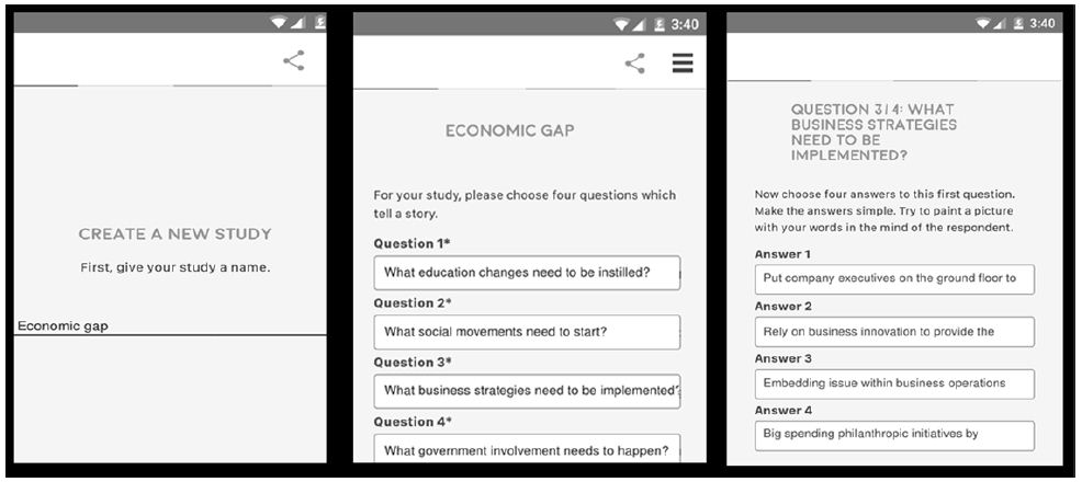
The set-up for these Mind Genomics studies is templated, enabling the researcher to follow a simple series of steps to provide the necessary information. Figure 1 shows the set-up template. Figure 2 shows two screens in the set-up template, screens that show the self-profiling classification, and an example of a vignette.

fig 1

Figure 1: The set-up template for the first Mind Genomics study on the solutions to problems.

fig 2

Figure 2: Example of the set-up screen for the third self-classification (left) and an example of the set-up page showing a test vignette (right).

This first study was run with 50 respondents. Each respondent rated the set of 24, unique vignettes created by mixing the 16 elements into combinations comprising 2-4 elements. Each question contributed at most one element to a vignette, but for four vignettes contributed no elements to the vignette. Every element appeared five times in 24 vignettes and was absent 19 times. The experimental design was set up to allow for an individual-level regression relating the presence/absence of the 16 elements to the responses. For this project, the preliminary analysis created four dependent variables:

  1. RATE1=Will encounter resistance … and… Probably won’t work. When the rating was ‘1’ on the 5-point scale RATE1 took on the value 100. When the rating was not ‘1’ on the 5-point scale, RATE1 took on the value 0. RATE1 corresponds to a belief that the solution will not help solve economic inequity, the problem posed in the introduction.
  2. RATE5=Will not encounter resistance … and… Probably will work. When the rating was 5 on the 5-point scale RATE5 took on the value 100. When the rating was not 5, RATE5 took on the value 0. RATE5 corresponds to the belief that the solution will help solve the problem of economic inequality.
  3. RATE3=Can’t honestly decide. When the rating was 3 on the 5-point scale RATE3 took on the value 100. When the rating was not 3 on the 5-point scale, RATE3 took on the value 0.
  4. RT – The measured response time from the time the vignette was presented to the time the rating was assigned

To ensure that there would be at least minimal variation in the dependent variable, viz., the newly created binary scales (RATE1, RATE3, RATE5), a vanishingly small random number (<10-5) was added to each newly created binary variable for every case. The added variability does not affect the regression but ensures that there is the requisite variability so that the regression does not crash.

The regression model was run without an additive constant, to allow direct comparisons of the coefficients across groups. The regression equation, estimated using OLS (ordinary least-squares) methods, is expressed as: Dependent Variable=k1(A1) + k2(A2) … k16(D4)

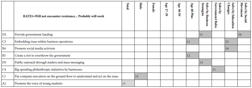
The self-profiling classification allows us to assign each respondent to gender, to age group, and to the way that problems of this type might be solved. The definition of the subgroups generates 10 different groups. We show only those elements with coefficient of 11 or higher, coefficients that would be clearly significant. The elements and the strong performing coefficients appear in Table 2. The elements are sorted by the sum of the strong performing coefficients. Thus, the strongest performing element in this reduced set of elements is D2 (Provide government funding). The weakest, but still strong performing elements are C4, C1, and A2, all with one strong group, and coefficients of 11.

Table 2: Strong performing elements by element and key self-defined subgroup for RATE5 vs the 16 elements. Only coefficients of 11 or higher are shown.

table 2

It is important to note that there is no clear pattern, either by element or by self-classification. Furthermore, half the elements simply fail to drive a perceived ability to drive a strong solution (viz., RATE5). We might have more elements appearing if we create the model based on a combination of RATE4 and RATE5, both saying that the solution will probably be successful, but RATE4 saying it will encounter resistance, and RATE5 saying it will not encounter resistance.

The importance of this first result is that there are no simple solutions. Either the solutions are weak, or the groups are so variable in what the people of the group believe to work that the power of the idea of the solution is attenuated.

An ongoing theme of Mind Genomics is that there exists in everyday experience a different group of ideas which constitutes ‘mind-sets.’ A mind-set comprises a set of ideas which ‘travel together’ and which can be interpreted. That is, the mind-set makes intuitive sense, and tells a meaningful story.

The mind-set emerges from the pattern of responses to the different elements. Once we see which elements emerge together as strong, we may find that the pattern almost ‘jumps out at us.’ When we work with a set of elements for a specific topic, usually about 2-3 mind-sets emerge. There could be more, but the ideal is to work with mind-sets that are interpretable (tell a story), and which are relatively few in number for the topic. Fewer mind-sets are better than many, even though as we extract more and more mind-sets from the same data the story gets clearer, because we focus on narrower and narrower ranges of ideas.

The mind-sets emerge from a simple mathematical analysis, and not from preconceived notions of the researcher. The mind-sets emerge sing the mathematical methods called clustering which puts into separate groups the various objects (viz. respondents) based upon some quantitative criterion. For example, one may put together individuals who show very similar patterns of coefficients. The similarity in the pattern of coefficients from one person to another suggests that these people think in similar fashion.

Our data provides the ideal set up for k-means clustering [18]. Each respondent evaluated 24 vignettes arranged according to an experimental design. We can create an individual level equation for each respondent. The equation will be written as it was before: Dependent Variable=k1(A1) + k2(A2) … k16(D4)

The clustering program works with the 51 sets of 16 coefficients, one set for each of the 51 respondents, one coefficient for each of the 16 elements. The clustering program first computes the ‘distance’ between each pair of respondents, defined as (1-Pearson R). The Pearson R is a measure of the strength of a linear relation. If two respondents show a perfect correlated set of 16 coefficients, the correlation is +1 their distance is 0 . The distance is 1-1=0.

The clustering was done using RATE5 as the dependent variable. The first step in the clustering was to run the 50 regression models, each without the additive constant, as noted above. The second step was to apply the k-means clustering, and extract three mind-sets. Two mind-sets produced a more parsimonious set, but the stories were not clear, viz., interpretability was not sufficient.

Finally, the k-means clustering program assigned each of the 51 respondents to one of the three clusters or mind-sets, based upon a measure of cohesiveness of the cluster. After each respondent was assigned to one of the three non-overlapping clusters, it was a simple matter to run four equations for each cluster, using only those respondents assigned to the cluster. The four equations were RATE1, RATE5 (Table 3), and RATE3 and Response time (Table 4).

Table 3 presents the results for Total panel and for the three mind-sets. Based upon the strong performing elements, we can call the mind-sets as following:

Table 3: Strong performing elements for total and for each mind-set, based upon the model for RATE1 (encounter, resistance and won’t work), and based upon the model for RATE5 (encounter no resistance, will work).

table 3

Mind-Set A1=Based on Rate 5: Business Takes the Lead

The business has to be open to new ideas, receptive to solving the problem as part of the business flow and be open to innovation. Avoid activism. The only solution which is problematic is listening to the voice of young people. There are those in Mind-Set3 who think it will work, and those who think it won’t work, based upon the strong performance of element A2 (Promote the voice of young students) for both RATE1 and RATE5.

Mind-Set A2– Can’t Think of Anything

Mind-Set 4 is interesting simply because nothing seems to have a chance of working. On the other hand, when it comes to this mind-set thinking about what absolutely won’t work, viz., how they perform on RATE1 (resistance/won’t work) they ae negative to the ideas which seen perfectly reasonable to others.

Mind-Set A3 – Big Picture Activists

They want major change, which can be through business practice, major philanthropic donations from business, or even through riots. They don’t believe in slow activist movements.

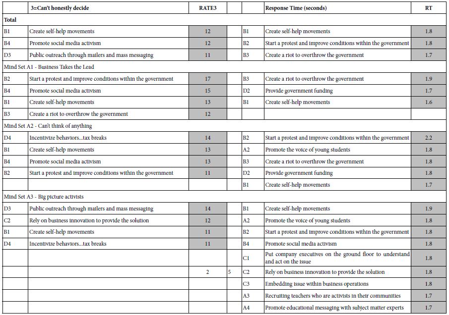
Table 4 presents the strong performing elements for RATE3 (cannot decide), and for response time (RT). The models were once again the standard linear models, without an additive constant. The dependent variable for RATE3 was the binary transformed value for ratings that were either 3 (transformed to 100), or not 3 (transformed to 0). The dependent variable for response time, the number of seconds did not need any added very small random number because there was clear variation among the different response times.

Table 4: Strong performing elements for total and the three mind-set segments, for RATE3 (can’t decide) and RT (response time).

table 4

In contrast to the interpretations for RATE1 (NO) or RATE5 (YES), the elements driving RATE3 do not tell a coherent story. There are three strong performing elements for Total Panel, and four strong performing elements for each mind-set. In no mind-set do we see a story.

The elements driving long response times are not related to the mind-set itself, but tend to of two types, either starting a riot or protest, or create a self-help movement Both of these seem emotionally evocative, suggesting that the response time measure is not a measurement of good/bad, but rather of the startle-value of the idea, coupled with the ability of the idea to paint a suggestive word picture.

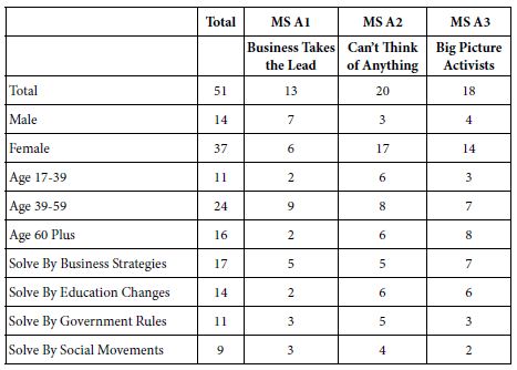
Table 5, showing the distribution of respondents in the three emergent mind-sets reveals no simple pattern. It often comes as a surprise that when we penetrate a topic, people faced with the same topic find radically different points of view when they evaluate specifics. These different points of view emerging from a ‘micro-topic’ often fail to emerge when the topics so large as to avoid specifics. Thus the 17 people who say that problems can be solved by business strategies do not fall into Mind-Set A1 (Business Takes the Lead). Only 5 of 17 respondents are assigned to the correct mind-set. Similarly, of the nine respondents who way that the problem can be answer by social movements, only two are assigned to Mind-Set A3 (Big Picture Activities).

Table 5: Distribution of the respondents across the three mind-sets for study 1 (Solutions).

table 5

Study 2 – How People as Icons or Emblems Drive Perceived Feasibility of Solutions

The second study moved from actual solutions, albeit general ones, to individuals who represent prospective problem solvers. The underlying thinking was that although people may not ‘know’ what solution to a problem ‘feels right’, they may have a feeling of WHO can solve their problem. Some of the thinking behind Study 2 comes from the notion that there might be ‘archetypes’ which emerge, based upon those who are perceived to be able to solve the problem [19,20].

Following the same Mind Genomics approach of a topic, four questions, and four answers to the questions, we did the same type of study. We begin with the self-profiling classification, the introduction to the topic, and the five-point anchored rating scale:

a. A set of self-profiling questions, including age, gender, and the third question below

Which political description fits YOU best?

 1=Old time Republican 2=Trump Republican 3=Democrat 4=None

b. The topic but the rating scale and the answers changed to fit the issue of solution providers, rather than solutions themselves:

What will happen when these people work together to solve this problem: Economic Gap: Rich people get richer, everyone else falls behind

RATE1=Cannot cooperate … and … No real solution will emerge

RATE2=Cannot cooperate … but … Real solution will emerge

RATE3=Honestly cannot tell

RATE4=Can cooperate … but … No real solution will emerge

RATE5=Can cooperate … and … Real solution will emerge

This time, however, we replace the questions and answers with those in Table 6.

The analysis for Study 2 on People as icons or emblems was done in precisely the same fashion as was done with Study 1 on problem solutions. Thus, the two studies can be compared, at least in their general morphologies, regarding the number and magnitude of coefficients emerging as strong drivers, the nature of the mind-sets.

Table 6: The four types of emblematic problem solvers, and four specific people or groups for each type.

table 6

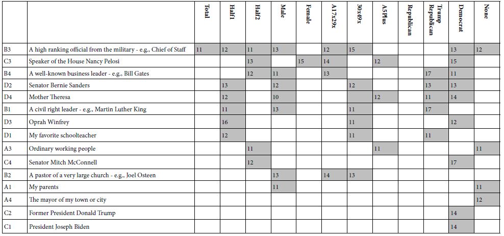
In contrast to the relatively sparse number of very strong performing elements for actual, albeit general solutions (Table 2), putting people in as problem solvers, and building models for RATE5 versus elements (no additive constant) shows many more strong elements (Table 7) The stronger performers are the ‘usual suspects. What is remarkable is that at the time of this study, when President Biden was doing reasonably well at the polls, and there were no looming disasters, President Biden was seen as a problem solver only by those who called themselves Democrats. Surprisingly, so did former President Trump, and only among Democrats. He scored poorly everywhere else.

Table 7: Strong performing elements by element and key self-defined subgroup. Only coefficients of 11 or higher are shown.

table 7

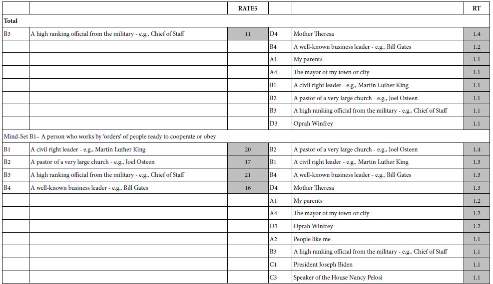
The clustering of respondents on the basis of the pattern of coefficients for RATE5 (RATE5=Can cooperate … and … Real solution will emerge) produced some strong surprises. First, no elements scored strongly on RATE1 (Cannot cooperate … and … No real solution will emerge) nor on RATE3 (honestly cannot tell). The failure to score strongly on these two response points suggests that people ‘know’ who they believe and trust, but their critical thinking may stop there. The data suggest an asymmetry in thinking between positives (people who are respected and probably liked), and negatives (people who are disrespected and probably disliked). Furthermore, only two clusters or mind-sets were needed. A three-cluster solution revealed two quite similar mind-sets, differing only in one of two elements.

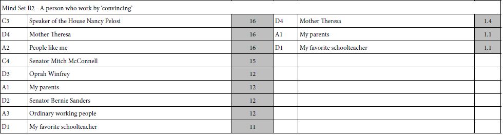
Table 8 shows the strong performing elements for RATE5, and for response time, by total panel, and by the two mind-sets emerging from study 2. The important thing to notice is the set of high coefficients for RATE5 meaning that the respondents feel strongly about their answers, AND the short response times. There is very little ‘shock value’ of people, except Mother Theresa, who would not be typically thought of as a problem solver.

Table 8: The strong performing elements for RATE5 and for Response Time (RT) for study 2, with the elements being people and the rating scale being ability to cooperate and solve the problem. RATE1 and RATE3 generated virtually no strong performing elements.

table 8(1)

table 8(2)

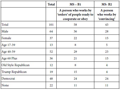
The group membership is more interesting for this second experiment (Table 9). The self-proclaimed Democrats appear equally in the two mind-sets, Mind Set B1 (working through orders) and Mind-Set B2 (working by convincing.) The self-proclaimed Republicans (both regular and Trump Republicans) appear far more frequently in Mind-Set B1 (working through orders).

Table 9: Distribution of the respondents across the three mind-sets for study 1 (Icons, Emblems).

table 9

Discussion and Conclusion

The original motivation for these studies was an interest how we think about solving social problems. The approaches to problem solving generally talk about strategies, about success stories. The strategies and success stories are so individuated that they either lack flavor entirely because they are generic (viz., strategies, such as points about solving issues), or they are so specific as to leave one wondering what to do. Furthermore, a glance at the literature about problem solving for social solutions did not bring up the role of the individual thinker, but rather the role of the situation, and the role of the expert.

The objective here was to approach the topi of problem solving of social issues from two angles, first specifics and then individuals. The specifics make sense; they are types of actions that can be taken to solve a problem. Which ones would work in the case of certain social issues, of which the economic inequality described here is one of them?

In a previous paper author Kover and Moskowitz introduced the idea of Projective Iconics, doing so within the realm of Mind Genomics [9]. The idea was to move beyond the rational to the emotion in the assessments of problems and solutions. The traditional methods for dealing with problems appeared to be all rational, left brain oriented with the utility of solving the problem (soft benefits), or harder, more economically measurable benefits. The test stimuli were always problems, the solutions were generally tangible, except for some feelings, and the evaluation was rational.

A different way had to be developed, one which would encompass something deeper than rational solutions, the act. We were taken with the adage than investors often say that they bet on the jockey, not on the horse. That is, it is the person leading the solution might be just as important as the solution itself. In that way, was born the version of Mind Genomics used here, labelled Projective Iconics. Rather than having solutions, we have combinations of problem solvers would that approach work?

Study 1 using the standard solutions suggests that people can evaluate good versus poor solutions. That is, across the set of respondents there are s number of solutions which clearly are not perceived to work, viz., RATE1, and another set of solutions which may or may not work, but people cannot decide. And, of course, quite a number of solutions which ae believed to work, especially when the total panel is broken out in subgroups. There are also a great number of solutions which are deemed not to work.

Study 2 upends the pattern, by suggesting that when we move from concrete solutions to icons on whom people can project their feelings, we are able to identify people or groups who can solve the problem but find it hard to assign people to groups who cannot solve the problem.

The conclusion here is that there is a profound difference in the way we think about the solution to problems, with far more concreteness when we talk about the actual solution, and far emotion when we talk about the problem solvers themselves.

References

  1. Durham Y, Hirshleifer J, Smith VL (1998) Do the rich get richer and the poor poorer? Experimental tests of a model of power. The American Economic Review 88: 970-983.
  2. Kotler PT, Lee NR (2009) Up and Out of Poverty: The Social Marketing Solution. Pearson Prentice Hall.
  3. Baumann S, Majeed H (2020) Framing economic inequality in the news in Canada and the United States. Palgrave Communications 6: 1-11.
  4. Kover A, Bejarano LER, Moskowitz H (2021) Social and business problems through the lens of projective iconics: Introducing a new systematics to understand and quantify perceptions of social issues. Psychology Journal Research Open 3: 1-9.
  5. Wright G (2018) The political implications of American concerns about economic inequality. Political Behavior 40: 321-343.
  6. Babu S, Pinstrup-Andersen P (2007) Social innovation and entrepreneurship: Developing capacity to reduce poverty and hunger. Twenty twenty (2020) focus brief on the world’s poor and hungry people/International Food Policy Research Institute (IFPRI).
  7. Knapp MS, Turnbull BJ, Shields PM (1990) New directions for educating the children of poverty. Educational Leadership 48: 4-8.
  8. Thorbecke E, Charumilind C (2002) Economic inequality and its socioeconomic impact. World development 30: 1477-1495.
  9. Kover A, Moskowitz HR, Pagajorgji P (2021) The Fraying of America, in Review.
  10. Stroh DP (2015) Systems thinking for social change: A Practical Guide to Solving Complex Problems, Avoiding Unintended Consequences, and Achieving Lasting Results. Chelsea Green Publishing.
  11. Cliff N (1983) Some cautions concerning the application of causal modeling methods. Multivariate Behavioral Research 18: 115-126.
  12. Moskowitz HR (2012) ‘Mind Genomics’: The experimental, inductive science of the ordinary, and its application to aspects of food and feeding. Physiology & Behavior 107: 606-613.
  13. Moskowitz HR, Gofman A (2007) Selling Blue Elephants: How to Make Great Products that People Want Before They Even Know They Want Them, Pearson Education.
  14. Green PE, Krieger AM, Wind Y (2001) Thirty years of conjoint analysis: Reflections and prospects. Interfaces 31: S56-S73.
  15. Gofman A, Moskowitz H (2010) Isomorphic permuted experimental designs and their application in conjoint analysis. Journal of Sensory Studies 25: 127-145.
  16. Milutinovic V, Salom J (2016) Mind Genomics: A Guide to Data-Driven Marketing Strategy. Springer.
  17. Salom J (2021) Mind Genomics with big data for digital marketing on the internet. Handbook of Research on Methodologies and Applications of Supercomputing, 282-289. IGI Global.
  18. Likas A, Vlassis N, Verbeek JJ (2003) The global k-means clustering algorithm. Pattern recognition 36: 451-461.
  19. Harootunian JA, Quinn RJ (2008) Identifying and describing tutor archetypes: The pragmatist, the architect, and the surveyor. The Clearing House: A Journal of Educational Strategies 82: 15-20.
  20. Bradshaw TK (2007) Theories of poverty and anti-poverty programs in community development. Community Development 38: 7-25.

Preimplantation Genetic Testing (PGT) as Tool for Human Leukocyte Antigens (HLA) Compatible Stem Cell Transplantation

DOI: 10.31038/MGJ.2021431

Abstract

Preimplantation HLA typing (PGT-HLA) provides patients with an option not only to avoid an inherited risk, but also to establish a pregnancy with an exact HLA match to benefit the affected family member. So HLA typing is now an established PGT indication, to achieve stem cell transplantation treatment of affected siblings in need for compatible transplant. It is also applied as primary indication for cases not requiring preimplantation genetic testing for monogenic disorder (PGT-M), when no HLA-compatible donor is available. The most frequent applications of PGT-HLA were for families with hemoglobinopathy and congenital immunodeficiency siblings, both resulting in total cure when compatible donor was obtained through PGT-HLA. We present here the progress in the application of PGT-HLA tool, based on our practice of 485 PGT-HLA cycles, resulting in obtaining an 117 HLA matched births, providing stem cells for transplantation treatment in 35 different congenital and acquired disorders.

Keywords

Preimplantation HLA typing (PGT-HLA), Hemoglobinopathy, Immunodeficiency, Stem cell transplantation, Recombination, Outcome of transplantation treatment with HLA compatible stem cells obtained through PGT-HLA, Probability of obtaining of HLA matched progeny in PGT-HLA

Introduction

Preimplantation HLA typing (PGT-HLA) was first introduced over twenty years ago to perform bone marrow transplantation treatment of a child with Fanconi anemia (FA) [1,2]. As a totally matched bone marrow is required for transplantation treatment success in this condition, PGT-HLA was an exclusive option, to ensure the birth of an unaffected baby, also to pre-select only those FA free embryos that are also an exact HLA match to the affected child. This was the world’s first case of PGT-HLA with the objective of establishing an unaffected pregnancy to yield a potential donor progeny who could provide bone marrow for stem cell transplantation. Since then this approach has been applied for increasing number congenital disorders that require an HLA-compatible donor for bone marrow transplantation [3-8]. Further it was also applied as a primary indication for cases not requiring mutation testing, but awaiting an HLA-compatible donor [9]. In this paper we will review the progress of application of PGT-HLA both as primary indication, as well as together with PGT-M for increasing number of different congenital disorders.

Inherited Disorders for Which PGT-HLA was Performed Concomitantly with PGT-M

Our experience of PGT- HLA is presented in Table 1, summarizing the results of 485 PGT-HLA cycles performed for 239 patients. A total of 424 HLA matched embryos were identified for transfer (1.46 HLA matched embryos per transfer on the average) in 291 of 485 (68.6%) cycles, resulting in 125 (43.0%) clinical pregnancies and birth of 117 healthy HLA matched children, representing stem cell donors for their affected siblings [8]. Among conditions requiring HLA-compatible stem cell transplantation, hemoglobinopathies were one of the most prevalent [10-13], with a total of 188 cycles, allowing detecting and transferring unaffected HLA-matched embryos in 103 (54.8%) of them. A total of 159 (1.54 on the average) embryos predicted to be either unaffected carriers or normal and HLA-identical to the affected siblings, which is not significantly different from the expectation (Table 2). This resulted in 32 unaffected HLA-identical pregnancies and the birth of 32 healthy children, from whom umbilical cord blood or bone marrow was collected, with the bone marrow transplantation resulting in a successful hematopoietic reconstitution or pending [8].

Table 1: Preimplantation HLA TESTING (PGT-HLA) WITH AND WITHOUT PGT-M.

Disease

Gene #Patient #Cycle #Transfers #Embryos transferred Pregnancy

Birth

HLA genotyping 60 119 73 108 25

22

HLA + ADADENOSINE DEAMINASE  DEFICIENCY; ADA ADA

1

1 1 1 1

1

HLA +  ADRENOLEUKODYSTROPHY; ALD ABCD1

3

7 2 2 1

2

HLA +  CARDIOMYOPATHY, FAMILIAL HYPERTROPHIC, 4; CMH4 MYBPC3

1

1 1 1 1

1

HLA + GRANULOMATOUS DISEASE, CHRONIC, AUTOSOMAL RECESSIVE; CDG1 NCF1

1

3 2 2 1

1

HLA +

DIAMOND-BLACKFAN ANEMIA 1; DBA1

DIAMOND-BLACKFAN ANEMIA 2; DBA2

DIAMOND-BLACKFAN ANEMIA 3; DBA3

DIAMOND-BLACKFAN ANEMIA 5; DBA5

DIAMOND-BLACKFAN ANEMIA 9; DBA9

RPS19,

RPS20,

RPS24,

RPL35A,

RPS10

10

17 14 20 8

8

HLA +  GLANZMANN THROMBASTHENIA; GT  MUSCULAR DYSTROPHY, DUCHENNE TYPE; DMD ITGA2B,

DMD

1

2 2 4 1

0

HLA +  MYOTONIC DYSTROPHY 1; DM1 DMPK

1

2 1 2 1

1

HLA + ECTODERMAL DYSPLASIA AND IMMUNODEFICIENCY 1; EDAID1 IKBKG

3

10 8 10 3

4

HLA +  EPIDERMOLYSIS BULLOSA DYSTROPHICA, AUTOSOMAL DOMINANT; DDEB COL7A1

1

1 1 1 1

1

HLA +  FANCONI ANEMIA, COMPLEMENTATION GROUP A; FANCA FANCA

18

56 29 42 14

13

HLA +  FANCONI ANEMIA, COMPLEMENTATION GROUP C; FANCC FANCC

3

6 6 9 2

2

HLA +  FANCONI ANEMIA, COMPLEMENTATION GROUP D2; FANCD2 FANCD2

1

3 2 3 1

1

HLA +  FANCONI ANEMIA, COMPLEMENTATION GROUP F; FANCF FANCF

1

3 2 3 0

0

HLA +  FANCONI ANEMIA, COMPLEMENTATION GROUP G; FANCG FANCG

2

2 1 2 1

2

HLA +  FANCONI ANEMIA, COMPLEMENTATION GROUP I; FANCI FANCI

1

2 2 3 0

0

HLA +  FANCONI ANEMIA, COMPLEMENTATION GROUP J; FANCJ BRIP1

2

4 4 3 1

1

HLA +  GRANULOMATOUS DISEASE, CHRONIC, X-LINKED; CDGX CYBB

11

16 12 15 7

6

HLA + HBB SICKLE CELL ANEMIA; BETA-THALASSEMIA HBB

92

188 103 159 35

32

HLA +  IMMUNODEFICIENCY WITH HYPER-IgM, TYPE 1; HIGM1 CD40LG

11

16 10 15 9

8

HLA +  KRABBE DISEASE GALC

1

1 1 2 1

2

HLA +  MYELODYSPLASTIC SYNDROME; MDS GATA2

1

2 1 1 1

1

HLA +  NEUTROPENIA, SEVERE CONGENITAL, 1, AUTOSOMAL DOMINANT; SCN1 ELANE

3

5 4 4 4

3

HLA +  SHWACHMAN-DIAMOND SYNDROME; SDS SBDS

4

9 3 3 2

2

HLA +  THROMBOTIC THROMBOCYTOPENIC PURPURA, CONGENITAL; TTP ADAMTS13

1

2 2 4 1

1

HLA  + THROMBOCYTHEMIA 1; THCYT1 SH2B3

1

2 2 2 2

1

HLA +  WISKOTT-ALDRICH SYNDROME; WAS WAS

1

1 0 0 0

0

HLA + POLYCYSTIC KIDNEY DISEASE 1; PKD1

PKD1

1 1 1 2 1

1

HLA+  PYRUVATE KINASE DEFICIENCY OF RED CELLS PKLR

1

2 1 1 0

0

HLA + HYPER-IgE RECURRENT INFECTION SYNDROME, AUTOSOMAL RECESSIVE DOCK8

1

1 0 0 0

0

TOTAL

239

485 291 424 125

43%

117

Table 2: Chances for detection of disease-free and HLA-matched embryo in preimplantation HLA typing (PGT-HLA).

HLA MATCH only – ¼ (25%)
Autosomal-recessive or X-linked free + HLA MATCH – ¾ × ¼ = 3/16 (18.75%)
Autosomal-dominant free + HLA MATCH – ½ × ¼ = 1/8 (12.5%)

Similar experience was reported from other large series, including 626 PGT-HLA cycles performed for 312 couples (122 HLA only and 504 with PGT-M), resulting in 128 thalassemia-free children [14,15]. Stem cells of 66 of these children were used for cord blood or bone marrow transplantation, which resulted in successful bone marrow reconstitution in all but two of them (transplantation treatment of the remaining 57 siblings pending).

Severe congenital immunodeficiency (SCID) is another large group of conditions, for which PGT-HLA and stem cell transplantation is required [8,16]. Without compatible bone marrow transplantation affected neonates with SCID cannot survive, with the HLA-matched stem cell transplantation improving and completely replenishing the immune system. This group involved a variety of conditions leading to SCID, including incontinentia pigmenti (IP), hyper-IgM type 1 immunodeficiency (HIGM1),  chronic X-linked granulomatous disease (CGD), hypohidrotic ectodermal dysplasia with immune deficiency (HED-ID),  Wiscott-Aldrich syndrome (WAS), ataxia-telangiectasia (AT), Type 1 X-linked agammaglobulinemia, Omenn syndrome (OMS), X-linked immunodysregulation, polyendocrinopathy and enteropathy (IPEX), autosomal recessive severe combined immunodeficiency, X-linked severe combined immunodeficiency (SCIDX1), chronic granulomatous disease, and severe congenital neutropenia 1 (SCN1) (Table 1).

The other large group for which PGT-HLA was applied was FA, for which we performed the word’s first PGT-HLA mentioned [1,2]. This is an autosomal-recessive disorder causing bone marrow failure with increased predisposition to leukemia. Bone marrow transplantation is the only treatment, restoring hematopoiesis in FA patients. However, because any modification of the conditioning is too toxic for these patients, leading to a high rate of transplant-related mortality, the HLA-identical stem cell transplantation from a sibling is the only option to avoid late complications due to severe graft-versus-host disease (GVH).

Couples at risk for producing a progeny with FA included carriers of IVS 4+4A-T mutation in the FANCC gene, FANCD2, FANCF, FANCI, FAMCCJ, and FANCA. Overall, 65 unaffected HLA-matched embryos were transferred in 46 of 76 cycles, resulting in 19 unaffected pregnancies and 18 FA-free and HLA-matched neonates, representing potential donors for their older siblings (Table 1).

Of special interest is a case of PGT-HLA involving a consanguineous couple carrying the identical FANCG deletion mutation, who had an affected child with FANCG, requiring stem cell transplantation treatment. Following embryo testing by mutation and linked STR analysis, 2 HLA-matched and disease free (normal and carrier) embryos were transferred, resulting in a twin pregnancy. As couple did not accept confirmatory invasive prenatal diagnosis, a special non-invasive test was developed which allowed confirming unaffected status and HLA matched results for both twins at 15 weeks gestation, which is the world’s first case of non-invasive prenatal diagnosis for FA and HLA match [17]. Bone marrow obtained from the twins was transplanted to the affected sibling resulting in a total cure.

Another condition of special interest was a case of PGT-HLA performed for hyperimmunoglobulin M Syndrome (HIGM), which is a rare immunodeficiency characterized by normal or elevated serum IgM levels, with absence of IgG, IgA, and IgE, that results in an increased susceptibility to infections. No radical treatment is available, so PGT-HLA is the only choice for those who lack a suitable HLA match among their relatives. A total of 16 PGT-HLA cycles were performed for 11 couples with HIGM (Table 1), with transfer of 15 unaffected HLA matched embryos in 10 cycles, yielding 9 clinical pregnancies and birth of 8 unaffected HLA matched children, the ideal HLA matched donor for the affected siblings.

PGT-HLA assisted stem cell transplantation is also extremely useful for X-linked hypohidroticectodermal displasia with immune deficiency (HED-ID), which is caused by two dozen different mutations in the IKK-gamma gene (IKBKG, or NEMO). The disease is characterized by susceptibility to microbial and streptococcal infections, dys-gamma-globulinemia, poor polysaccharide-specific antibody responses, and depressed antigen-specific lymphocyte proliferation. To prevent mortality during the first year, bone marrow transplantation is required resulting in a radical treatment, as demonstrated in our experience of 10 PGT-HLA cycles performed for HED-ID patients.

Thus, PGT-HLA provides couples at risk with the option to avoid the affected pregnancy and have a progeny free of the condition and also with an access to the HLA-identical stem cell transplantation through selection and transfer of those unaffected embryos which are also HLA-matched to the sibling. Because the finding of the HLA-identical stem cell donor is the key for achieving the success in stem cell transplantation, a complete cure was achieved in stem cell transplantation in affected siblings.

Preimplantation HLA Typing Without PGT-M

Preimplantation HLAtyping without testing for a causative gene was first performed for a sporadic Diamond–Blackfan anemia (DBA), requiring bone marrow transplantation treatment [9]. The sole indication in this case was HLA typing, so only a haplotype analysis of the paternal and maternal partners, and affected child was performed in the family prior to PGT-HLA, using a set of polymorphic STR markers located throughout the HLA region. This allowed detecting and avoiding misdiagnosis due to preferential amplification and ADO, potential recombination within the HLA region (see below), and a possible aneuploidy or uniparental disomy of chromosome 6, which may affect the diagnostic accuracy of HLA typing of the embryo. Our experience includes a total of 119 clinical cycles for 60 couples, with pre-selection of 108 HLA-matched embryos for transfer (Table 1). The proportion of embryos predicted to be HLA-matched to the affected siblings was 21.5%, not significantly different from the expected 25% (Table 2). The transfer of 108 HLA-matched embryos transferred in 73 clinical cycles resulted in 25 singleton clinical pregnancies and 22 HLA-matched children born. These results suggest that testing of an available number of embryos per cycle allows preselecting a sufficient number of the HLA-matched embryos for transfer to achieve a clinical pregnancy and birth of an HLA-matched progeny.

Presented data demonstrate the utility and reliability of PGT-HLA for families having affected children with bone marrow disorders who may wish to have another child. As seen from our data, HLA-matched embryos were preselected and transferred in almost in all cases performed, resulting in clinical pregnancies and the birth of HLA-matched children in almost every second transferred cycle.

Limitations of PGT-HLA and Prospect for Wider Application

One of important limitations of PGT-HLA is a relatively high frequency of recombination in the HLA region, with a few possible hot spots. Naturally, this may affect the accuracy of PGT-HLA, and the outcome of the whole procedure. In our experience, recombination events were observed both of maternal (3%) and paternal (1.5%) origin [8]. Prevalence of recombination was as even higher (6.1%) when the recombination analysis included siblings requiring HLA-compatible bone marrow transplantation. Recombination detected in a sibling for whom transplantation treatment is required may make PGT-HLA of no use, as the chance of finding of the total HLA match for these siblings is totally unrealistic. Thus, haplotype analysis prior to initiation of the actual cycle is required, so the couples may be informed about their possible options, taking into consideration that only a relatively close match may be detected, warranting discussions with the pediatric hematologist on acceptable HLA profiles.

The other important limitation is a relatively advanced reproductive age of the majority of PGT-HLA patients, which is one of possible explanation that many patients still undergo two or more attempts before achieving an HLA-identical offspring. As concomitant PGT for aneuploidy (PGT-A) appeared useful for improving the reproductive outcome in PGT-HLA [8,18], PGT-A is currently offered as an integral part of PGT-HLA for the patients of advanced reproductive age. Our experience shows that reproductive outcome of PGT-HLA combined with PGT-A is significantly higher than those PGT-HLA cycles without PGT-A [18,19].

The usefulness of PGT-A is also obvious for the diagnostic accuracy, as an error in detecting the number of chromosomes 6, in which HLA genes are mapped, may lead to misdiagnosis of HLA profile. Thus, in addition to avoiding chromosomally abnormal embryos from transfer, testing for the copy number of chromosome 6 may become an important requirement for achieving the accuracy of PGT-HLA. Nonetheless, PGT-A will have less utility when only a few embryos are available for testing. To overcome this limitation, two or more cycles are initiated to collect a sufficient number of embryos for analysis. But meaningful batching may not always be possible because some older patients are unable to produce additional oocytes. The possible approach in such cases is to offer these couple the option of HLA testing for the women’s younger sister, so that the sister’s HLA matched donor oocytes could potentially be used for PGT-HLA cycle. The usefulness of this option was demonstrated in one of our PGT-HLA cases [8], which is the world’s first example in using donor eggs from relatives, resulting in obtaining unaffected HLA matched progeny for HLA matched stem cells transplantation, using the PGT-HLA cycle involving a sibling as an HLA matched egg donor.

Despite the above limitations, our overall experience of pre-selection and transfer of the HLA-matched unaffected embryos was possible in 13.7% of the embryos tested, which is a bit lower than may have been predicted (Table 2). Even with such a relatively moderate success rate, PGT-HLA appeared to be attractive for couples with children requiring HLA-matched bone marrow transplantation, with the number of PGT-HLA requests increasing overall, as the key factor in achieving an acceptable engraftment and survival in stem cell therapy requires is availability of an HLA-identical stem cell transplant [20,21]. In fact, due to a small number of children per family, less than one-third of patients has a chance to find an HLA-identical familial donor. The majority for whom no HLA-matched family member exists, the search is extended to haplotype-matched unrelated donors, despite resulting in severe complications.

In conclusion, presented experience demonstrates an increasing attractiveness of PGT-HLA for couples with affected children requiring HLA-compatible stem cell transplantation. Thus, couples at risk of having children with congenital bone marrow disorders could clearly benefit from presently available option of PGT-HLA, allowing not only avoiding the birth of an affected child but also selecting a suitable stem cell donor for their affected siblings.

References

  1. Verlinsky Y, Rechitsky S, Schoolcraft W, Strom C, Kuliev A (2000) Designer babies-are they reality yet? Case report: simultaneous preimplantation genetic diagnosis for Fanconi anemia and HLA typing for cord blood transplantation. Reprod Biomed Online 1: 31. [crossref]
  2. Verlinsky Y, Rechitsky S, Schoolcraft W, Strom C, Kuliev A (2001) Preimplantation diagnosis for Fanconi anemia combined with HLA matching. JAMA 285: 3130-3133. [crossref]
  3. Rechitsky S, Kuliev A, Tur-Kaspa I, Morris R, Verlinsky Y (2004) Preimplantation genetic diagnosis with HLA matching. Reprod Biomed Online 9: 210-221. [crossref]
  4. Van de Velde H, Georgiou I, De Rycke M, Schots R, Sermon K, et al. (2004) Novel universal approach for preimplantation genetic diagnosis of β-thalassemia in combination with HLA matching of embryos. Hum Reprod 19: 700-708. [crossref]
  5. Kahraman S, Karlilaya G, Sertyel S, Karadayi H, Findicli N, et al. (2004) Clinical aspects of preimplantation genetic diagnosis of single gene disorders combined with HLA typing. Reprod Biomed Online 9: 529-532. [crossref]
  6. Goussetis E, Konialis CP, Peristeri I, Kitra V, Dimopoulou M, et al. (2010) Successful hematopoietic stem cell transplantation in 2 children with X-linked chronic granulomatous disease from their unaffected HLA-identical siblings selected using preimplantation genetic diagnosis combined with HLA typing. Biol Blood Marrow Transplant 16: 344-349. [crossref]
  7. Georgia Kakourou (2018) PGD for HLA (ESHRE study). Reprod Biomed Online, 2018; 36: 4-5.
  8. Kuliev A, Rechirsky S, Simpson JL (2020) Practical preimplantation genetic Testing. Third Edition. Springer, Nature.
  9. Verlinsky Y, Rechitsky S, Sharapova T, Morris R, Tharanissi M, et al. (2004) Preimplantation HLA typing. JAMA 291: 2079-2085.
  10. Kuliev A, Rechitsky S, Verlinsky O, Tur-Kaspa I, Kalakoutis G, et al. (2005) Preimplantation diagnosis and HLA typing for hemoglobin disorders. Reprod Biomed Online 11: 362-370.
  11. Kuliev A, Packalchuk T, Verlinsky O, Rechitsky S (2011) Preimplantation diagnosis: efficient tool for human leukocyte antigen matched bone marrow transplantation for thalassemia. Thalassemia Rep 1: 1.
  12. Kuliev A, Rechitsky S, Verlinsky O (2014) Atlas of Preimplantation Genetic Diagnosis. 3rd Edition. CRS, 2014 Press, Taylor and Francis, London.
  13. Kuliev A, Rechitsky S (2016) Preimplnatation HLA typing for stem cell transplantation treatment of genetic and acquired bone marrow failures. Hemat Med Oncol 1: 46-49.
  14. Kahraman S (2013) PGD for HLA: Clinical Outcomes of HLA compatible transplantation following PGD. Reprod Biomed Online 26: 9-10.
  15. Umay KB, Gavaz M, Kumtepe ÇY, Yelke H, Pirkevi Çetinkaya C, et al. (2019) Successful hemapoietic stem cell transplantation in 62 children from healthy siblings conceived from preimplantation HLA Matching: a clinical experience of 327 cycles. Reprod Biomed Online 39: 13-14.
  16. Rechitsky S, Pakhalchuk T, Prokhorovich M, San Ramos G, Verlinsky O, et al. (2018) Preimplantation genetic testing for inherited immunodeficiency. Hematol Transfus Int J 6: 218-220.
  17. Rechitsky S, Kuliev A, Leigh D et al. (2020) Single molecule sequencing: a new approach for preimplantation testing and noninvasive prenatal diagnosis confirmation of fetalgenotype. The Journal of Molecular Diagnostics 22: 220-227.
  18. Rechitsky S, Kuliev A, Sharapova T, Laziuk K, Ozen S, et al. (2006) Preimplantation HLA typing with Aneuploidy Testing. Reprod BioMed Online 12: 89-100.
  19. Rechitsky S, Pakhalchuk T, Goodman A, San-Ramos J, Zlatopolsky Z, et al. (2015) First systematic experience of combined PGD for single gene disorders and/or preimplantation HLA typing with 24-chromosome aneuploidy testing. Fertility & Sterility 103: 503-512. [crossref]
  20. Lucarelli G, Andreani M, Angelucci E (2002) The cure of thalassemia by bone marrow transplantation. Blood 16: 81-85.
  21. Gaziev J, Lucarelli G (2005) Stem cell transplantation for thalassaemia. Reprod Biom Online 10: 111-115.

Lactulose, but not Macrogol or Bisacodyl, Shows a Prebiotic Effect in a Computer-Controlled In Vitro Model of the Human Large Intestine

DOI: 10.31038/MIP.2021231

Abstract

Background: Patients with chronic constipation often suffer from dysbiosis and may benefit from prebiotic effects of laxatives.

Methods: Here we evaluate potential beneficial effects on the gut microbiome of the most commonly used laxatives Macrogol, Bisacodyl, and Lactulose in their usual daily dose for adults using the TIM-2 system, a computer-controlled model of the proximal large intestine with metabolically active, anaerobic microbiota of human origin.

Results: Only Lactulose increased the short-chain fatty acid levels and decreased the branched-chain fatty acid levels, pH, and ammonia. Five days of incubation with Lactulose increased the bacterial counts of Bifidobacterium and Lactobacillus which was not observed with Macrogol or Bisacodyl.

Conclusion: These data show that Lactulose, in contrast to Macrogol and Bisacodyl, exerts a prebiotic effect when compared in the same in vitro system.

Keywords

Lactulose, Microbial fermentation, Bifidobacteria, Lactobacilli, Laxative

Introduction

Dysbiosis in patients with constipation is not yet fully understood, but consists of increased counts of mucosal Bacteroides species and decreased fecal bifidobacteria and lactobacilli [1,2]. The reduced abundance of beneficial bacteria in constipated patients may be ameliorated by prebiotic laxatives. According to guidelines, Macrogol, Bisacodyl or its derivative sodium picosulfate are agents for first-line therapy of constipation [3], while Lactulose is frequently recommended for chronic constipation by pharmacies [4]. During pregnancy, Macrogol and Lactulose are recommended as first-line therapy [5] which is in line with general practice [6], whereas during lactation, Macrogol, Lactulose, Bisacodyl or sodium picosulfate may be used [5].

To date, Lactulose is clearly considered a prebiotic laxative [7-10]. However, only limited data are available regarding the prebiotic effects of Bisacodyl and Macrogol. Macrogol consists of polyethylene glycol (PEG). In general, PEG is known to affect the intestinal microbiota. Phylotype richness was reduced in PEG-induced diarrhea in human, while phylotype diversity and evenness were unaffected [11]. In rats [12], PEG treatment increased the number of Verrucomicrobia and decreased that of Firmicutes. In mice, Macrogol 3350/PEG decreased the microbial density [13] and relative abundance [14], while Lactulose increased it [13]. Bisacodyl increased the gut microbiota metabolites namely SCFA in rats [15]. Furthermore, a slight increase in bifidobacteria was observed after three months of constipation treatment in humans [1].

Data on direct comparison of the prebiotic effects of the three laxatives Lactulose, Macrogol and Bisacodyl are sparse. In patients with constipation, the efficacy of Lactulose was similar to that of PEG in relieving constipation in a 4 week treatment [16]. The levels of bifidobacteria, but not lactobacilli, were significantly increased in the patients receiving Lactulose, but not in the patients receiving PEG [16]. In contrary, the total amount of bacteria was rather decreased and the colonic fermentation inhibited by treatment with PEG [16]. To our knowledge, no further studies directly comparing at least two of the three laxatives are available, hindering the comparison of Lactulose, Bisacodyl and Macrogol regarding their prebiotic effect.

In our study, we investigated the prebiotic effect of Lactulose, Macrogol, and Bisacodyl in the TIM-2 model, an in vitro model of the proximal colon. The results of this study demonstrate that Lactulose contrary to Macrogol or Bisacodyl, increased the short-chain fatty acid production as well as the bifidobacterial and lactobacilli count, thereby showing a prebiotic effect.

Materials and Methods

Informed Consent

This is an in vitro study. It does not require IRB approval or informed consent.

Test Product

In this study Laevolac® (Fresenius Kabi Austria GmbH, Linz, Austria), an oral solution containing 670 mg/mL Lactulose, Macrogol 3350 (Norgine B.V., Amsterdam, The Netherlands) and Bisacodyl (Boehringer Ingelheim, Ingelheim, Germany) were used. Experiments without test products served as negative control.

Intestinal Conditions of the TIM-2 System

The TNO intestinal model TIM-2 is a dynamic in vitro model of the proximal colon [17,18]. In this system, essential parameters were maintained at standardized conditions: body temperature; pH in the lumen of the proximal colon (pH 5.8); delivery of a pre-digested substrate from the ‘ileum’ (SIEM); mixing and transport of the intestinal contents; dialysis-driven absorption of water and metabolic products. In addition, the system was strictly maintained anaerobic by flushing with nitrogen. Fermentation products, metabolites and other low molecular weight compounds were steadily removed from the lumen via dialysis using a semipermeable membrane system within the colon compartment.

SIEM (standardized ileum efflux medium) simulates the material passing the ileocecal valve in humans reaching the colon. SIEM was prepared as described previously [18-20] and contains the major non-digestible carbohydrates (pectin, xylan, arabinogalactan, amylopectin, starch) found in a normal western diet as well as protein (bactopepton, casein), some ox-bile, Tween 80, vitamins, and minerals. SIEM was added to the system at a speed of 2.5 ml/h. The speed of dialysis was 1.5 ml/min.

During the experiment, the intestinal contents were mixed continuously by the peristaltic movements of the TIM-2 system. The pH was maintained at pH 5.8 or above by automatic titration (minute by minute) with 2 M NaOH. The amount of administered NaOH was monitored, allowing to draw conclusions about the acid production induced by the different test compounds.

Before each experiment the secretion fluids and dialysis solutions were freshly prepared, the pH electrodes calibrated, and new membrane units were installed. The system was inoculated with a standardized microbiota of human origin, one day before the start of the test period. This standardized microbiota was prepared using fecal donations from a group of 4 healthy volunteers (1 male, 3 females (non-pregnant, non-lactating), age 38.8 ± 3.9 years; BMI 24.2 ± 1.5 kg/m2) as described [21]. After overnight adaptation the 120 h test period started.

Addition of the Test Product

The test products were added to the system at their indicated daily doses for adults, i.e. 10 g/day Lactulose, 13.125 g/day Macrogol 3350, or 5 mg/day Bisacodyl. Test products Lactulose and Macrogol were mixed ‘as is’ through the SIEM (described in more detail below) and added (semi-)continuously during the entire test period. Before its administration to TIM-2, Bisacodyl was incubated for 3 h in TIM-2 dialysate at pH 7.2 and subsequently overnight at pH 5.8. This measure allowed to soften the outer enteric coating of the formulation and to release Bisacodyl appropriately in TIM-2. Both the dialysate and the formulation were added as a daily bolus. The control runs were performed in quadruplicate, while the test products were studied in triplicates (Lactulose) or duplicates (Macrogol, Bisacodyl).

Sampling from TIM-2

Metabolites including the short-chain fatty acids (SCFA), branched-chain fatty acids (BCFA), ammonia and lactate produced in TIM-2 were continuously separated from the lumen using a semipermeable membrane unit. Dialysates were collected at the start of the test period and after 24, 48, 72, 96, and 120 h, respectively. Volumes were measured and samples were taken from the dialysates.

Luminal samples taken at the beginning and end of the experiment (t=0 h and t=120 h) allowed to investigate the composition of the microbiota. The samples were snap frozen in liquid nitrogen and stored at ≤−72 °C until analysis.

Sodium Hydroxide Usage (pH)

The pH was kept at pH 5.8 by automatic titration with 2 M NaOH.

Short-Chain Fatty Acids and Branched-Chain Fatty Acids

The dialysate and lumen fractions of TIM-2 were used to analyze SCFA (acetate, propionate and butyrate) and BCFA (iso-butyric acid and iso-valeric acid) with gas chromatography.

For SCFA/BCFA evaluation, samples were prepared and analyzed as described previously [22].

Lactate and Ammonia

Samples for lactate and ammonia analysis were centrifuged as described above. In the clear supernatant, both l- and d-lactate were determined enzymatically (based on Boehringer, UV-method, Cat. No. 1112821035, Roche Diagnostics, West Sussex, UK). Ammonia was determined based on the Berthelot reaction [23] in which ammonia reacts first ammonia with alkaline phenol and then with sodium hypochlorite to form indophenol blue. In the currently used method, due to its toxicity, phenol was replaced with salicylic acid.

16S rDNA Amplicon Sequencing

The bacterial population in the TIM-2 samples was analyzed using Next Generation sequencing. Total DNA from the collected TIM-2 lumen samples at the start (t=0 h) and at the end (t=120 h) of the experiments was isolated as described [24] with some minor adjustments: The samples were initially mixed with 250 μL lysis buffer (Agowa, Berlin, Germany), 250 μL zirconium beads (0.1 mm), and 200 μL phenol, before being introduced to a Bead Beater (BioSpec Products, Bartlesville, OK, USA) for twice 2 min. To determine the recovery of bacterial DNA from the samples, a quantitative polymerase chain reaction (qPCR) was used applying universal primers 16Suni-I-F, 5’-CGAAAGCGTGGGGAGCAAA-3’and 16Suni-I-R, 5’-GTTCGTACTCCCCAGGCGG-3’, and probe 16Suni-I probe, FAM-5’-ATTAGATACCCTGGTAGTCCA-3’-MGB specific for the bacterial 16S rRNA gene. Changes in the microbiota composition were analyzed by using mass V4 16S rDNA amplicon sequencing. For 16S rDNA amplicon sequencing of the V4 hypervariable region, 100 pg of DNA was amplified as described [25] using 30 amplification cycles, applying F533/R806 primers [26]. Primers included Illumina adapters and a unique 8-nt sample index sequence key [25]. Amplicon yield, integrity and size was analyzed on a Fragment Analyzer (Advanced Analytical Technologies, Inc., Heidelberg, Germany). The amplicon libraries were pooled in equimolar amounts and purified using agarose gel electrophoresis and subsequent the QIAquick Gel Extraction Kit (QIAGEN, Hilden, Germany). Paired-end sequencing of amplicons was conducted on the Illumina MiSeq platform (Illumina, Eindhoven, The Netherlands).

Processing of the sequencing data was performed using the Mothur pipeline. The differences between the two bacterial community profiles were identified by applying the LEfSe (Linear Discriminant Analysis Effect Size) analysis [27]. The method is based on categorical non-parametric hypothesis test and Linear Discriminant Analysis (LDA) which is a mathematical technique to characterize the difference between classes. This is a method for metagenomic biomarker discovery and therefore allows to find organisms that can help to identify significant differences between two microbial communities. For this a cut-off level of relative abundance of individual genera was included with 0.01% of total sequences. In the analysis, the different test items were each (as replicate) compared to the control experiments. This shows which genus became significantly more or less abundant as a consequence of a test product compared to the control.

Statistical Analysis

Mean values of the experiments were compared to mean values of the control experiments.

Results

Sodium Hydroxide Usage

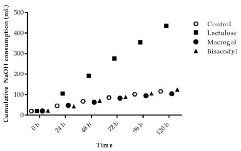
During fermentation of carbohydrates the microbiota produces acidic metabolites like SCFA and lactate. The increased use of NaOH during the experiments for maintenance of pH at 5.8 indicates the activity of microbiota fermenting the SIEM plus the test product added to the TIM-2 system. Adding Lactulose in the test period (t=0 h to t=120 h) showed an increased use of NaOH during the TIM-2 experiments as compared to the control (Figure 1). Macrogol and Bisacodyl showed a similar total NaOH usage as in the control experiments at 116 ± 6 ml (control), 104 ± 7 ml (Macrogol) and 124 ± 3 ml (Bisacodyl) compared to 436 ± 2 ml (Lactulose).

fig 1

Figure 1: Sodium hydroxide consumption during TIM-2 runs (mean of n=3 (Lactulose), n=2 (Macrogol and Bisacodyl) or n=4 (control)). Values at the start of the test period are on average 20.76 mL due to NaOH consumption during the adaptation period. All data points shown at the proximity of the individual time points indicated at the X-axis belong to these specific time points.

Short-chain Fatty Acids and Branched-chain Fatty Acids

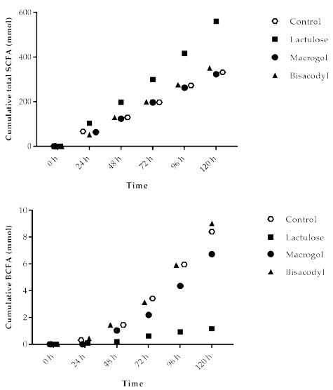
Figure 2a shows the cumulative total SCFA (acetate, propionate and butyrate) production during the 120 h test period in TIM-2. The results indicate that the amount of total SCFA increased with Lactulose (560 ± 20 mmol), while obtained values for control, Macrogol and Bisacodyl were comparable, with total SCFA amounts of 332 ± 34 mmol (control), 323 ± 22 mmol (Macrogol), 351 ± 17 mmol (Bisacodyl), respectively.

The total production of branched-chain fatty acids in 120 h (BCFA; iso-butyrate and iso-valerate) is shown in Figure 2b. During fermentation of proteins in the colon BCFA are produced next to H2, CO2, CH4, phenols and amines. The total amount of BCFA produced during the TIM-2 experiment was similar for Macrogol (6.7 ± 2.7 mmol) and Bisacodyl (9.0 ± 3.1 mmol) as compared to the control (8.4 ± 4.2 mmol), but was lower after addition of Lactulose (1.2 ± 0.2 mmol).

fig 2

Figure 2: Production of (A) total short chain fatty acids (SCFA, acetate, propionate, butyrate); (B) total branched-chain fatty acids (BCFA) (iso-butyrate and iso-valerate) in TIM-2 runs (mean of n=3 (Lactulose), n=2 (Macrogol and Bisacodyl) or n=4 (control)). Values at the start of the test period were set to zero. All data points shown at the proximity of the individual time points indicated at the X-axis belong to these specific time points.

Lactate

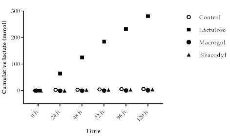
Lactate is an intermediate metabolite accumulating during fast fermentation processes. At the same time, bacteria use lactate as a substrate. The cumulative amount of lactate (Figure 3) produced in the experiment with Macrogol (1.2 ± 0.8 mmol) and Bisacodyl (4.3 ± 2.8 mmol) was low and similar to the control (5.8 ± 2.2 mmol). The results show that due to its fermentation much higher amounts of lactate (300.7 ± 10.4 mmol) are formed in the presence of Lactulose compared to the control as well as Macrogol and Bisacodyl.

fig 3

Figure 3: Cumulative lactate production over time during the 120 h test period in TIM-2 runs (mean of n=3 (Lactulose), n=2 (Macrogol and Bisacodyl) or n=4 (control)). All data points shown at the proximity of the individual time points at the X-axis belong to these specific time points.

Ammonia

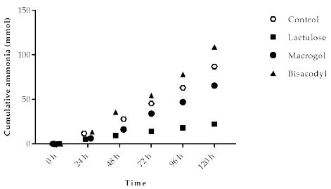
Ammonia is a metabolite produced by microbial fermentation of proteins (nitrogen). The cumulative (total) amount of ammonia, measured as ammonium salt in the TIM-2 model, is shown in Figure 4. The basal amounts of ammonia (total cumulative production) during the control experiments gives an indication of the ammonia production without intervention. Ammonia production for the different test products was lowest for Lactulose (22.2 ± 2.5 mmol) compared to 87.0 ± 27.9 mmol (control), 65.6 ± 11.2 mmol (Macrogol), and 108.9 ± 16.8 mmol (Bisacodyl), respectively.

fig 4

Figure 4: Cumulative ammonia production over time during the 120 h test period in TIM-2 runs (mean of n=3 (Lactulose), n=2 (Macrogol and Bisacodyl) or n=4 (control)). All data points shown at the proximity of the individual time points indicated at the X-axis belong to these specific time points.

Microbiota Composition

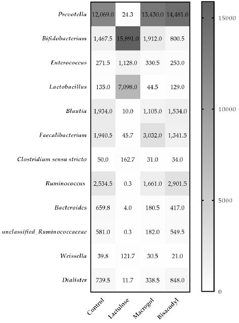
Analysis with mass V4 16S rDNA amplicon sequencing resulted in an overview of bacterial genera present in the microbiota of the lumen samples collected from the TIM-2 experiments after 120 h exposure to the different test conditions. The distribution of the number of reads ranged from 24,750 to 204,719. The lowest count of reads observed was 24,750 reads in a t=0 sample supplemented with Lactulose. The lowest number of reads was used for normalization of all samples to this read level. Figure 5 shows the effect of Lactulose, Macrogol and Bisacodyl on the relative abundance of bacteria up to a cut-off range of 1.0% relative abundance compared to control. The heatmap depicts the most abundant bacteria. The most significantly increased bacterial genera, Bifidobacterium and Lactobacillus increased more than 10-fold or 50-fold, respectively, in the presence of Lactulose. At the same time, Prevotella, Blautia, Ruminococcus, Faecalibacterium and Bacteroides were decreased more than 10-fold in the presence of Lactulose compared to the control. For the Macrogol and Bisacodyl no significant changes were observed compared to the control.

fig 5

Figure 5: The heatmap indicates the normalized average relative number n of the different bacterial genera in the microbiota in the different treatments with Lactulose, Macrogol, and Bisacodyl when compared to control, after 120 h of exposure in TIM-2 as represented by the 16S rRNA amplicon sequencing reads.

Discussion

This study showed that Lactulose, in contrast to Macrogol or Bisacodyl, has an effect on the active gut microbiota present in an in vitro model of the proximal colon. This effect includes an increase in NaOH consumption to keep the pH at a fixed level, suggesting a pH decrease by the net production of acidic metabolic products. This was confirmed by the observed increased levels of SCFA and lactate, and decreased levels in BCFA and ammonia. Contrary to this observation, Bisacodyl even lead to higher cumulative BCFA and ammonia levels than the control.

Five days of exposure to Lactulose strongly increased the levels of bifidobacteria (more than 10-fold) and lactobacilli (more than 50-fold). A slight increase in Bifidobacterium was also observed with Macrogol treatment, while Bisacodyl exposure slightly decreased the amount of this bacterium. After Macrogol treatment, the levels of Lactobacillus were decreased, while Bisacodyl exposure had no substantial effect. In summary, exposure to Lactulose was superior to Macrogol and Bisacodyl by increasing the relative abundance of Bifidobacterium and Lactobacillus.

Apart from Bifidobacteria and Lactobacilli, bacterial counts of several other bacteria present in more than 1% relative abundance with a more than 10-fold changed were observed after Lactulose treatment. Prevotella spp. are reduced close to zero after 120 h Lactulose treatment, while Macrogol and Bisacodyl treatment slightly increased the counts. Prevotella is suspected to exacerbate chronic (intestinal) inflammation [28,29] and to increase the risk of autoimmune disorders like rheumatoid arthritis [30-34]. Intestinal Prevotellaceae were associated with rheumatoid arthritis in Northern America, Europe and Japan, but not in a Chinese study [35]. Larger metagenome-wide association studies are required before a final conclusion on the role of Prevotella spp in the pathogenesis of rheumatoid arthritis and the potential for amelioration by Lactulose can be drawn.

Blautia were also reduced nearly 200-fold by Lactulose, while with both, Macrogol and Bisacodyl, only slight reductions could be identified. An increase in Blautia counts is considered pro-inflammatory [36] and increased counts are detected in neurodegenerative diseases like Parkinson or Multiple Sclerosis [36,37] or systemic lupus erythematosus [38]. The role of increased Blautia counts in the pathogenesis of diabetes is also discussed, but a causative association has not yet been determined [39-41].

Lactulose treatment for 120 h also showed a decrease in Faecalibacterium, while these bacteria were increased with Macrogol and slightly decreased with Bisacodyl. Within the genus of faecalibacteria, especially Faecalibacterium prausnitzii has been reported as one of the main butyrate producers in the gut [42,43]. Due to its anti-inflammatory properties it reduced the severity of inflammation in several murine models [44,45]. The genus Faecalibacterium was also increased in the intestinal content of obese children [46] and patients with psoriasis [47]. The impact of laxatives on levels of this genus remain to be studied in the future.

Ruminococcus was also strongly decreased by Lactulose treatment, slightly decreased by Macrogol and slightly increased by Bisacodyl. While increased levels of these mucolytic bacteria in inflammatory bowel disease (IBD) seem to be associated with the high load of mucins to be cleaved [48,49], nothing is known about the effect of an increased abundance in disorders like autism [50], allergic diseases [48] or coronary artery disease [51].

Finally, Lactulose treatment reduced the levels of Bacteroides, as to a lower extent also did Macrogol and Bisacodyl. This is in contrast to a previous study, where levels of Bacteroides were increased in healthy adults after PEG 4000 induced osmotic diarrhea [11]. The reasons for this difference may be in the test item (PEG 4000 versus PEG 3350), the setup of the study, the dose and the duration of treatment and cannot be fully elucidated here. Bacteroides are normal commensals in the gut, but may also be responsible for infections of significant morbidity, mainly caused by Bacteroides fragilis, like appendicitis, intra-abdominal sepsis, endocarditis, and others [52].

A limitation of this study is the fact that treatment duration was 120 h, while in the clinical situation longer treatment duration may be applicable. A more extended experiment in TIM-2 is possible. Based on previous experience, however, treatment longer than 72-120 h may not reveal significantly different results. Although experiments were conducted only as n=2, results allowed an adequate discrimination between the observed prebiotic effect of Lactulose versus Macrogol and Bisacodyl and more replicates would not have changed this finding.

This study clearly demonstrated that Lactulose has a strong prebiotic effect on Bifidobacteria and Lactobacilli indicating a beneficial support for the gut microbiota of constipated patients in contrast to Macrogol and Bisacodyl. In addition, a more pronounced impact on other gut bacteria was observed with Lactulose compared to Macrogol and Bisacodyl. There are, however, new generations of laxatives also exerting beneficial effects on the gut microbiota or prebiotics with a laxative effect that remain to be compared to Lactulose [53-58]. For example combination products, such as Bisacodyl combined with probiotics [59], or Macrogol mixed with inulin, may result in fierce competition to Lactulose [60]. However, this will remain to be elucidated in future studies, while this study focused on the comparison of the most frequently used single substance laxatives.

Acknowledgments

We thank Mark Jelier and Eveline Lommen for their excellent technical assistance.

References

  1. Khalif IL, Quigley EM, Konovitch EA, Maximova ID (2005) Alterations in the colonic flora and intestinal permeability and evidence of immune activation in chronic constipation. Dig Liver Dis 37: 838-849. [crossref]
  2. Ohkusa T, Koido S, Nishikawa Y, Sato N (2019) Gut Microbiota and Chronic Constipation: A Review and Update. Front Med (Lausanne) 6: 19. [crossref]
  3. Deutsche Gesellschaft für Neurogastroenterologie und Motilität (DGNM) und die Deutsche Gesellschaft für Verdauungs- und Stoffwechselkrankheiten (DGVS) (2013) “Chronische Obstipation: Definition, Pathophysiologie, Diagnostik und Therapie”. AWMF-Registriernummer 021/019.
  4. Eberlin M, Landes S, Biber-Feiter D, Michel MC (2020) Impact of guideline awareness in public pharmacies on counseling of patients with acute or chronic constipation in a survey of pharmacy personnel. BMC Gastroenterol 20: 191.
  5. Gharehbaghi K, Gharehbaghi DR, Wierrani F, Sliutz G (2016) [Treatment of Chronic Functional Constipation during Pregnancy and Lactation]. Z Geburtshilfe Neonatol 220: 9-15. [crossref]
  6. Shafe AC, Lee S, Dalrymple JS, Whorwell PJ (2011) The LUCK study: Laxative Usage in patients with GP-diagnosed Constipation in the UK, within the general population and in pregnancy. An epidemiological study using the General Practice Research Database (GPRD). Therap Adv Gastroenterol 4: 343-363. [crossref]
  7. Panesar PS, Kumari S (2011) Lactulose: production, purification and potential applications. Biotechnol Adv 29: 940-948. [crossref]
  8. Sitanggang AB, Drews A, Kraume M (2016) Recent advances on prebiotic lactulose production. World J Microbiol Biotechnol 32: 154. [crossref]
  9. Prasad VG, Abraham P (2017) Management of chronic constipation in patients with diabetes mellitus. Indian J Gastroenterol 36: 11-22. [crossref]
  10. Ruszkowski J, Witkowski JM (2019) Lactulose: Patient- and dose-dependent prebiotic properties in humans. Anaerobe 59: 100-106. [crossref]
  11. Gorkiewicz G, Thallinger GG, Trajanoski S, et al. (2013) Alterations in the colonic microbiota in response to osmotic diarrhea. PLoS One 8: e55817.
  12. van der Wulp MY, Derrien M, Stellaard F, et al. (2013) Laxative treatment with polyethylene glycol decreases microbial primary bile salt dehydroxylation and lipid metabolism in the intestine of rats. Am J Physiol Gastrointest Liver Physiol 305: G474. [crossref]
  13. Eduardo J Contijoch, Graham J Britton, Chao Yang, Ilaria Mogno, Zhihua Li et al. (2019) Gut microbiota density influences host physiology and is shaped by host and microbial factors. eLife 8: e40553. [crossref]
  14. Tropini C, Moss EL, Merrill BD, et al. (2018) Transient Osmotic Perturbation Causes Long-Term Alteration to the Gut Microbiota. Cell 173: 1742-1754. [crossref]
  15. Bustos D, Ogawa K, Pons S, Soriano E, Bandi JC, Bustos Fernandez L (1991) Effect of loperamide and bisacodyl on intestinal transit time, fecal weight and short chain fatty acid excretion in the rat. Acta Gastroenterol Latinoam 21: 3-9. [crossref]
  16. Bouhnik Y, Neut C, Raskine L, et al. (2004) Prospective, randomized, parallel-group trial to evaluate the effects of lactulose and polyethylene glycol-4000 on colonic flora in chronic idiopathic constipation. Aliment Pharmacol Ther 19: 889-899. [crossref]
  17. Minekus M, Smeets-Peeters M, Bernalier A, et al. (1999) A computer-controlled system to simulate conditions of the large intestine with peristaltic mixing, water absorption and absorption of fermentation products. Appl Microbiol Biotechnol 53: 108-114. [crossref]
  18. Venema K, Van Nuenen HMC, Smeets-Peeters M, Minekus M, Havenaar R (2000) TNO’s in vitro large intestinal model: an excellent screening tool for functional food and pharmaceutical research. Ernährung/Nutrition 24: 558-564.
  19. Maathuis A, Hoffman A, Evans A, Sanders L, Venema K (2009) The effect of the undigested fraction of maize products on the activity and composition of the microbiota determined in a dynamic in vitro model of the human proximal large intestine. J Am Coll Nutr 28: 657-666. [crossref]
  20. Maathuis AJ, van den Heuvel EG, Schoterman MH, Venema K (2012) Galacto-oligosaccharides have prebiotic activity in a dynamic in vitro colon model using (13)C-labeling technique. J Nutr 142: 1205-1212. [crossref]
  21. Bothe MK, Maathuis AJH, Bellmann S, et al. (2017) Dose-Dependent Prebiotic Effect of Lactulose in a Computer-Controlled In Vitro Model of the Human Large Intestine. Nutrients 9: 767. [crossref]
  22. Van Nuenen M.H., Meyer P., Venema K (2003) The effect of various inulins and clostridium difficile on the metabolic activity of the human colonic microbiota in vitro. Microb Ecol Health Dis 15: 137-144.
  23. Sims G., Ellsworth T., Mulvaney R (1995) Microscale determination of inorganic nitrogen in water and soil extracts. Commun Soil Sci Plant Anal 26: 303-316.
  24. Ladirat SE, Schols HA, Nauta A, et al. (2013) High-throughput analysis of the impact of antibiotics on the human intestinal microbiota composition. J Microbiol Methods 92: 387-397. [crossref]
  25. Kozich JJ, Westcott SL, Baxter NT, Highlander SK, Schloss PD (2013) Development of a dual-index sequencing strategy and curation pipeline for analyzing amplicon sequence data on the MiSeq Illumina sequencing platform. Appl Environ Microbiol 79: 5112-5120. [crossref]
  26. Caporaso J.G., Lauber C.L., Walters W.A., et al. (2011) Global patterns of 16s rrna diversity at a depth of millions of sequences per sample. Proc Natl Acad Sci USA 18: 4516-4522.
  27. Segata N, Izard J, Waldron L, et al. (2011) Metagenomic biomarker discovery and explanation. Genome Biol 12:R60. [crossref]
  28. Iljazovic A, Roy U, Galvez EJC, et al. (2021) Perturbation of the gut microbiome by Prevotella spp. enhances host susceptibility to mucosal inflammation. Mucosal Immunol 14: 113-124.
  29. Larsen JM (2017) The immune response to Prevotella bacteria in chronic inflammatory disease. Immunology 151: 363-374. [crossref]
  30. Guerreiro CS, Calado A, Sousa J, Fonseca JE (2018) Diet, Microbiota, and Gut Permeability-The Unknown Triad in Rheumatoid Arthritis. Front Med (Lausanne) 5: 349. [crossref]
  31. Lorenzo D, GianVincenzo Z, Carlo Luca R, et al. (2019) Oral-Gut Microbiota and Arthritis: Is There an Evidence-Based Axis? J Clin Med 8. [crossref]
  32. Maeda Y, Takeda K (2017) Role of Gut Microbiota in Rheumatoid Arthritis. J Clin Med 6.
  33. Maeda Y, Takeda K (2019) Host-microbiota interactions in rheumatoid arthritis. Exp Mol Med 51: 1-6. [crossref]
  34. Wells PM, Williams FMK, Matey-Hernandez ML, Menni C, Steves CJ (2019) ‘RA and the microbiome: do host genetic factors provide the link? J Autoimmun 99: 104-115.
  35. Moller B, Kollert F, Sculean A, Villiger PM (2020) Infectious Triggers in Periodontitis and the Gut in Rheumatoid Arthritis (RA): A Complex Story About Association and Causality. Front Immunol 11: 1108. [crossref]
  36. Frahm C, Witte OW (2019) Mikrobiom und neurodegenerative Erkrankungen. Der Gastroenterologe 14: 166-171.
  37. Gerhardt S, Mohajeri MH (2018) Changes of Colonic Bacterial Composition in Parkinson’s Disease and Other Neurodegenerative Diseases. Nutrients 10: 708. [crossref]
  38. Silverman GJ (2017) Abstract 1786: Patients with SLE show over-representation of Blautia genus in microbiome. American College of Rheumatology Annual Meeting. San Diego.
  39. Egshatyan L, Kashtanova D, Popenko A, et al. (2016) Gut microbiota and diet in patients with different glucose tolerance. Endocr Connect 5: 1-9. [crossref]
  40. Gurung M, Li Z, You H, Richard Rodrigues, Donald B Jump et al. (2020) Role of gut microbiota in type 2 diabetes pathophysiology. EBioMedicine 51: 102590. [crossref]
  41. Jamshidi P, Hasanzadeh S, Tahvildari A, et al. (2019) Is there any association between gut microbiota and type 1 diabetes? A systematic review. Gut Pathog 11: 49. [crossref]
  42. Barcenilla A, Pryde SE, Martin JC, et al. (2000) Phylogenetic relationships of butyrate-producing bacteria from the human gut. Appl Environ Microbiol 66: 1654-1661. [crossref]
  43. Duncan SH, Hold GL, Harmsen HJM, Stewart CS, Flint HJ (2002) Growth requirements and fermentation products of Fusobacterium prausnitzii, and a proposal to reclassify it as Faecalibacterium prausnitzii gen. nov., comb. nov. Int J Syst Evol Microbiol 52: 2141-2146. [crossref]
  44. Lopez-Siles M, Duncan SH, Garcia-Gil LJ, Martinez-Medina M (2017) Faecalibacterium prausnitzii: from microbiology to diagnostics and prognostics. ISME J 11: 841-852. [crossref]
  45. Miquel S, Martin R, Rossi O, et al. (2013) Faecalibacterium prausnitzii and human intestinal health. Curr Opin Microbiol 16: 255-261. [crossref]
  46. Balamurugan R, George G, Kabeerdoss J, Hepsiba J, Chandragunasekaran AM, Ramakrishna BS (2010) Quantitative differences in intestinal Faecalibacterium prausnitzii in obese Indian children. Br J Nutr 103: 335-338. [crossref]
  47. Codoner FM, Ramirez-Bosca A, Climent E, et al. (2018) Gut microbial composition in patients with psoriasis. Sci Rep 8: 3812. [crossref]
  48. Chua HH, Chou HC, Tung YL, et al. (2018) Intestinal Dysbiosis Featuring Abundance of Ruminococcus gnavus Associates With Allergic Diseases in Infants. Gastroenterology 154: 154-167. [crossref]
  49. Png CW, Linden SK, Gilshenan KS, et al. (2010) Mucolytic bacteria with increased prevalence in IBD mucosa augment in vitro utilization of mucin by other bacteria. Am J Gastroenterol 105: 2420-2428. [crossref]
  50. Wang L, Christophersen CT, Sorich MJ, Gerber JP, Angley MT, Conlon MA (2013) Increased abundance of Sutterella spp. and Ruminococcus torques in feces of children with autism spectrum disorder. Mol Autism 4: 42. [crossref]
  51. Toya T, Corban MT, Marrietta E, et al. (2020) Coronary artery disease is associated with an altered gut microbiome composition. PLoS One 15: e0227147. [crossref]
  52. Wexler HM (2007) Bacteroides: the good, the bad, and the nitty-gritty. Clin Microbiol Rev 20: 593-621. [crossref]
  53. Aguirre M, Bussolo de Souza C, Venema K (2016) The Gut Microbiota from Lean and Obese Subjects Contribute Differently to the Fermentation of Arabinogalactan and Inulin. PLoS One 11: e0159236. [crossref]
  54. Buddington RK, Kapadia C, Neumer F, Theis S (2017) Oligofructose Provides Laxation for Irregularity Associated with Low Fiber Intake. Nutrients 9: 1372. [crossref]
  55. Macfarlane GT, Steed H, Macfarlane S (2008) Bacterial metabolism and health-related effects of galacto-oligosaccharides and other prebiotics. J Appl Microbiol 104: 305-344. [crossref]
  56. Martinez RC, Cardarelli HR, Borst W, Simone Albrecht, Henk Schols et al. (2013) Effect of galactooligosaccharides and Bifidobacterium animalis Bb-12 on growth of Lactobacillus amylovorus DSM 16698, microbial community structure, and metabolite production in an in vitro colonic model set up with human or pig microbiota. FEMS Microbiol Ecol 84: 110-123. [crossref]
  57. Takayama K, Takahara C, Tabuchi N, Okamura N (2019) Daiokanzoto (Da-Huang-Gan-Cao-Tang) is an effective laxative in gut microbiota associated with constipation. Sci Rep 9: 3833. [crossref]
  58. Van den Abbeele P, Venema K, Van de Wiele T, Verstraete W, Possemiers S (2013) Different human gut models reveal the distinct fermentation patterns of Arabinoxylan versus inulin. J Agric Food Chem 61: 9819-9827. [crossref]
  59. Choi YI, Lee JJ, Chung JW, Kyoung Oh Kim, Yoon Jae Kim et al. (2020) Efficacy and Patient Tolerability Profiles of Probiotic Solution with Bisacodyl Versus Conventional Cleansing Solution for Bowel Preparation: A Prospective, Randomized, Controlled Trial. J Clin Med 9: 3286. [crossref]
  60. Gruenwald J, Busch R, Bentley C (2009) Efficacy and tolerability of Laxatan Granulat in patients with chronic constipation. Clin Exp Gastroenterol 2: 95-100. [crossref]

In Search of Beautiful Bodies: A Meta-analysis of Five Mind Genomics Cartographies – Equipment, Gyms, and Fitness Clubs

DOI: 10.31038/AWHC.2021453

Abstract

We present a meta-analysis of five Mind Genomics cartographies, done over a 20 year period, all dealing with exercise; purchasing exercise equipment (Buy It!, 2002), joining a branded, well know exercise spa franchised around the US (Curves, 2010), what to say to entice a person to join an exercise club or a gym (2012, student projects at Queens College), and, at the tail-end of a Covid-stricken 2019, how to lure customers back to using exercise equipment either at home and/or the same equipment in a gym (2020). We present the strong performing messages for each cartography, show the power of mind-set segmentation, the power of doing simple background research (student work in 2012), and introduce new foci as well, emotions linked with elements and engagement with messages revealed by response times. These five case histories, the paper shows how Mind Genomics was used by different people in the same ‘general space,’ over a 20-year period, and how Mind Genomics evolved to incorporate new measures alongside its basic measure.

Introduction

We live in a society focused on beauty, whether beauty of the face or of the body, occasionally of the spirit and even of the mind. Whereas among the ancients and their successors in the medieval and modern worlds the search for physical beauty was both artistic and philosophical, today it manifests itself in the world of cosmetics and the world of fitness. One can barely drive through a town, a city, even a rural area without seeing stores devoted to making people more beautiful.

Our focus in this paper is on the world of exercise, a world perhaps not as glamorous as the world of facial beauty and the world of fashion, but a world important, nonetheless. With increasing prosperity and with increasingly caloric intake, coupled with lessened demand on physical activity for work, there is the natural result of increased weight, of lessened body tone. Add that to the oft-feared factor of aging, and one has created a perfect storm for people to focus on what can turn back the clock of time.

The topic of gyms and fitness clubs has enjoyed a moderate amount of published research, and undoubtedly a great deal more one-off business studies deposited after use in the corporate files, presumably hidden away forever, or until the issue has been forgotten along with the research effort. The topics involved in gyms range from a focus on the trajectory of human development [1] to the emotions and motives for joining gyms [2], to health, both physical and psychological [3,4]. At the same time, there is the business aspect of clubs, the need to convince people that certain clubs are worth paying for [5-7].

During the past two decades, as Mind Genomics evolved into the science it is today, a variety of research efforts generated some interesting data on exercise, fitness, and related topics. We look at the salient results from five studies, one run 20 years ago, three run about 10 years ago, and one run a year ago. One study was run to understand how people wanted to shop for exercise equipment. The remaining four studies were run to understand what messages makes people want to join health spas and exercise gyms.

A Short Introduction to Mind Genomics

In 1964, mathematical psychologists R. Duncan Luce and John Tukey had been involved in creating a strong, new, axiom-based foundation for mathematical psychology, and particularly for powerful measurement without using numbers. The approach they developed was called conjoint measurement, the measurement of quantities by the measurement of combinations of such quantities. The approach sounds perfectly ordinary today; measurement mixtures of ideas and from the measurement of the mixtures deduce the measure of the components. The mathematics would appear in a daunting first paper in a new journal, the Journal of Mathematical Psychology, volume 1, number 1, first paper. IN other words, the premier new journal, and the lead article [8].

Conjoint measurement would have remained a stunning intellectual contribution, albeit an esoteric one, except for the efforts of Wharton business school professors Paul Green, Abba Krieger, and Yoram Wind, who would take it, make it practical, and apply it to various problems [9-11]. The literature using conjoint measurement would grow, until the approach would be used for products, for public policy, and so forth [12,13]. One needs only Google(r) the academic literature to get a sense of its applications.

Despite its popularity, most published papers, and indeed most likely research reports buried in corporate offices are one-off studies, executed to solve a particular problem. Conjoint measurement required knowledge of the variables, a painful creation of the combinations, a painful execution, and an analysis, not to mention an equal painful explanation of the method. In other words, the system was expensive, slow, and clunky, reserved for the most important (better read better-funded) project [14].

Mind Genomics emerged out of conjoint measurement, propelled by three key goals:

  1. Create a system which, like Conjoint Measurement, would be able to measure the strength of ideas by measuring combinations of ideas, so-called vignettes. There was recognition that responses to vignettes could not be easily ‘faked’ as well as the fact that compound messages were more typical in the everyday world than single messages comprising one idea.
  2. Make sure that each respondent evaluated a unique set of combinations of the same set of elements. This notion of different sets of the same elements emerged from the world of medicine, and the MRI, which takes pictures of the same tissue from different angles, and then recombines them in the analysis phase to come up with a single, 3-dimensional picture [15].
  3. Create a system which could generate information that would be databased, with the data comparable within a study, and across studies [16].

The studies reported here were run in the same way, following these steps:

    1. Raw Materials: Create a topic, create a set of questions which ‘tell a story’, and for each question provide a set of ‘answers’ which give different facts. The number of questions can vary but the number of answers for each question is always equal. The Mind Genomics method allows for a variety of such options, such as four questions with nine answers, six questions with six answers, four questions with four answers, etc. The most common study as of this writing (2021) is the design comprising four questions, each with four answers (16 elements).
    2. Test Combinations: Create a fixed set of combinations, specified as an experimental design The experimental design prescribes the precise set of combinations, doing so by specifying which elements are put together. The experimental design is set up so that the variables are statistically independent, allowing methods such as OLS (ordinary least-squares) regression to reveal how each element or message contributes to the rating assigned to the vignette, viz., to the combination. Respondents do not rate the components; they rate the vignettes, the combinations, which is more natural to them [17].
    3. Permute the Combination: There are a fixed set of combinations, but the combinations are permuted [15]. For example, one design comprised four questions, nine answers per question, 60 combinations, and many different variations of the underlying design with 60 combinations. This approach lets the ‘experiment’ cover much of the range. Thus, Mind Genomic trades off precision of measuring one small region of the possible combinations of messaging, and instead opts to measure a great deal of the region, albeit with less precision.
    4. Transform the Ratings in a Way Which Permits Managers to Understand the Results More Easily: In these five studies, four used a 1-9 scale anchored at each end; one used a 5-point scale. Managers who work with the data derived from scale often ask ‘what does a 6 mean’ or a ’4’ mean, etc. To make the data easier for managers to use, consumer researchers and political pollsters have learned transform a scale with many points to a binary scale, no/yes. Following this practice, the researcher transformed the ratings on the 9-point scale to a binary scale (1-6 transformed to 0, ratings of 7-9 transformed to 100). In the case of the 5-point scale, the conversion was 1-3 transformed to 0, 4-5 transformed to 100. In each case, a vanishingly small random number was added to every data point, whether transformed to 0 or to 100, respectively. The random number ensured that no dependent variable would ever be all 0’s or all 100’s for any single individual. This slight variation ensured that the OLS regression always worked for each individual respondent
    5. Create Equations Relating the Presence/Absence of the Elements to the Newly Created Binary Variables: The experimental design makes it possible to create the equation even with the data of one respondent. Whether the equation is created for a group of respondents, or even for a single individual, the equation is expressed in the same way:
    6. For those experiment designs using the 4×9 structure (four questions, nine answers for each question): Binary Variable (TOP3) = k0 + k1(A1) + k2(A2) … k36(D9)

      For those experimental; designs using the 6×6 structure (six questions, six answers for each question):

      Binary Variable (TOP3) = k0 + k1(A1) + k2(A2)… k36 (F6)

      For those experimental design using the 4×4 structure (four questions, four answers for each question): Binary Variable (Top2) = k0 + k1(A1) + k2(A2) … k16(D4)

    7. Uncover Mind-sets: We often divide people by factors that we can easily measure. The easiest of course are WHO a person is, and in today’s digital world, what a person DOES. One can also divide people by the patterns of their answers to sets of questions, the pattern of answers to these questions assigning a person to a group based on attitude. These groups are large, and not particularly actionable. That, knows what a person buys do not tell us what messages move the respondent to buy, and what messages are turnoffs. We don’t typically think like that – viz., having details information about how the world of people’s minds divide for a topic. Usually, the topic is too small, too irrelevant for a deep, detailed investigation.
    8. Mind Genomics create different groups of people, not based on who they are, but rather on the pattern of their reactions to limited types of information. That is, the division of people is not based on the way the person thinks about large (and important) problems, buts divides people on the pattern of responses to any topic, in ways which make sense. The method is called clustering [18]. Clustering is based upon mathematical criterion. However, the choice of the number of clusters to use is based upon two non-mathematical criteria. The first is parsimony – fewer clusters are better than more clusters. The second is interpretability – the clusters must tell a coherent story. Parsimony and interpretability are opposed; more clusters mean easier to tell a story, but only the truly relevant elements need be included in the cluster.

    9. Relate the Elements to the Transformed Rating Scale to Show the Impact of Each Element: The OLS (ordinary least-squares) regression analysis uses the data defined by the researcher Once members of the different groups have been identified (viz., respondents belonging to Total, to Males vs Females; to mind-sets 1 vs 2 vs 3), etc. The subgroups are defined either by how the respondent describes himself or herself (done in the context of the study, through self-profiling classification), or the mind-sets are created through clustering and the data from all respondents in a specific mind-set or cluster are combined to create one dataset, and the OLS regression run using all data from that dataset.

    Cartography 1 – Buying Exercise Equipment

    Study # 1 was done in 2002, just about 20 years ago. The study was part of a large group of studies which focused on the nature of messaging which represent one’s idea shopping experience [13]. Figure 1 shows the wall of studies. All studies were identical except for the name of the product, and certain features and stores. The respondent selected the study and was led to the introduction for that study shown in Figure 2.

    fig 1

    Figure 1: The wall of studies for Buy It! the respondent selected the study.

    fig 2

    Figure 2: Respondent instructions for the Buy It! Study. The introduction comes from the study dealing with exercise equipment.

    The different studies in the Buy It! project comprised four questions or silos, each with nine answers or elements. We will use the term element instead of answer. The 4×9 design (four questions, nine answers) generate 36 elements in total, combind according to an underlying experimental design into 60 vignettes. Each element appear an equal numbr of times across the 60 vignettes. Furthermore, the vignettes comprised 2-4 elements, so by design many of the vignettes were ‘incomplete,’ viz.,lacking an answer from one of the four questions. As noted above, each respondent evaluated a unique set of combinations, permutations of the original design.

    Table 1 shows only those elements which exhibit at least one strong performing element. The element had to have an estimated coefficient of +8 or higher when the dependent variable was defined as a binary scale (1-6 → 0; 7=9 → 100). Table 1 thus shows the highlights. We show the elements first in terms of total panel, then in terms of three mind-sets to emerge, and then in terms of gender.

    Table 1: Strong performing element for the 2002 Buy It! study on exercise equipment. (Table courtesy of It! Ventures).

    table 1

    1. The additive constant is a measure of the closeness of the vignette to one’s ideal shopping experience, in the absence of elements. The additive constant is purely theoretical, an estimated parameter. It does tell us, however, how positive the respondent is to the shopping experience. The additive constants are all low, between 26 and 34. It will be the elements which will make a difference.
    2. In most Mind Genomics studies we end up with a few elements which do well. The total panel shows two elements, C2 (Let’s you get your shopping done quickly), and B1 (The price is JUST RIGHT … ALL OF THE TIME). They score 9 and 8, weaker than we will see when we turn to the three mind-sets which emerged from clustering the respondents based upon the similarities among the set of 36 coefficients.
    3. It will be the mind-sets which show the big differences, differences which suggest three patterns:
    4. a. Mind-Set 1 responds to the stores

      b. Mind-Set 2 convenience

      c. Mind-Set 3 wants price and choice.

    5. It is mind-sets, not genders, which show the strong responses to the elements, a pattern which shows the power of Mind Genomics to uncover these basic groups in what would seem to be a population which is indifferent to the messages because the first data column. There is no indifference, but rather strong albeit different preference patterns.

    Cartography 2 – What Messages Drive Women to Say that They Will Join Curves

    Study # 2 was run in December 6-7, 2010, at the behest of Queens College, in collaboration with author HRM, and the mathematics department of Queens College. The study was part of the ‘vetting processes that Queens College used to create a mathematics course, Math 110, offered 2011-2013. Two of the owners of a local gymnasium were interested in signing up with Curves. They approached Queens College and funded the study, which was otherwise done on a pro bono basis with permission to publish the results of the study in two years.

    The ingoing brief for the study was the following:

    To prosper in the present economy Curves Owners must always be on the look-out for new ways to accommodate and engage their members. Curves owners need faster access to useful consumer insights in developing marketing messaging and programs, products and services. The Vision – Increase lasting memberships at Curves. The marketing and sales strategy to emerge from Mind Genomics was set forth at the set-up meeting:

    Attract prospects to come into your club by using optimum message appearing to the general marketplace through: Web coupons, Mailing Value Coupon packs, Web site landing page, E-mails, In person

    When the prospect comes in, lead the discussion with those Curves features that appeal most to each individual: Use a simple approach to tell you EXACTLY what to say to each individual

    Study # 2 was run on December 6-7, 2010, with a population of women of all ages across the US. The raw material for the study came from current (2010 basis) marketing and advertising messaging from Curves website as well as from websites of peer fitness clubs: Butterflylife, Contours express, Fitness club Forwomen, and Lady of America, respectively.

    Table 2 shows the strong performing elements for the study. There were 36 elements. Surprisingly, most of the elements fared quite poorly. That is, despite their use in the promotional literature, their actual performance was poor using the criterion of consumer reactions. This is often the finding of a Mind Genomics study, perhaps because the elements used have not been established ‘effective’, in a rigorous, unbiased manner. That is, most elements used in the study may well have been legacy elements, the origin and usefulness of lists lost if, in fact, they are really existed.

    Table 2: Strong performing elements for the ‘Curves’ study.

    table 2

    A key benefit of the Mind Genomics approach is the ability to assign new people to the appropriate mind-set. This is done with the PVI (Personal Viewpoint Identifier). The PVI uses statistical methods such as DFA (Discriminant Function Analysis), and Decision Trees to create a limited set of questions emerging from the elements or answers of the study. These are the elements which best differentiate the mind-sets from each other. Figure 3 shows an example of how the PVI appears in 2010, summarizing the process. The figure shows the objective, the respondent introduction (left column), and then one of the three questions and one of the three outputs (right column). The new respondent completes a short set of questions. The pattern of responses to the questions suffices to assign that respondent to one of the three mind-sets just uncovered. The process lasts about 30-45 seconds.

    fig 3

    Figure 3: The PVI (Personal Viewpoint Identifier), showing the introduction. one question (of three) from the PVI, and the feedback when the respondent is assigned to Mind-Set (Segment) 1. The figure shows the version of the PVI from 2010.

    Cartography 3 – Joining a Fitness Club

    Study #3 (as well as Study #4 on joining a gym) was done in 2012 at Queens College by a cadre of four students in the Math 110 course. The course was an experiment run for five semesters at Queens College of City University of New York. The idea was to teach the students a combination of critical/creative thinking with a dose of mathematics and mathematical thinking. The students were divided into groups of four individuals, instructed on the basics of Mind Genomics (at that time called Addressable Minds for business), and selected a topic. The two studies reported here, chosen by two separate groups of students, show the power of creative thinking, and the strong performance of the elements when the students were engaged in research, and challenged to do their best.

    Figure 4 shows the orientation page to the study and is similar to the orientation pages of previous studies. The student was interested both in what drives interest in joining a fit club (question #1), as well as the emotional reaction to after reaching each vignette (question #2). This presentation of data from Study # 4 focuses only on the data from Question #1 (joining) to demonstrate the richness of the results. Emotions will be shown in the next study on joining a gym (Cartography #4).

    fig 4

    Figure 4: The orientation page to the study on joining a fitness club.

    The actual design was a so-called 4×6 (four questions, six answers). Table 3 shows the strong performing elements by total panel, by gender, and by four emergent mind-sets. One mind-set, MS1, is very small, and should be discarded, but we leave it here for completeness. What emerges as remarkable in light of the previous two studies in the richness of the results, something that will be seen in the next study as well on joining a gym? The reason for the richness can be principally attributes to good up-front thinking by the four students who participated. The students took the project seriously, looked at the different messaging on the Internet, selected what seemed to be reasonable, and put that messaging into the study. The results, with 50 respondents, are no less than spectacular, with the number of very strong performing elements.

    Table 3: Performance of elements for joining a fitness club.

    table 3

    Mind-Set 1: Very modestly interested (additive constant 29), but attracted by the ‘shock’ value of services and prices

    Spa: full body massages, facials, waxing, sauna

    Dollar a day trial membership (3 months max))

    Mind-Set 2: Barely interested (additive constant 9) but attracted by some outstanding features

    Spa: full body massages, facials, waxing, sauna

    Child-care available with an indoor playground, recreational activities and professional supervision

    Ultra clean environment with towels for all members

    Olympic size pool with over ten swimming lanes.

    Mind-Set 3: Basically disinterested (additive constant -8) but exceptionally interested in cardio and fitness, as well as making it part of an easy daily schedule

    Achieve your ideal weight

    Free shuttle bus within a 15-mile radius of the gym

    Gymnastic classes that help improve flexibility

    Dollar a day trial membership (3 months max)

    Spinning classes offer an innovative alternative for cardio training.

    Mind-Set 4: Modestly interested (additive constant 25), and want machines for self-training

    Two floors of free weights and machines.

    The words of the four students are especially relevant here to summarize the results, and to show how new-to-the-approach students can learn to think more deeply about the topic.

    “Addressable Minds was able to help identify the immense importance the therapeutic effect can provide to its members in a fitness center. Mostly overlooked, due to cardio and weightlifting but equally important to fitness and health is the state of the mind and spirit. The high response rate for the “Spa” and “Organic Food Court” elements demonstrate members are seeking more than just a weight room. Eating the right food along with properly relaxing the mind and body allow members to perform better in the gym thus maximizing the results. Providing these added qualities are crucial to health inside and out but also allow members to get more out of it than a traditional fitness center. Furthermore “Child Care” allows the member to escape responsibilities for a time, to truly focus on strengthening the spirit and mind.”

    Cartography #4: Joining a Gym

    Study # 4 was done at the same time as Study # joining a health club, but by a different team of students in the same class, Math 110 in Queens College. The process was the same and the instructions were virtually the same except that the work ‘gym’ replaced the phrase ‘fitness club’.

    The data for this fourth cartography once again shows the power of doing one’s homework, of taking messages from competition. Table 4 shows low additive constant (-6) suggesting that it is the specifics of the gym which make a difference, not the basic interest in the gym. Table 4 also shows that the additive constant is higher for males (+24) and vanishing low for females (-16). For females, it will be the elements which must do the hard work to convince.

    Table 4: Performance of elements for joining a gym.

    table 4(1)

    table 4(2)

    The data becomes, more interesting when we look at the three mind-sets which emerge.

    Mind-Set 1 is basically uninterested in the gym but strongly differentiates among the messages, and actually loves most of the messages except for those dealing with children. The elements interesting Mind-Set 1 are:

    No enrollment fee

    Feeling some pain…come get a massage from our wonderful masseuses

    One on one time with private fitness trainer

    Take part in one of our 50 different classes (yoga, spinning, Zumba etc.)

    Not sure if you want to join…sign up for a week free membership

    Come workout with our brand new 200 + fitness equipment

    Diet plans to help and encourage your health and well- being.

    Mind-Set 2 likes the notion of joining a gym, although again it is what the gym offers (additive constant 20). The key elements interesting Mind-Set 2 are:

    Take part in one of our 50 different classes (yoga, spinning, Zumba etc.)

    Relax in the Sauna and hot tub after a tough workout.

    Mind-Set 3 has no predisposition to joining the gym (additive constant 8) but like a low price. Their response show that they are the opposite of Mind-Set 1, viz., interested in an activity with their children. The elements interesting Mind-Set 3 are:

    Low monthly cost just 30 dollars a month

    Full time student? …Show your school ID and only pay 25 dollars a month

    Fun summer camps to allow children to stay fit and meet friends

    Looking for competition…Weekly contests with prizes offered

    Free childcare while you work out

    Different types of sports available for all ages

    Mommy and me classes with a variety of times to suit working parents

    Keep your child active after school with enjoyable activities.

    Table 5 shows how the elements link with the choice of emotion. The analysis of the emotion responses was slightly different from the analysis of the ratings for joining. Recall that for the reactions about joining, the 9-point rating scale was converted to one binary variable, taking on the value ‘0 when the original rating was 1-6, and taking on the value ‘100’ when the original rating was 7-9.

    Table 5: Strong linkages (>=8) between elements and selected emotion for the cartography on selecting a gym.

    table 5(1)

    table 5(2)

    This type of transformation does not work for the emotion scale, known as a ‘nominal scale.’ The numbers are simply placeholders for different, not necessarily related emotions. The solution, simple and in the same spirit, was to create FIVE new binary variables, one binary variable for each of the five emotions. A selection of an emotion for a vignette would result in the value ‘100’ for the newly created binary variable corresponding to that emotion, and the value ‘0’ for the four new created binary variables corresponding to the emotions not selected. For example, when the respondent selected the emotion ‘5’ (Interested), the newly created binary variable ‘INTERESTED’ was assigned a value of ‘100’ and the remaining four binary variables (EXCITED, WEARY, CERTAIN, APPREHENSIVE) were all assigned a value of ‘0’. The vanishingly small random number (<10-5) was added to each newly assigned value, whether ‘0’ or ‘100’, respectively.

    The regression analysis relating the presence/absence of the elements to the selection of the emotion was run separately five times, once for each of the five newly created vignettes. The equation was the now familiar regression equation, but the equation was absent the additive constant. The rationale is that the additive constant would be the same for the five newly created binary variables and provides no additional information.

    The two emotions selected most often are confident and curious. Only the strong linkages are show, 8 or higher. The emotion confident links with elements giving the respondent control and choice:

    No hidden fees

    Don’t worry about not finding a spot with our free underground parking garage

    Come workout and feel better about yourself

    Take a dip in the clean and refreshing Olympic sized swimming pool

    Do a lap(s) on the indoor and outdoor running tracks

    Don’t wanna go to the gym alone… 4 free guest passes a month

    Take part in one of our 50 different classes (yoga, spinning, Zumba etc.)

    Different types of sports available for all ages

    Take a class with friends that are offered all day

    Top of the line staff to help you with any questions.

    The emotion curious links with diversion (movie), children, easy to access, and a personal trainer

    Spin away while watching a movie in our luxurious fitness theater

    Free childcare while you workout

    Keep your child active after school with enjoyable activities

    Easily accessible from public transportation

    One on one time with private fitness trainer.

    The new learning here is that by linking emotion with the elements, one begins to get a deeper sense of why the elements seem to do well. The respondent may not be able to articulate the reason for choice, but the nature of the linked emotion may provide that insight.

    Cartography 5: Gym-Two-Ways (2020)

    Study #5 was done in late 2020, during the waning period, after the height of the lockdown due to Covid-19. The objective was to see what type of basic messages would attract prospective customers, who had just been through the lockdown, and might be interested in return to a gymnasium, or having a home trainer work with them using the same equipment in their home.

    By 2020 Mind Genomics had transitioned to the much easier to use 4×4 design, comprising 16 elements (four answers each to four questions) The design generated 24 vignettes, which were permuted by the standard permutation approach, so that across the 106 respondents many of the possible vignettes were estimated. The rating scale was also reduced from 9 points to 5 points. The total time for the Mind Genomics exercise went from about 15 minutes to 3 minutes

    Table 6 shows a much-reduced set of strong performing elements. There are still themes emerging, but what is important is the reduced set of strong performers, and the much lower coefficients. The reason for this may be the emergence of a society whose ability to concentrate on messages and to become excited has diminished and continues to diminish. It may well be that over the period of a decade the prospective audience has been saturated, the so-called paradox of choice [19]. That paradox may reveal itself in what might be called a customer-based ennui, and a growing indifferent to messaging.

    Table 6: Performance of elements for GYM-TWO-WAYS.

    table 6

    Our final analysis concerns response time. The Mind Genomics program recorded the interval between the presentation of the vignette and the respondent’s rating. The interval is called the response-time, and presumably co-varies with internal psychological processes, including reading and decision-making [20,21]. We can look at the estimated response time of each element, with the estimation coming from the OLS (ordinary least-squares regression). Once again there is NO additive constant.

    Table 7 shows the longest and the shortest response times. Most response times are between 0.5 and up to, but not including one second. Only a few elements are processed very quickly or processed more slowly than the half-second range between 0.5 and 1.0 seconds.

    Table 7: Estimated response time for elements. Only the ‘short’ and the ‘long’ response times are shown.

    table 7

    Elements that are quickly (estimated response time <= 0.4 seconds)

    No preparation…just be willing (males)

    Choose intensity that intrigues you (male)

    Share inspiration with GYM-TWO-WAYS community. (MS2 – Expertise)

    Support transition from at-home to gym experience. (MS2 – Expertise)

    Coaches understand YOUR fitness journey. (MS2 – Expertise)

    Elements processed slowly (estimated response time >= 1.0 seconds).

    Expert instructors.(MS1 – Experience)

    Lifelong results through education and access to science. (MS1 – Experience)

    Learn at home. (MS2 – Expertise)

    Learn at your own pace. ( MS2 – Expertise).

    Discussion and Conclusion

    During the past six decades, since the early and middle 1960’s, researchers have focused on obtain increasing amounts of information from customers. Sixty years ago, it was sufficient to measure general attitudes towards products, desires for certain features, and perhaps the ‘gap’ between what was being offered and what was desired by consumers. This so-called ‘gap-analysis’ was satisfactory but over time the world of consumer goods and services would evolve to cut-throat competition. New methods were needed to understand the competitive frame.

    The heyday of consumer research saw the development of new ways to understand the mind of the consumer. In terms of goods and services, Professors Paul Green and Yoram Wind at Wharton pioneered the methods of experimental design to study the trade-offs that consumers would make when considering a service or a product. The notion of trade-off was not new, but the zeitgeist of the 1970’s was moving towards the study of mixtures as being the natural stimuli.

    It is in the spirit of this movement towards studying mixtures that Mind Genomics was born. The objectives were no longer to do single, difficult-to-execute studies, but rather to create a system that would be able to produce knowledge on demand for verticals such as buying products (Buy It!, source of the study on exercise equipment), or solutions to practical problems at the time, at low cost, with cycle times per iteration of a day or less (Curves, GYM-TWO-WAYS), or teaching tools, forcing first-year, non-quantitatively oriented college students to research the competitive frame, and to run a study which both taught them how to structure their inquiry, and how mathematics could provide important information.

    The studies here represent a collection of different issues, done by different researchers, at different times. The numbers are comparable. The coefficient is the percent of respondents saying ‘yes’. Thus, there is ongoing learning, revealed by the meta-analysis, the learning transcending the specific elements, and in addition showing how nature of the up-front research may provide information of higher value.

    References

    1. Biedenweg K, Meischke H, Bohl A, Hammerback K, Williams B, et al. (2014) Understanding older adults’ motivators and barriers to participating in organized programs supporting exercise behaviors. The Journal of Primary Prevention 35: 1-11. [crossref]
    2. Crossley N (2006) In the gym: Motives, meaning and moral careers. Body & Society 12: 23-50.
    3. Layden T (2004) Get out and play! Like the rest of Americans, school-age children are becoming overweight at an alarming rate. But innovative health experts and gym teachers are introducing kids to the benefits–and joys–of exercise through sports and games. Sports Illustrated 101: 19.
    4. Otto MW, Church TS, Craft LL, Greer TL, Smits JA, et al. (2007) Exercise for mood and anxiety disorders. Journal of Clinical Psychiatry 68: 669.
    5. Fogel J, Ustoyev S (2021) Social media advertisements with deposit contracts and fitness club/gym membership: are consumers persuaded? Journal of Consumer Marketing 38: 27-38.
    6. McKnight OT, Paugh R, McKnight J, Zuccaro L, Tornabene G (2014) Marketing athletic clubs, recreation centers and country clubs: Recruiting and retaining members using psychodemographics. American Journal of Management 14: 60-67.
    7. Whiteman-Sandland J, Hawkins J, Clayton D (2018) The role of social capital and community belongingness for exercise adherence: An exploratory study of the Cross Fit gym model. Journal of health Psychology 23: 1545-1556.
    8. Gustafsson A, Herrmann A, Huber F (2000) Conjoint analysis as an instrument of market research practice. In Conjoint measurement 5-45. Springer, Berlin, Heidelberg.
    9. Green PE, Wind Y, Carmone FJ (1972) Subjective evaluation models and conjoint measurement. Behavioral Science 17: 288-299.
    10. Green PE, Krieger AM, Wind Y (2001) Thirty years of conjoint analysis: Reflections and prospects. Interfaces 313: S56-S73.
    11. Krieger AM, Green PE, Wind Y (2004) Adventures in conjoint analysis: A practitioner’s guide to trade-off modeling and applications. Monograph, University of Pennsylvania.
    12. Milutinovic V, Salom J (2016) Mind Genomics: A Guide to Data-Driven Marketing Strategy. Springer.
    13. Moskowitz HR, Gofman A (2007) Selling Blue Elephants: How to Make Great Products That People Want Before They Know They Want Them, Pearson Education.
    14. Wind J, Green PE, Shifflet D, Scarbrough M (1989) Courtyard by Marriott: Designing a hotel facility with consumer-based marketing models. Interfaces 19: 25-47.
    15. Gofman A, Moskowitz H (2010) Isomorphic permuted experimental designs and their application in conjoint analysis. Journal of Sensory Studies 25: 127-145.
    16. Moskowitz HR, Gofman A, Beckley J, Ashman H (2006) Founding a new science: Mind genomics. Journal of Sensory Studies 21: 266-307.
    17. Moskowitz HR (2012) ‘Mind Genomics’: The experimental, inductive science of the ordinary, and its application to aspects of food and feeding. Physiology & Behavior 107: 606-613.
    18. Likas A, Vlassis N, Verbeek JJ (2003) The global k-means clustering algorithm. Pattern recognition 36: 451-461.
    19. Schwartz B (2004) January. The paradox of choice: Why more is less. New York: Ecco.
    20. Bergert FB, Nosofsky RM (2007) A response-time approach to comparing generalized rational and take-the-best models of decision making. Journal of Experimental Psychology: Learning, Memory, and Cognition 331: 107.
    21. Rubinstein A (2013) Response time & decision making: An experimental study. Judgment and Decision Making 8: 540-551.

The Prevalence of ASTRAZENECA COVID Vaccine Side Effects among Nigist Elleni Mohamed Memorial Specialized Hospital Health Workers: Cross Sectional Survey

DOI: 10.31038/IJAS.2021222

Abstract

Background: The best way to eradicate COVID 19 viral infection is mass vaccination. Many studies demonstrate vaccination is associated with some local and systemic side effects. This study aimed to provide evidence on ASTRAZENECA COVID vaccine side effects.

Method: Institutional based cross-sectional survey was conducted among 254 health workers at Nigist Elleni Mohamed Memorial Specialized Hospital (NEMMSH) from July 01/2021 to August 30/2021. Data were collected consecutively through self-administered online survey created on Google Forms of platform which had been randomly delivered via (Facebook or telegram pages). Demographic data of participants, side effect after first and second dose of vaccine were covered.

Result: The prevalence of at least one side effect after first dose was 91.3% and after second dose was 67%. Injection site pain (63.8% vs. 50.4%), headache (48.8% vs. 33.5%), fever (38.8% vs. 20.9%), muscle pain (38.8% vs. 21.7%), fatigue (26% vs. 28.7%, tenderness at the site (27.6% vs. 21.7%), and joint pain (27.6% vs. 20.9%) were the most commonly reported side effects after first and second dose vaccine respectively. Most of participants reported that their symptoms emerged after 6 h of vaccination and only less than 5% of participant’s symptoms lasted more than 72 h of post vaccination. The younger age (≤29 year) were more susceptible to at least one side effect (χ2=4.2; p=0.04) after first dose.

Conclusion: The prevalence of side effect after first and second dose vaccine was higher. Most of the symptoms were short lived and mild. This result might help to solve an emerging public health challenge (vaccine hesitancy) nurtured by misinformation related to vaccines safety.

Keywords

ASTRAZENECA COVID vaccine, Side effect, Wachemo University, Cross sectional study

Introduction

Corona viruses are single stranded RNA viruses that cause upper respiratory tract infection [1]. A clinical specimen from a patient having severe acute respiratory syndrome identified a novel coronal virus and named severe acute respiratory syndrome (SARS-CoV-2) [2].

The principal way for transmission of SARS-COVID 19 virus the exposure of the host to respiratory fluid containing the virus primarily Inhalation of air carrying virus, Deposition of virus onto exposed mucous membranes and touching surface exposed to respiratory fluid containing the virus [3].

Pathogenesis of COVID 19 begins when glycoprotein spike on the surface of the virus binds with ACE receptor of host cell [4]. After binding the viral particle get access to host cell through endocytosis [5]. The fused viral genome carries out a series enzymatic process transported by Golgi vesicles to the cell membrane and released into the extracellular space through exocytosis [6].

Multiple genomic sequence of the virus has made the development of effective vaccine to be limited [7]. 259 vaccine trials are proceeding from November 11, 2020 and the lack of effective vaccine has cost many lives. Several vaccines are developed from numerous trials, from those vaccine one of the vaccine made by ASTRAZENECA COVID vaccine [8].

COVID-19 Vaccine AstraZeneca is indicated for active immunisation to prevent COVID-19 caused by SARS-CoV-2, in individual’s ≥18 years old. The Vaccine AstraZeneca is a monovalent vaccine composed of a single recombinant, replication-deficient chimpanzee adenovirus (ChAdOx1) vector encoding the S glycoprotein of SARS-CoV-2. Following administration, the S glycoprotein of SARS-CoV-2 is expressed locally stimulating neutralising antibody and cellular immune responses [9].

COVID-19 Vaccine AstraZeneca has been assessed based on an short-term analysis of pooled data from four on-going randomised, blinded, controlled trials: a Phase I/II Study, COV001, in healthy adults 18 to 55 years of age in the UK; a Phase II/III Study, COV002, in adults ≥18 years of age (including the elderly) in the UK; a Phase III Study, COV003, in adults ≥18 years of age (including the elderly) in Brazil; and a Phase I/II study, COV005, in adults aged 18 to 65 years of age in South Africa [9].

The vaccination course consists of two separate doses of 0.5 ml each. The second dose should be administered between 4 and 12 weeks after the first dose. Individuals who have taken the first dose of COVID-19 Vaccine AstraZeneca should receive the second dose of the same vaccine to complete the vaccination course. The most frequently reported adverse reactions were injection site tenderness injection site pain, headache, fatigue, myalgia, malaise [10].

Vaccine Hesitancy (VH) refers to the “delay in acceptance or refusal of vaccines despite availability of vaccine services”; it is an emerging public health challenge nourished by misinformation related to vaccines effectiveness and safety [11]. This finding was supported in the context of COVID-19 vaccines, because a fear of side effects was the most prominent reason to decrease the readiness of healthcare workers and students in Poland to accept the vaccination [12]. Published data to support adverse reaction of ASTRAZENECA COVID-19 vaccine are lacking which is a driver of vaccine hesitancy. The knowledge about what happens post vaccination in the actual world among the general population is still modest, thus, by describing what to expect after 1st and 2nd dose of vaccination will help in lowering the apprehension about this type vaccines, increased the public confidence in the vaccines, safety, and accelerates the vaccination process against COVID-19.

The results of this study will be reassuring to those who are fearful of the ASTRAZENECA COVID-19 vaccine. So, the goal of this study to provide evidence on ASTRAZENECA COVID vaccine side effects after receiving 1st and 2nd dose of it.

Method

An institutional based cross sectional survey was conducted at Nigist Elleni Mohamed specialized hospital (NEMMSH), from July 01/2021 to August 30/2021 at Nigist Elleni Mohamed Memorial specialized hospital found in Hossana town, the capital of Hadya zone, Ethiopia (Figure 1).

fig 1

Figure 1: The duration of side effects of among NEMMSH health workers after first dose of ASTRAZENECA COVID vaccine from July 01/ 2021 to August 30/2021.

The required data were collected after obtaining ethical clearance from Wachemo University College of medicine and health science institutional review committee. Written informed consent form that included statements about voluntary participation and anonymity was sought from all the respondents prior to data collection. This was accomplished by sending a standardized general invitation letter with the survey link to accept or decline participation to those who took both dose of ASTRAZENECA COVID vaccine.

The participant who declined consent was not permitted to open the survey and participate in the study, and participants could withdraw from the survey at any time. The members who clicked on the link were directed to the Google forms and to avoid the missing data, the participants will be requested to fill all the questions of the survey or else could not proceed to the next section. No incentives or compensations have been given to participants.

The study employs a self-administered online survey created on Google Forms of platform which had been randomly delivered to NEMMSH health workers via (Facebook or telegram pages). Potential participants are directed to a page that included brief introduction to the aim and purpose of the study. Data were collected from all who took both dose of the vaccine and sent response during data collection period.

The survey will include two sections, the first section included demographic questions such as (gender, age, profession) second section reviewed the presence of participant’s chronic conditions and ASTRAZENECA COVID-19 vaccine side effects (pain at the vaccination site, tenderness, redness, fever, headache, fatigue, nausea, diarrhoea, muscle pain, back pain). For pilot testing, a questionnaire was passed randomly to 15 participants recently vaccinated and filled the questionnaire after taking the two doses and have been excluded from the study.

The Statistical Package for the Social Sciences (SPSS) version 20.0 was used to carry out descriptive statistics for the demographic variable’s similarly, chi square test analysis were performed to assess the correlation between the presence of vaccine side effects and demographic variables. The results were presented by using text, tables, charts and graph.

Results

Demographic Characteristics of Participants

A total of 261 responses were received from respondents. From the total number of responses 7 participants data was incomplete and totally 254 participants were included in the final analysis. 98 (38.6%) were females, 156 (61.4%) were males and the mean age of the respondents was 29.9 ± 5.8 years old with the median age of 28.5. About 13 (5.1%), 68 (26.8%), 124 (48.8%), 37 (14.6%) and 12 (4.7%) were Anaesthetists, Medical doctors, Nurse/Midwife, Pharmacy professional/Lab technicians and Public health experts, respectively. From the total participated health workers, 149 (59%) have ≤5 year of work experience and the rest of participants work experience was >5 years (Tables 1 and 2).

Table 1: Demographic characteristic of participants who took ASTRAZENECA covid vaccine from July 01/ 2021 to August 30/2021 in NEMMSH.

Variables

Category

Frequency (%)

Sex Female

98 (38.6%)

Male

156 (61.4%)

Age ≤29 year old

145 (57%)

>29 year old

109 (43%)

Year of experience ≤5 year

149 (59%)

 >5 year

105 (41%)

Profession Anaesthetist

13 (5.1%)

Medical doctors

68 (26.8%)

Nurse/ Midwife

124 (48.8%),

Pharmacy professionals/ Lab technician

37 (14.6%)

Public health officer

12 (4.7%)

Table 2: The prevalence of side effects among NEMMSH health workers after first dose of ASTRAZENECA COVID vaccine from July 01/ 2021 to August 30/2021.

Side effects

 Category
Yes

No

Injection site pain

162 (63.8%)

92 (36.2%)

Tenderness at the site

70 (27.6%)

184 (72.4%)

Fever

98 (38.6%)

156 (61.4%)

Muscle pain

98 (38.6%)

156 (61.4%)

Fatigue

66 (26%)

188 (74%)

Back pain

52 (20.5%)

202 (79.5%)

Joint pain

70 (27.6%)

184 (72.4%)

Diarrhoea

14 (5.5%)

240 (94.5%)

Headache

124 (48.8%)

130 (51.2%)

Nausea

12 (4.7%)

242 (95.3%)

Prevalence of Side Effects after First Dose Vaccine

From the total number of respondents (254), 91.3% (232) participants have reported at least one side effect after first dose of vaccine. Over all, injection site pain was the most prevalent side effect followed by headache (48.8%), fever (38.8%) and muscle pain (38.8%). The prevalence of at least one side effect is slightly greater on males (93.5% vs. 87.7%). At least one side effect among the younger age group (≤29 year old) is nearly greater than participants whose age was >29 year old (94.4%vs 87.7%, respectively).

Onset and Duration of Side Effects after First Dose of Vaccine

From the total number of respondents who experienced Side effect, 52.5% of them felt the side effect after 6 h of vaccination and followed by 26.7% (after 1 to 2 h), 18% (3 to 5 h), and 3% (immediately).

Prevalence of Side Effects after Second Dose Vaccine

A total of 69.7% of participants reported to have at least one side effect after second dose of ASTRAZENECA COVID vaccine. From the rest of side effects, again injection site pain was the most reported symptom with the magnitude of 50.4% and followed by headache 33.5%, fatigue 28.7%, and tenderness at the site 21.7%, fever 20.9% and joint pain 20.9%. There was no difference on the prevalence of at least one side effect between participants whose age is ≤29 year old and >29 year old (69.7% vs. 69.7%). Regarding sex, there was also no much difference on prevalence of at least one side effect between the two group’s male and female (68.5% vs. 71%, respectively) (Tables 3 and 4).

Table 3: The prevalence of side effects among NEMMSH health workers after second dose of ASTRAZENECA COVID vaccine from July 01/ 2021 to August 30/2021.

Side effects

Category
Yes

No

Injection site pain

128 (50.4%)

126 (40.6%)

Tenderness at the site

55 (21.7%)

199 (78.3%)

Fever

53 (20.9%)

201 (79.1%)

Muscle pain

55 (21.7%)

199 (78.3%)

Fatigue

73 (28.7%)

181 (71.3%)

Back pain

52 (20.5%)

202 (79.5%)

Joint pain

53 (20.9%)

201 (79.1%)

Diarrhoea

14 (5.5%)

240 (94.5%)

Headache

85 (33.5%)

169 (66.5%)

Nausea

22 (8.7%)

232 (91.3%)

Table 4: The correlation of participant’s age and side effect after first and second dose of ASTRAZENECA covid vaccine.


 Frequency (%)

Chi-square
Age ≤29 (year) (n= 145) Age >29 (year) (n= 109)

 P value

Side effect after 1st dose

137 (94.4%)

95 (87.7%)

0.04

Side effect after 2nd dose

101 (69.7%)

76 (69.7%)

0.999

Chi-squared test were used with a significance level of <0.05.

Onset and Duration of Side Effects after Second Dose of Vaccine

From the total participants who has experienced at least one side effect, most of emerged after 6 h (39%) of vaccination and followed by 35% (within 1 to 2 h), 14.7% (within 3 to 5 h) and 11.3% of them immediately. 54.3% of participants who experience at least one side effect didn’t take any treatment measure for the symptoms and about 16.1% of respondents just took bed rest. 29.5% of participants took antipain to relieve the symptoms.

The Correlation between Side Effects and Participant’s Age

After first dose of vaccine, the study finding reveals there is significant difference (p=0.04) between those who were under the age of 29 years and suffering from COVID-19 vaccine side effects and those over the age of 29. There was no significant difference between the two groups (Age ≤29 vs. >29) on side effect reported after second dose of vaccine (Table 5).

Table 5: The correlation of participant’s sex and side effect after first and second dose of ASTRAZENECA covid vaccine.


 Frequency (%)

Chi-square
Male (n= 156) Female (n= 98)

P value

Side effect after 1st dose

146 (93.5%)

86 (87.7%)

0.108

Side effect after 2nd dose

107 (68.5%)

70 (71%)

0.63

Chi-squared test were used with a significance level of <0.05.

The Correlation between Side Effects and Participant’s Sex

The study result demonstrates there were no significant differences in the number of female participants who reported side effects compared to males after both first and second dose of vaccine.

Discussion

Most of the studies assessed the adverse reaction of Pfizer, Moderna and BioNTech vaccines. There were no sufficient published studies done on side effect of ASTRAZENECA COVID vaccine. The first shipment of the AstraZeneca vaccines produced by Serum Institute of India (SII) arrived in Ethiopia on 6 March 2021.

Over all the finding of this study demonstrates the side effects of this vaccine appear to be mild. According to this study more than 90% of respondents have experienced side effect during the first shot. The prevalence of side effect during the second shot of vaccine was lower than the first dose (69.7%), none of this symptoms are serious in nature and requires hospitalization. This result is in line with the cross-sectional survey-based study among German healthcare workers, the frequency of experiencing at least one side effect were 88.1% [13]. Another study conducted in India, 65.9 % of respondents reported at least one post-vaccination symptom [14] cross sectional survey conducted on residents of Poland shows, Among those vaccinated with the first dose of the AstraZeneca vaccine, 96.5% reported at least one post-vaccination reaction. 17.1% of respondents reported all the side effects listed in the survey [15,16]. The variation in prevalence might be related with unequal sample size or difference in demographic distribution.

According to our study finding, injection site pain was the most prevalent side effect during both first and second dose of vaccine (63.8% vs. 50.4%) and followed by headache (48.8% vs. 33.5%), fever (38.8% vs. 20.9%), muscle pain (38.8% vs. 21.7%), fatigue (26% vs. 28.7%, tenderness at the site (27.6% vs. 21.7%), and joint pain (27.6% vs. 20.9%). Injection of drug at contracted muscle leads to pain at the site. Injection site pain was reported by many studies to be the most frequent side effect of post vaccination. Cross sectional survey conducted in Czech Republic health workers demonstrates 89.8% of participants reported to have injection site pain and followed by fatigue (62.2%), headache (45.6%), muscle pain (37.1%), and chills (33.9%) [15]. Another study conducted on Saud Arabian inhabitant also reported the short term side effect after first and second dose of COVID vaccine. According to this study the most common symptoms were injection site pain, headaches, flu-like symptoms, fever, and tiredness. [17].

According to our study, most of respondent’s side effects emerged after 6 h of vaccination during both first and second dose of COVID vaccine (52.5% vs. 39%, respectively). Nearly quarter of respondents after first dose and 35% of respondents after second dose reported the onset of symptom was after 1 to 2 h of post vaccination. Regarding the duration of symptoms, most of participants responded their symptoms disappeared with in the first 24 to 48 h of vaccination on both first and second dose of vaccine (44% vs. 34%, respectively) (Figure 2). Only 3% of respondent’s symptoms after first dose and 5% of respondent’s symptoms after second dose have lasted more than 72 h of post vaccination. This finding is in line with many of studies undergone to assess the side effect of COVID vaccine [13,14,16,17].

fig 2

Figure 2: The duration of side effects of among NEMMSH health workers after second dose of ASTRAZENECA COVID vaccine from July 01/ 2021 to August 30/2021.

In our study the younger age (≤29 year) were more susceptible to at least one side effect (χ 2=4.2; p=0.04) after first dose of ASTRAZENECA COVID vaccine. This result is in line with a study done to assess the side effect of COVID vaccine among German health workers [13] and another Cross sectional survey undergone among individuals in UAE [18]. However difference in terms of side effect between male and female were not statistically significant after both first and second dose vaccine.

Strength and Limitation of the Study

The finding of this study should be interpreted cautiously regarding the external validity since sex and profession of participants are not equally distributed. The data was collected online through Google form so that only respondents who are motivated will fill and submit the questions which might result for selection bias. Data were collected from health workers who have good understanding about the nature of items, so the outcome were expected to be reported correctly. The data were self-reported which strengthen its objectivity. To the best of our knowledge, this is the first study conducted to assess the side effect of ASTRAZENECA COVID vaccine among health workers resource limited setting.

Conclusion

The prevalence of side effect after first and second dose vaccine was higher. Most of the symptoms were short lived, mild and doesn’t require hospitalization. This result might help to solve an emerging public health challenge (vaccine hesitancy) nurtured by misinformation related to vaccines safety.

Ethics Approval and Consent to Participate

The required data were collected after obtaining ethical clearance from Wachemo University College of medicine and health science institutional review committee. In addition permission from both health institutions and written consent from each participant was obtained.

Acknowledgements

This work is dedicated to thousands of fatalities and their families who have fallen victim to COVID-19 in Ethiopia. The authors would also like thank respondents who gave their time to fill and submit the questioner.

References

  1. El-Sahly HM, Atmar RL, Glezen WP, et al. (2000) Spectrum of clinical illness in hospitalized patients with “common cold” virus infections. Clinl Infect Dis 31: 96-100. [crossref]
  2. Kaur A, Bhalla V, Salahuddin M, Rahman SO, Pottoo FH (2021) COVID -19 infection: Epidemiology, Virology, Clinical Features, Diagnosis and Pharmacological Treatment. Curr Pharm Des.
  3. National Center for Immunization and Respiratory Diseases (NCIRD), Division of Viral Diseases. CDC COVID-19 Science Briefs [Internet]. Atlanta (GA): Centers for Disease Control and Prevention (US); 2020-. Scientific Brief: SARS-CoV-2 Transmission. [Updated 2021 May 7].
  4. Lu R, Zhao X, Li J, et al, (2020) Genomic characterisation and epidemiology of 2019 novel coronavirus: implications for virus origins and receptor binding. Lancet 395: 565-574.
  5. Rothan HA, Byrareddy SN (2020) The epidemiology and pathogenesis of coronavirus disease (COVID-19) outbreak. J Autoimmun 109: 102433. [crossref]
  6. Guo Y-R, Cao Q-D, Hong Z-S, Tan YY, Chen SD, et al. (2020) The origin, transmission and clinical therapies on coronavirus disease 2019 (COVID-19) outbreak – an update on the status. Mil Med Res 7: 11. [crossref]
  7. Coleman CM, Frieman MB (2014) Coronaviruses: important emerging human pathogens. J Virol 88: 5209-5212. [crossref]
  8. Haidere M, Ratan Z, Nowroz S, Zaman S, Jung Y, et al. (2021) COVID-19 Vaccine: Critical Questions with Complicated Answers. Biomolecules & Therapeutics 29: 1-10. [crossref]
  9. Medicine and health care regulatory agency, Regulation 174 Information for UK healthcare professionals, sept, 2021.
  10. Norweighan medicine agency, Reported suspected adverse reactions to coronavirus vaccine, 2021.
  11. Dror AA, Eisenbach N, Taiber S, Morozov NG, Mizrachi M, et al. (2020) Vaccine hesitancy: The next challenge in the fight against COVID-19. Eur J Epidemiol 35: 775-779.
  12. Szmyd B, Karuga FF, Bartoszek A, Staniecka K, Siwecka N, et al. (2021) Attitude and Behaviors towards SARS-CoV-2 Vaccination among Healthcare Workers: A Cross-Sectional Study from Poland. Vaccines 9: 218. [crossref]
  13. Klugar M, Riad A, Mekhemar M, Conrad J, Buchbender M, et al. (2021) Side Effects of mRNA-Based and Viral Vector-Based COVID-19 Vaccines among German Healthcare Workers. Biology (Basel) 10: 752. [crossref]
  14. Dr Rajeev Jayadevan, Dr Ramesh Shenoy, Ms. Anithadevi TS (2021) Survey of symptoms following COVID-19 vaccination in India, medRxiv.
  15. Riad A, Pokorná A, Attia S, Klugarová J, Košˇcík M, et al. (2021) Prevalence of COVID19 Vaccine Side Effects among Healthcare Workers in the Czech Republic. J Clin Med 10: 1428.
  16. Andrzejczak-Grządko S, Czudy Z, Donderska M (2021) Side effects after COVID-19 vaccinations among residents of Poland. Eur Rev Med Pharmacol Sci 25: 4418-4421. [crossref]
  17. l-Shitany NA, Harakeh S, Badr-Eldin SM, Bagher AM, et al. (2021) Minor to Moderate Side Effects of Pfizer-BioNTech COVID-19 Vaccine Among Saudi Residents: A Retrospective Cross-Sectional Study. Int J Gen Med 14: 1389-1401. [crossref]
  18. Saeed BQ, Al-Shahrabi R, Alhaj SS, Alkokhardi ZM, Adrees AO (2021) Side effects and perceptions following Sinopharm COVID-19 vaccination. Int J Infect Dis 111: 219-226. [crossref]

Encouraging Citizens to Register to Vote: A Mind Genomics Cartography of Messages to the New York Voter

DOI: 10.31038/PSYJ.2021344

Abstract

460 New York City based respondents participated in a Mind Genomics study to identify the messages which promote registering to vote. Each respondent evaluated 48 different vignettes, combinations of messages, created from a base of 36 messages. The vignettes for each respondent were unique, prescribed by an underlying permuted experimental design. The Mind Genomics design enables discoveries of mind-sets in the population (segmentation), and synergies among pairs of elements (scenario analysis). Data from the total panel revealed no strong performing elements driving intent to register to vote. Data emerging from three mind-sets revealed strong-performing elements for each mind-set. Scenario analysis, an analytic strategy which reveals synergies between elements. revealed the existence of far stronger messaging which could emerge by combining specific pairs of elements. The data and straightforward analytic process suggest that systematic exploration of issues in public policy can quickly create a repository of archival knowledge for the science of policy, as well as direct recommendations of actions to be taken. The speed of the approach furthermore allows the method to be even more powerful, as the iterations retain the strong performing elements, eliminate the weak performing elements, and replenish with new, hitherto untested messages.

Introduction

The case history we present grew out of a student competition to create more effective messaging regarding voting, specifically getting people to say that they intend to register to vote. Pollsters and other political professionals often have a sense of what is important to the voter, in terms of substantive topics, such as the economy, the looming issues with health care, and so forth. There is a plethora of possible messages from which to choose, with the problem being which specific topical message for which candidate. However, the important question on the table is, in the first place, how to get people to register to vote. For the more diffuse issue of ‘voting itself’, like the issue of ‘health maintenance itself,’ we deal with a more difficult problem. There is no pressing need, no issue to solve, no ‘pain points’ to address. Indeed, it is the exact opposite. There is an indifference to the democratic process, one that need not be explained nor studied, and whose origins are not relevant unless those origins can be marshalled to help identify an actionable solution. In other words, the general issue of ‘registering to vote’ is more difficult to understand [1]. There is no pressing fear on the part of the population. Rather, there is a creeping indifference, something which alarms a few people, but is irrelevant to many others until the consequences of such indifference destabilize the country or state or city, and the citizen’s pain begins [2]. The year-on-year decline in those who do not vote has been noted by a variety of sources [3,4]. The issues holding people back range from economics [5] to social alienation (Engler & Weisstanner, 2021), to inconvenience and forgetfulness in the wake of other commitments [6], all occurring in the advanced economies where there is freedom. The situation in the United States is interesting because at the same time that voting is deemed to an important civic duty, registering for voting entails passively registering to serve on a jury, an opportunity to do one’s duty, but not a popular one [7]. In other countries the change in voting over years emerges as a mixed set of patterns. There are a variety of countries where the voting is declining, and others where the voting is increasing. And then there are the dictatorship, where it is mandatory to vote, and of course to agree with the slate offered by the party. The increasing apathy of voters over the years has not gone unnoticed. In 2016, coauthor Markovitz, teaching a marketing class, used Mind Genomics to identify the messages that one could use, and the venues for those messages, both with the objective to increase voting. The idea way to find the different media used for each respondent, identify the strongest messages for the respondent (or group of respondents, called mind-sets), and then recommend the messages for each group, and the place to pick the messages. This dual strategy, optimize the message, and identify the right media, was done by the marketing class, and the results recommended [8].

The reanalysis presented looks more deeply at the nature of respondents, and the possible existence of synergies between elements.

  1. Stability of judgment across the array of evaluations: Are there respondents who change their minds during the course of the Mind Genomics evaluation? If so, how much do they change their mind? Are there those who increase their interest in voting with repeat evaluations, and if so, what messages appeal to them? And are there those whose interested decreases with repeat evaluation, and if so what messages appeal to them, but also what messages turn them off.
  2. Mind-Sets: Can we discover intrinsically different, structurally meaningful mind-sets of voters in the population of respondent? One of the foundations of Mind Genomics is its approach to uncover new-to-the-world mind-sets, different ways of making decisions about the same facts. Rather than differentiating voters on the basis of WHO they are, we focus on the way they weight information to make their decision, either YES – Register to vote, or NO – Do not register to vote, respectively.
  3. Interactions of messages: Can we identify synergisms between elements, so that with deep knowledge we can find those ‘nuggets’ of messages with the ability to break through the indifference?

Mind Genomics as a New Way to Accelerate Impossible-to-Game Measurement

Mind Genomics began in the world of experimental design, with the pioneering work of mathematical psychologists and statisticians R. Duncan Luce and John Tukey [9]. The objective was to create a new form of fundamental measurement. Their treatment is mathematical and filled with axioms. What is important to note is the word ‘conjoint’. The goal was to measure individual quantities by the behavior of mixtures of these quantities. In other words, to create variables, mix them, measure the reaction to the mixture, and then estimate the part-worth contribution of each element. Although conjoint measurement may seem a little too theoretical, the reality is that within a few years, consumer researchers at Wharton and other places (Green, Wind, etc.) would apply a version of Conjoint Measurement to features of services and products [10]. The engine of analysis would move from theoretical issues to practical applications in the world of marketing to focus on services and products. The early versions of conjoint measurement involved difficult-to-execute studies, where the respondent would compare two ‘bundles’ of ideas or offers and select one. The study required that the researcher know what to test ahead of time and know what to combine to get the best results, such knowledge coming from both experience with the topic. As a result, the early conjoint methods were cumbersome, requiring a significant knowledge of the topic with the study providing a little extra information.

There was a clear need to create a knowledge-development system, which could start at ‘ground zero’, with no knowledge, be easy to implement, be robust statistically, and be iterative. Thus was born the Mind Genomics approach, used here [11].

The foundations were simplified:

  1. Conceptualize the problem as a mix-and-match, rate, deconstruct, evaluate, discard, replace, move on. The steps were in part modeled after the classic books Plans and Structure of Behavior, by Miller, Galanter, and Pribram [12]. Their abbreviation for the process was TOTE, Test, Operate, Test, Exit
  2. The system should work with no starting knowledge and should NOT require much in the way of thinking by the researcher. All of the ‘hard’ work would be done in the template, the hard work being the up-front thinking of some ideas. The rest is mechanical [13,14].
  3. The process would become a discovery tool, open to inexpensive, rapid iteration, so that one would build up a great of knowledge at every iteration. The iterations should take no more than a few hours
  4. The data to be shown were collected by students, with little experience in the topic of voting or public polling, but who were able to create a powerful knowledge base in the matter of days.

Explicating the Mind Genomics Methods through a Case History

Step 1 – Create the Raw Materials

Mind Genomics works by presenting the respondent with specific combinations of messages, viz., so-called ‘elements.’ Step 1 creates these elements. The process begins by the selection of a topic (convincing people to register to vote). The process then proceeds by creating a set of questions which ‘tell a story’, and in turn a set of ‘answers’ or ‘elements’ for each question. In this study, we used a version of Mind Genomics set up for six questions, each question having six answers. The questions are not really questions, per se, but rather what one might call ‘topic sentences’ in writing and rhetoric. They move the account along. Ideally, they should fall into a logical order. Table 1 presents these six questions, and the six answers for each question.

In the Mind Genomics study, the questions are not shown to the respondents. As a result, the answers or elements must ‘stand on their own.’ During the evaluation, the respondent will find it easy to ‘graze’ through the different answers presented in the test combinations and make a judgment. The structure of the question, its clarity, is far less important than the structure of the answer, the element. Ideally, there should be no subordinate clauses, as few connectives as possible, and very little if-then thinking. In other words, simple declarative statements are best.

Table 1: The raw material for the Mind Genomics study, comprising six questions, and six answers (elements) to each question.
table 1(1)

table 1(2)

Step 2: Create Vignettes, the Stimuli to be Evaluated

One of the foundations of Mind Genomics is that the respondents should be required to evaluate vignettes, combinations of elements created according to an underlying experiment design [15]. The experimental design is a set of recipes, in this case 48 different recipes or vignettes for each respondent. Of these, 36 vignettes comprise four elements, with no question contributing more than one element. The remaining 12 vignettes comprise three vignettes, again with no question contribute more than one element. One of the differences between Mind Genomics and conventional research is the way that the underlying patterns are uncovered, viz., in terms of dealing with variability or ‘noise.’ The standard scientific approach is to suppress the noise by doing one element at a time so the respondent can focus on the element, or by testing the same vignette with many respondents, so that the variability can be averaged out. In both cases the research must perforce be limited to the 48 vignettes chosen, so it is good research practice to know a lot about the topic, so that the choice of the elements and the creation of the vignettes is ‘close to as good as it can be.’ The strategy seems adequate, unless of course one does not know much about the answer and does not even know where to start. In such a case, there is a reluctance to spend a lot of money on solid research. The Mind Genomics approach is quite different. The ingoing assumption is that the research should cover as wide a space of alternative combinations as possible, rather than be focused on a small, and presumably promising area. This strategy of covering a wide swath of the ‘design space,’ the world of possible combinations, is accomplished by a permutation strategy [15]. The basic mathematical structure of the experimental design is maintained, but the actual combinations differ. The happy consequence is that each respondent evaluates a different portion of the design space. That is, each respondent evaluates all elements, each element five times in different combinations, but it is the combinations which vary. Only at the end, when the ratings are deconstructed into the contribution of the individual elements do we get a consensus value for each element, the coefficient which is the key to the analysis, the ‘secret sauce’ in the parlance of business.

It is worth noting here that the systematic permutation and the potential for iteration means that the researcher really does not have to know, or even ‘guess’ what are the correct elements, and what are the combinations which will be most productive to reveal the answers to the problems. Rather, the underlying computer program for Mind Genomics will create the combinations for a respondent, present these combinations to the respondent, get the ratings, and store the data. The process is fast, the creation of the different sets of combinations is automatic, built into the system, allowing the entire process, from start to finish, from creating the elements to evaluating the analyzed results, to occur in a matter of hours, or a day at most.

Step 3 – Create the Additional Material for the Study

This material included the orientation page, comprising a short introduction to the topic, as well as a 9-point rating scale. As we see below, the orientation creates very little expectation on the part of the respondent about what the correct answer will be. It will be the task of the elements (Table 1), combined into vignettes (Step 2) which will drive the response. The orientation is simply a way to introduce the respondent to the task. The orientation for this study is simply the question ‘How likely are you to register to vote based on the information above?’. The respondent’s task was simple; read the vignette and rate the vignette. There was not deep information about the need for voting, etc. That information would be provided by the elements. The actual ‘look’ of the question appears below. Note that the vignette occupied the top of the screen, and the rating scale occupied a small section of the bottom of the screen:

box

In addition to the orientation and rating, the respondents were instructed to fill out a short questionnaire on who they were, and gave the researcher the permission to contact them, and to append additional third-party data of a non-confidential source. That additional information augmented the information obtained in the Mind Genomics experiments, allowing the researcher to understand the preferences and way of thinking of individuals based upon WHO they are, and WHAT they do. Such information is the typical type of information served up in studies. By itself the information informs but does not guide directly. Coupled with understand the important elements to drive a person to say she or he will register to vote, the information becomes far more valuable. One can then prescribe, rather than just describe.

Step 4 – Execute the Experiment

The respondents were from New York City participants who were members of a nation-wide panel company, Luc.id. Since around 2010 it has become increasingly obvious that it is virtually impossible to do online research, even with short interviews of more than 30 seconds without compensating the respondent. The days of massive responses to studies are finished, simply because people are both starved for time, and inundated with on-line surveys for every ‘trackable behavior’ of economic relevant. The refusal rate for interviews is skyrocketing. Thus, the use of online panel providers has dramatically increased, removing the onerous tasking of finding respondents for these short studies.

The study encompassed 460 respondents, with an interview lasting about 8-10 minutes. The compensated panelists generally do not ‘drop out’ of the study mid-way, as is the case for unpaid volunteers, where it is difficult to get panelists, and difficult to retain panelists to finish the task.

Table 2 gives a sense of the depth of information obtain about each respondent. Some of the questions were asked of the respondent at the time of the interview. Other questions were answered by third-party data purchased for the project.

Table 2: Example of some direct self-profiling classification questions and additional third-party data available and matched to the respondents by matching email addresses. A total of 145 additional data points were ‘matched’ to the study data of each of the 460 respondents.
table 2(1)

table 2(2)

Step 5: Create Models Which Relate the Presence/Absence of the Elements to the Rating

The respondent rated the vignettes on a 9-point scale. One might ordinarily wish to relate the presence/absence of the elements to the 9-point rating. The issue there is that we do not know, intuitively, what a 7 means, or what a 2 means, etc. We do know that the higher numbers mean that the respondent is more likely to register to vote, and that the lower numbers mean that the respondent is less likely to register to vote. That information is directional, but not sufficient.

In consumer and social research circles, there has been a movement to re-code scales such as the 1-9 or similar scales, to make the interpretation easier. We created six new binary scales, as follows:
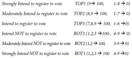
box 2

The statistical analysis OLS (ordinary least squares) regression needs some minimum amount of variation in the dependent variable. Across the entire set of 460 respondents, it is very likely that the respondents will not generate the same rating (e.g., TOP3, all respondents rating the 48 respondents 7-9). If the respondents were to somehow do so, the statistical analysis would crash. On the other hand, for individual respondents, it is likely that a respondent might confine all ratings to 1-3, making BOT3 always 100. IN that case, the OLS regression would crash when creating a model or equation for that one respondent, bringing the entire processing to a halt.

To forestall the problem of a ‘crash; we add a vanishingly small number to each of the binary transformed variables that we just create ensuring that the actual transformed ratings vary a very little but do vary around the levels of 0 and 100, respectively. There is no meaningful effect on the regression coefficients emerging after performing this small prophylactic adjustment, but we prevent crashes. Indeed, without this adjustment, about 5% of the respondent models ‘crash’ because the respondent’s transformed numbers either all map to 100 or all map to 0.

The experimental design at the level of both the individual and at the level of the group allows us to create equations relating the presence absence of the elements to the transformed, binary ratings. We create six equations, each expressed as:

Binary Rating = k0 + k1(A1) + k2(A2) … k35(F5) + k36(F6)

Each equation is characterized by its own additive constant, and its own array of 36 coefficients. We interpret the additive constant as the expected percent of the respondents who will register to vote or not register to vote (according to the variable definition), albeit in the absence of elements. The additive constant is a purely estimated parameter but can be used as an index for predilection to register to vote. We expect increasing magnitudes of the additive constant as we go from TOP1 (Definitely intend to register to vote) to TOP3 (Intend to register to vote), and we expect a decreasing magnitude of the additive constant as we go from BOT3 (intend not to register to vote) to BOT1 (definitely not intend to register to vote). For the first analysis, we create six equations or models, based on the data from the total panel, and using each of the newly created binary variables as a dependent variable. With 36 elements, and six dependent variables, the OLS regression generates a massive amount of data (six additive constants, 216 coefficients, viz., 36 coefficients for each of the binary variables). That amount of information overwhelms the researcher, disguising patterns where they exist. To uncover the pattern, we blanked out all coefficients of 3 or lower, only to end with no strong performing elements. For the Total Panel only, we looked at elements with coefficients of +2 or higher. For all other analyses of coefficients, we look at elements with coefficients of +3 or higher. We begin first with the additive constant, the estimated propensity to register to vote, in the absence of elements. As we expected looking for individuals who feel strongly about voting generates a low additive constant of 10 (viz., for TOP1). We are likely to find only about 10% of the responses to be a ‘9’, in the absence of elements. When we make the criterion easier, accepting a 7, 8, or 9, (viz., TOP3) the additive constant jumps to 27.

Table 3 shows us that despite our efforts to find motivating elements, only six elements passed the relatively easy screen, viz., a coefficient of +2. The coefficient of +2 is very low in the world of Mind Genomics. Table 3 shows that the effort to find drivers of voting produced only three elements which show any promise, using the data from the total panel, and the promise they show is less than enthusiastic.

A4 You’ll be done registering in 5 minutes or less.

B2 You can get immediate answers for voter registration questions by calling, 1-800-FOR-VOTE.

D6 Voting allows you to be an advocate for your family and for your community: control your leadership and control your life.

When we move to the response ‘Not Register to Vote’ we see a similar pattern. The additive constants are similar in magnitude and go in the right direction. The strong statement about not voting, a rating of 1, captured by the variable BOT1, suggest that 10%, saying they would not definitely register to vote when the criteria are made less strict.

These are the three elements, presumed at the start of the experiment to drive positive voting, but instead drive the opposite, not registering to vote:

D3 Be an example for those who look up to you.

E5 You may have your things unpacked, but you haven’t moved in until you’ve registered.

F2 Government “of the people and by the people” requires your participation. The solution to your problems starts by registering.

Table 3: “Strong’ performing elements from the total panel, defined operationally as a coefficient of at least +2. Only those coefficients are shown. Missing elements failed to generate any coefficients of 2.0 or higher for any of the binary dependent variables.
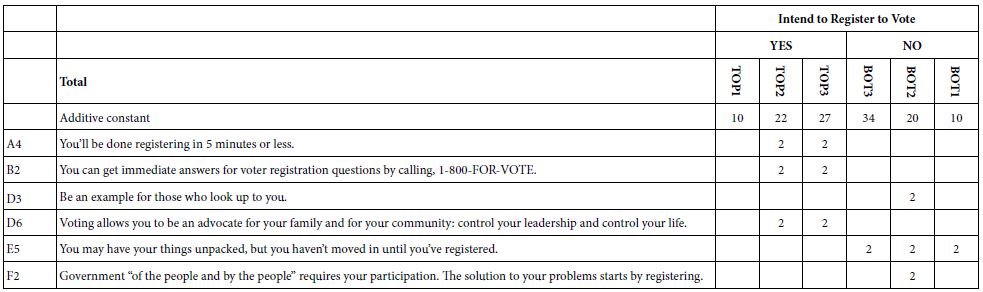
table 3

Do People Change Their Stated Likelihood of Voting During the Interview?

Having now looked at the data from the total panel, and finding very little, we must pursue the reason why we fail to discover strong elements from the total panel. If we did not have the underlying structure, we would not know how weak the data are from the total panel. We would simply choose the strongest performing vignette and work with that vignette. Such an approach characterizes the research where the stimuli are put together, without structure. If we have one or two or even three or four elements varying, we might make a good guess, but we could not be sure. Mind Genomics take us in a different direction, to uncover the performance of the elements. It is those elements which constitute the building blocks of revised potentially better performing elements. Our first analysis looks at the (possible) change in the rating assigned by the respondents as the interview or experiment progresses. Recall that each respondent evaluated 48 unique vignettes, each vignette comprising 36 combinations of four elements (one from each of four questions), and 12 combinations or vignettes of three elements (one from each of three questions). By design, and by the systematic permutation of the vignettes, respondents saw different vignettes. We cannot measure change in the response to a specified vignette which most likely appeared just a few times, but we can measure the relation (if any) between the average rating assigned by the respondent and the order in the study (rating 1-9 for each vignette, order 1-48).

Our analysis uses OLS regression, done at the level of the individual respondent. For each respondent we know what was assigned to each vignette rated by the respondent, as well as the order of testing. We express the relation as: Rating (9-point scale) = k0 + k1(Order of Testing). The slope, k1, tells us the effect of repeating the interview. We are interested in the sign of the slope, k1, and then the magnitude of the slope. When k1 is positive we conclude that the respondent becomes more interested in registering to vote as the interview or experiment goes on. It may be linked to the respondent being more sensitive to messaging. When k1 is negative we conclude that the respondent becomes less interested in registering to vote as the interview or the experiment on. The respondent may be turned off. In turn, the magnitude of the slope, viz. the numerical value of k1, tells us how many rating points on a 9-point scale will be added to the rating or subtracted from the rating for each additional vignette evaluated. Figure 1 shows the estimated magnitude of change in the rating assigned by a respondent across the 48 vignettes. Most of the respondents show a small change in the rating from vignette #1 to vignette #48. Most the respondents are within +/- two points on the 9-point rating scale. Keep in mind that the regression analysis generating the data was did not look at the actual range, but simply the pattern of changes manifesting itself at the individual respondent level.
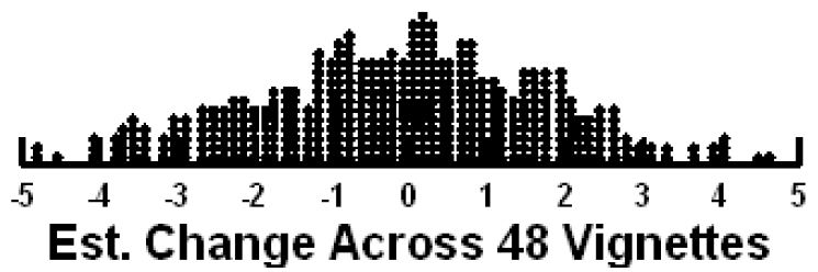
fig 1

Figure 1: The distribution of expected ranges to be expected as the respondent proceeds to evaluate 48 vignettes. Most of the range lies between an increase of 2 points to a decrease of 2 points from first vignette to last vignette.

Thus far we know the behavior of the respondent and can differentiate those respondents who are likely to increase versus decrease their ratings. We do not know anything about their criterion for making their judgments. We could ask the respondents to tell us their criteria, but it’s unlikely that they could tell us. The interview is so short, the vignettes judged so quickly, and the attention to the topic only modest while the interview is going on. Despite what might be wished for by novice researchers, most experienced researchers in these types of studies KNOW that their respondents are barely interested in the topic and are answering automatically to stimuli which much seem to them like a ‘blooming, buzzing confusion’. Those are the words of Harvard psychologist William James, when describing how a baby must perceive the world. Fortunately, Step 2 above tells us that despite the response of the respondent (or professional) asked to describe the test stimuli, there is a strongly laid structure underlying each respondent’s set of 48 vignettes. The structure prescribes exactly which elements belong in each vignette, doing so down to the level of a single respondent. We divide the respondents into three groups, defined qualitatively as those with positive range (one point or greater increase in the rating from vignette #1 to vignette #48), those with a flat range (between -1 and +1 point across 48 vignettes), and those with negative range (one point or greater decrease in the rating across 48 vignettes). The first become more interested in registering to vote, the second don’t really change their rating, and the get turned off.

Table 4 shows the strong performing elements for each group. Again, we select only those elements which have a breakthrough coefficient, now defined as +4, but which could easily be changed. The objective is to reduce the ‘wall of numbers’ to a limited set with the patterns coming through.

We see the following patterns emerging:

  1. There are breakthrough elements for Groups 1 (positive range) and Group 3 (negative range), but no strong elements for Group 2 (flat range)
  2. Despite the differences between the groups, and the differences in the patterns of the additive constants, there is no clear ‘story’ about what is driving Group1 (positive range) vs. Group 3 (negative range).

Table 4: Strong performing elements for three groups created on the basis of the range of the 9-point rating to be observed as the respondents proceeds to rate vignette 1 to vignette 48.
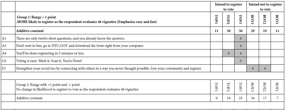
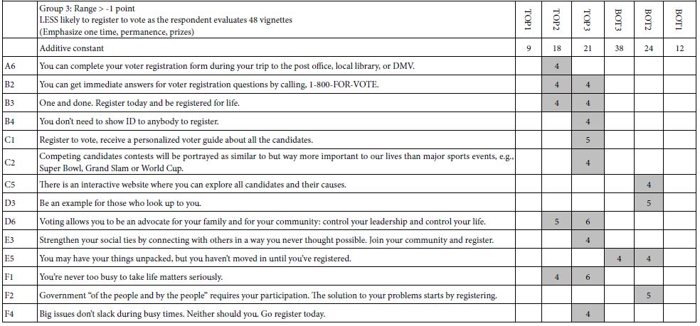
table 4(1)

fig 4(2)

We conclude that if there is a story, it is deeper than the observed patterns of responses. Looking at large morphological differences in the patterns of responses gives us a lot of data, a lot of comparisons, but sadly no insight.

Uncovering Underlying Mind-sets based on the Pattern of Coefficients

One of the hallmark features of Mind Genomics is its focus on the decision-making of the everyday, and the recognition that the variability often observed in the data may be result in part from the combination of underlying groups with different criteria. A good metaphor is white light without color. One who looks at white light would say that it is colorless, but the structure of white is that emerges from three primary colors, red, blue, and yellow, respectively. Continuing the metaphor, what if the lack of strong, interpretable patterns in the data come not so much from lack of patterns, nor from intractable variability, but rather from the class of different mind-sets, having different criteria. The failure to uncover strong patterns may be the result of mutual cancellation. Mind Genomics researchers have worked out simple ways to identify these mutually exclusive primary groups, without the benefit of ‘theory’ about how the topic actually works, but simply on the basis of ‘hands-off’, clustering. Recall that each respondent evaluated a unique set of 48 vignettes, embodying the 36 elements in different combinations, with the data from each respondent constituting a complete experimental design. That is, each respondent both evaluated different combinations, but the mathematics of each set of combinations allows us to create a model for that individual [15].

To create these primary groups, or ‘mind-sets’, we followed these steps, adapting the Mind Genomics process, but incorporating two dependent variables simultaneously, register to vote (TOP2), and not register to vote (BOT2).

  1. Create the mind-sets on the basis both of drivers of registering to vote, and drivers of NOT registering to vote. That is, we were interested in moving beyond one direction (drivers of registering to vote)
  2. For each of the 460 respondents, create a model for TOP2 relating the presence/absence of the 36 elements to the TOP2 value. Create another model for BOT2. We thus have 460 pairs of coefficients, each pair comprising 36 coefficients.
  3. When estimating the model for each respondent, do not use the additive constant. The rationale is that we will be combining the two sets of 36 coefficients to create a set of 72 coefficients for each respondent. All the information must be available solely in the coefficients. The technical appendix shows that estimating the coefficients without an additive constant produces the same pattern of coefficients as estimating the coefficients with an additive constant. The only difference is the magnitude of the coefficient. Figure 2 in the Technical Appendix shows the high co-variation between the two sets of coefficients, estimated for the same data, one without and one with the additive constant, respectively.
  4. Create the 460 rows of data, comprising 36 coefficients for TOP2, and 36 coefficients for BOT2. Each respondent now has 72 coefficients.
  5. Use principal components factor analysis to reduce the size of the matrix, by extracting all factors with eigenvalues of 1 or higher. This produced 19 factors.
  6. Rotate the factors by a simplifying method, Quartimax, to produce a set of 19 new factors, rather than 72. Each respondent becomes a set of 19 numbers, the factor scores in the structure, rathe than a set of 72 numbers. We van be sure that the 19 factors are independent of each other.
  7. Extract two and three clusters, or mind-sets, based on strictly numerical criteria [16]. The cluster method is the k means clustering, with the measure of distance between any two people defined by (1-Pearson Correlation between the two people on the 19 factors). In practical terms, any clustering method will do the job, since the clustering is simply a heuristic to divide the 460 respondents into similar-behaving groups
  8. The principal component factor analysis allows us to create models for two segments (mind-sets) corresponding to the two-cluster solution, and three segments (mind-sets) corresponding to the three-cluster solution. The three-cluster solution was clearer. One could extract ore clusters, or mind-sets, but we opted for parsimony.

Create the six equations, with additive constants, for each of the three mind-sets, using the respondents allocated to the mind-sets. Eliminate all elements which fail to exhibit a coefficient of +4 in any model. This step winnows out most of the elements. The elements which remain show strong performance, and also suggest an interpretation, something not seen the previous data because variables did not have ‘cognitive richness’.

Table 5 suggests that there are three subtly different groups

MS 1 – A sense of voting is easy, fun, like sports. Don’t want to be reminded of the ‘seriousness’ of voting

MS 2 – Make it easy, make it simple, learn. They are ready. Nothing really turns them off.

MS 3 – Hates lines, make it easy. That’s all. Avoid talking about social responsibility. It’s a turnoff

The additive constants suggest that Mind-Set 1 (voting as fun) is most likely to register, without messages

Mind-Set 2 is likely to register. Nothing really turns them off.

Mind-Set 3 can be swayed by the right or wrong messages

The three mind-sets differ both in the pattern of likelihood to register and in the topics which turn them off, if there are any. Only Mind-Set 3 really responds in a way that suggest they are turned off.

Table 5: Strong performing elements for three emergent mind-sets (coefficient > = 4).
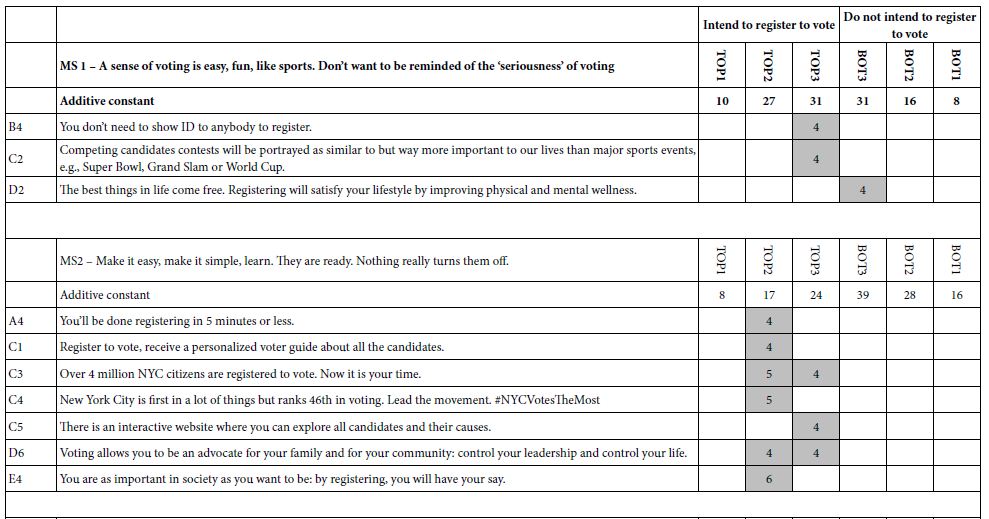
table 5(1)

table 5(2)
 
fig 2

Figure 2: Scatterplot based on the data from the total panel, showing the strong co-variation of the 36 coefficients when estimated with an equation with an additive constant, vs. absent an additive constant.

Synergisms in Messages – Increasing the Likelihood of Mind Set 1 to Say They Will Register to Vote

As noted above, most conjoint measure studies with experimental design focus on a limited set of combinations, with the respondent testing all or only some of the combinations. None of the methods use permuted designs. It is the permuted design which allows the research to explore a great deal of the design space. One of the unexpected benefits is the ability to identify synergism and suppressions between pairs of elements. It to the study of interactions, and the search for synergism that we now turn.

Moskowitz and Gofman [11] introduced the notion of ‘scenario analyses for Mind Genomics. The guiding notion is that pairs of elements may synergize with each other, but the synergy could be washed out in a larger design. A better way to find out whether elements synergize is to select one of the questions (e.g., F), and separate all the data in the study into one of seven different strata, specifically all those vignettes where there is no F (by design), all those vignettes where F is held constant at F1, all those vignettes where F is held constant as F2, etc. Our starting data, therefore, is a set of several strata. We will end up running seven equations of the same type, one equation for each stratum. The equation will have only 30 independent variables (A1-E6), because for each stratus there is a single value of F, a single element. The set of elements from F are no longer independent variables. They simply exist in the vignette, or in the case of F0 deliberately left out of the vignettes. We can now select a target population, e.g., Mind Set 1, and run the regression seven times, once for each stratum. We will choose the most stringent dependent variable, TOP1 (definitely register to vote). The independent variables will be A1-E6, 30 out of the 36 variables. The additive constant is still the expected percent of response TOP1 (rating of 9, definitely register to vote), in the absence of the elements. The coefficients are the incremental percent of responses ‘will register to vote’ when the element appears in the vignette. Armed with that information let us now run the reduced model on each of the seven strata. Table 6 shows the coefficients. The columns correspond to the seven different strata. The rows correspond to the elements which show coefficients of at least +10 in one stratum. These are elements which are expected to synergize. To make navigating easier, and to uncover the strong performing combination, we present only those cells with positive coefficients of +4 or higher. The simplest way to discover combinations is to search for the shaded cells with the highest coefficient and add that high coefficient to the additive constant. The result will be the estimated score for that pair of elements as the key message. There are several very strong combination, combinations that we would not have guessed, first in the absence of mind-set segmentation, and second, in the absence of ability to uncover synergistic (or suppressive) combinations. A good example is the synergistic pair (F4, B6), and then ‘finished off’ with element D5. Table 6 suggests that the total score for TOP1 (definitely would register to vote) would be 11 for the additive constant, 15 for the synergistic pair (F4, B6, or 26 points. There is room for one more element, which we are free to choose, as long as the element makes intuitive sense and fits with F4 and B6. One example could be D5:

F4 = Big issues don’t slack during busy times. Neither should you. Go register today.

B6 = Everything you like and everything you don’t like in government came from elected officials. Your vote does matter.

D5 = Regret is the result of knowing you could have done more for your life. Register today, regret nothing tomorrow.

A possibly better strategy emerges when we look at F2 as an introductory phrase. The element itself does not bode well (additive constant of -1), but it synergizes with four of the six elements show in the stub (row) of Table 6.

F2 Government “of the people and by the people” requires your participation. The solution to your problems starts by registering.

B2 You can get immediate answers for voter registration questions by calling, 1-800-FOR-VOTE.

C4 New York City is first in a lot of things but ranks 46th in voting. Lead the movement. #NYCVotesTheMost

D2The best things in life come free. Registering will satisfy your lifestyle by improving physical and mental wellness.

E4 The best things in life come free. Registering will satisfy your lifestyle by improving physical and mental wellness.

Table 6: Strong pairwise- interactions between elements F1-F6, and the remaining elements. The data come from respondents in Mind-Set 1.
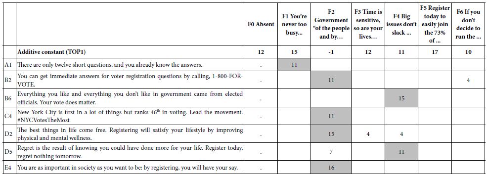
table 6

Discussion and Conclusions

The world of public policy requires that the citizens perform their duties. Some of these duties are mandatory, such as military service, education, and obeying the law. Some are rights, not necessarily duties, such as registering to vote. Ask any group of people about how they feel about registering to vote, and you are likely to get a range of answers, from affirmation of patriotism, to indifference, to the absolute dislike of registering to vote because it is at once disinteresting, a duty, and worst of all, it puts one on the list for jury duty, another public service not in great favor. The sentiments around registering to vote are often simply measured as ‘yes/no’, e.g., will you register to vote or not register to vote. In this Mind Genomics study (really experiment), we have gone into the topic as it were a product or service, being offered to the respondent. We have used the language often used to ‘convince,’ only to discover that across the entire panel respondents, there are really no strong messages. If voting were a service or a product, we would ‘go back to the drawing board’ and try again

The speed, simplicity, cost, and templated structure of Mind Genomics, especially with smaller versions of the study presented here, 16 rather than 36 elements, makes it now possible to iterate through, testing different messages of a ‘public service’ nature. Public service messages may be viewed as a necessary evil, to be checked off, even though they contain little of a sales nature, and are primarily exhortations to do one’s duty and to be good citizens. Or, as Mind Genomics suggest, public service messages may provide the necessary matrix of ideas to use as a way to understand and to motivate the citizen. The study run here itself constitutes a larger-than-usual study in terms of the ideas explored. The results suggest a lack of knowledge of ‘what really motivates people,’ or more correctly a lack of understanding of people who are the targets of communication for a topic which is at best unromantic, quotidian, ordinary, and perhaps even potential negative because it could lead to jury duty. How interesting, however, the study becomes when we peel back the layers, understand the minds of people through segmentation, and through understanding of synergies where two messages combine to do far more than one expected. This type of information, collected across different types of studies, in an iterative process, builds a bank of knowledge for messaging about the common weal, the common good. Having a process such as Mind Genomics embedded in our societal life and in our political process offers far greater benefits to society than we can imagine today. Just imagine messaging for the social good, and doing it expeditiously, inexpensively, effectively.

Technical Appendix Relation between Coefficients Estimated with vs. without the Additive Constant

Mind Genomics is founded on the use of experimental design and OLS (ordinary least-squares) regression. Experimental design creates the test stimuli (vignettes) by specifying the specific combinations. OLS regression deconstructs the response to the vignettes, to estimate the part-worth contribution of each element to the respondent. Traditional Mind Genomics has worked with OLS regressions estimated with an additive constant. The constant is a measure of the likelihood of the response in the absence of the stimulus, a purely theoretical parameter. In this study, comprising six questions, each with six answers or elements, the experimental design called for 48 vignettes. Each element appeared 5x in the 48 vignettes and was absent 43 times. We can estimate two equations for the Total Panel, or indeed two equations for any subgroup, both equations using the same data.

Equation 1: Equation with the additive constant

Binary Dependent Variable (e.g., TOP2) = k0 +k1(A1) + k2(A2) … k36(F6)

Equation 2…which looks exactly like equation 1, but has no additive constant

When we estimate the coefficients, and plot one set against the other in a scatterplot, Figure 2 tells us that the patterns are the same, although the coefficients are higher when there is no additive constant. Figure2 shows an almost perfect co-variation of coefficients estimated in the two ways (R=0.94), with different values, however for the same element.

Acknowledgments

The authors wish to acknowledge the contributions of those students at Pace University, New York, who designed, executed, and wrote up the study for presentation to the Office of the Mayor of New York City. The strategy and messaging were used prior to the elections to encourage New Yorkers to register to vote in the upcoming election. The students then presented the study to professional direct marketers, at a direct marketing conference. In their own words ‘this is a great, practical tool which taught us a lot as we used it and got to see what we could accomplish.’

References

  1. Harder J, Krosnick JA (2008) Why do people vote? A psychological analysis of the causes of voter turnout. Journal of Social Issues 64: 525-549.
  2. Gershtenson J, Plane DL, Scacco, J.M. & Thomas, J., (2013) Registering to vote is easy, right? Active learning and attitudes about voter registration. Journal of Political Science Education 9: 379-402.
  3. Jennings W, Wiezien C (2018) Election polling errors across time and space. Nature Human Behaviour 2: 276-283.
  4. Rubado ME, Jennings JT (2020) Political consequences of the endangered local watchdog: newspaper decline and mayoral elections in the United States. Urban Affairs Review 56: 1327-1356.
  5. Kaufman RR, Haggard S (2019) Democratic decline in the United States: What can we learn from middle-income backsliding? Perspectives on Politics 17: 417-432.
  6. Dale A, Strauss A (2009) Don’t forget to vote: Text message reminders as a mobilization tool. American Journal of Political Science 53: 787-804.
  7. Knack S (1993) The voter participation effects of selecting jurors from registration lists. The Journal of Law and Economics 36: 99-114.
  8. Xu AJ, Wyer Jr RS (2012) The role of bolstering and counterarguing mind-sets in persuasion. Journal of Consumer Research 38: 920-932.
  9. Krantz DH (1964) Conjoint measurement: The Luce-Tukey axiomatization and some extensions. Journal of Mathematical Psychology 1: 248-277.
  10. Green PE, Krieger AM, Wind Y (2001) Thirty years of conjoint analysis: Reflections and prospects. Interfaces 31: S56-S73.
  11. Moskowitz HR, Gofman A (2007) Selling blue elephants: How to make great products that people want before they even know they want them. Pearson Education.
  12. Miller GA, Galanter EH, Pribram KH (2017) (Orig. 1960). Plans and the Structure of Behavior, Routledge.
  13. Moskowitz HR (2012) ‘Mind Genomics’: The experimental, inductive science of the ordinary, and its application to aspects of food and feeding. Physiology & Behavior 107: 606-613.
  14. Moskowitz HR, Gofman A, Beckley J, Ashman H (2006) Founding a new science: Mind Genomics. Journal of Sensory Studies 21: 266-307.
  15. Gofman A, Moskowitz H (2010) Isomorphic permuted experimental designs and their application in conjoint analysis. Journal of Sensory Studies 25: 127-145.
  16. Xu R, Wunsch D (2008) Clustering (Vol. 10). John Wiley & Sons.

Social Determinants Do Not Determine Me

DOI: 10.31038/AWHC.2021452


The apartment complex in which I lived growing up was called, “The Bellagio,” and its name was written in golden, cursive letters on the exterior of the building. As a child I always thought this name sounded so elegant, like a ballet dance step. But if you unlocked the front door, you would notice the dingy grey carpet, the cracked and yellowing blinds, and the faint stench of tobacco emanating from the apartment of the old man who lived in the unit below. It wasn’t elegant, but to my single mother and me, it was home.

My mother frequently tells me, “I didn’t want us to be another statistic.” What she meant was that as young, Hispanic women who lived below the poverty line, society expected our lives would amount to very little. These multidimensional identities – female, poor, Hispanic – had placed us at the front doorstep of intergenerational poverty, which we would have to defy serious odds to overcome. In medicine, we call these obstacles the “social determinants of health,” which we use to predict and explain health outcomes. But these issues do more than impact risk of disease: they extend their roots into class, career, and community. From the air quality of a neighborhood to the processed sugars in affordable food, they act as the cloudy weather that influences how readily the blossoms of life can bloom. My reflections on my childhood inform my understanding of how these social determinants both did and did not “determine” my life and provide a unique opportunity to serve and advocate for poor families, Hispanic families, and especially those families led by single parents.

Recent data demonstrates that families headed by single mothers are most vulnerable to poverty [1,2] and that their children face greater obstacles related to educational achievement and adjustment in school [3]. Indeed, for many years my mother and I relied on government assistance programs, including Aid to Families with Dependent Children (AFDC), Women, Infants and Children (WIC), and Medicaid, which funded the bare necessities required for child rearing. I remember spending afternoons in a grey government building playing with communal toys that had been well-loved by many children before me while my mother secured diapers and milk for another week.

Despite these barriers, I was fortunate to be among the 6.8% of Hispanic applicants that are accepted to medical school [4,5] a percentage that shrinks even further if you control for class, gender, and single-parent households. This felt strange to me, given that almost 18.5% of the American population is Hispanic or Latino, a number that continues to rise [6]. Together, these statistics suggest a severe underrepresentation of Hispanic medical school applicants and matriculants relative to the age-adjusted US population [5].

I felt the effects of my minority status almost immediately after starting medical school. During my first week, a group of peers were recounting their favorite travel stories. They took turns sharing tales of Icelandic landscapes and tropical paradises. In that moment, I realized I was one of very few to not have had those same kinds of experiences. My only travel history was my semester abroad, and I had taken out extra loans just to afford the plane ticket. It felt like no one else in my medical school cohort had a background like mine. The voice in my head told me that if you’re standing in a space where no one relates to you, that’s an unspoken affirmation that maybe you don’t belong there. This became a pattern, as I was reminded again and again that my peers and I had very different upbringings, leaving me searching for a personal connection to medicine.

Despite these peer interactions that colored my early medical school experience, I found that in clinical practice, many of my patients did share in my life experiences. It felt familiar interacting with patients who lived in poor areas reminiscent of my own neighborhood, or who were children of single parents. These patients remind me that I belong in medicine, and that my visibility and perspective are important. All patients can benefit from encountering physicians that look like them and relate to their background. These relationships can decrease subconscious bias [7], bridge gaps in health care delivery, and build a deeper bond of trust. Interactions with this patient population remind me that I represent the children of poor, Hispanic, single-parent households, and my personal connection to medicine is found in serving them.

One story from my clinical experiences that has remained with me is an encounter I had on the Mother-Baby Unit during my pediatric rotation. We were rounding on a one-day-old Hispanic baby girl whose mother was a single parent. After asking the mother about whether she needed financial assistance, the attending physician handed her a pamphlet on WIC, then wished her a genuine “good luck” before we hurried on to see the next family. As we left, I noticed that the mother had started to cry.

I couldn’t stop thinking about this mom and her child, and how closely this family dynamic mirrored the experience of my own mother. Alone and at the starting line of single parenthood, had someone once handed my mom a pamphlet on WIC? I couldn’t shake the need to go back to her room and take some time to initiate a heartfelt conversation. I rehearsed the different ways I could tell her that I understood her situation first-hand. I wanted her to know that single parenthood didn’t have to define what her and her daughter’s lives could be, and that there was every possibility that her daughter could accomplish anything she wanted, even end up in medical school someday.

As we finished rounding, I walked back to her room and stood outside the door. I started to doubt myself. I wondered if this conversation was inappropriate or unprofessional, or if I was somehow overstepping my boundaries as a medical student. I lingered outside her room for a few minutes, and when I finally walked in, she was asleep. I wish I could say that I came back later, spoke with her, and made a meaningful impact. But instead, I let the fear of repercussions get the best of me. Looking back, that experience taught me that if I want to make a difference in the lives of my patients, I must be brave and bold, as well as confident that these conversations and visibility are needed and necessary.

While I enjoy working with my peers to provide quality care, my sense of community is fulfilled by working with underserved patients. I am motivated to share my stories and explore the ways in which medical professionals can better advocate for and communicate with them. With these efforts, I strengthen my personal value system, bridge gaps in health equity, and pay homage to my upbringing. I am proud to be an example of how although “social determinants” may have an impact on life, they do not automatically determine worth, value, or achievement.

Abbreviations

AFDC: Aid to Families with Dependent Children

WIC: Women, Infants and Children

References

  1. McLanahan S, Percheski C (2008) Family structure and the reproduction of inequalities. Annu Rev Sociol 34: 257-276.
  2. Damaske S, Bratter JL, Frech A (2017) Single mother families and employment, race, and poverty in changing economic times. Social science research 62: 120-133. [crossref]
  3. Carlson MJ, Corcoran ME (2001) Family structure and children’s behavioral and cognitive outcomes. Journal of marriage and family 63: 779-792.
  4. https://www.aamc.org/data-reports/students-residents/interactive-data/2020-facts-applicants-and-matriculants-data Accessed July 19th, 2021.
  5. Lett LA, Murdock HM, Orji WU, Aysola J, Sebro R (2019) Trends in racial/ethnic representation among US medical students. JAMA network open 2: e1910490-e1910490. [crossref]
  6. United States Census Bureau: QuickFacts. 2019. https://www.census.gov/quickfacts/fact/table/US/RHI725219. Accessed June 16th, 2021.
  7. Bean MG, Stone J, Badger TA, Focella ES, Moskowitz GB (2013) Evidence of nonconscious stereotyping of Hispanic patients by nursing and medical students. Nursing research 62: 362-367. [crossref]

Hematological Changes Associated with Amoxicillin, Paracetamol and Their Combinations on Rabbits

DOI: 10.31038/IJVB.2021542

Abstract

Extensive use or misuse of antibiotic and analgesic may lead to hematological changes. This study characterized the hematological changes associated with chronic gavage of Amoxicillin and Paracetamol in rabbits.

Amoxicillin, Paracetamol and their combination were dissolved in distilled water and given a rate of (0 mg/kg), (8 mg/kg), (24 mg/kg) and (4 mg/kg+12 mg/kg) to four groups of rabbits (control, amoxicillin, paracetamol and mixture group) respectively for 2 weeks period followed by 6 weeks relaxation period. Then rabbits were authenticated and sacrificed, blood samples were collected in EDTA-containing tubes and analyzed for complete blood counts using the standard blood analysis method.

Results showed significant increase in white blood cell (WBC) count only in paracetamol treatment. Furthermore, significant increases in hemoglobin (HGB), hematocrit (HCT) were observed in all treatments, whereas platelet (PLT) levels significantly increased in amoxicillin and paracetamol treatments and reduced in mixture treatment. In conclusion, the tested compounds significantly changed blood parameters suggesting potential hematotoxicity due to use of amoxicillin, paracetamol or their combination.

Keywords

Amoxicillin, Blood parameters hematotoxicity, Paracetamol

Introduction

Misuse of amoxicillin (an antibiotic) and paracetamol (an analgesic) may become one of the most difficult problems facing the health sector, which must have a quick and effective solution.

Antibiotic are specific chemicals that kill, slow or stop bacterial growth, they are commonly used by physicians to treat bacterial infections. Amoxicillin was first produced in UK in 1970 and used as antibacterial infections for gram positive bacteria [1]. It has a wide spread application for medical treatments [2]. It may cause liver injury [3,4], health risks due to its side effect to many organisms including fish [5,6].
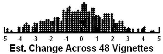
Paracetamol/acetaminophen is one of the most widely used analgesics, clinical studies indicated many side effects [6]. So far, paracetamol or its metabolites may cause severe hepatic failure [7-9], acute live injury and cell death [10,11], inhibition of excessive amount of N-acetyl-p-benzoquinone imine formation [12], binding quinone reductase 2 in the kidney and liver [13] kidney damage [14] and inhibition of mitochondrial respiration [15].

Hematological changes associated with amoxicillin, paracetamol or their combinations among human beings are not fully understood, a gap of information is still missing. The authors designed this study to measure the hematological changes associated with use of amoxicillin, paracetamol and their mixture on rabbits. Rabbits were chosen as experimental animals because they are big enough, and have similar physiology to human beings [16].

Amoxicillin

Amoxicillin is a (2S,5R,6R)-6-[[(2R)-2-Amino-2-(4-hydroxyphenyl)acetyl]amino]-3,3-dimethyl-7oxo-4-thia-1-aza-bicyclo[3.2.0]heptane-2-carboxylic acid, semi-synthetic, acid stable drug belongs to a class of antibiotics called the Penicillins (B-lactam antibiotics).

Materials and Methods

Chemicals

Amoxicillin and Paracetamol (purity 99%) were obtained from Middle East Pharmaceutical and cosmetics laboratories Co .LTD. All other chemicals used in the experiment were purchased from standard commercial suppliers.

Experimental Animals

Adult male rabbits were purchased from locally certified farms. They were housed in a suitable room equipped with air conditioning according to US-EPA 2004 for a period of two weeks initially to acclimate to insure a stable experimental condition. The rabbits were properly maintained according to the principles and guidelines issued by the Ministry of Agriculture in Gaza And US-EPA2004 for animal care, rabbits were individually placed in appropriate steel cages at 22-26°C, 40-70% humidity and a clean environment with a light/12 hour cycle. A suitable diet of balanced feed and clean water has been provided for the duration of the total experiment.

Preparation of Amoxicillin and Paracetamol Solution

One gram (1000 mg) of Amoxicillin was dissolved in 100 ml of distilled water and1000 mg of Paracetamol was dissolved in 100 ml of distilled water under magnetic steering to ensure complete solubility of drugs . This was visualized by clean solution of water.

Experimental Design

Rabbits were randomly subdivided into four groups five rabbits each group, and monitored during 10 weeks, study period, (2 weeks of acclimatization +2 weeks of treatment +6 weeks without treatment). After acclimatization period, rabbits received the following treatments:

Group 1: Each rabbit received by oral administration amoxicillin at a rate of 8 mg/kg BW for 14 days; Group 2: Each rabbit received by oral administration paracetamol dose at a rate of 24 mg/kg BW for 14 days; Group 3: Each rabbit received by oral administration a mixture of Amoxicillin and paracetamol at a rate of 4 mg/kg BW+12 mg/kg BW for 14 days; and Group 4: control group, each rabbit received by oral administration 1 ml distilled water/rabbit for 14 day. Photo 1 shows the gavage process of the tested compounds.
photo 1

Photo 1: Oral administration of the tested compounds on rabbits

Collection of Blood Samples

At the end of the experimental period (10 weeks) rabbits were authenticated to for blood sample collections via cardiac puncture into sterile tubes containing EDTA to prevent blood clotting, then analyzed for CBC using standard method and previously described [17].

Statistical Analysis

Average and standard deviation were calculated. Analysis of Variances (ANOVA) was employed to detect significant differences among treatments at p-value 0.05. p-value ≤ 0.05 indicates significant differences among treatments whereas values > 0.05 are not significant.

Results

Effects on the Blood

Effects of the tested compounds on white blood cells (WBC) are shown in Figure 1.

fig 1

Figure 1: Chemical structure of amoxicillin and paracetamol.

It can be seen that concentration of WBC was increased in the treated rabbits above that of the control group. Statistical analysis detected significant differences only in paracetamol treatment.

Effects on blood lymph (LYM) are shown in Figure 2.

fig 2

Figure 2: Concentrations of WBC in rabbit treated with Amoxicillin, Paracetamol, and their mixture. Error bars represent standard deviation. Columns have the same letter are not significantly different at p ≤ 0.05.

Similarly, to the effects on WBC (Figure 2) increased levels of LYM were observed in rabbits treated with the tested compounds but statistical analysis did not detect significant differences among treatments.

Effects of the tested compounds on red blood cells are shown in Figure 4. Similarly, to the effects on lymph, increased level of red blood cells were observed in the treated rabbits but no significant differences were detected.

fig 4

Figure 4: Concentrations of RBC in rabbit treated with Amoxicillin, Paracetamol, and Their mixture. Error bars represent standard deviation.
Columns have the same letter are not significantly different at p ≤ 0.05.

Effects of the tested compounds on the blood hemoglbine (HGB) are shown in Figure 5. Increased levels of HGB were observed in the treated rabbits. Satstical analysis detected significant difference among all treatment. this suggests an occurrence different biochemical reactions between HGB and the tested compounds.
fig 5

Figure 5: Concentrations of HGB in rabbit treated with Amoxicillin, Paracetamol, and Their mixture. Error bars represent standard deviation.
Columns have the same letter are not significantly different at p ≤ 0.05.

Effects of the tested compounds on hematocreate (HCT) are shown in Figure 6. Similarly to the above effects, increased level of HCT were found in the treated rabbits but statistical differences were detected only in Amoxicillin and mixture treatments.
fig 6

Figure 6: Concentrations of HCT in rabbit treated with Amoxicillin, Paracetamol, and Their mixture. Error bars represent standard deviation.
Columns have the same letter are not significantly different at p ≤ 0.05.

Effects of the tested compounds on the platlets (PLT) are shown in Figure 7. Similarly to the above effects, increased level of PLT were found in the treated rabbits. Statistical analysis detected significan differences.
fig 7

Figure 7: Concentrations of PLT in rabbit treated with Amoxicillin, Paracetamol, and Their mixture .Error bars represent standard deviation.
Columns have the same letter are not significantly different at p ≤ 0.05.

The concentration of WBC and PLT in rabbits blood treated with Paracetamol were the highest among all treatments then Amoxicillin, whereas the concentration in rabbits treated with Mixture were lower than those of the control samples.

Discussion

Amoxicillin used as an antibiotic against bacteria [18] whereas paracetamol used as an analgesic for many diseases. There usage was associated with many complications as mentioned above. Furthermore, their chemical structure (Figure 1) shows the presence of highly water soluble groups such as (OH; C=O) which facilitate interaction and movement of the compounds in aqueous phase such as blood system. Additionally, the chemical structure includes phenyl ring which may enable covalent bonding with liver, kidney, and/or other tissue causing induced injury, in accordance with Lee et al. [19] who revealed similar phenomenon with other cases. Photo 1 show the oral gavage process of the tested compounds. The data in Figure 2, clearly demonstrates the effects of tested compounds on WBC. It can be seen that Amoxicillin and paracetamol increased WBC above that of the control, whereas the combination reduced the values. This suggests that treatments with Amoxicillin and paracetamol enhance the immune system to produce more WBC to defend the body from amoxicillin and paracetamol. Thus an increase of WBC cell would have occurred to enrich the body with the required level of WBC to insure health body. Our explanation agree with Díaz et al., [20] and Zarkesh et al., [16] who revealed the importance of WBC count on blood levels as long as the body exposed to bacterial infections and/or toxic chemicals [21,22].

On the other hand, the combination of the compounds did not increase the WBC. This suggests that the amoxicillin and paracetamol may antagonize each other in the combination accordingly no increase in WBC was observed (Figure 2). Furthermore, it can be suggested that application of the compounds in combination may provide a protection against possible injury. This suggestion is in agreement with [9] who revealed the activity of chiisanoside against liver injury induced by paracetamol in mice.

Nevertheless, the data in Figure 3, clearly shows increased levels of LYM but they remained insignificant with the control sample. This suggests that LYM does not involve in the immune system in the body. Similarly, no significant effects on RBC (Figure 4). This indicates that RBC is not involved in the immune system. On the other hands, HGB levels (Figure 5) are significantly increased in the treated rabbits. This suggests that HGB is involved in the defense systems throughout antibody antigen reactions. Our results are in accordance with El Menyiy et al. [23] and Biu et al. [24] who found that paracetamol significantly increased hemoglobin and platelet count as compared to the control group. An explanation of these results is that amoxicillin and paracetamol caused a dehydration process to the tested animal (data not shown) which may result in a hem concentration. Additionally, it can be suggested that paracetamol and/or amoxicillin can directly interact with blood system to further enhance the production of hemoglobin. Furthermore, it was reported that Paracetamol bond quinone reductase 2 in liver and kidney which modulated reactive oxygen species generation. This may further enhance the toxicity of paracetamol via quinone reductase 2 mediated superoxide production [13].
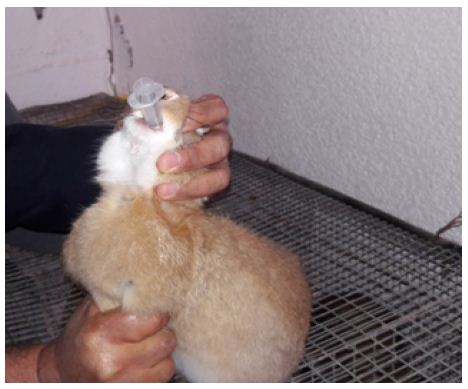
fig 3

Figure 3: Concentrations of LYM in rabbit treated with Amoxicillin, Paracetamol, and Their mixture. Error bars represent standard deviation.
Columns have the same letter are not significantly different at p ≤ 0.05.

So far, lack of hemoglobin due to paracetamol or amoxicillin exposure may enhance the body to produce more hemoglobin to compensate the losses consequently an increase in hemoglobin level may be observed. Furthermore, the tested compound may cause hematotoxicity by restoring almost normal counts of the hematological parameters through oxidative stress. Our explanation agrees with Oyedeji et al. [25] who report oxidative stress in rat experiments. Influence of the tested compounds on HCT (Figure 6) showed significant increase in the treatment of Amoxicillin and mixture. The explanation on these results is similar to that given above for HGB. On the other hands significant increases in PLT levels (Figure 7) were observed in all treatments. An explanation of these results is that the tested compounds directly interact with PLT counts resulting in either activation as in amoxicillin and paracetamol or aggregation phenomenon as in mixture. Thus PLT tends to increase or decrease (Figure 7). Our explanation is in accordance with Siauw et al. [26] who provided evidence of the direct involvement of platelets with bacterial toxins.
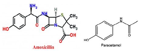
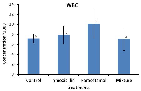
Mode of Interactions

It can be suggested that amoxicillin and/or paracetamol be oxidized by dehydrogenase enzymes in human or animal body producing oxygen reactive species (ORS) as shown in Figure 8. Then these ORS react with blood systems resulting in elevation of HGB, HCT, and PLT in case of amoxicillin and WBC and PLT in case of paracetamol.
fig 8

Figure 8: Possible mode of action of amoxicillin (A) and paracetamol (B) on blood systems after oxidation by dehydrogenase enzyme.

Moreover, the antagonistic effects of amoxicillin and paracetamol in the combination may result from the fact that both molecules have some similarity in the chemical structure such as phenyl ring, C=O, NH2, CH3, OH,. This similarity enhance hydrogen bonding, hydrophobic interactions and possible covalent bonding between both molecule resulting in a larger size molecule than parent ones (paracetamol, amoxicillin). This molecule can move freely in the human body and may not be able to be oxidized by dehydrogenases consequently no ORS were produced. Accordingly, WBC, HGB, LPT HCT contents remained in the acceptable range. This explanation is in accordance with El-Nahhal [27] who revealed hydrogen bonding and hydrophobic interactions between an organic molecules and acetylcholine esterase in human blood. Furthermore, previous reports [28,29] revealed the solubility of similar organic molecules to each other in aqueous solution. Similar observations were recently reported with other cases [30-34]. Additionally, our results are in accordance with Mwafy and Afana who revealed changes in hematological parameters, serum iron and vitamin B12 levels in hospitalized Palestinian adult patients treated with amoxicillin.

Conclusion

The rational of this work emerged from the fact that paracetamol and amoxicillin are widely used pharmaceuticals and their hematological effects are poorly investigated. Elevation of WBC, HGB, LPT HCT levels in treated rabbits were significantly increased indicating high potential of hematological changes. Amoxicillin has a tremendous effect on blood components more that paracetamol has. Combination of both molecules did not produce significant changes on blood parameters indicating a possible protection to blood components. An interesting outcome of the study is that combination of both molecules can be a safe administration for this case.

References

  1. Kaur SP, Rao R, Nanda S (2011) Amoxicillin: a broad spectrum antibiotic. Int J Pharm Pharm Sci 3: 30-37.
  2. Tong DC, Rothwell BR (2000) Antibiotic prophylaxis in dentistry: a review and practice recommendations. The Journal of the American Dental Association 131: 366-374. [crossref]
  3. Abenavoli L, Libri E, Bosco D, Gallo D, Luzza F (2012) Drug-induced liver Recenti Prog Med 103: 79-84. [crossref]
  4. Nicoletti P, Aithal GP, Bjornsson ES, Andrade RJ, Sawle A, et al. (2017) Association of Liver Injury From Specific Drugs, or Groups of Drugs, With Polymorphisms in HLA and Other Genes in a Genome-Wide Association Study. Gastroenterology 152: 1078-1089. [crossref]
  5. Elizalde-Velázquez A, Martínez-Rodríguez H, Galar-Martínez M, Dublán-García O, Islas-Flores H, et al. (2017) Effect of amoxicillin exposure on brain, gill, liver, and kidney of common carp (Cyprinus carpio): The role of amoxicilloic acid. Environ Toxicol 32: 1102-1120. [crossref]
  6. Jóźwiak-Bebenista M, Nowak J Z (2014) Paracetamol: mechanism of action, applications and safety concern. Acta poloniae pharmaceutica 71: 11-23. [crossref]
  7. Hinson JA, Roberts DW, James LP (2010) Mechanisms of acetaminopheninduced liver necrosis. Handb Exp Pharmacol 196: 369-405. [crossref]
  8. James LP, McCullough SS, Knight TR, Jaeschke H, Hinson JA (2003) Acetaminophen toxicity in mice lacking NADPH oxidase activity: role of peroxynitrite formation and mitochondrial oxidant stress Free. Radic Res 37: 1289-97. [crossref]
  9. Bian X, Wang S, Liu J, Zhao Y, Li H, et al. (2018) Hepatoprotective effect of chiisanoside against acetaminophen-induced acute liver injury in mice. Nat Prod Res 15: 1-4. [crossref]
  10. deLemos AS, Ghabril M, Rockey DC, Gu J, Barnhart HX, et al. (2016) Drug-Induced Liver Injury Network (DILIN) Amoxicillin-Clavulanate-Induced Liver Injury. Dig Dis Sci 61: 2406-2416. [crossref]
  11. Cao P, Sun J, Sullivan MA, Huang X, Wang H, et al. (2018) Angelica sinensis polysaccharide protects against acetaminophen-induced acute liver injury and cell death by suppressing oxidative stress and hepatic apoptosis in vivo and in vitro. Int J Biol Macromol 111: 1133-1139. [crossref]
  12. Bajt ML, Knight TR, Lemasters JJ, Jaeschke H (2004) Acetaminopheninduced oxidant stress and cell injury in cultured mouse hepatocytes: protection by N-acetyl cysteine. Toxicol Sci 80: 343-9. [crossref]
  13. Miettinen TP, Björklund M (2014) NQO2 is a reactive oxygen species generating off-target for acetaminophen. Mol Pharm 11: 4395-404. [crossref]
  14. Ghosh J, Das J, Manna P, Sil PC (2010) Acetaminophen induced renal injury via oxidative stress and TNF-alpha production: therapeutic potential of arjunolic acid. Toxicology 268: 8-18. [crossref]
  15. Satav JG, Bhattacharya RK (1997) Respiratory functions in kidney mitochondria following paracetamol administration to young-adult and old rats. Indian J Med Res 105: 131-5. [crossref]
  16. Zarkesh M, Sedaghat F, Heidarzadeh A, Tabrizi M, Bolooki-Moghadam K, et al. (2015) Diagnostic value of IL-6, CRP, WBC, and absolute neutrophil count to predict serious bacterial infection in febrile infants. Acta Med Iran 53: 408-11. [crossref]
  17. El-Nahhal Y, Al_shareef A (2018) Effective biomarkers for successful management of sepsis. Trends in Medicine 18: 1-8.
  18. Kim BJ, Kim JG (2013) Substitutions in penicillin-binding protein 1 in amoxicillin-resistant Helicobacter pylori strains isolated from Korean patients. Gut Liver 7: 655-660.
  19. Lee J, Ji SC, Kim B, Yi S, Shin KH, et al. (2017) Exploration of Biomarkers for Amoxicillin/Clavulanate-Induced Liver Injury: Multi-Omics Approaches. Clin Transl Sci 10: 163-171. [crossref]
  20. Díaz MG, García RP, Gamero DB, González-Tomé MI, Romero PC, et al. (2016) Lack of Accuracy of Biomarkers and Physical Examination to Detect Bacterial Infection in Febrile Infants. Pediatr Emerg Care 32: 664-668. [crossref]
  21. El-Nahhal Y (2017) Risk Factors among Greenhouse Farmers in Gaza Strip. Occupational Diseases and Environmental Medicine.
  22. El-Nahhal Y, Lubbad R (2018) Acute and single repeated dose effects of low concentrations of chlorpyrifos, diuron, and their combination on chicken. Environmental Science and Pollution Research.
  23. El Menyiy N, Al-Waili N, El Ghouizi1 A, Al-Waili W, Lyoussi B (2018) Evaluation of antiproteinuric and hepato-renal protective activities of propolis in paracetamol toxicity in rats. Nutrition Research and Practice 12: 535-540. [crossref]
  24. Biu AA, Yusufu SD, Rabo JS (2009) Studies on the effects of aqueous leaf extracts of Neem (Azadirachta indica A juss) on haematological parameters in chicken. Afr Sci 10: 189-92.
  25. Oyedeji KO, Bolarinwa A, Ojeniran SS (2013) Effect of paracetamol (acetaminophen) on haematological and reproductive parameters in male albino rats IOSR. J Pharm Biol Sci 4: 65-70.
  26. Siauw C, Kobsar A, Dornieden C, Beyrich C, Schinke B, et al (2006) Group B streptococcus isolates from septic patients and healthy carriers differentially activate platelet signaling cascades. Thromb Haemost 95: 836-849. [crossref]
  27. El-Nahhal Y (2018) Accidental Zinc Phosphide Poisoning among Population: A Case Report. Occupational Diseases and Environmental Medicine 6: 37-49.
  28. El-Nahhal Y, Safi J (2004) Adsorption behavior of phenanthrene on organoclays under different salinity levels. Journal of Colloid and Interface Science 269: 265-273.
  29. El-Nahhal Y, Safi, J (2004) Stability of an organo clay complex: effects of high concentrations of sodium chloride. Applied Clay Science 24: 129-136.
  30. El-Nahhal Y, Raaed Lubbad, Mohammad R Al-Agha (2020) Toxicity Evaluation of Chlorpyrifos and Diuron below Maximum Residue Limits in Rabbits Toxicology and Environmental Health Sciences.
  31. Matozzo V, Battistara M, Marisa I, Bertin V, Orsetti A (2016) Assessing the Effects of Amoxicillin on Antioxidant Enzyme Activities, Lipid Peroxidation and Protein Carbonyl Content in the Clam Ruditapes philippinarum and the Mussel Mytilus galloprovincialis Environ Contam Toxicol 97: 521-7. [crossref]
  32. Mwafy SN, Afana WM (2018) Hematological parameters, serum iron and vitamin B12 levels in hospitalized Palestinian adult patients infected with Helicobacter pylori: a case-control study. Hematol Transfus Cell Ther 40: 160-165. [crossref]
  33. Mihalaş E, Matricala L, Chelmuş A, Gheţu N, Petcu A, et al. (2016) The Role of Chronic Exposure to Amoxicillin/Clavulanic Acid on the Developmental Enamel Defects in Mice. Toxicol Pathol 44: 61-70. [crossref]
  34. Seal P, Sikdar J, Roy A, Haldar R (2017) Acetaminophen interacts with Human Hemoglobin: Optical, Physical and Molecular modeling studies. J Biomol Struct Dyn 35: 1307-1321. [crossref]

Acupuncture Emergency Service in Brazilian Public Health System: Quantitative Analysis of Cases Attended in a Semester

DOI: 10.31038/PEP.2021247

Abstract

Background: Acupuncture is an effective technique for pain relief and is usually practiced in outpatient clinic setting. It can also be applied in emergency setting focusing on pain relief from non-life threatening diseases.

Objectives: This quantitative, retrospective and descriptive study aimed to demonstrate the dynamics of the Acupuncture Emergency Service at Hospital São Paulo (AES-HSP), linked to the Paulista School de Medicine of the Federal University of São Paulo (Escola Paulista de Medicina – EPM / UNIFESP), which provides free care for the population since 1998.

Methods: Data were collected from the care records of the second half of 2019, assessing gender, age group, complaint, technique (s) used, percentage of improvement reported by the patient and Visual Analogue Scale before (VASb) and after treatment (VASa).

Results: We identified 7647 visits, of which 78.3% (n=5986) were female; the mean age was 60.8 ± 14.3 years-old; the most common complaints were low back pain (26.4%), followed by shoulder pain (17.5%) and knee pain (14.8%); systemic acupuncture was used in a total of 7032 cases, only acupuncture microsystems were used in 615 cases, microsystems and systemic acupuncture were combined in 1815 cases; VASb average was 6.29 ± 2.17, while VASa average was 1.44 ± 1.42; in 21.4% of 6423 visits properly registered, patients reported 100% improvement and 72.2% reported more than 50% improvement.

Conclusion: Our service provides effective pain relief, allowing to receive a great demand from patients with fast execution in an emergency setting, reducing the use of pain killers and its side effects.

Keywords

Acupuncture analgesia, Traditional Chinese Medicine, Public health, Pain Control

Introduction

Musculoskeletal pain (MSP) is classified as acute or chronic, and is the most prevalent symptom in the world population. Its prevalence has increased in recent years due to higher prevalence of risk factors related to lifestyle habits, such as smoking, anxiety, physical inactivity, sleep disorders. Additional influences include low educational level, precarious family income and social isolation [1,2]. In addition, MSP represents an important cause of morbidity, with a large impact on quality of life and in the economic sphere, for example, absence from work, sometimes requiring long periods of recovery [3].

European data related that 15-20% of primary health care appointments are due to musculoskeletal problems [4].

In Brazil, a meta-analysis performed in 2012 estimated the prevalence of chronic MSP ranging from 14.1-85.5%. Considering only Brazilian studies were evaluated in the meta-analysis, the most affected sites were the dorsal spine and the lower limbs [5].

The impact of chronic pain on national economy also reaches a large proportion. For example, in 2007, Australia, a country with approximately 22.7 million inhabitants, had an estimated cost of $34.3 billion for expenses related to chronic pain, with an average of $10,847 per person with chronic pain [6].

The western medicine approach to MSP is mainly based on the use of common analgesics, opioids, anti-inflammatories and physical therapy. Allopathic drugs, however, are not exempt from adverse effects [7]. In addition, the presence of comorbidities, such as high blood pressure, diabetes, and chronic kidney disease, may restrict the use of such medications. Moreover, the inadequate follow-up of prescriptions and the practice of self-medication predispose to the overuse of anti-inflammatory drugs, which may cause serious complications, such as acute renal dysfunction, upper gastrointestinal bleeding due to peptic ulcer disease and occurrence of cardiovascular events [8-10]. The excessive use of opioids, in turn, might result in an increasing number of drug overdose, addiction and deaths [7].

Acupuncture has an energetic propaedeutic role, capable of detecting and treating an individual’s imbalances before they evolve into organic diseases. In addition to the preventive aspect, it is an effective and safe therapeutic tool for many diseases [11].

The mechanism of action of acupuncture involves stimulation of peripheral nociceptors at specific points, which reach the nervous system through neuronal pathways. Neuromodulation occurs at three levels: local, spinal and supraspinatus, resulting in the release of different substances, such as neurotransmitters, that modulate motor, sensory, autonomic, neuroendocrine and emotional responses [12]. Is important to achieve the Te Qi needling sensation, characterized as a set of sensations, such as pain, burning, tingling, pressure, weight, anesthesia and/or shock, directly related to clinical efficacy [13].

In the west, the growing demand for acupuncture treatment is due to its effectiveness in pain complaints, especially in individuals with limitations to traditional pharmacological treatment [14].

In Brazil, the practice of acupuncture was introduced for the first time in SUS in 1999, through Ordinance No. 1230/GM [15], and was reinforced by its inclusion in the National Policy of Integrative and Complementary Practices (PNPIC), published in Ministerial Ordinance No. 971 of May 2006 [15].

In 1992, the Chinese Medicine-Acupuncture Group of the Department of Orthopedics and Traumatology at Paulista School of Medicine of Federal University of São Paulo (EPM/UNIFESP) was created by Ysao Yamamura M.D., PhD. This physician established this group to foment academic undergraduate and graduate activities, including clinical research, of the institution.

Initially, the therapeutic proposals were exclusively provided on an outpatient basis, resulting in great demand by the population, with an average number of 90 patients daily. Due to increasing demand, it was necessary to establish a more dynamic service. The AES-HSP, characterized by providing public assistance predominantly focused on analgesia under free demand access, was opened in 1998.

The AES-HSP team is composed of resident physicians, preceptors, graduate students and interns in the Chinese Medicine-Acupuncture Group. We have four patient care rooms in the outpatient clinic building of Hospital São Paulo (HSP), located in the Vila Clementino neighborhood in the city of São Paulo, state of São Paulo, Brazil. Clinic is held Monday to Friday from 8 am-3 pm, except on holidays. Patients are referred by basic health units or present directly; they are attended to based on arrival order.

In our service, a minimum number of acupuncture points with immediate effect of analgesia is used, with emphasis on the Yamamura System techniques of Acupuncture (SYA/EPM).

Microsystems, or somatotopies, are representations of the entire organism in smaller areas of the body. When the organism is sick, reactive points emerge in the microsystem in the areas corresponding to the compromised region. Through the manipulation of these reflex points, it is possible to act positively on the disease or symptomatology in question. In our service, we use internationally-renowned techniques, such as Yamamoto New Scalp Acupuncture (YNSA), Chinese Scalp Acupuncture and Chinese Auriculotherapy, as well as exclusive techniques developed by Dr. Yamamura [16-18] including the Yamamura Nasal Bone Acupuncture System (Figure 1), Yamamura Acupuncture System Hair Implantation (SYALIC) (Figure 2), Yamamura Long Bone Acupuncture System (SYAOL) (Figure 3), Yamamura Occipital Bone Acupuncture System (Figure 4), Yamamura System of Cranial Sutures and 5 Zang in parietal suture (Figure 5). Some of the main techniques are described below, and may be used isolated or associated with systemic acupuncture. Image of the systems of the Yamamura Acupuncture System were kindly provided by Dr. Yamamura.

fig 1

Figure 1: Yamamura acupuncture system of nasal bone.

fig 2

Figure 2: SYALIC – Yamamura acupuncture system of hair implantation line.

fig 3

Figure 3: Yamamura acupuncture system of cranial sutures and 5 Zang on squamous suture.

fig 4

Figure 4: Yamamura acupuncture system of occipital bone.

fig 5

Figure 5: SYAOL – Yamamura acupuncture system of Long bone.

Methods

We collected data from the attendance records at the AES-HSP, between July-December 2019, using a standardized form completed by the attending physician. The parameters evaluated included gender, age group, complaint, technique(s) used, percentage of improvement reported by the patient and Visual Analogue Scale before treatment (VASb) and after treatment (VASa).

We considered the total number of visits, not discriminating whether the same patient was seen on more than one occasion, and the main and associated complaints. Regarding treatment, we grouped the different approaches into isolated systemic therapy, non-systemic techniques or a combination of both.

A focused anamnesis and physical examination was performed for each patient and was directed to the patient’s complaint in order to correctly select treatment points and techniques. Local asepsis was performed with cotton soaked in 70% alcohol, and sterile, disposable, 0.30 mm x 40 mm stainless steel acupuncture needles supplied by HSP were used. Needle insertion at specific points was performed until the Te Qi sensation was obtained, according to the depth characteristics. In auricular acupuncture, we used mustard seeds affixed to tape and manipulated with the aid of surgical tweezers.

Statistical analysis was performed descriptively, denoting average, median, minimum and maximum values, standard deviation, absolute and relative frequencies in percentage (%), using Microsoft Excel® 2019 software by Microsoft. The graphs of columns and lines were elaborated using Microsoft PowerPoint® 2019 software by Microsoft.

Results

We identified 7,647 visits, of which 78.3% (n=5986) were female and 21.7% (n=1661) were male. Regarding the age group, the mean age was (mean ± standard deviation) 60.8 ± 14.3 years, with a median of 64 years; 85.7% of participants were between 41-80 years (Graph 1), with a predominance in the range of 61-80 years, with a value of 53.4%. The average number of visits corrected for working days in the semester (120) was 63.7 visits/day. The average number of patients per operating time (7 hours) was approximately 9.1 patients/hour, resulting in a duration of care of approximately 6.5 minutes/patient.

graph 1

Graph 1: Distribution by age group (%) (n=7647).

Regarding complaints, low back pain (26.4%), followed by shoulder pain (17.5%), knee pain (14.8%), neck pain (11.7%), upper back pain (5.9%), lower limb pain (5.4%), upper limb pain (4.9%), foot pain (4.9%), polyarthralgia (4.3%), hip pain (2.7%), polymyalgia (2.3%), wrist pain (1.3%), non-restorative sleep (1.3%), hand pain (0.9%), finger pain (0.7%), facial palsy (0.7%) and ankle pain (0.5%). This data is depicted in Graph 2.

graph 2

Graph 2: Percentage of most prevalent pain sites.

In the analysis of the VAS, the data referring to the index in VASb (n=4080 visits) corresponds to an average of 6.29, with a median of 6 and standard deviation of 2.17. For the index in VASa (n=3913), there was an average of 1.44, median of 1 and standard deviation of 1.42. There was a failure to register 46.6% (n=3567) of the VAS in relation to the total number of cases in the semester. The total visits (n=6423) analyzed from the perspective of the degree of response to the treatment perceived by the patient were grouped into five categories: worsening (0%), without improvement (2%), less than 50% improvement (4.3%), more than 50% improvement (72.2%) and 100% improvement (21.4%). This information is presented in Graphs 3 and 4.

graph 3

Graph 3: VAS before treatment (VASb) and after treatment (VASa).

graph 4

Graph 4: Continuous comparison of pain level before treatment (VASb) and after treatment (VASa).

Considering the total number of visits, non-systemic techniques were used 2,430 times. These techniques included: the Bregma craniometric point (22.2%), Anatomical Trains (14.6%), Auriculotherapy (13.2%), Yamamoto New Scalp Acupuncture-YNSA (12.1%), Pterion craniometric point (9.1%), Symmetry (7.8%), Lambda Craniometric point (6.7%), Asterion craniometric point (4.6%), 5 Zang in parietal suture (2.8%), Yamamura Acupuncture System Hair Implantation-SYALIC (1.7%), Yamamura Long Bone Acupuncture System-SYAOL (0.8%), Yamamura Occipital Bone Acupuncture System (0.5%), Yamamura Nasal Bone Acupuncture System ( 0.4%), Yamamura Acupuncture System of the Musculoskeletal System of Sutures (0.4%), Vertebral Points (0.3%), and Chinese Scalp Acupuncture (0.1%) [15-17]. Graph 5 depicts this information.
graph 5

Graph 5: Distribution of non-systemic techniques most used (n=2430).

Systemic acupuncture techniques were used in 7,032 cases, corresponding to 91.9% of total cases. The use of non-systemic techniques alone occurred in 615 cases, corresponding to 8% of the total. Microsystems and systemic acupuncture were combined in 1815 cases (23.7%).

Discussion

Our study identified a female prevalence rate three times higher than males. This information is in agreement with other studies, which state that the prevalence of women reporting chronic pain is generally higher than men, which can be influenced by the way men and women experience pain [19]. Another possible explanation is the social expression of each gender. Women are usually taught to express emotions and seek help, while men are generally inhibited from expressing themselves [20]. Thus, male patients are less likely to report chronic pain and seek medical assistance.

When we analyzed age group, we found that more than half of patients were between 41-80 years of age. According to the literature, older patients have a higher prevalence of chronic pain than younger patients. This may result from the increase in number of comorbidities presented in the elderly [21].

According to the Global Burden of Disease Study in 2016, low back pain and neck pain are the main causes related to disability worldwide [22]. Another study highlights low back pain as the main cause of disability globally [23]. The present study is in agreement with this worldwide incidence since the most frequent complaint was low back pain. Regarding shoulder pain, we found involvement in 17.5% of individuals. This data differs from the Brazilian meta-analysis by Miranda et al. (2012) that assessed the prevalence of musculoskeletal disorders in the elderly population in Brazil and found the spine as the most affected location and the lower limb the second-most affected [5]. Chronic knee pain presented as an important highlight in the visits, since it was the third most prevalent complaint.

Patients suffering from chronic pain often have more than one affected site, as demonstrated in a British demographic survey, in which only one-third of the participants with pain had localized symptoms [2]. Thus, in the prevalence chart of the most frequent complaints, the statistics of different sites of pain must be interpreted separately, only in relation to the total number of cases once the sum of painful sites exceeds the number of visits, because patients usually had more than one complaint.

The VAS was chosen to assess the degree of pain before (VASb) and after (VASa) the treatment with acupuncture because it is a validated instrument of easy applicability and reproducibility, low cost, and widely used in global literature, which allows comparison of the results [24,25]. Despite the failure to complete the VAS in almost half of patient visits, it was possible to perceive a clear reduction in the degree of pain, according to the mean and median between VASb and VASa registered in the graphs, implying an effective analgesia with acupuncture. Such efficacy was also reinforced by the degree of improvement reported by patients.

The failure to register VAS can be explained by the fact that it is an academic service and has a considerable turnover of people who required a new adaptation to the routine of functioning and data recording. Another possibility is the socioeconomic level of many patients who had difficulties understanding the VAS and unable to adequately grade their pain, occurring often enough to compel the attending physician to only ask about degree of pain improvement.

As it is an Emergency Service, highly effective techniques with few acupuncture points and manual stimulation are recommended, in the goal of obtaining a good response in a short period of time. In this way, microsystems are a very effective tool for simplicity in application and good resolution to pain, as well as in the selection of traditional systemic points of high effectiveness. The Chinese Medicine-Acupuncture Group has developed treatment techniques validated by wide use in the AES-HSP that has proven to be highly effective, with some points being more used than traditional microsystems. Of the total number of consultations, the use of non-systemic techniques occurred 2,430 times, either alone or in combination with systemic points. The most used point for treatment was one of the craniometric points idealized by the Chinese Medicine-Acupuncture Group, Bregma, which was used in a total of 539 visits.

Patients are aware of the service we offer, based on referral from general practitioners, family doctors and specialists, or through information obtained from acquaintances who have previously been assisted or the internet. As a result, they directly seek care, which assists a large population of patients awaiting care in outpatient clinics, where there is often a waiting list with months of delay. Due to the volume of patients, we had to consider the total number of visits, and new patients were not distinguished from return patients.

One of the difficulties with the present work was the lack of standardization of completing the attendance forms by the doctors of the service, resulting in some missing information, as occurred in the registration of the VAS. During the transfer of information in written form to Microsoft Excel®, the complaints were summarized in the key terms that motivated the patient visit in order to facilitate statistical analysis in the evaluation of the cases, which could represent a registration bias due to data simplification. However, this may be counteracted by the transcribing physician, who performs the role of organizing symptoms and signs in validated medical terms.

The services provided to these patients is important due the provision of immediate pain relief, reducing the demand for patients with chronic pain to utilize other emergency services. As a result, the physical and emotional impact of pain on patients’ work and personal routine are minimized. The AES-HSP also reduces the time patients spend obtaining non-pharmacological pain therapy, for example, as in the Brazilian public unified health system, which has a waiting list for physiotherapy, which is another approach commonly used to manage MSP.

Conclusion

Acupuncture treatment to acute and chronic pain may reduce the use of self-medication, what decreases the risks of side effects of pain killers.

Our acupuncture emergency service provides effective care in pain relief in a fast and focused manner, resulting in significant demand from patients. Over its 22 years of existence, the services of the AES-HSP is considered an alternative approach to provide analgesia to patients with chronic pain and serves as a model for the creation of new emergency care in acupuncture in public health systems.

Authors’ Contributions

José Udevanier Rebouças da Silva Júnior M.D., Lorena Anunziato Sant’Ana M.D., and Mary Clea Ziu Lem Gun M.D. wrote the manuscript, constructed the graphs and translated image subtitles to English.

João Roberto Bissoto M.D., Ysao Yamamura M.D., PhD., Marcia Lika Yamamura M.D., MSc., and Silvana Maria Silva Fernandes M.D., PhD. reviewed the manuscript, assisted in writing the manuscript and are supervisors of our Medical Residency Program.

Ysao Yamamura M.D., PhD. is also the author of many techniques (microsystems) used in our service and owner of the pictures of the microsystems.

References

  1. Bergman S, Herrström P, Högström K, Petersson I.F, Svensson B, Jacobsson L.T. (2001) Chronic musculoskeletal pain, prevalence rates, and sociodemographic associations in a Swedish population study. The Journal of Rheumatology 28: 1369-77. [crossref]
  2. Urwin M, Symmons D, Allison T, Brammah T, Busby H, Roxby M (1998) Estimating the burden of musculoskeletal disorders in the community: the comparative prevalence of symptoms at different anatomical sites, and the relation to social deprivation. Annals of the Rheumatic Diseases 57: 649-55. [crossref]
  3. Henry J. L (2008) The need for knowledge translation in chronic pain. Pain Res Manag 13: 465-476. [crossref]
  4. European Commission (2003) Indicators for monitoring musculoskeletal problems and conditions: musculoskeletal problems and functional limitation. Oslo: University of Oslo.
  5. Miranda V. S, Carvalho V. B. F. de, Machado L. A. C, Dias J. M. D. (2012) Prevalence of chronic musculoskeletal disorders in elderly Brazilians: a systematic review of the literature. BMC Musculoskeletal Disorders 13: 82. [crossref]
  6. Report by Access Economics Pty Limited for MBF Foundation in collaboration with University of Sydney Pain Management Research Institute. The High Price of Pain: The Economic Impact of Persistent Pain in Australia. Sydney, Australia, 2007.
  7. Volkow N. D, McLellan A. T. (2016) Opioid Abuse in Chronic Pain — Misconceptions and Mitigation Strategies. New England Journal of Medicine 374(13): 253-1263. [crossref]
  8. Varga Z, Sabzwari S. R. A, Vargova V (2017) Cardiovascular Risk of Nonsteroidal Anti-Inflammatory Drugs: An Under-Recognized Public Health Issue. Cureus 9(4): e1144. [crossref]
  9. Cannon P. J. (1986) Prostaglandins in congestive heart failure and the effects of nonsteroidal antiinflammatory drugs. American Journal Medicine 81: 123-132. [crossref]
  10. Garcia-Rodriguez L. A, Jick H (1994) Risk of upper gastrointestinal bleeding and perforation associated with individual non-steroidal anti-inflammatory drugs. Lancet 43: 769-772. [crossref]
  11. Yamamura Y, Yamamura M (2010) Propedêutica Energética – Inspeção e Interrogatório, 1st edition, Center AO publisher.
  12. Zhang R, Lao L, Ren K, Berman B. M (2014) Mechanisms of Acupuncture-Eletroacupuncture on Persistent Pain. Anesthesiology 120(2): 482-503. [crossref]
  13. Yang X. Y, Shi G. X, Li Q. Q, Zhang Z. H, Xu Q, Liu C. Z. (2013) Characterization of Deqi Sensation and Acupuncture Effect. Evid-Based Complement Alternat Med 319734.  [crossref]
  14. Birch S, Lee M. S, Alraek T, Kim, T. H. (2018) Overview of Treatment Guidelines and Clinical Practical Guidelines That Recommend the Use of Acupuncture: A Bibliometric Analysis. The Journal of Alternative and Complementary Medicine 24(8): 752-769. [crossref]
  15. Ministry of Health of Brazil (2006) National Policy of Integrative and Complementary Practices in SUS – PNPIC – SUS: attitude of expanding access. Brasília: Ministry of Health, (Series B. Basic Health Texts).
  16. Wirz-Ridolfi. A (2019) The History of Ear Acupuncture and Ear Cartography: Why Precise Mapping of Auricular Points Is Important. Medical Acupuncture 31(3): 145-156. [crossref]
  17. Aoyama, N, Fujii, O, Yamamoto, T (2017) Efficacy of Parietal Acupoint Therapy: Scalp Acupuncture for Neck/Shoulder Stiffness with Related Mood Disturbance. Medical Acupuncture 29(6): 383-389. [crossref]
  18. Wang, J, Pei, J, Khiati, D, Fu, Q, Cui, X, et al. (2017) Acupuncture treatment on the motor area of the scalp for motor dysfunction in patients with ischemic stroke: study protocol for a randomized controlled trial. Trials 18(1): 287. [crossref]
  19. Greenspan J. D, Craft R. M, LeResche L, Arendt-Nielsen L, Berkley K. J, et al. Studying sex and gender differences in pain and analgesia: A consensus report. Pain 132: S26-S45. [crossref]
  20. El-Shormilisy N, Strong J, Meredith P. J. (2015) Associations among Gender, Coping Patterns and Functioning for Individuals with Chronic Pain: A Systematic Review. Pain Research and Management 20(1): 48-55. [crossref]
  21. Barnett K, Mercer S.W, Norbury M, Watt G, Wyke S, Guthrie B (2012) Epidemiology of multimorbidity and implications for health care, research, and medical education: a cross-sectional study. Lancet 380: 37-43. [crossref]
  22. Vos T, Allen C, Arora M (2017) Global, regional, and national incidence, prevalence, and years lived with disability for 328 diseases and injuries for 195 countries, 1990-2016: a systematic analysis for the Global Burden of Disease Study 2016. Lancet 390: 1211-1259.
  23. Colvin L. A, Rice A. S. C. (2019) Progress in pain medicine: where are we now? British Journal of Anaesthesia 123(2): e173ee176. [crossref]
  24. Chapman C. R, Casey K. L, Dubner R, Foley K. M, Gracely R. H, (1985) Reading, A. E. Pain measurement: an overview. Pain 22(1): 1-31. [crossref]
  25. Huskisson E. C. (1974) Measurement of pain. Lancet 2(7889): 1127-31. [crossref]

Revision of Sex Hormone Replacement Therapy for CKD Pediatric Cases

DOI: 10.31038/EDMJ.2021541

Letter to the Editor

According to the North American Pediatric Renal Transplant Cooperative Study (NAPRTCS), children with Chronic Kidney Diseases (CKD) have considerable height deficits in comparison to the normal children. Additionally, short stature and poor growth of CKD children are associated with an increased risk of death [1]. Although complex medical regimens including bicarbonate therapy, iron, erythropoietin, salt-water supplementation, and Growth Hormone (GH) can improve final height, however, these children experience progressive height deficit after the age of 6 y compared to their normal counterparts [2]. We believe that CKD pediatric cases with short stature and delayed puberty should receive Sex Hormone Replacement Therapy (SHRT) at the same time when majority of the normal boys and girls have started maturation. We thus propose that SHRT should be started in CKD cases with the same rationale as in hypo/hyper-gonadothropic hypogonadism patients to improve their final height as adults.

Puberty

Ninety five percent of contemporary normal girls start their Thelarche by the age of 11 y [3] and the mean age of puberty stage 2a and 2b in contemporary normal boys are 12.1 and 12.7 y, respectively [4]. Sex hormones (estrogen and testosterone) have an essential role in pubertal growth spurt by enhancing synthesis and secretion of IGF1 that has anabolic effects on bone growth plates [5]. Despite good acid-base management and nutritional support, CKD can interfere with the hypothalamic-pituitary-gonadal axis at different levels which leads to delay in onset of puberty [6]. Pulsatile secretion of Luteinizing Hormone (LH) is impaired along with serum LH level elevation in CKD children due to uremia. Lack of nocturnal LH secretion causes delay in puberty in these patients [7]. Pediatricians should evaluate pubertal delay in CKD children, if no Thelarche starts by the age of 11 y in girls and no sign of puberty at 13 y in boys.

In normal children, standardized height averagely increases 1.3 SDS from pre-puberty to post-puberty, while patients with delayed puberty have significantly less increase in standardized height (+0.9 SDS) [7]. CKD Children have approximately 2.5 years lag in the onset and progression of gonadarche in comparison with their peers. In addition, their pubertal growth spurt is shortened by 1.5 y, and at start of the pubertal spurt, they have less mean height velocity in comparison with the healthy adolescents [7-9]. Thus, an irreversible height deficit occurs during puberty in CKD children [9] because of disturbed puberty and impaired pubertal growth spurt.

Growth Hormone

Practitioners have tried to enhance CKD children growth deficit with GH, however, optimal final height was not achieved with this treatment. In CKD children who received GH from late pre-pubertal stage, GH therapy had no overall effect on the improvement of pubertal height gain and they still had a prominent height deficit [8,10]. Also, the mean peak height velocity during the pubertal growth spurt was not significantly higher in GH treated CKD children compared to the control CKD children [8].

Conclusion

According to the best of our knowledge, CKD girls and boys with short stature who do not start puberty till 11 and 13 y respectively are at high risk of height deficit in spite of GH therapy. As 20 to 25 cm of FH was obtained by pubertal growth spurt [11], experts have referred this height deficit to the delayed puberty and shorten pubertal growth spurt duration in CKD children [7]. SHRT in boys with CKD and delay puberty is challenging and needs more personalized decision making because Testosterone could aggravate uremic side effects [12,13]. However, we recommended SHRT in short CKD girls with delay puberty at 11 y to enhance their final height besides improving bone density.

Conflict of Interest

On behalf of all authors, the corresponding author states that there is no conflict of interest.

Keywords

Growth retardation, Delayed puberty, GH treatment, Estrogen replacement therapy, Chronic Kidney Disease

References

  1. Furth SL, Stablein D, Fine RN, Powe NR, Fivush BA (2002) Adverse clinical outcomes associated with short stature at dialysis initiation: a report of the North American Pediatric Renal Transplant Cooperative Study. Pediatrics 109(5):909-13. [crossref]
  2. Franke D, Winkel S, Gellermann J, Querfeld U, Pape L, Ehrich JH, et al. (2013) Growth and maturation improvement in children on renal replacement therapy over the past 20 years. Pediatric Nephrology (Berlin, Germany)28(10):2043-51. [crossref]
  3. Cabrera SM, Bright GM, Frane JW, Blethen SL, Lee PA (2014) Age of thelarche and menarche in contemporary US females: a cross-sectional analysis. Journal of Pediatric Endocrinology and Metabolism 27(1-2):47-51. [crossref]
  4. Biro FM, Lucky AW, Huster GA, Morrison JA (1995) Pubertal staging in boys. The Journal of Pediatrics 127(1):100-2. [crossref]
  5. Grob F, Zacharin M (2020) Puberty in chronic inflammatory conditions. Current Opinion in Endocrine and Metabolic Research.
  6. Silverstein D (2018) Growth and Nutrition in Pediatric Chronic Kidney Disease. Front Pediatr 6: 205 doi: 103389/fped. [crossref]
  7. Haffner D, Fischer D-C (2012) Growth and pubertal development in dialyzed children and adolescents. Pediatric Dialysis: Springer 453-81.
  8. Haffner D, Schaefer F, Nissel R, Wühl E, Tönshoff B, Mehls O (2000) Effect of growth hormone treatment on the adult height of children with chronic renal failure. New England Journal of Medicine 343(13):923-30. [crossref]
  9. Schärer K (1990) Growth and development of children with chronic renal failure. Study Group on Pubertal Development in Chronic Renal Failure. Acta paediatrica Scandinavica Supplement 366:90-2. [crossref]
  10. Nissel R, Lindberg A, Mehls O, Haffner D (2008) Factors predicting the near-final height in growth hormone-treated children and adolescents with chronic kidney disease. The Journal of Clinical Endocrinology & Metabolism 93(4):1359-65. [crossref]
  11. Scheffler C, Hermanussen M (2018) Growth in childhood and adolescence. The International Encyclopedia of Biological Anthropology 1-11.
  12. Johansen KL (2004) Testosterone metabolism and replacement therapy in patients with end-stage renal disease. Seminars in Dialysis. [crossref]
  13. Zhao JV, Schooling CM (2020) The role of testosterone in chronic kidney disease and kidney function in men and women: a bi-directional Mendelian randomization study in the UK Biobank. BMC Medicine 18:1-10. [crossref]