Author Archives: author

The Effect of Preoperative Cardiopulmonary Rehabilitation on Pulmonary Infection after Cardiac Surgery

DOI: 10.31038/JCCP.2022515

Abstract

In recent years, the incidence of heart disease remains high, which is closely related to people’s diet and living habits, and in cardiac surgery due to tracheal intubation, bed rest and other problems easy to cause postoperative pulmonary infection, we all know that cardiopulmonary rehabilitation training can improve the cardiopulmonary function of patients, our article on preoperative cardiopulmonary rehabilitation training on pulmonary infection after cardiac surgery to review.

Cardiovascular disease has become an important disease endangering the health of Chinese people, and its mortality rate accounts for 67.1% of the total number of cardiovascular disease deaths. In recent years, with the progress of medical technology such as various cardiac surgeries, the mortality rate has gradually decreased, but due to the inability to recover postoperative cardiopulmonary function, it is still unable to live normally or be weaned from the ventilator, and the quality of life has decreased.

A large number of evidence shows that cardiopulmonary rehabilitation can effectively improve the cardiopulmonary function of patients, mainly through respiratory rehabilitation and exercise training to improve the overall cardiopulmonary function of patients, and can improve the mental status of patients and improve exercise capacity, and cardiopulmonary rehabilitation also allows us to rehabilitation of heart disease from treatment to prevention, this paper mainly from the overview of cardiopulmonary rehabilitation and exercise methods to prevent pulmonary infection in patients after cardiac surgery.

Overview of Cardiopulmonary Rehabilitation

Definition of Cardiac Rehabilitation

Cardiac rehabilitation is to relieve the clinical symptoms of patients through comprehensive rehabilitation medical treatment, improve the daily life ability of patients, improve the quality of life, return to normal social life, and prevent the recurrence of cardiovascular disease. It is currently an important means of treating the chronic phase of the heart. The contents of cardiac rehabilitation include regular medication, exercise therapy, psychotherapy, diet therapy, and behavior therapy [1-14].

Definition of Pulmonary Rehabilitation

Pulmonary rehabilitation is an intervention for patients with discomfort symptoms and reduced daily activities, or decreased activities of daily living, chronic respiratory diseases. Pulmonary rehabilitation intervention modalities are comprehensive assessment and rehabilitation programs and implementation strategies involving multidisciplinary teams on the basis of evidence-based medicine. Pulmonary rehabilitation can stabilize and reverse the systemic manifestations of the disease, reduce symptoms, optimize functional status, increase activities of daily living and social participation, reduce the rate of acute onset and rehospitalization, and reduce the cost of medical care. Pulmonary rehabilitation has two main goals, to maximize physical, psychological, and social function, to educate patients how to improve mobility and self-care ability in daily life, to improve quality of life, and to reduce dependence on hospitalization.

Cardiopulmonary Rehabilitation Exercise Mode

Respiratory Training

Abdominal respiratory training quiet, supine, the abdomen put a sandbag of moderate weight, self-control of the thorax through the abdominal undulation uniform respiratory training.

Inspiratory resistor breathing training to control inspiratory volume and time.

It is required that after deep inspiration, the expiration is as thin and slow as a whistle, the airflow is gradually exhaled, and respiratory training should be done, and the training volume should be grasped, generally less than ten seconds each time, about ten times, and three groups should be done continuously, and the speed should be slow.

Passive training, requiring manual training by professional therapists, such as thorax, back, and scapular extrusion.

Aerobic Exercise and Resistance Training

Aerobic training belongs to the training of long-distance endurance, also known as “cardiopulmonary function training”. It is through continuous and repeated activities, and in a certain period of time, with a certain speed and a certain training intensity, it is required to complete a certain amount of exercise, so that the heartbeat rate is gradually increased to the specified highest and lowest safe heartbeat range. Common training methods are brisk walking, jogging, Tai Chi and bicycle.

Resistance training, also known as resistance training, is a movement against resistance, the main purpose is to train the muscles of the human body, and traditional resistance training includes push-ups, dumbbells, barbells and other items.

Effect of Cardiopulmonary Rehabilitation on Pulmonary Infection after Cardiac Surgery

Study on the effect of cardiopulmonary rehabilitation on pulmonary function after cardiac surgery found that respiratory training can enhance the muscle strength and endurance of respiratory muscles, improve pulmonary ventilation, improve pulmonary function, but also increase the blood flow and activity of diaphragm, while reducing the standby time, can pull out the endotracheal tube as soon as possible, transfer out of ICU, return to the general ward and get out of bed as soon as possible.

Effect of cardiopulmonary rehabilitation on cardiac function after cardiac surgery Aerobic exercise enhances the ability of the cardiovascular system to deliver oxygen to muscles, allowing the body to adapt to higher intensity and longer lasting exercise, while reducing heart rate at rest, improving cardiac function, and improving quality of life.

Effect of cardiopulmonary rehabilitation on quality of life. Cardiac rehabilitation can enhance exercise tolerance and improve quality of life in patients. Moreover, exercise training can promote patients with coronary heart disease to maintain a positive and optimistic attitude to life, respiratory and exercise-based cardiopulmonary rehabilitation can shorten the length of hospital stay, promote patients to return to normal life as soon as possible, and improve the quality of life.

Conclusion

Respiratory training and exercise training are the core contents of cardiopulmonary rehabilitation, respiratory training can improve pulmonary ventilation, improve pulmonary function, in order to reduce hypoxia, and regular exercise training can increase myocardial oxygen supply, improve the work ability of the heart and arterial blood flow reserve capacity, and improve the quality of life of patients with disease. As rehabilitation workers, we should carry out detailed evaluation for patients and intervene in precise treatment after evaluation, so as to reduce the probability of postoperative pulmonary infection, reduce the cost and hospital stay, and return to the family as soon as possible.

References

  1. Ashtonre, Tew GA, Aning JJ, et al. (2020) Effects of shortterm, medium-term and long-term exercise training on cardio-metabolic health outcomes in adults: systematic review with meta-analysis [J]. Br J Sports Med 54: 341-348. [crossref]
  2. Zhang H, ChangR (2019) Eflects of Exercise after Percutaneous Coronary Intervention on Cardiac Function and Cardiovascular Adverse Events in Patientswith Coronary Heart Disease: SystematicReview and Meta-Analysis [J]. Journal of sports once& medicine 18: 213-222. [crossref]
  3. Rezaei-Hachesu P, Oliyaee A, Safaie N, et al. (2017) Comparison of coronary artery disease guidelineswith extracted knowledge from data mining [J]. J Cardiovasc ThoracRes 9: 95-101.
  4. Lanz J, Wyss D, R ber L, et al. (2019) Mechanical complications in patients with ST-segment elevation myocardial infarction: a single centre experience [J]. PLoS One 14: 209502. [crossref]
  5. Gomes Neto M, Duraes AR, Conceicao LSR, et al. (2018) High intensity interval training versus moderate continuous intensity training on exercise capacity and quality of life in patients with heart failure with reduced ejection fraction: a systematic review and meta-analysis [J]. Int J Cardiol 261: 134-141. [crossref]
  6. Wu Yan, Wang Xiujuan, Kang Xiaoyan, et al. (2018) Effect of preoperative rehabilitation training on cardiopulmonary function in patients with early stage cancer undergoing thoracoscopic surgery [J]. Journal of Clinical Pulmonary Medicine 23: 1217-1221.
  7. Gao Zhenzhen, Ji Peng, Xia Yueqing, et al. (2015) Effects of different intensity aerobic exercise on cardiac function and exercise tolerance in patients after percutaneous coronary intervention [J]. Chinese Journal of Rehabilitation Medicine 30: 344-348.
  8. Li Xue, Shanyan, Jiang Tingting, et al. (2021) Research progress of resistance exercise in nursing care of maintenance hemodialysis patients complicated with sarcopenia [J]. Nursing Research 35: 643-647.
  9. Wang Lei, Gao Zhenzhen, Pan Huaping (2015) Effect of individualized aerobic exercise on heart rate recovery and exercise capacity in patients with coronary heart disease [J]. Chinese Journal of Rehabilitation Medicine 30: 242-246.
  10. Zhang Lingyun, Bai Chuanchuan, Shu Bin (2018) Research progress on the protective effect of exercise training on heart after myocardial infarction and its mechanism [J]. Chinese Journal of Rehabilitation 33: 53-55.
  11. Jiao Haixu (2020) Research progress on cardiac rehabilitation of patients with cardiovascular disease by resistance exercise [J]. Journal of Qiqihar Medical College 41: 1140-1141.
  12. McMahon SR, Ades PA, Thompson PD (2017) The role of cardiac rehabilitation in patients with heart disease [J]. Trends Cardiovasc Med 27: 420-425. [crossref]
  13. SIMON M, KORN K, CHO L, et al. (2018) Cardiac rehabilitation: A class1 recommendation [J]. Cleve Clin J Med 85: 551-558. [crossref]
  14. Anderson L (2014) Cardiac rehabilitation for peoplewith heart disease: an overview of Cochrane systematic reviews. Cochrane Database Syst Rev 2014: 011273 [crossref]

Appraisal of Abnormal Movement Disorders among Aged Schizophrenics: A Pilot Study

DOI: 10.31038/ASMHS.2022633

Abstract

Introduction: Tardive dyskinesia (TD) includes involuntary choreiform or athetoid movements of the jaw, lower face, tongue, and extremities, developing in association with the use of an antipsychotic medication, and may develop in about 20 to 40 percent of patients who require long-lasting hospitalization. In the present study, the prevalence of this condition has been measured among an elderly group of schizophrenic patients.

Methods: One hundred and one elderly schizophrenic patients, who were hospitalized in the chronic section of a community psychiatric hospital, were selected for the present cross-sectional study. Abnormal Involuntary Movement Scale (AIMS) was employed to screen for patients with schizophrenia who also had TD. Scale for Assessment of Positive Symptoms, Scale for Assessment of Negative Symptoms, Schedule for Assessment of Insight, and Clinical Global Impressions – Severity of illness, as well, had been used as ancillary scales for evaluation of severity of general psychopathology of schizophrenia, and comparing the TD patients with the group of patients without TD, for probing the intervening parameters.

Results: While abnormal movements were clear in 38.61% (n=39) of elderly schizophrenic patients, only seven of them (6.93 %) could be diagnosed as TD, based on the above-mentioned criteria. All of them were using conventional antipsychotic medications, accompanied with anticholinergic medications. Among TD patients, three cases had only abnormal facial and oral movements, one patient had atypical facial and oral movements as well as anomalous extremity movements, one patient had irregular facial and oral movements in addition to unusual trunk movements, and lastly, two patients had nonstandard extremity movements. In addition, around 71% of patients with TD were aware of their unusual movements. Between-group analysis did not show any significant difference between patients with TD and patients without TD in age, duration of illness, positive symptoms, negative symptoms, insight, and general psychopathology.

Conclusion: According to the findings of the present study, the prevalence of Tardive Dyskinesia among elderly schizophrenic patients, who were using typical antipsychotic medications, is very lower than what has been indicated thus far.

Keywords

Schizophrenia; Typical antipsychotic drug; Atypical antipsychotic drug; Extrapyramidal symptoms; Tardive Dyskinesia; Medication induced movement disorder

Introduction

Tardive dyskinesia (TD) includes involuntary choreiform or athetoid movements of the jaw, lower face, tongue, and extremities, developing in association with the use of an antipsychotic medication for at least a few months, though symptoms may appear after a shorter period in older persons. In some patients, movements of this kind may appear after cessation, or after alteration or decrease in dosage of antipsychotic drugs. Tardive syndrome includes other forms of movement complications, such as akathisia or dystonia, which are distinguished by their late appearance in the course of management and their potential perseverance for months to years, even despite antipsychotic discontinuation or dosage lessening [1]. TD can appear in various ways. Initial clinical symptoms are primarily messy movements in the facial areas, mouth and tongue, which seem uncontrollable and repetitive. Also, TD symptoms can affect movement of the torso, limbs, head and neck, and patients with severe disorders may also suffer from vague speech, abnormal postures and problematic swallowing [2]. The severity of the movements may range from slight to obviously incapacitating. TD is worsened by stress and vanishes during sleep [3]. TD develops in about 10 – 20 percent of patients who are treated for more than a year. About 20 – 40 percent of patients who require long-standing hospitalization have TD [4,5]. The occurrence of TD can also depend on whether the antipsychotic drug is atypical or typical, with around 13.1% incidence with atypical antipsychotic medications and about 32.4% rate with typical antipsychotic drugs [6,7]. Females, children, patients who are more than fifty years of age, and patients with brain injury or affective disorders are at higher risk [3,9]. Increased antipsychotic medication exposure (particularly typical antipsychotics), African-American ethnicity, cognitive disturbance, alcohol or substance abuse, early occurrence of drug-induced parkinsonism, diabetes, and HIV, as well, have been accounted as other risk factors for the development of TD [10,11]. Moreover, drugs used to treat Parkinson’s disease can cause TD [12,13] (Table 1). Up to now, sustained D2 receptor blockade resulting in receptor hypersensitivity is the most common theory explaining the development of TD. Besides, genetic studies have indicated a possible relationship with polymorphisms in the DA2 receptor, DA3 receptor, dopamine transporter (DAT1), and the serotonin 2A receptor genes. Oxidative stress and cell demise secondary to augmented glutamatergic neurotransmission triggered by blockade of presynaptic dopamine receptors is also hypothesized [14-18]. Although proof proposes a genetic susceptibility to TD [19], evidence suggests that a genetic protection against TD exists [20]. Furthermore, some studies suggest that D3, D4, and D5 receptors are also involved in the pathogenesis of TD [21,22]. Since anticholinergic agents are also associated with TD, an imbalance of acetylcholine and dopamine is likely involved in TD pathogenesis [23]. While usage of adjunctive agents, like vitamin B6, procholinergic agents (e.g., donepezil [Aricept]), Ondansetron (Zofran), a selective 5-HT3 receptor antagonist, cyproheptadine (Periactin), a 5-HT and histamine antagonist, and levetiracetam (Keppra) is of limited benefit [24] (Table 1), the use of deep brain stimulation for severe and refractory TD offers hope to those who are rigorously incapacitated [24]. Among patients with schizophrenia, the life quality of patients with TD may drop radically [25], and leads to a decline in patients’ social functioning, and may affect quality of life and treatment compliance meaningfully [26]. Additionally, TD can increase the difficulty in handling the primary disorder, thus increasing the economic burden on the patient’s family [27]. Currently, appropriate proof for effectiveness exists for two Vesicular monoamine transporter 2 (VMAT2) inhibitors, valbenazine and deutetrabenazine [28,29]. Among them, Valbenazine was the first drug that has been approved for TD in the United States [30,31].

Table 1: Medications that may induce or alleviate TD

Medications That Can Induce TD

Medications and Supplements Used to Treat TD

Antipsychotic Drugs Cholingergic Agents
Anticholinergic Agents Clozapine, Quetiapine, Olanzapine
Antidepressants (Trazodone, doxepin, clomipramine, and amitriptyline, Fluoxetine, sertraline, Selegiline, Rasagiline, Phenelzine) Apomorphine

Vesicular monoamine transporter 2 (VMAT2) inhibitor

Antiemetics [Tetrabenazine, Tetrabenazine Analogs
Anticonvulsants (Phenytoin carbamazepine and lamotrigine) (Valbenazine and Deutetrabenazine)]

Clonazepam

Antihistamines Propranolol
Decongestants (Phenylpropanolamine) Amantadine
Antimalarials Branched-Chain Amino Acids
Antiparkinson Agents Ginkgo Biloba
Anxiolytics (Barbiturates, meprobamate benzodiazepines) Antioxidant Medications and Supplements (zonisamide, yi gan san (a Chinese herb),
Biogenic Amines(Tyramine) Mood Stabilizers (Lithium) Stimulants Levetiracetam, melatonin, omega-3 fatty acids, piracetam, resveratrol, vitamin B6, and vitamin E)

Methods

One hundred and one elderly patients (≥55 years old), who received a diagnosis of schizophrenia, according to the ‘Diagnostic and Statistical Manual of Mental Disorders, 5th edition (DSM-5)’ [1], and were hospitalized in the chronic section of a community psychiatric hospital in south of Tehran, had been selected for the present cross-sectional study, which had been performed in June 2006. While the study was carried out consistent with the ‘Declaration of Helsinki and Ethical Principles for Medical Research Involving Human Subjects’ [32], the patients were informed about the procedure, and a signed informed consent was received from those who were interested in participating in the study or from a legal guardian or representative. Abnormal Involuntary Movement Scale (AIMS) was employed to screen for patients with schizophrenia who also had TD. AIMS is a 12-item tool developed at the National Institute of Mental Health (NIMH) and has been utilized by clinicians to give a numeric measure to the observed atypical movements in various sections of the body [33,34]. The AIMS has a global rating of severity, a rating of incapacitation because of the irregular movements, and an evaluation of the patient’s attentiveness to the atypical movements. Moreover, it can be used to measure anomalous movements in different types of patients, including adults, children, and adolescents. The entire test can be completed in about 10-15 minutes. These items are rated on a five-point scale of severity from 0–4. The scale is rated between 0 (none), 1 (minimal), 2 (mild), 3 (moderate), and 4 (severe). Two of the 12 items denote dental care. The remaining 10 items denote body movements. Test-retest reliability at 6-8 weeks ranges from 0.40-0.82 for each item and is 0.71 for overall severity. The scale can be done as part of a physical-neurological examination by a trained clinician. The AIMS does not make the diagnosis of the disorder causing the movement abnormality unless some criteria have been established already to ease the diagnostic process. The Schooler–Kane research criteria are commonly used to find probable antipsychotic-induced TD, and need that three criteria are met: [1] symptoms occur after at least 3 months of treatment with an antipsychotic, [2] abnormal, involuntary movements must occur in 2 or more body regions if mild, or 1 body region if moderate to severe, as determined by a rating scale such as the AIMS, and [3] there are no other conditions that may have caused the abnormal movement patterns [35]. So, in the present appraisal, patients whose abnormal involuntary movements were induced by medical or neurological diseases were excluded. Scale for Assessment of Positive Symptoms (SAPS) [36], Scale for Assessment of Negative Symptoms (SANS) [37], Schedule for Assessment of Insight (SAI) [38], and Clinical Global Impressions – Severity of illness (CGI-S) [39], as well, had been used as ancillary scales for evaluation of severity of general psychopathology of schizophrenia, and comparing the TD patients with the group of patients without TD, for probing the intervening parameters.

Statistical Analysis

Baseline characteristics were compared by ‘t tests’ for continuous variables. Between-group analysis, too, with respect to ancillary scales, like SANS, SAPS, SAI, and CGI-S, was performed by ‘t tests’. Statistical significance is defined as P-value ≤0.05. ‘Med-Calc’ statistical software, version 15.2, was the statistical software tool for analysis.

Results

While abnormal movements were clear in 38.61% (n=39) of elderly schizophrenic patients, only seven of them (6.93 %) could be diagnosed as TD, based on the above-mentioned criteria. Medication induced Extrapyramidal adverse effects, like Parkinsonism or tremor, and other abnormal movements like Tic, Chorea, Myoclonus, Ballismus and rigidity, which were present either before initiation of illness or in advance of prescription of neuroleptic, or were generated later due to comorbid medical or neurological ailments, constituted the rest of abnormal movements in the present sample of aged schizophrenic patients. Among the said group with TD, and based on the assessment by AIMS, three patients had only abnormal facial and oral movements with minimal to mild severity (code: 1-2), one patient had atypical facial and oral movements in addition to odd extremity movements with mild to moderate (code: 2-3) and minimal to mild severity (code: 1-2), respectively, one patient had anomalous facial and oral movements in addition to irregular trunk movements with minimal to mild (code: 1-2) and mild to moderate severity (code: 2-3), respectively, and lastly two patients had unusual extremity movements with minimal to moderate severity (code: 1-3). While two of them, one patient with abnormal extremity movements and the other patient with atypical facial and oral movements, had problems with teeth, the rest of the patients usually wore dentures. In addition, in the present survey, around 71% of patients with TD were aware of their unusual movements. In this regard, while two patients with only anomalous facial and oral movements had no awareness of their odd movements (code: 0), one of the patients in the said cluster was aware of mild distress (code: 2). Two patients with irregular extremity movements were aware of the uniqueness of their atypical movements, with mild distress in one of them (code: 2) and no distress in the other one (code: 1). The patient with abnormal facial and oral movements plus atypical trunk movements was aware of moderate distress (code: 3). The same was applicable, as well, for the patient with nonstandard facial and oral movements in addition to strange extremity movements. Nevertheless, none of them could be considered as severely incapacitated due to the said abnormal movements. All of them were using conventional antipsychotic medications, like chlorpromazine, haloperidol, perphenazine and trifluoperazine [Mean ± SD mg/d Chlorpromazine equivalent = 464.28 ± 118.66], in companion with anticholinegic medications (biperiden or trihexyphenidyl). While between-group analysis did not show any significant difference between patients with TD and patients without TD about some demographic parameters, like age and duration of illness, no significant difference, as well, was evident between them with respect to measuring positive symptoms, negative symptoms, insight, and general psychopathology, which had been assessed by the said ancillary scales (Table 2).

Table 2: Comparative Analysis of Demographic and Psychopathologic Parameters

Variables

Patients with TD

(n=7)

Patients without TD

(n=94)

T P

CI

Age (y/o)

66.14 ± 4.99

66.01 ± 7.36 0.046 0.96

-5.50, 5.76

Duration of illness (years)

33.57 ± 3.06

31.79 ± 6.93 0.672 0.50

-3.47, 7.03

Mean (sd) mg/d

Chlorpromazine equivalent

464.28 ± 118.66

431.96 ± 159.03 0.526 0.60

-89.64, 154.28

SAPS

63.71 ± 9.62

57.44 ± 10.16 1.580 0.11

-1.60, 14.14

SANS

55.38 ± 6.40

49.96 ± 8.37 1.674 0.09

-1.00, 11.84

SAI

7.61 ± 2.97

8.83 ± 3.11 1.004 0.31

-3.63, 1.19

CGI-S

4.10 ± 2.35

3.22 ± 1.16 1.776 0.07

-0.10, 1.86

Abbreviations: SAPS: Scale for Assessment of Positive Symptoms; SANS: Scale for Assessment of Negative Symptoms; SAI: Schedule for Assessment of Insight; CGI-S: Clinical Global Impressions – Severity of illness; TD: Tardive Dyskinesia

Discussion

Medication-induced TD is a complex and distinctive neurologic condition [40]. While the reported incidence of TD seems to be reduced with the usage of atypical antipsychotic drugs, the risk of developing TD remains with these medications. Furthermore, several other medication classes have a high prevalence of TD and yet are not commonly considered to be TD-inducing [41-43]. Drug-induced Parkinsonism and TD are stigmatizing movement disorders linked with exposure to dopamine receptor blocking agents such as antipsychotic drugs, but they differ in their pathophysiology and clinical management. Treatment for one may exacerbate the other, and there are important diagnostic signs that help in making a precise evaluation and founding a sensible treatment strategy. On the other hand, since the presentation differs greatly among people, it often goes undiagnosed or can be easily misdiagnosed [27]. Though movement disorders were once thought to be associated with conventional antipsychotic medications, increasing attention is being given to the possibility of induction of movement disorders by most atypical antipsychotics [44]. On the other hand, some researchers believe that published prevalence rates of TD may be falsely low [45]. This is probably due to the insidious development of TD [46]. Back to our discussion and along with the findings of the current evaluation, the frequency of TD among our sample was lesser than what had been indicated by Koning et al. [4], Waln et al. [5], Kim et al. [6], Carbon et al. [7], Ward et al. [25], Saltz et al. [47], and Huang et al. [27], though it was slightly comparable to the finding of the last study [27]. Findings of Kim et al. [6], as well, were a bit comparable with the outcomes of the present assessment, though it was about atypical antipsychotic medications. On the other hand, maybe the presence of only male patients in the current estimation has altered the results adversely, which could be greater by the addition of female patients, especially when it has been declared that women are more likely to be affected than men [3,5]. Also, while the elderly schizophrenic patients shaped the present sample and increasing age is known as a risk factor for the development of TD [7], other similar studies are mostly about the prevalence of TD among adult patients aged between 20 and 70 [27]. Nevertheless, once more, the present outcome is remarkably less than the indicated measurements [3]. But, the present conclusion is somewhat similar to the findings of Go et al. [48], who found that patients of Filipino and Asian descent had a lower frequency of TD compared to patients of Caucasian descent, even though the Filipino and Asian patients consistently took a daily dose of 700 mg chlorpromazine for at least 5 years. Moreover, in contrary to the findings of Huang et al. [27], in the present survey no significant relationship was clear between TD and dosage of antipsychotic medication, scores of negative symptoms, and severity of symptoms or age. But in the current survey, too, the occurrence of movement disorders in the facial and oral areas of chronic schizophrenic patients with TD was the most frequent finding [2,27]. This outcome is consistent with the earlier reports that the anomalous involuntary movements in head and facial zones, whose classic symptom is the mouth-tongue-cheek triple sign, are seen the most in patients with TD [49]. Also, in the existing appraisal, abnormal extremity movements were more prevalent than abnormal trunk movements, and the proportion of TD patients with multiple affected areas in comparison with TD patients with a single affected area was higher, outcomes which were comparable to the conclusions of Huang et al. [27]. But, the proportion of TD patients with self-awareness about their abnormal movements in the present assessment was remarkably higher than what has been recounted by Huang et al. [27]. Anyway, as said by some scholars, we do not have a deep understanding of this disorder due to its vague etiology, various clinical symptoms, many affected areas and wide variation in demonstration by patients [27]. So, the uncertain pathophysiology of TD remains to be a problem for the effective treatment of this ailment [40], particularly, by taking into consideration that TD may also occur in never-medicated patients with schizophrenia [3]. Accordingly, the best strategy against TD is prevention. Prevention of drug-induced TD is focused around clinical considerations for pharmacologic physiognomy [40]. Therefore, healthcare staff are liable for teaching themselves and their patients about the risks associated with antipsychotic drugs and other TD-inducing prescriptions and following up the patients’ compliance, and only allow patients to stay on these drugs for long periods if absolutely compulsory [40]. On the other hand, in many low- and middle-income countries there is also a lack of mental health resources, which results in a poorer ratio of medical staff to patients. In clinical practice, this may cause less time obtainable for each patient and hence a later recognition and diagnosis of TD [27]. Consequently, the APA has recommended monitoring patients with schizophrenia for the development of TD every 3-12 months, depending on the patient’s risk factors and the class of antipsychotic drug. Principles include every six months for patients on a typical antipsychotic drug to every twelve months for patients on an atypical antipsychotic medication [50]. Though implementation of the study in the senior group of schizophrenic patients could be accounted for as an advantage on behalf of the present valuation, small sample size, male gender, and lack of control group were among the weaknesses of the current appraisal, which could prevent generalization of the conclusion and thus confirm it as a pilot study. Further methodical studies in future with larger sample sizes and a broader spectrum of oldness may bring about more apposite results and will probably make the existing state of affairs brighter.

Conclusion

According to the finding of the present study, prevalence of Tardive Dyskinesia among elderly schizophrenic patients, who were using typical antipsychotic medications, is very lower than what has been indicated thus far.

Acknowledgement

The author acknowledges physicians and personnel of Razi Psychiatric Hospital for their valuable support and assistance.

References

  1. American Psychiatric Association (APA) (2013) Diagnostic and Statistical Manual of Mental Disorders. 5th ed. Washington, DC: American Psychiatric Association.
  2. Stacy M, Jankovic J (1992) Tardive tremor. Mov Disord 7: 53-57.
  3. Janicak PG, Hussain K (2017) Medication-Induced Movement Disorders In: Sadock BJ, Sadock VA, Ruiz P, eds. Kaplan & Sadock’s Comprehensive Textbook of Psychiatry. 10th ed. Philadelphia: Wolters Kluwer 2941-2942.
  4. Koning JP, Tenback DE, van Os J, Aleman A, Kahn RS, et al. (2010) Dyskinesia and parkinsonism in antipsychotic-naive patients with schizophrenia, first-degree relatives and healthy controls: a meta-analysis. Schizophr Bull 36: 723-731. [crossref]
  5. Waln O, Jankovic J (2013) An update on tardive dyskinesia: from phenomenology to treatment. Tremor Other Hyperkinet Mov 12: 3. [crossref]
  6. Kim J, Macmaster E, Schwartz TL (2014) Tardive dyskinesia in patients treated with atypical antipsychotics: case series and brief review of etiologic and treatment considerations. Drugs Context 9: 212259. [crossref]
  7. Carbon M, Hsieh CH, Kane JM, Correll CU (2017) Tardive dyskinesia prevalence in the period of second-generation antipsychotic use. J Clin Psychiatry 78: 264-278. [crossref]
  8. Boland RJ, Verduin ML, Ruiz P, eds. (2021) Tardive Dyskinesia. Kaplan & Sadock’s Synopsis of Psychiatry. 12th Philadelphia: Lippincott Wolters Kluwer 1893-1896.
  9. Aquino CC, Lang AE (2014) Tardive dyskinesia syndromes: current concepts. Parkinsonism Relat Disord 20: 113-117. [crossref]
  10. Solmi M, Pigato G, Kane JM, Correll CU (2018) Clinical risk factors for the development of tardive dyskinesia. J Neurol Sci 389: 21-27. [crossref]
  11. Jankelowitz SK. Treatment of neurolept-induced tardive dyskinesia. Neuropsychiatr Dis Treat 2013; 9: 1371-1380. [crossref]
  12. Tenback DE, Bakker PR, Van Harten PN (2015) Risk factors for tardive movement disorders in schizophrenia [in Dutch]. Tijdschr Psychiatr 57: 120-124. [crossref]
  13. Wonodi I, Adami HM, Cassady SL, Sherr JD, Avila MT, et al. (2004) Ethnicity and the course of tardive dyskinesia in outpatients presenting to the motor disorders clinic at the Maryland psychiatric research center. J Clin Psychopharmacol 24: 592-598. [crossref]
  14. Janicak PG, Marder S, Pavuluri M (2011) Principles and Practice of Psychopharmacotherapy. 5th ed. Philadelphia, PA: Lippincott Williams & Wilkins 65-180.
  15. Pappa S, Dazzan P (2009) Spontaneous movement disorders in antipsychotic-naive patients with firstepisode psychoses: a systematic review. Psychol Med 39: 1065-1076. [crossref]
  16. Rana AQ, Chaudry ZM, Blanchet PJ (2013) New and emerging treatments for symptomatic tardive dyskinesia. Drug Des Devel Ther 7: 1329-1340. [crossref]
  17. Kulkarni SK, Naidu PS (2003) Pathophysiology and drug therapy of tardive dyskinesia: current concepts and future perspectives. Drugs Today (Barc) 39: 19-49. [crossref]
  18. Jensen N, Oliveira JRM (2014) Basal ganglia vulnerability to oxidative stress. Front Neurosci 8: 80. [crossref]
  19. Gałecki P, Pietras T, Szemraj J (2006) Manganese superoxide dismutase gene (MnSOD) polimorphism in schizophrenics with tardive dyskinesia from central Poland [in Polish]. Psychiatr Pol 40: 937-948. [crossref]
  20. Fedorenko OY, Loonen AJM, Lang F, Toshchakova VA, Boyarko EG, et al. (2014) Association study indicates a protective role of phosphatidylinositol-4-phosphate-5-kinase against tardive dyskinesia. Int J Neuropsychopharmacol 18: 67-73. [crossref]
  21. Liao DL, Yeh YC, Chen HM, Chen H, Hong CJ, et al. (2001) Association between the Ser9Gly polymorphism of the dopamine D3 receptor gene and tardive dyskinesia in Chinese schizophrenic patients. Neuropsychobiology 44: 95-98. [crossref]
  22. Zai CC, Tiwari AK, Basile V, Luca VD, Muller DJ, et al. (2009) Association study of tardive dyskinesia and five DRD4 polymorphisms in schizophrenia patients. Pharmacogenomics J 9: 168-174. [crossref]
  23. Clayton AH (1995) Antidepressant-induced tardive dyskinesia: review and case report. Psychopharmacol Bull 31: 259-264. [crossref]
  24. Chang EF, Schrock LE, Starr PA, Ostrem JL (2010) Long-term benefit sustained after bilateral pallidal deep brain stimulation in patients with refractory tardive dystonia. Stereotact Funct Neurosurg 88: 304-310. [crossref]
  25. Ward KM, Citrome L (2018) Antipsychotic-Related Movement Disorders: Drug-Induced Parkinsonism vs. Tardive Dyskinesia-Key Differences in Pathophysiology and Clinical Management. Neurol Ther 7: 233-248. [crossref]
  26. Browne S, Roe M, Lane A, Gervin M, Morris M, et al. (1996) Quality of life in schizophrenia: relationship to sociodemographic factors, symptomatology and tardive dyskinesia. Acta Psychiatr Scand 94: 118-124. [crossref]
  27. Huang Y, Pan L, Teng F, Wang G, Li C, et al. (2017) A Cross-Sectional Study on the Characteristics of Tardive Dyskinesia in Patients with Chronic Schizophrenia. Shanghai Archives of Psychiatry 29: 295-303.
  28. Kane JM, Correll CU, Liang GS, Burke J, O’Brien CF (2017) Efficacy of Valbenazine (NBI-98854) in Treating Subjects with Tardive Dyskinesia and Schizophrenia or Schizoaffective Disorder. Psychopharmacol Bull 47: 69-76. [crossref]
  29. Anderson KE, Stamler D, Davis MD, Factor SA, Hauser RA, et al. (2017) Deutetrabenazine for treatment of involuntary movements in patients with tardive dyskinesia (AIM-TD): a double-blind, randomised, placebo-controlled, phase 3 trial. Lancet Psychiatry 4: 595-604. [crossref]
  30. Hauser RA, Factor SA, Marder SR, Knesevich MA, Ramirez PM, et al. (2017) KINECT 3: a phase 3 randomized, double-blind, placebo-controlled trial of valbenazine for tardive dyskinesia. Am J Psychiatry 174: 476-484. [crossref]
  31. Factor SA, Remington G, Comella CL, Correll CU, Burke J, et al. (2017) The effects of valbenazine in participants with tardive dyskinesia. J Clin Psychiatry 78: 1344-1350.
  32. World Medical Association (2013) World Medical Association Declaration of Helsinki: ethical principles for medical research involving human subjects. JAMA 310: 2191-2194. [crossref]
  33. Lane RD, Glazer WM, Hansen TE, Berman WH, Kramer SI (1985) Assessment of Tardive Dyskinesia using the Abnormal Involuntsry Movement Scales. J Nerv Ment Dis 173: 353-357. [crossref]
  34. Munetz MR, Benjamin S (1988) How to Examine Patients Using the Abnormal Involuntary Movement Scale. Hosp Community Psychiatry 39: 1172-1177. [crossref]
  35. Schooler NR, Kane JM (1982) Research diagnoses for tardive dyskinesia. Arch Gen Psychiatry 39: 486-487. [crossref]
  36. Andreasen N (1984) The Scale for Assessment of Positive Symptoms (SAPS), University of Iowa, Department of Psychiatry, Iowa City, Iowa.
  37. Andreasen N (1981) The Scale for Assessment of Negative Symptoms (SANS), University of Iowa, Department of Psychiatry, Iowa City, Iowa.
  38. David AS (1990) Insight and Psychosis. Br J Psychiatry 156: 798-808. [crossref]
  39. Clinical Global Impressions, “ECDEU Assessment manual for psychopharmacology, Guy W, ed, Rockville: U.S Department of Health , Education , and Welfare, 1976, DHEW Publication NO. (ADM) 76-338.
  40. Cornett EM, Novitch M, Kaye AD, Kata V, Kaye AM (2017) Medication-Induced Tardive Dyskinesia: A Review and Update. Ochsner Journal 17: 162-174. [crossref]
  41. Khouzam HR (2015) Identification and management of tardive dyskinesia: A case series and literature review. Postgraduate Medicine 127: 726-737. [crossref]
  42. Ward KM, Citrome L (2018) Antipsychotic-Related Movement Disorders: Drug-Induced Parkinsonism vs. Tardive Dyskinesia-Key Differences in Pathophysiology and Clinical Management. Neurol Ther 7: 233-248. [crossref]
  43. Woods SW, Morgenstern H, Saksa JR, Walsh BC, Sullivan MC, et al. (2010) Incidence of tardive dyskinesia with atypical versus conventional antipsychotic medications: a prospective cohort study. J Clin Psychiatry 71: 463-474. [crossref]
  44. Kane JM, Woerner M, Lieberman J (1988) Tardive dyskinesia: prevalence, incidence, and risk factors. J Clin Psychopharmacol 8: 52-56. [crossref]
  45. Tarsy D, Baldessarini RJ (2006) Epidemiology of tardive dyskinesia: is risk declining with modern antipsychotics? Mov Disord 21: 589-598. [crossref]
  46. Weiden PJ, Mann JJ, Haas G, Mattson M, Frances A (1987) Clinical nonrecognition of neuroleptic-induced movement disorders: a cautionary study. Am J Psychiatry 144: 1148-1153. [crossref]
  47. Saltz BL, Woerner MG, Kane JM, Lieberman JA, Alvir JM, et al. (1991) Prospective study of tardive dyskinesia incidence in the elderly. JAMA 266: 2402-2406.
  48. Go CL, Rosales RL, Caraos RJ, Fernandez HH (2009) The current prevalence and factors associated with tardive dyskinesia among Filipino schizophrenic patients. Parkinsonism Relat Disord 15: 655-659. [crossref]
  49. Caroff SN, Hurford I, Lybrand J, Campbell EC (2011) Movement disorders induced by antipsychotic drugs: Implications of the CATIE schizophrenia trial. Neurol Clin 29: 127-148. [crossref]
  50. Lehman AF, Lieberman JA, Dixon LB, McGlashan TH, Miller AL, et al. (2004) Practice guideline for the treatment of patients with schizophrenia, second edition. Am J Psychiatry 161: 1-56.

Supporting Hospital Efficiency at the Community Level

DOI: 10.31038/JCRM.2022523

Introduction

Historically, the need for health care efficiency has been an important challenge to the economy of the United States. The following information identified specific challenges and efforts to address them in the metropolitan area of Syracuse, New York.

The need for efficiency in hospitals has been an important economic issue in United States hospitals. A major driver of health care expenses has been inpatient surgery. These procedures include inpatient orthopedics, open heart, and neurosurgery. During the past five years, hospitals have shifted larger numbers of orthopedic procedures, especially joint replacements, from inpatient to outpatient care.

The data in Table 1 describe the movement of orthopedic joint procedures from inpatient to outpatient settings. The data demonstrate that many of these procedures have a low severity of illness and can readily be accommodated in outpatient settings.

Table 1: Hospital Inpatient Discharges by Severity of Illness Orthopedic Joint Replacement Surgery – APR DRGs 301-302, 322 Syracuse Hospitals January – March 2017, 2019, 2022

Number of discharges should be centered over all the cells [Minor, Moderate, Major, Extreme, Total]

Total
Minor Moderate Major

Extreme

2017

600

432 31 5

1,068

2019

502

498 51 16

1,067

2022

91

93 25 17

226

Percent Difference 2017 – 2022

-84.8

-78.5 -19.4 240

-78.8

Data include patients aged 18 years and over.
Source: Hospital Executive Council.

The movement of orthopedic surgery to outpatient care has improved hospital efficiency by eliminating clinical expenses in hospitals. It has also reduced hospital administrative expenses. These changes have made hospital capacity available for patients with higher severity of illness.

An alternative approach to improving hospital efficiency is through length of stay reduction. This approach to utilization management retained the inpatient admission while reducing the number of days in the stay. After discharge, the hospital inpatients completed their stays at home or in long term care services.

In the Syracuse hospitals, length of stay reduction has included efforts to reduce some of the longest hospital stays through approaches such as following hospital patients who are Difficult to Place in nursing homes. They have included the development of subacute and complex care programs to support extended stays in nursing homes rather than hospitals.

The data in Table 2 identify lengths of stay for patients in the Syracuse hospitals by severity of illness. They demonstrate how one of the hospitals consistently generated efficient stays by severity of illness and saved large numbers of inpatient days.

Table 2: Inpatient Hospital Mean Lengths of Stay by Severity of Illness Adult Medicine and Adult Surgery Hospital A January-March 2022

Severity of Illness

  Minor Moderate Major Extreme

Total

Adult Medicine
Mean Length of Stay

1.98

3.01 5.00 8.94

4.91

Severity Adjusted National Average Mean Length of Stay

2.65

3.72 5.65 10.30

5.72

Patient Days Difference

-153.43

-417.48 -546.00 -579.36

-1,696.27

Adult Surgery
Mean Length of Stay

2.02

3.42 6.54 15.03

5.36

Severity Adjusted National Average Mean Length of Stay

3.12

4.26 8.83 20.6

7.26

Patient Days Difference

-433.40

-442.68 -735.09 -1,130.71

-2,741.88

Adult medicine data exclude Diagnosis Related Groups concerning surgery, obstetrics, psychiatry, alcohol/substance abuse treatment, rehabilitation, and all patients aged 0-17 years.
Adult surgery data exclude Diagnosis Related Groups concerning medicine, obstetrics, psychiatry, alcohol/substance abuse treatment, and all patients aged 0-17 years.
Source: Hospital Executive Council.

Another approach to utilization management that has improved health care efficiency in Syracuse has involved the community’s response to the coronavirus. The advent of the virus resulted in avoiding large numbers of inpatient admissions through cancelling surgery and diverting incoming ambulances. This utilization management improved efficiency through drastic measures.

Data collected by the Hospital Executive Council have demonstrated that the Syracuse hospitals have offset 60 percent of the hospital admissions avoided during the coronavirus epidemic. Further information will identify whether the remaining 40 percent can be restored.

Historically, the development of efficiency has been a major interest of health planners in the United States. Available information suggests that this is a challenging undertaking, but one which can be developed at the community level. In the current health care environment, improving efficiency can help address staffing issues and support effective patient care.

Steps towards an Integrated Database of the Citizen’s Mind Using Mind Genomics

DOI: 10.31038/MGSPE.2022214

Abstract

We present an approach to database the mind of the citizen on topics, using a set of interlocked studies created through Mind Genomics, in which the elements stay the same, but the topic changes. The database allows the creation of models, equations relating the rating of systematically varied vignette to the presence/absence of 16 elements (statements), as well as estimating the effects of features describing the respondent (gender, age, belief in what method best solves social problems). The data uses experimental design to the create the test stimuli (vignettes), dummy variable regression analysis to show the contributions of the elements and the features describing the respondent, as well as clustering to create new to the world mind-sets, different ways to look at a topic. The paper closes with the suggestion of how to create these databases in either an ad hoc fashion, or preferably in a systematized way, year over year.

Introduction

The academic dealing with social issues, especially problems dealing with the plethora of economics-based problems, is simply enormous, and cannot be straightforwardly summarized. What is missing, however, appears to be an integrated approach to studying these social issues from the mind of the typical citizen. There are various public polls of consumer sentiment), and one-off polls, really studies, about current issues, usually sponsored by an organization involved in public affairs and conducted by a market research company using strict rules of consumer research (e.g., Axios polls conducted by IPSOS, a marketing research conglomerate well known to fits work in the area).

The information about public issues, e.g., studies about what bothers people, appears in documents, summarized, and simplified for public consumption by the media. The rest of the information may go into the innumerable topic-related books published by commercial publishers, or go into reports circulated to politicians and other public servants. Studies such as the Quinnipiac polls [1] are executed year after year, and the database compiled, both for those interested in current problems as well as those interested in the study of changing social scene over time. Some of the thinking can be traced to the discipline known as SSM, soft systems methodology [2].

For studies done an ad hoc basis, there is no reason to create this integrated database of the mind. Such as concept might be interesting, but it does not fit the view of those who want to focus on the moment, and report what is happening in the ‘her and now.’ Those who database their information would be more likely to appreciate an integrated database, contents able to be cross-referenced. Classic books on the mind of the citizen in society might have benefited from the availability of such a database, although that statement is more of a conjecture than a point of fact. Yet, we might consider how earlier efforts might have been enhanced by this type of data, such as the pioneering book by [3]. The current precis of their book, available in 2022, describes the research effort for which the database might be invaluable:

Presents a review and analysis of theoretical and empirical issues in the mechanisms and functions of interpersonal behaviors and their development in social encounters. The relationship of social cognitive structures in the individual to societal structures, developmental, emotional, and economic aspects of interpersonal relations… [4]

The vision of Mind Genomics to provide a database of the citizen’s mind began in the early 2000’s. At that time there was a growing interest in the mind of the citizen about social issues. Twenty years, ago, however, the focus was simply on understanding social issues from the inside of a person’s mind. The senior author participated in studies of response to the voting platform of candidates e.g., the voting platform of Kerry [5]. Inspiration for the work came from the newly emerging interest in computers for data acquisition and the use of experimental designs to create combinations of ideas that the respondent would then evaluate [6]. The effort continues today, suggesting that there is an underlying current of acceptance of conjoint measurement to understand citizen minds [7], along with the recognition that understanding mind-sets can help impact education for students, and create a better world [8].

At the same time, there was an obvious lack of integrate databases about the mind of the citizen about ordinary problems of daily life. The media as well as the journals were and continue to be populated with either continuing stories in the case of media, or well executed but one-off studies by academics using the most powerful social science tools. The senior author executed one large scale study on different situations causing anxiety, using the Mind Genomics tool described below, finding the approach to generate a reasonable integrated database. That database revealed far more than would have been revealed by 15 disconnected studies on the same topics. The success of integrated the 15 parallel studies into a single database called ‘Deal With It’ (for colloquiality) generated the vision that one could use the disciplined approach by the emerging science of Mind Genomics to create a database of the citizen mind, and perhaps make a contribution to the emerging discipline of citizen science [9-11].

The Mind Genomics Approach and Its Use in a Societal Issues Database

Key issues facing the citizen are often approached by researchers using qualitative (depth) interviews, either with single individuals or groups, usually to get a sense of ‘what’s happening in the mind of the citizen.’ Beyond that there may be polls or surveys about the topic. Beyond that is the sociological approach of looking at people in groups, as well as studies of the way a society works. There are no databases to speak of which go into the mind of the citizen, at least no systematized databases updated on a yearly basis, across aspects of the citizen’s life.

Traditional research answers the various questions in an adequate way, but often the data is in a somewhat disorganized format because there is the need to tell a coherent story after digesting and integrating the various sources and types of information. The astute, insightful investigator can pick up the thread of the story, and, with the right data, weave the story together so it morphs into a compelling narrative. When the topic is of sufficient importance, other efforts may be initiated to fill the gaps, and round out the topic.

What is missing from the foregoing is a systematic way to explore the world of the citizen from the inside of the citizen’s mind, doing so with groups of related topics, doing so with people around the world, and on a systematic basis. The data produced by a systematic approach can become invaluable, supplying insights, revealing patterns, increasing our factual knowledge, and promoting the discovery of patterns. If, perchance, the approach is also affordable, then society has the capability to profile itself, worldwide, over time, creasing a database that might well reveal short term and long term patterns.

Mind Genomics as an Affordable, Efficient, Scalable System

The entire Mind Genomics process is templated, from start to finish, including the analysis. Through the templating, the technology forces the researcher to learn a new way of disciplined thinking, a way which ends up being an algorithm for solving a problem, or even for innovation. We begin with the three steps, shown in Figure 1.

fig 1

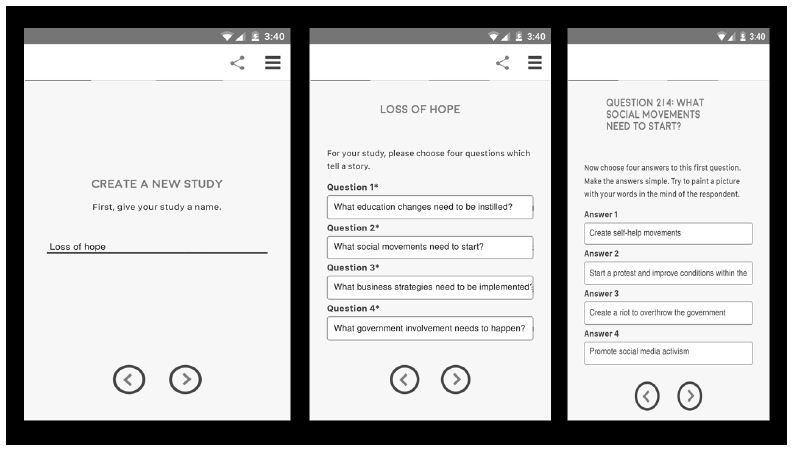
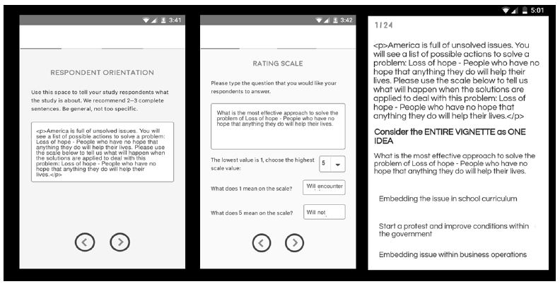
Figure 1: The first three templated steps for set up, choose the topic (left panel), select four questions (middle panel), and generate four answers to each question (question 2 on the right panel)

Step 1: Choose the Topic

Figure 1 (left panel) shows that the study topic is ‘Loss of Hope.’ The database includes the results from these five economics-oriented studies, chosen from the full set of 26:

  1. College Expense – Education for people in College is too expensive.
  2. Economic Gap – Rich people get richer, everyone else falls behind.
  3. Loss of hope – People who have no hope that anything they do will help their lives.
  4. Poverty – Poverty so that some people don’t have enough to eat.
  5. Social Security – People not sure that Social Security will last.

Step 2: Select Four Questions or Dimensions Which ‘Tell a Story’

Our ‘story’ is not a story but rather four sources of solutions (education, social, business, and governments.

Step 3: Create the Element, Four Specifics from Each Type of Solution, or 16 Elements

The set of 26 studies dealt with the solutions of social problems. The solutions were to be appropriate to ‘solving’ the fundamental or underlying issues which led to the problems, not to the actual specific solutions, which would be topic-specific, and would defeat the purpose of an integrated database incorporating many problems. Table 1 shows the four different solutions (education change; social movements; business strategies and government involvement), posted as a question, and for each solution, four specifics.

Table 1: The four types of solutions, and the four specific solutions for each type

table 1

Step 4 – Create the Self-profiling Classification Questions to Learn the Respondent’s Gender, Age, and Optional Behavior Provided by the Third Question

The third question in the self-profiling question. The actual topic of the study was given (Loss of hope), and then the four alternatives. The same format applied to all studies. Only the topic of the actual study change.

Preliminary Question: What is the most effective approach to solve the problem of Loss of hope – People who have no hope that anything they do will help their lives

1=Education Changes

2=Social Movement

3=Business Strategies

4=Government Rules

Step 5 – Create the Test Combinations Using Experimental Design

Conventional research works with single ideas (idea screening or promise testing), or with completed ‘concept’ or even advertisements. Typically, one has no way of knowing what ideas will win, or how a concept will score. The astute researcher limits risk by narrowing down the effort, generating a good sense of what answer will be obtained, and choreographing the research to accept or reject the ingoing hypothesis. Thus, in the end, most research is not so much to ‘discover’ and to confirm, presumably because most researcher is subtly based upon a ‘pass/fail’ system.

Mind Genomics is different. Mind Genomics screens ideas, combinations of the elements in Table 1, almost metaphorically in the way an MRI takes pictures of the tissue from different angles, and then combines these pictures at the end to produce an in-depth visual representation. No one picture is correct. Rather, it is the many different combinations which are processed to generate a pattern. The MRI does not ‘test,’ but rather recreates from different angles. Mind Genomics uses the same approach, albeit metaphorically, by testing different combinations of the elements, getting reactions, and from the patterns of the reactions, showing elements which drive solutions to the problems, and elements which did not.

Mind Genomics works by experimental design, systematic combinations of answers to problem. The problem is presented, and then the Mind Genomics program presents different combinations of these solutions. The respondent simply rates the combinations on a scale. The respondent ends up doing the rating by intuition, rather than trying to guess what the right answer is

Step 6 – Create an Orientation Paragraph, Introducing the Respondent to the Topic

For most research it is not necessary to create a long-set up. A short paragraph, even a single sentence will do the job. For this study we put together a more general paragraph, which could work with the different problems. The orientation ended with the specific problem, here shown in italics, but in normal font in the actual study. Figure 2, left panel, show how the orientation is typed into the BimiLeap template. The actual text follow, with the topic of the study in bold.: America is full of unsolved issues. You will see a list of possible actions to solve a problem: Loss of hope – People who have no hope that anything they do will help their lives. Please use the scale below to tell us what will happen when the solutions are applied to deal with this problem: Loss of hope – People who have no hope that anything they do will help their lives

fig 2

Figure 2: The template acquisition form for the orientation (left panel), the rating scale (middle panel), and an example of one of the vignettes (three elements; right panel)

Step 7 – Create the Rating Scale

The rating scale makes up five labelled points. The enables the researcher to deal with two dimensions, resistance (no/yes), and work (no/yes). Figure 2 (middle panel) shows the templated screen to type in the rating scale.

What is the most effective approach to solve the problem of Loss of hope – People who have no hope that anything they do will help their lives.

1=Will encounter resistance … and… Probably won’t work

2=Will not encounter resistance… but … Probably won’t work

3=Can’t honestly decide

4=Will encounter resistance… but … Probably will work

5=Will not encounter resistance … and… Probably will work

Step 8: Present Each Respondent with 24 Vignettes

Figure 2 (right panel) shows an example of a vignette. Each respondent begin with the self-profiling classification, then read the orientation page, and then rated 24 vignettes on the 5-point scale. The program presented the combination, acquired the rating (5-point scale), and the number of seconds, to the nearest tenth of second, between the time the vignette was presented and the time that the response was made.

Step 9 – Prepare the Data for Statistical Modeling

A key benefit of Mind Genomics is ‘design thinking.’ Rather than getting data and testing hypotheses, Mind Genomics is set up to create a database. The data itself forms rows of data. Each respondent generates 24 rows of results, with the following columns.

a. Columns 1-3: The columns record the topic, the respondent identification code, the age, gender, and answer to the third classification questionnaire. These are the same for the 24 rows of data for that respondent.

b. Columns 4-19: There are 16 elements that could be incorporated into a vignette. Each of the next 16 columns corresponds to an element, with the value ‘1’ inserted when the element appeared in that vignette, else the value ‘0’ inserted when the element was absent from that vignette. The experimental design prescribed which set of 2-4 elements would appear. Thus, any row would show two, three, or four ‘1’s,’ and the rest 0’s.

c. Columns 20-22: The respondent rated the vignette on the 5-point scale. The next three columns show order of test (1-24) of the vignette, the rating assigned by the respondent (1-5), and the number of seconds to the nearest 10th of second between the appearance of the vignette and the respondent’s rating (0-8 seconds; all times > 8 seconds were truncated to 8).This is called the RT, the response time.

d. Columns 23-27: The datafile was manually reshaped by augmenting it with five new variables (R1-R5), showing which rating was assigned. For example, when the respondent to rate the vignette ‘5’, R5 took on the value 100 (with a vanishingly small random number added), whereas R4, R3 R2 and R1 each took on the value 0 (also with a vanishingly small random number added). The random number is a prophylactic measure for the downstream regression models, yet to come.

e. Columns 28-31: Four new variables were created, allowing the database to feature a single variable emerging from both instances of an answer. For example, the phrase ‘Probably will work’ appears in R4 and R5. Thus, R45 takes on the value ‘100’ (plus the vanishingly small random number) when the rating was either 4 or 5, respectively. R45 takes on the value 0 (Plus the vanishingly small random number) when the rating was 1,2 or 3, respectively. The four newly created variables of this type are:

R45 Probably will work

R25 will not encounter resistance

R12 Probably won’t work

R14 will encounter resistance

Step 10 – Use Clustering to Create New to the World Mind-sets, Individuals Who View the World the Same within this Specific Framework of Problems and Solutions

At the start of the on-line experiment, the respondent completed a small, three-question self-profiling questionnaire, to record gender, age, and select of which approach would be the best way to solve the problem. A hallmark of the Mind Genomics approach is to let pattern of responses to the granular issue generate possibly new-to-the-world groupings of respondents, not based on who they are, but based on how they respond to the granular issues (here solutions to problems). These groups are mind-sets. The respondent may or may not even be aware of belonging to a mind-set, but the response pattern to the 24 vignettes will reveal that membership, after the responses to the vignettes are deconstructed into the part-worth contributions of each of the 16 elements.

Clustering is a well-accepted group of statistical methods which divide objects into non-overlapping groups based upon patterns of features shared by the objects. In our case the pattern of features will be the degree to which each of the 16 elements drives the response. The elements will be coded as 0’s and 1’s, in the database, and the criterion variable will be R45, the rating of ‘probably will work’. The analysis, purely mathematical, will create a profile of 16 numbers (coefficients) for each respondent, each coefficient attached to one of the16 elements. The clustering program [12] will put respondents into two groups, and then three groups, based strictly on mathematical criteria, not judgment. It will be the job of the researcher to select which set of groupings makes sense (two groups vs. three groups). The criteria will be parsimony (the fewer the number of groups or clusters, the better), and interpretability (the groups must make sense).

The novel approach here is that the clustering will be done on the coefficients of all 257 respondents. Thus, the clustering will look at the way the respondents feel a problem can be solved, with the problem varying by experiment, and clearly stated at the start of the experiment. Psychologists call this process priming [13].

The method for creating clusters follows the rules of statistics. The total data-set includes five studies, slightly more than 50 respondents per study. Recall that the 24 vignettes for each respondent were laid out by an experimental design. Even though the combinations were different for each respondent, the mathematical structure was the same. This is called a permuted design [14]. The benefit of the individual level experimental design it that it allow the researcher to use OLS (ordinary least-squares) to relate the presence/absence of the 16 elements either to the rating, to the binary transformed rating, or to response time

When OLS regression is applied to the data, one respondent at a time, using the option of ‘no additive constant,’ the individual level regression appears as:

Binary Response (R45)=k1(A1)+k2(A2)+… k16(D4)

The foregoing equation expressed how the 16 different answers shown in Table 1 can be combined to estimate the rating of R45, the newly created variable ‘probably will work.’ Thus, the regression analysis extracts order from the data, allowing patterns to appear. High coefficients suggest that when the element in inserted into the vignette, the rating is likely to be either 4 or 5, both corresponding to probably will work. Low coefficients suggest that when the element is inserted into the vignette, the rating is likely not to be 4 or 5.

The individual level, and for that matter the group models, do not have an additive constant. This revised form allows the direct comparison of the 16 elements. It is vital to be able to compare the elements, side by side, across groups. The additive constant is more correct statistically, but makes the comparisons difficult. Thus, for this r set of analyses we choose not to use the additive constant, even though the model will not fit the data as well.

The five studies were treated identically, considered simply as part of a one big study. To the regression analysis the structure of the inputs and output was identical. At the end of the regression analysis the result was a data matrix forming 16 columns, one for each element, and 257 rows, one for each respondent. The numbers in the data matrix were the coefficients.

A k-means clustering program divided the 257 respondents into two groups and three groups based upon the distances between the respondents. Respondents separated by large distance, to be defined now, were put into different clusters, or mind-sets The ‘distance’ between people was operationally defined as (1-Pearson Correlation), computed on the 16 coefficients of pairs of respondents, not matter whether they were i the same study or different studies. the structure of their data allowed that.

The Pearson correlation shows the strength of a linear relation between two objects (e.g., respondents). The value of R varies from+1 through 0 to -1. R takes on the highest value, 1, when the two objects are perfectly linearly related. R take on the lowest value, -1, when two objects are perfectly inversely related. The distance between two people goes from a low of 0 when the 16 pairs of coefficients generate a Pearson R of+1 (D=0), to a high of 2 when the 16 pairs of coefficients generate a Pearson R of -1 (D=2).

Step 11 – Create Group Models, Incorporating All the Data from a Group

The final modeling consist of creating a general model which uses all 16 elements as predictors, as well as study, gender, age group, belief in what is the best way to solve the problem, and finally mind-set. The modeling thus puts all the variables on the same footing, allowing the researcher to instantly understand the contribution or driving power of each element or respondent feature to three selected dependent variables. These three variables are R45 (probably will work), R3 (can’t make a decision), and RT (response time in seconds).

The general model is expressed as:

Dependent Variable=k1(A1)+k2(A2)+… k16(D4)+k17(College Expenses)+k18(Economic Gap)+k19(Loss of Hope)+k20(Poverty)+k21(Social Security)+k22(Female)+k23(Male)+k24(Age 17-29)+k25(Age 30-49)+k26(Age 50-64)+k27(Age 65-80)+k26(Business)+k27(Education)+k28(Government)+k29(Social Movement)+k30(Mind-Set 1)+k31(Mind-Set 2)+k32(Mind-Set 3)

The foregoing equation is easy to estimate, even for large data sets. It is important to keep in mind that the 16 elements (A1-D4) were designed to be statistically independent and thus always appear in the equation. Not so, however, with the other variables. In every regression model, exactly one of the classifications from each group will be missing, and given a value 0 by the regression. That is because the coefficients for the classification features are relative, not absolute. Thus, when looking at males versus females, there is a variable called male, and another variable called female. One of them will have a coefficient showing its relative contribution (viz. female). The other will be set to 0 (viz. male)

How do the Respondents Distribute Across the Different Classification Criteria?

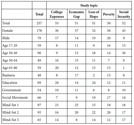
Table 2 shows the distribution of the respondents across the five studies, each column corresponding to a study. The rows correspond to the distinct groups into which a respondent could be put, either from the up-front self-profiling classification, or from the clustering into three mind-sets.

Table 2: Distribution of respondents across the five studies

table 2

What is the Pattern of Ratings Assigned by the Respondents in the Separate Groups?

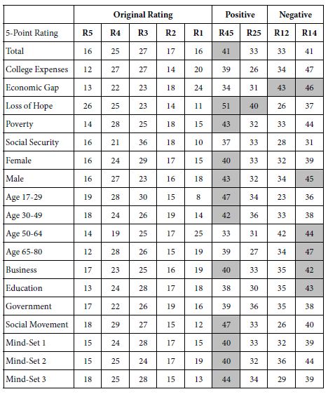
Our first analysis focuses on the pattern of ratings, something that would be the natural first step of any research. We have five ratings (R5, R4, R3, R2, R1, the simple five point scale), as well as four combining scales: Probably will work (R45), Won’t encounter resistance (R25), Probably won’t work (R12), and Will encounter resistance (R14), respectively.

Faced with the data, and absent consideration of the underlying experimental design, the standard analytics would begin by compiling a list of frequencies of ratings by key subgroups (Table 3). After doing that, the typical analysis might look for departures, such as groups in the studies seeming to depart from the general pattern.

Table 3: Percent of responses for each group assigned to original ratings (adds to 100), and then both positives (Probably work, Encounter no resistance), and negative (Probably not work, Encounter resistance)

table 3

This surface analysis looks at the pattern for the Total Panel versus the pattern for a specific group, such as the study topic ‘Loss of Hope’, which seems aberrantly positive. The surface analysis provides observations, but little in the way of deep insight.

How the Ratings Change with Repeated Evaluations

Conventional research often asks a limited number of questions perhaps in a randomized order to forestall order bias. The data from these five studies across 50+respondents and 24 vignettes per respondent allow the researcher to get a sense repeating the same task 24 times. The skeptic would say that it is impossible, and that no one can be consistent across 24 vignettes. That skepticism brings up the question of just what happens when the respondent continues to focus on the same topic for 24 vignettes; the vignettes are all different from each other, so we cannot look at the ratings for the same vignette over time. But we can look at the average ratings of vignettes in the same position of time, to see whether we can find a pattern of average vs. time, recognizing of course that the no two vignettes are alike. The issue is whether there is a noticeable position effect.

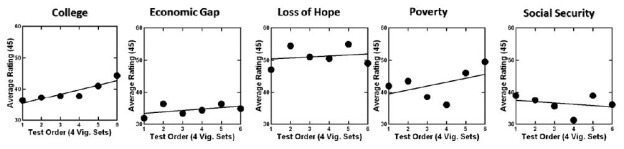
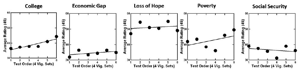
To understand the issue of stability with repeated exposure to the same problem we looked at the average rating by position. Rather than looking at 24 positions, we reduced the 24 positions to six by creating six sets of positions (e.g., 1-4, 5-8, et.) and then averaging the four ratings for each respondent to generate six new ‘ratings’.

The foregoing analysis allows us to create averages of ratings for each of the six orders, doing so for all respondents in a study, and by each of the five studies. Figure 3 shows the scatterplot of average rating of the 5-point scale versus the new set of six positions. There is a clear order effect, stronger for some (e.g., College Expenses and Economic Gap, less clear for others such as Loss of Hope, Poverty and Social Security). The reason for the differences of average ratings by order of testing is not clear because the five studies were done in the same way.

The change in average rating is important to deal with. It is not usually addressed in conventional research, where the topic is only broached once, and rated. There is nothing to discuss in Figure 3, because we only have a surface measure. However, we deal with Figure 3 as part of a later analysis.

fig 3

Figure 3: Change in the average rating over the 24 vignettes by each of the five studies

Creating Enhanced Models for the Study Using OLS Regression

In Step 11 above we presented the expression for the enhanced regression model, considering both the elements, as well as the study, gender, age, selected belief about the best solution, and mind-set. The 16 elements are presented as 0’s and 1’s, the remaining factors (study through mind-set) as category variables which can be deconstructed into separate variables.

As noted above, the equation is:

Dependent Variable=k1(A1)+k2(A2)+… k16(D4)+k17(College Expenses)+k18(Economic Gap)+k19(Loss of Hope)+k20(Poverty)+k21(Social Security)+k22(Female)+k23(Male)+k24(Age 17-29)+k25(Age 30-49)+k26(Age 50-64)+k27(Age 65-80)+k26(Business)+k27(Education)+k28(Government)+k29(Social Movement)+k30(Mind-Set 1)+k31(Mind-Set 2)+k32(Mind-Set 3)

We run the regression equation by total in the next analysis. In the appendix, we present the parameters of the model by study, by gender, by age, by belief in the best solution, and by mind-sets, as well as by the first and last set of vignettes (to deal with the issue of just what changes as the person evaluates the vignettes)

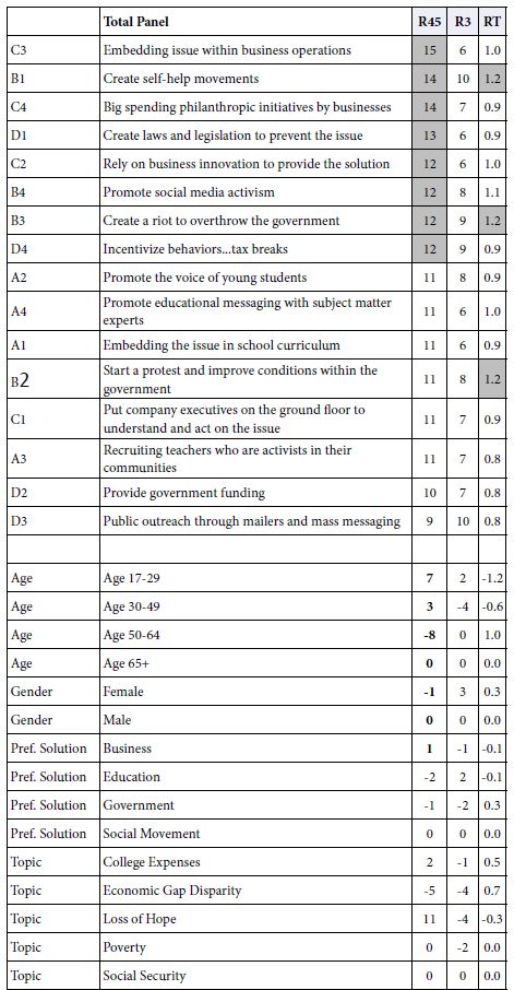
Table 4 shows the coefficients of models for R45 (Probably work), R3 (Cannot answer), and RT (Response time), respectively. Our first set of analyses focuses only on the coefficients of the 16 elements.

Table 4: Models for total panel relating the presence/absence of the 16 elements, the different self-profiling classifications, and the topic study to R45 (probably solve), R3(cannot decide) and RT (response time in seconds)

table 4

The first data column, labelled RT45 corresponds to the coefficients for the rating of ‘probably can solve,’ viz., R4 and R5 combined. Surprisingly, eight of the 16 elements generate coefficients of 12 or higher. There are surprises, such as B2 (create a riot to overthrow the government.) This element might not have appeared had the respondents simply rated what ideas would lead to a possible solution, presumably because of an ‘internal editor’ which tries to be politically correct, and automatically attach a negative response to the element. It is only because the element is embedded in mixture of other elements that the respondent becomes far less capable to be politically correct, simply because it is impossible to be so when confront with what sees a ‘blooming buzzing confusion.’ The analogy here might be the emergence of negative qualities when a respondent interprets a Rorschach blot. Negative ideas are not easily suppressed in the narrative.

C3 Embedding issue within business operations

B1 Create self-help movements

C4 Big spending philanthropic initiatives by businesses

D1 Create laws and legislation to prevent the issue

C2 Rely on business innovation to provide the solution

B4 Promote social media activism

B3 Create a riot to overthrow the government

D4 Incentivize behaviors…tax breaks

The second column, labelled R3, shows the strong elements driving ‘I cannot decide’.. There are no strong performers, viz elements which generate coefficients of+12 or higher. There are two elements which come close. However these are elements which confuse respondents. We would not have really known that, except for the power of this emergent dataset that we are creating.

B1 Create self-help movements

D3 Public outreach through mailers and mass messaging

The third column, labelled RT, shows the reaction time ascribable to each element. The Mind Genomics algorithm measured the time from the appearance of the element to the rating, and used that as a dependent measure. Again, these are estimated times needed to read the element and contribute to the decision. The response time can be s a measure of engagement, of reading the information and thinking about it. the response time itself is neither good nor bad, but simply a measure of behavior. The elements which require time to process are those dealing with actions that the person takes:

B1 Create self-help movements

B3 Create a riot to overthrow the government

B2 Start a protest and improve conditions within the government

Our next analysis looks at the contribution of ‘the group’ of respondents. Following the set of 16 elements (sorted in order) we see four groups. These are the four ways that we divided the respondents, ahead of the study itself. These are age, gender, preferred method of solving problems (all three from the self-profiling classification), and then topic of the study.

One option of each set is always assigned the value 0 because these alternatives in each set are not statistically independent of each other. The respondent must belong to one of the four ages, be one of the two genders, select one of the four preferred methods for solving problems, and take part in one of the five studies. Consequently, incorporating these variables into the regression program meant leaving one of the options out for each group. That option is not estimated in the larger equation, but instead is left out, and in the reporting is automatically assigned the value 0 for its coefficient. It makes no difference which four options are selected. All the coefficients for the options are estimated with respect to the optionally deliberately omitted from the estimation, and automatically assigned the value 0. The four options are Age 65+; Male; Social Movement; Social Security.

The coefficients for each of these four groups can only be compared within the group, not to the other groups, and not to the elements. Nonetheless, we still get a sense of the effects. For example, when it comes to the coefficients for R45, Probably Work, respondents end up generating higher rating when the study topic is “Loss of Hope” with a coefficient of+11. This is independent of all other factors, including elements and ways of classifying the respondent. In contrast ‘economic disparity’ is the least likely to be solved, at least from these data, with a coefficient of -5.

Looking at the differences between the coefficients for R45, we can conclude that:

  1. Age 17-29 is the most positive (+7 ), whereas age 50-64 is most negative (-8)
  2. There are no big differences across the four groups, based on the way they define themselves in terms of what best solves the problem.
  3. There is no difference in gender
  4. The is a substantial difference in the topic. The coefficient is highest for Loss of Hope (+11) meaning in general people are optimistic that this can be solved. The coefficient is lowest for economic gap disparity (-5) meaning people are least optimistic that this can be solved.

One again it is important to note that this type of information could not be easily obtained from conventional data sources, but becomes a simple byproduct of the data base, trackable over time, and across cultures and events.

We could do the same analysis for R3, the inability to make a judgment. There are no noteworthy group differences in R3, in the way there were for R45.

Finally, the analysis for RT for the age groups suggest that the response for the youngest respondents (age 17-29) is dramatically faster than the response time for the two older groups (age 50-64, age 65-80). The coefficient for age 17-29 is -0.6. The coefficient for age 50-64 is+1.0 On average, the speed is the response of the older respondents is 1.6 seconds longer for each element.

On the Nature of Micro and Macro Differences among the Three Emergent Mind-sets

The standard analysis by Mind Genomics usually reveals dramatically different, clearly explainable differences across the different mind-sets. Table 5 shows the performance of the elements of these three mind-sets, and the labelled assigned to each. This type of information become increasingly important as the researcher tries to uncover macro pattern among people. It is straightforward to uncover macro patterns when one has commensurate data for all the individuals, as one has here, based on the 16 coefficients.

Table 5: Performance of the 16 elements by the three mind-sets

table 5

Traditionally, Mind Genomics stopped after showing the underlying mind-sets and their coefficients. Do we learn any more from knowing the average coefficient in a mind-set, not of the coefficient, but of the different groups?. Are the groups similar, or do the groups differ from each other?

Table 6 shows that there remains heterogeneity across similar groups, even within a mind-set. The variation in coefficients has already been reduced by the clustering, which generated three mind-sets. The remaining variation, that due to the age, gender, preferred solution, and topic, is more of a baseline ‘adjustment’ value, like the intercept in an equation. One might say that the variables of age, gender, preferred solution of the problem and study topic, respectively are simply additive correction factors of different magnitudes.

Table 6: The pattern of coefficients for the total panel, and for the three different mind-sets

table 6

The Nature of the Differences between the First and the Last Sets of Four Vignettes

Recall that Figure 3 shows the change in the average rating from the start of the evaluation to the end of the evaluation. Each of the filled circles corresponded to the average of R45 for a set of four vignettes (positions 1-4, 5-8, 9-12, 13-16, 17-20, 21-24). Below figure shows clear that there is an effect. Ordinarily the researcher would report this observation, and move on. The modeling approach allows us to create a full model for each of the six sets of four vignettes. We can create the grand model for the first quartet of vignettes (order 1,2,34), for the last quartet (order 21,22,23, 24) and discover the magnitude of the effect by subtracting the coefficients (Difference=Coefficient for Position 21-24 MINUS coefficient for position 1-4).

Table 7 shows the largest differences for the three dependent variables. There is no need to explain the differences. The intent here is simply to show that these deeper questions can be explore though the database in a way that allows the research to uncover patterns, perhaps unexpected ones, and from that effort generate a working hypothesis.

Table 7: “Large”differences between corresponding coefficients for Positions 21-24 MINUS Position 1-4. The table shows only those major differences, for three dependent variables, R45, R3, and RT

table 7

Discussion and Conclusions

The goal of this paper is to demonstrate a new way of thinking about social issues, one which moves out of the realm of hypothesis testing, and more into the realm of databasing, with objectives to record the citizen’s mind in a new way, and as a byproduct lead to hypothesis generation. The novelty of the approach is the facile, rapid, affordable, and scalable creation of databases having to do with different topics in the same domain.

The It! studies of two decades ago began this effort, but at that time it the value of having the precise elements across all topics was ignored. The It! studies attempted to customize the elements, but at the same time maintain a logical structure spanning all the studies. The result was that each study had to be analyzed separately. The emergence of similar mind-sets across foods [9] was encouraging, but the further analytic power emerging from directly comparability was missing. It was a matter of hoping that the same mind-sets would appear, rather than creating the conditions to use all the data to create a common set of groups spanning all the experiments.

The next logical step can be the expansion of the database across more people within a country, countries beyond the United States, and the creation of the database year after year, or even in an ad hoc way during period of social change. The simplicity and affordability of the database approach as demonstrated here allows for the expansion of this databasing approach to other verticals. In that spirit, the other verticals will feature other topics, and so the topics will change to fit the vertical.

The long term view of the process maybe something like creating a collection of perhaps eight such databases, each dealing with a ‘vertical,’ viz different facets in of life, each vertical comprising perhaps seven different but precisely parallel studies (topics in the database), each study run with 100 respondents (rather than 50), and study created to be exactly alike and run the same way in 20 countries. This totals 8 (databases/one per vertical) x 7(studies per database) x 100(respondents per study) x 20(countries) or 1,120 studies, each study run with 100 respondents. Verticals could be situations such as conflicts, negotiations, social problems, empowering citizens, enhancing education, and the like. The cost would be minimal (1,120 studies x 400-$600$ per study as of this writing, Winter, 2022, according to www.BimiLeap.com).

The potential to understand society, its problems, its issues, and opportunities to create a better world through knowledge is the key deliverable from these studies. One might end up with keys which allow groups of people to understand each other, information about communications between hostile parties in conflict situations, along with the ability to update the information, focus that information, or expand the scope as the need arises.

Acknowledgement

Author HRM gratefully acknowledge the conversations about these databases with his colleagues, too many to list, and most to the unwavering encouragement of his wife, Arlene Gandler, who inspired the vision of databasing for world issues during the early, foundational years of Mind Genomics.

References

  1. Searles K, Ginn MH, Nickens J (2016) For whom the poll airs: Comparing poll results to television poll coverage. Public Opinion Quarterly 80: 943-963.
  2. Holwell S (2000) Soft systems methodology: other voices. Systemic Practice and Action Research 13: 773-797.
  3. Foa UG, Foa EB (1974) Societal structures of the mind. Charles C Thomas
  4. PsycINFO Database Record 2016 APA (Foa and Foa, 1974)
  5. Moskowitz HR, Gofman A (2007) Selling Blue Elephants: How to Make Great Products that People Want Before They Even Know They Want Them. Pearson Education, 2007.
  6. Hunt JD, Abraham JE, Patterson DM (1995) Computer generated conjoint analysis surveys for investigating citizen preferences. In Proceedings of the 4th International Conference on Computers in Urban Planning and Urban Management, Melbourne, Australia, 13-25.
  7. Stadelmann S, Dermont C (2020) Citizens’ opinions about basic income proposals compared–A conjoint analysis of Finland and Switzerland. Journal of Social Policy 49: 383-403.
  8. Lilley K, Barker M, Harris N (2015) Exploring the process of global citizen learning and the student mind-set. Journal of Studies in International Education 19: 225-245.
  9. Moskowitz HR, Beckley J (2006) Large scale concept response databases for food and drink using conjoint analysis, segmentation, and databasing. The Handbook of Food Science, Technology, and Engineering, 2. ed. Y H Hui chapter 59 Taylor and Francis
  10. Foley M, Beckley J, Ashman H, Moskowitz HR (2009) The mind-set of teens towards food communications revealed by conjoint measurement and multi-food databases. Appetite 52: 554-560. [crossref]
  11. Moskowitz HR (2004) Evolving conjoint analysis: From rational features/benefits to an off-the-shelf marketing database. Marketing Research and Modeling: Progress and Prospects (215-230). Springer, Boston, MA.
  12. Likas A, Vlassis N, Verbeek JJ (2003) The global k-means clustering algorithm. Pattern Recognition 36: 451-461.
  13. Molden DC (2014) Understanding priming effects in social psychology: An overview and integration. Social Cognition 32: 243-249.
  14. Gofman A, Moskowitz H (2010) Isomorphic permuted experimental designs and their application in conjoint analysis. Journal of Sensory Studies 25: 27-145.

Nano-Periodontics: A Step Forward In Periodontal Treatment

DOI: 10.31038/JDMR.2022513

Introduction

The term “Nano” refers to a unit of measurement that is equal to one billionth of a kilometer (10-9). To get closer to “how much Nano is”, it is worthy to know that the length of a normal human being ranges from one and a half to two meters, while, if we move to something smaller, such as a mobile phone, it can be measured by 12 cm, and if we move to smaller things, ants for example are about 2 mm long, while if we take a human hair, its diameter measures about 100 micrometers. Viruses are much smaller ranging in size between 30 and 50 nanometers, and a DNA molecule has a size of about 2.5 nanometers. Taking into account that the approximate size of the sun is 1.4 billion meters, this means that a nanoparticle for a human is the same as the size of a human in relation to the sun [1].

Nanotechnology is the science of engineering and technology that is practiced at the nanoscale and ranges between 1 and 100 nanometers. The ideas and concepts of nanotechnology began to appear in 1959, while the modern practice of it actually began in 1981 [2].

One of the factors associated with miniaturization and nanotechnology is the surface-to-volume ratio. This criterion is of great importance and fundamental in applications that include Nano and chemical stimulus in physical process. In general, the surface-to-volume ratio increases with the decrease in the dimensions of the material and vice versa, so the lower the volume of the material, we find a larger part of the atoms on the surface compared to the atoms on the inside, and since chemical reactions occur on the surface, nanoparticles are much more effective than other materials made up of larger particles [1].

Nanotechnology in Periodontics

Nanotechnology has become a thriving field in human medicine and dentistry in recent years, as the use of nanotechnology in periodontology referred to as “Nanoperiodontics”. The Nanoperiodontics works to maintain oral health by linking nanomaterials with biotechnology, and although they are in the initial stages, they have a significant impact on clinical outcomes on one hand, and commercial availability of materials on the other hand. The applications of nanoparticles in periodontics can be discussed according to 3 main headings; namely prevention, detection, and treatment.

Prevention

Mouthwashes built in nanorobots and selenium nanoparticles can control halitosis by destroying the volatile Sulphur compounds produced by bacteria.

Toothpastes combined with nanorobots can destroy the pathogenic flora and at the same time preserve more than 500 types of commensal organisms, but it is still under study at the present time [3].

Detection

Introducing the Lab-on-chip concept which is a small chip, that does more than one measuring device, can give us the concentrations of Interlukin-1ß (IL-1ß) [4], C-reactive Protein (CRP) [5], and Tumor Necrosis Factor-α (TNF-α) [6], which are proteins found in saliva that increase in the presence of periodontitis from a single saliva sample [3].

Treatment

In a clinical study conducted on the effect of slider nanoparticles on patients with chronic periodontitis [7], patients were divided into 3 groups; Group A: Scaling and root planning (SRP) with sub-gingival delivery of silver nanoparticles gel, Group B: SRP with sub-gingival delivery of tetracycline gel, and Group C: SRP alone. Diagnostic indices were recorded for each patient before and after application of the gel, which included Plaque Index (PI), Gingival Index (GI), Probing Pocket Depth (PPD) and Clinical Attachment Level (CAL). The results showed that the effectiveness of using silver nanoparticles is similar to the effectiveness of using tetracycline gel, but the use of silver nanoparticles compared to other materials used was non-toxic, easy to apply, and showed no side effects.

Curcumin (CUR) is a natural polyphenolic compound that has been studied for its antioxidant effects. In a study conducted by Pérez-Pacheco CG et al. (2021), prepared buccal discs containing CUR-loaded lipid nanocarriers confirmed the ability of nanostructured lipid (NLC) to enhance CUR penetration through lipophilic domains of the mucosa [8].

The advantages of high drug loading, specific site release, and prolonged drug action have also made nanomaterials very promising for treating periodontitis [9].

In another study, Shaheen et al. (2020) found that nanomaterials loaded with antioxidants can be administered locally into periodontal pockets to effectively treat periodontitis [10]. They prepared a micellar nanocarriers containing coenzyme Q10 by a modified nanoprecipitation method and then evaluated the treatment effects of this innovative system in moderate periodontitis. Loading Q10 into ultra-small size nanoparticles could improve its aqueous dispersibility and bioavailability. In their study, Q10 was formulated in nano-micelles (NMQ10) that was incorporated in situ gelling systems, followed by injection into the periodontal pockets of periodontitis patients. The results showed that the NMQ10 was able to penetrate into the required site well. Periodontitis patients who received the administration of NMQ10 obtained a significant therapeutic effect, with significantly reduced oxidative stress markers and improved periodontal evaluation parameters.

In terms of Nanomaterials for periodontal tissue engineering, several biomaterials are used in periodontal tissue engineering in order to obtain a three-dimensional scaffold, which can promote bone regeneration. A systematic study conducted in 2020 on the use and efficacy of a chitosan-based scaffold (CS-BS) in the process of alveolar bone regeneration showed that the potential for periodontal regeneration is higher in the case of CS-BS scaffolds combined with other polymeric biomaterials and bio-ceramics [11].

Conclusion

Periodontitis is one of the most common diseases involving tooth and its supporting structures. Management of periodontitis is important for improvement of quality of life of the patient that ultimately has its impact on overall health of an individual. With improvement of various treatment methodologies for treatment of periodontitis, nanotechnology has evolved as a promising mode of treatment. Nanotechnology is an emerging field in medicine and dentistry that would extend its horizons right from the diagnosis to the treatment and rehabilitation phase.

References

  1. Mohanraj VJ, Chen Y (2006) Nanoparticles-a review. Tropical Journal of Pharmaceutical Research 5: 561-73.
  2. Huang Z, Chen H, Yip A, Ng G, Guo F, et al. (2003) Longitudinal patent analysis for nanoscale science and engineering: Country, institution and technology field. Journal of Nanoparticle Research 5: 333-363.
  3. Parvathi TH, Vijayalakshmi R, Jaideep Mah, Ramakrishnan T, BurniceNalinaKumari C (2020) Nanotechnology in Periodontics: An Overview. Medico-legal update Dec.
  4. Marianna E Gr, Spiridon-Oumvertos Ko, Phoebus N Ma, Jorg-Rudolf St (2010) Interleukin-1 as a genetic marker for periodontitis: review of the literature. Quintessence Int 41: 517-25. [crossref]
  5. T Bansal, A Pandey, Deepa D, Ash K Asthana (2014) C-Reactive Protein (CRP) and its Association with Periodontal Disease: A Brief Review. J Clin Diagn Res 8: 21-24. [crossref]
  6. Pr Singh, Narender Dev Gu, Af Bey, S Khan (2014) Salivary TNF-alpha: A potential marker of periodontal destruction. J Indian Soc Periodontol 18: 306-310. [crossref]
  7. Po Kadam, Sw Mahale, Pr Soner, Di Chaudhari, Sh Shimpi, An Kathurwar (2020) Efficacy of silver nanoparticles in chronic periodontitis patients: a clinico-microbiological study. Iberoam J Med 2.
  8. Pérez-Pacheco CG, Fernandes NA, Primo FL, Tedesco AC, Bellile E, et al. (2021) Local application of curcumin-loaded nanoparticles as an adjunct to scaling and root planing in periodontitis: Randomized, placebo-controlled, double-blind split-mouth clinical trial. Clinical Oral Investigations 25: 3217-3227. [crossref]
  9. Goyal G, Garg T, Rath G, Goyal A K (2014) Current nanotechnological strategies for an effective delivery of drugs in treatment of periodontal disease. Crit Rev Ther Drug Carrier Syst 31: 89-119. [crossref]
  10. Shaheen MA, Elmeadawy SH, Bazeed FB, Anees MM, Saleh NM (2020) Innovative coenzyme Q 10-loaded nanoformulation as an adjunct approach for the management of moderate periodontitis: preparation, evaluation, and clinical study. Drug Deliv Transl Res 10: 548-564. [crossref]
  11. Do Lauritano, Lu Limongelli, Gi Moreo, Gi Favia, Fr Carinci (2020) Nanomaterials for Periodontal Tissue Engineering: Chitosan-Based Scaffolds. A Systematic Review. Nanomaterials (Basel) 10: 605. [crossref]

Association of Pre-Pregnancy BMI and Gestational Weight Gain with Neonatal Body Size: A Cross- Sectional Study

DOI: 10.31038/IGOJ.2022513

Abstract

Background: Pre-pregnancy BMI and GWG partially reflect maternal nutrition. The study aimed to explore the effects of pre-pregnancy BMI and GWG on the body size of neonates at birth.

Methods: A total of 546 mothers and their babies were selected from August 2017 to April 2018 at Obstetrical Department of the 3rd Affiliated Hospital of Zhengzhou University. The levels of leptin and adiponectin in cord blood were measured. The mass of placenta was evaluated based on the size. The maternal subjects were defined as low (BMI<18.5), normal (18.5≤BMI<25.0) and overweight/ obese (BMI≥25.0) groups. Moreover, the maternal subjects were divided into low, normal and high GWG groups corresponding to the guidelines of GWG. The neonates were divided into small (SGA), large (LGA) and appropriate (AGA) for gestational age groups based on their birth weight and gestational weeks.

Results: The incidence of SGA was higher in low pre-pregnant weight group than that in normal and overweight/obese groups (both P<0.05). The incidence of LGA was higher in high GWG group than that in normal and low GWG groups (both P<0.05). The correlation analysis showed that the birth weight (BW), body length (BL), head circumference (HC), and Ponderal Index (PI) of neonates were positively correlated with pre-pregnancy BMI and GWG (P<0.05, P<0.01). Neonatal BW, BL, HC, PI, placental weight and placental volume were positively correlated with the levels of adiponectin and leptin in umbilical cord blood respectively (P<0.05).

Conclusions: Pre-pregnancy BMI and GWG are positively correlated with the full term neonatal size. It is crucial for neonatal physical development to maintain appropriate BW before and during pregnancy. The adiponectin and leptin in cord blood were positively correlated with neonatal physical development suggests that both them play an important role in regulating fetal growth and development.

Keywords

Gestational weight gain, LGA, BMI, SGA

Introduction

For the newborns, Birth Weight (BW), Body Length (BL), and Head Circumference (HC) are the most intuitive indicators of physical development. Abnormal physical development not only increases the risk of neonatal illness or death, but also significantly affects the occurrence of several chronic diseases in childhood/adulthood [1]. Adequate maternal nutrition plays a crucial role in providing nourished uterine environment for fetal development. Inadequacy or deficiency of maternal nutrition is associated with disruption of fetoplacental exchange. Maternal nutrition not only impacts neonatal development, but also has a long term influence on his/her health till adulthood [2]. Several epidemiological investigations and experimental studies confirmed that malnutrition during pregnancy will cause neonatal organ dysplasia, endocrine disorder, and even some chronic diseases during adulthood [3-6]. Optimized nutrition at early life, especially during fetal period is the most important factor for one’s whole life. Some studies have indicated that nutrition at early stage of life has an impact on the development of some chronic non-communicated diseases at adulthood, such as obesity, diabetes, gout, hypertension, and coronary heart disease [7,8].

As the critical parameter of prenatal care, Gestational Weight Gain (GWG) consisted of fetus, placenta, amniotic fluid, maternal adipose tissue and breast tissue growth, could reflect the health and nutrition condition of the pregnant women. Other researches showed that maternal malnutrition could influence neonatal development and even increase the incidence of low BW, while maternal over nutrition and excessive GWG also increases the risk of adverse birth outcomes [9-11].

Reasonable dietary intake during gestation is important for appropriate neonatal growth and also helpful to prevent the chronic diseases in the adulthood. Up to date, the data regarding the effect of pre-pregnant Body Mass Index (BMI) and GWG on neonatal physical development were limited. Therefore, this study would explore the association of pre-pregnant BMI and GWG with neonatal development.

Methods

Subject Inclusion and Information Collection

A cross-sectional study was conducted. The subjects were the pregnant women who planned to deliver their babies at Obstetrical Department of the 3rd Affiliated Hospital of Zhengzhou University, from August 2017 to April 2018. The inclusion criteria were monocyesis and full-term delivery without significant diseases both of the mother and baby. The exclusion criteria included multiplets, premature delivery, pregnancy complications, such as gestational diabetes mellitus, hypertension, and pre-eclampsia, and accompanied with other severe diseases. The basic information of the subjects was collected through medical record and questionnaires, and informed consents were obtained.

This research was in accord with the Helsinki Declaration, and was approved by Zhengzhou University Life Science Ethics Review Board (ZZUIRB 2021 – 139).

Grouping of the Subjects

According to the standard of BMI for Asian adults [12], the maternal subjects were divided into three groups based on their pre-pregnant BMI: low weight (BMI<18.5), normal weight (18.5≤BMI<25.0), and overweight/obese (BMI≥25.0). The case number of obese women was small in the study, thus the overweight and obese subjects were combined as overweight/obese.

The levels of GWG recommended by Institute of Medicine guideline (IOM, 2009) are 12.5~18 kg, 11.5~16 kg, 7~11.5 kg, and 5~9 kg, for low weight, normal weight, overweight, and obese women of pre-pregnancy, respectively [13]. Based on the recommendation of IOM, the subjects were divided into low (below IOM guideline), normal (within the range of IOM guideline), and high (above IOM guideline) GWG groups.

The Neonatal Body Size

The body measurements included BW, BL, and HC of the neonates. The newborns were weighted using electronic scale at the accuracy scale of 0.01 kg and measured for BL and HC using measuring tape at the accuracy of 0.1cm. Ponderal Index (PI) [14] was calculated based on BW and BL, which is the index for estimating the nutrition condition of the neonates [PI = 100 × weight (g)/ length (cm)3].

Based on the BW and gestational age, the neonates were divided into three groups [15]: (1) Small for gestational age (SGA): BW below the 10th percentile for the corresponding gestational age; (2) Large for gestational age (LGA): BW above the 90th percentile for the corresponding gestational age; (3) Appropriate for gestational age (AGA): BW between the 10th and 90th percentile for the corresponding gestational age.

Measurement of Adiponectin and Leptin in Umbilical Cord Blood

After fetal delivery, 10 ml of umbilical venous blood was drawn immediately before delivery of the placenta. Then the serum was separated after centrifuged at 3000 rpm for 10 min and stored at -80°C for later tests. The serum levels of leptin and adiponectin were determined through Enzyme-linked immunoassay. The assays were conducted according to instructions using the ELISA kits (Shanghai Fusheng Industrial Co., Ltd. China).

After delivery, the placenta was weighed and its volume was estimated based on the formula. Placental volume (cm3) = π/4 × long diameter (cm) × short diameter (cm) × thickness (cm) (placental surface was considered as oval like).

Statistical Analysis

The database was established using Epi Data 3.1 and the software of SPSS 21.0 was employed for data analysis. Continuous variables were expressed as mean±SD (x-bar ± s), and categorical variables were presented as frequencies and percentages. The chi-square test, t-test, analysis of variance, and bivariate correlation analysis were used to analyze the data. The significant level was set as α=0.05.
Results

General Information of the Subjects

A total of 546 mothers and their newborns were included in the study. The average age of the mothers was 29.5 ± 4.4 years old, the means of pre-pregnancy BMI and GWG were 21.2 ± 2.7 kg/m² and 17.2 ± 4.9 kg, respectively. According to the pre-pregnancy BMI, 374 (68.5%) were in normal weight group, 89 (16.3%) and 83 (15.2%) were in low weight and overweight groups, respectively. Additionally, among the 546 pregnant women, 180 (33.0%) were in normal GWG, 50 (9.2%) were in low GWG, and 316 (57.9%) were in high GWG groups. The average BW, BL, and HC of neonates were 3.4 ± 0.4 kg, 51.1 ± 1.9 cm, and 34.8 ± 1.2 cm, respectively. Among the 546 neonates, 25 were in SGA (4.6%), 356 were in AGA (65.2%) and 165 were in LGA (30.2%) groups respectively (Table 1).

Table 1: General information of the pregnant women and newborns (n=546)


n (%)

`x ± s

Mothers    
Age (y)

29.5 ± 4.4

Educational Level  

Middle school or lower

53 (9.7)


High school

110 (20.1)


College and above

383 (70.1)

 
Parity  

1

371 (67.9)


≥2

175 (32.1)

 
Delivery pattern  

Vaginal Delivery

244 (44.7)


Cesarean Section

302 (55.3)

 
Gestational weeks

39.3 ± 1.2

Pre-pregnancy BMI (kg/m2)

21.2 ± 2.7

GWG (kg)

17.2 ± 4.9

Pre-pregnancy BMI    

Low Weight

89 (16.3)


Normal Weight

374 (68.5)


Overweight/Obese

83 (15.2)

 
GWG    

Low

50 (9.2)


Normal

180 (33.0)


High

316 (57.8)

 
Newborns    
BW (kg)

3.4 ± 0.4

BL (cm)  

51.1 ± 1.9

HC (cm)  

34.8 ± 1.2

SGA

25 (4.6)

 
AGA

356 (65.2)

 
LGA

165 (30.2)

Note: BMI: Body Mass Index; GWG: Gestational Weight Gain; BW: Birth Weight; BL: Body Length; HC: Head Circumference; SGA: Small for Gestational Age; AGA: Appropriate for Gestational Age; LGA: Large for Gestational Age

Relationship between Pre-pregnancy BMI and GWG

Noticeably, the highest GWG was in pre-pregnant normal weight group and the lowest GWG was in overweight group, but the differences among the three groups were not significant (P>0.05) (Table 2).

Table 2: Association of GWG with pre-pregnancy BMI (x ± s)

Pre-pregnancy BMI

n (%)

GWG (kg)

Low Weight

89 (16.3)

16.83 ± 4.52

Normal Weight

374 (68.5)

17.50 ± 4.89

Overweight/Obese

83 (15.2)

16.38 ± 5.46

F

2.112

P

0.122

Note: BMI: body mass index; Low weight: pre-pregnancy BMI<18.5 kg/m2; Normal weight: 18.5 kg/m2≤pre-pregnancy BMI<25.0 kg/m2; Overweight/Obese: pre- pregnancy BMI≥25.0 kg/m2. GWG: gestational weight gain

Effect of Pre-pregnancy BMI on Neonatal Size

The frequency distribution of newborn birth weight was different among pregnant women with different pre-pregnant BMI (χ2=17.625, P<0.01). Through pairwise comparison (α=0.05/3), the distribution of neonatal birth weight in low pre-pregnant weight group was distinctly different from normal weight and overweight groups (χ2=11.224, P<0.01; χ2=15.404, P<0.01). By further analysis, we found that the incidence of SGA in low pre-pregnant weight group was significantly higher, but the incidence of LGA was lower than that in pre-pregnancy normal and overweight groups (both P<0.05) (Table 3).

Table 3: The distribution of neonatal body size in different pre-pregnancy BMI groups

Pre-pregnancy BMI

n SGA n (%) AGA n (%) LGA n (%) BW (kg) BL (cm) HC (cm)

PI (g/cm3)

Low Weight

89

8(9.0) 67 (75.3) 14(15.7) 3.2 ± 0.5 50.7 ± 2.1 34.5 ± 1.24

2.5 ± 0.2

Normal Weight

374

14(4.0) 244(65.0) 116(31.0) 3.4 ± 0.4* 51.2±1.8* 34.8 ± 1.2*

2.5 ± 0.2

Overweight/Obese

83

3(3.6) 45(54.2) 35(42.2) 3.5±0.5*# 51.4±1.8* 35.0 ± 1.1*

2.6±0.3*

χ2/F

17.625

7.95 3.688 3.233

3.109

P

0.001

<0.001 0.026 0.040

0.045

Note: BMI: Body Mass Index; Low weight: pre-pregnancy BMI<18.5 kg/m2; Normal weight: 18.5 kg/m2≤pre-pregnancy BMI<25.0 kg/m2; Overweight/Obese: pre-pregnancy BMI≥25.0 kg/m2; SGA: small for gestational age; AGA: appropriate for gestational age; LGA: large for gestational age. Compared with low weight group, *P<0.05; Compared with normal weight group, #P<0.05

The effect of pre-pregnancy BMI on neonatal BW, BL, HC and PI was remarkable (P<0.01, P<0.05, P<0.05, P<0.05). By pairwise comparison, the average BW of neonates in pre-pregnant normal weight and overweight groups was significantly higher than that in low pre-pregnant weight group (both P<0.01), and the average BW in pre-pregnant overweight group was higher than that in normal weight group (P<0.05); Besides, the BL (P<0.05, P<0.01) and HC (both P<0.05) of neonates were higher in pre-pregnant normal and overweight groups than that in low weight group; Moreover, the neonatal PI were significantly higher in pre-pregnant overweight group than that in low weight group (P<0.05) (Table 3). Correlation analysis demonstrated that BW, BL, HC, and PI of neonates were positively correlated with pre-pregnant BMI (P<0.01, P<0.05, P<0.01, P<0.05).

To investigate whether GWG has the effect on the neonatal BW, BL, HC, and PI among women with different pre-pregnancy BMI levels, we studied the associations between BW, BL, HC, and PI and pre-pregnancy BMI in the low, normal, and high GWG groups. The results showed that in normal GWG group, the average BW and BL of neonates were significantly higher in normal than that in low pre-pregnant BMI group (P<0.05, P<0.05); In high GWG group, the PI was higher in overweight than that in low pre-pregnant BMI group. Moreover, in same GWG group, the BW, BL, HC, and PI of neonates had the trend being higher along with the increase of pre-pregnancy BMI, but the difference was not significant (P>0.05) (Table 4).

Table 4: Association of pre-pregnancy BMI with neonatal body size in different GWG groups (x-bar ± s)

GWG

pre-pregnancy BMI n BW (kg) BL (cm) HC (cm)

PI (g/cm3)

Low            
Low weight

11

3.1 ± 0.4 49.7 ± 2.5 34.0 ± 1.1

2.5 ± 0.2

Normal weight

37

3.1 ± 0.4 50.5 ± 2.1 34.2 ± 1.4

2.4 ± 0.2

Normal
Low weight

46

3.1 ± 0.5 50.2 ± 1.6 34.3 ± 1.3

2.5 ± 0.2

Normal weight

121

3.3 ± 0.4* 50.8 ± 1.8* 34.7 ± 1.2

2.5 ± 0.2

Overweight/Obese

13

3.3 ± 0.5 50.8 ± 2.4 34.5 ± 0.9

2.5 ± 0.2

High
Low weight

32

3.4 ± 0.4 51.7 ± 2.2 34.9 ± 1.1

2.5 ± 0.2

Normal weight

216

3.4 ± 0.4 51.5 ± 1.8 35.0 ± 1.1

2.5 ± 0.2

Overweight/Obese

68

3.5 ± 0.5 51.6 ± 1.7 35.1 ± 1.1

2.6 ± 0.3*

Note: GWG: gestational weight gain; Low: GWG below IOM guideline; Normal: GWG within IOM guideline; High: GWG above IOM guideline; BMI: body mass index; Low weight: pre-pregnancy BMI<18.5 kg/m2; Normal weight: 18.5 kg/m2≤pre-pregnancy BMI<25.0 kg/m2; Overweight/Obese: pre-pregnancy BMI≥25.0 kg/m2; BW: birth weight; BL: body length; HC: head circumference; PI: Ponderal index; Compared with low weight group in same GWG group, *P<0.05

Effect of GWG on Neonatal Physical Development

The frequency distribution of newborn birth weight was different among different GWG groups (χ2=36.274, P<0.01). Through pairwise comparison (α=0.05/3), the distribution of neonatal birth weight in high GWG was distinctly different from normal and low GWG groups (χ2=18.629, P<0.01; χ2=25.248, P<0.01). Further analysis showed that the incidence of LGA was higher in high GWG group than that in low and normal GWG groups (both P<0.05), and the incidence of SGA was lower than the other two groups (both P<0.05) (Table 5).

Table 5: The distribution of neonatal body size in different GWG groups

GWG

n SGA

n(%)

AGA

n(%)

LGA

n(%)

BW

(kg)

BL

(cm)

HC

(cm)

PI

(g/cm3)

Low

50

6(1.2) 40 (80.0) 4(8.0) 3.1 ± 0.4 50.3 ± 2.1 34.1 ± 1.3

2.4 ± 0.2

Normal

180

11(6.1) 131(72.8) 38(21.1) 3.3 ± 0.4* 50.6 ± 1.8 34.6 ± 1.2*

2.5 ± 0.2*

High

316

8(2.5) 185(58.5) 123(38.9) 3.5 ± 0.4*# 51.5 ± 1.8*# 35.0 ± 1.1*#

2.5 ± 0.2*

χ2/F

36.274

22.089 18.043 15.41

3.696

P

<0.001

<0.001 <0.001 <0.001

0.025

Note: GWG: gestational weight gain; Low: GWG below IOM guideline; Normal: GWG within IOM guideline; High: GWG above IOM guideline; SGA: small for gestational age; AGA: appropriate for gestational age; LGA: large for gestational age. Compared with low GWG group, *P<0.05; Compared with normal GWG group, #P<0.05

The BW, BL, HC, and PI of neonates were significantly different (P<0.01, P<0.01, P<0.01, P<0.05) in the three GWG groups. The average neonatal BW in normal and high GWG groups were significantly higher than that in low GWG group (P<0.05, P<0.01) and neonatal BW was notably higher in high GWG than that in normal GWG group (P<0.01). Besides, neonatal BL was significantly longer in high GWG group than that in low and normal GWG groups (both P<0.01). Neonatal HC was significantly larger in high and normal GWG groups than that in low GWG group (both P<0.01), and HC was significantly larger in high GWG than that in normal GWG group (P<0.01). Moreover, the neonatal PIs were significantly higher in normal and high GWG groups than that in low GWG group (P<0.05, P<0.01) (Table 5). The correlation analysis showed that the BW, BL, HC, and PI of neonates were positively correlated with GWG (all P<0.01).

After adjusting pre-pregnancy BMI, in low pre-pregnant BMI group, the neonatal BW, BL, and HC were significantly higher in high GWG than that in low (P<0.05, P<0.01, P<0.05) and normal GWG groups (P<0.01, P<0.01, P<0.05). In addition, in normal pre-pregnant BMI group, neonatal BW, HC and PI were significantly higher in the normal GWG group than that in low GWG group (P<0.05, P<0.05, P<0.01), and the BW and BL were significantly higher in high GWG group than that in low (both P<0.01) and normal GWG group (both P<0.01), and the HC and PI of neonates were significantly higher in high GWG group than that in low GWG group (both P<0.01). Within the pre-pregnant overweight group, the BW, BL, HC, and PI of neonates in different GWG groups had no significant difference (P>0.05) (Table 6).

Table 6: Association of GWG with neonatal body size in different pre-pregnancy BMI groups (x-bar ± s)

Pre-pregnancy BMI

GWG n BW (kg) BL (cm) HC (cm)

PI (g/cm3)

Low weight
Low

11

3.1 ± 0.4 49.7 ± 2.5 34.0 ± 1.1

2.5 ± 0.2

Normal

46

3.1 ± 0.5 50.2 ± 1.6 34.3 ± 1.3

2.5 ± 0.2

High

32

3.4±0.4*## 51.7 ± 2.2**## 34.9 ± 1.1*#

2.5 ± 0.2

Normal weight
Low

37

3.1 ± 0.4 50.5 ± 2.1 34.2 ± 1.4

2.4 ± 0.2

Normal

121

3.3 ± 0.4* 50.8 ± 1.8 34.7 ± 1.2*

2.5 ± 0.2**

High

216

3.4±0.4**## 51.5 ± 1.8**## 35.0 ± 1.1**

2.5 ± 0.2**

Overweight/Obese
Normal

13

3.3 ± 0.5 50.8 ± 2.4 34.5 ± 0.9

2.5 ± 0.2

High

68

3.5 ± 0.5 51.59 ± 1.7 35.08 ± 1.1

2.6 ± 0.3

Note: BMI: body mass index; Low weight: pre-pregnancy BMI<18.5 kg/m2; Normal weight: 18.5 kg/m2≤pre-pregnancy BMI<25.0 kg/m2; Overweight/Obese: pre- pregnancy BMI≥25.0 kg/m2; GWG: gestational weight gain; Low: GWG below IOM guideline; Normal: GWG within IOM guideline; High: GWG above IOM guideline; BW: birth weight; BL: body length; HC: head circumference; PI: Ponderal index; Compared with low GWG group, *P<0.05, **P<0.01. Compared with normal GWG group, #P<0.05, ##P<0.01

Comparison of Leptin and Adiponectin in Umbilical Cord Blood of Different Pre-pregnancy BMI, GWG and Neonatal Birth-weight

The levels of leptin and adiponectin in cord blood were not significantly different among different Pre-pregnancy BMI groups (P>0.05), as well as different GWG groups (P>0.05) (Table 7).

Table 7: Serum leptin and adiponectin levels of cord blood in different pre-pregnancy BMI, GWG and neonatal birth-weight groups (x-bar ± s)

Groups

n Leptin (μg/L) F P Adiponectin (pg/ml) F

P

Pre-pregnancy BMI
Low

21

14.2 ± 6.0 0.461 0.631

2081.9 ± 866.1

1.192

0.307

Normal

106

13.5 ± 4.2

1769.1 ± 648.5

Overweight/Obese

37

12.8 ± 4.1

1836.9 ± 629.9

GWG
Low

19

12.5 ± 4.5 1.138 0.324

1766.3 ± 676.9

0.160

0.853

Normal

53

12.8 ± 4.2

1851.9 ± 634.1

High

92

13.8 ± 4.5

1786.0 ± 683.3

Newborns
SGA

6

11.2 ± 4.6 6.102 0.003

1539.9 ± 488.4

5.096

0.007

AGA

108

12.4 ± 3.7

1696.6 ± 605.2

LGA

50

14.9±5.1*##

2043.8 ± 746.3##

Note: BMI: body mass index; Low: pre-pregnancy BMI<18.5 kg/m2; Normal: 18.5 kg/m2 ≤ pre-pregnancy BMI<25.0 kg/m2; overweight/obese: pre-pregnancy BMI≥25.0 kg/m2. GWG: gestational weight gain; Low: GWG below IOM guideline; Normal: GWG within IOM guideline; High: GWG above IOM guideline. SGA: small for gestational age; AGA: appropriate for gestational age; LGA: large for gestational age. Compared with SGA group, *P<0.05; Compared with AGA group, ##P<0.05

The levels of leptin and adiponectin in umbilical cord blood were significantly different among different neonatal birth-weight groups (P<0.01). The serum level of leptin was higher in LGA group than that in SGA and AGA groups (P<0.05, P<0.01), and the level of adiponectin was higher in LGA group than that in AGA group (P<0.01) (Table 7).

Relationship between Serum Leptin, Adiponectin of Cord Blood and Neonatal Body Size

The levels of leptin and adiponectin in cord blood were positively correlated with neonatal BW, BL, HC, PI, Placental volume and Placental weight (P<0.05) (Table 8).

Table 8: Relationship between serum leptin, adiponectin of cord blood and neonatal body size

Indexes

BW (kg) BL (cm) HC (cm) PI (g/cm3) PV (cm3) PW (g)
r P r P r P r P r P r

P

Leptin (μg/L)

0.309

0.000 0.254 0.002 0.213 0.010 0.174 0.035 0.179 0.032 0.222

0.038

Adiponectin (pg/ml)

0.273

0.001 0.198 0.016 0.175 0.037 0.178 0.030 0.195 0.019 0.213

0.011

Note: BW: birth weight; BL: body length; HC: head circumference; PI: Ponderal index; PV: Placental volume; PW: Placental weight

Discussion

Maintaining optimal GWG and pre-pregnancy BMI are essential for health and well-being of both mother and child. This study investigated the effects of GWG and pre-pregnant BMI on neonatal size. BW is a key index in evaluating neonatal health condition and predicting some adulthood chronic diseases, too low or too high BW could increase the risk of neonatal diseases [16-19].

In our study, the means of pre-pregnant BMI and GWG were 21.15 ± 2.7 kg/m² and 17.22 ± 4.93 kg, respectively. The percentages of pre-pregnant low weight and overweight were 16.3% and 15.2%, respectively, which are consistent with another study in China [20]. Women with low pre-pregnancy BMI are associated with an increased risk of preterm deliveries and having an SGA infant [21]. It is reported that infants at smaller birth size and born at SGA have higher incidences of neonatal morbidity and mortality than those normal birth weight ones [22]. In addition, pre-pregnancy overweight may increase the risk of adverse neonatal outcomes. The incidences of macrosomia and dystocia are increased along with the increase of pre-pregnant BMI [23]. Therefore, pre-pregnancy BMI is an important predictor of fetal growth. Our study showed that the percentages of low, normal, and high GWG were 9.2%, 33.0%, and 57.9% respectively, which means that more than half of the pregnant women gained more body weight than the recommended level, especially in the pre-pregnant normal and overweight groups, which is associated with some misleading information such as more food intake, especially high protein intake is good for pregnancy, might contribute to the over GWG [24,25]. There is an eminent need for the scientific and reasonable guidance of the pre-pregnancy BMI and GWG.

The present study showed that the incidences of SGA, AGA, and LGA were 4.6%, 65.2%, and 30.2% respectively, which is different from a cohort study [24], but similar to the MINA cohort study in Lebanon and Qatar25. The 4.6% proportion of SGA from our study was slightly lower than the 6.7% among MINA participants in Lebanon and Qatar [25]. However, LGA was found in about 30.2% of infants which is slightly higher than that reported recently from the MINA cohort in Lebanon and Qatar (24.6%) [25]. Some reports indicated that the incidences of LGA and macrosomia are higher in obese women than that in normal weight ones [26-29]. In our study, the incidence of SGA was lower while the incidence of LGA was higher in pre-pregnant normal and overweight groups than that in pre-pregnant low weight group. Moreover, the incidence of LGA was higher in high GWG group than that in low and normal GWG group, while the incidence of SGA was higher in low GWG group than that in the other groups, which is similar to other studies [20,31,32]. Excessive GWG and pre-pregnant overweight imply that pregnant women have more fat deposit and even have potential risk of dyslipidemia [33], which could result in increased energy flow to fetus through the placenta [34].

In present study, the average BW, BL, and HC of newborns were 3.4 ± 0.4 kg, 51.1 ± 1.9 cm, and 34.8 ± 1.2 cm respectively, which were similar with other studies [25,35,36]. The three parameters plus PI were positively correlated with pre-pregnant BMI and GWG. In the other words, the BW, BL, HC, and PI of neonates are increased along with the increase of pre-pregnant BMI and GWG. These findings are in accord with the reported study by Stamnes Koepp et al [37]. However, after the adjustment of GWG, the association of pre-pregnancy BMI with BW, BL, HC, and PI of neonates could not be seen, which implied that the effect of pre-pregnancy BMI on neonatal BW, BL, HC, and PI may not necessarily be involved with GWG or may be related to the small sample size of each group after stratification. Nevertheless, too low or high pre-pregnant BMI is not conducive to the health of mother and child. Women who are underweight or overweight and obese should try to achieve a healthy weight before pregnancy in order to have a better pregnancy outcome. After adjusting pre-pregnant BMI, the neonatal BW, BL, HC, and PI were increased along with GWG in low and normal pre-pregnant weight group, which indicates that the influence of GWG on BW, BL, HC, and PI is constant regardless of pre-pregnancy BMI. Nutritional plan should be personalized based on the pre-pregnancy BMI and the importance of appropriate GWG should be emphasized for the optimal fetal growth [38-40].

Leptin is a protein product expressed by obesity genes. As an intermediary molecule linking to fetal neuroendocrine system and adipose tissue, leptin participates in the regulation of fetal body mass growth throughout the gestational period, especially in the 2nd and 3rd trimesters [41]. Adiponectin is mainly secreted by adipocytes and plays important roles in the insulin sensitivity, anti-inflammation, anti-atherosclerosis, and maintenance of metabolism and energy balance. A study found that changes in serum adiponectin levels could reflect weight gain in the early period of newborns [42]. Our research found that the serum leptin and adiponectin levels in umbilical cord blood were not significantly different among different Pre-pregnancy BMI or GWG groups. Theoretically, substances with molecular weights of more than 500 Da could not pass through the placental barrier [43]. However, the molecular weights of leptin and adiponectin are 16 kDa and 30 kDa [44,45], respectively. Therefore, maternal serum leptin and adiponectin could not contribute to the leptin and adiponectin levels in the fetal circulation. Our study also found that the serum leptin and adiponectin levels in umbilical cord blood were higher in LGA group than that in SGA and AGA groups, and were significantly positively correlated with neonatal BW and Placental weight, which suggests that placenta and fetal adipose tissue, rather than maternal production, may be the main source of leptin and adiponectin production. This finding was consistent with the previous report [46,47]. Moreover, the significant correlation between the serum leptin and adiponectin levels in umbilical cord blood and the neonatal body size may imply that they can participate in the growth and development of fetuses.

Several limitations of this study should be addressed. First, the sample size is relative small and the results need to be further confirmed through large scale study or prospective cohort studies. Second, the study focused only the effect of pre-pregnancy BMI and GWG on BW, BL, HC, PI, Placental volume and Placental weight of neonates, without considering the effects of heredity and ethnicity.

Conclusion

The present study indicated that both pre-pregnancy BMI and GWG are positively associated with physical development of neonates. Pre-pregnant low weight strongly associates with the incidence of SGA, and excess GWG might increase the risk of LGA. Therefore, both pre-pregnant body weight and GWG should be considered for optimal physical development of neonates, which requires appropriate nutritional guide for child-bearing women. Moreover, the positive correlation between serum leptin and adiponectin of cord blood and neonatal physical development suggests that cord blood levels of leptin and adiponectin might be involved in the regulation of fetal growth and development.

Acknowledgments

We would like to thank the obstetrical department of the 3rd Affiliated Hospital of Zhengzhou University for their support during the study. We are grateful to all the participants in this study.

Funding

This study was supported by a Grant for Key Research Items (project number: 201203063) in Medical science and Technology Project of Henan Province from Henan Provincial Health Bureau. The funder had no role in study design, data collection and analysis, decision to publish, or preparation of the manuscript.

References

  1. Zhang Q, Wu Y, Zhuang Y, Cao J, et al. (2016) Neurodevelopmental outcomes of extremely low birth weight and very low birth weight infants and related influencing factors. Chinese Journal of Contemporary Pediatrics 18: 683-687. [crossref]
  2. Ramakrishnan U, Grant F, Goldenberg T, Zongrone A, et al. (2012) Effect of women’s nutrition before and during early pregnancy on maternal and infant outcomes: a systematic review. Paediatr Perinat Epidemiol 26: 285-301. [crossref]
  3. Fall CH (2013) Fetal malnutrition and long-term outcomes. Nestle Nutr Inst Workshop Ser 74: 11-25. [crossref]
  4. Karchmer S, Aguilar Guerrero JA, Cinco Arenas JE, Chávez Auela J, et al. (1967) Influence of maternal malnutrition on pregnancy, puerperium and on the newborn. Gac Med Mex 97: 1310-1326. [crossref]
  5. Yan X, Zhao X, Li J, He L, et al. (2018) Effects of early-life malnutrition on neurodevelopment and neuropsychiatric disorders and the potential mechanisms. Prog Neuropsychopharmacol Biol Psychiatry 83: 64-75.
  6. Ramakrishnan U, Imhoff-Kunsch B, Martorell R (2014) Maternal nutrition interventions to improve maternal, newborn, and child health outcomes. Nestle Nutr Inst Workshop Ser 78: 71-80. [crossref]
  7. Alderman H, Fernald L (2017) The nexus between nutrition and early childhood development. Annu Rev Nutr 37: 447-476. [crossref]
  8. Moreno Villares JM (2016) Nutrition in early life and the programming of adult disease: the first 1000 days. Nutr Hosp 33: 8-11. [crossref]
  9. Kaur S, Ng CM, Badon SE, Jalil RA, et al. (2019) Risk factors for low birth weight among rural and urban Malaysian women. BMC Public Health 19: 539. [crossref]
  10. Ben Naftali Y, Chermesh I, Solt I, Friedrich Y (2018) Achieving the recommended gestational weight gain in high-risk versus low-risk pregnancies. Isr Med Assoc J 20: 411-414. [crossref]
  11. Haby K, Berg M, Gyllensten H, Hanas R (2018) Mighty Mums – a lifestyle intervention at primary care level reduces gestational weight gain in women with obesity. BMC Obes 5: 16. [crossref]
  12. Sun C (2017) Nutrition and Food Hygiene. 8th edition. Beijing: People’s Medical Publishing House 215.
  13. Rasmussen KM, Yaktine AL & Institute of Medicine (US) and National Research Council (US) Committee to Reexamine IOM Pregnancy Weight Guidelines (Eds.) (2009). Weight Gain During Pregnancy: Re-examining the Guidelines.. Washington (DC): National Academies Press (US). doi: 10.17226/12584.
  14. Nawal M Nour (2017) Obstetrics and gynecology in low-resource settings: a practical guide. Cambridge, MA: Harvard University Press.
  15. Xue X (2013) Pediatrics. 2nd Beijing: People’s Medical Publishing House 100.
  16. Barker DJ, Gelow J, Thornburg K, Osmond C, et al. (2010) The early origins of chronic heart failure: impaired placental growth and initiation of insulin resistance in childhood. Eur J Heart Fail 12: 819-825. [crossref]
  17. McGuire SF (2017) Understanding the implications of birth w Nurs Womens Health 21: 45-49. [crossref]
  18. Wang J, Moore D, Subramanian A, Cheng KK, et al. (2018) Gestational dyslipidaemia and adverse birthweight outcomes: a systematic review and meta-analysis. Obes Rev 19: 1256-1268. [crossref]
  19. Li C, Zeng L, Wang D, Dang S, et al. (2019) Effect of maternal pre-pregnancy BMI and weekly gestational weight gain on the development of infants. Nutr J 18: 6.
  20. Zhao R, Xu L, Wu ML, Huang SH, et al. (2018) Maternal pre-pregnancy body mass index, gestational weight gain influence birth weight. Women Birth 31: e20-25. [crossref]
  21. Watanabe H, Inoue K, Doi M, Matsumoto M, et al. (2010) Risk factors for term small for gestational age infants in women with low prepregnancy body mass index. J Obstet Gynaecol Res 36: 506-512. [crossref]
  22. McIntire CD, Bloom SL, Casey BM, Leveno KJ (1999) Birth weight in relation to morbidity and mortality among newborn infants. N Engl J Med 340: 1234-1238. [crossref]
  23. Wang F, Chen Q, Yang L, Cai X, et al. (2020) Effect of pre-pregnancy weight and gestational weight gain on neonatal birth weight: a prospective cohort study in Chongqing City. Wei Sheng Yan Jiu 49: 705-710. [crossref]
  24. Horng HC, Huang BS, Lu YF, Chang WH, et al. (2018) Avoiding excessive pregnancy weight gain to obtain better pregnancy outcomes in Tai wan. Medicine (Baltimore) 97: e9711. [crossref]
  25. Arora P, Tamber Aeri B (2019) Gestational weight gain among healthy pregnant women from Asia in comparison with Institute of Medicine (IOM) Guidelines-2009: a systematic review. J Pregnancy 2019: 3849596. [crossref]
  26. Kurtoğlu S, Hatipoğlu N, Mazıcıoğlu MM, Akın MA, et al. (2012) Body weight, length and head circumference at birth in a cohort of Turkish newborns. J Clin Res Pediatr Endocrinol 4: 132-139. [crossref]
  27. Abdulmalik MA, Ayoub JJ, Mahmoud A, Nasreddine L, et al. (2019) Pre-pregnancy BMI, gestational weight gain and birth outcomes in Lebanon and Qatar: Results of the MINA cohort. PLoS One 14: e0219248. [crossref]
  28. Athukorala C, Rumbold AR, Willson KJ, Crowther CA (2010) The risk of adverse pregnancy outcomes in women who are overweight or obese. BMC Pregnancy Childbirth 10: 56. [crossref]
  29. Nowak M, Kalwa M, Oleksy P, Marszalek K, et al. (2019) The relationship between pre-pregnancy BMI, gestational weight gain and neonatal birth weight: a retrospective cohort study. Ginekol Pol 90: 50-54. [crossref]
  30. Life Cycle Project-Maternal Obesity and Childhood Outcomes Study Group, Voerman E, Santos S, Inskip H, Amiano P, et al. (2019) Association of gestational weight gain with adverse maternal and infant outcomes. JAMA 321: 1702-1715. [crossref]
  31. Morisaki N, Nagata C, Jwa SC, Sago H, et al. (2017) Pre-pregnancy BMI specific optimal gestational weight gain for women in Japan. J Epidemiol 27: 492-498. [crossref]
  32. Abreu LRS, Shirley MK, Castro NP, Euclydes VV, et al. (2019) Gestational diabetes mellitus, pre-pregnancy body mass index, and gestational weight gain as risk factors for increased fat mass in Brazilian newborns. PLoS One 14: e0221971. [crossref]
  33. Nelson SM, Matthews P, Poston L (2010) Maternal metabolism and obesity: Modifiable determinants of pregnancy outcome. Reprod. Update 16: 255-275. [crossref]
  34. Alfaradhi MZ, Ozanne SE (2011) Developmental programming in response to maternal over nutrition. Front Genet 2: 27. [crossref]
  35. Chen Y, Wu L, Zou L, Li G, et al. (2017) Update on the birth weight standard and its diagnostic value in Small for Gestational Age (SGA) infants in China. J Matern Fetal Neonatal Med 30: 801-807. [crossref]
  36. Davis SM, Kaar JL, Ringham BM, Hockett CW, et al. (2019) Sex differences in infant body composition emerge in the first 5 months of life. J Pediatr Endocrinol Metab 32: 1235-1239. [crossref]
  37. Stamnes Koepp UM, Frost Andersen L, Dahl-Joergensen K, Stigum H, et al. (2012) Maternal pre-pregnant body mass index, maternal weight change and offspring birthweight. Acta Obstet Gynecol Scand 91: 243-249. [crossref]
  38. Goldstein RF, Abell SK, Ranasinha S, Misso M, et al. (2017) Association of Gestational Weight Gain With Maternal and Infant Outcomes: A Systematic Review and Meta-analysis. JAMA 317: 2207-2225. [crossref]
  39. Goldstein RF, Abell SK, Ranasinha S, Misso ML, et al. (2018) Gestational weight gain across continents and ethnicity: systematic review and meta-analysis of maternal and infant outcomes in more than one million women. BMC Med 16: 153. [crossref]
  40. Shi X, Yue J, Lyu M, Wang L, et al. (2019) Influence of pre-pregnancy parental body mass index, maternal weight gain during pregnancy, and their interaction on neonatal birth weight. Zhongguo Dang Dai Er Ke Za Zhi 21:783-788. [crossref]
  41. Raghavan R, Zuckerman B, Hong X, Wang G, et al. (2018) Fetal and Infancy Growth Pattern, Cord and Early Childhood Plasma Leptin, and Development of Autism Spectrum Disorder in the Boston Birth Cohort. Autism Res 11: 1416-1431. [crossref]
  42. Li J, Tang W, Zheng H, Lu X (2015) Correlation study of adiponectin in umbilical cord blood of severe pre-eclampsia with the neonatal outcomes. Jiangxi Medical Journal 50: 19-22.
  43. Cunningham FG, Gant NF, Leveno KJ, Gilstrap LC, et al (2006) Williams’ Obstetrics, 21th ed. China, Shandong science & technology press.
  44. Zhu D (2009) Physiology. Beijing: People’s Medical Publishing House 374-375.
  45. Kishore U, Reid KB (1999) Modular organization of proteins containing C1q-like globular domain. Immunopharmacology 42: 15-21. [crossref]
  46. Chan TF, Yuan SS, Chen HS, Guu CF, et al. (2004) Correlations between umbilical and maternal serum adiponectin levels and neonatal birth weights. Acta Obstet Gynecol Scand 83: 165-169. [crossref]
  47. Ma W, Xu N. Research progress of neonatal cord blood leptin. Journal of Baotou Medical College 2007: 209-213.

Are Ingested B. anthracis Spores a Contribution to Anthrax Disease Progression in the Mouse Aerosol Challenge Model?

DOI: 10.31038/IDT.2022313

Abstract

Balb/c mice were challenged orally with increasing amounts or either B. anthracis Sterne or Ames spores in order to determine lethal gastrointestinal dose levels. Only a single animal succumbed at the 1010 spore challenge dose for Sterne. The oral LD50 for Ames was 108 spores with 100% survival at a challenge dose of 105. Re-challenge of the 109 and 1010 Sterne challenge and the surviving 106, and 107 Ames challenge animals with a lethal aerosol challenge of Ames resulted in all animals succumbing and no increase in mean time to death indicating no lasting immunological response was elicited after survival of oral-dosed spore challenge.

Keywords

Anthrax, Mouse, Oral challenge, Spores

Introduction

The murine-anthrax aerosol challenge model has become a proof of concept standard in the evaluation and development of therapeutics for the treatment of B. anthracis infections [1-6]. Because the model relies on a whole body exposure there have been concerns raised that murine ingestion of the anthrax spores through daily grooming after challenge may lead to gastrointestinal infection via the oral route thus complicating interpretation of study results. Additionally, post therapy survival could be enhanced by elicitation of an immune response through ingestion of anthrax spores [7,8].

Materials and Methods

B. anthracis Ames and Sterne spores were prepared according to the method of Leighton and Doi and were maintained in sterile water for injection [9]. Spores were diluted in sterile water to concentrations ranging from 100 to 1011 CFUs/ml to deliver in a 0.1ml oral volume challenge doses were administered by oral gavage to female Balb/c mice (6-8 weeks old) ranging from 10 to 1010 CFUs/mouse. To verify final bacterial concentrations and exposure doses, colonies were enumerated after serial dilution and plating on sheep blood agar (SBA) plates. The plates are incubated at 35ºC and colonies enumerated. Animals were observed 4 times per day and deaths recorded. All analyses were performed employing a stratified Kaplan-Meyer analysis with a log-rank test as implemented on Prism Version 5, GraphPad Software. Research was conducted under an IACUC approved protocol in compliance with the Animal Welfare Act, PHS Policy, and other Federal statutes and regulations relating to animals and experiments involving animals. The facility where this research was conducted is accredited by the Association for Assessment and Accreditation of Laboratory Animal Care, International and adheres to principles stated in the 8th Edition of the Guide for the Care and Use of Laboratory Animals, National Research Council, 2011.

Surviving animals from the 109 and 1010 CFU Sterne and the 106 and 107 CFU Ames oral challenge groups were re-challenged two months later with an inhaled dose of 50-75 LD50 (LD50 = 3.4 x 10⁴ CFU) of B. anthracis Ames strain spores by whole-body aerosol [1]. Aerosol was generated using a three-jet Collison nebulizer [10]. All aerosol procedures were controlled and monitored using the Automated Bioaerosol Exposure system operating with a whole-body rodent exposure chamber [11]. Integrated air samples were obtained from the chamber during each exposure using an all-glass impinger (AGI). Aerosol spore concentrations were determined from the AGIs by serially dilution and plating on SBA, as described above. The inhaled dose (CFU/mouse) of B. anthracis was estimated using Guyton’s formula [12].

Results

Survival results for the Ames spore oral challenge are shown in Figure 1. All mice receiving oral doses of 105 CFUs and below resulted in no deaths and all animals remained active without any clinical signs of infection. More importantly for oral challenge the development of clinical signs of illness or death was found to be two orders of magnitude above the aerosol LD50 of 3.4 x 10⁴ CFUs for whole body exposure [1]. Animals challenged with spores from the Sterne strain were unaffected with only a single death observed at the highest dose of 1010 CFUs. The remainder of the animals all appeared healthy and active throughout the post challenge period. The lack of afforded protection as measured by survival (Figure 2) using mice pre orally challenged with either Ames or Sterne to a lethal aerosol challenge dose of Ames spores indicates that there is no long term immunity conveyed by orally delivered spores. In addition there was no shift in the calculated mean time to death of 48hrs between any of these groups and the control group, further evidence indicating a lack of protection by orally delivered spores.

fig 1

Figure 1: Female Balb/c mice (6-8 weeks old) in groups of 10 animals were challenged with oral doses of spores prepared from the B. anthracis Ames strain. Challenge amounts ranged from 10 to 1010 spores per mouse in 0.1 ml. Animals were observed and deaths recorded. The 10-105 challenges doses resulted in no deaths. A similar experiment was performed with spores of the Sterne strain resulting in only a single death at the 1010 CFU challenge dose (data not shown)

fig 2

Figure 2: Surviving animals from the oral-LD50 studies were challenged two months after initial oral challenge with multiple LD50s of aerosolized B. anthracis Ames spores

Discussion

The oral LD50 for the Ames strain at 108 CFUs is well above any theoretical ingestion possibility in the aerosol model. Even if one were to assume that an entire aerosol dose would be deposited on only the fur of all the caged mice and one animal groomed itself and all nine of the cage mates, the maximum theoretical oral dose possible would be 105 CFUs which would be still be well below the LD50. Clearly, considering a realistic distribution of the spores during an aerosol challenge experiment, the maximum potential ingested dose would be one or more magnitudes below this predicted 105 CFU limit. In addition, from these experiments the observation of only a single death at only the 1010 CFUs challenge dose for the Sterne strain again indicates the importance of the capsule for virulence in any murine challenge model. These results are also consistent with previously described gastrointestinal models, which used Sterne strain susceptible mouse strains A/J [13] or DBA/2 [14] and required >107 CFUs/mouse in combination with anti-acid addition to achieve an LD50. Therefore the data would indicate that potential ingestion of anthrax spores following whole body aerosol challenge does not affect the currently understood inhalational disease progression as observed in the Balb/c mouse [1]. Additional evidence is in the lack of any pathology associated with the digestive tract following aerosol challenges [1,15(D. Fritz personal communication)]. The lack of any increase in mean time to death would also seem to reduce the possibility that any orally ingested spores would affect therapeutic results and their interpretation. These results do not rule out the possibility of short term stimulation of an innate immune response after aerosol challenge resulting from animal ingestion of spores. However, based on the results from this study, the oral dose would be so low it seems unlikely to invoke a meaningful immunologic response.

Conclusion

In conclusion, potential oral ingestion of anthrax spores after whole-body aerosol challenge is highly unlikely to have any effect on mortality, disease progression, immunity or therapeutic outcomes.

Funding

This research was funded by a Joint Science and Technology Office – Defense Threat Reduction Agency – Chemical Biological Defense grant: CB3848 (CBCALL12-THRFDA1-2-0209) PPE3.

References

  1. Heine HS, Bassett J, Miller L, Hartings JM, Ivins BE, et al. (2007) Determination of Antibiotic Efficacy against Bacillus anthracis In a Mouse Aerosol Challenge Model. Antimicrob Agents Chemother 51: 1373-1379. [crossref]
  2. Heine HS, Bassett J, Miller L, Purcell BK, Byrne WR (2010) Efficacy of Daptomycin Against Bacillus anthracis in a Murine Model of Anthrax-Spore Inhalation. Antimicrob Agents Chemother 54: 4471-4473. [crossref]
  3. Heine HS, Purcell BK, Bassett J, Miller L, Goldstein BP (2010) Activity of Dalbavacin against Bacillus anthracis In Vitro and in a mouse Inhalation Anthrax Model. Antimicrob Agents Chemother 54: 991-996. [crossref]
  4. Gill SC, Rubino CM, Bassett J, Miller L, Ambrose PG, et al. (2010) Pharmacokinetic-Pharmacodynamic Assessment of Faropenem in a Lethal Murine Bacillus anthracis Inhalation Postexposure Prophylaxis Model Antimicrob Agents Chemother 54: 1678-1683. [crossref]
  5. Heine HS, Bassett J, Miller L, Bassett A, Ivins BE, et al. (2008) Efficacy Oritavancin in a Murine Model of Bacillus anthracis Spore Inhalation Anthrax. Antimicrob Agents Chemother 52: 3350-3357. [crossref]
  6. Heine HS, Shadomy SV, Boyer AE, Chuvala L, Riggins R, et al. (2017) Evaluation of combination drug therapy for treatment of antibiotic-resistant inhalational anthrax in a murine model. Antimicrob Agents Chemother 61: e00788-17. [crossref]
  7. Kathania M, Zadeh M, Lightfoot YL, Roman RM, Sahay B, et al. (2013) Colonic Immune Stimulation by Targeted Oral Vaccine. Plos One 8: e55143. [crossref]
  8. Glomski IJ, Pris-Gimenez A, Huerre M, Mock M, Goossens PL (2007) Primary involvement of pharynx and peyer’s patch in inhalational and intestinal anthrax. Plos Path 3: e76. [crossref]
  9. Leighton TJ, Doi RH (1971) The stability of messenger ribonucleic acid during sporulation in Bacillus anthracis. J. Biol. Chem 246: 3189-3195. [crossref]
  10. May KR (1973) The Collison nebulizer description, performance and applications. J. Aerosol Sci 4:235-243.
  11. Hartings JM, Roy CJ (2004) The automated bioaerosol exposure system: preclinical platform development and a respiratory dosimetry application with nonhuman primates. J Pharm and Toxicol Meth 49:39-55.
  12. Guyton AC (1947) Measurement of the respiratory volumes of laboratory animals. Am J Physiol 150:70-77. [crossref]
  13. Xie T, Sun C, Uslu K, Auth RD, Fang H, et al. (2013) A new murine model for gastrointestinal anthrax infection. PLOS one 8: e66943.
  14. Tonry JH, Popov SG, Narayanan A, Kashanchi F, Hakami RM, et al. (2013). In vivo murine and in vitro M-like cell models of gastrointestinal anthrax. Microbes and Infection 15:37-44. [crossref]
  15. Lyons CR, Lovchik J, Hutt J, Lipscomb MF, Wang E, et al. (2004) Murine model of pulmonary anthrax: kinetics of dissemination, histopathology, and mouse strain susceptibility. Infect. Immun 72:4801-4809. [crossref]

Future in Physiological Pacing? State of the Art

DOI: 10.31038/IMROJ.2022711


I have read recently some papers about sophisticated methods for cardiac pacing [1]. Here are some comments and present perspectives.

Physiological pacing as a new paradigm has been the subject of papers from a good number of authors for many years. In my particular case I have been witness of discussions within the global electrophysiology community about the best pacing site in terms of physiological pacing and the future of cardiac resynchronization therapy [2].

It is well known that different physiological pacing modalities are being used: selective His bundle pacing S-HBP), non-selective His bundle pacing or NS-HBP (which we prefer to call para-Hisian pacing) and more recently left bundle branch pacing (LBBP).

There is an ongoing evolution on the reasons for using different pacing techniques and electrode site, among them long-term safety. In my opinion S-HBP is neither the safest nor the most effective in patients with conduction disturbances. This technique is losing preference and this is the reason for the wider use of LBBP trying to avoid the known difficulties of S-HBP. However, there is not enough experience with LBBP at the moment.

The third option is NS-HBP or para-Hisian pacing. There is still some resistance to use it due to the lack of specific reference about the optimal pacing site. In our group we use the so-called Synchromax mapping for para-Hisian pacing. It is a simple and effective technique to achieve the best lead location [3].

The paper that we are commenting here [1] shows a tri-dimensional mapping for optimal lead placement, others look for His positioning using a recording from the catheter, but the reason for the existence of so many techniques shows that none of them is generically accepted.

In our South American region we are using the above mentioned system, based in the ECG without the need of special tools, sheaths or navigators; this is important here due to the lack of huge resources in the healthcare system. This noninvasive method also allows an important reduction in implant time which is in turn a good safety issue because we reduce the infections risks.

My purpose is to acknowledge the initiative shown in this paper and to contribute with new tools.

Time will tell which the best pacing time is, but in general I believe that the future will be para-Hisian pacing aided with the most convenient mapping method, good for all patients including those with conduction disturbances or heart failure.

References

  1. Bastian D, Gregorio C, Buia V (2022) His bundle pacing guided by automated intrinsic morphology matching is feasible in patients with narrow QRS complexes. Sci Rep 12: 3606.
  2. Ortega DF (2019) Is Traditional Resynchronization Therapy Obsolete? Is Para-Hisian Pacing the New Paradigm? Editorial by Rev Electro y Arritmias 11: 38-40.
  3. Daniel O, Emilio L, Analía P, Nicolás M, María Paula Bonomini MS (2020) Novel implant technique for septal pacing. A noninvasive approach to nonselective his bundle pacing Journal of Electrocardiology 63: 35-40.

Advancing Ubiquitous Collaboration for Telehealth – A Framework to Evaluate Technology-mediated Collaborative Workflow for Telehealth, Hypertension Exam Workflow Study

DOI: 10.31038/JPPR.2022513

Introduction

Healthcare systems are under siege globally regarding technology adoption; the recent pandemic has only magnified the issues. Providers and patients alike look to new enabling technologies to establish real-time connectivity and capability for a growing range of remote telehealth solutions. The migration to new technology is not as seamless as clinicians and patients would like since the new workflows pose new responsibilities and barriers to adoption across the telehealth ecosystem. Technology-mediated workflows (integrated software and personal medical devices) are increasingly important in patient-centered healthcare; software-intense systems will become integral in prescribed treatment plans [1]. My research explored the path to ubiquitous adoption of technology-mediated workflows from historic roots in the CSCW domain to arrive at an expanded method for evaluating collaborative workflows. This new approach for workflow evaluation, the Collaborative Space – Analysis Framework (CS-AF), was then deployed in a telehealth empirical study of a hypertension exam workflow to evaluate the gains and gaps associated with a technology-mediated workflow enhancements. My findings indicate that technology alone is not the solution; rather, it is an integrated approach that establishes “relative advantage” for patients’ in their personal healthcare plans. Results suggest wider use of the CS-AF for future technology-mediated workflow evaluations in telehealth and other technology-rich domains.

Need for a Collaborative Evaluation Framework

The adoption of new technology has permeated every aspect of our personal and professional lives with the promise of performing work processes more efficiently and with greater capability. In 1984, the term, “computer-supported cooperative work,” (CSCW) was coined by Grudin [2:19] in order to focus on the “understanding of the way people work in groups with enabling technologies,” i.e., technology-mediated workflows. My research built on the core CSCW mission with an updated context for CSCW to include the seamless integration of the three key elements of infrastructure, interaction (i.e., collaboration), and informatics into a system aimed at improved efficiency and expanded capability. New technologies impact the way we function in our daily lives – both from a personal perspective as consumers and in our professional lives as knowledge workers. The integration of new technology into collaborative workflows introduces many variables of great concern to companies, organization, and individuals (e.g., costs of development, switching costs associated with migrating from the current workflow to a new technology-mediated workflow, and details of how the new workflow functions, compared to the current workflow). What processes should be avoided? What should be retained? What should be revised? How is user behavior associated with adoption of the new technology? Organizations have a difficult time determining the scope of a new technology initiatives, including how the capability and complexity of new technology will provide measurable benefit (i.e., relative advantage) in some quantified or qualified way, compared to the existing workflow (Figure 1).

fig 1

Figure 1: Cross-disciplinary domains incorporated into the CS-AF [3]

A need is apparent for a cross-disciplinary generalizable approach to evaluate a collaborative technology-mediated workflow that focuses on a specific task to be done in a specific workflow – a model that incorporates a view at the current approach, compared to the enhanced approach resulting from the new technology. My research incorporated collaborative evaluation metrics from Computer Science/Human Computer Interaction (CSCW/HCI), Behavioral Sciences, Organizational Management, and Industrial Engineering (IE) domains to formulate an evaluation model and methodology (Collaborative Space – Analytical Framework, CS-AF) and tests this framework with a comprehensive empirical study for hypertension exam workflow.

Collaborative Workflow Evaluation – Related Works

CSCW strives to incorporate a wide terrain of interdisciplinary interests, thus establishing a single generalizable model to evaluate “collaborative activities and their coordination” [4] has been difficult. Historically, CSCW tends to focus on qualitative research guided by frameworks with varying degrees of flexibility. Neal et al. suggest that there are three types of CSCW frameworks that emerge from CSCW research: methodology-oriented, conceptual, and concept-oriented. Each CSCW framework type has a valuable focus, but no single framework addresses the full range of CSCW needs [5,6]. To this day, CSCW and HCI continue with heightened interest to understand the obstacles and opportunities associated with integrating technology-mediated enhancements into existing workflows in order to promote a better collaborative experience [1]. Two important perspectives emerge: the evaluation and measurement of the impact that technology-mediated enhancements have on humans, both individually and collaboratively, and the impact that new technology has on the organization, which ultimately equates to a financial impact. The primary contributions of Weiser, one of the original authors of “ubiquitous computing,” is the promotion for ethnomethodologically-oriented ethnography, which “ … reveal[s] that it is not the setting of action that is the important element in design, but uncovering what people do in the setting and how they organize what they do” [7:399]. Goulden et al. posit the importance of ethnographic research in computer science [8]. Conducting ethnographic work practices research with a scientific methodology to observe the user of a workflow in the natural state, while incorporating the principles of reflexivity, was a complementary element of my research. This important contribution from the social sciences domain fortifies the methodology and goals of this research towards a generalizable model to observe and to analyze collaborative workflows in multiple domains [9]. The integration of reflexivity into ethnographic practice enables a closed-loop process for semi-structured field engagement, based on theoretical process that iteratively informs the next field engagement [10]. Peneff suggests that ethnographic researchers need to cope with the ad hoc nature of field settings by “formalizing tasks in a manner naturalistic enough that the human participant might engage as if it was a conversation with a trusted acquaintance” [11:520]. Computing systems from their inception purport a value proposition of efficiency, expanded capability, and collaborative integration for the benefit of both humans and the organization. Carroll defines the mission of HCI as “… understanding and creating software and other technology that people will want to use, will be able to use, and will find effective when used…We (CSCW) will most likely need to develop new concepts to help us understand collaboration in complex organizations” [12:514]. Weiseth et al. posit that organizations must “take action and make it possible for people to collaborate in effective ways” [13:242]. The researchers suggest that organizations must provide collaborative support in the form of organizational measures (collaborative best practices), services (collaborative process), and tools (collaborative methods) to enable technology-mediated workflow enhancements. Weiseth et al. introduced the Wheel of Collaboration Tools as a topology of collaborative functions in efforts to illuminate the important connection between the subtle day-to-day collaborative activities of workers and the integration of the “system” (infrastructure, content [information/informatics], and human-interface) for collaborative gain [13]. Neale, Carroll, and Rosson introduce the “Activity Awareness Model” and identified three historic issues associated with evaluating collaborative workflows: logistics of remote locations, complex number of variables, and the need to validate the re-engineered of future-state workflow [5]. “Few methods have been developed with creating engineering solutions in mind. It is possible, but researchers must be continually cognizant about how data collection and analysis methods will translate into design solutions” [5:114]. The re-engineered workflow needs to be examined in its natural setting in order to understand the collaborative impact of the technology-mediated enhancements and that this is the “central priority in CSCW evaluation.” In order to accomplish the goals of ubiquitous computing and deliver collaborative human-computer interactive systems, a comparative evaluation of incremental improvements made through each technology-mediated transformation is important [14]. Kellogg et al. posit that success in HCI comes from “immersive understanding of the ever-evolving tasks and artifacts” [15:84]. Millen et al. state that understanding the context of the user environment and interaction is increasingly recognized as a key to new product innovation and good product design [16]. A need is apparent for a generalizable approach to evaluate a collaborative technology-mediated workflow that focuses on a specific task to be done in a specific workflow – a model that incorporates a view at the current approach, compared to the enhanced approach as a result of the new technology. Arias et al. suggest that a shift to intended use or intended work vs. the computing system is necessary [17]. Baeza-Yates posits that future work should focus on the research method, the data collection, the data analysis, and the domain of study [18]. Plowman, Rogers, and Ramage add that designers might attend to the “work” of the setting, as well as the interactional methods or practices of the members as the work is being performed. The “job of work” in the “work of a setting” are the actions and interactions that inhabit and animate the work setting [19,20]. CSCW and HCI involve the integration of many unique disciplines; therefore, accurately framing the environment and conditions associated with the targeted cooperative work is necessary for a precise evaluation [16,21]. Millen states that “understanding the context of the user environment and interaction is increasingly recognized as a key to new product/service innovation and good product design” [16:285]. CSCW and HCI conceptual models help researchers formulate a framework to describe a particular context in focus [22]. Neale et al. posit activity awareness as an overarching concept to describe a comprehensive view of collaboration from the activity perspective [5,6]. The research of Neale et al. attempts to identify the relationship between important collaboration variables; contextual factors are foundational, and work coupling is assessed from loosely to tightly coupled, depending on the distributed nature of the work. The research posits that the more tightly coupled the work, the more cooperative and collaborative it needs to be in order to be effective. The research is intended as a “step in the direction of better approaches for evaluation of collaborative technologies” [5,6]. The Model of Coordinated Action (MoCA) is another conceptual model developed for framing the context of complex collaborative situations [23]. A new model is needed beyond the focus on work or technology to include rapidly increasing diversity of socio-technical configurations. The MoCA ties together the significant contextual dimension that have been covered in CSCW and HCI literature into one integrated contextual model. The MoCA provides a way to tie up many loose threads. It provides “conceptual parity to dimensions of coordinated action that are particularly salient for mapping profoundly socially dispersed and frequently changing coordinated actions” [23:184]. Lee and Paine suggest that this model provides a “common reference” for defining contextual settings, “similar to GPS coordinates” [23:191].

The primary focus of Davis’s TAM (Technology Assessment Model) and its wide-scale use is the parsimonious focus on two primary vectors used to evaluate adoption: Ease-of-Use (EU) and Perceived Usefulness (PU) [24]. At the most basic level, humans look for two resonating value propositions from new technology: an easy and more efficient way to perform an existing task, and/or opportunities for new features previously unavailable to them [24]. Davis et al. state that the “goal of the TAM is to be capable of explaining user behavior across a broad range of end-user computing technologies and user populations, while at the same time being both parsimonious and theoretically justified” [24:985]. The TAM is easy to understand and deploy, and it has been adapted by other researchers to include additional attributes that deliver complementary determinants [24]. The first modified version of the TAM was proposed in 2000, also by Davis and Venkatesh, to address two primary areas: (1) to introduce new determinants; to uncover social influences and “cognitive instrumental processes” and (2) to provide a view at specific time intervals that were meaningful to users associated with determining technology acceptance [25:187]. The notion of conducting a time view at key intervals of adoption has been a particular interest of mine. In TAM 2, Davis and Venkatesh evaluate three time-intervals (pre-implementation, one-month post-implementations, and three- month post-implementations); this approach provides a valid snapshot, yet it does not go far enough to establish a detailed quantitative baseline measure that can be easily compared in a complementary sense with the qualitative survey questions. It is my belief that there is an opportunity for improvement to the TAM with more a rigorous time-interval evaluation using the Industrial Engineering (IE) technique of Value Stream Mapping (VSM). VSM, combined with TAM and other components, will address limitations expressed with the TAM approach and introduce a much-needed task orientation to the evaluation. Specifically, this research incorporated the integration of the VSM approach used in Industrial Engineering to complement the evaluation breadth of the TAM. VSM incorporates quantitative time-series data into the analysis of workflow at the task-level which fortifies weakness identified with TAM and other less rigorous approaches. The TAM can also be extended to include the USE questionnaire developed by Lund 2001 [26] to uncover the relationship among Ease-of-Use, Perceived Usefulness, Satisfaction, and Ease of Learning. The USE questionnaire is used to gauge the user’s confidence in the system. The results of the USE analysis are represented in a four-quadrant radar chart. The percentage of positive reactions is based on the maximum percentage of positive feedback from the user experience. When the USE questionnaire is combined with traditional TAM questions and other evaluation metrics, such as Net PromoterÔ [27], a more comprehensive view of each user’s perspective toward the new technology can be identified and analyzed.

Health Information Technology (HIT) Related Works

The HIT domain, like many other collaborative workflow domains, is charged with the complex task of vetting the emerging needs of users (i.e., patients and practitioners) and of assessing opportunities for new technologies that might be integrated to deliver better efficiency, new capability, or both. The patient-centered healthcare approach assumes expanded participation and collaboration by doctors and patients, yet is riddled with gaps in the processes, technology, and human computer interaction (HCI) necessary for optimum workflow. Technology adoption opportunities in this space are complicated by the collision of consumer electronics technology with HIT. Wide-scale adoption of micro-health devices and Web surfing for health and wellness information are mainstream consumer-patient activities. Simultaneously, hospitals and practitioners strive for improved connectivity through patient-portals enabled through Electronic Health Records (EHR), integration of high-tech equipment, and mining of big data as means to advance services, while making them more patient-centered. The HIT domain is a complex domain with tremendous needs for constant evaluation and advancement with new technology. Patients actively seek more information on medical conditions, lifestyle information, treatment protocols, and natural versus prescription options, etc. Websites such as WebMD provide rich content that patients actively seek in an effort to reconcile various healthcare information options. Pew Research found that “53% of internet users 18-29 years old, and 71% of users 50-64 years old have gone online for health information” [28]. Further integration complexity is introduced for patients with the growing number of personalized microsensor devices available. Real-time patient data from non-clinical sources, such as microdevices, has potential to enhance patient-centered care, yet clinicians are not inclined to reference that data, since there is no standardization of the data nor of the interface. Estrin states that we need to capture and record our small data. “Systems capture data reported by clinicians and about clinical treatment (EHR), not patients’ day-to-day activities” [29:33]. The microdata from daily activities can be leveraged with other data to provide a 360-degree patient view. Winbladh et al. state that “patient-centered healthcare puts responsibility for important aspects of self-care and monitoring in patients’ hands, along with the tools and support they need to carry out that responsibility” [1:1]. Patients armed with rich content pose a unique collaborative problem for practitioners, who must now deal with the reconciliation of non-doctor-vetted content with patients. Research conducted by Dr. Helft, University of Indiana, found that “when a patient brings online health information to an appointment, the doctor spends about 10 extra minutes discussing it with them” [30]. Neel Chokshi, MD, the Director of the Sports Cardiology and Fitness Program at Penn Medicine’s research team, “we haven’t really told doctors how to use this information. Doctors weren’t trained on this in medical school” [31,32:2]. Collaboration is the fulcrum point for enabling optimized workflow in HIT systems. A complete understanding of collaboration is essential in order to refine certain aspects of the workflow that affect a streamlined process. Weir et al. provide a functional definition of collaboration as “the planned or spontaneous engagements that takes place between individuals or among teams of individuals, whether in-person or mediated by technology, where information is exchanged in some way (explicitly, i.e., verbally/written; or implicitly, i.e., through shared understanding of gestures, emotions, etc.), and often occur across different roles (i.e., physician and nurse) to deliver patient care” [33:64]. Skeels and Tan found that more collaborative communications across the “care setting” can provide a large impact on the quality of services for patients [34]. Successful integration of personalized health data with other meaningful data sources is an important HCI requirement for end-to-end HIT solutions. Eikey et al.’s systematic review of the role of collaboration in HIT over the past 25 years comprised a list of 943 articles with HIT collaboration references; the compilation was refined to 224 articles that were reviewed, analyzed, and, categorized [35]. Their study summaries a composite view into the key elements that affect collaboration in HIT with their Collaborative Space Model (CSM) (Figure 2).

fig 2

Figure 2: Eikey et al.’s HIT Collaborative Space Model [35]

The CSM illustrates a foundational view summarized by the researchers as a starting place for future investigation into the critical dynamics of collaboration in HIT. Although the CSM is a useful reference model for categorizing the various aspects of collaboration, based on a systematic HIT literature review, the model was not field tested, and does not cover attitude and behavior perspectives. Eikey et al. suggest that future research should “focus on the expanded context of collaboration to include patients and clinicians, and collaborative features required for HIT systems” [35:274]. This research builds on the observations of Eikey and others in the HIT domain, with the introduction of a cross-disciplinary evaluation framework (CS-AF) and field engagement methodology. Prior to conducting this hypertension exam workflow study, a complete pilot study was conducted in the graphic arts domain to test the CS-AF approach [36]. Increased focus and demand in telehealth has heightened the need for continuous monitoring and improvement to the doctor-patient collaborative workflows in telehealth. Piwek et al. posit that “moving forward, practitioners and researchers should try to work together and open a constructive dialogue on how to approach and accommodate these technological advances in a way that ensures wearable technology can become a valuable asset for health care in the 21st century [37]. In the research of consumers’ adoption of wearable technology, Kalantari et al. suggest that future research should test “demonstrability” (i.e., whether the outcome of using the device can be observed and communicated), mobility, and the experience of flow and immersion when using these devices [38]. The objective for this research was to utilize the CS-AF and methodology to evaluate doctor-patient collaborative workflow for hypertension by using a blood pressure device and a smartphone app that is common to doctors, and most importantly, by incorporating doctors and their patients in this empirical study. This research and empirical study included the documentation and analysis of the current hypertension workflow for a set of patients and two medical doctors using the CS-AF, the development and integration of a technology-mediated workflow that would be introduced to the same set of users, and the analysis of both the current and technology-enabled workflows using the CS-AF.

Current-state Workflow: Hypertension (Blood Pressure) Exam

The current or baseline hypertension (i.e., blood pressure) exam workflow incorporates a clinician and outpatients needing their blood pressure (BP) measured (i.e., a current-state workflow). One dilemma associated with hypertension treatment is the obtaining of timely and accurate patient BP readings. The current workflow requires patients to visit their doctor’s office for a BP reading. This current-state workflow process is time-consuming and riddled with issues affecting the accuracy of readings (time-of-day fluctuations, “white-coat hypertension”, food consumption or hours of sleep) [39]. From a doctor’s perspective, there is no current way to view and analyze patient-introduced microdevice BP data in the context of their standard practice and workflow. Their only way of collecting patient BP data is an office visit, a time-consuming and prohibitive practice when close monitoring of hypertension patients happens on a more frequent basis. The American Heart Association’s protocol is: take two BP readings first thing in the morning (before food or medication), one minute apart, then averaged, followed by two readings at the end of the day (before bed), one minute apart, then averaged. The a.m. and p.m. averages are then averaged for the daily BP reading [40,41]. This would be impossible in an in-office setting. Patient reading of BP data, while extremely valuable (i.e., timely and accurate) when compared to in-office BP data, is not well-integrated within the doctors’ standard workflow, nor does it provide real-time visibility or opportunities for doctors to collaborate with patients. This research included an empirical study of 50 hypertension patients, assigned as “matched pairs” by gender and age bands. The matched pairs were evaluated on the current state BP exam workflow for hypertension, introduced an alternative workflow: “technology-mediated” or “manual workflow” (control group). A second evaluation to determine the gains and gaps between the two pre- and post-hypertension exam workflows was also conducted. This research introduced the Collaborative Space-Analysis Framework (CS-AF) and methodology as means to measure and evaluate alternative workflows (technology-mediated and manual), compared with a baseline workflow, through a cross-disciplinary set of evaluation metrics. The technology-mediated workflow designed for this study attempts to address the problems identified in the current-state workflow with the development of a custom-designed Apple/Android smartphone app (Wise&Well) integrated with the Omron BP Monitor to facilitate a remote asynchronous hypertension exam telehealth workflow.

Collborative Space – Analyis Framework (CS-AF) Model and Methodology

Collaborative Space – Analysis Framework

The CS-AF methodology is utilized onsite where work gets done.

It comprises a carefully integrated set of cross-disciplinary components that have been purposefully selected to enhance the view that any one single approach has on its own and to integrate the complementary attributes that each of these best-in-class models generates. The CS-AF’s five areas of investigation are Context, Process, Technology, Attitude and Behavior, and Outcomes.

CS-AF: Context Determinants

The Model of Coordinated Action (MoCA) was developed for framing the context of complex collaborative situations [42]. The seven dimensions of MoCA (Synchronicity, Distribution, Scale, Number of Communities of Practice, Nascence, Planned Permanence, and Turnover) provide researchers, developers, and designers with a vocabulary and range of concepts that can be used to tease apart the aspects of a coordinated action that make them easy or hard to design for” [42:191]. Using the MoCA as a standard component of the CS-AF fortifies the overall framework with a practical and structured approach to capturing the workflow context.

CS-AF: Process Determinants

The IE workflow analysis method of Value Stream Mapping (VSM) has been incorporated into the CS-AF [43], [44,45]. VSM incorporates a hierarchical task analysis technique to uncover a quantitative view of the workflow from a cycle-time perspective (by task) and qualitative measures of the information quality at each workflow juncture.

For the empirical study conducted for this research, logical workflow steps were defined. The research engaged users with semi-structured observation, and structured and unstructured questions associated with each step in the workflow and the overall workflow experience. [45-50].

CS-AF: Technology Determinants

The Technology Acceptance Model (TAM) introduces two crucial constructs aimed to uncover user perspectives related to the adoption of technology. Does the technology enhance the workflow and deliver a more useful and easier to use solution? Davis et al. believed that the two determinants, Perceived Usefulness (PU – enhancement of performance) and Perceived Ease of Use (PEU – freedom from effort), are the essential elements of technology acceptance, and when coupled with a view of the user’s attitude toward using the technology, provide a parsimonious and functional model that can deliver a meaningful evaluation of technology adoption [51]. The survey approach used in empirical studies for the original TAM can be complemented with Lund’s USE questionnaire [52]. When TAM survey questions surrounding PU and PEU are complemented with two other determinants (Satisfaction and Ease-of-Learning), a more comprehensive evaluation of the collaborative experience can be collected, analyzed, and compared. The CS-AF also integrates the TAM approach with the USE questionnaire, represented in a 4-facet radar chart that provides the researcher with a visual representation of each facet simultaneously [52].

CS-AF: Attitude & Behavior Determinants

Establishing a baseline view of the workflow from several vantage points, then capturing an updated view of the same workflow from the same metrics for new technology-mediated improvements enables a meaningful comparison and respects the research principles suggested by Ajzen et al. [53]. They establish four different elements from which attitudinal and behavior entities may be evaluated: “the action (work task), the target at which the action is directed, the context in which the action is performed, and the time at which it is performed” [emphasis theirs] [53,54]. These four elements have been incorporated into the CS-AF. The original TAM includes evaluation of Attitude Towards Using and Behavioral Intent to Use determinants adapted from Ajzen, et al. [53,54]. In order to collect an expanded assessment of the user’s perspective towards the workflow, the baseline TAM attitude and behavior constructs are complemented in the CS-AF by additional semi-structured qualitative questions. CS-AF also incorporates the Net Promoter ScoreÔ (NPS) [55] in attempts to further understand the Attitude determinant [51]. It measures how likely users are to promote the product to others in their circle of influence.

CS-AF: Outcomes Determinants

Critics of the TAM believe that putting too much weight on external variables and behavior intentions, and not enough on user goals in the acceptance and adoption of technology, is a limitation of the TAM [56,57]. The CS-AF incorporates a provision to evaluate user goals leveraging CSCW/HCI concepts in awareness and goals setting established in the Activity Awareness Model [56,58]. The five elements of the CS-AF (Context, Process, Technology, Attitude and Behavior, and Outcomes) are integrated with a field survey and statistical evaluation methodology for empirical studies of collaborative workflows (Figure 3).

fig 3

Figure 3: Collaborative Space – Analysis Framework [3]

CS-AF Field-Engagement Methodology

All information was collected on-site through detailed workflow audits and semi-structured interviews following the CS-AF survey instrument with the participants in the workflow. The research also requires a development and implementation phase whereby the technology-mediated enhancements are integrated into the workflow. Following the transformation of the collaborative workflow, the same participants are re-evaluated using the same CS-AF survey instrument and procedures. When all the data for both the current-state and technology-mediated collaborative workflows are collected, the two workflow scenarios are evaluated and analyzed, and a summary perspective is derived. The CS-AF methodology includes five sequential steps [36] (Figure 4).

fig 4

Figure 4: Bondy’s CS-AF Field Study Methodology [3]

Field Trial Step 1

Immersive discovery in the target domain. Ethnographic analysis of the target workflow, including contextual inquiry, work-task analysis, use-case modeling was conducted to determine the specific workflow steps and existing user requirements. From this immersive discovery, the CS-AF survey instrument is adjusted to represent the specific steps for the targeted workflow. The hypertension exam workflow included five workflow steps (Pre-Visit, Registration, Exam, Treatment, and Post-Visit).

Field Trial Step 2

Baseline evaluation (all 50 test participants) using the CS-AF survey instrument for the current-state in-office BP exam workflow.

Field Trial Step 3

Participants randomly assigned to two groups that incorporate the alternate workflows to be evaluated.

Group 1: Manual BP exam workflow (control group)

Group 2: Technology-mediated BP exam workflow

Field Trial Step 4

All test participants (both Group 1 and Group 2) conducting a second CS-AF evaluation survey using the same CS-AF survey instrument as was used for the baseline.

Field Trial Step 5

Systematic analysis of the survey data recorded from the two surveys, including a comparison of the between and within groups across each of the determinants.

CS-AF Statistical Analysis Methodology

The CS-AF survey instrument is an integrated set of qualitative statements ranked by participants using a 7-point Likert scale (from 1- Extremely Easy through 7 – Extremely Difficult) for the five major areas of investigation (Context, Process, Technology, Attitudes & Behaviors, and Outcomes). The survey instrument incorporates single-response statements such as “How easy-to-use is the technology that is incorporated in each step of the ‘at home’ manual BP exam workflow to you?.” For this research, with validation of a normal distribution, a parametric repeat measures ANOVA (rANOVA) was run across five workflow stages for each group. When rANOVA within and between groups analysis generates significant p-values <0.05, subsequent 2-sample matched-pairs t-test was used to analyze whether there is statistical evidence that the mean difference between paired observations on a particular outcome is significantly different from zero for specific group-to-group analysis at the determinate or dependent variable level.

CS-AF Statistical Basis and Analysis Procedure

The CS-AF survey data was collected for both the pre- and post- workflow trials for Group 1 and Group 2, and the following analysis (as shown in Figure 4 and described in more detail in Section 3.1.1) was conducted using the CS-AF survey data (Figure 5).

fig 5

Figure 5: CS-AF statistical analysis process [3]

Empirical Study: Pre-Post-Hypertension Exam Workflow

The baseline (current-state) workflow analysis of 50 hypertension test participants (selected on age/gender) was conducted using the CS-AF survey instrument, followed by a random selection of one participant from each pair to the manual workflow (control group) and one to the technology-mediated workflow. The field engagement was completed via a second survey of all participants, enabling a thorough evaluation, comparison, and analysis of the current-state workflow, compared to the alternative workflows using the CS-AF survey instrument (baseline workflow vs. the manual and technology-mediated workflows).

CS-AF Field Methodology (Survey Instrument and Test Protocol)

The CS-AF survey instrument incorporated 104 (7-point) Likert-scale questions, 20 quantitative time-series questions, and 15 subjective questions across the five components of the CS-AF. The CS-AF survey questions are revised for any empirical study to reflect the unique steps in the workflow; the exact same survey is used for the pre-/post-surveys. All participants were trained on the survey and associated workflow technology via remote video sessions for each group, and responded to the CS-AF surveys via an online digital survey platform.

The target sample size was 50 participants – 25 matched-pairs, matched on gender and 1 of 6 age bands. Of the 80 participants who were recruited, 50 were selected; all 50 participants completed the study. The hypertension exam workflow study included a baseline evaluation and survey of the current in-doctor’s-office blood pressure (BP) exam by all 50 test participants. Participants were randomly divided into two groups based on their specific matched-pairs (described above). The participants in the manual workflow group (Group 1 – control group) were assigned a wrist-cuff blood pressure device. Those in the technology group (Group 2) were assigned a Bluetooth wireless bicep-cuff blood pressure device and a blood pressure app (iOS/Android) developed specifically for this study. The clinician team involved in the study participated with patients directly during the baseline BP exam workflow and remotely through the app (BP alerts and doctor push messages) for the technology-mediated workflow, and with limited interaction for the manual wrist-cuff workflow. All test participants attended a training session on specific test protocol and operational use of the systems they were provided. All 50 test participants conducted twice-daily BP readings per the American Heart Association’s BP reading protocol [41]: two in the am (1 minute apart) and two in the pm (1 minute apart). All BP data was averaged for each day based on those four BP readings. Participants from Group 1 and 2 completed a second CS-AF survey (identical to the first), following a three-week trial period. The CS-AF survey data was analyzed within groups and between groups. The hypertension exam workflow survey dataset comprised the analysis of 10,400 Likert-scale questions, time-series data, and 1500 subjective responses.

Sample Size and Participants

The sample-size determination for the two-sample, paired t-test is estimated by the following process, resulting in a sample-size of approximately 25 pairs.

  • Type I error rate alpha = 0.05 (default value in most studies)
  • The least power of the test wanted to achieve (=70%)
  • Effect size (here, for example, = 0.5, for a pilot study to estimate this effect size)
  • Standard deviation of the change in the outcome (for example, = 1; a pilot study can be used to estimate this parameter).

To conduct a matched-pair t-test based on age and gender, 25 pairs of male and female patients were needed. A minimum of four male and four female hypertension patients from each of the six age bands were selected for this study; there was a minimum of 25 pairs or 50 patient-participants. Within each pair, subjects were randomly assigned to two groups (Group 1: manual workflow and Group 2: technology-mediated workflow). Based on the data, a paired test could be performed to evaluate the response values between the baseline workflow of two groups and their respective manual workflow vs. technology-mediated workflow. The hypothesis examined the difference of the observation means between two groups. If the assumption of a normal distribution of the differences was unjustified, a non-parametric paired two-sample test (Wilcoxon matched-pairs signed-ranks test) would be performed [59-64]. Following the initial data collection for the current-state BP exam workflow using the CS-AF survey instrument and training on the manual or technology-mediated workflows, respectively, test participants conducted twice-daily readings (two per interval) for a three-week period following a consistent BP measurement procedure. The three-week test period duration was followed to adequately accommodate a complete technology adoption-cycle (introduction, highly motivated use, through acceptance, and tailing-off of use) [65,66].

Baseline – Current-state Hypertension (BP) Exam Workflow

For the current-state (in-office) hypertension workflow, the completed preliminary field work involved shadowing and recording the specific sequential steps as a silent observer. Care was taken for this preliminary analysis to observe the natural setting and hypertension reading process in an obstructed manner with no interactions with the administrative staff, patient, nor clinician. The discrete workflow steps identified for the hypertension exam workflow were defined as a result of the initial field analysis and were reviewed for completeness with the doctors participating in this study.

This current-state hypertension exam workflow process established for this empirical study followed these steps:

  • Pre-Visit: Patient or Doctor determines the need for an in-office BP reading and schedules the appointment with the administrative staff.
  • Registration: For the appointment, the patient arrives at the doctor’s office and checks-in at the registration desk. Following check-in, the patient waits for a clinician to conduct the BP exam.
  • Exam: The clinician leads the patient to the examination room and conducts the BP exam. After completing the BP exam, the clinician advises the doctor that the exam is complete.
  • Treatment: The doctor enters the examination room, greats the patient, reviews the BP exam results, and discusses the results and possible follow-up treatment plan with the patient.
  • Post-Visit: The doctor updates the patient’s electronic health record, and patient checks out with the administrative staff, leaves the office, and completes any follow-up treatment prescribed by the doctor (e.g., self-treatment; follow-up visits with the doctor, lab, or specialists) (Figure 6).

fig 6

Figure 6: Current-state (baseline) Hypertension Exam Workflow

Manual Workflow (Control Group)

The manual hypertension BP exam workflow was used to establish the control group for the field trial (Group 1). Patients enrolled into the manual BP workflow group received a personal wrist-cuff BP monitor device, along with instructions and a daily BP log form to manually record daily BP readings. Test participants enrolled into the manual BP exam workflow followed a daily BP exam workflow; all BP readings performed on the wrist-cuff BP monitor were recorded manually on the log form that provided to each participant. Test participants conducted two a.m. BP readings, then took those the values and divided them by two, then wrote that a.m. average on the form; those participants completed the exact same procedure for the two p.m. BP readings. Manual BP test participants (Group 1) received an online video training session, accompanied by a printed instructional manual that describes the daily procedure to be followed for the manual BP workflow process (Figure 7).

fig 7

Figure 7: Manual BP Exam Workflow (Group 1)

Technology-Mediated Workflow

The technology-mediated BP exam workflow development goals are to enable a more streamlined and collaborative workflow that addresses both the needs of the doctor and those of the patient together in an integrated experience. The Wise & Well Blood Pressure Monitor (WW-BPM) was designed to facilitate the timely and accurate BP reading, and the communication of patient BP data in real time to the patient’s doctor in a collaborative application that enables doctor-patient interaction. The WW-BPM user interface allows users to monitor the statistics of their BP readings. To provide a more accurate representation of the patient’s true BP, the readings are averaged daily. The application also delivers this BP data and notices to the doctors when patients’ BP readings are elevated beyond an acceptable range. Based on their specific health profile, patients also received wellness data associated with hypertension accelerators (e.g., smoking, salt intake, diet, exercise, weight, and alcohol consumption). To facilitate future informatics portraying the functional use of the system, the application incorporated a database of transactions that can be further monitored and analyzed. Technology introduced in this research (Omron BP monitor and the Wise & Well BP Monitor (WW-BPM) that is integrated with the patient’s doctor) reflected in the technology-mediated workflow to follow, as shown in Figure 8. A complete Design Verification test and Usability Test was conducted for the technology-mediated workflow prior to formal engagement with test participants (Figure 8).

fig 8

Figure 8: Technology -Mediated BP Exam Workflow (Group 2)

Results and Analysis

The CS-AF Summary Scorecard incorporates summary ratings of each workflow evaluated with metrics from the CS-AF, including a color-coded visualization of the progress of each key metric toward the ultimate goal of a highly adopted solution by participants across all facets of the CS-AF (Context, Process, Technology, Attitude and Behavior, and Outcomes). The rANOVA was incorporated to compare mean values for each CS-AF determinant within and between groups. When statistically significant change in mean values occurred (p-value <0.05), further pair-wise t-test analysis was conducted to compare means at the workflow stage-level; positive and negative changes in mean values were recorded as a method for evaluating the gains and gaps between the workflows tested. This statistical approach proved to be a valid and replicable method for evaluating the workflows studied. From subjective questions across the five sections of the survey, participants expressed further details regarding each CS-AF aspect in question. Results were collected and analyzed to determine significant themes that might complement or contradict the statistical findings from the Likert-scale survey mean-data previously analyzed via rANOVA and paired t-test.

Within Group 1 Summary Analysis

The Context for the manual BP exam workflow, compared with the respective baseline, indicates an expected shift to a remote asynchronous workflow, which is indicative of a self-exam context. This manual workflow has transformed to become more distributed across more locations, with fewer participants and communities of practice, somewhat more developing and short-term in nature, and with less turnover than for the baseline workflow. There were no surprises with these results; Group 1 responded as predicted. CS-AF reveals a marked improvement in the Process times of the manual workflow, compared with the baseline, as participants recorded dramatic time reduction and overall workflow optimization. The enabling of the manual workflow to conduct the BP exam at home and on their own was the primary reason for the time optimization. However, the manual solution required recording of BP data by hand and no contact with clinicians, which translated to minimal impact of the relevance and importance of the BP information obtained versus the baseline. From a technology adoption perspective, participants did not view the manual BP exam process (device and procedure) to be particularly “useful” or “easy to use”. In fact, participants actually felt the process was less useful and easy to use than the traditional in-office BP exam. Further exploration using the USE model did show participants to be more satisfied with the manual BP workflow, yet felt that the workflow as not as easy to learn, compared with the baseline. Attitude and Behavior proved to be difficult metrics to advance regarding the manual workflow; in every instance, all responses (other than the NPS metric) decreased from an already low level recorded for the baseline workflow. The results indicate a serious need for a much more comprehensive solution that motivates participants’ “attitude toward use” and “intent to use” the manual workflows which are required for successful adoption. The NPS advanced from a negative-state (Detractor) to a neutral-state (Passive), which was a significant advance, yet more opportunity exists for improvement here. Group 1 participants also felt that there was less “awareness” of their goals amongst clinicians in the manual workflow, compared with the baseline, and “information quality” was only enhanced by their own efforts to record manual BP readings. These factors form the Group 1 participants’ opinion that there was a decrease in goal alignment, indicating a belief that they were isolated with their BP data and there was no collaborative exchange with clinicians during the process.

Within Group 2 Summary Analysis

The Context for the technology-mediated BP exam workflow, compared with the baseline, indicates a shift to a remote asynchronous workflow, as hypothesized, which is indicative of a self-exam context. This technology-mediated workflow has transformed to become more distributed across more locations, with fewer participants and communities of practice, somewhat more developing and short-term in nature, and with less turnover than for the baseline workflow. There we no surprises with these results; Group 2 responded as predicted. CS-AF reveals a marked improvement in the Process times of the technology-mediated workflow, compared with the baseline, as participants recorded dramatic time reduction and overall workflow optimization, as hypothesized. The fact that the technology-mediated workflow enabled participants to conduct the BP exam at home and on their own was the primary reason. The technology-mediated solution automated the recording of BP data and enabled real-time visibility of all participants’ BP data with clinicians. Clinicians also had the option to send personal notes to participants; all received a series of time-sequenced info graphs segmented to be relevant to their specific profile in the form of a push notification of proactive information. These features translated to only a slight positive movement on the relevance and importance of the BP information obtained for the technology-mediated workflow, versus the baseline. From a technology adoption perspective, participants did not view the technology-mediated BP exam workflow (Wise&Well and Omron device) to be significantly “useful” or “easy to use”, compared with the baseline. Group 2 participants recorded a slight improvement in all areas of the workflow, except for Stage 3 (BP exam), which was rated less useful and easy to use than the traditional in-office BP exam. Further exploration using the USE model did show participants to be more satisfied with the technology-mediated BP workflow, yet they felt that the workflow was not as easy to learn, compared with the baseline. Similar to results from Group 1, Attitude and Behavior also proved to be difficult metrics to advance regarding the technology-mediated workflow; all responses (other than the NPS metric) decreased from an already low level recorded for the baseline workflow for Group 2. The results indicate a serious need for a much more comprehensive solution that motivates participants’ “attitude toward use” and “intent to use” the technology-mediated workflows for successful adoption. The NPS advanced from a negative-state (Detractor) to a neutral-state (Passive); this was a significant advance; yet more opportunity exists for improvement towards the promotability of the solution. Group 2 participants also felt that there was less “awareness” of their goals amongst clinicians for the first three stages of the workflow in the technology-mediated workflow, compared with the baseline. There was, however, a slight increase awareness, information quality and goal alignment for Stages 4 and 5, including a significant increase in goal alignment for Stage 4 of the tech-mediated workflow. The data reflects an improvement in the areas of treatment and post-exam, indicating that Group 2 participants felt more empowered and informed regarding their BP than did the participants in the baseline workflow. This is a small move in the positive direction, yet there remains a large gap in the front-end part of the workflow and the exam itself to more tightly integrate the collaborative efforts of patients with clinicians. Telehealth technologist will need to investigate ways to improve the collaborative workflow between patients and clinicians during remote self-care exams to positively impact the goal alignment of patients and more beneficial outcomes.

Between Group 1 and Group 2 Summary Analysis

Analysis between Group 1-Manual Workflow and Group 2-Technology-Mediated Workflow participants indicates similar results. Both of the workflows proved to be successful regarding process times; in fact, Group 1’s manual workflow was the most optimized in all stages of the workflow except for Stage 3 (the BP Exam). The data reflects the simplicity of the manual wrist-cuff workflow as more optimized for all stages except the BP Exam since all BP data was recorded manually, in comparison to the more automated readings of the technology-mediated workflow. Group 1 participants did not have any complex technology to contend with, other than the simple wrist-cuff device itself. The tech-mediated workflow also scored better in the areas of information relevance and importance than did Group 1, indicating the graph-plots of real-time BP information, info graphs, alerts, and doctor messages slightly improved the quality of the information from the manual workflow. Technology adoption determinants rated lower than hypothesized for both workflows; yet, the technology-mediated solution proved slightly more “useful” than the manual solution for the first three stages of the workflow where the results flipped for Stages 4 and 5. Participants from both groups indicated that technology could improve usefulness; however, the lowest rating for this variable was in Stage 3, indicating participants’ perspective that technology could be more impactful in the front- and back-ends of the respective workflows. Group 1 participants rated the manual workflow to be “easier to use” than Group 2 participants rated their respective workflow. The manual solution was reported to be easier to use, compared with tech-mediated solution; however, Group 2 participants reported a higher rating for technology’s ability to improve the ease of use, most significantly in the front-end process (stages 1, 2). Both groups agreed that the BP exam workflow would be more beneficial with automation for the registration and appointment scheduling aspects of the workflow. Group 1 participants were overall more satisfied with the manual workflow than Group 2 participants were with the tech-mediated workflow. Both groups found the “ease of learning” for the alternative workflow to be difficult, with a surprising, slight advantage in ease-of-learning to Group 2. Both groups rated variables for Attitude and Behavior for the alternative workflows evaluated as low overall for all stages. Group 2 scored slightly higher for all but Stage 5 for “attitude toward using” and for “intent to use”. Group 2 was also slightly higher than Group 1 for all stages but Stage 2. This data indicates a slightly improved attitude and behavioral intent of Group 2 participants to the technology-mediated workflow than to the manual workflow. However, of all the metrics incorporated in the CS-AF, the attitude and behavior determinates were overall the lowest score reported. This underscores the tremendous importance of attitude and behavior on adoption in collaborative workflow and a target area for further discussion. The comparison of Outcomes between groups indicated a similar reaction by participants for “awareness” and “information quality”, with lower scores from their respective baseline workflows in Stages 1, 2, and 3, and some minor improvements in Stages 4 and 5. These low scores indicate a lack of collaborative connection with clinicians in the alternative workflow. Participants stated that they would like more interaction and access to clinicians during the exam process to ask real-time questions and obtain support as needed. Regarding “goal alignment”, Group 1 reported lower scores for the first four stages of the manual workflow and a slight increase in Stage 5. Group 2 reported a slight increase in goal alignment for Stages 1, 4, and 5, with a Stage 4 increase being significant, compared with the baseline. Both groups reported that the problem areas in the workflow associated with goal alignment are primarily in the front-end process (pre-visit, register). This data confirms other CS-AF data and subjective comments from participants that clinicians seem detached from their specific goals in the baseline workflow; this theme extends further in the alternate workflow, since being remote is a further disconnect from clinicians that is already problematic. Further effort is needed in the goal alignment and communication for patients to be satisfied with the remote nature of telehealth self-exams.

Discussion

The hypertension exam study (the collaborative BP exam workflow) proved to be valuable for testing the capability of the CS-AF and its expanded analysis methodology to investigate collaborative technology-mediated workflows. A variety of themes emerged from the study regarding the learnings and limitations derived from the CS-AF approach and the data that was analyzed.

Theme 1: Capture the Context

The context of the workflow in its current state is an essential reference point to secure future evaluations and comparisons. Barrett et al. posit that understanding the context for telehealth is an essential aspect of evidenced-based research and is critical to refinement of the applications in this space [39]. The CS-AF integrates “context determinants” from the MoCA (Synchronicity, Physical Distribution, Participants, Communities of Practice, Nascence, Planned Permanence, Turnover) because it ties together the context-centric construct from Ajzen with significant contextual dimension from CSCW and HCI literature into one integrated contextual model. The MoCA provides a way to tie up many loose threads related to context. More specifically, the researchers posit that the model provides “conceptual parity to dimensions of coordinated action that are particularly salient for mapping profoundly socially dispersed and frequently changing coordinated actions” [42:184]. Lee and Paine suggest that this model provides a “common reference” for defining contextual settings, “similar to GPS coordinates” [42:191] (Figure 9-10).

fig 9

Figure 9: CS-AF Context Scorecard [3]

fig 10

Figure 10: CS-AF–MoCA [cite] Context determinants [3]

Theme 2: A Holistic “Task-focused” View is Needed

This study underscored the importance of an end-to-end view of the workflow and participants’ perspectives at each workflow stage. Early examples of the TAM in field research incorporated data point intervals at various times pre- and post-technology-mediated implementation; however, in most instances, the TAM approach lacks the pre- and post-technology-mediated implementation view at the task level necessary to pinpoint where in the workflow the gain and gaps exist. Yousafzai et al. posit that the “lack of task-focus in evaluating technology” with the TAM has led to some mixed results. They further suggest that an opportunity to incorporate usage models for the TAM may strengthen predictability, yet caution is needed to manage model complexity [67], [68]. The CS-AF approach leads the evaluation effort down the path of a holistic view of the workflow taking into account all five aspects of the CS-AF for the entire workflow experience. The CS-AF integrates the practice of Value Stream Mapping (VSM) into the evaluation to collect and analyze quantitative time data for each step of the targeted workflow that are weakly defined in the TAM [67,68]. Incorporating VSM into the CS-AF established a common language and procedural methodology for characterizing the BP exam workflow in a quantitative manner; each step in the workflow was measured for both the baseline and alternative workflow. By identifying each significant step in the workflow, and collecting time and quality data, a value stream map was created, indicating the cycle/lag time for the workflow and identifying all quality issues throughout the BP exam process. This approach confirms the important role of “task and technology” stated by adoption experts Brown, Dennis, and Venkatesh [69] in research on technology adoption. Incorporating VSM with the CS-AF proved to be a valuable guiding focus for this study and was instrumental in uncovering specific gains and gaps for the workflow evaluated with formal measurement and analysis at the task-level often invisible to developers (Figure 11).

fig 11

Figure 11: CS-AF Scorecard Process determinants [3]

Theme 3: Time Equals Money, but is not the Only Answer

Further value of collecting and analyzing task data using the CS-AF approach is evidenced in the potential use of process times for financial analysis of technology adoption. Although financial analysis is outside the scope of this research, collection of the task-time data enables further cost-effectiveness analysis (CEA) analysis, if necessary. Woertman et al. posit that CEA is an integral part of technology adoption assessments globally in health care [70]. Their research underscores the importance of calculating the cost associated with a current process and evaluating the financial benefit of the new innovation. Most management metrics associated with CEA are derived from process times and are calculated as efficiency gains or gaps. This research identified specific time comparisons between the baseline workflow, then alternative workflows at the task level. Participants across the board were pleased with the optimization of the alternative workflows; however, even with a marked improvement in time, participants did not feel the solutions were more “useful,” and their attitude and behavioral “intent to use” was actually reduced, compared with the baseline workflows. The data underscore the importance of process time and identifies that, although time-optimization is crucial, it is far from being the only key to collaborative workflow adoption. It essential that technology solutions providers realize that time optimization is just the beginning of creating a successful collaborative workflow (Figure 12).

fig 12

Figure 12: CS-AF Process Times: VSM time series analysis [3]

Theme 4: Technology is not a Substitute for 1:1 Communication

The CS-AF captured an important assessment of information quality across the stages in the workflows evaluated. The data showed a large gap in the expectations of participants regarding communication with clinicians during the telehealth experience. Group 2 participants were exposed to a variety of “automated” communications options in the technology-mediated workflow, including graph-plots of real-time BP information, info graphs, alerts, and doctor messages; yet these technology enhancement only showed a slight improvement in the quality of the information from the baseline and manual workflow. The collaborative information flow is under-supported for telehealth. Practitioners are not trained for, or equipped to, support a growing network of remote asynchronous patients, and the technology is not designed for real-time in-app support and communications. As growth in telehealth continues, expanded capability and resources are needed in the area of patient facilitators. In a study of the role of patient-site facilitators in tele-audiology, Coco et al. identified gaps with the number of facilitators in support of the growing telehealth demand and the associated training to equip these individual with the knowledge needed to successfully support remote telehealth patients [71] (Figure 13).

fig 13

Figure 13: CS-AF Scorecard – Technology determinants [3]

Telehealth patients also bear some responsibility for the connection and flow of quality information in the workflow. Juin-Ming Tsai et al., in their research of “acceptance and resistance of telehealth” research, suggest that “… individuals should establish the concept of healthy self-management and disease prevention. Only when the public is more aware of self-health management can they fully benefit from telehealth services” [72:9]. The migration to self-health requires added commitment of patients towards the information and processes associated with telehealth. Until patients’ attitude and behaviors are accepting of this added responsibility, telehealth adoption will be challenged, regardless of the technology available and the support of patient-site facilitators. The distinct requirement for quality information exchange across telehealth workflows puts further demands on both providers and patients for timely communications, monitoring, and support.

Theme 5: Technology that is Easy to Use, is not Always Adopted

The integration of TAM determinates for “usefulness” and “ease of use” within the CS-AF uncovered interesting results associated with collaborative workflow adoption in telehealth. This research reveals the complexity of technology-mediated innovation and the synchronization of the features with users’ propensity to adopt. Adoption researchers have shown that Perceived Usefulness has a significant impact on technology adoption and Ease of Use is less of a determinate for adoption (Juin-Ming, et al., 2019, Chen & Hsiao, 2012; Cheng, 2012; Cresswell & Sheikh, 2012; Despont-Gros et al., 2005; Kim & Chang, 2006; King & He, 2006; McGinn et al., 2011; Melas et al., 2011; Morton & Wiedenbeck, 2009; Yusof et al., 2008). Juin-Ming et al.’s research states, “Telehealth has a close connection with individual health. Therefore, a user-friendly interface is not the first priority. In other words, as long as telehealth can improve users’ quality of life and provide better healthcare service, users will be more likely to try the functions that it provides” [72:7]. They further state that developers should focus on Perceived Usefulness to help patients find the practical integration path to incorporating the technology-mediated solution into their health management plans. “Therefore, individuals should establish the concept of healthy self-management and disease prevention” [72:9]. Developing an easy-to-understand user experience is an important aspect of the solution; however, the research shows the solution needs to be determined as a useful and viable solution with practical use on a daily basis for patients to increase their intention to use. Obviously, there is also a direct connect between users’ attitudes and behavior, and their perception that the technology-mediated workflow will be a useful experience. The important point verified in this study is that user perception on Ease of Use and Perceived Usefulness both scored lower than were hypothesized; the reason was not necessarily the user interface, but likely the misalignment on the complete solution with the integrated way that users would like to experience telehealth. Both the provider facilitation and personal health management come into play as adoption enablers (Figure 14).

fig 14

Figure 14: CS-AF – USE (Lund) Technology Acceptance determinants [3]

Theme 6: Relative Advantage Drives Attitude and Behavior to Adopt

Ajzen et al.’s research found a high correlation between attitude and behavior, specifically when there was both a direct correspondence between attitude and behavior [53]. A key omission of the Eikey, et. al theoretical Collaborative Space Model (CSM) for health information technology . The researchers suggest that “to predict behavior from attitude, the investigator has to ensure high correspondence between at least the target and action elements of the measures he employs” [54:188]. The CS-AF evaluates both behavior and attitude across the five stages of the BP exam workflow. The data reveal a more negative “attitude towards”, and “behavioral intent to use” the alternative workflows from the baseline workflows measured. Participants were not convinced that the alternate solution provided enough of a relative advantage to deem it as “useful” enough to shift their beliefs (Figure 15).

fig 15

Figure 15: CS-AF Attitude and Behavior Scorecard [3]

This is an important understanding uncovered by other researchers in telehealth technology adoption. Zanaboni and Wootton’s research [73] builds off of Rogers’ Diffusion of Innovations research to investigate how adoption occurs in telehealth. The research finds that, of the five Rogers attributes for adoption (relative advantage, compatibility, trialability, observability, and complexity), relative advantage is the key determinant effecting attitude and behavior to adopt in telehealth [73:2]. The importance of helping users identify with the “advantages” of the technology-mediated workflow is the crucial determinant of the speed of adoption of technology in healthcare, as reported by Greenhalgh et al. [74] and Scott, et al. [75].

Theme 7: Goal Alignment Requires Group Alignment

As large populations shift to telehealth, “awareness” and “common ground”, instinctive in the face-to-face setting, may be overlooked in remote asynchronous telehealth workflows. Reddy et al. posit that “awareness” is not as natural, and breaks-downs occur in technology-mediated telehealth workflows [76:269]. Furthermore, technology-mediated telehealth solutions can disrupt the traditional approach that healthcare providers have toward establishing common ground, or shared goals, amongst their patients [77] (Figure 16).

fig 16

Figure 16: CS-AF Outcomes Scorecard [3]

The CS-AF incorporates determinants for evaluating both awareness and goal alignment across the stages in the BP exam workflow. The results of the analysis showed a slight positive movement in goal alignment and awareness with the technology-mediated solutions, yet the progress in this area was still not acceptable. Much more emphasis is needed to deliver holistic solutions for telehealth that allow patients to feel as connected toward their goals in a remote context as they feel in the face-to-face setting. Eikey et al. state that “HIT needs to be designed to support specific processes of collaborative care delivery and integrate the collaborative workflows of different healthcare professionals [35:270]. Whitten and Mackert suggest that providers have an integral role in the deployment of telehealth solutions, including the use of project managers and remote-care facilitators to show overall provider awareness and to establish dependable common ground with remote patients for telehealth to be adopted widescale [78:517-521].

Limitations

Incorporating more participants for a longer period of time, with perhaps multiple check points, would provide a long-term view and potentially more information. Because of the COVID pandemic, all semi-structured sessions were covered via video conference, creating somewhat of a communications barrier regarding typical interactivity that would happen in a face-to-face setting. Self-reporting of BP exam timing could pose some inconsistency in reporting; however, the baseline data was similar between the two independent groups for BP exam timings. In retrospect, there were too many subjective questions (15 total) for 50 participants across 2 surveys (1500 responses). The analysis was cumbersome and time-consuming, yet the themes extracted were complementary to the statistical analysis of the survey questions. Expanded support from the clinician team for the alternate workflow experiences would be more beneficial to participants. The support for the alternative workflow was delivered by this researcher and, although responsive, may not have been excepted, as well, had the support come from the same clinical team.

Implications for Healthcare Providers

For the provider-clinician community to be successful with telehealth, it must be viewed as an entire new implementation paradigm, complementary with on-site care system, yet with a different set of objectives, leadership, and sponsorship. Practitioners need to understand that technologies are moving at a faster rate than the medical system’s ability to incorporate new capability into their operations. The pace of technology will not slow; it is more likely to accelerate. Practitioners must establish permanent operational processes for continuous technology adoption, ensuring that a pipeline of new technologies at various stages of maturity are properly vetted, prototyped, and integrated into the telehealth system. Practitioners incorporating telehealth services must learn to redefine the context of a “patient” and the support mechanisms that will empower patients to be successful in their remote and asynchronous environments. Clinicians will need to establish new teams, including remote-care facilitators, project managers, and technical support specialists that are properly trained and assigned to the charter of telehealth delivery [79].

Proper protocols and technology infrastructure are needed to allow the telehealth solutions to be led by a structured deployment system that anticipates all possible threats. Sanders et al.’s research on barriers to participation adoption found that some telehealth patients expressed concern with being “dependent” on technology [78]. Greenhalgh et al. reported findings that telecare users had concerns about security and that there was a “perception of surveillance” [74]. Practitioners will need to understand that many of telehealth users are elderly and may have sight, hearing, and dexterity issues, amongst the typical anxiety concerns evidenced in this demographic’s perception of new technology [72,80].

Implications for Patients

Telehealth users have a responsibility to establish their own health plan in a manner the improves their own attitude to use, then adopt telehealth solutions and advocate for their specific healthcare plan with the practitioner community. Telehealth users should spend the time to define a formal healthcare plan in a manner the fleshes out the ambiguity for themselves and provides a formal reference for providers to better understand their specific healthcare needs. Equally as important is the need for future telehealth users to have a technology-adoption mindset. Patients need to know that there is a learning curve associated with technology and assume that there will be start-up difficulty, but work to overcome these barriers with a mindset that the upside use of the technology far outweighs the hurdles to establishing a new norm. Bem’s research in self-perception theory states that when individuals rely on their past behavior as a guiding force towards new adoption, they wrongfully position themselves to poorly perceive the relative advantage of the new technology [80]. Davis, the originator of the TAM, states that individuals accept a technology to the extent that they believe it will meet their needs; when users shift their mindset to include the cost of adoption, they are more accepting of a delay in relative advantage to accommodate the learning curve [51].

Implications for Developers

Developers of telehealth technology can benefit from this research by shifting attention to the functional use of the technology in the field with real patients through iterative agile development involving lead users. Since the telehealth ecosystem is just now formulating, real insight into the unmet needs of patient will be found by working directly with patients that have an interest in adopting telehealth; they can be spokespeople for their community needs [81,82]. Developers need to comprehend the findings in this study associated with the subtle migration of non-adopters to adopters and realize that the primary motivator is a relative advantage that triggers attitude towards use and behavioral intent to use, which feeds perceived usefulness of the technology-mediated solution for new telehealth users [73-75]. Developers will also need to explore the technology’s future space and contemplate new systems design platforms that integrate a variety of telehealth solutions into a common patient dashboard, so that patients can quickly habituate with a user experience paradigm. This approach will allow patients to gain additional relative advantage by adding in additional telehealth capability into an already familiar framework that they are comfortable with [43,83]. Developers will need to explore new ways to collaborate with the practitioner community during each stage in the product development lifecycle. Yen and Bakken advocate an extended development lifecycle with emphasis on the front-end part of the process and iterative in nature with lead users [83,84]. The telehealth development community is not as established as other sectors, such as consumer electronics and business software solutions. Developers need to investigate best practices in more mature sectors and incorporate those development lifecycle practices into their standard operating procedures to ensure predictability [85,86].

Implications for Researchers

This builds off of the historic CSCW research in collaborative workflows to introduce the CS-AF as replicable approach for evaluating workflows with the aim at workflow improvements. The research expands on the future research directives suggested by Eikey et al.’s comprehensive review of collaboration in HIT by expanding on their summary view of the space and need for “field investigation methods”, including the key omission of attitude and behavior measures [35]. The research successfully incorporated a select set of cross-disciplinary elements in efforts to obtain a comprehensive view of the collaborative workflows. The research objectives of the CS-AF addressed not only the those identified by Eikey, but it also addressed directives from a host of HCI/CSCW researchers, such as Grudin and Weiser, amongst others, that challenge researchers to continue to refine approaches to engage in immersive discovery on the specific tasks at the point where work is done. “We (CSCW) will most likely need to develop new concepts to help us understand collaboration in complex organizations” [58:514]. Rojas et al. conducted a literature review of process evaluation techniques in healthcare (examining 74 papers), to determine reoccurring approaches; they concluded that, “Efforts should be made to ensure that there are tools or solutions in place which are straightforward to apply, without the need of detailed knowledge of the tools, algorithms or techniques relating to the process mining field. In addition, new methodologies should emerge, which use reference models and be able to consider the most frequently posed questions by healthcare experts” [86:234]. Bringing the expertise of CSCW researchers to the telehealth domain in a collaborative effort with HIT professionals and the use of the CS-AF will undoubtedly facilitate a comprehensive view of the workflow. The CS-AF field engagement methodology and cross-disciplinary survey instrument provide a functional methodology for researchers to design, conduct, and statistically evaluate subsequent collaborative workflows, enabling a clear visibility to the gains and gaps of each workflow iteration.

Keywords

Telehealth, Ubiquitous collaboration, Workflow, Technology-mediated, Adoption

CCS Concepts: Ubiquitous Computing, Telehealth, Doctor-Patient Collaboration, Human-Centered Computing, Applied Computing, Health Informatics, Health Information Technology

References

  1. Winbladh K, Ziv H, Richardson DJ (2011) Evolving requirements in patient-centered software, in Proceedings of the 3rd Workshop on Software Engineering in Health Care, Honolulu, HI, May 22-23.
  2. Grudin J (1994) Computer-Supported cooperative work: History and focus. Computer 27 (5): 19-26.
  3. Bondy, Christopher (2021) A Framework for Evaluating Technology-Mediated Collaborative Workflow. Thesis. Rochester Institute of Technology.
  4. Ackerman M (2000) The intellectual challenge of CSCW: The gap between social requirements and technical feasibility. Human-Computer Interaction 15 (2): 179-203.
  5. Neale DC, Carroll JM, Rosson MB (2004) Evaluating computer-supported cooperative work: Models and frameworks, in Proceedings of Conference on Computer Supported Cooperative Work.
  6. Neale DC, Hobby L, Carroll JM, Rosson MB (2004) “A laboratory method for studying activity awareness,” in Proceedings of 3rd Nordic Conference on Human-Computer Interaction 1: 313-322.
  7. Weiser M (1996) Ubiquitous Computing.
  8. Goulden M, Greiffenhagen C, Crowcroft J, McAuley D, Mortier R, et al. (2017) Wild interdisciplinarity: Ethnography and computer science. International Journal of Social Research Methodology 20(2): 137-150.
  9. Blomberg J, Karasti H (2013) Reflections on 25 Years of Ethnography in CSCW. The Journal of Collaborative Computing and Work Practices 22: 373-423.
  10. Clough PT (1992) Poststructuralism and postmodernism: The desire for criticism. Theory and Society 21: 543-552.
  11. Peneff J (1988) The observers observed: French survey researchers at work. Social Problems 35: 520-535.
  12. Carroll J (2002) Human-Computer Interaction in the New Millennium. New York: ACM Press.
  13. Weiseth PE, Munkvold BE, Tvedte B, Larsen S (2006) “The wheel of collaboration tools: A typology for analysis within a holistic framework,” in Proceedings of the 20th Anniversary Conference of Computer Supported Cooperative Work. pg: 239-248.
  14. Norman DA (2011) Living with Complexity. Cambridge, Mass: MIT Press.
  15. Carroll JM, Kellogg WA, Rosson MB (1991) “The Task-Artifact Cycle” In Carroll JM (eds) Designing Interaction: Psychology at the Human-Computer Interface. New York: Cambridge University Press.
  16. Millen D (2000) Strategies for HCI Field Research. Red Bank, NJ: AT&T Labs-Research.
  17. Arias E, Eden H, Fischer G, Gorman A (2000) Transcending the individual human mind: Creating shared understanding through collaborative design. Transactions on Computer-Human Interaction 7(1): 84-113.
  18. Baeza-yates, Pino JA (1997) A First Step to Formally Evaluate. In Proceedings of the International ACM SIGGROUP on Supporting Group Work: The Integration Challenge, Phoenix, Arizona.
  19. Plowman L, Rogers Y, Ramage M, (1996) “What are workplace studies for?” in Proceedings of the Fourth European Conference on Computer Supported Cooperative Work, Stockholm, Sweden, April.
  20. Workman M (2004) Performance and perceived effectiveness in computer-based and computer-aided education: Do cognitive styles make a difference. Computers in Human Behavior 20(4): 517-534.
  21. Baecker RM, eds (1995) Readings in Human-Computer Interaction: Toward the Year 2000. Burlington, Massachusetts: Morgan Kaufmann Publishers.
  22. The Encyclopedia of Human-Computer Interaction (2nd ed.) 2009 “Human computer interaction: Brief introduction” Interaction Design Foundation.
  23. Lee CP, Paine D (2015) From the matrix to a model of coordinated action (MoCA) in Proceedings of the18th ACM Conference on Computer Supported Cooperative Work and Social Computing.
  24. Davis RF (1989) Perceived usefulness, perceived ease of use, and user acceptance of information technology. MIS Quarterly 13.
  25. Venkatesh V, Morris M, Davis G, Davis F (2003) User acceptance of information technology: Toward a unified view. MIS Quarterly 27(3): 425-47.
  26. Lund AM (2001) Measuring usability with the USE questionnaire. Usability Interface. 8(2): 3-6.
  27. Reichheld FF (2006) “The microeconomics of customer relationships. MIT Sloan Management Review 47: 73-78.
  28. Fox S, Rainie L (2002) Vital Decisions: A Pew Internet Health Report. Pew Research Center: Internet and Technology 22.
  29. Estrin (2014) Small data, where n=me. Communications of the ACM 57(4): 32-34.
  30. Helft PR, Hlubocky F, Daugherty CK (2003) “American oncologists’ views of internet use by cancer patients: A mail survey of American society of clinical oncology members. Journal of Clinical Oncology 21.  [crossref]
  31. Chokshi NP (2018) Loss‐Framed financial incentives and personalized goal‐setting to increase physical activity among ischemic heart disease patients using wearable devices: The ACTIVE REWARD randomized trial. The Journal of the American Heart Association 13. [crossref]
  32. Brown D (2019) Doctors say most metrics provided by your Apple Watch, Fitbit aren’t helpful to them. USA TODAY.
  33. Weir CR, Hammond KW, Embi PJ, Efthimiadis EN, Thielke SM, et al. (2011) An exploration of the impact of computerized patient documentation on clinical collaboration. International Journal of Medical Informatics 80 (8): e62–e71. [crossref]
  34. Skeels MM, Tan D (2010) “Identifying opportunities for inpatient-centric technology,” presented at International Health Informatics Symposium (IHI’10) Arlington, Virginia, November 11-12,.
  35. Eikey E, Reddy M, Kuziemsky C (2015) Examining the role of collaboration in studies of health information technologies in biomedical informatics: A systematic review of 25 years of research. Journal of Biomedical Informatics 57: 263-277. [crossref]
  36. Bondy, Christopher (2018) Exploring the association between current state and future state technology-mediated collaborative workflow: Graphic communications workflow technical association of the graphic arts. Presented at The Annual TAGA Convention, Washington, D.C., March 19.
  37. Piwek l, Ellis D, Andrews S, Joinson A (2016) The Rise of consumer health wearables: Promises and barriers. PLOS Medicine 13(2). [crossref]
  38. Kalantari M (2016) Consumers adoption of wearable technologies: Literature review, synthesis, and future research agenda. International Journal of Technology Marketing. 12(3): 274-307.
  39. Rothwell P (2010) Limitations of the usual blood-pressure hypothesis and importance of variability, instability, and episodic hypertension. The Lancet 375(9718): 938-948. [crossref]
  40. Ogedegbe G, Pickering T (2010) Principles and techniques of blood pressure measurement. Cardiology Clinics 28(4): 571-586. [crossref]
  41. American Heart Association recommended blood pressure levels (2018) 501.
  42. Lee CP, Paine D (2015) “From the matrix to a model of coordinated action (MoCA)” in Proceedings of the18th ACM Conference on Computer Supported Cooperative Work and Social Computin,.
  43. Bondy C (2017) “Understanding critical barriers that impact collaborative doctor-patient workflow,” presented at The 2017 IEEE International Conference on Biomedical and Health Informatics, Orlando, Florida.
  44. Musat D, Rodríguez P (2010) Value Stream Mapping integration in Software Product Lines PROFES ’10 Copenhague, Denmark.
  45. Rother M (2009) Learning to See: Value Stream Mapping to Add Value and Eliminate MUDA. Boston, MA: Lean Enterprise Institute, Inc.
  46. Shoua W, Wang J, Wu P, Wang X, Chong HY (2017) A cross-sector review on the use of value stream mapping. International Journal of Production Research 55(13): 3906-3928.
  47. Snee RD (2010) Lean Six Sigma: Getting better all the time. International Journal of Lean Six Sigma 1 (1): 9-29.
  48. Haizatul S, Ramian R (2015) Patient Process Flow Improvement: Value Stream Mapping. Journal of Management Research 7(2).
  49. Roth N, Franchetti M (2010) Process improvement for printing operations through the DMAIC Lean Six Sigma approach: A case study from Northwest Ohio, USA. International Journal of Lean Six Sigma 1(2): 119-133.
  50. Acharyulu GVRK (2014) Supply chain management practices in printing industry. Operations and Supply Chain Management 7(2): 39-45.
  51. Davis RF (1989) Perceived usefulness, perceived ease of use, and user acceptance of information technology. MIS Quarterly 13(3).
  52. Lund AM (2001) Measuring usability with the USE questionnaire. Usability Interface 8(2): 3-6,.
  53. Ajzen I (1991) The Theory of Planned Behavior. Organizational Behavior and Human Decision Processes 50(2): 179-211.
  54. Ajzen J, Fishbein M (1977) Attitude-Behavior relations: A theoretical analysis and review of empirical research. Psychological Bulletin 84(5): 888-918.
  55. Reichheld FF (2006) The microeconomics of customer relationships. MIT Sloan Management Review 47: 73-78.
  56. Oliveira T, Oliveira Martins (2010) Literature review of information technology adoption models at firm level. Revista de Administração 45(1): 110-121.
  57. Samaradiwakara GDMN (2014) Comparison of existing technology acceptance theories and models to suggest a well improved theory/model. International Technical Sciences Journal 1(1).
  58. Neale DC, Carroll JM, Rosson MB (2004) “Evaluating computer-supported cooperative work: Models and frameworks,” in Proceedings of Conference on Computer Supported Cooperative Work.
  59. Divine G, Norton HJ, Hunt R MD, Dienemann J (2013) Review of Analysis and Sample Size Calculation Considerations for Wilcoxon Tests. Anesthesia and Analgesia 117(3): 699-710.
  60. Minitab Blog Editor, “Best way to analyze Likert item data: Two sample t-test versus Mann-Whitney” The Minitab Blog.
  61. Wilcoxon F (1945) Individual comparisons by ranking methods. Biometrics Bulletin 1(6): 80-83.
  62. Meek GE, Ozgur C, Kenneth D (2007) Comparison of the t vs. Wilcoxon Signed-Rank Test for Likert scale data and small samples. Journal of Modern Applied Statistical Methods 6(1).
  63. Salkind NJ (2020) Repeated Measures Design. SAGE Research Methods,
  64. Glen S, ANOVA test: Definition, types, examples.” Com: Elementary Statistics for the Rest of Us!.
  65. Brandao ARD (2016) Factors influencing long-term adoption of wearable activity trackers. RIT Scholar Works.
  66. Barrett D, Thorpe J, Goodwin N (2015) “Examining perspectives on telecare: Factors influencing adoption, implementation, and usage. Smart Homecare Technology and TeleHealth 3: 1-8.
  67. Yousafzai S, Foxall S, G., and J. (2007) “Technology acceptance: A meta‐analysis of the TAM: Part 1”, Journal of Modelling in Management 2(3): 251-280.
  68. Yousafzai S, Gordon RF, John GP (2007) Technology acceptance: A meta‐analysis of the TAM: Part 2. Journal of Modelling in Management 2(3): 281-304.
  69. Brown SA, Dennis AR, Venkatesh V (2010) Predicting collaboration technology use: Integrating technology adoption and collaboration research. Journal of Management Information Systems 27(2): 9-53.
  70. Woertman WH, Van De Wetering G, Adang EMM (2014) Cost-effectiveness on a local level: Whether and when to adopt a new technology. Medical Decision Making 34(3): 379-386. [crossref]
  71. Coco L, Davidson A, Marrone N (2020) The role of patient-site facilitators in tele-audiology: A scoping review. American Journal of Audiology 29: 661-675. [crossref]
  72. Tsai JM, Cheng MJ, Tsai HH, Hung SW, Chen YK, et al., (2019) Acceptance and resistance of telehealth: The perspective of dual-factor concepts in technology adoption. International Journal of Information Management 49: 34-44.
  73. Zanaboni P, Wootton R (2012) Adoption of Telemedicine: From pilot stage to routine delivery,” BMC Medical Informatics and Decision Making 12(1). [crossref]
  74. Greenhalgh T, Robert G, Macfarlane F, Bate P, Kyriakidou O (2004) “Diffusion of innovations in service organizations: Systematic review and recommendations,” Milbank Quarterly 82(4): 581-692. [crossref]
  75. Scott SD, Plotnikoff RC, Karunamuni N, Bize R, Rodgers W (2008) Factors influencing the adoption of an innovation: An examination of the uptake of the Canadian Heart Health Kit (HHK). Implementation Science 3(41).
  76. Reddy MC, Shabot MM, Bradner E (2008) Evaluating collaborative features of critical care systems: A methodological study of information technology in surgical intensive care units. Journal of Biomedical Informatics 41: 479-487. [crossref]
  77. Weir CR, Hammond KW, Embi PJ, Efthimiadis EN, Thielke SM, et al. (2011) An exploration of the impact of computerized patient documentation on clinical collaboration. International Journal of Medical Informatics. 80: e62–e71. [crossref]
  78. Whitten PS, Mackert MS (2005) Addressing telehealth’s foremost barrier: Provider as initial gatekeeper. International Journal of Technology Assessment in Healthcare 21(4): 517-521,
  79. Abdullah F, Ward R (2016) Developing a General Extended Technology Acceptance Model for E-Learning (GETAMEL) by analyzing commonly used external factors. Computers in Human Interaction 56.
  80. Bem DD (1972) Self-Perception Theory, In Berkowitz L (eds) Advances in Experimental Social Psychology. New York: Academic Press.
  81. von Hippel E, Thomke S, Sonnack M (1999) Creating breakthroughs at 3M. Harvard Business Review 79: (5): 3-9.
  82. Jalil S, Myers T, Atkinson I, Soden M (2019) Complementing a clinical trial with human-computer interaction: Patients’ user experience with telehealth. JMIR Human Factors 6(2).
  83. Yen PY, Bakken S (2012) Review of health information technology usability study methodologies. Journal of the American Medical Informatics Association 19(3): 413-422.
  84. Bondy C, Rahill J, Povio ML (2007) Immersion & iteration: Leading edge approaches for early stage product planning,” Masters’ Project, Product Development, Rochester Institute of Technology, Rochester, NY.
  85. Dorsey E, Topol E (2016) State of Telehealth. The New England Journal of Medicine 375(2): 154-161.
  86. Eric Rojas, Jorge Munoz-Gama, Marcos Sepúlveda, Daniel Capurro (2016) Process mining in healthcare: A literature review. Journal of Biomedical Informatics 61: 224-236. [crossref]

Rumination Behavior and Its Association with Milk Yield and Composition of Dairy Cows Fed Partial Mixed Ration Based on Corn Silage

DOI: 10.31038/IJVB.2022611

Abstract

The objective of this study was to characterize the variation in rumination time and its association with milk yield and composition in dairy Holstein Friesian cows fed with corn silage. Rumination time was recorded 24 h/day using direct visual observation. Cows were divided into 2 groups to facilitate the visual observation and to ensure similar parties, days in milk (DIM) and milk yields between groups of cows. All the cows were fed with a partial mixed ration (PMR) based on corn silage. Rumination was defined as the time cow spends chewing a regurgitated bolus until it swallows back. Each cow was recorded continuously for periods of 2 hours at a time to complete a full 24 hours (12 values per day). Data from cows were assigned to three groups: based on individual cow average daily rumination time – low rumination cows up to 451 min/day (L=up to 25th rumination percentile), medium rumination cows from 451 to 566 min/day (M=between the 25th and 75th percentile) and high rumination cows above 566 min/day (H from the 75th percentile). Cows from all the groups (H. M. L.) ruminated approximately 497.5 min/day ranging from 311 to 594 min/day. High rumination cows (mean 581 min/day) produced 4.05% more energy corrected milk (ECM) compared with L rumination cows (mean 403 min/day). Rumination time was found to be positively associated with milk yield of cows fed a PMR based on corn silage.

Keywords

Corn silage, Holstein Friesian cow, Milk production, Partial mixed ration, Rumination behavior

Introduction

Dairy producers, animal nutritionist and veterinarians have long recognized the importance of rumination as an indicator of dairy cattle health and performance. The rumination process allows dairy cattle to eat forage that are not able to be eaten by other non-ruminant animals.

The mechanics of eating and ruminating in cattle are well understood [1]. During eating the lips, teeth, and tongue of the cow are used to move feed intro the mouth. Where is chewed. Feed is chewed by lateral movements of the mandible, resulting in a grinding action that shears, rather than cuts the feed. The feed is chewed by the molar teeth on one side of the mouth at given time [1]. A large amount of saliva is secreted during the eating process to enable a bolus to be formed and swallowed [2].

Rumination is a unique defining characteristic of ruminants. During rumination, digesta from the rumen is regurgitated, remasticated and reswallowed [3]. This clinical process is influenced by several primary factors including dietary and forage-fiber characteristics, health status, stress and the cow management environment [4,5]. Rumination is controlled by the internal environment of the rumen and the external environment of the cow, i.e. the management environment.

Rumination facilities digestion, particle size reduction and subsequent passage from the rumen thereby, influencing dry matter intake. Rumination also stimulates salivary secretion and improves ruminal function buffering [6]. Rumination is positively related to feeding time end dry matter intake (DMI). Following periods of high feed intake, cows spend more time ruminating. Restriction feed intake reduces rumination a 1-kg decrease in dry matter intake (DMI) has been associated with a 44 min/day reduction in rumination [7].

Rumination activity has been consistently associated with intake of physically effective NDF (peNDF) which combines dietary particle length and dietary Neutral Detergent Fibre (NDF) content and is directly related to chewing activity and rumination [8]. As the level of peNDF increases in the diet the cows is stimulated to ruminate more [9]. Under acute and chronic stress environments, ruminations is depressed. Several key components of the management environment that may reduce the cow’s expected rumination response to dietary peNDF, fiber digestibility or fiber fragility are heat stress (-10 to -22%), overcrowding (-10 to -20%), excessive head leek (-14%), mixed parity pens (-15%) [10].

Under ideal conditions mature cows will spend 480 to 540 min/day ruminating [11]. If rumination is depressed by 10 to 20% due to poor management, then we can reasonably predict compromised ruminal function and greater risk for associated problems such as sub-acute rumen acidosis, poor digestive efficiency, lameness and lower milk fat and protein output [10]. Dominance hierarchy also affects rumination activity, lower ranked cows ruminated 35% less than higher ranked cows [12]. The effect of social interactions on rumination needs to be considered in grouping strategies for a farm; primiparous cows ruminate and lie down less when are mixed with mature cows. Grant (2012) [13] measured up to a 40% reduction in rumination activity for primiparous cows when they were resting in stalls known to be preferred by dominant cows within a pen.

Cows prefer to ruminate with lying down [14,15]. Most rumination occurs at night and during afternoon. When ruminating, whether lying or standing, cows are quiet relaxed, with heads down and eyelids lowered. The cow’s favorite resting posture is sternal recumbency with left side laterality (55-60% left-side preference). The left-side laterality and upright posture is thought to optimize positioning of the rumen within the body for most efficient rumination [16,17]. Rumination activity also increases with advancing age as do number of boli and time spent chewing each bolus [10]. Total ruminative chewing increases linearly from 2 years of age forward [18]

A decrease in rumination time is a good sign that something is affecting ruminal function and cow well-being. Rumination often responds to a stressor 12 to 24 hours sooner than traditionally observed measures such as elevated body temperature, depressed feed intake or reduced milk yield [19]. Changes in rumination time for a variety of management routines and biological processes have been reported based on accumulated on-farm observations with diverse monitoring systems such as visual observation (V.O.), automated systems (transducer that transformed jaw movements into electrical signals), pressure sensors, pneumatic systems or microphone-based monitoring system [20]. Deviations in rumination from a baseline provides useful management information.

Cows ruminate for approximately 500-550 minutes per day and reported deviations in rumination include: calving – 255 min/day; estrus – 75 min/d; heaf trimming – 39 min/d; heat stress – 20 to 70 min/d and mastitis – 63 min/d [20]. The target for making management decisions would be a deviation in rumination of greater than 30 to 50 min/d for either an individual cow or a group cows [10]. Often, changes in rumination measured on-farm reflect changes in feed or feed management, cow grouping or cow movement, and overall cow comfort. It is not necessarily to be monitored the time spent ruminating each day, but the change in rumination time from day-to-day it is most important.

Currently, several companies produce commercially available rumination monitoring systems. The rumination sensors are usually integrated into activity monitor devices, ear tags or neck collars. Some rumination monitoring systems use a bolus placed in the rumen of the animal or a pressure sonsor located on a nose band. Numerous independent research studies have validated the accuracy and precision of some systems on the market ([21,22] for CowManger Sensoor ear tags and [23,25] for SCR Hi-Tag neck collars).

In recent years, there has been an increase in research studies regarding using rumination as an indicator of changes in animal performance and welfare. Activity and rumination monitoring systems are growing in popularity, but their on farm applications are mostly focused on management of reproduction and health [25].

The objective of this study was to characterize the variation in rumination time and its influence on milk, fat and protein production in dairy Holstein Friesian cows.

Material and Methods

Animals

Dairy cows used in this experiment were located at Agriculture Research Development Station (ARDS) Simnic – Craiova, Romania. The experiment was performed in compliance with European Union Directive 86/609/Ec. on Holstein Friesian dairy cattle that belonged to a long and large genetic improvement program. The dairy farm has a 140 – cow Holstein Friesian milking herd. Six trials were conducted during 2018, 2019 and 2020.

Trial 1 (January, 2018): Six multiparous milking cows were selected and balanced for days in milk (DIM: mean ± SD 101.5 ± 4.3 days), milk production (9219.3 ± 279.7 kg) and number of lactation (L=3). The cows were then allocated to 2 different groups: group 1(G1) DIM 97.6 ± 1.7 d and milk production 9024.6 kg and groups 2 (G2) DIM 105.3 ± 3.0 d and milk production 9414.0 ± 200 kg, with 3 cows in each group. Each group was housed (loose housing) in contiguous pens that share identical characteristics: area of feed and water trough, rest area with straw (5 m2/cow). Cows were fed with a partial mixed ration (PMR): corn silage 60% (fresh weight PMR proportion) alfalfa hay 3% concentrate mix 30% and fodder beet 7% with additional concentrate fed to yield in the house. Water was supplied at libitum. The cows were milked twice daily at 06:00 and 17:00.

Trial 2 (November 2018): Six multiparous milking cows were selected and balanced for DIM 103.3 ± 2.2, milk production 9011.6 ± 106.3 kg number of lactation (L=3). The cows were than allocated to 2 different groups: groups 1 (G1) DIM (104 ± 2 days), milk production (8923.3 ± 66.6 kg) and number of lactation (L=3) and G2 DIM (102.6 ± 2.5 d), milk production (9100 ± 20 kg) and number of lactation (L=3) with 3 cows in each group, housed (loose housing) in contiguous pens that share identical characteristics: area of feed and water troughs, rest area with straw and exercise area. Cows were fed with a partial mixed ration (PMR): corn silage 58% (fresh weight PMR proportion), alfalfa hay 3%, concentrate mix 32% and fodder beet 7%, with additional concentrate fed to yield in the house. Water was supplied ad libitum, and cows were milked twice daily at 06:00 and 17:00.

Trial 3 (February 2019): Six multiparous milking cows were selected and balanced for DIM (97.5 ± 189.2 kg) and number of lactation (L=4). The cows were allocated to 2 different groups: G1 DIM (97.3 ± 1.5 d), milk production (8806.7 ± 162.9 kg) and number of lactation (L=4) and G2 DIM (97.6 ± 2.5 d), milk production (9060 ± 12.6 kg) and number of lactation (L=4), with 3 cows in each group. Each group was housed in the same pens as in trial 2. Cows were fed a PMR (corn silage 56 %, fresh weight PMR proportion) alfalfa hay 4% concentrate mix 30% and fodder beet 10%, with additional concentrate fed to yield in the house. Cows were milked twice daily at 06:00 and 17:00.

Trial 4 (December 2019): Eight multiparous milking cows were selected and balanced for DIM (109.6 ± 2.6 days), milk production 8978.7 ± 135 kg and number of lactation (L = 3). The cows were allocated to 2 different groups: G1 DIM (108 ± 1.8), milk production (8895 ± 147.3) and number of lactation (L = 3) and G2 DIM (111.2 ± 2.5) and number of lactation (L =3) with 4 cows in each group. Each group was housed (loose housing) in contiguous pens that share identical characteristics: area of feed and water troughs, rest area (5 m2/cow) with straw and exercise area (5 m2/cow). Cows were fed with a PMR: corn silage 60% (fresh weight PMR proportions), alfalfa hay 4%, concentrate mix 28% and fodder beet 8%, with additional concentrate fed to milk yield in the house. Water was supplied at libitum. The cows were milked twice daily at 06:00 and 17:00.

Trial 5 (February 2020): Six multiparous milking cows were selected and balanced for DIM (119.8 ± 5.4 d), milk production (8866.6 ± 169 kg) and number of lactation (L = 4). The cows were allocated to 2different groups: G1 DIM (116 ± 4 d), milk production (8960 ± 158.7 kg) and number of lactation (L = 4), and G2 DIM (123.6 ± 3.8), milk production (8773.3 ± 141.9 kg) and number of lactation (L = 4), with 3 cows in each group. Each group was housed (loose housing) in contiguous pens as in trial 2.

Cows were fed a PMR: corn silage 57% (fresh weight PMR proportion) alfalfa hay 4%, concentrate mix 30% and fodder beets 9% with additional concentrate fed to milk yield in the house. Cows were milked twice daily at 06:00 and 17:00. Trial 6 (November 2020): Eight multiparous milking cows were selected and balanced for DIM (116.3 ± 6.1 d), milk production (8620 ± 141.7 kg) and number of lactation (L = 4). The cows were allocated to 2 different groups: G1 DIM (111.3 ± 3 d), milk production (8575 ± 121.5 kg) and number of lactation (L = 4), and G2 DIM (121.3 ± 3 d), milk production (8665 ± 163.4), and number of lactation (L = 4) with 4 cows in each group. Each group was housed in the same pens as in trial 4. Cows were fed a PMR: corn silage 56% (fresh weight PMR proportion), alfalfa hay 5%, concentrate mix 29% fodder beet 10%, with additional concentrate fed to milk yield in the house. Water was supplied ad libitum and cows were milked twice daily at 06:00 and 17:00.

In this experiment cows were divided into 2 groups to facilitate the visual observation and to ensure similar parties, DIM and milk yields between groups of cows. All the cows were identified with a unique number by color spray. After milking cows received a minimum of 0.5 kg and a maximum 5 kg of concentrate per cow and day. Cows were given 2 weeks to adapt with diet and house and the measurements were taken in the third week.

Data Collection

Visual observation is the standard and more reliable method to reassure rumination [24]. This can be done either through direct observation or by analysis of video recordings.

In this experiment we used direct observation by a trained research personnel; one for G1; observer 1, and one for G2; observer 2.

All cows were housed indoors. The observers were standing in places of the house where all the behaviors of a specific cow were easily recorded and the observer’s presence had no effect on the cow’s routine and behavior [24]. Behaviors (eating, drinking, idling, and ruminating), were recorded according to the ethogram ([24], Table 1). Rumination was defined as the time a cow spends the time a cow spends chewing a regurgitated bolus until it swallows back. Each cow was recorded continuously for periods of 2 hours at a time to complete a full 24 hours period per week.

Table 1: Behavioral ethogram used in trials 1 to 6

Behavior Definition
Eating Cow head over or in the feed trough
Drinking Cow head over or in the water trough
Ruminating Time the cow spends chewing a regurgitated bolus until swallowing back
Idling No ruminating, eating or drinking behaviour

Daily milk production was obtained from the farm management system (DeLaval 2×5), and fat and protein content was analysed in the laboratory with Ekomilk Ultrasonic Milk Analysers (Bultuh 2000 LTD). Fat and protein contents were used for calculating energy-corrected milk (ECM). The ECM was calculated according to Reist et al., (2002) [26] as [(0.038 x g crude fat + 0.024 x g crude protein + 0.017 x g lactose)] x kg milk/3.14.

Forage, concentrate and PMR representative samples were collected for analysis using wet chemistry. The particle size distribution of PMR samples was determined using. Pen State Particle Separator system with 3 sieves (19 mm, 8 mm, 1.18 mm and a bottom pan) [27]. The mean retention of particle were: 6% > 19 mm, 48% 8-19 mm, 40.5% 1.8-8 mm, and 5.5% < 1.18 mm. PMR and concentrates ingredients and nutritional value are shown in Table 2.

Table 2: Average ingredients and nutrient composition of PMR and concentrates

PMR ingredients (fresh weight PMR proportion):
Corn silage

57.8

Alfalfa hay

3.8

Concentrate mix

29.8

Fodder beet

8.5

Nutritional value:
Net Energy Lactation

1.51 Mcal/kg DM

Crude protein

148 g/kg DM

Rumen undegradable protein

33%

Neutral detergent fiber

348 g/kg DM

Acid detergent fiber

228 g/Kg DM

Non-fiber carbohydrates

380 g/kg DM

Concentrate mix:
Net energy lactation

1.7 Mcal/ kg DM

Crude protein

230 g/kg S.U.

Additional concentrate:
Net energy lactation

1.9 Mcal/kg DM

Crude protein

260 g/kg S.U.

Concentrate mix and additional concentrate based on soybean meal, sunflower, corn, wheat and barley grains and minerals, vitamins and feed additives.

Statistical Analysis

The data were entered into Microsoft Excel computer program 2007 – STATA Version 14 was used to summarize the data and descriptive statistics were used to express the results. The p-values obtained for the difference between the estimated means for rumination group were adjusted using Tukey’s method.

Results and Discussion

Rumination behavior was recorded in 480 – 2 – hour – periods from all cows (n = 40) and all were used for the analysis to determine their influences on milk performance of Holstein Friesian cows. Data from cows were assigned to three groups based on individual cow average daily rumination time: low rumination cows up to 451 min/day (L = up to 25th rumination percentile), medium rumination cows from 451 to 566 min/day (M between the 25th and 75th percentile) and high rumination cows above 566 min/day (H. from the 75th percentile). Each observer recorded rumination data in 2 hours intervals (i.e., 12 values per day), and rumination time was measured in minutes recorded within each 2 – hour interval. The daily rumination time of cow was calculated by adding 12 measurements of the day.

Differences in rumination time were observed between all the three groups: L (402.7 ± 28.4 min/day), M (508.8 ± 31.6 min/d) and H (581.1 ± 9.2 min/day).

Daily pattern of rumination time expressed in minutes per 2 – hour intervals for all three groups of cows is presented in Figure 1. The means rumination time for L, M and H groups of cows were 33.6 minutes, 42.4 minutes and 48.4 minutes respectively per 2 hours. Most rumination activity occurs during night (Figure 1). The system used in our trials to measure Rumination Time (RT) allowed us to record the pattern of RT during daytime and night time.

fig 1

Figure 1: Daily pattern of rumination time expressed in minutes per 2 hours intervals for all three groups of cows (L = green bars; M = blue bars and H = yellow bars).
* mean in minutes per 2 hours

High rumination cows had a mean milk production of 27.76 kg compared with the M and L groups (27.5 kg and 27.2 kg, respectively; Table 3). Low rumination cows had a mean milk fat percent of 3.51% compared with the M and H groups (3.58% and 3.61%, respectively). High rumination cows had a mean milk protein percent of 3.15% compared with the M and L groups (3.11% and 3.04% respectively).

The fat and protein ratio was higher in high rumination cows (1.16) compared to the Low (1.15) and medium (1.15) rumination cows 5 (Table 3). High rumination cows had an effect on milk production (1.7% more milk) compared with Low rumination cows. Also, high rumination cows produced 4.05% more ECM compared with low rumination cows, and 1.17% more ECM compared with medium rumination cows (Table 3). Medium rumination cows produced 1.03% more ECM compared with low rumination cows.

Table 3: Means rumination time and milk production low (L), medium (M) and high (H) ruminations cows

Rumination groups

L M

H

Rumination time (min/day)

402.7 ± 28.4a

508.8 ± 31.64b

581.1 ± 9.24c

Milk (kg/day)

27.200a

27.500b

27.670b

ECM (kg/day)

24.950a

25.660b

25.960c

Fat (%)

3.51a

3.58b

3.61b

Protein (%)

3.04a

3.11b

3.15c

Fat: protein

1.15a

1.15a

1.16b

The means within a row with different superscripts differ (p < 0.05)

Mean fat percent of High rumination cows was 3.61% compared with 3.58% and 3.51% for medium rumination cows and low rumination cows respectively. Mean fat: protein ratio of High rumination cows was 1.16 compared with 1.15 for medium and low rumination cows. Cows from all the groups (H, M and L) ruminated approximately 497.5 min/day ranging from 311 to 594 min/day.

White et al., 2017 [28] reported a mean rumination time of 436 min/day ranging from 236 to 610 min/day. Zetouni et al., 2018 [29] recorded 443 min/day in Danish Holstein cows. A positive relationship between rumination time and milk production in early lactation was reported by Soriani et al., 2013 [30]. Main factors of rumination time are connected with the chemical and physical characteristics of the diet. Beauchemin et al. [31] described a positive relationship between rumination time and dry mater intake in dairy cows.

An increase in rumination time should be directly connected with better rumen homeostasis and fiber microbial degradation and an increase in fat percentage [9].

Rumination time had a slight effect on milk protein percentage (3.15% for High rumination cows compared with 3.11% and 3.04% for Medium and Low rumination cows respectively). Kaufman et al., [32] found no association between milk protein and rumination time in dairy cows in early lactation.

Conclusion

Measurements of RT obtained by direct visual observation proved to be acceptable for the conditions of this study when cows were housed inside the shed. Rumination time was found to be positively associated with milk yield of dairy fed with a PMR based on corn silage. Further research is needed to support the use of RT as predictor for milk yield different conditions.

References

  1. Hofmann RR (1988) Anatomy of the gastrointestinal tract. In: The Ruminant Animal: Digestive Physiology and Nutrition. D.C. Church (ed.). Prentice Hall, Englewood Cliffs New Jersey. pp. 14-43.
  2. Church DC (1975) Ingestion and mastication of feed D.C. Church (Ed.) The Ruminant Animal: Digestive Physiology and Nutrition of Ruminants. Vol. 1 Digestive physiology (2nd ) O&B Books, Corvallis, OR Pg No: 46-60.
  3. Ruckebusch Y (1988) Motility of the gastro intestinal tract. D.C. Church (Ed.) The Ruminant Animal: Digestive Physiology and Nutrition. Prentice Hall, Englewood Cliffs NJ pp: 64-107.
  4. Grant RJ, JL Albright (2000) Feeding behavior, in Farm Animal Metabolism and Nutrition. J.P.F. D’Mello, ed. CABI International, Wallingford, UK, Pg No: 365-382.
  5. Calamari LN, Soriani, G Panella, F Petrera, A Minuti, et al. (2014) Rumination time around calving: an early signal to detect cows at greater risk of disease. Dairy Sci 97: 1-13.
  6. Beauchemin KA (1991) Ingestion and mastication of feed by dairy cattle. Clin. North Am. Food Anim. Pract. 7: 439-463.
  7. Metz JHM (1975) Time patterns of feeding and rumination in domestic cattle. Ph. D. Dissertation Agricultural University, Wageningen, The Netherlands.
  8. Yang WZ, KA Beauchemin (2006) Increasing the physically effective fiber content of dairy cow diets may lower efficiency of feed use. Dairy Sci 89: 2694-2704.
  9. Zebeli Q, JR Aschenbach, M Tafaj, J Boguhn, BN Ametaj, et al. (2012) Invited review: Role of physically effective fiber and estimation of dietary fiber adequacy in high-producing dairy cattle. Dairy Sci 95: 1041-1056.
  10. Grant RJ, HM Dann (2015) Biological Importance of Rumination and Its Use On-Farm. Presented at the 2015 Cornell Nutrition Conference for Feed Manufactures. Department of Animal Science in the College of Agriculture and Life Sciences at Cornell University.
  11. Van Soest PJ (1994) Nutritional ecology of the ruminant. Cornell University Press, Ithaca, N.Y., USA.
  12. Ungerfeld R, C Cajarville, MI Rosas, JL Repetto (2014) Time budget differences of high- and low-social rank grazing dairy cows. New Zeeland J. Agric. Res 57: 122-127.
  13. Grant RJ (2012) Economic benefits of improved cow comfort. NOVUS int. St. Charles, MO. https://www.dairychallenge.org/pdfs/2015_National/resources/NOVUS.Economic_Benefits.
  14. Cooper MD, DR Arney, CJ Phillips (2007) Two-or four-hour lying deprivation on the behavior of lactating dairy cows. Dairy Sci 90: 1149-1158.
  15. Schirmann K, N Chapinal, DM Weary, W Heuwieser, MAG von Keyserlingk (2012) Rumination and its relationship to feeding and lying behavior in Holstein dairy cows. Dairy Sci 95: 3212-3217.
  16. Grant RJ, VF Colenbrander, JL Albright (1990) Effect of particle size of forage and rumen cannulation upon chewing activity and laterality in dairy cows. Dairy Sci 73: 3158-3164.
  17. Albright JL, CW Arave (1997) The behavior of cattle. CAB International, New York, NY, USA.
  18. Gregorini P, B DelaRue, M Pourau, CB Glassey, JG Jago (2013) A note on rumination behavior of dairy cows under intensive grazing system. Prod. Sci 158: 151-156.
  19. Bar D, R Solomon (2010) Rumination collars: what can they tell us? Pages 214-215 in Proc. First North Am Corif. Precission Management, Toronto, Canada.
  20. SCR (2013) Rumination monitoring white paper. SCR Engineers, Ltd. SCR Israel, Netanya, Israel.
  21. Bikker JP, H van Laar, P Rump, J Doorenbos, K van Meurs, (2014) Technical note: Evaluation of an ear-attached movement sensor to record cow feeding behavior and activity. Dairy Sci 97: 2974-2979.
  22. Borchers MR, YM Chang, IC Tsai, BA Wadsworth, JM Bewley (2016) A validation of technologies monitoring dairy cow feeding, ruminating and lying behaviors. Dairy Sci 99: 7458-7466.
  23. Schirmann K, MA von Keyserlingk, DM Weary, DM Veira, W Heuwieser (2009) Technical note: Validation of a system for monitoring rumination in dairy cows. Dairy Sci 92: 6052-6055.
  24. Ambriz-Vilchis V, NS Jessop, RH Fawcett, DJ Shaw, AI Macrae (2015) Comparison of rumination activity measured using rumination collars against direct visual observation and analysis of video recordings of dairy cows in commercial farm environments. Dairy Sci 98: 1750-1758.
  25. LS Sjostrom, BJ Heins, MI Endres, RD Moon, JC Paulson (2016) Short communication: Relationship of activity and rumination to abundance of pest flies among organically certified cows fed 3 levels of concentrate. Dairy Sci 99: 9942-9948.
  26. Reist M, D Erdin, D von Euw, K Tschuemperlin, H Leuenberger, (2002) Estimation of Energy Balance at the individual and Herd level using Blood and Milk Traits in High-Yielding Dairy Cows. Dairy Sci 85: 3314-3327.
  27. Kononoff PJ, AJ Heinrichs, DR Buckmaster (2003) Modification of the Penn State Forage and Total Mixed Ration Particle separator and the Effects of Moisture Content on its Measurements. Dairy Sci 86: 1858-1863.
  28. White RR, MB Hall, JL Firkins, PJ Kononoff (2017) Physically adjusted neutral detergent fiber system for lactating dairy cow rations. II: Development of feeding recommendations. Dairy Sci 100: 9569-9584.
  29. Zetouni L, GF Difford, J Lassen, MV Byskov, E Norberg, (2018) Is rumination time an indicator of methane production in dairy cows? Dairy Sci 101: 11074-11085.
  30. Soriani N, G Panella, L Calamari (2013) Rumination time during the summer season and its relationship with metabolic conditions and milk production. Dairy Sci 96: 5082-5094.
  31. Beauchemin KA (2018) Invited review: Current perspectives on eating and rumination activity in dairy cows. Dairy Sci 101: 4762-4784.
  32. Kaufman EL, VH Asselstine, SJ LeBlanc, TF Duffield, TJ DeVries (2017) Association of rumination time and health status with milk yield and composition in early-lactation dairy cows. Dairy Sci 101: 462-471.