Author Archives: author

A Pilot Oral Health Continuing Education Program in In-Hospital Medicine

DOI: 10.31038/JDMR.2019214

Abstract

Objectives: The purpose of the project is to initiate an educational opportunity for hospital based physicians on their understanding of the relationship between oral health and systemic health. The project investigated the current level of oral health knowledge among medical health professionals.

Methods: Harvard School of Dental Medicine (HSDM) and Mount Auburn Hospital (MAH) offered an oral health session for in-patient clinicians (Hospitalists, Medicine Residents, and Physician Assistants) to investigate the current level of oral health knowledge among medical health professionals and introduce them to the concept of oral health. In-patient clinicians at MAH were asked to fill out a pre-session survey online, regarding their familiarity with basic oral health concepts and their comfort level with performing oral examinations, and a post-session survey on paper that repeated the pre-session questions.

Results: Fifty-three in-patient clinicians participated in the pre-session surveys, of which fourteen attended the educational information session and completed the post-session survey. Results showed that the session aided clinicians’ understanding of the relevance of oral health in overall patient care.

Conclusion: The oral health education session can be a useful tool in contributing to awareness of oral health and understanding the link between oral diseases with systemic issues for in-patient clinicians.

Introduction

A greater integration of dental and medical education and practice provides options for prevention, diagnosis and therapy that can produce improvement for a team based, comprehensive approach to care. To deliver patient services in a more inter-professional and cost-conscious environment, oral health providers will require a more extensive preparation in basic biologic science and will engage in more extensive collaboration and interaction with other health providers, especially physicians. Conversely, physicians will need a greater understanding of oral health and its implications for overall health. The integration of oral health into overall medical care is essential especially for patients with chronic diseases, as oral health has been shown to be closely associated with cardiovascular disease, diabetes, and pregnancy outcomes [1–3]. It is important to engage clinicians across the health care professions in the prevention and detection of oral conditions. Oral health is integral to systemic health and our approach to patient care should reflect the need for collaboration among health care professionals for health promotion and maintenance. It is widely established that dental and oral diseases are closely connected to associated systemic health conditions and disease prevention [4–6]. Therefore, it is imperative that primary care medical professionals contribute in the treatment of oral diseases and the maintenance of good oral health. The Harvard School of Dental Medicine (HSDM) in conjunction with Mount Auburn Hospital (MAH) offered an oral-health program to attending in-hospital physicians at MAH. This pilot program sought to introduce medical professions to the intraoral and extraoral examination as performed by dental professionals, and raise the physicians’ awareness of the evident links between oral health and systemic health. The purpose of this study was to evaluate our pilot program by evaluating the physicians’ perspectives on oral health and disease before and after the continuing education session on oral health.

Methods

Educational contents and setting

Harvard School of Dental Medicine (HSDM) and Mount Auburn Hospital (MAH) presented the first Oral Health Session for in-hospital clinicians at MAH. Clinicians included Hospitalists, Medicine Physician Assistants, and Internal Medicine Residents. A ten-question pre-session survey was distributed electronically to participants. Upon completion of the oral health lecture, participants received a post-participation survey at the end of the session. It took approximately five minutes to complete the survey. The inclusion criterion for participation was attending the oral health education seminar series. All post-participation surveys were completed using paper forms. The Oral Health Session was designed to give an overview of general oral anatomy and the experience of performing an oral examination. HSDM faculty presented topics on basic oral anatomy and oral health’s relationship to systemic health and clinical oral health and dental treatment. Following the lectures, HSDM faculty supervised small group exercises (10 participants per group), which included a tutorial case study and hands-on oral examinations by the medical and dental students. Students were also given toothbrushes, toothpaste and dental floss as part of oral hygiene instructions upon completion of the session.

Study design and data collection

The survey-based quantitative study used the survey questionnaires based on a survey design from a previous study [7]. The final survey instrument included 10 questions measuring the perception of participating in-hospital physicians using a 5-point-Likert scale. Participants were asked to rate their perceived understanding of oral health topics, awareness of oral health’s link to system health, and oral health’s usefulness in overall patient care. Participation was voluntary and survey responses were collected anonymously through the online survey tool, Survey Monkey (CA, USA). The study was approved by the institutional review board (IRB) at all participating institutions including at Harvard Medical School (HMS)/ HSDM and MAH.

Statistical analysis

All analyses were performed using SPSS software version 15.0 (SPSS Inc., Chicago, IL, USA). For the 5-point-Likert scale, data contain the outcomes of a nonparametric Chi square to determine the association, if any, between pre-session and post-session reporting for each item. Likert Scale score for each survey question was noted for their significant difference at p<0.05.

Results

Fifty-three clinicians completed the pre-session survey, of which 14 attended the oral health education session and completed the post-session survey. Pre-session survey results showed that in-patient clinicians who participated in the study had clinical experiences in the range of less than one to more than 15 years. Based on the post-session survey results, respondents generally found the session to be helpful in raising both their awareness of basic oral health issues and their comfort level with performing oral examinations. Table 1 shows the responses for questions on basic oral health issues and oral examinations on the pre-session and post-session surveys. Major findings from the pre-session data included that 40% of the participants were very or somewhat comfortable providing basic oral health information to patients before the session, which increased to 86% after the session. 45% of participants were very aware of the importance of oral health screenings before the oral health session, which increased to 71% after attending the education session. Also, 45% of participants were not very or not at all comfortable performing an oral examination before the session, and only 7% after the session. All participants (100%) reported oral health is important to overall health and well-being, and they all agreed that it is important for primary care health professionals to collaborate with dentists after the oral health session.

The data showed statistically significant results at a p-value of < 0.05 for five of the ten questions: awareness of the causes and prevention of periodontal disease, recognition of risks for oral disease, comfort with conducting an oral examination, provision of basic oral health information to patients, and whether it is important for health professionals to collaborate with dentists (Table 1).

Table 1. Pre- and post-oral health session survey results of in-hospital physicians.

Question

Category

Pre-Survey

Post-Survey

SD

Are you familiar with the causes, prevention, and signs of dental caries?

Very

7%

36%

6.6959

p = .153

Somewhat

64%

57%

Neutral

11%

0

Not Very

13%

7%

Not at All

4%

0

Are you familiar with the causes and prevention of periodontal disease?

Very

2%

29%

10.5971

p = .031

Somewhat

60%

50%

Neutral

9%

7%

Not Very

21%

14%

Not at All

7%

0

Are you aware of links between tobacco use and oral cancer?

Very

68%

93%

4.607

p = .330

Somewhat

28%

7%

Neutral

4%

0

Not Very

0

0

Not at All

0

0

Are you aware of the importance of oral health screening?

Very

45%

71%

2.2563

p = .689

Somewhat

34%

29%

Neutral

6%

0

Not Very

13%

0

Not at All

2%

0

Can you recognize risks for oral disease?

Always

4%

43%

14.5452

p = .006

Sometimes

60%

50%

Neutral

17%

7%

Not Often

15%

0

Never

4%

0

Are you comfortable conducting an oral examination?

Very

2%

21%

10.9733

p = .027

Sometimes

40%

43%

Neutral

13%

29%

Not Very

26%

7%

Not at All

19%

0

Are you comfortable providing basic oral health information to patients?

Very

6%

36%

10.8381

p = .028

Somewhat

34%

50%

Neutral

19%

14%

Not Very

32%

0

Not at All

9%

0

How important is oral health to overall health and well-being?

Very

62%

93%

5.3535

p = .253

Somewhat

32%

7%

Neutral

6%

0

Not Very

0

0

Not at All

0

0

How important is it for primary care health professionals to collaborate with dentists?

Very

42%

93%

9.599

p = .048

Somewhat

40%

7%

Neutral

15%

0

Not Very

4%

0

Not at All

0

0

Discussion

The findings in this study suggest that the oral health education session positively influenced how in-patient clinicians perceived the relationship between oral condition and overall systemic health. It is well established that oral health plays a significant role in one’s morbidity and mortality [8]. The World Health Organization (WHO) emphasized the extent of this connection when their Global Oral Health Programme released the Oral Health Report of 2003. As outlined in this report, prevention of oral disease must be integrated with that of chronic disease as these conditions are tightly linked [9]. With over half of the US population over the age of 30 suffering from periodontitis or gingivitis, [10] it is critical to continue to find ways of expanding oral health promotion and disease prevention into patient care. One such method would be to expand the scope of care of physicians to include the prevention of oral disease.

In 2001, 7.0% of the patients seeking dental-related care received treatment from a physician, with 2.7% receiving said care in the emergency department [6, 11]. This is reflected in that 110 million dollars is spent yearly for services provided in the ED directly related to dental caries [6, 12]. This care is palliative in nature, as patients usually receive prescription for antibiotics and pain medications without any treatment of the underlying active disease or without receiving an appropriate dental referral [6, 13–15]. Although dental-related care in the ED is often less than ideal, many patients, especially those of the lower socio-economic status, are left with the ED as their only option because Medicaid does not cover care from a dental provider for most adults [6, 16–19]. Physicians encountering these patients lack the knowledge and comfort in discussing oral health, losing opportunities to counsel patients on the topic [6].

Fortunately, some medical schools are now trying to incorporate oral-health related topics into their curriculum as these subjects are now tested on Step 2 and Step 3 of the United States Medical Licensure Examination [20]. However, in 2009, the deans of education at over 69 U.S. medical schools admitted that they offer less than five hours of oral health curriculum or none at all [20]. In addition, in 2012, family medicine residency directors of US programs were surveyed, and only a third of respondents reported themselves as being satisfied with their residents’ competency on the subject of oral health [21].

It is essential that physicians have an understanding of oral disease and its prevention, as collaboration between medical and dental providers is effective, especially in lower socio-economic groups [1, 22]. In addition, the interest among medical providers for training in oral health and disease is well established, [6, 23, 24] and those who receive such training are proven to be equipped in diagnosing oral disease and making the appropriate dental referrals [6, 25, 26]. In addition, most states reimburse physicians for certain preventative measures of oral disease, such as the application of fluoride varnish, [27, 28] but 95% of medical professionals in the US have never applied varnish [29]. This may be attributed to a lack of comfort and knowledge, obstacles which may be overcome with physician-targeted training sessions. The future direction for this program involves further developing the oral health topics and measuring evidence of impact in the overall patient care experience. This project could have a significant effect on patient care outcomes. A medical professional who is aware of oral health conditions and cognizant of the link between oral and systemic health and can provide a higher level of care to patients, and projects that could measure the effect of this level of care on patient care outcomes are being designed.

Conclusion

An initial project to provide an educational opportunity for in-patient clinicians on oral health increased their understanding of the relationship between oral health and systemic health. Understanding of oral health knowledge among medical health professionals can play a positive role in overall patient care in linking oral diseases with systemic issues.

References

  1. Hale KJ; American Academy of Pediatrics Section on Pediatric Dentistry (2003) Oral health risk assessment timing and establishment of the dental home. Pediatrics 111: 1113–1116. [crossref]
  2. Mouradian WE, Reeves A, Kim S, Evans R, Schaad D, et al. (2005) An oral health curriculum for medical students at the University of Washington. Acad Med 80: 434–442. [crossref]
  3. Donoff B, McDonough JE, Riedy CA (2014) Integrating oral and general health care. N Engl J Med 371: 2247–2249. [crossref]
  4. Formicola AJ (2002) Dentistry and medicine, then and now. J Am Coll Dent 69: 30–34. [crossref]
  5. Vargas CM, Isman RE, Crall JJ (2002) Comparison of children’s medical and dental insurance coverage by sociodemographic characteristics, United States, 1995. J Pub Health Dent 62: 38–44.
  6. Cohen LA (2013) Expanding the physician’s role in addressing the oral health of adults. Am J Public Health 103: 408–412. [crossref]
  7. Park SE, Donoff RB, Saldana F (2017) The Impact of Integrating Oral Health Education into a Medical Curriculum. Med Princ Pract 26: 61–65. [crossref]
  8. Inglehart MR, Filstrup SL, Wandera A (2002) Oral health and quality of life in children. In Oral health- related quality of life. Chicago: Quintessence Publishing Co; Pg No: 79–88.
  9. Petersen PE (2009) Global policy for improvement of oral health in the 21st century–implications to oral health research of World Health Assembly 2007, World Health Organization. Community Dent Oral Epidemiol 37: 1–8. [crossref]
  10. Thornton-Evans G, Eke P, Wei L, Palmer A, Moeti R, et al. (2013) Periodontitis among adults aged ≥30 years – United States, 2009–2010. MMWR Suppl 62: 129–135. [crossref]
  11. Cohen LA, Manski RJ (2006) Visits to non-dentist health care providers for dental problems. Fam Med 38: 556–564. [crossref]
  12. Nalliah RP, Allareddy V, Elangovan S, Karimbux N, Allareddy V (2010) Hospital based emergency department visits attributed to dental caries in the United States in 2006. J Evid Based Dent Pract 10: 212–22. [crossref]
  13. Graham DB, Webb MD, Seale NS (2000) Pediatric emergency room visits for nontraumatic dental disease. Pediatr Dent 22: 134–140. [crossref]
  14. Tapper-Jones L (1993) A comparison of general medical and dental practitioners’ attitudes to diagnosis and management of common oral and medical problems. Postgrad Educ Gen Pract 4: 192–197.
  15. Lewis C, Lynch H, Johnston B (2003) Dental complaints in emergency departments: a national perspective. Ann Emerg Med 42: 93–99. [crossref]
  16. US Department of Health and Human Services. Oral Health in America: A Report of the Surgeon General. Rockville, MD: National Institute of Dental and Craniofacial Research; 2000.
  17. Katz S (2011) The individual and program impacts of eliminating Medicaid dental benefits in the Oregon Health Plan. Find Brief 14: 1–3. [crossref]
  18. Smith VK, Gifford K, Ellis E, Rudowitz R, O’Malley Watts M, Marks C (2009) The Crunch Continues. New York: Kaiser Commission on Medicaid and the Uninsured Kaiser Family Foundation.
  19. McGinn-Shapiro M (2008) Medicaid coverage of adult dental services. State Health Policy Monit 2: 1–6
  20. Ferullo A, Silk H, Savageau JA (2011) Teaching oral health in U.S. medical schools: results of a national survey. Acad Med 86: 226–230. [crossref]
  21. Silk H, King R, Bennett IM, Chessman AW, Savageau JA (2012) Assessing oral health curriculum in US family medicine residency programs: a CERA study. Fam Med 44: 719–722. [crossref]
  22. [No authors listed] (2000) Oral health in America: a report of the Surgeon General. J Calif Dent Assoc 28: 685–695. [crossref]
  23. Edwards PC, Kanjirath P (2010) Recognition and management of common acute conditions of the oral cavity resulting from tooth decay, periodontal disease, and trauma: an update for the family physician. J Am Board Fam Med 23: 285–294. [crossref]
  24. Davis MM, Hilton TJ, Benson S, Schott J, Howard A, et al. (2010) Unmet dental needs in rural primary care: a clinic-, community-, and practice-based research network collaborative. J Am Board Fam Med 23: 514–522. [crossref]
  25. dela Cruz GG, Rozier RG, Slade G (2004) Dental screening and referral of young children by pediatric primary care providers. Pediatrics 114: e642–652. [crossref]
  26. Mouradian WE, Berg JH, Somerman MJ (2003) Addressing disparities through dental-medical collaborations, part 1. The role of cultural competency in health disparities: training of primary care medical practitioners in children’s oral health. J Dent Educ 67: 860–868. [crossref]
  27. Sams LD, Rozier RG, Wilder RS, Quinonez RB (2013) Adoption and implementation of policies to support preventive dentistry initiatives for physicians: a national survey of Medicaid programs. Am J Public Health 103: e83–90. [crossref]
  28. Quinonez RB, Kranz AM, Lewis CW, Barone L, Boulter S, et al. (2014) Oral health opinions and practices of pediatricians: updated results from a national survey. Acad Pediatr 14: 616–623. [crossref]
  29. Shimpi N, Schroeder D, Kilsdonk J, Chyou PH, Glurich I, et al. (2016) Medical Providers’ Oral Health Knowledgeability, Attitudes, and Practice Behaviors: An Opportunity for Interprofessional Collaboration. J Evid Based Dent Pract 16: 19–29. [crossref]

The Effect of Eruption Level and Angulation of Third Molars on Interdental Root Proximity: A Case-Control Study

DOI: 10.31038/JDMR.2019213

Abstract

This study was designed to assess the possible relationship between the level of eruption or impaction status and angulation of third molars (TMs) and the interdental root proximity (RP) in this quadrant, in adults with healthy periodontium and in patients with history of periodontitis. Root proximity was studied in the interdental spaces of 250 patients with periodontitis and 80 subjects with healthy and intact periodontium. Linear measurements were performed in digital radiographs. Root proximity was detected when the distance at the closest proximity level between the roots of adjacent teeth was < 0.8 mm. Eruption level was classified as full or partial, based on occlusal plane. Impaction status was assessed as semi or complete, based on coverage by soft tissues or alveolar bone. The Z-test, X2, Fisher’s exact test and Mann-Whitney test were used for the statistical analysis. In total, 718 TMs and 4,308 interdental spaces were studied in 330 subjects. In subjects with healthy periodontium, the angulation of mandibular TMs statistically significantly influenced the presence of root proximity in the interdental space between first and second molars. In periodontitis subjects, TM angulation statistically significantly affected the presence of root proximity in the interdental space between first and second molars in the maxillary left and mandibular right quadrants as well as in the interdental space between the mandibular right premolars. The eruption level or impaction status of TMs statistically significantly affected the presence of root proximity only between the first and second mandibular right molars both for subjects with healthy periodontium and for periodontitis patients. Within its limits, this study found that the angulation and eruption level or impaction status of third molars seem to be related to root proximity among the adjacent teeth, especially between lower first and second molars, irrespective of the presence or absence of periodontitis.

Key words

Angulation, Digital Radiography, Eruption, Interdental Root Proximity, Periodontitis, Periodontal Health, Third Molar, Third Molar Positioning

Introduction

Third molars (TMs) are the last in the tooth eruption sequence. The calcification of the TMs starts at 7 to 10 years of age and the calcification of the TM crown is completed at 12 to 16 years of age. Their eruption begins at the age of 17 to 21 years. The time of their formation varies widely due mainly to variations in crown and root morphology. TMs have the highest rate of development abnormalities. More than 20% of humans fail to develop at least one TM [1, 2], whereas TM agenesis accounts for about 75% of all affected teeth [3]. They are often impacted, with higher impaction rate for the mandible than the maxilla. The incidence of TM impaction may increase up to 50% in patients who have been orthodontically treated [4].

TMs are associated with a reduced amount of growth and with a more downward than forward direction of tooth eruption. The eruption status of TMs depends on the dimensions of the retromolar area. If there is sufficient space in the retromolar area, the TMs may completely or partially erupt depending on their axial positioning. The full or semi impaction of TM is often the result of a tooth/tissue disharmony or crowding. The retromolar area is the only significant variable associated with lateral asymmetry in the eruption or impact status of TMs. Hattab and Alhaija [5] assessed radiographically 213 mandibular TMs in 134 subjects and found that there was a strong positive relationship between the frequency of TM impaction and the degree of TM angulation and that the former was inversely associated with the retromolar area width. Inadequate retromolar area space was the most significant factor associated with TM impaction. Most impacted TMs had retromolar space/crown ratios of less than 1.

The position or angulation of TMs might change, mainly when they are visible clinically or partially impacted [6]. Such changes might occur even after completion of the jaw growth and TMs might erupt to the occlusal plane, yet at one third of vertically positioned impacted teeth during the third decade of life [7–9] or especially by the time the individual reached 24 [10] or 26 years of age [11]. It still remains unanswered whether the changes in position or angulation influence the root proximity of adjacent teeth, especially the interdental spaces between second and first molars. The extraction of impacted third molars (ITMs) seems a rather prophylactic surgical procedure for young adults, especially for orthodontic patients. The ideal orthodontic treatment plan should include rationale and recommendations for TMs extractions, whenever indicated [12, 13]. The purpose of the present study was to evaluate the relationship between the level of eruption or impaction status and angulation of TMs and the root proximity (RP), in adult individuals with healthy periodontium and in adult patients with history of periodontitis.

Materials and Methods

Study sample

The study sample was taken from 330 full mouth sets of conventional periapical radiographs belonging to 330 patients originating from the pool of the patients of the Department of Periodontology, School of Dentistry, National and Kapodistrian University of Athens and from private dental practices. Each subject signed an informed consent form prior to enrollment to the study. The study protocol was approved by the Ethics and Research Committee of the School of Dentistry, National and Kapodistrian University of Athens. Two groups of subjects were studied. Specifically, there were 80 subjects (31 men and 49 women; mean age 27.5 ± 0.6 years) with healthy and intact periodontium, who were classified in group A (control group) and 250 subjects (82 men and 168 women; mean age 44 ± 0.5 years) with moderate to advanced periodontitis, who were classified in group B (test group). The diagnosis of periodontitis was based on the clinical attachment level measurements [14]. The patient inclusion criteria were: presence of at least 28 teeth, presence of 26 interdental spaces, presence of full-mouth periapical radiographs and absence of third molar extraction and/or surgical intervention in the posterior jaw sextants for the last 5 years. The patient exclusion criteria were: orthodontic treatment, periodontal treatment (either non-surgical or surgical) for the last six months, medical condition or medication affecting the periodontium and presence of supernumerary or impacted teeth, except for third molars.

All radiographs were taken with the long-cone paralleling technique with the central beam directed to the alveolar crest and then assessed for sings of RP between adjacent teeth. Radiographic images with possible RP were transformed into digital images, to a resolution of 300 dpi with 8 bits of gray level resolution per pixel. RP was defined as an interdental distance of less than 0.8 mm (<0.8 mm) at the closest proximity level [15–17], as assessed from the digitized image in pixels (10 pixels = 1 mm). All interdental spaces were evaluated for RP (M2-M1: interdental space between second and first molar, M1-P2: interdental space between first molar and second premolar, P2-P1: interdental space between second and first premolar, P1-C: interdental space between first premolar and canine, C-I2: interdental space between canine and lateral incisor, I2-I1: interdental space between lateral and central incisor).

In total, 718 TMs were studied, of which 238 belonged to group A and 480 to group B. For each TM, the level of eruption or status of impaction and the angulation were recorded, as assessed from conventional periapical radiographs. Erupted TMs were classified in relation to the level of eruption into fully erupted (FETMs), when erupted to the level or above the occlusal plane, and partially erupted (PETMs), when erupted below the occlusal plane. Impacted TMs were classified in relation to the status of impaction into semi impacted (SITMs), when partially covered by soft tissues or alveolar bone, and completely impacted (CITMs), when completely covered by soft tissues and alveolar bone [18, 19]. TM angulation was assessed relative to the long axis of the adjacent second molar [20], specifically the angle (in angle degrees) formed by the long axis of the TM and the long axis of the adjacent second molar [6] was recorded. All radiographic measurements, linear or angular, were performed by one investigator (A-M. L.) with the Emago/Advanced dental image archiving software (3 EXE, Oral Diagnostic System, Amsterdam, The Nederlands). Each measurement was assessed twice (3 weeks apart) and the average value was taken for further analyses. The intra-examiner agreement was very high, with the weighted k between 0.92 and 0.94.

Statistical methods

Descriptive statistics for eruption status and angulation of TM were calculated as mean ± standard deviation (SD) for both groups (A and B). The Z-test was used for the comparison of two percentages on the incidence of RP per group, jaw or quadrant. The Z-test was used for the comparison of the two percentages of TM quadrant distribution between the two subject groups (A and B). The X2 was used for the comparison of the distribution of TMs between the two subject groups and between interdental spaces with or without RPs. Fisher’s exact test was performed for the comparison of the presence of RP in the interdental spaces in relation to the TM eruption level or impaction status. Mann-Whitney test was performed for the comparison of the mean angulation values between interdental spaces with or without RP for both groups (A and B). The level of statistical significance was set at 5% (p = 0.05). Statistical analysis was conducted using the STATA 0.9 software package.

Results

In total, 718 TMs were studied, of which 238 belonged to group A subjects and 480 to group B subjects. TM distribution did not statistically significantly differ between subject groups (A and B) both in total (X2 = 5.79 and p>0.05) and in quadrants (upper right-URTMs: Z = 1.775, p = 0.076, upper left-ULTMs: Z = 1.091, p = 0.275, lower left-LLTMs: Z = 1.421, p = 0.151, lower right-LRTMs: Z = 1.312, p = 0.192) (Table 1). The quadrant distribution of TMs in response to eruption level, impaction status and angulation for groups A and B is presented in tables 2 and 3, respectively. For group A, mean TM angulation was greatest for LRTMs (21.6ο ± 23.7ο) and least for URTMs and ULTMs (11.4ο ± 8.6ο and 11.7ο ± 8.7ο, respectively) (Table 2). For group B, mean TM angulation was greatest for LRTMs (16.2ο ± 16.7ο) and least for URTMs (11.4ο ± 8.8ο) (Table 3).

Table 1. Comparison of the distribution of third molars in total and in quadrants between the subject groups (A and B).

Groups

URTMs Number (%)

ULTMs Number

(%)

LLTMs Number

(%)

LRTMs Number

(%)

TMs in total Number

(%)

Total

171

(23.82%

164

(22.84)

199

(27.71%)

184

(25.63%)

718

(100.00%)

Group A

66

(9.19%)

60

(8.36%)

58

(8.07%)

54

(7.52%)

238

(33.14%)

Group B

105

(14.63%)

104

(14.48%)

141

(19.64%)

130

(18.11%)

480

(66.86%)

Z-testa

1.775

1.091

1.421

1.312

8.378

p-value

0.076

0.275

0.151

0.192

0.00

TMs: third molars, URTMs: upper right third molars, ULTMs: upper left third molars, LLTMs: lower left third molars, LRTMs: lower right third molars.
a:Comparison of the two percentages of TM quadrant distribution between the groups.

Table 2. Quadrant distribution of third molars (URTMs, ULTMs, LLTMs, LRTMs) in response to eruption level (FETMs, PETMs) or impaction status (SITMs, CITMs) and angulation for group A.

Parameters

FETMs

(147)

PETMs

(30)

SITMs

(50)

CITMs

(11)

Total
 (238)

URTMs

Number

(%)

46

(57.5%)

6

(7.5%)

13

(16.25%)

1

(1.25%)

66

(82.5%)

Angle (º)

x ± SD*

10.2 ± 6.6

20.8 ± 16.3

12.5 ± 8.0

 4**

11.4 ± 8.6

ULTMs

Number

(%)

37

(46.25%)

8

(10%)

10

(12.5%)

5

(6.25%)

60

(75.0%)

Angle (º)

x ± SD*

9.5 ± 5.1

9.3 ± 5.8

15.1 ± 13.0

24.6 ± 11.7

11.7 ± 8.7

LLTMs

Number

(%)

33

(41.25%)

11

(13.75%)

11

(13.75%)

3

(3.75%)

58

(72.5%)

Angle (ο)

x ± SD*

6.6 ± 4.9

9.1 ± 8.0

36.9 ± 2.3

46 ± 40.1

14.9 ± 18.8

LRTMs

Number

(%)

31

(38.75%)

5

(6.25%)

16

(20.0%)

2

(2.5%)

54

(67.5%)

Angle (ο)

x ± SD*

8.1 ± 5.9

16.8 ± 13.4

45.3 ± 26.1

52 ± 33.9

21.6 ± 23.7

URTMs: upper right third molars, ULTMs: upper left third molars, LLTMs: lower left third molars, LRTMs: lower right third molars, FETMs: fully erupted third molars, PETMs: partially erupted third molars, SITMs = semi impacted third molars, CITMs = completely impacted third molars.
* mean value ± standard deviation
** only one observation

Table 3. Quadrant distribution of third molars (URTMs, ULTMs, LLTMs, LRTMs) in response to eruption level (FETMs, PETMs) or impaction status (SITMs, CITMs) and angulation for group B.

Parameters

FETMs a

(373)

PETMs a

(34)

SITMs a

(58)

CITMs a

(15)

Total

(480)

URTMs

Number

(%)

77

(30.8%)

6

(2.4%)

18

(7.2%)

4

(1.6%)

105

(42%)

Angle (ο)

x ± SD*

8.2 ± 4.8

12.7 ± 7.5

21.6 ± 10.9

29.0 ± 7.5

11.6 ± 8.8

ULTMs

Number

(%)

80

(32%)

8

(3.2%)

11

(4.4%)

5

(2%)

104

(41.6%)

Angle (ο)

x ± SD*

8.3 ± 4.6

13.4 ± 3.9

30.3 ± 17.7

35.8 ± 11.7

12.3 ± 11.3

LLTMs

Number

(%)

112

(44.8%)

13

(5.2%)

13

(5.2%)

3

(1.2%)

141

(56.4%)

Angle (ο)

x ± SD*

10.2 ± 6.2

18.2 ± 11.5

38.3 ± 14.9

37.7 ± 31.9

14.1 ± 12.5

LRTMs

Number

(%)

104

(41.6%)

7

(2.8%)

16

(6.4%)

3

(1.2%)

130

(52%)

Angle (ο)

x ± SD*

10.7 ± 6.9

22.4 ± 23.5

37.5 ± 19.7

77.3 ± 10.7

16.2 ± 16.7

URTMs: upper right third molars, ULTMs: upper left third molars, LLTMs: lower left third molars, LRTMs: lower right third molars, FETMs: fully erupted third molars, PETMs: partially erupted third molars, SITMs = semi impacted third molars, CITMs = completely impacted third molars.
* mean value ± standard deviation
** only one observation

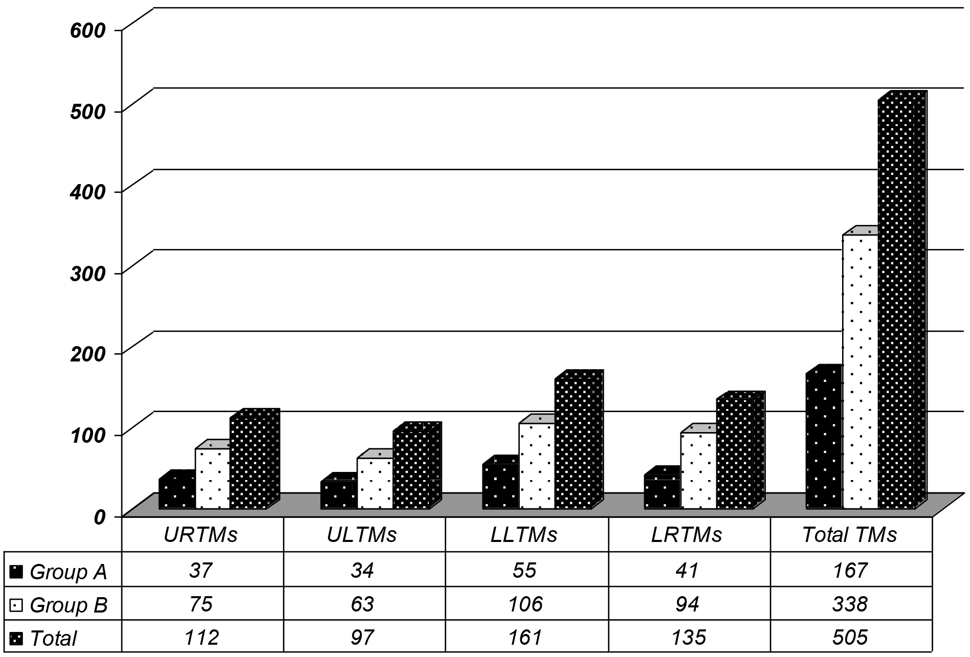
In total, 4,308 interdental spaces were studied for RP, of which 1,428 belonged to group A subjects and 2,880 to group Β subjects. RP was detected in 505 interdental spaces (11.72%), specifically in 167 group A interdental spaces (11.69%) and in 338 group B spaces (11.73%). The distribution of RP did not statistically significantly differ between the two subject groups (A and B) both in total (Z = 0.038, p = 0.976) and in quadrants (URTMs: Z = 0.007, p = 0.99, ULTMs: Z = 0.916, p = 0.93, LLTMs: Z = 0.364, p = 0.72, LRTMs: Z = 0.791, p = 0.43) (Figure 1).

JDMR-19-113- Eudoxie Pepelassi_Greece_F1

Figure 1. Distribution of root proximities (RP) in quadrants by subject group (A and B).

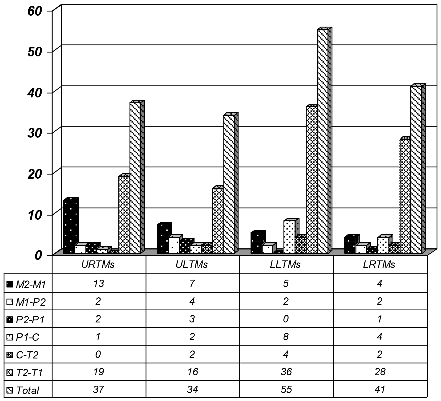
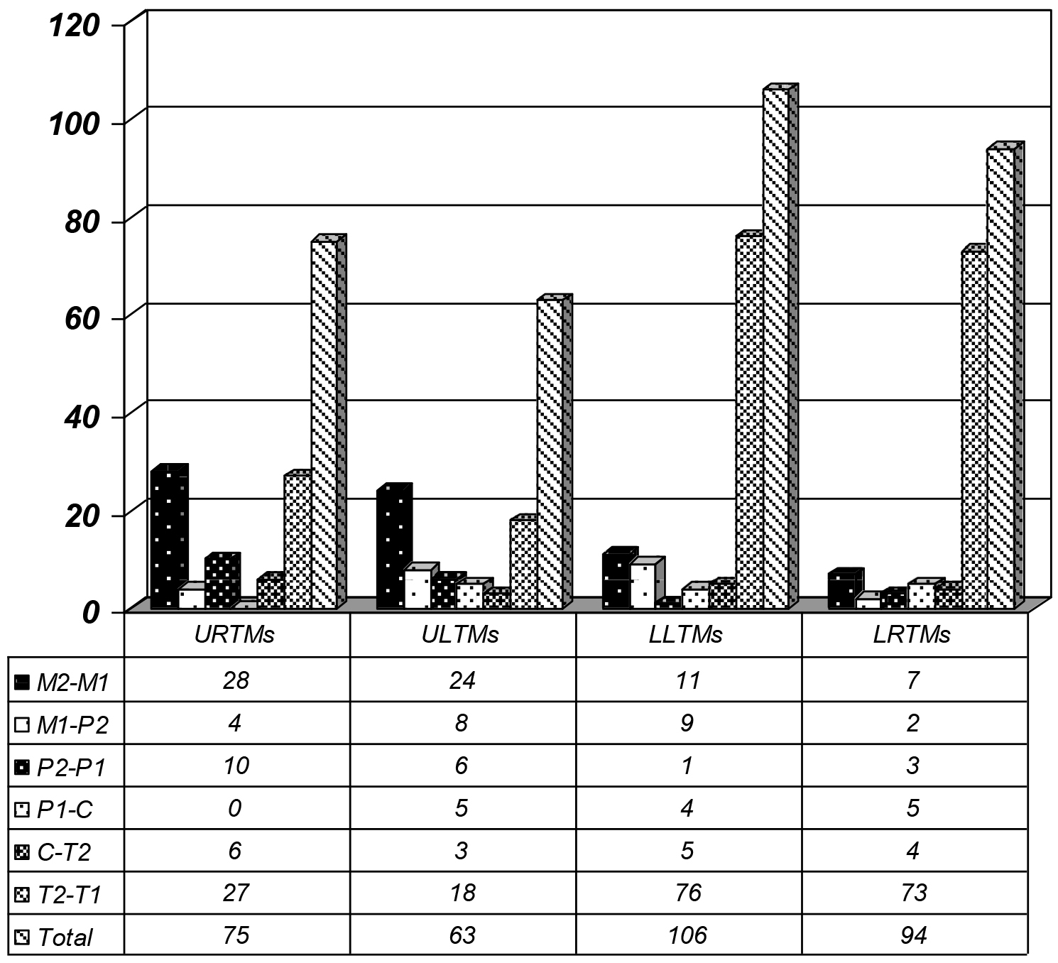
For group A, the highest frequency of RP for all four quadrants was found for the I2-I1 interdental space. In descending order, the second most frequent interdental space presenting RP was the M2-M1 space for both maxillary quadrants, the P1-C space for the mandibular left quadrant and the M2-M1 , P1-C spaces for the mandibular right quadrant (Figure 2). For group B, the highest frequency of RP for both maxillary quadrants was found for the M2-M1 interdental space, whereas the highest frequency of RP for both mandibular quadrants was found for the I2-I1 interdental space. In descending order, the second most frequent interdental space presenting RP was the P2-P1 space for the maxillary right quadrant, the M1-P2 space for the maxillary left quadrant and the M2-M1 space for both mandibular quadrants (Figure 3).

JDMR-19-113- Eudoxie Pepelassi_Greece_F2

Figure 2. Distribution of root proximities (RP) in interdental spaces for group A.

JDMR-19-113- Eudoxie Pepelassi_Greece_F3

Figure 3. Distribution of root proximities (RP) in interdental spaces for group B.

The relation between factors concerning the TM, specifically the eruption level, impaction status and angulation, and the presence of RP in the same quadrant was studied for each subject group. For group A, there were statistically significant differences in TM eruption or impaction status and angulation between the mandibular right M2-M1 interdental spaces presenting RP and those non-presenting RP as well as there were statistically significant differences in TM angulation between the mandibular left M2-M1 spaces presenting RP and those non-presenting RP (Table 4). For group B, there were statistically significant differences in TM angulation between the maxillary left M2-M1 spaces presenting RP and those non-presenting RP as well as there were statistically significant differences in TM eruption or impaction level between the mandibular right M2-M1 spaces presenting RP and those non-presenting RP and the mandibular right P2-P1 spaces presenting RP and those non-presenting RP (Table 5).

Table 4. Comparison of the presence of root proximity in the inetrdental spaces (M2-M1, M1-P2, P1-C, C-I2, I2-I1) in relation to the third molar eruption or impaction status (Fisher’s exact test) and comparison of the mean third molar angulation values between interdental spaces with or without root proximity (Mann-Whitney test) for group A.

Interdental spaces

M2M1

M1-P2

P2-P1

P1-C

C-I2

I2-I1

URTMs

Eruption or impaction status, p-value*

1.00

0.24

1.00

1.00

0.94

Angle, p-value**

0.10

0.11

0.61

ULTMs

Eruption or impaction status, p-value*

0.21

0.71

2.24

0.33

0.42

0.14

Angle, p-value**

0.39

0.48

0.12

0.92

0.08

LLTMs

Eruption or impaction status, p-value*

0.09

1.00

0.67

0.85

0.29

Angle, p-value**

0.02

0.32

0.69

0.62

LRTMs

Eruption or impaction status, p-value*

0.03

1.00

1.00

0.06

0.33

0.77

Angle, p-value**

0.03

0.33

0.09

URTMs: upper right third molars, ULTMs: upper left third molars, LLTMs: lower left third molars, LRTMs: lower right third molars, M2-M1: interdental space between second and first molars, M1-P2: interdental space between first molar and second premolar, P2-P1: interdental space between second and first premolars, P1-C: interdental space between first premolar and canine, C-I2: interdental space between canine and lateral incisor, I2-I1: interdental space between lateral and central incisors.
*Fisher’s exact test, **Mann-Whitney test, Bold indicates statistical significance.

Table 5.Comparison of the presence of root proximity in the inetrdental spaces (M2-M1, M1-P2, P1-C, C-I2, I2-I1) in relation to the third molar eruption or impaction status (Fisher’s exact test) and comparison of the mean third molar angulation values between interdental spaces with or without root proximity (Mann-Whitney test) for group B.

Interdental spaces

M2-M1

M1-P2

P2-P1

P1-C

C-I2

I2-I1

URTMs

Eruption or impaction status, p-value*

0.07

0.72

0.71

1.00

0.78

Angle, p-value**

0.07

0.97

0.94

0.08

0.57

ULTMs

Eruption or impaction status, p-value*

0.14

1.00

0.08

1.00

1.00

0.06

Angle, p-value**

0.005

0.46

0.05

0.59

0.30

0.63

LLTMs

Eruption or impaction status, p-value*

0.08

0.49

1.00

0.61

1.00

0.82

Angle, p-value**

0.58

0.66

0.81

0.76

0.86

LRTMs

Eruption or impaction status, p-value*

0.01

1.00

1.00

0.68

1.00

0.48

Angle, p-value**

0.47

0.10

0.02

0.74

0.33

0.47

URTMs: upper right third molars, ULTMs: upper left third molars, LLTMs: lower left third molars, LRTMs: lower right third molars, M2-M1: interdental space between second and first molars, M1-P2: interdental space between first molar and second premolar, P2-P1: interdental space between second and first premolars, P1-C: interdental space between first premolar and canine, C-I2: interdental space between canine and lateral incisor, I2-I1: interdental space between lateral and central incisors.
*Fisher’s exact test, **Mann-Whitney test, Bold indicates statistical significance.

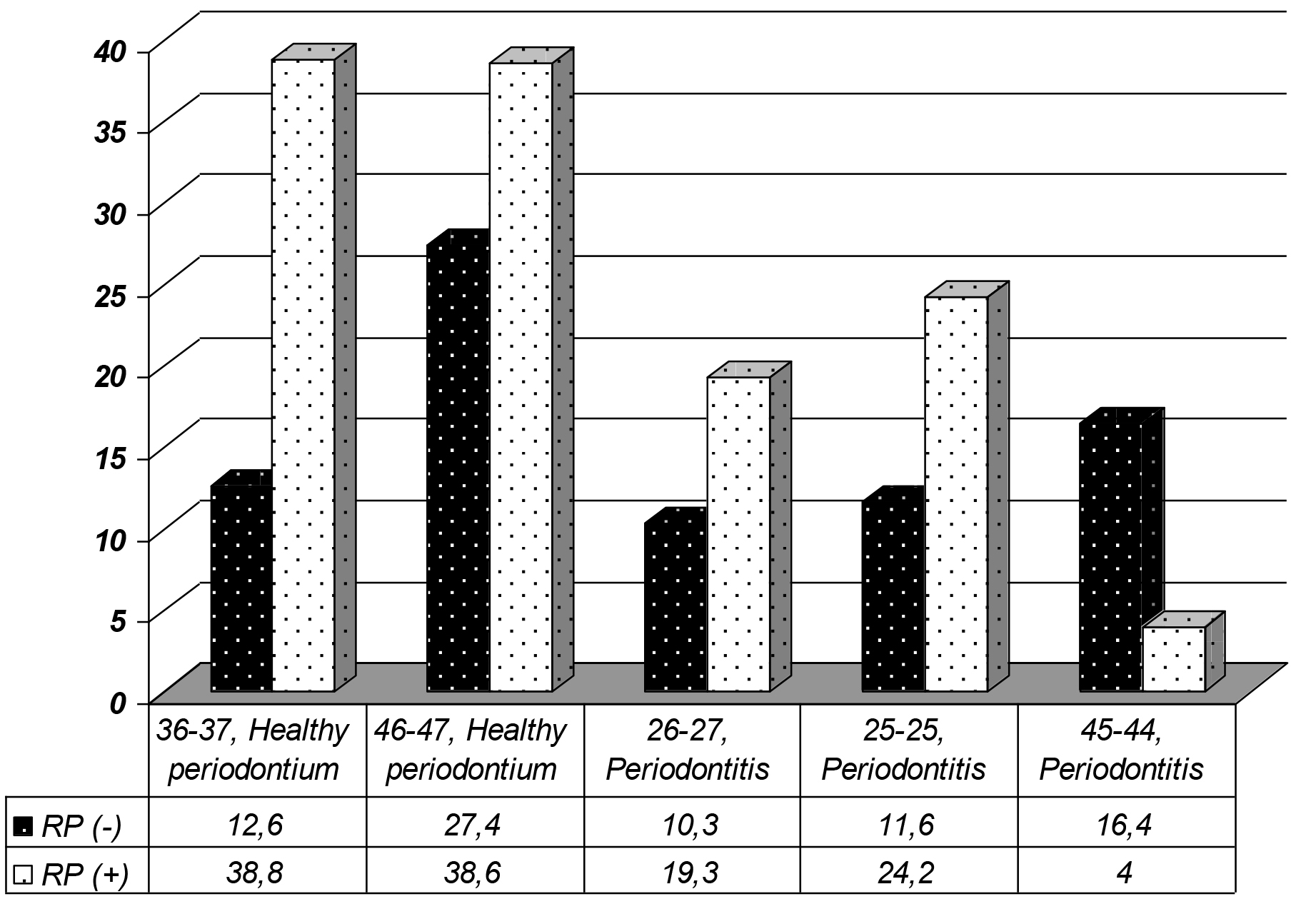
Concerning group A, for both right and left mandibular M2-M1 spaces, the mean value of TM angulation was greater for sites with RP than without RP (LLTMs: 38.6ο ± 12.8ο and 12.6ο ± 2.2ο, respectively, LRTMs: 26.8ο ± 9.2ο, 13.7ο ± 2.5ο) (Figure 4). For group B, whenever there was statistical significance in the TM angulation between sites with or without RP, the mean value of TM angulation was greater for sites with RP than without RP (M2-M1 space/ ULTMs: 19.3ο ± 14.8ο versus 10.3ο ± 9.1ο, P2-P1 space/ LRTMs: 16.4ο ± 16.8ο versus 4.0ο ± 1.0ο) (Figure 4).

JDMR-19-113- Eudoxie Pepelassi_Greece_F4

Figure 4. Mean third molar (TM) angulation by root proximity (RP) for interdental spaces where TM angulation was statistically significantly different between the spaces with RP and those without RP.

Discussion

The present retrospective study was designed to assess the effect of the eruption level or impaction status and angulation of third molars (TMs) on the presence of interdental root proximity (RP) in this quadrant, both in adults with healthy periodontium and in patients with history of periodontitis. In total, 718 TMs and 4,308 interdental spaces were studied in 330 subjects. The results of this study demonstrated that in subjects with healthy periodontium, the angulation of mandibular TMs significantly influenced the presence of root proximity in the interdental space between first and second molars. In periodontitis subjects, TM angulation significantly affected the presence of root proximity in the interdental space between first and second molars in the maxillary left and mandibular right quadrants as well as in the interdental space between the mandibular right premolars. The eruption level or impaction status of TMs significantly affected the presence of root proximity only between the first and second mandibular right molars both for subjects with healthy periodontium and for periodontitis patients.

Comparing the results of the present study to previous findings is not feasible, since the role of TMs on the presence of RP in the neighboring interdental spaces has not been addressed in the literature yet. However, there are well-documented studies on RP, in which the importance of RP in the presence and progression of periodontitis is investigated [13, 16, 17]. Moreover, there are studies reporting root resorption of second molars in proximity to non-erupted third molars and suggesting the early extraction of impacted third molars, especially in cases with a mesial TM angulation of 60o or more and an apical TM location in proximity to the distal root of the second molar [21, 22]. It is widely accepted that one of the main causes for TM impaction, especially for the mandible, is the absence of adequate retromolar space for TM eruption. A limited retromolar space that prevents TM eruption might be implicated in the development of root proximity in the neighboring interdental space. Several factors have been reported to enhance, to a greater or lesser extent, the development of the limited retromolar space. Most of them are related to the time period of development, such as the distal eruption pattern of the teeth, the vertical direction of the condyloid growth which is associated with a decrease in bone resorption of the anterior border of the mandibular ramus, changes in the longitudinal growth of the mandible and delays in the development of facial structures [23, 24]. However, TMs might get erupted later in adult life, after completion of the jaw growth. In such case they often remain partially erupted. It has been claimed that in certain cases TM angulation tends to get reduced with time mainly between 10 and 21 years of age, whereas in other cases TM mesial inclination is increased with time. Orthodontic treatment might increase the retromolar space hoping that this might increase the chances for TM eruption, depending on the initial TM positioning. This seems to have a more favorable effect for the maxillary than the mandibular TMs. The present association between increased TM angulation and RP in the neighboring mandibular molar interdental space in subjects with healthy periodontium might be explained by the forces exerted by the inclined TM in the attempt to erupt.

There are well-established indications for the surgical extraction of impacted TMs [25]. Prophylactic surgical extraction of impacted TMs, which are free of any pathology, has been justified on the basis that TMs do not have important role in the function of the oral cavity, the need to minimize the risk of further disease as cysts and tumors [26] and the risk of mandibular angle fracture [27, 28] as well as the increased difficulty of TM surgical extraction with age [26].

Early literature data reported that second molars adjacent to partially or completely erupted TMs, especially in the mandible, were more frequently affected by periodontal disease and were at highest risk to develop periodontitis [29]. Later, it was demonstrated that in case of a visible TM the odds of finding at least one site with periodontal probing depth of 5 mm or deeper at the adjacent second molar becomes double [30]. Then, it was found that young adults with visible asymptomatic TMs were more likely (almost twice) to have periodontal disease around the adjacent first and second molars than subjects without visible TMs [31]. Moreover, periodontal probing of at least 4 mm deep was significantly more frequent at proximal molar sites [32] and in case of a visible TM, significantly more sites with clinical attachment loss of at least 3 mm were detected at the adjacent first and second molars [33]. These finding may partly be explained by the difficulty in successfully removing the dental plaque from the TM area. Plaque accumulation around the TM results in periodontal involvement at the distal surface of the adjacent second molar and may serve as a potential reservoir for oral pathogens colonizing more anteriorly located dental sites [34–36]. It has been suggested that orthodontically-aided extraction of impacted TMs might improve the periodontal condition of the adjacent tooth, though such a treatment plan should be considered only when TM extraction is associated with a high risk of postoperative complications [37]. The presence of root proximity between the third and second molars has been documented as well as the difficulties to control periodontal inflammation at that site [6, 38]. The present study showed that 25.63% of the subjects presented agenesis of at least one TM, which was more frequent for the maxilla than the mandible in group A. The prevalence of partially or completely impacted TMs was 19.06%. These findings of TM agenesis are similar to those by Hattab et al. [39] and Rozkovcona et al. [40] but greater than those by Sandhu and Kaur [23] and Celikoglu et al. [2]. These differences might be partly attributed to differences in the age of the subject populations studied, since TM angulation might slightly improve with time up to the age of 24 or 26 years, especially when the initial angulation is 35o or more [10].

Concluding, within its limits this study found that, the angulation and eruption level or impaction status of third molars seem to be related to interdental root proximity among the adjacent teeth, especially between lower first and second molars, irrespective of the presence or absence of periodontitis.

References

  1. Polder BJ, Van’t Hof MA, Van der Linden FP, Kuijpers-Jagtman AM (2004) A meta-analysis of the prevalence of dental agenesis of permanent teeth. Community Dent Oral Epidemiol 32: 217–226. [crossref]
  2. Celikoglu M, Miloglu O, Kazanci F (2010) Frequency of agenesis, impaction, angulation, and related pathologic changes of third molar teeth in orthodontic patients. J Oral Maxillofac Surg 68: 990–995. [crossref]
  3. Nieminen P (2009) Genetic basis of tooth agenesis. J Exp Zool 312: 320–342. [crossref]
  4. Tarazona B, Paredes V, Llamas J-M, Cibrián R, Gandia JL (2010) Influence of first and second premolar extraction or non-extraction treatments on mandibular third molar angulation and position. A comparative study. Med Oral Pathol Oral Cir Bucal 15: 760–766. [crossref]
  5. Hattab FN, Alhaija ES (1999) Radiographic evaluation of mandibular third molar eruption space. Oral Surg Oral Med Oral Pathol Oral Radiol Endod 88: 285–291. [crossref]
  6. Nance PE, White RP Jr, Offenbacher S, Phillips C, Blakey GH, et al. (2006) Change in third molar angulation and position in young adults and follow-up periodontal pathology. J Oral Maxillofac Surg 64: 424–428. [crossref]
  7. Von Wowern N, Nielsen HO (1989) The fate of impacted lower third molars after the age of 20. A four-year clinical follow-up. Int J Oral Maxillofac Surg 18: 277–280. [crossref]
  8. Ventä I, Murtomaa H, Turtola L, Meurman J, Ylipaavalniemi P (1991) Assessing the eruption of lower third molars on the basis of radiographic features. Br J Oral Maxillofac Surg 29: 259–262. [crossref]
  9. Ventä I, Turtola L, Ylipaavalniemi P (1999) Change in clinical status of third molars in adults during 12 years of observation. J Oral Maxillofac Surg 57: 386–389. [crossref]
  10. Hattab FN (1997) Positional changes and eruption of impacted mandibular third molars in young adults. A radiographic 4-year follow-up study. Oral Surg Oral Med Oral Pathol Oral Radiol Endod 84: 604–608. [crossref]
  11. Kruger E, Thomson WM, Konthasinghe P (2001) Third molar outcomes from age 18–26: findings from a population-based New Zealand longitudinal study. Oral Surg Oral Med Oral Pathol Oral Radiol Endod 92: 150–155. [crossref]
  12. Beeman CS (1999) Third molar management: a case for routine removal in adolescent and young adult orthodontic patients. J Oral Maxillofac Surg 57: 824–830. [crossref]
  13. Kim T, Miyamoto T, Nunn ME, Garcia RI, Dietrich T (2008) Root proximity as a risk factor for progression of alveolar bone loss: the veterans affairs dental longitudinal study. J Periodontol 79: 654–659. [crossref]
  14. Armitage GC (1999) Development of a classification system for periodontal diseases and conditions. Ann Periodontol 4: 1–6. [crossref]
  15. Artun J, Osterberg SK, Kokich VG (1986) Long-term effect of thin interdental alveolar bone on periodontal health after orthodontic treatment. J Periodontol 57: 341–346. [crossref]
  16. Vermylen K, De Quincey GN, van’t Hof MA, Wolffe GN, Renggli HH (2005a) Classification, reproducibility and prevalence of root proximity in periodontal patients. J Clin Periodont 32: 254–259. [crossref]
  17. Vermylen K, De Quincey GN, Wolffe GN, van ‘t Hof MA, Renggli HH (2005) Root proximity as a risk marker for periodontal disease: a case-control study. J Clin Periodontol 32: 260–265. [crossref]
  18. Van der Sanden WJ, Mettes DG, Plasschaert AJ, Grol RP, van’t Hof MA, et al. (2002) Effect of selected literature on dentists’ decisions to remove asympomatic, impacted lower third molars. Eur J Oral Sci 110: 2–7. [crossref]
  19. Van der Sanden WJ, Mettes DG, Plasschaert AJ, Grol RP, Mulder J, et al. (2005) Effectiveness of clinical practice guideline implementation on lower third molar management in improving clinical decision-making: a randomized controlled trial. Eur J Oral Sci 113: 349–354. [crossref]
  20. Hugoson A, Kugelberg CF (1988) The prevalence of third molars in a Swedish population, an epidemiologic study. Community Dent Health 5: 121–128. [crossref]
  21. Nemcovsky CE, Libfeld H, Zubery Y (1996) Effect of non-erupted 3rd molars on distal roots and supporting structures of approximal teeth. A radiographic survey of 202 cases. J Clin Periodontol 23: 810–815. [crossref]
  22. Nemcovsky CE, Tal H, Pitaru S (1997) Effect of non-erupted third molars on roots of approximal teeth. A radiographic, clinical and histologic study. J Oral Pathol Med 26: 464–469. [crossref]
  23. Sandhu S, Kaur T (2005) Radiographic evaluation of the status of third molars in the Asian-Indian students. J Oral Maxillofac Surg 63: 640–645. [crossref]
  24. Ay S, Agar U, Biçakçi AA, Köşger HH (2006) Changes in mandibular third molar angle and position after unilateral mandibular first molar extraction. Am J Orthod Dentofacial Orthop 129: 36–41. [crossref]
  25. Adeyemo WL (2006) Do pathologies associated with impacted lower third molars justify prophylactic removal? A critical review of the literature. Oral Surg Oral Med Oral Pathol Oral Radiol Endod 102: 448–452. [crossref]
  26. Baykul T, Saglam AA, Aydin U, Basak K (2005) Incidence of cystic changes in radiologically normal impacted lower third molar follicles. Oral Surg Oral Med Oral Pathol Oral Radiol Endod 99: 542–545. [crossref]
  27. Hanson BP, Cummings P, Rivara FP, John MT (2004) The association of third molars with mandibular angle fractures: a meta-analysis. J Can Dent Assoc 70: 39–43. [crossref]
  28. Iida S, Nomura K, Okura M, Kogo M (2004) Influence of the incompletely erupted lower third molar on mandibular angle and condylar fractures. J Trauma 57: 613–617. [crossref]
  29. Ash MM, Costich ER, Hayward JR (1962) A study of periodontal hazards of third molars. J Periodontol 33: 209–213.
  30. Elter JR, Cuomo C, Offenbacher S, White RP Jr (2004) Third molars associated with periodontal pathology in the Third National Health and Nutrition Examination Survey. J Oral Maxillofac Surg 62: 440–445. [crossref]
  31. Blakey GH, Gelesko S, Marciani RD, Haug RH, Offenbacher S, et al. (2010) Third molars and periodontal pathology in American adolescents and young adults: a prevalence study. J Oral Maxillofac Surg 68: 325–329. [crossref]
  32. Moss KL, Serio AD, Offenbacher S, Beck JD, Mauriello SM, et al. (2007) The oral and systemic impact of third molar periodontal pathology. J Oral Maxillofac Surg 65: 1739–1745. [crossref]
  33. Moss KL, Oh ES, Fisher E, Beck JD, Offenbacher S, et al. (2009) Third molars and periodontal pathologic findings in middle-age and older Americans. J Oral Maxillofac Surg 67: 2592–2598. [crossref]
  34. Blakey GH, Jacks MT, Offenbacher S, Nance PE, Phillips C, et al. (2006) Progression of periodontal disease in the second/third molar region in patients with asymptomatic third molars. J Oral Maxillofac Surg 64: 189–193. [crossref]
  35. White RP Jr, Offenbacher S, Blakey GH, Haug RH, Jacks MT, et al. (2006) Chronic oral inflammation and the progression of periodontal pathology in the third molar region. J Oral Maxillofac Surg 64: 880–885. [crossref]
  36. Moss KL, Serio AD, Offenbacher S, et al Beck JD, White RP Jr (2008) Third molars and the efficacy of mechanical debridement in reducing pathogen levels in pregnant subjects: a pilot study. J Oral Maxillofac Surg 66: 1565–1569. [crossref]
  37. Güven O, Keskin A, Akal UK (2000) The incidence of cysts and tumors around impacted third molars. Int J Oral Maxillofac Surg 29: 131–135. [crossref]
  38. Akarsian ZZ, Kocabay C (2009) Assessment of the associated symptoms, pathologies, positions and angulations of bilateral occurring mandibular third molars: is there any similarly?. Oral Surg Oral Med Oral Pathol Oral Radiol Endod 108: 26–32. [crossref]
  39. Hattab FN, Rawashdeh MA, Fahmy MS (1995) Impaction status of third molars in Jordanian students. Oral Surg Oral Med Oral Pathol Oral Radiol Endod 79: 24–29. [crossref]
  40. Rozkovcová E, Marková M, Lánik J, Zvárová J (2004) Agenesis of third molars in young Czech population. Plaque Med Rep 105: 35–52. [crossref]

Is Temporal Summation or Conditioned Pain Modulation Associated with Pain and Functional Outcomes in Patients with Orofacial Pain?

DOI: 10.31038/IJOT.2019213

Abstract

Objective: To determine if two psychophysical quantitative sensory tests, temporal summation and conditioned pain modulation are associated with treatment outcomes in patients with orofacial pain.

Methods: During the initial examination of 40 patients with orofacial pain, data were collected on physical function and pain; and measurements of Temporal Summation (TS) and Conditioned Pain Modulation (CPM). At 6 – 8-weeks follow-up, these pain and function measures were repeated and subjects were asked to rate their perceived level of change.

Results: Insufficient evidence of association between temporal summation and functional outcomes were seen in patients with orofacial pain. However, conditioned pain modulation was associated with subjects’ perceived change and least pain reported over one-week periods which reflect symptomatic and functional changes from treatment.

Discussion: Results suggest that impairments in CPM affect changes in some measures of pain perception. The implications of CPM as a psychophysical testing paradigm on short term pain outcomes and individual pain experience is a critical piece of consideration in patients who receive treatment for orofacial pain.

Keywords

temporal summation, conditioned pain modulation, pain and disability, orofacial pain

Introduction

The International Association for the Study of Pain describes orofacial pain as pain perceived in the face and/or oral cavity 1]. In a recent study, investigators estimated the 1-year period prevalence of orofacial pain to be over 16% of the adult population [2]. Prolonged or intense pain has been shown to trigger neuroplastic changes in the central and peripheral nervous systems in some individuals [3]. The result of these changes includes heightened sensitivity to cutaneous, tactile or noxious stimuli in local or distant body regions, and the sensation of persistent pain in the absence of a triggering stimulus [4,5]. These changes in pain perception increase the individuals’ likelihood of developing and perpetuating chronic pain [6–9]. Several studies have explored the utility of inducing experimental pain using quantitative sensory tests to identify individuals with altered pain processing mechanisms [10–12].Two methods of indirectly detecting increased sensitivity to pain include Temporal Summation (TS) and Conditioned Pain Modulation (CPM) testing [13]. Both methods have been studied in patients with orofacial pain [10,14,15].

The utility of these tests to identify individuals with abnormal pain responses who might be less likely to respond to standard pain intervention strategies has the potential to provide researchers and clinicians alike with a valuable tool for developing effective treatment strategies that minimize the likelihood of developing chronic pain. A crucial step in this process is to establish the construct validity of these quantitative sensory tests. TS occurs when a series of equally intense noxious neural impulses arrive at a synapse at a frequency such that the duration of these impulses is smaller than the postsynaptic potential, causing a build-up of neurotransmitters released by a single presynaptic neuron. This results in the perception that the intensity of the stimulus increases during the administration of the series of neural impulses, when in fact the intensity remains unchanged. Individuals with altered in pain processing mechanisms experience greater pain from repeated noxious stimuli than what would be expected in neurologically healthy individuals. The response to TS is commonly tested by administering a train of uniform and consecutive noxious stimuli at a constant intensity at the site of pain or at a neutral, pain-free site [16–18, 21]. Prior to testing, the subject is instructed to rate the pain intensity of the first and the last stimulus from a train of 10 stimuli applied at equal intensity and frequency of one stimulation per second. Pain intensity is measured using a Numerical Pain Rating Scale (NPRS). The last pain measurement is subtracted from the first pain measurement, thereby representing the difference between the two measurements of pain perception, given stimuli of equal intensity. A larger difference indicates a greater impairment in pain processing. The noxious stimulus used to test TS is most often mechanical (using pin prick or pressure stimulus), thermal (using heat or cold) or ischemic (using a blood pressure cuff). When evaluated using pressure algometry [19], ischemia via cuff compression [20], and heat pulses [18], TS has been shown to demonstrate acceptable reliability. To the author’s knowledge, the reliability of TS has not been studied using a pinprick stimulus. Temporal summation has been evaluated in several studies in patients with nonspecific orofacial pain. In relation to pain free controls, TS was enhanced when tested using a pinprick [10] and a heat probe [11,15]. There were no differences between groups, however when TS was tested using pressure pain [16]. CPM is a phenomenon whereby the individual perceives less pain when receiving two noxious stimuli administered simultaneously at different body regions, when compared with the perceived intensity of pain associated with the application of one noxious stimuli. This experience is often described as one in which ‘pain inhibits pain’ [13,22].

One of the two stimuli is referred to as the ‘test’ stimulus, whereas the other, the ‘conditioned’ stimulus. The test stimulus is administered and measured in a similar manner as with TS testing. Subjects with normal pain processing mechanisms experience a less dramatic increase in pain from TS when the conditioned stimulus is being applied than when the conditioned stimulus is not present. For measurement purposes, the conditioned stimulus measurement is subtracted from the test stimulus, or TS measurement. A smaller difference thereby indicates a greater impairment in pain processing. As is the case with TS testing, test stimuli sites for measuring CPM can be located at the site of pain or at a neutral site, and typically involve mechanical, thermal or ischemic stimuli. Conditioning stimulus sites are located at a neutral site, and are typically produced by thermal or ischemic stimuli. Two different studies addressed the reliability of CPM testing. Both used mechanical pressure as the test stimuli, and ischemic arm pain as the conditioned stimulus [19,20]. In one of these studies, the investigators also studied thermal (cold) stimuli as the conditioned stimulus [20]. Reliability was good when using the cold stimuli [20], but conflicting conclusions were drawn regarding ischemic pain. In one study, the investigators reported ‘excellent’ intra-session reliability, but poor inter-session reliability for the ischemic pain measure, whereas in the other study, the reliability was described as ‘acceptable’ [19]. To the author’s knowledge, the reliability of CPM has not been studied using heat as a conditioned stimulus.

The question of whether measures of CPM are more impaired in patients with orofacial pain has been addressed in the research. In relation to pain free controls, there was no difference between groups when a pinprick test stimulus was paired with a thermal (cold) conditioned stimulus [10]. Conversely, when a pinprick test was paired with pressure as the conditioned stimulus, CPM measures were more impaired in subjects with orofacial pain when tested at the site of pain when compared with pain free controls, but not when tested at a pain free site [14]. These studies addressing TS and CPM in subjects with orofacial pain versus healthy controls suggest that impairments in pain processing can be identified using either of these quantitative tests. The ultimate goal in identifying these subjects with pain processing impairments, once identified, is to determine appropriate interventions for this subpopulation of subjects who are more likely to develop chronic pain. A next step in this process is therefore to determine if greater impairments in TS and CPM are associated with poorer outcomes following treatment. This question has not been addressed to date in patients with orofacial pain. Additionally, no study has addressed the more fundamental questions of whether impairments in TS and/or CPM are correlated with measurements of physical function and pain in patients with orofacial pain when measured concurrently.

Therefore, the aims of this study are twofold:

  1. To determine if TS and CPM tests, performed on subjects with orofacial pain, are correlated with physical function and pain measurements during the initial visit for treatment of their orofacial pain, and
  2. To determine if TS and CPM tests, performed on subjects with orofacial pain during their initial visit for treatment of their orofacial pain, are associated with changes in physical function and pain at 6 to 8-weeks follow-up.

Materials and Methods

This study was a prospective cohort, approved by the Rutgers University Institutional Review Board. Subjects being seen for an initial examination at the Center for Temporomandibular Disorders and Orofacial Pain, Department of Diagnostic Sciences, in the New Jersey School of Dental Medicine, Rutgers University who were between the ages of 18 and 89 were recruited. Subjects were excluded if pregnant, or if any intervention was received during the initial examination visit before all baseline measures could be collected. Written informed consent was obtained from all subjects. This convenience sample was assessed for baseline for measurements of TS and CPM. Baseline data on age, gender, physical function and pain levels were also collected. At between 6 and 8 weeks follow-up, data collection on physical function and pain was repeated, and subjects were asked to rate their perceived change in status. This time frame allowed the author to contact the subject multiple times in the event that initial attempts to contact the subjects failed. All follow-up data were collected via telephone interview. Subjects were tested for pain responses under conditions of TS using #5.46 von Frey filaments (Stoteling Ltd., USA). A single stimulus (pin prick) and then a train of 10 consecutive stimuli were applied at a frequency of one stimulation per second to the volar forearm of the dominant arm. Subjects were asked to rate the level of pain after the single stimulus was applied, and then at the end of the train of 10 consecutive stimuli using an 11-point (0 = no pain, 10 = worst possible pain) Numeric Pain Rating Scale (NPRS). TS scores were calculated by subtracting the first-stimulation pain rating score from the tenth-stimulation pain rating score.

To measure CPM, subjects placed their non-dominant hand into a warm water (46 degrees Celsius) bath. After the hand had been immersed for 30 seconds, a train of 10 consecutive stimuli was applied to the distal aspect of the dominant forearm using #5.46 von Frey filaments, and subjects were instructed to rate their level of discomfort on the NPRS after the first of 10 stimuli was administered, and again after the 10th stimuli was applied. To quantify CPM, the 10th pain report was subtracted from the first, and this number was then subtracted from the score obtained during TS testing. Function was assessed using the Therapeutic Associates Outcome System (TAOS), also known as the Care Connections Outcomes System. The TAOS is a questionnaire designed to address activities specific to 5 anatomic locations, one of which is the temporomandibular joint. It has been shown to demonstrate good test-retest reliability [23,24], as well as concurrent [23], content [23] and criterion [24] validity. The TAOS has been used in one prior study in which subjects were patients with temporomandibular joint pain [25]. Answers are based on a 6-point Likert scale. The author summed scores addressing physical function due to subjects’ orofacial pain from 10 questions addressing talking, eating, concentration, headaches and reading, resulting in a possible range of scores from 0 to 50. Data were coded such that higher numbers indicated greater function.

The author measured pain using the NPRS. Specifically, subjects were instructed to rate the worst pain experienced over the past 24 hours, the least pain over the past 24 hours and the least pain over the past 7 days. The NPRS is used extensively in pain research. Abbott et al., (2014) reported that in subjects with musculoskeletal conditions, the minimal clinically important difference of the NPRS is 1.5 points [26]. To the author’s knowledge, psychometric properties of the NPRS have not been studied specifically in subjects with orofacial pain. Several authors have suggested that TS and/or CPM measurements might differ by age [27,28] or gender [15,29,30,31]. Therefore, this study evaluated for potential confounding effects by both age and gender in our analyses of the association between TS and CPM, and change in pain and function. All subjects received individualized treatment for their orofacial pain based on diagnostic tests and clinical findings. Treatment consisted of medication, trigger point injections, physical therapy, appliance use, and/or patient education. Subjects were contacted by telephone between 6 and 8 weeks following their initial evaluation, at which time data collection on function and pain were repeated, and data were collected on subjects’ perceived change in their condition.

Perceived change over the 6 to 8-week follow-up period were measured using the Global Rating of Change (GROC) scale. The GROC constitutes a single question addressing the patient’s perceived change regarding a particular condition over a specified period of time on a 15-point Likert scale, with 0 representing no change. Psychometric properties of the GROC have been addressed in several studies. In relation to lower extremity conditions, the author have concluded that the GROC does not accurately reflect changes in functional levels, but rather is weighted toward the patient’s status at follow-up [32,33]. In a different study of subjects with shoulder pain, a GROC of 5 or greater was associated with a perceived change in the subject’s condition, although it was not associated with changes in physical function [34]. These findings suggest that GROC scores are highly subjective in nature, and might be influenced by location of pain. To the author’s knowledge, the GROC has not been studied in patients with orofacial pain. Data were analysed using SAS version 9.3. Since most continuous variables were not normally distributed, Spearman correlation coefficients were calculated. Univariate linear regression models were constructed to estimate the effect of TS and CPM on function, pain and perceived change. Age and gender were then added to the models to estimate their potential confounding effects. Models were evaluated to determine if they met the assumptions of linear regression. In cases in which the assumption of homoscedasticity was violated, heteroscedasticity-consistent estimators were calculated.

Results

Sixty subjects contributed data at the initial evaluation. Of these, 40 subjects contributed data at follow-up, resulting in a 66.7% completion rate. The 20 subjects with missing follow-up data were more likely to have lower TAOS scores, but were not different in relation to any of the 3 pain measures or age or gender [see Table 1].

Table 1. Comparison between subjects with complete data at intake and follow-up, and those with missing follow-up data.

Variable
p-value for the difference between groups

Subjects with complete data at intake and follow-up (n = 40)
mean or percentage
(standard deviation)

Subjects with missing follow-up data (n = 20)
mean or percentage
(standard deviation)

Temporal Summation
p = 0.96

1.67
(1.86)

1.70
(1.89)

Conditioned Pain Modulation
p = 0.93

0.45
(1.88)

0.50
(1.70)

Therapeutic Associates Outcome System (TAOS) score
p = 0.01

17.47
(4.90)

13.80
(5.75)

24-hour worst pain
p = 0.58

5.95
(2.96)

6.40
(2.93)

7-day worst pain
p = 0.11

6.81
(2.95)

8.10
(2.67)

7-day least pain
p = 0.21

3.07
(2.84)

4.05
(2.68)

Age
p = 0.78

45.05
(16.12)

46.67
(12.08)

Gender
p = 1.00

75% female

75% female

Descriptive statistics for all variables are provided in table 2. Subjects demonstrated statistically significant improvements in all outcome measures over the 6 to 8-week follow-up period. Specifically, subjects improved in relation to TAOS scores by 1.10 points (p = 0.03), 24-hour worst pain by 2.05 points (p<0. 01), 7-day worst pain by 2.24 points (p <0.01), and 7-day least pain by 1.05 points (p = 0.00). The mean GROC score was 2.30, indicating a perceived improvement of between ‘a little bit better’ and ‘somewhat better’. Change in 24-hour worst pain and 7-day worst pain exceeded the minimal clinically important difference for pain. TS and CPM were both significantly positively correlated with TAOS scores at intake (see Table 3), indicating that greater function was associated with less impaired measurements of CPM measurements, but more impaired TS measurements. None of the 3 intake pain measures were correlated with either TS or CPM measurements. The potential confounding influence of age and gender in the association between intake TS and CPM measurements were evaluated, including the change in function and pain, using the criteria that a 10% change in the effect measure when adding the potential confounder(s) to the baseline model represents meaningful confounding [35]. Analyses suggest that while there is confounding by gender alone or a combination of age and gender in most of the analyses addressing TS, there was no meaningful confounding by either age or gender or both when evaluating the effects of CPM [see Tables 4 and 5]. In relation to change in function or pain over the 6 to 8 week follow up period, there was no evidence of an association between TS and changes in any of the outcome measures irrespective of confounding by age and/or gender [see Table 4]. In univariate analyses, CPM was associated with subjects’ reported change in least pain over the past week and with perceived change, but was not associated with any other outcome [see Table 5].

Table 2. Descriptive Statistics of all Dependent and Independent Variables (n = 40).

Variable

Mean or percentage
(standard deviation)
Range

Temporal Summation

1.67
(1.86)
-1 – 7

Conditioned Pain Modulation

0.45
(1.88)
-4 – 5

Age

45.05
(16.12)
22 – 79

Gender

75% female

Therapeutic Associates Outcome System (TAOS) score at initial visit

17.47
(4.90)
6 – 25

24-hour worst pain at initial visit

5.95
(2.96)
0 – 10

7-day worst pain at initial visit

6.81
(2.95)
0 – 10

7-day least pain at initial visit

3.07
(2.84)
0 – 10

Therapeutic Associates Outcome System (TAOS) score at 6 to 8 weeks follow-up

18.57
(4.78)
9 – 25

24-hour worst pain at 6 to 8 weeks follow-up

3.90
(3.14)
0 – 10

7-day worst pain at 6 to 8 weeks follow-up

4.57
(2.96)
0 – 10

7-day least pain at 6 to 8 weeks follow-up

2.02
(2.17)
0 – 8

Global Rating of Change

2.30
(2.48)
-3 – 7

Table 3. Spearman correlation coefficients for the correlation between measures of temporal summation and conditioned pain modulation; and function, pain, age and gender at initial evaluation.

Temporal Summation
rs
p-value

Conditioned Pain Modulation
rs
p-value

Therapeutic Associates Outcome System (TAOS) score

4.69
0.00

0.43
0.01

24-hour worst pain

-0.01
0.97

0.07
0.65

7-day worst pain

0.05
0.77

0.04
0.82

7-day least pain

0.11
0.49

0.18
0.26

Age

-0.19
0.24

-0.20
0.23

Gender (female vs. male)

0.06
0.70

0.09
0.58

Table 4. Association between temporal summation and change in function, pain and global rating of change.

Outcome Variable

Baseline model for the association between temporal summation and outcome
beta
p-value
model r2

Baseline model + age
beta
p-value
model r2

Baseline model + gender
beta
p-value
model r2

Baseline model + age + gender
beta
p-value
model r2

Change in Therapeutic Associates Outcome System (TAOS) score

-0.02
0.95
0.65

0.02
0.95
0.65

0.00
0.99
0.65

0.03
0.91
0.65

Change in 24-hour worse pain

-0.10
0.64
0.42

-0.06
0.80
0.43

-0.18
0.41
0.46

-0.13
0.58
0.47

Change in 7-day worse pain

-0.19
0.43
0.19

-0.12
0.65
0.21

-0.28
0.25
0.27

-0.20
0.42
0.30

Change in 7- day least pain

-0.16
0.12
0.54

-0.20
0.17
0.55

-0.20
0.15
0.56

-0.22
0.13
0.56

Global Rating of Change

0.32
0.14
0.06

0.33
0.16
0.06

0.38
0.09
0.09

0.38
0.11
0.09

Table 5. Association between conditioned pain modulation and change in function, pain and global rating of change.

Outcome Variable

Baseline model for the association between conditioned pain modulation and outcome
beta
p-value
model r2

Baseline model plus age
beta
p-value
model r2

Baseline model plus gender
beta
p-value
model r2

Baseline model plus age and gender
beta
p-value
model r2

Change in Therapeutic Associates Outcome System (TAOS) score

0.07
0.77
0.65

0.08
0.76
0.65

0.08
0.77
0.65

0.08
0.76
0.65

Change in 24- hour worse pain

-0.35
0.09
0.46

-0.34
0.10
0.47

-0.34
0.10
0.49

-0.33
0.11
0.51

Change in 7-day worse pain

-0.30
0.21
0.21

-0.28
0.23
0.24

-0.29
0.21
0.27

-0.27
0.23
0.31

Change in 7- day least pain

-0.39
0.00
0.64

-0.39
0.00
0.64

-0.39
0.00
0.65

-0.39
0.00
0.65

Global Rating of Change

0.41
0.05
0.10

0.41
0.05
0.10

0.40
0.06
0.11

0.40
0.06
0.12

Discussion

The study’s first aim was to determine if TS and CPM tests are correlated with physical function and pain measurements during the initial visit for treatment of their orofacial pain. As expected, study results demonstrated a significant correlation between higher levels of function at intake and blunted pain response from concurrent noxious stimuli during CPM testing. In contrast, higher levels of function at intake were significantly correlated with heightened pain response from consecutive noxious stimulation during TS testing. Equally surprising is the absence of a statistically significant correlation between the three self-reported pain scores at intake, and TS and CPM measurements, since both TS and CPM are believed to be measures of an elevated response to pain. These latter findings call into question the validity of either TS or CPM testing to identify patients with orofacial pain whose pain is at least partially explained by heightened centrally and/or peripherally-mediated pain processes.

To the author’s knowledge, the correlation between self-reported baseline pain intensity measures and psychophysical quantitative sensory tests using TS and CPM have not been closely studied among subjects with orofacial pain. However, these tests have been used to compare pain processing mechanisms between patients with orofacial pain and pain-free controls in 3 separate studies. Contrary to this study’s results, Kothari et al. (2015) found heightened TS to pinprick sensation among subjects with orofacial pain compared with healthy controls [10]. However, no differences between both groups were reported in CPM test outcomes when pinprick test stimulus was concurrently applied with a cold conditioning stimulus [10]. This was the case irrespective of whether the test stimulus was applied to the site of pain or at a distal site. Oono, et al., (2014) paired a pinprick test stimulus with pressure as the conditioned stimulus and found that CPM test results were more impaired in subjects with orofacial pain compared with pain free controls when the painful stimulation was applied at the site of pain but not over a distal, pain free site [14]. In this study, significant correlation were found between CPM test outcomes and one of three pain outcomes when test stimulus was applied at a site distal to pain.

Differences in reported study outcomes are likely due in part to differences in TS and CPM testing protocol and instrumentation used across studies. There is currently no strong evidence supporting the most effective method for conducting TS or CPM testing in patients with orofacial pain, however the method chosen to test TS did not demonstrate construct validity in relation to its correlations with function or pain, whereas the method we chose to test CPM demonstrated somewhat more promising results. The second aim was to determine if TS and CPM tests, performed on subjects with orofacial pain during their initial visit for treatment of their orofacial pain, are associated with changes in physical function and pain at 6 to 8-weeks follow-up. In relation to TS testing, there were no significant differences between intake TS measurements, and any of the outcome measures tested, suggesting that the method of TS testing used in this study may not be a useful tool for predicting change in function or pain in patients with orofacial pain.

Statistically significant association between CPM test scores were found; and change in least pain reported over the 7-day period prior to follow up, including perceived change over the 6 to 8-week follow-up period. Specifically, a more heightened response to painful stimuli with CPM testing was associated with less pain reduction and perceived improvement at follow-up. There were no significant differences between intake CPM scores and changes in function or in changes in 24-hour worst or 7-day worst pain. The finding that CPM measures were associated with only two of five clinically important outcomes suggests that the instrumentation or measurement strategies administered as part of this study are not sensitive enough to effectively discriminate between different levels of perceived pain and function, or that there simply is not an association between CPM scores and changes in function and most measurements of pain.

This study had several limitations, all of which relate to the study design, where a sample of convenience with orofacial pain were recruited, and therefore cannot determine how representative this sample is of the population of orofacial pain patients. Additionally, 33% of subjects who contributed data at initial evaluation did not contribute follow-up data. These subjects who were lost to follow-up were more likely to have lower physical function levels, indicating a possible bias affecting study results. Finally, data on potential confounders other than age and gender, such as pain duration were not collected, which could influence study outcomes.

Conclusion

Study results suggest that TS testing, as implemented in this study is not useful for identifying patients with orofacial pain who have heightened pain sensitivity; or who are more likely to have poorer function and pain outcomes, or less perceived improvement following treatment for their orofacial pain. Similarly, CPM testing did not demonstrate utility in identifying orofacial pain patients with impaired pain processing at the initial examination, although it demonstrated some promise in identifying subjects who are likely to have worse pain outcomes and lower levels of perceived improvement. Nevertheless, additional research is warranted before considering the use of CPM testing as a measurement tool in the clinical or research setting.

Funding Details

This work was supported by the University of Medicine and Dentistry of New Jersey – School of Health- Related Professions Pre-Doctoral Fellowship Grant.

Acknowledgement

The author wishes to recognize the following individuals for their contributions: Susan Edmond, PT, DSc, OCS, School of Health Professions, Rutgers University Newark, NJ, USA; Gary M. Heir, DMD and Cibele Nasri-Heir, DDS, MSD, School of Dental Medicine, Rutgers University, Newark, NJ, USA.

References

  1. Merskey H, Bogduk N (1994) Part III: Pain terms, a current list with definitions and notes on usage. Classification of chronic pain, 2nd ed. International Association in the Study of Pain Task Force on Taxonomy. International Association in the Study of Pain. Available from: http://www.iasp-pain.org.
  2. Horst OV, Cunha-Cruz J, Zhou L, Manning W, Mancl L, et al. (2015) Prevalence of pain in the orofacial regions in patients visiting general dentists in the northwest practice-based research collaborative in evidence-based dentistry research network. J Am Dent Assoc 146: 721–728. [crossref]
  3. de Siqueira SR, Teixeira MJ, de Siqueira JT (2013) Orofacial pain and sensory characteristics of chronic patients compared with controls. Oral Surg Oral Med Oral Pathol Oral Radiol 115: 37–45. [crossref]
  4. Greenspan JD, Slade GD, Bair E, Dubner R, Fillingim RB, et al. (2013) Pain sensitivity and autonomic factors associated with development of TMD: the OPPERA prospective cohort study. J Pain 14: 63–74. [crossref]
  5. Fernandez-de-las-Penas C, Galan-del-Rio F, Fernandez-Carnero J, Pesquera J, Arendt-Nielsen L, et al. (2009) Bilateral widespread mechanical pain sensitivity in women with myofascial temporomandibular disorder: evidence of impairment in central nociceptive processing. J Pain 10: 1170–1178. [crossref]
  6. Greenspan JD, Slade GD, Bair E, Dubner R, Fillingim RB, et al. (2011) Pain sensitivity risk factors for chronic TMD: Descriptive data and empirically identified domains from the OPPERA case control study. Journal of Pain 12: 61–74. [crossref]
  7. Gustin SM, Peck CC, Wilcox SL, Nash PG, Murray GM, et al. (2011) Different pain, different brain: thalamic anatomy in neuropathic and non-neuropathic chronic pain syndromes. J Neurosci 31: 5956–5964. [crossref]
  8. Staud R (2012) Abnormal endogenous pain modulation is a shared characteristic of many chronic pain conditions. Expert Rev Neurother 12: 577–585. [crossref]
  9. Vierck CJ, Wong F, King CD, Mauderli AP, Schmidt S, et al. (2014) Characteristics of sensitization associated with chronic pain conditions. Clin J Pain 30: 119–128. [crossref]
  10. Kothari SF, Baad-Hansen L, Oono Y, Svensson P (2015) Somatosensory assessment and conditioned pain modulation in temporomandibular disorders pain patients. Pain 156: 2545–2555. [crossref]
  11. Maixner W, Fillingim R, Sigurdsson A, Kincaid S, Silva S (1998) Sensitivity of patients with painful temporomandibular disorders to experimentally evoked pain: evidence for altered temporal summation of pain. Pain 76: 71–81. [crossref]
  12. Staud R, Robinson ME, Price DD (2007) Temporal summation of second pain and its maintenance are useful for characterizing widespread central sensitization of fibromyalgia patients. J Pain 8: 893–901. [crossref]
  13. Pavlaković G, Petzke F (2010) The role of quantitative sensory testing in the evaluation of musculoskeletal pain conditions. Curr Rheumatol Rep 12: 455–461. [crossref]
  14. Oono Y, Wang K, Baad-Hansen L (2014) Conditioned pain modulation in temporomandibular disorders (TMD) pain patients. Experimental Brain Research 232: 3111–3119. [crossref]
  15. Sarlani E, Garrett PH, Grace EG, Greenspan JD (2007) Temporal summation of pain characterizes women but not men with temporomandibular disorders. Journal of Orofacial Pain 21: 309–317. [crossref]
  16. Nie H, Graven-Nielsen T, Arendt-Nielsen L (2009) Spatial and temporal summation of pain evoked by mechanical pressure stimulation. European Journal of Pain 13: 592–599. [crossref]
  17. Koltyn KF, Knauf MT, Brellenthin AG (2013) Temporal summation of heat pain modulated by isometric exercise. European Journal of Pain 17: 1005–1011. [crossref]
  18. Kong JT, Johnson KA, Balise RR, Mackey S (2013) Test-retest reliability of thermal temporal summation using an individualized protocol. The Journal of Pain 14: 79–88. [crossref]
  19. Cathcart S, Winefield AH, Rolan, P, Lushington K (2009) Reliability of temporal summation and diffuse noxious inhibitory control. Pain Research & Management 14: 433–438. [crossref]
  20. Lewis GN, Heales L, Rice DA, Rome K, McNair PJ (2012) Reliability of the conditioned pain modulation paradigm to assess endogenous inhibitory pain pathways. Pain Research & Management: The Journal Of The Canadian Pain Society 17: 98–102. [crossref]
  21. Sato H, Saisu H, Muraoka W, Nakagawa T, Svensson P, et al. (2012) Lack of temporal summation but distinct aftersensations to thermal stimulation in patients with combined tension-type headache and myofascial temporomandibular disorder. Journal of orofacial pain 26: 288–295. [crossref]
  22. Moont R, Pud D, Sprecher E, Sharvit G, Yarnitsky D (2010) ‘Pain inhibits pain’ mechanisms: Is pain modulation simply due to distraction? Pain 150: 113–120. [crossref]
  23. Schunk C, Rutt R (1998) TAOS functional index orthopaedic rehabilitation outcomes tool. Journal of Rehabilitation Outcomes Measurement 2: 55–61.
  24. Hoekstra CJ, Deppeler DA, Rutt RA (2014) Criterion validity, reliability and clinical responsiveness of the care connections functional index. Physiotherapy Theory and Practice 30: 429–437.
  25. Badke MB, Dussault L, Boissonnault W (2007) Influence of symptom longevity on outcomes following a customized rehabilitation program for painful temporomandibular disorders. Physiotherapy Canada. 59: 10–21.
  26. Abbott JH, Schmitt J (2014) Minimum important differences for the patient-specific functional scale, 4 region-specific outcome measures, and the numeric pain rating scale. J Orthop Sports Phys Ther 44: 560–564. [crossref]
  27. Lautenbacher S, Kunz M, Strate P, Nielsen J, Arendt-Nielsen L (2005) Age effects on pain thresholds, temporal summation and spatial summation of heat and pressure pain. Pain 115: 410–418. [crossref]
  28. Cole LJ, Farrell MJ, Gibson SJ, Egan GF (2010) Age-related differences in pain sensitivity and regional brain activity evoked by noxious pressure. Neurobiology of Aging 31: 494–503. [crossref]
  29. France CR, Suchowiecki S (1999) A comparison of diffuse noxious inhibitory controls in men and women. Pain 81: 77–84. [crossref]
  30. Shinal RM, Fillingim RB (2007) Overview of orofacial pain: epidemiology and gender differences in orofacial pain. Dent Clin North Am 51: 1–18, [crossref]
  31. Martel MO, Wasan AD, Edwards RR (2013) Sex differences in the stability of conditioned pain modulation (CPM) among patients with chronic pain. Pain Med 14: 1757–1768. [crossref]
  32. Schmitt JS, Abbott JH (2014) Patient global ratings of change did not adequately reflect change over time: a clinical cohort study. Physical Therapy 94: 534–542. [crossref]
  33. Schmitt JS; Abbott JH (2015) Global ratings of change do not accurately reflect functional change over time in clinical practice. Journal of Orthopaedic & Sports Physical Therapy 45: 106–111. [crossref]
  34. Garrison JC, Shanley E, Thigpen C, Hegedus E, Cook C (2011) Between-session changes predict overall perception of improvement but not functional improvement in patients with shoulder impingement syndrome seen for physical therapy: An observational study. Physiotherapy Theory and Practice27: 137–145. [crossref]
  35. Rothman KJ (1986) Modern Epidemiology. Little, Brown and Company, Boston/Toronto, USA.

The Biology of 3’-Utrs and Ran Gtpase in Mammalian Cell Growth and Development

DOI: 10.31038/JMG.2019211

1. Abstract

Major scientific advances have recently shown that the 3’-UTR (UnTranslated Regions) of mRNAs play crucial roles in regulating post-transcriptional events, such as translational repression, RNA degradation and RNA intracellular localization. Specifically, the discovery of microRNAs and their ability of silencing genes via translational repression at 3’-UTRs have transformed the way we think about the limited roles of RNAs and are guiding us towards a whole new world of RNA-regulated biological events. Likewise, Ran GTPase is a fascinating molecule that affects diverse biological phenomena including macromolecular nucleocytoplasmic transport, cell cycle progression, and immune response. Mutational difference at the 3’-UTR of Ran, resulting in predictable changes in Ran protein and RNA localization, in its nuclear/ cytoplasmic ratio, and in Ran-mediated biological functions, will provide us a manipulable genetic means for not only understanding Ran-mediated biological functions, but also for treating diseases in which abnormalities in host immune response and Ran-mediated biological processes are the key features.

Key Words

Ran GTPase, NF-κB, Nuclear/cytoplasmic ratio, MicroRNA, siRNA, RNA localization, Nuclear transport, Immune response, Septic shock, Cardiovascular diseases, Cancer, AIDS, Biodefense, Review

2. Introduction

Scientific breakthroughs can transform the way we live, learn, do science and practice medicine. Recent wonders in the RNA world, especially the world of 3’-UTR (UnTranslated Region) of mRNA, have revealed a number of very exciting findings; each of which has the above revolutionary effects. The stories we are going to tell are also extremely revealing in that they represent lessons for budding young scientists to remember – that great discoveries may not get appreciated right away, and they often take time to show their majestic beauty.

When Fire, Mello and coworkers 1] announced the RNA interference (RNAi) technology – injecting worms (nematodes) with double stranded RNAs (dsRNAs) and observing gene silencing effects because of it, the scientific community recognized that it will be extremely useful to use it as an experimental tool for learning gene functions and potentially applying it to medical applications. Highly informative data at an impressive rate have been generated since 1998. Scientific curiosities have led to many questions, one of which is the biological significance of dsRNAs and whether they exist in nature. As it turns out, similar double stranded RNAs do exist in nature. In fact, wonderful surprises there are: 1] Such existence – the microRNAs (or, simply, miRNAs) – are present in living organisms as diverse as plants, bacteria, worms, and all the way up to humans, [2] They exist in abundance! How come they are discovered only now? God only knows! [3] They have great revolution potential, some of which are already evident in challenging or revising dogmas (see below). [4] Gene silencing by miRNA was discovered and reported in plants in 1990 [2, 3], and worms in 1993 [4], a long time ago! The genetic elements through which miRNAs exert their gene silencing effects are predominantly present in 3’-UTRs.

Ran GTPase is a unique member within a large family of G proteins, all of which are membrane associated. Unlike other G proteins, Ran does not associate with the cell membrane when it is present in the cytoplasm, and it prefers to stay in the nucleus at steady state. It is also known to play important roles in diverse biological phenomena, including cell cycle progression, spindle formation during mitosis, nuclear envelope assembly, and macromolecular nuclear transport [5–8]. Extensive studies have been carried out over the last 3 decades trying to understand how Ran plays such important roles in diverse biological phenomena. In 1996, Kang et al. showed that Ran is involved in another important biological phenomenon – host immune response against a bacterial product [9]. Using forward genetics approach, Wong and associates [10–12] further showed that the 3’-UTR of Ran’s mRNA plays a major role in altering the magnitude of host immune response against pathogenic substances. Expression of two Ran mutant alleles, differing from each other by a single nucleotide in the 3’-UTR, results in differential Ran protein and mRNA localization, Ran’s nuclear/ cytoplasmic (N/C) ratio, and hence host immune response. Since Ran is involved in diverse biological phenomena, this manipulable genetic change and hence its predictable corresponding changes in N/C ratio will be invaluable not only in uncovering a unique 3’-UTR mediated mechanism akin to that seen in developing embryos of lower vertebrates, but also in medical applications, as its in vivo delivery produced an efficacious outcome in mice, a problem not yet resolved in RNAi technology, has been demonstrated.

This article highlights important recent advances, especially those in mammalian systems. It is impossible to include all relevant articles, and the advances mentioned in this article have foundations and insights gained from fundamental discoveries using non-mammalian systems, some of which out from necessity are discussed here. Three important RNA regulations at the 3’-UTR of several genes are reviewed here; they include translational suppression, RNA degradation and RNA intracellular localization. Although absolutely clear mechanistic details are absent in any of these three types of RNA regulation, common principles governing each of them are evident. They include [1] the presence within the 3’-UTR of one or tandem repeats of the regulatory element (also called motif) to which more than one factor (RNA-binding proteins or miRNA complementary sequences) recognizes and binds; [2] changes in consensus sequence of the motif affecting the nature of this recognition or interaction; and [3] difference in binding affinity (or base-pairing) of various factors to a particular motif. These principal features dictate the nature and intensities of these molecular interactions and therefore the corresponding biological outcome.

3. Translational Repression

3.1. Conventional – the LOX (lipoxygenase)

Translational repression is the inhibition of protein synthesis without reduction of mRNA levels. One of the clearest examples for this is the regulation of 15- LOX mRNA in reticulocytes – precursors of red blood cells. LOXs are enzymes responsible for lipid degradation. Erythroid 15-LOX degrades phospholipids, hence internal membranes such as those of mitochondria, making room for hemoglobin accumulation during red cell maturation. LOX mRNAs are synthesized in reticulocytes during early erythropoiesis (red blood cell development) but their translation into the enzymes is suppressed until after the reticulocytes move to the blood circulation and mature into red blood cells. This repression has been shown, in reticulocytes and in vitro, to be due to the binding of 10 tandem repeats of a pyrimidine-rich 19-nt motif located within the 3’-UTR erythroid LOX mRNA by a 48kDa protein without reduction of its mRNA levels [13, 14]. The 48kDa protein is a complex of two hnRNPs (heterogeneous nuclear ribonucleoproteins) called K and E1. Release of this repression occurs when hnRNP K becomes phosphorylated by Src tyrosine kinase, abrogating its binding to the 19-nt motif [15].

3.2. Unconventional – the RNAi technology

Another very different type of translational repression is related to the discovery of dsRNA, called RNAi, for RNA interference technology. Introduction of long dsRNAs into nematode produces gene silencing effects [1]. How does it work? These dsRNAs are cleaved into short pieces of RNAs, each 20–25 nucleotides (nt) long, principally by an enzyme called Dicer (an RNA III endonuclease). These short RNAs, called siRNAs (small interfering RNAs), along with a protein complex called RISC (RNA induced silencing complex), match the target sequence motifs usually located at the 3’-UTRs of the gene to be silenced. After binding, mainly due to base-pairing via sequence complementation, repression of translation or degradation of target mRNAs ensues.

As pointed out earlier, this RNAi technology led to recognition of interest in miRNAs in terms of their biological significance and potential practical applications [16–19]. The first miRNA, lin-4, was discoved more than a decade ago in the roundworm, C. elegans [4, 20]. It is known to affect the timing and sequence of worm’s embryonic development. Mutant lin-4 worms were arrested at the L1 larval stage and could not develop further [21]. Its 61nt long RNA can form a stem loop (also called a hairpin) structure, which is recognized and processed by the enzyme Dicer to produce a 22-nt RNA. This short RNA has antisense complementarity with multiple sites (or motifs) on the 3’-UTR of lin-14 gene, and its base pairing to these motifs reduces the production of LIN-14 protein. Since reduction of LIN-14 protein triggers the transition from cell divisions of the first larval stage to those of the second, alteration of LIN-14 protein levels explains lin-4 mutant worms arrested at L1 larval stage.

MiRNAs are similar but not identical to siRNAs; the latter are mostly created experimentally, as discussed above; other siRNAs are present in the genome as endogenous siRNAs. MiRNAs differs from endogenous siRNAs in a number of ways. While miRNAs come from (Figure 1) Perfect sequence complementation with target motif results in RNA degradation. Near-perfect sequence complementation results in translational repression, less repression occurs with progressive decrease in sequence complementation. For therapeutic application, the power of RNAi rests on perfect sequence complementation with the target sequence motif. Recent evidence suggests that this may not be so. Therefore, theoretically, a particular siRNA recognizing specific motifs on a set of genes (mRNAs) whose products have similar biological functions would be ideal (such as targeted mRNAs all of which encode for proteins involved in proliferation, marked in green). Conversely, a particular siRNA that targets a mRNAs encoding for proteins involved in various different biological functions would not be good (marked in red).

JMG- P M Wong_F1

Figure 1. The nature of translational regulation by miRNAs or siRNAs.

The genome independent from the target genes, endogenous siRNAs often come from the target mRNAs. The processing of miRNAs comes from local hairpin formation of the target transcripts but that of siRNAs long bimolecular RNA duplexes. MiRNAs are single stranded RNAs, each 20–24nt long, and they do not encode for proteins. They have been found in all multicellular organisms, from plants to humans; they are abundant, estimated to be 3,000 – 40,000 molecules per cell. Computational and microarray analyses scanning for short, conserved repetitive sequences capable of forming secondary structures showed that genes encoding miRNAs composed of about 1% of the predicted genes in each species; hence, there are about 250 out of 30,000 genes in human genome, 100 in nematode and 80 in Drosophila [22].

MiRNAs are also unusual in their expression patterns. For example, lin-4 mentioned above is developmentally stage specific, so are many others [23]. Yet some are cell type or tissue-specific. For example, MiR-1 is preferentially expressed in mammalian heart [24], MiR-122 in the liver and MiR-124 in mouse brains, [25, 26], MiR-223 in granulocytes and macrophages of mouse bone marrow [27], and MiR-290 to MiR-295 in mouse embryonic stem cells [28]. Thus it appears that each developmental stage, cell type or tissue may have a distinctive MiR expression profile. Added to these unique expression profiles of MiR is the fact that more than 90% of all known MiR target genes encode for transcription factors, which regulate expression levels of many other structural or functioning genes, in plants and animals. Bartel interpreted these unique MiRs as “micromanagers” for gene transcription [17]. While this makes perfect sense, this unique expression profiling of MiR might pose significant concerns and require serious considerations when the siRNA technology is applied therapeutically. For example, what if the stem cell “micromanagers” are introduced through siRNAs and expressed in granulocytes or in livers? This issue would be related to the issues of true specificity of MiR targets, being discussed in the next paragraph.

Gene silencing via RNAi technology is achieved principally via base-pairing complementarity to target mRNA (some even to genomic DNA affecting transcription, which is beyond the scope of this article). Perfect sequence complementarity, as observed in siRNA-mediated gene silencing, results in degradation of the target mRNA (Figure 1, gene A). On the other hand, near perfect or incomplete complementation, as in the case of miRNA-mediated gene silencing, leads to inhibition without RNA degradation [16, 17, 19] (Figure 1, genes B-D). Mutational analyses on the known miRNAs and their target motifs indicated that the first 2–8nt of these miRNAs are often perfectly complementary to sequence motifs at the 3’-UTR involved in translational repression [29], and appear to be highly conserved among many different species [30, 31]. Unlike siRNAs, which usually target the genes from which they originate, miRNAs target many genes, perhaps a few thousand genes for each miRNA [16, 17]. Given that there are about 200–250 different miRNAs, the number of different species of mRNAs that are regulated by translational silencing can easily be in the thousands [22]. Taken together, there appear to be a set of genes to which a particular miRNA target, with a hierarchy of differential base-pairing affinities, as shown in Figure 1; the higher the complementarity in base-pairing, the more effective translational repression will be. Based on the above picture, introduction of a stem cell “micromanager” into a non-stem cell biological environment, as was raised in the last paragraph, may result in “mismanagement”, as would be the case of therapeutic applications using RNAi technology. This issue is hard to address without extensive knowledge on the nature of the set of genes that are target for any particular miRNA. One would not anticipate major problems if all the target genes of a particular miRs fall into the same category in biological functions. Conversely, major problems could appear if the target genes of a particular MiR are involved in various biological functions. This would not be true if there is a particular MiR that is ubiquitously expressed and is not “micromanaging” any specific cell type, tissue or developmental stage. Concerns have been raised regarding the recent observation of activation of a broad spectrum of non-specific siRNA-mediated immune responses in siRNA-transduced cells [32, 33]. These undesirable effects could be related to the concept of a particular “micromanager” being placed in a “wrong work environment”. The search for a non-micromanger MiR, if it exists, would be an important advancement from the standpoint of medical applications.

4. Rna Degradation

4.1. ARE elements

Messenger RNA turnover is a highly regulated process that involves both cis-acting sequence and trans-acting proteins. One of the ways in which mRNA turnover is controlled is through AU-rich motifs in the 3’UTR. These AU-rich elements (ARE) are comprised of a large class of cis-acting 3’UTR sequence that regulate RNA stability. These elements were first identified in the 3’UTR of mouse and human tumor necrosis factor (TNFa) mRNA, and then subsequently identified in other unstable RNAs [34]. This idea that AU-rich elements enhanced mRNA turnover was further supported when the 51 nucleotide ARE of granulocyte macrophage colony stimulating factor (GM-CSF) replaced the 3’UTR of the b-actin gene and caused rapid decay of the mRNA [35].

These ARE elements also appear to be highly conserved, more so than the coding regions of these genes. For example, in the c-fos gene the 3’UTR has 80% homology among diverse species (36). AU elements consist of either U-rich stretches of sequence, the pentamer AUUUA, or the nonamer, UUAUUUA(U/A)(U/A), and have been divided into three classes [see review in 36, 37]. Class I ARE control cytoplasmic deadenylation of mRNAs. All parts of the polyA tail are degraded at the same rate, resulting in intermediates that are completely degraded. They consist of 1–2 copies of AUUUA next to a U-rich region and examples of mRNAs include the transcription factors c-fos and c-myc. Class II ARE elements cause asynchronous cytoplasmic deadenylation resulting in degradation of the polyA tail at different rates in different transcripts. They consist of tandem AUUUA repeats and examples include GM-CSF, IL-2, TNFa, and IFNa. Class III ARE degrade mRNA in a similar mechanism as seen in Class I AREs, however, they do not contain an AU element. Class III elements contain U-rich segments and examples include c-jun and renin mRNA [37].

The exact mechanism by which AREs regulate mRNA stability has been unclear. Multiple repeats of the ARE sequence are necessary and both the structure and sequence in this region may be important for function. Evidence for secondary structure arises from RNA folding predictions of the VPR/VEGF ARES. There is 93 % homology between human and rat in forming two stem loops and hairpin region [38]. The similarity of the folding suggests that the structure is important and extremely conserved throughout diverse organisms.

AREs may also rely on other protein components and factors to regulate instability, and in some cases, stability of RNA transcripts. Evidence that ARE binding proteins play a role in regulating degradation has been seen in pathways that are involved in cellular responses to metabolic changes or environmental factors. These trans-acting proteins regulate decay in both gene specific and function specific mechanisms and are expressed differentially in different tissues at different times during development.

4.2. ARE binding proteins

The ARE binding proteins could influence rapid mRNA turnover by either direct recruitment or activation of RNAses, or through indirectly making contact with factors that bind ARE, independent of nucleases. These binding proteins can have either positive or negative effects, and can regulate stability, translation, or subcellular localization. Most of these experiments to identify putative AU-binding proteins have been performed using UV cross-linking and gel-shift assays [37, 38].

Seventeen proteins have been identified that bind to AU-rich elements. These include the heteronuclear ribonucleoproteins [hnRNP A1, hnRNP C [39], and hnRNP D [AUF-1,40] which bind these elements selectively and with different avidity. There are also RNQA binding proteins that display enzymatic activities, such as GAPDH [41] and AUH [42]. HuR proteins have also been identified and include hel-N1, HuC, HuD, and the ubiquitously expressed HuR [43]. Finally, there are other proteins that bind ARE including AU-A, AU-B, AU-C, tristetraprolin (TTP), butyrate response factor-1, KSRP, TIA-1, and TIAR [44].

The mechanism by which these proteins affect mRNA turnover remains unclear. One possibility is that the proteins bind the deadenylase and modulate degradation in this way. An alternative is that the proteins alter interactions for degradation by influencing the local structure providing better access for the ribonuclease. A third possibility is that these proteins recruit the exosome complex directly. Proteins that stabilize the mRNA trascript may do so by not allowing access of the exosome, while destabilizing AU binding proteins may directly recruit the exosome complex, resulting in rapid degradation [45].

4.3. Examples of proteins involved in mRNA turnover

Tristetraprolin (TTP) is a protein containing CCCH tandem zinc finger motifs [46] and has been demonstrated to destabilize class II ARE of TNFa and GM-CSF [39]. The destabilization requires two zinc fingers for binding activity, and TTP mutants that do not bind the GMCSF or TNFa ARE inhibit RNA turnover. TTP exists in many phosphorylated forms and may be a target in many signaling pathways. TTP is phosphorylated by p42 MAPK, p38, and MAPK activated protein kinase. TTP binds to 14–3-3 protein for cytoplasmic localization and has also been associated with the nuclear shuttle protein HuR in T-lymphocytes. The shuttling properties of this protein may contribute to cytoplasmic and nuclear decay of mRNA [47, 48].

K-homology type splicing regulatory protein (KSRP) binds c-fos and TNFa AREs and may contribute to exosome mediated degradation of mRNA [49]. KSRP is a shuttle protein that contains four copies of an RNA binding K homology domain. These domains are important in that mutations in these regions cause disease or differentiation defects [50].

AUF-1 is an AU-binding protein that is present as four isoforms. P42 and p45 are nuclear, while p37 and p40 are cytoplasmic [51]. The protein complex of p37 and p40 are able to destabilize c-myc in vitro. Phosphorylation appears to be involved as p38 inhibition stabilizes ARE through inactivation of AUF-1 [52]. Of these isoforms, in p37, two non-identical recognition motifs have been identified, an octameric RNP-1, and a hexameric RNP-2. Both are essential for the binding activity of AUF-1.

HuR is an AU-binding protein that stabilizes transcripts. It is a member of a family of proteins whose expression is developmentally regulated and tissue specific. HuR is ubiquitiously expressed. HuR is a nuclear/cytoplasmic shuttle protein that is predominantly nuclear. HuR contains RNA recognition motifs that bind RNA and shuttle it from the nucleus to cytoplasm. It may be this shuttling and the associated nuclear and cytpolasmic proteins that determine the stability of the RNA that is bound by HuR [43].

The regulation of these proteins is dependent on conditions and stimuli. In the cases of TTP and HuR, phophorylation by p38 (a mitogen activated protein kinase) could direct mRNA decay. PI-3 kinase and p38 MAPK independently stabilize IL-3 in NIH 3T3 cells. It may be the dynamic equilibrium between stabilization/degradation by TTP and HuR that determine the fate of this transcript. AUF-1 may act in a similar way with HuR. The exosome also plays an important role in degradation of transcripts and may be affected by accessibility and local topology of the 3’UTR ARE and the proteins that are bound [53].

5. Intracellular Localization

5.1. Cell motility and mobility

One way polarized cells establish their asymmetry is to localize mRNA transcripts to specific subcellular localization. RNA subcellular localization has been observed in oocytes and developing embryos of Frogs (Xenopus) and flies (Drosophila) [54–58]. In mammalian system, b-actin is expressed abundantly in all cells and it has many biological functions, including polarity and motility, protein synthesis, and various enzymatic biological processes. In motile chicken embryonic fibroblasts, b-actin mRNA has been shown to be highly expressed at the leading lamellae [59]. Rapid changes in actin polymerization at the leading edge drive extension of the lamellipodia, hence cell movement. Likewise, b-actin protein and mRNA colocalize to the leading lamellae of endothelial cells in response to wounding [60]. A 54-nt segment, called “zip-code” motif, located at the 3’-UTR of b-actin mRNA, is found to be responsible for such subcellular localization; this motif is thought to be distinct from those that mediate RNA stability or translational repression, as treatment of antisense oligonucleotides specific to the zip-code affected delocalization of b-actin mRNA but not RNA stability or suppression of actin synthesis. [61].

This zip code motif is highly conserved in primary sequence within b-actin mRNA from all species analyzed, including those of humans. Unlike the AU-rich sequence motif that affects RNA stability, there is, however, little sequence conservation among localization motifs that are present within the 3’-UTR of different mRNAs. Further studies identified ZBP1 (zip code binding protein) that binds to this zip-code with high affinity [62]. ZBP1 also colocalize with b-actin mRNA at the leading edge during cell movement, suggesting its involvement in binding b-actin mRNA, anchoring the mRNA to this region. To identify various components of the machinery responsible for this cell movement caused by polymerization of b-actin protein, similar co-localization studies of suspected molecules have been conducted. Elongation factor 1a(EF1a), involved in protein synthesis, and F-actin, a component of microtubule, have been shown to be involved in the binding and co-localization of b-actin mRNA at leading lamellae [63]. These studies suggest the involvement of an active protein translation apparatus and cytoskeleton in anchoring b-actin mRNA to the protrusion in crawling cells.

While the 54-nt zip code motif is clearly involved in its localization of b-actin mRNA to the leading edge of embryonic fibroblast, deletion of part or whole zip code reduces but does not eliminate its targeted localization activity, suggesting the involvement of additional motif other than the zip code motif [61]. Indeed, there is a homologous 43-nt zip code like element that also contributes to the full activity, albeit its activity is significantly less than that of the zip code. These results also suggest the presence of a number of genetic elements, within or outside the 3’-UTR, that are interacting with one another during localization of the target mRNA. The consequence of these interactions could be localized synthesis of proteins with optimal and effective execution of a function required at that location, such as the polymerization of b-actin being synthesized at leading edge of motile fibroblasts and myocytes, and growth cone of neuronal cells (see below). Consistent with this idea is that extremely intriguing observations are those reported by Elizabeth Gavis, who showed that in Drosophila oocytes, about 96% nanos mRNAs are unlocalized and distributed thoroughout the cytoplasm of the oocytes, and only the remaining portion of the mRNAs that are localized in the posterior end of the oocytes, via a 90-nt localization motif, are translationally active and functioning [64].

Not only more than one zip code motif can be involved in intracellular localization, more than one motif-binding protein can also be involved, each with different binding affinity to the target sequence. Recent work done by Singer and co-workers showed that as many as 5 proteins bind to the 54-nt zip code [65, 66]. ZBP1 binds with high affinity; mutational analyses showed that the protein contains domains responsible for granule formation, microtubule association, and of course, b-actin mRNA binding. Another protein is ZBP2, also an hnRNP protein like ZBP1, and has a human homologue. Unlike ZBP1, which contains a nuclear export signal and is predominantly cytoplasmic, ZBP2 contains a 47aa nuclear localization signal and is predominantly nuclear but it does shuttle in and out of the nucleus. Therefore mRNA localization process could begin in the nucleus: ZBP2 brings the b-actin mRNA out of the nucleus, and then ZBP1 takes over and escort the mRNA to the leading lamellae, through the microtubule assembly, where translation would begin. After protein synthesis, polymerization of b-actin would drive lamillipodia directionally and the cells move forward.

5.2. Neural transmission

Synaptic plasticity is a complex biological phenomenon that is associated with long-term potentiation (LTP), hence long-term memory storage in the brain. The strength of synapses appears to change in response to activation of neurotransmitter receptors present on cell surfaces of dendrites, and modulation of synaptic strength has been shown to be dependent on de novo protein synthesis, or localized protein synthesis in dendrites or synaptic sites as a function of synaptic activity [67–69]. Therefore, local protein synthesis within dendrites associated with mRNA intracellular localization represents an extremely interesting mechanism that can explain this activity dependent synaptic plasticity. Evidence supporting this model is quite clear.

In neurons, the majority of mRNAs are located in the cell body; however, a number of them are specifically located to the dendrites. Using high resolution in situ hybridization and image processing methods, Singer, Bassell and associates [70] showed that while b-actin mRNA and protein are distributed uniformly throughout the cytoplasm, b-actin mRNA and protein are localized in dendrites and growth cones of neurons. Likewise, the Arc mRNA and protein are also found to be localized to the synapse only in response to synaptic activation [71, 72].

The zip code motif has been shown to be responsible for b-actin mRNA localization in dendrites [65, 70, 73] Transport of specific mRNAs to dendrites is achieved through microtubules in the form of granules that apparently contain an active transport unit and translational machinery. The association of the zip code binding proteins, including ZBP1, with granules on microtubules has been shown to be dynamically dependent on KCl-induced neural depolarization and there is a rapid efflux of ZBP1 from the cell body to the dendrites [74]. This activity dependent trafficking of ZBP1 suggests selective targeting of b-actin mRNA to postsynaptic sites within dendrites in response to synaptic activity.

Localized mRNA and translational activation of protein kinases are also found to be present in dendrites or synaptic sites. One example is CaMKIIa (Calcium/ calmodulin-dependent protein kinase II alpha), whose induction and maintenance in LTP is known, and it has been implicated in dendritic mRNA transport. By in situ hybridization, CaMKIIa mRNA is localized in dendrites, and using GFP (green fluorescent protein) fusion constructs in the studies for visualization, CaMKIIa 3’-UTR has been shown to be responsible for such localization [75, 76]. The CaMKIIa mRNA is also found in microtubule granules, and synaptic activity, reflected by the degree of neuronal depolarization, increase the number of granules in the dendrites [76]. These data are consistent with in vivo observations. Mice lacking the CaMKIIa 3’-UTR exhibit disruption of CaMKIIa mRNA localization, reduced expression of this protein in dendrites, diminishing long-term potentiation and impairments of several forms of associative learning, suggesting that localized protein synthesis contributes to synaptic plasticity [77]. Full characterization of this localization motif and trans-acting factors binding to it has yet to be defined.

Another example in which localized translational activation is linked to synaptic sties is PKMz (protein kinase M zeta). PKMz is an atypical protein kinase C and is known to be involved in synaptic activity-dependent LTP and memory storage in the brain. Its mRNA has been shown to be rapidly transported and localized to synaptodendritic neuronal domain after induction [78]. Two localization motifs, called dendritic targeting elements (DTE), have been identified. One is at the 5’-UTR (DTE1) and the other is at the 3’-UTR (DTE2). DTE1 appears to direct somato-dendritic export of the mRNA, whereas DTE2 appears to deliver the mRNA to the dendrites.

6. The Uniqueness of Ran Gtpase

Ran GTPase is a unique member of a large family of G-proteins. It is expressed abundantly in all nucleated mammalian cells, and at steady state, most but not all of them reside in the nucleus. Ran GTPase is also (Figure 2) Various microbial pathogens invade cells using different Toll-like receptors (TLR) or other receptors on the cell surface, initiating one or more signaling transduction pathways many of which act through biochemical modification of NF-κB inhibitor IκB. This results in the release and activation of NF-κB, which translocates into the nucleus without the need to associate with Ran, binds to DNA sequence of immune response genes and activates transcription of these genes that encode for pro-inflammatory cytokines such as TNFa, IL-1 and IL-6. More nuclear Ran or higher N/C ratio of Ran, as in RanC/d-transduced cells, would enhance nuclear export of NF-κB via the Ran/Exp1 complex, reducing NF-κB transcriptional activation, hence down-modulating immune response. Conversely, more cytoplasmic Ran, hence lower N/C, as in RanT/n-transduced cells, would discourage nuclear export of NF-κB, hence no reduction of NF-κB transcriptional activity in the nucleus. More cytoplasmic Ran would also directly stimulate signal transduction pathways involved in immune response through binding to adaptor molecules such as RanBPM (see text).

JMG- P M Wong_F2

Figure 2. Ran-mediated immune modulation of host immune response.

Intimately involved in several very fundamental processes in cell cycle progression [5–7]. At interphase, it is a key molecule involved in the transport of a majority of all macromolecules in and out of the nuclear membrane. During mitosis, Ran is required for mitotic microtubule spindle formation and nuclear envelope assembly. It also prevents DNA re-replication during S phase [79]. Obviously then, it is amazing how Ran gets itself involved in all these important molecular events and how all these crucial regulatory events translate to biological phenomena. At the cellular and organismic levels in mammalian system, the clue comes from the identification of genetic changes at the 3’-UTR of Ran, producing corresponding and predictable changes in Ran’s RNA structure, in Ran’s nuclear/ cytoplasmic ratio, and in modulating Ran-mediated host immune response [8–10].

6.1. Single nucleotide change in 3’-UTR of Ran leading to changes in protein and RNA localization and other biological changes

By functional cDNA expression cloning, followed up with forward genetic analyses, we identified two Ran alleles, RanC/d and RanT/n, that differ from each other only by a single nucleotide, located at the 3’-UTR [8–12, 80–82]. This single base change leads to striking changes in RNA structure (12). As a result of this RNA structural change, we demonstrated difference in protein and RNA intracellular localization. Expression of RanC/d leads to a rapid nuclear localization and down-modulation of pro-inflammatory cytokine production, correlated with protection of mice from endotoxin-induced shock. Conversely, expression of the other allele, RanT/n, results in a predominant cytoplasmic localization of Ran proteins and an up-regulation of pro-inflammatory cytokine production, correlated with increase susceptibility to endotoxic shock. Subsequent studies provide more detailed biological changes in mechanistic terms as a result of this single nucleotide change and these details are strengthened by several other findings in the literature.

First, this single nucleotide change in Ran 3’-UTR correlates with changes in proteins and Ran RNA intracellular localization and is entirely consistent with the existence of localization sequence motif, the majority of which are located within the 3’-UTRs [54–56, 58]. Second, this difference in Ran intracellular localization results in changes in Ran’s nuclear/cytoplasmic (N/C) ratio Figure 2. In RanC/d-transduced cells, more nuclear Ran (Figure 3) The main principle of this model is the same as we predicted before – cytoplasmic Ran can initiate signal transduction events independent of nuclear Ran, by association with other signaling molecules in the cytoplasm [M and B in Figure 3 of [82]. Green ovals are RanGDP, blue ovals are RanGTP, BPM = Ran-BPM, GAP = RanGAP, LFA = LFA-1, AR = androgen receptor, Met = Met receptor for hepatic growth factor, RCC1 = Regulator of chromosome condensation, N/C ratio = nuclear/ cytoplasmic ratio. At steady state, most Ran GTPases reside in the nucleus, and some are located outside the nucleus by virtue of sumoylation of Ran-GAP that hydrolyses RanGTPs as soon as they are exported from the nucleus. Most cytoplasmic Ran there cycle back into the nucleus, some remain in the cytoplasm. Complex formation of cytoplasmic Ran, BPM and other molecules initiates signaling for cell motility and migration, proliferation, cell adhesion, modulation of immune response and other cytoplasmic functions. Complex formation of nuclear Ran and RCC1, or perhaps other molecules, would encourage nuclear events such as mitotic spindle formation, nuclear envelope assembly or DNA re-replication. These two sets of events could be opposing to each other; the final outcome is dictated by the absolute amounts of Ran in each compartment, as well as their relative amount, which is the N/C ratio of Ran.

JMG- P M Wong_F3

Figure 3. A model of Ran GTPase-mediated biological response.

Increases the N/C ratio; more nuclear Ran also increases the export of NF-κB from the nucleus to the cytoplasm because nuclear export of NF-κB is completely Ran dependent [8, 83–86]. Increase nuclear export of NF-κB results in decrease in its transcriptional activation of immune response genes, including those encoding for pro-inflammatory cytokines (manuscript submitted). Conversely, in RanT/n-transduced cells, more cytoplasmic Ran decreases the N/C ratio, resulting in reduced nuclear export of NF-κB, enhanced transcriptional activity of NF-κB, increased immune response and sensitivity to endotoxic shock. Third, the observed biological changes did not correlate perfectly with the N/C ratio of Ran, over-expression of either Ran allele did not result in overt growth damage (manuscript in preparation), yet in cells or mice transduced with RanT/n cDNA, increased immunological sensitivity as a result of RanT/n expression is apparent. More than likely, therefore, cytoplasmic Ran, in the form of RanGDP, possesses a function independent of the N/C ratio and that this function enhances the biological outcome induced by the change of N/C ratio. Indeed, cytoplasmic Ran has been shown to bind to Ran-BPM [87,88], an adaptor molecule that binds between Ran and a number of molecules involved in modulation of host immune response, cell migration, cell fate and wound healing; they include androgen receptor [89], LAF-1 [90], Met kinase receptor for hepatic growth factor [91,92], and others.

We propose that this interdependence between the absolute amount of Ran in each cellular compartment and their relative amount, i.e. N/C ratio, is the key to Ran’s role in the regulation of many fundamental aspects of mammalian cell growth and differentiation, a model we previously proposed [82], and is now more refined in (Figure 3). Because of this interdependent relationship, the interactions of Ran with other molecules must be characteristically dynamic. The abundance and ubiquity of Ran in all cells attest to the validity of this concept, as the endogenous Ran would be acting as a very strong buffer, biochemically speaking. Extension of this principle points to the immense potential of applying Ran as a genetic therapeutic vaccine in a variety of clinical applications in which the key fundamental molecular defect is Ran-dependent, be it a change in Ran nuclear/cytoplasmic ratio, or in RanGTP/GDP ratio. This clinical potential is further support by our recent data showing that over-expression of either RanT/n or RanC/d allele results in similar transient growth alterations but is non-toxic (manuscript in preparation).

6.2. The issue of C versus T

Sequence alignments have been performed in the past indicating that Ran GTPAse protein is highly conserved [9, 93–95]. Alignment of 3’-UTR Ran sequences from various species reveal the presence of a C residual at position 870 and the corresponding position for sequences of other species. What then is the origin of the RanT/n allele? RanT/n was first isolated and cloned from a cDNA library made from mRNAs of endotoxin-induced splenic B cells of C3H/HeOuJ, an LPS (lipopolysaccharide) responsive inbred mouse strain [9]. Identification of such cDNA was accomplished via functional conversion of B cells of C3H/HeJ, an LPS resistant mouse strain, from a state of hypo-responsiveness to a state of responsiveness upon LPS stimulation. Did RanT/n come from the genome of C3H/HeOuJ mice, or not? (Table 1).

Nucleotide position indicates the nucleotide regions in the 3’UTR that were mutagenized with single base pair substitutions. These regions are also indicated in the (figure 4). Significant structural changes were scored arbitrarily as being structure predictions determined by the M-fold program that disrupted the original structure of the region (i.e. alteration of the stem loop and bulge regions). Nucleotide clustering indicates the regions or specific nucleotides that were most apparent in altering the predicted secondary structure. This table is not intended to give a complete analysis of the 3’UTR, but rather a mean for modeling where single base changes may affect local secondary structure. The numbers in parentheses indicate the number of structures found in that particular region.

JMG- P M Wong_F4

Figure 4. RNA secondary structure of RanC/d and RanT/n 3’-UTR. A.

Table 1. Summary of single base substitutions influencing change in predicted RNA secondary structures of mouse and human Ran 3’UTR.

Nucleotide Position (Mutagensis Regions)

Significant Structural Changes

Nucleotide Clustering

Mouse

767–807

5

767–807 (1)

787–805 (4)

832–867

13

832–844 (8)

859–867 (5)

Human

756–775

2

765, 771

825–925

20

887, 899, 902, 905,

908, 913–925, 993

The above alignment analysis would have provided a very clear answer had Ran gene existed in the mouse genome in single copy. This is obviously not the case. Blasting our Ran sequence deposited in GenBank (accession number AF159256) against the mouse genome showed that there are as many as 7 Ran isoform genes, each is located on a different chromosome. Existence of at least 7 Ran isoform genes was reported by D’Eutaschio, Rush and colleagues at NYU some years ago [93–95]. Among the 7 isoform genes, 4 sequences contain the “C” residue at position 870, one has a “G”, and two do not have sufficient information. Strictly speaking, therefore, the origin of RanT/n could not be ascertained one way or another until all Ran isoform sequences in the mouse genome have been clarified. Regardless of its origin, RanT/n was identified using functional cDNA expression cloning, where RanT/n expression in B cells from LPS-resistant C3H/HeJ mice restored their LPS responsiveness [9].

6.3. More sequence analysis predicting RNA structure

The single point mutation in Ran’s 3’-UTR studies suggest the presence of zip code motif to which specific proteins bind and escort the mRNA to specific intracellular locations. More RNA analysis will be helpful along this direction. Folding the whole 3’UTR of both ran alleles (870C and 870T) using the M-fold program and default parameters [96, 97] suggest that a single nucleotide change may change the folding in the local region (Figure 4). Previous folding using the GCG Squiggles program also suggests that there is a change in the secondary structure [12]. Such prediction of striking RNA structural difference between RanT/n and RanC/d was confirmed by digestion of in vitro transcribed RNAs from T/n and C/d templates with RNase T1, an RNA endonuclease that cleaves single-stranded RNA but not double stranded RNA portions preserved by stem-loops or hairpin structures [12].

Additional RNA secondary structures of Ran 3’UTRs were also generated by mutating, base by base, approximately 100 nucleotides 5’of the 870 position in both mouse and human Ran. Single nucleotide substitutions were inserted into the sequence and folded using the M-fold server [97]. The data from these analyses suggest that the region around 870 is very susceptible to single nucleotide changes in both human and mouse Ran mRNA (Table 1). Phylogenetic comparison of 3’UTR sequences from more organisms would help in identifying consensus motifs and to generate a consensus secondary structure. As reviewed earlier, since “RNA localization element” within the 3’-UTRs is not well conserved and multiple elements may exist in orchestrating localization of Ran to the nucleus periphery, systematic site-directed mutagenesis would aid in the identification of this Ran PNLE – “peri-nuclear localization element”.

6.4. Conserved regulatory element in 3’UTRs of “family member”

Conservation in the 3’UTR has also been observed in another ras family member, Rab1a. It is a regulatory protein necessary for the transport of vesicles from the endoplasmic reticulum to the Golgi apparatus. Sequence analysis of the 3’UTR in 27 different species yielded a 92% similarity between the most distant species (man and turtle), and 95% or greater between more closely related organisms such as mammals [98]. However, this sequence is not homologous to other Rab genes or Ras family members. This observation, along with the high sequence conservation of the 3’UTR of Rab1a, suggests that it has a specific function for location and/or stability of its RNA.

Alignment of the 3’UTR of Ran to other Ras family members does not yield a significant amount of homology (not shown). The Ran 3’UTR aligns best (~50% similar) to human n-Ras 3’UTR sequence as described by Hall & Brown [99]. This also suggests that the 3’UTR has a function specific for Ran mRNA localization. This lack of alignment does not preclude any undefined elements that may be present in the Ras family members that are present in their respective 3’UTR elements. This information will be used to identify potential motifs and tested for changes in localization of mRNA.

6.5. Ran 3’UTR has it all

The 3’-UTR has been thought of as a repository of many post-transcriptional regulators. Indeed, when the 3’-UTR of Ran was blasted against the UTR database, it provided two interesting observations. Plant and mouse Ran 3’-UTR contained an IRES element (internal ribosome entry site) whose functions is to allow independent translation of downstream sequences from this point on. Its role in Ran biology is presently unknown. In addition to the presence of IRES in the 3’- (Figure 4) A. RanC/d, B, RanT/n. The T/C change at position 870 in both structures is indicated with an asterisk. RNA structure was determined using the M-fold program with default parameters. C-G base pairing is indicated with red dots, while U-A base pairing is indicated with blue dots.

UTR region, mouse, human and songbird Ran 3’-UTRs also contain K box consensus sequences, TGTGAT. K boxes are highly conserved and ubiquitous, often found in 3’-UTR regions, and in genes affecting cell growth and development. It was initially found in the 3’-UTR of genes that regulate Notch receptors, which have been shown to play important roles in the development of neural and hematopoietic system. Genetic analyses in Drosophila show that a sequence motif negatively regulates translation of the mRNA in which K box resides, and deletion of this motif results in a gain of function [100,101]. Therefore, K box appears to function through translational repression. The significance of K box in the context of Ran biology is presently unknown.

Ran’s 3’-UTR therefore clearly has many post-transcriptional regulatory elements. Given that Ran GTPase is abundantly expressed and is expressed ubiquitously, the functions of these elements may operate in a coordinated yet flexible fashion to accommodate Ran’s diverse biological roles. Research emphasis on Ran’s 3’-UTR will certainly uncover important and fundamental principles illuminating its roles in cell cycle progression, nucleocytoplasmic transport, DNA re-replication, signal transduction, and Ran-mediated immune responses. Extension of these principles to clinical medicine will be highly beneficial. One example is our discovery of mutational changes within Ran’s 3’-UTR, resulting in predictable modulated host immune response.

7. Conclusion

The discovery of miRNAs and its renewed intense studies has revealed new roles of small RNAs in regulating cell growth and development. The “micromanagers” of miRNAs in specific tissues or cells during a particular stage of development attest to their important roles in many aspects of biology. Understanding of the significance of these biological regulations and how they work have been greatly facilitated by RNAi technology. Therapeutic applications of this technology, however, require more thorough understanding regarding the nature and the specificity of target genes, especially with the knowledge that 2–8nt of any particular miRNA, and therefore, very possibly, any particular siRNA, can have any where in the genome sequence complementation with recognition motifs of the intended target genes.

The 3’-UTR of Ran GTPase contains regulatory motifs involved in translational repression, RNA degradation and RNA intracellular localization. This unique feature emphasizes the importance of post-transcriptional regulation of Ran GTPase. This unique feature is consistent with its many important roles in many aspects of cell cycle progression, nucleocytoplasmic transport and immune response functions, but has apparent contradiction with its abundant and ubiquitous expression, which is more in line with functions of housekeeping proteins. Further over-expression appears to exert only a temporary growth alteration effects (manuscript in preparation). Mechanisms therefore must exist in adjusting not only its absolute levels within the cells through proteolytic degradation, but also its relative amount in each cellular compartment, reflected by either the nuclear/cytoplasmic ratio or the Ran GTP/GDP ratio. On this basis, the discovery of genetic mutants at its 3’-UTR capable of altering both the absolute and relative amounts of Ran, with expected corresponding and predictable functional and biological changes at the molecular, cellular and organismic levels, is invaluable. Such value has already been supported by the demonstration that RanC/d expression can down-modulate host immune response and confer resistance to septic shock, and that RanT/n expression has opposite effects. More such genetic studies in Ran will reveal more of its majestic beauty and its immense clinical applications including but not limited to cancer, AIDS, cardiovascular disorders, infectious diseases, neurologic, metabolic and genetic disorders.

8. Acknowledgement

Work done on Ran GTPase in our laboratory has been supported by NIH RO1 grants from NCI and NIAID.

References

  1. Fire A, S Xu, MK Montgomery, SA Kostas, SE Driver, et al. (1998) Potent and specific genetic interference by double-stranded RNA in Caenorhabditis elegans. Nature 391: 806–811.
  2. Napoli C, C Lemieux, R Jorgensen (1990) Introduction of a chimeric chalcone synthase gene into Petunia results in reversible co-Suppression of homologous genes in trans. Plant Cell 2: 279–289.
  3. van der Krol AR, Mur LA, Beld M, Mol JN, Stuitje AR (1990) Flavonoid genes in petunia: addition of a limited number of gene copies may lead to a suppression of gene expression. Plant Cell 2: 291–299. [crossref]
  4. Lee RC, Feinbaum RL, Ambros V (1993) The C. elegans heterochronic gene lin-4 encodes small RNAs with antisense complementarity to lin-14. Cell 75: 843–854. [crossref]
  5. Dasso M (2001) Running on Ran: nuclear transport and the mitotic spindle. Cell 104: 321–324. [crossref]
  6. Hetzer M, O. J. Gruss, IW Mattaj (2002) The Ran GTPase as a marker of chromosome position in spindle formation and nuclear envelope assembly. Nat Cell Biol 4: E177–184.
  7. Weis K (2003) Regulating access to the genome: nucleocytoplasmic transport throughout the cell cycle. Cell 112: 441–451.
  8. Wong PMC, SW Chung (2003) A functional connection between RanGTP, NF-?B and septic shock. J Biomed Sci 10: 468–474.
  9. Kang AD, PMC Wong, H Chen, R Castagna, SW Chung (1996) Restoration of lipopolysaccharide-mediated B-cell response after expression of a cDNA encoding a GTP-binding protein. Infect Immun 64: 4612–4617.
  10. Wong PMC, A Kang, H Chen, Q Yuan, P Fan, et al. (1999) Lpsd/Ran of endotoxin-resistant C3H/HeJ mice is defective in mediating lipopolysaccharide endotoxin responses. Proc Natl Acad Sci USA 96: 11543–11548.
  11. Yuan Q, F Zhao, SW Chung, P Fan, BM Sultzer, et al. (2000) Dominant negative down-regulation of endotoxin-induced tumor necrosis factor alpha production by Lpsd/Ran. Proc Natl Acad Sci USA 97: 2852–2857.
  12. Wong PMC, Q Yuan, H Chen, BM Sultzer, SW Chung (2001) A single point mutation at the 3’-untranslated region of Ran mRNA leads to profound changes in lipopolysaccharide endotoxin-mediated responses. J Biol Chem 276: 33129–33138.
  13. Ostareck DH, A Ostareck-Lederer, M Wilm, BJ Thiele, M Mann, et al. (1997) mRNA silencing in erythroid differentiation: hnRNP K and hnRNP E1 regulate 15-lipoxygenase translation from the 3’ end. Cell 89: 597–606.
  14. Ostareck-Lederer A, D H Ostareck, N Standart , BJ Thiele (1994) Translation of 15-lipoxygenase mRNA is inhibited by a protein that binds to a repeated sequence in the 3’ untranslated region. EMBO J 13: 1476–1481.
  15. Ostareck-Lederer A, D H Ostareck, C Cans, G Neubauer, K Bomsztyk, et al. (2002) c-Src-mediated phosphorylation of hnRNP K drives translational activation of specifically silenced mRNAs. Mol Cell Biol 22: 4535–4543.
  16. Novina CD, PA Sharp (2004) The RNAi revolution. Nature 430: 161–164.
  17. Bartel DP (2004) MicroRNAs: genomics, biogenesis, mechanism, and function. Cell 116: 281–297. [crossref]
  18. Bartel DP, CZ Chen (2004) Micromanagers of gene expression: the potentially widespread influence of metazoan microRNAs. Nat Rev Genet 5: 396–400.
  19. He Z, Sontheimer EJ (2004) “siRNAs and miRNAs”: a meeting report on RNA silencing. RNA 10: 1165–1173. [crossref]
  20. Wightman B, I Ha, (1993) G Ruvkun Posttranscriptional regulation of the heterochronic gene lin-14 by lin-4 mediates temporal pattern formation in C. elegans. Cell 75: 855–862.
  21. Rougvie AE (2001) Control of developmental timing in animals. Nat Rev Genet 2: 690–701. [crossref]
  22. Lim LP, Glasner ME, Yekta S, Burge CB, Bartel DP (2003) Vertebrate microRNA genes. Science 299: 1540. [crossref]
  23. Ambros V (2004) The functions of animal microRNAs. Nature 431: 350–355. [crossref]
  24. Lee RC1, Ambros V (2001) An extensive class of small RNAs in Caenorhabditis elegans. Science 294: 862–864. [crossref]
  25. Lagos-Quintana M, R Rauhut, A Yalcin, J Meyer, W Lendeckel, et al. (2002) Identification of tissue-specific microRNAs from mouse. Curr Biol 12: 735–739.
  26. Lagos-Quintana M, R Rauhut, W Lendeckel, T Tuschl (2001) Identification of novel genes coding for small expressed RNAs. Science 294: 853–858.
  27. Chen CZ, L Li, HF Lodish, DP Bartel (2004) MicroRNAs modulate hematopoietic lineage differentiation. Science 303: 83–86.
  28. Houbaviy HB, Murray MF, Sharp PA (2003) Embryonic stem cell-specific MicroRNAs. Dev Cell 5: 351–358.
  29. Lai EC (2002) Micro RNAs are complementary to 3’ UTR sequence motifs that mediate negative post-transcriptional regulation. Nat Genet 30: 363–364.
  30. Stark A, Brennecke J, Russell RB, Cohen SM (2003) Identification of Drosophila MicroRNA targets. PLoS Biol 1: E60. [crossref]
  31. Lewis BP, IH Shih, MW Jones-Rhoades, DP Bartel, CB Burge (2003) Prediction of mammalian microRNA targets. Cell 115: 787–798.
  32. Bridge AJ, Pebernard S, Ducraux A, Nicoulaz AL, Iggo R (2003) Induction of an interferon response by RNAi vectors in mammalian cells. Nat Genet 34: 263–264. [crossref]
  33. Sledz CA, Holko M, de Veer MJ, Silverman RH, Williams BR (2003) Activation of the interferon system by short-interfering RNAs. Nat Cell Biol 5: 834–839. [crossref]
  34. Caput D, B Beutler, K Hartog, R Thayer, S Brown-Shimer et al. (1986) Identification of a common nucleotide sequence in the 3’-untranslated region of mRNA molecules specifying inflammatory mediators. Proc Natl Acad Sci U S A 83: 1670–1674.
  35. Shaw G, R Kamen A (1986) conserved AU sequence from the 3’ untranslated region of GM-CSF mRNA mediates selective mRNA degradation. Cell 46: 659–667.
  36. Dalgleish G, Veyrune JL, Blanchard JM, Hesketh J (2001) mRNA localization by a 145-nucleotide region of the c-fos 3’–untranslated region. Links to translation but not stability. J Biol Chem 276: 13593–13599. [crossref]
  37. Mignone F, Gissi C, Liuni S, Pesole G (2002) Untranslated regions of mRNAs. Genome Biol 3: REVIEWS0004. [crossref]
  38. Levy NS, MA Goldberg, AP Levy (1997) Sequencing of the human vascular endothelial growth factor (VEGF) 3’ ubtranslational region (UTR) conservation of fice hypoxia-inducible RNA-protein binding sites. Biochem Biophys Acta 1352: 167–173.
  39. Hamilton BJ, E Nagy, JS Malter, BA Arrick, WF Rigby (1993) Association of heterogenous nuclear ribonucleoprotein A1 and C proteins with reiterated AUUUA sequences. J Biol Chem 268: 8881–8887.
  40. Zhang w, BJ Wagner, K Ehrenman, AW Schaefer, CT DeMaria, et al. (1993) Purification, characterization and cDNA cloning of an AU-rich element RNA-binding protein, AUF1. Mol Cell Biol 13: 7652–7665.
  41. Nagy E, WFC Rigby (1995) Glyceraldehyde-3-phosphate dehydrogenase selectively binds AU-rich RNA in the NAD+-binding region (Rossmann fold). J Biol Chem 270: 2755–2763.
  42. Nakagawa J, H Waldner, S Meyer-Monard, J Hofsteenge, P Jeno, (1955) AUH, a gene encoding an AU-specific RNA binding protein witn intrinsic enoyl-CoA hydratase activity. Proc Natl Acad Sci USA 92: 2051–2055.
  43. Brennan CM, Steitz JA (2001) HuR and mRNA stability. Cell Mol Life Sci 58: 266–277. [crossref]
  44. Piecyk M, Wax S, Beck AR, Kedersha N, Gupta M, et al. (2000) TIA-1 is a translational silencer that selectively regulates the expression of TNF-alpha. EMBO J 19: 4154–4163. [crossref]
  45. Chen CY, Gherzi R, Ong SE, Chan EL, Raijmakers R, et al. (2001) AU binding proteins recruit the exosome to degrade ARE-containing mRNAs. Cell 107: 451–464. [crossref]
  46. Carballo E, WS Lai, PJ Balckshear (1998) Feedback inhibition of macrophage tumor necrosis factor alpha production by tristetraprolin. Science 281: 1001–1005.
  47. Tchen CR, Brook M, Saklatvala J, Clark AR (2004) The stability of tristetraprolin mRNA is regulated by mitogen-activated protein kinase p38 and by tristetraprolin itself. J Biol Chem 279: 32393–32400. [crossref]
  48. Brooks SA, JE Connolly, WFC Rigby (2004) The role of mRNA turnover in the regulation of tristetraprolin expression: Evidence for an extracellular signal-regulated kinase-specific, AU-rich element-dependent, autoregulatory pathway. J Immunol 172: 7263–7271.
  49. Min H, CW Turck, JM Nikolic, DL Black (1997) A new regulatoru protein, KSRP, mediates exon inclusion through an intrionic splicing enhancer. Genes Dev 11: 1023–1036.
  50. Gherzi R, Lee KY, Briata P, Wegmüller D, Moroni C, et al. (2004) A KH domain RNA binding protein, KSRP, promotes ARE-directed mRNA turnover by recruiting the degradation machinery. Mol Cell 14: 571–583. [crossref]
  51. Wagner BJ, CT deMaria, Y Sun, GM Wilson, G. Brewer (1998) Structure and genomic organization of the human AUF1 gene: alternative pre-mRNA splicing generated four protein isoforms. Genomics 1: 195–202.
  52. Wilson GM, J Lu, K Sutphen, Y Sun, Y Huynh, et al. (2003) Regulation of A + U-rich element-directed turnover involving reversible phosphorylation of AUF1. J Biol Chem 278: 33029–33038.
  53. Dean JLE, G Sully, AR Clark, J Saklatvala (2004) The involvement of AU-rich element-binding proteins in p38 mitogen-activated protein kinase pathway-mediated mRNA stabilization. Cell Signal 16: 1113–1121.
  54. Kloc M, Zearfoss NR, Etkin LD (2002) Mechanisms of subcellular mRNA localization. Cell 108: 533–544. [crossref]
  55. Jackson RJ (1993) Cytoplasmic regulation of mRNA function: the importance of the 3’ untranslated region. Cell 74: 9–14. [crossref]
  56. Hazelrigg T (1998) The destinies and destinations of RNAs. Cell 95: 451–460. [crossref]
  57. Mowry KL, Cote CA (1999) RNA sorting in Xenopus oocytes and embryos. FASEB J 13: 435–445. [crossref]
  58. Kuersten S, Goodwin EB (2003) The power of the 3’ UTR: translational control and development. Nat Rev Genet 4: 626–637. [crossref]
  59. Lawrence JB, R. H (1986) Singer Intracellular localization of messenger RNAs for cytoskeletal proteins. Cell 45: 407–415.
  60. Hoock TC, PM Newcomb, IM Herman (1991) Beta actin and its mRNA are localized at the plasma membrane and the regions of moving cytoplasm during the cellular response to injury. J Cell Biol 112, 653–664.
  61. Kislauskis, E H, X Zhu, R H. (1994) Singer Sequences responsible for intracellular localization of beta-actin messenger RNA also affect cell phenotype. J Cell Biol 127: 441–451.
  62. Ross AF, Oleynikov Y, Kislauskis EH, Taneja KL, Singer RH (1997) Characterization of a beta-actin mRNA zipcode-binding protein. Mol Cell Biol 17: 2158–2165. [crossref]
  63. Liu G, Grant WM, Persky D, Latham VM Jr, Singer RH, et al. (2002) Interactions of elongation factor 1alpha with F-actin and beta-actin mRNA: implications for anchoring mRNA in cell protrusions. Mol Biol Cell 13: 579–592. [crossref]
  64. Bergsten SE, Gavis ER (1999) Role for mRNA localization in translational activation but not spatial restriction of nanos RNA. Development 126: 659–669. [crossref]
  65. Gu W, F Pan, H Zhang, GJ Bassell, RH Singer (2002) A predominantly nuclear protein affecting cytoplasmic localization of beta-actin mRNA in fibroblasts and neurons. J Cell Biol 156: 41–51.
  66. Farina KL, S Huttelmaier, K Musunuru, R Darnell, RH Singer (2003) Two ZBP1 KH domains facilitate beta-actin mRNA localization, granule formation, and cytoskeletal attachment. J Cell Biol 160: 77–87.
  67. Nguyen PV, Abel T, Kandel ER (1994) Requirement of a critical period of transcription for induction of a late phase of LTP. Science 265: 1104–1107. [crossref]
  68. Frey U, M Krug, KG Reymann, H Matthies (1988) Anisomycin, an inhibitor of protein synthesis, blocks late phases of LTP phenomena in the hippocampal CA1 region in vitro. Brain Res 452: 57–65.
  69. Stanton PK, Sarvey JM (1984) Blockade of long-term potentiation in rat hippocampal CA1 region by inhibitors of protein synthesis. J Neurosci 4: 3080–3088. [crossref]
  70. Bassell GJ, Zhang H, Byrd AL, Femino AM, Singer RH, et al. (1998) Sorting of beta-actin mRNA and protein to neurites and growth cones in culture. J Neurosci 18: 251–265. [crossref]
  71. Steward O, PF Worley (2001) Selective targeting of newly synthesized Arc mRNA to active synapses requires NMDA receptor activation. Neuron 30: 227–240.
  72. Steward O, Worley P (2001) Localization of mRNAs at synaptic sites on dendrites. Results Probl Cell Differ 34: 1–26. [crossref]
  73. Bassell GJ, Singer RH, Kosik KS (1994) Association of poly(A) mRNA with microtubules in cultured neurons. Neuron 12: 571–582. [crossref]
  74. Tiruchinapalli DM, YOleynikov, S Kelic, SM Shenoy, A Hartley, et al. (2003) Activity-dependent trafficking and dynamic localization of zipcode binding protein 1 and beta-actin mRNA in dendrites and spines of hippocampal neurons. J Neurosci 23: 3251–3261.
  75. Mayford M, D Baranes, K Podsypanina, ER Kandel (1996) The 3’-untranslated region of CaMKII alpha is a cis-acting signal for the localization and translation of mRNA in dendrites. Proc Natl Acad Sci USA 93: 13250–13255.
  76. Rook MS, M Lu, KS Kosik (2000) CaMKIIalpha 3’ untranslated region-directed mRNA translocation in living neurons: visualization by GFP linkage. J Neurosci 20: 6385–6393.
  77. Miller S, M Yasuda, J K Coats, Y Jones, M E Martone, et al. (2002) Disruption of dendritic translation of CaMKIIalpha impairs stabilization of synaptic plasticity and memory consolidation. Neuron 36: 507–519.
  78. Muslimov IA, V Nimmrich, A I Hernandez, A Tcherepanov, TC Sacktor, et al. (2004) Dendritic transport and localization of protein kinase Mzeta mRNA: Implications for molecular memory consolidation. J Biol Chem 279: 52613–52622.
  79. Yamaguchi R, Newport J (2003) A role for Ran-GTP and Crm1 in blocking re-replication. Cell 113: 115–125. [crossref]
  80. Chung SW, XY Huang, J Song, R Thomas, PMC Wong (2004) Genetic immune medulation of Ran GTPase against different microbial pathogens. Front BioSci 9: 3374–3383.
  81. Wong PMC (2002) Hypothesis: Ran GTPase-based potential therapeutic interventions against lethal microbial infections. The Scientific World JOURNAL 2: 684–689.
  82. Zhao F, Q Yuan, BM Sultzer, SW Chung, PMC Wong (2001) The involvement of Ran GTPase in lipopolysaccharide endotoxin-induced responses. J Endo Res 7: 53–56.
  83. Askjaer P, Jensen TH, Nilsson J, Englmeier L, Kjems J (1998) The specificity of the CRM1-Rev nuclear export signal interaction is mediated by RanGTP. J Biol Chem 273: 33414–33422.
  84. Lee SH, M Hannink (2001) The N-terminal nuclear export sequence of IkappaBalpha is required for RanGTP-dependent binding to CRM1. J Biol Chem 276: 23599–23606.
  85. Turpin P, RT Hay, C Dargemont (1999) Characterization of IkappaBalpha nuclear import pathway. J Biol Chem 274: 6804–6812.
  86. Tam WF, L H Lee, L Davis, R Sen (2000) Cytoplasmic sequestration of rel proteins by IkappaBalpha requires CRM1-dependent nuclear export. Mol Cell Biol 20: 2269–2284.
  87. Nakamura M, H Masuda, J Horii, K Kuma, N Yokoyama, et al. (1998) When overexpressed, a novel centrosomal protein, RanBPM, causes ectopic microtubule nucleation similar to gamma-tubulin. J Cell Biol 143: 1041–1052.
  88. Nishitani H, E Hirose, Y Uchimura, M Nakamura, M Umeda, et al. (2001) Full-sized RanBPM cDNA encodes a protein possessing a long stretch of proline and glutamine within the N-terminal region, comprising a large protein complex. Gene 272: 25–33.
  89. Rao MA, H Cheng, AN Quayle, H Nishitani, CC Nelson, et al. (2002) RanBPM, a nuclear protein that interacts with and regulates transcriptional activity of androgen receptor and glucocorticoid receptor. J Biol Chem 277: 48020–48027.
  90. Denti S, Sirri A, Cheli A, Rogge L, Innamorati G, et al. (2004) RanBPM is a phosphoprotein that associates with the plasma membrane and interacts with the integrin LFA-1. J Biol Chem 279: 13027–13034. [crossref]
  91. Wang D, Li Z, Messing EM, Wu G (2002) Activation of Ras/Erk pathway by a novel MET-interacting protein RanBPM. J Biol Chem 277: 36216–36222. [crossref]
  92. Wang D, Z Li, SR Schoen, EM Messing, G Wu (2004) A novel MET-interacting protein shares high sequence similarity with RanBPM, but fails to stimulate MET-induced Ras/Erk signaling. Biochem Biophys Res Commun 313: 320–326.
  93. Drivas G, Massey R, Chang HY, Rush MG, D’Eustachio P (1991) Ras-like genes and gene families in the mouse. Mamm Genome 1: 112–117. [crossref]
  94. Drivas GT, Shih A, Coutavas E, Rush MG, D’Eustachio P (1990) Characterization of four novel ras-like genes expressed in a human teratocarcinoma cell line. Mol Cell Biol 10: 1793–1798. [crossref]
  95. Coutavas EE, Hsieh CM, Ren M, Drivas GT, Rush MG, et al. (1994) Tissue-specific expression of Ran isoforms in the mouse. Mamm Genome 5: 623–628. [crossref]
  96. Mathews DH, J Sabina, M Zuker, DH Turner (1999) Expanded sequence dependence of thermodynamic parameters improves prediction of RNA secondary structure. J Mol Biol 288: 911–940.
  97. Zuker M (2003) Mfold web server for nucleic acid folding and hybridization prediction. Nucleic Acids Res 31: 3406–3415. [crossref]
  98. Wedemeyer N, T Schmitt-John, D Evers, C Thiel, D Eberhard, et al. (2000) Conservation of the 3’-untranslated region of the Rab1a gene in amniote vertebrates: exceptional structure in marsupials and possible role for posttranscriptional regulation. FEBS Lett 477: 49–54.
  99. Hall A, Brown R (1985) Human N-ras: cDNA cloning and gene structure. Nucleic Acids Res 13: 5255–5268. [crossref]
  100. Lai EC, C Wiel, GM Rubin (2004) Complementary miRNA pairs suggest a regulatory role for miRNA: miRNA duplexes. RNA 10: 171–175.
  101. Lai EC, C Burks, JW Posakony (1998) The K box, a conserved 3’ UTR sequence motif, negatively regulates accumulation of enhancer of split complex transcripts. Development 125: 4077–4088.

Occurrence of kissing molars in a population

DOI: 10.31038/JDMR.2019212

Abstract

Introduction: Aim of the study was to examine the occurrence of kissing molars from the nationwide Health 2000 Survey carried out on the Finnish adult population aged 30 years and older. Kissing molars refer to impaction of a mandibular third molar and a neighboring molar with occlusal surfaces facing towards each other. At present, prevalence of kissing molars at a national level is unknown.

Methods and materials: From the two-staged stratified cluster-sample of 8028 subjects, panoramic radiographs and clinical oral examinations were carried out for 5989 subjects (46% men, 54% women; mean age 52.5 years; SD 14.6; range 30?97). Radiographs were examined for presence of third molars and kissing molars. Clinical measurements included total number of clinically visible teeth and total number of molars. From the demographic data, age, gender, place of residence, and level of education were included. Statistical significances were evaluated with Fisher’s exact test and Mann-Whitney U test. SAS Callable SUDAAN software was used to obtain weighted distributions of kissing molars representative of the population aged 30 years and older, and separately of people with third molars.

Results: Kissing molars occurred in 0.05% of the adult population (5 per 10000 adult inhabitants) and in 0.1% of those subjects with third molars (10 per 10000 such subjects). In subjects with kissing molars, the mean numbers of clinically visible teeth (p = 0.021) and molars (p = 0.016) were smaller compared to those without kissing molars. The demographic features analyzed, showed no statistically significant association with the occurrence of kissing molars.

Conclusion: This is the first study published to date on the prevalence of kissing molars at the population level. The prevalence of kissing molars in the population was very small. For the sake of comparison, kissing molars are not seen as often as supernumerary teeth in third molar region.

Keywords

Adult, Health Survey, Molar, Third, Prevalence, Radiography, Panoramic, Tooth, Impacted

Introduction

Third molars are associated with common diseases, such as pericoronitis, but also with uncommon diagnoses, such as mandibular fractures, supernumerary teeth, and kissing molars. The prevalence of fractures related to extractions is between 0.0034% and 0.0075% [1]. Supernumerary teeth (i.e. fourth molars) occur with an incidence between 0.9% and 2.2% [2]. However, the prevalence of kissing molars at a national level is unknown, because population-based oral health studies do not usually include panoramic radiographs.

Kissing molars occur when a third molar is impacted together with the neighboring tooth, with occlusal surfaces facing towards each other. A Dutch researcher first described this phenomenon as “kissing molars” in a case report in the 1970s [3]. At present, most information about kissing molars derives from case reports. The third molar may be impacted together with the second molar [4–11] or with the fourth molar [11, 12–14]. Kissing molars may be an incidental finding from the panoramic radiograph [4, 8, 9, 15] or they may cause symptoms, such as pain, swelling, and suppuration [6, 7, 10, 11, 13, 14]. The age of the patient at diagnosis varies between 18 and 48 years [7, 15]. Treatment options consist of operative extraction, sometimes with sagittal split osteotomy, [9] or orthodontic treatment [16].

The aim of the study was to examine the occurrence of kissing molars at a national level from the population-based Health 2000 Survey with subjects aged 30 to 100 years. The nationwide material included both clinical oral examinations and panoramic radiographs.

Methods and Materials

Our study was part of the Health 2000 Survey [17] organized by the National Institute for Health and Welfare during the years 2000 and 2001 (BRIF8901, Bioresource Research Impact Factor). A sample of 8028 subjects was created with a two-staged, stratified cluster-sampling method representing the entire population aged 30 years or older [18]. The subjects reflected a population of 2806169 inhabitants aged 30 years or older [18]. The Health 2000 Survey included general health examination, interview, questionnaires, clinical oral examination, and a panoramic radiograph. After clinical oral examinations, 6115 panoramic radiographs were taken. Due to inaccuracy around the third molar area, 110 radiographs were excluded. After excluding 16 subjects that had participated only in the radiograph, the final sample consisted of 5989 subjects, of whom both clinical and radiographic data were enrolled. From the demographic data, age and gender were included as well as level of education (basic, medium, and high), and place of residence (city, town, and countryside). From the clinical data, total number of clinically visible teeth in the mouth and total number of molars were used. Among the subjects with kissing molars, clinical probing depth of the first molar adjacent to kissing molars and over-eruption of corresponding maxillary molars were observed.

Digital panoramic radiographs were taken with Planmeca 2002 CC Proline (Planmeca, Helsinki, Finland) equipment using 58 to 68 kV and 4 to 10 mA depending on the size of the subject. The first author examined the radiographs in relation to third molar findings using the Romexis software version 3.6.0.R (Planmeca, Helsinki, Finland). A subject with third molars was recorded if at least one third molar or a remnant of it was found in the panoramic radiograph. Kissing molars were defined as a finding with an impacted mandibular third molar and a neighboring molar – either a second molar or a supernumerary molar – with occlusal surfaces facing towards each other. If the occlusal surfaces were in inclined position towards each other, such teeth were named as “pseudo-kissing molars”. Identification of kissing molars was simple, but for accuracy of recognition of third molars, 47% of the radiographs were examined twice. The intra-examiner reliability of the measurements was defined from the 10% of radiographs that were re-examined: the agreement was 93% for recognition of third molars and the kappa-value was 0.882.

Occurrence of kissing molars was reported separately for all subjects and for those subjects with third molars. Analyses were computed with IBM SPSS Statistics software version 24 (IBM Corp., Armonk, NY, USA). Differences between subgroups were evaluated with Fisher’s exact test for frequencies and Mann-Whitney U nonparametric test for means of independent samples. SAS Callable SUDAAN software version 11.0.1 (Research Triangle Institute, Research Triangle Park, NC, USA) was used to account for the complex sampling method, and to obtain weighted distributions of kissing molars representative of whole population aged 30 years and older, and separately representative of all people with third molars.

Permission for the study was acquired from the National Institute for Health and Welfare. The subjects had signed a written informed consent before health examinations. Ethical approvals for the clinical and radiographic examinations were obtained from the Ethics Committee of the National Public Health Institute and the Ethics Committee of Epidemiology and National Health in the Hospital District. The protocol was in compliance with the 1964 Helsinki Declaration. A safety license was granted by the Radiation and Nuclear Safety Authority.

Results

Among our 5989 subjects, 46% were men and 54% were women, and the overall mean age was 52.5 years (SD 14.6; median 51; range 30–97 years). Altogether 2805 (47%) subjects had at least one third molar or a remnant of it; 54% were men and 46% women, and their mean age was 47.6 years (SD 12.2; median 46; range 30–93 years). The panoramic radiographs revealed three subjects with kissing molars, two men and one woman (Figure 1).

JDMR-19-112-Irja Ventä_Finland_F1

Figure 1. Cropped panoramic radiographs of the subjects with kissing molars. A. Impacted second and third molars on the right side in a 48-year-old woman. B. Impacted second and third molars on the left side in a 46-year-old man. C. Impacted second and third molars (pseudo-kissing) on the right mandible in a 39-year-old man with also other impacted teeth in the jaws.

Probing depth of the first mandibular molar adjacent to kissing molars in case C was clinically measured as 4?6 mm. Over-erupted maxillary molars opposite to kissing molars were not identified. In the analysis of the characteristics of all 5989 subjects with and without kissing molars, the demographic features showed no statistically significant association with the occurrence of kissing molars
(Table 1). In the subgroup of the 2805 subjects with third molars, there were two statistically significant differences between the groups: the mean number of clinically visible teeth (Mann-Whitney U statistic 7427.5, p = 0.021) and also the mean number of molars (Mann-Whitney U statistic 7565.0, p = 0.016) were smaller in subjects with kissing molars than in those without kissing molars (Table 2). The weighted distributions were as follows: kissing molars occurred in 0.05% (standard error SE 0.03) of the adult population and in 0.1% (SE 0.06) of those subjects with third molars. In other words, 5 per 10000 inhabitants and 10 per 10000 subjects with third molars had kissing molars.

Table 1. Comparison of characteristics of subject with kissing molars and without kissing molars in all 5989 subjects. The number of teeth refers to the total number of clinically visible teeth. The number of molars refers to the total number of clinically observed molars.

Characteristics

With kissing molars

(n = 3)

Without kissing molars

(n = 5986)

P-value

Age

Mean (SD) years

44.3 (4.7)

52.5 (14.6)

0.330a

No. of teeth

Mean (SD)

19.0 (1.7)

19.8 (10.7)

0.315a

No. of molars

Mean (SD)

3.0 (1.0)

5.3 (3.8)

0.299a

Gender

Male

2

2747 (46%)

0.597b

Female

1

3239 (54%)

Educationc

Basic

2

2332 (39%)

0.783b

Medium

1

1924 (32%)

High

0

1708 (29%)

Place of residence

City

2

3648 (61%)

0.498b

Town

1

858 (14%)

Countryside

0

1480 (25%)

aMann-Whitney U non-parametric test.

bFisher’s exact test.

cLevel of education was not available for 22 subjects.

Table 2. Comparison of characteristics between subject with kissing molars and without kissing molars (n = 2805 subjects with third molars). The number of teeth denotes to total number of clinically visible teeth per subject. The number of molars denotes to total number of clinically detected molars per subject.

Characteristics

With kissing molars

(n = 3)

Without kissing molars

(n = 2802)

P-value

Age

Mean (SD) years

44.3 (4.7)

47.6 (12.2)

0.738a

No. of teeth

Mean (SD)

19.0 (1.7)

25.4 (6.2)

0.021a

No. of molars

Mean (SD)

3.0 (1.0)

7.5 (2.9)

0.016a

Gender

Male

2

1519 (54%)

0.563b

Female

1

1283 (46%)

aMann-Whitney U nonparametric test.

bFisher’s exact test.

Discussion

This is the first study published to date on the prevalence of kissing molars at the population level. The occurrence of kissing molars at 0.05% in our population was small. If it is compared to the prevalence of supernumerary teeth in the third molar region, it is found that supernumerary teeth (at 0.9% and 2.2%) are more common than kissing molars [2]. When the occurrence of kissing molars is compared to the incidence of mandibular fractures in relation to third molars, it is found that kissing molars are more common than fractures at 0.0034% and 0.0075% [1]. The occurrence of kissing molars at 0.05% in our population was about the same as the prevalence of 0.06% among all surgical patients at a university clinic [19]. Our occurrence at 0.1% in subjects with third molars was, however, only one-third of the 0.3% reported among third molar patients at a military hospital [20]. This discrepancy is explained by the fact that our sample represented the population, whilst the military-hospital study analyzed patient material.

In the first published case report, the kissing molars were second and third molars on both sides of the mandible [3]. Later, the terminology of kissing molars has been attributed also to other teeth, e.g. first and second molars [16, 20]. In the first case report, the occlusal surfaces were facing completely towards each other [3]. In recent case reports, teeth in inclined positions towards each other are also named as kissing molars [11, 15, 16, 19]. Such molars might be called “pseudo-kissing”. Therefore, we included in our analysis a case with pseudo-kissing molars in angulated (50 degrees) position towards each other (Figure 1C). The majority of the kissing-molar case reports were published in the 2000s, however, they failed to present the year of diagnosis of the patient. Therefore, it is difficult to decide whether the prevalence of kissing molars has increased during the 2000s, as the number of publications indicates. This increase of cases may be due to increased possibilities of imaging, but may also depend on an increased number of journals accepting case reports for publication. Similar examples of exceptional impaction of mandibular molars together with a neighboring tooth are already presented in older text books, for example in Stafne’s Oral Roentgenographic Diagnosis, at least from the third edition (1969) onwards [21]. Thus, kissing molars are not a new discovery, but the illustrative name was not used until 1973.

In our study, kissing molars showed no other pathology in the radiographs than impaction. However, pathological probing depth of the first molar in the case C was reported as 4–6 mm. Over-eruption of the maxillary molars was not observed in spite of long-standing absence of mandibular molars. Earlier studies have shown cases with enlarged follicular space, with a cyst, or resorption of the crown [6, 10, 11, 13, 14]. The majority of the earlier cases with pathology were younger than our subjects. For our cases, surveillance rather than surgery would be the preferred treatment of choice. However, the subjects should be informed about the presence of kissing molars.

Generally, younger age, female gender, and higher education are associated with good oral health [22]. It is not expected that demographic characteristics have an association with the development of kissing molars, but they may have a role in the behavior of the subject in seeking dental care. As regards kissing molars, the demographic features analyzed, i.e. age, gender, the level of education, and the place of residence, showed no statistically significant association with the occurrence of kissing molars, obviously due to the rarity of the phenomenon. However, our results showed that the total number of clinically visible teeth and also molars were smaller in subjects with kissing molars compared to those without such teeth. This may be explained by the chain reaction of long-standing absence of mandibular molars, followed by extraction of over-erupted maxillary molars, poor occlusion, and still more extractions.

In the literature, the age of diagnosis falls between 18 and 48 years, [7, 15] and 53% of subjects were younger than 30 years and 47% were 30 years or older. In our material, we had the age limit, and therefore, the youngest examined subjects were 30 years old. If the prevalence in the case reports and our material were similar, it might be extrapolated that in our material three subjects more could be found among subjects younger than 30 years. However, earlier extractions of third molars, perhaps also kissing molars, were not available in our data. By making deductions based on our results and earlier case reports, it can be estimated that almost 3000 adults in our country (with a population of 5.5 million) may have kissing molars. The presence of kissing molars imposes clinical implications on the subject. That is to say that kissing molars may weaken the mandibular bone. In traffic accidents, sports injuries, fighting, and falling, the fracture line likely goes through the impacted teeth in the angle of the mandible. This risk of fracture may also be evident in relation to extraction of these teeth. Due to the rarity of the phenomenon, scientific evidence on this is not available. It is concluded that in this first study published to date on the prevalence of this phenomenon at the population level, the prevalence of kissing molars in the population was very small. For the sake of comparison, supernumerary teeth in third molar region are slightly more common than kissing molars.

Acknowledgment: The field surveys were organized by the National Institute for Health and Welfare in Finland and partly funded by the Finnish Dental Society Apollonia, the Finnish Dental Association, and Planmeca Oy.

Conflict of interest:The authors declare that they have no competing interests.

References

  1. Joshi A, Goel M, Thorat A (2016) Identifying the risk factors causing iatrogenic mandibular fractures associated with exodontia. A systemic meta-analysis of 200 cases from 1953 to 2015. Oral Maxillofac Surg 20: 391–396. [crossref]
  2. Shahzad KM, Roth LE (2012) Prevalence and management of fourth molars: a retrospective study and literature review. J Oral Maxillofac Surg 70: 272–275. [crossref]
  3. Van Hoof RF (1973) Four kissing molars. Oral Surg Oral Med Oral Pathol 35: 284. [crossref]
  4. Robinson JA, Gaffney W Jr, Soni NN (1991) Bilateral ‘kissing’ molars. Oral Surg Oral Med Oral Pathol 72: 760. [crossref]
  5. McIntyre G (1997) Kissing molars: an unexpected finding. Dent Update 24: 373–374. [crossref]
  6. Krishnan B (2008) Kissing molars. Br Dent J 204: 281–282. [crossref]
  7. Scheuber S, Bornstein M (2014) Kissing molars. Ein spezieller radiologischer Befund. (German). Swiss Dent J 124: 16–17.
  8. Narayanankutty A, Velayudhannair V, Sunila T, Vineet AD, Thomas J, et al. (2015) Till surgery do us part: unexpected bilateral kissing molars. Clinics and Practice 5: 688–689. [crossref]
  9. Cansiz E, Isler SC, Gultekin BA (2016) Removal of deeply impacted mandibular molars by sagittal split osteotomy. Case Rep Dent Available: https://www.hindawi.com/journals/crid/2016/1902089/.
  10. Zerener T, Bayar GR, Altug HA, Kiran S (2016) Extremely rare form of impaction bilateral kissing molars: Report of a case and review of the literature. Case Rep Dent Available:https://www.hindawi.com/journals/crid/2016/2560792/.
  11. Arjona-Amo M, Torres-Carranza E, Batista-Cruzado A, Serrera-Figallo MA, Crespo-Torres S, et al. (2016) Kissing molars extraction: Case series and review of the literature. J Clin Exp Dent 8: 97–101. [crossref]
  12. Nakamura T, Miwa K, Kanda S, Nonaka K, Higash S, et al. (1992) Rosette formation of impacted molar teeth in mucopolysaccharidoses and related disorders. Dentomaxillofac Radiol 21: 45–49. [crossref]
  13. Bakaeen G, Baqain ZH (2005) Interesting case: kissing molars. Br J Oral Maxillofac Surg 43: 534. [crossref]
  14. Boffano P, Gallesio C (2009) Kissing molars. J Craniofac Surg 20: 1269–1270. [crossref]
  15. Kiran HY, Bharani S, Kamath RA, Manimangalath G, Madhushankar GS et al. (2014) Kissing molars and hyperplastic dental follicles: Report of a case and literature review. Chin J Dent Res 17: 57–63. [crossref]
  16. Barros SE, Janson G, Chiqueto K, Ferreira E, Rösing C (2018) Expanding torque possibilities: A skeletally anchored torqued cantilever for uprighting “kissing molars”. Am J Orthod Dentofacial Orthop 153: 588–598. [crossref]
  17. National Institute for Health and Welfare. Health 2000 in brief. Available: https://thl.fi/en/web/thlfi-en/research-and-expertwork/projects-and-programmes/health-2000–2011/health-2000-in-brief..
  18. Heistaro S (2008) Methodology report. Health 2000 Survey. Publications of the National Public Health Institute; B 26/2008. Helsinki; National Public Health Institute, Available: http://www.julkari.fi/bitstream/handle/10024/78185/2008b26.pdf?sequence =1.w
  19. Yanik S, Ayranci F, Isman Ö, Büyükçikrikci S, Aras MH (2017) Study of kissing molars in Turkish population sample. Niger J Clin Pract 20: 659–664. [crossref]
  20. Gulses A, Varol A, Sencimen M, Dumlu A (2012) A study of impacted love: kissing molars. Oral Health Dent Manag 11: 185–188. [crossref]
  21. Stafne EC (1969) Malposition of teeth. In: Stafne EC (ed). Oral Roentgenographic Diagnosis. Philadelphia, PA: WB Saunders Pg No: 42–54.
  22. Suominen-Taipale L, Nordblad A, Vehkalahti M, Aromaa A (eds). (2008) Oral health in the Finnish adult population. Health 2000 Survey. Publications of the National Public Health Institute B25/2008, Helsinki; National Public Health Institute, Available: http://www.julkari.fi/handle/10024/103030.

An Initial Foray into a Social Issue of Expressing Feelings through Technology: A Mind Genomics Exploration

DOI: 10.31038/ASMHS.2019313

Abstract

This study assessed the variation of concerns about expressing emotions in social relations, emerging from the increasing use of smartphones. Fifty respondents from the continental U.S.A participated through an application of Mind-Genomics Science. Two mind-set segments emerged. People in the first mind-set were concerned about the increasingly use of smartphones for social interaction, and the need for instant feedback. People in this segment stressed the need to put on a mask when presenting only a happy successful face. This segment was also preoccupied with our changing language skills, and with the increasing lack of privacy because everything one with smartphones is trackable. People in the second mind-set segment expressed concerns regarding the negative social effects of using smartphones to express emotions: less interaction at meals, isolation from personal relationships, fewer expressions of feelings, losing patience more quickly, and emerging health issues. A PVI (personal viewpoint identifier) is presented to allow discovery of these two mind-sets among new individuals, enabling a deeper understanding of the mind-sets by future researchers.

Introduction

An increasing array of studies have begun to document both the positive and the negative contributions to health and well-being benefits associated when people expression their feelings through this modern device, a multi-purpose mobile computing device, inexpensive, and widely used. The smartphone has become ubiquitous, and now a necessity in people’s lives offering, among others, new opportunities to interact in social relations. This study assesses concerns with the relation between use of smartphones and the changing patterns and abilities in a person’s expression of emotions.

Smartphone use produces both positives and negatives. One is example is self-esteem. Communication through smartphones did not predict self-esteem. The smartphone also has an effect on interpersonal relations. The smartphone is a way to express caring feelings. People wanted to use smartphones to bond with each other, thus reducing depression [1].

Interesting patterns emerge when the research focuses on the use of smartphones in the evening, rather than during the day. Those who work in the evening felt that using the smartphone to express emotions diminished a feeling of well-being, suggesting that smartphones used in the worktime (here evening) to express emotion, was simply not effective. There should be a time when smartphones are used to express emotions, and that time is not when one works. Furthermore, using smartphones in the evening for work increased psychological detachment [2].

When a person uses the smartphone compulsively, an increasingly behavior, certain psychological correlates emerge. In a study of links between psychological traits and the behaviors of smartphone users, Lee, Chang, Lin, and Cheng [3] reported that compulsive use of smartphone for expressing emotions was positively related to: locus of control, anxiety regarding social interaction, and finally a need for touching.

The growing evidence on negative effects of using smartphones raises the question about attitudes of people towards this use, which is the focus of this study. Compulsive use of smartphones provides a wonderful psychological ‘petri dish,’ emerging out of an increasingly used technology. The issues involve social relations, as well as well as characteristics of various types: Personal, psychological, emotional, and social-environmental, respectively [4–6].

  1. Social isolation, family discord, divorce, academic failure, job loss and debt [7].
  2. People with depression, loneliness, social anxiety, impulsivity and distraction may easily become compulsive users in expressing emotions through smartphones [8]. Fifty-four percent of compulsive users reported a prior history of depression; 34% had an anxiety disorder; and 52% had a history of alcohol and drug abuse.
  3. The place offering internet access, the degree of time to use the internet, peer relationships, parenting types were also linked to compulsive use [5].
  4. Most of compulsive users did not have proper school, work or interpersonal relationship, respectively [5]. They felt anxious and lonely without their smartphones [9].

Defining The Problem – What Concerns about Emotions and Empathy in this New World

The preponderance of social research about trends comes either from observing trends of behavior, and/or asking people about their feelings, either through surveys or discussions, such as focus groups with people discussing a topic, or in-depth interviews with one or two people to probe deeply. From these investigations one learns what is happening, and why it is happening. The two questions provide a good idea of the nature of the trend and may even suggest what will be the trajectory of the trend.

Mind Genomics approaches the problem of what and why through a different approach, one grounded in experimental psychology, and based in the notion of experiments to understand causality. Mind Genomics approaches the issue by presenting the respondent with a variety of vignettes, descriptions of a situation, a feeling, an observation. These vignettes are created by a Socratic technique, involving asking four questions about the topic, questions which tell a story, providing four answers to each question, mixing the answers together by a systematic approach, presenting these mixtures or vignettes to respondents, obtaining ratings, and then determining which element or answer in the vignette is a ‘driver’ of the rating.

The foregoing approach sounds very circuitous to answer a problem of ‘what is the trend,’ or ‘how do you feel?’ Yet, as the data will show below, this presentation of vignettes, getting responses, extracting the contributions of the elements, and uncovering the pattern provides a richness of insight that could otherwise not be obtained.

Approaching the problem by Mind Genomics

Mind Genomics begins with the raw material, ideas, and messages. These are called silos (questions) and elements (answers to the questions.) The actual study will involve mixing these elements into combinations, but before the mixing can occur, one must assemble the raw material, relevant statements about the issue, and sort them into questions and answers.

The actual work of creating silos and elements, questions and answers, is not presented here. Only the final set of test material is presented, as shown in Table 1. The task of developing the questions and answers is separate, and appropriate for any effort which wants to ‘sharpen’ a person’s mind. By expanding a topic such as loss of empathy into questions and answers, silos and elements, we force the researcher to ‘rewire’ thinking, proceeding in a more structure, and more methodical, more inclusive manner than the superficial thinking which accompanies the activities of ordinary daily life.

The four questions and the four answers to each question represent just a small sample of the many different ‘ideas’ involved in the possible loss of empathy through the overuse of today’s smartphone and similar devices. It is important to emphasize the that Mind Genomics does not try to answer the ‘big question’ by one study, but rather builds up a picture of the topic through many small studies whose combined information reveals an underlying pattern. The study reported here deals with only a limited number of meaningful aspects of the smartphone experience as it drives and affects interpersonal interactions and empathy. One could easily repeat this study, with new questions, new answers, and in doing so obtain another answer, or more correctly another ‘slice’ of the answer. The metaphor with the MRI should become clear. The MRI takes different pictures, from different angles. Mind Genomics does so as well, but pictures of big topics, not pictures of tissues [10].

Creating Combinations of Elements or Answers by Experimental Design

Today’s course of science education teachers that the scientific method works by isolating variables and studying the variables in detail. In such a way, one obtains a sense of ‘how nature works.’ The notion of studying interactions among variables is, of course, part of the basic topic. Interactions are, for the main part, studied with the belief that one studies a single variable, in the presence of other variables which affect that single, studied variable. That is, the focus is still on the single variable. The interaction of two variables is presented as how one or several variables ‘affect’ the response to the variable being studies.

Mind Genomics works in a different way, perhaps more in the spirit of everyday life. The focus of Mind Genomics is how bigger ideas emerge from the composition of smaller ideas, with these smaller ideas evaluated in combination with each other. Mind Genomics might be the study of art, where the focus is on the study of an emergent experience that experience coming from the combination of different independent variables. For Mind Genomics, it is the compound idea which is important, that compound idea coming from mixing together the different elements or answers.

Mind Genomics is taken from mathematical psychology, as adapted by the late Professor Paul Green and his colleagues at the Wharton School of the University of Pennsylvania [11].

Table 2 shows an example of six vignettes, i.e., combinations of elements or answers. Each combination is a defined mix of elements or answers, the exact composition coming from a prescription of combination to be followed. The table shows the element identifying codes for each vignette (top) and the binary expansion of the design, as a preparatory step for data analysis by OLS (ordinary least-squares) regression.

Table 2. Experimental design underlying six vignettes, i.e., combinations of elements.

Question/Silo

Vig1

Vig2

Vig3

Vig4

Vig5

Vig6

A

A4

A4

A1

A1

B

B2

B4

B1

B1

B3

B2

C

C2

C3

C1

C1

D

D3

D1

D1

D3

D3

D4


Binary Expansion of the design for regression analysis

A1

0

0

0

1

0

1

A2

0

0

0

0

0

0

A3

0

0

0

0

0

0

A4

1

0

1

0

0

0

B1

0

0

1

1

0

0

B2

1

0

0

0

0

1

B3

0

0

0

0

1

0

B4

0

1

0

0

0

0

C1

0

0

0

0

1

1

C2

1

0

0

0

0

0

C3

0

1

0

0

0

0

C4

0

0

0

0

0

0

D1

0

1

1

0

0

0

D2

0

0

0

0

0

0

D3

1

0

0

1

1

0

D4

0

0

0

0

0

1

It is important to note that the combinations, the vignettes, are not complete. That is, some vignettes comprise four elements, one element or answer from each silo or questions. Examples include Vig1 and Vig6. The remaining four show only three elements in a vignette. There are also others which show only two elements in the vignette.

The rationale for incomplete vignettes is that the elements must be statistically independent of each other. The only way to do that is to ensure that they are uncorrelated. In turn, uncorrelated means that knowing the components three of the components of the vignette should not affect the fourth at all. If, for example, we set up the rule that the vignette must have exactly one element from each silo, i.e., one answer from each of the four questions, then knowing three of the vignettes automatically tells us e which specific set of elements will constitute the source of the fourth element in the vignette. In such a situation, the elements are not truly independent of each other in a statistical sense. The regression analysis will fail because of so-called multi-collinearity.

The experimental design itself prescribes 24 vignettes or combinations of elements. Although the combinations might seem to be created in a haphazard fashion, the reality is quite the opposite. There is one basic design which is ‘efficient.’ By the word ‘efficient’ we mean that the respondent is required to evaluate a minimal number of vignettes (here 24), that all 16 elements appear equally often, that a vignette has at most one element from a silo (i.e., one answer from a question), and that the combinations can change from person to person, but the basic design remains the same. The latter, so-called permuted designs, enables Mind Genomics to test many different combinations of elements, with each respondent evaluating a unique set of 24 combinations [12]. Once again, the analogy here is the MRI, which takes many pictures, many ‘slices’ of the tissue, and combines these pictures to get a more complete picture.

Figure 1 shows an example of a vignette as the computer presents the vignette to the respondent. The figure is presented in the way the vignette would appear on the screen of a smartphone.

ASMHS 2019-103 - Howard USA_F1

Figure 1. Example of a vignette as it appears on the screen of a smartphone.

Figure 1 shows a very simple format, easy to use. The introduction to the topic appears on the top of the figure. This introduction never changes from screen to screen. The only change is the content of the vignette, information that the respondent is instructed to consider as one, and only one idea. The respondent reads, or more realistically skims, the set of vignettes, and selects an answer. The screen immediately changes to the next vignette, reducing the onerous nature of the interview.

The respondent also provides answers to age (year born), gender, and a third question dealing with attitudes or behaviors towards the topic. For this study, the third question was phrased as follows:

Choose who you want to be in one year

1 = smartphone for fun and calling

2 = smartphone for calls only

3 = smartphone primarily for fun

4 = no addiction to a smartphone

5 = Not applicable

The information collected about the respondent, age, gender, and the third question (Choose who you want to be) allows the researcher to divide the respondents by who they say they ARE, what they say they DO, or what they say they BELIEVE, respectively.

The actual experience and the response measures

The study was set up on an APP (BimiLeap), which required the construction of the study in a simple format, beginning with study name, then the selection of four questions which ‘tell a story’ (see Table 1), creation of four answers for each question, and a rating scale. The information, once entered in the APP was sent to the e-panel recruiters, specializing in these studies, and affiliated with the APP (Luc.id, Inc.) There were no respondent qualifications, other than an approximate equal distribution of genders.

The respondents were selected by Luc.id, and then invited to participate. Working with Luc.id ensured that the entire study with 25 respondents could be done within the space of less than one hour, with a full report three minutes after the close of the study.

The respondents participated, the study was closed, and the data were analyzed.

The computer program measured two things:

  1. Rating the vignette – The direct cognitive response. The rating reveals the conscious degree of concern with what was being read on the screen [11].
  2. Response time – The cognitive load. The response time covaries with the effort was being expended to ‘process’ the information, with response time [13].

The computer program first measured the response time, in seconds, between the time that the vignette appeared on the screen, and the time that the respondent rated the vignette. Response times of 10 seconds or longer were converted to 10 seconds, based upon previous experience with response times, showing that only a small proportion of response times were longer than 9 seconds, and of these, most were 15 seconds or longer. We surmise that the respondent was otherwise engaged for a moment while participating, and thus we truncated the range of response times to 0–9 seconds.

The ratings on the 9-point scale were converted to a binary scaling by bisecting the scale into two regions. Ratings of 1–6 were converted to 0, and ratings of 7–9 were converted to 100, respectively. A small random number (<10–5) was added to each converted number. The rationale for the binary conversion is that for most studies of this kind, it is easier to understand binary data (no/yes) than to understand scalar data. One does not know what the scale points mean. This analysis produces only a slight loss of information at the top and the bottom of the rating scale. Figure 2 shows a scatterplot of average ratings from each of the 50 respondents. Each filled circle corresponds to the average from one respondent, the average based on the ratings of the 24 vignettes (abscissa), or the average based on the binary transformed value for the 24 vignettes (ordinate.)

ASMHS 2019-103 - Howard USA_F2

Figure 2. Scatterplot of average ratings from each of the 50 respondents, based on the 9-point rating (abscissa) or the binary transformed rating (ordinate). Each filled circle corresponds to one respondent.

Morphology – Patterns of Responses

The first analysis concerns the distribution of responses for the ratings of concern, based on the 1–9 scale, and the response times. The results appear in Figure 3. The density plot combines the data from all 50 respondents, each respondent evaluating 24 vignettes, bringing the total number of data points to 50 × 24 or 1,200.

ASMHS 2019-103 - Howard USA_F3

Figure 3. Distribution of ratings of concern, and distribution of response times. The distribution emerges from responses to the 1200 vignettes.

Figure 3 suggests a range of levels of concern across the individual vignettes, as well as a range of response times. As noted above, response times greater than 9 seconds were automatically transformed to 9 seconds because most of the responses take no more than 7–8 seconds. Longer responses MAY indicate deeper thought, but it is more likely that these longer times signal that the respondent was in some way interrupted.

An analysis of average ratings across the 50 respondents shows dramatic person-to-person differences. There are respondents who, on the average are only modestly concerned with the loss of empathy, whether the concern is measured on the original 9-point scale, or on the binary transformed scale. There are also respondents who rate the vignettes very quickly, faster than three seconds on average, and in contrast, respondents who rate the vignettes very slowly, on average taking six seconds or longer to rate a vignette. Figure 4 shows the distribution of these averages.

ASMHS 2019-103 - Howard USA_F4

Figure 4. Distribution of average patterns of responses. Each filled circle corresponds to the average response of one of the 50 respondents, each respondent evaluating 24 vignettes.

The final analysis of the morphology of responses concerns the questions whether those who are more concerned, on average, respond more quickly. The answer to this question is NO, at least for the data on empathy. Figure 5A shows a scatterplot, with each filled circle corresponding to one of the 50 respondents. The plot suggests a random relation between the degree of concern manifested by the average rating (after transformation to binary) shown on the abscissa, and the average response time in seconds shown on the ordinate.

It is important to note that up to now we have looked at the data in terms of what economists called a ‘cross-sectional’ analysis. That is, we have not looked deeply at the composition of the vignettes. Rather, we have searched for emergent patterns from ‘different but complete’ representatives of a domain. What we mean by ‘different but complete’ is that each of the respondents is a separate, measurable entity. We do not know what that entity comprises. We are simply interested in discovering some type of explainable regularity, a pattern, emerging when we plot different measures taken on the same set of entities. We are searching for an unplanned, possibly happenstance regularity of nature, without necessarily doing the experiment to create the possibility of discovering that regularity.

ASMHS 2019-103 - Howard USA_F5a

Figure 5A. Relation between average response time (ordinate) and average degree of concern (binary transform, abscissa). The straight line is the estimated best fit. Each filled circle corresponds to one of the 50 respondents.

Deep Analysis – Relating the elements (answers) to the binary ratings

The basic ‘project’ of Mind Genomics is to discover the ‘algebra of the mind.’ Mind Genomics does so by experiments. Rather than relying on cross-sectional analysis of already-completed test stimuli, with the hope that a pattern emerges, and the further hope that the pattern can be explained, Mind Genomics creates the conditions for finding a meaningful pattern. Mind Genomics does so by systematically creating combinations of ideas (the answers), presenting these combinations of known composition to respondents, obtaining ratings, and deconstructing the response to the part-worth contribution of the components.

The contribution of experimental design cannot be sufficiently lauded. Experimental design allows us to create MANY possible combinations, test each one, and combine the data into one analysis. The strategy, as explained below, forces the emergence of a meaningful pattern just by the very nature of how the elements are combined. Mind Genomics does not look for patterns as much as finds the patterns, and perhaps even cavalierly expressed, ‘trips over the abundant patterns.’ It is the task of Mind Genomics to record these patterns which so easily emerge, and then to label the patterns, and move on to understanding more about these discoveries.

The data from the experimentally designed vignettes allows for analysis by standard statistical methods, specifically OLS (ordinary least-squares) regression and then cluster analyses. The former, OLS regression, relates the presence/absence of the 16 elements to the rating, or more correctly to the binary transformed rating (0/100). The latter, cluster analysis, allows the discovery of groups of respondents showing similar patterns of coefficients from the OLS regression. These groups, called clusters or segments, represent like-minded individuals, who show similar patterns of responses to the test elements. They become Mind-Sets in the language of Mind Genomics.

We begin with the OLS regression. The inputs are the independent variables and the dependent variable. There are 16 independent variables, one for each of the 16 elements shown in Table 1.
Table 2, top, shows the composition of six of the vignettes, in terms of the specific elements. The regression analysis cannot deal with this type of data. We transform the data to binary, creating first a set of 16 new variables (A1-D4). The variables take on the value 0 when the element is absent from the vignette, and they take on the value 1 when the element is present in the vignette. These are called ‘dummy variables,’ because they have only two values, 0 or 1. They convey no other information other than absent or present, respectively.

The dependent variable for the OLS regression is the binary transformed rating, namely 0 or 100. We add a small random number during the transformation to ensure that the 0 or 100 become a more variable set of numbers. This strategy of adding a very small random number ensures that we can use OLS regression for respondents who limit their ratings to the lower part of the scale (1–6, all transformed to 0), or who limit their ratings to the higher part of the scale (7–9, all transformed to 100.) The very slight variation in the ratings suffices to protect against a ‘crash’ of the regression program due to the problem of ‘no variation in the dependent variable.’

When we run the OLS regression we obtain output as shown in Table 3. The OLS regression uses all 1200 observations or cases as input. The number 1200 comes from the 50 respondents, each of whom evaluated 24 vignettes, totally 1200. Although the experimental design allows us to run OLS on the data of each respondent, we choose to combine all the relevant data together, and run one OLS model, the so-called Grand Model.

Table 3. Performance of the elements, based on the total panel, and the binary transformed rating. Each number shows the contribution to the likelihood of saying concerned (rating 7–9.) The elements are sorted in descending order of coefficient.

Coeff 

t-stat

p-value 

Additive constant

54.02

6.96

0.00

A4

We are isolated from personal expressions of feeling because of smartphones

6.51

1.37

0.17

A3

Fewer long and detailed expressions of feelings

6.15

1.30

0.19

B4

Texting causes misinterpretation of many feelings by others

4.63

0.97

0.33

B1

Far less talking with each other at meals

4.42

0.92

0.36

A1

More and more EMOJIS used to state emotions

3.65

0.77

0.44

D4

Everything we write and do is permanent trackable and for sale

3.39

0.72

0.40

D3

The small screen creates posture problems. eye problems

2.99

0.64

0.53

A2

Type short abbreviations to express feelings

2.63

0.56

0.58

B2

Lose experience of seeing another person having feelings

2.15

0.46

0.65

D1

We are developing a need for instant feedback

0.75

0.16

0.87

C1

We believe EMOJIS say it all

0.20

0.04

0.97

C2

We talk less and text a lot

0.17

0.04

0.97

D2

Our language skills are changing

-0.03

-0.01

1.00

B3

Lose patience with others if they are not ALWAYS ON

-0.30

-0.06

0.95

C4

We feel alone because others seem so happy and successful

-0.43

-0.09

0.93

C3

We present only our happy successful face

-0.95

-0.20

0.84

The Grand Model is expressed by the simple linear equation: Binary Rating = k0 + k1(A1) … k16 (D4)

Table 3 shows the following parameters

  1. The additive constant, k0, which is the estimate value of the binary rating in the absence of elements. It can be interpreted as a baseline, namely the likelihood or probability that a response will be ‘YES’ (rating 7–9), in the absence of elements. Of course, all the vignettes comprised 2–4 elements, by design, so the additive constant is a purely computed parameter.
  2. The coefficients, k1-k16 value in the model. A coefficient tells us the incremental percent (positive coefficient) or the decremental percent (negative coefficient) of responses being ‘YES’ when the element is incorporated into the vignette. We look for reasonably high positive elements, those around 7.51 or higher, which, from many studies, appears to correspond to meaningful behavior of other sorts, such as buying an item when the rating scale is likelihood to buy.
  3. The t-stat or t-statistic, showing the ratio of the coefficient to the standard error of the coefficient. We want a high ratio, to indicate to us that the coefficient differs from 0. The t-stat may be likened to a measure of signal/noise. The t-stats for the total panel are relatively low, suggesting that the coefficients, even the high ones, are based on results with a great deal of noise or intrinsic variability. For example, element A4, ‘We are isolated from personal expressions of feeling because of smartphones,’ with a coefficient of 6.51 may really result from dramatically different points of view, some strongly positive, and others strongly negative. We would like to see t-statistics which are very high, suggesting that they are based on a lot of agreement, not just the result of a ‘tug of war’ between dramatically different points of view.
  4. The p-value is the probability that the coefficient comes from a sampling distribution with a true value of 0, rather than what we observe. We always look for low p-values. That is, we always look for low probabilities. When we have a high probability, it means that the coefficient may look different from 0 (e.g., be 3 or 4, or -1 or -5), but the reality could be that the true value of the coefficient is closer to 0.
  5. The data we see in Table 3 do not simply provide us with numbers. They allow us to get a sense of the underlying structure of the mind as the mind comes to grips with these statements about the smartphone and empathy.
  6. We begin with the additive constant, which tells us the expected percent of times that we will observe a rating of 7–9 when we talk about ‘concern’ but don’t talk about anything specifically other than the general introduction to the problem. Our coefficient is 54.02, meaning that in the absence of elements, a purely theoretical situation but a good baseline, about half the responses will be ‘I am concerned,’ i.e., a rating of 7–9.
  7. Each element either adds or subtracts a percent of responses about concern. For example, when we incorporate element A4 (We are isolated from personal expressions of feeling because of smartphones), our coefficient is 6.51. This means that an additional 6.51% of the responses will turn from indifferent/unconcerned (rating of 1–6) to concern (rating 7–9.) A vignette with this one element is expected to generate a percent of ‘concerned’ responses equal to the sum of the additive constant and this single element, or 54.02 + 6.51 = 60.53.
  8. Not every element drives concern. Some elements drive no concern, and some even reduce concern. Here are the elements which actually have little impact.

    Our language skills are changing

    Lose patience with others if they are not ALWAYS ON

    We feel alone because others seem so happy and successful

    We present only our happy successful face

  9. We can compose new combinations, and estimate the reactions to these combinations, by summing the additive constant and the individual coefficients of the elements being incorporated. We must be careful to limit the number of elements to a maximum of four, and preferably combine elements from the different silos or questions in Table 1, not from the same silo.

Building a Model for Response-Time

When a respondent evaluates a test vignette, the respondent must read the vignette, whether slowly or quickly, following which the respondent presses one key to assign the rating. The time between the appearance of the vignette and the response can be deconstructed by OLS regression into the contributions of the component elements. The independent variables are the presence/absence of the 16 elements, and the dependent variable is the response-time, the time between appearance of the vignette and the rating of that vignette.

We follow the same procedure as we did for the ratings, namely put all the data together into one database, and build a single model. The model is written similarly to the equation above, relating the binary transformed response to the presence/absence of elements. The only difference is that there is no additive constant. The ingoing hypothesis is that in the absence of elements the response time is defined to be 0. The following equation expresses the model:

Response Time = k1(A1) + k2(A2) … + k16(D4)

Table 4 suggests a small range of responses for the individual elements, with the fastest response given to A1, because of the lowest coefficient, and the slowest response given to D4, because of the highest coefficient. A1 is a simple fact. D4 is a more frightening proposition, forcing people to stop a bit, if only to think of the implications of being tracked.

Table 4. Response times to the elements based on the total panel.  Each number (coeff) shows the estimated number of seconds required to read and process the information in the vignette.

Element

Coeff.

t-stat

A1

More and more EMOJIS used to state emotions

0.98

3.50

A2

Type short abbreviations to express feelings

1.01

3.62

C1

We believe EMOJIS say it all

1.06

3.80

D2

Our language skills are changing

1.09

3.84

D1

We are developing a need for instant feedback

1.12

4.02

B4

Texting causes misinterpretation of many feelings by others

1.13

4.11

A3

Fewer long and detailed expressions of feelings

1.16

4.12

B2

Lose experience of seeing another person having feelings

1.16

4.20

B1

Far less talking with each other at meals

1.25

4.61

B3

Lose patience with others if they are not ALWAYS ON

1.29

4.74

C4

We feel alone because others seem so happy and successful

1.33

4.72

C3

We present only our happy successful face

1.33

4.85

A4

We are isolated from personal expressions of feeling because of smartphones

1.34

4.82

D3

The small screen creates posture problems. eye problems

1.37

4.83

C2

We talk less and text a lot

1.63

5.82

D4

Everything we write and do is permanent trackable and for sale

1.73

6.19

Do we respond faster or slower to elements which concern us?

Now that we have deconstructed the vignettes into the contribution of the elements towards making the respondent concerned, as well as the time need to process the elements (response time), we can begin to understand the dynamics of concern. The first question is whether there is a clear relation between response time for the element and concern about the element? We look at the relation based upon responses to the elements, rather than response patterns by different individuals, as we had done in Figure 4.

Figure 5B shows the scatterplot. Each of the filled circles corresponds to one of the 16 coefficients. It is clear from Figure 5B that there is virtually no relation between response time and concern, when we look at the pattern generated by the total panel for the 16 individual elements.

ASMHS 2019-103 - Howard USA_F5b

Figure 5B. Relation between the response time (ordinate) and concern (abscissa) for the total panel. Each filled circle corresponds to one of the 16 elements.

Patterns Emerging from Subgroups

The initial analysis of the results suggested both that the respondents could differentiate the elements when we consider their coefficients for both transformed binary ratings (concern), and for response time. Some elements drive concern, some do not. Yet, there is a sense that combining the respondents into one group and creating a model for that group may mask differences among the elements in terms of which drive concern, and which are responded to slowly versus quickly.

As an example of the group-to-group differences that one can find, consider two elements, the first being the strongest performing for the total panel (A4: We are isolated from personal expressions of feelings because of smartphones), and the second being virtually irrelevant for the total panel (C2: We talk less and text a lot.) The results of a group-to-group analysis appear in Table 5.

Table 5. Example of how the same element may be judged dramatically differently by respondents in different subgroups.

Element A4
We are isolated from personal expressions of feeling because of smartphones

Coefficient

t-stat

p-Value

 TOTAL

6.51

1.37

0.17

 GENDER = Male

7.34

1.07

0.29

 GENDER = Female

5.47

0.83

0.40

 AGE = 18–25

-1.28

-0.08

0.94

 AGE = 26–39

6.38

0.64

0.52

 AGE = 40+

7.85

1.35

0.18

 BIN = 2A (Segmented on coefficients from Binary Transform)

13.28

2.02

0.04

 BIN = 2B (Segmented on coefficients from Binary Transform)

-0.26

-0.04

0.97

 TIME = 2C (Segmented on coefficients from Response Time)

7.05

1.05

0.30

 TIME = 2D (Segmented on coefficients from Response Time)

5.50

0.83

0.41

Element C2
We talk less and text a lot

Coefficient

t-stat

p-Value

TOTAL

0.17

0.04

0.97

GENDER = Male

1.54

0.22

0.82

GENDER = Female

-1.48

-0.23

0.82

AGE = 18–25

-6.81

-0.43

0.67

AGE = 26–39

8.14

0.83

0.41

AGE= 40+

-0.79

-0.14

0.89

BIN = 2A (Segmented on coefficients from Binary Transform)

-2.62

-0.40

0.69

BIN = 2B (Segmented on coefficients from Binary Transform)

4.06

0.59

0.55

TIME = 2C (Segmented on coefficients from Response Time)

-9.25

-1.38

0.17

TIME= 2D (Segmented on coefficients from Response Time)

8.63

1.30

0.19

Our groups are the following:

  1. Total
  2. Gender – Male vs Female
  3. Age – 18–25; 26–39, 40+
  4. Two mind-sets based upon patterns of binary coefficients (2A, 2B)
  5. Two mind-sets based upon patterns of response time (2C, 2D)

The coefficients for an element different by group, sometimes only by a little, sometimes by a lot. Just because an element performs well for the total panel does not mean that it will always perform well when we look at subgroups. This is especially the case for Mind-Set segments based upon similar patterns of coefficients, with the coefficients coming either from the binary transform of concern (2A vs 2B) or coming from the response time (2C vs 2D.)

Table 6. Key differences by gender


Male

Female

Concern – Women are more generally concerned than are men. Men are concerned about the loss of detailed expression of feelings

Additive constant

47

62

A3

Fewer long and detailed expressions of feelings

8

3

Response Time – Men react more quickly than do women

B4

Texting causes misinterpretation of many feelings by others

0.6

1.6

A1

More and more EMOJIS used to state emotions

0.8

1.1

C1

We believe EMOJIS say it all

0.9

1.2

A3

Fewer long and detailed expressions of feelings

0.9

1.4

B1

Far less talking with each other at meals

1.0

1.6

A2

Type short abbreviations to express feelings

1.0

1.0

B3

Lose patience with others if they are not ALWAYS ON

1.0

1.7

D1

We are developing a need for instant feedback

1.0

1.3

Table 7. Key differences by age group


Age 18–25

Age 26–39

Age 40+

Concern – The youngest respondents are most concerned at a basic level.
Those 26–39 are strongly concerned about many specific behaviors, especially the loss of expressing feelings
Those 40+ are concerned about the social isolation emerging from the over-use of smartphones.

Additive constant

75

32

59

A3

Fewer long and detailed expressions of feelings

21

13

1

C1

We believe EMOJIS say it all

12

10

-4

C3

We present only our happy successful face

-5

15

-5

D4

Everything we write and do is permanent trackable and for sale

-31

14

5

B4

Texting causes misinterpretation of many feelings by others

-8

11

4

B1

Far less talking with each other at meals

-6

11

2

A2

Type short abbreviations to express feelings

-2

9

1

B3

Lose patience with others if they are not ALWAYS ON

-5

9

-3

C2

We talk less and text a lot

-7

8

-1

D3

The small screen creates posture problems. eye problems

-15

8

4

A4

We are isolated from personal expressions of feeling because of smartphones

-1

6

8

Response Time – The youngest respondents react most quickly.
Respondents 26–39 react most strongly to the issues of EMOJIS, and short messages.
Respondents 40+ respond most slowly. Response time may be a function of age.

B4

Texting causes misinterpretation of many feelings by others

-0.5

1.2

1.3

A2

Type short abbreviations to express feelings

-0.2

0.3

1.4

B3

Lose patience with others if they are not ALWAYS ON

-0.2

0.9

1.7

B2

Lose experience of seeing another person having feelings

0.1

1.4

1.2

B1

Far less talking with each other at meals

0.3

1.5

1.3

C3

We present only our happy successful face

0.4

1.4

1.5

C1

We believe EMOJIS say it all

0.7

0.8

1.2

A3

Fewer long and detailed expressions of feelings

1.3

0.5

1.3

A1

More and more EMOJIS used to state emotions

1.7

0.8

1.0

D2

Our language skills are changing

2.3

1.5

0.7

We now turn to listing the key differences by complementary subgroups. We look only at those elements which generate a coefficient of +8 or more for concern based upon the binary transform, or those elements which generate a response time less than 1.0 seconds.

Segmenting the Respondents on The Basis of the Pattern of Responses (Concern Versus Response-Time)

One of the hallmark features of Mind Genomics is the focus on Mind-Sets. A Mind-Set is defined as a way of thinking about a topic. Operationally the Mind-Set is defined as a set of mutually-consistent and compatible ideas which are held by an individual. Although the statement incorporates people, the Mind-Set is really a set of ideas, not the person. It is the person, the physical individual, who responds and manifests the Mind-Set. In this way Mind Genomics looks at the ideas first, and then who holds these ideas.

The Mind-Sets are developed by the statistical method of clustering [14] the underlying idea is that the thinking pattern of each person can be represented numerically by the pattern of the coefficients, whether the coefficients relate to the binary-transformed ratings of concern or relate to response time, respectively.

When we cluster the respondents based upon the binary-transformed ratings of concern, we look for a small number of mutually complementary groups of individuals who show different and interpretable patterns. That is, the strongest performing elements for each Mind-Set should ‘tell a story.’ This is the first criterion, ‘interpretability.’ The second criterion, parsimony, requires that we create as few Mind-Sets as possible. It is better to emerge with fewer, somewhat less precise, Mind-Sets, than more Mind-Sets, albeit one which are each more precise.

Table 8 shows us the two Mind-Sets emerging from segmenting or clustering the respondents using coefficients from the binary-transformed rating.

Table 8. The two Mind-Sets emerging from segmenting or clustering the respondents using coefficients from the binary-transformed rating.

BIN 2A

BIN 2B

Concern
BIN 2A is more concerned about internal changes due to smartphones.
BIN 2B is more concerned with the breakdown of social interaction
Both Mind-Sets show similar basic levels of concern (additive constant)

Additive constant

53

52

D4

Everything we write and do is permanent trackable and for sale

14

-8

A4

We are isolated from personal expressions of feeling because of smartphones

13

0

A3

Fewer long and detailed expressions of feelings

11

4

A1

More and more EMOJIS used to state emotions

10

-1

D3

The small screen creates posture problems. eye problems

8

-4

D1

We are developing a need for instant feedback

8

-7

B4

Texting causes misinterpretation of many feelings by others

-4

15

B1

Far less talking with each other at meals

-1

11

C1

We believe EMOJIS say it all

-5

8


Response Time
BIN 2A – responds quickly to changes in one’s ability to express feelings
BIN 2B – responds quickly to the interactions with others

A1

More and more EMOJIS used to state emotions

0.8

1.2

D2

Our language skills are changing

0.8

1.3

D1

We are developing a need for instant feedback

1.0

1.3

B4

Texting causes misinterpretation of many feelings by others

1.6

0.6

A2

Type short abbreviations to express feelings

1.4

0.6

B3

Lose patience with others if they are not ALWAYS ON

1.6

1.0

Table 9 shows the two Mind-Sets emerging from clustering respondents using the coefficients from response time.

Table 9. The two Mind-Sets emerging from clustering respondents using the coefficients from response time.


TIME 2C

TIME 2D

Concern
TIME 2C shows higher basic concern, but not concerned about anything specific
TIME 2D shows lower basic concern, and is concerned about minimal communication (texts, EMOJIS)

Additive constant

67

44

C2

We talk less and text a lot

-9

9

C1

We believe EMOJIS say it all

-8

8

Response Time
TIME 2C: Responds quickly to statements about interpreting the emotions of others
TIME 2D: Responds quickly to statements about expressing one’s own emotions

C1

We believe EMOJIS say it all

0.5

1.6

B4

Texting causes misinterpretation of many feelings by others

0.6

1.6

C4

We feel alone because others seem so happy and successful

0.6

1.9

C3

We present only our happy successful face

0.8

1.9

B2

Lose experience of seeing another person having feelings

0.8

1.4

A1

More and more EMOJIS used to state emotions

2.0

0.1

A3

Fewer long and detailed expressions of feelings

2.1

0.3

A2

Type short abbreviations to express feelings

1.5

0.6

A4

We are isolated from personal expressions of feeling because of smartphones

2.1

0.7

D2

Our language skills are changing

1.3

0.9

Do we Get Faster as we have More Experience with the Vignettes?

As respondents go through the experiment, looking at 24 vignettes and rating them, we can measure the average response time. For ease of analysis, we have broken up the data into the vignettes appearing in the first third, the second third, and the final third of the experiment, i.e., in sets of eight vignettes. Table 10 shows clearly that there is a large reduction in response time between the first eight vignettes, and the remaining vignettes.

The response time does not, however, quicken in a monotonic way, as the respondent goes through the experiment. There are three elements which show erratic behavior, with the response time actually increasing as we go from the middle of the experiment (vignettes 9–16) to the end of the experiment (vignettes 17–24). The common factor is the word ‘other.’

We feel alone because others seem so happy and successfulTexting causes misinterpretation of many feelings by others Far less talking with each other at meals

Finding Mind-Sets 2A and 2B (Concern) In the Population

The essence of Mind Genomics is the discovery of how people think about a topic, and, of course, the emergence of different ways of thinking about the same topic. Now that we have demonstrated at least two different mind-sets, the next issue is to explore how these mind-sets distribute in the population, and then discover co-variations of these mind-sets, whether in terms of who the people ARE, how the people THINK, and/or what the people DO. Can we discover new knowledge regarding these mind-sets, and if so how, when our basic science need be developed with only 25–50 people?

As noted before, discovering mind-sets is straightforward, and can be done easily and quickly with a small sample of people. That discovery is akin to discovering the primary colors. We do not need to sample thousands of objects to discover the primary colors. On the other hand, to relate membership in a mind-set to other aspects of the person (ARE, THINK, DO) requires that we assign people to one of the mind-sets, and then look for relations between these people whose mind-sets have been established and other aspects of the people.

We create a PVI, a personal viewpoint identifier, using the data in Table 9, but with the table expanded to show the coefficients of all 16 elements emerging from Mind-set 2A and Mind-set 2B, respectively. The PVI requires the respondent to rate six different ‘questions’ emerging from the data, with each question corresponding to one of the 16 elements. The questions are chosen from those elements which best differentiate between two mind-sets, or in the case of three or four mind-sets, the elements which best differentiate among the three or four mind-sets, respectively. In turn, the questions are answered on a binary scale. The underlying algorithm then assigns the respondent to one of the two (or when appropriate three/four) mind-sets. Figure 6 shows a worked example which is available at http://162.243.165.37:3838/TT08/.

Table 10. Change in the response time as the experiment proceeds.


Vig 1–8

Vig 9–16

Vig 17–24

D1

We are developing a need for instant feedback

2.0

0.6

0.8

A4

We are isolated from personal expressions of feeling because of smartphones

2.0

0.8

0.8

C4

We feel alone because others seem so happy and successful

1.9

0.8

1.6

A3

Fewer long and detailed expressions of feelings

1.8

0.9

1.0

B3

Lose patience with others if they are not ALWAYS ON

1.8

0.9

0.7

B4

Texting causes misinterpretation of many feelings by others

1.1

1.0

1.4

B1

Far less talking with each other at meals

1.4

1.0

1.6

D4

Everything we write and do is permanent trackable and for sale

3.0

1.4

0.5

C1

We believe EMOJIS say it all

1.7

1.3

0.6

D2

Our language skills are changing

1.7

1.2

0.6

A2

Type short abbreviations to express feelings

1.5

1.1

0.7

C3

We present only our happy successful face

1.8

1.5

0.7

A1

More and more EMOJIS used to state emotions

1.2

1.0

0.8

D3

The small screen creates posture problems. eye problems

2.0

1.0

0.8

B2

Lose experience of seeing another person having feelings

1.3

1.1

1.0

ASMHS 2019-103 - Howard USA_F6

Figure 6. The PVI (Personal Viewpoint Identifier) and the feedback information about the respondent. The upper part shows the Welcome screen of the PVI with the five binary questions, while the bottom part presents the feedback to the two mind-sets.

Discussion

Looking at the two mind-set segments we learn that people in the first mind-set segment were concerned with the need to use smartphones for social interaction and for instant feedback from others. People in this segment stressed their concerns about one’s need to put on a carnival mask when presenting only a happy successful face [15]. This segment was also preoccupied with increasing trends of changing language skills, and the increasing lack of privacy because everything on the web is trackable.

People in the second mind-set segment expressed concerns regarding the effects of using smartphones to express emotions: less talking at meals, isolation from personal relationships, fewer expressions of feelings, losing patience more quickly, and creating or aggravating health issues. Even with the stated benefits of expressing more with less energy could not counteract the concern regarding the negative health effects was raised.

The most important outcome of this study is the support for previously raised concerns and a recommendation. This study supports previous studies which warned against compulsive use of smartphones and the difficulty to treat it [4,5]. We call work organizations to take responsibility and limit the use of smartphones in the evening for work purposes.

Acknowledgment

Attila Gere thanks the support of the Premium Postdoctoral Researcher Program of the Hungarian Academy of Sciences

References

  1. Park N, Lee H (2012) Social implications of smartphone use: Korean college students’ smartphone use and psychological well-being. Cyberpsychology, Behavior, and Social Networking 15: 491–497.
  2. Ohly S, Latour A (2014) Work-related smartphone use and well-being in the evening. Journal of Personnel Psychology 13: 174–183.
  3. Lee YK, Chang CT, Lin Y, Cheng ZH (2014) The dark side of smartphone usage: Psychological traits, compulsive behavior and technostress. Computers in human behavior 31: 373–383.
  4. Choi NY, Han EG (2006) Predictors of children’s and adolescents’ game addiction: Impulsivity, communication with parents and expectation about the internet games. Journal of Korean Home Management Association 24: 209–219.
  5. Kim H (2013) Exercise rehabilitation for smartphone addiction. Journal of exercise rehabilitation 9: 500.
  6. Kim K, Ryu E, Chon MY, Yeun EJ, Choi SY, et al. (2006) Internet addiction in Korean adolescents and its relation to depression and suicidal ideation: a questionnaire survey. International journal of nursing studies 43: 185–192.
  7. Young K, Pistner M, O’MARA JAMES, Buchanan J (1999) Cyber disorders: The mental health concern for the new millennium. CyberPsychology & Behavior 2: 475–479.
  8. Kim MO (2001) A study on the effects of family resilience of adoption of family of children with disabilities. Korean J Family Social Work 8: 9–39.
  9. Online news. Youth serious smartphone addiction. 2013. Available from http://www.kyeonggi.com/news/articleView.html?idxno=675154.
  10. Moskowitz HR, Gofman A, Beckley J, Ashman H (2006) Founding a new science: Mind genomics. Journal of sensory studies 21: 266–307.
  11. Green PE, Krieger AM, Wind Y (2001) Thirty years of conjoint analysis: Reflections and prospects. Interfaces 31: S56-S73.
  12. Gofman A, Moskowitz H (2010) Isomorphic permuted experimental designs and their application in conjoint analysis. Journal of Sensory Studies 25: 127–145.
  13. Brunken R, Plass JL, Leutner D (2003) Direct measurement of cognitive load in multimedia learning. Educational psychologist 38: 53–61.
  14. Jain AK, Murty MN, Flynn P (1999) Data clustering: a review. ACM computing surveys (CSUR) 31: 264–323.
  15. Bakhtin M (1984) Rabelais and his world (Vol. 341). Indiana University Press.
  16. Van Deursen AJ, Bolle CL, Hegner SM, Kommers PA (2015) Modeling habitual and addictive smartphone behavior: The role of smartphone usage types, emotional intelligence, social stress, self-regulation, age, and gender. Computers in human behavior 45: 411–420.

What Resonates about Professional Caregiving in the Mind of the Ordinary Person?

DOI: 10.31038/ASMHS.2019312

Abstract

We present an exploratory study to understand the mind of people with respect to what they want from caregivers. Using experimental design of ideas, we present typical respondents with mixtures of ideas about caregivers, obtain a response, and deconstruct the response to the contribution of the component ideas. The decomposition revealed three mind-set segments: Devotion to the job and to the well-being of the patient; Treat them like family; Focus on empathy, respect, and competence. The mind-sets can be found in the population at large through the use of a PVI (personal viewpoint identifier). The study using Mind Genomics opens up the possibility of better understanding the mind and inner world of professional caregiving, and suggest the different psychological needs and wants of the professional caregiver, a long-neglected group.

Introduction

As chronic illness is expanding and life expectancy is growing the focus on ideals for professional caregivers for the aging ill is introduced. Ideals are translated into daily conduct and living circumstances that are vitally linked to well-being and life quality. Ideals held by nursing homes often do not represent ideals held by professional caregivers [1].

Since agitated patients create a heavy burden on professional caregivers, qualified professional caregivers perceived subjective values such as alleviating anxiety and striving for a peaceful and calm environment as very important [2]. Objective values that are linked to contributions of professional caregivers to a high quality of life were: empowering patients to choose for themselves; going outside; offering pleasant experiences, recognizing their mental world as being authentic; encouraging being active and; facilitating the freedom of movement [2].  There may be conflicting ideals in some cases between safety and being active or empowerment and provoking anxiety.

Daily caregivers, however, were mostly concerned with promoting pleasant experiences for patients [1]. Qualified professional caregivers were characterized by being attentive, empathetic, understanding; listening and assuring Safety. There is a paucity of research on the public expectations from caregivers. This study stimulates a discussion as to attributes of professional caregivers in the framework of a good life quality.

Since care and assistance for the ill are no longer limited to compensating for the functional consequences of the chronic illness, caregiving today aims at preserving quality in life of people with chronic illness, particularly in psychogeriatric. Thus, professional caregivers aspire to create the best possible quality of life to clients they care for.

In the literature dimensions of quality of life are: safety, privacy, self-determination and freedom, being useful/giving meaning to life and spirituality [3]. But the strongest effects on quality of life as shared by chronically ill people with professional caregivers are health and illness, mobility, deafness, being able to do less and less, not knowing the way anymore and forgetfulness [4].

Interviewed people with caregivers who fully understood questions outlined various aspects of caregivers that contribute to their life quality: cheerfulness, happiness, being happy with life, humor, tranquility, being allowed to express positive feelings and/or being approached by others in a positive manner. Chronically ill people at home mentioned nature, good and bad weather, and listening to classical music as contributing to life quality [5]

Nursing home resident with caregivers added self-esteem, self-image, being involved in the things around you, living in the midst of your family, feeling attached, being understood and being accepted as positively influenced their quality of life [6]. People who live in nursing homes for long derive much support from relationships and for them seeing the grandchildren, the partner, knowing that they are doing well and that the contact with them is good greatly affects their life quality [7].  Residents of nursing home perceived attention they are get, making friends, feeling loved, communication, one-on-one contact, and contacts with professional caregivers as mostly influencing their quality of life [8,9].

In addition, they also mention hobbies such as reading, watching television, watching movies, taking walks and going on vacation. The absence of favorite activities decreases life quality.

This study examines perceptions of people as to what makes a good professional caregiver.  This study aims at developing the mind-genomics of caregiving attributes that affect quality of life. The science of Mind-Genomics will provide preconditions for making professional caregiving more effective, customer-driven, customer-oriented to enhance quality of life.

Issues with Knowing what is Important

Discovering what is important to people has become increasingly important in our service-oriented economy. As individuals live longer, have more disposable income, and more choices, a knowledge about what people ‘want’ becomes a strategic advantage both for driving choice, and for driving satisfaction.

There is no shortage today of studies on what is important. In virtually every sphere of human endeavor, researchers, business people, and even those who provide the specific service want to need, and in fact need to know ‘how am I doing?’ and ‘what is important to you?’ The enthronement of such information is such that there is a whole field of science and application called ‘customer satisfaction,’ featuring questionnaires, scoring methods, and so forth.  On the simplest side, consultant Fred Reicheld, for example, has stated that there is only one question that one needs to answer about satisfaction, and that is ‘would you recommend this to your friends?’ [10] On the other, more complex side, are various handbooks of marketing and services scales [11].

Simply having a plethora of questions and scales does not tell us what is important. We know that the scales cover different aspects of service, but there is also the ongoing realization that people differ from each other. Marketers have long since recognized that these person-to-person differences are not random, but may come from fundamentally different groups in the populations, psychographic segments [12].

The Contribution of Mind Genomics

Mind Genomics is a recently emerging science which deals with the way people make decisions. The fundamental notion is that individuals have frames of reference for the products and experiences of everyday life. These frames of references are unknown but can be uncovered experimentally by presenting respondents with different combinations of statements about a situation of experience, obtain ratings, and deconstruct the response to the contribution of each statement. When the statements with specifics of an experience, one sees quickly which elements are ‘important’ and which are either only modestly relevant or even complete irrelevant.

Through experiments, Mind Genomics continues to the reveal that for almost all situations encountered in normal life, there are a variety of different frames of reference, or mind-sets. These mind-sets can be uncovered through experimentation, and specifically by clustering the pattern of respondents for different individuals.  Mind Genomics reveals that for most situations, there are a limited number of mind-sets or basic frames of references, usually two or three, occasionally one or two more.

For this study, the Mind Genomics experiment involves a set of steps, beginning with a topic (what makes a good caregiver), proceeding to four questions, and then providing four answers to each question, or a total of 16 answers. The four questions ‘tell a story,’ and are used to elicit the four answers. It is the answers which provide specific information.

Table 1 presents the four questions and the four sets of four answers. By the nature of caregiving, there are many more facets to explore. The objective of Mind Genomics is to provide cartography of the situation, and not an exhaustive, complete answer. Mind Genomics has been designed to understand limited parts of an experience in a way that is easy, quick, inexpensive, and instructive.  Thus, in the world of Mind Genomics, it is not one long, expensive, comprehensive study which provides the answer, but rather a series of short, simple, focused studies, whose data provide, in combination, much of the information needed to understand the topic.

Table 1. The four questions, and four answers for each question regarding what makes a good caregiver

Question 1 – what does it take to be a good care manager?

A1

having the ability to ensure all residents are been treated equally.

A2

be devoted and dedicated to your job

A3

treat all residents with respect, love and dignity

A4

be understanding, self-sufficient and very patient.

Question 2 – How do you know a resident needs help?

B1

sometimes they tend to pace back and forth which can be very unusual

B2

they make uncomfortable noise which can be a sign for medical treatment or simply need to be taken to the bathroom

B3

most residents are unable to speak so it’s also good to pay attention

B4

be alert

Question 3 – How should you communicate with your resident?

C1

ensure you speak softly, kind and very clear and understanding manner

C2

speak so they are able to hear you

C3

speak to them with respect

C4

 listen to their complaints and try to figure out a way to assist them

Question 4 – how should you treat your resident at all times?

D1

protect them

D2

show them love, gratitude let them feel at home like family

D3

show acknowledgment instead of letting them feel invisible

D4

try spending as much time with them

The Test Stimuli – Vignettes

In most survey research the respondent is presented with one question at a time, and instructed to answer that question. This type of research relies on the memory of the respondent, as well as on the attitude of the respondent towards the specific topic. There is always the problem that the respondent will answer the question in the way that the respondent feels the question ‘should be answered.’  This ‘interviewer’ bias occurs because the respondent wants to please the interviewer, as well as be considered to be appropriate and ‘politically correct.’

Mind Genomics gets around the problem of interviewer bias and political correctness, giving the appropriate response, by present the stimuli in the form of combination statements (so-called vignettes), getting the respondent to rate the entire vignette as a single entity, and then deconstructing the response to a set of vignettes into the part-worth contribution of the component statements using OLS, ordinary least squares regression.

The intellectual origins of the Mind Genomics approach, working with combinations and then deconstructing the response, come from the field of mathematical psychology known as conjoint measurement [13] The underlying notion is that people respond to combinations of messages in everyday life, knowing almost intuitively what they like, and what they do not like. In daily life the norm is to be exposed to these combinations, and for decisions to emerge rapidly, without conscious deconstruction into the components. Of course, the respondent can always justify the response to these combinations, but the judgment is automatic. And thus, Mind Genomics mirrors the behavior of ordinary life.

The test vignettes are created by experimental design. For this particular version of Mind Genomics, comprising four questions or silos, and four answers or elements, the experimental design dictates 24 combinations, with each of the combinations of vignettes comprising 2–4 answers or elements. Each vignette comprises at most one element or answer.  The design ensures that most of the combinations are incomplete.

Table 2 shows the basic experimental design for one respondent. Each respondent, in turn, evaluates a unique set of 24 vignettes, created by different versions of the experimental design. The structure of the underlying experimental design is maintained. The only difference is the specific combinations, which differ from respondent to respondent. This strategy ensures that Mind Genomics covers a wide number of alternative combinations in the study, a strategy similar to the MRI for studying the brain, which takes many ‘pictures’, combining them to form a picture of the brain.

The Respondent Experience

Table 2. Experimental design underlying the vignettes

A

B

C

D

Number of elements

4

4

3

2

4

0

2

1

4

3

3

4

0

4

3

2

1

0

2

3

2

4

4

0

3

2

4

2

3

4

1

1

2

4

4

4

2

0

2

3

3

1

1

2

4

0

1

2

1

3

1

0

3

1

3

4

1

3

3

4

0

3

3

4

3

2

2

4

0

3

4

3

2

1

4

3

0

1

1

3

0

4

4

2

3

1

2

3

1

4

1

0

4

0

2

4

3

0

0

2

1

3

1

3

4

3

2

2

3

4

2

0

1

4

3

3

3

4

3

4

Mind Genomics studies are executed on the web. The respondent is invited through a panel provider, here Luc.id, Inc. The panel provider specializes in the recruitment of respondents for these types of short studies. For this study we simply requested an approximately even break in terms of the proportion of male versus female respondents, and an approximately even distribution across ages.

The actual experience, taking a total of 4–5 minutes, began with the invitation. The respondents, motivated to participate by their membership in the Luc.id panels, responded to the email invitation by clicking an embedded link. The respondents were led to an orientation page, explaining the study in general terms.  The respondents then completed a classification page, requesting information about age, gender, and a third classification about whether the respondent was a caregiver. About half the respondents participate as caregivers in one way or another (26 of 56 respondents.)

Figure 1 shows an example of the vignette. The vignette presents the introduction, the 2–4 elements or answers centered and stacked on atop the other, and then the rating question at the bottom. The format makes it easy for the respondent to examine the vignette and assign a rating. The information presented is most important. Of far less importance is the way the vignette ‘looks.’ As long as the respondent can locate the relevant information, the format does its job.

ASMHS 2019-102 - Howard USA_F1

Figure 1. A typical vignette as it appears on a respondent’s smartphone.

When the respondent selects a rating, there is no need to press ‘next.’ The study automatically progresses to the next vignette, a feature which makes the study less onerous to the respondent, who needs to do far less work.  The vignette is written in the language that most people find is comfortable with smartphones, namely with abbreviations (u for the word ‘you.’) As society progresses increasingly towards smartphones, such changes in usage, and even hitherto ‘incorrect spellings and diction’ are becoming the norm for regular conversation and texting. We felt it important to adopt the language of the everyday, rather than to make the interview more formal in its language.

Preparing Mind Genomics Data for Analysis through the Binary Transform of the Rating Scale

Although the use of category (Likert) scales is widespread, all-too-often it is unclear to the user of the scale what the scale means. A great deal of effort may be expended on assigning names to the scale points in order to make the scale meaningful to those who must make practical decisions with the results. A good example of this effort is the work on assigning the proper names to the nine scale points of the so-called Hedonic Scale [14].

An alternative to the nine-point scale used here is to convert the scale to binary, with a convention established by author Moskowitz for 35 years, since 1984. The convention is to transform the ratings of 1–6 to 0, and the ratings of 7–9 to 100, and then add a very small random number to each transformed value, the small random number being in the vicinity of (10–5.)  This transformation makes the results ‘binary,’ no or yes, with the subsequent property that anyone can now understand the meaning of the response. The transformation may be stricter (1–7 transformed to 0) or less strict (1–5 transformed to 0), but the effect is the same. The results are easier to understand by scientists, managers, and the general readership, who are accustomed to issues with a binary choice, no versus yes, respectively. The transformation reduces some of the metric information, but the interpretability of the results more than makes up for that loss of metric information and ‘discriminatory fineness.’

What Resonates in The Mind of the Respondent Regarding a Professional Caregiver?

The first analysis uses OLS (ordinary least-squares) regression. The data from all 56 respondents are included in the analysis, with the total number of cases or observations totaling 1,344 (56×24.) The regression modeling does not pay any attention to which the respondent IS, nor the order of testing. All the observations are treated equally.  The regression model tried to fit a linear equation of the form:

Binary Rating = k0 + k1(A1) + k2(A2)…k16(D4)    The parameters of the model for the total panel is shown in Table 3.

Table 3. The performance of the elements on Question 1: How much do you like the caregiver


The coefficients are the binary transformed values.

Coefficient

t-stat

p-Value

Additive Constant – Total

74.14

12.19

0.00

D2

show them love, gratitude let them feel at home like family

7.73

2.10

0.04

A4

be understanding, self-sufficient and very patient.

6.07

1.64

0.10

A2

be devoted and dedicated to you job

5.05

1.36

0.17

A1

having the ability to ensure all residents are been treated equally.

4.08

1.10

0.27

C3

speak to them with respect

3.81

1.02

0.31

C2

speak so they are able to hear you

3.16

0.85

0.40

C1

ensure you speak softly, kind and very clear and understanding manner

2.66

0.71

0.48

D4

try spending as much time with them

2.41

0.65

0.52

A3

treat all residents with respect, love and dignity

1.82

0.49

0.62

C4

listen to their complaints and try to figure out a way to assist them

1.21

0.33

0.75

B4

be alert

0.59

0.16

0.88

D1

protect them

-0.19

-0.05

0.96

D3

show acknowledgment instead of letting them feel invisible

-0.33

-0.09

0.93

B3

most residents are unable to speak so it’s also good to pay attention

-3.03

-0.81

0.42

B1

sometimes they tend to pace back-and-forth which can be very unusual

-4.06

-1.08

0.28

B2

they make uncomfortable noise which can be a sign for medical treatment or simply need to be taken to the bathroom

-5.23

-1.41

0.16

The foregoing equation states that the binary rating (our transformed variable from the original scale) is equal to the additive constant (k0), and 16 individual weights or coefficients, one for each of the 16 elements.

The additive constant tells us the conditional probability or percent of responses expected to be 7–9 in the absence of elements. Of course, all vignettes comprised a minimum of two and a maximum of four elements, respectively, meaning that the additive is simply an estimated parameter. Nonetheless, it is a useful indicator of the degree of predisposition to like a professional caregiver. For our data the additive constant in Table 3 is 74.14, meaning that even without elements, the odds of a person liking a professional caregiver is 74%.  It will be the elements which do the work.

Looking down the column labelled ‘Coefficient,’ we have sorted the 16 elements from high to low, Despite the very high constant, there is one strong performing element, D2, ‘show them love .. Gratitude, let them feel at home like family.’ This element has a coefficient of 7.73.  There is one other strong element, A4, ‘be understanding, self-sufficient, and very patient.’

Not every element drives liking. Some elements, those having to do with the problems or issues encountered with residents, those who are being taken care of, generated negative coefficients. These are elements that are not liked. They are from Question or Silo B, ‘How do you know that a resident needs help?’

B3      most residents are unable to speak so it’s also good to pay attention

B1      sometimes they tend to pace back and forth which can be very unusual

B2      they make uncomfortable noise which can be a sign for medical treatment or simply need to be taken to the bathroom

The coefficients do not describe the data perfectly. The model shown in Table 3 is known as a cross-sectional model, which uses the raw data. We are interested, of course, in the coefficients, but also in the degree to which we can believe that the coefficients represent a ‘real contribution’ to the rating.  The degree to which the coefficients represent a departure from 0, the 0 signifying no contribution, comes from the t-statistic and the p-value, shown in the right-most two columns.

Every one of the coefficients comes from what is known as a sampling distribution. What we observe in Table 3 in terms of the value of the coefficient is only one value from many values that the coefficient could take on.  Were we to repeat the experiment or study 100 times, would we get a coefficient that is not closer to 0, or even 0 itself? That question is answered by the t-statistic, which is the ratio of the coefficient that we observe to the standard error of the coefficient, i.e., to the standard deviation of the coefficient were we to do the study 100 times, or so. We look for high t-statistics, preferably 2.00 or more, but at least 1.6 or more. That ratio tells us that the ratio of the signal to the noise, i.e., the ratio of the coefficient to the standard error of the coefficient, is reasonably high.  In turn, when we work with a t-statistic around 1.64 or so, we have a 10% probability that the ‘real’ coefficient is 0. We accept the coefficient as significant, as important.

As a matter of experience, the coefficients are typically not particularly significant for the total, but tend to become more significant with subgroups, especially mind-set segments. As a rule of thumb, we look at coefficients of 7.51 or higher (8 in rounded format) as being important, signaling that the element plays an important role to people. Previous observations in many studies by author Moskowitz suggest that coefficients around 8 correspond to elements which are relevant to people who make decisions based on these elements.

Gender Differences

Men and women are identical in their basic liking of a professional caregiver. Their coefficients are  76 for males, and 73 for females, respectively.  It is in the specific elements which drive liking that we see the differences (Table 4). Men want the interaction to be efficient, speaking with respect so that the person cared for is heard. It is on the activity itself. In contrast, women want to see that there is an emotional connection, patience, and love. It is not so much on being efficient as in bonding.  The same difference between efficient/effective activity and emotional understanding/bonding occurs for those elements which are not strong for either gender, but elements showing large differences in the coefficient. A good example of this is D3: show acknowledgment instead of letting them feel invisible.

Table 4. Gender differences for the performance of the elements on Question 1: How much do you like the caregiver


Male

Fem

Additive constant

76

73

Elements important to men

C3

speak to them with respect

9

-1

C2

speak so they are able to hear you

9

-2

Elements important to women

D2

show them love, gratitude let them feel at home like family

6

10

A4

be understanding, self-sufficient and very patient.

3

9

D4

try spending as much time with them

-4

8

Elements which show 7-point or bigger differences between the genders

B2

they make uncomfortable noise which can be a sign for medical treatment or simply need to be taken to the bathroom

-14

3

D3

show acknowledgment instead of letting them feel invisible

-4

3

B3

most residents are unable to speak so it’s also good to pay attention

-7

0

Age Differences

We see strong effects due to age. Table 5 shows that the additive constant is high across the four age groups, ranging from 17 to 80. Table 5 is arranged in descending order to highlight the remarkable differences.  All additive constants are high, 70 and above, but the additive constants of the youngest respondents, ages 17–25 is remarkably high, 90. This very high additive constant suggests that the younger respondents are prepared to like virtually any description of a professional caregiver.

Table 5. Age differences for the performance of the elements on Question 1: How much do you like the caregiver


80–61

60–41

40–26

25–17

Additive constant

70

70

76

90

Age 61–80 (Oldest respondents) – respect and warmth

D2

show them love, gratitude let them feel at home like family

11

10

2

9

C1

ensure you speak softly, kind and very clear and understanding manner

10

2

-3

5

C2

speak so they are able to hear you

10

-2

3

-1

C3

speak to them with respect

10

6

-2

5

C4

listen to their complaints and try to figure out a way to assist them

9

-2

-3

1

A4

be understanding, self-sufficient and very patient.

-2

11

10

-3

D4

try spending as much time with them

-1

9

3

-12

Age 41–60 – Exhibit patience

Age 26–40 – Be dedicated to the job

A1

having the ability to ensure all residents are been treated equally.

-5

6

13

-9

A2

be devoted and dedicated to you job

-2

6

8

5

A3

treat all residents with respect, love and dignity

0

1

8

-4

Age 17–25 – Nothing important, but don’t seem to want to hear about practical issues with which caregivers must deal

D1

protect them

2

1

0

-13

D3

show acknowledgment instead of letting them feel invisible

-1

4

0

-11

B2

they make uncomfortable noise which can be a sign for medical treatment or simply need to be taken to the bathroom

-6

7

-2

-41

B4

be alert

6

4

-3

-10

B3

most residents are unable to speak so it’s also good to pay attention

-4

7

-6

-12

B1

sometimes they tend to pace back-and-forth which can be very unusual

-3

3

-7

-12

The age differences emerge quite strongly when we look at the different ages:

Age 61–80 respond to statements about respect and warmth

Age 41–60 respond to statements about patience

Age 26–40 respond to statements about being dedicated to the job

Age 17–25 find nothing important in a positive sense, but don’t seem to want to hear about practical issues with which caregivers must deal

Emergent Mind-Sets

One of the hallmarks of Mind Genomics is its focus on underlying mind-sets or ways of looking at the world, as a key way to understand a topic, and differences in judgments. What may seem to some to be ‘irrational behavior’ exhibited by some individuals may, in fact, simply be the fact that the individual has a different frame of reference, and different weights in the criteria.

Tables 4 and 5 show differences in the importance between the genders (Table 4) and across ages (Table 5.) It may well be that the differences among people are deeper, comparable to differences among people in terms of genes. The name ‘Mind Genomics,’ in fact, is taken from the metaphor of genetic differences, not applied to the physical chromosomes of people, but to the way different people focus on the same situation, but different in what is important.

In order to uncover the mind-genomes, or ‘mind-sets,’ we simply cluster the 16 coefficients generated for each respondent. Mind Genomics allows us to create an individual-level model for each respondent relating the presence/absence of the 16 elements to the binary rating of ‘Like the caregiver.’ Each individual is one object among a set of 56 objects. Clustering, a well-accepted statistical method, divides the 56 objects, our respondents, into a small set of non-overlapping groups. The criteria for division is the minimization of ‘distance’ between pairs of our 56 respondents, with the property that the emergent clusters or mind-sets be both parsimonious (the fewer the better), and interpretable (the clusters tell meaningful stories)

Our data suggest three separate clusters or mind-sets, shown in Table 6. The division into the clusters or mind-sets

Table 6. Emergent mind-sets for the performance of the elements on Question 1: How much do you like the caregiver

MS1

MS2

MS3

Additive constant

63

75

82

Mind-Set 1 – Devotion to the job and to the well being of the patient

A2

be devoted and dedicated to you job

25

-1

-6

A1

having the ability to ensure all residents are been treated equally.

24

-1

-7

A4

be understanding, self-sufficient and very patient.

20

3

-3

A3

treat all residents with respect, love and dignity

18

-6

-3

C2

speak so they are able to hear you

9

-6

8

Mind-Set 2 – Treat them like family

D2

show them love, gratitude let them feel at home like family

5

16

2

D4

try spending as much time with them

0

8

0

Mind-Set 3 – Focus on empathy, respect, and competence

C1

ensure you speak softly, kind and very clear and understanding manner

-2

-2

11

C3

speak to them with respect

5

-1

8

C4

listen to their complaints and try to figure out a way to assist them

-2

-2

8

Elements which do not drive strong responses from any mind-set

B4

be alert

-3

-2

6

B1

sometimes they tend to pace back and forth which can be very unusual

0

-13

1

B3

most residents are unable to speak so it’s also good to pay attention

-2

-4

-3

D1

protect them

-2

4

-4

D3

show acknowledgment instead of letting them feel invisible

3

2

-6

B2

they make uncomfortable noise which can be a sign for medical treatment or simply need to be taken to the bathroom

-8

0

-8

Mind-Set 1 – Be devoted to the job, and to the well-being of the patient. This mind-set shows the lowest additive constant (63), but strongly to a few of the elements, and not to the others. These respondents react strongly to devotion and professionally competent behavior.

Mind-Set 2 – Respond to caregivers who treat their patients as family. They show a higher additive constant (75).

Mind-Set 3 – Respond to a focus on empathy, respect and competence. This mind-set shows the highest additive constant (82.)

There are six of the 16 elements which do not drive a strong response by any of the three mind-sets.

Beyond Liking to Decision Making

One needs to observe everyday life for just a moment to realize that most of the decision is either unconscious, or virtually automatic. One can always inquire ‘why’ a specific decision or action was done, but the reality of life is that without the automatic behaviors that we exhibit we simply could not function the environment around us is simply too complicated, with too many conflicting cues

The previous tables showed us that there is meaningful order in a person’s reaction to what is considered a good professional caregiver. That is, there is a story which seems to emerge. The differences between the genders, among the ages, and among the mind-set segments make sense.

What we don’t know is the speed with which the decision is made, and whether or not there is a relation between how much someone ‘likes’ a message and how ‘fast’ the person processes that message. Liking something may be entirely different from processing. Valences, emotions, may have something or perhaps nothing with how quickly we react, although when it comes to food quite often we will observe a disgust reaction quite quickly.

The data that were collected from this study, ratings, were accompanied by another, parallel type of information, response times.  Each vignette appeared on the screen and was rated. We have already dealt with the relation between the elements in the vignette and the rating, or more correctly, the binary transform of the rating. We now turn to the response time.

How Fast People Respond to these Vignettes – a ‘Morphological Analysis’ of the Data Patterns

As in everyday life, people do not focus on what they read, but simply pay attention, and make a judgment. Our previous data looking at the ‘liking’ rating suggest that the data makes ‘sense.’ Some of the 56 respondents take a long time to respond, others take a short time to respond.’  Figure 2 shows that there is a distribution of average response times across respondents (ordinate) as well as a distribution of average rating times across the same respondents. There is no simple relation between the two. People who take longer to rate the vignettes are neither more accepting nor more rejecting of what they read. The pattern appears random.

ASMHS 2019-102 - Howard USA_F2

Figure 2. Scatterplot plot showing the average rating of liking on the 9-point scale (abscissa) versus the average response time (ordinate.) Each filled circle corresponds to one of the 56 respondents.

A clearer picture of group to group differences emerges when we compute the averages, specifically of the rating question (liking), the binary transformed rating, and the response time.  Table 7 shows that the groups do not differ very much in terms of the 9-point rating (range of 7.1 to 7.7), somewhat more for the binary transformed rating (69 to 85), and most dramatically in terms of response times.   For response times, males respond more quickly than do females, younger participants respond more quickly than do older respondents, and the mind-set segments respond at different speeds, with Mind-Set 1 (devotion to the job and to the well-being of the patient) responding most quickly and Mind-Set 3 (focus on empathy, respect and competence) responding most slowly

Table 7. Average ratings, binary transformed ratings, and response times, for total and subgroups.

Group

9-Point Liking Rating

Binary transformed rating

Response time with first position

Response time without first position

1

Total

7.5

79.5

4.6

4.3

2

Male

7.4

77.5

4.0

3.8

3

Female

7.5

81.4

5.1

4.8

4

A17t25x

7.1

69.2

3.0

2.7

5

A26t40x

7.5

80.7

3.5

3.3

6

A41t60x

7.7

84.9

4.8

4.5

7

A61t80x

7.4

76.5

6.7

6.3

8

Mind-Set 1 – Devotion to the job and to the well- being of the patient

7.4

81.9

3.1

2.8

9

Mind-Set 2 – Treat them like family

7.2

73.7

4.3

4.1

10

Mind-Set 3 – Focus on empathy, respect, and competence

7.8

83.0

6.2

5.9

Response times tell about how long a respondent requires to ‘process’ the information. We do not know the neurophysiological correlates, but we can surmise that those respondents requiring a longer processing time as somehow considering the message in a different way, especially when we have response times of over a second or two.

In previous studies (unpublished observations) it appears that the first position may be very ‘noisy’ with respect to response time. We can eliminate the ‘noise’ by considering the response without the measures in position #1, the first position in the set of 24. Table 7 shows that there about a change of 0.3 seconds, three tenths of a second in the average response.

Deconstructing Response Time

The experimental design allows us to deconstruct the measured response time into the contribution of the individual response times. Since we were not able to monitor the respondents, we could not determine whether the respondent was multi-tasking, a behavior which would lead to very long response times. In order to remove the biases due to multitasking, which could make the response time go from a few seconds to a few hundred seconds, we arbitrarily set a cut-off of 15 seconds. Any response time of 15 seconds or higher was brought down to 15 seconds.  A few respondents generated response times in the hundreds of seconds, but the majority of response times were far shorter, as Figure 3 shows.

ASMHS 2019-102 - Howard USA_F3

Figure 3. Distribution of response time for the 56 respondents, and the vignettes in position 2–24.

A key emerging aspect of Mind Genomics is the focus on possible neurophysiological correlates of ratings. One of the most popular of these neurophysiological measures is ‘response-time,’ which is presumed to reflect underlying processes.  Table 8 shows the results from OLS regression, for the total panel. All of the vignettes were included in the regression modeling, which related the presence/absence of the 16 elements to the response times.  The model is expressed as a simple linear function, without an additive constant.

Rating Time (Seconds) = k1(A1) + k2(A2) … k16(D4)

The pattern in Table 8 suggests a ratio of about 2.5/0.8, or 3/1 in terms of the number of seconds required to process the different messages. By inspection, it appears that the shorter elements take less time to process. The very longest is a sentence which requires additional cognitive processing, first because it is long, and second because it has a second and third clause, respectively. Each clause must be processed to understand the full meaning of the sentence.

Table 8. Response time deconstructed into the contribution of the individual elements (coefficient), as well as the statistical significance of the coefficient (t-statistic)


Response-Time, Total Panel

Coefficient

t-stat

p-Value

D1

protect them

0.80

2.20

0.03

C1

ensure you speak softly, kind and very clear and understanding manner

0.94

2.62

0.01

A2

be devoted and dedicated to you job

0.95

2.66

0.01

C3

speak to them with respect

1.18

3.31

0.00

D2

show them love, gratitude, let them feel at home like family

1.21

3.32

0.00

C4

listen to their complaints and try to figure out a way to assist them

1.21

3.38

0.00

C2

speak so they are able to hear you

1.24

3.47

0.00

A3

treat all residents with respect, love and dignity

1.24

3.43

0.00

A1

having the ability to ensure all residents are been treated equally.

1.42

3.95

0.00

B4

be alert

1.48

4.21

0.00

A4

be understanding, self-sufficient and very patient.

1.48

4.13

0.00

B3

most residents are unable to speak so it’s also good to pay attention

1.50

4.25

0.00

D4

try spending as much time with them

1.51

4.20

0.00

D3

show acknowledgment instead of letting them feel invisible

1.59

4.33

0.00

B1

sometimes they tend to pace back-and-forth which can be very unusual

1.76

5.07

0.00

B2

they make uncomfortable noise which can be a sign for medical treatment or simply need to be taken to the bathroom

2.04

5.76

0.00

First clause: they make uncomfortable noise

Second clause:  which can be a sign for medical treatment

Third clause:  or simply need to be taken to the bathroom

It may be that each clause takes roughly about 0.8 seconds or so to process if it has a major idea. A minor idea might add another 0.4 seconds, rather than another 0.8 seconds.

Does response time co-vary with liking?

Do people respond more quickly to what they like?  If they do in the aggregate, does this co-variation remain when we look at different subgroups, such as gender, age, and mind-set, respectively?  The answer to this question requires that we deconstruct the binary-transformed ratings into the contribution of the 16 elements, and the response times into the contributions of the 16 elements, do the two analyses separately. Each analysis generates a coefficient for each of the 16 elements. We plot the coefficient for response time against the corresponding coefficient for binary-transform rating.

The results appear in Figure 4A for total panel, Figure 4B for gender, Figure 4C for age, and Figure 4D for mind-set.  The results tell a story, but one whose character changes with the r group being analyzed. There is no suggestion of total randomness, however, although there are plots showing a great deal of noise.

ASMHS 2019-102 - Howard USA_F4a

Figure 4A. How response time covaries with liking. The darkened circles correspond to the coefficients of the 16 elements.

ASMHS 2019-102 - Howard USA_F4b

Figure 4B. How response time covaries with liking. The darkened circles correspond to the coefficients of the 16 elements. The plot is by gender

ASMHS 2019-102 - Howard USA_F4c

Figure 4C. How response time covaries with liking. The darkened circles correspond to the coefficients of the 16 elements. The plot is by gender

ASMHS 2019-102 - Howard USA_F4d

Figure 4D. How response time covaries with liking. The darkened circles correspond to the coefficients of the 16 elements. The plot is by segment or mind-set

Total Panel (Figure 4A) – As an element is liked more, it is responded to faster.

Males (Figure 4B) – As an element is liked more, it is responded to faster.

Females (Figure 4B) – Response time and liking covary randomly;

Age 17–25 (Figure 4C) – Response time and likin covary randomly.

Age 26–40 (Figure 4C) – As an element is liked more, it is responded to more slowly, suggesting the item is being considered, perhaps for a relative.

Age 41–60 (Figure 4C) – As an element is liked more, it is responded to more slowly, suggesting the item is being considered, perhaps for a relative.

Age 61–80 (Figure 4C) – As an element is liked more, it appears to be responded to more quickly, but the relation is quite ‘noisy.’

Seg1 (Figure 4D) – Devotion to the job and to the well-being of the patient. The relation appears to be almost random, certainly very noisy.

Seg2 (Figure 4D) – Treat them like family. The relation appears to be almost random, as well.

Seg3 (Figure 4D) – Focus on empathy, respect, and competence.  The relation appears to be almost random as well.

It appears that the difference in processing speed is not a function of the respondent’s mind-set, but rather a function of WHO THE RESPONDENT IS.

Finding Mind-Sets from Mind-Genomics in the Population

This first paper in the Mind Genomics effort to understand and improve professional caregiving has easily revealed at least three mind-sets in the population of individuals who may some day be responsible for hiring caregivers for themselves or for an ill relative.  Mind Genomics suggests that although almost all of the idea or messages about caregivers are either modestly or strongly positive, that surface positivity is not the case when we dig into the details, and uncover mind-sets. The mind-sets, pervasive in the population, respond to different aspects of the caregiver’s attitude and job. What pleases one mind set may not please another mind-set. We do not see radical opposite points of view, as we might for foods of various types (e.g., spicy versus bland foods), but we see the opportunity to optimize the fit of a caregiver with the person who hires that caregiver.

How can a person find out who she or he IS if a caregiver, and whom she or he WANTS when hiring a caregiver?  One way is to assign a new person, either client or caregiver, to the mind-set, through a short questionnaire, the PVI, the personal viewpoint identifier. The identifier, created by author Gere, uses the 16 coefficients for the three mind-sets respectively (Table 6), and creates a set of questions to be answered NO or YES. The pattern of responses to the questions assigns a person, either client or caregiver, to one of the three mind-sets.  Figure 5 shows the PVI, with the top part showing the test itself, and the bottom showing the three outputs, which can be either given to the caregiver and/or to the person hiring the caregiver.  The objective in future Mind-Genomics studies on caregiving is to expand the scope of the different aspects of caregiving, and for each probe far more deeply. The present study is thus the ‘first salvo’ in that effort.

ASMHS 2019-102 - Howard USA_F5

Figure 5. The PVI (Personal Viewpoint Identifier) for Professional Caregiving

Discussion and Conclusion

In this exploratory study of responses to professional caregivers, we have opened a new area in the emerging science of Mind Genomics. The topic is the response of potential clients of professional caregivers to what the caregiver should do, and what constitutes preferred behavior and conduct versus behavior and conduct that are disliked. The elements chosen for this initial study were all positive, developed by the senior author, Ellis, a professional caregiver, is author Frazier.

With the rapid aging of the population, the increase in dementia and other debilitating illnesses, studies of this type are called for in the world of caregiving. With caregivers currently at a financial disadvantage, it is hoped that this first paper on Mind Genomics and what is desired by the population of a good caregiver can become a stimulus for recognition of the very valuable service, and a tool for continual improvement and increased professional and public recognition of their efforts.

Acknowledgement: Attila Gere thanks the support of the Premium Postdoctoral Research Program of the Hungarian Academy of Sciences.

References

  1. Kalis A, Schermer MH, van Delden JJ (2005). Ideals regarding a good life for nursing home residents with dementia: views of professional caregivers. Nursing ethics 12: 30–42.
  2. Zingmark K, Sandman PO, Norberg A (2002) Promoting a good life among people with Alzheimer’s disease. J Adv Nurs 38: 50–58. [crossref]
  3. Ettema TP, Dröes RM, Lange J de, Ooms ME, Mellenbergh GJ, et al (2005). The concept of quality of life in dementia in the different stages of the disease. International Psychogeriatrics 17: 353–370.
  4. Thorgrimsen L, Selwood A, Spector A, Royan L, De Madariaga Lopez M,Woods RT, Orrell M (2003) Whose quality of life is it anyway? The validity and reliability of the Quality of Life-Alzheimer’s Disease (QOL-AD) scale. Alzheimer Disease and Associated Disorders 17: 199–200
  5. Dröes, R. M., Boelens-Van Der Knoop, E. C., Bos, J., Meihuizen, L., Ettema, T. P., Gerritsen, D. L., & SchöLzel-Dorenbos, C. J. (2006). Quality of life in dementia in perspective: An explorative study of variations in opinions among people with dementia and their professional caregivers, and in literature. Dementia, 5, 533–558.
  6. Dröes RM, Meiland FJM, Schmitz M, & Tilburg W van (2004). Effect of combined support for people with dementia and carers versus regular day care on behaviour and mood of persons with dementia: Results from a multi-centre implementation study. International Journal of Geriatric Psychiatry  19: 1–12
  7. Lyketsos CG, Gonzales-Salvador T, Chin JJ, Baker A, Black B, & Rabins P (2003) A follow-up study of change in quality of life among persons with dementia residing in a long-term care facility. International Journal of Geriatric Psychiatry 18: 275–281.
  8. Ready RE, Ott BR (2003) Quality of Life measures for dementia. Health Qual Life Outcomes 1: 11. [crossref]
  9. Ready RE, Ott BR & Grace J (2004). Patient versus informant perspectives of quality of life in mild cognitive impairment and Alzheimer’s disease. International Journal of Geriatric Psychiatry 19: 256–265.
  10. Reichheld FF (2003) The one number you need to grow. Harv Bus Rev 81: 46–54. [crossref]
  11. Gilmore A and McMullan R (2009) Scales in services marketing research: a critique and way forward. European Journal of Marketing 43: 640–651.
  12. Wells WD  ed.,( 2011). Life style and psychographics. Marketing Classics Press.
  13. Green PE, Krieger AM and Wind Y, (2001) Thirty years of conjoint analysis: Reflections and prospects. Interfaces, 31(3_supplement), S56-S73.
  14. Peryam DR and Pilgrim FJ (1957) January The hedonic scale method of measuring food preference. In Food technology 11, 32–32).

Hookworms Infection and The Gynecological and Obstetric Effects on Girls and Women: A Short Note

DOI: 10.31038/IGOJ.2019213

Short Commentary

Hookworms is the vulgar name of the nematode worms, Ancylostoma duodenale and Necator americanus, which live in the intestine, jejunum, of the human, causing ancylostomiasis and necatoriasis, respectively. Booth specie are also known as old and new world hookworms, respectively, and the infections are included in the soil-transmitted helminth infections. According to WHO [1]: (i) more than 1.5 billion people, or 24% of the world,s population, are infected with soil-transmitted helminth infections worldwide; (ii) infections are widely distributed in tropical and subtropical areas, with the greatest number occurring in Sub-Saharan Africa, the Americas, China and East Asia; (iii) over 267 million preschool-age children and over 568 million school-age children live in areas where these parasites are intensively transmitted, and are in need of treatment and preventive interventions.

As to transmission, the eggs, in the two species, are passed out in the faeces and are usually at the four-celled stage of development. When the eggs reach moist soil the larvae develop and hatch out in approximately one day. Larvae feed in the soil, moult twice then reach the infective third stage in a few days (usually five days, but depending on environmental conditions). The third stage larvae, also known as filariform larvae, do not feed, and can live in the soil for a few weeks. When any part of the human body (e.g. an unpropected foot, buttock, hands) contact soil where filariform larvae of the parasite (infective stage) exist, they penetrate the human skin, and penetrate into blood vessels and are carried to the lungs where they break into the alveolar spaces. There is also, according to [2], the possibility of the filariform larvae being ingested by humans. The larvae grow and mature, pass up the respiratory tree and are swallowed, finally developing to adults in the intestine – jejunum. In N. americanus the anterior ends of an adult has cutting plates in the mouth, and in A. duodenale there are teeth, for biting off pieces of mucosa. These bites cause some histological changes in the mucosa, and abandoned feeding sites may continue to bleed for some time after the worm has moved elsewhere, because of the secretion of anticoagulant by the parasite. They change attachment site often. Then, as general results of the parasitism for hookworms in humans, we found: (i) a local dermatitis a few days after penetration of the larvae, known as ground itch, after repeated infections and this may be severe with blisters and papular eruptions; (ii) two to four weeks after infection, pneumonitis develops, caused by migrating larvae in the lungs, and associated with a Loeffer” syndrome [3]; (iii) in heavier infections there are likely to be epigastric pains; (iv) hookworms being blood feeders, the most serious consequence is an iron deficiency anemia, in heavy infections; (v) in endemic areas, high worm loads are sometimes associated with severe anemia with ensuing cardiac symptoms and oedema.

These results of the parasitism for hookworms in humans show that it may cause devastating morbidity with severe consequences in general and in the female reproductive health. Here our objective is to alert medical practitioners of gynaecology and obstetrics for effects of hookworms on girls and women of reproductive age.

Considering the mode of transmission of the hookworms, we must recognize the fact that the high risk of infection occurs in regions where the human population is in contact with the soil during domestic work, and agricultural activities that in several African countries are specially attributed to girls and women, and where there is a lack of a water canalization system, and basic sanitation. In this context, hookworms can be accepted as parasites of major significance and as a primary cause or important contributing factor to human disease or in pregnancy. Considering the pregnancy, the anemia contributes towards maternal morbidity and increased risk for mortality associated with conditions such as postpartum hemorrhage [4]. Maternal anemia has also led to anemia of the fetus and subsequently to anemia in the infant. Long term childhood adverse effects include impaired brain development [5].

On the other hand, in a general context, the anemia can be caused by parasitic diseases, especially malaria, hookworm infections and schistosomiasis, diseases that can coexist in an individual [6]. This coexistence, certainly aggravates significantly the health of the individual.

According [1], the WHO recommend for treatment of people against intestinal worms – albendazol (400mg) and mebendazol (500mg) – which are effective, inexpensive and easy to administer by non-medical personnel (e.g. teachers). They have been through extensive safety testing and have been used in millions of people with few and minor side-effects. Both, Albendazol and Mebendazol, are donated to national ministries of health through WHO in all endemic countries for the treatment the all children of school age. The global target is to eliminate morbidity due to soil-transmitted helminthiases in children by 2020. This is be obtained by regularly treating at least 75% of the children in endemic areas (an estimated 836 million in 2016). Over 267 million preschool age children and over 568 million school-age school children live in areas were these parasites are intensively transmitted, and are in need of treatment and prevention interventions. WHO recommends periodic medicinal treatment (deworming without previous individual diagnosis) to all at-risk people living in endemic areas. Treatment should be given once a year when the baseline prevalence of soil-transmitted helminth infection in the communities is over 20%, and twice a year when the prevalence is over 50%. This intervention reduces morbidity by reducing the worm burden in addition.

Considering prevention, according to WHO [7] preventive chemotherapy (deworming) in children should be delivered together with promotion of health and hygiene, to reduce transmission by encouraging health behaviours, such as hand washing, use of footwear and proper disposal of feces. Preventive chemotherapy is an important part of a comprehensive package to eliminate morbidity due to soil-transmitted helminths in at-risk population. However, long term solutions to soil transmitted helminth infections will need to address many factors, including improvements in water, sanitation and hygiene.

In [8] we have a good article on “Helminthiasis a neglected cause for reproductive ill-health and stigma”, which we recommend. The authors cite in their conclusion: “the most effective way to reduce the prevalence and spread of helminthiasis is through well-coordinated prevention and control programs. Interventions that focus on early diagnosis and treatment can reduce the prevalence and the infection rates of these infections considerably and consequently improve the community’s health status”. We are in agreement with these authors, because human health may be protected and pregnant and lactating girls and women may be give special attention.

Final conclusion: 1- we think that it was here demonstrated the importance of the helminthiases, namely hookworm infections, as an underlying cause of gynecolological and obstretics disorders: 2 – we hope that with the attention that is being given to children concerning the treatment of the hookworm infection, the future girls and woman can be free of the hookworm infections and consequently, of its tragic gynecological and obstetrics effects.

Keywords

anemia; Ancylostoma duodenale; Gynecology; Hookworms; Necator americanus; obstetric; Pregnancy; Soil Transmitted Infections

References

  1. WHO (20 February 2018) soiltransmittedhelminthicinfections. Keyfacts.
  2. Pawlowski ZS (1986) Soil transmitted helminthiases. Clin Trop Med & Comm Dis 1: 617–642.
  3. Miller TA (1979) Hookworm infection in man. Adv Parasitol 17: 315–384. [crossref]
  4. Huchon C, Dumont A, Traoré M, Abrahamowicz M, Fauconnier A, et al. (2013) A prediction score for maternal mortality in Senegal and Mali. Obstet Gynecol 121: 1049–1056. [crossref]
  5. Koura GK, Ouedraogo S, Le Port A, Watier L, Cottrel G, et al (2012) Anemia during pregnancy: impact on birth outcome and infant hemoglobin level during the first 18 months of life. Trop Med Int Health 17: 283–291. [crossref]
  6. Grácio MA, Nhaque AT, Rollinson D. Schistosomiasis in Guinea Bissau, contract TS2 -0205- Science and Technology for Development, Second program (1987–1991), European Commission, vol 2 – Parasitology: 239–247.
  7. Siteli MC, Injete SD, Wanyony WA (2015) Helminthiasis a neglected cause for reproductive ill-health and stigma. Parasitol United J 8: 87–94.
  8. WHO (2017) Preventive chemotherapy to control soil-transmitted helminth infections in at-risk population groups .Geneve. http://www.who.int/nutrition/populations/guidelines/deworming/en/

Pasta… Messaging Food and Inner Beauty Together… an Experiment in Cognitive Economics

DOI: 10.31038/NRFSJ.2019211

Abstract

We present a new approach to design foods at the conceptual stage. The approach mixes and matches ideas about the food using experimental design, presents these combinations of ideas, and instructs respondents to rate the combinations. The approach forces respondents to make trade-offs among different aspects, but at an almost unconscious level. What emerges is a sense of what specifically is important, as well as the existence of two or more different mind-sets. The approach efficiently screens through ideas at low cost, producing both information for decisions, and archival, intellectual property for ongoing business and scientific efforts.

Introduction

The world of commercial food has evolved from staples to a myriad of assorted flavors of different, common foods, such as pasta sauces, mustards, teas. Indeed, there is a so-called ‘paradox of choice’ emerging, wherein the consumer is bombarded with so many alternatives of a product, often touted as ‘new and different,’ that the consumer withdraws to a limited set of alternatives of a product, flavors, textures, i.e., different SKU’s (shop-keeping units) in the language of the retail trade. Schwartz, 2004 [1].

Beyond the different flavors lies the whole new world of ‘food as medicine.’ These are so-called nutraceutical foods, foods which are good-for-you, and good tasting. We are not talking here of supplements which are not foods, but rather foods touted as having some health-benefits. Scarcely a day goes without one or another food being ‘discovered’ to be good for one or another condition which ails humans. The story changes as well. One day caffeine in coffee is bad. Another day, someone finds that daily cups of coffee are actually good for one’s heart [2]

A newly emerging trend is food as a promoter of beauty, so-called ‘beauty from within’ (Tabor and Blair, 2009.) The ingoing notion is that by eating the right foods, one can become beauty. The beauty can be achieving the proper weight, or having a beautiful skin, and so forth. Beauty from within is an attractive idea, combining as it does the desire to eat ‘well’ and to ‘look well,’ certainly a powerful combination.

A lot of the work on ‘good for-you-foods’ is reported in newsletters, from stories released for the public by companies. The expectation is that these stories somehow will be ‘picked up,’ and enter the minds of the public, not so much as an isolated factoid whose origin is well known, but rather as something which will seep into one’s mind to become simply a ‘fact’ of the world, the way ‘things are.’ There are papers in refereed scientific journals, but the scientific community and certainly the world of reputable scientific publications has no fighting chance against the tidal wave of food claims, especially food claims which are technically ‘legal,’ at least on the surface, and do not seem to have anything to do with so-called ‘fake news,’ even ‘fake nutrition news.’

The contribution of Mind Genomics and Cognitive Economics to understanding the nutraceutical aspects of pasta

From the above-mentioned discussion of the food in the light of claims, it makes eminent sense to study how PEOPLE respond to what is claimed. Do the claims convince? Are they Believable? Will people pay for these claims? Our focus is pasta, a very popular food, eaten around the world in different forms, a long-term staple, and a food that can modified in many ways to appeal to consumers, whether in terms of taste, health, versatility, and so forth. Just think, about the popularity of mac n cheese among children, and at the same time the pastas served at high end restaurant. It should be no surprise that in Google Scholar®, there are 33,000+ citations for pasta and consumer benefits. [3,4]

By presenting the issue of nutraceutical claims in terms of belief and dollar value, we move out of the world of nutrition and food science, and into the world of consumer research. Our focus is not on what is true ‘scientifically,’ but rather what is believed to be true. Can we discover what is believed to be true, and move out from that to understand, possibly, what about the message itself might drive this belief? While we are doing so, we might even discover different groups of people, different ‘Mind-Sets,’ or ways of looking at the same messages, so one Mind-Set might believe certain types of messages, and not others, whereas a second-mind set might believe different messages. The same might hold for the dollar value of these messages.

The science to help us address these issues of belief and monetary value is a newly-emerging field of consumer science and psychology known as Mind Genomics. The premise of Mind Genomics is that for every topic of experience where judgment is called for, e.g., belief in claims, there are a small number of groups of ideas which move together. There may be one, two, three, four, or perhaps even five or more of these groups of ideas, known as Mind-Sets. The Mind-Set can be likened, metaphorically, the three basic colors, red, yellow, and blue. At any one time a person is presumed to hold one Mind-Set, one mental genome, one set of primary ideas for a topic area [5,6].

In contrast to color primaries and physical genes, Mind-Sets are constructed on an ad hoc basis, looking at the pattern of responses to a set of related ideas, these ideas in our case dealing with the nutritional and health aspects of pasta. The Mind-Sets emerge from a statistical process, clustering, so that people showing the same pattern of responses to a set of elements are presumed to hold the same Mind-Set.

Moving beyond Mind Genomics we have the topic of perceived subjective value. What is the respondent will to pay for these features and benefits of a pasta which is ‘good for you?’ Will the respondent simply pay more for the pasta she or he likes? Or does homo economicus, economic man, the part of our mind dealing with price, somehow obey different rules?

When we introduce economics, price, we introduce a new factor, a new consideration. We are asking the respondent to tell us what something is worth, a more rational decision than simply do you like what you read. In previous studies by author HRM it continued to emerge that homo economicus was more conservative than homo emotionalis, the evaluation of liking.

We explore the subjective value by a newly emerging tool from the world of behavioral economics. Rather than asking the respondent how much she or he would pay for the product, we present the product as an offering from a company and ask how many shares of the company the respondent feels that he would purchase, based upon what was just presented in the test vignette (Mind Genomics terms for the test concept.) The approach is called predictive markets. In many applications, the respondent is given actual money to invest. In our study, predictive markets are simply another way of assigning a dollar value to the business proposition described by the vignette.

Approach

Mind Genomics proceeds in a systematic fashion to understand the way people make decisions. The process, explained in expanded form below, mixes ideas, presents these mixtures as vignettes, obtains responses to the vignettes, and deconstructs the responses to the part-worth contribution of each idea. The result reveals the internal weights used by the respondent to make judgments, whether these be judgments of believability or judgments of price willing to pay.

  1. The raw materials. The first step acquires the raw materials, the specific messages. The messages are categorized into silos. Table 1 shows the set of six silos, each silo having six elements (messages). We have edited the names of the silos so that they are questions. This editing is done for didactic reasons, to make the process more Socratic, more tutorial. By asking questions and giving answers, the user begins to think in a more structured fashion, making further studies easier when one uses Mind Genomics as the investigatory tool.

Table 1. The silos and the elements

Silo A: How are GOOD CARBS Food for ‘Brain, Brawn or Beauty’?

A1

Eating the right kinds of carbohydrates is your secret to losing weight… choose ‘Good Carbs’ pasta to stay slim

A2

Good Carbs pasta lowers cholesterol levels, helps to remove toxins from the body…bringing out your inner beauty

A3

Increase your energy, naturally and dramatically by selecting the wholesome, ‘Good Carbs’ our bodies were designed to eat

A4

Greater thermic effect in good carbs pasta, naturally stimulates metabolism and promotes fat loss…so you are always quick on your feet

A5

Make a BIG difference to your mental faculties with regular intake of Good Carbs pasta…your companion in higher order thinking

A6

High in fiber good carbs pasta helps you stay full longer and avoid overeating…so your mind stays focused and razor sharp

Silo B: What does GOOD CARBS have in terms of vitamins and minerals?

B1

Iron, when consumed in the diet, builds concentration among students and professionals…another reason to choose Fortified Pasta

B2

Since oxygen supply to blood is aided by iron, incorporate fortified pasta into your eating plans… get more ‘smarts’ out of your food

B3

Would you like to have radiant looking skin? Fortified Pasta takes multigrain to a whole new level… giving you many vitamins & minerals… for that flattering look

B4

Only one cup of enriched fortified pasta is a good source of nutrients… iron and several B-vitamins…so you look your BEST

B5

Enriched pasta is fortified with folic acid – essential to your muscle health

B6

Iron deficiency is a natural cause of fatigue… Fortified Pasta keeps your hemoglobin and energy levels high

Silo C: Describe Your Feelings (Associated Moods, Emotions) after eating Good Carbs

C1

A healthy ‘Good Carbs’ pasta serving…your favorite comfort food… for a dose of optimism

C2

A filling Good Carbs pasta meal makes you calm and reduces stress

C3

Relax…put away your fear of carbs… by choosing Good Carbs Pasta!

C4

Put some pep in your step: feel confident with the extra energy boost from Fortified Pasta!

C5

Eat your serving of Fortified Pasta…find yourself smiling through the day

C6

Feeling dull? Losing concentration by mid-day? Fortified Pasta nutrients… will help you regain focus

Silo D: How do you purchase these products?

D1

Get the most out of your dollar: buy Fortified pasta, an affordable goodness!

D2

Get quality & value: purchase Fortified pasta – your sensible choice

D3

Fortified pasta… goodness in a pack…worth the extra money

D4

Try our Pasta trio… with Good Carbs pasta + sauce + seasoning: 3-in-one pack

D5

Love to stock-up on Good Carbs pasta deals…such as weekly specials and coupons

D6

Look out for the unique Quality Assurance mark … on Good Carbs Pasta packaging

Silo E: What are the sensates and physiological reactions to these products?

E1

Enjoy the rich and artisanal taste of Good carbs pasta

E2

Amplified flavors of Good Carbs pasta… deeper and more vibrant on the tongue

E3

Good Carbs pasta, slow dried at low temperatures… so as not to eradicate molecular structure… preserving flavors and aroma

E4

 Inviting appearance of Fortified pasta …. with visible ridges…allowing each strand to hug the sauce

E5

 Smooth and glazed look of Fortified pasta… appetizing…for the entire family

E6

Mild taste and texture of Fortified Pasta … with that little hint of an earthy/ wheaty tone

Silo F: What is the personality of the eater (Profiling Type Extraverts vs Introverts)/

F1

Pretty convincing…. for a confirmed carb skeptic

F2

Not particularly convincing… for a confirmed carb skeptic

F3

Love social interactions? Tend to be enthusiastic, verbal, and assertive? Fortified pasta boosts YOUR sociability!

F4

Like interacting with people and offering your opinions freely? Fortified pasta keeps YOU going!

F5

Prefer activities that you can do alone or with a close friend, such as reading, reflecting? Good Carbs pasta … a positive effect on YOUR mood!

F6

 Find social gatherings draining after some time? Good Carbs pasta reduces daily stress & irritability

The elements were generated according to author Batalvi’s approach, called the 5-Keys (Batalvi, Personal Communication, 2011.) The 5-key method, used in Batalvi’s psychotherapy work, allows the therapist to understand the way a therapy client ‘thinks’ about a certain problem. It was Batalvi’s suggestion to use 5-Keys as an organizing principle to identify the key dimensions for a product experience.

The Test Vignettes

Mind Genomics works by combining the elements
(Table 1) into short, easy-to-read combinations called test vignettes.
Figure 1A presents one of the vignettes, showing the combination, and the rating scale at the bottom. The rating scale, discussed below, deals with believability Figure 1B shows the same vignette, i.e., the exact same combination, but with the second question, on amount willing to pay, expressed as shares that one would invest.

NRFSJ 2019-101 - Howard Moskowitz USA_F1a

Figure 1A. A vignette showing four elements, with the first rating scale, believability.

NRFSJ 2019-101 - Howard Moskowitz USA_F1b

Figure 1B. The same vignette showing the four elements, with the second rating scale, “shares” of stock that one would purchase.

The vignette presents the respondent with a set of different elements, selected from the set of elements in Table 1. The elements are presented as centered, with no effort made to connect the phrases. The ingoing approach of Mind Genomics is that the respondent searches through the vignette to find the relevant information to make their judgment, the nature of that judgment defined by the rating scale.

Underneath the vignettes lies an experimental design, a specific ‘menu’ of combinations. For this study the experimental design is known, in Mind Genomics terms, as ‘6 × 6’, meaning 6 silos (questions) × 6 element/silo (answers), i.e., 36 input elements. These 36 elements are combined into short, easy-to-read vignettes. The 6×6 design specifies a precise set of 48 vignettes, 36 vignettes comprising four elements, and 12 vignettes comprising three elements. No more than one element may appear from any silo, but with the maximum of four elements per vignette, and the minimum of three elements per vignette, there are two or three silos absent from each vignette.

Traditional experimental designs specify one specific set of combinations, with each respondent testing either all the vignettes or a specific subset of vignettes. In the traditional research paradigm, the replication of the same stimuli across respondents is done in order to obtain judgments from different types of judges (respondent), and in the end to reduce the magnitude of the sampling error around the rating of each vignette. Mind Genomics travels in a different direction. Each respondent tests a different set of combinations, but all the combinations or vignettes tested by a single respondent suffice to create a model or equation for that respondent, the model created relating the presence/absence of the 36 elements to the ratings. This strategy permutes the combinations but keeps the experimental design intact. All that that happens is that the specific combinations change. The basic structure does not change. By so doing, Mind Genomics acts metaphorically like the MRI machine, taking ‘different slices’ of the possible set of combinations of elements. Each slice is complete within itself, but the set of different slices gives a very good sense of the underlying structure [7].

The Respondent Experience

The respondents were invited by a company (Amazon’s Mechanical Turk, [8]). The respondents had previously volunteered to participate in these studies and were compensated by the panel organizer. The study did not specify any qualifications.

The fielding proceeds in a standardized fashion, appropriate for the second decade of the 21st Century. At the start of the 21st Century one could invite thousands of respondents to participate in these studies and be reassured of a reasonable participation rate around 15% – 25%. One could increase the response rate dramatically by offering some incentive, such as points towards purchasing a gift card, and so forth. The study here was run in 2013, when the respondents were recruited to participate with the help of the e-panel provider. The panel provider mailed out invitations to qualified respondents, which in this study comprised individuals aged 18+. With three days the study garnered 142 respondents, and was ‘closed,’ with the data analyzed.

The Orientation Page

Respondents who agreed to participate clicked a link embedded in their email invitation. The respondents were told that the study was about pasta, but nothing more, until they agreed to participate. Those respondents who agreed to participate were presented with the orientation page (Figure 2). The orientation page tells the respondent about the topic of the experiment but does not provide much specific information. Most of the orientation is devoted to what the respondent must do, in terms of test mechanics. It is up to the elements to drive the actual rating, which is why we spend little time telling the respondent much about the product. That information, what the product it, what it does, and so forth, is what we want to present, and whose impact we want to measure.

NRFSJ 2019-101 - Howard Moskowitz USA_F2

Figure 2. The orientation screen, introducing the study.

It is important to tell the respondent what they should provide (their ‘gut’ or ‘instinctive’ response to the vignette.) Often the respondent tries to be overly analytical. The text usually works well, disabusing the respondent from striving to be ‘correct,’ and reduces the tendency to give answers that the respondent thinks would be ‘socially appropriate’

The respondent read the orientation page (Figure 2) and evaluated 48 vignettes constructed in the format of Figures 1A and Figure 1B, respectively. Each vignette was rated on two questions. At the end of the evaluation section, the respondent completed an extensive questionnaire about WHO the respondent is, what the respondent DOES, and what the respondent BELIEVES. This self-profiling classification provides a rich source of additional data about the respondent, and will be used to complement the data uncovered about Mind-Set segments

Results

Do those respondents who tend to ‘believe’ also say that they will invest more?

Each respondent evaluated 48 vignettes on believability and on price, respectively. Is there any relation between the two? We expect that when the respondents feel that the vignette is not believable, that they would not invest. In contrast, we should not expect any relation at all between high believability and willingness to invest. Our analysis will look at each respondent as a single point, with an average rating of believable across all of the 48 vignettes, and a corresponding rating of the number of shares one would purchase. Our analysis is thus ‘cross-sectional,’ looking at the pattern created by the ratings of different people, rather than at the pattern generated by one person across different stimuli.

Figure 3 shows a remarkable pattern. Each filled circle in Figure 3 corresponds to the average ratings of one of the 142 respondents across 48 vignettes. We can conclude from Figure 3 that those few respondents who strongly believe what they read will invest more. These are respondents whose average rating on ‘believe’ is 7.0 or higher. For the remaining respondents, showing lower average ratings of ‘believe’ across the 48 vignettes, there is a general but noisy pattern suggesting that those who believe what they read will tend to invest somewhat more. The pattern is much more diffuse when we deal with those who are skeptical. Finally, there are respondents who will invest absolutely nothing, whether or not they believe what they read. These are the respondents with the lowest average ratings of number of shares. Whether they believe or not makes no difference.

NRFSJ 2019-101 - Howard Moskowitz USA_F3

Figure 3. Relation between the average rating of believability (abscissa) and the average rating of amount that one would invest.

What elements drive believability and investment, respectively for the pasta

The focus of Mind Genomics is the relation between the elements in the vignette, our messages about pasta, and the ratings assigned by the respondents, here believability and shares one would purchase as an investment in the product. The vignettes themselves are simply the matrix in which the messages are embedded, presenting to the respondent a reasonable offer.

Our first effort to understand the contribution of the individual elements is to revisit the scales and transform them to measures that can be easily understood by managers. That transformation will make the analysis much easier, and the results more compelling.

Although respondents can easily rate the vignettes on a 9-point scale, the manager presented with the information does not know what to do with the different scale points, and indeed does not really understand the scale points. One could spend what could end up being a lot of time assigning a label to each scale point, in order to facilitate the manager’s interpretation of the data. An easier way to make the result more understandable and ‘user-friendly’ turns the scale into a binary scale. Ratings of 1-6 become ‘0’ to denote little or no believability in the vignette. Ratings of 7-9 become ‘100’ to denote a lot of believability in the vignette. The subsequent analysis will be much easier to interpret.

After the ratings for believability are transformed to their binary equivalents, we add a small random number (<10–5) to each one. The number does not affect the results but becomes very important when we build individual-level models later on when we deal with Mind-Set segmentation.

Deconstructing the response to the contribution of the individual elements

The easiest way to understand the results comes from deconstructing the overall binary rating (plus random number) to the contributions of the 36 individual messages, the elements in Table 1. The respondent usually is unable to explain to the research how the decision was made for any particular vignette, even though it appeared fairly easy to do. Despite the seeming elusive nature of one’s decision processes, at least the fact that one does not know them, the results make sense when regression analysis is used to relate the presence/absence of the elements to the binary (post-transformation) ratings.

Table 2 shows the linear model relating the presence/absence of the 36 elements to the rating of believability. The model incorporates the data of all of the 142 respondents, with each of the 48 vignettes corresponding to a single case.

Table 2. The performance of the elements on rating scale #1, believability, after the binary transformation.


Coeff

t Stat

p-value


Additive Constant

23.37

5.05

0.00

A6

High in fiber good carbs pasta helps you stay full longer and avoid overeating…so your mind stays focused and razor sharp

6.90

3.20

0.00

A3

Increase your energy, naturally and dramatically by selecting the wholesome, ‘Good Carbs’ our bodies were designed to eat

4.86

2.22

0.03

A1

Eating the right kinds of carbohydrates is your secret to losing weight… choose ‘Good Carbs’ pasta to stay slim

4.69

2.18

0.03

D4

Try our Pasta trio… with Good Carbs pasta + sauce + seasoning: 3-in-one pack

4.37

2.03

0.04

D1

Get the most out of your dollar: buy Fortified pasta, an affordable goodness!

3.60

1.70

0.09

B6

Iron deficiency is a natural cause of fatigue… Fortified Pasta keeps your hemoglobin and energy levels high

2.83

1.32

0.19

C3

Relax…put away your fear of carbs… by choosing Good Carbs Pasta!

2.24

1.04

0.30

B5

Enriched pasta is fortified with folic acid – essential to your muscle health

1.86

0.87

0.39

A2

Good Carbs pasta lowers cholesterol levels, helps to remove toxins from the body…bringing out your inner beauty

1.84

0.85

0.40

A4

Greater thermic effect in good carbs pasta, naturally stimulates metabolism and promotes fat loss…so you are always quick on your feet

1.76

0.81

0.42

C2

A filling Good Carbs pasta meal makes you calm and reduces stress

1.59

0.74

0.46

D5

Love to stock-up on Good Carbs pasta deals…such as weekly specials and coupons

1.55

0.73

0.47

B4

Only one cup of enriched fortified pasta is a good source of nutrients… iron and several B-vitamins…so you look your BEST

1.51

0.71

0.48

E5

Smooth and glazed look of Fortified pasta… appetizing…for the entire family

1.25

0.59

0.55

E6

Mild taste and texture of Fortified Pasta … with that little hint of an earthy/ wheaty tone

1.10

0.52

0.60

C4

Put some pep in your step: feel confident with the extra energy boost from Fortified Pasta!

0.99

0.47

0.64

B1

Iron, when consumed in the diet, builds concentration among students and professionals…another reason to choose Fortified Pasta

0.97

0.45

0.65

D6

Look out for the unique Quality Assurance mark … on Good Carbs Pasta packaging

0.92

0.43

0.67

E4

Inviting appearance of Fortified pasta …. with visible ridges…allowing each strand to hug the sauce

0.86

0.41

0.68

D3

Fortified pasta… goodness in a pack…worth the extra money

0.84

0.40

0.69

E1

Enjoy the rich and artisanal taste of Good carbs pasta

0.36

0.17

0.87

E3

Good Carbs pasta, slow dried at low temperatures… so as not to eradicate molecular structure… preserving flavors and aroma

0.24

0.11

0.91

D2

Get quality & value: purchase Fortified pasta – your sensible choice

0.21

0.10

0.92

B2

Since oxygen supply to blood is aided by iron, incorporate fortified pasta into your eating plans… get more ‘smarts’ out of your food

-0.09

-0.04

0.97

A5

Make a BIG difference to your mental faculties with regular intake of Good Carbs pasta…your companion in higher order thinking

-0.49

-0.23

0.82

E2

Amplified flavors of Good Carbs pasta… deeper and more vibrant on the tongue

-0.86

-0.41

0.68

C6

Feeling dull? Losing concentration by mid-day? Fortified Pasta nutrients… will help you regain focus

-0.91

-0.43

0.67

F1

Pretty convincing…. for a confirmed carb skeptic

-1.00

-0.46

0.65

B3

Would you like to have radiant looking skin? Fortified Pasta takes multigrain to a whole new level… giving you many vitamins & minerals… for that flattering look

-1.06

-0.50

0.62

C1

A healthy ‘Good Carbs’ pasta serving…your favorite comfort food… for a dose of optimism

-1.36

-0.64

0.52

C5

Eat your serving of Fortified Pasta…find yourself smiling through the day

-1.47

-0.69

0.49

F5

Prefer activities that you can do alone or with a close friend, such as reading, reflecting? Good Carbs pasta … a positive effect on YOUR mood!

-2.39

-1.10

0.27

F4

Like interacting with people and offering your opinions freely? Fortified pasta keeps YOU going!

-3.07

-1.41

0.16

F6

Find social gatherings draining after some time? Good Carbs pasta reduces daily stress & irritability

-3.73

-1.72

0.09

F3

Love social interactions? Tend to be enthusiastic, verbal, and assertive? Fortified pasta boosts YOUR sociability!

-5.77

-2.66

0.01

F2

Not particularly convincing… for a confirmed carb skeptic

-6.03

-2.75

0.01

  1. The additive constant estimates the conditional probability of a study participant saying ‘I believe what I read’ (rating 7-9 on the first scale), in the absence of elements. Of course, the experimental design ensured that each vignette comprised a minimum of three elements, and a maximum of four elements. Thus, the additive constant is a purely estimated parameter, similar to the additive constant in the age-income relation, where it is the income at age ‘0.’ The additive constant is 23.37, suggesting that almost a quarter of the responses will ‘believe,’ even in the absence of elements.
  2. The t-statistic tells us the ratio of the coefficient to the standard error of estimate. The higher the t statistic, the greater is the strength of the signal, or in our case, the more that we can believe that our value of 23.27 really differs from 0.
  3. The p-value, associated with the t-statistic, gives us the probability that the t value comes from a sampling distribution whose mean is actually 0. We want to make the p-value as low as possible. A high p value means that it is likely that the t-statistic comes from a distribution whose true mean is 0. When we see a high p-value, we typically conclude that the ‘real value’ of the coefficient is probably 0.
  4. Table 2 shows the coefficients in rank order, from high to low. It is always more interesting to see what is a true signal, what is likely to be a real ‘effect’ than something which looks real, but statistically is likely to be 0.
  5. We set a criterion, above which we will not go. For the purposes of this paper, let us set the criterion as a p-value of +0.10. We will focus on those elements whose coefficients are sufficiently high in a positive direction, so that their p-value is lower than 0.10.
  6. Here are the five strongest elements for believability, i.e., the elements which end up driving believability when they are incorporated into a vignette. In other words, these elements are those that are believed. We don’t know how attractive they are to the consumer, but they are certainly believed to be true.

High in fiber good carbs pasta helps you stay full longer and avoid overeating…so your mind stays focused and razor sharp

Increase your energy, naturally and dramatically by selecting the wholesome, ‘Good Carbs’ our bodies were designed to eat

Eating the right kinds of carbohydrates is your secret to losing weight… choose ‘Good Carbs’ pasta to stay slim

Try our Pasta trio… with Good Carbs pasta + sauce + seasoning: 3-in-one pack

Get the most out of your dollar: buy Fortified pasta, an affordable goodness!

We now turn to the second rating scale, shares. This time we simply transform the dependent variable, the original 9-point scale, to the number of shares corresponding to each scale point. Again, we add a very small random number to ensure that the regression does not fail. This will become important when we create individual-level models in preparation for uncovering Mind-Sets.

The traditional analyses of responses couched in terms of money fits a regression model without an additive constant. The rationale is that in the absence of information about the offer (viz., in the absence of elements in the vignette) one does not invest, and therefore the expected rating is 0. The reality is that it makes little difference whether we estimate the model with an additive constant or without an additive constant. The coefficients are different, but they are almost perfectly correlated (see Figure 4).

NRFSJ 2019-101 - Howard Moskowitz USA_F4

Figure 4. The coefficients for the 36 elements, estimated with the model having an additive constant (abscissa) and without an additive constant (ordinate).

When we look at the elements which generate the highest share value (those with p-values less than 0.10), we find five very elements commanding the high price (see Table 3.)

Table 3. Models for shares, showing the parameters of the models when the model is estimated with an additive constant (left set of parameters), and when the model is estimated for the same data, but without an additive constant (right set of parameters.)

Coeff

t-stat

p-val

Coeff

t-stat

p-val


Additive constant

27.19

8.01

0.00

NA

NA

NA

A1

Eating the right kinds of carbohydrates is your secret to losing weight. Choose `Good Carbs’ pasta to stay slim

3.54

2.25

0.03

10.79

8.33

0.00

D4

Try our Pasta trio. with Good Carbs pasta + sauce + seasoning: 3-in-one pack

2.75

1.75

0.08

10.01

7.73

0.00

A2

Good Carbs pasta lowers cholesterol levels, helps to remove toxins from the body…bringing out your inner beauty

2.62

1.66

0.10

9.98

7.70

0.00

A3

Increase your energy, naturally and dramatically by selecting the wholesome, ‘Good Carbs’ our bodies were designed to eat

2.61

1.62

0.11

10.28

7.93

0.00

A6

High in fiber good carbs pasta helps you stay full longer and avoid overeating.so your mind stays focused and razor sharp

2.53

1.60

0.11

9.91

7.66

0.00

A4

Greater thermic effect in good carbs pasta, naturally stimulates metabolism and promotes fat loss.so you are always quick on your feet

2.05

1.29

0.20

9.40

7.26

0.00

B4

Only one cup of enriched fortified pasta is a good source of nutrients. iron and several B-vitamins.so you look your BEST

1.53

0.98

0.33

8.68

6.69

0.00

B1

Iron, when consumed in the diet, builds concentration among students and professionals…another reason to choose Fortified Pasta

1.51

0.96

0.34

8.67

6.68

0.00

B6

Iron deficiency is a natural cause of fatigue. Fortified Pasta keeps your hemoglobin and energy levels high

1.47

0.93

0.35

8.73

6.75

0.00

C4

Put some pep in your step: feel confident with the extra energy boost from Fortified Pasta!

1.37

0.88

0.38

8.27

6.36

0.00

C2

A filling Good Carbs pasta meal makes you calm and reduces stress

1.34

0.86

0.39

8.45

6.50

0.00

C3

Relax…put away your fear of carbs. by choosing Good Carbs Pasta!

1.28

0.81

0.42

8.58

6.61

0.00

D5

Love to stock-up on Good Carbs pasta deals…such as weekly specials and coupons

1.27

0.81

0.42

8.30

6.39

0.00

E4

Inviting appearance of Fortified pasta .. with visible ridges…allowing each strand to hug the sauce

1.18

0.76

0.45

8.01

6.16

0.00

D3

Fortified pasta. goodness in a pack…worth the extra money

1.01

0.65

0.52

8.01

6.16

0.00

B3

Would you like to have radiant looking skin? Fortified Pasta takes multigrain to a whole new level. giving you many vitamins & minerals. for that flattering look

0.98

0.62

0.53

8.05

6.19

0.00

E6

Mild taste and texture of Fortified Pasta. with that little hint of an earthy/wheaty tone

0.92

0.59

0.55

7.64

5.87

0.00

D1

Get the most out of your dollar: buy Fortified pasta, an affordable goodness!

0.90

0.58

0.56

7.85

6.05

0.00

B5

Enriched pasta is fortified with folic acid – essential to your muscle health

0.85

0.54

0.59

8.04

6.18

0.00

C6

Feeling dull? Losing concentration by mid-day? Fortified Pasta nutrients. will help you regain focus

0.56

0.36

0.72

7.45

5.74

0.00

D6

Look out for the unique Quality Assurance mark … on Good Carbs Pasta packaging

0.54

0.35

0.73

7.71

5.94

0.00

B2

Since oxygen supply to blood is aided by iron, incorporate fortified pasta into your eating plans. get more `smarts’ out of your food

0.40

0.26

0.80

7.70

5.94

0.00

E3

Good Carbs pasta, slow dried at low temperatures. so as not to eradicate molecular structure. preserving flavors and aroma

0.15

0.10

0.92

6.67

5.12

0.00

D2

Get quality & value: purchase Fortified pasta – your sensible choice

0.05

0.03

0.97

6.89

5.30

0.00

E1

Enjoy the rich and artisanal taste of Good carbs pasta

0.04

0.02

0.98

6.77

5.19

0.00

C1

A healthy `Good Carbs’ pasta serving…your favorite comfort food. for a dose of optimism

-0.14

-0.09

0.93

6.90

5.31

0.00

E5

Smooth and glazed look of Fortified pasta. Appetizing…for the entire family

-0.25

-0.16

0.87

6.36

4.87

0.00

F1

Pretty convincing…. for a confirmed carb skeptic

-0.26

-0.16

0.87

7.31

5.66

0.00

A5

Make a BIG difference to your mental faculties with regular intake of Good Carbs pasta…your companion in higher order thinking

-0.27

-0.17

0.87

7.28

5.63

0.00

C5

Eat your serving of Fortified Pasta…find yourself smiling through the day

-0.33

-0.21

0.84

6.76

5.21

0.00

E2

Amplified flavors of Good Carbs pasta. deeper and more vibrant on the tongue

-0.68

-0.44

0.66

6.06

4.65

0.00

F4

Like interacting with people and offering your opinions freely? Fortified pasta keeps YOU going!

-0.76

-0.48

0.63

6.78

5.24

0.00

F5

Prefer activities that you can do alone or with a close friend, such as reading, reflecting? Good Carbs pasta … a positive effect on YOUR mood!

-1.26

-0.80

0.43

6.19

4.78

0.00

F6

 Find social gatherings draining after some time? Good Carbs pasta reduces daily stress & irritability

-1.44

-0.91

0.36

5.98

4.62

0.00

F2

Not particularly convincing… for a confirmed carb skeptic

-2.29

-1.43

0.15

5.42

4.20

0.00

F3

Love social interactions? Tend to be enthusiastic, verbal, and assertive? Fortified pasta boosts YOUR sociability!

-3.27

-2.05

0.04

4.23

3.27

0.00

Eating the right kinds of carbohydrates is your secret to losing weight. Choose `Good Carbs’ pasta to stay slim

Try our Pasta trio. with Good Carbs pasta + sauce + seasoning: 3-in-one pack

Good Carbs pasta lowers cholesterol levels, helps to remove toxins from the body…bringing out your inner beauty

Increase your energy, naturally and dramatically by selecting the wholesome, ‘Good Carbs’ our bodies were designed to eat

High in fiber good carbs pasta helps you stay full longer and avoid overeating.so your mind stays focused and razor sharp

The strongest messages, commanding the highest prices, address dramatically different needs and uses, ranging from weight loss, ease of preparation, to body health and energy. It may well turn out that there are dramatically different Mind-Sets when we dive more deeply into the results.

Will respondents pay more for what they believe to be true?

What happens when we plot the coefficients for shares (model without additive constant) against the coefficients for believability. Although there is no a priori reason to think that what is believed is more highly valued, the data suggest that this may be the case, at least for the pasta product dealt with in this experiment. Figure 5 shows that the coefficient for shares (ordinate) covaries strongly with the coefficient for believability (abscissa.)

NRFSJ 2019-101 - Howard Moskowitz USA_F5

Figure 5: Scatterplot of 36 coefficients for shares (ordinate, based on model without additive constant) and the 36 coefficients for believability (abscissa, based on model with additive constant.

Dividing the respondents into Mind-Sets based upon the patterns of their coefficients

A key tenet of Mind Genomics is that for any topic where human judgment is involved, we can uncover different Mind-Sets, different sets of elements to which the respondent attend, and which are important in forming the judgment. As we saw in the previous data, there are a number of different elements to which the respondent attends which making a judgment of ‘believability’ or when deciding to ‘invest,’ at least in terms of the respondent saying that the respondent would invest. The data from the total panel suggest that there are far fewer elements driving ‘believability,’ and far more elements driving ‘investment’.

We now turn to uncovering groups of respondents with different points of view about what is Believable, and in turn, what is worth an investment. The method used is called ‘clustering.’ The objective is to divide the population of 142 respondents into a small number of non-overlapping groups, so that the respondents in the same group show similar patterns of what they feel to be ‘Believable,’ and, afterwards, again divide the same respondents into a small number of non-overlapping groups so that respondents in the same group show similar patterns of what they feel to warrant an investment.’ In effect we perform two cluster analyses, first for ‘believe’ and second for ‘invest.’

Each respondent generated two sets of coefficients, one for Believable, and one for shares of investment. We use the method of k-means clustering, specifically defining a distance between each pair of respondents. Our first defines the distance between each pair of respondents as the quantity (1- Pearson R), where the Pearson R (Pearson correlation coefficient) shows the strength of a linear relation. The Pearson R ranges from a high of +1 when two respondents are perfectly aligned (distance thus becomes 0), to a low of -1 when the respondents are perfectly aligned, but in the exact opposite direction (distance thus becomes 2.) Clustering then emerges with a limited set of groups, with the property that the distance between pairs of respondents in the group is low, and the distance between the centroids of the groups is high.

The general results from clustering the respondents into three Mind-Sets

To better understand the differences between believability and investing, i.e., between simple emotion and emotion expressed in economic terms, we clustered the respondents into three Mind-Sets, first on the 36 coefficients for believability, and then on the 36 coefficients for shares to invest.

Table 4 compares some of the externalities of the Mind-Sets versus the total panel.

Table 4. The surface or summary data about the different subgroups.

Believe Total

Believe 3A

Believe 3B

Believe 3C

Invest Total

Invest 3D

Invest 3E

Invest 3F

Base size

142

96

27

19

142

53

48

41

Additive Constant

23

25

31

2

NA

NA

NA

NA

Mean Coefficient

1

-1

1

9

8

7

7

9

Standard Deviation Coefficient

3

2

7

7

1

2

2

2

Minimum Coefficient

-6

-4

-16

-6

4

3

4

4

Maximum Coefficient

7

3

16

22

11

13

11

15

Range of Coefficients

13

7

32

28

7

10

7

11

F Ratio (Signal/Noise)

1.71

0.65

1.73

1.64

0.88

0.85

0.34

0.58

P Value Regression

0.004

0.95

0.005

0.011

0.66

0.72

1.00

0.92

  1. Believability clusters into three quite unequal size Mind-Sets. Investment clusters into three approximately equal-sized Mind-Sets. The clustering into approximately equal-sized segments for investment may indicate that there is no simple ‘real’ segmentation when ‘money’ is the evaluative criterion. It may be that inferences about one’s mind from observing responses to economic-based questions, such as investment here, will not shed any light on the real motivations of respondents, nor shed any additional information on what to communicate to motivate behavior.
  2. The average coefficients for the investment Mind-Sets are approximately equal. The average coefficients for believability are low for two Mind-Sets (Mind-Set 3A and 3B) and very low for the third Mind-Set (3C.) It is the elements which must do the work, especially for Mind-Set 3C for believability.
  3. The standard deviation of the coefficients shows magnitude the variation of the coefficients within a group, whether total or Mind-Set, as does the range of coefficients. Believability shows a large standard deviation and range for two of the three Mind-Sets, and a third Mind-Set which shows relatively less variability, The two Mind-Sets for Believability, 3B and 3C, dramatically differentiate among the elements. The third Mind-Set, 3A, does not. Investment also shows a large standard deviation and range for two of the three Mind-Sets, and a third Mind-Set which shows a lower range.
  4. The analysis of variance done for believability and for invest, respectively, gives a sense of the ‘signal to noise’ ratio. The high the F ratio, the ‘stronger the signal.’ The F ratio and the p value associated with the F ratio both suggest more differentiation on believability than on investment. This suggests that ‘homo-emotionalis’ is far more expansive than ‘homo-economicus.’

We finish the analysis with a look at the strongest performing elements for each rating variable, for total panel and for the three Mind-Sets. We look only at the high scoring elements for Believable and for invest, respectively (Table 5.) The summary below suggests the same three groups, albeit with somewhat different elements.

Table 5. Strongest performing elements for each Mind-Set.

Believable – Mind Set 3A Base= 96 No strong elements

Believable – Mind Set 3B Base = 27 Pasta as a good, inexpensive food

Believable – Mind Set 3C Base = 19 Pasta contains good ingredients for body health

Invest – Mind Set 3D        Base = 53 No strong elements (Like MS 3A)

Invest – Mind Set 3E         Base = 48 Product appeal (Like MS 3B)

Invest – Mind Set 3F         Base = 41 Body tone and energy (Like MS 3C)


Believe – Total Panel – No Strong Elements

Bel Total


Believe – Mind-Set 3A – No Strong Elements

Bel 3A


Believe – Mind-Set 3B – Pasta as good and inexpensive food

Bel 3B

A6

High in fiber good carbs pasta helps you stay full longer and avoid overeating…so your mind stays focused and razor sharp

16

D4

Try our Pasta trio… with Good Carbs pasta + sauce + seasoning: 3-in-one pack

13

D5

Love to stock-up on Good Carbs pasta deals…such as weekly specials and coupons

13

A3

Increase your energy, naturally and dramatically by selecting the wholesome, ‘Good Carbs’ our bodies were designed to eat

12

Believe – Mind Set 3C – Pasta contains good ingredients for body health

Bel 3C

B6

Iron deficiency is a natural cause of fatigue… Fortified Pasta keeps your hemoglobin and energy levels high

22

B5

Enriched pasta is fortified with folic acid – essential to your muscle health

20

A6

High in fiber good carbs pasta helps you stay full longer and avoid overeating…so your mind stays focused and razor sharp

19

D4

Try our Pasta trio… with Good Carbs pasta + sauce + seasoning: 3-in-one pack

19

A1

Eating the right kinds of carbohydrates is your secret to losing weight… choose ‘Good Carbs’ pasta to stay slim

17

A2

Good Carbs pasta lowers cholesterol levels, helps to remove toxins from the body…bringing out your inner beauty

15

E1

Enjoy the rich and artisanal taste of Good carbs pasta

15

E4

 Inviting appearance of Fortified pasta …. with visible ridges…allowing each strand to hug the sauce

14

A3

Increase your energy, naturally and dramatically by selecting the wholesome, ‘Good Carbs’ our bodies were designed to eat

12

A4

Greater thermic effect in good carbs pasta, naturally stimulates metabolism and promotes fat loss…so you are always quick on your feet

12

C2

A filling Good Carbs pasta meal makes you calm and reduces stress

12

D1

Get the most out of your dollar: buy Fortified pasta, an affordable goodness!

12

F1

Pretty convincing…. for a confirmed carb skeptic

12

B4

Only one cup of enriched fortified pasta is a good source of nutrients… iron and several B-vitamins…so you look your BEST

10

C3

Relax…put away your fear of carbs… by choosing Good Carbs Pasta!

10

C4

Put some pep in your step: feel confident with the extra energy boost from Fortified Pasta!

10

C6

Feeling dull? Losing concentration by mid-day? Fortified Pasta nutrients… will help you regain focus

10

D6

Look out for the unique Quality Assurance mark … on Good Carbs Pasta packaging

10


Invest Total – No clear pattern


A1

Eating the right kinds of carbohydrates is your secret to losing weight… choose ‘Good Carbs’ pasta to stay slim

11

A3

Increase your energy, naturally and dramatically by selecting the wholesome, ‘Good Carbs’ our bodies were designed to eat

10

D4

Try our Pasta trio… with Good Carbs pasta + sauce + seasoning: 3-in-one pack

10

A2

Good Carbs pasta lowers cholesterol levels, helps to remove toxins from the body…bringing out your inner beauty

10

A6

High in fiber good carbs pasta helps you stay full longer and avoid overeating…so your mind stays focused and razor sharp

10

Invest 3D – Product appeal


D4

Try our Pasta trio… with Good Carbs pasta + sauce + seasoning: 3-in-one pack

13

E4

 Inviting appearance of Fortified pasta …. with visible ridges…allowing each strand to hug the sauce

10

A3

Increase your energy, naturally and dramatically by selecting the wholesome, ‘Good Carbs’ our bodies were designed to eat

10

A6

High in fiber good carbs pasta helps you stay full longer and avoid overeating…so your mind stays focused and razor sharp

10

E6

Mild taste and texture of Fortified Pasta … with that little hint of an earthy/ wheaty tone

10

Invest 3E -Body tone and energy


A3

Increase your energy, naturally and dramatically by selecting the wholesome, ‘Good Carbs’ our bodies were designed to eat

11

A2

Good Carbs pasta lowers cholesterol levels, helps to remove toxins from the body…bringing out your inner beauty

10

A4

Greater thermic effect in good carbs pasta, naturally stimulates metabolism and promotes fat loss…so you are always quick on your feet

10

Invest 3F – Health features


A1

Eating the right kinds of carbohydrates is your secret to losing weight… choose ‘Good Carbs’ pasta to stay slim

15

C4

Put some pep in your step: feel confident with the extra energy boost from Fortified Pasta!

14

D4

Try our Pasta trio… with Good Carbs pasta + sauce + seasoning: 3-in-one pack

13

A2

Good Carbs pasta lowers cholesterol levels, helps to remove toxins from the body…bringing out your inner beauty

12

B5

Enriched pasta is fortified with folic acid – essential to your muscle health

12

A4

Greater thermic effect in good carbs pasta, naturally stimulates metabolism and promotes fat loss…so you are always quick on your feet

11

A6

High in fiber good carbs pasta helps you stay full longer and avoid overeating…so your mind stays focused and razor sharp

11

C3

Relax…put away your fear of carbs… by choosing Good Carbs Pasta!

11

C2

A filling Good Carbs pasta meal makes you calm and reduces stress

11

B2

Since oxygen supply to blood is aided by iron, incorporate fortified pasta into your eating plans… get more ‘smarts’ out of your food

11

A5

Make a BIG difference to your mental faculties with regular intake of Good Carbs pasta…your companion in higher order thinking

11

B1

Iron, when consumed in the diet, builds concentration among students and professionals…another reason to choose Fortified Pasta

11

B6

Iron deficiency is a natural cause of fatigue… Fortified Pasta keeps your hemoglobin and energy levels high

11

B3

Would you like to have radiant looking skin? Fortified Pasta takes multigrain to a whole new level… giving you many vitamins & minerals… for that flattering look

10

D6

Look out for the unique Quality Assurance mark … on Good Carbs Pasta packaging

10

C5

Eat your serving of Fortified Pasta…find yourself smiling through the day

10

D5

Love to stock-up on Good Carbs pasta deals…such as weekly specials and coupons

10

D3

Fortified pasta… goodness in a pack…worth the extra money

10

D2

Get quality & value: purchase Fortified pasta – your sensible choice

10

A3

Increase your energy, naturally and dramatically by selecting the wholesome, ‘Good Carbs’ our bodies were designed to eat

10

F4

Like interacting with people and offering your opinions freely? Fortified pasta keeps YOU going!

10

B4

Only one cup of enriched fortified pasta is a good source of nutrients… iron and several B-vitamins…so you look your BEST

10

Finding the three Believe-based mind-sets in the population

The value of Mind Genomics is to understand what is important, believable, or worth investing. The key discovery is that there are different mind-sets. What might be an average-performing element to the total panel might, in fact, be very important to a mind-set. It can increase believability, or it can increase the amount that one says she or he is willing to invest.

These mind-sets do not distribute in the more typical ways in which we divide the population. Indeed, a person may not even know the mind-set to which she or he belongs. It may require an external test, similar metaphorically to a genetic test, to discover the mind-set to which a person belongs. How then, does one proceed to create a mind-set or ‘viewpoint’ identifier.

The approach followed here identifies the elements which best differentiate among the segments, based upon a binary response (no or yes.) The pattern of responses to these elements, phrased as questions, assigns a respondent to a one of the three mind-set patterns for believability.

The following website shows the Personal Viewpoint Identifier, and as of this writing (January, 2019) is available: http://162.243.165.37:3838/TT06/. Figure 6 shows the welcome screen of the personal viewpoint identifier. Figure 7 shows the three feedback screens, based upon the pattern of responses. Depending upon how the individual respondents, the individual will be assigned to one of the three mind-sets for believability.

NRFSJ 2019-101 - Howard Moskowitz USA_F6

Figure 6. Welcome screen of the online deployed typing tool.

NRFSJ 2019-101 - Howard Moskowitz USA_F7

Figure 7. The result screens presenting the mind-set memberships and short mind-set descriptions of each mind-set.

Once the Personal Viewpoint Identifier is created, it is a simple matter to use it to assign new individuals to the just-uncovered mind-sets, and then relate mind-set memberships to many other variables of behavior that would be infeasible with the small group of 142 respondents.

Discussion and Conclusion

The focus of this paper has been on a cartography of the mind, specifically on the area of a food (pasta), positioned as a ‘good-for-you’ product both in terms of health, and in terms of appearance/performance, and with evaluation using two different types of criteria, believability and amount willing to invest.

With the emerging science of Mind Genomics, virtually any topic involving human judgment can be explored in depth, using cognitively meaningful input, and criteria of judgment which may differ from the usual criteria of liking or purchase intent.

With metaphor of cartography, and with the tools of Mind Genomics, we emerge quickly with a deeper understanding of how people ‘think’ about a product or a situation. Mind Genomics moves us closer to what might be called quantitative patterns of qualitative experience. Ideas in the mind of people emerge with numbers based upon the criteria used for judgment. In turn, we end up with a global picture of how the topic is considered in the minds of people. Finally, mind-sets emerge, so what was hitherto a group of individuals perhaps defined by WHO THEY ARE can now be defined by HOW THEY THINK. How they think, in terms, is the quick, intuitive response, the ‘fast thinking’ more indicative of ordinary life, rather than the slow, considered thinking used primarily for the rare, unusual, risk situation [9].

To sum up, the benefit to science is the richness of the data, its systematized format, allowing us to understand either responses to single ideas (believability, amount willing to invest), patterns relating people (believers versus investors), or patterns relating ideas (belief in the idea versus how much willing to invest.)

References

  1. Schwartz B (2004) The paradox of choice: Why more is less. New York: Ecco. Tabor A, Blair RM (eds). (2009) Nutritional cosmetics: Beauty from within. William Andrew.
  2. Rimm EB (1996) Invited commentary—alcohol consumption and coronary heart disease: good habits may be more important than just good wine. American journal of epidemiology 143: 1094–1098.
  3. Dhar R, Wertenbroch K (2012) Self-signaling and the costs and benefits of temptation in consumer choice. Journal of Marketing Research 49: 15–25.
  4. Di Monaco R, Cavella S, Di Marzo S, Masi P (2004) The effect of expectations generated by brand name on the acceptability of dried semolina pasta. Food Quality and Preference 15: 429–437.
  5. Moskowitz HR, Gofman A (2007) Selling blue elephants: How to make great products that people want before they even know they want them. Pearson Education.
  6. Moskowitz HR, Gofman A, Beckley J, Ashman H (2006) Founding a new science: Mind genomics. Journal of sensory studies 21: 266–307.
  7. Gofman A, Moskowitz H (2010) Isomorphic permuted experimental designs and their application in conjoint analysis. Journal of Sensory Studies 25: 127–145.
  8. Mason W, Suri S (2012) Conducting behavioral research on Amazon’s Mechanical Turk. Behav Res Methods 44: 1–23. [crossref]
  9. Kahneman D, Egan P (2011) Thinking, fast and slow. New York: Farrar, Straus and Giroux.
  10. Kazmi SQ (2012) Consumer perception and buying decisions (the pasta study). International Journal of Advancements in Research & Technology, 1: 1–10.

Alcohol and HIV: Barriers and opportunities to improving women’s sexual and reproductive health

DOI: 10.31038/AWHC.2019221


In spite of recent scientific advances, HIV continues to exact a significant toll on morbidity, mortality and societal resources in many parts of the world, including the United States (U.S.). In the US, between 2010–2014, 207, 120 new HIV cases were diagnosed [1]. HIV prevalence increased by 9.1% during this period, and by 2014 there were 1.1 million persons living with HIV (PLWHA) [1]. Despite the availability of rapid diagnostic tests, 17.1% of PLWHA remain unaware of their infection [1]. However, HIV is not uniformly distributed among U.S. populations. Minority women bear a disproportionate burden of the epidemic, with 24.9/100,000 Black women and 5.0/100,000 Latinas being diagnosed with HIV in 2017, as opposed to 1.7/100,000 White women [2]. Heterosexual contact accounted for 85.5% of all new HIV diagnoses among women in 2017 [2].

As is well established in the literature, while risk factors, singly, may increase risk of HIV acquisition, these risk factors often occur in clusters, further amplifying woman’s HIV risk, and reflect multi-level social determinants of health among minority women. A socio-ecological framework that includes individual, interpersonal, neighborhood and societal-level factors provides a lens for identifying and, more importantly for a public health perspective, understanding the mechanisms through which these social determinants create disparities in HIV infections and related health outcomes [3]. For example, epidemiologic data at the individual level suggests that risky sexual practices, such as number of lifetime sexual partners and noncondom use by male partners, early sexual debut, and substance use, increase risk for HIV and other sexually transmitted infections (STIs) [4]. Conversely, efficacy in negotiating male partner’s condom use, assertive communication skills, intention to use condoms, and stronger ethnic identification have been observed to be protective factors for sexual risk-taking among Latina and Black female adolescents [5–9]. However, while informative, individual-level predictors do not fully account for marked inequities observed in HIV and STI rates [10, 11]. At the interpersonal level, unprotected sex with risky, mainly primary, sex partners, such as those with existing HIV or STI infections, place minority women at elevated risk [11, 12]. A study found that Black female adolescents were at 5-fold risk for STIs, relative to White peers; the observed risk disparity was largely attributable to male sex partner characteristics [4]. Conversely, a systematic review of sexual health among Latinas found that partner communication about birth-control methods predicted contraceptive use and that woman’s power in the relationship was associated with lower risk of pregnancy [8]. Attitudes and expectancies with regards to sexual behavior informed by gender norms underlie some of the observed disparities in sexual and reproductive health risk; [4, 13] for instance, overall, more equitable relationships are associated with sexual health [14]. At the broader structural level, neighborhood overcrowding and economic deprivation have been associated with higher rates of chlamydia, gonorrhea and HIV infection [15, 16]. Discrimination based on race/ethnicity coupled with socioeconomic disadvantage is associated with segregated high-risk sexual networks; networks with a high prevalence of HIV and other STIs, which limit minority women’s male partner choice [10, 17, 18].

Within this socio-ecological framework, alcohol use interacts with sexual behaviors and HIV risk and disease progression at all levels. Alcohol is by far the most common psychoactive drug consumed in the U.S. According to the 2015 National Survey on Drug Use and Health (NSDUH), 78.3% of women in the U.S. ever drank alcohol; and almost half (47.4%) did so in the last month [19]. In 2015, 1 in 5 adult women (20.5%) engaged in heavy episodic drinking [20]. Over the past 10 years, there has been a significant increase in alcohol use (0.3% per year) and binge drinking (0.7% per year) in the U.S., particularly among women [21]. On average, an estimated 26,000 women die annually from alcohol-related causes [22], making alcohol the third leading preventable cause of death in the U.S. Globally, alcohol consumption is the leading cause of death among 15–49 year-old women [23]. The costs of excessive alcohol consumption in the U.S. is estimated at $223.5 billion, or $746 per person, 76.4% attributable to binge drinking [24].

Individual, interpersonal, and social level factors are linked to alcohol consumption and poor sexual health. A study among Latinas found that heavy episodic drinking was associated with higher odds of having more lifetime partners, regretting sexual initiation after alcohol use, and noncondom use [25]. Even at non abuse levels, alcohol consumption predicts STI acquisition and noncondom use with casual partners among Black females [26]. Another study revealed that female Black adolescents with high alcohol consumption were more likely than those with lower alcohol consumption to test positive for STIs, use condoms inconsistently, report multiple male sexual partners, and engage in anal sex [27]. Among PLWHA, alcohol use is associated with poorer antiretroviral treatment (ART) adherence and could hinder ART effectiveness, by interfering with drug metabolism [28]. In a Brazilian study, PLWHA who were alcohol dependent were nine times (p<0.01) more likely to have CD4 cell count ≤200/mm, independent of ART adherence [29]. Several reviews have identified any level of alcohol consumption to be associated with unprotected sex among PLWHA [28, 30]. Unfortunately, despite the observed health risks of alcohol use, few woman are engaged in alcohol treatment. For instance, one study found that only 19% of HIV+ women with alcohol use disorders utilized any alcohol treatment [31]. Gender-based violence is also associated with both woman’s and male partner’s alcohol consumption. In the context of abusive relationships, often fueled and intensified by male partner’s alcohol abuse, women are less likely to initiate sexual negotiation and engage in safe sex [14, 32]. A study of HIV+ Russian women found that non condom use was not significantly associated with the woman’s alcohol consumption, but with male partner’s alcohol consumption [33]. At the environmental level, higher concentrations of alcohol outlets have been associated with lower ART adherence and increased alcohol consumption among PLWHA [34]. Substantial evidence links exposure to alcohol marketing with earlier initiation of alcohol use and engagement in heavy episodic drinking [35, 36]. A study found that in high-income countries higher quantities of drinking among youth were mediated by liking alcohol ads [37]. A South Africa study identified pathways by which access to alcohol contributes to women’s poor health at multiple levels; [38] increased access to alcohol and exposure to alcohol advertisements was associated with negative pregnancy outcomes, intimate partner violence, heavy episodic drinking among partners, and community-level hazardous drinking [38].

There is growing evidence to support no safe threshold for alcohol consumption [39]. However, the alcohol industry continues to invest substantial sums of fiscal resources in lobbying and advertisement in the U.S. and abroad [40]. In 2015, the alcohol sector spent 13.2 million USD lobbying in state legislatures, and donated 27 million USD to Congressional representatives in 2016 alone [41]. In 2011, the 14 major alcohol beverage companies invested 3.45 billion USD on marketing activities [41, 42]. In spite of evidence that exposure to alcohol advertisement is positively associated with number of drinks consumed, and that young people consume more in markets with more expenditure in ads [35, 43], alcohol marketing is ubiquitous. In New York City, for example, 90% of retail-dense blocks have some type of stationary alcohol advertisement [44] and, before the ban, over half (53.1%) of subway stations with any advertisement displayed at least one alcohol advertisement [45]. Since then, in 2017, New York City’s Metropolitan Transit Authority has followed the lead of other large urban centers, such as Los Angeles, San Francisco, Detroit, Seattle, San Diego, and Baltimore, and banned alcohol advertisement [46].

Curtailing availability, increasing prices and restricting marketing have been found to be cost-effective policies for regulating alcohol consumption [37, 47]. Restrictions on alcohol outlet density and age and time of sale, alcohol taxes, self-screening and commercial liability are CDC recommended strategies to curtail excessive drinking [48]. The most cost-effective public health strategies for reducing drinking have been raising the price of alcohol and banning advertising [49]. Based on this evidence, the World Health Organization recommends the establishment of a global framework, with clear monitoring and enforcement mechanisms, to regulate marketing of alcohol [43].

 It will be challenging to prevent the harmful effects of alcohol consumption for as long as it is socially acceptable [50]. Similar to tobacco control, continuing to restrict alcohol availability and marketing, while increasing access to treatment to those with an alcohol use disorder coupled with public health messaging about harm reduction, is necessary to make alcohol less socially acceptable [40]. While reducing public acceptability of alcohol, it is also critical to implement and scale up multi-level interventions to reduce alcohol consumption targeted specifically to women [51], their partners and their communities. These interventions should be targeted to prevent adverse sexual and reproductive health outcomes for HIV+ women [52]. Linking the women most affected by alcohol, including PLWHA, with prevention programs that address alcohol use in the context of sexual behavior are needed, and these interventions may be more effective if they engage male partners to promote gender equitable relationships.

Improving woman’s sexual and reproductive health requires a coordinated and concerted multi-sectoral effort. Without addressing key drivers of woman’s risk for HIV, other STIs, and unintended pregnancy, programs are not likely to be optimally effective. And, importantly, strategies need to address multiple risk factors, across ecological domains. The resolve of governments, academia, and private sector agencies, to implement and sustain these health promotion programs will be critical for enhancing woman’s sexual and reproductive health.

References

  1. Satcher Johnson A, Song R, Hall HI (2017) Estimated HIV Incidence, Prevalence, and Undiagnosed Infections in US States and Washington, DC, 2010–2014.  J Acquir Immune Defic Syndr 76: 116–122. [crossref]
  2. Centers for Disease Control and Prevention (2017) HIV Surveillance Report, 2016. Atlanta, GA: CDC.
  3. Scribner R, Theall KP, Simonsen N, Robinson W (2010) HIV risk and the alcohol environment: advancing an ecological epidemiology for HIV/AIDS. Alcohol research & health: the journal of the National Institute on Alcohol Abuse and Alcoholism 33: 179–183. [crossref]
  4. Pflieger J, Cook E, Niccolai L, Connell C (2013) Racial/Ethnic Differences in Patterns of Sexual Risk Behavior and Rates of Sexually Transmitted Infections Among Female Young Adults. Am J Public Health 103: 903–909. [crossref]
  5. Widman L, Choukas-Bradley S, Helms SW, Golin CE, Prinstein MJ (2013) Sexual Communication Between Early Adolescents and Their Dating Partners, Parents, and Best Friends. The Journal of Sex Research 51:731–741. [crossref]
  6. Widman L, Golin CE, Noar SM (2013) When do condom use intentions lead to actions? Examining the role of sexual communication on safer sexual behavior among people living with HIV. J Health Psychol 18: 507–517. [crossref]
  7. Noar SM, Carlyle K, Cole C (2006) Why communication is crucial: meta-analysis of the relationship between safer sexual communication and condom use. J Health Commun 11: 365–390. [crossref]
  8. Morales-Aleman MM, Scarinci IC (2016) Correlates and predictors of sexual health among adolescent Latinas in the United States: A systematic review of the literature, 2004–2015. Prev Med 87: 183–193. [crossref]
  9. Belgrave FZ, Van Oss Marin B, Chambers DB (2000) Culture, contextual, and intrapersonal predictors of risky sexual attitudes among urban African American girls in early adolescence. Cultural Diversity & Ethnic Minority Psychology 6: 309–322. [crossref]
  10. Crawford ND, Galea S, Ford CL, Latkin C, Link BG, et al. (2014) The relationship between discrimination and high-risk social ties by race/ethnicity: examining social pathways of HIV risk. J Urban Health 91: 151–161. [crossref]
  11. Graves SK, Little SJ, Hoenigl M (2017) Risk profile and HIV testing outcomes of women undergoing community-based testing in San Diego 2008–2014. Scientific Reports 7: 42183. [crossref]
  12. Conley TD, Matsick JL, Moors AC, Ziegler A, Rubin JD (2015) Re-examining the effectiveness of monogamy as an STI-preventive strategy. Preventive medicine78: 23–28. [crossref]
  13. Wingood GM, DiClemente RJ (2000) Application of the Theory of Gender and Power to Examine HIV-Related Exposures, Risk Factors, and Effective Interventions for Women. Health Education & Behavior 27: 539–565. [crossref]
  14. Wingood GM, DiClemente RJ (1998) Partner influences and gender-related factors associated with noncondom use among young adult African American women. Am J Community Psychol 26: 29–51. [crossref]
  15. Krieger N, Waterman PD, Chen JT, Soobader M-J, Subramanian S (2003) Monitoring Socioeconomic Inequalities in Sexually Transmitted Infections, Tuberculosis, and Violence: Geocoding and Choice of Area-Based Socioeconomic Measures—The Public Health Disparities Geocoding Project (US). Public Health Reports 118: 240–260. [crossref]
  16. Zierler S, Krieger N, Tang Y, Coady W, Siegfried E, et al. (2000) Economic deprivation and AIDS incidence in Massachusetts. Am J Public Health 90: 1064–1073. [crossref]
  17. Adimora AA, Schoenbach VJ (2005) Social Context, Sexual Networks, and Racial Disparities in Rates of Sexually Transmitted Infections. The Journal of Infectious Diseases 191: 115–122. [crossref]
  18. Adimora AA, Schoenbach VJ, Taylor AM, Khan MR, Schwartz RJ (2011) Concurrent Partnerships, Nonmonogamous Partners, and Substance Use Among Women in the United States. Am J Public Health 101: 128–136. [crossref]
  19. Substance Abuse and Mental Health Services Administration (SAMHSA) (2016) 2015 National Survey on Drug Use and Health (NSDUH). Table 2.41B—Alcohol Use in Lifetime, Past Year, and Past Month among Persons Aged 12 or Older, by Demographic Characteristics: Percentages, 2014 and 2015. Rockville, MD: SAMHSA, Center for Behavioral Health Statistics and Quality. Rockville, Maryland 20857, USA.
  20. Zhai Y, Santibanez TA, Kahn KE, Srivastav A (2017) Parental-Reported Full Influenza Vaccination Coverage of Children in the U.S. Am J Prev Med 52: e103-103e113. [crossref]
  21. Grucza RA, Sher KJ, Kerr WC, Krauss MJ, Lui CK, et al. (2018) Trends in Adult Alcohol Use and Binge Drinking in the Early 21st-Century United States: A Meta-Analysis of 6 National Survey Series. Alcohol Clin Exp Res 42: 1939–1950. [crossref]
  22. Centers for Disease Control and Prevention (2011) Alcohol and Public Health: Alcohol-Related Disease Impact (ARDI). Average for United States 2006–2010 Alcohol-Attributable Deaths Due to Excessive Alcohol Use.
  23. GBD 2016 Alcohol Collaborators (2018) Alcohol use and burden for 195 countries and territories, 1990–2016: a systematic analysis for the Global Burden of Disease Study 2016. Lancet 392: 1015–1035. [crossref]
  24. Bouchery EE, Harwood HJ, Sacks JJ, Simon CJ, Brewer RD (2011) Economic costs of excessive alcohol consumption in the U.S., 2006. Am J Prev Med 41: 516–524. [crossref]
  25. Hahm H, Lee J (2010) Acculturation and sexual risk behaviors among Latina adolescents transitioning to young adulthood. Journal of Youth and Adolescence 39: 414–427. [crossref]
  26. Seth P, Wingood GM, DiClemente RJ, Robinson LS (2011) Alcohol use as a marker for risky sexual behaviors and biologically confirmed sexually transmitted infections among young adult African-American women. Women Health Iss 21: 130–135. [crossref]
  27. Seth P, Sales JM, DiClemente RJ, Wingood GM, Rose E, et al. (2011) Longitudinal examination of alcohol use: a predictor of risky sexual behavior and Trichomonas vaginalis among African-American female adolescents. Sex Transm Dis 38: 96–101. [crossref]
  28. Hahn JA, Samet JH (2010) Alcohol and HIV disease progression: weighing the evidence. Curr HIV/AIDS Rep 7: 226–233. [crossref]
  29. Malbergier A, Amaral RA, Cardoso LD (2015) Alcohol dependence and CD4 cell count: is there a relationship? AIDS Care 27: 54–58. [crossref]
  30. Scott-Sheldon LA, Walstrom P, Carey KB, Johnson BT, Carey MP, et al. (2013) Alcohol use and sexual risk behaviors among individuals infected with HIV: a systematic review and meta-analysis 2012 to early 2013. Curr HIV/AIDS Rep 10: 314–323. [crossref]
  31. Hu X, Harman J, Winterstein AG, Zhong Y, Wheeler AL, et al. (2016) Utilization of Alcohol Treatment Among HIV-Positive Women with Hazardous Drinking. J Subst Abuse Treat 64: 55–61. [crossref]
  32. Stockman JK, Lucea MB, Campbell JC (2013) Forced sexual initiation, sexual intimate partner violence and HIV risk in women: a global review of the literature. AIDS Behav 17: 832–847. [crossref]
  33. Brown JL, DiClemente RJ, Sales JM, et al. (2016) Alcohol Use, Partner Characteristics, and Condom Use Among HIV-Infected Russian Women: An Event-Level Study. J Stud Alcohol Drugs 77: 968–973. [crossref]
  34. Theall KP, Felker-Kantor E, Wallace M, Zhang X, Morrison CN, et al. (2018) Considering high alcohol and violence neighborhood context using daily diaries and GPS: A pilot study among people living with HIV. Drug Alcohol Depend 187: 236–241. [crossref]
  35. Jernigan D, Noel J, Landon J, Thornton N, Lobstein T (2017) Alcohol marketing and youth alcohol consumption: a systematic review of longitudinal studies published since 2008. Addiction 112: 7–20. [crossref]
  36. Smith LA, Foxcroft DR (2009) The effect of alcohol advertising, marketing and portrayal on drinking behaviour in young people: systematic review of prospective cohort studies. BMC Public Health 9: 51. [crossref]
  37. Casswell S, Huckle T, Wall M, Parker K, Chaiyasong S, et al. (2018) Policy-relevant behaviours predict heavier drinking and mediate the relationship with age, gender and education status: Analysis from the International Alcohol Control Study. Drug Alcohol Rev37: S86-S95. [crossref]
  38. Amanuel H, Morojele N, London L (2018) The Health and Social Impacts of Easy Access to Alcohol and Exposure to Alcohol Advertisements Among Women of Childbearing Age in Urban and Rural South Africa. Journal of Studies on Alcohol and Drugs 79: 302–308. [crossref]
  39. Wood AM, Kaptoge S, Butterworth AS, et al. (2018) Risk thresholds for alcohol consumption: combined analysis of individual-participant data for 599?912 current drinkers in 83 prospective studies. The Lancet 391: 1513–1523.
  40. Hawkins B, Holden C, Eckhardt J, Lee K (2018) Reassessing policy paradigms: A comparison of the global tobacco and alcohol industries. Glob Public Health 13: 1–19. [crossref]
  41. Jernigan D (2017) Alcohol marketing: Overview of the landscape. Dartmouth University, Hanover, USA.
  42. Federal Trade Commission (2014) Self-Regulation in the Alcohol Industry: Report of the Federal Trade Commission, Washington, DC 20580, USA.
  43. World Health Organization (2018) Global status report on alcohol and health 2018. Geneva, Switzerland: WHO.
  44. Thihalolipavan S, Goranson C, Heller D (2011) Alcohol advertising visible at the street level in retail-dense areas of NYC. New York City Department of Health and Mental Hygiene, New York.
  45. Fullwood M (2018) Transit Advertising with Alcohol and Violent Content on Public Platforms: A Descriptive Study of Advertisements within the New York City Subway System. New York, NY, Teachers College, Columbia University.
  46. Schultz EJ (2017) As Alcohol Ads Sprawl Elsewhere, New York Buses and Trains Go Dry. October 26.
  47. World Health Organization (2011) From Burden to “Best Buys”: Reducing the Economic Impact of Non-Communicable Diseases in Low and Middle-Income Countries. Geneva, Switzerland: WHO.
  48. Centers for Disease Control and Prevention (2018) The Community Guide: CPSTF Findings for Excessive Alcohol Consumption. https://www.thecommunityguide.org/content/task-force-findings-excessive-alcohol-consumption.
  49. Anderson P, Chisholm D, Fuhr DC (2009) Effectiveness and cost-effectiveness of policies and programmes to reduce the harm caused by alcohol. Lancet 373: 2234–2246. [crossref]
  50. Pechey R, Burge P, Mentzakis E, Suhrcke M, Marteau TM (2014) Public acceptability of population-level interventions to reduce alcohol consumption: a discrete choice experiment. Soc Sci Med 113: 104–109. [crossref]
  51. Fitzgerald N, Angus K, Emslie C, Shipton D, Bauld L (2016) Gender differences in the impact of population-level alcohol policy interventions: evidence synthesis of systematic reviews. Addiction 111: 1735–1747. [crossref]
  52. Myers JE, Braunstein SL, Xia Q, Scanlin K, Edelstein Z, et al. (2018) Redefining Prevention and Care: A Status-Neutral Approach to HIV. Open Forum Infect Dis 5: ofy097. [crossref]