DOI: 10.31038/CST.2023833

Abstract

Prostate cancer is a widely recognized form of cancer characterized by the proliferation of malignant cells in the prostate gland, a small organ responsible for producing seminal fluid in men. Typically, the progression of prostate cancer is slow and initially confined to the prostate gland, often causing minimal harm. Common symptoms include frequent urination, weak urine flow, blood in the urine or seminal fluid, and pain during urination. However, the current method for detecting prostate cancer, known as Driving While Intoxicated (DWI), suffers from several limitations such as low accuracy, complexity, high computational requirements, and the need for extensive training data. To address these challenges, researchers in the medical imaging field are exploring different Convolutional Neural Networks (CNNs) models and techniques for object detection and segmentation. In this study, a modified CNN system is proposed to develop an automated algorithm capable of detecting clinically significant prostate cancer using DWI images of patients. The study employed a clinical database consisting of 970 DWI images from individuals, with 17 cases diagnosed with prostate cancer (PCa) and 14 cases considered healthy. The performance of the proposed system was evaluated using a training database containing 940 patients, while the remaining 20 patients were reserved for testing. The results demonstrated that the proposed system exhibited improved sensitivity, reduced computational requirements, high performance, and lower time complexity compared to the current prototype system.

Keywords

Detection, Prediction, Neural networks, CNN, Prostate cancer, Deep learning, DWI, CAD, Image processing and classification.

Introduction

In the year 2020, prostate cancer ranked as the third highest cause of cancer-related fatalities in men in the United States. During this period, there were an estimated 161,461 new cases of prostate [1,2] cancer, constituting 19% of all newly diagnosed cancer cases. Additionally, prostate cancer was responsible for 26,831 deaths, accounting for 8% of all cancer-related deaths. While prostate cancer is the most frequently occurring cancer among men, the prognosis for treatment is considerably favorable when the disease is detected in its early stages. Consequently, the implementation of effective monitoring and early detection methods plays a crucial role in enhancing the survival rates of patients. Machine Learning (ML) is an integral component of Artificial Intelligence (AI) that employs statistical, probabilistic, and historical tools to make informed decisions or predictions based on new data. Within the realm of clinical imaging, the fusion of imaging and ML techniques has given rise to computer-assisted detection and diagnosis. This innovative approach has demonstrated substantial potential in assisting radiologists with precise diagnoses, reducing diagnosis time, and enhancing diagnostic accuracy [3,4]. The conventional method for constructing ML models entails extracting quantitative imaging features like shape, volume, intensity, and other data attributes from the image data. These features are subsequently utilized in conjunction with ML classifiers such as Support Vector Machine (SVM) or Decision Trees (DT). Deep learning techniques have demonstrated their efficacy in various computer vision tasks, encompassing segmentation, detection, and classification. These techniques leverage convolutional layers to extract distinctive features, progressing from low-level local patterns to high-level global patterns within input images. The incorporation of a fully connected layer at the end of the convolutional layers enables the conversion of intricate patterns into probabilities assigned to specific labels [5,6]. The performance of deep learning-based methods can be further enhanced by employing different types of layers, such as batch normalization layers, which normalize layer inputs to possess a zero mean and unit variance, and dropout layers, which randomly exclude selected nodes. Nevertheless, achieving optimal performance necessitates identifying the ideal combination and configuration of these layers, as well as precise tuning of hyperparameters. This challenge persists as one of the primary obstacles in the application of deep learning techniques across diverse domains, including medical imaging. In the context of clinical imagery, each MRI slice contains valuable information pertaining to the location and size of prostate cancer. Ishioka et al. conducted a cut-level analysis involving 318 patients, utilizing U-Net and Res Net models. Remarkably, they achieved an impressive AUC (Area Under the Curve) value of 0.78 on the test set, utilizing only 16 separate slices, without any additional training or validation steps [7,8].

The research paper focuses on the following areas: Our study aims to predict the recurrence of prostate cancer using H&E stained tissue images without relying on manually designed features. Instead, we utilize deep learning techniques to automatically learn a hierarchical representation of features, enabling the differentiation between recurring and non-recurring morphological patterns [9,10]. We propose a two-stage deep learning-based approach to classify H&E stained tissue images and estimate the probability of prostate cancer recurrence. This approach can also be extended to predict other specific tissue classes, such as cancer grades, types, and molecular subtypes, across different organs to facilitate precise treatment planning. In the first stage, we employ a convolutional neural network (CNN) to accurately identify the locations of nuclear centers within a given tissue image. Our core location algorithm is trained to detect both epithelial and stromal cores within tumor areas as well as non-tumor regions of the tissue images. For the second stage, we utilize another modified CNN that takes patches centered on the identified nuclear centers as input, producing patch-wise predictions of cancer recurrence likelihood. This stage can be easily adapted and retrained to estimate the likelihood of different cancer subtypes in diverse types of tissue images [11,12]. The final estimation of subtype likelihood for a given patient (indicating the likelihood of recurrence) is determined by aggregating the patch-wise probabilities obtained from the modified CNN. To address unwanted variations in tissue images caused by staining and scanning discrepancies across medical clinics, we incorporate a color standardization step as a preprocessing technique. This helps correct the effects of such variations. Additionally, we conducted a literature survey where Jemal [1] proposed a cancer journal targeting clinicians, providing information on the number of reported deaths in 2012 categorized by age for the top 10 leading causes of death, including the 5 leading causes of cancer-related deaths [13,14].

Literature Survey

Jemal [1] introduced a publication called the “cancer journal for Clinicians,” which presents data on the actual number of deaths in 2012 categorized by age for the top 10 leading causes of death, including the top 5 leading causes specifically related to cancer. The NAACCR (North American Association of Central Cancer Registries) indicated that all cancer cases were classified using the International Classification of Diseases for Oncology, with the exception of cancers occurring in children and adolescents. Causes of death were documented based on the International Classification of Diseases [15,16]. To account for potential delays in data collection, the disease recurrence rate provided in the current study was adjusted whenever possible. These delays might arise due to the flexibility in data capture or the process of reviewing and updating the data. The likelihood of receiving a diagnosis of invasive cancer is higher in men (42%) compared to women (38%). In 2016, it was estimated that approximately 10,380 children (from birth to 14 years) would be diagnosed with cancer, excluding benign/marginal brain tumors. Among those diagnosed, 1,250 children were projected to succumb to the disease. The calculation method used for 2016 does not include case estimates for benign and marginal brain tumors, as reporting data on these tumors was not mandatory until 2004 [17,18]. From 1975 to 2012, the incidence rates of cancer in children and adolescents exhibited an annual increase of 0.6%. A publication called Cancer Inst. Monogr [2] proposed that “Overdiagnosis of prostate cancer” can be attributed to two main factors. Firstly, there is a relatively large, asymptomatic population affected by this disease, as indicated by postmortem studies and histologic examination of prostates removed for other reasons. Secondly, the widespread use of screening methods such as prostate-specific antigen (PSA) tests and digital rectal examinations, which have been implemented among various groups of men in the United States over the past two decades, contributes to the over-diagnosis of prostate cancer. Cancer overdiagnosis refers to the detection of cancers that would not have become clinically evident during a patient’s lifetime or would not have led to cancer-related death. Importantly, these studies identified instances of cancer even in men in their twenties, with a prevalence ranging from 8% to 11%, highlighting the long period of latency between the development of prostate cancer and the appearance of symptoms in some individuals [19,20]. The incidence of prostate cancer observed in the group undergoing screening showed a 58% higher rate compared to what would be expected in a contemporary US population, as determined using Surveillance, Epidemiology, and End Results (SEER) data. In addition, there was a substantial 200% increase in incidence when compared to men from the pre-PSA era. These findings suggest the potential for significant overdiagnosis when annual screening is conducted over many years, as practiced in the PLCO (Prostate, Lung, Colorectal, and Ovarian Cancer Screening Trial). Furthermore, assessments of overdiagnosis can be influenced by racial disparities. Etzioni et al., using SEER registry data from 1988 to 1998, demonstrated how racial differences impact the over-diagnosis of prostate cancer [21,22]. The majority of prostate tumors detected through screening are asymptomatic and localized within the clinical setting. According to SEER data from 2004 to 2005, approximately 94% of newly diagnosed men exhibit T1 or T2 disease classification. While the existence of overdiagnosis poses challenges, an even greater concern is the subsequent overtreatment of tumors detected through screening. In the United States, a significant number of men with such diseases receive aggressive treatment. Efforts have been made to improve the identification of aggressive prostate cancer by utilizing prostate-specific antigen (PSA) testing. One approach to mitigate over diagnosis involves selectively implementing screening and biopsy procedures solely for individuals at a higher risk of prostate cancer-related mortality. Various research groups have assessed the effectiveness of serum PSA as a predictor of future aggressive disease. Recently, Williams et al. developed a prediction model based on the Early Detection Research Network (EDRN) and validated it using the placebo group of the Prostate Cancer Prevention Trial. This model incorporates clinical factors to selectively identify only those cases exhibiting aggressive cancer [23,24]. As per the article titled “Prostate Magnetic Resonance Imaging Interpretation Varies Substantially Across Radiation Oncologists,” the proposed system underwent evaluation using diffusion-weighted imaging (DWI) datasets from 40 patients. Among these patients, 20 cases were benign while the other 20 were malignant, and the datasets were collected at seven different b-values. The evaluation revealed that the proposed system achieved an impressive area under the curve (AUC) of 0.99 after the second stage of classification. This indicates that the performance of the proposed system surpasses that of other systems that do not involve segmentation [25,26]. In recent statistics, it was reported that approximately 164,690 new cases of prostate cancer were diagnosed in 2018, resulting in about 29,430 deaths. The utilization of prostate-specific antigen (PSA) screening has played a role in reducing the mortality rate associated with prostate cancer by more than 20%. Magnetic resonance imaging (MRI) techniques have demonstrated the potential for detecting and localizing prostate cancer without the drawbacks associated with invasive procedures. Computer-aided detection (CAD) systems have been developed utilizing various features, such as dynamic, wavelet, and co-occurrence, derived from T2-weighted MRI, dynamic contrast-enhanced MRI (DCE-MRI), and apparent diffusion coefficient (ADC) maps. One particular CAD system was assessed using datasets obtained from three different institutions, and the highest AUC achieved was 0.71, with an accuracy of 88%. A novel Computer-Aided Detection (CAD) system is proposed for the non-invasive identification of prostate cancer through the utilization of Diffusion-Weighted Imaging (DWI). The system employs a two-stage classification approach, where refined Apparent Diffusion Coefficient (ADC) volumes at different b-values are utilized for training. What sets this proposed system apart is its ability to detect prostate cancer using DWI without the requirement for precise prostate segmentation. The accuracy of the system is assessed by evaluating DWI datasets acquired from two distinct scanners with different magnetic field strengths. In the paper titled “Prostate Imaging Reporting and Data System Version 2 (PIRADS v3): A Graphic Appraisal” authored by Hassan Zadeh et al., a suggestion is made to employ kernel methods in image analysis. These methods leverage Mercer kernel functions, which enable the mapping of input vectors into a higher-dimensional feature space. This mapping facilitates the efficient computation of inner products without the need to explicitly calculate the feature vectors. This technique, commonly known as the “kernel trick,” has found widespread application in various domains, including sequence analysis and regression analysis [27]. The recursive least-squares (RLS) algorithm is widely employed in the fields of signal processing, communications, and control. It serves as an efficient online method for finding the least-squares straight Predictor. In the work by Rosencrantz, A. B. et al. [5], titled “Inter observer reproducibility of the pi-rads form 2 dictionaries: a multi-center education of six knowledgeable prostate radiotherapists,” a method is proposed to enhance the reliability of the pi-rads form 2 dictionaries among multiple observers. The proposed approach aims to eliminate the dictionary entry with the least impact on the overall system when a new sample is added to the dictionary. The objective of the paper is to develop a pruning technique for Kernel Least Mean Square (KLMS) that is online, computationally simple, and capable of addressing three key issues mentioned earlier. Although the computational complexity of the critical condition remains high, scaling as O(K^2), the use of a recursive approach is motivated. The proposed pruning method, in conjunction with QKLMS (Quantized Kernel Least Mean Square), solves a fixed-budget KLMS algorithm and is referred to as QKLMS-FB [1]. The QKLMS algorithm incorporates a basic vector quantization (VQ) technique to quantize the feature space and control the size of the adaptive filter within the system. However, many existing VQ algorithms are unsuitable for online bit learning due to offline training of the codebook and heavy computational burden. In contrast, the proposed method distinguishes itself from other approaches by updating the coefficients with each new data sample, enabling real-time monitoring of dictionary growth. The computational complexity of Ek(i) is substantial as it involves all the learned observations. In the case of uniform input data distribution and fixed input statistics, the critical value is directly proportional to the magnitude of the coefficient data. Hence, our pruning rules focus on eliminating points with the smallest magnitudes. The Gaussian function is well-suited for piece methods because of its general, differentiable, and continuous characteristics. It offers the advantage that when two Gaussian functions are convolved, the resulting function is another Gaussian function with modified mean and variance. This property simplifies the integration process. By employing recursive exploitation, the computational complexity of the feature space can be significantly reduced from O(K^2) to O(K), which is typically sufficient for most piece methods [2].

Related Work

Existing System

In recent times, there have been multiple endeavors to create techniques utilizing quantitative image processing and artificial intelligence to achieve precise predictions of prostate cancer recurrence. The ability to accurately predict recurrence during the initial diagnosis stage assists healthcare professionals in determining suitable treatment options, including radical prostatectomy, radiation therapy, chemotherapy, hormone therapy, and active surveillance for less aggressive tumors. By accurately forecasting the tumor’s response to treatment, long-term treatment outcomes can be improved, and the risks associated with unnecessary treatment can be minimized [3]. There is a growing demand for recurrence prediction models based on image processing techniques. Previous attempts using clinical, pathological, and demographic factors have not been successful in accurately stratifying the majority of patients with intermediate cancer grades, such as Gleason scores of 3+4 or 4+3. Additionally, these models tend to overestimate the probability of recurrence for low-risk patients [5]. It is worth mentioning that in many image analysis-based approaches, the available image data from multiple patients is divided into case-control pairs. The cases consist of patients who experienced biochemical recurrence within a specified follow-up period (typically five years), while the controls are patients who did not experience recurrence. The case-control pairs are usually matched based on clinical and demographic factors such as age, Gleason score, pathological stage, and race, which help in the development of new biomarkers. In this paper, we will outline some of the previous methods used to predict prostate cancer recurrence solely based on H&E-stained images of the prostate tissue [6]. In recent times, various endeavors have been made to develop methods based on quantitative image processing and artificial intelligence (AI) that can effectively predict the recurrence of prostate cancer. Precisely predicting recurrence during the initial diagnosis stage enables healthcare professionals to make informed decisions regarding treatment options. Additionally, accurate prediction of tumor response to treatment contributes to improved long-term treatment outcomes and minimizes the risks associated with unnecessary treatment. Previous attempts utilizing clinical, pathological, and demographic factors have struggled to accurately stratify a significant portion of patients with intermediate cancer grades, such as Gleason scores of 3+4 or 4+3. Furthermore, these models generally tend to overestimate the likelihood of recurrence for patients at low risk. In previous studies, several approaches have been proposed to predict prostate cancer recurrence using H&E-stained tissue images. Jafari-Khouzani et al. were among the early contributors in this field, introducing a method that utilized second-order image intensity surface features extracted from co-occurrence matrices of H&E stained tissue images. Teverovskiy et al. conducted a comparative analysis to assess the predictive power of image-based features, such as nuclear shape and texture, along with clinical features like Gleason score, for prostate cancer recurrence prediction. Lee et al. presented a data integration scheme that incorporated both imaging and non-imaging data, such as proteomics, to enhance prediction accuracy [4]. Expanding on this data integration approach, Golugula et al. proposed an extension that included histological images in combination with proteomics data. Additionally, methods utilizing graph-based features, including co-occurring organ tensors, co-occurring organ angularity, and cell cluster graphs, have been suggested for distinguishing between recurrent and non-recurrent cases. Texture-based features derived from image analysis, such as first-order statistical intensity and steerable orientation channels (e.g., Gabor channels), have also been explored for prostate cancer recurrence prediction. In a recent development, Lee et al. introduced a novel data integration approach known as supervised multi-view canonical correlation analysis (SMVCCA). This method combines data from histology images and proteomic tests to predict prostate cancer recurrence more accurately [7]. While many of the aforementioned methods employ supervised learning using H&E stained tissue images to assess the probability of prostate cancer recurrence in a patient, they heavily rely on hand-crafted features. These features often necessitate extensive human effort for selection and are typically dependent on expert knowledge. Moreover, these features often struggle to generalize effectively across diverse patient populations, and some may require manual parameter tuning (e.g., edge orientations in surface-based features) before application to new images. Consequently, it is crucial to develop methods for automatic feature extraction to enhance the predictive capabilities of prostate cancer recurrence algorithms [8]. With this motivation, we propose a deep learning-based approach that exclusively utilizes tissue images, without relying on any additional data sources, to distinguish between recurrent and non-recurrent patients who have undergone radical prostatectomy. We believe that through thorough training, the proposed model will demonstrate robust generalization capabilities on independent external validation datasets. Before introducing our proposed approach for predicting prostate cancer recurrence, we provide a concise overview of the compelling field of deep learning [9]. Convolutional neural networks (CNNs) have demonstrated outstanding performance in image classification tasks, particularly when a large amount of labeled data is available for training. Traditional machine learning approaches often required substantial effort to preprocess raw data, such as image pixels, into suitable feature vectors, often involving manual feature engineering. In contrast, deep learning architectures, such as CNNs, learn data representations automatically, capturing multiple levels of abstraction within hierarchical layers of artificial neurons. These advancements, combined with improved training algorithms and hardware capabilities, have significantly enhanced accuracy across various domains, including speech recognition, visual object recognition, drug discovery, and economics [10]. To harness the capabilities of deep CNNs in extracting meaningful representations from raw image data, the proposed approach aims to predict prostate cancer (PCa) recurrence using tissue images from patients who have undergone radical prostatectomy. By leveraging the power of deep CNNs, the algorithm automatically learns and extracts relevant features from the provided tissue images. The subsequent sections will provide a detailed explanation of the proposed algorithm [11].

Disadvantages of the Existing System:

• It has less accuracy.
• It has high time complexity.
• The Existing System has less performance.
• The Existing System has High Computational Cost.
• The Existing System uses a lot of training data.

Applied Prototype (System)

The applied system is a hybrid CNN-Deep Learning technique (CNN-RNN) having the following extremely efficient advantages:

Pros of Applied Approach (System): Below are furnished Pros of the applied system:

• The Proposed System has high accuracy.
• The Proposed System has low time complexity.
• The Proposed System has high performance.
• The Proposed System reduces Computational costs.
• The Proposed System applies extremely well with less training database (Figure 1).

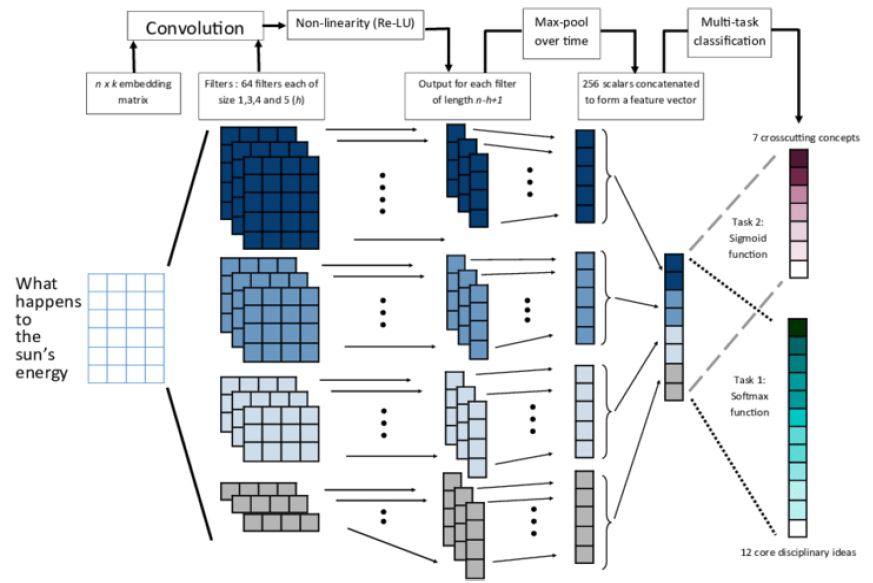
Figure 1: Architecture of modified CNN

Implementation Prototype

The term “System Design” refers to the process of specifying the strategy, components, interfaces, artifacts, and documents of a system in order to meet certain requirements. It can be thought of as the application of systems theory to component development and often involves collaboration between the fields of systems analysis, systems design, and systems engineering. The success of a system is measured by its performance or effectiveness in providing the desired output. Requirement analysis is a critical step in the development of a system, as accurate and complete requirement information is necessary to design a system that will function appropriately in the desired environment. It is the responsibility of the users of the system to provide this information, as they are the individuals who will ultimately use the system.

Project Implementation Details

System Modules

There are three modules

• Collecting Data Sources
• Processing data sets
• Feature Learning

Collecting Data Sources: Here 2 types of data sets are used to perform risk assessment.

♦ Structured Data. It refers to records with an excessive degree of association, to such a quantity that incorporation in a social database is steady and right away seek with the aid of using basic, direct net crawler calculations or different hunt activities. This is normally visible in .csv format.

Here data set related to hypertension shown in the following table refers to attributes used to predict either high or low risk (Table 1).

Table 1: Structured data

Name	Data type
Age	int
Sex	int
cp(chest pain)	int
Trestbps (threshold blood pressure)	int
chold	int
smoke	int
Physical inactivity	int
Thalach (max heart rate)	int
Ckd (chronic kidney disease)	int
Pt (potassium levels in mg/mol)	int
Stress levels	int
Ca (blood vessels)	int
Thal (sugar levels)	int
target	int

♦ Unstructured Data. The text is typically composed of words and sentences, but it may also include information such as dates, numbers, and facts. As a result, it often contains inconsistencies and ambiguities, which make it difficult to analyze using standard methods compared to data stored in structured form in databases or semantically labeled documents.

This looks as in the following manner:

Preprocessing data sets:

• Properties i.e., qualities thru sufferers are exaggerated and removed from the (fact) datasets.
• Preferring perhaps getting rid of replica values and including lacking values
• Each characteristic significance in affecting the affected person may be determined by the usage of correlation evaluation or among max combining phases.
• Unstructured facts to established facts with designated goals.

Feature learning:

• The extracted features are passed into modified CNN layers to train the neural network structure.
• Then extract the high-level features from the modified CNN.
• Modified CNN consists of the following layers in this model:

1. Contribution values
2. Hybrid Hidden values
3. Production values

• This neural network has parameters (w, b) = {h1, h2, h3, b1, b2, b3}
• The accuracy rate is predicted.
• The results demonstrate that our method has the advantage to infer the prediction of such fatal diseases over the other three methods (KNN, Decision Tree, and Gaussian Naive Bayes).

Here Implementation goes on with structured data and unstructured data and then the obtained results are compared with performance metrics. Through them can know the best method for predicting the risk of hypertension.

Implementing Using Structured Data

This is done using three MLA (Machine Learning Algorithms) [8] like DT i.e., Decision

Tree, KNN i.e., K-Nearest Neighbor, and NB i.e., Naive Bayes. For implementation can use Python and Implementation starts with,

• Load the data set in .csv format.
• Then pre-process the data to remove any noisy data.
• Need to do some correlation analysis so that how attributes are related to the target class using heat map in correlation matrix with the diverging palette.
• Then need to divide the data set for training purposes to build the model.
• Like here the cardinality of the data set is 303*14. So, need to split the data by giving test size and random state. Here test size is mentioned as 33% so 203 rows for training the model and the rest 100 rows to test the model and this could be randomly divided as the random state is given.
• Here while doing this splitting the target class must not be included as the model is developed using only attributes.
• Then after splitting always scale the features after splitting the data set because we want to ensure that the validation data is isolated. This is because the validation data acts as new, unseen data. Any transformation on it will reduce its validity.
• Now we are finally ready to create a model and train it. Remember that this is a two-class classification [15] problem. We need to select a classifier, not a regression.
• Let us analyze three models, Decision Tree Classifier, Gaussian Naive Bayes Classifier, and KNN Classifier.

Decision Tree

Decision Tree builds a hybrid prototype that forecasts the output features based on characteristic splitting criterion here GINI index is used based on the calculation with respect to values tree is constructed using the following algorithm:

Input – Preparing related records and their associated group names; qualities, list, and competitor arrangement qualities; Attribute choice technique, a system to decide the parting rule comprises of parting trait and, conceivably, but fragmented-point or parting subsection.

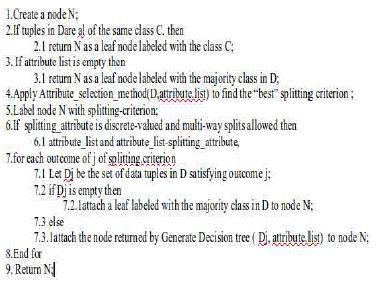
Output: A DT (decision tree).

Approach:

KNN-Nearest Neighbor

The K-Nearest Neighbor (KNN) specification [15] is provided by the preparation dataset, & Nearest K-case in preparation informational collection is originated. KNN is essential to decide the estimation of separation and the optimal K-value. The information is standardized at first. At that point, we utilize the Euclidean separation to gauge the separation. With respect to the choice of attributes K, it has been found that the prototype is most efficient if the k=5. Hence, pick k=5. The algorithm is as follows:

Data Intake

Consider, D (dataset), is a dataset of experimental-related records and groups;

K-assumption value;

Data Result: KNN approach;

Approach:

1. Begin
2. K-value and simu() function initiation;
3. Experiment with the provided dataset (D);
4. Di is experimenting set and y is evaluating the dataset.
5. Calculate simu(Di,y);
6. The biggest K-scores of simu(Di,y);
7. Calculate average of simu() for KNN (K-Nearest Neighbors);
8. Assume average of simu() is larger than edge
9. The cancer patient output is ‘y’;
10. Else, not a cancer patient;
11. Finished.

Naive Bayes

Naive Bayes classification [15] is a basic probabilistic classifier. It requires ascertaining the likelihood of highlighting traits. This algorithm is as follows:

Input: D: a set of tuples Output: Calculates probability with respect to every member of the target class.

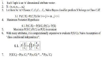
Method. These models are now capable of ‘predicting’ whether a patient is at high risk or low risk of hypertension.

Implementing Using Unstructured Data

Implementation using unstructured data can be trained using Convolutional [20] Neural Network techniques.

Neural Networks

• NN (Neural Networks) are mathematical computational components known as AN (Artificial Neurons).
• Inspired by the Neural Activity of the brain, they try to replicate similar behavior mathematically. (Practically far simpler than neurons in the brain).
• Neural Networks are better than traditional machine learning algorithms [8] and perform well with huge data.
• Because the machine learning algorithm’s performance saturates when the data set size grows.
• The input layer is where data is provided.
• Each neuron in the input layer corresponds to the value of a feature.
• The Hidden Layer is where computation takes place.
• Simple Neural Networks generally contain 1 or 2 hidden layers

The output Layer generates the result of the neural network (Figure 2).

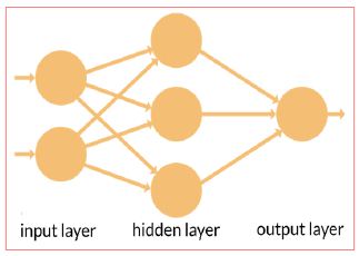
Figure 2: Neural Network Showing Layers

Neuron

There are weights associated with each neuron. Consider the figure to below. There are three features namely X1, X2, X3 (Figure 3).

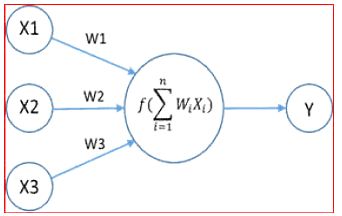
Figure 3: Neuron Computation with Weights

Why not TRADITIONAL machine learning?

• Data from medical [14] data centers is usually a huge data set.
• As shown in the figure traditional machine learning algorithm’s performance saturates when the data set size grows.
• There is an under-utilization of data in decision-making. Deep Learning [19] systems are built just for that purpose (Figure 4).

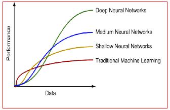
Figure 4: Performance Comparison

Procedure

Implementing the modified CNN is through using unstructured data because this predicts with high accuracy. This entire computation could be seen in hidden layers. This could be done in five stages.

• At first, unstructured data which consists of patient data is taken to create vector values.
• Then the data is organized into 2 columns such that one with text and the other with target class to experiment on NN (Neural Network) model & test predictions using the vector values.

Step 1: Representation of Text Data

1. Each word can be spoken to as a vector of numerical qualities (A section grid).
2. All words spoken to RD-characteristics vector, if d = 50 i.e., we speak to each word as a section vector (segment framework) containing 50 lines.
3. Presently the content can be spoken to by attaching the segment vectors meaning we stack up the section vectors one next to the other to make of network of measurement d x n. (Just words are stacked next to each other in a sentence).

Step 2: Convolution Layer of Text MCNN

1. Start a pointer at position 1. (1st word)
2. Expecting the pointer is at the position I, take words locations I-1, I-2, I, i+2, i+1.
3. Transpose every one of them to shape push grids of 50 segments and annex them next to each other changing over them into a solitary column vector of size 960×960.
4. Addition the pointer and change to a new line.
5. For first, second, and n-1 and nth words we have openings i.e., for the essential word we don’t have two past words. In such a case fill them with zero vectors.
6. Toward the finish of the above procedure, we get an nx250 network which is our convoluted grid.
7. The weight network W1∈R100×250 is of size 100×250. This means we are expecting the neural system to separate 100 highlights for us.
8. Presently we complete the accompanying computation.
   h1i,j =f(W1[i]·sj+b1)
9. This is the speck result of lattices. b1 is a segmented network of 100 lines. The inclination is utilized to use to move the learning procedure.
10. Without including it, it is the straightforward weighted whole of highlights and there is no learning procedure.
11. We get a 100xn element chart h1.f is an actuation work that is utilized to get non-linearity. We utilized Tanh’s actuation work.
    h1 =(h1i,j)100×n

Step 3: POOL Layer of Text Modified CNN

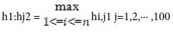
1. From the element diagram h1 which is 100xn dimensional, we pick the most extreme component in each line of the lattice acquiring 100 greatest qualities from each line.
2. From these 100 qualities we develop a 100×1 lattice h2 (segment vector).
3. The explanation of picking max pooling activity is that the job of each word in the content isn’t totally equivalent, by most extreme pooling we can pick the components which assume key jobs in the content.
4. Before the finish of Step 3 we have separated 100 highlights from unstructured information.

Step 4: Full Connection Layer of Text Modified CNN

1. At that point give this grid as a contribution to a neural system that conveys the accompanying calculation which is like that of in sync 2. (dot result of networks).
2. W3 is the weighted network of the full association layer and b3 is inclination.
   h3 =W3h2+b3

Step 5: Modified CNN Classifier

1. Delicate max classifier as yield classifier which predicts the danger of the disease (high or low).
2. This calculation goes with the sigmoid formula and calculates the probabilistic value to predict (Figure 5).

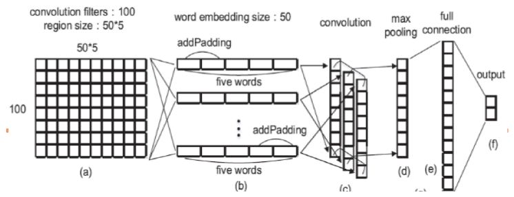
Figure 5: Modified CNN Step-wise Implementation

The algorithm or step-by-step procedure is as follows:

# At first unstructured data is taken and sent to the word2Vec algorithm to create vector values.

1. train    pd.read_csv(fname)
2. train    train[“TEXT”]
3. train    str.lower()
4. corpus    str.split()
5. patient corpus    Word2Vec(corpus, size=50,min_count=3)
6. patientcorpus.save(‘patientwordvec’)

# Then data is organized so that one contains text and other with target class.

1. X and Y  placeholder_value(n_W0,n_C0, n_y, n_H0,)
2. Initialize_attributes()
3. Propagation_forward(parameters, X)
4. Calculate_cost(Y,Z2)
5. FineTuner tf.train.GradientDescentOptimizer(learning_rate=learning_rate).minimize(cost)
6. inittf.Initializer_global_variables()
7. tf.Session() of session:
8. 9.1 session_run(initialization)
   9.2 epoch in range (epochs_num):
   9.2.1epcost 0.
   9.2.2 for j in range (0, m):
   9.2.2.1d j+1
   9.2.2.2 cost_tempsession_run([cost,optimizer],dictionary_feed={X:X_training[j:d][:][:][:],Y:Y_training[j:d][:]}
   9.2.2.3 epcost += temp_cost
9. if print_cost == True
10. 1print (“Cost after epoch%i:%f”% (epochs, epcost))
11. if epochs% 1 == 0 and print_cost == True:
    12.1costs.append (epcost)
12. correct_prediction = tf.equal(Z2, Y)
13. predict_op           Z2
14. Calculate accuracy using experimental dataset and evaluating dataset.

NN (Neural Network) Logical flow:

In this, can observe at first input value is sent to the neural network then based on weights convoluted matrix is built. Then predictions are made and adjusted by calculating the squared mean error means loss function. This loss score is done by using a gradient descent optimizer and then weights are updated again and prediction goes on (Figure 6).

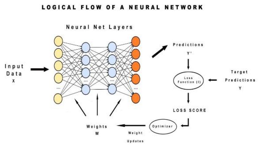
Figure 6: Logical Flow of Neural Network

Results

Analysis of Structured Data

The structured hypertension data set used for analysis is in the following Figures 7 and 8.

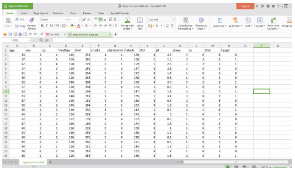
Figure 7: Hypertension structured data

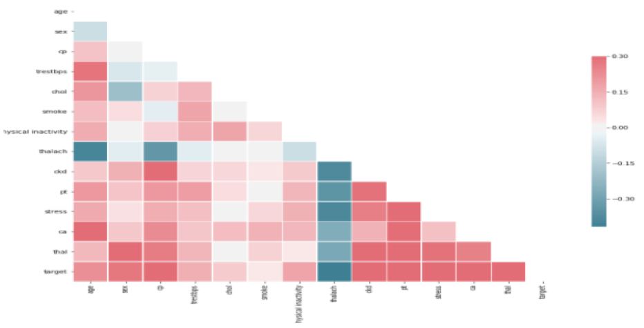
Figure 8: Correlation Analysis

Here is the view of correlation analysis of attributes with target by knowing significant attributes with help of diverging palette. Before predicting scaling need to be done for the train data set and test data set. This could be seen in following Figure 9.

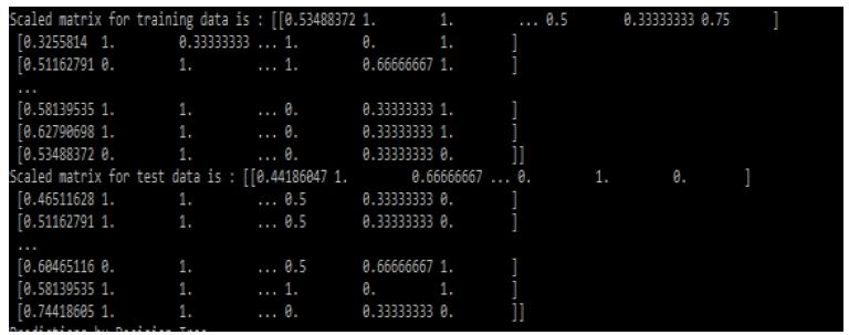
Figure 9: Scaled Matrices for Training and Test data sets

Then the results that means predictions obtained by three algorithms [8] are shown in the following Figure 10:

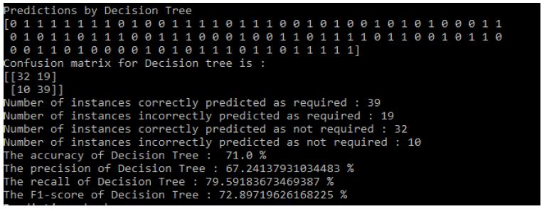
Figure 10: Decision Tree Results

Results of Decision Tree: Figure 10

Results of KNN: Figure 11

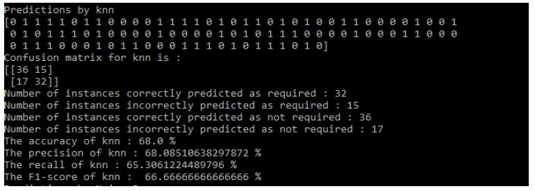
Figure 11: KNN Results

Results of Naive Bayes: Figure 12.

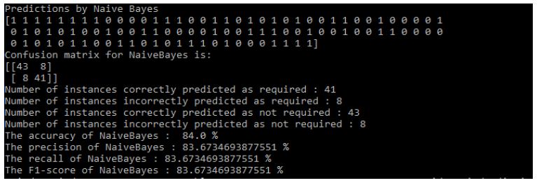
Figure 12: Naive Bayes Results

Analysis of Unstructured Data

The unstructured hypertension data set used for analysis to get numerical values for vector values is in following Figure 13. Then data need to be organized into the following way to experiment NN (Neural Network) dataset, test, and to predict (Figure 14). Then after training the neural network when the model is built sent to test set for predictions (Figure 15).

Figure 13: Unstructured Data Sent to Word2Vec for Create Numerical Values

Figure 14: Unstructured Data Processed to Structured Format

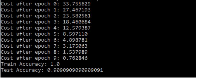
Figure 15: Modified CNN Results

Validation Metrics

For the exhibition evaluation withinside the test. Initially, we suggest to calculate precision, accuracy, and recall.

• Accuracy of Decision Tree: 71.0%
• The precision of Decision Tree: 67.24137931034483%
• The recall of Decision Tree: 79.59183673469387%
• The F1-score of Decision Tree: 72.89719626168225%
• The accuracy of KNN: 68.0%
• The precision of KNN: 68.08510638297872%
• The recall of KNN: 65.3061224489796%
• The F1-score of KNN: 66.66666666666666%
• The accuracy of NaiveBayes: 84.0%
• The precision of NaiveBayes: 83.6734693877551%
• The recall of NaiveBayes: 83.6734693877551%
• The F1-score of NaiveBayes: 83.6734693877551%.

In organized information or structured data, the NB classification [15] is the best in test. In any case, it is likewise seen that we cannot precisely anticipate whether the patient is in a high hazard as indicated by the patient’s age, sex, clinical lab, and other organized information. In other words, on the grounds that cerebral dead tissue is an ailment with complex side effects, we can’t foresee where the patient is in a high-hazard gathering just in the light of these straightforward highlights.

• The Train Accuracy of modified CNN: 1.0
• The Test Accuracy of modified CNN: 90.90909090909091%
• The precision of Modified CNN: 83.6734693877551%
• The recall of Modified CNN: 83.6734693877551%
• The F1-score of Modified CNN: 83.6734693877551% (Figure 16).

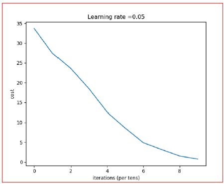
Figure 16: Iteration vs. Cost

Taking everything into account, for illness chance demonstrating, the precision of hazard expectation relies Upon the various range spotlight of the medical [14] medical institution information, i.e., the higher is the detail portrayal of the ailment, the better the exactness will be. To find the precision rate can arrive at 90.00% to all the more likely assess the hazard. The following bar plots show the comparison: Figure 17.

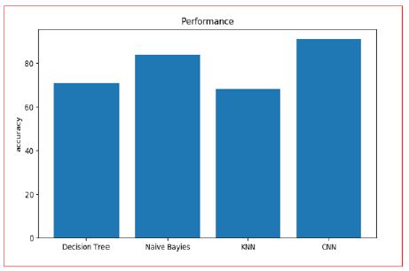
Figure 17: Accuracy Analysis of Different Algorithms

Research Implementation Time-Period

It takes few seconds for the execution. The mission execution additionally relies upon at the gadget overall performance. System overall performance is primarily based totally at the gadget software, gadget hardware and area to be had with inside the gadget (Figures 18-21 and Table 2).

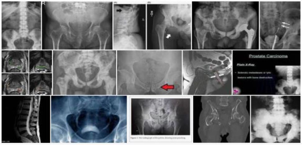
Figure 18: Prostate Cancer Data set

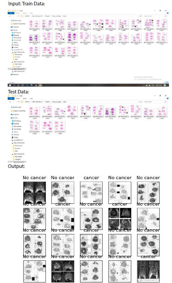
Figure 19: Patients with and without prostate Cancer

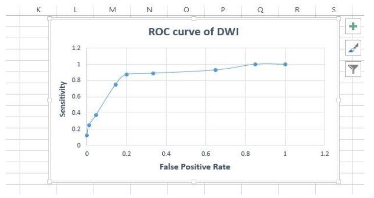
Figure 20: Roc Curve for accuracy

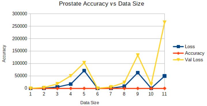
Figure 21: Prostate Accuracy vs. Data Size

Table 2: Comparison of different models vs different sizes of the dataset

Model	Size	Top-1/Top-5 error	Layers	Model Description
Decision Tree	218	53/90	8	5 Conv + 3fc layer
Naive Bayes	440	38.66/7.2454	13	13 Conv + 3 fc layer
KNN	562	27.3312/11.3214	16	16 Conv + 3fc layer
CNN	668	19.456/10.767	19	19 Conv + 3fc layer
MCNN	740	12.7878/8.357	21	21 Conv + 3fc layer

Conclusion

The current research in the area of clinical big data analysis has not focused on both structured and unstructured types of information. The proposed framework outperforms several typical prediction algorithms in terms of accuracy, performance, and conjunction speed. This is achieved through a hybrid Convolutional Neural Networks approach that utilizes both structured and unstructured data from hospitals. Data mining and deep learning play critical roles in various fields including machine learning, artificial intelligence, and database systems, with the main aim of improving the performance of prediction models. The performance of the proposed algorithm was statistically compared with various approaches, including linear regression and SVM principals, and was found to be superior. Furthermore, there are several advanced strategies that can be used to further improve the accuracy of the model. Compared to other common prediction algorithms, our proposed algorithm achieved an accuracy of 91% with a faster assembly speed.

Conflicts of Interest

All authors involved in this research journal affirm that this article has no conflict of interest and has collectively contributed towards its goal and objectives.

Data Availability

The data used to support the findings of this study is available from the corresponding author upon request (head.research@bluecrest.edu.lr).

Funding

This research work was done independently by the authors who had not received any funds for it from Liberia Government because this country is in crisis and poor, and from the University.

Authors Contribution

Asadi Srinivasulu contributed to the conceptualization, references collection, data curation, formal analysis, methodology, software, data curation, investigation, resources, software selection, writing the original draft, methodology, supervision, writing review, and editing, project administration, visualization, and investigation. Participated in the formal analysis. Contributed to proofreading of the research article in data collection and environment, and participated in the plagiarism check and correction process. Saad Ali Alahmari contributed formal analysis, methodology, software, data curation, investigation, methodology, software, data curation, and investigation, and contributed analysis, visualization and data collection, plagiarism, paraphrasing, and diagrams.

References

1. Neeraj Kumar, Ruchika Verma, Ashish Arora, Abhay Kumar, Sanchit Gupta, Amit Sethi, and Peter H. Gann “Convolutional neural networks for prostate cancer recurrence prediction”, Proc. SPIE 10140, Medical Imaging 2017: Digital Pathology, 101400H (1 March 2017); https://doi.org/10.1117/12.2255774.
2. Siegel, RL, Miller, KD, Jemal A (2017) Cancer statistics, 2017. CA: a cancer journal for clinicians 67: 7-30.
3. Sandhu GS, Andriole GL (2012) Over diagnosis of prostate cancer. J. Natl. Cancer Inst. Monogr. 2012: 146-151 (2012)10/12.
4. Sonn GA, et al. (2017) Prostate magnetic resonance imaging interpretation varies substantially across radiologists. Eur Urology Focus. [crossref]
5. Hassanzadeh E, et al. Prostate Imaging Reporting and Data System Version 2 (PIRADS v2): A pictorial review. Abdom Radiol 42: 278-289. [crossref]
6. Rosenkrantz AB, et al. (2016) Inter observer reproducibility of the pi-rads version 2 lexicon: a multicenter study of six experienced prostate radiologists. Radiology 280: 793-804. [crossref]
7. Nasrabadi, NM (2007) Pattern recognition and machine learning. J. electronic imaging 16: 049901.
8. Goldberg DE, Holland, JH (1988) Genetic algorithms and machine learning. Mach. learning 3: 95-99.
9. Michalski RS, Carbonell JG, Mitchell TM (2013) Machine learning: An artificial intelligence approach (Springer Science, Business Media, 2013)
10. Cameron A, Khalvati F, Haider MA, Wong A (2016) Maps: a quantitative radiomics approach for prostate cancer detection. IEEE Transactions on Biomed Eng 63: 1145-1156. [crossref]
11. Litjens G, Debats O, Barentsz J, Karssemeijer N, Huisman H (2014) Computer-aided detection of prostate cancer in MRI. IEEE Transactions on Medical Imaging 33: 1083-1092.
12. Wang S, Burtt K, Turkbey B, Choyke P, Summers, RM (2014) Computer aided-diagnosis of prostate canceron multi-parametric mri: a technical review of current research. BioMed Research International 2014.
13. Fehr D, et al. (2015) Automatic classification of prostate cancer Gleason scores from multipara metric magnetic resonance images. Proc Natl Acad Sci 112, E6265-E6273. [crossref]
14. Erickson BJ, Korfiatis P, Akkus Z, Kline, TL (2017). Machine learning for medical imaging. Radiographics 37: 505-515.
15. Orru G, Pettersson-Yeo W, Marquand AF, Sartori G, Mechelli A (2012) Using support vector machine to identify imaging biomarkers of neurological and psychiatric disease: a critical review. Neurosci Biobehav Rev 36: 1140-1152. [crossref]
16. Krizhevsky A, Sutskever I, Hinton, GE (2012) Imagenet classification with deep convolutional neural networks. In Advances in neural information processing systems, 1097-1105.
17. Long J, Shelhamer E, Darrell T (2015) Fully convolutional networks for semantic segmentation. In Proceedings of the IEEE conference on computer vision and pattern recognition, 3431-3440. [crossref]
18. He K, Zhang X, Ren S, Sun J (2016) Deep residual learning for image recognition. In Proceedings of the IEEE conference on computer vision and pattern recognition, 770-778.
19. Ioffe S, Szegedy C (2015) Batch normalization: Accelerating deep network training by reducing internal covariate shift. arXiv preprint arXiv: 1502.03167.
20. LeCun Y, Bengio Y, Hinton G (2015) Deep learning. Nature 521: 436.
21. Simonyan K, Zisserman A (2014) Very deep convolutional networks for large-scale image recognition. arXivpreprint arXiv: 1409.1556.
22. Srinivasulu Asadi and G.M.Chanakya, “Health Monitoring System Using Integration of Cloud and Data Mining Techniques”, Copyright © 2017 Helix ISSN 2319 – 5592 (Online), HELIX multidisciplinary Journal – The scientific explorer, Vol 5, Issue 5, and Helix Vol. 7(5): 2047-2052, September 2017.
23. Litjens G, Kooi T, Bejnordi BE, Setio, AAA, Ciompi F, Ghafoorian M, Sánchez CI (2017) A survey on deep learning in medical image analysis. Medical Image Analysis 42: 60-88. [crossref]
24. Gulshan V, Peng L, Coram M, Stumpe MC, Wu D, Narayanaswamy A, Webster DR (2016) Development and validation of a deep learning algorithm for detection of diabetic retinopathy in retinal fundus photographs. JAMA 316(22): 2402-2410. [crossref]
25. Abrol E, Khanna P, Jain A (2018) Prostate cancer detection from histopathology images using machine learning techniques: A review. Journal of Healthcare Engineering.
26. Litjens G, Debats O, Barentsz J, Karssemeijer N (2014) Computer-aided detection of prostate cancer in MRI. IEEE Transactions on Medical Imaging 33(5): 1083-1092.
27. Varghese BA, Chen F, Hwang DH, Stephens GM, Yoon SW, Fenster A (2019) Deep learning for automatic gleason pattern classification for grade group determination of prostate biopsies. Medical Physics 46(10): 4565-4575.