Author Archives: author

Caring for Confused Community Dwelling Seniors: Contributing and Obstructing Factors in Daily Care for Healthcare Assistants in District Nursing

DOI: 10.31038/ASMHS.2019321

Abstract

Older people with confused behavior, have behavioral problems due to dementia, mental problems or social problems. For the Healthcare Assistant (HA) in district nursing, it is a daily challenge to care for older people with confused behavior. Aim of this research is to achieve an insight in the strategies the HA uses to deal with the daily care for older people with confused behavior. It is also the aim to have insight in factors which contribute to the daily care in a positive or negative way. Method: a qualitative explorative research. 17 HA’s in district nursing participated in semi-structured interviews. All respondents had experience with caring for older people with confused behavior. The most important influencing factors are the experienced relationship between HA and the client and the experienced support by the team. Particularly behavioral problems due to mental problems can impede a relationship with the client. Further research is recommended to study the level of knowledge and competences of all levels of employees in district nursing.

Keywords

Confused persons, vulnerable elderly, older adults living at home, mental disorder, home care staff, district nursing

Short Commentary

The number of seniors confronted by chronic illness and dementia is rising, due to the fact that people are getting older and stay at home longer. Because of rising healthcare costs, people are to assumed to stay at home as long as possible [1]. Though, age-related physical and cognitive decline can make aging at home challenging [2]. Psychiatric problems among community dwelling seniors is frequently recognized by healthcare assistants (HA’s) in district nursing [2]. One of the consequences of these problems is an increase of the so-called confused community dwelling seniors. Seniors with confused behaviour show problems like agitation, aggression or apathy. For HA’s it is a daily challenge to manage the care for confused community dwelling seniors. It is important that HA’s have sufficient knowledge of confused behaviour in seniors in order to recognize and manage psychiatric problems [2]. However, little is known about what HA’s experience themselves as contributing or obstructing factors to daily care and how to respond in a right way to confused behaviour as well as to provide good care. We conducted an explorative research among seventeen HA’s in the Netherlands to gain insight in these contributing and obstructing factors. The qualified HA’s, with a variety in age and work experience, provide basic personal care under supervision of a district nurse.

The professionals were asked, in an individual interview, to share their experiences with confused community dwelling seniors and how they manage daily care. The Cohen-Mansfield mapping of problem behaviour, an instrument for assessing agitation, was used to stimulate participants to give more detailed information and examples of problem behaviour they experienced [3]. Most of the participants experience an increase of confused community dwelling seniors, which was in line with research conducted by Grundberg and colleagues concerning the role of home care assistants recognizing mental health problems in community dwelling seniors [4]. HA’s reported daily difficulties and challenges in caring for confused community dwelling seniors. The HA’s were confronted with verbal aggressive behaviour like threats, berate or curse by the seniors. They were also confronted with physically non-aggressive behaviour like compulsive or risky behaviours of the seniors. According to the HA’s, there is no ‘standard recipe’ to manage problem behaviour: the way the HA’s approach confused seniors depends on factors related to the seniors as well as characteristics of the HA. These factors are for example age and work experience of the professional as well as the type and cause of behaviour problem of the senior. The presence or absence of a relation of trust, information and support are the main contributing or obstructing factors.

Despite the fact that a relation of trust is seen as essential for providing good care, it seems very difficult to achieve such a relation with confused community dwelling seniors. According to the HA’s, a relation of trust can be reached when they have the opportunity to get to know the client. HA’s experience more difficulties to become familiar with the senior and building up a relation of trust in case a diagnose is missing and psychiatric problems are suspected. A study of Gleason and Coyle regarding the experiences of home care workers providing homecare to clients diagnosed with mental and behavioural problems, also mentioned the struggles in building a relation of trust in such cases [5]. In addition, in cases where psychiatric problems are suspected, the HA’s in our study seemed to have less tendency to build this relation of trust. Several factors might explain this low tendency: having a primary focus on personal care and not on a relation of trust, uncertainty of the HA or not having the required knowledge on how to respond to clients with (suspected) psychiatric diagnoses. These factors are also identified in a study on how nursing staff in a hospital manage patients with psychiatric problems [6].  Also a lack of collaboration with professionals in social care can obstruct a relation of trust [7].

The second factor, as mentioned by the HA’s, is the presence or absence of information on the underlying cause of the behaviour problem, for example dementia or loneliness of the senior. Olivera and colleagues studied the factors contributing to the development of psychiatric problems in community dwelling seniors [8]. When professionals in home care are aware of these factors, problems could be recognized at an early stage. In our study, HA’s stated that when information about the cause and reason of the behaviour is available, this increases their ability to recognize the problems. In such cases, HA’s experience a better management of problem behaviour and they feel like they succeed (more) in providing daily care.

At last, the HA’s perceive the available support of the district nursing team as a contributing or obstructing factor in the daily care for confused community dwelling seniors. Important is sharing knowledge and experiences within the team and with other professionals in healthcare and social care The importance of exchanging knowledge and experiences is confirmed in a study by Gleason and Coyle [5]. When confronted with problem behaviour, (emotional) support of other experts seems very important. Of course, attention is also still needed by strengthen (theoretical) knowledge about psychiatric problems and how to recognize such problems.

Stay longer at home by seniors, including confused community dwelling seniors might be desired and needed because of rising health costs. Though professionals both health and social care need help and more attention to overcome contributing and obstructing factors. Specifically providing information and (emotional) support, can support professionals in district nursing and can increase their feeling of being capable of building up a relation of trust with confused community dwelling seniors. Subsequently, this relation of trust can contribute to the provision of optimal care to the client.  Development of further collaboration of health care and social care professionals can contribute to more optimal and integrated care for both personal and mental health care [1, 7].

Note: Accepted for publication in the Dutch Journal of Gerontology and Geriatrics in Dutch (Tijdschrift voor Gerontologie en Geriatrie).

References

  1. Josefsson K, Meranius, MS (2018) Complexity in daily living of older adults with multimorbidity: health, social and informal care utilization and costs. J Gerontol Geriatr Med 4:017.
  2. Haddad M, Plummer S, Taverner A, Gray R, Lee S, Payne F, Knight D (2005) District nurses’ involvement and attitudes to mental health problems: a three-area cross-sectional study. J Clin Nursing 14: 976–985. [Crossref]
  3. Cohen-Mansfield J, Marx MS, Rosenthal AS (1989) A description of agitation in a nursing home. J Gerontology 44: 77–84. [Crossref]
  4. Grundberg A, Hansson A, Religa D, Hilleras P (2016) Home care assistants’ perspectives on detecting mental health problems and promoting mental health among community-dwelling seniors with multimorbidity. J Multidisciplinary Healthcare 9: 83–95. [Crossref]
  5. Gleason HP, Coyle CE (2016) Mental and behavioral conditions among older adults: implications for the home care workforce. Aging Mental Health 20: 848–855. [Crossref]
  6. Lethoba KG, Netswera FG, Rankhumise E (2006) How professional nurses in a general hospital setting perceive mental ill patients. Curationis, 29: 4–11. [Crossref]
  7. Rämgård M, Blomqvist K, Petersson P (2015) Developing health and social care planning in collaboration. J Interprofessional Care, 29: 354–358. [Crossref]
  8. Olivera J, Benabarre S, Lorente T, Rodrigues M, Barros A, Quintana C, Pelegrina V, Aldea C (2011) Detecting psychogeriatric problems in primary care: factors related to psychiatric symptoms in older community patients. J Mental Health in Family Medicine 8: 11–19. [Crossref]

Synovial Chondromatosis with Os Trigonum

DOI: 10.31038/IJOT.2019221

Case

A 25-year old male physical therapist had severe right ankle pain immediately following a workout with lunges, drop jumps, and single leg hops. The patient reported 10/10 anterior and posterior ankle pain and was unable to run or fully weight bear immediately or for the next 24-hours.  The patient had a long history of multiple inversion sprains resulting in ankle pain and edema throughout his prior high school/college football career.

Motion loss of 10 degrees in dorsiflexion/plantarfexion resulting in a reduced stance, stride, and push-off (antalgic gait) was evident. Palpation tenderness was noted over the anterior talus and distal tibia. The patient referred himself to an orthopedic physician two days following the injury due to the palpatory tenderness over the anterior distal tibia and pain with weight bearing (Ottawa Ankle Rules) [1].

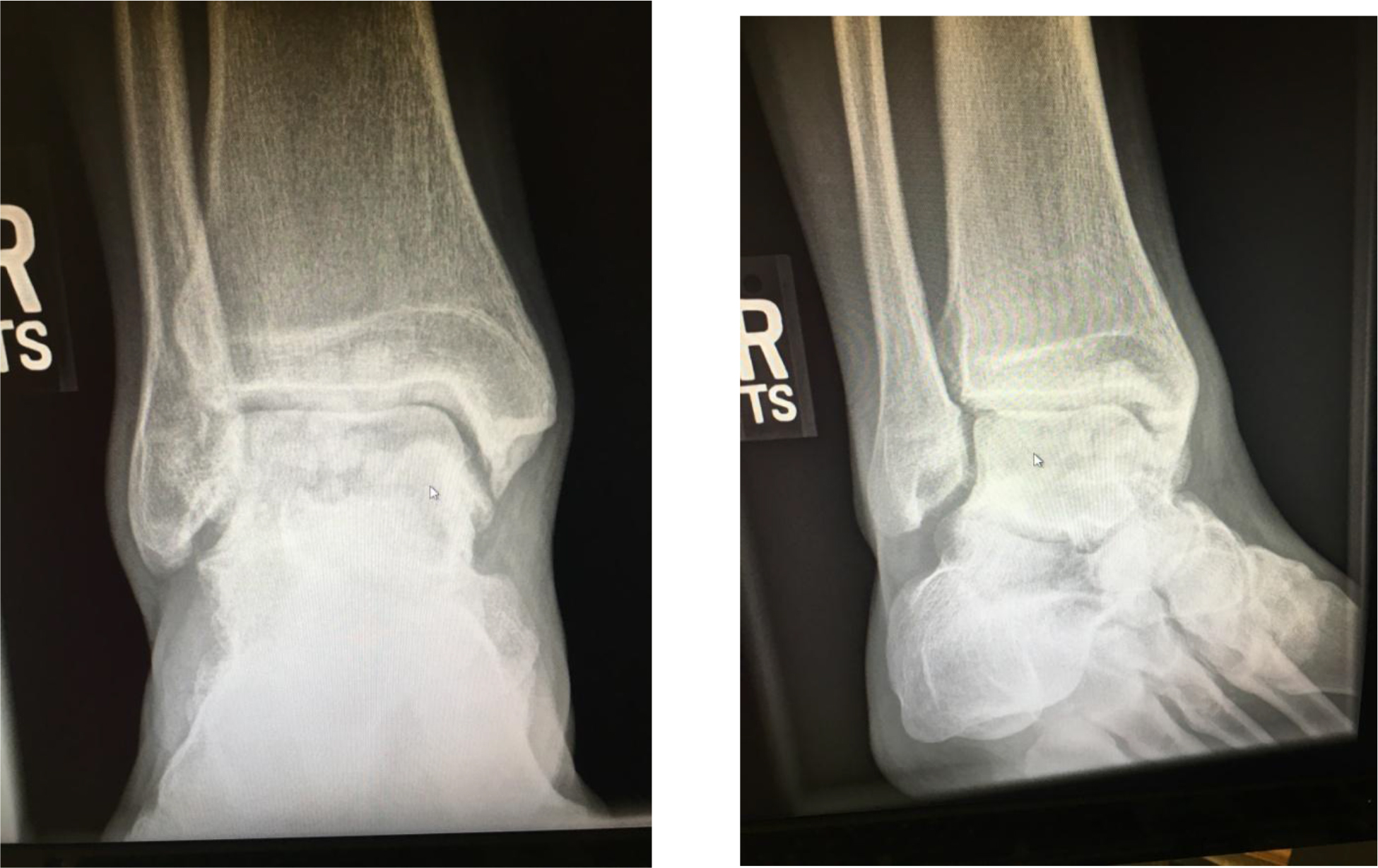
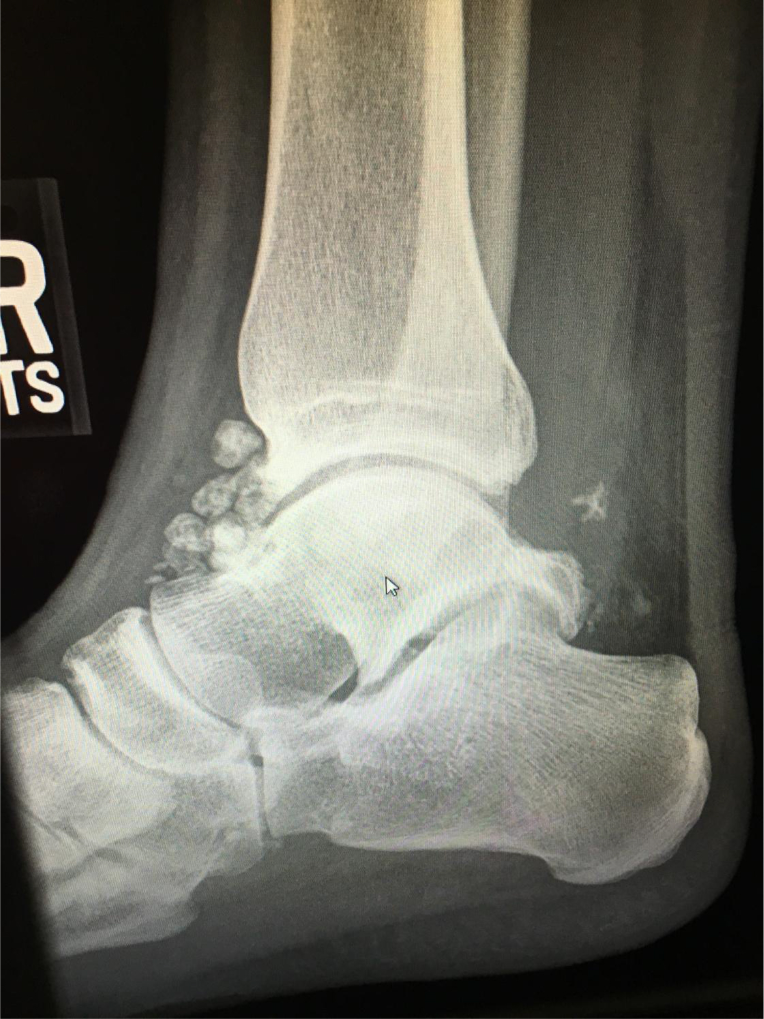
No evidence of a fracture was noted on the anterior-posterior or mortise radiographic views of the ankle (Figure 1). Synovial chondromatosis [2], or “popcorn” was present on both anterior-posterior and lateral views.  Os trigonum [3] (an accessory ossicle) was also present between the posterior talus and calcaneus (Figure 2).   MRIs confirmed radiographic findings. The patient was referred to an orthopedic ankle surgeon for an arthroscopic resection of the os trigonum and synovial osteochondromatosis 3-weeks post-injury date. The patient wore a CAM boot for 2-weeks at WBAT status and resumed full weight bearing ambulation at 3-weeks post-op without residual pain or dysfunction. He resumed running at 2-months post-surgery without pain.

IJOT 19 - 113_Marsha Rutland_F1

Figure 1. Anterior- posterior and Mortise view radiographs of the right ankle. Some small chondromatosis is seen in mid area of distal tibia and talus.

IJOT 19 - 113_Marsha Rutland_F2

Figure 2. Lateral view radiograph of right ankle, demonstrating significant synovial chondromatosis in the anterior aspect of the tibia and talus. Os trigonum is also present between the posterior talus and calcaneous.

References

  1. Stiell IG, McKnight RD, Greenberg GH, et al (1994) Implementation of the Ottawa ankle rules. J Am Med Assoc 271:827-832.  [Crossref]
  2. Sedeek SM, Choudry Q, Garg S (2015) Synovial chondromatosis of the ankle joint: clinical, radiological, and intraoperative findings. Case Rep Orthop. 2015.
  3. D’Hooge P, Alkhelaifi K, Almusa E Tabben M, Wilson MG, Kaux JG (2018) Chronic lateral ankle instability increases the likelihood for surgery in athletes with os trigonum syndrome. Knee Surg Sports Traumatol Arthrosc 2018.

Successful Delivery at 37 Weeks via C-Section and Simultaneous Total Hysterectomy, After IVF Oocytes Donor Transfer in an Ovarian Cancer Patient

DOI: 10.31038/IGOJ.2019223

Abstract

A salpingo-oophorectomy due to an ovarian malignancy could be accompanied with great stress and a number of risks for childless but, still fertile women. This situation poses a great challenge for an obstetrical point of view. A successful twin pregnancy at 37 weeks via c-section with simultaneous total hysterectomy is reported to a woman who was diagnosed with ovarian cancer (sex cord granulose tumor) and treated with right salpingo-oophorectomy 3 years prior to a successful fourth trial of IVF implantation. This woman underwent a c-section at 37 weeks, giving birth to twin females neonates with a simultaneous total hysterectomy. Antenatally, no complications were reported, rather than an admission due to premature contractions at 26+3, which resolved with adequate medication 5 days later, when the patient was fit for discharge and appointed for the operation. Her post-operative course was uneventful.

Introduction

Infertility causes a great deal of stress to a large number of women all over the world. Imaging complicates an already complex situation with the presence of ovarian cancer. Time limits become narrower and the obstetric team needs to evaluate and assess the risk of cancer versus the risk of failure in conception. Ovarian sex cord-stromal tumors (SCSTs) are extremely rare with a favorable long-term prognosis [1]. These types of ovarian cancer results to 7% of the all ovarian tumors [2]. For the reasons above, fertility sparing technique should be encouraged. Since the majority of women affected are young and at a reproductive age the safety of fertility-sparing operations must be assessed [3]. More specifically, GCTs illustrate a 5-year-survival prognosis of 92% to 100% in cases of surgical staging [4, 5].

History

A 40-yer-old gravida 1 para 0 with a history of thrombophilia (antithrombin III deficiency) underwent a laparoscopy due to a cyst foun via ultrasound suring her preIVF assessment in late 2014. Due to the size of the cyst, the specimen had to be resected in order to be removed through the trocar openings. The pathologist review revealed a sex cord ovarian tumor-granulosa cell tomor (GCT) stage IC. The stage of the tumor was possibly overestimated since the resected specimen could not provide to the pathologist clear limits for staging. After 2 months, the patient underwent an open surgery removal of right adnexa, appendicectomy and omentomectomy. No chemotherapy was proposed. In addition, she received IVF with 2 cycles of citric clomifaine ovarian hyperstimulation without any result since she had an incident of miscarriage at 8 weeks. Another 2 courses of treatment with donor ovarian foccicles were perfomed. The first led to a miscarriage at 5 weeks but the latest led to success with 2 MCDA twin female embryos. During her pregnancy no pathology was noted. At 26+3 weeks she was admitted in the hospital due to premature contractions for which she received 2 courses of Atosiban till 27+4 weeks. At 27+5 she was discharged by the hospital and she was appointed for a ceasearian section at 37 weeks with a simultaneous hysterectomy and left salpingo-ophorectomy. The perinatal outcome was successful resulting to twin healthy females neonates with an Apgar score 10 out of 10 within the first minute of their birth and adequate weight. They required no incubators.

Literature Review

Fertility-sparing operation has been proposed in order to achieve a viable pregnancy for women who are younger and usually present with early stages of cancer [6]. Nevertheless, the risk of recurrence is high, almost 45% in cases of cystectomy which means that fertility methods must work in a timely manner [6, 7]. In this case no chemotherapy was proposed, since international literature suggests platinum-based chemotherapy in cases of advanced ovarian cancer or recurrent disease [8].

Due to the rarity of this GCTs, no large scale randomized trials have been conducted, leaving a vague approach in cases, where fertility must be preserved [9, 10]. However, it seems that women at stage I have a very low risk of further recurrence, when adequate surgical staging has been performed [3]. Further investigation in literature reveals a unexpected increased female neonates ratio as well as a full term births for women in pregnancies complicated with SCTs [11]. Usually after delivery, a second operation must be perform [12, 13]. Total hysterectomy with bilateral salpingo-oophorectomy must be performed ± chemotherapy [14].

Conclusion

The evolution of obstetrics and gynecology even in severe cases such as ovarian cancer, gives women, who wish to maintain their fertility, many options. In this case, this patient not only was treated for ovarian cancer, patient’s fertility was preserved for further pregnancy. IVF treatment was successful and the obstetrics team achieved an appointed birth via c-section at 37 weeks despite all odds.

Discussion

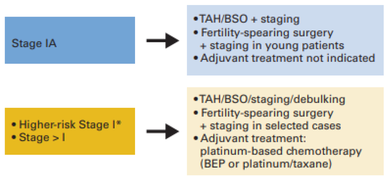
For complicated cases as the one presented above, a multidisciplinary team must be sought [15–17]. The need for a collaboration of an obstetrician, a pediatrician, an oncologist and a pathologist is self-explanatory [18]. Platinum –based chemotherapy should be sought since the stage of the ovarian tumor is higher than I. (see figure 1 below) [19].

IGOJ - Orestis Tsonis - F1

Authors have no conflict of interest.

References

  1. Serov SF, Scully RE, Sobin LH (1973) Histological typing of ovarian tumours: Citeseer.
  2. Koonings PP, Campbell K, Mishell JD, Grimes DA (1989) Relative frequency of primary ovarian neoplasms: a 10-year review. Obstetrics and Gynecology 74: 921–926.
  3. Evans AT 3rd, Gaffey TA, Malkasian GD Jr, Annegers JF (1980) Clinicopathologic review of 118 granulosa and 82 theca cell tumors. Obstet Gynecol 55: 231–238. [crossref]
  4. Malmström H, Högberg T, Risberg B, Simonsen E (1994) Granulosa cell tumors of the ovary: prognostic factors and outcome. Gynecologic oncology 52: 50–55.
  5. Zhang M, Cheung MK, Shin JY (2007) Prognostic factors responsible for survival in sex cord stromal tumors of the ovary-an analysis of 376 women. Gynecologic oncology 104: 396–400.
  6. Cadron I, Leunen K, Van Gorp T, Amant F, Neven P, et al. (2007) Management of borderline ovarian neoplasms. Journal of clinical oncology 25: 2928–2937.
  7. Marret H, Lhommé C, Lecuru F (2010) Guidelines for the management of ovarian cancer during pregnancy. European Journal of Obstetrics & Gynecology and Reproductive Biology 149: 18–21.
  8. Colombo N, Parma G, Zanagnolo V, Insinga A (2007) Management of ovarian stromal cell tumors. J Clin Oncol 25: 2944–2951. [crossref]
  9. Gershenson DM (2005) Fertility-sparing surgery for malignancies in women. J Natl Cancer Inst Monogr 43–47. [crossref]
  10. Morice P, Denschlag D, Rodolakis A (2011) Recommendations of the Fertility Task Force of the European Society of Gynecologic Oncology about the conservative management of ovarian malignant tumors. International Journal of Gynecological Cancer 21: 951–963.
  11. Blake EA, Carter CM, Kashani BN (2014) Feto-maternal outcomes of pregnancy complicated by ovarian sex-cord stromal tumor: a systematic review of literature. European Journal of Obstetrics & Gynecology and Reproductive Biology 175: 1–7.
  12. Young RH, Dudley AG, Scully RE (1984) Granulosa cell, Sertoli-Leydig cell, and unclassified sex cord-stromal tumors associated with pregnancy: a clinicopathological analysis of thirty-six cases. Gynecologic oncology 18: 181–205.
  13. Behtash N, Zarchi MK, Gilani MM, Ghaemmaghami F, Mousavi A, et al. (2008) Ovarian carcinoma associated with pregnancy: a clinicopathologic analysis of 23 cases and review of the literature. BMC pregnancy and childbirth 8: 3.
  14. Zhao X, Huang H, Lian L, Lang J (2006) Ovarian cancer in pregnancy: a clinicopathologic analysis of 22 cases and review of the literature. International Journal of Gynecological Cancer 16: 8–15.
  15. Bernhard LM, Klebba PK, Gray DL, Mutch DG (1999) Predictors of persistence of adnexal masses in pregnancy. Obstet Gynecol 93: 585–589. [crossref]
  16. Wong H, Low J, Chua Y, Busmanis I, Tay E, et al. (2007) Ovarian tumors of borderline malignancy: a review of 247 patients from 1991 to 2004. International Journal of Gynecological Cancer 17: 342–349.
  17. Amant F, Van Calsteren K, Halaska MJ (2011) Gynecologic cancers in pregnancy: guidelines of an international consensus meeting. Rare and Uncommon Gynecological Cancers: Springer 209–227.
  18. Sherard GB 3rd, Hodson CA, Williams HJ, Semer DA, Hadi HA, et al. (2003) Adnexal masses and pregnancy: a 12-year experience. Am J Obstet Gynecol 189: 358–362. [crossref]
  19. Schneider DT, Calaminus G, Wessalowski R, Pathmanathan R, Selle B, et al. (2003) Ovarian sex cord-stromal tumors in children and adolescents. J Clin Oncol 21: 2357–2363. [crossref]

Oral Drug Compounding in Pediatric Patients: a Japanese Perspective

DOI: 10.31038/JPPR.2019231

Body Text

Many medicines used for pediatric patients are not available in pharmaceutical forms adapted to their needs. Actually, most oral medications are developed for adults as tablets and capsules. These forms are lack of dosing flexibility and it does not meet dosage requirements for pediatric patients from neonates to adolescents [1]. According to the updated review that including new pediatric formulations marketed in the United States (US), the country of European Union (EU), and Japan spanning the years 2007 to 2018, 16 kinds of pediatric oral formulations of which 7 drugs are ready-to-use and manipulation is required in 9 drugs, and 51 total new pediatric oral formulations of which 21 drugs are ready-to-use and manipulation is required in 30 drugs [2]. Furthermore in Nigeria, that is one of the low-middle income countries, 121 of 143 oral essential medicines (85%) were not available as flexible solid oral dosage forms and manipulation is forced [3].  When this manipulation is forced, the adult dosage forms are manipulated by either a health care provider, such as pharmacist, or by the parents and caregivers (e.g., crashing or grinding a tablet, capsule opening and sprinkling it into some foods or drink). These processes are called compounding and are commonplace for those medicines that lack pediatric formulations. Compounding procedures are regulated by provincial pharmacy standards, based on guidelines published by the National Pharmacy Regulatory Authorities (NPRA) in Canada or the US Pharmacopeia (USP). However, compounded medicines are not approved by rigorous process in each country such as Food and Drug Administration (FDA), European Medical Agency (EMA), Health Canada, Pharmaceuticals and Medical Devices Agency (PMDA) and the other region’s regulatory authorities.

The compounded medication’s characteristics and its physical property and specifications are not always known, and its compounding procedure is not well established or controlled and validated before their use in children. This is particularly true with reference to: stability, potency, content uniformity, purity or bioavailability, and so on. First and most important, the administration of the appropriate dose cannot be guaranteed. Moreover, most of the compounded medicines have an unpleasant and bad taste, which leads to adherence challenges. Even if every compounding process is taken to ensure, errors have a potential to do occur. Some compounding is needed in oncologic drugs with the concerns and obvious health risks to health providers and/or caregivers. It has the potential to expose the entire family to these toxic chemical agents.  Furthermore, the vehicle (e.g., juice, milk or yogurt) used to dissolve drugs and administer these compounded medicines, or to mask the bad taste of compounded drugs, has a potential to influence drug absorption. Especially, physicians and pharmacist need to be aware of the consequences of compounded medicines for drugs with a narrow therapeutic and safety drug index. Compounding at home also increase the variability in the product by inaccurate measurement, issues with stability or errors in instruction for manipulation [4]. Caregivers often mistake the procedure of the extemporaneous preparation [5]. A lack of bioequivalence study of compounded drugs is also concerned [6]. It is important as the formulation can lead the difference between successful treatment and therapeutic failure.

According to our survey results of 328 hospitals that have a pediatric department in Japan, that account for approximately a half of pediatric department, a total of 320 compounded drugs were identified and most of them were administered as a powder formulation. Top five percentile of compounded drugs were briefly indicated in Table 1. In Canada, the Goodman Pediatric Formulation Center which is a not-for-profit organization that is working as a facilitator between industry, regulatory and reimbursement agencies to bring commercialized pediatric formulations into Canada, also conducted a survey with hospital pharmacists from a dozen pediatric Canadian institutions in 2017. A total of 12 drugs were identified as a priority by at least one third of investigated institutions. Noteworthy, 11 of 16 drugs were same with the result of our survey, suggesting that a lack of appropriate formulation for pediatric patient is common issue in the world and global drug development may be an effective solution (Table 1, the 5th column).

Table 1. The current state of compounding in 328 hospitals that have pediatric departments in Japan and availability in other regulatory authorities.

Active ingredients name

Frequency of compounding No. (%)

Pre-compounded dosage form (strength)

Compounded Dosage Form

Common desired flexible dosage forms among Japan and Canadaa

Already approved flexible dosage forms in FDA, MHRA and EMAb

Dantrolene sodium hydrate

67 (20.6%)

Capsule (25mg)

Powder

N/A

Ramelteon

65 (20.0%)

Tablet (8mg)

Powder

N/A

Baclofen

58 (17.9%)

Tablet (10mg)

Powder

Oral liquid 5mg/5ml

Hydrocortisone

56 (17.2%)

Tablet (10mg)

Powder

N/A

Dexamethasone

49 (15.1%)

Tablet (0.5mg)

Powder

Elixir 0.1mg/mL

Prednisolone

49 (15.1%)

Tablet (5mg)

Powder

Syrup 3mg/mL

Enalapril maleate

45 (13.9%)

Powder (5mg)

Powder (dilution)

Oral solution 1mg/mL

Tadalafil

42 (12.9%)

Tablet (20mg)

Powder

N/A

Carvedilol

41 (12.6%)

Tablet (2.5mg)

Powder

N/A

Sildenafil citrate

30 (9.2%)

Tablet (20mg)

Powder

Powder for oral suspension 10mg/ml

Clonidine hydrochloride

30 (9.2%)

Tablet (75µg)

Powder

N/A

Levothyroxine sodium

30 (9.2%)

Tablet (50µg)

Powder

Oral solution 100µg/5ml

Diazoxide

26 (8.0%)

Tablet (25mg)

Powder

Oral suspension 50mg/mL

Aspirin

23 (7.1%)

Powder (1g/g)

Powder (dilution)

N/A

Propranolol hydrochloride

22 (6.8%)

Tablet (10mg)

Powder

Oral solution 8mg/mL

Methotrexate

22 (6.8%)

Tablet (2.5mg)

Powder

Oral solution 2mg/ml

a. The information about compounding in Canadian hospital was provided by the Goodman Pediatric Formulations Centre. Check marks (✔) indicate the common drugs that are desired from both Canada and Japan.
b. Approved drug information was searched using the websites provided from Food and Drug Administration (FDA) in the United States, Medicines and Healthcare products Regulatory Agency (MHRA) in the United Kingdom, and European Medical Agency (EMA)
Compounded drugs in the top 5 percentile was indicated. No., number; N/A, not available.

If the global product development is proceeding, which formulation is acceptable?

In many cases, commercialized pediatric formulations are available in other jurisdictions, such as in the US and in Europe and these are often developed as liquids or suspensions (Table 1, right column). Oral liquid medicines have some disadvantages over solid medicines. The major barrier in development of oral liquid formulations is taste-masking of drugs as almost all of health provider for pediatric patients in the US reported that a taste and palatability were the greatest barriers to appropriate medication [7]. The excipients used in the development of a product need to be safe and acceptable for use in children. Excipients are typically used to optimize the formulation of the medicine to improve palatability, shelf-life and/or manufacturing processes [8]. Another problem is that liquid medicines are less chemically stable than solid medicines and require refrigeration in hot climates to guarantee their quality and efficacy. When a company manufactures develop a product for different regions, it may be necessary to adapt tastes and flavors in order to different regional preferences. Having knowledge about caregivers’ perceptions would also be needed. These issues become a bottleneck restricting to facilitating the age-appropriate drug development. In 2008, the challenges of ensuring access to appropriate drug formulations for pediatric patients led the World Health Organization (WHO) to propose flexible solid oral dosage forms as the preferred formulations for them [9]. The use of oral solid dosage forms such as dispersible tablets, powders, granules, films or sprinkles for reconstitution have a potential to be an excellent substitute for liquid formulations, because the solid product has typically better stability compared with a liquids. However, the instructions for reconstitution can be complicated for untrained or uneducated individuals, yet it is important that the final product contains the correct dosage for the patients. If these forms are administered in the absence of water they are only applicable to infants who are accepting solid such as a baby food. The risk of any error also remains.

From these compelling issues, the Academy of Pharmaceutical Science and Technology in Japan and its subcommittees named ‘the individualized medicine focus group’ and ‘the clinical formulation focus group’, decided to prepare countermeasures in medically ensured compounding procedures. We aimed to collect accurate information about the present status of compounding and unclose what information is needed to the medically ensured compounding procedure.

To facilitate the drug development globally, no regulatory and financial drivers to develop age-appropriate medicines for pediatric patient become a heavy drag, especially about off-patent drugs. In the European countries, there is a significant number of existing drugs where age-appropriate formulations are needed [10, 11]. Almost all of these drugs are generic drugs developed in the remote past for which there are no incentives or any intellectual property protection, making these drugs less interesting to invest time and cost. Requesting an age-appropriate drug development to industrial companies is one of the best solutions, however, ensuring the quality of compounded formulation by the health professionals is required as an urgent issue. While the future of ideal pediatric oral formulations may increasingly be with taste-masked, preservative-free, and user-friendly formulations including multi-particulate solid dosage forms such as mini-tablets, orally disintegrating tablets, and granules, to assure the quality of compounded drug that is not on the radar of manufacturer is needed.

Acknowledgement

This work was supported by a Research Program from the Japanese Agency for Medical Research and Development under Grant Number JP19mk0101134, awarded to H.N. We are grateful to collaborated 328 hospital pharmacists who supported us to perform our survey.

References

  1. Venables R, Marriott J, Stirling H (2012) FIND OUT: key problems with children’s medicines formulations … It’s a taste issue! Int J Pharm Pract 20: 23.
  2. Strickley RG (2019) Pediatric oral formulations: an updated review of commercially available pediatric oral formulations since 2007. J Pharm Sci 108: 1335–1365.
  3. Orubu ES, Tuleu C (2017) Medicines for children: flexible solid oral formulations. Bull World Health Organ 95: 238–240.
  4. Richey RH, Shah UU, Peak M, Craig JV, Ford JL, et al. (2013) Manipulation of drugs to achieve the required dose is intrinisic to paediatric practice but is not supported by guidelines or evidence. BMC Pediatr 13: 1–8.
  5. Tomlin S, Cokerill H, Costello I, Griffith R, Hicks R, et al. (2009) Making medicines safer for children – guidance on the use of unlicensed medicines in paediatric patients. Guidelines 1–12.
  6. Batchelor HK, Marriott JF (2015) Formulations for children: problems and solutions. Br J Clin Pharmacol 79: 405–418.
  7. Milne CP, Bruss JB. (2008) The economics of pediatric formulation development for off-patent drugs. Clin Ther 30: 2133–2145.
  8. Fabiano V, Mameli C, Zuccotti GV. (2011) Paediatric pharmacology: remember the excipients. Pharmacol Res 63: 362–365.
  9. WHO. Annex 5. (2012) Development of paediatric medicines: points to consider in formulation. World Health Organ Tech Rep Ser 970: 197–225.
  10. EMA. (2013) Revised provisional priority list for studies into off-patent paediatric medicinal products. EMA/98717/2012: 1–12.
  11. WHO. (2015) WHO Model List of Essential Medicines for Children. 5th Edition: 1–42.

Comparison of Various Selection Strategies Used for Isolation of Human Monoclonal scFv Antibody Specific to GPCRs Heteromers

DOI: 10.31038/JPPR.2019224

Abstract

Currently, novel drug design focused on the searching pharmacological compounds acting via influence on GPCRs heteromers. The strategy allows obtaining highly selective effects since these heteromers appear only on specific cells and tissues. Therefore, human monoclonal scFv antibodies able to recognizing GPCRs heteromers may constitute a valuable tool in modern therapies. Antibody phage display technique together with high throughput screening play a key role in the development of clinically useful immunomolecules. Therefore in the present work we focused on the comparison of various strategies used for biopanning process during phage display procedure, dedicated to isolation scFv antibodies specifically recognizing GPCRs heteromers. Experiments were conducted in two different cell lines (CHO-K1 and HEK 293) and six various selection procedures were described. Elimination of nonspecific bindings constitutes a key point during the process. Results obtained duing selection conducted in the conditions promoting internalization process were the most satisfactory.

Keywords

Phage Display, scFv antibody, GPCRs, Hetromer, Biopanning

1. Introduction

Recently heteromers (receptor heterodimers) formed by human G-Protein Coupled Receptors (GPCRs) constitute extremely important targets in the design of modern treatment strategies [1]. Alteration of pharmacological properties of the receptors included in the heterocomplex have been proven and widely described in the literature [1–3]. Research focused on finding therapeutic compounds able to selective recognition of GPCRs heteromers are currently very popular. Such strategy allows to obtain a tissue-specific acting, since the interaction between receptors engaged in the complex formation can only take place when the receptors are simultaneously expressed on the same cell. Recent data indicate the existence of clinically relevant GPCRs heteromers, important in the treatment of, among others, pain, asthma or Parkinson’s disease [3–7].

Creation of the human monoclonal antibodies with specificity towards membrane GPCRs heteromers still remains sizable challenge. To fulfil its role, the kind of antibody must recognize the structural epitope formed within the GPCRs heteromeric structure and, at the same time, not show specificity for monomeric or homomeric forms of the receptors. The phage display technology provided the best conditions for the isolation of human monoclonal antibody specifically recognizing the spatial epitope formed by GPCRs heteromers.

Currently phage display technology attracts most attention since the methods is a powerful tool, among others, in drug discovery, nanotechnology, immunology, agriculture, diagnostics, neurobiology, molecular imaging etc [8–12]. The technology developed by George P. Smith in 1985 [13] constitutes a very useful tool for the study of protein–protein, protein–peptide, and protein–DNA interactions [14]. The methodology is based on the fact that phage phenotype and genotype are physically linked [14]. A gene encoding a protein of interest inserted into a gene of bacteriophage coat protein is expressed and presented on the phage surface. The concept is simple: a population of phage is engineered to express random-sequence peptides, proteins or antibodies on their surface [8]. From this population, a selection is made of those phage that bind the desired target [8]. Hereby, large proteins libraries can be screened and unique molecules which bind to their targets with high affinity and specificity can be isolated [15]. The advantage of the method is the possibility of the production of monoclonal antibodies recognizing antigens that cannot be used to immunize an animal due to their toxicity, non-immunogenicity or presence in complexes on the surface of cell membranes [16].

ScFvs (Single Chain Variable  Fragment) are small monoclonal antibody fragments composed of immunoglobulin-heavy (VH) and light chain-variable (VL) regions with a flexible peptide linker designed to connect the two chains such that the antigen binding site is retained in a single co-linear molecule [17]. The kind of antibodies can be derived from phage display libraries [18,19]. ScFvs are very useful in pharmacology and diagnostic fields as well as in drug delivery issues since they can function as targeting ligands. Functionalization of the surface of drug carriers by scFvs enable controlled transport of pharmacological compounds directly to the desired place of action [20].  ScFvs, in comparison to the much larger Fab, F(ab)2, and IgG forms, are characterized by better tissue penetration, lower retention times in non-target tissues, faster blood clearance and, above all, reduced immunogenicity. These features cause that they are very useful for therapeutic applications [21].

The main purpose of presented work was the description of different strategies which may be used during phage display procedure for the isolation of scFvs antibodies specifically recognizing human GPCRs heteromers. To separate the phages that effectively bind defined heteromer it is extremely important to carry out the selection rounds in conditions most similar to those in which desirable receptors occur naturally in the cells, which allowed to preserve the native spatial conformation of the heteromer. Elimination of nonspecific binding without losing rare specific ones seems a serious challenge. Therefore, in the work several various types of selection were presented. The experiments were independently conducted for two GPCRs pair: dopamine D2 (D2R) and serotonin 5-HT1A (5-HT1AR) receptors as well as  dopamine Dand serotonin 5-HT2A receptors. Similar results were obtained for both cases. For simplicity in the work the outcomes for D2–5-HT1A were presented.

2. Materials and Methods

2.1 Cell culture and Transfection

CHO-K1 cells (ATCC) were grown in RPMI (Sigma) medium; HEK 293 cells (ATCC) were grown in minimal essential medium (MEM) (Sigma) with 1% L-glutamine. Both medium were supplemented with 10% heat-inactivated fetal bovine serum (FBS) (Sigma). All cells were cultured at 37 °C inside a humidified incubator in an atmosphere of 5% CO2. Transient and stable transfections were made by using the TurboFect reagent (Thermo Sci.) according to the manufacturer’s protocol. Early passages of CHO-K1 as well as HEK 293 cells were stably transfected (1.5 µg DNA) with the plasmid pcDNA3.1(+) encoding the human 5-HT1AR or the human D2R (UMR cDNA Resource Centre) separately or cotransfected with both vectors. Stable cell lines expressing D2R and/or 5-HT1AR were obtained after the addition of the selection antibiotic, G418 (Sigma), at a final concentration of 0.75 mg/ml. Cells resistant to the antibiotic and stably expressing investigated receptors were analysed by RT-PCR (data not shown). Forty-eight hours before the selection experiment, stable cell lines were, additionally, transiently transfected with 0.5 µg DNA (per 10 mm plate area) encoding the desired receptors.

2.2 Screening of phage-displayed scFv libraries

The human antibody scFv phagemid library Tomlinson I+J (Geneservice) was used. The library J was amplified and titrated (used the library size was 1.9×10¹² cfu) according to the manufacturer’s protocols using E. coli TG1 cells [18]. Biopanning was performed on positive (+) and negative (-) cells expressing desired receptors. CHO-K1 as well as HEK 293 cell lines were used. CHO+ and HEK+ cells constituted cells expressing D2–5–HT1A heteromers whilst CHO- and HEK- cells expressed separately D2R or 5–HT1AR and were mixed before experiment in a 1:1 ratio. Four – six positive rounds of selection followed by prenegative selection and one final negative selection were performed independently on both mentioned above cell lines. Briefly, during preselection amplified phages were blocked for 2 hr at room temperature (RT) in 3% MPBS (with stirring from time to time) and then were added to the negative cells (growing on 150 mm plates (15x) 95% confluence) or to the cells suspension – 108 cells) for 2 hr at RT (with stirring from time to time). Next, the cells were collected and centrifuged (10 min at 1000 rpm). Supernatant containing unbound phages was used to positive selection. The final negative selection were performed similarly to preselection.

2.2.1 Positive selection – type A and B

Phages derived from preselection were added to the culture medium of positive cells growing on 150 mm plates (10x, 95% confluence) and were incubated with shaking for 2 hr at 37 °C (type A) or at RT (type B). After that time, unbound phages were washed away with PBS buffer. The number of washes after each round of selection has been shown in Table 1. In the next step, the cells were collected, centrifuged and resuspended in PBS containing 1 mg/ml trypsin. The suspension was incubated on the rotator for 10 min at RT and then centrifuged (10 min, 1000rpm, 4 °C). The supernatant containing the desired phages after titration and amplification was used for another round of biopanning.

Table 1. Number of washing steps performer after each round of selection during phage display procedure.

NUMBER OF WASHING STEPS

Selection case

I

II

III

IV

V

VI

A

5

10

20

30

30

30

B

5

10

20

30

30

30

C

3

6

12

24

30

30

D

4

6

8

10

12

15

E

4

6

8

10

12

15

F

4

6

8

10

12

15

2.2.2 Positive selection – type C

Positive cells growing on 150 mm plates (10x, 95% confluence) were used. Phages after preselection were added to the cell medium for 2 hr (at 0 °C). Then, the medium was removed and cells were washed 3 times with cold PBS. Between washings, RPMI medium was added, and the cells were incubated on ice for 10 min. Then, the temperature of incubation was changed to 37 °C for 20 min. In the next step, the cells were washed 4 times using elution buffer (100 mM glycine, 150 mM NaCl, pH 2.8). The number of washes increased (twice each time) with subsequent rounds of selection. Finally, cells were harvested from the plates and resuspended in PBS containing trypsin (1 mg/ml) for approximately 15 min (until cell lysis). Then, the obtained suspension was centrifuged (10 min, 4000 rpm, 4 °C), and the supernatant containing the desired phages after titration and amplification was used for another round of biopanning.

2.2.3 Positive selection – type D

The experiment was performed in the cells suspension expressing both desired receptors (positive cells). The number of used cells (in the first round was 2 × 10⁷) increased twice with subsequent rounds of selection. Phages were incubated with the cells for 2 hr with shaking at RT. Then unbounded phages were eliminated by washing (PBS) and centrifugation (10 min, 1000 rpm, RT) (Table 1). In the next step cell pellet was resuspended in PBS containing trypsin (1 mg/ml) for approximately 5 min. Then the suspension was centrifuged (10 min, 4000 rpm, RT), the supernatant was collected and after titration and amplification was used for another round of biopanning.

2.2.4 Positive selection – type E and F

In case E and F experiments were performed similarly to type D. Differences appeared at the stage of acquiring bounded phages. In type E, after washing steps cell pellet was incubated with H2O (caused cell lysis) for 10 min with shaking at RT. Then trypsin (1 mg/ml) in PBS was added to the suspension for 10 min incubation at RT. Finally, the desired phages were obtained from the supernatant after centrifugation (10 min, 4000 rpm, RT).

In case F, after washing steps the cell pellet was incubated for 15 min at RT with clozapine (10–9 M). Then, after centrifugation (10 min, 1000 rpm, RT) the supernatant was collected and the trypsin (1 mg/ml) in PBS was added. Obtained phages after titration and amplification were used for another round of biopanning.

2.3 Polyclonal phage ELISA

The quality of the biopanning process was monitored using polyclonal phage ELISA. Amplificated phages (50 µl) obtained after selection rounds were incubated with 50 µl of 4% MPBS for 2 hr at 37 °C. Then, 1.5 × 10⁵ cells (resuspended in 50 µl of medium with 5% FBS) were mixed with previously blocked phages. Both the positive (CHO+ or HEK+ cells expressing D2–5-HT1A heteromers) and the negative (CHO- or HEK- cells  expressing a single type of receptor mixed at the 1:1 ratio) probes were used. After 1 hr ice incubation, the washing step was conducted 3 times at 4 °C using 200 µl cold PBS. Each washing round ended with centrifuging (1000 rpm x g, 10 min, 4 °C), and the supernatant rejection. Detection of bound phages were determined by horseradish peroxidase (HRP)-conjugated anti-M13 monoclonal antibodies (GE Healthcare). Briefly, after washing, the probes were incubated with the antibody resuspended in a 1:5000 ratio in 3% MPBS for 30 min on ice and then washed 4 times as described above. Finally, 100 µl of TMB substrate (GE Healthcare) and 100 µl of 1 M HCl (per well) were used to induce the reaction. The absorbance was measured at 450 nm. Experiments were performed in triplicate.

2.4 Monoclonal phage ELISA

Based on the results of polyclonal phage ELISA, phage clones from rounds characterized by the highest affinity against positive cells (CHO+ or HEK+) cells were randomly selected for monoclonal phage ELISA experiments. Individual bacterial colonies were inoculated into 96-well plates containing 100 µl 2xTYAG (2xTY (Bioshop) with 100 μg/ml ampicillin (Sigma) and 1% glucose (Bioshop)) medium per well and cultured overnight at 37 °C (250 rpm shaking). Then, 5 µl of the culture (from each well) was added to fresh 200 µl 2xTYAG medium and cultured with shaking (250 rpm) at 37 °C for 2 hr. Next, 109 helper phages were added to the each well and incubated for 1 hr and at 37 °C with shaking at 250 rpm. After centrifugation (1800 x g, 10 min), the supernatants were removed, and bacterial pellets were resuspended in 200 µl 2xTYAKG (2xTY containing 100 μg/ml ampicillin, 50 µg/ml kanamycin (Sigma) and 1% glucose) medium and incubated overnight at 30 °C (250 rpm). Finally, after plates centrifugation (1800 x g, 10 min), the 50 µl of supernatants (containing monoclonal phages) were used in the phage ELISA as described above (2.3).

3. Results and Discussion

The phage display technology has provided the ability to create antibody libraries that contain a great number of phage particles, from which each one encodes and displays different molecules (106–1011 different ligands in a population of > 1012 phage molecules) [14]. Finding the most suitable molecule that reflects desired properties depends largely on proper conduction of biopanning experiments. It is extremely important especially in case of isolation of monoclonal scFv antibodies directed towards GPCRs heteromers.  Because the kind of antibody must recognize spatial epitope that naturally occurs within heteromer structure, the key issue constitute such choice of experimental conditions which would ensure a natural environment in which heteromers may be formed. Generally the biopanning method is based on repeated cycles of incubation, washing, amplification and reselection of bound phage [14]. The target molecule may be immobilized on solid support as microtiter plate wells, PVDF membrane column matrix or immunotubes magnetic beads and even on whole cells [14]. In our case target antigen (defined heteromer) was presented on the surface of living cells. This kind of biopanning process is more complicated than in case when purified antigen is immobilized on the plate surface. A large number of variables can affect the behaviour of cells, which can translate into the quality of expressed heteromers and the key parameter here is the presentation of the ideal heteromer structure for the selection.

Several parameters affect biopanning efficiency, including antigen concentration, temperature, washing stringency (washing number and composition of wash buffer) as well as blocking and elution buffer composition [22]. Therefore, in the present work six various strategies (types A-F) of selection were described. Experiments were performed depending on the temperature (0 oC, RT, 37 oC), in the conditions that promote internalization process (type C), in the conditions where heteromer-bounded phages were isolated from interior of the cells after water lysis (type E), in the conditions where heteromer-bounded phages were displaced by clozapine (type F). Moreover during experiments washing stringency was maintained (Table 1). Additionally, two different cell line (CHO-K1 and HEK 293) were adopted to the procedure. Experiments were performed for attached cells as well as in the cells suspension. CHO-K1 cells are well attached to the surface than HEK 293 cells which makes them better for experiments conducted on plates where rigours washing steps are made. Comparison both used cell lines indicate that results obtained for such experiments using HEK 293 cells were definitely worse (Table 2 A,B). Probably most phages were lost during washing steps which was related to the easy detachment of cells from the plate.

Table 2. Titre of phages after each selection round (I-VI positive selection followed by negative preselection, VII – negative selection). Procedure performed on A) CHO-K1 cells, B) on HEK 293 cells.

A) CHO-K1 cell line

Selection type

I

II

III

IV

V

VI

VII

A

1,4 ×10⁵

2,3 ×10⁷

2,8 ×10⁸

4,4 ×10⁸

6,1 ×10⁹

B

2,6 ×10⁵

1,2 ×10⁷

3,1 ×10⁸

2,4 ×10⁸

6,7 ×10⁹

C

4,0 ×10³

2,1 ×10⁶

1,9 ×10⁶

3,2 ×10⁸

6,4 ×10⁹

D

2,9 ×10⁴

2,6 ×10⁶

1,5 ×10⁷

3.2 ×10⁷

4,7 ×10⁸

E

1,9 ×10³

0,5 ×10⁶

0,9 ×10⁶

1,2 ×10⁷

2,1 ×10⁷

F

6,8 ×10⁴

4,7 ×10⁶

2,8 ×10⁷

4,8 ×10⁷

5,2 ×10⁸

B) HEK 293 cell line

Selection

type

I

II

III

IV

V

VI

VII

A

0,9 ×10⁴

5,3 ×10⁵

1,8 ×10⁶

1,2 ×10⁶

2,3 ×10⁶

1,7 ×10⁶

6,8 ×10⁶

B

7,6 ×10³

1,6 ×10⁵

3,9 ×10⁵

2,7 ×10⁶

2,9 ×10⁶

1,9 ×10⁶

3,7 ×10⁶

C

3,0 ×10³

2,7 ×10⁴

1,9 ×10⁵

2,3 ×10⁵

2,7 ×10⁶

1,9 ×10⁶

5,4 ×10⁶

D

2,1 ×10³

4,2 ×10⁴

5,4 ×10⁶

1,4 ×10⁷

4,1 ×10⁸

3,8 ×10⁸

1,8 ×10⁹

E

0,9 ×10³

2,1 ×10³

4,5 ×10⁴

6,7 ×10⁴

9,5 ×10³

1,2 ×10⁵

4,8 ×10⁵

F

2,9 ×10³

5,1 ×10⁵

7,1 ×10⁶

8,3 ×10⁷

9,7 ×10⁷

4,3 ×10⁷

1,9 ×10⁸

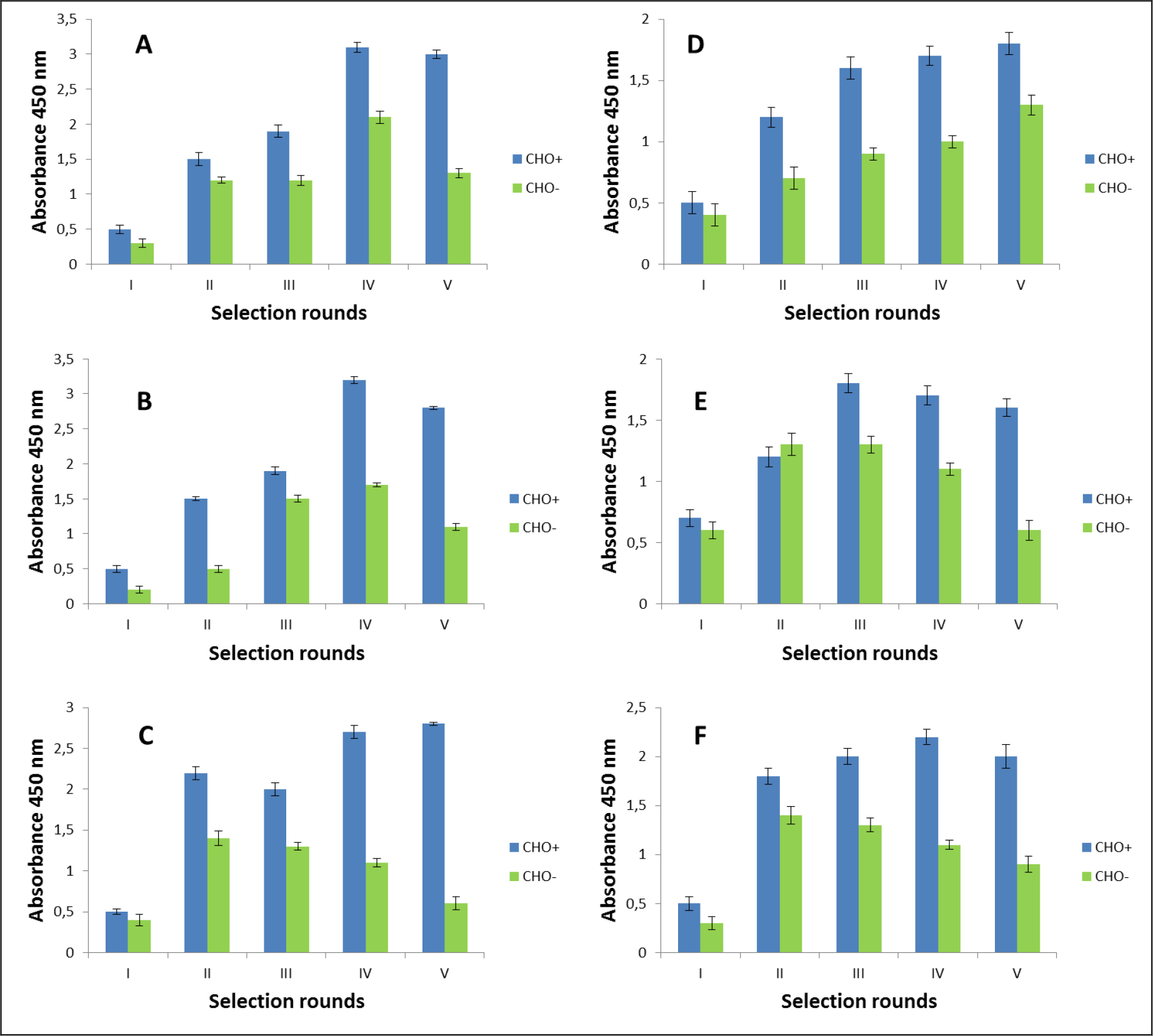
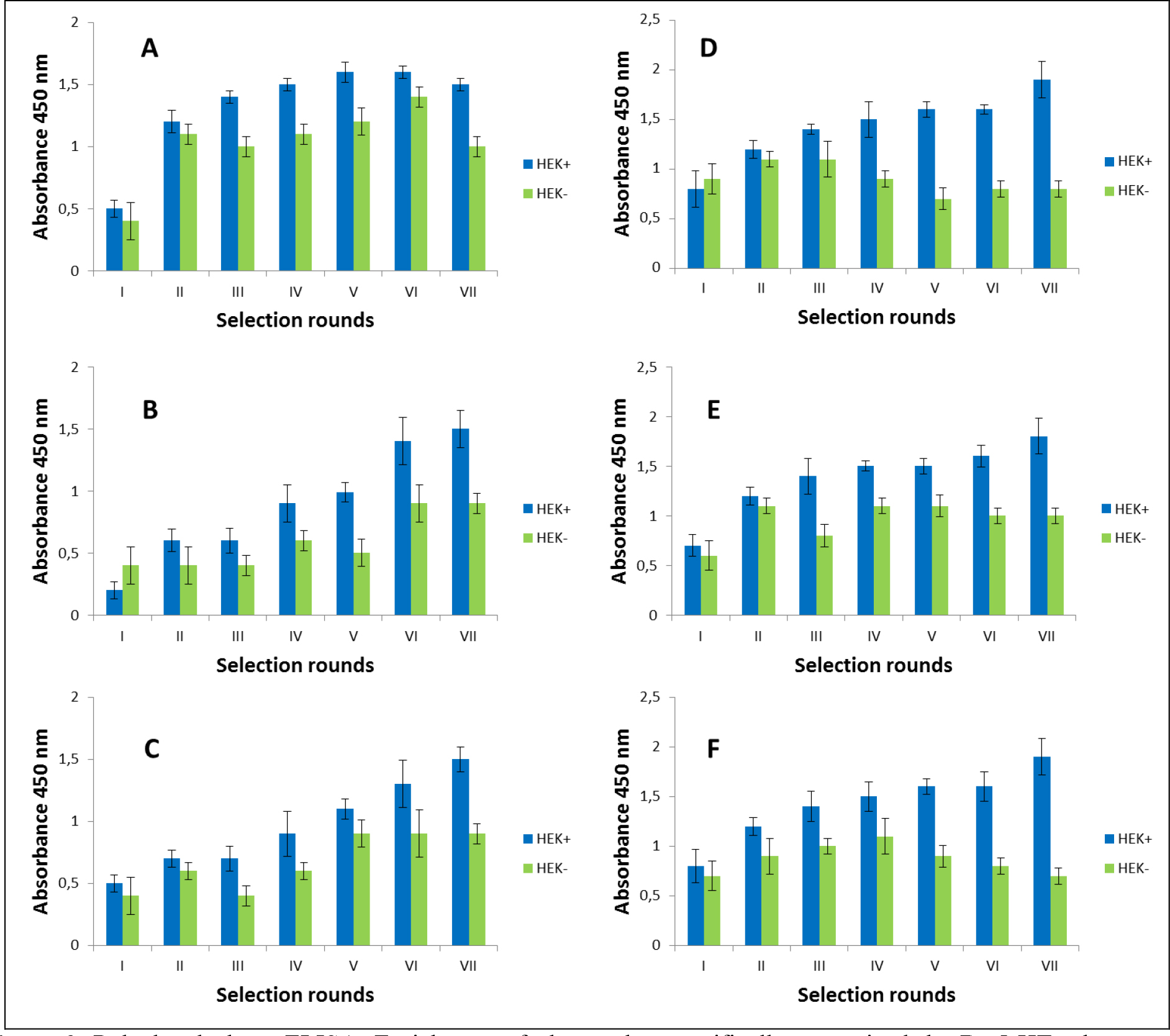
The selection process was assessed by monitoring the enrichment ratio and polyclonal phage ELISA. The increasing titre of phages as well as polyclonal phages ELISA results indicates the correctness of the biopanning process and corresponds with the enrichment of phages that specifically recognized the defined heteromer. Preselection conducted on negative cells provided initial elimination of phages exhibited binding affinity towards monomeric forms of receptors included into D2–5-HT1A heteromers as well as towards other molecules presented on the cell surface. It was very important and critical move because it enrich the amount of phages acquiring potentially, desired binding properties before the actual positive selection. Results obtaining during experiments performed without negative preselection was not as satisfying as expected (data not shown). The biopanning rounds were repeated until the obtained results (phages titre and polyclonal ELISA) related to positive (specific to defined heteromer) phages reached a plateau or started to decline (Figure 1,2, Table 2A,B). In case of experiments performed on CHO-K1 cells the plateau was achieved faster (after 4 round of selection) (Table 2A). For both cell lines. the level of polyclonal phages binding to positive cells increase with the number of selection. Moreover, in the initial rounds the difference between “phages” binding affinity to positive vs. negative cells was much smaller than in case of further rounds. Similarly to preselection, the last, only negative selection plays also an important role in the elimination of nonspecific bounded phages. As we can see the phages titre as well as binding specificity significantly increased after the last negative selection. Conducting further, only negative selection did not caused further increase of phages titre and binding affinity (data nor shown).

JPPR 19 - 114 Sylwia Łukasiewicz_F1

Figure 1. Polyclonal phage ELISA. Enrichment of phages that specifically recognized the D2–5-HT1A heteromer. Experiments performed in CHO-K1 cell line. A-F various selection types.

JPPR 19 - 114 Sylwia Łukasiewicz_F2

Figure 2. Polyclonal phage ELISA. Enrichment of phages that specifically recognized the D2–5-HT1A heteromer. Experiments performed in HEK 293 cell line. A-F various selection types.

After the selection process, the specific binding of individual monoclonal phages to cells presenting defined heteromers was determined by monoclonal phage ELISA techniques. Such tests were conducted on various cell lines (CHO-K1, HEK293) expressing desired receptors in pairs or individually. The kind of experiment enable real identification of monoclonal phages displaying desired scFv molecules on the surface. About 1000 phages obtained after each type of selection were tested. Table 3 presents the results obtained for the three best phages for a given type of selection. The most satisfactory results (the highest heteromer specificity) were obtained in case of selection in conditions conducive to internalisation (type C) as well as in case of selection F where phages were displaced by clozapine. Clozapine is a pharmacological compounds which well-known affinity towards both D2R and 5-HT1AR [23–25]. Moreover its influence on various GPCRs heteromer formation has been documented [26–27]. As we can see here (Fig 1,2, Table 2), the titre of phages after final selection round (type F) was not as higher as in C case, however, the quality of isolated scFvs were very promising (Table 3).

Table 3. Binding level of various monoclonal phages specific to D2–5HT1A heteromer (results for 3 the best phages) presented on positive cells (CHO+ or HEK+ cells) in relation to: CHO-K1, CHO- cells – or HEK 293, HEK- , determined by ELISA technique. [R] –ratio of positive (absorbance 450nm positive cells) vs negative signal (absorbance 450nm negative cells).

Phage code

CHO-K1
[R]

CHO-
[R]

Phage
code

HEK 293
[R]

HEK-
[R]

Selection A

5E/5r1

4.44

4.67

experiments were not carried out due to the poor results of polyclonal ELISA

1F/5r4

3,54

3,21

1G/5r3

5,26

4,31

Selection B

1E/5r1

5,01

5,76

experiments were not carried out due to the poor results of polyclonal ELISA

10F/5r1

4,87

4,56

2G/5r2

6,89

7,02

Selection C

10G/5r1

38.81

36.82

experiments were not carried out due to the poor results of polyclonal ELISA

6H/5r2

16.87

16.32

2D/5r4

22.57

23.86

Selection D

2C/5r2

6,77

7,32

1G/7r4

10,54

11,23

1E/5r3

3,73

4,77

1H/7r3

4,67

3,32

1G/5r3

5,21

4,88

1G/7r3

5,32

4,54

Selection E

6D/5r1

2,32

2,76

10G/7r1

2,13

2,44

1C/5r3

3,91

2,98

1D/5r2

2,67

1,87

6F/5r2

3,76

1,76

4E/7r3

2,31

1,76

Selection F

2H/5r4

16,21

14,32

4G/7r3

14,36

14,21

6D/5r4

15,44

13,21

5B/7r2

9,37

7,32

3C/5r1

10,17

10,09

7G/6r2

7,67

6,88

Comparison of the results obtained for both used cell lines indicates that in case of experiments performed on HEK 293 cells, effects were not as promising as in case of CHO-K1 cells. The visible differences appeared only at the monoclonal phages analysis stage. Phages, isolated based on selection on HEK 293 cells were less specific to desired heteromer (Table 3). The phenomenon, beyond the quality of the experiment itself, may be correlated with endogenous expression of D2R on the HEK 293 cell surface.

4. Conclusion

In conclusion presented results indicate the phage display technique as a valuable tool for isolation of human monoclonal scFv antibodies towards GPCRs heteromers. At the same time, they point to the key role of appropriate conditions during biopanning process. Based on our experience the best binding parameters were obtained for phages isolated after selection in the conditions promoting internalization process. A very important is also a proper choice of cell line dedicated to such procedure.  Elimination of nonspecific bindings by negative preselection as well as the last round of the only negative selection constitutes a key point during the biopanning process.

5. Acknowledgment

The Faculty of Biochemistry, Biophysics and Biotechnology is partner with the Leading National Research Centre (KNOW) supported by the Ministry of Science and Higher Education. The work was also co-financed from European Union within Regional Development Fund – Grants for innovation – PARENT/BRIDGE Programme – POMOST/2011–4/5 and N N401 009640 project.

References

  1. Gomes I, Ayoub MA, Fujita W (2016) G Protein-Coupled Receptor Heteromers. Annu Rev Pharmacol Toxicol 56: 403–425. [crossref]
  2. Rozenfeld R, Devi LA (2011) Exploring a role for heteromerization in GPCR signalling specificity. Biochem J 433: 11–18. [crossref]
  3. Albizu L, Moreno JL, González-Maeso J, Sealfon SC (2010) Heteromerization of G protein-coupled receptors: relevance to neurological disorders and neurotherapeutics. CNS Neurol Disord Drug Targets 9: 636–650.
  4. Fujita W, Gomes I, Devi LA (2014) Revolution in GPCR signalling: opioid receptor heteromers as novel therapeutic targets: IUPHAR review 10. Br J Pharmacol 171: 4155–4176.
  5. Derouiche L, Massotte D (2018) G protein-coupled receptor heteromers are key players in substance use disorder. Neurosci Biobehav Rev 29: 0149–7634.
  6. Kamal M, Jockers R (2011) Biological Significance of GPCR Heteromerization in the Neuro-Endocrine System. Front Endocrinol (Lausanne) 1 2: 2.
  7. Carriba P, Ortiz O, Patkar K (2007) Striatal adenosine A2A and cannabinoid CB1 receptors form functional heteromeric complexes that mediate the motor effects of cannabinoids. Neuropsychopharmacology 32: 2249–2259.
  8. Hamzeh-Mivehroud M, Alizadeh AA, Morris MB, Church WB, Dastmalchi S (2013) Phage display as a technology delivering on the promise of peptide drug discovery. Drug Discov Today 18: 1144–1157.
  9. Kushwaha R, Payne CM, Downie AB (2013) Uses of phage display in agriculture: a review of food-related protein-protein interactions discovered by biopanning over diverse baits. Comput Math Methods Med 2013: 653759.
  10. Hairul Bahara NH, Tye GJ, Choong YS, Ong EB, et al. (2013) Phage display antibodies for diagnostic applications. Biologicals 41: 209–216.
  11. Bradbury AR (2010) The use of phage display in neurobiology. Curr Protoc Neurosci Apr;Chapter 5:Unit 5.12.
  12. Cochran R, Cochran F (2010) Phage display and molecular imaging: expanding fields of vision in living subjects. Biotechnol Genet Eng Rev 27: 57–94.
  13. Smith GP (1985) Filamentous fusion phage: novel expression vectors that display cloned antigens on the virion surface, Science 228: 1315–1317.
  14. Bazan J, Calkosinski I, Gamian A (2012) Phage display-a powerful technique for immunotherapy: 1. Introduction and potential of therapeutic applications. Hum Vaccin Immunother 8: 1817–1828.
  15. Tan Y, Tian T, Liu W, Zhu Z, J Yang C (2016) Advance in phage display technology for bioanalysis. Biotechnol J 11: 732–745. [crossref]
  16. Pansri P, Jaruseranee N, Rangnoi K, Kristensen P, Yamabhai M (2009) A compact phage display human scFv library for selection of antibodies to a wide variety of antigens. BMC Biotechnol 9: 6. [crossref]
  17. Bird RE, Hardman KD, Jacobson JW, Johnson S, Kaufman BM, et al. (1988) Single- chain antigen-binding proteins, Science 242: 423–426.
  18. Barbas CF (2001) Phage display: a laboratory manual. Cold Spring Harbor, NY: Cold Spring Harbor Laboratory Press.
  19. Lee CM, Iorno N, Sierro F, Christ D (2007) Selection of human antibody fragments by phage display. Nat Protoc 2: 3001–3008. [crossref]
  20. Lockman PR, Mumper RJ, Khan MA, Allen DD (2002) Nanoparticle technology for drug delivery across the blood-brain barrier. Drug Dev Ind Pharm 28: 1–13. [crossref]
  21. Frenzel A, Hust M, Schirrmann T (2013) Expression of recombinant antibodies. Front Immunol 4: 217. [crossref]
  22. Rahbarnia LL, Farajnia S, Babaei H, Majidi J, Veisi K, et al. (2016) Invert biopanning: A novel method for efficient and rapid isolation of scFvs by phage display technology, Biologicals 44:567–573.
  23. Newman-Tancredi A, Kleven MS (2011) Comparative pharmacology of antipsychotics possessing combined dopamine D2 and serotonin 5-HT1A receptor properties. Psychopharmacology 216: 451–473.
  24. Lukasiewicz S, Blasiak E, Szafran-Pilch K, Dziedzicka-Wasylewska M (2016) Dopamine D2 and serotonin 5-HT1A receptor interaction in the context of the effects of antipsychotics – in vitro studies. J Neurochem 137: 549–560.
  25. Meltzer HY, Huang M (2008) In vivo actions of atypical antipsychotic drug on serotonergic and dopaminergic systems. Prog Brain Res 172: 177–197. [crossref]
  26. Lukasiewicz S, Faron-Górecka A, Kedracka-Krok S, Dziedzicka-Wasylewska M (2011) Effect of clozapine on the dimerization of serotonin 5-HT(2A) receptor and its genetic variant 5-HT(2A)H425Y with dopamine D(2) receptor. Eur J Pharmacol 659: 114–123.
  27. Lukasiewicz S, Polit A, Kedracka-Krok S, Wedzony K, Mackowiak M, Dziedzicka-Wasylewska M. Hetero-dimerization of serotonin 5-HT(2A) and dopamine D(2) receptors. Biochim Biophys Acta. (2010) 1803:1347–1358.

Can One-Stage In Vitro Dissolution Using Water As Medium Represent Guaifenesin Release From Extended- Release Bilayer Tablets?

DOI: 10.31038/JPPR.2019223

Abstract

Guaifenesin is used as an expectorant. One of its available over-the-counter tablets is immediate- and extended-release bilayer in design. The purposes of this project were [1] to compare the in vitro release profiles between one-stage dissolution (using water as medium) and two-stage dissolution (using 0.1 N HCl and phosphate buffer pH 6.8), and [2] to explore the polymeric release mechanism from the tablet. We also proposed a less acidic liquid chromatographic mobile phase, 50% methanol (which stability indication method was validated), to compare with the mobile phase described in the Guaifenesin Tablets monograph (methanol/water/glacial acetic acid, 40:60:1.5 v/v/v). With the dissolution duration, temperature, paddle stir rate, and sampling schedule being kept the same, the release profiles using Monograph mobile phase to quantify the samples collected from both dissolution methods were found similar (n = 4). When the same set of two-stage dissolution samples were subject to two different mobile phases, the profiles in the acid stage were similarly. But 50% methanol quantified the Buffer Stage samples less than Monograph mobile phase since hour 3, when 250 mL of 0.2 N tribasic sodium phosphate was added and the medium adjusted with 2 N NaOH to pH 6.8. The differences were 12.7% ± 1.4% at hour 4, and 20.9% ± 1.6% at hour 12 (n = 4, p < 0.001). As to the polymeric control, the computed exponent (n value) in the Peppas power law approximation was in the range of 0.7, which suggested release mechanism is anomalous transport. The cross-section of the retrieved tablets at end of the dissolution studies supported the inference.

Keywords

Extended-Release Bilayer Tablets, Liquid Chromatography, One-Stage Vs. Two-Stage In Vitro Dissolution, Peppas Power Law Approximation, Polymeric Control.

Introduction

Guaifenesin, an expectorant, is available over-the-counter in two strengths, 600 mg and 1200 mg [1, 2]. One brand is ER bilayer tablets containing white Immediate Release (IR) and blue ER layers (Figure 1). The Guaifenesin Tablets monograph in USP-NF 2018 (3) describes its dissolution procedure as medium: water; 900 mL; apparatus 2: 50 rpm; time: 45 min and procedure: determine the amount dissolved using UV absorbance at 274 nm, the tolerance was not less than 75% (Q) of the labeled amount dissolved in 45 min [3]. Judging from the dissolution time of 45 min, it is for IR. There are no guidelines specifically written for Guaifenesin ER Tablets in the monograph.

JPPR 19 - 113 Monica Chuong_F1

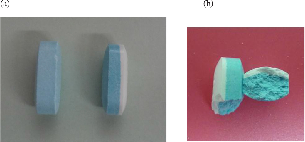
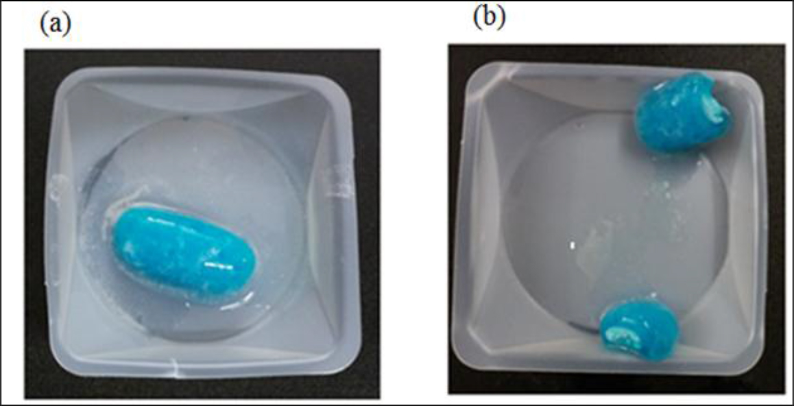
Figure 1. Guaifenesin 1200-mg bilayer ER tablets. (a) Dissecting an intact tablet illustrated no coating was applied to the core tablet, (b) a tablet retrieved from a dissolution vessel at the end of the 12-h study.

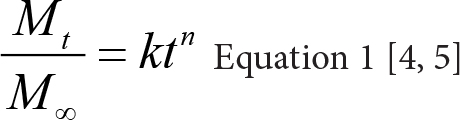
Nicholas Peppas introduced a power law approximation to describe drug release from a dosage form. Both the exponent n and the prefactor k of the equation depend on the dosage form geometry, the relative importance of relaxation and diffusion in the pure polymer swelling controlled drug delivery system [4, 5]. Therefore, the first objective of this project was to search within the General Chapters of USP-NF [3] for an in vitro dissolution method, which might be used to study Guaifenesin ER Tablets. Second, a less acidic Liquid Chromatographic (LC) mobile phase (50% methanol, apparent pH 7.0). Both the Monograph mobile phase (methanol/water/glacial acetic acid, 40:60:1.5, apparent pH 3.08) and the proposed mobile phase (50% methanol) were used to establish standard curves of guaifenesin dissolved in the media used for dissolution study, and quantify the dissolution samples to determine the cumulative drug release from the tablet. Third, it aimed at the comparison of the in vitro release profiles between a one-stage dissolution method × 12 h (using water as medium) and two-stage method (composed of Acid Stage × 3 h, and then Buffer Stage × 9 h). Furthermore, the in vitro release data were plotted according to power law approximation to differentiate the drug release mechanism among Fickian diffusion, anomalous transport and polymer chain relaxation (polymer swelling).

Materilas and Methods

Materials

Over-the-counter 1200 mg Guaifenesin ER Bi-layer Tablets containing a white IR layer, and a blue ER layer for 12 h release (Lot BY646, distributed by Reckitt Benckiser, NJ) were purchased from a local pharmacy. Guaifenesin (Spectrum Chemical, Lot 2EC0288), methanol, glacial acetic acid, 10 mL syringes, 0.22 micron 25 mm Nylon syringe filters were obtained from VWR International (Bridgeport, NJ).

Methods

Examination of Tablet Formulation Development

Four tablets randomly taken from the original container were weighed. The tablets were cut vertically to inspect any coat being applied to the tablet core. The inactive ingredients and their pharmaceutical functions were conducted through literature search [3, 6].

Standard Preparations

Guaifenesin powder was dissolved in three different matrices to address the aims of this study. They were deionized water, 0.1 N HCl and phosphate buffer pH 6.8. In deionized water it was made into 2 mg/mL as the stock solution. It was further diluted with a diluent (made of one part of water and four parts of 45% methanol) into different concentrations of standard preparations, 0.0002, 0.002, 0.08, 0.2, 0.4, 1, 1.2, 2 and 10 mg/mL. For constructing the standard curves with 0.1 N HCl and phosphate buffer 6.8, the standard stock solution was prepared into 10 mg/mL. It was further diluted with a diluent: water – 45% methanol (1:4, v/v) to ensure the work ranges were covered.

UV Spectroscopy

The Scan mode of a Cary 50 UV-Vis Spectrophotometer from Agilent Technologies determined the optimal wavelength of guaifenesin, and Sample Read mode recorded the absorbance of standard solutions.

Liquid Chromatographic Conditions

Agilent Series 1100 (Hewlett Packard) contained Vacuum Degasser, Binary Pump, Auto Sampler, Column Thermostated Compartment, and Variable Wavelength Detector. Two different mobile phases quantifying the standard solutions and in vitro dissolution samples were the mobile phases which may be found in Guaifenesin Tablet Monograph (methanol/water/glacial acetic acid, 40:60:1.5, v/v/v [3], apparent pH was 3.08), and our proposed mobile phase (50% methanol, apparent pH was 7.0). The flow rate was set at 1.0 mL/min and run time 7 min/cycle. The selected column was Luna C18 (USP L1, 4.6 × 150 mm, 5 µm) and the injection volume was 20 microliters.

Potency tests determine the drug content in a sample using HPLC, titration or microbial assay. Stability test, shelf-life and beyond-use date are interchangeable.

Methods of determining potency may or may not be stability indicating, but a stability-indication method can determine both potency and stability [7]. Because we proposed using 50% methanol as the mobile phase, which was considered as a new LC method, the stability-indication method must be validated. A know amount of guaifenesin was dissolved in water (one-stage dissolution medium) and in two-stage dissolution media (0.1 N HCl, and phosphate buffer at pH 6.8 respectively). The samples were subject to the following conditions: (a) 50 oC Heat for 1 h, then cooled to room temperature quickly, (b) 0.1 N HCl (acid) for 1 h prior to neutralized by 0.1 N NaOH, (c) 0.1 N NaOH (base) for 1 h and neutralized with 0.1 N HCl, and (d) 3% hydrogen peroxide solution for 5 min (8). The samples were then quantified using our proposed mobile phase (50% methanol) to ensure the degradant peaks generated by the experimental conditions were separated from analyte (guaifenesin) peak by the resolution (Rs) ≥ 2 [8].

In Vitro Dissolution Methods

Within the USP-NF 2018 two different dissolution methods are stated. One method is in the section of Extended-release Dosage Forms of General Chapters: <711> Dissolution. It describes as “Procedures and medium are as directed for Immediate-Release Dosage Forms in the monographs. But the test-time points generally are three and are expressed in hours.” The dissolution procedures and medium were searched within Guaifenesin Tablets monographs as directed in General Chapters: <711>. The description was medium: 900 mL water; Apparatus 2: 50 rpm; and time: 45 min. This method will refer as one-stage method in the remaining text. The second method is a two-stage acid-buffer method. It is present in General Chapters: <711> Dissolution, but in the section of Delayed-release Dosage Forms, Method A and Method B. This project followed Method a procedure to avoid contamination, loss of tablets, or breakage of a dissolution vessel. The dissolutions and assays are briefly described in the below.

One-stage Dissolution

The one-stage 12-h dissolution study followed the guidelines in Guaifenesin Tablets monograph (medium: 900 mL water; apparatus 2: 50 rpm), except the time was extended to 12 h to study the drug release mechanism. The sampling schedule was at 0.25, 0.75, 1, 3, 4, 6, 8, 10 and 12 h. One part of each dissolution sample was diluted with four parts of 45% methanol prior to subject to LC assay using mobile phases, 50% methanol as well as methanol/water/glacial acetic acid, 40:60:1.5, respectively. The LC AUC of each time point was converted into the cumulated amount of drug release using the established standard curve which medium in the one-stage dissolution was water (n = 3).

Two-stage Dissolution

For the two-stage 12-h dissolution study, an ER bilayer tablet (Figure 1a) was placed in a vessel of USP Dissolution Apparatus 2 containing 750 mL of 0.1 N HCl at 37.0 ± 0.5 oC and stirred at 50 rpm for 3 h. Then 250 mL of 0.2 M tribasic sodium phosphate was added, pH was adjusted to 6.8 with 2 N NaOH. The study continued for another 9 h at 50 rpm while the vessel medium maintained at 37.0 ± 0.5°C. Sampling schedule was selected the same for both one-stage and two-stage dissolution groups, 0.25, 0.75, 1, 3 h (Acid Stage), and 4, 6, 8, 10, and 12 h (Buffer Stage). One part of a dissolution sample was diluted with four parts of 45% methanol (diluent) prior to LC assay. Both mobile phases stated in Section 2.2.4 were applied in the LC system, respectively. The LC AUC of each time-point dissolution sample was converted into the cumulated amount and cumulative percent of drug release using the established standard curves which media were 0.1 N HCl and phosphate buffer pH 6.8.

Data Management for Peppas Power Approximation

After the amount of drug release at a sampling time was known (Mt), it was divided by the infinite amount of release (M), which equaled the tablet label strength (1200 mg). This ratio was then plotted against time (in h) to form a power equation (Equation 1) using the power trend line option in the scatter chart of an Excel worksheet. The power exponent (n) and prefactor (k) in the Peppas equation [6] were thus known from the trend line. The obtained values of release exponent from power trend line was further matched the n value in Table 1 [4, 5] to determine the drug release mechanism.

JPPR 19 - 113 Monica Chuong_SF14

Table 1. The release exponent n of the Peppas power equation and drug release mechanism from polymer-controlled delivery systems in cylinder geometry (4, 5)

Exponent (n)

Drug Release Mechanism

0.45

Fickian diffusion

0.45 < n < 0.89

Anomalous transport

0.89

Polymer swelling

Results

Examination of Tablet Rational Development Approach

The ER bilayer tablets taken from its original container were weighed as 1.454 ± 0.011 g (n = 4, relative standard deviation of the tablet weight was 0.76%). Judging from the dissection the tablet cores were not coated (Figure 1a). The inactive ingredients are FD&C blue #1 aluminum lake (coloring agent), hypromellose (controlled-release agent), magnesium stearate (lubricant), microcrystalline cellulose (tablet diluent and disintegrant), and sodium starch glycolate (tablet disintegrant).

Ultraviolet Spectrophotometric and HPLC Linearity

Guaifenesin dissolved in water to prepared into two different concentrations, 0.008 and 0.2 m/mL, then they were scanned from 190 to 790 nm using Cary 50 spectrophotometer (Agilent). In addition to 274 and 276 nm described in the Guaifenesin and Guaifenesin Tablets monographs [3], 270 nm can also be used as the wavelength to quantify guaifenesin. Thererfore, 270 nm was used in the remaining project including assaying dissolution samples. The standard linearity built using water as solvent and quantified using UV spectrophotometer was 0.001 mg/mL to 0.2 mg/mL (100 fold), while that quantified using LC was 0.001 mg/mL to 1.2 mg/mL (1200 fold). The R2 (coefficiency of determination) when LC AUC (y-axis) in correlation with UV absorbance (x-axis) ranged from 0.001 to 0.2 mg/mL was 0.9999.

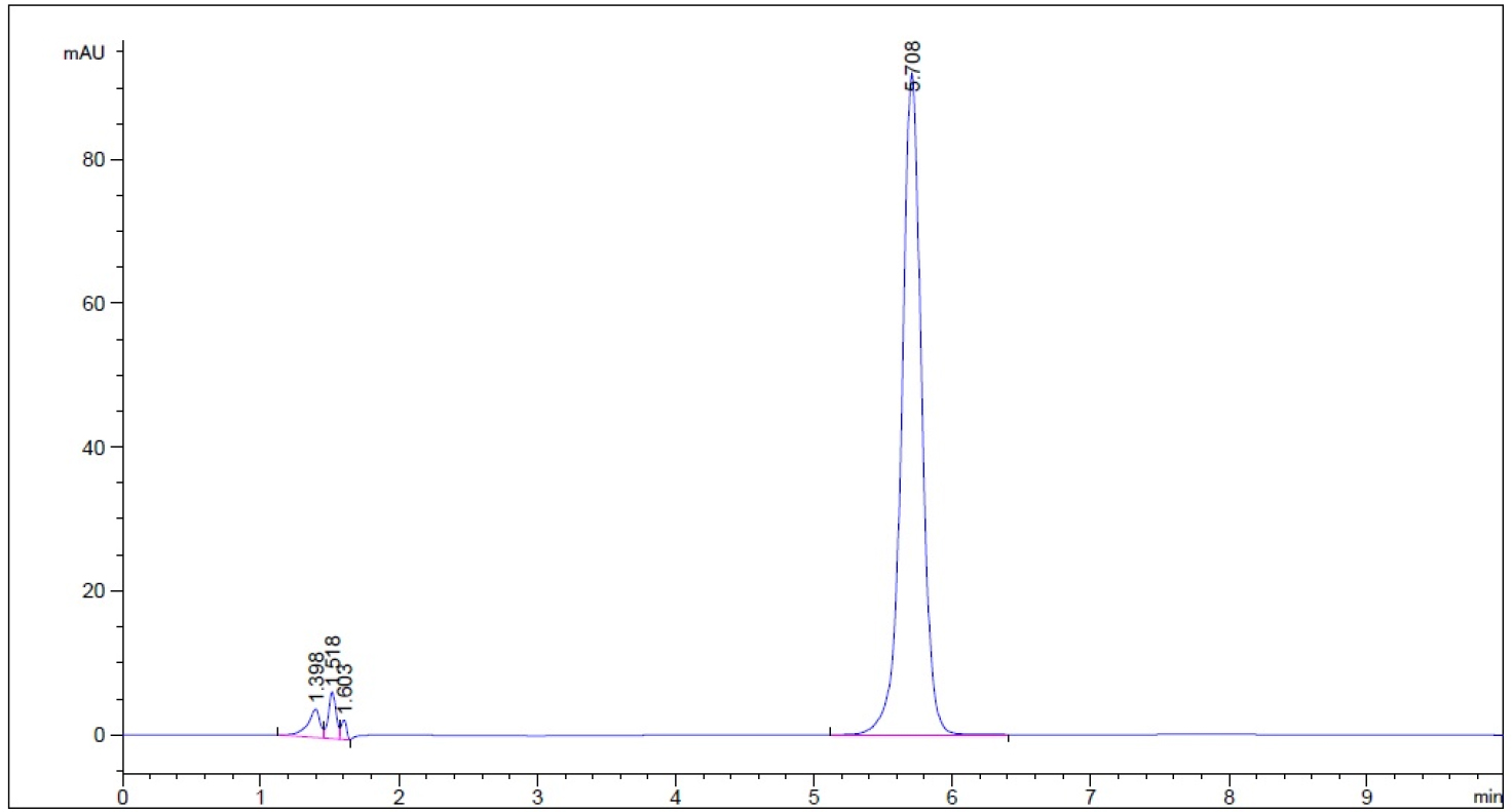
The chromatograms of stability indication method showed the degradant peaks generated by subjecting to 0.1 N HCl (acid), 0.1 N NaOH (base), 50 oC (heat) and 3% hydrogen peroxide solution under the exposure time periods described in Section 2.24 either did not produce degradant peak or separated well from analyte (guaifenesin) peak. All the resolution (Rs) were greater than 2 (Please refer to supplemental file).

One-stage In Vitro Dissolution Study Using Water as Medium

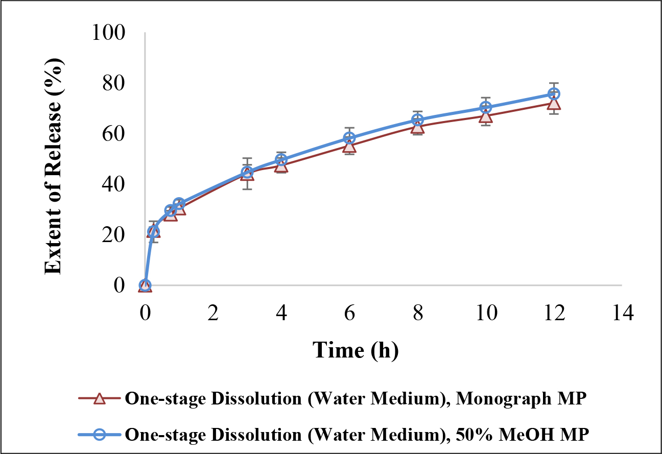
The dissolution duration and temperature, paddle stir rate, and sampling schedule were chosen as 12 h, 37.0 ± 0.5 oC, 50 rpm and 0.25, 0.75, 1, 3, 4, 6, 8, 01 and 12 h. When the dissolution samples were quantified using Monograph mobile phase, the bilayer ER tablets released 28.0 ± 1.4 % guaifenesin into water at 45 min, 30.4 ± 1.7 % at 1 h, 44.1 ± 6.0 % at 3 h, and 72.1 ± 4.4 % at 12 h (n = 4, Table 2a). When the same samples were assayed using 50% methanol as the mobile phase, the drug releases were: 29.5 ± 1.5 % at 45 min, 32.2 ± 1.6 % at 1 h, 44.7 ± 3.0 % at 3 h, and 75.7 ± 4.3 % at 12 h (n = 4, Table 2a). The dissolution profiles were almost identical and displayed as bi-phasic release when either mobile phase was used to quantify the same set of dissolution samples (n = 4, Figure 2).

JPPR 19 - 113 Monica Chuong_F2

Figure 2. Similarity of one-stage 12-h in vitro dissolution profiles between the Monograph mobile phase (methanol/water/glacial acetic acid, 40:60:1.5, v/v/v) and the proposed mobile phase (50% MeOH) when water was the chosen dissolution medium.

Table 2. Cumulative percent of guaifenesin release from bi-layer tablets at key sampling points

(a) One-stage dissolution with different mobile phases

Sampling Time (h)

Monograph MP

50% MeOH
as MP

P Value*
Paired-t test
(Independent-t test)

0.75

28.0 ± 1.4

29.5 ± 1.5

< 0.001 (< 0.05)

1

30.4 ± 1.7

32.2 ± 1.6

< 0.001 (> 0.05)

3

44.1 ± 6.2

44.7 ± 3.0

< 0.001 (> 0.05)

4

47.4 ± 2.9

49.6 ± 3.0

< 0.001 (> 0.05)

12

72.1 ± 4.4

75.7 ± 4.3

< 0.01 (> 0.05)

*Two-tailed distribution

(b) Different dissolution methods, but same mobile phase (monograph MP) to assay

Sampling
Time (h)

Cumulative Release (%) in One-stage Method (Water)

Cumulative Release (%) inTwo-stage Method
(0.1 N HCl 3 h, Buffer 9 h)

P Value*
Independent-
t test

0.75

28.0 ± 1.4

31.7 ± 4.1

> 0.05

1

30.4 ± 1.7

36.3 ± 4.0

< 0.05ξ

3

44.1 ± 6.2

56.4 ± 4.4

< 0.01ξ

4

47.4 ± 2.9

55.2 ± 2.1

< 0.01ξ

12

72.1 ± 4.4

79.4 ± 1.9

< 0.05ξ

*Two-tailed distribution
ξ Statistically significant

(c) Same two-stage (0.1 N HCl 3 h, then Buffer 9 h) dissolution method with different mobile phases

Dissolution

Sampling

Time (h)

Cumulative Release (%) Using

Monograph MP

Cumulative Release (%) Using 50% MeOH as MP

P Value*

Paired-t test

(Independent

t-test)

0.1 N HCl

0.75

31.7 ± 4.1

32.2 ± 2.8

> 0.05 (> 0.05)

1

36.3 ± 4.0

36.0 ± 3.0

> 0.05 (> 0.05)

3

56.4 ± 4.4

55.0 ± 5.6

> 0.05 (> 0.05)

Phosphate Buffer

4

55.2 ± 2.1

45.8 ± 0.9

< 0.001
(< 0.001)¥

pH 6.8

12

79.4 ± 1.9

62.3 ± 0.7

< 0.001
(< 0.001)¥ 

*Two-tailed distribution
¥ Statistically significant in both paired and independent t-tests.

One-stage versus Two-stage In Vitro Dissolution Study Using Monograph Mobile Phase

The dissolution duration and temperature, paddle stir rate, and sampling schedule were kept the same as Section 3.4, but only the Monograph mobile phase (methanol/water/glacial acetic acid, 40:60:1.5, v/v/v [3], apparent pH was 3.08) was used. The drug release between one-stage and two-stage methods were 28.0 ± 1.4 % vs. 31.7 ± 4.1 % at 45 min, 30.4 ± 1.7 % vs. 36.3 ± 4.0 % at 1 h, 44.1 ± 6.2 % vs. 56.4 ± 4.4 % at 3 h, and 72.1 ± 4.4 % vs. 79.4 ± 1.9 % at 12 h (n = 4, Table 2b). These releases in these sampling points were different statistically after 45 min dissolution study (Table 2b, Figure 3a).

JPPR 19 - 113 Monica Chuong_F3

Figure 3. Dissolution method and mobile phase as factors impacting guaifenesin release profiles: (a) design of dissolution method: one-stage in water versus two-stage (acid and buffer stages) when USP Guaifenesin Tablets monograph mobile phase, and (b) selection of mobile phase: 50% MeOH versus USP Guaifenesin Tablets monograph mobile phase. A depression of 12.7% ± 1.4% (n = 4) present 1 h after the medium pH was adjusted to 6.8 (that is the end of 4 dissolution hours). This depression continued until dissolution ended (see text).

Two-stage In Vitro Dissolution Study Using 50% Methanol versus Monograph Mobile Phase

The dissolution method was a tablet was placed in 750 mL of 0.1 N HCl for 3 h, and then 250 mL of 0.2 M tribasic sodium phosphate was added into the apparatus vessel with the pH being adjusted to 6.8. The dissolution duration and temperature, paddle stir rate, and sampling schedule were kept the same as Section 3.4, but both monograph mobile phase (methanol/water/glacial acetic acid, 40:60:1.5, v/v/v [3], apparent pH was 3.08) and the proposed mobile phase (50% methanol) were used respectively. The resultant AUC were converted into cumulative % of release and compared. The release profiles in Acid stage (time 0 to 3 h) quantified by both mobile phases were almost identical (Figure 3b). The cumulative percent of releases in Acid stage using Monograph mobile phase and 50% methanol as mobile phase were 31.7 ± 4.1 % vs. 32.2 ± 2.8 % at 45 min, 36.3 ± 4.0 % vs. 36.0 ± 3.0 % at 1 h, 56.4.1 ± 4.4 % vs. 55.0 ± 5.6 % at 3 h (Table 2c). Never the less, the profiles were statistically different in the Buffer stage (3 to 12 h, Figure 3b, and Table 2c). The cumulative percent of releases in Buffer stage using Monograph mobile phase and 50% methanol as mobile phase were 55.2 ± 2.1 % vs. 45.8 ± 0.9 % at 4 h (which means one hour after the pH had been adjusted to 6.8), 79.4 ± 1.9 % vs. 62.3 ± 0.7 % at 12 h (Table 2c).

Power Law Approximation

On order to fit Power Law Approximation equation, the data had to be taken from extended release region. Since the studied tablet was designed as IR/ER bilayer, we subtracted the cumulative amount of release from the dissolution study at a particular sampling point from the cumulative amount of drug release in the first hour (immediate layer) as Mt iin Equation 1, and further divided Mt by M. M was the label amount (1200 mg) minus cumulative amount in 1 hour. The fraction was then plotted against the time of drug released from the ER layer (the total dissolution time minus 1 hour in immediate release layer). Power equations in different dissolution methods and mobile phases were obtained using Excel scatter plot trendline options. The value of the power exponent (n) was 0.767 for both mobile phases, while the prefactor (k) was 0.1007 for Monograph mobile phase and 0.1068 for the proposed mobile phase (50% methanol). The reason of choosing data from hour 2 to hour 12 to fit Peppas power law was based on General Chapter <1088> In Vitro and In Vivo Evaluation of Dosage Forms describes that “For immediate-release dosage forms the in vitro dissolution process typically requires no more than 60 min…” [3]. According to Table 1, the obtained power exponent illustrate that the ER layer of this bi-layer tablet follows Fickian diffusion (Table 3). The Peppas power law was also applied to two-stage dissolution from hour 2 to hour 12 as well as hour 4 to hour 12 using both mobile phases. But the data from hour 2 to hour 12 in the two-stage dissolution method using either mobile phase to quantify are not reported here due to the transition of Acid stage into Buffer stage at the end of hour 3 (Table 3) to avoid misguiding.

Table 3. The release exponent n of the Peppas power equation and drug release mechanism using the ER layer dissolution data from hour 2 to hour 12, and hour 4 to hour 12

Dissolution Method

Dissoultion

Period

LC

Mobile Phase

Exponent (n)

Drug Release Mechanism

One-stage

h 2 to h 12

Monograph

0.767

Anomalous transport

One-stage

h 4 to h 12

Monograph

0.692

Anomalous transport

One-stage

h 2 to h 12

50% methanol

0.767

Anomalous transport

One-stage

h 4 to h 12

50% methanol

0.703

Anomalous transport

Two-stage

h 2 to h 12

Monograph

Not reported*

Two-stage

h 4 to h 12

Monograph

0.639

Anomalous transport

Two-stage

h 2 to h 12

50% methanol

Not reported*

Two-stage

h 4 to h 12

50% methanol

0.775

Anomalous transport

*Due to the transition between acid stage and buffer stages at hour 3 (see text).

Discussion

Hydrogels are polymer networks that contain a substantial amount of water. Dry polymer networks can absorb tens, hundreds, or even thousands of times their weight in water without or with dissolving. They have the properties to those of soft biological tissues and of great utility in pharmacy due to a low interfacial tension and less irritation [9]. The polymer network was able to sustain its own structural integrity through cross-linkage [10]. According to General Chapters: <1088> In Vitro and In Vivo Evaluation of Dosage Forms describes that “For immediate-release dosage forms the in vitro dissolution process typically requires no more than 60 min…”. Using this definition, the drug load in an ER bilayer tablet was determined as approximate ≤ 30% in IR white layer, and the remaining in ER blue layer. The residual tablets were retrieved at the end of the 12-h dissolution study showed white layer of the ER bilayer tablet disappeared, but the blue layer swelled but the integrity was still kept (Figure 4). When the bilayer tablet was cut vertically, the polymers in the core were still densely packed reflecting that dissolution medium had penetrated into the tablet core, but the polymer had not yet fully swelled or disintegrated, which resulted in the tolerance for only about 70% to 75% (Q) of the labeled amount. In addition, the leaching of the colorant and erosion of polymer were evidenced by the dissolution medium changed from clear into light blue and the medium became more viscous and slightly sticky in the 12-h release study.

JPPR 19 - 113 Monica Chuong_F4

Figure 4. A studied tablet was retrieved from a dissolution vessel: (a) at the end of the 12-h study, and (b) the cross-section shows the core was still densely packed. No significant difference was noticed whether the tablet was retrieved from water or phosphate butter pH 6.8.

The in vitro release data of the ER bilayer tablets from 2 h to 12 h (as the extended release region based on General Chapter < 1088 >) was able to format into a power equation with the power exponent (n) in the range of 0.7 (n = 4, Table 3). Matching the exponent (n value) with those cylindrical geometry in Table 1, its release mechanism was anomalous transport (between Fickian diffusion and polyer swelling), but was closer to polymer swelling mechanism. Peppas and coworkers [4, 5, 6] studied theophylline release from poly(HEMA-co-NVP) [poly(2-hydroxyethylmethacrylate-co-N-vinylpyrrolidone)] disks into distilled water. The tablet geometry of this project was a caplet shape (Figure 1). Siepmann J and Siepmann F also mentioned that the thicker the samples a slightly slowing down of release with time is displayed [6]. This was probably due to drug diffusion becoming increasing more rate limiting. Diffusion is slower at greater distances. When plotting the cumulative amount of drug release versus time, geometry, drug solubility and inhomogeneous initial drug distribution [4, 5, 6] may also impact the value of n (power exponent).

The six inactive ingredients of the ER bilayer tablets and their pharmaceutical functions were stated in Section 3.1. They were composed of coloring agent, controlled-release agent, lubricant, tablet diluent, tablet disintegrant, and gelling agent. Therefore, photos taken after a tablet retrieved from the vessel at the end of a dissolution study were dissected to support the release mechanism of anomalous transport determined from Peppas power law power exponent (n). As seen in Figure 4, there is a clearly defined font between the swollen polymer layer and damped tablet core suggesting that polymer relaxation is required for guaifenesin to be released into either water or phosphate buffer pH 6.8.

Conclusion

In vitro dissolution study may be applied to approximate the drug loaded in IR layer and ER layers of an oral tablet. The current study also supports the use of water as the dissolution medium for extended release dosage forms, because time efficacy and green laboratory practice bring affordable products to our patients. Never the less the selection of a proper mobile phase is of essential. The project suggests that for sake of accuracy and precision, one-stage and two-stage dissolution profiles be compared with the same selected mobile phase. If they are similar, the one-stage study using water as dissolution medium may then be preceded. From Peppa power law as well as the dissection examination of retrieved tablets, the ER layer of the bilayer tablet most likely used anomalous transport mechanism to release guaifenesin.

References

  1. https://medical-dictionary.thefreedictionary.com/guaifenesin
  2. http://www.mucinex.com/media/854/drug-facts-maximum-strength-mucinex-se.pdf
  3. U.S. Pharmacopeial Convention (2018) USP Monographs: Guaifenesin, Guaifenesin Tablets, NF Monographs: Sodium Starch Glycolate, General Chapters: <711> Dissolution. In: USP42-NF37. Rockville MD: U.S. Pharmacopeia; 2018: 2121, 2124, 5962, and 6870.
  4. Peppas NA (1985) Analysis of Fickian and non-Fickian drug release from polymers. Pharmaceutica Acta Helvetiae 60: 110–111.
  5. Siepmann J, Peppas NA (2001) Modeling of drug release from delivery systems based on hydroxypropyl methycellulose (HPMC). Adv Drug Deliv Rev 48: 139–157.
  6. Siepmann J, Siepmann F (2012) Swelling Controlled Drug Delivery Systems. In: Siepmann J, Siegel RA, Rathbone MJ (eds.), Fundamentals and Applications of Controlled Release Drug Delivery. Springer Pg No: 154–162.
  7. Rowe RC, Sheskey  PJ, Quinn ME (2009) Handbook of Pharmaceutical Excipients, 6thedn: Pharmaceutical Press: London, UK.
  8. Kupiec T, Skinner R, Lanier L (2008) Stability Versus Potency Testing: The Madness is in the Method. Int J Pharmaceutical Compounding, 12: 50–55.
  9. L.R, Kirkland JJ, Glajch JL (1997) Completing the Method: Validation and Transfer. In: L.R., Kirkland J.J., Glajch J.L. (Eds.), Practical HPLC Method Development. Snyder John Wiley & Sons Pg No: 709
  10. Siegel RA, Alvarez-Lorenzo C (2017) Hydrogels. In: Hillery A, Park K (eds.), Drug Delivery: Fundamentals and Applications CRC Press Pg No: 333.
  11. Hydrogel Materials (2014) Drug Delivery: Materials Design and Clinical Perspective. In: Holowka EP, Bhatia SK (eds.), Springer Pg No: 225.

Supplemental Material

Validation of HPLC Method to Assay Guaifenesin in Acid Stage, Buffer Stage Media and Water Using Proposed Mobile Phase (50% Methanol)

Stability Indication Method of Guaifenesin in Acid Stage, Buffer Stage Media and Water using HPLC with the proposed mobile phase (50% Methanol): in acid-stage medium and subjected to 0.1 N HCl for 1 h; (b) in acid-stage medium and subjected to 0.1 N NaOH for 1 h; (c) in acid stage medium and subjected to 50oC for 1 h; (d) acid-stage medium and subjected to 3% hydrogen peroxide for 5 min; (e) in buffer stage medium and subjected to 0.1 N HCl for 1 h; (f) in buffer stage medium and subjected to 0.1 N NaOH for 1 h; (g) in buffer stage medium and subjected to 50 oC for 1 h; (h) in buffer stage medium and subjected to 3% hydrogen peroxide for 5 min; (i) in purified water and subjected to 50 oC for 1 h; (j) in purified water and subjected to 0.1 N HCl for 1 h; (k) in purified water and subjected to 0.1 N NaOH for 1 h; (l) in purified water and subjected to 3% hydrogen peroxide for 5 min; and (m) in purified water without guaifenesin and subjected to 3% hydrogen peroxide for 5 min as control.

  1. Guaifenesin in acid stage medium (0.1 N HCl) – subject to 0.1 N HCl for 1 hour prior to being neutralized with 0.1 N NaOH to neutral pH (n = 3, please refer to pdf version of chromatograms.)

    JPPR 19 - 113 Monica Chuong_SF1

  2. Guaifenesin in acid stage medium (0.1 N HCl) – subject to 0.1 N NaOH for 1 hour prior to being neutralized with 0.1 N HCl to neutral pH (n = 3, please refer to pdf version of chromatograms.)

    JPPR 19 - 113 Monica Chuong_SF2

  3. Guaifenesin in acid stage medium (0.1 N HCl) – subject to 50 oC for 1 hour prior to cooling to room temperature (n = 3, please refer to pdf version of chromatograms)

    JPPR 19 - 113 Monica Chuong_SF3

  4. Guaifenesin in acid stage medium (0.1 N HCl) – subject to 3% hydrogen peroxide for 5 min prior to decomposing hydrogen peroxide into water and oxygen and allowing the excess oxygen to escape (n = 3, please refer to pdf version of chromatograms.)

    JPPR 19 - 113 Monica Chuong_SF4

  5. Guaifenesin in buffer stage medium (phosphate buffer, pH 6.8) – subject to 0.1 N HCl for 1 hour prior to being neutralized with 0.1 N NaOH to neutral pH (n = 3, please refer to pdf version of chromatograms.)

    JPPR 19 - 113 Monica Chuong_SF5

  6. Guaifenesin in buffer stage medium (phosphate buffer, pH 6.8) – subject to 0.1 N NaOH for 1 hour prior to being neutralized with 0.1 N HCl to neutral pH (n = 3, please refer to pdf version of chromatograms.)

    JPPR 19 - 113 Monica Chuong_SF6

  7. Guaifenesin in buffer stage medium (phosphate buffer, pH 6.8)– Subject to 50 oC for 1 hour prior to cooling to room temperature (n = 3, please refer to pdf version of chromatograms)

    JPPR 19 - 113 Monica Chuong_SF7

  8. Guaifenesin in buffer stage medium (phosphate buffer, pH 6.8) – subject to 3% hydrogen peroxide for 5 min prior to decomposing hydrogen peroxide into water and oxygen and allowing the excess oxygen to escape (n = 3, please refer to pdf version of chromatograms.)

    JPPR 19 - 113 Monica Chuong_SF8

  9. Guaifenesin in purified water – subject to 50 oC for 1 hour prior to cooling to room temperature (n = 3, please refer to pdf version of chromatograms)

    JPPR 19 - 113 Monica Chuong_SF9

  10. Guaifenesin in purified water – subject to 0.1 N HCl for 1 hour prior to being neutralized with 0.1 N NaOH to neutral pH (n = 3, please refer to pdf version of chromatograms.)

    JPPR 19 - 113 Monica Chuong_SF10

  11. Guaifenesin in purified water – subject to 0.1 N NaOH for 1 hour prior to being neutralized with 0.1 N HCl to neutral pH (n = 3, please refer to pdf version of chromatograms.)

    JPPR 19 - 113 Monica Chuong_SF11

  12. Guaifenesin in purified water – subject to 3% hydrogen peroxide for 5 min prior to decomposing hydrogen peroxide into water and oxygen and allowing the excess oxygen to escape (n = 3, please refer to pdf version of chromatograms.)

    JPPR 19 - 113 Monica Chuong_SF12

  13. Purified water without guaifenesin – subject to 3% hydrogen peroxide for 5 min prior to decomposing hydrogen peroxide into water and oxygen and allowing the excess oxygen to escape (as a control group)

    JPPR 19 - 113 Monica Chuong_SF13

Action of an Indolinone Derivative on Plasma Hemostasis

DOI: 10.31038/JPPR.2019222

Abstract

The action of a new pharmaceutical substance of indolinone series, an sGC inducer with antiplatelet activity, on rat blood plasma hemostasis was studied. It was shown that the antiplatelet substance after single oral administration to rats considerably increases thrombin time after 3 hours (24.5 versus 17.3 in control, р < 0.05). Other plasma hemostasis parameters were unchanged.

Key words

antiplatelet, indolinone derivative, plasma hemostasis.

Introduction

Thrombosis plays a key role in the development of acute coronary syndrome, making antiplatelet therapy an important part of prevention and treatment of cardiovascular diseases [1]. One of the main risk factory of cardiovascular disease relapse is insufficiency of existing therapy in people resistant to aspirin and clopidogrel [2,3]. This problem can be solved by using antiplatelet drugs with a novel mechanism of action. Also, increased blood clotting plays a role in cardiovascular complications [4,5]. There were no earlier studies of the action of the indolinone derivative on blood plasma hemostasis.

Study goal – Assess the action of a new antiplatelet compound on rat blood plasma hemostasis after oral administration.

Materials and Methods

Test article – pharmaceutical substance 2-[2-[(5RS)-5-(hydroxymethyl)-3-methyl-1,3-oxazolidine-2-yliden]-2-cyanoethylidene]-1H-indol-3(2H)-one.

Outbred Wistar rats (n=10) were used as test system. Rat handling was performed in accordance with the European Convention and other regulating documents [6].

Intact blood was sampled from common carotid artery of anesthetized rats. The blood was stabilized with 3.8% solution of sodium citrate in 9:1 (v:v) ratio, blood plasma was produced by centrifuging at 2000 g for 20 min.

Plasma hemostasis was assessed by fibrinogen content, activated Partial Thromboplastin Time (aPTT), Prothrombin Time (PT) and Thrombin Time (TT). These parameters were assessed by KG-4 coagulometer (Cormay, Poland). Fibrinogen content was assessed using Claus method.

The antiplatelet drugs were administered to rats once orally in 10 mg/kg dose. At the end of experiment the animals were sacrificed by СО2.

Statistical analysis was performed by «R» software. The data is presented as mean values and mean standard deviation (M ± m). Significance of difference (р<0.05) between the tests was assessed using Mann–Whitney U test.

Result and Discussion

No significant changes of main parameters of plasma hemostasis: fibrinogen, aPTT and PT, were found 3 hours after single oral administration of the antiplatelet drug in 10 mg/kg dose. TT was increased by 42% compared to the control group (Table 1).

Table 1. Effects of the new antiplatelet drug (10 mg/kg) on rat blood plasma hemostasis.

Group

Fibrinogen

aPTT

PT

TT

Control (n=5)

2.0 ± 0.1

14.8 ± 0.7

20.4 ± 0.6

17.3 ± 2.3

Antiplatelet drug (n=5)

1.8 ± 0.1

15.2 ± 0.6

20.1 ± 0.3

24.5 ± 1.0*

Note: * –р < 0.05 compared to control.

The new antiplatelet drug doesn’t affect blood plasma fibrinogen content, activated partial thromboplastin time and prothrombin time, but considerably increases the thrombin time, 3 hours after single oral administration in 10 mg/kg dose [7]. The reduction of platelet aggregation by the new drug leads to reduced exit of active components of the coagulation system from the platelets, which may account for the lengthening of thrombin time. There may also be other explanations for this. Additional studies are required for confirmation or discovery of another mechanism, including, possibly, direct inhibition of thrombin.

References

  1. Popova LV, Axenova MB, Khlevchuk TB (2016) Antiplatelet activity in cardiology. Clinical medicine 10: 729–36.
  2. Shantsila E, Lip GY (2009) Variability of response to antiplatelet therapy: what should we do next? Fundam Clin Pharmacol 23: 19–22. [crossref]
  3. Lee PY, Chen WH, Ng W, Cheng X, Kwok JY, et al. (2005) Low-dose aspirin increases aspirin resistance in patients with coronary artery disease. Am J Med 118: 723–727. [crossref]
  4. Frere C, Cuisset T, Quilici J, Camoin L, Carvajal J, et al. (2007) ADP-induced platelet aggregation and platelet reactivity index VASP are good predictive markers for clinical outcomes in non-ST elevation acute coronary syndrome. Thromb Haemost 98: 838–843. [crossref]
  5. Patrono C (2003) Aspirin resistance: definition, mechanisms and clinical read-outs. J Thromb Haemost 1: 1710–1713. [crossref]
  6. Carkishenko NN, Grachev SV (2003) Guidelines on laboratory animals and alternative models in biomedical technology. Profile: Moscow.
  7. Triplett DA (2000) Coagulation and bleeding disorders: review and update. Clin Chem 46: 1260–1269. [crossref]

Manual Therapy Techniques and their Effectiveness on Improving Posture in Adults: A Narrative Review of the Literature

DOI: 10.31038/IJOT.2019216

Abstract

Objective: To review the literature regarding the use of manual therapy techniques and their effectiveness on improving posture in adults.

Background: Hyperkyphosis of the upper spine is a condition that increases with age and leads to decreased pulmonary function, balance, and muscle strength. Numerous reviews have looked at the effect of therapeutic exercise, but few have examined the effects of manual therapy techniques on hyperkyphotic posture.

Methods: Three electronic databases were searched. All of the studies published in English that have considered the effects of manual therapy (including soft tissue mobilization and joint mobilizations) on posture were included in this review (7 randomized controlled trials, 4 case studies, and 1 preliminary trial).

Results: Of the 7 randomized controlled trials, 2 studies utilized soft tissue mobilizations, 3 used joint mobilizations of the cervical and/or thoracic spine, and 2 used both techniques. 3 of the studies also combined the manual therapy treatment with other techniques, including stretching, taping, and therapeutic exercise. Outcome measures varied and included thoracic index, inclinometer or kyphometer readings, and goniometric measurements. All but one of the randomized studies found manual therapy to be an effective intervention for improving posture. Of the 4 case reports, each used a different manual therapy approach, but all were either joint mobilizations of the spine or shoulder girdle or myofascial release. 3 of the reports combined the manual therapy with other types of treatment, including proprioceptive neuromuscular facilitation (PNF) and therapeutic exercise. Postural alignment was found to improve in all of the cases, though this was measured subjectively via photo or visual analysis by 3 of the studies, while 1 study used goniometric measurements.

The final study included was a non-randomized preliminary study using an ATM2 machine to assist with joint mobilizations using Mulligan’s mobilization-with-movement concept. This study found mobilizations to be effective for improving posture as assessed by photographic analysis.

Conclusion: Of the 12 studies reviewed, 11 demonstrated an improvement in posture after treatment with manual therapy techniques. This indicates that manual therapy is a promising treatment for a condition that affects a large proportion of individuals as they age.

Introduction

As people age, their thoracic spine tends to undergo an increase in angle of kyphosis, or forward rounding of the back, which can affect both the cervical and lumbar spine [1, 2]. While the normal values for angle of thoracic kyphosis in adults aged 20–39 are 27.66° for males and 27.62° for women, these values increase more in women after age 40 [3]. The mean value for women aged 60–69 is 44.86°, compared with 34.67° for males [3].

Hyperkyphosis is defined as a value greater than 40° and such a condition leads to decreased pulmonary function, balance, and muscle strength [4, 5]. Because of these potentially harmful consequences, an intervention must be sought for treatment to prevent or correct hyperkyphosis in older adults.

The etiology behind this increase in kyphosis with age is multi-factorial, and many of the underlying causes are linked to one another. It has long been assumed that vertebral fractures related to osteoporosis play the most important role in determining whether or not someone develops hyperkyphosis. While having multiple vertebral fractures (especially thoracic anterior wedge fractures) may increase the risk of hyperkyphosis, it is far from the only cause. Other factors commonly associated with aging include degenerative disc disease, loss of proprioception, muscle weakness or atrophy, and ligamentous degeneration. Muscle weakness, especially in the spinal extensors, often leads to habitually poor posture, which increases spinal kyphosis [1, 4].

Treatments that have been studied to prevent and treat hyperkyphosis include exercise, bracing, taping, and manual therapy [4]. Therapeutic exercise is the most commonly studied intervention for poor posture and hyperkyphosis, and it has shown promising results as a conservative treatment [1, 4]. Manual Therapy (MT) is a technique used to treat various musculoskeletal conditions including but not limited to adhesive capsulitis [6], subacromial impingement syndrome [7], and osteoarthritis [8]. Treatment using manual therapy techniques has not been studied as extensively as the other therapeutic modalities, and therefore a literature review on the topic was conducted to determine if it is a viable treatment for kyphotic posture.

Methods

Selection Criteria

Studies included randomized controlled trials, nonrandomized trials, and case studies and the search was restricted to papers published in English. Because of the fact that poor posture is often linked to other conditions and the limited number of studies conducted on the topic, studies including patients with various orthopedic conditions such as osteoporosis, ankylosing spondylosis, cystic fibrosis, neck pain, and scoliosis were included in the search. Studies focusing on neurological disorders were not included in the search.

Studies where at least one application of manual therapy (including joint mobilization, soft tissue techniques, or massage) was administered were included. Body parts receiving the therapy included one or more of the following areas: shoulder girdle, pectoral muscles, cervical spine, or lumbar spine. Studies that combined MT with other forms of therapy were also included if the MT technique was an independent variable. Age of study participants was limited to adults (over 18) because both the causes and the prognosis of hyperkyphosis may differ in children, whose bodies are still developing. Only studies that compared the posture of patients before and after treatment were included in the search.

Search Strategy

A search was conducted for published articles that answer the question: do manual therapy techniques improve posture in adults? An electronic search of databases including Ovid, PubMed, and Web of Science was conducted through August 2016. Search terms included a variety of phrases related to posture and MT. The summary of search terms can be seen in table 1, and common strings included “posture”, “manual therapy”, “musculoskeletal manipulations”, “spinal mobilization”, “soft tissue mobilization”, and “kyphosis”. The first search was limited to ages 65 and older, but subsequent searches were expanded because there was found to be limited research in this age group. Supplementary searches were conducted by screening reference lists of relevant articles for additional studies.

Table 1. Search Strings

Database

Date

Search Terms

Hits

Articles Used

Ovid

9/21/2016

“posture” AND “musculoskeletal manipulations” (limited to “all aged 65 and over” OR “aged 80 and over”)

76

1

Ovid

9/21/2016

“posture” and “musculoskeletal manipulations” and “physical therapy modalities”

371

4

PubMed

9/26/2016

“physical therapy modalities” AND “musculoskeletal manipulations” OR “manual therapy” OR “spinal manipulation” OR “manipulation, osteopathic” AND “posture”

1152

4

Web of Science

9/26/2016

“posture” and “manual therapy” OR “spinal mobilization” OR  “soft tissue mobilization” AND “kyphosis”

298

2

Reference list review

9/29/2016

“posture” AND “physical therapy” OR “manual therapy”

3

3

Data Synthesis

7 RCTs (n = 236) from 1897 hits on database searches and reference list screenings were included. 4 case reports and 1 nonrandomized intervention were also included and will be analyzed separately.

Manual therapy interventions included soft tissue mobilization [5, 6, 10], myofascial release [11], thoracic spine mobilizations [5, 11–13], cervical joint mobilizations [13, 14], and rib mobilizations [11]. MT was used in isolation [10, 13, 14], or in combination with stretching [9], exercise [5, 11, 12], taping [5, 12], or postural reeducation [11]. Controls included no Physical Therapy (PT) [5, 1012], PT without mobilizations [11], passive light manual placebo touch and pectoralis major stretching [9], or cervical mobilization only [13, 14].

Treatment length varied with one study assessing the outcomes after a single MT session (Wong et al), one with 6 sessions over 6 weeks [11], one with 10 sessions over 10 weeks [5], two with 12 sessions over 4 weeks [13, 14], one with 16 sessions over 2 weeks [10], and one study with 18 sessions over 12 weeks [12].

Outcome measures used to assess changes in posture also varied considerably between studies, with each one using differing techniques. One study measured the distance from the acromion to the table, a process that has been used in several previous studies to measure rounded shoulder posture [9]. Three studies measured thoracic kyphosis, two using inclinometers [5, 12], and the other finding thoracic index by using a flexible ruler to determine the thoracic curve in the sagittal plane [11]. One study measured both cervical kyphosis using a pair of compasses and a ruler as well as thoracic and lumbar kyphosis using a kyphometer [10]. Two studies measured cervical lordosis using the absolute rotation angle [14], or cranial vertical angle and cranial rotation angle [13].

6 of the 7 randomized trials found an improvement in posture with MT techniques versus control. The one study that showed no difference between groups compared MT to no PT treatment, with 10 sessions over 10 weeks and used thoracic kyphosis as the primary outcome measure [5]. The patient population in this study was one of the two RCTs with a mean age above 60 years, focusing on osteoporotic patients with vertebral fracture. This study utilized passive accessory central posterior-anterior mobilization of the thoracic spine with 5 movements at each level and 2 reps, applying a grade II or III mobilization and MT was used in combination with exercise and taping techniques [5].

For the case studies and nonrandomized trial, approaches to MT that were used included cervical [15], scapular [15], lumbar [16], and lumbosacral mobilizations [17], myofascial release [18], and the use of an ATM2 machine to assist with thoracic and lumbar mobilizations-with-movement [19].

Two of the studies did not combine MT with other forms of treatment [18, 19]. The other 4 studies combined MT with therapeutic exercise [17], breathing and therapeutic exercise [15], or Proprioceptive Neuromuscular Facilitation (PNF) [16]. The PNF technique used was described as dynamic reversal of antagonist technique of the shoulder [16].

Treatment was also wide-ranging in both duration and frequency of the treatment. The shortest treatment duration was 4 weeks, with 3 studies choosing this time frame but varying the number of sessions with either 8 [19], 11 [15], or 12 [16]. One study chose a 6-week time frame with 12 sessions [18]. The final study chose a 16-week duration, with 9 sessions [17].

Outcome measures to demonstrate changes in posture that were used included visual assessment [15, 18, 19], video assessment [17], and angle of spinal curvature using a spinal mouse [16]. An additional case study did not specifically look at posture as an outcome measure, but rather function (assessed with the Oswestry), quality of life (assessed with the QUALEFFO), and pain (McGill Pain Scale) [20]. This study was not included as part of the review but is mentioned here because it was looking for adverse effects of manual therapy on a patient with osteoporosis, which is an important group to consider for the assessment of older adults with kyphosis.

All 4 of the case reports measuring posture as an outcome measure showed improvement after treatment with MT, and the case report that measured quality of life, pain, and function also showed no adverse effects with MT treatment. The nonrandomized trial likewise showed similar improvements in posture after spinal mobilization treatments [20].

Discussion

The MT approaches varied between studies in the RCT group. The one study that utilized Soft Tissue Mobilization (STM) performed 3 minutes of strumming perpendicular to the pectoralis minor muscle belly [9]. Of the studies utilizing joint mobilizations of the spine, only one described using a grade II or III mobilization [5]. One study described the number of repetitions as 10–15 free passive angular movements of thoracic spine with end-range positions held for 5 seconds or as tolerated [12]. The next study gave a limited description of active angular and passive mobility exercises in 4 directions (flexion, extension, lateral flexion, and rotation) [10]. In the study by Gong et al, passive motion analysis was done on the cervical spine and then mobilization was applied by checking mobility in the joint of interest while preventing motion in surrounding joints [14]. The study by Lee et al applied passive extension mobilizations at end range for the cervical spine joints and for the thoracic spine “the therapist pushed hard at the end range to increase mobility” [13]. The final study did not include details on how the manual therapy was applied [11].

For the case study group, one case described using grade III mobilizations of the lumbar spine [16], while the other three studies utilizing mobilizations described only the joints at which the techniques were applied [15, 17], or the number of sets and repetitions [19]. The final study in this group used myofascial release techniques applied for 90–120 seconds at each muscle group [18].

The wide ranging descriptions of the manual therapy techniques used in each of these studies points to the need for more precise documentation in future studies. The details provided in the text of a study should allow another researcher to replicate the treatment protocol, which means that manual mobilizations should not only be described in detail, but the grade(s) of pressure used should also be noted.

While all of the RCTs utilized physical therapists to administer MT intervention, two studies specifically used certified Orthopedic Clinical Specialist physical therapists [9, 13]. Only one other RCT mentioned training the therapists involved in the study to perform interventions in a specified manner [5]. The case study authors were less descriptive of the physical therapists administering treatment, but in the studies where the PT credentials were not explicitly mentioned, therapy was conducted by the study author. One study utilized MFR treatment by a licensed massage and bodywork therapist [18], while another used a PT that had completed a Kaltenborn-Evjenth Orthopedic Manual Therapy (KEOMT) spine advanced course [16].

The number of physical therapy sessions and study length for both the RCT group and the case study group was about equal, with an average of 10.7 and 10.4 manual therapy sessions. The number of weeks over which the sessions occurred was also very similar, with an average of 7.2 weeks for the RCT group and 7.3 weeks for the case study group. There was greater variance between studies, however, with most studies either lasting one month or about 3 months. The shorter, one month time frame is more likely to be clinically realistic. As far as number of sessions goes, a Dutch study of 41 PT practices found that there was an average of 9.9 treatment sessions among patients with a diagnosis of low back pain [21]. Therefore, having an average of 10.5 treatment sessions for the studies listed here is not unrealistic, but this number could vary depending on the laws in the particular country of treatment.

In an assessment of the outcome measures used to measure the postural improvements, each of the randomized trials utilized highly reliable measurement tools. The distance from the posterior border of the acromion to the table used by Wong et al was shown to have a reliability of 0.88–0.94, and this measurement is also easy to learn and replicate [22]. The spinal mouse used by Bautmanns et al and the Debrunner kyphometer used by Widberg et al were both shown to have a both a very high inter-rater and intra-rater reliability [23]. The rotation angle to measure cervical posture used by Gong et al and Lee et al was also shown to have a high Interclass Correlation Coefficient (ICC) [24]. And finally, the thoracic index (measured using a flexible ruler) used by Sandsund et al had an ICC of 0.94. The validity of the measurement tools used in these studies further increases the evidence that posture can be improved by manual therapy techniques.

Table 2. RCT: Study Characteristics

Author, Year

MT Approach

Other Treatment

Patient Population

Mean age

Study Size

Treatment Length

Outcome Measures

Results

Wong et al, 2009

Pectoralis minor STM and self-stretching

Yes – stretching

Healthy patients with rounded shoulder posture (RSP);40% female

25.5

n = 56; 31 experimental, 25 control

1 session with 2 week follow-up

RSP measuring distance from acromion to exam table

One session of pec minor STM and self-stretching significantly reduced RSP for up to 2 weeks

Bautmans et al, 2010

Thoracic spine manual mobilizations

Yes – taping, exercise

Elderly postmenopausal patients with osteoporosis; 100% female

76

n = 38; 21 experimental, 16 control

18 sessions over 12 weeks

Thoracic kyphosis using Spinal Mouse (hand-held inclinometer)

Thoracic kyphosis improved significantly

Widberg et al, 2008

Self and manual soft tissue mobilizations

No

Patients with ankylosing spondylosis; 100% male

35.8

n = 32; 16 experimental, 16 control

8 weeks; 1 hr 2x/week + HEP

Pair of compasses and a ruler (cervical); Debrunner’s kyphometer (thoracic & lumbar)

Improved sagittal plane posture in c-spine; improved posture in neutral position at t-spine

Gong et al, 2015

Passive motion analysis vs. regular cervical joint mobilization

No

University students with postural deficits

22.4

n = 40; 20 experimental, 20 control

3x/week for 4 weeks

Absolute rotation angle – cervical lordosis

Decreased forward head posture and improved cervical lordosis and ROM

Sandsund et al, 2011

Mobilizations of rib cage and t-spine; myofascial release

Yes – Alexander technique, regular PT

Patients with CF; 50% female

27

n = 20; 10 experimental, 10 control

12 weeks; 6 weekly visits

Thoracic index – thoracic curve in sagittal plane using flexible ruler

Thoracic index decreased, showing improvement

Lee et al, 2012

Cervical and thoracic mobilization vs cervical mobilization only (control)

No

Patients with neck pain and forward head posture

Adults

n = 30; 15 experimental, 15 control

15 min 3x/week for 4 weeks

Cranial vertical angle (CVA) and cranial rotation angle (CRA)

CVA increased and CRA decreased. Cervical + thoracic mobilizations are more effective than cervical alone.

Bennell et al, 2010

Soft tissue massage, thoracic mobilizations

Yes – taping, exercise

Patients with osteoporotic vertebral fracture; 85% female

66.2

n = 20; 11 experimental, 9 control

10 weeks; 1x/week + HEP

Thoracic kyphosis using Dualer Electric Inclinometer

No difference between groups

Table 3. Case Study: Study Characteristics

Author

MT Approach

Other Treatment

Patient Characteristics

Treatment Length

Outcome Measures

Results

Roehrig, 2006

Neurodevelopmental treatment-cervical and scapular mobilization

Yes – breathing, exercise

78 year old female with kyphosis and osteoporosis

11 visits over 4 weeks; mobilizations began at visit 4

Visual assessment; goniometric measure

Posture improved

LeBauer et al, 2008

Myofascial release

No

18 year old female with idiopathic scoliosis

6 weeks; 1 hr 2x/week

Visual assessment via grid photography

Posture improved

Staes et al, 2011

Lumbosacral manual therapy

Yes – exercise

26 year old female

9 30 min. sessions over 4 months

Forward head posture and shoulder position via video screening

Postural alignment improved

Park et al, 2014

Kaltenborn-Evjenth orthopedic manual therapy (lumbar)

Yes – PNF

29 year old female with chronic LBP and lumbar transitional vertebra

4 weeks 40 min. 3x/week

Angle of spinal curvature

Spinal curvature and ROM  increased

*Lewis et al, 2014

ATM2 using Mulligan’s mobilization-with-movement (thoracic and lumbar)

No

43 patients aged 14–63 with mild-to-moderate scoliosis; 86% female; mean age 43.5

 4 week intervention 2x/week + HEP

Visual assessment via photography

Posture improved

*Not a case study but a preliminary trial

In the RCT by Bennell et al, while no change was shown in posture, other outcome measures such as pain, physical function, and back and shoulder muscle endurance showed significant positive changes [5]. This finding leads to the hypothesis that other outcome measures can be used to measure change in studies involving MT techniques. Of the 7 RCTs presented here, 4 used some subjective measure of quality of life or function [5, 10–12]. These outcome measures are important because they measure changes that the patient cares more about. Two of the studies also measured lung expansion, which can be an indicator of whether or not a patient is able to breathe easily [10, 11].

Future studies are needed to demonstrate the effectiveness of MT techniques for improvement of posture specifically in older adults (over age 60). Only 2 of the randomized controlled trials had a mean age over 60 [5, 12], and one of these did not find a significant change in posture after intervention. Just one out of 4 of the case studies were performed on an older adult. Therefore, it is not clear if the positive effects of manual therapy on posture are equally as significant in older populations, where the change in kyphosis is more pronounced.

Conclusion

This review found promising evidence for the use of manual therapy as a means to improve posture in adults. 11 of the 12 studies measuring postural improvement as an outcome measure showed a significant positive change in patients receiving manual therapy. The one RCT that did not find an improvement in posture over the control group did show significant changes in other outcome measures, including decreases in pain, improvement in physical function, and improvement in quality of life in the experimental group [5]. Outcome measures that may also be appropriate to show change include subjective measures of quality of life and physical functioning as well as lung function tests. These results demonstrate that even when postural gains are not made due to the use of manual therapy, other positive outcomes can still be seen that warrant the therapy. For the clinician seeking to help a patient improve their posture, manual therapy techniques can be an effective intervention that may also help improve their quality of life and physical functioning.

References

  1. Kado DM (2009) The rehabilitation of hyperkyphotic posture in the elderly. European Journal of Physical and Rehabilitation Medicine 45: 583–593.
  2. Staff MC Kyphosis. 2014 5 June 2014 20 September 2015]; Available from: http://www.mayoclinic.org/diseases-conditions/kyphosis/basics/definition/con-20026732.
  3. Fon GT, Pitt MJ, Cole Thies JA (1980) Thoracic kyphosis: range in normal subjects. American Journal of Radiology 134: 979–963.
  4. Wendy B, Katzman P, DPTSc (2010) Age-related hyperkyphosis: its causes, consequences, and management. Journal of Orthopedic Sports Physical Therapy 40: 352–360.
  5. Bennell KL (2010) Effects of an exercise and manual therapy program on physical impairments, function and quality-of-life in people with osteoporotic vertebral fracture: a randomised, single-blind controlled pilot trial. BMC Muscluoskeletal Disorders 11: 36.
  6. Page MJ, Green S, Kramer S, Johnston RV, McBain B, et al. (2014) Manual therapy and exercise for adhesive capsulitis (frozen shoulder) (Review). Cochrane Database of Systematic Reviews (8): CD011275.
  7. Gebremariam L (2014) Subacromial impingement syndrome_effectiveness of physiotherapy and manual therapy. British Journal of Sports Medicine 48: 1202–1208.
  8. French HP, Brennan A, White B, Cusack T (2011) Manual therapy for osteoarthritis of the hip or knee – a systematic review. Man Ther 16: 109–117. [crossref]
  9. Christopher Kevin Wong P, OCS (2010) The effects of manual treatment on rounded-shoulder posture, and associated muscle strength. Journal of Bodywork & Movement Therapies 14: 326–333.
  10. Widberg K, Karimi H, Hafstrom I (2009) Self-and manual mobilization improves spine mobility in men with ankylosing spondylitis – a randomized study. Clinical Rehabilitation 23:  599–608.
  11. Sandsund CA (2011) Musculoskeletal techniques for clinically stable adults with cystic fibrosis: a preliminary randomized controlled trial. Physiotherapy 97: 209–217.
  12. Ivan Bautmans P (2010) Rehabilitation using manual mobilization for thoracic kyphosis in elderly posmenopausal patients with osteoporosis. Journal of Rehabilitation Medicine 42: 129–135.
  13. Jaehong Lee P (2013) The Effects of Cervical Mobilization Combined with Thoracic Mobilization on Forward Head Posture of Neck Pain Patients. Journal of Physical Therapy Science 25: 7–9.
  14. Wontae Gong P (2015) The effects of cervical joint manipulation, based on passive motion analysis, on cervical lordosis, forward head posture, and cervical ROM in university students with abnormal posture of the cervical spine. Journal of Physical Therapy Science 27: 1609–1611.
  15. Susan M, Roehrig P (2006) Use of neurodevelopmental treatment techniques in a client with kyphosis: A case report. Physiotherapy Theory and Practice 22: 337–343.
  16. Si-Eun Park P, Joong-San Wang P (2015) Effect of joint mobilization using KEOMT and PNF on a patient with CLBP and a lumbar transitional vertebra: a case study. Journal of Physical Therapy Science 27: 1629–1632.
  17. Staes FF (2009) Physical therapy as a means to optimize posture and voice parameters in student classical singers: A case report. Journal of Voice 23: 91–101.
  18. Aaron LeBauer L, SDPT, Robert Brtalik S, Katherine Stowe S (2008) The effect of myofascial release (MFR) on an adult with idiopathic scoliosis. Journal of Bodywork & Movement Therapies 12: 356–363.
  19. Clare Lewis D, PsyD (2014) A preliminary study to evaluate postural improvement in subjects with scoliosis: active therapeutic movement version 2 device and home exercises using the Mulligan’s mobilization-with-movement concept. Journal of Manipulative Physiol Ther 27: 502–509.
  20. Sran MM, K.M. Khan (2006) Is spinal mobilization safe in severe secondary osteoporosis? – a case report. Manual Thearpy 11: 344–351.
  21. Swinkels IC (2005) What factors explain the number of physical therapy treatment sessions in patients referred with low back pain; a multilevel analysis. BMC Health Services Research 5.
  22. Struyf F, Nijs J, Mottram S, Roussel NA, Cools AM, et al. (2014) Clinical assessment of the scapula: a review of the literature. Br J Sports Med 48: 883–890. [crossref]
  23. Barrett E, McCreesh K, J Lewis (2013) Intrarater and interrater reliability of the flexicurve index, flexicurve angle, and manual inclinometer for the measurement of thoracic kyphosis. Rehabilitation Research and Practice 2013: 7.
  24. Harrison DE, Harrison DD, Cailliet R, Troyanovich SJ, Janik TJ, et al (2000) Cobb method or Harrison posterior tangent method: which to choose for lateral cervical radiographic analysis. SPINE 25: 2072–2078.

The Mind Assesses Aggression – Russia vs the Ukraine: A Mind Genomics Exploration

DOI: 10.31038/ASMHS.2019315

Abstract

We introduce a system to rapidly explore a topic, focusing both on the direct conscious judgment of information (cognition), and on the time it takes the mind to process the same information (neuroprocessing.) The system begins with the experimental design of easily constructed mixtures of messages. With human respondents, the system measures the cognitive response to these mixtures (ratings), and at the same time, the processing rate of these same mixtures (response-time to assign a rating.) The system is affordable and scalable, working with as few as 10 respondents to as many as several thousand. The outcome data reveal what messages are important, and the response-time to process these same messages. The analysis is virtually automatic, providing a simple, readily used new tool to study decision making. All the tools are standard, easily used by professionals and novices alike, with the results immediately presented in the format of data tables and a PowerPoint® report ready for distribution.

Introduction – the conflict between ‘objective’ and ‘subjective’ in experimental psychology

During the past seventy years, since the auspicious days of the 1950’s shortly after World War II, the field of experimental psychology has been deeply involved in the measurement of subjective experience. During the previous generations it was thought that people could not be accurate instruments to assess the magnitude of external stimuli, although they could react in ways which had desired effects on their life and on their environment. Many professionals believed that people could not act as valid measuring instruments, despite the fact that people could engineer their environment to exacting tolerances. Rather than focusing on the cognitive reactions to stimuli, many experimental psychologists felt that the more appropriate measures were non-cognitive, but rather autonomic nervous system reactions. These were assumed to be more ‘truthful.’ At the very simplest level were measures such as GSR (galvanic skin response), pupil dilation, and heart rate. The feeling was that these measures were more ‘objective indicators’ of one’s reactions to external stimuli, perhaps even better than attitudinal measures. Over time, however, researchers began to recognize that they needed people to respond to the world, using scales, in order to measure the private subjective experience that could otherwise not be measured. During the period, beginning in the 1920’s but accelerating dramatically after World War II, researchers created many different standardized scales in order to measure innate feelings and proclivities. These scales range from political conservatism to fear of new foods, just to give a sense of the range.

The nature of the ‘test stimulus’ – cognitively poor vs cognitively rich

One of the ongoing issues of these experiments is the artificial nature of the stimulus, and the limits of what can be learned. In most studied focusing on what can be learned by ‘objective measures.’ The respondents are presented with test stimuli, either of a meaningless nature in terms of cognition (e.g., lights), or of a modestly meaningful nature in terms of cognitions (e.g., pictures without a context.) It is vital to do so because the typical approach of the scientific method in virtually all fields requires that the researcher isolate the variable to as pure as possible and compare the response of the organism when the variable is present versus when the variable is absent. In this manner, the difference is ascribed to the variable being studied. In such manner one begins to understand the dynamics of the so-called objective measure.

In sum, then, the reactions of the subjects in task involving those cognitively poor stimuli are analyzed to uncover patterns, which help understand how people process information. It must be emphasized here that the knowledge gleaned is from the patterns, the regularities in the response, and not from the response to the individual test stimuli, which, in the real-world, are without any real meaning. It is the opinion of the authors that a new science of the Mind is needed, one which combines the rigor of scientific interventions with test stimuli having meaning. As we will see in the study reported here, quite a bit can be learned about the way people process meaningful information, using direct judgments to understand the process of conscious judging, and using measures of response-time to understand some of the underlying neurophysiological processes.

Mind Genomics – Learning from the reactions to cognitively rich test stimuli

Author HRM was educated as a sensory psychophysicist in the middle 1960’s, with experiments involving the sense of taste. The test stimuli were aqueous mixtures of water with a taste stimulus (e.g., sugar solutions of different concentration), or aqueous mixtures of water with two taste stimuli (e.g. sugar and salt, both dissolved in the same solution.) Sensory psychophysics showed the scientific community that one could learn a great about subjective sensory perceptions. In some extensions of the sensory work, Eugene Galanter pioneered the work in scaling the utility of money [1], and Stevens himself, father of modern psychophysics inspired the use of psychophysical scaling to measure the seriousness of crimes [2].

More relevant insights into the way we think emerged when the researchers began studying responses to combinations of ideas. The combinations of ideas, i.e., mixtures of message, constitute ideal stimuli, simple and inexpensive to create and to test with people. The mixture, in the words of psychologist William James, present a ‘blooming, buzzing confusion.’ The respondent must extract the relevant information quickly from the mixture, and assign a rating to that mixture. The underlying experimental design allows the researcher to estimate the contribution of each element in the mixture. These early studies suggested responses to combinations of messages, created by experimental design, could teach us a great deal about decision-making [3].

Once researchers recognized that they could learn about the respondent’s mind from deconstructing responses to compound mixtures, it was almost a natural step to create a science of decision-making. The science of Mind Genomics was born. Mind Genomics uses the analysis of responses to mixtures of ideas in order to understand the mind of consumers to all sorts of ideas, ranging from the law to religion, to products, and so forth [4, 5] When we combine cognitive measures such as conscious judgments about these mixtures of ideas with measures that reflect neurophysiological processing of information, an easy one being response-time (RT), we may well be able to glean new insights about the way we think. When the stimuli are cognitively rich, e.g., dealing with a meaningful and possibly interesting topic, and when the measures are both conscious ratings and so-called objective physical measures, there is the greater opportunity for patterns to emerge, patterns which would never appear when the stimuli are simplistic, boring, and relatively meaningless. The world of neurophysiological studies for consumer research is beginning to grow dramatically. This paper is part of that trend [6, 7].

Comparing judgments with the time needed to make those judgments

This paper compares the content of judgments with the time needed to make the judgments. The approach uses Mind Genomics, measuring both the response to the test combinations (vignettes), and the time needed to assign the response. The experiment goes deeper, in two ways. First, the analysis separately deconstructs the response (rating), and then the response-time, into the part-worth contribution of the elements, to determine how each element or messages ‘drives’ the responses. Second, the analysis creates two Mind-Sets for the respondents based on how the elements drive the ratings (clustering on cognitive judgments), and then a separate set of two Mind-Sets for the same respondents, this time based on how the elements drive the response-time (clustering on neurophysiological data.)

We present our approach, using a small, web-based experiment with 25 respondents, set up, executed, automatically analyzed, and automatically reported in a matter of 45 minutes. We deliberately keep the study small to see how much information and insight can be extracted from a simple, cost-effective effort. Our long-term objective is to lay the foundation to easy-to-do studies, combining cognitively meaningful stimuli, judged with relevant scales by ordinary people, with the co-variate of response-time measured at the same time. We attempt to demonstrate that Mind Genomics can make researchers out of almost anyone (scalability of use), can do so inexpensively, and can investigate almost any topic where the ‘mind is king.’

The steps for the process appear in Table 1, along with the rationale for each step

Table 1. The research process combining Mind Genomics and measures of response-time.

Step

Action

Explication

1

The three goals

Relevance: The topic is relevant to people. The topic is the 2018 conflict between the Russians and the Ukrainians. The study does not look for patterns using essentially meaningless test stimuli.

Cognitively Meaningful: The topic is structured so that the individual test stimuli, the elements, are meaningful in and of themselves. The messages are stand-alone ideas.

Controls: There is one ‘ringer,’ a stimulus message which reads like an element, but has no cognitive meaning. This element is A1: Russia declares Aaron the Ukraine

2

Choose the topic

The Russian – Ukrainian conflict of 2018. This is an interesting topic, involving the potential of a strong emotion from the anticipation of a possible war

3

Choose the silos (questions)

The silos or questions should ‘tell a story.’ The silos will not be presented to the respondents, but rather used to elicit different answers, the elements. It will be the elements that will be presented in the experiment.

4

Choose the elements (answers)

Select elements which make sense, but which need not have happened, but could have happened in the past, or could happen in the future. Couch every element as a ‘fact’ using a simple declarative statement.

5

Specify the combinations (vignettes)

The elements are combined by an experimental design. The design ensures that the 16 elements are represented equally, that they are statistically independent, and that each vignette comprises at most one element or answer from each silo.

Each respondent evaluates a unique set of 24 vignettes, different from the 24 vignettes evaluated by other respondent. The uniqueness of each experimental design is guaranteed by a permutation strategy, which maintains the underlying mathematical structure, but changes the actual combinations.

6

Choose an orientation page

The orientation page tells the respondents relatively little. It presents the topic in one sentence, tells the respondents they will evaluate a set of vignettes, and instructs them to consider all the elements in a vignette as part of one idea.

7

Choose the rating scale

The rating scale is typically bipolar, comprising nine points, with the lowest and highest scale points anchored with descriptor terms.

8

Invite the respondents

Use a small, affordable base of respondents, obtained from a commercial company (e.g., Luc.id, Inc.), specializing in so-called e-panels. Use a sufficient number to obtain meaningful results, but a small enough number to afford many studies. The study here involves 25 respondents, sufficient to reveal patterns, both in direct judgment of what is read, and in response-time to make the judgment.

9

Orient the respondents

Respondents do not know what to do. The orientation page presents the name of the project, and instructions to read the entire vignette or combination as a single idea.

10

Present 24 vignettes in a form easy to read

The layout of the vignette is such that no effort is made to connect the different ideas.

The design enables the respondent to ‘graze’ comfortably, rather than be encumbered by a set of connectives to be disentangled during the course of reading and comprehending.

We are interested in presenting the respondent with a set of ideas which must battle among themselves to drive the respondent’s rating. We are not interested in adding an additional complexity to the already compound stimulus.

11

Acquire ratings, measure response-time

Rating scale:    1=Tension goes away … 9= War likely to break out

12

Convert the ratings to binary

Managers don’t understand the Likert rating scale. They respond to binary (no/yes). The scale is bifurcated. Ratings of 1–6 are converted to 0 to denote ‘no war likely’. Rates of 7–9 are converted to 100 to denote ‘war likely.’

A small random number (<10–5) is added to every binary value to ensure that the regression model can be estimated, even when a respondent confines the ratings, respectively, either to 1–6 (all transformed to 0), or to 7–9 (all transformed to 100.)

13

Truncate the RT

All response-times greater than 30 are brought to 30.  These represent response-times which signal that the respondent interrupted the experiment to do something else.

14

Build models (equations) using regression analysis

Use OLS (ordinary least squares) regression to relate the presence/absence of the 16 elements to either the binary transformed ratings, or to the response-time, respectively.

15

Segment respondents into two groups, Mind-Sets, doing so twice.

On an individual-by-individual basis, relate the presence/absence of the elements to the binary transformed ratings or response-time, respectively. The modeling creates 16 coefficients for the binary transformed ratings, and another 16 coefficients for the   response-time, respectively.

Then, either for the binary transformed models or for the response-time models, cluster the respondents into two, complementary, non-overlapping groups, or mind-sets.

The foregoing represents two clustering efforts, based first on the coefficients for the ratings, then based second on the coefficients for response-time.

16

Assess the Mind-Sets

Do the Mind-Sets ‘make sense’

17

Plot response-time versus rating

Using the 16 coefficients, plot the coefficient for response-time (ordinate) against the coefficient for rating (binary, on the abscissa). Look for a relation between ‘meaning’ and response-time

The study

The Russian- Ukrainian conflict of 2018, began some years back [8, 9]. The topic, a geo-political conflict, is meaningful in terms of everyday life, but not widely understood. Even when the respondents are not familiar with the topic, the test stimulus (vignette) presents sufficient information for the respondent to make judgments based upon what is presented, and based upon their own understanding of current events, whether deep or only superficial. Thus, the messages can talk about peace and war, as realistic, but rather ‘remote’ topics. Our comparison of cognitive measures (ratings) and neurophysiological measures, will make sense in terms of dealing with ‘real world’ issues.

Table 2 shows the set of four questions, and the four answers to each question. (Table 2) also shows the number of ‘key words’ (information) in each element.

Table 2. The four questions and the four answers to each question. The topic is the Russian Ukrainian conflict in 2018.

Questions and Answers

Question A: What does Russia do?

A1

Russia declares Aaron the Ukraine

A2

Russia block the strait between Crimea and rest of Ukraine

A3

Russia imposes economic sanctions on Ukraine

A4

Russia show muscle in surrounding areas

Question B: What do the Ukraine do?

B1

Ukraine seeks help from NATO

B2

Ukraine seeks help from the United States

B3

Ukraine confiscates Russian property

B4

Ukraine seeks military help from NATO

Question C: What does the US do?

C1

United States provides military help to Ukraine

C2

United States block access of Russia to money

C3

United States militarizes countries surrounding Russia

C4

United States through President Trump makes its displeasure public

Question D: What does NATO do?

D1

NATO provides military forces

D2

United Nations provides military force

D3

United Nations brings Russia to the international court

D4

NATO grants membership to countries surrounding Russia

One of the key features of Mind Genomics is that it enables the researcher to use relatively few respondents for exploratory studies, such as the one reported here, or many respondents to define a topic area with a large, representative sample of respondents. The power of Mind Genomics, and its ability to work with few respondents, comes from the use of ‘permutable’ experimental designs, with each respondent presented with a full experimental design, different in combinations from the experimental design of the same material presented to another respondent [10] Thus, even with as few as 25 respondents, one can cover a wide space of 600 alternative combinations of messages, far more than most conjoint studies ever attempt to explore [11].

The respondent’s experience

The respondent reads each of the 24 vignettes, rating each vignette as a totality. The Mind Genomics APP (BimiLeap) records the rating and the response-time. (Figure 1) shows an example of the layout of the study on smartphone. The respondent can also participate with a personal computer or a tablet. There are biases in surveys. One of these biases is the desire of the respondent to please the researcher or the interviewer, by giving politically appropriate, non-confrontational answers to questions. This tendency to please the interviewer is promoted both by a personal interview, and by having questions on the interview which allow a person to slant her or his answers in the appropriate way. In contrast to the foregoing, Mind Genomics experiments are virtually impossible to ‘game.’ Mind Genomics experiments are done in the privacy of one’s home, on a computer, away from other people, so there is no interviewer bias. More importantly, however, Mind Genomics studies are impervious to the desire to be ‘politically correct.’ Test stimuli continually change, with ever-changing combinations appearing one after another.

Mind Genomics-013 - ASMHS Journal_F1

Figure 1. Example of the respondent experience. The figure shows the presentation of a vignette on a respondent’s smartphone. The Mind Genomics study can be done using any device which can show websites, such as smartphones, personal computers, and tablets, respectively.

Results

A very simple first analysis computes the average rating, and the average response-time, respectively, for each of the 24 positions. Every respondent evaluated 24 unique vignettes. It is not the vignette itself which interests us, but rather whether there is a position effect. Figures 2A-2C show that there is no clear position effect for the average 9-point rating by position (Figure 2, left panel), nor for the average binary-transformed value by position (Figure 2, middle panel.) There is a clear position effect for the response-time, RT. The first position shows a higher average response-time, perhaps because the respondent is discovering what to do (Figure 2, right panel.) The strong position effect means that it will be more judicious to consider, where appropriate, the data without taking into account the first test vignette, i.e., the vignette in position #1.

Mind Genomics-013 - ASMHS Journal_F2

Figure 2. The covariation with response order of ratings of the 9-point scale (left panel), the binary transformed scale (middle panel), and the response-time (right panel.)

The deconstruction of the responses is done by OLS, ordinary least-squares. The independent variables are the presence/absence of the 16 elements or answers to the four questions. They take on the value ‘1’ when present in a vignette, or ‘0’ when absent. The dependent variables are either the binary values (0/100) after transformation of the original 9-point ratings, or the response-time in seconds, from the time the vignette appeared to the time that the respondent assigned a rating.

Clustering respondents on the basis of ratings of the elements

Clustering is a well-accepted method in statistics to divide objects by their patterns. The software is readily available [12]. The r clustering method is a matter of choice. The clustering used here computes a measure of ‘distance’ between each pair of respondents based upon the Pearson correlation between their corresponding 16 coefficients, one per element. The distance is expressed as (1-Pearson R.) When two respondents show a perfect linear relation, the Pearson R is +1 and the distance is 0. When two respondents show a perfect inverse relation, the Pearson R is -1 and the distance is 2.

Table 3 shows the results for the deconstruction of the binary values, for the total panel and for three mind-set segments emerging from clustering the respondents based on the set of 16 coefficients generated from the individual models. The dependent variable was always the respondent’s rating, either 0/100.

Table 3. Parameters of models relating the presence/absence of the 16 elements in vignettes to both the binary-transformed ratings (also called Top3), and to the response-time (RT). The table shows the results from the total panel and from two Mind-Sets (segments) emerging from clustering. The clustering was done based upon the coefficients for the ratings (binary transformed, Top3) of the 16 elements, from the 25 respondents.


Segment by Cognitive Response

(Binary Transformed =Top3 Rating for ‘War’)


From Grand Model w/o Test Order #1

Top 3 – Total

Top 3 – MS1

Top 3 – MS2

RT – Total

RT – MS1

RT – MS2


 Additive Constant

25

27

21

Top3Mind-Set 1:

 War if direct military action

C2

United States blocks access of Russia to money

9

19

0

1.2

1.8

0.7

B1

Ukraine seeks help from NATO

8

17

2

1.4

1.0

1.8

A4

Russia show muscle in surrounding areas

3

11

-5

1.5

1.3

1.5

B3

Ukraine confiscates Russian property

-2

9

-11

2.1

1.1

3.0

A2

Russia block the strait between Crimea and rest of Ukraine

2

9

-5

2.2

1.8

2.6

Top3 Mind-Set 2:

War if military build-up

C3

United States militarizes countries surround Russia

8

1

15

1.1

1.8

0.6

C1

United States provides military help to Ukraine

8

3

14

0.9

1.4

0.5

D1

NATO provides military forces

8

4

13

1.1

1.1

1.0

D4

NATO grants membership to countries surrounding Russia

7

3

13

1.3

1.0

1.5

D2

United Nations provides military force

7

0

12

2.0

2.0

2.1

C4

United States through President Trump makes its displeasure public

3

0

9

1.0

2.1

0.2

No clear perception of potential war

D3

United Nations brings Russia to the international court

5

5

5

1.4

1.5

1.3

B2

Ukraine seeks help from the United States

3

6

-1

2.3

1.7

2.7

A3

Russia imposes economic sanctions on Ukraine

-1

-1

-1

1.8

1.6

1.8

A1

Russia declares Aaron the Ukraine

-3

-4

-1

2.7

1.4

3.6

B4

Ukraine seeks military help from NATO

2

8

-2

1.8

1.0

2.5

After clustering to reveal the two pairs of Mind-Sets, each respondent was assigned to the appropriate Mind-Set for the binary rating, and the appropriate Mind-Set for Response Time. For all models, the data from the first vignette (Response Order 1) was discarded. Then, the first vignette tested by each respondent was eliminated from the data set, and OLS regression was run on all the data from all the respondents in the particular Mind-Set. This is the so-called Grand Model. The analysis thus generated four Grand Models.

Table 3 shows the parameters of the Grand Models created from the group data (Total Panel, Respondents in MS1, and Respondents in MS2). The first three columns of data show the coefficients from the binary models (called Top3). The second three columns of data show the coefficients from the response-time (RT) models for the same respondents, segmented using their ratings of the vignettes.

It is clear that there are two Mind-Sets, based on clustering respondents according to their ratings of perceived likelihood of war. Mind-Set 1 feels that war will break out if there is direct military action. Mind-Set 2 feels that war will break out if there is an arms build-up.

Associated with each of these elements is also a response-time measure. Those response times of two seconds or longer are shown in bold and shaded. These are elements which ‘stop’ the respondent, engaging the respondent. We do not know whether the respondent could verbalize that these particular elements are engaging, but the regression analysis deconstructs the response time into the contribution of these elements (Table 3).

The response-time data become more interesting when the response-time coefficient is plotted against the binary-transformed or Top3 coefficient, either for the total panel, or for the Mind-Sets. (Figure 3) shows a clear pattern for total panel, as well as for the two Mind-Sets. As the perception of ‘likelihood of war’ increases (abscissa) the response-time of the element diminishes. For this cognitively relevant task, evaluation of the likelihood of war, we see a definite pattern relating a neurophysiological-based measure, response-time, to a judgment criterion, likelihood of war. The more likely the sense of ‘war’ breaking out, the faster the response time, when the plot is at the level of the 16 individual elements. In other experiments by author HRM, dealing not with critical events but with ordinary products, like yogurt, this straightforward pattern does not emerge (see appendix to this paper).

Mind Genomics-013 - ASMHS Journal_F3

Figure 3. The relation between the coefficient for response-time (RT) for the element (ordinate) and the coefficient of the same element from the model for ‘likelihood of war’ (abscissa.) The Mind-Set segments, MS1 and MS2 were obtained by segmenting the 25 respondents based upon the coefficient for Top3, the binary-transformed response of the rating scale.

Does segmentation on the basis of response-time produce meaningful patterns?

Just as one may cluster the respondents based on their judgments of what they perceived to drive the likelihood of war, so one may cluster the same respondents on the pattern of what drives response-times. The mechanics of clustering remain the same. The only differences are the nature of the models, and the interpretation of the meaning of the segmentation.

The clustering process begins by building a model for each respondent, using all 24 vignettes, despite the bias encountered with the first vignette. There is no other option. Each respondent generates a pattern of 16 coefficients, which can be divided into two (or more) clusters. Table 4 shows the parameters of the models for the 16 elements, for models using as the dependent measure response-time (first three data columns), and the binary transformed rating (Top 3, second three data columns.)

Table 4. Parameters of models relating the presence/absence of the 16 elements in vignettes to both the binary-transformed ratings (also called Top3), and to the response-time (RT). The table shows the results from the total panel and from two Mind-Sets (segments) emerging from clustering. The clustering was done based upon the coefficients for response-time of the 16 elements, from the 25 respondents.

Segmented by Response-time


From Grand Model w/o Vignettes in Test Order #1

RT Total

RT MS1

RT MS1

Top3 Total

Top3 MS1

Top3 MS2


Additive constant –

NA

NA

NA

25

35

15

RT Mind Set 1 – Engaged the image of third forces coming into the fray

D2

United Nations provides military force

4.1

7.7

1.2

7

0

13

A1

Russia declares Aaron the Ukraine

5.0

6.9

2.6

-3

-16

8

B2

Ukraine seeks help from the United States

4.6

6.3

3.3

3

-8

14

RT Mind Set 2 – Engaged by reading about description of actions

A2

Russia block the strait between Crimea and rest of Ukraine

3.0

2.2

3.5

2

-14

14

B3

Ukraine confiscates Russian property

2.3

2.0

2.6

-2

-14

9

C2

United States block access of Russia to money

-0.7

-4.4

2.6

9

14

6

C4

United States through President Trump makes its displeasure public

-0.9

-4.9

2.5

3

-3

5

C3

United States militarizes countries surround Russia

-0.6

-3.8

2.4

8

3

11

B4

Ukraine seeks military help from NATO

1.9

1.5

2.2

2

-7

10

A4

Russia show muscle in surrounding areas

1.9

1.7

2.0

3

-11

15

Not strongly engaging

A3

Russia imposes economic sanctions on Ukraine

2.2

2.3

1.9

-1

-11

10

B1

Ukraine seeks help from NATO

1.5

1.1

1.5

8

1

15

D4

NATO grants membership to countries surrounding Russia

1.4

1.8

1.4

7

2

14

D1

NATO provides military forces

1.4

1.7

1.3

8

5

12

D3

United Nations brings Russia to the international court

1.5

1.4

1.2

5

-5

12

C1

United States provides military help to Ukraine

-1.1

-3.7

1.2

8

14

1

In order to assess the ‘meaningfulness’ of the segmentation based on response-time, it is necessary to look at the nature of the clusters in terms of what is responded to most rapidly. It appears that the words ‘United States’ drive the fastest response for Mind-Set1, and the words’ United Nations’ and ‘NATO;’ drive the fastest response for Mind-Set2.

It might well be that the segmentation and clustering on the basis of cognitive responses identify group differences due to ‘ideas’, whereas segmentation and clustering on the basis of response-time identify group differences due to specific ‘words.’ Finally, Figure 4 shows the relation between the coefficient for response-time for the element (ordinate) and the coefficient from the model for ‘likelihood of war.’ This time the Mind-Set segments MS1 and MS2 come from the segmentation by response-time. Mind-Set 1 in (Figure 4), focusing on the search for words, shows a clear relation between response-time and belief that war will break out. Mind-Set 2 in Figure 2 shows no such relation (Table 4).

Mind Genomics-013 - ASMHS Journal_F4

Figure 4. The relation between the coefficient for response-time (RT) for the element (ordinate) and the coefficient of the same element from the model for ‘likelihood of war’ (ordinate.) The Mind-Set segments, MS1 and MS2 were obtained by segmenting the 25 respondents based upon the coefficients for Response-Time.

Applying the approach – assigning a new person to a mind-set

Our small study here identified a potential pair of mind-sets in the population, those who believe that the path to war occurs by direct action (Mind-Set 1) versus occurs by military build-up (Mind-Set 2.) We used only 25 respondents, but we were able to uncover two mind-sets when we clustered on the basis the coefficients derived from the ratings. The analogy here is the discovery of basic colors, the red, yellow and blue, with a small set of test stimuli. Mind Genomics allows us to identify these basic mind-sets even with a small group of respondents.

The next level of effort is to use this discovery of two mind-sets to understand the world. Examples of such understanding and fundamental problems to be addressed in light of our small discovery are:

How do these two mind-sets distribute around the world, by age, by gender, by government, by personal history?

Over time, does a person remain in the same mind-set? Are these two mind-sets fixed, or can a person first be a member of one mind-set, but through life experience change into the other mind-set?

Is there a relation between membership in a mind-set and education?

If one can do many of these studies on the political world, then can one extract other mind-sets for other topics, such as negotiation, and study the membership pattern of a single individual across many mind-sets?

Does membership in the mind-set co-vary with any exogenous, measured behavior, such as political activism?

And perhaps, most controversial, is there a relation between the genetics of an individual (e.g., revealed by chromosomal mapping) and membership in a mind-set?

One approach to predicting mind-set membership looks at the pattern of coefficients for the mind-sets (Table 3), and selects elements showing the greatest differentiating power, i.e., the biggest difference for the average panelist. Each selected element is then edited to become a question, to be answered NO or YES, or some other appropriate pair of responses for the same type of binary decision. The questions are incorporated into a short questionnaire (Figure 5, left panel.) The pattern of responses shows which mind-set is the likely mind-set of the respondent (Figure 5, right panel.) The approach is simple, quick, and works on summary data. The important thing to keep in mind is that the objective is to have the respondent rate single elements that are most discriminating between two mind-sets or among three mind-sets. It will be the pattern of ratings which will end up being most appropriate for a person in a specific mind-set. The algorithm will then assign the new person to the mind-set segment most likely to generate the pattern just obtained from the new respondent, the person waiting to be assigned.

Mind Genomics-013 - ASMHS Journal_F5

Figure 5. The PVI, the personal viewpoint identifier, showing the questions and simple answers, used to assign a new person to one of the two mind-sets. The platform independent, online-based personal viewpoint identifier of the study is currently available directly through the following link: http://162.243.165.37:3838/TT03/.

Discussion and conclusions

During the past decades scientific inquiries have grown more expensive, longer, often harder to implement, and with results limited to a specific topic, almost ‘filling a hole in the literature.’ Mind Genomics, as we have presented it here, is evolving in an independent direction. Mind Genomics takes a ‘snapshot of reality’ in terms of the reactions of people to cognitively meaningful messages or ideas about a single topic of experience, relevant to the person’s life. The ideas in this paper are issues which are best put into the world of ‘current events’ but the ideas can range from moral issues to economic issues, education, and so forth.

The positive news from the study is that is appears quite possible to use small, inexpensive, easy-to-run studies to quantify how people respond to the world around them, and at the same time prevent the system from being ‘gamed.’ The further positive news is that, even with the low base size, it is often quite easy and affordable to uncover emergent mind-sets, putting the potential of discovery in the hands of experimenters without the concomitant cost. Thus, Mind Genomics in the current format, the BimiLeap APP, democratizes research, putting research and discovery into the hands of everyone. The negative news is that Mind Genomics cannot uncover a general clear relation between response-time, a physiological measure, and the response to elements, a cognitive measure. The two mind-sets created according to response-times emerge, as they must from clustering, but they make only modest intuitive sense. Although we can easily see differences in response pattern to elements after segmenting the pattern of coefficients for ratings, we see no correspondingly clear differences between two mind-sets emerging from the pattern of coefficients for response-times. Our first effort, using the physiological measure of response-time to understand mental processing, must be considered only modestly successful. We emphasize here that the only difference in the two clustering efforts, the first based on coefficients for ratings, the second based on coefficients for response-time, is the nature of the measure, cognitive versus so-called neuro or physiological. It may be that response-time in this form has to be further analyzed, incorporating other variables besides the element itself. The predictor variables might be the element and some morphological features of the elements as well. That effort is left to future research [13–15].

References

  1. Galanter E, Pliner, P (1974) Cross-modality matching of money against other continua. In Sensation and measurement, Reidel Pg No: 65–76.
  2. Stevens SS (1975) Psychophysics: Introduction to its perceptual, neural and social prospects. New York, John Wiley.
  3. Box GEP, Hunter WP, Hunter JS (1978) Statistics for experimenters, New York, John Wiley.
  4. Moskowitz HR (2012) ‘Mind genomics’: The experimental, inductive science of the ordinary, and its application to aspects of food and feeding. Physiology & behavior 107: 606–613.
  5. Moskowitz HR, Gofman A, Beckley J, Ashman H (2006) Founding a new science: Mind genomics. Journal of sensory studies 21: 266–307.
  6. Fugate DL (2007) Neuromarketing: a layman’s look at neuroscience and its potential application to marketing practice. Journal of Consumer Marketing 24: 385–394.
  7. Genco SJ, Pohlmann AP, Steidl P (2013) Neuromarketing for dummies. John Wiley & Sons.
  8. Charap S, Colton TJ (2018) Everyone loses: The Ukraine crisis and the ruinous contest for post-Soviet Eurasia. Routledge.
  9. Russell W (2018) Russian Relations with the “Near Abroad”. In Russian Foreign Policy Since 1990 (pp. 53–70). Routledge.
  10. Gofman A, Moskowitz H (2010) Isomorphic permuted experimental designs and their application in conjoint analysis. Journal of Sensory Studies 25: 127–145.
  11. Moskowitz HR, Silcher M (2006) The applications of conjoint analysis and their possible uses in Sensometrics. Food quality and preference 17: 45–165.
  12. De Hoon MJ, Imoto S, Nolan J, Miyano S (2004) Open source clustering software. Bioinformatics 20: 1453–1454. [crossref]
  13. Bercík, Jakub, Elena Horská, Wang WY, Ying-Chun Chen (2015) How can food retailing benefit from neuromarketing research: a case of various parameters of store illumination and consumer response. In 143rd Joint EAAE/AAEA Seminar, March 25–27, 2015, Naples, Italy, no. 202714. European Association of Agricultural Economists.
  14. Lee N, Broderick AJ, Chamberlain L (2007) What is ‘neuromarketing’? A discussion and agenda for future research. International journal of psychophysiology 63: 199–204.
  15. Stipp H (2015) The Evolution of Neuromarketing Research: From Novelty to Mainstream: How Neuro Research Tools Improve Our Knowledge about Advertising. Journal of Advertising Research 55: 120–122.

Appendix

Nine recent studies with base sizes of 25-50 respondents, conducted in the same way as the current study. The graphs show the relation for the total panel, between the coefficient of response-time (ordinate) and the coefficient for interest (binary transformed, abscissa). The models were created from the ‘total panel data’ after the data in the first position was eliminated from the data set, leaving only 23 vignettes evaluated by each respondent.

Mind Genomics-013 - ASMHS Journal_F6

Going into Your Own Franchise Business: A Mind Genomics Exploration

DOI: 10.31038/PSYJ.2019111

Abstract

Some years back, the authors were introduced to the International Franchise Association (IFA). The issue was raised as to how the emerging science of Mind Genomics might help the IFA to better understand the mind of the person contemplating involvement with a franchise. In response, we did a study to investigate the drawing power to franchises of elements. Our target population comprised people who were not currently franchisees, but who might be with the right messages. Mind Genomics deconstructed the current messages of franchises, and then recombined these by experimental design, tested among these non-franchisee prospects, only to reveal that many of the commercially uses messages do not motivate. Mind Genomics revealed that the appeal of franchise ideas could not be optimized for the total population as a single cohort, but only for the different mind-set segments ready to accept certain types of messages. The first mind-set could be characterized as You won’t have to go it alone respond to messages with this theme. The second mind-set segment could be characterized as You’ll be secure responds most strongly to one message that promises that. The third mind-set segment t responds to messages with the theme: You can run your business better. This group comprises a quarter of the respondents and constitutes the target group for franchising.

Introduction

Have you ever been at a franchise like Dunkin Donuts, a Mavis Tires or the Tru Value Hardware store? Chances are that you have, and either eaten there or bought something or had something repaired. The likelihood is that one of these stores is just like any another, but that the proprietor, if you were lucky enough to meet him, was a proud owner of this commercial enterprise which looked like hundreds, perhaps thousands of its fellow stores.

A franchise is a business which uses a parent company’s name to sell a product while maintaining a degree of independence from the parent. The parent company is called the franchisor, and the person opening one of these satellite firms is the franchisee. They latter buys the franchise, the right to use the name, the right to sell the products offered to the franchisees as long as they fulfill certain requirements, like buying their raw materials or decorate the store in a specific way, and so forth [1].

The ultimate decision whether to franchise a product or service concept rests with the franchisor. Resarch into the motivation underlying the creation of a franchise relationship has focused almost entirely on the franchisor. An impressive amount of theoretical and empirical economic research has been conducted to explain why firms choose to distribute their products or service offerings through franchise channels [2].

The reasons why individuals join franchise systems and the characteristics that predict which individuals are likely to be interested in becoming franchisees have received little attention [2–4]. In the economic literature, the decision of the franchisee to purchase a franchise has been assumed to be a rational response to an attractive investment opportunity [2].

Researchers have sought the most important perceived advantage(s) of franchising among various groups. For example, in one study British franchisees identified national affiliation (affiliation with a nationally known trademark) as the most important [5]. Knight [6] found known trade name to be most important to a group of Canadian franchisees. We all know that franchisors spend freely on national advertising and marketing for their product line. The purpose of this advertising is to promote sales for the entire franchise chain, and the franchisee benefits from this publicity. Withane [7] found proven business format to be the most important feature to another sample of Canadian franchisees. In a study of U.S. franchisees, Peterson & Dant [3] found that people with no self-employment history ranked training as very important. Franchisors offer technical assistance to franchisees. This type of assistance includes the training of a franchisee in effective management techniques, linking the franchisee with suppliers of materials or resources that are needed in production, and so on. Another important factor was greater independence [3]. Many prospective franchisees are driven by frustration in jobs where they didn’t have enough control to influence results in the way they wanted. Maybe they had a micro-managing boss, a parent corporation that wouldn’t listen, or something similar. Whatever the details, they’re drawn to the idea of being their own boss, having the last say in business decisions and knowing – for better or worse – that they’re responsible.

A key business benefit is that franchises are fairly easy to organize. Like other businesses, the franchisee must abide by local zoning rules. The franchisee’s creditworthiness typically gets a boost from being associated with a major franchise chain such as McDonald’s, Radio Shack, or H&R Block. The franchisor may even help finance the start-up costs for your business. This is important because the range of start-up costs runs from thousands of dollars to hundreds of thousands of dollars [8].

To summarize, franchising is a popular way to start an entrepreneurial business. Franchising is a wonderful way to run a business, offering the freedom and control running one’s own establishment, while at the same time capitalizing on demand created because the business has been in existence many years, and has a loyal following.

Origin of the Mind Genomics Study on the Mind of a Person Thinking about Franchising

The authors were introduced to the International Franchise Association (IFA), headquartered in a meeting in Washington, D.C. Through discussions the issue was raised as to how might Mind Genomics help the IFA better understand the mind of the person thinking about franchising. One could go to the website to learn about franchising, but it wasn’t clear what elements were ‘hot buttons’ to prospects. And so, this study was run, as part of the outcome of that discussion.

Exploring the full world of franchising in one study is an impossible task. There are thousands of franchises of different types just in the United States alone. We decided to study factors that would interest people who aren’t necessarily franchisees at the moment but might be interested. We had no idea about what the ‘hot buttons’ would be.

We began the study by developing the elements. Some of the elements appear in Table 1. The task of developing elements in a new topic area can be made very easy by ‘research.’ Research in this case consists of going to different websites that deal with franchising and specific franchises, downloading the text, and abstracting key phrases [9].

Table 1. Some of the elements from the franchise study.

Silo A – Support to the franchisee

Up to date operations manuals are provided to all franchisees

Silo B – Problems (business, social, individual) that the franchise helps to solve

80% of independent businesses fail over 5 yrs – only 5% of franchisees fail over same period

Silo C: Financial benefits of owning a franchise

Delivers consistent brand promise and customer service

Silo D: Managing the different financial aspects of the operation

Effective system to deal with brand management

Silo E: The type of business

A great idea if you want to open a product-based business

Silo F: Positives about franchise employees

Franchise employees tend to manage costs better than company employees

Silo G: Additional benefits from franchising

Franchisees help drive the major innovations – not always from HQ

The research effort was productive. In fact, going through more than a dozen websites we ended up with 128 different elements or simple phrases. The real question then is how to deal with this richness. We discovered different topics, some topics more diffuse and going in many directions, others quite focused with elements that could be easily substituted for each other.

For the franchise study, we sorted the elements into silos. There are no standard rules which dictate what the silos should be. That decision is left to the investigator. The only requirement is that the structure of the element follows one of the pre-designed templates. The template ensures that each silo comprises a limited number of elements, and that each silo comprises the same number of elements. In this study we developed seven silos with five elements each.

How the Mind Genomics Experiment Proceeds on the Internet

The research ‘protocol’ or steps in the experiment is straightforward when one does Mind Genomics experiments on the Internet. Only the venue changes, from an interview on a computer in a central location to a computer in the privacy of one’s home, used when it is convenient. The respondent receives an e-mail invitation. The respondent ‘clicks’ on the embedded link in the invitation and is taken to the Mind Genomics interview.

We see the introductory screen in Figure 1. There is nothing special about this screen. It simply tells the respondents what the study is about (i.e., franchise programs), a bit about the topic, and then the rating question. Very little is said about the topic, other than a general introduction. The objective is to set the scene, with the elements themselves driving the response.

Mind Genomics-012 PSYJ Journal_F1

Figure 1. The orientation page.

The interview continues with the different test vignettes, an example of which appears in Figure 2. The Mind Genomics experiment is straightforward. It mixes and matches the elements to create small, easy to read combinations of elements, the franchise vignettes. Mind Genomics creates different vignettes for each respondent. Each respondent rates 63 unique combinations. Elements in the combinations appeared independently of each other, as free agents, directed by an underlying experimental design. The design ensured that each element appeared equally often, and that only one element or no elements from a silo appeared in the test vignette. The size of the vignettes varied from 2–4 elements, so that no vignette could be considered complete. In the language of research design the vignette is a so-called ‘partial profile.’

Mind Genomics-012 PSYJ Journal_F2

Figure 2. The PVI, personal viewpoint identifier and three feedback screens, one for each mind set to which a person might be assigned.

These types of vignettes are easy to read. The elements are placed one atop the other, in centered format, without any connectives. The respondents can quickly examine the vignette and react. Such formats for Mind Genomics allow the respondent to evaluate many dozens of vignettes without becoming fatigued. There is no need to ‘search through’ the vignette to find the relevant information.

Each respondent evaluated a unique set of 63 vignettes. The underlying experimental design was maintained throughout, but the specific combinations varied from respondent to respondent [10]. It was strategically more effectively to sample more combinations with less precision than just a few combinations with greater precision. The latter, fewer stimuli but greater precision, typifies the current thinking about research, but has the implicit requirement that these few combinations truly represent the underlying space of alternatives. In contrast, Mind Genomics assumes no knowledge, and covers a wide spectrum of different combinations, in what might be metaphorically called an ‘MRI of one’s thoughts about a topic.’

Converting the Ratings from a 9-Point Scale to a Binary Scale

Consumer researchers are the ‘intellectual children’ of sociologists. They’re not the real children of course, but the thinking of a consumer researcher comes from sociology. Sociology focuses on people in groups, not on the microcosm of a person’s head. So, when a sociologist or consumer researcher looks at the 9-point scale, the real question is whether a person is interested or not interested. That is, to what group does the respondent belong? The notion of ‘belonging’ does not have to apply to the respondent as a person, but rather can apply to the particular response to a question. Continuing along that line of thought, when a respondent rates a vignette 1–6, we say that the respondent belongs to the group who is not interested that vignette. When the respondent rates a vignette 7–9, we say that the respondent belongs to the group who is interested that vignette. We also add a very small random number (<10–5) to the transformed number, the 0 or 100, respectively. The small random number ensures that there is at least a little bit of variation in the binary transformed number, even when the respondent confines his or her ratings either to the low end of the scale (1–6) or to the high end of the scale (7–9). With the addition of the small random there is guaranteed variation in dependent variable, and the analysis will run, without problems.

Now that we have moved to a binary system, ratings of 1–6 are to be considered as ‘not interested,’ and so we will re-code as 0 and ratings of 7–9 are to be considered as ‘interested,’ and we will re-coded as 100, we can do our analysis, using OLS (Ordinary Least-Squares) regression. The independent variables are the 35 elements for franchising. They take on the value 0 when they are absent from a vignette, and the value 1 when they are present in a vignette.

Creating the Models Relating the Franchising Elements to the Responses

Experimental designs are important in Mind Genomics. Because of the systematic arrangement we can develop a descriptive model. The model, an equation, shows how many rating points is contributed by each element, in the opinion of each respondent. We deduce the contribution of each element by looking at the pattern of responses, and how that pattern co-varies with the different elements in the shown vignettes. It can be readily analyzed by the statistical method of ordinary least squares [11]. OLS is one of a class of methods called curve-fitting. OLS finds the relation between the ‘independent variables’ – the appearance of an element within a vignette – and the dependent variable, the 9-point rating.

OLS uses statistical procedures to create an equation of the form:

Concept Rating = k0 + k1(Element A1) + k2(Element A2) … k35(Element G5)

The foregoing equation summarizes the relation between the variables, A1 – G5, and the rating. Each element either appears in a vignette, in which case the element is coded ‘1’, or the element does not appear in a vignette, in which the element is coded ‘0’. This is called ‘dummy coding.’ The term is based upon the fact that the independent variable is either absent (0) or present (1). The rating is the 9-point rating, assigned by the respondent.

Each respondent generates 35 coefficients, one for each tested element as well as an additive constant. The additive constant is defined as the expected score in the absence of any elements. Obviously, no one simply rated franchising without something to rate. However, when we do curve fitting, as OLS does, we use a linear equation of the form Y = mx + B. Our additive constant is B. The additive constant is a purely estimated parameter.

Let’s now look at the results of the modeling. We create the model for each one of our 102 respondents. Recall that each respondent evaluated a totally unique set of combinations, albeit created with the same 35 elements. When we run the OLS regression to create the model, we do this regression 102 times. Modern statistical programs can estimate the additive constant and the 35 coefficients in a matter of seconds. The average additive constant and coefficients for the 35 elements appear in Table 3. We created the 102 Interest Models, and simply averaged the corresponding parameters across the 102 respondents.

We begin with the additive constant. The additive constant tells us the conditional probability (in %) of respondents who would have rated the vignette 7–9 in the absence of any elements. The constant is 22. By design, all vignettes comprised 3–4 elements, so the additive constant is an estimated parameter. Yet the additive constant has informational value. It is a baseline, telling us the basic interest or predilection to be interested in franchising. It’s not high, only one person in five. That means, the elements must do most of the work to convince, at least for the total panel. We’ll see other results in a moment that are more promising, but just starting with total panel tells us we have to get the right messaging, or we have what’s colloquially called a ‘non-starter.’

We sorted the elements from highest to lowest. That stratagem allows us to discover the range of coefficient values, and in turn whether or not we have any coefficient values which really stand out. Statistical analysis as well as observations from many thousands of these Mind Genomics studies suggest that we’re likely to see significant and meaningful effects when the coefficient value for an element is +10 or higher or -5 or lower.

The most important thing to strike our note in Table 2 is the very narrow range of coefficient values. The highest coefficients are +4, and are quite discouraging. Nothing seems to excite respondents. The elements come from different silos, and do not show any consistent patterns. The lowest coefficients are -3

Table 2. Coefficients for the 35 elements from the franchise study. The numbers come from the total panel, and from the Interest Model. The elements are sorted from highest coefficient to lowest coefficient.

Mind Genomics study on responses to franchise definitions and benefits

Total Sample

Base size

102

Additive constant

22

A1

Up to date operations manuals are provided to all franchisees

4

A3

Franchises receive store design courses to create the optimal settings

4

A4

Continuing systems support -available at all times

4

C3

A franchise creates successful distributions systems with benefits to business and customers

4

C5

Allows people to open more locations quickly with less capital

4

E4

A great idea if you want to open a home-based business

4

G4

You can operate with smaller corporate and field organizations than traditional business

4

G5

When you are a franchisee you are backed by a stabilizing force

4

A2

You will receive helpful site selection support to maximize visibility

3

A5

Franchises are automatically part of a network of other franchisees… share tips to succeed

3

B1

80% of independent businesses fail over 5 yrs – only 5% of franchisees fail over same period

3

B2

Franchisors help franchisees minimize mistakes based on their development and learning of that franchise

3

B3

A franchise has enforceable standards to protect franchise system and brand

3

C1

Delivers consistent brand promise and customer service

3

C2

You will get high returns on your invested capital

3

G2

You can experience rapid market penetration

3

B4

A franchise helps transfer business technology to emerging markets

2

C4

A franchise gives you the ability to replicate your franchise in other locations inexpensively

2

E1

A great idea if you want to open a product-based business

2

E2

A great idea if you want to open a service driven business

2

F1

Franchise employees tend to manage costs better than company employees

2

D2

Effective system to manage pricing

1

E5

A great idea if you want to open a mail-based business

1

G1

Franchisees help drive the major innovations – not always from HQ

1

D3

Effective system to manage national accounts

0

D5

Effective system to manage IT systems, such as point of sale innovations, accounting, centralized billing and collections

0

F2

Franchise employees tend to reduce spoilage and shrinkage

0

F4

Franchise employees are usually better focused when making hiring decisions

0

F5

Franchise employees are usually better at controlling wages and benefits

0

G3

Franchises allow the pooling the capabilities, know-how and expertise of franchisors with capital and motivated efforts of franchisee

0

E3

A great idea if you want to open a hi-tech business

-1

F3

Franchise employees tend to manage labor costs better

-1

B5

Can be used to solve critical issues like malaria, clean water etc.

-2

D1

Effective system to deal with brand management

-2

D4

Effective system to manage inventory purchasing

-3

Table 3. Coefficient values for strongest and weakest elements from the franchise study. The numbers from the three mind-set segments

Mind-Set

1

2

3

Base size

55

22

25

Additive constant

21

26

22

Mind-Set 1 – You won’t have to go it alone

Up to date operations manuals are provided to all franchisees

8

-4

4

Allows people to open more locations quickly with less capital

7

-5

5

Franchises receive store design courses to create the optimal settings

7

-4

3

Continuing systems support -available at all times

7

0

3

Can be used to solve critical issues like malaria, clean water etc.

-6

6

1

Mind-Set2 – You’ll be secure

80% of independent businesses fail over 5 yrs – only 5% of franchisees fail over same period

-4

13

11

Delivers consistent brand promise and customer service

6

-7

5

Franchise employees tend to manage costs better than company employees

3

-7

7

Mind-Set 3 – You can run your business better

You can operate with smaller corporate and field organizations than traditional business

-2

4

15

Effective system to manage pricing

-4

-4

14

When you are a franchisee you are backed by a stabilizing force

0

3

12

80% of independent businesses fail over 5 yrs – only 5% of franchisees fail over same period

-4

13

11

Franchises allow the pooling the capabilities, know how and expertise of franchisors with capital and motivated efforts of franchisee

-4

-3

10

You can experience rapid market penetration

1

2

9

A franchise helps transfer business technology to emerging markets

-1

-1

9

Franchisors help franchisees minimize mistakes based on their development and learning of that franchise

-1

6

8

A franchise creates successful distributions systems with benefits to business and customers

6

-4

8

A great idea if you want to open a hi-tech business

1

-2

-4

What do we conclude from these coefficients? They certainly are low, both in basic interest and in the drawing power of the individual elements. On reflecting about the results, we should not be particularly surprised. We are talking here to a general population, not to individuals who are ready to buy into a franchise. Perhaps, then, the answer lies in subgroups, which it does, as we will see in the next section.

Three Mind-Sets Regarding Franchising

Mind-set segmentation has proven to be a very strong outcome in the world of Mind Genomics, and continues to do so, as we will see from these data. We cluster the 102 respondents on the basis of their individual coefficients [12]. Through our experiments using Mind Genomics we find that segmentation reveals groups of related elements which score strongly among a specific group of people.

Whereas most segmentation divides people and then hopes to find ideas moving in tandem with that division, we are doing the exact opposite. We identify the ideas, find the different basic groups of ideas, and then assign a respond to a group based on his behavior specific to the topic.

Although we went into the franchise study not knowing much except what was presented at the website, the respondents appear to know more than we might believe. We say this because our initial foray into the results suggested that nothing worked, nothing ‘popped,’ and that the entire exercise could be classified as simply one big yawn. And we would be correct. We could ascribe it to the fact that we didn’t have the correct elements, or that we didn’t poll the correct respondents, or that we didn’t ask the correct questions.

Now let’s look at what happens when we have an almost self-organizing system, without our conscious intervention, and without any knowledge ahead of time. Our inputs comprise the stimuli, the raw material from the websites on franchising, and respondents, the minds of regular, ordinary, run-of-the-mill respondents who may or may not be interested in franchising. What happens when we cluster these people, dividing them into groups with similar patterns of coefficients?

We end up with three segments. The clustering is a simple, almost mechanical procedure, searching for patterns in data. The patterns must be statistically valid, which is ensured by the clustering algorithm (k-means.) The clustering must be conceptually valid, meaning that the clusters or mind-sets emerging from the clustering effort must make sense in two ways:

  1. The clusters must be parsimonious. Fewer clusters or mind-sets are better than many clusters.
  2. The clusters must ‘tell a story’. The strongest performing elements in each cluster must combine in a way to send a harmonious message, rather than ‘fighting with each other and going in different directions.’ This coherence is subjective, left to the researcher.

Table 3 shows the highlights from the clustering, which emerged with three segments or mind-sets about franchising. All three mind-sets segments begin with low additive constants, meaning that the respondents in the mind-set are not fundamentally interested in franchising. It will be the elements which do the work to convince. The mind-sets suggest to us that there will be three patterns of elements which convince, and that a person will be more likely to be convinced by one of the three patterns, and less likely to be convinced by the other two patterns.

  1. Mind-Set 1: People from this segment respond to messages with the theme You won’t have to go it alone. However, despite their homogeneity, the truth of the matter is that this general group isn’t particularly responsive to the elements.
  2. Mind-Set 2: This segment responds most strongly to one message that tells them You’ll be secure.
  3. Mind-Set 3: Although they begin with a low additive constant (22), they respond quite strongly to many of the messages. The key messages are those with the theme: You can run your business better. This group comprises a quarter of the respondents and constitutes the target group for franchising.

It is clear, therefore, that the big opportunity for franchising is both identifying the key messaging, and then sending those messages to the correct person. By segmenting the respondents according to the type of message to which they respond, we see that we can take what might otherwise be a bland set of messages from a website, and both discover ‘what works, and with whom.’

We are missing only one thing; how do we find these segments in the population. And strategies for finding them will be our next and last section in this chapter.

Finding the Segments in the Population

When we look at the segmentation results from Table 3, we should be struck by the fact that there is really only one group of respondents who comprise our target. These individuals are the respondents in Mind-Set 3. Ordinarily we might look for individuals who fall into this mind-set. That makes a great deal of sense. Mind-Sets 1 and 2 do not comprise people who respond particularly strongly to ideas about franchising. Indeed, the truth of the matter is that the basic idea of franchising is not appealing, with a low additive constant (25 or less). It’s the elements which must do the ‘heavy lifting’ to convince, and the elements only work among Segment 3.

In order to type a person, we apply an approach used by today’s doctors. Rather than relying on family history, still a valuable source of information, we can use short interventions. Physicians do this all the time. The beginning of most medical exams comprises a blood test, or an electrocardiogram, and so forth. These are interventions, small tests that interact with the respondent, measure a response, and then compare that response to a set of norms and diagnostics.

Recently, author Gere has developed an algorithm to assign a new person to one of the mind-sets. The approach has been used to assign new people to a mind set in a variety of different applications, ranging from medicine to food. The approach has been made deliberately simple to make it applicable with data collected in previous studies.

The sequence below describes the process, first for two mind sets, and then noting how to extend the approach to three minds.

  1. First, we subtract the two vectors (element by element) and compute their absolute difference (e.g. abs(x-y))
  2. Then look for the five highest differences e.g. we look for the elements that are the farther from each other in terms of the response of the two mind sets.
  3. Open up a new worksheet, and list all the elements and their absolute difference
  4. Each chosen element (the five in step 2) receives one vote.
  5. Add random noise to the two vectors of elements and repeat steps 1–4.
  6. Repeat steps 1–4 a total of 1,000 times. This is called a Monte Carlo simulation with bootstrapping
  7. At the we look at the table created in step 4 and chose those five elements which were chosen as most discriminating the most times.
  8. In the case of three segments we do the same but in the first step we create three additional variables (S1-S2, S1-S3 and S2-S3) instead of one variable (S1-S2) and choose 6 elements not five.
  9. Steps 1–8 produce the necessary information to create a basic PVI, personal viewpoint identifier, which uses the five or six elements, in the form of questions, and assigns a new person to one of the two (or three) mind sets.
  10. Create an interface which accepts the input data from a new person, and returns with the assignment, as well as storing other information about the respondent. For this project, the PVI is, of this writing (March, 2019), located at: http://162.243.165.37:3838/TT17/

Figure 2 shows an example of the PVI for this study, and the three feedback screens which emerge after a new person is assigned to one of the three mind-sets. The screens can be adjusted to accord with he the requirements of the project, may be sent to the candidate doing the typing, or to an interviewer who is ‘vetting’ the candidate for a franchise, or even attached to a person’s data record for further use by other parties interested in working with the candidate.

Summing Up

Franchising is growing our economy because it provides certain benefits of a big company, while at the same time letting a person be his own ‘boss.’ Yet, as our Mind Genomics exercise shows, the messages that are offered on commercial franchise websites are not particularly motivating.

Our exercise suggested that a great deal motivation might emerge from segmenting the respondents in terms of their mindsets. The Mind Genomics exercise suggests at least three mind-set segments, although there might be more. Two mind-set segments did not suffice. The problem, however, is to identify the mind-set segment to which a person belongs.

We introduced the notion of an intervention by mind-typing. The respondent rates a set of elements, namely those coming from the original Mind Genomics exercise, and then using the ratings, assign the person to the appropriate mind-set segment. The results of the exercise are likely to provide better fits of people and franchises, as well as providing a new avenue for the application of Mind Genomics to the issues dealt with in applied psychology.

Acknowledgement

Attila Gere thanks the support of the Premium Postdoctoral Research Program of the Hungarian Academy of Sciences.

Reference

  1. Lafontaine F, Kaufmann PJ (1994) The evolution of ownership patterns in franchise systems, Journal of Retailing 70: 97–113.
  2. Kaufmann PJ, Stanworth J (2002) The decision to purchase a franchise: A study of prospective franchisees. Journal of Small Business Management 33: 22.
  3. Peterson A, Dant R (1990) Perceived advantages of the franchise option from the franchisee perspective: Empirical insights from a service franchise, Journal of Small Business Management 28: 46–61.
  4. Stanworth J, Purdy D (1994) The Blenheim / University of Westminster Franchise Survey No. 1. London, England: International Franchise Research Centre, University of Westminster.
  5. Stanworth J (1977) A Study of Franchising in Britain. London, England: University of Westminster.
  6. Knight RM (1986) Franchising from the franchisor and franchisee points of view, Journal of Small Business Management 25: 8–15.
  7. Withane S (1991) Franchising and Franchisee Behavior: An Examination of Opinions, Personal Characteristics, and Motives of Canadian Franchisee Entrepreneurs, Journal of Small Business Management 29: 22–29.
  8. O’Connor DE, Faile C (2000) Basic Economic Principles: A Guide for Students. Publisher: Greenwood Press, Westport, CT.
  9. Moskowitz HR, Gofman A (2007) Selling Blue Elephants: How to Make Great Products that People Want Before They Even Know They Want Them. Pearson, New York.
  10. Box GE, Hunter JS, Hunter WG (2005) Statistics for experimenters: design, innovation, and discovery (Vol. 2). New York: Wiley-Interscience.
  11. Cohen GJ, Cohen P (1983) Applied Multiple Regression/Correlation Analysis for the Behavioral Sciences Lawrence Erlbaum Associates, Publishers. Hillsdale, New Jersey London.
  12. Keren C, Lewis G ED (1993) A Handbook for Data Analysis In The Behavioral Sciences: LAWRENCE ERLBAUM ASSOCIATES, Lawrence Erlbaum Associates, Publishers. Hillsdale, New Jersey London.