Author Archives: author

Seismicity of Antarctica: Features

DOI: 10.31038/GEMS.2019112

Abstract

In this paper, the spectral characteristics of seismic data obtained at various seismic stations in Antarctica are studied using the spectral histogram method developed by the authors and the study of regional structures. This takes into account the fundamental features of the geological, geophysical and astrophysical picture of the entire continent; significant component of fragile crustal structures. The possibility of the existence in the polar region of the ancient structures of the plume during its formation experienced the impact of centrifugal forces from the rotation of the Earth and the inhibition of the top of the plume in the low-temperature near-surface layer. One of the most significant attractions of the region is the existence of a large-sized ozone “hole”. All the above features have found their reflection in the seismic fields of Antarctica.

Keywords

Antarctica, seismic fields, plume tectonics, ozone holes, modulated solar wind, solar oscillations

Introduction

Probable plume tectonics It is likely that the Antarctic bears the signs of a super plume (Fig. 1). A similar example of a modern “hot spot” is about. Iceland. The thickness of the ocean-type crust under this island reaches 40 km. (usually the thickness is 7 km). Paleo – Iceland’s counterparts – a giant Antarctic uplift, etc. Until now, volcanic activity has been observed in Antarctica (Figure 1).

GEMS-19-101_Khavroshkin OB_F1

Figure 1. There is an example of the plume development. At the final stage, the tip of the Antarctic plume, due to the anomalously cooled surface rocks of the crust, will assume a more subtle and probably not continuous form.

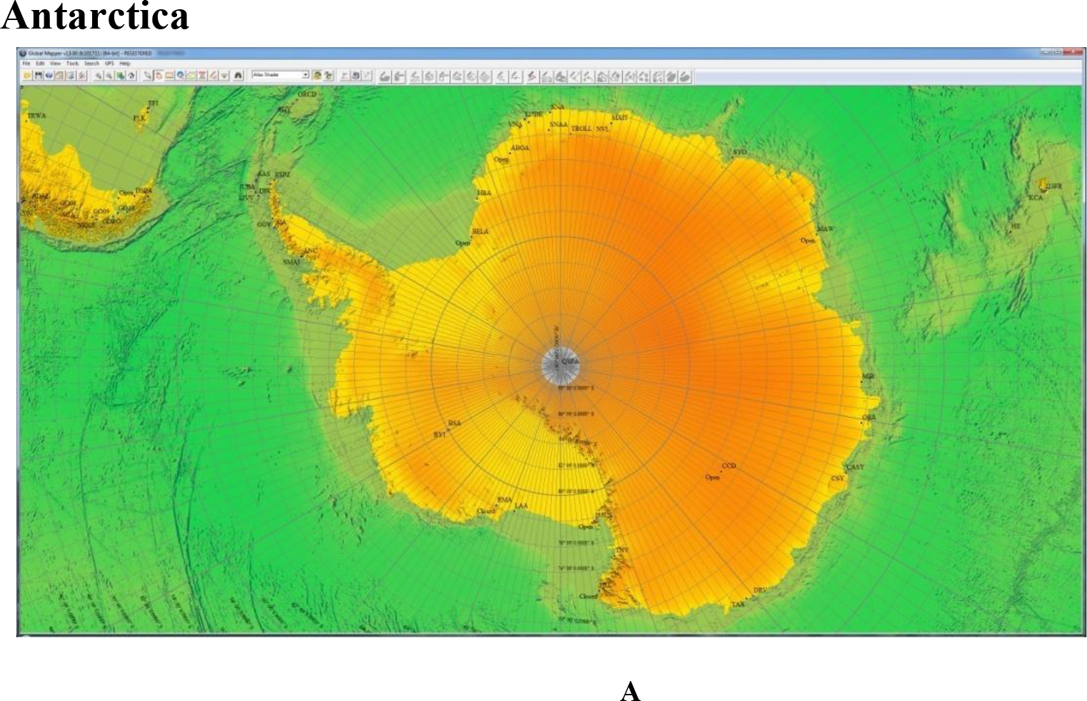
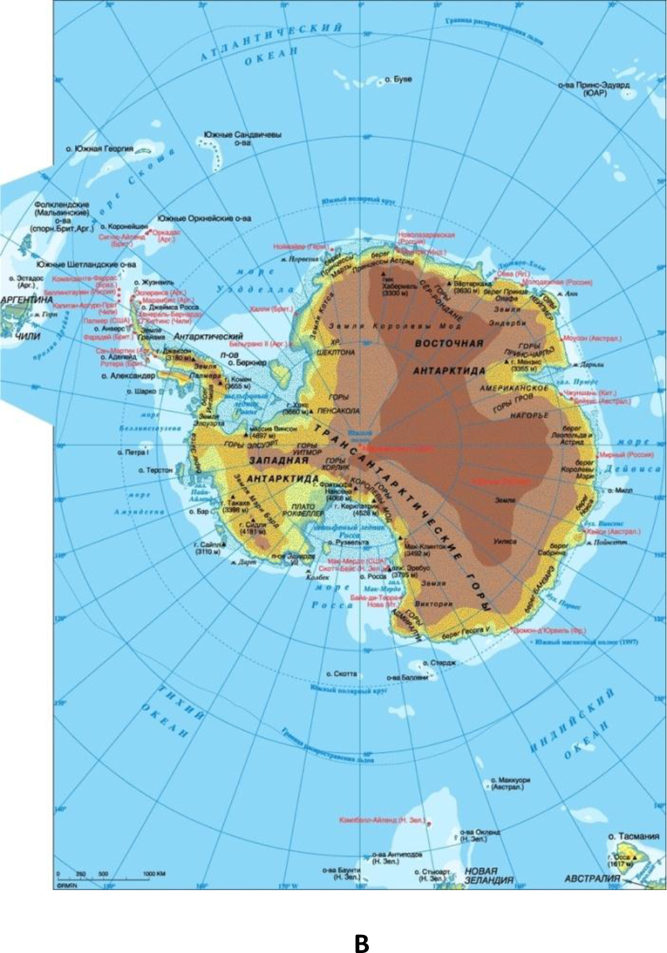
The modern map of Antarctica quite well shows similarities with the elements of the super – plume  (Fig. 2.) (Figure. 2a,b).

GEMS-19-101_Khavroshkin OB_F2

GEMS-19-101_Khavroshkin OB_F2b

Figure 2. A, B. This is modern map of Antarctica. With the exception of the peninsula, the coasts are rounded, forming a super plume.

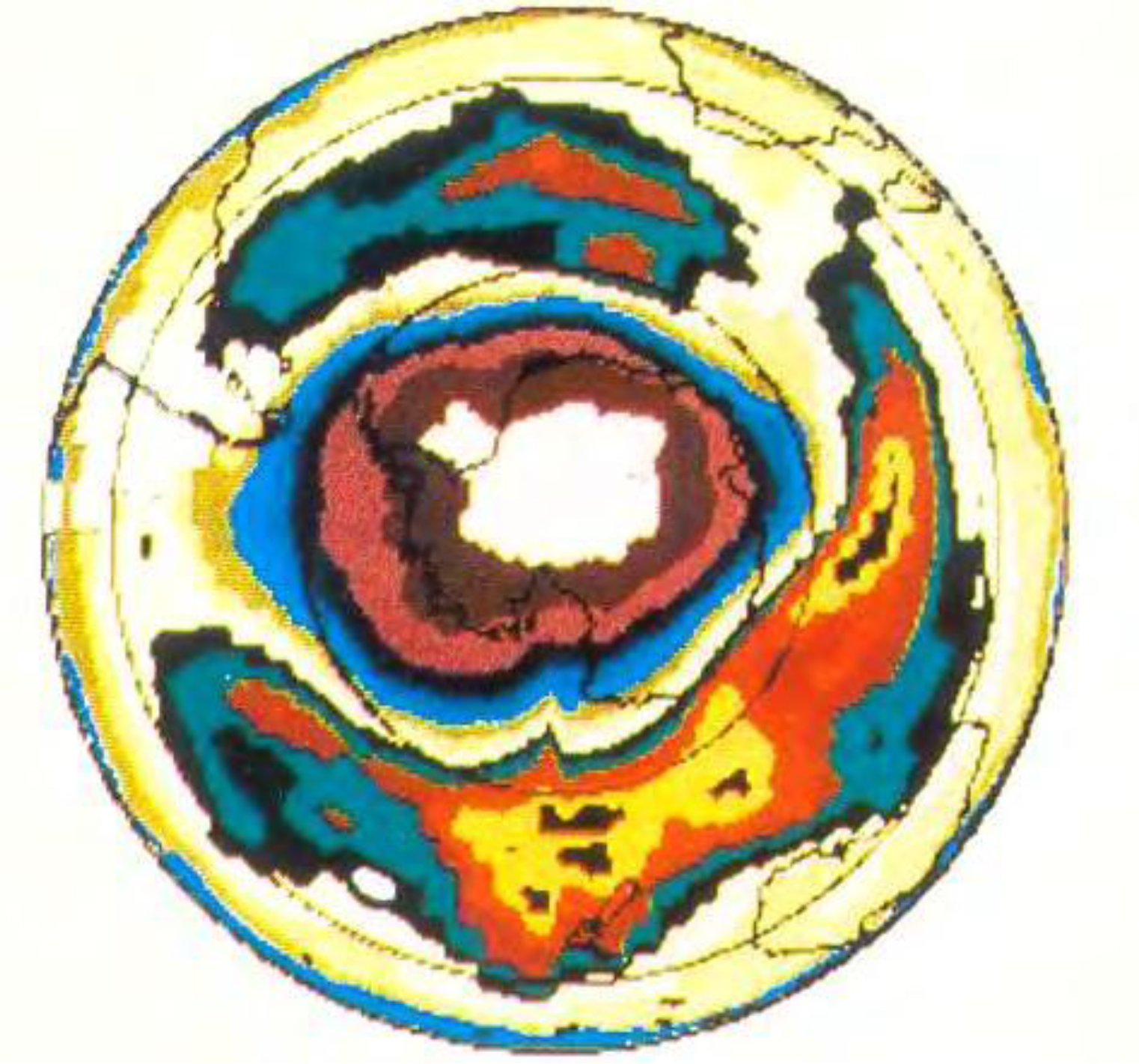
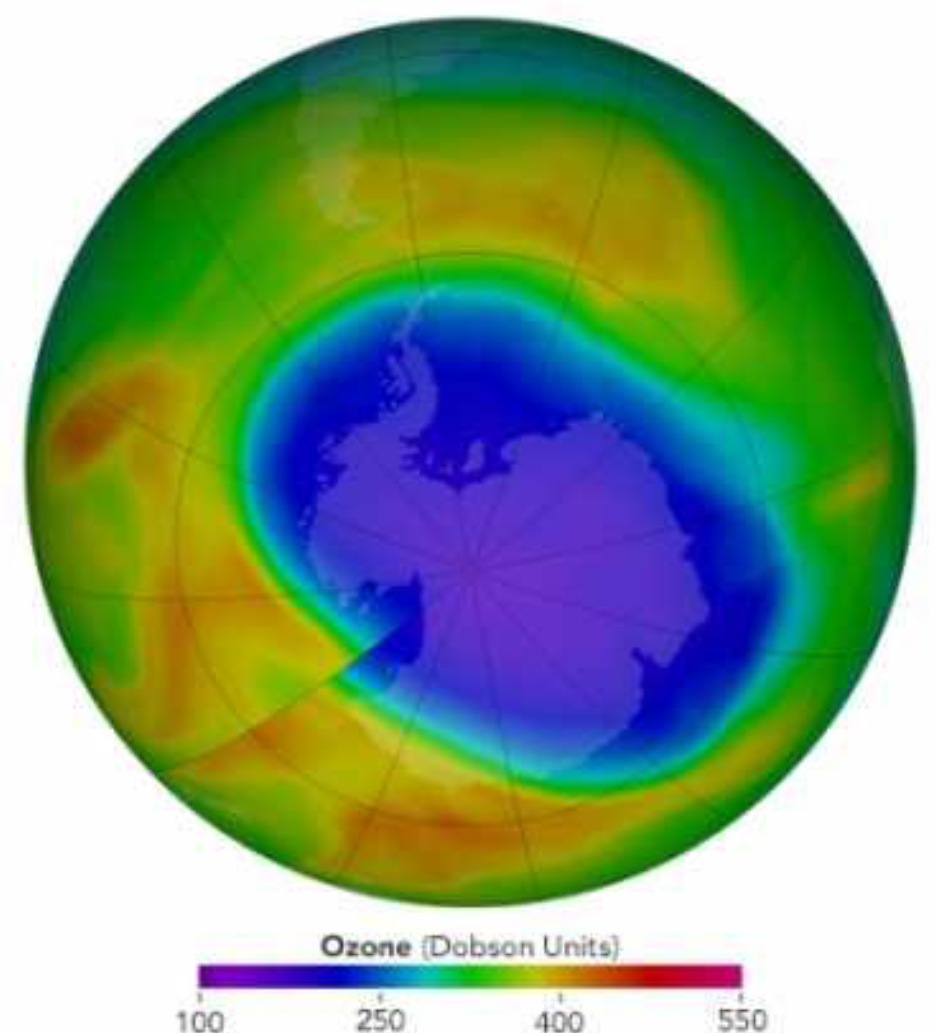
Given the thickness of the ice cover (up to 9 km), and the structure of the crustal rocks, as well as thermal and coastal processes, we should expect the existence of various seismic fields. In addition, there are many caves in the coastal zone, possibly remnants from the periphery of the plume. During the Second World War, a submarine base of Germany existed in the caves off the coast. There is the existence of the ozone hole over the continent. Large-scale, ozone-free atmospheric space above the continent (Figure 3) makes radical additions to the description of Antarctic seismicity. There are such effects that are impossible for terrestrial seismicity. The absence of ozone protection makes available the effect on the surface of many solar processes: radiation (from ultraviolet radiation to x-rays and gamma radiation), solar cosmic rays and flares, muons, modulated solar wind and interplanetary shock waves (MUV). A similar picture is observed for lunar seismicity. Many of the effects are almost constantly modulated, for example, by solar oscillations which make it possible to observe waves at solar frequencies in the spectrum of the seismic field (Table 1).

GEMS-19-101_Khavroshkin OB_F3

Figure 3. Map of the ozone hole over Antarctica.

Table 1. Periods of oscillations of the standard model of the Sun with the relative content of heavy elements Z = 0.02 according to calculations by Iben n Makhefi

Mode

Period (min)

Mode

Period (min)

l=0

l=1

l=2

l=3

l=4

l=1

l=2

l=3

l=4

p1

62,29

57,25

42,50

39,53

37,58

f

45,90

40,97

38.82

p2

40,94

36,98

32,19

29,42

27,62

g1

61,58

55,05

47.94

44,15

P3

30,93

27,88

25,09

23,21

21,92

g2

84,4

63.03

54.88

49,59

p4

24,49

22,30

20,52

19,26

18,31

g 3

105,3

72,58

61.88

57,73

p5

20,19

18,08

17,39

16,44

15,72

g 4

127,3

83,49

67,78

61,11

p6

17,17

16,04

15,10

14,38

13,81

g 5

148.2

95.38

74,9

64,89

p7

14,93

14,08

13,35

12,77

12,32

g 6

171,1

107,7

88,1

70,30

p8

13,21

12.55

11,97

11,51

11,14

g 7

120,2

91,8

76.83

p9

11,85

11,34

10,87

10,49

10,18

g 8

132.9

100,7

83.62

p10

10,78

10.35

9,97

9,85

9,39

g 9

145.9

109,7

90,56

p11

9,90

9,54

9.21

8.94

8,71

g 10

158,9

118,9

97,62

p12

9.15

8,84

8,56

8,32

8,11

g 11

172.1

128,1

104,5

p23

8,50

8,25

7,99

7.78

7.60

g 12

137,8

111,7

p14

7.94

7,71

7,49

7,31

7,15

g 23

147,0

118,9

p15

7.45

7,25

7,06

6,89

6,75

g 14

156.5

126,5

p16

7.02

6,84

6,67

6,52

6,39

g 15

166,7

133,3

p17

6.64

6,47

6,32

6,18

6,06

g 16

175,9

141,5

p18

6.39

6.14

6,00

5,87

5,77

g 17

148,6

p19

5.98

5,84

5,71

5,60

5,50

g 18

156,4

p20

5.69

5,58

5,45

5.34

5.25

g 19

164,0

g 20

171,1

In Table 1: p, g, f-modes of the natural oscillations of the Sun; L-form of natural oscillations.

Moreover, the excitation of these waves is not due to the indirect interaction of terrestrial radioactive geological structures with solar neutrinos, but directly. This means that instrumental and methodological development of seismic expeditions to the Moon, Mars and other space bodies devoid of ozone protection should be carried out on Antarctica, as the closest to the external conditions of the landfill (Figure 3).

The ozone hole over the Antarctic and its adjacent territories is quite dynamic: it grew for the first time in recent years, covering an area of 28 million square kilometers (press service of the NASA Goddard Space Flight Center). Previously, the ozone layer was considered to be a natural shield that protects the surface of the Earth from hard ultraviolet radiation, which is dangerous to living organisms. Now it is a parameter of the atmosphere, which allows studying the Sun, solar-terrestrial relations and some astrophysical problems. A sharp drop in the concentration of stratospheric ozone during the winter season was first detected over the Antarctica in the 1980s. Every winter, the ozone hole over Antarctica grows, reaching a maximum area in September, and shrinking in summer. Large sizes fully correspond to how ozone behaves in relatively cold weather in the upper atmosphere of the Earth (Paul Newman, Paul Newman, USA). Due to the slow reduction, the thickness of the ozone layer in some deep regions of the Antarctic has fallen to absolute zero for the first time in many years. This means that the Suns freely “bombard” the polar ice that is under similar areas, for example, the Amundsen – Scott station at the South Pole. The level of ozone began to fall sharply in September, with the result that its concentration decreased by 95% by the first of October. This year, the fall continued for two “extra weeks”, which led to a 100% decrease in the level of ozone by October 15”says another climatologist, Brian Johnson, USA. However, the smaller ozone hole in 2017 is the result of natural variability and is not necessarily a signal of rapid “healing”. Scientists use the word “hole” as a metaphor for an area in which the ozone concentration falls below the historical threshold of 220 Dobson units. A sharp drop in the concentration of stratospheric ozone during the winter season was first discovered over Antarctica in the 1980s. The reason for this was the release of a large number of Freon’s into the atmosphere of the Earth, whose molecules destroy ozone in the upper layers of the atmosphere at low air temperatures. Every winter, the ozone hole over Antarctica grows, reaching a maximum area in September, and shrinking in summer. January 29, 2016, 14:31 – January 27, a huge ozone hole covered northern Eurasia from the Atlantic to the Pacific Ocean. Most of it fell on the territory of Russia. The anomaly center is located in the north of Western Siberia, however, the effect of ozone holes is not yet known to seismologists.  Observations in 2017 showed that the hole in the ozone layer of the Earth, which forms over Antarctica at the end of the southern winter, has become the smallest since 1988. According to NASA satellites, the ozone hole reached its one-year maximum of September 11, spreading to 7.6 million square miles (19.6 sq. km), which is 2.5 times the area of the United States. Ground-based measurements and measurements from balloons, carried out by the National Oceanic and Atmospheric Administration, confirmed satellite data. Since 1991, the average maximum area of ozone holes has been approximately 26 million square kilometers (Fig. 4.)  (Figure  4).

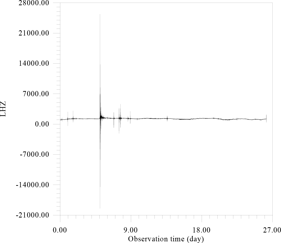
In view of the above, a start was made to study the seismic fields of Antarctica (Figure 5).

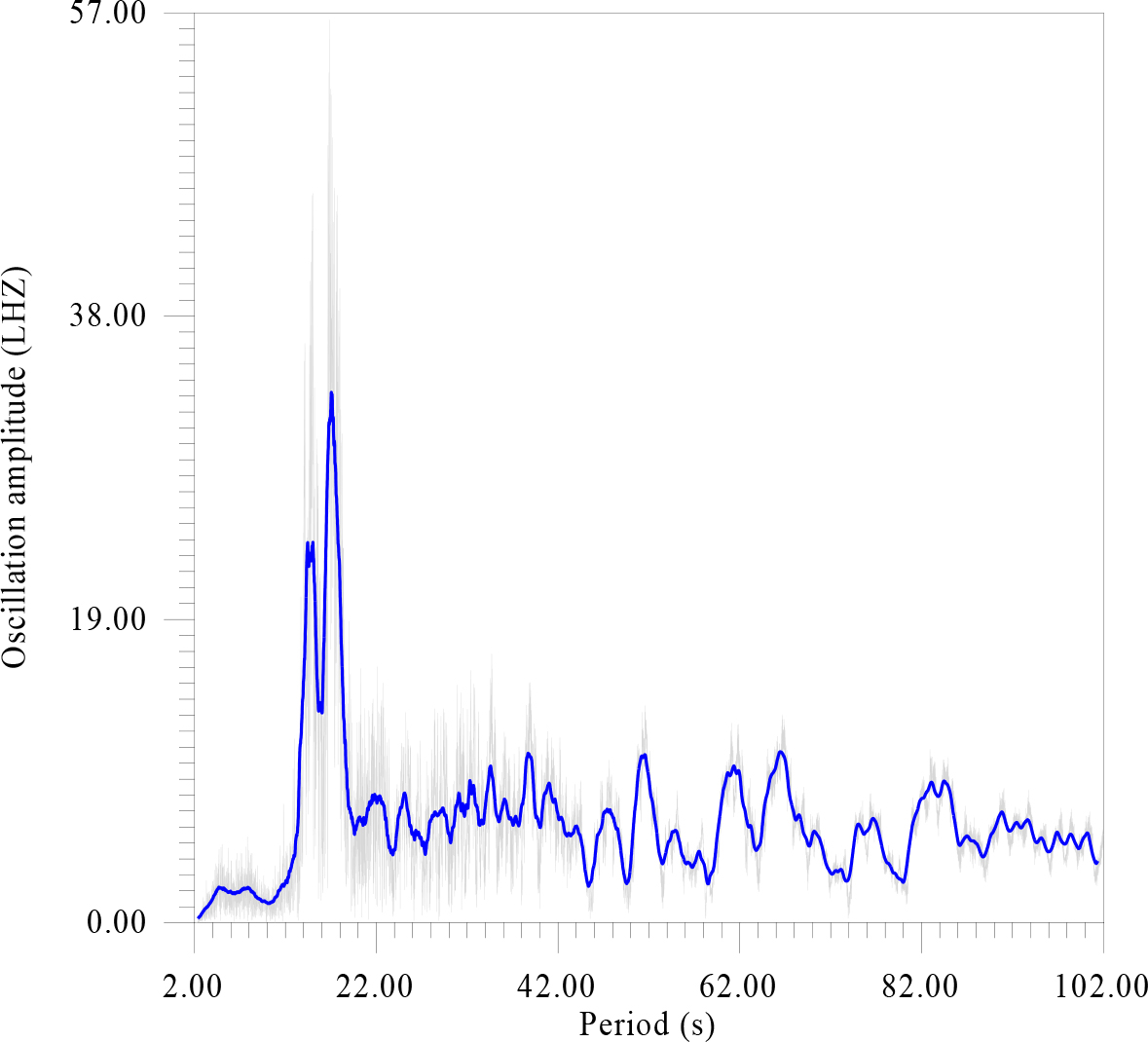
As follows from Figure 5, considerable seismic material has been collected and processed, primarily relating to the coastal zone and partly of the shelf The IRIS Data Management Center (IRISDMC): http://service.iris.edu/fdsnws/dataselect/1/. The study of data was started with spectral analysis (see Fig. 6) (Figure 6).

GEMS-19-101_Khavroshkin OB_F4

Figure 4. Concentration of ozone over Antarctica. October, 2017. © NASA

GEMS-19-101_Khavroshkin OB_F5

Figure 5. Seismic recording of LHZ-component 60 channel Streckeisen STS-2.5 sensor IU network of QSPA station (89.9289°S, 144.4382°E). The record contains 2265013 seconds. For convenience, the graphical representation is averaged over 120 points in 1 minute increments.

GEMS-19-101_Khavroshkin OB_F6

Figure 6. There is amplitude spectrum of seismic data in the range from 2 to 102 sec. in increments of 0.01 seconds. with averaging values of 1 sec.

According to fig.6 the spectrum of seismicity has two peaks dominant in amplitude, for 18 and 20 sec., which, probably, given the proximity of the ocean, should be referred to as “storm” and note also the existence of resonant structures at the Antarctic ice sheet (Figure 7).

GEMS-19-101_Khavroshkin OB_F7

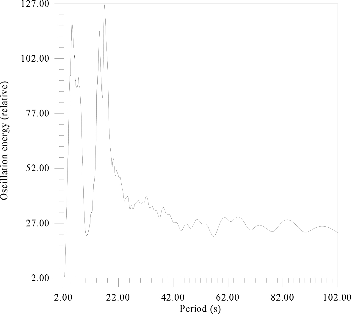
Figure 7. There is the energy spectrum of data Figure 6.

The energy spectrum revealed a more subtle structure of the peaks, at 4 and 18 sec. These peaks are not uncommon when considering seismic fields of complexly constructed and non-linear structures. For greater clarity, the same seismic material was processed by a more complex, but informative method (Fig.8 A, B)  (Figure 8 a,b).

GEMS-19-101_Khavroshkin OB_F8

GEMS-19-101_Khavroshkin OB_F8b

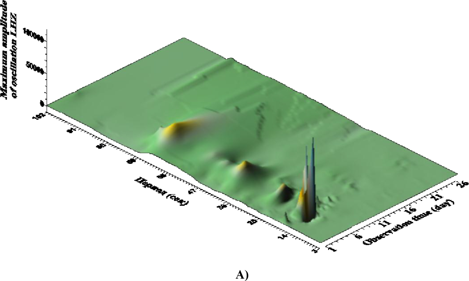
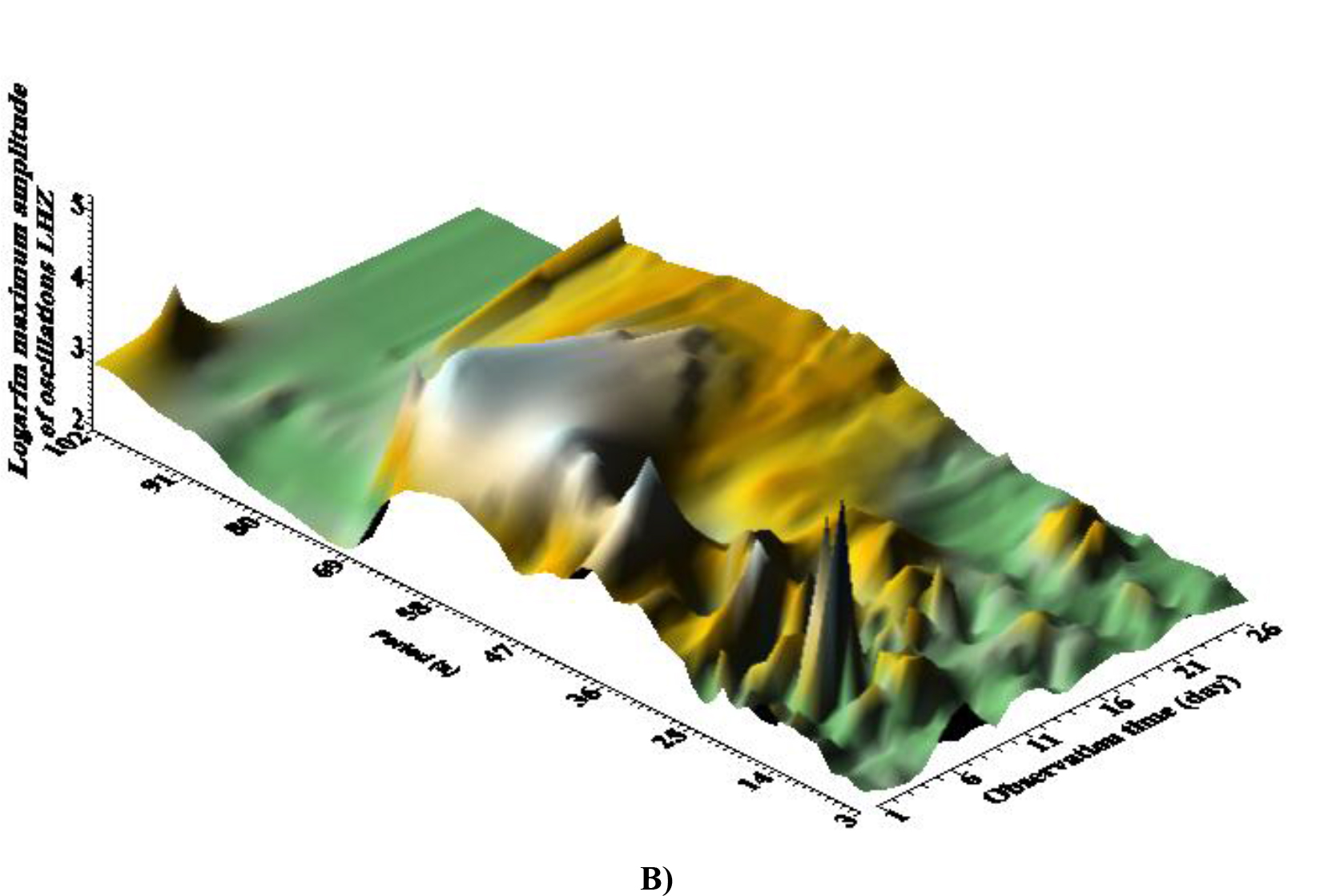
Figure 8. A, B. These are dependence of the maximum amplitude of seismic vibrations A) and its logarithm B), from the observation time and the corresponding period. The interval of the period change is from 2 to 102 sec with a step of 0.1 sec. The time step is 2 minutes (120 seconds). The window is 628 seconds.

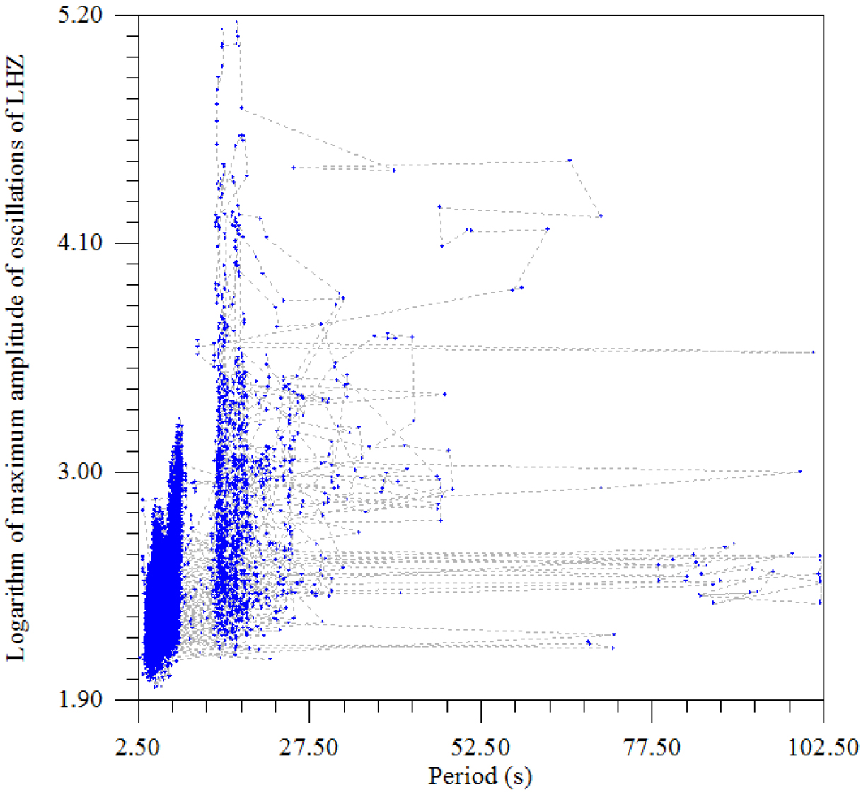
According to Fig. 8 (A) for several days, resonant peaks of good quality on micro seismic periods of 14–20 sec can be observed in the wave field; their double period manifests itself in the form of ill-galling small amplitude manifestations. According to Fig. 8 (B) in Antarctica in the general seismic wave field it is possible to distinguish three groups of waves with ranges of periods: relatively high-frequency (periods 3–25 seconds), the longest and with maximum amplitude (periods 49–60 seconds) and short duration of existence as a single peak on period ~ 100 sec. Probably, the longest are associated with existing in the coastal zone and on the shelf of the network of caves and channels (Figure 9).

GEMS-19-101_Khavroshkin OB_F9

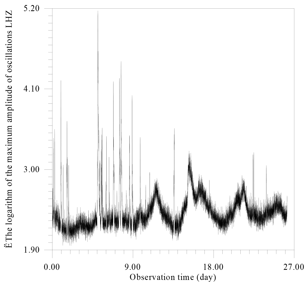
Figure 9. There is the dependence of the logarithm of the maximum amplitude of oscillations on the observation time.

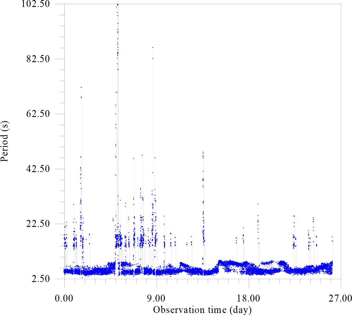
According to Fig. 9, there are two independent types of noise – one high-frequency, constantly existing with an unstable modulation frequency (~ 4–5 days) and the second in the form of very short irregular high-amplitude emissions (Figure 10,11).

GEMS-19-101_Khavroshkin OB_F10

Figure 10. The dependence of the period corresponding to the logarithm of the maximum amplitude of oscillations from the time of observation.

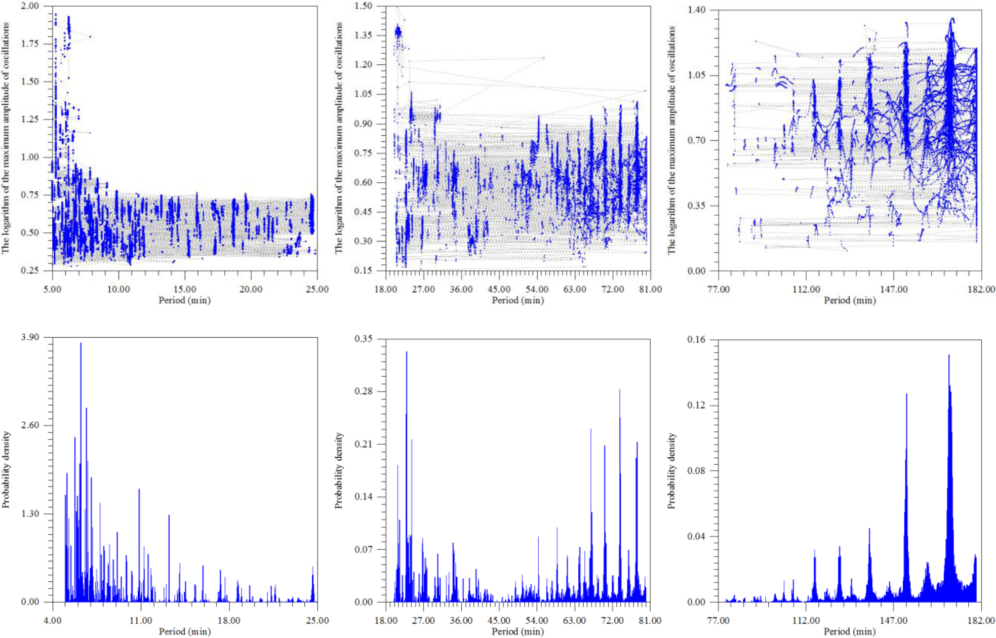
The dependence of the logarithm of the maximum amplitude on the period (Fig. 11) most clearly highlights the zone 3.0 – 7–8.0 s, that is, a known section of storm microseisms. Since such habitual microseisms are usually recorded, for example, in the Baltic and in Europe, and the geological and structural environment of this region and the Antarctic are fundamentally different, a source of probable general influence should be found. Since high-frequency solar oscillations have a constant activity, especially at periods of 5–6 min, and the lack of ozone protection from the Sun allows for higher frequency effects, these microseisms are inherently strongly associated with solar activity. Another, even more active area lies within 20–25 seconds, which is also recorded in other regions of the Earth (Figure-12).

GEMS-19-101_Khavroshkin OB_F11

Figure 11. The dependence of the logarithm of the maximum amplitude of oscillations on the period.

GEMS-19-101_Khavroshkin OB_F12

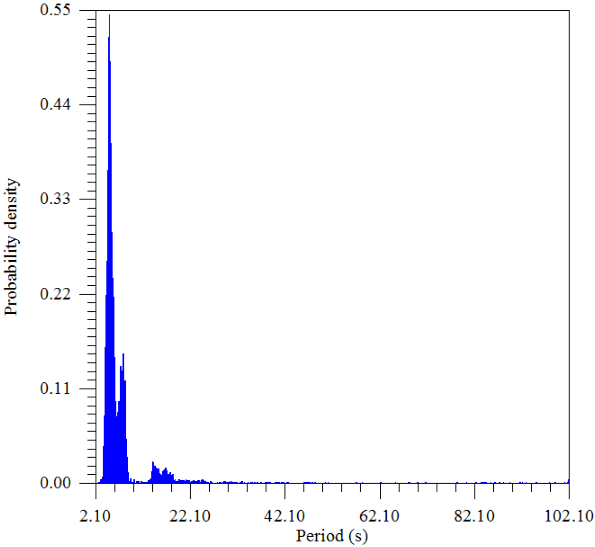
Figure 12. The density distribution of the maximum amplitude of the period.

The distribution of the maximum amplitude over periods divides the seismic vibrations into two groups – powerful ~ 3–6 sec and weak, but connected as resonant harmonics ~ 18–20 sec., which was observed earlier in other regions of the Earth (Figure 13–20).

GEMS-19-101_Khavroshkin OB_F13

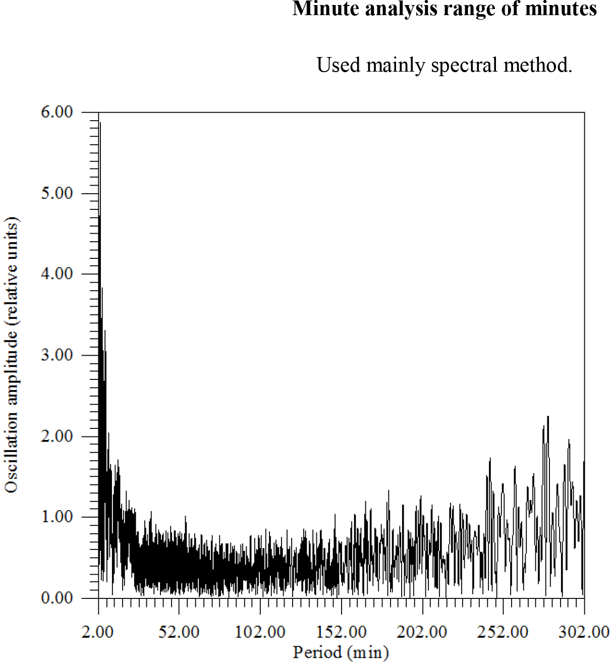
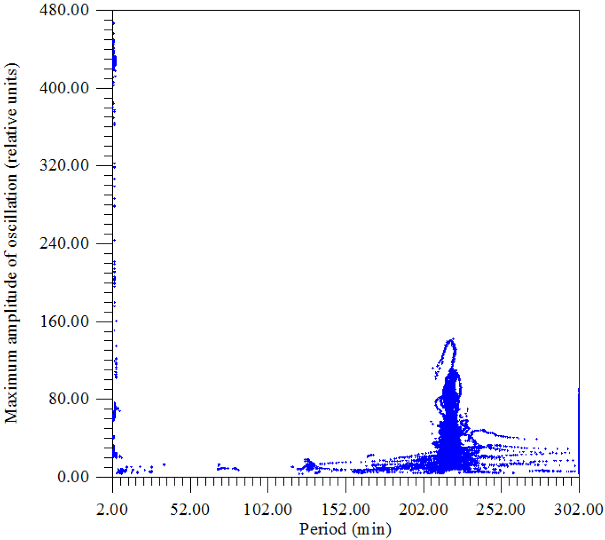
Figure 13. There is amplitude spectrum from 2 to 302 min with a step of 0.03 min.

GEMS-19-101_Khavroshkin OB_F14

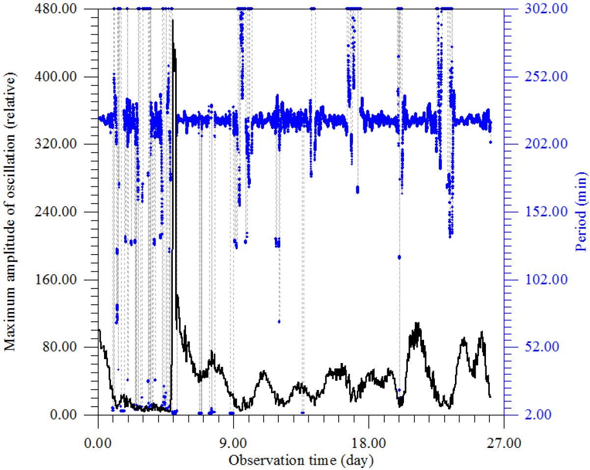
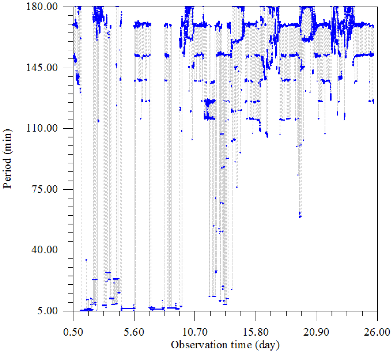
Figure 14. The dependence of the period corresponding to the maximum amplitude of oscillations from the time of observation.

GEMS-19-101_Khavroshkin OB_F15

Figure 15. Dependence of the logarithm of the maximum amplitude of oscillations on the period

GEMS-19-101_Khavroshkin OB_F16

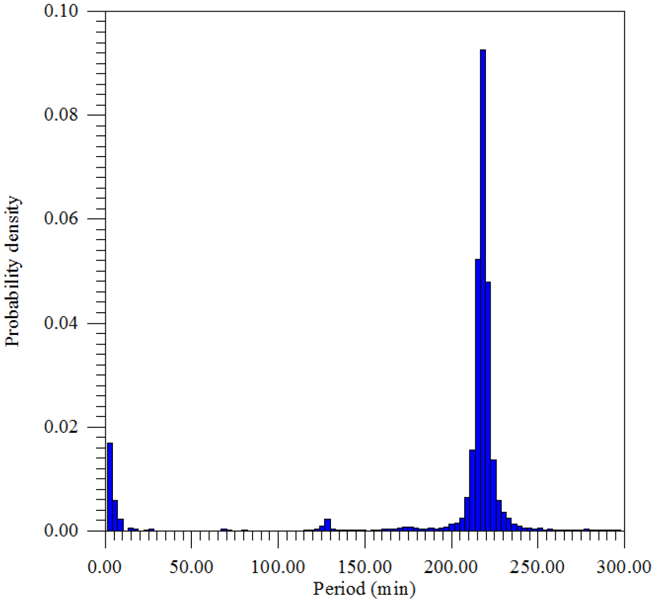
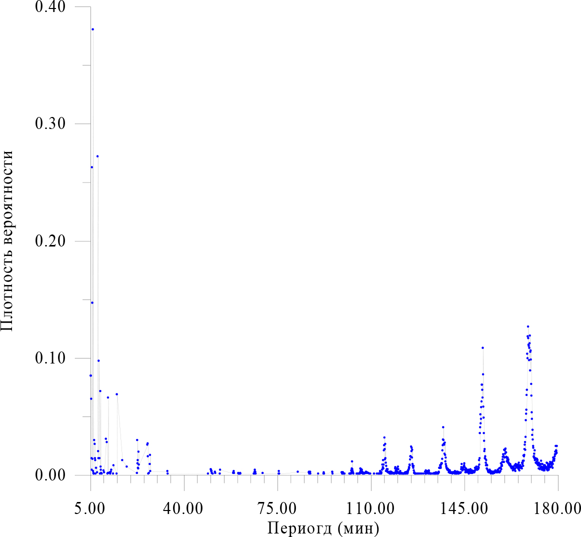
Figure 16. The density distribution of the maximum amplitude of the period.

GEMS-19-101_Khavroshkin OB_F17

Figure 17. The dependence of the period corresponding to the maximum amplitude of oscillations from the time of observation.

GEMS-19-101_Khavroshkin OB_F18

Figure 18. The density distribution of the maximum amplitude of the period.

GEMS-19-101_Khavroshkin OB_F19

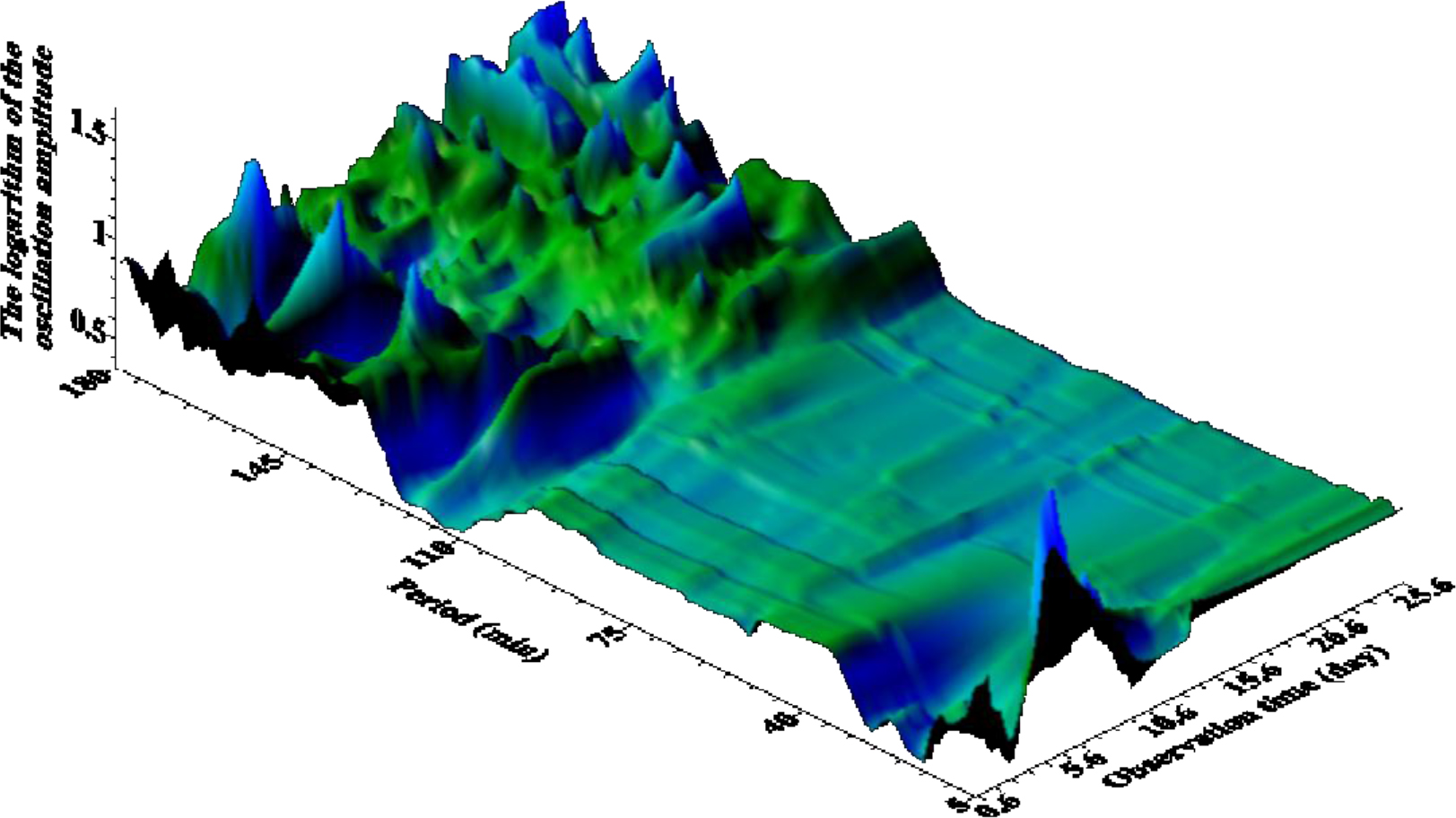
Figure 19. The dependence of the logarithm of the maximum amplitude of oscillations on the time of observation and the corresponding period. The interval of the period is change from 2 to 302 minutes. in 0.3 min steps Time step 2 min. Window – 314 minutes.

GEMS-19-101_Khavroshkin OB_F20

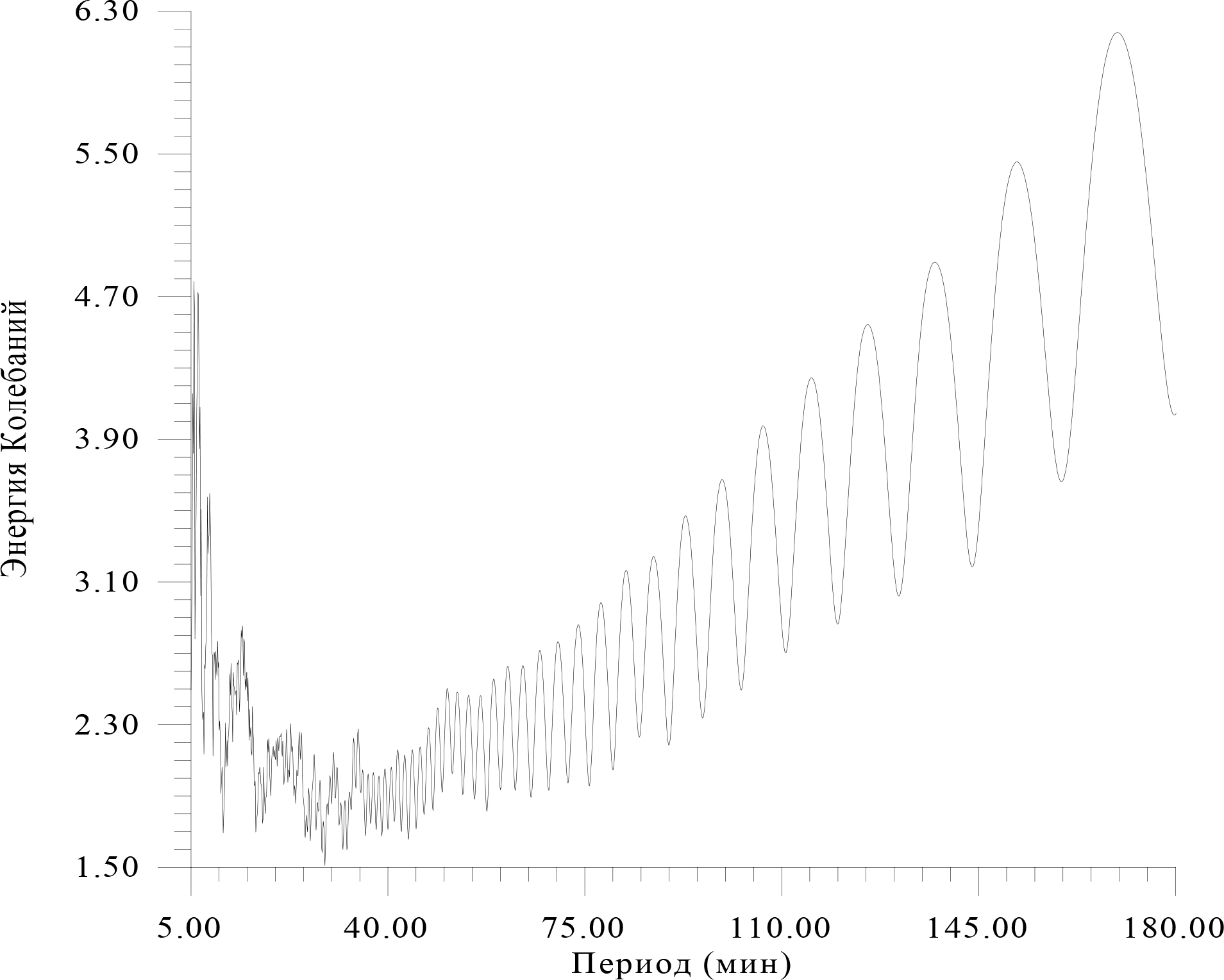
Figure 20. There is energy spectrum data Figure 19.

This energy spectrum characterizes the constant component. Therefore, it is still early to draw final conclusions about their reliability and significance. We must try to modify the program a bit, or use the resonance method (Table-2).

Table 2. Distribution of time intervals for which the periods correspond (N≥10)

Period (min)

N

Period (min)

N

Period (min)

N

Period (min)

N

Period (min)

N

Period (min)

N

5.4002

153

124.5683

11

149.7827

12

161.0891

26

167.6929

30

173.1961

18

5.5003

153

124.6683

10

150.5831

12

161.1892

20

167.7930

39

173.2961

16

5.6003

117

124.7684

15

150.6832

10

161.2893

25

167.8930

46

173.3962

13

5.7004

25

124.8685

14

150.7833

22

161.3893

22

167.9931

50

173.5963

15

5.9005

476

124.9685

23

150.8833

15

161.4894

26

168.0931

38

173.6963

15

6.0006

266

125.0686

28

150.9834

25

161.5894

18

168.1932

58

173.7964

10

6.1006

24

125.1686

28

151.0834

64

161.6895

21

168.2933

84

173.8965

16

6.2007

690

125.2687

27

151.1835

73

161.7895

23

168.3933

94

173.9965

21

6.7010

53

125.3687

43

151.2835

93

161.8896

18

168.4934

100

174.0966

12

6.9011

47

125.4688

36

151.3836

79

161.9897

16

168.5934

123

174.1966

11

7.0011

25

125.5689

41

151.4837

86

162.0897

16

168.6935

131

174.4968

16

7.1012

22

125.6689

26

151.5837

104

162.1898

14

168.7935

187

174.5969

11

7.4014

10

125.7690

38

151.6838

113

162.2898

16

168.8936

180

174.9971

11

8.0017

493

125.8690

16

151.7838

139

162.3899

16

168.9937

214

175.0971

14

8.2018

36

125.9691

13

151.8839

139

162.4899

15

169.0937

229

175.3973

14

8.3019

25

126.0691

12

151.9839

131

162.5900

12

169.1938

211

175.5974

10

8.4019

176

126.1692

10

152.0840

119

162.6901

13

169.2938

201

175.6975

12

8.7021

25

126.2693

13

152.1841

196

162.7901

12

169.3939

199

175.7975

10

9.0023

129

135.8747

10

152.2841

155

162.8902

10

169.4939

177

175.8976

10

9.1023

12

135.9748

10

152.3842

105

163.0903

10

169.5940

196

175.9977

11

11.1035

55

136.0749

10

152.4842

88

163.1903

12

169.6941

203

176.0977

18

11.4037

50

136.1749

14

152.5843

64

163.2904

10

169.7941

215

176.3979

17

11.9039

119

136.2750

10

152.6843

52

163.3905

11

169.8942

161

176.5980

14

13.9051

14

136.3750

12

152.7844

36

163.6906

10

169.9942

190

176.6981

12

15.2058

124

136.4751

10

152.8845

39

163.9908

13

170.0943

192

176.7981

14

17.2070

22

136.5751

15

152.9845

25

164.1909

14

170.1943

178

176.9982

10

18.9079

12

136.6752

17

153.0846

28

164.4911

16

170.2944

140

177.0983

14

22.8102

53

136.7753

17

153.1846

24

164.5911

13

170.3945

122

177.1983

16

22.9102

17

136.8753

17

153.2847

18

164.6912

12

170.4945

96

177.2984

11

23.0103

22

136.9754

24

153.3847

14

164.7913

13

170.5946

86

177.3985

19

23.1103

10

137.0754

37

153.4848

22

164.8913

11

170.6946

61

177.4985

11

23.2104

9

137.1755

45

153.5849

15

164.9914

13

170.7947

69

177.5986

17

23.3105

35

137.2755

54

153.7850

14

165.0914

15

170.8947

54

177.6986

16

23.4105

15

137.3756

73

158.6878

10

165.1915

10

170.9948

44

177.7987

17

26.6123

46

137.4757

53

158.8879

10

165.2915

12

171.0949

41

177.8987

17

26.7124

48

137.5757

47

158.9879

17

165.3916

15

171.1949

27

177.9988

13

26.8125

28

137.6758

47

159.1881

13

165.4917

12

171.2950

28

178.0989

17

27.5129

16

137.7758

46

159.2881

15

165.6918

18

171.3950

32

178.1989

19

27.6129

30

137.8759

32

159.3882

13

165.7918

10

171.4951

25

178.2990

10

103.2561

20

137.9759

49

159.4882

19

165.9919

13

171.5951

37

178.3990

16

114.5626

15

138.0760

30

159.5883

23

166.0920

14

171.6952

22

178.4991

26

114.7627

11

138.1761

20

159.6883

27

166.1921

14

171.7953

23

178.5991

22

114.8627

22

138.2761

26

159.7884

31

166.2921

10

171.8953

25

178.6992

25

115.0629

15

138.3762

16

159.8885

19

166.3922

11

171.9954

18

178.7993

23

115.1629

37

138.4762

13

159.9885

28

166.4922

12

172.0954

24

178.8993

21

115.2630

45

138.5763

11

160.0886

19

166.5923

10

172.1955

24

178.9994

24

115.3630

57

144.1795

11

160.1886

38

166.6923

12

172.2955

17

179.0994

28

115.4631

39

144.2795

16

160.2887

26

166.8925

18

172.3956

20

179.1995

31

115.5631

23

144.4797

10

160.3887

37

166.9925

16

172.4957

24

179.2995

35

115.6632

47

144.9799

11

160.4888

32

167.0926

18

172.5957

16

179.3996

31

115.7633

25

145.0800

12

160.5889

39

167.1926

21

172.6958

22

179.4997

44

115.8633

18

145.1801

14

160.6889

40

167.2927

13

172.7958

15

179.5997

37

116.0634

13

145.2801

17

160.7890

34

167.3927

29

172.8959

14

179.6998

36

119.4654

11

145.3802

11

160.8890

34

167.4928

21

172.9959

18

179.7998

33

120.4659

12

149.2824

10

160.9891

27

167.5929

28

173.0960

9

179.8999

44

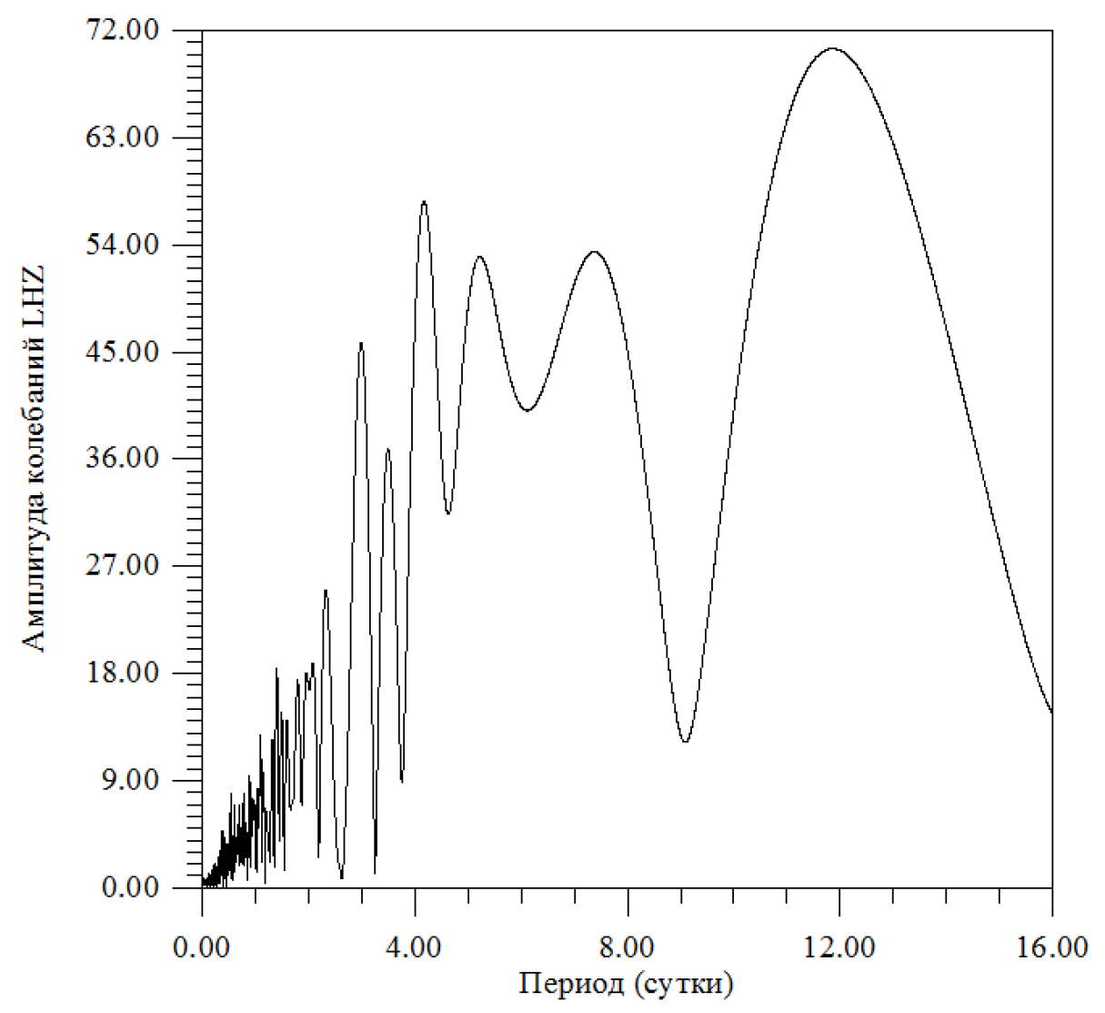
This table could also be rebuilt according to a different number of intervals by period. It is noteworthy that in the range of 28÷103 min the number of intervals is very small (Table 3) (Figure 21) (Table 4).

GEMS-19-101_Khavroshkin OB_F21

Figure 21. There is amplitude spectrum of the daily range.

Table 3. The distribution of time intervals for which the periods correspond to Amax

Period (min)

N

Period (min)

N

Period (min)

N

2.6000

946

146.3120

4

221.1620

2686

5.5940

325

149.3060

4

224.1560

762

8.5880

122

152.3000

1

227.1500

332

11.5820

1

155.2940

9

230.1440

196

14.5760

30

158.2880

13

233.1380

140

17.5700

15

161.2820

18

236.1320

71

20.5640

1

164.2760

17

239.1260

54

23.5580

9

167.2700

25

242.1200

36

26.5520

20

170.2640

36

245.1140

36

32.5400

2

173.2580

42

248.1080

24

68.4680

17

176.2520

44

251.1020

31

71.4620

6

179.2460

26

254.0960

13

74.4560

2

182.2400

20

257.0900

15

77.4500

2

185.2340

18

260.0840

10

80.4440

7

188.2280

33

263.0780

10

116.3720

3

191.2220

22

266.0720

9

119.3660

6

194.2160

35

269.0660

7

122.3600

15

197.2100

47

272.0600

11

125.3540

48

200.2040

71

275.0540

11

128.3480

128

203.1980

86

278.0480

17

131.3420

19

206.1920

135

281.0420

10

134.3360

14

209.1860

359

284.0360

5

137.3300

5

212.1800

868

287.0300

7

140.3240

4

215.1740

2932

290.0240

3

143.3180

6

218.1680

5189

293.0180

6

296.0120

6

Table 4. The summary of daily periods.

Period
(day)

Amplitude
fluctuations

(rel. units)

Period
(day)

 Amplitude
fluctuations
(rel. units)

Period
(day)

Amplitude
fluctuations
(rel. units)

  0.00417

  2.19146

  0.38750

  2.34914

  0.79306

  7.95374

  0.00972

  1.39646

  0.39861

  3.12503

  0.82917

  4.96194

  0.11806

  1.05268

  0.40694

  4.69761

  0.88750

  9.37318

  0.13194

  1.14954

  0.41806

  2.71686

  0.93750

  7.53833

  0.13750

  1.06967

  0.42917

  2.80484

  0.97639

  7.36167

  0.16806

  1.43672

  0.43750

  3.39350

  1.04583

  8.34664

  0.18750

  1.28783

  0.44583

  3.64884

  1.09583

 12.86868

  0.20139

  1.51607

  0.46250

  1.25450

  1.15139

  9.73151

  0.20972

  1.87710

  0.47083

  3.53236

  1.20972

  6.42397

  0.22083

  1.91259

  0.48750

  3.70950

  1.31806

 12.39736

  0.22917

  2.03499

  0.50417

  2.77930

  1.40139

 18.42374

  0.24028

  2.07343

  0.51528

  3.61388

  1.49028

 14.78352

  0.25139

  1.51939

  0.52917

  6.31336

  1.59306

 14.11028

  0.26528

  1.78014

  0.54028

  7.88273

  1.79306

 17.42602

  0.28194

  1.69116

  0.55417

  3.96956

  1.95972

 18.00527

  0.29306

  1.73287

  0.56528

  1.75607

  2.07917

 18.77936

  0.29861

  2.50799

  0.57639

  1.94631

  2.32639

 25.01781

  0.30972

  2.22962

  0.59028

  4.55191

  2.99028

 45.80661

  0.31528

  2.12205

  0.60694

  6.98497

  3.49583

 36.81036

  0.32917

  2.22865

  0.62361

  4.12886

  4.17083

 57.67608

  0.33472

  3.07918

  0.64861

  3.80290

  5.22083

 52.97682

  0.35139

  2.24693

  0.66806

  3.72560

  7.37917

 53.38868

  0.35694

  4.71118

  0.68750

  6.98646

 11.85972

 70.47160

  0.37361

  2.58232

  0.71528

  4.98707

  0.38194

  3.51410

  0.76250

  7.11657

Conclusion

As expected, (see Tables 2–4), the structure of the seismic fields of Antarctica is saturated with wave fields determined by cosmic processes, primarily by the Sun’s own oscillations (see Table 1). Seismic Antarctica turns it into a unique and indispensable landfill for testing and testing of seismic and geophysical equipment intended for the study of the Moon and planets.

Attachments

GEMS-19-101_Khavroshkin OB_F22

References

  1. Khavroshkin OB, Tsyplakov VV (2001) Meteoroid stream impacts on the Moon: information of duration of seismograms // Proc. Conf. Meteoroids 2001 (ESA SP-495). Noordwijk, The Netherlands: ESA Publ Division Pg No: 13–21.
  2. Khavroshkin OB, Tsyplakov VV (2001) Temporal structure of meteoroid stream and lunar seismicity according to Nakamura’s catalogue // Proc. Conf. Meteoroids 2001 (ESA SP-495). Noordwijk, The Netherlands: ESA Publ. Division Pg No: 95–105.
  3. Khavroshkin OB, Tsyplakov VV, Sobko AA (2011) Solar activity and seismicity of the Moon. Engineering Physics 3: 40–45.
  4. Christensen Dalsgaard J, Gough DO, Morgan JG (1979) Dirty Solar Models. Astron. Astrophys 73: 121–128 .
  5. Patrick S. McIntosh, Murray Dryer (1972) Solar activity: observations and predictions. The Massachusetts Institute of Technology, Virginia, USA.
  6. Syun-Ichi Akasofu, Sydney Chapman (1972) Solar-Terrestrial Physics. The Clarendon Press, California, USA.
  7. Khavroshkin O, Tsyplakov V (2013) Nonlinear Seismology: The Cosmic Component. Saarbrücken: Palmarium Academic Publishing.
  8. Oleg Khavroshkin, Vladislav Tsyplakov (2013) Sun, Earth, radioactive ore: common periodicity. The Natural Science (NS) 5: 1001–1005.
  9. Khavroshkin OB, Tsyplakov VV (2013) Radioactivity, solar neutrinos, interactions. Engineering Physics 8: 53–61.
  10. Khavroshkin OB, Tsyplakov VV (2013) Ore sample radioactivity: monitoring. Engineering Physics 8: 53–62.
  11. Khavroshkin OB, Tsyplakov VV (2013) Natural radioactivity as an open system. Engineering Physics 12: 40–54.
  12. Starodubov AV, Khavroshkin OB, Tsyplakov VV (2014) From periodicities of radioactivity to cosmic and metaphysical oscillations. Metaphysics. Moscow. Peoples’ Friendship University of Russia 1: 137–149.
  13. Rukhadze AA, Khavroshkin OB, Tsyplakov VV (2015) The frequency of natural radioactivity. Engineering Physics 5.
  14. Khavroshkin OB, Tsyplakov VV (2014) Hydrogen maser: solar periodicity. Engineering Physics 3: 25–31.

Capillary Hemangioma of the Hard Palate: A Rare Childhood Tumor

DOI: 10.31038/JDMR.2019245

Abstract

Hemangioma are benign tumor of childhood occurs due to proliferation of endothelial cells of blood vessels. Although hemangioma of the head and neck region are common, these tumors are rarely seen in the oral cavity especially hard palate. Normally, such rare cases of hemangiomas can be misdiagnosed as any other pathologies. So the proper diagnosis and management is very important to reduce the intraoperative and postoperative complications.This case report presents a case of a 7 years old male who was reported in the department of Oral and Maxillofacial Surgery with the chief complaints of swelling in the left maxilla since 4 months. After excisional biopsy and histopathological study, the lesion was finally diagnosed as capillary hemangioma of the palate.No recurrence was noted at 6 months follow-up.

Keywords

Hemangioma, intraoperative complication, excision

Introduction

Hemangiomas are benign tumor of vascular endothelial origin which are painless, slow progressive in growth and can involve superficial and deep blood vessels .They are mostly seen during early childhood occurring in about 5–10% of children <1 year of age, which involutes over time [1]. Hemangiomas are common in the head and neck region but rare in the oral cavity2. The lesions in the oral cavity generally appear on the lips, buccal mucosa and tongue, but rarely on hard and soft palate [2,3]. Incidence of hemangiomas are more in female than males. These proliferative tumors can be seen as a single lesion in 80% of the time but 20% it can be seen as multiple lesions. The proliferation of endothelial cells does not usually undergo malignant transformation. They appear as pale macules which can be lobulated sessile or pedunculated with variable size. They may have smooth or irregular boarders. As the lesion can be confused with other common lesions in oral cavity like pyogenic granuloma, histopathological examination is very important for the final diagnosis. The variants of hemangiomas are capillary, cavernous or central depending on the vasculization system. Following case report represent an unusual location of capillary hemangioma on the hard palate of a 7 years old male patient who reported to the department of oral and maxillofacial surgery. Following the surgical excision, lesion was sent for histopathological diagnosis and confirmed as capillary hemangioma. Regular follow up of the patient was done.

Case History

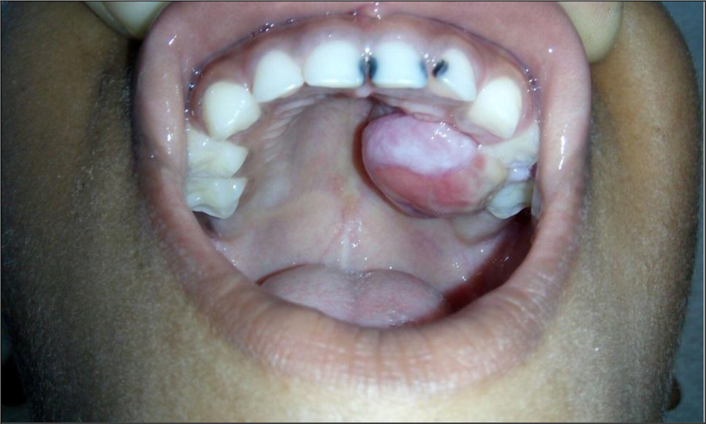
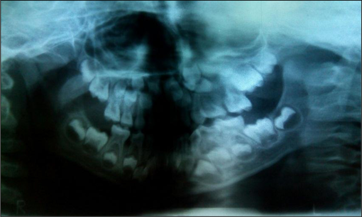
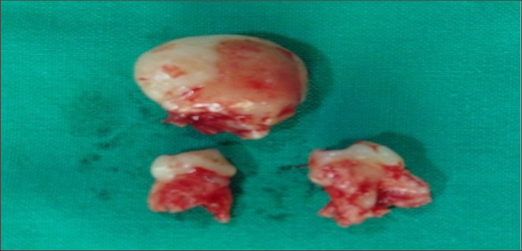
A male patient aged 7 years reported to the department of oral and maxillofacial surgery with a progressively enlarging painless swelling in upper left posterior teeth region for the past 4 months. The swelling was insidious in onset, gradually progressive and there was no history of any pain, discharge or bleeding. Extra orally no abnormalities detected (Figure 1). Intraoral examination revealed a solitary broad based pinkish growth of size 1.5×1.5 cm, present on the left posterolateral part of the hard palate just 0.5 cm lateral to the midline on the left side in relation to the deciduous left maxillary first and second molars. Swelling has a well-defined border, which was not interfering the occlusion (Figure 2). On palpation swelling was non-tender and firm in consistency. Panoramic radiograph did not reveal any pathological changes in relation to 64 and 65 (Figure 3). A provisional diagnosis of hemangioma was made based on clinical and radiographic findings. The lesion was excised under general anesthesia and tooth no. 64 and 65 were extracted (Figure 4). Wound was sutured. . Following that, the tissue specimen was sent for histopathological study, which shows lobulated cellular growth which containing proliferating endothelial cells, combination of numerous well and poorly canalized blood vessels which are lined by endothelial cells. The epithelium is parakeratotic stratified squamous type. The intervening connective tissue stroma is fibrillar composed of loose bundles of collagen fibers. It is sparsely infiltrated with chronic inflammatory cells predominantly lymphocytes and plasma cells. On the basis of clinical and histopathological findings lesion was finally diagnosed as capillary hemangioma of the hard palate. Satisfactory uneventful wound healing occurred after 1 month .Nance palatal arch space maintainer was delivered to the patient .No recurrence of the lesion was noted after 6 months of follow-up.

JDMR-19-125- Rilna P_India_f1

Figure 1.

JDMR-19-125- Rilna P_India_f2

Figure 2.

JDMR-19-125- Rilna P_India_f3

Figure 3.

JDMR-19-125- Rilna P_India_f4

Figure 4.

Discussion

Vascular lesions can be generally divided into hemangiomas and vascular malformations. In 1982, Mullikan and Glowacki described the classification based on clinical and microscopic features [4]. Hemangiomas are considered as true neoplasm of the vascular endothelial cells, but some controversy still occurs whether to classify hemangiomas as malformation or hamartomas [5]. Lesions commonly occurs as small or large superficial growth and can be unicentric or multicentric. Normally capillary hemangiomas are seen as superficial small pedunculated lesions which differ from other variants like central and cavernous which occurs as large superficial or deep lesions [1]. Also capillary hemangiomas can be seen as sessile or pedunculated lesions which are painless unless traumatized. In the present case, lesion was superficial and pedunculated which suggestive of capillary variant. Since there are no particular criteria for the diagnosis of capillary hemangiomas, proper clinical history and histopathological study can help to diagnose the lesion. In the present case, history of occurrence of lesion within few months with slow progressive in growth and clinical examination helps to suggest the lesion as capillary hemangioma. Ocurrence of hemangiomas is very rare especially in the hard palate and very few cases were reported in literature of occurrence in the oral cavity. Usually hemangiomas do not affect the adjacent bone which supports the present study which does not shows any involvement of adjacent bone. Pyogenic Granuloma (PG), peripheral giant cell granuloma, epulis granulomatosa, and squamous cell carcinoma should be included in the differential diagnosis of hemangiomas [6,7]. Management is based on age of the patient, size extend and variant of hemangiomas in the oral cavity [8]. Normally no intervention is required in early stages since there is a chance of involution of the lesion on aging. But in the present case, since the lesion was small without any bony involvement and to finalize the diagnosis, excisional biopsy was planned. Small lesions can successfully excised without any complications and with the support of proper bleeding control [9,10].

In the present case, since the hemangioma was small and superficial, excision of the lesion was done as the management. Most common complication which can occurs can be intraoperative bleeding, which has to be controlled with proper measures to minimize the blood loss. In the present case bleeding was controlled using local pressure application and cauterization. And the wound healing was uneventful. Recently reported treatment modalities for hemangiomas in the literature includes steroid therapy, electrosurgery, Nd:YAG laser, CO2 laser, cryosurgery, and sclerotherapy [11,12]. Nowadays, sclerotherapy is used largely because of its ability and efficiency to preserve the surrounding tissue [13].

In our patient, since the tumor was causing difficulty in swallowing and was impairing speech, surgical excision was carried out. Some studies have reported the recurrence of hemangioma after surgical management [14,15]. The case described here demonstrates that there has been no subsequent hemorrhage or other evidence of recurrence.

Conclusion

Dental practitioners and oral surgeons need to be aware with such unusual presentations of hemangioma in the oral cavity, so that they are treated appropriately without any serious intraoperative and postoperative bleeding risks.

References

  1. Neville BW, Damm DD, Allen CM et al. (2009) Oral and maxillofacial pathology. (3rdedn), St Louis: Saunders 2008.
  2. Dilsiz A, Aydin T, Gursan N (2009) Capillary hemangioma as a rare benign tumor of the oral cavity: a case report. Cases J 2: 8622.
  3. Yoon RK, Chussid S, Sinnarajah N (2007) Characteristics of a pediatric patient with a capillary hemangioma of the palatal mucosa: a case report. Pediatr Dent 29: 239–42.
  4. Mulliken JB, Glowaki J (1982) Hemangioma and vascular malformation in infants and children: classification based on endothelial characterstics. Plast Reconstruct Surg 69: 412–20.
  5. Barnes L (1985) Tumours and tumour-like lesions of the soft tissues. In: Barnes L (ed.), Surgical pathology of the head and neck. New York, NY: Marcel Dekker Pg No: 725–880
  6. Singh P, Parihar AS, Siddique SN, et al. (2016) Capillary hemangioma on the palate: a diagnostic conundrum. BMJ Case Rep 2016.
  7. Mufeed A, Hafiz A, George A, et al. (2015) Pedunculated hemangioma of the palate. BMJ Case Rep 2015
  8. Kumari VR, Vallabhan CG, Geetha S, Nair MS, Jacob TV (2015) Atypical presentation of capillary hemangioma in oral cavity- A case report. J Clin Diagn Res 9: 26–8.
  9. Rachappa M, Trivedi MN (2010) Capillary haemangioma or pyogenic granuloma: a diagnostic dilemma. Contem Clin Dent 1: 119–22.
  10. Van Doorne L, De Maeseneer M, Stricker C, Vanrensbergen R, Stricker M (2002) Diagnosis and treatment of vascular lesions of the lip. Br J Oral Maxillofac Surg. 40: 497–503.
  11. Varma S, Gangavati R, Sundaresh KJ, et al. (2013) Lobulated capillary haemangioma: a common lesion in an uncommon site. BMJ Case Rep 2013.
  12. Acikgo¨z A, Sakallioglu U, Ozdamar S, et al. (2010) Rare benign tumours of oral cavity—capillary haemangioma of palatal mucosa: a case report. Int J Paediatr Dent 10: 161–165
  13. Kamala KA, Ashok L, Sujatha GP (2014) Cavernous hemangioma of the tongue: A rare case report. Contemp Clin Dent 5: 95–8.
  14. Kocer U, Ozdemir R, Tiftikcioglu YO, Karaaslan O (2004) Soft tissue hemangioma formation within a previously excised intraosseous hemangioma site. J Craniofac Surg 15: 82–3.
  15. Sznajder N, Dominguez FV, Carraro JJ, Lis G (1973) Hemorrhagic hemangioma of gingiva: report of a case. J Periodontol 44: 579–82.

Body Composition Changes in Patients with Head and Neck Cancer Underactive Treatment: A Scoping Review

DOI: 10.31038/NDN.2019112

Abstract

Background: Head and neck cancer (HNC) patients experience significant weight loss before diagnosis, during and after treatment, and even during the first year of follow-up. However, the prognostic value of weight loss depends on body mass index, and this may be associated with low skeletal muscle mass, masking its loss. Thus, body composition changes occurring during HNC management warrant further investigation.

Objective: The aim of this scoping review was to evaluate body composition changes and the methods to assess it in HNC patients under oncological treatment with curative intent.

Inclusion Criteria: All published studies in English, Spanish and Portuguese during 2000-2019 focusing on body composition changes in HNC patients aged 18 years or older in the context of treatment with curative intent were considered. Surgical treatment approach was excluded to avoid excess heterogeneity. A three-step search strategy was undertaken.

Presentation of results: HNC patients suffer from serious loss of lean body mass, skeletal muscle or free fat mass after treatment compared with baseline. This can be demonstrated either by triceps skin fold thickness, bioelectrical impedance analysis, dual-energy x-ray absorptiometry or computed tomography. Nutritional deterioration occurs up to 8-12 months after treatment and has a remarkable impact on survival, quality of life, and risk for complications.

Conclusion: HNC patients experience a significant depletion of lean body mass, fat-free mass and skeletal muscle, accompanied by body fat mass, while undergoing (chemo) radiotherapy. Bioelectrical impedance analysis seems to be a feasible body composition assessment tool as it is inexpensive and non-invasive and usually readily available.

Keywords

Head and Neck Cancer, Body Composition, Skeletal Muscle, Lean Body Mass, Adipose Tissue, Fat Free Mass

Background

Head and neck cancer (HNC) is a term that refers to a heterogenous group of cancers that occur in the upper aerodigestive tract i.e. oral cavity, pharynx, larynx, paranasal sinuses, nasal cavity or salivary glands [1, 2]. Certain subtypes of these cancers demonstrate a strong increasing incidence and in general they are related to a low survival outcome. The most frequently found risk factors for HNC are the use of alcohol, tobacco, human papillomavirus (HPV)/Epstein-Barr virus (EBV) infection and poor oral hygiene3. Given their complexity and location, interference with the anatomical and physiological characteristics, the tumors and their treatment are able to promote aesthetic alterations and disturbance of functions such as phonation, swallowing, hearing and breathing [2, 4]. Dysphagia (difficulty in swallowing) is a prevalent risk factor for morbidity prior, during and following oncological treatment for HNCs, affecting most patients at some stage over the course of treatment, and is often rated as the most significant factor affecting quality of life amongst HNC survivors [1, 5]. Prior to treatment, HNC patients may experience swallowing dysfunction due to pain, obstruction or an uncoordinated swallowing mechanism[5], contributing to insufficient dietary intake, which may occur if the estimated energy intake is <60% of the individual requirement for more than 1 and 2 weeks [6]. However, not only the location of the tumor may result in problems in eating and drinking, but the cancer treatments (surgery and (chemo)radiotherapy either alone or in combination) also cause, in addition to dysphagia, alterations in swallowing function, which may persist for several months or even years, as xerostomia, thick saliva, difficulty in chewing, anorexia and nausea/vomiting [1-8]. These symptoms, either related to the acute toxicity or the anatomic changes caused by these treatments, may exacerbate nutrition deterioration by compromising dietary intake [2]. Even partial reduction in dietary intake (i.e. daily deficit >25%, >50%, or >75% of energy requirements) results in large caloric deficits over time, and the expected duration, as well as the degree of depletion of body reserves, should be considered. Both conditions result in weight loss and, consequently, in body mass index (BMI) reduction, which may be severe [6]. Apparently, age, race, gender, smoking and alcohol consumption, and radiation dose, do not independently predict severe weight loss [7]. The negative energy balance and skeletal muscle mass (SMM) loss observed in cancer patients is driven by a combination of reduced food intake and metabolic derangements (e.g. elevated resting metabolic rate, insulin resistance, lipolysis, and proteolysis which aggravate weight loss and are caused by systemic inflammation and catabolic factors), which may be host- or tumor-derived [6].

When compared with other cancer-patient populations, patients with HNC have the second highest prevalence of malnutrition, after upper gastrointestinal tract cancer patients [9]: 20-67% are malnourished or at high risk of becoming malnourished at diagnosis [7] and this will worsen throughout the treatment [2]. Significant weight loss (i.e., the involuntary weight loss of 5% body weight in 1 month or 10% in 6 months)[10]  is a common phenomenon before HNC diagnosis, during and after treatment, and occurs for up to a year following treatment [7]. A meta-analysis conducted by Couch et al. (2015) showed a relation between the extent and prevalence of weight loss and the location and stage of the tumor. Patients with advanced-stage HNC (stage III/IV) experience weight loss significantly more often when compared with those with early-stage (stage I/II) disease [10]. Weight loss alone is often the most common clinical measurement of cachexia [10] and forms one of the independent negative prognostic factors [2] for HNC patients, having a negative impact on quality of life (QOL) and morbidity as well [10]. Cancer cachexia is a term that refers to a multifactorial syndrome defined by an ongoing loss of SMM (with or without loss of fat mass) unable to be fully reversed by conventional nutritional support and leading to progressive functional impairment [11]. An early detection of malnutrition aims to improve oncological outcomes, and minimize acute toxicities, treatment interruptions and enhance survival [2]. Body composition (BC) has gained increasing interest in oncology and refers to the amount and distribution of lean tissue and adipose tissue in the human body [12]. The published studies have shown the importance of the changes in BC in various cancer patients [2] and more specifically loss of SMM, with or without loss of fat has proven to be a significant parameter [8]. Further, muscle loss determines the limiting dose of some antineoplastic drugs due to high distribution volume in adipose tissue, resulting in a slower drug elimination [2], and in a higher chemotherapy toxicity, and increase in mortality [8]. Different parameters can be used to assess BC, but the best-known parameter is BMI [12]. However, the role of this anthropometric tool is still unclear in HNC patients [8]. In recent years, several studies have shown a clear dissociation between total body weight loss and SMM loss, reflecting the increased prevalence of obesity in the population. The prognostic value of weight loss depends on the BMI, and this may be associated with low SMM, masking its loss. Thus, weight loss itself poorly predicts outcome in HNC patients when compared with depleted SMM, illustrating the inadequacy of BMI as an accurate method to reflect nutritional status [8]. An assessment method would be needed for rapid clinical implementation, to adequately evaluate BC in HNC patients in order to reveal significant malnutrition, appropriate chemotherapy dose, and to identify high risk patients [8]. Besides questionnaires like Patient-Generated Subjective Global Assessment (PG-SGA) that allow the assessment of the nutritional status, the existing techniques to evaluate nutritional status and/or BC include anthropometric measurements for weight and BMI, measurement of skinfold thickness, biochemical parameters, bioelectrical impedance analysis (BIA), computed tomography (CT), magnetic resonance (MRI) or dual-energy x-ray absorptiometry (DEXA) [13].

Many studies have shown the impact of CT image of L3 as the reference method to measure BC2. Chamchod et al. (2016) showed that lean body mass (LBM) estimation for HNC patients, especially post-therapy, should be performed using CT image-based assessment, otherwise, measurement error of >10 kg should be presupposed. However, because all HNC patients do not routinely have this image available, bioelectrical impedance analysis (BIA) has been reported as a method with a good consistency along the treatment [2]. This method is widely used, non-invasive, portable, inexpensive, and feasible to assess BC in humans [14]. It is based on impedance of a low-voltage current passing through the body [14], which can then be used to calculate an estimate of total body water (TBW). Further, TBW can be used to estimate fat-free mass (FFM) by comparing with body weight and body fat [8]. Dual-energy X-ray absorptiometry (DEXA) has gained popularity in quantifying LBM for being non-invasive, carrying low cost and radiation dose, and being able to measure LBM, fat mass, and bone mineral density. However, DEXA values depend on the precision error of the DEXA machine, which may be affected by the diffuse inflammatory changes caused by chemotherapy. It remains an important area for research, because there are no recommendations on this issue, and it is important to understand how chemotherapy may affect precision error, in order to accurately interpret changes in BC [15]. This scoping review was guided by the methodologically rigorous manual by The Joanna Briggs Institute (JBI), for scoping reviews [16], and aimed to synthesise and map the BC changes in HNC patients, which occur during treatment. The main objective was to provide a descriptive overview of what these changes are and how they can be measured. The purpose of a scoping review is to map and examine the existing evidence in literature in a given field, providing an overview, as a preliminary exercise prior to the conduct of a systematic review, regardless of quality of the contributing studies, unless otherwise specified. Therefore, a scoping review does not intend to recommend clinical practices or to provide guidelines [16]. An initial search of the JBI Database of Systematic Reviews and Implementation Reports, MEDLINE and CINAHL demonstrated that there were no systematic reviews, meta-analyses or scoping reviews (published or in progress) on this topic. The objective, inclusion criteria and methods for this scoping review were specified in advance and documented in a protocol [16].

Review question/objective

The purpose of this scoping review was to examine and map the BC changes in HNC patients, under active treatment, and to determine which methods are useful to assess BC in these patients. The current review was guided by the following research questions, built on the ‘PCC’ mnemonic (Population, Concept and Context):

  1. What is known from the existing literature about the changes in BC in head and neck cancer patients under active oncological treatment?

    Two other questions were identified to guide the subsequent steps of the scoping review, and broader complement the research question above.

  2. Which methods are useful for assessing BC changes in HNC patients under active treatment?
  3. What are their reported strengths and weaknesses?

Inclusion Criteria

As well as the title and the research question, the eligibility criteriawere built on the ‘PCC’ mnemonic (Population, Concept and Context):

Types of participants

The current review considered HNC patients, aged 18 years or older, who had not been submitted to any training or dietary program.

Concept

This scoping review considered all studies that focused on the BC changes.

Context

This scoping review considered the studies that evaluated the BC changes in the context of treatment, with curative intent. These included antineoplastic agents, chemotherapy, adjuvant chemotherapy, radiotherapy, adjuvant radiotherapy, and adjuvant chemoradiotherapy. Surgical treatment approach was not included. Adjuvant treatment was included, but not when this was surgery alone.

Types of sources

This scoping review considered only published studies, both quantitative and qualitative data, with an abstract available. Due to time constraints, only published studies were considered for the review, retrieved from databases, excluding unpublished studies.

Search strategy

The search strategy aimed to find only published studies, within the last 19 years from 2000 to 2019. A three-step search strategy was conducted on this review.An initial limited search of MEDLINE (via PubMed) and CINAHL Plus with Full Text (via EBSCO) was undertaken through an analysis of the index terms used to describe the articles. A second search using all index terms identified was undertaken across both databases included. Thirdly, the reference lists of all identified reports and articles will be searched for additional studies. Studies published between January 2000 and July 10, 2019 in English, Spanish and Portuguese were considered for inclusion in this review.  Initial keywords/search terms were used: head and neck cancer; body composition OR body weight OR body weight change OR body mass index OR fat-free mass OR skeletal muscle; antineoplastic agents OR radiotherapy OR radiotherapy, adjuvant OR chemotherapy, adjuvant OR chemoradiotherapy OR chemoradiotherapy, adjuvant.  The search in PubMed provided most articles, and the search are shown in Appendix I. The search strategy conducted in Cinahl Plus with Full Text followed the same strategy mentioned in Appendix I. Search results run in the different databases were consolidated, and duplicated studies were excluded. After the duplicates were removed, two independent reviewers screened the articles to exclude those that do not meet the eligibility criteria identified in the second stage of the protocol, based on the titles and abstracts. For those fulfilling the eligibility criteria, the full-text article was obtained. Disagreements on study eligibility of the sampled articles were discussed between the two independent reviewers. Studies identified from reference lists were assessed for relevance based on their title and abstract.

Extraction of results

Relevant data were extracted from the included studies to address the review question using the template developed in the protocol (Appendix II), as indicated by the methodology for scoping reviews developed by the Joanna Briggs Institute [16]. In accordance with the purpose of scoping reviews, the quality of data extracted was not appraised before inclusion. Two reviewers extracted data independently. Disagreements on study eligibility of the sampled articles were discussed between the two independent reviewers, or with a third reviewer. The data extracted included author(s)/year of publication, aims and purpose of the study, sample size, study design, type of treatment, measurement points and component(s) of BC evaluated, BC assessment methods, main results/findings.

Results

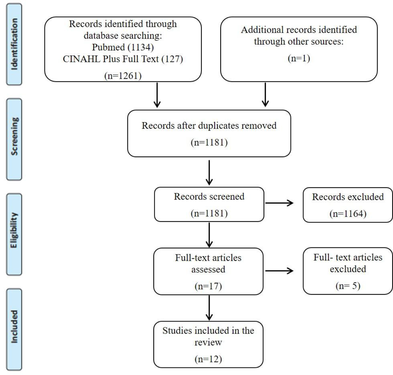
The database searches provided a total of 1180 citations after duplicates were removed. One additional citation was found in the reference list review. A total of 17 papers met the inclusion criteria, based on the titles and abstracts. The full-text, of these 17 citations, were obtained and read, and 5 of them were excluded for the following reasons: only assessing skeletal muscle before treatment (n=1), only assessing phase-angle variations during radiotherapy (n=1), only assessing nutrition status, phase-angle and body weight (n=1), patients received exercise training, during and after treatment (n=2), which may serve as a possible confounding for changes body weight or lean body mass. A total of 12 studies were included in this review. A flowchart showing the study selection process is detailed in Figure 1.

NDN-19-101- Paula Ravasco_F1

Figure 1. PRISMA flow chart for the scoping review process.

From: Moher D, Liberati A, Tetzlaff J, Altman DG, The PRISMA Group (2009). Preferred Reporting Items for Systematic Reviews and MetaAnalyses: The PRISMA Statement. PLoS Med 2009; 6 (7): e1000097

Characteristics of Study Design and Data Collection

The review reports found from 12 studies published from 2004 to 2018, had been conducted almost worldwide: China (2) [17, 18] Netherlands (2) [14, 19], United States of America (3) [8, 20, 21] Turkey (1) [22], Brazil (1) [23], Spain (1) [2], Canada (1) [24] and Sweden (1) [25]. A summary of the characteristics of studies included are described in Appendix III. The population size for the included studies ranged from 202to 215 participants [8] comprising a total of 891 HNC patients (75, 3% male; 24, 7% female), over 18 years old. Ten studies had used a prospective cohort design [2, 14, 17, 18-21, 22-25] and two studies had used a retrospective cohort design [8, 20].

Body Composition Changes (Concept)

BC analysis included variables such as: LBM, measured by five studies [8, 17, 19-21] FFM measured by five studies [2, 14, 18, 23, 25] two of which estimated fat-free mass index (FFM (kg) divided by body height2 (m2)) [18, 25]. Fat mass/adipose tissue were measured by seven studies [8, 17, 18, 19, 22-24] one of which estimated fat mass index (FM (kg) divided by body height2 (m2)) [18], and another estimated subcutaneous fat [22].. Skeletal muscle was measured by two studies, normalized for height in meters squared, reported by skeletal muscle index (SMI) [18, 24]. Reviewing the articles and synthesizing findings from baseline to the end of treatment, all studies reported BC changes, especially loss of LBM or FFM. Appendix IV shows the BC changes reported from the baseline to the end of treatment. The BC analysis data collected at baseline were set as the reference to analyses whether significant changes were observed at different measurement points. One study [2] reported a positive change in FFM during induction chemotherapy (iCT), which increased until the begin of concomitance treatment, and then declined significantly, while another study [21] reported also a positive change during iCT, but this was related to weight gain and not specifically to FFM. The greatest change in body mass occurred in LBM at 1-month post-concurrent chemoradiotherapy (CRT). The loss in LBM occurred despite dietary consumption, and reduced significantly for all body compartments: arms, legs, and trunk [21]. One study [25] reported a decrease of FFM of 6, 5 kg in >10% weight loss group, and 2, 7 kg in ≤ 10% weight loss group. One study [24] including 28 HNC patients found that approximately half of lost body weight was attributed specifically to muscle loss (3.4 kg) and the other half could be explained by 3.6 kg fat loss, both visceral and subcutaneous adipose tissue. The same results were reported in another the study [19], where LBM significantly declined during treatment, corresponding a sixty-two percent of weight loss. However, there were no significant changes between first and second post treatment assessment, which is in agreement with the results found by the same authors, but in a more recent study14 showing a significant decline in FFM (p<.05) during the treatment period but remaining stable 4 months after the end of treatment. One study [17] reported a significant decline in body fat mass and LBM at the different time points after radiotherapy (RT) compared with pre-RT. During the recovery time from the end of treatment to 6 months post-RT, lean body mass remained largely static, whereas body fat mass continued to decrease. Two studies [7, 20] reported different results by sex. In men, a significantly dropped of LBM post-treatment compared with pre-treatment was found, decreased from @ 58kg to @ 51kg after RT, whereas mean estimated LBM in women remained fairly stable, decreasing from @ 38.0 kg to @ 36 kg RT. Additionally, another study [8] reported that the mean fat mass dropped in both men and women after treatment. Two studies [22, 23] showed that TST measurements significantly deteriorated in the end of RT, what means a significant loss of subcutaneous fat, corroborated by BIA analysis, which demonstrated a significant reduction in body fat and FFM, which continued to decline one month after the end of treatment [23]. One study [18] reported statistically and clinically significant changes also in fat mass, FFM, and SMM, during concurrent CRT.  Synthesizing these findings shows how HNC patients suffer from serious LBM, skeletal muscle, body fat or FFM loss, during and after treatment compared with baseline.

Body composition assessment methods

In five studies [2, 14, 18, 23] BC was assessed by BIA, two of which also used DEXA [14] or TSF [23], respectively. In three studies [8, 20, 24] the assessment method was CT, at the level of the third lumbar (L3) vertebra. DEXA, as a single measurement, was applied in other three studies [17, 19, 21] and in one study [22] BC was assessed by TSF. One study [2] considered BIA as a method with good application consistency in patients with locally advanced HNC providing useful information, especially for evaluating FFM, since these patients do not have image of L3 at the CT available in a regular daily basis. However, also referred that the validity and interpretation of maintenance in FFM through the treatment in his study, need to be taken cautiously as the BC values were estimated from changes in voltage across the body. In another study [17] on nasopharyngeal cancer patients managed in Hong Kong, the authors did not find a systematic difference between BIA and DEXA measures, although the BIA had slightly underestimated FFM by <1 kg, both pre- and post-treatment, and accordingly to these results, one study [18] in locally advanced nasopharyngeal carcinoma patients showed that BC assessed by BIA could reflect the change of nutritional status when compared with other methods such as DEXA. One study [8] including HNC patients (various tumor subsites) recommended routine use of quantitative imaging (CT and DEXA) in HNC patients, especially in those prone to changes in nutritional status, as opposed to general population-based height-weight formulae, because the last are not sufficient for body mass quantification. One study [22] used triceps skinfold thickness (TSF) to estimate subscutaneous fat in a series of 54 HNC patients. This is a inexpensive and non-invasive method, and it is widely available [13]. On the other hand, eight studies [17, 19-25] did not report any advantage or disadvantage of using BIA, L3 image at CT, TSF or DEXA. In summary, these findings show that BIA has the great advantage for being available on a regular basis for assessing BC in HNC patients, is inexpensive, noninvasive, and it is a good method to be applied when no imaging techniquesare available. Further, it can be performed by a clinical dietitian [18] if the protocol is followed.

Discussion

This scoping review report’s findings from 12 articles identified through a systematic literature search, published over a 14-year period, that investigated or described the BC changes in HNC patients under active oncological treatment, with curative intent. The patient group with surgical treatment approach was not included in this review for uniformity reasons, as this would have increased the heterogenous nature of the patient population. In general, the studies displayed different oncological treatment modalities, the sample sizes in the retrospective studies suffer from dropout, and the prospective studies from small samples. The studies included in this scoping review also comprised different ‘’measurement points’’, evaluated different components of BC, as well as the methods to assess it in HNC patients, which makes it challenge to synthesizing findings. Studies of human BC using CT scans have provided proof-of-concept that variability in drug disposition and toxicity profiles may be partially explained by different features in BC [26]. The depletion of skeletal muscle before and after RT is strongly associated with decreased survival in patients with solid tumors [20], a higher risk for complications and reduced response to cancer treatment [19]. BC analysis results indicated that the BC components, such as LBM, FFM, body fat and skeletal muscle, change at different measurement points, and that these changes in HNC patients, receiving RT, cannot be effectively monitored by measuring their weight, and BMI [27].. Two studies [19, 24] reported a loss of LBM corresponding to more than half the weight lost, showing that weight loss itself poorly predicts outcome in HNC patients [8]. Low dietary intake due to treatment related nutrition impact symptoms seems to be one of the main contributing factors for muscle loss in HNC patients, because they not meet the recommended calorie and protein intake. In additional to low dietary intake, inflammation could exacerbate muscle loss during cancer treatment [24], as well as impairments in physical performance, contributing to aberrant changes in BC [20]. However, there was a positive change in FFM during iCT [2], reported by Arribas et al. (2017), which may be related to the improvement of the symptoms that initially limited the oral intake and could contribute to minimize further deterioration, proving the role of the nutritional intervention from the beginning of the treatment [2]. Besides these two studies, and this specific measurement point, all the studies included in this review reported loss of LBM, FFM, fat mass and skeletal muscle during the treatment. Post-treatment nutritional deterioration is evident among HNC patients in all included studies, occurring up to 8-12 months during follow-up, although there appears to be a slight recovery. Different findings were observed between Jager-Wittenaar et al (2010) and Kenway et al. (2004) related to body-weight increase after treatment. Jager-Wittenaar et al. (2010) reported a weight gain, characterized by increase of fat mass instead of FFM, while Kenway et al. (2004) found a continously decline of body fat after treatment. Changes in BC after cancer treatment warrant further investigation as this phenomenon might affect recovery from therapy-related side effects and more importantly, even prevent complications. A systematic review by Correia et al.(2019) addressing the methods for BC assessment in clinical settings found that the reference methods for BC assessment in cancer patients are DEXA and L3 in CT imaging, but these examinations are not routinely performed in the management of HNC. This finding is consistent with this review where some authors chose BIA as the preferred method as an alternative to more invasive and expensive methods like DEXA and CT, and because it is available on in routine HNC management. BIA is recommended to be increasingly implemented in nutritional assessment [18]. Citak et al. (2017) used TSF to estimate subscutaneous fat, and only highlight advantages for its use, because all anthropometric measurements were performed by the same person [22]. However, poorer accuracy and precision in obese/oedematous individuals [28], and its sensitive to technician skills, type of calliper and prediction equations used it [13], need to be taken into account. All the BC changes that occur during management of HNC patients, as well as choosing the most feasible, accurate and practical method to assess these changes, represents a challenge for further investigation, in order to assess and improve nutritional status, and disease-associated processes.

Limitations of the review

Although the quality of data extracted was not appraised before inclusion, since it is not relevant for a scoping review, some limitations should be reported so as to provide valuable information to future investigation:

The present scoping review is a pragmatic mean of dealing with the lack of evidence available on BC changes in HNC patients under active treatment;

  • The present scoping review aims to use 2 electronic databases and the search has been refined to increase the likelihood of retrieving as many relevant published articles as possible;
  • Only published studies, in English, Portuguese and Spanish in scientific journals were considered eligible for inclusion;
  • A quality assessment of the articles included in the scoping review was not performed;
  • Due to time constraints, the search strategy didn’t include the MeSH term “neoplasms”, what may had excluded some relevant references;
  • The difference in results may be the result of including a heterogeneous group of patients receiving different types of treatment, and of the variability of BC assessment tools;
  • The interval of BC assessment between pre- and post- RT varied, and some patients may have recovered muscle mass during this period whereas other may have continued to lose muscle mass after the end of treatment;
  • The variability in quality of imaging, which may affect skeletal muscle mass, contouring and adipose tissue segmentation.

Conclusion

HNC patients experience a significant depletion of LBM, FFM and skeletal muscle, accompanied by body fat mass, while undergoing (chemo) radiotherapy, demonstrated either by the TSF, BIA, DEXA or CT. This loss has a significant impact on their survival, quality of life, on the risk for complications and may result in a reduced response to cancer treatment. Thus, BC assessment should become an integral component of the care of HNC patients, beyond weight and BMI, and should be carried out at different times throughout treatment. Based on this review, further investigations are recommended applying measurements at same time points and assessing BC changes with comparable methods in order to obtain evidence for the impact of body composition changes in this patient population.

Appendix I – Search Strategy

PubMed – search conducted on 10/07/2019

Search Strategy

Results

(((“Head and Neck Neoplasms”[Mesh] OR (head[Title/Abstract] AND Neck neoplasms[Title/Abstract])) OR (Head[Title/Abstract] AND neck cancer[Title/Abstract])) AND (((((((((“Muscle, Skeletal”[Mesh] OR (“muscle, skeletal”[MeSH Terms] OR (“muscle”[All Fields] AND “skeletal”[All Fields]) OR “skeletal muscle”[All Fields] OR (“muscle”[All Fields] AND “skeletal”[All Fields]) OR “muscle, skeletal”[All Fields])) OR (“Adipose Tissue”[Mesh] OR Adipose Tissue[Title/Abstract])) OR (“Adiposity”[Mesh] OR Adiposity[Title/Abstract])) OR (“Body Composition”[Mesh] OR body composition[Title/Abstract])) OR (“Body Mass Index”[Mesh] OR Body Mass Index[Title/Abstract])) OR (“Weight Loss”[Mesh] OR weight Loss[Title/Abstract])) OR (“Weight Gain”[Mesh] OR Weight Gain[Title/Abstract])) OR (Body Weight Changes[Title/Abstract] OR “Body Weight Changes”[Mesh])) OR (“Body Weight”[Mesh] OR Body Weight[Title/Abstract]))) AND ((((((“Chemoradiotherapy, Adjuvant”[Mesh] OR Adjuvant Chemoradiotherapy[Title/Abstract]) OR (“Chemoradiotherapy”[Mesh] OR Chemoradiotherapy[Title/Abstract])) OR (“Radiotherapy, Adjuvant”[Mesh] OR Adjuvant Radiotherapy[Title/Abstract])) OR (“Chemotherapy, Adjuvant”[Mesh] OR Adjuvant Chemotherapy[Title/Abstract])) OR (“Radiotherapy”[Mesh] OR Radiotherapy[Title/Abstract])) OR (“Antineoplastic Agents”[Mesh] OR Chemotherapy[Title/Abstract])) AND (hasabstract[text] AND (“2000/01/01”[PDAT] : “3000/12/31”[PDAT]) AND “humans”[MeSH Terms] AND (English[lang] OR Portuguese[lang] OR Spanish[lang]))

1134

Appendix II: Data extraction instrument

Scoping Review Title: Body composition changes in head and neck cancer patients under active treatment: a scoping review

Review Objective/s: Examine and map the body composition changes in head and neck cancer patients, under active treatment, and determine which methods are used to assess body composition in these patients.

Review Question/s:

  1. What do we known from the existing literature about the changes in BC in head and neck cancer patients under active treatment?
  2. Which methods are useful for assessing BC changes in head and neck cancer patients under active treatment?
  3. What are their strengths and weaknesses, reported by the authors?

Inclusion/Exclusion Criteria

Population: Head and neck cancer patients, aged 18 years or older, who have not been submitted to any training or dietary program.

Concept: Body composition changes.

Context: Treatment: This include antineoplastic agents, chemotherapy, adjuvant chemotherapy, radiotherapy, adjuvant radiotherapy, chemoradiotherapy and adjuvant chemoradiotherapy.

Types of Study: Only published studies, both quantitative and qualitative data, and systematic reviews, with abstract available.

Study Details and Characteristics

Author/Year_____________________________________________________________

Aims/Purpose of the study__________________________________________________

Sample Size_____________________________________________________________

Study design_____________________________________________________________

Type of treatment_________________________________________________________

Measurement points_______________________________________________________

Component(s) of body composition evaluated___________________________________

Body composition assessment method_________________________________________

Main results/findings_______________________________________________________

Appendix III: C haracteristics of Study Design and Data Collection

Author(s)/ Year of publication

Aims/ Purpose of the study

Sample Size/Stage

Study Design

Type of treatment

Measurement Points

Component(s) of body composition evaluated

Body composition assessment method

Main results/findings

Arribas et al2 2017

To evaluate changes in BC and nutritional status that occur throughout the oncological treatment in HNC patients

N = 20 HNSCC (Men = 19; women = 1)

Prospective cohort study

iCT flollowed by CRT or RT plus Cetuximab

Baseline Post iCT; After RT;

1 month post RT; 3 months post RT

Fat Free Mass

BIA

FFM decrease significantly over the course of treatment, but after the iCT there was an increase in FFM

Silander et al25 2012

To identify predictors of malnutrition at time of diagnosis in order to identify patients at risk and enable early nutritional support and prevent malnutrition

N = 119 Pharyngeal cancer, oral cancer, or unkwon primary with malignant neck nodes in stage III ou IV

(Men = 81; women = 38)

Prospective cohort study

Chemotherapy and RT, or surgery followed by RT

Baseline; After 5 months follow up

Fat Free Mass

BIA

The decrease of FFM was more than twofold for the malnourished patients, applying a definition of >10% weight loss compared to the non-malnourished during the 6-month time period, 6.5 kg versus 2.7 kg

Nejatinamini et al24 2018

To assess changes in vitamin status during HNC treatment in relation to BC, inflammation and mucositis

N = 28 HNSCC of the oral cavity, pharynx and larynx (Men = 23; women = 5)

Prospective cohort study

RT, with or without chemotherapy

Baseline; Post treatment (=6 months)

Skeletal muscle and body fat

Computed tomography at the level of the third lumbar (L3) vertebra

Approximately half of lost body weight was attributed specifically to muscle loss (3.4 kg) and the other half could be explained by 3.6 kg fat loss. Patients experienced a significant decrease in both visceral and subcutaneous adipose tissue

Kenway et al17 2004

To investigate the nutritional status of NPC patients before and after RT and the factors affecting nutritional by examining the relation among changes in body weight, BC, and basal metabolic rate; calorie intake; and total energy expenditure and adjusting for tumor stage, patient age, and gender

N = 38 Nasopharynx cancer (Men = 30; women = 8)

Prospective cohort study

Radiotherapy

Baseline;

post-RT;

2 months post RT; 6 months post RT

Body Fat and lean body mass

DEXA

Body fat mass and lean body mass at the different time points post-RT were all significantly lower than that at pre-RT. During the recovery time from end-RT to 6 months post-RT, lean body mass remained largely static, whereas body fat mass continued to decrease

Jager-Wittenaar eta I19 2010

To test whether nutritional status (including body weight, lean mass, and fat mass) of patients with head and neck cancer changes during and after treatment

N = 29 HNSCC of the oral cavity, pharynx and larynx (Men = 23; women = 6)

Prospective cohort study

Radiotherapy, either alone or combined with chemotherapy or surgery

1 week before treatment;

1 month posttreatment;

4 months posttreatment

Lean body mass and fat mass

DEXA

Body weight, BMI, and lean mass significantly declined during treatment. Sixty-two percent of weight loss was loss of lean mass. Lean mass declined significantly in all body regions

Grossberg et al20 2016

To determine whether lean body mass before and after RT for HNSCC predicts survival and locoregional control

N = 190 HNSCC (Men = 160; women = 30)

Retrospective cohort study

Primary surgery, single-modality RT or concurrent CRT

Before and after RT (= 8-12 months)

Lean body mass

Computed tomography at the level of the third lumbar (L3) vertebra

In Men, mean estimated LBM decreased from 58.4kg to 51.6kg after RT, whereas mean estimated LBM in women remained fairly stable, decreasing from 38.0 kg to 35.7 kg after RT

Citak et al22 2017

To assess the nutritional status and to define its determinants in patients with HNC undergoing RT

N = 54 HNC (Men = 49; women = 5)

Prospective cohort study

RT, with or without chemotherapy, after surgery, or not.

Baseline After RT;

1 month post RT; 3 months post RT

Subcutaneous fat

Triceps Skinfold Thickness (TST)

TST measurements were significantly deteriorated in the end of RT

Silver et al21 2006

To determine changes in body mass and BC in relation to energy balance, inflammatory state, and physical function before and after concurrent CRT

N = 70 HNSCC of the oral cavity, hipopharynx and larynx (Men = 15; women = 55)

Prospective cohort study

Concurrent CRT

Baseline;

1 month post CRT

Lean body mass

DEXA

The greatest change in body mass occurred in LBM at 1- month postconcurrent CRT. The loss in LBM occurred despite dietary consumption, and reduced significantly for all body compartMents: arms, legs, and trunk.

Carvalho et al23 2013

To examine the involveMent of antitumor treatment, including surgical resection and/or CRT, in the nutritional and metabolic status of patients with SCCHN

N= 32 HNSCC (Men = 31; women = 30)

Prospective cohort study

CRT, with or without previously surgery

10 to 20 days before the beginning of CRT; 30 to 40 days after finishing CRT

Body fat and FFM

BIA

There was significant reduction in body fat and FFM. The weight loss was accompanied by a significant reduction in body fat percentage calculated from TST and BIA

Ding et al18 2018

To investigate BC changes in patients with nasopharyngeal carcinoma undergoing concurrent CRT and a comparison of the Patient-Generated Subjective Global assessment (PG_SGA) and the ESPEN (European Society for Clinical Nutrition and Metabolism) diagnostic criteria as evaluation methods.

N = 48 Nasopharyngeal Carcinoma (Men = 36; women = 12)

Prospective cohort study

Concurrente CRT, with or without iCT

Baseline; weekly until the end of treatment

Fat mass, FFM and skeletal muscle

BIA

During concurrent CRT, there were statistically and clinically significant changes in most BC parameters, including body cell mass, fat mass, FFM, and SMM, as well as body weight, BMI, and PG-SGA scores

Chamchod et al8 2016

To determine if one or more height-weight formula(e) can be clinically used as a surrogate for direct CT- based imaging assessment of BC before and after RT for HNC patients, who are at risk for cancer and therapy- associated cachexia/sarcopenia.

N = 215 HNC (Men = 184; women = 31)

Retrospective cohort study

Concurrent chemotherapy or RT, with or without surgery

Pre- and posttreatment

Lean body mass

Computed tomography at the level of the third lumbar (L3) vertebra

Mean LBM dropped significantly posttreatment compared to pre-treatment for Men but didn’t reach statistical significance in women. Additionally, mean fat mass dropped in both Men and women after treatment

Jager-Wittenaar et al14 2014

To validate BIA using the Geneva equation for FFM in HNC patients

N = 24 HNC (Men = 20; women = 4)

Prospective cohort study

RT, with or without chemotherapy, or after surgery

The week before the treatment;

1 month after treatment;

4 months treatment

Fat Free Mass

DEXA and BIA

Body weight, BMI, FFM, volume of body fluids, phase angle, and impedance ratio significantly declined during the treatment period . There was no systematic difference between the BIA and DXA measurements.

Appendix IV: BC changes reported from the baseline to the end of treatment

Author(s)

Body composition assessment method

Component(s) of body composition evaluated

Baseline

Post iCT

Post RT

1-2 months post treatment

3-4 months post treatment

5-6 months post treatment

8-12 months post treatment

Arribas et al2

BIA

Fat free mass (kg)*

53,69 (8,16)

55,96 (9,06)

51,54 (5,89)

52,08 (6,70)

50,05 (7,66)

Silander et al25

BIA

Fat free mass index*

(2,6)
(WL S 10% group)
(2,7)
(WL > 10% group)

– 2,7 kg FFM (WL < 10% group) -6,5 kg FFM (WL > 10% group)

Nejatinamini et al24

Computed

Skeletal muscle index (cm2/m2)*

52,6 (11,1)

45,5 (9,1)

tomography

Body fat (kg)*

28,3 (8,1)

24,7 (6,9)

Kenway et al17

DEXA

Lean body mass (kg)*

46,2 (8,3)

42,1 (7,8)

42,8 (7,6)

43,3 (7,5)

Body fat (kg)*

15,1 (4,9)

12,4 (4,7)

10,9 (3,8)

10,4 (3,5)

Jager-Wittenaar

DEXA

Lean body mass (kg)*

54,6 (11,4)

52,1 (10,7)

52,3 (10,3)

et al 19

Body fat (kg)*

20,0 (9,8)

18,9 (8,1)

19,0 (7,0)

Grossberg et al20

Computed

tomography

Lean body mass (kg)*

58,4 (9,6) (men) 38,0 (7,3) (women)

51,6 (7,8) (men) 35,7 (6,6) (women)

Citak et al22

Triceps Skinfold Thickness (TST)

Subcutaneous fat (mm)*

21,79 (4,47)

21,31 (3,98)

21,5 (3,93)

21,81 (4,00)

Silver et al21

DEXA

Lean body mass (kg)*

52,25 (11,33)

46,64 (96,52)

Carvalho et al23

Triceps Skinfold Thickness (TST)

Subcutaneous fat (mm)*

10,84 (5,78)

8,41 (4,56)

BIA

Body fat (%)*

27,27 (7,44)

23,36 (7,70)

Fat free mass (kg)*

48,30 (9,84)

45,90 (8,75)

Fat mass index (kg2/m2)*

7,66 (1,99)

6,61(1,87)

Ding etal18

BIA

Fat free mass index (kg2/m2)*

15,79 (1,82)

14,79 (2,02)

Skeletal muscle (kg)*

24,47 (6,01)

22,93 (5,86)

Chamchod et al8

Computed

Lean body mass (kg)*

58,0 (9,69) (men) 37,56 (7,0) (women)

51,52 (8,31) (men) 36,2 (7,13) (women)

tomography

Body fat (kg)*

18,48 (1,36) (men) 17,56 (1,16) (women)

15,61 (0,98) (men) 15,42 (1,00) (women)

Jager-Wittenaar

DEXA

Fat Free Mass (kg)*

56,4 (10,9)

54,2 (10,0)

54,4 (9,9)

et al14

BIA

55,7 (10,0)

53,9 (9,4)

54,4 (9,4)

* Mean, standard deviation WL-Weigh Loss

References

  1. Govender R, Smith CH, Taylor SA, Grey D, Wardle J et al. (2015) Identification of behaviour change components in swallowing interventions for head and neck cancer patients: protocol for a systematic review. Systematic Reviews 4: 89. [crossref]
  2. Arribas L, Hurtós L, Taberna M, Peiró I, Vilajosana E et al. (2017) Nutritional changes in patients with locally advanced head and neck cancer during treatment. Oral Oncology 71: 67–74. [crossref]
  3. Yanni A, Dequanter D, Lechien JR, Loeb I, Rodriguez A et al. (2019)Malnutrition in head and neck cancer patients: Impacts and indications of a prophylactic percutaneous endoscopic gastrostomy. Eur Ann Otorhinolaryngol Head Neck Dis136: 27–33.[crossref]
  4. Formigosa JAS, Costa LS, Vasconselos EV (2018) Social representations of patients with head and neck cancer before the alteration of their body image. Rev Fund Care Online 10: 180–189.
  5. Stenson KM, MacCracken E, List M, Haraf DJ, Brockstein B et al.(2000) Swallowing function in patients with head and neck cancer prior to treatment. Arch Otolaryngol – Head Neck Surg 126: 371–377. [crossref]
  6. Arends J, Bachmann P, Baracos V, Barthelemy N, Bertz H et al. (2017) ESPEN guidelines on nutrition in cancer patients. ClinNutr 36: 11–48. [crossref]
  7. Van Liew J, Brock R, Christensen A, Karnell, L, Pagedar N et al. (2017) Weight loss after head and neck cancer: A dynamic relationship with depressive symptoms. Head Neck 39: 370–379. [crossref]
  8. Chamchod S, Fuller C, Mohamed A, Grossberg A, Messer J et al. (2016) Quantitative Body Mass Characterization Before and After Head and Neck Cancer Radiotherapy: A Challenge of Height-Weight Formulae Using Computed Tomography Measurement. Oral Oncology 61: 62–69. [crossref]
  9. Marshall KM, Loeliger J, Nolte L, Kelaart A (2018) Prevalence of malnutrition and impact on clinical outcomes in cancer services: A comparison of two time points. ClinNutr 38: 1–8. [crossref]
  10. Couch MEDittus KToth MJ, Willis M, Guttridge D et al. (2015) Cancer cachexia update in head and neck cancer: Definitions and diagnostic features. Head Neck 37: 594–604. [crossref]
  11. Fearon K, Strasser F, Anker SD, Bosaeus I, Bruera E et al. (2011) Definition and classification of cancer cachexia: an international consensus. Lancet Oncol 12: 489–495. [crossref]
  12. Deluche E, Leobon S, Desport JC, Venat-Bouvet L, Usseglio J et al. (2018) Impact of body composition on outcome in patients with early breast cancer. Support Care Cancer 26: 861–868. [crossref]
  13. Correia I, Neves P, Makitie A, Ravasco P (2019) Body Composition evaluation in Head and Neck Cancer Patients: A Systematic Review (2019) Under Review in Frontiers in Nutrition.
  14. Jager-Wittenaar H, Dijkstra PU, Earthman CP, Krijnen W, Langendijk J et al. (2014) Validity of bioelectrical impedance analysis to assess fat-free mass in patients with head and neck cancer: an exploratory study. Head Neck 36: 585–591. [crossref]
  15. Chang HC, Lin YC, Ng SH, Cheung YC, Wang CH et al. (2019) Effect of Chemotherapy on Dual-Energy X-ray Absorptiometry (DXA) Body Composition Precision Error in Head and Neck Cancer Patients. J Clin Densitom 22: 437–443. [crossref]
  16. Peters MD, Godfrey CM, McInerney P, Soares CB, Khalil H et al. (2015) Joanna Briggs Institute Reviewers’ Manual 2015: Methodology for JBI Scoping Reviews. South Australia: The Joanna Briggs Institute.
  17. Ng K, Leung SF, Johnson PJ, Woo J (2004) Nutritional Consequences of Radiotherapy in Nasopharynx Cancer Patients. Nutrition and Cancer 49: 156–161. [crossref]
  18. Ding H, Dou S, Ling Y, Zhu G, Wang Q et al. (2018) Longitudinal Body Composition Changes and the Importance of Fat-Free Mass Index in Locally Advanced Nasopharyngeal Carcinoma Patients Undergoing Concurrent Chemoradiotherapy. Integr Cancer Ther 17: 1125–1131. [crossref]
  19. Jager-Wittenaar H, DijkstraPU, Vissink A, Langendijk JA, van der Laan BF et al. (2010) Changes in nutritional status and dietary intake during and after head and neck cancer treatment. Head & Neck 33: 863–870. [crossref]
  20. Grossberg AJ, Chamchod S, Fuller CD, Mohamed ASR, Heukelom J et al. (2016) Association of body composition with survival and locoregional control of radiotherapy-treated head and neck squamous cell carcinoma. JAMA Oncol 2: 782–789. [crossref]
  21. Silver HJ, Dietrich MS, Murphy BA (2007) Changes in body mass, energy balance, physical function, and inflammatory state in patients with locally advanced head and neck cancer treated with concurrent chemoradiation after low-dose induction chemotherapy. Head & Neck 29: 893–900. [crossref]
  22. Citak E, Tulek, Z, Uzel O (2018) Nutritional status in patients with head and neck cancer undergoing radiotherapy: a longitudinal study. Supportive Care in Cancer. Support Care Cancer 27: 239–247. [crossref]
  23. De Carvalho TMR, Miguel Marin D, da Silva CA, de SouzaAL, Talamoni M (2014) Evaluation of patients with head and neck cancer performing standard treatment in relation to body composition, resting metabolic rate, and inflammatory cytokines. Head & Neck 37: 97–102. [crossref]
  24. Nejatinamini S, Debenham BJ, Clugston RD, Mawani A, Parliament M et al. (2018) Poor vitamin status is associated with skeletal muscle loss and mucositis in head and neck cancer patients. Nutrients 10. [crossref]
  25. Silander E, Nyman J, Hammerlid E (2013) An exploration of factors predicting malnutrition in patients with advanced head and neck cancer. Laryngoscope 123: 2428–2434. [crossref]
  26. Prado CMM (2013) Body composition in chemotherapy: The promising role of CT scans. CurrOpinClinNutrMetab Care 16: 525–533. [crossref]
  27. Tang PL, Wang HH, Lin HS, Liu WS, Chen LM et al. (2018) Body Composition Early Identifies Cancer Patients with Radiotherapy at Risk for Malnutrition. Journal of Pain and Symptom Management 55: 864–871. [crossref]
  28. Wells JCK, Fewtrell MS (2006) Measuring body composition. Arch Dis Child 91: 612–617.

Food industry wastewaters and Nutrition, Dietetics & Nutraceuticals

DOI: 10.31038/NDN.2019111

Editorial

I am pleased to present the inaugural issue of the journal of Nutrition, Dietetics & Nutraceuticals (NDN) from the open access international publishing house Research Open World. NDN provides a platform covering in an interdisciplinary manner all areas of Nutrition, Dietetics & Nutraceuticals. The goal of NDN is to publish actual, original and high-quality research articles, reviews, and short communications, which can be divided into three categories: The science of nutrition, Community Nutrition and Therapeutic nutrition and dietetics.

Specific studies and developments of interest for the journal comprise Nutrition and Food Sciences and Food Biotechnology. Food industry uses extensively a high quantity of water in the industrial processes, namely, heating and cooling systems and washing of equipment and facilities. Consequently, it produces a large quantity of problematic wastewaters. Food industry wastewaters constitute a complex subject for the environment and public health due to the presence of high concentrations of organic matter monitored by chemical oxygen demand (COD), biochemical oxygen demand (BOD) and total organic carbon (TOC), salinity (high conductivity values), total and suspended solids and nutrients (calcium, magnesium, phosphorus, potassium, sodium and chloride). Food industry wastewater can be responsible for soil contamination, accumulation of toxic compounds in ecosystems, eutrophication phenomena, rapid oxygen depletion, and surface and groundwater contamination. Within this type of wastewater, it can be highlighted the dairy, winery, slaughterhouse and olive oil mill wastewater. However, appropriate and innovative treatment processes are required. Conventional treatment processes of food industry wastewaters are based on biological principles, for instance, aerobic [1, 2] and anaerobic [3] digestion and wetlands [4]. However, these biological processes have some limitations. Several physicochemical processes have been applied in order to reduce organic and inorganic contamination, for example, coagulation−flocculation with FeSO4, Al2(SO4)3, and FeCl3 for cheese whey wastewater [2] and winery wastewater [5], coagulation with chitosan, starch, alum and ferric chloride for olive oil wastewater [6], acid precipitation with H2SO4, HNO3 and HCl for cheese whey and slaughterhouse wastewater [7, 8], basic precipitation with NaOH and Ca(OH)2 for cheese whey wastewater [9, 8], oxidation with Ca(ClO)₂, H2O2 and CaO₂ for slaughterhouse wastewater [7], Fenton-like oxidation system for pretreated cheese whey wastewater [10], ozone-based advanced oxidation processes (O3, O3/UV and O3/UV/H2O2) for winery wastewater [11], photocatalytic/photolytic reactor system for winery wastewater [12], solar photochemical for winery wastewater [13], electrochemical advanced oxidation [14]  and solar driven advanced oxidation [15] for the pretreated winery wastewater, use of clay–polymer nano composites for olive oil mill and winery wastewater [16], reverse osmosis for winery wastewater [17], electrolysis system for olive oil mill wastewater [18], electro-coagulation for olive oil mill wastewater [19] and slaughterhouse wastewater [20], Fenton’s Reagent for olive oil mill wastewater [21], conductive-diamond electrooxidation (CDEO), ozonation and Fenton oxidation for olive oil mill wastewater [22] and alkaline and enzymatic hydrolysis for slaughterhouse wastewater [23]. The application of these effluents on the soil can also be an alternative [24, 25]. However, some precautions should be taken when these effluents are applied at long-term. Thus, NDN can receive important works in the area of biological and physicochemical treatment, recovery and reuse of the food industry wastewaters.

Thank you for your contribution to the Journal of Nutrition, Dietetics & Nutraceuticals

Sincerely,
Ana R. Prazeres

Acknowledgments

The author thanks to the Alentejo Regional Operational Program (ALENTEJO 2020, Portugal 2020) for the financing of the HYDROREUSE project – Treatment and reuse of agro-industrial wastewater using an innovative hydroponic system with tomato plants (ALT20-03-0145-FEDER-000021), through the Regional Development European Fund (FEDER).

References

  1. Petruccioli M, Duarte JC, Eusebio A, Federici F (2002) Aerobic treatment of winery wastewater using a jet-loop activated sludge reactor. Process Biochemistry 37: 821–829.
  2. Rivas J, Prazeres AR, Carvalho F, Beltrán F (2010) Treatment of Cheese Whey Wastewater: Combined Coagulation−Flocculation and Aerobic Biodegradation. Journal of Agricultural and Food Chemistry 58: 7871–7877. [crossref]
  3. Yu H, Zhu Z, Hu W, Zhang H (2002) Hydrogen production from rice winery wastewater in an upflow anaerobic reactor by using mixed anaerobic cultures. International Journal of Hydrogen Energy 27: 1359–1365.
  4. Serrano L, de la Varga D, Ruiz I, Soto M (2011) Winery wastewater treatment in a hybrid constructed wetland. Ecological Engineering 37: 744–753.
  5. Braz R, Pirra A, Lucas MS, Peres JA (2010) Combination of long term aerated storage and chemical coagulation/flocculation to winery wastewater treatment. Desalination 263: 226–232.
  6. Meyssami B, Kasaeian AB (2005) Use of coagulants in treatment of olive oil wastewater model solutions by induced air flotation. Bioresource Technology 96: 303–307. [crossref]
  7. Prazeres AR, Fernandes F, Madeira L, Luz S, Albuquerque A et al. (2019) Treatment of slaughterhouse wastewater by acid precipitation (H2SO4, HCl and HNO3) and oxidation (Ca(ClO)2, H2O2 and CaO2). Journal of Environmental Management 250. [crossref]
  8. Prazeres AR, Luz S, Fernandes F, Jerónimo E (2019) Cheese wastewater treatment by acid and basic precipitation: application of H2SO4, HNO3, HCl, Ca(OH)2 and NaOH. Journal of Environmental Chemical Engineering. In press.
  9. Rivas J, Prazeres AR, Carvalho F (2011) Aerobic Biodegradation of Precoagulated Cheese Whey Wastewater. Journal of Agricultural and Food Chemistry 59: 2511–2517. [crossref]
  10. Prazeres AR, Carvalho F, Rivas J (2013) Fenton-like application to pretreated cheese whey wastewater. Journal of Environmental Management 129: 199–205. [crossref]
  11. Lucas MS, Peres JA, Puma GL (2010) Treatment of winery wastewater by ozone-based advanced oxidation processes (O3, O3/UV and O3/UV/H2O2) in a pilot-scale bubble column reactor and process economics. Separation and Purification Technology 72: 235–241.
  12. Agustina TE, Ang HM, Pareek VK (2008) Treatment of winery wastewater using a photocatalytic/photolytic reactor. Chemical Engineering Journal 135: 151–156.
  13. Lucas MS, Mosteo R, Maldonado MI, Malato S, Peres JA (2009) Solar Photochemical Treatment of Winery Wastewater in a CPC Reactor. Journal of Agricultural and Food Chemistry 57: 11242–11248.
  14. Moreira FC, Boaventura RA, Brillas E, Vilar VJ (2015) Remediation of a winery wastewater combining aerobic biological oxidation and electrochemical advanced oxidation processes. Water Research 75: 95–108. [crossref]
  15. Souza S, Moreira FC, Dezotti MWC, Vilar VJP, Boaventura RAR (2013) Application of biological oxidation and solar driven advanced oxidation processes to remediation of winery wastewater. Catalysis Today 209: 201–208.
  16. Rytwo G, Lavi R, Rytwo Y, Monchase H, Dultz S et al. (2013) Clarification of olive mill and winery wastewater by means of clay–polymer nanocomposites. Science of The Total Environment 442: 134–142. [crossref]
  17. Ioannou LA, Michael C, Vakondios N, Drosou K, Xekoukoulotakis NP et al. (2013) Winery wastewater purification by reverse osmosis and oxidation of the concentrate by solar photo-Fenton. Separation and Purification Technology 118: 659–669.
  18. Israilides CJ, Vlyssides AG, Mourafeti VN, Karvouni G (1997) Olive oil wastewater treatment with the use of an electrolysis system. Bioresource Technology 61: 163–170.
  19. Inan H, Anatoly Dimoglo, Şimşek H, Karpuzcu M (2004) Olive oil mill wastewater treatment by means of electro-coagulation. Separation and Purification Technology 36: 23–31.
  20. Asselin M, Drogui P, Benmoussa H, Blais JF (2008) Effectiveness of electrocoagulation process in removing organic compounds from slaughterhouse wastewater using monopolar and bipolar electrolytic cells. Chemosphere 72: 1727–1733.
  21. Rivas FJ, Beltrán FJ, Gimeno O, Frades J (2001) Treatment of Olive Oil Mill Wastewater by Fenton’s Reagent. Journal of Agricultural and Food Chemistry 49: 1873–1880. [crossref]
  22. Cañizares P, Lobato J, Paz R, Rodrigo MA, Sáez C (2007) Advanced oxidation processes for the treatment of olive-oil mills wastewater. Chemosphere 67: 832–838.
  23. Masse L, Kennedy KJ, Chou S (2001) Testing of alkaline and enzymatic hydrolysis pretreatments for fat particles in slaughterhouse wastewater. Bioresource Technology 77: 145–155. [crossref]
  24. Prazeres AR, Carvalho F, Rivas J, Patanita M, Jóse Dôres (2013) Growth and development of tomato plants Lycopersicon Esculentum Mill. under different saline conditions by fertirrigation with pretreated cheese whey wastewater. Water Science and Technology 67: 2033–2041. [crossref]
  25. Sierra J, Martı́ E, Montserrat G, Cruañas R, Garau MA (2001) Characterisation and evolution of a soil affected by olive oil mill wastewater disposal. Science of The Total Environment 279: 207–214.

A Rare Case of Sequelae of Iatrogenic Volkmann Syndrome Successfully Treated by Shortening of the Two Bones of the Forearm

DOI: 10.31038/IJOT.2019255

Abstract

Introduction: Volkmann’s syndrome, usually due to fracture of the forearm bones, is a condition that requires emergency fasciotomy. But the case that we report today is unusual: an ischemic retraction installed following immobilization of the forearm by a traditional splint without any evidence of fracture. To date, at the height of our knowledge, no similar case has been reported. The aim of this work was to show that the shortening of both bones realized is an attractive alternative to treat severe sequelae of this syndrome in our context.

Case Report: He is a 9-year-old boy who fell from games and had a closed trauma to his left forearm. At 3 months post-traumatic when we saw him, we note serious sequelae already installed consisting of wrist flexum and invincible claws fingers. The radiography realized a posteriori was normal. The preoperative electromyogram concludes that the 3 nerves of the forearm have been affected. We performed a shortening of the 2 bones of the forearm with contention by 2 intramedullary pins completed by a plaster splint to maintain the reduction obtained intraoperatively. The radio-clinical and electromyographic control post-operative showed a clear improvement anatomical and functional.

Discussion and Conclusion: The incidence of Volkmann syndrome in upper limb fractures is estimated at 1%. The absence of fractures would promote the diagnostic delay. In this case, two contributing factors were added, a fracture-free contusion treated with a traditional constrictive splint aggravating ischemia. This case of Volkmann syndrome, due in part to ignorance but treated favorably, challenges us in a cultural context where the traditional healer paradoxically enjoys great confidence. Beyond stigma, it is important for us to project the bases of a collaboration in the interest of the patients.

Keywords

Africa, Sequelae, Treatment, Volkmann Syndrome

Introduction

The ischemic retraction syndrome of the hand flexors described by Volkmann in 1881 results from a conflict between the inextensible muscular chambers and the extensible forearm muscles. It is a surgical emergency that requires rapid release of superficial but sometimes deep muscle compartments. It is most often a diaphyseal fracture of the 2 bones of the forearm or a distal fracture of the radius. This syndrome occurs even more often in supra-condylar fractures of the child’s elbow associated with vascular injury. But the case we report today is unusual: it is an ischemic retraction that has occurred following immobilization of the forearm by a traditional healer without any radiological evidence of a fracture. To date, at the best of our knowledge, no similar case has been reported.

Case Report

The 9-year-old boy, who fell to the games, had a closed trauma to his left forearm and was driven, as is often the case in the hinterland,  to a traditional healer. He was then immobilized by a splint of braided bamboo or millet stems as is often the case in our practice conditions (Figure 1). No X-ray was performed to confirm the existence of broken bones in the injured forearm. Faced with the appearance of edema, cutaneous lesions like phlyctens, cutaneous wounds, retraction and paralysis of the fingers, the splint would have been removed but it was too late because the compartments syndrome was already constituted with irreversible sequelae already installed. Unfortunately, this type of complications is not isolated in our environment. We also performed a necrotic finger amputation treated under the same conditions (Figure 2). We received it after about 3 months post-traumatic period. He then had severe sequelae consisting of wrist flexum, severe invincible fingers claw with Metacarpophalangeal (MP) hyper-extension, hyperflexion of Proximal Interphalangeal (PIP) and irreducible Distal Interphalangeal (DIP) joints (Figure 3). The radiography performed on site before the consultation shows that there was no bone lesion that required external restraint (Figure 4).

The compared Electromyogram (EMG) requested preoperatively concludes to an attack of the 3 nerves of the forearm (medial > cubital > radial) with signs of Wallerian degeneration. The involvement is more severe on the left median and the functional prognosis on the physiological basis of this nerve is considered pour. On the left ulnar and the radial nerves, the lesion is less severe with a more favorable recovery prognosis according to the neurologist who performed this examination. We intervened to try a lengthening of the flexors including the short and long palmar which a priori had no effect on the correction of retractions. We resolved to shorten proximal metaphysis of the 2 bones of the forearm and to achieve the internal fixation by 1 respective intramedullary pin at the level of the radius and the ulna. The intraoperative examination shows a good reduction of the retractions, we obtain a passive extension of the wrist, a passive flexion of the MP, an extension, at the limit of the position of function of the PIP and DIP joints of 20 ° and 30 ° respectively. We set up a plaster cast brace to sustain this reduction obtained to keep for 6 weeks. The radiographic assessment of postoperative control is satisfactory (Figure 5). We had the plaster removed and prescribed re-education of the wrist and fingers of the hand. At the last consultation, the function recovered from the wrist and the hand was satisfactory (Figure 6).

IJOT 19 - 131_Giordano S_F1

Figure 1. An example of a traditional splint used to immobilize a fracture of the 2 bones of the leg: we can see the formation of an edema of the foot upstream (white arrow).

IJOT 19 - 131_Giordano S_F2

Figure 2. Ischemic necrosis on contusion without fracture of the 3rd finger treated by traditional splint (white arrows): the finger was amputated.

IJOT 19 - 131_Giordano S_F3

Figure 3. Preoperative appearance of sequelae: scars of skin lesions, wrist flexion, and extension of metacarpophalangeal joints and hyper-flexion of proximal interphalangeal joints.

IJOT 19 - 131_Giordano S_F4

Figure 4. The radiograph performed “a posteriori” shows no fracture lesion that would have required immobilization.

IJOT 19 - 131_Giordano S_F5

Figure 5. The postoperative X-Ray (D 117) showing the shortening of the proximal metaphysis of the 2 bones and contention with intramedullary pins with onset of consolidation.

IJOT 19 - 131_Giordano S_F6

Figure 6. The anatomical (A) and functional (B) result is quite satisfactory especially for large (large objects) and fine (finer objects) pollici-digital grip.

Discussion

The Volkmann syndrome, ischemic retraction of flexors, first described in 1881 by the same one who bears his name, is a relatively rare surgical emergency [1]. This syndrome is most often associated with trauma including fractures, penetrating wounds, contusion of soft tissues, animal or insect bites, infections, reperfusion ischemia or external compression by dressing or plaster, burns or crushing injuries. The incidence of occurrence in upper limb fractures is estimated at 1% [2]. In this case we can think that there are two contributing factors, a fracture-free bruise treated by traditional constrictive splint worsening ischemia: “a chicotte on an abscess” according to a well-known Fulani saying. At this stage, an alcoholic dressing renewed 2 or 3 times a day and nonsteroidal anti-inflammatory drugs and especially a regular follow-up for a few days would have been enough. It should be noted that the absence of a fracture has been considered by some authors as a factor delaying the diagnosis and worsening the prognosis [3,4]. The fractures of the child likely to lead to the syndrome of the lodges of the forearm are essentially the diaphyseal fractures of the 2 bones of the forearm and supra-condylar fractures of the elbow with or without a fracture of the forearm, distal end of the radius in a floating elbow chart [2, 5–7]. Matsen [8] explained that the lodge syndrome has several vascular mechanisms that all contribute to cell necrosis. The clinical diagnosis is characterized by acute pain, poorly localized, not very sensitive to the usual analgesics and culminating 2 to 6 hours after the trauma. The other signs are a hard swelling, renitence, neuro-vascular disorders like pallor of the extremities, abolition of peripheral pulses, paresthesia and paralysis. Treatment of acute ischemic syndrome requires emergency fasciotomy. In this case it is a severe Volkmann syndrome according to the classification of Tsuge [9], at the stage of serious sequelae attributable to a lack of knowledge by the traditional healer of the anatomophysiological mechanisms at the origin of this syndrome. There is a therapeutic arsenal of interest to the soft tissues and the bone. For the soft tissues extensive excision of infarcted tendons with secondary reconstruction [10–12], Z lengthening of contractured tendons [13], tendon transfer [13] has been proposed. We started by lengthening the flexors but we realized that it had little effect on contracture correction. Surgical techniques concerning the bone, proximal carpectomy [13,14], wrist arthrodesis [13,15]. We preferred the shortening of the 2 forearm bones recommended by Rolands et al [16], Domanasiewicz [17], Pavanini and Volpe [18]. All these methods have their disadvantages, in particular the shortening is criticized for having a non-selective effect on both the extensors and the flexors, the worsening of the shortening already favored by ischemia and a high rate of non-union and refracture of the shortening osteotomy site of the 2 forearm bones. It is too early to say about the bone consolidation that we hope will be favorable in children in this case. However, the first current anatomical and functional results are satisfactory and encouraging.

Conclusion

This case of Volkmann syndrome and other similar pathologies that we encounter in our conditions of practice but unimaginable elsewhere in the West, due mainly to ignorance challenge us in a cultural context where however this same traditional healer enjoys great confidence. Beyond stigma, it is important for us to lay the foundations of a bridge to approach us in the interest of patients.

List of abbreviations:

Metacarpophalangeal (MP)

Proximal interphalangeal (PIP)

Distal interphalangeal (DIP)

Acknowledgement

We sincerely thank:

  1. Dr SAÏD HAMDJA for his confidence in referring us this little patient;
  2. All the Managers and Staff of the Maria Rosa Nsisim Foundation of Ahala I in Yaoundé for creating the conditions for the good conduct of this work.

References

  1. Volkmann R (1881) Die ischaemischen muskellaehmungen und kontrakturen. Centrabl f Chir 51: 801.
  2. Grottkau B, Epps H, Di Scala C (2005) Compartment syndrome in children and adolescents. J Pediatr Surg 40: 678–682.
  3. Hope M, Mcqueen M (2004) Acute compartment syndrome in the absence of fracture. J Orthop Trauma 18: 220–224.
  4. Prasam ML, Ouellette EA (2011) Acute compartment syndrome of the upper extremity. J Am Acad Orthop Surg 19: 49–58.
  5. Blakemore L, Cooperman D, Thompson G, Wathey C, Ballock RT (2000) Compartment syndrome in ipsilateral humerus and forearm fractures in children. Clin Orthop Relat Res 376: 32–38.
  6. Kalyani B, Fisher B, Roberts C, Giannoudis PV (2011) Compartment syndrome of the forearm: a systematic review. J Hand Surg [Am] 36: 535–543.
  7. Yuan P, Pring M, Gaynor T, Mubarak SJ, Newton PO (2004) Compartment syndrome following intramedullary fixation of pediatric forearm fractures. J Pediatr Orthop 24: 370–375.
  8. Matsen FA (1975) 3rd Compartmental syndrome. A unifed concept. Clin Orthop Relat Res 113: 8–14.
  9. Tsuge K (1964) Treatment of established Volkmann’s contracture. J Bone Joint Surg Am 57: 925–929.
  10. Seddon H (1964) Volkmann’s ischaemia. Br Med J 1: 1587–1592. 11. Seddon HJ (1956) Volkmann’s contracture: treatment by excision of the infarct. J Bone Joint Surg Br 38: 152–174.
  11. Tsuge K (1975) Treatment of established Volkmann’s contracture. J Bone Joint Surg Am 57: 925–929.
  12. Goldner J (1975) Volkmann’s ischemic contracture. In: Flynn J (ed.). Hand surgery, New York, Williams & Wilkins, Pg No: 599–618.
  13. Zancolli E (1979) Classifcation of established Volkmann’s ischemic contracture and the program for its treatment. In: Zancolli E (ed.). Structural and dynamic bases of hand surgery, Philadelphia, JB Lippincot.
  14. Botte MJ, Fronek J, Pedowitz RA, Hoenecke HR Jr, Abrams RA, et al. (1998) Exertional compartment syndrome of the upper extremity. Hand Clin 14: 477–482.
  15. Rolands R, Lond M (1905) A case of Volkmann’s contracture treated by shortening of the radius and ulna. Lancet 2: 1168–1171.
  16. Domanasiewicz A, Jabłecki J, Kocieba R, Syrko M (2008) Modifed Colzi method in the management of established Volkmann contracture–the experience of Trzebnica Limb Replantation Center (preliminary report). Ortop Traumatol Rehabil 10: 12–25.
  17. Pavanini G, Volpe A (1975) [Diaphysary resection using Colzi’s method in the treatment of Volkmann’s syndrome]. Clin Ortop 26: 287–292.

Urinary Prothrombin Fragment 1 + 2 as an Endogenous Marker of Venous Thromboembolism

DOI: 10.31038/IMROJ.2019424

Abstract

Hypercoagulability may lead to Venous Thromboembolism (VTE) which is a common and potentially fatal disease. The symptoms of VTE are often non-specific and imaging is needed to confirm the diagnosis. Clinical probability models together with a D-dimer test are used to reduce the number of unnecessary radiological procedures. Numerous assays to detect thrombin generation have been developed where D-dimer measured in plasma is regarded as the pretest gold standard. The aim of this manuscript is to outline the present knowledge of using urinary prothrombin fragment 1 + 2 (F1 + 2) as a marker to determine coagulation activation in patients at risk of Deep Vein Thrombosis (DVT) or Pulmonary Embolism (PE). Papers were identified by searching PubMed for studies in which F1 + 2 were measured in urine to determine coagulation activity in patients at risk of venous thromboembolism. Urinary F1 + 2 levels can be used to identify patients at risk of VTE after hip and knee replacement surgery. Further, it reflects thrombin generation in patients with imaging verified DVT. However, in patients with imaging verified PE, the F1 + 2 levels were not increased compared to those without PE. Compared to D-dimer and F1 + 2 measured in plasma, urinary F1 + 2 was inferior at discriminating VTE. Contrary to the mentioned results, in one study on patients undergoing total hip arthroplasty, urinary F1 + 2 did not reflect post-operative coagulation activation. Urine may be an attractive substrate to detect ongoing coagulation activation. However, tests specifically meant for urine analyses must be further developed.

Keywords

Venous thromboembolism, Prothrombin Fragment 1 + 2, Urine

Introduction

The major pathological determinants for venous thrombosis formation were postulated by Rudolph Virchow in 1856 and are known as Virchow`s triad. These factors include vessel wall damage, alterations of blood flow with stasis and abnormalities in platelet, coagulation and fibrinolytic pathways [1]. Venous thromboembolism (VTE), a common and potentially fatal disease which is mainly caused by hypercoagulability, can manifest as deep vein thrombosis (DVT) or pulmonary embolism (PE) [2,3]. Venous thrombi most often occur in the deep leg veins at sites of pathological blood flow or venous stasis, in areas of endothelial damage and in valve pockets [4]. If a clot originates in or propagates to the popliteal vein or more proximal veins, there is an increased risk of embolization to the pulmonary arteries with subsequent variable degrees of obstruction [3].

The precise incidence of VTE is unknown but it is estimated that it affects between 1 and 2 per 1000 of the population annually in the U.S. and that one third of these patients are diagnosed with PE [5]. In 2007, Cohen et al. estimated the number of non-fatal symptomatic VTE events and VTE related deaths in the European Union to be 684,019 DVT events, 434,723 PEs and 543,545 VTE related deaths in a total population of 454.4 million [6]. Venous thromboembolism is a rare condition in children younger than 15 years [7,8]. The incidence of DVT and PE increases with age. For those 65–69 years of age, the incidence per 1000 person years is 1.8. This increases to 3.1 per 1000 person years for those aged 85–89 years [9]. Due to increased use of sensitive imaging techniques which can detect smaller and often insignificant pulmonary emboli, the hospital admissions for this disease have doubled over the last decades [10].

Clinical signs and symptoms of VTE may be obscure. Calf pain, swelling, heat and tenderness are clinical signs of DVT while PE patients may present with dyspnea, chest pain, hemoptysis, hypotension and tachycardia [3]. However, the symptoms are non-specific and DVT can resemble, for example, cellulitis and PE may be indistinguishable from myocardial infarction [10]. Due to the non-specific symptoms, imaging is needed to confirm the diagnosis of DVT or PE. Compression Ultrasonography (CUS) has high diagnostic accuracy for DVT [11]. Computer Tomography (CT) and Magnetic Resonance Imaging (MRI) are alternative or complementary DVT modalities with accuracy similar to that of CUS [12,13]. The reference modality for PE diagnosis is CT angiography [14]. Ventilation-perfusion lung scanning combined with chest X-ray is an alternative in patients who cannot undergo CT angiography such as pregnant women [15]. In order to reduce the number of negative imaging investigations, models based on clinical signs and patient history have been developed to categorize the probability that a patient has VTE before a confirmatory test is performed. In those patients with an unlikely clinical probability and a negative D-dimer test, thrombosis can be excluded without additional imaging [16–18]. Over the years numerous thrombin generation biomarker tests have been developed as VTE pretests including prothrombin fragment 1 + 2 (F1 + 2), thrombin-antithrombin complex (TAT) and D-dimer levels measured in plasma. Tests such as thrombin generation, procoagulant phospholipid-dependent clotting time and soluble P-selectin are currently used in research to identify prothrombotic risk [19]. The aim of this manuscript is to outline the present knowledge related to the use of urine as a substrate to determine coagulation activity in patients with clinical risk of DVT and PE.

Methods

PubMed was searched using the terms prothrombin fragment 1 + 2, urine prothrombin fragment 1 + 2 and coagulation activation detection in urine. The resulting manuscripts that related to patients with risk of DVT or PE or both were selected for a manual review.

Prothrombin fragment 1 + 2

Prothrombin fragment 1 + 2 is a non-thrombotic polypeptide which is cleaved from prothrombin during its conversion to thrombin. F1 + 2 is released into the blood stream where it has half-life of approximately 90 minutes [20, 21]. Due to the low molecular weight of F1 + 2 (~31 kDa) it is excreted in the urine where it can be detected by Enzyme-Linked Immuno-Sorbent Assay (ELISA) [22,23].

Results of the Clinical Trials on Urinary F1 + 2 Measurement in Various Studies

Prothrombin fragments have been detected in urine for many years and been shown to correlate with clinical symptoms of coagulation system activation [23,24].

Prothrombin fragment 1 + 2 in urine as an indicator of sustained coagulation activation after total hip arthroplasty [25]

Patients undergoing Total Hip Arthroplasty (THA) were followed post-surgery to document the occurrence of Vascular Thrombotic Complication (VTC) events and deaths. Pre- and postoperative levels of urine F1 + 2 were measured. Increased urine levels of F1 + 2 were observed immediately after the surgery and reached a peak level on postoperative day 3 before decreasing toward day 7 and normalizing at follow-up on day 35±5. A Receiver Operator Characteristic (ROC) curve with Area under the Curve (AUC) of urinary F1 + 2 levels performed on postoperative day 5 showed that F1 + 2 levels in urine could accurately discriminate patients with and without increased risk of developing a VTC. Levels of F1 + 2 in urine were significantly higher in patients who developed a VTC or death compared to the event-free patients.

Differences in urinary prothrombin fragment 1 + 2 levels after total hip replacement in relation to venous thromboembolism and bleeding events [26]

 This study assessed whether urinary F1 + 2 measurements could be useful in identifying the risk of VTE or bleeding events in patients undergoing Total Hip Replacement (THR) surgery. Significantly higher levels of urinary F1 + 2 were observed on post-operative day 3 in the VTE group compared to the event-free patients. At the same time the urine levels of F1 + 2 in the bleeding group were significantly lower than in the event-free group. Finally, the urinary F1 + 2 levels were significantly higher on day 3 in the patients with VTE compared to those with bleeding events.

Urinary prothrombin fragment 1 + 2 in relation to development of non-symptomatic and symptomatic venous thromboembolic events following total knee replacement [27]

Urinary F1 + 2 were measured on consecutive days in patients undergoing Total Knee Replacement (TKR) surgery. Bilateral venography was performed postoperatively (day 5–9) and about half of the patients (140 of 282 patients) were diagnosed with a VTE. Compared to the event free patients, those diagnosed with VTE had significantly higher levels of urinary F1 + 2.

Thrombin split products (prothrombin fragment 1 + 2) in urine in patients with suspected deep vein thrombosis admitted for radiological verification [28]

This study evaluated urine F1 + 2 levels in patients with suspected DVT referred for radiological verification. Patients with imaging-verified DVT (CUS supplemented with unilateral venography when inconclusive) had significantly higher urinary F1 + 2 levels compared to those without, both in patients with, and without, known comorbidities. Although not statistically significant, levels of urine F1 + 2 were higher in patients with DVT symptoms of more than one week compared to those with shorter symptom duration.

Prothrombin fragment 1 + 2 in urine as a marker on coagulation activity in patients with suspected pulmonary embolism [29]

A study which measured prothromin fragment 1 + 2 levels in urine from non-selected patients with suspected PE referred for imaging confirmation with contrast enhanced CT pulmonary angiography. Patients with imaging-verified PE had increased, however, not statistically significant, levels of urinary F1 + 2 compared to the PE negative patients. Patients with high embolic burden, i.e. pulmonary artery obstruction index (PAOI) ≥ 25%, had two-fold higher, however not significant, levels of urinary levels of F1 + 2 compared to those with a lower burden.

D-dimer and prothrombin fragment 1 + 2 in urine and plasma in patients with clinically suspected venous thromboembolism [30]

D-dimer and F1 + 2 levels measured in plasma and urine from patients with suspected VTE were significantly higher in those with imaging confirmed VTE compared to those without. In addition, there was a significant and positive correlation between D-dimer and F1 + 2 levels in plasma and between F1 + 2 in plasma and urine. D-dimer had better predictive value for VTE than plasma F1 + 2 followed by urinary F1 + 2 and there was no overlap in the ROC curves. There was a large variation of F1 + 2 levels between the plasma and urine samples with about 10-fold higher levels in plasma.

Thrombin generation in patients with suspected venous thromboembolism  [31]

Patients with imaging confirmed VTE had markedly higher levels of D-dimer, plasma F1 + 2 and urine F1 + 2 compared to VTE negative patients. Similar findings were observed for the ex vivo measured Lagtime (LT) and Time to Peak (TTP) derived from a thrombin generation assay. There were similar associations between plasma and urine F1 + 2 and patient characteristics and the measured ex vivo biomarkers.

Prothrombin fragment F1 + 2 in plasma and urine during total hip arthroplasty [32]

A study evaluating peri-operative levels of plasma and urinary F1 + 2 in patients undergoing THA was performed. None of the included patients had VTE or serious bleeding events. Plasma and urine F1 + 2 levels were significantly increased post-operatively with normalization of plasma levels on post-operative day 1 while urine levels remained significantly increased. There was a poor statistical correlation between F1 + 2 levels in plasma and urine.

Discussion

Studies using urine as the matrix to determine or monitor the extent of coagulation activation are rather limited compared to the number of studies performed on plasma biomarkers. A study in 2007 indicated that urine can be used to monitor the postoperative coagulation activity after THA surgery and to identify in which patients thromboprophylaxis can be discontinued after the first week [25]. The following year a publication on VTE and bleeding events after THR surgery stated that measurement of urinary F1 + 2 could discriminate patients at risk of a VTE or major or clinically relevant, non-major bleeding [26]. In 2011 a study on TKR surgery patients found considerably higher urinary F1 + 2 levels in these patients compared to the previous THR study and the authors indicated that this was due to a more intense coagulation activation after TKR than THR surgery, probably due to more bone and soft tissue trauma [25,27]. Further, they concluded that by measuring F1 + 2 in urine it was possible to identify those patients in need of continued thromboprophylaxis due to persistent coagulation activation [27]. In a study on patients with clinically suspected DVT it was shown that measurement of urinary F1 + 2 had the potential to reflect thrombin generation in DVT positive patients and that a DVT per se was responsible for this increase in patients without known comorbidities. However, underlying procoagulant conditions tend to mask the thrombin formation caused by a DVT. The urinary F1 + 2 levels in the DVT positive patients showed a tendency to vary through the pathophysiological course of thrombus formation [28]. Pulmonary embolism, in contrast to a DVT, did not significantly increase the levels of F1 + 2 in the urine. A possible explanation for this observation was the vast number of underlying procoagulant conditions in the PE population that might have contributed to increased urine F1 + 2 baselines level and thus masked the additive coagulation event. In addition, with a short half-life, F1 + 2 was likely measurable at the time of initial clot formation but had cleared by the time the clot embolized. Although insignificant, a high embolic burden increased measured urine F1 + 2 levels indicating that thrombus burden did impact detected prothrombin fragment levels [29].

Compared to the gold-standard of biomarker pre-tests which is currently D-dimer, plasma F1 + 2 showed inferior ability to discriminate a VTE followed by F1 + 2 in urine. The F1 + 2 concentrations in urine were substantially lower compared to plasma, which might be due to urine dilution of F1 + 2 or chemical and bacterial differences that decreased the ELISA kit sensitivity on the urine samples [30]. Urinary F1 + 2 levels reflected procoagulant conditions in the same manner as F1 + 2 in plasma and had similar association with measured ex vivo biomarkers. However, urinary F1 + 2 levels did not exhibit identical analytic sensitivity [31].

Contrary to the previous studies, a study on THR surgery patients published in 2017 showed increased post-operative levels of F1 + 2 in plasma and urine, however, the correlation was poor and urinary F1 + 2 levels did not reflect coagulation activation post-operatively [32]. Thrombin measurements in urine have been reported for the diagnosis of crescenting glomerulonephritis [33]. Increased thrombin levels as measured by using amidolytic methods were associated with fibrin deposits in the kidney and other associated pathologic manifestations. Other biomarkers of thrombin generation including fibrin monomers, TAT and protein C cleavage peptide have been measured in plasma and may be of interest for urinary measurements [34]. Additionally, fibrinopeptide B measured in urine has shown promising results to identify patients at risk of VTE [35].

Conclusion

The levels of F1 + 2 in plasma were about 10-fold higher than corresponding urinary levels and plasma F1 + 2 clearly had superior ability to determine whether or not a DVT or PE was present. Measurements of F1 + 2 in urine was performed using ELISA kits designed for plasma analyses and the reason for its inferior performance may be that the sensitivity of the tests used is too low. However, we believe that with further development urine may be an attractive substrate to detect and determine ongoing coagulation.

References

  1. Virchow R (1856) Gesammelte Abhandlungen zur Wissenschaftlichen Medizin. Meidinger; Frankfurt.
  2. López JA, Kearon C, Lee AY (2004) Deep venous thrombosis. Hematology Am Soc Hematol Educ Program 2004: 439–456. [crossref]
  3. Tapson VF (2008) Acute pulmonary embolism. N Engl J Med 358: 1037–1052. [crossref]
  4. Nicolaides AN, Kakkar VV, Field ES, Renney JT (1971) The origin of deep vein thrombosis: a venographic study. Br J Radiol 44: 653–663. [crossref]
  5. Beckman MG, Hooper WC, Critchley SE, Ortel TL (2010) Venous thromboembolism: a public health concern. American journal of preventive medicine 38: 495–501.
  6. Cohen AT, Agnelli G, Anderson FA, Arcelus JI, Bergqvist D, et al. (2007) Venous thromboembolism (VTE) in Europe. The number of VTE events and associated morbidity and mortality. Thrombosis and haemostasis. 98: 756–764.
  7. Heit JA, Silverstein MD, Mohr DN, Petterson TM, Lohse CM, et al. (2001) The epidemiology of venous thromboembolism in the community. Thromb Haemost 86: 452–463. [crossref]
  8. Stein PD, Patel KC, Kalra NK, El Baage TY, Savarapu P, et al. (2002) Deep venous thrombosis in a general hospital. Chest 122: 960–962.
  9. Kniffin WD Jr, Baron JA, Barrett J, Birkmeyer JD, Anderson FA Jr (1994) The epidemiology of diagnosed pulmonary embolism and deep venous thrombosis in the elderly. Archives of internal medicine 154: 861–866.
  10. Tritschler T, Kraaijpoel N, Le Gal G, Wells PS (2018) Venous Thromboembolism: Advances in Diagnosis and Treatment. Jama 320: 1583–1594.
  11. Goodacre S, Sampson F, Thomas S, van Beek E, Sutton A (2005) Systematic review and meta-analysis of the diagnostic accuracy of ultrasonography for deep vein thrombosis. BMC medical imaging 5: 6.
  12. Sampson FC, Goodacre SW, Thomas SM, van Beek EJ (2007) The accuracy of MRI in diagnosis of suspected deep vein thrombosis: systematic review and meta-analysis. European radiology 17: 175–181.
  13. Thomas SM, Goodacre SW, Sampson FC, van Beek EJ (2008) Diagnostic value of CT for deep vein thrombosis: results of a systematic review and meta-analysis. Clinical radiology 63: 299–304.
  14. van Beek EJ, Brouwerst EM, Song B, Stein PD, Oudkerk M (2001) Clinical validity of a normal pulmonary angiogram in patients with suspected pulmonary embolism–a critical review. Clin Radiol 56: 838–842. [crossref]
  15. Sostman HD, Miniati M, Gottschalk A, Matta F, Stein PD, et al. (2008) Sensitivity and specificity of perfusion scintigraphy combined with chest radiography for acute pulmonary embolism in PIOPED II. Journal of nuclear medicine : official publication, Society of Nuclear Medicine 49: 1741–1748.
  16. van der Hulle T, Dronkers CE, Klok FA, Huisman MV (2016) Recent developments in the diagnosis and treatment of pulmonary embolism. Journal of internal medicine 279: 16–29.
  17. Wells PS, Anderson DR, Bormanis J, Guy F, Mitchell M, et al. (1997) Value of assessment of pretest probability of deep-vein thrombosis in clinical management. Lancet (London, England) 350: 1795–1798.
  18. Wells PS, Anderson DR, Rodger M, Forgie M, Kearon C, et al. (2003) Evaluation of D-dimer in the diagnosis of suspected deep-vein thrombosis. N Engl J Med 349: 1227–1235. [crossref]
  19. Riva N, Vella K, Hickey K, Bertu L, Zammit D, Spiteri S, et al. (2018) Biomarkers for the diagnosis of venous thromboembolism: D-dimer, thrombin generation, procoagulant phospholipid and soluble P-selectin. Journal of clinical pathology 71: 1015–1022.
  20. Lippi G, Cervellin G, Franchini M, Favaloro EJ (2010) Biochemical markers for the diagnosis of venous thromboembolism: the past, present and future. Journal of thrombosis and thrombolysis 30: 459–471.
  21. Páramo JA, Orbe J, Beloqui O, Benito A, Colina I, et al. (2004) Prothrombin fragment 1+2 is associated with carotid intima-media thickness in subjects free of clinical cardiovascular disease. Stroke 35: 1085–1089. [crossref]
  22. Lau HK, Rosenberg JS, Beeler DL, Rosenberg RD (1979) The isolation and characterization of a specific antibody population directed against the prothrombin activation fragments F2 and F1 + 2. J Biol Chem 254: 8751–8761. [crossref]
  23. Lind SE, Goldshteyn S, Barry CP, Lindquist JR, Piergies AA, et al. (1999) Assessment of coagulation system activation using spot urine measurements. Blood coagulation & fibrinolysis: an international journal in haemostasis and thrombosis 10: 285–289.
  24. Bezeaud A, Aronson DL, Menache D, Guillin MC (1978) Identification of a prothrombin derivative in human urine. Thromb Res 13: 551–556. [crossref]
  25. Borris LC, Breindahl M, Ryge C, Sommer HM, Lassen MR; uF1+2 study group (2007) Prothrombin fragment 1+2 in urine as an indicator of sustained coagulation activation after total hip arthroplasty. Thromb Res 121: 369–376. [crossref]
  26. Borris LC, Breindahl M, Lassen MR, Pap AF, Misselwitz F (2008) Differences in urinary prothrombin fragment 1 + 2 levels after total hip replacement in relation to venous thromboembolism and bleeding events. Journal of thrombosis and haemostasis: JTH 6: 1671–1679.
  27. Borris LC, Breindahl M, Lassen MR, Pap AF (2011) Urinary Prothrombin Fragment 1+2 in relation to Development of Non-Symptomatic and Symptomatic Venous Thromboembolic Events following Total Knee Replacement. Thrombosis 201: 150750.
  28. Wexels F, Haslund A, Dahl OE, Pripp AH, Gudmundsen TE, et al. (2013) Thrombin split products (prothrombin fragment 1 + 2) in urine in patients with suspected deep vein thrombosis admitted for radiological verification. Thromb Res 131: 560–563. [crossref]
  29. Wexels F, Dahl OE, Pripp AH, Seljeflot I, Borris LC, et al. (2014) Prothrombin fragment 1+2 in urine as a marker on coagulation activity in patients with suspected pulmonary embolism. Thrombosis research 134: 68–71.
  30. Wexels F, Seljeflot I, Pripp AH, Dahl OE (2016) D-Dimer and prothrombin fragment 1 + 2 in urine and plasma in patients with clinically suspected venous thromboembolism. Blood coagulation & fibrinolysis : an international journal in haemostasis and thrombosis 27: 396–400.
  31. Wexels F, Dahl OE, Pripp AH, Seljeflot I (2017) Thrombin Generation in Patients With Suspected Venous Thromboembolism. Clinical and applied thrombosis/hemostasis: official journal of the International Academy of Clinical and Applied Thrombosis/Hemostasis 23: 416–421.
  32. Borgen PO, Reikeras O (2017) Prothrombin fragment F1+2 in plasma and urine during total hip arthroplasty. Journal of orthopaedics 14: 475–479.
  33. Kitamoto Y, Arizono K, Fukui H, Tomita K, Kitamura H, et al. (2015) Urinary thrombin: a novel marker of glomerular inflammation for the diagnosis of crescentic glomerulonephritis (prospective observational study). PloS one 10: 0118704.
  34. Boisclair MD, Lane DA, Wilde JT, Ireland H, Preston FE, et al. (1990) A comparative evaluation of assays for markers of activated coagulation and/or fibrinolysis: thrombin-antithrombin complex, D-dimer and fibrinogen/fibrin fragment E antigen. British journal of haematology 74: 471–479.
  35. Morris TA, Marsh JJ, Burrows CM, Chiles PG, Konopka RG, et al. (2003) Urine and plasma levels of fibrinopeptide B in patients with deep vein thrombosis and pulmonary embolism. Thrombosis research 110: 159–165.

The Fatal Consequences of a Priori in the Natural Sciences, to be Replaced by Facts

DOI: 10.31038/GEMS.2019111


The conception of the universe through the ages

Let us first speak, in Astronomy, of the original conception of the Universe, based on appearances. Every man, sailing on the sea, far from the coast, in good weather, sees the sky horizontally, in all directions, and vertically. He speaks of “celestial vault,’’ an apparent sphere on which, by clear night, moves, together with the stars “carried” by it. That was what was described by Aristotle in his “De Coelo”. Four centuries later, the astronomer Claude Ptolémée, in his work “L’Almageste”, reporting on measurements of the positions of known planets he had compiled, consecrated the philosophical theory of Aristotle as a scientific theory, which were taught in Christian universities in the Middle Ages. However, in the 3rd century BC, Aristarchus of Samos, adopting also the existence of the sphere of the fixed stars, postulated that the sun was the center. There were then, in the time of Ancient Greece and Rome, two philosophical schools, which agreed on the existence of this sphere carrying the fixed stars, but opposed on which star was at the center, either the Earth or the sun. This quarrel would re-emerge in the midst of Christianity in the Middle Ages. Copernicus, canon and astronomer, wondering about the irregular orbits described by the planets around the Earth, completed the calculations of the positions of the planets of Ptolemy and “demonstrated” that they revolved around the sun; he, however, attributed to them, by his approximate calculations of their distance from the sun, circular orbits which Kepler soon showed to be ellipses whose sun was a focus. Copernicus reported his theory in the work “De Revolutionibus Orbium Caelestium”, published in 1543, which was sent after his death, by his friend Osiander, to Pope Paul III.

In his Preface, Copernicus, applying to the Earth the status of a planet, affirmed without proving that it revolved around the sun, and that, therefore, it was the sun that was the center of the world, quoting Trismegistus. who called the sun “visible god”. Pope Paul III and his successors did not react. Tycho Brahé, astronomer of the king of Denmark, made at this time many measurements of the position and distance of the planets in the solar system, that Kepler would use and supplement by the particular study of Mars, which would lead him to formulate his three Laws in “Astronomia Nova” and “Harmonices Mundi”. Tycho Brahé had just remarked that the apparent position of the sun and the planets, seen from the Earth, remained the same whether the sun revolved around the Earth or vice versa. But the temptation to consider the Earth as any other planet was too strong and Kepler adopted the Copernicus hypothesis.

Then came Galileo. The latter, a teacher at the University of Padua and persuaded of his success in astronomy, affirmed himself high and strong Copernican.

The Church then reacted by the decree of 1616, which condemned two Copernican propositions:

  1. The sun is the center of the world, and
  2. The Earth is not the center of the world and moves.

Despite this condemnation, Galileo wrote “Il Dialogo” which will have him condemned in 1633, by the Holy Office.

The first proposition of Galileo: “The sun is the center of the world and it is absolutely deprived of local movement”, was also condemned by the Tribunal of the Holy Office in the following terms: “it is absurd and false in philosophy and formally heretical as contrary to the Holy Scriptures “.

The second proposition: “The earth is not the center of the world and it moves not only in space but also diurnal movement on itself”, was also considered “absurd and false in philosophy and (to) be theologically considered at least erroneous in faith “.

Galileo did not demonstrate that the sun was the center of the world. But the condemnation of the second proposition results from the influence of Aristotle within the Church.

This condemnation created reactions among philosophers.

To start with, the “Discourse on the Method” of Descartes (1637), considered that a complete mathematization of science, made science no longer rest on facts, but first on clear and distinct ideas, making reason the natural light, hence the “philosophy of enlightenment”. This will not be without consequences on the other scientific disciplines, as we will see in geology, because rationalism reverses scientific reasoning, when, instead of relying on the observed and experienced facts from which hypotheses are induced, it privileges the a priori of reason as its foundation: principles, postulates, laws …, and retains only the facts, sometimes misinterpreted, which comfort them. Thus, from Descartes to Hegel, the rationalisms developed, first against the Church, as Voltaire is the example, then against the monarchy, in France, where the Revolution generated the terror of Robespierre and the wars of Napoleon.

Astronomy

In 1958, the journal of the Ecole Polytechnique published an article by Maurice Allais, X31, Nobel Prize in Economics, who was interested in gravimetry by making pendular experiments, showing that, besides the FOUCAULT effect, the result of the diurnal rotation of the Earth, an azimuthal displacement was manifested. In addition, pendulous experiments initiated by Maurice ALLAIS during solar eclipses also revealed an azimuthal displacement of the pendulum. This, according to Maurice ALLAIS questioned the law of Newton, which led me to read the book of Newton, the “Principia Mathematica”,  published in 1687, where he expressed his laws.

In his work, he writes in his PROPOSITION VI, page 82: “That the fall of the grave, takes place in equal times while ignoring, at least, the delay caused by a very weak existence of the air, others than me have observed it for a long time”. Newton then formulates new laws of motion.

Law 1: “All bodies persevere in their state of rest or of uniform movement, unless imprinted forces compel them to change”. This law does not define the effect of gravitation.

Law 2: “The change of movement is proportional to the imprinted motive force, and is affected along the line in which this force is imprinted”. The imprinted force is the weight, therefore proportional to the mass of each body, which does not correspond to the gravitation which imprints the fall of the grave in equal times.

Law 3: “The reaction is always contrary and equal to the action”. Newton refers to other actions than gravitation, such as pressure or pull or shock on another body, and a horse pulling a stone attached, forgetting the case where the galloping horse, drives the stone, in which case the action of the horse is not equal to the reaction of the stone. These examples are all alien to the action of gravitation, of which the only law, recalled by Newton, is expressed in Proposition VI.

This puts into question the reciprocal attraction between two orbital stars F = F ‘= G

 M M ´´

D² ,  where F and F ´´ express the mutual force of attraction, M and M ´´ the masses of the bodies, D their distance, and G a constant. It is this reciprocity that has determined the calculation of the masses of the sun and the planets. In February 2014, the Royal Society brought together the main specialists measuring the G constant, on the theme: “The Newtonian constant of gravitation, a constant too difficult to measure”, whose differences ranging from 6,672 to 6,676. Is the constant, constant or not?

Let us add that at present, we know the effect of gravitation, but not the cause.

I therefore concluded an experimental gravitation contract with the Royal Observatory of Belgium, directed by Professor Michel van Ruymbeke [1] .
GEMS-19-102_Kate Mariana_F

The experiment consists in subjecting a vertical pendulum to the attraction of masses of the same volume, copper, aluminum, Plexiglas, nonmagnetic, and magnetic iron, mounted on a pulley. The result of the measurements shows that the attraction does not depend on the material used, magnetic or not, but only on the attractive mass. The second experiment will consist in checking the Earth’s screen effect on solar attraction, measured by a pendulum, exposed or not to this attraction, according to the terrestrial rotation.

The other question concerns the interferometric experiments of Michelson (in 1881), Michelson and Morley (1887) and Morley-Miller (1902–1905) which did not evidence the speed of the Earth of 30 km/s in the ether which was supposed to be immobile. These results plunged the physicists into an enormous embarrassment, and led Einstein to state the two postulates of his special relativity in 1905. Such a theory was by no means necessary. The failure of these experiments implied that of the immobile ether hypothesis. It had to be admitted that the speed of the ether on the earth’s surface was, according to the interferometric experiments carried out to date, either null according to most of them, or weak according to Miller, as had justified Maurice Allais. Let’s come to the Big Bang. This is based on the fact that the spectrum of light emitted by distant galaxies has a red shift. Based on the Doppler effect, which is the apparent frequency variation of the sound of a whistle of a train that crosses the observer (higher as it gets closer, lower when it moves away), and in applying it to light, it has been shown that galaxies recede. In 1928, Hubble will formulate his law v = Hr, where v is the speed of recession of the galaxy, r its distance, H a constant. Georges Lemaitre then made the thesis of a recess of galaxies from a single explosion, called the Big Bang. This is not demonstrated with facts. But we can, with facts, explain the phenomenon differently. The sun is yellow at the zenith, red-orange at bedtime. The color is a function of the path in the atmospheric air of the rays that are observed. The rays emitted by distant galaxies cross the gaseous atmosphere of many galaxies, resulting in a red shift.

Geology

Let us come to the other great discipline, whose a priori has had as many implications: Geology.

Its founder, Nicolas Stenon, who intended to “walk in a very exact and orderly way, according to the method of Descartes”, defines the foundations in 1667 in his book “Canis Calchariae”, interpreting the superposition of strata as a succession of sedimentary deposits [2], lacked of underwater observations. He deduced in 1669, in “Prodromus”, the principles of stratigraphy, namely, superposition, continuity and original horizontality of strata, which are at the base of the relative scale of geological time. Charles Lyell defines from it absolute chronologies. In 1828 he traversed the Auvergne, and became interested in laminated deposits of fresh water. Noticing foliated strata of less than a millimeter that he attributed to an annual deposit, he realized that the whole (230 meters), took hundreds of thousands of years to form. In his “Principles of Geology” (1832), he noted that the fauna was renewed by 5% during the “ice age”. Assuming a constant rate of renewal (uniformitarian hypothesis), it will take twenty times longer for a “revolution” in wildlife to occur. But Lyell has had four revolutions since the end of the secondary era, and eight more for earlier times since the beginning of the primary era. And as his contemporary James Croll estimated, for astronomical reasons, that the ice ages lasted a million years, Lyell sets the primary base at 240 million years. Duration increased to 560 million years ago by radiometric dating in the 20th century.

It was this succession of species during a very long time that led Darwin to express, in 1859, his theory in his work “The Origin of Species”. It is that of the natural selection of species by the struggle for life, inducing their evolution over time. Two years later, Marx wrote to Lassalle: “Very significant is the work of Darwin, which suits me as a foundation in the natural sciences of the class struggle in history”. Engels on his side, in “Ludwig Feuerbach and the End of German Philosophy” acknowledged “Darwin’s overall demonstration made for the first time that all the products of nature that now surround us, including men, are the product of a long process of development from a small number of unicellular germs originally, and that the latter are, in turn, from a protoplasm or albuminoid body made by chemical means”. And he immediately deduced from Darwin’s “discovery” a law of evolution of societies: “But what is true of nature and also recognized as a process of historical development, is also true of history of society in all its branches and all of the sciences that deal with human and divine things “.

Scientific socialism thus derives from Darwin, as does National Socialism, which preached the supremacy of the Aryan race. Hence the Gulag, and the Shoah, which have claimed more than 60 million lives. As for the historical geology, based on the interpretation of Stenon, this one is not proved, because no one has witnessed stratification.

That is why I started an experimental program to study stratification in 1970. There exists in the sedimentary rocks, layers of slight thickness, millimetric, or “laminae”, which are similar to the “foliated strata” observed by Lyell, mentioned earlier. I took a sample of “Fontainebleau sand”, presenting these “laminae”, weakly cemented. I broke the cement and obtained heterogranular sand, that is to say composed of particles of different sizes.

I dropped the sand into a glass tube, and saw the same lamination in the deposit similar to that of the sample, and this at whatever rate of sedimentation that I operated. As shown in the attached photos. I understood then that this phenomenon could result from sand being a powder whose mechanics is intermediate between that of liquids and solids. If, in a tube, three solid bodies are successively dropped, these bodies are arranged in the order of their succession. Whereas if three liquids of different densities, mercury, oil, water, are dropped, they will be superimposed in the order of decreasing densities, under the effect of gravity. Gravity could therefore be expected to cause repetitive granulation of the sand particles according to their size. Lamination is a mechanical phenomenon, not a chronological one. As a result, the thousands of “foliated strata” observed by Lyell do not correspond to hundreds of thousands of years (Figure1 and 2).

The report of my experiments was presented by Professor Georges Millot, Director of the Institute of Geology of Strasbourg, Dean of the University, member of the institute, then President of the Geological Society of France, at the Paris Academy of Sciences, which published it in its reports in 1986 [3]. Thereafter, the Professor admitted me to the Geological Society of France, as a sedimentologist. I then did the same experiment with a laminate sample containing fossils. The result was the same, and was also published by the Academy of Sciences in 1988, presented by Georges Millot [4].
GEMS-19-102_Kate Mariana_F1

Figure 1. Diatomite sample

GEMS-19-102_Kate Mariana_F2

Figure 2. Lamination resulting from dry run

What about thick stratification?

A report titled “Jewel Creek Flood” [5], published in the US, authored by American geologist Edwin Mac Kee, reported stratified deposits on the banks of “Bijou Creek” resulting from a flood of the river from the Rocky Mountains, due to snowmelt and increased by heavy rains. This phenomenon did not last more than 48 hours. Given the continuity of the flow, there was no question of supposing that a first stratum had become rock, before the second covered it, as the principle of superposition had affirmed. The strata were about 10 cm thick (see Figure 3a,b).
GEMS-19-102_Kate Mariana_F3a

GEMS-19-102_Kate Mariana_F3b

Figure 3. Sedimentary structures of the East Bijou stream flood in 1965
a) alternating strata of sand and muddy sand – b) stratification of deposits

To explain the phenomenon, it must be taken into account that the river in flood reached a velocity of 7 m/s in turbulent regime, and where, in each area of the river, the speed of the current varies alternately from the surface to the bottom. However, sedimentologists such as Hjulstrom and Lichstvan-Lebedev [6], have experimentally determined the critical rates of deposition of particles of different sizes. In a flood situation, the sediment transport capacity of the current is very high, and the speed variation in each area, when it becomes critical, causes the sedimentation of quantities of particles of different sizes, so that the gradation observed in calm water becomes thick “layers” of several centimeters. Similarly, in 2008, the Journal Sedimentology published an article on the 2004 tsunami in Southeast Asia, which presents photos of the tsunami’s deposit in a few hours, showing strata of 20 cm superimposed.

It seemed to me necessary to study stratification in the laboratory. An experimental report from a group of American sedimentologists operating at the University of Colorado Hydraulic Laboratory, of a flowing canal, showed the presence of strata in the deposit. I therefore proposed to study the causes, and went there for this occasion. I signed a contract with the University, and it was the group’s assistant, Pierre Yves Julien, a young Canadian hydraulist and sedimentologist, who carried out the experiences of the contract. In a canal, the water mixed with sand, whose large particles are black and the small white, is pumped in a circulating circuit. The color contrast of the particles allows the observation of the stratification in the sedimentary deposit which develops both laterally, in the direction of the current, and vertically as it thickens. The deposit is laminated and stratified. A lateral section of the deposit shows a superposition of layers several centimeters thick, as shown in the photos below. The report of this experiment was published in 1993 in the Bulletin of the Geological Society of France [7] (Figure 4–6).
GEMS-19-102_Kate Mariana_F4

Figure 4. Formation of granulated layers
GEMS-19-102_Kate Mariana_F5

Figure 5. Transverse section of the deposit
GEMS-19-102_Kate Mariana_F6

Figure 6. Longitudinal view of the deposit

To develop a chronology resulting from sedimentation, it is necessary to refer, as cause, to the marine movements, ascending or descending, which deposit stratified sets called “sequences”.

The book “Base of Sédimentologie” of the Association of French Sedimentologists, says: “Sedimentology studies how are formed the solid envelopes of the Earth and planets, subject to the action of water, wind and gravity “. Stenon’s a priori are no longer the basis. In the early 2000s, the time came for me to apply the lessons learned from my experiences, complemented by other sources on the ground. Being 75 years old, there was no way I could participate. But I was lucky when I went to Moscow at that time to meet a young geologist and sedimentologist, Alexandre Lalomov, who took a great interest in my published works. Thanks to him, I was able to publish in 2002, under the title “Analysis of the main principles of stratigraphy on the basis of experimental data”, in “Lithology and mineral resources”, journal of the Academy of Sciences and the Institute of Geology of Russia, a report of our work conducted in the USA [8].

In 2004, the same magazine published my, “Sedimentological Interpretation of the Tonto Group”, explaining that the facies of a geological series are both superimposed and juxtaposed on the deposit area, which is due to the current Sediment supply [9]. My work was also published in China [10].

Alexander Lalomov determined, in several regions of Russia, the hydraulic and sedimentary genesis of rock formations in Crimea, the Urals and the Saint Petersburg region [11].The most decisive of his works was the determination of the sedimentation time of rock formations, such as the Cambrian-Ordovician sandstone formations of the Saint Petersburg region. Sedimentary mechanics assess the sediment transport capacity of currents from critical paleo current velocities, as a function of particle size. The quotient of the volume of the rock formation studied by this capacity, per unit of time and volume, indicates the corresponding sedimentation times. This method is applied by many sedimentologists, names of which I would quote HA Einstein. The time determined by this method, applied to the aforementioned Cambrian-Ordovician sandstones, represents 0.05% of the time of the geological scale. The report of this study was published in 2011 in “Lithology and Mineral Resources”, journal of the Academy of Sciences and the Institute of Geology of Russia [12].

The sedimentary chronology is no longer based on stratification. This is why the stratigraphic chronology is belied by the aforementioned experimentation. In addition, sedimentary rocks are not radiologically dated, only igneous rocks can be.

Golovkinskii (Kazan-1868), on rocks, and Walther (1894), on marine sediments, established that: “Only facies and facies areas juxtaposed on the surface, could be superimposed originally” [13]. As it was shown, in my 2002 publication, facies, both superimposed and juxtaposed, constitute a sequence resulting from a transgression or marine regression. A succession of sequences included between a transgression followed by a final regression is a “series”. The data of the sequential stratigraphy and the experiments mentioned above, show that a series corresponds to a period. Therefore, the sequence should be considered as the base reference of the relative chronology, instead of the stage.

Today, sedimentologists, based on the results of their underwater observations and their laboratory experiments, have established relationships between hydraulic conditions, depth and particle size. This makes it possible to determine the critical transport speeds below which a particle of a given size is sedimented. The St. Petersburg Hydraulic Institute has carried out at my request an experimental program of erosion of sedimentary rocks by strong currents (v <27 m / s) to complete these relations [14]. Others will have to follow. For information, all our publications and experiences are on my website www.sedimentology.fr. By clicking on “Video”, you can see my experiences.

As a result, the geological time scale must no longer be based on the superposition of strata. It must be based previously on the sedimentary genesis, involving on the one hand gravitation, for the formation of the lamination, and on the other hand the turbulent flow velocity, for the formation of superimposed and juxtaposed stratified facies, constituting the sequences. As for absolute time, the foliated strata that Lyell observed, and taken for annual deposits, are mainly laminae which, as I have shown experimentally, do not characterize any absolute time. The same is true of his 240 million-year chronology, based on the biological “revolutions” that Professor Gohau has described as an “unproven, uniformitarian hypothesis”. Professor Gohau in his book “A History of Geology” [15] said, “What measures the time, these are the times of sedimentation and not those of orogens and “biological revolutions”. I add that the radiometric dating of rocks is questionable. As evidence, the potassium / argon dating of rocks, resulting from volcanic eruptions of known historical date, sometimes indicate millions of years. This results from an excess of argon largely from the lava that gave rise to the rock [16]. Christian Marchal, of ONERA, polytechnician also, published in 1996 in the “Bulletin of the Museum of Natural History of Paris” (completed by an erratum published in “Geodiversitas” – 1997), a study entitled “A probable cause of the large displacements of the terrestrial poles “ [17], showing that the uplift of a large mountain range like the Himalayas modifies by several million the moments of inertia of the Earth, which is enough to move the position of stable equilibrium of the poles by tens of degrees. This study indicates that these pole displacements, combined with the rotation of the Earth, result in large transgressions and regressions of the oceans, their amplitude being much greater than the variations of the level of the oceans due to the melting of the glaciers consecutive to cyclical variations of orbital parameters of the Earth. This may explain, in addition to the paleo-hydraulic analysis data, the existence of diluvian conditions in the geological past, generated by the orogeny of mountain ranges, in addition to those attributed to the fall of meteorites. As it is said in the Eocene Bulletin, the North Pole, before the Himalayan orogeny, was at the mouth of the Siberian Yenisei River at 72 degrees north latitude. After the orogenesis, he was in a position close to what it is today, after a shift of 18 degrees. The direction of the transgressions and regressions following each of the 19 orogeneses occurring since the beginning of the Primary era, corresponds to the succession of the resulting sequence facies, such as sandstone, clay, limestone. An example is the Tonto Group in the Cambrian. It proceeds from the Cadomian orogeny, at the beginning of the Cambrian, and results from a transgression from the Pacific Ocean to New Mexico. Other directions may be determined by other orogeneses that occurred elsewhere on Earth.

Contemporary marine fauna varies with depth, latitude and longitude, and such diversification exists in the geological timescale. The apparent change of fossilized marine organisms from one series to another following an orogenesis may result from different faunas transported by currents from different places resulting from successive orogenesis. What has been attributed to a biological change may be ecological in nature, explained by fauna from different orogeneses, taking into account the short time of sedimentation. It should be added that dating by radiocarbon (C14) is done nowadays on the collagen of fossil dinosaur bones, which reduces their calculated age from 65 million years to less than 40,000 years. But this C14 dating is based on the assumption that the C14 concentration of the atmosphere remained constant over time, which cannot be verified. Overall, the radiometric dates are not conclusive. In conclusion of the geological chapter, a relation can be established between cause and effect. Orogeny, that is, rising mountains, which is contingent on volcanic eruptions [18], is the cause of displacements of the axis of rotation of the poles, which causes marine series and creates deposits, thus sedimentary rocks. The duration of these deposits being much shorter than the time indicated by the geological timescale leads to its necessary revision. I expressed this causal relationship in “Towards a refoundation of historical geology” [19], published in “Georesources”, Journal of the Kazan University (12/2012), and in “Orogenesis, cause of sedimentary formations” [20], published in “Open Journal of Geology” at the International Conference of Geology and Geophysics held in Beijing (06/2013) [21].  I presented it at the Kazan Geology Conference in October 2014.

In his report, “Orogenesis of the Tertiary Age of the Ural Mountain System”, Alexandre Lalomov draws the following conclusions:

Based on the geomorphology and velocities generated by current surface movements, the time required for the uplift of the Ural Mountain system is much less (0.5 to 0.7%) than the corresponding time interval of the stratigraphic timescale.

Based on the sediment lithology and the geomorphology of the Ural valleys, the time required for the erosion of the valleys of most Ural rivers is much less (0.02 to 0.7%) than the corresponding time interval of the stratigraphic timescale.

The distribution of fossils in the Ural Orogeny deposits can be explained on the basis of ecological and facial zonings of the preogenic environment.

The report of “Reconstruction of Paleohydraulic conditions of deposition of the upper permian strata of the Kazan region” of A. Lalomov, G. Berthault, VG Izotov, LM Sitdikova, MA Tugarova was published in “Georesources” in 2017[22] and presented by Lalomov and myself on November 7, 2017 at the Kazan Geology Institute.

Conclusion

The fatal consequences of the a priori in natural sciences invites to base these on the observed and experienced facts, eliminating the a priori and errors of reasoning, which should be the subject of research by specialists of artificial intelligence. The history of the last centuries shows us well this sequence. Copernicus and Galileo affirmed, but without proof, that the sun was the center of the world. Had they merely spoken hypothetically, what Cardinal Bellarmin had asked Galileo to do, they would not have been condemned by the Holy Office, which, therefore, would not have denied the probable mobility of the Earth. There would have been no reaction against the Church. Similarly Descartes, if he had attached himself to the facts, he would not have based his judgments on the only clear and distinct ideas, persuasive ideas that led Stenon to his a priori, and Newton to his inexact laws set before the empirical evidence. Descartes thus engendered the philosophy of enlightenment, which, led the notoriously antireligious Voltaire to the revolution of 1789 and the fall of the monarchy of the Bourbons, replaced by Napoleon I and later Napoleon III, who unleashed wars. Objectively, these events should not have taken place. And without a historical geology based on an inexact a priori, Darwin would not have been led to write “The origin of species”, postulating this struggle for life between species which inspired Marx and Engels to advocate for the class struggle. So Stalin might have remained a seminarian and Hitler, a painter, which would have saved us the Second World War. Their a priori having been revealed, the previous incidences collapse. We cannot change history. But by becoming once again objective, we should be able to make history return to the path of Truth, from a scientific, political, metaphysical, moral and spiritual point of view. Man, having no proof of an evolutionary cause of the universe, must, as did ancient civilizations, ask himself the question : “Who created the universe?”. For believers, there is a spiritual response expressed by the Bible whose chronology has been challenged by the millions of years attributed to living species, including Man. Having challenged the foundations and chronology of historical geology, believers, freed from this geological challenge, can once again adhere to the credibility of the Bible, be it Jews, Christians or Muslims.

References

  1. van Ruymbeke M (1979) A horizontal pendulum with zero method makes it possible to measure the constant of the universal gravitation G. Thesis Annex phd UCL.
  2. Stenon N, Stensen N (1667) Canis Carchariae Dissectum Caput, KIU Aus., lat. u. engl. The earliest geological treatise.
  3. BG Sedimentology (1986) Experiments on Lamination of Sediments, Resulting from a Periodic Graded-Bedding Subsequent to Deposit. report of the Academy of Sciences 303.
  4. Berthault G (1988) Sedimentation of a Heterogranular Mixture. Experimental Lamination in Still and Running Water. report of the Academy of Sciences 306: 717–724.
  5. McKee ED, Crosby EJ, Berryhill HL Jr (1967) Flood Deposits, Bijou Creek, Colorado, June 1965. Journal of Sedimentary Petrology 37: 829–851.
  6. Lischtvan-Lebediev (1959) Gidrologia i gidraulika v mostovom doroshnom. Straitielvie. Leningrad.
  7. Pierre Y Julien, Yongqiang Lan, Guy Berthault (1993) Experiments on Stratification of Heterogeneous Sand Mixtures. Bulliten Of The Geological Society Of France 164: 649–660.
  8. Berthault G (2002) Analysis of Main Principles of Stratigraphy. Lithology and Mineral Resources 37: 509–515.
  9. Berthault G (2004) Sedimentological Interpretation of the Tonto Group Stratigraphy, Grand Canyon Colorado River. Lithology and Mineral Resources 39: 504–508.
  10. Berthault G (2002) Geological Dating Principles Questioned Paleohydraulics a New Approach. Journal of Geodesy and Geodynamics 22: 19–26.
  11. Lalomov A (2007) Reconstruction of Paleohydrodynamic Conditions during the Formation of Upper Jurassic Conglomerates of the Crimean Peninsula. Lithology and Mineral Resources 42: 268–280.
  12. Berthault G, Lalomov A, Tugarova MA (2011) Reconstruction of Paleolithodynamic Formation Conditions of Cambrian-Ordovician Sandstones in the Northwestern Russian Platform. Lithology and Mineral Resources 46: 60–70.
  13. Middleton GV (1973) Johannes Walther’s law of the correlation of facies. Geological Society of America 84: 979–988.
  14. Berthault G, Veksler AL, Donenberg VM, Lalomov A (2010) Research on Erosion of Consolidated and Semi-Consolidated Soils by High Speed Water Flow. Izvestia VMG 257: 10–22.
  15. Gohau G (1990) A history of geology. Paris Seuil Pg No: 277.
  16. Funkhauser JC, Naughton JJ (1968) Radiogenic helium and argon in ultramafic inclusions from Hawai. Journal Geological Research 73: 4601–4607.
  17. Marchal C (1997) Earth’s Polar Displacements of Large Amplitude. A Possible Mechanism. Bulletin of the National Museum of Natural History 19.
  18. Rampino MR, Prokoph A (2013) Are Mantle Plumes Periodic?. EOS Transactions American Geophysical Union 94: 113–120.
  19. Berthault G (2012) Towards a Refoundation of Historical Geology. Georesources Pg No: 4–36.
  20. Berthault G (2013) Orogenesis, cause of sedimentary formations. Open Journal of Geology 3: 22–24.
  21. Dilly R, Berthault G, Lalomov A (2015) Orogenesis, cause of sedimentary formations, 8ème conférence lithologique Evolution des processus sédimentaires dans l’histoire de la terre, Académie des Sciences et Université gouvernementale du pétrole et du gaz, Moscow.
  22. Lalomov A, Berthault G, Izotov VG, Sitdikova LM, Tugarova MA (2017) Reconstruction of Paleohydraulic conditions of deposition of the upper permian strata of the Kazan region. 19: 101–110.
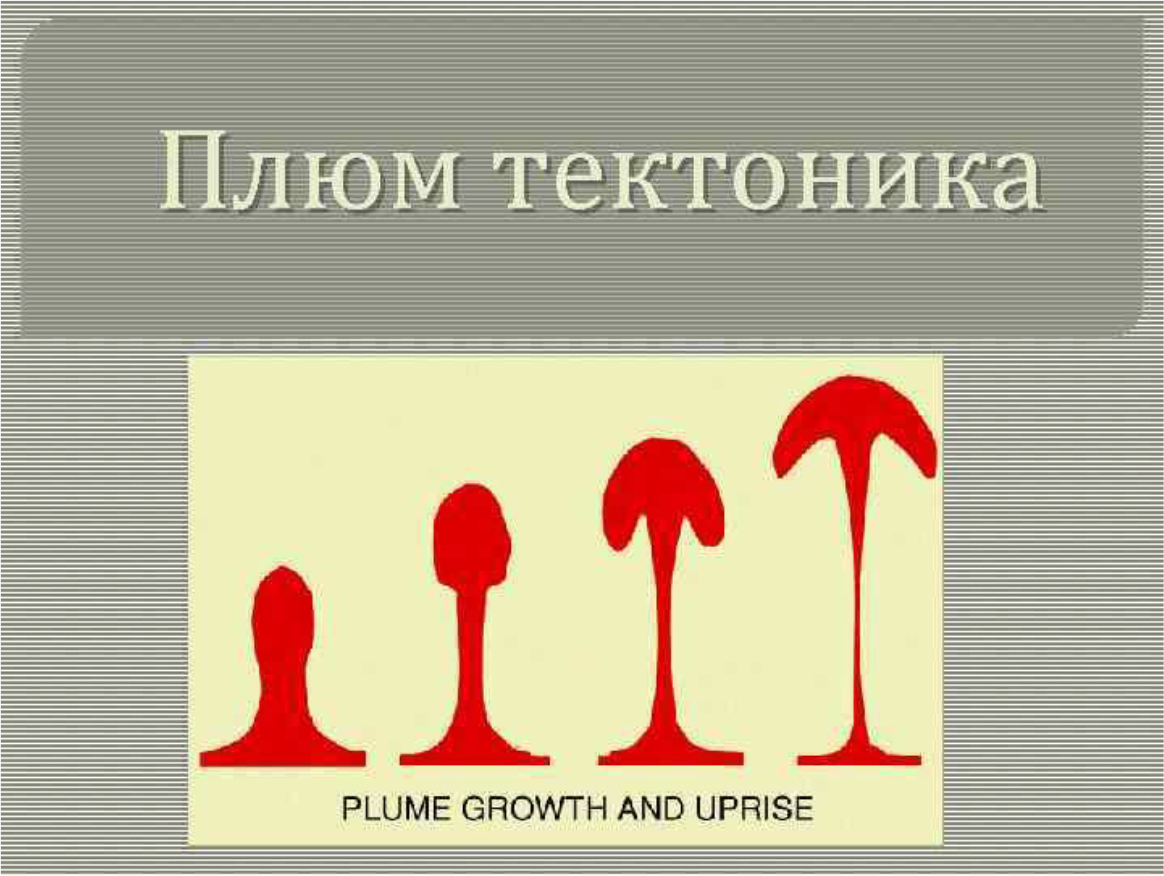
Evaluation of a Direct Oral Anticoagulant Stewardship Program: Analysis of a Drug Consult Review Process and Population-Based Management Tool

DOI: 10.31038/JCCP.2019221

Abstract

Background: With the approval of Direct Oral Anticoagulants (DOAC), anticoagulation management has been transformed in both stroke prevention and venous thromboembolism prophylaxis and treatment. Despite evidence-based dosing guidance there has been large variation in prescribing practices that may lead to negative outcomes. The purpose of this two-part study is to evaluate the impact of a DOAC stewardship program on appropriate DOAC prescribing and use.

Methods: Patients were included in part one of the study if they were prescribed initial DOAC therapy from October 15, 2017 – October 15, 2018 with either a general or DOAC specific drug consult. A manual chart review was then conducted for data points including: anticoagulation indication, DOAC dose, serum creatinine, weight, age, consult approval or denial, and reasons for denial. Part two of the study included patients identified through a VA Population-Based Management Tool (PBMT) from January 1, 2018 – September 30, 2018. A manual chart review was then conducted for data points including: flag category, interventions made, and interventions accepted. Patients were excluded in both arms of the study if the duration of DOAC therapy was less than 20 days, incomplete chart review, or if DOAC therapy was prescribed by a non-VA provider.

Results: A total of 592 consults were included in the final analysis in part one of the study. Of the 233 general consults evaluated, 212 (91.0%) were deemed appropriate, 15 (6.4%) inappropriate, and 6 (2.6%) as clinical grey areas. Of the 233 DOAC specific drug consults evaluated, 218 (93.6%) were deemed appropriate, 1 (0.4%) inappropriate, and 14 (6.0%) as clinical grey areas. There was a significant difference in consults worked inappropriately (p=0.0004). A total of 317 PBMT interventions were included in the final analysis in part two of the study. Of those interventions that were actively acknowledged, 233 (95.9%) interventions were completed.

Conclusion: Implementation of a DOAC stewardship program in a healthcare system promotes appropriate and optimal use as well as safety monitoring of DOACs. A drug-specific consult review process improves inappropriate approval or denial of DOAC therapy while the utilization of a population-based management tool efficiently identifies critically important interventions necessary to ensure safe and appropriate use of DOACs.

Introduction

Two disease states that often require anticoagulation for either prophylaxis or treatment are nonvalvular atrial fibrillation (AF) and venous thromboembolism (VTE). Until recently, the primary option for oral anticoagulation was warfarin, a vitamin K antagonist. In 2010, the first Direct Oral Anticoagulant (DOAC), dabigatran, was FDA approved and since then, other DOACs have received FDA approval within the United States (rivaroxaban, apixaban and edoxaban) [1–4]. With the approval of these agents, anticoagulation management has been transformed in both stroke prevention and VTE prophylaxis and treatment. DOACs require no routine lab monitoring to assess anticoagulation effect due to their favorable pharmacokinetic and pharmacodynamic profile when compared with warfarin. However, DOACs are still associated with serious bleeding risks and possess characteristics different from warfarin, including: renal elimination, short duration of action, different drug-drug interactions, administration considerations, and dosing based off of appropriate indication.

Despite evidence-based dosing guidance, there has been large variation in prescribing practices that may lead to negative outcomes. Steinberg and colleagues were the first to analyze the association between DOAC doses and clinical outcomes in patients with nonvalvular AF. Their study, through the ORBIT-AF II Registry, concluded that off-label doses of DOAC therapy for prevention of stroke in nonvalvular AF are associated with increased risk for adverse events [5]. In addition to prescribing practices, adherence to anticoagulants effects patient outcomes. Shore, et al assessed the adherence component of DOAC therapy by specifically studying patients on dabigatran in Veterans Affairs (VA) hospitals. Their study found that one-quarter of patients demonstrated sub-optimal adherence to dabigatran and poor adherence was associated with an increased risk for stroke and all-cause mortality [6]. Dreijer and colleagues determined 8.3% of medication errors from the hospital and primary care settings were caused from anticoagulation agents, with most error reports concerning the prescribing phase of the medication process [7]. With these results and common practices today, it is imperative that prescribers are aware of the need for oversight of DOAC prescribing. Additionally, studies have shown that a pharmacist driven monitoring program improves appropriate prescribing and monitoring of DOACs used for FDA approved indications. Miele, et al. revealed that appropriate prescribing of DOAC therapy was improved after implementing a pharmacist driven monitoring program through a pre- and post-intervention study. They found that 32.4% of doses administered in the pre-intervention group were considered inappropriate, compared to 13.8% in the post-intervention group. Appropriate prescribing included FDA approved indications and appropriate doses of DOAC therapy based on renal function [8].

Tennessee Valley Healthcare System (TVHS) has pioneered a DOAC stewardship program that includes a DOAC drug specific consult to ensure appropriate prescribing at initiation and then long-term surveillance of patients on DOAC therapy by an ongoing population-based management tool. The goal of this stewardship program is to improve appropriate DOAC utilizations by streamlining the initial DOAC consult process along with ongoing management by utilizing anticoagulation clinical pharmacy specialists (ACC CPS) and a DOAC population-based management tool (PBMT). Previously, DOAC therapy was approved through a generic drug consult review process evaluated by a general clinical pharmacy specialist (CPS). This created a lack of consistency between DOAC approval on a patient to patient basis. The newly developed drug consult review process utilizes both a DOAC drug specific consult along with an ACC CPS. TVHS hopes to improve DOAC utilization with regards to appropriate indication, dosing, and safety through a more specific format of DOAC approval. The DOAC PBMT is used within the VA system to allow for continuous review of safety and compliance parameters for optimal care of patients who are prescribed DOAC therapy. The management tool identifies eight flags including: appropriate dosing, valve replacement, notable labs, overdue labs, critical drug interactions, active Non-Steroidal Inflammatory Drug (NSAID) use, overdue refill greater than 4 weeks and renewal due in next 30 days. It is the responsibility of the ACC CPS to actively review the PBMT daily. Upon review, if a flag is present, the ACC CPS will document their assessment in the patient’s electronic medical record; therefore, notifying the provider of a recommendation or change regarding the patient’s current DOAC therapy. In this study, we will evaluate the impact of a DOAC stewardship program on DOAC utilization at TVHS.

Methods

This multi-site, single center, retrospective cohort study was conducted at TVHS, which includes sites in Nashville and Murfreesboro, TN, as well as patients enrolled at any of the healthcare system’s 13 Community Based Outpatient Clinics (CBOCs) throughout Middle Tennessee, southern Kentucky, and northern Georgia.

Patients were included in part one of the study if they had an active DOAC prescription from October 15, 2017 to October 15, 2018 and 18 years of age or greater. Patients were excluded if the prescription was prescribed for short term therapy (inpatient use only and traveling veterans), written by orthopedics, there was an incomplete data set, or if a consult was denied based on criteria for use (CFU). Patients were included in part two of the study if they had an active DOAC prescription from January 1, 2018 to September 30, 2018 with a note title “Anticoagulation Eval and Mgt Secure Messaging” in the electronic medical record indicating an ACC CPS intervention and 18 years of age or greater. Patients were excluded if the prescription was prescribed for short term therapy (inpatient use only and traveling veterans), if the note title was used in error or the patient relocated to a different VA system. The primary endpoint of this study is to determine the appropriate use of DOAC therapy through a drug consult review process. The secondary endpoints are to determine how the drug consult review process and the utilization of a population-based management tool influences safety outcomes of initial and ongoing DOAC therapy including, concomitant antiplatelet therapy in part one and the PBMT flag categories in part two.

Patients who were prescribed direct oral anticoagulation therapy from October 15, 2017 – October 15, 2018 were identified through data warehouse extraction. A manual chart review was conducted for data points including: anticoagulation indication, DOAC dose at time of consult submission, initial or renewal consult, documented labs, documented weight, consult approval or denial, and rational for approval or denial. Evaluated consults were then categorized as appropriate, inappropriate, or clinical grey areas (Appendix 1). Patients followed by the PBMT from March 24, 2018 to September 24, 2018 were identified through data warehouse extraction using the note title “Anticoagulation Eval & Mgt Secure Messaging.” A manual chart review was conducted for data points including the PBMT flag categories (Appendix 2), interventions actively acknowledged and interventions completed. The sample size was calculated based on the primary objective to determine appropriate use of DOAC therapy through a drug consult review process. The sample included all patients who meet study criteria that received DOAC therapy during the pre-determined timeframe. We wanted to see at least a 15% difference regarding the number of appropriate approvals/denials between the generalized and the specialized consult review process. Using these two data points, the effect size was found to be 15% with alpha set at 0.05 and beta set at 0.20. The study required 133 patients in each arm to be adequately powered. Chi square and fisher exact were used to calculate the p-value for the categorical data presented.

Results

Table 1 displays the baseline demographics and clinical characteristics of the two cohorts. The two groups did not different significantly with respect to age, gender, and race. However, there was a statistically significant difference found in use of rivaroxaban and dabigatran between the two cohorts. The authors attribute this difference to the delineated questions of the drug-specific consult. (Table 1)

Table 1. Baseline characteristics for the consult review process

Generalized Consult
n = 233 (%)

DOAC Specific Consult
n = 233 (%)

P-value

Age

Average ± SD

70.9 ± 11

69.9 ± 12

0.3489

Male sex – no. (%)

231 (99.1)

227 (97.4)

0.2848

Race or ethnic group – no. (%)

White

194 (83.3)

204 (87.5)

0.2375

Black or African American

20 (8.6)

17 (7.3)

0.7323

Asian

0

1 (<1)

1.0000

Native Hawaiian or Pacific Islander

0

0 (0)

1.0000

American Indian or Alaska Native

1 (<1)

1 (<1)

1.0000

Unknown

18 (7.7)

10 (4.3)

0.1715

Direct Oral Anticoagulant (DOAC) – no (%)

Apixaban

85 (36.5)

82 (35.2)

0.8468

Rivaroxaban

56 (24)

78 (33.5)

0.0316

Dabigatran

91 (39.1)

65 (27.9)

0.0141

Edoxaban

1 (<1)

3 (1.3)

0.6156

No preference

0 (0)

5 (2.1)

0.0721

Indication for Use

Nonvalvular atrial fibrillation

162 (69.5)

177 (76)

0.1452

Venous Thromboembolism (VTE)

64 (27.5)

46 (19.7)

0.0637

Other

7 (3)

10 (4.3)

0.6212

*Indication for Use – “other” includes non-FDA approved indications

Part I: Drug consult review process

Primary Outcomes

Two thousand twenty-one unique patients were extracted from October 15, 2017 – October 15, 2018. Due to time constraints and sample size being met, after the initial data pull the date range was shortened to January 13, 2018 to July 13, 2018. All consults in the generalized cohort were evaluated (n=296) and consults in the specialized cohort were randomized to meet a matching sample size (n=296); therefore, a total of 592 DOAC consults were evaluated. In the generalized cohort, 233 consults were included for study evaluation with 63 excluded for various reasons (incomplete data set, orthopedic patients, denial based on CFU). In the specialized cohort, 233 consults for study evaluation with 63 excluded for various reasons (short term therapy, incomplete data set, orthopedic patient, denial based on CFU). Table 2 illustrates the number of evaluated consults deemed appropriate, inappropriate, and those classified as clinical grey areas. Of the 233 general consults worked, 212 were deemed appropriate, 15 inappropriate, and 6 as clinical grey areas. Of the 233 DOAC Specific Drug consults worked, 218 were deemed appropriate, 1 inappropriate, and 14 as clinical grey areas. Statistical significance was seen only in those consults worked inappropriately. (Table 2)

Table 2. Categorization of consult approval or denial

Process

Appropriate (%)

Inappropriate (%)

Clinical Grey Area (%)

Generalized (n=233)

212 (91)

15 (6.4)

6 (2.6)

Specialized (n=233)

218 (93.6)

1 (0.4)

14 (6)

P values

0.3859

0.0004

0.1075

Of the 15 consults worked inappropriately in the generalized process, inappropriate interventions identified included: non-FDA approved dosing, critical drug-drug interactions, non-FDA approved indications, no indication provided, and hepatic dysfunction. The one consult worked inappropriately in the specialized process, the inappropriate intervention identified was non-FDA approved dosing.

Secondary Outcomes

There were no interventions made in the generalized consult review process regarding concomitant antiplatelet use, however there were 29 recommendations made to either discontinue the P2Y12 inhibitor or discontinue/decrease the dose of aspirin in the DOAC specific consult process. Of the 29 recommendation that were made, 13 (45%) recommendations were completed, specifically 9 (69%) were discontinued and 4 (31%) doses were decreased.

Part II: Population Based Management Tool

One thousand fourteen notes with the title “Anticoagulation Eval and Mgt Secure Messaging” were extracted from March 24, 2018 to September 24, 2018 and randomized using Microsoft excel. Three hundred four notes were evaluated to collect the pertinent information as noted above in the “data collection” section. Two-hundred ninety-two notes were included as 12 notes were excluded for various reasons (orthopedic patient, use of wrong note title, relocation to another VA and no active DOAC prescription). Of the 292 notes that were evaluated, 267 notes only included interventions made on one flag, where as 25 notes included interventions on 2 flags resulting in a total of 317 interventions made.

Table 3 displays the number of interventions made regarding the flag category specified by the population-based management tool. By far, the intervention that was made most commonly was alerting the provider that the prescription needed to be renewed (30%), followed by overdue refill > 4 weeks (22%), overdue labs (15%) and inappropriate dosing (11%). From the 317 interventions that were made 242 (76.7%) interventions were actively acknowledged. Of those that were actively acknowledged, 233 (95.9%) interventions were completed (meaning a medication was renewed, refilled, labs were ordered, medications changed, etc.) with specific percentages regarding each flag noted in table 4. (Table 3, Table 4)

Table 3. Interventions made via the population-based management tool

Interventions made
n = 317 (%)

Overdue labs

49 (15)

Notable labs

19 (6)

Active NSAID use

35 (11)

Overdue refill > 4 weeks

69 (22)

Dosing

39 (12)

Critical drug-drug interactions

11 (3)

Valve replacement

1 (0.33)

Renewal due

95 (30)

P2Y12i use

2 (0.66)

Table 4. Interventions actively acknowledged and completed

Interventions actively acknowledged
n = 243

Interventions completed n = 233

Percent completed based on those actively acknowledge

Overdue labs

28

27

96.4%

Notable labs

12

10

83.3%

Active NSAID use

21

16

76.1%

Overdue refill > 4 weeks

53

52

98.1%

Dosing

31

24

77.4%

Critical drug-drug interactions

9

7

77.8%

Valve replacement

1

0

0%

Renewal due

87

87

100%

P2Y12i use

1

0

0%

Discussion

As the anticoagulation paradigm begins to shift from warfarin to DOAC therapy, the use of these medications should still be managed and monitored carefully to prevent unwanted harm. To our knowledge, this is the one of the first studies analyzing the implementation of an ACC CPS run DOAC stewardship program that includes a drug-specific consult and a continuous PBMT evaluated by ACC CPS. When using a generalized consult review process, more consults were deemed to be evaluated inappropriately compared to a specialized consult review process. The generalized process included a consult with minimal requirements for completion (drug, dose, and reason why patient was not candidate for preferred formulary agent, dabigatran) and was then reviewed by a general clinical pharmacy specialist. With the implementation of a DOAC stewardship program, a drug-specific consult was created and is now reviewed by an ACC CPS. For completion, the drug-specific consult must include: drug, dose, indication (as well as details associated with indication), appropriate baseline labs (Hgb/Hct, SCr, AST/ALT), bleeding history, antiplatelet use, NSAID use, and use of pillbox.

The results of this study are consistent with previous studies finding that implementing a pharmacist driven monitoring program reduced inappropriate prescribing of DOAC therapy in adult patients with an indication for nonvalvular AF and/or VTE prophylaxis and treatment [8]. In our study, the following inappropriate uses of DOAC therapy were identified: non-FDA approved indications (apical thrombus, cryptogenic stroke), critical drug-drug interaction (strong CYP3A4 and P-glycoprotein inducers), non-FDA approved dosing (lead-in dosing provided for AF, subtherapeutic use of apixaban, use of apixaban with CrCl75 years old or declining renal function, denial of dabigatran due to use of pillbox, and use of rivaroxaban for ease of compliance. By utilizing the PBMT, our study illustrates that continuous monitoring of DOAC therapy is necessary as patient’s clinical status has the potential to change while on DOAC therapy. The authors attribute the one-fourth of interventions not actively acknowledge as due to the lack of education provided to prescribers prior to the implementation of the DOAC stewardship program. However, almost 96% of the interventions that were actively acknowledge were completed, showing the importance of additional surveillance methods rather than relying on prescriber chart reviews. Moving forward, the authors plan to provide educational sessions to prescribers regarding the importance of the PBMT hoping to eliminate alert fatigue and engage providers in the ongoing efforts of the DOAC stewardship program.

There are a few limitations of this study to consider. First, when categorizing the evaluated consults, clinical grey areas have the potential to differ depending on the consult reviewer’s clinical interpretation of current literature. Second, throughout data collection, four reviewers were trained based on the derived protocol; however, due to the abundant number of unique patients and charts to be reviewed data could have been assessed differently between reviewers. Impacts of this study support the need for a DOAC stewardship program in a healthcare system to promote appropriate and optimal use as well as safety monitoring of DOACs. A drug-specific consult review process improves inappropriate approval or denial of DOAC therapy while the utilization of a PBMT efficiently identifies critically important interventions necessary to ensure safe and appropriate use of DOACs.

Appendix 1: Clinical Grey Areas

  • Use of apixaban due to age >75 years old
  • Denial of dabigatran due to use of pillbox
  • LV Thrombus (if failed or cannot take warfarin)
  • Weight (>120kg)
  • Labs not collected within 90 days
  • Use of DOAC versus heparin or enoxaparin for lead-in for treatment of VTE
  • Non-FDA approved use of DOACs per Landmark Clinical Trials
  • CrCl 15–25 mL/min for use of apixaban in A. Fib
  • CrCl 15–30 mL/min for use of rivaroxaban in A. Fib

Appendix 2: Population-Based Management Tool (PBMT) Flags

  • Overdue labs
    • Results include all patients where either their most recent hemoglobin OR most recent platelet OR most recent serum creatinine is overdue per patient’s monitoring frequency
    • Monitoring frequency defaults to 12 months for all labs except 6 months for serum creatinine for patients that are 75 years of age or more and/or have a CrCl of less than 60 mL/min
    • Once the overdue lab(s) are resulted (once daily in the morning) the patient will no longer appear in this column. In addition, after review of the patient, monitoring frequency (for serum creatinine) can be reset to 2 weeks, 1, 3, 6 or 12 months as determined clinically appropriate
  • Notable labs
    • Most recent platelets <100 x 109 /L if the second most recent value was above 100 x 109 /L OR any platelet value < 50 × 109 /L OR hemoglobin < 10 g/dL or AST/ALT > 135/120 U/L OR a hemoglobin drop > 2 g/dL since previous hemoglobin with resultant value < 13.1 g/dL for males and <11.0 g/dL for females
  • Active NSAID use
    • Patients with an active non-aspirin NSAID based on VA Drug Class MS101 and MS102
    • Active includes prescriptions with status ‘ACTIVE’, ‘SUSPENDED’, ‘PROVIDER HOLD’, ‘HOLD’, ‘PENDING’
    • This will include non-VA prescriptions
  • Valve replacement
    • Results include all patients with an ICD code for a prosthetic (bioprosthetic or mechanical) heart valve on their problem list, attached to two outpatient visits within the last 2 years, or as inpatient discharge diagnosis within the last two years
  • Dosing flag
    • Results include all patients whose renal function (by Cockcroft-Gault with actual body weight) falls above or below specified cutoffs based on agent, indication and if applicable selected drug interactions as per FDA approved package inserts
    • Results also include patients whose dose does not appear to match indication and duration or other non-renal dose modifying characteristics (e.g. high dose apixaban for PE/DVT > 6 months, low dose apixaban for PE/DVT within first 6 months, dose/indication mismatch based on age and body weight)
  • Overdue refill > 4 weeks
    • Results include patients for whom it has been more than 4 weeks since their day supply would be expected to run out (based on released date plus one additional week to allow for shipment)
    • Renewal due in next 30 days
    • Patients for whom the ordered days supply is scheduled to expire within the next 30 days
  • P2Y12i use
    • Antiplatelet therapy includes aspirin, clopidogrel (Plavix ®), ticagrelor (Brilinta®), prasugrel (Effient ®)
    • Critical drug-drug interactions

DOAC

Drug Interactions

Dabigatran

Flag if active warfarin, apixaban, edoxaban, rivaroxaban, rifampin, primidone, St. John’s Wort, phenobarbital, carbamazepime, phenytoin, dronedarone, cyclosporine, tacrolimus, itraconazole, ketoconazole, pasaconazole, voriconazole, rifampicin, saquinavir, ritonavir, indinavir, nelfinavir, amprenavir, lopinavir, fosamprenavir, atazanavir, tipranavir or darunavir

Rivaroxaban

Flag if active warfarin, apixaban, edoxaban, dabigatran, rifampin, primidone, phenobarbital, carbamazepime, phenytoin, itraconazole, ketoconazole, pasaconazole, voriconazole, rifampicin, saquinavir, ritonavir, indinavir, nelfinavir, amprenavir, lopinavir, fosamprenavir, atazanavir, tipranavir, darunavir or St. John’s Wort

Edoxaban

Flag if active warfarin, apixaban, rivaroxaban, dabigatran, rifampin, primidone, phenobarbital, carbamazepime, phenytoin, rifampicin, saquinavir, ritonavir, indinavir, nelfinavir, amprenavir, lopinavir, fosamprenavir, atazanavir, tipranavir, darunavir or St. John’s Wort

Apixaban

Flag if active warfarin, rivaroxaban, edoxaban, dabigatran, rifampin, primidone, phenobarbital, carbamazepime, phenytoin, itraconazole, ketoconazole, pasaconazole, voriconazole, rifampicin, saquinavir, ritonavir, indinavir, nelfinavir, amprenavir, lopinavir, fosamprenavir, atazanavir, tipranavir, darunavir or St. John’s Wort

  • Other critical drug interactions
  • Active cancer pharmacotherapy
  • Flag if: active VA cancer pharmacotherapy in a patient with diagnosis of DVT/PE ± atrial fibrillation or atrial flutter
  • Active includes prescriptions with status ‘ACTIVE’, ‘SUSPENDED’, ‘PROVIDER HOLD’, ‘HOLD’, ‘PENDING’ for any of the interacting drugs or cancer pharmacotherapy
  • Non-VA medications will be included in the analysis for critical drug-drug interactions. Patients with non-VA DOAC prescriptions will not be identified by this tool

References

  1. Eliquis [package insert]. New York, NY: Pfizer Pharmaceuticals, Inc; 2012.
  2. Xarelto [package insert]. Titusville, NJ: Janssen Pharmaceuticals, Inc; 2011.
  3. Pradaxa [package insert]. Ridgefield, CT. Boehringer Ingelheim Pharmaceuticals, Inc; 2011.
  4. Savaysa [package insert]. Tokyo, Japan. Daiichi Sankyo Company, Limited; 2017.
  5. Steinberg B, Shrader P, Thomas L, Ansell J, Fonarow GC, et al. (2016) Off-label dosing of non-vitamin K antagonist oral anticoagulants and adverse outcomes, The ORBIT-AF II Registry. JACC 68: 2597–2604.
  6. Shore S, Carey E, Turakhia M, Jackevicius CA, Cunningham F, et al. (2014) Aherence to dabigatran therapy and longitudinal patient outcomes: insights from the Veterans Health Administration. Am Heart J 167: 810–817.
  7. Dreijer AR, Diepstraten J, Bukkems VE, Mol PGM, Leebeek FWG, et al. (2019) Anticoagulant medication errors in hospitals and primary care: a cross-sectional study. Int J Qual Health Care 31: 346–352.
  8. Miele C, Taylor M, Shah A (2017) Assessment of direct oral anticoagulant prescribing and monitoring pre- and post-implementation of a pharmacy protocol at a community teaching hospital. Hosp Pharm 52: 207–213.

Water Heating By Solar Tile

DOI: 10.31038/NAMS.2019245

Introduction

The paper deals with the use of combination solar tiles-heat pump for domestic water heating. The paper presents testing of solar tile-heat pump combination. Black-coloured water which absorbs solar radiation flows through solar tiles made of transparent polymethyl methacrylate CH2C(CH3)COOCH3. At the same time, solar tiles are used as a roof covering and as a solar radiation collector. Hot water from solar tiles is led to the heat pump, which increases the temperature of water entering the boiler heating coil. The heat of water heated in solar tiles serves as a source of anergy for the heat pump. On that way Coefficient of Performance (COP) of heat pump is increased. Since we wanted to evaluate realistically the efficiency of combimation solar tiles-heat pump, we carried out extensive tests. The experiments were carried out in rainy, cloudy and clear weather.

Test rig

Conventionally, all types of collectors and heat pumps are used separately. In the paper, it is a suggestion to join both systems in a serial connection. Heated water that is coming from the solar tiles is led directly into the input side of a heat pump to gain the higher temperatures. This serial connection should ensure higher temperatures of heating as each heating system works independently.

To verify the effectiveness of the serial connection solar tiles – heat pump, a convenient test rig was built. Measurements of suitable quantities were carried out and analyzed. The test rig consists of a solar tiles, water-water heat pump, and boiler.

The tests were carried under various weather conditions in the summer and winter seasons. Inlet and outlet temperatures from the flat plate collector and heat pump were measured, as well as the ambient air temperature and the water temperature in the boiler.

Figure 1a shows a measurement diagram and Figure 1b the installation of solar tiles. The surface area of tiles was 2 m2. On the lower side, the tiles were insulated, resulting in a decrease by half of the contact surface of the air with the tiles in the case of cloudy weather and darkness, when convective heat transfer prevails. The insulation is appropriate when heat is generated from the radiant part of the heat transfer. The water/water heat pump had thermal power of 1.5 kW under standard conditions and it heated a 300 l boiler. The measured parameters included:

NAMS-2019_Milan Marčič_F1

Figure 1. a) Measurement diagram, b) Installation of solar tiles

  • outlet water temperature from a solar tile (T1);
  • boiler water temperature (T2);
  • inlet water temperature to a solar tile (T3);
  • outlet water temperature from a heat pump (T4);
  • inlet water temperature to a heat pump (T5);
  • ambient air temperature (T6);
  • water flow (Q).

Tests results

The measurements shown in Figure 2 were made in clear sunny and totally cloudy weather. The difference between temperatures T1 (outlet water temperature from a solar tile) and T6 (ambient air temperature) was as high as 20 °C. Between 13:00 and 15:30, it was totally cloudy, which is why the T1-T6 difference dropped to 0 °C. At 15:30, the sky was fully cleared and the temperature difference increased again to 8 °C. From an energy point of view, the solar tile-heat pump combination is certainly the best solution in clear weather for heating of residential  houses and domestic water.

NAMS-2019_Milan Marčič_F2

Figure 2. Temperature measurements – Weather: sunny and windy

References

  1. Dubey S and Tiwari GN (2009) Analysis of PV/T flat plate water collectors connected in series. Solar Energy 83: 1485–1498.
  2. Haložan H (2000) Heat-Pumping Technologies, Journal of Mechanical Engineering. 46: 2000: 445–453.