Author Archives: author

Dosimetric Comparison and Clinical Toxicity in Cervical Cancer Patients Treated with Intensity- Modulated and Three-Dimensional Conformal Radiotherapy: Real-World Data

DOI: 10.31038/CST.2020541

Abstract

Background: Predominantly used in external beam radiotherapy (EBRT) are intensity modulated radiotherapy (IMRT) and three-dimensional conformal radiotherapy (3DCRT). However, the superiority between these two techniques remains inconclusive. This study aim to evaluate the late clinical toxicity of cervical cancer patients treated with intensity-modulated radiation therapy (IMRT) compared to three-dimensional conformal radiation therapy (3D-CRT) and dosimetrically compare the planning target volume (PTV) plan of 3D-CRT to the PTV plan of IMRT based on target coverage and bladder and rectum doses at different volumes.

Methods and Materials: From September 2011 – December 2015, 146 patients with International Federation of Gynaecology and Obstetrics (FIGO) stage IB2-IIB squamous cell carcinoma of the cervix were analysed retrospectively. The patients received EBRT of 50 Gy in 25 fractions of the whole pelvic delivered with IMRT or 3D-CRT. Seventy-five (75) patients received 3D-CRT and seventy-one (71) patients received IMRT.

Results: The 2 years’ overall survival (OS) was 92% in the IMRT group and 88% in the 3D-CRT group (p-value = 0.073). The disease-free survival outcome (DFS) was 83% and 80% in IMRT and 3D-CRT group respectively (p-value). Acute genitourinary (GU) and gastrointestinal (GI) toxicity were lower in IMRT patients compared to 3D-CRT patients (GU, 21.1% vs. 37.3%, p-value = 0.179; GI, 46.5% vs. 49.3%, p-value = 0.436). The mean coverage of the prescribed dose in IMRT and 3D-CRT techniques was 50.02 ± 0.10 Gy and 50.10 ± 0.23 Gy respectively with a non-significant p-value of 0.005 for 95 percent (D95) of the PTV. Also, the mean coverage of 5% (D5) of the PTV was 52.66 ± 0.39 Gy and 53.89 ± 0.76 Gy of the prescribed dose in IMRT and 3D-CRT techniques respectively with a significant p-value of 0.0001.

Conclusion: Patients treated with IMRT had a lower dose to bladder and rectum, a lesser rate of late toxicity and comparable clinical outcome than 3D-CRT. We admonish larger sample size studies and longer follow-up in subsequent studies to affirm our results.

Keywords

Cervical cancer; IMRT; 3D-CRT; Rectum; Bladder

Introduction

Cancer has become a significant public health problem in China since 2010 due to increasing incidence and mortality, making it the number one cause of death in the country [1,2]. External beam radiotherapy (EBRT) is a vital method of treatment for cervical cancer management. Most often than not EBRT and brachytherapy in addition to chemotherapy are often used when treating and managing locally advanced cancer of the cervix. The primary goal of EBRT is in the delivering of maximum radiation to the malignant tissue, with minimum radiation to healthy organs. This treatment can be noxious, and about 20-25% of patients are reported to have severe side effects [3]. Hence, reliable dose-response knowledge in malignant lesions and organs at risk (OAR) is therefore very vital. Before advancement into new treatment planning and imaging technique, most cervical cancer patients were treated using 2D (Two-dimensional) planning. In 2D treatment planning, the contour of the patient is captured with x-ray using lead wire, and bony landmarks and is transcribed on a graph paper sheet with an identified reference point, [4] which results in the target volume being inadequately uncovered. With the limitation of 2D planning, 3D treatment planning and conformal radiotherapy became the standard for EBRT in the 90ths [5]. This treatment planning uses computer tomography (CT) scan images with patients required to be positioned in the planning set-up and requires a computerised treatment planning system (TPS). 3D-CRT is a form of EBRT which uses computers and unique imaging technologies to optimize the radiation beams precisely in other to reduce radiation to surrounding healthy tissues; and was started to be used for effective management of patients since it could give a maximum target coverage and also has the tendency for dose optimization to normal healthy tissues. It makes use of several high photon beams to amply deliver a high dose to a centrally located target volume with minimum dose to superficial structures in the pelvis. Intensity-modulated radiation therapy (IMRT) allows radiation to be more precisely shaped to fit the target volume by using heterogeneous fluences beams from different directions thereby optimises high radiation dose to the target volume and also limiting the amount of radiation received by the normal healthy organs. With IMRT, the beam intensity is able to be optimised as it orients around the patients using computer algorithms [6]. The ‘inverse method’ in treatment planning forms the basis of this process hence able to generate significant dose gradients in the adjacent structures and target volume to accomplish dose-volume prescription [7]. In IMRT, many beams with varying intensity levels are used in treating the tumour while 3D-CRT uses uniform intensity radiation beams hence the constraint of the latter is evident whenever a tumour is wrapped around an organ. Many experts indicated that IMRT is capable of reducing doses to the bone marrow, rectum and bowel and are linked with reduced levels of haematological, gastrointestinal (GI) and genitourinary (GU) toxicity compared to conventional radiation therapy. Nevertheless, these studies were usually defined by small sample sizes and the absence of clinical outcome data. Additionally, brachytherapy patients were involved in their selection criteria and this could influence toxicity. Retrospective reviews comparing IMRT and 3D-CRT technique for cervical cancer patients treated by radiotherapy are deficient, and also there has been inconsistency finding in dose to OAR. The purpose of this study was to analyse retrospectively the clinical toxicity of cervical cancer patients treated with IMRT compared to 3D-CRT and secondly, to compare the PTV plans of 3D-CRT to the PTV plan of IMRT on the basis of target coverage and doses to bladder and rectum at different volumes.

Materials and Methods

Patient Selection

146 stage IB2-stage IIB cervical cancer patients were treated from September 2011-December 2015. The eligibility criteria were [8]:

I.     Biopsy confirmation of squamous cell carcinoma or adenocarcinoma.

II.    Cytological /histological diagnosis of cervical cancer.

III.   No previous surgery, chemotherapy or radiation.

IV.   No evidence of distance metastasis.

V.    KPS performance score 70-80.

Pre-Treatment Evaluation

The pre-treatment workup included a comprehensive medical history, vagina-recto-abdominal examination. Radiological studies like CT-scan of the abdomen-pelvis, chest x-ray and MRI in a few selected patients. Laboratory studies included a complete blood count (CBC), Liver function test (LFT), Blood Chemistries, BUN/Cr, SCC blood test. The clinical-stage was defined according to the International Federation of Obstetrics & Gynaecology (FIGO) staging system.

CT-Simulation

All patients were immobilised with a thermoplastic sheet and underwent CT simulation for planning in a supine position. Philips CT scanner was used for simulation and 3 mm slice images of the abdomen and pelvis area were obtained. The Pinnacle treatment planning system (TPS) (Version 9.2) was used for planning and target contouring.

Treatment Planning

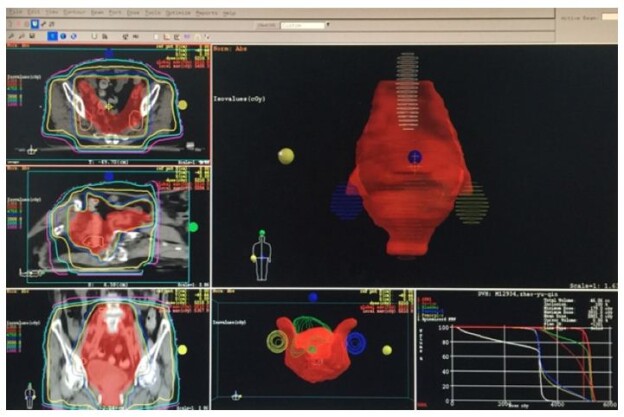
The clinical target volume (CTV) and organs at risk (OAR) were contoured using the concept and definition of volume targets from ICRU reports [9,10]. The gross tumour volume (GTV) and clinical target volume (CTV) were contoured on each single axial CT slice. The CTV included palpable tumour and areas expected to be affected with subclinical tumours. Therefore, the CTV included the pelvic lymph node (external, internal and common iliac), cervix, vagina upper section and uterus. A margin of 10 mm was generated around the CTV to define the planning target volume (PTV). Four fields (two lateral and PA-AP fields) with zero-degree (0°) couch angle were used to generate the 3D-CRT plans (Figure 1). The isocenter was positioned at the PTV’s geometric centre. 10 megavolt (MV) photon energy was used for all plans to improve coverage of PTV and reduce dose to the skin. The beam aperture was shaped to the PTV in each beam’s eye view and a margin of 0.5 cm in all directions accounting for the beam penumbra. The PTV was prescribed a total dose of 50 Gy (2Gy per fraction). The bladder and rectum were protected with a 4-cm central shield after 40 Gy. IMRT plans were generated using 10 megavolt energy with six coplanar fields (Figure 2). Patients had whole pelvic radiotherapy prescribe to 50 Gy with either 3D-CRT or IMRT in 1.8-2 Gy per fractions from Monday – Friday. Chemotherapy involving cisplatin (25 mg/m2) was given concurrently to all patients from second to fifth week during radiotherapy treatment. None of the patients received high dose rate-intracavitary brachytherapy.
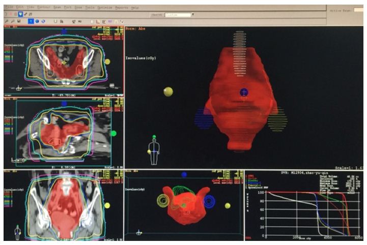
fig 1

Figure 1: Shows the 4-field beam arrangement and isodose curve in 3D-CRT.
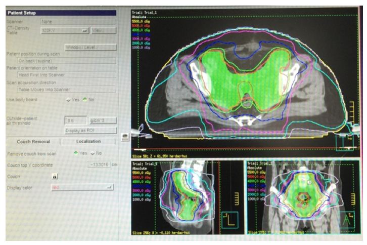
fig 2

Figure 2: Shows the beam arrangement and isodose curve in IMRT technique.

Plan Evaluation

All plans were passed and accepted after more than 95% of the PTV received more than 95% of the dose prescribed (PD). The dose-volume histograms (DVHs) were used in evaluating the PTV coverage, rectum and bladder between 3D-CRT and IMRT plans. The parameter analysed for bladder and rectum included D15D50D80 (dose to 15%, 50% and 80% of organ volume) while PTV coverage was based on D5 and D95 (Dose to 5% and 95% of the PTV respectively). The conformity index (CI) and homogeneity index (HI) was calculated in both techniques using the formulae below.

HI95% = D5/D95; where D5 is the minimum dose of 5% of the target volume indicating the maximum dose, and D95 is the maximum dose of 95% of the target volume indicating the minimum dose. The Homogeneity Index (HI) is an accurate method for analysing the homogeneity of the target volume dose distribution. HI, therefore, demonstrates in all terminology the ratio between both the minimum and maximum dose in the target volume and the lower value demonstrates a more homogeneous distribution of the dose within this volume.

The ideal value is 1, and it increases as the plan become less homogeneous.

CI95% = Total volume receiving 95% of prescribed dose/planning target volume. The ideal value is 1.

Statistical Analysis

All statistical analyses were carried out using SPSS 18, and a substantial difference in each set of dosimetric variables was determined using an independent sample test and chi-square. The rate of survival was evaluated after treatment was completed. The Kaplan – Meier method was used to calculate overall survival (OS) and disease-free survival (DFS). With the aid of the log-rank test, the significance of the difference was analyzed and a p-value < 0.05 was considered significant statistically.

Follow-Up

One month after treatment, patients had a gynaecological examination and pelvic CT/MRI. Afterwards, they were followed at a regular interval of 3 months for the first 2 years and at an interval of 6 months thereafter and then once a year. Version 3.0 of the Common Terminology Criteria for Adverse Events (CTCAE) was used in evaluating chronic and acute toxicity.

Results

Characteristics and Treatment of patients

146 stage IB2-stage IIB cervical cancer patients were treated from September 2011-December 2015. Seventy-five (75) were treated with 3D-CRT and the median age was 50 years (range, 39-68). Seventy-one (71) were also treated with IMRT and the median age was 53 years (range, 32-78). The squamous cell carcinoma histology type was seen in one hundred and thirty-seven (137, 93.8%) patients and nine (9, 6.2%) patients with adenocarcinoma. Table 1 shows a summary of the patients’ characteristics.

Table 1: Patients clinical characteristics.

Characteristics

IMRT 3D-CRT

p-value

Age
Median

53

50

Range

32-78

39-68

Histology type
SCC

64 (93.8%)

73 (97.3%)

Adenocarcinoma

7 (9.9%)

2 (2.7%)

0.071

Stage
IB2

6 (8.5%)

7 (9.3%)

IIA1

29 (40.8%)

44 (58.7%)

IIA2

2 (2.8%)

2 (2.7%)

0.131

IIB

34(47.9%)

22 (29.3%)

Grade
1

8 (11.3%)

12 (16.0%)

0.166

2

59 (83.1%)

53 (70.7%)

3

5 (5.6%)

10 (13.3%)

Tumour Size
<4 cm

45 (63.4%)

50 (66.7%)

0.677

≥ 4 cm

26 (36.6%)

25 (33.3%)

LVSI
Yes

30 (42.3%)

39 (52.0%)

0.238

No

41 (57.7%)

36 (48.0%)

Pelvic Node
Yes

19 (26.8%)

17 (22.7%)

0.540

No

52 (73.2%)

57 (76.0%)

Dose-Volume Histogram (DVH) Outcomes

The 95% PTV mean value was 50.02 ± 0.10 Gy and 50.10 ± 0.23 Gy of the prescribed dose in IMRT and 3D-CRT techniques respectively with a significant p-value of 0.005. Also, the mean coverage of 5% of the PTV was 52.66 ± 0.34 Gy and 53.89 ± 0.76 Gy of the prescribed dose in IMRT and 3D-CRT techniques respectively with a significant p-value of 0.001. Hence the target coverage was esteemed satisfactory and appropriate in both groups.

The HI mean value was 1.052 ± 0.008 and 1.083 ± 0.021 in IMRT and 3D-CRT plans respectively, and the p-value 0.001, indicates the statistical significance of HI in both plans. The CI mean value was 1.330 ± 0.103 and 1.109 ± 0.214 in IMRT and 3D-CRT plans respectively, with a significant 0.001 p-value. Table 2 shows the outcomes of the CI, HI and target coverage in both treatment technique.

Table 2: Outcomes of the CI, HI and target coverage in both treatment technique.

Dosimetric Parameters

 IMRT 3D-CRT

P-value

D5

52.66 ± 0.39

53.89 ± 0.76

 0.001

D95

50.02 ± 0.10

50.10 ± 0.23

0.005

CI

1.330 ± 0.103

1.109 ± 0.214

0.001

HI

1.052 ± 0.008

1.083 ± 0.021

0.001

The dose received by 15% (D15), 50% (D50) and 80% (D80) of the bladder in IMRT was 51.30Gy, 46.79 Gy and 38.69 Gy respectively while that of 3D-CRT was also 52.96 Gy, 51.30 Gy and 41.95 Gy at D15, D50 and D80 respectively. The dose difference between these two techniques at D15, D50 and D80 was highly significant with p-value 0.0001 at all level. Furthermore, dose received by 15% (D15), 50% (D50) and 80% (D80) of the rectum in IMRT was 51.04 Gy, 48.82 Gy and 43.72 Gy respectively while that of 3D-CRT was also 52.24 Gy, 50.99 Gy and 48.08 Gy at D15, D50 and D80 respectively. The dose difference between these two techniques at D15, D50 and D80 was highly significant with p-value 0.001 at all level. Table 3 shows the detailed values of rectum and bladder dose at D15, D50 and D80.

Table 3: Summary of rectum and bladder dose.

Dosimetric Parameters

IMRT 3D-CRT

P-value

Bladder
D15

51.300.39

52.96 ± 0. 88

0.001

D50

46.792.28

51.30 ± 1.72

0.001

D80

38.69 ± 3.63

41.95 ± 6.14

0.001

Rectum
D15

51.04 ± 0.52

52.24 ± 0.89

0.001

D50

48.82 ± 0.97

50.99 ± 0.75

0.001

D80

43.72 ± 2.59

48.08 ± 2.97

0.001

Survival Outcome and Failure Patterns

The 2 years’ overall survival (OS) was 92% in the IMRT group and 88% in the 3D-CRT group with a non-significate p-value of 0.073 and the median follow-up time was 28 months. The disease-free survival outcome (DFS) was 83% and 80% in IMRT and 3D-CRT group respectively. Locoregional failure was noticed in 5 patients. Three (3) from the 3D-CRT group and 2 from the IMRT group. Distant metastasis was observed in one patient in the three-dimensional conformal radiotherapy group in addition to the locoregional failure. Six (6) death rate was recorded during the follow-up, two (2) from the IMRT group and 4 from the 3D-CRT group. The causes of death were pulmonary embolism (1 patient), heart failure (3 patients) and natural death (2).

Clinical Toxicity Outcome

Table 4 shows the percentage of patients with acute genitourinary (GU), haematological and gastrointestinal (GI) toxicity and their grades. Less acute genitourinary (GU) and gastrointestinal (GI) toxicity were noticed in the IMRT patients compared to the 3D-CRT patients (p-value = 0.436 and 0.179 respectively). None of the patients experienced grade 4 genitourinary (GU) and gastrointestinal (GI) toxicity in both groups. Two patients in the IMRT category developed oedema while 12 patients in the 3D-CRT category experienced the same effect. None significant statistical difference was noticed between the two groups when the various clinical toxicity was considered.

Table 4: Clinical toxicity between IMRT and 3D-CRT.

Toxicity

Grade 3D-CRT arm, n (%) IMRT arm, n (%) x2

p-value

Hematologic

0

43 (57.3%) 47 (5.3%) 1.834

0.608

1

21 (28.0%)

18 (25.4%)

2

8 (10.7%)

4 (5.6%)

3

3 (4.0%)

2 (2.8%)

GI

0

47 (62.7%) 56 (78.9%) 4.907

0.179

1

22 (29.3%)

12 (16.9%)

2

5 (6.7%)

2 (2.8%)

3

1 (1.3%)

1 (1.4%)

GU

0

28 (37.3%) 22 (31.0%) 2.726

0.436

1

33 (44.0%)

31 (43.7%)

2

10 (13.3%)

16 (22.5%)

3

4 (5.3%)

2 (2.8%)

Edema

Yes

12 (16.0%) 2 (2.8%) 7.311

0.007

No

63 (84.0%)

69 (97.2%)

Discussion

Previous epidemiological studies have shown that most cervical cancer patients mostly report to the hospital in advance stages of the disease. The public, accepted management for locally advanced cervical cancer (LACC) is brachytherapy with concurrent cisplatin chemoradiotherapy. Conventional radiotherapy continues to be the golden standard for LACC. There has been a reduction in the clinical outcomes and toxicities of IMRT compared with 3D-CRT from preliminary studies. The utilisation of IMRT for gynaecologic tumours including locally advanced cervical cancer has upsurge over these years even though there is insufficient retrospective randomised data to support its usage. From our results, both techniques attained the desired target coverage since 95% of the PTV had above 95% of the prescribed dose (PD). Also, there was better CI, HI and PTV coverage in IMRT compared to 3D-CRT because IMRT uses computer optimised intensity beams and multiple beam angles. Secondly, by using computer algorithms, the intensity of the beam can be optimised in IMRT as it orients around the patient, therefore, allowing radiation to be more precisely shaped to fit the target volume. The results of previous studies, when compared to this present study, confirmed that both IMRT and 3D-CRT are useful in PTV coverage hence no difference in our PTV coverage when compared with previous studies. Van De Bunt et al. [11] reported that IMRT is superior to conformal and conventional treatment in sparing critical organs with ample target volume coverage and also stated that IMRT remains superior after EBRT of 30 Gy regardless of internal organ movement and tumour deterioration.

Mell et al. [12], reported IMRT that there was a reduction in doses to the bone marrow and small bowel when patients were treated with IMRT. A study by Naik et al. [13], reported that doses to organ volume of bladder and rectum were reduced in IMRT patients compared to 3D-CRT. Fiorino et al. [14] concluded that IMRT was superior regarding bowel sparing for doses above 30Gy and also a correlation exists between toxicity and the amount of radiation received by an organ. Central target volume boost is possible with IMRT for patients whom brachytherapy is not possible due to a reduction in doses to OAR thereby allowing higher dose up to 66-70 Gy to be delivered using IMRT. Retrospective studies have accounted that decrease in dose to healthy organs may present a clinical benefit in clinical toxicities reduction. Jereczek – Fossa et al. [15] examined 317 postoperative endometrium carcinoma patients and reported that there was a statistically significant correlation between late and acute bowel reactions. The morbidity and complications among cervical cancer patients after a long-term treatment survivor was assessed by Kamal et al. [16] and reported that the rate of obstruction of the small intestines was comparable in IMRT and 3D-CRT with no significant p-value in both groups. Ajeet et al. [17] reported grade 2 diarrhoea, tenesmus and constipation in patients treated with 3D-CRT compared to a lower grade in IMRT patients. Avinash et al. [18] concluded that there were no differences in both techniques when the grade of haematological toxicities was considered every week even though there was a statistically significant difference between IMRT and 3D-CRT during the second week when the total count and Neutrophils count were assessed. Our results showed that less acute genitourinary (GU) and gastrointestinal (GI) toxicity was noticed in the IMRT patients compared to the 3D-CRT patients (p-value = 0.436 and 0.179 respectively). None of the patients experienced grade 4 genitourinary (GU) and gastrointestinal (GI) toxicity in both groups. Two patients in the IMRT category developed oedema while 12 patients in the 3D-CRT category experienced the same effect. In general, lower clinical toxicities were observed in the IMRT patients than the 3D-CRT patients even though there wasn’t any statistical significance between the two techniques.

Past studies [19-27] in postoperative patients treated with IMRT have normally shown suitable survival outcomes. Chen et al. [28] analyzed 35 patients receiving four-field radiation therapy and 33 patients receiving intensity-modulated radiotherapy and concluded that IMRT improved locoregional control. An update of the study of the Gynaecologic Oncology Group showed 3-year overall survival and progression-free survival rates of 88% and 86% respectively in stage IB cervical cancer patients. Results from the Radiation Therapy Oncology Group 0418 study, involving 48 patients showed an estimated 2-year OS and DFS rates of 94.6% and 86.9% respectively with a median follow-up duration of 2.68 years. In Folkert et al. [29] studies involving 34 patients, the 3 years OS was 91.1% and the 5 years DFS was 91.2%. Our findings were similar to this study.

Our study’s major limitation is the short follow-up period. Furthermore, using bone marrow-sparing methods could reduce the higher rates of haematological toxicity recorded in treated patients with intensity-modulated radiotherapy. In addition, more focus should be given to the target margin in order to leave an adequate margin in IMRT planning for PTV expansion.

Conclusion

In conclusion, patients treated with IMRT had a lower dose of bladder and rectum, a lesser rate of clinical toxicity and comparable clinical outcome than 3D-CRT. We admonish larger sample size studies and longer follow-up in subsequent studies to affirm our results.

References

  1. Shan J (2014) Cervical cancer increases among young Chinese women.
  2. Ostor AG, Rome RM (1994) Micro-invasive squamous cell carcinoma of the cervix: a clinico-pathologic study of 200 cases with long-term follow up. Int J Gynecol Cancer 4: 257-264.
  3. Chen W, Zheng R, Baade PD, Zhang S, Zeng H, et al. (2016) Cancer statistics in China, 2015. CA Cancer J Clin 66: 115-132.
  4. Hochman A, Ratzkowski E, Schrieber H (1955) Incidence of carcinoma of cervix in Jewish women in Israel. Br J Cancer 9: 358-364.
  5. Perez CA (1998) Uteri cervix. In: Perez CA, Brady LW, Principles and practice of radiation oncology 3rd edition. Philadelphia, PA: Lippincott-Raven Publishers 1998: 1733-1834.
  6. Low D, Purdy JA, Perez CA et al. (1992) Intensity modulated radiation therapy, In: Levitt SH, Potish RA, Khan FM, Perez CA eds. Levitt and Tapley’s technological basis of radiation therapy: Clinical application 3rd edition. Baltimore, MD: Lippincott Williams and Wilkins 1992: 126-146.
  7. Khan FM (2007) Treatment Planning in Radiation Oncology, 2nd edition, Philadelphia: Lippincott Williams and Wilkins.
  8. Drokow EK, Zi L, Qian H, Xu L, Foli F, et al. (2020) Tolerability, efficacy and feasibility of concurrent gemcitabine and cisplatin (CGP) combined with intensity modulated radiotherapy for loco-regionally advanced carcinoma of the cervix. Journal of Cancer 11: 2632-2638. [crossref]
  9. ICRU Report 50 (1993) Prescribing, recording and reporting photon beam therapy: ICRU, Bethesda, MD,
  10. ICRU Report 62 (1999) Prescribing, recording and reporting photon beam therapy (Supplement to ICRU report 50): ICRU, Bethesda, MD.
  11. Van de Bunt L, van der Heide UA, Ketelaars M, de Kort GA, Jurgenliemk-Schulz IM (2006) Conventional, conformal, and intensity-modulated radiation therapy treatment planning of external beam radiotherapy for cervical cancer: the impact of tumor regression. Int J Radiat Oncol Biol Phys 64: 189-196. [crossref]
  12. Mell LK, Tiryaki H, Ahn KH, John C Roeske, Bulent Aydogan et al. (2008) Dosimetric comparison of bone marrow-sparing intensity-modulated radiotherapy versus conventional techniques for treatment of cervical cancer. Int J Radiat Oncol Biol Phys 71: 1504-1510. [crossref]
  13. A Naik, O.P. Gurjar, P. Bagdare et al. (2016) Dosimetric comparison between IMRT and 3D-CRT planning. J. Radiat 14: 189-196.
  14. Fiorino C, Alongi F, Perna L Et al. (2009) Dose–volume relation- ships for acute bowel toxicity in patients treated with pelvic nodal irradiation for prostate cancer. Int J Radiat Oncol Biol Phys 75: 29-35. [crossref]
  15. Jereczek-Fossa BA, Jassem J, Badzio A (2002) Relationship between acute and late normal tissue injury after postop- erative radiotherapy in endometrial cancer. Int J Radiat Oncol Biol Phys 52: 476-482. [crossref]
  16. Kamal A Elghamrawi (2011) Treatment complications among long-term survivors of cervical cancer: treated by surgery or radiotherapy. Oncology Reviews 5: 261-266.
  17. Gandhi AK, Sharma DN, Rath GK, Julka PK, Subramani V, et al. (2013) Early clinical outcomes and toxicity of intensity modulated versus conventional pelvic radiation therapy for locally advanced cervix carcinoma: a prospective randomized study. Int J Radiat Oncol Biol Phys 87: 542-548. [crossref]
  18. Avinash HU, Arul Ponni TR, Janaki M G, Kirthi Koushik A S, Kumar SM (2015) A prospective dosimetric and clinical comparison of acute haematological toxicities in intensity modulated radiation therapy and three-dimensional conformal radiotherapy with concurrent chemotherapy in carcinoma cervix. J Can Res Ther 11: 83-87. [crossref]
  19. Hui Beina MD, Zhang, Yingbing MD, Shi Fan MD, Wang Juan PhD, et al. (2014) Association Between Bone Marrow Dosimetric Parameters and Acute Hematologic Toxicity in Cervical Cancer Patients Undergoing Concurrent Chemoradiotherapy: Comparison of Three-Dimensional Conformal Radiotherapy and Intensity-Modulated Radiation Therapy. International Journal of Gynecological Cancer 24: 1648-1652. [crossref]
  20. Wang YM, Wang CJ, Fang FM, Chen HC, Hsu HC, et al. (2017) Differences in the outcomes and complications between elderly and younger uterine cervical cancer patients treated by definitive radiotherapy – a propensity score-matched study. Gynecol Oncol 145:277-283.
  21. Hui B, Zhang Y, Shi F, Wang J, Wang T, et al. (2014) Association between bone marrow dosimetric parameters and acute hematologic toxicity in cervical cancer patients undergoing concurrent chemoradiotherapy: comparison of three-dimensional conformal radiotherapy and intensity modulated radiation therapy. Int J Gynecol Cancer 24:1648-1652. [crossref]
  22. Chang Y, Yang ZY, Li GL, Li Q, Yang Q, et al. (2016) Correlations between radiation dose in bone marrow and haematological toxicity in patients with cervical cancer: a comparison of 3DCRT, IMRT, and Rapid ARC. Int J Gynecol Cancer 26:770-776. [crossref]
  23. Mell LK, Sirak I, Wei L, Tarnawski R, Mahantshetty U, et al. (2017) Bone marrow-sparing intensity modulated radiation therapy with concurrent cisplatin for stage IB-IVA cervical cancer: an international multicenter phase II clinical trial (INTERTECC-2). Int J Radiat Oncol Biol Phys 97:536-545. [crossref]
  24. Tanderup K, Fokdal LU, Sturdza A, Haie-Meder C, Mazeron R, et al. (2016) Effect of tumor dose, volume and overall treatment time on local control after radio-chemotherapy including MRI guided brachytherapy of locally advanced cervical cancer. Radiother Oncol 120:441-446. [crossref]
  25. Sturdza A, Potter R, Fokdal LU, Haie-Meder C, Tan LT, et al. (2016) Image guided brachytherapy in locally advanced cervical cancer: improved pelvic control and survival in RetroEMBRACE, a multi-center cohort study. Radiother Oncol 120: 428-433. [crossref]
  26. Weiping W, Xiaorong H, Junfang Y, Jie S, et al. (2017) Outcome and toxicity of radical radiotherapy or concurrent chemoradiotherapy for elderly cervical cancer women. BMC Cancer 17:510. [crossref]
  27. Mei-Ling LAN, Xian YU, He XIAO et al. (2016) Clinical outcomes and toxicity of postoperative intensity-modulated versus three-dimensional conformal radiation therapy in patients with cervical cancer. Asia-Pacific Journal of Clinical Oncology 12: 430-436. [crossref]
  28. Chen MF, Tseng CJ, Tseng CC, Yu CY, Wu CT, et al. (2008) Adjuvant concurrent chemoradiotherapy with intensity modulated pelvic radiotherapy after surgery for high-risk, early stage cervical cancer patients. Cancer J 14: 200-206. [crossref]
  29. Folkert MR, Shih KK, Abu-Rustum NR et al. (2013) Postoperative pelvic intensity-modulated radiotherapy and concurrent chemotherapy in intermediate- and high-risk cervical cancer. Gynecol Oncol 128: 288-293. [crossref]
CAR-T Neurotoxicity Causing Severe Brain Oedema and Tonsillar Herniation in a Young Child with Relapse ALL – A Case Report

DOI: 10.31038/CST.2020534

Abstract

Background: Cellular immunotherapy with autologous T cells genetically engineered to express chimeric antigen receptors is emerging as a promising new class of immunotherapeutic agents, however may cause unique symptoms of neuro-toxicity, such as toxic encephalopathic state with symptoms of confusion and delirium, and occasionally seizures and cerebral oedema.

Case presentation: Hereby, we report a case of a 4-year-old boy, with B-cell precursor acute lymphoblastic leukemia and refractory CNS involvement, which was treated with CAR T-cells. The patient developed severe encephalopathy, high fever and seizures, and was treated with steroids and anticonvulsants. Nevertheless, the patient rapidly deteriorated and developed diffused brain oedema and herniation of cerebellar tonsils. Unfortunately, the patient showed no neurological improvement and suffered brain death.

Conclusion: Neurotoxicity is an important and common complication of CAR-T cell therapies. Usually, severe neurological symptoms are manageable in most patients, which respond to standard interventions. Early detection of neurological deterioration is of paramount importance, and pediatric intensivists should consider pre-emptive management for brain oedema, even prior to radiological evidence. Randomized prospective studies of treatment algorithms are urgently needed to improve patient monitoring and management.

Keywords

Chimeric antigen receptors (CAR), cytokine-release syndrome (CRS), Immune effector cell-associated neurologic syndrome (ICANS), Neurotoxicity

Background

Cellular immunotherapy with autologous T cells genetically engineered to express chimeric antigen receptors (CARs) is emerging as a promising new class of immunotherapeutic agents in relapsed and refractory B-cell malignancies [1,2]. As CAR T-cell therapies become more widely used, recognition of their unique toxicities, which are distinct from those seen with traditional chemotherapies, monoclonal antibodies, and small-molecule targeted therapies, is of the utmost importance [1]. The two most commonly observed toxicities with CAR-T-cell therapies are: 1) cytokine-release syndrome (CRS), characterized by high fever, hypotension, hypoxia, and/or multiorgan toxicity; and 2) Immune effector Cell-Associated Neurologic Syndrome (ICANS), which may occur in more than 60% of patients treated with CAR T-cells [2]. ICANS is typically characterized by a toxic encephalopathic state with symptoms of confusion and delirium, and occasionally seizures and cerebral oedema, and can occur with or after CRS [1] with peak incidence occurring 4–6 days after infusion [3-5]. About 20% of patients will present severe neurotoxicity [5], and grade 5 fatal neurotoxicity has been described in clinical studies in adults treated with CD19-directed CAR T-cells, with an incidence of up to 3% [4]. Hereby, we are the first to present an extreme form of neurotoxicity in a young child, resulting in brain oedema and death.

Case Presentation

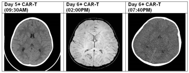
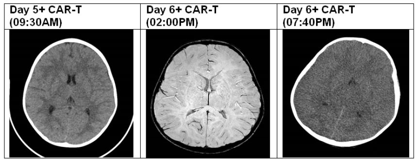
We report a case of a 4-year-old boy, with B-cell precursor acute lymphoblastic leukemia (ALL) with CNS involvement. Due to high risk relapse/refractory disease he was enrolled on a clinical trial using CD19 CAR T-cells. The patient developed CRS on day +3 (grade 1), and due to encephalopathy, high fever and seizures he was transferred to pediatric intensive care (PICU) on day 5 of CAR-T treatment. Prior to transfer to PICU, due to a clinical diagnosis of ICANS grade 3, he was commenced on dexamethasone, on top of Levetiracetam prophylaxis (started on day -3). Following this event, a brain CT was performed and was normal, showing no intracranial bleeding or oedema. EEG revealed general encephalopathy. Following repeated tonic-clonic seizures despite increase in the Levetiracetam dose and steroids treatment, he was loaded with phenytoin as well as a few midazolam boluses to stop the seizures. During the first 24 hours in PICU, the patient remained stable, encephalopathic, however maintained GCS of 8-10. The following day (+6) a brain MRI was performed under general anesthesia, showing high T2-FLAIR signal involving the hemispheral sub-cortical white matter, hippocampi and capsule externa, in addition to high signal in the thalami bilateral. Furthermore, there were cortical areas with diffusion strain which correlate with ICANS. The patient was extubated and returned to PICU drowsy but responsive. Upon returning from MRI the patient had a sudden acute deterioration, with apneic episode and GCS which dropped to 3, therefore was immediately intubated. An urgent repeat CT brain was performed revealing diffused brain oedema with developing herniation of cerebellar tonsils (Figure 1). During the next 24 hours he received mannitol, hypertonic saline, and noradrenaline to maintain proper cerebral perfusion pressure and reduction of oedema, he was started on broad spectrum antibiotics and anti-viral empiric therapy for possible meningo-encephalitis, as well as pulse methylprednisolone and tocilizumab. Unfortunately, the patient showed no neurological improvement and had absent brain stem reflexes and anisocoric pupils. SPECT was performed showing absent flows which correlates with brain death.

fig 1

Figure 1: CT/MRI findings.

Discussion

We describe a young child with relapse ALL that was commenced on CAR-T therapy and very rapidly, after 5 days of treatment, developed severe ICANS presenting as encephalopathy and seizures. He received the acceptable treatment with anti-epileptic drugs and steroids, unfortunately suffered from very extreme and rare complication of CAR-T treatment as of brain oedema, followed by tonsillar herniation and death. The oedema itself may have risen as the sequelae of some other underlying process, and in our patient might have been main cause of the neurological deterioration. Neurotoxicity is an important and common complication of CAR-T cell therapies. Acute neurologic signs and/or symptoms occur in a significant proportion of patients with clinical manifestations that include headache, confusion, delirium, language disturbance, seizures and rarely, acute cerebral oedema. The mechanisms that lead to neurotoxicity remain unknown, but data from patients and animal models suggest there is compromise of the blood-brain barrier, associated with high levels of cytokines in the blood and cerebrospinal fluid, as well as endothelial activation [6]. This cytokine production is correlated to early onset of severe CRS, or may be associated with expansion and activation of CAR T-cells that lead to a direct parenchymal CAR T-cell infiltration [5]. Such toxicities have also been observed in patients treated with other redirected-T-cell therapies and bispecific T-cell-engaging antibodies [1]. Gust et al., [4] described a potential mechanism for the cases of diffuse and often fatal cerebral oedema, with findings of widespread endothelial activation as well as findings of meningeal inflammation from a mouse model of CAR T-cell neurotoxicity [7]. Toxicity may also be primarily mediated by the inflammatory cytokine surge that accompanies CAR-T cell expansion in the marrow, rather than the CAR-T cells themselves [6].

The management of ICANS remains an area of active investigation. Therapy rests upon symptomatic management, seizure control, and corticosteroids. Despite the widespread use of corticosteroids, it is unknown to what degree they influence CAR T cell–mediated anticancer effects [2]. Presently, corticosteroids and tocilizumab are the mainstays of treatment for both CRS and neurotoxicity [1]. However, treatment with tocilizumab for CRS causes serum IL-6 to rise, which may predispose to more severe neurotoxicity [6]. In sicker patients with depressed level of consciousness, dexamethasone should be added and seizures need to be ruled out and controlled. In the sickest patients who are unarousable, with status epilepticus, motor weakness or diffuse cerebral oedema, or when brain MRI identifies focal or diffuse oedema, high dose methylprednisolone should be started. Anakinra (anti-interleukin-1 receptor antagonist) has been anecdotically proposed [5,6]. Although symptoms could present at virtually any time within the first few weeks after CAR T-cell infusion, patients who developed early CRS are more likely to develop severe neurotoxicity. Severe neurotoxicity represents a negative prognostic factor for overall survival with potential therapy-related mortality and underline the importance of rigorous monitoring of these patients [2]. Usually, ICANS is manageable in most patients, although some require monitoring and treatment in the intensive-care setting. It is thus imperative that clinicians remain vigilant in their workup and management of all neurological symptoms, especially those that deviate from the expected course of recovery and responsiveness to standard interventions. The role of intensivists is crucial and PICU specialists may help anticipate the risk for developing organ dysfunction or sepsis, based on patient’s frailty, immunity and comorbid conditions. After CAR-T infusion, when patients develop subacute fever and mild organ derangement, early PICU admission is recommenced. PICU intensivists should consider early management for brain oedema with possible intubation and secure airway, hyperosmolar therapy, and raising the cerebral perfusion pressure by vasoactive support. All of these measures should be considered at a very early stage of ICANS, even prior to radiological evidence, as most if not all patients will have brain oedema to some degree at presentation with encephalopathy. Diabetes ketoacidosis is a similar example where an inflammatory state associated with an immune and systemic inflammatory response results in disruption in the integrity of brain capillaries tight junctions which causes capillary permeability and brain oedema [8]. Our problem in clinical practice is that we are unable to quantify BBB function in real time during the acute course of ICANS treatment. Hence, from a pragmatic perspective, recognizing and providing preemptive treatment is paramount for pediatric intensivists.

Conclusion

Early detection of neurological deterioration is of paramount importance after CAR-T cell treatment, and PICU intensivists should consider early management for brain oedema, even prior to radiological evidence. Randomized prospective studies of treatment algorithms are urgently needed to improve patient monitoring and management.

List of Abbreviations

CAR: Chimeric antigen receptors

CRS: Cytokine-Release Syndrome

ICANS: Immune Effector Cell-Associated Neurologic Syndrome

ALL: Acute Lymphoblastic Leukemia

PICU: Pediatric Intensive Care

Declarations

  • Ethics approval and consent to participate.
  • Consent for publication – there is an ethical approval and consent to participate by the local IRB committee.
  • Availability of data and materials – all data was described in references.
  • Competing interests – no competing interests.
  • Funding – no funding.
  • Authors’ contributions – RKL wrote the manuscript with the help of EJ. Initiated, supervised and finally edited and approved by GP. All authors read and approved the final manuscript.
  • Acknowledgements – not applicable.

References

  1. Neelapu SS, Tummala S, Kebriaei P, William Wierda, Cristina Gutierrez, et al. (2017) Chimeric antigen receptor T-cell therapy—assessment and management of toxicities. Nat Rev Clin Oncol 15: 47-62.
  2. Philipp Karschnia, Justin T. Jordan, Deborah A. Forst, Isabel C. Arrillaga-Romany, Tracy T. Batchelor, et al. (2019) Clinical presentation, management, and biomarkers of neurotoxicity after adoptive immunotherapy with CART cells. Blood:
  3. Makita S, Yoshimura K, Tobinai K (2017) Clinical development of anti- CD19 chimeric antigen receptor T-cell therapy for B-cell non-Hodgkin lymphoma. Cancer Sci 108:1109-111.
  4. Juliane Gust, Kevin A Hay, Laïla-Aïcha Hanafi, Daniel Li, David Myerson, et al. (2017) Endothelial Activation and Blood-Brain Barrier Disruption in Neurotoxicity after Adoptive Immunotherapy with CD19 CAR-T Cells. Cancer Discov Dec 7: 1404-1419.
  5. Elie Azoulay, Michael Darmon, Sandrine Valade (2020) Acute life‑threatening toxicity from CAR T‑cell therapy. Intensive Care Med 46:1723-1726.
  6. Daniel B. Rubin, Husain H. Danish, Ali Basil Ali, Karen Li, Sarah LaRose, et al. (2019) Neurological toxicities associated with chimeric antigen receptor T-cell therapy.
  7. Margherita Norelli, Barbara Camisa, Giulia Barbiera, Laura Falcone, Ayurzana Purevdorj, et al. (2018) Monocyte-derived IL-1 and IL-6 are differentially required for cytokine-release syndrome and neurotoxicity due to CAR T cells. Nature Medicine 24: 739-748.
  8. Robert CT, Carlo LA (2014) Cerebral edema in children with diabetic ketoacidosis: vasogenic rather than cellular? Pediatric Diabetes 15: 261-270.

COVID-19 Pandemic: Non-Contact Strategies for Protecting Healthcare Workers

DOI: 10.31038/IDT.2020123


The outbreak of severe acute respiratory syndrome coronavirus 2 (SARS-COV-2) has evolved into a pandemic with more than 49 million confirmed cases and almost 1,239,000 deaths globally [1]. SARS-CoV-2 infection occurs mainly via respiratory droplets from face-to-face contact and, to a lesser extent, via contaminated surfaces [2]. The virus is highly infectious and increasing evidence of hospital-based transmission has been observed [3]. In the United States, among the 156,306 COVID-19 health care workers, 789 have died [4]. The protection of health care workers is a challenge that calls for the development of effective measures.

In order to relieve the current shortage of medical resources, novel preventive and control technologies and equipment, especially those that make use of modern information technology (IT), may prove to be effective and efficient [5,6]. 3D-printed personal protective equipment (PPE) has been developed in some regions to alleviate severe shortages of masks in times of crisis [7]. A hospital has introduced a negative airway pressure respirator (NAPR), which is used in patients for bronchoscopy, to better protect health care workers from aerosols produced in the upper and lower respiratory tracts [8]. To this end, the First Affiliated Hospital of Gannan Medical University developed a new integrated IT platform comprising a series of non-contact or low-contact in-hospital screening, diagnosis, and monitoring devices for protecting health care workers from COVID-19 [9].

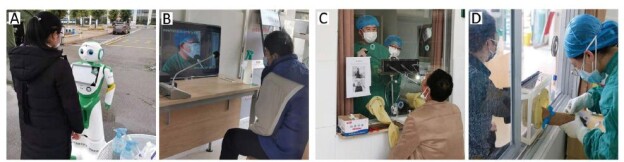
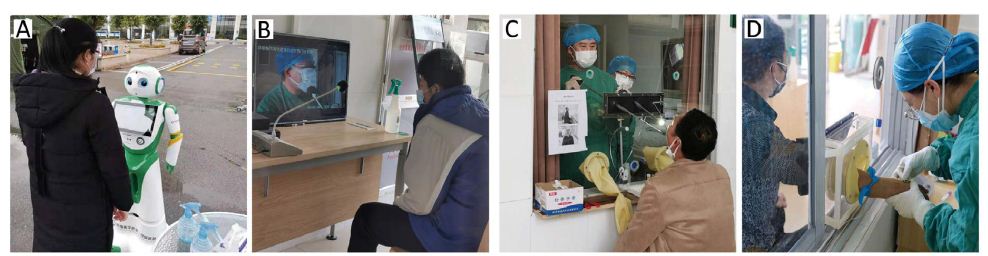
First, at the entrance of the hospital, patients place their identification cards against a sensor, which automatically reads their name, gender, and age, and transfers this information to the hospital information network. For triage, an automatic infrared temperature imaging and measurement system is used to determine whether the patient has a fever. Based on a series of preset questions, a designated robot automatically ascertains whether the patient had a fever or other respiratory symptoms in the past three days or a history of exposure to a SARS-CoV-2-infected individual in the last two weeks. This robot intelligently analyzes the response obtained to guide the patient into the fever clinic or outpatient clinic (Figure 1A).

Second, a non-contact television consultation system (Figure 1B) is used to interview the patient in the fever clinic. The doctor and the patient sit in different rooms, preventing direct contact. For examination, researchers employ a novel low-contact sampling and examination system, which comprises an endoscopic throat swab specimen collection system (Figure 1C), an isolated blood collection device (Figure 1D), and a two-side isolated stethoscope and electrocardiogram-acquisition system. In addition, a computed tomography room for disease screening was independently reserved for performing lung imaging examinations on patients to protect health care workers from COVID-19.

fig 1

Figure 1: Non-contact in-hospital screening devices: enquiry and triage (A), non-contact television consultation (B), endoscopic throat swab specimen collection (C), and isolated blood collection (D).

Third, based on the recommendation of clinicians considering the examination results and the specific conditions of patients ascertained via the consultation, the patients are classified into three categories: non-COVID-19 patients, COVID-19suspected patients, and COVID-19 patients. It is recommended that non-COVID-19 patients be sent home for observation or special outpatient treatment. COVID-19 suspected patients should be placed in isolation for observation. COVID-19 patients are transferred to a designated hospital for treatment. Moreover, digital high-definition video cameras were installed in areas where COVID-19 suspected patients pass through in the hospital. Once the COVID-19 suspected patient is confirmed, clinicians can use digital cameras to track and intelligently analyze the patients’ movements and search for contacts with high infection risk contacts. Thus, clinicians can identify individuals in intimate contact with the patient for immediate isolation and observation to further protect health care workers from COVID-19.

In addition, an intelligent infrared thermal imaging and high-definition video monitoring system is installed in emergency departments, outpatient clinics, and waiting rooms. This system is used to locate and monitor patients with fever who may have been missed. After these patients are identified, they are guided to the fever clinic for further screening and diagnosis. Finally, this system can intelligently identify individuals not wearing masks or not adhering to standard protective measures and automatically provide warnings or friendly reminders. This not only protects health care workers from COVID-19 but also increases public awareness regarding protection against respire a story infections. Between January 20 2020, and July 31, 2020, the First Affiliated Hospital of Gannan Medical University received 546,413 out patients, of which 7,933 were placed in fever clinic, and 11,098 throat swab specimens were collected by this system. Among these patients, five were diagnosed as COVID-19-positive, and none of the health care workers were infected. Overall, this integrated system minimizes direct contact between health care workers and patients, reduces the risk of infection for health care workers, and conserves medical supplies. Researchers will continue collecting feedback on relevant information throughout the application of this system and continuously improve it to develop a new integrated IT platform that comprises a complete contact less COVID-19 hospital screening, diagnosis and monitoring system for the protection of health care workers from COVID-19. Given our preliminary results, this system maybe valuable to other regions and countries where the outlook of COVID-19 prevention and control is not optimistic.

Declaration of Interests

We declare no competing interests.

Role of Funding Source

Funding: This project was supported by Science and Technology Department of Jiangxi Province and the Gannan Medical University (COVID-19 Emergency Science and Technology Project of Gannan Medical University) [grant number YJ202004].

Acknowledgement

We would like to thank Editage (www.editage.cn) for English language editing.

References

  1. WHO Coronavirus Disease (COVID-19) (2020).
  2. Wiersinga WJ, Rhodes A, Cheng AC, Peacock SJ, Prescott HC (2020) Pathophysiology, transmission, diagnosis, and treatment of coronavirus disease 2019 (COVID-19): A Review. JAMA 324: 782-793. [crossref]
  3. Rivett L, Sridhar S, Sparkes D, Routledge M, Jones NK, et al. (2020) Screening of healthcare workers for SARS-CoV-2 highlights the role of asymptomatic carriage in COVID-19 transmission. Elife 9: 58728. [crossref]
  4. Cases & Deaths among Healthcare Personnel (2020).
  5. McCall B (2020) COVID-19 and artificial intelligence: protecting health-care workers and curbing the spread. Lancet Digital Health 2: 166-167. [crossref]
  6. Chen X, Tian J, Li G, Li G (2020) Initiation of a new infection control system for the COVID-19 outbreak. Lancet Infectious Diseases 20: 397-398. [crossref]
  7. Exchange NDP (2020) A collection of biomedical 3D printable files and 3D printing resources supported by the National Institutes of Health (NIH).
  8. Khoury T, Lavergne P, Chitguppi C, Rabinowitz M, Nyquist G, et al. (2020) Aerosolized particle reduction: a novel cadaveric model and a negative airway pressure respirator (NAPR) system to protect health care workers from COVID-19. Otolaryngol Head Neck Surg 63: 151-155.
  9. News Jiangxi (2020) The First Affiliated Hospital of Gannan Medical University developed the first non-contact visualized nosocomial intelligent screening, diagnosis and prevention and control system for novel coronavirus infection.

Risk Factors for Early and Late Onset Preeclampsia in Women without Pathological History: Confirmation of the Paramount Effect of Excessive Maternal Pre-Pregnancy Corpulence on Risk for Late Onset Preeclampsia

DOI: 10.31038/IGOJ.2020331

Abstract

Objectives: Several major risk factors for preeclampsia being internationally consensual, we investigated risk factors for EOP and LOP in a “knock-out (KO) population” where we excluded 8 risks factors: all women with multiple pregnancies, pre-existing diabetes mellitus, chronic hypertension, history of previous preeclampsia, “coagulopathies”, renal or thyroid diseases and smokers.

Study design: South-Reunion University’s maternity (Reunion Island, Indian Ocean). 19 year-observational population-based cohort study (2001-2019). Epidemiological perinatal data base with information on obstetrical and neonatal risk factors. All consecutive singleton pregnancies (>21 weeks) compared with all preeclamptic pregnancies delivered in the south of Reunion island.

Main outcome measures: Comparing crude risk factors between EOP and LOP, and logistic regression model between EOP and LOP women with the general “KO population”.

Results: The 56,570 women belonging to the “knock-out population” comprised 72% of all women having delivered singleton babies during the 19- year survey and 63% of all preeclamptic cases. In this “virgin population”, we over-confirm that overweight and different classes of obesities are linearly and increasingly linked with only LOP, and completely disconnected with EOP. For EOP, this KO population revealed that history of previous perinatal death (mainly intra-uterine fetal deaths) have a tendency to be an independent factor (aOR 1.69, p=0.07). “New paternity” was an independent factor for both EOP and LOP (aOR 3.5 for EOP, p=0.006, and aOR 4.3, p<0.0001 for LOP).

Conclusion: Besides the indications of aspirin prevention as soon as the 16th week of gestation to prevent EOP (some 60% possible decreased risk), new paternity could be further investigated. Concerning the LOP risk, maternal pre-pregnancy high BMIs should be monitored through adequate gestational weight gains since the first prenatal visit to lower the incidence of LOP possibly by 30-40%.

Keywords

Preeclampsia, Epidemiology, Early onset preeclampsia, Late onset preeclampsia, Gestational weight gain

Introduction

This is the fourth study of a tetralogy on our population-based preeclamptic singleton cohort in Reunion island (Ocean Indian, French overseas department). First [1], on this same population we have described that ‘Placental preeclampsia’ (defective placentation) being linked to early onset preeclampsia (EOP, <34 weeks gestation) while ‘maternal preeclampsia’ (maternal cardiovascular predisposition) being typically manifesting as the late form of the disease LOP is not systematically verified: As a matter of fact: EOP women were older than LOP 29.5 vs. 28.6 years, p=0.009, primigravidas were prone to LOP. History of preeclampsia (aOR 12.8 vs. 7.1), chronic hypertension (aOR 6.5 vs. 4.5) had much higher adjusted odds ratios for EOP than for LOP, p<0.001. Specific to EOP: coagulopathies (see methods for definitions, aOR 2.95, p=0.04), stimulated pregnancies (aOR 3.9, p=0.02). Specific to LOP: renal diseases (aOR 2.0, p=0.05) and protective effect for smoking (aOR. 0.75, p=0.008). EOP women were prone to have a lower BMI [1]. This was somehow unexpected that the strongest factors associated with EOP are those concerning multiparas, although preeclampsia is particularly considered as a disease of the first pregnancy [2]. On the other hand, first pregnancies (primigravidity) and younger maternal age (especially <25 years) were rather associated with LOP, and not as expected with EOP. These findings (confirming a first study in 2017 [3], with similar results in a cohort in Madagascar [4]) completely disowned our proposed model in 2007 based on maternal ages [5]: the model we proposed then was that older ages should be more prone to LOP (by a “physiological” looming out of vascular and metabolic predispositions), while at younger ages women should be more prone to EOP (first pregnancies, less vascular and metabolic predispositions at these ages).

Then, and second, we verified if these unexpected results for us were not an effect of a “international bad choice” for the consensual cut-off of 34 weeks to discriminate between EOP and LOP internationally adopted since 2013 [6]. We tested different definitions of EOP-LOP (simulating different cut-offs from 30 weeks gestation to 37 [7]), and fundamental results remained quite identical whatever the cutoff chosen, especially the specific effect of rising maternal ppBMI on LOP [7]. Third, we deepened our analysis [8] and showed that in a multivariate analysis with EOP or LOP as outcome variables compared with controls (normotensive), maternal age and pre-pregnancy BMI were independent risk factors for both EOP and LOP. However, analyzing by increment of 5 (categories of 5 years for the ages, categories of 5 kg/m² for BMI) rising maternal ages and incidence of preeclampsia were similar for EOP and LOP, while increment of BMI was more specifically associated with LOP [8]. Also, and very important, controlling for maternal ages and booking/pre-pregnancy BMI, gestational diabetes mellitus was no more an independent risk factor neither for EOP nor for LOP. Further, smoking during pregnancy was protective only on LOP (30% decrease) and not on EOP [8].

After these three studies [1,7,8], we noticed that women with the 8 major well-known risk factors for preeclampsia that we confirmed (multiple pregnancies, chronic hypertension, diabetes, smoking, renal and thyroid diseases, “coagulopathies” and multiparous having a previous history of preeclampsia) represented indeed only 28% of our parturients. What about the other 72%? Therefore, we sought to explore what are the risk factors for EOP and LOP in women “without morbidities and past” (after excluding the 8 major risk factors). This is the purpose of the present study.

Materials and Methods

From January 1st, 2001, to June 30, 2019, the hospital records of all women delivered at the maternity of the University South Reunion Island (ap. 4 300 births per year) were abstracted in standardized fashion. The study sample was drawn from the hospital perinatal database which prospectively records data of all mother-infant pairs since 2001. Information is collected at the time of delivery and at the infant hospital discharge and regularly audited by appropriately trained staff. These epidemiological perinatal data base which contained information on obstetrical risk factors, description of deliveries and neonatal outcomes. For the purpose of this study records have been validated and have been used anonymously. As participants in the French national health care system, all pregnant women in Reunion Island have their prenatal visits, biological and ultasonographic examinations, and anthropological characteristics recorded in their maternity booklet.

Preeclampsia, gestational hypertension and eclampsia were diagnosed according to the definition issued by the International Society for the Study of Hypertension in Pregnancy (ISSHP) relatively to the guidelines in force at the year of pregnancy.

Design and Study Population

The maternity department of Saint Pierre hospital is a tertiary care centre that performs about 4 300 deliveries per year, thus representing about 80% of deliveries of the Southern area of Reunion Island, but is the only level 3 maternity (the other maternity is a private clinic, level 1 which is not allowed to follow/deliver preeclamptic pregnancies). Reunion Island is a French overseas region in the Southern Indian Ocean. The entire pregnant population has virtually access to maternity care. This is provided free of charge by the French healthcare system, which combines freedom of medical practice with nationwide social security.

Definition of Exposure and Outcomes

Renal diseases were defined as patients with known pre-existing nephropathies (glomerulopathies,tubulopathies, renal failure, diabetic nephropathies) and urological pathologies were excluded. Thyroid diseases were defined as hypo/hyperthyroidy, goitre, thyroiditis, thyroidectomy. Coagulopathies were defined as antiphospholipid syndrome, protein C/protein S deficit, factor 5 Leyden or other coagulation factors deficits at any time they were reported in the records (they were not systematically screened in all women as in a case-control study).

Preeclampsia was defined according to the World Health Organization recommendations [9-11] and the International Society for the study of Hypertension in Pregnancy [12] as the new onset of hypertension (BP ≥140 mmHg systolic or ≥90 mm Hg diastolic) at or after 20 weeks’ gestation and substantial proteinuria (>0.3 g/24 hours). Early onset preeclampsia was defined as preeclampsia that developed before 34 weeks of gestation.

The “primipaternity” item (changing father for the index pregnancy) has been added in the database in 2018 and has been prospectively recorded since then. It is the sum of all primigravidas (and not primiparas) plus multiparous having changed partner for the index pregnancy. For the other years (2001-2017), we retrospectively looked at all free commentaries (possible in each record) for “changing father, changing paternity, new father, new partner etc….” (therefore probably non-exhaustive), but we retrieved hundreds of cases (N=552).

Statistical Analysis

Data is presented as numbers and proportions (%) for categorical variables and as mean and standard deviation (SD) for continuous ones. Comparisons between groups were performed by using χ2-test; odds ratio (OR) with 95% confidence interval (CI) was also calculated. Paired t-test was used for parametric and the Mann-Whitney U test for non-parametric continuous variables. P-values <0.05 were considered statistically significant. Epidemiological data have been recorded and analysed with the software EPI-INFO 7.1.5 (2008, CDC Atlanta, OMS), EPIDATA 3.0 and EPIDATA Analysis V2.2.2.183. Denmark.

Further, to validate the independent association of maternal pre-pregnancy BMI, or maternal ages and other confounding factors on EOP or LOP we realized a multiple regression logistic model. Variables associated with in bivariate analysis, with a p-value below 0.1 or known to be associated with the outcome in the literature were included in the model. A stepwise backward strategy was then applied to obtain the final model. The goodness of fit was assessed using the Hosmer-Lemeshow test. A p-value below 0.05 was considered significant. All analyses were performed using MedCalc software (version 12.3.0; MedCalc Software’s, Ostend, Belgium).

Results

During this 19 year period (1st January 2001-31st of December 2019), there were 2007 preeclamptic women (PE) in the south of the island of Reunion, of which 115 multiple pregnancies. Out of 76,591 singleton pregnancies, the baseline population consisted of 1,892 singleton preeclamptic pregnancies, incidence 2.5% (614 EOP and 1,278 LOP).

For the purpose of the present study, we excluded from all our database 1) multiple pregnancies 2) chronic hypertension 3) diabetic women 4) smokers 5) renal diseases 6) thyroid diseases 7) “coagulopathies” (see methods) and 8) multiparous having a previous history of preeclampsia. What we propose to call the “knock-out (KO)” population.

The KO population (preeclamptics and controls) became 1,198 preeclamptics/56,570 singleton pregnancies (incidence 2.1%). The KO population represents then 72% of all parturients and 63% of all preeclamptics.

We tested first in Table 1 crude risk factors’ comparisons between women presenting EOP or LOP (Odds ratios being EOP vs. LOP). In bold are the results of the entire population (1,892 singleton preeclamptics/76,591, detailed in preceding studies [1,7]), in italic the same risk factors in women belonging to the KO population. Plus or minus, the comparisons are similar. We have added in the present study the item “primipaternity” which did not existed in the preceding studies [1,7,8]. Like primiparity, primipaternity is associated slightly more with LOP than with EOP (p=0.04 and 0.07). It is of note that women declaring to live single appear in KO women to be a risk factor rather for LOP (OR 0.69 for EOP, p=0.004). Therefore, we have included this item in the logistic model.

Table 1: Crude differences between EOP and LOP. In bold, crude results in the entire 19-year cohort (N=76,0000), already detailed in preceding studies [1,7]. In italic, crude results in the “knock-out” population (N=56,570)

Non significant results

Left numbers EOP N=662, knock-out KO N=378

Right numbers LOP N=1345, knock-out KO N=820


P value

Significant results

EOP vs. LOP

ODDS ratios

[95% CI]


P value

Gestity (mean, SD)       2.91 vs.  2.73

       KO                               2.49 vs. 2.31


0.10

0.10

Mother Age (years, SD)  29.5 vs. 28.6

        KO                 28.2 vs. 26.9

0.009

0.002

Parity (mean, SD               1.28 vs. 1.18

      KO                                 0.93 vs. 0.85

0.25

0.37

Primigravidity   

31.5% vs. 37.2% OR=0.78 [0.63-0.96]

KO  40.1% vs. 46.2%   0.78 [0.61-1.0]


0.02

0.05

  Primiparity    45.8% vs. 49.7%    OR 0.85 [0.70-1.0]

     KO  56.6% vs. 58.8% OR 0.91


0.05

0.24

Adolescents (<18y)       3.0% vs.  3.4% OR 0.89

     KO                                  4.3% vs. 4.8%        OR 0.88

0.67

0.68

First couple’pregnancy (“primipaternity”)

34.9% vs. 39.0% OR 0.84 [0.69-1.0]


KO First couple’s pregnancy    

42.9%vs 47.3%   OR=0.83 [0.65-1.06]

0.04


0.07

35 years +                        25.8 vs. 23.8%       OR=1.10

     KO                          19.8% vs. 16.1%     OR=1.28

0.39

0.12

Pre-pregnancy/booking BMI 26.4 vs. 27.1 Kg/m²

         KO        25.42 vs. 26.0 Kg/m²


0.06

0.19

Grand multiparae  (5+)    10.8% vs. 9.6%    OR=1.14

     KO                                  7.5% vs. 5.7%        OR=1.34

0.41

0.24

Atcd perinatal. Deaths 12% vs. 7.4%      1.78   [1.1-2.6]

KO 9.5% vs. 4.9%  2.06 [1.09-3.9]


0.008

0.02

Single            34.7% vs.  38.2%   OR=0.86

    KO          32.1% vs. 40.8%     OR=0.69 [0.53-0.89]


0.14

0.004

Stimulated pregnancies     0.8% vs. 0.2%       OR=3.4

KO .1% vs. 0.4%    OR=2.83


0.07

0.15

Years school ≥ 10.     56.9% vs. 55.6%     OR=1.06

      KO                           61.4% vs. 59.7%          OR=1.08

0.60

0.58

 
BMI ≥ 25 kg/m²         54.5% vs. 53.7%     OR=1.03

 KO           46.8% vs. 45.1%          OR=1.07

0.76

0.60

 
BMI ≥ 30 kg/m²         27.7% vs. 30.6%    OR=0.87

    KO        22.6% vs. 24.2%          OR=0.91

0.23

0.57

 
Atcd miscarriage        30.9 % vs. 31.4% OR=0.98

  KO                      30.4% vs. 31.1%     OR=0.96

0.85

0.83

 
Atcd abortion          27.0% vs. 23.3%  OR=1.22

       KO                      30.4% vs. 24.3%     OR=1.36

0.15

0.09

 
In vitro fecundation    1.3% vs. 1.0%     OR=1.36

  KO      0.8% vs. 0.9%           OR=0.90

0.50

0.88


                                               Excluded from this study population [results in 1,7]
Pre-existing diabetes     3.9% vs. 4. %9    OR=0.79

                   (knock out excluded)

0.37  
Smoking                    9.7% vs.  8.7%     OR=1.10

                   (knock out excluded)

0.58  
Coagulopathy*             1% vs. 0.5%           OR=2.04

                   (knock out excluded)

0.21 Gestational diabetes   11.9% vs. 17.9% 0.68  [0.51-0.90]

                         (knock out excluded)

0.009
Atcd thyroid disease#   2.5 % vs. 1.6%    OR=1.53

                   (knock out excluded)

0.21 Chronic hypertension 12.7% vs. 9.2%   1.43   [1.05-1.9]

                          (knock out excluded)

0.02
Atcd renal disease      1.5% vs. 0.9%      OR=1.67

                   (knock out excluded)

0.25 Atcd preeclampsia       18.1% vs. 11.4%    1.70 [1.2-2.5]

                          (knock out excluded)

0.002

#Goitre, hypo-hyperthyroidy, thyroidectomy, thyroid node, thyroiditis * antiphospholipid syndrome, protein C/protein S deficit, factor 5.

Leyden or other coagulation factors deficits.

In Table 2, logistic model, we adopted a different strategy: with the outcomes EOP and LOP, we compared cases and all the general KO population (n=56,270), taking into account the crude results comparing EOP with LOP (Table 1) to choose the selected risk factors . The upper table of the model includes primiparity (therefore also women with possible previous miscarriages or abortions). Below, the lower table includes instead “primipaternity”: primigravidas (therefore no possible previous miscarriages or abortions) and multiparas having changed the male partner for the index pregnancy.

Table 2: Adjusted Odds ratios. “Knockout preeclamptics” vs. all women (“knock-out” singleton pregnancies N=56,570).

Primiparity in the model EOP Knockout

aOR

P val LOP Knockout

aOR

P val
Age5 (increment 5 years) 1.046

[1.02-1.07]

0.002 1.042

[1.02-1.04]

0.001
BMI5 (increment 5kg/m²) 1.05

[1.03-1.07]

<0.0001 1.055

[1.04-1.07]

<0.0001
Primiparity 2.9

[2.0-4.3]

<0.0001 2.59

[1.98-3.4]

<0.0001
Atcd  abortion 1.17

[0.83-1.7]

0.31 0.95 0.72
Atcd miscarriage 1.06

[0.76-1.5]

0.70 1.01

[0.80-1.27]]

0.89
Single 0.85 0.33 1.05 0.64
ART stimulated 3.6

[0.87-15.1]

0.07 0.82 0.85
IVF 0.96 0.97 0.90 0.86
Primipaternity# (instead of primiparity) in the model EOP Knockout

aOR

P val LOP Knockout

aOR

P val
Age5 (increment 5 years) 1.026

[1.00-1.05]

0.03 1.025

[1.01-1.04]

0.002
BMI5 (increment 5kg/m²) 1.046

[1.02-1.07]

<0.0001 1.05

[1.04-1.07]

<0.0001
Primipaternity# 3.5

[1.4-8.6]

0.006 4.3

[2.4-7.6]

<0.0001
Atcd  abortion 1.49

[1.09-2.05]

0.01 1.19 0.13
Atcd miscarriage 1.33

[0.97-1.81]

0.07 1.26

[1.02-1.55]

0.03
Single 0.88 0.44 1.11 0.27
ART stimulated 4.7

[1.15-19.5]

0.03 1.06 0.95
Atcd perinatal deaths 1.69

[0.96-2.99]

0.07 1.15 0.54
IVF 0.96 0.97 0.90 0.86

#Primipaternity : primiparous and multiparous having changed partner for the index pregnancy.

First, primiparity and primipaternity are independent factors for both EOP and LOP (OR ≈ 3/4, p<0.0001).

Second, increase of maternal age (by increment of 5 years) is also an independent factor: increase of 4% per 5 years of age for primiparity and increase of 2% per 5 years for primipaternity ( both EOP and LOP).

Third, increase of maternal pre-pregnancy BMI (by increments of 5kg/m²): increase of 5% per 5 kg/m² for primiparity and primipaternity ( both EOP and LOP).

Fourth, associated only with EOP: antecedents of perinatal deaths (mainly intrauterine fetal deaths) and medically induced pregnancies by stimulation of ovulation (stronger effect in primipaternity than with primiparity OR 4.7 vs. 3.6, p=0.03). In vitro fecundations are not associated neither with EOP nor with LOP.

Fifth, history of abortion and miscarriages is not associated with preeclampsia risk in the primiparity model. In the primipaternity model, history of abortions is specifically associated with the risk of EOP. History of miscarriages is slightly associated (OR≈ 1.3, p=0.03) with both EOP and LOP.

Figures 1 and 2 show the comparisons between our entire population (N ≈ 76,591 singleton pregnancies, already detailed in preceding publications [1,7]) and our “knock-out” population (N ≈ 56,570).

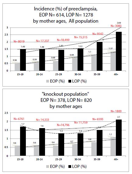
Figure 1 depicts the effect of increasing maternal ages: in both cases, EOP and LOP increase with maternal ageing.

fig 1

Figure 1: Comparisons of preeclampsia Incidences (%) by mother ages in 1) all our population 2) in the “knock-out” population.

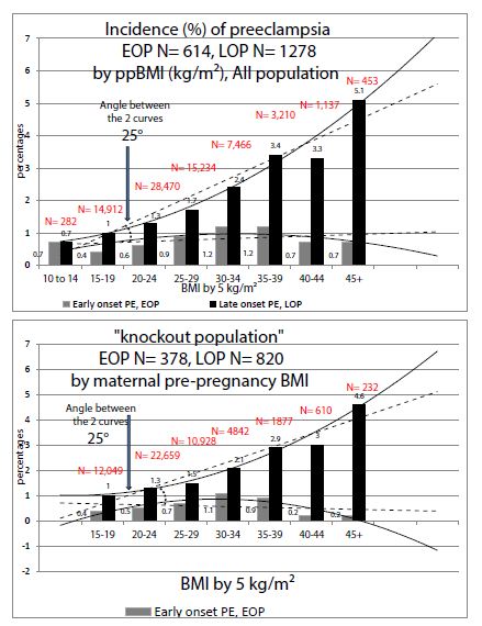
Figure 2 depicts the effect of increasing maternal pre-pregnancy BMI: in the KO population (women without past and morbidities) the paramount effect of increase of BMI is specific with the increase of only LOP. In the KO population, the ppBMI has a nil effect on the occurrence of EOP (stronger effect than in the entire population).

fig 2

Figure 2: Comparisons of preeclampsia Incidences (%) by maternal pre-pregnancy Body Mass Index (BMI) in 1) all our population 2) in the “knock-out” population.

Discussion

First of all, “women without morbidities and past” (multiple pregnancies, chronic hypertension, diabetes, smoking, renal and thyroid diseases, “coagulopathies” and multiparous having a previous history of preeclampsia, or “knock-out population”, KO) comprise 72% of a female reproductive community. It is also of note that they also comprise 63% of all preclampsia cases (PE incidence of 2.1% vs. 2.5% in the general population).

Second, Late Onset Preeclampsia (LOP): this study on a “pure population” confirms the paramount effect of increased pre-pregnancy BMI targeted mainly on late onset preeclampsia (≥ 34 weeks gestation) that we had already previously described [8]. In KO women “without past and morbidities”, the effect is absolutely stronger than in our entire population (see comparisons in Figure 2). The BMI increase has a very poor effect on the early onset (EOP) form. Obesity is a well-known risk factor for late-onset preeclampsia [9], but this effect varies within different classes of obesities (ClassI to III) [8]. Very recently Bicocca, Sibai et al. [10] also thought to have a look at these 3 classes of obesity in a large cohort in the USA and noticed also that rising classes of obesities are significantly and linearly associated with the risk of hypertensive disorders of pregnancy (HDP). They found that the slope for EOP was different than with LOP (with an angle of 16°). We have found in 2019 similar results in a preeclamptic population-based in Reunion island, but our association was quite only associated with LOP and poorly with EOP, and our slopes made an angle of 25° [8], see also Table 2. However, there were two major methodological differences with Bicocca et al. and our study [8]: we took only preeclamptic women (and not all HDP), and used the PRE-PREGNANCY BMI, which is then predictive before any pregnancy, Bicocca et al. used maternal BMI AT DELIVERY which includes then the gestational weight gain (GWG). As a matter of fact, GWG is different if you deliver at 29 or at 38 weeks, and GWG comprises also edemas.

This specific association between maternal pre-pregnancy corpulence and LOP is not a detail, as LOP is by far the predominant form of preeclampsia (90% in literature from developed countries, some 70% in the rest of the world [11]). This confirmation is the major findings of this “knock-out” epidemiological study and, there, we might have an immediate leverage of action (prevention) very soon [12,13].

Third, concerning Early Onset Preeclampsia (EOP), this study made on a “virgin-risk population” may reveal some tracks. Besides a predictive screening by what we may call the “Nicolaides-Poon’s algorithms” [14-17], some clinical items may be added to the EOP risk: the involvement of a new male partner for the index pregnancy and history of previous perinatal death (mainly intra-uterine fetal deaths).

A)  Primipaternity and History of Abortions and Miscarriages in Multigravidas

In this study, we have indirect approach of a male partner involvement, and, interestingly rather a risk for EOP (therefore a possible target for aspirin prevention?). First of all, history of abortions or miscarriages in multiparas were not associated with any preeclampsia risk in the general population (Table 1, bold results), and in our logistic model including primiparity (Table 2, upper Table) and in the results of preceding studies on this same population [1]. In the present study of a KO population, crude results (Table 1, italic results) and in the primipaternity model (Table 2, lower Table), history of abortions is specifically associated with the risk of EOP, and miscarriages equally between EOP and LOP. At first, the well-known effect of primiparity (cornerstone of all epidemiological studies on preeclampsia) is also confirmed in primipaternity (Table 2). For primipaternity, we may assume that women having changed male partner for the index pregnancy may have had preceding abortions with different partner(s) [18].

B)  Primipaternity and Medically Induced Pregnancies

It is of note (Table 2) that in vitro-fecundations (including ICSI) are not independently associated with any kind of preeclampsia risk (EOP & LOP) in primiparas and “primipaternity-multiparas”, Table 2. In our ART centre in Reunion, 88% of our IVF are made with the habitual male partner of the couple, with very few oocyte donations (N=31 in 19 years) and very few with unknown donor sperm. Contrary to IVF, in our experience, medically induced pregnancies by stimulation of ovulation were a strong independent factor specifically associated with EOP. We have verified and 2/3 (66.6%) of our stimulated pregnancies were primiparas, and 48% primigravidas. Antecedents of abortions as risk factors specific to EOP in women having a new partner suggest the “male effect” as possible etiology of preeclampsia, and more specifically in this study for EOP [19-22].

C)  Antecedents of Perinatal Deaths

Controlling for primipaternity (Table 2, lower Table), previous perinatal deaths have a tendency to be an independent factor for the EOP risk, p=0.07 (NB: not associated with previous history of preeclampsia, as these women have been removed from the study population).

The Centre Hospitalier Universitaire Sud-Reunion’s maternity (Level 3, European standards of care) is the only public hospital in the southern part of Reunion Island (Indian Ocean, French overseas department). It serves the whole population of the area (ap. 360,000 inhabitants, and 5,100 births per year). With 4,300 births per year, the university maternity represents 82% of all births in the south of the island. But, as a level 3 (the other maternity is a private clinic, level 1), we are sure all the preeclampsia cases were referred to our hospital during the 19- year period. This is therefore a real population-based study. As a limitation of the study, we have to consider the retrospective nature of the study that, although the number of information that is recorded, some characteristics may miss like length of sexual relationship and/or primipaternity. The “primipaternity” item, being quoted mainly retrospectively for the period 2001-2017, is not completely reliable. “Coagulopathies” were not systematically screened in all women (cases and controls). However, every time that a woman was known to have one of these characteristics, they were scrupulously included in the database. The strengths of this study are mostly related to the homogeneity of data in such a large cohort as they were collected in a single center (no intercenter variability) and not based on national birth registers but directly from medical records (avoiding inadequate codes).

Conclusion

This study made on a population exempt from the eight internationally consensual major risk factors for preeclampsia may be of some interest. 1) for late onset preeclampsia LOP: it confirms the specific association between high maternal BMI and the immense burden of late-onset preeclampsia (LOP) [8]. This is of major importance in a planet where the overweight-obesity problem is constantly rising. Here, there is a reasonable hope to have a positive intervention by a monitored management of gestational weight gain since the beginning of any pregnancy allowing to lower the LOP incidence by some 30-40% [12,13]. 2) For early onset preeclampsia EOP (here we may expect a 60% decrease by aspirin prevention [14,15]), this KO population revealed underlying risk factors: history of preceding perinatal deaths (intra-uterine fetal deaths) and arguments for “new paternity”. International efforts should be focused on asking to all first-couple’s pregnancies (primiparas and multiparas having changed the male partner) the length of cohabitation before conception. A sexual cohabitation of less than 6 months could be a risk factor for EOP and, if confirmed, beneficiate of early aspirin prevention since the 16th week of gestation [14-17].

References

  1. Robillard PY, Dekker G, Scioscia M, Bonsante F, Iacobelli S, et al. (2020) The blurring boundaries between placental and maternal preeclampsia: a critical appraisal of 1800 consecutive preeclamptic cases. J Matern Fetal Neonatal Med 6: 1-7. [crossref]
  2. Burton GJ, Redman CW, Roberts JM, Moffett A (2019) Pre-eclampsia: pathophysiology and clinical implications. BMJ 366: 2381. [crossref]
  3. Iacobelli S(1), Bonsante F(2), Robillard PY(2) (2017) Comparison of risk factors and perinatal outcomes in early onset and late onset preeclampsia: A cohort based study in Reunion Island. J Reprod Immunol 123: 12-16. [crossref]
  4. Ratsiatosika AT, Razafimanantsoa E, Andriantoky VB, Ravoavison N, Andrianampanalinarivo Hery R, et al. (2019) Incidence and natural history of preeclampsia/eclampsia at the university maternity of Antananarivo, Madagascar: high prevalence of the early-onset condition. J Matern Fetal Neonatal Med 32: 3266-3271. [crossref]
  5. Robillard PY, Dekker G, Chaouat G, Hulsey TC (2007) Etiology of preeclampsia: maternal vascular predisposition and couple disease–mutual exclusion or complementarity? J Reprod Immunol 76: 1-7. [crossref]
  6. Tranquilli AL, Brown MA, Zeeman GG, Dekker G, Sibai BM (2013) The definition of severe and early-onset preeclampsia. Statements from the International Society for the Study of Hypertension in Pregnancy (ISSHP). Pregnancy Hypertens 3: 44-77. [crossref]
  7. Robillard PY, Dekker G, Scioscia M, Bonsante F, Iacobelli S, et al. (2020) Validation of the 34-week gestation as definition of late onset preeclampsia:Testing different cutoffs from 30 to 37 weeks on a population-based cohort of 1700 preeclamptics. Acta Obstet Gynecol Scand.
  8. Robillard PY, Dekker G, Scioscia M, Bonsante F, Iacobelli S, et al. (2019) Increased BMI has a linear association with late-onset preeclampsia: a population-based study. PLoS One 14: 0223888. [crossref]
  9. Lisonkova S, Joseph KS (2013) Incidence of preeclampsia: risk factors and outcomes associated with early-versus late-onset disease. Am J Obstet Gynecol 209: 544. [crossref]
  10. Bicocca MJ, Mendez-Figueroa H, Chauhan SP, Sibai BM (2020) Maternal Obesity and the Risk of Early-Onset and Late-Onset Hypertensive Disorders of Pregnancy. Obstet Gynecol 136: 118-127. [crossref]
  11. Robillard PY, Dekker G, Chaouat G, Elliot MG, Scioscia M (2019) High incidence of early onset preeclampsia is probably the rule and not the exception worldwide 20th anniversary of the reunion workshop. A summary. J Reprod Immunol 133: 30-36.
  12. Robillard PY, Dekker G, Boukerrou M, Boumahni B, Hulsey T, et al. (2020) Gestational weight gain and rate of late-onset preeclampsia: a retrospective analysis on 57 000 singleton pregnancies in Reunion Island. BMJ Open 10: 036549.
  13. Robillard PY, Dekker GA, Boukerrou M, Boumahni B, Hulsey TC, et al. (2020) The urgent need to optimize gestational weight gain in overweight/obese women to lower maternal-fetal moribidities: a retrospective analysis on 59,000 singleton term pregnancies. Archives Women Health Care 3: 1-9.
  14. Roberge S, Bujold E, Nicolaides KH (2018) Aspirin for the prevention of preterm and term preeclampsia: systematic review and metaanalysis. Am J Obstet Gynecol 218: 287-293. [crossref]
  15. Rolnik DL, Nicolaides KH, Poon LC (2020) Prevention of preeclampsia with aspirin. Am J Obstet Gynecol 21: 30873-30875.
  16. Poon LC, Shennan A, Hyett JA, Kapur A, et al. (2019) The International Federation of Gynecology and Obstetrics (FIGO) initiative on pre-eclampsia: A pragmatic guide for first-trimester screening and prevention. Int J Gynaecol Obstet 145: 1-33. Erratum in: Int J Gynaecol Obstet 146: 390-391. [crossref]
  17. Wright D, Nicolaides KH (2019) Aspirin delays the development of preeclampsia. Am J Obstet Gynecol 220: 580. [crossref]
  18. Saftlas AF, Levine RJ, Klebanoff MA, Martz KL, Ewell MG, et al. (2003) Abortion, changed paternity, and risk of preeclampsia in nulliparous women. Am J Epidemiol 157: 1108-1114. [crossref]
  19. Robillard PY, Dekker GA, Hulsey TC (1999) Revisiting the epidemiological standard of preeclampsia: primigravidity or primipaternity? Eur J Obstet Gynecol Reprod Biol 84: 37-41. [crossref]
  20. Dekker GA, Robillard PY (2005) Preeclampsia: a couple’s disease with maternal and fetal manifestations. Curr Pharm Des 11: 699-710. [crossref]
  21. Dekker GA (2014) Pre-eclampsia – A disease of an individual couple. Pregnancy Hypertens 4: 242-243.
  22. Dekker G, Robillard PY, Roberts C (2011) The etiology of preeclampsia: the role of the father. J Reprod Immunol 89: 126-132. [crossref]

Letter to the Editor – Open Bite Malocclusion: Analysis of the Underlying Components

DOI: 10.31038/JDMR.2020333


Anterior open bite (AOB) can be considered one of the most challenging malocclusions to treat. Its complexity arises from the multi-factorial etiology, the involvement of various components and the uncertain stability.

There is abundance of literature on the AOB classifications, the different etiologies and the possible treatment options. However, most of the articles focus on treatment of AOB malocclusions, neglecting the deeper search into the components involved into that malocclusion which is essential for proper treatment planning.

AOB can be attributed to skeletal or dental underlying causes/components, yet it may result from a combination of both. Analysis of these components would allow the orthodontist to depict the underlying causative factor of the presenting AOB malocclusion and customize a proper treatment plan. This is expected to result in a successful outcome, better stability, improved esthetics and more importantly enhance patient satisfaction.

Treatment of AOB should not be viewed as simple as placing a tongue crib for growing individuals, and treating adult patients with posterior segments intrusion or orthognathic surgery. Tongue size & position, incisal show at rest and on smiling, mandibular plane steepness and lip competence should all be closely monitored before planning what should be done. There is still a need for a detailed systematic analysis of all these components and relating these findings to the possible treatment options to serve as a guide for orthodontists in dealing with such difficult cases. This is currently our area of interest and we are working as a team to establish a schematic approach, aiming to specifically recognize the exact components of AOB malocclusion and target our treatment accordingly.

Italian and Lombardy County Art Post-Covid Pandemic Scenarios

DOI: 10.31038/EDMJ.2020451

Abstract

Purpose: Aim of the present study is to report two possible scenarios, one optimistic and one cautelative, on ART activity in Italy and Lombardy County after the COVID-19 lockdown.

Methods: Based on historical data from the ART Italian National Register in general and Lombardy County in particular, we derived two ipothesis, on how the lockdown in Italy after Covid-19 epidemic, could affect the reduction in ART activity. The first one is considered a “cautelative” hypothesis and we modeled a substantial ART activity reduction.

Results: In both proposed scenarios there is data evidencing a reduction in the number of cycles and of babies born. In the cautelative hypothesis there is a reduction of the number of cycles by 55% and in the optimistic one by 35.5%. The total National loss in babies born will be between 6,719 and 5,913 and in Lombardy between 2,093 and 1,256 according to the 2 different scenarios.

Conclusions: The impact of Covid-19 epidemic on ART treatments will greatly reduce the number of babies born in the foreseable future. This not only to lockdown measures but also to reduced accessibility to treatments, even in a region like Lombardy carries out 30% of all the ART cycles in the country, mostly supported by public resources. Italian ART centres will face a great challenge in the management of the new policies for covid 19 containment. It will be difficult to find the right balance between maintaining enough available procedures, keeping both couples and staff safe.

Keywords

Covid-19 infection, Assisted reproductive techniques, Gamete donation, Lombardy county, ART National Register

Introduction

On January 30, 2020 the first case of Covid-19 was detected in Italy, probably from a couple of tourists arriving from China; but it was February 22, 2020 the date when the infection spread dramatically, and a lot of cases were discovered especially in Lombardy County [1-4]. A National integrated surveillance system of Covid-19 has been created, coordinated by the Istituto Superiore di Sanità, analyzing data beginning on the 27th of February, and it suddenly showed a pattern of infection breakouts in Lombardy, and then in other northern regions [5].

The government, in a first round, decided to close only some specific municipality in Lombardy County, where most of the cases were diagnosed, calling these area “the red zone”. In these territories a strict lockdown was enforced. Due to emergency regulations people could go out only for specific activities. School were closed, including universities, factories, shops, cinemas, theaters, and every activity not considered essential, like pharmacies or supermarkets, was closed. This strict lockdown procedures were implemented in Italy 4 to 6 weeks ahead of other European countries. Subsequently, from March 9th, 2020, the entire Italian territory was put under the same quarantine regimen.

Consequently, all health treatments considered not urgent were stopped, including ART procedures, in order not to overload hospitals and medical staff already engaged in the handling of covid-19 pandemic [6-13].

Many doctors working in ART units were reallocated in Covid-19 department, and spaces and facilities were quickly re adapted to create places for infected patients [14,15].

Recommendations from the major Italian Scientific Societies for Reproductive Medicine and from the Ministry of Health suggested stopping all new ART treatments and to continue only procedures for patients who had already begun ovarian stimulation. In these cases, freeze all strategy has been recommended. Only fertility preservation for cancer patients was continued [16-19].

In Italy since 2005 a National Register collecting information on Assisted Reproductive Technologies is in force by law since 2005. Data collection is mandatory, and all the 201 Centres, performing ART procedures, plus 160 performing only IUI (Intra Uterine Insemination), send data to the Register. A retrospective Data collection is made every year on a web site, www.iss.it/rpma with a dedicated access for each Centre and for each Region.

Comparing temporal trends of data collected from 2010 till 2018 from the Italian ART National Register [20,21], we have tried to make a reliable estimation of the impact of Covid-19 pandemic on ART procedures in Italy for the 2020 data set. All Italian ART Centers must report their activity to the Register and 100% comply with this requirement. Data were considered for all the Italian Centers and for Lombardy County, which represent around 30% of the country ART activity.

Materials and Methods

We analyzed the temporal trend of all the data collected on ART cycles, from the Italian ART National Register from year 2010 till 2018, to compare them with estimated projections on the percentages of ART activity reduction that will occur during 2020, according to 2 different scenarios: a cautelative hypothesis (a) and an optimistic one (b). First, we analyzed the all National data, then specifically for the Lombardy County. Donation cycles were excluded and in line with the 2019 total number of ART procedures, our prediction models were taking in consideration already a reduced number of fresh cycles and a higher number of frozen ones. We considered various scenarios and after observing the ongoing situations in public and private centers and different opening policy in different regions of the country, we formulated what could be the most suitable hypothesis. Assuming that the activity for the first two months of 2020, January and February has remained quite stable, then, for March that the activities were reduced by the 40% than the 2019 number, due to a progressive amount of interrupted procedures, and that in April and May all the activity has been suspended with a residual 10% of procedures performed due to different closing policy, then from June on, we hypotise an activity resumption with different reductions scenarios. We have speculated for the residual seven months, (June/December 2020) that in a 2020 precautionary scenario (a), there will be a 40% recovery in activity compared to 2019, while in a 2020 optimistic scenario (b), we consider a 70% recovery in activity. Considering the different steps of ART treatments, from the number of started cycles to the oocyte retrieval, fresh and frozen embryo transfer, pregnancies, deliveries obtained, and babies born, we calculated the delta value of the variables examined according to the two-different hypothesis for the different techniques categories, fresh cycles and frozen cycles.

Some measures such as comulative pregnancy rate and pregnancy lost to follow up rate were tested with a z-test to find difference. A p-value of 0.05 was considered significant. The statistical analysis was performed with IBM SPSS Statistics 26.

Results

We considered first the National data and then the Lombardy County performance. The Lombardy region, due probably to higher reimbursement than other regions of the country has an over 99% of the cycles covered by public resources, most of the larger volume centers concentrated in this area and in the 2018, even with all the bias of aggregated data analysis, a significantly higher (p<0.01) cumulative pregnancy rate per retrieval (34.1% with IC95% 33.4-35.0) than the overall rest of the country (31.3% IC95% 30.9-31.7) with a significantly lower (p<0.01) lost to follow up rate (3.4% IC95% 2.9-4.0) versus a general higher national percentage (9.1% IC95% 8.6-9.5). Public reimbursement is important in our country since few or no insurances cover ART procedures [22].

Therefore, many infertile couples in Italy, (27% of all the cycles are applied on couples coming from another County report ISS) move from their County to another one, to achieve reimbursed ART treatments [23].

Comparing the 2019 data set with the two scenarios, the conservative with a 40% recovery in activity, and the optimistic with 70% recovery, we have calculated the delta value for each step of the treatments: number of cycles, retrievals, and transfer for fresh plus frozen cycles, and for each technique alone, we have considered the number of pregnancies obtained and the number of babies born [24].

We estimated that the total number of ART cycles, fresh plus frozen in 2019 will be 71,991 (the final data is not available yet), and that in 2020 we will have 32,396 cycles for the worst hypothesis and 44,994 for a more favorable scenario, with a delta value respectively of 39,595 and 26,997, considering all Italian cycles (Table 1).

Table 1: Number of procedures performed in Italy in the period 2018-2019 and according to a cautelative (- 55%) and optimistic (- 37.5%) and optimistic hypothesis calculation the possible loss in the 2 described scenarios.

Italy 2018-2019 2020 Cautelative

hypothesis

2020 Optimistic hypothesis Delta Cautelative hypothesis loss Delta Optimistic hypothesis loss
Fresh + Frozen Cycles 71.991 32.396 44.994 39.595 26.997
Fresh + Frozen Transfers 50.636 22.786 31.648 27.850 18.989
Fresh Cycles 51.086 22.989 31.929 28.097 19.157
Oocytes Retrievals 46.387 20.874 28.992 25.513 17.395
Fresh Transfers 30.584 13.763 19.115 16.821 11.469
Frozen Transfers 20.052 9.023 12.533 11.029 7.520
Pregnancies (fresh + frozen) 14.525 6.536 9.078 7.989 5.447
Babies Born 10.751 4.838 6.719 5.913 4.032

Considering the transfers, we estimated 50,636 for 2019 and 22,786 for scenario a, and 31,648 for scenario b, with delta values of 27,850 and 18,989 for the two models, respectively. For fresh cycles the estimated 2019 number was 51,086, while 22,989 in the 2020 first scenario, and 31,929 in the second one, delta values of 28,097 and 19,157, respectively. Transfers in 2019 fresh cycles were 30,584, compared with 13,763 for 2020 (hypothesis a) and 19,115 for 2020 (hypothesis b). Delta values will be 16,821 and 11,469, respectively. Oocyte retrievals will be 46,387 in 2019 versus 20,874 and 28,992 for the cautelative and the optimistic model of 2020 with a delta value of 25,513 and 17,395, respectively. The number of frozen transfers was 20,052 in 2019 compared with 9,023 for 2020 hypothesis and 12,533 for hypothesis b, delta values of 11,029 and 7,520 respectively.

The activity performed in 2020 will be then reduced by 45%, compared to the one of the previous year, with a loss of 55% of total activity in the cautelative hypothesis, and of the 62.5% of 2019 total with a loss of 37.5% in the optimistic scenario (Table 1).

Concerning pregnancies, we had 14,525 pregnancies in 2019 with a reduction to 6,536 in the precautionary scenario and 9,078 in the optimistic for the year 2020. Delta values will be 7,989 and 5,447 respectively. The number of babies born for year 2019 is expected to be (most of pregnancies still ongoing) 10,751 with a prevision for the 2020 hypothesis of only 4,838 newborns and of 6,719 for the 2020 hypothesis b; relative delta values will be 5.913 and 4.032 (Figure 1).

fig 1

Figure 1: In Italy Post Covid 2020 cautelative and optimistic hypothesis loss in pregnancies and babies born.

Analyzing in more details the number of babies born we observed a mean reduction of newborns of 896 per month, specifically we will have 1,792 newborns in January/February, only 358 in March, 179 for April/May, and 4,390 from June to December 2020 for the optimistic scenario.

Lombardy county data 2019, always estimating 2018 comparable data, had 21,367 fresh + frozen cycles, 13,658 retrievals, 16,169 fresh + frozen transfers (9,770 fresh and 6,399 frozen). The general yearly loss will be of 11,752 cycles in the cautelative hypothesis and of 8,013 in the opstimistic option (Table 2).

Table 2: Number of procedures performed in Lombardy in the period 2018-2019 and according to a cautelative (-55%) and optimistic (- 37.5%) hypothesis calculation the possible lost in the 2 described scenarios.

Lombardy 2018-2019 2020 Cautelative Hypotesys 2020 Optimistic Hypotesys Delta Cautelative Hypotesys loss Delta Optimistic Hypotesys loss
Fresh + Frozen Cycles 21.367 9.615 13.354 11.752 8.013
Fresh + Frozen Transfers 16.169 7.276 10.106 8.893 6.063
Fresh Cycles 14.968 6.736 9.355 8.232 5.613
Oocytes Retrevals 13.658 6.146 8.536 7.512 5.122
Fresh Transfers 9.770 4.397 6.106 5.374 3.664
Frozen Transfers 6.399 2.880 3.999 3.519 2.400
Pregnancies (fresh + frozen) 4.665 2.099 2.916 2.566 1.749
Babies Born 3.348 1.507 2.093 1.841 1.256

Considering the 2019 estimates of 4,665 pregnancies and 3,348 babies born, the two 2020 models will project 2,099 pregnancies and 1,507 born babies according to the cautelative hypothesis and 2,916 pregnancies and 2,093 born babies according to the 2020 optimistic prevision. In 2020 there will be a loss of 2,566 pregnancies and 1,841 born babies in the cautelative and 1,749 and 1,256 in the optimistic prevision (Figure 2).

fig 2

Figure 2: In Lombardy Post Covid 2020 cautelative and optimistic hypothesis loss in pregnancies and babies born.

Discussion

In the so-called phase 2 of the epidemic in Italy, that has started May 4th, in which ART centres could restart their activity, couples will have fewer financial resources to support the birth of a child and less resources to access ART costs on a private scheme. Even if most scientific authorities support a more widly coverage of ART treatment [22,25] this is still poorly undertood in most regions of our country. So we are offering less ART cycles to our infertile population in comparison with some northen European Countries The public and contracted facilities will have to reconvert spaces and staff now dedicated to other activities and will experience a difficult phase and a longer period for restarting even with a reduced number of cycles [16,17]. Private facilities will be more likely to resume faster, but the number of couples with available resources to afford ‘out of pocket’ cost will be less than previously, even if gonadotrophins are financially supported by a National regulation until 45 years of age and for an FSH level < to 30 UI/ml. In 2019 > 99% of treatments in Lombardy compared to a National average of about 69% (2018 data) were paid for by the Regional and/or National Health System. Couples moving from the Regions of the country to access to ART cycles has been always high in Italy reaching rates over 50% of performed cycles in some counties, in Lombardy it was the 33.1% only in 2018. This rate is significantly lower than the rate of out of county patients treated for other pathologies. Everyone will experience the transformation of work for the protection measures of couples and staff [26,27].

Many things are still unknown and studies on the effects of COVID 19 on reproductive cells are ongoing, even if reasssuring data on pregnancy outcome have been published [13,18,28-30].

Recent real world data from the Humanitas Fertility until October 31th show a 31% of total number of 2020 performed procedures with a possibile reduction due to the probable new lockdown at least in some Italian Regions as Lombardy to over 50% of the 2019 perfomed procedures.

Conclusions

Whatever scenario will really appear at the end of year 2020 [14], regarding the reduction on ART activity, the impact of Covid-19 pandemic will be really strong for all the Italian ART Centers, not only because of the reduction of cycles performed and subsequently babies born, but because of the diminished availability of procedures [31], even in a Region like Lombardy that carries out 30% of all the ART cycles in the Country, mostly supported by public resources. Being compliant with new rules to protect couples and staff from the risk of infection, will determine a shortage in the number of patients treated. Only a strong willingness and a great organizing capacity of the ART Centers could partially overcome the burden of the impact of Covid-19 epidemic that will continue in the next months. In this emergency situation, in a Country with the lowest natality rate in Europe, where the Assisted reproductive techniques contribute for the 3% of the babies born annually, and plays an important role answering to the need of infertile couples, Government and Regional local authorities should encourage and support ART activity and promote access for infertile couples with dedicated actions [32,33].

Ultimately, given the ethical concerns raised by public health recommendations regarding pregnancy avoidance, strong justification for any such advice is needed and the criteria to be fulfilled during certain public health emergencies (e.g., a radiation emergency with continuing exposure), we don’t believe that the risks associated with Covid-19 meet the bar [1].

Data Availability

The datasets generated for this study are available on request to the corresponding author.

Conflict of Interest

Conflict of Interest Statement: The authors declare that the research was conducted in the absence of any commercial or financial relationships that could be construed as a potential conflict of interest.

Author Contributions Statement

PELS wrote the research project, analyzed data and prepared the final draft, RDL analyzed data, GS and MB and RDL contributed to the data, the manuscript and references preparation.

We would like to thank Pasquale Patrizio, Yale Fertility Center, for his support in manuscript revision.

Acknowledgments

The authors thank all the Italian and Lombardy County Centers contributing with their aggregated data to this work.

References

  1. Grasselli G, Pesenti A, Cecconi M. et al. (2020) Critical Care Utilization for the COVID-19 Outbreak in Lombardy, Italy: Early Experience and Forecast during an Emergency Response. JAMA. [crossref]
  2. Wang R, Pan M, Zhang X, Fan X, Han M, Zhao F, et al. (2020) Epidemiological and clinical features of 125 Hospitalized Patients with COVID-19 in Fuyang, Anhui, China. Int J Infect Dis. [crossref]
  3. Wakam GK, Montgomery JR, Biesterveld BE, Brown CS, et al. (2020) Not Dying Alone – Modern Compassionate Care in the Covid-19 Pandemic. N Engl J Med. [crossref]
  4. Nicastri E, Petrosillo N, Bartoli TA, Lepore L, Mondi A, Palmieri F, et al. (2020) National Institute for the Infectious Diseases “L. Spallanzani”, IRCCS. Recommendations for COVID-19 clinical management. Infect Dis Rep 12(1): 8543. [crossref]
  5. Guerci C, Maffioli A, Bondurri AA, Ferrario L, Lazzarin F, Danelli P, et al. (2020) COVID-19: How can a department of general surgery survive in a pandemic? Surgery 167(6): 909-11. [crossref]
  6. American Society for Reproductive Medicine (ASRM). Patient management and clinical recommendations during the Coronavirus (COVID-19) pandemic. Update 3. April 24, 2020.
  7. Gruppo di Interesse Speciale sulla Sterilità (GISS) della Società Italiana di Ginecologia ed Ostetricia (SIGO). Raccomandazioni sulla gestione contestuale dell’accesso e della circolazione dei pazienti presso le strutture dedicate alle procedure di P.M.A. April 4, 2020.
  8. Vaiarelli A, Bulletti C, Cimadomo D, Borini A, Alviggi C, Ajossa S, et al. (2020) COVID-19 and ART: the view of the Italian Society of Fertility and Sterility and Reproductive Medicine. Reprod Biomed Online 40(6): 755-9. [crossref]
  9. Centro Nazionale Trapianti (CNT) – Registro Nazionale Procreazione Medicalmente Assistita (PMA) Istituto Superiore di Sanità (ISS). misure di prevenzione della trasmissione dell’infezione da nuovo Coronavirus (SARS-CoV-2) in Italia per le cellule riproduttive e i trattamenti di PMA (procreazione medicalmente assistita). www.trapianti.salute.gov.itAggiornamento del 29/4/2020 e 5/5/2020.
  10. De Santis L, Anastasi A, Cimadomo D, Klinger FG, Licata E, Pisaturo V, et al. (2020) COVID-19: the perspective of Italian embryologists managing the IVF laboratory in pandemic emergency. Hum Reprod. [crossref]
  11. Rodriguez-Wallberg KA, Wikander I. (2020) A global recommendation for restrictive provision of fertility treatments during the COVID-19 pandemic. Acta Obstet Gynecol Scand 99(5): 569-70. [crossref]
  12. Rome BN, Avorn J. Drug (2020) Evaluation during the Covid-19 Pandemic. N Engl J Med. [crossref]
  13. Di Mascio D, Khalil A, Saccone G, Rizzo G, Buca D, Liberati M, et al. (2020) Outcome of Coronavirus spectrum infections (SARS, MERS, COVID 1 -19) during pregnancy: a systematic review and meta-analysis. Am J Obstet Gynecol MFM
  14. Remuzzi A, Remuzzi G. (2020) COVID-19 and Italy: what next? Lancet 395(10231): 1225-8.
  15. Ferrario L, Maffioli A, Bondurri AA, Guerci C, Lazzarin F, Danelli, et al. (2020) P. COVID-19 and surgical training in Italy: Residents and young consultants’ perspectives from the battlefield. Am J Surg. [crossref]
  16. La Marca A, Niederberger C, Pellicer A, Nelson SM. et al. (2020) COVID-19: lessons from the Italian reproductive medical experience. Fertil Steril. [crossref]
  17. Alviggi C, Esteves SC, Orvieto R, Conforti A, La Marca A, Fischer R, et al. (2020) COVID-19 and assisted reproductive technology services: repercussions for patients and proposal for individualized clinical management. Reprod Biol Endocrinol 18(1): 45. [crossref]
  18. Liang H, Acharya G. (2020) Novel corona virus disease (COVID-19) in pregnancy: What clinical recommendations to follow? Acta Obstet Gynecol Scand 99(4): 439-42. [crossref]
  19. Sirohi B, Rohatgi TB, Lambertini M. et al. (2020) Oncofertility and COVID-19-cancer does not wait. Ecancermedicalscience 14: ed101. [crossref]
  20. Scaravelli G DLR, Vigiliano V, Bolli S, Spoletini R, Fiaccavento S, Bertini A, Speziale L, et al. (2019) ATTIVITÀ DEL REGISTRO NAZIONALE ITALIANO DELLA PROCREAZIONE MEDICALMENTE. DATI 2017. Istituto Superiore di Sanità, Centro Nazionale di Epidemiologia, Sorveglianza e Promozione della Salute, Centro operativo adempimenti Legge 40/2004, Registro Nazionale della Procreazione Medicalmente Assistita. salute.gov.it2019.
  21. Scaravelli G, Levi-Setti PE, Livi C, La Sala G, Ubaldi FM, Greco E, et al. (2019) Contribution of cryopreservation to the cumulative live birth rate: a large multicentric cycle-based data analysis from the Italian National Registry. J Assist Reprod Genet 36(11): 2287-95. [crossref]
  22. Chambers GM, Hoang VP, Sullivan EA, Chapman MG, Ishihara O, Zegers-Hochschild F, et al. (2014) The impact of consumer affordability on access to assisted reproductive technologies and embryo transfer practices: an international analysis. Fertil Steril 101(1): 191-8.e4. [crossref]
  23. Scaravelli G, Vigiliano V, Bolli S, Spoletini R, Fiaccavento S, Bertini A, et al. (2018. 2020) ATTIVITÀ DEL REGISTRO NAZIONALE ITALIANO DELLA PROCREAZIONE MEDICALMENTE. DATI in press.
  24. Requena A, Cruz M, Vergara V, Prados N, Galliano D, Pellicer A, et al. (2020) A picture of the covid-19 impact on IVIRMA fertility treatment clinics in Spain and Italy. Reprod Biomed Online 41(1): 1-5. [crossref]
  25. Vélez MP, Connolly MP, Kadoch IJ, Phillips S, Bissonnette F, et al. (2014) Universal coverage of IVF pays off. Hum Reprod 29(6): 1313-9. [crossref]
  26. Colenda CC, Applegate WB, Reifler BV, Blazer DG, et al. (2020) COVID-19: Financial Stress Test for Academic Medical Centers. Acad Med. [crossref]
  27. El Kassas M, Al Shafie A, Abdel Hameed AS, Mahdi M, et al. (2020) Emergency endoscopic variceal band ligation in a COVID-19 patient presented with hematemesis while on mechanical ventilation. Dig Endosc. [crossref]
  28. Paoli D, Pallotti F, Turriziani O, Mazzuti L, Antonelli G, Lenzi A, et al. (2020) SARS-CoV-2 presence in seminal fluid: Myth or reality. Andrology. [crossref]
  29. Younis JS, Abassi Z, Skorecki K, et al. (2020) Is there an impact of the COVID-19 pandemic on male fertility? The ACE2 connection. Am J Physiol Endocrinol Metab 318(6): E878-E80. [crossref]
  30. Segars J, Katler Q, McQueen DB, Kotlyar A, Glenn T, Knight Z, et al. (2020) Prior and novel coronaviruses, Coronavirus Disease 2019 (COVID-19), and human reproduction: what is known? Fertil Steril 113(6): 1140-9. [crossref]
  31. De Geyter C, Calhaz-Jorge C, Kupka MS, Wyns C, Mocanu E, Motrenko T, et al. (2020) ART in Europe, 2015: results generated from European registries by ESHRE. Hum Reprod Open. (1): hoz038. [crossref]
  32. Chambers GM, Sullivan EA, Ishihara O, Chapman MG, Adamson GD, et al. (2009) The economic impact of assisted reproductive technology: a review of selected developed countries. Fertil Steril 91(6): 2281-94. [crossref]
  33. Rasmussen SA, Lyerly AD, Jamieson DJ, et al. (2020) Delaying Pregnancy during a Public Health Crisis – Examining Public Health Recommendations for Covid-19 and Beyond. N Engl J Med. Epub 2020/09/30. doi: 10.1056/NEJMp2027940. PubMed PMID: 32997931. [crossref]

Applying Linear Elastic Glucose Behavior Theory and AI Auto-Correction to Predict A1C Variances over the Ninth Period Using GH-Method: Math-Physical Medicine (No. 354)

DOI: 10.31038/EDMJ.2020452

Abstract

In this case study, the author analyzed, predicted, and interpreted a type 2 diabetes (T2D) patient’s hemoglobin A1C variance or A1C value based on nine time periods, ~5 months each, utilizing the GH-Method: math-physical medicine (MPM) approach. He utilized the same method and calculation formulas since 1/1/2014. This particular article emphasizes the ninth period (Period I) ranging from 5/20/2019 to 10/21/2020.

Unlike the previous eight periods, in the ninth period, he used the continuous glucose monitor (CGM) sensor collected glucose data, which he implemented with the recently developed linear elastic glucose behavior theory (Reference 7, No. 352) to calculate his postprandial plasma glucose (PPG) difference.

Utilizing an auto-learning and auto-correction technique of artificial intelligence (AI), his software system would learn from lab-tested A1C values and then make necessary corrections. Therefore, in Period I, he utilized a higher conversion factor of 17.13 from glucose to HbA1C instead of 12.5 in the previous seven periods (Period A throughout Period G). He wrote two articles for the eighth period (Period H) using 12.5 (No. 329) and 17.13 (No. 329B), respectively. The difference on the final HbA1C results is a mere 0.01% which increased his predicted HbA1C from 6.31% to 6.39%, while the lab-tested HbA1C was 6.4%.

There are 10 hemoglobin A1C lab-tested results, with his 10 predicted HbA1C values using his developed methods:

  • 6.7% on 4/9/2017 (predict 6.7%)
  • 6.1% on 9/12/2017 (predict 6.1%)
  • 6.9% on 1/26/2018 (predict 6.9%)
  • 6.5% on 6/29/2018 (predict 6.5%)
  • 6.6% on 10/22/2018 (predict 6.6%)
  • 6.8% on 4/4/2019 (predict 6.8%)
  • 6.6% on 9/25/2019 (predict 6.6%)
  • 6.6% on 12/20/2019 (predict 6.6%)
  • 6.4% on 5/20/2019 (predict 6.4%)
  • 6.2% on 10/21/2020 (predict 6.2%).

It should be pointed out that all of his 10 predicted HbA1C values match 100% with his lab-tested HbA1C values.

The author focused on nine periods over 1,299 days. It contains 3,897 meal data, including key contribution factors such as carbs/sugar intake, post-meal exercise, weather, and more. This study demonstrated a high degree of accuracy for the calculation and prediction of the patient’s forthcoming HbA1C value by using the GH-Method: math-physical medicine approach. In this article, the author also utilized CGM sensor glucose data with AI-tuned conversion factor between glucose and HbA1C. Furthermore, he also implemented his developed linear elastic glucose behavior theory (Reference 7) for his PPG calculation in order to obtain a better estimation for the final HbA1C value.

Once the healthcare professionals and T2D patients understand the HbA1C mathematical prediction method, then the overall diabetes condition for the patient can be easier to control. The purpose for this research paper is to help people with T2D by preventing further damage to their internal organs caused by elevated A1C values, before taking the laboratory test.

If healthcare professionals and diabetes patients have an interest to delve deeper regarding the formation of tested glucose and mathematical predicted A1C, they should focus on the influential factors and their respective weighted contribution percentages described in the author’s previous papers.

Here is the summary:

  1. The most important month which contributes to the A1C is the month prior to the lab test.
  2. PPG contribute >2/3 of HbA1C.
  3. Body weight controls ~77% or more of the fasting plasma glucose (FPG) which contributes <1/3 of HbA1C; therefore, it is important to keep BMI below 25.
  4. Carbs/sugar amount contributes ~39% to PPG. For T2D patients, it is safe to keep carbs/sugar intake amount below 15 grams per meal.
  5. Post-meal walking steps contributes ~41% to PPG. It is recommended to maintain post-meal walking exercise around 4,000 steps after each meal.
  6. A combined effort of diet and exercise controls ~80% to PPG formation.

Introduction

In this case study, the author analyzed, predicted, and interpreted a type 2 diabetes (T2D) patient’s hemoglobin A1C variance or A1C value based on nine time periods, ~5 months each, utilizing the GH-Method: math-physical medicine (MPM) approach. He utilized the same method and calculation formulas since 1/1/2014. This particular article emphasizes the ninth period (Period I) ranging from 5/20/2019 to 10/21/2020.

Unlike the previous eight periods, in the ninth period, he used the continuous glucose monitor (CGM) sensor collected glucose data, which he implemented with the recently developed linear elastic glucose behavior theory (Reference 7, No. 352) to calculate his postprandial plasma glucose (PPG) difference.

Utilizing an auto-learning and auto-correction technique of artificial intelligence (AI), his software system would learn from lab-tested A1C values and then make necessary corrections. Therefore, in Period I, he utilized a higher conversion factor of 17.13 from glucose to HbA1C instead of 12.5 in the previous seven periods (Period A throughout Period G). He wrote two articles for the eighth period (Period H) using 12.5 (No. 329) and 17.13 (No. 329B), respectively. The difference on the final HbA1C results is a mere 0.01% which increased his predicted HbA1C from 6.31% to 6.39%, while the lab-tested HbA1C was 6.4% [1-7].

Method

As shown in Figure 1, there are 10 hemoglobin A1C lab-checkup results, with his 10 predicted HbA1C values using his developed methods:

fig 1

Figure 1: HbA1C history during a long period of 4/1/2017 through 10/21/2020.

  • 6.7% on 4/9/2017 (predict 6.7%)
  • 6.1% on 9/12/2017 (predict 6.1%)
  • 6.9% on 1/26/2018 (predict 6.9%)
  • 6.5% on 6/29/2018 (predict 6.5%)
  • 6.6% on 10/22/2018 (predict 6.6%)
  • 6.8% on 4/4/2019 (predict 6.8%)
  • 6.6% on 9/25/2019 (predict 6.6%)
  • 6.6% on 12/20/2019 (predict 6.6%)
  • 6.4% on 5/20/2019 (predict 6.4%)
  • 6.2% on 10/21/2020 (predict 6.2%).

It should be pointed out that all of his 10 predicted HbA1C values match 100% with his lab-tested HbA1C values.

The author selected nine periods of almost equal length with ~5 months each, then observed their measured A1C changes (variances) against the previous period as follows:

  • Period A (4/1/2017 – 8/31/2017): -0.6%
  • Period B (9/1/2017 – 1/31/2018): +0.8%
  • Period C (2/1/2018 – 6/30/2018): -0.4%
  • Period D (6/29/2018 – 10/22/2018): +0.1%
  • Period E (10/22/2018 – 4/4/2019): +0.2%
  • Period F (4/4/2019 – 9/25/2019): -0.2%
  • Period G (9/25/2019 – 12/20/2019): +0.0%
  • Period H (12/20/2019 – 5/20/2020): -0.2%
  • Period I (5/20/2020 – 10/21/2020): -0.2%.

He applied his developed GH-Method: math-physical medicine approach along with the following seven contribution factors of HbA1C:

  1. A1C variances contributed by FPG between 15% to 35%, where he used 25% in his calculation for this article.
  2. FPG variance due to weight change with ~77% contribution.
  3. Colder weather impact on FPG with a decrease of each Fahrenheit degree caused 0.3 mg/dL decrease of FPG.
  4. A1C variances contributed by PPG between 65% to 85%, where he used 75% in his calculation for this article.
  5. PPG variance due to carbs/sugar intake with ~39% weighted contribution on PPG.
  6. PPG variance due to post-meal walking with ~41% weighted contribution on PPG.
  7. Warm weather impact on PPG with an increase of each Fahrenheit degree caused 0.9 mg/dL increase of PPG.

It should be noted that his developed mathematical HbA1C prediction model is based on different weighted ratio for the previous 4-month glucose data, instead of the standard concept of the three-month average glucose for A1C with equal weighting factors. He chose 120 days for his HbA1C calculation which is based on the fact that the average human red blood cells (RBC), after differentiating from erythroblasts in the bone marrow, are released into the blood and survive in circulation for approximately 115 days.

In 2019, he developed the following simple linear equation for PPG prediction:

Predicted PPG = (measured FPG * 0.97) + (carbs/sugar intake amount * GH-modulus) – (post-meal walking K-steps * 5).

Where 97% of FPG can be served as the baseline PPG.

In 2020, after re-arranging the above equation into the following two new terms with a newly defined coefficient, the “GH-modulus”:

X = carbs/sugar amount

Y = measured PPG – (FPG * 0.97) + (post-meal walking k-steps * 5)

where X functions as the input, stress, or stimulator on the liver, and Y functions as the output, strain, or consequence from the liver. Both X input and Y output are related to each other through the coefficient of GH-modulus, as shown below:

GH-modulus = (Y output)/(X input)

in endocrinology of biomedical science

and

Young’s modulus (E) = stress/strain

in linear elasticity of engineering strength of materials.

The author has applied this linear elastic glucose theory in his PPG calculation for estimating his HbA1C value in the ninth period.

Please note that other than his acquired biomedical knowledge and his findings from previous research work, there are no other complicated or sophisticated mathematical tools being used in this analysis.

Results

Based on the author’s numerous publications of HbA1C contributions by FPG and PPG, along with the prediction models of these two glucoses and HbA1C, a summarized chart of these HbA1C values over nine periods from 4/1/2017 to 10/21/2020 are observed in Figure 1.

This long period of ~3.5 years, ~43 months, 1,299 days are divided into nine periods of almost equal length of 4.6 months. Although his calculated daily A1C data and curves are fluctuating, the 10 lab-checkup dates with two sets of A1C values (predicted A1C and lab-tested A1C) are identical to each other.

Figure 2 shows the step-by-step background data table of Period I. During this time, his primary input data for the “linear elastic glucose equation” are:

fig 2

Figure 2: HbA1C step-by-step calculation table during 9 periods (4/1/2017 – 10/21/2020).

Average FPG = 100.84 mg/dL

Average carbs = 12.24 grams

GH-modulus = 3.9 (Reference 7)

Averaged walking = 4.122 k-steps

Predicted PPG = (measured FPG * 0.97) + (carbs/sugar intake amount * GH-modulus) – (post-meal walking K-steps * 5)

Therefore,

Predicted average PPG in Period I

= (100.84*0.97)+(12.24*3.9)-(4.122*5)

= 125 mg/dL

This value has been used in the calculation of obtaining the 6.2% HbA1C value in the ninth period.

Figure 3 depicts his weight, carbs/sugar intake, post-meal walking, sensor FPG, and sensor PPG in Period I from 5/20/2020 to 10/21/2020.

fig 3

Figure 3: Weight, carbs/sugar intake, post-meal walking, sensor FPG, and sensor PPG during the ninth period (period I from 5/20/2020 to 10/21/2020).

Conclusion

The author focused on nine periods over 1,299 days. It contains 3,897 meal data, including key contribution factors such as carbs/sugar intake, post-meal exercise, weather, and more. This study demonstrated a high degree of accuracy for the calculation and prediction of the patient’s forthcoming HbA1C value by using the GH-Method: math-physical medicine approach. In this article, the author also utilized CGM sensor glucose data with AI-tuned conversion factor between glucose and HbA1C. Furthermore, he also implemented his developed linear elastic glucose behavior theory (Reference 7) for his PPG calculation in order to obtain a better estimation for the final HbA1C value.

Once the healthcare professionals and T2D patients understand the HbA1C mathematical prediction method, then the overall diabetes condition for the patient can be easier to control. The purpose for this research paper is to help people with T2D by preventing further damage to their internal organs caused by elevated A1C values, before taking the laboratory test.

If healthcare professionals and diabetes patients have an interest to delve deeper regarding the formation of tested glucose and mathematical predicted A1C, they should focus on the influential factors and their respective weighted contribution percentages described in the author’s previous papers.

Here is the summary:

  1. The most important month which contributes to the A1C is the month prior to the lab test.
  2. PPG contribute > 2/3 of HbA1C.
  3. Body weight controls ~77% or more of the fasting plasma glucose (FPG) which contributes <1/3 of HbA1C; therefore, it is important to keep BMI below 25.
  4. Carbs/sugar amount contributes ~39% to PPG. For T2D patients, it is safe to keep carbs/sugar intake amount below 15 grams per meal.
  5. Post-meal walking steps contributes ~41% to PPG. It is recommended to maintain post-meal walking exercise around 4,000 steps after each meal.
  6. A combined effort of diet and exercise controls ~80% to PPG formation.

References

  1. Hsu, Gerald C. eclaireMD Foundation, USA. “Biomedical research methodology based on GH-Method: math-physical medicine (No. 310).”
  2. Hsu, Gerald C. eclaireMD Foundation, USA. “A Case Study on the Prediction of A1C Variances over Seven Periods with guidelines Using GH-Method: math-physical medicine (No. 262).”
  3. Hsu, Gerald C. eclaireMD Foundation, USA. “A Case Study on the Investigation and Prediction of A1C Variances Over Six Periods Using GH-Method: math-physical medicine (No. 116).”
  4. Hsu, Gerald C. eclaireMD Foundation, USA. “A Case Study of Investigation and Prediction of A1C Variances Over 5 Periods Using GH-Method: math-physical medicine (No. 65).”
  5. Hsu, Gerald C. eclaireMD Foundation, USA. “Segmentation and pattern analyses for three meals of postprandial plasma glucose values and associated carbs/sugar amounts using GH-Method: math-physical medicine (No. 326).”
  6. Hsu, Gerald C. eclaireMD Foundation, USA. “Using GH-Method: math-physical medicine to Conduct Segmentation Analysis to Investigate the Impact of both Weight and Weather Temperatures on Fasting Plasma Glucose (No. 68).”
  7. Hsu, Gerald C. eclaireMD Foundation, USA.  “Investigation of linear elastic glucose behavior with GH-modulus linking carbohydrates/sugar intake and incremental PPG via an analogy of Young’s modulus from theory of elasticity and engineering strength of materials using GH-Method: math-physical medicine, Parts 1, 2, and 3 (No. 352).”

Revisiting the Paper on “Prediction of Human Immunodeficiency Virus Protease Cleavage Sites in Proteins”

DOI: 10.31038/AMM.2020112

HIV Protease Cleavage Sites

About 25 years ago a very important paper on prediction of human immunodeficiency virus protease cleavage sites in proteins [1] was published.

Ever since then, a series of papers for predicting HIV protease cleavage sites in proteins have been stimulated (see, e.g., [2-36]). All these papers are very useful for developing new drugs against human immunodeficiency.

References

  1. C. Chou (1996) Review: Prediction of human immunodeficiency virus protease cleavage sites in proteins, Anal. Biochem 233 1-14.[crossref]
  2. D. Cai, K.C. Chou (1998) Artificial neural network model for HIV protease cleavage sites in proteins, Advances in Engineering Software, 29 119-128. [crossref]
  3. D. Cai, H. Yu, K.C. Chou (1998) Using neural network for prediction of HIV protease cleavage sites in proteins, J. Protein Chem 17 607-615. [crossref]
  4. W. Cameron, A.J. Japour, Y. Xu, A. Hsu, J. Mellors, C. Farthing, C. Cohen, D. Poretz, M. Markowitz, S. Follansbee, J.B. Angel, D. McMahon, D. Ho, V. Devanarayan, R. Rode, M. Salgo, D.J. Kempf, R. Granneman, J.M. Leonard, E. Sun, et al (1999) Ritonavir and saquinavir combination therapy for the treatment of HIV infection, Aids, 13 213-224. [crossref]
  5. W. Doms, J.P. Moore (2000) HIV-1 membrane fusion: targets of opportunity, J. Cell Biol 151 F9-14. [crossref]
  6. W. Doms (2001) Chemokine receptors and HIV entry, Aids, 15 Suppl 1 S34-35. [crossref]
  7. M. Eckert, P.S. Kim (2001) Design of potent inhibitors of HIV-1 entry from the gp41 N-peptide region, Proc. Natl. Acad. Sci. U. S. A 98 11187-11192. [crossref]
  8. J. Root, M.S. Kay, P.S. Kim (2001) Protein design of an HIV-1 entry inhibitor, Science, 291 884-888. [crossref]
  9. M. Zorzenon dos Santos, S. Coutinho (2001) Dynamics of HIV infection: a cellular automata approach, Phys. Rev. Lett 87 168102. [crossref]
  10. A. Bewley, J.M. Louis, R. Ghirlando, G.M. Clore (2002) Design of a novel peptide inhibitor of HIV fusion that disrupts the internal trimeric coiled-coil of gp41, J. Biol. Chem 277 14238-14245. [crossref]
  11. D. Cai, X.J. Liu, X.B. Xu, K.C. Chou (2002) Support Vector Machines for predicting HIV protease cleavage sites in protein, J. Comput. Chem 23 267-274.
  12. Fellay, C. Marzolini, E.R. Meaden, D.J. Back, T. Buclin, J.P. Chave, L.A. Decosterd, H. Furrer, M. Opravil, G. Pantaleo, D. Retelska, L. Ruiz, A.H. Schinkel, P. Vernazza, C.B. Eap, A. Telenti, et al (2002) Response to antiretroviral treatment in HIV-1-infected individuals with allelic variants of the multidrug resistance transporter 1: a pharmacogenetics study, Lancet, 359 30-36. [crossref]
  13. Rognvaldsson, L. You (2004) Why neural networks should not be used for HIV-1 protease cleavage site prediction, Bioinformatics, 20 1702-1709. [crossref]
  14. R. Yang, A.R. Dalby, J. Qiu (2004) Mining HIV protease cleavage data using genetic programming with a sum-product function, Bioinformatics, 20 3398-3405. [crossref]
  15. Sirois, T. Sing, K.C. Chou (2005) Review: HIV-1 gp120 V3 loop for structure-based drug design, Current Protein and Peptide Science, 6 413-422. [crossref]
  16. Sirois, C.M. Tsoukas, K.C. Chou, D.Q. Wei, C. Boucher, G.E. Hatzakis, et al (2005) Selection of Molecular Descriptors with Artificial Intelligence for the Understanding of HIV-1 Protease Peptidomimetic Inhibitors-activity, Medicinal Chemistry, 1 173-184.
  17. Gray, S.S. Karim, T.N. Gengiah (2006) Ritonavir/saquinavir safety concerns curtail antiretroviral therapy options for tuberculosis-HIV-co-infected patients in resource-constrained settings, AIDS, 20 302-303. [crossref]
  18. N. Gao, D.Q. Wei, Y. Li, H. Gao, W.R. Xu, A.X. Li, K.C. Chou, et al (2007) Agaritine and its derivatives are potential inhibitors against HIV proteases, Medicinal Chemistry, 3 221-226. [crossref]
  19. Kontijevskis, J.E. Wikberg, J. Komorowski (2007) Computational proteomics analysis of HIV-1 protease interactome, Proteins, 68 305-312. [crossref]
  20. Rognvaldsson, L. You, D. Garwicz (2007) Bioinformatic approaches for modeling the substrate specificity of HIV-1 protease: an overview, Expert Rev Mol Diagn, 7 435-451.
  21. Sirois, M. Touaibia, K.C. Chou, R. Roy (2007) Review: Glycosylation of HIV-1 gp120 V3 loop: towards the rational design of a synthetic carbohydrate vaccine, Current Medicinal Chemistry, 14 3232-3242.
  22. Kim, Y. Zhang, Y.S. Heo, H.B. Oh, S.S. Chen (2008) Specificity rule discovery in HIV-1 protease cleavage site analysis, Comput Biol Chem, 32 71-78. [crossref]
  23. Nanni, A. Lumini (2008) Using ensemble of classifiers for predicting HIV protease cleavage sites in proteins, Amino Acids, Accepted Mar-27-2008. [crossref]
  24. B. Shen, K.C. Chou (2008) HIVcleave: a web-server for predicting HIV protease cleavage sites in proteins, Anal. Biochem 375 388-390. [crossref]
  25. M. Andrianov (2009) Immunophilins and HIV-1 V3 loop for structure-based anti-AIDS drug design, J. Biomol. Struct. Dyn 26 445-454. [crossref]
  26. M. Andrianov, I.V. Anishchenko (2009) Computational model of the HIV-1 subtype A V3 loop: study on the conformational mobility for structure-based anti-AIDS drug design, J. Biomol. Struct. Dyn 27 179-193. [crossref]
  27. Nanni, A. Lumini (2009) A Further Step Toward an Optimal Ensemble of Classifiers for Peptide Classification, a Case Study: HIV Protease, Protein & Peptide Letters, 16 163-167. [crossref]
  28. Nanni, A. Lumini (2009) Using ensemble of classifiers for predicting HIV protease cleavage sites in proteins, Amino Acids, 36 409-416. [crossref]
  29. H. Wong, T.B. Ng, Y. Jiang, F. Liu, S.C. Sze, K.Y. Zhang (2010) Purification and characterization of a Laccase with inhibitory activity toward HIV-1 reverse transcriptase and tumor cells from an edible mushroom (Pleurotus cornucopiae), Protein & Peptide Letters, 17 1040-1047.
  30. Huang, Z. Xu, L. Chen, Y.D. Cai, X. Kong (2011) Computational Analysis of HIV-1 Resistance Based on Gene Expression Profiles and the Virus-Host Interaction Network, PLoS ONE, 6 e17291. [crossref]
  31. Maria Velasco, A. Becerra, R. Hernandez-Morales, L. Delaye, M.E. Jimenez-Corona, S. Ponce-de-Leon, A. Lazcano, et al (2013) Low complexity regions (LCRs) contribute to the hypervariability of the HIV-1 gp120 protein, J. Theor. Biol 338 80-86.
  32. Dev, D. Park, Q. Fu, J. Chen, H.J. Ha, F. Ghantous, T. Herrmann, W. Chang, Z. Liu, G. Frey, M.S. Seaman, B. Chen, J.J. Chou, et al (2016) Structural Basis for Membrane Anchoring of HIV-1 Envelope Spike, Science 353 172-175. [crossref]
  33. Chen, J.J. Chou (2017) Structure of the transmembrane domain of HIV-1 envelope glycoprotein, FEBS J, 284 1171-1177. [crossref]
  34. Piai, J. Dev, Q. Fu, J.J. Chou (2017) Stability and Water Accessibility of the Trimeric Membrane Anchors of the HIV-1 Envelope Spikes, J. Am. Chem. Soc 139 18432-18435. [crossref]
  35. Fu, M.M. Shaik, Y. Cai, F. Ghantous, A. Piai, H. Peng, S. Rits-Volloch, Z. Liu, S.C. Harrison, M.S. Seaman, B. Chen, J.J. Chou, et al (2018) Structure of the membrane proximal external region of HIV-1 envelope glycoprotein, Proc. Natl. Acad. Sci. U. S. A 115 E8892-E8899. [crossref]
  36. J. Mei, J. Zhao (2018) Prediction of HIV-1 and HIV-2 proteins by using Chou’s pseudo amino acid compositions and different classifiers, Sci Rep, 8 2359.

Prevalence of Soil Transmitted Helminth Infections in the Rural North of Ghana

DOI: 10.31038/IJVB.2020424

Abstract

Soil transmitted helminth infections are still prevalent in many villages in Northern Ghana despite several interventions such as school-based deworming programmes. The study assessed the prevalence and socio-demographic characteristics of soil transmitted helminth (STH) infections among the people of Bunkpurugu in Northern Ghana. A sample size of 396 stool samples were collected from respondents and analyzed using the Kato-Katz technique (cellophane faecal thick smear) to determine the level of intestinal ova/eggs in collected stool samples. The overall prevalence for STH was 20.86%. The prevalence of hookworm was 19%, followed by Taenia at 1.4%, other soil transmitted helminths at 0.4%. There was a statistical relationship between sex and hookworm (P<0.001). Respondents between the ages of 11-15 years (OR 7.125, CI: 0.640-79.267) were seven times more likely to be tested positive for hookworm, those between 16-20 years (OR 5.55, CI: 0.541-56.907) were five times more likely to test positive for hookworm and those between the ages of 21-25 years (OR 10.87, CI: 1.058-111.757) were 10 times more likely to test positive for hookworm. Several helminths were recorded in this study with hookworm being the most predominant. The study therefore recommends that proper education and regular de-worming programmes should be organized in the study area.

Keywords

Helminths, Socio-demographic, Prevalence, Kato-Katz, Socio-demographic

Introduction

Soil transmitted helminth infections represent a significant burden on the developing world. The affected populations are typically the marginalized living in squalid conditions and representing the bottom billion people of the world [1]. In sub-Sahara Africa, approximately 250 million people are estimated to be infected with one or more helminths, thus polyparasitsm is a high possibility. Children of school going age usually bear the greatest brunt of helminthic infections. In these children, helminthic infections affect the cognitive development and hence accounting for regular school based de-worming programmes [2]. The World Health Organization estimates that approximately 1.5 billion people are infected with soil-transmitted helminths worldwide [3]. Hookworm infections represent the most prevalent among the soil transmitted helminth infections [4]. Hookworm disease caused by Ancylostoma duodenale and Necator americanus can cause iron deficiency and protein deficiency [5,6]. Most studies have neglected the role of socio-demographic factors and their influence on these helminthic infections. To properly target interventions to reduce the burden of these helminth infections, understanding of demographic factors such as age and sex distribution is very critical. This study therefore looked at the prevalence and socio-demographic determinants of helminth infections among the people of Bunkpurugu in the Northern part of Ghana.

Materials and Methods

Study Area

The study was conducted between April 2015 and September 2010 with the approval of the Ethics Committee of the Nugochi Memorial Institute for Medical Research, University of Ghana in the Bunkpurugu Constituency in the Bunkpurugu-Yunyoo District of the Northern Region of Ghana. The district occupies an area of about 70,383 square kilometers and is the largest region in Ghana in terms of land area.

Study Design and Sample Size

The sample size for this study was determined taking into consideration the estimated prevalence of the variable of interest, the acceptable margin of error (5%) and the desired level of confidence [95% Confidence level]. The sample size required was calculated as follows:

formula

Where;

N = required sample size

Z = confidence level at 95%

p = estimated prevalence of Hookworm in the study district

m = margin of error at 5%.

At the end of the field work, the realized sample size was 396 for the parasitological studies.

Stool Sample Collection and Examination

Stool samples were collected over a five-month period from a random representative sample of 278 community members aged 10 years and above from the constituency.

Stool sample collection was done by recruited and trained research staff. All eligible participants were identified through a random selection of compounds/houses in selected communities using community registers. Stool sample containers were distributed to study participants in their homes a day before sample collection for them to provide samples the next morning. Fifty to sixty stool samples were collected in a day to allow for processing within 24 hours. Samples were appropriately labeled with the date of collection, identification and house numbers.

The collected samples were transported in ice-chests on ice parks to the Bimbagu Junior High School and processed the same day. Prepared slides were stored in a refrigerator and later transported to the parasitology laboratory of the Department of Animal Biology & Conservation Science, University of Ghana for examination by qualified laboratory personnel.

The Kato-Katz technique (cellophane faecal thick smear) was employed for the determination of the level of intestinal hookworm ova/eggs in collected stool samples [6]. The infestation was determined by microscopically examining 41.7mg of faecal material and systematically counting the eggs in the faecal specimens. To increase the visibility of the parasite eggs, the cellophane was soaked in a 3% methylene blue for 24 hours before usage. Quality control on 10% of the prepared slides (both positive and negative) was later done by an independent technologist.

Results and Discussion

Soil transmitted helminth infections are very common in resource-poor settings of the world where access to sanitation and water facilities is very problematic. This study affirms a study from Ethiopia which recorded that helminth infections account for the second most predominant causes of outpatient morbidity primarily due to lack of access to safe drinking water and improved sanitation facilities [7]. The major sources of drinking water for households in the District are borehole/pump/tube well, river/stream and unprotected well [8]. According to the 2010 Population and Housing Census, majority of households (80.5%) in the District do not have toilet facilities [8]. Most households resort to open defecation which leads to a high faecal load in the environment. The risk therefore of re-infection is very high even after deworming programmes [9]. The current study assessed and analysed various helminths and it was found that, hookworm was the predominant parasite (19%), followed by Taenia (1.4%) and other soil transmitted helminth infections (0.4%). No Ascaris and H. nana were recorded in this study. Soil transmitted helminth infections especially hookworm account for a global burden of 3.2 million disability adjusted life years [10,11]. It can be observed and emphasized that, out of the various helminths analysed, most of the respondents (19%) tested positive for hookworm eggs while the other helminths had less than 2% read among respondents. Despite the apparent importance of these helminths and the greater number of people infected, helminthic infections are classified as part of the Neglected Tropical Diseases and not part of the routinely diagnosed diseases in our public health system. These diseases are not less important as those of malaria, HIV/AIDS and tuberculosis (Figure 1 and Tables 1-6) [12].

fig 1

Figure 1: Frequency of various helminths from the study. From the table, 19% representing 53 respondents out of 278 tested positive for hookworm eggs, a percentage tested positive for Taenia while 99% tested negative. All 278 respondents representing 100% tested negative for H. nana. Another 100% tested negative for Ascaris while 1 respondent tested positive for other soil transmitted helminth infections.

Table 1: General Description of participants.

Variables

Frequency

Percentage

Gender    
 Males

176

44

 Females

220

56

 Total

396

100

Participants with laboratory read

278

70

Participants without laboratory read

118

30

From the table, a little above half (56%) females and 44% were males. In all, 396 respondents participated in the study. Out of this, 278 respondents had laboratory read and 118 respondents had no laboratory read.

while 1 respondent tested positive for other soil transmitted helminth infections.

Table 2: Analysis for Participants with laboratory read (278).

Variable

Frequency

Percentage %

Hookworm eggs

   
 Positive

53

19.1

 Negative

225

80.9

 Total

278

100

Taenia

   
 Positive

4

1.4

 Negative

274

98.6

 Total

278

100

Ascaris

   
 Positive

─

─

 Negative

278

100

 Total

278

100

H. nana

   
 Positive

─

─

 Negative

278

100

 Total

278

100

Others

   
 Positive

1

0.4

 Negative

277

99.6

 Total

278

100

From the table, 19% representing 53 respondents out of 278 tested positive for hookworm eggs, a percentage tested positive for Taenia while 99% tested negative. All 278 respondents representing 100% tested negative for H. nana. Another 100% tested negative for Ascaris while 1 respondent tested positive for other soil transmitted helminth.

Table 3: Prevalence of soil transmitted helminth infections.

Prevalence= Number of positive test X 100%

                                                              Total number tested (278)

Parasitic organism

Positive Test

Prevalence (%)

Hookworm

53

19

Taenia

4

1.4

Other soil transmitted helminths

1

0.4

From the table, the prevalence of hookworm was 19%, Taenia was 1.4% and other soil transmitted helminth was 0.4%.

Table 4: Relationship between Hookworm, Taenia and socio-demographic characteristics of participants.


Hookworm


Attributes

Yes; n (%)

No; n (%)

P-value

Gender

     
 Male

53 (30.1)

123 (69.9)

.001

 Female

0 (0)

102 (100)

Age

   
 5-10

8 (21.1)

30 (78.9)

.223

 11-15

20 (20)

80 (80)

 
 16-20

16 (14.7)

93 (85.3)

 
 21-25

6 (31.6)

13 (68.4)

 
 26+

3 (25)

9 (75)


  Taenia

Gender

 
 Male

4 (2.3)

172 (97.7)

.063

 Female

0 (0)

102 (100)

Age

 5-10

2 (5.3)

36 (94.7)

.093

 11-15

2 (2)

98 (98)

 
 16-20

0 (0)

109 (100)

 
 21-25

0 (0)

19 (100)

 
 26+

4 (1.4)

274 (98.6)


A bivariate analysis was conducted to ascertain the association between the outcome variable and various independent variables. The results indicate that gender (P<0.000) had a relationship with whether respondents will test positive or negative for hookworm. Age (P=0.223) had no relationship with been tested with hookworm. It was also found that, gender (P=0.063) and age (P=0.093) had no relationship as to whether a respondent will test positive or negative for Taenia.

Table 5: Odds ratio between Hookworm and age distribution of participants.

Hookworm

Adjusted Odds Ratio


95% CI

Age

     
 5-10

Ref

 11-15

7.125

.640

79.267

 16-20

5.550

.541

56.907

 21-25

10.875

1.058

111.757

 26+

4.000

.329

48.656

In order to control for confounders and determine the predictors of hookworm, a logistic regression was calculated. The model took into consideration all significant variables at the simple logistic regression level, of which age was the only significant variable. The result indicates that, respondents between the ages of 11-15 years (OR 7.125, CI: 0.640-79.267) were seven times more likely to be tested with hookworm, those who were between 16-20 years (OR 5.55, CI: 0.541-56.907) were five times more likely to be tested with hookworm and finally those between the ages of 21-25 years (OR 10.87, CI: 1.058-111.757) were 10 times more likely to be tested with hookworm.

Table 6: Gender and Age distribution of Hookworm eggs. Laboratory analysis on hookworm only (n=53).

Gender

Hookworm eggs

Total

Low counts

High counts

 Male

13

13

26

 Female

27

0

27

 Total

40

13

53

Age
 5-10

2

6

8

 11-15

15

5

20

 16-20

15

1

16

 21-25

5

1

6

 26+

3

0

3

 Total

40

13

53

Table 5 shows the gender distribution and the count of hookworm eggs for respondents who tested positive for hookworm. Out 0f 53 respondents, 27 females had low count of hookworm eggs, 13 males had high counts and the other 13 had low hookworm counts. On the age distribution, 15 respondents who were between the ages 11-15 years had low counts of hookworm, another 15 respondents between the ages of 16-20 years had low counts and 6 respondents between the ages of 5-10 years had high counts of hookworm eggs.

The overall prevalence of soil transmitted helminth infection found in this study was 20.86%. This is particularly corroborated by a study in Ethiopia who also found the prevalence of STH to be 20.9% [13]. Similarly high prevalence was recorded in Uttar Pradesh in India [14]. High prevalence means that interventions such as school-based deworming programmes have failed to yield the needed result.

The results of the study demonstrated that hookworm infection in the study area varies with demographic factors such as age and sex. The study established a statistical relationship between gender and hookworm (P<0.001). Males were more likely to test positive for hookworm than females. A study in Thailand also found similar results [3]. This could be attributed to the high-risk behaviours of males. With respect to hookworm and age, respondents between the ages of 11-15 years (OR 7.125, CI: 0.640-79.267) were seven times more likely to be tested with hookworm, those who were between 16-20 years (OR 5.55, CI: 0.541-56.907) were five times more likely to be tested with hookworm while those between the ages of 21-25 years (OR 10.87, CI: 1.058-111.757) were over seven times more likely to be tested with hookworm. Similar studies have also shown strong correlations of hookworm infections with age [15,16].

People become infected with hookworm when they get into contact with the soil contaminated with the hookworm larvae. Hookworm infection is also common among people who walk barefoot in especially places with warm climate and compromised sanitation. This is exactly the situation in the study area. Access to improved sanitation in the area is difficult and people resort to open defecation [17].

Conclusions and Recommendations

The study recorded an overall prevalence of STH was 20.86%. The predominant helminth was hookworm (19%). No H. nana and Ascaris were recorded in the study. This could be due to the low sensitivity of technique used. Demographic variables such as age and gender influenced whether a person became infected with hookworm or not.

Acknowledgement

The authors want to sincerely thank all the participating schools and communities for their immense support during this survey.

References

  1. Boatin BA, Basanez MG, Prichard RK, Awadzi K, Barakat RM, et al. (2012) A Research Agenda for Helminth Diseases of Humans: Towards Control and Elimination. PLoS Negl Trop Dis 6: 1547. [crossref]
  2. Addo HO, Ako-Nnubeng IT (2014) The Impact of the School Based Deworming Program on Education in the Kwahu West Municipality of Ghana. Env and Earth Sci
  3. Punsawad C, Phasuk N, Bunratsami S, Thongtup K, Siripakonuaong N, et al. (2017) Prevalence of intestinal parasitic infection and associated risk factors among village health volunteers in rural communities of Southern Thailand. BMC Public Health 17: 564. [crossref]
  4. Forrer A, Vounatsou P, Sayasone S, Vonghachack Y, Bouakhasith D, et al. (2015) Risk Profiling of Hookworm infection and Intensity in Southern Lao People’s Democratic Republic Using Bayesian Models. PLoS Negl Trop Dis 9: 0003486. [crossref]
  5. Bethony J, Brooker S, Albonico M, Geiger SM, Loukas A, et al. (2006) Soil-transmitted helminth infections: ascariasis, trichuriasis, and hookworm. Lancet 367: 1521-32. [crossref]
  6. Katz N, Chaves A, Pellegrino JA (1972) Simple Device for the quantitative stool thick-smear technique in Schistosoma mansoni. Rev Inst Med Trop Sao Paulo 14: 397-400. [crossref]
  7. Alemu A, Atnafu A, Addis Z, Shiferaw Y, Teklu T, et al. (2011) Soil transmitted helminths and Schistosoma mansoni infections among school children in Zarima town, northwest Ethiopia. BMC Infect Dis 11: 189. [crossref]
  8. Ghana Statistical Service, Population and Housing Census, 2010.
  9. Jia TW, Melville S, Utzinger J, King CH, Zhou XN (2012) Soil-transmitted helminth re-infection after drug treatment: a systematic review and meta-analysis. PLoS Negl Trop Dis 6: 1621. [crossref]
  10. Murray CJL, Vos T, Lozano R, Naghavi M, Flaxman AD, et al. (2012) Disability-adjusted life years (DALYs) for 291 diseases and injuries in 21 regions, 1990-2010: a systematic analysis for the Global Burden of Disease Study 2010. Lancet 380: 2197-2223. [crossref]
  11. Pullan RL, Smith JL, Jasrasaria R, Brooker SJ (2014) Global numbers of infections and disease burden of soil transmitted helminth infections in 2010. Parasit Vectors 7:37. [crossref]
  12. Hotez PJ, Molyneux DH, Fenwick A, Kumaresan J, Sachs SE et al. (2007) Control of Neglected Tropical Diseases. N Engl J Med 357: 1018-1027. [crossref]
  13. Shiferaw MB, Mengistu AD (2015) Helminthiasis: Hookworm Infection Remains a Public Health Problem in Dera District, South Gondar, Ethiopia. PLoS ONE
  14. Ganguly S, Barkataki S, Karmakar S, Sanga P, Boopathi K, et al. (2017) High Prevalence of soil-transmitted helminth infections among primary school children, Uttar Pradesh, India. Infect Dis Poverty 6: 139. [crossref]
  15. Gandhi NS, Jizhang C, Khoshnood K, Fuying X, Shanwen L, et al. (2001) Epidemiology of Necator americanus hookworm infections in Xiulongkan village, Hainan Province, China: high prevalence and intensity among middle-aged and elderly residents. J Parasitol 87: 739-743. [crossref]
  16. Jardim-Botelho A, Brooker S, Geiger SM, Fleming F, Souza Lopes AC, et al. (2008) Age patterns in undernutrition and helminth infection in a rural area of Brazil: associations with ascariasis and hookworm. Trop Med Int Health 13: 458-467. [crossref]
  17. Halpenny CM, Paller C, Koski KG, Valdes VE, Scott ME (2013) Regional, household and individual factors that influence soil transmitted helminth reinfection dynamics in preschool children from rural indigenous Panama. PLoS Negl Trop Dis 7: 2070. [crossref]

Isolation and Cultivation of a Phaeodactylum tricornutum Strain from the East Coast of Australia for EPA Production

DOI: 10.31038/GEMS.2020222

Abstract

P. tricornutum has been found in several locations worldwide. This study first isolated a P. tricornutum strain from the east coast of Australia. The newly isolated strain grew well at salinity levels from 25 ppt to 45 ppt. However, it could not survive when the temperature was higher than 30°C. Ammonia was toxic to this species when the concentration was higher than 2 mM, and ammonium can be used as an alternative nitrogen source for this species. The main fatty acids are C16:0, C16:1 and C20:5 (eicosapentaenoic acid; EPA), together accounting for 85% of total fatty acids, and the EPA content was about 4% per dry weight. After nutrient starvation, the total fatty acid accumulated in the newly isolated strain at 25 ppt (by 110%) and 35 ppt (by 76%) salinity levels, as well as EPA content per dry biomass. P. tricornutum has the potential for the EPA production.

Keywords

Phaeodactylum tricornutum, Salinity, Temperature, Eicosapentaenoic acid

Introduction

With the increasing emissions into the atmosphere, the concentration of CO2 increased not only in the air but also in the ocean [1]. The greenhouse effect may affect the nutrient content in the ocean as well as the distribution of marine diatoms. The cell size of P. tricornutum is significantly smaller by approximately 15% under N-limited conditions. However, with simulated increased CO2 concentrations (expected by the end of this century), the growth rate was not significantly increased [1]. Brisbane is located in the southeast corner of Queensland, Australia, and has a humid subtropical climate. The minimum mean temperature is 16.6°C and the maximum mean temperature is 26.6°C. East coast sea water temperatures peak in the range of 26°C to 28°C around early February and the lowest in about mid August, in the range 20°C to 22°C. P. tricornutum has been found in several places around the world, typically in coastal areas with wide fluctuations in salinity [2]. Therefore, it is reasonable to consider that the local water system may harbour this species. This part of the research isolated a local strain of P. tricornutum and discovered new properties from it, such as ammonia tolerance. Growth and EPA content comparisons were made between local strains and control strains (Tasmania originated strains).

Materials and Methods

Sample Collection and DNA Extraction

Water samples were collected from the Brisbane River, Gold Coast, Moreton Bay, and Yamba. All samples were stored in 500 mL sealed bottles. A light microscope (OLYMPUS CX21LEDFS1) was used to identify the morphtypes of the cells. After that, a 100 µL sample was used for the DNA extraction by using a DNA extraction kit (DNeasy Plant Mini Kit) according to the manufacturer’s instruction. The extracted DNA was stored at -20°C. The control strain used in this study for benchmarking is P. tricornutum CS-29/8, which originates in Tasmania and was obtained from the Commonwealth Scientific and Industrial Research Organisation (CSIRO) and stored in the Queensland Microalgae Culture Collection.

Specific Primers Design

Specific primers were designed for P. tricornutum. The length of the primers should be around 20 bases, and the G-C composition should be 40%-60%. Before submitting requests for synthesis, the designed primers were checked for self-annealing and potential primer dimer formation. In addition, if homologies to non-target regions higher than 70% were found, those primers were not used. Table 1 shows the primers used in this study. The primers were synthesised by Integrated DNA Technologies, Inc.

Table 1: Primers used in this study.

Name

Sequence 5’-3’

Tm GC content

length

e-cls1-F

TCGGCAGTTACAATCCCCAC 57.4°C 55.0%

20

e-cls1-R

AATGCCCACGCCAAGAGTAA 57.1°C 50.0%

20

5.8s-F

TCGGCGTCTTTTTACCACGA 56.8°C 50.0%

20

5.8s-R

GTATCGCATTTCGCTGCGTT 56.4°C 50.0%

20

PCR and Electrophoresis

After DNA extractions, PCR assays were performed. The total reaction volume for PCR was 25 µL, which contains 1 µL extracted DNA templates, 5 µL 5xBuffer (Mg2+-free), 0.5 µL dNTPs (10 mM), 0.5 µL MgSO4 (100 mM), 0.5 µL primers (10 µM, forward and reverse), 0.125 µL Taq DNA polymerase, and 16.875 µL PCR grade water. The program for PCR was set as follows: stage 1, 95°C for 5 min; stage 2, 35 cycles of 95°C for 30 s, 52°C for 30 s, and 72°C for 1 min; stage 3, 72°C for 10 min and hold on 10°C. For gel electrophoresis, 5 µL of PCR products were mixed with 1 µL DNA Gel Loading Dye (6X). Then the mixtures were injected into the slots of an agarose gel (2% TAE buffer, with 1 drop of ethidium bromide). The current was set to 110 mA (BioRAD PowerPac300). After 30 min, the gel was placed onto the gel reader (UVItec BIS-26.LM).

Single Colony Isolation

For this part of the research, a 1.5% agar plate was used to cultivate water samples, which contained F/2 medium with 35 ppt sea salts. 100 µL samples were spread onto the surface of the agar plate. The cells grew slowly in the solid medium. After the formation of a single colony (approximately 30 days), a sterilised loop was used to pick up the single colony and then suspended in liquid medium.

Scale Up and Optimise Growth Conditions

After the newly isolated P. tricornutum strains had been successfully grown in the liquid medium, growth conditions were measured under different temperatures and salinities, and a comparison was made between newly isolated strains and previously stored strains. For the temperature test, temperature pads (heat mats) were used and set to 25°C, 30°C, and 35°C. The growth conditions were measured using the optical density (OD) value at 750 nm. A spectrophotometer (UV-1800, Shimadzu, Japan) was used in this study. For the salinity test, 25 ppt, 35 ppt, and 45 ppt sea salt levels were used to cultivate both strains (distilled water mixed with commercial sea salt). The ammonia tolerance was also tested in this study: different concentrations of ammonium sulfate were prepared in the culture. The pH was adjusted to 8 and 10 by using 1 N NaOH and HCl. Nitrate and phosphate concentrations were tested every day during the experiment by using API Nutrient testing kits according to the user’s manual. Algae were cultivated in 500 mL flasks in this study, and grown in a light-controlled room with 16 h light and 8 h dark cycle. The light intensity was set to 100 μmol m−2 s−1. Filtered (0.45 µm) air was pumped into the flasks with 137.2 kPa.

Fatty Acid Analysis

For fatty acids analysis, a previously reported method was used [3,4].

Results and Discussion

Samples Collection and DNA Extraction

Samples were collected from different areas around Brisbane. They were from Brisbane River (in the Brisbane city), Gold Coast (south-east of Brisbane), Moreton Bay (north of Brisbane), and Yamba (further south of Brisbane). Figure 1 shows the microscopic images of all water samples. All samples contained microorganisms, however, different samples had different dominant microbes. The fusiform microbes account for the majority in the Yamba sample (bottom right). P. tricornutum shows the fusiform shape when grown in liquid medium, however, oval cells occupy the bulk part when grown in solid medium [5]. Therefore, it is reasonable to suspect that the Yamba sample contains P. tricornutum, however, further DNA evidence is required.

fig 1

Figure 1: Microscopic imaging of samples from Brisbane River, Gold Coast, Moreton Bay, and Yamba with 100x magnification.

PCR Results

Figure 2A shows the electrophoresis result of using 5.8S rDNA primers for PCR using DNA from the water samples as template. The 5.8S ribosomal RNA gene is widely found in microalgal species and regulates the synthesis of the large subunit of ribosomes. Samples from the Gold Coast, Moreton Bay, and Yamba had a positive result, which indicated that all these three samples contained detectable microalgal species. However, samples from Brisbane River showed no bands, which indicates that the microalgal content might be lower than the detection limit. In order to further confirm whether the water samples contain P. tricornutum, specific primers (e-cls1) were used to identity this species. P. tricornutum eukaryotic-type cardiolipin synthase 1 (e-cls-1) gene is a specific gene of this species [5]. When subjecting the gene sequence to the Basic Local Alignment Search Tool (BLAST) it was confirmed that only P. tricornutum contains this gene in Genbank data. Figure 2B shows the electrophoresis result of using e-cls1 primers for PCR. Just as expected, Yamba samples (line 7 & 8) gave positive results, which indicates that the P. tricornutum content from Yamba is higher than that from other samples. The sample from Yamba was hence selected for further isolation.

fig 2

Figure 2: Electrophoresis results. A. The use of 5.8S rDNA primers. Lines 1, 2, 3 and 4 indicate the different DNA templates from water samples. Line 1 is from the Brisbane River; Line 2 is from the Gold Coast; Line 3 is from Moreton Bay; Line 4 is from Yamba; Line M is the marker; B. The use of using e-cls1 primers. Line 1 to 8 indicate the different DNA templates from different water samples. Line 1 and 2 are from the Brisbane River; Line 3 and 4 are from the Gold Coast; Line 5 and 6 are from Moreton Bay; Line 7 and 8 are from Yamba; Line M is the marker.

Single Colony Isolation

Solid medium and semi-solid medium could be used for the isolation of microalgae, and it is easy to pick up individual colonies [6]. The water sample from Yamba was spread onto the surface of an agar plate (solid medium). The cells grew slowly in the solid medium. In solid medium, the main shape of the cells was oval. However, in liquid medium, the majority of the shapes was fusiform. Only P. tricornutum possesses this property. The ovoid cell walls contain silicified frustules, and are five times stiffer than the other two shapes. And the maximal growth rate of fusiform cells is 1.4 times higher than oval cells [5]. After approximately 30 days’ cultivation, single colonies were formed (Figure 3A). Five different colonies were selected to continue growth in liquid medium (F/2 nutrients with 35 ppt sea salt). After another 15 days’ cultivation, two flasks showed a brown colour, which indicated successful growth of P. tricornutum (Figure 3B). This (4th) flask had more biomass and displayed dark brown colour, which suggested that P. tricornutum was successfully isolated in this flask. Figure 3C shows a microscopic photo of P. tricornutum in the 4th flask after 15 days of cultivation. The shape of the cells underwent a transition from oval (in the solid medium) to fusiform (in the liquid medium), which further confirmed that P. tricornutum was successfully isolated. The newly-isolated strain was named “Yamb” in this study.

fig 3

Figure 3: Colonies isolation. A. Single colonies on solid medium after 30 days of cultivation; B. 5 different colonies grew in liquid medium after 15 days; C. Microscopic picture of a cell in the 4th flask with 400x magnification.

Growth Test

After this local P. tricornutum strain had been successfully isolated, a comparison was made to the previously stored strain CS-29/8 under different growth environments. Temperature is an important factor that can strongly affect the growth of this species. Jiang [7] tested the growth conditions of P. tricornutum at different temperatures (10, 15, 20, 25 and 30°C). They found that the optimum temperature for P. tricornutum growth was 20°C, and it grew slower at higher or lower temperatures, and it hardly showed any growth at 30°C. Bernard [8] constructed a model for the prediction of the growth rate of P. tricornutum, according to the published datasets. In this model, the optimal temperature for growth of P. tricornutum is around 23°C. According to the model, the growth rate decreases sharply at higher temperatures, however, it decreases gradually towards lower temperatures. In the present study, 25°C, 30°C, and 35°C were used to test the growth conditions of the newly isolated strain (Yamb), as well as the previously obtained strain CS-29/8 (as a control), as it was hypothesised (based on its original habitat) that the new strain may display better growth tolerance at higher temperatures. Figure 4A shows the growth conditions of both strains under different temperatures. However, both strains could not survive at 30°C or higher, which is consistent with former results [8]. This phenomenon could be explained by the decrease of photosynthesis rate as well as the carbon assimilation when the temperature is higher than 25°C [9]. Moreover, the relative expression level of small heat-shock protein (shsp) gene is 566 folds higher under thermal stress [10], which may further reduce the growth of this species. Although isolated from a location with warm climate, the local strain could still not survive when the temperature was 30°C or higher, which suggested that P. tricornutum cannot grow in open ponds during the hottest months of the year (From December to February). As for the salinity test, the growth-permitting salinity of P. tricornutum ranges broadly from 5 ppt to 70 ppt [2]. There were no significant differences in growth conditions of salinity levels ranging from 25 ppt to 45 ppt for both strains (Figure 4B). 35 ppt (sea water salinity) was the best growth environment for this species, and was selected to use throughout this study.

fig 4

Figure 4: Growth conditions of P. tricornutum under different temperatures (A); and salinities (B). Yamb: newly isolated strain; Control: Tasmania-originating strain CS-29/8. Shown are mean values ± SD of three separately-grown cultures, each.

Ammonia (NH3) can be used as an additional nitrogen source for microalgae. When dissolved in water, there is an equilibration between ammonia and ammonium (NH4+):

NH3 + H2O↔NH4+ + OH–

If the pH decreases, the equilibration moves to the right side, and more ammonia molecules are converted into ammonium. On the contrary, if the pH increases, the equilibration moves to the left side, and more ammonia molecules are in the solution. It has been reported that, when ammonia was used as the main nitrogen source without adjusting the pH, the growth rate P. tricornutum was very low, about 10% of cell numbers per millilitre compared to a nitrate-based culture, and the pH dropped to below 5 [11]. If the pH was adjusted to 8.2, the higher concentration of ammonia could also inhibit the growth of P. tricornutum. It has been reported that 545 gene transcripts altered in P. tricornutum under ammonia treatment [12]. In the present study, different concentrations of ammonium sulfate were used, and the pH was adjusted to 8 and 10. Figure 5A shows the growth conditions of P. tricornutum in different ammonia concentrations at pH 8. Growth was certainly inhibited by the increasing concentrations of ammonia, which in accordance with previous research [12]. And the growth conditions decreased sharply when the ammonia concentration was higher than 2 mM after 4 days of cultivation. Figure 5B shows the growth curves of P. tricornutum in different ammonia concentrations at pH 10. The cultures became cloudy when the pH was adjusted to 10, due to the precipitation of Ca(OH)2 in the culture. These results also indicate that ammonia was toxic to P. tricornutum when the concentration was higher than 2 mM, and that ammonium can be used as an alternative nitrogen source to grow this species. Knowledge of the ammonia tolerance of P. tricornutum is also important when using ammonia to control predators in the culture.

fig 5

Figure 5: Growth conditions of P. tricornutum in different ammonia concentrations under pH 8 (A); and pH 10 (B).

Fatty Acids Analysis

Different strains of P. tricornutum may have different lipid profiles, as well as total fatty acid compositions. In this study, fatty acid profiles were analysed. Figure 6A shows the fatty acid content per dry biomass of both strains at different salinity levels on day 5 and day 8 after inoculation. The nitrate ran out on day 5. After this, the cells went into the stationary growth phase, and day 8 was in the early stationary growth phase. EPA contents increased from day 5 to day 8 under 25 ppt salinity level for both strains, as well as the Yamb strain under 35 ppt. However, there were no significant differences in the control strain CS-29/8 from day 5 to day 8 under the 35 ppt salinity level. As for 45 ppt, the EPA content decreased from day 5 to day 8 for both strains. The total fatty acid content per dry biomass showed a similar trend for both strains (Figure 6B). After nutrient starvation, the total fatty acid contents per dry biomass increased in the Yamb strain under 25 ppt (by 110%) and 35 ppt salinity (by 76%) levels. The fatty acid composition of both strains under different salinity levels displayed no significant difference on day 5 and on day 8 (Figure 6C). However, a decrease of EPA percentage was observed from day 5 to day 8 in both strains. Accordingly, the proportion of saturated fatty acids and monounsaturated fatty acids (C16:0 and C16:1) increased. Taken together, this indicates that, after nutrient starvation, both strains could accumulate EPA and total fatty acids under a low salinity level (25 ppt). However, the contents of EPA and total fatty acid per dry biomass decreased under a higher salinity level (45 ppt). The percentage of EPA of total fatty acids decreased from day 5 to day 8; however, the proportion of saturated fatty acids and monounsaturated fatty acids (C16:0 and C16:1) increased in both strains. There were no significant differences in the EPA content between both strains from 25 ppt to 45 ppt. C16:0, C16:1, and C20:5 (EPA) are the main fatty acids for this species, and together account for approximately 85% of the total fatty acids. The acyl-CoA pool composition of P. tricornutum also indicated that C16:0, C16:1, and EPA were the most abundant fatty acids (Hamilton et al., 2014). The EPA content per dry biomass could reach 5% in the present experiment, which indicates that P. tricornutum is a promising candidate that could be used for EPA production.

fig 6

Figure 6: Fatty acid profile of P. tricornutum at different salinity levels on day 5 and day 8 after inoculation. Graphs show A, Fatty acid contents per dry biomass; B, Total fatty acid contents per dry biomass; C, Fatty acid composition. Shown are mean values ± SD of three separately-grown cultures.

Conclusion

A local P. tricornutum strain had been successfully isolated from the east coast of Australia and named Yamb in this study. Growth comparisons between P. tricornutum Yamb and P. tricornutum CS-29/8 showed that there are no significant differences. Both strains cannot survive when the temperature is higher than 30°C. It seems that P. tricornutum has a better living strategy when exposed to different salinity levels. Both strains grew well from 25 ppt sea salt level to 45 ppt sea salt levels. Ammonium could be used as an additional nitrogen source for this species, and it could facilitate the growth of P. tricornutum when the pH is at 8. However, ammonia is toxic to this species when the concentration is higher than 2 mM at pH 10. C16:0, C16:1, and C20:5 (EPA) are the main fatty acids for this species, together accounting for about 85% of the total fatty acids. The EPA content per dry biomass could reach 5% in both strains, which makes P. tricornutum a potential source for EPA production.

Acknowledgement

This work was supported by a Cooperative Research Centre Project (CRC-P50438) jointly funded by the Australian Government, Qponics Limited, Nutrition Care Pharmaceuticals and The University of Queensland, and an Advance Queensland Biofutures Commercialisation Program (AQBCP00516-17RD1) jointly funded by the Queensland Government, Woods Grain Pty Ltd and The University of Queensland.

References

  1. Li W, Gao K, Beardall J (2012) Interactive Effects of Ocean Acidification and Nitrogen-Limitation on the Diatom Phaeodactylum tricornutum. PLoS ONE
  2. Cui Y, Thomas-Hall SR, Schenk PM (2019) Phaeodactylum tricornutum microalgae as a rich source of omega-3 oil: Progress in lipid induction techniques towards industry adoption. Food Chemistry
  3. CuiY, Thomas-Hall SR, Chua ET, Schenk PM (2020) Development of high-level omega-3 eicosapentaenoic acid (EPA) production from Phaeodactylum tricornutum. Journal of Phycology.
  4. Sabir JSM, Theriot EC, Manning SR, Almalki AL, Khiyami MA, et al. (2018) Phylogenetic analysis and a review of the history of the accidental phytoplankter, Phaeodactylum tricornutum Bohlin (Bacillariophyta). PLOS ONE
  5. Tian HF, Feng JM, Wen JF (2012) The evolution of cardiolipin biosynthesis and maturation pathways and its implications for the evolution of eukaryotes. BMC Evolutionary Biology [crossref]
  6. Cho JY, Choi JS, Kong IS, Park SI, Kerr, et al. (2002) A procedure for axenic isolation of the marine microalga Isochrysis galbana from heavily contaminated mass cultures. Journal of Applied Phycology 14: 385-390.
  7. Jiang H, Gao K (2004) Effects of lowering temperature during culture on the production of polyunsaturated fatty acids in the marine diatom Phaeodactylum tricornutum (bacillariophyceae). Journal of Phycology 40: 651-654.
  8. Bernard O, Rémond B (2012) Validation of a simple model accounting for light and temperature effect on microalgal growth. Bioresource Technology 123: 520-527.
  9. Li KW, Morris I (1982) Temperature adaptation in Phaeodactylum tricornutum Bohlin: Photosynthetic rate compensation and capacity. Journal of Experimental Marine Biology and Ecology 58: 135-150.
  10. Egue F, Chenais B, Tastard E, Marchand J, Hiard S, et al. (2019) Expression of the retrotransposons Surcouf and Blackbeard in the marine diatom Phaeodactylum tricornutum under thermal stress. Phycologia 54: 617-627.
  11. Fidalgo JP, Cid A, Abalde J, Herrero C (1995) Culture of the marine diatom Phaeodactylum tricornutum with different nitrogen sources: Growth, nutrient conversion and biochemical composition. BioI. Mar 36: 165-173.
  12. Osborn HL, Hook SE (2013) Using transcriptomic profiles in the diatom Phaeodactylum tricornutum to identify and prioritize stressors. Aquatic Toxicology 138-139. [crossref]