Author Archives: author

Incivility from Undergraduate Nursing Students in the United Kingdom

DOI: 10.31038/IJNM.2020111

Abstract

There is growing evidence that under-graduate nursing students are demonstrating inappropriate and uncivil behaviour towards academics which is also reported as harassment and contra-power harassment. Harassment is unwanted behaviour which an individual finds offensive or which makes them feel intimidated or humiliated and unwanted behaviours include verbal or written words of abuse such as offensive emails, comments on social media network sites, stalking and sexually motivated behaviours. Contra-power harassment is defined as the harassment of individuals in formal positions of power and authority by those that are not. One of the most cited reasons for inappropriate behaviour by undergraduate students is related to grading of course work and course progression, but literature relating to what extent this is occurring towards nurse academics is nominal.

Aim: The aim of this study is to understand the extent to which nursing academics experience inappropriate, uncivil or harassing behaviour deemed as harassment from students.

Method: Nursing academics in Universities in the United Kingdom, which provided undergraduate nursing programmes, were invited to complete an online questionnaire; an introductory letter and participant information sheet was provided. A 41-item Likert scale (strongly agree-strongly disagree) was used to elicit academics’ experiences of contra-power harassment and their views regarding possible contributing factors.

Results: The responses from UK academics indicated that students were disrespectful and demanding in their written communications; that they challenging academic integrity; and they expected to be coached more to gain a higher degree classification. This mirrored the Australian responses [1] which indicated that inappropriate behaviour was related to consumerism of higher education and a sense of entitlement from students as they paid for a degree and that academics experiencing the highest levels of student harassment related to assessment grades.

Conclusions: Incivility, poor and demanding behaviour is becoming more common place in higher education and this is causing academics to question their own interactions and understanding of student psychology and culture and the need to develop coping strategies. Appreciation of the risk factors of poor behaviour can aid academics in ensuring that not only is there an appropriate harassment prevention policy but that the implementation of appropriate prevention strategies is in place.

Highlights

  • Students harass academics to try to gain a higher grade in their academic work.
  • Students demonstrate poor language skills in electronic communications.
  • Undergraduate students’ uncivil behaviour is affecting academics.

Keywords

Harassment, Incivility, Contra-power, Student nurses

Introduction

Research is showing that violence in society is increasing and can cause suffering and ruin lives. Socially aggressive behaviour can occur across the life span and is where individuals may be irritable, impulsive, angry and violent; accordingly, individuals will be more aggressive due to developmental transitions, a range of medical and / or psychiatric diagnoses [2]. Whilst not everyone may be subjected to violent behaviour literature suggesting that unsociable behaviour is increasing, and that it is shaped by society, led to the City University of London establishing The Violence and Society Centre (2019) [3], it’s aim to ‘produce the evidence to build the theory needed to inform policy, politics and practice to move towards zero violence’. One can suggest therefore that students entering higher education may have been on the receiving end of socially aggressive behaviour, and as such have the potential to demonstrate violent behaviour in the university. They may also demonstrate unacceptable behaviour because they are vulnerable to the newness of the university environment, and/or have a new stressful living environment, and the social pressures of belonging and the need to achieve is great [4]. Research exploring the behaviour of nursing students is showing that they are behaving in an uncivil, aggressive and harassing manner toward academics. Lee [5] and Christensen [1] suggest that poor behaviour is a result of the commercialisation of higher education with it being seen as an economic investment, pay-as-you-go access to a university education. Kopp and Finney [6] discuss how perceptions of academic entitlement has been theoretically linked with uncivil student behaviour. However, entitlement and the reality of higher education are too often incompatible as the effort needed to obtain a degree and the demands of the course are too high for some students to achieve and non-achievement is a threat to investment which manifests itself in poor uncivil behaviour [1,5,7].

Background

Inappropriate, uncivil contra-power harassing behaviour towards academics by students is becoming more common place. Research has focused on different types and potential causes. White [7-9], all identified that contra-power harassment was characterised by verbal, task, personal and isolationist attack. Verbal abuse is reported as being the most common form of incivility and consists of shouting, swearing, inappropriate language or verbally aggressive language, name calling or heckling. Nursing student incivility in the USA identified that the three major disruptive behaviours were inattentiveness in class, attendance problems and lateness [10]; over 40% (n: 409) of respondents identified that they had been subjected to verbal abuse and over 23% being subjected to offensive physical contact / violence which included hitting or slapping. White’s [7] UK research also found that malicious rumour mongering was rife and this is identified as social and emotional abuse. Blizard [8] discusses isolation attack and how this can be students using mobile phones or talking during lessons, or when individual students using the collective voice to air their displeasure and harass.  De Souza & Fansler’s [9] work on contra-power sexual harassment found that personal attack manifested in comments of a sexual nature being written in unit/module evaluations, stalking and in some cases sexual harassment. They found that over 50% of academics had experienced some form of sexual harassment or unwanted sexual attention from students. White’s [10] study described how female academics where the targets of sexual innuendo or seen as sexual objects by male students, and where male academics where offered sexually explicit picture texts as bribery for favourable assessment results. Lashley and DeMeneses [10-13] identified that incivility in nursing students was demonstrated by lateness, inattention, absenteeism, academic dishonesty, verbal abuse, aggressive behaviours (including use of mobile technology). Task harassment was also identified and this included contacting academics outside normal working hours, allegations of bias marking, and fabricating evidence against an academic and character assassination on social media. Other literature which focuses on non-nursing students found similarities [13-18]. Despite workplace bullying and harassment being unlawful in the UK (UK Equality Act 2010) it is still occurring. This is mirrored in the USA by the Workplace Bullying Institute [19] who estimates that one in three employees has been bullied. Lampman [9] found that women in academia reported significantly more negative outcomes as a result of harassment than men as they were more likely to receive threats, episodes of intimidation or bullying from students. It should be noted here that there is a prevalence of females in nurse academia because nursing in the UK is predominantly a female profession (in 2016 only 11.4% were male). Nurses are regulated by the Nursing and Midwifery Council (NMC) – [20] and must abide by the NMC Code of professional conduct (NMC 2018).  This states that nurses must ‘treat people with kindness, respect and compassion’ and ‘recognise diversity’ and ‘respect and uphold people’s human rights’ and as such nurses need to have exceptional communication and interpersonal skills and hold an empathetic disposition. However, there is a national and international scrutiny of healthcare which suggested that nurses, especially nursing students, do not hold the disposition necessary to be a nurse [21]. Phillips [22], and Rosser [23] longitudinal study however showed that student nurse did hold caring values; and Scammell [24] identified that higher education recruitment strategies in the UK upheld a values based selection and admission criteria. Yet Watson [25] suggest that service users, and their families and carers, are dissatisfied with healthcare and that worldwide political influences are impacting on healthcare provision [26-29] is causing discontent. Literature is suggesting that incivility towards academics is becoming a commonly occurring phenomenon and is causing academics to be concerned. Kopp and Finney [6], Lampman [9] and Christensen [1] suggest that part of the reasons for growing incivility is that there is a growing sense of entitlement and a shifting of cultural norms by the present generation of students accessing higher education. Alarmingly Christensen [1] found that students neither concerned nor cared about the consequences of harassing the academics. In Lee’s [5] UK work she highlighted how there is power imbalance in favour of the university student. Indeed, Keashly and Neuman [30] noted that for many academics, caught in the ‘cycle of abuse’, had very little recourse and feared repercussions if not being believed if they spoke out and this left them powerless. Indeed, academics’ being bullied by students is also being reported on in national press] and how the abuse is making staff extremely anxious [31].

Aim

The aim of this study is to better understand the extent to which nursing academics experience contra-power harassment from undergraduate nursing students.

Method, Setting and Sample

A convenience sample of 19 universities across the UK were invited to take part. Heads of nursing departments / Deans of faculties were asked to disseminate an online survey. A participation information sheet outlining the aim of the study, study protocol, ethical approval, what participation entailed and link to the study were emailed to the heads / Deans. Anonymity of the university and respondents was emphasised (Table 1).

Table 1: Participant Demographics (n=17).

Age 36-40 2
41-45 1
46-50 5
51-55 4
56-60 4
>60 1
Gender Female 12
Male 5
University Faculty Health 6
Science & Engineering 2
Business 4
Arts & Humanities 1
Other 3
Academic Level Associate Lecturer 1
Lecturer 2
Senior Lecturer 10
Principle Lecturer 3
Associate Professor 1
Years’ Experience 2-5 1
6-10 1
11-15 8
16-20 4
21-25 1
26-30 2
Current Work Status Full-Time 15
Part-Time 2
Teaching Space Undergraduate 13
Post Graduate 4

[NB: 1 participant did not follow through with completing the survey].

Ethics

Ethics approval was sought and granted by the ethics committees in the authors universities (Western Sydney University & Bournemouth University).

Data Collection

Data was collected from November 2018 to May 2019. The Likert scale statements were developed from the literature. For validity a draft survey was sent to five experienced research active nursing academics, after which refinements were made until consensus reached. The survey had three sections 1) demographics, 2) experiences of contra-power harassment and 3) possible contributing factors. Demographic data asked for age, gender, years of academic experience, majority of teaching practice (under-graduate or postgraduate), and academic level. A total of 41 Likert scale statements were included in sections two and three. Section two used a five-point scale ‘never-always’ scale and contained contra-power harassment statements (Table 2). Section three used a five-point scale ‘strongly disagree – strongly agree’ scale with pre-worded statements which focused on perceptions of contributing factors (Table 3).

Table 2: Academics Experiences of Contra-Power Harassment (n=16).

  Scoring: Never (1) – Always (5) Sometimes

N (%)

Often

N (%)

Always

N (%)

Median (Mean) Std. Dev
Q1 I feel that when a student complains, their word is believed, whereas I have to justify my actions 3 (18) 5 (31) 3 (18) 3 (3.31) 1.25
Q2 I receive criticism about my student feedback, that is not constructive 4 (25) 4 (25) 2 (2.56) 1.09
Q3 I feel my role is less about educating students, and more about me being a provider of marks/grades 6 (37) 5 (31) 2 (12) 3 (3.25) 1.18
Q4 I have had experiences of students being aggressive and disrespectful to me in their response to their marks and grades 10 (62) 2 (12) 3 (2.81) .75
Q5 Students do not take responsibility for their learning, and then insist it’s my fault for not teaching them well enough 8 (50) 6 (37) 3 (3.19) .83
Q6 I feel like retaliating against a student who has been unfairly critical of me, on a personal level 7 (43) 1 (6) 2 (2.25) 1.00
Q7 I find students challenge my authority, my experience and my expertise 5 (31) 3 (18) 2 (2.56) .96
Q8 I notice that some students’ expectations of their academic ability are too high or unachievable, and this is reflected in how they communicate with me 5 (31) 8 (50) 3 (3.25) .93
Q9 In my experience, as student expectations of their academic ability increase, so do complaints 5 (31) 7 (43) 1 (6) 3 (3.38) .89
Q10 I feel powerless to discipline a student who is harassing me 4 (25) 3 (18) 3 (18) 3 (3.00) 1.41
Q11 I have been ‘stalked’ by students when outside of the university physically and/or electronically 3 (18) 1 (1.56) .81
Q12 I have had students repeatedly contact me when outside of the normal classroom times, by email or phone messages 3 (18) 6 (37) 3 (2.69) 1.25
Q13 I have had students criticise the marks and /or feedback other academics have given them 10 (62) 6 (37) 3 (3.38) .50
Q14 I feel that the student harassment I experience is because students behave unprofessionally with university academics 4 (25) 7 (43) 1 (6) 3 (3.19) 1.17
Q15 I have had students argue about their marks simply because they want a higher grade 4 (25) 7 (43) 3 (3.13) .89
Q16 I have had students complaining about their mark when they have compared their work with other students because they want a higher grade 10 (62) 4 (25) 3 (3.13) .62
Q17 I feel I am being perceived by students not as a knowledgeable expert, but as one who provides a service 6 (37) 4 (25) 1 (6) 3 (2.94) 1.12
Q18 I have been the centre of unfounded student accusations of impropriety of a sexual nature
Q19 I sometimes engage in displaced aggression against other individuals as a result of student harassment 1 (6) 1 (1.38) .619
Q20 I feel angry when students harass me unnecessarily 5 (31) 2 (12) 3 (18) 3 (2.94) 1.39
Q21 I feel scared and fear for my physical safety when a student is verbally aggressive 3 (18) 1 (6) 0 2 (1.88) .96
Q22 I feel helpless and powerless when students personally attack me on social media 1 (6) 1 (6) 3 (18) 1 (2.27) 1.67
Q23 I am irritated when students actively engage with their electronic devices (e.g. mobile phones, tablets, laptops) in the lesson I’m teaching 4 (25) 5 (31) 2 (12) 3 (3.19) 1.17
Q24 I have been accused of being racist because students are not happy with the mark they have been awarded or don’t feel supported as they would expect 1 (6) 1 (6) 1 (1.44) .89
Q25 I am concerned for my professional reputation when I respond to a student who has harassed me 4 (25) 2 (12) 2 (2.31) 1.30

Note: Std Dev – Standard Deviation.

Table 3: Academics attitudes to the contributing factors associated with Contra-Power Harassment.

Scoring: Strongly Disagree (1) – Strongly Agree (5) Percentage % (n=16) Median (Mean) Std. Dev
Q1 There is a lot of pressure on academics to answer emails from students quickly 75 (12) 4 (4.19) .98
Q2 Some students write emails that can be misconstrued as abusive and disrespectful because they have poor written language skills 68 (11) 4 (3.63) .96
Q3 I am distressed when student emails attack me personally and when they are demanding or confrontational 75 (12) 4 (3.75) 1.07
Q4 I believe that consumerism in higher education leads some students to believe that they hold a greater balance of power than the academics 75 (12) 5 (4.31) 1.13
Q5 Sometimes, I am not sure whether it is in my best interests to report student harassment of me to the University 31 (5) 3 (2.88) 1.26
Q6 I feel that students harass academics because students do not have the ability to cope with academic and personal stressors 62 (10) 4 (3.75) 1.00
Q7 Sometimes I feel I have not received support from the University when I report a student’s harassment 24 (3) 3 (2.69) 1.19
Q8 It is usually when assignments or exams are due that I get the most unacceptable behaviour from students 55 (9) 4 (3.38) 1.09
Q9 I believe widening participation has led to increased levels of student harassment of academics 30 (5) 2 (2.81) 1.22
Q10 I believe students hold the view that academics owe them something because they are paying for their degree 81 (13) 5 (4.31) .94
Q11 The commercialisation of higher education has led to some students being self- absorbed and self-centred, and as a result they are quick to blame others rather than accept responsibility 81 (13) 4 (4.19) 1.05
Q12 The diversity of the student cohort has led to me being harassed more frequently 18 (3) 2 (2.31) 1.20
Q13 When students are unclear or unsure of the programme and/or university requirements, they display more aggressive and unacceptable behaviours 68 (11) 4 (3.88) .72
Q14 Students today use aggression to exert power over academics 43 (7) 3 (3.25) 1.07
Q15 I believe that there is often a cultural clash when students behave aggressively or inappropriately towards me 62 (10) 3 (2.75) 1.13
Q16 The way some students communicate with me is belittling 37 (6) 2 (2.81) 1.05

Note: The higher the mean the more negatively nursing academics responded; Percentage indicates those that responded either “Agree” or “Strongly Agree”; Std Dev=Standard Deviation.

Data Analysis

Non-parametric testing using Mann Whitney U was used to analyse the demographical data and experiences of and contributing factors associated with contra-power harassment. Cronbach’s-Alpha was also performed to assess internal consistency of the Likert scale statements. Inferential statistics, measures of central tendency and Cronbach’s-Alpha were used to assess consistency of Likert Scale statements. Inductive content analysis was used to identify patterns in the four open ended questions and generic themes identified.

Findings

There were 16 respondents – more females than male. Respondents were lecturer and senior lecturer grades with between 6 and 9 years’ experience of teaching undergraduate students predominantly in Southern England.

Responses to questions which focused on nursing academics experiences of contra-power harassment clearly showed that respondents had experienced harassment from nursing students. Analysis showed 3 main themes: – entitlement, desire for higher grade and societal culture. One of the main forms of harassment related to language skills in the form of poorly written and / or demanding emails from the nursing student and this being supported by harassing emails from their parents.

‘People sometimes forget to say please and thank you before and after a request and this makes the request read like a demand’; ‘Students use words/ comments such as “unfair” or “I am displeased with my mark”. On their own they don’t sound particularly abusive but when it is part of a longer email it all starts to build to feel more threatening’.

‘high achieving parents expect much from their children which can result in the children behaving in unacceptable ways due to the pressure and their parents undertake some bullying behaviour’.

‘More and more parents are getting involved and there can be some very bullying tones’

Another form of harassment related to teaching credibility and challenging academic judgement.

They [students] lash out, insult my credibility and teaching content’; ‘I’ve had students challenge my academic judgement (at the time feedback and marks are released) but my feedback is comprehensive and specific’; ‘stating they have not received help or guidance when what is required is covered in lectures, seminars, drop in sessions and 1:1 meetings, but these students are the ones who have not attended’.

‘A group of low performing students pursued a systematic but completely spurious complaint in a very rude and obnoxious manner; one male student was particularly aggressive’.

Responses to questions which asked nursing academics about the contributing factors associated with contra-power harassment clearly showed that most unacceptable behaviour occurred around assessments and the students desire to have a high class degree.

‘I WANT A BETTER MARK’ (capitals denoting shouting) or ‘I want a first’.

‘They are paying therefore they expect to get good marks’.

‘Students pay a lot of money and some believe they are buying a degree’.

‘We always had 60% as a trigger point, e.g. below 60% students were likely to challenge but this has now, over the last 5 years or so, moved to being 70% so now we get challenged is students aren’t given 70%+’.

‘When academic judgement is overturned it makes it appears that despite regulations the student will win’.

‘Grade grabbing has increased and the uni appeals procedure encourages personal attacks’.

The question asking whether widening participation had increased harassment tended to show that academic disagreed, although academics perceived that struggling students expected more help and school attainment had not helped with the independent study needed at university.

Schools let students resubmit work until they get a good mark. We don’t. They are frustrated by the lack of a second chance which they are used to’.

‘Students seek coaching rather than guidance’.

‘Often these students appear to have less social skills to cope with criticism – they take it personally and not about the piece of work submitted’.

Other comments indicating societal expectations included sexism and racism:

As a female I do feel that sometimes students from the Middle East do not always respect female academics’.

‘As a female and international academic, the wider cohort is more condemning and sceptical of my ability compare to a ‘white British male’ teaching the exact same content’.

‘Respect for academics seems to have gone out of the window with students swearing at academics telling them to ‘F’ off. This seems to happen to the much younger academics where the age differences are small’.

Discussion

The results from this study suggest that undergraduate student nurses are being uncivil towards academics and this takes form in a variety of ways. It is suggested that incivility is due to a societal culture because students feel entitled to more help and an expectation of a higher grade. Findings from this, like others, shows that students harass academics to give them higher grades. Indeed, in the UK universities have been exploring potential grade inflation. Statistics show that the increase has been part of a long term trend and in the early 1990’s about 8% of students achieved a first class degree whereas in 2018 it was 26%, a rise from 18% in 2012 – 2013 (Higher Education Statistics Agency 2018) – [32], and internal audit is subjecting academics to justify the grades given. Research is also highlighting that students are trying to increase their grades by what is now called ‘contract cheating’. It is suggested that as a university education is a commodity, rather than a development of thinking, learning and reasoning, students are buying essays, being dishonest in their essay writing (i.e. parents are writing the essays) and that they do not feel this is wrong [33-36]. The results from this study are not too dissimilar to other research which highlights that student aggression and contra-power harassment is exhibited in a variety of ways. However, what the research is not showing is that UK academics are subjected to constant assessment and one could suggest that tolerance of uncivil behaviour is lessened. In recent years, university managers, leaders and academics have been expected to be responsive to diverse student needs and expectations, a decline in funding, a competitive research environment together with an increase in fiscal accountability. Houston [37] state that ‘meeting challenges to deliver outputs and outcomes is a complex balancing act’ as academics are not only required to balance teaching commitments, income generate, meet research outputs and publishing requirements but they are constantly subjected to internal and external accountability and a number of national measurements’. There are three such measurements. One is the National Student Survey which was introduced in 2005 and is managed by the Office for Students (the independent regulator of higher education in England). This survey assesses undergraduate student’s opinions of the quality of their degree programmes and whilst the results have made institutions take student feedback seriously it has also been used by university managers to discipline staff if scores are low. Another tool is the Research Excellence Framework (REF) which was introduced in 2008 by the Higher Education Funding Council for England (initially called the Research Assessment Exercise and replaced by the REF in 2014). The aim being to produce UK-wide indicators of research excellence providing a quality international benchmark to drive funding and assesses the impact of academic’s research. The third tool, introduced in 2017, is the Teaching Excellence Framework (TEF). This measures excellence in three areas: teaching quality, learning environment and the educational and professional outcomes achieved by students. Consequently, academic are being assessed by internal and external measures and these are key matrices and important consideration for academics applying for promotion and career progression. Positive student feedback in NSS and high scores in TEF and REF are also important in the mandate for supporting university funding. At the same time that academics are being assessed via these national frameworks they are being subjected to excessive demands from students. Student expectations are high and a consumer identity which is being recognised by students are making them demand more from the university [38-40]. Not only is there a growing body of research which shows that academics are being harassed by undergraduates but there is a growing body of research that is showing that horizontal violence (an umbrella term used to describe a range of aggressive behaviours between colleagues) between nurses is as rife [41-48]. Student nurses in the UK spend half of the duration of their programme in practice (2300 hours over three years) and one could suggest that if they are subjected to horizontal violence, or witness to it, and as such they may assume it is ‘normal’ behaviour. For example, research identifies that nurses tolerate low level incivilities, such as condescending tone or gossip or eye-rolling, and consequently student nurses are socialized to accept these behaviours as part of the job and one could suggest that  they may transpose it into the university setting by being uncivil to academics. There is also evidence that academics, despite universities have anti-bullying policies, are being bullied by their employers and that victims pay a high price (such as job loss). The outcome of bullying is often hidden from the public and The Guardian [49] – a renowned British newspaper – reported that in two years UK universities have spent nearly £90m on payoffs to staff who have been subjected to bullying and that as many as 4,000 settlements occurred, some of which are thought to relate to allegations of bullying. However they reported that these payoffs came with “gagging orders”. The British Broadcasting Corporation also undertook an independent survey and identified that ‘Dozens of academics were made to sign Non-Disclosure Agreements after being “harassed” out of their jobs following the raising of’ complaints’ (BBC 2019) [50]. Reports such as this raise fear, stress and reduced motivation for work and one could suggest that this and the constant inspection of their work is preventing staff from achieving high levels of performance. Khan [51-53] systematic review clearly identified that academics that are exposed to the excessive demands of work are subject to burnout resulting in physical and psychological issues and a consequence of this is that universities less productive due to poorly performing academics who have a lower sense of commitment.

Conclusion

There is no doubt that undergraduate students are demonstrating uncivil behaviour that this is having an effect on academics and there are many studies that have looked at the potential causes of this behaviour and its effects on academics. This study has added to the body of knowledge because it specifically relates to undergraduate student nurses and their behaviour towards nurse academics. It is showing that nurse academics are experiencing harassment due to students demands for higher grades and when the students have not achieved they appear to have less social skills in order to cope with the feedback. What has also discussed is a controversial issue which is that academics are less able to manage student behaviour because they are facing constant assessment themselves from internal and external forces. Also this study has suggested that incivility in the nursing profession is acting as role model for student and this is manifesting itself in university.

Study Limitations

This survey was originally sent to academics in the UK, Australia and New Zealand. However, the UK responses were very few in comparison to Australia (n=82) [1] and although the overall findings were not too dissimilar one questioned why responses might have been so few. One might suggest that recent discourse in the UK universities had led to academics being fearful of completing the questionnaire or general disharmony with working life causing anxiety and fatigue, and high workloads do not allow time for participating in research such as this. Of course they may be also suffering from survey fatigue as they are expected to complete returns for REF, TEF and respond to NSS feedback.

References

  1. Christensen M, White S, Dobbs S, Craft J, Palmer C (2019) Contra-power harassment of nursing academics. Nurse Education Today 74: 94-96.
  2. Liu J, Lewis G, Evans L (2013) Understanding Aggressive Behaviour Across the Life Span. Journal of Psychiatric Mental Health Nursing 20: 156-168. [crossref]
  3. City University of London (2019) Violence and Society Centre. https://www.city.ac.uk/about/schools/interdisciplinary-city/violence-and-society
  4. Rith-Najarian LR, Boustani MM, Chorpita BF (2019) A systematic review of prevention programs targeting depression, anxiety, and stress in university students. Journal of Affective Disorders 257: 568-584. [crossref]
  5. Lee D (2006) University Students Behaving Badly. Trentham Books, Stoke on Trent.
  6. Kopp JP, Finney SJ (2013) Linking academic entitlement and student incivility using latent means modelling. Journal of Experimental Education 81: 322-336.
  7. White SJ (2010) Upward harassment: harassment of academics in post-1992 English universities. Unpublished PhD Thesis. University of Wales, Cardiff.
  8. Blizard LM (2014) Faculty members’ Perceived Experiences and Impact of Cyber bullying from Students at a Canadian University: A Mixed Methods Study. Unpublished PhD Thesis. Simon Fraser University.
  9. Lampman C, Crew EC, Lowery SD, Tompkins K (2016) Women faculty distressed: descriptions and consequences of academic contra-power harassment. NASPA Journal about Women in Higher Education 9: 169-189. [crossref]
  10. Lashley FR, DeMeneses M (2001). Student civility in nursing programs: a national survey. Journal of Professional Nursing 17: 81-86. [crossref]
  11. DeSouza E, Fansler A (2003) Contrapower sexual harassment: a survey of students and faculty members. Sex Roles 48: 519-542.
  12. White SJ (2013) Student nurses harassing academics. Nurse Education Today 33: 41-45. [crossref]
  13. Ibrahim SAEA, Qalawa SA (2016) Factors affecting nursing students’ incivility: as perceived by students and faculty staff. Nurse Education Today 36: 118-123.
  14. Ziefle K (2018) Incivility in nursing education: generational differences. Teaching and Learning in Nursing 13: 27-30.
  15. Kolanko K, Clark C, Heinrich K, Olive D, Serembus J, et al. (2006) Academic dishonesty, bullying, incivility ad violence: difficult challenges facing nursing education. Nurse Education Perspectives 19: 34-43. [crossref]
  16. Riech S, Crouch L (2007) Connectiveness and civility in online learning. Nurse Education in Practice 7: 425-432.
  17. Workplace Bullying Institute. 2012. https: //www.workplacebullying.org/ – [17]
  18. Clark C, Farnsworth J, Landrum E (2009) Development and description of the incivility in nursing education survey. The Journal of Theory Construction and Testing 13: 7-15.
  19. Nursing and Midwifery Council (2018) The Code. Professional standards of practice and behaviour for nurses, midwives and nursing associates. https: //www.nmc.org.uk/globalassets/sitedocuments/nmc-publications/nmc-code.pdf
  20. McCabe D (2009) Academic dishonesty in nursing schools: an empirical investigation. Journal of Nurse Education 48: 614-623. [crossref]
  21. Mc Crink A (2010) Academic misconduct in nursing students: behaviours, attitudes, rationalisations and cultural identity. Journal of Nurse Education 49: 653-659. [crossref]
  22. Willis Commission (2012) Quality with compassion: the future of nursing education. Royal College of Nursing. London.
  23. Phillips J, Cooper K, Rosser E, Scammell J, Heaslip V, et al. (2015) An exploration of the perceptions of caring held by students entering nursing programmes in the United Kingdom: A longitudinal qualitative study phase 1. Nurse Education in Practice 15: 403-408. [crossref]
  24. Rosser EA, Scammell J, Heaslip V, White SJ, Phillips J, et al. (2019) Caring values in undergraduate nurse students: A qualitative longitudinal study. Nurse Education Today 77: 65-70. [crossref]
  25. Scammell J, Tait D, White SJ (2017) Challenging nurse student selection policy: using a lifeworld approach to explore the link between care experience and student values. Nursing Open 4: 218-229. [crossref]
  26. Watson J (2009) Caring Science and Human caring theory: transforming personal and professional practices of nursing and health care. Journal of Health and Human Services Administration 31: 466-482. [crossref]
  27. Francis R (2010) Robert Francis Inquiry report into Mid-Staffordshire NHS Foundation Trust. The Stationery Office, London.
  28. Carlisle D (2012) Crunch time for US nurses. Nursing Standard 27: 16-18.
  29. Lindebaum D (2019) When (and why) students bully academics. Times Higher Education. April. https://dirklindebaum.eu/wp-content/uploads/2019/05/When-and-why-students-bully-academics-Times-Higher-Education-THE.pdf
  30. Francis R (2013) Report of the Mid Staffordshire NHS Foundation Trust Public Inquiry: Executive summary. The Stationery Office, London.
  31. Ward-Smith P (2013) The Affordable Care Act: Can we all achieve Presidential Health?. Urologic Nursing 33: 201-202.
  32. Keashly L, Neuman JH (2008) Final Report: Workplace Behaviour (Bullying) Survey. Minnesota State University, Mankato.
  33. Morrish L (2019) Higher Education Policy Institute: The University has become an anxiety machine. https://www.hepi.ac.uk/2019/05/23/the-university-has-become-an-anxiety-machine/
  34. Walker M, Townley C (2012) Contract Cheating: A new Challenge for Academic honesty?. Journal of Academic Ethics 10: 27- 44.
  35. Sattler S, Wiegel C, van Veen F (2017) The use Frequency of 10 different methods for Preventing and Detecting Academic Dishonesty and the Factors Influencing their use. Studiers in Higher Education 42: 1126-1144.
  36. Harper R, Bretag T, Ellis C, Newton P, Rozenberg P, Saddiqui S, et al. (2018) Contract cheating: a survey of Australian University Staff. Studies in Higher Education 44: 1857- 1873.
  37. Ross J (2019) Mums and dads ‘bigger problem’ than essay mills. Times Higher Education. 29th
  38. Houston D, Meyer LH, Paewai S (2007) Academic staff workloads and job satisfaction: Expectations and values in academe. Journal of Higher Education Policy and Management 28: 17-30.
  39. Kandiko CB, Mawer M (2013) Student Expectations and Perceptions of Higher Education. London: Kings Institute.
  40. Tomlinson M (2016) Students’ Perception of Themselves as ‘Consumers’ of Higher Education. British Journal of Sociology of Education 38: 450-467.
  41. Bunce L, Baird A, Jones SE (2017) The student-as-consumer approach in higher education and its effects on academic performance. Studies in Higher Education 42: 1958-1978.
  42. Vessey JA, DeMarco RF, Gaffney DA, Budin WC (2009) Bullying of staff registered nurses in the workplace: a Preliminary study for developing personal and organisational strategies for the transformation of hostile to healthy workplace Environments. Journal of Professional Nursing 25: 299-306. [crossref]
  43. Purpora C, Blegen MA, Stotts NA (2014) Horizontal violence among hospital staff nurses related to oppressed self or oppressed group. Journal of Professional Nursing 20: 24-30.
  44. Lachman VD (2014) Ethical Issues in the Disruptive Behaviours of Incivility, Bullying, and Horizontal / Lateral Violence. Ethics, Law and Policy 23: 56-60.
  45. Lachman VD (2015) Ethical Issues in the Disruptive Behaviours of Incivility, Bullying, and Horizontal / Lateral Violence. Urologic Nursing 35: 39-42. [crossref]
  46. Taylor RA, Taylor SS (2017) Enactors of horizontal violence: The pathological bully, the self-justified bully and the unprofessional co-worker. Journal of Advanced Nursing 73: 3111-3118. [crossref]
  47. Bloom EM (2019) Horizontal violncve among nurses: Experinces, responces and job perforamnce. Nurisng Forum 54: 77-83. [crossref]
  48. Lewis-Pierre L, Anglade D, Saber S, Gatlamorta, Kand Piehl D (2019) Evaluating Horizontal Violence and Bullying in the Nursing Workforce of an Oncology Academic Medical Centre. Journal of Nursing Management 27: 1005-1010.
  49. Thompson R (2019) What if you’re the bully?. American Nurse Today 14: 22-25
  50. The Guardian (2019) Bullying of Academics in Higher Education. https://www.theguardian.com/education/2019/apr/17/uk-universities-pay-out-90m-on-staff-gagging-orders-in-past-two-years
  51. 2019. UK universities face ‘gagging order’ criticism. https://www.bbc.co.uk/news/education-47936662
  52. Khan A,Ud Din S,Anwar M (2019) Sources and Adverse Effects of Burnout Among Academic Staff: A Systematic Review. City University Research Journal (CURJ) 9: 350-363.
  53. United Kingdom Government. 2010. Equality Act. https: //www.gov.uk/workplace-bullying-and-harassment

Understanding the Algebra of the Restaurant Patron: A Cartography Using Cognitive Economics and Mind Genomics

DOI: 10.31038/NRFSJ.2020311

Abstract

The studies reported here extended the range of Mind Genomics beyond considering how people feel about a situation (homo emotionalis) to what type of economic impact would be occasioned by that situation (homo economicus). The topic here is the familiar experience of observing the behavior of the staff with each other, and with the customer, in a restaurant. Respondents rated the expected price of the check using a relative scale (25% less vs. 25% more). Shifting the focus to economic consideration revealed fewer strong performing messages, and fewer, and less clear mind-sets, based upon the pattern of individual respondents. Confirming previous unpublished observations, the data from the three studies suggest that shifting the attention of the respondent to economics rather than emotions forces the respondent into a conservative stance. Studies on pricing must take this emergent conservatism into account when attempting to understand how people actually ‘feel’ about a situation.

Introduction – From The Outside Looking In

Today’s social sciences for the most part deal with normative behavior, behavior that is typical in situations. A term for this behavior is nomothetic, from the Greek word nomos, meaning general rule or normative rule. The focus on the nomothetic can be seen from studies of how patrons think of restaurants in a general sort of way, and from the unbelievable omnipresence of customer satisfaction surveys focusing on the food, the service, the décor, and so forth [1-4]. Customer satisfaction is a growing business. The hospitality industry is one of the biggest users, in order to understand the experience, from what happens, to how it happens. For the most part, researchers use a set number of questions about the experience, breaking down the questions into responses about the décor, the server’s attitudes, the food, and so forth. In a typical survey the objective is to obtain a quick measure of the subjective impression of the restaurant, an impression which is tallied with many others to generate a profile of performance, or a set of composite scores [1]. The end result is knowledge about what is important to the customer, information relevant for journals and the science, as well as how did a specific establishment perform on a certain day, information important for business. The typical questions focus on the person’s feelings, attempting to link feelings to economic implications, such as the increase or decrease of the business.

When researchers try to understand a situation, they can avail themselves of a variety of techniques. Anthropological observation, depth interviews, focus groups, and surveys are the major tools. Most of these tools are used within the context of understanding the business as a social entity (anthropology, sociology), or as a money-making enterprise that can be analyzed and fine-tuned to increase the revenues and the profitability, as well as increase both employee satisfaction and customer satisfaction. The world of the restaurant is of continuing interest to researchers. The restaurant is a microcosm, of interest to businesspeople, organization psychologists, those in the world of food service, and so forth. There are no lack of papers and journals devoted to the world of restaurants in general, and to the world of food service in particular. Most of the papers look at the restaurant from the ‘outside,’ observing either the behavior, or asking the customer to evaluate the experience. There have been some papers looking at the mind of the restaurant consumer in some depth, moving beyond the standard surface questions [5,6]. Most of these deeper-focused papers deal with the topic from the point of view of the profession hospitality, and not from the point of view of psychology.

The Contribution of Mind Genomics to Understanding the Perception of the Restaurant Experience

Mind Genomics is a newly developing science, dealing with the nature of how we make decisions in our daily lives. Rather than focusing on unusual and artificial situations to propose or disprove a hypothesis, Mind Genomics can be better considered to be a cartography, a study of the landscape, with the goal to uncover patterns in everyday life, specifically patterns involved in the way people take in information, and make decisions. Mind Genomics differs from social psychology which observes behavior and hypothesizes inner structures of the mind and differs from experimental psychology which sets up artificial situations, measures responses, and develops hypotheses about mental processes. In contrast, Mind Genomics creates mixture of communication elements about the specifics of a topic, measures the responses to meaningful combinations of messages created according to an experimental design, and deduces the ‘algebra’ of the mind regarding how the person weights the information. Mind Genomics thus combines the methods of market research (concept evaluation), statistical design (systematic variations of combinations of messages), and experimental psychology (evaluating and deconstructing the patterns of response of respondents, viz., ‘subjects’ who participate in an experiment disguised as a simple survey).

In previous studies using the methods of Mind Genomics, the focus has been on the emotional or affective response to the test messages. These responses may either be ratings (e.g., dislike/like, not buy/buy; not believe/believer), the selection of a usage occasion or even the selection of an emotion [7]. The approach of instructing a respondent to give an opinion may be described as investigating ‘homo emotionalis,’ emotional man. In recent years, researcher have begun to consider economic aspects. In concept testing and in conjoint measurement, for example, researchers have mixed price with other features, and instructed the respondent to select the preferred combination of price + features (pairwise trade-off) or rate interest in a selling proposition about a product or a service, with price being one of the features in the proposition (concept testing). During the past two decades, author Moskowitz has occasionally explored the potential of using price as a dependent variable. The respondent is instructed to read a test concept, and instead of (or in addition to) rating the product on liking, the respondent is instructed to select a price. The analysis re-codes the rating, replacing each rating by the price attached to it. The price may be presented in irregular order so that the respondent has to search for the price in a set of price. That approach ensures that the price is not simply used as a Likert scale of magnitude [8].

The integrated set of three studies here, dealing with the response to customers observing the behavior of managers and servers in a restaurant extends the use of Mind Genomics and economics. Author Rappaport has coined the term ‘cognitive economics’ for the extension, where economic considerations, rather than ratings of emotions, serve as the dependent variable [9].

Attribution Instead of Rating

The new direction in Mind Genomics, Attribution, will follow the approach pioneered with the direct estimation of price. In the latter studies, where price was the rating variable, the respondent evaluated different combinations of product features and benefits, selecting a price that might be appropriate for a product or service described by the concept or test vignette. The terms vignette, concept and test combination are used interchangeably. The analysis by OLS (ordinary least-squares) regression revealed the part-worth value of each benefit or feature, or even brand name and tag line. Since the rating was expressed in terms of dollars and cents, the equation uncovered the dollar value of each element. The OLS equation was expressed as: Dollar Value = k1(A1) + k2(A2) … k16(D16), as an example. The equation shows the dollar value selected by the respondent deconstructed into 16 smaller dollar values, k1 – k16, for 16 elements (features, benefits, brand names, tag lines, etc.). Attribution in Mind Genomics moves the focus from the evaluation of price for a specific item whose components are known to the estimated price that would be paid for a situation to be described, where there are no features, but rather actions. One might call this the ‘dollar value of a smile.’ The undergirding hypothesis is that one can present vignettes about situations, such as staff behavior in a restaurant, and ask respondents to judge the relative magnitude of the check for a meal, the relative magnitude from more expensive to the same to less expensive.

The notion of attribution is new, without any exploratory data to be found. There is a well-developed science for the dollar value of product and service features, but the dollar value pertains to what is being purchased. There is an expectation that the dollar value will change with the different features. We are accustomed to paying more or less for certain benefits, features, and even brands. The act of judging is straightforward, at least at a subjective level. Whether the judgments are correct or not can be determined through experiment. In contrast, attribution explores a potentially tenuous relation, if any, between money and the perception of behavior, in a world where the two may not be linked at all. The process of measuring this variable we call ‘attribution’ will become clear as we move through three studies dealing with the estimated size of the ‘check’ for a meal, based upon a description of the behavior of the server and the manager. Each experiment begins with four questions about the situation, and four answers to each question. The role of the question is to set up the structure of information, and to create a structure for the answer. The respondent never sees the question but rather sees only a set of combinations of answers. The respondent 24 different combinations of answers, viz., 24 ‘vignettes’ or test concepts, and rates each vignette on the expected size of the check that the meal would cost. The study does not ask the respondent what she or he would pay for the meal, but rather instructs the respondent to guess about the size of the check to be given by the server. There is no direct cue about price, since the source of the size of the check is unknown, and the respondent is being told that the check is simply delivered.

The origin of these studies emerges from ongoing discussions about the lack of knowledge about the mind of the customer, other than the sociological and market research studies of the type cited above. That is, there is little known about the everyday formation of impressions about the restaurant by customers who walk into a restaurant, are seated, and observe what is going on. The information of interest to most people is the restaurant itself, and the criteria for judgment as to whether one wants to return to the restaurant. The standard knowledge emerging from the experiments is surface. It should be noted that this set of three exploratory studies is both novel and routine. The novelty is the use of pricing as a dependent measure to assess a subjective impression. The dollar value of an experience is not new [9,10], just as the dollar value of product quality is not new [11]. What is new is the use of a seemingly unrelated measure, the dollar value of the check or bill for the meal. There is no clear or necessary or ‘right’ relationship between the dollar value of the check and the description of the restaurant.

The Three Experiments – Mind Genomics Applied to Cognitive Economic Attribution

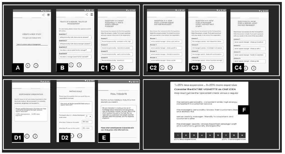
Mind Genomics works according to a systematized process, following a user-friend path. The software makes the set up straightforward. The set-up system is simple, shown by Figure 1, which represents the different steps that the researcher follows, and at each point types in the relevant information onto a computerized form. Figure 1 is meant to be schematic, showing an actual sequence of completed forms, in the sequence presented to the user. The user is led through a series of forms to complete. The process is virtually self-explanatory but is absent bells and whistles. The format is simple, to the point, and guides the researcher through the process, step by step, beginning with the selection of the topic, the requirement to create four questions, the requirement to create four answers for each question, and finishing with the introduction to the experiment, the rating scale, and the anchor points for the rating scale (highest and lowest).

FIG 1

Figure 1: The set-up system for the Mind Genomics project.

It is worth noting that the ‘difficulties’ encountered in these studies are not from the study itself, but typically because people think in an undisciplined fashion. The form in Figure 1 forces the respondent to think in a systematical fashion, beginning with the topic, then proceeding to the questions, and finally moving to creating four answers for each question. After the first one or two experiences, the thinking of the typical researcher changes, as the respondent begins to follow the disciplined path demanded by the computer program. We illustrate the set up with the first of the three studies, traits of the server. We deal with the results in detail, and then follow up with a cursory analysis of the key findings for the other two studies, the interaction among the staff (Study 2) and the interaction with the customer (Study 3).

Step 1 (Panel A)

Select the name of the topic. This first step requires the researcher to give a name to the project. As simple and as direct as it sounds, Step 1 requires the researcher to focus on the topic as a coherent ‘whole,’ rather than thinking about the topic in a diffuse way. The research then records the name on the proper screen. The study here is Traits of Servers.

Step 2 (Panel B)

Select four questions which tell a story about the topic. It is at Step 2 that the topic should crystallize in the mind of the respondent. The text is typed onto the computer form, one question after another. The questions are never seen directly by the respondent, but simply used as an aid to help generate the creation of the four answers to each question. It is relevant to note here that Step 2 is the most difficult step in the entire process. Most people do not approach problems and knowledge acquisition in a structured, disciplined fashion. Two or three experiences suffice.

Step 3 (Panels C1-C4)

Repeat each question (automatically done by the computer), and instruct the respondent to type in the four different answers to the question in exactly the language and format that the respondent will see it. It is straightforward here to copy text from other languages and other alphabets, and then paste into the computer form. Each of the four panels corresponds to one of the questions. Table 1 shows the four questions, and the four answers to each question.

Table 1: The four questions and the four answers to each question for Study #1.

Study 1: Traits of server and manager
Question A: what personality traits does a server possess?
A1 the server’s personality: consistent smile; high energy; competent in customer service
A2 the server’s personality: insensitive to people with different personalities who show up
A3 the server’s personality: easily communicates with people similar to themselves regarding their specific needs like special dietary requests
A4 the server’s personality: sensitive to customer’s/coworker’s cultural differences; understands we are all different
Question B: what personality traits does a manager possess?
B1 the manager’s personality: stern disposition; takes on an authoritative role
B2 the manager’s personality: knows their customers likes and dislikes the
B3 the manager’s personality: knows their staff’s strengths and weaknesses
B4 the manager’s personality: knows their staff’s weaknesses and strengths
Question C: how does a server assist his/her manager?
C1 server assists manager: shows up to work on time on a consistent basis
C2 server assists manager: shows up with a can-do, team player attitude
C3 server assists manager: friendly to coworkers and customers alike
C4 server assists manager: shows up late
Question D: how does a manager assist his/her wait staff?
D1 the manager assists: stern disposition; takes on an authoritative role
D2 the manager assists: knowledge in all aspects of restaurant tasks
D3 the manager assists: deals with confrontations between staff and customers in a bias manner
D4 the manager assists: shows favoritism amongst staff and customers; generally disrespectful

The rationale for four questions and four answers per question comes from the vision of the researchers to create an easy-to-use system to answers questions about specific topics, such as products, political candidates, and social situations. The original goal was to make the number of possible messages about a topic virtually unlimited. With repeated experience, it became clear that most issues could be satisfied with 36 elements, such as four questions with nine answers (36 elements, 60 vignettes), or six questions with six answers each (36 elements, 48 vignettes). Over time it was the design comprises four questions with four different alternatives (16 elements, 24 vignettes) which emerged as the most practical. Note that elements B3 and B4 are the same, except for a reversal of the order of elements. B3 began with strengths and finished with weaknesses. B4 began with weaknesses and finished with strengths. The Mind Genomics process lets us explore these side issues of order, and study different ways of expressing the same idea, whether these be minor differences (e.g., order of ideas) or major differences (different tonality of language.)

Step 4 (Panels D1 and D2)

Orient the respondent (D1) and then create the rating questions, selecting the number of points, and the rating scale (D2). There are three sequential steps to create the rating scale, comprising the text, the number of scale points, and the anchor points for the low end of the scale and the high end of the scale. Only two scale anchors are allowed in the current version. For other formats, the actual scale points and their anchors are typed out.  For this study, the rating scale is:

Please read the vignette below. How much would you expect the price to be for your meal
1= 25% lower  …   9= 25% higher

Step 5 (Panel E)

Show the actual vignette. This is not part of the set up, but is what the vignette looks like on a computer tablet or a PC. There is a slightly different ‘look’ for a smartphone, due to the difference in size and dimension. Each respondent evaluates a unique set of 24 vignettes, comprising either two, threeor four elements, viz., answers. A vignette can contain a maximum of one answer from a question, never two or more answers, This simple bookkeeping device ensures that the respondent will never be presented with a vignette comprising mutually contradictory elements. at least contradictory by presenting different altenratives to the same question.

Each respondent evaluated a different set of 24 vignettes, created by permuting the basic experimental design [12]. This strategy maintains  the power of an experimental design even at the level of the individual respondent, but ensures that each respondent evlauated a unique set of 24 vignettes. Two benefits emerge, the first beiug the ability to analyze the data by creating a model at the level of the individual (important for clustering), and the second ensuring that the study covers a wide range of possible combinations and thus needs absolutely no knowledge about the most promising combinations to test.

Step 6

Create the database (Table 2). The project generates 24 rows of data for each person. An example of the database appears in Table 2, with the table transpose for presentation purpooses. . The data are set up for immediately stastical anaysis.

Table 2: Example of the database prepared for analysis. The actual matrix format for data analysis is transposed 90 degrees.

Panelist Each respondent has a unique identification number (UID) 1 2 3 4 5 6
Row in database The 30 respondents generate 24 rows of data each, one for each vignette 246 407 478 583 642 678
Gender Male or Female, obtained from an up-front classification question Fem Male Fem Male Fem Male
Age The respondent gives year of birth 36 23 19 24 23 20
Age Group After-the fact grouping into two ages Old Old Young Old Old Young
Self-Profiling (Answer one only) Who do you relate to most in a restaurant setting?

1= Wait staff ( food )

2= Owner

3= Bus ( drinks, setup, cleanup )

4=Cashier/host

1 1 1 1 3 1
Test Order The computer records the order of trial 12 23 17 6 18 22
A1 Each element in the study us coded 1 when appearing in the vignette, and 0 when absent from the vignette 0 0 0 0 0 0
A2 0 1 0 0 0 0
A3 0 0 0 0 0 0
A4 0 0 0 0 0 1
B1 0 0 1 0 0 0
B2 0 0 0 0 0 0
B3 1 0 0 1 1 0
B4 0 0 0 0 0 1
C1 0 0 0 0 0 1
C2 1 0 0 0 1 0
C3 0 0 1 1 0 0
C4 0 0 0 0 0 0
D1 0 1 1 0 0 0
D2 0 0 0 0 0 0
D3 1 0 0 0 1 0
D4 0 0 0 1 0 0
Rating The 9-point rating scale anchored at 1 (25% lower) and 9 (25% higher) 8 4 8 6 7 2
Price The percentage departure from 0 19 -6 19 6 13 -19
Rtseconds Response time to the vignette in the nearest 10th of a second 1.2 0.8 5.0 4.9 1.1 4.0
Clusters2 Membership in one of the two clusters 1 2 1 1 2 2
Clusters3 Membership one of the three cluster 1 3 1 3 2 2

Step 7: Convert the Data to Percent

The nine ratings of price are transformed to relative price, with a rating of 9 transformed to +25 (25% higher), a rating of 5 transformed to 0 (same expected price), and a 1 transformed to -25 (25% lower).

Step 8

Build separate equations for the predefined groups (total, gender, age) The data from each of the self-defined groups, total, gender, and age, were analyzed to create an equation of the form:

Percent Departure of Check from Typical (+25 to – 25) = k1(A1) + k2(A2) … k16(D4)

The coefficient for an element is relative change (percent) is size of the check when the element is inserted into the vignette: (increase in expected check when positive, decrease in expected check when negative).

Table 3 shows the coefficients for the different groups. We highlight only those elements which generate positive or negative changes of 8% or higher in the check. The interesting finding from the first group of respondents is that there are no elements which drive up the value of the check, or drive it down, as least strongly. No coefficient is 8 or higher, viz., no element can be attributed to be a major driver of the check price.

Step 9

Create new to the world mind-sets by dividing the respondents into groups based upon the patterns of their coefficients. Each respondent generates an equation with 16 coefficients, the equation relating the presence/absence of the 16 elements to the percent change expected for the check. The percent is shown as a whole number. A 25% increase in the check is shown as +25; 25% decrease in the check is shown as -25). The pattern of coefficients allows the use of k-means clustering [7]. The clustering program computes a measure of ‘distance’ between pairs of respondents, the measure D defined as (1-Pearson Correlation, viz. 1-R.) The Pearson Correlation, R, measures the strength of a linear relation between two variables, based upon the different observations. There are 16 observations for each respondent. The Pearson Correlation varies from a high of +1 when two variables are perfectly linearly related to each other, to 0 when two variables are not related to each other, to -1 when two variables are inversely related to each other.

Step 10

Create the models for two and three clusters emerging from the clustering. The segmentation or clustering does not know anything about the ‘meaning’ of the elements, but simply works with the coefficients, and the distance values. The clustering yields five new models, two for two-mindsets, and three for three-mind sets. It is the task of the researcher to name these mind-sets, based upon the pattern of strong performing positive elements. We will only present the results for the three mind-sets.

Results – Study #1 (Traits of Servers and Manager)

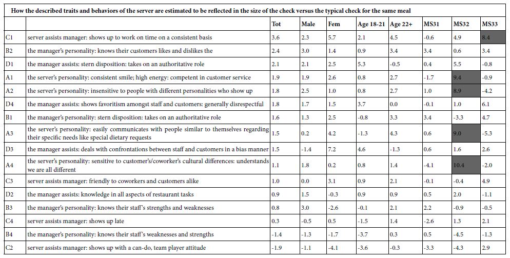
The first analysis comprises the deconstruction of relative price based on the traits of the staff. Table 3 shows that nearly all elements increase the expected bill, but each element increases the expected size of the check to a small degree. There are no elements which stand out as strong contributors of the magnitude of the check, at least when we deal with respondents classified by gender or by age, respectively.

Table 3: Study #1: How the traits and behaviors of the server and the manager drives the relative size of the check. Numbers in the cells are the increment or decrement of the size of the check, expressed as percent, attributable to the element.

table 3

The respondent who is instructed to assign monetary value to a situation (so-called homo economicus) often is more conservative than the respondent who is instructed to assign a rating of a feeling. These data suggest a conservative response. For the Total Panel, the highest contribution to the checks only 3.6% (server assists manager: shows up to work on time on a consistent basis.) For the Total Panel, the lowest contribution to the check is -1.9% (server assists manager: shows up with a can-do, team player attitude.) There are similar, small contributions for the subgroups defined by gender and by age. At least for the total panel and for the key subgroups defined by age and gender, there is no clear relation between the positive behavior of the staff, their interaction, and the price of the check. We see a clearer set of contributions when we divide the respondents into ‘mind-sets’ based upon the pattern of their coefficients for the relative price, rather than by who they are (mind-sets versus conventional geo-demographic subgroups). Yet, as both Table 3 shows for all the data, and Table 4 shows for the strong-performing elements by mind-set, there are still very few elements which drive an expectation of a large increment or decrement of the check.

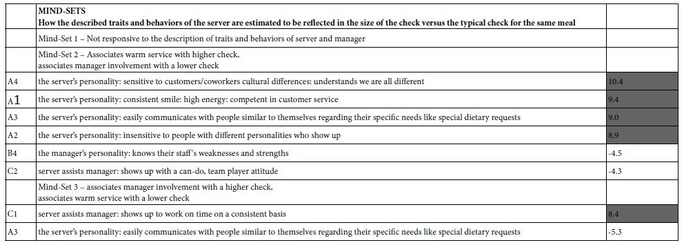
Table 4: Study #1: How the traits of the server and the manager drives the relative size of the check. Data from the strongest elements for the three mind-sets.

table 4

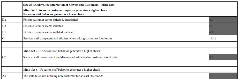
The division of respondents into three mind-sets suggests that:

Mind-Set 1

No clear elements drive change in size of the check

Mind-Set 2

Associates warm service with a higher check, associates manager involvement with a lower check. It may be that these respondents feel that any focus on the server’s personality will increase the check.

Mind-Set 3

Expects to pay more for a server who does the job. Expects to pay less for a server who is friendly, and with whom the customer identifies.

Study 1 on the Traits of the Server and Manager suggests that,, in contrast to homo emotionalis who can be shown to have expansive feelings, these patterns emerging when the mind-sets are separated, homo economicus still shows a constrained range of feelings, even when the different mind-sets are identified by the same clustering method, k-means.

Study #2 (Behavior of Staff as the Customer Enters the Restaurant)

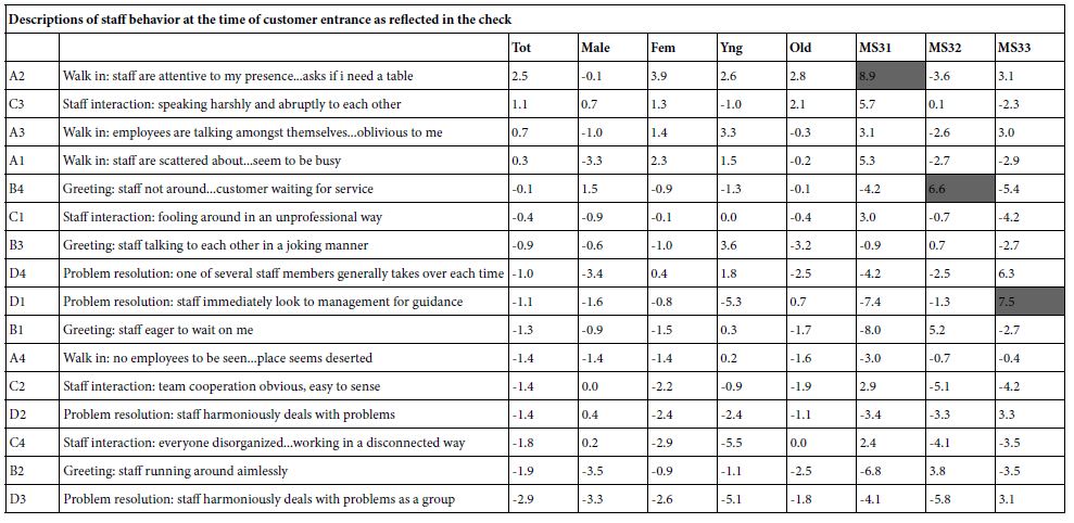
The second study moves to what the customer might observe when walking into the restaurant, but before the customer has been seated. We see no clear relation between the incremental or decremental size of the check and staff behavior at the entrance to the restaurant (Table 5)

Table 5: Study #2: How the behavior of the staff at the time of customer entrance to the restaurant drives the relative size of the check. Numbers in the cells are the increment or decrement of the size of the check, expressed as percent, attributable to the element.

table 5

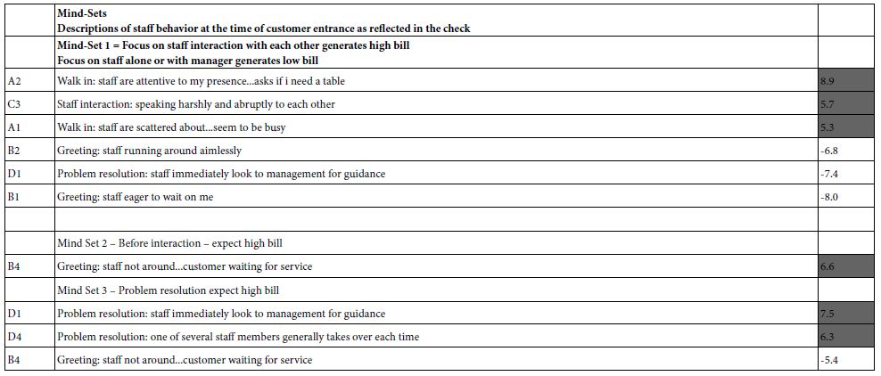
The key differences which emerge come from the three mind-sets (Table 6).

Table 6: Study #2: How the behavior of the staff at the time of customer entrance to the restaurant drives the relative size of the check. Data from the strongest elements for the three mind-sets.

table 6

Mind-Set 1 appears to expect to pay more for staff which look busy, whether they are harmoniously busy or not. Mind-Set appears to expect to pay less for staff seemingly eager to wait on the customer.

Mind-Set 2 expects to pay more when the staff look busy.

Mind-Set 3 expects to pay more when the staff look competent and resolve a problem. Mind-Set 3 expects to pay less for incompetent service.

Study #2 reaffirms that when the respondent is asked to use economics, specifically money as a measure of something that is not usually appraised in economic terms, viz., behavior and service, homo economicus takes over, and forces the respondent in a conservative, judgmental stance. No elements emerge as dramatically strong drivers of the magnitude of the check.

Study # 3 – Dollar Value of Description of the Interaction Between Server and Customer

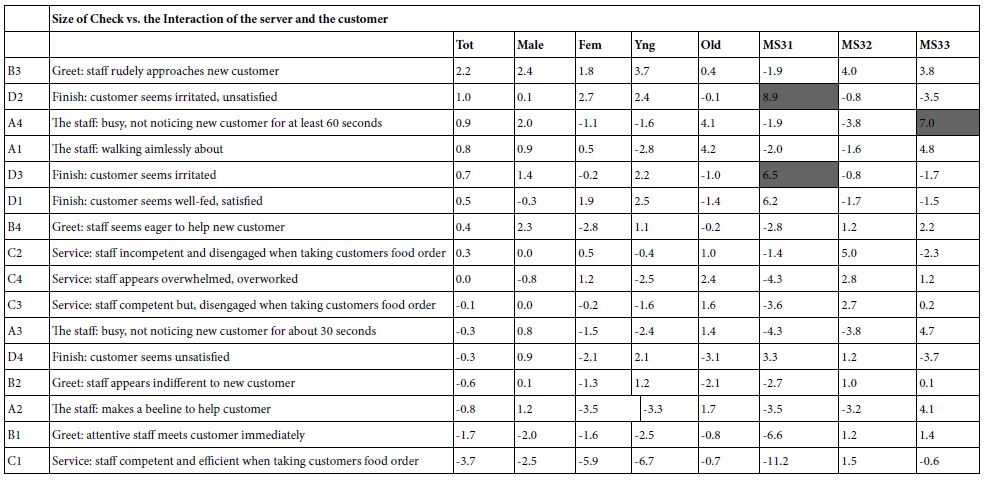
Study #3 was run exactly as studies 1 and 2.This time, however, the topic was the interaction of the server and the customer. Once again, no patterns emerge for the total panel and for the key subgroups of gender and age (Table 7). The key results emerge for the mind-sets (Table 8)

Table 7: Study #3: How the interaction of the server with the customer drives the relative size of the check. Numbers in the cells are the increment or decrement of the size of the check, expressed as percent, attributable to the element.

table 7

Table 8: Study #3: How the interaction of the server with the customer drives the relative size of the check. Data by mind-set

table 8

Mind-Set 1

Focus on the customer generates an expectation of a higher check. Focus on the server generates an expectation of a lower check.

Mind-Set 2

Weak effects. No strong expectations either direction.

Mind-Set 3

Focus on incompetence drives the expectation of a slightly higher check.

Again, in contrast to homo emotionalis, we see homo economicus is far more conservative, especially when there is attribution without clear linkage, rather than evaluation with clear linkage. An example of the evaluation would be the expectation of the price of the check when the messages deal with the actual food, rather than the service.

Beyond Cognitive Responses of Homo Economicus to A Focus on Engagement Time (Response Time)

The second aspect of the analysis involves the amount of time that a respondent spends making a decision. The data from the deconstruction suggests that the respondent is conservative, at least at a conscious level. At the level of the unconscious, however, can we discover anything more about homo economics and attribution? That is, if we are able to measure the time needed to make a decision, do we learn anything more? Or, in fact, is attribution more elusive? One of the features of the Mind Genomics system is the ability to measure response times, defined as the number of seconds between the time the vignette appears o the screen and the time that the respondent assigns a rating. The response time shortens and reaches a steady stage after 2-3 experiences with the task. Since each respondent evaluated all of the elements in different combinations, and each element appeared many times in each position, one need not eliminate the first 1-3 vignettes. They can simply be included because the slow response should distribute itself approximately equally across all respondents and all elements.

The respondents could not have known their own response times for each element, for three reasons:

  1. The respondent was not aware that the response time was being measured
  2. There was too much to do when evaluating 24 vignettes
  3. Each vignette comprised 2-4 elements.

The response times are measured as a totality. Any response time of 9 seconds or longer was defined as 9 seconds. The randomization of experimental designs ensured that the vignettes requiring 9 seconds or longer would most likely comprise similar elements.

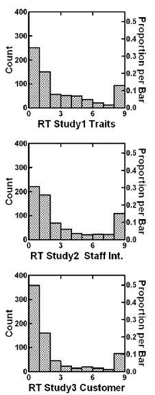
Figure 2 shows the distribution of the response times for each element. The three histograms are plotted in a vertical fashion, allowing the eye to compare the shape of the histograms. It is clear that the response times tend to be longest when the task is to attribute relative price of the check to the traits of the server and the manager. It is clear that the response times tend to be shortest when the task is to attribute relative price of the check to the interaction of the server with the customer. These patterns make intuitive sense, because the respondent can identify with the situation of the server interacting with the respondent. There is little to think about. The reaction is quick because the situation is familiar.

FIG 2

Figure 2: Histograms of the frequencies of the response times for the vignettes. Each graph pertains to one study.

A deeper look into the data reveals the number of seconds that can be ascribed to each element. The analysis is similar to the previous analysis linking the presence/absence of the element to the relative magnitude of the check (1=25% less to 9=25% more). This time, the dependent variable is the response time to the nearest tenth of a second. The equation showing the deconstruction of the response time once again has no additive constant: Response Time (Seconds) = k1(A1) + k2(A2) … k16(D4)

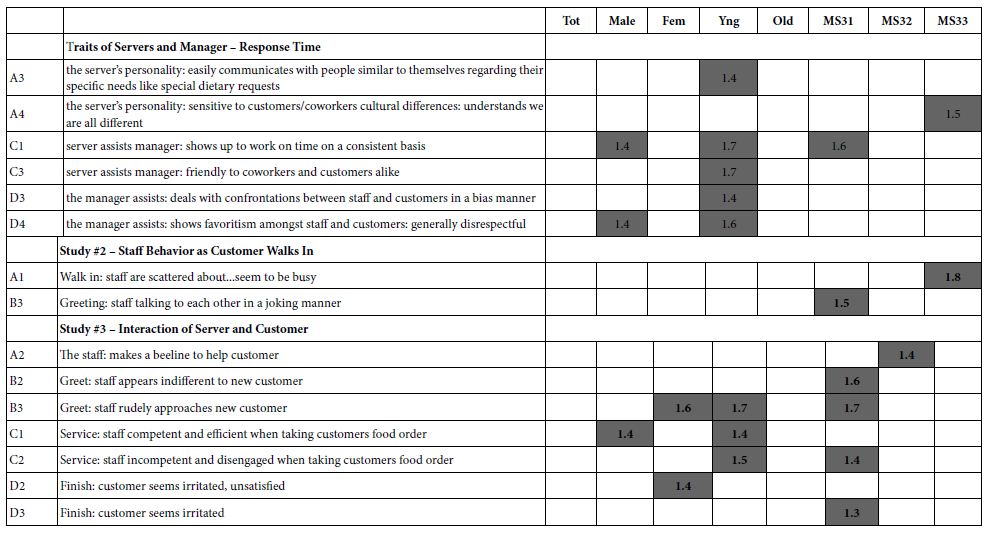
Table 9 shows the combination of element and subgroup for elements defined to ‘engage the respondent.’ In this study, engagement is operationally defined as an element whose deconstructed value of response time is 1.4 seconds or longer. The number 1.4 seconds is an operational definition of engagement, emerging from the analysis of hundreds of studies of this type. The typical engagement times for elements are generally 0.3 to 0.7 seconds, but the engagement times vary by seriousness of topic. Thus, 1.4 seconds for estimated response time is a safe estimate for an element which engages, albeit an estimate of convenience since there is no agreed-upon definition of engagement vs. response time.

Table 9: Response times (engagement) to individual elements by respondents in key subgroups. Only those elements generating response times of 1.4 seconds or more are shown in the table.

table 9

Table 9 suggests that there are some elements which engage the respondent in for dramatically longer times.

The total panel shows no long engagement times.

Males engage with the elements about assisting, whether server assists manager or manager assists server. In contrast, females engage in the element talking about a negative end to the meal.

Younger respondents engage with assistance as well, whether positive or negative. They also respond to elements talking about the nature of the service. Older respondents do not engage with any element.

Mind-Set 1 engages with all types of elements, positive and negative, and at all stages of the staff-customer interaction.

Mind-Set 2 engages with speed of service (‘beeline’).

Mind-Set 3 engages most with the staff being busy.

The use of response time reveals a somewhat more detailed story, suggesting that the attribution of dollar value to staff behavior may not reveal itself as much in the conscious evaluation of ‘how much money will change hands’ but rather in the unconscious variation in engagement time (response time to individual elements).

Discussion and Conclusion

The emerging science of Mind Genomics has been previously used to understand how people respond in an emotional fashion to the description of features and attributes of products and situations [13], as well as understand the dollar value of features and products [10,11]. The approach here moves from the evaluation of concrete descriptions of products and situations to the attribution of value to situations which have no intrinsic value in an of themselves. The introductory studies here are the atmosphere and behavior of service and managerial staff in a restaurant, and the attributed value of such service to one economic indicator, the magnitude of the check.

The data suggest that it is difficult to link economics (e.g., value of the check) to behavior which is not directly related to the product. The Mind Genomics experiment works, at least in practice. What emerges, however is a greatly constricted pattern, a conservatism which does show itself dramatically when one is rating the concrete situation based on feelings, or when one is rating the dollar value of a tangible item or clearly defined service for which one will pay. The implications of this study are great. We live in an economic society where the focus is on customer satisfaction, and the expected economic returns of customer satisfaction. These data suggest that such efforts may be more difficult than one might think. It is all well and good to measure the satisfaction of customers, but just how does that translate into what people will pay. The data from this study suggests that the results of a Mind Genomics study might not be very clear, whether the study deals with the evaluation of a situation without a customer (Study #1: Traits of Server and Manager), the evaluation of a situation where the customer is being introduced into the situation (Study #2: Staff Behavior as Customer Walks In), or even the evaluation of a situation describing the interaction with the staff (Study #3: Interaction of Server and Customer). Or to summarize, how then do we measure the dollar value of customer satisfaction? What have we missed?

References

  1. Han H, Ryu K (2009) The Roles of the Physical Environment, Price Perception, and Customer Satisfaction in Determining Customer Loyalty in the Restaurant Industry. Journal of Hospitality & Tourism Research 33: 487-510.
  2. Namkung Y, Jang S (2007) Does Food Quality Really Matter in Restaurants? Its Impact On Customer Satisfaction and Behavioral Intentions. Journal of Hospitality & Tourism Research 31: 387-409.
  3. Qin H, Prybutok VR (2009) Service quality, customer satisfaction, and behavioral intentions in fast-food restaurants. International Journal of Quality and Service Science 1: 78-95.
  4. Ryu K, Han H (2010) Influence of the Quality of Food, Service, and Physical Environment on Customer Satisfaction and Behavioral Intention in Quick-Casual Restaurants: Moderating Role of Perceived Price. Journal of Hospitality & Tourism Research 34: 310-329.
  5. Jang S, Liu Y, Namkung Y (2011) Effects of authentic atmospherics in ethnic restaurants: investigating Chinese restaurants. International Journal of Contemporary Hospitality Management 23: 662-680.
  6. Teng CC (2011) Commercial hospitality in restaurants and tourist accommodation: Perspectives from international consumer experience in Scotland. International Journal of Hospitality Management 30: 866-874.
  7. Zemel R, Choudhuri SG, Gere A, Upreti H, Deite Y, et al. (2019) Mind, consumers, and dairy: Applying artificial intelligence, mind genomics, and predictive viewpoint typing.
  8. Moskowitz H, Baum E, Rappaport S, Gere A (2019) Estimated Stock Price Based on Company Communications: Mind Genomics and Cognitive Economics as Knowledge-Creation Tools for Behavioral Finance. Edelweiss Applied Science and Technology 4: 60-69.
  9. Moskowitz H, Rappaport S, Moskowitz D, Porretta S, Velema B, et al. (2017) Chapter 14 – Product design for bread through mind genomics and cognitive economics. In D. Bagchi & S. Nair (Eds.), Developing New Functional Food and Nutraceutical Products 249-278.
  10. Moskowitz HR (2012) ‘Mind genomics’: the experimental, inductive science of the ordinary, and its application to aspects of food and feeding. Physiol Behav 107: 606-613.
  11. Moskowitz HR (1995) The dollar value of product quality: The effect of pricing versus overall liking on consumer stated purchase intent for pizza. Journal of Sensory Studies 10: 239-247.
  12. Gofman A, Moskowitz H (2010) Isomorphic Permuted Experimental Designs and Their Application in Conjoint Analysis. Journal of Sensory Studies 25: 127-145.
  13. Gere A, Harizi A, Bellissimo N, Roberts D, Moskowitz H (2020) Creating a mind genomics wiki for non-meat analogs. Sustainability 12: 5352.

Quantification of Tooth Wear by Selected Desensitizing Polishing Pastes Using White Light Profilometry

DOI: 10.31038/JDMR.2020344

Abstract

Objectives: To analyse tooth wear using white light non-contact profilometry following the polishing of the tooth surface with selected polishing pastes.

Methods: Three polishing pastes containing a range of particles sizes and different coarseness (extra-fine, medium, course) were compared with commercially available prophylaxis pastes (Nupro with Novamin® and Nupro with Fluoride) as controls. Particle size distribution was analysed using a using particle size analyser and quantified using Masterizer software. Teeth were in 70% ethanol prior to evaluation. 25 extracted human premolar teeth were distributed in five groups (n=5), and the teeth were mounted in a silicone putty matrix leaving an exposed buccal surface. White light profilometry with Proscan 2000 software was used to scan each tooth surface before and after polishing. Scantron ProForm software was used to superimpose images and measure surface loss and analyse the difference between the two surfaces-scans by the Proscan 2000 software.

Results: Particle size analysis indicated that all samples consisted of a wide distribution of particles’ sizes (DX 10, 50, and 90). The course polishing paste had the largest DX 90 whereas Nupro with Fluoride had the lowest DX 90. The extra-fine pumice had the lowest DX 90, although this paste had larger values for DX 10 and DX 50 compared to the medium paste. The volume tooth loss analysis demonstrated that the course pumice had the most tooth surface loss compared to the extra-fine pumice which had the least amount of tooth surface loss. The average volume loss per group was 0.808, 0.022, 0.014, 0.022, 0.026 (course, medium, extra-fine, Nupro with Fluoride, and Nupro with Novamin®) respectively.

Conclusions: The results indicated that the larger the DX 90 within the paste, the more tooth surface loss occurred due to the abrasivity of the paste. There was however minimal or no significant difference in the amount of tooth loss between the control polishing pastes.

Keywords

Prophylaxis polishing pastes, Abrasion, White light profilometry, Particle size analysis

Introduction

Dental materials are frequently used in polishing procedures during periodontal procedures in daily dental practice and the abrasives in these materials may subsequently have an impact on tooth surface loss and wear. Several factors are indicated in the aetiology of tooth wear with or without Dentine Hypersensitivity (DH) such as erosion, attrition and, abrasion. Furthermore, different materials other than a tooth can cause tooth contact when it contacts a tooth (so-called two-body or three- body contact [Tribology]) [1]. The term wear is, therefore, a better descriptive term to define the loss of tooth structure [2]. Tooth wear can be defined as the net loss of tooth structure when it is under function [1]. Previous studies have reported a growing interest in quantifying tooth structure loss which is called ‘wear quantification’ both in vivo and in vitro in three dimensions. Volume and mean height are the most clinically relevant parameters that can be used to analyse tooth loss [3]. It is essential to have a systematic, reliable and, repeatable data using a wear quantification method. The method itself is time consuming, which requires an experienced operator to apply the different software packages that are available commercially for wear quantification [4]. It is, however, a useful method to compare and evaluate the effect of different new materials, which may cause tooth wear in vitro. An accurate surface topographic representation of a tooth both pre- and post-wear testing is essential for any in vitro wear qualification to be valid. There are three main types of sensors that are used for scanning and subsequently quantifying the wear namely: 1) contact sensors [5], 2) non-contact sensors [6] and 3) white light [7] which are all suitable for systematic studies [4]. Investigators have previously utilised white light non-contact profilometric techniques as a quantifiable measure of tooth loss/abrasive wear and/or erosion [7-9]. White light profilometry uses effective sensors to measure the distance in which they can split the white light beam into its constituent wavelength [10]. Each wavelength matches to its corresponding distance which creates its monochromatic image point. Therefore, the image reflects the surface topography of a scanned specimen which it can provide a quantitative measure of shape, texture, microtopography, microform and roughness [10].

Aim

The aim of this in vitro study was to analyse tooth wear on extracted human teeth using contactless white light profilometry following professional polishing with selected polishing pastes with different types of pumice used in the polishing of teeth during periodontal procedures.

Material and Method

This exploratory study was based on two procedures. The first part described in this paper was to quantify tooth wear using a white light profilometry following polishing of the teeth to choose the ideal abrasivity of the pumice that would be incorporated into future prophy-paste formulations. The second part of the study was the evaluation of selected pastes to determine their effectiveness in tubular occlusion and this will be reported in a subsequent paper.

Particle Size Analysis

The same weight (50 mg) of the polishing prophylaxis paste samples were dissolved separately in 50 mL deionised water. Once the solid particles were dispersed, the diluted solution was transferred into a system that uses the MASTERSIZER 3000E (MALVERN software) to initiate the measurements and analysing the particle sizes through the laser diffraction method using a dispersion of particles in a liquid, wet, Hydro EV, deionised water with a 1.33 refractive index. The Mastersizer E used is designed to obtain values for a wide particle size range of 0.1 to 3500 µm. The setting of the software was pre-set manually to a duration of 15 seconds background measurement(s) and 10 seconds sample measurements. The diluted solution was added in small quantities until the obstruction range of 5-20% was achieved. A speed of 2000 rpm for the hydro pump speed was used for all tested samples. Four different measurements for each sample were automatically reported, analysed, and averaged by the software. The median for different volume distributions DX 10, 50, and 90 were recorded and the data was subsequently exported into an Excel file for analysis.

Preparation of Materials

A total of 30 extracted, caries free human premolars were collected from the walk-in dental polyclinics from Kuwait in 2017 after obtaining verbal consent from patients for the use of their teeth in research. The teeth were stored in a small container of Listerine mouthwash (Johnson and Johnson, UK) and brought to the UK by HFH under QMUL guidelines UK. The teeth were transferred and stored in a 70% Ethanol solution in a specimen container at room temperature within the Department of Physical Sciences Unit at Mile End, London in accordance with HTA regulations. The extracted premolars were distributed into five groups (n=5) and teeth were mounted in a silicon putty matrix (Zetaplus plus mixed with an indurent gel (Zhermack SpA, Italy), leaving an exposed buccal surface to evaluate. The groups were numbered from 1 to 5 and they were stored in the 70% Ethanol solution at room temperature within the Department.

Prior to scanning the samples were prepared by placing three divots using a ½ round bur at high speed on the flattest buccal (facial) surface of each tooth. Three polishing pumices with a range of particle sizes and different coarseness of pumice (extra-fine, medium, course) (Kemdent Works, Swindon UK) were compared to commercially available prophylaxis pastes namely, Nupro with Novamin®, Nupro with Fluoride (Dentsply International, USA)(Controls). A battery-operated dental polisher portable handpiece (Dentitex model number TP-01; 8000 rpm motor), was used as a polishing carrier device instead of a slow speed handpiece for practical purposes. Its cup has the same size as a dental office polishing cup. To avoid any contamination of the materials, each cup was dedicated for a specific prophylaxis paste. Three different pumice powders (course, medium and extra-fine) (Kemdent; Swindon, UK) were characterized in terms of their particle size distribution (Masterizer software). The exact weight measure of the samples was dissolved separately in 50 mg deionised water. The diluted solution was transferred to initiate the measurements and analysing the particle sizes through a laser diffraction method using a dispersion of particles in a liquid, Hydro EV, deionised water with 1.33 refractive index (Mastersizer 3000E from Malvern software).

Quantification of Tooth Surface Loss

White Light Profilometry (WLP)

Two software programmes were used for analysing the tooth surface loss; namely: a Proscan 2000 and a Scantron ProForm. The Proscan 2000 software is designed for shape analysis, object digitisation and accurate surface analysis. The Scantron ProForm software is designed for analysing the differences between two surfaces-scans made by the Proscan 2000 software accuracy.

Three divots on the buccal surface of every tooth were placed to define reference points and the surfaces scanned. The pumice was used with water only, and the tooth was polished for two minutes using the portable polishing handpiece (Dentitex). The tooth was gently rinsed with water until all pumice particles were no longer observed on the tooth surface. A second scan was undertaken using white light profilometry. The two scans were then superimposed in a different software Scantron ProForm to measure any surface volume loss and analyse the difference between the two surfaces-scans. An area of 0.4 x 0.4 µm² was randomly selected between the three divots as a standard dimension for all samples (Figure 1).

fig 1

Figure 1: shows a) superimposing of pre-treated and post-treated tooth surface using course pumice. b) Random selection of area 0.4×0.4 µm² between the three created divots on the tooth.

Results and Discussion

The particle size analysis showed that all samples consisted of a wide distribution of particle sizes (DX 10, 50, and 90). Table 1 and Figure 2 show the particle size distribution for each sample. The course pumice sample had the largest amount of DX 90 particle size whereas Nupro with Fluoride had the smallest DX 90. The extra-fine pumice sample had the smallest DX 90 for the pumice powders but had larger values for DX 10 and DX 50 than the medium pumice sample.

Table 1: Distribution of DX 10, 50, and 90 µm particle sizes of the five groups.

DX 10 (µm)

DX 50 (µm)

DX 90 (µm)

Course Pumice

53.4

119

253

Medium Pumice

4.04

21.0

75.1

Extra-Fine Pumice

4.33

23.7

62.0

Nupro with F

5.27

19.1

53.8

Nupro with NovaMin®

13.8

44.4

121

fig 2

Figure 2: Particle Size Distribution DX 10, 50, and 90 particle sizes of the five materials.

The tooth surface loss volume was analysed using white light non-contact profilometry following the polishing of the tooth surface with the selected polishing pastes. The results demonstrated that the course pumice had the most tooth surface loss compared to the extra-fine pumice which had the least amount of tooth surface loss. The average volume loss per group was 0.808, 0.022, 0.014, 0.022, 0.026 mm3 (course, medium, extra-fine, Nupro with Fluoride, and Nupro with Novamin®) respectively (Table 2 and Figure 3). The t-test between the Medium vs. Extra-Fine samples was 0.0098 which indicated a significant difference in surface loss. Based on this result an extra-fine pumice was recommended to be incorporated in the prophy-paste formulation in subsequent studies. The results indicated that the larger the DX 90 value of the paste, the more tooth surface loss occurred due to the abrasivity of the paste. Thus, it seems that the coarse particles in the particle size distribution close to D90 dominate the tooth loss. There were no significant differences in the amount of tooth loss between the two control samples.

Table 2: The average of tooth surface loss in (mm3) for the different materials analysed where T is the tooth sample that was used.

Sample/Material

Course

Medium Extra-Fine Nupro with Fluoride

Nupro with Novamin®

T1

1.074

0.019 0.013 0.0303

0.021

T2

0.708

0.021 0.009 0.0196

0.017

T3

0.633

0.017 0.015 0.008

0.026

T4

0.877

0.029 0.017 0.0236

0.039

T5

0.749

0.025 0.018 0.0294

0.028

Average

0.8082

0.0222 0.0144 0.0222

0.0262

Standard Deviation

0.1729

0.0048 0.0036 0.0091

0.0083

fig 3

Figure 3: The average of tooth surface loss (mm3) between the selected prophy-pastes after removing the course particle sample: T is the tooth sample that was used.

Table 2 shows the average of tooth surface loss in (mm3) for the different materials analysed where T is the tooth sample that was used.

Conclusion

The results from this exploratory study on the effect of the particle size distribution on tooth surface loss indicated that the larger the DX 90 particle size of the pumice samples, the more tooth surface loss and wear. The extra-fine pumice sample should be incorporated into a prophylaxis paste to reduce any potential tooth surface loss.

References

  1. Addy M (2000) Dentine hypersensitivity: Definition, prevalence, distribution and etiology. In: Addy M, Embery G, Edgar WM, Orchardson R, editors. Tooth wear and sensitivity: Clinical advances in restorative dentistry. London: Martin Dunitz 2000: 239-248.
  2. Smith RG (1997) Gingival recession. Reappraisal of an enigmatic condition and a new index for monitoring. J Clin Periodontol 24: 201-205. [crossref]
  3. Pintado MR, Anderson GC, DeLong R, Douglas WH (1997) Variation in tooth wear in young adults over a two-year period. J Prosthet Dent 77: 313-320. [crossref]
  4. Heintze SD, Cavalleri A, Forjanic M, Zellweger G, Rousson V (2006) A comparison of three different methods for the quantification of the in vitro wear of dental materials. Dent Mater 22: 1051-1062. [crossref]
  5. Magne P Oh WS, Pintado MR, DeLong R (1999) Wear of enamel and veneering ceramics after laboratory and chairside finishing procedures. J Prosthet Dent 82: 669-679. [crossref]
  6. Mehl A, Gloger W, Kunzelmann KH, Hickel R (1997) A new optical 3-D device for the detection of wear. J Dent Res 76: 1799-1807. [crossref]
  7. Vieira A, Overweg E, Ruben JL, Huysmans MC (2006) Toothbrush abrasion, simulated tongue friction and attrition of eroded bovine enamel in vitro. J Dent 34: 336-342. [crossref]
  8. Hara AT, Zero DT (2008) Analysis of the erosive potential of calcium-containing acidic beverages. Eur J Oral Sci 116: 60-65. [crossref]
  9. Theocharopoulos A, Zou L, Hill R, Cattell MJ (2010) Wear quantification of human enamel and dental glass-ceramics using white light profilometry. Wear 269: 930-993.
  10. Litwin D, Galas J, Blocki N (2006) Variable wavelength profilometry, in: Proceedings of the Symposium on Photonics Technologies for 7th Framework Program (Wroclaw, 2006). 476-479.

PI3K Signaling Pathway Regulates the Caspase-9 in Renal Tubular Epithelial Cells

DOI: 10.31038/JPPR.2020331

Abstract

Background: To evaluate how resveratrol regulates the IL-6 signaling in renal cell, pCMV6-IL-6 was overexpressed in the renal tubular epithelial cell line NRK-52E.

Methods: IHC and TUNEL assay were used to identify the localization and apoptosis detection of the overexpression of IL-6 in NRK-52E cells. To identify the effect of overexpressed IL-6, the mitochondrial fraction was isolated and caspase activities and western blotting were performed.

Results: Our results revealed that pCMV6-IL-6 was overexpressed in the nucleus and around the nuclear membrane of the cells. Moreover, the cell membrane showed no IL-6 overexpression, which may be suggest absence of the IL-6/IL-6R binding effect on the cell membrane. Furthermore, the results of the TUNEL assay demonstrated that pCMV6-IL-6-transfected cells showed features of apoptotic cells. The results of the caspase activity assay revealed that resveratrol significantly attenuated IL-6-induced caspase-3 activity but not attenuated IL-6-induced caspase-9 activity, indicating the antiapoptotic ability of resveratrol response on caspase-3 activity. The PI3K inhibitor could decrease the caspase-9 level, suggesting that the reduction of the caspase-9 level mediate by through the PI3K signaling pathway.

Conclusions: Taken together, our results demonstrated that IL-6 expression not only in the cytosol but also in the nucleus of renal tubular epithelial cells. The PI3K signaling pathway regulates the caspase-9 in renal tubular epithelial cells.

Keywords

IL-6, p-STAT3, Caspase-3, Caspase-9, PI3K, Resveratrol

Introduction

Resveratrol is a naturally occurring stilbene that has been used in anticancer, antiaging, and anti-inflammatory treatment; it has also been applied for cardioprotection and nephroprotection in oxonate-induced hyperuricemic mice and for central nervous system protection [1-3]. Resveratrol provides protection against both acute and chronic kidney injury because of its antioxidant properties and ability to activate sirtuin [4]. Therefore, resveratrol is a useful alternative treatment for renal injury. A previous study suggested that resveratrol acts as an antihyperuricemic and nephroprotective agent in hyperuricemic mice; however, whether resveratrol has beneficial effects on kidney disease in humans and other hyperuricemic animal models remains unclear. Interleukin-6 (IL-6) is a multifunctional cytokine that regulates numerous biological processes including organ development, acute-phase responses, inflammation, and immune responses [5]. The role of IL-6 is not restricted to the immune system; it is also involved in the regulation of metabolic processes. Although IL-6 is a proinflammatory cytokine that promotes inflammation under various pathological conditions involving trans-signaling, its anti-inflammatory and regenerative properties mediated by classic signaling have increasingly been recognized [6-8].The local activation of IL-6 classic and trans-signaling pathways is implicated in renal autoimmune and inflammatory diseases, indicating the importance of IL-6 regulation in renal disease [9]. All kidney resident cells can secrete IL-6 in certain milieu, but only podocytes express the IL-6 receptor (IL-6R); however, other kidney resident cells do not express IL-6R and use classic IL-6 signaling. Moreover, IL-6 is a well-known activator of signal transducer and activator of transcription 3 (STAT3) [10]. STAT3 has been studied as a transcription factor; a small pool of STAT3 was localized in the mitochondria, where it functioned as a positive regulator of the mitochondrial electron transport chain [11,12]. To clarify the regulation of IL-6 in renal cells, recombinant pCMV6-IL-6 was overexpressed in the renal tubular epithelial cell line NRK-52E. Our studies demonstrated that IL-6 expression both in the cytosol and nucleus of renal cells. Resveratrol attenuated IL-6-induced caspase-3 and caspase-9 activities. The PI3K inhibitor could decrease the caspase-9 level, suggesting that the PI3K signaling pathway regulates the caspase-9 in renal tubular epithelial cells.

Method

Preparation of NRK-52E Cells and Transfection

A normal rat kidney tubular epithelial cell line, NRK-52E (BCRC60086), was purchased from the Food Industry Research and Development Institute, Taiwan. The cells were cultured in Dulbecco’s Modified Eagle Medium containing 4.5 g/L glucose, 4 mM L-glutamine, and 5% bovine calf serum (Thermo Fisher Scientific Inc., Waltham, MA, USA) and were grown at 37°C in a humidified environment with 5% CO2. pCMV6 and pCMV6-IL-6 cDNA plasmid were purchased from OriGene. The cells were transfected with 2 μg of pCMV6 or pCMV6-IL-6 in each well by using lipofectamine (Thermo Fisher Scientific Inc., Waltham, MA, USA), according to the manufacturer’s instructions.

Treatment with Resveratrol

After NRK-52E cells reached 50-70% confluence, 10 mM of resveratrol (Sigma-Aldrich Corp. MO, USA) were added to the culture medium, and the culture was incubated for 24 h. Control cells were maintained at 37°C in a humidified environment with 5% CO2.

Immunohistochemistry

The cells were fixed in 10% phosphate-buffered formalin, blocked with antibody diluent buffer (Dako, Agilent Technologies, Santa Clara, CA, USA), and incubated with anti-DDK antibody (OriGenen Technologies, Inc., Rockville MD, USA) diluted at 1:500 for 60 min at room temperature. Subsequently, the cells were incubated with secondary antibodies conjugated with horseradish peroxidase (HRP) polymer for 30 min at room temperature. The cells were then treated with a chromogen, 3,3ʹ-diaminobenzidine tetrahydrochloride (Vector Laboratories, CA, USA), for 10 min. Images were captured using an inverted Nikon ECLIPSE TE2000-S (Nikon Instruments Inc., Melville, NY, USA).

DeadEnd™ Colorimetric Apoptosis Detection

The apoptotic cells were assayed using the terminal deoxynucleotidyl transferase (TdT) dUTP Nick-End Labeling (TUNEL) colorimetric method according to the manufacturer’s protocol (Promega Corporation, Madison WI, USA). Briefly, fixed cells were washed, permeabilized, and then incubated with 100 μL of TdT end-labeling cocktail for 60 min at 37°C in a humidified chamber. The cells were blocked with 0.3% hydrogen peroxide and bound with streptavidin HRP. After washing with PBS, and the cells were incubated with 100 μL of 3,3′-diaminobenzidine substrate solution for 10 min at 25°C. Images were captured using an inverted Nikon ECLIPSE TE2000-S (Nikon Instruments Inc., Melville, NY, USA).

Caspase-3/CPP32 and Caspase-9 Colorimetric Assay

Caspase-3 and caspase-9 activities were determined using the caspase-3/CPP32 and caspase-9 colorimetric assay kit (BioVision Inc., Milpitas CA, USA), respectively. The cells were washed in cold PBS, resuspended in 50 mL cell lysis buffer, and incubated on ice for 10 min. Cell lysates were pelleted, followed by the transfer of supernatants to microcentrifuge tubes. Subsequently, 50 mL of cell lysates and 50 mL of the reaction buffer was added to microplate wells; 5 mL of 4mM DEVD-pNA substrate for caspase-3 and 4mM LEHD-pNA substrate for caspase-9 were added and then incubated at 37°C for 2 h. A control reaction of treated cells without DEVD-pNA or LEHD-pNA was included. The absorbance was measured at 405 nm using the BioTek Synergy H1 ELISA reader (BioTek Instruments Inc., Winooski VT, USA).

Mitochondrial Fraction Isolation

The cells were lysed in cytosol extraction buffer containing DTT and protease inhibitors. The samples were maintained on ice for 10 min and then centrifuged at 700xg for 10 min at 4°C. The supernatant was then transferred to a fresh microcentrifuge tube and centrifuged at 10,000xg for 30 min at 4°C. The supernatant was collected as cytosolic fraction, and the pellet was resuspended in mitochondria extraction buffer containing DTT and protease inhibitors as mitochondrial fraction.

SDS-PAGE and Western Blotting

The protein concentration of supernatants was measured using a BCA kit (Pierce Biotechnology, Inc., USA). For each sample, 10 μg or 50 μg of the protein lysate was separated on 10% or 15% polyacrylamide gels and then transferred to PVDF membranes by using a semidry transfer apparatus (Bio-Rad, Hercules, CA, USA). The membranes were blocked in 5% nonfat dry milk in TBST buffer (25 mM of Tris at pH 7.5, 135 mM of NaCl, and 0.15% Tween-20) for 1 h and then incubated with anti-β-Actin (Santa Cruz Biotechnology, Inc.) for 1 h or with anti-DDK (FLAG) antibody (OriGnen Technologies, Inc., Rockville, MD, USA), anti-p-STAT3-Tyr705 (Santa Cruz Biotechnology, Inc.), or anti-caspase-3, anti-caspase-9, anti-COX IV, anti-p-Akt-Ser473, and anti-p-p38 MAP kinase-Thr180/Tyr182 (Cell Signaling Technology, Inc., Danvers, MA,USA) at 4°C for overnight. The blots were washed using TBST and then incubated for 50 min with secondary antibodies conjugated with horseradish peroxidase (Invitrogen, Thermo Fisher Scientific Inc., Waltham, MA, USA). The immunoreactive proteins were detected using an enhanced chemiluminescence detection system (GE Healthcare Bio-Sciences, Marlborough, MA, USA) according to the manufacturer’s instructions.

Statistical Analysis

All data in this study are presented as mean ± standard error of the mean (SEM) from triplicate measurements. The stained blots were scanned and quantified using ImageJ 1.52a software (NIH, USA). A p value of <0.05, <0.01, or <0.001 (one-way ANOVA) was considered significant. All statistical analyses were performed using SigmaPlot, Version 13.0 (Systat Software Inc., San Jose, CA, USA).

Results

IL-6 Overexpression was found in the Nucleus and Around the Nuclear Membrane

As shown in Figure 1c, pCMV6-IL-6 was overexpressed in the nucleus and around the nuclear membrane of the cells. Moreover, the cell membrane showed no IL-6 overexpression, which may be suggest absence of the IL-6/IL-6R binding effect on the cell membrane. Besides, IL-6-overexpressing cells showed the presence of apoptotic bodies, as detected using DeadEndTM colorimetric apoptosis detection assay (Figure 2d), suggesting that IL-6 regulation may be related to apoptosis.

fig 1

Figure 1: Immunohistochemistry staining of overexpressed IL-6 in NRK-52E cells. (a) The immunohistochemistry staining of the control group. (b) The cells transfected through a pCMV6 vector. (c) The cells transfected through pCMV6-IL-6. The arrow indicates the cell overexpressed IL-6.

Resveratrol Attenuated IL-6-induced Caspase-3 Activities in NRK-52E Cells

As shown in Figure 3a, IL-6 overexpression significantly promoted caspase-3 activity in NRK-52E cells (p = 0.014). Moreover, resveratrol significantly attenuated caspase-3 activity not only in treatment alone (Figure 2b, p = 0.002) but also in pCMV6 transfection cells (Figure 2b, p = 0.046) and in pCMV6-IL-6 transfection cells (Figure 2b, p = 0.002). Furthermore, IL-6 overexpression could not regulate caspase-9 activity and resveratrol also could not regulate overexpressed-IL-6-induced caspase-9 activity (Figure 3c).

fig 2

Figure 2: DeadEnd colorimetric apoptosis staining of overexpressed IL-6 in NRK-52E cells. Colorimetric staining of overexpressed IL-6 in NRK-52E cells. (a) The negative control of colorimetric staining. (b) The cells transfected through the pCMV6 vector. (c) Cells transfected through the pCMV6-IL-6 vector. (d) The amplified apoptotic nuclei cells (brown).

Resveratrol Attenuated IL-6-induced p-STAT3 Expression

As shown in Figure 4b, pCMV6-IL-6 expression was found in both cytosol and mitochondrial fractions, and high pCMV6-IL-6 expressed was found in the mitochondrial fraction, indicating the IL-6 may be involved in the mitochondria regulation of cell function. Moreover, IL-6 overexpression significantly promoted both cytosol and mitochondrial p-STAT3 levels, and resveratrol significantly attenuated the IL-6-induced p-STAT3 level in both cytosol and mitochondrial fractions (Figure 4c and 4d, p < 0.001). Furthermore, IL-6 overexpression increased STAT3 mRNA expression, and resveratrol attenuated IL-6-induced STAT3 mRNA expression (Figure 4d). Our results showing that IL-6 could activate STAT3 activity in NRK-52E cells.

Overexpressed IL-6 Promoted the Caspase-9 Protein Level in Mitochondrial Fraction

As shown in Figure 4b and 4g, resveratrol significantly promoted the IL-6-induced caspase-9 level only in the mitochondrial fraction (Figure 4g, p < 0.001). Moreover, IL-6 overexpression significantly reduced the caspase-9 level in the cytosol fraction (Figure 4f, p < 0.001) but increased the level in the mitochondrial fraction (Figure 4g, p < 0.001). Interestingly, resveratrol promoted the IL-6-induced caspase-9 level (Figure 4g, p < 0.001) in the mitochondrial fraction but attenuated IL-6-induced caspase-9 activity in both the cytosol (Figure 3c, p = 0.036) and mitochondria (Figure 4h, p = 0.024) fractions, suggesting that resveratrol attenuated IL-6-induced caspase-9 activity not only in the cytosol fraction but also in the mitochondrial fraction.

Caspase-9 was Mediated by PI3K Signaling Pathway in NRK-52E Cells

As shown in Figure 5, the caspase-9 level decreased after the PI3K inhibitor LY294002 was added to the culture medium. However, the p38 MAPK inhibitor SB203580 and the STAT3 inhibitor stattic did not influence the caspase-9 level (data not shown), suggesting that the regulation of the caspase-9 may mediate by through the PI3K signaling pathway. Moreover, LY294002 and SB203580 did not affect the p-STAT3 level or the caspase-3 level, suggesting p-STAT3 and caspase-3 levels are mediated through other pathways.

Discussion

Resveratrol affects multiple cellular processes and is an excellent candidate for use in human disorders. Numerous experimental studies and clinical trials have been conducted to analyze the systemic anti-inflammatory, antioxidative, multiorgan protective effects of resveratrol [13-15]. Our previous study explored the resveratrol is a potentially therapeutic strategy for hyperuricemia rats and disclosed immunoreactivity of IL-6 in renal cortex [16]. In this study, to evaluate how resveratrol regulates IL-6 in renal cells, pCMV6-IL-6 was overexpressed in the rat tubular epithelial cell line NRK-52E. The IL-6 mRNA level in NRK-52E cells was upregulated after treatment with uric acid and was downregulated after treatment with resveratrol, suggesting the anti-inflammatory property of resveratrol (data not shown). It has been demonstrated that the IL-6 exerts proapoptotic effects through the IL-6 trans-signaling pathway and exerts antiapoptotic effects through the classic pathway [9,17,18]. IL-6 signaling through the membrane-bound IL-6R is mostly regenerative and anti-inflammatory, and the signaling of IL-6/sIL-6R has been termed IL-6 trans-signaling, which induces the proinflammatory properties of IL-6. As demonstrated by Nechemia-Arbely et al., IL-6 trans-signaling mediates a protective response to renal injury [19]. In Nechemia-Arbely’s study, the administration of an IL-6/sIL-6R fusion protein prevented the onset of acute kidney injury and significantly enhanced survival. Therefore, the role of IL-6 in the process of cell injury is still controversial. Our study showed that IL-6 was expressed in the cytosol and nuclear of the renal cells (Figure 1), and low IL-6R mRNA expression was found in the cells (data not shown), indicating the absence of the IL-6/IL-6R binding effect on the cell membrane. Moreover, IL-6-overexpression cells presented apoptotic bodies, as revealed in the DeadEndTM colorimetric apoptosis detection assay, suggesting that the regulation of IL-6 may be related to the apoptosis process (Figure 2). Apoptosis is regulated by two interrelated signaling pathways: the extrinsic or death-receptor pathway and the intrinsic or mitochondrial pathway; both pathways use the caspase cascade [20]. Caspase-9 is a key player in the intrinsic or mitochondrial pathway that is involved in various stimuli, including chemotherapy, stress agent, and radiation [21]. Cytochrome c is released from the mitochondria to the cytoplasm in cells in response to intrinsic stimuli and forms the apoptosome, which mediates caspase-9 activation [22]. Moreover, caspase-3 is a major executioner caspase that is cleaved and activated by both caspase-8 and caspase-9 initiator caspases [22]. In the present study, the results showed that IL-6 overexpression significantly promoted caspase-3 activity (Figure 3a) but did not affect caspase-9 activities (Figure 3c) suggesting the caspase-3 activity may regulate the overexpressed IL-6-induced apoptosis. However, IL-6 overexpression significantly reduced the cytosolic caspase-9 protein level (Figure 4f, p < 0.001) but significantly promoted the mitochondrial caspase-9 protein level (Figure 4g, p < 0.001). The possibility of caspase-9 shifting from the cytosol to mitochondria, induced by IL-6 overexpression, remains to be further studied. Moreover, resveratrol only significantly attenuated IL-6-induced caspase-3 activities (Figure 3b, p = 0.002) but no effect on caspase-9 activities or overexpressed-IL-6-induced caspase-9 activity (Figure 3c) indicating that resveratrol exerts antiapoptotic ability in attenuated caspase-3 activities induced by IL-6 overexpression in NRK-52E cells. STAT3 has been studied as a transcription factor, and a small pool of STAT3 was localized in the mitochondria, where it functioned as a positive regulator of mitochondrial electron transport chain [11-12]. IL-6 is a well-known activator of STAT3 [10]. In the present study, as shown in Figure 4b, pCMV6-IL-6 expression was found in both cytosol and mitochondrial fractions, and pCMV6-IL-6 expression was high in the mitochondrial fraction, indicating that IL-6 may be involved in the mitochondrial regulation of cell function. As expected, IL-6 overexpression significantly promoted both cytosol and mitochondria p-STAT3 levels (Figure 4c and 4d, p < 0.001), indicating that IL-6 could activate STAT3 activity in NRK-52E cells. Resveratrol can exert its anticancer effects by negative regulation of STAT3/5 signaling cascade [23]. Our results also showed that resveratrol not only significantly attenuated the IL-6-induced p-STAT3 level in both cytosol and mitochondrial fractions (Figure 4c and 4d, p < 0.001) but also significantly decreased IL-6-induced STAT3 mRNA expression (Figure 4e, p < 0.05), indicating that resveratrol may downregulate IL-6-induced STAT3 mRNA expression. Human caspase-9 is phosphorylated on Ser196 by Akt/PKB, resulting in the attenuation of its activity, which suggests that the PI3K signaling pathway plays a central role in antiapoptosis [24]. Moreover, the ERK MAPK pathway inhibits caspase-9 activity through direct phosphorylation at Thr 125 [25]. Past studies have suggested that at least one signaling pathway modulates caspase-9. Our study showed that the caspase-9 level was inhibited by the PI3K inhibitor (LY294002) (Figure 5) but could not be inhibited by the MAPK inhibitor (SB203580) or STAT3 inhibitor (stattic) (data not shown), indicating that in NRK-52E cells, the regulation of capase-9 may mediated by PI3K signaling.

fig 3

Figure 3: Caspase-3 and caspase-9 activity assays of IL-6 overexpressed NRK-52E cells. (a) Caspase-3 activity of overexpressed IL-6. (b) Caspase-3 activity of overexpressed IL-6 cells containing 10 mM resveratrol. (c) Caspase-9 activity of overexpressed IL-6 cells containing 10 mM resveratrol. Data are presented as mean ± standard error of the mean for the three measurements.

fig 4

Figure 4: Western blotting analysis of overexpressed IL-6 in cytosol and mitochondrial fractions. Cytosolic fraction corresponds to 50 μg of protein lysate prepared. Mitochondrial fraction corresponds to 10 μg of protein lysate prepared. (a) Overexpressed IL-6 in with or without resveratrol treatment. (b) Protein level of overexpressed IL-6, p-STAT3, STAT3, p-Akt, Akt, caspase-9, caspase-3, actin and COX IV. (c and f) p-STAT3 and caspase-9 expression in the cytosol, respectively. (d and g) p-STAT3 and caspase-9 expression in the mitochondria, respectively. (e) The mRNA expression of STAT3. (h) Mitochondrial caspase-9 activity. Anti-IV COX indicates the mitochondrial marker. Data are presented as mean ± standard error of the mean for the three measurements. *p < 0.05; **p < 0.01; ***p < 0.001.

fig 5

Figure 5: Western blotting analysis of NRK-52E cells treatment with protein inhibitors. Lanes correspond to 50 μg of protein lysate prepared. (a) Lysates were analyzed with corresponding antibodies against p-Akt (Ser473), p-P38 (Thr180/Tyr182), caspase-9, p-STAT3 (Tyr705), caspase-3, and β-Actin. (b) LY294002 containing lysates were analyzed with corresponding antibodies against p-Akt (Ser473), caspase-9, p-STAT3 (Tyr705) and β-Actin.

Taken together, our important finding in this study explored: (1) The overexpressed IL-6 both located in the cytosol and nucleus of renal cells. (2) IL-6 overexpression significantly reduced the caspase-9 level in the cytosol fraction but increased the level in the mitochondrial fraction. (3) The PI3K signaling pathway regulates the caspase-9 in renal tubular epithelial cells. Further research is particularly important on elucidate IL-6 overexpression how to mediate the reduction of the caspase-9 level and the possibility of caspase-9 shifting from the cytosol to mitochondria in response to IL-6.

Abbreviations

IL-6: Interleukin-6

IL-6R: IL-6 Receptor

STAT3: Signal Transducer and Activator of Transcription 3

p-STAT3: p-Signal Transducer and Activator of Transcription 3.

Acknowledgement

This study was funded by grant from Ministry of Science and Technology, Taiwan (MOST 106-2320-B-390-001) and Zuoying Branch of Kaohsiung Armed Forces General Hospital, Kaohsiung, Taiwan (ZBH106-08).

Conflict of Interest Statement

The authors have declared no conflict of interest.

Funding

This study was funded by grant from Ministry of Science and Technology, Taiwan (MOST 106-2320-B-390-001) and Zuoying Branch of Kaohsiung Armed Forces General Hospital, Kaohsiung, Taiwan (ZBH106-08).

Author Contributions

Wu, P.F. and Lee, C.T. conceived, designed and performed the experiments. Wu, P.F. analyzed the data and wrote the paper.

References

  1. Alkhalaf M, El-Mowafy A, Renno W, Rachid O, Ali A, et al. (2008) Resveratrol-induced apoptosis in human breast cancer cells is mediated primarily through the caspase-3-dependent pathway. Arch Med Res 39: 162-168. [crossref]
  2. Kovacic P, Somanathan R (2010) Multifaceted approach to resveratrol bioactivity: Focus on antioxidant action, cell signaling and safety. Oxid Med Cell Longev 3: 86-100. [crossref]
  3. Meng Y, Ma QY, Kou XP, Xu J (2005) Effect of resveratrol on activation of nuclear factor kappa-B and inflammatory factors in rat model of acute pancreatitis. World J Gastroenterol 11: 525-528.
  4. Malhotra A, Bath S, Elbarbry F (2015) An Organ System Approach to Explore the Antioxidative, Anti-Inflammatory, and Cytoprotective Actions of Resveratrol. Oxid Med Cell Longev
  5. Scheller J, Chalaris A, Schmidt-Arras D, Rose-John S (2011) The pro- and anti-inflammatory properties of the cytokine interleukin-6. Biochim Biophys Acta 1813: 878-888. [crossref]
  6. Akeson G, Malemud CJA (2017) Role for Soluble IL-6 Receptor in Osteoarthritis. J Funct Morphol Kinesiol [crossref]
  7. Hirano T (1998) Interleukin 6 and its receptor: ten years later Int Rev Immunol 16: 249-284. [crossref]
  8. Rose-John S (2012) IL-6 trans-signaling via the soluble IL-6 receptor: importance for the pro-inflammatory activities of IL-6. Int J Biol Sci 8:1237-1247. [crossref]
  9. Su H, Lei CT, Zhang C (2017) Interleukin-6 Signaling Pathway and Its Role in Kidney Disease: An Update. Front Immunol [crossref]
  10. Heinrich PC, Behrmann I, Müller-Newen G, Schaper F, Graeve L (1998) Interleukin-6-type cytokine signalling through the gp130/Jak/STAT pathway. Biochem J 334: 297-314. [crossref]
  11. Wegrzyn J, Potla R, Chwae YJ, Sepuri N.B, Zhang Q, et al.(2009) Function of mitochondrial Stat3 in cellular respiration. Science 323: 793-797. [crossref]
  12. Yang R, Rincon M (2016) Mitochondrial stat3, the need for design thinking. Int J Biol Sci; 12: 532-544. [crossref]
  13. Carter LG, D’Orazio JA, Pearson KJ (2014) Resveratrol and cancer: focus on in vivo evidence. Endocr Relat Cancer [crossref]
  14. Xia N, Daiber A, Förstermann U, Li H (2017) Antioxidant effects of resveratrol in the cardiovascular system. Br J Pharmacol 174: 1633-1646. [crossref]
  15. Vervandier-Fasseur D, Latruffe N (2019) The Potential Use of Resveratrol for Cancer Prevention. Molecules [crossref]
  16. Lee CT, Chang LC, Liu CW, Wu PF (2017) Negative correlation between serum uric acid and kidney URAT1 mRNA expression caused by resveratrol in rats. Mol Nutr Food Res [crossref]
  17. Rose-John S, Waetzig GH, Scheller J, Grötzinger J, Seegert D (2007) The IL-6/sIL-6R complex as a novel target for therapeutic approaches. Expert Opin Ther Targets 11: 613-624. [crossref]
  18. Rothaug M, Becker-Pauly C, Rose-John S (2016) The role of interleukin-6 signaling in nervous tissue. Biochim Biophys Acta 1863(6 Pt A): 1218-1227. [crossref]
  19. Nechemia-Arbely Y, Barkan D, Pizov G, Shriki A, Rose-John S, et al. (2008) Axelrod JH. IL-6/IL-6R axis plays a critical role in acute kidney injury. J Am Soc Nephrol 19: 1106-1115. [crossref]
  20. Salvesen GS (2002) Caspases: opening the boxes and interpreting the arrows. Cell Death Differ 9: 3-5. [crossref]
  21. Li P, Zhou L, Zhao T, Liu X, Zhang P, et al. (2017) Caspase-9: structure, mechanisms and clinical application. Oncotarge 8: 23996-24008. [crossref]
  22. Jin Z, El-Deiry WS (2005) Overview of cell death signaling pathways. Cancer Biol Ther 4: 139-163.
  23. Kim C, Baek SH, Um JY, Shim BS, Ahn KS (2016) Resveratrol attenuates constitutive STAT3 and STAT5 activation through induction of PTPε and SHP-2 tyrosine phosphatases and potentiates sorafenib-induced apoptosis in renal cell carcinoma. BMC Nephrol 25: 17. [crossref]
  24. Cardone MH, Roy N, Stennicke HR, Salvesen GS, Franke TF, Stanbridge E, Frisch S, Reed JC (1998) Regulation of cell death protease caspase-9 by phosphorylation. Science 282: 1318-1321. [crossref]
  25. Allan LA, Morrice N, Brady S, Magee G, Pathak S, et al. (2003) Inhibition of caspase-9 through phosphorylation at Thr 125 by ERK MAPK. Nat Cell Biol 5: 647-654. [crossref]

Differentiation of Sediment Source Regions in the Southern Benue Trough and Anambra Basin, Nigeria: Insights from Geochemistry of Upper Cretaceous Strata

DOI: 10.31038/GEMS.2020224

Abstract

It is widely accepted that the lithic fill of the Anambra Basin, Southern Nigeria was sourced from the reworked pre-Santonian rocks of the Benue Trough. However, this hypothesis cannot account for the large sand volumes within the basin especially as the lithic fill of the Southern Benue Trough comprises mudstones, carbonates and subordinate sandstone units. In this study, we set out to investigate the provenance of the Mamu Formation as well as pre-Santonian Awgu and Eze-Aku groups by undertaking geochemical evaluation of cuttings from 5-wells spread across the Anambra Basin. The results of the well data, which was integrated with our previously generated data on the western margin of the Anambra basin as well as published data on the eastern margin reveal that the pre-Santonian units are characterized by a lower degree of chemical alteration and were sourced from basement complex rocks. By contrast, the more chemically altered Mamu Formation is sourced from recycled Southern Benue Trough strata, basement complex rocks as well as, anorogenic granites. In addition, the pre-Santonian units show spatio-temporal compositional variability, which is due to a large proportion of detrital contribution accruing from mafic rocks in the latest Cenomanian to early Turonian, whereas from middle Turonian to Coniacian the detrital contribution was more from felsic sources. Furthermore, the observed spatial geochemical variability of the Mamu Formation is adduced to be a consequence of detrital contribution from three source regions: the eastern, western and northern provenance regions. The eastern provenance region is characterized by a stronger mafic signature, low levels of Nb, Ta, Sn and Ti, high levels of W, Pb and Zn, strong Pb-Zn covariation as well as enrichment of Zn over Pb (Pb/Zn < 1), whereas the western and northern regions show higher levels of Nb, Ta, Sn and Ti. In addition, the western provenance is characterized by higher Pb over Zn (Pb/Zn >1) and lower W concentration, which is distinct from the northern provenance with Pb/Zn <1 and higher W concentration. Discriminant plots show clear evidence of mixing of provenance regions especially in the Idah-1 and Amansiodo-1 well whose sediments show secondary Pb, Sn and W mineral enrichment respectively.

Keywords

Chemical alteration, West African Rift system, mineral enrichment, Trans-Saharan Seaway

Introduction

Several hypotheses have been put forward to explain the provenance of the Anambra basin’s lithic fill. The leading hypothesis posits that the lithic fill of the Anambra Basin was sourced from reworked pre-Santonian rocks of the Benue [1-3]. This is preferred over sourcing from the basement complex in the eastern highlands (Oban Massif and Cameroun highlands) [3,4]. The main drawback of the former is its inability to account for the large sand volumes in the post-Santonian units [5,6], especially the dominantly sandy Ajali Formation since the pre-Santonian rocks in the Southern Benue Trough are predominantly made up of mudstone and limestone units. The latter hypothesis does not convincingly explain the clear evidence of sediment recycling inferred from the textural, mineralogical and geochemical characteristics, which has been observed in the post-Santonian units [3,7-9]. Besides the aforementioned hypotheses, further data and reports, support that more than one provenance region exists. Petters [10] opined that sediment contribution from the palaeo-River Niger and the Southern Benue Trough exists. This hypothesis has been somewhat reinforced by recent palaeogeographic and palaeo-drainage models of Bonne, Markwick and Edegbai [11-15]. Tijani [8], who undertook textural and geochemical analysis of the Ajali Formation, hypothesized a sediment provenance in the Adamawa-Oban Massif highlands as well as from the pre-Santonian strata of the Southern Benue Trough. Our previous findings in the western segment of the Anambra basin [9] using high resolution multidisciplinary techniques suggested some detrital contribution from basement complex rocks in the southwest (minor) as well as the pre-Santonian rocks (major). It is against this background that we undertook this study, which seeks to investigate the provenance of the Awgu and Eze-Aku groups, and the Mamu Formation as a basis for deciphering the provenance regions of the Anambra Basin’s lithic fill using geochemical data from outcrops in the western and eastern margin [9,13] as well as from 5 wells spread across the Anambra Basin. Furthermore, data from regional geochemical analysis of sediments from streams draining parts of southwestern and northcentral Nigeria, reports form Pb-Zn deposits in the Benue Trough [11,12] as well as reports from mineralized pegmatite [16] and biotite granite [17] domains in southwestern and north central Nigeria, respectively, complemented this study.

Geologic Overview

The Benue Trough is a NE-SW trending depression approximately 1000 km by 100 km in dimension, which comprises a suite of depocenters broadly grouped into Northern, Central and Southern Benue Trough (Figure 1) [18,19]. It is part of a much larger west and central rift system (WCARS) that formed due to stresses arising from the opening of the South Atlantic Ocean in the Barremian age [18-23]. The opening of the Equatorial Atlantic Ocean consequent upon the final separation of the African plate from the South American plate in the Albian [24] resulted in flooding of the Southern Benue Trough, leading to the deposition of the Asu-River Group. Due to global sea level rise, this flooding, which peaked in the Cenomanian-Turonian boundary con Turonian tinued into the Turonian [25,26], were floodwaters from the equatorial Atlantic Ocean connected with floodwaters from the Tethys Ocean to establish the Trans-Saharan seaway through the Benue Trough. This resulted in the deposition of the Eze-Aku and Awgu groups [10,27]. The Eze-Aku and Awgu groups belong to one depositional episode spanning latest Cenomanian to Coniacian [27]. Gebhardt [28] reported that these units could only be differentiated based on fossil content. In the southern Benue Trough, the Eze-Aku group comprises chiefly of highly fossiliferous calcareous mudstone intercalated with sands, and limestone units deposited in environments ranging from continental to deep marine environments [29-36]. The Awgu Group consists of limestone, mudstone interstratified with thin limestone and marl units [27], as well as subordinate sands. Coal units have been documented at the top of the stratigraphic succession. These units are interpreted to have been deposited in delta plain to marine conditions [10,19,28]. The Trans-Saharan Seaway was short lived and eventually broken in the Santonian primarily due to a change in stress regime, which brought about reactivation of NE-SW trending faults, folding, volcanism as well as exhumation of pre-Santonian strata of which the southern Benue trough was the most affected [37]. After the Santonian inversion, came a phase of renewed subsidence west of the Southern Benue Trough, which formed the Anambra Basin. The Anambra Basin (Figure 1) represents the sag phase of the Benue Trough evolution. The oldest and youngest parts of its lithic fill comprises the Nkporo Group whose facies is dominantly marine, but shows fluvial to fluvio-marine character at the marginal parts of the basin [6,19] and the brackish Nsukka respectively.
fig 1

Figure 1: Map of Nigeria showing areas underlain by sedimentary and basement rocks. Below is a W-E cross section showing lithostratigraphic packages of southern Nigeria ranging from Barremian to Ypresian (Edegbai et al., 2019b).

The Mamu Formation comprises mudstone, sand, limestone, carbonaceous and calcareous mudstone, as well as coal and minor ironstone units, which exhibit spatio-temporal variability with respect to thickness and facies [9,36,38,39] Simpson in [19,31,40]. In recent times, these units have been adduced to represent estuarine to shallow marine depositional conditions [9,36,39]. In addition, variable ages ranging from middle Maastrichtian in the North (Gebhardt, 1998) – 22 to late Campanian to middle Maastrichtian in the South implying later sedimentation of the Mamu in northern Anambra-Basin have been reported (Figure 2) [31,38,40,41].

Materials and Methods

Elemental Analysis

Ninety drill cuttings and core samples from the Nzam-1, Idah-1, Owan-1, Amansiodo-1 wells (Figure 3a-3g) representing the post-Santonian Mamu Formation as well as the pre-Santonian Eze-Aku and Awgu groups were obtained from the Nigerian Geological Survey Agency storage Core Repository at Kaduna, Nigeria. A combination of cluster and systematic sampling techniques (modified by sample availability and stratigraphic control based on well logs and original reports from oil companies) was employed. Sample preparation entailed homogenization and mechanical pulverization into powder, succeeded by near total multi-acid digestion and elemental analysis using ICP-MS at Activation Laboratories, Ontario, Canada.
fig 3

Figure 3: a-d, Lithology of the Mamu Formation penetrated by Owan-1, Idah-1, Nzam-1 and Amansiodo-1 wells respectively. e-f, Lithology of the Awgu Group penetrated by the Amansiodo-1 and Akukwa-II wells. g, Lithology of the Eze-Aku Group penetrated by the Akukwa-II well. See Edegbai, et al., (2019b) for the lithology of outcropping units of the Mamu Formation on the western margin.

Results

The results of major and trace element analysis were integrated before comparison with previously generated data from outcrops located at the western flank of the Anambra Basin by the authors [some of which have been published [9] as well as data from the eastern margin [13]. As observed [42], argillaceous sediments and fine sands better preserve the provenance signature of source units than coarser units. Consequently, for the purpose of our study, only data from the outcropping dark mudstone lithofacies in the western flank, which has been subdivided into marsh, bay and central basin subenvironments in order of proximality [9], was integrated with data from the drill cuttings. A summary of the elemental analysis results is presented in Appendix 1a-c.

Major Elements (Ca, Fe, Mg, Mn, Ti and Al)

Outcropping Mamu Formation

On the western margin, Al and Fe are the most abundant major elements in the sediment samples (Appendix 1a, Figure 4a-b). 65.2 %, 95.7 %, 96.1 % of samples from the marsh, bay and central basin subenvironments are above the average upper continental crust [43] limit for Al. All samples from the marsh subenvironment have concentrations below the UCC limit for Fe (UCC = 3.5 %), whereas 50 % and 91.3 % of the samples from the central basin and bay subenvironments, respectively fall below the UCC limit for Fe. While all samples have concentrations below the UCC limits for Ca, K, Mg, and Na (UCC = 3 %, 2.8 %, 1.33 %, and 2.89 % respectively), the Ti concentrations are above the UCC composition (UCC = 0.41 %) (excluding one outlier from the central basin subenvironment). Outcrop data [13] for the eastern margin suggests that Al and Fe are the most abundant major elements (Appendix 1a, Figure 4a-b). The concentrations of Ca, K, Mg and Na concentration in the samples are below the respective UCC limits. 88.9% and 66.7% of the samples have Al and Fe concentrations below the respective UCC, while all the samples have Ti concentration above the UCC for Ti (Appendix 1a, Figure 4a-b). In broad terms, the more distal and saline central basin subenvironment shows the highest concentration of Ca, Fe, K, Mg, Mn, Na and Al in all the dark mudstone samples (Appendix 1a, Figure 4a-b). These are very similar in their median values to those reported [13] (Appendix 1a, Figure 4a-b), whereas the lowest concentrations are recorded from the more proximal less saline marsh subenvironment (Appendix 1a, Figure 4a-b).
fig 4

Figure 4: Variograms showing the median concentrations of major and high field strength elements for all sample locations as well as regional data from western and northcentral Nigeria (Lapworth et al., 2012).

Well Data

Mamu Formation

Aluminium and Fe are the most abundant among the major elements (Appendix 1a, Figure 4a-b). In the Owan-1 well, all samples are below the UCC limits for Ca, Fe, K, Mg, and Na, while 71.4 % and 14.3 % of the samples have concentrations above the respective UCC limits for Ti and Al. All samples from the Amansiodo-1 well have Fe, Ti, Al, K, Mg, and Na concentrations below the respective UCC limits. In addition, 33.3% of the samples have Ca concentration above the UCC limit. All the samples from the Idah-1 and Nzam-1 wells have concentrations below the UCC limits for Ca, K, Mg and Na. Furthermore, all the samples from the Nzam-1 well have Ti concentrations above the UCC limit, as do bulk of the samples (90.5%) from the Idah-1 well. With respect to Fe and Al concentrations, 87.5% and 75% of samples from the Nzam-1 well, as well as 85.7% and 61.9% of samples from the Idah-1 well have Fe and Al concentrations greater than the respective UCC. The data from Amansiodo-1 (closest to the eastern boundary) and the Owan-1 (on the western margin) wells show very distinct major element distribution in comparison to results from the more central Nzam-1 and Idah-1 wells. The Amansiodo-1 samples possess the largest median concentrations of Ca as well as much lower concentrations of the other major elements. The median values of the major element data from Owan-1 are very comparable with the marsh outcrop samples, which are also depleted in Ca and Mg (Appendix 1a, Figure 4a-b). The samples from Idah-1and Nzam-1 wells show greater Ca, Fe, K, Mg, Mn, Na and Ti concentrations (Appendix 1a, Figure 4a-b), in comparison to data from the marginal wells. Furthermore, the Idah-1 well also shows subtle variation in major element concentration when compared to the southern Nzam-1 well. Greater concentrations of Ca, Mg, Mn and Ti abound in the Idah-1well in comparison to the Nzam-1 well, which shows greater concentrations of K, Na and Al (Appendix 1a, Figure 4a-b).

Pre-Santonian Units.

Aluminum and Fe are the most abundant major elements in the samples from the Awgu Group (Appendix 1a, Figure 4a-b). Whereas all samples show Fe, Ti and Al concentrations above the respective UCC limits (except an outlier from the Akukwa-II well), the concentrations of Ca, K, Mg and Na in the samples (except an outlier from the Amansiodo-1 well) remain below their respective UCC limits (Appendix 1a, Figure 4a-b). Furthermore, the major element distribution in the Awgu Group shows slight variability. Whereas samples from the Amansiodo-1 well are slightly more enriched in Fe, K, Ti and Al, the Akukwa-II well samples are slightly more enriched in Ca and Na (Appendix 1a, Figure 4a-b). In the Eze-Aku Group, Al and Fe are the most abundant major elements (Appendix 1a, Figure 4a-b). All the samples show K and Na concentrations below their respective UCC limits, while 85% and 95.2% of the samples have Ca and Mg concentrations below the respective UCC limits. In addition, the concentration of Fe and Al in the bulk of the samples is above the UCC limit. In general, samples from the Eze-Aku Group show slight enrichment in Na and Ca over the samples from the Awgu Group that reveal higher concentrations of Fe, K, Mg, Ti and Al. In addition, the major element distribution in the pre-Santonian units are quite comparable to those observed from the centrally positioned Nzam-1 and Idah-1wells (Appendix 1a, Figure 4a-b).

High Field Strength Elements (HFSE: Th, U, Ta, Nb, Zr, Y, Hf)

Outcropping Mamu Formation

All the dark mudstone samples on the western margin have U and Nb concentrations above the respective UCC limits (UCC for U and Nb = 2.8 ppm and 12.0 ppm respectively) (Appendix 1b, Figure 4c-d). The Th and Ta concentrations of all the samples from marsh and bay subenvironments, and the bulk of the samples (92.3% and 88.5% respectively) from the central basin subenvironment are above the respective UCC limits for Th (UCC = 10.7 ppm) and Ta (UCC = 1 ppm). In addition, a very large proportion of the dark mudstone samples have concentrations below the UCC for Zr and Hf (UCC for Zr and Hf = 190 and 5.8 ppm, respectively). Furthermore, 56.5%, 34.8%, and 38.5% of samples from the marsh, bay and central basin subenvironments respectively have Y concentration above the UCC limit (UCC = 22 ppm). On the eastern margin, data from Odoma et al. (2015), show that all the samples are enriched above the UCC concentration for Th, U, Nb, Zr and Hf (Appendix 1b, Figure 4c-d). In general, with the exception of Zr and Hf, which are much higher, the concentration of the other HFSE being discussed are more comparable to the outcrops at the Benin flank than the well data (Appendix 1b, Figure 4c-d).

Well Data

Mamu Formation

As observed in the major element distribution, the Amansiodo-1 well samples show very distinct geochemical distribution of the HFSE (Th, U, Ta, Nb, Zr, Y, and Hf) as indicated by very low concentrations that are at least one order lower than those obtained from the outcropping units (Appendix 1b, Figure 4c-d). The HFSE abundance from the Owan-1 well, though much higher than the data from the Amansiodo-1 well, is subordinate to the outcropping units (Appendix 1b, Figure 4c-d). In the more centrally located Nzam-1 and Idah-1wells, a very large proportion of the samples show enrichment in Th, U, Ta, and Nb above the respective UCC (Appendix 1b, Figure 4c-d). In the Idah-1 well, 57%, 85.7% and 28.6 % of the samples have concentration above the respective UCC for Zr, Y, and Hf (Appendix 1b, Figure 4c-d). The Zr, Y and Hf concentrations that are higher than the outcropping units on the western margin are subordinate to the Zr and Hf on the eastern margin [13]. By contrast, the outcropping units on the western margin show more enrichment in Th, U, Ta, and Nb than the sediments in the Nzam-1 and Idah-1wells (Appendix 1b, Figure 4c-d). Furthermore, with the exception of Th, the median concentrations of the HSFE being discussed decreases from samples from Idah-1 well location to the samples from Nzam-1 well (Appendix 1b, Figure 4c-d). In the Nzam-1 well, the bulk of the samples, which show enrichment in Th, U, Ta and Nb above the respective UCC limit, show depletion in Zr, Y, and Hf concentrations.

Pre-Santonian units

The Awgu Group samples from the Amansiodo-1 well show more enrichment in Th, U, Ta, Nb, Zr, Y and Hf in comparison to samples from the Akukwa-II well (Appendix 1b, Figure 4c-d). The median values of the HFSE are comparable to the Mamu Formation data from the Idah-1and Nzam-1 wells. In addition, a large proportion of the samples from the Amansiodo-1 well show enrichment above the respective UCC for Th, U, Ta and Nb and Y (Appendix 1b, Figure 4c-d). Conversely, the samples are depleted below the respective UCC composition for Zr and Hf (Appendix 1b, Figure 4c-d). A much lower proportion of the samples from the Akukwa- II well show enrichment above the respective UCC limits for U, Ta, Nb and Y. Furthermore, none of the samples are enriched above the UCC concentrations for Th, Zr and Hf (Appendix 1b, Figure 4c-d). In broad terms, when compared with the post-Santonian Mamu Formation (excluding the samples from Owan-1 well and the Amansiodo-1 well), the Awgu Group is depleted in Th, U, Ta, Nb, Zr and Hf concentrations (Appendix 1b, Figure 4c-d). In contrast, the concentration of La and Y is much higher than in post-Santonian units (Appendix 1b, Figure 4c-d). The bulk of the samples from the Eze-Aku Group show depletion in Th, U and Hf concentrations below the respective UCC composition (Appendix 1b, Figure 4c-d). In addition, none of the samples show enrichment in Zr and Hf above the respective UCC limits (Appendix 1b, Figure 4c-d). Conversely, a larger proportion of the samples are enriched in Ta and Nb above the respective UCC limits. The HFSE distribution within the Eze-Aku Group is very comparable to the data from the Awgu Group in the Akukwa II well, except that much lower Zr concentrations are present (Appendix 1b, Figure 4c-d).

Transition Trace Elements [(TTE) Ni, Co, V, Cr and Sc)]

Outcropping Units

A large proportion of the marsh and bay samples are depleted in Ni, Co and Sc content. Conversely, the bulk of the samples show enrichment in Cr (Appendix 1b, Figure 5a-b). There is a distinction in the V content of the marsh and bay samples. Whereas the bulk of the Marsh samples are enriched above the UCC limit for V (UCC = 107 ppm), only 8.7 % of the Bay samples show V enrichment above the UCC limit. In comparison to the marsh and bay units, the central basin samples are much more enriched in TTE, only subordinate to the marsh unit in V concentration (Appendix 1b, Figure 5a-b). On the eastern margin, data [13] shows depletion of Ni and Co, whereas a substantial proportion of the samples show enrichment above the Cr and Sc of the respective UCC composition (UCC = 83 ppm and 13.6 ppm, respectively) (Appendix 1b, Figure 5a-b). In addition, 44.4% of the samples are enriched above the UCC mean for V. In general, the central basin unit shows the most enrichment in TTE when compared with the other outcrop units (Appendix 1b, Figure 5a-b), which is perhaps due to the redox conditions prevailing. The V and Cr content in the eastern margin is much lower than the marsh and central basin units in the western margin are (Appendix 1b, Figure 5a-b). Furthermore, excluding the central basin unit, all other outcrop samples are depleted in Ni and Co concentrations (Appendix 1b, Figure 5a-b).
fig 5

Figure 5: Variograms showing the median concentrations of TTE as well as Pb, Sn, W, Zn, Mo, and Cu for all sample locations as well as regional data from western and northcentral Nigeria (Lapworth et al., 2012).

Well Data

Mamu Formation

The TTE distribution in samples from the Owan-1 and Amansiodo-1 wells are very distinct from the more centrally located wells due to their lower TTE concentrations. The samples from the Nzam-1 well show significant enrichment above the samples from the Idah-1well (Appendix 1b, Figure 5a-b). The Ni concentration in majority of the well samples are below the UCC limit (UCC = 44 ppm). In addition, while the V, Cr and Sc abundances of all samples from the Owan-1 and Amansiodo-1 wells as well as the majority of the samples from the Idah-1well fall below the respective UCC composition (Appendix 1b, Figure 5a-b), the Co content in the majority of the samples are above the UCC mean (UCC = 17 ppm). In general, the outcropping units on the western margin contain higher levels of V, Cr and Sc than their well counterparts (Appendix 1b, Figure 5a-b).

Pre-Santonian Units

Excluding the Cr concentration, which is depleted in the samples from Akukwa – II well, the TTE distribution in the Awgu Group is quite similar with a dominance of samples enriched above the respective UCC limits. Excluding the Ni concentration, which are much lower, the Eze-Aku unit shows similar distribution of TTE with those of the Awgu Group in the Akukwa –II well (Appendix 1b, Figure 5a-b). In broad terms, higher V, Co, Ni, and Sc concentrations persist in the pre-Santonian units when compared with the Mamu Formation, which is more enriched in Cr.

Pb, Sn, W, Zn, Mo and Cu Bivalent Metals

Outcropping Mamu Formation

The marsh unit contains significantly lower Pb, Sn, Zn and Cu concentration when compared with the bay and central basin units (Appendix 1a, Figure 5c-d). The bay unit shows more enrichment in Pb, Sn, Mo and W when compared with the central basin unit that has a much higher Zn concentration (Appendix 1a, Figure 5c-d). A large proportion of the central basin samples have Sn, W, Mo and Zn below the respective UCC limits (UCC = 5.5 ppm, 2 ppm, 1.5 ppm, and 71 ppm, respectively), whereas 58% of the samples show enrichment in Cu above the UCC limit (UCC = 25 ppm). In addition, sizeable proportions of the marsh samples have W, Zn, and Cu below the respective UCC limits, whereas a majority of the bay samples shows enrichment in W, Mo, and Cu as well as depletion of Zn when compared with the respective UCC means. Furthermore, all the samples show enrichment in Pb above the UCC limit (UCC = 17 ppm), whereas a sizeable proportion show enrichment in Mo above the UCC limit. On the eastern margin [13], all the samples show enrichment in Pb above the UCC limit (Appendix 1a, Figure 5c-d). In addition, 53% and 26% of the samples show enrichment in Zn and Cu, respectively, when compared with the UCC. In general, the outcropping units along the western margin show higher levels of Pb and Sn than the eastern margin, which shows more enrichment in Zn (Appendix 1a, Figure 5c-d).

Well Samples

Mamu Formation

All the well samples show enrichment at or above the UCC concentration of W, whereas the bulk of the well samples show depletion in Mo. Excluding a few samples from the Idah-1well, all others are depleted in Sn and Cu when compared with the respective UCC average (Appendix 1a, Figure 5c-d). A very large proportion of the samples from the Idah-1and Nzam-1 wells shows enrichment above the UCC limits for Pb and Zn (Appendix 1a, Figure 5c-d). The samples from Idah-1well in particular shows very high levels of Pb and Zn as well as Sn in some intervals. The Owan-1 and Amansiodo-1 wells show some distinction, as a large proportion of the samples from both wells is depleted in Zn when compared with the centrally located wells (Appendix 1a, Figure 5c-d). In addition, all the samples from the Amansiodo-1 well show enrichment above the UCC for Pb, whereas only 28.6% of samples from the Owan-1 well have Pb concentration above the UCC.

Pre-Santonian Units

All the samples from the Awgu Group across the wells are enriched in Pb, W and Zn above the respective UCC, whereas by contrast, are depleted in Sn (Appendix 1a, Figure 5c-d). The samples from Akukwa-II well show higher levels of Zn, W, Mo and Cu, thus contrasting with samples from the Amansiodo-1 well. In addition, nearly all the samples from the Akukwa-II well are enriched above the UCC limits for Mo and Cu, whereas a lower proportion of samples from the Amansiodo-1 well (60% and 53.3% respectively) are enriched above the respective UCC. A very large proportion of the samples from the Eze-Aku Group show enrichment in Pb, W, Zn, Mo, and Cu, whereas all the samples are depleted in Sn (Appendix 1a, Figure 5c-d). In addition, the Eze-Aku group is more enriched in Mo, W, and Zn when compared with samples from the Awgu Group. In general, the pre-Santonian units show enrichment in W, Zn, Mo, and Cu when compared with data from the post-Santonian Units (Appendix 1a, Figure 5c-d). There is significantly more enrichment of Pb in the Mamu Formation when compared with data from the pre-Santonian Awgu and Eze-Aku Groups.

Discussion

Degree of Chemical Alteration

The order of stability of major elements as suggested [44] implies that Si, Fe, Ti and Al are the most stable elements. Thus, the proportion of major elements can provide some clues as to the degree of chemical alteration in the source region. The most depleted elements are Na, Ca, and Mg indicative of a high degree of initial weathering, except in the case of the Eze-Aku Group in the Akukwa-II well and the Mamu Formation in Amansiodo-1 well that are enriched in non-silicate Ca. Na/K, Mg/K, K/Al and Na/Al, which reflects the proportion of less stable minerals like plagioclase, biotite, chlorite, smectite, vermiculite and illite relative to more stable K-feldspar, illite and Kaolinite has been shown to track the degree of weathering of crustal material [45]. A higher degree of chemical alteration is inferred for the outcropping units on the western and eastern margins as well as the samples from the Owan well based on the low Na/Al, K/Al, Mg/K and Na/K. This is illustrated further by the major element distribution [(Na, Ca, Mg) <K<Ti<Fe<Al] as well as low Mg/Ti (Appendix 1a, c Figure . 4a-b, 6a-c). In addition, higher Na/Al, K/Al, Mg/K (Appendix 1c, Figure 6c) recorded for the central basin mudstones as well as the samples from the eastern margin [13] suggests relatively lower degrees of chemical alteration. This is adduced to authigenic illite and smectite formation arising from an increase in salinity [9]. Furthermore, in comparison with the outcropping units, data from the Amansiodo-1 well as well as the more centrally placed Nzam-1 and Idah-1wells show much higher Na/Al, K/Al, Mg/K, Na/K, Mg/Ti values (Appendix 1c, Figure 6c). This indicates a lower degree of chemical alteration regardless of carbonate dilution (calcite cement) in the Amansiodo-1 well (Na<K<Mg<Ti<Al<Fe <Ca) that has modified the major element distribution pattern. We hypothesize that the higher salinities in these areas as suggested by early Maastrichtian paleogeographic reconstruction [6] may account for some increment in the Na/Al, K/Al, Mg/K, Na/K, Mg/Ti values as well as the extent of mixing from provenance regions (discussed in section 5.3). In addition, data from the eastern margin as well as the central basin mudstones, which show higher K relative to Ti (which increases with higher Mg/Ti) further illustrates this. The data from the Awgu Group is comparable to those observed in the Nzam-1 and Idah-1 wells) except in Mg/Ti, which is much higher (Appendix 1c, Figure 6c). The observed major element trend (Ca<Na<Ti<Mg<K<Fe<Al) at the Amansiodo-1 well is distinct from that of the Awgu (Ca<Ti<Na<Mg<K<Fe<Al) and Eze-Aku (Ti<Mg<Na<K<Ca<Fe<Al) groups observed at the Akukwa-II well, which have lower Ti relative to Na, Mg and K (Appendix 1a, Figure 4a-b, 6c). This implies a higher degree of chemical alteration of the Awgu Group in the Amansiodo well. In general, regardless of carbonate dilution in the samples from the Eze-Aku Group, we can infer that a much lower degree of chemical alteration and consequently mineralogical immaturity persists in the pre-Santonian units when compared with the Mamu Formation. This is based on the much higher Na/Al, K/Al, Mg/K, Na/K, Mg/Ti (Appendix 1c, Figure 6c), as well as higher percentages of smectite, illite and mixed layered clays reported for these units, in comparison to those reported for the Mamu Formation [7,9,27]. Furthermore, our findings are consistent with published results of petrographic analysis, which reported textural and mineralogical immaturity of the pre-Santonian units as distinct from the more texturally and mineralogically mature post-Santonian units of which the Mamu Formation subsists [3,5,7,46]. This is in spite of the humid equatorial climatic conditions that prevailed at during the Cenomanian-Turonian and Campanian- Maastrichtian stages [47].
fig 6

Figure 6: Ternary plots showing the distribution of K, Na, Mg, Ca, Na and Ti concentrations of all sample locations as well as a variogram of median values of Mg/Ti, Mg/K, Na/Al, and K/Al.

Source Rock Composition

Some trace elements common to felsic and mafic rocks have reduced mobility when subjected to weathering, erosion, transportation, and diagenesis [48-53]. Consequently, their concentrations in sedimentary rocks can give valuable insight in provenance studies [52]. To reduce the uncertainty regarding the accuracy of provenance determination using trace elements, we utilized trace elements whose concentrations are least affected by redox conditions. We assume that the concentration of these conservative trace elements in our samples preserve the geochemistry of the sediment provenance regions. The Th/Sc vs. La/Sc, TiO2 vs. Zr, Th/Sc vs. Sc, as well as Th/Sc vs. Zr/Sc discriminant plots [50,52] (Figure 7a-h) highlight intra- and interformational variation in the geochemical characteristics of the pre-Santonian units and the Mamu Formation, which are useful in determining the chemical composition of source units.
fig 7

Figure 7: TiO2 vs. Zr (a-b) (after Hayashi et al., 1997), Th/Sc vs. La/Sc (c-d) (after Cullers, 2000) and binary plots showing source composition of the pre-Santonian units as well as the Mamu Formation. Th/Sc vs. Sc (after McLennan and Taylor, 1991) (e-f) and Th/Sc vs. Zr/Sc (g-h) (McLennan et al., 1993) binary plots indicate variable basement sources for pre-Santonian strata as well as a combination of felsic basement rocks and recycled pre-Santonian strata sources for the Mamu Formation.

Pre-Santonian Units

Samples from the pre-Santonian units show a uniform Sc concentration (averaging ~ 15ppm) (Figure 7e-f), whereas the Th, Zr and La content of these units are highly variable (Figure 7a-h, Appendix 1b). The geochemical characteristics of the pre-Santonian units suggests a basement source rock with compositional variability as shown by the Th/Sc < 1 (Figure 7c-f) [50]. This is illustrated further by the Th/Sc vs. Zr/Sc binary plot [54] (Figure 7g-h), which indicate that these units were not sourced from reworked older sedimentary rocks. Intraformational compositional variability is visible in the Awgu Group (across the Amansiodo-1 and Akukwa-II wells) as well as the Eze-Aku Group. In the Akukwa-II well, a mafic to intermediate source rock composition is inferred due to the much lower Th, Zr, La and other HFSE concentrations, whereas in the Amansiodo-1 well, which has much higher concentration of HFSE, an intermediate to felsic source rock composition is inferred (Appendix 1b, Figure 4c-d, 7a-d). The observed spatial variation in degree of chemical alteration in the Awgu group (highlighted in section 5.1) is in part due to the more felsic nature of the source rocks for the sediments from the Amansiodo-1 well. The Eze-Aku unit shows source rock composition varying from (predominantly) mafic to felsic basement rocks owing to a range of Th, Zr, and La concentrations, which are the lowest among the pre-Santonian units (Appendix 1b, Figure 4c-d, 7a-d).

Mamu Formation

Samples from the pre-Santonian units show a non-uniform Sc concentration as well as variable Th, Zr, and La concentrations. This depicts a (predominant) felsic to intermediate source composition (Figure 7b, d, f) hypothesized to be derived from reworked pre-Santonian units as well as (predominantly) silica rich igneous and metamorphic rocks. Evidence for recycling of pre-Santonian units is illustrated by a higher degree of chemical alteration (see section 5.1), low index of compositional variability [9], a large proportion of the samples having Th/Sc > 1 (characteristic of recycled sedimentary rocks), as well as inferences from Th/Sc vs. Zr/Sc and Th/Sc vs. Sc (Figure 7f, h) discriminant plots [50,54]. In addition, the better textural and mineralogical maturity reported for the post-Santonian units [3,5,7,46] is attributable to a significant proportion of their provenance originating from reworked pre-Santonian units. Furthermore, Th/Sc < 1 reported for some samples (Appendix 1c), inferences from Th/Sc vs. Zr/Sc and Th/Sc vs. Sc (Figure 7f, h) discriminant plots [50,53], as well as variability in the degree of chemical alteration (discussed in section 5.1) provides evidence for detrital contribution from silica rich igneous and metamorphic rocks. This is further illustrated by the high concentration of W reported for the sediments (especially in the Owan-1, Amansiodo-1 and Idah-1 wells) (see section 5.3), which are much higher than those recorded for the pre-Santonian units points to detrital contribution from basement rocks, as W is not known to survive several weathering and sedimentation cycles [17].

Provenance

Leveraging on the reports of geochemical observations of the north central and southwestern basement complex, as well as Pb-Zn deposits in southern Benue trough [12,17], we attempted to work out the dominant source regions in different parts of the Anambra Basin during the late Campanian to early Maastrichtian time.

Three of the factors controlling element associations, which were identified by Lapworth, proved to be quite useful in this study. These are:

a) An iron-oxide/hydroxide and ilmenite factor, which explains the low to moderate positive covariation between Fe and Cu, Cr, Mo, V, Zn, Co, Sn, and Ti. The presence of ilmenite allows for a positive covariance between Fe and Ti or Sn;

b) A mafic factor, which explains the positive covariation between Fe, Mn, and Mg due to the presence of ferromagnesian minerals such as olivine, pyroxene, hornblende, and biotite;

c) A coltan factor. Coltan abundance covaries positively with Ta, Nb, Ti, Sn, and W.

Mamu Formation

On the western margin, the outcropping units show a broad Pb-Zn covariation (Figure 8a-c), as well as an enrichment of Pb over Zn (Pb/Zn > 1) (Appendix 1c). There is a moderate influence from moderate Fe-oxide/hydroxide factor, which is observed only in the more proximal marsh unit as well as a strong to moderate coltan influence for Sn and W as shown by the positive Sn and W covariation with Nb, Ta and Ti (Figure 8a-c). The Sn vs. Pb and W vs. Pb show a broad distribution in the bay unit, whereas a moderate positive covariation is observed in the central basin and marsh units (Figure 8a-c).
fig 8

Figure 8: Correlation matrix for major and element abundances in sediments of the Mamu Formation on the western and eastern margins as well as the Owan-1 well.

On the eastern margin, a weak positive Pb-Zn covariation exists with Pb/Zn < 1. In addition, there is a strong influence from the mafic factor as well as a minimal influence from the Fe-oxide/hydroxide/ilmenite factor. The absence of Sn and W data prevents a discussion of the coltan factor. However, a moderately positive Pb vs. Nb covariation (Figure 8d) suggests some potential influence by the coltan factor. There is a coltan source, which exerts a minor influence on the distribution of Ti, Sn, and W in samples from the Owan-1 well (Figure 8e). By contrast, the distributions of Sn and W are strongly controlled by the ilmenite factor as shown by the strong positive covariation of Ti with Sn, Fe and W (Figure 8e). There is also a moderate influence from a mafic source as well as a good Pb-Zn covariation (Pb/Zn < 1). In the Amansiodo-1 well, there is a moderate mafic factor influence, a broad Pb-Zn covariation (Pb/Zn <1), as well as a strong Fe-oxide/hydroxide/ilmenite factor (Figure 8e). In contrast to the sediments from the Owan-1 well wherein a moderate positive covariation of Pb vs. Sn is observed, the sediments from the Amansiodo-1 well show a broad Pb vs. Sn covariation as well as a moderate positive coltan influence for Ti and Sn (Figure 9a). Furthermore, in the Owan-1 well there is broad W vs. Pb covariation as well as good W vs. Zn covariation (Figure 8e), whereas the Amansiodo-1 well there is a good positive W vs. Pb covariation as well as a moderate positive W vs. Zn covariation (Figure 9a).
fig 9

Figure 9: Correlation matrix for major and element abundances in sediments of the Mamu Formation and pre-Santonian units.

The Pb vs. Zn shows a poor covariation in sediments from the Idah-1well (Pb/Zn >1), which becomes moderate in the Nzam-1 well (Pb/Zn>1) (Figure 8b-c). The influence of a coltan source for Sn and W improves from being weak in the Idah-1 well samples to moderate in the Nzam-1 well samples (Figure 8b-c). In addition, the influence of the mafic factor as well as the Fe-oxide/hydroxide factor is moderate in samples from these wells (Figure 8b-c).

Awgu Group

As observed earlier, this unit exhibits strong spatial geochemical variability. In sediments from the Amansiodo-1 well, the Fe-oxide/hydroxide/ilmenite influence is minimal to non-existent (Figure 9d). There is also a strong mafic component as well as good positive Pb-Zn covariation (Figure 9d) (median Pb/Zn = 0.23). Conversely, the sediments from Akukwa-II well show a moderate positive Pb-Zn covariation (median Pb/Zn = 0.17), as well as a fair to strong influence from the mafic and Fe-oxide/hydroxide/ilmenite factors (Figure 9e). Furthermore, whereas the sediments from the Akukwa-II well show a strong positive covariation of Ta with Sn as well as a strong negative covariation of W with Ta (Figure 9e), the sediments from the Amansiodo-1 well show the opposite. This is illustrated by the moderate covariation of Ta with W as well as a strong negative covariation of Sn with Ta (Figure 9d).

Eze-Aku Group

In the Eze-Aku Group, the influence of the coltan, mafic, as well as the Fe-oxide/hydroxide components are strong (Figure 9f). Sn moderately covaries positively with Nb, Ta, and Ti, whereas W shows a broad to moderately negative covariation with Nb, Ta and Ti (Figure 9f). There is a good positive Pb-Zn covariation (median Pb/ Zn = 0.22). In general, the pre-Santonian units show a stronger mafic influence as well as a stronger Pb-Zn covariation, which is a function of the composition of the source rocks (section 5.2).

Differentiation of Provenance Regions

Pre-Santonian Units

Based on field observations, petrographic studies and paleocurrent measurements, earlier studies favoured the granites, gneisses and metasediments in the eastern highlands and southwestern basement complex of Nigeria (Figure 2) [5,7,9,46] as the provenance sources for the pre-Santonian units. The identification of a dominant mafic provenance for the Eze-Aku unit from our data (Figure 7a, c, e), which is strengthened by the strong mafic factor influence as illustrated by the strong positive covariation between Fe vs. Mg, Fe vs. Mn as well as negative covariations of Fe vs. Pb and Fe vs. Sn (Figure 9f) Lapworth is quite an interesting find as this has only been advanced for the Asu-River Group [7]. The basement complex in the eastern highlands have been adduced to be the provenance for the Awgu and Eze-Aku groups in the eastern segment of the Anambra Basin [7,34]. However, we hypothesize a significant detrital contribution from the mineralized biotite granites as well the basement complex rocks of north central Nigeria (Figure 10a-b) due to the Nb, Ta and W that are above the respective UCC as well as Sn (Appendix 1a-b, Figures 4c and 5c). A strong detrital contribution from north central Nigeria is adduced to be responsible for the distinct geochemical character observed in the sediments from Amansiodo-1 well in comparison to the Akukwa-II well. This is illustrated by the more felsic character or the sediments, higher degree of chemical alteration, higher Th, U, Nb, Ta, Sn (Figures 4c and 5c, Appendix 1a-b), higher enrichment of Nb over Ta [16], as well as inference from the Nb/W vs. Nb/Ta bivariate plot (Figure 10a). Conversely, the sediments from Akukwa-II well, which show a higher W (Figure 5c) as well as the strong negative to broad Ta vs. W covariation (Figure 9e-f) strongly suggests a large proportion of detrital contribution from the eastern highlands (Figure 10a-b) whose pegmatites are enriched in W, but barren with respect to Sn, Ta and Nb [55,56].
fig 2

Figure 2: Conceptual early Maastrichtian paleogeographic model with sample locations, ore deposits and mineralized granites or pegmatites.
fig 10

Figure 10: a, Nb/W vs. Nb/Ta binary plot differentiating provenance regions of pre-Santonian units. b, conceptual early Turonian paleogeographic model showing contribution from eastern and northcentral highlands.

Furthermore, we hypothesize a spatio-temporal variation in detrital contribution from the various lithostratigraphic units that make up the eastern highlands and north central Nigeria. Detrital contribution was more from mafic rocks in the latest Cenomanian to early Turonian, whereas from middle Turonian to Coniacian the detrital contribution was more from felsic sources (Figure 7a-f). This is consistent with the findings [7].

Mamu Formation

From the geochemical characteristics highlighted above, we hypothesize that the Mamu Formation is sourced from basement complex rocks as well as recycled pre-Santonian strata. In addition, we can distinguish three broad provenance regions: a Northern provenance, Western provenance, and an Eastern provenance (Figure 11).
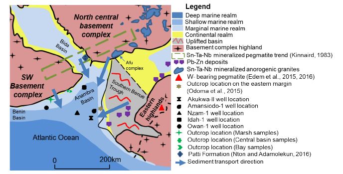
fig 11

Figure 11: Provenance regions of the Anambra Basin

Western Provenance Region

This region comprises the southwestern basement complex rocks as well as pre-Santonian units, relics of which exist as inliers within the basement complex rocks (Figure 11). In general, this provenance region is characterized by a strong coltan factor controlling the enrichment of Nb, Ta, Sn, W (and Pb to a certain extent), high levels of Th, U, Ta, Nb, Sn, Pb as well has higher Pb/Zn (Pb/Zn >1) when compared to the eastern province. Leveraging on published data [8], the main difference between the western provenance terrain from those of the southwestern portion of the north central province is the much higher Pb abundance, which is consistent with the findings of Lapworth. There is some variability in the element pattern of the western provenance, as a portion of it is not strongly influenced by the coltan factor as shown by much lower Pb, Sn, Nb, Ta, and Y concentrations, lower Pb/Zn (Pb/Zn < 1), as well as much higher W recorded from sediments of the Owan-1 well. The very weak positive covariation for Nb vs. Ti and Nb vs. Sn illustrate further evidence for this (Figure 8e). In addition, the good positive covariation between Ti vs. Sn suggests an alternative source for Ti instead of coltan, which is suspected to be ilmenite Lapworth as well as minerals in the ilmenite-geikielite (MgTiO3) and ilmenite-pyrophanite (MnTiO3) solid solution series due to good to moderate positive covariation of Ti vs. Fe, Mn, and Mg (Figure 8e). These Titanium bearing minerals have been documented to occur in the southwestern basement complex rocks [57-60].

Eastern Provenance Region

The eastern provenance region (Figure 8) comprises the pre-Santonian strata from the Southern Benue Trough as well as the basement complex rocks from the eastern highlands (Figure 11). In general, higher Zn, TTE, Cu, Mo, and major element (excluding Al and Ti) concentrations, much lower Pb/Zn ratios (Pb/Zn <1), a strong W enrichment [55-56], as well as lower levels of Nb, Ta and Sn in comparison with the northern and western provenance regions characterize the eastern provenance. In addition, there exists a good positive Pb vs. Zn covariation, as well as a less strong coltan influence for Sn, which in contrast with the western provenance region shows a broad or strong negative covariation with W. The much higher major element concentrations characteristic of this provenance region is a function of the strong mafic influence on the sediments.

Northern Provenance Region

The anorogenic biotite granites as well as the basement complex rocks in the north central provenance region is hypothesized to have contributed detritus for sediments in the northern segment of the basin, sediments close to the western margin, the area around the Amansiodo-1 well, as well as intervals within the Idah-1 well. We came to this conclusion because some intervals in the Idah-1 well have W concentration above 23.2 ppm (Fig. 12a), which is the highest W concentration reported for stream sediments draining the southwestern portion of the north central basement complex Lapworth. High levels of W concentration have been reported for the biotite granites in the Afu complex, north central Nigeria [17]. In addition, these units show high levels of Nb, Y, Th, Zn, Ti, and U, higher enrichment of Nb over Ta [16], as well as low V and Pb/Zn (Pb/Zn < 1).

Mixing of Provenance Regions

Our published data on the outcropping units on the western margin posit that the marsh samples are the most proximal units of the dark mudstone lithofacies [9]. This implies that the geochemistry of this unit is the least influenced by mixing from the northern and eastern provenance regions. The bay samples are the most affected by mixing as illustrated by higher median concentrations of HFSE as well as Pb, Sn, and W recorded from the bay samples (Figure 12a-d) when compared with the marsh and central basin samples. This is due to contribution from multiple source regions as depicted by the broad distributions of Pb vs. Sn and W vs. Pb (Figure 8b), the fractionation (concentration gradient) of Pb, Nb, W, and Sn between the outcropping Patti Formation (Bida Basin), sediments from the Idah-1 and Owan-1 wells, as well as the outcropping Mamu Formation on the western margin (Figure 12a-d).
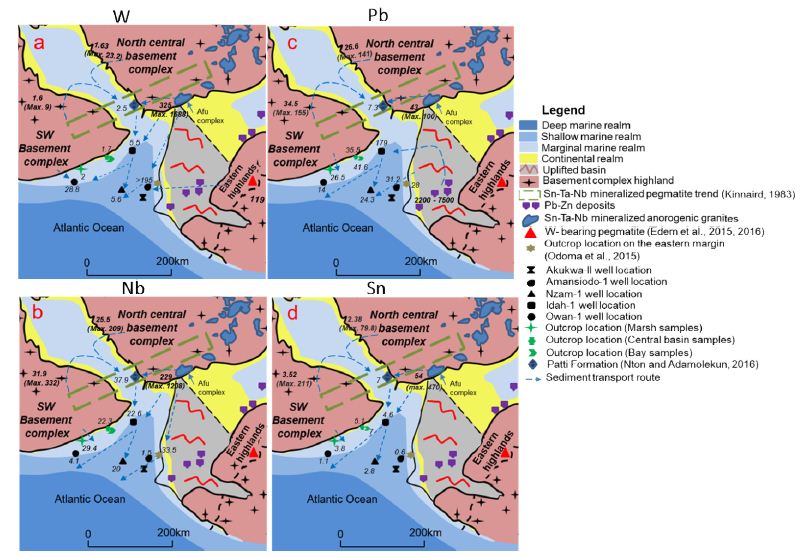
fig 12

Figure 12: Evidence of mixing of provenance regions deduced from median concentrations of Pb, W, Nb, and Sn from spatial units of the Mamu and Patti formations.

The sediments of the more centrally located Idah-1 and Nzam-1 wells also show clear evidence of mixing of source terrains. This is clearly illustrated by the Pb/Nb vs. Pb/Sn as well as the Pb vs. Sn bivariate plots (Figure 13a-b). We hypothesize that the high Pb values associated with sediments from the Idah-1 well is due to mixing of detritus from all three-provenance regions, as concentrations well above the lower thresholds for Pb and Zn (100 ppm and 200 ppm respectively) in Pb-Zn mineralized regions of the eastern provenance [11,12] abound. In addition, the high levels of W recorded in some intervals in the Idah-1 well as well as the Amansiodo-1 well (Appendix 1a) are within the range reported for the Sn-Nb-Ta mineralized biotite granites of the Afu complex [17] located in the Northcentral provenance region.
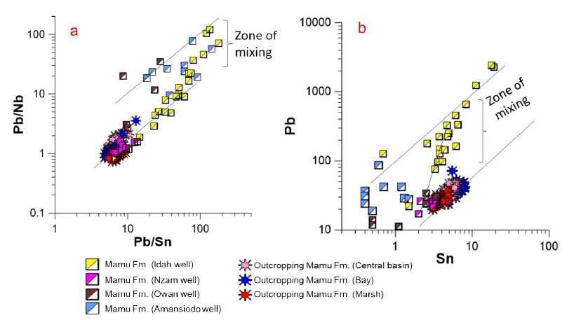
fig 13

Figure 13: Pb/Nb vs. Pb/Sn (a) and Pb vs. Sn (b) binary plots showing further evidence of mixing of source regions.

Conclusion

This study reports the following findings:

  • The pre-Santonian units are sourced from compositionally variable basement complex rocks, ranging from felsic to mafic in composition.
  • There is evidence for spatio-temporal variability in the detrital contribution from the basement complex rocks. Detrital contribution was more from mafic rocks in the latest Cenomanian to early Turonian, whereas from middle Turonian to Coniacian the detrital contribution shifted to more felsic sources.
  • The provenance of the Mamu Formation is from felsic source rocks comprising of basement complex rocks as well as recycled pre-Santonian rocks. The significant detrital contribution from basement complex rocks provides clear insight regarding to the origin of large sand volumes in the post-Santonian Anambra basin. These hitherto could not be accounted for, due to the predominance of argillaceous and carbonate rocks in the Southern Benue Trough
  • Three provenance regions comprising the northern, western, eastern sectors contributed detritus during the Campano-Maastrichtian with evidence of mixing of provenance sources.
  • The Mamu Formation shows evidence of secondary Pb, Sn, and W mineral accumulation.

Acknowledgement

This research received support from University of Benin Research and Publications Committee, the Fulbright Commission (15160892), the Niger Delta Development Commission, Nigeria (NDDC/DEHSS/2015PGFS/EDS/011), and DAAD (ST32 – PKZ: 91559388). Julius Imarhiagbe and Reuben Okoliko assisted with fieldwork and sampling of cuttings and core at the Nigerian Geological Survey Agency respectively. In addition, the first author wishes to acknowledge the motivation, guidance and instruction provided by Prof. W.O. Emofurieta and Mr. Sam Coker during the early phase of this research (Table 1a-1c).

References

  1. Ladipo KO (1986) Tidal shelf depositional model for the Ajali Sandstone, Anambra Basin, Southern Nigeria. J Afr Earth Sci 5: 177-185.
  2. Ladipo KO (1988) Paleogeography, sedimentation and tectonics of the Upper Cretaceous Anambra Basin, Southeastern Nigeria. J Afr Earth Sci 7: 865-871.
  3. Amajor LC (1987) Paleocurrent, petrography and provenance analyses of the Ajali sandstone (upper cretaceous), southeastern Benue Trough, Nigeria. Sediment Geol 54: 47-60.
  4. Obi GC, Okogbue CO (2004) Sedimentary response to tectonism in the Campanian–Maastrichtian succession, Anambra Basin, Southeastern Nigeria. J Afr Earth Sci 38:99-108.
  5. Hoque M (1977) Petrographic differentiation of tectonically controlled Cretaceous sedimentary cycles, southeastern Nigeria. Sediment Geol 17: 235-245.
  6. Edegbai AJ, Schwark L, Oboh-Ikuenobe FE (2019a) A review of the latest Cenomanian to Maastrichtian geological evolution of Nigeria and its stratigraphic and paleogeographic implications. J Afr Earth Sci 150: 823-837.
  7. Odigi MI (2007) Facies architecture and sequence stratigraphy of Cretaceous formations, southeastern Benue Trough, Nigeria. Unpublished Ph.D thesis, University of Portharcourt, Nigeria, p: 288.
  8. Tijani MN, Nton ME, Kitagawa R (2010) Textural and geochemical characteristics of the Ajali Sandstone, Anambra basin, SE Nigeria: Implication for its provenance. Comptes Rendus Geoscience 342: 136-150.
  9. Edegbai AJ, Schwark L, Oboh-Ikuenobe F.E (2019b) Campano-Maastrichtian paleoenvironment, paleotectonics and sediment provenance of Western Anambra Basin, Nigeria: Multi-proxy evidences from the Mamu Formation. J Afr Earth Sci 156: 203-239.
  10. Petters SW (1978) Stratigraphic evolution of the Benue Trough and its implications for the Upper Cretaceous paleogeography of West Africa. J Geol 86: 311-322.
  11. Bonne KPM (2014) Reconstruction of the evolution of the Niger river and implications for sediment supply to the equatorial Atlantic margin of Africa during the cretaceous and the Cenozoic. Geol Soc London Spl Publ 386: 327-349.
  12. Markwick PJ (2018) Palaeogeography in exploration. Geol Mag 1-42.
  13. Odoma AN, Obaje NG, Omada JI, Idakwo SO, Erbacher J (2015) Mineralogical, chemical composition and distribution of rare earth elements in clay-rich sediments from Southeastern Nigeria. J Afr Earth Sci 102: 50-60.
  14. Lapworth DJ, Knights KV, Key RM, Johnson CC, Ayoade E, Adekanmi MA, Arisekola TM, Okunlola OA, Backman B, Eklund M, Everett PA, Lister RT, Ridgway J, Watts MJ, Kemp SJ, Pitfield PEJ (2012) Geochemical mapping using stream sediments in west-central Nigeria: implications for environmental studies and mineral exploration in West Africa. Applied Geochemistry 27, 1035–1052.
  15. Olade MA, Van de Kraats AH, Ukpong EE (1978) Effects of environmental parameters on metal dispersion patterns in stream sediments from the lead-zinc belt. Benue Trough, Nigeria. Geologie en Mijnb 58: 341-351.
  16. Olade MA (1987) Dispersion of Cadmium, Lead and Zinc in Soils and Sediments of a Humid Tropical Ecosystem in Nigeria. In: T. C. Hutchinson and K. M. Meema (Eds.), Lead, Mercury, Cadmium and Arsenic in the Environment. John Wiley & Sons Ltd, New York, Scope 31: 303-313.
  17. Kinnaird JA (1984) Contrasting styles of Sn-Nb-Ta-Zn mineralization in Nigeria. J Afr Earth Sci 2: 81-90.
  18. Imeokparia EG (1982a) Abundance and distribution of tungsten in the Afu Younger Granite complex, central Nigeria. J of Geochem Expl 17: 93-108.
  19. Benkhelil J (1989) The origin and evolution of the Cretaceous Benue Trough, Nigeria. J Afr Earth Sci 8: 251-282.
  20. Nwajide CS (2013) Geology of Nigeria’s Sedimentary Basins. CSS Bookshop Ltd., Lagos, pg: 565.
  21. Fairhead JD (1988) Mesozoic plate tectonic reconstructions of the central South Atlantic Ocean: the role of the West and Central African rift system. In: Scotese, C.R., Sager, W.W. (Eds.), Mesozoic and Cenozoic Plate Reconstructions. Tectonophysics 155: 181-191.
  22. Fairhead JD, Green CM (1989) Controls on rifting in Africa and the regional tectonic model for the Nigerian and East Niger rift basins. J Afr Earth Sci 8: 231-249.
  23. Fairhead JD, Binks RM (1991) Differential opening of the central and south Atlantic oceans and the opening of the West African Rift System. Tectonophysics 187: 191-203.
  24. Fairhead JD, Green CM, Masterton SM, Guiraud R (2013) The role that plate tectonics, inferred stress changes and stratigraphic unconformities have on the evolution of the West and Central African Rift System and the Atlantic continental margins. Tectonophysics 594: 118-127.
  25. Moulin M, Aslanian D, Unternehr P (2010) A new starting point for the south and equatorial Atlantic Ocean. Earth Sci Rev 98: 1-37.
  26. Adeleye DR (1975) Nigerian late Cretaceous stratigraphy and palaeogeography. Am Assoc Pet Geol (AAPG) Bull. 59: 2302–2313.
  27. Reyment RA, Dingle RV (1987) Palaeogeography of Africa during the Cretaceous period. Palaeoclimatol Palaeoecol 59: 93-116.
  28. Petters SW, Ekweozor CM (1982) Petroleum Geology of Benue Trough and Southeastern Chad Basin, Nigeria. AAPG (Am Assoc Pet Geol) Bull. 66: 1141-1149.
  29. Gebhardt H (1999) Cenomanian to Coniacian ostracods from the Nkalagu area (SE Nigeria): biostratigraphy and palaeoecology. Paläontol Z 73: 77-98.
  30. Banerjee I (1981) Storm lag and related facies of the bioclastic limestones of the Eze-Aku Formation (Turonian), Nigeria. Sed Geo 30: 133-147.
  31. Umeji OP (1984) Ammonite palaeoecology of the Eze-Aku Formation, southeastern Nigeria. Nigerian Journal of Mining and Geology 21: 55-59.
  32. Gebhardt H (1998) Benthic foraminifera from the Maastrichtian lower Mamu Formation near Leru (Southern Nigeria): paleoecology and paleogeographic significance. J Foraminifer Res 28: 76-89.
  33. Kuhnt W, Herbin JP, Thurow J, Wiedmann J (1990) Distribution of Cenomanian-Turonian Organic Facies in the Western Mediterranean and Along the Adjacent Atlantic Margin. In: Huc, A. Y. (Ed.): Deposition of Organic Facies. American Association of Petroleum Geologists, Studies in Geology 30: 133-160.
  34. Igwe EO, Okoro AU (2016) Field and lithostratigraphic studies of the Eze-Aku Group in the Afikpo synclinorium, southern Benue Trough, Nigeria. J Afr Earth Sci 119: 38-51.
  35. Dim CIP, Okwara IC, Mode AW, Onuoha KM (2016) Lithofacies and environments of deposition within the middle–upper Cretaceous successions of southeastern Nigeria. Arabian J Geosci 9: 1-17.
  36. Dim CIP, Onuoha KM, Okwara IC, Okonkwo IA, Ibemesi PO (2019) Facies analysis and depositional environment of the Campano – Maastrichtian coal bearing Mamu Formation in the Anambra Basin, Nigeria. J AfrEarth Sci
  37. Guiraud R, Bosworth W (1997) Senonian basin inversion and rejuvenation of rifting in Africa and Arabia. Synthesis and implications to plate-scale tectonics. Tectonophysics 282: 39-82.
  38. Okoro AU, Igwe EO (2018a) Sequence stratigraphy and controls on sedimentation of the Upper Cretaceous in the Afikpo Sub-basin, southeastern Nigeria. Arabian Journal of Geosciences
  39. Okoro AU, Igwe EO (2018b) Lithostratigraphic characterization of the Upper Campanian – Maastrichtian succession in the Afikpo Sub-basin, southern Anambra Basin, Nigeria. J Afr Earth Sci 147: 178-189.
  40. Akande SO, Mücke A (1993) Tectonic and sedimentation framework of the lower Benue Trough, southeastern Nigeria. J Afr Earth Sci 17: 445-456.
  41. Zaborski PMP (1983) Campano-Maastrichtian ammonites, correlation and palaeogeography in Nigeria. J Afr Earth Sci 1: 59-63.
  42. Cullers RL, Stone J (1991) Chemical and mineralogical comparison of the Pennsylvanian Fountain Formation, Colorado, U.S.A. (an uplifted continental block) to sedimentary rocks from other tectonic environments. Lithos 27: 115-131.
  43. McLennan SM (2001) Relationships between the trace element composition of sedimentary rocks and upper continental crust. Geochem Geophys Geosyst DOI: 542 10.1029/2000GC000109
  44. Anderson DH, Hawkes HE (1958) Relative mobility of the common elements in weathering of some schist and granite areas. Geochim Cosmo 14: 204-210.
  45. Nesbitt HW, Young GM (1982) Early Proterozoic climates and plate motions inferred from major element chemistry of lutites. Nature 299: 715-717.
  46. Igwe EO (2017) Composition, provenance and tectonic setting of Eze-Aku Sandstone facies in the Afikpo Synclinorium, Southern Benue Trough, Nigeria. Environ Earth Sci 76: 1-12.
  47. Hay W, Floegel S (2012) New thoughts about the Cretaceous climate and oceans. Earth Sci Rev 115: 262-272.
  48. Bhatia MR, Crook KAW (1986) Trace element characteristics of greywackes and tectonic setting discrimination of sedimentary basins. Contrib Mineral Petrol 92: 181-193.
  49. Wronkiewicz DJ, Condie KC (1990) Geochemistry and mineralogy of sediments from the Ventersdorp and Transvaal Supergroups, South Africa: Cratonic evolution during the early Proterozoic. Geochem Cosmochim Acta 54: 343-354.
  50. McLennan SM, Taylor SR (1991) Sedimentary rocks and crustal evolution: tectonic setting and secular trends. J of Geology 99: 1-21.
  51. Cullers RL (1995) The controls on the major- and trace-element evolution of shales, siltstones and sandstones of Ordovician to tertiary age in the Wet Mountains region, Colorado, U.S.A. Chem Geol 123: 107-131.
  52. Cullers RL (2000) The geochemistry of shales, siltstones and sandstones of Pennsylvanian- Permian age, Colorado, U.S.A.: implications for provenance and metamorphic studies. Lithos 51: 181-203.
  53. Potter PE, Maynard JB, Depetris PJ (2005) Mud and Mudstones: Introduction and Overview. Springer-Verlag, pg: 297.
  54. McLennan SM, Hemming S, McDaniel DK, Hanson GN (1993) Geochemical approaches to sedimentation, provenance, and tectonics. In: In: Johnsson MJ, Basu, A (Eds.), Processes Controlling the Composition of Clastic Sediments: Boulder, Colorado, vol. 284. Geological Society of America Special Paper, pg: 21-40
  55. Edem GO, Ekwueme BN, Ephraim BE (2015) Geochemical signatures and mineralization potentials of precambrian pegmatites of southern Obudu, Bamenda Massif, southeastern Nigeria. International Journal of Geophysics and Geochemistry 2: 53-67.
  56. Edem GO, Ekwueme BN, Ephraim BE, Igonor EE (2016) Preliminary investigation of pegmatites in Obudu area, southeastern Nigeria, using stream sediments geochemistry. Global Journal of Pure and Applied Sciences 22: 167-175.
  57. Nton ME, Adamolekun OJ (2016) Sedimentological and geochemical characteristics of outcrop sediments of Southern Bida Basin, central Nigeria: implications for provenance, paleoenvironment and tectonic history. Ife Journal of Science 18: 345-369.
  58. Mücke A, Woakes M (1986) Pyrophanite: a typical mineral in the Pan-African Province of Western and Central Nigeria. J Afr Earth Sci 5: 675-689.

Table 1a-1c: Summary table showing the results of elemental analysis as well as elemental ratios.

Appendix 1a

S/N Lithostratigraphic Unit Location Ca Fe K Mg Mn Na Ti Al TiO2 Pb Sn W Zn Mo Cu
U1 IA Mamu

Formation

Western margin

(Marsh

subenvironment)

0.021 0.94 0.32 0.07 0.004 0.015 0.91 8.05 1.68 27.8 3.6 2.1 14 3 7.1
U1 1C 0.014 0.57 0.26 0.05 0.003 0.015 0.83 6.83 1.58 21.9 3.2 1.7 14 2.6 8.7
U1 2A 0.014 1.19 0.30 0.05 0.003 0.015 0.89 7.89 1.68 23.4 3.8 2 9 2.2 7.7
U1 2B 0.014 0.72 0.23 0.04 0.003 0.015 0.80 6.46 1.48 26.5 3 1.7 18 0.9 4.6
U1 2C 0.014 0.57 0.31 0.06 0.003 0.015 0.94 7.89 1.79 32.4 3.5 1.9 9 2.3 4.2
U1 3A 0.014 1.09 0.32 0.06 0.004 0.015 0.93 7.73 1.75 25.6 3.7 2.2 15 1.1 6
U1 3B 0.014 0.86 0.38 0.07 0.003 0.022 0.95 9.10 1.81 28.6 4.3 2.2 15 1.9 5.8
U1 5A 0.021 0.80 0.36 0.07 0.004 0.022 0.90 11.70 1.63 29.1 4.1 2 15 2.5 6.5
U1 5B 0.021 0.92 0.36 0.07 0.004 0.022 0.85 12.54 1.56 27.7 4 2 12 2 5.1
U1 6A 0.021 0.87 0.37 0.07 0.003 0.015 0.87 11.75 1.60 25.6 4.1 2.2 13 1.1 6.6
U1 7A 0.029 1.84 0.25 0.08 0.006 0.022 0.76 10.69 1.47 23.8 3.2 1.7 211 2.1 27.4
U1 7B 0.014 0.60 0.27 0.07 0.004 0.015 0.87 9.84 1.60 25.9 3.7 1.9 83 1 11.3
U1 8A 0.014 1.45 0.23 0.07 0.004 0.007 0.78 10.50 1.36 23.9 3.6 1.5 139 0.8 15.6
U1 8B 0.057 1.27 0.25 0.08 0.008 0.022 0.87 7.62 1.64 26.2 3.5 2 132 1.4 10.6
U1 8C 0.014 0.49 0.17 0.05 0.008 0.015 0.80 5.72 1.46 20.1 3.1 1.8 241 3.8 6.8
U1 8D 0.014 0.66 0.22 0.05 0.004 0.022 0.82 8.36 1.55 27.2 3.7 1.9 155 0.7 6.8
U1 9B 0.014 1.67 0.27 0.05 0.007 0.015 0.93 10.22 1.69 31.4 3.9 2.2 38 2.5 16.3
U1 9C 0.014 0.83 0.29 0.05 0.005 0.022 0.96 11.06 1.74 30.9 4.5 2.4 33 1.3 14.2
U1 10 0.014 0.87 0.20 0.04 0.002 0.015 0.96 14.08 1.77 36.7 4.8 2.4 11 2 14
U1 18 0.014 1.76 0.26 0.04 0.003 0.015 0.97 13.07 1.82 31 4.9 2.4 10 1.5 31.4
U1 19 0.007 0.73 0.19 0.04 0.003 0.007 0.95 11.61 1.73 26.1 4.8 1.9 10 1.1 33.1
AU-1a 0.021 1.07 0.70 0.16 0.004 0.022 0.80 10.27 1.51 27.9 3.9 1.8 21 1.9 36.2
AU 2 0.021 1.55 0.88 0.21 0.003 0.022 0.81 12.13 1.49 26.2 4.2 1.8 27 1 23.1
Mean 0.02 1.0 0.3 0.07 0.004 0.017 0.9 9.8 1.6 27.2 3.8 1.9 54 1.8 13.4
Median 0.01 0.9 0.3 0.06 0.004 0.015 0.9 10.2 1.6 26.5 3.8 2.0 15 1.9 8.7
SD 0.01 0.4 0.2 0.04 0.002 0.005 0.1 2.3 0.1 3.7 0.5 0.3 70 0.8 9.9
IM 2B Mamu

Formation

Western margin

(Central Basin

subenvironment)

0.04 2.84 0.99 0.22 0.006 0.02 0.86 14.77 1.59 39.6 5.6 2.4 43 1.8 25.9
1M 2C 0.03 2.63 1.00 0.23 0.006 0.03 0.97 13.44 1.72 41.9 5.5 2.5 57 1.5 19.6
1M 2D 0.03 2.90 1.01 0.24 0.006 0.03 0.87 13.44 1.62 47.2 5.5 2 71 0.6 28.7
1M 2E 0.064 4.57 0.98 0.30 0.016 0.03 0.84 13.60 1.50 36.7 5.1 2.2 96 1.3 22.7
IM 4A 0.021 4.59 0.71 0.18 0.007 0.03 0.71 10.48 1.24 32 4.3 1.7 43 1 14.7
IM 11A 0.06 7.20 0.60 0.22 0.008 0.02 0.66 12.60 1.13 46.2 6.3 1.6 127 1 30.5
IM 11B 0.06 4.02 1.00 0.29 0.010 0.03 0.69 16.62 1.12 30.7 5.6 1.8 67 1 32.1
IM 11C 0.19 5.01 1.14 0.34 0.014 0.03 0.66 12.54 1.13 39.5 5.3 1.6 125 0.6 28.1
IM 13A 0.11 7.41 1.00 0.41 0.092 0.03 0.60 13.44 1.05 26.8 4.7 1.6 106 1.2 31.1
1M 13B 0.043 3.30 1.06 0.30 0.008 0.03 0.76 15.35 1.30 29.2 5.4 2.2 94 1.1 35.1
IM 14A 0.54 5.32 1.08 0.32 0.021 0.04 0.64 12.60 1.11 38.8 4.3 1.7 191 2 32.2
IM 16A 0.26 12.52 1.20 0.42 0.253 0.02 0.39 11.86 0.70 25.9 3.8 1.3 128 2.2 28.9
IM 16B 0.19 7.13 1.36 0.41 0.084 0.03 0.46 13.23 0.82 31 4 1.6 122 1.7 24.3
1M 16C 0.09 3.97 1.45 0.35 0.021 0.03 0.54 13.92 0.96 33.7 4.7 1.5 69 1.5 19.2
1M 16D 0.06 2.91 1.35 0.30 0.008 0.03 0.57 13.23 1.02 23.4 4.4 1.7 38 0.5 17.9
IM 18a 0.79 0.93 1.06 0.13 0.004 0.03 0.42 11.63 0.72 28.5 2.75 0.9 47 1.1 9.75
IM 18C 0.13 1.41 0.81 0.18 0.004 0.02 0.66 17.78 1.12 47 5.9 2.1 34 1.5 24.2
IM 19A 0.10 1.96 1.10 0.24 0.004 0.02 0.61 17.25 1.05 41.9 5.4 1.9 37 2 36.5
IM 19B 0.07 2.34 1.10 0.24 0.003 0.02 0.57 16.99 0.98 34 5.3 1.7 32 1 43.1
IM 19D 0.05 3.43 0.92 0.19 0.007 0.03 0.61 16.53 1.08 46.3 5.1 2.2 33 1 209.1
IM 19E 0.04 1.88 1.05 0.22 0.005 0.03 0.71 17.36 1.22 38.1 5.8 2.3 30 1.9 19.3
IM 2A 0.04 3.18 0.74 0.16 0.004 0.02 0.76 13.50 1.34 33.7 4.6 1.9 30 1.7 11.3
IM 4B 0.014 4.12 0.48 0.11 0.007 0.01 0.65 7.55 1.10 29.5 3.5 1.3 32 1.4 22.8
IM 14C 0.24 6.67 1.15 0.39 0.020 0.04 0.52 13.60 0.91 37.7 4.5 1.5 128 3.3 44
IM 18B 0.16 1.50 0.70 0.15 0.004 0.02 0.64 16.68 1.01 41.1 5.9 1.7 36 2.2 111.1
IM 19C 0.07 3.81 0.96 0.21 0.004 0.03 0.58 16.20 0.96 31.1 5 1.7 29 1.3 147.4
Mean 0.13 4.1 1.0 0.3 0.02 0.03 0.7 14.1 1.1 35.8 4.9 1.8 71.0 1.4 41.1
Median 0.07 3.6 1.0 0.2 0.01 0.03 0.7 13.6 1.1 35.4 5.1 1.7 52.0 1.4 28.4
SD 0.17 2.5 0.2 0.1 0.05 0.01 0.1 2.4 0.3 6.9 0.8 0.4 44.2 0.6 45.3
OK 7A Mamu

Formation

Western margin

(Bay

subenvironment)

0.014 3.28 0.46 0.12 0.004 0.015 0.86 12.01 1.51 46.6 5.7 2.3 80 3.2 18.3
OK 7B 0.014 2.71 0.23 0.06 0.008 0.015 0.63 6.93 1.09 23.7 4.9 1.4 174 6.4 13
OK 7C 0.014 6.76 0.46 0.12 0.018 0.030 0.50 15.61 0.90 71 5.5 1.7 96 7.9 40.7
OK 7D 0.014 5.38 0.42 0.10 0.005 0.022 0.60 15.88 1.06 52.7 6.2 1.7 118 2.9 38.8
OK 7E 0.014 2.42 0.40 0.08 0.002 0.022 0.94 14.98 1.76 48.7 6.5 2.8 145 2.5 25.7
OK 7F 0.014 2.02 0.42 0.08 0.005 0.022 0.72 17.04 1.31 34.6 5.5 2.1 149 1.5 26.7
OK 7G 0.021 1.96 0.47 0.07 0.003 0.030 0.73 11.54 1.34 35 6.5 2 29 1.8 18
OK 7H 0.014 1.19 0.37 0.07 0.005 0.015 0.83 12.54 1.53 29.3 6.1 2 30 2.6 15.7
OK 7I 0.021 1.43 0.39 0.07 0.003 0.022 0.87 15.24 1.51 46.9 7 2.1 37 2.8 30
OK 7J 0.021 1.60 0.44 0.07 0.005 0.022 1.03 13.81 1.88 47.7 7.5 2.6 31 4.3 29.9
OK 9 0.021 0.80 0.42 0.08 0.002 0.015 0.76 16.88 1.37 41.1 5.6 2 33 1 19.1
OK 11A 0.014 1.63 0.64 0.12 0.005 0.022 0.99 15.40 1.71 36.4 7 2.7 31 3.3 17.8
OK 11B 0.021 1.57 0.88 0.16 0.003 0.022 1.05 15.88 1.84 42.9 7.3 2.9 28 2.1 13.8
OK 13A 0.014 1.29 0.45 0.07 0.004 0.022 0.88 13.07 1.56 38.4 7.2 2.2 30 3.5 27.1
OK 13B 0.014 1.14 0.50 0.08 0.003 0.022 0.99 15.61 1.74 49 7.7 2.5 37 1.8 29.9
OK 15 0.021 0.62 0.51 0.05 0.004 0.030 0.94 8.10 1.70 36.8 7.3 2.3 18 1.5 13.7
OK 17 0.021 0.75 0.47 0.05 0.005 0.022 0.90 11.75 1.64 34.9 6.4 2.1 23 1.8 36.7
OK 19A 0.014 0.68 0.41 0.06 0.003 0.022 0.93 13.92 1.66 37.7 7.2 2.2 31 1.1 59.3
OK 19B 0.014 1.04 0.47 0.08 0.003 0.022 1.04 15.72 1.78 47.5 7.6 2.7 37 1.9 32.7
OK 21A 0.029 1.20 0.60 0.09 0.003 0.022 1.14 10.43 2.00 41.6 8 2.9 23 1 20.3
OK 21B 0.021 1.55 0.62 0.10 0.003 0.022 1.11 11.91 2.01 40.7 7.9 2.7 23 1.7 17.8
OK 24A 0.014 0.62 0.42 0.06 0.002 0.022 0.96 13.87 1.65 42.5 7.5 2.3 30 1.5 63.6
Ok 24B 0.014 0.64 0.41 0.05 0.004 0.022 0.88 10.06 1.53 43.4 6.2 1.9 19 1.9 26.4
Mean 0.017 1.8 0.5 0.08 0.004 0.022 0.9 13.4 1.6 42.1 6.7 2.3 54.4 2.6 27.6
Median 0.014 1.5 0.5 0.08 0.004 0.022 0.9 13.9 1.7 41.6 7 2.2 31.0 1.9 26.4
SD 0.004 1.5 0.1 0.03 0.003 0.004 0.2 2.7 0.3 9.3 0.7 0.4 47.4 1.7 13.4
Nz-16 Mamu

Formation

Nzam-1 Well 0.74 4.35 1.36 0.65 0.07 0.514 0.57 7.74 0.96 25.9 2.1 7.5 89 1.6 15
Nz-17 0.51 4.96 1.17 0.58 0.04 0.625 0.65 9.34 1.09 25 2.9 16.8 126 2.3 18.7
Nz-18 0.47 6.31 1.06 0.81 0.02 0.619 0.54 > 20 0.90 27.2 3.4 3.7 155 2 27.3
Nz-19 0.17 3.61 2.02 0.39 0.03 0.404 0.81 10.00 1.36 24.8 3.4 81.9 119 1.3 22.2
Nz-20 0.32 3.97 0.79 0.46 0.03 0.485 0.44 6.95 0.74 17 2 2 65 2.5 21.1
Nz-21 0.34 4.29 1.29 0.50 0.05 0.566 0.66 8.60 1.11 23.3 2.8 2 94 1.4 17.3
Nz-22 0.34 3.13 1.16 0.32 0.03 0.564 0.61 7.89 1.02 23.8 2.5 3.4 64 1.2 13.7
Nz-39 0.36 6.69 1.13 0.65 0.18 0.467 0.81 7.73 1.36 20.9 3.1 36.6 95 1.6 18.7
Mean 0.4 4.7 1.3 0.6 0.056 0.531 0.6 8.3 1.1 23.5 2.8 19.2 100.9 1.7 19.3
Median 0.4 4.3 1.2 0.5 0.034 0.539 0.6 7.9 1.1 24.3 2.9 5.6 94.5 1.6 18.7
SD 0.2 1.3 0.4 0.2 0.051 0.077 0.1 1.1 0.2 3.22 0.5 27.9 31.1 0.5 4.3
ID-3 Mamu

Formation

Idah-1 Well 0.07 0.25 0.02 0.01 0.005 0.014 0.28 0.15 0.46 126 0.7 7.9 9 0.3 2.3
ID-4 0.02 1.07 1.59 0.06 0.006 0.074 0.57 4.80 0.94 22 1.5 103 31 1.6 8.9
ID-5 0.23 2.45 0.61 0.37 0.040 0.126 0.33 3.66 0.54 179 2.6 3.2 52 0.6 9.8
ID-6 0.37 4.80 1.26 0.80 0.046 0.462 0.81 8.28 1.34 75.4 3.3 3.2 88 1.4 20.3
ID-7 0.48 5.27 1.34 0.71 0.050 0.469 1.09 6.70 1.82 148 3.8 4.9 92 1.9 24.2
ID-8 0.43 5.78 1.19 0.84 0.079 0.432 0.71 7.56 1.18 2290 19.1 23.2 186 1.4 21.4
ID-9 0.48 5.00 1.05 0.71 0.065 0.454 0.63 7.24 1.06 2400 18 51.6 241 1.6 19.9
ID-10 0.73 6.82 0.80 1.09 0.083 0.314 0.62 4.87 1.04 325 4.7 25.1 152 1.7 14
ID-11 0.43 4.74 0.83 0.77 0.066 0.402 0.84 5.78 1.40 222 3.7 4.8 95 1.3 19.7
ID-12 0.73 7.05 0.93 0.83 0.080 0.280 0.64 6.19 1.07 450 6.1 57.2 138 1.7 21.8
ID-13 0.58 5.81 1.09 0.55 0.051 0.315 0.77 7.74 1.29 126 3.8 16.6 187 1.5 20.7
ID-14 0.39 6.47 1.17 0.64 0.051 0.377 0.82 9.23 1.37 1250 11.3 13.1 146 1.4 23.4
ID-15 0.40 7.13 1.08 0.66 0.063 0.341 0.77 8.47 1.28 249 5 3.1 139 1.5 20.8
ID-16 0.25 4.82 1.11 0.48 0.018 0.366 1.23 9.59 2.05 31.5 4.6 17.1 114 1.1 22.8
ID-17 0.16 4.81 1.02 0.44 0.029 0.229 0.90 10.70 1.49 163 6.2 76.1 150 1.4 21.4
ID-18 0.35 7.09 1.05 0.53 0.047 0.256 0.71 10.00 1.19 666 8.3 2.4 136 0.8 24.3
ID-19 0.44 5.97 0.88 0.54 0.031 0.231 0.67 9.47 1.12 334 6.6 2.9 214 1.3 20.4
ID-20 0.36 5.94 1.07 0.68 0.047 0.334 0.69 9.92 1.15 222 4.8 2.3 160 1.7 21.7
ID-21 0.69 5.34 1.30 1.06 0.024 0.452 0.57 10.70 0.95 146 4.4 2.2 208 0.7 25.4
ID-22 0.53 5.27 1.40 1.09 0.031 0.446 0.57 10.80 0.95 97.1 3.6 2.1 151 0.6 23.5
ID-23 0.71 5.23 1.20 0.98 0.050 0.431 0.63 9.37 1.05 97.7 4.1 5.5 203 0.9 22.4
Mean 0.4 5.1 1.1 0.7 0.05 0.32 0.7 7.7 1.2 458.1 6.0 20.4 137.7 1.3 19.5
Median 0.4 5.3 1.1 0.7 0.05 0.34 0.7 8.3 1.2 179 4.6 5.5 146 1.4 21.4
SD 0.2 1.8 0.3 0.3 0.02 0.13 0.2 2.7 0.4 683.5 4.7 28.1 60.8 0.4 5.9
OW-10 Mamu

Formation

Owan-1 Well 0.02 0.76 0.03 0.02 0.004 0.010 0.46 1.54 0.76 11.3 1.1 > 200 30 1.3 1.4
OW-11 0.03 0.70 0.32 0.06 0.005 0.018 0.74 9.72 1.23 30.2 3.5 2.9 100 0.2 29.8
OW-12 0.01 0.34 0.07 0.02 0.004 0.010 0.13 3.54 0.22 14 0.5 4.4 26 < 0.1 4.7
OW-13 0.01 0.20 0.07 0.02 0.003 0.009 0.30 2.93 0.50 11.8 0.5 15.4 18 0.2 3.9
OW-14 0.04 1.66 0.19 0.08 0.011 0.012 0.73 7.37 1.21 34.1 2.5 42.1 66 3.9 13.6
OW-15 0.12 1.47 0.21 0.05 0.008 0.016 0.92 6.45 1.54 24 2.5 169 40 1.3 11.2
OW-16 0.03 0.76 0.10 0.02 0.004 0.008 0.45 2.44 0.75 11.1 1.1 185 50 0.6 5.2
Mean 0.04 0.8 0.1 0.04 0.006 0.012 0.5 4.9 0.9 19.5 1.7 69.8 47.1 1.3 10
Median 0.03 0.8 0.1 0.02 0.004 0.010 0.5 3.5 0.8 14 1.1 28.8 40 1 5.2
SD 0.04 0.5 0.1 0.03 0.003 0.004 0.3 3.0 0.5 9.8 1.2 84.4 28.3 1.4 9.7
Am-3 Mamu

Formation

Amansiodo-1

Well

4.82 0.62 0.04 0.07 0.007 0.024 0.06 0.65 0.10 28.5 1.3 > 200 61 1.5 20.9
Am-4 6.28 0.69 0.03 0.09 0.009 0.022 0.06 0.72 0.11 27.7 1.5 > 200 78 1.6 28.1
Am-5 3.95 1.67 0.05 0.12 0.014 0.050 0.08 0.87 0.14 42.2 1.2 > 200 111 1.8 21.1
Am-6 1.16 0.52 0.03 0.03 0.008 0.015 0.06 0.54 0.11 19 0.5 191 37 0.9 13.5
Am-7 0.51 0.62 0.04 0.02 0.005 0.014 0.06 0.62 0.11 42.2 0.7 > 200 59 1.2 6.5
Am-8 0.38 0.54 0.04 0.02 0.005 0.014 0.07 0.66 0.12 36.4 0.4 195 55 1 4.7
Am-9 0.10 0.43 0.03 0.02 0.003 0.010 0.05 0.51 0.08 24.1 0.4 > 200 34 1 3.9
Am-10 0.50 0.57 0.02 0.02 0.004 0.007 0.03 0.26 0.05 31.2 0.4 195 31 2.5 5.3
Am-11 0.85 2.50 0.03 0.04 0.012 0.011 0.07 0.62 0.12 86.5 0.6 196 58 1.4 8.2
Mean 2.1 0.9 0.03 0.05 0.007 0.019 0.06 0.6 0.1 37.5 0.8 194.3 58.2 1.4 12.5
Median 0.9 0.6 0.03 0.03 0.007 0.014 0.06 0.6 0.1 31.2 0.6 195 58 1.4 8.2
SD 2.1 0.6 0.01 0.03 0.003 0.012 0.01 0.15 0.02 20.0 0.4 2.2 24.9 0.5 8.9
Enu 1.1 Mamu

Formation

Eastern margin 0.04 4.16 0.95 0.36 0.04 0.16 0.86 10.24 0.86 35 122 30
Enu 1.2 (Odoma et al.,

2015)

0.03 3.11 1.11 0.28 0.02 0.24 0.97 8.03 0.97 30 53 18
Enu 1.3 0.03 1.90 1.19 0.30 0.01 0.27 1.01 8.46 1.01 29 53 11
Enu 1.4 0.03 3.68 1.04 0.22 0.03 0.23 0.93 8.91 0.93 32 69 25
Enu 1.5 0.03 3.64 1.02 0.28 0.03 0.19 0.88 8.94 0.88 29 78 27
Enu 2.2 0.02 8.25 0.85 0.25 0.01 0.13 0.85 10.76 0.85 25 51 22
Enu2.3 0.03 5.71 0.87 0.25 0.01 0.14 1.02 10.56 1.02 24 39 26
Enu2.4 0.03 2.58 1.46 0.37 0.01 0.16 0.92 11.64 0.92 23 51 31
Enu2.5 0.04 4.71 0.96 0.27 0.01 0.17 1.21 10.37 1.21 27 152 27
mean 0.03 4.2 1.1 0.3 0.02 0.19 1.0 9.8 1.0 28.2 74.2 24.1
median 0.03 3.7 1.0 0.3 0.01 0.17 0.9 10.2 0.9 29 53 26
SD 0.01 1.9 0.2 0.1 0.01 0.05 0.1 1.2 0.1 3.9 38.1 6.3
Mamu Formation

average

0.05 5.1 1.4 0.9 0.05 1.06 0.7 9.3 1.1 29.6 3.8 5.5 52.5 1.4 20.1
Pre-Santonian Units
Am-23 Awgu

Group

Amansiodo-1

Well

0.54 8.56 1.18 0.78 0.121 0.453 1.05 10.30 1.75 24.5 3.8 5.9 106 1.7 26.7
Am-24 0.34 5.56 1.96 0.83 0.046 0.528 0.99 12.0 1.64 27.8 4 8 125 2.6 31.4
Am-25 0.27 5.64 1.62 0.74 0.039 0.526 0.98 11.60 1.64 27.2 4 9.7 107 1.5 29
Am-26 0.46 6.18 2.25 1.03 0.076 0.610 0.87 11.40 1.45 25.6 3.7 12.4 119 1.3 28.5
Am-27 0.31 5.41 1.93 1.16 0.042 0.646 0.77 11.90 1.28 28.7 4 5.3 123 1.5 23.7
Am-28 0.29 5.24 1.51 0.95 0.042 0.590 0.84 11.60 1.41 25.6 3.8 4.2 110 1.6 24.6
Am-29 0.33 5.89 1.48 1.01 0.056 0.640 0.77 12.50 1.28 27.1 3.9 3.8 109 0.9 23.2
Am-30 0.31 5.98 1.27 0.99 0.047 0.649 0.76 11.40 1.27 30.8 4.4 6.1 194 1.3 25.4
Am-31 0.29 5.79 1.43 1.04 0.052 0.706 0.76 12.90 1.27 25.4 4 2.4 132 1.5 24.9
Am-32 0.34 5.74 1.44 1.01 0.048 0.723 0.86 12.90 1.43 24.8 4 5.5 104 2.4 23.3
Am-33 0.28 5.73 1.77 1.01 0.045 0.654 0.83 13.0 1.39 25.9 4 4.9 103 3.8 33.6
Am-34 0.27 5.76 1.70 1.06 0.055 0.721 0.77 12.70 1.29 26.6 3.9 2.6 89 3.7 42.1
Am-35 1.10 4.74 3.75 1.08 0.073 0.569 0.65 12.70 1.08 32.6 4.4 12 160 5.3 30.5
Am-36 1.28 8.86 1.16 1.56 0.110 0.743 0.56 9.69 0.93 23.4 3.6 9.3 88 2.7 17.7
Am-37 0.78 5.99 1.65 1.21 0.075 0.763 0.65 10.90 1.08 23.4 4.2 12 87 2.1 22.7
Mean 0.5 6.1 1.7 1.0 0.062 0.635 0.8 11.8 1.4 26.6 4 6.9 117.1 2.3 27.2
Median 0.3 5.8 1.6 1.0 0.052 0.646 0.8 11.9 1.3 25.9 4 5.9 109 1.7 25.4
SD 0.3 1.1 0.6 0.2 0.025 0.090 0.1 1.0 0.2 2.6 0.2 3.4 28.4 1.2 5.8
Ak-3 Awgu

Group

Akukwa-II Well 0.66 6.87 1.15 1.20 0.07 0.742 0.517 10.20 0.86 22.3 3.1 5.9 147 2.3 35
Ak-4 0.53 5.73 1.25 0.74 0.024 0.733 0.551 10.90 0.92 24.9 3.3 6.8 130 2.8 49.8
Ak-5 0.54 5.38 1.09 0.76 0.027 0.729 0.711 11.80 1.19 28 3.8 5.7 161 3.3 34.8
Ak-6 0.53 4.95 1.11 0.92 0.025 0.719 0.614 10.90 1.02 21.6 3.3 11.7 125 2.2 40.1
Ak-7 0.38 5.58 0.95 1.12 0.091 0.778 0.708 10.60 1.18 25.5 3.2 10.4 122 2.7 32.7
Ak-8 0.29 5.03 1.29 1.03 0.028 0.814 0.710 11.70 1.18 28.6 3.6 9.2 174 4.1 33.3
Ak-9 0.46 5.91 1.27 1.14 0.075 0.697 0.674 11.20 1.12 26.8 3.3 9.7 158 2.6 32.9
Ak-10 0.42 3.19 0.86 0.44 0.041 1.340 0.281 6.60 0.47 26.4 1.7 68.1 82 1.9 14.4
Ak-11 0.31 5.47 1.45 0.79 0.045 0.689 0.800 11.0 1.33 24.4 3.6 8.8 128 2.3 30.5
Mean 0.5 5.4 1.2 0.9 0.047 0.805 0.618 10.5 1.0 25.4 3.2 15.1 136.3 2.7 33.7
Median 0.5 5.5 1.2 0.9 0.041 0.733 0.674 10.9 1.1 25.5 3.3 9.2 130 2.6 33.3
SD 0.1 1.0 0.2 0.3 0.025 0.204 0.154 1.6 0.3 2.4 0.6 20 27.4 0.7 9.3
Ak-12 Eze-Aku

Group

Akukwa-II Well 0.30 5.30 1.22 0.84 0.052 0.725 0.767 11.80 1.28 24.2 3.6 7.6 225 2.2 34.3
Ak-13 0.42 5.43 1.25 0.92 0.066 0.737 0.702 11.30 1.17 18.9 3.3 15.3 133 3.1 31.8
Ak-14 0.73 12.80 1.28 2.53 0.470 0.430 0.431 7.65 0.72 24.4 2.3 2.5 55 0.7 18.2
Ak-15 0.36 4.84 1.76 0.86 0.060 0.659 0.694 10.30 1.16 23.3 3.6 15.4 134 2.4 29.7
Ak-16 0.38 5.11 1.28 0.94 0.042 0.760 0.673 9.68 1.12 22.2 3.3 13.6 147 2.6 30
Ak-17 0.27 5.46 1.19 0.97 0.057 0.829 0.762 11.60 1.27 29.2 3.9 9.4 134 2.1 32.8
Ak-18 0.39 4.64 1.38 0.87 0.043 1.060 0.633 10.0 1.06 21.3 3.6 13.4 190 3 28.3
Ak-19 6.77 4.31 1.24 0.85 0.053 0.925 0.519 7.90 0.87 19.6 3.1 11 153 12.7 28.7
Ak-20 1.62 4.82 1.47 0.96 0.049 1.070 0.659 9.43 1.10 16.8 3.6 14.1 137 3.2 27.9
Ak-21 1.55 4.57 1.44 0.89 0.052 1.040 0.663 9.13 1.11 24.6 3.6 13.8 150 3.1 26.6
Ak-22 1.82 4.08 1.43 0.71 0.037 1.430 0.647 9.25 1.08 24 3.4 16.7 119 2.8 21.9
Ak-23 12.90 5.60 0.99 0.75 0.102 0.664 0.369 6.56 0.62 113 4 21.3 383 11.3 177
Ak-24 2.43 5.47 2.04 1.15 0.074 1.430 0.757 10.50 1.26 38.5 4.4 18.1 135 2.9 30.2
Ak-25 2.11 5.76 1.89 1.12 0.072 1.530 0.771 10.50 1.29 44.8 4.6 15.5 145 3.8 34.3
Ak-26 2.07 5.77 1.95 1.15 0.080 1.520 0.781 9.98 1.30 35.6 4.5 18.5 111 3.8 21.9
Ak-27 1.49 5.06 1.52 0.92 0.055 1.230 0.655 8.64 1.09 39.1 3.9 13.2 100 2.9 31.9
Ak-28 2.14 5.07 1.76 0.94 0.050 1.420 0.724 8.62 1.21 30.8 4 22.2 88 1.7 20.2
Ak-29 1.49 4.33 1.29 0.81 0.042 1.040 0.524 7.86 0.87 27.4 3.5 24.2 92 3.1 30.8
Ak-30 2.13 5.01 1.64 0.90 0.045 1.140 0.661 8.67 1.10 24 4.2 8.1 109 5.1 29.9
Ak-31 3.56 4.13 1.41 0.52 0.043 1.280 0.451 8.18 0.75 32.4 3.5 36.5 98 3.8 28.3
Ak-32 3.12 4.41 1.48 0.78 0.047 1.210 0.529 8.21 0.88 32.8 3.5 26.7 131 4.2 25.9
Mean 2.3 5.3 1.5 1.0 0.076 1.054 0.637 9.3 1.1 31.8 3.7 16.1 141 3.8 35.3
Median 1.6 5.1 1.4 0.9 0.052 1.060 0.661 9.3 1.1 24.6 3.6 15.3 134 3.1 29.7
SD 2.9 1.8 0.3 0.4 0.092 0.319 0.121 1.4 0.2 20.0 0.5 7.4 66.0 2.9 32.8
UCC 3.0 3.5 2.8 1.33 0.06 2.89 0.41 8.04 0.68 17 5.5 2.0 71 1.5 25

Appendix 1b

S/N Lithostratigraphic Unit Location Ni Co V Cr Sc Th U Ta Nb Zr Y Hf La
U1 IA Mamu

Formation

Western margin

(Marsh

subenvironment)

14.7 3.5 110 108 9 14.8 5 2.1 30.3 173.2 24.4 4.6 50.2
U1 1C 11.3 2.1 90 96 6 11.8 4.3 2 28 157 20.6 4.2 43.9
U1 2A 11.4 2.1 115 100 7 13.1 4.5 2.1 31.8 171.8 22.5 4.4 47.2
U1 2B 8 1.7 102 65 7 11.2 3.8 1.8 26.7 155.8 20.6 3.9 43
U1 2C 10.6 2.2 113 97 9 12.6 4.6 2.1 31.4 176.6 22.7 4.6 47.8
U1 3A 10.3 2.2 110 76 9 12.4 4.6 2.2 33.6 186.1 23.8 5 48.7
U1 3B 16.3 2.9 101 97 10 12.3 4.6 2.5 34.9 193.3 25.8 5.2 49.6
U1 5A 15.1 3.1 159 131 13 14.8 5.1 2.2 30.5 160.7 26.8 4.3 42.8
U1 5B 15.3 2.9 166 128 13 13.4 4.5 2 27.6 149.9 22.6 4.4 35.9
U1 6A 14.3 3.6 166 104 12 13.3 4.4 2.1 29.4 155 20.9 4.7 43.3
U1 7A 50 34.5 148 124 15 16.3 4.5 1.8 24.4 133.1 22 4 47.2
U1 7B 26.2 15 145 66 12 12.6 4.4 1.9 29.1 146 22.5 4 46.1
U1 8A 37.5 23.9 149 85 13 15.1 4.1 1.8 25.5 126.5 19.7 3.6 38.8
U1 8B 31.9 17.9 128 80 13 14.4 4.5 2 28.9 154.9 24 4.1 52.2
U1 8C 31.9 16.5 103 86 10 13.8 4.3 1.8 25.4 142.2 19.6 3.9 42.1
U1 8D 62.2 27.5 172 66 12 11.9 5.4 1.9 28.8 161.5 23.1 4 39.4
U1 9B 37 25.9 157 111 13 15.3 5.5 2.2 32 173.1 22.1 4.4 50.7
U1 9C 31.2 20.4 151 91 13 12.4 5.2 2.4 33.3 178.6 17.3 4.5 40.1
U1 10 22.4 7.4 184 142 12 17.7 4.1 2.3 33.2 182 20.9 4.9 63.5
U1 18 10.6 2 154 128 17 16.7 5.1 2.4 33.2 198.7 20.4 5.8 56.4
U1 19 9.9 1.9 137 93 13 14.6 4.7 2.1 31.4 180.1 19.5 4.7 47.1
AU-1a 15.9 3.5 113 102 13 14.3 4.7 1.8 24.3 138.3 30.6 4 47.2
AU 2 15.6 3.9 127 109 16 13.4 4.1 1.7 25 134 25 3.8 30.1
Mean 22.2 9.9 134.8 99.4 11.6 13.8 4.6 2.1 29.5 162.1 22.5 4.4 45.8
Median 15.6 3.5 137.0 97.0 12.0 13.4 4.5 2.1 29.4 160.7 22.5 4.4 47.1
SD 14.2 10.3 26.9 21.6 2.8 1.7 0.4 0.2 3.2 20.1 2.9 0.5 6.9
IM 2B Mamu

Formation

Western margin

(Central Basin

subenvironment)

42.7 23 159 103 17 18.1 6.8 2.3 30.6 111.8 20.6 3.4 31.5
1M 2C 32.9 13.2 161 105 16 19.9 7.2 2.4 32.8 123.4 30.5 3.8 40.6
1M 2D 32.1 16.1 150 99 16 20.9 7 2.2 30.7 112.6 26.8 3.4 41.8
1M 2E 46.7 22.5 151 109 16 18.6 5.9 2.1 28.4 102.4 25.9 3.2 42
IM 4A 12 123 75 11 19.5 5.4 1.7 24.4 98.2 19.9 2.8 50.4
IM 11A 53.5 30.7 139 95 15 30.9 9.8 1.8 25 151.4 20.5 4.9 61.3
IM 11B 50.3 21 144 114 21 16.1 7 1.6 24.3 78.2 11.4 2.3 23.6
IM 11C 54.7 31.2 140 125 24 30.3 8.5 1.6 23 111.3 54.8 3.6 87.2
IM 13A 58.8 32 133 131 16 23.8 6.4 1.4 20.3 74.2 21.3 2.3 50
1M 13B 47.7 22.5 146 113 21 18.2 6 1.8 26.6 89.4 14.4 3 28.9
IM 14A 61.9 29.9 131 111 20 23.1 8.3 1.5 21.2 100.5 64.8 2.9 72.1
IM 16A 59.1 26.1 104 104 17 13.4 4.5 0.9 13.1 63.9 30.6 1.9 37.5
IM 16B 60.9 25.1 103 99 18 13.2 4.7 1 15.9 80.8 62.2 2.4 34.8
1M 16C 46.1 15.1 118 101 16 13.3 4.4 1.3 18.2 91.9 31.9 2.8 27.8
1M 16D 39.2 19.2 115 97 17 17.9 4.8 1.3 19.5 108 18.1 3.3 40.2
IM 18a 45.9 3.15 68.5 67.5 19 20.2 12.2 0.9 13.5 93.3 57.6 2.7 89
IM 18C 32.9 6.3 94 94 21 15.3 10.8 1.5 22.5 78.5 14.7 2.3 26.3
IM 19A 28.2 7.6 111 107 20 14.2 8.6 1.5 20.2 98.3 18.3 3.1 27.9
IM 19B 43.2 13.4 109 100 13 13 7.5 1.3 19.9 93 11.9 2.8 20
IM 19D 54.5 36.8 102 105 14 14.2 5.6 1.3 20.6 99.9 13.9 2.7 31.7
IM 19E 26.9 7.4 128 109 20 10.1 5.9 1.7 23.7 114 7.9 3.3 13.3
IM 2A 29.2 9.5 131 101 13 14 6 1.8 27.3 92.9 16.3 2.7 37.2
IM 4B 24.9 11.8 99 68 9 18.6 4.6 1.6 23.6 100.6 19.9 2.9 50.6
IM 14C 75.4 27.5 110 99 19 16.2 7.7 1.2 17.6 70.6 36.7 2 46.8
IM 18B 33.3 8.8 91 89 11 9.6 8.5 1.5 22.1 66.4 10.5 2 11.5
IM 19C 62.6 34.8 98 108 14 16.1 7.7 1.4 18.4 91.8 18.8 2.8 36.1
Mean 45.7 19.5 121.5 101.1 16.7 17.6 7.0 1.6 22.4 96.1 26.2 2.9 40.8
Median 46.1 20.1 120.5 102 16.5 17.5 6.9 1.5 22.3 95.7 20.2 2.8 37.4
SD 13.5 9.8 23.5 14.6 3.6 5.2 2.0 0.4 5.0 19.1 16.3 0.6 19.5
OK 7A Mamu

Formation

Western margin

(Bay

subenvironment)

33.8 16.2 95 92 13 26.4 7.2 2.5 32.7 120.2 36.9 3.6 62.6
OK 7B 21.6 7.8 69 118 10 24.5 5.6 2 23.5 115.3 32.1 3.8 60
OK 7C 65.7 36.9 114 102 17 19.2 9 1.5 19.9 46.6 39.8 1.3 40.5
OK 7D 57.1 28.8 93 104 17 20.5 11.6 1.8 24 59 43.3 1.9 39.4
OK 7E 43.9 22.9 101 91 16 19.3 8.7 2.9 37.8 110.1 32.7 3.5 42.9
OK 7F 88.4 29.1 98 72 15 11.9 8.5 2.2 28 98.1 14 2.7 16.9
OK 7G 52.5 12.5 105 70 15 26 7.9 2.6 30.4 184.4 21.4 5.8 60
OK 7H 26.4 6.2 67 97 11 20 8.2 2.6 34.1 135.2 12.8 4.3 36.4
OK 7I 26.9 8.9 83 86 14 17.3 12 2.5 34.2 108.5 10.1 3.2 27.1
OK 7J 29.4 6.2 104 119 17 25.7 13.7 3.2 43.3 169.2 17.2 5.2 45.4
OK 9 47.2 6 88 88 14 19.6 10.8 2.5 31.7 111.5 13.2 3.5 35.4
OK 11A 25.3 5.6 103 105 15 14.8 10.3 2.7 37.8 150.7 13.9 4.6 20.1
OK 11B 22.2 5 110 93 15 14.4 8 2.9 39.2 168.1 14.1 5.1 22.6
OK 13A 25.4 5.2 86 99 16 20.5 10.5 2.8 35.1 112 16.7 3.4 40.5
OK 13B 29.2 6.6 96 94 18 13.3 14 3.1 41.2 120.8 13.2 3.7 25.1
OK 15 27.3 3.1 54 56 12 36.4 8.3 3.4 39.1 255.4 24.1 8.1 73.6
OK 17 42.7 4.6 61 84 24 35.1 11.8 3 36.4 185.3 21.3 5.7 64.7
OK 19A 29.8 6.1 76 96 27 23.8 19.5 3.1 38.2 157.2 18.9 5 43.2
OK 19B 35.3 6.5 88 100 18 19.7 12.1 3.1 43.1 125.9 14.6 3.8 34.3
OK 21A 24.1 3.3 94 72 18 35.3 12.4 3.7 45.6 245.8 27.9 7.8 77.7
OK 21B 22.3 4.2 97 90 16 28 10.8 3.5 44.6 219.1 23.1 6.5 71
OK 24A 33.9 5.3 76 86 16 15.9 31.2 3 40 119.4 20.6 3.6 51.9
Ok 24B 25.9 4.2 73 76 15 25.2 11.5 2.9 34.9 156 20.5 5.1 64
Mean 36.4 10.5 88.3 90.9 16.0 22.3 11.5 2.8 35.4 142.3 21.8 4.4 45.9
Median 29.4 6.2 93 92 16 20.5 10.8 2.9 36.4 125.9 20.5 3.8 42.9
SD 16.5 9.6 16.1 15.0 3.7 6.9 5.2 0.5 6.8 52.0 9.4 1.7 18
Nz-16 Mamu

Formation

Nzam-1 Well 32.3 14.9 88 100 11 14.4 2.7 1.1 16.8 171 20.9 4.5 39.9
Nz-17 36.3 17.5 120 74 14 16.3 3.1 1.3 20.8 144 21.7 3.8 45.5
Nz-18 50.8 20.2 183 89 17 13.7 2.5 1.1 17.4 95.8 21.5 2.5 39.2
Nz-19 38.5 33.5 126 78 16 18.5 5.9 1.7 25.2 187 26.4 5.2 54.6
Nz-20 26 12.1 89 92 11 13.3 2.4 0.7 12.5 119 16.3 3.2 36.1
Nz-21 33.6 17.7 117 95 13 15.6 3.6 1.4 21.2 152 23 4.1 43
Nz-22 26.1 13 89 89 11 15.9 3 1.3 19.3 156 19.1 4.2 40.1
Nz-39 36.3 25.7 121 86 14 11.8 4.2 1.5 20.6 173 29.1 4.4 42.5
Mean 35 19.3 116.6 87.9 13.4 14.9 3.4 1.26 19.2 149.7 22.25 3.99 42.61
Median 35 17.6 118.5 89 13.5 15 3.05 1.3 19.95 154 21.6 4.15 41.3
SD 7.9 7.2 31.3 8.5 2.3 2.08 1.16 0.30 3.75 30.03 4.01 0.83 5.61
ID-3 Mamu

Formation

Idah-1 Well 3.6 4.9 13 19 2 8.2 1.1 0.1 1.8 23.4 5.9 0.3 18.6
ID-4 14 26.4 43 53 6 12.9 3.3 0.5 11.6 215 17 6.4 38
ID-5 14.5 7.8 53 49 7 7.9 2.1 0.4 8.2 70.7 12.7 2 22.1
ID-6 36 22.4 109 71 14 12.2 6.6 1.8 26 204 28.5 5.5 41
ID-7 35.9 25 103 66 13 13.1 7.8 1.9 31.2 258 35.4 6.6 47.5
ID-8 32.7 21.7 98 78 13 12.5 4.9 1.5 22.1 185 27.2 5.1 40.7
ID-9 33.3 17.4 87 67 12 11.7 4.5 1.4 19.9 179 24.6 5 37.1
ID-10 19.8 16.4 62 54 9 10.5 4.6 1 19.5 194 24.7 5.1 34.4
ID-11 27.6 16.1 76 68 11 11.9 5.4 1.4 24.9 220 27.1 6 38.5
ID-12 29.6 24.1 72 83 11 12.3 4.7 1 20.2 172 27.7 4.6 39.5
ID-13 28.8 21.3 90 76 13 14.4 6.1 1.8 25.6 226 30.5 6.3 45.9
ID-14 34 23.8 103 67 15 15.2 6 1.9 26.9 201 29.6 5.7 45.9
ID-15 33.7 21.9 96 77 14 15.5 5.8 1.8 26.2 206 29.6 5.8 47.6
ID-16 33.5 26.8 121 83 16 17.3 7.1 2.2 38 293 37.2 7.6 58.6
ID-17 36.8 35 92 64 15 19.7 7.2 2.3 32.5 237 30.7 7.3 56.8
ID-18 41 23.4 113 67 16 17.6 7.9 0.6 18.2 194 33.4 5.6 53.1
ID-19 33.6 23.8 84 54 14 18.5 6.3 1.9 26.3 188 27.5 5.6 52.3
ID-20 43.3 29.6 98 62 15 16.6 6.5 1.8 24.6 199 27.6 5.8 47.1
ID-21 45.7 21.5 118 84 16 13.3 4.6 1.4 18.7 128 28.2 3.8 42.8
ID-22 41.3 20.5 113 78 17 17.4 4.8 1.4 19.1 138 27.3 4 47.1
ID-23 43 22.4 113 71 15 13 6.3 1.5 22.6 157 39.2 4.4 47.9
Mean 31.51 21.5 88.43 66.24 12.57 13.89 5.41 1.41 22.1 185.2 27.22 5.17 42.97
Median 33.6 22.4 96 67 14 13.1 5.8 1.5 22.6 194 27.7 5.6 45.9
SD 10.7 6.60 27.39 14.90 3.80 3.19 1.74 0.604 8.09 59.39 7.64 1.67 9.86
OW-10 Mamu

Formation

Owan-1 Well 7.3 32.6 37 35 3 13 3 0.5 9.5 196 10.3 6.2 27.2
OW-11 35.9 30.9 50 82 18 24 8.5 < 0.1 1.5 114 40.4 4.5 66.4
OW-12 4.6 11.6 10 36 5 13.7 3 < 0.1 0.4 120 14.6 3.6 27.9
OW-13 4.8 23 19 29 4 9 1.9 < 0.1 1 96.1 9.8 2 21.3
OW-14 21 15.4 91 82 11 18.8 4.2 1.3 21.7 228 24.2 6.8 47.8
OW-15 18.7 41.7 71 82 9 18.6 4.4 0.2 7.8 228 27.3 6.1 49.3
OW-16 12.2 29.4 43 38 5 10.6 3.2 0.1 4.1 144 12.4 4.1 29.1
Mean 14.93 26.4 45.86 54.86 7.86 15.38 4.03 0.53 6.57 160.9 19.86 4.76 38.43
Median 12.2 29.4 43 38 5 13.7 3.2 0.35 4.1 144 14.6 4.5 29.1
SD 11.29 10.4 28.22 25.54 5.30 5.30 2.14 0.54 7.53 55.67 11.34 1.71 16.36
Am-3 Mamu

Formation

Amansiodo-1

Well

4.5 35.9 12 11 1 1.8 0.6 < 0.1 1.2 11.5 4 0.4 6.8
Am-4 5.3 35.7 14 16 1 1.6 0.6 < 0.1 1.5 11.5 4.6 0.3 7.1
Am-5 6.4 51.3 22 21 2 2.3 0.8 < 0.1 1.6 24.6 4.9 0.7 7.9
Am-6 2.5 35.1 10 10 1 1.8 0.8 < 0.1 2 50.5 3.3 0.6 5.8
Am-7 3 45.5 10 11 1 1.6 0.6 < 0.1 1.4 13.3 3.4 0.3 5.6
Am-8 2.4 39.2 10 13 1 1.7 0.7 < 0.1 1.9 13.3 3.4 0.3 5.7
Am-9 2.1 40.6 9 12 < 1 1.3 0.5 < 0.1 1 22.8 2.8 0.5 4.6
Am-10 1.9 40.4 6 10 < 1 1.1 0.5 < 0.1 0.4 11 2.2 0.3 3.6
Am-11 3.5 50.2 21 24 2 2.3 0.9 < 0.1 1.5 10.7 3.8 0.3 7.2
Mean 3.51 41.54 12.67 14.22 1.29 1.72 0.67 1.39 18.8 3.6 0.41 6.03
Median 3 40.4 10 12 1 1.7 0.6 1.5 13.3 3.4 0.3 5.8
SD 1.57 6.13 5.45 5.09 0.49 0.40 0.14 0.48 12.98 0.84 0.15 1.36
Enu 1.1 Mamu

Formation

Eastern margin

(Odoma et al.,

2015)

42 34 119 100 22 21 6 31 296 9
Enu 1.2 22 16 95 88 12 22 6 33 717 21
Enu 1.3 19 14 103 90 10 19 8 34 700 18
Enu 1.4 31 23 101 81 23 19 6 31 395 17
Enu 1.5 35 28 103 86 17 18 7 31 375 8
Enu 2.2 20 6 120 86 16 18 5 34 363 14
Enu2.3 18 5 101 83 10 17 8 38 409 10
Enu2.4 21 9 120 92 14 21 6 34 287 6
Enu2.5 27 17 125 96 22 23 6 43 491 14
mean 26.11 16.89 109.67 89.11 16.22 19.78 6.44 34.33 448.1 13.0
median 22 16 103 88 16 19 6 34 395 14
SD 8.31 9.91 11.12 6.11 5.17 2.05 1.01 3.94 159.5 5.07
Mamu Formation

average

25.45 18.85 99.5 88 13.75 14.35 5.15 1.5 22.45 149 20.5 4.28 41.3
Pre-Santonian

Units

Am-23 Awgu

Group

Amansiodo-1

Well

42.8 29.4 140 81 19 16.6 7.6 1.8 28.6 222 59.4 5.1 60.5
Am-24 46.6 28 154 87 20 15.6 5.4 1.7 27.1 208 37.5 4.8 52.1
Am-25 46.7 28.7 145 83 19 16.5 5.9 1.7 27.4 208 35.4 4.7 53.6
Am-26 45.1 29.5 172 101 20 14.5 4.2 1.5 25 179 32.2 4.1 47.4
Am-27 47.3 25.3 162 113 20 14.1 3.5 1 22 174 27.8 4.2 46.3
Am-28 45.8 23.9 165 102 19 15.7 4.3 0.7 19.9 189 30.8 4.3 51.1
Am-29 45.9 24 151 93 19 16.1 4.1 0.2 14 155 30.7 3.8 52.6
Am-30 46.4 24.5 150 93 18 15.9 4 0.2 17 161 34.7 4.5 48.7
Am-31 46.2 21.9 171 120 19 15.9 3.7 0.8 19 132 28.8 3.4 49.2
Am-32 46.1 23.4 174 121 19 15.6 4.1 1.4 24.5 151 32.3 3.6 49.9
Am-33 45.3 22.3 174 118 19 15.8 4 1.2 23.1 143 29.3 3.6 51.5
Am-34 45.5 21.4 173 120 20 15.9 3.7 0.9 19.7 133 25.3 3.2 48.5
Am-35 42.3 21.7 145 89 17 20.7 2.9 1.6 23.3 82.2 25.7 2.4 60.1
Am-36 42.9 19 119 152 16 15.1 2.4 0.9 14.9 55.6 59.9 1.5 51.6
Am-37 43.8 19.9 142 77 17 17.1 2.8 1.3 19.7 71.7 23.6 2 51.4
Mean 45.25 24.2 155.8 103.3 18.73 16.07 4.17 1.13 21.68 151 34.23 3.68 51.63
Median 45.8 23.9 154 101 19 15.9 4 1.2 22 155 30.8 3.8 51.4
SD 1.56 3.38 16.17 20.43 1.22 1.49 1.31 0.51 4.46 50.20 1.05 4.05
Ak-3 Awgu

Group

Akukwa-II Well 48.1 16.5 168 89 15 6.6 2.3 1 16.1 121 21.6 2.9 14.6
Ak-4 56.6 22.3 193 110 16 4.1 2.9 0.9 15.4 97.3 21.7 2.4 6.5
Ak-5 50.6 20 159 109 17 7.3 2.9 1.3 22 146 28.9 3.5 14.5
Ak-6 53.5 22.7 171 60 16 3.7 2.6 1 16.5 104 24.5 2.5 8.8
Ak-7 47.2 21.8 137 53 15 4 3 1.1 18.6 137 25.5 3.3 12.2
Ak-8 55.6 25.3 182 66 17 3 3.2 1.1 19.3 124 24 3 13
Ak-9 47.9 19.8 160 65 16 5.7 2.8 1.1 17.5 117 24.8 2.9 17.4
Ak-10 20.9 17.8 87 42 8 7.4 1.6 0.6 9.6 66.8 12.4 1.6 23.5
Ak-11 46.6 19.8 157 69 17 3.8 3.4 1.3 21.7 129 24.5 3.2 14.7
Mean 47.44 20.7 157.1 73.67 15.22 5.07 2.74 1.04 17.41 115.8 23.1 2.81 13.91
Median 48.1 20 160 66 16 4.1 2.9 1.1 17.5 121 24.5 2.9 14.5
SD 10.62 2.67 30.72 23.92 2.82 1.7 0.53 0.21 3.74 23.75 4.55 0.58 4.88
Ak-12 Eze-Aku

Group

Akukwa-II Well 53.7 22 165 62 17 2.8 3.3 1.2 20.3 129 25.3 3.1 12.2
Ak-13 46.6 20.6 167 64 16 2.4 3.1 1.1 19.3 117 27.8 2.8 10.8
Ak-14 29.1 20.1 107 81 16 11.7 2.6 0.1 7.8 82.8 17.7 2.2 37.7
Ak-15 43.9 17.1 161 58 15 1.8 2.8 1.2 21.4 132 25.1 3.2 11.1
Ak-16 39.8 17.7 157 63 14 2.7 2.6 1.1 18.4 105 24.2 2.6 10.3
Ak-17 45.1 22.1 179 101 16 9.7 3.5 1.3 21.2 108 23.1 2.8 21.8
Ak-18 40.2 17.6 132 65 14 3.2 2.5 1.1 18.6 79.7 20.8 2.1 10.8
Ak-19 66.5 28.5 226 77 13 5.7 4.2 1 16 73.2 21.6 1.9 17.7
Ak-20 45.2 20.3 168 67 14 4.2 2.6 1.1 18.7 69.4 20.9 1.8 13.1
Ak-21 44.1 22 145 65 13 5.2 2.7 1.1 19.2 83.3 20.8 2.2 14.9
Ak-22 39.1 17.5 157 81 13 8 2.9 1.2 18.9 77 20.7 2 20
Ak-23 43.9 19 96 65 10 5.2 1.8 0.7 12.8 59.9 23.9 1.3 12.2
Ak-24 43.9 27.3 149 102 16 15.9 2.6 1.3 22 45.6 22.3 1.2 39.2
Ak-25 43.7 20.7 141 101 16 17.1 2.6 1.4 21.2 43.7 21 1.2 50.2
Ak-26 43.5 22.2 142 102 16 15.4 2.6 1.3 21.2 41.1 21.6 1.1 50.2
Ak-27 43.2 19.8 119 80 14 3.2 2.3 1 17.9 37.4 19.6 1.1 11.3
Ak-28 41.7 21.8 138 81 14 5.6 2.6 1.3 20.1 41 18.5 1.1 17.8
Ak-29 37.3 30.5 118 67 13 2.7 2.3 0.9 16.5 35.7 19.8 1 9.5
Ak-30 48.9 16.9 134 89 14 3 2.5 1.1 17.8 36.7 20.3 1 8.5
Ak-31 37.7 17 115 68 13 3 2.4 1 15.3 33.2 18.1 0.9 9.9
Ak-32 44.6 23.4 128 67 13 2.9 2.5 1 16.2 32.3 19 0.9 9.6
Mean 43.89 21.1 145 76.48 14.29 6.26 2.71 1.07 18.13 69.67 21.53 1.79 18.99
Median 43.9 20.6 142 68 14 4.2 2.6 1.1 18.7 69.4 20.9 1.8 12.2
SD 7.08 3.78 28.72 14.77 1.65 4.84 0.49 0.27 3.32 33.08 2.60 0.78 13.35
UCC 44 17 107 83 13.6 10.7 2.8 1.0 12 190 22 5.8 30

Appendix 1c

S/N Lithostratigraphic Unit Location Ni Co V Cr Sc Th U Ta Nb Zr Y Hf La
U1 IA Mamu

Formation

Western margin

(Marsh

subenvironment)

14.7 3.5 110 108 9 14.8 5 2.1 30.3 173.2 24.4 4.6 50.2
U1 1C 11.3 2.1 90 96 6 11.8 4.3 2 28 157 20.6 4.2 43.9
U1 2A 11.4 2.1 115 100 7 13.1 4.5 2.1 31.8 171.8 22.5 4.4 47.2
U1 2B 8 1.7 102 65 7 11.2 3.8 1.8 26.7 155.8 20.6 3.9 43
U1 2C 10.6 2.2 113 97 9 12.6 4.6 2.1 31.4 176.6 22.7 4.6 47.8
U1 3A 10.3 2.2 110 76 9 12.4 4.6 2.2 33.6 186.1 23.8 5 48.7
U1 3B 16.3 2.9 101 97 10 12.3 4.6 2.5 34.9 193.3 25.8 5.2 49.6
U1 5A 15.1 3.1 159 131 13 14.8 5.1 2.2 30.5 160.7 26.8 4.3 42.8
U1 5B 15.3 2.9 166 128 13 13.4 4.5 2 27.6 149.9 22.6 4.4 35.9
U1 6A 14.3 3.6 166 104 12 13.3 4.4 2.1 29.4 155 20.9 4.7 43.3
U1 7A 50 34.5 148 124 15 16.3 4.5 1.8 24.4 133.1 22 4 47.2
U1 7B 26.2 15 145 66 12 12.6 4.4 1.9 29.1 146 22.5 4 46.1
U1 8A 37.5 23.9 149 85 13 15.1 4.1 1.8 25.5 126.5 19.7 3.6 38.8
U1 8B 31.9 17.9 128 80 13 14.4 4.5 2 28.9 154.9 24 4.1 52.2
U1 8C 31.9 16.5 103 86 10 13.8 4.3 1.8 25.4 142.2 19.6 3.9 42.1
U1 8D 62.2 27.5 172 66 12 11.9 5.4 1.9 28.8 161.5 23.1 4 39.4
U1 9B 37 25.9 157 111 13 15.3 5.5 2.2 32 173.1 22.1 4.4 50.7
U1 9C 31.2 20.4 151 91 13 12.4 5.2 2.4 33.3 178.6 17.3 4.5 40.1
U1 10 22.4 7.4 184 142 12 17.7 4.1 2.3 33.2 182 20.9 4.9 63.5
U1 18 10.6 2 154 128 17 16.7 5.1 2.4 33.2 198.7 20.4 5.8 56.4
U1 19 9.9 1.9 137 93 13 14.6 4.7 2.1 31.4 180.1 19.5 4.7 47.1
AU-1a 15.9 3.5 113 102 13 14.3 4.7 1.8 24.3 138.3 30.6 4 47.2
AU 2 15.6 3.9 127 109 16 13.4 4.1 1.7 25 134 25 3.8 30.1
Mean 22.2 9.9 134.8 99.4 11.6 13.8 4.6 2.1 29.5 162.1 22.5 4.4 45.8
Median 15.6 3.5 137.0 97.0 12.0 13.4 4.5 2.1 29.4 160.7 22.5 4.4 47.1
SD 14.2 10.3 26.9 21.6 2.8 1.7 0.4 0.2 3.2 20.1 2.9 0.5 6.9
IM 2B Mamu

Formation

Western margin

(Central Basin

subenvironment)

42.7 23 159 103 17 18.1 6.8 2.3 30.6 111.8 20.6 3.4 31.5
1M 2C 32.9 13.2 161 105 16 19.9 7.2 2.4 32.8 123.4 30.5 3.8 40.6
1M 2D 32.1 16.1 150 99 16 20.9 7 2.2 30.7 112.6 26.8 3.4 41.8
1M 2E 46.7 22.5 151 109 16 18.6 5.9 2.1 28.4 102.4 25.9 3.2 42
IM 4A 12 123 75 11 19.5 5.4 1.7 24.4 98.2 19.9 2.8 50.4
IM 11A 53.5 30.7 139 95 15 30.9 9.8 1.8 25 151.4 20.5 4.9 61.3
IM 11B 50.3 21 144 114 21 16.1 7 1.6 24.3 78.2 11.4 2.3 23.6
IM 11C 54.7 31.2 140 125 24 30.3 8.5 1.6 23 111.3 54.8 3.6 87.2
IM 13A 58.8 32 133 131 16 23.8 6.4 1.4 20.3 74.2 21.3 2.3 50
1M 13B 47.7 22.5 146 113 21 18.2 6 1.8 26.6 89.4 14.4 3 28.9
IM 14A 61.9 29.9 131 111 20 23.1 8.3 1.5 21.2 100.5 64.8 2.9 72.1
IM 16A 59.1 26.1 104 104 17 13.4 4.5 0.9 13.1 63.9 30.6 1.9 37.5
IM 16B 60.9 25.1 103 99 18 13.2 4.7 1 15.9 80.8 62.2 2.4 34.8
1M 16C 46.1 15.1 118 101 16 13.3 4.4 1.3 18.2 91.9 31.9 2.8 27.8
1M 16D 39.2 19.2 115 97 17 17.9 4.8 1.3 19.5 108 18.1 3.3 40.2
IM 18a 45.9 3.15 68.5 67.5 19 20.2 12.2 0.9 13.5 93.3 57.6 2.7 89
IM 18C 32.9 6.3 94 94 21 15.3 10.8 1.5 22.5 78.5 14.7 2.3 26.3
IM 19A 28.2 7.6 111 107 20 14.2 8.6 1.5 20.2 98.3 18.3 3.1 27.9
IM 19B 43.2 13.4 109 100 13 13 7.5 1.3 19.9 93 11.9 2.8 20
IM 19D 54.5 36.8 102 105 14 14.2 5.6 1.3 20.6 99.9 13.9 2.7 31.7
IM 19E 26.9 7.4 128 109 20 10.1 5.9 1.7 23.7 114 7.9 3.3 13.3
IM 2A 29.2 9.5 131 101 13 14 6 1.8 27.3 92.9 16.3 2.7 37.2
IM 4B 24.9 11.8 99 68 9 18.6 4.6 1.6 23.6 100.6 19.9 2.9 50.6
IM 14C 75.4 27.5 110 99 19 16.2 7.7 1.2 17.6 70.6 36.7 2 46.8
IM 18B 33.3 8.8 91 89 11 9.6 8.5 1.5 22.1 66.4 10.5 2 11.5
IM 19C 62.6 34.8 98 108 14 16.1 7.7 1.4 18.4 91.8 18.8 2.8 36.1
Mean 45.7 19.5 121.5 101.1 16.7 17.6 7.0 1.6 22.4 96.1 26.2 2.9 40.8
Median 46.1 20.1 120.5 102 16.5 17.5 6.9 1.5 22.3 95.7 20.2 2.8 37.4
SD 13.5 9.8 23.5 14.6 3.6 5.2 2.0 0.4 5.0 19.1 16.3 0.6 19.5
OK 7A Mamu

Formation

Western margin

(Bay

subenvironment)

33.8 16.2 95 92 13 26.4 7.2 2.5 32.7 120.2 36.9 3.6 62.6
OK 7B 21.6 7.8 69 118 10 24.5 5.6 2 23.5 115.3 32.1 3.8 60
OK 7C 65.7 36.9 114 102 17 19.2 9 1.5 19.9 46.6 39.8 1.3 40.5
OK 7D 57.1 28.8 93 104 17 20.5 11.6 1.8 24 59 43.3 1.9 39.4
OK 7E 43.9 22.9 101 91 16 19.3 8.7 2.9 37.8 110.1 32.7 3.5 42.9
OK 7F 88.4 29.1 98 72 15 11.9 8.5 2.2 28 98.1 14 2.7 16.9
OK 7G 52.5 12.5 105 70 15 26 7.9 2.6 30.4 184.4 21.4 5.8 60
OK 7H 26.4 6.2 67 97 11 20 8.2 2.6 34.1 135.2 12.8 4.3 36.4
OK 7I 26.9 8.9 83 86 14 17.3 12 2.5 34.2 108.5 10.1 3.2 27.1
OK 7J 29.4 6.2 104 119 17 25.7 13.7 3.2 43.3 169.2 17.2 5.2 45.4
OK 9 47.2 6 88 88 14 19.6 10.8 2.5 31.7 111.5 13.2 3.5 35.4
OK 11A 25.3 5.6 103 105 15 14.8 10.3 2.7 37.8 150.7 13.9 4.6 20.1
OK 11B 22.2 5 110 93 15 14.4 8 2.9 39.2 168.1 14.1 5.1 22.6
OK 13A 25.4 5.2 86 99 16 20.5 10.5 2.8 35.1 112 16.7 3.4 40.5
OK 13B 29.2 6.6 96 94 18 13.3 14 3.1 41.2 120.8 13.2 3.7 25.1
OK 15 27.3 3.1 54 56 12 36.4 8.3 3.4 39.1 255.4 24.1 8.1 73.6
OK 17 42.7 4.6 61 84 24 35.1 11.8 3 36.4 185.3 21.3 5.7 64.7
OK 19A 29.8 6.1 76 96 27 23.8 19.5 3.1 38.2 157.2 18.9 5 43.2
OK 19B 35.3 6.5 88 100 18 19.7 12.1 3.1 43.1 125.9 14.6 3.8 34.3
OK 21A 24.1 3.3 94 72 18 35.3 12.4 3.7 45.6 245.8 27.9 7.8 77.7
OK 21B 22.3 4.2 97 90 16 28 10.8 3.5 44.6 219.1 23.1 6.5 71
OK 24A 33.9 5.3 76 86 16 15.9 31.2 3 40 119.4 20.6 3.6 51.9
Ok 24B 25.9 4.2 73 76 15 25.2 11.5 2.9 34.9 156 20.5 5.1 64
Mean 36.4 10.5 88.3 90.9 16.0 22.3 11.5 2.8 35.4 142.3 21.8 4.4 45.9
Median 29.4 6.2 93 92 16 20.5 10.8 2.9 36.4 125.9 20.5 3.8 42.9
SD 16.5 9.6 16.1 15.0 3.7 6.9 5.2 0.5 6.8 52.0 9.4 1.7 18
Nz-16 Mamu

Formation

Nzam-1 Well 32.3 14.9 88 100 11 14.4 2.7 1.1 16.8 171 20.9 4.5 39.9
Nz-17 36.3 17.5 120 74 14 16.3 3.1 1.3 20.8 144 21.7 3.8 45.5
Nz-18 50.8 20.2 183 89 17 13.7 2.5 1.1 17.4 95.8 21.5 2.5 39.2
Nz-19 38.5 33.5 126 78 16 18.5 5.9 1.7 25.2 187 26.4 5.2 54.6
Nz-20 26 12.1 89 92 11 13.3 2.4 0.7 12.5 119 16.3 3.2 36.1
Nz-21 33.6 17.7 117 95 13 15.6 3.6 1.4 21.2 152 23 4.1 43
Nz-22 26.1 13 89 89 11 15.9 3 1.3 19.3 156 19.1 4.2 40.1
Nz-39 36.3 25.7 121 86 14 11.8 4.2 1.5 20.6 173 29.1 4.4 42.5
Mean 35 19.3 116.6 87.9 13.4 14.9 3.4 1.26 19.2 149.7 22.25 3.99 42.61
Median 35 17.6 118.5 89 13.5 15 3.05 1.3 19.95 154 21.6 4.15 41.3
SD 7.9 7.2 31.3 8.5 2.3 2.08 1.16 0.30 3.75 30.03 4.01 0.83 5.61
ID-3 Mamu

Formation

Idah-1 Well 3.6 4.9 13 19 2 8.2 1.1 0.1 1.8 23.4 5.9 0.3 18.6
ID-4 14 26.4 43 53 6 12.9 3.3 0.5 11.6 215 17 6.4 38
ID-5 14.5 7.8 53 49 7 7.9 2.1 0.4 8.2 70.7 12.7 2 22.1
ID-6 36 22.4 109 71 14 12.2 6.6 1.8 26 204 28.5 5.5 41
ID-7 35.9 25 103 66 13 13.1 7.8 1.9 31.2 258 35.4 6.6 47.5
ID-8 32.7 21.7 98 78 13 12.5 4.9 1.5 22.1 185 27.2 5.1 40.7
ID-9 33.3 17.4 87 67 12 11.7 4.5 1.4 19.9 179 24.6 5 37.1
ID-10 19.8 16.4 62 54 9 10.5 4.6 1 19.5 194 24.7 5.1 34.4
ID-11 27.6 16.1 76 68 11 11.9 5.4 1.4 24.9 220 27.1 6 38.5
ID-12 29.6 24.1 72 83 11 12.3 4.7 1 20.2 172 27.7 4.6 39.5
ID-13 28.8 21.3 90 76 13 14.4 6.1 1.8 25.6 226 30.5 6.3 45.9
ID-14 34 23.8 103 67 15 15.2 6 1.9 26.9 201 29.6 5.7 45.9
ID-15 33.7 21.9 96 77 14 15.5 5.8 1.8 26.2 206 29.6 5.8 47.6
ID-16 33.5 26.8 121 83 16 17.3 7.1 2.2 38 293 37.2 7.6 58.6
ID-17 36.8 35 92 64 15 19.7 7.2 2.3 32.5 237 30.7 7.3 56.8
ID-18 41 23.4 113 67 16 17.6 7.9 0.6 18.2 194 33.4 5.6 53.1
ID-19 33.6 23.8 84 54 14 18.5 6.3 1.9 26.3 188 27.5 5.6 52.3
ID-20 43.3 29.6 98 62 15 16.6 6.5 1.8 24.6 199 27.6 5.8 47.1
ID-21 45.7 21.5 118 84 16 13.3 4.6 1.4 18.7 128 28.2 3.8 42.8
ID-22 41.3 20.5 113 78 17 17.4 4.8 1.4 19.1 138 27.3 4 47.1
ID-23 43 22.4 113 71 15 13 6.3 1.5 22.6 157 39.2 4.4 47.9
Mean 31.51 21.5 88.43 66.24 12.57 13.89 5.41 1.41 22.1 185.2 27.22 5.17 42.97
Median 33.6 22.4 96 67 14 13.1 5.8 1.5 22.6 194 27.7 5.6 45.9
SD 10.7 6.60 27.39 14.90 3.80 3.19 1.74 0.604 8.09 59.39 7.64 1.67 9.86
OW-10 Mamu

Formation

Owan-1 Well 7.3 32.6 37 35 3 13 3 0.5 9.5 196 10.3 6.2 27.2
OW-11 35.9 30.9 50 82 18 24 8.5 < 0.1 1.5 114 40.4 4.5 66.4
OW-12 4.6 11.6 10 36 5 13.7 3 < 0.1 0.4 120 14.6 3.6 27.9
OW-13 4.8 23 19 29 4 9 1.9 < 0.1 1 96.1 9.8 2 21.3
OW-14 21 15.4 91 82 11 18.8 4.2 1.3 21.7 228 24.2 6.8 47.8
OW-15 18.7 41.7 71 82 9 18.6 4.4 0.2 7.8 228 27.3 6.1 49.3
OW-16 12.2 29.4 43 38 5 10.6 3.2 0.1 4.1 144 12.4 4.1 29.1
Mean 14.93 26.4 45.86 54.86 7.86 15.38 4.03 0.53 6.57 160.9 19.86 4.76 38.43
Median 12.2 29.4 43 38 5 13.7 3.2 0.35 4.1 144 14.6 4.5 29.1
SD 11.29 10.4 28.22 25.54 5.30 5.30 2.14 0.54 7.53 55.67 11.34 1.71 16.36
Am-3 Mamu

Formation

Amansiodo-1

Well

4.5 35.9 12 11 1 1.8 0.6 < 0.1 1.2 11.5 4 0.4 6.8
Am-4 5.3 35.7 14 16 1 1.6 0.6 < 0.1 1.5 11.5 4.6 0.3 7.1
Am-5 6.4 51.3 22 21 2 2.3 0.8 < 0.1 1.6 24.6 4.9 0.7 7.9
Am-6 2.5 35.1 10 10 1 1.8 0.8 < 0.1 2 50.5 3.3 0.6 5.8
Am-7 3 45.5 10 11 1 1.6 0.6 < 0.1 1.4 13.3 3.4 0.3 5.6
Am-8 2.4 39.2 10 13 1 1.7 0.7 < 0.1 1.9 13.3 3.4 0.3 5.7
Am-9 2.1 40.6 9 12 < 1 1.3 0.5 < 0.1 1 22.8 2.8 0.5 4.6
Am-10 1.9 40.4 6 10 < 1 1.1 0.5 < 0.1 0.4 11 2.2 0.3 3.6
Am-11 3.5 50.2 21 24 2 2.3 0.9 < 0.1 1.5 10.7 3.8 0.3 7.2
Mean 3.51 41.54 12.67 14.22 1.29 1.72 0.67 1.39 18.8 3.6 0.41 6.03
Median 3 40.4 10 12 1 1.7 0.6 1.5 13.3 3.4 0.3 5.8
SD 1.57 6.13 5.45 5.09 0.49 0.40 0.14 0.48 12.98 0.84 0.15 1.36
Enu 1.1 Mamu

Formation

Eastern margin

(Odoma et al.,

2015)

42 34 119 100 22 21 6 31 296 9
Enu 1.2 22 16 95 88 12 22 6 33 717 21
Enu 1.3 19 14 103 90 10 19 8 34 700 18
Enu 1.4 31 23 101 81 23 19 6 31 395 17
Enu 1.5 35 28 103 86 17 18 7 31 375 8
Enu 2.2 20 6 120 86 16 18 5 34 363 14
Enu2.3 18 5 101 83 10 17 8 38 409 10
Enu2.4 21 9 120 92 14 21 6 34 287 6
Enu2.5 27 17 125 96 22 23 6 43 491 14
mean 26.11 16.89 109.67 89.11 16.22 19.78 6.44 34.33 448.1 13.0
median 22 16 103 88 16 19 6 34 395 14
SD 8.31 9.91 11.12 6.11 5.17 2.05 1.01 3.94 159.5 5.07
Mamu Formation

average

25.45 18.85 99.5 88 13.75 14.35 5.15 1.5 22.45 149 20.5 4.28 41.3
Pre-Santonian

Units

Am-23 Awgu

Group

Amansiodo-1

Well

42.8 29.4 140 81 19 16.6 7.6 1.8 28.6 222 59.4 5.1 60.5
Am-24 46.6 28 154 87 20 15.6 5.4 1.7 27.1 208 37.5 4.8 52.1
Am-25 46.7 28.7 145 83 19 16.5 5.9 1.7 27.4 208 35.4 4.7 53.6
Am-26 45.1 29.5 172 101 20 14.5 4.2 1.5 25 179 32.2 4.1 47.4
Am-27 47.3 25.3 162 113 20 14.1 3.5 1 22 174 27.8 4.2 46.3
Am-28 45.8 23.9 165 102 19 15.7 4.3 0.7 19.9 189 30.8 4.3 51.1
Am-29 45.9 24 151 93 19 16.1 4.1 0.2 14 155 30.7 3.8 52.6
Am-30 46.4 24.5 150 93 18 15.9 4 0.2 17 161 34.7 4.5 48.7
Am-31 46.2 21.9 171 120 19 15.9 3.7 0.8 19 132 28.8 3.4 49.2
Am-32 46.1 23.4 174 121 19 15.6 4.1 1.4 24.5 151 32.3 3.6 49.9
Am-33 45.3 22.3 174 118 19 15.8 4 1.2 23.1 143 29.3 3.6 51.5
Am-34 45.5 21.4 173 120 20 15.9 3.7 0.9 19.7 133 25.3 3.2 48.5
Am-35 42.3 21.7 145 89 17 20.7 2.9 1.6 23.3 82.2 25.7 2.4 60.1
Am-36 42.9 19 119 152 16 15.1 2.4 0.9 14.9 55.6 59.9 1.5 51.6
Am-37 43.8 19.9 142 77 17 17.1 2.8 1.3 19.7 71.7 23.6 2 51.4
Mean 45.25 24.2 155.8 103.3 18.73 16.07 4.17 1.13 21.68 151 34.23 3.68 51.63
Median 45.8 23.9 154 101 19 15.9 4 1.2 22 155 30.8 3.8 51.4
SD 1.56 3.38 16.17 20.43 1.22 1.49 1.31 0.51 4.46 50.20 1.05 4.05
Ak-3 Awgu

Group

Akukwa-II Well 48.1 16.5 168 89 15 6.6 2.3 1 16.1 121 21.6 2.9 14.6
Ak-4 56.6 22.3 193 110 16 4.1 2.9 0.9 15.4 97.3 21.7 2.4 6.5
Ak-5 50.6 20 159 109 17 7.3 2.9 1.3 22 146 28.9 3.5 14.5
Ak-6 53.5 22.7 171 60 16 3.7 2.6 1 16.5 104 24.5 2.5 8.8
Ak-7 47.2 21.8 137 53 15 4 3 1.1 18.6 137 25.5 3.3 12.2
Ak-8 55.6 25.3 182 66 17 3 3.2 1.1 19.3 124 24 3 13
Ak-9 47.9 19.8 160 65 16 5.7 2.8 1.1 17.5 117 24.8 2.9 17.4
Ak-10 20.9 17.8 87 42 8 7.4 1.6 0.6 9.6 66.8 12.4 1.6 23.5
Ak-11 46.6 19.8 157 69 17 3.8 3.4 1.3 21.7 129 24.5 3.2 14.7
Mean 47.44 20.7 157.1 73.67 15.22 5.07 2.74 1.04 17.41 115.8 23.1 2.81 13.91
Median 48.1 20 160 66 16 4.1 2.9 1.1 17.5 121 24.5 2.9 14.5
SD 10.62 2.67 30.72 23.92 2.82 1.7 0.53 0.21 3.74 23.75 4.55 0.58 4.88
Ak-12 Eze-Aku

Group

Akukwa-II Well 53.7 22 165 62 17 2.8 3.3 1.2 20.3 129 25.3 3.1 12.2
Ak-13 46.6 20.6 167 64 16 2.4 3.1 1.1 19.3 117 27.8 2.8 10.8
Ak-14 29.1 20.1 107 81 16 11.7 2.6 0.1 7.8 82.8 17.7 2.2 37.7
Ak-15 43.9 17.1 161 58 15 1.8 2.8 1.2 21.4 132 25.1 3.2 11.1
Ak-16 39.8 17.7 157 63 14 2.7 2.6 1.1 18.4 105 24.2 2.6 10.3
Ak-17 45.1 22.1 179 101 16 9.7 3.5 1.3 21.2 108 23.1 2.8 21.8
Ak-18 40.2 17.6 132 65 14 3.2 2.5 1.1 18.6 79.7 20.8 2.1 10.8
Ak-19 66.5 28.5 226 77 13 5.7 4.2 1 16 73.2 21.6 1.9 17.7
Ak-20 45.2 20.3 168 67 14 4.2 2.6 1.1 18.7 69.4 20.9 1.8 13.1
Ak-21 44.1 22 145 65 13 5.2 2.7 1.1 19.2 83.3 20.8 2.2 14.9
Ak-22 39.1 17.5 157 81 13 8 2.9 1.2 18.9 77 20.7 2 20
Ak-23 43.9 19 96 65 10 5.2 1.8 0.7 12.8 59.9 23.9 1.3 12.2
Ak-24 43.9 27.3 149 102 16 15.9 2.6 1.3 22 45.6 22.3 1.2 39.2
Ak-25 43.7 20.7 141 101 16 17.1 2.6 1.4 21.2 43.7 21 1.2 50.2
Ak-26 43.5 22.2 142 102 16 15.4 2.6 1.3 21.2 41.1 21.6 1.1 50.2
Ak-27 43.2 19.8 119 80 14 3.2 2.3 1 17.9 37.4 19.6 1.1 11.3
Ak-28 41.7 21.8 138 81 14 5.6 2.6 1.3 20.1 41 18.5 1.1 17.8
Ak-29 37.3 30.5 118 67 13 2.7 2.3 0.9 16.5 35.7 19.8 1 9.5
Ak-30 48.9 16.9 134 89 14 3 2.5 1.1 17.8 36.7 20.3 1 8.5
Ak-31 37.7 17 115 68 13 3 2.4 1 15.3 33.2 18.1 0.9 9.9
Ak-32 44.6 23.4 128 67 13 2.9 2.5 1 16.2 32.3 19 0.9 9.6
Mean 43.89 21.1 145 76.48 14.29 6.26 2.71 1.07 18.13 69.67 21.53 1.79 18.99
Median 43.9 20.6 142 68 14 4.2 2.6 1.1 18.7 69.4 20.9 1.8 12.2
SD 7.08 3.78 28.72 14.77 1.65 4.84 0.49 0.27 3.32 33.08 2.60 0.78 13.35
UCC 44 17 107 83 13.6 10.7 2.8 1.0 12 190 22 5.8 30

Appendix 1c

S/N Lithostratigraphic Unit Location Th/Sc Zr/Sc La/Sc Pb/Zn K/Al Mg/K Mg/Ti Pb/Nb Pb/Sn Na/Al Na/K Nb/Ta Nb/W
U1 IA Mamu

Formation

Western margin

(Marsh

subenvironment)

1.64 19.24 5.58 1.99 0.04 0.21 0.07 0.92 7.72 0.002 0.05 14.4 14.4
U1 1C 1.97 26.17 7.32 1.56 0.04 0.21 0.07 0.78 6.84 0.002 0.06 14.0 16.5
U1 2A 1.87 24.54 6.74 2.6 0.04 0.18 0.06 0.74 6.16 0.002 0.05 15.1 15.9
U1 2B 1.60 22.26 6.14 1.47 0.04 0.18 0.05 0.99 8.83 0.002 0.06 14.8 15.7
U1 2C 1.40 19.62 5.31 3.6 0.04 0.2 0.06 1.03 9.26 0.002 0.05 15.0 16.5
U1 3A 1.38 20.68 5.41 1.71 0.04 0.19 0.07 0.76 6.92 0.002 0.05 15.3 15.3
U1 3B 1.23 19.33 4.96 1.91 0.04 0.19 0.08 0.82 6.65 0.002 0.06 14.0 15.9
U1 5A 1.14 12.36 3.29 1.94 0.03 0.2 0.08 0.95 7.1 0.002 0.06 13.9 15.3
U1 5B 1.03 11.53 2.76 2.31 0.03 0.2 0.09 1.0 6.93 0.002 0.06 13.8 13.8
U1 6A 1.11 12.92 3.61 1.97 0.03 0.2 0.08 0.87 6.24 0.001 0.04 14.0 13.4
U1 7A 1.09 8.87 3.15 0.11 0.02 0.32 0.1 0.98 7.44 0.002 0.09 13.6 14.4
U1 7B 1.05 12.17 3.84 0.31 0.03 0.24 0.08 0.89 7.00 0.002 0.05 15.3 15.3
U1 8A 1.16 9.73 2.99 0.17 0.02 0.29 0.09 0.94 6.64 0.001 0.03 14.2 17.0
U1 8B 1.11 11.92 4.02 0.2 0.03 0.32 0.09 0.91 7.49 0.003 0.09 14.5 14.5
U1 8C 1.38 14.22 4.21 0.08 0.03 0.31 0.07 0.79 6.48 0.003 0.09 14.1 14.1
U1 8D 0.99 13.46 3.28 0.18 0.03 0.22 0.06 0.94 7.35 0.003 0.10 15.2 15.2
U1 9B 1.18 13.32 3.90 0.83 0.03 0.18 0.05 0.98 8.05 0.001 0.05 14.5 14.5
U1 9C 0.95 13.74 3.09 0.94 0.03 0.19 0.06 0.93 6.87 0.002 0.08 13.9 13.9
U1 10 1.48 15.17 5.29 3.34 0.01 0.21 0.04 1.11 7.65 0.001 0.07 14.4 13.8
U1 18 0.98 11.69 3.32 3.10 0.02 0.16 0.04 0.93 6.33 0.001 0.06 13.8 13.8
U1 19 1.12 13.85 3.62 2.61 0.02 0.19 0.04 0.83 5.44 0.001 0.04 15.0 16.5
AU-1a 1.1 10.64 3.63 1.33 0.07 0.23 0.2 1.15 7.15 0.002 0.03 13.5 13.5
AU 2 0.84 8.38 1.88 0.97 0.07 0.23 0.25 1.05 6.24 0.002 0.03 14.7 13.9
Mean 1.25 15.03 4.23 1.53 0.03 0.22 0.08 0.93 7.08 0.002 0.06 14.4 14.9
Median 1.14 13.46 3.84 1.56 0.03 0.2 0.07 0.93 6.93 0.002 0.06 14.4 14.5
SD 0.29 4.99 1.37 1.09 0.01 0.05 0.05 0.11 0.86 0.001 0.02 0.6 1.1
IM 2B Mamu

Formation

Western margin

(Central Basin

subenvironment)

1.07 6.58 1.85 0.92 0.07 0.22 0.25 1.29 7.07 0.002 0.02 13.3 12.8
1M 2C 1.24 7.71 2.54 0.74 0.08 0.23 0.24 1.28 7.62 0.002 0.03 13.7 13.1
1M 2D 1.31 7.04 2.61 0.67 0.08 0.24 0.28 1.54 8.58 0.002 0.03 14.0 15.4
1M 2E 1.16 6.40 2.63 0.38 0.07 0.31 0.36 1.29 7.20 0.002 0.03 13.5 12.9
IM 4A 1.77 8.93 4.58 0.74 0.07 0.25 0.25 1.31 7.44 0.003 0.04 14.4 14.4
IM 11A 2.06 10.09 4.09 0.36 0.05 0.37 0.34 1.85 7.33 0.002 0.04 13.9 15.6
IM 11B 0.77 3.72 1.12 0.46 0.06 0.29 0.42 1.26 5.48 0.002 0.03 15.2 13.5
IM 11C 1.26 4.64 3.63 0.32 0.09 0.30 0.51 1.72 7.45 0.002 0.03 14.4 14.4
IM 13A 1.49 4.64 3.13 0.25 0.07 0.41 0.68 1.32 5.70 0.002 0.03 14.5 12.7
1M 13B 0.87 4.26 1.38 0.31 0.07 0.28 0.39 1.10 5.41 0.002 0.03 14.8 12.1
IM 14A 1.16 5.03 3.61 0.20 0.09 0.30 0.50 1.83 9.02 0.003 0.03 14.1 12.5
IM 16A 0.79 3.76 2.21 0.20 0.10 0.35 1.08 1.98 6.82 0.002 0.02 14.6 10.1
IM 16B 0.73 4.49 1.93 0.25 0.10 0.30 0.89 1.95 7.75 0.002 0.02 15.9 9.9
1M 16C 0.83 5.74 1.74 0.49 0.10 0.24 0.65 1.85 7.17 0.002 0.02 14.0 12.1
1M 16D 1.05 6.35 2.37 0.62 0.10 0.22 0.53 1.20 5.32 0.002 0.02 15.0 11.5
IM 18a 1.06 4.91 4.68 0.61 0.09 0.12 0.30 2.11 10.36 0.003 0.03 15.0 15.0
IM 18C 0.73 3.74 1.25 1.38 0.05 0.22 0.27 2.09 7.97 0.001 0.03 15.0 10.7
IM 19A 0.71 4.92 1.40 1.13 0.06 0.22 0.39 2.07 7.76 0.001 0.02 13.5 10.6
IM 19B 1.00 7.15 1.54 1.06 0.07 0.22 0.41 1.71 6.42 0.001 0.02 15.3 11.7
IM 19D 1.01 7.14 2.26 1.40 0.06 0.21 0.32 2.25 9.08 0.002 0.03 15.8 9.4
IM 19E 0.51 5.70 0.67 1.27 0.06 0.21 0.31 1.61 6.57 0.002 0.03 13.9 10.3
IM 2A 1.08 7.15 2.86 1.12 0.06 0.22 0.22 1.23 7.33 0.002 0.03 15.2 14.4
IM 4B 2.07 11.18 5.62 0.92 0.06 0.23 0.17 1.25 8.43 0.002 0.03 14.8 18.2
IM 14C 0.85 3.72 2.46 0.30 0.09 0.33 0.74 2.14 8.38 0.003 0.03 14.7 11.7
IM 18B 0.87 6.04 1.05 1.14 0.04 0.21 0.23 1.86 6.97 0.001 0.02 14.7 13.0
IM 19C 1.15 6.56 2.58 1.07 0.06 0.21 0.35 1.69 6.22 0.002 0.03 13.1 10.8
Mean 1.10 6.06 2.53 0.71 0.07 0.26 0.43 1.65 7.34 0.002 0.03 14.5 12.6
Median 1.06 5.89 2.41 0.64 0.07 0.23 0.36 1.70 7.33 0.002 0.03 14.5 12.6
SD 0.39 1.94 1.24 0.40 0.02 0.06 0.22 0.36 1.21 0.001 0.01 0.7 2.1
OK 7A Mamu

Formation

Western margin

(Bay

subenvironment)

2.03 9.25 4.82 0.58 0.04 0.26 0.14 1.43 8.18 0.001 0.03 13.1 14.2
OK 7B 2.45 11.53 6.0 0.14 0.03 0.26 0.10 1.01 4.84 0.002 0.06 11.8 16.8
OK 7C 1.13 2.74 2.38 0.74 0.03 0.25 0.23 3.57 12.91 0.002 0.07 13.3 11.7
OK 7D 1.21 3.47 2.32 0.45 0.03 0.23 0.16 2.20 8.50 0.001 0.05 13.3 14.1
OK 7E 1.21 6.88 2.68 0.34 0.03 0.20 0.08 1.29 7.49 0.001 0.06 13.0 13.5
OK 7F 0.79 6.54 1.13 0.23 0.02 0.20 0.12 1.24 6.29 0.001 0.05 12.7 13.3
OK 7G 1.73 12.29 4.0 1.21 0.04 0.14 0.09 1.15 5.39 0.003 0.06 11.7 15.2
OK 7H 1.82 12.29 3.31 0.98 0.03 0.18 0.08 0.86 4.80 0.001 0.04 13.1 17.1
OK 7I 1.24 7.75 1.94 1.27 0.03 0.19 0.08 1.37 6.70 0.001 0.06 13.7 16.3
OK 7J 1.51 9.95 2.67 1.54 0.03 0.16 0.07 1.10 6.36 0.002 0.05 13.5 16.7
OK 9 1.40 7.96 2.53 1.25 0.03 0.19 0.10 1.30 7.34 0.001 0.04 12.7 15.9
OK 11A 0.99 10.05 1.34 1.17 0.04 0.18 0.12 0.96 5.20 0.001 0.04 14.0 14.0
OK 11B 0.96 11.21 1.51 1.53 0.06 0.18 0.15 1.09 5.88 0.001 0.03 13.5 13.5
OK 13A 1.28 7.0 2.53 1.28 0.03 0.16 0.08 1.09 5.33 0.002 0.05 12.5 16.0
OK 13B 0.74 6.71 1.39 1.32 0.03 0.16 0.08 1.19 6.36 0.001 0.05 13.3 16.5
OK 15 3.03 21.28 6.13 2.04 0.06 0.11 0.06 0.94 5.04 0.004 0.06 11.5 17.0
OK 17 1.46 7.72 2.70 1.52 0.04 0.10 0.05 0.96 5.45 0.002 0.05 12.1 17.3
OK 19A 0.88 5.82 1.60 1.22 0.03 0.15 0.07 0.99 5.24 0.002 0.06 12.3 17.4
OK 19B 1.09 6.99 1.91 1.28 0.03 0.17 0.08 1.10 6.25 0.001 0.05 13.9 16.0
OK 21A 1.96 13.66 4.32 1.81 0.06 0.15 0.08 0.91 5.20 0.002 0.04 12.3 15.7
OK 21B 1.75 13.69 4.44 1.77 0.05 0.17 0.09 0.91 5.15 0.002 0.04 12.7 16.5
OK 24A 0.99 7.46 3.24 1.42 0.03 0.14 0.06 1.06 5.67 0.002 0.05 13.3 17.4
Ok 24B 1.68 10.4 4.27 2.28 0.04 0.12 0.06 1.24 7.00 0.002 0.06 12.0 18.4
Mean 1.45 9.25 3.01 1.19 0.04 0.18 0.10 1.26 6.37 0.002 0.05 12.8 15.7
Median 1.26 7.86 2.60 1.26 0.03 0.17 0.08 1.10 5.77 0.002 0.05 13.1 16.0
SD 0.56 3.93 1.44 0.57 0.01 0.04 0.04 0.57 1.77 0.001 0.01 0.7 1.7
Nz-16 Mamu

Formation

Nzam-1 Well 1.31 15.55 3.63 0.29 0.18 0.48 1.13 1.54 12.33 0.066 0.38 15.27 2.24
Nz-17 1.16 10.29 3.25 0.20 0.13 0.50 0.89 1.20 8.62 0.067 0.53 16.0 1.24
Nz-18 0.81 5.64 2.31 0.18 0.76 1.49 1.56 8.0 0.58 15.82 4.70
Nz-19 1.16 11.69 3.41 0.21 0.20 0.19 0.48 0.98 7.29 0.040 0.20 14.82 0.31
Nz-20 1.21 10.82 3.28 0.26 0.11 0.58 1.04 1.36 8.50 0.070 0.61 17.86 6.25
Nz-21 1.20 11.69 3.31 0.25 0.15 0.39 0.75 1.10 8.32 0.066 0.44 15.14 10.60
Nz-22 1.45 14.18 3.65 0.37 0.15 0.28 0.53 1.23 9.52 0.071 0.49 14.85 5.68
Nz-39 0.84 12.36 3.04 0.22 0.15 0.58 0.80 1.02 6.74 0.060 0.41 13.73 0.56
Mean 1.14 11.53 3.23 0.25 0.15 0.47 0.89 1.25 8.67 0.063 0.46 15.44 3.95
Median 1.18 11.69 3.30 0.23 0.15 0.49 0.85 1.22 8.41 0.066 0.46 15.21 3.47
SD 0.22 2.95 0.43 0.06 0.03 0.18 0.33 0.22 1.71 0.011 0.13 1.20 3.55
ID-3 Mamu

Formation

Idah-1 Well 4.10 11.70 9.30 14.00 0.13 0.50 0.04 70.0 180 0.093 0.70 18.0 0.23
ID-4 2.15 35.83 6.33 0.71 0.33 0.04 0.11 1.90 14.67 0.015 0.05 23.20 0.11
ID-5 1.13 10.10 3.16 3.44 0.17 0.61 1.14 21.83 68.85 0.034 0.21 20.50 2.56
ID-6 0.87 14.57 2.93 0.86 0.15 0.64 0.99 2.90 22.85 0.056 0.37 14.44 8.13
ID-7 1.01 19.85 3.65 1.61 0.20 0.53 0.65 4.74 38.95 0.070 0.35 16.42 6.37
ID-8 0.96 14.23 3.13 12.31 0.16 0.71 1.19 103.6 119.9 0.057 0.36 14.73 0.95
ID-9 0.98 14.92 3.09 9.96 0.15 0.68 1.12 120.6 133.3 0.063 0.43 14.21 0.39
ID-10 1.17 21.56 3.82 2.14 0.16 1.36 1.76 16.67 69.15 0.064 0.39 19.50 0.78
ID-11 1.08 20.00 3.50 2.34 0.14 0.93 0.92 8.92 60 0.070 0.48 17.79 5.19
ID-12 1.12 15.64 3.59 3.26 0.15 0.89 1.29 22.28 73.77 0.045 0.30 20.20 0.35
ID-13 1.11 17.39 3.53 0.67 0.14 0.51 0.71 4.92 33.16 0.041 0.29 14.22 1.54
ID-14 1.01 13.40 3.06 8.56 0.13 0.55 0.78 46.47 110.6 0.041 0.32 14.16 2.05
ID-15 1.11 14.71 3.40 1.79 0.13 0.61 0.86 9.50 49.8 0.040 0.32 14.56 8.45
ID-16 1.08 18.31 3.66 0.28 0.12 0.43 0.39 0.83 6.85 0.038 0.33 17.27 2.22
ID-17 1.31 15.80 3.79 1.09 0.10 0.43 0.49 5.02 26.29 0.021 0.23 14.13 0.43
ID-18 1.10 12.13 3.32 4.90 0.11 0.51 0.74 36.59 80.24 0.026 0.24 30.33 7.58
ID-19 1.32 13.43 3.74 1.56 0.09 0.61 0.80 12.70 50.61 0.024 0.26 13.84 9.07
ID-20 1.11 13.27 3.14 1.39 0.11 0.64 0.99 9.02 46.25 0.034 0.31 13.67 10.70
ID-21 0.83 8.00 2.68 0.70 0.12 0.82 1.87 7.81 33.18 0.042 0.35 13.36 8.50
ID-22 1.02 8.12 2.77 0.64 0.13 0.78 1.92 5.08 26.97 0.041 0.32 13.64 9.10
ID-23 0.87 10.47 3.19 0.48 0.13 0.82 1.56 4.32 23.83 0.046 0.36 15.07 4.11
Mean 1.26 15.40 3.75 3.46 0.14 0.65 0.97 24.56 60.44 0.05 0.33 16.82 4.23
Median 1.10 14.57 3.40 1.61 0.13 0.61 0.92 9.02 49.80 0.04 0.32 14.73 2.56
SD 0.70 5.95 1.47 4.12 0.05 0.25 0.52 33.81 44.01 0.02 0.12 4.15 3.71
OW-10 Mamu

Formation

Owan-1 Well 4.33 65.33 9.07 0.38 0.02 0.67 0.04 1.19 10.27 0.006 0.33 19
OW-11 1.33 6.33 3.69 0.30 0.03 0.19 0.08 20.13 8.63 0.002 0.06 0.52
OW-12 2.74 24.0 5.58 0.54 0.02 0.29 0.16 35.0 28.0 0.003 0.14 0.09
OW-13 2.25 24.03 5.33 0.66 0.02 0.29 0.07 11.80 23.60 0.003 0.13 0.06
OW-14 1.71 20.73 4.35 0.52 0.03 0.42 0.11 1.57 13.64 0.002 0.06 16.69 0.52
OW-15 2.07 25.33 5.48 0.60 0.03 0.24 0.05 3.08 9.60 0.002 0.08 39.0 0.05
OW-16 2.12 28.80 5.82 0.22 0.04 0.20 0.05 2.71 10.09 0.003 0.08 41.0 0.02
Mean 2.37 27.79 5.62 0.46 0.03 0.33 0.08 10.78 14.83 0.003 0.13 28.92 0.21
Median 2.12 24.03 5.48 0.52 0.03 0.29 0.07 3.08 10.27 0.003 0.08 29.00 0.08
SD 0.97 18.05 1.70 0.16 0.01 0.17 0.04 12.76 7.76 0.002 0.10 12.85 0.24
Am-3 Mamu

Formation

Amansiodo-1

Well

1.80 11.50 6.80 0.47 0.06 1.75 1.23 23.75 21.92 0.037 0.60
Am-4 1.60 11.50 7.10 0.36 0.04 3.0 1.43 18.47 18.47 0.031 0.733
Am-5 1.15 12.30 3.95 0.38 0.06 2.40 1.48 26.38 35.17 0.057 1.0
Am-6 1.80 50.50 5.80 0.51 0.06 1.0 0.48 9.50 38.0 0.028 0.50 0.01
Am-7 1.60 13.30 5.60 0.72 0.07 0.50 0.31 30.14 60.29 0.023 0.35
Am-8 1.70 13.30 5.70 0.66 0.06 0.50 0.29 19.16 91.0 0.021 0.35 0.01
Am-9 0.71 0.06 0.67 0.42 24.10 60.25 0.020 0.333
Am-10 1.01 0.08 1.0 0.71 78.0 78.0 0.027 0.35 0.002
Am-11 1.15 5.35 3.60 1.49 0.05 1.33 0.58 57.67 144.20 0.018 0.37 0.008
Mean 1.54 16.82 5.51 0.70 0.06 1.35 0.77 31.91 60.81 0.029 0.51 0.007
Median 1.60 12.30 5.70 0.66 0.06 1.00 0.58 24.10 60.25 0.027 0.37 0.009
SD 0.24 13.16 1.14 0.32 0.01 0.79 0.43 19.62 35.55 0.011 0.21 0.003
Enu 1.1 Mamu

Formation

Eastern margin

(Odoma et al.,

2015)

0.95 3.27 0.29 0.09 0.38 0.42 1.13 0.02 0.16
Enu 1.2 1.83 6.50 0.57 0.14 0.25 0.29 0.91 0.03 0.22
Enu 1.3 1.90 8.20 0.55 0.14 0.25 0.30 0.85 0.03 0.22
Enu 1.4 0.83 2.91 0.46 0.12 0.21 0.24 1.03 0.03 0.22
Enu 1.5 1.06 3.65 0.37 0.11 0.27 0.32 0.94 0.02 0.18
Enu 2.2 1.13 3.38 0.49 0.08 0.30 0.30 0.74 0.01 0.15
Enu2.3 1.70 7.60 0.62 0.08 0.28 0.24 0.63 0.01 0.16
Enu2.4 1.50 5.36 0.45 0.13 0.25 0.40 0.68 0.01 0.11
Enu2.5 1.05 3.60 0.18 0.09 0.28 0.22 0.63 0.02 0.18
mean 1.33 4.94 0.44 0.11 0.28 0.30 0.84 0.02 0.18
median 1.13 3.65 0.46 0.11 0.27 0.30 0.85 0.02 0.18
SD 0.41 2.03 0.14 0.02 0.05 0.07 0.18 0.01 0.04
Mamu Formation

average

1.04 10.84 3.00 0.18 0.15 0.63 1.36 1.32 6.83 0.11 0.74 14.97
Pre-Santonian

Units

Am-23 Awgu

Group

Amansiodo-1

Well

0.87 11.68 3.18 0.23 0.12 0.66 0.74 0.86 6.45 0.044 0.38 15.89 4.85
Am-24 0.78 10.40 2.61 0.22 0.16 0.42 0.84 1.03 6.95 0.044 0.27 15.94 3.39
Am-25 0.87 10.95 2.82 0.25 0.14 0.46 0.75 0.99 6.80 0.045 0.33 16.12 2.82
Am-26 0.73 8.95 2.37 0.22 0.20 0.46 1.19 1.02 6.92 0.054 0.27 16.67 2.02
Am-27 0.71 8.70 2.32 0.23 0.16 0.60 1.51 1.31 7.18 0.054 0.34 22.0 4.15
Am-28 0.83 9.95 2.69 0.23 0.13 0.63 1.13 1.29 6.74 0.051 0.39 28.43 4.74
Am-29 0.85 8.16 2.77 0.25 0.12 0.68 1.32 1.94 6.95 0.051 0.43 70.0 3.68
Am-30 0.88 8.94 2.71 0.16 0.11 0.78 1.30 1.81 7.00 0.057 0.51 85.0 2.79
Am-31 0.84 6.95 2.59 0.19 0.11 0.73 1.37 1.34 6.35 0.055 0.49 23.75 7.92
Am-32 0.82 7.95 2.63 0.24 0.11 0.70 1.18 1.01 6.20 0.056 0.50 17.50 4.45
Am-33 0.83 7.53 2.71 0.25 0.14 0.57 1.21 1.12 6.48 0.050 0.37 19.25 4.71
Am-34 0.80 6.65 2.43 0.30 0.13 0.62 1.37 1.35 6.82 0.057 0.42 21.89 7.58
Am-35 1.22 4.84 3.54 0.20 0.30 0.29 1.67 1.40 7.41 0.045 0.15 14.56 1.94
Am-36 0.94 3.48 3.23 0.27 0.12 1.35 2.79 1.57 6.50 0.077 0.64 16.56 1.60
Am-37 1.01 4.22 3.02 0.27 0.15 0.73 1.87 1.19 5.57 0.070 0.46 15.15 1.64
Mean 0.86 7.96 2.77 0.23 0.15 0.65 1.35 1.28 6.69 0.054 0.4 26.58 3.89
Median 0.84 8.16 2.71 0.23 0.13 0.63 1.30 1.29 6.80 0.054 0.39 17.50 3.68
SD 0.12 2.42 0.34 0.03 0.05 0.24 0.51 0.31 0.45 0.009 0.12 21.21 1.94
Ak-3 Awgu

Group

Akukwa-II Well 0.44 8.07 0.97 0.15 0.11 1.04 2.32 1.39 7.19 0.073 0.65 16.10 2.73
Ak-4 0.26 6.08 0.41 0.19 0.12 0.59 1.34 1.62 7.55 0.067 0.59 17.11 2.26
Ak-5 0.43 8.59 0.85 0.17 0.09 0.70 1.07 1.27 7.37 0.062 0.67 16.92 3.86
Ak-6 0.23 6.50 0.55 0.17 0.10 0.83 1.50 1.31 6.55 0.066 0.65 16.50 1.41
Ak-7 0.27 9.13 0.81 0.21 0.09 1.18 1.58 1.37 7.97 0.073 0.82 16.91 1.79
Ak-8 0.18 7.29 0.77 0.16 0.11 0.80 1.45 1.48 7.94 0.070 0.63 17.55 2.10
Ak-9 0.36 7.31 1.09 0.17 0.11 0.90 1.69 1.53 8.12 0.062 0.55 15.91 1.80
Ak-10 0.93 8.35 2.94 0.32 0.13 0.51 1.57 2.75 15.53 0.203 1.56 16.00 0.14
Ak-11 0.22 7.59 0.87 0.19 0.13 0.55 0.99 1.12 6.78 0.063 0.48 16.69 2.47
Mean 0.37 7.66 1.03 0.19 0.11 0.79 1.50 1.54 8.33 0.082 0.73 16.63 2.06
Median 0.27 7.59 0.85 0.17 0.11 0.80 1.50 1.39 7.55 0.067 0.65 16.69 2.10
SD 0.23 0.99 0.75 0.05 0.02 0.23 0.39 0.48 2.75 0.046 0.32 0.55 1.01
Ak-12 Eze-Aku

Group

Akukwa-II Well 0.17 7.59 0.72 0.11 0.10 0.69 1.10 1.19 6.72 0.061 0.59 16.92 2.67
Ak-13 0.15 7.31 0.68 0.14 0.11 0.74 1.31 0.98 5.73 0.065 0.59 17.55 1.26
Ak-14 0.73 5.18 2.36 0.44 0.17 1.98 5.87 3.13 10.61 0.056 0.34 78.00 3.12
Ak-15 0.12 8.80 0.74 0.17 0.17 0.49 1.24 1.09 6.47 0.064 0.37 17.83 1.39
Ak-16 0.19 7.50 0.74 0.15 0.13 0.73 1.40 1.21 6.73 0.079 0.59 16.73 1.35
Ak-17 0.61 6.75 1.36 0.22 0.10 0.82 1.27 1.38 7.49 0.071 0.7 16.31 2.26
Ak-18 0.23 5.69 0.77 0.11 0.14 0.63 1.37 1.15 5.92 0.106 0.77 16.91 1.39
Ak-19 0.44 5.63 1.36 0.13 0.16 0.69 1.64 1.23 6.32 0.117 0.75 16.00 1.45
Ak-20 0.30 4.96 0.94 0.12 0.16 0.65 1.46 0.90 4.67 0.113 0.73 17.00 1.33
Ak-21 0.40 6.41 1.15 0.16 0.16 0.62 1.34 1.28 6.83 0.114 0.72 17.45 1.39
Ak-22 0.62 5.92 1.54 0.20 0.16 0.50 1.10 1.27 7.06 0.155 1.0 15.75 1.13
Ak-23 0.52 5.99 1.22 0.30 0.15 0.76 2.03 8.83 28.25 0.101 0.67 18.29 0.60
Ak-24 0.99 2.85 2.45 0.29 0.19 0.56 1.52 1.75 8.75 0.136 0.70 16.92 1.22
Ak-25 1.07 2.73 3.14 0.31 0.18 0.59 1.45 2.11 9.74 0.146 0.81 15.14 1.37
Ak-26 0.96 2.57 3.14 0.32 0.20 0.59 1.47 1.68 7.91 0.152 0.78 16.31 1.15
Ak-27 0.23 2.67 0.81 0.39 0.18 0.61 1.41 2.18 10.03 0.142 0.81 17.90 1.36
Ak-28 0.40 2.93 1.27 0.35 0.20 0.53 1.30 1.53 7.70 0.165 0.81 15.46 0.91
Ak-29 0.21 2.75 0.73 0.30 0.16 0.63 1.55 1.66 7.83 0.132 0.81 18.33 0.68
Ak-30 0.21 2.62 0.61 0.22 0.19 0.55 1.36 1.35 5.71 0.131 0.7 16.18 2.20
Ak-31 0.23 2.55 0.76 0.33 0.17 0.37 1.15 2.12 9.26 0.156 0.91 15.30 0.42
Ak-32 0.22 2.49 0.74 0.25 0.18 0.53 1.47 2.03 9.37 0.147 0.82 16.20 0.61
Mean 0.43 4.85 1.30 0.24 0.16 0.68 1.61 1.91 8.53 0.115 0.71 19.64 1.39
Median 0.30 5.18 0.94 0.22 0.16 0.62 1.40 1.38 7.49 0.117 0.73 16.91 1.35
SD 0.30 2.10 0.80 0.10 0.03 0.32 1.00 1.67 4.79 0.036 0.16 13.40 0.68

Current Utility of Chimeric Antigen Receptor T-Cell Therapy in Non-Small Cell Lung Cancer

DOI: 10.31038/CST.2020542

Abstract

Although the utilization of chimeric antigen receptor (CAR) T-cells for the treatment of non-small cell lung cancer (NSCLC) has traditionally been severely limited, numerous recent technological advancements have allowed for rapid progression of the field in various forms. With the maturation of techniques such as genotyping, immunohistochemistry, large-scale antibody production, and ultra-high throughput screening among many others, the production of novel NSCLC-focused CAR T-cells encompassing a wide array of structural designs and functions has yet to undergo a transition comparable to that of the previous decade. Indeed, the number and quality of modern antigens, antibodies, short-chain variable fragment (scFv) sequences, ligands, and inhibitors available for designing and bioengineering CARs have allowed for a markedly increased understanding of the mechanisms and processes necessary for the successful production of a CAR T-cell line. Most notably, advances in antigen understanding, targeting, and manipulation, CAR module integration, interaction, and compatibility, and immune cell modulation are three approaches currently at the focal point of NSCLC-focused CAR T-cell production. Herein, we briefly discuss the current status of each of these three strategies; novel targeting of NSCLC tumor-specific antigens, bispecific and physiological CAR T-cells, and inhibitory CAR T-cells, in the ongoing development of viable NSCLC management options.

Keywords

Non-small cell lung cancer, Chimeric antigen receptor, T-cell, Short-chain, Variable fragments, Antigen specificity [200]

Introduction

Despite the numerous modern-day treatments, therapies, and procedures, lung cancer continues to claim more lives than any other cancer, accounting for 23% (72,500/year) and 22% (63,220/year) of all cancer deaths in males and females, respectively, in the United States [1]. Additionally, while other forms of cancer, such as Ewing tumor, transformed from a 0% to a 90% 5-year survival rate between 1970 and 1994, lung cancer, from 1973-2000, only saw a 10.7% to 17.0% increase in 5-year survival rate despite the addition of several modalities of treatment to the physician’s arsenal [2-4]. Indeed, lung cancer, in particular non-small cell lung cancer (NSCLC), which comprises 85% of all lung cancer cases, has long eluded therapeutic interventions largely due to the lack of identified and targetable tumor-specific motifs that allow for sparing of host tissue from simultaneous destruction in addition to adequate tumor stroma penetration, solid tumor T-cell infiltration, and generation of an immune response capable of overcoming the tumor’s immunosuppressive microenvironment [5].

With the advancement of immunotherapeutic techniques and approaches, however, NSCLC treatment began to dramatically evolve and, from 2000-2014, 5-year survival rate had increased from 17.0% to 21.2%, or at a rate that is 29% faster than that generated through progress between 1973 and 2000 [2-4]. These new-age immunotherapeutic techniques and approaches, namely adoptive cell therapy (ACT, mainly referring to chimeric antigen receptor T-cell therapy, CAR T-cells), general/nonspecific immunotherapeutic approaches (e.g complement system-targeted approaches), monoclonal antibodies, oncolytic cancer viruses, and cancer vaccines, have all made significant progress since their introduction with CAR T-cells of the ACT subtype recently making very significant advancements for the first time in solid tumor therapy since they were first developed by Kuwana et al. in 1987 [6].

Indeed, although CAR T-cells were first produced in 1987 by Kuwana et al., it was not until 2013 that Feng et al. conducted the first clinical trial to study the safety and possibility of using CAR T-cells as immunotherapy for patients with NSCLC in which 2 out of 11 patients displayed partial response (PR) and 5 out of 11 patients had stable diseases (SD) [7]. Feng et al. used an endothelial growth factor receptor-binding (EGFR) single chain fragment variable (scFV) sequence to generate an anti-EGFR scFv-CD137-CD3z CAR which was then cloned into the lentiviral backbone pWPT which produced a plasmid that was subsequently transfected into patient CAR T cells [7]. In addition to the aforementioned results, this study also paved the way for establishing acceptable safety and toxicity outcomes of CAR T-cell therapy in that the most common adverse reactions were grades 1-2 skin irritation, nausea, vomiting, dyspnea, serum amylase elevation, and hypotension with one patient experiencing a cytokine level fluctuation-independent transient grade 3-4 serum lipase elevation [7].

Since Feng et al. conducted their study, numerous other groups have taken on to not only developing their own CAR T-cells, but also to modifying the molecular components of the CAR such that the cells demonstrate higher potency while simultaneously inducing fewer and less severe toxic effects [8]. In this review, we aim to summarize the current status of CAR T-cell immunotherapy and its modified derivative approaches with respect to NSCLC treatment. Although the use of CAR T-cells has yet to mature into a first line NSCLC treatment, recent developments have greatly increased the potential to effectively implement CAR T-cells in the targeting of tumor antigens and subsequent cytotoxic tumor eradication. Following is a description of newly developed CAR T-cell approaches and modifications along with a curation of newly identified, NSCLC-specific target antigens and their adoption into CAR T-cells.

Novel Targeting of NSCLC Tumor-Specific Antigens

Selectively targeting a tumor-specific antigen is one of the largest hurdles CAR T-cell therapy must overcome in order to effectively causes solid tumor regression, such as is the case in NSCLC, thus, until the recent surge in both antigen identification and antigen-specific targeting molecular candidates, development of CAR T-cells for the use in NSCLC had been largely stagnant [9-11]. For example, K1, the first monoclonal antibody isolated with affinity for mesothelin, was isolated in 1992, however, the potential to utilize it as an immunotherapeutic or diagnostic tool did not present until 2007 when Ho et al. both quantitatively and qualitatively characterized its expression in both healthy and NSCLC tissue through a combination of reverse transcription-polymerase chain reaction (RT-PCR), immunoblotting, immunohistochemistry, and flow cytometry [12-14]. In characterizing its expression, Ho et al. determined mesothelin to be a therapeutic target candidate as its expression was significantly elevated in NSCLC with the mesothelin precursor protein presenting in 82% of lung adenocarcinomas and the mature form in 55% [13].

These advancements catalyzed the field’s understanding of mesothelin expression as further studies, such as Kachala et al.’s, found an association between mesothelin expression and reduced overall survival (OS) and recurrence free survival (RFS) rates, indicating a significant potential for mesothelin to be targeted by a CAR T-cell [15]. Multivariate analysis following adjustment for previously identified risk factors revealed an association between mesothelin expression and both reduced OS and RFS (HR = 1.78; 95% CI, 1.26-2.50; P < 0.01 and HR = 1.67; 95% CI, 1.21-2.27; P < 0.01, respectively) which presented in vitro in the form of increased cell proliferation, invasion, and migration [15]. Furthermore, their cohort study (n = 1,209) analyzing tissue microarrays of tumors and normal lung tissue found mesothelin expression in 69% of lung adenocarcinomas with 20% of patients expressing high levels while normal lung tissue showed no mesothelin expression, thus further implicating mesothelin as a CAR T-cell target with potential for reduced off-target toxicity [15].

In a similar manner, the membranous-bound prostate stem cell antigen (PSCA) and mucin-1 (MUC1) proteins were also found to be associated with NSCLC through protein expression studies. In the case of PSCA, Kawaguchi et al. investigated its expression in NSCLC through the analysis of primary tumors (n = 97) and metastatic lymph nodes (n = 21) using immunohistochemistry and found elevated PSCA expression in 94 out of 97 primary tumors and in all metastatic lymph nodes [16]. In addition, Kawaguchi et al. found a positive correlation between PSCA expression level and advanced pathological T-factor and stage (T1 vs. T2-T4, P = 0.014; Stage 1 vs. Stage II-IV, P = 0.029) along with a significantly higher disease-free survival (DFS) rate for patients with low PSCA expression, overall insinuating a potentially pathological function of PSCA in NSCLC and its viability as a CAR T-cell target [16]. Situ et al. conducted a similar study with MUC1 through the analysis of 178 NSCLC specimens via immunohistochemistry and found elevated MUC1 expression, as defined via immunohistochemical scoring and subsequent receiver operating characteristic curve analysis, in 74.1% of NSCLCs along with associated worse OS and DFS (P = 0.011 and P = 0.008, respectively) [17]. Through multivariate analysis, MUC1 was confirmed as an independent prognostic factor for NSCLC in terms of both OS and DFS (P = 0.008 and P = 0.004, respectively), further suggesting MUC1’s role as an adverse indicator of NSCLC and thus as a potential target antigen [17].

Less than a decade later, Wei et al. investigated the significance of MUC1 and PSCA’s elevated levels in NSCLC and made second generation MUC1-specific CAR T-cells and PSCA-specific CAR T-cells consisting of short-chain variable fragments (scFv) derived from humanized 1G8 anti-PSCA and anti-MUC1 HFMG2 antibodies coupled with signaling domains from CD28 and CD3z [18]. Lentiviral vectors encoding the CARs were transfected into pre-activated human T cells and final expression of anti-MUC1 and anti-PSCA CAR in T cells was confirmed via RTPCR analysis of the scFv sequences. Preliminary in vitro data showed significant killing of both PSCA+ and MUC1+ cell lines and confirmed PSCA-CAR and MUC1-CAR T cell specificity [18]. In vivo data generated using a PDX mouse model originating from a PSCA+, MUC1- patient tumor demonstrated significant suppression of NSCLC tumor mass growth following PRCA-CAR T-cell therapy and no significant effect in mice treated with MUC1-CAR T cells alone [18]. When MUC1 and PSCA-CAR T-cells were used to treat a PDX mouse model generated from a PSCA+, MUC1+ NSCLC patient tumor, both treatments resulted in dramatically inhibited tumor growth [18]. Furthermore, when both MUC1 and PSCA-CAR T-cells were co-administered, tumor inhibition, in the form of mass, was reduced significantly more than either MUC1 or PSCA-CAR T-cell treatment (P = 0.001 and P = 0.01, respectively) [18].

Vascular endothelial growth factor (VEGF), an angiogenic factor, has also been identified as a potential CAR T-cell target and underwent initial investigation based on the successful application of platinum-based chemotherapeutics in combination with a VEGF-A-specific mAb in providing an overall survival benefit for advanced disease NSCLC patients [19,20]. In their retrospective study, Bonnesen et al. conducted immunohistochemical studies on 102 NSCLC patient tissue samples by incubating the tissues in monoclonal antibodies to both VEGF-A and its receptor, vascular endothelial growth factor receptor 2 (VEGFR2), and assessed semi-quantitatively via intensity-percentage estimation and through Kaplan-Meier survival curves for evaluation of the proteins’ expression-prognosis relationship [20]. Analysis showed 98 out of 102 samples expressing VEGF-A and 95 out of 102 samples expressing VEGFR2 with overall indication for poor prognosis in co-expression as shown by Seto et al. and Koukourakis et al but not according to Bonnesen et al.’s analysis [20-22].

Throughout their studies, Chinnasamy et al. utilized the ubiquitous appearance of VEGFR2 in tumor vasculature and to develop a VEGFR2-CAR T-cell line that showed the ability to produce CAR T cells with not only the capacity to traffic to solid tumors, but also to operate in concert with exogenous interleukin 2 (IL-2) to enhance the immune system’s ability to overcome the immunosuppression caused by the tumor microenvironment (TME) [23]. Building off of these results, Zhang et al. devised a method to engineer a CAR T-cell with inducible protein expression via IL-12 composite promoter-containing binding motif mediated through a TCR-activated nuclear factor [24]. IL-12 was chosen due to its ability to act as a proinflammatory cytokine that mediates both adaptive and innate immune responses [25]. In a subsequent study, the group tested their VEGFR2-CAR T-cells on a five different solid tumors and found that, when the tumors expressed VEGFR2, only those treated with the IL-12-producing VEGFR2-CAR T-cells were effective in mediating tumor regression and could do so without the need for any exogenous IL-2 administration as previously required [25].

Zhang et al. also focused on growth factors, however, they instead investigated EGFR variant III (EGFRvIII), a tumor-specific, mutated version of EGFR which was first documented to greatly enhance tumorigenic capacity by Nishikawa et al. in 1994 [26,27]. Zhang et al. utilized a third-generation CAR designed by subcloning EGFRvIII single chain antibody, CD8a hinge, CD28 and 4-1BB costimulatory molecules, and CD3z glycoprotein into a pMSCV plasmid and subsequent transfection of the virus-packaging cell line [27]. Anti-tumor activity of the EGFRvIII-CART T-cell line was evaluated in vitro which revealed EGFRvIII-CAR T-cells co-cultured with EGFRvIII-expressing A549 cells proliferate at a much higher rate than the control group, suggesting a greater ability of the cell line to express and secrete its cytotoxic factors such as perforin, granzyme B, IFNg, and TNFa [27]. Subsequent in vivo testing in a human A549 metastatic mouse model of lung cancer revealed that, 90 days following treatment, EGFRvIII-CAR T-cell treatment significantly reduced the number of metastatic lesions formed and increased the OS to 62.5% from 0% as observed in the control group [27].

Bispecific and Physiological Chimeric Antigen Receptor T-cells

While advancements in antigen identification and modulation allowed for multiple expressed proteins to become CAR T-cell targets in the treatment of NSCLC, the risk of on-target toxicity persists as the aforementioned tumor-associated antigens (TAA) are rarely completely exclusive to malignant tissue and can frequently be found in lower numbers as a part of normal tissue. For example, with the advent of second generation CAR T-cells came an increased potency, and thus, even antigens expressed at low levels outside of the tumor were present in sufficient levels to cause an autoimmune-induced on-target toxic effect in the form of a cytokine storm such as was the case in a patient undergoing anti-ERBB2 CAR T-cell therapy for metastatic colon cancer [28]. In order to mitigate the potential for on-target toxicity, some groups, such as Lanitis et al., have turned to engineering bispecific tandem CAR T-cells in which the activating CAR component is dissociated from the costimulatory signal CAR component with the intention of requiring both undergoing independent stimulation reactions prior to any cytotoxic effect from the CAR T-cell occurring [29]. The concept behind this approach is such that the two antigens required to stimulate both the activating component and costimulatory component can be selected to both primarily reside on tumor tissue and as two targeted tumor antigens are an exceedingly rare occurrence on normal tissue, requiring the same CAR T-cell to interact with both dramatically relieves the on-target toxic burden [29]. Lanitis et al. developed one of the first bispecific tandem CAR T-cell line, opting to target mesothelin and a-folate receptor (FRa) as the group had previously constructed applicable lentiviral vector backbone constructs [30]. The anti-mesothelin CAR was composed of a P4 scFv linked to a CD8a hinge with transmembrane domain and connected solely via CD3z signaling component while the costimulatory anti-FRa CAR was composed of the MOv-19 scFv, a CD8a hinge, and a CD28 transmembrane region and intracellular motif [30]. In vivo mouse studies demonstrated significantly more potent inhibition of tumor growth in the bispecific tandem CAR T-cell treatment group than anti-mesothelin CAR alone on tumors that coexpressed the two TAAs of interest (P = 0.028) while simultaneously displaying much lower activity against cells displaying only one TAA of interest (P = 0.0045) [30].

Kloss et al. employed a similar approach using prostate-specific membrane antigen (PSMA) and PSCA and encountered similar phenomena as Lanitis et al.; treatment with bispecific cells in tissues expressing both TAAs of interest resulted in significantly more potent inhibition of tumor growth than single TAA-targeting CAR T-cells (P = 0.01), however, their anti-PSMA and anti-PSCA bispecific CAR T-cell did not spare tissues expressing single TAAs of interest [31]. This was attributed to utilizing two highly efficient CARs, thus, upon switching to a less specific scFv for PSCA, Lz1, Kloss et al. demonstrated simultaneous eradication of tumors coexpressing both TAAs and sparing of cells expressing a single TAA of interest (P = 0.05 and P = 0.05) [31].

One of the first groups to apply bi-specific physiologic CAR T-cells to NSCLC, Chu et al., did so by developing an anti-fluorescein-5-isothiocyanate (FITC) CAR to indirectly target FRa and FRb through the direct targeting of a bispecific ligand composed of FITC bound to folate to function as a bridge between the anti-FITC CAR and FRa/b, acting as a “switch” that induces the formation of a pseudoimmunological synapse [8]. Chu et al. tested the efficacy of their anti-FITC CAR T-cells in combination with folate-FITC ligand to determine whether it can redirect the anti-FITC CAR T cells to an FRa-expression A549 cell line and, through the measurement of lactate dehydrogenase (LDH) released into culture media, determined a highly potent, cytolytic reaction had taken place (EC50 = 0.094 +- 0.116 nM) against the A549-FRa cells while the same cells in the presence of control CAR T-cells failed to present any signs of cytolytic activity [8]. Additionally, Che et al.’s bispecific ligand also showed a dose-titratable, highly potent cytolytic activity towards FRb-positive cells, thus suggesting that a single CAR T-cell can not only target tumor cells, but also the FRb-expression tumor-associated macrophages in NSCLC [8].

Next Generation CAR T-Cells: Inhibitory Chimeric Antigen Receptors

A younger modality of CAR T-cell modification and effect modulation revolves around altering the endogenous T-cell inhibitory pathways in order to reduce potential CAR toxicity or broaden cell applicability and enhance anti-tumor efficacy [32]. An application of iCARs with strong prospects for the treatment of NSCLC constructed by Riese et al. in which a negative regulator of the T-cell receptor (TCR) signaling pathway was deleted with the intention of inhibiting an inhibitor to increase signaling efficiency [33]. Riese et al. focused on two highly expressed isoforms of diacylglycerol kinase (dgk), dgka and dgkz, which function to metabolize diacyl glycerol (DAG) such that downstream RAS and extracellular signal-regulated kinase (ERK) are limited in activation and reduce the stimulation of nuclear transcription factors [33,34]. The augmentation of TCR signal transduction is hypothesized to play a major role in overcoming CD8+ T-cell inhibition by the TME and potentially lead to a more robust anti-tumoral response [33]. Dgkz deficient mice were challenged with Listeria-ova in order to generate activated dgkz-deficient CD8+ T-Cells which were subsequently transferred to tumor-bearing mice and showed significantly reduced tumor size (P = 0.05) and increased persistence of effector cells, however, tumors were not fully eradicated, thus indicating treatment via dgkz knockout is not sufficient individually [33]. As a result, additional modification resulted in an anti-mesothelin CAR transduction into the activated CD8+ T-cells which demonstrated enhanced cytotoxicity in dgkz single knock-out T cells [33]. These effects were profoundly increased in dgkz, dgka double knock-out (DKO), anti-mesothelin CAR transduced CD8+ T-cells (P = 0.0001) along with augmentation of ERK signaling, CD 69 expression, FASL and TRAIL expression, and TGFb resistance [33]. Lastly, DKO anti-mesothelin CAR T-cells were subcutaneously coinfected with mesothelin-expressing TC1 cells, a murine NSCLC, with tumors excised following a 10-day incubation period, the results of which suggested significant DKO anti-mesothelin CAR T-cell efficacy against the mesothelin-expressing TC1 NSCLC cell line [33].

Conclusion

The application of CAR T-cells for the treatment of solid tumors, in particular NSCLC, is a quickly developing paradigm and its many recent successes indicate it to be an increasingly promising field. As discussed, CAR T-cells, in a very short duration of time, have made tremendous progress in a field that merely a decade ago seemed utterly out of reach through the development and evolution of novel tumor-specific antigen targeting, bispecific and physiological CARs, and iCARs. While progress has been extraordinarily fast-paced and widespread, novel and ongoing investigations must continue not only in the form of developing CAR T-cells, but also bettering our understanding of the tumor microenvironment in NSCLC and the underlying mechanisms so as to develop survival prolonging techniques via a multi-faceted approach.

References

  1. Rebecca L. Siegel, Kimberly D. Miller, Ahmedin Jemal (2020) Cancer statistics. CA: A Cancer Journal for Clinicians 70: 7-30.
  2. Guido Pastore, Maria Luisa Mosso, Fabrizio Carnevale, Luca Cordero di Montezemolo, Marco Forni, et al. (2001) Survival trends of childhood cancer diagnosed during 1970-1994 in Piedmont, Italy: A report from the Childhood Cancer Registry. Med Pediatr Oncol 36: 481-488.
  3. Janakiraman Subramanian, Thomas Regenbogen, Gayathri Nagaraj, Alex Lane, Siddhartha Devarakonda, et al. (2013) Review of Ongoing Clinical Trials in Non–Small-Cell Lung Cancer: A Status Report for 2012 from the ClinicalTrials.gov Web Site. Journal of Thoracic Oncology 8: 860-865. [crossref]
  4. Claudia Allemani, Tomohiro Matsuda, Veronica Di Carlo, Rhea Harewood, Melissa Matz, et al. (2018) Global surveillance of trends in cancer survival 2000-14 (CONCORD-3): Analysis of individual records for 37 513 025 patients diagnosed with one of 18 cancers from 322 population-based registries in 71 countries. The Lancet 391: 1023-1075. [crossref]
  5. Nan Chen, Xiaoyu Li, Navin Chintala K, Zachary Tano E, Prasad Adusumilli S (2018) Driving CARs on the uneven road of antigen heterogeneity in solid tumors. Curr Opin Immuno 51: 103-110. [crossref]
  6. Yoshihisa Kuwana, Yoshihiro Asakura, Naoko Utsunomiya, Mamoru Nakanishi, Yohji Arata, et al. (1987) Expression of chimeric receptor composed of immunoglobulin-derived V resions and T-cell receptor-derived C regions. Biochemical and Biophysical Research Communications, 149: 960-968. [crossref]
  7. Kaichao Feng, Yelei Guo, Hanren Dai, Yao Wang, Xiang Li, et al. (2016) Chimeric antigen receptor-modified T cells for the immunotherapy of patients with EGFR- expressing advanced relapsed/refractory non-small cell lung cancer. Sci China Life Sci 59: 468-479. [crossref]
  8. Wenqi Chu, Yixiong Zhou, Qi Tang, Min Wang, Yongjia Ji, et al. (2018) Bi-specific ligand-controlled chimeric antigen receptor T-cell therapy for non-small cell lung cancer. Biosci Trends 12: 298-308. [crossref]
  9. Stefan Kiesgen, Leonardo Chicaybam, Navin Chintala K, Prasad Adusumilli S (2018) Chimeric Antigen Receptor (CAR) T-Cell Therapy for Thoracic Malignancies. J Thorac Oncol 13: 16-26. [crossref]
  10. Masha Zeltsman, Jordan Dozier, Erin McGee, Daniel Ngai, Prasad Adusumilli S (2017) CAR T-cell therapy for lung cancer and malignant pleural mesothelioma. Transl Res 187: 1-10. [crossref]
  11. Diana Darowski, Sebastian Kobold, Christian Jost, Christian Klein (2019) Combining the best of two worlds: Highly flexible chimeric antigen receptor adaptor molecules (CAR- adaptors) for the recruitment of chimeric antigen receptor T cells. MAbs 11: 621-631. [crossref]
  12. Kai Chang, Ira Pastan, Mark Willingham C (1992) Isolation and characterization of a monoclonal antibody, K1, reactive with ovarian cancers and normal mesothelium. Int J Cancer 50: 373-381. [crossref]
  13. Ho M, Bera TK, Willingham MC, Onda M, Hassan R, et al. (2007) Mesothelin Expression in Human Lung Cancer. Clinical Cancer Research 13: 1571-1575. [crossref]
  14. Nelson Ordóñez G (2003) Application of Mesothelin Immunostaining in Tumor Diagnosis. The American Journal of Surgical Pathology 27: 1418-1428. [crossref]
  15. Kachala SS, Bograd AJ, Villena-Vargas J, Suzuki K, Servais EL, et al. (2014) Mesothelin Overexpression Is a Marker of Tumor Aggressiveness and Is Associated with Reduced Recurrence-Free and Overall Survival in Early-Stage Lung Adenocarcinoma. Clinical Cancer Research 20: 1020-1028. [crossref]
  16. Takeshi Kawaguchi, Masayuki Sho, Takashi Tojo, Ichiro Yamato, Takeo Nomi (2010) Clinical Significance of Prostate Stem Cell Antigen Expression in Non-small Cell Lung Cancer. Japanese Journal of Clinical Oncology 40: 319-326.
  17. Dongrong Situ, Jian Wang, Yun Ma, Zhihua Zhu, Yi Hu, et al. (2011) Expression and prognostic relevance of MUC1 in stage IB non-small cell lung cancer. Med Oncol 28: 596-604. [crossref]
  18. Xinru Wei, Yunxin Lai, Jin Li, Le Qin, Youdi Xu, et al. (2017) PSCA and MUC1 in non- small-cell lung cancer as targets of chimeric antigen receptor T cells. Oncoimmunology 6: 1284722. [crossref]
  19. Alan Sandler, Joan H Schiller, David H Johnson, Rober Gray, Michael Perry C, et al. (2006) Paclitaxel–Carboplatin Alone or with Bevacizumab for Non–Small-Cell Lung Cancer. N engl J med 355: 2542-2540. [crossref]
  20. Barbara Bonnesen, Helle Pappot, Julie Holmstav, Birgit Guldhammer Skov (2009) Vascular endothelial growth factor A and vascular endothelial growth factor receptor 2 expression in non-small cell lung cancer patients: Relation to prognosis. Lung Cancer 66: 314-318. [crossref]
  21. Takashi Seto, Masahiko Higashiyama, Hiroko Funai, Fumio Imamura, Kazutsugu Uematsu, et al. (2006) Prognostic value of expression of vascular endothelial growth factor and its flt-1 and KDR receptors in stage I non-small-cell lung cancer. Lung Cancer 53: 91-96. [crossref]
  22. Michael I Koukourakis, Alexandra Giatromanolaki, Philip E Thorpe, Rolf A Brekken, Efthimios Sivridis, et al. (2000) Vascular Endothelial Growth Factor/KDR Activated Microvessel Density versus CD31 Standard Microvessel Density in Non-Small Cell Lung Cancer. Tumour Bilogy
  23. Dhanalakshmi Chinnasamy, Zhiya Yu, Marc Theoret R, Yangbing Zhao, Rajeev Shrimali K, et al. (2010) Gene therapy using genetically modified lymphocytes targeting VEGFR-2 inhibits the growth of vascularized syngenic tumors in mice. J Clin Invest 120: 3953-3968. [crossref]
  24. Ling Zhang, Sid Kerkar P, Zhiya Yu, Zhili Zheng, Shicheng Yang, et al. (2011) Improving Adoptive T Cell Therapy by Targeting and Controlling IL-12 Expression to the Tumor Environment. Molecular Therapy 19: 751-759. [crossref]
  25. Chinnasamy D, Yu Z, Kerkar SP, Zhang L, Morgan RA, et al. (2012) Local Delivery of lnterleukin-12 Using T Cells Targeting VEGF Receptor-2 Eradicates Multiple Vascularized Tumors in Mice. Clinical Cancer Research 18: 1672-1683. [crossref]
  26. Nishikawa R, Ji XD, Harmon RC, Lazar CS, Gill GN, et al. (1994) A mutant epidermal growth factor receptor common in human glioma confers enhanced tumorigenicity. Proceedings of the National Academy of Sciences 91: 7727-7731.
  27. Zhao Zhang, Jun Jiang, Xiaodong Wu, Mengyao Zhang, Dan Luo, et al. (2019) Chimeric antigen receptor T cell targeting EGFRvIII for metastatic lung cancer therapy. Front Med 13: 57-68, February. [crossref]
  28. Richard Morgan A, James Yang C, Mio Kitano, Mark Dudley E, Carolyn Laurencot M, et al. (2010) Case Report of a Serious Adverse Event Following the Administration of T Cells Transduced With a Chimeric Antigen Receptor Recognizing ERBB2. Molecular Therapy 18: 843-851. [crossref]
  29. Eugene A Zhukovsky, Richard J Morse, Marcela V Maus (2016) Bispecific antibodies and CARs: Generalized immunotherapeutics harnessing T cell redirection. Current Opinion in Immunology 40: 24-35. [crossref]
  30. Lanitis E, Poussin M, Klattenhoff AW, Song D, Sandaltzopoulos R, et al. (2013) Chimeric Antigen Receptor T Cells with Dissociated Signaling Domains Exhibit Focused Antitumor Activity with Reduced Potential for Toxicity In Vivo. Cancer Immunology Research 1: 43-53. [crossref]
  31. Christopher Kloss C, Maud Condomines, Marc Cartellieri, Michael Bachmann, Michel Sadelain (2013) Combinatorial antigen recognition with balanced signaling promotes selective tumor eradication by engineered T cells. Nat Biotechnol 31: 71-75. [crossref]
  32. Fan Zou, Lijuan Lu, Jun Liu, Baijin Xia, Wanying Zhang, et al. (2019) Engineered triple inhibitory receptor resistance improves anti-tumor CAR-T cell performance via CD56. Nat Commun 10: 4109.
  33. Riese MJ, L-C Wang S, Moon EK, Joshi RK, Ranganathan A, et al. (2013) Enhanced Effector Responses in Activated CD8+ T Cells Deficient in Diacylglycerol Kinases. Cancer Research 73: 3566-3577. [crossref]
  34. Daniel Ritt A, María Abreu-Blanco T, Lakshman Bindu, David Durrant E, Ming Zhou, et al. (2016) Inhibition of Ras/Raf/MEK/ERK Pathway Signaling by a Stress-Induced Phospho-Regulatory Circuit. Molecular Cell 64: 875-887. [crossref]

Long-Term Conductivity Measurements as a Source of Knowledge about Tree Life Cycles

DOI: 10.31038/GEMS.2020223

Abstract

The underlying physiological processes for tree activities in winter are still unclear, and changes occurring during the growing season have been observed mainly on the basis of tedious phenological research. Devices, constructed and tested in a 3-year cycle by the Department of Forest Sites and Ecology, allows for tracking the activity of a tree throughout the year by using integrated measurements of conductivity, temperature and air humidity. That can be tracked online (see web site https://thingspeak.com/channels/698713). Observations on the impacts to four tree species (Acer pseudoplatanus, Alnus glutinosa, Carpinus betulus, Fagus sylvatica), were made for when temperatures fall below 0°C, during the spring activity phase, during the maximum of summer activity and during the autumn decline in activity. Thanks to the conductivity measurement method, tracking the activity of the trees year-round is easy. The sensors showed that the trees were active (although at a low level) during the winter; the real dormancy period was noted when the air temperature dropped below – 5.7 Co. For some temperature values, the conductivity is inhibited both in winter and in summer. The described method in this paper of measuring the conductivity of a tree may be very useful for future research related to trees, phenology, climate change and other ecological research. It can also be used as a utility tool that may, for example, be of interest to producers of maple syrup, as it indicates the moment when trees enter the phase of its most intensive production.

Keywords

Conductivity, Tree phenology, Winter dormancy period

Introduction

Climate change and its causes and consequences are one of the most important themes of modern natural sciences. These changes are most visible, among others, in phenological studies. Phenology (the science that measures the timing of life cycle events for plants and animals) is strongly controlled by climate and has consequently become one of the most reliable bioindicators of ongoing climate change [1]. Equally, due to the climate change, over the past two decades there has been a renewed interest in the overall impact of phenological shifts in forest ecosystems, [2] but sometimes the beginning (or end) of a season or a phenophase is difficult to define[3]. Unambiguously determining the factors trigging phenological phases is even more difficult. Some authors have suggested that the life cycle phases of plants, such as bud bursting, leafing or flowering are linked to the chilling period length [46], while others are linked to the photoperiod, [7-10] temperature of the previous autumn [11], nutrient availability [12], precipitation [13,14], humidity [15] or light regime [16]. An overwhelming number of phenological studies have confirmed that temperature is the main driver for phenological events, [17] while all other factors are supposed to capture some of the remaining, unexplained variance. The underlying physiological processes for this temperature sensitivity remain unclear, and temperature sensors for budburst have not yet been found [18,19]. Generally, high volumes of data have indicated a prolonged vegetative period in plants growing in a temperate climate, [2023] and the changes in the development phases of trees during the growing season are widely understood, but our knowledge of trees entering the winter dormancy period is limited. The aim of the current paper was to show the potential of using conductivity as a measure of tree activity during a long-term period in an ecological approach. Additionally, the following hypotheses were set for the current research study:

  • Trees species differ in their measured conductivity values,
  • Conductivity can be a measure of differences in the daily and seasonal activities of trees,
  • Trees can remain active during the “dormancy period”,
  • Conductivity can be a useful tool in determining the correlation between tree activities and factors such as temperature and humidity.

The electrical conductivity of any medium is proportional to the number and mobility of its electrical charges (i.e., ions, dissociated molecules, and surface absorbed ions). During the conduction of an electric current, the ionic charges do not move and the passage of the electric current (including in plant tissues) is achieved by transferring the induced electromagnetic field between neighbouring ions, regardless of whether they are free or attached to the membranes or cell wall surfaces. The path of the current in healthy tissues is through channels of the cell walls, resulting in a current that is related to impedance due to the separation of charges (ions) at tissue boundaries [24]. The existing methods for measuring the flow of fluids in trees illustrate the water management of plants and determine the intensity of transpiration of a single tree. Currently, the most common method of measuring the flow of fluids in trees is the thermal method, which uses the measurement of the water flow rate in the tree trunk. This is called “sap-flow,” which consists of delivering a single or long-lasting heat pulse to the stem and measuring the temperature of the fluid at a short distance over the heated trunk zone. The use of sap-flow techniques requires the use of an energy-consuming heating element, which limits the use of these devices over a long period in most field conditions. The individual sap-flow methods also have limitations in capturing slow and fast flows [25]. Sap flow sensors are a low-cost and practical option to measure tree transpiration. However, there remain significant errors with theoretical and empirical equations that aim to directly estimate transpiration from thermal based measurements. The heat pulse velocity based methods are excellent in correlating relative changes in transpiration rates but exhibit large errors in estimating amounts of transpiration. Where whole plant water use or the amount of transpiration is of primary interest, sap flow sensors must be calibrated [26] and due to some model assumptions, it does not reflect the daily and seasonal activity of trees. Trees in temperate climate zones, due to environmental and mainly climatic factors, undergo periods of active growth and rest [27]. Tree activity is regulated by biochemical processes that change the chemical composition of the cellular cytoplasm and permeability (fluidity) of cell membranes [28]. These processes are also reflected in the sap-flow and the changing rate of its flow both throughout the day and the whole year, in connection with the regulation of the water management of the plant. Thanks to their anatomical structure, trees can transport water with mineral salts (xylem vessels) and nutrients (phloem vessels). The transport of electrolyte juices (a substance capable of conducting electricity) is a feature that only living organisms possess, and the transport intensity depends on the activity of a given tree. Dry wood is a dielectric and does not conduct electricity. Using these properties, the Department of Forest Sites and Ecology (Poznań University of Life Sciences, Faculty of Forestry) has constructed a set of sensors (ConTeH) that automatically register the tree conductivity, temperature and humidity at an assumed time interval. Following long term testing, sensors were first placed in beech and sycamore trees, and then in alder and hornbeam trees in natural conditions. The aim of the paper was to show the potential of using conductivity measurements as the method of registering the daily and seasonal activity and the method’s effects on environmental and ecological studies. This study’s results should help in understanding the environmental factors trigging tree phenology and may possibly assist in increasing the ease and precision of phenology research. Sanders-DeMott and Templer [29] wrote that “the influence of winter climate change on ecosystem responses to warming may have important implications for our understanding of terrestrial ecosystem function in a changing climate”, called “for the integration of established winter climate change methods with ecosystem-scale warming approaches in regions with seasonal snow cover” and highlighted “the need for additional attention to the gap in our understanding of how climate change across seasons influences ecosystem processes”. We believe that the method and the results described in our manuscript may help fill this gap.

Methods

Data Logger Description

The device used in this study is a compact data logger that comprehensively records microhabitat factors such as temperature, relative humidity and light intensity. The sensor has also been equipped with an innovative measurement system for the physiological activity of trees that examines the electrical properties of their living tissues. The device records changes in the electrical conductivity of a tree between the probes placed in its trunk (Figure 1). The control processor at every defined time interval activates a generator that sends a current pulse with alternating characteristics to the probes (to avoid electrolysis). Depending on the conductivity of the resulting system (probe-tissue-tree-probe) to the microcontroller returns a signal of unique frequency, which is a measurement of the conductivity of the tree. The device can be powered by the built-in rechargeable battery from a photovoltaic cell integrated to the device, thereby ensuring constant, stabilized voltage from three 1.5 V batteries. The device has an electrically erasable memory that allows uninterrupted recording of the data set for 270 days. The device’s accurate temperature-compensated, real-time clock system is in operation, which starts the procedure of measuring and recording data at a strictly defined time. Complementing the apparatus is a General Packet Radio Service (GPRS) module sending data to the server, which transmits the results to the indicated mobile devices (smartphone, tablet, laptop). The idea of the device is to create a capacitor with a wooden dielectric between the probes of the device. Due to the constant transport and movement of sap-flow in the tree, the dielectric properties of the system (probe-wood-probe) depend on the amount of sap-flow in the pores (vessels) of the wood. The microcontroller, which has a fixed time interval (1 hour), uses a generator to pulse a small, alternating electric field on the device probes. Being analogous to conductometry (which is used only in liquids) and solutions used in the measurement of admittance, to avoid an unfavourable electrolysis phenomenon between the probes, the presented solution was also used to pass through the alternating current system. Depending on the amount of electrolyte (plant juice) present in the phloem and xylem, the electrical capacity of the system is unique, and thus demonstrates the value of the current flowing between the probes. The consequence of the different capacities of the system is the different amount of current conduction through the wood tissue. Variable values of the flowing current, which reflect the activity of the trees and is expressed in Hz (during the first tests – mV) affect the frequency of the generator. Because the cell chemistry and the rate of transpiration are variable over a 24-hour period, as well as annually, this measurement is the determinant of the tree’s activity at a given moment. During the growing season, depending on the species, these values range (also within 24 hours) from a few hundred to approximately 4000 Hz. With the decrease in activity, the number of Hz decreases to the minimum level recorded by the device of 50 Hz (equivalent to approximately 20 pF (picofarad)) corresponding to the lack of conductivity, which indicates the cessation of processes responsible for transport and active change in the chemical composition of vegetable juice. The device additionally records the date and time of the measurement along with microclimatic parameters, i.e., air temperature and relative humidity.

fig 1

Figure 1: Characteristics of the examined trees. T, H, and Con in the graph mean temperature, humidity and conductivity measured by the data loggers, respectively.

Tree Selection

The prototype of the device was developed for research studying the causes of mass beech (Fagus sylvatica) bark stripping by deer in the northern part of Poland.

The second prototype device was mounted on sycamore (Acer pseudoplatanus). This species was chosen due to intensive production of sap, similar to popular maple syrup usually made from the xylem sap of sugar maple and other maple species. The difference between juice leakage in beech and sycamore is clearly visible when wounding the trees in spring, but no measurements have been made so far.

The method of embedding devices on trees and the features of the trees and their locations are given in Figure 1. Trees of similar height, circumference and age were chosen.

The devices were mounted at a height of 2.5 m, on the north side of both types of trees so that direct light would not fall on them.

Results

The results of measurements received between April 8, 2016 to August 8, 2016 were quite intriguing. In addition to the assumed effects, among which both species of trees showed a low early spring conductivity, high conductivity in the summer and a definite difference in the conductivity between beech and sycamore (Figure 2), an anomaly was also noted. This anomaly contained an almost simultaneous reaction from both trees, manifested by a rapid, short-lived increase in conductivity (Figures 2 and 3) on April 12-13, 2016 and April 16-17, 2016.

fig 2

Figure 2: Changes in conductivity in sycamore and beech trees in the period from April 8, 2016 to August 8, 2016.

fig 3

Figure 3: Enlarged section of Figure 2, with the anomaly periods.

The two black arrows indicate an anomaly in the course of the graph, constituting an identical reaction of sycamore and beech growing 220 km away from each other (Figure 1). The vertical dashed lines (brown and green) mark the entry of trees in the summer period, when they were full of tree activity after the period of spring leaf development. The black circles indicate other peaks of Fagus conductivity. An enlarged section of Figure 2 with anomalies is given in Figure 3.

This coincidence for both tree species was not observed after April 17, but after this date additional interesting changes are still visible in the beech graph, according to the following dates: April 26, May 16 and 31, June 8, 16 and 24 (Figure 2). Explaining such rapid changes of tree activity with the influence of air temperature or air humidity is difficult, as at the time there was standard variability in the weather conditions prevailing in the spring in Poland, with warm days and cool nights (Figure 4). A correlation between the indicated anomalies and the intensity of storm phenomena [30] and moon phases was not found either.

fig 4

Figure 4: Changes in the air temperature for the period shown in Figure 3.

Preliminary results proved to be highly promising in terms of the reaction of trees to changing environmental conditions, so they were used for long-term observations of changes that occur in other tree species. The result of a year-round conductivity measurement cycle is shown for Alnus glutinosa (Figure 5). This species was selected due to its different life cycle, which, as in all deciduous species in Poland, depends on the seasons; however, the black alder additionally depends on the hydrological cycle and is characterized by significant fluctuations in the depth of the groundwater table, from water occurring on the surface to a depth of 140 cm below ground (Figure 5).

fig 5

Figure 5: Changes in conductivity in an alder tree and the groundwater table at the edge of an alder forest between November 11, 2017 to November 22, 2018.

In addition to the conductivity, data were collected on the course of changes in air temperature (Figure 6) and air humidity (Figure 7).

fig 6

Figure 6: Changes in air temperature in an alder forest between November 11, 2017 to November 22, 2018.

fig 7

Figure 7: Changes in air humidity in an alder forest between November 11, 2017 to November 22, 2018.

A correlation coefficient was calculated for conductivity and temperature (Figure 8), which gave quite an interesting result.

fig 8

Figure 8: Correlation coefficient (r) between the conductivity of the black alder tree and the air temperature.

This coefficient gives high positive values in the autumn and winter period, when the temperature decrease correlates with a drop in the conductivity and in the summer period when the temperature rise is also related to the increase in conductivity. A comparison of the conductivity and groundwater table (Figure 5) indicates a strong relationship between the increase in conductivity in the summer and the sharp decrease in the groundwater level. The examined tree, as well as other alders in its surroundings, can be assumed to have strongly transpired, thereby causing a loss of water in the habitat. Notably, however, the decrease in the correlation coefficient to the negative values during the period of maximum humidity of the habitat occurred during very high (as for Polish conditions) temperatures. The root system at its full soil water capacity did not conduct enough water to supplement the deficiency associated with strong transpiration. Data are also provided by analysing the course of conductivity in short cycles (several days), which is shown by comparing the aforementioned alder and 2 hornbeams (Carpinus betulus) growing at a distance of 100 m from Alnus glutinosa (Figure 9).

The combination of these data clearly indicates a relationship of conductivity with a temperature drop, with the negative values of the conductivity values in both tree species approaching each other. Notably, on January 11, both species showed a marked decrease in conductivity at the same time, while the air temperature increased. Additionally, the conductivity value in the alder at that moment fell to below 50 Hz, which meant no conductivity was measured. Notably, the dormancy period for the tested trees began when temperatures fell below -5°C. The relationship between low air temperatures and conductivity is also thoroughly illustrated by Figures 11 and 12, which are a continuation of the changes in air and conductivity temperatures, as shown in Figures 9 and 10, respectively.

fig 9

Figure 9: Changes in the conductivity of the alder (A.g.1) and two hornbeam trees (C.b. 1, C.b. 2) from January 6, 2018 to January 13, 2018.

fig 10

Figure 10: Changes in air temperature in the alder forest and oak-hornbeam forest from January 6, 2018 to January 13, 2018.

fig 11

Figure 11: Changes in conductivity of the alder (A.g.1) and two hornbeam trees (C.b. 1, C.b. 2) from March 1, 2018 to March 8, 2018.

fig 12

Figure 12: Changes in air temperature in the alder forest and the oak-hornbeam forest from March 1, 2018 to March 8, 2018.

The period from March 1-8, 2018 shown in Figures 11 and 12 was chosen due to the extremely low temperatures (-16.3°C) recorded in the studied area with reference to the black alder and hornbeam. Admittedly, the temperature course shown in Figure 12 fluctuated strongly throughout the day, assuming higher values during the day and lower values at night, but the cumulative long period of low temperatures brought all the tested trees to dormancy. The spring awakening from this state took place on March 5, when the air temperatures exceeded values above 0°C for a long period. The fullness of spring, which in Poland usually falls in May, resulted in increased activity of the trees described above, simultaneously showing differences between species (hornbeam showed much higher conductivity), as well as individual differences within the same species (Figures 13).

fig 13

Figure 13: Combined changes of conductivity and air temperature for the black alder (A.g.) and hornbeams (C.b. 1, C.b. 2) from May 8, 2018 to May 15, 2018.

Discussion

Many papers devoted to seeking the relationship between climatic factors and plant phenology have problematically researched single factors rather than their comprehensive and combined action [4,3135]. A certain factor may, however, have a unique effect in different years, depending on the complex impacts of other factors. For example, Chuine & Courb [34] studied the effect of budburst summer temperatures on the growth timing. They finished their studies in one growing season, although the effects may be different in different years depending on the humidity of the given period. This phenomenon is indicated, among others, by Laube et al. [15], who concluded that air humidity influenced the onset dates, and suggested that air water uptake via aboveground tissue might be involved. The obtained results presented in this paper can confirm this theory. Undoubtedly, the conductivity measurement method in this study can be used in phenological studies, thereby combining in a more precise way the tree phenological stages with the combined impacts of air temperature, air humidity, and water resources available for plants and its transport in tree tissues. Preliminary results show that the life cycle phases of plants cannot be considered in the context of individual factors such as the chilling period, photoperiod, temperature, precipitation, humidity or light regime, but it is instead always a complex combination of factors with varying intensity depending on the season. However, the relationship between air temperature and water resources available for trees always plays a key role in these analyses, which results in correlating the daily and seasonal activity of trees with air temperature, atmospheric precipitation and air humidity. This study’s method provides such future research possibilities. The described anomaly recorded for sycamore and beech is likely a cumulative effect of several factors that are difficult to capture. The mechanism of this phenomenon may be similar to the formation of ocean rogue waves, as described by Birkholz et al. [36]. In this study, the authors stated that practical predictions likely appear unrealistic, despite the determinism in the system. However, the described phenomenon gives grounds for further research in this direction. In the context of research on phenology, the behaviour of trees in the dormancy period, as well as in research into the impact of climate change on trees, the data shown in Figures 11 and 12 are considered particularly valuable. Figure 11 shows how the alder and hornbeams awoke from the dormancy period on March 3, when the temperature rose sharply from -15.7 to 3.6°C, and when the winter period finally ended between March 4 and March 5, when the temperature was last recorded -7.5 (Figure 12). From that moment, all the trees that hitherto had no activity, entered the awakening phase, albeit with varying intensity. This phenomenon appears to be the first spectacular demonstration of the ending of the dormancy period.

Conclusion

The sensors used in this study underwent a three-year period of tests performed on 4 tree species (Acer pseudoplatanus, Alnus glutinosa, Carpinus betulus and Fagus sylvatica), thereby providing data that allow us to draw the following conclusions:

a) The study device passed the tests successfully at the air temperature range from -17.4°C to 33.7°C;

b) The system used to supply the device with energy allows for maintenance-free operation for up to 270 days in battery mode or for an unlimited period of time when the batteries are supported by a photovoltaic cell;

c) The device provides a data transfer via the GPRS network and tracks the results in the online mode;

d) Thanks to the conductivity measurement method, tracking the activity of the trees year-round is easy;

e) The sensors showed that the trees were active (although at a low level) during the winter; the real dormancy period was noted when the air temperature dropped below – 5.7;

f) The increase of tree conductivity is related to air temperature, but this relationship varies depending on the season and available water resources; in the spring season, the increase in air temperature increases the conductivity value, but in the summer heat period’s high temperatures lead to a decrease of conductivity;

g) For some temperature values, the conductivity is inhibited both in winter and in summer;

h) Differences in the conductivity between the examined tree species were also demonstrated;

i) An anomaly manifested by a simultaneous, rapid and short-lived increase in the conductivity of trees growing 220 km away from each other was also observed, although the reason for this phenomenon has not been explained yet;

j) The conducted experiment allows us to conclude that the applied method of conductivity measurements can be widely used in research related to phenology, physiology and tree ecology; it can also have a practical aspect through using measurements to determine the condition of trees.

Acknowledgment

We are grateful to Leśny Dwór and Międzychód Forest Divisions for the support.

Conflict of Interest

No potential conflict of interest was reported by the authors.

Author Contributions

PR and TW conceived the ideas and designed methodology. PR, TW and MK conducted field work and analysed the data. MK and PR wrote the manuscript.

Data Accessibility

The authors agree to deposit the data to a public repository.

References

  1. Gordo O, Sanz JJ (2010) Impact of climate change on plant phenology in Mediterranean ecosystems. Global Change Biology
  2. Vitasse Y, Lenz A, Körner C. (2014) The interaction between freezing tolerance and phenology in temperate deciduous trees. Frontiers in Plant Science.
  3. Denny EG, Gerst KL, Miller-Rushing AJ, Geraldine LT, Theresa M, et al. (2014) Standardized phenology monitoring methods to track plant and animal activity for science and resource management applications. International Journal of Biometeorology. 58: 591-601.
  4. Murray MB, Cannell MGR, Smith RI (1989) Date of budburst of 15 tree species in Britain following climatic warming. Journal of Applied Ecology 26: 693-700.
  5. Sogaard G, Johnsen O, Nilsen J, Junttila O (2008) Climatic control of bud burst in young seedlings of nine provenances of Norway spruce. Tree Physiology 28: 311-320. [crossref]
  6. Laube J, Sparks TH, Estrella N, Höfler J, Ankerst DP, et al. (2014) Chilling outweighs photoperiod in preventing precocious spring development. Global Change Biology 20: 170-182.
  7. Heide OM (1993) Daylength and thermal time responses of budburst during dormancy release in some northern deciduous trees. Physiologia Plantarum 88: 531-540. [crossref]
  8. Körner C, Basler D. (2010) Phenology under global warming. Science 327: 1461-1462.
  9. Caffarra A, Donnelly A (2011) The ecological significance of phenology in four different tree species: effects of light and temperature on bud burst. International Journal of Biometeorology 55: 711-721.
  10. Basler D, Körner C (2012) Photoperiod sensitivity of bud burst in 14 temperate forest tree species. Agricultural and Forest Meteorology 165: 73-81.
  11. Heide OM (2003) High autumn temperature delays spring bud burst in boreal trees, counterbalancing the effect of climatic warming. Tree Physiology 23: 931-936. [crossref]
  12. Jochner S, Höfler JBI, Göttlein A, Ankerst DP, Traidl-Hoffmann C, Menzel A (2013) Nutrient status: a missing factor in phenological and pollen research?. Journal of Experimental Botany 64: 2081-2092. [crossref]
  13. Penuelas J, Filella I, Comas P (2002) Changed plant and animal life cycles from 1952 to 2000 in the Mediterranean region. Global Change Biology 8: 531-544.
  14. Estiarte M, Puig G, Penuelas J (2011) Large delay in flowering in continental versus coastal populations of a Mediterranean shrub, Globularia alypum. International Journal of Biometeorology 55: 855-865.
  15. Laube J, Sparks TH, Estrella N, Menzel A (2014) Does humidity trigger tree phenology? Proposal for an air humidity based framework for bud development in spring. New Phytologist 202: 350-355.
  16. Linkosalo T, Lechowicz MJ (2006) Twilight far-red treatment advances leaf bud burst of silver birch (Betula pendula). Tree Physiology 26: 1249-1256. [crossref]
  17. Chuine I, Morin X, Bugmann H (2010) Warming, photoperiods, and tree phenology. Science 329: 277-278. [crossref]
  18. Samach A, Wigge PA (2005) Ambient temperature perception in plants. Current Opinion in Plant Biology 8: 483-486. [crossref]
  19. Penfield S (2008) Temperature perception and signal transduction in plants. New Phytologist 179: 615-628. [crossref]
  20. Menzel A, Fabian P (1999) Growing season extended in Europe. Nature
  21. Menzel A, Sparks TH, Estrella N, Elisabeth Koch, Anto Aasa, et al. (2006) European phenological response to climate change matches the warming pattern. Global Change Biology 12: 1969-1976.
  22. Ibáñez I, Primack RB, Miller-Rushing AJ, Elisabeth Koch, Anto aasa, et al. (2010) Forecasting phenology under global warming. Philosophical Transactions of the Royal Society 365: 3247-3260.
  23. Way DA (2011) Tree phenology responses to warming: spring forward, fall back?. Tree Physiology 31: 469-471.
  24. Nadler A, Raveh E, Yermiyahu U, Lado M, Nasser A, et al. (2008) Detecting Water Stress in Trees Using Stem Electrical Conductivity Measurements. Soil Science Society of America Journal 72: 1014-1024.
  25. Vandegehuchte MW (2013) Measuring sap flow and stem water content in trees: a critical analysis and development of a new heat pulse method (Sapflow+). PhD thesis, Ghent University, Belgium.
  26. Forster MA (2017) How Reliable Are Heat Pulse Velocity Methods for Estimating Tree Transpiration?. Forests 8.
  27. Kieliszewska-Rokicka B (1991) Physiology of growth and development (in Polish: Fizjologia wzrostu i rozwoju): Białobok S. (ed.) Nasze drzewa leśne, Lime-trees (in Polish: Lipy), Poznań, Arkadia. 15: 104-118.
  28. Wojtyla Ł, Adamiec M, Sobieszczuk-Nowicka E (2014) What do plants do in winter?. 1: 3-11.
  29. Sanders-DeMott R, Templer PA (2017) What about winter? Integrating the missing season into climate change experiments in seasonally snow covered ecosystems. Methods in Ecology and Evolution 8: 1183-1191.
  30. Machowski Summary of the storm season 2016.
  31. Hänninen H (1990) Modelling bud dormancy release in trees from cool and temperate regions. Acta Forestalia Fennica 213: 1-47.
  32. Hunter AF, Lechowicz MJ (1992) Predicting the timing of budburst in temperate trees. Journal of Applied Ecology 2: 597-604.
  33. Kramer K (1994) Selecting a model to predict the onset of growth of Fagus sylvatica. Journal of Applied Ecology 31: 172-181.
  34. Chuine I, Cour P (1999) Climatic determinants of budburst seasonality in four temperate-zone tree species. New Phytologist 143: 339-349.
  35. Kramer K, Ducousso A, Gömöry D, Hansen JK, Ionita L, et al. (2017) Chilling and forcing requirements for foliage bud burst of European beech (Fagus sylvatica L.) differ between provenances and are phenotypically plastic. Agricultural and Forest Meteorology 234: 172-181.
  36. Birkholz S, Brée C, Demircan A, Steinmeyer G (2015) Predictability of Rogue Events. Physical Review Letters.

Presentation of Results Using Poly-L-Lactic Acid in the Treatment of Orofacial Harmonization

DOI: 10.31038/IJOT.2020333

Abstract

This work aims to present a case report with the use of poly-L-lactic acid for facial rejuvenation, aiming to restore the loss of soft tissue volume resulting from the natural aging process. The patient underwent treatment in 2018. The product was reconstituted in 6 ml of saline, left to stand for a period of 48 hours and at the time of application 2 ml of 2% lidocaine without vasocontritor were added. The treatment was individualized according to the patient’s specific volume and facial contour. The results were analyzed using pre- and post-procedure photographs and taking into account the perception of the harmonization context. The patient was satisfied with the result obtained. Despite the immense range of injectable products to increase facial volume, including hyaluronic acid, calcium hydroxyapatite and polymethylmethacrylate, poly-L-lactic acid proved to be a differentiated product presenting excellent results.

Keywords

Poly-L-lactic acid, Collagen, Facial rejuvenation

Introduction

Aging is a slow, progressive and inevitable process. Its occurrence involves a conjunction of intrinsic and extrinsic factors. Intrinsic aging, recognized as chronological, is physiological and natural, a result of decreased cellular metabolic activity and generally influenced by the genetic factor. But far beyond organic occurrences are factors extrinsic to aging, components that interfere and even intensify the natural events already described. Excessive exposure to ultraviolet rays and smoking can be considered the strongest determinants of the aging process. Such events involve the organism globally, but the structural loss of bone, muscle and skin is evident in regard to aesthetic repercussions, including the facial [1].

Structural loss of facial support tissues associated with physiological factors trigger a series of occurrences such as wrinkles (dynamic or static), displacement and ptosis of fat bags in addition to facial flaccidity, the latter resulting from a decrease in the production of collagen and elastin. Given the facts, the search for youthful appearance became necessary, bringing to reality the development of innovative techniques, invasive or not, in addition to the expansion of technology for the production of cosmetic products such as hyaluronic acid, calcium hydroxyapatite and polymethylmethacrylate.

Promising products include poly-L-lactic acid, approved by the Food and Drug Administration (FDA) in August 2004 and later in Europe, Canada, Australia and Brazil. Initially indicated for the treatment of lipodystrophy caused by HIV (in English, human immunodeficiency virus), the indication was extended to healthy patients who envisioned aesthetic resolution in cases of facial flaccidity [2]. This study aims to present the experience obtained in a clinical case, in which poly- L-lactic acid was used for cosmetic purposes, seeking to restore facial volume and improving its quality through the treatment of static wrinkles, mainly in the middle and lower thirds of the face.

Literature Review

Since the middle of 1898, the inclusion of materials on the face has been accepted in order to improve aesthetics. With the advent of anesthesia and the improvement of surgical procedures, in the middle of the 19th century, aesthetic procedures became more invasive. Initially, most common procedures used fat as a graft to fill volumes after trauma. In the 20th century, autologous fat became the most common filler. However, removing fat and transporting it is an invasive and time-consuming procedure that in many cases has no lasting effect. The search for an effective material with a bio stimulating effect resulted in the discovery of poly-L-lactic acid [3].

In fact, the best indication for the product is using it as a biostimulator in patients who want a natural appearance associated with the improvement of the facial flaccidity. These effects are obtained with the injection of the product mainly in the facial contour regions, including mandibular lines, nasogenian grooves, temporal region, malar region in addition to the correction of marionette lines [4].

Poly-L-lactic acid is a stimulator of neocolagenesis, showing results that last for about 2 years, longer than it’s tissue degradation (approximately 9 months), showing the stability of the collagen fibers produced. The technology involved in the production of the material is based on the fermentation of corn dextrose, which allows the synthesis of a heavy molecule (140 k Dalton), crystalline, with 2 µm to 50 µm in diameter and that under non-enzymatic tissue hydrolysis degrades to lactic acid monomers. Such monomers are phagocytosed by macrophages, degraded to glucose and carbon dioxide that will be eliminated by the respiratory route. It has a biocompatible and biodegradable character, and, in addition, allergic testing is not necessary [3].

Its clinical effects are due to the stimulus of a desired controlled subclinical inflammatory response, which leads to the recruitment of monocytes, macrophages and fibroblasts. As poly-L-lactic acid is metabolized, collagen deposition is increased with a consequent increase in dermal thickness. The production of type I collagen begins about 10 days after application and continues for a period ranging from eight to 24 months. During it’s period of activity, poly-L-lactic acid is gradually degraded by hydrolysis followed by oxidation of lactic acid. At the end of metabolization, substrate excretion occurs through urine, feces and respiration [5].

The product is packaged in a glass bottle containing a sterile lyophilized powder composed of microparticles of Poly-L-lactic Acid (PLLA), non-pyrogenic mannitol and sodium carboxymethylcellulose. It is recommended to be reconstituted with 6 ml of serum (depending on the case it can be changed to 8 ml). The bottle should not be shaken immediately after reconstitution, to avoid depositing particles not yet hydrated on its wall. After reconstitution, the product should be left to stand for a period of 24 to 72 hours before application and preferably be storage at ambient temperature (up to 30°C) or refrigerated (from 2°C to 8°C) for up to 72 hours. The longer the resting time, the greater the hydration and, consequently, the easier it is to apply without obstructing the needle. After this period, 2 mL of lidocaine (without vasoconstrictor) must be added to the vial, immediately before application; the final volume will be 10 mL, 8 mL of poly-L-lactic acid hydrated with distilled water and 2 mL of anesthetic. Immediately before it’s use, the product should be gently stirred for better homogenization, but not vigorously, in order to avoid foaming inside the bottle [2].

The PLLA use should be avoided in some facial areas, such as perioral and periorbital regions, which are regions of muscle hypermobility, and are not indicated for lip filling. Adverse reactions related PLLA use appear mainly at the injection sites of the product, such as bruises, edema, papules, nodules and granulomas [4].

Case Report

Leucoderma patient, female, 58 years old, attended the dental clinic of the specialization course in Orofacial Harmonization with a complaint of saggy skin and numerous expression lines (Figure 1).

fig 1

Figure 1: Start day.

The product was reconstituted following the manufacturer’s recommendations: 6 mL of 0.9% saline 48 hours before the procedure. Prior to the injections, 2 ml of 2% lidocaine without vasoconstrictor were added. After the aseptic maneuvers of the skin and adequate anesthesia, the product was introduced into the deep dermis, close to the subcutaneous tissue, using 22G cannulas through retroinjection technique. We gave priority to the middle and lower third of the face, including regions of the malar, maxilla, nasogenian groove and mandibular contour. At the end, a massage of the treated area was carried out in order to distribute and unify the product.

After 15 days of application, it’s possible to notice an improvement in the quality of the skin with a considerable decrease in static wrinkles in the middle third (Figure 2). The patient denies having felt or presented any type of adverse reaction to the procedure.

fig 2

Figure 2: Initial day and 15 days.

After 30 days, a significant improvement in the mandibular contour is observed, as well as the smoothing of the expression lines and attenuating facial sagging (Figures 3 and 4).

fig 3

Figure 3: 30 days.

fig 4

Figure 4: 30 days.

Final Considerations

The use of poly-L-lactic acid has been shown to be effective in the treatment of sagging skin, softening expression lines, improving mandibular contour and contributing to the restoration of facial harmony.

References

  1. Sveikata K, Balciuniene I, Tutkuviene J (2011) Factors influencing face aging. Literature review. Stomatologija, Baltic Dental and Maxillofacial Journal 13: 113-115. [crossref]
  2. Haddad A, Kadunc BV, Guarnieri C, Noviello JS, Gonzaga da Cunha M, et al. (2017) Conceitos atuais no uso do ácido poli-l-láctico para rejuvenescimento facial: Revisão e aspectos práticos. Surg Cosmet Dermatol 9: 60-71.
  3. Silva RMSF, Cardoso GF (2013) Uso do ácido poli-L-láctico como restaurador de volume facial. Rev Bras Cir Plást 28: 223-226.
  4. Machado Filho CDS, Santos TC, Rodrigues APLJM, Cunha MG (2013) Ácido PoliLLáctico: Um agente bioestimulador. Surg Cosmet Dermatol.
  5. Antonio CR, Tridico LA (2019) Biomodulação celular: O futuro da Dermatologia. Surg Cosmet Dermatol.

Circulatory Support as a Bridge in Pediatric Heart Transplantation in Virtue of Dilated Cardiomyopathy after Appendectomy

DOI: 10.31038/JCCP.2020335

Abstract

Extracorporeal membrane oxygenator (ECMO) is utilized in the recovery of patients with cardiogenic shock, as temporary hemodynamic support for the purpose of myocardial recovery or to bridge the patient to cardiac transplantation. A 13 years old man, after appendectomy, with a complaint of facial edema, reduction in the volume of diuresis, hypotension and reduction of appetite, diagnosed with dilated cardiomyopathy, biventricular systolic dysfunction and extensive myocardial fibrosis, requiring the use of mechanical circulatory support. The patient was transplanted after 31th day of ECMO support and 116th day hospitalized was discharged. This study elucidated the importance of ECMO in the management of critically patients that progress to heart failure.

Introduction

Extracorporeal membrane oxygenation (ECMO) first successfully utilized in 1975 by Robert Bartlett, therefore, its use has become popular in adults, neonates and pediatrics patients. Used for therapy in cases of heart and/or pulmonary failure, to promote myocardial recovery, it is also used as a bridge for transplantation and implantation of long-term ventricular assist devices [1,2]. Venovenous (VV) configuration is the modality of choice in cases of respiratory failure and venoarterial (VA) is utilized in cardiorespiratory arrest or cardiogenic shock. Cannulation in patients undergoing ECMO support should be individualized, the central cannulation site can be used in patients post-cardiotomy and percutaneous femoral cannulation is the most used to patients on intensive care unit (ICU), however, percutaneous cannulation is associated with vascular involvement of the lower extremity [1,3,4].

ECMO circuit consists in a centrifugal pump, membrane oxygenator and heat exchanger, allowing keeping the patient in normothermia. The circuit induces the acute kidney injury and in these cases, it is possible to insert a hemoconcentrator to remove fluid, reduce interstitial edema and can raising the hematocrit level [3].

Case Report

A 13 years old man, 150 cm, 34 kg, after appendectomy, was seen in the emergency room with a complaint of facial edema, reduction in the volume of diuresis, tingling in the lower limbs, pallor, complaining of weakness, hypotension and reduction of appetite. Arterial pressure 80 x 50 mmHg, heart rate 80 bpm, sinus rhythm, using carvedilol, enalapril, aldactone, acetylsalicylic acid and ferrous sulphate. Patient was submitted to chest X-ray, transthoracic echocardiogram Table 1 and magnetic resonance imaging Table 2, has been shown enlargement cardiac area, the right cardiac chambers was slightly dilated and chambers demonstrated important dilatation, having diffuse left ventricular hypokinesis, mitral regurgitation. Dilated right and left pulmonary artery, enlarged pulmonary trunk diameter, biventricular systolic dysfunction, pulmonary hypertension, mild pericardial effusion and with areas of late enhancement of diffuse mesocardial non-coronary pattern, suggestive of extensive myocardial fibrosis. The diagnosis was inflammatory cardiomyopathy; however, the hypothesis giant cell myocarditis has not discarded.

Table 1: Transthoracic Echocardiogram after patient admission.

Parameter rating

Value

Reference value

Aorta (mm)

23 mm

17-23 mm

Left atrium (mm)

48 mm

19-28 mm

Right atrium (mm)

23 mm

07-26 mm

LV in diastole (mm)

70 mm

32-45 mm

LV in systole (mm)

62 mm

Interventricular septum (mm)

05 mm

06-07 mm

Posterior wall (mm)

05 mm

06-07 mm

Ejection fraction (%)

24%

60%

Table 2: Magnetic resonance imaging with paramagnetic contrast injection after patient admission.

Parameter rating

Value

Reference value

Left atrial volume (mL)

90 mL

44-102 mL

Volumetric index left atrium (mL/m²)

76 mL/m²

26-53 mL/m²

Right atrium volume (mL)

51 mL

44-102 mL

Volumetric index right atrium (mL/m²)

43 mL/m²

43 mL/m²

Anteroseptal wall thickness (mm)

04 mm

7-12 mm

Lower lateral wall thickness (mm)

03 mm

7-12 mm

End- diastolic diameter (mm)

67 mm

37-55 mm

End-systolic diameter (mm)

60 mm

End-diastolic volume (mL)

210 mL

Ejection fraction LV (%)

24%

50-70%

End-diastolic volume index (mL/m²)

176 mL/m²

53-97 mL/m²

End-systolic volume index (mL/m²)

134 mL/m²

10-34 mL/m²

Left ventricular mass (g)

58 g

Right ventricular long axis (mm)

79 mm

65-95 mm

right ventricular short axis (mm)

39 mm

22-44 mm

End-diastolic volume (mL)

58 mL

End-systolic volume (mL)

40 mL

RV Ejection fraction (%)

30%

40-60%

End-diastolic volume index (mL/m²)

49 mL/m²

67-111 ml/m²

End-systolic volume index (mL/m²)

34 mL/m²

20-48 mL/m²

Presented low cardiac output and right heart failure, the patient was referred to the pediatric ICU for hemodynamic stabilization, was necessary dobutamine infusion, furosemide administration and hydration with 0.9% sodium chloride. There was clinical worsening with reduced left ventricular ejection fraction (EF Simpson de 23% to 17%), decreased kidney function, elevation of C-reactive protein, congestive liver dysfunction, drop in oxygen saturation, nausea and vomiting. For presenting difficulty in hemodynamic management, it was necessary to increase the dose of dobutamine and started the primacor infusion, the patient was subsequently included on heart transplant waiting list. He presented severe metabolic acidosis, adrenaline 0.15 mcg/Kg/min was staterd, the intubated patient receiving mechanical ventilation and opted for the installation of ECMO circulatory support.

ECMO circuit with 3/8 diameter tubes, centrifugal pump (Rotaflow Centrifugal Pump®) and polymethylpentene oxygenator membrane (Quadrox-ID Adult – Bioline Coated – MAQUET Cardiopulmonary AG) was installed. The circuit was primed with 0.9% sodium chloride and red cell concentrate. Cannulation was performed with dissection of the right femoral artery and vein, an arterial cannula number 16 and an intravenous number 22 were introduced. A temporary intravascular shunt was placed for distal reperfusion of the femoral artery, to maintain the viability of the limb.

The heparinization was performed at a dose of 50 IU/kg bolus, thereafter heparin was infused continuously at a rate of 10 IU/kg/h, adjusted according to the activated coagulation time (ACT) (MCA 2000 FAJ®) and activated partial thromboplastin time (aPTT). Circulatory support was initiation with the flow 80 ml/ kg/min, gas flow of 0.9 and FiO² at 50%. 06 hours later after installation, it was possible to observe improvement in the patient’s hemodynamics, with return of diuresis, reduction of vasoactive drugs infusion and improvement in peripheral circulation Table 3.

12 hours later of ECMO installation, it decided a treatment of dialysate solution which circulates past the hemodiafiltration membrane, with the purpose of promoting the improvement of renal function and reducing interstitial edema. The technique was performed throughout the period in circulatory Support. The hemodialfiltration is a safe and effective technique based on hemodialysis, performed by the hemoconcentrator applied to the ECMO circuit. It is common for patients in ECMO to develop renal failure due to volume overload, and an alternative to minimize this condition is the use of continuous renal replacement therapy (CRRT), however, the disadvantages of this method are related to the pressure alarm in the entry and exit routes of the CRRT, which can interrupt the procedure and cause hemolysis and microembolism. An alternative to the use of CRRT is continuous hemofiltration that is easy to perform on the ECMO circuit [5].

Table 3: Clinical and hemodynamic parameters before and after implantation of the ECMO.

Parameters

Before ECMO After 6 h

After 12 h

Arterial pressure

85 x 58 mmHg 102 x 90 mmHg

80 x 78 mmHg

Heart rate

110 bpm 109 bpm

108 bpm

Lactate

14,7 6,0

2,8

Bicarbonate

16,2 27,8

29,7

pH

Severe metabolic acidosis 7,38

7,49

Diuresis

200 mL 870 mL

2025 mL

Vasoactie drugs

Dobutamine 10 mcg/Kg/min

Milrinone 0,5 mcg/Kg/min

Adrenalin 0,15 mcg/Kg/min

Milrinone 0,5 mcg/Kg/min

Adrenalin 0,15 mcg/Kg/min

Milrinone 0,5 mcg/Kg/min

Adrenalin 0,15 mcg/Kg/min

The patient evolved with difficulty in ventilation with unsatisfactory tidal volume. After chest X-ray examination, an important left pleural effusion was detected, which subsequently led to an improvement in pulmonary auscultation and effusion. 48 hours after ECMO installation, left ventricular decompression was realized due to a pinkish frothy discharge was found in the endotracheal tube, suggestive of acute pulmonary edema. An atrial septostomy was performed with a 9.6 mm balloon with a mean gradient of 2 mmHg. Compression of left ventricular chamber occurs due to the retrograde flow of arterial cannula, increasing afterload on left ventricular, which can result in an increase in LV end diastolic pressure and pulmonary capillary pressure, consequently in a complication of pulmonary congestion presented by the patient [4]. The patient received a transfusion of irradiated red blood cells, maintaining a hemoglobin level above 10 g/dL, in addition to platelet concentrate, fresh frozen plasma and cryoprecipitate during all circulatory support. Nutrition was of the hypercaloric parenteral without lipid emulsion. Patient was sedated with midazolam, ketamine and morphine, presenting isochoric and photoreactive pupils.

The management of ECMO was performed according to the institutional protocol ICU. Two circuit changes were necessary, the first occurred on the 9th day of ECMO and on the 17th day, due to the presence of fibrin in the post-membrane of oxygenator, the anticoagulation was into parameters (TTpa 86 to 105 seconds; TTpa ratio 2.5 to 3; TCA 180-220 seconds). On the 31th day of ECMO support, the patient was offered the organ and underwent a heart transplant. The donor was man, 39 years old and 70 kg, declared death by hemorrhagic stroke. Receptor underwent a thoracotomy, with pericardiectomy, followed by cannulation of ascending aorta, inferior and superior vena cava. Subsequently, patient was submitted the cardiopulmonary bypass (CPB) and removed from circulatory support. The cardiopulmonary bypass time was 120 minutes, anoxia time 135 minutes and the implant 55 minutes. Flow in CPB was maintained between 80-100 mL/Kg/min, the patient was maintained in moderate hypothermia 32°C. After aortic unclamping, was observed the spontaneous return of cardiac function with recovery in sinus rhythm Table 4.

Table 4: Patient blood gas analysis in ECMO support, CPB at 37°C and post-CPB.

Blood gas analysis

ECMO CPB (37° C)

Post – CPB

pH

7,51 7,34

7,42

PCO2

33 40

41

PO2

197 275

106

SatO2

99,7 100

98,8

BE

3,3 – 3,9

2,4

CO2

27,9 22,8

28,5

HCO3

26,8 21,6

27,2

Cálcio

1,20 1,50

1,27

Lactate

1,1 3,3

2,8

Glucose

115 166

158

Hematocrit

32% 29%

29%

Hemoglobin

10,8 9,8

9,5

Sodium

134 135

138

Potassium

3,7 4,8

3,5

After cardiac transplantation, the patient was referred to the ICU with dose of dobutamine (3 mcg/Kg/min), primacor (0.5 mcg/Kg/min) and nitroprusside (1.8 mcg/Kg/min), and the beginning of methylprednisolone. Echocardiography showed 69% ejection fraction, with HR of 117 bpm and MAP of 136 x 69 mmHg. Renal function was adequate (160 mL/hr), with serum urea and creatinine at normal levels. On the 3rd postoperative day, the patient was referred to the pediatric ward, however, presented 3 episodes of seizures. A computed tomography scan of the skull was performed, which showed ischemia in the occipital, bilateral temporal and right frontal regions, these are an old injury. These were the only episodes, without sequelae, and levetiracetam was prescribed.

After 116th days hospitalized, the patient was discharged, with a final diagnosis of acute mild grade (1R) transplant rejection and continuous treatment of prednisolone, Prophylactic bactrim, everolimus, enalapril, folic acid, amlodipine and levetiracetam, nystatin, omeprazole, dipyrone and tramal if necessary. Figure 1 shows the timeline of the patient’s clinical course.

fig 1

Figure 1: Timeline clinical events of the patient.

Discussion

Technological advances and improvement of technique, the ECMO became safer and more effective, not being used only in post cardiotomy cardiogenic shock, but also being used in multifactorial cardiogenic shock and/or in cardiorespiratory arrest, being possible to increase the survival time of patient. Complications in ECMO can be mechanical, occurring in the circuit (pump, membrane oxygenator, PVC tubes and cannulation), or clinical, dependent on the patient’s physiological response. The longer time on circulatory support, the greater the incidence of complications, when its management is careful and based on an institucional protocol, complications almost always not affect the final result, favoring the patient’s recovery and justifying the cost-benefit, as seen in this case report. The study ratified the importance and cost-benefit of ECMO in the management of patients in serious condition and who progress with heart failure. This support promotes individual hemodynamic stability, which allows a longer waiting time for transplantation. It’s the important of multidisciplinary work in matters of pharmacology, physiotherapy and nutrition, in addition to the adequate clinical management of the patient and ECMO, aiming the patient’s discharge without comorbidities.

References

  1. Durães AR, Figueira FAMS, Lafayette AR, Juliana de Castro Solano Martins, Sá Juliano Cavalcante de (2015) Use of venoarterial extracorporeal membrane oxygenation in fulminant chagasic myocarditis as a bridge to heart transplant. Rev Bras Ter Intensiva 27: 397-401. [crossref]
  2. Díaz R, Fajardo C, Rufs J (2017) Historia Del ECMO (Oxigenación por membrana extracorpórea o soporte vital extracorpóreo). Rev Med Clin Condes 28: 796-802.
  3. Silva MP, Caeiro D, Fernandes P, Cláudio Guerreiro, Eduardo Vilela, et al. (2017) Oxigenação por membrana extracorporal na falência circulatória e respiratória – experiência de um centro. Rev Port Cardiol 36: 833-842. [crossref]
  4. Guglin M, Zucker MJ, Bazan VM, Biykem Bozkurt, Aly El Banayosy, et al. (2019) Venoarterial ECMO for Adults: JACC Scientific Expert Panel. J Am Coll Cardiol 73: 698-716. [crossref]
  5. Cyrino FOS (2019) Relato de caso: Hemofiltração venovenosa contínua associada ao líquido de hemodiálise durante a ECMO – Benefícios metabólicos e balanço hídrico. In: Congresso da Sociedade Brasileira de Cirurgia Cardiovascular, 2019, Belo Horizonte. Brazilian Journal of Cardiovascular Surgery 2-89.

SARS-CoV-2: It is Severe and Acute, but is it Only a Respiratory Syndrome?

DOI: 10.31038/JCCP.2020332

Introduction

The first Severe Acute Respiratory Syndrome Coronavirus (SARS-CoV) endemic was identified in the Guangdong Province of southern China in November of 2002 [1]. SARS-CoV was found to spread from person-to-person via respiratory secretions. This virus was capable of causing severe respiratory symptoms and death [2]. In 2012 the CDC declared SARS-CoV a “select” agent that could pose a severe threat to public health and safety [3]. SARS-CoV and SARS-CoV-2 are classified as beta coronaviruses which contain an extended loop that varies between viruses and is considered a hypervariable region [4]. Beta coronaviruses have been responsible for more severe symptoms when compared to alpha coronaviruses. Symptoms of this SARS-CoV infection include fever, malaise, myalgia, headache, diarrhea, rigors, and respiratory distress. In severe cases, intubation of the infected person to maintain oxygenation was necessary [1]. In December 2019, the world saw the emergence of the novel SARS-CoV-2 (COVID-19) in the Hubei province in Wuhan, China. The World Health Organization (WHO) declared SARS-CoV-2 a global pandemic on March 11, 2020 [5]. This article aims to serve as a systemic review of COVID-19 symptoms during an infection and seeks to understand the role of viral testing and clearance, relapses, asymptomatic persons, and sequelae after recovery.

Virus Nomenclature

Viral respiratory infection (VRI) is the name for several types of lung infections. Viral infections enter the body through the upper respiratory tract and can cause an upper respiratory infection or lodge in the lower respiratory tract and cause infection. Infections can be classified by the causative virus (i.e. influenza) or by the syndrome they cause (i.e. pneumonia) [6]. SARS and Avian Influenza are not seen as classic respiratory infections but are often classified along with 8 viruses that demonstrate spread through person to person contact causing infection in the respiratory system.

Virus Transmission and Infection

Viral respiratory infections replicate in ciliated cells of the lung causing cytolysis of the respiratory mucosa. Respiratory viruses generally have two main modes of transmission, large particle aerosols of respiratory droplets transmitted directly from person-to-person by coughing or sneezing, or by fomites. Fomite transmission occurs indirectly when infected respiratory droplets are deposited on hands or on inanimate objects and surfaces with subsequent transfer of secretions to a susceptible subject’s nose or conjunctiva.

In 2003, Li et al. determined that SARS entered human cells via the metallopeptidase, angiotensin-converting enzyme 2 (ACE2) [7]. Immunohistochemistry for localization of ACE2 was then performed by Hamming et al. in early 2004 [8]. Their research showed ACE2 was found in many human tissues including but not limited to the endothelial cells in arteries and veins, type 1 and type 2 alveolar epithelial cells, oral mucosa, nasal mucosa, the smooth muscle cells of the muscularis mucosae and muscularis propria of the stomach, small intestine, and colon. This wide distribution of ACE2 receptors in the body could be the reason for extensive symptoms of SARS-CoV-2 which has also been confirmed to enter the body via these receptors [9]. Analogous to SARS-CoV, SARS-CoV-2 stands for Severe Acute Respiratory Syndrome Coronavirus 2, which demonstrates fever, mild to severe respiratory symptoms, GI symptoms, and fatigue. As the virus continues to spread, many other symptoms and sequelae of this novel virus have been discovered.

The body often demonstrates a rapid and severe immune reaction to SARS-CoV-2 which leads to large amounts of cytokines released into the bloodstream. This release of cytokines leads to fever and has been dubbed a “cytokine storm”. The rapid release of cytokines causes fever, swelling, fatigue, and nausea. IL-6 is a major proinflammatory cytokine cited to be responsible for the severe immune reaction to SARS-CoV-2 [10]. It has been theorized that individuals who are immunosuppressed may not exhibit as severe a reaction to the virus.

Symptomology of Sars-Cov-2

Fever

Fever is a typical physiologic response to infection and has a protective effect. Fever has also been shown to enhance the immune system during infectious disease states [11,12]. During the COVID-19 pandemic, fever has been used as one of the main criteria of determining whether or not a person qualifies for nasopharyngeal testing due to its high association with infection. In one study, researchers found that fever was present in 88.5% of persons infected (Table 1) [13].

Table 1: CDC recognized symptoms of COVID-19 [11].

Fever or chills

Cough

Shortness of breath or difficulty breathing

Fatigue

Muscle or body aches

Headache

New loss of taste or smell

Sore throat

Congestion or runny nose

Nausea or vomiting

Diarrhea

Anosmia and Ageusia

Anosmia (the loss of smell) and ageusia (the loss of taste) are also symptoms reported by COVID-19 positive patients. In Trubiano et al. they hypothesize the loss of sensory function is due to the invasion of the olfactory neuroepithelium and the olfactory bulb [14]. This hypothesis is based on research showing substantial amounts of ACE2 in the respiratory system.

GI: Nausea, Diarrhea

SARS-CoV-2 enters cells via angiotensin-converting enzyme 2 (ACE2) which is present in the lung, airway epithelia, blood vessels, and cells of the small intestine [15]. This could explain why GI symptoms have been accounted for in almost 50% of patients with COVID-19. These symptoms include nausea, vomiting, diarrhea, and abdominal pain. A subset of those infected have shown predominately GI symptoms with little to no respiratory involvement [16].

Headache

In a meta-analysis by Bolay et al. researchers describe the headache caused by COVID-19 as a “moderate-severe bilateral headache with pulsating or pressing quality, exacerbated by bending over, in the temporoparietal region or sometimes more anteriorly to the forehead, periorbital area, and sinuses.” The study shows that 10% of patients reported headaches that were commonly unrelieved by common analgesics [17].

Hypercoagulability

COVID-19 associated hypercoagulability has been widely reported upon, although it has yet to be determined if the hypercoagulability is directly caused by SARS-CoV-2 infection or by the host immune response to the virus. Many markers of inflammation have been shown to be increased in patients with severe COVID-19 infections including increased d-dimer, PT, IL-6, CRP, ESR, and decreased levels of fibrinogen. Researchers have also discovered a COVID-19 endotheliopathy, likely due to viral entrance via ACE2 receptors, causing inflammation in host endothelial cells [18].

COVID Toes

Acrocyanotic lesions of the digits have been discovered in pediatric patients with suspected COVID-19 infections. Largely healthy appearing children have presented with reddish/purple lesions of the digits which then evolve to contain black crusts. The lesions have typically resolved within two weeks [19]. Dermatologists have noted pathology of the epidermis, dermis, and capillaries of the digits, including microthrombi in two cases [20]. It is hypothesized that the acrocyanotic lesions are due to microemboli associated with SARS-CoV-2 infection.

Cardiovascular

Although currently classified as a viral respiratory illness, SARS-CoV-2 has many devastating manifestations on the cardiovascular system. In some patients with severe COVID-19 infections, physicians are seeing an increase in troponin-I and troponin-T levels correlating to myocardial damage. Other cardiovascular complications include micro-infarctions, new-onset arrhythmias, myocarditis, and pericarditis [21]. It is still undetermined if damage to the myocardium is from the virus directly or from activated macrophages attempting to clear the virus.

Issues and Consequences of Infection

Relapse

There have been increasing reports of patients who test positive by reverse transcriptase polymerase chain reaction (RT-PCR) for SARS-CoV-2 after having been deemed recovered and discharged from the hospital. The World Health Organization (WHO) published guidelines that state a patient is able to be discharged after two consecutive negative PCR results 24 hours apart [22]. In Li et al. the researchers discovered the median RNA shedding period to be 53 days with other patients shedding even longer [23]. It has not yet been determined if the positive RT-PCR is due to persistent infection with false negative testing, or reinfection after discharge.

Sequelae of Infection

Persons infected with SARS-CoV-2 are seeing long term symptoms that have yet to go away including fatigue, weakness, low-grade fevers, shortness of breath, and tachycardia [24]. Other research is investigating whether or not SARS-CoV-2 can predispose a person to cancer [25].

Viral Testing

The standard testing for SARS-CoV-2 has been RT-PCR based assays of respiratory specimens gathered by nasopharyngeal swab without swabbing the tonsils or oropharynx. The nasopharynx is the primary site for swabbing due to the presence of the virus on day one of symptoms [26]. However, RT-PCR may not be the appropriate method of testing for asymptomatic individuals who may be carriers or in the incubation phase of infection. There have been documented cases of asymptomatic persons testing positive via stool specimens after testing negative via nasopharyngeal swab [27]. In addition to missing the asymptomatic persons with SARS-CoV-2, there has been an unusually higher number of persons suffering from co-infection with other respiratory viruses. In one cohort, 80% of patients were positive for co-infection with influenza A, influenza B, mycoplasma, or legionella pneumophila [28].

Other Biomarkers of Disease

Asymptomatic Carriers

A major complication of COVID-19 arises from those deemed “asymptomatic” after testing positive via RT-PCR and showing no symptoms of infection. Some of those asymptomatic patients go on to show signs and symptoms of the disease after a prolonged incubation period, but some never develop symptoms at all. In Kong et al. it is reported that 60% of all COVID-19 cases are potentially asymptomatic and 60% of those asymptomatic persons showed evidence of pneumonia on initial spiral CT (Table 2) [29-31].

Table 2: Testable markers in COVID-19 [18,29,30].

Increased

Decreased

C-Reactive Protein

Albumin

Lactate Dehydrogenase

Lymphocytes

Erythrocyte Sedimentation Rate

Leukocytes

Aspartate and Alanine Aminotransferases

Creatine Kinase

Bilirubin

Creatinine

Amyloid A

Procalcitonin

Discussion

SARS-CoV-2 affects more than the respiratory system; it appears to be a systemic illness. The wide variety and severity of symptoms may be attributed to SARS-CoV-2 beta coronavirus classification. Beta coronaviruses tend to act differently, with broader symptoms, more severe disease, and potential for entry of the virus through various modalities. There are also documented cases of SARS-CoV-2 where the respiratory system is spared. While the portal of entry can be the respiratory system, there are other ways in which people can become infected including GI and endothelial infection. The classic clinical picture of SARS-CoV-2 with cough, loss of taste, and fatigue may or may not be the most common presentation in the long term. As testing becomes more common, we will gain a better understanding of the range of illness. Until then, this respiratory syndrome could be considered part of a more severe acute systemic illness.

References

    1. World Health Organization (2020) SARS (Severe Acute Respiratory Syndrome). World Health Organization https://www.who.int/ith/diseases/sars/en/.
    2. Severe Acute Respiratory Syndrome (SARS) (2020) American Lung Association. https://www.lung.org/lung-health-diseases/lung-disease-lookup/severe-acute-respiratory-syndrome-sars
    3. SARS (2020) Centers for Disease Control and Prevention. https://www.cdc.gov/sars/index.html
    4. Betacoronavirus (2020) Betacoronavirus – an overview|ScienceDirect Topics. https://www.sciencedirect.com/topics/neuroscience/betacoronavirus
    5. Coronavirus disease 2019 (COVID-19) Situation Report-51 (2020) World Health Organization.
    6. Tesini B (2020) Overview of Viral Respiratory Infections – Infectious Diseases. https://www.merckmanuals.com/professional/infectious-diseases/respiratory-viruses/overview-of-viral-respiratory-infections
    7. Li W, Moore M, Vasilieva N, Jianhua Sui, Swee Kee Wong, et al. (2003) Angiotensin-converting enzyme 2 is a functional receptor for the SARS coronavirus. Nature 426: 450-454. [crossref]
    8. Hamming I, Timens W, Bulthuis M, AT Lely, GJ Navis, et al. (2004) Tissue distribution of ACE2 protein, the functional receptor for SARS coronavirus. A first step in understanding SARS pathogenesis. The Journal of Pathology 203: 631-637. [crossref]
    9. Xiao L, Sakagami H, Miwa N (2020) ACE2: The key Molecule for Understanding the Pathophysiology of Severe and Critical Conditions of COVID-19: Demon or Angel? Viruses 12: 491. [crossref]
    10. Moore JB, June CH (2020) Cytokine release syndrome in severe COVID-19. Science 368: 473-474. [crossref]
    11. Symptoms of Coronavirus (2020) Centers for Disease Control and Prevention. https://www.cdc.gov/coronavirus/2019-ncov/symptoms-testing/symptoms.html.
    12. Evans SS, Repasky EA, Fisher DT (2015) Fever and the thermal regulation of immunity: the immune system feels the heat. Nature Reviews Immunology 15: 335-349. [crossref]
    13. Li LQ, Huang T, Wang YQ, Zheng-Ping Wang, Yuan Liang, et al. (2020) COVID-19 patients’ clinical characteristics, discharge rate, and fatality rate of meta-analysis. J Med Virol 92: 577-583. [crossref]
    14. Jason A Trubiano, Sara Vogrin, Jason C Kwong, Natasha E Holmes (2020) Alterations in smell or taste – Classic COVID-19? Clinical Infectious Diseases [crossref]
    15. Klopfenstein T, Kadiane-Oussou NDJ, Royer P-Y, Toko L, Gendrin V, et al. (2020) Diarrhea: An underestimated symptom in Coronavirus disease 2019. Clinics and Research in Hepatology and Gastroenterology 44: 282-283. [crossref]
    16. Qureshi H (2020) The Digestive System and the COVID-19. Journal of the Pakistan Medical Association 70: 98-100.
    17. Bolay H, Gül A, Baykan B (2020) COVID-19 is a Real Headache! Headache: The Journal of Head and Face Pain.
    18. Connors JM, Levy JH (2020) COVID-19 and its implications for thrombosis and anticoagulation. Blood 135: 2033-2040. [crossref]
    19. https://www.fip-ifp.org/wp-content/uploads/2020/04/acroischemia-ENG.pdf Figure out how to Cite this one.
    20. El Hachem M, Diociaiuti A, Concato C, R Carsetti, C Carnevale, et al. (2020) A clinical, histopathological and laboratory study of 19 consecutive Italian paediatric patients with chilblain-like lesions: lights and shadows on the relationship with COVID-19 infection. J Eur Acad Dermatol Venereol.
    21. Su Yen-Bo, Kuo Ming-Jen, Lin Ting-Yu, Chien Chian-Shiu, Yang Yi-Ping, et al. (2020) Cardiovascular Manifestation and Treatment in COVID-19. Journal of the Chinese Medical 83: 704-709. [crossref]
    22. Hoang VT, Dao TL, Gautret P (2020) Recurrence of positive SARS-CoV-2 in patients recovered from COVID-19. Journal of Medical Virology.
    23. Li N, Wang X, Lv T (2020) Prolonged SARS-CoV-2 RNA shedding: Not a rare phenomenon. J Med Virol. [crossref]
    24. D’Ambrosio A (2020) COVID-19 Sequelae Can Linger for Weeks. Medical News and Free CME Online. https://www.medpagetoday.com/infectiousdisease/covid19/86482.
    25. Hays P (2020) Clinical sequelae of the novel coronavirus: does COVID-19 infection predispose patients to cancer? Future Oncology. [crossref]
    26. Sethuraman N, Jeremiah SS, Ryo A (2020) Interpreting Diagnostic Tests for SARS-CoV-2. Jama 323: 2249. [crossref]
    27. Tang A, Tong Z-D, Wang H-L, Ya-Xin Dai, Ke-Feng Li, et al. (2020) Detection of Novel Coronavirus by RT-PCR in Stool Specimen from Asymptomatic Child, China. Emerging Infectious Diseases 26: 1337-1339. [crossref]
    28. Xing Q, Li G, Xing Y, et al. (2020) Precautions are Needed for COVID-19 Patients with Coinfection of Common Respiratory Pathogens.
    29. Procalcitonin in patients with severe coronavirus disease 2019 (COVID-19): A meta-analysis. Diagnostics.
    30. Li H, Xiang X, Ren H, et al. (2020) Serum Amyloid A is a biomarker of severe Coronavirus Disease and poor prognosis. Journal of Infection 80: 646-655.
    31. Kong W, Wang Y, Hu J, Chughtai A, Pu H (2020) Comparison of clinical and epidemiological characteristics of asymptomatic and symptomatic SARS-CoV-2 infection: A multi-center study in Sichuan Province, China. Travel Medicine and Infectious Disease.