Author Archives: author

D-Dimer – As a Biomarker for Severity of COVID-19

DOI: 10.31038/EDMJ.2021531

Abstract

Introduction: Covid-19 disease is a global pandemic caused by severe acute respiratory syndrome coronavirus 2 (SARS‑CoV‑2). Researchers all over the world are trying their best to identify its causative factors, patho- physiology and treatment modalities. Retrospective cohort studies carried out in China showed significant mortality and morbidity associated with high D dimers value in admitted patients. We aimed to see the association of D dimers with the prognosis of covid-19.

Methods: This Retrospective Cross-sectional study was done at Benazir Bhutto hospital Rawalpindi during May –June 2020 obtaining a sample of 200 patients. All those patients being admitted in COVID ward were assessed on the basis of D dimers and their 28 day outcome. Ethical approval was solicited from the Institutional Research Forum of Rawalpindi Medical University.

Results: The study yielded 200 participants in which the patients with moderate severity of the disease had a mean age of 40.33±6.65, that with severe disease had a mean age of 53.18±12.1 and critical patients had a mean age of 56.67±14.79. The disease severity is significantly related to increased mean age of the patient (p = 0.050). Mean serum ferritin levels in patients with moderate disease was 235.67±22.27 micrograms per liter, the patients with severe disease had mean value of 760.75±574.63 micrograms per liter and critical patients had a mean ferritin level of 974.10±773.85 micrograms per liter. This revealed that the ferritin levels increased significantly in patients with severe disease

Conclusion: Our findings establish a consistent increase in the levels of D-dimers with increasing severity of the disease, from mild to severe to critical patients. D –Dimers are important predictors of prognosis and disease severity which can be utilized to evaluate the treatment outcomes in COVID-19 infection. Further studies are recommended to find out the cut-off value of D-dimers as a biomarker of disease severity.

Introduction

Covid-19 disease is a global pandemic caused by severe acute respiratory syndrome coronavirus 2 (SARS‑CoV‑2) [1]. It was initially identified in city of Wuhan in December 2019 [2]. World Health Organization declared corona virus as a pandemic on 11 March 2020 [3]. It is a virus of zoonotic origin thought to be transmitted by air borne route. Symptoms of COVID-19 can be relatively non-specific; most common symptoms are fever, dry cough ,sore throat ,shortness of breath, myalgias, abdominal pain ,diarrhea, loss of sense of smell and taste  [4]. Approximately one in five patients who become symptomatic become critical and suffer breathing difficulties, persistent chest pain, sudden confusion, difficulty waking, and bluish face or lips. Complications include pneumonia, acute respiratory distress syndrome, sepsis, septic shock, and kidney failure [5]. Covid-19 related complications are associated with high mortality rate.

Researchers all over the world are trying their best to identify its causative factors, patho- physiology and treatment modalities. Retrospective cohort studies carried out in China showed significant mortality and morbidity associated with high D dimers value in admitted patients [6]. COVID related  Acute Respiratory Distress Syndrome (ARDS) showed a pro coagulant pattern and this state depicted significant mortality with pulmonary embolism. Covid-19 infection triggered a inflammatory cytokine response which initiated a thrombotic state .It was observed in many studies mortality was reduced by anticoagulation with Low Molecular Weight Heparin (LMWH). The coagulation abnormalities seen in COVID are different from that seen in DIC (sepsis). In DIC, thrombocytopenia is a key finding along with elevated clotting time. However, in cohorts non-surviving patients had an average platelet count and a pro thrombin time which falls within the normal range. It thus may be more likely that local rather than disseminated thrombin generation is at play in COVID-19 patients [7-9].

The main aim of our study was to see the association of D dimers with the prognosis of covid-19. Our study investigated COVID patients and role of D dimers in their mortality and morbidity. There is lack of international & local studies, therefore our study will have a huge impact on researchers and the national data base.

Material & Methods

This Retrospective Cross-sectional study was done at Benazir Bhutto hospital Rawalpindi, which was nominated by Punjab government as COVID Dedicated Unit. Sampling technique used was consecutive sampling. Total sample size obtained was 200 patients. All those patients being admitted in COVID wards during 2 months May- June 2020 were assessed on the basis of D dimers and their 28 day outcome. As d dimers is an easy and inexpensive test was used a screening tool for risk stratification of Covid-19 patients.

Cases of corona virus infection were confirmed by RT-PCR. A patient diagnosed as COVID-19 on the basis of ABI 7500 Real Time RT-PCR detection system after RNA extraction (Qiagen Viral RNA Mini Kit) with internal and external positive controls, using the SARS-CoV-2 protocol.

Inclusion & Exclusion Criteria

Confirmed COVID-19 cases were included in our study where as pregnant women, patients having any hematologic malignancy, chronic liver disease, acute coronary syndrome, surgery or trauma within 30 days and patients without D-dimer testing upon admission were excluded from our study.

Data Collection Technique

Demographic, clinical lab data and outcome (survival or death) was collected form patient records and recorded on self-designed proforma. Disease Severity was be defined as per WHO criteria into moderate, severe, critical with ARDS and Critical with Sepsis/Septic shock. Patients were grouped into two : group A (D-dimer < 500ng/ml) and Group B ( D-dimer ≥ 500ng/ml).

Data Analysis

Data was analyzed via SPSSv25.0. Numerical data was represented as mean and standard deviation. Independent sample t test was used to compare difference of means of numerical variables across severity of the disease according to WHO criteria. Categorical variables were represented as frequencies (%). Distribution of frequencies across severity was compared by Chi-Square test. ROC curve was plotted to determine the cut-off point for D-Dimer to predict mortality.

Ethical Consideration

Ethical approval was solicited from the Institutional Research Forum of Rawalpindi Medical University before securing access to patient data.

Results

The study yielded 200 participants with a mean age of 53.82±12.94 years. On the basis of stratification of severity, the patients with moderate severity of the disease had a mean age of 40.33±6.65, that with severe disease had a mean age of 53.18±12.1 and critical patients had a mean age of 56.67±14.79. The disease severity is significantly related to increased mean age of the patient (p = 0.050). At the time of admission, the patients with moderate disease had a mean SpO2 of 94.67±1.15%, patients with severe disease had a mean SpO2 of 80.79±6.39%, and critical patients had a mean SpO2 of 70.43±15.46%. The mean oxygen saturation at the time of admission decreased with increasing severity (p = 0.000). The patients with moderate disease had a mean arterial partial pressure of oxygen (pO2) of 66.67±6.61 mmHg, patients with severe disease had a mean pO2 of 58.19±9.45 mmHg, and critical patients had a mean pO2 of 44.54±10.21 mmHg. The mean partial pressure of oxygen showed a decline with increasing severity (p = 0.000). Regarding mean arterial partial pressure of carbon dioxide in the patients, the patients with moderate disease had pCO2 of 34.67±6.61 mmHg, patients with severe disease had a mean pCO2 of 27.35±5.92 mmHg, and critical patients had a mean pCO2 of 25.06±3.99 mmHg. The mean partial pressure of carbon dioxide showed a decline with increasing severity (p = 0.002). Mean serum ferritin levels in patients with moderate disease was 235.67±22.27 micrograms per liter, the patients with severe disease had mean value of 760.75±574.63 micrograms per liter and critical patients had a mean ferritin level of 974.10±773.85 micrograms per liter. This revealed that the ferritin levels increased significantly in patients with severe disease. Upon investigating the levels of C-Reactive protein, mean serum CRP levels in patients with moderate disease was 235.67±22.27 mg/L, the patients with severe disease had mean value of 760.75±574.63 mg/L and critical patients had a mean ferritin level of 974.10±773.85 mg/L.

Discussion

Laboratory Hemostasis is believed to provide a very strong evidence in screening, definitive diagnosis and prognosis of many human pathologies [10]. Measuring the levels of D-dimers is one of them. D-dimers are the products of fibrin degradation, which serve as a biomarker in a lot of diseases associated with coagulopathies e.g in coronary artery atherosclerosis, Disseminated intravascular disease and Venous Thromboembolism [11]. D-dimer levels have played a significant role in the evaluation of patients suffering from Community Acquired Pneumonia [12], 2009 novel influenza A (H1N1) [13] and various other members of Coronaviridae family. Covid-19 has also been associated with an increased risk of Venous Thromboembolism [14-15-16]. Hence, the coagulopathy involved in Covid-19 infections can serve as a major determinant of disease prognosis [17]. The levels of D-dimers are consistently elevated in patients suffering from Covid-19 [18-19-20]. In this study, we aimed to explore the association of D-dimer levels with disease severity of Covid-19.

Our findings establish a consistent increase in the levels of D-dimers with increasing severity of the disease, from mild to severe to critical patients [Table 1]. The severity of these patients depended on the duration for which these patients remained in the hospital under care. A strong association was established between these two (Eta sq. 0.128). Many studies concluded the increasing levels of D-dimers to be associated with severity of Covid patients. Huang et al. studies the data of 41 patients and reported a five-fold increase in critical patients  (median: 2.4 mg/L; IQR: 0.6–14.4 mg/L) as compared to the non-critical ones (median: 0.5 mg/L; IQR: 0.3–0.8 mg/L; p  = 0.004) [21]. Another study was performed by Zhou et al. (16). He reported a nine-fold increase in patients who died of Covid (median: 5.2 mg/L; IQR: 1.5–21.1 mg/L) than in those who survived (median: 0.6 mg/L; IQR: 0.3–1.0 mg/L; p  < 0.001). Tand et al. [22] and Wang et al. [23] also had consistent findings as ours. Moreover, irrespective of age, BMI, sex, Hypertension or Diabetes, increased coagulation biomarkers in Covid patients invariably required an increased Oxygen supply, which again can be linked as increased severity in patients having adverse coagulopathies [24].

Table 1: Showing study variables and their severity along with p value.

Study variables

Number

(n)

Percentage

(%)

Severity  

p-value

Gender

Male

126 63 1 96 29 126 0.496
Female 74 37 2 53 19 74
Shortness of Breath

Yes

179 89.5 2 134 43 179 0.429
No 21 10.5 1 15 5

21

Fever

Yes

100 50.0 1 77 22 100 0.659
No 100 50.0 2 72 26 100
Cough

Yes

46 23.0 1 77 22 100 0.494
No 154 77.0 2 72 26 100
Sore Throat

Yes

19 9.5 0 17 2 19 0.282
No 181 90.5 3 132 46

181

Diarrhea

Yes

11 5.5 1 6 4 11 0.057
No 187 93.5 2 141 44

187

Diabetes Mellitus

Yes

94 47.0 2 62 30 94 0.033
No 106 53.0 1 87 18

106

Hypertension

Yes

94 47.0 0 73 21 94 0.212
No 106 53.0 3 76 27

106

Ischemic Heart Disease

Yes

37 18.5 0 27 10 37 0.648
No 163 81.5 3 122 38

163

Chronic Obstructive Pulmonary Disease

Yes

9 4.5 0 6 3 9 0.755
No 191 95.5 3 143 45

191

Asthma

Yes

11 5.5 0 9 2 11 0.810
No 189 94.5 3 140 46

189

Rheumatoid Arthritis

Yes

3 1.5 0 3 0 3 0.594
No 197 98.5 3 146 48

197

Chronic Kidney Disease

Yes

7 3.5 0 5 2 7 0.914
No 193 96.5 3 144 46

193

Hepatitis B/C Infection

Yes

7 3.5 0 6 1 7 0.773
No 193 96.5 3 143 47

193

Hypothyroidism

Yes

7 3.5 0 5 2 7 0.913
No 193 96.5 3 144 46

193

PCR

Positive

152 76.0 3 108 41 152 0.117
Negative 48 24.0 0 41 7

48

Arterial Blood Gases (ABG) Interpretation

Normal

68 34.0
Acute respiratory Failure 1 126 63.0

Acute respiratory Failure 2

2 1.0
Compensated/Chronic Respiratory Failure 4

2.0

Oxygen Flow

Normal

110 55.0
High Flow 60

30.0

Low Flow

30

15.0

Oxygen Support Device

NRBM

108 54.0
Nasal canula 3

1.5

BIPAP

8 4.0
Face Mask 42

21.0

Ventilator

30 15.0
None 8

4.0

Methylprednisolone Therapy

Yes

101 50.5 2 73 26 101 0.702
No 99 49.5 1 76 22 99
Dexamethasone Therapy

Yes

156 78.0 2 73 26 101 0.151
No 44 22.0 1 76 22 99
Ivermectin Therapy

Yes

117 58.5 3 98 16 117 0.000
No 83 41.5 0 51 32

83

Tocilizumab Therapy

Yes

25 12.5 0 20 5 25 0.692
No 175 87.5 3 129 43 175
Heparin Therapy

Yes

177 88.5 3 134 40 177 0.377
11.5 0 15 8 23
Outcome

Expired

36 18.0 0 0 36 36 0.000
Improved 160 80.0 3 148 9

160

Critical

4 2.0 0 1 3 4
Severity

Moderate

3 1.5
Severe 149

74.5

Critical

48

24.0

The underlying biological plausibility and pathogenesis behind increased D-dimers in Covid-19 can be understood by the disease triggering an inflammatory response. Covid-19 is associated with increased acute phase reactant proteins e.g CRP, as shown in [Table 2] of our findings. Other studies also show a consistent increase in CRP levels with an associated mortality rate of 30 days in coronavirus patients [25]. In the consequence of inflammation, proinflammatory cytokines such as Interleukin 1 (IL-1), Interleukin 6 (IL-6) and tumor necrosis factor-α (TNF-α) are elevated [20]. This results in a cytokine storm that triggers monocytes and macrophages to express tissue factor which leads to thrombin generation [26]. There is also an endothelial damage which results in increased plasma concentrations of tissue-type plasminogen activator (t-PA), upto six-fold increase [27]. This explains the increased levels of D-dimers in Covid-19 patients. Moreover, an accompanied increase in metalloproteinases explains the extracellular matrix modification, resulting in capillary damage and pulmonary edema. The remarkable fibrinolytic profile of Covid patients has also been explained by the studies performed in mice [28]. However, it is noteworthy that increased fibrinolytic profile can still not be translated as DIC or hyper fibrinolytic state. Although coagulopathy may reflect some similar findings, but Covid coagulopathy has a very complex etiology, resulting from intricate interactions between the immune system and coagulation system in the host [29].

Table 2: Showing underlying biological plausibility and pathogenesis behind increased D-dimers in Covid-19.

table 2 (1)

table 2(2)

table 2(3)

table 2(4)

table 2(5)

The ROC curve of our findings for the D-dimer test with severity of Covid diseases is shown in [Figure 1]. The area under the curve (AUC) is 0.699.  It can be utilised to determine a definitive cut-off value to support the International Society of Thrombosis and Haemostasis (ISTH) arbitrary definition of raised D-dimers in coronavirus patients as done by Zhang et al [30].

fig 1

Figure 1: ROC for D-Dimer as a Predictor of Outcome in COVID-19 Infection Area Under the Curve (AUC) is 0.669

Limitations

There are a few limitations in our study that need to be known. Firstly, the burden of the pandemic itself and an emergency situation in Pakistan has hindered the practicality of Cohort, Case-control or Randomized Control Trial- which could have provided a greater pool of Clinical and Lab findings; making even better associations possible. Secondly, we cannot exclude the strong association of confounding factors with coagulopathies- hence a stratified analysis of these confounders can give us a better picture of using D-dimers as a prognostic marker in Covid-19 patients. Moreover, limitations in the measurement of plasma D-dimer concentration may also exist at the level of Laboratory methods and skills involved at human level [31].

Conclusion

COVID-19 infection is characterized by hypercoagulability, inflammation, and multi-organ damage mediated by cytokines. These pathologies are manifested by appearance of several acute phase proteins and inflammatory markers in the serum. The levels of these biomarkers are variable in various stages of COVID-19 infection in relation to severity. The prognosis can be predicted by these serum biomarkers. In this study, D-dimers are measured in patients at various stages of disease severity. D-dimers are important predictors of prognosis and disease severity. These biomarkers can be utilized to evaluate the treatment outcomes in COVID-19 infection. Further studies are recommended to find out the cut-off value of D-dimers as a biomarker of disease severity.

Conflict of Intrest

Nill to disclose

Funding

Nill to disclose

References

  1. Zu ZY, Jiang MD, Xu PP, et al. (2020) Coronavirus Disease 2019 (COVID-19): A Perspective from China. Radiology Aug;296(2):E15-E25. doi: 10.1148/radiol.2020200490. Epub 2020 Feb 21. [crossref]
  2. Sahin AR, Erdogan A, Agaoglu PM, et al. (2020) 2019 novel coronavirus (COVID-19) outbreak: a re-view of the current literature. EJMO 4(1):1_7.
  3. https://www.who.int/news/item/23-01-2020-statement-on-the-meeting-of-the-international-health-regulations-(2005)-emergency-committee-regarding-the-outbreak-of-novel-coronavirus-(2019-ncov)
  4. Hopkins C. “Loss of sense of smell as marker of COVID-19 infection”. Ear, Nose and Throat surgery body of United Kingdom. Retrieved 28 March 2020.
  5. Interim Clinical Guidance for Management of Patients with Confirmed Coronavirus Disease (COVID-19)”. S. Centers for Disease Control and Prevention (CDC) Retrieved 11 April 2020. https://www.cdc.gov/coronavirus/2019-ncov/hcp/clinical-guidance-management-patients.html.
  6. Lippi G, Favaloro EJ (2020) D-dimer is Associated with Severity of Coronavirus Disease 2019: A Pooled Analysis. Thromb Haemost May;120(5):876-878. doi: 10.1055/s-0040-1709650. Epub 2020 Apr 3. [crossref]
  7. Tang N, Li D, Wang X, et al. (2020) Abnormal coagulation parameters are associated with poor prognosis in patients with novel coronavirus pneumonia. J Thromb Haemost Apr;18(4):844-847. doi: 10.1111/jth.14768. Epub 2020 Mar 13. [crossref]
  8. Ranucci M, Ballotta A, Di Dedda U, et al. (Jul. 2020) The procoagulant pattern of patients with COVID-19 acute respiratory distress syndrome. J Thromb Haemost 18(7):1747-1751. doi: 10.1111/jth.14854. Epub 2020 May 6. [crossref]
  9. Wang T, Chen R, Liu C, et al. (May 2020) Attention should be paid to venous thromboembolism prophylaxis in the management of COVID-19. Lancet Haematol 7(5):e362-e363. doi: 10.1016/S2352-3026(20)30109-5. Epub 2020 Apr 9. [crossref]
  10. Lippi G, Favaloro EJ (Jun. 2018) Laboratory hemostasis: from biology to the bench. Clin Chem Lab Med 27;56(7):1035-1045. doi: 10.1515/cclm-2017-1205.  [crossref]
  11. Soomro AY, Guerchicoff A, Nichols DJ, et al. (Jul. 2016) The current role and future prospects of D-dimer biomarker. Eur Heart J Cardiovasc Pharmacother 2(3):175-84. doi: 10.1093/ehjcvp/pvv039. Epub 2015 Sep 27. [crossref]
  12. Chalmers J.D., Singanayagam A., Scally C., et al. (2009) Admission D-dimer can identify low-risk patients with community-acquired pneumonia. Emerg. Med. 53:633–638. doi: 10.1016/j.annemergmed.2008.12.022. [crossref]
  13. Wang Z.F., Su F., Lin X.J., et al. (2011) Serum D-dimer changes and prognostic implication in 2009 novel influenza A(H1N1). Res 127:198–201. doi: 10.1016/j.thromres.2010.11.032. [crossref]
  14. Helms J., Tacquard C., Severac F., et al. (2020) High risk of thrombosis in patients with severe SARS-CoV-2 infection: A multicenter prospective cohort study. Intensive Care Med 46:1089–1098. doi: 10.1007/s00134-020-06062-x. [crossref]
  15. Leonard-Lorant I., Delabranche X., Severac F, et al. Acute Pulmonary Embolism in COVID-19 Patients on CT Angiography and Relationship to D-Dimer Levels. Radiology. 2020:201561. doi: 10.1148/radiol.2020201561. [crossref]
  16. Fauvel C., Weizman O., Trimaille A., et al. (2020) Pulmonary embolism in COVID-19 patients: A French multicentre cohort study. Heart J. 41:3058–3068. doi: 10.1093/eurheartj/ehaa500. [crossref]
  17. Tang N., Li D., Wang X., et al. (2020) Abnormal coagulation parameters are associated with poor prognosis in patients with novel coronavirus pneumonia. Thromb. Haemost. 18:844–847. doi: 10.1111/jth.14768. [crossref]
  18. Thachil J (2020) All those D-dimers in COVID-19. Thromb. Haemost. doi: 10.1111/jth.14939. [crossref]
  19. Lippi G. (2020) Favaloro E.J. D-dimer is Associated with Severity of Coronavirus Disease 2019: A Pooled Analysis. Haemost. 120:876–878. doi: 10.1055/s-0040-1709650. [crossref]
  20. Huang C, Wang Y, Li X et al. (2020) Clinical features of patients infected with 2019 novel coronavirus in Wuhan, China. Lancet 395(10223):497–506. [crossref]
  21. Zhou F, Yu T, Du R et al. (2020) Clinical course and risk factors for mortality of adult inpatients with COVID-19 in Wuhan, China: a retrospective cohort study. Lancet S0140-6736(20)30566-3. [crossref]
  22. Tang N, Li D, Wang X, et al. (2020) Abnormal coagulation parameters are associated with poor prognosis in patients with novel coronavirus pneumonia. J Thromb Haemost Doi: 10.1111/jth.14768. [crossref]
  23. Wang D, Hu B, Hu C, et al. (2020) Clinical characteristics of 138 hospitalized patients with 2019 novel coronavirus-infected pneumonia in Wuhan, China. JAMA Doi: 10.1001/jama.2020.1585. [crossref]
  24. https://onlinelibrary.wiley.com/doi/10.1111/jth.15067
  25. Huang I, Pranata R, Lim MA, et al. (Jan.-Dec. 2020) C-reactive protein, procalcitonin, D-dimer, and ferritin in severe coronavirus disease-2019: a meta-analysis. Ther Adv Respir Dis 14:1753466620937175. doi: 10.1177/1753466620937175. [crossref]
  26. Levi M, Thachil J. (2020) Coronavirus disease 2019 coagulopathy: disseminated intravascular coagulation and thrombotic microangiopathy-either, neither, or both. Semin Thromb Hemost 46:781–784. doi: 10.1055/s-0040-1712156. [crossref]
  27. Liu ZH, Wei R, Wu YP, et al. (2005) Elevated plasma tissue-type plasminogen activator (t-PA) and soluble thrombomodulin in patients suffering from severe acute respiratory syndrome (SARS) as a possible index for prognosis and treatment strategy. Biomed Environ Sci BES 18:260–264. [crossref]
  28. Gralinski LE, Bankhead A, Jeng S, et al. (2013) Mechanisms of severe acute respiratory syndrome coronavirus-induced acute lung injury. mBio 4:e00271–e313. doi: 10.1128/mBio.00271-13. [crossref]
  29. Iba T, Levy JH, Levi M, et al. (Sep. 2020) Coagulopathy of Coronavirus Disease 2019. Crit Care Med 48(9):1358-1364. doi: 10.1097/CCM.0000000000004458. [crossref]
  30. Zhang L et al. (2020) D-dimer levels on admission to predict in-hospital mortality in patients with Covid-19. Journal of Thrombosis and Haemostasis 18, 1324–1329. [crossref]
  31. Hardy M., Lecompte T., Douxfils J, et al. (2020) Management of the thrombotic risk associated with COVID-19: Guidance for the hemostasis laboratory. J. 18:17. doi: 10.1186/s12959-020-00230-1. [crossref]

Severity of 1st and 2nd Curve of COVID-19 Pandemic in Islamabad, Pakistan

DOI: 10.31038/EDMJ.2021533

Abstract

Introduction: Coronavirus disease of 2019 started started in Wuhan China as an epidemic causing pneumonia-like illness. It became a global pandemic in a period of two months. On January 30, 2020, the World Health Organization (WHO) declared the outbreak of COVID-19 as the sixth global public health emergency (PHEIC), and on March 11, 2020, the WHO declared COVID-19 a pandemic. The waves in the epidemiological curve of the pandemic show the the progression of the pandemic. Our study aims at evaluating the the patient characteristics in first and second curve of COVID-19 pandemic.

Materials and Methods: We conducted a prospective study of all hospitalized cases of SARS COV-2 infection in KRL Hospital Islamabad, admitted between March 2020 and February 2021. All patients admitted upto August 2020 were considered in 1st wave & all those admitted from September 2020 to February 2021 were considered in 2nd wave which divided the study groups into two equal parts i.e., 6 months.

Results: In this study, the average length of stay in both waves was similar (10 days). The second wave of the pandemic inflicted younger patients greater than the first wave of the pandemic. The difference of severity of disease in the patient presenting in the first and second waves was insignificant (p > 0.05).

Conclusion: COVID-19 cases presented differently in both first and second waves of COVID-19 pandemic. The comparison of case presentation and severity of disease may help the healthcare professionals and epidemiologists to valuate the treatment and management methods. It may highlight the effectiveness of administrative aspects of controlling the pandemic.

Introduction

Coronavirus-19 (COVID-19), produced by the acute respiratory tract coronavirus 2 (SARS-CoV-2), has become a global epidemic, posing a serious health threat worldwide. Several countries have seen the pattern of two reported cases, the first wave in spring and the second in late summer and autumn [1-3]. On January 30, 2020, the World Health Organization (WHO) declared the outbreak of COVID-19 as the sixth global public health emergency (PHEIC), and on March 11, 2020, the WHO declared COVID-19 a pandemic [4]. The first case of COVID-19 was reported from Karachi on February 26, 2020, when the estimated population of Pakistan was 204.65.3,4 million [5]. As a result of the outbreak, the government introduced a series of rigorous prevention measures, including home confinement, followed by a three-month period of increased social networking, performance and hard work. With social life in the country it was back to normal, without the obligation to wear a mask and keep the public space safe. Unfortunately, the number of patients with COVID-19 began to skyrocket in August and a month later it showed the same numbers as in April. This has forced the government to reinstate drastic measures to prevent, including the closure of facilities and facilities, the closure of parks, restaurants, cultural and sports activities, and the curfew. The number of cases in Pakistan has continued to grow since then, sometimes downwards, and at the time of writing this article seems to be declining slightly. The second wave of COVID-19 was predicted months ago and already existed in some countries [6]. After the relaxation of the measures in the summer, the second wave began in mid-September 2020 and expanded until March 2021 [7]. While some countries have a second wave that is much better than the first. Meanwhile more than 20,000 people have died compared to less than 10,000 across the first wave, which is a clear indication that the medical services at hospitals were second only around [8].

This study investigated the severity and characteristics of the two waves in hospitalized patients in Islamabad.

Material & Methods

We conducted a prospective study of all hospitalized cases of SARS COV-2 infection in KRL Hospital Islamabad, admitted between March 2020 and February 2021.

All patients admitted unto August 2020 were considered in 1st wave & all those admitted from September 2020 to February 2021 were considered in 2nd wave, which divided the study groups into two equal parts i.e. 6 months.

All the patients who were hospitalized with diagnosis of SARS-COV-2 (Covid Pneumonia) were included in the study. Those with suspected SARS-COV-2 infection but no laboratory confirmation were excluded from the study. SARS-COV-2  infection was confirmed using RT-PCR using swab samples from upper respiratory tract  (nasopharyngeal / oropharyngeal swabs).

The Ethical Review Board, KRL Hospital Islamabad, approved this study.

Results

fig 1

Figure 1: (1st wave) showing month wise data of all COVID-19 PCR tests conducted and positivity rate for COVID-19 infection. 57027 tests performed till 30th September 2020. COVID-19 PCR positivity rate was 2.1% which equal to national positivity rate.

fig 2

Figure 2: (1st wave)The average length of stay was 10 days with high recovery rate at 99%.

fig 3

Figure 3: (1st wave) Asymptomatic: With no symptoms, only PCR positive. Mild Symptoms: Fever (1000F – 1020F) shortness of breath on exertion, body aches, maintaining>95% oxygen saturation at room air. Moderate: Fever (1010F – 1030F) shortness of breath, myalgia’s, oxygen saturation at 3-5 liters max with NIV nasal cannula. Sever Disease illness: Fever (1010F – 1030F) shortness of breath, body aches, myalgia, prominent changes on imaging and difficulty in maintaining blood oxygen saturation with NIV nasal cannula (highly oxygen dependent).

fig 4

Figure 4: Second Wave showing month wise data of all COVID-19 PCR tests conducted and positivity rate for COVID-19 infection.

fig 5

Figure 5: (Second Wave) The average length of stay was 10 days with high recovery rate at 99%.

fig 6

Figure 6: (Second Wave) Asymptomatic: With no symptoms, only PCR positive. Mild Symptoms: Fever (1000F – 1020F) shortness of breath on exertion, body aches, maintaining >95% oxygen saturation at room air. Moderate: Fever (1010F – 1030F) shortness of breath, myalgia’s, oxygen saturation at 3-5 liters max with NIV nasal cannula. Sever Disease illness: Fever (1010F – 1030F) shortness of breath, body aches, myalgia, prominent changes on imaging and difficulty in maintaining blood oxygen saturation with NIV nasal cannula (highly oxygen dependent).

Discussion

Pakistan is one of the most populous countries globally, which had about 0.9 million cases of COVID-19 until now [9]. The time span for the first wave ranged till August 2020, and that of the second was from September 2020 to February 2021, and both these waves had their peak for around about one month in which we reported the highest cases. It was observed that there was an inverted U wave pattern of seroprevalence of SARS CoV-2 infection; the same pattern was observed in another study [10]. One of the significant thing that came into account is the age of patients who were infected by the deadly and lethal virus, which was surprisingly younger people, children, and women, as also revealed by Fan G. et al [11] which may be due to poor compliance with social distancing and other Standard Operating Procedures (SOPs) may have resulted in spreading of the pandemic in younger patients. This may be due to some myths that the virus can only infect the elderly, which is a foolish thing to say, but these young people can also infect their own elderly, and when they do, the prudent time will be gone.

The high incidence of seropositive COVID-19 in younger patients resulted in depression in the case fatality rate, as shown by Iftimie S et al. [12]. There were many reasons for decreased case fatality rate, which includes firstly, the younger the patients, the better would be the immunity; secondly, now we had better understandings, perceptions, and comprehension of pathophysiology of plague, thirdly, Dexamethasone was used frequently because of the results published by Horby PW et al. [13], and Remdisivir was also proved to be a benchmark in preventing death and mitigating the hospital stay of the patient, which other researchers also witnessed [14] and last but not least the Planned and organized effort of Government in implementing the smart lock-down policy was worth it. However, the treatment plan of COVID-19 patients was changed in the second wave, so it was impossible to compare the effectiveness of the management plan.

Although we had a high proportion of patients having moderate and severe symptoms in the second wave as compared to the first wave, which is contrary to other studies [15-16-17], the recovery rate wasn’t changed despite the higher number of severe seropositive COVID-19 patients, which is mainly due to reasons mentioned above. At the same time, hospital stay remained consistent in both of the waves.

As Pakistan conducted lesser Real-Time Polymerase Chain Reaction (RT-PCR) tests than other major countries of the world, it would be useless to compare the number of the confirmed cases of SARS CoV with that of foreign countries. However, considering the number of deaths in western countries is much more than in Pakistan, albeit the exact reason is not known, genetic makeup could also be the reason for significantly fewer deaths [18].

This study has some limitations, including a small sample size and uni-centric research, due to which we couldn’t apprehend the bigger picture. And due to limited resources and restricted contact tracing measures, we can only locate the tip of the iceberg, but the real problem which should be addressed wasn’t in our hands. The cases of re-infection couldn’t be examined in detail because of the lack of facilities that depict viral genome, and the determinants of infectivity in first and second waves couldn’t be studied in detail. And as we know, there was a whole different set of medications in treatment for COVID-19 patients in both waves, so that will be unfruitful to compare the effectiveness of medicines.

In summary, we had a slightly higher seroprevalence of COVID-19 in the second wave; it was more common in younger patients. At the same time, the hospital admission tenure in both of the waves was the same. There were more severe and moderate category cases, but now, the mortality rate hasn’t changed because of having a better approach towards this ailment. Pre-existing comorbidities in the second wave were the same as that of the first one. Developing countries like Pakistan cannot afford different waves of COVID-19 because our healthcare is always working on its total efficiency; any more addition will result in the collapse of the system. Our only way out from this is to vaccinate the mob as much as possible so that the level of herd immunity can be achieved. Being healthcare professionals, our moral and ethical obligation is to spread awareness about the disease and the vaccine. And we also have to break myths which is one of the biggest obstacles in not getting the jab.

Conclusion

Covid-19 pandemic struck the world extremely hard in terms of world wide spread and mortality. The pattern of COVID-19 spread and severity varied during first and second waves of the pandemic. The account of the changes in the behavior of the waves of the pandemic is crucial for the evaluation of the preparedness for the pandemic. The evolution of the pandemic can be halted by active surveillance and adequate measures to bring the epidemiologic curve to the baseline.

References

  1. Vahidy FS, Drews AL, Masud FN, Schwartz RL, Boom ML, Phillips RA, et al. (2020) Characteristics and outcomes of COVID-19 patients during initial peak and resurgence in the Houston metropolitan area. JAMA 324: 998–1000. [crossref]
  2. Fan G, Yang Z, Lin Q, Zhao S, Yang L, He D. (2020) Decreased case fatality rate of COVID-19 in the second wave: a study in 53 countries or regions. Transbound Emerg Dis. Epub ahead of print. [crossref]
  3. Saito S, Asai Y, Matsunaga N, Hayakawa K, Terada M, Ohtsu H, et al. (2020) First and second COVID-19 waves in Japan: A comparison of disease severity and characteristics: Comparison of the two COVID-19 waves in Japan. J Infect. S0163-4453(20)30693-9. [crossref]
  4. World Health Organization. Naming the coronavirus disease (COVID-19) and the virus that causes it. https://www.who.int/emergencies/diseases/novel-coronavirus-2019/technical-guidance/naming-the-coronavirus-disease-(covid-2019)-and-the-virus-that-causes-it. Accessed March 16, 2020.
  5. Government of Pakistan; Ministry of Planning, Development & Special Initiatives; Pakistan Bureau of Statistics. Pakistan Statistical Year Book 2018 (Provisional).
    http://www.pbs.gov.pk/sites/default/files//PAKISTAN%20STATISTICAL%20YEAR%20BOOK%202018.pdf.
  6. Renardy M, Eisenberg M, Kirschner D. (2020) Predicting the second wave of COVID-19 in Washtenaw County, MI. J Theor Biol. 507: 110461. [crossref]
  7. Vicente Soriano, Pilar Ganado-Pinilla, Miguel Sanchez-santos, et al. (2021) Main differences between the first and second waves of COVID-19 in Madrid, Spain. International Journal of Infectious Diseases, 105 (2021) 374-376. https://doi.org/10.1016/j.ijid.2021.02.115. [crossref]
  8. Graichen H. (2021) What is the difference between the first and the second/third wave of Covid-19? – German perspective. J Orthop. Mar-Apr;24:A1-A3. doi: 10.1016/j.jor.2021.01.011. Epub 2021 Jan 27. [crossref]
  9. Official Updates Coronavirus – COVID-19 in Pakistan (https://www.covid.gov.pk/)
  10. Hattori T, Saito A, Chiba H, Kuronuma K, Amishima M, Morinaga D, Shichinohe Y, Nasuhara Y, Konno S. (Mar. 2021) Characteristics of COVID-19 patients admitted into two hospitals in sapporo, Japan: Analyses and insights from two outbreak waves. Respiratory Investigation 1;59(2):180-6. [crossref]
  11. Fan G, Yang Z, Lin Q, Zhao S, Yang L, He D. (Mar. 2021) Decreased case fatality rate of COVID‐19 in the second wave: a study in 53 countries or regions. Transboundary and emerging diseases 68(2):213-5. [crossref]
  12. Iftimie S, López-Azcona AF, Vallverdú I, Hernández-Flix S, De Febrer G, Parra S, Hernández-Aguilera A, Riu F, Joven J, Andreychuk N, Baiges-Gaya G. (Mar. 2021) First and second waves of coronavirus disease-19: A comparative study in hospitalized patients in Reus, Spain. PloS one 31;16(3):e0248029. [crossref]
  13. Horby PW, Mafham M, Bell JL, Linsell L, Staplin N, Emberson J, Palfreeman A, Raw J, Elmahi E, Prudon B, Green C. (Oct. 2020) Lopinavir–ritonavir in patients admitted to hospital with COVID-19 (RECOVERY): a randomised, controlled, open-label, platform trial. The Lancet 24;396(10259):1345-52. [crossref]
  14. Costanzo M, De Giglio MA, Roviello GN. (Aug. 2020) SARS-CoV-2: recent reports on antiviral therapies based on lopinavir/ritonavir, darunavir/umifenovir, hydroxychloroquine, remdesivir, favipiravir and other drugs for the treatment of the new coronavirus. Current medicinal chemistry 1;27(27):4536-41.
  15. Sho Saito MD, Terada M, Shinya Tsuzuki MD. First and second COVID-19 waves in Japan: A comparison of disease severity and characteristics. [crossref]
  16. Shen KL, Yang YH, Jiang RM, Wang TY, Zhao DC, Jiang Y, Lu XX, Jin RM, Zheng YJ, Xu BP, Xie ZD. (2020) Updated diagnosis, treatment and prevention of COVID-19 in children: experts’ consensus statement (condensed version of the second edition). World Journal of Pediatrics 16(3):232-9. [crossref]
  17. Dong Y, Mo X, Hu Y, Qi X, Jiang F, Jiang Z, Tong S. (2020) Epidemiology of COVID-19 among children in China. Pediatrics 1;145(6). [crossref]
  18. Ellinghaus D, Degenhardt F, Bujanda L, Buti M, Albillos A, Invernizzi P, Fernández J, Prati D, Baselli G, Asselta R, Grimsrud MM. (June 2020) Genomewide association study of severe COVID-19 with respiratory failure. N Engl J Med https://doi. org/10.1056/NEJMoa2020283. [crossref]
  19. Saeed, U., Uppal, S.R., Piracha, Z.Z. et al. (2021) Evaluation of SARS-CoV-2 antigen-based rapid diagnostic kits in Pakistan: formulation of COVID-19 national testing strategy. Virol J18 https://doi.org/10.1186/s12985-021-01505-3. [crossref]

Italian Digestive Endoscopists and Anesthesiologists Publish a Joint Document of Good Clinical Practice: It was Time!

DOI: 10.31038/IMROJ.2021645

Introduction

The problem of sedation in Digestive Endoscopy (DE) has been a source of debate and controversy both within the world of endoscopists and anesthetists and this not only in Italy but in Europe and around the world. Finally the Italian Society of Digestive Endoscopy (SIED) was able to initiate a debate with Italian Society of Anesthesia Analgesia Intensive Care Resuscitation (SIAARTI) and produce a common document of Good Clinical Practice applicable to all Services of national, public and accredited private Digestive Endoscopy Centers, in which the Anesthesiologists Specialist (AS) should be present. Therefore, in this article, a summary of the document is proposed which, starting from the European guidelines of the two disciplines [1-3], wanted to outline appropriate and sustainable clinical- organizational paths, identifying the risks and the necessary skills, as well as the responsibilities, to guarantee the quality and safety of the diagnostic-therapeutic treatments offered in DE.

Methodology

A Panel of experts was set up, made up of 5 representatives from each of the two Scientific Societies who shared the methodology, defined a series of “clinical questions” to which answers in terms    of operative proposals. Then  the  group  proceeded  to  carry  out  the Literature Review updated, to elaborate a Survey at the Italian Endoscopy Centers to have “current information “ on clinical practices in ED, to prepare a document and submit it to the respective Councils and scientific boards.

The Document

The document is divided into 7 points:

  1. Definition of Sedation-Analgesia-Procedural, in
  2. Pre-procedural assessment and risk stratification of patients who are candidates for SAP in ED, defining the precautions to be activated (starting with the withdrawal times of solids and liquids).
  3. SAP settings and minimum monitoring
  4. Responsibility profiles for SAP in Definition of the role of the doctor of ED.
  5. Drugs for sedation and definition of an appropriate use of Propofol for
  6. Post-procedural control of the patient undergoing SAP, and management of possible
  7. Definition of the training path and maintenance of the skills of the candidate personnel to perform the SAP in

As part of the document, the authors have introduced and shared some updated and appropriate standard concepts or approaches:

A first concept intoduced is included in the definition of Procedural Sedation-Analgesia (PSA) which defines  a  condition  obtained  with a hypnotic and/or analgesic to make an effective diagnostic or therapeutic endoscopic procedure possible, ensuring that the patient is closely monitored to prevent potential adverse effects! The “PSA” definitively replaces the ambiguous concept and term of “conscious” or “alert” sedation as sedation always determines a reduction in the level of consciousness and from being conscious it can become deep even without the use of hypnotics. Another important concept is that the figure of the “non-anesthesiologist operator who becomes” Anesthesia provider”, or sedo-anesthesia administrator, is also contemplated in the anesthesiological literature [4].

Is absolutely mandatory for the endoscopist who wants to sedate the patient that first of all defines the risk of the patient (ASA score) [5]. Based on this assessment, the endoscopist must decide who to sedate independently and who to submit to anesthesiologist assistance and clearly summarizes the criteria for candidacy for Non-anesthesiologist sedation (NAS).

Are reported and shared the minimum standards that are necessary to perform the SAP in security and also specifies which and how many human resources are required for the correct management of the SAP.

Furthermore, for the first time in the Italian context, the profiles of responsibility in sedation are declared and shared: it is the endoscopist who decides the type of drug/s and the dosage, but administration and monitoring are the responsibility of the nurse in a team that has obviously been trained for the monitoring and management of sedation [1,6,7].

With  regard to sedation drugs in particular, the paragraph of   the document addresses the problem of the use of Propofol in NAS. This problem which remains very controversial in the world but in particular in Italy where the Italian Drugs Agency (AIFA) has also recently expressed itself restrictively, reiterating that the use of Propofol remains the prerogative of anesthesiologists. Despite this, the panel based on the new knowledge/information and clinical evidence emerging from the current scientific literature [3,7-13] which demonstrates the safety of the drug if used with adequate training states that it is necessary to take into account the effective skills of the endoscopist teams, that if they are prepared for the administration   of Propofol, in agreement with the AR of their own hospital they  can choose to administer Propofol in the NAS. Particularly valuable then is the part of the document on the management of the possible complications of sedation which are all listed explaining the cause, prevention and possible treatment.

The training and maintenance of the skills of the candidate personnel to perform the SAP in ED is described in the last paragraph. but in reality is the “core” of the Document and of the problem of self-managed sedation by non-anesthesiologist. In fact, if the staff is trained according to the SAP program performed in NAS as proposed by the main scientific societies in the sector [6,14], it increases the safety of sedoanalgesia performed with all available drugs including Propofol.

Conclusion

The document reports the position of the Panel of experts on some points summarized in a final “Take Home Message”:

  • It is not possible to perform diagnostic and therapeutic endoscopic procedures without sedation
  • Sedation today is Procedural Sedation-Analgesia (SAP) which defines a condition obtained with a hypnotic and/or an analgesic
  • A pre-procedural  assessment  and  risk  stratification   of the patients to be sedated in Settings appropriate to the recommendations of the Reference Guidelines is

In accordance with the “Profiles of responsibility”, the endoscopy teams can autonomously sedate ASA1 and 2 patients for procedures that are not too long or too complex after adequate training provided by the Departments/Units of RA.

References

  1. Hinkelbein J, Lamperti M, Akeson J, et (2017) European Society of Anaesthesiology and European Board of Anaesthesiology guidelines for procedural sedation and analgesia in adults. Eur J Anaesthesiol 34: 1-19. [crossref]
  2. Foley EM, Wolfe RE, Burstein J, et al. (2016) Utility of Procedural Sedation as a Marker for Quality Assurance in Emergency Medicine. J Emerg Med 50: 711-714. [crossref]
  3. Dumonceau JM, Riphaus A, Schreiber F, et al. (2015) Non-anesthesiologist administration of propofol for gastrointestinal endoscopy: European Society of Gastrointestinal Endoscopy, European Society of Gastroenterology and Endoscopy Nurses andAssociates Guideline – Updated June 2015. Endoscopy 47: 1175-1189. [crossref]
  4. World Health Organization-World Federation of Societies of Anaesthesiologists (WHO-WFSA) International Standards for a Safe Practice of Anesthesia (2018) Adrian Gelb, Wayne W. Morriss, Walter Johnson, Alan F. Merry, on behalf of the International Standards for a Safe Practice of AnesthesiaWorkgroup. Can J Anesth 126: 2047-2055. [crossref]
  5. Mayhew D, Mendonca V, Murthy BVS (2019) A review of ASA physical status – historical perspectives and modern Anaesthesia 74: 373-379. [crossref]
  6. Dumonceau JM, A Riphaus, U Beilenhoff, et al. (2013) European Curriculum for Sedation Training in Gastrointestinal Endoscopy: Position Statement of the European Society of Gastrointestinal Endoscopy (ESGE) and European Society of Gastroenterology and Endoscopy Nurses and Associates (ESGENA ) Endoscopy 45: 496-504. [crossref]
  7. Burtea ED, Dimitriu A, Maloş AE et (2018) Periprocedural role of Nurses during Interventional Endoscopic procedures under deep sedation. Curr Health Sci J 44: 14-18. [crossref]
  8. Vargo JJ, Zuccaro G Jr, Dumot JA, et al. (2002) Gastroenterologist –administered propofol versus meperidine and midazolam for advanced upper endoscopy : a prospective, randomized trial . Gastroenterology 123 : 373-375. [crossref]
  9. Conigliaro R, Fanti L, Manno M, Brosolo P (2017) Italian Society of Digestive Endoscopy (SIED). position paper on the non-anaesthesiologist administration of propofol for gastrointestinal Dig Liver Dis. 49: 1185-1190. [crossref]
  10. Rex DK, Deenadayalu VP, Eid E, et (2009) Endoscopist-directed administration of Propofol: a worldwide safety experience. Gastroenterology 137: 1229-1237. [crossref]
  11. Byrne MF, Chiba N, Singh H, et (2008) Propofol use for sedation during endoscopy in adults: a
  12. Canadian Association of Gastroenterology position statement. Can J Gastroenterol 22: 457-459. [crossref]
  13. Vargo JJ, Cohen LB, Rex DK, Kwo PY (2009) American Association for the Study of Liver Diseases; American College of Gastroenterology ; American Gastroenterological Association, American Society for Gastrointestinal Endoscopy Position statement: nonanesthesiologist administration of Propofol for GI endoscopy. Gastroenterology 137: 2161-2167.
  14. Daza JF, Tan CM, Fielding RJ, et (2018) Propofol administration by endoscopists versus anesthesiologists in gastrointestinal endoscopy: a systematic review and meta- analysis of patient safety outcomes. Can J Surg 61: 226-236. [crossref]
  15. Cabadas Avión R, Baluja A, OjeaCendón M, et al. (2019) Effectiveness and safety of gastrointestinal endoscopy during specific sedation training program for non – anesthesiologists. Rev Esp Enferm Dig 111: 199-208. [crossref]

Effects of Radiation on Mitochondrial Defective Lymphoblastoid Cells

DOI: 10.31038/IMROJ.2021643

Abstract

Background: Ionizing radiation results in an increase in ROS and can be further enhanced in cells with damaged mitochondria, inducing persistent damage and genomic instability, leading to cancer. DNA damage response (DDR) is activated post radiation, and combined with ROS can result in telomere length changes. Mitochondria play a key role in mediating non-targeted effects post radiation exposure. Mitochondrial DNA (mtDNA), due to its less efficient repair as compared to nuclear DNA, is more severely affected by radiation exposure and mutations in essential mtDNA genes can further exacerbate oxidative stress.

Aim: We evaluated the impact of mitochondrial defects on radiation-induced DDR and telomere length changes, biomarkers that can foreshadow cancer development.

Methods: To better understand this relationship, we have used lymphocytes containing various mitochondrial mutations and studied the kinetics of DNA damage and telomere length changes over time post radiation exposure. In this study we investigated the kinetics of DNA damage response and telomere length changes in cells in lymphoblastoid cell lines with known mitochondrial mutations following a 0.5 Gy dose of Xray or 1 GeV/um Fe ion.

Results: Our studies suggest that cells containing different mitochondrial mutations have unique DNA damage and telomere length effects following radiation exposure. The effects on telomere length also reveal differences dependent upon the radiation quality of exposure. Results revealed cells with a mitochondrial mutation in the ND4 subunit of complex 1 showed a decreased growth rate, higher levels of persistent DNA damage, and telomere instability as compared to wild type. In contrast the ATPase 6 mitochondrial mutant showed more subtle changes.

Conclusion: These findings point to the importance of mitochondrial integrity and the role it may play in cellular changes that promote cancer. In total results indicate mitochondrial mutations can influence DNA damage kinetics and telomere length and have long-term consequences in regaining homeostasis following radiation exposure. These results may aid in understanding the rationale for the persistent genomic instability following a low dose of radiation and changes leading to cancer promotion.

Keywords

DNA Damage, Mitochondria, Radiation, Telomere

Introduction

Ionizing radiation is believed to cause changes within cells that lead to either the initiation and/or promotion of cancer. Although previous studies have focused mainly on mutations as the primary culprit in increasing cancer risk, non-targeted effects are also thought to impact cancer risk [1]. Reactive oxygen species (ROS) are induced by ionizing radiation and can persist for long time periods following radiation [2], perhaps playing a role in non-targeted effects that lead to cancer development.

ROS are produced by water radiolysis following ionizing radiation exposure, and generated more predominantly by γ-rays and X-ray (low linear energy transfer, or LET, radiation) as compared to high LET radiation, which causes more direct effects [3]. Unrepaired mitochondrial and nuclear DNA damage is thought to further increase ROS levels and increase oxidative stress within the cells [4] and thus increases in ROS have been linked to higher levels of DNA damage [5]. Mitochondrial mutations can result in a chronic production of superoxide radicals within the cytoplasm [6]. This is especially important given the DNA within the mitochondria is less efficiently repaired [7], and thus at a greater risk to the effects of radiation. In addition, mtDNA mutations have been associated with aging and cancer [8-10].

Early studies out of the Little laboratory were some of the first to note that cells may exhibit damage following radiation that is not from direct exposure. In these studies, they noted an increase in sister chromatid exchanges which were much higher than expected given the low dose exposure the cells received [11]. This elevated level also lasted for many generations following the exposure, indicating a persistent nature of the insult. Since this time additional studies investigating the nature of this damage have been initiated and more recent work has revealed an important role for the mitochondria in non-targeted effects (NTE) within cells following radiation [12]. In this latter work they noted that irradiated cells released mtDNA into vesicles that acted as signals to bystander cells, whereas irradiated cells lacking mtDNA did not show an increase in DNA damage levels in un-irradiated bystander cells. This work strengthens the notion that mtDNA play important roles within the cell and influence the DNA damage response in a non-targeted manner.

Mitochondria have essential roles within cells providing energy and generating ATP [13]. Established lymphoblastoid cell lines containing mitochondrial mutations have been used to study how radiation effects may differ in cells with defective mitochondria [14,15]. One such line, from a patient with Leigh’s syndrome, contains a mutation in a region of the mtDNA that encodes for the ATP6 gene, a part of complex V in ATP synthesis [16]. Another cell line is from a patient with Leber’s optic atrophy and has a mutation in the ND4 gene, a component of complex I in the ATP synthesis machinery [17]. A previous study by Kulkarni et al., [15] noted that cell lines with mitochondrial mutations responded uniquely to ionizing radiation as compared to normal human lymphoblastoid cells, showing increased chromosomal aberrations and reduced mitotic indices. Further subsequent work from this same group [14] also revealed differences in mitochondrial gene expression over time post radiation exposure and suggested that people with these mitochondrial mutations are likely sensitive to mutagens and that caution should be used if they are provided radiation therapy.

In this study we were interested in better understanding the contribution defective mitochondria have on the biological effects observed post a dose of radiation which most normal cells can easily repair damages (0.5 Gy). To test the impact of radiation on cells containing defective mitochondria, we assayed DNA damage foci and telomere length kinetics over time, focusing on persistent and late effects (weeks post exposure), in lymphoblastoid cells with and without known mitochondrial defects. Much later time points were focused on due to the link between persistent longer-term DDR signaling and cancer [18]. Additionally, given that differential effects may be expected following low vs high LET radiation exposure, we also assayed telomere length changes in these cell lines exposed to both radiation qualities. In total, our findings implicate the mitochondria as playing an important role in the biological effects observed, and suggest that particular mitochondrial defects result in more or less severe outcomes.

Methods

Cell Lines

All lymphoblastoid cell lines were acquired from Coriell cell repositories (Camden, NJ) and passaged to produce enough frozen down stocks of similar passage for these experiments. GM15510 and GM15036 are normal human lymphoblastoid cell lines without known mutations, whereas GM13740 and GM10744 are cell lines containing mitochondrial mutations. GM13740 was obtained from a male subject 12 years of age, diagnosed with Leigh Syndrome. GM13740 contains a T to G transversion at the nucleotide pair 8993, resulting in a leucine to arginine at position 156 in subunit 6 of the mitochondrial H(+)-ATPase. GM10744 is from a male 53-year-old subject diagnosed with Leber Optic Atrophy, and contains a causing a guanine to adenine transition mtDNA mutation at position 11778 (11778G>A) in the NADH dehydrogenase subunit 4 gene (MTND4). All cell lines were cultured in 1640 RPMI medium (Gibco) containing 15% Fetal bovine serum (Gibco), 1.1% Antibiotic-antimitotic (Gibco) and 2 mM L-glutamine (Gibco). Cell culture flasks were kept in a humidified incubator at 37°C and at 5% CO2 concentration.

Radiation Exposures

Cells were seeded at 1 x 10⁶ cells/mL in 8 mL of culture medium and placed into T25 vented flasks (Corning) for each timepoint acquisition and incubated overnight. Cells were then exposed to 0 Gy (Control) and 0.5 Gy of X-ray at a dose rate of approximately 0.55 Gy/min using a Faxitron X-Ray Source. Once irradiated, the cells were returned to the incubator and harvested on days 1, 3, 8, 10, 13, and 16 days (depending upon the endpoint, not all days were each endpoint collected, see figures for specifics) post X-Ray or Fe ion exposure. For 1 GeV/um Fe ion exposure NASA’s Space Radiation Laboratory (NSRL) was used. Fe ion exposure was at a dose rate of approximately 23.52 cGy/min. NSRL uses heavy ions from Brookhaven National Laboratory’s (Upton, NY) booster accelerator to produce the various ion beams used for testing cellular effects to space radiation.

Growth Curve

Cells were counted and set up in multiple T25 flasks, and total numbers of cells were counted on various days following this initial set up. Half the flasks for each line were irradiated to define effects of 0.5 Gy dose of X-ray on growth. Separate flasks were set up in duplicate to count on days 1, 3, 8, 10, 13, and 16 post X-ray or mock irradiation. Flasks for future cell counts were all fed on days which cell counts were performed. To count cells, cells were removed from flasks, spun down, supernatant removed and trypan blue used to define % viability (typically between 75-90% for all lines) on each day counts were taken. Cells from a portion of the culture were also counted on a coulter counter to define absolute numbers of cells within the culture. The average number of total cells on each day with SEM is shown in Figure 1. The population doublings were calculated during exponential growth from counts on Days 3 and 10 and compiled in Table 1.

fig 1(1)

fig 1(2)

Figure 1: Growth curves for wild type (GM15510 and GM15536) and mitochondrial defective (GM13740 and GM13744) lymphoblastoid lines. Comparison of growth for lines without radiation (A) and following 0.5 Gy of X-ray (B). The growth for each line is also compared below this for control (0 Gy) and irradiated (0.5 Gy), for GM15510 (C), GM15036 (D), GM13740 (E) and GM10744 (F). Cells were seeded into multi-well plates on day 0 and counted on days 1, 3, 8, 10, 13 and 16.

Table 1: Days required for one population doubling for each lymphoblastoid line.

Cell Line

0 Gy

0.5 Gy

GM15510

2.47

3.70

GM15036

2.67

3.56

GM13740

2.98

4.45

GM10744

3.21

5.69

Gh2ax Foci Staining and Analysis

On days 1, 3, and 13 post X-ray exposure cells were plated onto poly-l-lysine coated chamber slides (Lab Tek), fixed twice with 1.5% PFA for 10 minutes at room temperature, followed by a 100% methanol fixation for 10 minutes at 4°C. Within a week post fixation, slides were subsequently stained for γH2AX. Primary and secondary antibodies were diluted 1:1 in a 1%BSA/Odyssey Buffer (LI-COR, Lincoln, NE) mixture. Cells were blocked with 1% BSA for one hour and then incubated with an anti-phospho-histone H2A.X (Ser139) antibody, clone JBW301, at a dilution of 1:600 (Millipore, Sigma, Burlington, MA). Wells were washed three times for 10 minutes each with a 1:1 solution of 1%BSA in PBS and Odyssey Buffer mixture, and then incubated with a secondary antibody (1:800) Alexa Fluor 594 goat anti-rabbit (Life Technologies, Carlsbad, CA). Cells were washed two times in PBS for 10 minutes each before counterstaining with 300 nM DAPI. Cells were mounted with Vectashield Mounting Medium (Vector Laboratories, Burlingame, CA) and imaged using a Nikon Eclipse TE2000 Inverted microscope with a 40X Objective. Two independent experiments were performed a total of at least 400 cells were scored for each cell line and treatment group to define numbers of gH2AX radiation induced foci (RIF). In a few cases we were unable to score 400 cells, and in these cases between 130-275 cells were scored.

Telomere Length Measurements

The Flow-FISH Assay for Quantifying Telomere Length

The Telomere PNA (peptide nucleic acid) Flow-FISH/ FITC kit (Agilent, Santa Clara, CA) was used to examine telomere length on days 3 and 16 post X-Ray or Fe ion exposure. Briefly, cells were counted and 1 x 10⁶ cells frozen down in 80% FBS/20% DMSO on each day of collection and kept at -80°C until further analysis. Vials were thawed at 37°C, brought up in medium containing 10% serum and washed in PBS. Each sample was divided into four aliquots and placed into 1.5 ml Eppendorf tubes and labeled A-D. Samples were centrifuged at 500 x g and supernatant removed. 300 ul of hybridization solution was added to 2 of the tubes and 300 ul of telomere PNA/Probe/FITC in Hybridization solution was added to the other 2 tubes. Lids were closed and tubes mixed by vortexing. The tubes were placed on a pre-warmed heating block adjusted to 82°C. Tubes were removed after 10 minutes and again mixed using the vortex and placed in the dark at room temperature overnight. The following day 1 ml of 1X wash solution was added to each of the 4 tubes and vortexed. The tubes were then placed on a pre-warmed heating block at 40°C for 10 minutes. Samples were then mixed on the vortex and centrifuged at 500 x g. This was repeated a second time following removal of the supernatant and a DNA staining solution (containing RNAse and PI) was then added and samples were left at 2-8°C for 2-3 hours prior to analysis on a BD FACSCalibur flow cytometer.

Analysis of Flow Cytometry Files

Samples were analyzed using a logarithmic scale FL1-H for FITC probe (levels of FITC corresponding to lengths of telomere) and on linear scale FL3-H for DNA staining. Samples were analyzed using Flowjo software (Becton Dickinson) and strategy for gating is noted in Figure 2. For analysis, the average fluorescent levels (corresponding to the length of the telomere) for each sample are compared to its non-irradiated control level of fluorescence.

fig 2

Figure 2: Gating Scheme for telomere analysis. A visual example of a cell stained with PNA telomere probe in (A). Stained cells were analyzed on a BD FACSCaliber and resulting files gated using Flowjo software (BD). Primary cell population was gated on in FSC vs SSC (B) and doublets were eliminated by plotting FL1 (H) vs (W) (C). This gated population was then used to identify the G1 population (D) and the mean FL1 (FITC) fluorescence (E) was then determined based on the total G1 population of cells. Mean FL1 values are compared to controls levels to provide the relative telomere lengths for each cell line and treatment.

Statistical Analysis

To examine potential cell line differences for telomere length changes and for the percentage of cells with >3 foci, we utilized a resampling statistical procedure to construct a bootstrapped sampling distribution of the difference between values for each comparison. Each bootstrap distribution was constructed from 10,000 resamples, which were then used to construct a 95% confidence interval of the resulting differences. Using this method, and under a null of no difference, confidence intervals not containing a zero difference are significant at p < 0.05. We utilized the program R bootstrapping routine (as implemented in artofstat.com/web-apps).

Results

Growth of Lymphoblastoid Lines

The growth rate plus and minus 0.5 Gy X-ray was defined for each lymphoblastiod line (Figure 1). Cell counts were defined on days 1-16 after having seeded 5 x 10⁶ cells on day 0. Duplicate samples were set up and counted each day using a coulter counter (Beckman Coulter, Indianapolis, IN).

All lines grew fairly similarly both plus and minus radiation with the exception of one of the mitochondrial mutant lines, GM10744, appeared to slightly decrease the growth rate for all cell lines. When viewing population doubling times as calculated during exponential growth (Day 3 to Day 10) for each line (Table 1) the mitochondrial mutant lines showed a slightly higher number of days needed for a population doubling as compared to the normal wild type lines, both with and without radiation.

Gh2ax Foci Kinetics

The kinetics of γH2AX radiation induced foci (RIF) were defined over time post 0.5 Gy X-ray. γH2AX are generally regarded to be a marker a marker of DNA double strand breaks (DSB) [19], and the activation of the DNA damage response (DDR) has been shown to be an important element in the progression of cancers [2,20]. Levels of RIF were binned based on the number of foci per cell and the number of cells containing greater than 3 foci quantified for days 1, 3 and 10 post X-ray exposure (Figure 3). which grew at a lower rate as compared to the other lines. In comparing each line’s growth following 0.5 Gy X-ray to the same line without radiation (C-F), radiation.

Normal control cells can contain lower numbers of RIF in the process of normal growth, so to better distinguish cells that were more heavily affected by the radiation exposure we centered on cells with at least 3 RIF. A representative image of cells showing various binned categories of foci is shown in Figure 3A. Our results show fairly similar levels of foci in control non-irradiated cells for all cell lines. Day 1 post radiation maximal levels were observed for all lines (Figure 3B), with the mitochondrial defective line (GM10744) showing the greatest induction. Levels of RIF decreased for wild type cells in subsequent days but remained elevated over control for the two mitochondrial defective lines. On day 10 post radiation, we observe that both GM15510 and GM15536 returned to per-radiation levels. Only the mitochondrial defective lines GM13740 and GM10744 showed residual foci above control levels. This persistent DDR would predict that these cell lines would have a greater potential of becoming genomically unstable and having a greater risk of becoming transformed.

fig 3(1)

fig 3(2)

Figure 3: Kinetics of gH2AX foci post 0.5 Gy X-ray. A representative image of cells taken using a 40X objective shows the various categories of foci scored for each cell line, treatment and day (A). The percent of cells with greater than 3 RIF in averaged control samples and on days 1, 3 and 10 post exposure for all lines (B) and for each line separately (C–F).

Radiation Quality Effects on Telomere Length and Influence of Mitochondrial Mutations

The change in telomere length following X-ray exposure was also monitored on days 3 and 16 (Figure 4). Relative telomere lengths as compared to controls are plotted. Significant differences are noted on day 3 between the mitochondrial defective line GM10744 and both GM15536 (WT) and GM13740 on day 3. GM10744 was the only line to show a lengthening of the telomere on day 3 which increased further in length on day 16. On day 16 significant differences were noted between both WT lines, with GM15536 showing a slightly higher average length and GM15510 a slightly lower average telomere length. All lines on day 16 were significantly different from GM10744 which showed a marked increase in average telomere length. Given low LET radiation, like X-ray, is known to produce its more of its effects through indirect action, whereas high LET radiation, like Fe ions, is known to produce more direct effects, we chose to also compare telomere length changes for these lines following a high LET exposure. Following high LET exposure, we did not see the persistent lengthened telomere phenotype we noted post X-ray but instead a shorter averaged telomere length on both day 3 and 16 for the mitochondrial defective cell line GM10744. All lines showed significant differences with GM10744 on both days. The WT line GM15510 also showed a longer average telomere length on day 3 post Fe ion but then returned to close to base line levels on day 16. It is of interest that opposite effects are observed for the mitochondrial mutant line GM10744 depending on whether the exposure is a result of high or low LET radiation, and that persistent effects are observed and appear to be unresolved even weeks post exposure.

fig 4(1)

fig 4(2)

Figure 4: Relative average telomere lengths for various lymphoblastoid cell lines. Average relative telomere lengths were determined for each cell line on day 3 post X-ray (A), day 16 post X-ray (B), day 3 post 1 GeV/um Fe ion exposure (C) and day 16 post 1 GeV/um Fe ion exposure (D). The Y axis is the relative telomere length as compared to control fluorescence levels, thus if equal to control levels it would have a value of 1.0.

Discussion

In total, this work suggests that mitochondrial mutations may be important in affecting radiation outcomes and potentially impacting cancer risk. Persistent DNA DSBs have been shown to serve as a biomarker of cancer and was one of the endpoints we chose to assay over time. In addition, telomere length has been associated with cancer risk, thus another endpoint assayed for in this study. We used lymphoblastoid lines with and without known mitochondrial mutations to help shed light on the importance of the mitochondria on the biological outcome following radiation exposure and its effect on cancer risk.

In terms of cell growth, both mitochondrial defective lines revealed slightly delayed growth, exhibiting longer population doubling times, both with and without radiation (Figure 1 and Table 1). In comparing the effects on growth with and without radiation within each cell line, wild type lines showed a decrease of 50% in population doubling comparing irradiated samples to controls, whereas irradiated mitochondrial defective lines decreased population doubling time by 70% of control values. Thus, there was a slightly greater effect of radiation on the growth in the mitochondrial mutant cells. Previous work by Kulkarni et al. [14] comparing the normalized cell viability for GM15036, GM13740 and GM10744 using the MTS assay, revealed that GM13740 appeared resistant to radiation as compare to other lines. In addition, GM13740 showed a slight decrease in normalized cell viability as compared to controls. This would indicate that the mitochondrial mutant line GM10744 grows equally well whether irradiated or not and only GM13740 shows a decrease in viability following radiation exposure using the MTS assay. Our results using standard absolute counts did not reveal GM10744 to show any greater resistance to radiation, in fact all lines showing a slight decrease with irradiation. We suspect the differences observed between our results and the work by Kuldarni et al. [14] are due to the assay used and the normalization of viability. Although the slight differences in growth we observed were not a major point of in this paper, future studies verifying these differences using a different method of quantifying the changes would be important to conclusively prove how growth is affected with and without radiation in these mitochondrial cell lines.

Other higher dose gH2AX studies have been done previously by others with these cell lines (2 and 4 Gy) looking at earlier time points (1-24 h) post exposure [14]. In this previous work they observed that post radiation exposure GM13740 had more breaks than either GM10744 or GM15036 at both 1 and 24 h timepoints. Whereas GM10744 and GM15036 levels of phosphorylation returned to baseline by 24 h. In our studies evaluating the kinetics of DNA damage response at later time points, to define persistent DDR, we noted that the mitochondrial mutant line, GM10744, revealed the greatest induction as well as the greatest persistence over the period of study (Days 1-10). However significant differences (p<0.05) were only noted on days 3 and 10, and only between one of the wild type lines, GM15036 and the mitochondrial mutant line, GM10744 (Figure 3B). In comparing levels within each cell line on each day, significant differences were noted in wild type line, GM15510, between control and day 1, and control and day 3. The other wildtype line, GM15036, did not show much of an induction on day 1 and revealed levels fluctuating around control on subsequent days. The mitochondrial mutant line, GM13740, revealed a unique pattern of a slight induction, which did not vary on subsequent days and remained at this persistently elevated state that was not significantly elevated over controls. Lastly, the second mitochondrial mutant line, GM10744, showed maximal phosphorylation levels on day 1, and some reduction on subsequent days, still showing significant elevation on days 3 and 10, and the greatest level of persistent DDR for any of the lines. Thus, our results suggest that mitochondrial mutations can impact the level of DNA damage signaling and its persistence, both of which are known risk factors in cancer [7]. Our results at 0.5 Gy fit well with previous work looking at levels of expression of various DNA repair genes in these cell lines. Following the 0.5 Gy dose the GM13740 line did not show a decrease in the repair genes, whereas the GM13744 line did. At higher doses (1-4 Gy) however, both of these cell lines showed a reduction in DNA repair protein expression (~50% reduction).

Telomeres play important roles in chromosome maintenance and genome stability, and previous studies have suggested a connection between telomere dysfunction and cancer initiation and development [8]. Thus, in the current work we also assayed telomere length for changes post radiation in this cohort of cell lines. Our results at 0.5 Gy fit well with previous work looking at levels of expression of various DNA repair genes in these cell lines [20]. Following the 0.5 Gy dose the GM13740 line did not show a decrease in the repair genes, whereas the GM13744 line did. At higher doses (1-4 Gy) however, both of these cell lines showed a reduction in DNA repair protein expression (~50% reduction). As high LET radiation is thought to exert its effects through more of a direct, rather than indirect mechanism (that often involves ROS), we also assayed telomere length following a 0.5 Gy dose of 1 GeV/um Fe ion exposure. Surprisingly, unique effects were observed following high LET as compared to low LET radiation. The mitochondrial mutant line, GM10744, showed a significantly shorter telomere length than any of the other lines and this shorter length was persistent from day 3 to day 16. Other differences were also noted in the other cell lines comparing high to low LET radiation, including an early lengthening and delayed lengthen for the wild type lines, GM15510 and GM15036, respectively. GM13740, the other mitochondrial mutant line showed a greater shortening with high LET exposure, which was significantly different from wild type lines on day 3 but then lengthened to wildtype line GM15036 length by day 16. Thus, all telomeres appear to be more destabilized following the high LET radiation but in particular mitochondrial mutant lines are more severely affected.

Prior telomere studies have more often seen a link between short telomeres and certain cancers (skin, urogenital, breast, lung, head and neck and lymphoma [21-27]. However, additional published work has indicated various disease states are related to extremes in both short and long telomere lengths, and suggested that long telomeres carried a greater risk of cancer susceptibility than short telomere length in humans [28]. Cancers which have been associated with long telomeres include melanoma [29,30], soft tissue sarcomas [31] and non-Hodgkin lymphoma [3]. Thus, both extremes in both long and short telomeres as measured in peripheral blood lymphocytes may increase cancer risk. The rationale for the link between shortened telomeres and cancer risk is that short telomeres are unable to properly cap the ends of their chromosomes and these sticky ends can then fuse to other chromosomes, resulting in genomic instability. However, the molecular mechanisms for telomere lengthening is uncertain, but been speculated that longer telomeres cause an elevated cancer risk as they allow cells to continue to proliferate, evade cellular senescence, and this then allows these cells to accumulate genetic lesions [32]. Future studies would be needed to uncover the mechanism involved and to determine whether additional cancer types are associated with a longer or shorter telomere phenotype and the relationship to radiation quality.

There are at three primary ways that have been used to measure telomere length, and strengths and weakness for each method. In this study we chose to perform flow FISH as previous work had shown it to be more accurate and reproducible as compared to the qPCR method to determine telomere length [33]. Flow-FISH was also shown to have a better agreement with TRF analysis results by Southern blot (typically much more labor-intensive but often regarded as the gold standard) as compared to qPCR [33]. Thus, we believe our study results using flow FISH are accurate but further studies using another means could be useful in validating our results.

Although the work suggests that mitochondrial mutations may impact the DNA damage kinetics and telomere length of the cells following radiation, to better substantiate these findings additional experiments using the GM10744 corrected for this mutation should be studied. Cell lines corrected for this mutation and/or another cell lines with the same mutation in MTND4, would aid in more firmly establishing the importance of mitochondrial mutations and their effect on these processes and their potential link to cancer development.

Conclusion

In total this work reveals that both the DDR and telomere dysfunction are more prevalent in cells containing mitochondrial mutations. The severity of the effect however appears to related to the underlying mitochondrial mutation. This work suggests that damage to mtDNA may lead to increases in genomic instability and pave the way to a greater cancer risk. This work also highlights the fact that different qualities of radiation impact the biological results and predict that high LET radiation may be more damaging. Future more detailed studies monitoring ROS expression and its relationship to DDR and telomere length, as well as assaying for telomerase levels may help to better understand the mechanism linking defective mitochondria to these findings and the relationship to cancer formation.

References

  1. Kadhim M, Salomaa S, Wright E, Hildebrandt G, Belyakov OV , et al. (2013) Non-targeted effects of ionising radiation–implications for low dose risk. Res 752: 84-98. [crossref]
  2. Bartkova J, Horejsi Z, Koed K, Kramer A, Tort F, et al. (2005) DNA damage response as a candidate anti-cancer barrier in early human tumorigenesis. Nature 434: 864-870. [crossref]
  3. Lan Q, Cawthon R, Shen M, Weinstein SJ, Virtamo J, et al. (2009) A prospective study of telomere length measured by monochrome multiplex quantitative PCR and risk of non-Hodgkin lymphoma. Clinical cancer research an official journal of the American Association for Cancer Res 15: 7429-7433. [crossref]
  4. Rowe LA, Degtyareva N, Doetsch PW (2008) DNA damage-induced reactive oxygen species (ROS) stress response in Saccharomyces cerevisiae. Free rad. biol. & med 45: 1167-1177. [crossref]
  5. Yang JL, Weissman L, Bohr VA, Mattson MP (2008) Mitochondrial DNA damage and repair in neurodegenerative disorders. DNA repair 7: 1110-1120. [crossref]
  6. Hahn A, Zuryn S (2019) Mitochondrial Genome (mtDNA) Mutations that Generate Reactive Oxygen Species. Antioxidants 8. [crossref]
  7. Yakes FM, Van Houten B (1997) Mitochondrial DNA damage is more extensive and persists longer than nuclear DNA damage in human cells following oxidative stress. PNAS 94: 514-519. [crossref]
  8. Jakupciak JP, Maragh S, Markowitz ME, Greenberg AK, Hoque MO, et al. (2008) Performance of mitochondrial DNA mutations detecting early stage cancer. BMC cancer 8: 285. [crossref]
  9. Sun N, Youle RJ, Finkel T (2016) The Mitochondrial Basis of Aging. Cell 61: 654-666. [crossref]
  10. Brandon M, Baldi P, Wallace DC (2006) Mitochondrial mutations in cancer. Oncogene 25: 4647-4662.
  11. Nagasawa H, Little JB (1992) Induction of sister chromatid exchanges by extremely low doses of alpha-particles. Cancer res 52: 6394-6396. [crossref]
  12. Ariyoshi K, Miura T, Kasai K, Fujishima Y, Nakata A, et al. (2019) Radiation-Induced Bystander Effect is Mediated by Mitochondrial DNA in Exosome-Like Vesicles. Scientific reports 9: 9103.
  13. Trifunovic A, Wredenberg A, Falkenberg M, Spelbrink JN, Rovio AT, et al. (2004) Premature ageing in mice expressing defective mitochondrial DNA polymerase. Nature 429: 417-423.
  14. Kulkarni R, Marples B, Balasubramaniam M, Thomas RA, Tucker JD (2010) Mitochondrial gene expression changes in normal and mitochondrial mutant cells after exposure to ionizing radiation. Res 173: 635-644. [crossref]
  15. Kulkarni R, Reither A, Thomas RA, Tucker JD (2009) Mitochondrial mutant cells are hypersensitive to ionizing radiation, phleomycin and mitomycin C. Res 663: 46-51. [crossref]
  16. Sofou K, De Coo IF, Isohanni P, Ostergaard E, Naess K, et al. (2014) A multicenter study on Leigh syndrome disease course and predictors of survival. Orphanet journal of rare diseases 9: 52. [crossref]
  17. Yu-Wai-Man P, Griffiths PG, Hudson G, Chinnery PF (2009) Inherited mitochondrial optic neuropathies. Journal of medical genetics 46: 145-158. [crossref]
  18. Noda A (2018) Radiation-induced unrepairable DSBs their role in the late effects of radiation and possible applications to biodosimetry. rad. Res 59. [crossref]
  19. Bonner WM, Redon CE, Dickey JS, Nakamura AJ, Sedelnikova OA, et al. (2008) GammaH2AX and Nat. Rev. Cancer 8: 957-967. [crossref]
  20. Gorgoulis VG, Pefani DE, Pateras IS, Trougakos IP (2018) Integrating the DNA damage and protein stress responses during cancer development and treatment. Pathol 246: 12-40. [crossref]
  21. Kulkarni R, Thomas RA, Tucker JD (2011) Expression of DNA repair and apoptosis genes in mitochondrial mutant and normal cells following exposure to ionizing radiation. mol. Mutagen 52: 229-237. [crossref]
  22. Deng Y, Chang S (2007) Role of telomeres and telomerase in genomic instability, senescence and cancer. Laboratory investigation a journal of technical methods and pathology 87: 1071-1076. [crossref]
  23. Wang Z, Zhang Z, Guo Y, Shui H, Liu G, et al. (2018) Shorter Telomere Length Is Associated with Increased Breast Cancer Risk in a Chinese Han Population A Case-Control Analysis. breast cancer 21: 391-398. [crossref]
  24. Yamada-Hishida H, Nobeyama Y, Nakagawa H (2018) Correlation of telomere length to malignancy potential in non-melanoma skin cancers. Oncology let 15: 393-399. [crossref]
  25. Jang JS, Choi YY, Lee WK, Choi JE, Cha SI, et al. (2008) Telomere length and the risk of lung cancer. Cancer science 99: 1385-1389. [crossref]
  26. Yamada S, Misawa K, Mima M, Imai A, Mochizuki D, et al. (2021) Telomere shortening in head and neck cancer association between DNA demethylation and survival. Cancer 12: 2165-2172. [crossref]
  27. Widmann TA, Herrmann M, Taha N, Konig J, Pfreundschuh M (2007) Short telomeres in aggressive non-Hodgkin’s lymphoma as a risk factor in lymphomagenesis. Hem 35: 939-946.
  28. McNally EJ, Luncsford PJ, Armanios M (2019) Long telomeres and cancer risk the price of cellular immortality. Clin. Invest 129: 3474-3481. [crossref]
  29. Nan H, Du M, De Vivo I, Manson JE, Liu S , et al. (2011) Shorter telomeres associate with a reduced risk of melanoma development. Cancer res 71: 6758-6763. [crossref]
  30. Burke LS, Hyland PL, Pfeiffer RM, Prescott J, Wheeler W, et al. (2013) Telomere length and the risk of cutaneous malignant melanoma in melanoma-prone families with and without CDKN2A mutations. PloS one 8: e71121. [crossref]
  31. Xie H, Wu X, Wang S, Chang D, Pollock RE, et al. (2013) Long telomeres in peripheral blood leukocytes are associated with an increased risk of soft tissue sarcoma. Cancer 119: 1885-1891. [crossref]
  32. Hackett JA, Greider CW (2002) Balancing instability dual roles for telomerase and telomere dysfunction in tumorigenesis. Oncogene 21: 619-626. [crossref]
  33. Gutierrez-Rodrigues F, Santana-Lemos BA, Scheucher PS, Alves-Paiva RM, Calado RT (2014) Direct comparison of flow-FISH and qPCR as diagnostic tests for telomere length measurement in humans. PloS one 9: e113747. [crossref]

How are Vitamin B12 and S-Adenosylmethionine Related?

DOI: 10.31038/IMROJ.2021642


An important biological form of Vitamin B12, known as coenzyme B12 or 5’-deoxyadenosylcob(III)alamin (AdoCbl), features a weak covalent bond between cobalt(III) and C5’ of 5’-deoxyadenosine. AdoCbl functions as a coenzyme for enzymes that catalyze isomerization reactions following a chemical pattern in which a carbon-bound hydrogen changes places with a group bonded to an adjacent carbon. Approximately a dozen such reactions are known in mammals and bacteria, but not in plants. These include methylmalonyl-coenzyme A mutase, glycol dehydratases, glutamate mutase, lysine 5,6-aminomutase and others. All of these reactions proceed by homolytic scission of the Co(III)—C5’ bond in AdoCbl to form cob(II)alamin and the 5’-deoxyadenosyl-5’-yl radical, which abstracts a hydrogen atom from the substrate to form, transiently, 5’-deoxyadenosine and a substrate-based radical. The substrate radical undergoes the requisite rearrangement to the product-related radical, which is quenched by hydrogen transfer from C5’ of 5’-deoxyadenosine to form the final product and regenerate AdoCbl.

For many years the AdoCbl-dependent reactions were regarded as a unique family [1]. However, in 1970 H. A. Barker and associates discovered a pyridoxal phosphate (PLP)) and S-adenosyl-L-methionine (AdoMet)-dependent lysine-2,3-aminomutase (LAM) in bacteria and found it to follow the chemical pattern of AdoCbl-dependent lysine 5,6-aminomutase but not to require AdoCbl [2]. In 1987 Moss and Frey found that C5’ in the 5’-deoxyadenisyl group of AdoMet mediates H-transfer in exactly the same manner as the 5’-deoxyadenosyl moiety of AdoCbl in the B12-dependent reactions [3].

In AdoMet, the bond linking C5’-of the 5’-deoxyaenosyl group to sulfur in methionine is strong (> 60 kcal/mol), unlike the weak Co‑C5’ bond in AdoCbl, (31 kcal/mol) complicating cleavage of AdoMet to the 5’-deoxyadenosyl radical. The finding of an iron-sulfide cluster in LAM in 1991-92 [4,5] offered a possible solution. LAM purified anaerobically was found to contain a [3Fe–4S] cluster and to be activated by Fe2+ and a reducing agent, to form [4Fe–4S]1+. Electron transfer from the reduced cluster to AdoMet could lead to cleavage of the C5’—S bond, with transient formation of the 5’-deoxyadenosyl radical.

Electron transfer-dependent cleavage of AdoMet suggested a chemical reaction mechanism involving four radicals. Lysine bound through its 6-aminogroup as an aldimine with PLP could react with the 5’-deoxyadenosyl radical to form the PLP-lysyl-C3 radical, which would rearrange to a PLP-lysyl-C2 radical through an aza-cyclopropyl radical intermediate. Three of these four radicals have been identified as kinetically competent intermediates by rapid-mix freeze-quench electron paramagnetic spectroscopy [6].

AdoMet, formerly regarded solely as the principal biochemical methylating agent, was found to be required for four apparently unrelated enzymes in 1984-2000: pyrivate-formate lyase [7,8], biotin synthase [9], lipoyl synthase [10], and anaerobic ribonucleoside triphosphate reductase [11]. All of the reactions involved the cleavage of unreactive C–H bonds in substrates, and all of them were found in the 1990s to incorporate the [4Fe–4S] cluster.

By the turn of the century, the genes encoding the above-referenced enzymes had been published. Heidi J. Sofia and her associates compared the translated amino acid sequences of these enzymes and found the iron-sulfide binding motif CxxxCxxC in common. They then searched the available genomic database for this motif and an AdoMet binding motif. They found nearly 600 proteins with the CxxxCxxC and an AdoMet binding motif in the database available at that time [12]. The members of this group were associated with more than forty distinct biochemical processes in all three kingdoms of life. Dr. Sofia and associates named this the Radical SAM superfamily.

At the time of its discovery, the Radical SAM enzymes engaged in catalysis of key steps in metabolism, the biosyntheses of vitamins and antibiotics, chemical modifications of enzymes and nucleic acids, activation of glycyl radical enzymes,, and maturation of complex metalloenzymes, as well as methylation of chemically unreactive, non-nucleophilic carbon and phosphorus atoms in metabolites. With the increase in genomic information, the size of the Radical SAM superfamily has grown to more than 500,000 proteins engaged in more than 90 distinct biological processes. Increasingly penetrating mechanistic investigations have verified the intermediacy of the 5’-deoxyadenosyl radical [13,14]. The number of Radical SAM enzymes utilizing AdoMet as the source of the 5’-deoxyadenosyl radical now outnumbers those utilizing AdpCbl by a factor of at leas six. The former primacy of AdoCbl in this capacity is overthrown by the simpler molecule AdoMet. Presumably, the Radical SAM enzymes preceded the AdoCbl enzymes in evolution.

References

  1. Frey PA (2010) Cobalamin coenzymes in enzymology. In Comprehensive Natural Products II Chemistry and Biology, Mander L, Lui HW, (Eds.), Elsevier: Oxford 7: 501-546.
  2. Chirpich TP, Zappia V, Costilow RN, Barker HA (1970) Lysine 2,3-aminomutase. Purification and properties of a pyridoxal phosphate and S-adenosylmehtionine-activated enzyme. J Biol Chem 245: 1778-1789. [crossref]
  3. Moss M, Frey PA (1987) The role of S-adenosylmethionine in the lysine 2,3-aminomutase reaction. J Biol Chem 262: 14859-1462. [crossref]
  4. Petrovich RM, Ruzicka FJ, Reed GH, Frey PA (1991) Metal cofactors of lysine 2,3-aminomutase. J Biol Chem 266: 7656-7660.
  5. Petrovich RM, Ruzicka FJ, Reed GH, Frey PA (1992) Characterization of iron-sulfur clusters in lysine 2,3-aminomutase by electron paramagnetic resonance spectroscopy. Biochemistry 31: 10774-10781. [crossref]
  6. Frey PA, Hegeman AD, Ruzicka FJ (2008) The radical SAM superfamily. Crit. Rev. Biochem Mol Biol 43: 63-88. [crossref]
  7. Knappe J, Neugebauer FA, Blaschkowski HP, Gänzler M (1984) Post translational activation introduces a free radical into pyruvate-formate lyase. Proc Natl Acad Sci USA 81: 1332-1335. [crossref]
  8. Broderick JB, Henshaw TF, Cheek J, Wojtuszewski K, Smith SR, et al. (2000) Pyruvate formate lyase-activating enzyme: strictly anaerobic isolation yields active enzyme containing a [3Fe–4S]+ cluster. Biochem Biophys Res Commun 269: 451-456. [crossref]
  9. Sanyal I, Cohen G, Flint DH (1994) Biotin synthase: purification, characterization as a [2Fe–2S] cluster protein, and in vitro activity of the Escherichia coli bioB gene product. Biochemistry 33: 3625-3631. [crossref]
  10. Ollagnier-de Choudens S, Fontecave M (1999) The lipoate synthase from Escherichia coli is an iron-sulfur protein. FEBS Lett. [crossref]
  11. Ollagnier S, Mulliez F, Schmidt PP, Eliasson R, Gaillard J, et al. (1997) Activation of the anaerobic ribonucleotide reductase from Escherichia coli. The essential role of the iron-sulfur center for S-adenosylmethionine reduction. J Biol Chem 272: 24216-24223. [crossref]
  12. Sofia HJ, Chen G, Hetzler BG, Reyes-Spindola JF, Miller NE (2001) Radical SAM, a novel protein superfamily linking unresolved steps in familiar biosynthetic pathways with radical mechanisms: functional characterization using new analysis and information visualization methods. Nucleic Acids Res 29: 1097-1106. [crossref]
  13. Magnusson OT, Reed GH, Frey PA (2001) Characterization of an allylic analogue of the 5’-deoxyadenosyl radical: an intermediate in the reaction of lysine 2,3-aminomutase. Biochemistry 40: 7773-7782. [crossref]
  14. Broderick WE, Hoffman, BM, Broderick JB (2018) Mechanism of radical Initiation in the radical S-adenosyl=l=methionine superfamily. Acc Chem Res 51: 26.

Ovarian Cystadenocarcinoma with an Osteosarcoma Component

DOI: 10.31038/IMROJ.2021641

Abstract

Ovarian cystadenocarcinoma with an osteosarcoma component, is a very rare tumor. We aimed to describe a case of an osteosarcoma arising in an ovarian squamous cell carcinoma.

Keywords

Chemotherapy, Ovary osteosarcoma, Surgery

Introduction

Ovarian, cystadenocarcinoma with an osteosarcoma component (OCS) also known as malignant mixed müllerian tumor (MMMT), is a very rare gynecological malignancy accounting for 1-3% of ovarian malignancies [1]. OCS is a mixed tumor composed of carcinomatous and sarcomatous components. The sarcomatous component may be either homologous, including endometrial stromal sarcoma, fibrosarcoma and leiomyosarcoma, or heterologous. We report a case of ovarian cystadenocarcinoma with an osteosarcoma component.

Case Presentation

A 63-year-old woman presented a tumor in the abdomen in December 2020. The tumor was restricted. Imaging findings, including computed tomography and magnetic resonance imaging, revealed a multilocular cyst tumor. Imaging also showed that the patient had massive ascites.

Total abdominal hysterectomy, bilateral adnexectomy, omentectomy, lymphadenectomy (pelvic and para-aorta), peritonectomy of vesicouterine excavation, resection of disseminated lesion of Douglas’ pouch and a biopsy of the colonic mesentery were performed without residual disease.

The immunohistochemical analysis showed that the sarcomatous component was positive for vimentin, alpha SMA and CD10 and negative for AE1/AE3, CK7, CK20, desmin, CD31, CD34, AFP, hCG, HMB-45, S-100 and factor VIII; the Ki-67 (MIB-1) index was 30%.

For cystadenocarcinoma the immunohistochemical analysis showed positivity for AE1/AE3 and EMA and negativity for PAS, ALB, CK7, CK20, vimentin, alpha SMA, desmin, CD10, CD34, AFP, HCG, CD56 and synaptophysin, chromogranin; the Ki-67 (MIB-1) index was 25%.

Postoperatively, the patient was treated with six cycles of combination chemotherapy with paclitaxel and carboplatin as adjuvant therapy. The patient was free of disease at the 7-month follow-up consultation.

Discussion

OCS is an extremely rare tumor among ovarian cancers, with a frequency of occurrence of 1-3% [1]. Carcinosarcomas of the female genital tract are often found after menopause at a median age of 60 to 70 years old. OCS has a worse survival rate than high-grade ovarian cancer at the same FIGO stage, with a median overall survival ranging from 7 to 27months [1].

Histologically, OCS contains both carcinomatous (malignant epithelial) and sarcomatous (mesenchymal) components. The sarcomatous component may consist of homologous tissue that are native to the ovary or heterologous tissue not native to the ovary. The optimal treatment of OCS remains uncertain due to this tumor’s rare occurrence. Many cases of OCS undergo surgical treatment and chemotherapy, similar to epithelial ovarian cancer [2]. In one of the larger studies, including 50 patients with OCS, the disease-free survival for patients with complete resection was 19 months. The overall survival of complete resection and optimal and suboptimal surgery is reportedly 47, 18 and 8 months, respectively [3]. Optimal surgical cytoreduction, including total abdominal hysterectomy, bilateral adnexectomy, omentectomy, pelvic and para-aortic lymph node dissection, and tumor debulking is important for improving the prognosis of OCS. Following debulking surgery for OCS, adjuvant chemotherapy is typically recommended. However, there is no consensus regarding the most effective regimen for such a rare malignancy [4]. in this it was difficult to decide on the chemotherapy regimen. The prognosis of ovarian squamous cell carcinoma is extremely poor compared with that of typical epithelial ovarian cancer, which has a 5-year survival rate of 50% in stage I, 25% in stage II, 12% in stage III and 0% in stage IV [5]. In OCS, similar to epithelial ovarian cancer, platinum-based chemotherapy is considered a key drug. Combination chemotherapy, such as carboplatin and paclitaxel or ifosfamide, exhibits a higher response rate than single-agent platinum chemotherapy [5]. Several studies have described the clinical effectiveness of combination chemotherapy with carboplatin and paclitaxel in ovarian squamous cell carcinoma [6,7]. Given the above findings, combination chemotherapy with carboplatin and paclitaxel was selected in the present case.

Conclusion

This is a rare report of Ovarian cystadenocarcinoma with an osteosarcoma. Combination chemotherapy with paclitaxel and carboplatin may be an effective choice as adjuvant. Further study is required in order to identify the best principles of treatment and how to manage the new cytotoxic drug, targeted therapy and immunotherapy for OCS.

References

  1. Berton-Rigaud D, Devouassoux-Shisheeboran M, Ledermann JA, et al. (2014) Gynecologic Cancer InterGroup (GCIG) consensus review for uterine and ovarian carcinosarcoma. Int J Gynecol Cancer 24: S55-60.
  2. Rutledge TL, Gold MA, McMeekin DS, Huh WK, Powell MA, et al. (2006) Carcinosarcoma of the ovary-a case series. Gynecol Oncol 100: 128-132. [crossref]
  3. Rauh-Hain JA, Growdon WB, Rodriguez N, Goodman AK, Boruta DM 2nd, et al. (2011) Carcinosarcoma of the ovary: a case-control study. Gynecol Oncol 121: 477-481.
  4. Shylasree TS, Bryant A, Athavale R (2013) Chemotherapy and/or radiotherapy in combination with surgery for ovarian carcinosarcoma. Cochrane DatebaseSyst Rev 28: CD006246. [crossref]
  5. Kashimura M, Shinohara M, Hirakawa T, Kamura T, Matsukuma K (1989) Clinicopathologic study of squamous cell carcinoma of the ovary. Gynecol Oncol 34: 75-79. [crossref]
  6. Duska LR, Garrett A, Eltabbakh GH, Oliva E, Penson R, et al. (2002) Paclitaxel and platinum chemotherapy for malignant mixed müllerian tumors of the ovary. Gynecol Oncol 85: 459-463. [crossref]
  7. Eltabbakh GH, Hempling RE, Recio FO, O’Neill CP (1998) Remarkable response of primary squamous cell carcinoma of the ovary to paclitaxel and cisplatin. Obstet Gynecol 91: 844-846. [crossref]

A Case Study of Fisheries Governance and Management in a Reservoir of Lao PDR: Perspectives for Improvement

DOI: 10.31038/AFS.2021335

Abstract

Starting from a framework defining a fishery as a combination of environmental, biological, social, economic and policy components, we review the development process and current status of the reservoir fishery of Nam Theun 2 Dam in Lao PDR. The aquatic environment was extensively studied and fishing monitored; the reservoir features a low productivity. Regulation remains weak and social studies focused mainly on socioeconomic aspects, without documenting aspirations or constraints of the fishing community nor detailing fish consumption. Fish prices were monitored, but non-official trades, demands and competitions remain to be assessed. Facilitation and restrictions are documented but the trade policy framework is not, nor the consequences of regulatory measures. We last identify the degrees of control of managers over the fishery system and its components. This analysis highlights the need to apprehend a controlled reservoir fishery as a combination of aquatic habitat, fish, fishers and their economic and policy environment.

Keywords

Lake; Asia; Fish resource; Management, Tropical

Introduction

Given the increasing demand for electricity, hydropower is promoted to power supply in many developing countries [1]. In the Mekong basin in particular, massive hydropower development has occurred during the past two decades, at risk of compromising native fishery resources [2]. However, dam development also results in the creation of reservoirs, providing new habitats for fishery development in Africa [3,4] India [5], South America [6] and Asia [7]. In Asia, Lao People’s Democratic Republic (PDR) has a good case study with 32 hydropower reservoirs operational, 31 under construction and 56 planned [8]. In this country, 40% of the fish production originates from reservoirs [9].

Among Laos’ existing dams, the Nam Theun 2 project (Figure 1) stands out because the development of a reservoir fishery was one of the objectives of an integrated development approach from the start [10]. We review the Nam Theun 2 case study using a simple conceptual framework of a fishery as a whole to review achievements and gaps. The framework and the case study are aimed at informing options, needs and constraints for the development of sustainable fisheries in subtropical reservoirs.

fig 1

Figure 1: Location map; map data (Google Earth, Landsat).

The focus is on the fishery as a whole, i.e. the combination of fish, environment, fishers, and economic and policy context [11,12]. The need to integrate customer demand and marketing to sustainable fisheries management is highlighted in several studies, in particular in the Mekong basin [13]. Thus, we consider here fish supply, fish demand/marketing and the environment policy as the three main pillars of a sustainable fishery, knowing that several other factors such as biological productivity, algae blooms, limnological aspects, land-uses in the catchment areas, fishing gears are also important [14]. Our study focuses only on a reservoir fishery, it does not include upstream or downstream fisheries. We set the stage by identifying the various components of a generic tropical reservoir fishery, and then document how much is known and has been done about each component in the case of Nam Theun 2. This highlights strengths and weaknesses in the knowledge base needed for the management of the system. Ultimately, the various degrees of control of managers over the fishery system and its components are identified.

Components of a Fishery: the Conceptual Perspective

This case study review is based on the analysis of Nam Theun 2 environment, fish resource, fishing, fishers, fish trade, and policies studies, mainly from international publications and technical reports, academic theses, and presentations at conferences. They are complemented with project planning documents, reports of the panel of experts who monitored the project, project reviews, and studies of fisheries in other Lao reservoirs. In total, 167 documents were reviewed and 61, the most accessible and synthetic are referenced.

Fisheries are social–ecological systems including fish and fishers, but also economic drivers as well as beliefs and behaviors [15,16]. [17,18] assessment frameworks serve as a basis for the present analysis (Figure 2). The fish supply, or yield, results from the interaction between fishers (number, strategies), their fishing effort and the fish stock. Put simply, the stock reflects species (local biodiversity) and their environment, the latter being a combination of water quality, limnological parameters and habitats. Similarly, the fishing effort reflects the number of boats, the number and nature of fishing gears and the intensity of activity. Fishers and their effort are influenced mainly by the level of organization, access to credit and alternatives outside the fishery sector. “Fishing effort” could be seen as a sub-component of the “Fishers” component, but for clarity purposes, we distinguish social aspects (motivations, organizational modalities, livelihood alternatives, etc.) from purely technical aspects such as gears or boat types. With the exception of a self-consumption fraction, particularly important in the Mekong basin [19], the fish supply is entering the market.

fig 2

Figure 2: Components of an inland fishery as illustrated by the Nam Theun 2 reservoir fishery.

Fish marketing consists mainly of value adding, trade, infrastructure and buyers. Value adding corresponds to transformation and quality control. Fish trade is influenced by competition (or a monopoly situation), and access of traders to credit. Infrastructure plays a key role, in particular landing sites and market places, transport options, and preservation options such as ice or smoking facilities. Last, buyers are the often neglected but ultimate drivers of the fishery, with the weight of individual preferences (for wild fish, for some particular species) and also the competition between different fish suppliers or with the aquaculture sector.

The policy environment, expressed through rules and regulations, applies to both fish supply and fish marketing; it defines and controls access rights, creates constraints (e.g., bans, taxes) or facilitates business (e.g., incentives, subsidies). The level of information about each component for the Nam Theun 2 fishery is detailed in the following sections.

The Nam Theun 2 Reservoir

The Nam Theun 2 hydropower dam is a 1070 MW trans-basin project releasing the turbined water from the Nam Theun 2 Reservoir into the Xe Bangfai River through a 27 km long downstream channel (Figure 1) [20]. The Nam Theun 2 reservoir impounded in 2008 is shallow (8 m depth on average) and its surface area varies between 489 km2 at full supply level to 86 km2 in the dry season. Sixteen hamlets are established along the reservoir, a part from resettlement, with a total households of more than 2,000 in 2014 and around 85% of that population is involved in fishing [21].

Fish Supply

Catch monitoring based on landings started in 2008 [21] and has been regularly implemented since then. The catch varied between 6.2 kg/household/day in 2009 just after impoundment and 2.8 kg/household/day in 2012-2013, with a rebound after 2013 (4.3 kg/household/day in 2015; [22]. The annual yield varied between 1027 tons the year following the impoundment and 576 tons in the three following years, then increased again to about 1300 tons in 2016 [22]. The latter corresponds to a low productivity of 27 kg per hectare related to the oligo-mesotrophic status of the reservoir [21]. Currently the production results from naturally established populations and there is no institutional stocking nor aquaculture program. Overall, the fish component of the Nam Theun 2 reservoir fishery has been subject to extensive monitoring and is well documented [21,23].

Fishers

Fishers as a social group were mainly characterized through socio-economic studies linked to resettlement [21,24]. In 2015, among the 2384 households around the reservoir, 71% were eligible to register as fishing households [25]. Out of these 1682 households, 27% registered to Village Fishing Groups, and 301 households identified themselves as full-time commercial fishers [22]; only 16% of the population entitled to buying a commercial fishing license actually bought one. Despite access limited to local markets, fisheries account for about 38% of resettled communities’ source of income [26], more than agriculture (20%) that failed to become the main income component [27]. Fishing is a part-time activity whose intensity varies depending on cost-benefit considerations (in particular the price of fuel) and in relation to alternative income generating activities. Thus, although fishing is repeatedly recognized as a main source of income for villagers living by the reservoir, in particular vulnerable and poor households [28], the activity is in fact marginally profitable and constrained by external factors unrelated to the resource. For these reasons, livelihoods based on fisheries tend to be limited to a small number of households characterized by enough means and knowledge to get enough catches, while for the majority this activity only provides occasional income and a supplemental source of protein. Beyond an evaluation of community engagement in fisheries management [29], no social or anthropologic analysis detailed fishers’ ambitions (e.g., preferred livelihood options in the long term, investment preferences), priority needs (e.g., subsistence vs. income, ice supply vs. transport improvement), opportunities (such as fishery organization types and modalities) or constraints (for instance access to credit) in relation to the sustainability of the activity. Multiple studies have highlighted the importance of fish in the nutrition and food security of rural populations in Laos [19]. Most resettled households in Nam Theun 2 reservoir fish, at least partly, for subsistence [22]. Nam Theun 2 Power Company [10] mentions a self-consumption of around 60 kg per person per year, and more recent estimates (unpublished NTPC annual fisheries reports) value fish consumption around the reservoir at 33 kg per person and per year. In 2016, with a population around the reservoir reaching 11,000 people, a total registered catch of 1,347 tons and 17.5% of self-consumption (12.5% fresh and 5% processed), self-consumption could be valued at 21 kg/person/year.

Fishing Effort

Fishing effort was monitored from November 2008 to June 2018 and reported in NTPC’s annual Fisheries Reports. Daily catches were related to boat type and their number (from 610 to 646 registered boats). Overall, the number of registered fishing boats decreases, whereas the catch went up between 2013 and 2016. One major constraint in assessing the actual fishing effort lies in the fact that i) only residents of the displaced villages are eligible for a fishing license and ii) only eligible fishing households are allowed to register fishing boats. Non-eligible households’ fish without a license or have boats registered in the name of eligible households, and eligible households do not always register all of their boats. Thus, it is believed, based on independent assessment and samples [21], that only about four out of seven commercial fishing households are registered. This situation reflects the low intensity of law enforcement and the limited risk of being fined when fishing without a license. Fishing is also acknowledged in protected zones, with a correlation between years of higher catch and of poor enforcement in these zones [21]. Overall, regulation of fishing effort in the Nam Theun 2 reservoir has been recognized weak, with a high potential for improvement [26].

Fish Surveys

The reservoir fish stock and its dynamics have been assessed by scientific fish survey monitoring combined with hydro-acoustic surveys [23,24]. Monitoring started in 2008 prior to reservoir impoundment and used experimental gillnet surveys [30]; length-weight relationships and life traits were also collected [31-33]. Results illustrate a typical three-phase process [34], with a trophic explosion and the proliferation of some species (2008-2009), followed by a rapid trophic depletion within a few months (2009-2010) and then a stabilization with a reduced variability and the dominance of very few species: five species make up to 94% of the total catch [30]. Two years after impoundment, the reservoir was characterized by a low annual fish production of about 20 kg/ha [21]. This productivity is the maximum expected; ensuring fishery sustainability would mainly consist in securing such production level. Using hydro-acoustic data, the fish stock was estimated in the deepest zones of the reservoir and showed a very low fish biomass of around 1 kg/ha [23].

Fish Diversity

Fish biodiversity studies started in 1996 during the environmental impact assessment and the discovery of several dozen new species [35,36]. Thus, taxonomic surveys triggered by dam construction resulted in an explosion of fish biodiversity records. Within the reservoir, [30] and [21] showed that the original riverine fish community evolved after impoundment towards a lentic pattern, the formerly dominant native high value river species being replaced by two fast-growing limnophilic low value species, an ubiquist Barb (Hampala macrolepidota) [32] and the non-indigenous opportunistic Tilapia (Oreochromis niloticus) [33].

Environmental Parameters

The environment of the reservoir has been subject to multiple studies [20], starting with a hydrodynamic and water quality model based on the monitoring of 15 parameters [37]. A 3D model allows assessing the impact of watershed management on the primary productivity of the reservoir [38,39]. Plankton monitoring indicates the trophic status of the reservoir [20,40], but results have not been used to predict the evolution of fish stock. Despite the remaining terrestrial vegetation (mainly hard wood, the labile organic matter was decomposed in the first five years after impoundment) the reservoir is meso-oligotrophic, with a limited nutrient concentration, in particular in phosphorus. This evolution and apparent stabilization pattern was rapid when compared to that of other newly created tropical reservoirs [30]. Ten reservoir habitats were monitored to assess the relationships between fish catches and habitat characteristics [30]. Studies conclude that dense submerged forests are favorable to fish, with a number of species and of individuals at least twice higher than in other habitats. [24] determined that inundated habitat has a positive influence on the fish stock, as long as these habitats remain protected from fisheries activities. The reservoir fish stock also benefits from peripheral habitats such as upstream rivers and transition zones of special interest for conservation and resource protection [30].

Fish Marketing

Value adding includes all operations aimed at increasing the fresh fish marketability, such as processing, hygiene and quality control, packaging and labelling. In Lao PDR, processing fish mainly consists of drying fish for trade and making fermented fish sauce for self-consumption [10]. Fish processing groups were created in 2015 at Nam Theun 2, with the aim to increase income from the fishery, and new processed products such as fish powder as protein supplement for children were tested [41]. However, many species have a higher value fresh than processed [22]. Around the reservoir, only 5-10% of the reported catch is processed [21]. Thus, fish processing is valued only when freshly caught fish cannot be sold, or when there is an oversupply. In a context of challenging fish trading, quality control in relation to hygiene, packaging and labeling standards may increase the value of fishery products and contribute to the economic sustainability of the fishery. However, no quality control was put in place at Nam Theun 2 – even though Village Fishing Groups recently focused on hygiene improvement with for example installation of water system at the fish processing group facilities. The monitoring of landing sites allowed quantifying the quantity, proportion and value of the yield sold, as well as the amount kept fresh or processed – even though that information was never published. Thus, between 2012 and 2016 the number of landing sites decreased by 40%, but the mean catches and the mean value per landing more than doubled. In particular, the value of tilapia went down but that of wild species increased.

Yet, several aspects of the fishery remain undocumented, in particular factors driving fish sale, marketing strategies or trade channels. For instance, informal discussions with fishers indicate that less desirable species are sold at landing sites while high value ones are sold elsewhere; that traders often provide fishing gear to fishers in exchange of exclusivity, and that fish prices are fixed by traders and vary daily, depending on the overall catch of the day. Traders themselves seem to reflect a bottleneck at the level of final buyers, as there is not enough demand for all the fish harvested to be sold at a valuable price. Overall, beyond monitored but little popular landing sites, not much is known about fish sold within communities, at village markets and to wandering fish traders.

Infrastructure (landing sites, ice plants, market places, storage places and access roads) is essential for fish commercialization and subsequently for the sustainability of a fishery. The lack of investment into basic infrastructure and facilities for local fishing communities is considered as one of the reasons for the failure of fishing cooperatives at Nam Ngum reservoir [42]. Around Nam Theun 2 reservoir, each relocated hamlet had a fish landing site and market facilities constructed. Few years after the construction, activity varies between landing sites: four of them are operated yearlong while others are only functioning a few months per year [22]. The relative success of a landing site is mainly influenced by the location in the vicinity of productive fishing grounds. Of the ice plants constructed by NTPC around the reservoir, only one is still functional and operated by the fish processing group of the village. In all other communities, traders who use ice buy it from the district town. Because fish are usually sold a few hours after being caught, there is limited interest in preservation systems. Roads to bigger markets are good, and transport is not an issue for most northern villages and landing sites. The road network is more limited in southern villages but the fish is mainly transported by boat to northern landing sites [27]. The most significant constraint to transport reported is the price of fuel for boat engines. The marketability of a given fish species depends on its competitiveness in relation to other species, to similar species from closer origin or to aquaculture fish. In the case of Nam Theun 2, fish are subject to competition with fish from other inland fisheries (e.g., from Nam Ngum reservoir), with marine fish (e.g., horse mackerel) and with farmed fish (Phonvisay, 2013). The disappearance of high value capture species such as snakehead (e.g., Channa striata) and catfish (e.g., Hemibagrus spp.) in landings and the over-reliance on low value species, especially tilapia and hampala barb, limits the profitability of the fishery. Tilapia for instance (73% of catches), is massively farmed along the Mekong River, with a constantly low price. Another issue is the relatively large size of Nam Theun 2 reservoir tilapia, when buyers prefer smaller sizes. While several market options were initially considered, including export to Thailand and Vietnam [10], the current destinations remain within Laos, and nothing has been initiated nor conceptualized on this part of the fishery. Overall, trade networks and their contribution to the sustainability of the fishery have never been assessed; similarly, interventions in relation to final buyers and consumers have never been considered by any projects in Nam Theun 2 reservoir.

Environment Policy in Relation to Fishing

Administratively, fisheries are under the jurisdiction of the Province and District Agriculture and Forestry Offices (PAFO and DAFO) [43]. At the local level, fishers must be members of a Village Fishers Group (FVG). Each group elects members to join the Reservoir Fishers Association (RFA), whose representatives are part of the Reservoir Management Coordination Authority (RMCA). DAFO, Resettlement Management Units, the Nam Theun 2 Power Company and the Watershed Management and Protection Authority (WMPA) are also part of the RMCA, ensuring collegial decision-making about fisheries [43]. The Nam Teun 2 policies and operation are based on the Fisheries National law recently revised in 2016, with only a few exceptions concerning access, as detailed below.

The reservoir fishery was originally structured as a limited access fishery [10]: exclusive fishing rights have been granted for 20 years, until 2028, to residents of villages bordering the reservoir, resettled households and the second generation of resettled households [21]. Non-eligible fishers can buy a daily fishing license from either the Village Fishing Groups or the Reservoir Fisheries Association, for a maximum catch of 5 kg/day. In practice, eligibility is flexible, with frequent migration, marriage/divorce and unclear village records of residents. It is also easy to bypass legal requirements for boat registration and membership to village fishing groups. Actually, the number of fishing licenses has steadily declined over the years. Developing the fishery was seen as a way to provide an alternative livelihood and improve income among villagers displaced by the dam project [10]; this is why fishery access rights are restricted to villagers around the reservoir. Since the creation of the reservoir, policies have been driven by the intention of sustaining or improving the income of fishers. Policy facilitation also included the involvement of Village Fishers Group and of a Reservoir Fishers Association in reservoir management. Acknowledging that only 9% of households originally owned a boat, between May-November 2008 the NTPC resettlement program provided the 1310 eligible households with 660 fishing boats, about 7 meters long, mostly shared between 2 households, as well as a set of fishing gear to each household. The budget also covered construction of Reservoir Fisheries Association offices, construction of ice plants, improvement of road access to landing sites, creation of and financial support to the Reservoir Fisheries Association, establishment of revolving funds and training in fishing and processing [44]. A Watershed Management Protected Area (WMPA) was established in 2008 and Village Protected Areas were established in 2013-2015. Fishing is banned in these protected areas [10] and at the connection between three north-east tributaries and the main reservoir (Figure 1).

Zoning was defined by the RMCA and enforcement was expected through peer control, i.e. by fishers themselves – although the risks of such approach were also foreseen [10]. To date, fishers keep operating in protected areas [21,45], fish protection areas remain to be established [26] and access restriction enforcement remains a challenge, linked initially to insufficient patrolling [26]. RMCA addressed in 2016-2018 by i) re-imposing manned checkpoints on the entry of selected conservation areas with high ecological significance and ii) improving the co-patrolling systems.

Policy Environment in Relation to Trade

In Nam Theun 2, the policies that facilitate or restrict fish commercialization consist of i) a legal framework (national, regional and communal legislations) and their local implementation; ii) local regulations (such as rules set up among Village Fisheries Groups), and iii) possible interference of local official or unofficial powers. The stability of regulations and to what extent they apply to all is another important parameter: in the case of the Nam Ngum reservoir fishery, the variable environment policy and changing practices of controlling fish market, fish prices and taxation system by the local provincial authorities are considered to have contributed to the failure of fishers’ organization [42].

In order to operate around the reservoir, fish traders need to register and pay an annual license fee to District Trading Office. Fifteen to twenty fish traders were initially expected and fish trade was not meant to be regulated [10]. However, in 2017, fish trade became regulated and licenses became only accessible to villagers living around the reservoir, which resulted in their number dropping.

Initially, facilitation by NTPC consisted of a credit scheme meant to help traders set up their business. That scheme covered main investment costs, e.g. access road improvement and provision of concrete slabs and shelter for fish trade. Assistance to the establishment of a fishing cooperative also involved in trading was also considered. In recent years, new initiatives were implemented to improve market accessibility to resettled communities with the aim of providing additional sources of incomes [26,41]. Rules and regulations around fish trade include ban to selling fish outside official landing sites and 7% taxes on transaction prices to the benefit of Village Fishing Groups and the Reservoir Fisheries Association. Actually, fishers and traders try to escape these taxes: the amount of fish sold at legal landing sites in 2016 is estimated at only 18-25% of the total amount sold, which compromises the funding and functioning of the above organizations [22,26]. A much more aggressive repression of illegal marketing was considered, but in practice, some Village Fishing Groups refrain from collecting taxes because it would reduce the chance of traders showing up. Since monitoring transactions also consumes up to 80% of the tax proceeds, it is questionable if full legal trade would benefit households more than the current situation. Overall, the trade channels are less studied or known than the biological resource [9]. In particular, the pros and cons of facilitation and constraint policy options have never been deeply discussed, and suggestions to liberalize trade, lift fishing licenses requirement and boat registration remain to be considered.

Discussion

The review of ten years of fisheries management at Nam Theun 2 illustrates how the multiple components of a fishery can be more or less covered by the promoters and managers of this fishery. What was not done and questions left unanswered are also aspects essential and are lacking for a comprehensive management for sustainability.

The connection between environmental studies and fishery management has mainly been through the identification of high ecological value areas to be protected. Beyond improving fish stock resilience, the social consequences of setting up conservation zones [46], and the differential impact on the various villages around the lake has not been considered. Yet experience from Marine Protected Areas in Southeast Asia shows that this management approach can produce “successful” biological outcomes but less successful social outcomes [47]; this calls for use of criteria measuring both biological and social success. Fishing effort, well monitored and documented, focused on registered boats, but field data indicates that close to 60% of the fishing effort originates from unregistered boats – which also affects knowledge of the fish supply. Regulation of the fishing effort remains a weak point. Annual harvest monitoring underline the evolution of the reservoir towards an oligo-mesotrophic status, with a naturally limited fish production. The social component of the fishery is well documented, although not published. The focus has been on socio-economics (income, fishing effort, etc.), in relation to the resettlement program of the company. However, there have been no studies about aspirations or constraints of the fishing community. Socio-cultural drivers of fishers’ involvement or behavior are an important component of the sustainability of a fishery [48]. In the case of Nam Theun 2 reservoir, questioning the functioning of fisher associations could have flagged representativeness or ownership issues [49]. Researching why fishers do not comply with regulations (respective role of deterrence, moral support and authority [50,51] as well as cultural and psychological dimensions (e.g., degree of concern about management for sustainability in a context of severe environmental modification, skepticism about benefits to be expected from access restriction in protected areas, etc. [52] could have suggested management options closely matching fishers’ perspectives. More generally, understanding better how changes in a fishery system influence social networks, community cohesion, culture and local institutions [53] could have helped better address villagers’ adaptation challenges. Consumption of fish by fishing families (“self-consumption”) has been a strong argument in favor of fishery development and nutritional improvement. This theme was covered in several technical reports, but the project has not produced any specific study on this point.

Fish prices and the value of the fish officially traded have received specific attention. However, a detailed study of the dominant trading outside official channels, of the demand variability, of trade drivers or of arrangement between fishers and traders remains to be undertaken. More generally, the role of middlemen is usually overlooked, yet experience from marine fisheries shows that credit arrangements, reciprocal agreements and financial guarantees also have stabilizing social effects and contribute to sustainability [54,55]. Infrastructure development received special attention (investment, documentation). However, it seems that economic factors limit the demand for processing, and this aspect has not been studied. Similarly, the demand for quality control, ice facilities and transport improvement has been limited. Activities have focused on the construction of landing sites and market places. Since the fishing pressure can be predominantly driven by cities and market access [56], it is important to understand social-ecological linkages in the fishery. Importantly, the demand from buyers has not been subject to any study nor strategic analysis. However, serious constraints apply at this level, in terms of fish species preferences, competitive price per species or competition with other sources of fish including aquaculture and imported marine fish. All these constraints have had a substantial influence on the success and sustainability of the fishery. On the policy side, the regulatory environment in relation to fishing is substantial but sparsely documented, with emphasis in facilitation initiatives (provision of 600 boats, etc.) and access restrictions. However, an analysis of the pros and cons of the various regulatory measures, in a context where enforcement is recognized as a major challenge, remains to be done. The same comments apply to the regulatory environment in relation to fish trade, and the latter is hardly documented. The efficiency of the current policy framework remains disputed, and simplification has been recommended by several sources: the current policy complexity and its implementation challenges do not seem to guarantee the sustainability of the reservoir fishery. The above elements are summarized in Figure 3.

fig 3

Figure 3: Mapping of the knowledge base about the various components of the Nam Theun 2 reservoir fishery

[57] underline the need to define, for a fishery, quantitative objectives guiding adaptive management (harvest, income, nutrition status or employment of targeted beneficiaries) – which was not developed at Nam Theun 2. [58] note that management objectives are ultimately political, and acknowledge that management bodies generally do not establish clear objectives. However, the need to set biological and social objectives to management decisions is widely recognized [59,60]. The challenge in setting measurable and realistic objectives is acknowledged, but the lack of clear biological, social or economic targets is a major risk in developing a fishery. Overall, sustainable management does not require the same high degree of knowledge about each component of the system, the information need being proportional to the degree of decision -making and control over a given component. A map of the extent of possible influence of the Nam Theun 2 fishery managers is proposed below (Figure 4). Nuances reflect the degree of freedom of the fishery actors and the technical feasibility of interventions in a given component.

fig 4

Figure 4: Degree of possible influence of fishery managers over the Nam Theun 2 reservoir fishery system

A comparison of what is known or done (Figure 3) with what can be influenced (Figure 4) highlights the strong points of a fishery (here good knowledge of the environment and of the resource, and investment in infrastructure) and the less managed or manageable ones (here actors and their drivers, marketing and the market demand). For the latter, additional knowledge might not immediately translate into influence over that component. These aspects are part of the challenges of small-scale fisheries governance and open to a contribution to the discussion on governability, i.e. the degree to which a fishery system is deemed governable [61-63].

References

  1. Zarfl C, Lumsdon AE, Berlekamp J, Tydecks L, Tockner K (2015) A global boom in hydropower dam construction. Aquatic Science 77: 161-170.
  2. Ziv G, Baran E, Nam S, Rodríguez-Iturbe I, Levin SA (2012) Trading-off fish biodiversity, food security, and hydropower in the Mekong River Basin. PNAS, 109: 5609-5614.
  3. Ainsworth R, Cowx IG, Funge-Smith SJ (2021) A review of major river basins and large lakes relevant to inland fisheries. FAO Fisheries and Aquaculture Circular No. 1170. Rome, FAO. Rome, FAO.
  4. Clay CH (1984) New reservoirs in Africa, 1980-2000. Ontario, Canada, CIFA Occasional Paper 23.
  5. Sugunan VV (1995) Reservoir fisheries of India (FAO Fisheries Technical Paper No. 345). Rome, Italy, Food and Agriculture Organization of the United Nations, 423.
  6. Petrere M (1996) Fisheries in large tropical reservoirs in South America. Lakes and Reservoirs: Research and Management 2: 111-133.
  7. De Silva SS (2001) Reservoir and culture-based fisheries: biology and management. Proceedings of an International Workshop held. Bangkok, Thailand, ACIAR Proceedings No. 98: 384.
  8. Wle Greater Mekong (2018) Dams in the Mekong River Basin, Laos: commissioned, under construction and planned dams in September 2017.
  9. Phonvisay S (2013) An introduction to the fisheries of Lao PDR. Report Mekong Development Series No. 6. Phnom Penh, Cambodia, Mekong River Commission 56.
  10. NTPC (2005) Nam Theun 2 hydroelectric project, Social development plan. Vientiane, Lao PDR, Nam Theun 2 Power Company 25.
  11. Arlinghaus R, Lorenzen K, Johnson BM, Cooke SJ, Cowx IG (2016) Management of freshwater fisheries: addressing habitat, people and fishes. In: J.F. Craig (Eds.), Freshwater Fisheries Ecology 557-579. Chichester, UK, Wiley Blackwell 920.
  12. Welcomme RL (2016) Fisheries governance and management. In: J.F. Craig (Eds.), Freshwater fisheries ecology 467-482. Chichester, UK, Wiley Blackwell, 920.
  13. Bush SR, Marschke M (2017) Social and political ecology of fisheries and aquaculture in Southeast Asia. In: P. Hirsch (Eds.), Routledge handbook of environment in Southeast Asia 224-238. London, UK, Routeledge Handbook, 522.
  14. Welcomme RL (2001) Inland Fisheries: Ecology and Management. Blackwell Science, Oxford.
  15. Wiber M, Berkes F, Charles A, Kearney J (2004) Participatory research supporting community-based fishery management. Marine Policy 28: 459-468.
  16. Pomeroy RS, Andrew N (2011) Small-scale fisheries management: frameworks and approaches for the developing world. Oxfordshire, UK, CAB International 260.
  17. Townsley P (1993) A manual on rapid appraisal methods for coastal communities. Madras, India, Bay of Bengal Programme.
  18. Pido MD, Pomeroy RS, Carlos MB, Garces LR (1996) A handbook for rapid appraisal of fisheries management systems. Manila, Philippines, International Centre for Living Aquatic Resources Management 85.
  19. Hortle KG (2007) Consumption and the yield of fish and other aquatic animals from the Lower Mekong Basin (MRC Technical Paper No. 16). Vientiane, Lao PDR, Mekong River Commission, 87.
  20. Descloux S, Cottet M (2016) Five years of monitoring of zooplankton community dynamics in a newly impounded sub-tropical reservoir in Southeast Asia (Nam Theun 2, Lao PDR). Hydroécologie Appliquée 19: 197-216.
  21. Cottet M, Visser TA (2017) Fish catch and fishing practices in the Nam Theun 2 Reservoir and watershed (Lao PDR). Lakes and Reservoirs: Research and Management 22: 334-348.
  22. Visser T (2016) Fisheries status in Nakai reservoir. Annual report 2016. Vientiane, Lao PDR, Nam Theun 2 Power Company, 48.
  23. Tessier A, Cottet M, Kue K, Chanudet V, Descloux S, et al. (2020) Low input of offshore areas to fisheries in a large tropical reservoir in Lao PDR. Limnology 21: 73-86.
  24. Tessier A, Guillard J (2018) Fish population of Nam Theun 2: stock, fisheries and life history traits of the main species. Thonon-les-Bains, France, UMR CARRTEL, Institut National de la Recherche Agronomique 146.
  25. Visser T (2018) Fisheries status in Nakai reservoir. Final report. Vientiane, Lao PDR, Nam Theun 2 Power Company.
  26. Mcdowell DK, Mann E, Talbo LM (2016) Lao People’s Democratic Republic Nam Theun 2 multipurpose project: twenty-fifth report of the international environmental and social panel of experts (Report No. 25). Vientiane, Lao PDR, World Bank Group 59.
  27. Ando S, Sakamoto M, Souksavath B (2017) Who is responsible for decision-making in participatory development? – Lessons learned from the social reconstruction plan for the Nam Theun 2 dam project. Journal of Asian Development 3: 146-161.
  28. World Bank and Asian Development Bank (2013) Nam Theun 2 annual update: project progress during 2013. Vientiane, Lao PDR, World Bank Group and Asian Development Bank.
  29. Phonesavath K (2017) Evaluation of community engagement in Nam Theun 2 hydropower project in Lao People’s Democratic Republic. Master Thesis of Water Resource Management). University of Canterbury, Canterbury, New Zealand.
  30. Cottet M, Descloux S, Guédant P, Cerdan P, Vigouroux R (2016) Fish population dynamic in the newly impounded Nam Theun 2 Reservoir (Lao PDR). Hydroécologie Appliquée 19: 321-355.
  31. Tessier A, Guillard J, Chanudet V, Cottet M (2017) Length–weight relationships of eight Asian freshwater fish species in Nam Theun 2 Reservoir (Laos PDR). Journal of Applied Ichthyology 33: 658-660.
  32. Tessier A, Beaune D, Guillard J, Kue K, Cottet M, et al. (2019a) Life history traits and exploitation of Hampala barb (Hampala macrolepidota -Cyprinidae) in a subtropical reservoir (Lao PDR). Cybium 43: 351-365.
  33. Tessier A, Blin C, Cottet M, Kue K, Panfili J, et al. (2019b) Life history traits of the exploited Nile Tilapia (Oreochromis niloticus – Cichlidae) in a subtropical reservoir (Lao PDR). Cybium 43: 71-82.
  34. Costa-Pierce BA (1997) From Farmers to Fishers: Developing Reservoir Aquaculture for People Displaced by Dams. Washington, USA, World Bank Publications, 56.
  35. Kottelat M (1998) Fishes of the Nam Theun and Xe Bangfai basins, Laos, with diagnoses of twenty-two new species (Teleostei: Cyprinidae Balitoridae, Cobitidae, Coiidae and Odontobutidae). Ichthyological Exploration of Freshwater 9: 1-128.
  36. Kottelat M (2016) The fishes of the Nam Theun and Xe Bangfai drainages, Laos. Hydroécologie Appliquée 19: 271-320.
  37. Chanudet V, Fabre V, Van Der Kaaij T (2012) Application of a three-dimensional hydrodynamic model to the Nam Theun 2 Reservoir (Lao PDR). Journal of Great Lakes Research 38: 260-269.
  38. Chanudet V, Guédant P, Rode W, Godon A, Guérin F, et al. (2016) Evolution of the physico-chemical water quality in the Nam Theun 2 Reservoir and downstream rivers for the first 5 years after impoundment. Hydroécologie Appliquée, 19: 27-61.
  39. Chanudet V, Smits J, Van Beek J, Boderie P, Guérin F, et al. (2016) Hydrodynamic and water quality 3D modelling of the Nam Theun 2 Reservoir (Lao PDR): predictions and results of scenarios related to reservoir management, hydrometeorology and nutrient input. Hydroécologie Appliquée 19: 87-118.
  40. Martinet J, Descloux S, Guedant P, Rimet F (2014) Phytoplankton functional groups for ecological assessment in young sub-tropical reservoirs: case study of the Nam-Theun 2 Reservoir, Laos, South-East Asia. Journal of Limnology 73: 536-550.
  41. NTPC (2017) Environment and Social Monitoring Report: Annual Progress Report January-December 2017. Vientiane, Loa PDR, Nam Theun 2 Power Company 417.
  42. Sommano P (2015) Review of fisheries management and development in large hydropower reservoirs of Lao PDR (case study of Nam Ngum 1). Secondary Review of fisheries management and development in large hydropower reservoirs of Lao PDR (case study of Nam Ngum 1). Vientiane, Lao PDR 20.
  43. Visser T (2013) Review of regulatory framework for developing fisheries management plan in Nakai Reservoir. Vientiane, Lao PDR, Nam Theun 2 Power Company, 50.
  44. Visser T, Buranakul N (2012) Nakai reservoir fisheries status report. Vientiane, Lao PDR, Nam Theun 2 Power Company, 54.
  45. Visser T (2015) Fisheries status in Nakai reservoir. Annual report 2014. Vientiane, Lao PDR, Nam Theun 2 Power Company, 36.
  46. Stevenson TC, Tissot BN, Walsh WJ (2013) Socioeconomic consequences of fishing displacement from marine protected areas in Hawaii. Biological Conservation 160: 50-58.
  47. Christie P (2004) Marine protected areas as biological successes and social failures in Southeast Asia. In J.B. Shipley (Eds.), American Fisheries Society Symposium 42: 155-164. Brasilia, Brazil, American Fisheries Society 301.
  48. Barclay K, Voyer M, Mazur N, Payne AM, Mauli S, et al. (2017) The importance of qualitative social research for effective fisheries management. Fisheries Research 186: 426-438.
  49. Rangel M, Pita C, Oliveira MM, Guimaraes MH, Rainha R, et al. (2019) Do fisher associations really represent their members’ needs and opinions? Marine Policy 101: 276-284.
  50. Gezelius SS, Hauck M (2011) Toward a theory of compliance in state-regulated livelihoods: a comparative study of compliance motivations in developed and developing world fisheries. Law and Society Review 45: 435-470.
  51. Tran TPH, Van Dijk H (2013) Fishery livelihoods and (non-)compliance with fishery regulations-a case study in Ca Mau Province, Mekong Delta, Viet Nam. Marine Policy 38: 417-427.
  52. Carr LM, Heyman WD (2012) It’s about seeing what’s actually out there”: Quantifying fishers’ ecological knowledge and biases in a small-scale commercial fishery as a path toward co-management. Ocean and Coastal Management 69: 118-132.
  53. Katikiro R, Deepananda KHMA, Macusi E (2015) Interplay between perceived changes in fishery and social structures in Tanzanian coastal fishing communities. Fisheries Research 164: 249-253.
  54. Crona B, Nyström M, Folke C, Jiddawi N (2010) Middlemen, a critical social-ecological link in coastal communities of Kenya and Zanzibar. Marine Policy 34: 761-771.
  55. Ferrol-Schulte D, Ferse SCA, Glaser M (2014) Patron-client relationships, livelihoods and natural resource management in tropical coastal communities. Ocean and Coastal Management 100: 63-73.
  56. Phonvisay A, Bualaphanh V, Sichanh S, Singhanouvong D, Hortle KG (2006) Monitoring of fish markets in Vientiane and Luang Prabang Province, Lao PDR, using logbooks. In T.J. Burnhill TJ Warren (Eds.), Proceedings of the 7th Technical Symposium on Mekong Fisheries 47-60. Ubon Ratchathani, Thailand, Mekong River Commission 324.
  57. Cochrane KL, Garcia SM (2009) A fishery manager’s guidebook. Chichester, UK, Food & Agriculture Organization of the United Nations and Wiley Blackwell 536.
  58. Marasco RJ, Miller ML (1989) The role of objectives in fisheries management. In: W.S. Wooster (Eds.), Fishery science and management: objectives and limitations 171-186. Seattle, USA, Springer, 338.
  59. Mardle S, Pascoe S, Boncoeur J, Le Gallic B, García-Hoyo JJ, et al. (2002) Objectives of fisheries management: case studies from the UK, France, Spain and Denmark. Marine Policy 26: 415-428.
  60. Brooks K, Schirmer J, Pascoe S, Triantafillos L, Jebreen E, et al. (2015) Selecting and assessing social objectives for Australian fisheries management. Marine Policy 53: 111-122.
  61. Jentoft S, Chuenpagdee R (2015) Interactive governance for small-scale fisheries: global reflections. Switzerland, Springer.
  62. Song AM, Bower SD, Onyango P, Cooke SJ, Akintola SL, et al. (2018) Intersectorality in the governance of inland fisheries. Ecology and Society 23: 2-17.
  63. Descloux S, Guedant P, Phommachanh D, Luthi R (2016) Main features of the Nam Theun 2 hydroelectric project (Lao PDR) and the associated environmental monitoring programmes. Hydroécologie Appliquée 19: 5-25.

Merged Data Hides Differences in the Catch Trends of Scottish Salmon

DOI: 10.31038/AFS.2021334

Abstract

Since the early 1990s, rod catches of wild Atlantic salmon (Salmo salar L.) from the north-western (NW) Scottish Highlands have reportedly been in decline, whilst those elsewhere across Scotland have increased. This study separates catches of grilse (one winter at sea) and salmon (more than one winter at sea) recorded in official Scottish rod fishery statistics. Catches of salmon from the NW Highlands have declined overall since 1952 as have salmon returns across Scotland. Catches of grilse, however, were found to have increased both in the NW Highlands and across Scotland. These observations are in line with longer term cyclical trends identified from over two hundred years of net catch data from east coast rivers that also show grilse catches have increased since the 1960s. Analysis of the make-up of total NW Highland catches shows that the larger proportion of salmon caught masks important trends in these regional catches. Varying cycles of grilse and salmon catches highlight the importance of presenting both salmon morphs in evaluations of Scottish salmon and the dangers of relying on aggregated data that can hide important nuances that can have a bearing on management of Scotland’s wild salmon.

Keywords

Atlantic salmon, Catch data, Fisheries Management, Grilse, Salmo salar L.

Introduction

Numbers of salmon returning to Scottish rivers from their marine feeding grounds have fallen overall since at least 1971 [1]. This has led to widespread concerns about the poor state of wild salmon populations around Scotland [2]. These concerns have grown in recent years with [3-5] all showing total annual catches of Atlantic salmon have declined significantly in rivers in the NW Highlands. Recreational rod catch data recorded by Marine Scotland, however, hints at a more complex picture of Scottish salmon which appear to have been relatively stable overall between 1950 and 2010 (Figure 1).

fig 1

Figure 1: Scottish rod catch of Atlantic salmon (Salmo salar L.) 1952-2020 (from Anon 2021).

To better evaluate why reports of declining salmon  returns  seem to be contrary to recreational catch records it is important to first understand the life history of Atlantic salmon. These salmon exhibit a partially heritable polymorphism in which the morphs are distinguished by the duration of the sea phase of their lifecycle [6]. Commercial net fisheries have recorded catches of the two morphs: smaller grilse versus larger salmon over three hundred years. By aging salmon using scale growth ring measurements, [7] found that grilse were not simply stunted salmon but rather salmon that had spent just one winter at sea unlike the larger salmon that had spent at least two winters at sea [2].

Commercial net fisheries have identified that at times the number of grilse caught have dominated Atlantic salmon catches whilst, during other periods, salmon have outnumbered grilse  [8-11].  These changes have occurred concurrently in several different rivers implicating multi-variate factors as possible causes to the different ratios returning to Scotland’s rivers. [8] found a positive correlation for returns of larger salmon with higher sea surface temperatures near Iceland and a negative correlation for grilse.

Despite different theories regarding how and why grilse versus salmon numbers fluctuate in Scotland – such as variation in marine growth rates [12], differences in inherited characteristics [13] and changing sea temperature [8] – relatively little investigative work has been conducted to evaluate the state of wild Atlantic salmon stocks using rod catch data, even though Marine Scotland Science (MSS) recognise that rod catch is the most accurate measure of Atlantic salmon stock for many Scottish rivers [14]. Since 1952, it has been a statutory requirement for riparian owners in Scotland to supply      a record of all the salmon caught from their part of the river to the Scottish authorities. Catch time series recorded by MSS are therefore extensive, spanning 1952 to 2018, and are separated into grilse versus salmon, yet overall trends and consensus regarding Scottish salmon stocks are based on total catches that combine both morphs.

Using 66 years of recreational salmon rod catch statistics reported annually in Scotland, I investigate the patterns in salmon catches dividing catch numbers by grilse and salmon. The aim is to shed more detailed light on patterns in Scottish salmon abundance. I specifically focus on comparisons between the whole of Scotland versus fishery districts (named by river) in the NW Highlands that illustrate the importance of key insights into understanding the differences between the morph types in officially reported salmon statistics.

Materials and Methods

Data used herein comes from MSS annual salmon fishery statistics [15] – (Version used recorded catches to 2018).

Catch time series of salmon, grilse, and salmon and grilse combined were compared across 3 different geographic areas: the whole of Scotland, the NW Highlands (a combination of MSS fishery regions North West, West Coast and Outer Hebrides [16] and NW Highlands per river (Ewe, Gruinard, Awe, Moidart) (Table 1). Ordinary Least Squares (OLS) regression has been used as the standard analysis yet because annual recruitment and subsequent annual catch can be highly variable in fish stocks, 5-year moving averages are also useful to help avoid overweighting long-term trends based on exceptionally high or low years in the time series. I therefore use both analytical methods to look at the trends in salmon, grilse, and salmon combined with grilse across the different geographies for the entire times series available (1952 to 2018). OLS regressions of the five-year moving averages are included in the supplementary materials.

Table 1: Time series comparisons used to investigate trends in Scottish salmon rod catch data.


Salmon morph


NW Highlands (total)


Scotland (total)

NW Highland per fishery district
Gruinard Ewe Moidart Awe

Salmon + Grilse

S+G S+G S+G S+G S+G

S+G

Salmon

S

S S S S

S

Grilse

G

G G G G

G

To understand the contribution of large salmon in rod catches across Scotland, I also calculate the percentage of salmon in rod catches across the time series. All statistics from the analyses were run in R version 4.1.1 and are reported using adjusted R-squared values and P values with an alpha value of 0.05. All lines are plotted with shaded 95% confidence intervals.

Results

NW Highlands and Whole of Scotland Combined Data

Rod catches varied between 1952 and 2018 and show varied trends depending on the morph type and the region (NW Highlands versus whole of Scotland) (Figure 2). Catches of grilse and salmon combined from the NW Highland region overall show a significant, shallow decline across the entire times series (P = <0.01, R2 = 0.115). Catches of grilse and salmon combined for the same period for the whole of Scotland, however, show the reverse trend: a significant, positive trend over time (P < 0.01, R2 = 0.179). Catches of salmon only data from the NW Highland region overall show a significant, steep decrease across the entire times series (P = <0.001, R2 =0.457). Catches of salmon only data for the same period for the whole of Scotland, show a shallow, positive trend over time, although not significant (P = 0.079, R2 = 0.034). Catches of grilse only data from the NW Highland region show a significant, steep increase across the entire times series (P < 0.001, R2 =0.191). Catches of grilse only data for the same period, for the whole of Scotland, also show a significant, positive trend over time (P < 0.001, R2 = 0.68).

fig 2(1)

fig 2(2)

Figure 2: OLS regressions of salmon and grilse combined for the NW Highlands (blue lines) and whole of Scotland combined (orange lines) between 1952 and 2018 (a) (b) = salmon and grilse combined (c) (d) = salmon (e) (f) = grilse (source: Anon, 2021)

NW Highlands – Fishery-District-Specific Trends

Total salmon and grilse data (combined) for fishery districts in the NW Highlands show varied linear trends. The Gruinard showed a significant positive trend in salmon and grilse catches (P < 0.01, R2 = 0.189) (Figure 3a). The Ewe showed no significant trend in salmon and grilse catches (P = 0.178, R2 = 0.014) (Figure 3b). The Moidart and Awe showed significant negative trends in combined salmon and grilse catches (Moidart: P <0.01, R2 = 0.316 (Figure 3c), Awe: P<0.01, R2 = 0.316 (Figure 3d)).

fig 3

Figure 3: OLS regressions of combined salmon and grilse annual catch for the (a) Gruinard (b) Ewe (c) Moidart and (d) Awe fishery districts in the NW Highlands between 1952 and 2018 (source: Anon, 2021).

Salmon data for fishery districts in the NW Highlands show varied linear trends somewhat similar to those time series that combined salmon and grilse data. The Gruinard and Ewe showed no significant trends in salmon catches (Gruinard: P = 0.46, R2 = -0.007, Ewe: P = 0.734, R2 = -0.014) (Figure 4a and 4b).

The Moidart and Awe showed significant negative trends in salmon catches (Moidart: P <0.01, R2 = 0.451, Awe: P < 0.01, R2 = 0.097) (Figure 4c and 4d).

fig 4

Figure 4: OLS regressions of salmon annual catch for the (a) Gruinard (b) Ewe (c) Moidart and (d) Awe fishery districts in the NW Highlands between 1952 and 2018 (source: Anon, 2021).

The Gruinard showed a significant positive trend in grilse catch (P < 0.01, R2 = 0.367) similar to the data for combined salmon and grilse (Figure 5a). The Ewe also showed a significant positive trend in grilse catch (P < 0.01, R2 = 0.102), unlike the combined salmon and grilse data (Figure 5b). The Moidart showed no significant trend in grilse catches (P = 0.227, R2 = 0.008) (Figure 5c) whilst grilse catches for the Awe fishery district showed a significant negative trend (P = 0.04, R2 = 0.052) (Figure 5d).

fig 5

Figure 5: OLS regressions of grilse annual catch for the (a) Gruinard (b) Ewe (c) Moidart and (d) Awe fishery districts in the NW Highlands between 1952 and 2018 (source: Anon, 2021).

Calculating the percentage of large salmon in rod catches across all NW Highland rivers showed a significant negative trend over the time series (P < 0.001, R2 = 0.766) (Figure 6).

fig 6

Figure 6: Percentage of large salmon in the rod catch from NW Highland rivers.

Discussion

Limitations of Methods and Data

The data presented herein is considered comprehensive regarding the length of the time series it represents and the fact that it is an officially reported data source by the Scottish government (MSS). However, a few limitations of the data must be highlighted for the sake of transparency.

The data herein is all based on catch data from recreational rod fishing. There is no fishing effort data to accompany this data. This has a bearing on being able to draw firm conclusions on the potential sustainability of the rod catches recorded. This, however, has little bearing on the interpretations I make below because my investigation is not one that primarily concerns the sustainability of recreational Scottish salmon fishing. Rather, the purpose is to illustrate the importance of considering the different morphs within the combined salmon data published by MSS.

In total there are 109 fishery districts in Scotland, of which 59 are located in the NW Highlands. The data presented herein has  been selected for the 4 fishery districts that most clearly illustrate the importance of disaggregation of the Scottish salmon landings data into morph types. There is merit in running the same analyses on every river catchment in Scotland to attempt to quantify how ubiquitous the trends shown are throughout Scotland. However, such a large analysis, which would likely highlight that the trends in catch vary widely depending on the size of the river catchment, its location, and the amount it is fished, is beyond the scope of the present investigation.

The statistical power of running linear regressions to understand annual trends in catches is somewhat limited. It would be preferable to run the same analyses by using monthly data and look at cycles   in salmon returns, although this would be difficult to discern from catch-only data. The choice to run OLS (annual) and 5-year averages somewhat addresses the issue of cyclical patterns hiding any trends, but a full investigation of cyclical versus linear trends is beyond the scope of this investigation.

Trends in Scottish Salmon

The simple analyses presented herein tell a clear story. There is a significant difference in catches between the different morphs, both in the NW Highland region and across Scotland as a whole.

Catches of Atlantic salmon by rod and line across all of Scotland have more than doubled from just under 40,000 in 1952 to a peak catch of 109,000 fish in 2010 [15]. By comparison, catches of Atlantic salmon from the rivers of the Scottish NW Highland region have declined from a peak of 14,000 fish to a low of under 3,000 [15]. However, catches from this region have shown sizeable variation with some catches in 1952 lower than in 2010 [15].

This variation may be due to changing fishing effort, but this  has not been recorded by MSS. It could also be due to the differing geography of the NW Highlands compared to the rest of Scotland. Rivers of the region tend to be short spate rivers compared to the long meandering rivers found elsewhere. The longer rivers, especially of the east coast, have a much greater stock of fish than present in the NW Highlands. In some years, the catch of Atlantic salmon from the River Tweed exceeds that of the 59 NW Highland fishery districts combined. Typically, the catch from the NW Highland region accounts for less than 10% of the total Scottish catch [5].

Despite the considerable variation in catches and the overall small size of the salmon catch in the NW Highlands, various authors [3-5] have all shown that salmon catches have been in decline from the 1970s. The small size of the catches in the region mean that the differences between those years in which catches have increased versus decreased are minor and [17] demonstrated that catches did show a slight increase between 1952 and 1990.

Catches of salmon have declined in the NW Highlands and across all of Scotland, despite a continuous increase in national catches [15].  By comparison, catches of smaller grilse have increased both in the NW Highlands and throughout all of Scotland. There is no published research on the recent changes to grilse and salmon catches, however, the local statutory fishery boards have observed some  changes  in grilse catches in recent years. The Spey Fishery Board report that the official catch returns showed that the percentage of grilse caught by rod on the river increased with grilse forming 40% of the catch during the 1980s, and that by 1988, the grilse catch surpassed the salmon catch [18]. This supports the findings presented herein which show that although trends in salmon generally appear to show declines, this is certainly not always the case for grilse. In addition, salmon anglers anecdotally refer to some rivers of the NW Highlands as ‘grilse rivers’. For example, the Lochaber Fishery Trust describe the River Lochy as ‘predominantly a grilse river’, but there does not appear to be any peer-reviewed research to support this view.

[19] describe the net catch data from Scotland’s east coast fisheries as an ‘impressive’ set that shows parallel long-term trends in the proportion of grisle in several eastern Scottish rivers. Of these, the River Tweed has the longest time series [6]. The records show a common period of high grilse numbers between 1790 and 1840. This was followed by a period of low grilse catches from 1890 to 1940 after which grilse counts started to increase again. [20] compared grilse net counts from four east coast rivers including the River Tweed, the River Spey, the River Tay, and the River Don. These four rivers all showed similar patterns of increasing and decreasing grilse counts up until the 1990s. This indicates that cyclical patterns may be the cause of the more recent increasing trends seen in some NW Highland rivers compared to the larger salmon in the same rivers.

Analysis of the catch data for grilse, salmon, and grilse and salmon combined shows that the presentation of combined salmon and grilse catches hides important differences between salmon and grilse,  when they are considered separately. Analysis of the make-up of the grilse and salmon components of the catch shows that larger salmon dominated NW Highland catches until about 1990, even though they were in decline. This decline masked the increased catches of grilse, which would eventually dominate the total catch between 1990 and 2010. The observed overall decline in salmon reflected the decline in large salmon catches that has occurred across all of Scotland. At the same time, grilse catches have increased in the NW Highlands but not enough to show a noticeable increase in the total catch when grilse and salmon data are considered together.

It is apparent that more detailed analysis and presentation of Scottish salmon catch data is required to ascertain the true underlying trends of salmon catches in Scottish rivers. This is important because salmon catch data is often used as an indication of the state of local and national stocks [14]. Without presenting the full picture, which in this case is a presentation of both grilse and salmon data separately, it is difficult to expect regional management and riparian owners to be able to respond appropriately to changes in salmon catches to help ensure the long-term conservation of stocks.

References

  1. ICES (2021) Working Group on North Atlantic Salmon (WGNAS) ICES Scientific Reports 2: 358.
  2. Bacon PJ, Palmer SCF, MacLean JC, Smith GW, Whyte BDM, et (2009) Empirical analyses of the length, weight, and condition of adult Atlantic salmon on return to the Scottish coast between 1963 and 2006. ICES Journal of Marine Science 66: 844-859.
  3. Ford JS, Myers RA (2008) A global assessment of salmon aquaculture impacts on wild salmonids. PLoS Biol 6: 33.
  4. Vøllestad LA, Hirst D, L’Abée-Lund JH, Armstrong JD, MacLean JC, et al. (2009) Divergent trends in anadromous salmonid populations in Norwegian and Scottish rivers. Proceedings of the Royal Society 276: 1021-1027.
  5. Middlemas SJ, Smith GW, Armstrong JD (2016) Using catch data to examine the potential impact of aquaculture on salmon and seat trout 4.
  6. Gurney WSC, Bacon PJ, Speirs DC, McGinnity P, Verspoor E (2012) Sea-age variation in maiden Atlantic salmon spawners: phenotypic plasticity or genetic polymorphism? Bulletin of Mathematical Biology 74: 615-640. [crossref]
  7. Calderwood WL (1907) The Life of the Salmon with Reference More Especially to the Fish in Edward Arnold Publishing, London. 574.
  8. Martin JHA, Mitchell KA (1985) Influence of sea temperature upon the number of grilse and multi-sea winter Atlantic salmon caught in the vicinity of the River Dee. Canadian Journal of Fisheries and Aquatic Sciences 42: 1513-1521.
  9. Mills DH (1989) Ecology and Management of Atlantic Salmon London Chapman Hall 351.
  10. Shearer WM (1986) An evaluation of the data available to assess Scottish salmon stocks. In: The Status of the Atlantic salmon in Scotland-Institute of Terrestrial Ecology Symposium 1: 91-111.
  11. Turrell WR, Shelton RGJ (1993) Climatic change in the north-eastern Atlantic and its impacts on salmon stocks. In D H Mills (ed) Salmon in the Sea and New Enhancement Strategies Oxford Fishing News Books 40-78.
  12. Saunders RL, Henderson EB, Glebe DB, Loudenslager EJ (1983) Evidence of a major environmental component in the determination of the grilse: larger salmon rates in Atlantic salmon (Salmon salar) Aquaculture 107-118.
  13. Gardner MLG (1976) A review of factors which may influence the sea-age and maturation of Atlantic salmon (Salmo salar ). Journal of Fish Biology 9: 289-327.
  14. Anon (2015a) Status of Scottish salmon and sea trout Marine Scotland Science Report 01/15
  15. Anon (2021) Salmon Fisheries Statistics Marine Scotland Science Topic Sheet no 68.
  16. Anon (2015b) Collecting the Marine Scotland salmon and sea trout fishery statistics. Marine Scotland Science Topic Sheet 67.
  17. Walker AF (1994) Sea trout and salmon stocks in the Western In Problems with sea trout and salmon in Western Highlands. Atlantic Salmon Trust. Pitlochry 6-18.
  18. Spey Fishery Board (2021) Salmon Information.
  19. Hindar KC, Garcia de Leaniz, Koljonen ML, Tufto J, Youngson AF (2007) Fisheries Exploitation in The Atlantic Salmon, Genetics, Conservation and Eds. Verspoor E, Stradmeyer L, Nielsen L. Blackwell Publishing 299-324.
  20. Summers DW (1995) Long-term changes in the sea-age at maturity and seasonal time of return of salmon Salmo salar to Scottish Rivers. Fisheries Management & Ecology 2: 147-156.

A Serotonin 2A-Receptor Decoy Peptide Potently Lowers Blood Pressure in Male Zucker Diabetic, Fatty, Hypertensive Rats

DOI: 10.31038/EDMJ.2021523

Abstract

Aims: To test whether a novel 5-hydroxytryptamine 2A decoy receptor peptide, SN..8 (Sertuercept), administered via intraperitoneal injection, acutely lowers arterial blood pressure in obese, hypertensive male Zucker diabetic rats (ZDF). To examine the safety, tolerability and possible reno-protective effects following chronic alternate daily administration of Sertuercept (for 10 weeks) in the male ZDF rat.

Methods: Systolic and diastolic blood pressure were determined at baseline and regular intervals for up to 48 hours after a single IP administration of either Sertuercept (2 mg/kg), vehicle (saline) or an identical concentration of a scrambled sequence of the decoy receptor peptide, LN…8, in male ZDF and Zucker lean rats using tail cuff plethysmography. Plasma autoantibodies were obtained in thirteen male ZDF rats for determination of 5-hydroxytryptamine 2A receptor-mediated neurotoxicity using an acute neurite retraction assay in mouse neuroblastoma cells. Rats were sacrificed at 25-weeks of age, the kidneys were perfused, fixed and sections were stained using Masson’s trichrome for semi-quantitative determination of glomerular and interstitial fibrosis.

Results: Sertuercept (2 mg/kg IP) potently lowered systolic and diastolic blood pressure in both 11-week-old and 25-week-old male ZDF rats and in a subset of hypertensive Zucker lean rats. There was no significant blood pressure-lowering effect of vehicle (saline) or scrambled peptide sequence (LN.8). Blood pressure-lowering was rapid in onset (15-30 minutes following IP injection) and sustained for at least 24 hours. Alternate daily IP administration of 2 mg/kg dose of Sertuercept vs. scrambled peptide (for 10 weeks) was safe, well-tolerated and associated with a significant decrease in glomerulosclerosis in 25-week-old male ZDF rats. Plasma autoantibody-induced neurotoxicity correlated significantly with the global index of renal fibrosis severity in 25-week-old male ZDF rats.

Conclusions: These data indicate potent arterial blood pressure-lowering efficacy from a decoy receptor peptide comprised of a second extracellular loop region of the human 5-hydroxytryptamine receptor. Chronic administration of the decoy receptor peptide (10 weeks) was safe, well-tolerated and protected against renal glomerulosclerosis in the male ZDF rat.

Introduction

Obesity-associated hypertension is a major risk factor for adverse cardiovascular and renal outcomes in adult type 2 diabetic populations [1,2]. The underlying pathophysiologic mechanisms are complex and may include inflammation, lipotoxicity, and endothelial cell dysfunction as contributory factors [1]. Obesity is thought to drive sympathetic nervous system overactivation in the kidney [3] contributing to hypertension and the development of left ventricular hypertrophy [4]. Left ventricular hypertrophy is a risk factor for heart failure and myocardial infarction which both increase substantially in adult obese, hypertensive type 2 diabetes mellitus [5,6].

Volume and pressure overload cardiac hypertrophy is driven by catecholamines [7] and other hormones (e.g. angiotensin II) which (in the case of alpha 1β adrenergic R) activates Gq/phospholipase C-coupled signaling pathways in cardiac cells [8]. A hallmark feature of classical ligand-G-protein receptor interaction(s) is ligand-occupied receptor desensitization (via phosphorylation) mediated by G-protein coupled receptor kinases (GRKs) [8]. Receptor autoimmunity, on the other hand, is characterized by humoral IgG receptor-targeting autoantibodies (e.g. TSH receptor or beta-adrenergic receptor) that elicit longer-lasting receptor activation underlying various human pathologies such as Graves’ disease [9] or dilated cardiomyopathy, respectively [10]. Recently, we reported that subsets of human diabetic micro-vascular disease, stroke, refractory hypertension and/or chronic kidney disease harbored increased plasma IgG, 5-hydroxytryptamine 2A receptor (5-HT2AR)-targeting autoantibodies that caused long-lasting Gq11/phospholipase C/Ca2+ signaling activation in endothelial cells and in neurons [11-13].

The 5-HT2AR is expressed on arterial vascular smooth muscle cells where it mediates 5-HT induced arterial vasoconstriction [14]. We developed a novel decoy receptor peptide comprised of a subregion of the second extracellular loop of the 5-HT2A receptor involved in mediated long-lasting receptor activation [15]. The decoy receptor peptide, SCLLADDN (Sertuercept) prevented human 5-HT2AR-targeting IgG autoantibodies’ endothelial and neuronal cell toxicity in vitro [13]. The aim of the present study was to test whether the decoy (5HT2A) receptor peptide (Sertuercept) acutely lowers blood pressure in an animal model of obesity-associated hypertension harboring spontaneously-occurring plasma 5-HT2AR agonist autoantibodies [16].

The male Zucker diabetic fatty rat (ZDF) is a well-known genetic model of obese, hypertensive, dyslipidemic type 2 diabetes mellitus [17,18]. In the ZDF rat, agonist plasma 5-HT2AR targeting IgG autoantibodies appeared to develop around the same time as obesity and diabetes and caused persistent Gq11/PLC/Ca2+ signaling in cells [16]. We tested whether chronic administration of active decoy 5HT2A receptor peptide vs. scrambled peptide (for ~10 weeks) might protect against deleterious cardiac hypertrophy or glomerulosclerosis associated with chronic moderate-severe hypertension in the ZDF rat.

Methods

Synthetic Peptides

All synthetic peptides were synthesized at Lifetein Inc. (Hillborough, NJ). The lyophilized peptides were aliquoted and stored (in the presence of dessicant) at -40 degrees C prior to use. On the day of intraperitoneal (IP) administration, an aliquot of lyophilized peptide was reconstituted in sterile saline at the appropriate concentration of 2 mg/kg. Reconstituted peptide was prepared fresh before each injection. Lyophilized peptide was stored for up to 4 weeks (at – 40 deg C) prior to obtaining newly-synthesized peptide needed in chronic drug administration experiments.

Sertuercept (Decoy Receptor Peptide)

A linear synthetic peptide, SCLLADDN, having amino acid sequence identical to that of a fragment of the second extracellular loop region of the human 5-hydroxytryptamine 2A receptor was synthesized and had ≥95% purity.

Scrambled Peptide Sequence LD..8

The scrambled peptide had a sequence of LASNDCLD (LD.8) and a purity of 96.37%, MW 849.91.

Animals

All procedures were conducted according to the National Institutes of Health (NIH) Guide for the Care and Use of Laboratory Animals and approved by the Institutional Animal Care and Use Committee of the Veterans Affairs Medical Center (East Orange, New Jersey). Male ZDF and lean (+/?) Zucker rats were obtained from Charles River Laboratories (Kingston, NY) at approximately 6-7 weeks of age. All rats were single housed upon arrival, without enrichment. Rats were acclimatized for two weeks prior to experimental procedures. Rats were provided ad libitum access to food and water and maintained in a 12 h light/dark cycle with lights on at 0630. All procedures occurred during the light phase of the cycle. Blood pressure testing and the effects of chronic peptide administration (for 10 weeks) on cardiac or renal endpoints was conducted in several cohorts of animals.

Cohort 1: Three 25-week-old male ZDF and three, age-matched, male Zucker lean rats(ZLR) treated acutely with IP Sertuercept (ZDF) vs. saline (vehicle) (ZLR).

Cohort 2: 11-week old male ZDF (n=5) and Zucker lean rats (n=4) treated acutely with IP Sertuercept.

Cohort 3: Two groups of 12-week-old male ZDF rats (n=6/group underwent chronic treatment with alternate daily IP, free Sertuercept (2 mg/kg) vs. IP scrambled LD..8 (2 mg/kg) continuously between 13.5-23.5 weeks of age, i.e for 10 weeks. The rats were sacrificed at 25 weeks of age. Body weight was determined immediately before sacrifice and after perfusion. The hearts were excised and weighed for determination of the heart-to-(perfused) body weight ratio.

Cohorts 1 & 3: 25 weeks of age: Rats were anesthetized with xylazine/ketamine prior to undergoing non-survival surgery during which they were perfused with 4% paraformaldehyde in PBS. The kidneys were post-fixed for 24-48 hours in 4% paraformaldehyde and then stored in 70% ethanol at 4 deg C prior to shipment to Histoserve, Inc. (Germantown, MD) where they were sectioned and stained with H&E and Masson’s trichrome. Blood was obtained by cardiac puncture immediately before non-survival surgery for isolation of plasma IgG autoantibodies.

Blood Pressure Monitoring

Tail cuff blood pressure measurement was performed using an automated CODA noninvasive blood pressure system (Kent Scientific, Torrington, CT.). Rats were placed on an insulated warming platform in a well-heated room to ensure proper body temperature. Cuff monitors were provided in different sizes to accommodate rats of different ages and having different body weights. After the animal was positioned in the clear plastic restraint holder, the appropriate-sized cuff was slid over the rat’s tail. The blood pressure system uses volume pressure recording tail-cuff technology and displays up to six blood pressure measurements per cycle.

Renal Histology

Comparisons between untreated male Zucker strain (lean vs. fatty) or male ZDF rats randomized to 10 week’s treatment with (Sertuercept vs. scrambled peptide) were made by Dr. Jerrold M. Ward (veterinary pathologist) using Masson’s trichrome fibrosis score. The fibrosis score ranged from 0-4, where 0 = no fibrosis, 1= minimal fibrosis, 2= mild fibrosis, 3= moderate fibrosis, and 4= severe fibrosis. An individual glomerular score and an interstitial score (for the one kidney examined from each individual rat) was determined separately. The glomerular score consisted of the number of glomeruli affected by fibrosis among 30-40 glomeruli examined per kidney. In addition, the overall glomerular score was divided into two sub-scores: one sub-score each was derived from glomeruli examined in regions unaffected or affected by interstitial fibrosis. Glomeruli affected by fibrosis represents an average of the two individual subscores obtained in 30-40, mean 37.5 glomeruli, examined per kidney. The veterinary pathologist examiner was unaware of the treatment assignment group during examination of histologic sections of rat kidneys. An ‘index of renal fibrosis’ global severity score was comprised of the interstitial fibrosis score (1-4) times the (percent affected glomeruli per kidney x 10).

Protein G Affinity Chromatography

Rat IgG autoantibodies were isolated from 25-week-old male ZDF plasma by protein G affinity chromatography as previously reported [16].

Acute Neurite Retraction Assay

A 1/100th dilution of the protein G eluate of ZDF rat plasma was added to 35 mm dishes containing mouse neuroblastoma (N2A) cells (ATCC, Rockville, MD) cultured in DMEM with 10% fetal calf serum. Acute neurite retraction was determined after 5-10 minutes incubation in the presence of rat IgG autoantibodies as previously reported [16].

Mouse Neuroblastoma (N2A) Cell Survival Assay

The assay was performed using an MTT assay as previously reported [16].

Urine Albumin/Creatinine Ratio

One day prior to sacrifice, rats were individually housed in metabolic cages for 3-4 hours for collection of urine samples. Thymol was added to urine samples to inhibit bacterial growth and the samples were kept frozen at -40 C prior to determination of albumin and creatinine concentrations. The rat albumin ELISA kit was obtained from Novus Biologics, Inc (Centennial, CO); the creatinine colorimetric assay kit was obtained from Cayman Chemicals, Inc (Ann Arbor, MI).

Statistical Analysis

Comparisons were made using Student’s unpaired t-test.

Results

Acute Blood Pressure-lowering Effect of SN..8 Peptide (2 mg/kg IP) in Male ZDF Rats

The male ZDF rat spontaneously develops hypertension by age 8-10 weeks, and manifests proteinuric nephropathy by approximately 18 weeks of age [19]. Sertuercept is a linear synthetic peptide having an amino acid sequence SCLLADDN identical to a region of the second extracellular loop of the 5-HT2A receptor involved in mediating long-lasting activation [15]. A single 2 mg/kg IP dose of Sertuercept caused highly significant (41-42%) acute decreases in systolic and diastolic blood pressure in three 25-week-old male ZDF rats tested, rats that were naïve to prior drug exposure (Table 1). The onset of acute blood pressure-lowering occurred between 15-40 minutes following IP drug injection. In two of three rats tested, IP Sertuercept administration caused sedation and borderline hypotension both of which resolved spontaneously after approximately ten minutes. Rechallenge (1 week later) with a single IP (2 mg/kg) dose of Sertuercept caused reproducibly large drops in systolic and diastolic blood pressure which were sustained for 4 hours or longer (Figure 1). There were no untoward acute or long-term side effects observed for up to 18 days following the repeat drug exposure. Taken together these data demonstrate that a single 2 mg/kg intraperitoneal injection of the peptide SCLLADDN (dissolved in sterile isotonic saline) causes acute substantial lowering of systolic, diastolic and mean arterial blood pressure in the older adult 25-week-old, hypertensive Zucker diabetic fatty rat.

Table 1: Change in systolic blood pressure in 25-week-old male ZDF rats before and after peptide SCLLADDN injection.

Systolic blood pressure

Animals Day-2. Day 0, pre-injection 15-40 mins post-injection.

P-value*

ZDF 1-3

166 + 24 161 + 21 95 + 13

0.018

DIASTOLIC BLOOD PRESSURE

ZDF 1-3 101 + 23 112 + 2 65 + 11

0.05

Percent lowering of systolic blood pressure after peptide (161-95)/161 = 41.
Percent lowering of diastolic blood pressure after peptide (112-65)/112 = 42.
Percent lowering of mean arterial pressure (125-75)/125 =40.
Results are mean mm Hg ± SD in three, obese male Zucker diabetic fatty rats (25-weeksold),
average weight approximately 500g who had blood pressure monitored two days before, 30 minutes before and then 15-40 minutes after receiving 2 mg/kg intraperitoneal injection of the linear synthetic peptide SCLLADDN in sterile saline.
*P-value is comparing mean systolic or diastolic blood pressure immediately before and
after the peptide injection.

fig 1a

fig 1b

Figure 1: A single intraperitoneal dose of Sertuercept (2 mg/kg) acutely lowered systolic (A) and diastolic blood pressure (B) in the Zucker diabetic fatty rat. Each point represents the mean ± SEM values in two-three, 25-week-old male ZDF rats.

Acute Effect of IP Administration of Saline in Older Male Zucker Lean Rats

Age-matched male Zucker lean rats do not manifest diabetes, obesity or hypertension when fed the same diet as ZDF rats. Baseline mean systolic and diastolic blood pressure was in the normal range in 25-week-old male ZLR rats (N=3), and it did not change significantly following IP administration of 0.5 mL vehicle (sterile saline) in each rat (Table 2).

Table 2: Effect of saline injection on systolic blood pressure in Zucker lean, non-obese rats (ZLR).

Systolic blood pressure

Animals Day-2. Day 0, pre-injection 15-40 mins post-injection.

P-value*

ZDF 1-3

166 + 24 161 + 21 95 + 13 0.018

DIASTOLIC BLOOD PRESSURE

ZDF 1-3

101 + 23 112 + 2 65 + 11

0.05

Intraperitoneal injection of 0.5 mL of sterile saline had no significant effect on diastolic blood pressure in three Zucker lean male rats, 25-weeks-old.
*P-value comparing mean systolic and diastolic blood pressure before and after saline injection.

Acute Effect of Sertuercept in Younger Male ZDF and Zucker Lean Rats

We next tested a 2 mg/kg IP dose of Sertuercept in 11-week-old male ZDF rats (N=5), and age-matched male Zucker lean rats (N=4). Sertuercept caused acute significant mean systolic and diastolic blood pressure-lowering (19-23%) in five of five 11-week-old male ZDF rats tested (Table 3). Acute blood pressure-lowering was well-tolerated; none of the five male ZDF rats experienced any untoward side effects including hypotension or acute sedation.

Table 3: Acute blood pressure- lowering effect of SN..8 in 11-week-old male ZDF rats.

Systolic blood pressure

 Animals Before 15-45 mins post-injection

P-value*

 ZDF (N=5)

167 ± 24 (N=10) 135 /-+ 18 (N=17) 0.0004

Diastolic blood pressure

 ZDF (N=5)

118 + 22 (N=10) 91 + 15 (N=17)

0.002

Results are mean ± SD.
Mean acute SBP-lowering (167-135)/167 = 19%.
Mean acute DBP-lowering (118-91)/118 = 23%
Mean acute MAP-lowering (134-106)/134 = 21%.
*P-value: comparing mean systolic or diastolic blood pressure before and after IP injection
of 2 mg/kg dose of Sertuercept (SN..8).

Three of four, 11-week-old Zucker lean rats tested had normal blood pressure at baseline and Sertuercept (2 mg/kg IP) did not significantly alter blood pressure acutely in normotensive rats (Table 4). In one of four Zucker lean rats that manifested baseline hypertension, a single dose of Sertuercept (2 mg/kg IP) acutely lowered systolic and diastolic blood pressure to statistically significantly lower levels compared to baseline (Table 4). These data suggest that 2 mg/kg IP Sertuercept effectively lowers blood pressure in both young and older male ZDF rats and in a subset of hypertensive Zucker lean rats.

Table 4: Acute effect of Sertuercept on blood pressure in 11-week-old male Zucker lean rats.

Blood pressure

Before injection

30 minutes after injection

P-value*

Zucker lean #1

130/72

120/78

NS

Zucker lean #2

124/80

122/83

NS

Zucker lean #3

130/85

132/98

NS

Zucker lean #4

149/102 (N=6)

130/91 (N=4)

<0.05

*P-value comparing mean blood pressure before and after IP injection of 2 mg/kg Sertuercept.

Sustained Blood Pressure Lowering Effect of Sertuercept in Adult Male ZDF Rat

The duration of Sertuercept’s blood pressure-lowering action was evaluated in 25-week-old male ZDF rats (N=3) administered a single IP 2 mg/kg dose. The control group were age matched male ZDF rats (N=3) who received 2 mg/kg IP administration of LD..8, a scrambled peptide sequence comprised of the same eight amino acids as in Sertuercept arranged in a random order. Sertuercept caused 25-30% significant systolic and diastolic blood pressure-lowering which was sustained for 24 hours or longer (Figure 2A). Blood pressure returned to baseline elevated levels 48 hours after Sertuercept administration (Figure 2A). The scrambled peptide LD.8 sequence (2 mg/kg IP) had no significant systolic or diastolic blood pressure-lowering effect at time points up to 24 hours (Figure 2B). These data suggest that a single 2 mg/kg Sertuercept dose (but not a scrambled peptide having the same amino acids) promotes relatively long-lasting significant systolic and diastolic blood pressure-lowering in adult hypertensive male ZDF rats.

fig 2a

fig 2b

Figure 2: Sertuercept (SN..8) (2 mg/kg) single intraperitoneal injection caused long-lasting systolic (A) and diastolic blood pressure-lowering (B) in 25-week- old male ZDF rats. Each point represents the mean ± SEM values as described in Materials and Methods.

Cardio-protective Effect of Chronic Administration of Sertuercept in Male ZDF Rats

Two groups of 13.5-week-old male Zucker fatty rats (n=6/group) having matching baseline mean capillary glucose concentration and body weight (Table 5), were randomly assigned to chronic 10 weeks’ treatment (between 13.5 and 23.5-weeks of age) with either alternative daily Sertuercept (2 mg/kg) or an identical 2 mg/kg concentration of LD..8 scrambled peptide. These animals were part of a neuroprotection experiment and at 14-weeks of age, half in each drug treatment group (n=3) experienced mild traumatic brain injury (via lateral fluid percussion) or sham injury. One rat in each drug assignment group (assigned to mild traumatic brain injury) failed to gain significant weight post-injury and was excluded from the analysis. In the remaining 10 rats (n=5/peptide drug group) 10 weeks’ IP treatment with Sertuercept was associated with a significantly lower mean heart-to-body weight ratio (3.3 mg/g vs. 4.0 mg/g; P =0.02, Figure 3) compared to scrambled peptide treatment. These data suggest that 10 weeks’ alternate daily IP administration of Sertuercept (2 mg/kg) may have reduced the development of cardiac hypertrophy – a serious long-term complication of moderate, uncontrolled hypertension.

Table 5: Baseline characteristics in 13-week-old ZDF rats before chronic peptide administration.

Scrambled peptide (N=6)

Sertuercept (N=6)

P-value

Body weight (g)

374.2 ± 24.7

 385.8 ± 34.2

0.55

Capillary glucose (mg/dL)

442 ± 54

 381 ± 120

0.32

Results are mean ± SD. Capillary glucose concentration was determined by tail nick method as previously reported [16].

fig 3

Ten weeks treatment of male ZDF rats with alternate daily SN..8 (2 mg/kg) (vs. scrambled peptide) was associated with significantly lower heart-to-body weight ratio.

Figure 3: Chronic administration of alternate daily intraperitoneal Sertuercept (2 mg/kg) was associated with significantly lower heart-to-body weight ratio than in baseline matched ZDF rats treated with IP scrambled LD.8 peptide (2 mg/kg). Results are mean ± SEM.

Reno-protective Effect of Chronic Administration of Sertuercept in Male ZDF Rats

Interstitial renal fibrosis occurs spontaneously in male Zucker diabetic fatty rats. In two groups of untreated male Zucker diabetic fatty or lean rats, Masson’s trichrome stain of kidney sections was used as an indicator of severity of interstitial renal fibrosis. There was a significantly greater degree of interstitial renal fibrosis in the twenty-five-week-old male ZDF rat compared to age-matched male Zucker lean rats (Figures 4, 5a and 5b). Interstitial fibrosis is the most important renal lesion in male ZDF rats. It can be present as early as 5 months of age in some male ZDF rats, but in other rats may take a considerably longer time (8-12 months) to develop. In twelve male ZDF rats who were randomized to 10 weeks’ treatment with either Sertuercept or scrambled peptide, one rat in each treatment group was excluded from the analysis because of inherent ‘fast progression’ to renal fibrosis. In the remaining ten rats, male ZDF rats treated for 10 weeks with Sertuercept (vs. scrambled peptide) manifested a significantly lower percentage of glomeruli affected by fibrosis (10% vs. 21.5%; P = 0.03; Figure 6). Representative images of 25-week-old male ZDF rat kidney sections in which glomeruli are affected by fibrosis are shown in Figure 7A and 7B. The pattern of fibrosis is consistent with focal segmental glomerulosclerosis. Glomerular changes associated with collagen deposition in the rat glomeruli included: loss of normal glomerular structure, obliteration of capillaries, increased mesangium, adhesion to Bowman’s capsule and periglomerular fibrosis (Figure 7). Vascular lesions were not easily seen, and there was only minimal interstitial inflammation (not shown in Figure 7).

fig 4

Untreated twenty-five- week old male Zucker diabetic fatty rats experience significantly greater interstitial renal fibrosis compared to age-matched, untreated male Zucker lean rats.

Figure 4: Male Zucker diabetes fatty rats (N=3) or Zucker lean rats (N=6) who did not receive chronic administration of blood-pressure lowering or control peptide(s) were sacrificed at 25-weeks of age for renal histopathologic examination. Interstitial renal fibrosis-the most important indicator of renal disease in the male ZDF rat was significantly increased compared to age matched male Zucker lean rat.

fig 5a

fig 5b

Figure 5: Representative 10X Massons trichrome stain of kidney from age-matched, 25-week-old Zucker lean (A) or Zucker diabetic fatty rat (B) showing lack of interstitial fibrosis in Zucker lean strain compared to mild interstitial fibrosis (blue staining, arrow) in ZDF rat kidney.

fig 6

Ten weeks continuous treatment with alternate daily SN..8 (mg/kg) (vs. scrambled Peptide) was associated with significantly less glomerular fibrosis (sclerosis) in 25-week old male ZDF rat.

Figure 6: Chronic administration of alternate daily intraperitoneal Sertuercept (2 mg/kg) was associated with significantly less glomerular sclerosis (fibrosis) than in baseline matched ZDF rats treated with IP scrambled LD.8 peptide (2 mg/kg). Results are mean ± SEM.

fig 7a

fig 7b

Figure 7: Representative 10X (A) and 20X (B) Massons trichrome stain of kidney from a 25-week-old ZDF rat affected by mild glomerular fibrosis (blue staining, arrows).

In the ZDF rat, plasma IgG autoantibodies were previously reported to cause dose-dependent acute neurite retraction in mouse N2A cells downstream of 5-HT2A receptor-mediated PLC/IP3/Ca2+ and RhoA/Rho kinase signaling pathways activation [16]. Here we tested whether plasma autoantibody neurotoxicity (a marker of long-lasting 5-HT2AR activation) was correlated with increased global renal fibrosis (interstitial and glomerular) in 13 male ZDF rats, 5 treated and 8 others not treated with the decoy receptor peptide. There was a statistically significant overall correlation between ZDF rat plasma autoantibody neurotoxicity and increased global renal fibrosis index in the male ZDF rats (Figure 8). Mean urine albumin/creatinine excretion ratio did not differ significantly in 25-week-old ZDF rats who were matched for baseline body weight and glucose concentration prior to assignment to 10 weeks’ alternate daily treatment with Sertuercept vs. scrambled peptide [0.826 ± 0.527 g/g (N=5) vs. 0.818 ± 0.391 g/g (N=6); P =0.98)].

fig 8

Index of renal fibrosis global severity in 25-week-old male ZDF rats is linearly significantly correlated with plasma autoantibody serotonin 2A receptor bioactivity.

Figure 8: Index of renal fibrosis global severity was linearly, significantly correlated with neurotoxicity in plasma (obtained at the time of sacrifice) autoantibodies isolated from the same rats. A 1/100th dilution of ZDF rat autoantibodies was incubated with mouse N2A cells for 5-10 minutes. Acute neurite retraction was determined as described in Material and Methods. Results on acute neurite retraction were compared to global renal fibrosis severity score obtained from histologic examination of the kidney from the same ZDF rats.

Taken together these data suggest that plasma autoantibodies which activate PLC/IP3/Ca2+ signaling leading to acute neurite retraction may contribute (in part) to renal fibrosis which is the most important renal lesion in the ZDF rat. Although the precise mechanism is unknown, Sertuercept may afford renoprotection in part by interfering with autoantibody-induced long-lasting 5-HT2A receptor activation coupled to PLC/IP3/Ca2+ signaling activation in renal glomerular cells.

Discussion

Chronic hypertension is a significant risk factor for the later occurrence of adverse cerebrovascular, cardiovascular and renal outcomes in humans [20-22]. Hypertension, diabetes, and obesity each increases the risk of heart failure occurrence in humans [23]. The global prevalence(s) of aging, obesity and diabetes is expected to increase over the next several decades driving further increase in the global prevalence of obesity-associated hypertension [24].

In the 2015 Global Burden of Disease Study, systolic blood pressure was the leading risk factor accounting for the largest number of global deaths and disability-adjusted life years [24]. In a systematic review and meta-analysis of the cardiovascular effect of blood pressure-lowering, every 10 mm Hg reduction in systolic blood pressure was associated with significant reductions in the risks for major cardiovascular events, coronary heart disease, stroke, heart failure and all-cause mortality [25]. In high risk patients without diabetes (SPRINT), intensive vs. standard blood pressure-lowering was associated with substantially lower rates of cardiovascular death and all-cause mortality [26].

Long-term adherence to anti-hypertensive medication regimen is critical in reducing cardiovascular event occurrence and mortality risk [27]. Yet few once-daily, long-acting anti-hypertensive medications achieved sustain substantial blood pressure-lowering over 24 hours.

For example, in a study comparing valsartan and long-acting amlodipine, four-fold escalation of the initial starting dose of each medication, i.e. valsartan (40 to 160 mg) and amlodipine (2.5 to 10 mg) was undertaken. Even then, once-daily long-acting amlodipine (10 mg) caused a 10% reduction in systolic blood pressure and once-daily valsartan (160 mg) had no significant systolic blood pressure-lowering effect after 24 hours [28]. Single IP administration of (2 mg/kg) Sertuercept caused 19-27% reductions in systolic and diastolic blood pressure after 24 hours.

Sustained, substantial blood pressure-lowering by Sertuercept could lead to improved medication adherence, and perhaps be useful in the treatment of acute severe hypertension (in the emergency room) by obviating the need for costly, hospitalization. Sertuercept was generally well-tolerated except at the highest doses tested (2.5 mg/kg or slightly higher) at which dose a few animals experienced brief somnolence likely secondary to spontaneously-reversible hypotension.

Our observation that ten weeks’ alternate daily chronic IP treatment with Sertuercept (2 mg/kg) vs. scrambled peptide (2 mg/kg) resulted in significantly lower heart-to-body weight ratio (in male ZDF rats matched for diabetes and obesity) suggests Sertuercept may be cardioprotective perhaps in part via a sustained blood pressure-lowering, i.e. hemodynamic, effect. Chronic administration (for 10 weeks) of Sertuercept (2 mg/kg) in the same cohort of rats was associated with significantly less glomerulosclerosis compared to age-matched male ZDF rats treated with an identical concentration of scrambled peptide sequence.

“It is of interest that the global severity of renal fibrosis index in the male ZDF rat was correlated significantly with plasma autoantibody neurotoxicity, neurotoxicity shown previously to be mediated via 5-HT2A receptor positively coupled to PLC/IP3/Ca2+ and RhoA/Rho kinase signaling pathways activation [16]. Plasma IgG from a male ZDF rat that experienced early progression to moderate renal fibrosis (Fig 9A) displayed five-seven- fold greater potency (in neurite retraction assay) compared to IgG in three age-matched male ZDF rats who experienced only mild- minimal renal fibrosis at 25-weeks of age (Fig 9B).  Rat IgG autoantibody-induced acute neurite retraction was dose-dependently inhibited (IC50 = 18 ug/mL) by co-incubation with Sertuercept (Fig 9C), a peptide comprising a sub-region of the second extracellular loop of the human 5-HT2AR located near the orthosteric binding pocket [15] and which normally functions to prevent constitutive receptor activation.

fig 9a,b

fig 9c

Figure 9: Marked difference in potency of acute neurite retraction in mouse N2A cells induced by autoantibodies from A) a 25-week-old male ZDF rat having moderate global renal fibrosis index or B) three 25-week old male ZDF rats, each having mild global renal fibrosis index C) dose-dependent inhibition of bioactivity by Sertuercept (SN..8).

In a prior report, ZDF rat plasma autoantibodies displayed increased binding (in an ELISA) to a linear synthetic peptide corresponding to the second extracellular loop region of the human 5-HT2A receptor [16].  The 5-HT2A receptor peptide binding autoantibodies first appear in the male ZDF rat plasma around 8.5 weeks of age and persist in the circulation until at least 30 weeks of age [16]. In addition to their presence in plasma during the period of development of renal fibrosis, we used protein G affinity chromatography to recover autoantibody from urine in a subset of male ZDF rats that also displayed increased binding in the 5-HT2A receptor ELISA.

Proteinuria is a leading risk factor for chronic kidney disease progression, however, residual risk for disease progression is substantial and may be mediated in part by additional factors associated with chronic inflammation and immune dysregulation.   One such factor may be autoantibodies which target receptors expressed on cells in the renal glomerulus. Identification of the relevant target receptors may lead to novel therapies to reduce residual risk for CKD progression.

In 15 of 20 older adults with chronic kidney disease previously tested (including diabetic and hypertensive nephropathy) plasma IgG displayed mean 3-fold increased binding (vs. background) to a linear synthetic peptide corresponding to the second extracellular loop of the human 5-HT2A receptor. [13].   In one such patient having biopsy-proven hypertensive glomerulosclerosis which progressed to end-stage-renal disease (Fig 10), Gq11/IP3-mediated neurotoxicity in the plasma autoantibodies was dose-dependently inhibited by co-incubation of N2A cells with low microgram per milliliter concentrations of the second extracellular loop region 5-HT2AR peptide (Fig 10).  Co-incubation of the patient’s autoantibodies (100 nM) with a 20 ug/mL concentration of Sertuercept nearly completely prevented (95%) IP3-mediated acute neurite retraction (in vitro) [13].  A 2 mg/kg IP dose of Sertuercept is expected to result in a plasma concentration of roughly 30 ug/mL in the ZDF rat, i.e. sufficient concentration to neutralize the bioactivity in moderately potent 5-HT2AR targeting autoantibodies.”

fig 10a,b

fig 10c

Figure 10: Human hypertensive glomerulosclerosis plasma IgG autoantibody caused A) dose-dependent inhibition of mouse neuroblastoma cell survival (MTT assay) and B) acute neurite retraction in mouse N2A cells which was prevented by co-incubation with low microgram per milliliter concentrations of a linear synthetic peptide having identical amino acid sequence as the second extracellular loop (ECL2) of the human 5-HT2AR C) 10X Masson’s trichrome stain of renal biopsy specimen showing global and segmental glomerulosclerosis (lines) and hyaline arteriolosclerosis (arrow).

The 5-HT2A receptor is expressed on renal mesangial cells where it promotes protein kinase C/MAPK/ERK signaling pathway activation and increased transforming growth factor-beta expression which promotes renal fibrosis and scarring [29]. Prior studies from a number of different laboratories reported reno-protective effects from various 5-HT2A receptor antagonists in animal models of CKD or in humans [30].

The mechanism of action of Sertuercept is not known, but it may differ from other 5-HT2A receptor antagonists. In a recent report, brief exposure of neuroblastoma cells to active, human diabetic 5-HT2AR targeting autoantibodies resulted in significant downregulation of mRNA expression in the G protein-coupled receptor kinase 3 gene (GRK3) [31].

G-protein receptor kinases are a family of serine-threonine kinases which are activated by certain ligand occupied G-protein coupled receptors causing phosphorylation of the GPCR and directing arrestin-mediated receptor desensitization [8]. G-protein receptor kinase 3 has an in vivo substrate specificity for ligand occupied-alpha-1B adrenergic receptor [8] which mediates norepinephrine-induced blood pressure elevation or the ionotropic effect of epinephrine and norepinephrine in cardiac muscle. In a recent study [8], transgenic mice harboring a cardiac specific, constitutively-active mutant alpha1b adrenergic receptor developed cardiac hypertrophy which could be prevented by simultaneous cardiac overexpression of GRK3.

One possible mechanism of action of Sertuercept may be preventing downregulation of GRK mRNA expression by agonist 5-HT2AR autoantibodies thereby restoring normal level of GRK3 mRNA expression in vascular tissues expressing both 5-HT2AR and alpha-1 adrenergic receptor.

Of interest, GRK3 mRNA expression in human lymphocytes was reported to be inversely associated with systolic and diastolic blood pressure [32] perhaps consistent with a regulatory role for GRK3 gene expression in the maintenance of normal blood pressure in humans.

In summary, the decoy 5-HT2A receptor peptide (SCLLADDN) which is identical to a second extracellular loop subregion implicating in promoting long-lasting receptor activation, caused acute and relatively long-lasting significant systolic and diastolic blood pressure-lowering in the Zucker hypertensive diabetic fatty rat. There were no untoward long-term side effects after chronic (10 weeks’) administration, and early data suggested chronic blood pressure-lowering may have been reno-protective and cardioprotective in a small cohort of rats matched for baseline diabetes severity and obesity.

Acknowledgments

Mihal Grinberg and Julia Burton for expert technical assistance. The study was supported by grants from the Department of Veterans Affairs Technology Transfer Program/BLRD (ORD, Washington, DC) and a grant from the New Jersey Commission on Brain Injury Research (Trenton, New Jersey). The views expressed in this article are solely those of the author and do not necessarily represent the position or policy of the Department of Veterans Affairs or the United States Government.

Disclosure

Dr. Zimering is the Inventor on a pending patent assigned to the United States Government pertaining to results presented herein.

References

  1. Landsberg L, Aronne LJ, Beilin LJ, Burke V, Igel LI, Lloyd-Jones D, Sowers J (2013) Obesity-related hypertension: pathogenesis, cardiovascular risk, and treatment–a position paper of the Obesity Society and The American Society of Hypertension. Obesity (Silver Spring) 21(1): 8-24. [crossref]
  2. Hall J, Kuo J, daSilva A, DePaula R, Liu J, Tallam L (2003) Obesity associated hypertension and kidney disease. Curr Opin Nephrol Hypertens 12: 195-200. [crossref]
  3. Esler M, Rumantir M, Wiesner G, Kaye D, Hastings J, Lambert G (2001) Sympathetic nervous system and insulin resistance: from obesity to diabetes. Am J Hypertens 14(11 Pt 2): 304S-309S. [crossref]
  4. Woodiwiss A.J. Norton G.R. (2015) Obesity and left ventricular hypertrophy: The hypertension connection. Hypertens Rep 17: 539. [crossref]
  5. Kenny HC, Abel ED (2019) Heart Failure in Type 2 Diabetes Mellitus. Circ Res 124(1): 121-141. [crossref]
  6. Adlerberth AM, Rosengren A, Wilhelmsen L (1998) Diabetes and long-term risk of mortality from coronary and other causes in middle-aged Swedish men: a general population study. Diabetes Care 21: 539-545. [crossref]
  7. Rossi MA, Carillo SV (1991) Cardiac hypertrophy due to pressure and volume overload: distinctly different biological phenomena? Int J Cardiol 31(2): 133-141. [crossref]
  8. Eckhart AD, Duncan SJ, Penn RB, Benovic JL, Lefkowitz RJ, Koch WJ (2000) Hybrid transgenic mice reveal in vivo specificity of G protein-coupled receptor kinases in the heart. Circ Res 86(1): 43-50. [crossref]
  9. Adams DD (1988) Long-acting thyroid stimulator: how receptor autoimmunity was discovered. Autoimmunity 1(1): 3-9. [crossref]
  10. Jahns R, Boivin V, Hein L, Triebel S, Angermann CE, Ertl G, Lohse MJ (2004) Direct evidence for a beta 1-adrenergic receptor-directed autoimmune attack as a cause of idiopathic dilated cardiomyopathy. J Clin Invest 113(10): 1419-1429. [crossref]
  11. Zimering MB (2017) Diabetes Autoantibodies Mediate Neural- and Endothelial Cell- Inhibitory Effects Via 5-Hydroxytryptamine- 2 Receptor Coupled to Phospholipase C/Inositol Triphosphate/Ca2+ Pathway. J Endocrinol Diabetes 4(4): 10.15226/2374-6890/4/4/00184. [crossref]
  12. Zimering MB (2018) Circulating Neurotoxic 5-HT2A Receptor Agonist Autoantibodies in Adult Type 2 Diabetes with Parkinson’s Disease. J Endocrinol Diabetes 5(2): 10.15226/2374-6890/5/2/01102. [crossref]
  13. Zimering MB (2019) Autoantibodies in Type-2 Diabetes having Neurovascular Complications Bind to the Second Extracellular Loop of the 5-Hydroxytryptamine 2A Receptor. Endocrinol Diabetes Metab J 3(4): 118. [crossref]
  14. Watts SW, Morrison SF, Davis RP, Barman SM (2012) Serotonin and blood pressure regulation. Pharmacol Rev 64(2): 359-88. [crossref]
  15. Wacker D, Wang S, McCorvy JD, Betz RM, Venkatakrishnan AJ, et al. (2017) Crystal Structure of an LSD-Bound Human Serotonin Receptor. Cell 168: 377-389. [crossref]
  16. Zimering MB, Grinberg M, Burton J, Pang K. (2020) Circulating Agonist Autoantibody to 5-Hydroxytryptamine 2A Receptor in Lean and Diabetic Fatty Zucker Rat Strains. Endocrinol Diabetes Metab J 4(3): 413. [crossref]
  17. Kurtz TW, Morris RC (1989) Pershadsingh HA The Zucker fatty rat as a genetic model of obesity and hypertension. Hypertension 13: 896-901. [crossref]
  18. Clark JB, Palmer CJ, Shaw WN (1983) The diabetic Zucker fatty rat. Proc Soc Exp Biol Med 173(1): 68-75. [crossref]
  19. Coimbra T, Janssen U, Grone H, Ostendorf T, Kunter U, Schmidt H, Brabant G, Floege J (2000) Early events leading to renal injury in obese Zucker (fatty) rats with type II diabetes. Kidney Int 57: 167-182. [crossref]
  20. Werle M, Bernkop-Schnürch A (2006) Strategies to improve plasma half life time of peptide and protein drugs. Amino Acids 30(4): 351-67. [crossref]
  21. Fredersdorf S, Thumann C, Ulucan C, Griese DP, Luchner A, Riegger GA, Kromer EP, Weil J (2004) Myocardial hypertrophy and enhanced left ventricular contractility in Zucker diabetic fatty rats. Cardiovasc Pathol 13(1): 11-19. [crossref]
  22. Mazzaglia, G, Ambrosioni, E, Alacqua, M, Filippi, A, Sessa, E, Immordino, V, Borghi, C, Brignoli, O, Caputi, AP, Cricelli, C, Mantovani, LG (2009) Adherence to antihypertensive medications and cardiovascular morbidity among newly diagnosed hypertensive patients. Circulation 120: 1598-1605.
  23. Bui AL, Horwich TB, Fonarow GC (2011) Epidemiology and risk profile of heart failure. Nat Rev Cardiol 8(1): 30-41. [crossref]
  24. GBD 2015 Risk Factors Collaborators (2016) Global, regional, and national comparative risk assessment of 79 behavioural, environmental and occupational, and metabolic risks or clusters of risks, 1990-2015: a systematic analysis for the Global Burden of Disease Study 2015. Lancet 388(10053): 1659-1724. [crossref]
  25. Ettehad D, Emdin CA, Kiran A, Anderson SG, Callender T, Emberson J, Chalmers J, Rodgers A, Rahimi K (2016) Blood pressure lowering for prevention of cardiovascular disease and death: a systematic review and meta-analysis. Lancet 387(10022): 957-967. [crossref]
  26. SPRINT Research Group. Wright JT, Williamson JD (2015) A randomized trial of intensive versus standard blood-pressure control. N Engl J Med 373: 2103-2116.
  27. The Japanese Society of Hypertension Guidelines for the Management of Hypertension (JSH 2009). Hypertens Res 32: 3-107. [crossref]
  28. Eguchi K, Kario K, Hoshide Y, Hoshide S, Ishikawa J, Morinari M, Ishikawa S, Shimada K (2004) Comparison of valsartan and amlodipine on ambulatory and morning blood pressure in hypertensive patients. Am J Hypertens 17(2): 112. [crossref]
  29. Kasho M, Sakai M, Sasahara T, Anami Y, Matsumura T, Takemura T, Matsuda H, Kobori S, Shichiri M (1998) Serotonin enhances the production of type IV collagen by human mesangial cells. Kidney Int 54(4): 1083-92.
  30. Kaur, G. Krishan, P. (2020) Understanding Serotonin 5-HT2A Receptors-regulated cellular and molecular Mechanisms of Chronic Kidney Diseases. Ren Replace Ther 6, 25.  https: //doi.org/10.1186/s41100-020-00268
  31. Zimering MB, Delic V, Citron BA (2021) Gene Expression Changes in a Model Neuron Cell Line Exposed to Autoantibodies from Patients with Traumatic Brain Injury and/or Type 2 Diabetes. Mol Neurobiol. doi: 10.1007/s12035-021-02428-4. [crossref]
  32. Oliver E, Rovira E, Montó F, Valldecabres C, Julve R, Muedra V, Ruiz N, Barettino D, D’Ocon P (2010) beta-Adrenoceptor and GRK3 expression in human lymphocytes is related to blood pressure and urinary albumin excretion. J Hypertens 28(6): 1281-9. [crossref]

Mitigating Risks from Negative Press through Rapid, Affordable, and Iterated Discovery of Effective, Targetable Messages

DOI: 10.31038/PSYJ.2021342

Abstract

The paper presents a novel, cost-effective, data-driven, rapid and scalable way to deal with crises in any industry where the crisis is the result of easily swayed consumer opinion. We introduce here a system which allows anyone to understand the complexities of a problem by dimensionalizing the problem into four relevant questions, and four answers to each question. This dimensionalization is accomplished through an interactive ‘consulting chat’ which guides anyone through to the deeper understanding by the foregoing deconstruction. The deconstructed elements (answers to the questions), are combined into vignettes, combinations of the answers, presented to a small, cost-effective group of consumer respondents through the web, who rate the combination in terms an aspect deemed relevant (here, the feeling towards the food industry, either negative or positively, respectively). The results are automatically and immediately analyzed, to reveal the contribution of each of the 16 answers, sending the researcher a user-friendly, presentation-ready data in an Excel format. The presentation provides a full analysis of the data, showing the contribution of each answer both to the rating (cognitive), and to the response time to the vignette (non-conscious physiological measure). The presentation further shows the contributions of each answer to the ratings, first by total panel, then by gender, then age, and finally uncovers both two and three new ‘mind-set’ segments, possibly unknown previously, with these segments defined on the basis of patterns of responses to the 16 answers. The approach is illustrated by simple, easy-to-implement study on the controversial topic of the ‘food industry’s responsibilities in the obesity crisis.’

Introduction – lies and today

Proliferating media, and today’s increasingly simple ways to send messages, are mixed blessings. Certainly, information gets passed around. And, in the case of truly helpful information, an increasing number of people have an opportunity to get to that helpful information. The result is an increasingly interconnected world, with the blessing of communications that can be shared to help people.

Today’s communication environment is not, however, an unmixed blessing, as the topic of ‘fake news’ continues to reveal, day after day, local crisis after local crisis. An aphorism often attributed to the pundit and writer Mark Twain, but probably more likely originating with that arch cynic, Jonathan Swift, is ‘a lie can travel halfway around the world while the truth is putting on its shoes.’ In Swift’s original statement, more than three centuries ago, written in the Examiner of 1710.

Besides, as the vilest Writer has his Readers, so the greatest Liar has his Believers; and it often happens, that if a Lie be believ’d only for an Hour, it has done its Work, and there is no farther occasion for it. Falsehood flies, and the Truth comes limping after it; so that when Men come to be undeceiv’d, it is too late; the Jest is over, and the Tale has had its Effect…

(Wikipedia, https://quoteinvestigator.com/2014/07/13/truth/)

How does one combat lies, disinformation, or today’s popular phrase, Fake News? One cannot stop the issue at the source. Yet, it might be possible to fight using information derived from the mind of the citizen, uncovering just what messages are relevant, and just what messages are believable. That is, knowing the mind of the audience ahead of time or during the time of crisis may provide the necessary arms by which to defeat false information, not by power, but by enhanced, knowledge-driven persuasion.

Experiments instead of opinions

The thesis of this paper is that professionals in an industry can prepare for the often-unexpected onslaughts of bad news, fake news, and outright lies by doing their homework ahead of time. The homework begins by identifying the topics which could become the center of controversy. When the time is appropriate, and the situation warrant, all that is needed is an iterative set of small, affordable, focused ‘experiments’, studies on the response to messaging. The messaging deals with the topic. The experiments produce solid knowledge, insights, but beyond the general insight, specific phrases to use, and specific phrases to avoid.

The goal of the experiments is to identify simply ‘what really works’, what produces the ‘right persuasion,’ not just nice to know facts. The approach presented here comes not from today, but from an aphorism of the great doctor, Louis Pasteur, who opined ‘chance favors the prepared mind.’ A modern corollary of this aphorism might be ‘Knowledge casts a light, cauterizing the ghosts of opinions which infect the shadows.’ (Source author HRM)

The notion of being prepared for negative situations is not a new one. It lies at the heart of every expertise. “Practice makes perfect” and other aphorisms, or perhaps platitudes, too numerous to count, are taken as truth, and they are. What is new in this paper is the use of experimental designs of ideas, to ‘dimensionalize’ issues and situations, identify problems, and identify different statements and counterstatements that could be made, all within an empirical, defensible, cost-effective framework. The notion is iterative experiments as tactics, not experiments as sources of grand knowledge. In other words, experiments to answer the issues of the ‘here and now’, in the same frame, ‘here and now.’

The origin of the ideas comes from two sources. In the mid 1990’s, author Jeffrey Ewald began to work with IdeaMap®, the precursor of today’s Mind Genomics. An ‘Early Adopter,’ Ewald explored the use of systematic study of arguments and refutations, first in business with the objective of the client selling something, and then with the objective of the client having a ready-made set of tested communications to use in a crisis.

The second source was legal research done by author Moskowitz and colleagues, at the behest of author (Professor) James Wren of the Baylor State University School of Law. With several colleagues, including R Rex Parris, a noted trial lawyer, Wren encouraged Moskowitz to work with law cases, reducing them to message components, and then test combinations of these messages as arguments in a law case, in order to identify which argument drove the response of the jury in the desired direction. The efforts eventuated in a recently published book on Mind Genomics and the law [1]. Further, Parris has used the approach to win in law cases, including one substantial award of several hundred million dollars, which he attributed to this use of experimental design of ideas [2].

Demonstrating the approach in a vertical – the world of food

We all eat. To the average citizen, food is good, food companies are bad, news about food is available everywhere, often simply interesting content such as favorite flavors of the season or cooking shows with notable personalities. And then there is the not-so-good side. The food companies are under siege for presumably making us obese, for hooking us on salt, sugar, and fat, for destroying the quality of tomato, especially the tomato flavor for the tomato to last longer and shipper better.

The list is endless. The food industry has many issues to face, more coming almost each day. We have to eat. Food is, for the most part, perishable. Little animals and plants like to attack food, ruining it during their effort to survive by poaching on what should be the domain of human beings. And, since food is necessary, and is really for all living creatures, the adaptations we have made to get and consume food manifest themselves in a society where food plays many important roles, some of which are grist for the mill of social and health issues. And so, the never-ending, swirling controversies around food, new ones cropping up every day.

Introducing the steps

Our focus here is on affordable yet ‘industrial-grade’ production of knowledge about the mind of the citizen, specifically what messages convince the citizen about a topic, and what messages do not convince the citizen. It is vital that we create a system to generate the necessary information easily, rapidly, at a low cost, and in a format that can be used by industry sectors and their associated PR firms, not to mention professionals and students alike. Most important, however, is that the information be valid from a rigorous, scientific perspective, and that the approach must be, like Caesar’s wife, above reproach.

To accomplish our goals, we turn to the experimental design of ideas or messages, known by the rubric of Mind Genomics. Mind Genomics has been vetted by peer review in a variety of different areas [3]. The science of Mind Genomics furthermore traces back to well accepted methods in experimental psychology, specifically the pioneering work of the late R Duncan Luce in mathematical psychology [4], and in the ongoing work of Norman Anderson [5]. A Google Scholar® search of the terms ‘conjoint measurement’ and ‘conjoint analysis,’ will bring up many papers of a refereed nature, reaffirming the acceptance by both the academic and business communities.

At its inception, conjoint measurement was a labor-intensive approach. It would soon be simplified and expanded by Wharton Professor, the late Paul Green, in the 1970’s through the late 1990’s [6, 7]. The vision of creating a fast system, self-authoring, inexpensive, and powerful, was introduced by Moskowitz and colleagues at the start of the 21st Century, and the rapid adoption of the Internet [8].

The actual steps have been developed to fit into the form of a smartphone APP, a symbol of today’s focus on fast, easy, connection, and democratic. Thus, as we go through the first example (with results) in detail, the reader will be able to see how the thinking behind the problem immediately transfers into steps that one follows to bring the project to life. We illustrate the approach using an example from the issue of ‘obesity,’ motivated by the oft-heard canard that somehow the food industry is causing obesity by its practices. The fact that obesity is increasing, is clear from statistics, and well-accepted. That is a ‘fact on the ground’. What is not true, however, is the canard. How then do we fight it with a strategy and with knowledge and data from consumers?

Introducing the process and illustrating how it is tailored for everyday problems

Step 1 – Rethink the notion of the scientific ‘project,’ and look at the effort in service of an issue

We all eat. Many are fanatic in their pursuit of healthier lifestyles. As the world uses machinery, cutting down on the expenditure of calories, the natural course of people is to consume more than they need, leading to food-based problems, such as obesity. The food industry, people, orientations about lifestyle, and an increasingly contentious, better-informed, information-swamped, less critical thinking public all combine for a perfect storm. The storm, to mix metaphors, generates a lot of heat, controversy, sometimes light. And all too often a mentality of jousting, fighting, and perhaps most distressing, ‘grandstanding’ in the name of something, whether that something has value or not.

We deal with one topic in depth, obesity, showing what can be done in a matter of a few hours, at low cost. We show how the scientific process need not be long and ponderous, need not be a process which requires months and years of expertise, but rather can be a disciplined way to create the necessary knowledge. The rationale is that we want to show how very straightforward it is to run a relatively simple experiment (or several iterative experiments) in just a few hours per experiment, in order to prepare for onslaughts in the media, whether that is broadcast media, text media, or social media.

There is a subtext to the choice. We are writing this paper as a demonstration that almost anyone can use knowledge to properly address issues raised by adversaries, whether interviewers looking for sensationalism, or simply groups of people putting in potentially incorrect, even inflammatory material. Furthermore, we take our ‘own medicine,’ here, setting up a study easily (in 20 minutes), and running the study. We also show how the study can be set up as a ‘chat,’ further making the science available to those who don’t even need to realize that they are ‘doing science.’

We also show the type of information one can obtain from so-called convenience sample, small groups of individuals, easy-to-find on the internet, or to recruit using a so-called consumer panel supplier. We show that the knowledge obtained comes not from the proper sampling of people (confusing people with the ideas that they have), but rather from identifying clusters of ideas (mind-sets), using the people almost as simply the carriers of mind-sts. In other words, using the language and metaphor of genomics, we are interested in the mental genomes, not in the body which happens for the moment to be carrying the mental genomes.

Finally, we are not presenting the well thought out, magnificently produced set of brochures in the way well-established, richer corporations do. Rather, we are appealing to those in a cash-starved environment, with no resources, no magic ‘white knight’ riding in at the last minute to save the day.

Step 2 – Describe the tool which allows us to create knowledge quickly

The tool to be used is BimiLeap (www.BimiLeap.com). BimilLeap is a reduced version of a larger technology known as Mind Genomics. Mind Genomics, in turn, is a statistics-based research tool, used to conduct experiments in which respondents are presented with systematically varied vignettes (descriptions of ideas of situations), and rate the vignette on a defined scale [9].

Although this instantiation of Mind Genomics appears to be nothing more than a plain-vanilla survey, the reality is that the Mind Genomics interview is really an experiment. The respondent is presented with a set of systematically varied vignettes, the variation being the selection of what individual messages are combined in the vignette to create the totality. By systematically varying the composition of the vignettes, and having respondents rate each vignette as a single test concepts, the subsequent statistical analysis (regression analysis) reveals the contribution of every element or independent variable to the response.

The experiment design embodied in a Mind Genomics study dovetails well with the topics being explored above. The topic is made explicit and concrete by asking four relevant questions, which tell a story. The relevant questions, in turn, are answered by four separate statements for each question or a total of 16 answers or ‘elements.’ The selection of the topic, the four questions, and the four answers to each question remains in the purview of the researcher. Although one is forever plagued by the nay-sayer’s aphorism ‘garbage in, garbage out,’ the reality of the exercise is that one is forced to think. Not everything is garbage, and indeed, with practice, one learns to think critically, with the data upon repeated practice, suggesting ‘less garbage, more substance.’

Step 3 – Example: Addressing the contention that ‘The Food Industry Causes Obesity’

An instructive way to appreciate the approach instantiated by the APP is through a case history of an actual problem. The study that we discuss here was presented to a large audience at the Chicago 2018 Annual Meeting of the Institute of Food Technologists (IFT). The session topic was how to communicate as professionals.

The rationale for the topic came from the ongoing attacks faced by the food industry. The food industry is often accused as active participants in the growth of obesity world-wide. The rationale for such accusations ranges from anger at the R&D efforts which are believed to use any ingredients which make economic sense, to marketing which is accused in the sensationalist press of communicating misleading information to consumers. And then there are those who argue that there is, in some unwritten way, an implicit contract between the company and its consumers for the company to take an active role in the consumer’s health.

How then does the BimiLeap, work in such a situation, especially in the hands of novices, who do not have the resources of a corporation behind them, a corporation with trained lawyers, a well-paid public relations firm, an advertising (or several) advertising agencies, and a legion of consultants? What happens when the research effort to build the requisite knowledge must be accomplished, from start to finish, in two hours or less. How can this be done, with a reasonable number of respondents (30 or more), each participating in an experiment lasting 4-5 minutes?

Observation from dozens of different studies suggest that the selection of the topic is easy. What becomes difficult is the following set of steps, after the topic is introduced.

It is important to keep in mind that the study that we report was set up in less than ½ hour, was easy to implement on the web, could have taken as little as one hour to complete had we used an easy source of respondents rather than asking people to volunteer for free. The study, when completed, generated a full report Excel, within one minute of the end of the study. The Excel file was emailed to the researcher (author Zemel), within two minutes after the end of the study.

Step 1 – Set up the ‘contents’ of the study (Table 1, Figures 1-5).

The set up comprises selecting a name for the study (viz., the topic), creating four questions, and for each question providing four answers. Table 1 shows the questions as one might fully ask them. Figure 1 shows the way they are recorded in BimiLeap (www.BimiLeap.com).

Table 1: The four questions and their answers. The table shows the four questions in actual question format.

table 1

fig 1

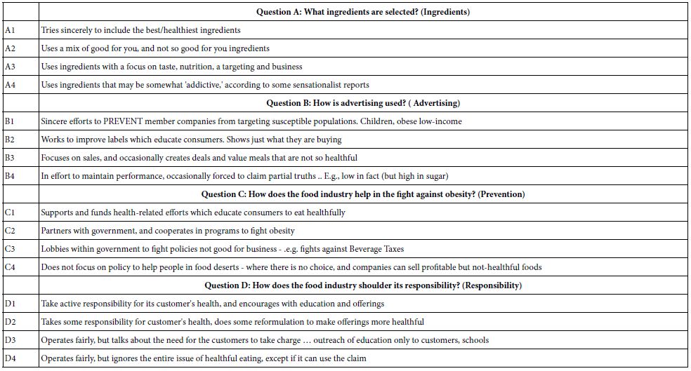
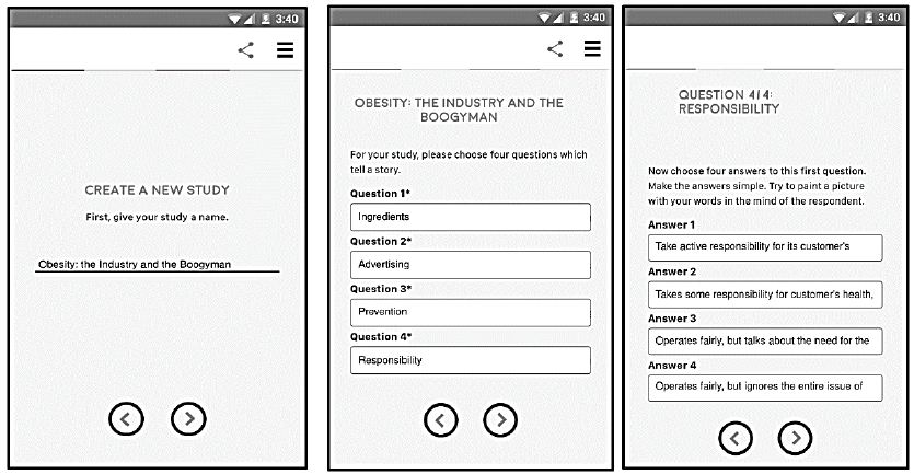
Figure 1: Define the name of the study, create four questions, and for each question provide four answers. The figure comes from the report, automatically generated at the end of the study, with all of the relevant set up slides captured as part of the research documentation.

fig 2

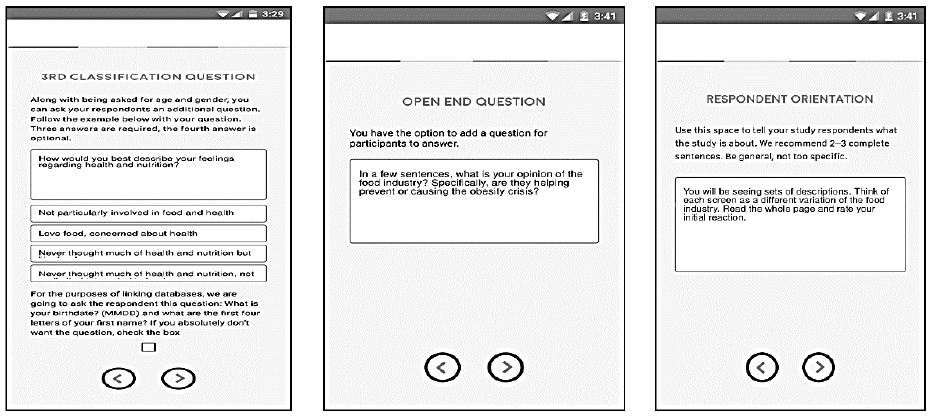
Figure 2: Create a third classification question (the first two are age, gender), create an open-ended question for the respondents to complete, and create an orientation page.

fig 3

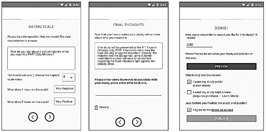
Figure 3: The rating scale (left panel). Final thoughts of the researcher (middle panel), and number of respondents desired for the study (right panel).

fig 4

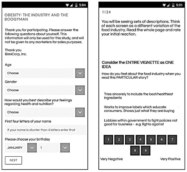
Figure 4: The respondent experience showing the classification question (left panel), and then one of the 24 vignettes shown as it would appear on a smartphone (right panel).

fig 5

fig 5 and 6

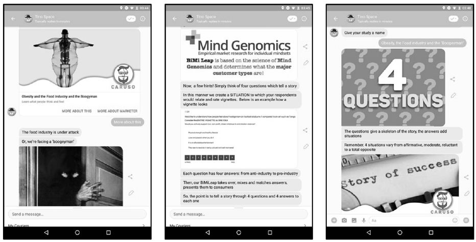
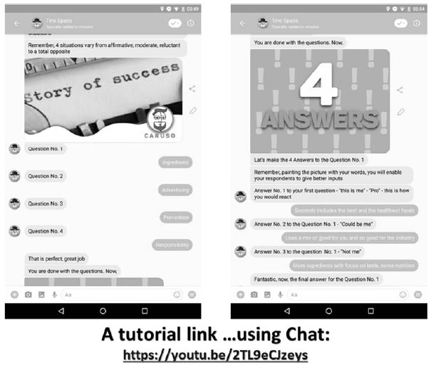
Figure 5 and 6: The Tino Space Chat. The figure shows the interchange between the researcher setting up the study and the chatbot. The objective is to make the set-up an interactive experience which simulates coaching.

It is as this stage that one is forced to think in a creative way. The selection of the topic, obesity and food, is straightforward. It is not hard to think of a topic, or even to refine our topic. The difficulty begins when it becomes time to ‘structure’ our inquiry, by asking four questions, and providing four answers to each question.

The first ‘stumbling block’ is the decreasing ability to think in a ‘systematic fashion’ We are not programmed in our education to think by asking a set of structured questions, although in reality that’s the easiest way to learn. A child asks questions. Despite the difficulties encountered by the researcher, it is vital that the researcher ‘stick with the script,’ and provide four questions. We simply require that the sequence of questions tell a story.

Figure 1 (middle panel) might have an actual question posted, such as ‘what is the advertising policy of the company?’ rather than just the word ‘advertising.’ Framing the question as a question versus framing the question as a simple statement makes no difference to the respondent, who will only see combinations of answers, and never the see the questions. The role of the questions is simply to facilitate the creation of answers.

From the point of view of science and education, it is becoming increasingly clear that we think easily in general terms, concepts, but have a hard time putting concrete ideas against those general terms. This step, questions, requires thought about STRUCTURE. We found formulating the four cogent question, to be modestly difficult for the researcher. Once the researcher formulates the four questions, a lot of the hard work has been done.

The four questions in Figure 1 are shown as one word each (ingredient advertising, prevention, responsibility, respectively.) The questions are short because they were selected by author Zemel, who had extensive previous experience. Instead of asking ‘what are the ingredients being discussed?’ Zemel simply put down the word ‘ingredients,’ knowing full well that the question is only used to generate the answers. The respondent never sees the underlying questions, but rather only sees the answers. The questions are selected to drive the production of the answers.

For each question, create four phrases which answer the question in different ways. The four answers pose a different challenge. Now, the task is not to think about structure, but rather to think about CONTENT. During the development of the BimiLep APP, it was first unclear how to generate this content. Putting the exercise into the form of question and answer made sense. The next issue was to determine the nature of the answers, how to make them readable, because it would be the answers, more correctly it would be the combinations of answers that would constitute the test stimuli.

The early efforts with BimiLeap ended up with researchers producing long-winded answers, complicated phrases involving different twists and turns of thinking. Others were simple one-word or two-word statements, i.e., very terse responses with little content. Neither type of ‘answer’ worked well. It became obvious that we need to specify how to write an answer. We came up with the suggestion that the answer be single-minded, and no longer than (approximately) 12 words. Formulating one’s thought in this structured manner called into play what might be called one’s ‘mental editor.’ No longer was the researcher grasping for structure in thinking, but rather now forced to provide answers selected with a focus on clarity of expression.

Advertising executives will recognize this step as one of the ways to create good ‘copy,’ i.e., good advertisements. Often, this creative step is described by the phrase ’problem-solution,’ namely pose a problem and then present a solution to that problem.

This step moves beyond the creation of a single, well-executed advertisement, or more correctly, a single, tested, vetted ‘concept,’ from which the advertising is to be created. Instead, the objective of this step is to create a bank of messages to be presented to the respondent in small, easy-to-read combinations. This first step, before creating the combinations, is to create the messages themselves, in a way which allows virtually ANYONE to do the basic creating. The question-answer format has been found by the authors to make the task easier. The question-answer format does not necessarily create brilliant ideas that will convince, but rather the format democratizes the process of coming up with material

Typically, consumer research studies using these approaches allow the researcher to ask many questions about who the respondent is, what the respondent believes, how the respondent has behaved with respect to the topic. The opportunity to acquire so much information about the respondent from the interview often ‘backfires,’ leading to data paralysis. The prevailing, typical attitude is ‘let’s not rush in and get the wrong information.’ Faced with the plethora of choice which potentially might produce analysis paralysis, the speed of the process is jettisoned in favor of ‘getting everything we can.’

BimiLeap was designed to be fast, modestly flexible, and inexpensive. The objective is to identify the ‘answers’, also known as element, which perform best, rather than acquire as much information about the respondent as possible. As of this writing (summer, 2021), BimiLeap acquires only three pieces of information about the respondent (age, gender, and a third question left to the researcher to select). The focus is clearly on the answers, the elements, not on the acquisition of extraneous information which ‘might somehow be useful.’

Figure 2 shows this third classification question. It is a sacrifice, of course, to leave information un-gathered, but it’s more important to have the study run quickly, and to recognize that deep knowledge will emerge when the researcher can do several of these small-scale studies, rapidly and affordably, building knowledge in a sequential, empirical, structured way. And, of course, create a library of responses to ideas, a library that can be searched easily to create even new constructs based upon the pattern of data from a set of somewhat related studies, dealing with one topic, or with a set of related topics.

Figure 1 shows how the app forces the researcher to ‘think through’ the issue by defining the topic, creating four questions, and then as an example, for the question regarding responsibility, provide four answers. BimiLeap forces the researcher into a structured way of thinking, beginning therefore with an undifferentiated issue, then a differentiation forced by the questions, and finally a further differentiation forced by the four answers to each question.

Once the questions are asked and the elements generated, the next steps create a rating scale (Figure 3, left panel), write instructions to have the researcher give some private, archival information about why the study and experiment were created (Figure 3, middle panel), and finally choose whether the study will be run free with data available to the world, or whether the study will be privatized, so that only the researcher knows the study and the data (see Figure 3, right panel).

Rating Scale: It is the rating question which allows the respondent to share his or her feelings. The objective of our project is to obtain a quick, almost intuitive response to the situation or the prospective client, which in this case is the world of food companies. A simple, rating question is:

 Based upon what you just read (the vignette). Please rate your feeling on the scale below

1=Feel very negative about the food industry … 9=Feel very positive about the food industry

Privatization: The privatization option was created to make the approach attractive to researchers who wanted to keep their efforts private, yet still wanted to use BimiLeap to create the data. There are always several constituencies when it comes to research. Everyone would like the research to be free, and instantly available, such as source material from Google about all sorts of information, as well as so-called Big Data. No one necessarily realizes that data ‘cost.’ The plaint is that ‘after all, the data are out there and freely available. How can you charge me for what I can get for free?’ The foregoing plaint is very real, altogether too common, and destined to produce stillborn, meager results if followed. Privatization addresses the need to satisfy the constituency which wants to do the research for their own interests. The default position of BimiLeap is that the data are public, when not ‘privatized.

The policy of BimiLeap is to be free for anyone to use, with the stipulation that the study is ported to the web, and parts available for anyone to see. One can purchase the study results in their entirety for a nominal sum. If the researcher wants to keep the results entirely private, the researcher need only select the ‘privatize option.’

Experimental design, test vignettes, and the respondent experience

We are accustomed to survey research, which asks a question, gets one of several possible answers, and analyzes the frequency with which each answer is provided. The results of this exercise give us a sense of what the respondent thinks about a topic, when asked a single-focus question.

Our experience here was also instructive. Many of us who have come from traditional backgrounds in testing products, but also in testing concepts and advertisements, are accustomed to the conventional practice of presenting one test stimulus, after which the respondent rates that test stimulus on a dozen or more scales, or rating attributes. What happens when one has many stimuli, but only one rating scale? The reason for the many stimuli is obvious; it is in the pattern of responses to the stimuli where the real knowledge lies. And the reason for only one rating scale is that with 24 test vignettes and a limited time, with unwilling or uninterested respondents, it is better to have a short interview than a long one.

Mind Genomics and BimiLeap follow a different path because they emerge from the heritage of experimentation, not the heritage of surveys. The respondent is presented with a set of elements, in our case a set of answers to the questions. The questions do not appear. The task of the respondent is to inspect this seeming random combination of messages (viz.,, answers, elements), and assign a single rating to the combination. The task is a bit jarring at first, because the respondent tries to be ‘accurate,’ carefully reading each of the combinations, the so-called vignettes. The combinations comprise different types of information, often information which may be somewhat contradictory, and certainly not put together in the most felicitous prose. Nonetheless, the respondent’s task is to read the test combination, preferably quickly, and assign a ‘gut-level’ reaction, an unintellectualized response.

The effort to force respondents to evaluate these disparate combinations of answers, our test elements, often produces a nervous respondent. Some complain that they don’t want to participate in a study where the ‘test stimuli do not make sense.’ They drop out. The remainder, most participants from a paid research panel, do not drop out, and end up responding in the desired ‘gut-level’ or intuitive fashion.

The aforementioned experimental design dictates the 24 combinations of elements, with the property that the 24 combinations comprise 2-tuples of elements 3-tuples, and 4-tuples, so that each element (i.e. answer) appears equally often, and that no vignette ever comprises more than one answer from the same question The 16 elements, embedded in the 24 vignettes, are combined in a way which makes the 16 elements statistically independent of each other, permitting regression analysis to be performed on the ratings, to relate the rating to the presence/absence of each element.

Finally, each respondent evaluates a different set of vignettes. The underlying experimental design is the same, but the combinations, the structure of the vignette is such that each respondent evaluates a unique set of combinations. This is called a ‘permuted design’ [10, 11]. The permuted design allows the research to cover a wide array of possible combinations, so one need not know anything about the topic, and yet the experiment will quickly reveal the important versus the unimportant elements.

Before the respondent begins to evaluate the vignettes, it is important to tell the respondent a little bit about the study, but not much. The introduction is the orientation page which tells the respondent about the study. The orientation page should be short, to the point, without giving information which could lead the respondent to answer one way or another. The orientation simply tells the respondent the least amount of information. Figure 4 (right panel) shows the orientation, at the top of the screen, and a specific vignette, or combination of elements below, with the rating scale at the bottom.

In terms of the actual user experience, today’s panel participants have moved beyond paper and pencil, and have even moved beyond the traditional computer screen, and onto a smartphone. Smartphones are ubiquitous. In light of the use of smartphones as both communication devices by phone, and as browsers with which to text information and to traverse the net, we created BimiLeap so that it would perform well when the respondent was browsing on a smartphone. Indeed, in today’s world, it’s not even clear whether consumers have computers. It’s best to allow the interview to occur on a smartphone, on the screen. Figure 4 shows the respondent screens, set up for a smart phone.

Improving the set-up experience by means of Chat

initial experiences with BimiLeap suggested that the actual process would be fairly simple. That suggestion turned out to be more optimistic than was the case. The early uses of the APP were made by individuals with a great deal of experience in setting up studies for Mind Genomics. When others began to use the APP it soon became obvious that their experience was far less smooth than was thought at the start of the process. It became obvious that a novice researcher, doing the Mind Genomics process for the first time was facing a host of problems, most of which were more complex than frustrating than had been the case before.

The problems encountered by those setting up both the obesity study and others ranged from hard-to-understand instructions about what it means to ‘ask a question,’ to ‘provide an answer,’ and even to create rating scales and open-ended questions. Quite simply, what appeared simple to experienced researchers required ‘coaching,’ and perhaps even more.

Author Savicevic suggested that the process move in a direction made possible by a chat bot. We are all becoming increasingly with chats, which engage in a simulated conversation. The chat was designed by the staff at Savicevic company, Tino Space, to act as a more intuitive, chat-based acquisition. Figures 5 and 6 show the set-up process, this time by a chat. The chat set-up, now in refinement, appears to be a substantial improvement in the user experience, at least for the researcher who has to do the set-up work.

The researcher experience – automatically-analyzed results in presentation-ready format (Figures 7-8)

fig 7

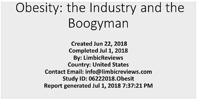
Figure 7: Full report in PowerPoint format.

fig 8

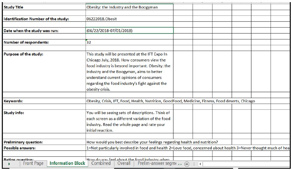
Figure 8: Information from the Excel file.

Today’s world operates on bites, small bits of information, presented in an entertaining fashion, or at least in a fashion which allows the information to be assimilated quickly. Rather than reading papers, even in areas which are very relevant, many people prefer to have the information presented in a manner that is exemplified by PowerPoint®. That is, rather than digesting the information for themselves from detailed text requiring thinking, many people prefer to have information ‘spoon-fed’ to them in a way which allows them to grasp the most important information.

In light of the emerging desire for fast, easy-to-understand information, called ‘the bottom-line’ or the ‘top-line,’ respectively, we have arranged BimiLeap to generate its own pair of reports, the first being a PowerPoint comprising all the relevant information (see Figure 7), and then an extensive, formatted Excel file with the relevant information, the summarized tables, and the raw data prepared for additional analysis (see Figure 8).

The report is a presentation-ready PowerPoint. The PowerPoint report is emailed to the researcher immediately after the close of the project, with the typical receipt of approximately one minute (by email). All the information in the report is either boilerplate or dynamically generated from the particular study being analyzed.

Accompanying the PowerPoint report is an excel file, also formatted, and presentation ready. The information page in Figure 8 is only one tab of a multi-tab Excel file, allowing the researcher to do further analysis of the data with other statistical analysis programs.

Part II – Explicating the resulting data – The food Industry and the issue of obesity

Illustrating how a study becomes one block in a scalable knowledge warehouse

An instructive way to appreciate the approach instantiated by the APP is through the data from our history. The study explicated here was presented to a large audience at the 2018 Annual Meeting of the Institute of Food Technologists (IFT), July 2018, in Chicago. The issue of the session was how to communicate as professionals.

The specific topic selected addresses the issue of combating ongoing negative press from activists and others who present their points of view in a variety of formats. The food industry is often accused as active participants in the growth of obesity world-wide. The rationale for such accusations ranges from anger at the R&D efforts which are believed to use any ingredients which make economic sense, to anger at marketing which is accused in the sensationalist press of communicating misleading information to consumers. And then there are those who argue that there is, in some unwritten way, an implicit contract between the company and its consumers for the company to take an active role in the consumer’s health.

How then does the, BimiLeap, work in such a situation, especially in the hands of novices, who do not have the resources of a corporation behind them, a corporation with trained lawyers, a well-paid public relations firm, an advertising (or several) advertising agencies, and a legion of consultants? What happens when the effort must be done expeditiously, to address a problem, and find the necessary messaging? The word ‘expeditiously’ means that there is relatively little time, perhaps a day or two at most, allowing perhaps one to six affordable, rapid iteration, each iteration totally complete, from start to finish in at most two hours. The challenge is to develop this approach, so that in 12 hours one can be fairly certain what to say and do, at least in terms of messaging.

This study, executed rapidly, shows what can be now done (2021), in as short a time as 1-2 hours, using a base of 30 respondents. A base of 100-200 respondents, easy to find on the Internet with online panel providers would take about the same time, approximately 1-2 hours at most. Note that the experiment from the point of view of the respondent takes about 4-5 minutes.

The foregoing sections have shown the set-up of this particular study on obesity and the perceived role of the food industry. We now move to the results, which emerged from the execution of the study with this small number of respondents. Just what emerged? And what conclusions can be made? The reader should keep in mind that the 32 respondents need not be the total number. There could be 132, or more respondents, just as easily. The question is really whether 32 respondents provide enough basic information, and whether one would be better off with the same study comprising 100 respondents, or say three studies, building upon each other, with say 32 respondents each. The answer to the foregoing question is not within the purview of this paper, other than to say that the opinion of the authors is that more studies, not more people for one study, provide a better strategy, assuming of course that there is a requisite minimum number of respondents for any one study.

Data analysis by building a model

The benefit of using the experimental design strategy emerges from the more powerful analytics which deconstruct the combinations, the vignettes, to the contribution of the individual elements, the messages or answers in Table 1. A paragraph is often more realistic than a single element, with the single element providing very little context. The respondent cannot ‘game’ the system, because too many different messages are present. This ‘blooming, buzzing confusion’ forces the respondent to assume a much less intellectualized role, and in turn to respond at almost a ‘gut level,’ the ‘System 1’ response so popular now in research thinking [12].

The actual ratings assigned by the respondent are transformed to a binary scale. The rationale for the binary scale, and thus the rationale for the transformation, is that managers and indeed almost everyone, more readily understands the meaning of a binary no/yes response, versus understanding the ‘meaning’ of a rating scale. Thus, when one is asked to rate ‘feeling about the food industry,’ the answers ‘feel positive’ versus ‘feel negative’ are easier to understand that the graded rating of ‘positive to ‘negative.’ We naturally gravitate to binary response, to no versus yes. For this study, ratings of 1-6 were transformed to 0, ratings of 7-9 were transformed to 100. Afterwards, the program added a very small random number to each transformed value, a value around 10-5. The random number ensures that the OLS (Ordinary Least-Squares) regression modeling incorporated in BimiLeap system does not ‘crash, when creating the model for the group, or the 32 individual respondent models, even when a respondent limits all the ratings of the 24 vignettes either to the low range of 1-6 (transformed to 0), to the high range (transformed to 100).

BimiLeap also measured the number of seconds from the moment that the test stimulus (combination of elements) appeared on the screen to the time that the response was made. BimiLeap then deconstructed the response time to the contributions of the individual elements, revealing what elements were processed more quickly (shorter response times), and what elements were processed more slowly (longer response times). The response time data warrants a totally separate paper by itself, and thus will not be reported here.

The experimental design and its permutations ensure that OLS regression can build an equation either for each person separately (individual-level model), and a model incorporating the data from many individuals, ranging from the total panel to a group incorporating, for example, only males versus only females (grand models). The specifics of experimental design and regression are well known and accepted in the academic and scientific communities [13].

At either the individual respondent level (so-called individual-level model), or at the group level (so-called grand model, BimiLeap computes the coefficient of a simple regression model, written as: Transformed Rating (Binary + random number) = k0 +k1(A1) …. k16D4). The small random number added to the transformed rating ensures that the OLS, ordinary least squares regression, will not crash, even though a particular respondent may have confined all 24 ratings to the range 1-6, or to the range 7-9. Confining the ratings to that range will result in all 24 cases for regression having the same value, 0 or 100, respectively. The small random number makes sure that such a situation will not a happen, for when that situation happens, the OLS regression ‘crashes.

Table 2, specifically the first set of numbers, shows the results from the total panel of 32 respondents. The data in Table 2 are sorted by the coefficient for the total panel. Despite what one might call a ‘thin sample,’ i.e., rather few people, even this small sample shows dramatic differences in the degree to which a specific element can drive a positive versus a negative feeling about the food industry.

Table 2: Parameters of the model relating the presence/absence of the elements to the binary variable ‘Feel positively about the food industry.’ Only positive coefficients are shown for the element.

table 2

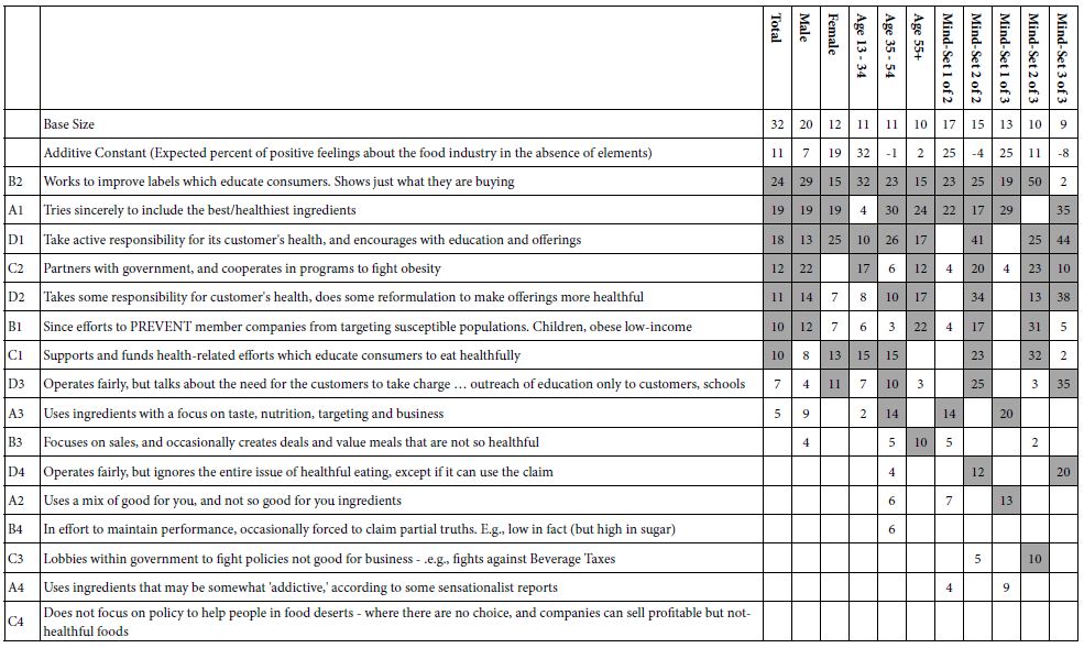
Table 2 shows the data from total panel, gender, age, and then mind-set segments, to be discussed in the next section. The specific data are not the focus, as much as the structure of the data, and what the data provide.

  1. The additive constant tells us the basic likelihood that in the absence of elements, the respondent will have a positive feeling towards the food industry (rating of 7-9 on a 9-point scale, in the absence of any elements). The additive constant is a purely estimate parameter from regression analysis but does have this meaning of a ‘baseline.’
  2. Each coefficient tells us the incremental percent of respondents who would be positive (rate the combination 7-9) if the specific phrase, the element or answer, were to be incorporated into the combination. The important coefficients are those 10 or higher. Conventional practice from thousands of these experiments suggests that coefficients around 8 or higher correspond to relevant, meaningful elements in terms of driving external behaviors. The cut-off is not ‘fixed in stone,’ however.
  3. Negative coefficients mean that when the element is incorporated into a combination, we would observe a reduction in the number of respondents who would assign a combination the rating of 7-9. The negative coefficients are not relevant to disclose the pattern and are not shown in Table 2. Rather, the cell is left blank.
  4. The practical implication here is that one rapid study provides a great deal of specific information need to make a corporation ‘smarter’ in its dealings. The aggregation of these studies creates a database with structured form, linking together the corporation, the topic, the response of different people, all in a coherent fashion with numbers that can be compared to each other.
  5. To summarize, the binary variable used as the dependent variable is created by transforming the ratings 7-9 to 100, and the ratings of 1-6 to 0. The rating 7-9 means that the respondent is pro-food industry when reading the vignette. The coefficients and the additive constant can be combined with the sum showing how likely it would be to obtain a rating of 7-9 when the respondent reads the combination comprising the elements whose coefficients are being additive.

Different mind-sets and the opportunity provided through targeted, effective messaging

During the past sixty years, since approximately 1960, marketers and then others have realized that the world does not comprise individuals who think alike. Whereas this statement seems obvious now, it was not always so, especially during the early part of the 20th century and before, when people were classified by ‘who they were,’ not by ‘what and how they thought.’ Marketers have successfully used the notion of ‘segmentation’ to divide consumers into groups, and have struggled, occasionally successfully, to message to these segments in the appropriate ways [14].

Dividing people into like-groups, segmentation, is often done at first by what people are, and by what they do, and occasionally by how they ‘think’ about a topic. With respect to our project here on the food industry and obesity, the researcher might divide the respondents by who they are (age, gender, body type, where they live, etc.), by what they do (e.g., the types of foods they say they eat, the types of restaurants they frequent, etc.), and by what they think (e.g., how do they respond to topics such as who is responsible for behavior, what is important – health vs pleasure, when it comes to food).

Segmentation of the above type, based on general measures about a person, may or may not help us understand the nature of what is important when it comes to communicating about the food industry and its role (or non-role) in the obesity epidemic. One would hope that dividing the population into traditional subgroups, based either on WHO A PERSON IS, or HOW A PERSON THINKS would reveal clearly different ways of thinking about a topic. Table 2 suggests that dividing people by gender or by age may show differences, not necessarily clear patterns which can form the basis of deeper knowledge and thus more effective actions in the world of messaging. Traditional ways of dividing people assume, without proof, that WHO a person IS determines WHAT a person THINKS. It may not be the case, and in general, it is not the case.

A better way to address the problem of mind-set segments comes from creating these segments from the materials closest to the topic. Beyond the conventional breakout of respondents into self-defined groups, BimiLeap performs a ‘k-means clustering’ [15] of the regression coefficients, first constructing two mind-set segments, then constructing three mind-set segments. These segments are called ‘mind-sets’ because they divide the respondents in the study by the pattern of the coefficients, i.e., by the pattern emerging when the respondent is confronted with a specific, targeted, defined, and quite limited situation.

In our case, we create or perhaps really discover underlying mind-set segments of a specific nature, relating to the issue of how one feels about the food industry, based upon the pattern of responses to the 16 messages. Since each respondent generated a set of 17 numbers (additive constant, 16 coefficients, one per answer), it is straightforward to cluster the respondents based on the pattern of the 16 coefficients.

For these data the k-means clustering, done on the 16 coefficients for the 32 respondents, suggested either two or three different clusters or mind-sets. Selecting the appropriate number of clusters is a subjective matter. The authors’ criteria are parsimony (fewer clusters are better), and interpretability (the clusters should tell a meaningful story).

The two-mind-set solution suggested one group interested in the food industry as a purveyor of ingredients, and the second group interested in the food industry as responsible for the well-being of its customers. Here are the strongest performing elements for the two-cluster solution, i.e., the solution which suggests two mind-sets.

For the purposes of this chapter, it is important to note that the performance of these elements is dramatic, +15 or higher, meaning that dividing people into mind-sets, viz., how they think, produces more knowledge and possibly better actions than simply dividing people by who they are. Such high coefficients almost never occur when these studies divide respondents by who they ARE, for the simple reason that a typical subgroup of individuals who LOOK SIMILAR from the outside often think in many different ways, ways, never be fathomed by simply knowing who a person IS.

Mind-Set 1 of 2 – Focuses on corporate moral responsibility to SELL better ingredients.

B2 Works to improve labels which educate consumers. Shows just what they are buying 23

A1 Tries sincerely to include the best/healthiest ingredients 22

Mind-Set 2 of 2 – Focuses on the corporate responsibility to EDUCATE consumers in healthy eating

D1 Take active responsibility for its customer’s health, and encourages with education and offerings 41

D2 Takes some responsibility for customer’s health, does some reformulation to make offerings more healthful 34

B2 Works to improve labels which educate consumers. Shows just what they are buying 25

D3 Operates fairly, but talks about the need for the customers to take charge..  outreach of education only to customers, schools 25

C1 Supports and funds health-related efforts which educate consumers to eat healthfully 23

The three-mind-set solution suggests that the original Mind-Set 2 of 2 (the food industry is ‘responsible to EDUCATE,’) really comprises two smaller groups, Mind-Set 2 of 3 feeling that the food industry is only partly responsible for the customer’s health/well-being for food, and Mind-Set 3 of 3feeling that the food industry and the customer are partners in the customer’s health-well-being.

Mind-Set 1 of 3 – Focuses on corporate moral responsibility to SELL better ingredients.

A1 Tries sincerely to include the best/healthiest ingredients 29

A3 Uses ingredients with a focus on taste, nutrition, targeting and business 20

B2 Works to improve labels which educate consumers. Shows just what they are buying 19

Mind-Set 2 of 3- Focuses on corporate moral responsibility to EDUCATE consumer.

B2 Works to improve labels which educate consumers. Shows just what they are buying 50

C1 Supports and funds health-related efforts which educate consumers to eat healthfully 32

B1 Since efforts to PREVENT member companies from targeting susceptible populations. Children, obese, low-income 31

D1 Take active responsibility for its customer’s health, and encourages with education  and offerings 25

C2 Partners with government, and cooperates in programs to fight obesity 23

Mind-Set 3 of – Focuses on corporate moral responsibility to SELL better ingredients AND EDUCATE.

D1 Take active responsibility for its customer’s health, and encourages with education  and offerings 44

D2 Takes some responsibility for customer’s health, does some reformulation to make offerings more healthful 38

D3 Operates fairly, but talks about the need for the customers to take charge … outreach of education only to customers, schools 35

The three-cluster solution may or may be useful. Certainly the two-cluster solution helps us a great deal to understand deep differences in the attitudes of the population. Cluster analysis, recall, is simply a heuristic to divide objects, here people, into homogeneous groups, homogeneity defined by mathematical criteria. It is the job of the research to choose the most parsimonious number of mind-sets. The goal is interpretability (the segments must be dramatically different in terms of that to which they respond), and parsimony (the ideal is as few mind-sets as possible.

We have focused on uncovering potentially new-to-the-world mind-sets, simply by running the Mind Genomics experiment. How, then, can the practitioner make use of this discovery? Before we finish up with the last topic, another new discovery, response times (engagement time), let us remain with the discovery of the two mind-sets. The PR strategist working for the food industry, or even a scientist interested in the minds of consumers, might wish to move beyond simply discovering the mind-sets. The practical application of the knowledge tells the food professional in the industry what to emphasize. But what should the professional say to a new person, a person not known beyond basic information about WHO and PURCHASE BEHAVIOR?

Recently, authors Moskowitz and Gere have created a system called the Personal Viewpoint Identifier, or PVI. The objective of the PVI is to create a small questionnaire, six questions long, the pattern of responses to which assign a person to the correct mind-set, with a probability substantially greater than change, although not perfect.

Figure 9 shows the PVI as seen by a respondent, after the PVI is set up. The actual PVI program can be accessed at www.PVI360.com. The research need only put in specified information emerging from the Mind Genomics study, information readily available from the Excel results (see Figure 8). Figure 9 shows three panels.

The left panel acquires relevant information about WHO the respondent IS

The middle panel allows the respondent to answer up to four relevant questions

The right panel presents the six questions in randomized order, these elements selected automatically by the PVI to maximize the chances of a correct assignment.

The PVI is sent out by link, the PVI is done by a person, and the feedback (mind-set membership, feedback information etc.) is sent both to the person and to a database under the researcher’s control. In this fashion, the mind-sets emerging from the study move from ‘nice to know’ facts to a way to optimize messaging to a given individual even immediately after the PVI have been completed.

Discussion & Conclusion

The project of science, and the process empowered by Mind Genomics and BimiLeap

Science, as commonly taught in schools, relies on the isolation and study of variables. There is an often- unstated belief and practice that careful, meticulous, painstaking work is the preferred approach to science. That which we know, according to such worldviews, must be obtained with care, and analyzed with precision. It may be acceptable in the everyday real world to do things ‘in the moment,’ but real science must be done with agonizing precision in order to be perceived as relevant and meaningful.

The research approach promoted in this article moves in a different direction. The notion is that with a reasonably powerful process to acquire knowledge and to understand the world, it may not be necessary to be as meticulous. In fact, the reality of the everyday is that we function quite well by grazing information, rather than sitting down to comprehend the information.

Corporate (and other) learning gained in short, easy-to-do, scalable arrays of studies

The most important outcome of this study is ‘what did we learn,’ and ‘was it worth the effort?’ We can answer those two questions easily. In additional to answering the question for the total panel we discovered new-to-the-world mind-sets with respect to an issue of obesity as a social issue linked with the food industry, Discovering mind-sets in the way we did it, with very few respondents (32), means that we are using the research to uncover sets of ideas which ‘travel together.’ We are not studying the entire world to discover these mind-sets, but rather using a convenience sample to discover the existence of the mind-sets. The distribution of such mind-sets in the population remains an issue to be addressed by larger-scale studies, powered by the PVI, the personal viewpoint identifier.

What is important to keep in mind is that we have established of mind-sets, done with a small sample of randomly chosen individuals, differentiating that discovery from the equal important but quite different question of these segments distribute in the population, another question that we can address, given a parallel piece of easy-to-use software.

There is a second outcome. That is the possibility learning a ‘lot more by simply doing a lot more.’ The evolution of science has been to increasingly larger, more expensive, more ponderous studies. That may be the case for the natural sciences and the physical sciences. As yet, it is not the case for applied science dealing with those topics where ‘the mind of man about external topics is king.’ Where topics can be broken up into aspects, dimensionalized, and studied with small, convenience samples, the Mind Genomics process will flourish, powered by BimiLeap and PV3I60.

Finally, anyone can become a researcher, not just those with advanced degrees, funding, and the permission of an IRB, Internal Review Board. We can envision an entire world of young and not so young researcher, in school, in companies, in play groups, all adding to the sum of knowledge through these experiments.

Envisioning one possible future of knowledge-building made possible by Mind Genomics

The efforts made in this study are, in actuality, quite simple, and the execution expedient. The objective of the effort was not to study the problem in detail, producing an archival document which investigates the problem from many different aspects. This latter approach characterizes much of today’s science, namely the attempt to define the parameters of the problem, and proffer a solution through experimentation, with one solution for one problem added to one solution to another problem, until the general issue is somewhat solved, or at least illuminated by the concatenation of these often-disparate solutions to a set of connected problems.

The approach presented here moves in a different direction, presenting the approach as a standardized method for create knowledge about a topic. There is already the ingoing assumption that the solution will not be perfect, that the range of the aspects studied will be limited, and that the data will be obtained through a small sample of respondents, not a large sample. We can liken this approach to an MRI of the mind, as the mind deals with various topics. Each study, comprising four questions, sixteen answers, perhaps 30-50 respondents, can be likened to one MRI photograph. The brain, or in our case, the mind, does not come into view and cannot be understood by one snapshot, one study alone. Rather, it is the buildup of the snapshots, the dozens, hundreds, thousands, tens of thousands of studies, and perhaps more, which begin to produce a general outline of what’s happening in the mind. Each snapshot alone is a minor effort, but the array of snapshots put together becomes the MRI of the mind, the picture of the mind, taken through this simple, scalable, affordable approach.

Acknowledgment

AG thanks the support of the Premium Postdoctoral Researcher Program

References

  1. Moskowitz H, Wren J, Papajorgji P (2020) Mind Genomics and the Law. 1st Edition. LAP LAMBERT Academic Publishing.
  2. Parris RR (2009 ) Jury Hands Down Stunning $370 Million Verdict Against Georges Marciano, GUESS? Inc Founder and Art Dealer, Announces R. Rex Parris. GES| 7/28/2009 5:21:29 PM LOS ANGELES, Jul 28, 2009 (Globe Newswire via COMTEX News Network).
  3. Moskowitz HR, Porretta S, Silcher M (2005) Concept Research in Food Product Design & Development. Ames, IA: Blackwell Publishing Professional.
  4. Luce RD, Tukey JW (1964) Simultaneous conjoint measurement: A new type of fundamental measurement. Journal of Mathematical Psychology 1: 1-27.
  5. Anderson NH (2001) Empirical Direction in Design and Analysis. Scientific Psychology Series. Routledge. Taylor & Francis Group New York.
  6. Green PE, Krieger AM (1991) Segmenting markets with conjoint measurement. Journal of Marketing 55: 20-31.
  7. Green PE, Srinivasan V (1990) Conjoint analysis in marketing: new developments with implications for research and practice. Journal of Marketing 54: 3-19.
  8. Moskowitz HR, Gofman A, Itty B, Katz R, Manchaiah M, et al. (2001) Rapid, inexpensive, actionable concept generation and optimization – the use and promise of self-authoring conjoint analysis for the foodservice industry. Foodservice Technology 1: 149-116.
  9. Moskowitz HR (2012) ‘Mind Genomics’: The experimental, inductive science of the ordinary, and its application to aspects of food and feeding. Physiology & behavior107: 606-613. [Crossref]
  10. Gofman A, Moskowitz HR (2010) Application of isomorphic permuted experimental designs in conjoint measurement. Journal of Sensory Studies 25: 127-145.
  11. Moskowitz HR, Gofman A (2004) System and method for performing conjoint measurement. Provisional patent application, 60/538,787, filed.
  12. Kahneman D (2011) Thinking, fast and slow. New York: Farrar, Straus and Giroux.
  13. Box GEP, Hunter J, Hunter S (1978) Statistics for Experimenters. New York, John Wiley.
  14. Claritas (1999) “PRIZM Cluster Snapshots: Getting to Know the 62 Clusters”.
  15. Jain AK, (2010) Data clustering: 50 years beyond K-means. Pattern recognition letters 31: 651-666.