Author Archives: author

Saying NO to Drugs: Two Mind Sets & Messaging Direction

DOI: 10.31038/JPPR.2019232

Abstract

We present a way to understand what messages may resonate with ordinary people regarding the negative effects of drugs. We identify six Questions or categories of statements, mix and match them, and present the combinations (vignettes) to ordinary respondents, over the web. The responses to the vignettes are deconstructed into the contribution of each individual element. We find clear differences by gender, age, and education, but NO patterns which lead to general knowledge. We divide the respondents by the pattern of their individual responses to the elements, which division reveals two equal size mind-sets. Mind-set 1 responds to scare tactics, facts. There is little in the way of convincing these respondents. Mind-set 2 responds to what it will to them, personally, at an emotional level. These respondents can be reached and convinced by the proper messaging.

Introduction

The notion of ‘addiction’ is not a new one. The notion of a drug problem is certainly not a recent development. Historically, the drugs involved in the world of ‘drug problems’ have been related to the products created out of poppy seeds, products that promised relief from pain, but were found to be addictive. The literature, stories, poetry, plays, is replete with depictions of people in opium dens (ref.) Famous characters in the literature of the time were featured as addicts to one or another opium-derived product, such as the legendary detective created by Arthur Conan Doyle, namely Sherlock Holmes [1, 2]. Wars have been fought over drugs, such as the Opium Wars in China.

For a long time, the topic of addiction has been one applying to alcohol, tobacco, and drugs [3] As a species, homo sapiens appears to have a predilection to become addicted to something or other. People, in fact, can be described as being addicted to gambling, addicted to a sport, a hobby, even addicted to work [4]. We hear of addiction to foods, to sweets, with the word ‘crave’ used to describe the desire for food in the same way that the drug addict ‘craves’ a ‘fix.’ People can be even be said to be addicted to each other, especially at the early stages of infatuation. This paper focuses on addiction to drugs, specifically on what one communicates to avoid addiction.

The scholarly literature is replete with studies documenting the nature of addiction. These studies usually concern the nature of addiction of people at different stages of life, in different circumstances. There is a sense that the pattern of addiction may co-vary with who the person is, and the situation in which the finds himself or herself [5–7]. There is a notion, however, that the mind of the individual may be very important in the nature of the addiction to which a person is subject [8]. The point of view about the link between personality and addiction, and the possibly ‘addiction-leaning personality’ can be found in the research reports going back three quarters of a century, to 1944 [9], and undoubtedly earlier with the works of psychoanalysts such as Freud and Jung [10].

On almost a daily basis we hear stories about the opioid crisis, a drug problem which has taken the place of previous big stories about crack and heroin, and before that morphine and opium. As a species, we humans can become addicted quite easily to many of these drugs, which cause an initial rush or feeling of wellness, but which can slowly become the master of the person, forcing that person to do anything to get the daily ‘fix, ’ (Kolodny et. al., 2015.) Addiction has become more than a problem. It has become an entire causa-belli, war cry, as activists blame food companies for making food ‘addicting’ [12].

In Western Europe drugs have been a problem in the real life, as products like heroin and morphine, so touted for health and freedom from agonizing pain have been found to be remarkably addictive. The many studies on these drugs could themselves occupy several books, just for a literature review. The social issues of addiction, the change in personality, and the creation of entire subcultures of addiction have been documented again and again. One need only go to sources such as Google^® Scholar to see the dramatic, ever increasing number of papers devoted to drug dependency.

In recent years the focus on opium-based drugs has taken a back seat to the emerging problem of opiods, available by prescription (e.g., oxycontin), given for pain relief, and powerfully addictive. What started out as a new way to get rid of pain has, in turn, morphed into a social problem, involving over-prescriptions, unnecessary prescriptions to satisfy addiction, and a decline in the moral character of some individuals in the medical professional and cooperating pharmacies.

What is missing in all of these studies is a profound understanding of how to prevent drug addiction. There is now widespread appreciation of the addiction problem, especially its prevalence, and the group mantras of messages which are supposed to communicate the will to resist drugs and addictions, such as ‘Say NO to Drugs.’ These are important slogans, analogous to patriotic war slogans, memorable, rallying cries, designed to inspire. Yet there is a gaping lack of knowledge. What inspires an individual person? What specific messages can one use to communicate about avoiding drugs?

We deal here with applying the method of experimental design of messages to identify specific messages which might work. This study is not designed to provide the ultimate data, but rather designed to explore whether the methods subsumed in the science of Mind Genomics can be used to convey messages about drugs with the same efficacy as sending messages about food. The latter, messages about food and drink, are designed to persuade consumers to buy the product. The former, message about drugs and addiction, are designed to inform about the perils of addiction, with the hope of reducing drug abuse.

As part of a new effort to understand the mind of the next generation, the so-called ‘millennials, ’ we embarked on a series of projects in which millennial respondents of college age were to select a topic of interest to predefined groups of four researchers. It would be the task of this ad hoc ‘research group’ to generate the different messages to be tested within the structure of a Mind Genomics experiment. That is, we changed the typical structure of research, wherein professionals design the study, and test with the appropriate sample of respondents.

The rationale for letting the millennials become the researchers comes from the desire to understand how they respond about the topic of drugs. By instructing the millennials to come up with the test stimuli, and then test those stimuli, we discover both what is important to the millennial from the messages they choose, and how these messages convince respondents in the general population.

Method

The foundations of Mind Genomics have been treated in a variety of papers and books, to which the reader is referred [13–15] Briefly, Mind Genomics begins with a topic, asks a series of questions which ‘tell a story, ’ provides a set of answers to each question (messages), combines these messages into combinations, presents the combinations to respondents, obtains ratings, deconstructs the ratings into the contribution of the individual messages, and finally creates both new-to-the-world mind-sets, as well as a PVI, a personal viewpoint identifier, to assign new people to one of the mind-sets previously discovered through the Mind Genomics experiment.

We begin with the set of questions and answers, i.e., Questions or categories of ideas, and then the specific elements pertaining to each Question. The Questions and the elements appear in Table 1. We have phrased the Question as a question, which is how the development of the test elements occurs. The research group works with a topic, comes up with the requisite number of questions or Questions (here six), the order of the questions or Questions which thus ‘tell a story, ’ and then the relevant elements or answers to each question.

Table 1. The test stimuli.

	Question A: What is the damage that drugs can wreak on your body?
A1	Anything that makes you less than you is not for you, especially drugs and alcohol…
A2	Keep healthy teeth…smoking and other drugs harm them
A3	Drug use can make you ill and an overdose can kill Some drugs can kill your brain cells and brain cells cannot grow back
A4	Drug use can lower your lung capacity
A5	Keep a healthy heart…stay away from drugs
A6	Drug use can make you ill and an overdose can kill
	Question B: How do drugs affect your personality and social life?
B1	Drugs can change the person you are…without realizing it Enjoy every day of your life, without having to rely on drugs to make you feel normal Don’t associate with the wrong people…taking drugs isn’t cool
B2	A person can undergo a complete personality change when under the influence of drugs
B3	Friends are there to help when you’re down … Drugs drag you down further
B4	Drugs can limit the friends you keep
B5	Enjoy every day of your life, without having to rely on drugs to make you feel normal
B6	Don’t associate with the wrong people…taking drugs isn’t cool
	Question C: What are the effects of drugs on your family?
C1	Family will always be there, but the “high” will go away…
C2	Your bond with drugs can break the bonds in your family
C3	If your children look to you as an example, you are, in effect, giving them permission to abuse drugs
C4	Drug addicted parents can seldom offer a stable family life to their children
C5	Every minute spent using drugs is a minute lost with a loved one
C6	Babies of drug addicts are far more likely to be underweight and to suffer from birth complications
	Question D: What financial damage does drug addiction wreak on you?
D1	Drug use interferes with your ability, which can make it harder to earn money
D2	The price you pay for drugs is more expensive then you think…they can cost you your life
D3	Drugs cost a lot of money… which can be invested in more positive things
D4	Court costs, legal fees, fines, a higher insurance rates all come with drug abuse
D5	Drugs can make you sell your belongings for money
D6	Addiction does more than harm your body…it can do lasting damage to your pocketbook and future earnings
	Question E: How are drugs associated with crime and punishment?
E1	The #1 reason for arrest in the U.S is for Marijuana possession
E2	Buying and taking drugs supports criminals and terrorists
E3	Don’t be apart of crime…being under the influence can make you do things you’ll regret
E4	Possessing drugs is a crime…a criminal record limits what you can do
E5	Addicts guilty of NO other crime than illegal possession of narcotics, are filling the jails, prisons, and penitentiaries of the country
E6	Almost all the opium in the U.S is made and grown in Afghanistan and funds terrorist groups
	Question F: What are other social problems emerging from the addiction to drugs?
F1	You have NO idea how many people died getting that drug into America
F2	Everyone has hopes and dreams for the future, but for addicts those hopes and dreams only focus down to where the next score is coming from
F3	Taking drugs definitely gives you a new lifestyle, but it is the lifestyle of a sad loser with NO prospects
F4	Outdoor cannabis cultivation, particularly on public lands, is causing increasing environmental damage
F5	Some of the most bitter ethnic and religious conflicts worldwide are fueled by drug income
F6	Chronic cannabis smokers present low fertility

When we look at the six questions in Table 1, we see that the millennials focus on the damage done by drugs. This insight, simply by itself, is valuable. It means that the younger people focus on drugs and damage, on negative effects. One might say that their questions are obvious, but not necessarily? Would, in fact, a PR company given the same task come up with the same Questions as the millennials? We don’t know. We do know, however, that this type of exercise forces the millennials to think about drug abuse in their own way, from their own perspective.

Creating vignettes by experimental design

Mind Genomics uncovers the contribution of the different elements by incorporating these elements into combinations, test vignettes. The vignettes comprise either three or four elements, a maximum of one element from a Question, but often NO element from a Question. The composition of the vignettes is dictated by an underlying experimental design, ensuring that the 36 elements are statistically independent across the set of 48 vignettes created for each respondent. Each element appears five times across the 48 vignettes, and thus is missing from 43 of the 48 vignettes. Finally, each respondent evaluates a unique set of 48 vignettes, created according to the same experimental design, but with the combinations different [13] This strategy ensures that the test vignettes cover a wide number of possible combinations. Furthermore, the strategy means that one need not know which combinations to create ahead of time. The more conventional approach would create a fixed set of 48 vignettes, present this fixed set of vignettes in different orders to respondents, average the ratings, and by so doing get a stable data set. Mind Genomics dispenses with that single set of vignettes.

The interview

The actual experiment begins with an invitation to panelists who are members of an on-line panel. These individuals have agreed to participate, in return for rewards dispensed by the company which provides the panel. Working with a panel company makes it easy to do these experiments, in return for a modest payment per respondent for the participation.

When the respondent agrees to participate, the respondent hits the embedded link in the email invitation, from which the interaction begins. Figure 1 shows the orientation page for the study. The orientation page tells the respondent a little about the study but provides NO information about what is expected. That lack of information is important. Anything in the orientation page providing greater detail is likely to set up the expectations of a ‘correct answer’ and thus bias the data in ways that are unknown.

Mind Genomics-019 - JPPR Journal_F1

Figure 1. The respondent introduction to the study on abusing drugs.

Each respondent evaluated 48 different vignettes, rating each vignette on two rating scale attributes. This paper will present results only from the first scale (How likely are you to say NO to drugs based on this information.) Figure 2 shows an example of a vignette. The experimental design dictated that 36 of the 48 vignettes would comprise four elements, one from each of four Questions, and that the remaining 12 of the 48 vignettes would comprise three elements, one from each of three Questions.

Mind Genomics-019 - JPPR Journal_F2

Figure 2. Example of a four-element vignette created according to the experimental design, for a specific respondent.

Transformation of the ratings from a 9-point to a binary scale and regression modeling

One of the ongoing ‘discoveries’ emerging from Mind Genomics is that users of the data report that they have difficulty understanding exactly what a scale point means. They understand the anchors of the scale (not likely and very likely, respectively), but they do not know how to interpret the values on the scale. Rather than label each point, a task which itself is fraught with biases of interpretation, we transform the rating scale into a binary scale, with ratings 1–6 transformed to the number 0, and ratings 7–9 transformed to 100. This transformation has been consistently used since 1985, and appears to work well, except for some countries wherein the respondents often ‘up-rate’ the vignettes, and which require a slightly more stringent transformation (1–7 transformed to 0, 8–9 transformed to 100.)

The transformation accomplishes its purpose, which is to make the user’s interpretation of the results simple. The numbers now deal with either NO (not interested in saying NO to drug) or yes (interested in saying NO to drugs). In order to ensure that the OLS (ordinary least-squares) regression will not crash, we add a small random number (<10^–5) to each transformed number. The random number does not materially affect the results, but does ensure that the OLS regression will work for a respondent who limits his or her ratings either to the low end of the scale (1–6, all transformed to 0), or the high end of the scale *7–9, all transformed to 100).

OLS regression is the preferred way to analyze the data. OLS regression deconstructs the binary rating into the contribution of both the additive constant (basic interest in avoiding drugs, in the absence of elements, viz., an estimated baseline), and the contribution of the 36 individual elements. Even when the respondent avers that she or he simply cannot state how much of the rating is due to each element, the OLS regression reveals that contribution.

How the individual regression models fit the original 9-point ratings

During the past two decades, numerous complaints have emerged among communities of professionals engaged in polling consumers. The complaints emerge out of the reality that consumers are increasing being asked to fill out questionnaires, virtually for every action they take in the commercial environment. When a consumer purchases a product on line or in a store, when a consumer uses a bank service or a medical service, when a consumer travels and stays at a hotel, one can be fairly certain that in an increasing proportion of those transactions there will be a follow-up request for the consumer to rate the transaction and even to provide deeper responses, e.g., through an automated interview.

The consequence is that the respondents are increasingly hesitant to participate in the studies, and the quality of the data from those who do participate have dropped. In previous studies with Mind Genomics, we have presented the distribution of goodness of fit statistics across individuals to assess the quality of data. The statistic used, the multiple R-squared, shows the proportion of variability in the ratings accounted for by the multiple linear regression.

Figure 3 shows the distribution of the R-squared values across the 50 respondents. What is remarkable is the very high individual models for goodness of fit. We attribute the quality of data to the importance of the topic. For other topics of far less social relevance, such as a credit card, the good of fit statistics are far poorer. It should be noted that whether we average good fitting models (such as those for this study) or average ‘noisy’ models (such as those for a credit card), the measure of central tendency, will still reveal what is important, and what is not important. Our focus here is simply to show how respondents pay attention to this important topic.

Mind Genomics-019 - JPPR Journal_F3

Figure 3. Distribution of the goodness-of-fit of the 50 individual models for Say NO to Drugs. The model relates the presence/absence of the elements to the 9-point rating (before the binary transformation).

How the individual elements drive the interest in Saying NO to Drugs

Our first substantive analysis deals with the degree to which the 36 different messages drive the response to say ‘I’ll say not to drugs.’ (see Table 2.) Recall that the dependent variable, the 9-point scale, was transformed to a binary scale, after which the OLS regression was run on the 50 individual data sets, one from each respondent, with each data set comprising 48 cases or observations.

Table 2. Performance of all of the elements as drivers of ‘saying NO to drugs’.

	Say NO To Drugs (Question #1) – Coefficients of the Binary Model	Total
	Base Size	50
	Additive Constant	48
F2	Everyone has hopes and dreams for the future, but for addicts those hopes and dreams only focus down to where the next score is coming from	10
B5	Enjoy every day of your life, without having to rely on drugs to make you feel normal	9
B3	Friends are there to help when you’re down .. Drugs drag you down further	7
B4	Drugs can limit the friends you keep	7
C6	Babies of drug addicts are far more likely to be underweight and to suffer from birth complications	6
A6	Drug use can make you ill and an overdose can kill	5
C4	Drug addicted parents can seldom offer a stable family life to their children	5
D6	Addiction does more than harm your body…it can do lasting damage to your pocketbook and future earnings	5
F1	You have NO idea how many people died getting that drug into America	5
B1	Drugs can change the person you are…without realizing it Enjoy every day of your life, without having to rely on drugs to make you feel normal Don’t associate with the wrong people…taking drugs isn’t cool	4
F3	Taking drugs definitely gives you a new lifestyle, but it is the lifestyle of a sad loser with NO prospects	4
B2	A person can undergo a complete personality change when under the influence of drugs	3
E6	Almost all the opium in the U.S is made and grown in Afghanistan and funds terrorist groups	3
F5	Some of the most bitter ethnic and religious conflicts worldwide are fueled by drug income	3
A2	Keep healthy teeth…smoking and other drugs harm them	2
C3	If your children look to you as an example, you are, in effect, giving them permission to abuse drugs	2
C5	Every minute spent using drugs is a minute lost with a loved one	2
D4	Court costs, legal fees, fines, a higher insurance rates all come with drug abuse	2
E3	Don’t be a part of crime…being under the influence can make you do things you’ll regret	2
C2	Your bond with drugs can break the bonds in your family	1
F6	Chronic cannabis smokers present low fertility	1
A3	Drug use can make you ill and an overdose can kill Some drugs can kill your brain cells and brain cells cannot grow back	0
A1	Anything that makes you less than you is not for you , especially drugs and alcohol…	-1
D5	Drugs can make you sell your belongings for money	-1
E2	Buying and taking drugs supports criminals and terrorists	-1
A4	Drug use can lower your lung capacity	-2
B6	Don’t associate with the wrong people…taking drugs isn’t cool	-2
D1	Drug use interferes with your ability, which can make it harder to earn money	-2
D3	Drugs cost a lot of money… which can be invested in more positive things	-2
D2	The price you pay for drugs is more expensive then you think…they can cost you your life	-3
A5	Keep a healthy heart…stay away from drugs	-4
C1	Family will always be there, but the “high” will go away…	-4
E4	Possessing drugs is a crime…a criminal record limits what you can do	-4
E5	Addicts guilty of NO other crime than illegal possession of narcotics are filling the jails, prisons and penitentiaries of the country	-4
E1	The #1 reason for arrest in the U.S is for Marijuana possession	-5
F4	Outdoor cannabis cultivation, particularly on public lands, is causing increasing environmental damage	-5

Table 3. The strong performing elements, by gender, as drivers of ‘saying NO to drugs’.

		Male	Female
	Base Size	12	38
	Additive constant	29	54
B5	Enjoy every day of your life, without having to rely on drugs to make you feel normal	23	4
B4	Drugs can limit the friends you keep	20	3
F2	Everyone has hopes and dreams for the future, but for addicts those hopes and dreams only focus down to where the next score is coming from	18	7
F5	Some of the most bitter ethnic and religious conflicts worldwide are fueled by drug income	17	-1
A6	Drug use can make you ill and an overdose can kill	16	1
C6	Babies of drug addicts are far more likely to be underweight and to suffer from birth complications	16	3
B2	A person can undergo a complete personality change when under the influence of drugs	14	0
F3	Taking drugs definitely gives you a new lifestyle, but it is the lifestyle of a sad loser with NO prospects	14	1
D2	The price you pay for drugs is more expensive then you think…they can cost you your life	13	-8
E3	Don’t be a part of crime…being under the influence can make you do things you’ll regret	13	-2
A4	Drug use can lower your lung capacity	11	-6
B1	Drugs can change the person you are…without realizing it Enjoy every day of your life, without having to rely on drugs to make you feel normal Don’t associate with the wrong people…taking drugs isn’t cool	10	3
F6	Chronic cannabis smokers present low fertility	9	-2
A1	Anything that makes you less than you is not for you, especially drugs and alcohol…	8	-4
A2	Keep healthy teeth…smoking and other drugs harm them	8	0
D6	Addiction does more than harm your body…it can do lasting damage to your pocketbook and future earnings	8	3
B3	Friends are there to help when you’re down.. Drugs drag you down further	3	8

When we average the individual models from the 50 respondents, we see the following:

Additive constant = 48 = conditional probability that the respondent will say ‘NO to drugs” in the absence of any elements in a vignette. For the total the additive constant is 48, meaning that in the absence of elements, we already have a moderate predisposition to say that they will say NO to drugs. The experimental design ensures that each vignette comprises 3–4 elements, so the additive constant is an estimated parameter. The additional motivation will come from the elements themselves.
The sorted elements. Previous studies suggest that coefficients about 8 or higher correspond to elements which have a meaningful effect when used. We use the term ‘meaningful’ rather than statistically significant because a coefficient can have the value of 2 or 3 and be statistically significant owing to the large number of ratings, and thus the increased likelihood that even a small coefficient will be statistically significant.
The two elements which score strongly combine both the positive and the negative. It may well be that the key to increasing donation is a combination of the so-called ‘carrot and stick, ’ and not just the ‘stick’ alone.
Everyone has hopes and dreams for the future, but for addicts those hopes and dreams only focus down to where the next score is coming from

Enjoy every day of your life, without having to rely on drugs to make you feel normal

Gender differences

We now focus only on those elements which perform strongly (coefficient > 6.51) for either males or females. Our data suggests dramatic differences, and reveals a new, unexpected pattern emerging from the additive constant and the performance of the elements.

The study incorporated more females than males. That, however, is simply a observation, and does not affect the differences between the genders:
The additive constant is far higher for the females than for the males (54 vs 29.) In practical terms, this means that the interesting in ‘staying NO to drugs’ is basically higher among females than it is among males. In the absence of elements, the conditional probability of a female saying “NO” is almost twice as high as the conditional probability for a male.
Males respond very strong to some of messages, however, with coefficients of 15 or higher, a value that has been operationally accepted as a very strong driver of the dependent variable, in our case the likelihood of saying NO.
The strong messages for male are primarily emotional and personal, bringing in the respondent, but also talking about the negatives of drugs. The only exception is the element talking about ethnic and religious conflicts, which do not bring in the respondent to the element, but simply state a fact.
Enjoy every day of your life, without having to rely on drugs to make you feel normal

Drugs can limit the friends you keep

Everyone has hopes and dreams for the future, but for addicts those hopes and dreams only focus down to where the next score is coming from

Some of the most bitter ethnic and religious conflicts worldwide are fueled by drug income

Drug use can make you ill and an overdose can kill

Babies of drug addicts are far more likely to be underweight and to suffer from birth complications
There is only one strong message for females, the one which talks about friendship.
Friends are there to help when you’re down … Drugs drag you down further

Age differences

Do we see the same strong differences by age that we did by gender? Table 4 shows us that the three age groups exhibit virtually the SAME additive constant, 47–49. The quite large differences emerge in the performance of the elements.

Table 4. The strong performing elements, by age, as drivers of ‘saying NO to drugs’.

		Age 18–29	Age 30–52	Age 53+
	Base Size	13	19	18
	Additive constant	47	49	48
	Age 18–29 (Respond to concrete information)
F1	You have NO idea how many people died getting that drug into America	18	-1	3
F2	Everyone has hopes and dreams for the future, but for addicts those hopes and dreams only focus down to where the next score is coming from	13	6	10
F5	Some of the most bitter ethnic and religious conflicts worldwide are fueled by drug income	12	-11	12
C2	Your bond with drugs can break the bonds in your family	11	-7	4
C6	Babies of drug addicts are far more likely to be underweight and to suffer from birth complications	9	4	5
D3	Drugs cost a lot of money… which can be invested in more positive things	9	-8	-4
D5	Drugs can make you sell your belongings for money	9	-4	-5
A6	Drug use can make you ill and an overdose can kill	8	4	2
	Age 30–52 (Appeal to emotion and well-being)
B5	Enjoy every day of your life, without having to rely on drugs to make you feel normal	-3	12	14
A2	Keep healthy teeth…smoking and other drugs harm them	-9	10	1
B4	Drugs can limit the friends you keep	4	9	8
B3	Friends are there to help when you’re down … Drugs drag you down further	-3	7	13
	Age 53+ (information that a parent might convey to a child)
F3	Taking drugs definitely gives you a new lifestyle, but it is the lifestyle of a sad loser with NO prospects	3	-7	16
B1	Drugs can change the person you are…without realizing it Enjoy every day of your life, without having to rely on drugs to make you feel normal Don’t associate with the wrong people…taking drugs isn’t cool	-5	3	12
E3	Don’t be a part of crime…being under the influence can make you do things you’ll regret	-11	3	9
B2	A person can undergo a complete personality change when under the influence of drugs	-4	2	9
C4	Drug addicted parents can seldom offer a stable family life to their children	5	1	9
C3	If your children look to you as an example, you are, in effect, giving them permission to abuse drugs	-5	-1	9
D6	Addiction does more than harm your body…it can do lasting damage to your pocketbook and future earnings	-1	5	8
E6	Almost all the opium in the U.S is made and grown in Afghanistan and funds terrorist groups	1	1	8

The types of messages which drive the different ages to say NO suggest patterns, but there may be some elements which perform well but depart from that pattern. Nonetheless, Table 4 suggests different types of information to which the three age-groups respond:
Age 18–29: They respond to concrete information, messages which paint a clear ‘word-picture.’
Age 30–52: They respond to messages which talk about the loss of ‘feeling good.’
Age 53+: They respond to messages which sound very much like a parent or older adult might convey to a younger person.

Where the person lives

The three groups differ in the additive constant (especially city versus rural and suburban), as well aa differing dramatically in the messages which drive each group to say ‘NO to drugs’ (Table 5.)

Table 5. The strong performing elements, by where one lives, as drivers of ‘saying NO to drugs’.

		Rural	Suburban area outside a city	City
	Base Size	14	20	16
	Additive constant	42	46	56
	Rural – Elements which deal with about drugs and bad endings
B3	Friends are there to help when your down … Drugs drag you down further	19	4	-1
F2	Everyone has hopes and dreams for the future, but for addicts those hopes and dreams only focus down to where the next score is coming from	14	11	4
B1	Drugs can change the person you are…without realizing it Enjoy every day of your life, without having to rely on drugs to make you feel normal Don’t associate with the wrong people…taking drugs isn’t cool	12	4	-2
B6	Don’t associate with the wrong people…taking drugs isn’t cool	12	-5	-12
C3	If your children look to you as an example, you are, in effect, giving them permission to abuse drugs	12	5	-12
E6	Almost all the opium in the U.S is made and grown in Afghanistan and funds terrorist groups	12	2	-3
D6	Addiction does more than harm your body…it can do lasting damage to your pocketbook and future earnings	11	2	2
C5	Every minute spent using drugs is a minute lost with a loved one	10	1	-2
	Suburban – Bad for your wallet, your family, your social life
B5	Enjoy every day of your life, without having to rely on drugs to make you feel normal	8	22	-7
A6	Drug use can make you ill and an overdose can kill	5	15	-9
F1	You have NO idea how many people died getting that drug into America	-4	12	6
C6	Babies of drug addicts are far more likely to be underweight and to suffer from birth complications	9	10	-2
B2	A person can undergo a complete personality change when under the influence of drugs	7	10	-9
A2	Keep healthy teeth…smoking and other drugs harm them	6	8	-8
D4	Court costs, legal fees, fines, a higher insurance rates all come with drug abuse	5	8	-9
	City – Very little reaches them, other than changing lifestyle
B4	Drugs can limit the friends you keep	4	7	10
F3	Taking drugs definitely gives you a new lifestyle, but it is the lifestyle of a sad loser with NO prospects	-10	7	12

The additive constant, the basic proclivity to say ‘NO to drugs’ is higher for those respondents who live in the city, lower for those in a rural area.
Rural – talk about drugs and bad endings.
Suburban – talk about the financial problems with drugs, and the difficulties with family and social life.
City – very little reaches them except other than it eventuates in a less pleasant social life.

The respondent’s education

We see substantial differences by education, as shown by in
Table 6. The differences do not tell as clear a story as did the differences among the previous complementary subgroups.

Table 6. The strong performing elements, by one’s education, as drivers of ‘saying NO to drugs’.

		Completed high school	Some college	College Vocational School
	Base Size	10	17	23
	Additive constant	64	30	55
	High School – High constant, NO specifics
	Some College-NO clear pattern, but many elements drive positive response of ‘Say NO’
B4	Drugs can limit the friends you keep	-2	20	2
B5	Enjoy every day of your life, without having to rely on drugs to make you feel normal	1	19	6
D6	Addiction does more than harm your body…it can do lasting damage to your pocketbook and future earnings	-6	18	-1
C5	Every minute spent using drugs is a minute lost with a loved one	-3	17	-7
C4	Drug addicted parents can seldom offer a stable family life to their children	-2	14	1
A4	Drug use can lower your lung capacity	-13	14	-8
B1	Drugs can change the person you are…without realizing it Enjoy every day of your life, without having to rely on drugs to make you feel normal Don’t associate with the wrong people…taking drugs isn’t cool	-5	10	4
A2	Keep healthy teeth…smoking and other drugs harm them	-14	8	4
B2	A person can undergo a complete personality change when under the influence of drugs	-10	11	3
A3	Drug use can make you ill and an overdose can kill Some drugs can kill your brain cells and brain cells cannot grow back	-7	8	-3
F6	Chronic cannabis smokers present low fertility	-3	11	-5
A1	Anything that makes you less than you is not for you, especially drugs and alcohol…	-13	10	-5
D2	The price you pay for drugs is more expensive then you think…they can cost you your life	-19	11	-6
D1	Drug use interferes with your ability, which can make it harder to earn money	-10	11	-9
B6	Don’t associate with the wrong people…taking drugs isn’t cool	-3	8	-11
E4	Possessing drugs is a crime…a criminal record limits what you can do	-7	8	-12
	College and Vocational School – Focus on a bad life
F2	Everyone has hopes and dreams for the future, but for addicts those hopes and dreams only focus down to where the next score is coming from	3	11	11
B3	Friends are there to help when you’re down … Drugs drag you down further	-3	8	9
C6	Babies of drug addicts are far more likely to be underweight and to suffer from birth complications	-9	12	8
F1	You have NO idea how many people died getting that drug into America	-1	6	8
F3	Taking drugs definitely gives you a new lifestyle, but it is the lifestyle of a sad loser with NO prospects	0	-1	8

The key patterns are the following:

Those who finished their formal education in high school show the highest additive constant, 64. They will say NO to almost everything about drugs. The specific elements do not make much of a difference, and certainly do not drive a particularly strong response.
Those who have had some college, but did not finish, show a low additive constant (30), but they respond strongly to some elements, shown below. The elements do not suggest a specific pattern, but they seem to be the type of advice a parent might give to a child
Drugs can limit the friends you keep

Enjoy every day of your life, without having to rely on drugs to make you feel normal

Addiction does more than harm your body…it can do lasting damage to your pocketbook and future earnings

Every minute spent using drugs is a minute lost with a loved one
Those who have finished college and vocational school respond to drugs as destroying a person’s opportunities.
Everyone has hopes and dreams for the future, but for addicts those hopes and dreams only focus down to where the next score is coming from

(At least) two mind-sets for giving to ‘Say NO to drugs’

One of the key tenets of Mind Genomics is that within any sphere of experience where people make judgments, there are differences among people which are systematic, and t, for the particular topic, may be likened to color primaries, namely red, yellow, and blue, respectively. It is not that people are different, which of course they are, but rather that there are groups of ideas which ‘travel together. A person can be characterized as more likely to respond in one pattern or another. The pattern most resembling the way a person responds is the person’s mind-set.

The above-mentioned description of the mind-sets for a sphere of experience means that there are no single mind-sets across all behavior, but rather each individual sphere of experience can be described as having its own particular experience-relevant set of primaries. Furthermore, these primaries emerge from the actual topic-specific study. That is, to discover the primaries or mind genomes for ‘Say NO to drugs’ we have to do the study, and let these genomes emerge.

The statistics to uncover these genomes or primaries is quite simple:

For each respondent, create the model relating the presence/absence of the 36 elements to the binary response, which we did before.
Array the models as a series of rows, considering only the coefficients, and not the additive constant. Its will be the pattern of coefficients which interests us, not the magnitudes of the individual coefficients.
Define a distance all pairs of respondents, based upon the pattern of their 36 coefficients. The distance we choose is the quantity (1-R), where R is the Pearson correlation computed using the two sets of coefficients, one for each respondent. The Pearson correlation goes from a low of -1 (perfect inverse correlation, and thus maximal distance of 2) to no relation (distance of 1), to a perfect linear relation (distance of 0.)
Array the respondents in two groups so that the variability between the averages of the 36 coefficients in each group is high, and the variability with the groups is low. Today’s statistical packages do these analyses quickly.
Compute the average coefficient for each element for each of the two segments or clusters. If there is a clear story, not necessarily perfect, then stop at two clusters or segments, interpret the meaning of the clusters.
If there is no clear story, and if there is a sense that the clusters are jamming together different types of messages, then move to three segments, and look for the story.
The objective of the clustering is to create a minimal set of reasonably different groups, with ‘different’ defined as groups about which one can write a different story. By the tine one reaches four segments, most meaningful stories emerge.
The results from our 50 respondents suggest two equal sized groups, although equality of size is not necessary for meaningful segmentation.
The two segments represent two mind-sets. The two mind-sets show radically different responses to the elements, as the segmentation is set up to produce. The interesting part of the mind-sets is what they are, and how does one recognize a person as having a specific mind-set. The mind-sets are not simply distributed by gender, age, where the respondent lives, and the level of education that the respondent has attained.
Mind-set 1 comprises individuals who respond to ‘raw facts.’ They will be hard to convince. Their additive constant is 49, but there are only two strong elements
Drug use can make you ill and an overdose can kill

You have NO idea how many people died getting that drug into America
Mind-set 2 comprises individuals who respond strongly to word pictures about what drugs do, and what drugs will do to them. The key is that they respond to the more elaborate messages.

Identifying the messages and what to say

The emergence of at least two mind-sets suggests that it will be possible to adjust the message to be more effective for at least one of the two mind-sets, the Personalizer (Mind-Set 2.) These respondents react to descriptions of what drugs do, and how drugs affect their lives. These respondents react strongly to the messages that have been used to combat drug dependency. Sadly, however, they comprise only half the population, and generally are difficult to discover if all one knows is age, gender, and where one lives. Just because a person has a certain profile in terms of geo-demographics or even in terms of interests, attitudes, and behaviors does not mean that one will belong to one mind-set or the other.

What is needed is a way to penetrate the mind of a person, early on, uncover the mind-set of a person, and make sure that the person, as an individual, is targeted with the messages appropriate for the person’s mind-set. We see from this small study that only half of the respondents react to the standard messages used in public-service campaigns. The other half of the respondents simply do not react. Further work is needed to discover what messages are appropriate for the non-responsive mind-set.

One initial way to make great progress in finding the messaging to help ‘Say NO to drugs’ is to assign a person to one of the two mind-sets. If the person is in the responsive Mind-Set, one should simply give that individual the ‘message’ appropriate for the mind-set. If the person is in the other mind-set, i.e., the non-responsive group, the messages won’t work, but this respondent could be invited to participate to future studies of the type reported here, such studies to be done with members of the non-responsive mind-set until the proper, motivating messages are discovered.

How then does one find these people who belong to the non-responsive mind-set? One way creates a Personal Viewpoint Analyzer (PVI), a set of questions, the pattern of answers to which assigns a person to one of the two mind-sets. The method uses the pattern of coefficients in Table 7, selecting the messages which best differentiate between the two mind-sets. Figure 4 shows the PVI created specifically for this study, a device which can begin to separate new people into one of the two mind-sets. A working version of the PVI as of this writing (Spring, 2019) is located at this website: http://162.243.165.37:3838/TT28/.

Table 7. The strong performing elements, by two emergent mind-sets, as drivers of ‘saying NO to drugs’.

		Mind Set 1	Mind Set 2
	Base Size	24	26
	Additive Constant	49	47
	Mind-Set 1 – The raw facts
A6	Drug use can make you ill and an overdose can kill	9	0
	Mind-Set 2 Personalizer: Responds to words pictures of what drugs will do to them
B5	Enjoy every day of your life, without having to rely on drugs to make you feel normal	2	15
B1	Drugs can change the person you are…without realizing it Enjoy every day of your life, without having to rely on drugs to make you feel normal Don’t associate with the wrong people…taking drugs isn’t cool	-6	14
B3	Friends are there to help when you’re down … Drugs drag you down further	0	13
F2	Everyone has hopes and dreams for the future, but for addicts those hopes and dreams only focus down to where the next score is coming from	6	12
B4	Drugs can limit the friends you keep	3	11
E6	Almost all the opium in the U.S is made and grown in Afghanistan and funds terrorist groups	-4	10
C6	Babies of drug addicts are far more likely to be underweight and to suffer from birth complications	2	9
B2	A person can undergo a complete personality change when under the influence of drugs	-3	9
B6	Don’t associate with the wrong people…taking drugs isn’t cool	-15	9
D4	Court costs, legal fees, fines, a higher insurance rates all come with drug abuse	-5	8

Mind Genomics-019 - JPPR Journal_F4

Figure 4. The Personal Viewpoint Identifier (PVI) to assign new individuals to one of the two mind-sets. The pattern of responses to the five questions identifies a person as belonging to one of the two mind-sets.

Table 8. Number of mentions in the open-end question regarding reasons for avoiding drugs.

Reason for avoiding drugs Phrases emerging from the open end question	Number of Mentions
Harmful to Self/Family Friends	25
Too Expensive	7
Illegal	4
Past Addictions	1
Bad Example for my Child/Children	1

As in any work in progress, this PVI is simply a first approximation of what could be accomplished. The ideal approach would be to run 2–5 or more of these small-scale studies, changing the elements which don’t work, until one finds the elements which best put a group of 50–100 respondents into two or more clearly different, hopefully totally different mind-sets, strongly responsive to different messages. In our preliminary study we find only one of these groups. If circumstance dictate stopping here with the discovery of only one group, and messaging proceeds, that messaging should comprise elements which appeal to the other group (Mind-Set 1), which we label as ‘non-responsive’ and ‘only the facts.’

Open End Analysis

At the end of the session, and just before the study was over, the respondents were asked to write a short paragraph about the reasons that they find most compelling for avoiding drugs. The open-ends are not part of the study, per se, but rather enable the researcher to get additional information about drugs from individuals who have just been exposed to different sets of messages about what’s bad about drug.

The pattern of open-end responses suggests respondents say that they are most likely to avoid drugs because of the harmful effects (personal health) to themselves as well as to their families and friends. Cost is the next most frequently mentioned reasons. Other rationales for avoiding drugs include legal ramifications, past addiction, and a harmful example to children.

Discussion and conclusions

As of this writing (Spring, 2019), it is becoming increasingly clear that the so-called ‘drug problem’ is far more serious and insidious than ever before, primarily due to the increasing legality of some prescription drugs which cause addiction, e.g., opioids.

This paper presents an inexpensive, rapid, scalable way to attack the drug issue by understanding the mind of the individual, not treated like an addict, but rather treated like a consumer. That is, the objective is to understand how to communicate to ordinary people, before they become addicted, sending them messages. If we are to believe the preliminary numbers from a base of 50 respondents, then there are at two mind-sets. The first mind-set (‘The Raw Facts’) reacts to very little. More work is needed to find the deterring messages. The other mind-set reacts (‘Personalizer’) reacts strongly to messages about what the drug will do to them.

As we look at the increasing magnitude of the drug problem, could it be that the messaging is inadequate, and geared effectively to Mind-Set 2, the ‘Personalizer?’ Furthermore, could it be that we have not yet found the appropriate messages, if any, for Mind-Set 1, the ‘Raw Facts.’ Certainly, only one message or element among the 36 tested by this small sample suggests the need for more studies, studies that are remarkably inexpensive, easy to iterate, and scalable. Fortunately, the PVI, the personal viewpoint identifier, allows us to identify the individuals who belong to each mind-set, and thus enable us to classify each respondent ahead of time.

It would be ironic if the tools of today’s marketing, specifically the notion of mind-types and consumer segmentation, could be extended to the understanding and amelioration of addiction. The irony, of course, is that the same science used to drive consumers to purchase and to consume, themselves often called addiction in the most severe cases, would now be turned into the very tool used to message people to avoid sources of addiction. Certainly, the affordability of the Mind Genomics science deserves more application to the social and personal tragedies of addiction.

References

Dalby JT (1991) Sherlock Holmes’s cocaine habit. Irish Journal of Psychological Medicine 8: 73–74.
Peschel RE, Peschel E (1989) What physicians have in common with Sherlock Holmes: discussion paper. J R Soc Med 82: 33–36. [crossref]
Carver H, Elliott L, Kennedy C. and Hanley J (2017) Parent–child connectedness and communication in relation to alcohol, tobacco and drug use in adolescence: An integrative review of the literature. Drugs: education, prevention and policy 24: 119–133.
Vitaro F, Brendgen M, Ladouceur R & Tremblay RE (2001) Gambling, delinquency, and drug use during adolescence: Mutual influences and common risk factors. Journal of gambling studies 17: 171–190.
Hanneman GJ (1973) Communicating drug-abuse information among college students. Public Opinion Quarterly 37: 171–191.
Kandel DB & Logan JA (1984) Patterns of drug use from adolescence to young adulthood: I. Periods of risk for initiation, continued use, and discontinuation. American journal of public health 74: 660–666.
Yamaguchi K, Kandel DB (1984) Patterns of drug use from adolescence to young adulthood: II. Sequences of progression. Am J Public Health 74: 668–672. [crossref]
Kido T & Swan M (2013) March. Exploring the Mind with the Aid of Personal Genome-Citizen Science Genetics to Promote Positive Well-Being. In AAAI Spring Symposium: Data Driven Wellness.
Felix RH (1944) An appraisal of the personality types of the addict. American Journal of Psychiatry 100, 462–467.
Crowley RM (1939) Psychoanalytic literature on drug addiction and alcoholism. Psychoanalytic Review 26: 39–54.
Yamaguchi, K. & Kandel, D.B., 1984. Patterns of drug use from adolescence to young adulthood: III. Predictors of progression. American Journal of Public Health, 74, 673–681.
Lindgren E, Gray K, Miller G, Tyler R, Wiers CE, et al (2018) Food addiction: A common neurobiological mechanism with drug abuse. Froniers of Bioscience (Landmark Ed) 23: 811–836.
Gofman A & Moskowitz HR eds., (2012) Rule Developing Experimentation: A Systematic Approach to Understand & Engineer the Consumer Mind. Bentham Science Publishers.
Moskowitz HR (2012) ‘Mind genomics’: The experimental, inductive science of the ordinary, and its application to aspects of food and feeding. Physiology & behavior 107: 606–613.
Moskowitz HR & Gofman A, Inovation Inc, (2011) System and method for performing conjoint analysis. U.S. Patent 7,941,335.
Moskowitz HR, Gofman A, Beckley J & Ashman H (2006) Founding a new science: Mind genomics. Journal of sensory studies 21: 266–307.

Young Americans Reacting to Statements about Palestine & Israel: A Mind Genomics Exploration

Leave a reply

DOI: 10.31038/ASMHS.2019324

Abstract

Listening and reading to the partisan politics surrounding the ongoing conflict between the Palestinians and the Israelis, one gets the impression that this topic is all-consuming. A study using the science of Mind Genomics reveals that most respondents from a sample of young respondents do not care about the topic, nor are engaged by anything said in the media. The Mind Genomics study combined messages, policy statements, issued by the US government, presenting small vignettes, almost as news stories. The strategy prevents the respondent from responding in a politically-correct manner. The data suggest that most of the young respondents are not interested in the topic, when the data from the total panel is reported. Two mind-sets emerged, one feeling that stability and hope will be achieved through force, the other feeling that stability and hope will be achieved through economic development. The study presents a PVI (personal viewpoint identifier) to assign new people to one of the two mind-sets. The paper finishes with a discussion of the contribution of Mind Genomics to a deeper understanding of political thought and the emerging discipline of counter-factual history.

Introduction

A Long History, a Wide Scope, Inflamed Emotions

Depending upon one’s ethnic group and perhaps political / social leanings, the ongoing tensions in the Middle East, and especially between the Palestinians and the Israelis occupy either a great deal of one’s attention and concern, a moderate degree, or little at all, being even perhaps irrelevant. When talking to young people who are not politically involve and polarized, it is hard to discern the nature of the aspects which may concern them when faced with general indifference. In this exploratory paper it is impossible to deeply understand a topic which has been simmering for 70+ years, but it is possible through the science of Mind Genomics, described below, to take a ‘snapshot’ of the situation from the minds of younger people as they respond to statements about possible policy towards the Middle East.

This study represents an exploration of responses to policy statements that have been made, as well as ideas about potential economic help for the Palestinians, ideas that have not been made public, but have floated around. The focus of the study is on the degree to which any of the official statements has the power to influence young Americans, ages 17–30, either as statements which could lead to peace or which could fan the flames of war.

The published literature on the topic of Palestine vs Israel and vs the United States, as well as the actual details of the workings of the Palestinian state come in the form either of books and periodicals, or from news releases and the accumulation of a body of news both from the main mainstream media and now from the Internet. Books dealing with the topic are typically either learned articles or popular books dealing with the topic, or clearly partisan treatments of the topic, the appellation ‘partisan’ being a description of the emotions, not a judgment of the correctness of the treatment [1–4]. A list of the books dealing with the subject would stretch from the 1950’s to today, with no end in sight, as the Middle East continues to occupy the attention of the world, the eruptions in the Middle East, whether minor or major, causing discomfort, and then fear for the disruption of the world order.

When it comes to deeper understanding of the subjective feelings, there are the innumerable public opinion polls about every aspect of the situation, these polls taken often in Israel, and often in the rest of the world as well. The answers emerging from those polls comprise ‘factoids’, with a subsequent attempt tie together the factoids discovered in the polls, linking them to other information about the topic. Yet the deeper understand could become even deeper with better tools, providing a sense of the inside of the mind, in a way metaphorically analogous to the way the MRI technology provides a sense of the nature of body tissue. That will be the topic of this paper.

Polling versus Experimentation

The typical world of responses to public policy invokes the now-institutionalized business and discipline of opinion polling. Scarcely a day goes by that another people comes out to present to the thinking public what the people ‘think, believe, and do.’ The professional associations such as AAPOR (American Association of Public Opinion Research) for example, serves as a bedrock to validate the efforts of the pollsters who present their approaches as scientific. Public opinion research is presumed to be scientific, working with representative samples of respondents, statistical tests of different from the discipline of inferential statistics and of course best practices about how to phrase questions, how to phrase answers, and so forth.

A recurring key issue is that when one does a poll, one invites the respondent to invoke a ‘mental editor,’ to be politically correct. This mental editor thus skews the results, a skew that cannot necessarily be overcome by the best of the recommended practices. The researcher MUST ask the respondent questions in a direct fashion. Once the respondent can address each question, one question at a time, it is possible and indeed quite straightforward to adopt a stance, tailoring one’s responses to accord with that stance, whether the stance, the point of view truly represents or does not represent one’s inner feeling.

In contrast to polling and surveys or asking the respondent to describe or vote, there is the world of experimentation. Admittedly, experimentation is far easier when one can control the stimulus, varying the stimulus in predefined ways, measuring the responses, and attributing the ‘change’ in the dependent variable to the precise change in the controlled, independent variable. This approach works very well to understand the dynamics of simple things, such as how the physical ingredients of a food or beverage drive our liking, or the relation between the number of hours one studies for a test and the score on the test

Can experimentation be applied to understand the Palestine-Israel issue? Certain one cannot easily vary the features of a nation in the same way that one can vary the amount of sweetener in a beverage. Yet, what if one were to describe a social situation in different, systematically varied ways. What would happen if one presented a positive, upbeat message versus a negative, downbeat message? How would people react?

The foregoing idea notion involves experimenting with ideas, metaphorically combining the notion of experimentation using statistical design in the spirit of creating and testing aspects of notion of counterfactual history. Instead of presenting history or world issues as simple ides with aspects to be evaluated and discussed, we create scenarios or combinations of ‘facts’ about the issue, these facts having actually happened, or could have happened. We instruct respondents to read these ‘counterfactual combinations,’ vignettes, and respond to them. The respondents have no idea whether what they are reading is true, not true, possible, impossible, or even whether what they are reading comes from a completely different topic or subject area, merged into the set of stimuli.

The respondents simply evaluate these vignettes, from which we learn a great deal about how they perceive the situation and its features. We do not ask the respondent to act in a rational way, but rather present the respondent with the vignettes, and acquire their responses, at an almost intuitive level, a way labelled by Nobel Laureate Kahneman as ‘System 1’ [5]. The actual inspiration for such an approach comes not so much from a deep philosophical inspiration as it does from the way a company learns how to say the right things to the customer, for example, when marketing Jello^®.

The systematic experimentation opens a whole new branch of social science, akin to the alternative worlds create by science fictions. We are simply creating alternative situations, alternative realities to be tested. The approach, first used for marketing [6,7], and now for social issues, may be the experimental version of ‘counterfactual history.’

How Mind Genomics Studies Problems

It is clear from everyday life that people hold different views about the same topic. The differences can be vanishingly small, or dramatic. One need only read accounts of the same event in different media outlets to recognize the power of the report to present the same idea as an opportunity, and another report to present the same idea as the impetus for a debacle. Understanding the differences in the points of view of the reporters is clear, and can be done by the analysis of language, and so-called ‘sentiment analysis’ [8].

What is harder to understand is the deep response of ordinary people to the messages which describe a situation. What is meant here is not the initial, almost knee-jerk reaction to the message and the situation, but rather the deep, often automatic response to the message. Do people really pay attention to the individual messages in politically motivated writing, or is their response simply a generalized, undifferentiated reaction?

Mind Genomics enables us to understand the deeper responses to test stimuli. Mind Genomics does so by mixing and matching different messages, different ideas, into simple to read combinations, vignettes, and then secures the response of individuals to these vignettes, these mixtures. The vignettes being as they are, combinations, defy the desire of the response to be ‘correct’ because the compounding of the messages leaves the respondent unable to formulate what is a consistent response. The desired consequence is that respondent ends up abandoning the desire to be rational, correct, and consistent, and simply answers at almost an intuitive, ‘gut level.’ It is at this intuitive level that one’s true feelings emerge, guiding as they do the selection of the response (Moskowitz, 2012).

The Process of Mind Genomics

Mind Genomics follows a set of well-choreographed steps, beginning with the selection of cognitively meaningful stimuli (messages which are presumed to have real meaning), and ending with the discovery of possibly new-to-the-world mind-sets, different ways to think about the same problem. The phrase ‘Mind Genomics’ is a metaphor for the discover of these different mind-sets for a situation, similar to the discover of alleles for a gene.

Step 1 – Define the topic: It may seem very simple to ‘define a topic,’ but it is not. Mind Genomics operates at the granular level. A topic, for example, cannot be an overwhelmingly large issue like the entire Palestine-Israel issue. If anything, the topic should error on the side of being very small, localized, specific, yet with different aspects. Mind Genomics could do a good job on a topic such as how to arrange a seating room for a conference between Palestinians and Israelis. For this topic, we focus on the reactions of young people to pronouncements about the Palestine-Israel situation, made by the State Department, a topic which is large, but not overwhelmingly so.

Step 2 – Define four questions to be answered, with the structure that at some level the set of questions are arranged to ‘tell a story’: In every topic there exist many types of stories to be told. The objective of Mind Genomics is to determine what specific elements of the story, what messages, resonate with the respondent. In order to discover these resonating elements, we must embed the messages into a story, doing so by means of a method which combines the messages in a structure. The overriding structure, the story, must make intuitive sense, even when the individual messages when thrown together do not necessarily make sense. Hence, the four questions, which may be likened to the way a reporter structures a story (who, what, where, when, why, how). The four questions are left to the researcher. They will never be shown to the respondent, but rather they will serve as prompts to help develop the specific elements. Table 1 shows these four questions for our study on the language of pronouncements about Palestine and Israel.

Table 1. The four questions and the four answers to each question.

Question 1 – What is the U.S. Policy?
A1	U.S. Embassy moves to Jerusalem from Tel Aviv.
A2	U.S. recognizes Israeli sovereignty over the disputed Golan Heights… strategic plateau Israel acquired after the Six-Day War.
A3	U.S. passes Anti-Terrorism Clarification Act (ATCA)… ends U.S. funds to the West Bank & Gaza.
A4	U.S. President Donald Trump say U.S. aid cuts aimed at pressuring the Palestinians to return to peace talks.
Question 2 – What is the U.N. Policy?
B1	The U.N. general assembly has a permanent feature on its annual agenda titled “Human rights situation in Palestine & occupied Arab territories”.
B2	U.N. condemns the firing of rockets from Gaza into Israeli civilian areas
B3	Report from U.N. claims that Israeli security forces may have committed war crimes & should be held accountable for the deaths at protests in Gaza last year
B4	Israel was the most condemned country at the U.N. in 2018, with the General Assembly passing at least 20 resolutions against Israel
Question 3 -What do the Israelis and Palestinians say and do to express their goals?
C1	Israel says protests, described by Gazans as the Great March of Return, are particularly violent… could act as a cover for Hamas, to infiltrate Israel, carry out attacks.
C2	Prime Minister Netanyahu said Israel will annex settlements in the West Bank.
C3	As U.S. peace plan rollout approaches, Palestinians voice rejection.
C4	Thousands of Palestinians demonstrate along the Gaza border fence with Israel.
Question 4 – What are possible efforts to help economic development of the region? These are new ideas to be explored within the study
D1	U.S. offers economic development aid to create Middle East Institute of Competitive Excellence.
D2	U.S. groups approach Palestine with opportunity to work with Israel to create better economic conditions.
D3	U.S. creates Institute to help Palestinians become more entrepreneurial.
D4	U.S. Jewish organizations reach out to support economic cooperation between Palestine and Israel.

Step 3: Create four answers to each question: The answers, short statements or phrases, are the material that Mind Genomics combines, to produce the vignettes. The answers may be actual statements, possible statements, and even new ideas to be explored within the study. Table 1 presents the four questions, and for each question the four answers. Questions 1–3 and their answers were taken from news stories. Question 4 and its four answers were exploratory ideas developed by author Moskowitz over the past decade, but do not yet exist, at least in a well-recognized public forum. It is important to stress that one need not use the precise words, especially when the language is the less than ‘precise and punchy’ language of diplomacy and reporting favored by government.

Step 4: Combine the elements into an experimental design: The experimental design can be likened to a book of interconnected recipes, with each combination defined as having a specific answer from each of the four questions. An example of the experimental design appears in Table, which specifies the first nine combinations for Panelist #1. The experimental design ensures that each element or answer appears equally often, and that each element is statistically independent of every other element, allowing for OLS (ordinary least-squares) regression to be applied to the dataset. The vignettes are ‘partial,’ meaning that some vignettes or combinations lack an answer from one or two of the four questions. This lack is deliberate, ensuring that the coefficients estimated by the regression modeling have ‘absolute value,’ i.e., the ratios of coefficients are meaningful [9, 10,11].

Figure 1 presents a screen shot from one of the vignettes. The vignette is laid out to be simple, viewable on either a smartphone or a tablet/PC with the layout appropriate for the screen on which it is viewed, and to be available on any platform. The format is set up to be stark, with one element atop the other, lacking connectives. This format may seem a bit different from the more conventional ‘dense’ format of concepts with the proper language, paragraph form, and replete with connectives. The rationale for the stark format is that the format leads to easier ‘grazing’ for information, and is less tiring, especially when the respondent evaluates 24 such vignettes, one after the other. The easier the task can be made, the more likely that the respondent will complete the task, and not drop out, as is often the case.

Mind Genomics-018 - ASMHS Journal_F1

Figure 1. Example of a vignette as it appears on a smartphone.

Most studies with experimental design specify a certain, very limited number of combinations, all tested by many individuals. The objective of the replication is to more accurately estimate the average assigned to the combinations. The sampling of possible combinations is limited, but the ‘strength’ or ‘performance’ of each combination is accurately estimated. Mind Genomics works in a different fashion, more in the spirit of the MRI. Each respondent evaluates a unique combination of 24 vignettes or combinations, like a ‘snapshot’ of the topic. At the same time, since each respondent evaluates a different set of combinations, the Mind Genomics effort estimates the performance of different parts of the underlying ‘space.’ What is missing in the accuracy of one set of estimates provided by replication is more than made up by sampling a great deal more of the space by Mind Genomics.

The respondents were members of the Luc.id panel, comprising 20+ million prospective participants around the world, who had previously agreed to participate in these types of studies. The respondents were specified to be ages 18–30, to live in the United States, with half the panel being male and half the panel being female

Table 2 presents the structure and performance of the first nine vignettes (Vig1-Vig9) for the first respondent, an 18-year old female. The top part of Table 2 presents the specific combination. The regression program cannot use the data in this form. We ‘expand’ the design to generate 16 variables, one variable corresponding to each element or answer. When a vignette contains the element, the value is ‘1’, else the value is ‘0.’ In this form the regression model can easily analyze the data, to produce a model. Table 2 shows that five vignettes are incomplete. The rationale for this is that only with incomplete or so-called ‘partial profiles’ can the regression analysis return with absolute values for the estimates of the coefficients.

Table 2. The first nine vignettes for respondent #1, showing the combinations, the expanded design for statistical modeling by regression, and the set of dependent variables.

Row	Vig1	Vig2	Vig3	Vig4	Vig5	Vig6	Vig7	Vig8	Vig9
Specific Combination
Question A	A3	A1	A1	A4	A2	A2	A3	A4	A4
Question B	0	B4	B3	B4	0	B3	B2	B3	B1
Question C	C3	C1	0	C1	C4	C2	C2	C4	0
Question D	D1	0	D1	0	D2	D4	D3	D3	D4
Binary Expansion
A1	0	1	1	0	0	0	0	0	0
A2	0	0	0	0	1	1	0	0	0
A3	1	0	0	0	0	0	1	0	0
A4	0	0	0	1	0	0	0	1	1
B1	0	0	0	0	0	0	0	0	1
B2	0	0	0	0	0	0	1	0	0
B3	0	0	1	0	0	1	0	1	0
B4	0	1	0	1	0	0	0	0	0
C1	0	1	0	1	0	0	0	0	0
C2	0	0	0	0	0	1	1	0	0
C3	1	0	0	0	0	0	0	0	0
C4	0	0	0	0	1	0	0	1	0
D1	1	0	1	0	0	0	0	0	0
D2	0	0	0	0	1	0	0	0	0
D3	0	0	0	0	0	0	1	1	0
D4	0	0	0	0	0	1	0	0	1
Ratings
Rating	6	6	7	2	8	8	7	7	7
Response Time (seconds)	9.0	3.6	7.6	9.0	5.6	9.0	9.0	2.4	4.8
Top2	0	0	0	0	100	100	0	0	0
Bot2	0	0	0	100	0	0	0	0	0
Classification
Respondent	1	1	1	1	1	2	1	1	1
Gender (1=male, 2=female)	2	2	2	2	2	2	2	2	2
Age	18	18	18	18	18	18	18	18	18

Below the binary expansion we see the ratings.

The original ratings were on the anchored 1–9 scale: (1=more unrest, less hope) … (less unrest, more hope)
The response time is defined as the number of seconds between the appearance of the vignette on the ‘screen’ and the response. The response time is measured to the nearest tenth of a second.
The Top2 is a binary transformation of the original rating data. Ratings of 8–9, close to the high end of the scale (less unrest, more hope) are transformed to 100. The remaining seven scale points, 1–7, are transformed to 0 to denote that they are not positive responses. The ‘not positive’ does not mean negative, but rather means not strongly positive and optimistic.
The Bot2 is another binary transformation of the original rating data. Ratings of 1–2, close to the low end of the scale (more unrest, less hope) are transformed to 100. The remaining seven scale points, 3–9, are transformed to 0 to denote that they are not negative responses. Once again, the ‘not negative’ does not mean positive, but rather means not strongly negative and pessimistic.

Selecting the appropriate data to include in the analysis

The Mind Genomics effort creates a great deal of data, since each respondent evaluated 24 vignettes in terms of feelings (optimistic versus pessimistic), and since the response time was also measured. The Mind Genomics program records the response time in tenths of seconds. Typically, the first vignette requires an aberrantly long time, presumably because the respondent does not yet know what to do in terms of where the response key, and so forth. By the time the respondent rates the second vignette, the response times become more stable, and do not show aberrantly high values. All analyses reported here were done without the first vignette from each respondent, and without vignettes whose response time exceeded 10 seconds. Ongoing observations of these studies suggests that when a respondent multi-tasks, the response times are substantially, losing their ability to reflect on underlying behaviors.

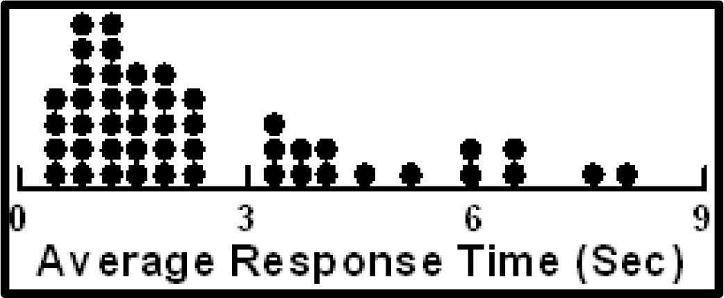
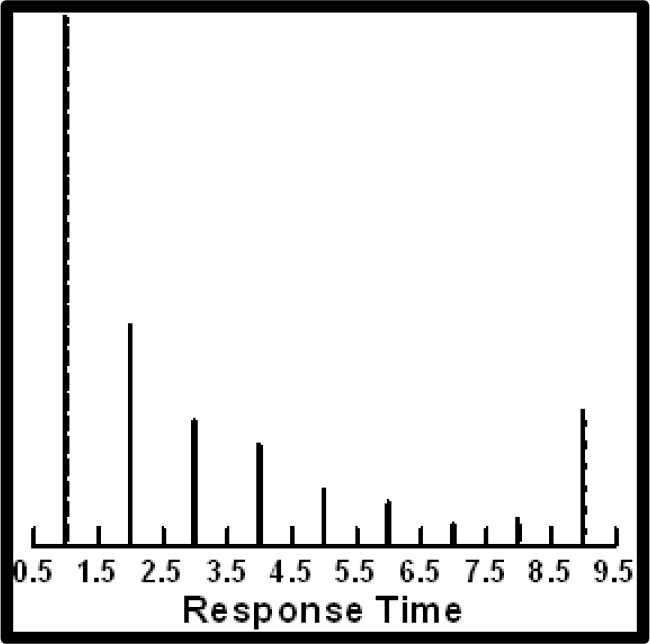
Do respondents read the information in the vignettes, or simply gloss over the information? We do not know whether a respondent reads the information in the vignette, pausing to interpret each message, or whether the respondent skips through. Figure 2 shows the distribution of average response times. The average responses are quite fast, 3 seconds or shorter. Similar types of ‘serious studies’ about public policy have shown longer response times, 5–6 or so, on average. In contrast, ‘fun studies’ about food and shopping generate many short response times. The many short response times coupled with the fact that the study is about a serious topic suggests that many of the respondents probably skim over the information, and do not absorb it. In contrast, the response times were systematically longer in another study conducted with different respondents, also from Luc.id, this study dealing with the interesting and relevant topic.

Mind Genomics-018 - ASMHS Journal_F2

Figure 2. Distribution of average response times across the respondents. The first vignette has been eliminated from the calculation of the average.

About the respondents themselves – pessimistic or optimistic on average?

Our 50 respondents each evaluated 24 vignettes. The initial data transformation created a binary scale for optimism (8–9=100, 1–7=0), and a binary scale for pessimism (1–2=100, 3–9=0). Thus, each respondent generated approximately 23 numbers for optimism, and 23 numbers for pessimism, corresponding to the 23 vignettes considered for analysis

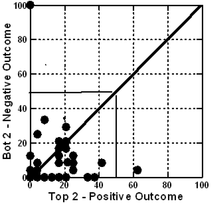
The average of the Top2 for one respondent gives a sense of the percent of the times that the respondent feels optimistic. In turn, the, the average of the Bot2 for one respondent gives a sense of the percent of the times that the respondent feels pessimistic. The averages can range from (0,0) to (100,0) or (0,100). The (0,0) average means that all the respondent’s ratings are in the middle, neither optimistic nor pessimistic. Averages of optimistic respondents fall near the bottom of the graph in Figure, where the abscissa is high (high percent of optimistic responses), and where the ordinate is low (low percent of pessimistic responses.) Figure 2 suggests about only about four respondents from the 50 are optimistic.

When we turn the focus to pessimistic respondents, we must look for respondents whose ordinates are high, but whose abscissas are low. These respondents have a large proportion of their responses suggesting pessimism of the outcome. Figure 3 suggests about only two-three respondents can be classified as pessimistic.

Mind Genomics-018 - ASMHS Journal_F3

Figure 3. Scatterplot of mean Bot2 vs Top2, for respondents, without the first vignette counted. Each circle corresponds to one of the respondents.

The results – what drives a sense of positivity (Top2), a sense of negativity (Bot2), or engages

The real ‘meat’ of a Mind Genomics study emerges when we look at the linkage between the 16 answers or elements, and the response. We created three models using the data from the 47 of the 50 respondents, after removing the first vignette evaluated by each respondent (rationale – learning to answer), and after removing all vignettes requiring more than 9 seconds to evaluate (rationale – respondent probably multi-tasking, so the response time of 30–120 seconds represents the impact of the other task, and not a real measure of the specific vignette which is associated with the very long response time.) Three respondents were over the age of 30, and so we eliminated their analysis because they did not fit the age criteria. The input data for each regression comprises ALL of the data from the vignettes, the so-called ‘Grand Model.’

Table 3 shows the three columns of data. We look at the data with the following analytic point of view, based upon hundreds of previous studies.

Table 3. Performance of the elements by total panel.

		Opti mistic	Pessi mistic	Resp Time
	Total Panel Results	Top2	Bot2	RT
	Additive constant	12	10	NA
D1	U.S. offers economic development aid to create Middle East Institute of Competitive Excellence.	5	-2	0.6
D4	U.S. Jewish organizations reach out to support economic cooperation between Palestine and Israel.	2	-5	0.9
C2	Prime Minister Netanyahu said Israel will annex settlements in the West Bank.	2	0	0.7
B2	U.N. condemns the firing of rockets from Gaza into Israeli civilian areas	1	2	0.9
D2	U.S. groups approach Palestine with opportunity to work with Israel to create better economic conditions.	1	-2	0.7
C4	Thousands of Palestinians demonstrate along the Gaza border fence with Israel.	1	0	0.4
D3	U.S. creates Institute to help Palestinians become more entrepreneurial.	0	-2	0.7
C3	As U.S. peace plan rollout approaches, Palestinians voice rejection.	0	0	0.5
B1	The U.N. general assembly, has a permanent feature on its annual agenda titled “Human rights situation in Palestine & occupied Arab territories”.	-1	-1	1.0
A2	U.S. recognizes Israeli sovereignty over the disputed Golan Heights… strategic plateau Israel acquired after the Six-Day War.	-1	-2	0.7
A1	U.S. Embassy moves to Jerusalem from Tel Aviv.	-1	-1	0.5
A4	U.S. President Donald Trump say U.S. aid cuts aimed at pressuring the Palestinians to return to peace talks.	-2	-2	1.1
B4	Israel was the most condemned country at the U.N. in 2018, with the General Assembly passing at least 20 resolutions against Israel	-2	2	0.7
A3	U.S. passes Anti-Terrorism Clarification Act (ATCA)… ends U.S. funds to the West Bank & Gaza.	-3	-2	0.8
B3	Report from U.N. claims that Israeli security forces may have committed war crimes & should be held accountable for the deaths at protests in Gaza last year	-3	4	0.8
C1	Israel says protests, described by Gazans as the Great March of Return, are particularly violent… could act as a cover for Hamas, to infiltrate Israel, carry out attacks.	-3	0	0.8

The additive constant: The OLS program estimates the additive constant, and the coefficient for each element. When we create the model with Top2 (Positive Outcome), the additive constant shows the conditional probability of a rating to the vignette being 8 or 9, albeit in the ‘absence of elements.’ In turn, when we create the model with Bot2 (Negative Outcome), the additive constant shows the conditional probability of a rating to the vignette being 1 or 2. We know for a fact that all vignettes comprised a minimum of two and a maximum of four elements, since the design specifies those specific combinations. Thus, the additive constant is an estimated parameter interpreted as ‘what would happen in the absence of elements.’ The additive constants are low for both positive and negative outcomes, 12 and 10, respectively. We interpret the low additive constants as meaning that in the absence of elements, the respondents simply don’t feel that anything will happen. Despite the rhetoric of interested parties, our young respondents don’t feel that anything of significant positive or negative will happen. It’s going to be all in the specifics, if positive or negative outcomes are to happen at all.
The strongest positive element (Top2.): Positive, high-scoring elements for Top2, represent the respondent’s belief that the action stated by the element will lead to a positive, peaceful outcome. We look for elements of 8 or higher, based upon similar types of studies in the past. When an element generates a coefficient of +8 or higher, it often covaries with other things or events in the ‘outside world.’ The number ‘+8’ is not absolute, but rather a convenient level. Our data in Table 3 from the total panel suggest only one element which even comes near the value, +8. This is element D1, ‘U.S. offers economic development aid to create Middle East Institute of Competitive Excellence.’ That ‘strong performing element,’ at least within the context of this experiment, generates a coefficient of +5.
The strongest negative element (Bot2): Positive, high-scoring elements for Bot2, represent the respondent’s belief that the action stated by the element will lead to a negative, combative outcome. Following the same logic as above (#2), we look for an element which generates a coefficient of +8 or higher on Bot2. The only element which does even modestly is B3, Report from U.N. claims that Israeli security forces may have committed war crimes & should be held accountable for the deaths at protests in Gaza last year. The coefficient, however, is only +4.
The most engaging elements: The model for response time (RT) does not have an additive the constant. The rationale is the response time is meaningless without elements. There are no norms from experience for response time, the technology having only been introduced in late 2018. The list below shows those elements requiring 0.9 seconds or longer to ‘process,’ based upon the grand model relating response time to the presence/absence of elements.
U.S. President Donald Trump say U.S. aid cuts aimed at pressuring the Palestinians to return to peace talks.

The U.N. General Assembly has a permanent feature on its annual agenda titled “Human rights situation in Palestine & occupied Arab territories”.

U.S. Jewish organizations reach out to support economic cooperation between Palestine and Israel.

U.N. condemns the firing of rockets from Gaza into Israeli civilian areas

When we break out the respondents by gender, we find the following:

Optimism (Top2)

The additive constant is slightly higher for females than for males (16 versus 10), which at the low end of the scale might signal that females are slightly more optimistic, but neither gender can be labelled ‘optimistic’.
In terms of elements, males are very optimistic regarding the prospect of formal efforts to increase economic cooperation and growth, especially the new idea of a Middle East Institute of Competitive Excellence. Surprisingly, females don’t feel optimistic in the face of stated efforts for economic growth.

Pessimism (Bot2)

The additive constants are low for both genders, 9 for males and 12 for females, suggesting no real innate pessimism, just like no real innate optimism.
No elements drive pessimism

The engaging elements from response time

For males a focus on direct efforts to help economics, and the focus on human rights
U.S. creates Institute to help Palestinians become more entrepreneurial.

U.S. President Donald Trump say U.S. aid cuts aimed at pressuring the Palestinians to return to peace talks.

The U.N. General Assembly has a permanent feature on its annual agenda titled “Human rights situation in Palestine & occupied Arab territories”.
For females a focus on direct efforts, involving a person (either PM Netanyahu or Pres. Trump)
Prime Minister Netanyahu said Israel will annex settlements in the West Bank

U.S. President Donald Trump say U.S. aid cuts aimed at pressuring the Palestinians to return to peace talks.

Uncovering the deeper structure of mind-set and the emergence of two new groups.

A key tenet of Mind Genomics is that for any topic area in which human judgment is involved, there are often different ways of perceiving and judging that which is presented. That is, people are not necessarily uniform in terms of their criteria. The Latin proverb, here translated, epitomizes the world-view of Mind Genomics: Of taste one does not dispute.

In order to uncover the different viewpoints, or mind-sets, it may be as simple as clustering the respondents based upon the pattern of coefficients, generally without the additive constant. Clustering is a well-accepted technique in statistics, a procedure to assign items into an exhaustive set of mutually exclusive groups, the aforementioned clusters. These non-overlapping clusters are created according to string mathematical criteria. It is left to the discretion of the researcher to choose the method of clustering and, after the statistics have been calculated, to select the number of clusters and to name them.

Clustering is mathematical, but we are faced with many different ways to cluster a group of test objects, such as people. We must look at clustering as a heuristic, helping us make sense of the data, and not prescribing the absolute truth. For Mind Genomics, the clustering algorithm as of this writing (2019), comprises the calculation of a distance between pairs of people, putting people in different clusters, and then trying to interpret the meaning of the cluster, if there is a story to be told.

The clustering procedure used here involved the creation of 47 models relating the presence/absence of the 16 to the binary value, Top2, one model or equation for each of the 47 respondents who were under 30. (The other three respondents were excluded entirely from the analysis.). The equation was estimated using all 24 vignettes evaluated by the respondent, because the underlying experimental design is set up to allow the estimation of the individual models when all 24 vignettes are used as cases in the regression model. That is, we included all vignettes, removing no vignette at all.

The OLS regression returned with an additive constant and 16 coefficients for each respondent. We used the 16 coefficients as input to the k-means clustering, defining the distance between any pair of respondents as (1-Pearson R). The Pearson R or correlation coefficient defines the degree of linear relation between two sets of objects. The k-means clustering put the 47 respondents into two clusters, attempting to maximize the distance between the two centroids (average coefficient for each element by group) and minimize the distance between pairs of respondents within the cluster.

The average coefficients for the two clusters or mind-sets appear in Table 5. The clustering was done on the Top2, the causes for optimism, but the table shows the results for Top2 (optimistic outcome), Bot2 (pessimistic outcome), and response time. The coefficients are sorted by the strong performers for the two mind-sets.

Table 4. Performance of the elements by gender.

		M	F	M	F	M	F
	By Gender	Optimistic TOP2		Pessimistic BOT2		Response Time
	Additive constant	10	16	9	12	NA	NA
D1	U.S. offers economic development aid to create Middle East Institute of Competitive Excellence.	12	-2	-4	0	0.7	0.6
D4	U.S. Jewish organizations reach out to support economic cooperation between Palestine and Israel.	6	-3	-5	-4	0.9	0.9
A1	U.S. Embassy moves to Jerusalem from Tel Aviv.	-7	4	1	-3	0.7	0.2
C2	Prime Minister Netanyahu said Israel will annex settlements in the West Bank.	1	3	2	-3	0.4	1.1
C4	Thousands of Palestinians demonstrate along the Gaza border fence with Israel.	1	1	4	-6	0.2	0.5
C3	As U.S. peace plan rollout approaches, Palestinians voice rejection.	0	1	3	-4	0.4	0.6
A2	U.S. recognizes Israeli sovereignty over the disputed Golan Heights… strategic plateau Israel acquired after the Six-Day War.	-2	0	0	-5	0.6	0.8
C1	Israel says protests, described by Gazans as the Great March of Return, are particularly violent… could act as a cover for Hamas, to infiltrate Israel, carry out attacks.	-7	0	1	-1	0.7	0.8
B2	U.N. condemns the firing of rockets from Gaza into Israeli civilian areas	2	-1	0	4	0.9	0.8
A3	U.S. passes Anti-Terrorism Clarification Act (ATCA)… ends U.S. funds to the West Bank & Gaza.	-4	-2	0	-5	0.7	0.9
D2	U.S. groups approach Palestine with opportunity to work with Israel to create better economic conditions.	4	-3	-3	-1	0.8	0.7
D3	U.S. creates Institute to help Palestinians become more entrepreneurial.	2	-3	0	-3	1.0	0.3
A4	U.S. President Donald Trump say U.S. aid cuts aimed at pressuring the Palestinians to return to peace talks.	-1	-3	1	-6	1.2	1.1
B4	Israel was the most condemned country at the U.N. in 2018, with the General Assembly passing at least 20 resolutions against Israel	-1	-4	2	3	0.5	0.9
B3	Report from U.N. claims that Israeli security forces may have committed war crimes & should be held accountable for the deaths at protests in Gaza last year	-1	-5	5	3	0.7	0.8
B1	The U.N. general assembly, has a permanent feature on its annual agenda titled “Human rights situation in Palestine & occupied Arab territories”.	4	-6	-1	-1	1.2	0.7

Table 5. Performance of the elements by mind-set.

		MS1	MS2	MS1	MS2	MS1	MS2
	By Two Mind Sets MS1 = Actions of any organized type will bring less unrest, more hope MS2 = Economic development will bring less unrest, more hope	Optimistic Top2		Pessimistic Bot2		Response Time
	Additive constant	13	10	7	14	NA	NA
	Elements driving Mind-Set 1 – Actions of any organized type will bring less unrest more hope
C2	Prime Minister Netanyahu said Israel will annex settlements in the West Bank.	5	-1	-4	3	0.4	1.1
C4	Thousands of Palestinians demonstrate along the Gaza border fence with Israel.	5	-4	-3	3	0.4	0.4
	Mind-Set 2 – Economic development will bring less unrest, more hope
D1	U.S. offers economic development aid to create Middle East Institute of Competitive Excellence.	1	10	2	-7	0.4	1.0
D2	U.S. groups approach Palestine with opportunity to work with Israel to create better economic conditions.	-4	8	1	-6	0.7	0.8
D4	U.S. Jewish organizations reach out to support economic cooperation between Palestine and Israel.	-1	6	-2	-8	0.7	1.2
	Does not drive responses of either mind-set
A1	U.S. Embassy moves to Jerusalem from Tel Aviv.	-4	3	-2	1	0.9	-0.1
A4	U.S. President Donald Trump say U.S. aid cuts aimed at pressuring the Palestinians to return to peace talks.	-5	3	-2	-2	1.3	0.8
B2	U.N. condemns the firing of rockets from Gaza into Israeli civilian areas	0	2	1	3	0.9	0.9
B1	The U.N. general assembly, has a permanent feature on its annual agenda titled “Human rights situation in Palestine & occupied Arab territories”.	-2	2	1	-3	0.7	1.2
D3	U.S. creates Institute to help Palestinians become more entrepreneurial.	-2	2	0	-5	0.9	0.6
A2	U.S. recognizes Israeli sovereignty over the disputed Golan Heights… strategic plateau Israel acquired after the Six-Day War.	-3	2	-2	-2	1.0	0.3
B4	Israel was the most condemned country at the U.N. in 2018, with the General Assembly passing at least 20 resolutions against Israel	-1	-2	2	3	0.7	0.7
A3	U.S. passes Anti-Terrorism Clarification Act (ATCA)… ends U.S. funds to the West Bank & Gaza.	-3	-2	-2	-2	0.8	0.7
B3	Report from U.N. claims that Israeli security forces may have committed war crimes & should be held accountable for the deaths at protests in Gaza last year	-3	-2	6	2	0.7	0.9
C3	As U.S. peace plan rollout approaches, Palestinians voice rejection.	3	-3	-2	2	0.4	0.7
C1	Israel says protests, described by Gazans as the Great March of Return, are particularly violent… could act as a cover for Hamas, to infiltrate Israel, carry out attacks.	0	-7	-2	2	0.7	0.9

The two mind-sets are defined by the strongest performing elements:

MS1 = Actions of any organized type will bring less unrest, more hope
MS2 = Economic development will bring less unrest, more hope

What emerges as very important are those

The two mind-sets have low basic optimism
Mind-set 1, looking for definitive ‘action’ of any type to bring hope, feels almost nothing will work
Mind-set 2, looking for economic development, shows a real hope for simple economic actions, even symbolic but real attempts.

Finding these mind-sets in the population through the PVI (personal viewpoint identifier)

The data suggest little basic optimism or pessimism, whether by gender or even by mind-set. The level of rhetoric surrounding the situation in the Middle East is not basically relevant. The low additive constants and the short response times attest to that basic level of disinterest. Yet, despite this discouraging initial finding, the existence of a pair of mind-sets suggests that this disinterest can be turned to more productive interest. Perhaps the first mind-set, those who want action of any sort, cannot be satisfied with destabilizing the region. It is hard to change governments and impossible to change history. The second mind-set, however, is easier to excite. They want concrete symbols and actions to drive economic development. Perhaps, for example, an effort to create this ‘MEICE’ might work, this Middle East Institute of Competitive Excellence, may work. Author Moskowitz has presented the idea to different countries

(https://www.dropbox.com/s/yhfncfid6b8nmjf/Economic%20Growth%20%20%20Middle%20East%20Institute%20Of%20Competitive%20Excellence.pdf?dl=0.)

Unlike the information about age and gender, people may or may not know the mind-set to which they belong for a specific topic. We know from these data that the mind-sets distribute about equally across genders, and across the self-defined ‘position’ or ‘interest’ in the topic (Table 6.) Furthermore, Table 6 shows us that despite the mind-sets, there is an exceptional level of disinterest.

Table 6. Distribution of the two mind-sets across gender and across self-declared nature of interest in the topic.

Gender	MS1 – Action	MS2-Development	Total	N
Male %	50	57	53	25
Female %	50	43	47	22
Total %	100	100	100
N	26	21		47

Self- declared attitude to the topic	MS1 – Action	MS2-Development	Total	N
Palestine is right %	23	19	21	10
Israel is right %	12	5	9	4
Both are right %	15	24	19	9
Not interested %	27	14	21	10
Not applicable %	23	38	30	14
Total %	100	100	100
N	26	21		47

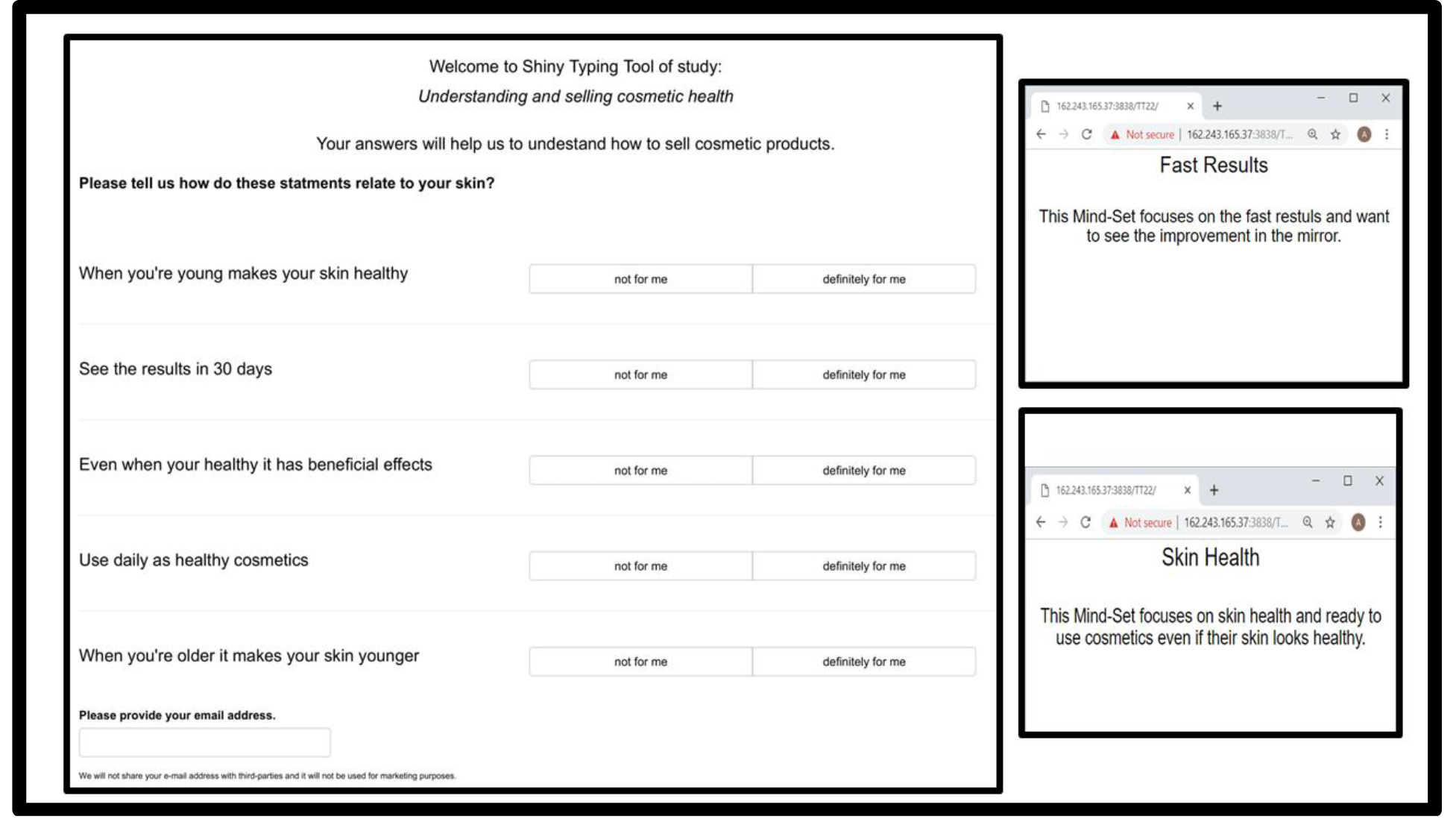
The PVI is constructed by considering the elements which best ‘separate’ the two segments. Figure 4 shows the PVI for this study, as well as the feedback which comes to the respondent. The actual PVI as of this writing (April, 2019) resides at the following website: http://162.243.165.37:3838/TT25/

Mind Genomics-018 - ASMHS Journal_F4

Figure 4. The PVI for the study of young Americans towards the policy pronouncements about the Middle East, specifically Palestine and Israel.

Discussion and Conclusion

What we learn about the young people

As we noted in the introduction to this paper, one need only look at the media, at the United Nations activities, at the popular pro-Palestinian movements such as BDS (Boycott, Divest, Sanction) SJP (Students for Justice in Palestine) to think that the situation is the Middle East is intractable. For all the efforts to stir up excitement, however, our data suggest that most of the young people whom we sampled simply don’t care. That is, they don’t expect much, neither in the way of peace and hope, nor hostilities and despair.

Yet, despite the apparent disinterest, when we probe deeper through Mind Genomics, we uncover two groups, two different mind-sets. Mind-Set 1 believes that peace and hope will come through definitive action on either side, perhaps believing that the status quo should be maintained. These are the ones who believe in the strength of power, Realpolitik. Mind-Set 2 believes that hope will be nurtured through direct economic help, help which gives to those of both sides in the Middle East an opportunity to grow their nations. To this end, the notion of a MEICE, the Middle East Institute of Competitive Excellence, makes sense. The structure and activities of that proposed idea are given in a link.

One might dismiss the findings by saying that the data are from a small sample. The reality of Mind Genomics is that it does not measure people per se, but like the science of color, established the basic colors (red, yellow, blue.) All ‘things’ with color comprise a certain percent of the primaries, yellow, red, and blue, adding up to 100%. A colorimeter is used to deconstruct the color of a ‘something’ into the percent of red, yellow, and blue, the primaries. In turn, the colorimeter becomes a tool to ‘measure the world,’ after the color science has been established. In the same way, our data suggests for this micro-topic the existence of two mind-sets, two ‘primaries,’ those interested in power as a stabilizer, and those interested in economic growth as a stabilizer. One can then use the PVI for this study to understand the feeling of people world-wide. The PVI provides a modern tool to understand the distribution of these mind-sets among the people of the world, because the Mind Genomics effort simply provided the science and the tool. This notion of basic primaries is not new, not original to this paper, having been recognized more than 15 years ago, and undoubtedly far earlier [12,13].

The role of experimentation in counterfactual history

A new and growing area of interest in the social sciences is the discipline of counterfactual history. The Mind Genomics approach we present here for policy fits right in with the notion of creating alternative narratives of what happened or what could happen, presenting these narratives, and getting responses. Most of the efforts are qualitative, teaching people to have a more critical way of thinking. Mind Genomics allows the creation of a systematic body of work for counterfactual history, teaching us both what could have been, and how people react to what could have been. Perhaps by institutionalizing the teaching of counterfactual history, one might excite an otherwise disinterested generation in understanding the ‘realpolitik’ of today [14].

References

De Boer C (1983) The Polls: Attitudes Toward the Arab-Israeli Conflict. The Public Opinion Quarterly 47: 121–131
Eit-Hallahmi BB (1972) Some psychosocial and cultural factors in the Arab-Israeli conflict: A review of the literature. Journal of Conflict Resolution 162: 269–280.
Spiegel SL (1986) The Other Arab-Israeli Conflict: Making America’s Middle East Policy, from Truman to Reagan Vol. 1. University of Chicago Press.
Vatikiotis PJ (2016) Conflict in the Middle East reissue of 1971 volume, Routledge, eBook ISBN9781317206323.
Kahneman D and Egan P (2011) Thinking, fast and slow. New York: Farrar, Straus and Giroux.
Green PE, Srinivasan V (1990) Conjoint analysis in marketing: new developments with implications for research and practice. The Journal of Marketing 54: 3–19.
Moskowitz HR, Gofman A (2007) Selling blue elephants: How to make great products that people want before they even know they want them. Pearson Education.
Pang B, Lee L (2008) Opinion mining and sentiment analysis. Foundations and Trends® in Information Retrieval 21–2, 1–135.
Box, G.E., Hunter, W.G. & Hunter, J.S., 1978. Statistics for experimenters, New York, John Wiley.
Moskowitz H, Gofman A, I novation Inc (2003) System and method for content optimization. U.S. Patent 6,662,215.
Gofman A and Moskowitz HR (2010) Isomorphic permuted experimental designs and their application in conjoint analysis. Journal of Sensory Studies 25: 127–145.
Alwin DF, Krosnick J A (1991) Aging, cohorts, and the stability of sociopolitical orientations over the life span. American Journal of Sociology 97: 169–195
Atkeson L R, Rapoport R B (2003) The more things change the more they stay the same: Examining gender differences in political attitude expression, 1952–2000. Public Opinion Quarterly 67: 495–521.
Mordhorst M (2008) From counterfactual history to counter-narrative history. Management & Organizational History 31: 5–26.

James (Jean/Jacques) Gardette (1756-1831)

Leave a reply

DOI: 10.31038/JDMR.2019221

James Gardette, Surgeon Dentist, was the second son of Jean Blaize Gardette, and was born 13th of August, 1756, in the town of Agen, departement de Lot et Garonne, France. His father died when James was quite a lad, and we are but little acquainted with this early period of his life : nor, indeed, does it enter into the plan for the performance of our task. We only know that he possessed a very trifling patrimony, insufficient for his maintenance or education, and that after his father’s death he was brought up by his paternal uncle, Blaize Gardette, who lived at Agen, and held the office of Prosecuting Attorney until an advanced age. His uncle designed James for the medical profession, and with that view, after the ordinary academical studies of that day in a provincial town of France, sent him to Paris. He remained at the capital about two years (from 1773 to 1775), pursuing the study of Anatomy and Surgery in the Royal Medical School; and thence he was removed to the Hospital at Toulouse, where he resided eighteen months as a pupil in the Institution [1; 5]. At the end of this period he was sent to Bayonne, and there was examined by the surgeons of the Admiralty, and commissioned as a surgeon in the French navy. On obtaining the commission in the navy, he received orders to embark in his professional capacity, on board the brig of war La Barquaize de St. Jean de Luz, destined for Boston, Massachusetts. He sailed in October, 1777, with La Fayette and the Count of Rochambeau [1]. He arrived at Plymouth early in January following (1778). The love of liberty and popular movement throughout France, which brought so many young Frenchmen to the United States, at the period of our «Declaration of Independence,» had no small influence in governing the course of Gardette. He made a cruise of four months, during which an engagement occurred with two British ships, lasting three hours and a half, and in which there were several killed and wounded on board the vessel of which he was the surgeon. This seems to have terminated his official duties and connection with the French navy, from which he resigned, intending to adopt this country as his home. When the French fleet and army arrived at Newport (1780), he was induced to visit that town, and commence practice as a Dentist, the officers affording him considerable and congenial occupation for a short time. He had received instructions in dental operations (as part of his profession of Naval Surgeon) from Mrs. Le Roy de la Faudinière et Louis Laforgue, Dentists at Paris, then in high repute. He had also provided himself with the best works extant (Fauchard and Bourdet) on the Teeth, and with a limited set of dental instruments : still we scarcely think he could have had any expectations of pursuing the profession of Dentist in this country, at the time he left France [2].

In 1781-1782, he became acquainted with a young American soldier, Josiah Flagg (1763-1816), whom he is thought to have instructed in the art of French dentistry and became one of the most famous American dentist [3].

He returned to Boston from Newport, and in the autumn of 1783 we find, went to New York. He was there when the American army, under General Knox, took possession of the city – an inactive but not indifferent spectator of the great events of that interesting epoch in American history. His professional success as a Dentist in New York, seems to have been comparatively small, and his limited knowledge of the English language was, as yet, a great impediment to making himself known or appreciated as he desired. It was not until the summer of 1784, and in Philadelphia, that he attained the position which determined his permanent residence in the United States. The pleasant and successful character of his occupation among the best class of citizens in Philadelphia, at the period when Fourth Street was its western boundary, needs, perhaps, no stronger comment than the fact, that he continued there in uninterrupted practice as a Dentist, from 1784 to 1830 – a period of forty-six years!

In 1796, James Gardette made for George Washington a set of dentures from hippopotamus ivory [4]. When asked about the teeth, Gardette claimed it was « impossible to distinguish them from the natural ones » and that a person could « take them out and fix them again themselves with the greatest ease ». However, others disagreed, describing them as « too large and clumsy. » In 1859, Rembrandt Peale (1778-1860) stated that Gardette’s dentures caused Washington’s « mouth to be changed. » Stuart said that when he painted Washington, « he had just had a set of false teeth inserted, which accounts for the constrained expression so noticeable about the mouth and lower part of the face. » Regardless of the success of Washington’s dentures,Gardette can be given credit for introducing the advanced techniques of Fauchard into American dentistry [3].

In 1808, he married Marie Julie Zulime Carriere (1781-1853) [3]. His education and manners as a gentleman – characteristics which, we may safely conclude, were not very commonly found among the soi-disant Dentists of our country at that remote day. Gardette devoted himself attentively to the pursuit and improvement of his profession, and acquired no unenviable reputation for knowledge and skill in its various departments. The difficulties which the Dentist then had to contend with were manifold : he was dependent chiefly upon his own judgment and inventive genius for his success, and that too for the benefit of patients who, in many instances, had but little confidence in the operations of Dentistry. Instruments were the passing existence afforded by a newspaper, it had probably never claimed notice here, but been allowed all the honor that belongs to undeserved and uncontradicted misrepresentation [2]. Among the improvements introduced into the practice of Dental Surgery by Gardette, whether in the way of instruments or operations, some few, at least, have been identified with his name. « 1822 : To James Gardette, Dentist, for three mechanical improvements in his profession, highly commended in Europe and in the United States ; and for a simple lever instrument for the easy and expeditious extraction of teeth and stumps of teeth – awarded, a medal ‘ to the most deserving,’ and twenty dollars. » The above «award of merit» is the highest permitted by the will of John Scott, who left the fund for the objects specified. He was the first Dentist who substituted the use of elastic flat gold bands or braces, in the place of ligatures of silk or fine gold wire for securing artificial teeth, when attached to the living ones [5]. He invented the manner of mounting natural teeth, which consists of a gold mortise plate to which the teeth are secured by means of gold pins, and which permits the tooth to rest upon the gum instead of the gold plate [5]. He was the first to apply the principle of suction or atmospheric pressure for maintaining sets of artificial teeth for the upper jaw, as early as 1800.

He secures artificial pieces without tying them, even when of limited extent. Laforgue said : « I have seen such, admirably secured, and am acquainted with no Dentist who equals him in this beautiful and valuable description of work. » Gardette related the following anecdote of port of entire sets of artificial teeth, dispensing with the use of spiral springs and the the chance which led to this important discovery. He had furnished, for the second time, an entire set of upper teeth (enamelled hipps) for Mrs. A. M’C, and owing to the short time the first set had lasted under the action of the saliva, he suggested that this set should be left much heavier. In order that the tongue should become accustomed to this increased bulk, necessarily contracting the limits for its free movements, the lady was desired to keep the new piece in her mouth as much as possible, during a few weeks, but not expecting her to use it for purposes of mastication or speech until the usual springs should be attached to it. Mr. G. promised, at the end of the period named, to call and arrange the piece for permanent use [5]. It was then still the custom for the Dentist to attend at the houses of his patients, and a busy season caused months instead of weeks to elapse, when Gardette called again: with an apology for neglect, his plyers and springs ready, he requested Mrs. M’C. to bring the artificial pieces. She replied, « I have them in my mouth, » much to the astonishment of her Dentist, with endless contrivances then in use, much to the inconvenience of those who wore them [1; 3].

Nor were his improvements less important in the cure of diseases to which the teeth and gums are lia-ble : he was the early advocate, if not the first who recognized the wisdom, of affording space for the healthy and good arrangement of the teeth, by judicious extractions in youth. He believed, and his long experience proved, that he thus obviated a great cause of decay, arising from lateral pressure. She stated that at first they were a little troublesome, but she had become accustomed to them now, and they answered every purpose as well without as with springs, and she was glad to dispense with them. The principle upon which the artificial piece thus adhered to the gum at once suggested itself to his mind, and suction, or atmospheric pressure, was henceforth depended upon, in numerous cases of the same kind [2]. He was one of the earliest Dentists who adopted gold foil, instead of lead or tin, as the best material for filling teeth; and related often that he had at one period, prepared gold foil for his own use from Dutch ducats, when no gold-beater was to be found in this country, or none, at any rate, who could furnish Dentist’s filling gold [2]. As an operator, Gardette displayed great judgment, care and dexterity, while he exhibited no misplaced or morbid sensibility inconsistent with the best performance of his painful professional duties.

In the mechanical departments of his art, his work evinced discrimination and good taste, as well as originality: his artificial pieces, at a period when no aid was to be derived from «Dental Laboratories,» possessed all the good workmanship and finish which are the result of mechanical skill and patient industry. His practice was characterized by the one strong motive of good to his patient, and not less by the liberal and benevolent feelings which should govern professional life [2]. His want of familiarity with the English language seems to have made him diffident about publishing his views or improvements in his profession; and it was not until 1827 that he was induced by his friend, the late Dr. James Mease, (a liberal and warm friend of the Arts and Sciences,) to furnish an article for the Medical Recorder on the « Transplantation of the Human Teeth », the first and the only publication that bears his name (seven pages published in January, 1827) [2]. As a practising Dentist, the usefulness of Gardette was much impaired during the latter years of his life by continued and severe suffering from the gout. He had long cherished a desire to return to France and end his days in his native country, but owing to unfortunate investments and various disappointments, this favorite plan was not accomplished until the year 1829, at the age of seventy-three, too late to realize the pleasant anticipations he had so long connected with such a step. His native village of Agen, which he revisited, was no longer what it had seemed to his longing heart, during an absence of half a century. He took up his residence at Bordeaux, where he died from an attack of gout, in August 1831 [1; 5].

JDMR-19-117 - Xavier Riaud_ France_F1

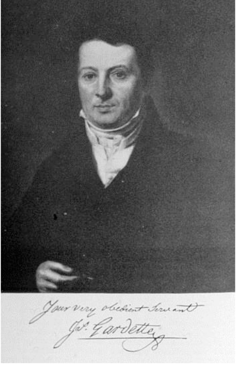
Jean Gardette (1756-1831) [3].

References

Rousseau C, « Histoire de l’aménagement opératoire du cabinet dentaire – L’aménagement opératoire des dentistes des jeunes Etats américains », in Actes de la Société française d’histoire de l’art dentaire, www.biusante.parisdescartes.fr, sans date.
Gardette E (1847) Biographical notice of James Gardette, surgeon dentist of Philadelphia, Philadelphia Pg No: 1–22.
James “Jacques” Gardette (1756-1831) 2019. www.findagrave.com
Kandra G (2016) « The whole tooth », in CBSEveningNews,) Pg No: 1-2. https://www.cbsnews.com
Laforgue L (1810) Théorie et Pratique de l’Art du Dentiste, Paris, pp. 20: 257–294.

Filarial Parasite-Derived New Potential Bio-Therapeutic Agents For Inflammatory Bowel Diseases

Leave a reply

DOI: 10.31038/AGHE.2019111

Inflammatory Bowel Disease (IBD) comprising of Crohn’s disease (CD) and Ulcerative Colitis (UC), is a chronic and relapsing inflammatory condition of the gastrointestinal tract 1]. There has been an alarming increase in the incidence of IBD during the past decade, leading to long-term morbidity that considerably affects the quality of patient’s life [1]. The incidence of UC has been rising globally since the mid-20th century [2]. Genetic factors are thought to play an important role in the pathogenesis of UC. Studies by Bengtson et al. [3] showed that the risk of developing colitis rises by 4.6-fold when a sibling has colitis. Similarly, if one of the monozygotic twins develops colitis, the risk of the other twin developing the disease is relatively 95 times higher [4]. Dietary factors have also been reported to play a role in the development of colitis. A diet containing high amounts of refined fat, meat, and sugar are risk factors for developing colitis [5]. Unfortunately, the mainstream therapies available currently for treating colitis are largely non-specific with short-term immunosuppressive effect and nearly all of them predispose the patients to opportunistic infections and/or increased risk for cancer development [6]. The most preferred method for treating mild to moderate UC is the administration of 5-aminosalicylates (5-ASA). Patients suffering from moderate to severe UC or those who do not respond to 5-ASA can be treated with antibiotics or corticosteroids but these treatment options come with various side effects like nausea, headache, diarrhea, insomnia, osteoporosis, and non-Hodgkin lymphoma [7, 8]. Similarly, anti-TNF-α therapy against UC is associated with the risk of hepatosplenic T cell lymphoma [9] and the effect of anti-TNF-α therapy reduces with time [10]. Recent advances to study the mechanism of inflammation in UC has provided a better understanding of the underlying molecular basis of the disease, which is helping in the development of new therapeutic approaches for UC [11, 12].

Parasites, more specifically the helminth parasites are notorious for suppressing the inflammatory- immune responses in their host [13]. This immunosuppression or immunomodulation is a strategy used by the parasites to survive and reproduce in their host. We are beginning to unravel the complex mechanisms by which the helminth parasites are able to achieve the immunomodulation in the host, despite the vigorous immune responses generated by the host against the parasites. In general, the host-derived inflammatory responses create a hostile environment for the helminth parasite resulting in the trapping of the parasite in the tissue leading to the killing of the parasite by antibodies and inflammatory cells or seriously damaging the fecundity of the female worms so the future generations of the parasites are suppressed or prevented. Thus, the major purpose of immunosuppression by the parasite in the host appears to be to evade the host attack and escape [14]. The helminth parasites predominantly achieve this by secreting key molecules that have potent anti-inflammatory activity [15]. Even though the host inflammatory responses towards the helminth parasites are largely local, the parasite-induced immunosuppression is more generalized with a non-specific suppressive effect on other inflammatory conditions in the host [16].

It is well established that acute infection with the filarial parasites, Brugia malayi and Wuchereria bancrofti is associated with generalized immunosuppression [17]. Clearing of the parasites with chemotherapy reverses this immunosuppressive state, confirming a role for the live parasite in this generalized immunosuppression [18]. Similarly, in filarial infected subjects, immunizations with Tetanus and BCG are found to be ineffective [17]. Similar generalized immunosuppression also occurs in the host during infections with gastrointestinal nematode parasites [19]. In 1989, David Strachan [20] reported a higher incidence of allergic rhinitis and hay fever in children who have better living conditions with good water quality, hygiene, improved sanitation, and medical care. However, children from smaller families, who were exposed to several parasitic infections, do not exhibit these allergic conditions. Based on this finding, he postulated the theory of ‘Hygiene Hypothesis’. Since then, several studies demonstrated the therapeutic potential of filarial parasitic infections in a variety of immune-mediated disorders such as arthritis, diabetes, multiple sclerosis, allergic and atopic conditions, and IBD [21–25]. Although controversial, several Phase 2 clinical trials show significant remission in the symptoms of IBD, MS, allergic rhinitis, autism, and peanut/tree nut allergy in patients following the treatment with live parasites [26]. Unfortunately, live parasites or ova are aesthetically not acceptable for many patients as a treatment. Another major hurdle is in obtaining regulatory approvals and product stability for live parasites because of the potential batch to batch variations. Few studies showed that worm homogenates can induce immunosuppressive activity similar to the live parasite [27]. This suggested that molecules produced by the live parasites can be used instead of the live parasites to induce the immunosuppressive effect. Since then, several laboratories started focusing on screening the parasite and its genome for identifying molecules that may have potential immunomodulatory activity.

Host immunomodulatory molecules have been isolated from several parasites such as Acanthocheilonema viteae, Schistosoma japonicum, Brugia malayi, Wuchereria bancrofti, Heligmosomoides polygyrus bakeri and Schistosoma mansoni [27, 28]. Lymphatic filarial parasites are notorious for suppressing host immune responses, especially during acute infections. Few reports suggest that lymphatic filariasis infected patients often do not suffer from autoimmune diseases [29]. Therefore, there has been significant interest among researchers to identify the immunomodulatory molecules of lymphatic filarial parasites that have significant immunosuppressive effect in experimental autoimmune diseases [27, 30–34]. Several filarial derived molecules have been identified as immunomodulatory agents, such as mammalian cytokine homologs, Abundant Larval Transcript (ALT) antigens, macrophage migration inhibitory factor (MIF), cysteine proteases and venom allergen-like proteins [35–38]. This commentary will focus mainly on the biotherapeutic properties of cysteine proteases and MIF. Both these molecules possess significant anti-inflammatory property in experimental arthritis and in IBD animal models [22, 27, 32, 39–41].

Cystatins, belong to the family of cysteine protease inhibitors superfamily. The three major families of cystatins include stefins (cystatins A and B), cystatins (Cystatin C, E, and S) and kininogens [42]. The cystatins are present in almost all living organisms. They are involved in a wide array of physiological and pathological processes. Misregulation of cystatins may lead to the disease state [42]. Nematode cystatins were first described in Onchocerca volvulus [42]. Subsequently, it was shown that the parasite cystatins are involved in the regulation of the molting of the parasites, establishment of active parasitism within the hosts, modulation of cathepsin activities and suppression of inflammation, antigen presentation, and lymphocyte activation in the host [17, 42, 43]. Experiments have demonstrated that Bm-Cystatin protease inhibitor-2 (CPI-2) blocked antigen processing of tetanus-toxoid protein in vitro by purified B cells and asparaginyl endopeptidases [42].

Although filarial and vertebrate cystatins do not share significant similarities, X-ray crystallographic studies showed conserved motifs in cystatins that form a wedge-shaped structure (Fig. 1), which blocks the active site of cysteine proteases [43]. Some of the conserved structural elements include N-terminal signal peptide, an approximately 100 aa domain, two disulfide bonds, a central Gln-XVal-X-Gly motif and a C-terminal Pro-Trp hairpin loop [43]. Three types of cystatin proteins were identified from B. malayi. At the genomic level, the intron positions are highly conserved among the three types of B. malayi cystatins, which might indicate the possible adaptation to the parasitic life cycle [43]. The conserved catalytic domains of cystatins could interfere with the cysteine proteases involved in the degradation of antigens within the endosomal compartment of APC, thus preventing the presentation of peptides to MHC class II molecules [42–44]. In addition to interfering with antigen presentation, the filarial cystatins can suppress antigen-induced proliferation of human Peripheral Blood Monocytes (PBMC), and down-regulate expression of human leucocyte antigen (HLA-DR) and the costimulatory molecule CD86 on human PBMC [42, 44]. These studies demonstrate potential mechanisms by which the filarial cystatins are inducing their immunomodulatory activity.

AGHE 19 - 101 Khatri V_F1

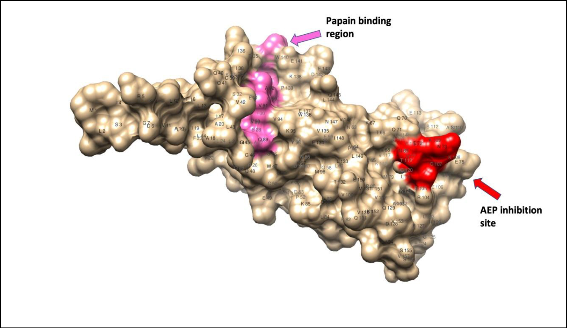
Figure 1. Homology modeling of cystatin-2 of B. malayi filarial parasite (157 a.a.) [69, 70]; 3D structure showing conserved papain-binding site (pink) and asparaginyl endopeptidase (AEP) inhibitory site (red).

Given its potent immunoregulatory role, cystatins of helminth parasites such as Ascaris lumbricoides, Schistosoma japonicum, Acanthocheilonema viteae, Clonorchis sinensis, B. malayi and Fasciola hepatica have been extensively studied for their therapeutic potential in various inflammatory immune conditions including UC [32, 45–50]. Schnoeller et al. [51] were the first one to uncover the therapeutic efficacy of a recombinant cystatin from A. vitae (Av17) in murine models of OVA-induced allergic airway responsiveness and DSS-induced colitis. Subsequent studies confirmed this immunomodulatory potential of AvCystatin for their ability to amelioration DSS-induced intestinal inflammation, characterized by decreased loss of body weight, reduction in the shortening of the colon length and minimal histopathological changes and myeloperoxidase activity in the colon tissues [48, 52]. Cystatin from S. japonicum has also been widely tested against different experimental disease models [53–55]. S. japonicum recombinant cystatin (rSj-Cys)-treated DBA/1 mice were protected from CIA-induced arthritis [53]. Similarly, rSjcystatin administration has also significantly ameliorated the TNBS-induced colitis condition [54]. Likewise, recombinant cystatin from A. lumbricoides (rAl-CPI) was able to ameliorate the DSS-induced colitis in a dose-dependent manner [45]. Type I cystatin (CsStefin-1) of the liver fluke, C. sinensis has also been shown to attenuate the DSS-induced colitis [49]. Recently, the therapeutic effect of S. japonicum cystatin (Sj-Cys) was demonstrated in an experimental animal model of sepsis [55]. Similarly, administration of filarial cystatin is shown to suppress the severity of mBSA-induced arthritis in mice [22, 40].

Our studies using B. malayi cystatin (rBmaCys) showed that this protein could alleviate the pathology of Ulcerative Colitis (UC) in a mouse model [32, 56]. Intraperitoneal administration of rBmaCys led to the reduction in the overall disease severity, decreased clinical symptoms and histopathological changes in both acute and chronic colitis [32, 56]. Although, the immunomodulatory function of rBmaCys is repeatedly demonstrated, the mechanism by which the rBmaCys achieves this anti-inflammatory effect is not fully understood. Some of the evidence shows a role for Treg cells and IL-10 in this immunosuppressive mechanism [unpublished observations].

Another parasite-derived molecule that has potent host immunomodulatory activity is the Macrophage Migration Inhibitory Factor (MIF) (Fig. 2). This molecule is different from the mammalian homolog of the MIF. The mammalian MIF is a potent pro-inflammatory molecule and is involved in several inflammatory diseases such as psoriasis, asthma, and IBD [57]. The mammalian MIF possesses two catalytic activities a Pro-2 dependent tautomerase and a Cys-Ala-Leu-Cys (CALC) dependent thiol oxidoreductase [58]. The association between catalytic activities of MIF and its immunogenic functions is not fully studied. Mutation in Cys60Ser abolishes the pro-inflammatory function of mammalian MIF [59]. Peptide fragment (50aa-65aa) with redox activity is present in mammalian MIF [60]. This suggested that oxidoreductase activity is directly involved in some of the immunological functions of MIF. In contrast, Pro2 dependent tautomerase activity failed to establish a link between the catalytic activity of MIF and its glucocorticoid overriding activity [58]. The testing of these catalytic mutants should assist further dissecting the molecular basis of the catalytic activities of mammalian MIF and their immunological roles in inflammatory diseases.

AGHE 19 - 101 Khatri V_F2

Figure 2. Homology modeling of macrophage migration inhibitory factor -2 of W. bancrofti filarial parasite (120 a.a.) [69, 70]; 3D structure showed the position of Pro-2-mediated tautomerase catalytic site (red) and C₅₈ & C₉₅mediated oxidoreductase catalytic site (pink).

Two homologs of mammalian MIF, MIF-1, and MIF-2 are reported from nematode parasites with 22% and 40% similarity with mammalian MIF respectively [61]. Similar to cystatin, the parasite-derived MIF can interact with CD74 receptor on antigen presenting cells and interfere with antigen presentation, suggesting that the parasite-derived MIF may be immunomodulatory [62]. B. malayi MIF-1 and MIF-2 are abundantly secreted in the excretory-secretory products of the larval stages of the parasite (microfilariae and molting L3 stages) [61, 63]. Infection with the filarial parasite results in less phagocytic and antigen processing ability in the host splenic macrophages. When soluble recombinant BmMIF-1 and BmMIF-2 were administered to mice, Ym1 expression was upregulated in the macrophages polarizing them to M2 phenotype that expressed high levels of IL-4R [64, 65]. Similar results were obtained when macrophages were incubated in vitro with the filarial MIF. Thus, it appears that parasite-derived MIF can promote the differentiation of alternatively activated macrophages (AAM), which can regulate inflammation, promotes wound healing and tissue repair, and probably contribute to the clearance of helminth parasites [66]. These findings suggested that the helminth-derived MIF may have an immunomodulatory function. Subsequent studies showed that in a mouse model of asthma, the MIF protein of A. simplex parasite can completely prevent the accumulation of eosinophils and prevent hyperplasia of goblet cells in the lungs a resulting in the amelioration of hypersensitivity reaction in the lungs [67]. Similarly, MIF-2 protein from A. simplex parasite can also ameliorate symptoms of colitis in a DSS induced colitis mouse model [57]. This immunomodulatory effect appears to be mediated by Treg cells because MIF-2 treatment increases the Treg population in the mouse [68]. One of our recent studies showed that filarial MIF-2 also has potent immunomodulatory effect in reducing the inflammation in the colon of a mouse with DSS-induced colitis (unpublished observations). These findings suggest that both cystatin and MIF-2 from filarial parasites have potent immunomodulatory activity in reducing inflammatory changes in colitis and IBD.

In summary, IBD and other inflammatory conditions greatly hamper the normal life of the patients and there is an urgent need to develop better therapeutics. Developing biotherapeutics from helminths, more specifically filarial parasites have tremendous potential to be used as complementary and alternative medicine. Our studies identified two such molecules (cystatin and MIF-2) from the filarial parasites that have tremendous potential as small molecules for the treatment of colitis. Since the administration of these molecules significantly reduces inflammation and reverses clinical symptoms, there is significant potential for developing these molecules as biotherapeutic agents for IBD.

Keywords

Inflammatory Bowel Disease, Helminth Therapy, Cystatin, Macrophage Migration Inhibitory Factor-2, Brugia malayi, Wuchereria bancrofti, Ulcerative Colitis

References

Zuo T, Ng SC (2018) The Gut Microbiota in the Pathogenesis and Therapeutics of Inflammatory Bowel Disease. Front Microbiol 9: 2247. [crossref]
Ng SC, Shi HY, Hamidi N, Underwood FE, Tang W, Benchimol EI, et al. (2018) Worldwide incidence and prevalence of inflammatory bowel disease in the 21st century: a systematic review of population-based studies. Lancet 390: 2769–78.
Bengtson MB, Solberg IC, Aamodt G, Jahnsen J, Moum B, Vatn MH, et al. (2010) Relationships between inflammatory bowel disease and perinatal factors: both maternal and paternal disease are related to preterm birth of offspring. Inflamm Bowel Dis 16: 847–55.
Halme L1, Paavola-Sakki P, Turunen U, Lappalainen M, Farkkila M, et al. (2006) Family and twin studies in inflammatory bowel disease. World J Gastroenterol 12: 3668–3672. [crossref]
Limdi JK (2018) Dietary practices and inflammatory bowel disease. Indian J Gastroenterol 37: 284–292. [crossref]
Taghipour N, Aghdaei HA, Haghighi A, Mossafa N, Tabaei SJ, Rostami-Nejad M. (2014) Potential treatment of inflammatory bowel disease: a review of helminths therapy. Gastroenterol Hepatol Bed Bench 7: 9–16.
Marchioni Beery R, Kane S (2014) Current approaches to the management of new-onset ulcerative colitis. Clin Exp Gastroenterol 7: 111–132. [crossref]
Büning C, Lochs H (2006) Conventional therapy for Crohn’s disease. World J Gastroenterol 12: 4794–4806. [crossref]
Thai A, Prindiville T (2010) Hepatosplenic T-cell lymphoma and inflammatory bowel disease. J Crohns Colitis 4: 511–522. [crossref]
Monaco C, Nanchahal J, Taylor P, Feldmann M2 (2015) Anti-TNF therapy: past, present and future. Int Immunol 27: 55–62. [crossref]
Neurath MF (2014) New targets for mucosal healing and therapy in inflammatory bowel diseases. Mucosal Immunol 7: 6–19.
Cheifetz AS, Gianotti R, Luber R, Gibson PR. (2017) Complementary and Alternative Medicines Used by Patients With Inflammatory Bowel Diseases. Gastroenterology 152: 415–29.
Maizels RM, McSorley HJ (2016) Regulation of the host immune system by helminth parasites. J Allergy Clin Immunol 138: 666–675. [crossref]
Geiger A, Bossard G, Sereno D, Pissarra J, Lemesre JL, Vincendeau P, et al. (2016) Escaping Deleterious Immune Response in Their Hosts: Lessons from Trypanosomatids. Front Immunol 7: 212.
Adisakwattana P, Saunders SP, Nel HJ, Fallon PG (2009) Helminth-derived immunomodulatory molecules. Adv Exp Med Biol 666: 95–107. [crossref]
Smallwood TB, Giacomin PR, Loukas A, Mulvenna JP, Clark RJ, Miles JJ (2017) Helminth Immunomodulation in Autoimmune Disease. Front Immunol 8:453.
Maizels RM, Gomez-Escobar N, Gregory WF, Murray J, Zang X (2001) Immune evasion genes from filarial nematodes. Int J Parasitol 31: 889–898. [crossref]
Hoerauf A, Satoguina J, Saeftel M, Specht S (2005) Immunomodulation by filarial nematodes. Parasite Immunol 27: 417–429. [crossref]
Cooper D, Eleftherianos I (2016) Parasitic Nematode Immunomodulatory Strategies: Recent Advances and Perspectives. Pathogens 5.
Strachan DP (1989) Hay fever, hygiene, and household size. BMJ 299: 1259–1260. [crossref]
Lopes F, Matisz C, Reyes JL, Jijon H, Al-Darmaki A, Kaplan GG, et al. (2016) Helminth Regulation of Immunity: A Three-pronged Approach to Treat Colitis. Inflamm Bowel Dis 22: 2499–512.
Ravi Shankar Prasad Yadav VK, Nitin Amdare, Kalyan Goswami, VB Shivkumar, Nitin Gangane, Maryada Venkata Rami Reddy (2017) Evaluation of preventive effect of Brugia malayi recombinant cystatin on mBSA-induced experimental arthritis. Indian Journal of Experimental Biology 55:5.
Amdare N, Khatri V, Yadav RS, Tarnekar A, Goswami K, Reddy MV (2015) Brugia malayi soluble and excretory-secretory proteins attenuate development of streptozotocin-induced type 1 diabetes in mice. Parasite Immunol 37: 624–34.
Santiago HC, Nutman TB (2016) Human Helminths and Allergic Disease: The Hygiene Hypothesis and Beyond. Am J Trop Med Hyg 95: 746–753. [crossref]
Wendel-Haga M, Celius EG (2017) Is the hygiene hypothesis relevant for the risk of multiple sclerosis? Acta Neurol Scand 201: 26–30. [crossref]
Fleming JO, Weinstock JV (2015) Clinical trials of helminth therapy in autoimmune diseases: rationale and findings. Parasite Immunol 37: 277–92.
Heylen M, Ruyssers NE, Gielis EM, Vanhomwegen E, Pelckmans PA2, et al. (2014) Of worms, mice and man: an overview of experimental and clinical helminth-based therapy for inflammatory bowel disease. Pharmacol Ther 143: 153–167. [crossref]
Wang M, Wu L, Weng R, Zheng W, Wu Z, Lv Z (2017) Therapeutic potential of helminths in autoimmune diseases: helminth-derived immune-regulators and immune balance. Parasitol Res 116: 2065–2074.
Buerfent BC, Golz L, Hofmann A, Ruhl H, Stamminger W, Fricker N, et al. (2019) Transcriptome-wide analysis of filarial extract-primed human monocytes reveal changes in LPS-induced PTX3 expression levels. Sci Rep 9: 2562.
Adisakwattana P, Nuamtanong S, Kusolsuk T, Chairoj M, Yenchitsomanas PT, Chaisri U (2013) Non-encapsulated Trichinella spp., T. papuae, diminishes severity of DSS-induced colitis in mice. Asian Pac J Allergy Immunol 31: 106–14.
Broadhurst MJ, Ardeshir A, Kanwar B, Mirpuri J, Gundra UM, Leung JM, et al. (2012) Therapeutic helminth infection of macaques with idiopathic chronic diarrhea alters the inflammatory signature and mucosal microbiota of the colon. PLoS Pathog 8: 1003000.
Khatri V, Amdare N, Tarnekar A, Goswami K, Reddy MV (2015) Brugia malayi cystatin therapeutically ameliorates dextran sulfate sodium-induced colitis in mice. J Dig Dis 16: 585–94.
Ferreira I, Smyth D, Gaze S, Aziz A, Giacomin P, Ruyssers N, et al. (2013) Hookworm excretory/secretory products induce interleukin-4 (IL-4)+ IL-10+ CD4+ T cell responses and suppress pathology in a mouse model of colitis. Infect Immun 81: 2104–11.
Heylen M, Ruyssers NE, De Man JG, Timmermans JP, Pelckmans PA, Moreels TG, et al. (2014) Worm proteins of Schistosoma mansoni reduce the severity of experimental chronic colitis in mice by suppressing colonic proinflammatory immune responses. PLoS One 9: 110002.
Chauhan N, Hoti SL (2016) Role of cysteine-58 and cysteine-95 residues in the thiol di-sulfide oxidoreductase activity of Macrophage Migration Inhibitory Factor-2 of Wuchereria bancrofti. Acta Trop 153: 14–20. [crossref]
Hewitson JP, Grainger JR, Maizels RM (2009) Helminth immunoregulation: the role of parasite secreted proteins in modulating host immunity. Mol Biochem Parasitol 167: 1–11. [crossref]
Maizels RM, Smits HH, McSorley HJ. Modulation of Host Immunity by Helminths: The Expanding Repertoire of Parasite Effector Molecules. Immunity 49: 801–18.
Ottesen EA (1984) Immunological aspects of lymphatic filariasis and onchocerciasis in man. Trans R Soc Trop Med Hyg 78 Suppl: 9–18. [crossref]
Gazzinelli-Guimaraes PH, Nutman TB (2018) Helminth parasites and immune regulation. F1000Res 7. [crossref]
Yadav RS, Khatri V, Amdare N, Goswami K, Shivkumar VB, Gangane N, et al. Immuno-Modulatory Effect and Therapeutic Potential of Brugia malayi Cystatin in Experimentally Induced Arthritis. Indian J Clin Biochem 31: 203–8.
Zakeri A, Hansen EP, Andersen SD, Williams AR, Nejsum P (2018) Immunomodulation by Helminths: Intracellular Pathways and Extracellular Vesicles. Front Immunol 9:2349.
Hartmann S, Lucius R (2003) Modulation of host immune responses by nematode cystatins. Int J Parasitol 33: 1291–1302. [crossref]
Gregory WF, Maizels RM (2008) Cystatins from filarial parasites: evolution, adaptation and function in the host-parasite relationship. Int J Biochem Cell Biol 40: 1389–1398. [crossref]
Zavasnik-Bergant T (2008) Cystatin protease inhibitors and immune functions. Front Biosci 13:4625–37.
Coronado S, Barrios L, Zakzuk J, Regino R, Ahumada V, et al. (2017) A recombinant cystatin from Ascaris lumbricoides attenuates inflammation of DSS-induced colitis. Parasite Immunol 39. [crossref]
Janssen L, Silva Santos GL, Muller HS, Vieira AR, de Campos TA, de Paulo Martins V (2016) Schistosome-Derived Molecules as Modulating Actors of the Immune System and Promising Candidates to Treat Autoimmune and Inflammatory Diseases. J Immunol Res 2016: 5267485.
Danilowicz-Luebert E, Steinfelder S, Kuhl AA, Drozdenko G, Lucius R, Worm M, et al. (2013) A nematode immunomodulator suppresses grass pollen-specific allergic responses by controlling excessive Th2 inflammation. Int J Parasitol 43: 201–10.
Ziegler T, Rausch S, Steinfelder S, Klotz C, Hepworth MR, et al. (2015) A novel regulatory macrophage induced by a helminth molecule instructs IL-10 in CD4+ T cells and protects against mucosal inflammation. J Immunol 194: 1555–1564. [crossref]
Jang SW, Cho MK, Park MK, Kang SA, Na BK, Ahn SC, et al. (2011) Parasitic helminth cystatin inhibits DSS-induced intestinal inflammation via IL-10(+)F4/80(+) macrophage recruitment. Korean J Parasitol 49: 245–54.
Falcon CR, Masih D, Gatti G, Sanchez MC, Motran CC, Cervi L (2014) Fasciola hepatica Kunitz type molecule decreases dendritic cell activation and their ability to induce inflammatory responses. PLoS One 9: 114505.
Schnoeller C, Rausch S, Pillai S, Avagyan A, Wittig BM, et al. (2008) A helminth immunomodulator reduces allergic and inflammatory responses by induction of IL-10-producing macrophages. J Immunol 180: 4265–4272. [crossref]
Whelan RA, Rausch S, Ebner F, Gunzel D, Richter JF, Hering NA, et al. (2014) A transgenic probiotic secreting a parasite immunomodulator for site-directed treatment of gut inflammation. Mol Ther 22: 1730–40.
Liu F, Cheng W, Pappoe F, Hu X, et al. (2016) Schistosoma japonicum cystatin attenuates murine collagen-induced arthritis. Parasitol Res 115: 3795–3806. [crossref]
Wang S, Xie Y, Yang X, Wang X, Yan K, Zhong Z, et al. (2016) Therapeutic potential of recombinant cystatin from Schistosoma japonicum in TNBS-induced experimental colitis of mice. Parasit Vectors 9:6.
Li H, Wang S, Zhan B, He W, Chu L, Qiu D, et al. (2017) Therapeutic effect of Schistosoma japonicum cystatin on bacterial sepsis in mice. Parasit Vectors 10: 222.
Togre N, Bhoj P, Goswami K, Tarnekar A, Patil M, Shende M. (2018) Human filarial proteins attenuate chronic colitis in an experimental mouse model. Parasite Immunol 40.
Cho MK, Lee CH, Yu HS. (2011) Amelioration of intestinal colitis by macrophage migration inhibitory factor isolated from intestinal parasites through toll-like receptor 2. Parasite Immunol 33: 265–75.
Bendrat K, Al-Abed Y, Callaway DJ, Peng T, Calandra T, et al. (1997) Biochemical and mutational investigations of the enzymatic activity of macrophage migration inhibitory factor. Biochemistry 36: 15356–15362. [crossref]
Kleemann R, Kapurniotu A, Frank RW, Gessner A, Mischke R, et al. (1998) Disulfide analysis reveals a role for macrophage migration inhibitory factor (MIF) as thiol-protein oxidoreductase. J Mol Biol 280: 85–102. [crossref]
Nguyen MT, Beck J, Lue H, Fünfzig H, Kleemann R, et al. (2003) A 16-residue peptide fragment of macrophage migration inhibitory factor, MIF-(50–65), exhibits redox activity and has MIF-like biological functions. J Biol Chem 278: 33654–33671. [crossref]
Zang X, Taylor P, Wang JM, Meyer DJ, Scott AL, et al. (2002) Homologues of human macrophage migration inhibitory factor from a parasitic nematode. Gene cloning, protein activity, and crystal structure. J Biol Chem 277: 44261–44267. [crossref]
Cho Y, Jones BF, Vermeire JJ, Leng L, DiFedele L, Harrison LM, et al. (2007) Structural and functional characterization of a secreted hookworm Macrophage Migration Inhibitory Factor (MIF) that interacts with the human MIF receptor CD74. J Biol Chem 282: 23447–56.
Bennuru S, Semnani R, Meng Z, Ribeiro JM, Veenstra TD, Nutman TB (2009) Brugia malayi excreted/secreted proteins at the host/parasite interface: stage- and gender-specific proteomic profiling. PLoS Negl Trop Dis. 3: 410.
Prieto-Lafuente L, Gregory WF, Allen JE, Maizels RM. (2009) MIF homologues from a filarial nematode parasite synergize with IL-4 to induce alternative activation of host macrophages. J Leukoc Biol 85: 844–54.
Mitre E, Taylor RT, Kubofcik J, Nutman TB (2004) Parasite antigen-driven basophils are a major source of IL-4 in human filarial infections. J Immunol 172: 2439–2445. [crossref]
Girgis NM, Gundra UM, Ward LN, Cabrera M, Frevert U, Loke P (2014) Ly6C(high) monocytes become alternatively activated macrophages in schistosome granulomas with help from CD4+ cells. PLoS Pathog 10:1004080.
Park SK, Cho MK, Park HK, Lee KH, Lee SJ, et al. (2009) Macrophage migration inhibitory factor homologs of anisakis simplex suppress Th2 response in allergic airway inflammation model via CD4+CD25+Foxp3+ T cell recruitment. J Immunol 182: 6907–6914. [crossref]
Cho MK, Park MK, Kang SA, Park SK, Lyu JH, Kim DH, et al. (2015) TLR2-dependent amelioration of allergic airway inflammation by parasitic nematode type II MIF in mice. Parasite Immunol 37: 180–91.
Kelley LA, Mezulis S, Yates CM, Wass MN, Sternberg MJ (2015) The Phyre2 web portal for protein modeling, prediction and analysis. Nat Protoc 10: 845–858. [crossref]
Pettersen EF, Goddard TD, Huang CC, Couch GS, Greenblatt DM, Meng EC, Ferrin TE (2004) UCSF Chimera—a visualization system for exploratory research and analysis. J Comput Chem 25(13): 1605–12.

Relationship of Physical Activity and Developmental Skills in Preschool Children

Leave a reply

DOI: 10.31038/IJOT.2019223

Abstract

Aims: This study investigated the relationship between time spent in physical activity and developmental skills.

Methods: Developmental skills of twenty-one children (M=49.18 months) were screened using the Ages and Stages Questionnaire (ASQ-3). Physical activity counts were collected using Actical accelerometers for 4 to 6 days.

Results: Positive correlations were identified between vigorous physical activity (VPA) and fine motor (FM) scores and gross motor (GM) scores. Children at risk for FM and GM developmental delay spent less time in VPA than the children categorized typically developing. Children at risk for FM delays also spent less time in moderate physical activity (MPA).

Conclusion: In this study, gross motor and fine motor skills were found to have a relationship with MPA or VPA. Additional research is needed to investigate the relationship between developmental skills and activity levels of young children beyond the gross motor skill domain.

Keywords

Physical activity, gross motor, fine motor, developmental skills, preschool, children

Introduction

Physical activity is considered a critical component of a healthy lifestyle; it can be utilized as preventative intervention for obesity in children. Pediatric health care providers can play a pivotal role in the management of pediatric obesity [1]. Caution must be utilized when recommending physical activity as an intervention for obesity in children because biomechanical changes, musculoskeletal anomalies, and pain have been associated with pediatric obesity [2].

It is evident that participation in physical activity has numerous health benefits [3]. Health behaviorists and practitioners are still exploring ways to facilitate the development of habits in young children that influence later physical fitness and healthy weight. The National Association for Sports and Physical Education (NASPE) recommends that preschoolers participate in at least 60 mintues of structured, developmentally-appropriate physical activity each day [4]. In addition, preschoolers should engage in at least 60 mintues, and up to several hours, of unstructured, developmentally-appropriate physical activity per day, and they should not be sedentary for more than 60 minutes at a time, except when sleeping [5, 6]. A clear understanding of global development is necessary for researchers, clinicians and educators to develop studies, activities or programs aimed at increasing physical activity in children. Head Start and Early Head Start (HS/EHS) programs measure school readiness according to five domains, approaches to learning, social and emotional, language and literacy, cognition, and perceptual, motor and physical development [7].

Understanding the relationship between development and physical activity levels may assist clinicians and educators in understanding the impact that one may have on the other. Most research concerning physical activity, pediatric obesity, and academic achievement has been conducted with children in elementary school and beyond, and generally not with children younger than six years old. Investigators found that 9- to 10-year-old children who spent more than three-quarters of their time engaging in sedentary behavior, such as watching television and sitting at computers, had up to nine times poorer motor coordination than did their more active peers [8]. It is unclear, in the literature, the role of physical activity and environmental engagement on overall development and academic achievement. Movement is considered a key component in cognitive development. Research investigating cognitive development and the relationship to physical activity in preschool-age children has not been published yet, but the relationship of exercise or physical activity and academic performance has been studied in school-age children [9, 10, 11]. Psychosocial benefits, improved social competence and externalizing problems, have been documented [12]. Spencer et al. [13] explained that as a child moves, cognitive development is reliant in part on the role of interaction between sensorimotor integration and the environment. A child’s action is influenced by his or her perception of the consequences of his or her action on the environment. This is the beginning of understanding the association of physical action and its effects, which leads to participation in physical activity. Further, games or physical activities that require problem solving potentially provide circumstances to nurture and encourage the development of cognitive skills [14]. Subsequently, one might assume that a relationship exists between physical activity and cognitive development.

It is important to understand that acquisition of developmental skills and levels of physical activity are not only inherent, but also influenced by the environment as well as anyone they may interact with daily [15, 16]. Educators and clinicians working with young children should emphasize (or strive to facilitate) positive peer interaction, improved developmental skills and continued engagement in physical activity. The purpose of this research was to investigate the association between time spent in physical activity and performance of global developmental skills in preschool age children.

Methods

Study Design

A non-experimental design was utilized to examine the relationship between physical activity and global developmental skills of preschool-age children. Amount of time spent in physical activity levels was determined through results of Actical Accelerometers worn by preschool-age children. To assess global developmental skills, each child’s parent or legal guardian completed the Ages and Stages Questionnaire, 3^rd edition (ASQ-3). The study was approved by a university Institutional Review Board (IRB).

Recruitment Procedures

The investigator contacted local preschools by phone or email, provided a description of the study, and requested cooperation.

Participants

A convenience sample was used with a goal to recruit a minimum of 20 participants. Twenty-two children and their caregivers participated in the study. Participants were recruited through disbursement of flyers, from the local YMCA, word-of-mouth, and snowball sampling. Inclusion criteria were as follows: 1. The child must be currently enrolled in preschool. 2. The child must be between the ages of 3 and 5 years, 4 months at time of informed consent. 3. The child must be independently ambulatory without assistance. In order to have a comparative sample of physical activity, children who were non-ambulatory were excluded from the study. Also, because the ASQ-3 could be used only with children up to 66 months of age, any child older than 64 months at time of informed consent were excluded to ensure adequate time to collect all data prior to the child turning 66 months old.

Twenty-two children, 11 boys and 11 girls, participated in the study. One child was eliminated for non-compliance with accelerometer use. Consequentially, ten boys completed the study. The range of children’s ages were 36 months to 63.47 months. The mean age of the participants was 49.18 months. Majority of the participants were Caucasian (71.4%), which is consistent with the demographics of the county (76.6%) and state (77.1%) in which the study was conducted [17]. Most lived in single family homes (81.0%) and had stairs in their home (71.4%). Refer to Table 1 for demographic information of participants.

Table 1. Individual Demographic Information as a Percentage of the Sample.

Characteristic	All n	%	At Risk^a n	%	Typical^b n	%
Race
Caucasian	15	71.4	8	80	7	63.6
African American	1	4.8			1	9.1
Bi-Racial	4	19.0	2	20	2	18.2
Middle Eastern(Arab)	1	4.8			1	9.1
Mother’s Highest Degree
HS/Technical/Associate degree	10	47.6	4	40	6	54.5
Bachelor’s degree or higher	11	52.4	6	60	5	45.5
Father’s Highest Degree
HS/Technical/Associate degree	10	47.6	3	30	7	63.6
Bachelor’s degree or higher	11	52.4	7	70	4	36.4
Type of Home
Single Family Home	17	81.0	8	80	9	81.8
Townhouse	3	14.3	2	20	1	9.1
Mobile Home	1	4.8			1	9.1
Stairs Present in Home
Yes	15	71.4	8	80	7	63.6
No	6	28.6	2	20	4	36.4
Child’s Birth Order
Only child	3	14.3	1	10	2	18.2
Oldest child	9	42.9	3	30	6	54.5
Middle child	2	9.5	1	10	1	9.1
Youngest child	7	33.3	5	50	2	18.2
Body Mass Index
Under/Healthy weight	14	66.7	6	60	8	72.7
Overweight/Obese	7	33.3	4	40	3	27.3

Note. N=21
^aChildren at risk for developmental delay in any domain according to performance on ASQ -3.
^bChildren not at risk for developmental delay in any domain according to performance on ASQ -3.

Measurement Tools

Demographic questionnaire

Parents completed the demographic questionnaire at the first appointment. Additionally, the participant’s height and weight were recorded on the demographic questionnaire. The investigator measured the participants’ height using a Komelon self-lock tape measure in standing and measured weight by asking the child to stand, unsupported, on a Health-o-meter LED digital bathroom scale [18].

Ages and Stages Questionnaire

The investigator utilized the ASQ-3 [19] to assess global development skills in five domains: communication, gross motor, fine motor, problem-solving, and personal social development. The purpose of the ASQ-3 is to identify children who may need developmental monitoring or additional developmental evaluation by comparing child scores to standardized norms from age-matched peers. The first cut-off score, 1 standard deviation below the standardized mean, corresponds with a potential need to be monitored and provided with developmental activities. The second cutoff score, 2 standard deviations below the standarized mean, corresponds with need for further evaluation to determine eligibility for services [19]. These cut-offs have been used to determine risk of developmental delay [20, 21, 22]. For this study, a cut-off score of one standard deviaiton or greater was used to identify participants at-risk of having developmental delay and were categorized as “at-risk.” Those who did not score one standard deviation or more below the mean were categorized as “typical.”

Accelerometer

Physical activity was objectively measured using an Actical accelerometer manufactured by Phillips Respironics (Bend, OR). The accelerometer was programmed to collect raw data continuously. Multiple studies have reported the accelerometer to be a valid, objective way to measure physical activity levels in preschool-age children [22, 23, 24]. For the accelerometer data, each epoch was identified as wear versus non-wear. Non-wear time was defined as greater than 20 minutes of continuous zero signal and was removed from further analysis. Time spent in physical activity epochs were derived according to validated and commonly cited activity counts for preschool age children. Validated threshold values for preschool children were used to derive time spent in light, moderate, and vigorous activity [4, 22, 23]. For this study, the Actical accelerometer cutpoints defined and validated in preschool children by Pfeiffer et al. [23] were used to categorize physical activity. The established cutoffs are 715 activity counts for moderate intensity and 1411 for vigorous activity.

Daily log

Parents were instructed to complete a brief, daily log to document any issues that arose during the days their child wore the accelerometer, e.g., if the child was sick or hurt and was not as active as typically expected or if there was a problem with the use of the accelerometer. Parent(s) also asked their child’s teacher to communicate whether the accelerometer was taken off during the day. The teachers did so orally or by making a note in their typical daily journal of communication to parents. This information was used to determine whether data collected by the accelerometer was a valid measure of the child’s typical physical activity level [12, 26, 27].

Data Collection Procedures

The researcher followed standard protocol and selected the appropriate ASQ-3 based on the child’s age at time of the screening [19]. For example, the 36 month ASQ-3 is appropriate for children 34 months, 16 days through 38 months, 30 days. See Table 2 for the frequencies of the ASQ-3 administered.

Table 2. Ages and Stages Questionnaire – 3^rd Edition Frequency of Questionnaires Administered.

Questionnaire	Frequency	Percentage
36 months	2	9.5%
42 months	6	28.6%
48 months	4	19.0%
54 months	4	19.0%
60 months	5	23.8%

The investigator then instructed parents to complete the ASQ-3 and add comments as needed. If items were unclear, or if parents were unsure of skill performance, the use of test materials to verify performance was encouraged with the assistance of the investigator. The ASQ-3 was completed during the first appointment, with the investigator available to answer questions and provide assistance. The investigator scored and analyzed the ASQ-3 at the first appointment using the ASQ-3 pre-defined scale and the results were reviewed with the parents.

After completion of the ASQ-3, the investigator instructed the child and the parent on the use of the accelerometer to measure physical activity. Explicit instructions were provided both verbally and in writing. Parents were instructed that the child was to wear the accelerometer from morning until evening for the following five to seven days, which constituted an average wear time of 8 – 10 hours daily. A follow-up appointment was held to return the accelerometers and daily logs to the investigator, as well as to distribute suggested developmental activity sheets.

Data Analysis Procedures

Data were analyzed using Microsoft Excel 2013 and IBM SPSS Statistics, version 21.0 (IBM Corp, Armonk, NY). Participant’s information and data were de-identified by assigning unique, computer-generated, 10-digit alphanumeric code.

The investigator recorded and verified the information on the demographic questionnaire and ASQ-3 in a password protected SPSS file, including the calculated BMI from the height and weight measures. The investigator defined BMI according to the Center for Disease Control [28] categories and grouped them as follows: underweight/healthy weight (HW) and overweight/obese (OW).

The accelerometer PA data was downloaded using the Actical software and exported into a data file. A record was generated of the child’s participation with the number of days within the week and labeled each day chronologically as week days and weekend days. The number of minutes/hours per day in which the accelerometer was worn was then calculated within a Microsoft Excel spreadsheet for each day the participant had accelerometer data. The epoch list was analyzed by the investigator to calculate non-wear time (greater than 20 minutes of consecutive zero for an activity count): The total number of minutes was calculated from when the accelerometer began to detect PA in the morning until there were consistently zero activity counts in the evening. The calculated non-wear time was then subtracted from the total minutes to calculate the daily wear time. The wear time calculated from the accelerometer data were cross referenced with the daily log completed by parents. Any parental entries in the log regarding removal or atypical physical activity patterns were cross referenced in the PA spreadsheet epoch list to verify the accelerometer wear time data.

For each day the participants had a minimum of six hours (360 minutes) of wear time, the log of their wear time and PA minutes, in each category, were analyzed. Each epoch list was analyzed to calculate light, moderate and vigorous activity using the following cutpoints: light activity > 275 but < 715 activity counts, moderate activity was > 715 but < 1411 activity counts, and vigorous activity was > 1411 activity counts. Activity counts <275 were considered sedentary and not analyzed in this study. Each minute in each of the PA intensities was tabulated. A final record for each category was calculated and recorded for each day individually. Physical activity data were calculated for each day’s light, moderate, and vigorous activity. Moderate to vigorous physical activity (MVPA) was calculated by adding together the time spent in moderate and vigorous PA for each participant to compare with NASPE recommended guidelines for children. Each participant’s physical activity data were entered into SPSS by a graduate assistant and verified by investigator.

A p value of an α ≤ .050 was considered to be statistically significant and all tests were two-sided. Descriptive statistics were computed to describe the sample, determine the parametric nature of continuous variables, and examine the relationship between physical activity and global development. Due to the small sample size, responses for parent/guardian level of education were placed into the following categories, < 4-year college degree and > 4-year college degree. Due to the small sample size and non-normal distribution of developmental scores, the non-parametric Spearman’s rank-order correlation coefficient was conducted between each of the developmental domain scores and time spent in 3 activity levels, i.e., moderate PA, vigorous PA and combined MVPA.

To determine whether there were significant differences in patient characteristics between the at-risk and typical groups, comparisons were conducted. A Fisher’s exact test was used to compare categorical data and independent t tests were used to compare groups on continuous variables. Due to the small sample size and non-normal distribution of the ASQ -3, the non-parametric Mann-Whitney U was used to test for significant difference between the developmental domain groups.

Results

There were 31 children for whom a parent expressed interest in obtaining information regarding the study via opt in/out letters, phone calls or email messages. Two chose not to participate after receiving the informed consent information. Two could not make the initial appointments and did not reschedule. Five expressed interest via email, phone call or voicemail, but did not respond to subsequent phone or email attempts by the investigator to schedule the first appointment. Twenty-two children between the ages of 36 months (3 years) and 64 months (5 years, 4 months) participated in this study. One participant withdrew due to non-compliance with wearing the accelerometer. Participation of 10 preschool aged children (48%) was obtained through local recruitment using flyers at a community preschool. Eleven additional participants (52%) contacted the investigator via email or phone calls after being informed of the study through snowball sampling (word of mouth), for a final sample size of 21 children. Descriptive statistics are presented in Table 3.

Table 3. Comparison of Demographic Variables Between At Risk (n = 10) and Typical (n = 11) Groups.

Variable	M (SD)			t^a
	Total	At Risk	Typical
Demographic
Age (months)	49.18 (8.38)	46.68 (7.30)	51.46 (8.97)	.199
BMI (kg/m²)	15.99 (1.80)	16.26 (1.68)	15.74 (1.94)	.519
Days played outdoors	1.43 (1.85)	1.95 (2.29)	.96 (1.27)	.228
Days played at park	1.02 (1.08)	1.25 (1.72)	.82 (1.06)	.492
Total screen time (hours)	2.78 (1.49)	2.79 (1.56)	2.77 (1.49)	.967

Note: M = mean, SD = standard deviation
^aequal variances assumed; t test for differences between at risk and typical groups significant at .05 level (2-tailed).
There were no significant differences between groups.

Spearman rank order correlation coefficients were conducted to investigate the relationships between physical activity and developmental skills as shown in Table 4. Specifically, there were statistically significant, moderately positive correlations between vigorous PA and fine motor score (r_s(19) = .447, p = .042) and gross motor score (r_s(19) = .481, p = .027).

Table 4. Bivariate Correlations (Spearman’s rho) Among Physical Activity and Developmental Skills.

Developmental Domain	Light PA	Mod PA	Vig PA	MVPA	Total PA
Communication score	-.301	-.361	-.053	-.298	-.349
Gross Motor score	-.151	.136	.481*	.290	.123
Fine Motor score	-.028	.169	.447*	.367	.245
Problem Solving score	.247	.188	.225	.181	.265
Personal Social score	.382	.132	-.239	-.120	.204

Note: PA = physical activity, MVPA= moderate to vigorous physical activity
* Correlation is significant at the .05 level (2-tailed)

Based on the scores from ASQ-3, participants were categorized into the two groups, at risk, n = 10, and typical, n = 11. Physical activity categories also were compared for at risk and typical groups; refer to Table 5 for the time spent in light, moderate, vigorous, and MVPA. There was no statistically significant difference in the amount of time spent in physical activity between the overall at risk and typical groups.

Table 5. Comparison of Outcome Variables Between At Risk (n = 10) and Typical (n = 11) Groups.

Variable	At Risk n = 10		Typical n = 11
	Mdn (IQR)	M (SD)	Mdn (IQR)	M (SD)	t
Developmental Domains
Communication score	42.50 (17.50)	41.00 (15.60)	50.00 (5.00)	52.73 (4.67)	.044^b
Gross Motor score	45.00 (15.00)	43.50 (13.55)	50.00 (10.00)	52.73 (6.07)	.055^a
Fine Motor score	42.50 (18.75)	40.00 (12.47)	50.00 (15.00)	50.00 (7.75)	.038^a
Problem-Solving score	47.50 (18.75)	48.00 (9.19)	60.00 (5.00)	56.82 (4.05)	.016^b
Personal Social score	60.00 (10.00)	55.00 (8.16)	60.00 (10.00)	55.00 (5.92)	1.00^a
Time Spent in Physical Activity (PA)
Light PA (min)	81.40 (53.70)	92.64 (29.10)	85.20 (46.0)	88.91 (26.82)	.763^a
Moderate PA (min)	46.43 (29.68)	46.69 (19.78)	42.33 (18.50)	49.55 (18.35)	.735^a
Vigorous PA (min)	26.3 (26.38)	27.66 (18.81)	34.00 (31.47)	41.68 (20.65)	.122^a
MVPA (min)	79.38 (28.67)	74.35 (34.83)	73.00 (45.83)	91.22 (37.40)	.299^a

Note: Mdn = median, IQR = interquartile range, M = mean, SD = standard deviation,
^a equal variances assumed; t test significant at the .05 level (2-tailed)
^b equal variances not assumed; t test significant at the .05 level (2-tailed)

Results from the comparison of mean time spent in the various PA categories between at risk and typical group, separated by developmental categories, are presented in Table 6. In all comparisons, the children that fell into the at-risk groups for communication, problem-solving or personal-social skills spent the same amount of time in light, moderate, and vigorous PA when compared to the children with typical developmental screening scores. The children at-risk for gross motor delays spent less time in vigorous PA as compared to the children in the typical group (U = 6.0, n₁= 5, n₂ = 16, p = .003). The children at risk for fine motor delays spent less time in both moderate (t(19) = -2.633; p = .017) and vigorous PA (t(19) = -2.499; p = .023).

Table 6. Comparison of mean time spent in physical activity categories between at risk and typical groups separated by developmental domains.

	Mean (SD)
	At Risk	n	Typical	n	U^a
Communication Domain		4		17
Light Physical Activity	94.38 (30.77)		89.82 (27.36)		1.00
Moderate Physical Activity^a	52.12 (25.61)		47.26 (17.48)		.517
Vigorous Physical Activity	33.14 (25.03)		35.43 (20.28)		1.00
Gross Motor Domain		5		16
Light Physical Activity	96.69 (31.03)		88.81 (28.83)		.548
Moderate Physical Activity	40.47 (20.91)		50.60 (17.87)		.548
Vigorous Physical Activity^*	15.06 (12.01)		41.23 (18.78)		.003*
Fine Motor Domain		2		19
Light Physical Activity	67.80 (2.26)		93.10 (27.61)		.286
Moderate Physical Activity^*	19.00 (1.98)		51.26 (16.74)		.010*
Vigorous Physical Activity^*	3.70 (0.42)		38.29 (18.72)		.010*
Problem-Solving Domain		2		19
Light Physical Activity	69.40 (4.53)		92.93 (27.75)		.343
Moderate Physical Activity	31.60 (15.84)		49.93 (18.37)		.286
Vigorous Physical Activity	14.00 (14.99)		37.21 (20.11)		.152
Personal-Social Domain		1		20
Light Physical Activity	59.00 (n/a)		92.27 (26.98)		.286
Moderate Physical Activity	33.67 (n/a)		48.9 (18.79)		.381
Vigorous Physical Activity	47.50 (n/a)		37.37 (20.92)		.571

^a Mann-Whitney U Test for comparison of mean physical activity amongst at risk and no risk groups in each developmental domain
^*p≤ .05

Discussion

Some evidence suggests that physical activity is associated with cognition [10, 11, 15, 29], motor skills [30, 31, 32], and psychosocial behavior [33, 34] in children. Participation in physical activity might be important in enhancing development in children. Conversely, developmental skills need to be considered when encouraging participation in physical activities [6, 35]. The two primary objectives of this study were to (a) describe the physical activity level of a sample of preschool children and (b) investigate whether there is an association between physical activity and performance of global developmental skills.

In the sample of 21 children 3- to 5-years old, the amount of time spent in physical activity, as measured with an Actical accelerometer, was variable based on the defined level of intensity. The majority of the physical activity exhibited by the participants was light physical activity, followed by moderate then vigorous physical activity. The inconsistency of published physical activity accelerometer cutpoints in preschool children [4, 23, 24, 36] as well as the interpretations of the NASPE guidelines, impacts the ability to determine if preschool-aged children are participating in adequate amounts of physical activity daily. Most of the children spent an average of at least 60 minutes per day in MVPA. Collectively, there were few days spent in 120 minutes or more of MVPA.

Grouping moderate and vigorous activity into MVPA was used to compare the sample’s PA to NASPE recommended amounts of physical activity. However, physiologically, responses to the various levels of physical activity differ [3, 12, 37]. Therefore, grouping the various levels of physical activity may not be appropriate in all circumstances. Investigators identified a moderate positive association between both fine and gross motor developmental skills on the ASQ-3 and vigorous physical activity levels of children 3- and 5-years old. Fine motor skills were also moderately correlated with moderate to vigorous physical activity and weakly correlated moderate physical activity. The findings suggest that 3- to 5-year old children who spend more time in vigorous physical activity have better developed motor skills. The results are consistent with previous literature [30, 32, 37]. Moderate physical activity was not related to gross motor skills, and a weak, inverse correlation between gross motor skills and light physical activity also supports that the amount of time spent in the various levels of physical activity may be important for gross motor development. The findings suggest that children with less developed gross motor skills spent more time in light physical activity; this is consistent with previous research of preschool children [32]. Researchers have found a positive association with moderate to vigorous physical activity and cognition in school-age children [29, 38, 39]. However, with this sample of preschool children, only a weak, statistically insignificant relationship was found between the physical activity and problem solving. The small sample size may have affected these results, warranting further investigation

Overall, children categorized as at risk (n = 10) participated in less vigorous physical activity than the children in the typical group (n = 11). The at-risk groups for each of the developmental domains yielded very small sample sizes. Due to the small sample sizes, if any child presented with a risk in any domain, they were categorized in the at-risk group. Even though development occurs in multiple domains simultaneously, the ASQ-3 is not intended to yield a global developmental score [21]. This may limit the validity of categorizing the groups based on potential development in any domain with the intent to compare the distribution of the continuous variables for potential predictive value.

Limitations

This study has limitations that merit recognition and discussion. Small sample size and limited diversity of the sample posed threats to generalizability of the results. Sampling bias was a limitation from two perspectives. The first was the cooperation of the YMCA, which accounted for 48% of the total participants. The program emphasizes healthy habits and requires participation in sports and swimming. Additionally, participants were self-selected, which may indicate the families were more active or aware of the recommended amounts of physical activity. The researcher did not collect information on the parents’ understanding of global development or recommended physical activity levels, which could have affected the amount of time spent in physical activity as well as the child’s exposure to activities that may have enhanced development.

Another limitation of the study was the timing of data collection. The majority of the data collection occurred during the winter months. It was the coldest winter on record with 231% of the typical snowfall [40]. This may have impacted time spent in any or all of the levels of PA, screen time and number of days per week of outside play.

The ASQ-3 that was used to assess developmental level in each domain is a developmental screening tool. It is not intended to be used for diagnostic purposes, rather to identify children at risk for developmental delay [21, 22, 41]. Because the purpose of the study was to compare developmental level with physical activity the overall sensitivity and specificity of the ASQ-3 were believed to be an adequate measure, utilizing the ASQ-3 was not a concern initially. However, the maximum score in each domain is 60, and the median children’s score in several of the domains was greater than 50 resulting thus reducing the variability of scores within the domain. This raises the question about whether this screening tool was sensitive enough for the study and whether a diagnostic tool as opposed to a screening would have been more appropriate. These concerns are supported by a recent study comparing developmental screening tools, ASQ-3 with the Parents’ Evaluation of Developmental Status (PEDS), which reported a significant incongruence between the screening tools [42].

Conclusions

This study extended the current body of literature on physical activity of preschool age children by providing a comprehensive description of the time spent in each type of physical activity as well as a comparison to the NASPE recommended guidelines of daily physical activity. This study also provided additional support of the relationship between motor skills and physical activity. Specifically, clinicians may consider encouraging developmentally appropriate, vigorous physical activities for children between the ages of 3- and 5-years old.

The relationship of global developmental skills and physical activity needs to be further examined. Research might consider recruiting children with documented developmental delay as well as children without a documented delay or utilize an assessment tool that (a) is valid to use with both typical and developmentally delayed preschool children, (b) can convert raw scores to standardized scores (t or z score), and (c) has higher specificity and sensitivity. Further research utilizing accelerometers as an objective measure of physical activity, establishing the cutpoints with a sample of preschoolers using the same accelerometers with additional physiologic measures such as oxygen consumption and heart rate [23, 25, 27] may also provide greater validation of physical activity. Longitudinal, experimental research is also needed to determine the long-term relationship between physical activity, and a child’s overall development in the motor, cognitive, and social emotional domains.

Acknowledgment

I would like to thank the faculty and administration the University of Indianapolis, College of Health Sciences and Krannert School of Physical Therapy.

References

McCurdy LE, Winterbottom KE, Mehta SS, Roberts JR (2010) Using nature and outdoor activity to improve children’s health. Curr Prob Pediatr Adolesc Health Care 40: 102–117.
Shultz SP, Anner J, Hills AP (2009) Paediatric obesity, physical activity and the musculoskeletal system. Obesity Rev 10: 576–582.
Adamo KB, Langlois KA, Brett KE, Colley RC (2012) Young children and parental physical activity levels: findings from the canadian health measures survey. Am J Prev Med 43:168–175.
Beets MW, Bornstein D, Dowda M, Pate RR (2011) Compliance With National Guidelines for Physical Activity in U.S. Preschoolers: Measurement and Interpretation. Pediatrics 127: 658–664.
U.S. Department of Health and Human Services (HHS) (2008) Physical Activity Guidelines for Americans. Washington, DC. Retrieved from: https://health.gov/paguidelines/pdf/paguide.pdf
McEntire N (2010) ACTIVE START: A Statement of Physical Activity Guidelines for Children Birth to Five Years. Childhood Education 86: 200.
Head Start. What is School Readiness? 2015; Early Childhood Learning and Knowledge Center. Available at: http://eclkc.ohs.acf.hhs.gov/hslc/hs/about,2015.
Lopes L, Santos R, Pereira B, Lopes VP (2012) Associations between sedentary behavior and motor coordination in children. Am J Hum Biology 24: 746–752.
Carlson SA FJ, Lee SM, Maynard M, Brown DR, Kohl (2008) Physical Education and Academic Achievement in Elementary School: Data From the Early Childhood Longitudinal Study. Am J Pub Health 98: 721–727.
Grissom J (2005) Physical fitness and academic achievement. J Exer Physiol Online 8: 11–26.
Telford RD, Cunningham RB, Fitzgerald R (2012) Physical education, obesity, and academic achievement: a 2-year longitudinal investigation of Australian elementary school children. Am J Pub Health 102: 368–374.
Timmons BW, LeBlanc AG, Carson V (2012) Systematic review of physical activity and health in the early years (aged 0–4 years). Appl Physiol Nutr Metab 37:773–792.
Spencer JP, Clearfield M, Corbetta D, Ulrich B, Buchanan P, et al. (2006) Moving toward a grand theory of development: in memory of Esther Thelen. Child Dev 77: 1521–1538. [crossref]
Tomporowski PD, Lambourne K, Okumura MS (2011) Physical activity interventions and children’s mental function: an introduction and overview. Prev Med 52: 3–9.
Gubbels JS, Kremers SPJ, van Kann DHH (2011) Interaction Between Physical Environment, Social Environment, and Child Characteristics in Determining Physical Activity at Child Care. Health Psychol 30: 84–90.
Hill JO, Wyatt HR, Reed GW, Peters JC (2003) Obesity and the environment: where do we go from here? Science 299: 853–855.
U.S. Census Bureau. Quick Facts: United States. 2017 Retrieved from: https://www.census.gov/quickfacts/fact/table/il,US/RHI125217.
Yorkin M, Spaccarotella K, Martin-Biggers J, Quick V, Byrd-Bredbenner C (2013) Accuracy and consistency of weights provided by home bathroom scales. BMC Public Health 13: 1194. [crossref]
Squires J, Bricker D (2009) Ages & Stages Questionnaires[R], Third Edition (ASQ-3[TM]): A Parent-Completed Child-Monitoring System. Brookes Publishing Company.
Guiberson M, Rodríguez BL (2010) Measurement properties and classification accuracy of two spanish parent surveys of language development for preschool-age children. Am J Speech-Lang Pathol 19: 225–237 213p.
Kerstjens JM, Bos AF, ten Vergert EM, de Meer G, Butcher PR, et al. (2009) Support for the global feasibility of the Ages and Stages Questionnaire as developmental screener. Early Hum Dev 85: 443–447 445p.
Kerstjens JM, de Winter AF, Bocca-Tjeertes IF, Bos AF, Reijneveld SA (2012) Risk of Developmental Delay Increases Exponentially as Gestational Age of Preterm Infants Decreases: A Cohort Study at Age 4 Years. Dev Med Child Neurol 54: 1096–1101.
Pate RR, Almeida MJ, McIver KL, Pfeiffer KA, Dowda M (2006) Validation and calibration of an accelerometer in preschool children. Obesity (Silver Spring) 14: 2000–2006. [crossref]
Pfeiffer KA, McIver KL, Dowda M, Almeida MJ, Pate RR (2006) Validation and calibration of the Actical accelerometer in preschool children. Med Sci Sports Exerc 38: 152–157. [crossref]
Puyau MR, Adolph AL, Vohra FA, Butte NF (2002) Validation and calibration of physical activity monitors in children. Obes Res 10: 150–157. [crossref]
Timmons BW, Naylor P-J, Pfeiffer KA (2007) Physical activity for preschool children – how much and how? Appl Physiol Nutr Metab 32: 122–S134.
Oliver M, Schofield GM, Kolt GS (2007) Physical activity in preschoolers: understanding prevalence and measurement issues. Sports medicine (Auckland, NZ) 37: 1045–1070.
Division of Nutrition PA, and Obesity. BMI Percentile Calculator for Child and Teen, English Version. http://nccd.cdc.gov/dnpabmi/Calculator.aspx. Accessed October 27, 2015.
Castelli DM, Hillman CH, Buck SM, Erwin HE (2007) Physical fitness and academic achievement in third- and fifth-grade students. J Sport Exerc Psychol 29: 239–252. [crossref]
Cliff DP, Okely AD, Smith LM, Kim M (2009) Relationships Between Fundamental Movement Skills and Objectively Measured Physical Activity in Preschool Children. Pediatr Exer Sci. 21: 436–449.
Potter D, Mashburn A, Grissmer D (2013) The family, neuroscience, and academic skills: An interdisciplinary account of social class gaps in children’s test scores. Social Sci Res 42: 446–464.
Williams HG, Pfeiffer KA, O’Neill JR (2008) Motor Skill Performance and Physical Activity in Preschool Children. Obesity (19307381) 16: 1421–1426.
Gabler-Halle D, et al. The Effects of Aerobic Exercise on Psychological and Behavioral Variables of Individuals with Developmental Disabilities: A Critical Review. Res Dev Disabil. 1993;14(5):359–386.
Hinkley T, Crawford D, Salmon J, Okely AD, Hesketh K (2008) Preschool children and physical activity: a review of correlates. Am J Prev Med 34: 435–441. [crossref]
Early Childhood Inclusion: A Joint Position Statement of the Division for Early Childhood (DEC) and the National Association for the Education of Young Children (NAEYC). Young Exceptional Children 2009 12: 42–47.
Pfeiffer KA, Dowda M, McIver KL, Pate RR (2009) Factors related to objectively measured physical activity in preschool children. Pediatr Exerc Sci 21:196–208.
Van Dusen DP, Kelder SH, Kohl HW, Ranjit N, Perry CL (2011) Associations of Physical Fitness and Academic Performance Among Schoolchildren. J School Health 81: 733–740.
Nunez-Gaunaurd A, Moore JG, Roach KE, Miller TL, Kirk-Sanchez NJ (2013) Motor proficiency, strength, endurance, and physical activity among middle school children who are healthy, overweight, and obese. Pediatr Phys Ther 25: 130–138; discussion 139.
Sibley BA, Etnier JL (2003) The relationship between physical activity and cognition in children: a meta-analysis. Pediatr Exer Sci 15: 243–256.
Kuhne M (2014) One of the Coldest Winters in 20 Years Shatters Snow Records. Accuweathercom. http://www.accuweather.com/en/weather-news/record-breaking-cold-winter-we/24831365. Accessed July 13, 2014.
Glascoe FP, Squires J (2007) Issues with the new developmental screening and surveillance policy statement. Pediatrics 119: 861–862. [crossref]
Sices L, Stancin T, Kirchner HL, Bauchner H (2009) PEDS and ASQ developmental screening tests may not identify the same children. Pediatrics 124: e640-647.

Fracture Liaison Service and the Prospect of Fragility Refracture in Osteoporotic Patients

Leave a reply

DOI: 10.31038/IJOT.2019222

Osteoporosis is a silent disease, but one who’s impact is not silent. Over 9 million Americans have been diagnosed with osteoporosis, and more than 2 million osteoporotic fractures occur per year. This means that one in every two women aged 50 and above will have an osteoporotic fracture in her lifetime. Osteoporosis is characterized by decreased bone strength, reduced bone quantity and a decrease in the bone quality. These three factors lead to an increased susceptibility to fractures.

Postmenopausal women incur a high incidence of osteoporosis and subsequently fragility fractures A (defined as a fracture with minimal or no trauma, that occurs to the spine, ribs, pelvis or extremity bones), with a 50% refracture rate within two years. Men are not immune from this as 30% of men over 50 will have it on average. The burden on society and cost are high (around 21 million dollars in 2006) and will only grow as the aging population increases worldwide. Measures to prevent and reduce refracture rates and thus readmission have been worked out.

One of these ideas is a Fracture Liaison Service (FLS). The FLS program was established by the National Osteoporosis Foundation in 1996. It is a coordinated preventative care model that is operated under the supervision of a bone health specialist, who also collaborates with the patient’s primary care physician.

The Fracture Liaison Service project follows patients after a fragility fracture occurs. These patients are examined in a clinic, undergoing multiple tests including serum calcium, vitamin D levels as well as a dual-energy X-ray absorptiometry (DEXA scan). Their fracture risk is assessed following multiple visits at regular intervals to evaluate any progression of disease and to determine the refracture rate.

At our hospital, we established a Fragility Liaison Service program which remains solely the responsibility of the treating surgeon. The clinic since its inception in 2015 has seen around 300 patients and significantly reduced refracture rates. We focused primarily on patients with fractures of the spine and were able to reduce refracture rates by 1/3 in all patients with refractures (56% without FLS vs 37% post FLS, p=0.01).

However, our clinic can only see a certain number of patients with vertebral fractures, thus the remaining patients with rib fractures, pelvic fractures and extremity fractures need to be addressed. This can only happen when third-party payers pay attention to the FLS program as it has proven beneficial.

A Literature Review of the Treatment of Black Triangles

Leave a reply

DOI: 10.31038/JDMR.2019215

Abstract

Black triangles are a result of periodontal disease and can also be a response to treatment and return of health. They can also be a result of orthodontic treatment and tooth and root shape and position. They are perceived as unaesthetic and there is an increase in the demand for treatment. This paper will look at some of the treatment options that are available to treat black triangles. The treatment is often multidisciplinary and can involve orthodontics, surgery and restorative. As aim of this thesis is to aid the prediction of black triangles, as a solution to them needs to be sought. This paper explores the treatment of black triangles to help the clinician give the patients the options if it is predicted a black triangle may be present.

Method: An OVID MEDLINE search was undertaken using the term Black triangle AND treatment. This yielded 32 papers and of these 14 were related to dental black triangles. These 14 papers were the hand searched for their cited references and this yielded an additional 17 papers.

Conclusion: The treatment for black triangles can be difficult and in the case of surgical management very unpredictable. More research into simple predictable management needs to take place.

Key words

Black Triangles, Embrasure Space, Gingival Veneers, Periodontal Surgery

Introduction

Black triangles are both unaesthetic and can be an area where food can get trapped, which can lead to a worsening of gingival health and speech problems 1, 2]. The balance between the gingiva and the teeth should be as natural as possible to improve the aesthetics [3, 4]. Before any treatment, such as periodontal and orthodontics, the possibility of black triangles should be discussed [5]. If the black triangle is to be treated then it is important to know the aetiology of it. A black triangle is present if the interdental papilla is not filling the space cervical to the interdental contact point.

Black triangles are associated with periodontal disease both treated and untreated, orthodontics and orthognathic surgery. They therefore become more common as patients get older and are more prevalent in adults [5, 6]. It has been shown that patients older than 20 are more likely to have a black triangle than patients who are younger than 20 years old [7]. Patients who suffer from osteoporosis are also at an increased risk of developing gingival recession [8]. The tooth and the root morphology play a role in the presence of a black triangle. If the crown of the tooth is of a triangular shape then the patient is more likely to have a black triangle as the embrasure space will be larger. The embrasure space also plays a role in the aetiology of the black triangle [7]. The major aetiological factor for the presence of a black triangle is the contact point to the crest of bone distance. In periodontal disease there is loss of the interdental bone and this will therefore increase this distance between the contact point and the crest of the bone. Tarnow described the presence of a black triangle to be related to this distance and suggested that should a distance of 5mm or less exist between the contact point and the crestal bone then a black triangle can be avoided. If the distance is greater than 6mm then a 44% chance of a black triangle exists and if this is 7mm or greater then in 73% of cases a triangle will be formed [9].

The more posterior area in the mouth, the larger the embrasure space is, and the smallest space is that between the central incisors [10, 11]. The contact point is in fact a contact area and in the central incisor it is approximately 2mm x 2mm [11]. There is a classification of loss of papilla height developed by Nordland and Tarnow [12]. They used three landmarks to classify the papilla loss: the contact point interdentally, the labial apical position of the Cemento-Enamel Junction (CEJ), and the interproximal coronal position of the cemento-enamel junction.

The classes were divided in to four groups (Figure 9.1).

Normal – The papilla fills the space to the contact point.
Class I – The papilla lies between the contact point and the most coronal position of the CEJ interproximally (the interproximal CEJ not visible).
Class II – The papilla tip lies at or below the interproximal CEJ but coronal to the labial CEJ.
Class III – The papilla tip lies at or above the labial CEJ.

JDMR-19-116-Ali Rizvi_UK_F1

Figure 9.1. Classification of papilla loss.

Black triangles are perceived as unattractive by both patients and professionals. The evidence that patients do not like black triangles comes from a study by Cunliffe and Pretty where patients were asked to rank black triangles against other dental problems and they found that patients ranked black triangles after caries and missing teeth [13]. Kokich demonstrated orthodontists identified a black triangle of 2mm was unattractive whereas, general dental practitioners as well as the general public were unable to detect an open embrasure unless it was 3mm in length [14]. Patients are more aware of dental aesthetics with the increase in media coverage and the rise of celebrity culture [15]. In the UK’s 2009 Dental Health Survey 16% of dentate adults had difficulty in smiling or showing their teeth [16].

Treatment for black triangles

The aetiology of black triangles is multifactorial; therefore it is best that each patient is assessed thoroughly in order to formulate the treatment which will best suit them [17]. The treatment may be a single modality but more often it is a multidisciplinary with orthodontic, surgical and restorative management.

Orthodontic management

Teeth of triangular morphology are liable to black triangle disease and can be treated with Inter-Proximal Reduction (IRP) and space closure. The IRP and space closure changes the contact to a more broad area therefore reducing the contact point distance resulting in a reduced embrasure space. IRP is performed with diamond strips or fine burs to remove the interproximal enamel and change the mesial contour of the teeth. Usually, only 0.5mm-0.75mm of enamel is removed to achieve the desired result [18]. Another factor to considerer is the root divergence as this increases the likelihood of black triangles. The normal angle between the roots of patients with normal inter-dental papilla was 3.65° and if this increases by 1° then there is an increase in the probability of a black triangle from 14%-21% [1]. Orthodontists must take care with the placement of brackets to reduce the risk of divergent roots. Therefore in adults with attrition, the brackets need to be placed perpendicular to the long axis of the tooth and not parallel to the incisal edge. In addition it is also useful to know the angulation of the roots before treatment and a periapical radiograph is advised [19]. As the roots become more parallel the contact point becomes more apical and lengthens. The result is the crowns become closer and the trans-septal fibres fill the space and relax, therefore reducing or eliminating the open space [18].

The amount of crowding that the anterior teeth have has little influence on black triangles after orthodontic treatment. In patients with less than 4mm crowding and 4mm to 8mm crowding there was similar number of patients who had black triangles post treatment [5]. When the crowding was over 8mm, the percentage of black triangles went up by 7%. As patients get older there is a decrease in the width/length ratio as the crown of the tooth wears and becomes shorter. This changes the position and proportion of the contact point [20]. When a patient with previously treated periodontal disease is treated with orthodontics, care must be taken to explain that there may be marked interproximal recession that may need restorative management post orthodontics [21]. The other orthodontic management procedure is to take advantage of the fact that as a tooth is extruded the gingiva comes with it, and this may restore the interdental papilla with assistance of surgery [22].

Periodontal condition

It is important to make sure that the periodontal tissues are healthy and stable. If they are not there will be continued bone loss, which means that the tissues will further recede. The loss of the bone leads to an increase in the distance between the contact point to the crest of bone and an increased risk of a black triangle. It has been shown in several studies that when the distance between the contact point to the crest of the bone increases over 5mm, the percentage chance of having a black triangle increases [9, 19, 23]. Other periodontal considerations such as gingival inflammation, interproximal cleaning and gingival biotype need to be taken into account when assessing the risk of black triangles [13].

Tooth brushing trauma can also lead to black triangles and this includes overzealous use of interdental products. If this is suspected then interproximal cleaning should be stopped to see if the papilla recovers [24]. Patients who have thin gingival biotypes have a restricted blood supply at the papilla which results in altered healing [6]. Thin tissue is susceptible to trauma therefore it is best to educate the patient on atraumatic interdental cleaning [25].

Surgical procedures

The tissue interproximally is very fragile and the blood supply to this area is poor. Surgery works best on patients with thick tissue type, but it is patients with thin tissue who are more susceptible to recession. The thick tissue type has a better blood supply and rebound than the thin, whereas the thin tissue type tends to have permanent recession. This is why it is less predictable to use surgical procedures to correct interdental black triangles. There is also limited space to perform the procedures and it is difficult to place grafts due to limited access. If the papilla is damaged surgically then there is a risk the situation could be made worse. There was a study in 1965 when two papilla of 16 dental students were surgically removed and 69% failed to return to their original dimensions [26]. There have been micro surgical procedures undertaken to generate interdental soft tissue. They are very technique sensitive and their success will depend very much on the clinician’s skill and experience. There have been some promising case studies that have shown some success [27, 28]. Recently there has been a pilot study on the use of micronised acellular dermal matrix allograft technique which found it promising as there was significant increase in the papilla index [29]. This study was undertaken on 12 patients with 38 papilla defects and involved the use of powdered dermal matrix mixed with saline. It was then injected into a pouch that was formed by releasing the gingival papillary complex to move it coronally.

In implant treatment it is harder to produce a papilla as there is no interdental crest between two implants. It has a flat plate of bone that does not support the papilla as well. Tarnow looked at the presence of the papilla from the crest of the bone to contact point distance and found that only an average of 3.4mm of gingival height could be achieved between two adjacent implants [30]. This group suggested that if two teeth need to be replaced in the aesthetic zone then it is better to place one and cantilever the other tooth from the implant. The edentulous area can be surgically enhanced with a connective tissue graft and an ovate pontic to develop an appearance of a papilla. When the area is enhanced with more soft tissue in the form of connective tissue grafts the amount of soft tissue above the bone can increase up to 9mm [31]. The ovate pontic was developed in the 1980s [32] and it has a convex surface. This design allowed the illusion of an emergence profile. There is a larger area of contact between the pontic and the soft tissue and there is a degree of light pressure [33]. To use an ovate pontic there needs to enough width of the ridge. In the case of a thin narrow ridge, if an ovate pontic is to be used, then there will need to be surgical ridge augmentation.

The classification for ridge defects was developed by Seibert [34].

Class I – Loss of width of the ridge but the height remains the same.
Class II – Loss of the height but the width remains the same.
Class III – Loss of the width and the height.

The techniques to augment the ridge are:

Socket preservation. Bone graft material is placed in the fresh extraction socket to reduce the collapse of the socket [35].
A full thickness soft tissue graft. Free gingival graft is used as an onlay to correct the defect [34].
Pouch flap. Involves the use of connective tissue being placed in a pouch to increase the width of the ridge. It was described by Garber and Rosenberg where the connective tissue was taken from the tuberosity [33]. This was a development from a previously described technique [36].
Hydroxyapatite implant where hydroxtapatite particles or a block is placed sub gingival [37, 38].
Connective tissue graft and partial thickness flap — These grafts are placed under the mucosa to increase the thickness of the tissue [39].
Provisional restoration. The temporary restoration is fitted after the extraction of a tooth and goes into the socket slightly to prevent the collapse of the socket [40].

The modified ovate pontic moves the apex from the centre to a more labial aspect (Figure 9.2)

JDMR-19-116-Ali Rizvi_UK_F2

Figure 9.2. Pontic designs.

1a. Ridgelap, 1b. Modified ridgelap, 1c. Ovate pontic, 1d. Modified ovate pontic.

The modified ovate pontic is easier to clean and needs less width which therefore reduces the need to augment the edentulous ridge. The height of the apex is 1mm-1.5mm apical to the tissue height and from the labial surface. There have been reports of inflammation and swelling with the use of these ovate pontics [41–43]. If oral hygiene is maintained, however, it was found that in the premolar and molar regions ovate pontics were not associated with clinically obvious inflammation. When the tissue was looked at histologically the keratin layer was thinner and there was a change in the subepithelial connective tissue [44]. Other studies have also found that if oral hygiene is good, and the pontic is cleaned with floss or superfloss, the tissue will be clinically healthy [45,46]. When the ovate pontic exerted pressure on the tissue there is a thinning of the tissue but no histological changes [47].

Another suggestion to aid the papilla adjacent to implants is to place a temporary restoration on the implant after the second stage surgery which can be used to guide the tissues before the definitive restoration is made [48]. The subgingival tissue in the interproximal area of the temporary restoration will guide the tissue to the desired position [49]. The position of the implant in the bucco-lingual is also important to the aesthetics. If a line is drawn from the facial aspects of the adjacent teeth the centre of the implant should be at least 4mm from this imaginary line [50]. This position reduces the risk of labial bone being lost which could lead to recession. The space that is needed mesio-distal is also important as there needs to be a minimum of 1.5mm from the edge of the implant to the adjacent tooth. This will allow oral hygiene and the development of a papilla. So with a 4mm implant there needs to be a 7mm space to place it [48]. Some authors have developed flaps to create papilla at the exposure stage, one of which was a palatal flap rotated and split into two parts: one for the mesial and one for the distal [51]. There have also been techniques described to make it appear there is a papilla [52, 53].

Restorative management

Restorative management can be the sole treatment for the management of black triangles or it may be used in combination with orthodontics. There is the interproximal striping as described above to change the shape of a triangular tooth in order to change the length and position of the contact point. There has also been the use of indirect crowns and/or veneers [54] to increase the length of the contact point to mask the interproximal space. The problem with these treatments is that they need temporisation which can have a detrimental effect on the health of the gingiva. In addition, if the definitive restoration impinges on the gingiva, it may have a detrimental effect on the gingival health [55, 56]. These have been also used with the pink porcelain where there is also labial recession but the problem with that is getting an exact colour match with the gingiva.

Over the years there have been improvements in bonding to enamel and dentine. There has also been much development in the aesthetics of composite resins and their wear and staining resistance. There has been an increase in the use of direct composite restoration to mask the embrasure space. This method is economically viable, quick and non-invasive. Bichacho suggested that there is no logical reason for macro mechanical preparation to close black spaces and achieve the desired contour [57]. It has also been shown to produce predictable results [58, 59]. The composite is placed slightly into the gingival sulcus which helps guide the shape of the interdental papilla [57, 60]. This technique using composite in the sulcus is described by Clark [61] who uses a matrix interproximally with an aggressive cervical contour and staged wedging.

For this technique to be successful the patient needs excellent oral hygiene otherwise the control over the gingiva will be lost, as the tissues will become inflamed due to the presence of plaque [47]. If the area that contacts the gingival is polished and smooth there will be no adverse effects if the patient has good oral hygiene [62]. These direct restorations to fill in the interdental space relies on the cervical contour [62] and the contact point position [9]. To allow the formation of the interdental papilla there needs to be 3mm-5mm of soft tissue present [63]. With this minimal thickness the tissue can compress and reshape.

Hyaluronic acid

The hyaluronic acid is derived from a streptococcus species of bacteria of a high degree of purity [64], and then cross linked up to 1% [65, 66] This product has been used to correct facial creases and bulk tissue in the face [67]. The commercial product used in the UK is Restylane^TM* and this is registered with the Medicines and Healthcare Products Regulatory Agency (MHRA) for adverse effects reporting. An adverse effects form has been made to record any reactions to the product (Appendix 5).

The product was first evaluated in Sweden and Italy [66, 68]. Both these studies showed good and sustained results at 6–8 months later. The adverse effects of the treatment were evaluated and it was found that in 1999 only one in every 650 (0.15%) of patients treated with Restylane had redness, local granulomatous reaction, swelling, acneiform or bacterial infection [69]. Since then the product has been purified even more and by 2000 this dropped to 0.06% [69]. As the purification process has improved and hypersensitivity reactions are as low as 0.02%, no skin testing is needed [70]. Hyaluronic acid is very hydrophilic, and can form a gel at low concentrations and has a large volume to mass [71]. This property makes it ideal to produce volume in the tissue. Becker et al carried out a self-funded study where 14 black spaces were treated with Hyaluronic acid (4 teeth and 10 implants). Each site was evaluated for the percentage change between the initial and final applications. 3 sites had 100% improvements whereas 8 sites had 88 to 97% improvement. All the patients thought the treatment was painless and 6 thought there was significant improvement [72].

Conclusion

Black triangles come about as a result of tooth shape, root angulation, orthodontic treatment and most often bone loss due to periodontal disease. The treatment can be multidisciplinary but before it is undertaken the aetiology of the recession needs to be explored because it may have a bearing on the treatment that is being done. Therefore treatment planning to reduce the formation of black triangles during treatment and careful work up is needed. Before any restorative treatment is undertaken it is important to do a diagnostic wax up the see the width/height ratio of the teeth after the restorations. It is advisable to not exceed the width of an anterior tooth by more than 80% of its length [73]. There may also be an imbalance in the proportions such as the ‘golden proportions’ [74]. As the treatment of black triangle can be unpredictable more research is needed to find simple, less invasive and more predictable methods.

References

Kurth JR, Kokich VG (2001). Open gingival embrasures after orthodontic treatment in adults: prevalence and etiology. Am J Orthod Dentofacial Orthop 120:116–123. [crossref]
Takei HH (1980) The interdental space. Dent Clin North Am 24: 169–176. [crossref]
Moskowitz ME, Nayyar A (1995) Determinants of dental esthetics: a rational for smile analysis and treatment. Compend Contin Educ Dent 16: 1164. [crossref]
Singh VP, Uppoor AS, Nayak DG, Shah D (2013) Black triangle dilemma and its management in esthetic dentistry. Dental research journal 10: 296–301. [crossref]
Ko-Kimura N, Kimura-Hayashi M, Yamaguchi M, Ikeda T, Meguro D, et al. (2003) Some factors associated with open gingival embrasures following orthodontic treatment. Australian Orthodontic Journal 19: 19–24. [crossref]
Chow YC, Eber RM, TsaoY, Shotwell JL, Wang H (2010) Factors associated with the appearance of gingival papillae. Journal of Clinical Periodontology 37: 719–727. [crossref]
Chang L (2007) The association between the embrasure morphology and and central papilla recession: a noninvasive method of assessment. Chang Gung Med J 30: 445–452. [crossref]
Shum I, Leung P, Kwok A, Corbet EF, Orwoll ES, et al. (2010) Periodontal Conditions in Elderly Men With and Without Osteoporosis or Osteopenia. Journal of Periodontology 81: 1396–1402. [crossref]
Tarnow DP, Magner AW, Fletcher P (1992) The effect of the distance from the contact point to the crest of bone on the presence or absence of the interproximal dental papilla. J Periodontol 63: 995–996. [crossref]
Blitz N (1997) Criteria for success in creating beautiful smiles. Oral Health 87: 38–42. [crossref]
Morley J, Eubank J (2001) Macroesthetic elements of smile design. J Am Dent Assoc 132: 39–45. [crossref]
Nordland WP, Tarnow DP (1998) A classification system for loss of papillary height. J Periodontol 69: 1124–1126. [crossref]
Cunliffe J, Pretty I (2009) Patients’ ranking of interdental “black triangles” against other common aesthetic problems. European Journal of Prosthodontics & Restorative Dentistry 17: 177–181. [crossref]
Kokich VO Jr, Kinzer GA (2005) Managing congenitally missing lateral incisors. Part I: Canine substitution. J Esthet Restor Dent 17: 5–10. [crossref]
Ahmad I (2010) Risk management in clinical practice. Part 5. Ethical considerations for dental enhancement procedures. British Dental Journal 209: 207–214.
Steele S, O’ Sullivan I (2011) Adult Dental Health Survey 2009 N. statistics, The Health and Social Care Information Centre.
AlAhmari F (2018) Reconstruction of Lost Interdental Papilla: A Review of Nonsurgical Approaches. Journal of Dental and Medical Sciences 17: 59–65.
Kokich VG (1996) Esthetics: the orthodontic-periodontic restorative connection. Semin Orthod 2: 21–30. [crossref]
Wu YJ, Tu YK, Huang S, Chan C (2003) The influence of the distance from the contact point to the crest of bone on the presence of the interproximal dental papilla. Chang Gung Med J 26: 822–828. [crossref]
Kokich VG, Spear FM (1997) Guidelines for managing the orthodontic-restorative patient. Semin Orthod 3: 3–20. [crossref]
Zachrisson B (2005) Orthodontics and periodontics. Clinicail periodontology and Implant dentistry – Jan Lindhe.
Carnio J (2004) Surgical reconstruction of interdental papilla using an interposed subepithelial connective tissue graft: a case report. Int J Periodontics Restorative Dent 24: 31–37. [crossref]
Chang LC (2008) Assessment of parameters affecting the presence of the central papilla using a non-invasive radiographic method. J Periodontol 79: 603–609. [crossref]
Tanaka OM, Furquim BD, Pascotto RC, Ribeiro GL, Bósio JA, et al. (2008) The dilemma of the open gingival embrasure between maxillary central incisors. J Contemp Dent Pract 9: 92–98. [crossref]
Kandasamy S, Goonewardene M, Tennant M (2007) Changes in interdental papillae heights following alignment of anterior teeth. Aust Orthod J 23: 16–23. [crossref]
Holmes CH (1965) Morphology of the interdental papillae. J Periodontol 36: 455–460. [crossref]
Nemcovsky CE (2001) Interproximal papilla augmentation procedure: a novel surgical approach and clinical evaluation of 10 consecutive procedures. Int J Periodontics Restorative Dent 21: 553–559. [crossref]
Checchi L, Montevecchi M, Checchi V, Bonetti GA (2009) A modified papilla preservation technique, 22 years later. Quintessence Int 40: 303–311. [crossref]
Geurs NC, Romanos AH, Vassilopoulos PJ, Reddy MS (2012) Efficacy of micronized acellular dermal graft for use in interproximal papillae regeneration. International Journal of Periodontics & Restorative Dentistry 32: 49–58. [crossref]
Tarnow D, Elian N, Fletcher P, Froum S, Magner A, et al. (2003) Vertical distance from the crest of bone to the height of the interproximal papilla between adjacent implants. Journal of Periodontology 74: 1785–1788. [crossref]
Elian N, Jalbout ZN, Cho SC, Froum S, Tarnow DP (2003) Realities and limitations in the management of the interdental papilla between implants: three case reports. Pract Proced Aesthet Dent 15: 737–744. [crossref]
Abrams L (1980) Augmentation of the deformed residual edentulous ridge for fixed prosthesis. Compend Contin Educ Gen Dent 1: 205–213. [crossref]
Garber DA, Rosenberg ES (1981) The edentulous ridge in fixed prosthodontics. Compend Contin Educ Dent 2: 212–223. [crossref]
Seibert JS (1983) Reconstruction of deformed, partially edentulous ridges, using full thickness onlay grafts. Part I. Technique and wound healing. Compend Contin Educ Dent 4: 437–453. [crossref]
Greenstein G, Jaffin RA, Hilsen KL, Berman CL (1985) Repair of anterior gingival deformity with durapatite. A case report. J Periodontol 56: 200–203. [crossref]
Langer B, Calagna L (1980) The subepithelial connective tissue graft. Journal of Prosthetic Dentistry 44: 363–367. [crossref]
Kaldahl WB, Tussing GJ, Wentz FM, Walker JA (1982) Achieving an esthetic appearance with a fixed prosthesis by submucosal grafts. J Am Dent Assoc 104: 449–452. [crossref]
Allen EP, Gainza CS, Farthing GG, Newbold DA (1985) Improved technique for localized ridge augmentation. A report of 21 cases. J Periodontol 56: 195–199. [crossref]
Langer B, Calagna LJ (1982) The subepithelial connective tissue graft. A new approach to the enhancement of anterior cosmetics. Int J Periodontics Restorative Dent 2: 22–33. [crossref]
Spear FM (1999) Maintenance of the interdental papilla following anterior tooth removal. Pract Periodontics Aesthet Dent 11: 21–28. [crossref]
Henry PJ, Johnston JF, Mitchell DF (1966) Tissue changes beneath fixed partial dentures. Journal of Prosthetic Dentistry 16: 937–947. [crossref]
Cavazos EJr (1968) Tissue response to fixed partial denture pontics. Journal of Prosthetic Dentistry 20: 143–153. [crossref]
Schield HW (1968) The influence of bridge pontics on oral health. J Mich State Dent Assoc 50: 143–147. [crossref]
Zitzmann NU, Marinello CP, Berglundh T (2002) The ovate pontic design: a histologic observation in humans. Journal of Prosthetic Dentistry 88: 375–380. [crossref]
Silness J, Gustavsen F, Mangersnes K (1982) The relationship between pontic hygiene and mucosal inflammation in fixed bridge recipients. J Periodontal Res 17: 434–439. [crossref]
Tolboe H, Isidor F, Budtz-Jörgensen E, Kaaber S (1987) Influence of oral hygiene on the mucosal conditions beneath bridge pontics. Scand J Dent Res 95: 475–482. [crossref]
Tripodakis AP, Constandtinides A (1990) Tissue response under hyperpressure from Convex pontics. Int J Periodontics Restorative Dent 10: 408–414. [crossref]
Zuccati G (1993) Implant therapy in cases of agenesis. J Clin Orthod 27: 369–373. [crossref]
Senty EL (1976) The maxillary cuspid and missing lateral incisors: esthetics and occlusion. Angle Orthod 46: 365–371. [crossref]
Adell R, Eriksson B, Lekholm U, Brånemark PI, Jemt T (1990) Long-term follow-up study of osseointegrated implants in the treatment of totally edentulous jaws. Int J Oral Maxillofac Implants 5: 347–359. [crossref]
Nemcovsky CE, Artzi Z, Moses O (2000) Rotated palatal flap in immediate implant procedures. Clinical evaluation of 26 consecutive cases. Clin Oral Implants Res 11: 83–90. [crossref]
Becker W, Becker BE (1996) Flap designs for minimization of recession adjacent to maxillary anterior implant sites: a clinical study. Int J Oral Maxillofac Implants 11: 46–54. [crossref]
Palacci P, Nowzari H (2008) Soft tissue enhancement around dental implants. Periodontol 2000 47: 113–132. [crossref]
de Araujo, E. M., Jr., L. N. Baratieri, et al. (2003) Direct adhesive restoration of anterior teeth: Part 2. Clinical protocol. Pract Proced Aesthet Dent 15: 351–357. [crossref]
Sorensen SE, Larsen IB, Jörgensen KD (1986) Gingival and alveolar bone reaction to marginal fit of subgingival crown margins. Scand J Dent Res 94: 109–114. [crossref]
Sorensen JA (1989) A rationale for comparison of plaque-retaining properties of crown systems. J Prosthet Dent 62: 264–269. [crossref]
Bichacho N (1998) Papilla regeneration by noninvasive prosthodontic treatment: segmental proximal restorations. Pract Periodontics Aesthet Dent 10: 75, 77–78. [crossref]
Portalier L (1996) Diagnostic use of composite in anterior aesthetics. Pract Periodontics Aesthet Dent 8: 643–652. [crossref]
De Araujo EM Jr, Fortkamp S, Baratieri LN (2009) Closure of Diastema and Gingival Recontouring Using Direct Adhesive Restorations: A Case Report. J Esthet Restor Dent 21: 229–241. [crossref]
Bichacho N, Landsberg CJ (1997) Single implant restorations: prosthetically induced soft tissue topography. Pract Periodontics Aesthet Dent 9: 745–752. [crossref]
Clark D (2008) “Restoratively driven papilla regeneration: correcting the dreaded ‘black triangle”. Tex Dent J 125: 1112–1115. [crossref]
Bichacho N (1996) Cervical contouring concepts: enhancing the dentogingival complex. Pract Periodontics Aesthet Dent 8: 241–254. [crossref]
Jacques LB, Coelho AB, Hollweg H, Conti PC (1999) Tissue sculpturing: an alternative method for improving esthetics of anterior fixed prosthodontics. Journal of Prosthetic Dentistry 81: 630–633. [crossref]
Baumann L (2004) Replacing dermal constituents lost through aging with dermal fillers. Seminars in cutaneous medicine and surgery 23: 160–166. [crossref]
Malson T, Lindqvist BL (1987) Gel of crosslinked hyaluronic acid for use as a vitreous humor substitute, Google Patents.
Duranti F, Salti G, Bovani B, Calandra M, Rosati ML (1998) Injectable hyaluronic acid gel for soft tissue augmentation. Dermatologic surgery 24: 1317–1325. [crossref]
Rohrich RJ, Ghavami A, Crosby MA (2007) The role of hyaluronic acid fillers (Restylane) in facial cosmetic surgery: review and technical considerations. Plast Reconstr Surg 120: 41–54. [crossref]
Olenius M (1998) The first clinical study using a new biodegradable implant for the treatment of lips, wrinkles, and folds. Aesthetic plastic surgery 22: 97–101. [crossref]
Friedman PM, Mafong EA, Kauvar AN, Geronemus RG (2002) Safety data of injectable nonanimal stabilized hyaluronic acid gel for soft tissue augmentation. Dermatologic surgery 28: 491–494. [crossref]
Medicis Aesthetics, I. Restylane injectable gel (nonanimal stabalized hyaluronic acid; NASHA) package insert, Scottsdale Ariz.: Medicis Aesthetics.
Alberts B, Johnson A, Lewis J, Raff M, Roberts K, et al. (2002) The molecular Biology of the Cell. New York, Garland Science 45.
Becker W, Gabitov I, Stepanov M, Kois J, Smidt A, et al. (2010) Minimally invasive treatment for papillae deficiencies in the aesthetic zone: a pilot study. Clin Implant Dent Relat Res 12: 1–8. [crossref]
de Araujo EM Jr, B. L., Monteiro S. Jr, et al. (2003) Direct adhesive restoration of anterior teeth: part 3: procedural considerations. Pract Proced Aesthet Dent 15: 433–437. [crossref]
Magne P, Belser U (2003) Bonded porcelain restorations in the anterior dentition: a biomimetic approach. Chicago (IL), Quintessence Books.

Long-Term Effect of a Short Sucrose/Xylitol Exposure on Survival of Permanent Teeth: A Practice-Based Study

Leave a reply

DOI: 10.31038/JCRM.2019221

SUMMARY

Background: In the original trial preschool children were randomly divided into two groups: 8,4g xylitol or sucrose chewing gum for two months, to investigate xylitol’s effect on acute titis media (AOM). Salivary mutans streptococci (sm) levels were taken before and after trial. Sm levels ≥10⁵CFU/1ml were considered high and those <10⁵ CFU/1ml low. Eighteen months after the exposure, oral health of the participants was investigated from patient records of the City of Oulu, Finland. If not available, the individuals were invited for check-up. Two months sucrose exposure caused a significant caries risk in primary dentition in high sm group.

Aim: Aim of this study was to examine the effect of sucrose/xylitol intervention of preschool children on their caries experience in following 10 years. Design Oral health data of the participants in AOM-trial were collected for analyses covering the period 2003–2008/2009 from the City of Oulu, Finland patient records with their permission. Kaplan-Meyer survival curves were drawn for each tooth. Statistical significance of difference in survival between groups was analysed by Wilcoxon test.

Results: There was no statistifically significant difference between xylitol and sucrose groups in the survival of any permanent teeth caries free. Low sm levels seemed to be a protective factor against caries. Caries history in pre-school age was the best predictor of caries experience in teenage.

Conclusions: Short sucrose exposure at preschool age does not increase the risk for permanent tooth decaying. Two months regular exposure to xylitol is too short for preventing caries in long run.

INTRODUCTION

The evidence of the role of sucrose in the manifestation and progression of dental caries is inevitable [1,2]. Widely used as a substitute for sucrose, xylitol has been reported to reduce caries incidence and have even anticariogenic potential [3]. Caries reduction based on xylitol’s ability to decrease the number of mutans streptococci in saliva and to inhibit plaque formation [4]. is reported to be at greatest during the first year of the eruption of teeth [5]. Additionally to numerous caries prevention research, the impact of xylitol on prevention of acute otitis media (AOM) has been investigated [6,7].

The present study is based on a randomized clinical trial conducted in 1995 [8], which investigated the impact of two-month regular use of xylitol chewing gum on prevention of AOM among children in a Finnish municipal day care center. Children in the intervention group got xylitol chewing gum whereas the control group got sucrose-sweetened chewing gum. Additionally, the growth inhibiting effect of xylitol against Streptococcus pneumoniae in pharynx of the children was examined. As an outcome, the two-month frequent xylitol exposure had a preventive effect against AOM but the carriage rate of S. pneumoniae between the xylitol and sucrose groups was not discovered. The use of sucrose chewing gum among the control group raised a question about the ethics of the study [9]. The rationale for the permission given by Finnish ethics committee for this AOM study was that the participants had regular dental check-ups in the Finnish municipal dental health care system [10]. Teeth of the children were not investigated prior or after the study, but salivary mutans streptococci levels before and after the trial were recorded [11]. All children were also customers of the municipal oral health care of the City of Oulu. At that time all children were examined at regular basis.

Findings of a study on the short-term effects of the original AOM trial did not indicate an increased risk of dental caries in the sucrose group of the original study population per se [11]. However, two months’ regular sucrose exposure for preschool aged children with high mutans streptococci levels at baseline caused a significant caries risk in primary dentition [11]. Analyses were carried out about two years after the original AOM trial.

The aim of the present study was to examine if a two-month daily sucrose/xylitol exposure had effects on caries prevalence 10 years later considering mutans streptococci levels at baseline. The hypothesis was that short sucrose/xylitol exposure at preschool age does not indicate permanent tooth decay 10 years later regardless of salivary mutans streptococci levels at baseline.

MATERIAL AND METHODS

Subjects

Original double-blinded, randomized, clinical intervention trial (AOM trial) was conducted in April-May 1995 in the city of Oulu, Finland [8]. Altogether 306 children in 11 day care centers were recruited and were randomly divided to those getting either sucrose or xylitol chewing gum for two months. The intervention group (n=157, mean age 5.0 ±1.4) received 8.4g xylitol a day (two pieces of chewing gum five times a day). Similar amount and number of pieces of sucrose gum were distributed for the sucrose group (n=149, mean age 4.9 ±1.5). Children in both groups attended municipal dental health care according to the normal schedule and individual need, including dental examinations, and necessary non-invasive and invasive treatments. No extra examinations nor preventive dental care were planned for the participants the trial. For the short-term analyses [11], data on oral health of 286 children was available for collection in the patient files of the municipal health care centre of the city of Oulu. Those with no data in the records after 1995, were clinically examined 18 months after the baseline trial [11].The xylitol group comprised 70 girls and 76 boys and, when the respective numbers in sucrose group were 76 and 64 (Table 1).

Table 1. Frequencies and distributions according to gender, intervention group and mutans streptococci (ms) level at baseline, ms level values of 19 children are missing.

Group	Gender n (%)
Group	Boy	Girl	Total
Sucrose	64 (45.7)	76 (54.3)	140
Xylitol	76 (52.1)	70 (47.9)	146
	140 (49.0)	146 (51.0)	286
ms +	42 (58.3)	30 (41.7)	72
ms –	89 (45.6)	106 (54.4)	195
	131(49.1)	136 (50.9)	267*

*19 missing

Data

In 2008–2009, oral health data during the period 2003–2008 of participants in AOM trial, were collected from the electronic patient files for analyses of the present study (Figure 1). A gap of 6 years (1997–2003) was caused by the fact that electronic system was not yet in use in Oulu. From patient files number of dental visits and examinations, caries lesions and restorations in permanent teeth were recorded by one author (IH). Observations on caries lesion were considered dentine caries or deeper, demanding restorative or endodontic treatment or extraction.

JCRM 2019-106 - Anttonen Finland_F1

Figure 1. Flow chart of the study protocol.

Salivary mutans streptocci samples of the participants were taken before (baseline, n=257) and after the AOM trial in 1995 (n=245) from the oral mucosa with a swab by an oral hygienists of the municipal health center of the city of Oulu. The samples were cultivated following the manufacturer’s protocol (Dentocult SM®, Orion Diagnostica: Espoo, Finland). The participants were divided into two groups according to their mutans streptococci levels at baseline: ≥10⁵ mutans streptococci CFU in one ml saliva was considered high level (ms+), and <10⁵low level (ms-)².

Statistical analyses

Frequencies and distributions according to gender, intervention group and ms level at baseline and after the intervention were calculated using cross-tabulation. Statistical significance was studied by chi-squared test. Mean DMF values according to age and original mutans streptococci levels (ms+/ms-) were calculated for the years 2005–2008 when the participants were 13–20 years old. The number/proportion of participants with healthy dentitions (dmf + DMF = 0) were determined in 1997 and 2007. For studying the change in mutans streptococci levels after sucrose/xylitol intervention cross-tabulation and a 2-sample test for equality of proportions were used.

The time from the birth of the child to the onset of dental caries lesion needing a restoration was recorded during the follow-up period separately for each permanent tooth. Non-parametric Kaplan-Meyer survival curves were drawn for each tooth to examine the survival of all permanent teeth caries free during the follow-up period. In the analysis, right censoring was used if there was no caries leading to restoration placed during the follow-up period. Wilcoxon test was used to investigate the statistical significance of difference of survival in sucrose and xylitol groups and also dividing the participants into sub groups according to their ms levels. To avoid pseudo replication, each tooth on one side of both jaws (maxilla and mandible) was chosen for the statistical analyses; for the pictures, however, data from both contralateral teeth were combined.

The association of caries status at baseline with the caries status 13 years after the intervention was analysed using a linear regression model; dmf+DMF at baseline as independent variable and DMF 13 years after intervention representing the outcome measure. An equation of the association was achieved.

The data were analyzed using SPSS (version 20.0, SPSS, Inc., Chicago, Il, USA), and R (version 2.11.1 Patched): a language and environment for statistical computing (R Foundation for Statistical Computing, Vienna, Austria, URL http://www.R-project.org), and SAS (version 9.2, SAS Institute Inc., Cary, NC, USA) software. Statistically significant difference between the groups was determined with p-values < 0.05.

Ethics

Ethical Committee of the City of Oulu had approved the original AOM trial and approval for this study was not necessary. Approval for collecting data from the dental records was received from the Chief of the Municipal Health Services of the City of Oulu. All participants were included in the study if their parents gave approval for it. Data in analyses did not include any personal identifications.

RESULTS

In 2008–2009, more than 10 years after the original sucrose/xylitol intervention trial, patient records of 239 participants were available for analyses, drop-out rate from the original AOM study⁸ being 22% and from the short-term dental health study in 1997 [11] 16%, respectively (Figure 1). On average 5.2 dental examinations per individual were performed during the entire follow-up period; 5.0 dental examinations in the sucrose group and 5.4 in the xylitol group (n.s.). Combinig both groups, the mean interval between dental examinations was 442 days before 1997 and 722 days during the period 2003–2008.

Mean DMF values between 2005 and 2008 varied between 0.25–9.25, with higher variation in ms+ than ms- group (Table 2). 1n 1997 the proportion of those with dmf/DMF=0 in the sm+ group was lower than in the sm- group (51% vs. 77%). Ten years later the proportions were lower but the difference remained (17% vs. 35%) n.s. (Table 3).

Table 2. Mean DMF during the years 2005–2008 according to the age and mutans streptococci (ms) levels.

Mean DMF
		ms –		ms +
Year	Age	n	DMF	n	DMF
2005	13	9	2.89	4	0.25
	16	10	1.80	5	3.00
	17	11	4.09	4	9.25
2006	14	8	2.88	1	1.00
	17	11	3.91	1	1.00
	18	11	3.55	5	7.80
2007	15	5	2.40	3	1.00
	18	4	2.25	4	3.00
	19	1	2.00	4	5.75
2008	16	8	5.75	2	1.00
	19	2	4.00	0
	20	2	1.50	0
Total		92		33

Table 3. Number of healthy dentitions (dmf / DMF = 0) after two months’ sucrose/xylitol intervention (1997) and ten years later (2007) according to age and mutans streptococci (ms) levels.

dmf / DMF = 0
Year 1997					Year 2007
	sm –		sm +			sm –		sm +
Age	n	%	N	%	Age	n	%	n	%
4	6	67	1	100	14	1	0	0
5	21	86	7	43	15	5	20	3	67
6	26	85	8	38	16	11	36	2	0
7	37	78	15	53	17	4	25	4	0
8	19	79	8	38	18	4	25	4	0
9	21	62	9	0	19	1	0	4	0
10	0		1	9

Mutans streptococci levels were recorded at baseline and after the trial for 122 children in sucrose group and 123 children in xylitol group. Levels remained either unchanged or changed only slightly among majority of the children during the trial despite the intervention group. In the xylitol group, ms levels decreased more and increased less than in the sucrose group, but the differences between the groups were not statistically significant (Table 4).

Table 4. Distribution of individuals in sucrose (A) and xylitol (B) groups according to salivary mutans streptococci (ms) levels at baseline and after two months’ sucrose/xylitol intervention. A group missing values for 10 individuals and B group missing values for 19 individuals.

After the trial
Sucrose group		ms 0	ms 1	ms 2	ms 3	Total n (%)
At baseline	ms 0	82.7 %	7.7 %	7.7 %	1.9 %	52 (42.6)
	ms 1	63.9 %	19.4 %	0 %	16.7 %	36 (29.5)
	ms 2	38.9 %	33.3 %	11.1 %	16.7 %	18 (14.8)
	ms 3	25.0 %	12.5 %	6.3 %	56.3 %	16 (13.1)
Total n (%)		77 (63.1)	19 (15.6)	7 (5.7)	19 (15.6)	122 (100.0)

After the trial
Xylitol group		ms 0	ms 1	ms 2	ms 3	Total n (%)
At baseline	ms 0	85.7 %	8.9 %	3.6 %	1.8 %	56 (45.5)
	ms 1	80.0 %	14.3 %	5.7 %	0 %	35 (28.5)
	ms 2	87.5 %	0 %	12.5 %	0 %	16 (13.0)
	ms 3	37.5 %	6.3 %	0 %	56.3 %	16 (13.0)
Total n (%)		96 (78.1)	11 (8.9)	6 (4.9)	10 (8.1)	123 (100.0)

No significant difference between the intervention group was found in survival of any permanent tooth caries free. As an example, Kaplan-Meier curves of maxillary incisors and first and second permanent molars were drawn (Figures 2 and 3). There was a tendency that the first molars became decayed sooner in the sucrose than in the xylitol group but not for them nor for any other molars the differences between the groups were statistically significant (Figure 3). During the 10-year-follow-up period, survival time of permanent teeth of individuals with high ms levels and having been in sucrose group was not significantly different from those in other subgroups. However, participants with high ms levels at baseline tended to have more caries lesions in the first molars than those with low ms levels. This was seen more undoubtedly in the first than in the second molars (Figure 4).

PowerPoint Presentation

Figure 2. Kaplan-Meier survival functions of permanent maxillary incisors. In the upper figure according to sucrose/xylitol group and in the lower figure according to sucrose/xylitol group and mutans streptococci levels (ms+/ms-).

PowerPoint Presentation

Figure 3. Kaplan-Meier survival functions of maxillary (upper) and mandibular (lower) first and second permanent molars according to xylitol and sucrose groups.

PowerPoint Presentation

Figure 4. Kaplan-Meier survival functions of first and second permanent molars in maxilla (upper) and mandible (lower) according to sucrose/xylitol groups and salivary mutans streptococci levels (ms+/ms-).

Median age for the placement of the first restoration in the first permanent molars was lower for individuals with ms+ in the xylitol group than in other subgroups; the difference between the groups was statistically significant for the first left lower molar, d. 36 (p =0.017), but not for any other teeth (Figures 3 and 4). To describe the influence of caries status in childhood to that in the teenage a regression equation DMFT = 2.55 + 0.65 * (dmf + DMF) was achieved with 95% CI regression coefficient for (dmf + DMFT) being (0.42, 0.88).

DISCUSSION

Findings of the present study are in concordance with our hypothesis that a short sucrose/xylitol exposure at preschool age does not indicate decaying of permanent dentition during a10 year-follow-up period regardless of the ms level at baseline. However, high ms level in preschool age does have some impact, it is somewhat associated with future decay in the first molars. The exposure was – luckily – too short for long-term effects of sucrose on permanent teeth even if there was a tendency that the first molars became decayed sooner in the sucrose than xylitol group. Same exposure for primary teeth was long enough to induce dental caries for children in the sucrose group when mutans streptococci levels were high [11].

Sucrose has been shown to be associated with dental caries prevalence since Vipeholm studies in 1954[12]. Regularly used polyol-based chewing gum, on the other hand, has been shown to prevent decaying among children and adolescents. In a 40-month double-blinded cohort study in Belize, South America, xylitol chewing gum was the most effective factor in reducing caries incidence compared with no-gum, sucrose gum, xylitol-sorbitol gum and sorbitol gum. In the Belize study sucrose gum use somewhat increased caries incidence. In the same study it was discussed, if simultaneous increased salivary secretion due to activation of masticatory system caused the positive outcome by xylitol [13]. In the previous short-term study [11], two months’ sucrose exposure was sufficient to cause decaying among those with high ms levels, but positive effect of xylitol in preventing caries was not seen. However, during the exposure there was a tendency that mutans streptococci levels of the participants changed towards better more often in the xylitol than in the sucrose group. In a recent study 5 weeks’ exposure to xylitol reduced ms counts, but had no affect on oral microbiome [14]. After 6 months regular xylitol use (11.6 g a day) salivary ms consertration has been shown to be lower in a xylitol group than in a control (non-sucrose) group among school-children [15]. If the sucrose exposure had continued longer in the present study, the effect could have been detectable even in permanent teeth due to changes in the microbiota towards acidogenic and aciduric. Most likely the participants did not keep up sufficient xylitol consumption after the intervention. Indeed, during the follow-up time 17% of Finnish boys in secondary school reported never using xylitol chewing gum [16].

Participants were randomly divided into the sucrose and xylitol groups. Children with poor oral hygiene and high ms consentration could fall into either group. Unfortunately, there is no information about oral health-related habits and preventive dental care during the follow-up period. However, the original AOM research was justified by the fact that at that time all children were quaranteed regular check-ups [10].

During the 13 year follow-up period after the intervention, children with high ms levels at baseline had lower dental attendance rates than their ms negative counterparts. Irregular dental care of any risk patient may increase caries risk. One or more missed dental appointments has been shown to cause a significant risk dental caries [17]. It can be speculated that a peak in caries prevalence and consequently dental treatments among those in the sucrose group with high ms levels during the intervention may have caused dental fear and avoidance of dental visits. This was seen as higher prevalence of caries lesions in the first molars.

Most likely the participants continued normal lifestyle after the exposure and for example use of sugar among sucrose group participants returned to the normal level. Long-term harmful effects of a short-term exposure to any one risk factor like sucrose cannot cause the disease. Also long-term effects of sugar exposure can be modulated by regular daily fluoride [18]. This may be true for those, who are hospitalized for some time and good oral hygiene cannot be practiced. Never the less, everything must be done to keep good standard oral health care even during hospitalization.

Kaplan Meier curves and Wilcoxon test were used to describe and analyze the survival time of permanent teeth. This method offers a demonstrative instrument to monitore teeth surviving caries free and restorations not needing replacement in cohorts as a function of time [19–21]. There were no differences between maxillary or mandibular and first or second permanent molars when considering only xylitol and sucrose groups. Our findings concerning the association of ms colonization and dental decay are in line with previous long-term study [22]. When considering also ms level, the difference between molars are seen here even 13 years after the intervention. First molars in the xylitol ms+ groups deacyed sooner than second molars. The lower first permanent molars are the first ones to erupt, which may have influenced the outcome here. It seems that the only thing affecting the difference between the teeth is the ms level.

Linear regression model showed a statistically significant, linear association with the caries status in pre-school and in teenage. Thus, this retrospective study supports earlierfindings of caries history prediciting future caries experience [23].

Even though the research group was not monitored by the research team after primary sucrose/xylitol trial, Finnish health care system allows achieving valid data from patient records. As all children until 18 years of age are entitled to free dental care, practically all those at that age group are treated in public, municipaly organized oral health care. This is a huge benefit for a practice-based follow-up study like this.

It can be concluded that the short sucrose exposure in childhood did not increase the risk for dental decay in permanent teeth. In the long run the only factor that seemed to effect survival of permanent teeth caries free were low mutans streptococci levels. However, the effect was significant only for one lower first molar.

CONFLICT OF INTEREST: The authors declare no conflict of interes

AUTHOR CONTRIBUTIONS: VA and IH conceived the ideas and designed the study; IH collected the data; JP, VA and HH analysed the data; HH and IH drafted the manuscript; VA and M-LL finalized the writing of the manuscript.

REFERENCES

Li Y. (2011) Controlling sugar consumption still has a role to play in the prevention of dental caries. J Evid Based Dent Pract. 11: 24–26. [Crossref]
Moynihan PJ, Kelly SA. (2014) Effect on caries of restricting sugars intake: systematic review to inform WHO guidelines. J Dent Res. 93: 8–18. [Crossref]
Tanzer JM. (1995) Xylitol chewing gum and dental caries. Int Dent J. 45(1 Suppl 1): 65–76. [Crossref]
Trahan L. (1995) Xylitol: a review of its action on mutans streptococci and dental plaque–its clinical significance. Int Dent J. 45(1 Suppl 1): 77–92. [Crossref]
Isokangas P, Tiekso J, Alanen P et al. (1989) Long-term effect of xylitol chewing gum on dental caries. Community Dent Oral Epidemiol. 17: 200–203. [Crossref]
Azarpazhooh A, Lawrence HP, Shah PS. (2016) Xylitol for preventing acute otitis media in children up to 12 years of age. Cochrane Database Syst Rev. 8: CD007095. doi: 10.1002/14651858.CD007095.pub3. [Crossref]
Uhari M, Kontiokari T, Niemelä M. (1998) A novel use of xylitol sugar in preventing acute otitis media. Pediatrics. 102 :879–84. [Crossref]
Uhari M, Kontiokari T, Koskela M et al. (1996) Xylitol chewing gum in prevention of acute otitis media: double blind randomised trial. BMJ. 313: 1180–1184. [Crossref]
White G. (1996) Commentary: what about the ethics? Comment on: BMJ 313: 1180–1184. [Crossref]
Anttonen V, Larmas M, Raitio M. (1999) Children were guaranteed regular check ups in dental study. BMJ. 319: 432.
Anttonen V, Halunen I, Päkkilä J et al. (2012) A practise-based study on the effect of a short sucrose/xylitol exposure on survival of primary teeth caries free. International Journal of Paediatric Dentistry. 22: 356–362. [Crossref]
Gustafsson BE, Quensel CE, Lanke LS et al. (1954) The Vipeholm dental caries study; the effect of different levels of carbohydrate intake on caries activity in 436 individuals observed for five years. Acta Odontol Scand. 11: 232–264. [Crossref]
Mäkinen KK, Bennett CA, Hujoel PP et al. (1995) Xylitol chewing gums and caries rates: a 40-month cohort study. J Dent Res. 74: 1904–1913. [Crossref]
Söderling E, El Salhy M, Honkala E, Fontana M, Flannagan S, Eckert G, Kokaras A, Paster B, Tolvanen M, Honkala S. Effects of short-term xylitol gum chewing on the oral microbiome. Clin Oral Investig. 2015; 19: 237–44.
Campus G, Cagetti MG, Sacco G et al. (2009) Six months of daily high-dose xylitol in high risk schoolchildren: a randomized clinical trial on plaque pH and salivary mutans streptococci. Caries Res. 43: 455–461. [Crossref]
Lukkari E, Myöhänen J, Anttonen V et al. (2008) Dietary and oral hygiene habits: Room for improvement among schoolchildren. Finn Dent J 15:22–27. (Finnish, English abstract)
Wigen TI, Skaret E, Wang NJ. (2009) Dental avoidance behaviour in parent and child as risk indicators for caries in 5-year-old children. Int J Paediatr Dent.19: 431–437. [Crossref]
Bernabe E, Vehkalahti M, Sheiham A, Lundquist A, suominen AL. (2016) The shape of the dose response relationship between sugars and caries in adults. J Dent Res. 95(2): 167–72.
Laitala ML, Alanen P, Isokangas P et al. (2013) Long-term effects of maternal prevention on children’s dental decay and need for restorative treatment. Community Dent Oral Epidemiol. 41: 534–540. [Crossref]
Käkilehto T, Siiskonen J, Vähänikkilä H et al. (2013) Caries experience in primary teeth of four birth cohorts – a practice-based study. Eur Arch Paediatr Dent. 14: 59–64. [Crossref]
Vähänikkilä H, Käkilehto T, Pihlaja J et al. (2014) A data-based study on survival of permanent molar restorations in adolescents. Acta Odontol Scand. 72: 380–385. [Crossref]
Laitala M, Alanen P, Isokangas P et al. (2012) A cohort study on the association of early mutans streptococci colonisation and dental decay. Caries Res. 46: 228–233. [Crossref]
Kassawara AB, Tagliaferro EP, Cortelazzi KL et al. (2010) Epidemiological assessment of predictors of caries increment in 7–10-year-olds: a 2-year cohort study. J Appl Oral Sci. 18(2): 116–20 [Crossref]

Risk of Foot Ulcer Development in Diabetic Patients – Relation to Isokinetic Muscle Strength, Sensory Function, and Clinical Findings

Leave a reply

DOI: 10.31038/EDMJ.2019333

Abstract

Aim: To investigate whether reduced muscle strength in the lower extremities in diabetic patients is associated to the development of Diabetic Foot Ulcer (DFU).

Methods: We conducted a retrospective cohort study on 95 diabetic patients who participated in studies on Diabetic Polyneuropathy (DPN) and motor function 12–16 years earlier. Isokinetic muscle strength at the ankle and knee, Neurological Impairment Scores (NIS), vibration perception thresholds (VPT), and demographic data were obtained from the initial studies. Patient files were systematically reviewed, and information on DFU occurrence and Macrovascular Disease (MVD) acquired.

Results: Twenty-six patients developed DFU. A temporal relationship was found for development of DFU among patients with reduced strength at both the ankle and knee (all P<0.05). Univariate analyses showed a relationship between DFU and reduced strength for ankle dorsal flexion (P<0.001), ankle plantar flexion (P<0.005), knee extension (P<0.001), and knee flexion (P<0.005). DFU was related to NIS (P<0.001) and MVD (P<0.05) in both univariate and multivariate regression analyses. After adjustment for MVD, all strength measures were related to DFU. When adjusting for NIS, a trend was only found for ankle dorsal flexion (P=0.08).

Conclusions: In DPN, muscle weakness at the ankle and knee contributes to development of foot ulcers.

Keywords

Type 1 diabetes mellitus, type 2 diabetes mellitus, polyneuropathy, muscle strength, foot ulcer, follow-up.

Introduction

Diabetic Foot Ulcers (DFU) lead to reduced quality of life in affected patients and impose considerable health care costs 1,2]. Several risk factors have been linked to the occurrence of ulceration in both type 1 and type 2 diabetic patients, including impaired glycaemic control, peripheral arterial disease, and Diabetic Polyneuropathy (DPN) [3–6]. Reduced sensation due to DPN allows minor trauma to evolve undetected, thereby contributing to the initial stages of foot ulceration [7]. In recent years also motor dysfunction as a result of DPN, has been implicated in the pathology underlying DFU. DPN leads to muscle atrophy and loss of muscle strength in the foot and in more advanced cases also in the lower legs [8–11]. In addition, patients with DPN develop foot deformities such as bony prominences and metatarsophalangeal joint deformities, which contribute to abnormalities of pressure distribution and ulcer formation [5, 12–14]. Exposure of pathologically altered bony structures due to atrophy of overlying tissue, concomitant with increased forefoot slap during gait cycle deceleration as a result of reduced muscle strength for ankle dorsal flexion, is believed to cause increased plantar pressure during gait, which is associated to foot ulceration [15–17]. Weakness of dorsal flexion at the ankle and great toe combined with reflex testing, have been identified as risk factors for development of DFU [18]. However, as muscle strength was assessed by manual testing, the degree of muscle weakness was likely underestimated which may have weakened the association to DFU development [19]. Isokinetic dynamometry provides a more accurate quantification of muscle strength in neuropathic patients which could strengthen the proposed relationship between loss of muscle strength in the lower extremities due to DPN and foot ulcer formation [20].

In the present retrospective study, we have evaluated the temporal relationship between reduced muscle strength at both the knee and ankle determined by isokinetic dynamometry and the occurrence of DFU. We included diabetic patients evaluated using isokinetic dynamometry 12–16 years previously. The patients were followed up by obtaining data collected from patient files with focus on the occurrence of DFU.

Materials and Methods

Study design

We conducted a retrospective cohort-study on 95 diabetic patients (65 type 1 and 30 type 2) who were recruited for cross-sectional studies on diabetic polyneuropathy and muscle strength at our laboratory 12–16 years prior to the present study [9,21]. Baseline data on isokinetic muscle strength at the ankle and knee, age, height, weight, Neuropathy Impairment Score (NIS), and Vibratory Perception Threshold (VPT) were acquired from the initial study protocol. Patient hospital files were then systematically reviewed for the period since participation in the initial studies until 31^st of December 2009, and information on foot ulcer occurrence and Macrovascular Disease (MVD) (defined as claudication, acute myocardial infarction, transient ischemic attack, or stroke) were recorded. A DFU was defined as an ulcer that required specialized treatment at the Diabetic Foot Centre located at the Department of Endocrinology, Aarhus University Hospital.

The study was approved by the Danish Data Protection Agency (Journal No. 2010-41-4811).

Measurements performed in initial cross-sectional studies

In the initial studies by Andersen et al. isokinetic dynamometry (Lido Active Multijoint; Loredan Biomedical, West Sacramento, CA) was applied to measure maximal muscle strength for extension and flexion of the knee and dorsal and plantar flexion of the ankle [9,21]. Maximal strength was measured as peak torque at slow movement velocities with subjects in a sitting position. Straps were applied proximally and distally to the respective joints. For ankle measurements, the foot was secured to a footplate. Standardized verbal feedback was given during the procedures.

NIS is a score obtained by performing a standardized clinical evaluation of muscle strength, activity of tendon reflexes, and sensation at the great toe and index finger. In the present study, all points due to muscle weakness have been omitted to avoid correlation bias.

VPT was evaluated at the dominant index finger pulp and non-dominant dorsum of the great toe, as described by Dyck et al [21].

Study population

Baseline data were obtained for 115 patients. Twenty patients were excluded as eleven patient files could not be located from the outpatient clinic archives, two patients had moved out of the geographical area, and five patients were lost to follow-up as they did not attend scheduled appointments at the outpatient clinic. Finally, foot ulceration following penetrating trauma complicated by infection occurred in one patient, and one patient had received chemotherapy for non-Hodgkin lymphoma known to cause polyneuropathy as a possible side effect. Thus, 95 patients were included in the present follow-up study.

In the initial studies, inclusion criteria for type 1 diabetic patients were duration of diabetes ≥ 20 years and age < 65 years, and for type 2 diabetic patients diabetes duration ≥ 5 years and age < 70 years. In short the exclusion criteria applied, secured that no participant had reduced levels of activity due to cardiac or lung disease, musculoskeletal disorders, suffered any neurological disorder or other endocrine disorder than diabetes mellitus, or was subject to symptomatic macroangiopathy. The criteria are stated in detail in the initial studies by Andersen et al [9,21].

Statistical analysis

Absolute values for muscle strength were converted to percentage of expected strength based on calculations adjusting for age, body mass, height, and gender as described earlier [21].

The two-sample t-test and Pearson’s Chi2 test were applied to compare demographic data in the group of patients that developed DFU with the group without DFU.

Logistic regression analysis was applied to evaluate the relationship between ulcer occurrence and degree of muscle weakness. Multiple logistic regression analysis was applied when adjusting for MVD and NIS, and to evaluate the influence of the strength measurements combined. As a minimum of ten outcome events are needed per predictor variable when performing multivariate analysis, only two variables were included in each multivariate analysis model [23].

For each strength measurement, patients were divided in groups according to percent of expected muscle strength; group 1: 0–74%, group 2: 75–99% and group 3: ≥100%. The groups were then compared using the log-rank test in order to evaluate the temporal relationship between muscle strength and DFU.

Results

The follow-up period was 13.9 (0.2–15.9) [median (range)] years, during which 26 patients developed DFU. No difference was found for diabetes type (65% type 1 vs. 70% type 1), age [54 [(26–69) years vs. 47 (26–69) years], duration of diabetes [26 (8–48) years vs. 23 (1–41) years], BMI [25 (19–37) vs. 25 (17–40)], or gender composition (19% female vs. 36% female) between patients who developed DFU and those without DFU, respectively (all P > 0.05). More patients with DFU were diagnosed with MVD during follow-up, as compared to patients that did not develop DFU (54% vs. 19%, P < 0.005).

Muscle strength, expressed as percent of expected strength, was lower at baseline for patients that developed DFU during follow-up than for patients that did not develop DFU for both ankle dorsal [68 (25–104)% vs. 92 (49–126)%, P < 0.0001] and plantar [73 (40–100)% vs. 85 (42–145)%, P < 0.01] flexion, as well as knee flexion [76 (50–103)% vs. 90 (56–129)%, P < 0.01] and extension [74 (55–106)% vs. 89 (59–133)%, P < 0.0001]. Further, NIS [24 (3–38) vs. 6 (0–31), P <0.0001] and VPT [99 (11–99) vs. 95 (32–99), P <0.01] scores were higher for patients who developed DFU.

Univariate analysis established a correlation between reduced muscle strength for both dorsal and plantar flexion at the ankle and flexion and extension at the knee, and the occurrence of DFU (Table 1). The odds ratios express the risk of developing DFU if muscle strength is reduced by one percent. Also, a high NIS and the occurrence of MVD were associated to foot ulceration. VPT, however, showed no relationship to DFU development.

Results of the multivariate regression analyses are shown in table 2. Reduced muscle strength for ankle dorsal flexion, ankle plantar flexion, knee extension, and knee flexion were all related to DFU occurrence when adjusting for MVD as shown in model 1, a-d. In model 2, muscle strength for flexion and extension at the ankle and knee were combined with NIS. All analyses found NIS to be an independent risk factor for DFU development, whereas a tendency was found for dorsal flexion, only. For movements at the ankle and knee, only ankle dorsal flexion and knee extension were related to DFU development (model 3, a+b). When combining ankle dorsal flexion and knee extension, only ankle dorsal flexion showed a relationship to DFU formation (model 3, c). NIS and the occurrence of MVD are included in model 4, and both were independently correlated to foot ulceration.

Figure 1, a-d, illustrates the association between lower extremity muscle strength and DFU development for patients grouped according to percentage of expected muscle strength at inclusion. For all movements measured, patients with expected strength of less than 75 % had higher probabilities of developing DFU during follow-up. Patient groups did not differ with regard to distribution of diabetes type.

EDMJ 2019-114 - Christer Zøylner Swan Denmark_F1

Figure 1. Kaplan Meier plot illustrating the probability of not developing foot ulcer in diabetic patients (65 type 1 and 30 type 2) according to percentage of expected strength for dorsal (a) and plantar (b) flexion at the ankle, and extension (c) and flexion (d) at the knee. Green line; patients with >/= 100% of expected strength for movement, red line; patients with 75–99 % of expected strength for movement, and blue line; patients with ≤ 74 % of expected strength for movement. *P < 0.05, **P < 0.005, ***P < 0.0005, and ****P < 0.0001.

Discussion

In this retrospective cohort study, we investigated the relationship between muscle strength in the lower extremities and the risk of developing DFU in 95 diabetic patients. We found that reduced muscle strength in the lower extremities is a risk factor for ulceration of the foot in diabetes. Reduced strength for ankle dorsiflexion and knee extension proved to be the strongest risk factors for the development of DFU. The odds ratios calculated for the models shown in tables 1 and 2, express the risk of developing a foot ulcer during a 14-year period if muscle strength is reduced by 1 %. When applied on the results presented in Table 1, the finding is exemplified by the 10 fold increased risk of developing a foot ulcer found for a patient with an expected muscle strength for ankle dorsal flexion of 60 % compared to that of a patient with normal muscle strength for this movement (60% vs 100% ; 1.06⁴⁰ = 10.3).

Table 1. Odds ratios (OR) for univariate analysis expressing the risk of developing diabetic foot ulcers (DFU) in diabetic patients (65 type 1 and 30 type 2) in relation to muscle strength for movements at the ankle and knee, Neuropathy Impairment Score (NIS), and Vibratory Perception Threshold (VPT) at baseline, and macrovascular disease (MVD) developed during 13.9 (0.2–15.9) [median (range)] years follow-up. ORs for ankle and knee movements express the increased risk of developing DFU following a 1% reduction in muscle strength. All data are shown as OR and 95% confidence intervals (95% CI). NS = non-significant.

	OR (95% CI)	P
Baseline
Ankle dorsal flexion	1.06 (1.02–1.09)	< 0.001
Ankle plantar flexion	1.04 (1.01–1.07)	< 0.005
Knee extension	1.09 (1.04–1.14)	< 0.001
Knee flexion	1.05 (1.02–1.09)	< 0.005
NIS	1.15 (1.09–1.22)	< 0.001
VPT	1.03 (0.98–1.08)	NS
Consecutively recorded data
MVD	5.03 (1.89–13.4)	< 0.005

Table 2. Multivariate analyses in which two predictor variables are applied in each analysis in relation to diabetic foot ulcer occurrence during 13.9 (0.2–15.9) [median (range)] years follow-up. In model 1, muscle strength for flexion and extension at the ankle and knee and macro vascular disease (MVD) are included. In model 2, muscle strength for flexion and extension at the ankle and knee and Neuropathy Impairment Score (NIS) are included. In model 3, muscle strength measurements at the ankle and knee are combined. In model 4, NIS and MVD are combined. All data are shown as odds ratios (OR) and 95% confidence intervals (CI 95%).

	OR (95% CI)	P
Model 1
a) Ankle dorsal flexion MVD	1.06 (1.02–1.09) 4.15(1.40–12.27)	< 0.005 < 0.05
b) Ankle plantar flexion MVD	1.04 (1.01–1.07) 4.96 (1.74–14.18)	< 0.05 < 0.05
c) Knee extension MVD	1.09 (1.03–1.15) 5.21 (1.61–16.91)	< 0.001 < 0.05
d) Knee flexion MVD	1.06 (1.02–1.10) 8.03 (2.43–26.55)	< 0.005 < 0.005
Model 2
a) Ankle dorsal flexion NIS	1.03 (0.99–1.07) 1.12 (1.05–1.19)	0.08 < 0.001
b) Ankle plantar flexion NIS	1.02 (0.98–1.05) 1.13 (1.07–1.21)	0.4 < 0.001
c) Knee extension NIS	1.04 (0.98–1.09) 1.12 (1.05–1.20)	0.18 < 0.005
d) Knee flexion NIS	1.03 (0.99–1.07) 1.14 (1.07–1.21)	0.17 < 0.001
Model 3
a) Ankle dorsal flexion Ankle plantar flexion	1.05 (1.02–1.08) 1.02 (0.99–1.06)	< 0.005 0.13
b) Knee extension Knee flexion	1.08 (1.02–1.15) 1.02 (0.96–1.05)	< 0.05 0.77
c) Ankle dorsal flexion Knee extension	1.06 (1.02–1.1) 1.05 (1.0–1.11	< 0.01 0.06
Model 4
NIS MVD	1.14 (1.08–1.21) 3.47 (1.07–11.30)	< 0.001 < 0.05

Further, we have illustrated the effect of muscle weakness on DFU development over time, strengthening the hypothesis of an association between alterations in gait due to loss of muscle strength and foot ulcer formation, possibly as a result of increased plantar pressure.

An association to DFU development was also found for MVD and NIS in both uni- and multivariate analysis, lending support to the multifactorial pathology presumed to underlie the development of foot ulcers in diabetes.

Several studies have described gait alterations in diabetic patients with DPN. Late firing of the anterior tibial muscle has been found to result in forefoot slap and, resultantly, increased plantar pressure, which contributes to development of DFU [15, 24]. In our study, reduced muscle strength for dorsal flexion at the ankle showed a close correlation to foot ulceration, thus our results support these findings as the anterior tibial muscle contributes to ankle dorsiflexion. A correlation between DFU and muscle strength for ankle dorsal flexion, toe extension, and finger abduction has been reported, however, muscle strength was evaluated manually [18]. As our muscle strength measurements were acquired using a standardized quantitative technique with a low coefficient of variation, and included ankle extension and muscle strength at the knee in addition to ankle dorsal flexion, the results bring substantial support to the association between muscle weakness in DPN and DFU occurrence. Patients with DPN experience atrophy of foot muscles, and a relationship between prior DFU and weakness of intrinsic as well as extrinsic foot muscles calculated by a semi quantitative scoring system has been reported [25]. As DPN is distributed in a length-dependent manner, an evaluation of the relationship between foot muscle weakness and DFU would have added valuable information, however these data were not obtained in the initial studies as dynamometric strength measurements of small foot muscles are not easily performed. Due to the retrospective nature of our study, important risk factors for foot ulceration associated to increased plantar pressure such as foot deformities and callus formation could not be adequately acquired.

The severity of DPN is a well-known risk factor for diabetic foot ulceration, a finding also supported in our study. When adjusting for the severity of DPN, expressed as NIS, in the multivariate analysis, strength of the ankle dorsal flexors no longer showed an association to foot ulceration. However, a trend towards a relationship between the variable and DFU development remained. This observation is not surprising since reduced muscle strength is caused by motor neuropathy, which occurs concomitantly with sensory neuropathy in DPN [26].

MVD was strongly associated to foot ulceration, a finding supported by other groups [3,5,27]. However, the influence of the association found in our study is most probably overestimated, as data on MVD were recorded consecutively throughout the follow-up period, and are therefore, unlike all strength measurements, NIS, and VPT, not baseline data.

VPT showed no relationship to DFU development when applying univariate analysis, although sensory neuropathy is a well-known risk factor for the development of DFU and increased thresholds for vibration occur in early stages of DPN [18]. In our analyses many patients presented with VPT exceeding the arbitrary unit 25 JND (Just Noticeable Difference), thus the lack of correlation may be due to a ceiling effect.

Increased physical activity has been suggested to play a role in DFU development due to repetitive mechanical stress of the plantar region of the foot. However, no increase in foot ulcer occurrence was observed among neuropathic diabetic patients enrolled in a twelve-month muscle-strengthening program, and further, another study suggested an overall lower activity in diabetic patients who developed DFU compared to those without this complication [28,29]. Thus, there are no convincing data to suggest that physical activity increases the risk of foot ulcer formation. It has been reported that specific training of the lower extremities in diabetic patients diagnosed with sensory neuropathy improve gait speed, balance, muscle strength and joint mobility [30]. As reduced muscle strength seems to be implicated in foot ulceration in diabetes, strengthening of lower extremity muscles may contribute to preservation of normal gait, and thereby reduce the risk of developing foot ulcers. Also, a randomized controlled trial evaluating the effect of leg muscle strengthening and gait exercises in neuropathic diabetic patients, reported a more expedient distribution of plantar pressure and gait execution [31]. However, as intention-to-treat analyses showed improvement and the intervention only administered for twelve weeks, exercises directed at enhancing lower extremity function may still play a role in DFU prevention. Based on the aforementioned study and our findings, a study evaluating the effect of strengthening of lower extremity muscles on DFU formation is highly relevant, however both the intervention and follow-up period must be of sufficient length as the mechanisms leading to DFU exert their detrimental impact over years.

In conclusion, we found a temporal relationship between reduced muscle strength at the knee and ankle and diabetic foot ulcer development. Notably reduced muscle strength for dorsal flexion at the ankle seemed to have a close relationship to foot ulceration, lending support to previous findings evaluating gait biomechanics in DPN and the proposed relationship between increased plantar pressure and DFU development. As motor dysfunction in DPN is a contributing factor in the multifactorial pathway involved in foot ulceration, it would be relevant to include quantitative strength measurements and gait analyses in large scaled prospective studies investigating the aetiology behind this feared complication to diabetes mellitus.

Authorship: A.B.P wrote the manuscript, took part in designing the study, and collected and analysed data. L.H. contributed to study design, data collection and analyses, and reviewed the manuscript. H.A. contributed to study conception and design, analyses, and reviewed/edited the manuscript. N.E. contributed to design, data collection, discussion, and reviewed the manuscript. C.S.A. contributed to study conception and design, researched data, conducted statistical analyses, and reviewed and edited the manuscript. All authors approved the final version of the manuscript. A.B.P. is guarantor of this work.

Acknowledgment

Results of the study were presented in a shortened form at the 21st Annual Meeting of the Diabetic Neuropathy Study Group of the EASD, held in Porto, Portugal, 8–11 September 2011.

References

American Diabetes Association (2008) Economic costs of diabetes in the U.S. In 2007. Diabetes Care 31: 596–615. [crossref]
Vileikyte L (2001) Diabetic foot ulcers: a quality of life issue. Diabetes/metabolism research and reviews 17: 246–249.
Abbott CA, Carrington AL, Ashe H, Bath S, Every LC, et al. (2002) The North-West Diabetes Foot Care Study: incidence of, and risk factors for, new diabetic foot ulceration in a community-based patient cohort. Diabetic medicine : a journal of the British Diabetic Association 19: 377–84.
Adler AI, Boyko EJ, Ahroni JH, Stensel V, Forsberg RC, et al. (1997) Risk factors for diabetic peripheral sensory neuropathy. Results of the Seattle Prospective Diabetic Foot Study. Diabetes care 20: 1162–1167.
Boyko EJ, Ahroni JH, Stensel V, Forsberg RC, Davignon DR, et al. (1999) A prospective study of risk factors for diabetic foot ulcer. The Seattle Diabetic Foot Study. Diabetes Care 22: 1036–1042. [crossref]
McNeely MJ, Boyko EJ, Ahroni JH, Stensel VL, Reiber GE, et al. (1995) The independent contributions of diabetic neuropathy and vasculopathy in foot ulceration. How great are the risks? Diabetes Care 18: 216–219. [crossref]
Shun CT, Chang YC, Wu HP, Hsieh SC, Lin WM, et al. (2004) Skin denervation in type 2 diabetes: correlations with diabetic duration and functional impairments. Brain 127: 1593–1605.
Andersen H, Gjerstad MD, Jakobsen J (2004) Atrophy of foot muscles: a measure of diabetic neuropathy. Diabetes Care 27: 2382–2385. [crossref]
Andersen H, Nielsen S, Mogensen CE, Jakobsen J (2004) Muscle strength in type 2 diabetes. Diabetes 53: 1543–1548. [crossref]
Andreassen CS, Jakobsen J, Andersen H (2006) Muscle weakness: a progressive late complication in diabetic distal symmetric polyneuropathy. Diabetes 55: 806–812. [crossref]
Andreassen CS, Jakobsen J, Ringgaard S, Ejskjaer N, Andersen H (2009) Accelerated atrophy of lower leg and foot muscles–a follow-up study of long-term diabetic polyneuropathy using magnetic resonance imaging (MRI). Diabetologia 52: 1182–1191. [crossref]
Cheuy VA, Hastings MK, Commean PK, Ward SR, Mueller MJ (2013) Intrinsic foot muscle deterioration is associated with metatarsophalangeal joint angle in people with diabetes and neuropathy. Clinical biomechanics (Bristol, Avon) 28: 1055–1060.
Raspovic A (2013) Gait characteristics of people with diabetes-related peripheral neuropathy, with and without a history of ulceration. Gait & posture 38: 723–728.
van Schie CH (2005) A review of the biomechanics of the diabetic foot. Int J Low Extrem Wounds 4: 160–170. [crossref]
Abboud RJ, Rowley DI, Newton RW (2000) Lower limb muscle dysfunction may contribute to foot ulceration in diabetic patients. Clinical biomechanics (Bristol, Avon) 15: 37–45.
Frykberg RG, Lavery LA, Pham H, Harvey C, Harkless L, et al. (1998) Role of neuropathy and high foot pressures in diabetic foot ulceration. Diabetes Care 21: 1714–1719. [crossref]
Stess RM, Jensen SR, Mirmiran R (1997) The role of dynamic plantar pressures in diabetic foot ulcers. Diabetes Care 20: 855–858. [crossref]
Abbott CA, Vileikyte L, Williamson S, Carrington AL, Boulton AJ (1998) Multicenter study of the incidence of and predictive risk factors for diabetic neuropathic foot ulceration. Diabetes care 21: 1071–1075.
Andersen H, Jakobsen J (1997) A comparative study of isokinetic dynamometry and manual muscle testing of ankle dorsal and plantar flexors and knee extensors and flexors. European neurology 37: 239–242.
Andersen H (1996) Reliability of isokinetic measurements of ankle dorsal and plantar flexors in normal subjects and in patients with peripheral neuropathy. Arch Phys Med Rehabil 77: 265–268. [crossref]
Andersen H, Poulsen PL, Mogensen CE, Jakobsen J (1996) Isokinetic muscle strength in long-term IDDM patients in relation to diabetic complications. Diabetes 45: 440–445.
Dyck PJ, O’Brien PC, Kosanke JL, Gillen DA, Karnes JL (1993) A 4, 2, and 1 stepping algorithm for quick and accurate estimation of cutaneous sensation threshold. Neurology 43: 1508–1512. [crossref]
Peduzzi P, Concato J, Kemper E, Holford TR, Feinstein AR (1996) A simulation study of the number of events per variable in logistic regression analysis. J Clin Epidemiol 49: 1373–1379. [crossref]
Shaw JE, van Schie CH, Carrington AL, Abbott CA, Boulton AJ (1998) An analysis of dynamic forces transmitted through the foot in diabetic neuropathy. Diabetes care 21: 1955–1959.
van Schie CH, Vermigli C, Carrington AL, Boulton A (2004) Muscle weakness and foot deformities in diabetes: relationship to neuropathy and foot ulceration in caucasian diabetic men. Diabetes care 27: 1668–1673.
Dyck PJ, Albers JW, Andersen H, Arezzo JC, Biessels GJ, et al. (2011) Diabetic polyneuropathies: update on research definition, diagnostic criteria and estimation of severity. Diabetes/metabolism research and reviews. 27: 620–628.
Monteiro-Soares M, Dinis-Ribeiro M (2010) External validation and optimisation of a model for predicting foot ulcers in patients with diabetes. Diabetologia 53: 1525–1533. [crossref]
Lemaster JW, Mueller MJ, Reiber GE, Mehr DR, Madsen RW, et al. (2008) Effect of weight-bearing activity on foot ulcer incidence in people with diabetic peripheral neuropathy: feet first randomized controlled trial. Physical Therapy 88: 1385–1398.
Armstrong DG, Lavery LA, Holtz-Neiderer K, Mohler MJ, Wendel CS, et al. (2004) Variability in activity may precede diabetic foot ulceration. Diabetes Care 27: 1980–1984. [crossref]
Allet L, Armand S, de Bie RA, Golay A, Monnin D, et al. (2010) The gait and balance of patients with diabetes can be improved: a randomised controlled trial. Diabetologia 53: 458–466. [crossref]
Sartor CD, Hasue RH, Cacciari LP, Butugan MK, Watari R, et al. (2014) Effects of strengthening, stretching and functional training on foot function in patients with diabetic neuropathy: results of a randomized controlled trial. BMC musculoskeletal disorders 15: 137-2474-15-137.

Understanding and Messaging A New Technology for Skin Health: A Mind Genomics Exploration

Leave a reply

DOI: 10.31038/JDST.2019111

Abstract

We present the application of the emerging science of Mind Genomics to understand what messages resonate with consumers regarding a skin cosmetic. Experimental design combines sixteen different messages, from four different ‘questions’ about the product, generating 24 unique vignettes for each of 50 respondents. The deconstruction of the responses reveals what messages best persuade, how messages ‘engage’ the respondent’s attention, how messages synergize or suppress each other when presented together, and then how to extract meaningful mind-sets effectively from a small, affordable, rapid, and easily executable study. Mind Genomics as presented here provides a way to understand the dimensions of everyday life in a scientifically rigorous and meaningful way, generating the potential of a science of behavior from the world previously dominated by one-off commercial efforts.

Introduction

For many years the notion of scientific research to identify the messaging for cosmetics was grudgingly accepted by the ‘beauty-business’ for the simple reason that many talented entrepreneurs ruled the business. To these individuals, cosmetics were ‘hope in a bottle,’ a phrased that may have been coined decades ago by Estee Lauder, typifying the attitude that cosmetics, and its sister world, perfumes, were the domain of art and intuition, the substance of magic and wizardry. Perfumery suffered from the ‘golden nose’ more than did cosmetics. Cosmetics had both aesthetic and functional properties, having to do with our skin. The topics were both beauty and functionality, a dual concern which would lead to the professionalization of the field, and the formation of the Society of Cosmetic Chemists. With the foregoing in mind, we are now three quarters of a century later, in 2019, as of this writing. The creation of cosmetics is now a science involving a great deal of chemistry as well as innovations in materials science, coupled with the realization and acceptance that the cosmetic product to be sold may be either for beauty or for functionality (skin) or both. Most of the literature in cosmetic science involve the deep study of the product, or better the ingredients of the product, and their combination. The source is biology and toxicology, as well as applied chemistry. There may be some general psychological or sociological studies, but little in the way of specifics relevant to solving a problem. That is, the chemistry of cosmetics, the formulation, and the possible toxicological aspects are part of the science of cosmetics, but the mind of the cosmetic customer is not. Of course there are general studies, but really very few of a specific nature to which a marketer can go to understand that customer mind [1–4] How does one communicate science and beauty in a simple way, especially when the science involves new technology (e.g. fullerenes with nano-properties appropriate for and valuable to cosmetic products; [5, 6]. What are the words which spark the interest of buyers, perhaps of both sexes? Is there a way to merge science of cosmetics with advertising, more in the manner of an ongoing process than as a fortuitous outcome of years of experimentation with consumers? What might be the happy consequence of a systematic, simple, affordable, scientifically rigorous of knowing how the consumer mind responds to information of both commercial and health importance.

Mind Genomics as the bridge between sales and science

The analysis of Mind Genomics has evolved from a bespoke, customized approach to one which can be ‘templated’ both in conception and now in action. The notion of discovering how components of a mixture contribute to the mixture was limited to the harder sciences, biology, chemistry, physics. Most work in applied psychological involved either self-reports or results from surveys. These approaches did not reveal how components drove ideas alone or mixed together to drives together. It would remain a matter of easy computation, and the recognition of creating solutions quickly, inexpensively, and ‘scalable’ that would led to the Mind Genomics approach. The objective of the analysis is to metricize the ideas in paragraph of ideas (test vignette), or the inverse, to use the metricization of ideas in a paragraph of ideas to understand how each idea operates. That is, we use mixtures of ideas, the normal way people see ideas, to understand the performance of single ideas. The approach, when first explained to a non-scientist, non-statistician, appears to fly in the face of the typical canon of science, whose principle rests on the ability to understand something by isolating it, varying it, and then thoroughly understand the idea after it has been put through a microscope.

The foregoing approximation, knowledge of components from measuring systematically varied mixtures, applies perfectly to the topics of Mind Genomics, these topics being the daily situations which confront us, and the decisions that we make in those situations. We cannot easily quantify daily life, although we might ask people to do so, hypothetically, in their mind, separating different ideas. An easier way to do the study and makes the measurements comes from the world of storytelling, and poetry. We can take a set of variables, mix them in different combinations, and instruct respondents to the combinations. The combinations, vignettes really, constitute very short stories. They are easy to rate.

The process of Mind Genomics – from customized science to a templatable operation

During the past three decades, since 1990, author Moskowitz has developed approaches to understand the mind of consumers using the experimental design of ideas [7] Experimental design involves the systematic combination of variables, and the measurement and analysis of these mixtures to determine how the variables interact to drive the response. Experimental design is not new to product development, whether done informally or formally. Most product developers know that the process of mixing to create different prototypes is the path to developing a better product. The same logic holds when we mix ideas [8, 9]. The original studies using experimental design of ideas were custom studies without a template. During the past 20 years the effort has moved from custom studies to template studies which generate knowledge more simply and readily [10] The efforts have moved from making the statistics the focus of the research (methodology) to making the application virtually off-the-shelf, so-called DIY (Do-it-yourself.)

The process follows these steps:

Define the problem or the topic. This step may seem irrelevant, but it is not. It is quite important to define just WHAT is the focus. For this study, the topic is ‘communicating a new cosmetic product, formulated with a novel ingredient (fullerene), responsible for a variety of benefits.

Define four questions? The Mind Genomics approach is going to work with combinations of ideas, or elements. The questions allow the researcher to create the sequence of a story through four questions and motivate the answers. The respondents will never see the questions, but they are the key to a successful experiment. The reality continues to emerge that formulating the correct or relevant four questions is the hardest part of the Mind Genomics experiment because it forces the researcher to really think deeply about the topic. (Table 1) presents the four questions (A-D.) In other version of Mind Genomics there may be more or fewer questions.

Table 1. The four questions and the four answers to each question.

	Question A: My worries about my skin?
A1	Skin is filled with spots
A2	Skin looks old
A3	Skin is dry
A4	Skin bruises
	Question B: What does this product do?
B1	Protects with fullerene
B2	Filters out and transforms harmful light
B3	Stimulates lasting production of collagen for three months
B4	Betters skin health, e.g. acne & wound heeling
	Question C: How do I use this product?
C1	Even when your healthy it has beneficial effects
C2	When you’re older it makes your skin younger
C3	Use daily as healthy cosmetics
C4	When you’re young makes your skin healthy
	Question D: What do I observe on my skin?
D1	See the results in 30 days
D2	See what your partner says to you
D3	Look at a mirror, what does it say
D4	Share with your friends so they all as good as you

For each question, provide four answers. One of the ‘traps’ of conventional research is that it relies in many cases on puffery and emotion, but without adequate ‘concrete’ specifics. That is, the conventional wisdom in much of advertising is to claim benefits, but one does not know the specific benefit, or has not tested the specific benefit. Instead, the common practice is to put in a general benefit. Mind Genomics works at a more concrete level, painting a ‘word picture’ for each answer. The word picture forces the researcher to think in concrete terms, to describe something to which one can point. In this spirit, the four answers to each of the four questions in Table 1 paint word pictures.

Combine the answers (but not the questions) into small vignettes, each vignette comprising a minimum of two answers, and a maximum of four answers. A vignette can incorporate at most one answer from a question, but often the vignette incorporates no answers from a question. (Table 2) shows eight vignettes for respondent #14, as well as the rating assigned by the respondent, the binary expansion of the rating, and the response time in seconds.

Table 2. The data from eight vignettes evaluated by one respondent, showing the combination of answers, the binary expansion, the rating, the binary-transformed rating and the response time.

Respondent #14, a woman age 50+, slightly interested in her skin condition
Vignette	1	7	9	13	19	20	23	24
Question A	3	1	Absent	1	4	Absent	4	2
Question B	3	2	3	1	Absent	4	3	3
Question C	2	2	3	2	2	1	4	1
Question D	3	Absent	2	Absent	Absent	4	3	4
Binary Transformed Design
A1	0	1	0	1	0	0	0	0
A2	0	0	0	0	0	0	0	1
A3	1	0	0	0	0	0	0	0
A4	0	0	0	0	1	0	1	0
B1	0	0	0	1	0	0	0	0
B2	0	1	0	0	0	0	0	0
B3	1	0	1	0	0	0	1	1
B4	0	0	0	0	0	1	0	0
C1	0	0	0	0	0	1	0	1
C2	1	1	0	1	1	0	0	0
C3	0	0	1	0	0	0	0	0
C4	0	0	0	0	0	0	1	0
D1	0	0	0	0	0	0	0	0
D2	0	0	1	0	0	0	0	0
D3	1	0	0	0	0	0	1	0
D4	0	0	0	0	0	1	0	1
Rating
9-Point Rating	6	7	9	5	7	9	4	6
Binary-Transformed Rating	0	100	100	0	100	100	0	0
Response Time (Seconds)	9.01	5	7	4	3	4	4	4

Create the vignettes according to the experimental design, run the study, and acquire the data [11] Figure 1 shows an example of one of the vignettes. The respondents are invited to participated by a company (Luc.id, Inc.), a strategic partner of Mind Genomics Associates, Inc. Luc.id maintains access of 20+million respondents. For this study the requirements were simply a balance of males and females, and approximate balance of ages. The study is run entirely on the Internet, with the respondents being members of the Luc.id panel, ensuring cost effective and rapid completion of the experiment. (Figure 1) shows an example of a vignette.

Figure 1. Example of a vignette as a respondent would see it on a smartphone. The vignette is configured slightly differently for tablets and computers.
‘Flag all response times of 9.1 or higher. (Figure 2) shows the distribution of response times for the total panel. All response times of 8.999 seconds or higher were brought to the value 9.0. The distribution suggests an unusually large number of response times beyond 9 seconds. These vignettes were considered to have been evaluated done while the respondents were doing something else. There was no way to check the truth of the assumption, but it seems reasonable in the light of the distribution.

Figure 2. Distribution of response times. Response times over 8.99 seconds were transformed to 9 seconds.
Transform the 9-point rating to a binary scale, in preparation for the modeling. The traditional use of scales has been to measure subjective magnitude, as it is done here. Quite often, however, managers have a difficult time understanding the meaning of the scale points. It is far easier to deal with binary responses, no/yes. The history of consumer research and polling suggests that the data can be more easily accepted by managers and by those having to use the data for technical purposes (e.g., guidance for next steps) when the data are presented in the form of ‘no/yes’, and the information is presented in terms of percentage saying no versus percentage saying yes. In this spirit we change the response to a binary response, with ratings of 1–6 converted to 0, and ratings of 7–9 converted to 100, respectively. We add a small random number (<10^–5) to the ratings to ensure that there is variability in the ratings for a single respondent, even when that respondent assigns all 24 vignettes ratings of 1–6 (converted to 0), or ratings of 7–9 (converted to 100.) The stratagem of adding a small random number ensures that the OLS (ordinarily least-squares regression) will always work.
Create the data set for modeling. The objective of Mind Genomics is to understand the part-worth contribution of the answers by deconstructing the response to the ratings, after the responses have been converted to binary (ratings of 1–6 converted to 0; rating of 7–9 converted to 100.) We can combine the data from the 50 respondents into large data set, keeping mind that we have extracted the first vignette from each respondent because we assume that to be a learning effort,’ and we further extracted all vignettes with response times above 9.02 seconds under the assumption that the respondent was otherwise engaged when reading that particular vignette. We may be eliminating some valid cases, but based upon the distribution of response times, response times of 9 seconds or longer seem to be out of keeping with the rest of the data (see Figure 2).
Apply OLS (ordinary least-squares) regression to the data to estimate the part-worth contribution of each of the 16 answers to interest. Previous experience suggests that the responses assigned to the first vignette of the 24 may be aberrant, primarily for response time. We eliminate that first vignette from each respondent, as well as eliminating all vignettes flagged as having a response time of 9 seconds or longer. After eliminating the first vignette and the flagged vignettes we are left with 1089 observations or cases, instead of 1200, with 50 observations eliminated as being the first vignette, and 61 observations as registering a suspiciously long response time.
We estimate the parameters of the model expressed by the equation: Interest (Binary Transform) = k₀ + k1(A1) + k₂(A2) … k₁₆₍D4)

Results – Total Panel – Interest

(Table 3) shows the coefficients, t-statistic and p-value for the key parameters of the model relating the presence/absence of the 16 elements to the binary-transformed rating. The model is created on the basis of the 1089 cases, namely without those vignettes in the first position, and without those vignettes with response times of 9 seconds or longer. The additive constant tells us the expected percent of respondents who say that they would be interested in the cosmetic product, but without knowing anything more about the product. The additive constant is a purely estimated parameter, since all vignettes by design comprised 2–4 elements. The additive constant, 36.45, tells us that only about 1/3 of the responses will be strongly positive. It will have to be the elements which do the work. The t-statistic is a measure of signal to noise, with values of 1.65 or being what we would call ‘significant,’ i.e., we can be pretty sure that the additive constant (or other parameter) does not come from a distribution which has a real value of 0. The important thing to note here is not the t-statistic or the p-value, but rather the magnitude of the coefficient. A rule of thumb is that a coefficient is ‘relevant’ when it is about 7–8 or higher. Based upon that rule of thumb, the only element which really can be considered ‘relevant’ is C3; Use daily as healthy cosmetics. For whatever reason, the other elements are simply unable to generate interest when they are presented in these vignettes, whereas C3 generates interest.

Table 3. Performance of the elements for the total panel, without the first vignette, and without any vignettes showing a response time of 9 seconds or longer.

		Coefficient	t-statistic	p-Value
	Additive constant	36.45	4.64	0.00
C3	Use daily as healthy cosmetics	7.36	1.53	0.13
C2	When you’re older it makes your skin younger	4.96	1.04	0.30
C1	Even when your healthy it has beneficial effects	3.54	0.74	0.46
C4	When you’re young makes your skin healthy	3.39	0.71	0.48
D1	See the results in 30 days	1.95	0.41	0.68
B1	Protects with fullerene	–0.18	–0.04	0.97
D3	Look at a mirror, what does it say	–1.76	–0.37	0.71
A3	Skin is dry	–1.83	–0.38	0.70
B3	Stimulates lasting production of collagen for three months	–1.97	–0.40	0.69
A2	Skin looks old	–2.58	–0.54	0.59
B4	Betters skin health, e.g. acne & wound heeling	–2.68	–0.55	0.58
B2	Filters out and transforms harmful light	–2.91	–0.60	0.55
A1	Skin is filled with spots	–3.75	–0.78	0.44
D2	See what your partner says to you	–4.25	–0.90	0.37
D4	Share with your friends so they all as good as you	–5.12	–1.07	0.29
A4	Skin bruises	–5.49	–1.13	0.26

Performance of elements – Key subgroups – WHO THE RESPONDENTS ARE

We expect that respondents of different genders and different ages will differ in the pattern of what they find interesting, especially in a skin product. Does that different manifest itself for this new product? The easiest way to answer that question is to do the modeling separately for each key group, beginning with gender (two parallel analyses), and then by age (three parallel analyses.) (Table 4) shows the results.

Table 4. Performance of the elements for the total panel, the two genders, and three age groups, estimated without the first vignette, and without any vignettes showing a response time of 9 seconds or longer.

		Total	Male	Female	A15–29	A30–49	A50+
	CONSTANT	36	30	43	32	18	74
C3	Use daily as healthy cosmetics	7	11	3	13	12	–1
C2	When you’re older it makes your skin younger	5	4	6	3	10	9
C1	Even when your healthy it has beneficial effects	4	4	3	8	7	–2
C4	When you’re young makes your skin healthy	3	7	0	6	11	–2
D1	See the results in 30 days	2	4	–1	–4	3	3
B1	Protects with fullerene	0	1	–1	2	–3	–3
A3	Skin is dry	–2	–3	–1	–7	11	–11
B3	Stimulates lasting production of collagen for three months	–2	–8	5	–6	9	–13
D3	Look at a mirror, what does it say	–2	1	–4	1	–6	4
A2	Skin looks old	–3	–5	–1	–6	3	–6
B2	Filters out and transforms harmful light	–3	–4	–1	–5	–2	–2
B4	Betters skin health, e.g. acne & wound heeling	–3	2	–7	–2	–2	–2
A1	Skin is filled with spots	–4	–8	0	–4	–1	–6
D2	See what your partner says to you	–4	–3	–6	–2	–9	2
A4	Skin bruises	–5	0	–12	–4	–1	–13
D4	Share with your friends so they all as good as you	–5	–1	–9	–4	–7	–7

In terms of gender, women are more interested in the topic than are men. This difference in interest emerges from the additive constant, which is 43 for females, and 30 for males, respectively.

In terms of strong performing elements, however, we have only one strong performer for either gender, C3, Use daily as healthy cosmetics.

We see greater differences among groups when we divide respondents by age. The additive constant for the oldest respondents, age 50+, is a remarkable 74. They begin interested, but some elements reduce their interest.

The middle group in terms of age are those respondents ages 39–49, with the lowest additive constant, but with the most impactful elements.

The youngest age group, 15–29, are interested, especially when the emphasis is on health (C3, C1).

We see no response to specific ingredients, e.g. fullerene.

Performance of elements – Key subgroups – HOW THE RESPONDENTS THINK

The division of respondents into self-defined skin concern (none/low versus moderate/high) shows a higher additive for those who define themselves as moderately to very concerned about their skin, and a lower additive constant for those who define themselves as not concerned or only slightly concerned with their skin (46 vs 31.) No elements, however, break through as driving interest. When we move to mind-sets, obtained by the method of clustering patterns of coefficients, we find that two mind-sets emerge. The clustering method puts the 50 respondents into two groups, based upon how ‘distance’ the respondents are from each other, in a mathematical sense. Distance between two people is based upon the simple number (1-Pearson Correlation.) The Pearson Correlation, R, measures the strength of a linear relation between two groups of data, with comparable measures. Our respondents generate 16 coefficients. When two respondents generate coefficients perfectly linearly related to each other (R=1), we assume that their distance is 0, namely 1–1 = 0. When two respondents generate coefficients perfect inversely related to each other (R=–1), we assume their distance to be 2, namely 1- –1 = 2. The clustering program (K-Means) assigns respondents to two and then three complementary groups, clusters, based upon mathematical considerations only, namely the distance between the respondents within a cluster is small, and the distance between the centroids of the clusters is large. Based upon this analysis, we find that two clusters suffice, as shown in (Table 5) (last two data columns.) We have sorted Table 5 by the strongest elements in the two mind-sets. Both mind-sets have virtually identical additive constants (38 vs 37.) The mind-sets will differ in the nature of the elements which score highest. From those elements we will name the mind-sets.

Table 5. Performance of the elements for the total panel, self-rated concern with skin, and mind-sets, estimated without the first vignette, and without any vignettes showing a response time of 9 seconds or longer.

		Total	Lesserr Skin Concern	Greater Skin Concern	Mind-Set 1 (Fast Results)	Mind-Set 2 (Skin Health)
	CONSTANT	36	31	46	38	37
C1	Even when your healthy it has beneficial effects	4	3	6	–6	12
C3	Use daily as healthy cosmetics	7	6	9	2	11
C2	When you’re older it makes your skin younger	5	7	3	0	8
C4	When you’re young makes your skin healthy	3	5	1	–2	8
D1	See the results in 30 days	2	3	0	8	–5
D3	Look at a mirror, what does it say	–2	–4	1	4	–8
B1	Protects with fullerene	0	–3	5	2	–2
B4	Betters skin health, e.g. acne & wound heeling	–3	–6	2	2	–8
D4	Share with your friends so they all as good as you	–5	–10	0	–1	–10
B2	Filters out and transforms harmful light	–3	–1	–5	–2	–5
D2	See what your partner says to you	–4	–3	–7	–3	–6
A1	Skin is filled with spots	–4	–5	–2	–4	–4
A3	Skin is dry	–2	–2	–1	–6	1
B3	Stimulates lasting production of collagen for three months	–2	0	–5	–6	1
A4	Skin bruises	–5	–5	–6	–7	–3
A2	Skin looks old	–3	–5	1	–8	2

Mind-Set 1 = Speed of action

Mind-Set 2 = Skin health

Finding the respondents in the population

Respondents can be easily classified according to WHO they are, but not easily classified into the WAY THEY THINK, especially when the way they think pertains to specifics, of a particular situation such as a new product. Researchers have classified respondents into very large groups, psychographic mind-sets differing along many general aspects of a topic, such as those who are eco-conscious versus those who are not. These large-scale psychographic studies are expensive to run, require many respondents, take a long time to analyze, and work only for ‘general’ topics. The opportunity in this study focuses on specific mind-set segmentation, for a limited topic, relatively small scale. For most of one’s life, especially experiences of the every-day, the mind-set segmentation is small-scale, specific, and does not warrant the large expenditures. In view of this need to increase the speed and decrease the cost to deploy the results, we have developed a simple system, the PVI or personal viewpoint identifier.

The strategy for the PVI follows these steps for a two-segment (cluster) solution in terms of mind-sets:
Begin with the 2 vectors containing the 16 coefficients of the elements.
Subtract the two vectors (element by element) and compute their absolute value (e.g. abs(x-y))
Look for the five highest values e.g. look for the elements which are the farthest from each other.
Open a new worksheet in excel and list the five elements under each other.
Each chosen element receives one vote (all the chosen ones from step 2).
Begin again with Step 1, but now add a standard random noise to our two vectors (random numbers around the mean of the original values) – this step is called Monte Carlo simulation
Repeat 2,3 and 5 on the new data just created and sum up the votes
Repeat steps 5 and 6 1000 times – this is called bootstrapping8) at the and we look at the table created in step 4 and chose those 5 elements which were chosen as most discriminating the most times.

In the case of 3 segments we do the same but in the first step we create 3 additional variables (S1-S2, S1-S3 and S2-S3) instead of one variable (S1-S2) and choose 6 elements not five. The actual implementation of the PVI for this cosmetic study appears in (Figure 3), showing the questionnaire, and the two feedback screens, each screen for the mind-set to which the new respondent is assigned. The questionnaire and the screen can be used in person in stores, on the web for e-commerce to direct the shopper to the more appropriate website for the shopper’s newly uncovered mind-set, and of course for research into covariates with mind-sets. As of this writing (April, 2019) the PVI for the cosmetic product study can be found at this location http://162.243.165.37:3838/TT22/

Mind Genomics-017 - JDST Journal_F3

Figure 3. The PVI for the cosmetic product.

Discovering which messages engage, capturing attention

Today’s world has often been characterized as one with the scarcest commodity being the attention of people, who are bombarded daily with a myriad of messages, and who, all too often, ‘tune out.’ Can the experimental design so useful to discover what ‘influences,’ also be used to discover what’ engages?’ One way to answer this question measures the response time for each vignette, and then deconstructs the response time into the component response times of the elements. Those elements with long response times (e.g., 1.0 seconds or longer, an operational definition for convenience in this study) may be assumed to be those which capture attention.

Parenthetical note: Increasing experience with the deconstruction of response time in these Mind Genomics studies suggests that studies with commercial products and ‘fun’ experiences generate short response times for the different elements, often response times ranging from 0.3 seconds to 0.7 seconds. In contrast, studies of more serious topics, of psychological or sociological relevance, conducted with the same type of respondent population reveal long response times of 1.0 or longer the various elements.

(Tables 6A and 6B) show the response times for the 16 elements, in decreasing order. Table 6A shows the response times for the genders and three age groups. Table 6B shows the response times for what people feel about their skin and their mind-sets, based upon their interest ratings. The key differences in response time emerge in Table 6A, showing WHO the person is, and NOT in Table 6B, showing how the person THINKS.

Table 6A. Response times for key subgroups, based upon WHO THE RESPONDENT IS.

		Total	Male	Female	A15–29	A30–49	A50+
B1	Protects with fullerene	0.9	0.7	1.1	0.6	1.1	1.3
B2	Filters out and transforms harmful light	0.9	0.8	1.0	0.4	1.0	1.5
B4	Betters skin health, e.g. acne & wound heeling	0.9	0.7	1.1	0.5	1.3	1.1
A4	Skin bruises	0.7	0.7	0.7	0.5	0.5	1.1
B3	Stimulates lasting production of collagen for three months	0.7	0.6	0.8	0.6	0.9	0.7
C2	When you’re older it makes your skin younger	0.7	0.7	0.7	0.2	1.1	1.0
A1	Skin is filled with spots	0.6	0.6	0.5	0.5	0.5	0.8
A2	Skin looks old	0.6	0.6	0.6	0.2	0.6	1.1
C3	Use daily as healthy cosmetics	0.6	0.6	0.5	0.3	1.1	0.4
D4	Share with your friends so they all as good as you	0.6	0.3	0.8	0.6	0.3	1.0
A3	Skin is dry	0.5	0.4	0.5	0.3	0.4	0.7
C4	When you’re young makes your skin healthy	0.5	0.5	0.5	0.2	1.1	0.0
D2	See what your partner says to you	0.5	0.4	0.6	0.8	0.1	1.0
D3	Look at a mirror, what does it say	0.5	0.2	0.7	0.5	0.1	1.2
C1	Even when your healthy it has beneficial effects	0.4	0.3	0.6	0.1	0.9	0.2
D1	See the results in 30 days	0.3	0.0	0.7	0.3	0.2	0.7

Table 6B. Response times for key subgroups, based upon WHAT THE RESPONDENT THINKS.

		Total	None/Low Concern	Medium / High Concern	Mind-Set 1 – Fast Results	Mind-Set 2 – Skin Health
B1	Protects with fullerene	0.9	1.1	0.7	0.9	0.9
B2	Filters out and transforms harmful light	0.9	0.9	0.8	0.9	0.8
B4	Betters skin health, e.g. acne & wound heeling	0.9	0.9	0.8	0.8	1.0
A4	Skin bruises	0.7	0.6	0.8	0.6	0.8
B3	Stimulates lasting production of collagen for three months	0.7	0.8	0.5	0.7	0.7
C2	When you’re older it makes your skin younger	0.7	0.8	0.5	0.6	0.8
A1	Skin is filled with spots	0.6	0.6	0.4	0.5	0.6
A2	Skin looks old	0.6	0.6	0.5	0.5	0.6
C3	Use daily as healthy cosmetics	0.6	0.6	0.5	0.5	0.7
D4	Share with your friends so they all as good as you	0.6	0.6	0.5	0.7	0.4
A3	Skin is dry	0.5	0.5	0.4	0.4	0.5
C4	When you’re young makes your skin healthy	0.5	0.6	0.4	0.5	0.6
D2	See what your partner says to you	0.5	0.5	0.5	0.7	0.3
D3	Look at a mirror, what does it say	0.5	0.6	0.3	0.6	0.3
C1	Even when your healthy it has beneficial effects	0.4	0.5	0.2	0.2	0.6
D1	See the results in 30 days	0.3	0.4	0.4	0.6	0.1

Total – No engaging elements

Males – No engaging elements, shorter response times than those for females

Females – Most engaging elements come from Question B, ‘what does the product do?’

Age 15–29 – Nothing engages

Age 30–49 – Health and protection, but skip over feedback as if it were consciously ignored

Age 50+ – Health and protection, with feedback from others, i.e., have accepted the situation

No/Low skin concern – engaged by the term fullerene

Med/High concern – nothing engages them

Mind-Sets 1 and 2 – nothing engages them

Scenario Analysis – Deeper ‘mental processing’ revealed by the pairwise interaction of elements

One of the premises of Mind Genomics is that the deconstruction of the vignettes into elements can reveal the way the mind processes information. Up to now, we have operated under the assumption that the elements we selected, our 16 answers to the questions, are statistically independent of each other. We ensured that statistical independence by permutable experimental designs [11] The structure of the permutations ensures that each respondent evaluated combinations in which the elements were statistical independent of each other. What happens, however, if the mind somehow deals with the combinations in a way which takes into account the logical coherence or lack of coherence of the elements? Said differently, when we look at vignettes with one type of stated condition (e.g., A1: skin is filled with spots) versus vignettes with another type of stated condition, A3: skin is dry), do we see any effect on the performance of the other elements (B1-B4, C1-C4, D1-D4, respectively)? This question, the nature of pairwise interactions between elements, can never be answered in conventional work with experimental design or conjoint measurement, simply because the combinations can never be tested both for single elements and for combinations of elements.

One way to look at these interactions separated the se of 1240 vignettes from the total panel into five strata, depending upon the element from Question A (skin condition) appearing in the vignette. The structure of the design allows us to separate these strata, then to create a model relating the presence/absence of the other 12 elements to interest and response time. Rather than one model, we end up with five parallel models. Question A or Silo A, skin condition, does not appear. When we look at the different scenarios, we see dramatic differences both in the additive constant and in the values of the coefficients. (Table 7) shows the coefficients for the scenario analysis, with the key stratification variable being Question or Silo A, skin condition.

Table 7. Scenario analysis, showing how each specific statement about Skin Condition (Question 1) interacts with the remaining elements, based upon the rating of the vignette.

		A0 No condition	A1 Skin is filled with spots	A2 Skin looks old	A3 Skin is dry	A4 Skin bruises
	Additive constant	22	44	28	23	40
B4	Betters skin health, e.g. acne & wound heeling	17	–16	–3	7	–15
C4	When you’re young makes your skin healthy	11	2	1	2	2
B1	Protects with fullerene	8	–4	2	–3	1
B2	Filters out and transforms harmful light	8	–14	7	0	–6
C3	Use daily as healthy cosmetics	5	18	–7	5	15
D2	See what your partner says to you	–7	–8	9	8	–16
D1	See the results in 30 days	5	–4	8	17	–15
C2	When you’re older it makes your skin younger	4	4	–4	13	7
C1	Even when your healthy it has beneficial effects	6	3	3	–1	7
B3	Stimulates lasting production of collagen for three months	7	–16	4	2	0
D3	Look at a mirror, what does it say	–2	1	4	3	–9
D4	Share with your friends so they all as good as you	4	–21	4	5	–15

The additive is the estimated value of the vignette when only the column element appears (e.g., A1, Skin is filled with spots), but no other elements appear. Thus, when we have absolutely no elements, the additive constant is 22 because the value is 22 for A0. When we go from absolutely no elements to different skin conditions, we find two very strong elements, A2 (skin is filled with spots) and A4 (skin bruises). The additive constants are very moderate (44 for spots, 40 for bruises). When we move from repair to appearance, we drop down to 28 (skin looks old) and 23 (skin is dry), respectively. Thus , we learn a great deal about the deep structure of decision making. We now move to interactions, after having factored out basic interest and specific issues, the basic interest from the additive constant A0 (22) and the specific issues provided by the additive constants for A0 – A4. Depending upon the particular issues with the skin, the same element may perform strongly or weakly. An example of this dependence of one element on another is the performance of two elements: D2 (See what your partner says to you) and D1 (See the results in 30 days). Both perform well in the present of A1 (skin looks old) and A3 (skin is dry) but poorly in the presence of A1 (skin is filled with spots) and A4 (skin bruises).

The benefit of the permuted designs for Mind Genomics become more apparent when we realize that the scenario analysis to discover hitherto unexpected interactions, positive synergisms and negative suppressions, could not have been possible with the permutations. The conventional research using conjoint analysis and one set of test stimuli could never have explored the proper combinations, and even were these combinations to have been tested, one would not have the design nor the analytical tools to uncover them.

Scenario Analysis – Deeper ‘understanding of engagement’ revealed by interaction of elements

We conclude the analysis with a parallel question about pairwise interactions, this time looking at response times. Whereas the ratings assigned to the vignettes were conscious, or at least the respondent was cognitive aware, the response times represent more automatic responses. We might expect that the response times for the same element would be unchanged in the presence of different messages about skin condition. That is, we expected it should take the same time to respond to an element, no matter what other elements are present with the element in question.

(Table 8) shows dramatic differences in response time to the same element as a function of the basic skin condition in the vignette. A good example of the interactions is three elements: Protects with fullerene; Filters out and transforms harmful light; and Stimulates lasting production of collagen for three months. These three elements are glossed over when the vignette is about dry skin. Yet, when the skin looks old, they engage the respondent, who pays attention.

Table 8. Scenario analysis, showing how each specific statement about Skin Condition (Question 1) interacts with the remaining elements, based upon the response time to the vignette.

		A0: No Condition	A1: Skin is filled with spots	A2: Skin looks old	A3: Skin is dry	A4: Skin bruises
B1	Protects with fullerene	1.9	1.5	1.2	0.6	0.6
B2	Filters out and transforms harmful light	1.9	0.5	1.3	0.9	0.8
B3	Stimulates lasting production of collagen for three months	1.6	0.5	1.0	0.2	1.2
B4	Betters skin health, e.g. acne & wound heeling	1.1	0.9	1.6	1.0	1.3
C3	Use daily as healthy cosmetics	–0.1	1.2	0.8	0.3	0.9
D2	See what your partner says to you	0.5	1.0	0.3	1.0	0.7
C2	When you’re older it makes your skin younger	0.0	0.8	1.4	0.9	1.0
D4	Share with your friends so they all as good as you	0.6	0.7	0.0	1.1	1.1
C4	When you’re young makes your skin healthy	0.4	0.3	0.3	0.9	1.1
C1	Even when your healthy it has beneficial effects	0.0	0.7	0.7	0.7	0.5
D1	See the results in 30 days	0.5	0.8	0.4	0.7	0.2
D3	Look at a mirror, what does it say	0.6	0.9	0.2	0.5	0.9

Discussion and Conclusion

When people think about research into cosmetics, the typical research either focuses on the performance of the products in ‘objective tests,’ or the economics of product sales and distribution. There are occasional reports incorporating information the key mind-sets in the world of cosmetics, but the reality is that these reports do not really focus on the psychology of cosmetics, except insofar as cosmetics is considered from the point of a person’s culture or daily routine. The topic of ‘how to communicate’ is left to the individual market research study, commissioned by a client in a company, presented, and more often than not left to molder in the stack of old, no-longer-useful reports.

Mind Genomics presents the opportunity to take topics of everyday life, like a new cosmetic, and convert a commercial report into a scientific effort. The opportunity to create science out of the everyday experience is not as recognized nor appreciated as it should be. The typical study today uses either cognitively meaningless stimuli such as non-sense syllables strung together in certain ways and presented quickly or slowly, or perhaps general stimuli in an area but none commercially meaningful. The goal is to learn about the way the mind works using the test stimuli. Perhaps an equally important goal is to learn about the performance of ‘relevant’ stimuli, using the mind as a measuring instrument. That is, create the science of the material studied, not the science of the mind. As demonstrated here, Mind Genomics does just that, using meaningful, ‘cognitively-rich’ stimuli, so both the mind doing the evaluation and the stimuli being evaluated are of interest.

Acknowledgment

Attila Gere thanks the support of the Premium Postdoctoral Researcher Program of the Hungarian Academy of Sciences.

References

Dimitriadis S, Papista E (2010) Integrating relationship quality & consumer-brand identification in building brand relationships: proposition of a conceptual model. The Marketing Review 10: 385–401.
Liao SH, Chen YJ, Hsieh HH (2011) Mining customer knowledge for direct selling & marketing. Expert Systems with Applications 38: 6059–6069.
Papista E, Dimitriadis S (2012) Exploring consumer-brand relationship quality and identification: qualitative evidence from cosmetics brands. Qualitative Market Research: An International Journal 15: 33–56.
Tuncay-Zayer L, Neier S (2011) An exploration of men’s brand relationships. Qualitative Market Research: An International Journal 14: 83–104.
Lens M (2011) Recent progresses in application of fullerenes in cosmetics. Recent Pat Biotechnol 5: 67–73. [crossref]
Mu L, Sprando RL (2010) Application of nanotechnology in cosmetics. Pharm Res 27: 1746–1749. [crossref]
Moskowitz HR, Gofman A, Beckley J, Ashman H (2006) Founding a new science: Mind genomics. Journal of sensory studies 21: 266–307.
Anderson NH (1981) Foundations of information integration theory. New York, Academic Press.
Green, PE, Srinivasan V (1990) Conjoint Analysis in Marketing: New Developments with Implications for Research and Practice. Journal of Marketing 54, 3–19.
Moskowitz H, Gofman A (eds.) (2012) Rule Developing Experimentation: A Systematic Approach to Understanding and Engineering the Consumer Mind. Bentham Science Publishing.
Gofman A, Moskowitz H (2010) Isomorphic permuted experimental designs and their application in conjoint analysis. Journal of Sensory Studies 25: 127–145.

References

1. Makepeace JM (1981) Courtship violence among college students. Family relations 97–102.
2. Poole C, Rietschlin J (2012) Intimate partner victimization among adults aged 60 and older: an analysis of the 1999 and 2004 General Social Survey. Journal of Elder Abuse & Neglect 24: 120–137.
3. Macmillan R, Gartner R (1999) When she brings home the bacon: Labor-force participation and the risk of spousal violence against women. Journal of Marriage and the Family 947–958.
4. Miller BA, Downs WR, Gondoli DM (1989) Spousal violence among alcoholic women as compared to a random household sample of women. Journal of Studies on Alcohol 50: 533–540.
5. Brinkerhoff MB, Grandin E, Lupri E (1992) Religious involvement and spousal violence: The Canadian case. Journal for the Scientific Study of Religion 15–31.
6. Dobash RP, Dobash RE, Wilson M, Daly M (1992) The myth of sexual symmetry in marital violence. Social problems 39: 71–91.
7. Fyfe JJ, Klinger DA, Flavin JM (1997) Differential police treatment of male-on-female spousal violence. Criminology 35: 455–473.
8. Stith SM, Farley SC (1993) A predictive model of male spousal violence. Journal of family violence 8: 183–201.