Author Archives: author

Experimental Studies and First Retrospective Clinical Data Suggest a Possible Benefit of CBD in COVID-19

DOI: 10.31038/JPPR.2021412

Abstract

SARS-CoV-2 damages human cells and organs by multiple mechanisms. Intriguingly, preclinical studies have demonstrated that cannabidiol (CBD) may interact in many ways with virus entry and cell stress on one hand, and with inflammatory mechanisms affecting the lung and other organs on the other. A number of very recent in vitro and in silico studies demonstrate that CBD may be able to affect a high number of different proteins that are involved in the infection process, among them the Glucose Regulated Protein 78, heme oxygenase 1 (HO1), the virus-specific protease SARS-CoV-2 Mpro and apelin. Furthermore, a number of animal studies confirmed independently the anti-inflammatory and organ protective properties of CBD. As there is still no optimal treatment known, highly purified magisterial phyto-CBD has been included to a standard therapy for COVID-19 as an adjunct anti-inflammatory drug. A retrospective analysis of data of 30 patients hospitalised for COVID-19 and who received adjuvant low dose CBD (up to 300 mg/day), show a more pronounced reduction of virus load, normalisation of lymphocyte counts and of other abnormal laboratory parameters when compared to a non-matched group of patients who did not receive CBD.

Keywords

Cannabidiol; CBD; Concomitant treatment; COVID-19; Drug repurposing; SARS-CoV-2

Introduction

Infections with SARS-CoV-2 as well as fatality rates continue to increase despite of efforts to limit the pandemic. Even with the availability of vaccines, the virus will never go away. Mutations cause variants of the virus which may have an influence on infection mechanisms and on the efficacy of vaccines. Therefore, continued research on effective and well tolerated treatments as complementary strategy is mandatory. Since the beginning of 2020, a large number of drugs and combinations have been repurposed for COVID-19. They target widely differing mechanisms related to the infection process and/or to the innate response of the human organism. Many articles have argued also an eventual role of cannabidiol (CBD) and of other cannabinoids in the infection with SARS-CoV-2, but potential inhibitory effects of CBD on virus entry and cell stress have – to the best of our knowledge – never been summarised. In addition, no treatment results have been published so far despite that pharmaceutical grade phyto-CBD received marketing authorisation in the United States already in June 2018 and in the European Community in September 2019. Furthermore, CBD is freely available since many years for magisterial prescription in Austria and Germany; in some cases it is also reimbursed by the social insurance. Based on preclinical studies which are briefly summarised below, highly purified, magisterial phyto-CBD was added to a standard treatment for patients suffering from COVID-19. Observations were compared indirectly to a cohort of patients who did not receive CBD.

Preclinical Data Suggest a Potential Benefit of Cannabidiol in COVID-19

Cannabidiol (CBD) may interfere with the attack of SARS-CoV-2 on host cells by multiple mechanisms. The primary target of SARS-CoV-2 is the membrane-bound angiotensin-converting enzyme 2 receptor (ACE2), whereby the spike protein (S) functions as “door opener”. ACE2 is expressed by most cell types, although in varying densities. Recently, 13 of 22 cannabis extracts high in CBD were shown to down-regulate ACE2 receptor expression and ACE2 protein levels in artificial 3D models of oral, airway, and intestinal human tissues [1]. Theoretically, this would limit SARS-CoV-2 virus entry and disease progression. Unfortunately, pure CBD was not included in this study, and other phyto-compounds may have contributed to the effects. Co-localised with ACE2 is another enzyme, the membrane-bound transmembrane protease serine subtype 2 (TMPRSS2), known to activate in vitro and in vivo a wide range of viruses such as influenza and corona viruses including SARS-CoV-2 [2]. This enzyme is found specifically in cells of the secretory epithelium of airways, and cleaves (primes) the spike protein of SARS-CoV-2, thus facilitating fusion with the host cell. As extracts high in CBD inhibited also TMPRSS2 in the study mentioned above, this may reduce virus invasion further [1]. Apart from TMPRSS2, SARS-CoV-2 can utilise other proteases for priming as well, namely cathepsin B and L (CatB/L) and furin. As a multiplicity of cleavage mechanisms increases the efficacy of infection by SARS-CoV-2, the simultaneous inhibition of proteases used by the virus would enhance the effectiveness of a blockade of cell invasion. Once attached to the receptors, fusion with the host cell membrane occurs as next step; further viral uptake is mediated by endocytosis. Another protein, supposed to act as co-receptor to facilitate the binding of SARS-CoV-2 to the host cell, is the Glucose Regulated Protein 78 (GRP78) [3,4]. GRP78 is a highly conserved protein normally residing inside the cell where it controls the correct folding of proteins. Under stress conditions such as virus multiplication, the expression of GRP78 is considerably increased, and GRP78 is actively translocated from the endoplasmic reticulum (ER) to the cell surface where it acts as co-receptor for spike protein. Indeed, levels of GRP78 were found to be significantly increased in COVID-19 patients [5]. In an in vitro model of cadmium (Cd)-induced neuronal toxicity, a low concentration of CBD (1 µM) significantly prevented the GRP78 increase and ER stress [6]. A reduced expression of GRP78 reduces also its translocation to the cell membrane and availability as co-receptor. Another protein potentially targeted by CBD is the virus-specific protease SARS-CoV-2 Mpro, (also known as nsp5 or 3CLpro) which cleaves the continuous viral polypeptide, generating non-structural proteins. Based on in silico and in vitro molecular docking studies it was found that CBD as well as other cannabinoids bind strongly to SARS-CoV-2 Mpro, resulting in a stable conformation [7]. In this study, CBD was the most potent out of five phyto-cannabinoids (cannabidiol, cannabidiolic acid, delta-9-tetrahydrocannabinol, delta-9-tetrahydrocannabinolic acid, cannabinol), and even more potent than the reference drugs lopinavir, chloroquine and remdesivir. Intriguingly, CBD may be able to bind also to the spike protein as has been demonstrated in a recent in silico study [8]. A further peptide possibly playing more than just one role in early infection is apelin. Apelin is a natural, ubiquitous anti-inflammatory peptide with vasodilatory and positive inotropic activities; it interferes with ACE2 [9]. With viral infection, apelin levels decrease. CBD (5 mg i.p./kg b.w., every other day for three injections), almost normalised levels of apelin in a mouse model where acute respiratory distress syndrome (ARDS) was induced by intranasal administration of polyinosinic:polycytidylic acid [Poly(I:C)], a synthetic analogue of double stranded RNA. In parallel, this reduced also symptoms of ARDS. As apelin serves as well as substrate for ACE2 it may compete with the binding of viruses [10]. The final step in the life cycle of CoV is viral shedding. Viruses can egress the infected cells by many ways; for SARS-CoV-2, an unconventional mechanism via lysosomal vesicles has been proposed recently [11]. However, it is currently unknown whether this represents the only and exclusive mechanism or not. Therefore, it is worth mentioning that in two different models, bacterial- and cancer cells [12,13], CBD was able to inhibit the release of exosomes and microvesicles in vitro. Another cannabinoid, the closely related delta-9-tetrahydrocannabinol (THC) decreased extracellular vesicles in the blood of macaques infected with Simian Immunodeficiency Virus (SIV) in a pharmacological dose of 0.18 mg/kg [14]. Furthermore, reduced plasma HIV-1 RNA viral loads have been observed in HIV-infected subjects with a heavy consumption of cannabis [15]. Taking all these observations together, it may be speculated that CBD could have an influence on the formation of virus-filled lysosomes and/or on the release of extracellular vesicles, although this still needs to be investigated. It should be remembered that CBD is a highly lipophilic substance which interferes with a wide range of membrane-bound receptors, ion channels and other targets [16]. Finally, lymphopenia, particularly of T-lymphocytes, is a well known characteristic of COVID-19. As natural killer cells play an important role in the immune response to virus infections, the observation that low doses of 2.5 mg CBD i.p./kg produced a significant increase in total numbers of NK- and NKT-cells in rats is particularly noteworthy [17].

CBD Likely Protects Cells and Organs Against SARS-CoV-2 Induced Damages In Vivo

Once the virus has hijacked the cell, viral RNA is released into the cytoplasm; transcription and replication starts whereby the virus uses extensively the machinery of the host for synthesising and assembling viral proteins. As has been mentioned, the infection causes oxidative stress of the endoplasmic reticulum (ER), the site of protein synthesis. CBD significantly prevented the ER stress and GRP78 increase in an in vitro model [6]. Also induced by oxidative stress is heme oxygenase 1 (HO1), a cytoprotective enzyme regulated by the nuclear transcription factor Nrf2 of which CBD is an indirect agonist via the peroxisome proliferator-activated receptor gamma (PPARg) pathway. HO1 degrades heme, generating biliverdin/bilirubin, iron/ferritin, and carbon monoxide. It plays a critical role in the prevention of vascular inflammation and survival of endothelial cells. CBD (6 and 10 µM) increases in vitro Nrf2 and the expression of HO1, therefore mitigating the generation of ferritin [18,19]. Infections with viruses or bacteria induce the production of highly reactive oxygen species (ROS) in the mitochondria. As a result, lipid- and protein-peroxide products are formed which induce a strong inflammatory response which may end up in a cytokine release syndrome (CRS), also called “cytokine storm”, even in the absence of (further) viral replication. CBD in low to moderate concentrations has demonstrated anti-inflammatory and immune-modulating properties in many models as has been reviewed recently [20]. It is cytoprotective, reduces oxidative cell stress by ROS, and protects against the cytokine release syndrome (CRS), whereby CBD acts as antioxidant via enzymatic as well as via non-enzymatic mechanisms (as radical scavenger). It stimulates on one hand the transcription of cytoprotective proteins by activating, although weakly, the nuclear factor Nrf2, and downregulates on the other the transcription of pro-inflammatory cytokines by inhibiting NFκB [21]. Consequently, this reduces the release of inflammatory cytokines such as IL-6, TNFa and IFNg, as well as the release of LDH which is a marker of cellular damage.

Different Models Show that CBD Reduces the Inflammation of Airways and Protects Against Acute Respiratory Distress Syndrome (ARDS)

The endocannabinoid system (ECS) also plays a role in the immune-pathogenic response to viral infections. When mice were infected with respiratory syncytial virus (RSV) it was observed that the infection of airways significantly induced the expression of CB1 receptors in lung cells. Activation of CB1 receptors with JZL184, a selective indirect agonist, decreased immune cell influx and cytokine/chemokine production, and alleviated lung damage [22]. In another animal model, the “one lung-injury” model, inhibition of fatty acid amide hydrolase (FAAH) attenuated lung injury and improved ventilation [23]. Interference of CBD with FAAH indirectly increases levels of anandamide (AEA), a CB1 agonist, which may have protective effects against lung injury. This therapeutic potential of CBD for airway inflammation has been reviewed recently [24]. When ARDS was induced in mice by intranasal application of synthetic RNA, a low dose of CBD (5 mg/kg i.p., every other day for a total of three doses) downregulated the level of pro-inflammatory cytokines and improved clinical symptoms of ARDS [21]. In other murine models of lung injury, CBD (20 mg i.p./kg) reduced lipopolysaccharide (LPS)-induced acute pulmonary inflammation[25,26]. Finally, in a mouse model of allergic asthma induced with ovalbumin, CBD (5 or 10 mg i.p./kg) improved lung mechanics, and decreased collagen fibre content in the airways, as well as the inflammatory and remodelling processes[27,28]. A particularly vulnerable group are patients with pulmonary arterial hypertension. Although uncommon with COVID-19, it is worth to mention that CBD (10 mg/kg/day) was able to reduce monocrotaline-induced pulmonary arterial hypertension in two animal models [29,30]. As lung injury in COVID-19 may be increased by hypoxic ischemic brain damage, brain-protective properties of CBD are of further importance.

CBD Reduces Neuroinflammation

Meanwhile, it has been reported repeatedly that SARS-CoV-2 shows brain-neurotropism. Several animal models have demonstrated that CBD may protect from neuroinflammation. CBD (5 mg i.p./kg) daily from days 1 to 7 post-infection demonstrated anti-inflammatory effects in a viral model of multiple sclerosis [31]. Treatment of U373-MG glial cells with low concentrations of CBD (0.5 µM) can enhance the secretion of the neuroprotective neurotrophin (NTF3) and the expression of insulin-like growth factor 1- (IGF-1) genes [32]. In addition, a large number of hypoxia-ischemia models have demonstrated that low doses of CBD (between 0.1 and 5 mg/kg) significantly reduced brain damage, neonatal hypoxia-ischemia induced myelination disturbances, haemodynamic impairment and functional deficits even if CBD was applied hours to days after the hypoxic event [33]. Intriguingly, brain hypoxemia, often silent, occurs also with COVID-19, potentially inducing long lasting sequelae even after remission. Furthermore, CBD mitigates in vivo widely differing forms of cardiomyopathies as has been shown in various animal models including ischemia/reperfusion arrhythmias, myocardial infarction, autoimmune myocarditis or diabetic cardiomyopathy (reviewed recently by [34,35]). This includes also a mouse model of doxorubicin-induced cardiotoxicity [36]. In most models, very low to moderate CBD doses between 0.05 and 10 mg/kg have been used. In short, based on a number of preclinical in vitro and in vivo studies, a benefit of CBD in protecting organs and in limiting the progression and severity of COVID-19 may be expected. Hypothetically, CBD could mitigate COVID-19 on two levels, the infection of cells by SARS-CoV-2, and the protection of host cells and organs against stress and overshooting inflammation (“cytokine storm”). Based on this, we included low dose, adjuvant CBD to the standard treatment for COVID-19 in our hospital where magisterial CBD is routinely used since many years, in a number of conditions and in accordance with relevant regulations.

Methods

Patients have been referred to our hospital by their treating physicians during the second wave of the pandemic in Austria, between September and November 2020. At admission, diagnosis of SARS-CoV-2 infection or COVID-19 respectively was confirmed by real time reverse transcriptase–polymerase-chain-reaction (RT-PCR), CT or X-ray imaging and included also routine laboratory tests. For the majority of PCR-test, the cycle threshold- (ct) value was also available. Patients received immediately oxygen as required and a standard treatment consisting of dexamethason 6 mg/d for 10 days, zinc-orotate 40 mg/d and vitamin C, 500 mg/d for the duration of their stay in the hospital. Patients who were severely ill, needing intubation, unable to swallow or to cooperate have been excluded. CBD was administered orally as a supportive, anti-inflammatory treatment, starting with twice 100 mg CBD/day during the first week, followed by 300 mg/day for the next two weeks. Capsules, each containing 100 mg, have been prepared by a local pharmacy. A limited amount of CBD (magisterial phyto-CBD, purity >99.8%) has been provided, free of charge, by Trigal Pharma GmbH, Vienna, Austria. At discharge, patients received an aliquot of CBD capsules for the remaining period. The local ethics committee had consented to the use of CBD. Other treatments including antibiotics were administered as needed. Patients also continued to receive their usual medication in case of concomitant disorders. All patients with a laboratory result before discharge and at least one further test result at admission were included in the analysis. Assessment was retrospectively; a cohort of 30 patients who received CBD was compared to 24 patients who received the same standard care except CBD as unmatched control group. None of the patients had a history of SARS-CoV-2 vaccination.

Results

Patient characteristics are summarised in Table 1. Patients of the CBD-group were younger (mean age 65.6 years versus 79.5 years), and the percentage of men was higher (57% vs. 42%). Comorbidities were frequent (CBD-group: 50% versus 79% in control patients); arterial hypertension was the most frequent concomitant disorder noted with 66.7% and 68.4% respectively. Sex and age are widely accepted risk factors for the course of COVID-19, with female sex and younger age favouring a better prognosis. The mean duration between onset of disease and hospitalisation was comparable (6.6 versus 6.9 days), as was the duration of hospitalisation (8.7 vs. 9.0 days).

Table 1: Patient characteristics.


Patients with CBD

Patients without CBD
  Male Female All Male Female

All

N

17

13 30 10 14

24

Mean age (y)

63.8

67.8 65.57 72.6 84.43

79.5

Age range (y)

42-90

47-85 42-85 52-90 67-96

52-96

≤50 years

4

1 5

0

51-60

3

3 6 3 0

3

61-70

5

2 7 1 0

1

71-80

3

6 9 2 4

6

>80 years

2

1 3 4 10

14

Number of patients with at least one comorbidity

15

19

Disease onset to hospitalisation (d)

6.9

6.6

Duration of stay in the hospital (d)

8.7

9.0

d – days; y – years.

Among the laboratory parameters which have been reported repeatedly as markers for COVID-19, the number of lymphocytes, the level of lactate dehydrogenase (LDH), C-reactive protein (CRP), ferritin and interleukin 6 (IL-6) have been analysed more closely as they may reflect the hypothetical mechanism of CBD. Results are summarised below (Table 2) and are presented as the number of patients with an abnormal value of the respective parameter at admission, and a normal test result at discharge, out of the total number of patients with values available for analysis.

Table 2: Patients with abnormal laboratory values at admission and normal results at the last control in the hospital (n/N total).

Parameter (normal range)

All with CBD

All without CBD

PCR negative at discharge*

88.5% (23/26)

52.2% (12/23)

Lymphocytes (1.100-4.500/µl)

76.5% (13/17)

31.3% (5/16)

CRP (<0.50 mg/dl)

18.5% (5/27)

0% (0/21)

LDH (≤ 250 U/L)

30.8% (4/13)

0% (0/20)

Ferritin (30-400 ng/ml)

17.6% (3/17)

0% (0/7)

IL-6 (≤ 7pg/ml)

65.0% (13/20)

66.7% (6/9)

*Includes patients with a cycle threshold (ct)-value >30.0 (transmission considered to be unlikely); patients with a ct-value above 30.0 at admission or missing ct-values have been excluded.

As can be seen, the greatest differences concern the reduction of the infectiousness (ct-value, 88.5% vs. 52.2%), the normalisation of lymphocyte counts (76.5% vs. 31.3%), CRP-value (18.5% vs. 0%), LDH (30.8% vs. 0%) and ferritin (17.6% vs. 0%). This suggests an enhanced virus clearance, although results must be seen with caution due to the retrospective evaluation, the low number of patients and heterogeneity of groups. No adverse reactions occurred with concomitant CBD. In summary, a number of preclinical data suggest that CBD could have a broad-spectrum of beneficial properties in combating infections with SARS-CoV-2, by interfering with the attachment of SARS-viruses, reducing intracellular stress, boosting lymphocyte counts and alleviating inflammation. Preliminary observations in patients with COVID-19 could eventually support experimental results. However, our data on patients infected with SARS-CoV-2 are still very limited, and for many reasons they must be interpreted with caution. For a conclusive demonstration of the effectiveness of CBD in COVID-19, randomised controlled clinical trials would be necessary.

Author Contributions

RL: supervision, medical treatment, review,

MK: medical treatment,

SNS: medical treatment,

GN: consulting physicians, conceptualisation, writing the manuscript.

Funding

None

Competing Interests

Authors declare no potential conflict of interest.

GN acts as independent consultant.

References

  1. Wang B, Kovalchuk A, Li D, Rodriguez-Juarez R, Ilnytskyy Y, et al. (2020) In search of preventative strategies: Novel anti- inflammatory high-CBD Cannabis sativa extracts modulate ACE2 expression in COVID-19 gateway tissues. Aging (Albany NY) 12: 22425-22444. [crossref]
  2. Stopsack KH, Mucci LA, Antonarakis ES, Nelson PS, Philip W Kantoff, et al. (2020) TMPRSS2 and COVID-19: Serendipity or ppportunity for intervention?. Cancer Discov 10:1-4. [crossref].
  3. Rangel HR, Ortega JT, Maksoud S, Pujol FH, Serrano ML, et al. (2020) SARS-CoV-2 host tropism: An in silico analysis of the main cellular factors. Virus Research [crossref]
  4. Ibrahim IM, Abdelmalek DA, Elshahat ME, Elfiky AA (2020) COVID-19 spike-host cell receptor GRP78 binding site prediction. Journal of Infection 80: 554-562. [crossref]
  5. Sabirli R, Koseler A, Goren T, Turkcuer I, Ozgur Kurt (2020) High GRP78 levels in Covid-19 infection: A case-control study. Life Sciences [crossref]
  6. Branca JJV, Morucci G, Becatti M, Carrino D, Carla Ghelardini, et al. (2019) Cannabidiol protects dopaminergic neuronal cells from Cadmium. Int J Environ Res Public Health [crossref]
  7. Raj V, Park JG, Cho KH, Choi P, Taejung K, et al. (2021) Assessment of antiviral potencies of cannabinoids against SARS-CoV-2 using computational and in vitro approaches. Int J Biol Macromol 168: 474-485.
  8. Bank S, Basak N, Girish GV, De SK, Smarajit Maiti (2020) In-silico analysis of potential interaction of drugs and the SARS-CoV-2 spike protein. Research Square.
  9. Chen LJ, Xu R, Yu HM, Chang Q, Chang ZJ (2015) The ACE2/Apelin signaling, microRNAs, and hypertension. Int J Hypertension. [crossref]
  10. Salles EL, Khodadadi H, Jarrahi A, Ahluwalia M, et al. (2020) Cannabidiol (CBD) modulation of apelin in acute respiratory distress syndrome. J Cell Mol Med 0:1-4.
  11. Ghosh S, Dellibovi-Ragheb TA, Kerviel A, Pak E, Qi Qiu, et al. (2020) β-Coronaviruses use lysosomes for egress instead of the biosynthetic secretory pathway. Cell 183:1520-1535. [crossref]
  12. Kosgodage US, Matewele P, Awamaria B, Kraev I, Purva Warde, et al. (2019) Cannabidiol is a novel modulator of bacterial membrane vesicles. Front Cell Infect Microbiol. 9. [crossref]
  13. Kosgodage US, Mould R, Henley AB, Nunn AV, Geoffrey W G, et al. (2018) Cannabidiol (CBD) is a novel inhibitor for exosome and microvesicle (EMV) release in cancer. Front Pharmacol [crossref]
  14. Lyu Y, Kopcho S, Mohan M, Okeoma CM (2020) Long-term low-dose delta-9-tetrahydrocannbinol (THC) administration to simian immunodeficiency virus (SIV) infected rhesus macaques stimulates the release of bioactive blood extracellular vesicles (EVs) that induce divergent structural adaptations and signaling cues. Cells [crossref]
  15. Milloy MJ, Marshall B, Kerr T, Richardson L, Silvia Guillemi, et al. (2015) High-intensity cannabis use associated with lower plasma human immunodeficiency virus-1 RNA viral load among recently infected people who use injection drugs. Drug Alcohol Rev 34: 135-140. [crossref]
  16. Nahler G, Jones T, Russo EB (2019) Cannabidiol and contributions of major hemp phytocompounds to the “Entourage Effect”; possible mechanisms. J Altern Complement Integr Med 5.
  17. Ignatowska-Jankowska B, Jankowski M, Glac W, Swiergiel AH (2009) Cannabidiol-induced lymphopenia does not involve NKT and NK cells. J Physiol and Pharmacol 60: 99-103. [crossref]
  18. Böckmann S, Burkhard H (2020) Cannabidiol promotes endothelial cell survival by heme oxygenase-1-mediated autophagy. Cells [crossref]
  19. Schwartz M, Böckmann S, Hinz B (2018) Up-regulation of heme oxygenase-1 expression and inhibition of disease-associated features by cannabidiol in vascular smooth muscle cells. Oncotarget 9: 34595-34616. [crossref]
  20. Nichols JM, Kaplan BLF (2020) Immune responses regulated by cannabidiol. Cannabis Cannabinoid Res 5:12-31. [crossref]
  21. Khodadadi H, Salles EL, Jarrahi A, Chibane F, Vincenzo Costigliola, et al. (2020) Cannabidiol modulates cytokine storm in acute respiratory distress syndrome induced by simulated viral infection using synthetic RNA. Cannabis and Cannabinoid Research 5:197-201. [crossref]
  22. Tahamtan A, Tavakoli-Yaraki M, Shadab A, Rezaei F, Sayed M M, et al. (2018) The role of cannabinoid receptor 1 in the immunopathology of Respiratory Syncytial Virus. Viral Immunol 31: 292-298. [crossref]
  23. Yin H, Li X, Xia R, Yi M, Yan Cheng , et al. (2019) Post treatment with the fatty acid amide hydrolase inhibitor URB937 ameliorates one-lung ventilation-induced lung injury in a rabbit model. J Surg Res 239: 83-91. [crossref]
  24. Costiniuk CT, Jenabian MA. (2020) Acute inflammation and pathogenesis of SARS-CoV-2 infection: Cannabidiol as a potential anti-inflammatory treatment?. Cytokine and Growth Factor Reviews 53: 63-65. [crossref]
  25. Ribeiro A, Ferraz-de-Paula V, Pinheiro ML, Vitoretti LB, Domenica P MS, et al. (2012) Cannabidiol, a non-psychotropic plant-derived cannabinoid, decreases inflammation in a murine model of acute lung injury: Role for the adenosine A2A receptor. Eur J Pharmacol 678: 78-85. [crossref]
  26. Ribeiro A, Almeida VI, Costola-de-Souza C, Ferraz-de-Paula V, Pinheiro M L, et al. (2015) Cannabidiol improves lung function and inflammation in mice submitted to LPS-induced acute lung injury. Immunopharmacol Immunotoxicol 37: 35-41. [crossref]
  27. Vuolo F, Petronilho F, Sonai B, Ritter C, Jaime E C H, et al. (2015) Evaluation of serum cytokines levels and the role of cannabidiol treatment in animal model of asthma. Mediators of Inflammation. [crossref]
  28. Vuolo F, Abreu SC, Michels M, Xisto DG, Natália G B, et al. (2019) Cannabidiol reduces airway inflammation and fibrosis in experimental allergic asthma. Eur J Pharmacol 843: 251-259. [crossref]
  29. Lu X, Zhang J, Liu H, Ma W, Yu L, et al. (2020) Cannabidiol attenuates pulmonary arterial hypertension by normalizing the mitochondrial function in vascular smooth muscle cells.
  30. Sadowska O, Baranowska-Kuczko M, Gromotowicz-Popławska A, Biernacki M, Aleksandra Kicman, et al. (2020) Cannabidiol ameliorates monocrotaline-induced pulmonary hypertension in rats. Int J Mol Sci [crossref]
  31. Mecha M, Feliu A, Inigo PM, Mestre L, Carrillo FJS, et al. (2013) Cannabidiol provides long-lasting protection against the deleterious effects of inflammation in a viral model of multiple sclerosis: A role for A2A receptors. Neurobiology of Disease 59: 141-150.[Crossref].
  32. Miandashti N, Safaralizadeh R, Hosseinpourfeizi MA, Mahdavi M (2019) Neuroprotective effect of cannabidiol on NTF-3 and IGF-1 genes expression. Indian Journal of Traditional Knowledge 18:739-743.
  33. Martinez-Orgado J, Villa M, del Pozo A (2021) Cannabidiol for the treatment of neonatal hypoxic-ischemic brain injury. Pharmacol 11. [crossref]
  34. Kicman A, Toczek M (2020) The effects of cannabidiol, a non-intoxicating compound of cannabis, on the cardiovascular system in health and disease. Int J Mol Sci [crossref]
  35. Garza-Cervantes JA, Ramos-González M, Lozano O, Jerjes-Sánchez C, García-RG (2020) Therapeutic applications of cannabinoids in cardiomyopathy and heart failure. Oxidative Medicine and Cellular Longevity.
  36. Hao E, Mukhopadhyay P, Cao Z, Erdelyi K, Eileen H, et al. (2015) Cannabidiol protects against doxorubicin-induced cardiomyopathy by modulating mitochondrial function and biogenesis. Molecular Medicine 21: 38-45. [crossref]

A Retrospective Comparison of the Modified Kakita Method and the Modified Cattel-Warren Anastomosis

DOI: 10.31038/JCRM.2020345

Abstract

Objective: This study compared the perioperative outcomes from patients who underwent pancreaticojejunostomy in pancreaticoduodenectomy via the modified Kakita method anastomosis (KMA) or the modified Cattell-Warren anastomosis (CWA).

Summary of background data: We retrospectively evaluated 43 consecutive patients who underwent pancreaticoduodenectomy between January 2006 and December 2012.

Methods: The modified CWA was exclusively performed before December 2009, and the modified KMA was exclusively performed after January 2010. To evaluate their simplicity and safety, we compared the perioperative outcomes for the patients who underwent CWA (n = 22) and the patients who underwent KMA (n = 21).

Results: Pancreatic fistula was significantly less frequent in the KMA group, compared to in the CWA group (4.8% vs. 36.3% respectively, p = 0.021). In addition, the rate of all surgical complications decreased after the introduction of KMA at our institution.

Conclusions: The results of this retrospective study appear to indicate that KMA is a simpler and safer technique, compared to CWA, for pancreaticojejunostomy in pancreaticoduodenectomy.

Keywords

Kakita method anastomosis, Pancreaticoduodenectomy, Pancreaticojejunostomy, Pancreatic fistula

Manuscript Summary

The major finding(s) from the study: Our results indicate that the modified Kakita technique provided a significantly lower frequency of pancreatic fistula, as well as non-significant reductions in other postoperative complications.

What the findings add to existing knowledge: We conclude that the modified Kakita technique may be simpler and more effective than the modified Cattel-Warren technique.

What is already known in the field: U-sutures may reduce shear forces at the fragile pancreatic parenchyma, and subsequently reduce the incidence of pancreatic fistula.

What should change as a result: We will perform the modified Kakita method anastomosis.

Introduction

The history of pancreaticojejunostomy in pancreaticoduodenectomy has been described throughout the literature, with Whipple et al. reporting the first cases of pancreaticoduodenectomy in 1935 [1]. Whipple also introduced pancreaticojejunostomy with complete one-stage reconstruction in 1946 [2]. However, in 1943, Cattell stated that pancreaticoenteric anastomosis was indispensable, and maintained that leakage of the pancreatic juice accounted for many postoperative complications and deaths among patients who underwent pancreaticoduodenectomy [3]. Therefore, Cattell recommended direct anastomosis of the pancreatic duct and jejunum in patients with a main pancreatic duct that had a sufficient diameter. However, for smaller pancreatic ducts, Cattell recommended the use of a “necrosing suture”, whereby the pancreatic duct was ligated and the cut surface of the pancreas was covered with the jejunal wall. Unfortunately, pancreaticoduodenectomy has historically had high rates of complications and operative mortality, which were often related to suture failure during pancreaticojejunostomy in pancreaticoduodenectomy. However, some high-volume institutions have reported mortality rates of <5% for pancreaticoduodenectomy [4-7], although the postoperative morbidity rates remain high, ranging from 30% to 50% [6-13].

Pancreatic fistula is a well-known complication of pancreaticoduodenectomy, with rates of 2–20% being recently reported [7-17]. To address this issue, several different anastomotic techniques have been used to minimize the incidence of pancreatic fistula [15,16]. These techniques include the modified Cattell-Warren anastomosis (CWA) 3, Peng’s method [16], Blumgart’s method [17], invaginating the pancreatic stump into the jejunal stump [18], and the modified Kakita method anastomosis (KMA) [19,20]. In this retrospective study, we compared the perioperative outcomes for pancreaticoduodenectomy among patients who underwent the CWA and KMA procedures.

Methods

Patients

Between January 2006 and December 2012, 43 consecutive patients underwent pancreaticoduodenectomy with pancreaticojejunostomy in the Department of Gastroenterological Surgery at Tomei Atugi Hospital, and were entered into our prospective database. The modified CWA method was exclusively performed before December 2009, and the modified KMA method was exclusively performed after January 2010. Using a before-after cohort design, we compared the perioperative outcomes for the CWA (n = 22) and the KMA (n = 21) groups.

Surgical Technique and Postoperative Management

All surgical procedures were performed by or under the supervision of experienced pancreatic surgeons. Most patients underwent subtotal stomach-preserving pancreaticoduodenectomy (SSpPD), which involves resection of the pyloric ring and preservation of >95% of the stomach, although some patients underwent conventional pancreaticoduodenectomy with distal gastrectomy. Reconstruction was performed using a modified Child’s technique for both SSpPD and conventional pancreaticoduodenectomy. The anastomosis was performed (in order of preference) between the jejunum and pancreas, bile duct, and stomach. Drain tubes (8-mm silicone tubes) ware placed at the ventral and dorsal sides of the pancreaticojejunostomy. Oral fluids were started at 72 h after the surgery, and oral intake was started at approximately 5 days after surgery, except in cases with postoperative complications, such as delayed gastric emptying. All abdominal drains were removed at day 7 after the surgery if the drainage fluid was clear, did not exceed 300 mL per 24 h, and contained a concentration of amylase that was <3-fold greater than the serum concentration. Second-generation cephem antibiotics were administered immediately before surgery and every 3 h during surgery, with continuation until day 3 after the surgery. In cases that contracted an infectious disease, the antibiotics were changes as necessary; octreotide was not routinely used.

The Modified KMA Technique

The pancreatic duct and jejunal mucosa were joined in an end-to-side fashion, using eight absorbable interrupted sutures (PDSII 5/0, ETHICON) via the duct-to-mucosa anastomosis. All patients who underwent KMA had a 4-Fr to 6-Fr polyvinyl catheter inserted into the main pancreatic duct for external drainage. The unique aspect of this modified KMA technique is the approximation of the pancreatic parenchyma to the jejunal seromuscular layer, using five or six non-absorbable interrupted penetrating sutures (Prolene 3/0, ETHICON) [19,20].

The Modified CWA Technique

The modified CWA was performed after a small incision was made at the antimesenteric side of the jejunal loop. Monofilament absorbable interrupted sutures (PDSII 3/0, ETHICON) were placed using an atraumatic needle, beginning at the posterior surface of the pancreas. The dorsal capsule of the pancreas was sutured to the seromuscular layer of the jejunum, and then the central portion of the anastomosis was completed as a duct-to-mucosa anastomosis, using interrupted sutures (PDSII 5/0, ETHICON). Finally, monofilament absorbable interrupted sutures (PDSII 3/0, ETHICON) were placed at the anterior surface of the pancreas [3]. All patients who underwent CWA had a 4-Fr to 6-Fr polyvinyl catheter inserted into the main pancreatic duct for external drainage.

Data Collection and Evaluation Parameters

We retrospectively reviewed our institution’s database to obtain the following case-specific information: age, sex, preoperative biliary drainage, diagnosis, medical history, preoperative laboratory findings (serum glutamic oxaloacetic transaminase, bilirubin, alkaline phosphatase, albumin, creatinine, lipase, amylase, hemoglobin, white cell count, C-reactive protein, and partial thromboplastin time), body mass index, pancreatic texture, operative time, intraoperative blood loss, number and type of postoperative local and systemic complications, and mortality. Postoperative morbidity was defined as any postoperative surgical or non-surgical complication. Postoperative pancreatic fistula (POPF) was diagnosed and graded based on the International Study Group on Pancreatic Fistula guidelines. The all-inclusive definition was a drain output of any measurable fluid volume on or after postoperative day 3, with amylase concentration of >3-fold higher than the serum amylase concentration. Three different grades of POPF (grades A, B, C) were defined according to the clinical signs of infection and/or a necessary change in the clinical management [21]. A fistula of grade B (fistula requiring any therapeutic intervention) or higher was considered clinically significant.

Statistical Analysis

Consecutive data were expressed as median (range) and were analyzed using the Mann-Whitney U test. Inter-group differences in numerical data were evaluated using the χ2 test (with Yates correction) or Fisher’s exact test when the n-value was <5. All statistical analyses were performed using Ystat2013 (Microsoft Excel), and differences with a p-value of <0.05 were considered statistically significant.

Results

Patient Characteristics

This study evaluated 22 patients who underwent CWA and 21 patients who underwent KMA; their characteristics are shown in Table 1. However, there were no significant differences in age or sex when we compared the two groups. In the CWA group, the pathological diagnoses were pancreatic cancer in 10 patients, cholangiocarcinoma in 9 patients, and intraductal papillary mucinous neoplasms in 3 patients. In the KMA group, the pathological diagnoses were pancreatic cancer in 10 patients, cholangiocarcinoma in 9 patients, and cystic intraductal papillary mucinous neoplasm in 2 patients. When we compared the two groups, no significant differences were observed for pancreatic texture (hard/soft), mean operative time, or intraoperative blood loss.

Table 1: Patient characteristics.

Modified Cattell-Warren anastomosis (n=22)

Modified Kakita method anastomosis (n=21) p-value
Age (years) 69 (56–86) 65 (32–84) 0.518
Sex (male/female) 16:06 14:07 0.92
Diagnosis

Pancreatic cancer

10 10 0.886
        IPMN* 3 2 1
        Cholangiocarcinoma 9 9 0.857
Pancreatic texture

Hard pancreas

9 10 0.892
        Soft pancreas 13 11 0.892
Duration of operation

(min)

580 520 0.345
Estimated blood loss

(mL)

978 933 0.5

IPMN: intraductal papillary mucinous neoplasm

Postoperative Complications

The types and frequencies of the postoperative complications are shown in Table 2. Pancreatic fistula occurred significantly less frequently in the KMA group, compared to in the CWA group (4.8% vs. 36.3%, p = 0.021), and one case of pancreatic fistula-related hemorrhage was observed in the CWA group. When we compared the specific incidences of pancreatic fistulas, grade B or C fistula was recognized in one case for the KMA group, compared to 7 cases for the CWA group, with latent presentation of a pancreatic fistula in one case. In the case with latent presentation of the pancreatic fistula, the drainage fluid amylase concentration was not elevated during the postoperative period, although the fistula was diagnosed via computed tomography after the drain was removed (Table 3). In addition, we observed a noticeable, although not significant, difference in the frequency of surgical complications after the introduction of KMA (23.8% after KMA vs. 45% after CWA; p = 0.242). Furthermore, the KMA group experienced fewer morbidities, although this difference was also not statistically significant (52.3% vs. 68.1%, p = 0.597). No cases of in-hospital mortality were observed for either group.

Table 2: Postoperative complication.

Modified Cattell-Warren anastomosis(n=22)

Modified Kakita method anastomosis (n=21)

p-value

Surgical complications

10 (45.4%)

5 (23.8%)

0.242

Wound infection

2 (9.0%)

3 (14.4%)

0.664

Intra-abdominal abscess

4 (18.2%)

1 (4.8%)

0.344

Chylous ascites

1 (4.5%)

1 (4.8%)

1

Anastomotic hemorrhage

1 (4.5%)

0

1

     Delayed gastric emptying

2 (9.1%)

1 (4.8%)

1

Hemorrhage of pseudoaneurysm

1 (4.5%)

0

1

Pancreatic fistula

8 (36.3%)

1 (4.8%)

0.021

Non-surgical complications

2 (9.0%)

5 (23.8%)

0.24

Enteritis

1 (4.5%)

2 (9.5%)

0.606

Deep venous thrombosis

0

1 (4.8%)

0.488

Respiratory events

0

3 (14.4%)

0.107

Catheter-associated infections

1 (4.5%)

1 (4.8%)

1

Total surgical and nonsurgical complications

12 (54.6%)

10 (47.6%)

0.649

Mortality

0

0

Table 3: Comparison of pancreatic fistula incidence for Cattell-Warren and Kakita method anastomosis.

Modified Cattell-Warren method anastomosis (n=22)

Modified Kakita anastomosis p-value (n=21)

p-value

No pancreatic fistula or

Grade A

14

20

0.0448

Grade B and Grade C

7

1

0.0448

Latent pancreatic fistula

1

0

1

Pancreatic fistula

8

1

0.0212

Comparing the Drainage Fluid Amylase Concentrations and Duration of Drain Insertion

When we compared the two groups, no significant differences were observed in the median drainage fluid amylase concentration in the CWA and KMA groups (CWA: 98 IU/L; range, 2–83,900 IU/L; KMA: 45 IU/L; range, 6–1,036 IU/L) (Figure 1). The drainage fluid amylase concentration exceeded 1,000 IU/L in 4 cases (3 cases in the CWA group and one case in the KMA group) on or after postoperative day 3. When we compared the duration of drain insertion for both groups, no significant difference in the median duration was observed (CWA: 16 days; range, 7–94 days; KMA: 14 days; range, 7–57 days) (Figure 2).

fig 1

Figure 1: Amylase concentrations in the drainage fluid for all cases.

No significant difference was observed when we compared the median amylase concentrations in the drainage fluids from the Cattell-Warren anastomosis (CWA) group (median, 98 IU/L; range, 2–83,900 IU/L) and the Kakita method anastomosis (KMA) group (median, 45 IU/L; range, 6–1,036 IU/L). P=0.088 via the Mann-Whitney U-test.

fig 2

Figure 2: Duration of drain insertion for all cases.

No significant difference was observed when we compared the median duration of drain insertion for the Cattell-Warren anastomosis (CWA) group (median, 16 days; range, 7–94 days) and the Kakita method anastomosis (KMA) group (median, 14 days; range, 7–57 days). P=0.501 via the Mann-Whitney U-test.

Discussion

The techniques that are used for reconstruction of the pancreatic stump after pancreaticoduodenectomy are closely related to the incidence of postoperative complications, mortality, and reduced quality of life. Pancreatic fistula is a well-known complication of pancreaticoduodenectomy, with rates of 2–20% being recently reported [7,8,10,12,14-17,20,22,23]. In many institutions, several different surgical procedures, such as Blumgart anastomosis, have been used to minimize the incidence of pancreatic fistula. Among these procedures, CWA is the most well-known procedure, and has been commonly used for a long period of time. In contrast, KMA is a relatively simple technique, and many surgeons in Japan perform KMA in pancreas-jejunum anastomosis. In this retrospective study, we found that KMA appeared to be a simpler and safer technique for pancreaticojejunostomy, compared to CWA. Moreover, the KMA technique significantly reduced the frequency of pancreatic fistula, with non-statistically significant reductions for other postoperative complications.

Patient age and intraoperative blood loss have been identified as perioperative risk factors for pancreatic fistula. In addition, soft pancreatic texture, pancreatic duct size, and pancreatic juice output have been reported to be predictive factors for pancreatic fistula [24,25]. In the present study, we observed similar trends within both groups, although there were no significant differences when we compared the risk and predictive factors between the two groups.

In CWA, multiple sutures are placed tangentially through the pancreatic capsule, which may create shear forces at the fragile pancreatic parenchyma. Furthermore, the knot-tying may cause the sutures to cut through the pancreas, and the use of multiple sutures is known to cause pancreatic microleakage during the knot-tying [17]. Therefore, it has been speculated that the use of too many sutures and/or too aggressive knot-tying may cause ischemia and necrosis of the pancreatic stump. In contrast, KMA uses only five or six non-absorbable interrupted penetrating sutures to approximate the pancreatic parenchyma to the jejunal seromuscular layer. Thus, this technique reduces the total number of sutures, avoids placing unnecessary shear forces on the fragile pancreatic parenchyma, and avoids some of the complicated manipulations that are required for other surgical techniques [19]. Furthermore, the KMA technique can help to reduce the risk of suture failure as a result of necrosis and ischemia.

Various previous studies have compared different anastomosis techniques, such as pancreaticojejunostomy versus pancreaticogastrostomy [25], Blumgart anastomosis versus modified CWA [17] or versus the Kakita type anastomosis [26], pancreaticojejunostomy with the invagination technique (dunking) versus duct-to-mucosa pancreaticojejunostomy [27], or binding anastomosis [28]. In addition, prospective randomized trials have compared pancreaticojejunostomy to pancreaticogastrostomy, and found that both procedures provided similar incidences of pancreatic fistula [25,29,30]. Similarly, a comparison of the invagination method and pancreatic duct jejunum anastomosis found no difference in the incidence of pancreatic fistula [6]. However, Blumgart anastomosis was associated with a lower incidence of pancreatic fistula, compared to the modified CWA (4% vs. 13%, respectively) [17] or to Kakita type anastomosis (2.5% vs. 36%, respectively) [26]. Similarly, the recessed method has been reported to provide a low incidence of pancreatic fistula [27], and Peng et al. have reported pancreatic leakage rates of 0% using a complex three-layer dunking anastomosis [29,31,32], although this procedure is technically difficult. Interestingly, the Blumgart and “dunking” invagination techniques use U-sutures [33,34], and these techniques provide relatively low complication rates. Therefore, U-sutures may reduce shear forces at the fragile pancreatic parenchyma, and subsequently reduce the incidence of pancreatic fistula. Similarly, the KMA method attempts to reduce the shear force in a manner that is similar to that performed with U-sutures.

Unfortunately, despite various techniques having been developed to manage the pancreatic remnant after pancreaticoduodenectomy, none of these techniques are associated with clearly superior outcomes. Thus, it is important to preserve the pancreatic capsule and to avoid bleeding from the pancreatic parenchyma during pancreaticojejunostomy, which can affect hemostasis in that tissue. Therefore, it is important to use surgical and suturing techniques that preserves as much of the parenchyma as possible (by not placing unnecessary shearing force on the pancreas).

This study has several limitations. First, because it is a retrospective single-center study, there are limitations regarding the generalizability of our data. In addition, over the course of 6 years, there is a possibility that the postoperative management may have changed slightly. Furthermore, it is impossible to completely exclude the potential effect of confounders (e.g., surgical standards and perioperative management), although it is unlikely that these factors strongly influenced the incidence of pancreatic fistula and suture insufficiency. Nevertheless, our results indicate that KMA was a simple and safe technique for reducing the incidence of pancreatic fistula and leakage rates after pancreaticojejunostomy.

References

  1. Whipple AO, Parsons WB, Mullins CR (1935) TREATMENT OF CARCINOMA OF THE AMPULLA OF VATER. Ann Surg 102(4): 763-779 [crossref]
  2. Whipple AO (1946) Observations on radical surgery for lesions of the pancreas. Surg Gynecol Obstet 82: 623-631 [crossref]
  3. Cattell RB (1949) The surgical treatment of carcinoma of the pancreatoduodenal area. Ann R Coll Surg Engl 4(4): 197-205 [crossref]
  4. Poon RT, Lo SH, Fong D, Fan ST, Wong J (2002) Prevention of pancreatic anastomotic leakage after pancreaticoduodenectomy. Am J Surg 183(1): 42-52 [crossref]
  5. Shapiro TM (1975) Adenocarcinoma of the pancreas: a statistical analysis of biliary bypass vs Whipple resection in good risk patients. Ann Surg 182(6): 715-721 [crossref]
  6. Bassi C, Falconi M, Molinari E, Mantovani W, Butturini G. et al. (2003) Duct-to-mucosa versus end-to-side pancreaticojejunostomy reconstruction after pancreaticoduodenectomy: results of a prospective randomized trial. Surgery 134(5): 766-771 [crossref]
  7. Buchler MW, Friess H, Wagner M, Kulli C, Wagener V. et al. (2000) Pancreatic fistula after pancreatic head resection. Br J Surg 87(7): 883-889 [crossref]
  8. Takano S, Ito Y, Watanabe Y, Yokoyama T, Kubota N. et al. (2000) Pancreaticojejunostomy versus pancreaticogastrostomy in reconstruction following pancreaticoduodenectomy. Br J Surg 87(4): 423-427 [crossref]
  9. Birkmeyer JD, Siewers AE, Finlayson EV, Stukel TA, Lucas FL (2002) et al. Hospital volume and surgical mortality in the United States. N Engl J Med 346(15): 1128-1137 [crossref]
  10. Yeo CJ, Cameron JL, Lillemoe KD, Sauter PK, Coleman J. et al. (2000) Does prophylactic octreotide decrease the rates of pancreatic fistula and other complications after pancreaticoduodenectomy? Results of a prospective randomized placebo-controlled trial. Ann Surg 232(3): 419-429 [crossref]
  11. Grobmyer SR, Rivadeneira DE, Goodman CA, Mackrell P, Lieberman MD (2000) Pancreatic anastomotic failure after pancreaticoduodenectomy. Am J Surg 180(2): 117-120 [crossref]
  12. Ohwada S, Ogawa T, Kawate S, Tanahashi Y, Iwazaki S. et al. (2001) Results of duct-to-mucosa pancreaticojejunostomy for pancreaticoduodenectomy Billroth I type reconstruction in 100 consecutive patients. J Am Coll Surg 193(1): 29-35 [crossref]
  13. Shyr YM, Su CH, Wu CW, Lui WY (2003) Does drainage fluid amylase reflect pancreatic leakage after pancreaticoduodenectomy? World J Surg 27(5): 606-610 [crossref]
  14. Strasberg SM, Drebin JA, Mokadam NA, Green DW, Jones KL, et al. (2002) Prospective trial of a blood supply-based technique of pancreaticojejunostomy: effect on anastomotic failure in the Whipple procedure. J Am Coll Surg 194(6): 746-758; discussion 759-760 [crossref]
  15. Rault A, SaCunha A, Klopfenstein D, Larroude D, Epoy FN, et al. (2005) Pancreaticojejunal anastomosis is preferable to pancreaticogastrostomy after pancreaticoduodenectomy for longterm outcomes of pancreatic exocrine function. J Am Coll Surg 201(2): 239-244 [crossref]
  16. Peng SY, Wang JW, Li JT, Mou YP, Liu YB, et al. (2004) Binding pancreaticojejunostomy–a safe and reliable anastomosis procedure. HPB (Oxford) 6(3): 154-160 [crossref]
  17. Kleespies A, Rentsch M, Seeliger H, Albertsmeier M, Jauch KW. et al. (2009) Blumgart anastomosis for pancreaticojejunostomy minimizes severe complications after pancreatic head resection. Br J Surg 96(7): 741-750 [crossref]
  18. Bugiantella W, Rondelli F, Mariani L, Longaroni M, Federici MT, et al. (2014) Pancreatico-jejunal anastomosis with invaginating jenunal “J”-loop. Preliminary report of a new technique. Int J Surg 12 Suppl 1: S87-90
  19. Kakita A, Yoshida M, Takahashi T (2001) History of pancreaticojejunostomy in pancreaticoduodenectomy: development of a more reliable anastomosis technique. J Hepatobiliary Pancreat Surg 8(3): 230-237
  20. Kakita A, Takahashi T, Yoshida M, Furuta K (1996) A simpler and more reliable technique of pancreatojejunal anastomosis. Surg Today 26(7): 532-535 [crossref]
  21. Bassi C, Dervenis C, Butturini G, Fingerhut A, Yeo C, et al. (2005) Postoperative pancreatic fistula: an international study group (ISGPF) definition. Surgery 138(1): 8-13 [crossref]
  22. Kanda M, Fujii T, Kodera Y, Nagai S, Takeda S, et al. (2011) Nutritional predictors of postoperative outcome in pancreatic cancer. Br J Surg 98(2): 268-274 [crossref]
  23. Lai EC, Lau SH, Lau WY (2009) Measures to prevent pancreatic fistula after pancreatoduodenectomy: a comprehensive review. Arch Surg 144(11): 1074-1080 [crossref]
  24. Kollmar O, Moussavian MR, Bolli M, Richter S, Schilling MK (2007) Pancreatojejunal leakage after pancreas head resection: anatomic and surgeon-related factors. J Gastrointest Surg 11(12): 1699-1703 [crossref]
  25. Bassi C, Falconi M, Molinari E, Salvia R, Butturini G, et al. (2005) Reconstruction by pancreaticojejunostomy versus pancreaticogastrostomy following pancreatectomy: results of a comparative study. Ann Surg 242(6): 767-771, discussion 771-763 [crossref]
  26. Fujii T, Sugimoto H, Yamada S, Kanda M, Suenaga M et al. (2014) Modified Blumgart anastomosis for pancreaticojejunostomy: technical improvement in matched historical control study. J Gastrointest Surg 18(6): 1108-1115 [crossref]
  27. Berger AC, Howard TJ, Kennedy EP, Sauter PK, Bower-Cherry M, et al. (2009) Does type of pancreaticojejunostomy after pancreaticoduodenectomy decrease rate of pancreatic fistula? A randomized, prospective, dual-institution trial. J Am Coll Surg 208(5): 738-747; discussion 747-739 [crossref]
  28. Peng S, Mou Y, Cai X, Peng C (2002) Binding pancreaticojejunostomy is a new technique to minimize leakage. Am J Surg 183(3): 283-285 [crossref]
  29. Yeo CJ, Cameron JL, Maher MM, Sauter PK, Zahurak ML, et al. (1995) A prospective randomized trial of pancreaticogastrostomy versus pancreaticojejunostomy after pancreaticoduodenectomy. Ann Surg 222(4): 580-588; discussion 588-592 [crossref]
  30. Duffas JP, Suc B, Msika S, Fourtanier G, Muscari F, et al. (2005) A controlled randomized multicenter trial of pancreatogastrostomy or pancreatojejunostomy after pancreatoduodenectomy. Am J Surg 189(6): 720-729 [crossref]
  31. Peng SY, Mou YP, Liu YB, Su Y, Peng CH, et al. (2003) Binding pancreaticojejunostomy: 150 consecutive cases without leakage. J Gastrointest Surg 7(7): 898-900 [crossref]
  32. Peng SY, Wang JW, Lau WY, Cai XJ, Mou YP, et al. (2007) Conventional versus binding pancreaticojejunostomy after pancreaticoduodenectomy: a prospective randomized trial. Ann Surg 245(5): 692-698 [crossref]
  33. Chen XP, Huang ZY, Lau JW, Zhang BX, Zhang ZW, et al. (2014) Chen’s U-suture technique for end-to-end invaginated pancreaticojejunostomy following pancreaticoduodenectomy. Ann Surg Oncol 21(13): 4336-4341 [crossref]
  34. Kennedy EP, Yeo CJ. (2011) Dunking pancreaticojejunostomy versus duct-to-mucosa anastomosis. J Hepatobiliary Pancreat Sci 18(6): 769-774 [crossref]

COVID-19 is a Nightmare of 2020

DOI: 10.31038/JPPR.2021411

Introduction

According to the World Health Organization (WHO), viral illnesses maintain to emerge and constitute a critical trouble to public health. In the ultimate twenty years, numerous viral epidemics including the excessive acute respiration syndrome coronavirus (SARS-CoV) in 2002 to 2003, and H1N1 influenza in 2009, had been recorded. Most recently, the Middle East respiration syndrome coronavirus (MERS-CoV) became first diagnosed in Saudi Arabia in 2012. In a timeline that reaches the existing day, an endemic of instances with unexplained low breathing infections detected in Wuhan, the biggest metropolitan place in China’s Hubei province, became first mentioned to the WHO Country Office in China, on December 31, 2019. Published literature can hint the start of symptomatic people lower back to the start of December 2019. As they have been not able to discover the causative agent, those first instances have been categorized as “pneumonia of unknown etiology.” The Chinese Center for Disease Control and Prevention (CDC) and nearby CDCs prepared an extensive outbreak research program. The etiology of this infection became attributed to a unique virus belonging to the coronavirus (CoV) family. On February 11, 2020, the WHO Director-General, Dr. Tedros Adhanom Ghebreyesus, introduced that the disorder resulting from this new CoV changed into a “COVID-19,” that is the acronym of “coronavirus disorder 2019”. In the beyond twenty years, extra CoVs epidemics have happened [1]. SARS-CoV provoked a large-scale epidemic starting in China and regarding dozen nations with about 8000 instances and 800 deaths, and the MERS-CoV that started out in Saudi Arabia and has about 2,500 instances and 800 deaths and nonetheless reasons as sporadic instances.

This new virus appears to be very contagious and has quick unfold globally. In a assembly on January 30, 2020, in step with the International Health Regulations (IHR, 2005), the outbreak changed into declared through the WHO a Public Health Emergency of International Concern (PHEIC) because it had unfold to 18 nations with 4 nations reporting human-to-human transmission. An extra landmark happened on February 26, 2020, because the first case of the disorder, now no longer imported from China, changed into recorded withinside the United States (US). Initially, the new virus was called 2019-nCoV. Subsequently, the task of experts of the International Committee on Taxonomy of Viruses (ICTV) termed it the SARS-CoV-2 virus as it is very similar to the one that caused the SARS outbreak (SARS-CoVs). The CoVs have become the major pathogens of emerging respiratory disease outbreaks. They are a large family of single-stranded RNA viruses (+ssRNA) that can be isolated in different animal species. For reasons yet to be explained, these viruses can cross species barriers and can cause, in humans, illness ranging from the common cold to more severe diseases such as MERS and SARS. Interestingly, these latter viruses have probably originated from bats and then moving into other mammalian hosts — the Himalayan palm civet for SARS-CoV, and the dromedary camel for MERS-CoV — before jumping to humans. The dynamics of SARS-Cov-2 are currently unknown, but there is speculation that it also has an animal origin. The capability for those viruses to develop to emerge as an epidemic global appears to be a critical public fitness risk. Concerning COVID-19, the WHO raised the chance to the CoV epidemic to the “very high” level, on February 28, 2020. On March 11, because the quantity of COVID-19 instances outdoor China has expanded thirteen instances and the quantity of nations concerned has tripled with greater than 118,000 instances in 114 international locations and over 4,000 deaths, WHO declared the COVID-19 an epidemic. World governments are at paintings to set up countermeasures to stem feasible devastating effects. Health companies coordinate records flows and troubles directives and hints to exceptional mitigate the effect of the chance. At the equal time, scientists round the sector paintings tirelessly, and records approximately the transmission mechanisms, the scientific spectrum of disease, new diagnostics, and prevention and healing techniques are unexpectedly developing. Many uncertainties stay in regards to each the virus-host interplay and the evolution of the pandemic, with precise connection with the instances while it’s going to attain its peak.

At the moment, the healing techniques to address the contamination are handiest supportive, and prevention aimed toward decreasing transmission withinside the network is our first-rate weapon. Aggressive isolation measures in China have caused a modern discount of cases. In Italy, in geographic areas of the north, initially, and eventually in the course of the peninsula, political and fitness government are making high-quality efforts to include a surprise wave this is seriously trying out the fitness system. In the midst of the crisis, the authors have selected to apply the “Statpearls” platform because, in the PubMed scenario, it represents a completely unique device that can permit them to make updates in real-time. The aim, therefore, is to gather statistics and medical proof and to offer an outline of the subject so one can be constantly updated.

Etiology

CoVs are positive-stranded RNA viruses with a crown-like look beneathneath an electron microscope (coronam is the Latin time period for crown) because of the presence of spike glycoproteins at the envelope. The subfamily Orthocoronavirinae of the Coronaviridae own circle of relatives (order Nidovirales) classifies into 4 genera of CoVs: Alphacoronavirus (alphaCoV), Betacoronavirus (betaCoV), Deltacoronavirus (deltaCoV), and Gammacoronavirus (gammaCoV). Furthermore, the betaCoV genus divides into 5 sub-genera or lineages. Genomic characterization has proven that in all likelihood bats and rodents are the gene reassets of alphaCoVs and betaCoVs. On the contrary, avian species appear to symbolize the gene reassets of deltaCoVs and gammaCoVs. Members of this massive own circle of relatives of viruses can motive respiratory, enteric, hepatic, and neurological sicknesses in one-of-a-kind animal species, together with camels, cattle, cats, and bats. To date, seven humans CoVs (HCoVs) — able to infecting humans — had been diagnosed. Some of HCoVs had been diagnosed withinside the mid-1960s, whilst others had been most effective detected withinside the new millennium.

In general, estimates advise that 2% of the populace are wholesome vendors of a CoV and that those viruses are answerable for approximately 5% to 10% of acute respiration infections [2].

  • Common human CoVs: HCoV-OC43, and HCoV-HKU1 (betaCoVs of the A lineage); HCoV-229E, and HCoV-NL63 (alphaCoVs). They can motive not unusual place colds and self-restricting higher respiration infections in immunocompetent individuals. In immunocompromised topics and the elderly, decrease respiration tract infections can occur.
  • Other human CoVs: SARS-CoV, SARS-CoV-2, and MERS-CoV (betaCoVs of the B and C lineage, respectively). These motive epidemics with variable medical severity offering respiration and extra-respiration manifestations. Concerning SARS-CoV, MERS-CoV, the mortality prices are as much as 10% and 35%, respectively.

Thus, SARS-CoV-2 belongs to the betaCoVs category. It has spherical or elliptic and frequently pleomorphic form, and a diameter of about 60–one hundred forty nm. Like different CoVs, it’s far touchy to ultraviolet rays and heat [3]. In this regard, even though excessive temperature decreases the replication of any species of virus. Currently, the inactivation temperature of SARS-CoV-2 have to be properly elucidated. It appears that this virus may be inactivated at approximately 27°C. On the contrary, it is able to face up to the bloodless even beneath 0°C. Furthermore, those viruses may be successfully inactivated through lipid solvents together with ether (75%), ethanol, chlorine-containing disinfectant, peroxyacetic acid, and chloroform besides for chlorhexidine. In genetic terms, Chan [4] have demonstrated that the genome of the brand new HCoV, remoted from a cluster-affected person with abnormal pneumonia after traveling Wuhan, had 89% nucleotide identification with bat SARS-like-CoVZXC21 and 82% with that of human SARS-CoV. For this reason, the brand-new virus changed into known as SARS-CoV-2-. Its single-stranded RNA genome consists of 29891 nucleotides, encoding for 9860 amino acids. Probably, numerous SARS-CoV-2 exist. Although the SARS-CoV-2 origins aren’t totally understood, genomic analyses propose that SARS-CoV-2 in all likelihood advanced from a stress discovered in bats. The ability amplifying mammalian host, intermediate among bats and humans, is, however, now no longer known. Since the mutation withinside the authentic stress ought to have immediately brought on virulence closer to humans, it isn’t always sure that this middleman exists.

Transmission

Because the primary instances of the COVID-19 ailment had been related to direct publicity to the Huanan Seafood Wholesale Market of Wuhan, the animal-to-human transmission turned into presumed as the primary mechanism [5,6]. Nevertheless, next instances had been now no longer related to this publicity mechanism. Therefore, it turned into concluded that the virus may also be transmitted from human-to-human, and symptomatic human beings are the maximum common supply of COVID-19 unfold. Because of the opportunity of transmission earlier than symptoms, and for this reason folks that continue to be asymptomatic may want to transmit the virus, isolation is the great manner to comprise this epidemic. As with different breathing pathogens, inclusive of flu and rhinovirus, the transmission is assumed to arise via breathing droplets (particles >5-10 μm in diameter) from coughing and sneezing. Aerosol transmission is likewise viable in case of protracted publicity to accelerated aerosol concentrations in closed spaces [7]. Analysis of statistics associated with the unfold of SARS-CoV-2 in China appears to suggest that near touch among people is necessary. Of note, pre-and asymptomatic people may also make a contribution to up 80% of COVID-19 transmission. The unfold, in fact, Is mainly restricted to own circle of relatives members, healthcare professionals, and different near contacts (6 feet, 1.8 meters). Concerning the length of infection on gadgets and surfaces, a examine confirmed that SARS-CoV-2 may be determined on plastic for up to two-three days, chrome steel for up to two-three days, cardboard for up to at least one day, copper for as much as four hours. Moreover, evidently infection is better in extensive care units (ICUs) than widespread wards and SARS-Cov-2 may be determined on floors, pc mice, trash cans, and sickbed handrails in addition to in air as much as four meters from patients.

Based on facts from the primary instances in Wuhan and investigations performed through the China CDC and neighbourhood CDCs, the incubation time might be commonly inside three to 7 days (median 5.1 days, just like SARS) and up to two weeks because the longest time from contamination to signs became 12.5 days (95% CI, 9.2 to 18) [8]. This fact additionally confirmed that this novel epidemic doubled approximately each seven days, while the fundamental replica number (R0-R naught) is 2.2. In different words, on average, every affected person transmits the infection to an extra 2.2 individuals. Of note, estimations of the R0 of the SARS CoV epidemic in 2002-2003 had been about three. It has to be emphasised that these statistics is the end result of the primary reports. Thus, in addition research are had to recognize the mechanisms of transmission, the incubation instances and the scientific course, and the length of infectivity.

Epidemiology

Data furnished via way of means of the WHO Health Emergency Dashboard document 3,679,499 showed instances of COVID-19, inclusive of 254,199 deaths. Of note, 6.90 of instances had been deadly (as of 6:32 pm CEST, 7 May 2020). To date, there are instances in 215 Countries. Considering case comparison, in Europe there are 1,626,037 showed instances; Americas 1,542,829; Eastern Mediterranean 235,398; Western Pacific; South-East Asia 82,852; Africa 35,470. The maximum deadly instances had been recorded withinside the US (65,197) accompanied via way of means of UK (30,076), and Italy (29,684).

The maximum up to date supply for the epidemiology of this rising pandemic may be observed at the subsequent reasserts:

The WHO Novel Coronavirus (COVID-19) Situation Board. The Johns Hopkins Center for Systems Science and Engineering web website online for Coronavirus 
Global Cases COVID-19, which makes use of brazenly public reassets to song the unfold of the epidemic.

Pathophysiology

CoVs are enveloped, positive-stranded RNA viruses with nucleocapsid. For addressing pathogenetic mechanisms of SARS-CoV-2, its viral shape, and genome need to be considerations. In CoVs, the genomic shape is prepared in a +ssRNA of about 30 kb in length — the biggest recognised RNA viruses — and with a 5′-cap shape and 3′-poly-Atail. Starting from the viral RNA, the synthesis of polyprotein 1a/1ab (pp1a/pp1ab) withinside the host is realized. The transcription works via the replication-transcription complex (RCT) prepared in double-membrane vesicles and through the synthesis of subgenomic RNAs (sgRNAs) sequences. Of note, transcription termination takes place at transcription regulatory sequences, positioned among the so-referred to as open analyzing frames (ORFs) that paintings as templates for the manufacturing of subgenomic mRNAs. In the abnormal CoV genome, as a minimum six ORFs may be present. Among these, a frameshift among ORF1a and ORF1b courses the manufacturing of each pp1a and pp1ab polypeptides which are processed with the aid of using virally encoded chymotrypsin-like protease (3CLpro) or primary protease (Mpro), in addition to one or papain-like proteases for generating sixteen non-structural proteins (nsps) [9]. Apart from ORF1a and ORF1b, different ORFs encode for structural proteins, inclusive of spike, membrane, envelope, and nucleocapsid proteins. And accent protein chains. Different CoVs gift unique structural and accent proteins translated with the aid of using committed sgRNAs.

Pathophysiology and virulence mechanisms of CoVs, and consequently additionally of SARS-CoV-2 have hyperlinks to the feature of the nsps and structural proteins. For instance, studies underlined that nsp is capable of block the host innate immune response. Among features of structural proteins, the envelope has a essential function in virus pathogenicity because it promotes viral meeting and release. However, a lot of those features (e.g., the ones of nsp 2, and 11) have now no longer but been described. Among the structural factors of CoVs, there are the spike glycoproteins composed of subunits (S1 and S2). Homotrimers of S proteins compose the spikes at the viral surface, guiding the hyperlink to host receptors [10]. Of note, in SARS-CoV-2, the S2 subunit — containing a fusion peptide, a transmembrane area, and cytoplasmic area — is extraordinarily conserved. Thus, it can be a goal for antiviral (anti-S2) compounds. On the contrary, the spike receptor-binding area provides handiest a 40% amino acid identification with different SARS-CoVs. Other structural factors on which studies ought to always cognizance is the ORF3b that has no homology with that of SARS-CoVs and a secreted protein (encoded through ORF8), that is structurally distinct from the ones of SARS-CoV. In global gene banks including GenBank, researchers have posted numerous Sars-CoV-2 gene sequences. This gene mapping is of essential significance permitting researchers to hint the phylogenetic tree of the virus and, above all, the popularity of traces that fluctuate consistent with the mutations. According to latest research, a spike mutation, which likely befell in past due November 2019, precipitated leaping to humans. In particular, Angeletti [11] as compared the Sars-Cov-2 gene series with that of Sars-CoV. They analyzed the transmembrane helical segments withinside the ORF1ab encoded 2 (nsp2) and nsp3 and located that function 723 affords a serine in place of a glycine residue, even as the placement 1010 is occupied through proline in place of isoleucine. The count of viral mutations is fundamental for explaining capacity disorder relapses. The studies might be had to decide the structural traits of SARS-COV-2 that underlie the pathogenetic mechanisms. Compared to SARS, for example, preliminary medical information display much less more breathing involvement, despite the fact that because of the dearth of large information, it isn’t feasible to attract definitive medical information.

The pathogenic mechanism that produces pneumonia appears to be specifically complex. Clinical and preclinical studies will need to give an explanation for many factors that underlie the unique medical displays of the disease. The information to date to be had appear to signify that the viral contamination is able to generating an immoderate immune response withinside the host. In a few cases, a response takes location which as an entire is categorised a ‘cytokine storm’. The impact is significant tissue harm with dysfunctional coagulation. Just some time ago, Italian researched added the time period of MicroCLOTS [12] (microvascular COVID-19 lung vessels obstructive thromboinflammatory syndrome) for underlying the lung viral harm related to the inflammatory response and the microvascular pulmonary thrombosis. While numerous cytokines which include the tumor necrosis thing α (TNF-α), IL-1β, IL-8, IL-12, interferon-gamma inducible protein (IP10), macrophage inflammatory protein 1A (MIP1A), and monocyte chemoattractant protein 1 (MCP1) are implicated withinside the pathogenic cascade of the disease, the protagonist of this typhoon is interleukin 6 (IL-6). IL-6 is produced more often than not through activated leukocytes and acts on a big variety of cells and tissues. It is capable of sell the differentiation of B lymphocytes, promotes the boom of a few classes of cells, and inhibits the boom of others. It additionally stimulates the manufacturing of acute-section proteins and performs a vital position in thermoregulation, in bone preservation and withinside the capability of the principal worried system. Although the primary position performed through IL-6 is pro-inflammatory, it could additionally have anti-inflammatory effects [13]. In turn, IL-6increases in the course of inflammatory diseases, infections, autoimmune disorders, cardiovascular diseases, and a few forms of cancer. It is likewise implicated withinside the pathogenesis of the cytokine launch syndrome (CRS) this is an acute systemic inflammatory syndrome characterised through fever and a couple of organ dysfunction. IL-6 isn’t always the handiest protagonist at the scene. It turned into proved, for instance, that the binding of SARS-CoV-2 to the Toll-Like Receptor (TLR) induces the discharge of pro-IL-1β that is cleaved into the energetic mature IL-1β mediating lung inflammation, till fibrosis.

Histopathology

Tian [14] And others pronounced histopathological records received at the lungs of sufferers who underwent lung lobectomies for adenocarcinoma and retrospectively discovered to have had the contamination on the time of surgery. Apart from the tumors, the lungs of both ‘accidental’ instances confirmed edema and crucial proteinaceous exudates as massive protein globules. The authors additionally pronounced vascular congestion blended with inflammatory clusters of fibrinoid fabric and multinucleated massive cells and hyperplasia of pneumocytes. More recently, Zhang [15] executed a postmortem transthoracic needle lung biopsy in an affected person who died of COVID-19. Immunostaining confirmed diffuse alveolar harm and a vital alveolar expression of viral antigens. In autopsies on COVID-19 cases, the authors provided an in-depth image of the histological styles in lung and extrapulmonary tissues. This image turned into characterised through capillary congestion, necrosis of pneumocytes, hyaline membrane, interstitial edema, pneumocyte hyperplasia, and reactive atypia. Platelet-fibrin thrombi in small arterial vessels have been the expression of intravascular coagulopathy. Moreover, withinside the lung they located infiltrates expressed as macrophages in alveolar lumens and lymphocytes withinside the interstitium. In summary, much like SARS and MERS, excessive COVID-19 lung harm turned into manifested in phrases of Diffuse Alveolar Disease (DAD) with excessive capillary congestion. Again, numerous findings have been suggestive for vascular dysfunction [16], in lung and different tissues.

History and Physical

The medical spectrum of COVID-19 varies from asymptomatic or paucisymptomatic bureaucracy to medical situations characterised with the aid of using respiration failure that necessitates mechanical air flow and assist in an ICU, to multiorgan and systemic manifestations in phrases of sepsis, septic shock, and more than one organ disorder syndromes (MODS). In one of the first reviews at the disease, Huang [17] Illustrated that patients (n. 41) suffered from fever, malaise, dry cough, and dyspnea. Chest automated tomography (CT) scans confirmed pneumonia with extraordinary findings in all cases. About a 3rd of those (13, 32%) required ICU care, and there have been 6 (15%) deadly cases. The case research of Li [7] posted withinside the New England Journal of Medicine (NEJM) on January 29, 2020, encapsulates the primary 425 instances recorded in Wuhan. Data imply that the patients’ median age turned into fifty-nine years, with various 15 to 89 years. Thus, they pronounced no medical instances in kids under 15 years of age. There had been no large gender differences (56% male). On the contrary, in different reviews there’s a decrease incidence withinside the woman gender. Clinical and epidemiological facts from the Chinese CDC and concerning 72,314 case records (confirmed, suspected, diagnosed, and asymptomatic instances) had been shared withinside the Journal of the American Medical Association (JAMA) [18], offering a primary crucial instance of the epidemiologic curve of the Chinese outbreak. There had been 62% showed instances, consisting of 1% of instances that had been asymptomatic, but were laboratory-positive (viral nucleic acid test). Furthermore, the general case-fatality rate (on showed instances) became 2.3%. Of note, the deadly instances had been basically aged sufferers, mainly the ones elderly ≥ eighty years (approximately 15%), and 70 to seventy-nine years (8.0%). Approximately half (49.0%) of the crucial sufferers and laid low with pre-existing comorbidities which include cardiovascular disease, diabetes, persistent breathing disease, and oncological diseases, died. While 1% of sufferers had been elderly nine years or younger, no deadly instances passed off on this group.

The authors of the Chinese CDC file divided the medical manifestations of the sickness through there severity:

  • Mild sickness: non-pneumonia and moderate pneumonia; this passed off in 81% of cases.
  • Severe sickness: dyspnea, breathing frequency ≥ 30/min, blood oxygen saturation (SpO2) ≤ 93%, PaO2/FiO2 ratio or P/F [the ratio between the blood pressure of the oxygen (partial pressure of oxygen, PaO2) and the percentage of oxygen supplied (fraction of inspired oxygen, FiO2)] < 300> 50% inside 24 to 48 hours; this passed off in 14% of cases.
  • Critical sickness: breathing failure, septic shock, and/or a couple of organ dysfunction (MOD) or failure (MOF); this passed off in 5% of cases.

Data available from reviews and directives supplied via way of means of fitness coverage agencies, permit dividing the medical manifestations of the ailment in step with the severity of the medical pictures. The COVID-19 might also additionally gift with mild, moderate, or intense illness. Among the intense medical manifestations, there are intense pneumonia, ARDS, sepsis, and septic surprise. The medical direction of the ailment appears to are expecting a positive fashion withinside the majority of patients. In a percent nevertheless to be described of cases, after approximately per week there’s a surprising worsening of medical situations with hastily worsening respiration failure and MOD/MOF. As a reference, the standards of the severity of respiration insufficiency and the diagnostic standards of sepsis and septic surprise may be used.

Uncomplicated (Slight Illness)

These sufferers commonly gift with signs and symptoms of a higher respiration tract viral infection, together with slight fever, cough (dry), sore throat, nasal congestion, malaise, headache, muscle pain, or malaise. New lack of flavor and/or smell, diarrhea, and vomiting are commonly observed. Signs and signs and symptoms of a extra severe disease, which include dyspnea, aren’t gift.

Moderate Pneumonia

Respiratory signs and symptoms which include cough and shortness of breath (or tachypnea in children) are gift with out symptoms and symptoms of extreme pneumonia.

Severe Pneumonia

Fever is related to extreme dyspnea, breathing distress, tachypnea (> 30 breaths/min), and hypoxia (SpO2 < 90% on room air). However, the fever symptom should be interpreted cautiously as even in extreme types of the disease, it could be mild or maybe absent. Cyanosis can arise in children. In this definition, the prognosis is clinical, and radiologic imaging is used for aside from complications.

Acute Respiratory Distress Syndrome (ARDS)

The prognosis calls for scientific and ventilatory criteria. This syndrome is suggestive of a severe new-onset breathing failure or for worsening of an already diagnosed breathing picture. Different types of ARDS are outstanding primarily based totally at the diploma of hypoxia. The reference parameter is the PaO2/FiO2, or P/F ratio:

  • Mild ARDS: two hundred mmHg < PaO2/FiO2 ≤ three hundred In not-ventilated sufferers or in the ones controlled via non-invasive ventilation (NIV) via way of means of the use of tremendous end-expiratory pressure (PEEP) or a non-stop tremendous airway pressure (CPAP) ≥ five cm H2O.
  • Moderate ARDS: one hundred mmHg < PaO2/FiO2 ≤ two hundred
  • Severe ARDS: PaO2/FiO2 ≤ one hundred

When PaO2 isn’t Always Available, a Ratio SpO2/FiO2 ≤ 315 is Suggestive of ARDS

Chest imaging applied consists of chest radiograph, CT scan, or lung ultrasound demonstrating bilateral opacities (lung infiltrates > 50%), now no longer absolutely defined through effusions, lobar, or lung collapse. Although in a few cases, the scientific state of affairs and ventilator facts may be suggestive for pulmonary edema, the number one respiration starting place of the edema is confirmed after the exclusion of cardiac failure or different reasons consisting of fluid overload. Echocardiography may be useful for this purpose [19].

Sepsis

According to the International Consensus Definitions for Sepsis and Septic Shock (Sepsis-3), sepsis represents a life-threatening organ disorder as a result of a dysregulated host reaction to suspected or demonstrated infection, with organ disorder. The scientific pics of sufferers with COVID-19 and with sepsis are specially serious, characterised through a huge variety of symptoms and symptoms and signs of multiorgan involvement. These symptoms and symptoms and signs encompass respiration manifestations inclusive of excessive dyspnea and hypoxemia, renal impairment with decreased urine output, tachycardia, altered intellectual status, and practical changes of organs expressed as laboratory statistics of hyperbilirubinemia, acidosis, excessive lactate, coagulopathy, and thrombocytopenia. The reference for the assessment of multiorgan harm and the associated prognostic importance is the Sequential Organ Failure Assessment (SOFA) rating, which predicts ICU mortality primarily based totally on lab outcomes and scientific statistics. A pediatric model of the rating has additionally acquired validation [20].

Septic Shock

In this scenario, that is related to elevated mortality, circulatory, and cellular/metabolic abnormalities including serum lactate stage more than 2 mmol/L (18 mg/dL) are present. Because sufferers commonly be afflicted by persisting hypotension in spite of quantity resuscitation, the management of vasopressors is needed to keep a median arterial pressure (MAP) ≥ 65 mmHg [20].

The Peculiar History of This New Disease

In a few sufferers, the medical records of this ailment happen with specific characteristics. It foresees that the affected person manifests specially fever, which isn’t always very conscious of antipyretics, and a nation of malaise. A dry cough is regularly associated. After 5-7 days, older sufferers with already impaired lung characteristic start to revel in shortness of breath and improved breathing rate. In extra fragile sufferers, however, dyspnea can also additionally already seem on the onset of symptoms. On the alternative hand, in more youthful topics and in people who do now no longer have primary breathing impairments or different comorbidities, dyspnea can also additionally seem later. In those sufferers experiencing worsening inflammatory-triggered lung injury, there may be a lower in oxygen saturation.

The situation is clearly notable because, for sufferers who’re paucisymptomatic and barely hypoxic, the primary healing technique is oxygen remedy. Although this approach is effective, the worsening of respiration failure can also additionally arise in a few sufferers. With the power preserved, the following step, consistent with logic, is the NIV. This remedy has a fast achievement with the aid of using growing the P/F. In a few sufferers, however, there’s a sudden, sudden worsening of scientific conditions. Patients fall apart below the operator’s eyes and require fast intubation and invasive mechanical air flow. However, after 24-48 hours the affected person may have a fast development with a boom in P/F. Operators are consequently tempted to continue with weaning. But very often, after a preliminary achievement, there’s a brand new worsening of respiration conditions, consisting of two require a brand new invasive remedy. Therefore, mechanical air flow has additionally been counselled for 1-2 weeks.

Evaluation

Most nations are making use of a few kind of scientific and epidemiologic facts to decide who ought to have trying out performed. In the US, standards were evolved for humans beneath investigation (PUI) for COVID-19. According to the U.S. CDC, maximum sufferers with showed COVID-19 have evolved fever and/or signs and symptoms of acute respiration illness (e.g., cough, trouble breathing). If someone is a PUI, it’s far advocated that practitioners at once installed area contamination manage and prevention measures. Initially, they advocate trying out for all different reassets of respiration contamination. Additionally, they advocate the usage of epidemiologic elements to help in choice making. There are epidemiologic elements that help withinside the choice on who to test. This consists of absolutely everyone who has had near touch with a affected person with laboratory-showed COVID-19 inside 14 days of symptom onset or a records of journey from affected geographic areas (currently China, Italy, Iran, Japan, and South Korea) inside 14 days of symptom onset [21,22].

Diagnosis

Molecular Test

The WHO recommends gathering specimens from each the top breathing tract (naso-and oropharyngeal samples) and decrease breathing tract along with expectorated sputum, endotracheal aspirate, or bronchoalveolar lavage. The series of BAL samples need to most effective be achieved in automatically ventilated sufferers as decrease breathing tract samples appear to stay superb for a extra prolonged period. The samples require garage at 4 tiers celsius. In the laboratory, amplification of the genetic fabric extracted from the saliva or mucus pattern is thru a opposite polymerase chain reaction (RT-PCR), which entails the synthesis of a double-stranded DNA molecule from an RNA mold. Once the genetic cloth is sufficient, the quest is for the ones quantities of the genetic code of the CoV which can be conserved. The probes used are primarily based totally at the preliminary gene series launched through the Shanghai Public Health Clinical Center & School of Public Health, Fudan University, Shanghai, China on Virological.Org, and next confirmatory assessment through extra labs. If the take a look at end result is positive, it’s miles encouraged that the take a look at is repeated for verification. In sufferers with showed COVID-19 diagnosis, the laboratory assessment ought to be repeated to assess for viral clearance previous to being launched from observation. The availability of checking out will range primarily based totally on which united states someone lives in with growing availability happening almost daily.

Serology

Despite the several antibody exams designed, so far serologic analysis has obstacles in each specificity and sensitivity. Again, outcomes from extraordinary exams vary. A CDC studies on a take a look at advanced through the United States Vaccine Research Center on the National Institutes of Health is ongoing. Of note, this takes a look at appears to have a specificity better than 99% with a sensitivity of 96%. Nevertheless, similarly studies are wanted for elucidating numerous elements of the matter. In particular:

  • If IgG antibodies will offer immunity from destiny SARS-CoV-2 infection.
  • On the protecting titer of antibodies.
  • On the period of the protection.

Serologic, however, will have a crucial position in broad-primarily based totally surveillance.

Laboratory Examinations Concerning Laboratory Examinations

  • In the early degree of the disease, an everyday or reduced general white blood mobileular rely (WBC) and a reduced lymphocyte rely may be Interestingly, lymphopenia seems to be a poor prognostic factor.
  • Increased values of liver enzymes, lactate dehydrogenase (LDH), muscle enzymes, and C-reactive protein may be
  • Unless a bacterial overlap, an everyday procalcitonin cost is found.
  • The improved neutrophil-to-lymphocyteratio (NLR), derived NLR ratio (d-NLR) [neutrophil count divided by the result of WBC count minus neutrophil count], and platelet-to-lymphocyte ratio, may be the expression of the inflammatory storm. The correction of those indices is an expression of a positive
  • Increased D-dimer
  • In essential patients, D-dimer valueis increased, blood lymphocytes decreased persistently, and laboratory changes of multiorgan imbalance (excessive amylase, coagulation disorders, etc.) are found [23].

Imaging

Chest X-ray Exam

Since the ailment manifests itself as pneumonia, radiological imaging has a essential function withinside the diagnostic process, management, and follow-up. Standard radiographic exam (X-ray) of the chest has a low sensitivity in figuring out early lung modifications and withinside the preliminary ranges of the ailment. At this stage, it may be absolutely negative. In the greater superior ranges of infection, the chest X-ray exam usually suggests bilateral multifocal alveolar opacities, which generally tend to confluence as much as the entire opacity of the lung. Pleural effusion may be associated.

Chest Computed Tomography

Given the excessive sensitivity of the technique, chest computed tomography (CT), especially excessive-decision CT (HRCT), is the technique of preference withinside the have a look at of COVID-19 pneumonia, even withinside the preliminary stages. Several non-particular HRCT findings and styles may be found. Most of those findings can also be discovered in different lung infections, including Influenza A (H1N1), CMV, SARS, MERS, streptococcus, and Chlamydia, Mycoplasma. The maximum not unusual place findings are multifocal bilateral “floor or floor glass” (GG) regions related to consolidation regions with patchy distribution, especially peripheral/subpleural and with extra involvement of the posterior areas and decrease lobes. The “loopy paving” sample may be additionally observed. This latter locating is characterised with the aid of using the presence of GG regions with superimposed interlobular septal thickening and intralobular septal thickening. It is a non-particular locating that may be detected in one-of-a-kind conditions. Other findings are the “reversed halo sign” that is a focal place of GG delimited with the aid of using a peripheral ring with consolidation, and the locating of cavitations, calcifications, lymphadenopathies, and pleural effusion.

Lung Ultrasound

Ultrasound method can permit comparing the evolution of the disease, from a focal interstitial sample up to “white lung” with proof frequently of subpleural consolidations.

It ought to be finished in the first 24 hours withinside the suspect and each 24/48 hours and may be beneficial for affected person follow-up, desire of the putting of mechanical ventilation, and for indication of inclined positioning. The most important sonographic functions are:

  • Pleural traces frequently thickened, irregular, and discontinuous till it nearly seems discontinuous; subpleural lesions may be visible as small patchy consolidations or nodules.
  • B traces. They are frequently motionless, coalescent, and cascade and may waft as much as the rectangular of “White lung”.
  • They are maximum glaring withinside the posterior and bilateral fields specially withinside the decrease fields; the dynamic air bronchogram in the consolidation is a manifestation of sickness evolution.
  • Perilesional pleural effusion.
  • In summary, throughout the direction of the disease, it’s miles feasible to become aware of the primary section with focal regions of constant B traces, a section of numerical boom of the traces B as much as the white lung with small subpleural thickenings, and in addition development till proof of posterior consolidations.

Treatment/Management

There isn’t any particular antiviral remedy encouraged for COVID-19, and no vaccine is presently available. The remedy is symptomatic, and oxygen remedy represents step one for addressing breathing impairment. Non-invasive (NIV) and invasive mechanical ventilation (IMV) can be important in instances of breathing failure refractory to oxygen remedy. Again, extensive care is wanted to address complex styles of the disease. Concerning ARDS remedy, amassing understanding at the pathophysiology of lung damage, have progressively triggered clinicians to check techniques for managing breathing failure.

As Gattinoni [24] Suggested, COVID-19-caused ARDS (CARDS) isn’t always a “Typical” ARDS. This element of the sickness is of essential significance and has probable negatively affected the healing technique withinside the early tiers of the pandemic. Indeed, notwithstanding at starting of the pandemic, early IMV became postulated because the higher approach for addressing CARDS, in COVID-19 pneumonia the standard ARDS respiration mechanics offering decreased lung compliance (i.e., cappotential to stretch and enlarge lungs) can’t be found. On the contrary, in CARDS, excellent pulmonary compliance may be demonstrated. As a consequence, and in assessment to what became to start with believed, NIV will have a key function in CARDS therapy.

O2 Fast Challenge

In an affected person with a SpO2 < 93> 28-30/min, or dyspnoea, the management of oxygen through a 40% Venturi masks have to be performed. After a five to ten mins reassessment, if the scientific and instrumental photo has stepped forward the affected person keeps the remedy and undergoes a re-assessment inside 6 hours. In case of failure improvement, or new worsening, the affected person undergoes a non-invasive remedy, if now no longer contraindicated.

HFNO and Non-invasive Ventilation

In regards to HFNO or NIV, the experts’ panel, factors out that those tactics done via way of means of structures with appropriate interface becoming do now no longer create great dispersion of exhaled air, and their use may be taken into consideration at low danger of airborne transmission.

HFNO

Because this technique has a more danger of aerosolization, it need to be utilized in terrible strain rooms.

Suggested Approaches to Control HFNO

  • Indication: while it’s far hard to hold SpO2 > 92% and/or now no longer stepped forward dyspnoea thru general
  • Setting: 30-forty L/min and FiO2 50-60%; alter consistent with medical
  • Switch to NIV if the symptomatology isn’t stepped forward after 1 hour with flow > 50 L/min and FiO2>70%.
  • HFNO also can be used for CPAP breaks (among CPAP cycles) and for assisted fibreoptic tracheal intubation in seriously sick
  • Contraindication to HFNO: hypercapnic patient.
  • Non-invasive air flow and Continuous Positive Airway Pressure NIV/CPAP has a key position in coping with COVID-19-related breathing
  • Suggested methods for acting NIV/CPAP:
  • Interface: Helmet is desired for minimizing the chance of aerosolization. In the case of NIV with face mask (full-face or oronasal), the usage of expiratory valve included and non-tubes with exhalation port, and insert an antimicrobial clear out out at the expiratory valve is recommended.

Setting

  • Continuous Positive Airway Pressure (CPAP): begin with 8-10 cmH2O and FiO2 60%
  • NIV (e.g., Pressure guide ventilation, PSV): begin with PEEP five cmH2O checking the tolerance of the affected person and produce to 8-10 cmH2O, FiO2 60%, PS 8-10 cmH2O • Management: do now no longer make many adjustments withinside the first 24 hours; after as a minimum 4-6 hours, if stabilized, detach for optimum 1 hour and permit the consumption of small portions of fluids; during the night, NIV continuously.

Intubation and Protecting Mechanical Air Flow

Special precautions are vital all through intubation. The method needs to be performed through a professional operator who makes use of non-public protecting equipment (PPE) together with FFP3 or N95 masks, protecting goggles, disposable robe lengthy sleeve raincoat, disposable double socks, and gloves. If possible, fast series intubation (RSI) need to be performed. Preoxygenation (100% O2 for five minutes) need to be performedviathe non-stop wonderful airway pressure (CPAP) method. Heat and moisture exchanger (HME) need to be located among the masks and the circuit of the fan or among the masks and the air flow balloon [25].

Mechanical air flow has to be with decrease tidal volumes (four to six ml/kg expected frame weight, PBW) and decrease inspiratory pressures, accomplishing a plateau pressure (Pplat) < 28 to 30 cm H2O. PEEP ought to be as excessive as feasible to hold the using pressure (Pplat-PEEP) as little as feasible (< 14 cm H2O). Moreover, disconnections from the ventilator should be averted for stopping lack of PEEP and atelectasis. Finally, the usage of paralytics isn’t always advocated except PaO2/FiO2 < 150> 12 hours in line with day, and the usage of a conservative fluid control method for ARDS sufferers without tissue hypoperfusion (robust recommendation) are emphasized [26].

Other Therapies

Among different healing strategies, despite the fact that systemic corticosteroids for the remedy of viral pneumonia or acute breathing misery syndrome (ARDS) have been now no longer recommended, in extreme CARDS those capsules are generally used (e.g., methylprednisolone 1 mg/Kg die). Unselective or beside the point management of antibiotics ought to be avoided, despite the fact that a few facilities advocate it. Although no antiviral remedies were approved, numerous procedures were proposed inclusive of lopinavir/ritonavir (400/a hundred mg orally each 12 hours). Nevertheless, a latest randomized, controlled, open-label trial tested no advantage with lopinavir/ritonavir remedy in comparison to conventional care [27]. Preclinical research recommended that remdesivir (GS5734) — an inhibitor of RNA polymerase with in vitro pastime towards more than one RNA viruses, together with Ebola — may be powerful for each prophylaxis and remedy of HCoVs infections [28]. This drug changed into undoubtedly examined in a rhesus macaque version of MERS-CoV infection [29]. Alpha-interferon (e.g., five million gadgets through aerosol inhalation two times according to day) changed into additionally used. Chloroquine (500 mg each 12 hours), and hydroxychloroquine (two hundred mg each 12 hours) have been proposed as immunomodulatory therapy. Of note, in a non-randomized trial, Gautret [30] confirmed that hydroxychloroquine turned into appreciably related to viral load discount till viral disappearance and this impact turned into greater with the aid of using the macrolides azithromycin. In vitro and in vivo studies, indeed, have proven that macrolides may also mitigate infection and modulate the immune system [31]. In particular, those tablets may also result in the downregulation of the adhesion molecules of the molecular surface, decreasing the production of pro-inflammatory cytokines, stimulating phagocytosis with the aid of using alveolar macrophages, and inhibiting the activation and mobilization of neutrophils. However, similarly research is wanted for recommending using azithromycin, by myself or related to different tablets inclusive of hydroxychloroquine, outdoor of any bacterial overlaps [32]. Again, interest should be paid with the concomitant use of hydroxychloroquine with azithromycin because the affiliation can cause a better danger of QT c program language period prolongation and cardiac arrhythmias. Chloroquine also can set off QT prolongation. Because COVID-19 sufferers have a better prevalence of venous thromboembolism and anticoagulant remedy is related to decreased ICU mortality, it’s miles recommended that sufferers ought to obtain thrombo-prophylaxis [33]. Moreover, within side the case ofknown thrombophilia or thrombosis, complete therapeutic-depth anticoagulation (e.g., enoxaparin 1 mg/kg two times daily) is indicated.

In Italy, a wonderful research led via way of means of the Istituto Nazionale Tumori, Fondazione Pascale di Napoli is targeted on using tocilizumab similarly to conventional therapies. It is a humanized IgG1 monoclonal antibody, directed towards theIL-6 receptorand usually used withinside the remedy of rheumatoid arthritis, juvenile arthritis, massive mobileular arthritis, Castleman’s syndrome, and for handling toxicity because of immune checkpoint inhibitors. Moreover, withinside the US, a Phase 2/3, randomized, double-blind, placebo-managed have a look at on sarilumab this is some other anti-IL-6R antibody, is ongoing [34,35]. When the disorder outcomes in complicated medical images of MOD, organ characteristic assist further to respiration assist, is mandatory. Extracorporeal membrane oxygenation (ECMO) for sufferers with refractory hypoxemia regardless of lung-protecting air flow ought to advantage attention after a case-by-case analysis. It may be recommended for people with bad outcomes to susceptible role air flow.

Prevention

Preventive measures are the cutting-edge method to restrict the unfold of cases. Because an endemic will growth so long as R0 is more than 1 (COVID-19 is 2.2), manage measures need to cognizance on lowering the price to much less than 1.

Preventive techniques are centered at the isolation of sufferers and cautious contamination manage, which includes suitable measures to be followed all through the prognosis and the supply of scientific care to an inflamed patient [35]. For instance, droplet, contact, and airborne precautions need to be followed all through specimen collection, and sputum induction need to be avoided.

  • The WHO and different businesses have issued the subsequent well-known recommendations:
  • Avoid near touch with topics stricken by acute breathing
  • Wash your fingers frequently, specifically after touch with infected people or their environment.
  • Avoid unprotected touch with farm or wild animals.
  • People with signs of acute airway contamination ought to hold their distance, cowl coughs or sneezes with disposable tissues or garments and wash their fingers.
  • Strengthen, in particular, in emergency medicinal drug departments, the utility of strict hygiene measures for the prevention and manipulate of infections.
  • Individuals which might be immunocompromised ought to keep away from public gatherings.

The maximum crucial method for the populous to adopt is to often wash their fingers and use transportable hand sanitizer and keep away from touch with their face and mouth after interacting with a probable infected environment. Healthcare employees being concerned for inflamed people need to make use of touch and airborne precautions to encompass PPE inclusive of N95 or FFP3 masks, eye protection, gowns, and gloves to save you transmission of the pathogen. Meanwhile, clinical studies are developing to expand a coronavirus vaccine. In current days, China has introduced the primary animal tests, and researchers from the University of Queensland in Australia have additionally introduced that, after finishing the three-week in vitro study, they’re shifting directly to animal testing. Furthermore, withinside the U.S., the National Institute for Allergy and Infectious Diseases (NIAID) has introduced that a segment 1 trial has begun for a singular coronavirus immunization in Washington state.

Differential Diagnosis

The signs of the early ranges of the sickness are nonspecific. Differential prognosis ought to consist of the opportunity of an extensive variety of infectious and non-infectious (e.g., vasculitis, dermatomyositis) not unusual place breathing disorders.

  • Adenovirus
  • Influenza
  • Human metapneumovirus (HmPV)
  • Parainfluenza
  • Respiratory syncytial virus (RSV)
  • Rhinovirus (not unusual place cold)

For suspected cases, speedy antigen detection, and different investigations have to be followed for comparing not unusual place respiration pathogens and non-infectious conditions. The Mayo Clinic proposed a COVID-19 self-evaluation device designed for setting up a ability candidate for a COVID-19 diagnostic test (https://www.Mayoclinic.Org/covid-19-self-evaluation-device).

Prognosis

Preliminary records indicate the suggested demise charge tiers from 1% to 2% pending at the take a look at and country. The majority of the fatalities have come about in sufferers over 50 years of age. Young youngsters look like mildly inflamed however might also additionally function a vector for extra transmission.

Complications

Long time period headaches amongst survivors of contamination with SARS-CoV-2 having clinically massive COVID-19 disorder aren’t but available. The mortality prices for instances globally stay among 1% to 2%. Follow-up research will make clear the quantity of the sequelae on organ functions, which include respiratory, renal, cardiovascular, in addition to psychological/psychiatric, and associated with persistent ache problems.

Deterrence and Patient Education

b

Patients and households have to acquire coaching to:

  • Maintaining correct social distance is obligatory for stopping the unfold of the disease.
  • Strict private hygiene measures (fingers wash) are essential for the prevention and manage of this contamination.
  • Avoid near touch with topics stricken by acute breathing
  • People with signs and symptoms of acute airway contamination have to preserve their distance, cowl coughs or sneezes with disposable tissues or clothes, and wash their fingers.

Immunocompromised sufferers have to keep away from public publicity and public gatherings. If an immunocompromised man or woman ought to be in a closed area with more than one people present, along with a assembly in a small room; masks, gloves and private hygiene with antiseptic cleaning soap need to be undertaken with the aid of using the ones in near touch with the individual. In addition, earlier room cleansing with antiseptic dealers need to be undertaken and executed earlier than publicity. However, thinking about the risk worried to those individuals, publicity need to be averted except a meeting, institution event, etc. Is a real emergency.

References

  1. Perlman S, Netland J (2009) Coronaviruses post-SARS: update on replication and pathogenesis. Nat Rev Microbiol 7: 439-450. [crossref]
  2. Chan JF, To KK, Tse H, Jin DY, Yuen KY (2013) Interspecies transmission and emergence of novel viruses: lessons from bats and birds. Trends Microbiol 21: 544-555. [crossref]
  3. Chen Y, Liu Q, Guo D (2020) Emerging coronaviruses: Genome structure, replication, and pathogenesis. J Med Virol 92: 418-423. [crossref]
  4. Chan JF, Kok KH, Zhu Z, Chu H, To KK, et al. (2020) Genomic characterization of the 2019 novel human-pathogenic coronavirus isolated from a patient with atypical pneumonia after visiting Wuhan. Emerg Microbes Infect 9: 221-236. [crossref]
  5. Guo ZD, Wang ZY, Zhang SF, Li X, Li L, et al. (2020) Aerosol and Surface Distribution of Severe Acute Respiratory Syndrome Coronavirus 2 in Hospital Wards, Wuhan, China, 2020. Emerging Infect Dis 126: 1583-1591. [crossref]
  6. Lauer SA, Grantz KH, Bi Q, Jones FK, Zheng Q, et al. (2020) The Incubation Period of Coronavirus Disease 2019 (COVID-19) From Publicly Reported Confirmed Cases: Estimation and Application. Ann Intern Med 172: 577-582. [crossref]
  7. Li Q, Guan X, Wu P, Wang X, Zhou L, et al. (2020) Early Transmission Dynamics in Wuhan, China, of Novel Coronavirus-Infected Pneumonia. N Engl J Med 382: 1199-1207.
  8. Bauch CT, Lloyd-Smith JO, Coffee MP, Galvani AP (2005) Dynamically modeling SARS and other newly emerging respiratory illnesses: past, present, and future. Epidemiology 16: 791-801. [crossref]
  9. Lei J, Kusov Y, Hilgenfeld R. (2018) Nsp3 of coronaviruses: Structures and functions of a large multi-domain protein. Antiviral Res 149: 58-74. [crossref]
  10. 
Song W, Gui M, Wang X, Xiang Y (2018) Cryo-EM structure of the SARS coronavirus spike glycoprotein in complex with its host cell receptor ACE2. PLoS Pathog. [crossref]
  11. Angeletti S, Benvenuto D, Bianchi M, Giovanetti M, Pascarella S, et al. (2020) COVID-2019: The role of the nsp2 and nsp3 in its pathogenesis. J Med Virol 92: 584-588. [crossref]
  12. Ciceri F, Beretta L, Scandroglio AM, Colombo S, Landoni G, et al. (2020) icrovascular COVID-19 lung vessels obstructive thromboinflammatory syndrome (MicroCLOTS): an atypical acute respiratory distress syndrome working hypothesis. Crit Care Resusc 22: 95-97. [crossref]
  13. Conti P, Ronconi G, Caraffa A, Gallenga CE, Ross R, et al. (2020) Induction of pro- inflammatory cytokines (IL-1 and IL-6) and lung inflammation by Coronavirus-19 (COVI-19 or SARS- CoV-2): anti-inflammatory strategies. J Biol Regul Homeost Agents 34: 327-331. [crossref]
  14. Tian S, Hu W, Niu L, Liu H, Xu H, et al. (2020) Pulmonary Pathology of Early-Phase 2019 Novel Coronavirus (COVID-19) Pneumonia in Two Patients With Lung Cancer. J Thorac Oncol 15: 700-704. [crossref]
  15. Zhang H, Zhou P, Wei Y, Yue H, Wang Y, et al. (2020) Histopathologic Changes and SARS-CoV-2 Immunostaining in the Lung of a Patient With COVID-19. Ann Intern Med 172: 629- 632.
  16. Menter T, Haslbauer JD, Nienhold R, Savic S, Hopfer H, et al. (2020) Post-mortem examination of COVID19 patients reveals diffuse alveolar damage with severe capillary congestion and variegated findings of lungs and other organs suggesting vascular dysfunction. Histopathology 77: 198-209. [crossref]
  17. Huang C, Wang Y, Li X, Ren L, Zhao J, et al. (2020) Clinical features of patients infected with 2019 novel coronavirus in Wuhan, China. Lancet 395: 497-506.
  18. Wu Z, McGoogan JM. (2020) Characteristics of and Important Lessons From the Coronavirus Disease 2019 (COVID-19) Outbreak in China: Summary of a Report of 72 314 Cases From the Chinese Center for Disease Control and Prevention. JAMA 323: 1239-1242. [crossref]
  19. Kogan A, Segel MJ, Ram E, Raanani E, Peled-Potashnik Y, et al. (2019) Acute Respiratory Distress Syndrome following Cardiac Surgery: Comparison of the American-European Consensus Conference Definition versus the Berlin Definition. Respiration 97: 518-524. [crossref]
  20. Singer M, Deutschman CS, Seymour CW, Shankar-Hari M, Annane D, et al. (2016) The Third International Consensus Definitions for Sepsis and Septic Shock (Sepsis-3). JAMA 315: 801-810. [crossref]
  21. Seymour CW, Kennedy JN, Wang S, Chang CH, Elliott CF, et al. (2019) Derivation, Validation, and Potential Treatment Implications of Novel Clinical Phenotypes for Sepsis. JAMA 321: 2003-2017.
  22. Matics TJ, Sanchez-Pinto LN (2017) Adaptation and Validation of a Pediatric Sequential Organ Failure Assessment Score and Evaluation of the Sepsis-3 Definitions in Critically Ill Children. JAMA Pediatr 171
  23. Yang AP, Liu JP, Tao WQ, Li HM (2020) The diagnostic and predictive role of NLR, d-NLR and PLR in COVID-19 patients. Int Immunopharmacol
  24. Gattinoni L, Coppola S, Cressoni M, Busana M, Rossi S, Chiumello D (2020) COVID-19 Does Not Lead to a “Typical” Acute Respiratory Distress Syndrome. Am J Respir Crit Care Med 201: 1299-1300. [crossref]
  25. Hui DS, Chow BK, Lo T, Tsang OTY, Ko FW, et al. (2019) Exhaled air dispersion during high-flow nasal cannula therapy versus CPAP via different masks. Eur Respir J
  26. Wu CN, Xia LZ, Li KH, Ma WH, Yu DN, et al. (2020) High-flow nasal-oxygenation-assisted fibreoptic tracheal intubation in critically ill patients with COVID-19 pneumonia: a prospective randomised controlled trial. Br J Anaesth
  27. Cao B, Wang Y, Wen D, Liu W, Wang J, et al. (2020) A Trial of Lopinavir-Ritonavir in Adults Hospitalized with Severe Covid-19. N Engl J Med 382: 1787-1799. [crossref]
  28. Gordon CJ, Tchesnokov EP, Feng JY, Porter DP, Götte M (2020) The antiviral compound remdesivir potently inhibits RNA-dependent RNA polymerase from Middle East respiratory syndrome coronavirus. J Biol Chem 295: 4773-4779. [crossref]
  29. de Wit E, Feldmann F, Cronin J, Jordan R, Okumura A, et al. (2020) Prophylactic and therapeutic remdesivir (GS-5734) treatment in the rhesus macaque model of MERS- CoV infection. Proc Natl Acad Sci USA 117: 6771-6776.
  30. Gautret P, Lagier JC, Parola P, Hoang VT, Meddeb L, et al. (2020) Hydroxychloroquine and azithromycin as a treatment of COVID-19: results of an open-label non- randomized clinical trial. Int J Antimicrob Agents [crossref]
  31. Zarogoulidis P, Papanas N, Kioumis I, Chatzaki E, Maltezos E, et al. (2012) Macrolides: from in vitro anti-inflammatory and immunomodulatory properties to clinical practice in respiratory diseases. Eur J Clin Pharmacol 68: 479-503. [crossref]
  32. Mercuro NJ, Yen CF, Shim DJ, Maher TR, McCoy CM, et al. (2020) Risk of QT Interval Prolongation Associated With Use of Hydroxychloroquine With or Without Concomitant Azithromycin Among Hospitalized Patients Testing Positive for Coronavirus Disease 2019 (COVID-19). JAMA Cardiol
  33. Kollias A, Kyriakoulis KG, Dimakakos E, Poulakou G, Stergiou GS, et al. (2020) Thromboembolic risk and anticoagulant therapy in COVID-19 patients: emerging evidence and call for action. Br J Haematol
  34. Buonaguro FM, Puzanov I (2020) Ascierto PA. Anti-IL6R role in treatment of COVID-19-related ARDS. J Transl Med
  35. Vittori A, Lerman J, Cascella M, Gomez-Morad AD, Marchetti G, et al. (2020) COVID- 19 Pandemic ARDS Survivors: Pain after the Storm?. Anesth Analg

Sexual Imagination Potency (SIP) Test to Explore the Unconscious Sexual Life of Humans

DOI: 10.31038/PSYJ.2021314

Abstract

Despite the importance of the sexuality in the human life, most studies performed up to now have been generally limited to the only evaluation of sexual behaviour and orientation, rather than the intimate sexual feeling in terms of sexual fantasies. Some preliminary results would suggest the existence of some same sexual fancies beyond the difference occurring between homo and hetero sexuality, in particular the fantasy of androgyny. On this basis a preliminary study was planned to elaborate a sexual test carried out to investigate not only the sexual behaviour but the dimension of sexual fancies and imagination, by proposing a specific analysis that we have called Sexual Imagination Potency (SIP). The study included 150 consecutive healthy volunteers and the test was accepted in 111/150 subjects. No significant difference in SIP mean values was observed between men and women. Within the evaluated fancies, a particular importance has been shown to be played by the manner to imagine the androgyny aspect, and the pleasure for pegging. In fact, the subjects with pleasure for pegging showed significantly higher SIP mean values with respect to those, who had no pleasure for pegging. These preliminary results, which have to be confirmed in greater number of healthy subjects, seem to demonstrate the importance of the androgyny image in influencing the sexual mood by connecting hetero and homo sexual fancies in a unique imaginative psychosexual world.

Keywords

Androgyny, Heterosexuality, Homosexuality, Sexual fancies

Introduction

Imagination and desire are looked upon as major determinants of sexuality [1]. Moreover, it has to be considered that the imagination represents one of the fundamental dimensions of human cognition [2]. During the early phases of development, the close interaction of imagination and erotic desire leads to the formation of psychical representatives of experiences of satisfaction, that influence sexual and nonsexual behaviours by establishing an internalized structure of blueprints for satisfaction [3]. These blueprints can also be viewed as an important step in the development of autonomy. Sex differences can be found primarily in the function and employment of erotic fantasies [4]. Generally, men tend to use their erotic imagery to a much in the higher degree with respect to the women, as a compensation for a lack of sexual satisfaction [5]. However at present the fantasies of women have still to be better investigated and understood. Then, it has to be confirmed the lower degree of fancies in women with respect to men. Proceeding from the conceptual distinction of erotic and everyday realities, reflections on the zeitgeist of sexuality and the relationship between the sexes are put forward focussing on the ambiguity of erotic imagination and the border crossing between the two realities [6]. Based on these reflections, the potential therapeutic aspects of imagination and desire are touched upon the problems of integrating erotic reality and everyday reality in long-term male-female relationships would have to be further investigated in the clinical practices [7]. Same preliminary clinical studies carried out for many years to investigate the sexual male and female fancies, have allowed us to hypothesize that the original and primary fancy is represented by the androgyny image, which could constitute the sexual fancy, from which would depend all other human sexual fantasies, involving both men and women irrespectively of the sexual orientation, by overcoming the opposition between hetero and homo sexual fancies [8]. On this basis, we have elaborated a simple and synthetic clinical test to explore the major fancies reflecting the androgyny status, and most in general the potency of the sexual imagination, independently of the degree of sexual satisfaction and activity.

Subjects and Methods

The study included 150 consecutive healthy volunteers (M/F: 69/81) to whom the SIP test whose proposed. Test of acceptance in 111/150 (74%) subjects, without statistically significant difference between man and woman (53/69 (77%) versus 58/81 (70%)). The characteristic of subject are reported in Table 1. The subject were subdivided on the basis of six major variables, including age, profession, grade of studies, religion faith, marriage status and affective status of relatives. The SIP test, which was differentiate in relation to the sex, was consisting of five essential question, with the three type of response, with a score ranging from 0 to 2, for a total maximum values of ten points. The SIP test was reported in Table 2. Data were statistically analyzed by the Chi Square test and the Student’s T Test.

Table 1: Characteristics of subjects.

N

Acceptance

M

F

150
111 (74%)

53 (47%)
58 (52%)

Marital status

-Marriage/cohabitation

-Single/widow

-Apart/divorced

45
47
19

Occupation

-Intellectual

-Practise


58

53

Education
 -Low-Middle-High

33
36
42

Faith

–          Christian

–          No faith

–          Other religions


74

22

15

Status of relationship among parents

–          Unity

–          Separated

92
19

Age

<50

> 0

57
54

Table 2: SIP Test values in a group of healthy women and men.

N

Question Response Points
1 Do you find more excitant the common vaginal

or the anal relation?

– No opinion

the vaginal relation

the anal relation

1

2

0

2 Do you find the pegging (the woman penetrate

the man) as an excitant sexual stimulation?

– No

– I do not know 1

– yes 2

1-2**

0

3 How do you imagine the trio, with another woman or with another man? – I do not like the trio

– With another woman 1-2*

– With another man

1

2

0

4 Do you feel more cheated on if your partner had a sexual relation with a person of the same sex

or the other sex?

 – With both sexes

– with the same sex

– With the other sex

0

5 How do you imagine the androgyne human subject? Like a trans – No idea

– Like a woman with the artificial penis

1

Note: *1 for man and 2 for woman; **1 for woman and 2 for man.

Results

The evaluation of each single fancy is reported in Table 3. As reported, not significantly difference occurred between men and women in the preferential of the type of sexual relation the genital and the anal one. On the same way not significantly difference between men and women was seen in relation to the fancy of man penetration by woman, the so-called pegging. As far as trio fancy with a male and a female is concerned, male subject statistically preferred a woman as third partner (p<0.05), whereas women did not show statistically significance preference between males and females. Moreover, in relation to the psychic sufferance due to betrayal with the another partner, the percentage of pain in the presence of betrayal with a person of the same sex was respect to a betrayal with a person of the other sex was lower in women and higher in men, but none of these difference was statistically significance. Finally in the women the androgyny is imagined more significantly as a women with the strap-on, while in the men as trans (p<0.05). SIP mean values in relation to the main characteristics of healthy subjects are reported in Table 4.

Table 3: Evaluation of the single fancy expressed in percentage in men and women.

Fancy

Men=53 Women=58

Men+Women= 111

Prefered sexual relation

– Vaginal

– Anal

– no idea


31 (59%)

14 (26%)

8 (15%)


42 (72%)

7 (12%)

9 (16%)

73 (81%)

15 (16%)

23 (25%)

Love of pegging

– Yes

– No

– no idea


13 (25%)

15 (28%)

25 (47%)


10 (17%)

39 (67%)

9 (16%)

25 (23%)
64 (57%)
22 (20%)

Trio

– with men

– with women

– no love


10 (19%)

6 (11%)

37 (70%)*


13 (22%)

13 (22%)

32 (55%)

19 (17%)

50 (45%)

42 (38%)

Hurt by betrayal of the partner

– Both

– with men

– with women


25 (47%)

6 (11%)


34 (59%)

9 (15%)

15 (26%)

59 (53%)

31 (28%)

21 (19%)

Androgynous

-b no idea

– trans

– women with strap-on


33 (62%)

14 (27%)*

6 (11%)


34 (59%)

7 (12%)

17 (29%)**

67 (60%)

21 (19%)

23 (21%)

Note: * p<0.05 vs women.

**p<0.05 vs men.

In the women the androgyny is imagined more significantly as women with the strap-on, while in the men as trans.

Table 4: SIP values (X± SE) in relation to the main characteristics of men and women.

Variables

Men

Women

N. X ± SE

N. X ± SE

Sex

53 3.9 0.5

58 3.3 0.6

Age
<50

26 4.7 0.4

31 3.5 0.5

>50

27 3.9 0.5

27 3.2 0.7

Religion
Christian

32 4.3 0.5

42 3.3 0.6

No faith

13 3.9 0.4

9 3.5 0.6

Other religion

8 3.0 0.6

7 3.0 0.7

Marriage Status
Married

20 4.2 0.5

25 2.2 0.4**

Single

24 4.5 0.4

23 3.6 0.2

Separate/divorced

9 3.3 0.6

10 5.1 0.6

Study Degree
Low

16 3.9 0.4

17 3.7 0.6

Middle

17 3.5 0.5

19 3.3 0.6

High

20 4.2 0.4

22 4.0 0.5

Profession
Practical

27 3.3 0.5

26 3.1 0.4

Intellectual

26 4.2 0.4

32 4.4 0.2

Affective Status of Relatives
Unity

44 4.4 0.4

48 3.8 0.3

Separation

9 3.0 0.7

10 2.3 0.4*

Note: ** p<0.05 vs. single women, p<0.01 vs. separated women.

* p<0.05 vs. united relatives.

The only statistically significance difference were those concerning the marriage status and the professional situation. In more detail, separate and divorced women showed SIP mean values significantly higher than those found in married women. On the contrary separate or divorced men showed lower SIP mean values than the married ones, even though the difference was not significance. In addiction both women and mans with an intellectual profession showed statistically significant higher SIP values then those with a practical professional. Finally, as far as an affective status of relations, relative separation was associated with a statistically significance redaction in SIP mean values in the only women (p<0.005). Table 5 shows SIP values in relation to the man androgyny-related fancies and the difference between man and women. SIP mean values were significantly higher in subjects who referred pleasure for Pegging (PG) than in those who did not like it in the only men (p<0.001), whereas in women the difference was not statistically significance. On the same way SIP values were significantly higher in men who referred pleasure for anal relation then in those who had no pleasure for it (p<0.005), whereas no significantly difference occurred in women. On the contrary both men and women, who referred pleasure for either pegging and anal relation showed statistically significance higher SIP values than those who had no interested for both pegging and anal relation ( p<0.001).

Table 5: SIP values (X±SE) in relation to the main androgyny-related fancies.

Type of Fancies

Men

Women

N. X ± SE

N. X±SE

Pleasure for pegging
Yes

15 6.8 0.4*

10 6.9 0.8

No

25 2.3 0.3

39 3.3 0.6

Pleasure for anal relation
Yes

8 6.7 0.6**

7 4.8 0.8

No

45 2.6 0.6

51 3.9 0.3

Pleasure for both pegging and anal relation
Yes

6 7.5 0.6*

5 8.0 0.5*

NO

36 2.5 0.5

46 3.6 0.4

Pleasure for sexual trio
yes

43 4.5 0.3

26 4.9 0.6**

no

10 2.3 0.8

32 1.6 0.3

Androgyny imagination
Like transexual men

13 5.5 0.5

8 3.6 0.8

Like woman with strap-on

7 6.3 0.8

16 7.1 0.4*

No opinion

33 3.3 0.4

34 1.7 0.5

Note: * p<0.001; ** p<0.05.

The pleasure for trio was associated with higher SIP values than in those who showed no interested for trio, even though they were statistically significantly higher in the only women (p<0.005). Finally subjects who had no imagination of androgyny showed SIP values lower than those who had same imagine of androgyny. But the SIP values were statistically significant higher with respect to subject, who referred no androgyny imagine in the only women, who had the vision of androgyny like a woman with a strap-on (p<0.001), whereas no difference occurred in women who imagined the androgyny like a transgender man. The maximal SIP values occurred in both men and women, who referred pleasure for both pegging and anal relation as well as in the only women who had androgyny imagine as woman with a strap-on. Table 6 shows SIP values in subjects with pleasure for pegging and anal sexual relation or both fancies in relation to their religion. Christian men, who referred pleasure for pegging or for anal relation showed statistically significant higher SIP values than men with other religion or no religion who showed the same fancies, whereas no difference occurred in women. On the contrary both Christian man and women who had pleasure for both pegging and anal relation showed statistically significant higher SIP values than subjects with the same fancies, but who were without religion or of other religion.

Table 6: Pleasure for pegging and anal sexual coitus in relation to androgyny image in men and women.

Androgyny Image

 Women

 Men

pleasure for pegging pleasure for anal relation

pleasure for pegging pleasure for anal relation

Like transexual man

2/8 (25%)* 2/8 (25%)

6/13 (46%) 3/13 (23%)

like woman with strap-on

8/16 (50%)** 4/16 (25%)

2/7 (29%) 2/7 (29%)

no image

2/34 (7%) 4/34 (12%)

9/33 (27%) 3/33 (9%)

Note: **p<0.01 vs. women without androgyny image; *p<0.05 vs. women without androgyny image.

Discussion

Even though limited to a relatively low number of normal subjects, this preliminary study seems to suggest that the maximal sexual imagination potency is associated with the fancies related to a change in the common manner to consider the male -female relation and interpretation of male-female identity and role, such as pleasure for pegging and sexual anal relation, which could be considered as an expression of the androgyny imagine. In more detail, the sexual imagination has appeared to be negatively influenced by the separation of relatives in the only women. The marriage was also associated with an evident decline in SIP values. On the contrary, the separation, the divorce and the single life were all associated with an evident increase in the sexual imagination power. In addiction this study shows that the pleasure for pegging was associated with the higher SIP values. Moreover, the apparently higher SIP values in Christian people than in those with other religion or no religion, would demonstrated the existence of interaction between spirituality and erotic profile, by suggesting that the interpretation of the Spirit may influence the human psychosexual life. Finally, this study seems to excluded that the men may have more sexual fantasies than women.

Then further studies would be required to analyze the sexual world of women. In fact, male subjects could have more sexual fantasies with the respect to women only from a quantitative point of view, but women could express more fantasies from a qualitative point of view, even though women are generally less unconscious on their sexual dimension. Unfortunately, most studies carried out up to now on the human sexuality, has been generally limited to the only sexual behaviour and orientation, rather than to explore the dimension of the sexual unconscious fancies [9-11]. Therefore, on the basis of the results of this study obtained in a group of healthy subjects, it would be interesting to evaluate in future studies the sexual profile and fancies occurring in the main human systemic diseases, namely cancer and autoimmunity.

In conclusion, by considering the difference between males and females in relation to androgyny imagination, this preliminary study would suggest that the original sexual fancy could be constituted of the image of androgyny itself, which could connected in the same sexual imagination homo and hetero fancies. Then, the only fancy, which may integrate hetero and homosexual fancies, in a same sexual imagination and excitation, is that of the androgyny status, which would constitute the origin of the human psychosexuality.

References

  1. Meuwissen I, Over R (1991) Multidimensionality of the content of female sexual Behav Res Ther 29: 179-189. [crossref]
  2. Smith D, Over R (1991) Male sexual fantasy: Multidimensionality in content. Behav Res Ther 1991; 29: 267-275. [crossref]
  3. Toledano R, Pfaus J (2006) The Sexual Arousal and Desire Inventory (SADI): A multidimensional scale to assess subjective sexual arousal and desire. Journal Sex Med 3: 853-877. [crossref]
  4. Goldey KL, Van Anders SM (2012) Sexual arousal and desire: Interrelations and responses to three modalities of sexual stimuli. Journal Sex Med 9: 2315-2329. [crossref]
  5. Hartmann U (1994) Imagination and desire: Reflections on the determination of male sexuality. Psychother Psychosom Med Psychol 44: 403-410. [crossref]
  6. Meana M (2010 Elucidating women’s (hetero) sexual desire: Definitional challenges and content expansion. Journal Sex Res 47: 104-122. [crossref]
  7. Carvalho J, Gomes AQ, Laya P, Oliveira C, Vilarinho S, et al. (2013) Gender differences in sexual arousal and affective responses to erotica: the effects of type of film and fantasy instructions. Arch Sex Behav 42: 1011-1019. [crossref]
  8. Tseng YH, Cheng CP, Kuo SH, Hou WL, Chan TF, et al. (2019) Safe sexual behaviors intention among female youth: The construction on extended theory of planned behavior. Adv Nurs. [crossref]
  9. Storms MD (1980) Theories of sexual orientation. Journal Person Soc Psychol 38: 783-792.
  10. Ngun TC, Vilain E (2014) The biological basis of human sexual orientation is the a role for epigenetics. Adv Genetics 86: 167-184. [crossref]
  11. Mitricheva C, kimura R, Logothetis NK, Noori HR (2019) Neural substrates of sexual arousal are not sex dependent. Proc Natl Acad Sci USA 116: 15671-15676. [crossref]

Implementation of the 1-Hour Sepsis Bundle and Evaluation of Staff Adherence: An Evidence-based Practice Quality Improvement Project

DOI: 10.31038/IJNM.2021211

Abstract

Objective: To implement an evidence-based sepsis implementation tool for nurses to use when initiating treatment for patients diagnosed with sepsis and to track time of administration of the Surviving Sepsis Campaign (SSC) 1-hour bundle interventions, mortality, and length of stay.

Design: An evidence-based practice quality improvement (EBP-QI) project.

Setting: A 38-bed observation/short stay unit within a 700-bed hospital in New York City.

Intervention: A sepsis implementation tool was created based on SSC 2018 1-hour guidelines. Sepsis champions delivered education on sepsis recognition, treatment, and management to the nurses, physicians, and other staff.

Main outcome measure: Following the practice change, audits of the sepsis implementation tool were done weekly for 5 months. A target of 85% completion for each of the bundle interventions was set.

Results: From May 8, 2019 to October 8, 2019 a total of 38 patients were diagnosed with sepsis in the emergency department or observation/short stay unit and of these 90% (n=33) had blood cultures drawn twice, 85% (n=34) had stat lactate, and 73% (n=26) had broad-spectrum antibiotics started within 1-hour. The target of 85% was met for 2 of the 3 bundle interventions.

Conclusion: The sepsis 1-hour bundle is best practice however, completion of the bundle interventions within 1-hour of sepsis diagnosis is challenging. In this EBP-QI project, the healthcare staff was successful in completing the majority of the bundle interventions within the hour. Future improvement efforts will focus on improving the initiation of antibiotics within 1-hour of sepsis diagnosis.

Introduction

In the US, sepsis, severe sepsis, and septic shock are associated with 6%, 15%, and 34% mortality rates and respective costs of $16,000, $25,000, and $38,000 per hospitalization [1]. Sepsis is a deadly and costly hospital condition that can be mitigated with early identification and initiation of lifesaving treatment. In 2004 there was a global initiative to bring together critical care and infectious disease experts in the diagnosis and management of sepsis to create the initial Surviving Sepsis Campaign (SSC) guidelines to improve awareness and outcomes of sepsis [2]. Initial guidelines included goal directed patient resuscitation during the first 6 hours after recognition, appropriate diagnostic studies to identify cause before initiating antibiotics, and early administration of antibiotics, all to be done as soon as possible within the first 24 hours. Subsequent recommendations in the following years grouped similar interventions into 6 and 3-hour bundles with the expectation that the interventions would all be completed within these shorter time frames. In 2018, the SSC developed the 1-hour sepsis bundle because the 3-hour window was associated with a significant increase in in-hospital mortality [3]. The bundle calls for lactate measures, blood cultures, antibiotics, if appropriate fluid resuscitation and vasopressors within 1-hour of sepsis recognition [3]. In 2015, The Centers for Medicare and Medicaid implemented its core bundle measure for Severe Sepsis and Septic Shock Early Management Bundle linking reimbursement to a hospitals’ ability to complete the SSC bundle interventions within 3 hours of sepsis recognition [4]. To help meet this quality measure, hospitals may benefit from initiatives aimed at improving the process of sepsis care and bundle completion within the 1 to 3-hour window. Meeting the SSC’s 1-hour implementation goal can be challenging. Historically, nurses have been responsible for initiating a sepsis protocol [5]. There are tools to facilitate timely initiation of bundle interventions [6]. The emergency room nurse sepsis screening tool significantly improved the time to bundle completion in patient’s diagnoses with severe sepsis and septic shock [7]. The nurse initiated emergency department sepsis protocol significantly reduced time to lactate measurements and antibiotic administration [8]. These tools are based on the five steps outlined in the SSC’s 2018 1-hour bundle.

Objective

The purpose of this project was to implement an evidence-based sepsis implementation tool for nurses to use when initiating treatment for patients diagnosed with sepsis and to track time of administration of the bundle elements, mortality, and length of stay.

Methods

Project Design

This EBP-QI project was completed over a 10-month period using a prospective before and after design. This consisted of a 5-month baseline period and a 5-month QI period. In the baseline period, the evidence-based sepsis implementation tool was created, and the sepsis champions delivered education on sepsis recognition, treatment, and management to the nurses, physicians, pharmacists, and other staff, and assessed sepsis knowledge. In the QI period, audits of the sepsis implementation tool were done weekly.

Setting

The Observation/Short Stay Unit (O/SSU) was the project setting. This unit is part of an 800-bed acute-care tertiary hospital in New York City that serves 37,000 patients annually. The hospital has several medical specialties (e.g. cardiology including care of vascular conditions, neurology, and oncology). The O/SSU, is considered part of the emergency department and can take up to 38 patients. O/SSU employs 71 nurses, with an average of 12-14 nurses and 2 charge nurses per shift. There are 2-3 patient care technicians per shift and 1 patient unit assistant for the day and evening shifts. The average daily census ranges from 15 to 35 patients and varies by the time of day. There is a unit nurse manager, assistant nurse manager, and a nurse manager administrative support supervisor. There is a pharmacist on the unit from 0800 to 2400. Between 0001 and 0759, pharmacists are accessible via telephone, and medications are sent via a pneumatic system. Common O/SSU diagnoses include; falls, acute coronary syndrome, transient ischemic attack, chronic obstructive pulmonary disease exacerbation, congestive heart failure, and skin, lung, and urinary infections. The average quarterly sepsis rate was 528 cases for the years 2015, 2016, 2017 and 2018, and 84% of these cases were patients with sepsis present on admission.

Participants

Participants were patients entering the hospitals’ emergency department from May 8, 2019 to October 8, 2019 and transferred to the O/SSU and met the following SSC sepsis screening criteria. Patients with 2 or more systemic inflammatory response syndrome (SIRS) criteria or suspected infection defined as sepsis [9] or with septic shock/sepsis-3 defined as organ dysfunction with SIRS criteria (SSC).

Intervention

The evidence-based sepsis implementation tool, displayed in Figure 1, was created using SSC’s 2018 guidelines and other evidence source. The nurse immediately notifies the provider when a patient has a positive screen and initiates the sepsis implementation tool with the provider in a safety huddle at the patient’s bedside. The nurse and provider collaborate to provide the first 4 interventions within 1-hour. The nurse documents the time each intervention was completed and initials. Providers document their reasoning for not initiating fluids. The next section of the tool is for nurses to document if a critical care consult was initiated during the first hour. At the 1-hour mark, the nurse and provider re-huddle and perform the next 5 interventions (e.g. review the lab results) to determine if the patient sepsis is worsening. The provider is then required to write a sepsis note in the electronic health record that includes the patient’s presenting condition, completed interventions and subsequent plan of care.

fig 1

Figure 1: Evidence-Based Sepsis Implementation Tool.

Quality Improvement Process

We used the Revised Iowa Model of Evidence Based Practice to guide this EBP-QI project. The Iowa model uses EBP and QI processes to promote excellence in healthcare [10,11]. This project was led by three individuals with complementary areas of expertise. The project manager was a doctoral-level nursing student with expertise in sepsis recognition, treatment, and management. The physician partner has extensive leadership knowledge and has led numerous multidisciplinary quality and safety initiatives in hospitals. The academic partner has an EBP certification, clinical expertise in critical care nursing, and expertise in dissemination.

Key stakeholders were the staff nurses and healthcare providers in the O/SSU. To gain their buy in and to form a group of sepsis champions, nurses were reminded that they could submit this project for promotion through a nursing professional advancement program. This strategy resulted in four staff nurses agreeing to be sepsis champions. Physicians and physician assistants interested in sepsis management were also included in the group of champions to help guide and lead other healthcare providers. Initially pharmacists were informed of the QI project to help expedite interventions. They were added as key stakeholders during the 5-month QI period when nurses reported delays in obtaining antibiotics. Our educational strategy was multidimensional and completed over several months. During the first 2 months, we assessed baseline knowledge of sepsis recognition, treatment and management, and attitude toward sepsis care using a questionnaire (See Supplement) that was given to O/SSU nurses and healthcare providers (n=101). We held several meetings to review and discuss questionnaire answers. For the next 3 months, the project manager and sepsis champions gave updates and education as needed at monthly staff meetings, provider meetings, and in real-time in the O/SSU using an iPad. The iPad contained the sepsis checklist, a power-point presentation on sepsis from [9], the sepsis questionnaire answers, and the EBP-QI project goals and intervention description. The iPad was and was left in a central place in the O/SSU that staff could access at any time throughout the 10-month project period. The education for nurses and healthcare providers included review of sepsis recognition and diagnosis, the 1-hour bundle interventions, and the nurse’s role in management including the new sepsis implementation tool. Nurses received additional education on how to complete the sepsis implementation tool and an explanation of the buddy badge strategy to facilitate timely completion of the 1-hour bundle interventions. A badge buddy is a laminated card that attaches to an existing hospital identification badge and lists the SIRS criteria and 1-hour bundle interventions that was given to all O/SSU nurses (Figure 2).

fig 2

Figure 2: Process Map: Sepsis Algorithm 1-hour Bundle for O/SSU.

The project manager and sepsis champions held monthly group meetings throughout the 10-month project to review the project progress and address any barriers. Champions followed-up with the nurses of patients with delayed bundle interventions within a week to debrief. Monthly emails were sent to all staff with updates on audits and current status of the project including staff feedback regarding barriers to the 1-hour bundle and how to overcome them.

Evaluation Measures

Baseline knowledge of sepsis recognition, treatment and management, and attitude toward sepsis care was measured using an established questionnaire (See Supplement). Adherence was measured by how often the nurses completed the initial lactate measure, blood cultures, and antibiotic administration within the 1-hour window of the patient being diagnosed with sepsis. We set a target of 85% of cases having all interventions completed within 1-hour. Length of stay was measured as the total number of days spent in hospital and mortality was measured as death occurring in the hospital.

Data Collection and Analysis

The completed sepsis implementation tools were retrieved weekly from the O/SSU. The project manager reviewed the tools and checked the electronic health record for 1-hour bundle intervention completion times. Data on mortality and length of stay were obtained after completing chart reviews for the patients included during the QI period (n=38). These data were inputted into an Excel spreadsheet and descriptive statistics were calculated for each outcome [12].

Ethical Considerations

Differentiating Quality Improvement and Research Activities Tool was used to determine that this was a QI project. The project aim was to improve sepsis care for all patients using evidence-based recommendation and no personal health information was collected therefore it did not qualify as human subjects’ research and institutional review board was not needed. Per hospital policy, the project was reviewed and approved by the institution’s Chief Nursing Officer [13].

Actions Taken to Barriers during Baseline QI Period

Table 1 displays the barriers identified by nursing, physicians, and physician assistants during the baseline QI period. These barriers fell into the categories of staffing, factors causing delays and patient specific concerns. Actions taken include; the requirement of two nurses to initiate sepsis protocol interventions, pharmacy added as key stakeholder, nurse to notify pharmacy of patient with sepsis to expedite interventions, notification of 2nd lactate included in the EHR, IV team able to place midlines, central lines, IO kit accessible on the unit, and additional vital sign machines provided. Providers are more vigilant with screening patients prior to arrival. Questionable admissions are evaluated while in the ED by O/SSU providers.

Table 1: Staff Identified Barriers and Actions Taken During Baseline Period.

Nurses Attending Physician Physician Assistant Pharmacy Actions Taken
Staffing
Lack of staff to assist with other patients Sometimes lack of adequate nursing staff 2 Nurses are required to carry out sepsis protocol interventions
Factors causing delays
Pharmacy delays Pharmacy delays Pharmacy delays Delay in delivery of antibiotic Pharmacy added as key stakeholder, nurse to notify pharmacy of patient with sepsis
Multiple high acuity patients on the unit at once affecting timing of orders placed 2nd lactate check delays Notification of 2nd lactate requirement will be included in the EHR
Delay in patient recognition Handoff from emergency department to O/SSU inaccuracy Time to place central line /IV access IV team can place lines. New IO kit added to the unit.
Lack of equipment (Vital sign machine, IV access) Additional equipment is on the unit
A new electronic method of sepsis protocol initiation and documentation was introduced during the QI period throughout the hospital Survey sent to all staff to evaluate knowledge of electronic sepsis alert system and education on its use will be provided.
Patient specific concerns
Patients are septic prior to arrival to O/SSU Providers are more vigilant with screening patients prior to arrival. Questionable patients are evaluated in the ED.
Trying to manage patients that require aggressive fluid resuscitation and patients that can be conservatively managed with judicious fluid resuscitation
Concern for heart failure worsening with IV fluids

Results

A total of 38 patients entered the hospital’s emergency department from May 8, 2019 to October 8, 2019, transferred to the O/SSU, and had a diagnosis of sepsis. Table 1 displays the completion rates for required bundle interventions in patients diagnosed with sepsis. Blood cultures were completed within an hour on all patients. Initial lactate measures were completed within 1-hour in more than 85% of cases. In 19 of the 26 patients, broad-spectrum antibiotics were administered within 1-hour. The median hospital length of stay was 5 days and no patients died. Staff knowledge scores include a mean score of 57% (0.216) for nurses 60% (0.213) for PA’s and 61% (0.222) for MDs (Table 2).

Table 2: Completion Rates of 1-hour Sepsis Bundle Interventions after Initiating the Sepsis Implementation Tool.

May 8, 2019 to October 8, 2019
Bundle Interventions n=38
f(%)
Blood cultures x 2 (n=38) 33(100)*
Initial lactate (n=34) 29(85.29)+
Broad spectrum antibiotics (n=26) 19(73.08)a
Hospital length of stay (median, range) 5 days (1 to 76 days)
Mortality 0

*5 had blood cultures drawn before sepsis diagnosis

+4had lactate done before sepsis diagnosis

a12 had antibiotics before sepsis diagnosis

Discussion

We successfully implemented the SSC 1-hour sepsis bundle in our O/SSU. Use of the evidence-based sepsis implementation tool for nurses resulted in exceeding the 85% benchmark for initial lactate measure and blood cultures within 1-hour of the patient being diagnosed with sepsis. However, antibiotic administration within the 1-hour window was achieved 73% of the time. Several experts have proclaimed that the goal for 1-hour antibiotic administration can be unrealistic in certain circumstances and may result in unnecessary antibiotic administration for patients who are not truly septic. Talan suspect that poorer outcome rates will not increase immediately without 1-hour antibiotic therapy for many patients with sepsis. The recommendation is to focus on gaining more insight by improving diagnostic accuracy including antibiotic decision making [14]. The Infectious Disease Society of America (IDSA) withheld its support for the SSC in 2018. One of the reasons includes when and how to use antibiotic prophylaxis and duration of therapy [15]. Additionally, in a 2015 systematic review and meta-analysis authors demonstrated no significant survival benefit of administering antibiotics within 3 hours of ED triage or within 1 hour of septic shock recognition in severe sepsis and septic shock [16]. Moreover, the 1-hour bundle poses challenges to providers to send virtually every SIRS positive patient through a rapid sepsis screening which may not be feasible in certain hospital settings including the ED [17].

The median length of stay was 5 days for this quality improvement project. Studies report a decrease or no change in LOS with protocolized care. Threatt [7] reported no change in LOS after implementing the use of a Sepsis Identification Tool using SSC’s guidelines. In contrast, the median length of stay was significantly shorter in the post implementation group in a descriptive retrospective review using qSOFA [18]. Another retrospective observational study reported a decrease in the median LOS after an introduction of a new triage model for sepsis patients from 9 to 7 days [19]. The implementation of an electronic sepsis alert system in the EHR also resulted in a decrease of mean LOS for patients with sepsis from 10.1 to 8.6 days following alert introduction in a time-series study of ED patients with severe sepsis and septic shock [20]. In terms of mortality rate, there were no deaths among the patients diagnosed with sepsis during the QI period. There is conflicting data regarding the relationship between sepsis bundle adherence and mortality rates. The evidence regarding mortality rates demonstrate either no change, or a decrease in the rate. Bruce et al reported no in-hospital mortality rate differences between pre-and post-protocol implementation. Park et al performed a systematic review and meta-analysis on the effect of early goal directed therapy (EGDT) using SSC guidelines for treatment of severe sepsis and septic shock and also found no significant difference in mortality between EGDT and control groups. Another study done at a tertiary hospital in Brazil found an overall 44% lower mortality rate and shorter ICU stays for individuals who received a 3-hour bundle compared with others who did not. Moreover, Milano et al performed an observational study and found that among 4,582 patients with sepsis, the overall mortality was lower among those who received bundle-adherent care compared to those who did not.

There were several barriers we encountered during the QI period including pharmacy delays in delivery of antibiotics, delay in patient recognition, 2nd lactate check delays, and lack of adequate nursing staff (Table 1). Several previous studies report similar barriers. A study [21] found that doctors and nurses demonstrated difficulty in identifying septic patients. Results of a cross sectional descriptive study using a self-completed questionnaire given to doctors and nurses related to sepsis identification, principles, resources, skill and education demonstrated that there was a lack of adequate nursing staff, and resources to deliver interventions within the hour [22-30].

Limitations

We focused on patients who arrived through the emergency department and we sent to the O/SSU so the impact of sepsis implementation tool on clinical outcomes in other units (e.g. emergency department, intensive care) is unknown.

A new electronic method of sepsis protocol initiation and documentation was introduced during the QI period throughout the hospital. This may have contributed to an inaccuracy in the documentation of the number of actual patients presenting with sepsis on the O/SSU due to the lack of checklist or electronic use in the EHR.

It is also difficult to determine if having pharmacy as key stakeholders earlier in the project would have affected time to antibiotics. The length of the QI period may also contribute to cyclical differences affecting results. Baseline data does not adequately represent the number of patients that presented with sepsis on the O/SSU. It is difficult to determine which components of the 1-hour bundle will affect patient outcomes. Based on the results, further investigation is needed to determine if the 1-hour bundle affects mortality and LOS.

Conclusion

Utilization of the sepsis 1-hour bundle has demonstrated an increase in timely sepsis management during the QI period. An electronic form of the checklist was added to the EHR system during a new QI cycle, eliminating the need for a paper tool. Completion of the bundle interventions within 1-hour of patients presenting with sepsis is challenging. In this practice change project, the healthcare staff was successful in completing many of the bundle interventions within the hour. Future improvement efforts such as inclusion of pharmacy alert as part of the EHR tool will focus on improving the initiation of antibiotics within 1-hour of sepsis diagnosis

Funding

The authors have no funding source to proclaim.

Conflict of Interest Statement

The authors have no conflict of interest to proclaim.

References

  1. Carly J Paoli, Mark A Reynolds, Meenal Sinha, Matthew Gitlin, Elliott Crouser, et al. (2018) Epidemiology and costs of sepsis in the United States — an analysis based on timing of diagnosis and severity level. Crit Care Med 46: 1889-1897. [crossref]
  2. David L T (2019) Improving Sepsis Bundle Implementation Times: A Nursing Process Improvement Approach. Journal of Nursing Care Quality.
  3. Levy MM, Evans LE, Rhodes A (2018) The Surviving Sepsis Campaign Bundle: 2018 Update. Critical Care Medicine 46: 997-1000.
  4. Milano PK, Desai SA, Eiting EA, Hofmann EF, Lam CN, et al. (2018) Sepsis Bundle Adherence Is Associated with Improved Survival in Severe Sepsis or Septic Shock. Western Journal of Emergency Medicine: Integrating Emergency Care with Population Health 19: 774-781. [crossref]
  5. Alberto L, Marshall AP, Walker R, Aitken LM (2017) Screening for sepsis in general hospitalized patients: a systematic review. Journal of Hospital Infection 96: 305-315. [crossref]
  6. Kleinpell R (2017) Promoting early identification of sepsis in hospitalized patients with nurse-led protocols. Critical Care 21. [crossref]
  7. Threatt DL (2020) Improving Sepsis Bundle Implementation Times: A Nursing Process Improvement Approach. Journal of Nursing Care Quality 35: 135-139. [crossref]
  8. Bruce HR, Maiden J, Fedullo PF, Son Chae Kim (2015) Impact of Nurse-Initiated Ed Sepsis Protocol on Compliance with Sepsis Bundles, Time to Initial Antibiotic Administration, and In-Hospital Mortality. JEN: Journal of Emergency Nursing 41: 130-137. [crossref]
  9. Surviving Sepsis Campaign (SSC). Hour 1 bundle (2018) Retrieved from http://www.survivingsepsis.org/Bundles/Pages/default.aspx
  10. Buckwalter KC, Cullen L, Hanrahan K, Kleiber C, McCarthy, et al. (2017) Iowa Model of Evidence-Based Practice: Revisions and Validation. Worldviews on Evidence-Based Nursing 14: 175-182. [crossref]
  11. Milano PK, Desai SA, Eiting EA, Hofmann EF, Lam CN, et al. (2018) Sepsis Bundle Adherence Is Associated with Improved Survival in Severe Sepsis or Septic Shock. Western Journal of Emergency Medicine: Integrating Emergency Care with Population Health 19: 774-781. [crossref]
  12. Rhodes A, Evans LE, Alhazzani W, Levy MM, Antonelli M, et al. (2017) Surviving Sepsis Campaign: International Guidelines for Management of Sepsis and Septic Shock: 2016. Intensive Care Medicine, 3: 304-377. [crossref]
  13. Foster J (2013) Differentiating quality improvement and research activities. Clinical Nurse Specialist: The Journal for Advanced Nursing Practice 27: 10-13. [crossref]
  14. Talan DA, Yealy DM (2019) Challenging the One-Hour Bundle Goal for Sepsis Antibiotics. Annals of Emergency Medicine 73: 359-362. [crossref]
  15. Winslow DL (2018) Why IDSA did not support the surviving sepsis campaign. Infectious Disease Alert 37 Retrieved from https://sacredheart.idm.oclc.org/login?url=https://search-proquest-com.sacredheart.idm.oclc.org/docview/2062753176?accountid=28645
  16. Sterling SA, Miller WR, Pryor J (2015) The impact of timing of antibiotics on outcomes in severe sepsis and septic shock: a systematic review and meta-analysis. Crit Care Med 43: 1907-1915. [crossref]
  17. Kalantari A, Rezaie S (2019) Challenging the One-Hour Sepsis Bundle. West J Emerg Med 20: 185-190. [crossref]
  18. Raines K, Sevilla Berrios RA, Guttendorf J (2019) Sepsis Education Initiative Targeting qSOFA Screening for Non-ICU Patients to Improve Sepsis Recognition and Time to Treatment. Journal of Nursing Care Quality 34: 318-324. [crossref]
  19. Rosenqvist M, Fagerstrand E, Lanbeck P, Melander O, Åkesson P (2017) Sepsis Alert – a triage model that reduces time to antibiotics and length of hospital stay. Infectious Diseases 49: 507-513. [crossref]
  20. Austrian JS, Jamin CT, Doty GR, Blecker S (2018) Impact of an emergency department electronic sepsis surveillance system on patient mortality and length of stay. Journal of the American Medical Informatics Association 25: 523-529. [crossref]
  21. Bentley J, Henderson S, Thakore S, Donald M, Wang W (2016) Seeking sepsis in the emergency department—identifying barriers to delivery of the Sepsis 6. BMJ Qual Improv Rep
  22. Breen SJ, Rees S (2018) Barriers to implementing the Sepsis Six guidelines in an acute hospital setting. British Journal of Nursing 27: 473-478. [crossref]
  23. Intensive versus conventional glucose control in critically ill patients with traumatic brain injury: long-term follow-up of a subgroup of patients from the NICE-SUGAR study (2015) Intensive Care Medicine 6: 1037-1047. [crossref]
  24. Michael DH, Andrew M D (2017) Management of Sepsis and Septic Shock. JAMA 8.
  25. Mitchell ML, Phillip RD, Sean RT, Walter TLZ, John CM, et al. (2010) The Surviving Sepsis Campaign: results of an international guideline-based performance improvement program targeting severe sepsis. Intensive Care Med 36: 222-231. [crossref]
  26. Moore LJ, Jones SL, Kreiner LA, et al. (2009) Validating of a screening tool for the early identification of sepsis. Journal of trauma, injury, infection and critical care 66: 1539-1547. [crossref]
  27. Nagdev AD, Merchant RC, Tirado-Gonzalez A, Sisson CA, Murphy MC (2010) Emergency Department Bedside Ultrasonographic Measurement of the Caval Index for Noninvasive Determination of Low Central Venous Pressure. Annals of Emergency Medicine 55: 290-295. [crossref]
  28. Picard KM, O’Donoghue SC, Young-Kershaw DA, Russell KJ (2006) Development and implementation of a multidisciplinary sepsis protocol. Critical Care Nurse 26: 43-54. [crossref]
  29. Pruinelli L, Westra BL, Yadav P, Hoff A, Steinbach M, et al. (2018) Delay Within the 3-Hour Surviving Sepsis Campaign Guideline on Mortality for Patients With Severe Sepsis and Septic Shock*. Critical Care Medicine 46: 500-505. [crossref]
  30. Singer M, Deutschman CS, Seymour CW, Shankar-Hari M, Annane D, et al. (2016) The Third International Consensus Definitions for Sepsis and Septic Shock (Sepsis-3). JAMA, The Journal of the American Medical Association 8: 801-810. [crossref]

Detailed Hydrogeological and Hydrochemical Reassessment of Coastal Basins of Southwestern Nigeria

DOI: 10.31038/GEMS.2021312

Abstract

Detailed knowledge of hydrogeological and hydrochemical characteristics of coastal basins is the prime basis for improved water quality management. This review presents a detailed hydrochemical and hydrogeological reassessment of coastal basins of southwestern Nigeria. Results indicate that the Abeokuta group is the oldest Formation and comprises the Ise, Afowo, and Araromi Formations. Despite the marked spatial variability of these formations, their lithology remains relatively the same. Also crucial in this area is the deltaic Formation, which contains alluvial deposits. The Ogun and Osse-Owena Basins are the central coastal basins in western Nigeria. Though the Osse-Owena Basin has not been fully explored hydrogeologically, it is not associated with good groundwater storage, since basement complex rocks underlie it. These coastal basins were further grouped into the upper surficial aquifer system; and the intermediate aquifer system. Also found in this area is the crystalline Basement Terrain. From the hydrogeologic point of view, unweathered basement rock contains negligible groundwater; though, a significant aquiferous unit can develop within the weathered overburden and fractured bedrock. The general hydrogeological condition in the area showed that groundwater is very localized. These basins’ hydrochemistry showed groundwater is relatively good in terms of its suitability for drinking, industrial and agricultural uses. Groundwater classification based on physical parameters showed mixed results, though groundwater sources are most suitable for drinking. Due to the increasing urbanization and other forms of land use in the area, preventive measures must protect groundwater from depletion.

Keywords

The Abeokuta Group; The Ilaro Formation; The deltaic formation and alluvial deposits; Hydrogeological condition; Groundwater chemistry

Introduction

Water is an indispensable prerequisite of life deemed an economic resource rather than a social good [1-4]. Even though freshwater storage in the ecosystem remains steady, freshwater pressure such as subsurface water has experience expansion due to population increase, development, dry season farming, and household activities [1,5]. Though, the quality and quantity of this economic resource are likewise critical factors in the perspective of modern water quality management, especially in coastal areas [1,6,7]. Factors such as quality of recharge, rock weathering and mineralogical composition of the underlying rock types, land use, and climate change usually play a vital role in groundwater chemistry, affecting groundwater quality [1,8].Understanding groundwater evolution involves the hydrochemical analyses of major dissolved ions of groundwater, discovering the principal geochemical processes, and evaluating the impacts of land-use types on groundwater quality in various regions of the world [1,9,10]. Many factors such as rock-water interactions, climate changes, precipitation or dissolution of mineral species, the intensity of chemical weathering of the different rock types, groundwater resources, exchange reactions, and human activities, prolonged residence time in the aquifer and saltwater intrusion account for the variability of hydrochemistry of groundwater in coastal aquifers [1,11-14]. The hydrochemistry of coastal aquifers of southwestern Nigeria is highly variable due to variation in geological configurations and human activities. Groundwater contamination stemming from human activities, and inadequate sewage discharge is on the rise in Nigeria [15-17]. Consequently, groundwater utilized for domestic uses is problematic and hence calls for scientific scrutiny. Examining hydrochemistry and groundwater quality in coastal regions is crucial to monitor and detect groundwater contaminants sources [18-21]. Groundwater quality analysis in Abeokuta South, Nigeria by Emenike, Nnaji [17] showed that water quality parameters exhibited wide variations from location to location. Sodium, magnesium, iron (++), and EC showed the most violation of drinking water quality standards. Anthropogenetic actions are escalating threat to groundwater quality and thus call for routine monitoring of groundwater in Abeokuta. Statistical and hydrochemical modelling of groundwater quality southwestern Nigeria showed a conjunctive imprint of anthropogenic and geogenic activities influencing the increasing dissolved chemical constituents in the groundwaters [1]. Hydrochemical analysis of groundwater quality along the coastal aquifers of southwestern Nigeria revealed that the primary process influencing the hydrochemistry is saltwater invasion while mineral dissolution and rainwater infiltration play less significant roles [22]. Nitrate controls biogeochemical process over Fe, and its concentrations are above the World Health Organization’s (WHO) standard for drinking water in most water samples in the Shallow Coastal Aquifer of Eastern Dahomey Basin, Southwestern Nigeria [8]. Integrated geophysical and geochemical investigations of saline water intrusion in a coastal alluvial terrain of southwestern Nigeria by Oyeyemi, Aizebeokhai [23], showed a lateral invasion and up coning of saline water within the aquifer systems. The water is alkaline, and salinity is high with a very high electrical conductivity. The impact of anthropogenic activities over groundwater quality of a coastal aquifer in Southwestern Nigeria indicated some metals such as Cu, Fe, Mn, Al, Zn, Pb, As, Cd, Cr and H2S) were detected in only some shallow wells. However, the effects on public health are still undocumented. The drainage, geology, chemistry and associated human factors play a vital role in the extent of shallow groundwater contamination in the area [24]. Potential sources of contaminants to the groundwater such as weathering of bedrocks, leachate from septic tanks and dumpsites, runoff of materials, hardness, nutrients from agricultural lands, and chlorine pollution were identified in basement rocks of Osun State, Southwest, Nigeria [25]. Groundwater in Abeokuta Southwestern, Nigeria, is not suitable for drinking but has good irrigation quality [26]. Assessment of the risks of groundwater pollution in the coastal areas of Lagos, southwestern Nigeria, showed that the lower aquifer is mostly affected with saline water intrusion while the phreatic aquifer pollutions are both from anthropogenic and saline sources [27]. While the hydrochemistry of coastal aquifers is well researched, studies combining the hydrogeological and hydrochemical analysis of groundwater are rare. This review presents a detailed hydrogeological and hydrochemical analysis of coastal basins of southwestern Nigeria.

Geographical Setting

Southwestern Nigeria’s coastal basins constitute the Benin Embayment’s eastern portion, forming an arcuate coastal basin [28-30]. The onshore parts underlie the coastal plains of southwestern Nigeria, Benin, and Togo [31]. The Okitipupa Basement Ridge separated the Benue Trough’s embayment until the Campanian-Maastrichtian period when subsidence and marine transgression united the two basins (Figure 1). Some basement chunks that underlie the Dahomey Embayment are displaced towards the basin’s northern and southern axis and the offshore [31]. An inventory of water resources in southwestern Nigeria confirms that water supplies are generally from surface sources, such as dams and weirs in streams and rivers. Borehole and shallow-wells, tapping groundwater, are used to complement the short supply from surface water. Existing data from UNICEF-water assisted projects suggests that boreholes in southwestern Nigeria are intended to tap water from the weathered regolith or the jointed/fractured basement rock aquifers. The Coastal Basins are comprising of the Osse, Ogun and Yewa River Basins.
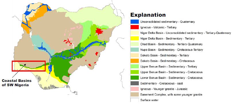
fig 1

Figure 1: Coastal Basins of Southwestern Nigeria. After Ola-Buraimo, Oluwajana [31].

These basins are grouped as the geological formations outcrop parallel to each other in an east-west direction and transgressing the basins in the same Coastal River Basins. The Osse River Basin is about 51400 sqkm in landmass. On the other hand, the Ogun River Basin has about occupied an area of about 88800 sqkm. The two basins are drained by many dendritic flowing streams, which empty their water into the sea. The Osse Basin is perhaps the lateral equivalent of the Benin-Owena River Basin [32]. The main drainage in the Osse-Osiomo systems is little streams and rivulets flowing straight into the sea and forming part of the Delta composite. Parallel streams with the same pattern drained the Ogun Basin, most protuberant being the Ogun, Osun, and Yewa river systems. This basin’s climate is archetypally coastal with very high rainfall, ranging from 2250 mm in the north to over 2600 mm along the coastal line. The relative humidity is very high, >80%. The mean annual temperature is about 21°C [32].

Geological Setting

The coastal basin of southwestern Nigeria is restricted to the west by the Ghana ridge, which is an extension of the Romanche Fracture Zone; and eastwards, by the Benin Hinge line, a basement escarpment which splits the Okitipupa Structure from the Niger Delta Basin and also marks the inland extension of the Chain Fracture Zone (Figure 2). The Nigeria portion of the basin spreads from Nigeria’s boundary and Benin’s Republic to the Benin Hinge Line. The stratigraphy of the sediments in the Nigerian sector of the Benin Basin is contentious. Different stratigraphic names have been suggested for the same Formation in different localities within the basin [31]. This problem can be attributed to the lack of adequate borehole reporting and satisfactory outcrops for comprehensive stratigraphic studies. As a result, the stratigraphy of the entire basin was divided into three chronostratigraphic compendia. These are (i) pre-lower Cretaceous folded sediments and (ii) Cretaceous sediments and Tertiary sediments (Figure 3).
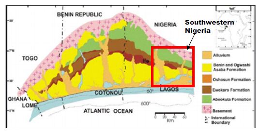
fig 2

Figure 2: The Nigerian portion of Dahomey (Benin) Basin. After Ola-Buraimo, Oluwajana [31].
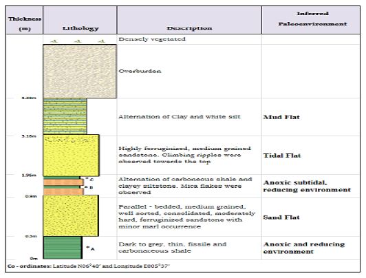
fig 3

Figure 3: A Lithologic section of Arimogija – Okeluse exposure. After Ola-Buraimo, Oluwajana [31].

In the Nigerian sector of the basin the Cretaceous sequence, as compiled from outcrop and borehole records, consists of the Abeokuta Group, further divided into three geologic units: Ise, Afowo, and Araromi Formations. Ise Formation overlies the basement complex unconformably and comprises of coarse conglomeratic sediments [33,34]. Afowo Formation is composed of transitional to marine sands and sandstone with variable but thick interbedded shales and siltstone [35,36]. Araromi is the uppermost Formation and comprises shales and siltstone with interbeds of limestone and sands. The Tertiary sediments comprise Ewekoro, Akinbo, Oshosun, Ilaro, and Benin (bare coastal sand). The Ewekoro Formation comprises fossiliferous, well-bedded limestone while Akinbo and Oshosun Formations are made up of flaggy grey and black shales [37,38]. Glauconitic rock bands and phosphatic beds define the boundary between the Ewekoro and Akinbo Formations. The Ilaro and Benin Formations are predominantly coarse sandy estuarine, deltaic, and continental beds [31].

The Abeokuta Group

The sedimentary Formation of southwestern Nigeria, otherwise known as the Eastern Dahomey Basin, extending from the Nigeria/Benin border in the west of Makun-Omi and broken in the east. The Abeokuta Group is the oldest Formation, and it comprises of main sands with intercalations of argillaceous sediments, which lie unconformably on the crystalline basement complex formation [39,40]. This group can be subdivided into three geologic units;

  • The lse Formation, which overlies the basement complex and consists of pre-drift sediments of grits and siltstones and overlain by coarse-medium grained, loose sands interbedded generally by kaolinitic clays;
  • The Afowo Formation comprises intermediate to marine sands and sandstone with variable but thick interbedded shales and siltstones. The shale to sand ratio Increase upwards with the sediment becoming highly fossiliferous. The whole arrangement represents paralic sedimentation; and
  • The Araromi Formation, which is the youngest of the stratigraphic sequence, comprises shales and siltstones with Interbeds of limestone and sands. It Is opulently fossiliferous.

The Abeokuta Formation usually has a basal conglomerate with about 1 meter thick and mostly comprises poorly rounded quartz pebbles with a silicified and ferruginous sandstone matrix or a soft gritty white clay matrix [39]. The formation outcrops where there is no conglomerate, a coarse, poorly sorted pebbly sandstone with copious white clay establishes the basal bed. The superimposing sands are coarse-grained, clayey, micaceous, and ill-sorted, suggestive short distances of transportation, or short duration of weathering and possible derivation from the granitic rocks located to the northwards. Upward stratigraphically along with the outcrop areas, the shale content increases progressively in some places, particularly around Ijebu-Ode. Close to the embayment’s eastern margin, thin beds of lignite may be present together with a high impregnation of bitumen in the sand and clays. These features are displayed in most of the eastern part of the embayment, locally referred to as Tar sand. The basal beds’ upper horizons were found in some outcrops to contain thin beds of Oolitic ironstone. The stratigraphic dating from palynological studies indicates that the ages of the lower and upper limits of the neostratotype Formation are late Albian and late Senonian. This is a characteristic species for the late Turonian-early Senonian of the Ivory Coast and was reported from Gabon’s Coniacian-Campanian. Therefore, this pollen occurrence implies a late Senonian age for the Formation’s upper layers [39].

The Ise-Afowo, Araromi, Akinbo, and Ilaro Formations

Ise and Afowo Formations are similar; thus, the two geologic units are treated together in most literature [39,41,42]. The two formations contain sand and sandstones, but the latter is interbedded by thick of shale units. Similarly, the Ise, Afowo, and Abeokuta Formations showed a similar lithologic and electric log. The uppermost beds of Abeokuta Formation which outcrop in the Ijebu-Ode, Itori, Wasimi, and Ishaga, consist mainly of fine-coarse-grained sand which is occasionally interbedded by shale, mudstone, limestone, and silt. In most recent literature the Ise and Afowo Formations are discussed as Abeokuta Formation. The Abeokuta Formation consists mainly of grits, loose sand, sandstone, kaolinitic clay, and shale. It was further characterized as usually having a basal conglomerate or a basal ferruginised sandstone [39]. The Araromi Formation overlies the Afowo Formation and has been described as the youngest Cretaceous sediment in the eastern Dahomey Basin. It is composed of fine to medium-grained sandstone at the base, overlain by shales, siltstone with interbedded limestone, marl, and lignite. This Formation is highly fossiliferous [43]. The Ewekoro Formation overlies the Araromi Formation. It is an extensive limestone body, which is traceable over a distance of about 320 km from Ghana in the west, towards the eastern margin of the Dahomey (Benin) Basin in Nigeria [44,45]. It is Palaeocene in age. Superimposing the Ewekoro Formation is the Akinbo Formation, which is mainly composed of shale and clayey sequence. The clay stones are concretionary and are largely kaolinite. The Formation’s base is defined by the presence of a glauconitic band with lenses of limestones [43]. The Akinbo Formation and consists of greenish-grey or beige clay and shale with interbeds of sandstones. The shale is thickly laminated and glauconitic. The basal beds may consist of either, sandstones, mudstones, claystones, clay-shale, or shale. The Ilaro Formation superimposes the Oshosun Formation and consists of massive, yellowish poorly, consolidated, cross-bedded sandstones. The youngest stratigraphic sequence in this basin is the Benin Formation, otherwise known as the Coastal Plain Sands and contains poorly sorted sands with layers of clay units. The sands are occasionally interbedded and show transitional to continental characteristics. The age is from Oligocene to Recent [43]. Most of the boreholes constructed in the basin are either single-screened or multiple-screened and occasionally open wells are constructed through fractured basement rocks that produce a considerable amount of water. The Depth to water level hardly exceeds 24 meters. Most aquifers in this basin are found around 40 meters below the surface. These aquifers are rarely confined, and very few boreholes tap water below 60 meters [46]. The mean yield from boreholes is ~0.4 l/s. In the crystalline basement section of the basin, a borehole depth of 40–80 m is estimated. Data from available boreholes in the southern end of Kwara State extending to Osun State, indicate the range between 25–68 meters borehole depth. The overburden thickness is also highly variable, ranging between 3–24 meters. In places around Ibadan, the overburden thickness and borehole depth are within the same range. The thickness of the overburden aquifer in the rural areas of Oyo State is correlated to the tectonic fractures rather than weathering (regolith).

Borehole yield ranging from 1–2 l/s in the basement complex section is considered suitable for installing motorized submersible pumps. Borehole yields less than 0.5 l/s are also considered good for handpumps. The recharge into the weathered aquifer is predominantly through the infiltration of rainwater. Therefore, continued yields from motorized pumps may not be workable. Midwestern Nigeria’s coastal basin’s principal aquifers occur in sandy units and overburden/superficial deposits confined by shale and clay formations. The aquifers’ thickness is highly variable with first and third horizons reaching a thickness of about 200 meters and 250 meters at Lekki headland. The second horizon is roughly 100 meters thick (Figure 4). The estimated groundwater stored in the first aquifer horizon is about 2.87 × 10³ m3. The water table is mostly shallow, ranging 0.4–21 meters below the ground surface. It is estimated that annual fluctuation is less than 5 meters. The principal aquifer is within bare coastal sands, occasionally underlain by impermeable horizons of shale and clay units. Many high-yielding boreholes provide more than 30% of the water supply in Lagos and its hinterlands [46].
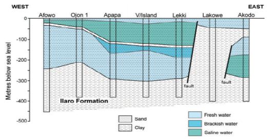
fig 4

Figure 4: Typical hydrogeological section of coastal basins of southwestern Nigeria. After Adelana, Vrbka [46].

The geological succession in these basins simple, forming a simple monocline against the basement outcrop northward, with a slight faulting indication. The inclines are reportedly about 1° or less southwestwards (Table 1). The Basement Complex rocks superimpose more than 50% of the Coastal basins [47-49]. The Abeokuta Formation is the oldest outcropping sedimentary formation in the Ogun and Osse River Basin. This appeared to cover the basement complex directly. The Formation is in turn superimposed by the Ewekoro, Ilaro, and Benin Formations. The is the substantial development of alluvium in the coastal areas and along the course of the major drainage systems of the Rivers Ogun and Osse.

Table 1: Hydrogeology of coastal basins of southwestern Nigeria.
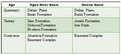
table 1

After Offodile [32]

The Abeokuta Formation

This is the oldest Formation in the Ogun Basin, outwardly covering the Basement Complex. The Formation thickness ranged from 250 to 300 meters, containing arkosic sandstones and grits, tending to be carbonaceous towards the bottom. There is an increase in thickness from about 250 meters in the western sections of the basin towards the Benin border. The basal conglomerates also were encountered. One of the outcrops gave the following units in Figure 5. The Abeokuta Formation has good potential for groundwater except that the bituminous constituents associated with the sands could affect groundwater quality. This Formation is being interrelated to the Nkporo Shale, east of the River Niger. The little report is existing about the groundwater potentials of the Abeokuta Formation. Nevertheless, its proximity to the Basement Complex and its high porosity, a substantial amount of groundwater is expected to be stored above the crystalline rock layer. This condition has been confirmed at the bottom near the Basement layer, intercepted by the borehole described in the following section. This Formation is outstanding in the basin. Hydrogeologically, groundwater in the basin’s northern parts is limited to the splintered and in-situ worn portions of the rocks. The in-situ worn portion either superimposes the unweathered basement or occurs within the unweathered basement [50].
fig 5

Figure 5: Section of Abeokuta Formation. After Offodile [32].

In the former, the worn materials create phreatic aquifers typically exploited through hand-dug shallow wells, while in the later, groundwater is confined in nature and can only be accessed through boreholes. Groundwater flow is strongly influenced by topography and two common types of springs, mainly, overland and slope springs have been observed in the area. Recharge to these aquifers is primarily by infiltrating rainfall and in some places, by the outflow from adjacent surface water. The recharge areas comprise decayed and splintered rocks in which pressure heads quickly spread through local water-bearing fractures and unified voids, thereby leading to an abrupt rise in ejections in response to rain. Spring discharges in the northern parts of the basin are very common in the rainy season but terminate totally during the dry season. The area underlain by sedimentary formations is regarded as having good groundwater potential due to an aquiferous sandy layer [50].

However, the success of boreholes in this basin is highly variable, and it could be credited to inferior drilling methods, or the frequent occurrence of the clayey matrix, which extends to seal the pores and reduce the absorptivity. The successful boreholes were reported from Aiyetoro and Ijebu Ode. Also, specific capacity ranging from 63 to 17550 list/hr/m (1300 gift) have been measured. Successful boreholes were also reported from Iboro, Imushin, and Ishaga as depicted below. In the eastern parts, within the Osse Basin, the Abeokuta Formation appears to thicken in Agenebode and Auchi’s higher regions, where the groundwater table is deep (120-300 meters). The low water table recorded is thought to be due to the aquifer’s high porosity, as typified in by the Kerri-Kerri Formation, in the Upper Benue Basin Nanka Sands of the Anambra Basin [32]. Some drilled boreholes in the Abeokuta Basin are shown in Figure 6. Figure 7 illustrates some successful boreholes in Abeokuta Formation. The GSN. BH. No. 2436 is located at Meko. The lies unconformably showed unconformity. It has a total depth of 57.9 meters. Although it penetrates the Basement Complex, yields are relatively low (1620 lits/hr (0.45 lits/sec)—the GSN. BH. No. 2612 was located at Igbogila. The borehole penetrates a Basement Complex section and has a total depth of 70.5 meters. Yield is relatively high (28350 lits/hr), or 7.87 lits/sec. it has a specific capacity of about 390.8 lits/hr—the GSN. BH. No. 2438 is located at Aiyetoro. The borehole penetrated a Basement Complex formation and showed unconformity. The total depth is about 55.9 meters. Yield is relatively low (2340 lit/hr), or 0.65 lits/sec (Offodile, 2002). Figure 7 further illustrates some boreholes penetrating the Abeokuta Formation. The GSN. BH. No. 2433 reached a depth of 48 meters below the ground level. This borehole’s actual location is unknown, but it is believed to penetrate the Abeokuta Formation. The borehole produced a yield of about 3600 lits/hr and had a specific capacity of 11880 lit/hr/m (Offodile, 2002). The GSN. BH. No. 2435 is located at Ishaga. It penetrated the basement complex (BC) and had a total depth of 75 meters. It had a yield of 31050 lits/hr. It also had a specific capacity of 3192.75 lit/hr/m [32]. The lithology is mainly sandy (Figure 7) – the GSN. BH. No. 2597 is located at Ijebu Ode about 46 km NE of the town. The borehole penetrated the BC and reached a depth of 54.6 meters. The yield obtained from this well is comparatively low (10800 lits/hr), with a specific capacity of 935.5 lits/hr/m. The last borehole in Figure 6 (GSN. BH. No. 1807), also lies unconformably on the BC. The well reached a depth of 72.8 meters and produced a yield of 13500 lits/hr, with a specific capacity of 4039.2 lit/hr/m [32]. Generally, boreholes penetrating the Abeokuta Formation has a higher proportion of sands.
fig 6

Figure 6: Lithological sections of boreholes in Abeokuta Formation. After Offodile [32].
fig 7

Figure 7: The lithology of boreholes in Abeokuta Formation. After Offodile [32].

The Ilaro Formation

The Ilaro Formation is comprised of fine to medium-grained which are reasonably well sorted. The Formation lies conformably on the Oshoshun Formation (Lower-Middle Eocene) and locally unconformably underneath the Benin Formation -Oligocene-Pleistocene [51-53]. The Ilaro Formation is typically Middle to Upper Eocene in age. The estimated thickness of this Formation is about 70 meters and displays rapid lateral facies changes. This can affect aquifer quality [54]. Hydrogeologically, not much information exists on the Ilaro Formation, though it is reported to be transitional to, and in part equivalent to the Ameki Formation. Given the Ilaro Formation’s geological physiognomies, its equivalent lateral part could be a good aquifer that can yield a substantial amount of water. However, GSN. BH. No. 2611 in Ilaro had reached a depth of 57 meters and gave a low yield of 2975 lits/hr and a specific capacity of 1023 lits/hr/m [32]. The lithology of this borehole is illustrated in Figure 8.
fig 8

Figure 8: The lithology of the borehole in Ilaro. After Offodile [32].

The Benin Formation

The Benin Formation (Miocene-Recent) consists of thick bodies of ferruginous and white sands. The Formation lies conformably on Ilaro Formation. Friable, poorly sorted with intercalation of shale, clay, and sandy clay with lignite [55]. The Benin aquifer is an important reservoir of groundwater. It is well developed in the Osse Basin and underlies more than 50% of its sedimentary section. The Benin aquifer is underlain by the sandstones of and shales of the upper Ilaro Formation, consists of a sequence of predominant continental sands and some lenses of shales and clays proved to be up to 107.7 meters thick in the area. The cross-section of the Benin Basin is further illustrated below. The Benin Aquifer gives very high yields of up to 4500 lits/hr (10000 g/hr) in most parts of the outcrop area.

The water table is relatively shallow, ranging between 20 to 25 meters. The water quality is also good. By this Formation, the land area underlain extends from Ado-Odo, Ilaro, Ikeja, and Mushin, passing through Okitipupa of Ogun Basin, into a broad area Benin-Ugheli-Agbo province of Osse Basin, in Edo and Delta States [32]. The lithology of boreholes from the Benin formation is illustrated in Figure 8. The GSN. BH. No. 2608 is located at Ikeja, had a total depth of 99 meters. The yield from this borehole is comparatively high (55350 lits/hr) [32]. Figure 9 illustrates the lithology of Benin formation [56].
fig 9

Figure 9: Hydrogeologic Cross-section of the Benin Basin. After Oteri and Ayeni [56].

Figure 10 shows the specific capacity of this borehole is 9,220 lits/hr/m. This well penetrates the Benin Formation. The GSN. BH. No. 927 is located in Otta. The well had a depth of 243 meters. The remaining lithologies were not accessed. Yield from this borehole was estimated to be 22500 lits/hr in GSN. BH. No. 2599, located at Mushin penetrates a similar sequence, attained a depth of 108.6 meters. This well gave a yield of 32850 lits/hr (9 lits/sec). The specific capacity was 1930.5 lits/hr/m. This prolific yield is typical of the Benin Formation across the southwestern river basins of Nigeria. The Benin Formation is also very important in the Osse Owena Basin, where it is the primary groundwater source [32].
fig 10

Figure 10: The lithology of the borehole in Ikeja and Otta. After Offodile [32].

The Deltaic Formation and Alluvial Deposits

This Formation contains alluvial deposits associated with Lagos’ coastal areas and the Osse Basin areas connecting to the Niger Delta Basin [57-59]. The hydrogeological conditions in areas were explained in studies on the Niger Delta Basin. Be sufficient to mention that the sandstone beds are limited in thickness and usually variable in the lateral extent. Furthermore, these aquifers have been exposed to saline water intrusion due to overdevelopment and seawater invasions. Correspondingly, the limitations in thickness and extent of the aquifers significantly reduce the boreholes’ specific capacity. The groundwater condition varies swiftly across the basins. In the Lagos region areas where the Formation appears to be least developed and has been polluted, the underlying Benin Formation provides a ready supply to the groundwater demand in the basin [32]. These comprise the Yewa, Ogun, and Oshun river networks’ vast basins, presenting a general alluvial development with considerable groundwater potential. The available drilling records have not distinguished this Formation. However, a 49275 lits/hr yield from GSN. BH. No. 2610 at Ibefun. The borehole was just 28.5 meters deep and had a specific capacity of 9234 lits/hr/m. This presents an excellent yield and underlines the high potential of these river basins’ alluvial deposits. The hydrogeology of these basins is similar to that of the Niger Delta Basin, discussed in the previous chapter.

Hydrogeological Condition in Coastal Basins of Southwestern Nigeria

The Ogun River Basin

The Ogun River Basin is one of the significant coastal basins located in southwestern Nigeria [60-62]. The basin is situated between latitudes 6° 26′ N and 9° 10’N and longitudes 2° 28’E and 4° 8 ‘E (Figure 11). About 98% of the basin area falls within Nigeria and the remaining 2% in the Benin Republic. The basin covers an of about 23,000 sqkm. The topography is generally low, with the gradient in the north-south direction. The Basin is drained by the Ogun River which had its source from the Iran hills at an elevation of about 530 meters above sea level. The river flows southwards over a distance of about 480 km before it discharges into the Lagos lagoon. The main tributaries of the Ogun River are the Ofiki and Opeki Rivers. Two seasons are distinguishable in the Ogun River Basin; a dry season from November to March and a wet season between April and October. The mean annual rainfall ranged from 900 mm in the northern parts to 2000 mm in the south. The total annual potential evapotranspiration ranged from 1600 and 1900 mm [63]. Hydrogeologically, very little is known about the Ogun Basin since the basin is often discussed in southwestern Nigeria’s coastal basins. However, Offodile [32], compiled data on borehole on borehole depths summarized in Table 2. There is not much reporting of hydrogeological physiognomies of the individual boreholes from western Nigeria’s coastal basins. Most of the boreholes in this basin penetrate the Pre Cambrian-Basement Complex. Yields from these boreholes are poorly known. However, GSN. BH. No. 2614 in Ewekoro gave an artesian flow of 90-135 lits/hr obtained near the borehole base. Similarly, GSN. BH. No. 1583 at Itori gave artesian flow at 81 meters. The estimated yield was 450 lits/hr and a specific capacity of 92.7 m 45000 lits/hr/m. Although, these two boreholes produced a substantial amount of water, a more detailed study on the hydrogeology Ogun Basin is required for further evaluation.
fig 11

Figure 11: Ogun-Osun River Basins and the Adjacent Basins. After Oke, Martins [63].

Table 2: Borehole information from Ogun Basin.

S/no.

Borehole Locality (Abeokuta Formation)

GSN. BH. No. Total Depth (m) Depth to First Water (m) Final Depth to Water (m) Yield (lits/hr) Draw Down (m) Specific Capacity (lits/hr/m)

Remarks

1

Aiyetoro 2

2438 63 31.2 31.2 2340 15

Pre Cambrian-45.9-63 m

2

Aiyetoro 2

2439 53.7 20.7 20.7 18900 3.6 5250

Pre Cambrian-45.9-63 m

3

Ijebu Ife

1808 57 42 39.9 10655 10.6 1035
4

Ijebu Ode

2620

Abandoned Pre Cambrian-Very shallow

5

Ijebu Ode

2597 69.9 46.2 46.2 10800 11.4 945

Pre Cambrian-54.6-69.6 m

6

Ijebu Ode

2598 54

Abandoned Pre Cambrian-18.3-54 m

7

Imushin

1807 87 55.8 52.8 13500 3.3 4080

Pre Cambrian-72.9-87 m

8

Imushin

2616 75.9 51.9 35100 1.8 19500

Pre Cambrian-65.4-75 m

9

Ishage

2435 75 29.1 19.8 31050 9.6 3225

Pre Cambrian-67.8-75 m

10

Meko

2436 57.9 42.3 42.3 1620 10.5

Pre Cambrian-54.6-57.9 m

(a)                 Borehole Locality (Fugar Area)
11

Agenebodo

2604 127.2 105.9 105.9

Not tested

12

Fugar

1136 69.3

Abandoned

13

Fugar

1179 157.5 129.6 4500

14

Fugar

2603 157.8 129.6 129.6

Not tested

15

Ogbona

2613 213 183.3

Not tested

(b)                 Borehole Locality (Ewekoro Formation)
16

Ewekoro

2614 90 58500

Artesian flow 90-135 lits/hr Obtained near the bottom of the hole

17

Iboro2

2433 48 13.5 10.2 36000 3 1200

18

Labour

2434 33.6 32850 3 10950

19

Ifon2

2602 79.5 64.5 61.8 12600 2.1 6000

20

Igbogila2

2612 70.5 11.4 10.2 28350 11.7 2415

21

Itori

1583 96

Artesian flow at 81 m, 450 lits/hr; at 92.7 m 45000 lits

22

Yemoji

1590 348

(c)                 Borehole Locality (Ibeshe Area)
23

Ibeshe2

2437 121.2 57.5 57.9 10.26 9.3 1095

24

Ilaro

2611 132.9 17.4 20.4 26.55 22.5 1170

(d)                 Borehole Locality (Imo Shale)
25

Sabon Gida

2601 121.2 41.4 13.05 51 255

Artesian flow 900 to 1350 lits/hr

After Offodile [32]

The Osse Owena Basin

Also known as the Benin-Owena, River Basin occurs in Edo-State. The basin is situated within the Western Littoral Hydrological Area HA-6, one of the eight hydrological areas into which Nigeria is subdivided. The gauge station at which the hydrometric measurements were made is located at Osse River at Iguoriahki [64-66]. Hydrogeologically, this basin has not been well explored. Earlier, Offodile [32] summarised borehole information on this basin. Base on the borehole information presented in Table 3, it is clear that this basin has not been fully explored hydrogeologically.

Table 3: Borehole information from Osse Owena Basin.

Borehole Locality (Ameki Formation)

GSN. BH. No.

Total Depth (m) Depth to First Water (m) Final Depth to Water (m) Yield (lits/hr) Draw Down (m) Specific Capacity (lits/hr/m)

Remarks

1 Asaba

72

27.6 23.1 8325

2 Asaba

72

22.5 25.5 9450 3 31

3 Asaba

67.5

16.5 17.4 18000

4 Asaba

45.6

25.2 22.2 95850 3 31950

5 Asaba2

44.7

26.4 24 95850 4.2 22815

6 Isse-Uku

112.5

102.5

Abandoned

7 Isse-Uku

120

Abandoned

8 Iuue

241.5

Abandoned

9 Ogwashi-Uku

89.7

Abandoned

10 Uburu

114

108.5

Abandoned

Borehole Locality (Benin Formation)
11 Abafon

45.6

41.4 16.67

12 Ado Odo

96

I1 45000 2.7 9990

13 Ado Odo

14 Agbon

63

45 40500

15 Agbon

75 7.5 45000 4.5

16 Agbon

75 7.5 45000 32.13

17 Benin City

110.4 56.4 29.25 27.55

Borehole Locality (Ameki Formation)
18 Benin City

61.8 15 67500 2.1

19

Ethiope

34.5 10.5 49500 1.8

20 Sapele

37.5 4.8 31500

21 Sapele

37.5

No Data

22 Sapele

37.5 5.1 27000

23 Sapele

No Data

After Offodile [32]

The Osun River Basin

The Osun basin is drained by the Osun River system which rises from Oke-Mesi ridge, about 5 km North of Effon Alaiye along the Oshun and Ekiti States border and flows North through the Itawure gap to latitude 7° 53′ before winding its way westwards through Oshogbo and Ede and Southwards to enter Lagos lagoon about 8 km east of Epe [63,67]. A considerable part of the basin is underlain by rocks of the Precambrian Basement Complex, most of which are very ancient. This Basement Complex rocks showed significant variations in grain size and mineral composition [63]. The rocks are quartz gneisses and schist consisting essential of quartz with small amounts of white micaceous minerals. Even though the outcrops are visible, large areas are overlain by layers of laterite soil formed by weathering and decomposing the parent rock material. The minerals’ origin has been dealt with based on heavy mineral studies along the river basin. Moreover, the sedimentary rocks of Cretaceous and Tertiary deposits are found in the southern sector of the basin [63]. Generally, in coastal basins of southwestern Nigeria, groundwater is contained in four principal aquifers [56]:

  • The first is the shallow aquifer, which contained the Recent Sediments along the Atlantic Sea coast and river valleys. It is used for minimal private domestic supplies through dug wells and shallow boreholes.
  • The second and third aquifers are in the Coastal Plains Sands Formation. They are exploited through hand-dug shallow wells in some areas, shallow – and profound – boreholes. These aquifers provide considerable amounts of water for water supplies. This is the principal aquifer exploited, particularly in Lagos and its environs.
  • The fourth aquifer is the deep and highly productive Abeokuta formation, which was discussed in previous sections.

A few boreholes located mostly in Ikeja industrial area in Lagos only extract water from the fourth aquifer. The water from this aquifer is hot with temperatures as high as 80°C recorded in a few boreholes. This aquifer is undergoing massive development in adjoining Ogun State when encountered at shallower depths of between 300 and 550 meters. Figure 12 is a north-south geologic cross-section showing various Formations in the sedimentary basin. In Figure 12, a hydrogeologic cross-section from west to east along the coast shows both the lithologic and water-quality variations in the Coastal Plains Sands and Recent Sediments [56].
fig 12

Figure 12: Hydrogeological cross-section of coastal basins along with Lagos State. After Oteri and Ayeni [56].

The delineation of shallow aquifers in the coastal plain sands of Okitipupa Area, Southwestern Nigeria, revealed two central aquifer units within the Okitipupa Area, Southwestern Nigeria [56]:

  • The upper/surficial aquifer system, which occurs at depths ranging from 5.8 m (around Agbabu) to 61.5 m (around Ikoya), and with materials of higher average resistivity (504.7 Ωm), suggestive of gravelly/coarse to medium-grained sand; and
  • The intermediate aquifer system, characterized by depth range of 32.1-127.5 m, average resistivity of 296.8 Ωm, typical of medium-grained sand saturated with water.

The highly resistive, impermeable materials overlying the aquifer units around Ajagba, Aiyesan, Agbetu, Ilutitun, Igbotako, and Erinj suggests that the aquifer units are less vulnerable to near-surface contaminants than in Agbabu, Igbisin, Ugbo, and Aboto where less resistive materials overlie aquifers. However, this indicates that the aquifer cannot be recharged in these areas. The geoelectric sequence suggests subsurface geology characterized by the alternation of sands/gravel, clay/shale, and sandstone occurring at varying depths with variable thicknesses. The sand and gravel layers constitute the aquifer units [56]. The aquifer units’ geoelectric parameters were determined by interpreting the sounding curves, assisted by the distinctive resistivity contrasts between the discrete geoelectric layers.

The upper and lower aquifer horizons work are referred to as the surficial (upper) and intermediate (lower) aquifers. In a different study by Adepelumi, Ako [68], which delineates saltwater intrusion into the freshwater aquifer of Lekki Peninsula, Lagos, Nigeria, the study delineates four distinct resistivity zones viz:

  • The unconsolidated dry sand having resistivity values ranging between 125 and 1,028 Xm represents the first layer;
  • The fresh water-saturated soil having resistivity values which correspond to 32–256 Xm is the second layer;
  • The third layer is interpreted as the mixing (transition) zone of fresh with brackish groundwater. The resistivity of this layer ranges from 4 to 32 Xm; and
  • Layer four is characterized by resistivities values generally below 4 Xm reflecting an aquifer possibly containing brine. The rock matrix, salinity, and water saturation are the major factors controlling the Formation’s resistivity. Furthermore, this study illustrates that saline water intrusion into the aquifers can be accurately mapped using the surface DC resistivity method.

The Crystalline Basement Terrain

The Basement Complex terrains of South-western Nigeria are underlain by Precambrian basement rocks, which comprise crystalline igneous and metamorphic rocks mostly granite/porphyritic granite, granite-gneiss, quartz-schist, migmatite as well as Augen-gneiss, Pegmatite intrusions and variably Migmatized Biotite-hornblende Gneiss [28,69,70]. Descriptions on the field and petrographic/mineralogical characteristics of the different rock types are subject to various works. Textural and compositional attributes are wide-ranging. Directional fabrics such as foliation, lineation, and lamination are often developed in the Gneisses, Schists, Quartzites, and Tectonized rocks [71]. From the hydrogeologic perspective, unweathered basement rock contains negligible groundwater; however, the significant aquiferous unit can develop within the weathered overburden and fractured bedrock. It is this weathered and fractured zone, which forms potential groundwater zones. However, several factors that usually contribute to the weathering and development of fracture systems in the basement rocks can be summarized as follows [71]: (i) Presence and stress components of fractures; as conduit zones, hydro-geomorphological conditions that dictate the influence of weathering agents; (ii) Hydro-climatic/temperature regimes that dictate chemical weathering pace; and (iii) Mineral contents of the rock which affect the degree of weathering/overburden thickness.

The availability of groundwater in Pre Cambrian-Basement of southwestern Nigeria depends not only on the geology but also on the complex interactions of the various hydroclimatic and geomorphologic factors [72,73]. Accordingly, several methods have been established to locate favourable sites for groundwater resources extraction within basement rocks. These include remote sensing geophysical methods and geomorphological studies [71]. Assessment of previous studies on groundwater in the crystalline basement terrain of southwestern Nigeria discovered that the hydrogeological setting of the terrain is characterized by weathered saprolite units with varied thickness over the different bedrock units, Porphyritic Granites, Granite-gneiss, Migmatite, Pegmatite, and Quartz-schist settings. Such a setting suggests the influence of rock types and mineralogy on the extent of fracturing and weathering. Consequently, groundwater occurrences in the study area are in localized, disconnected phreatic regolith aquifers, practically under unconfined to semi-confined conditions. Nonetheless, groundwater in the study area can be categorized under two central units: area with highly weathered and fractured bedrock units and poorly weathered/sparsely fractured bedrock units [71]. In an area with deeply weathered regolith and highly fractured zones, groundwater occurrences usually depend on the thickness of the water-bearing rock; this rock can be gravelly and fractured with possible quartz veins within the deep weathered zone of between 10 m to 30 m. These are characteristic of areas underlain in the study area by weathered crystalline and metamorphic rocks such as schist/quartz-schist, fractured granite-gneiss, and porphyritic granites as well as Augen gneiss with vertical fracture zones. These are generally characterized by moderate to high yield of about 75 m3/day and up to >150 m3/day. The borehole depth usually varies from 20 to 60 m, while the saturated thickness varies from 20 to 35 m below the ground surface [71]. In areas where the weathered zone is thin or absent, groundwater is usually tricky due to widely spaced fractures and the weathered zone’s localized zone/pockets. In the study area, these are characteristic of areas underlain by crystalline and metamorphic rocks, especially migmatite and variably Migmatized gneiss characterized by thin/shallow overburden unit of usually less than 10 meters in thickness and low yield of generally less than 75 m3/day. In such a setting also, the borehole depth varies from 20 to 30 m while saturated thickness varies from 8 to 20 m below the ground surface [71]. Nonetheless, towards the base of the weathered zone at the interface with the fresh bedrock, the permeability is usually high, allowing water to move freely due to the low proportion of clayey materials. However, deep-seated fractures are vital in such situations and can sometimes provide appreciable water supplies, mainly when tectonically controlled. Wells or boreholes that penetrate this horizon can usually provide sufficient water to sustain even hand-dug wells. Due to the complex interactions of the various factors affecting weathering in a typical basement complex setting like the study area, the groundwater potential zone distribution can be erratic and may not be present in some locations [71]. The analysis that involved characterization of weathered overburden revealed estimated overburden thickness using geoelectrical VES surveys from 3.8 to 50 meters with a mean value of about 20 meters as dictated by bedrock types. These values are within the range of values obtained for similar Basement Complex terrains of Africa. Furthermore, it was observed that areas with thin/shallow overburden coincided mostly with areas underlain by variably Migmatized gneiss complex, while the area with thicker overburden unit coincided with area mainly underlain by schist. However, the quartzite/quartz-schist setting coincided with areas of moderate to shallow overburden thickness [71]. In a nutshell, the varied thickness and the weathered overburden units’ isolated pockets also confirm the localized nature of weathered basement aquifers under the crystalline basement setting. The implication of this lies in the fact that there is the need for careful characterization and delineation of areas of possible fracturing and deep weathering as an aquiferous zone in respect of groundwater developments in Basement Complex settings of the study area. Therefore, the present study addresses the aspect of characterization of the groundwater potential using integrated GIS, RS, and MCDA techniques in conjunction with conventional hydrological and hydrogeological data [71]. Although the hydrogeology of southwestern Nigeria’s coastal basins is well described in the literature, a comprehensive description of its hydrochemistry has been lacking. The following section presents a synthesis of physicochemical physiognomies of groundwater in the basin.

Groundwater Chemistry

Physical Chemistry

Figures 13-15 present a summary of groundwater’s physical and chemical parameters in southwestern Nigeria’s coastal basins. Evaluation of pH concentration from 210 locations showed that pH ranged from 3.9 to 10.2 with a mean pH value of 7.4. Generally drinking water having pH < 7 is measured as acidic, and pH > 7 is considered basic. The normal range for pH in surface water systems is 6.5 to 8.5 and for groundwater aquifers 6 to 8.5 [74-76]. Unlike the Niger Delta Basin, groundwater in coastal basins of southwestern Nigeria is slightly alkaline. Alkalinity is a degree of the water’s capacity to resists a change in pH that would tend to make the water more acidic. The measurement of alkalinity and pH is needed to determine the water’s corrosivity [77-80]. The pH of clean water is 7 at 25°C, but when exposed to the atmosphere’s carbon dioxide, this equilibrium results in a pH of approximately 5.2. Because of the association of pH with atmospheric gasses and temperature, it is strongly recommended that the water is tested as soon as possible. The water’s pH is not a measure of the acidic or basic solution’s strength and alone does not provide a full picture of the characteristics or limitations with the water supply. In general, groundwater sources with low pH (< 6.5) could be acidic, soft, and corrosive. Therefore, the water could leach metal ions such as iron, manganese, copper, lead, zinc from the aquifer, plumbing fixtures, and piping. Consequently, groundwater with low pH could contain elevated levels of toxic metals, cause premature damage to metal piping, and have associated aesthetic problems such as a metallic or sour taste, laundry staining, and the characteristic blue-green staining of sinks and drains [81-83].

Groundwater sources having pH > 8.5 could indicate that the water is hard [84-86]. Hard water does not pose a health risk but can cause aesthetic problems. These problems include:

  • Formation of a ‘scale’ or precipitate on piping and fixtures causing water pressures and the interior diameter of piping to decrease;
  • Causes an alkali taste to the water and can make coffee taste bitter;
  • Formation of a scale or deposit on dishes, utensils, and laundry basins;
  • Difficulty in getting soaps and detergents to foam and Formation of insoluble precipitates on clothing, etc.; and Decreases efficiency of electric water heaters.

The temperature ranged from 22.7 to 30.5°C, with a mean value of 27.5°C. The causes for the temperature rise in aquifers are numerous, and these are directly linked to the continuing structural developments and the existing uses at the earth’s surface. These influences can be direct or indirect. The direct influences on the groundwater temperature include all heat inputs to the groundwater through the sewage network, district-heat pipes, power lines, and sources connected with groundwater heat use and storage [87-89]. The indirect influences on groundwater temperature processes are linked with urbanization-related changes in the heat balance in the near-surface atmosphere. The most important factors are:

  • The disturbance of the water balance due to a high degree of surface imperviousness;
  • The change of soil characteristics caused by an aggregation of structures (differences in the near-surface heat input and heat capacity);
  • Changes in the irradiance balance by changes in the atmospheric composition; and
  • Anthropogenic heat generation (domestic heating, industry, and transport).

The differences mentioned above cause changes in the heat balance by comparison with the areas surrounding the city. The city heats itself slowly, stores more heat overall, and passes it on again slowly to the surrounding areas, i.e., it can generally be considered an enormous heat storage unit [90,91]. Over the long term, this process increases the annual mean air and soil temperatures. The long-term warming of the near-surface soil also leads to a heating of the groundwater. Since the temperature affects the physical qualities and the groundwater’s chemical and biological nature, deterioration of groundwater quality and an impairment of the groundwater fauna may result from high temperatures [92-94]. The concentration of EC was synthesized from 177 locations from the basins. Conductivity values ranged from 31.9 to 1643 µS/cm with a mean value of 526.47 µS/cm. Electrical conductivity is widely used for monitoring the mixing of fresh and saline water, for separating stream hydrographs, and for geophysical mapping of contaminated groundwater [95,96]. Distilled water should typically have an EC of less than 0.3 µS/cm. For groundwater, EC values greater than 500 µS cm-1 indicate that the water may be polluted, although values as high as 2000 µS/cm may be acceptable for irrigation water [97,98]. In Europe, the EC of drinking water should be no more than 2500 µS/cm; water with a higher TDS may have water quality problems and be unpleasant to drink [99-101]. Synthesis of hardness from 211 locations revealed that hardness ranged from 11 to 3215 mg/l with a mean value of 467.05 mg/l. Initially, water hardness was understood to be the capacity of water to precipitate soap. Hard water does not allow soap to form as many suds. Water high in hardness is detrimental to plumbing and will reduce the life of water heaters. Water softeners will typically reduce hardness to below 10 mg/l. However, they replace the calcium and magnesium metals with sodium which is undesirable for low salt intake diets [102-104]. Water softener companies often discuss hardness in ‘Grains per Gallon’ instead of the standard units mg/l. To convert hardness from mg/L to grains per gallon, multiply mg/l by 17. Thus, 525 mg/l is equal to 31 gram/gallon. Salinity ranged from 0.08 to 1109 mg/l with a mean value of 178.90 mg/l. There is a substantial reporting on salinity in coastal basins of southwestern Nigeria. All-natural water holds some salt level, and in groundwater, the concentration can naturally vary from fresh to saltier-than-seawater. While small amounts of salt are vital for life, high levels can limit groundwater use and affect ecosystems that depend on groundwater. Small quantities of salt are deposited on the landscape every time it rains. Evaporation and plant transpiration remove water from the landscape but leave the salt behind. It concentrates salt over time. Evaporation can also directly increase groundwater salinity in areas where groundwater is close to the surface. Old groundwater can also become saltier as it passes through aquifers and picks up salts from dissolved minerals.

Although salt in the southwestern Nigeria landscape’s coastal aquifers is natural, groundwater and salt movement’s salinity into groundwater-dependent ecosystems can be increased by human activities. Increases in groundwater salinity can be caused by:

  • Increased groundwater recharge because of irrigation, which mobilizes salts naturally accumulated in the soil (irrigation salinity);
  • Increased groundwater recharge because of land clearing, bringing groundwater near the land surface, causing evaporation from the soil surface and salt accumulation (dryland salinity);
  • Leaking pipes, over-watering of gardens, and runoff from compacted surfaces can raise groundwater levels and concentrate salts in urban areas, which can lead to salt damage on buildings and roads (urban salinity);
  • Over-pumping near the coast, which can cause seawater to seep into replenishing water levels.

Groundwater salinity can also be reduced at times, such as when rapid recharge from flooding flushes out or dilutes salty groundwater. Broadscale changes in groundwater salinity occur very slowly, over decades or longer. Therefore, groundwater salinity is usually monitored rarely except where human impacts are of concern. Measurements on Turbidity, TSS, and Alkalinity were not much in the coastal basins of southwestern Nigeria. Turbidity ranged from 0.86 to 26.34 mg/l, with a mean value of 8.06 mg/l. This estimate was based on two studies (Figure 13f). Therefore, more reporting on turbidity is required in the basin. There is currently little information regarding turbidity in groundwater, and the cause is not fully understood. The common assumption is that groundwater turbidity indicates a fast transport pathway connecting potentially contaminated surface water with the aquifer. Studies found no relationship between turbidity and microbiology, although Chalk sources appear more susceptible to E. coli than other aquifers [105]. The occurrence of turbidity tends to be site-specific with a variety of causes. Mitigation measures in groundwater might include variable speed pumps, automatic pumping to waste, blending, or engineered solutions. Discussion on TSS was based on one study (Figure 13g). Total suspended solids ranged from 153 to 1109 mg/l with a mean value of 472.67 mg/l. Total Suspended Solids (TSS), also known as non-filterable residue, are those solids (minerals and organic material) that remain trapped on a 1.2 µm filter. Suspended solids can enter groundwater through runoff from industrial, urban, or agricultural areas [106]. Elevated TSS can reduce water clarity, degrade habitats, clog fish gills, decrease photosynthetic activity, and cause an increase in water temperature. TSS has no drinking water standard; drinking water with high TSS concentration can increase people’s severity with liver diseases. Similarly, there is not much reporting on alkalinity from these basins. Alkalinity ranged from 0.3 to 1.5 mg/l, with a mean concentration of 0.67 mg/l (Figure 13h). Alkalinity is not a chemical in water, but, instead, it is a property of water-dependent on the presence of certain chemicals in the water, such as bicarbonates, carbonates, and hydroxides. Groundwater aquifers with high alkalinity will experience less of a change in its acidity, such as acidic water, such as acid rain or an acid spill, introduced into the water body [107-109]. In a surface water body, such as a lake, the water’s alkalinity comes mostly from the lake’s rocks and land. Precipitation falls in the lake’s watershed, and most of the water entering the lake comes from runoff over the landscape. If the landscape is in an area containing rocks such as limestone, then the runoff picks up chemicals such as calcium carbonate (CaCO3), which raises the water’s pH and alkalinity. In areas where the geology contains large amounts of granite, lakes will have lower alkalinity. A pond in a suburban area, even in a granite-heavy area, as in some parts on the coastal basins (e.g., Lagos and its environs), could have high alkalinity due to runoff from home lawns where limestone has been applied. However, studies are required for further evaluation. Studies on dissolved oxygen from coastal basins of southwestern Nigeria are quite small in number. Ayolabi, Folorunso [110]’s integrated geophysical and geochemical methods for environmental assessment of the municipal dumpsite system in Lagos revealed DO ranging between 4 to 4.4 mg/l with a mean value of 4.1 mg/l. Similarly, Awomeso, Taiwo [111]’s study on the pollution of a waterbody by textile industry effluents in Lagos, Nigeria showed that COD concentration varies with distance from the discharge point. The concentration of was 890 mg/l at 0 meters, 600 mg/l at 50 meters, 214 mg/l at 100 meters, 1703 at 150 meters, 1172 ta 200 meters, 10 mg/l at 250 meters, 1693 mg/l at 300 meters, 860 mg/l at 350 meters, 1901 mg/l at 400 meters and 10 mg/l at 450 meters respectively. Omale and Longe [112]’s, assessment of the impact of abattoir effluents on River Illo, Ota, Nigeria showed that BOD ranged from 140 to 670 mg/l with a mean value of 333.33 mg/l. Most of the studies reporting BOD came from surface water bodies. Groundwater is yet to be fully explored in southwestern Nigeria’s coastal basins, based on these parameters. Dissolved oxygen significantly affects groundwater quality by regulating the valence state of trace metals and constraining dissolved organic species’ bacterial metabolism [113-115]. Consequently, the measurement of dissolved oxygen concentration should be considered vital in most water quality researches. Measurements of dissolved oxygen have been often ignored in groundwater monitoring. Oxygen has regularly been assumed absent below the water table; O2 measurements are not mandated by drinking water standards. Regular organic debris and organic waste derived from wastewater treatment plants, failing septic systems, and agricultural and urban runoff act as food sources for water-borne bacteria. Bacteria decompose these organic constituents using DO, consequently reducing the DO present for aquatic organisms. Chemical oxygen demand does not discriminate between biologically available and inert organic matter, and it is a measure of the total quantity of oxygen required to oxidize all organic material into carbon dioxide and water [116-119]. The COD values are always greater than BOD values, but COD measurements can be made in a few hours while BOD measurements take five days. Since parameters play a significant role in groundwater quality, it is recommended that such parameters are measured throughout the coastal basin of southwestern Nigeria. Figure 14 presents the groundwater classification based on pH, Hardness, Conductivity, and TDS. Based on pH 50.95% of groundwater sources in coastal basins of southwestern Nigeria fall in neutral class, 35.24% fall in acidic class, and 13.80% fall in alkaline class. Conversely, total hardness is also varying in the basin. About 43.37% of groundwater sources fall in soft class, 24.29% fall in intermediate class, 23.72% fall in hard class, and 9.60% fall in the very hard-water class. About 67.80% of groundwater sources have conductivity below 750 µS/cm, and 32.24% have EC values between 750 to 2250 µS/cm. Low TDS levels further show the low conductivity of groundwater sources in the basin. About 62.55% groundwater sources have TDS below 500 mg/l, 27.96% have TDS concentration between 500 to 1000 mg/l, 9.00% have TDS level between 1000 to 3000 mg/l and 0.47% have TDS above 3000 mg/l. This variability is further illustrated in Figure 14d.
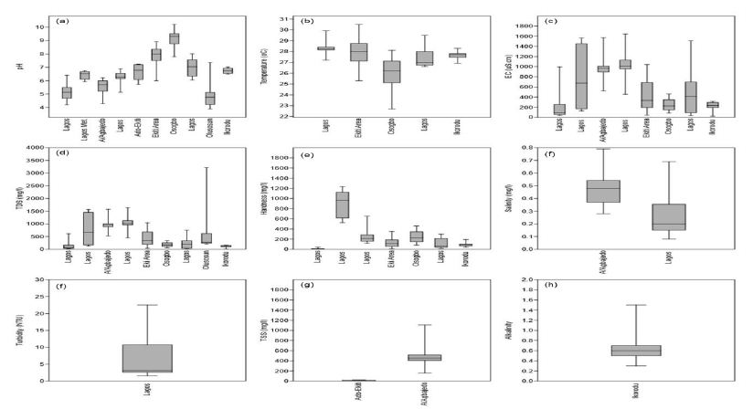
fig 13

Figure 13: Hydrogeological cross-section of coastal basins along with Lagos State.
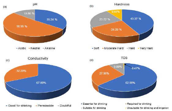
fig 14

Figure 14: Groundwater classification (a) pH, (b) Total hardness, (c) Conductivity and (d) TDS.

Cation Chemistry

Understanding the chemical physiognomies of groundwater is essential as a result of their contrasting sources. As soon as their concentration is above the suggested reference guidelines, these prerequisites may render groundwater unusable. Chemical essentials including Ca, Mg, Cu, Cd, B, Al, K, PO4, SO4 As, and Cl, for instance, are primarily derived from rocks. Nonetheless, elements like NO3 and SO4 are derived mainly from anthropogenic sources [118,119]. Understanding the derivation and absorption level of these chemical elements in groundwater is needed for effective groundwater management. Generally, there is little reporting on Al, NH4, and southwestern Nigeria’s coastal basins. For instance, Ayolabi, Folorunso [110]’s analysis of the municipal dumpsite system in Lagos showed Al ranged from 0.001 to 1.641 mg/l with a mean value of 0.29 mg/l.

Longe and Enekwechi [120] investigated potential groundwater impacts, and the influence of local hydrogeology on natural attenuation of leachate at a municipal landfill from Olusosun landfill showed that NH4 ranged from 0.14 to 1.5 mg/l with an average value of 0.41 mg/l. A review of the level of arsenic in potable water sources in Nigeria and their potential health impacts by Izah and Srivastav [121]’s analysis showed that arsenic concentration in western Nigeria ranged from 0.00 to 0.38 mg/l at Ibadan, 0.00 to 0.05 mg/l in Odeda region, 0.03 to 0.47 mg/l at Ijebu land and 0.01 to 0.70 mg/l at Igun-ijesha. People are exposed to elevated levels of inorganic arsenic through drinking contaminated water, using contaminated water in food preparation and irrigation of food crops, industrial processes, eating contaminated food and smoking tobacco. Long-term exposure to inorganic arsenic, mainly through drinking water and food, can lead to chronic arsenic poisoning. Skin lesions and skin cancer are the most characteristic effects. The SON has recommended 0.2 mg/l as a maximum permissible limit in drinking water. Aluminium is an excellent metal in the earth’s crust and is regularly found in the form of silicates such as feldspar. The oxide of Al known as bauxite provides a suitable source of uncontaminated ore. Aluminium can be selectively leached from rock and soil to enter groundwater aquifer. Aluminium is known to exist in groundwater in concentrations ranging from 0.1 ppm to 8.0 ppm. Al can be present as Aluminum Hydroxide, a residual from the municipal feeding of aluminium (Aluminum Sulfate), or as Sodium Aluminate from clarification or precipitation softening. It has been known to cause deposits in cooling systems and contributes to the boiler scale. Aluminium may precipitate at normal drinking water pH levels and accumulate as a white gelatinous deposit. Aluminium is controlled in drinking water with a recommended Secondary Maximum Contaminant Level (SMCL). SMCL’s are used when the taste, odour, or appearance of water may be adversely affected. In this case, the WHO [122] established that an Al concentration above 0.1–0.2 mg/l might impact colour but recognize that level may not be appropriate for all water supplies. The Nigerian Standard for Drinking Water Quality (NSDWQ) has recommended 0.2 mg/l as a maximum permissible limit because of potential neuro-degenerative disorders associated with high Al concentrations in water. The natural levels of NH4 in groundwater and surface water are usually below 0.2 mg/litre. Anaerobic groundwaters may contain up to 3 mg/l. Leached effluents from the concentrated rearing of farm animals can give rise to much higher levels in groundwater. Ammonia pollution can also rise from cement mortar pipe linings. Ammonia is an indicator of possible bacterial, sewage, and animal waste effluence. Contact from environmental sources is insignificant in comparison with the endogenous synthesis of NH4. Toxicological effects are observed only at exposures above about 200 mg/kg of body weight. Ammonia in drinking water is not of immediate health significance, and consequently, no health-based guideline value is proposed by SON. There are few studies on Barium concentration in groundwater from coastal basins of southwestern Nigeria. Odukoya and Abimbola [123]’s assessment of contamination of surface and groundwater within and around two dumpsites in Lagos revealed that Ba concentrations ranged from 40 to 100 mg/l with a mean value of 49 mg/l within and around abandoned dumpsite. Barium also ranged from <0.001 to 80 mg/l with a mean value of 56 mg/l within and around active dumpsite. Barium is available as a trace element in both igneous and sedimentary rocks. Even though it is not found free, it occurs in several compounds, most commonly barium sulfate (or barite) and, to a lesser extent, barium carbonate (or witherite). Barium goes into the environment naturally via the weathering of rocks and minerals. Anthropogenic releases are primarily connected with industrial processes. The over-all population is exposed to Ba through the ingestion of drinking water and foods, usually at low levels. Figure 15a presents a synthesis of Ca from groundwater from coastal basins of southwestern Nigeria. Calcium ranged from 1.49 to 1460 mg/l with a mean value of 56.78 mg/l. Calcium in drinking water is beneficial, but it is important to note that calcium is a significant constituent of hardness. Based on SON guidelines, Ca is not limited to drinking water. Based on the results of the WHO meeting of experts held in Rome, Italy, in 2003 to discuss nutrients in drinking water [124], the assembly focused its attention on Ca and Mg, for which, next to F, a sign of health benefits accompanied by their existence in drinking water is robust. The Ca’s insufficient consumption has been accompanied by increased risks of osteoporosis, nephrolithiasis (kidney stones), colorectal cancer, hypertension and stroke, coronary artery disease, insulin resistance, and obesity. Most of these disorders have treatments but no cures. Due to a lack of convincing evidence for Ca’s role as a single influential element about these diseases, estimates of the Ca requirement have been made based on bone health outcomes to improve bone mineral density. Calcium is exclusive among nutrients because the body’s reserve is also functional: increasing bone mass is correlated to a decrease in fracture risk. There relatively high Ca level in these basins could be beneficial to the health of the people living there. Figure 15b presents a synthesis of Mg from groundwater in coastal basins of southwestern Nigeria. Evaluation of Mg from 183 sites across these basins showed that Ca ranged from 0 to 108 mg/l with a mean value of 12.26 mg/l. Based on the NSDWQ [125] reference guidelines, 0.2 mg/l was suggested as the maximum permissible Mg concentration in drinking water. The relatively high Ca and Mg recorded in these basins have resulted in the hard water as 56.63% of groundwater in these basins is either moderately hard, hard, or very hard. Numerous epidemiologic researches carried out during recent years have established an inverse relationship between water hardness and death from cardiovascular disease. Many recommendations leave been offered concerning, the causal agent for the association between death from cardiovascular disease and water hardness. Two standards have been debated: a toxic effect brought by the contamination of lead or cadmium or a shielding effect from Ca or Mg’s water content. What is vital is to limit the concentrations of these elements in drinking water. Figure 15c presents a synthesis of Mn from groundwater across the coastal basins of southwestern Nigeria. Manganese ranged from <0.001 to 108 mg/l with a mean concentration of 10.05 mg/l. The SON has recommended 0.2 mg/l Mn as the maximum permissible limit in drinking water due to the neurological disorder associated with water ingestions having a high Mn level [125]. Manganese has recently come under inspection in drinking water due to its possible toxicity and its impairment to water distribution networks. Manganese is rarely found alone in groundwater. It is often found in iron-bearing waters but is rarer than iron. Chemically it can be measured as a close relative of iron since it occurs in much the same iron forms. When manganese is available in groundwater, it is as annoying as iron, perhaps even more. At low concentrations, it produces incredibly objectionable stains on everything with which it comes in contact. Evaluation of K from 207 sites (Figure 15d), in the coastal basin of southwestern Nigeria, showed that K ranged from <0.001 to 341.7 mg/l with a mean value of 24.77 mg/l. Potassium is an essential electrolyte, which is a mineral required by the body to function correctly. Potassium is especially vital for nerves and muscles, including the heart. While K is central to human health, too much ingestion of K can be just as harmful as, or worse than, not getting enough. Usually, kidneys keep a healthy balance of K by flushing excess potassium out of the body. However, for many reasons, the level of potassium in the blood can be too high. This is called Hyperkalemia, or high potassium. The NSDWQ [125], issued no guidelines on K levels in drinking water. Figure 15e presents a synthesis of Na from groundwater across the coastal basins of southwestern Nigeria. Sodium concentration from 152 sites showed that Na ranged from <90.001 to 483.42 mg/l with a mean value of 38.02 mg/l. There is an increasing call to use K in combination with Na to treat and soften drinking water. However, this would cause the level of K in drinking water to increase. The WHO found that the level of K found in drinking water would present no health concerns for healthy adults; though, for specific populations with comprised renal functions, such as infants or individuals suffering from specific diseases, there is the likelihood of adverse health effects. Sodium is not measured to be toxic. The human body requires Na to maintain blood pressure, control fluid levels, and normal nerve and muscle function. However, there are no health-based criteria for Na in drinking water. Only a small amount of the Na we ingest practically comes from water. As a substitute, the standard for Na is based on taste. The mean Na concentration in these basins is below [125] recommended value (200 mg/l).

Quality assessment of groundwater in the vicinity of dumpsites in Ifo and Lagos, Southwestern Nigeria by Majolagbe, Kasali [126], showed that Cd concentration was below the detection limit at Ifo, whereas, mean Cd concentration was 0.005 in Lagos. In the same vein, groundwater quality assessment in a typical rural settlement (Igbora, Oyo state,) in southwest Nigeria by Adekunle, Adetunji [127], showed Cd concentration varies with distance from dumpsites. The Mean Cd concentration was 0.78 mg/l at 50 meters, 0.30 mg/l at 100 meters, 0.32 mg/l at 150 meters, and 0.30 mg/l at 200 meters away from during the dry season. Cadmium concentration was 0.34 mg/l at 50 meters, 0.32 mg/l at 100 meters, 0.30 mg/l at 150 mg/l and 0.24 mg/l at 200 meters away from dumpsite during wet season. Ayolabi, Folorunso [110]’s assessment of the municipal dumpsite system in Lagos indicated that Cd ranged from <0.001 to 0.025 mg/l. There are many studies on Cd in these basins, but the underline reasons for higher Cd in groundwater need to be understood. Many studies have been carried out to decode relationships between geological environment, potable/drinking water, and diseases as they were considered to have caused suffering due to diseases among people. Chronic anaemia can be caused by protracted exposure to drink water polluted with Cd. The Cd’s accumulation is established in the kidney under such conditions, resulting in cancer and cardiovascular diseases. The NSDWQ [125] has limit Cd concentration in drinking water to be 0.003 mg/l. Cadmium is restrained in drinking water because of its toxic effects on the kidney. Assessment of groundwater fluoride and dental fluorosis in Southwestern Nigeria by Gbadebo [128], revealed that groundwater samples from Abeokuta Metropolis (i.e., basement complex terrain) had F concentrations in the range of 0.65 to 1.20 mg/l. These values were lower than the F contents in the groundwater samples from Ewekoro peri-urban and Lagos metropolis where the values ranged between 1.10 to 1.45 and 0.15 and 2.20 mg/l, respectively. The F concentrations in nearly all locations were generally above the WHO recommended 0.6 mg/l. The study also revealed that the F distribution of groundwater samples from the different geological terrain was more dependent on pH and TDS than on temperature. The result of the analyzed social-demographic characteristics of the residents indicated that the adults (between the age of 20 and >40 years) showed dental decay than the adolescent (<20 years). This indicates an incidence of dental fluorosis by the high fluoride content in the populace’s drinking water. Conversely, evaluation of groundwater contamination in Ibadan, South-West Nigeria by Egbinola and Amanambu [129], revealed that F concentration is above the recommended limits in 13% and 100% the dry and wet season samples. The occurrence of F in groundwater has become one of the most significant toxicological environmental hazards worldwide. Fluoride in groundwater is due to the weathering and leaching of fluoride-bearing minerals from rocks and sediments. When consumed in small quantities (<0.5 mg/l), F is advantageous in promoting dental health by reducing dental caries, but higher concentrations (>1.5 mg/l) may cause fluorosis [130]. It is projected that about 200 million people, from among 25 nations the world over, may suffer from fluorosis and the causes have been attributed to fluoride pollution in groundwater including Nigeria. High F concentration in groundwater is expected from sodium bicarbonate-type water, which is calcium deficient. The alkalinity of water also mobilises fluoride from fluorite (CaF2) [131-133]. Exposure to F in humans is related to:

i. Fluoride concentration in drinking water

ii. Duration of consumption; and

iii. The climate of the area. In hotter climates where water consumption is more significant, exposure doses of fluoride (F) need to be modified based on mean F intake.

Many cost-effective and straightforward measures for water defluoridation methods are already known. Nonetheless, the benefits of such methods have not reached the affected rural population due to limitations. Consequently, there is a need to develop workable plans to provide fluoride-safe drinking water to rural communities [130]. There are few studies reporting lead in groundwater from coastal basins of southwestern Nigeria. An assessment of drinking water quality using the Water Quality Index in Ado-Ekiti and environs, by Olowe, Oluyege [134], showed that Pb ranged from <0.001-7.0 mg/l with a mean value of 1.94 mg/l. The quality assessment of groundwater in the vicinity of dumpsites in Ifo and Lagos, Southwestern Nigeria by Majolagbe, Kasali [126], showed that Pb concentrations at Ifo were below the detection limit. The Pb level at Lagos was 0.003 mg/l, and this value is below NSDWQ [125], reference guidelines. The primary reason for restraining Pb in groundwater is that Pb is associated with cancer, interfering with Vitamin D metabolism, affects mental development in infants, and is toxic to central and peripheral nervous systems.

Studies on Mercury are few in coastal basins of southwestern Nigeria. The geostatistical exploration of the dataset assessing the heavy metal contamination in Ewekoro limestone, Southwestern Nigeria by Oyeyemi, Aizebeokhai [135], showed that Hg ranged from 0.002 to 0.38 mg/kg with an average value of 0.12 mg/kg. The absence of Hg reporting groundwater in these basins at the time of this study revealed a possible research gap in groundwater quality in southwestern Nigeria’s coastal basins. Mercury is a scarce element in the Earth’s crust, having an average crustal abundance by mass of only 0.08 parts per million (ppm). Typical Hg sources comprise volcanoes, geologic deposits of Hg, volatilization from the ocean, and some geothermal springs. Nearly half of all Hg released to the environment is natural in origin. About 5,000 tons of Hg is released to the environment per year due to anthropogenic activities worldwide. The NSDWQ [125] has recommended 0.001 mg/l of Hg as the maximum permissible limit for Hg in drinking water due to its health effects on the kidney and central nervous system [125].

Figure 15f presents a synthesis of Ni from groundwater in coastal basins of southwestern Nigeria. Ni ranged from <0.001 to 9.2 mg/l with a mean concentration value of 1.84 mg/l. The NSDWQ [125], set 0.02 mg/l as the maximum permissible limit of Ni in drinking water, because of possible carcinogenicity. The risk of developing cancer from the ingestion of Ni contaminated water is high in western Nigeria since the average Ni (1.84 mg/l) is very much higher than the NSDWQ [125] reference guidelines. Nickel absorptions in groundwater hang on the soil use, pH, and depth of sampling. The mean concentration in groundwater in the coastal basins of western Nigeria is 1.84 mg/l. This value is very much high. Acid rain raises the mobility of Ni in the soil and thus might increase Ni concentrations in groundwater. In groundwater with a pH below 6.2, Ni concentrations up to 0.098 mg/l have been measured. The acidic composition of groundwater sources (35.24%) perhaps is responsible for high Ni levels in the basins. Table 4 shows silica concentrations in groundwater from Abeokuta. Silica varied markedly between the studied locations. The range was higher at Ikereku 12.5-16.4 mg/l [136]. Silica in groundwater has become an exciting element to hydrogeologists as an index to aquifers’ general lithology. Groundwater travelling slowly in the subsurface will approach chemical equilibrium with minerals present in the aquifers. Under average temperature and pressure, mean silica concentrations in groundwater vary from low values of about 7 mg/l in carbonate aquifers to about 85 mg/l in aquifers containing unaltered rhyolitic ash. Groundwater from unweathered or slightly weathered basaltic aquifers generally ranges from 25 to 75 mg/l and has a mean silica value of ~45 mg/l.

Table 4: Silica concentrations in groundwater from Abeokuta.

S/No Location

No. of Sample

SiO2 (mg/l) S/No. Cont. Location Cont. No. of Sample Cont.

SiO2 (mg/l) Cont.

L1 Itoko

3

7.5-8.5 L25 Saje 6

6.9-8.2

L2 Erube

3

6.2-8.0 L26 Aregba 5

7.5-9.0

L3 Olumo

2

18.5-19.3 L27 Ikija 4

1.3-1.5

L4 Ijaye

2

8.7-10.5 L28 Ikereku 2

2.4-2.6

L5 Ago-Ika

2

4.6-5.4 L29 Efon 3

2.5-3.0

L6 Adatan

2

1.8-2.3 L30 Bode Olude 5

6.0-6.4

L7 Ake

2

2.0-4.3 L31 Housing Estate 5

6.5-6.8

L8 Ijemo

2

2.7-4.0 L32 Iberekodo 2

2.4-2.6

L9 Idomapa

2

3.6-6.3 L33 Lafiaji 2

7.9-8.2

L10 Ikija

2

4.0-6.0 L34 Ita Elega 7

3.9-4.5

L11 Kemta

2

4.0-4.9 L35 Mokola 3

2.0-2.5

L12 Itesi

2

2.3-2.6 L36 Adigbe 2

1.0-1.7

L13 Okejigbo

2

1.9-2.3 L37 Amolaso 2

3.3-3.9

L14 Oke Lantoro

2

0.5-1.8 L38 Ibara HE 5

3.8-4.7

L15 Ilugun

2

3.1-3.9 L39 Ijeja 5

1.2-2.6

L16 Itoku

2

1.4-1.6 L40 Isabo 4

2.1-2.5

L17 Iporo Ake

2

2.4-2.6 L41 Ita-Eko/Ita Iyalode 3

0.5-4.6

L18 Ijeun

2

8.5-9.0 L42 Kuto 5

2.0-3.6

L19 Sapon

2

3.1-4.7 L43 NEPA/NUD 7

1.2-1.6

L20

Lantoro

2 3.5-4.0 L44 Oke-Sokori 3

1.2-1.7

L21 Olorunsogo

2

3.2-3.5 L45 Oke-Ilewo 2

1.3-4.7

L22 Ikereku

2

12.5-16.4 L46 Onikolobo 2

1.4-2.6

L23 Ago Oko

2

5.5-6.5 L47 Quarry Rd 2

1.2-2.5

L24 Asero

6

9.0-13.6

After Offodile [32]

Hypothetically, if the water were in chemical equilibrium and if the thermodynamic properties and amounts of all minerals present were known, then the exact silica concentrations of water in the subsurface might be predicted. However, many reactions involving silicate minerals are sluggish, and equilibrium cannot be assumed, mostly in highly permeable basaltic aquifers. Moreover, the types and distribution of minerals may be quite varied and hard to determine in most aquifers. Notwithstanding these complicating factors, field data indicate that silica values for any given aquifer lithology are moderately uniform.

There are many studies on copper in coastal basins of southwestern Nigeria (Figure 15g). The concentrations of Cu ranged from 0.01 to 19.6 mg/l with a mean value of 2.86 mg/l. Dissolved Cu in groundwater can occasionally impart a light blue or blue-green colour and an unfriendly metallic, acrimonious taste to drinking water. Metallic Cu is soft, yielding, and an excellent thermal and electrical conductor. Groundwater analysis revealed high electrical conductivity, it may indicate high Cu concentrations, mainly if other ions, including Fe, Zn, Mn showed a lower concentration. Copper concentration is limited in drinking water since excessive ingestion (>1.0 mg/l), is associated with the gastrointestinal disorder [125]. Figure 15h presents a synthesis of Fe concentrations in groundwater from coastal basins of southwestern Nigeria. The Fe’s concentration was highly variable and ranged from 0 to 2.95 mg/l with a mean value of 0.31 mg/l. Fe in groundwater is a direct result of its natural availability in underground rock formations and precipitation water that infiltrates through these formations as the recharge water moves through the rocks some of the iron dissolves and accumulates in aquifers which serve as a source for groundwater. Since the earth’s underground rock formations contain about 5% iron, it is common to find iron in many geographical areas worldwide. Iron is naturally found in three significant forms and is rarely found in concentrations greater than 10 mg/l [137]. The degree to which Fe and Mn dissolve in groundwater hinge on the amount of oxygen in the water and, to a lesser extent, upon its degree of acidity, i.e., its pH. For instance, iron can occur in two forms: as Fe(++) and as Fe (+++). When the DO level is greater than 1-2 mg/l, iron occurs as Fe3+, while at lower DO levels, the iron occurs as Fe(++). Even though Fe(++) is very soluble, Fe(+++) will not dissolve substantially. Therefore, if the groundwater is oxygen-deprived, iron (and Mn) will dissolve more readily, especially if the water’s pH is on the acidic side. The DO content is decreased with an increased aquifer depth, mainly if the aquifer contains organic matter (OM). The OM decomposition depletes the oxygen in the water, and the iron dissolves as Fe(++) [138,139]. Under these circumstances, the dissolved iron often goes with dissolved manganese or hydrogen sulfide (rotten egg smell). When this water is pumped to the surface, the dissolved iron reacts with the oxygen in the atmosphere, changes to Fe(+++) (i.e., is oxidized), and forms rust-coloured iron minerals. Dissolved manganese may form blackish particulates in the water and cause similar coloured stains on fixtures. The mean Fe concentration is with the [125] reference guidelines, even though high Fe ingestion in drinking water is not associated with any health hazard. Figure 15i presents a synthesis of Zn concentration in groundwater from the coastal basins of southwestern Nigeria. The concentration of Zn ranged from 0 to 45.9 mg/l with a mean value of 3.65 mg/l. The Nigerian standard has set 3.0 mg/l as a maximum permissible limit of Zn in drinking water. Mean Zn (3.65 mg/l) is above the SON limits. Zinc is an indispensable nutrient needed for good health. Too little Zn in the diet is associated with adverse health effects such as loss of appetite, decreased sense of taste and smell, lowered ability to fight off infections, slow growth, slow wound healing, and skin sores. Eating or drinking too much Zn in a short period can lead to adverse health effects, such as stomach cramps, nausea, and vomiting. Eating large amounts of Zn for more extended periods may cause anaemia, nervous system disorders, damage to the pancreas, and lowered required cholesterol levels. There is no evidence that zinc causes cancer in humans.
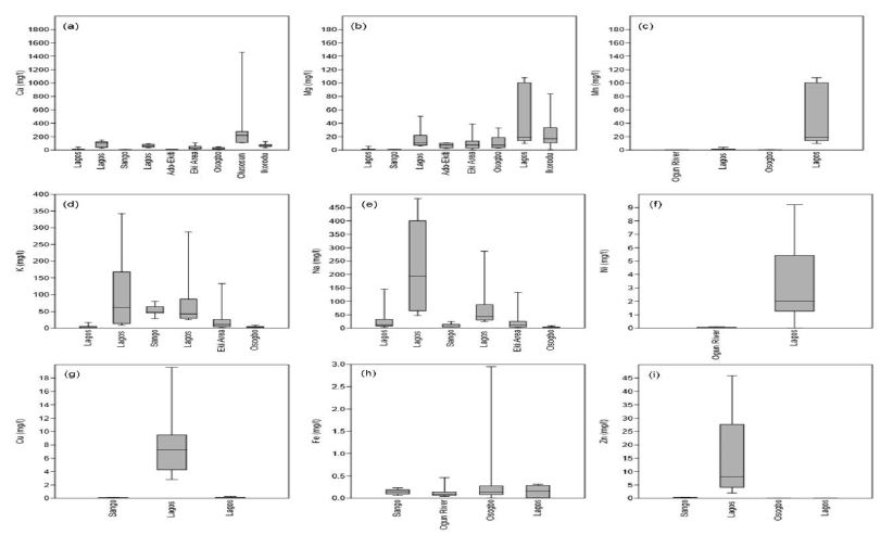
fig 15

Figure 15: Cation chemistry (a) Ca, (b) Mg, (c) Mn, (d) K, (e) Na. (f) Ni, (g) Cu, (h) Fe, and (i) Zn.

Anion Chemistry

Evaluation of HCO3 concentrations from 119 locations in coastal basins of southwestern Nigeria revealed that HCO3 ranged from 3.6 to 456.28 mg/l with a mean value of 116.98 mg/l (Figure 16a). There are no reference guidelines set up by NSDWQ [125]. Studies on CO3 were not accessed at the time of this study. The two ions are essential to water quality parameters because when CO3 and HC03 are joint with Ca and Mg, they form carbonate hardness. However, if soil concentrates on drying solution, it advances as CaCO3 or MgCO3. Ca and Mg decrease Na concentration levels and the SAR index rise, initiating an alkalizing effect and elevated pH levels. When groundwater analysis shows elevated pH levels, it may indicate the high content of carbonate and bicarbonate ions. Figure 16b presents a synthesis of Cl concentrations in the coastal basin of southwestern Nigeria. Evaluation of Zn in groundwater from 203 sites across the basin revealed that it ranged from 0.12 to 387 mg/l with a mean concentration value of 47.15 mg/l. The NSDWQ [125], has set 250 mg/l as the maximum permissible allowable drinking water limit. Chloride is one of the most common anions found in tap water. Chloride generally combines with Ca, Mg or Na to form various salts: for example, sodium chloride (NaCl) is formed when Cl and Na combine. Chloride occurs naturally in groundwater but is found in high concentrations where seawater and run-off from road salts can make their way into groundwater aquifers. Although Cl is harmless at low levels, groundwater sources having high in NaCl can harm plants if used for gardening or irrigation and give drinking water an unpleasant taste. Over time, NaCl’s high corrosivity will also damage the water system, appliances, and water heaters, causing toxic metals. Nitrate ranged from <0.001 to 50.6 mg/l with a mean value of 8.81 mg/l. There are very few studies on NO2 in coastal basins of southwestern Nigeria (Figure 16c). Akinbile and Yusoff [140]’s environmental impact of leachate pollution on groundwater supplies in Akure, Nigeria, showed that NO2 ranged from 0.7 to 0.9 mg/l with an average value of 0.8 mg/l. The impact of pit latrines on groundwater quality of Fokoslum, Ibadan, Southwestern Nigeria [141], showed that NO2 concentrations vary with pits’ distance. The mean NO2 concentration was 0.12 mg/l at 10.9 meters, 0.05 mg/l at 11.8 meters, 0.12 mg/l at 13.1 meters, 0.21 mg/l at 16.3 meters, 0.22 mg/l at 13.3 meters, 0.19 mg/l at 17.9 meters, 0.23 mg/l at 9.4 meters and 6.1 mg/l at 6.1 meters, respectively. The NO2 from these sites was below the NSDWQ [125] reference limits.

Figure 16d presents a synthesis of PO4 in groundwater from coastal basins of western Nigeria. The PO4 ranged from 0 to 3.5 mg/l with a mean value of 0.65 mg/l. High PO4 in drinking water is not associated with any severe health risks. The presence of PO4 in groundwater is an indicator of anthropogenic pollution since PO4 is mainly derived from organic wastes. The significance of PO4 is mostly linked to eutrophication of surface water bodies. High PO4 and NO3 in water, help plant and algal growths, leading to a variation of diurnal dissolved oxygen, blooms, and littoral slimes [142]. Figure 16e presents a synthesis of SO4 concentrations in groundwater from coastal basins of southwestern Nigeria. The Concentration of SO4 ranged from <0.001 to 1855 mg/l with a mean value of 52.01 mg/l. The NSDWQ [125], has set 100 mg/l as the maximum allowable limit of SO4 in drinking water, even though there is no health risk associated with high ingestion of SO4 drinking water. However, high concentrations of SO4 in drinking water can cause diarrhoea in humans, especially infants. However, adults usually become adapted to high SO4 concentrations after a few days [143].
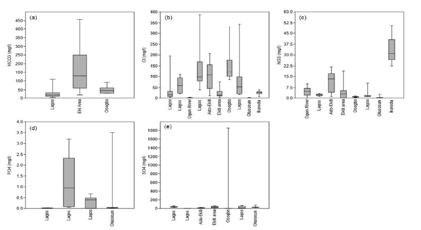
fig 16

Figure 16: The anion chemistry (a) HCO3, (b) Cl, (c) NO3, (d) PO4, and (e) SO4.

Conclusion

The literature is unanimous about the importance of understanding the hydrogeology and hydrochemistry of groundwater in coastal basins of southwestern Nigeria. Based on the reviewed works, the following remarks can be made:

i. In southwestern Nigeria’s coastal basins, the Abeokuta group is the oldest formation in the area. This group comprised of the Ise, Afowo, and Araromi Formations. Other formations in the basin include the Akinbo and Ilaro formations. Despite the marked spatial variability of these formations, their lithology remains relatively the same.

ii. Also found in this area is the deltaic formation, which contains alluvial deposits. The Ogun Basin is the central coastal basin in western Nigeria, followed by the Osse-Owena Basin. The later has not been fully explored hydrogeologically. The Osun Basin, drained by the Osun River, covers most Osun and Ekiti States parts. This basin is not associated with good groundwater storage, since basement complex rocks underlie it.

iii. These coastal basins were further grouped into the upper surficial aquifer system; and the intermediate aquifer system. Also found in this area is the crystalline Basement Terrain. From the hydrogeologic point of view, unweathered basement rock contains negligible groundwater; though, a significant aquiferous unit can develop within the weathered overburden and fractured bedrock. The general groundwater condition in the area showed that groundwater is very localized.

iv. Groundwater classification based on physical parameters showed mixed results, though groundwater sources are most suitable for drinking.

These basins’ hydrochemistry showed groundwater is relatively good in terms of its suitability for drinking, industrial and agricultural uses. Owing to the increasing urbanization in the area, reasonable measures are required to protect groundwater from overexploitation and pollution.

Acknowledgement

Federal University Birnin kebbi supported this review. Thanks to all anonymous contributors.

References

  1. Olofinlade WS, Daramola S, Olabode OF (2018) Hydrochemical and statistical modeling of groundwater quality in two contrasting geological terrains of southwestern Nigeria. Modeling Earth Systems and Environment 4: 1405-1421.
  2. Arfanuzzaman M, Atiq Rahman A (2017) Sustainable water demand management in the face of rapid urbanization and groundwater depletion for social-ecological resilience building. Global Ecology and Conservation 10: 9-22.
  3. Pahl-Wostl C (2019) The role of governance modes and meta-governance in the transformation towards sustainable water governance. Environmental Science & Policy 91: 6-16.
  4. Rao ND, Min J (2018) Decent Living Standards: Material Prerequisites for Human Wellbeing. Soc Indic Res 138: 225-244. [crossref]
  5. Ficke AD, Myrick CA, Hansen LJ (2007) Potential impacts of global climate change on freshwater fisheries. Reviews in Fish Biology and Fisheries 17: 581-613.
  6. Heathwaite AL (2010) Multiple stressors on water availability at global to catchment scales: understanding human impact on nutrient cycles to protect water quality and water availability in the long term. Freshwater Biology 55: 241-257.
  7. Peters NE, Meybeck (2000) Water Quality Degradation Effects on Freshwater Availability: Impacts of Human Activities. Water International 25: 185-193.
  8. Jamiu AA, Robert M. Kalin, Philippe Sentenac, Ibrahim Hassan, et al. (2020) Assessing the Impact of Climate Change on Groundwater Quality of the Shallow Coastal Aquifer of Eastern Dahomey Basin, Southwestern Nigeria. Water
  9. Md Enamul Huq, Shah Fahad, Zhenfeng Shao, Most Sinthia Sarven, Imtiaz Ali Khan, et al. (2020) Arsenic in a groundwater environment in Bangladesh: Occurrence and mobilization. J Environ Manage [crossref]
  10. Zacchaeus OO (2020) Effects of industrialization on groundwater quality in Shagamu and Ota industrial areas of Ogun State, Nigeria. Heliyon
  11. Asiwaju-Bello YA, Olabode, Ogunsuyi MT (2020) Pollution potential and causative hydrogeochemical processes in unconfined aquifer systems in a typical urban setting: emphasis on recharge and discharge areas. Applied Water Science 10: 1-23.
  12. Fan Feng, Yongfeng Jia,, Yu Yang, Huan Huan, Xinying Lian, et al. (2020) Hydrogeochemical and statistical analysis of high fluoride groundwater in northern China. Environ Sci Pollut Res Int 27: 34840-34861.
  13. Jebreen H (2018) Recharge, geochemical processes and water quality in karst aquifers: Central West Bank, Palestine. Environmental Earth Sciences 77: 1-16.
  14. Muhammad Afnan Talib, Zhonghua Tang, Asfandyar Shahab, Jamil Siddique, Muhammad Faheem, et al. (2019) Hydrogeochemical Characterization and Suitability Assessment of Groundwater: A Case Study in Central Sindh, Pakistan. International Journal of Environmental Research and Public Health 16: 1-21. [crossref]
  15. Osin OA, Yu, S Lin (2017) Oil refinery wastewater treatment in the Niger Delta, Nigeria: current practices, challenges, and recommendations. Environ Sci Pollut Res Int 24: 22730-22740. [crossref]
  16. Ibe KM, PU Agbamu (1999) Impacts of human activities on groundwater quality of an alluvial aquifer: A case study of the Warri River, Delta State, SW, Nigeria. International Journal of Environmental Health Research 9: 329-334.
  17. Emenike PC, CC Nnaji, IT Tenebe (2018) Assessment of geospatial and hydrochemical interactions of groundwater quality, southwestern Nigeria. Environmental Monitoring Assessment 190: 1-17.
  18. Güler C (2012) Assessment of the impact of anthropogenic activities on the groundwater hydrology and chemistry in Tarsus coastal plain (Mersin, SE Turkey) using fuzzy clustering, multivariate statistics and GIS techniques. Journal of Hydrology 414-415: 435-451.
  19. Huang G (2013) Impact of anthropogenic and natural processes on the evolution of groundwater chemistry in a rapidly urbanized coastal area, South China. Sci Total Environ 463-464: 209-21. [crossref]
  20. Ma F (2014) Hydrochemical characteristics and the suitability of groundwater in the coastal region of Tangshan, China. Journal of Earth Science 25: 1067-1075.
  21. Masoud AA (2014) Groundwater quality assessment of the shallow aquifers west of the Nile Delta (Egypt) using multivariate statistical and geostatistical techniques. Journal of African Earth Sciences 95: 123-137.
  22. Badmus GO (2020) Hydrochemical analysis of groundwater quality along the coastal aquifers in part of Ogun Waterside, Ogun State, southwestern Nigeria. Heliyon
  23. Oyeyemi KD, AP Aizebeokhai, MA Oladunjoye (2015) Integrated Geophysical and Geochemical Investigations of Saline Water Intrusion in a Coastal Alluvial Terrain, Southwestern Nigeria. International Journal of Applied Environmental Sciences 10: 1275-1288.
  24. Adelana SMA (2005) The impact of anthropogenic activities over groundwater quality of a coastal aquifer in Southwestern Nigeria. Aquifer Vulnerability and Risk, 2nd 4th International Workshop Congress on the Protection and Management of Groundwater Reggia di Colorno – Parma, 21-22-23 Settembre: p. 1-10.
  25. Awomeso JA, SM Ahmad, AM Taiwo (2020) Multivariate assessment of groundwater quality in the basement rocks of Osun State, Southwest, Nigeria. Environmental Earth Sciences 79: 1-9.
  26. A AJ, TA O (2013) Assessment of Groundwater Quality in Abeokuta Southwestern, Nigeria. Research Inventory: International Journal of Engineering and Science 2: 21-31.
  27. Yusuf MA, TA Abiye (2019) Risks of groundwater pollution in the coastal areas of Lagos, southwestern Nigeria. Groundwater for Sustainable Development
  28. Aizebeokhai AP, KD Oyeyemi, ES Joel (2016) Groundwater potential assessment in a sedimentary terrain, southwestern Nigeria. Arabian Journal of Geosciences
  29. Akaegbobi IM, GO Ogungbesan (2016) Geochemistry of the Paleocene limestones of Ewekoro Formation, Eastern Dahomey Basin, Southwestern Nigeria: Implication on Provenance and Depositional Conditions. Ife Journal of Science 18: 669-684.
  30. Ola-Buraimo AO (2014) Biostratigraphy of the Campano-Maastrichtian Uzeeba Shale deposit, Dahomey Basin Southwestern Nigeria. Elixir Geoscience 69: 22812-22818.
  31. Ola-Buraimo OA (2012) Palynological Investigation of a Type Section of Early Maastrichtian Arimogija – Okeluse Shale Sequence, Dahomey (Benin) Embayment, Southwestern Nigeria. International Journal of Science & Emerging Technologies 3: 37-45.
  32. Offodile ME (2002) Groundwater Study and Development in Nigeria, second edition, Mecon Geology and Eng. Services Ltd. Pg: 1- 453.
  33. Oli IC (2019) A Review of the Geology and Mineral Resources of Dahomey Basin, Southwestern Nigeria. International Journal of Environmental Sciences & Natural Resources 21: 1-5.
  34. Obomighie PO, JO Gwegwe, AG Oluwadebi (2016) Petrographic Studies and Paleoenvironmental Reconstruction of Some Outcropping Sediments in Parts of Eastern Dahomey Basin, South-Western, Nigeria. IOSR Journal of Applied Geology and Geophysics 4: 9-15.
  35. Nton NE, PR Ikhane, MN Tijani (2009) Aspect of rock-eval studies of the Maastrichtian-Eocene sediments from subsurface, in the eastern Dahomey basin southwestern Nigeria. European Journal of Scientific Research 25: 417-427.
  36. Olabode, S.O. and M.Z. (2016) Mohammed, Depositional Facies and Sequence Stratigraphic Study in Parts of Benin (Dahomey) Basin SW Nigeria: Implications on the Re-Interpretation of Tertiary Sedimentary Successions. International Journal of Geosciences 7: 210-228.
  37. Olabode SO, JA Adekoya (2008) Seismic stratigraphy and development of Avon canyon in Benin (Dahomey) basin, southwestern Nigeria. Journal of African Earth Sciences 50: 286-304.
  38. Olatinsu O (2017) Lithotype characterizations by Nuclear Magnetic Resonance (NMR): A case study on limestone and associated rocks from the eastern Dahomey Basin, Nigeria. Journal of African Earth Sciences 129: 701-712.
  39. Okosun EA (1990) A review of the Cretaceous stratigraphy of the Dahomey Embayment, West Africa. Cretaceous Research 11: 17-27.
  40. Adeoti L, OM Alile, O Uchegbulam (2010) Geophysical investigation of saline water intrusion into freshwater aquifers: A case study of Oniru, Lagos State. Scientific Research and Essays 5: 248-259.
  41. Mohammed S, M Opuwari, S Titinchi (2020) Source rock evaluation of Afowo clay type from the Eastern Dahomey Basin, Nigeria: insights from different measurements. Sci Rep
  42. Adeoye JA (2020) Geochemistry and paleoecology of shales from the Cenomanian-Turonian Afowo formation Dahomey Basin, Nigeria: Implication for provenance and paleoenvironments. Journal of African Earth Sciences
  43. Nton ME, PR Ikhane, MN Tijani (2009) Aspect of Rock-Eval Studies of the Maastrichtian-Eocene Sediments from Subsurface, in the Eastern Dahomey Basin Southwestern Nigeria. European Journal of Scientific Research 25: 417-427.
  44. Akaegbobi IM, GO Ogungbesan, JE Ogala (2011) Carbonate Microfacies and Major Element Content of The Paleocene – Eocene Sections Exposed at the Sagamu Quarry, Eastern Dahomey Basin, Nigeria. Global Journal of Geological Sciences 9: 241-251.
  45. PR I (2012) Petrography and Geochemical Appraisal of Afowo Sandstone Facies, Dahomey Basin, Southwestern Nigeria. Chemistry and Materials Research 2: 50-59.
  46. Adelana, SMA (2008) An overview of the geology and hydrogeology of Nigeria. Chapter 11. 15(11): pg: 171-198.
  47. Adekeye OA (2019) Biostratigraphic Analysis of the Cretaceous Abeokuta Group in the Eastern Dahomey Basin, Southwestern Nigeria. Journal of African Earth Sciences 152: 171-183.
  48. Joel ES (2019) Integration of aeromagnetic and electrical resistivity imaging for groundwater potential assessments of coastal plain sands area of Ado-Odo/Ota in southwest Nigeria. Groundwater for Sustainable Development
  49. Osinowo OO, AO Akanji, AI Olayinka (2014) Application of high-resolution aeromagnetic data for basement topography mapping of Siluko and environs, southwestern Nigeria. Journal of African Earth Sciences 99: 637-651.
  50. Aladejana JA, AO Talabi (2013) Assessment of Groundwater Quality in Abeokuta Southwestern, Nigeria. Research Inventy: International Journal of Engineering And Science 2: 21-31.
  51. Oyedele KF, EI Momoh (2009) Evaluation of Seawater Intrusion in Freshwater Aquifers in a Lagoon Coast: A Case Study of the University of Lagos Lagoon, Akoka, Nigeria. Report and Opinion 1: 1-12.
  52. Adeyemi GO (2013) Geophysical and Sedimentological Characterization of a Tar Sand Rich Area in South-western Nigeria. Journal of Environment and Earth Science 2: 71-83.
  53. Akinmosin A, AO Shoyemi (2010) Technical Feasibility of Direct Application of the Nigerian Tar Sand Deposits as Road Asphalt. The Pacific Journal of Science and Technology 11: 526-536.
  54. Adepelumi A, B Ako, T Ajayi (2001) Groundwater contamination in the basement-complex area of Ile-Ife, southwestern Nigeria: A case study using the electrical-resistivity geophysical method. Hydrogeology Journal 9: 611-622.
  55. Oyedele KF, S Oladele, C Okoh (2012) Geo-Assessment of subsurface conditions in Magodo Brook Estate, Lagos, Nigeria. International Journal of Advanced Scientific and Technical Research 2: 731-741.
  56. Oteri, UO, RA Ayeni (2016) The Lagos Mega City: Water Megacities and Global Change. Available at: http://eaumega.org/wp-content/uploads/2016/05/EN-Lagos-Monograph.pdf,: pg: 1-36.
  57. Amajor LC (1991) Aquifers in the Benin Formation (Miocene Recent), Eastern Niger Delta, Nigeria: Lithostratigraphy, Hydraulics, and Water Quality. Environmental Geology and Water Science 17: 85-101.
  58. Oomkens E (1974) Lithofacies relations in the Late Quaternary Niger Delta complex. Sedimentology 21: 195-222.
  59. Reijers TJA, SW Petters, CS Nwajide (1997) The Niger Delta Basin. African Basins. Sedimentary Basins of the World, 3 edited by R.C. Selley (Series Editor: K.J. Hsti) p. 151-172.
  60. Adeyemi O, F Olutoyin, O Olumide (2020) Downstream hydraulic geometry across headwater channels in Upper Ogun River Basin, Southwestern Nigeria. African Geographical Review 39: 345-360.
  61. Eludoyin AO, AO Adewole (2019) A remote sensing-based evaluation of an ungauged drainage basin in Southwestern Nigeria. International Journal of River Basin Management 18: 307-319.
  62. Olusola A (2020) Morphologic and hydraulic variability of small bedrock and alluvial channels in relation to lithological controls, Upper Ogun River Basin, Southwestern Nigeria. Physical Geography 41: 537-557.
  63. Oke MO (2015) Comparative analysis of groundwater recharge estimation value obtained using empirical methods in Ogun and Oshun river basins. Ife Journal of Science 17: 53-63.
  64. Ikhile CI (2012) The Impacts of Climate Change on the Discharge of OsseOssiomo River Basin, South Western Nigeria under Different Climatic Scenarios. An International Journal of Science and Technology Bahir Dar, Ethiopia 1: 1-13.
  65. Catherine II, O Lekan (2007) Application of GIS in land-use studies in the Osse-Ossiomo River basin, Nigeria. Remote Sensing for Environmental Monitoring and Change Detection (Proceedings of Symposium HS3007 at IUGG2007, Perugia, July 2007). IAHS Publ. 316: 245-251.
  66. Solomon O, O Prince (2013) Flood Frequency Analysis of Osse River Using Gumbel’s Distribution. Civil and Environmental Research 3: 55-59.
  67. Oke MO (2013) Comparative Analysis of Empirical Formulae Used in Groundwater Recharge in Ogun – Oshun River Basins. Journal of Scientific Research & Reports 2: 692-710.
  68. Adepelumi AA (2009) Delineation of saltwater intrusion into the freshwater aquifer of Lekki Peninsula, Lagos, Nigeria. Environmental Geology 56: 927-933.
  69. Bayewu OO (2017) Geophysical evaluation of groundwater potential in part of southwestern Basement Complex terrain of Nigeria. Applied Water Science 7: 4615-4632.
  70. Lateef TA (2012) Geophysical Investigation For Groundwater Using Electrical Resistivity Method – A Case Study Of Annunciation Grammar School, Ikere Lga, Ekiti State, South-Western Nigeria. IOSR Journal of Applied Physics 2: 1-6.
  71. Fashae OA (2014) Delineation of groundwater potential zones in the crystalline basement terrain of SW-Nigeria: an integrated GIS and remote sensing approach. Applied Water Science 4:19-38.
  72. Egbinola CN (2014) Amanambu, Christiana Ndidi Egbinola* and Amobichukwu Chukwudi Amanambu. SpringerPlus 3: 1-6.
  73. Akinyemi FO (2013) An assessment of land-use change in the Cocoa Belt of south-west Nigeria. International Journal of Remote Sensing 34: 2858-2875.
  74. DeSimone LA, JP Pope KM (2020) Ransom, Machine-learning models to map pH and redox conditions in groundwater in a layered aquifer system, Northern Atlantic Coastal Plain, eastern USA. Journal of Hydrology: Regional Studies
  75. Laluraj CM, G Gopinath (2006) Assessment on seasonal variation of groundwater quality of phreatic aquifers – a river basin system. Environ Monit Assess 117: 45-57.
  76. Takem GE (2015) Acidification of shallow groundwater in the unconfined sandy aquifer of the city of Douala, Cameroon, Western Africa: implications for groundwater quality and use. Environmental Earth Sciences 74: 6831-6846.
  77. Douglas TM, LS Robert (2015) Corrosion Control by Deposition of CaCO₃ Films: Part 1, A Practical Approach for Plant Operators. American Water Works Association 69: 592-599.
  78. Marc, E., R.S. Michael, and E.M. Travis (1996) Alkalinity, pH, and copper corrosion by-product release. American Water Works Association.
  79. Gouda VK (1970) Corrosion and Corrosion Inhibition of Reinforcing Steel: I. Immersed in Alkaline Solutions. British Corrosion Journal 5:198-203.
  80. Melidis P (2007) Corrosion control by using indirect methods. Desalination 213: 152-158.
  81. Asare-Donkor NK, DD Wemegah, AA Adimado (2013) Chemical Analysis of Freshwater Bodies in the Kumasi Metropolis and Its Environs, Ghana. Journal of Environment and Earth Science 3: 37-45.
  82. Bacha AA, MI Durrani, PI Paracha (2010) Physical and Bacteriological Characteristics of Drinking Water of Peshawar. Pakistan Journal of Nutrition 9: 1028-1033.
  83. Haziq MA, NA Qani (2017) Physiochemical Assessment of Drinking Water Quality in Kandahar City, Afghanistan. International Journal of Innovative Science and Research Technology 2: 7-24.
  84. Timothy AO, KH M (1978) The effect of pH and hardness metal ions on the competitive interaction between trace metal ions and inorganic and organic complexing agents found in natural waters. Water Research 12: 703-711.
  85. Karthikeyan S, PLR Palaniappan, S Sabhanayakam (2007) Influence of pH and water hardness upon nickel accumulation in edible fish Cirrhinus mrigala. Journal of Environmental Biology 28: 489-492.
  86. Ruiz-Ramirez J (2005) Relationship between water content, NaCl content, pH and texture parameters in dry-cured muscles. Meat Sci 70: 579-587.
  87. Florides G, S Kalogirou (2007) Ground heat exchangers—A review of systems, models and applications. Renewable Energy 32: 2461-2478.
  88. Green TR (2011) Beneath the surface of global change: Impacts of climate change on groundwater. Journal of Hydrology 405: 532-560.
  89. Keery J (2007) Temporal and spatial variability of groundwater-surface water fluxes: Development and application of an analytical method using temperature time series. Journal of Hydrology 336: 1-16.
  90. Alva G, Y Lin, G Fang (2018) An overview of thermal energy storage systems. Energy 144: 341-378.
  91. Zhu S (2020) Using seasonal temperature difference in underground surrounding rocks to cooling ventilation airflow: A conceptual model and simulation study. Energy Science & Engineering 8: 3457-3475.
  92. Boulton AJ, PJ Hancock (2006) Rivers as groundwater-dependent ecosystems: a review of degrees of dependency, riverine processes and management implications. Australian Journal of Botany 54: 133-144.
  93. Humphreys WF (2008) Hydrogeology and groundwater ecology: Does each inform the other?. Hydrogeology Journal 17: 5-21.
  94. Strona G (2019) AQUA LIFE Software: A New Tool for a Standardized Ecological Assessment of Groundwater Dependent Ecosystems. Water 11: 1-17.
  95. Hayashi M (2004) Temperature-electrical conductivity relation of water for environmental monitoring and geophysical data inversion. Environmental Monitoring and Assessment 96: 119-128.
  96. Beddows PA (2007) Decoupled fresh–saline groundwater circulation of a coastal carbonate aquifer: Spatial patterns of temperature and specific electrical conductivity. Journal of Hydrology 346: 18-32.
  97. Sargaonkar A, V Deshpande (2003) Development of an overall index of pollution for surface water based on a general classification scheme in Indian context. Environmental Monitoring and Assessment 89: 43-67.
  98. Zakir HM (2017) Quality and Metallic Pollution Level in Surface Waters of an Urban Industrialized City: A Case Study of Chittagong City, Bangladesh. Journal of Industrial Safety Engineering 4: 9-18.
  99. Güler C, M Alpaslan (2009) Mineral content of 70 bottled water brands sold on the Turkish market: Assessment of their compliance with current regulations. Journal of Food Composition and Analysis 22: 728-737.
  100. Karavoltsos S (2008) Evaluation of the quality of drinking water in regions of Greece. Desalination 224: 317-329.
  101. Naveen BP (2017) Physico-chemical and biological characterization of urban municipal landfill leachate. Environmental Pollution 220: 1-12.
  102. Rubenowitz-LundinKevin, E. and K.M. Hiscock, Water Hardness and Health Effects. In: Essentials of Medical Geology. Revised Edition. Eds: O. Selinus. Springer Dordrecht Heidelberg New York London, 2013: pg: 1-808.
  103. Ghernaout (2018) Combining lime softening with alum coagulation for hard Ghrib dam water conventional treatment. International Journal of Advanced and Applied Sciences 5: 61-70.
  104. Richards CS (2018) A 21st-Century Perspective on Calcium Carbonate Formation in Potable Water Systems. Environmental Engineering Science 35: 143-158.
  105. Farrell C (2018) Turbidity composition and the relationship with microbial attachment and UV inactivation efficacy. Sci Total Environ 624: 638-647.
  106. Edwards AC, PJA (2008) Withers, Transport and delivery of suspended solids, nitrogen and phosphorus from various sources to freshwaters in the UK. Journal of Hydrology 350: 144-153.
  107. Appleyard, S, T Cook (2008) Reassessing the management of groundwater use from sandy aquifers: acidification and base cation depletion exacerbated by drought and groundwater withdrawal on the Gnangara Mound, Western Australia. Hydrogeology Journal 17: 579-588.
  108. Mushtaq N (2018) Hydrogeochemical and isotopic evaluation of groundwater with elevated arsenic in alkaline aquifers in Eastern Punjab, Pakistan. Chemosphere 200: 576-586.
  109. Sabarathinam C, H Bhandary, A Al-Khalid (2020) Tracing the evolution of acidic hypersaline coastal groundwater in Kuwait. Arabian Journal of Geosciences 13: 1-19.
  110. Ayolabi EA, AF Folorunso, OT Kayode (2013) Integrated Geophysical and Geochemical Methods for Environmental Assessment of Municipal Dumpsite System. International Journal of Geosciences 4: 850-862.
  111. Awomeso JA (2010) Studies on the pollution of waterbody by textile effluents in.Lagos, Nigeria. Journal of Applied Sciences in Environmental Sanitation 5: 353-359.
  112. Omale DO, EO Longe (2008) An assessment of the impact of abattoir effluents on River Illo, Ota, Nigeria. Journal of Environmental Science and Technology 2: 56-64.
  113. Siljic Tomic A (2018) A linear and non-linear polynomial neural network modelling of dissolved oxygen content in surface water: Inter- and extrapolation performance with inputs’ significance analysis. Sci Total Environ 610-611: 1038-1046.
  114. Voisin J (2018) Aquifer recharge with stormwater runoff in urban areas: Influence of vadose zone thickness on nutrient and bacterial transfers from the surface of infiltration basins to groundwater. Sci Total Environ 637-638: 1496-1507.
  115. Ward, C.P. and R.M. Cory (2020) Assessing the prevalence, products, and pathways of dissolved organic matter partial photo-oxidation in Arctic surface waters. Environ Sci Process Impacts 22: 1214-1223.
  116. Baldock JA, JO Skjemstad (2000) Role of the soil matrix and minerals in protecting natural organic materials against biological attack. Organic Geochemistry 31: 697-710.
  117. Chu L (2009) Progress and perspectives of sludge ozonation as a powerful pretreatment method for minimization of excess sludge production. Water Res 43: 1811-22.
  118. Wali SU, N Alias, SB Harun (2020) Quality reassessment using water quality indices and hydrochemistry of groundwater from the Basement Complex section of Kaduna Basin, NW Nigeria. SN Applied Sciences
  119. Wali, SU, N Alias, BH Sobri (2020) Hydrogeochemical evaluation and mechanisms controlling groundwater in different geologic environments, Western Sokoto Basin, Northwestern Nigeria. SN Applied Sciences
  120. Longe, EO, LO Enekwechi (2007) Investigation on potential groundwater impacts and influence of local hydrogeology on natural attenuation of leachate at a municipal landfill. International Journal of Environmental Science and Technology 4: 133-140.
  121. Izah, SC, AL Srivastav (2015) Level of arsenic in potable water sources in Nigeria and their potential health impacts: A review. Journal of Environmental Treatment Techniques 3:15-24.
  122. WHO, Guidelines for drinking‑water quality: Fourth edition incorporating the first addendum. WHO Library Cataloguing-in-Publication Data. World Health Organization Geneva 2018: 631.
  123. Odukoya AM, AF Abimbola (2010) Contamination assessment of surface and groundwater within and around two dumpsites. International Journal of Environmental Science and Technology 7: 367-376.
  124. WHO, Guidelines for drinking-water quality: First Addendum to Third Edition Recommendations. World Health Organization Geneva, 2006 1: 595.
  125. NSDWQ, Nigerian Standard for Drinking Water Quality: Nigerian Industrial Standard NIS 554. Standards Organisation of Nigeria, 2007: 30.
  126. Majolagbe AO, AA Kasali, LO Ghaniyu (2011) Quality assessment of groundwater in the vicinity of dumpsites in Ifo and Lagos, Southwestern Nigeria. Advances in Applied Science Research 2: 289-298.
  127. Adekunle IM (2007) Assessment of Groundwater Quality in a Typical Rural Settlement in Southwest Nigeria. International Journal of Environmental Research and Public Health 4: 307-318.
  128. Gbadebo AM (2012) Groundwater fluoride and dental fluorosis in southwestern Nigeria. Environ Geochem Health 34: 597-604.
  129. Egbinola CN, AC Amanambu (2014) Groundwater contamination in Ibadan, South-West Nigeria. SpringerPlus 3: 1-6.
  130. Jha SK (2013) Fluoride in groundwater: toxicological exposure and remedies. Journal of Toxicology and Environmental Health, Part B 16: 52-66.
  131. Adimalla N, S Venkatayogi (2016) Mechanism of fluoride enrichment in groundwater of hard rock aquifers in Medak, Telangana State, South India. Environmental Earth Sciences 76:1-10.
  132. Jha SK (2013) Fluoride in groundwater: toxicological exposure and remedies. J Toxicol Environ Health B Crit Rev 16: 52-66.
  133. Singh CK (2011) Application of GWQI to Assess Effect of Land Use Change on Groundwater Quality in Lower Shiwaliks of Punjab: Remote Sensing and GIS-Based Approach. Water Resources Management 25: 1881-1898.
  134. Olowe B, J Oluyege, O Famurewa (2016) An Assessment of Drinking Water Quality Using Water Quality Index in Ado-Ekiti and Environs, Nigeria. American Chemical Science Journal 12:1-7.
  135. Oyeyemi KD, AP Aizebeokhai, HI Okagbue (2017) Geostatistical exploration of dataset assessing the heavy metal contamination in Ewekoro limestone, Southwestern Nigeria. Data Brief 14: 110-117.
  136. Gbadebo AM, AM Taiwo, AJ Adeola (2013) Assessment of Dissolved Silica Content of Groundwater from Southwestern Nigeria. Journal of Human Ecology 43: 273-279.
  137. Ityel D, Groundwater: Dealing with iron contamination. Available at https://www.sciencedirect.com/science/article/abs/pii/S001518821170043X. Retrieved on 09/09/2020, 2011: 1-3.
  138. Noffke A (2012) Benthic iron and phosphorus fluxes across the Peruvian oxygen minimum zone. Limnology and Oceanography 57: 851-867.
  139. Spuhler D, J Andrés Rengifo-Herrera, C Pulgarin (2010) The effect of Fe2+, Fe3+, H2O2 and the photo-Fenton reagent at near-neutral pH on the solar disinfection (SODIS) at low temperatures of water containing Escherichia coli K12. Applied Catalysis B: Environmental 96: 126-141.
  140. Akinbile CO, MS Yusoff (2011) Environmental Impact of Leachate Pollution on Groundwater Supplies in Akure, Nigeria. International Journal of Environmental Science and Development 2: 81-86.
  141. Ahaneku IE, PA Adeoye (2014) Impact of Pit Latrines on Groundwater Quality of Fokoslum, Ibadan, Southwestern Nigeria. British Journal of Applied Science & Technology 4: 440-449.
  142. EPA, Parameters of water quality: Interpretation and Standards. An Ghniomhaireacht um Chaomhnu Comhshaoil. Ireland. 2001 1-132.
  143. Miao Z (2012) Sulfate reduction in groundwater: characterization and applications for remediation. Environ Geochem Health 34: 539-50.
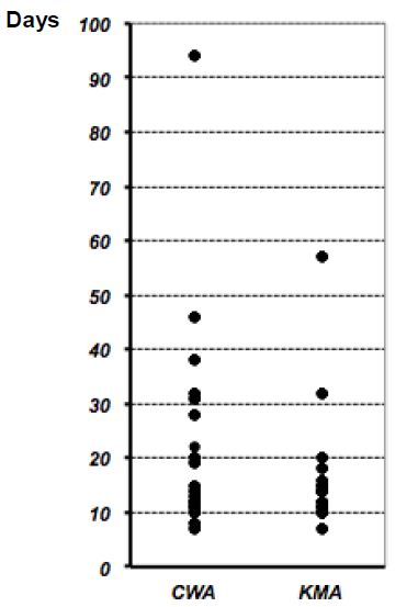
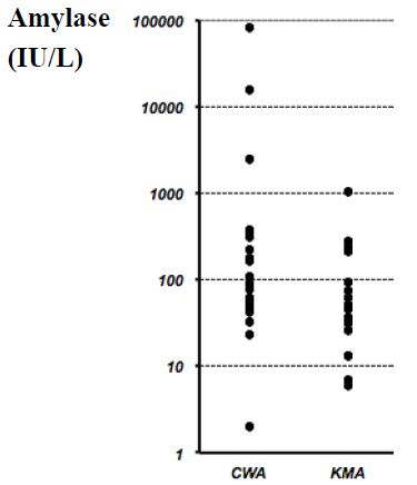
Formulation of Rivastigmine, a Liquid Drug Substance, for Use in a Simulating Study of Hollow Microstructured Transdermal Delivery System

DOI: 10.31038/JPPR.2020333

Abstract

Rivastigmine, used in the treatment of Alzheimer’s Disease, is in liquid state at controlled room temperatures. This project was aimed at developing a 0.5-mL isotonic liquid containing rivastigmine with the choice of 0.9% NaCl or 5% Dextrose Solutions for Injection as a simulating study to formulate a liquid dosage form per description of 3M hollow microneedles (https://multimedia.3m.com/mws/media/1004089O/solid-microstructured-transdermal-system-smts-sell-sheet.pdf). The surfactants were compared among Span 20, Span 80, Tween 40 and Tween 80 with benzyl alcohol or chlorobutanol as a preservative. Those formulations which formed microemulsions were further studied for stability at 4°C and 25°C up to one month. HPLC confirmed that there were no drug losses among the four microemulsions. Based on zeta potential and particle size analysis, Tween 80 with benzyl alcohol in 0.9 % NaCl is the best project formulation.

Keywords

Benzyl alcohol, chlorobutanol, Hollow Microstructured Transdermal System (hMTS), microneedles, rivastigmine, Tween and Span

Introduction

Alzheimer’s disease is an irreversible, progressive neurodegenerative disorder subsequently becoming a common cause of death [1]. Alzheimer’s is the most common cause of dementia affecting an estimated 5.8 million people in the United States [1]. In 2018, the approximate cost of caring for people with Alzheimer’s disease and other dementias was $290 billion USD, making it a huge economic burden for both patients’ families and our society and leading to a major public health problem. It is a huge economic burden for patients’ families and our society. Unfortunately, there has not been an effective treatment for Alzheimer’s disease thus far. One of the reasons is that the exact mechanism of disease development is still unclear. Acetylcholinesterase inhibitors such as donepezil, rivastigmine and galantamine, and N-methyl D-asparate receptor antagonist, and memantine are therapeutic agents. Among them, rivastigmine has the advantage of inhibiting both acetylcholinesterase (AChE) and butyrylcholinesterase (BuChE). It is also superior to the aforementioned other drugs in having two US FDA approved commercial dosage forms, that is oral capsules and transdermal patches (Table 1) [2,3]. Unfortunately, nausea and vomiting have been reported by patients taking rivastigmine oral dosage form [4]. Transdermal delivery system has a better tolerability and more efficacy compared to oral capsules [5] and enables patients who have difficulties in swallowing to take medicine more easily, and less frequently (once daily, Table 1b) [6]. However, it was reported that transdermal patch may cause skin irritation when a 24-h patch is worn. Therefore, this study focuses on the feasibility of formulating rivastigmine for use of microneedle administration and formulation characterizations. Microneedle has been gathering attention on their merits, including shorter time to reach Cmax and penetrating more drugs, especially macromolecules, than the transdermal patch dosage form [7].

Table 1: Rivastigmine dosage forms on the market: (a) oral capsules, and (b) extended release transdermal films [2,3].

(a) Oral capsules

Strength Manufacturers Applicant Holder
EQ 1.5, 3, 4.5, 6 mg BASE Brand name product Novartis
EQ 1.5, 3, 4.5, 6 mg BASE Generic products Alembic; Apotex; Aurobindo; Cadila; Chartwell; Dr. Reddy’s; Macleods; Orchid; Sun; Watson

(b) Extended release transdermal film

Strength Manufacturers Applicant Holder
4.6, 9.5, 13.3 mg/24 h Brand name product Novartis
4.6, 9.5, 13.3 mg/24 h Generic products Alvogen malta operations;

Amneal; Mylan; Zydus

Microneedles devise a pain-free penetration feature (minimally invasive device which pierces through the stratum corneum without touching the nerve endings and capillaries). Its other merits are avoidance of the first-pass, improvement of skin permeability and permeation, the delivery of both small and large molecules, achieve stable plasma concentrations for up to 7 days and possibly improvement of bioavailability. There are four subtypes of microneedles: solid, coated, dissolving, and hollow [8-10].

Colloidal Dispersions, Emulsions and Microemulsions

Colloids are heterogeneous mixture systems. Colloidal dispersion is characterized by their particle sizes and shapes. A particle size ranged between 1 nm and 1 μm makes the properties of colloids fall between solution and suspensions. Whether their particles are small enough to separate on standing or are large enough to scatter light (a phenomenon called Tyndall effect, which makes the liquid’s appearance cloudy or opaque) depends on the particle size. Therefore, colloidal dispersions are further divided into molecular colloids (solutions), association colloids and dispersion colloids [11]. Emulsions are composed of two or more immiscible liquids and suitable emulsifying agent(s), which appear milky and nontransparent because of the different optical refraction of the components. Depending on the hydrophilic and lipophilic characters, emulsions may be divided into oil in water (O/W) and water in oil (W/O) subtypes. In addition to these, multiple phases of emulsions exist as W/O/W and O/W/O microemulsions. Emulsions are kinetically stable but thermodynamically unstable based on their dispersed state and the corresponding high interfacial energy. On the other hand, microemulsions are fundamentally different from emulsions in terms of appearance, structure, and properties, which are considered between micellar solution and emulsions. Their appearances vary from transparent to opalescent, moderately viscous, and optically isotropic. Microemulsions are thermodynamically stable [11,12].

Materials

Rivastigmine (1 g and 0.5 g HY-17368 in two separate orders; liquid state in controlled room temperature) was obtained from MedChem Express (Monmouth Junction, NJ). 5 % Dextrose (also known as D5W, Lot J4J577) and 20 mL syringes were acquired from Cardinal Health (Dublin, OH). Sodium chloride (Lot: 284929), Tween 40 (polyxyethylene sorbitan monopalmitate, Lot: D5ZONHK, TGI Tokyo, Japan), methanol and 0.2 micron VWR syringe filters were ordered from VWR International (Randor, PA). Span 20 (Sorbitan monolaurate, Lot: C1885020), Span 80 (sorbitan monooleate, Lot: C182545), Tween 80 (polysorbate, Lot: C188508), benzyl alcohol (Lot: C171703), chlorobutanol, and sodium phosphate dibasic were bought from PCCA (Houston, TX).

Methods

Determination of High Performance Liquid Chromatographic (HPLC) Column

USP43-NF38 2020 recommended to assay rivastigmine and its tartrate salt by using Symmetry C18, Nova Pak C18, and Spherisorb C8 columns [13]. Buffer was first prepared as 8.9 g/L of dibasic sodium phosphate dihydrate in water (0.05 M). Mobile phase was the mixture of methanol and Buffer (0.05M sodium phosphate dibasic) in 58:42 v/v ratio. The solution was let cool to controlled room temperature before the pH adjustment to the value of 8.45 using phosphoric acid. The LC assay conditions were flow rate of 1.0 mL/min, and column temperature at 40°C. The detection wavelength was chosen at 214 nm for all study LC columns with run time at 20 minutes initially. When no impurities were seen, the run time was reduced to 15 minutes or shorter to avoid the generation of biohazard wastes from the prolonged use of mobile phase containing methanol.

Standard Curve

Ten mL of rivastigmine (which density is 1.0 g/mL) initially placed in a volumetric flask to determine its weight. A sufficient amount of the mobile phase was then added to make it into 10 mL as the stock solution, which has a concentration of 1 mg/mL (because the density of rivastigmine is 1 g/mL). This stock solution was further diluted 5-fold with mobile phase each time for sequentially six times with the eighth sample only being diluted two-fold from the seventh sample. One mL of each was transferred into a HPLC vial for assay injection. Accuracy is determined based on how close a measured value is to the actual (true) value. One of the actual (true value) may rely on the use of USP Reference Standard for comparison. Precision is determined based on how close the measured values are to each other. Since Rivastigmine USP Reference Standard was not available for the free base form to report Accuracy (but available as Rivastigmine Tartrate). This project reported the Precision instead. The HPLC conditions were as the follows: wavelength at 214 nm; flow rate 1.0 mL/min; run time 12 min; column temperature 40°C.

Formulation Preparation

3M Hollow Microstructured Transdermal System (hMTS) is an integrated device containing actuator, glass injection cartridge, delivery spring, adhesive, hollow microstructured array and application spring with information available at 3M, St. Paul, MN [12]. Each glass cartridge may house 0.5 mL to 2 mL of intradermal delivery solution (Figure 1a and 1b). In this project, 4.6 μL of rivastigmine (that is 4.6 mg) was selected to develop into 0.5 mL of liquid dosage form as a single dose. As aforementioned, rivastigmine is in liquid state at controlled room temperature, its density is 1.0 g/mL. Therefore, rivastigmine was measured by volume, instead of weight in this project. Suitable excipients such as solution for injection, surfactant and preservative were added into the final volume of 0.5046 mL, which is within the glass cartridge capacity between 0.5 mL to 2 mL. The selection of excipients such as Solutions for Injection, surfactants, and preservatives are briefly described as follows. Isotonic 0.9% saline and 5% dextrose (D5W) were chosen as Solutions for Injection. Since rivastigmine is lipophilic and in liquid state at controlled room temperature (23 ± 2°C), four surfactants (Span 20; Span 80; Tween 40 and Tween 80 (Figure 2) were added respectively to check compatibility. In addition, two preservatives (benzyl alcohol or chlorobutanol) were included. Each formulation in the saline group was composed of 0.9 g of NaCl, 5.0 g of surfactants and 1.0 g of benzyl alcohol (or 0.5g of chlorobutanol) in 100 mL final volume. The D5W group contained 5.36 g of surfactants, 1.0 g of benzyl alcohol (or 0.5 g of chlorobutanol) with sufficient amount of D5W in the total of 100 mL final volume. After mixing, the degree of transparency vs. cloudiness of all formulations were visually observed to determine candidacy for further testing. Rivastigmine 0.92 mL was taken and mixed with each 100 mL of liquid to assess particle size, zeta potential and conduct HPLC.

fig 1

Figure 1: Hollow Microneedle Transdermal System (hMTS): (a) 3M device, (b) scheme showed the inside view of the integrated device, and (c) polymer microneedle array with 12 hollow microneedles, each approximately 1500 µm [12].

fig 2

Figure 2: The appearance of surfactants from left to right: Span 20 (HLB 8.6), Span 80 (HLB 4.0), Tween 40 (HLB 15.6) and Tween 80 (HLB 15.0).

Visual Characterization

The miscibilities of resultant formulations after rivastigmine mixed with one of the two Solutions for Injection, one of the four surfactants and one of the two preservatives were visually observed.

Particle Size Analysis and Zeta Potential

Rivastigmine (9.2 μL, density 1 g/mL) was added to the aforementioned different blank formulations into the total volume of 2 mL for each. The formulations were analyzed by the NanoBrook 90 Plus Particle Sizer. The refractive indexes of rivastigmine, Span 20, Tween 40, Tween 80, benzyl alcohol, and chlorobutanol used in particle size analysis were 1.518, 1.474, 1.470, 1.473, 1.539, and 1.491, respectively (Refractive index of a medium is the ratio of the speed of light in vacuum to the speed of light in the medium. Therefore, it has no units). The zeta potentials of formulations were analyzed using NanoBrook 90 Plus Zeta Potential Reader.

One-Month Stability Study

Each formulation sample containing 4.6 μL of rivastigmine (equivalent to 4.6 mg) was subject to HPLC assay as Time 0 samples. The LC method was adopted from USP-NF 2020 [13]. One half mL of this liquid plus 4.6 μL (4.6 mg) of rivastigmine was then taken into an amber vial and crimped with an aluminum cap (as a single dose) and stored at 4°C and 25°C respectively (n = 3) for one month prior to HPLC assay to determine the drug loss and compare the stabilities among formulation candidates.

Statistics

AUCs obtained from HPLC were statistically assessed by one way or two way ANOVA tests when normality and equal variance were met. Kruska-Wallis test was used if normality and equal variance were not met. Tukey as postdoc was used to compare the three groups. Population differences are considered significant at P < 0.05.

Results

Visual Observation

When using D5W as the Solution for Injection and mixed with one of the four surfactants, the Span 20 group looked homogeneous, but Span 80 appeared as heterogeneous. Tween 40 formed a yellowish clear solution. Tween 80 was a pale yellowish clear solution. Therefore, Span 80 was excluded from further experiments. Next, one of the two preservatives was added into these formulations. Preservative (either benzyl alcohol and chlorobutanol) in Span 20 formed milky microemulsion (Table 2). Benzyl alcohol with Tween 40 resulted in colloidal dispersion, while chlorobutanol formed microemulsion. Like Tween 40, chlorobutanol with Tween 80 formed microemulsion but benzyl alcohol had colloidal dispersion. Using 0.9 % NaCl for Solution for Injection, in contrast with D5W, Span 20 and Span 80 were heterogeneous and immiscible. From these results, they were eliminated from the formulation. Tween 40 in 0.9% NaCl was a yellowish clear solution. When benzyl alcohol was added as a preservative, it formed yellowish colloidal dispersion, while chlorobutanol formed precipitations. Tween 80 in 0.9% saline was also a clear solution. When either preservative was added to Tween 80, they formed clear microemulsion.

Table 2: Miscibilities of surfactants and preservatives in D5W or 0.9% NaCl Solution.

Surfactant

Preservative

D5W

0.9% NaCl

Span 20 Benzyl Alcohol

Emulsion

Non-miscible

Chlorobutanol

Emulsion

Non-miscible

Span 80

Non-miscible

Non-miscible

Tween 40 Benzyl Alcohol

Colloidal dispersion

Colloidal dispersion

Chlorobutanol

Microemulsion

Precipitation

Tween 80 Benzyl Alcohol

Colloidal dispersion

Microemulsion

Chlorobutanol

Microemulsion

Microemulsion

Particle Size and Zeta Potential Analyses

Span 20 with each preservative in D5W, Tween 80 with chlorobutanol in D5W and Tween 80 with each preservative in 0.9% NaCl were good candidates only in terms of particle sizes (Table 3). Among D5W, Tween 40 was significant different with Span 20 and Tween 80. However, there was no significant difference by using one or the other preservatives. Within benzyl alcohol in D5W, Span 20 and Tween 40 showed significantly different. Nevertheless, Span 20 and Tween 80 or Tween 40 and Tween 80 showed no difference. Furthermore, within chlorobutanol, between Tween 40 and Span 20 or Tween 80 showed a significant difference. Among the sample groups made of 0.9 % NaCl as Solution for Injection, there is no significant difference neither caused by surfactants nor by preservatives. Tween 80 with chlorobutanol in D5W and Tween 80 with either preservative in 0.9% NaCl can especially be considered as good candidates at time zero. Zeta potentials were also showed in the first right column of Table 3. There was no significant difference in terms of which surfactant or preservative was used in D5W or 0.9% NaCl. This suggests the stabilities of all formulation were similar at time zero.

Table 3: Particle sizes and Zeta potentials of six formulas using D5W as Solution for Injection and three formulas using 0.9% NaCl as Solution for Injection.

(a) D5W as Solution for Injection

Surfactant

Preservative

Particle Size (nm)

Mean ± SD

Zeta Potential (mV)

Rivastigmine in D5W alone

434.27 ± 74.90

Span 20


Benzyl Alcohol

105.08 ± 25.53

-2.40 ± 5.85

Chlorobutanol

148.67 ± 60.42

-4.49 ± 9.67

Tween 40

Benzyl Alcohol

6356.20 ± 6314.59

-4.90 ± 1.26

Chlorobutanol

7186.41 ± 5069.88

-2.14 ± 3.10

Tween 80

Benzyl Alcohol

1749.11± 1902.47

-5.88 ± 0.62

Chlorobutanol

10.33 ± 0.17

-1.31 ± 4.77

(b) NaCl as Solution for Injection

Surfactant

Preservative

Particle Size (nm)

Mean ± SD

Zeta Potential (mV)

Rivastigmine in 0.9% NaCl alone 360.93 ± 16.68  –
Tween 40

Benzyl Alcohol

13063.80 ± 13634.23

-4.13 ± 6.75

Tween 80

Benzyl Alcohol

12.74 ± 0.17

10.54 ± 16.86

Chlorobutanol

11.49 ± 0.10

5.46             18.06

HPLC Assay

Column Selections and Standard Curve Linearity Range

Three LC columns (Symmetry C18, Nova Pak C18, and Spherisorb C8) were evaluated in this project. The tailing factors of column kinetics showed that Symmetry C18 was the best column to assay both rivastigmine and its tartrate salt form. The limit of detection of rivastigmine dissolved in mobile phase, and assayed by HPLC according to the method described in Section 5.5 was 0.00032 μL (0.0000320 mg/mL). The limit of quantification was 0.00064 μL (0.0000640 mg/mL). The linearity ranged from 0.000032 mg/mL to 1.0 mg/mL.

The AUC of the formulations which were compounded with different combinations of Solutions for Injection, surfactants and preservatives were assayed and converted into concentrations by applying with an established standard curve. In the group of using D5W as the Solution for Injection, whether the preservative was benzyl alcohol or chlorobutanol, the sample containing Span 20 had a significantly low concentration than those containing Tween 40 and Tween 80 (n = 4, p < 0.01, Figure 3a). There was no difference between either preservative (benzyl alcohol and chlorobutantol) whether the surfactant was Span 80, Tween 40 or Tween 80 (Figure 3a). When 0.9% NaCl solution was used as the solution for injection, there were no differences between Tween 40 and Tween 80 as surfactant while benzyl alcohol was the preservative (Figure 3b). Also, when Tween 80 was used as the surfactant, there was also no difference in using either preservative. The formulation containing benzyl alcohol and Tween 40 was not different to the formulation containing chlorobutanol and Tween 80 in 0.9% NaCl (n = 3, p > 0.05, Figure 3b).

fig 3

Figure 3: The rivastigmine concentrations of time 0 formulation candidates after chromatographic AUC being converted into concentrations using standard curves: (a) they were differed when D5W was used as the Solution for Injection; while (b) there was no differences when 0.9% NaCl solution was used as the solution for injection. (**p < 0.01, and ***p < 0.001).

One-Month Stability Study

Table 2 showed four of the studied formulations formed into microemulsion. They were further followed up with a stability study at 4°C and 25°C. They were Tween 40 and Tween 80 with chlorobutanol in D5W, and Tween 80 with either chlorobutanol or benzyl alcohol in 0.9% NaCl. When the samples were assayed by HPLC for drug content, there was no significant difference between time 0 and one-month in the metal-cap sealed glass vial samples stored at 4°C and 25°C, respectively (Table 4).

Table 4: The Concentration of Each Formulation at Time 0 and Stored at 4 and 25°C.

Solution for Injection

Surfactant

Preservative Mean ± SD (n = 3)
Time 0 4°C

25°C

D5W

Tween 40

Chlorobutanol 0.5165 ± 0.06047 0.5178 ± 0.06480

0.5537 ± 0.06496

D5W

Tween 80

Chlorobutanol 0.4655 ± 0.03859 0.4571 ± 0.04455

0.4693 ± 0.03319

0.9 % NaCl

Tween 80

Benzyl Alcohol 0.4358 ± 0.01938 0.4472 ± 0.00303

0.4424 ± 0.01940

0.9 % NaCl

Tween 80

Chlorobutanol 0.4519 ± 0.01719 0.4490 ± 0.00949

0.4539 ± 0.01468

After One-Month

Discussion

The stability test performed by EMEA was for up to 5 years reported that rivastigmine free base is very sensitive to oxidation, moisture and heat [14]. Degradation is accelerated by the influence of heat. Therefore, it is recommended to be stored at 5 ± 3°C with protection from light and with protective gas [14]. Although the commercial Exelon Rivastigmine Patches also used free base drug, and the FDA approved labels indicated that they may be stored at controlled room temperature, perhaps it is because this commerical patch is packaged in aluminum pouch with an internal polymer coat and external composite printable surface. In our study, we compared the product concentrations at Time 0 and after one month and found no drug loss threatened by oxidation and moisture whether the formulations were stored at 4°C or 25°C. It was because our formulation was packed in metal-cap sealed glass vials prior to being subject to each storage temperature. Since the product of this project is in liquid form (unlike the transdermal patches and oral capsules which are solids), it is suggested that the long-term storage temperature be studied.

Conclusion

When the rivastigmine concentrations among the three surfactants (Span 20, Tween 40 and Tween 80) using benzyl alcohol as the preservative in D5W were compared, Span 20 was significantly different from Tween 40 (p < 0.01). It was also different from Tween 80 (p < 0.01), while Tween 40 and Tween 80 were no different (p = 0.981). This identified that Span 20 is not a suitable surfactant. The same results were acquired when using chlorobutanol as the preservative in D5W. Span 20 was different from Tween 40 (p < 0.001) and Tween 80 (p < 0.001), while Tween 40 and Tween 80 were no different (p = 0.996). Therefore, rivastigmine is not emulsifiable by Span 20 whether the continuous phase is D5W or 0.9% NaCl. Microneedle dosage form is pain-free, minimal invasive and can be administered by health care professionals in clinics and hospital settings, trained home care personnel, or patients themselves at home. This is due to the short injection time to administer 0.5 to 2 mL without having to use a battery or electrical power (Figure 1a and 1b). Syringe filtration of 0.2 micron was applied to obtain the required sterilization of project formulations. Vacuum filtration may be tested as the first sterilization strategy in scale up due to the small volume per dose before studying another method. Future investigation can also focus on whether a preservative in the formulation of this single dose sealed product can be omitted. In the dermis dendritic cells function as immune system responses. Therefore, there will be great potential to deliver vaccines or large molecules using different subtypes of microneedles into the dermis, especially for pediatric, geriatric and other special needs patient populations.

References

  1. Alzheimer’s Association (2019) Alzheimer’s Disease Facts and Figures. Alzheimers Dement 17-57.
  2. https://www.accessdata.fda.gov/scripts/cder/ob/search_product.cfm (Accessed Nov 22, 2020).
  3. Exelon Scientific Discussion. Available at: https://www.ema.europa.eu/en/documents/scientific-discussion-variation/exelon-h-c-169-x-0038-epar-scientific-discussion-extension_en.pdf (accessed Nov 22, 2020).
  4. Birks JS, Chong LY and Grimley Evans J. (2015). Rivastigmine for Alzheimer’s disease. Cochrane Database Syst Rev. [crossref]
  5. Cummings J, Lefèvre G, Small G, Appel-Dingemanse S (2007) Pharmacokinetic rationale for the rivastigmine patch. Neurology [crossref]
  6. Sadowsky CH, Micca JL, Grossberg GT, Velting DM (2014) Rivastigmine from capsules to patch: therapeutic advances in the management of Alzheimer’s disease and Parkinson’s disease dementia. Prim Care Companion CNS Disord. [crossref]
  7. Donnelly RF, Singh TRR, Morrow DIJ, Woolfson MAD (2012) Microneedle-Mediated Transdermal and Intradermal Drug Delivery. Wiley.
  8. Dharadhar S, Majumdar A, Dhoble S and Patravale V (2019) Microneedles for transdermal drug delivery: a systematic review. Drug Development and Industrial Pharmacy 45: 188-201. [crossref]
  9. Larraneta E, Lutton RE, Woolfson DA and Donnelly RF (2016). Microneedle arrays as transdermal and intradermal drug delivery systems: Materials science, manufacture and commercial development. Materials Science and Engineering R 104: 1-32.
  10. Corrie SR, Kendall MAF (2017) Transdermal Drug Delivery. In: Hillery A, editor. Drug Delivery: Fundamentals and Applications, CRC Press, pg: 225-226.
  11. 3: Physical and Physicochemical Principles of Drug Formulation, and Ch. 18 Emulsions. (2018). In: Fahr A, Voigt’s Pharamaceutical Technology . Wiley, pg: 41-42, 549-550.
  12. https://multimedia.3m.com/mws/media/1004089O/solid-microstructured-transdermal-system-smts-sell-sheet.pdf (Accessed Nov 22, 2020)
  13. S. Pharmacopeial Convention (2020) USP Monographs: Rivastigmine. In: USP43-NF38. Rockville MD: U.S. Pharmacopeia, pg: 3922.
  14. Scientific Discussion (2007). London: EMEA. https://www.ema.europa.eu/en/documents/scientific-discussion-variation/exelon-h-c-169-x-0038-epar-scientific-discussion-extension_en.pdf (Accessed Nov 22, 2020).

Incidence and Factors of Prolonged Postoperative Ileus in Gastric Cancer Surgery

DOI: 10.31038/CST.2021612

Abstract

Objective: Prolonged Postoperative Ileus (PPOI) is a common complication after abdominal surgery, but data about incidence and risk factors of PPOI for patients with gastric cancer are rare. We sought to investigate the incidence and related incidental factors of PPOI.

Methods: A retrospective cohort study was carried out using a registry database consecutively collected from June 2016 to October 2016. The incidence and incidental factors of PPOI after gastric cancer surgery were calculated and analyzed.

Results: There were 22 patients diagnosed with PPOI. The incidence of PPOI after gastric cancer surgery was 26.5%. There were significant differences in the PPOI among ages, postoperative body temperature, postoperative opioid agents use (Dezocine) (P<0.05). Logistic regression analysis results showed that the age ≥65 years, postoperative temperature ≥38℃, the use of Dezocine after surgery were the independent risk factors of PPOI after gastric cancer surgery.

Conclusion: The occurrence of PPOI after gastric cancer surgery has great relationship with age, postoperative temperature, the use of Dezocine after surgery. We may accelerate the course of convalescence by strengthening the management of perioperative periodandtaking reasonable measures to against the risk factors.

Keywords

Gastric cancer, Prolongedpostoperative ileus, Incidental factor

Prolonged Post-Operative Ileus (PPOI) is an aberrant pattern of gastrointestinal motility, most frequently occurring after abdominal surgery. The clinical manifestations include abdominal pain, nausea, vomiting, moderate to severe sick, intolerable of a solid diet and a delayed passage of flatus and stool, which usually resolves spontaneously within 2 to 3 days [1,2]. If the symptoms persist for more than 4 days, Prolonged Postoperative Ileus (PPOI) is defined [3]. PPOI hampers the patients’ recovery, increases postoperative morbidity and leads to longer length of hospital stay [4]. Understanding the incidence and factors of PPOI can help clinicians take effective measures to reduce the incidence of PPOI, and ultimately achieve rapid recovery of patients. This study retrospectively collected the clinical information of gastric cancer patients who received surgical treatment in our department, analyzed the related factors of PPOI occurrence, in order to take targeted prevention and treatment measures.

Materials and Methods

1. Study Population

A retrospective cohort study was carried out using a PPOI registry database consecutively collected between June 2016 and October 2016 in Chinese PLA General Hospital. Among them, 62 were male and 21 were female, the ratio of male to female was about 3:1, they were between 39 and 89 years old , and the average age was (60.1 ± 11.0) years . Among them, 34 cases underwent total gastrectomy, 40 cases underwent distal gastrectomy and 9 cases underwent proximal gastrectomy.

2.  Diagnosis of PPOI

The definition of PPOI was adopted from the results of a systematic review and global survey [3]. The validity of this concept was universally accepted by a variety of investigators [5-8]. Accordingly, diagnoses of PPOI were identified if two or more of following events after day 4 postoperatively: (a), nausea or vomiting; (b) inability to tolerate an oral diet over the prior 24 hour; (c) absence of flatus over the prior 24 hours; (d) abdominal distension; (e) radiologic confirmation.

3.  Method

The clinical data of 83 patients with gastric cancer were collected, including gender, age, BMI index, previous abdominal surgery history, surgical method, surgical resection range, abdominal incision length, operation time, intraoperative blood loss, postoperative body temperature, postoperative serum leukocyte level, preoperative serum albumin level, postoperative serum albumin level, preoperative serum K + level, postoperative blood loss, the level of serum K +, the use of dezocine after operation, perioperative blood transfusion, the first time to get out of bed after operation and pathological stage. Objective to analyze the influence of various factors on the occurrence of PPOI.

Statistical Analysis

SPSS 22.0 software was used for statistical analysis. c2-test was used for count data. Logistic regression model was used for independent factor analysis. P < 0.05 was considered as statistical significance.

Results

1. Postoperative Complications of PPOI

There were 30 patients who did not exhaust and defecate within 96 hours after gastric operation, 14 patients with moderate to severe nausea and vomiting, and 28 patients with moderate to severe abdominal distension. According to the diagnostic criteria, 22 cases of PPOI occurred in 83 patients (including 3 cases of non-exhaust defecation combined with moderate to severe nausea and vomiting within 96 h, 15 cases of non-exhaust defecation combined with moderate to severe abdominal distension within 96h, and 4 cases of non-exhaust defecation combined with moderate to severe nausea, vomiting and moderate to severe abdominal distension within 96h), with an incidence of 26.5%. After conservative treatment, the clinical symptoms of 22 patients with PPOI were improved.

2. Relationship between PPOI and Clinical Factors

Univariate analysis showed that age (P = 0.001), postoperative body temperature (P = 0.031), postoperative serum K + level (P = 0.017) and postoperative analgesia with dezocine (P = 0.014) were significantly associated with PPOI. See Table 1.

Table 1: The results of the univariate analysis for factors related to PPOI.

Subgroup

Number of study’s PPOI [ (%)] X2 Value P Value
Sex

Male

62 17 (27.4) 0.105 0.746
Female 21

5 (23.8)

Age (years)

≥65 26 13 (50.0) 10.727

0.001

<65

57

9 (15.8)

BMI (kg/m²)

≥24 49 12 (24.5) 0.250

0.617

<24

34

10 (29.4)

Previous abdominal surgery

Yes 16 4 (25.0) 0.023

0.879

No

67 18 (26.9)
Operation methods

Open surgery

31 10 (32.3) 0.840 0.359
Laparoscopic surgery 52

12 (23.1)

Surgical resection range

Total stomach 34

10 (29.4)

0.279

0.870

Distal stomach

40

10 (25.0)

Proximal stomach

9

2 (22.2)

Length of abdominal incision (cm)

>10 34

9 (26.5)

0

0.995

≤10

49 13 (26.5)
Operation time (h)

≥4

39 9 (23.1) 0.444 0.505
<4 44

13 (29.5)

Operative blood loss (ml)

≥200 39

7 (17.9)

2.765

0.096

<200

44

15 (34.1)

Postoperative body temp (℃)

≥38.0 17

8 (47.1)

4.636

0.031

<38.0

66

14 (21.2)

Postoperative WBC (×109/L)

≥10 66

17 (25.8)

0.093

0.761

<10

17

5 (29.4)

Preoperative albumin (g/L)

≥30

82

21 (25.6)

2.807

0.094

<30 1

1 (100.0)

Postoperative albumin (g/L)

≥30 62 14 (22.6) 1.938

0.164

<30

21

8 (38.1)

Preoperative K+ (mmol/L)

≥3.0 83 22 (26.5)

<3.0

0

0

Postoperative K+ (mmol/L)

≥3.0 81 20 (24.7) 5.682

0.017

<3.0

2 2 (100)
Postoperative analgesia with Dezuocine

Yes

38 15 (39.5) 6.050 0.014
No 45

7 (15.6)

Blood transfusion

Yes 22 7 (31.8)

0.434

0.510

No

61 15 (24.6)
Postoperative ambulation time (h)

≥24

47 15 (31.9) 1.627 0.202
<24 36

7 (19.4)

Postoperative tumor stage

Ⅲ~Ⅳ 41

13 (31.7)

1.125

0.289

Ⅰ~Ⅱ

42

9 (21.4)

The results showed that age ≥ 65 years old, postoperative body temperature ≥ 38 ℃, postoperative use of dezocine analgesia were the independent risk factors of PPOI in patients after gastric surgery. See Table 2.

Table 2: The results of the multivariable logistic analysis for factors related to PPOI.

B

SE Wald P OR

95CI

Age(years)≥65

2.857 1.177 5.895 0.015 17.415 0.3505-0.6495
Postoperative body temp (℃) ≥38 2.764 1.110 6.202 0.013 15.855

0.2066-0.7334

Postoperative analgesia with Dezuocine

3.062 1.189 6.631 0.010 21.379

0.2859-0.4941

Discussion

Ambiguity surrounding the definition of PPOI has obscured the ability to accurately determine its incidence, although studies have typically placed this at between 10-25% following major elective abdominal surgery [9,10]. In our study, the incidence of PPOI after gastric surgery was 26.5%, which was lower to that reported by Huang et al., (32.4%) in gastric cancer [6]. The incidence of PPOI was variable in different studies due to the ambiguity about the definition. Controversies have mainly focused on the duration of ileus that should be regarded as prolonged. An observational study of 2400 consecutive patients determined 3 days as prolonged ileus, whereas Dai et al., specified 4 days and Artinyan et al., defined more than 6 days [5,11,12]. A global survey and systematic review extracted definitions from 52 identified trials and proposed 4 days as a standardized endpoint for PPOI [2]. It was well accepted in subsequent studies, and we also adopted this definition as diagnostic criteria in our study [4,13]. Given the variability in the definitions of this significant complication, further research is necessary to establish a more precise, validated definition.

Advanced age (>65 years) was identified as an independent risk factor for PPOI in our study, consistent with the finding of several previous studies [6,14]. A previous mechanism research has demonstrated that imbalances between pro- and anti-inflammatory mechanisms may be the underlying pathophysiology for the increased susceptibility to POI and the increased severity and duration of POI observed in the elderly. Moreover, elderly patients generally have a decreased nutritional and functional condition, as reflected by a higher NRS 2002 score and a higher prevalence of anemia and hypoalbuminemia in this study. Preoperative hypoalbuminemia and comorbidities were reported to be independent risk factors for PPOI in several previous studies, indicating that the decreased nutritional and functional status may play a role in the development of PPOI. In our study, these factors were associated with PPOI in the univariate analysis (Table 1), but when they were included in the multivariate analysis, these associations became not significant, which can be explained by their connections with advanced age. This result suggested that advanced age can reflect a more comprehensive body functional and nutritional status, serving as an independent risk factor for PPOI.

In the present study, we identified postoperative body temperature as an independent risk factor for PPOI. The postoperative fever after gastric surgery is mostly absorbed heat which was caused by the absorption of aseptic necrotic substances and inflammatory factors, generally no more than 38.5°C. Some fever was caused by postoperative infection, drug allergy and other reasons. Gastrointestinal tract is dominated by sympathetic nerve, parasympathetic nerve and enteric nerve. Sympathetic nerve usually inhibits gastrointestinal motility and gland secretion, while parasympathetic nerve regularly does the opposite. Fever may cause sympathetic nerve excitation, parasympathetic nerve inhibition and more water evaporation , thus causing gastrointestinal motility hypofunction, decreased secretion of digestive juice and decreased activity of digestive enzymes lead to anorexia, dry oral mucosa, abdominal distension and other clinical signs [15]. In this study, postoperative use of dezocine analgesia is also an independent risk factor for PPOI. Opiates have been widely reported to be independently associated with POI after colorectal surgery. [16-18]. This conclusion was also confirmed in gastric cancer surgery by our study. It has been demonstrated that the inhibitory effect of opiates on postoperative gastrointestinal motility was mediated by peripheral μ-opioid receptors. Postoperative opiates dose is one of the most important modifiable risk factors for POI. Therefore, various measures should be adopted to reduce the usage of opiates, including using nonsteroidal anti-inflammatory drugs as alternatives to opiate analgesics and using thoracic epidural analgesia.

In addition, it was reported that open surgery, previous abdominal surgery, hypoproteinemia, excessive infusion, perioperative blood transfusion, and delayed ambulation after operation were not conducive to the recovery of gastrointestinal function [19,20]. However, no significant statistical difference was found in the occurrence of PPOI among the above clinical indicators in this study. The reason may be related to the sample size.

There are several other limitations in this study. First, our current study is a single-center study. However, we optimized the study design to minimize possible bias. Second, there was a lack of robust external validation of the scoring system. Therefore, whether the proposed scoring system will retain its predictive capability in an independent dataset is yet to be determined. A prospective multiple-center study is required to provide evidence for the validation of the scoring system in the future.

References

  1. Vather R, Bissett I (2013) Management of prolonged post-operative ileus: Evidence-based recommendations. ANZ J Surg 83: 319-324. [crossref]
  2. Wolthuis AM, Bislenghi G, Lambrecht M, fieuws S, Buck van Overstraeten A, et al. (2017) Preoperative risk factors for prolonged postoperative ileus after colorectal resection. Int J Colorectal Dis 32: 883‐ [crossref]
  3. Vather R, Trivedi S, Bissett I (2013) Defining postoperative ileus: Results of a systematic review and global survey. J Gastrointest Surg 17: 962-972. [crossref]
  4. Mao H, Milne T, O’Grady G, Vather R, Edlin R, et al. (2018) Prolonged postoperative ileus significantly increases the cost of inpatient stay for patients undergoing elective colorectal surgery: results of a multivariate analysis of prospective data at a single institution. Dis Colon Rectum 62: 631‐ [crossref]
  5. Chapuis PH, Bokey L, Keshava A, Rickard MJFX, Stewart P, et al. (2013) Risk factors for prolonged ileus after resection of colorectal cancer: An observational study of 2400 consecutive patients. Ann Surg 257: 909‐ [crossref]
  6. Huang DD, Zhuang CL, Wang SL, Pang WY, Lou N, et al. (2015) Prediction of prolonged postoperative ileus after radical gastrectomy for gastric. Medicine (Baltimore) 94: 2242. [crossref]
  7. Moghadamyeghaneh Z, Hwang GS, Hanna MH, et al. (2016) Risk factors for prolonged ileus following colon surgery. Surg Endosc 30: 603‐
  8. Wolthuis AM, Bislenghi G, Fieuws S, de Buck van Overstraeten A, Boeckxstaens G, et al. (2016) Incidence of prolonged postoperative ileus after colorectal surgery: A systematic review and meta‐ Colorectal Dis 18: 1‐9.
  9. Kronberg U, Kiran RP, Soliman MSM, Hammel JP, Galway U, et al. (2011) A characterization offactors determining postoperative ileus after laparoscopic colectom enables the generation of a novel predictive score. Ann Surg 253: 78-81. [crossref]
  10. Millan M, Biondo S, Fraccalvieri D, Frago R, Golda T, et al. (2012) Risk factors for prolonged postoperative ileus after colorectal cancer surgery. World J Surg 36: 179-185. [crossref]
  11. Dai X, Ge X, Yang J, Zhang T, Xie T, et al. (2016) Increased incidence of prolonged ileus after colectomy for inflammatory bowel diseases under ERAS protocol: a cohort analysis. J Surg Res 212: 86‐ [crossref]
  12. Artinyan A, Nunoo‐Mensah JW, Balasubramaniam S, Gauderman J, Essani R, et al. (2008) Prolonged postoperative ileus‐definition, risk factors, and predictors after surgery. World J Surg 32: 1495‐ [crossref]
  13. Vather R, Josephson R, Jaung R, Kahokehr A, Sammour T, et al. (2015) Gastrografin in prolonged postoperative ileus: a double‐blinded randomized controlled trial. Ann Surg 262: 23‐ [crossref]
  14. Hain E, Maggiori L, Mongin C, Prost AlDJ, Panis Y (2018) Risk factors for prolonged postoperative ileus after laparoscopic sphincter‐saving total mesorectal excision for rectal cancer: An analysis of 428 consecutive patients. Surg Endosc 32: 337‐ [crossref]
  15. Wolthuis AM, Bislenghi G, Fieuws S, Overstraeten AB, Boeckxstaens G, et al. (2016) Incidence of prolonged postoperative ileus after colorectal surgery: A systematic. Colorectal Dis 18: 1-9.
  16. Bragg D, El-Sharkawy AM, Psaltis E, Maxwell-Armstrong CA, Lobo DN, et al. (2015) Postoperative ileus: Recent developments in pathophysiology and management. Clin Nutr 34: 367-376. [crossref]
  17. Thomas J (2008) Opioid-induced bowel dysfunction. J Pain Symptom Manage 35: 103-113.
  18. Wood JD, Galligan JJ (2004) Function of opioids in the enteric nervous system. Neurogastroenterol Motil 16: 17-28.
  19. Kibler VA, Hayes RM, Johnson DE, Anderson LW, Just SL, et al. (2012) Cultivating quality: early postoperative ambulation: Backtobasics. Am J Nurs 112: 63-69. [crossref]
  20. Brandstrup B (2006) Fluid therapy for the surgical patient. Best Pract Res Clin Anaesthesiol 20: 265-283. [crossref]

Distinction between Natural and Anthropogenic Contaminants of Atmospheric Precipitates from Northeastern Kansas Based on Their Elemental Contents and Strontium Isotopic Signatures

DOI: 10.31038/GEMS.2021311

Abstract

This study was designed to identify and possibly evaluate the changing occurrence of major pollutants in different atmospheric precipitates (rain, snow and hail) that were collected in northeastern Kansas next to the Konza Prairie Preservation site by analyzing their elemental and Sr isotope compositions. Potential pollutants like the local soils and their clay material, as well as the fly ash of a nearby coal-burning power plant were also analyzed. Positively correlated with K in the analyzed precipitates, the Na contents suggest a supply of fertilizers and/or natural plant organics. Combining the four identified pollutants of the precipitates that is to say the soils, the fly ash, the fertilizers and the plants allows evaluation of their changing contribution during a single precipitation event. The duration of the rain events monitors also the changing contribution of the identified pollutants. Variations of the 87Sr/86Sr ratio from precipitates during lasting events are confirmed by changing distribution patterns of the REEs. In fact, soil minerals contribute mostly at the beginning of the precipitation events and are replaced progressively by the industrial fly ash that becomes dominant towards the end of the precipitation events, depending on the duration and wind directions. At last not least, the different contaminants are recognizable by changing elemental contributions, REE distribution patterns and 87Sr/86Sr ratios. Their variable occurrence can be followed in the wet solutes, but a strict quantification cannot be provided due to elemental and isotopic interconnections between the natural and the anthropogenic contributors.

Keywords

Wet precipitates; Major, Trace and rare-earth elemental contents; Sr isotopic compositions; Soil particles; Fly ash from a power plant; Fertilizers; Plant organics; Northeastern Kansas, USA

Introduction

Myriads of complex chemical reactions between vapor-liquid molecules and dust particles of multifarious types of organic and inorganic origin constitute important links in the atmosphere between continental land and ocean mass. The survey of the solute compositions of such wet atmospheric precipitations during successive seasons or years as monitoring experiments is of high practical value to various human issues. In fact, the contents of rain solutes vary temporally and spatially in most cases due to interactions between moisture often of marine source and local nanometer-sized solid particles of natural and/or anthropogenic sources. Much information about these parameters provides sound bases for a critical understanding of the bio-geochemical influences in ecological standings on the continents and in the oceans, often on the basis of anion analyses. In fact, identification and quantification of such interactions in a given temporal and spatial setting helps understand atmospheric responses to changes in continental and oceanic conditions impacted more and more heavily by human activities. Finding the nature of the chemical imprints of atmospheric rainwaters may, therefore, increase the identification of the contributors influencing and possibly modifying the interactions between solid particles and atmospheric moist. Reconstructing chemical paths of solute atmospheric precipitations remains a challenging task as the components of rain solutes can be, even during a single precipitation event, of multiple sources including sea-spay, a wide variety of land-derived aerosols (fine erosional debris of organic and inorganic origins from land surfaces, cultivated or not), a mix of aerosols from local and regional industrial activity, together with secondary aerosols resulting from reactions in the cloudy atmosphere. In fact, nearly similar chemical and isotopic signatures may correspond to different sources, and different sources may combine to produce the same effects. The main interest, if not the only one, in the selection of specific effects in natural processes should be in the identification of the natural and anthropogenic contributors with as many criteria as possible to identify and evaluate all side impacts. The challenge is then in the identification of specific geochemical signatures that are the keys to shed light on the source or the sources of solutes in diverse atmospheric precipitations over a given region and during a given period of time. Of course, the literature is abundant with documents on the significance of the currently analyzed anions [1,2], as well as on the presence of metals and non-metals, of atmospheric precipitations for the reconstruction of their chemical evolution [3]. In many instances, they have been used to portray the potential sources of the solutes and to contribute to the understanding of elementary fluxes.

However, not speaking about organic aerosols that have been identified often in wet clouds [4], another type of rain components was seldom mentioned in the identification process, for instance the organic remnants of the plants from the Earth surface. In turn, the contours of the components from rain solutes include potentially: (1) sea-spray (and hence sea-derived solutes), (2) continental dust consisting of soil minerals, (3) industrial aerosols including atmospheric condensation products formed from industrial-derived reactants, and (4) various chemical aerosols carried by solid compounds [5]. Therefore, organic pollutants of rainwaters collected in cities [6] or in mountain snow [7] represent apparently additional components that can help identifying and evaluating the degree of natural relative to industrial pollution. However, to the best of our knowledge, an identification of natural organics deriving strictly from terrestrial plants and contaminating wet precipitations has not been addressed often until now, excluding the organics of the clouds [8] and those integrating dissolved organic carbon [9,10]. Exploring this potential organic contribution is one of the challenges of the present attempt based on elemental contents and Sr isotopic signature from varied local atmospheric precipitates, not including intentionally the anionic components. In fine, another purpose here was the use of less conventional tools susceptible to balance the supply of varied natural or anthropogenic contaminants of organic or inorganic origin in order to explore another way to analyze wet precipitates than by their anionic compositions. In addition to the major- and trace-element analyses as origin markers, the potentials of rare-earth elements (REEs) and 87Sr/86Sr isotopic ratios were also addressed to decrypt the chemical characteristics of atmospheric solutes that were collected over a local area to the NW of the city of Manhattan in eastern Kansas, U.S.A. (Figure 1A). The REE data of rainwaters, for instance, were already used as tracers of natural and anthropogenic pollution [11-14] and were included in studies of continental and oceanic aquatic systems [15]. The sampling of snow, rain and hail precipitates was completed on the site of the Kansas State University at the northwestern part of the city of Manhattan in northeastern Kansas (U.S.A.), not as a long term monitoring experiment but as a comparative determination of the chemical compositions of precipitate solutes in order to identify the major “contaminants”, natural and anthropogenic, organic and inorganic. This sampling location was chosen because it is close to the Konza National Preservation Site and about 40 km to the SWS of the operational Jeffries coal-powered electric plant of Pottawatomie. The ash rejections of this power plant were also collected and analyzed, as well as soil samples of nearby agricultural fields outside the city of Manhattan. A reason of the location choice is also the nearby occurrence of the Flint Hills that represent a huge natural space that extends from Nebraska to the N to Oklahoma to the S (Figure 1A) as alternating limestones and shales covered by surficial soils, especially along valley cuts. The basement rocks and the associated soils contain large amounts of cherts that rendered difficult crop cultivation, which explains in turn why this regional landscape is mostly covered by grass for cattle ranching [16]. Some land is also farmed next to the Flint Hills, on which the farmers spread fertilizers, another temporary pollutant of the atmosphere and the wet precipitations.

GEMS 2021-311-Fig1-Updated

Figure 1: (A) The extend of the Flint Hills in Kansas and the locations of the Konza Prairie and the Jeffries power plant with the names of the nearby cities highlighted in grey (modified from Reichman, 1991); (B) Locations of the Konza Prairie to the South of the city of Manhattan and the collection site to the North-West.

Materials and Methods

The collection period of the precipitates for the present study started at the end of 2003 until the middle of 2005 with, even, a hail event in June 2008 (Table 1). The successive wet samples were stored after collection in large super-clean polyethylene containers rinsed first with the ambient rainwaters before collection, and were analyzed right after. In the case of the long-lasting rainfalls, individual sets of samples were collected successively and were analyzed (Table 1). The pHs were measured immediately after collection and before analysis. Then, the precipitates were filtered through Gelman 0.4 μm filters and stored in super clean polyethylene bottles that were rinsed with purified nitric acid solution, and several times afterwards with deionized water. An aliquot of each precipitate was pored into a 100 cm3 clean bottle for storage, and the remainder kept in the acidified state at a pH of approximately 2.5 by adding a few drops of highly purified, vacuum distilled concentrated HNO3 acid. As the rainwaters were filtered at a 0.4 μm cut-off size, it is assumed that the analyses were completed on the total contents of the rain solutes, that is to say on the dissolved compounds and the nanometer-sized solids. A given amount of filtered and acidified rains, snow and hail-melts (generally 1500 to 2000 ml with 15 to 20 ml of highly purified 1.5N HNO3 acid) was transferred into super-clean Teflon© bottles for evaporation to dryness and re-dissolution of the evaporated mass at a known volume. The contents of the major elements were measured by inductively coupled plasma atomic emission spectrometry (ICP-AES) and those of the rare-earth elements were determined by inductively coupled plasma mass spectrometry (ICP-MS). The contents of the other metals were measured either by ICP-MS or ICP-AES, depending on their concentrations. Based on a weakly analysis of the international geo-standards like GL-O and BE-N, the analytical precisions are at a ±3.5% precision level for the concentrations of the major-elements, whereas that of the trace metals is better than ±5% and that of the REEs better than ±10% on the basis of Samuel [17] procedure. The procedural blanks for the analyses were typically below 1%, while the blank solutions were systematically below detection limit. The nanometer-sized solids that could have potentially contaminated the wet precipitations, such as minerals and organics of the local soils and the fly ash released by the coal power plant were also analyzed for their chemical contents and their 87Sr/86Sr ratios. Conversely, due to the large variety of fertilizers available on the marked [18], which obscures any average composition, this component was deliberately not analyzed, as its composition might not correspond to the local/regional situation. Alternatively, the contribution of the fertilizers was evaluated by the P contents of the precipitates, based also on the fact that fertilizers from carbonatites yield higher contents of REE, Sr, Ba and Th than fertilizers from phosphorites that are characterized by higher contents of metals, such as Cd, U and As [18]. As for the rainwaters, the major elements of the potential solid contaminants were analyzed following the same sample preparation and analysis by ICP-AES and/or ICP-MS depending on the contents. As stated, the analytical accuracy of the method was controlled routinely by the weekly analysis of the glauconite (GL-O) and basalt (BE-N) international geo-standards. The REE concentrations of the solids and precipitates were normalized relative to either the contents of the Post-Archean Average Shale [19] or compared among each other. The 87Sr/86Sr ratios of the wet precipitates and of two soil samples, their extracted <2 μm clay fractions and the ash falls were also determined. Approximately 3 to 5 μg of Sr of each liquid and solid sample were separated prior to Sr isotope analysis following a standard ion chromatography procedure on a clean cation-exchange column with double-distilled 2N HCl as the eluent [20]. Total blank Sr was less than 0.5 ng for the entire procedure including filtration, storage and chemical separation. After the column separation, about 1 μg of Sr was loaded onto a Ti filament and analyzed for the 87Sr/86Sr ratio on a multi-collector mass spectrometer. To compensate for any isotope fractionation during the isotope measurements, the measured 87Sr/86Sr ratios were normalized to an 86Sr/88Sr ratio of 0.11940. The external reproducibility of the 87Sr/86Sr ratio was controlled by periodic analysis of the NBS 987 standard that provided a mean ratio of 0.710227 ± 0.000017 (2σ of the mean for n = 70) at the time of the study. The internal precision of the 87Sr/86Sr ratio was close to 10 x 10-6 expressed as 2σ errors. Also to consolidate best the analytical database, the analyses of the soil and fly ash samples were systematically duplicated.

Table 1: Some information about the snow, rain and hail events and the collected precipitate samples.

Sample IDs

Agenda Timing pHs

Comments

Snow1

Snow2

Snow3

Snow4

26 jan. 2004

31 jan.-1 feb. 2004

1 feb.-2 feb. 2004

5 feb. 2004

8:05 AM-9:05 AM

10:40 PM-10:30 AM

3:00 PM-2:30 AM

1:00 PM-11:00 AM

nd

nd

4.55

4.71

Snow storm

same lasting snow storm

Rain1

Rain2

Rain3

Rain4

Rain5

Rain6

Rain7

Rain9

Rain10

Rain11

Rain12

Rain13

Rain14

Rain15

Rain19

Rain25

2 dec. 2003

2 dec. 2003

9 dec. 2003

25 jan. 2004

19 feb. 2004

29 feb. 2004

29 feb. 2004

3 mar. 2004

3 mar. 2004

4 mar. 2004

4 mar. 2004

21 mar. 2004

18 apr. 2004

29 apr. 2004

1 may 2004

18 june 2005

11:00 AM-11:30 AM

4:30 PM-6:30 PM

8:00 AM-8:30 AM

9:30 PM-11:00 PM

11:00 AM-1:00 PM

1:00 PM-2:30 PM

1:30 AM-4:00 AM

10:45 AM-11:15 AM

8:30 AM-11:30 AM

11:30 AM-7:30 PM

4:30 AM-8:30 AM

4.87

4.39

4.51

4.35

4.76

4.92

4.20

2.82

3.26

3.73

3.84

3.95

3.62

4.87

4.99

4.69

After the previous rain

at 10:00 AM-12:00 AM: pH 5.03

1 hour later during the same event

beginning pH at 2.82

1 hour later during the same event

Hail1

2 june 2008 10:00 AM 5.52

Hailstorm

Results

The Chemical Composition of the Solids

The contents of most major elements from soils are significantly different from those of the fly ash (Table 2). Some of these differences can be helpful to distinguish these two major contributors to the precipitates with a Si/Al ratio of the soil samples about 8 times higher than that of the fly ash, a Si/Mg ratio about 21 times higher, a Si/Ca ratio 30 to 50 times higher, a Si/Fe ratio about 9 times higher, and a Si/P ratio 40 to 50 times higher. The comparison of the major elemental contents of the rain1 and rain2 precipitates with the solid particles that passed the 0.4 μm diameter of the filter pores, with those of the elemental contents of the fly ash show about 2 to 12 times more major oxides in the wet solutes than in the fly ash (Table 3). Some precipitates contain up to 10 times more Si than Al, while others yield 4 times more Si than Al or as much Si as Al (Figure 2A). Others remain with the same Si/Al ratio during the whole length of the event (rain6 and rain7, or rain9 and rain10) unless their Si content increases. As for the Si and Al contents, those of Mg and Ca vary in the precipitates (Figure 2B), but the contents may also remain constant during a single event such as for rain6 and rain7, or for rain1 and rain2, while the ratio Na/K can change from a factor 2 during the event rain6 to rain7, to a factor 22 in rain9 to rain10 episode (Figure 2C). Similar significant differences are also visible for the trace elements with, for instance, about 7 times more Sr in the fly ash than in the soils or 43 times more Cu (Table 3). The REE contents of the fly ash are about 4 times higher than in the soils, also with different distribution patterns relative to the PAAS reference: that of the soils is irregularly increasing from La to Lu with a somewhat intermediate flat pattern from Sm to Er (Figure 3A). The REE pattern of the fly ash shows also a somewhat strong up and down centered on a positive Eu anomaly.

Table 2: Major, trace and rare-earth elemental contents of the collected precipitate samples. The contents of the major elements are in μg/g, and those of the trace and rare-earth elements are in pg/g. ∑ stands for the sum of all elements and nd for not determined.

snow1 snow2 snow3 snow4 rain1 rain2 rain3 rain4 rain5 rain6 rain7 rain9 rain10 rain11 rain12 rain13 rain14 rain15 rain19 rain25 hail1

(μg/g)

Si

14.5 20.1 7.5 5.1 19.6 69.8 20.5 2.6 37.2 4.3 29.4 3.6 7.1

1.0

1.7 5.3 9.2 12 6.5 4.6 3.2

Al

11.6 11.9 1.8 4.2 12.8 14.2 2.2 1.2 3.4 1.4

24.3

3.3 3.7 0.4 1.0 1.5 2.2 1.6 1.8 2.5 60.3

Mg

24.7 29.1 11.5 17.2 39.1 53.1 24.9 2.9 110 20.7 11.4 7.3 11.0 0.9 2.2 13.2 11.1 33.4 20.4 33.1 33.2

Ca

315 421 105 264 528 670 337 33.0 179 175 92.7 105 132 11.2 21.1 215 114.4 284 216 1646 427

Fe

8.2 12.5 1.4 1.8 11.5 9.9 0.8 1.2 0.9 0.6 4.4 1.5 1.2 0.3 0.2 0.6 1.4 0.7 4.7 1.7 2.2

Mn

1.4 2.3 0.6 1.3 2.6 6.3 2.8 0.2 3.2 1.1 1.0 1.0 0.8 0.1 0.1 0.9 1.3 3.6 2.0 1.1 2.2

Na

130 177 23.8 157 205 114 60.4 21.7 605 126 36.4 55.5 75.9 1.8 2.6 64.0 41.6 215 39.1 74.9 205

K

24.5 49.1 7.2 18.2 63.2 65.4 125 15.8 402 67.8 32.8 3.0 4.7 5.1 3.4 6.0 6.7 7.8 14.9 25.4 94.6

P

2.2 3.8 0.7 2.0 4.2 3.8 4.5 1.5 6.9 5.6 4.2 2.0 2.0 0.7 1.4 2.9 4.3 4.5 2.4 1.7 1.1

532 727 160 471 887 1007 578 79.9 1339 403 237 182 238 21.5 33.7 909 192 563 308 1791 829

(pg/g)

Sr

1.2 1.7 0.8 1.1 1.8 2.5 1.2 0.1 4.9 0.6 0.6 0.4 1.1 0.1 0.1 0.6 0.5 1.9 0.9 6.8 2.0

Rb

31.3 57.3 10.9 18.8 53.8 102 73.2 17.3 153 35.4 43.3 15.4 18.9 6.3 7.2 30.5 28.4 42.4 22.5 28.2 88.7

Ni

nd nd nd nd nd nd nd nd nd nd 30.0 40.0 45.0 19.0 17.0 50.0 49 67 140 82.0 279

Cu

nd nd nd nd nd 614 nd nd nd nd 170 180 195 88 52 270 410 318 346 1330 6536

Th

1.4 1.1 0.3 0.7 nd 2.9 1.1 0.2 1.5 0.5 1.6 0.4 0.4 0.9 0.1 0.4 0.21 1.12 1.95 0.30 0.40

U

2.5 2.2 0.8 1.3 nd 2.3 0.8 0.2 1.5 0.6 1.9 0.3 0.6 0.1 0.06 0.4 0.42 0.67 1.08 2.46 0.63

(pg/g)

La

9.8 13.7 3.2 5.1 22 110 8 1.7 7.4 3.8 7.0 3.3 3.8 2.3 nd 4.0 3.8 4.6 3.6 2.7 3.0

Ce

15.2 24.0 5.2 7.4 35.7 40.6 14.7 2.0 12.9 6.7 8.7 6.0 6.1 4.0 nd 4.7 7.1 8.6 5.4 1.7 1.9

Pr

1.9 2.9 0.64 0.9 4.8 5.5 1.9 0.2 2.0 0.9 1.0 0.8 0.9 0.4 nd 0.6 0.7 0.9 0.6 0.2 0.3

Nd

7.7 11.8 3.2 5.3 18.5 21.5 7.7 1.0 10.1 4.1 4.3 3.5 3.8 1.7 nd 2.4 3 3.8 2.4 1.0 1.2

Sm

1.7 2.5 0.6 0.8 4.0 4.8 1.7 0.2 1.9 0.8 0.8 0.7 0.7 0.6 nd 0.5 0.7 0.9 0.7 0.2 0.2

Eu

0.7 1.0 0.2 0.4 1.2 0.9 0.5 0.1 1.3 0.3 0.3 0.2 0.3 0.1 nd 0.2 0.2 0.2 0.2 0.1 0.05

Gd

2.0 2.8 0.6 0.9 4.3 4.2 1.8 0.2 1.9 0.9 0.7 0.7 0.8 0.4 nd 0.6 0.8 0.9 0.5 0.3 0.2

Tb

0.3 0.4 0.1 0.1 0.7 0.6 0.3 0.03 0.3 0.1 0.1 0.1 0.1 0.1 nd 0.1 0.1 0.1 0.1 0.03 0.03

Dy

1.3 1.9 0.4 0.6 2.8 3.4 1.2 0.2 1.3 0.6 0.6 0.5 0.6 0.3 nd 0.4 0.6 0.1 0.4 0.2 0.2

Ho

0.3 0.4 0.1 0.1 0.6 0.7 0.2 0.03 0.3 0.1 0.1 0.1 0.1 0.1 nd 0.1 0.1 0.2 0.1 0.04 0.04

Er

0.8 1.12 0.2 0.4 1.5 1.9 0.6 0.1 0.8 0.3 0.4 0.3 0.4 0.2 nd 0.2 0.3 0.5 0.2 0.1 0.1

Tm

0.1 0.2 0.03 0.05 0.2 0.3 0.07 0.01 0.1 0.04 0.05 0.04 0.05 0.02 nd 0.03 0.04 0.06 0.03 0.02 0.02

Yb

0.7 1.0 0.2 0.3 1.3 1.6 0.5 0.07 0.7 0.3 0.3 0.3 0.4 0.2 nd 0.2 0.28 0.4 0.2 0.1 0.2

∑REE

42.5

63.7 14.6 22.3 97.5 196 108 5.81 40.9 18.9 24.2 16.5 18.0

10.2

nd

13.8

17.7

21.9

14.1

6.7

7.4

Table 3: 87Sr/86Sr ratios of 5 rainwater samples with some information about the collection day, the timing of the rain event and their pH values.

Sample IDs

SiO2 Al2O3 MgO CaO Fe2O3 Mn3O4 TiO2 Na2O K2O P2O5 LoI

Total

Soil 1

61.4 9.27 1.52 2.90 3.00 0.08 0.58 0.92 2.39 0.24 17.71 100.0
Soil 1 Duplicate 64.4 10.1 1.76 3.31 3.32 0.09 0.63 0.97 2.51 0.28 11.75

99.12

Soil 2

65.4 9.73 1.44 4.62 3.13 0.07 0.67 1.10 2.48 0.17 11.37 98.73
Soil 2 Duplicate 65.5 10,0 1.48 4.70 3.25 0.07 0.69 0.92 2.46 0.18 9.44

98.73

Fly ash

17,0 20.5 8.53 37.3 6.35 0.03 1.41 2.64 0.35 2.44 3.79 100.3
Fly ash duplicate 17,0 20.8 9.08 37.1 5.99 0.03 1.41 2.32 0.36 2.53 2.21

98.82


Sample IDs Sr Cu Ni Rb Th U
Soil 1 266 bdl 66 81.8 8.86 2.53
soil 1 duplicate 286 16.0 30 nd nd nd
soil 2 140 17.0 73 nd nd nd
soil2 duplicate 141 20.0 42 69.7 9.71 2.85
fly ash 7420 360 144 13.9 34.8 17.4
fly ash duplicate 6670 422 129 nd nd nd


Sample IDs La


Ce


Pr


Nd


Sm


Eu


Gd


Tb


Dy


Ho


Er


Tm


Yb


Lu


Total
Soil 1 28.1 56.8 6.74 25.0 4.98 1.00 4.09 0.68 3.95 0,90 2.41 0.40 2.56 0.39 138.0
Soil 2 31.3 63.2 7.54 27.7 5.40 1.00 4.38 0.71 4.09 0,93 2.55 0.42 2.72 0.42 156.2
Fly ash 117 198 29.2 114 22.7 6.62 19.7 2.96 16.3 3,57 8.96 1.34 8.25 1.17 549.8


sample IDs 87Sr/86Sr (±2σ)
soil 1

soil <2 μm

fly ash

0.708607

0.708890

0.712912

11 (10-6)

46 (10-6)

14 (10-6)


Ratios Soil 1 Soil 2 Fly ash
 

SiO2/Al2O3

SiO2/MgO

SiO2/CaO

SiO2/Fe2O3

Na2O/K2O

SiO2/P2O5

Sr/Ca (10-3)

Rb/K (10-3)

U/Th


6.62

40.4

21.2

20.5

0.38

256

92.0

34.0

0.29


6.72

45.4

14.2

20.9

0.44

385

31.0

28.0

0.29


0.83

1.99

0.46

2.68

7.54

6.97

199

40.0

0.50

nd stands for not determined.

fig 2

Figure 2: (A) Si contents of the rain solutes relative to the corresponding Al contents; (B) Mg contents in the rain solutes relative to Ca contents; (C) K contents in the rain solutes relative to Na contents.

fig 3

Figure 3: (A) Rare-earth elemental distribution in the soil samples relative to that in the PAAS reference with the 2σ uncertainty; (B) REE distribution in the fly ash of the power plant relative to that in the PAAS reference; (C) REE distribution in the fly ash of the power plant relative to that in the local soils.

The pH Values of the Wet Precipitations

Systematically below 5.0 except for the hail1 precipitates, the pH was as low as 2.82 in rain9 (Table 1). Such low values are commonly attributed to industrial effects, primarily to sulfuring acid production from coal-burning sulfur dioxide production [21]. Significant SO4 concentrations represent a complementary lowering impact on pH values of rainwaters (e.g., [22], but as the anion concentrations in the solutes were not investigated in the present study, this aspect will not be discussed further hereunder. According to a regional correlation between rainwater pHs and the corresponding implemented type of the wet precipitations by [23], the pHs obtained here suggest that 90% of the precipitations are within the “acid rains” category from beginning of the 2000 decade.

The Major Elemental Contents of the Wet Precipitate Solutes

In the Snow Crystals

The contents of the major elements range from 160 to 726 μg/g in the four snow solutes (Table 2). Two samples (snow2 and snow3) were collected successively during the same event with progressively decreasing contents of all major elements. Most elements are also correlated: Si with Al, Na with K and Mg, and Fe with Ca. The fact that P decreases significantly during the progress of the snowfall suggests that some major elements could have originated from fertilizers. The two other snow solutes yield major elemental contents that are systematically between those of snow2 and snow3, often with lower contents of the correlative Si, Al, Fe, Na and K elements. Only Na yields higher contents relative to P for the snow1 and snow4 samples, suggesting a complementary contamination. Sample snow3 yields also the highest Mg/Ca and Sr/Ca ratios, probably resulting from a pronounced decrease in Ca, and the lowest K/Rb ratio due to an even more pronounced decrease in K.

In the Rainwaters

The total contents of the major elements are extremely variable in the rain precipitates: from as low as 21.5 μg/g to as high as 1339 μg/g. In fact, from sixteen analyzed solutes eight yield less than 400 μg/g of solute loads and only three yield more than 1000 μg/g. Most of them contain limited amounts of major elements: less than 2.5 μg/g Al, 5 μg/g Si, 10 μg/g Mg, 2 μg/g Fe, more than 20 μg/g Na and K, and often more than 250 μg/g Ca. This high Ca content is not surprising in a vast region characterized by outcropping Paleozoic carbonate-rich sediments and amended by fertilizers that could be of carbonated type. When two samples were collected during the same rain episode, the Si and Al contents increase systematically when the event lasted, significantly from rain1 to rain2 and from rain6 to rain7 solutes, much less from rain9 to rain10 and from rain11 to rain12 (Figure 2A). Alternatively, the Ca and Mg contents are not significantly modified during the same rain event (Figure 2B), whereas the Na content decreases significantly at least in two cases (Figure 2C). In fact, the decrease of the K and Na contents, together with P, ends close to the intersection of the two coordinates of the diagram in which the correlative contents of both elements are plotted (Figures 4A and 4B). This implies a positive relationship between these three elements, as well as between K and Na when P is absent. In turn, the correlations between P and Na, and P and K suggest that the supplies of Na and K do not originate from a single donor, because the correlation is either driven by high or by low Na and K contents. The correlations between Si and Al, Mg and Ca, and Ca and Fe are similar, as 5 ng/g of Si are detected in the solutes when Al is lacking, Ca of 60 ng/g when Fe is lacking, and Mg of 6 ng/g when Ca is lacking. In the case of the Ca vs. Mg correlation, it looks like there is only one supplier for both, except for the rain5 and rain25 samples (Figure 4C).

fig 4

Figure 4: (A and B) Correlation diagrams based on P vs. Na and K contents, respectively, in the rain solutes; (C) Correlation diagram of Ca relative to Mg contents in the rain solutes.

In the Hail

The Si contents of the hail1 sample are within those of the rain samples and above those of the snow samples. Their Mg and Ca contents are within those of the rain- and snowfalls. Potassium and Na yield both contents on the high side of the results (Table 2).

The Trace Elemental Contents of the Precipitates

The unexpected contents of trace elements from precipitates are those of Cu. Ranging between 52 and 1330 pg/g, they reach even 6536 pg/g in the hail1 sample. With only one hail analysis it is difficult to give any further thought to this high content, but it suggests a periodic and significant Cu pollution (Table 2). A study [24] showed that superphosphate is the fertilizer that contains the highest concentrations of Cd, Co, Cu and Zn impurities. As a matter of fact, all rain solutes, except two, yield far more than 100 pg/g Cu, especially during spring and can be suspected to have been supplied by fertilizers. The Sr, Th and U contents are generally low in the precipitates (Table 3), between 0.1 and 6.8 pg/g of Sr with two values beyond 5 pg/g. Those of Th vary between 0.9 and 2.9 pg/g with two values above 2 pg/g, while those of U vary from 0.1 to 2.5 pg/g with the high contents in the snow samples. The U/Th ratios vary between 1.8 and 2.7 in the snow samples, while only 5 times (less than one third of the sampling) above 2.0 in the rain solutes. The other trace elements were not determined systematically. However the contents of Zn are also very high: as much as 7472 pg/g in the rain2 and 7268 pg/g in the hail1 samples. Also, six Pb analyses appear quite high between 40 and 510 pg/g, half being below 60 and half above 150 pg/g. For Zn and Pb, a contamination by fertilizers can also be suspected on the basis of Gimeno-Garcia et al. study [24].

The Distribution Patterns of the Rare-Earth Elements from Precipitates

The REE contents of the precipitates were normalized relative to those of the Post-Archean Australian Shales [25] that are often used as a reference for materials from Earth-surface environments. This kind of comparison with the PAAS is visually accurate: those of the PAAS reference yield a higher, however flat distribution relative to the precipitates analyzed here with a fractionation of any of the REEs subsequently detected easily. The REE distribution patterns of the wet solutes were also compared to those of the soil particles and of the fly ash. The reason is that if rain solutes carry soil particles and/or fly ash from power plant, the normalization should theoretically also provide flat distribution patterns. Relative to the PAAS pattern, those of the two soil samples are increasing irregularly from La to Lu (Table 2 and Figure 3A). In a similar pattern, the fly ash outlines a significant positive Eu anomaly with progressively increasing light REEs (LREEs) and decreasing heavy REEs (HREEs; Table 2 and Figure 3B). Relative to that of the PAAS reference, the REE distribution patterns of the 4 snow samples display a flat pattern with a marked positive Eu anomaly. Also, a slight but not significant negative Ce anomaly is visible in some of the samples (Figure 5). In the case of the rain samples, the REE distribution patterns organize into three groups and some individual patterns, relative to the PAAS reference. Those of the rain3, rain6 and rain9 samples are similar to those of the three snow samples with a marked positive Eu anomaly, a slight but not significant Ce anomaly and a Gd content slightly higher than that of Sm, which somehow distorts the pattern (Figure 5). The second group consisting of the rain4, rain7 and rain13 samples is similar to the previous one with a supplementary specific marked positive La anomaly (Figure 5). The next group assembles the rain11, rain14, rain15 and rain19 samples with a similar distribution than those of the samples from previous group and the Gd or Sm contents closer to that of Eu, which gives a rounded top to the positive anomaly (Figure 5). Also the positive La anomaly even if not large is easily detectable. This pattern is very similar to that of sample rain1, whereas those of rain2 and of hail1 are very different: none yields a Eu anomaly but they include a significant positive La anomaly (Figure 5). Sample rain5 has a very straight pattern for most REEs except for the Eu anomaly. The two last rain10 and rain25 samples yield patterns with some unexpected data: the abnormally low Eu content in rain25 gives a unique pattern. The rain10 pattern is distorted by a very high Eu content, a significant negative Ce anomaly and an abnormally high Tb content, which all suggest analytical aspects. Therefore, this last sequence of patterns will not be discussed further hereunder.

GEMS 2021-311-Fig5-PNG

Figure 5: Some characteristic rare-earth elemental distribution patterns of rain solutes relative to the PAAS reference.

The 87Sr/86Sr Ratios of the Rainwaters

Five rainwater samples were analyzed for their 87Sr/86Sr ratios (Table 4). The ratios range quite widely from 0.708599 ± 0.000004 (2σ) for rain7 to 0.710278 ± 0.000005 (2σ) for rain12. It has been shown that rainwaters of successive local events can display quite large ranges of 87Sr/86Sr ratios [26] and that they may vary away from 87Sr/86Sr ratio of nearby marine waters, as is the case for those analyzed over the French territory that borders an ocean to the W and a large sea to the S [27]. Also, 87Sr/86Sr ratios of rainwaters do not necessarily remain constant during a single event [28] with values again away from nearby marine sources. Therefore, it looks like the original marine sea-spray can be discarded as a contributing component of the Kansas precipitates. The results suggest rather a changing 87Sr/86Sr ratio with a tendency to increase when the events last, such as in the case of the rain10 and rain12 samples (Figure 6). Conversely, the 87Sr/86Sr ratios of the land soil (soil 1) and of its <2 μm size fraction are quite constant at 0.708607 ± 0.000011 (2σ) and 0.708890 ± 0.000046 (2σ), respectively. This suggests that the soil supplies to the wet precipitations mostly consists of constant <2 μm sized minerals. As these values are also within those of the rainwaters, most of the soil supply being probably of carbonate origin, unless the supply of fertilizers of carbonated origin predominate. The same ratio of the fly ash is significantly higher at 0.712912 ± 0.000014 (2σ), which is clearly outside the rainwater values, and therefore not a determining argument for an identification of the major contributor to the local precipitates.

Table 4: Table combining the pertinent information on the contaminants, the determining elemental contents and ratios.

 Sample IDs Dates Timing pHs

87Sr /86Sr (±2σ in 10-6)

Rain7

29 feb. 2004 1:00 PM-2:30 PM 4.20 0.708599 (3.7)
Rain9 3 mar. 2004 1:30 AM-4:00 AM 2.82

0.708341 (4.9)

Rain10

3 mar. 2004 10:45 AM-11:15 AM 3.26 0.709167 (4.3)
Rain11 4 mar. 2004 8:30 AM-11:30 AM  3.73

0.710278 (5.0)

Rain12

4 mar. 2004 11:30AM-7:30 PM 3.84

0.709529 (4.7)

fig 6

Figure 6: Evolution of the 87Sr/86Sr ratio and the rare-earth elemental distribution in rain solutes relative to the duration of a long-lasting event.

Discussion

The relatively monotonous geological and environmental context of the State of Kansas makes that three major contaminants can be suspected to pollute the precipitates collected and analyzed here. These consist of soil particles, fly ash of the power plant and fertilizers spread periodically by the farmers to which plant organics issued from regional tall grass covering most of the Flint Hills may be added and possibly other long-distance materials transported by the winds. Considered are also the chemical components adsorbed on the potentially polluting nanometer-sized soil particles, especially on clays but also soluble carbonate crystals. In fact, while the chemical compositions of the soil particles and the fly ash were detailed, those of the fertilizers and the plant organics were only evaluated on the basis of the P contents and the P/Na, P/K and K/Rb ratios of the precipitates for reasons invoked above. If the collected wet precipitates would be polluted only by fly ash, their REE patterns should be rigorously flat. As this is not the case, it can be stated that the rain solutes incorporated several components at any time during the precipitation event and often not with the fly ash as the predominant contributor. In the detail, two waters yield a positive anomaly of either Eu in rain5, or of La in the rain2, snow2 and hail1, while rain25 yields both. Positive anomalies of La, Ce and Eu were observed in rain7, rain13, rain14, rain15 and rain19, and snow1, in fact in most studied samples.

The Major Elements of the Rain Solutes

Among the major elements dissolved or dispersed in the wet precipitates, three of the obtained correlations are especially informative: Si vs. Al, Mg vs. Ca and K vs. Na. Various correlations were obtained for the first pair with a coefficient of about 1 during the rain6-rain7 event during which both elements increase simultaneously (Figure 2). Alternatively, Si increased much more than Al in the rain1-rain2 episode with a ratio between 1/1 and 3/1. The final correlation for these two elements is at a ratio of 10/1 in favor of Si. In fact, these correlations point towards a contamination of the local outcropping rock minerals: the 10/1 ratio in favor of Si suggests a quartz contribution, whereas the ratio of 3/1 suggests an occurrence of clay-type particles. On the other hand, the ratio of 1/1 in the precipitates is similar to that of the fly ash with a significant contribution in the sample rain7. Of interest is also the changing Si/Al ratio of the rain1-rain2 event that suggests a change in the pollutants during the same episode. Calcium is positively correlated with Mg in all analyzed precipitates (Figure 4C). Its contents are about 10 to 15 times higher than those of Mg, except for one sample in which its content is up to 50 times that of Mg. As a marine origin of the rain solutes can be discarded, Ca of the wet precipitates derives probably also from regional rock outcrops that are mainly of carbonate composition. The Na vs. K correlation is also systematically positive, with the rain9, rain10, rain11, rain12, rain13, rain14 and rain15 sequence of low contents of K and increasing Na contents. In most of the other precipitates, the content of Na is 1.5 to 3.5 times that of K. Rain5 yields an abnormally high K content with a decrease of either Na in the rain1-rain2 episode, or of both Na and K in that of rain6-rain7, when the event lasts. The high alkali contents, especially that of Na, result most probably from a contribution of dissolved chlorides or sulfates to the solutes. The contents of P in the three types of precipitates, snow, water and hail can certainly be considered as representative of a fertilizer supply, supported in turn by the high contents in Cu, Zn and Pb. In fact, the contents of P are generally low and quite constant in all precipitates (Table 2), ranging from 0.7 to 3.8 μg/g in the snow samples, from 0.7 to 6.9 μg/g in the rain samples, at 1.1 μg/g in the hail sample. In fact, if fertilizers contaminated significantly the wet precipitations, their contribution was limited to those with the high P contents, probably beyond 4.5-5.0 μg/g, that is to say only in a few rain precipitates such as rain3, rain5, rain6 and rain15.

The Trace Elements in the Rain Solutes

Due to their high contents, some trace elements such as Cu and Ni suggest a predominant contamination by fly ash and fertilizers. Indeed, Cu and Ni occur in extremely high concentrations up to 1330 and 140 pg/g in the rain19 for both and in the hail1 for Ni. It could also be the case in the rain solutes with contents arbitrarily set beyond 200 pg/g, that is to say in the rain2, rain13, rain14, rain15 and rain19. High Cu concentrations in atmospheric concentrates of Ireland were, for instance, related to local mining and smelting activities [29]. These trace-elemental concentrates set a further frame for the recurrent contamination of regional precipitates.

The Signatures of the Rare-Earth Elements

The negative Ce anomaly is very typical for components that originated in marine environments due to oxidation conditions, whereas the positive Eu anomaly characterizes usually an impact of feldspar-derived materials, especially of plagioclases, in the mineral world [30,31]. However, it can also result from a diagenetic impact on clay-rich sediments [32]. As a marine supply has not yet been demonstrated on the basis of other data, the reason for the negative Ce remains to be explained. For the Eu anomaly, the presence of nanometer-sized feldspar crystals in the rain solutes can also not be denied, as well as a diagenetic impact in regionally occurring shally sediments. However, the possibility of other soluble contributions to the solutes could be more appropriate. The combined REE patterns of the main potential contributors to the rain solutes, that is to say the soil and fly-ash particles, are quite similar with a negative Ce and a positive Eu anomaly combined with a regular decrease from Gd to Lu (Figure 3C). Suzuki [33] noticed also a Tb positive anomaly with that in Eu in the airborne particulate matter from the Tokyo region, which is not visible here in any of the collected sample. As no determining differences could be evidenced among the distributions, the REE patterns of the precipitates were also compared with those of the soil particles and the fly ash. Among this quite voluminous database, the diagrams of one snow, two rainwaters and the hail were selected to provide more information about the REE patterns of each type of these precipitates (Figure 7). The two diagrams of snow2 are significantly different: that relative to the soil pattern is characterized by a positive Eu anomaly with an almost flat background for most other REEs. This background is at a precipitation/soil ratio of about 0.2. In the case of the diagram comparing the REE contents of the snow with those of the fly ash, the distribution is more irregular with again a high positive Eu anomaly, but also with a zigzagging increase from light to heavy REEs. The background of the lowest contents remains also quite stable at 0.10 to 0.12 for the comparison with the PAAS. Conversely, the two diagrams of rain5 are somehow similar with a visible positive Eu anomaly, together with increasing LREEs and decreasing HREEs. The differences are in the height of the Eu anomaly of about 1.0 in the case of the rainwater-to-soil comparison and of about 0.1 in that of the rainwater-to-ash comparison. The second difference is in the level of the flat backgrounds of the patterns, which yields an average of 0.3 for the comparison between rain and soil and of 0.8 for the comparison between rain and ash. The rain2 sample yields a different pattern: flat with no Eu anomaly but with a high La anomaly. This abnormally high La content in a few samples raises an analytical problem that relates to the non-correction for Sb-oxide in the analyses by an ICP-MS equipment like is the case here and, in turn, needs to be kept in mind. Therefore, the overall ratio between the rain and the soil as contributor is of 1, while only of 0.2 when ash is the contributor. For the hail, the two patterns relative to the soil and the ash are similar: flat with a significant positive La anomaly and a positive Lu anomaly for the comparison with the soil. As for all other diagrams, the ratios among the solutes and the contributors are up to four times higher than with the ash by comparison with the soil: at 0.04 and 0.01, respectively. No straight interpretation being obvious on the basis of these diagrams, they need to be combined with other parameters such as the metal contents, the timing and duration of the precipitations and the 87Sr/86Sr ratios to sort out the combining contaminants. The metal contents are especially high in the rain2, rain13, rain14, rain15, and rain19 and in the hail1 that were collected the 2nd of December, the 21st of March, the 18th of April, the 29th of April, the 1st of May and the 2nd of June, respectively. In summary, most of the precipitates were collected during springtime when farmers spray fertilizers on their fields. Also, soil material did probably contribute less to the solutes in wintertime when the ground is frozen, while the nearby power plant is at its highest activity.

fig 7

Figure 7: Rare-earth elemental distribution in the rain solutes relative to the soil samples in the left-side column and to the fly ash in the right-side column.

The 87Sr/86Sr Ratios of the Rain Solutes

The long rain event from 29th of February 2004 to the 4th of March 2004 provides an appropriate basis for the interpretation of the 87Sr/86Sr ratio of rain solutes (Figure 6). At the start of the event, the 87Sr/86Sr ratio was of 0.708599 ± 0.000004 (2σ), decreasing slightly to 0.708341 ± 0.000005 about 35 hours later, increasing again to 0.709167 ± 0.000004 about another 10 hours later, continuing to increase at 0.710278 ± 0.000005 about 21 hours later, and ending at a lower 0.709529 ± 0.000005 right after. To be compared to these values are those of the bulk soil at 0.708607 ± 0.000011, of its clay fraction at 0.708890 ± 0.000046, and of the ash fly at 0.712912 ± 0.000014. The bulk rock having the 87Sr/86Sr ratio of the initially collected rainwater, it was apparently the main or even the sole solid contributor, while ash was progressively added after 35h of rain to reach a maximum supply after about 50h of rain, decreasing afterwards. During this long event, the combined 87Sr/86Sr ratios of the solutes and of the potential contributors show that soil minerals contributed most at the beginning of the rain. Later, this natural supply was replaced progressively by released ash until the end of the rain.

The K/Rb Ratio of the Precipitations as the Potential Contribution of Natural Organics

Before Chaudhuri et al.‘s [34] study, plant-sourced K was not considered as a major contributor in the published models picturing the sources of K in global river [35-37]. This alternative model took into consideration the role of the land plants on the basis of the K/Rb ratio of all potential contributors. The authors estimated also the amount of K supplied by the vegetables to range between 46 and 68% of the total K contribution to the global river budget, which is significantly more than the 19 to 43% contribution by taking only the weathering of silicate-type rock material into account. On the basis of Chaudhuri et al. [34] calculations, the K/Rb ratio of silicate minerals ranges from 50 to 650, that of plants from 800 to 4,270 and that of fertilizers from 2,700 to 65,000. Here, this ratio is at 786 for the fly ash, at 356 for the soils and between 184 and 2633 for the precipitates. Considering all solutes with K/Rb ratios significantly above the K/Rb ratios attributed to the silicate minerals and the ash, a value of 800 can be viewed as critical to differentiate an organic from a mineral supply. Above 800, the K/Rb ratio of the solutes is then suggesting a contribution of natural plants, while the main contamination becomes as either natural by the silicates from soils or industrial by the rejections from power plant with a value below 800. However, because of the extremely high K/Rb ratios in fertilizers, their contribution cannot be excluded either. In summary, all rain solutes with K/Rb ratios above 800 that is to say in snow2 and snow4, as well as in rain1, rain3, rain4, rain5, rain6, rain25 and hail1, could have been potentially polluted by plant organics, which is reasonable for a collection site in the Flint Hill area that is extensively covered by tall grass and with winds oriented North to South.

How Can Natural Contaminants Differentiated from Anthropogenic Releases

The available chemical information does not allow here a quantification of the different supplies, or even a distinction between natural and anthropogenic contamination of the precipitates. In turn, the results need to support an identification of: (1) those elements characterizing the soil materials or the ash particles; (2) the abnormal elemental contents in the solutes; (3) the potential contributions of the organics from soil plants; and (4) the relative impact of the rainfall timing in a seasonal calendar. If one sets the limit between “high” and “low” contents of the major elements from different precipitates at 500 μg/g, two snow samples are on the high side (snow1 and snow2) and two are on the low side (snow3 and snow4). Among the rainwaters, nine (rain4, rain6, rain7, rain9, rain10, rain11, rain12, rain14 and rain19) are on the low side with seven even at the very low side of <250 μg/g, the total amount of major elements in hail1 being on the high side. As the SiO2/Al2O3 ratio of the soil particles at 6.7 is about 8 times higher than that of the fly ash at 0.8, wet precipitates with ratios of about 10 (Figure 2A) can then be considered to be potentially loaded with soil materials (snow3, snow5), whereas those with a ratio of 6 to 7 may be contaminated by fly ash (rain4, rain15). The precipitates with Si/Al ratios at about 1 cannot yet be classified on the basis of these criteria. The Si/Ca ratio can also be of use as it differentiates soil particles of either carbonate or silicate origin. It amounts here from 14 to 21 in the soil samples, whereas only about 0.5 in the ash. In fact, this ratio is far smaller, between 0.03 and 0.1, in the precipitates which means that there is much more Ca in the atmospheric solutes than in natural silicate and/or ash supplies. Another supplier could then be the carbonate outcrops and not the alluvial soils in and close to the study area, unless the overall mass of the locally used fertilizers is carbonated. In fact, the limestones often build low shelters in the landscape and it is then possible that the rainwaters with very low Si/Ca ratios originated outside the area of the Flint Hills. If one sets the limit of local Ca contribution at 100 μg/g in the precipitates, most of it originated clearly outside the mainly carbonated Flint Hills, which points towards the fertilizers. Another selective ratio for comparing here the potential supplies of natural soil materials and fly ash to the rain solutes combines Na and K. This ratio distinguishes the feldspars from clay materials in the geologic materials and soluble salts from solid silicates. Here the Na/K ratio is at about 0.5 for the soil components and at about 7.5 in the ash. Only the rain3, rain11 and rain12 samples yield a lower Na/K ratio. On the other hand, the snow4 and the rain14 yield Na/K ratios far higher at about 7. The P contents of the soil particles with a Si/P ratio of about 320 are even lower in the ash at about 7, while ranging from 3.5 to 10 in the snow, rain and hail samples, which suggests in turn an ash contribution in most precipitates. On the basis of significantly different K/Rb ratios for soil and ash materials, it can reasonably be considered that another contaminating component might yield K/Rb ratios above a value set at 800. As discussed earlier, such high ratios were identified in plant organics at the Earth surface and in global rivers [31]. However, it might also be remembered that fertilizers can yield very high K/Rb ratios depending on their composition [22]. The pollution of the atmospheric precipitates by either natural or industrial supplies can also be traced by their metal contents. Due to their very different contents in soil and ash particles, Cu and Ni, for instance, support an industrial pollution by the fly ash in the present case. For instance, contents arbitrarily set beyond 200 pg/g that is to say for those in rain2, rain13, rain14 and rain15 can also relate to a contamination by fertilizers. The differences in the REE contribution to the rain solutes are more in the contents than in the distribution patterns. Indeed, the most characteristic positive anomalies in La and Eu were observed in comparing the REE patterns of the rain solutes and of the potential contributors. The ratios are of 0.04 instead 0.01 when compared to the soils than to the ashes. Therefore, depending if the base line of the REE distribution patterns is lowest or highest, the major contributor can be expected to be either ash or soil materials. In summary, the potential contributions can be identified on the basis of the combined major- and metallic elemental supplies, the K/Rb ratios and the base lines of the REE patterns. Their overall combination does not allow a strict but a reasonable selection (Table 5). In the detail and on the basis of the parameters evaluated here, the compilation of the four potential contributors suggests that the precipitates carried: (1) mostly or even only ash particles in the rain11 and rain12, (2) soil components and fertilizers in the snow1, rain2, rain9 and rain10, (3) soil components and plant organics in the snow2, snow4, rain1, rain3, rain4 and rain6, (4) soil and ash components in the rain7, (5) ash and fertilizers in the snow3 and the rain14, (6) soil components, ash and fertilizers in the rain13, rain15 and rain19, and (7) ash, plant organics and fertilizers in the rain25 and the hail1. Fly ash probably occurred in five groups of precipitates, soil particles and fertilizers in four groups and plant organics in two groups. The occurrence of soil particles in the rain solutes is monitored by the contents of the major elements, the ratios K/Rb above 250 and the REE patterns. The occurrence of the ash is mainly shown by the major and metal contents and by the REE patterns. Supply of fertilizers is related to the high Ca contents (>100 mg/L), which in turn points towards fertilizers of carbonate origin, and that of organics to the high K/Rb ratios (>800).

Table 5: Distribution of the contaminant supplies as soil particles, fly ash, fertilizers and plant organics in the wet precipitates depending on elemental contents, ratios and patterns.

 Type of supply


Soil particles


Fly ash


Fertilizers


Plant organics


Major elements

rw3, rw5 rw4, rw7, rw15
Metal elements

rw2, rw13, rw14, rw15

Ca content (>100mg/L)

sn1, sn3, rw2, rw5,

rw9, rw10, rw13, rw14, rw15, rw19,

rw25, hail1

K/Rb ratio (>800)

sn2, sn4, rw1, rw3, rw4

rw5, rw6, rw25, hail1

K/Rb ratio (<250)

rw9, rw10, rw13, tw14, rw15
REE patterns

sn1, sn2, sn4, rw1, rw2

rw3, rw5, rw6, rw7, rw9,

rw10, rw13, rw15, rw19

Collection time

Winter Winter, spring, summer

Winter, spring, summer

The timing of the precipitations might be another potential aspect for differentiating the nature of the contaminants. Here, most precipitates were collected during winter (the four snow samples and the rain1 to rain13 samples), which weakens a seasonal comparison as only rain25 was collected in summer. The dominant soil supply detected mostly in the snow and the rain samples during winter appears somewhat surprising, as snow precipitates occur basically when the ground is frozen and, therefore, when the soil particles are not very sensitive to wind actions, while the soil contribution seems to be quite permanent here on the basis of the above evaluated parameters. In other words, either the parameters for identification of the soil particles in the atmospheric solutes are not accurate enough, or the soil materials are from beyond the local scale. Fly ash has also been detected in the precipitates of three seasons (winter, spring and summer), which is plausible because the power plant is located near the sample-collection place, and because it is probably in activity all year around as it produces electricity. Normally spread during springtime, fertilizers are also expected in precipitates until summertime. An estimate of the changing contamination during the same precipitation event was also addressed by comparing the contents of successively collected samples from long-lasting event. The snow2-snow3 succession highlights an initial combination of soil particles and organics that are replaced by fertilizers mixed with ash. In the case of the successive rain1 and rain2 precipitations, the organics detected in the starting rain decrease, replaced by fertilizers with soil particles. During the long rain event that was already examined for the changing 87Sr/86Sr signature of the solutes (Figure 6), collection of six successive precipitates (rain6, rain7, rain9, rain10, rain11, rain12) points towards a variable contamination that started with soil particles mixed with plant organics, continuing with a replacement of the organics by fertilizers mixed with soil particles until rain10, while ash dominates the other supplies of the solutes during the final stage. Beyond the fact that soil particles appear as the most common contaminant in this example, it shall be mentioned that the rain events started often with organics in the solutes, probably the easiest accessible to winds.

Conclusion

The present study focuses on variations of major and metallic elements, and on REE distributions that were combined with Sr isotope compositions of various atmospheric precipitations (rain, snow and hail) from northeastern Kansas. This approach does not allow a quantification of the different contaminants in precipitation solutes, but it allows a clear distinction between the contributing contaminants, which highlights another approach for the rain pollution than the more basic anionic method. In the detail, the Ca contents of the wet precipitates are positively correlated with those of Mg, as well as the Na contents with those of K. The correlation between P and Na or K allows a distinction between a fertilizer and an organic contamination. Combining soil particles, fly ash, fertilizers and plant organics as the four major contributors describes changing supplies during the lasting precipitation events. The duration is also an impacting aspect for the variable contribution of the contaminants. An extended rain event provides a descriptive variation of the 87Sr/86Sr ratio of the solutes due to the evolving mixture of the contributors, which is confirmed by the changing distribution patterns of the REEs. Combining the elemental contents and the 87Sr/86Sr ratios of precipitates, as tried here, does not provide straight answers about the respective amounts of the contributing contaminants, because some contributing components yield similar chemical data. However, the approach explored here shows that the soil minerals and natural organics appear to contribute quite systematically, and mostly at the beginning of the precipitation events for the former. When the rain events last, this initial soil supply is replaced by the industrial fly ash from nearby power plant that becomes progressively dominant towards the end of the rain events depending on the duration.

Acknowledgement

We thank the Department of Geology of Kansas State University for having made available the necessary material for the collection of the precipitates. The analyses were made at the Centre de Géochimie de la Surface of the University Louis Pasteur at Strasbourg, France. Our sincere thanks are for the technicians of these places for their help. This study was not specifically funded.

References

  1. Khemani LT, Ramana Murty BV (1968) Chemical composition of rain water and rain characteristics at Dehli. Tellus.
  2. Sanusi A, Wortham H, Millet M, Mirabel P (1996) Chemical composition of rainwater in eastern France. Atmospheric Environment 30: 59-71.
  3. Noguchi I, Kato T, Akiyama M, Otsuka H, Mastxumoto Y (1995) The effect of alkaline dust decline on the precipitation chemistry in northern Japan. Water Air Soil Pollution 85: 2357-2362.
  4. McNeill VF (2015) Aqueous organic chemistry in the atmosphere: sources and chemical processing of organic aerosols. Environmental Science Technology 49: 1237-1244. [crossref]
  5. Ervens B, Turpin BJ, Weber RJ (2011) Secondary organic aerosol formation in cloud droplets and aqueous particles (aqSOA): a review of laboratory, field and model studies. Atmospheric Chemistry and Physics 11: 11069-11102.
  6. Malik MR, Wang F, Dirpaul JM, Zhou N, Polowick PL, et al. (2007) Transcript profiling and identification of molecular markers for early microspore embryogenesis in Brassica napus. Plant Physiology 144: 134-154. [crossref]
  7. Gröllert C, Kasper A, Puxbaum H (1997) Organic compounds in high Alpine snow. International Journal of Environmental. Analytical Chemistry 117: 157-173.
  8. Carlton AG, Turpin BJ, Alteri KE, Seitzinger SP, Mathur R, et al. (2008) CMAQ model performance enhanced when in-cloud secondary organic aerosol is included: Comparisons of organic carbon predictions with measurements. Environmental Science Technology 42: 8798-8802.
  9. Hansen LD, Eatough DJ (1991) Organic chemistry of the atmosphere. CRC-Press, pg: 343.
  10. Schwarzenbach RP, Gschwend PM, Imboden DM (2016) Environmental Organic Chemistry. 3rd edition, Wiley & Sons Inc. Hoboken, USA, pg: 1005.
  11. Sholkovitz ER, Church TM, Arimoto R (1993) Rare earth element composition of precipitation particles and aerosols. Journal of Geophysical Research 98: 20587-20599.
  12. Zhang J, Liu CQ (2004) Major and rare earth elements in rainwaters from Japan and East China Sea: Natural and anthropogenic sources. Chemical Geology 209: 315-326.
  13. Kulkarni P, Chellam S, Fraser MP (2006) Lanthanum and lanthanides in atmospheric fine particles and their apportionment to refinery and petrochemical operations in Houston, TX. Atmospheric Environment 40: 508-520.
  14. Iwashita M, Saito A, Arai M, Furusho Y, Shimamura T (2011) Determination of rare-earth elements in rainwater collected in suburban Tokyo. Geochemical Journal 45: 187-197.
  15. Ryu JS, Lee KS, Lee SG, Lee D, Chang HW, et al. (2007) Seasonal and spatial variations of rare earth elements in rainwaters, river waters and total suspended particles in air in South Korea. Journal of Alloys and Compounds 437: 344-350.
  16. Reichman OJ (1991) Konza Prairie: A Tallgrass Natural History, University Press of Kansas pg: 240 .
  17. Samuel J, Rouault R, Besnus Y (1985) Standardized multi-element analysis of geological materials in plasma emission spectrometry for inductive coupling. Analysis 13: 312-317.
  18. Otero N, Vitoria L, Soler A, Canals A (2005) Fertiliser characterisation: Major, trace and rare earth elements. Applied Geochemistry 20: 1473-1488.
  19. Taylor SR, McLennan SM (1985) The continental crust: Its Composition and Evolution. Blackwell, Malden, Mass, pg: 312 .
  20. Schaltegger U, Stille P, Rais N, Piqué A, Clauer N. (1994) Nd and Sr isotopic dating of diagenesis and low-grade metamorphism of argillaceous sediments. Geochimica and Cosmochimica Acta 58: 1471-1481.
  21. Srivastava RK, Miller CA, Erickson C, Jambhekar R (2004) Emissions of sulfur trioxide from coal-fired power plants. Journal of the Air and Waste Management Association 54: 750-762.
  22. Charlson RJ, Rohde H (1982) Factors controlling the acidity of natural rainwater. Nature 295: 683-685.
  23. Herut B, Starinsky A, Katz A, Rosenfeld D (2000) Relationship between the acidity and chemical composition of rainwater and climatological conditions along a transition zone between large deserts and Mediterranean climate, Israel. Atmospheric Environment 34: 1281-1292.
  24. Gimeno-García E, Andreu V, Boluda R (1996) Heavy metals incidence in the application of inorganic fertilizers and pesticides to rice farming soils. Environmental Pollution 92: 19-25.
  25. McLennan SM (1989) Rare earth elements in sedimentary rocks; influence of provenance and sedimentary processes. Reviews in Mineralogy and Geochemistry 21: 169-200.
  26. Probst A, El Dah’mari A, Aubert D, Fritz B, McNutt R (2000) Strontium as a tracer of weathering processes in a silicate catchment polluted by acid atmospheric inputs, Strengbach, France. Chemical Geology 170: 203-219.
  27. Negrel P, Guerrot C, Millot R (2007) Chemical and strontium isotope characterization of rainwater in France: Influence of sources and hydrogeochemical implications. Isotopes in Environmental Health Studies 43: 179-196.
  28. Dupré B, Négrel P, Seimbille F, Allègre CJ (1994) 87Sr/86Sr ratio variation during a rain event. Atmospheric Environment 28: 617-620.
  29. Rosca C, Tomlinson EL, Geibert W, McKenna CA, et al. (2018) Trace element and Pb isotope fingerprinting of atmospheric pollution sources: A case study from the east coast of Ireland. Applied Geochemistry 96: 302-326.
  30. Weill DF, Drake MJ (1973) Europium anomaly in plagioclase feldspar: experimental results and semi quantitative model. Science 180: 1059-1060. [crossref]
  31. Chaillou G, Anschutz P, Lavaux G, Blanc G (2006) Rare earth elements in the modern sediments of the Bay of Biscay (France). Marine Chemistry 100: 39-52.
  32. MacRae ND, Nesbitt HW, Kronberg BI (1992) Development of a positive Eu anomaly during diagenesis. Earth Planetary Science Letters 109: 3-4.
  33. Suzuki Y, Suzuki T, Furuta N (2010) Determination of rare earth elements (REE) in airborne particulate matter (APM) collected in Tokyo, Japan, and a positive anomaly of europium and terbium. Analytical Sciences 26: 929-935. [crossref]
  34. Chaudhuri S, Clauer N, Semhi K. (2007) Plant decay as a major control of river dissolved potassium: A first estimate. Chemical Geology 243: 178-190.
  35. Meybeck M (1987) Chemical weathering of surficial rocks estimated from river dissolved loads. American Journal of Sciences 287: 401-428.
  36. Meybeck M (1988) How to establish and use world budgets of river material. In: Physical and Chemical Weathering in Geochemical Cycles. ln: A. Lerman and M. Meybeck, Kluwer, Dordrecht, (eds.). Netherlands pg: 247-272.
  37. Berner EK, Berner RA (1996) Global Environment: Water, Air and Geochemical Cycles. Prentice Hall, New Jersey, pg: 376.

The Prognostic Value of Lymphocyte-to-Monocyte Ratio and Nutritional Index for Ovarian Cancer Patients with Normal CA125 Level

DOI: 10.31038/CST.2021611

Abstract

Background: Ovarian Cancer (OC) cases with low CA-125 concentration during routine physical examination testing are troublesome and raise false negative findings ratio. The aim of this analysis was to determine whether the Lymphocyte-To-Monocyte Ratio (LMR) and the Nutritional Index (NI) of OC patients with normal CA-125 levels had a predictive role.

Methods: This retrospective study enrolled a total of 102 OC-diagnosed patients who underwent primary cytoreductive surgery and adjuvant platinum-based chemotherapy from 2010 to 2019. Using Receiver Operating Characteristic Curves (ROC) for survival analysis, optimum cut-off values for NI and LMR were calculated. The Kaplan-Meier (KM) curve and Cox regression determined the prognostic value for Overall Survival (OS) and Progression-Free Survival (PFS).

Results: The results showed that the optimal cutoff values were 47.5 and 4.25, respectively, for NI and LMR. NI was shown to be significantly correlated with FIGO stage, Grade, the involvement of malignant ascites, and platinum response, and LMR with FIGO stage, lymph node metastasis, malignant ascites, and platinum response when the population was separated using optimized cut-off. The 5-year OS and PFS were greatly enhanced by a high NI (≧47.5). A low LMR (<4.25) was associated significantly with poor 5-year PFS and OS. Both NI and LMR were independent prognosticators for the 5-year OS in multivariate analysis.

Conclusions: In CA125-normal ovarian cancer cases, elevated NI and LMR are positive prognosticators.

Keywords

Ovarian cancer, Lymphocyte-To-Monocyte Ratio (LMR), Nutritional Index (NI), Prognosis; CA125

Introduction

One of the leading causes of cancer-related mortality in women, Ovarian Cancer (OC) accounts for 295,000 new cancer cases and 185,000 deaths worldwide annually. Among malignant gynecological tumors, the OC mortality rate is the largest, which severely endangers the health of women [1]. CA-125 is the gold standard tumor marker and has thoroughly been studied in OC [2]. For OC screening and clinical evaluation help, thirty-five kilounits/L is the cut off value of serum CA125 concentration [3]. However, during the clinical examination for OC screening, not all OC patients show perfect testing outcomes. Around 20% of women with OC have serum CA125 concentrations smaller than 35 kilounits/L [4]. Elevated false negative findings are obtained during OC screening due to these low CA125 concentration cases, which do not facilitate early diagnosis of OC.

Inflammation increases the risk and development of cancer, including initiation, promotion, malignant conversion, invasion, and metastasis [5-7]. It is considered to play an important role in tumorigenesis. Recent studies have shown a negative prognostic value of higher neutrophil-to-lymphocyte ratio and lower Lymphocyte-To-Monocyte Ratio (LMR) in OC patients, suggesting that low LMR is an independent survival prognostic factor in OC patients [8]. However, the predictive role of LMR in ovarian cancer with low CA125 concentration has not been explored.

Nutritional impairment has also been shown to have a detrimental effect on clinical outcomes [9]. At the time of diagnosis, patients with OC are also subject to starvation because of inadequate nutritional consumption due to cancer-related discomfort or psychiatric issues [10]. The prognostic Nutritional Index (NI), measured as mentioned above, could be particularly useful since both inflammation and nutritional status may serve as a surrogate marker [11]. To demonstrate the connection between postoperative complications and prognosis in patients with esophageal carcinoma [12], this index was originally examined. In this study, a low NI was seen as a poor survival predictor. However, the predictive role of NI in ovarian cancer with low CA125 concentration has not been explored.

Based on these observations, it seems urgent to determine a way to prevent false negative results due to low CA125 concentration. The objective of this research was to determine the effects of NI and LMR on OC patients with low CA125 concentration.

Materials and Methods

Patient population

The research approved by Ethics Committee of Soochow University retrospectively enrolled a total of 102 OC patients who underwent primary debulking and adjuvant paclitaxel and carboplatin chemotherapy in university hospitals between January 2010 and January 2019. Due to potential influences on laboratory test outcomes, patients with any inflammatory disorder were omitted. No neoadjuvant chemotherapy was given to the patient. Histological diagnosis were based on WHO guidelines, and an expert pathologist examined all microscope slides. Information collection of absolute lymphocyte, monocyte counts, and albumin tests using a peripheral blood sample were performed within one week prior to treatment. Clinical variables of concern, including clinicopathological attributes, such as such as, age, FIGO stage, Grade, LN metastasis, malignant ascites, CA125 level, residual mass, Histopathology types, and platinum response were collected and evaluated, as shown in Table 1.

Table 1: Clinical and pathologic characteristics according to NI or LMR in 102 patients.

Variable    

All Case

NI p value LMR

p value

<47.5

47.5 < 4.25

4.25

Age <50

51

14 37 0.774 34 17

0.635

≧50

51

15 36 31

20

FIGO stage
I/II

60

24 36 0.005* 33 27

0.025*

III/IV

42

5 37 32

10

Grade
G1/G2

58

25 33 0.003* 12 46

0.531

G3

44

4 40 14

30

Histopathology
Serous

76

55 30 0.634 50 26

0.642

Others

28

14 8 16

12

LN metastasis
No

80

26 54 0.377 50 30

0.031*

Yes

22

5 17 18

4

Malignant ascites
No

67

24 43 0.046* 35 32

0.011*

Yes

35

5 30 30

5

Residual mass
<1 cm

81

26 55 0.255 51 30

0.147

≧1 cm

21

3 18 15

6

Platinum response
Sensitive

80

28 52 0.008* 48 32

0.033*

Resistant

22

3 19 17

5

Note: FIGO, International Federation of Gynecology and Obstetrics; LN, lymph node.

By dividing the baseline total peripheral lymphocyte count (cells/mm3) by the absolute peripheral monocyte count (cells/mm3), the LMR was computed. The NI was measured as follows: 10* serum albumin baseline (g/dL) + 0.005* absolute lymphocyte baseline count (cells/mm3).

Statistical Analysis

The R software x64 (version 4.0) was used to analyze the results. To evaluate variations between proportions, the Chi-square test was used, and Kaplan-Meier analysis using the log-rank test obtained the OS and PFS curves. In evaluating hazard ratios (HR) and multivariate analysis, Cox regression analysis was used. The P-values presented are two-sided, and statistical significance was considered at P<0.05.

Results

Study Population Characteristics

The normal concentration of CA125 was described in our study as patients with a concentration equal to or below 35 U/ml. The following optimal cut-off values were identified: 4.25 for LMR (AUC = 0.748, P < 0.001) and 47.5 for PNI (AUC = 0.755, P < 0.001), as shown in Figure 1. Therefore, patients with LMR > 4.25 were referred to High-LMR and patients with NI > 47.5 were referred to High-NI. Among those 102 patients, the median age was 53 years. As previously stated, in our patients, early stage disease was more frequent than advanced disease, 60 patients had stage I to II, and 42 had stage III to IV disease. The histopathological type (76 patients) is mostly serous epithelial carcinoma. Eighty-one patients were optimally debulked with less than one cm of residual disease at primary surgery. Almost all patients are sensitive to platinum (Table 1).

fig 1

Figure 1: Receiver operating characteristic curves. Receiver operating characteristic curves for predicting the survival outcome. (A) Lymphocyte to Monocyte Ratio (LMR) (B) Nutritional Index (NI).

Relations between NI, LMR and Clinical Features

The Chi-square test was used to evaluate the association between the levels of NI, LMR and clinical characteristics (Table 1), including Age, FIGO stage, Grade, Histopathology, LN metastasis, Malignant ascites, Residual mass , and Platinum response. NI was shown to be significantly correlated with FIGO stage (P = 0.005), Grade (P = 0.003), malignant ascites (P = 0.046), and platinum response (P = 0.008), and LMR with FIGO stage (P = 0.025), lymph node metastasis (P = 0.031), malignant ascites (P = 0.011), and platinum response (P = 0.033) when the population was separated using optimized cut-off.

KM analysis found that patients in the low NI group had worse PFS (P = 0.023) and OS (P = 0.046) selected for this research than patients in the high NI group. In terms of PFS (P = 0.003) and OS (P <0.016), patients in the high LMR group had greater treatment outcomes than those in the low LMR group, as shown in Figure 2.

fig 2

Figure 2: Kaplan-Meier survival curves. Kaplan-Meier survival curves by different level of LMR and NI. (A) LMR for Overall survival. (B) LMR for Progression-free survival. (C) NI for Overall survival. (D) NI for Progression-free survival.

Prognostic Values of NI and MLR

Univariate analyses showed that interactions with FIGO stage (P < 0.001), Grade (P < 0.001), LN metastasis (P = 0.002), malignant ascites (P = 0.003), histopathology (P = 0.004), residual mass (P = 0.005), platinum reaction (P = 0.009), NI (P = 0.043) and LMR (P = 0.004) were identified in the findings obtained for PFS. Multiple cox regression analysis was used to analyze the association between survival outcomes and clinical features found in univariate analysis. A FIGO level (III-IV stage) (4.022 (1.754-9.322), P=0.001), grade III (2.640 (1.333-5.229), P=0.005), residual mass 1 cm (2.540 (1.074-5.929), P=0.005) and immune platinum reaction (3.575 (2.672-6.752), P = 0.009), a low LMR (2.640 (2.364-5.731), P = 0.005) and a low NI (1.367 (0.243-2.254), P = 0.019), as shown in Table 2.

Table 2: Univariate and multivariate analyses of PFS of patients according to clinicopathological characteristics including LMR and NI.

Variable

Univariate

Multivariate

HR (95% CI)

p value HR (95% CI)

p value

Age (≥50 vs. <50)

1.544 (0.832-2.774)

0.123
FIGO stage (III/IV vs. I/II)

8.337 (3.874-14.665)

< 0.001 4.022 (1.754-9.322)

0.001*

Grade (III vs. I/II)

6.367 (2.575-10.254)

< 0.001 2.640 (1.333-5.229)

0.005*

Histopathology (Others vs. Serous)

4.723 (3.687-7.263)

0.004 1.224 (0.875-3.354)

0.479

LN metastasis (Yes vs. No)

2.633 (1.377-5.357)

0.002 1.239 (0.994-2.995)

0.632

Malignant ascites (Yes vs. No)

3.627 (1.756-6.233)

0.018 0.994(0.383-3.411)

0.255

Residual mass (≥1 cm vs. <1 cm)

4.540 (1.383-5.929)

0.015 2.540 (1.074-5.929)

0.005*

Platinum response (Resistant vs. Sensitive)

10.367 (7.575-12.254)

0.009 3.575 (2.672-6.752)

0.009*

LMR (<4.25 vs. ≥4.25)

3.066 (1.432-6.229)

0.004 2.640 (2.364-5.731)

0.005*

NI (≥47.5 vs. <47.5)

1.795 (1.575-4.254)

0.043 1.367 (0.243-2.254)

0.019*

Note: HRs was obtained from Cox s proportional hazard model. HR, hazard ratio; CI, confidence interval; NI, neutrophil lymphocyte ratio; LMR, lymphocyte monocyte ratio; FIGO, The International Federation of Gynecology and Obstetrics; LN, lymph node.

Likewise, univariate analysis showed important relationships between the following factors and OS: FIGO stage (P < 0.001), Grade (P < 0.001), LN metastasis (P = 0.033), histopathology (P = 0.014), residual mass (P = 0.007), platinum reaction (P = 0.001), NI (P = 0.034) and LMR (P = 0.001). However, COX multivariate analysis showed only the following were independent poor prognostic factor of OS, FIGO level (III-IV stage) (6.172 (2.315-10.112), P=0.003), grade III (3.640 (2.371-6.551), P=0.015), residual mass 1 cm (3.230 (2.099-4.872), P=0.035) and immune platinum reaction (6.533 (3.232-7.992), P = 0.001), a low LMR (3.540 (2.724-6.133), P = 0.002) and a low NI (1.667(0.349-3.692), P = 0.014), as shown in Table 3.

Table 3: Univariate and multivariate analyses of OS of patients according to clinicopathological characteristcs including LMR and NI.

Variable

Univariate

Multivariate

HR (95% CI)

p value HR (95% CI)

p value

Age (≥50 vs. <50)

1.454 (0.730-2.668)

0.313
FIGO stage (III/IV vs. I/II)

9.127 (3.765-20.175)

< 0.001 6.172 (2.315-10.112)

0.003*

Grade (III vs. I/II)

7.367 (3.723-12.557)

< 0.001 3.640 (2.371-6.551)

0.015*

Histopathology (Others vs. Serous)

3.436 (2.227-8.923)

0.014 2.367 (1.445-3.674)

0.331

LN metastasis (Yes vs. No)

1.783 (1.267-4.349)

0.033 1.211 (0.749-1.995)

0.362

Malignant ascites (Yes vs. No)

4.007 (1.366-5.273)

0.147
Residual mass (≥1 cm vs. <1 cm)

4.880 (2.367-6.429)

0.007 3.230 (2.099-4.872)

0.035*

Platinum response (Resistant vs. Sensitive)

9.237 (6.945-10.322)

0.001 6.533 (3.232-7.992)

0.001*

LMR (<4.25 vs. ≥4.25)

6.014 (2.397-7.379)

0.001 3.540 (2.724-6.133)

0.002*

NI (≥47.5 vs. <47.5)

1.993 (1.235-5.641)

0.033 1.667(0.349-3.692)

0.014*

Note: HRs was obtained from Cox s proportional hazard model. HR, hazard ratio; CI, confidence interval; NI, neutrophil lymphocyte ratio; LMR, lymphocyte monocyte ratio; FIGO, The International Federation of Gynecology and Obstetrics; LN, lymph node.

Discussion

For women with OC, the high fatality risk is largely attributed to a lack of early diagnosis. There is no diagnosis for certain women until the late stage, so early diagnosis of OC is urgent. The main method used for ovarian cancer screening during physical examination is actually the concentration of serum CA125 monitoring. Furthermore, CA125 concentration can also be used to evaluate longevity following surgery in women who have been diagnosed with OC. Unfortunately, not all women with OC show high concentration of CA125. The low concentration of preoperative CA125 in OC patients was 20% [13], according to a retrospective study. It indicated that certain patients were preoperative CA125-normal OC patients and that there was a lack of effective serum biomarkers to determine the prognosis.

LMR was elevated in epithelial ovarian cancer in pretreatment and showed prognostic importance after following treatment. Immune Complexes (ICs) are formed against the antigen by the antigen and antibody, and free ICs circulating are Circulating Immune Complexes (CICs) [14]. Any medium-sized CICs, however, cannot be washed and stay in the circulatory system. Inflammatory reaction, which is a central mechanism for immune-complex diseases, could be triggered by these CICs. Daniel demonstrated the presence of CICs affecting CA125 in 2010, and proposed that CA125 CICs offer a reason for ovarian cancer with normal CA125 level [15]. LMR should be a good predictor of ovarian cancer based on both of these results.

A low PNI demonstrated a decrease in serum albumin and/or a low lymphocyte absolute count. Serum albumin is an essential component in the nutritional status and inflammatory response of the host [16]. It is often considered that the absolute lymphocyte count is a significant participant in inhibiting cancer growth by initiating a cytotoxic immune response [17]. It has been documented that low immune-nutritional status is associated with an immunosuppressed disorder that offers a favorable micro-environment for tumor relapse. That may be the reason why the bad results may be caused by this immunosuppressed syndrome in low-NI patients. Important advancement in research on immune control points in tumor immunity has made it possible to elucidate the molecular mechanism underlying the immunological resistance of tumor growth. The relation between peripheral inflammatory biomarkers and immunotherapy treatment effects appears to be uncertain. These biomarkers could serve in the future as a helpful indicator of immunotherapy in the treatment of OC.

Taken together, this current literature has demonstrated that a severely compromised immune system may be affected by starvation and lymphocytopenia. The NI cutoff value reported in previous studies was 40-60 for other cancer forms [18-20]. In our study, patients with NI < 47.5 had dramatically decreased survival when multivariate regression was corrected for other prognostic factors. Furthermore, our findings have shown that low LMR is a predictor of poor prognosis in OC patients with average levels of CA125. According to the multivariate study, patients with LMR < 4.25 had a substantial decrease in OS and PFS. Moreover, since the LMR and NI are very quickly collected, the cost-effectiveness is in line with the criteria of regular screening markers.

Any of the present study’s limitations merit attention. First, we were unable to thoroughly validate the prognostic value of LMR and NI due to the retrospective aspect of the analysis. Second, LMR is a non-specific inflammation marker, and while we omitted patients with any inflammatory disorder, the existence of other unrecognized systemic inflammatory disorders could have impaired laboratory findings. The strength of our research is that it is the first attempt to evaluate the prognostic importance of LMR and NI in OC patients with normal CA125 level.

Conclusion

In summary, our current study showed that patients with higher pretreatment LMR (≧ 4.25) showed significantly better survival than those with lower LMR (<4.25); Patients with higher NI (≧47.5) revealed pretreatment LMR and NI were also an independent prognostic factor that predicts OS and PFS.

Declarations

Ethics Approval and Consent to Participate

The authors are accountable for all aspects of the work in ensuring that questions related to the accuracy or integrity of any part of the work are appropriately investigated and resolved. The study protocol was approved by the Hospital Ethics Committee of the Second Affiliated Hospital of Soochow University.

References

  1. Jelovac D, Armstrong DK (2011) Recent progress in the diagnosis and treatment of ovarian cancer. CA Cancer J Clin 61: 183-203. [crossref]
  2. Pauler DK, Menon U, McIntosh M, Symecko HL, Skates SJ, et al. (2001) Factors influencing serum CA125II levels in healthy postmenopausal women. Cancer Epidemiol Biomarkers Prev 10: 489-493. [crossref]
  3. Cramer DW, O’Rourke DJ, Vitonis AF, Matulonis UA, Dijohnson DA, et al. (2010) CA125 immune complexes in ovarian cancer patients with low CA125 concentrations. Clin Chem 56: 1889-1892. [crossref]
  4. Simmons AR, Fourkala EO, Gentry-Maharaj A, Ryan A, Sutton MN, et al. (2019) Complementary Longitudinal Serum Biomarkers to CA125 for Early Detection of Ovarian Cancer. Cancer Prev Res (Phila) 12: 391-400. [crossref]
  5. Mason M, Maurice C, McNamara MG, Tieu MT, Lwin Z, et al. (2017) Neutrophil-lymphocyte ratio dynamics during concurrent chemo-radiotherapy for glioblastoma is an independent predictor for overall survival. J Neurooncol 132: 463-471. [crossref]
  6. Wang W, Bian C, Xia D, et al. (2017) Combining Carcinoembryonic Antigen and Platelet to Lymphocyte Ratio to Predict Brain Metastasis of Resected Lung Adenocarcinoma Patients. Biomed Res Int 2017: 8076384. [crossref]
  7. Suh KJ, Kim SH, Kim YJ, He JX, Hai P, et al. (2018) Post-treatment neutrophil-to-lymphocyte ratio at week 6 is prognostic in patients with advanced non-small cell lung cancers treated with anti-PD-1 antibody. Cancer Immunol Immunother 67: 459-470. [crossref]
  8. Lu C, Zhou L, Ouyang J, Yang H (2019) Prognostic value of lymphocyte-to-monocyte ratio in ovarian cancer: A meta-analysis. Medicine (Baltimore) 98: e15876. [crossref]
  9. Oba T, Maeno K, Ono M, Ito T, Kanai T, et al. (2021) Prognostic Nutritional Index Is Superior to Neutrophil-to-lymphocyte Ratio as a Prognostic Marker in Metastatic Breast Cancer Patients Treated with Eribulin. Anticancer Res 41: 445-452. [crossref]
  10. Wang Z, Wang Y, Zhang X, Zhang T (2018) Pretreatment prognostic nutritional index as a prognostic factor in lung cancer: Review and meta-analysis. Clin Chim Acta 486: 303-310. [crossref]
  11. Okadome K, Baba Y, Yagi T, Kiyozumi Y, Ishimoto T, et al. (2020) Prognostic Nutritional Index, Tumor-infiltrating Lymphocytes, and Prognosis in Patients with Esophageal Cancer. Ann Surg 271: 693-700. [crossref]
  12. Jordan T, Mastnak DM, Palamar N, Kozjek NR (2018) Nutritional Therapy for Patients with Esophageal Cancer. Nutr Cancer 70: 23-29. [crossref]
  13. Zhang H, Huo Q, Huang L, Cheng Y, Liu Y, Bao H (2019) Neutrophil-to-Lymphocyte Ratio in Ovarian Cancer Patients with Low CA125 Concentration. Biomed Res Int 2019: 8107906.
  14. Yoshimoto T, Tanaka M, Homme M, Yamazaki Y, Takazawa Y, et al. (2017) CIC-DUX4 Induces Small Round Cell Sarcomas Distinct from Ewing Sarcoma. Cancer Res 77: 2927-2937. [crossref]
  15. Cramer DW, O’Rourke DJ, Vitonis AF, Matulonis UA, Dijohnson DA, et al. (2010) CA125 immune complexes in ovarian cancer patients with low CA125 concentrations. Clin Chem 56: 1889-1892. [crossref]
  16. Mirili C, Yılmaz A, Demirkan S, Bilici M, Basol Tekin S (2019) Clinical significance of prognostic nutritional index (PNI) in malignant melanoma. Int J Clin Oncol 24: 1301-1310. [crossref]
  17. Mantovani A, Allavena P, Sica A, Balkwill F (2008) Cancer-related inflammation. Nature 454: 436-444.
  18. Salcedo MP, Sood AK, Dos Reis R, Ramalingam P, Chen C, et al. (2019) Perineural invasion (PNI) in vulvar carcinoma: A review of 421 cases. Gynecol Oncol 152: 101-105. [crossref]
  19. Shen Y, Li H, Yuan ZQ, et al. (2020) Low pretreatment PNI correlates with worse survival in patients with stage III/IV NSCLC who received chemotherapy. Neoplasma 67: 394-401. [crossref]
  20. Lv X, Zhang Z, Yuan W (2020) Pretreatment Prognostic Nutritional Index (PNI) as a Prognostic Factor in Patients with Biliary Tract Cancer: A Meta-Analysis. Nutr Cancer 1-10. [crossref]