Author Archives: author

Bionomic Parameters Significance in Covid-19 Contagion Dynamics, Monza-Brianza Province (Italy)

DOI: 10.31038/PEP.2021231

Abstract

Background: In etiopathology, a reductionistic asymmetry favors biology and marginalizes ecology. This misunderstanding is a challenge to overcome because health and disease depend on the entire life organization’s state. This research underlines how the Bionomics discipline is capable of completing the study on Covid-19 contagion dynamics in Monza-Brianza province.

Methodology: After a recall of the principles of Bionomics, the bionomic state of the Monza-Brianza (M-B) province is exposed. The bionomic functionality (BF) of each municipality, evaluated as landscape unit (LU), is compared with the mortality rate (MR) and the Covid-19 infections (%).

Results: Bionomic functionality (BF) emerges as the strongest correlation in opposition to the ecological density of the population, which becomes dominant after 2.5% of infected people. Other parameters, as PA (population age), seem to be less critical.

Interpretation: Environmental exposure and exchanges, and their interaction with the body’s biological systems and apparatuses, play an essential role in disease development. The main processes will be underlined. Significantly Prevention must change perspective, leading Medicine more systemic, from sick care to health care.

Keywords

Covid-19, Landscape Bionomics, contagion dynamics, macro-scale biologic processes.

Introduction

In many seminars and publications, Ingegnoli affirmed that traditional Biology focused on small scales (from biomolecule to the organism) is still mainly reductionist, so marginalizing broad scales (from community to landscape and biosphere). For instance, Medicine seems to be interested only in traditional Biology. Nevertheless, the ‘rock in the pond’ [1] of the Systemic Turn in scientific paradigms imposes to change our vision: biology does not concern only micro-scales.

We can see that the biological studies on bio-chemical molecules, genetics, viruses, metabolism brought to great successes, but also made insidious errors as, for instance, the statement of DNA as the “central dogma of molecular biology” [2], wrong because the DNA is not a set of formed characters but a set of potentialities [3]. Another tricking error is just the marginalization of macro-scales, which brought to refuse a proper scientific role to the researches in this field. In Medicine, we can see two reactions: (a) many researchers think even today to the fallacy of ecological aspects in etiology, and (b) some doctors app It is deepening the Systemic Theory,  the difference between what reciate the problems that come with environmental degradation but, generally, see them as someone else’s problem to solve, while they focus on repairing the damage. So, it is not entirely clear what the medical profession/students are meant to ‘do’ with the ecological problems and how they can use them to help patients. However, recently, some Medical communities recognize that human alteration of Earth’s ecological systems threatens humanity’s health. This fact has given rise to Global Health and Planetary Health, which are interdisciplinary while, first of all, they must be systemic and pursue a preferential relationship between advanced Ecology and Medicine [4].

This misunderstanding between Medicine and Ecology is a challenge: we must overcome this impasse! Thus, we cannot discuss the unity of Life, but we have to understand better how its scalar interrelations may influence our health. The alterations of Life at macro-scales can damage human health, not unlike at small ones. Note that the underestimation of the environment is rooted in Neo-Darwinian’s thinking: concepts such as the struggle for existence and natural selection are metaphors [5], not theories, so Darwin’s hypothesis becomes “the best-adapted individuals are more likely to have descendants.” Thus, other limits of Darwinism appear:

  • In biology, it is possible to demonstrate that the struggle for existence is less significant than cooperation and symbiosis [6, 7];
  • Mathematics has shown that in a complex system, a random variation always produces damage: e.g., Arnold, Moser, and Kolmogorov’s theory, [8];
  • Bio-semeiotics has shown that, in addition to genetic codes, there are other organic and mental codes [9] involved in evolution;
  • The epigenetic control of gene expression due to DNA methylation demonstrates that the phenotype is not directly expressed by the genotype [10], and part of the genome’s methylation pattern can be inherited in the Lamarckian sense.

The dependence of gene expression on the environment is now clear, as confirmed by Psycho-Neuro-Endocrine-Immunology [11]. We move from a mechanistic vision to a complex and systemic one: not only what is written in the sequence of the DNA bases matters, but also their modulation due to the information that the environment and behavior express.

After this introduction, we can see that overcoming the mentioned misunderstanding between Medicine and Ecology needs a theoretical premise on Landscape Bionomics [12] and an example of application that correlates bionomics, landscape health, and a disease’s incidence.  Starting from a recently published study on Covid-19 incidence in the province of Monza-Brianza at the beginning of this pandemic (March-November 2020) [13], it could be stimulating to complete the study on this contagion dynamics in the second substantial increase (November 20-May 21). Therefore, an innovative discussion will follow.

Theoretical References

From Traditional Ecology to Bionomics

Traditional Ecology asserts that Life organization consists of hierarchic levels: cell, organism, population, communities (i.e., the “biological spectrum” sensu EP Odum [14]) and their life support systems. However, we may observe that the world around Life (an organism, a community) concerns other life systems; so, the concept of ‘support’ must be changed into that of ‘integration’. That is why the concept of Life cannot be limited to a single organism or a group of species, but it also includes ecocoenotopes, landscapes, ecoregions, and the entire ecosphere (eco-bio-geo-noosphere): as all remember, the Gaia Theory [15] has claimed that the Earth can be considered a near-living entity.

Inquiring into what stated by Bionomics (i.e., the Theory of Life Organization on Earth) [12,16,17], Life on Earth is a complex open process, operating as a hyper-complex system with a continuous exchange of matter, energy, and information with its environment: information is the exchange (interrelation) that allows the emergence of cognitive distinction (order) between players (the components of the system). Thus, Life on Earth is organized in a hierarchy of six interrelated space-time-information levels (Tab.1)and each level cannot exist without its proper environment because of these integrations and exchanges.

Understanding the Systemic Theory, it is evident the difference between what exists (Real Systems: Life on Earth organized in Living Entities) and the different approaches to studying the environment (viewpoints). As exposed in Tab.1: it is a complete transformation of the main principles of traditional ecology by being aware that hierarchical levels are types of living complex systems; so, it is possible to define a state of health for each level.

Table 1: Hierarchic levels of Biological Organisation on the Earth

Scale of Real Systems

Viewpoints BIONOMICS
SPACE1 CONFIGURATION  

BIOTIC2


FUNCTIONAL3

CULTURAL-ECONOMIC4

Global (Earth)

Geosphere

Biosphere Ecosphere Noosphere

Geo-eco-bio-noosphere

Continental (Region)

Macro-chore

Biome Biogeographic system Regional Human systems

Ecoregion

Territorial (Province)

Chore

Set of communities Set of Ecosystems District Human systems

Landscape

Local (District)

Micro-chore

Community Ecosystems* Local Human systems

Ecocoenotope

Stationary

Habitat

Population Population niche Cultural/Economic

Meta-population

Singular

Living space

Organism Organism niche Cultural agent

Meta-organism

1= not only a topographic criterion, but also a systemic one; 2= Biological and general-ecological criterion;

3= Traditional ecological criterion; 4= Cultural intended as a synthesis of anthropic signs and elements;

Bionomics = Types of living entities really existing on the Earth as spatio-temporal-information proper levels

*The term Ecosystem may be available following the functional viewpoint but, if we refer to the whole system, it must be identified as Ecocoenotope.

Some Basic Concepts of Environmental Functionality

As one can read within the book “Frontiers of Life,” edited by Baltimore, Dulbecco, Jacob, and Levi-Montalcini and published by Treccani (Rome) and Academic Press (Boston) 1999-2001, the section on Landscape Ecology [18] already stated that…

(a) Processes allowing life definitions are ontological, but each specific biological level emerges, expressing these processes adequately.

(b) The relation between pathology and ecology of the systems will allow a diagnosis of each of them in a clinical sense.

(c) Territorial and regional space-time-information scale and the related living systems (landscape and ecoregions) are the most directly involved in human pathology insurgence.

(d) Both the landscape and the system of landscapes (=region[1]) are complex systems, existing as a biological entity within an entire Life’s Hierarchy, whose character and behavior are morethan the result of the action and interaction of natural and human components [18]. Thus,

(e) The landscape structure is not an ecological mosaic, as stated by conventional ecology, but an ecotissue: a multidimensional structure, as a histologic tissue, which represents the hierarchical intertwining of the ecological upper and lowers biological levels and of all their relationships within the landscape (Fig.1, a).

(f) As living systems, landscapes are self-organizing, adaptive, dynamic, self-regulating, dissipative, metastable.

(g) The crucial role in ensuring Life and structuring landscapes pertains to vegetation communities, the physiology of which leads to the concept of the ‘latent capacity of homeostasis’ of a phytocoenosis: it needs to dissipate their energy’s excess to maintain their organizational and metastability level, through a flux (Mcal/m2/year) evaluable by a systemic function, the Biological Territorial Capacity of Vegetation (BTC) [18,19].

The natural landscape units and sub-units, with the dominance of natural components and biological processes, capable of healthy self-regulation, represent the Natural Habitat (NH). By contrast, the transformed sub-units of human landscape (e.g., urban, industrial, and rural areas) but also the semi-human ones (e.g., semi-agricultural, plantations, ponds, managed woods), each with its proper weighted average value of human apport of subsidiary energy and technology, represent the systemic state function named Human Habitat (HH) able to evaluate how much men can affect and limit the natural systems’ self-regulation capability. Following Bionomics, the HH cannot be the entire territorial (geographical) surface (% of Landscape Unit, LU).

Processes, functions, and roles within landscapes, relating abiotic components, vegetation, fauna, and humans, are performed through formal elements organized as Landscape Apparatuses. The main Landscape Apparatuses can be defined as follows (Fig.1, b):

  1.  HGL = Hydro-geologic (emerging geotopes or elements dominated by geomorphic processes)
  2.  RNT = Resistant (elements with high metastability, e.g., forests)
  3.  RSL = Resilient (elements with high recovery Capacity, e.g., prairies or shrublands)
  4.  PRT = Protective (elements that protect other components or parts of the mosaic)
  5.  PRD = Productive (elements with high production of biomass: agricultural fields, meadows)
  6.  SBS = Subsidiary (systems of human energetic and work resources) as industrial and trade
  7. RSD = Residential (systems of human residence and dependent functions)

Note that both the natural and the anthropic Landscape Apparatuses present natural and human aspects (Fig.1b).
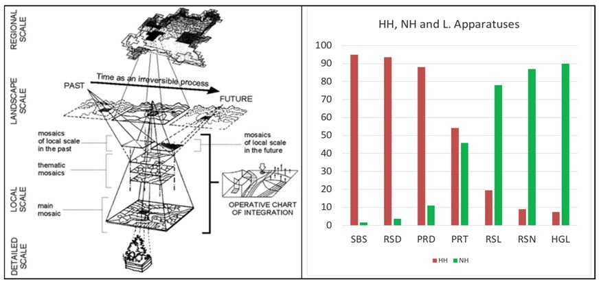
fig 1

Figure 1: (a) The concept of ecotissue is represented to the left (from Ingegnoli, 2002) [19]. (b) The main landscape apparatuses are expressed related to the concept of HH and NH. Both the pictures are referred to the Lombardy region, North of Italy.

The set of portions of the landscape apparatuses (within the examined LU) indispensable for an organism to survive is better known as Standard Habitat per capita (SH). It represents the state function strictly related to the previous concepts (m2/inhabitant) [12]. It is available for an organism (man or animal), divisible in all its components, biological and relational. In the case of human populations, we will have SHHH, that is an SH referred to the human habitat (HH):

SHHH = (HGL+PRD+RES+SBS+PRT) areas / N° of people [m2/inhabitant]

The connected Minimum Theoretical Standard Habitat per capita (SH*) is the state function estimated as dependent on (a) the minimum edible Kcal/day per capita [1/2 (male + female ) diet]; (b) the productive capacity (PRD) of the minimum field available to satisfy this energy for one year, taking into account the production of primary crops of organic farming; (c) an appropriate safety factor for current disturbances; (d) the need for natural or semi-natural protective vegetation for the cultivated patches[12]. It is estimable for each type of animal population too. Finally, the ratio SH/SH*, named Carrying Capacity (s) of a LU, is the state function able to evaluate the self-sufficiency of the human habitat (HH), a basilar question for sustainability and ecologicalterritorial planning.

Biological Territorial Capacity of Vegetation (BTC)

This function represents the fundamental state function of a territorial system, proved the fundamental role of vegetation communities (both natural and anthropized, even if with different significance) in managing the whole system’s energy to reach, rebalance and maintain its proper metastable equilibrium.

It can be studied on the basis of: (a) the concept of resistance stability; (b) the type of vegetation community; (c) its metabolic data (biomass, net or gross primary production, respiration, B, NP, GP R); (d) their metabolic relations R/GP (respiration/gross production) and (e) their order relations R/B (respiration/biomass) = dS/S (antithermic maintenance). Two coefficients can be elaborated:

ai = (R/GP)i / (R/GP)max      bi = (dS/S)min/(dS/S)i

ai measures the degree of the relative metabolic capacity of principal vegetation communities;

bi measures the degree of the relative anti-thermic (i.e., order) maintenance of the same central vegetation communities.

The degree of the homeostatic capacity of a phytocoenosis is proportional to its respiration. It can be expressed as the flux of energy that the phytocoenosis must dissipate to maintain its condition of order and metastability [Mcal/m2/year].

BTCi = (ai + bi ) Ri  w   (Mcal/m2/year)

where w = 1.4-1.6 (root biomass coefficient)

Therefore, the BTC function is essential because it is systemic and can evaluate the flux of energy available to maintain the order reached by a complex system.

The comparison between two very different agrarian landscapes near Milan in Fig.2 shows HH’s useful applications and BTC’s exposed concepts. Note that the BTC level difference is very sharp: Oltre-Po BTC = 1.75 Mcal/m2/year Vs. Chiaravalle BTC = 0.73 Mcal/m2/year, while the HH are closer. This example may also demonstrate bionomic principles’ capability to evaluate a complex ecological system’s health in a very synthetic view.
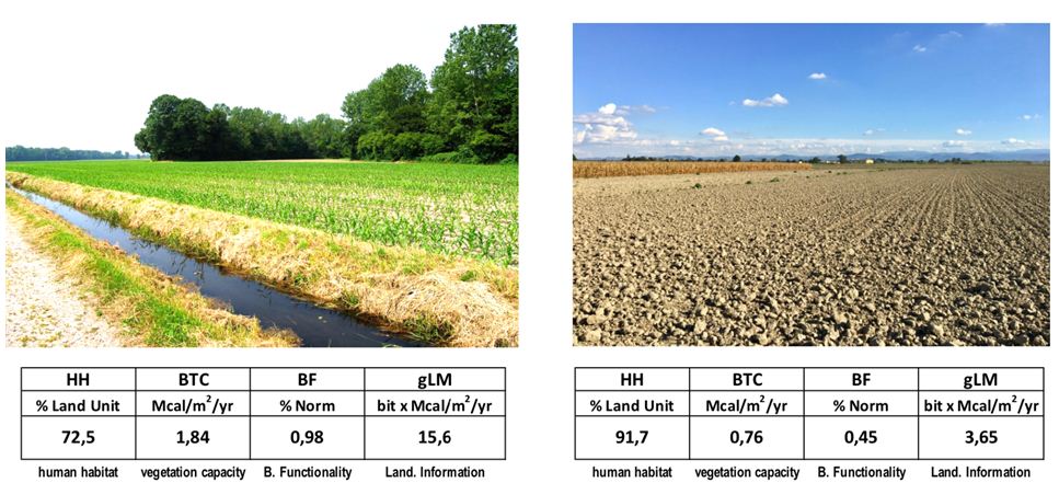
fig 2

Figure 2: The comparison between two very different agrarian landscapes near Milan. The difference in BTC level is very sharp and the two measures of HH, and BTC can demonstrate the capability of bionomic principles to evaluate the health of a complex ecological system in a very synthetic view. Bionomic Functionality and Landscape Information level are related to the ethological unconscious alarm recording process, as we will see later.

Bionomics Functionality (BF)

Focusing on the possibility to reach a simple way to frame the general health state of a territorial unit, after the study of 45 landscape units (in North Italy), an excellent correlation between the Biological Territorial Capacity of Vegetation (BTC) and the Human Habitat (HH) was found with an R2 = 0.95 and a Pearson’s correlation coefficient of 0.91 (significance = 2.93).

As we can see in Fig.3, it was possible to build the simplest mathematical model of bionomic normality, available for the first framing of landscape units’ dysfunctions.
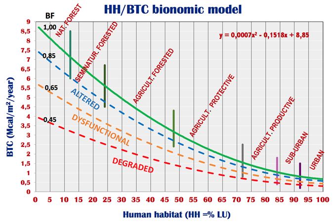
fig 3

Figure 3: The HH/BTC model, able to measure the bionomics state of a LU. Dotted lines express the BF level, that is the bionomics functionality of the surveyed LU. From Ingegnoli [12].

Below normal values of bionomic functionality (BF= 1.15- 0.85), with a tolerance interval (0.10-0.15 from the curve of normality) we can register three levels of distorted BF: altered (BF = 0.85-0.65), dysfunctional (BF = 0.65-0.45) and highly degraded (BF < 0.45). The vertical bars divide the main types of landscapes, from Natural-Forest (high BTC natural) to Dense-Urban: each of them may present a syndrome.

Again, this model is indispensable to reach a first eco-bionomics diagnosis on the health of an examined landscape unit (LU), thus to give a simple suggestion of the eco-bionomic quality of the place where patients live, to control the effects of a territorial planning design, to study the landscape transformations, etc. It is a complex model because both HH and BTC are not two simple attributes, and their behavior is not linear.

Methodology

The Bionomic State of the Monza-Brianza (M-B) province (Lombardy)

The study on the environment-health alterations in M-B (2011-2017) had many reasons: this province presents the higher ecological density of population (25.1 people/ha) with a high human habitat (HH = 82 %), is the nearest to Milan, and it is characterized by a wide landscape gradient, from dense-urban to agricultural-protective.

The research started on the correlation between bionomic functionality (BF) and the mortality rate (MR), adding to M-B the area of Milan City (Ingegnoli & Giglio) [12, 20]. This basilar study allows the deep knowledge of the state of the environment following bionomics principles.

Pollution could be considered as homogeneous in our sample land area (Fig.4, left). The biological territorial capacity of vegetation (BTC) was estimated using field surveys (LaBiSV method, sensu Ingegnoli) [21,22,23], primarily referred to as forest patches. Fig.4, right, exposes the most significant set of forest assessments surveyed on the field. The fair value of the mean BTC = 5·84 Mcal/m2/year (a low value) is confirmed by the presence of 57·14 % of altered and weak forests, Vs. only 19·05 % of good ones (BTC > 7.0).
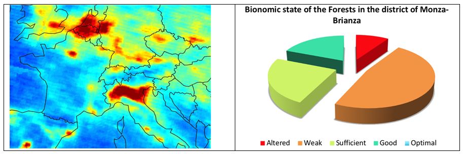
fig 4

Figure 4: In the Po plain, the distribution of air pollution is relatively homogeneous and one of the highest in the EU, ESA [24]. Not only Milan but also Monza-Brianza are inserted in this wide polluted area. (right) The bionomic state of the forest formations on the Province of Monza-Brianza shows only 19·05 % of the right conditions, and no one is truly optimal.

As shown in Fig.5, the blue line indicates a territory covered by the 55 + 17 = 72 municipalities (landscape units, LU) of the province of Monza-Brianza and Milan city (left). This land is compared with the bionomic metropolitan area of Milan (red), the N-E part of which is comprised in Monza-Brianza. Tab.2 shows the ecological and bionomic parameters per landscape type.

Bionomic principles and methods can find the landscape gradient, composed of six types (from agricultural to dense urban) and its relations with the mortality rate (MR), the bionomic functionality (BF), and the population Age (PA).  In Fig.5., the decrease of BF (blue) is related to MR’s increase (red). Elaborating the bionomic parameters (Tab.2) we note an average of BF = 0.78 (low value), indicating an altered environment.
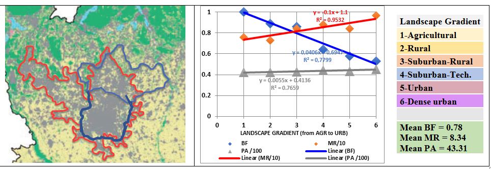
fig 5

Figure 5: The blue line indicates the land area of experimentation: Monza-Brianza [Milan City is just South of Monza]. This territory covers 656 Km2 with a population of 2.3 x 10⁶ inhabitants and with a gradient of 6 landscape types. (base map from DUSAF-Ersaf). Note, in the plot, the inverse proportionality between MR (red) and BF (blue), while PA remains near constant. From [20].

Table 2: Gradient of landscape types emerged analysing 72 municipalities from Milan to the Brainza hills.
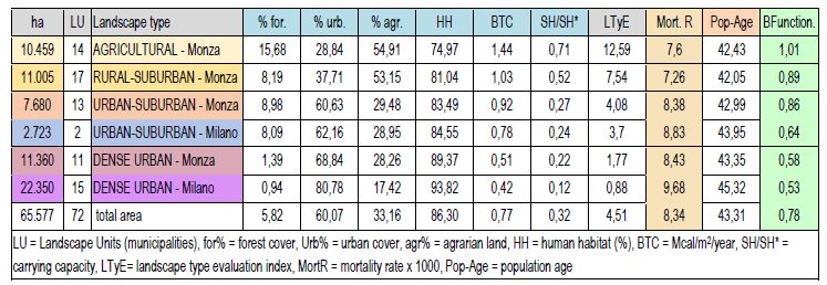
table 2

Covid-19 Contagion Dynamics in Monza Brianza (M-B)

Another figure (Fig.6) was developed for each municipality of M-B province, showing: Population (2018), FOR % (forest cover), URB% (urbanized), AGR % (cultivated land), HH% (Human Habitat), BTC (Mcal/m2/year), HS/HS* (Carrying Capacity), BF (Bionomic Functionality).  In October 2020 and May 2021, we added these data, the Covid-19 (infected people) and Covid-19 (%). The colors distinguishing the data are related to the landscape types of urban (violet), suburban (grey), and agrarian (yellow). The landscape gradient is very mixed, so a trend of instability emerges per each landscape type (here seven), even if the ecological density (ED) increases with urbanization.

Another figure (Fig.6) was developed for each municipality of M-B province, showing: Population (2018), FOR % (forest cover), URB% (urbanized), AGR % (cultivated land), HH% (Human Habitat), BTC (Mcal/m2/year), HS/HS* (Carrying Capacity), BF (Bionomic Functionality).  In October 2020  and May 2021, we added to these data, the Covid-19 (infected people) and Covid-19 (%). The colors distinguishing the data are related to the landscape types of urban (violet), suburban (grey) and agrarian (yellow). The landscape gradient is very mixed, so a trend of instability emerges per each landscape type (here seven), even if the ecological density (ED) increases with the urbanization.
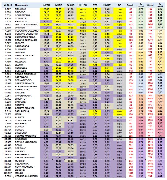
fig 6

Figure 6: Note that the colors marking the data are related to the landscape types of urban (violet), suburban (grey) and agrarian (yellow). The landscape gradient is mixed, so a trend of instability emerges per each landscape type (2 agricultural, 2 rural, 2 suburban, 2 urban), even if the ecological density increases with the urbanization. Comparison between Covid-19 influence, Oct 20th Vs. May, 1st.

It is possible to demonstrate that bionomic parameters played a crucial role in infective development, not considered among the mentioned conventional factors. In Tab.4, the yellow, grey, and violet colours underline the data related to the rural, suburban, and urban-type landscapes. The bionomic data (HH, BTC, HS/HS*, and BF) are complex indicators obtained applying Landscape Bionomics’ principles and methods, as exposed in the cited volume Biological-Integrated Landscape Ecology [12].

The Covid-19 incidence in this Province [26], presents three phases: (a) March-May 2020, reaching about 5,000 infected, (b) September-October passed from 6,000 to 30,000 and (c) November 2020 – May 2021 from 30,000 to 75,000. The surveys to verify possible correlations with bionomic and ecological parameters were six: (i) April 19 (4,100 infected), (ii) July 31 (5,880 infected), (iii) October 20 (9,360 infected), (iv) November 16 (33,900), (v) March 30 (68,800), (vi) May, 01 (75,000) [24].

Results

The Mortality Rate as a function of BF

Previous research [20] demonstrated that the mortality rate (MR) is correlated with the BF (Fig.7). Note that even the population age (PA) is growing with the degradation of the LU, but the increase of MR is more than four times the increase of PA (0.76 Vs. 0.24); so, the rise of MR with Landscape degradation is mainly due to other physiologic and bionomic processes, first of all, the landscape diseases [12, 20].
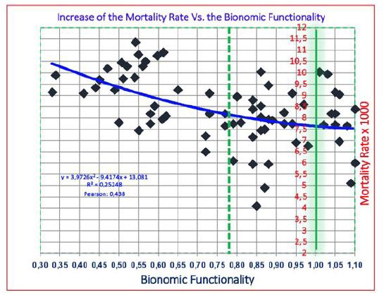
fig 7

Figure 7: An evident increase of mortality rate MR [x 1000] is correlated with the increase of landscape dysfunction: we pass from MR = 7.64 in not altered landscapes (BF = 1.0) to MR = 9.5 in the landscape with deprivation of 50% (BF = 0.50) of the normal state. The correlation significance (Pearson) is 1.85.

To evaluate a preliminary Risk Factor from the MI-MB Model [BF = 0.78]:

ΔMRBF = (MRBF – MRBF=1) x 76% = (8.34 – 7.64) x 0.76 = 0.532 x10⁻³

The correlations Covid-19 Vs. bionomic parameters

The first correlation is presented in Fig.8, left (Oct-20). The trend line has a modest R2 value (0.1513) but its Pearson Coefficient [26] is sufficiently high (0.38). So, at proper bionomic functionality conditions (BF=1.0) the incidence of Covid-19 is pair to 0.90 %, while at weak BF=0.45, Covid-19=1.2 % (+133%).

The statistical population of 55 LU of Monza-Brianza province registers a minimum Pearson Coefficient value pair to 0.266. So, the correlation Covid-19 Vs. BF results 0.38/0.266 = 1,45: an available significance of correlation. A still more important correlation is expressed in Fig.8, dx, where the ecological density (ED), which represents the inverse of SH, presents in March 2021 a value of significance equal to 1.77.
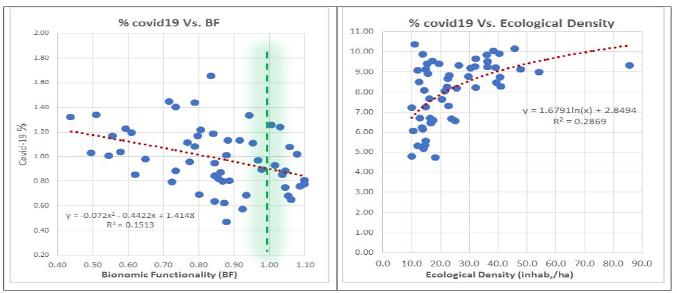
fig 8

Figure 8: The most meaningful correlations between Covid-19 (%) and Bionomic parameters: (sx) bionomic functionality (BF) in the third survey (OCT, 20), and (dx) ecological density (ED) in the last survey (MAR, 21). Note that values on the y axis changes due to the increase of the disease incidence.

The tested parameters (Tab.3) where: (1) Ecological Density (ED) [people/ha], (2) Bionomic Function (BF) [BTC/BTCNORM], (3) Population Age (PA) [mean years], (4) Forest Cover (For) [% of LU], (5) Agricultural Land (Agr) [% of LU], (6) Urbanized Cover (Urb) [% of LU], (7) Human Habitat (HH) [% of LU]. The period: 423 days.

Table 3: Pearson Significances of the main Ecological-Bionomic Parameters Vs. Covid-19 contagion in Monza-Brianza Province: Note that Agr. and Urb. are comprised in ED, while For. And HH in BF (see Fig.10).
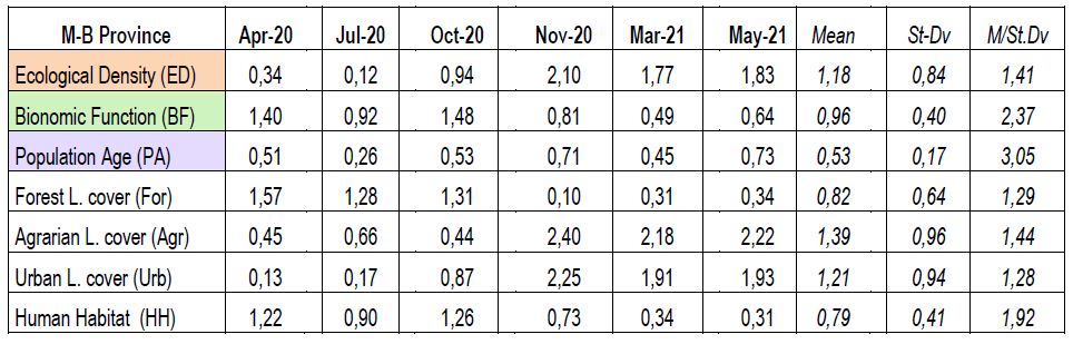
table 3

Remember that the essential bionomic parameters are: ED, relating Agrarian fields, Urban and Human Habitat; BF, relating Forest, Agriculture, Human Habitat; and Population Age. Note that ED presents an excellent average significance (ED = 1.18 ± 0.84); so, the standard deviation is very high. BF presents a bit less average but a better standard deviation: BF = 0.96 ± 0.40. The correlation significance of PA presents an average still more homogeneous but at a decidedly lower value: PA = 0.53 ± 0,17. Moreover, the averages of ED and BF are not significantly different (1.18 Vs. 0.96) but they seem to be in opposition: for the first 238 days ED (mean = 0.47) is low and BF high (mean BF = 1.27), while for the other period (185 days) is the contrary (ED = 1.81 Vs. BF = 0.65). Unlike the other parameters, PA remains lower and almost constant.

The Pearson’s correlation significances of the seven parameters are shown in Fig.9. Forest, Human Habitat, and their synthesis (BF) are shown in green and blue lines, while their opposites Agrarian, Urbanized, and their synthesis (ED), are shown in brown and red lines. PA (violet) remains near-constant, even if older people’s presence leads to high mortality.
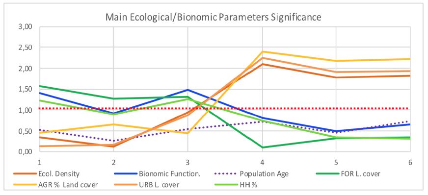
fig 9

Figure 9: The dynamics of Pearson’s Correlation significances of the seven parameters. We can see two opposite trends, guided by BF (green) and ED (brown). PA (dotted blue) remains of lower significance and near constant.

To study the Covid-19 contagion dynamics we need to consider only the three main parameters significances (BF, ED) related to time (days) and the increase of infection percentages in the period (1.16 year) (Fig.10).
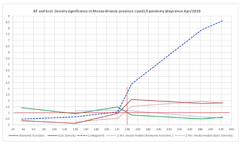
fig 10

Figure 10: Dynamics of the essential correlations significances between BF and ED in the first year of Covid-19 pandemic in the province of Monza-Brianza. Only when the contagion reached 2.5 % of the population, after 238 days, the ED became the leader environmental correlation in this territory.

This result is notable because the infection has grown where the environment was altered (BF average significance = 1.27) in the first 238 days (65.2 % of the year), leaving the ED contributions as marginal (average significance = 0.47). When the threshold of 2.5 % of infected people was exceeded, ED became the dominant correlation reducing the BF average significance to 0.64 (but not eliminating the correlation). So, a good BF can be considered a defense against infections, slowing down the contagion for 2/3 of a year.

Note that the ecological density ED (inhabitant/ha) is a bionomic parameter related to the concept of the human habitat (HH); so, it has nothing to do with the traditional geographic population density (GD, inhabitant/km2): being the average human habitat HH = 82 %, the ecological density ED = 26.3, while the geographic density GD = 21.5 (inhabitant/ha), with a difference of about + 22 %.

Discussion

Main Processes in Macro-Scale Biology: The Influence of Stress

We affirmed that health and disease depend on the state of the entire organization of life. Consequently, biology’s study should be extended to macro-scales, trying to understand their “anatomical” components, physiological processes and state functions, transformation processes, clinical-diagnostic evaluation, pathologies, and rehabilitation therapies. Here some examples:
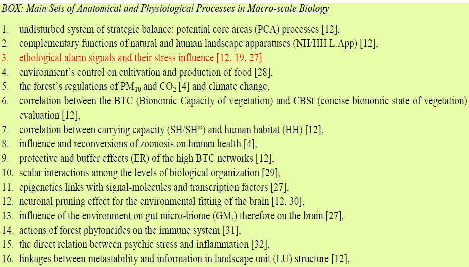
box

All these sets of processes, and more, need a more advanced ecological discipline because the traditional General Ecology does not elaborate landscape principles and methods, and Landscape Ecology only partially. That is why Ingegnoli founded Landscape Bionomics’ new ecological discipline, the main criteria of which we presented in the second paragraph. It can, therefore, be shown that alteration of life at the macro-scales can damage human health no less than at the micro-scales, for instance, recalling point (3) ethological alarm signals and their stress influence (Fig.11).
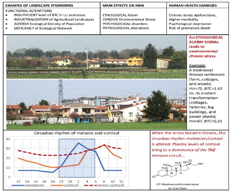
fig 11

Figure 11: An example of how Biological macro-scale alterations and derived physiological processes are damaging human health. Environmental stress can be registered by the ethological concept of “value judgment”. The sympathetic nervous system and the hypothalamus-pituitary-adrenal axis mediate the integrated responses of the human organism to stress. Note the crucial importance of cortisol.

Many of the stressors are due to landscape structural dysfunctions, even in the absence of pollution. An Ethological Alarm Signal leads to environmental stress, which can be chronic. Stressors simultaneously activate:

(a) neurons in the hypothalamus, which secrete CRH (Corticotropin-releasing hormone), and

(b) adrenergic neurons

These responses potentiate each other. The final effect of the activation of neurons that secrete CRH is the increase in cortisol levels, while the net effect of adrenergic stimulation is to increase plasma levels of catecholamine (Dopamine, norepinephrine, and epinephrine).

The negative feedback exerted by cortisol can limit an excessive reaction, which is dangerous for the organism. However, when the stress became chronic, the circadian rhythm of melatonin/cortisol is altered. Plasma cortisol levels bring to a dominance of the Th2 immune circuit, with production of typical catecholamine (e.g., IL-4, IL- 5, IL-13) and the circuit Th17 [27].

Note that the Th2 immune response is not available to counteract viral infections, neo-plastic cells, auto-immune syndromes, which need a Th1 response. So, the premature death risk increases.

Widening the Categories of Environmental Alterations Influencing Human Health

Genome-Wide Association Studies (GWAS) revealed a limited causal effect (estimated less than 20%) of genetic susceptibility on phenotypic variance. Consequently, environmental exposure plays a crucial role in disease development, both in infectious (IDs) and non-communicable diseases (NCDs), such as viruses and bacterial infections (IDs), cancer, asthma, cardiovascular and endocrine diseases (NCDs). In reality, we have to underline that environmental exposure and exchanges, and their interaction with the body’s biological systems and apparatuses, play an essential role in disease development.

Note that the concept of exposure (e.g., the exposome, sensu Wild [33]) may be necessary but not sufficient because of the complex structures and interrelations of life. Even if, generally, only three categories are mentioned, we have to distinguish at least four categories of environmental alterations capable of influencing human health through exposure and interactions:

(a) internal processes, e.g., metabolism, hormonal balance, gut microbiota, aging, etc.,

(b) specific external factors, e.g., infections, pollutants, smoking, drugs, etc.,

(c) general external factors, e.g., socioeconomic status, technological behaviors, climate change, etc., and

(d) landscape structure/function alterations, e.g., concerning hierarchical relations, the biological territorial capacity of vegetation, vital space per capita, ratio human/natural habitats, etc. (see box).

Widening the concept of Anamnesis and Therapy Integration

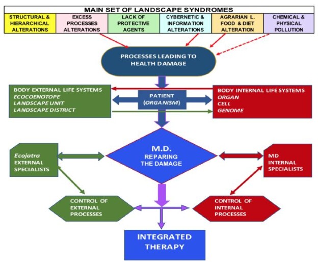
We will see that Landscape Bionomics, while sustaining the listed physiological processes (green Box), opens new perspectives to etiopathology, health prevention and therapy integrations, and anamnesis. So, new linkages between the two disciplines, Landscape Bionomics and Medicine, emerge following the new systemic paradigm, both in diagnostic and therapeutic fields in etiology and anamnesis. We can indicate an answer to what is not entirely clear to the medical profession/students (see Introduction): what they are meant to ‘do’ with the ecological problems and how they can use them to help patients (Fig.12).

Fig.12 shows that the primary set of landscape syndromes can be grouped in six categories: (1) structural and hierarchical alterations, (2) excess processes alterations, (3) lack of protective agents, (4) cybernetic and information alterations, (5) agrarian landscape food and diet alterations, (6) chemical and physical pollutions. These processes, frequently cumulative (at least partly), lead to health damage with an interchange between the body’s external and internal life systems. MD’s responsibility is to repair the damage, but in doing this, MD should contact internal specialists and external ecojatra: at least to avoid reintroducing the patient into the same environment that contributed to the insurgence of the disease. Moreover, to add, first, a wider anamnesis and then an integrated therapy.
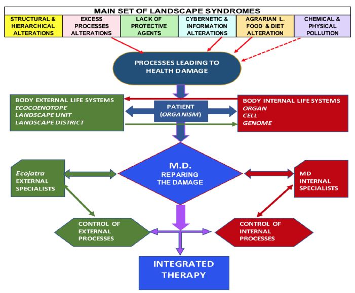
fig 12

Figure 12: This flow diagram tries to explain that MD have to repair the damages to human health but, being the majority of these damages due to environmental alterations and being the organism linked with body internal and external life systems, MD have to collaborate with internal and external specialists, arriving TO an integrated therapy.

Conclusion

In conclusion, we have to underline that environmental exposure and exchanges, and their interaction with the body’s biological systems and apparatuses, play an essential role in disease development. Studying the M-B province, we started showing the importance of broad-scale biology:

1.1) The mortality rate (MR) correlated with Bionomic Functionality (Pearson significance 1.85) 2015;

1.2) Bionomic Functionality correlated with Covid-19 % (Pearson significance 1.45) 2020, October;

1.3) Ecological Density correlated with Covid-19 % (Pearson significance 1.66), 2021, May;

1.4) Emergence of a Contagion dynamics: BF and ED inverted their dominance of correlation after the threshold of infected people = 2.5 %;

Therefore, we had to pass from qualitative to quantitative considerations related to macro-scale biology’s influence on human health scientifically, as suggested by landscape bionomics principles and methods. This fact underlines a more efficient control of environmental rehabilitation to enhance prevention against infectious (IDs) and non-communicable diseases (NCDs) [40] and indicates therapeutic integration between chemical and natural care.

On the other side, the possibility to evaluate the bionomic state of the landscape units and consequently to correlate its bionomic functionality (BF) with the mortality rate [21] reinforces the possibility to control the environmental syndromes and reduce the impacts of transformation, and advise the local Authorities for the necessity to ecological rehabilitation.

References

  1. Urbani-Ulivi L ed. (2019) The Systemic Turn in Human and Natural Sciences. A Rock in the Pond. Springer-Nature, Switzerland.
  2. Crick, FH (1958). On Protein Synthesis. In F. K. Sanders (ed.).Symposia of the Society for Experimental Biology, Number XII: The Biological Replication of Macromolecules. Cambridge University Press  138–163.
  3. Waddington CH (1961) The nature of life. Atheneum, New York.
  4. Frumkin H, Myers S (2020) Planetary Health, Protecting Nature to Protect Ourselves. Island Press, USA.
  5. Popper K, Lorenz K (1985) Il Futuro è Aperto. Bompiani.
  6. Margulis L (1975) Symbiotic theory of the origin of eukaryotic organelles; criteria for proof.In: Symposia of the Society for Experimental Biology 21-38. PMID. [crossref]
  7. Simard S, Roach WJ, Defrenne C et al. (2020) Harvest Intensity on Carbon Stocks and Biodiversity Are Dependent on Regional Climate in Dougles.Fir Forests of British Columbia. In: Frontiers I Forests and Global Change
  8. Scott-Dumas H (2014) The KAM story: a friendly introduction to the content history and significance of classical Kolmogorova Arnolda Moser Theory. In: World Sc. Publ.
  9. Barbieri M (2008) A new understanding of life. Naturwiessenshaften Pub.
  10. Holliday R (2006) Epigenetics : A Historical Overview. In : of Epigebetics Pp. 76-80.
  11. Bottaccioli F (2014) Epigenetica e Psiconeuroendocrinoimmunologia, le due facce della rivoluzione in corso nelle scienze della vita. Edra spa, Milano.
  12. Ingegnoli V (2015) Landscape Bionomics. Biological-Integrated Landscape Ecology. Springer, Heidelberg, Milan, New York Pp. XXIV + 431.
  13. Ingegnoli V, Giglio E (2020) Covid-19 Incidence and its Main Bionomics Correlations in the Landscape Units of Monza-Brianza Province, Lombardy. J Environ Sci Public Health 4 (4):349-366, USA.
  14. Odum EP (1971) Fundamentals of Ecology. Saunders, Philadelphia, USA.
  15. Lovelock J, Margulis L (1974) Atmospheric Homeostatsis by and for the Biosphere: the Gaia Hypothesis. Tellus
  16. Ingegnoli, V. (2011). Bionomia del paesaggio. L’ecologia del paesaggio biologico-integrata per la formazione di un “medico” dei sistemi ecologici. Springer-Verlag, Milano pp. XX+340.
  17. Ingegnoli V, Bocchi S, Giglio E (2017) Landscape Bionomics: a Systemic Approach to Understand and Govern Territorial Development. WSEAS Transactions on Environment and Development 13, pp. 189-195.
  18. Ingegnoli V (2001) Landscape Ecology. In: Baltimore D., Dulbecco R., Jacob F., Levi- Montalcini R. (Eds.) Frontiers of Life. New York, Academic Press Vol IV, pp 489-508.
  19. Ingegnoli, V (2002) Landscape Ecology: A Widening Foundation. Berlin, New York. Springer XXIII+357.
  20. Ingegnoli V, Giglio E (2017) Complex environmental alterations damages human body defence system: a new bio-systemic way of investigation. WSEAS Transactions on Environment and Development 170-180.
  21. Ingegnoli V, Giglio E (2005) Ecologia del Paesaggio: manuale per conservare, gestire e pianificare l’ambiente. Sistemi editoriali SE, Napoli pp. 685+XVI.
  22. Ingegnoli V. (2005) An innovative contribution of landscape ecology to vegetation science. Israel Journal of Plant Sciences 53: 155-166.
  23. Ingegnoli V, Pignatti S (2007) The impact of the widened Landscape Ecology on Vegetation Science: towards the new paradigm. Springer Link: Rendiconti Lincei Scienze Fisiche e Naturali, s.IX, vol.XVIII, pp. 89-122.
  24. ESA (2015) Air quality pollution. IUP, Heidelberg.
  25. Regione Lombardia (2021) Covid-19 Dashboard in Lombardy.
  26. Garson GD (2013) Correlation. Statistical Associates “Blue Book” Series Book 3.
  27. Bottaccioli F, Bottaccioli AG (2020) Psychoneuroendocrineimmunology and the science of integrated care, Edra, Milan.
  28. Ceccarelli S (2013) Produrre i propri semi. Manuale per accrescere la biodiversità e l’autonomia nella coltivazione delle piante alimentari. Libreria Editrice Fiorentina, Firenze.
  29. Ingegnoli V (2021) Enlighten the Intrinsic Relation Between Agricultural Landscape Health and Global Health. In: Raviglione M (coord.), Master on Global Health, Lesson on Disruption of Agrarian landscapes, slide 12 Unimi, Centre for Multidisciplinary Research in Health Science (Mach).
  30. Gogtay N, Giedd JN, Lusk L et al. (2009) Dynamic mapping of human cortical development during childhood through early adulthood. Proceedings of the National Academy of Sciences of the United States of America 101 (21), pp. 8174- 8179. [crossref]
  31. Li Q (2009) Effect of forest bathing trips on human immune function. Environ Health Prev Med 2010 Jan: 15(1):9-17. [crossref]
  32. Slavich GM, Thornton T, Torres LD, Monroe SM, Gotlib IH et al. (2009) Targeted rejection predicts hastened onset of major depression.Journal of Social and Clinical Psychology 28(2): 223–243. [crossref]
  33. Wild CP (2012) The exposome: from concept to utility. In: Int J Epidemiol 41:24-32. https://doi.org/10.1093/ije/dyr236. [crossref]
Accelerating the Uptake of Tranexamic Acid to Treat PPH in Zambia

DOI: 10.31038/IGOJ.2021421

Abstract

Objective: To identify barriers to utilization of TXA to treat PPH and conduct training and mentorship programs to improve uptake.

Design: A cross sectional study encompassing a sample of 25 health workers among them Doctors, Nurses and Midwives. Participants were drawn from selected hospitals in five provinces namely Central, Eastern, Copperbelt, Lusaka and Southern. The hospitals were selected on the basis that they receive patients at high risk of PPH or receive referred patients with PPH according to information provided by Ministry of Health.

Methods: The study began with a baseline assessment on the availability and usage of Tranexamic Acid (TXA) by collection of information on barriers to uptake captured via questionnaire and checklist sent to trainees of a one-day workshop that took place centrally in Lusaka on 12 September 2019.The training covered the following topics: The Woman Trial – Over view, Accelerating the Uptake TXA to treat PPH in Zambia, Management of PPH, Maternal Mortality in Zambia-Causes (2016-2018 DHIS2 Data/MDSR), Key strategies to addressing maternal mortality in Zambia, The TXA Study Questionnaire, consent form and checklist. Following the training these representatives were tasked to go and disseminate this information to their sites by making presentations with regard to utilisation of TXA with the hope of influencing change at their hospitals. A mentorship visit was conducted between 7 and 16 October 2019 by two specialist obstetricians with criteria for adequacy of TXA availability and use for PPH. An endline visit took place after 07 months in May 2020 to determine the impact of the training and the mentorship visit to all the sites. The same checklist that was used at baseline was administered at this time to determine the availability of items required to treat PPH, including availability of TXA.

Results: Lack of availability of Tranexamic acid was the cause of no increased uptake of TXA. There were limited supplies of TXA from the Ministry of Health (MOH), Zambia at baseline and one hospital had a donation at baseline. At endline, a part from limited supplies from the MOH, most health institutions were buying TXA from their own internally generated funds. Knowledge on benefits of use of TXA was now universal at endline with algorithms for PPH that included TXA in all the sites.

Conclusion: Training and mentorship improved knowledge and usage of TXA among health workers with regard to PPH. Most supplies are done centrally by MOH, not regularly, and not in appropriate amounts to meet the needs of each hospital. There is a need to advocate for TXA to treat PPH, improve the supply chain of this life saving drug and evidence-based practice in Zambia.

Introduction

Postpartum Haemorrhage (PPH) affects approximately 2% of all women who give birth. It is the primary cause of maternal mortality in Low-Income Countries (LIC), and the leading cause of approximately. 25% of maternal deaths globally [1]. In Zambia, approximately 250 deaths/annum were attributed to PPH in 2016.

Tranexamic Acid (TXA) was included in the WHO’s 2017 recommendations for the prevention and treatment of PPH. TXA has been shown to reduce death due to bleeding in women with clinically diagnosed PPH by approximately 30% if the treatment is administered intravenously (and in addition to the pre-2017 standard of care) within 3 hours of giving birth [2]. It is available as part of a PPH treatment package free of charge in all hospitals in Zambia, demonstrating the commitment of the Zambian government to reducing deaths due to PPH. However, the drug appears to be underutilised, indicating that there are barriers to the uptake of TXA to treat PPH that are not associated with its availability.

We aimed to identify some of these barriers whilst simultaneously boosting the confidence and competence of healthcare professionals to treat PPH in five Zambian Provinces through training programmes.

Methodology

As a starting point, a baseline assessment of existing status of utilisation of TXA to prevent treat PPH was established by collecting the information from routine data collected at the Ministry of Health (MOH) Zambia by engaging the procurement office and Directorate of Monitoring & Evaluation. This was done by using TXA-utilisation data (proxy-measure) and data on PPH-related deaths reported to the Ministry of Health MOH. We subsequently conducted a day training workshop with representatives from five provinces of Central, Eastern, Copperbelt, Lusaka and Southern from selected hospitals. The hospitals were selected on the basis that they receive patients at high risk of PPH or receive referred patients with PPH according to information provided by the MOH.

This training was preceded by collection of information on barriers to uptake captured via questionnaire and checklist sent to these representatives before they came for the training to a central place in Lusaka on 12 September 2019. 25 people attended the training, among them Doctors, Nurses and Midwives. The training covered the following topics: The Woman Trial-Over view, Accelerating the Uptake of TXA to treat PPH in Zambia, Management of Post-Partum Haemorrhage (PPH), Maternal Mortality in Zambia-Causes (2016-2018 DHIS2 Data/MDSR), Key strategies to addressing maternal mortality in Zambia, The TXA Study Questionnaire, consent form, checklist.

Following the training these representatives were tasked to go and disseminate this information to their sites by making presentations about the utilisation of TXA with the hope of influencing change at their hospitals. Several communication platforms, among them WhatsApp, were used to disseminate information on TXA among staff in hospitals involved in conducting deliveries and likely to come in contact with women who may experience PPH.

A follow-up site visit to the hospitals was conducted by the 2 investigators between 7 and 16 October 2019 with one covering Lusaka, Central and Copperbelt provinces (targeting teaching hospitals) while the other one visited Eastern part of Central and Southern Provinces mainly targeting district hospitals. This visit was aimed at collecting information and reporting on the findings. A check list was administered at this time to determine availability of items required to treat PPH including the availability of TXA. If at least 10 ampoules were available on the day of the interview, the site was considered to have enough TXA. At the end of the interview a PPH drill was conducted to determine if the staffs was aware of and were using TXA. This survey was supported by MOH Zambia and was approved by the University of Zambia Biomedical Research Ethics Committee, approval reference number 003-05-19. Following the training and after the investigators visit on a subsequent occasion, contact continued between the trainees and with the investigators through the WhatsApp platform and sometimes through phone calls if they had questions. During this time the trainees were encouraged to continue lobbying for and using TXA.

After the initial visit by the investigators, which enabled the collection of the study’s baseline information, a repeat visit was made in May 2020 to determine the impact of the training and the mentorship. At this time, the same checklist was administered, as at baseline, to determine availability of the items required to treat PPH including the availability of TXA. If at least 10 ampoules were available on the day of the interview, the site was considered to have enough TXA. In addition, statistics related to maternal mortality, where available, were collected from MOH to hopefully show a pattern from 2015 to 2019.

Results

The results relating to Lusaka, Central and Copperbelt provinces (targeting teaching hospitals) and Eastern province including part of Central and Southern Provinces (mainly targeting district hospitals) are shown below under the stated headings:

1. Barriers to the use of TXA

• Availability of items required to treat PPH

• Availability and utilisation of TXA

• Knowledge dissemination among staff in the labour wards, pharmacy and theatre

2. PPH Management

• Availability of algorithm

1) Barriers to the uptake of TXA

a) TXA

i) Availability

Data and information on the availability of TXA, as a barrier to uptake, was collected from the questionnaire. During the site visits, the training was conducted for the 25 staff from the 11 hospitals and the checklist was also administered.

It was observed that only 3 facilities had availability of Tranexamic acid at the time of the site visit in 2019, as reflected in the table below:

b) Sources of TXA

From the gathered data, the MoH supplied two batches of TXA to selected facilities. The distribution of the two supplies in 2018 and 2019 are tabulated below. There is no comparison distribution list for 2020; the reason provided for this was the disruption to the supply chain brought by COVID-19. Some hospitals like Mazabuka General Hospital were given donations of TXA from some well-wishers and a pharmaceutical company in 2019. However, we found 2 ampoules of TXA which had expired. Even if TXA was available at the MoH, and in limited amounts, it seems that good procurement managers supported by the hospital administrations. Were able to advocate for their hospitals to ensure that TXA was always available. Some institutions that performed poorly at baseline did improve while others did not improve; despite good knowledge about TXA as reported below in (b).

c) Knowledge

During the site visit it became apparent that there were some knowledge gaps on how to manage PPH. One of the gaps amongst the staff that we interacted with in 2019 was how to administer TXA and the infusion of intra venous fluids. However, in 2020 all the staffs in the sites were knowledgeable about TXA and were ready to use it appropriately.

2) PPH Management

• Availability of Algorithm

• Does the Algorithm include TXA

Of the visited facilities, all of them included TXA.

Discussion

Tranexamic acid reduces death due to bleeding in women with post-partum haemorrhage with no adverse effects. When used as a treatment for postpartum haemorrhage, tranexamic acid should be given as soon as possible after bleeding onset [1]. Primary post-partum haemorrhage, usually defined as a blood loss of more than 500 mL within 24 h of giving birth, is the leading cause of maternal death worldwide, responsible for about 100 000 deaths every year [3-5]. Most of the deaths occur soon after giving birth and almost all (99%) occur in low-income and middle-income countries [6,7].

From this study is obvious that TXA is available in Zambia but that it is not uniformly or consistently distributed, or in similar quantities (Table 1c). However some institutional leaders, even if they are not obstetricians, have made sure that TXA is always available even if they have to use internally generated funds, if the MoH MOH does not provide the drug.

Table 1c: Tranexamic acid distribution list.

2018 2019 2020-no list available
S/N Facility Name No. of Health centres received TXA UNIT TOTAL No. Health centres received TXA UNIT TOTAL No. Health centres received TXA UNIT TOTAL
1 Ndola 9 12 220 9 10 90
2 Kitwe 14 12 168 14 5 70
3 Luanshya 6 12 72 6 5 30
4 Masaiti 32 12 384 32 5 160
5 Mpongwe 12 12 144 12 5 60
6 Kalulushi 13 12 155 13 10 130
7 lufwanyama 22 12 265 22 10 220
8 Mufulira 7 12 84 7 10 70
9 Chingola 14 12 168 14 5 70
10 Chililabombwe 3 12 50 3 10 30
11 Ndola Teaching Hospital 1 500 550 1 200 200
12 Kitwe Teaching Hospital 1 500 500 1 250 250
13 Nchanga North Hospital 1 60 60 1 30 30
14 Ronald Ross General Hospital 1 60 60 1 30 30
15 Roan Antelope General Hospital 1 60 60 1 30 30
16 Kabwe General Hospital 1 60 60 1 30 30
138 1360 3000 138 645 1500 0 0 0

Typical examples are Ndola and Kitwe teaching hospitals, which are among the 3 major hospitals in Zambia, led by a surgeon and physician in the leadership respectively. At baseline we found no TXA in Ndola which was attributed to over- use by surgeons because of patients experiencing haemorrhage. However, by the endline site visit they had enough TXA which they said was procured from the MoH and they were also prepared to buy TXA if they ran out of stock. Importantly, all of the PPH sets at Ndola included TXA. In contrast, Kitwe hospital had enough stock of TXA both at the baseline and endline site visits.

Monze hospital had zero stocks at baseline but had enough TXA at the endline. This can be attributed to a young specialist posted there who understood the importance of TXA. Another great improvement was seen at Mwanawasa teaching hospital – they had no stock at baseline but more than enough stock at endline. This can also be attributed to a specialist who had been transferred from the Women and New-born Hospital to take leadership of the obstetrics department and was passionate about TXA use (Table 1a and 1b).

Table 1a: Availability of TXA 1g iv during site visits-2019.

Hospital Name

1 g IV vials needed 1 g IV Available

Comment

       
Mumbwa District Hospital

10

0

TXA not available; Have never been supplied before
Nyimba District Hospital

10

0

TXA not available; Have never been supplied before
Petauke District Hospital

10

0

TXA not available; Have never been supplied before
Mazabuka General Hospital

10

8

Available from a donation by a pharmaceutical company
Monze General Hospital

10

0

Not available
Kapiri mposhi Dist Hospital

10

0

Not available
Women and Newborn UTH

10

20

Plenty, supplied
Levy Mwanawasa Teaching Hospital

10

0

Out of stock
Kabwe Central Hospital

10

0

Not available, None in stock
Ndola Teaching Hospital

10

0

Not available, None in stock
Kitwe Teaching Hospital

10

15

Available, supplied by MOH

Source of Data: Checklist administered in Labour wards and observation from PPH Kit.

Table 1b: Availability of TXA 1 g IV during site visits-2020.

Hospital Name

1 g IV vials needed 1 g IV Available

Comment

Mumbwa District Hospital

10

2

Bought with user fees-an improvement
Nyimba District Hospital

10

0

TXA not available; Have never been supplied before
Petauke District Hospital

10

0

TXA not available; Have never been supplied before
Mazabuka General Hospital

10

2

Available from a donation by a pharmaceutical company-expired
Monze General Hospital

10

10

Improved from baseline
Kapiri mposhi Dist Hospital

10

0

Not available
Women and Newborn UTH

10

0

Not available due to overuse
Levy Mwanawasa Teaching Hospital

10

60

Was zero at baseline
Kabwe Central Hospital

10

0

Not available, None in stock
Ndola Teaching Hospital

10

10

Was zero at baseline due to overuse
Kitwe Teaching Hospital

10

10

Available, supplied by MoH

Source of Data: Checklist administered in Labour wards and observation from PPH Kit.

Kabwe did not perform well who, apart from being close to Lusaka where it is possible to get supplies, lacked other important stock such as intravenous fluids, gloves etc. The specialist based there was reported to have been away from the station for a long time. The sources of TXA were identified to be mainly from central medical stores and a smaller amount from private sources. One private source was found in Mazabuka where a pharmaceutical company made a donation which was identified at the baseline but not at the endline.

Table 2: Hospitals and availability of an algorithm for PPH that includes TXA.

Algorithm available

Hospital Name

Yes

No

Mumbwa District Hospital

Yes

Nyimba District Hospital

Yes

Petauke District Hospital

Yes

Mazabuka General Hospital

Yes

Monze General Hospital

Yes

Kapiri mposhi Dist Hospital

Yes

Women and Newborn UTH

Yes

Levy Mwanawasa Teaching Hospital

Yes

Kabwe Central Hospital

Yes

Ndola Teaching Hospital

Yes

Kitwe Teaching Hospital

Yes

Source of Data: Questionnaire administered in Labour wards and observation from PPH Kit.

Another option is for health facilities to buy TXA from their own resources, although the managers did not consider this to be a priority. Specialists in Zambia have a WhatsApp group where they discuss best practices, especially after they held the annual symposium under the umbrella of their Association, the Zambia Association of Gynaecologists and Obstetricians (ZAGO). It is no wonder that the smaller district hospitals did not perform well in terms of having supplies both at baseline and endline as there is no specialist to give them this kind of leadership. There is need to conduct training on the Use of TXA in PPH management in the district hospitals to increase uptake.

Obstetric haemorrhage remains the commonest cause of maternal mortality in Zambia. In the sites visited, of the 49 women experiencing obstetric haemorrhage, 46 (93.9%) was due to PPH according to the 2019 records. This included the big hospitals and confirms the need to roll out TXA use throughout the country. Of these deaths, strangely most deaths occurred in the health facilities rather than in the community. It is gratifying that big hospitals, which are more likely to receive referrals of PPH and its complications, have now embraced the use of TXA and that almost all facilities had PPH algorithms that include TXA. In Rwanda, a program targeting 21 health centres in two rural districts that supported the implementation of MOH evidence-based protocols demonstrated significant improvement in a number of quality-of-care indicators. Emphasis on individual provider and systems-level issues, integration within MOH systems, and continuous monitoring efforts were instrumental to these successes. Their experience and results demonstrate that it is feasible to rapidly implement a district-wide, nurse focused mentorship program that addresses quality of care at both individual provider and systems levels. This strategy has meaningful potential to support nurses and improve the quality of care delivered in rural Rwanda, as well as other resource-limited settings [7].

Similar, another study found that incorporating mentorship and coaching activities into health systems strengthening strategies was associated with improvements in quality of care and health systems, and mentorship and coaching represents an important component of health systems support activities designed to improve not just coverage, but even further effective coverage, in achieving Universal Health Care [8].

Conclusion

Training and mentorship improved knowledge and usage of TXA among health workers with regard to PPH management. Most supplies are done centrally by MOH, not regularly and not in appropriate amounts to meet the needs of each hospital. There is need to advocate for TXA to treat PPH, improve the supply chain of this life saving drug and evidence based practice in Zambia.

References

  1. WHO recommendation on tranexamic acid for the treatment of postpartum haemorrhage. 2017.
  2. Collaborators WT (2017) Effect of early tranexamic acid administration on mortality, hysterectomy, and other morbidities in women with post-partum haemorrhage (WOMAN): an international, randomised, double-blind, placebo-controlled trial. Lancet 389: 2105-2116. [crossref]
  3. Carroli G, Cuesta C, Abalos E, Gulmezoglu AM (2008) Epidemiology of postpartum haemorrhage: a systematic review. Best Pract Res Clin Obstet Gynaecol 22: 999-1012. [crossref]
  4. WHO, UNFPA and the World Bank. Trends in maternal mortality: 1990 to 2010 – WHO.UNICEF, UNFPA and The World Bank estimates. 2012.
  5. Ronsmans C, Graham WJ, LMSSS Group (2006) Maternal mortality: who, when, where, and why. Lancet 368: 1189-1200. [croosref]
  6. Say L, Chou D, Gemmill A, Tunçalp Ö, Moller AB, et al. (2014) Global causes of maternal death: a WHO systematic analysis. Lancet Glob Health 2: e323-e33. [crossref]
  7. Anatole M, Magge H, Redditt V, Karamaga A, Niyonzima S, et al. (2013) Nurse mentorship to improve the quality of health care delivery in rural Rwanda. Nursing Outlook 61: 137-144. [crossref]
  8. Manzi A, Hirschhorn LR, Sherr K, Chirwa C, Baynes C, et al. (2017) Mentorship and coaching to support strengthening healthcare systems: lessons learned across the five Population Health Implementation and Training partnership projects in sub-Saharan Africa. BMC Health Serv Res 17: 831. [crossref]

Astronomical Control of the Hydroclimate During the Past 1.2 Million Years

DOI: 10.31038/GEMS.2021323

Abstract

Although extensively studied, the particular contribution of the Earth’s orbital parameters to the intensity and periodicity of the Pleistocene glacial–interglacial cycles remains unresolved. Here, I approach the issue from the perspective of hydroclimatic variation by reconsidering the available palaeoclimatic records of the past 1.2 million years. Correlation of various direct and indirect hydroclimatic proxies consistently converges to highlight a hyetal spectrum of hydroclimatic intensity driven by quasi-22-kyr insolation oscillations due to eccentricity-modulated precession of the Earth’s rotational axis. The only and striking exception occurs at ~880 kyr, coinciding with the onset of the quasi-100-kyr glacial periodicity and the extremely cool and arid period known as the “900-kyr event”. The high insolation prevailing during that period suggests that the climate anomaly was not orbitally forced but instead was due to a currently undefined feedback perturbation of the Earth’s internal climate system. Furthermore, lower and higher hyetal periods seem to be closely related to glacial and interglacial cycles, respectively. The real mechanism of that relation is currently not well understood and might constitute a missing link coupling the Earth’s orbital and climatic histories.

Keywords

Early-to-Middle pleistocene transition, Earth’s orbital parameters, Glacial–interglacial cycles, glaciation, Hydroclimate, Pleistocene

Introduction

The onset of the current geologic period, the Quaternary [Holocene and Pleistocene; 2.58 million years (Myr) to present], was characterised by the intensification of Northern Hemisphere glaciation and variation in the intensity, shape, and duration of glacial–interglacial cycles [1]. During those cycles, relatively short interglacial periods with relatively warm climate and duration of a few thousand years were separated by colder periods lasting several tens of thousands of years. The reasons for that climatic variation have been a subject of study for almost two centuries and have been attributed to factors both internal and external to the climate system (ref. [2-4], and references therein). The astronomical hypothesis is one of the oldest explanations but was not formulated as a theory until 1941, when it presented by the Serbian geophysicist and astronomer Milutin Milanković [3]. The Milanković theory claims that the palaeoclimate was driven by perturbations of the Earth’s orbit and rotational axis. That view was largely disputed until the mid-1970s, when critical climatic information was recovered by the Ocean Drilling Programs (ODP) that demonstrated that the pace of the climatic variation matched the variation of the Earth’s orbital parameters [2]. More recent studies revealed, however, that the climate feedback on the Earth is more complicated than a simple linear system. For example, although the Milanković theory claims that obliquity-dominated oscillations in incoming solar radiation (insolation) at latitudes >65°N are the main factor controlling glacial cycles, the Earth is currently going through an interglacial culmination, but the current insolation has the same magnitude as that during the glacial culmination that occurred about 18,000 years ago [5]. Similarly, although the Milanković theory predicts the occurrence of glacial cycles in accordance with the 41-kyr periodicity of the tilt of the Earth’s axis (obliquity), which has a relatively large effect on insolation, most analyses of the last ~900,000 years of climatic history have concluded a quasi-100-kyr periodicity for glacial cycles, which is most compatible with the variation in the eccentricity of the Earth’s orbit, a parameter with a relatively small effect on insolation [2,6]. The inability to demonstrate a linear relationship between the insolation variation and the intensified glacial–interglacial cycles of the last ~900,000 years (from the onset of the middle Pleistocene to today) has led some researchers to introduce a stochastic parameter into their models of the climate system [7], whereas others have concluded that we are currently unable to understand the real mechanism driving glaciation [3,8]. The relationship between the global climate cycles and the Earth’s orbital parameters has been exhaustively investigated through palaeotemperature proxies. I took a different approach by exploring that relationship in terms of the variation in another important climatic factor, the hydroclimatic variation. To that end, I reconsidered the global palaeoclimatic record of the last 1,200,000 years in order to reconstruct the global trends in hydroclimatic intensity during the late Quaternary. The correlation of that variation with the oscillations of orbital parameters and palaeotemperature proxies allows further investigation of whether and how all those parameters are related to one another.

Materials and Methods

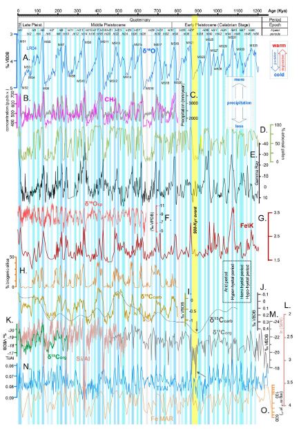
The global palaeoclimatic record of the last 1,200,000 years was reconsidered to investigate whether there are direct and indirect palaeohydroclimatic proxies with satisfactory resolution and precise timescale that can reliably reconstruct the global trends in the variation of the late Quaternary hydroclimatic intensity (Figure 1).

fig 1

Figure 1: Correlation of palaeotemperature (A) and various direct and indirect hydroclimatic proxies of the last 1.2 million years (see the Materials and Methods). A) Stack of 57 globally distributed benthic δ18O records [6] (palaeotemperature proxy). MS=Marine Stage. B) Atmospheric methane record from the EPICA Dome C ice core, Antarctica [36]. C) LOVECLIM simulation of the annual mean precipitation amount for the Lake Ohrid [63]. D) Palynologic record, Tenagi Philipon, Greece [25]. E) Gamma ray series at ODP Site 1119, east of South Island, New Zealand [64]. F) Composite δ18Osp from Chinese caves as a proxy of the Asian Monsoon [9]. G) Iron/potassium (Fe/K) ratio, IODP Site U1467, Maldives Archipelago [22]. H) Biogenic silica accumulation, Lake Baikal, Russia [29]. I) Stack of three Southern Ocean carbonate carbon isotope (δ¹³Ccarb) records ODP 1090, ODP 1089, and GeoB1211 [65]. J) Stacked and smoothed carbonate carbon isotope (δ¹³Ccarb) from benthic foraminifera of the global ocean [66]. K) Organic carbon isotope record (δ¹³Corg) of marine sediments including predominantly terrestrial material from Niger deep-sea fan (GeoB 4901), West Africa [18]. L) Log-ratio of silica to aluminium as a proxy of sediment opal content (ODP Site 658, subtropical North Atlantic [48]. M) Organic carbon isotope record (δ¹³Corg) of marine sediments including equivalently mixed material of terrestrial and marine photosynthesis, ODP Site 1077, Angola Basin [67]. N) Ti/Al ratio, ODP Sites 967 and 968, eastern Mediterranean [17]. O) Mass Accumulation Rate (MAR) of iron deposition, ODP Site 1090, Southern Ocean [30]. The vertical bars in different shades of blue form a hyetal spectrum highlighting periods of various hydroclimatic intensity. The green δ¹³Corg graph from the Niger deep-sea fan and the magenta loess xfd record from China are superimposed on other graphs for comparison. Black arrows show the remarkable values of various proxies during the 900-kyr event.

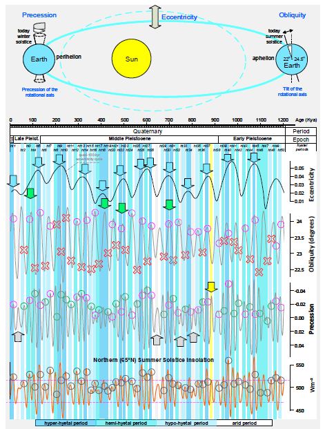
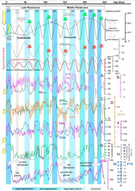
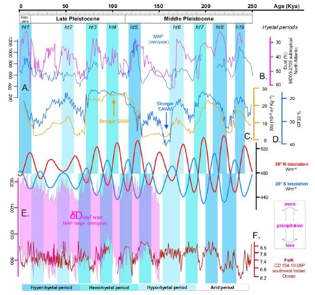
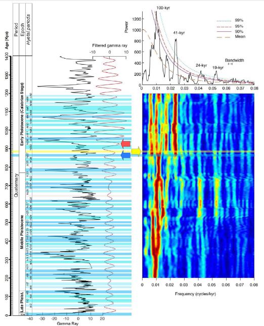
The correlation of that variation with the oscillations of both orbital parameters and palaeotemperature proxies allows further investigation of whether and how all of those parameters are related to one another (Figure 2). The investigation considered not only direct and well-established proxies of hydroclimatic intensity but also other proxies that might be indirectly related through mechanisms that are not well understood (Figures 1, 3 and 4). Potential covariation of the latter with the direct hydroclimatic proxies is expected to either confirm their physical property as hydroclimatic proxies or to reveal information about the specific mechanism responsible for the observed covariation. Among the well-established hydroclimatic proxies are the oxygen-isotopic composition in speleothems (δ18Osp) [9,10] and the loess-paleosol profiles [10,11]. Speleothems are inorganic carbonate deposits (mostly calcite and aragonite) that grow in caves and form from drip water that is supersaturated with CaCO3. Speleothems are highly suitable for radiometric dating using uranium-series disequilibrium techniques and can provide high temporal resolution ranging from a seasonal scale to a scale of ~100 years, depending on the sampling resolution. The δ18Osp records provide information that can be used to reconstruct past changes in precipitation and atmospheric circulation [10,12]. Here, a composite δ18Osp record from Chinese caves spanning the past 640 kyr was used (Figure 1F) as proxy of the Asian Monsoon [11]. Loess is a deposit of wind-blown silt that blankets large areas of the continents. Loess accumulated during dry periods when dust fall was high and vegetation was predominantly short grasses. During episodes of warmer and wetter conditions, a reduction in loess deposition and in situ weathering of the loess already on the ground led to accretionary soil formation [10]. Today, the alternating sequence of loess units and paleosols forms the longest and most complete terrestrial record of Quaternary palaeoclimatic conditions on the continents. The magnetic susceptibility and grain size of loess are two well-accepted proxies of summer and winter monsoon climates, respectively [10,13]. Here, loess frequency-dependent magnetic susceptibility (xfd) (Figure 4C) and loess grain-size data expressed as GT32 (>32 μm particle content) (Figure 4D) from the Luochuan loess section, China, have been arrayed in Figure 4 as proxies of the warm/humid southerly East Asian summer monsoon and the dry/cold northerly East Asian winter monsoon, respectively [9]. Continuous archives of terrestrial lithogenic inputs such as concentrations of terrigenous elements (Fe, K, Al, Si, Mg, and Ti) in marine sediments are considered to reflect wet versus dry conditions in the source areas. Moreover, elementary ratios such as the Ti/Al ratio have been used to remove dilution effects of carbonate in order to clarify palaeohydroclimatic information [14-16]. Accordingly, the Ti/Al ratio can also be considered a well-established palaeohydroclimatic proxy. A continuous Ti/Al record from the eastern Mediterranean [17] was arrayed in Figure 1N. In Figure 3E, the Mediterranean record is correlated with another Ti/Al record from the Niger Delta [18]. The hydrogen isotopic composition of sedimentary leaf waxes (δDwax) has been shown to primarily reflect precipitation (δDp) and is often taken to reflect the amount of precipitation [19]. The results of such a dataset from the Limpopo catchment, South Africa, were previously analysed [20] through a transient run with the isotope-enabled climate model iLOVECLIM and inferred to the arrayed graph of the mean annual precipitation range (Figure 4E). 10Be is a long-lived cosmogenic radionuclide produced in the atmosphere, where it attaches to dust and then is deposited mainly through wet precipitation events. Hence, the 10Be flux from the atmosphere is considered to be a proxy for rainfall (ref. [21] and references therein). Meteoric 10Be preserved in Pleistocene Chinese loess has been used as a proxy for monsoon palaeo-rainfall [21]. In Figure 4A, such a graph was arrayed for comparison with the other hydroclimatic proxies. Among the not well-established palaeohydroclimatic proxies is the elementary Fe/K ratio, which was recently considered as an alternative to the Ti/Al ratio in marine sediments [22]. A continuous Fe/K record from the Maldives Archipelago [22] was arrayed in Figure 1G. Another Fe/K record from the southwest Indian Ocean [23] was arrayed in Figure 4F. Other potential hydroclimatic proxies include the organic carbon isotope records of sediments containing terrestrial vegetation material (δ13Corg-w) and, in a secondary role, the carbon isotope variation in marine carbonates (δ13Ccarb) [24], the accumulation ratio of biogenic silica in freshwater lakes [10], the continuous arboreal palynologic records [10,25], the dust and iron deposition records in marine sediments [26,27], and the records of atmospheric methane concentration [28]. The variation in the organic carbon isotope fractionation extracted from terrestrial vegetation (δ13Corg-w) has long been considered a good proxy of wet/arid climate modes (ref. [24] and references therein). Fossilised wood debris, often stored in near-shore marine sediments, are the best proxies of that variation, given that they provide sedimentary organic material that can safely be regarded as having originated from terrestrial vegetation. The extracted hydroclimatic information can be biased, however, because of the fact that marine-produced organic material is not influenced directly by hydroclimatic variation [24]. Biogenic silica records of lake sediments, such as the one of Lake Baikal (Figure 1H), are considered proxies of diatom productivity [10,29], which is sensitive to changes in the orbital parameters, although the specific climatic factor influencing the records is currently unknown [29]. Two such records, one terrestrial and one marine, were correlated in Figure 1 for comparison (Figure 1H and 1L). Wind-borne mineral aerosol (‘dust’) from marine sediments and ice cores carries considerable information about the aridification history of source areas and atmospheric circulation over different timescales [26]. Eolian dust fluxes in ice ages tend to be greater than those in interglacial periods. That phenomenon can be attributed to a strengthening of dust sources, together with a longer lifetime for atmospheric dust particles in the upper troposphere resulting from a reduced hydrological cycle [27]. Consequently, palaeo-dust records can be a good proxy of the past hydroclimate. In Figure 1O, a dust record derived from the analysis of marine sediments from ODP Site 1090, located in the Atlantic sector of the subantarctic zone [30], was arrayed for correlation together with another record from the marine sediment core MD03-2705 [31]. The latter is located directly adjacent to Ocean Drilling Program Site 659 and includes information of Saharan dust deposition across the subtropical North Atlantic that is considered to reflect the West African monsoon strength (ref. [31] and references therein).

fig 2

Figure 2: Correlation of the hyetal spectrum with the Earth’s orbital parameters [68, 69]. Blue arrows point out that hyper-hyetal periods always occur during the orbital periods of high eccentricity. Coloured circles indicate the coincidence of the onset of a hyetal period with either the climatic precession and/or the obliquity maxima: green circles indicate exclusive identity; magenta circles indicate coincidence with both orbital phenomena. Red X symbols indicate failures of either climatic precession or obliquity to explain the onset of a hyetal period, that is, whenever their oscillations coincide with decreasing rather than increasing solar insolation trends. The grey arrows note that precession minima correspond to hypo-hyetal and/or arid periods only during periods of eccentricity minima. To emphasise the precessional effect, hyetal cycles are correlated with the insolation oscillations at 65°N high latitude (bottom graph), which is an area mainly dominated by obliquity-dependent insolation. The horizontal magenta dashed lines correlate the insolation power range of the 880-kyr climate anomaly (yellow vertical bar) with those of the hyetal cycles. Note that the astronomical precession minima correspond to climatic precession maxima.

Variation in palynologic records is also known to reflect climate variability [10]. The continuous 1.3 million-years arboreal pollen record from Tenagi Philipon, Makedonia, Greece [25], which is used here as the main proxy (Figure 1D), is expected to have been primarily influenced by palaeohydroclimatic variation rather than by palaeotemperature variation. That is because in palynologic analyses of other locations in Greece [32,33], the hydroclimate was shown to be the dominant factor influencing the vegetation distribution. The records of atmospheric methane (CH4) concentration have been found to covary closely with the hydrological cycles [34,35], suggesting the CH4 records to be very good hydroclimatic proxies. In Figure 1B, the 800,000 years atmospheric methane record from the EPICA Dome C ice core, Antarctica [36], was arrayed for correlation. All records were arrayed for correlation against their original timescales. All graphs are oriented so that wetter periods are represented by downward oscillations and drier periods are represented by upward oscillations. Hyetal and arid periods were defined on the basis of visual inspection of the graphs and the appearance of covariation among the proxies. Hyetal periods were defined by the occurrence of distinct downward peaks at least in three proxies, whereas arid periods were defined by the presence of zero to two peaks. The classification of the hyetal periods into categories of intensity was based on the amplifications of the oscillation peaks. Although the resulting hyetal spectrum is somewhat generalised, the resolution is satisfactory and in line with the purpose of the analysis. The separation of the hydroclimatic intensity into hyetal subcategories was done in order to cover a gap in the hydrological terminology by offering a term for the rainfall strength based not on the amount of rain water (precipitation) but on the amount of continental weathering caused by the rainfall. The concluded hyetal spectrum is thus mainly a contribution of proxies from weathering on land.

Results

Figure 1 shows how the best direct and indirect hydroclimatic proxies (see the Materials and Methods) correlate with the palaeotemperature and CO2 records of the last 1,200,000 years. The covariation of hydroclimatic proxies converges to highlight 50 hyper-hyetal, hemi-hyetal, hypo-hyetal, and arid periods characterised by high, semi-high, low, and very low levels of hydroclimatic intensity and continental weathering, respectively. The result is the synthesis of the spectrum of hydroclimatic intensity affecting Eurasia and tropical and northern Africa or, approximately, the Northern Hemisphere. In Figure 2, that spectrum is compared to the Earth’s orbital parameters. Figure 2 shows that hyper-hyetal periods and hypo-hyetal to arid periods largely coincide with the maxima and minima of the quasi-100-kyr eccentricity periods, respectively. Moreover, all of the hyetal periods start during high-insolation peaks, at the culminations of the eccentricity-modulated precession minima. Orbital precession minima correspond to times when the distance between the Earth and the Sun is smallest, resulting in higher insolation and maxima of another term, the climatic precession [37]. Climatic precession also depends on the Earth–Sun distance at the summer solstice. The highest-insolation hyper-hyetal periods occur when the solstice of boreal summer shifts towards the perihelion (e.g., as it was 10,000 years ago). Arid periods, in contrast, occur when the perihelion shifts towards the solstice of boreal winter (e.g., as it is today; see Figure 3). Obliquity plays only an auxiliary role in the configuration of the hyetal spectrum: it amplifies but never triggers hyetal periods. Indeed, there is no visible hyetal period corresponding to a high-insolation peak caused exclusively by an obliquity maximum, although there are plenty caused by climatic precession maxima (green circles in Figure 2). In addition, there are intermediate arid periods caused by precession minima, although they coincide with obliquity maxima (green arrows in Figure 2). As all hyetal periods correspond to insolation highs, this can be explained by the fact that even in the northern high (>65°N) latitudes, where the effect of obliquity on insolation is stronger than that of precession [37], insolation peaks always correspond or are close to precession minima (see the bottom of Figure 2 and Figure 3, where higher resolution data are correlated). Precession minima (climatic precession maxima) correspond to hypo-hyetal and/or arid periods only during periods of eccentricity minima (grey arrows in Figure 2). The only exception to that rule occurs at ~880 kyr (marked by a yellow arrow and a yellow vertical bar in Figures 1 and 2), coinciding with an event that signalled, and probably caused, the onset of the 100-kyr glacial periodicity (see the Discussion). The correlation of the palaeotemperature proxy with the hyetal spectrum in Figure 1 suggests that lower and higher hyetal periods are closely related to glacial and interglacial cycles, respectively. Indeed, in Figure 3 (see also Figure 4 for the Southern Hemisphere), it can be seen that, within the quasi-100-kyr eccentricity cycles, quasi-22-kyr hyetal/arid cycles form ramps of descending hyetal amplitude (from hyper-hyetal to arid) following the eccentricity-modulated precession of the Earth’s rotational axis [centred on a major cycle of ~23,000 years (23,700 and 22,400 years precisely) and a minor cycle of 19,000 years]. Both the CO2 records and the temperature records seem to be in good agreement with the hyetal cycles (Figure 3), suggesting a relationship that is closer than was previously thought.

fig 3

Figure 3: Comparison of the Earth’s orbital parameters [68, 69] to hydroclimate proxies supporting the hyetal spectrum of the last 250 thousand years. A) Stable hydrogen isotopic composition of leaf waxes from the Gulf of Aden (core RC09-166) corrected for ice volume contributions [70]. B) Oxygen-isotopic composition of cave calcites (δ18Osp) from Chinese caves, a proxy of the Asian Monsoon intensity [71]. C) Organic carbon isotope record from the Niger deep-sea fan (core GeoB 4901) [18]. D) Log-ratio of silica to aluminium as a proxy of sediment opal content (ODP Site 658, subtropical North Atlantic [48]. E). Titanium/aluminium (Ti/Al) ratio of sediments from Niger deep-sea fans (core GeoB 4901) [18]. F) Ti/Al ratio of sediments from ODP Sites 967 and 968, eastern Mediterranean [17]. G) Continuous palynologic record, Tenagi Philipon, Greece [25]. H) Pollen composition of cool-temperate deciduous broad leaf trees from lake Nojiri, Japan [72]. I) Atmospheric CO2 record from EPICA Dome C core, Antarctica [73]. J) Stable isotope ratios of oxygen and hydrogen in the Vostok ice core record, Antarctica [74]. Green arrows show the onsets of hyetal events that apparently coincide with climatic precession maxima and obliquity minima (red arrows). Grey vertical bars highlight that even the weakest hypo-hyetal periods coincide with precession maxima: their low hydroclimatic intensity can be justified by the low eccentricity. The “Green Sahara” interval (~11,000 to 5,000 years before present) [75], during which the area of the modern Sahara Desert received high amounts of rainfall, falls within the hyper-hyetal period ht1; however, today we are crossing the ht1 termination and entering into the subsequent arid period. Yellow arrows show the data indicating the current entry into an arid period.

fig 4

Figure 4: Correlation between the insolation variation and hydroclimatic proxies in the Northern and Southern Hemispheres. A) Meteoric 10Be record from Pleistocene China as a proxy for monsoon palaeo-rainfall [21]. B) Saharan dust deposition across the subtropical North Atlantic recovered from the marine sediment core MD03-2705 [31] and considered to reflect the West African monsoon strength. C) Loess frequency-dependent magnetic susceptibility (xfd), Luochuan, China [11]. D) Loess grain-size rate (>32 μm particle content), Luochuan, China [11]. E) Hydrogen isotopic composition of sedimentary leaf waxes (δDwax) from the Limpopo catchment, South Africa, as a proxy of the range in the mean annual precipitation [19]. δD values are reported in permille (‰) versus the Vienna Standard of Mean Ocean Water (VSMOW) standard. F) Continuous record of elemental ratios of Fe/K from the marine sediment core CD154-10-06P, southwest Indian Ocean [23].

Discussion

The relationship between variation in orbital precession and eccentricity and the Earth’s hydroclimatic cycles is fundamental in cyclostratigraphy because of the stable 405-kyr period of the eccentricity over hundreds of millions of years [38]. Eccentricity by itself does not influence the variation of annual insolation, but it plays an important role in modulating the amplitude of the precessional cycles [37,38]. Accordingly, precession-driven hydroclimatic cycles have been traced in stratigraphical sequences of the Cenozoic [39,40] and Mesozoic [41,42]. They have also been demonstrated in several climatic models [e.g. 43-45]. On the other hand, the combined influence of precession and obliquity has been found in the configuration of past hydroclimate systems such as that of Mediterranean [46] and the western Pacific Intertropical Convergence Zone [47] (see also Figure 5).

fig 5

Figure 5: Correlation of the inferred hydroclimatic spectrum with the cyclostratigraphy of the original gamma ray series at ODP Site 1119, east of South Island, New Zealand (modified from ref. [76]: Supplementary Figure 4 with permission). Left: Original gamma ray series from ref. [64]. The original age model [64] has been fine-tuned on the basis of the filtered 40.9-kyr obliquity cycles (Gaussian filter, red line) [76]. Right: 2π power spectrum and evolutionary spectrograms for inspecting stratigraphic frequencies and patterns of the gamma ray series (see methodology in ref. [76]). Notice that all hyper-hyetal periods correspond to gamma ray peaks apart from the ht37 (blue arrow), which follows the 880-Kyr anomaly (yellow arrow and yellow horizontal bar). Although the domination of the 41-kyr obliquity-related cycles seems to have declined since ~930 kyr (red arrow), the transition from 41-kyr obliquity-related cycles to quasi-100-kyr eccentricity-related cycles seems to have been completed at ~870 kyr, succeeding the 880-kyr anomaly.

The correlations of the various palaeoclimatic records in the current study agree with previous results. Furthermore, they open a new window for observations into not only the Earth’s climate history but also the nature of the records, which in one way or another seem to covary in the hyetal spectrum. Specifically, the close matching of the oscillations of well-established proxies of hydroclimatic intensity, such as the oxygen-isotopic composition of speleothems (δ18Osp) [9,10] and the loess-paleosol profiles [10,11], and also those of indirect or not-well-established hydroclimatic proxies [e.g., the organic carbon isotope records of sediments containing terrestrial vegetation material (δ13Corg-w) [24], the elemental ratios of iron and potassium (Fe/K) in marine sediments [22], and the records of atmospheric methane concentration [28] (see the Materials and Methods) confirms both the hydroclimatic property of the proxies and the robustness of the concluded hyetal spectrum. In addition, it calls into question the natural processes that were previously inferred from some other records, such as those of the opal precipitation in the Atlantic coast of northwest Africa [48]. Specifically, the opal precipitation peaks during the glacial terminations have been considered to be evidence of deglacial loss of the North Atlantic intermediate water [48]; however, they are understood here as a proxy of hydroclimatic intensity (see Figure 1 and Figure 3). Accordingly, the opal precipitation peaks could be a result of multiple hyper-hyetal “Green Sahara” intervals [49] that caused strong weathering on the Sahara desert, increased riverine runoff, fertilisation of the sea (Saharan dust, rich in iron and phosphorus, fertilises Amazonia even today) [50], growth of diatom blooms, and biogenic opal precipitation through the demise phase of diatom blooms [51]. Indeed, more recent data showed that the ODP Site 658 from which the opal record originated [48] is located on the front of the estuary of the huge palaeoriver Tamanrasett, which had a giant drainage system in the western Sahara [52]. Hydroclimatic intensity and weathering are also suggested to be the previously unrecognised climate factor [29] responsible for diatom productivity in lake sediments such as those of Lake Baikal (Figure 1J). That would also explain why the sedimentary record of biogenic silica from the high-latitude (51.5–56°N) Lake Baikal shows a surprisingly weak obliquity signal, with eccentricity and precessional frequencies dominating the record [10]. Likewise, the δ13Corg-w variation (Figure 1O and 1P) should be seen as a direct hydroclimatic proxy containing information about mean annual precipitation [22]. In contrast, the carbon isotope records of marine carbonates (δ13Ccarb) seem to contain indirect hydroclimatic information more closely related to continental weathering and carbon sequestration by terrestrial vegetation (Figure 1K and 1L), as previously suggested [22]. The covariation between the temperature oscillations (a proxy of glacial/interglacial climatic cycles) and the hyetal cycles shown in Figure 1 is of particular interest concerning the nature of that relation and its driving mechanism. Is the concluded hyetal spectrum a result of the temperature variation among the glacial/interglacial cycles, or are the latter driven by the eccentricity-modulated precessional hyetal periods? Given that the exact mechanism causing the glacial/interglacial cycles is yet unclear [53], it does not seem unreasonable to ask that question, although today the current consensus is that the physical and biological processes of the oceans are the main climate feedback system responding to orbital oscillations [e.g. 53]. Indeed, the greater precipitation rates characterising the interglacial periods might be considered as a plausible consequence of the prevailing warmer temperatures in the biosphere. As such, interglacial precipitation rates would increase with a rate of approximately 2% per degree of surface warming as a result of an increase in the radiative flux divergence of the atmosphere at a rate of 2% per K [54]. In that way, the change of the global mean annual precipitation would be a slow procedure depending on and following the glacial/interglacial biosphere temperature variation. However, the magnitude of the intense, convectively generated precipitation develops independently of those conditions and increases following the Clausius-Clapeyron law at the same rate as the column moisture, that is, a ~7% increase in specific humidity per K of surface warming [54]. Thus, even with cold glacial mean annual temperatures, strong midday insolation on land (Figure 6) could cause Violent Hydroclimate Perturbation (VHP) and intensified hyetal phenomena, such as the heavy convective rainfalls observed on tropical islands just after the hottest time of day [55].

fig 6

Figure 6: Simplified schematic explanation of the strong influence of insolation on the creation of convective rainfalls. Increased insolation drives an enhanced land–ocean thermal gradient and moisture convergence over land that strengthens and forces the monsoon to bring rainfall deep into inland areas (A). In contrast, weak insolation moves the cold continental wind masses toward the ocean, keeping the inland arid (B).

Therefore, during the periods of climatic precession maxima, high insolation could maximise the hydroclimatic intensity driven directly by the daily incoming solar radiation and independently of the prevailing mean annual temperatures in the biosphere. Conclusively, it is suggested here as a working hypothesis for future climate simulation models that the missing link coupling the Earth’s orbital and climate histories might be the directly orbitally forced hydroclimatic intensity. Indeed, given that the glacial/interglacial biosphere temperature is driven by atmospheric CO2 variation, it is worth noting that the Antarctic records of CO2 and CH4 concentrations covary [56] in precessional pace [36]. In addition, CH4 sources have been found that originated in tropical wetlands and seasonally inundated floodplains [57,58], which are known to have been dominated by a precession-driven hydroclimate. On the other hand, the essential contribution of the huge quantities of carbon stored in high-latitude permafrost regions [59] would prove to be more critical in deglaciation only after it was demonstrated that convective hyetal phenomena developed in the Arctic during climatic precession maxima. Such intensified hyetal phenomena might have led to quicker permafrost thawing and carbon release into the atmosphere [60], which otherwise are slow processes that would follow and not precede deglaciation [57]. In addition to the questions about the cause of Pleistocene glaciation, conclusions can be inferred from the hyetal spectrum regarding the mechanism controlling the periodicity of the glacial–interglacial cycles during the last ~900,000 years. The age of 900 kyr (MIS 22) is a threshold in the Pleistocene glaciation because it marks the currently not well understood passing from 41-kyr obliquity-related glacial cycles to quasi-100-kyr eccentricity-related glacial cycles [2,6,7]. That “900-kyr event” [61,62] signals the first long glacial period of the Pleistocene and is characterised by extremely low sea surface temperatures (SSTs) in the North Atlantic and tropical-ocean upwelling regions, increased aridity in Africa and Asia, a δ13Ccarb minimum (see Figure 1L), sustained decreased carbonate in the subtropical south Atlantic, northward migration of the Antarctic Polar Front, and major change in the deep-water circulation of the oceans [61,62]. The 900-kyr event is believed to have possibly started as early as the MIS24 (~940,000 years ago; see Figure 1E and Figure 5) and was due to orbital changes resulting in minima in the insolation amplitude [7,61,62]. A thorough observation of the hyetal spectrum reveals, however, that the main arid period characterising the 900-kyr event is the only arid period of the hyetal spectrum that falls within a high-insolation interval of both high eccentricity and high climatic precession; in other words, a period that should have resulted in a hyetal period rather than an arid period. That anomaly, dated at ~880,000 years ago (yellow vertical bars in Figures 1 and 2), perfectly coincides with the exact time of transition to the quasi-100-kyr glacial periodicity (see the spectral analysis in Figure 5). Therefore, the 900-kyr event is not a result of any change in insolation. Instead, it should be considered as a currently unexplained feedback perturbation of the Earth’s internal climate system (e.g., a permanent change in the circulation of ocean currents that resulted in large-scale changes in atmospheric circulation).

Declaration of Competing Interest

The author declares no competing interests.

Acknowledgments and Funding Sources

This research was not funded by public, commercial, or not-for-profit grants.

References

  1. Ogg JG, Ogg GM, Gradstein FMA (2016) coincise geological timescale (Elsevier, Amsterdam, 2016).
  2. Hays JD, Imbrie J, Shackleton NJ (1976) Variations in the Earth’s orbit pacemaker of the ice ages. Science 194: 1121-1132.
  3. Paillard D (2015) Quaternary glaciations: From observations to theories. Quaternary Science Reviews 107:11-24.
  4. Hodell DA, Channell, JET (2016) Mode transitions in Northern Hemisphere glaciation: Co-evolution of millennial and orbital variability in Quaternary climate. Climate of the Past 12: 1805-
  5. Maslin MA, Ridgwell AJ (2005) Mid-Pleistocene revolution and the ‘eccentricity myth’. Geological Society, London, Special Publications 247: 19-34
  6. Lisiecki LE, Raymo MEA (2005) Pliocene-Pleistocene stack of 57 globally distributed benthic d18O records. Paleoceanography 20.
  7. Maslin MA, Brierley CM (2015) The role of orbital forcing in the early middle Pleistocene transition. Quaternary International 389: 47-55.
  8. Raymo ME, Huybers P (2008) Unlocking the mysteries of the ice ages. Nature 451: 284-285.
  9. Hai Cheng, R. Lawrence Edwards, Ashish Sinha, Christoph Spötl, Liang Yi, et al. (2016) The Asian monsoon over the past 640,000 years and ice age terminations. Nature 534: 640-646.
  10. Bradley RS (2014) Paleoclimatology: Reconstructing climates of the Quaternary (3rd edn. Academic Press/Elsevier, Amsterdam,
  11. Qingzhen Hao, Luo Wang, Frank Oldfield, Shuzhen Peng, Li Qin, et al. (2012) Delayed build-up of Arctic ice sheets during 400,000-year minima in insolation variability. Nature 490: 393-396.
  12. Caley T, Roche DM, Renssen H (2014) Orbital Asian summer monsoon dynamics revealed using an isotope-enabled global climate model. Nature Communication 5.
  13. LinZeng, ShuangwenYi, WenfangZhang, HanFeng, Anqi Lv, et al. (2020) Provenance of loess deposits and stepwise expansion of the desert environment in NE China since ~1.2 Ma: Evidence from Nd-Sr isotopic composition and grain-size record. Global and Planetary Change 185.
  14. Boyle EA (1983) Chemical accumulation variations under the Peru Current during the past 130,000 years. Journal of Geophysical Research 88: 7667-7680
  15. Shimmield G, Mowbray SR (1991) The inorganic geochemical record of the northwest Arabian Sea: A history of productivity variation over the last 400 k.y. from sites 722 and 724. Proceedings of the Ocean Drilling Program, Scientific Results 117: 409-429.
  16. Holtvoeth J,Kolonic S,Wagner T (2005) Soil organic matter as an important contributor to Late Quaternary sediments of the tropical West African continental margin. Geochimica et Cosmochimica Acta 69: 2031-2041
  17. Konijnendijk TYM, Ziegler M, Lourens LJ (2015) On the timing and forcing mechanisms of late Pleistocene glacial terminations: Insights from a new high-resolution benthic stable oxygen isotope record of the eastern Mediterranean. Quaternary Science Reviews 129: 308-320.
  18. MatthiasZabelRalph RSchneiderThomasWagnerAdesina TAdegbieUwede Vries, et al. (2001) Late Quaternary climate changes in central Africa as inferred from terrigenous input to the Niger fan. Quaternary Research 56: 207-217.
  19. Dirk Sachse, Isabelle Billault, Gabriel J. Bowen, Yoshito Chikaraishi, Todd E. Dawson, et al. (2012) Molecular paleohydrology: Interpreting the hydrogen-isotopic composition of lipid biomarkers from photosynthesizing organisms. Annual Review of Earth and Planetary Sciences 40: 221–249.
  20. Caley, Thibaut; Jimenez-Espejo, Francisco J; García-Comas, Carmen, et al. (2018) A two-million-year-long hydroclimatic context for hominin evolution in southeastern Africa. Nature 560: 76-79.
  21. J Warren Beck, Weijian Zhou, Cheng Li, Zhenkun Wu, et al. (2018) A 550,000-year record of East Asian monsoon rainfall from 10Be in loess. Science 360: 877-881.
  22. Tereza Kunkelova, Simon JA Jung, Erica S de Leau, Nick Odling, Alex L Thomas, et al. (2018) A two million year record of low-latitude aridity linked to continental weathering from the Maldives. Progress in Earth and Planetary Science 5.
  23. Margit H. Simon, Martin Ziegler, Joyce Bosmans, Stephen Barker, Chris J.C. Reason, et al. (2015) Eastern South African hydroclimate over the past 270,000 years. Scientific Reports 5.
  24. Brikiatis L (2019) Arido-eustasy: A new example of non-glacial eustatic sea level change. Gondwana Research 70: 25-35.
  25. Tzedakis PC, Hooghiemstra H, Pälike H (2006) The last 1.35 million years at Tenaghi Philippon: Revised chronostratigraphy and long-term vegetation trends. Quaternary Science Reviews 25: 3416-3430.
  26. BA Maher, JM Prospero, D Mackiec, D Gaierod, PP Hesse, et al. (2010) Global connections between aeolian dust, climate and ocean biogeochemistry at the present day and at the last glacial maximum. Earth-Science Reviews 99: 61-97.
  27. Lambert, B Delmonte, JR Petit, M Bigler, PR Kaufmann, et al. (2008) Dust-climate couplings over the past 800,000 years from the EPICA dome C ice core. Nature 452: 616-619.
  28. Michael Bock, Jochen Schmitt, Jonas Beck, Barbara Seth, Jérôme Chappellaz, et al. (2017) Glacial/interglacial wetland, biomass burning, and geologic methane emissions constrained by dual stable isotopic CH4 ice core records. PNAS 114: E5778–E5786.
  29. Mackay AW, Edlund MB, Khursevich G (2010) Diatoms in ancient Lakes in The diatoms: Applications for the Environmental and Earth Sciences (edsb: Smol, J. P. & Stoermer, E. F.) pg: 209-228 (2nd edn, Cambridge University Press).
  30. Alfredo Martínez-Garcia, Antoni Rosell-Melé, Samuel L. Jaccard, Walter Geibert, Daniel M. Sigman, et al. (2011) Southern Ocean dust–climate coupling over the past four million years. Nature 476: 312-315.
  31. C Skonieczny, D McGee, G Winckler3, A. Bory3, LI Bradtmille, et al. (2019) Monsoon-driven Saharan dust variability over the past 240,000 years. Science Advance
  32. Tzedakis PC, Lawson IT, Frogley MR, Hewitt GM, Preece RC (2002) Buffered tree population changes in a quaternary refugium: Evolutionary implications. Science 297: 2044-2047.
  33. Lawsona I, Frogley M, Bryant C, Preece R, Tzedakis P (2004) The Lateglacial and Holocene environmental history of the Ioannina basin, north-west Greece. Quaternary Science Reviews 23: 1599-1625.
  34. Tzedakis PC, Pälike H, Roucoux KH, de Abreu L (2009) Atmospheric methane, southern European vegetation and low-mid latitude links on orbital and millennial timescales. Earth and Planetary Science Letters 277: 307-317.
  35. Konijnendijk TYM, Weber SL, Tuenter E, van Weele M (2011) Methane variations on orbital timescales: A transient modeling experiment. Climate of the Past 7: 47-77.
  36. Laetitia Loulergue, Adrian Schilt, Renato Spahni, Valérie Masson-Delmotte, Thomas Blunier, et al. (2008). Orbital and millennial-scale features of atmospheric CH4 over the past 800,000 years. Nature 453: 383-386.
  37. Berger A (1978) Long-term variations of caloric insolation resulting from the earth’s orbital elements. Quaternary Research 9: 139-167.
  38. Hinnov LA (2014) Cyclostratigraphy and its revolutionizing applications in the earth and planetary sciences. GSA Bulletin 125: 1703-1734
  39. Röhl U, Bralower TJ, Norris RD, Wefer G (2000) New chronology for the late Paleocene thermal maximum and its environmental implications. Geology 28: 927-930.
  40. De Menocal PB (1995) Plio-Pleistocene African climate. Science 270: 53-59.
  41. SK Hüsing, A Beniest, A van der Boon, HA Abels, MHL Deenen, et al. (2014) Astronomically-calibrated magnetostratigraphy of the Lower Jurassic marine successions at St. Audrie’s Bay and East Quantoxhead (Hettangian–Sinemurian; Somerset, UK). Palaeogeography Palaeoclimatology Palaeoecology 403: 43-56.
  42. Jingeng Sha, Paul E. Olsen, Yanhong Pan, Daoyi Xu, Yaqiang Wang, et al. (2015) Triassic–Jurassic climate in continental high-latitude Asia was dominated by obliquity-paced variations (Junggar Basin, Ürümqi, China). PNAS 112: 3624-3629.
  43. Kutzbach JE (1981). Monsoon climate of the early Holocene: Climate experiment with the earth’s orbital parameters for 9000 years ago. Science 214: 59-61.
  44. A Marzocchi, DJ Lunt, R Flecker, CD Bradshaw, A. Farnsworth, et al. (2015) Orbital control on late Miocene climate and the North African monsoon: Insight from an ensemble of sub-precessional simulations. Climate of the Past 11: 1271-1295.
  45. Jalihal C, Bosmans JHC, Srinivasan J, Chakraborty A (2019) The response of tropical precipitation to Earth’s precession: The role of energy fluxes and vertical stability. Climate of the Past 15: 449-462.
  46. StefanKlotz, SéverineFauquette, NathalieCombourieu-Nebout, DieterUhl, Jean-Pierre Suc, et al. (2006) Seasonality intensification and long-term winter cooling as a part of the Late Pliocene climate development. Earth and Planetary Science Letters 241: 174-187.
  47. Yi Liu, Li Lo, Zhengguo Shi, Kuo-Yen Wei, Chien-Ju Chou, et al. (2015) Obliquity pacing of the western Pacific Intertropical Convergence Zone over the past 282,000 years. Nature Communications 6.
  48. AN Meckler, DM Sigman, KA Gibson, R François, A Martínez-García, et al. (2013) Deglacial pulses of deep-ocean silicate into the subtropical North Atlantic Ocean. Nature 495: 495-498.
  49. Isla S. Castañeda, Stefan Mulitza, Enno Schefuß, Raquel A. Lopes dos Santos, Jaap S. Sinning, et al. (2009) PNAS 106: 20159-20163.
  50. Bristow CS, Hudson‐Edwards KA, Chappell A (2010) Fertilizing the Amazon and equatorial Atlantic with West African dust. Geophysical Research Letter 37.
  51. Smetacek VS (1985) Role of sinking in diatom life-history cycles: Ecological, evolutionary and geological significance. Marine Biology 84: 239-251.
  52. C Skonieczny, P Paillou, A Bory, G Bayon, L Biscara, et al. (2015) African humid periods triggered the reactivation of a large river system in Western Sahara. Nature Communications 6.
  53. Kohfeld KE, Ridgwell A (2009) Glacial-interglacial variability in atmospheric CO2 in Surface Ocean/Lower Atmosphere Processes (Eds: Le Quéré, C. & Saltzman, E.) (Geophysical Monograph Series 37, American Geophysical Union, Washington).
  54. Igel MR, Biello JA (2019) A reconstructed total precipitation framework. Climate and Atmospheric Science 2.
  55. Cronin TW, Emanuel KA, Molnar P (2014) Island precipitation enhancement and the diurnal cycle in radiative‐convective equilibrium. Q J Royal Meteorological Society 141: 1017-1034.
  56. Past Interglacials Working Group of PAGES (2016) Interglacials of the last 800,000 years. Reviews of Geophysics 54: 162-219
  57. Michael Bock, Jochen Schmitt, Jonas Beck, Barbara Seth, Jérôme Chappellaz, et al. (2017) Glacial/interglacial wetland, biomass burning, and geologic methane emissions constrained by dual stable isotopic CH4 ice core records. PNAS 114: E5778–E5786.
  58. Eric Monnin, Andreas Indermühle, André Dällenbach, Jacqueline Flückiger, Bernhard Stauffer, et al. (2001) Atmospheric CO2 concentrations over the Last Glacial Termination. Science 291: 112-114.
  59. K A Crichton, N Bouttes, DM Roche, J Chappellaz, G. Krinner, et al. (2016) Permafrost carbon as a missing link to explain CO2 changes during the last deglaciation. Nature Geoscience 9: 683-686.
  60. Rebecca B. Neumann, Colby J. Moorberg, Jessica D. Lundquist, Jesse C. Turner, Mark P. Waldrop, et al. (2019) Warming effects of spring rainfall increase methane emissions from thawing permafrost. Geophysical Research Letter 46: 1393-1401
  61. Peter U Clark, David Arche, David Pollard, Joel D.Blum, Jose A Rial, et al. (2006) The middle Pleistocene transition: mechanisms, and implications for long-term changes in atmospheric PCO2. Quaternary Science Reviews 25: 3150-3184.
  62. Kemp AES, Grigorov I, Pearce RB, Naveira Garabato AC (2010) Migration of the Antarctic Polar Front through the mid-Pleistocene transition: Evidence and climatic implications. Quaternary Science Reviews 29: 1993-2009
  63. Wagner B, Vogel H, Francke A (2019) Mediterranean winter rainfall in phase with African monsoons during the past 1.36 million years. Nature 573: 256-260.
  64. Carter RM, Gammon P (2004) New Zealand maritime glaciation: Millennial-scale southern climate change since 3.9 Ma. Science 304: 1659-
  65. Lisiecki LE (2010) A simple mixing explanation for late Pleistocene changes in the Pacific-South Atlantic benthic δ¹³C gradient. Climate of the Past 6: 305-314.
  66. Hoogakker BAA, Rohling E.J, Palmer MR, Tyrrell T, Rothwell RG (2006) Underlying causes for long-term global ocean delta C-13 fluctuations over the last 1.20 Myr. Earth and Planetary Science Letters 248: 15-29.
  67. Jahn B, Schneider RR, Müller PJ, Donner B, Röhl U (2005) Response of tropical African and East Atlantic climates to orbital forcing over the last 1.7 Ma. Geological Society, London, Special Publications 247: 65-84
  68. J Laskar, P Robutel, F Joutel, M. Gastineau, ACM Correia, B. Levrard et al. (2004) A long-term numerical solution for the insolation quantities of the Earth. Astronomy and Astrophysics 428.
  69. Laskar, J., Fienga, A., Gastineau, M. & Manche, H., 2011. La2010: A new orbital solution for the long-term motion of the Earth. Astronomy and Astrophysics 532, A89. http://dx.doi.org/10.1051/0004-6361/201116836
  70. Tierney JE, de Menocal PB, Zander PD (2017) A climatic context for the out-of-Africa migration. Geology 45: 1023-1026.
  71. Hai Cheng, R Lawrence Edwards, Wallace S Broecker, George H Denton, Xinggong Kong , et al. (2009) Ice age terminations. Science 326: 248-252.
  72. Kumon F, Tawara T (2009) Detailed reconstruction of paleoclimate based on total organic carbon proxy of lake sediment during the past 160 ka in central Japan. The Journal of the Geological Society of Japan 115: 344-356
  73. Dieter Lüthi, Martine Le Floch, Bernhard Bereiter, Thomas Blunier, Jean-Marc Barnola, et al. (2008) High-resolution carbon dioxide concentration record 650,000-800,000 years before present. Nature 453: 379-382.
  74. Sime LC, Wolff EW, Oliver KIC, Tindall JC (2009) Evidence for warmer interglacials in East Antarctic ice cores. Nature 462: 342-345.
  75. Tierney JE, Pausata FSR, de Menocal, Peter B (2017) Rainfall regimes of the Green Sahara. Science Advance 3.
  76. Li M, Hinnov LA, Huang C, Ogg JG (2018) Sedimentary noise and sea levels linked to land–ocean water exchange and obliquity forcing. Nature Communications 9.

Anthocyanin Effects in Reducing Platelet Hyperactivity and Thrombotic Risk in Type 2 Diabetes

DOI: 10.31038/EDMJ.2021513

Abstract

Background: Platelet hyperactivity has a crucial role in initiating vascular thrombosis and subsequent cardiovascular disease (CVD) in type 2 diabetes mellitus (T2DM). This study aims to assess the effect of anthocyanins on several risk markers of thrombosis in T2DM. Twenty-three patients with T2DM consumed 320 mg of AC/day in the form of Medox® capsules for 28 days. Blood pressure and anthropometric measures were taken before and after the intervention period. Fasting blood samples were collected pre and post-intervention to perform different analyses. Analysis of platelet activation measured the platelet activation measured the expression of platelet surface marker. Surface markers included CD41a and P-selectin in adenosine diphosphate (ADP) stimulated platelets. Platelet aggregation, full blood examination, coagulation and biochemistry profile analyses were also evaluated pre and post-intervention.

Results: Flow cytometric analysis showed no effect of AC on the expression of P-selectin. There were significant reductions in ADP and collagenstimulated platelet aggregation. The hematologic measurements showed no impact of AC. Coagulation analysis demonstrated a non-significant change of prothrombin time, activated partial thromboplastin time, or fibrinogen level in the blood. This study showed a reduction of platelet aggregation and total serum cholesterol. These results suggest that AC positively impacts attenuating platelet function potential improvement in lipid profile, minimising thrombotic risk.

Keywords

anthocyanin, antiplatelet, platelet activation, diabetes mellitus type 2

Introduction

Hyperactivity of platelets, inflammation, and increased oxidative stress have a central role in the pathogenesis of several conditions, including, type 2 diabetes mellitus (T2DM), thrombosis, and cardiovascular disease (CVD) [1]. T2DM is associated with increased macro-vascular complications, which significantly elevate the risk of cardiovascular mortality among these individuals [2]. Platelets are enucleated blood cells that play a vital role in primary haemostasis. Platelet hyperactivity, in the presence of free radicals, can significantly accelerate the progression of atherosclerosis. Free radicals have a significant effect on developing oxidative stress before platelet hyperactivity [3]. For instance, impaired muscle glucose uptake, endothelial dysfunction, and lipid oxidation are predisposed by oxidative stress detected in disorders such as T2DM [4-6]. Platelet activation and coagulation exemplify a biological indicator to predict vascular events in the future [7]. Endothelial damage of the vascular wall or injury of atheromatous plaque is a primary step in platelet–associated thrombogenesis. Platelets stick to the site of endothelial injury and change their shape. Consequently, platelets undergo degranulation and activation process. Activation of platelets leads to fibrinogen binding to platelet receptors and finally, the formation of thrombus.

Aspirin is an antiplatelet drug that reduces platelet hyperactivity. Aspirin target the cyclooxygenase-2 (COX-2) pathway and inhibiting thromboxane A2 (TXA2) production. Although aspirin is still the first-line antiplatelet agent [8] used in the treatment of acute coronary syndromes (ACS), many studies have recently highlighted aspirin resistance [9, 10] and its side effects, especially in individuals with T2DM. With aspirin and clopidogrel, two anti-platelet therapies are the most widely used antiplatelet treatment to treat ACS [8, 11, 12]. A plethora of studies has demonstrated the potential of plantbased antioxidants is not only inhibiting platelet activity but also in alleviating several risk factors that are associated with atherosclerosis and subsequent cardiovascular disease.

Several studies show the positive effects of consuming antioxidantrich diet, especially fruits and vegetables [13-15] in 2004, Hung and colleagues [16] conducted a cohort study recommending to consuming five or more servings of fruits and vegetables to lower CVD risk. Antioxidants reduce or suppress atherosclerotic progression and alleviate CVD development [16-18]. This anti-thrombotic potential of phytochemicals has encouraged nutraceutical industries to explore the use of natural antioxidants as a complementary therapy to the currently used anti-platelet treatment [7]. The effect of natural antioxidants such as anthocyanins to reduce platelet hyperactivity is due to blocking variable platelet receptors and inhibiting free radicals, which initiate platelet activity, thereby eliminates the risk of thrombus [19] [17, 18, 20-23] [7]. Although the effect of polyphenols on overall health is well documented, their actions on function and activity of platelets are changeable [7]. The variability in these findings increases the necessity to conduct a controlled and well-designed human intervention trial. Therefore, this study aims to examine the effect of pure Anthocyanins extracted from bilberries and blackcurrant (Medox®) on platelet activity and thrombotic risk in patients with type 2 DM.

Materials and methods

Participant recruitment and study design

This study was approved by Griffith University Human Research Ethics Committee, Griffith University, Queensland, Australia (GU Ref No: MSC/07/14/HREC) and is registered with Australia and New Zealand Clinical Trials Registry (ACTRN12615000293561). Twentythree patients with T2DM were recruited from the general population after signing an informed consent before the commencement of the study. All the participants included in the study were carefully screened using health questionnaires and interviews to ensure that they were non-smoking and without bleeding disorders or liver disease. Participants taking an anti-inflammatory, anti-platelet agents or anticoagulants were not included in the study.

Before the commencement of the study, anthropometric measurements and blood pressure were checked. Also, baseline fasting blood samples were collected to determine the presence of any underlying health condition using results from full blood examination, platelet function assays, enzyme-linked immunosorbent assay (ELISA), coagulation and biochemistry profiles. Upon completion of the initial screening, the participants were requested to consume four AC extract caps (80mg per capsule) per day (320mg of AC extract per day) for 28 days. The current study has used this dosage based on previous studies that have demonstrated that AC supplementation at 320 mg per day has significant beneficial effects on reducing risk factors of CVD such as inflammation, lipid profile and thrombosis [24-26]. The four-week intervention was also finalised based on previous clinical trials conducted by our research team, that have shown that four week AC supplementation can significantly reduce platelet aggregation, activation and overall risk of thrombosis in individuals [27-29]. Anthropometric measurements and blood pressure were rechecked. Fasting blood samples were collected after the 28 days supplementation period. Adherence and compliance of AC capsule intake were monitored by checking the capsule strips returned by the participant after the supplementation and by personally interviewing them.

Supplement Information

Patients were assigned to twenty-eight days of AC intervention in capsule form at a daily dose of 320 mg AC. AC supplement (Medox®) is a hemicellulose capsule, which contains powder of anthocyanins extracted from Bilberries (Vaccinium myrtillus) and Black Currants (Ribes nigrum). Table 2 shows the relative amount of the primary AC components used in the intervention in each capsule. Each capsule contains 80 mg of AC. More details of the relative amount of each AC compounds has been reported in the literature [25]. Patients were asked to consume four capsules per day (two capsules twice daily) after any two main meals of the day, i.e., breakfast, lunch or dinner. Participants were asked to maintain their habitual lifestyle and diet during the study period.

Table 1: Baseline demographic and anthropometric measures of 23 participants with T2DM.

Parameter

 participant’s value

Age range (year)

40-78

Gender (male/female)

16/7

Weight (kg) mean

93.1

BMI (kg/m2) mean

31.5

Table 2: Anthocyanins components included in those capsuled which were used in the trial.

Anthocyanin components

Percentage of ingredients

·         Delphinidin 3-O-β-glucosides

·         Delphinidin 3-O-β-galactosides

·         Delphinidin 3-O-β-arabinosides

59%

·         Cyanidin 3-O-β-glucosides

·         Cyanidin 3-O-β-galactose

·         Cyanidin 3-O-β-arabinosides

33%

·         Malvidin 3-O-β-glucosides

·         Malvidin 3-O-β-galactose

·         Malvidin 3-O-β-arabinosides

3%

·         Peonidin 3-O-β-glucosides

·         Peonidin 3-O-β-galactose

·         Peonidin 3-O-β-arabinosides

2.5%

·         Petunidin Petunidin 3-O-β-glucosides

·         Petunidin 3-O-β-galactose

·         Petunidin 3-O-β-arabinosides

2.5%

Total

100%

Anthropometric measurements and blood pressure

Weight and body mass index (BMI) were measured before and after the intervention period. Measurements were taken in light clothing, without shoes, watches, or other accessories. Height was determined to the closest 0.1 cm with a rod stadiometer (Surgical & Medical Products, Australia), anybody mass was measured using a BC- 601 digital body composition scale (Tanita Corporation, Australia). Body mass index (BMI) was calculated by dividing the body weight in kilograms by the height in metres and square. Systolic and diastolic blood pressure values were checked before and after the intervention period. The automatic device was used to monitor blood pressure reading. According to the device manual, all instructions were followed carefully during blood pressure measurement.

Blood sample collection and full blood examination

Fasting blood samples pre and post AC supplementation period were collected from the median cubital vein by a trained phlebotomist. The blood was then carefully aliquoted into one Ethylenediaminetetraacetic acid (EDTA; 1.8mg/ml) tube for FBE analysis, three tri-sodium citrate (28.12g/L) tubes for platelet function and coagulation studies and into one serum separation tubes (SST) for biochemical analysis. Beckman Coulter ACTTM 5Diff CP haematology analyzer (Coulter Corporation, Miami, Florida, USA) was used to perform FBE analysis.

Platelet aggregation assay

Platelet-rich plasma obtained (PRP) from whole blood collected into trisodium citrate anticoagulant tubes was used to perform platelet aggregation studies. PRP was extracted by the spinning of citrated whole blood at 180×g for 10 minutes, followed by which platelet-poor plasma (PPP) was obtained by spinning the same tube at 2000×g for 10 minutes. Platelet agonists stimulated platelet aggregation. The agonists were collagen (2 μg/mL), adenosine diphosphate (ADP; 5 μM), Arachidonic Acid (AA) (200 μg/mL). Recording percentage aggregation was conducted for 6 minutes at a constant temperature of 37°C. Platelet aggregation studies were performed using Helena AggRam Platelet Aggregometer (Helena laboratory, Beaumont Texas, USA). Platelet aggregation testing was completed within 2 hours of the blood collection.

Evaluation of platelet activation

Trisodium citrate anticoagulated whole blood was used to evaluate platelet activation. Monoclonal antibodies conjugated with specific fluorophores were used to identify and assess platelet activation, degranulation and formation of monocyte-platelet aggregates. CD 41a conjugated with Peridinin-chlorophyll-protein Complex CY5.5 (PerCP-CY5.5) was used to identify platelets. CD62P conjugated with allophycocyanin (APC) was used to quantify platelet degranulation. For analysis, citrated whole blood was diluted in 1:5 ratio with modified Tyrod’s Buffer (MTB). A mixture of monoclonal antibodies was added to the diluted blood and incubated for 15 minutes at room temperature in the dark. ADP (5 μM) was added as an agonist to stimulate platelet activation, followed by which the samples were further incubated for 10 minutes. The samples were then fixed by adding 800 μl of 10% RBC lysing solution (BD Biosciences) and later analyzed on BD LSRFortessa flow cytometer.

Coagulation profile

Platelet-poor plasma (PPP) was used to perform coagulation assays. Coagulation testing was performed on the Stago R-Evolution Coagulation Analyserutilising the Stago STA-R software to run coagulation assays prothrombin time (PT), activated partial thromboplastin time (aPTT) and Fibrinogen concentration as per the manufacturer’s instructions.

Biochemistry profile

Blood collected in serum separation tubes (SST) was centrifuged for 10 minutes at 2000xg at RT to extract serum for biochemical analysis. Serum levels of glucose, cholesterol, high-density lipoprotein (HDL), low-density lipoprotein (LDL), triglyceride (TG), and uric acid (UA) were determined using Integra Cobas 400 Biochemistry Analyser (Roche Diagnostics, Switzerland). Quality controls and calibrators were run before testing to ensure the accuracy of the analyser.

Pro-inflammatory and adhesion markers

Interleukin-8 (IL-8), vascular cell adhesion molecule (VCAM-1) and intercellular adhesion molecule (ICAM-1) were detected using plasma samples collected into EDTA tubes. Human Magnetic Luminex® Assays kit (R&D), and Bio-Plex Analyser 200 (Bio-Rad, Texas, USA) were used to quantify each analyte based on superparamagnetic beads coated with analyte-specific antibodies. Beads recognizing different target analytes are mixed and incubated with the sample. Captured analytes are subsequently detected using a cocktail of biotinylated detection antibodies and a streptavidinphycoerythrin conjugate. A magnet in the analyserattracts and holds the super-paramagnetic microparticles in a monolayer. Two spectrally distinct Light Emitting Diodes (LEDs) illuminate the beads. One LED identifies the parameter that is being spotted and the second LED determines the magnitude of the PE-derived signal, which is in direct proportion to the amount of analyte bound. Each well is imaged with a CCD camera.

Samples were screened for the named pro-inflammatory biomarkers. Individual sets of samples from the same participants were run in the same assay kit. Plasma samples were thawed on ice and spun down at 14000×g for 10 minutes at fouroC, before two-fold dilution and further processing. The assay was conducted according to the manufacturer’s instruction. A further 1/10th dilution of standard curves was considered to optimise the assay for low-level detection of analytes. As recommended by the manufacturer, a magnetic plate washer was used to guarantee higher yields of analytes.

Statistical analysis

Statistical analysis was performed using a Graph Pad Prism® version 6 for windows. Paired t-test was used to analyse the data, and the values were expressed as mean ± SME. The p value <0.05 was considered statistically significant.

Results

Full blood examination

Table 3 shows data of ten hematological indices, including differential white blood cells count. There was no change of the blood count under the effect of AC. Most of the hematological indices were similarly affected under both treatments’ conditions (pre and post). There were trends of increased or decreased blood cell counts after AC treatment, but they were non-significant.

Table 3: Descriptive values of FBE parameters in 23 participants pre and post AC supplementation.

Haematological

Indices

Pre-AC

Mean ± SEM

Post-AC

Mean ± SEM

P value

Reference Range

WBC (X 109/L)

6.96±0.33

7.16±0.31 0.99

4.0 – 11.0

RBC (X 1012/L)

5.22±0.15

5.04±0.11 0.91

3.8 – 6.5

HGB (g/L)

145.63±2.70

143.38±3.27 0.98

120 – 180

HCT (%)

0.44±0.01

0.43±0.01 0.95

0.36 – 0.54

MCV (fL)

85.90±1.65

86.04±1.015 0.99

80 – 100

MCH (pg)

28.07±0.52

28.37±0.38 0.97

27 – 31

MCHC (g/L)

327.063±4.28

330.15±2.99 0.94

320 – 360

RDW (%)

12.88±0.37

12.45±0.29 0.79

11.0 – 15.0

PLT (X 109/L)

250.45±14.52

271.51±15.23 0.68

150 – 400

MPV (fL)

8.92±0.18

8.80±0.14 0.94

6.0 – 10.0

Values are represented as mean± SEM. No significant difference in FBE parameters was observed pre and post AC supplementation. Abbreviations: AC, anthocyanin; WBC, white blood cell; RBC, red blood cell; HGB, Haemoglobin; MCV, mean cell volume; MCH, mean cell haemoglobin; MCHC, mean corpuscular haemoglobin concentration; RDW, red cell distribution width; PLT, platelet; MPV, mean platelet volume.

Anthropometric measurements

The post-intervention measurement did not show any significant changes in the anthropometric data, including BMI and body weight, of participants, as shown in figure 1.

fig 1

Figure 1: Anthropometric measurements show both body weight and body mass index. Data presented as mean ± SEM.

Blood pressure measurements

Blood pressure measurement showed no change in patients with T2DM after consumption of AC, as illustrated by figure 2.

fig 2

Figure 2: Blood pressure measurements. were collected before and after ingestion of AC. Data presented as mean ± SEM.

Platelet aggregation study

Mean platelet aggregation was measured by platelet aggregometry. Three different agonists were used, including ADP, collagen, and arachidonic acid (AA). Figure 3 showed three diagrams and each bar chart displays mean platelet aggregation in the presence of a corresponding agonist. This study detected a significant reduction of mean platelet aggregation in the presence of the ADP (p= 0.0198) and collagen (p= 0.0158) agonists respectively, but there is no effect on AA-stimulated platelet aggregation.

fig 3

Figure 3: Platelet aggregation study. stimulated by different agonists including ADP, Collagen, and AA. Data presented as mean ± SEM.as mean ± SEM.

Immunophenotyping of platelet activation

The flow-cytometry assay demonstrated the cell surface expression of P-selectin (CD62p), which is an activation marker of platelets. The analysis of platelet activation markers showed no effect of AC on platelet activation in patients with T2DM, as shown in figure 4.

fig 4

Figure 4: Immunophenotyping of platelet activation. Flow-cytometry analysis of expression of surface marker of P-selectin in activated platelets. Data presented as mean ± SEM.

Biochemical analysis

As shown by table 4. The results showed a significant reduction in total cholesterol in response to AC consumption. However, there were trends of insignificantly reduced blood levels of LDL and triglycerides.

Table 4: Biochemical analysis of some parameters under the effect of AC.

Biochemistry Assay

Pre-AC

Mean ± SEM

Post-AC

Mean ± SEM

P value

Reference range

TC (mM)

5.1±0.29

4.6±0.32 0.0051*

<5.5

HDL (mM)

0.94±0.04

0.89±0.04 0.1010

>1.1

TG (mM)

2.4±0.27

1.9±0.22 0.1015

<2.6

FBG (mM)

6.00±0.35

5.9±0.39 0.8211

4.1 – 6.0

UA

312±22

307±19 0.7418

202 – 416

LDL (mM)

3.4±0.23

3.1±0.27 0.1237 2.0 – 3.4

Values are represented as mean± SEM. A significant reduction in total cholesterol levels was observed post AC supplementation. Abbreviations: AC, anthocyanin; TC, total cholesterol; HDL, high-density lipoprotein; TG, triglycerides; FBG, fasting blood glucose; UA, uric acid; LDL, low-density lipoprotein. *P<0.05.

Coagulation analysis

AC supplementation did not influence clotting times for prothrombin time (PT) and activated partial thromboplastin time (aPTT) coagulation assays. Fibrinogen and D-Dimer also showed no change under AC effect observed post AC supplementation, as shown in figure 5.

fig 5

Figure 5: coagulation analysis. Coagulation assay of samples of T2DM participants before and after consumption of AC. Data presented as mean ± SEM.
Abbreviations:

Cellular adhesion molecules

Analysis of vascular cell adhesion molecule (VCAM-1) and intercellular adhesion molecule (ICAM-1) shows no effect of AC, as shown in figure 6.

fig 6

Figure 6: cellular adhesion molecules. Soluble adhesion markers under AC effects in patients with diabetes: Abbreviations: vascular-cellular adhesion molecule (VCAM-1) and intercellular adhesion molecule (ICAM-1). The above figures show serum levels of adhesion molecules under 320 mg/ day AC consumption for four weeks intervention. There was no change in their blood levels post-intervention trial. Data presented as mean ± SEM.

Proinflammatory analytes

As illustrated by figure 7, both biomarkers, including high sensitive C-reactive protein (CRP-HS) and IL-8, demonstrate no change in their serum levels under the effect of AC.

fig 7

Figure 7: proinflammatory analytes. Proinflammatory molecules under AC effects in patients with diabetes: Abbreviations: high sensitivity C reactive protein (HSCRP) and interleukin-8 (IL-8). Data presented as mean ± SEM.

Discussion

The study aim was to investigate the anti-platelet and antithrombotic effects of AC in patients with diabetes. Anthropometric measurements and blood pressure values were measured before and after the treatment period. The aggregation and activation of platelets were assessed by platelet aggregometry and flow cytometry. Coagulation analysis and proinflammatory and adhesion markers were conducted. This study also investigated haematological indices and biochemical blood tests.

Platelet aggregability increases in T2DM due to multifactorial process. Intrinsic platelet factors and high platelet sensitivity to different agonists enhance platelet aggregation [30]. In the present study, three exogenous agonists, including ADP, collagen and AA, were used to stimulate platelet aggregation. These agonists represent three different mechanistic pathways of platelet activation. The P2Y G protein-coupled receptors located on the platelet surface are responsible for ADP induced platelet activation and aggregation that will result in platelet shape change, granule release and thromboxane A2 production. ADP mechanistically has initiated platelet activation by binding to the P2Y1 and P2Y12 receptors to induce internal calcium mobilisation and degranulation. Previously, anti-thrombotic drugs such as clopidogrel have been used to blunt the expression of P2Y1 and P2Y12 receptors and inhibit platelet activation and aggregation. The results from this study have demonstrated that AC supplementation for 28 days can significantly inhibit the ADP-induced platelet aggregation in patients with T2DM. Hence, suggesting that AC extract from bilberries and blackcurrant may exert its anti-platelet effect by blunting the P2Y1 and P2Y12 receptor-mediated platelet activation and aggregation similar to anti-platelet drug clopidogrel.

The observed inhibitory effect of AC supplementation agrees with the finding of several other studies that showed an AC rich diet could inhibit ADP induced platelet aggregation. In a recent study by Thomson K et.al., 28 day AC supplementation inhibited ADP induced platelet aggregation by 29% in the sedentary population [27]. Also, the results from this study have shown that AC supplementation for four weeks can significantly inhibit the collagen-induced platelet aggregation. Anthocyanins are part of other antioxidants family of flavonoids which has an antagonising effect on collagen-stimulated platelet aggregation by mitigating the oxidative burst which is initiated after binding platelets with collagen [31]. There are two primary receptors for collagen on platelets, namely glycoprotein six (GPVI) and the integrin α2β1, which both have a crucial role in the process of haemostasis [32]. Collagen receptors on binding, initiate intracellular signalling pathway and consequently trigger platelet activation and aggregation [32]. The data of this study is parallel with Aviram and colleagues. They detected an 11% reduction of platelet aggregation due to the inhibitory effects of phenolic compounds, including AC, in a dietary intervention study investigating collagen-stimulated platelet aggregation (32).

This study showed no change in AA-stimulated platelet aggregation. This effect is probably due to improved production of thromboxane-A2 as platelets produce more TXA2 in response to different stimuli in T2DM [30, 33]. However, several other in vivo studies have demonstrated that other sources of AC such as strawberries and Queen Garnet plum can inhibit AA-induced platelet aggregation [29, 34].

P-selectin is an adhesion molecule present on the membrane of α-granules expressed to the surface only upon platelet activation by the process of exocytosis [35]. It is believed that the desensitisation of platelet activation-dependent superficial receptors by AC interferes with signal transduction, thus reducing P-selectin release of α-granule contents following platelet activation [36]. Flavonoids, including AC, may reduce platelet production of superoxide anion, and increase platelet nitric oxide production [37], which inhibit platelet adhesion and activation. The inhibitory effect of AC on the expression of P-selectin on activated platelets can reduce platelet hyperactivity in response to various stressors such as oxidative stress and shear stress that lead to thrombotic events and CVD [28, 38].

However, there was no impact of AC on reducing expression of P-selectin in patients with T2DM in the current study. Diminished effect of AC on lowering platelet activity as shown by the expression of CD62P in this study may be due to increased expression of CD62P and upregulation P-selectin receptors on platelets in patients with T2DM [30, 39, 40]. Also, the limited action of AC in T2DM might be due to increased oxidative stress, particularly in uncontrolled patients [30]. Oxidative stress eliminates endothelial nitric oxide synthase activity and lowers the formation of nitric oxide, and augments intracellular signalling of platelet receptors [30]. This action might increase the burden on the current dose and time of AC (320 mg/day)consumption to alleviate the expression of platelet activation marker of CD62p in the current trial.

Other studies have also investigated the effect of AC in reducing P-selectin expression on platelets; however, the source of AC and its concentration, the sample population, or the agonist used for platelet activation were different. Song et al. discovered an inhibitory effect of AC on the level of P-selection in hypercholesteremic patients [41]. Yao et al. found a significant inhibitory effect of cyanidin-3-glucoside on the expression of CD62P [42]. Yang et al. detected a considerable reduction of P-selection in dyslipidaemic rats supplemented with AC extract from black rice [43]. Andreas et al. found an inhibitory effect of AC on the expression of P-selectin of resting and activated platelets [36]. This effect is not consistent with findings of others regarding the impact of AC on the expression of CD62P on the surface of Platelets [27, 28, 37]. However, the sample population in the current trial is different from populations of those studies. The duration of the intervention was short in this study. More extended intervention in future studies may provide more positive results.

There is no effect of AC on levels of adhesion molecules in this study. However, other studies have shown that AC reduces vascular cell adhesion molecules [44, 45]. Cellular adhesion biomarkers have a crucial impact on the pathophysiology of ischemic events and might be used as predictors of high thrombotic risk [46]. It has been shown that increased oxidative stress upregulates adhesion molecules expression [46].

The current study demonstrates no impact of AC on serum levels of pro-inflammatory markers, including HS-CRP and IL-8. Few other studies have also measured the effect of AC in lowering pro-inflammatory biomarkers, but the sample population, type of inflammatory markers, and the source of AC were different. It has been shown by other studies which implemented diverse sample populations and doses and duration of AC treatment, that AC has demonstrated more powerful impact on lowering inflammatory markers [47-52].

Supplementation of AC showed a significant reduction of total cholesterol but no other analytes of the lipid profile nor other biochemical markers in the current trial. It has been hypothesized that AC may improve lipid profile by lowering of HMG-CoA reductase gene activation. It is thus reducing the synthesis of cholesterol in different ways. First, inhibit cholesteryl ester transfer protein (CEPT) which reduces circulating concentrations of LDL [53]. Second, it lowers apolipoprotein B and apolipoprotein C-III–lipoprotein levels in the blood [24, 53].

Additionally, anthocyanin facilitates the excretion of cholesterol through faeces [54]. LDL and triglycerides and fasting blood glucose in patients with T2DM. The inhibitory effect of antioxidants on biochemical parameters has been shown by other researchers [55-57]. The link between dyslipidaemia and inflammation may be attributed by the fact that elevated serum cholesterol is associated with a higher level of pro-inflammatory cytokines. Hence, the protective effect of anthocyanin could also be dual [58, 59]. It has been shown that AC improves glucose tolerance and reduce hyperglycaemia by improving beta-cell function and increase insulin secretion [60].

According to the current study data, there is no impact of AC on different parameters of haematological indices. Few other studies have investigated the effect of AC on variable haematological indices, but they used various sources and concentrations of AC on different sample populations, too [61-63]. Piekarska et al. conducted an animal study to show the impact of AC on increasing different blood cell counts, including RBC, HGB, MCH, MCHC, RDW, and WBC [61]. The most significant strength of this clinical trial is that, to our knowledge, the current clinical trial is one of the few studies that have demonstrated the benefits of AC supplementation in individuals with T2DM. However, compliance with consuming AC capsules and changes to the participant’s diet are self-reported by the participants, which are one of the limitations for the current study.

Conclusion

Anthocyanin (AC)-rich food has been defined to reduce thrombotic susceptibility by attenuating aggregation pathways of platelets potentially. Although many epidemiological studies have shown the effect of anthocyanin-rich food in reducing platelet hyperactivity, those dietary intervention studies have not demonstrated the direct biological action of AC components on the platelet function and activity. Additionally, the bioavailability of AC changes prominently because of other food constituents. Those elements involve micronutrient, macronutrients, and other antioxidants and exist in the ingested foods, altering the absorptive and antioxidant capacities of AC. However, in this study, the effect of AC metabolites has not been identified, and this might be one of the limitations of detecting the direct impact of AC. This study shows that AC applied an inhibitory effect on platelet aggregation, which ADP and collagen have stimulated in patients with T2DM. There was a significant reduction in the blood level of cholesterol under the impact of AC. In summary, AC can potentially alleviate thrombotic risks and probably lessen the risk of cardiovascular events in patients with T2DM. Moreover, further studies are warranted looking at each mechanistic pathway involved in platelet activity.

Acknowledgment and conflict of interest

The corresponding author acknowledges the Iraqi government/Ministry of higher education and scientific research scholarship program and the Australian government, research training program scholarship. The authors declare no conflicts of interest statement.

References

  1. Davi G, Falco A (2005) Oxidant stress, inflammation and atherogenesis. Lupus 14(9):760-4. [cross-ref]
  2. Abdul-Ghani M, DeFronzo RA, Del Prato S, Chilton R, Singh R, Ryder RE, et al. (2017) Cardiovascular disease and type 2 diabetes: has the dawn of a new era arrived? Diabetes Care 40(7):813-20. [cross-ref]
  3. Freedman JE (2008) Oxidative stress and platelets. Arteriosclerosis, thrombosis, and vascular biology ; 28(3):s11-s6. [cross-ref]
  4. Wellen KE, Hotamisligil GS (2005) Inflammation, stress, and diabetes. The Journal of clinical investigation 115(5):1111-9. [cross-ref]
  5. Hassan RH, de Sousa ACP, Mahfouz R, Hainault I, Blachnio-Zabielska A, Bourron O, et al. (2016) Sustained action of ceramide on the insulin signaling pathway in muscle cells implication of the double-stranded RNA-activated protein kinase. Journal of Biological Chemistry 291(6):3019-29. [cross-ref]
  6. Boullier A, Bird DA, CHANG MK, Dennis EA, Friedman P, GILLOTTE‐TAYLOR K, et al. Scavenger receptors, oxidized LDL, and atherosclerosis. Annals of the New York Academy of Sciences. 2001;947(1):214-23. [cross-ref]
  7. Santhakumar AB, Bulmer AC, Singh I (2014) A review of the mechanisms and effectiveness of dietary polyphenols in reducing oxidative stress and thrombotic risk. Journal of Human Nutrition and Dietetics 27(1):1-21. [cross-ref]
  8. McFadyen JD, Schaff M, Peter K (2018) Current and future antiplatelet therapies: emphasis on preserving haemostasis. Nature Reviews Cardiology 15:181. [cross-ref]
  9. Paven E, Dillinger J, Sollier CBD, Vidal-Trecan T, Launay J, Dautry R, et al. (2018) Determinants of aspirin loss of efficacy in type 2 diabetic patients. Archives of Cardiovascular Diseases Supplements 10(1):114-5.
  10. Vernstrøm L, Funck KL, Grove EL, Laugesen E, Baier JM, Hvas A-M, et al. (2018) Antiplatelet effect of aspirin during 24h in patients with type 2 diabetes without cardiovascular disease. Thrombosis research 161:1-6. [cross-ref]
  11. Angiolillo DJ, Fernandez-Ortiz A, Bernardo E, Ramírez C, Sabaté M, Jimenez-Quevedo P, et al. (2005) Platelet function profiles in patients with type 2 diabetes and coronary artery disease on combined aspirin and clopidogrel treatment. Diabetes 54(8):2430-5. [cross-ref]
  12. Lepäntalo A, Virtanen KS, Reséndiz JC, Mikkelsson J, Viiri LE, Karhunen PJ, et al. (2009) Antiplatelet effect of clopidogrel in patients with aspirin therapy undergoing percutaneous coronary interventions–Limited inhibition of the P2Y 12 receptor. Thrombosis research 124(2):193-8. [cross-ref]
  13. Vitseva O, Varghese S, Chakrabarti S, Folts JD, Freedman JE (2005) Grape seed and skin extracts inhibit platelet function and release of reactive oxygen intermediates. Journal of cardiovascular pharmacology 46(4):445-51. [cross-ref]
  14. Erlund I, Koli R, Alfthan G, Marniemi J, Puukka P, Mustonen P, et al. (2008) Favorable effects of berry consumption on platelet function, blood pressure, and HDL cholesterol. The American journal of clinical nutrition 87(2):323-31. [cross-ref]
  15. Kuehl KS, Perrier ET, Elliot DL, Chesnutt JC (2010) Efficacy of tart cherry juice in reducing muscle pain during running: a randomized controlled trial. Journal of the International Society of Sports Nutrition 7(1):1. [cross-ref]
  16. Hung H-C, Joshipura KJ, Jiang R, Hu FB, Hunter D, Smith-Warner SA, et al. (2004) Fruit and vegetable intake and risk of major chronic disease. Journal of the National Cancer Institute 96(21):1577-84. [cross-ref]
  17. Genkinger JM, Platz EA, Hoffman SC, Comstock GW, Helzlsouer KJ (2004) Fruit, vegetable, and antioxidant intake and all-cause, cancer, and cardiovascular disease mortality in a community-dwelling population in Washington County, Maryland. American journal of epidemiology 160(12):1223-33. [cross-ref]
  18. Wallace TC (2011) Anthocyanins in Cardiovascular Disease. Advances in Nutrition: An International Review Journal 2(1):1-7. [cross-ref]
  19. Holt RR, Actis-Goretta L, Momma TY, Keen CL (2006) Dietary flavanols and platelet reactivity. Journal of cardiovascular pharmacology 47:S187-S96. [cross-ref]
  20. Benavente-Garcıa O, Castillo J, Lorente J, Ortuno A, Del Rio J (2000) Antioxidant activity of phenolics extracted from Olea europaea L. leaves. Food Chemistry 68(4):457-62.
  21. Aviram M, Fuhrman B (2002) Wine flavonoids protect against LDL oxidation and atherosclerosis. Annals of the New York Academy of Sciences 957(1):146-61. [cross-ref]
  22. Borochov-Neori H, Judeinstein S, Greenberg A, Fuhrman B, Attias J, Volkova N, et al. (2008) Phenolic antioxidants and antiatherogenic effects of Marula (Sclerocarrya birrea Subsp. caffra) fruit juice in healthy humans. Journal of agricultural and food chemistry 56(21):9884-91. [cross-ref]
  23. Martín S, González‐Burgos E, Carretero ME, Gómez‐Serranillos MP (2013) Protective effects of Merlot red wine extract and its major polyphenols in PC12 cells under oxidative stress conditions. Journal of food science 78(1):H112-H8. [cross-ref]
  24. Li D, Zhang Y, Liu Y, Sun R, Xia M (2015) Purified Anthocyanin Supplementation Reduces Dyslipidemia, Enhances Antioxidant Capacity, and Prevents Insulin Resistance in Diabetic Patients–3. The Journal of nutrition 145(4):742-8. [cross-ref]
  25. Qin Y, Xia M, Ma J, Hao Y, Liu J, Mou H, et al. (2009) Anthocyanin supplementation improves serum LDL-and HDL-cholesterol concentrations associated with the inhibition of cholesteryl ester transfer protein in dyslipidemic subjects. The American journal of clinical nutrition 90(3):485-92. [cross-ref]
  26. Zhu Y, Xia M, Yang Y, Liu F, Li Z, Hao Y, et al. (2011) Purified anthocyanin supplementation improves endothelial function via NO-cGMP activation in hypercholesterolemic individuals. Clinical chemistry 57(11):1524-33. [cross-ref]
  27. Thompson K, Hosking H, Pederick W, Singh I, Santhakumar AB (2017) The effect of anthocyanin supplementation in modulating platelet function in sedentary population: a randomised, double-blind, placebo-controlled, cross-over trial. The British journal of nutrition 118(5):368-74. [cross-ref]
  28. Santhakumar AB, Kundur AR, Fanning K, Netzel M, Stanley R, Singh I (2015) Consumption of anthocyanin-rich Queen Garnet plum juice reduces platelet activation related thrombogenesis in healthy volunteers. Journal of Functional Foods 12(0):11-22.
  29. Santhakumar AB, Kundur A, Sabapathy S, Stanley R, Singh I (2015) The potential of anthocyanin-rich Queen Garnet plum juice supplementation in alleviating thrombotic risk under induced oxidative stress conditions 747-57 p.
  30. Gaiz A, Mosawy S, Colson N, Singh I (2017) Thrombotic and cardiovascular risks in type two diabetes; Role of platelet hyperactivity. Biomedicine & pharmacotherapy 94:679-86. [cross-ref]
  31. Faggio C, Sureda A, Morabito S, Sanches-Silva A, Mocan A, Nabavi SF, et al. (2017) Flavonoids and platelet aggregation: A brief review. European Journal of Pharmacology 807:91-101. [cross-ref]
  32. Pollitt AY, Hughes CE, Watson SP (2013) Chapter 11 – GPVI and CLEC-2. In: Michelson AD, editor. Platelets (Third Edition): Academic Press 215-31.
  33. Willecke F, Nagareddy PR, Murphy AJ (2017) Mechanisms of Platelet Activation in Diabetes Mellitus. Platelets, Haemostasis and Inflammation: Springer 137-52.
  34. Santhakumar AB, Kundur A, Fanning K, Netzel M, Stanley R, Singh I (2015) Consumption of anthocyanin-rich Queen Garnet plum juice reduces platelet activation related thrombogenesis in healthy volunteers 11-22 p.
  35. Krga I, Vidovic N, Milenkovic D, Konic-Ristic A, Stojanovic F, Morand C, et al. (2018) Effects of anthocyanins and their gut metabolites on adenosine diphosphate-induced platelet activation and their aggregation with monocytes and neutrophils. Archives of Biochemistry and Biophysics 645:34-41.
  36. Guerrero JA, Navarro‐Nuñez L, Lozano ML, Martínez C, Vicente V, Gibbins JM, et al. (2007) Flavonoids inhibit the platelet TxA2 signalling pathway and antagonize TxA2 receptors (TP) in platelets and smooth muscle cells. British journal of clinical pharmacology 64(2):133-44. [cross-ref]
  37. Vita JA (2005) Polyphenols and cardiovascular disease: effects on endothelial and platelet function–. The American journal of clinical nutrition 81(1):292S-7S. [cross-ref]
  38. Semenov AV, Kagan-Ponomarev MY, Ruda MY, Komarov AL, Panchenko EP, Chazova IE, et al. (2000) Soluble P-selectin – A marker of platelet activation and vessel wall injury. Increase of soluble P-selectin in the blood plasma of patients with myocardial infarction, massive atherosclerosis and primary pulmonary hypertension. Terapevticheskii arkhiv 72(4):15-20. [cross-ref]
  39. Eibl N, Krugluger W, Streit G, Schrattbauer K, Hopmeier P, Schernthaner G (2004) Improved metabolic control decreases platelet activation markers in patients with type-2 diabetes. European journal of clinical investigation 34(3):205-9.
  40. Colwell JA, Nesto RW (2003) The platelet in diabetes: focus on prevention of ischemic events. Diabetes Care 26(7):2181-8. [cross-ref]
  41. Song F, Zhu Y, Shi Z, Tian J, Deng X, Ren J, et al. (2014) Plant food anthocyanins inhibit platelet granule secretion in hypercholesterolaemia: Involving the signalling pathway of PI3K–Akt. Thrombosis and haemostasis 112(5):981-91.
  42. Yao Y, Chen Y, Adili R, McKeown T, Chen P, Zhu G, et al. (2017) Plant-based Food Cyanidin-3-Glucoside Modulates Human Platelet Glycoprotein VI Signaling and Inhibits Platelet Activation and Thrombus Formation. The Journal of nutrition 147(10):1917-25. [cross-ref]
  43. Yang Y, Andrews MC, Hu Y, Wang D, Qin Y, Zhu Y, et al. (2011) Anthocyanin Extract from Black Rice Significantly Ameliorates Platelet Hyperactivity and Hypertriglyceridemia in Dyslipidemic Rats Induced by High Fat Diets. Journal of Agricultural and Food Chemistry 59(12):6759-64.
  44. Jayaprakasam B, Vareed SK, Olson LK, Nair MG (2005) Insulin secretion by bioactive anthocyanins and anthocyanidins present in fruits. J Agric Food Chem 53(1):28-31. [cross-ref]
  45. Gaiz A, Mosawy S, BusAdmin G, Colson N, Singh I (2018) Potential of Anthocyanin to Prevent Cardiovascular Disease in Diabetes. Alternative Therapies in Health & Medicine 24(3). [cross-ref]
  46. Robson R, Kundur AR, Singh I (2018) Oxidative stress biomarkers in type 2 diabetes mellitus for assessment of cardiovascular disease risk. Diabetes & Metabolic Syndrome: Clinical Research & Reviews 12(3):455-62. [cross-ref]
  47. Del Bo’ C, Roursgaard M, Porrini M, Loft S, Møller P, Riso P (2016) Different effects of anthocyanins and phenolic acids from wild blueberry (Vaccinium angustifolium) on monocytes adhesion to endothelial cells in a TNF‐α stimulated proinflammatory environment. Molecular nutrition & food research 60(11):2355-66. [cross-ref]
  48. Carvalho FB, Gutierres JM, Bohnert C, Zago AM, Abdalla FH, Vieira JM, et al. (2015) Anthocyanins suppress the secretion of proinflammatory mediators and oxidative stress, and restore ion pump activities in demyelination. The Journal of nutritional biochemistry 26(4):378-90.
  49. Kim S-M, Min H-K, Baek S-Y, Woo J-W, Park J-S, Cho M-L, et al. (2015) Anthocyanin extracted from black soybean seed coats prevents autoimmune arthritis by suppressing the development of Th17 cells and synthesis of proinflammatory cytokines by such cells, via inhibition of NF-κB (THER3P. 972). Am Assoc Immnol. [cross-ref]
  50. Chen KC, Yang CH, Li TT, Zouboulis CC, Huang YC (2019) Suppression of Propionibacterium acnes‐stimulated proinflammatory cytokines by Chinese bayberry extracts and its active constituent myricetin in human sebocytes in vitro. Phytotherapy Research 33(4):1104-13. [cross-ref]
  51. Knobloch TJ, Uhrig LK, Pearl DK, Casto BC, Warner BM, Clinton SK, et al. (2016) Suppression of proinflammatory and prosurvival biomarkers in oral cancer patients consuming a black raspberry phytochemical-rich troche. Cancer Prevention Research 9(2):159-71. [cross-ref]
  52. Kim S, Hong J, Jeon R, Kim H-S (2016) Adzuki bean ameliorates hepatic lipogenesis and proinflammatory mediator expression in mice fed a high-cholesterol and high-fat diet to induce nonalcoholic fatty liver disease. Nutrition Research 36(1):90-100. [cross-ref]
  53. Qin Y, Xia M, Ma J, Hao Y, Liu J, Mou H, et al. (2009) Anthocyanin supplementation improves serum LDL-and HDL-cholesterol concentrations associated with the inhibition of cholesteryl ester transfer protein in dyslipidemic subjects–. The American journal of clinical nutrition 90(3):485-92. [cross-ref]
  54. Souza MOd, Silva LS, Magalhães CLdB, Figueiredo BBd, Costa DC, Silva ME, et al. (2012) The hypocholesterolemic activity of açaí (Euterpe oleracea Mart.) is mediated by the enhanced expression of the ATP-binding cassette, subfamily G transporters 5 and 8 and low-density lipoprotein receptor genes in the rat. [cross-ref]
  55. Shah K, Shah P (2018) Effect of Anthocyanin Supplementations on Lipid Profile and Inflammatory Markers: A Systematic Review and Meta-Analysis of Randomized Controlled Trials. Cholesterol 2018:12. [cross-ref]
  56. de Pascual-Teresa S, Moreno DA, García-Viguera C (2010) Flavanols and anthocyanins in cardiovascular health: a review of current evidence. International journal of molecular sciences 11(4):1679-703. [cross-ref]
  57. Zhu Y, Ling W, Guo H, Song F, Ye Q, Zou T, et al. (2013) Anti-inflammatory effect of purified dietary anthocyanin in adults with hypercholesterolemia: a randomized controlled trial. Nutrition, Metabolism and Cardiovascular Diseases 23(9):843-9. [cross-ref]
  58. Stokes KY (2006) Microvascular responses to hypercholesterolemia: the interactions between innate and adaptive immune responses. Antioxidants & redox signaling 8(7-8):1141-51. [cross-ref]
  59. Busnelli M, Froio A, Bacci ML, Giunti M, Cerrito MG, Giovannoni R, et al. (2009) Pathogenetic role of hypercholesterolemia in a novel preclinical model of vascular injury in pigs. Atherosclerosis 207(2):384-90.
  60. Gowd V, Jia Z, Chen W (2017) Anthocyanins as promising molecules and dietary bioactive components against diabetes – A review of recent advances. Trends in Food Science & Technology 68:1-13.
  61. Piekarska J, Szczypka M, Kucharska AZ, Gorczykowski M (2018) Effects of iridoid-anthocyanin extract of Cornus mas L. on hematological parameters, population and proliferation of lymphocytes during experimental infection of mice with Trichinella spiralis. Experimental Parasitology 188:58-64.
  62. Al Groom RM, Al-Kubaisy K (2016) Anthocyanin–rich red dye of Hibiscus sabdariffa L. Calyx Modulates CdCl2-induced hypochromic microcytic anaemia and oxidative stress in rat red blood cells. J Environ 5(1):13-8.
  63. Maslachah L, Sugihartuti R, Wahyuni RS (2019) Hematologic changes and splenic index on malaria mice models given Syzygium cumini extract as an adjuvant therapy. Veterinary world 12(1):106. [cross-ref]

Do Pathogenic Chronic Infections Cause Host Senescence?

DOI: 10.31038/TVI.2021122


Aging and senescence are words used as synonyms, and refer to the progressive and deleterious changes that occur in cells, tissues and organs, which alter their functionality [1]. In complex multicellular organisms such as animals, aging begins as soon as embryonic development reaches its maximum stage of differentiation. Aging cannot solely be explained by telomere shortening optics, but rather a combination of factors,including protein assembly and packaging errors, somatic mutations and errors in DNA repair, free radicals, reactive oxygen species, and epigenetic modifications such as hypermethylation [2]. Through molecular control, cells in their maximum state of differentiation stop dividing or reduce their cell division rates. Even tissues of intense proliferation accumulate mutagenic events, whether by environmental factors, by pathogenic infection, or by the events described above that stimulate senescence. Physiologically, our body uses strategies to eliminate senescent cells, damaged cells, or are able to recycle malformed organelles or proteins without the need for cellular elimination. Through autophagy or the removal of senescent cells by the immune system, our body prevents the accumulation of these cells, thus controlling, for example, the growth of tumors3. This is why there is a higher incidence of tumors in the elderly [3].

Through the action of NK cells and CD8+ T cells, the immune system is able to eliminate any cells whose surface protein expression indicates signs of damage and/or malignant transformation. During senescence, there is a significant reduction in the ability of immune cells to fight pathogens, leading to chronic infection [4]. A classic example of senescent cell control and elimination is the red blood cells. Mature red blood cells are anucleated cells whose half-life is approximately 115 days. After this period they become senescent, with the gradual deterioration of their capacity, and they are subsequently eliminated in the spleen. Red blood cells have surface molecules that signal their state of senescence, indicating the right time to eliminate them. The formation of band 3 protein aggregates (one of the most abundant red cell transmembrane proteins), when stabilized by oxidized hemoglobin molecules (hemichromes), are recognized as antigens by autologous IgG antibodies and complement system. With the deposition of a critical density of antibodies and complement molecules, senescent red blood cells are recognized and eliminated [5].

The senescent red blood cells expose phosphatidylserine on the outer portion of their plasma membrane, a sign that indicates that the cell should be phagocytosed. In healthy cells this phospholipid is actively maintained in the cytoplasmic portion of the plasma membrane. Concomitantly, there is down-regulation of the CD47 molecule, a transmembrane protein whose normal expression indicates a non-phagocytic signal. The exposure of phosphatidylserine coupled with the reduction of CD47 expression stimulates phagocytosis and the elimination of these red blood cells [6]. In 2001, Bratosin [7] and colleagues described a process similar to apoptosis occurring in red blood cells, later called erythrosis [8]. Eryptosis has several similarities to apoptosis, regardless of the trigger, induction of an eripotic state usually involves extracellular calcium entry into the cell, caspase and calpain activation, which causes changes in membrane asymmetry, phosphatidylserine exposure and cell shrinkage. and membrane. Erythrosis has been associated with several pathologies, including metabolic syndromes, uremic syndromes, anemias such as sickle cell anemia and thalassemia, and can be triggered by several signs, including osmotic shock and xenobiotics [5].

Infectious processes also induce erythrosis, such as Plasmodium infection that cause malaria [5]. Infection with P. falciparum induces oxidative stress, promoting the opening of calcium channels. Erythrosis also appears to be induced in uninfected red blood cells, both in P. yoelii [9] and P. falciparum infections [10]. That is, chronic infection during malaria induces early red blood cell senescence. Autophagy is a physiological mechanism that allows cells to recognize damaged proteins or organelles and destroy them. In situations of mitochondrial stress, such as the increase of reactive oxygen species, autophagic processes may induce apoptosis cell death [11]. Autophagy also participates in the protection against some intracellular pathogens, although some are able to escape phagolysosome degradation. The relationship between autophagy and senescence is that the latter is characterized precisely by cells resistant to apoptosis and whose autophagic processes do not occur [12].

Like malaria, other chronic infections can also induce host aging. Some bacteria, viruses and protozoa are capable of causing tissue stress leading to molecular and physiological changes in host cells leading to a senescence process. In individuals with cystic fibrosis caused by Pseudomonas aeruginosa, it is believed that the pyocyanin bacterial toxin prevents autophagy. This is due to the increased production of reactive oxygen species, preventing the scaling of the pulmonary epithelium and thus facilitating bacterial colonization [13]. Furthermore, chronic infection with Chlamydia trachomatis, induces increased DNA methylation, and consequently senescence [14].

In infection with Mycobacterium tuberculosis, it is believed that autophagy would function as a protective factor against infection, representing an efficient antimicrobial factor. Although the bacterial toxin ESAT-6 inhibits autophagosome maturation, it is believed that inhibition of autophagy is an activated factor of senescence, so factors that induce autophagosome maturation, such as IFN-gamma, would be inhibitors of senescenia [3]. Coinfection between M. tuberculosis and HIV induces high viremia and functionally altered CD8+ T lymphocytes, which are associated with increased expression of cellular markers associated with this characteristic, as well as the absence of other activation factors such as perforins, granzymes and intracellular IFN-gamma [15].

This state of T lymphocytes is compatible with immunosenescence, which is the aging of the immune system that can be caused by chronic infections, such as HIV, Plasmodium spp., or also by tumors [16]. As with M. tuberculosis infection, Trypanosoma cruzi infection is another example of a chronic infection that induces host senescence related to autophagy blockade [17]. In Chagas disease, we observed lymphopenia and signs of T-cell senescence. In patients infected with T. cruzi, CD8+ and CD4+ T cells display markers of immunosensitivity and show a depleted functional phenotype with decreased production of IFN-gamma and IL-23. Along with evasion of the immune system, T. cruzi can also prevent autophageal intracellular degradation by compromising autophagosome maturation. Autophagy blockade contributes, as the protection of cellular stress, to the activation of senescence [3].

References

  1. Balcombe N, Sinclair A (2001) Ageing: definitions, mechanisms and the magnitude of the problem. Best Pract Res Clin Gastroenterol 15: 835-849. [crossref]
  2. Teixeira INDO, Guariento ME (2010) Biology of aging: theories, mechanisms, and perspectives. Ciênc. Saúde Coletiva 15: 6.
  3. Aguilera MO, Delgui LR, Romano PS, Colombo MI (2018) Chronic Infections: A Possible Scenario for Autophagy and Senescence Cross-Talk. Cells7: 162. [crossref]
  4. Franceschi C, Bonafe M, Valensin S, Olivieri F, De Luca M, et al. (2007) Inflammaging and anti-inflammaging: a systemic perspective on aging asd longevity emerged from studies in humans. Mech Ageing Dev 128: 92-105. [crossref]
  5. Lang F and Qadri SM (2012) Mechanisms and Significance of Eryptosis, the Suicidal Death of Erythrocytes. Blood Purif 33: 125-30. [crossref]
  6. Boulet C, Doering CD, Carvalho TG (2018) Manipulating eryptosis of human red blood cells: a nnovel antimalaraial strategy? Frontiers in Cellular and Infection Microbiology 8: 1-18. [crossref]
  7. Bratosin D, Estaquier J, Petit F, Arnoult D, Quatannens B, et al. (2001) Programmed cell death in mature erythrocytes: a model for investigating death effector pathways operating in the absence of mitochondria. Cell Death Differ 8: 1143-1156. [crossref]
  8. Lang K, Lang P, Bauer C, Duranton C, Wieder T, Huber S, et al. (2005) Mechanisms of suicidal erythrocyte death. CPB 15: 195-202. [crossref]
  9. Totino PRR, Pina RA, De-Oliveira ACAX, Banic DM, Daniel-Ribeiro CT, et al. (2013) Apoptosis of non-parasitised red blood cells in Plasmodium yoelii malaria. Mem Inst Oswaldo Cruz 108: 686-690. [crossref]
  10. Totino PRR, Magalhães AD, Silva LA, Banic DM, Daniel-Ribeiro CT, et al. (2010) Apoptosis of non-parasitized red blood cells in malaria: a putative mechanism involved in the pathogenesis of anaemia. Malar J 9: 350. [crossref]
  11. Dikic I (2007) Proteasomal and Autophagic Degradation Systems. Rev. Biochem 86: 193-224.
  12. Campisi J, D’Adda Di Fagagna F (2007) Cellular senescence: When bad things happen to good cells. Rev. Mol. Cell Biol 8: 729-740. [crossref]
  13. Luciani A, Villella VR, Esposito S, Brunetti-Pierri N, Medina D, et al. (2010) Defective CFTR induces aggresome formation and lung inflammation in cystic fibrosis through ROS-mediated autophagy inhibition. Cell Biol 12: 863-875. [crossref]
  14. Kessler M, Hoffmann K, Fritsche K, Brinkmann V, Mollenkopf H-J, et al. (2019) Chlamydia infection in human organoids increases stemness and promotes age-dependent CpG methylation. Nature Communications 10: 1194. [crossref]
  15. Barathan M, Mohamed R, Vadivelu J, Chang LY, Vignesh R, et al. (2017) CD8+ T cells of chronic HCV-infected patients express multiple negative immune checkpoints following stimulation with HCV peptides. Immunol 313: 1-9. [crossref]
  16. Chou JP, Effros RB (2013) T Cell Replicative Senescence in Human Aging. Current Pharmaceutical Design 19: 1680-1698. [crossref]
  17. Onizuka Y, Takahashi C, Uematsu A, Shinjo S, Seto E, et al. (2017) 1. Inhibition of autolysosome formation in host autophagy by Trypanosoma cruzi Acta Trop 170: 57-62. [crossref]

The Trojan Horse Strategies of Parasites

DOI: 10.31038/TVI.2021121


The Trojan Horse is a legendary figure of a wooden horse used by the Greeks during the Trojan War to invade and destroy the Trojan city. Inside this seemingly harmless horse, supposedly sent as a sign of truce, were Greek warriors who at dusk, when the Trojan defenses were unarmed, took advantage to attack the city. This legendary figure can be used as an excellent analogy for the mechanisms some pathogens have adopted to invade the host and evade detection by the immune system. The ‘Trojan Horse Theory’ in immunology describes the ability of some microorganisms, using cells of the immune system itself as vectors, to escape the immune response.

The cells commonly used by these pathogens are phagocytes, such as neutrophils and macrophages, which are the first cells to reach the site of infection. These cells have microbicidal mechanisms that are able to eliminate the pathogen and aid in the control of infection. These mechanisms depend on the production of cytokines and chemokines, as well as the production of reactive oxygen and interferon species. However some pathogens are able to circumvent or inhibit some of these mechanisms thus allowing their survival, as well as enabling their dissemination to target sites, where they will multiply protected from the action of the immune system [1].

The neutrophil is the first cell that migrates to infected tissue after inoculation of the promastigote form of the protozoan parasites of the genus Leishmania. Leishmania is capable of inhibiting neutrophil proinflammatory cytokine production, such as TNF-α, increasing the production of anti-inflammatory cytokines, such as TGF-β, as well as preventing neutrophil microbicidal activity by negatively regulating IFN-γ. In addition, the parasite is capable of retarding neutrophil apoptosis, which would naturally go into apoptosis 6-10 hours after activation, to up to two days. Leishmania achieves this by interfering with the caspase pathway, preventing the processing of pre-caspase into caspase 3 [2,3].

The infected and apoptotic neutrophil secretes high levels of the chemokine MIP-1b, which attracts macrophages to the infection site. The moment the infected neutrophil becomes apoptotic and releases MIP-1b coincides with the peak migration of macrophages into infected tissue, so in situ macrophages encounter apoptotic neutrophils containing intracellular parasites rather than free Leishmania promastigotes. Since apoptotic cell phagocytosis is an anti-inflammatory signal, macrophage microbicidal functions are not activated, and the parasite survives [3].

The Trojan Horse Theory can also used to explain how some microorganisms can overcome the blood-brain barrier to reach the brain. The blood-brain barrier is composed of endothelial cells lining the vascular and cerebral system and plays an essential role in the maintenance of hemostasis of neurons and glial cells, and blocking access of endogenous or exogenous toxic substances, including microorganisms [4]. However, some pathogens are able to cross this barrier. The first step is the infection of a phagocyte in the periphery. Once internalized, the pathogen can actively manipulate the phagocyte to promote brain migration; alternatively, it can suppress phagocyte activation and consequent sequestration in the source tissue, allowing the infected cell to circulate normally throughout the body. When an infected phagocyte reaches the brain, it adheres to the luminal side of the brain capillaries (with or without activation of BMECs) and crosses the blood-brain barrier between or through endothelial cells. Upon entry into the brain, the pathogen can exit its Trojan horse to infect other neural structures [5]. This model has been elucidated in more detail for HIV6 and other viruses, but other studies indicate similar strategies are utilized by some bacteria, fungi and protozoa, such as Listeria monocytogenes [6-10], Cryptococcus neoformans [11] and Plasmodium spp [12].

The dendritic cell (DC) can also act as a Trojan horse in some infections. During HIV infection, DCs perform two contradictory functions. On the one hand they are essential for building an efficient response against the virus, and are even the target of several studies for the development of HIV vaccines, whilst on the other hand it carries the virus directly to its target cell, the CD4+ T lymphocyte [13]. The CD4 molecule is the HIV-1 receptor, its binding to this receptor and the CCR5 or CXCR4 co-receptors allows the virus to enter the cell and follow its conventional viral cycle, including retrotranscription of its genetic material and integration into the genome. Productive CD infection is a very rare event, less frequent than CD4+ T lymphocyte infection. The type-C lectin receptor, DC-SIGN, which is highly expressed in local DCs.

References

  1. Medzhitov R (2007) Recognition of microorganisms and activation of the immune response. NATURE 449: 18. [crossref]
  2. van Zandbergen G, Klinger M, Muller A, Dannenberg S, Gebert A, (2004) b. Cutting edge: neutrophil granulocyte serves as a vector for Leishmania entry into macrophages. J Immunol 173: 6521-6525. [crossref]
  3. Laskay T, Zandbergen G, Solbach W (2007) Neutrophil granulocytes as host cells and transport vehicles for intracellular pathogens: Apoptosis as infection-promoting factor. Immunobiology 213: 183-191. [crossref]
  4. Daneman R, Prat A (2015) The blood-brain barrier. Cold Spring Harb Perspect Biol 7: a020412. [crossref]
  5. Santiago-Tirado FH, Doering TL (2017) False friends: Phagocytes as Trojan horses in microbial braininfections. PLOS Pathogens 13(12). [crossref]
  6. Kim WK, Corey S, Alvarez X, Williams K (2003) Monocyte/macrophage traffic in HIV and SIVencephalitis. J Leukoc Biol 74: 650-656. [crossref]
  7. Prats N, Briones V, Blanco MM, Altimira J, Ramos JA, et al. (1992) Choroiditis and meningitis in experimental murine infection with Listeria monocytogenes. Eur J Clin Microbiol Infect Dis 11: 744-747. [crossref]
  8. Drevets DA, Bronze MS (2008) Listeria monocytogenes: epidemiology, human disease, and mechanisms of brain invasion. FEMS Immunol Med Microbiol 53: 151-165. [crossref]
  9. Drevets DA, Jelinek TA, Freitag NE (2001) Listeria monocytogenes-infected phagocytes can initiate central nervous system infection in mice. Infect Immun 69: 1344-1350. [crossref]
  10. Join-Lambert OF, Ezine S, Le Monnier A, Jaubert F, Okabe M, et al. (2005) Listeria monocyto- genes-infected bone marrow myeloid cells promote bacterial invasion of the central nervous system. Cell Microbiol 7: 167-180. [crossref]
  11. Srikanta D, Santiago-Tirado FH, Doering TL (2014) Cryptococcus neoformans: historical curiosity to modern pathogen. Yeast 31: 47-60. [crossref]
  12. Wykes MN, Horne-Debets J (2012) Dendritic cells: The Trojan horse of malaria? International Journal for Parasitology 42: 583-587. [crossref]
  13. Martín-Moreno A, Muñoz-Fernández MA (2019) Dendritic Cells, the Double Agent in the War Against HIV-1. Front Immunol 10: 2485. [crossref]

Invasion Potential, Impact and Population Structure of Non-native Fish Species, Cyprinus carpio (Linnaeus, 1758) from the Tributary of the Ganga River, Central India

DOI: 10.31038/AFS.2021332

Abstract

Fish population is a subject to natural control processes in respect of resource and a renewable resource if they are exploited in a systematic and planned manner. Random fish samples of Cyprinus carpio were collected. A total of 548 fish specimens in size ranges between 97 to 687 mm and age classes of 0+ to 9+ were used in present study. Invasion potential and population structure of C. carpio was studied during February 2019 to January 2020 from Sirsa fish landing centre at Prayagraj, Uttar Pradesh, Central India. C. carpio is of great socioeconomic importance for the region and keeps active a population of about 100 to 150 fishermen communities in Sirsa at Prayagraj, Uttar Pradesh. The age classes (0+ to 9+) indicated that the C. carpio was powerfully invaded in the Tons river. In total stock, male population comprised 49.63% and female population 50.36% of the total catches. In the pooled samples, 1+ age group was most dominated with 24.09%. Stock of this age group was most abundant in the Tons river. The mesh size of the nets and length of net was also more harvested this age group compared to other age groups. The 7+, 8+ and 9+ age groups were shared minute proportion with 2.19%, 0.91% and 0.55%, respectively. These age groups considered as old age groups. In case of pooled samples, 0+, 2+, 3+, 4+, 5+ and 6+ age groups contributed as 6.35%, 21.35%, 18.61%, 13.87%, 7.85% and 3.83%, respectively.

Keywords

Population structure, Invasion potential, Cyprinus carpio, stock health, Tons river, Ganga basin, Riverine ecosystem

Introduction

The non-native fish impact assessment and native fish stock management in respect of ecosystem function, biodiversity, recruitment pattern and fish stock, presently disputing both environmental executives (e.g. policy maker/government) and scientific communities especially in riverine sector and other large water bodies in developing countries [1-4]. Non-native species may become invasive and are capable of decreasing biodiversity through competition, spreading exotic diseases, predation and habitat degradation, genetic deterioration of wild populations through hybridization and gene introgression in short or long course of time [5-8]. Non-native fish species are also responsible for reduction of fish lenght, damage breeding ground and change food web structure and population structure of indigenous fish species and also earlier introduced fish species [9-13].

Fish stocks are altering, damaging and invading by human activities like as domestic, business, ornamental or trial purposes [14-18]. The Indian riverine fisheries are mostly disturbed by various stressors as like invasion of fishes (example alien species), overexploitation, domestic and industrial effluents [19-22]. Alien or exotic fish species have the great capacity to cause considerable ecological consequences in introducing or receiving ecosystems especially rivers, streams and reservoirs [23-25].

Cyprinus carpio is commonly called as common carp is non-native fish species or an exotic major carp for India. C. carpio forms a capture fishery of great value in the Ganga river system and other major riverine system and large water bodies of the country, apart from being one of the important species in the culture fishery of the country due to high consumer preference and higher production with Indian major carp (Catla catla, Labeo rohita, Cirrhinus mrigala) [3,16,25,26]. It is widely distributed in the inland water in India [27,28]. The present study was thus undertaken to estimate invasion potential and population structure of C. carpio from the Tons river at Prayagraj, Uttar Pradesh, Central India. This study will help in enhancing the productivity of the river and formulating the fishery management policies of C. carpio from the Tons river in respect of Indian major carp.

Material and Methods

The fish samples of Cyprinus carpio were collected from Sirsa fish landing centre at Prayagraj, Uttar Pradesh, India during February 2019 to January 2020 (Map 1). Samples of the key scales from 548 fish specimens in the length ranges between 97 to 687 mm were examined for determination of age group and population structure. The key scales were removed from the row above lateral line and below dorsal fin region [17,29]. The scales were cleaned in 5% KOH solution to remove adhering- tissues and finally washed in distilled water. The scales were then pressed between two glass plates while drying in order to avoid their curling. The total length (mm) from the tip of snout to the end of largest caudal fin rays was measured and key scales were taken from below the dorsal fin (3 or 4 rows) and above the lateral line. The annulus or annuli formation was determined according to the criterion suggested by [30,31]. A percentage frequency table was prepared on the basis of age and to compute in different sexes (male and female). Population structures of male and female fish were determined on the basis of age group.

map 1

Map 1: Tons river map with Allahabad district now Prayagraj district. The sampling site Sirsa is confluence of Tons river from the Ganga river at Prayagraj, Uttar Pradesh.

Result and Discussion

Cyprinus carpio is one of the most desirable fish species for food and commercial purposes by majority consumers in this region (Tons river basin). The population structure of the male and female C. carpio was varied from 85 to 472 mm (total length) and 0+ to 9+ age groups. This species is of great socioeconomic importance for the region and keeps active a population of about 100 to 150 fishermen communities at Sirsa at Prayagraj, Uttar Pradesh. In stock, male population comprised 49.63% and female population 50.36% of the total catches (Table 1 and Figure 1). In general, female fishes are more active compared to male in breeding season. Female population was higher due to twice or thrice breeding season.

Table 1: Population structure of Common carp (Cyprinus carpio) from the Tons river at Prayagraj, India.

Age classes

Number of male Percentage Number of female Percentage Pooled samples Percentage
0+ 20 7.35 17 6.16 37

6.75

1+

64 23.53 68 24.64 132 24.09
2+ 57 20.95 60 21.74 117

21.35

3+

50 18.38 52 18.84 102 18.61
4+ 37 13.60 39 14.13 76

13.87

5+

20 7.35 23 8.33 43 7.85
6+ 12 4.41 9 3.26 21

3.83

7+

7 2.57 5 1.81 12 2.19
8+ 3 1.11 2 0.72 5

0.91

9+

2 0.73 1 0.36 3 0.55
Total 272 49.63 276 50.36

548


fig 1

Figure 1: Population structure of male and female from the Tons river at Prayagraj, Uttar Pradesh, Central India.

In the pooled samples, 1+ age group was most dominated with 24.09%. Stock of this age group was most abundant in the Tons river, Uttar Pradesh, Central India (Figure 2). The mesh size of the nets was also more harvested this age group compared to other age groups. The 7+, 8+ and 9+ age groups were shared small proportion with 2.19%, 0.91% and 0.55%, respectively. These age groups considered as old age groups. In case of pooled samples, 0+, 2+, 3+, 4+, 5+ and 6+ age groups contributed as 6.35%, 21.35%, 18.61%, 13.87%, 7.85% and 3.83%, respectively (Figure 2). The 9+ age group indicated that the ecological condition was most favorable for C. carpio from the Tons river. The age classes also indicated that the C. carpio was powerfully invaded in the Tons river. It is believed that this healthy stock (0+ to 9+ age groups) of C. carpio from the Tons river due to habitat degradation and water quality of the river. Overall, population distribution was systematic in the pooled samples. The 5+ age group probably remain unexploited. Distribution pattern indicated that the population of C. carpio in future will be increased (Figure 2).

fig 2

Figure 2: Population structure of stock fishes (Pooled samples) from the Tons river at Prayagraj, Uttar Pradesh, Central India.

According to the percentage occurrence 1+ age group was also most dominated with male (23.53%) and female (24.64%) of the total stocks (Table 1). Male population was contributed in 0+, 2+, 3+, 4+, 5+ and 6+ age groups with percentage shared as 7.35%, 20.95%, 18.38%, 13.60%, 7.35% and 4.41%, respectively (Table 1). The old age groups 7+, 8+ and 9+ were contributed minute proportion with 2.57%, 1.11% and 0.73%, respectively.

While female population was contributed in 0+, 2+, 3+, 4+, 5+ and 6+ age groups with percentage as 6.16%, 21.74%, 18.84%, 14.13%, 8.33% and 3.26%, respectively (Table 1). The old age groups 7+, 8+ and 9+ were contributed very minute proportion with 1.81%, 0.72% and 0.36%, respectively (Table 1). In the present study, C. carpio indicates that occurrences of males and females are difference in number; this is possibly caused by the incidence of fish pairs near to the nest area where females take care of their broods. It breeds twice or thrice per year. The frequency of the breeding is more suitable for the stabilization of the stocks in the river.

Present time, the ecological condition of Tons river at Prayagraj is most fitting (example age composition, population structure) for C. carpio. [32] reported that the population structure of Labeo bata, female was greater than male in the Ganga river at Allahabad. The age group 1+ of C. carpio was dominant (21.54%) and constituted nearly one fifth of the total population from the Ganga river at Allahabad [33]. [34] reported that the O. niloticus of males comprised 56.1% and females 43.9% of the catches in Barra reservoir, Brazil. [35] determined the population structure of the Himalayan Mahseer (T. putitora) in the foothill section of the Ganga river and reported that the samples comprised of 1+ to 9+ age groups individuals. Of these 2+ and 4+ age groups constituted 66.01%, while 1+ was nearly 8.07% of the total stock. Most wild fish stocks (example indigenous fish species) in Indian rivers have been over exploited or have reached their maximum sustainable yield but stock of exotic species increasing day by day [26,36,37]. C. carpio with a known capability to adjust to different environmental situation and its high prospective for aquaculture, can now be found in many rivers of India [38-41].

References

  1. Hooper DU, Chapin FS, Ewel JJ, Hector A, Inchausti P, et al. (2005) Effects of biodiversity on ecosystem functioning: a consensus of current knowledge. Ecological Monographs 75: 3-35.
  2. Dwivedi AC, Mayank P, Tripathi S, Tiwari A (2017) Biodiversity: the non-natives species versus the natives species and ecosystem functioning. Journal of Biodiversity, Bioprospecting and Development
  3. Dwivedi AC, Mayank P (2018) Suitability of ecosystem determination through biology and marketing of exotic fish species, Oreochromis niloticus (Linnaeus, 1757) from the Ganga River, India. Journal of Aquatic Research and Marine Sciences 1: 69-75.
  4. Dudgeon D, Arthington AH, Gessner MO, Zen-Ichiro K, Knowler DJ, et al. (2006) Freshwater biodiversity importance, threats, status and conservation challenges. Biological Review 81: 163-182. [crossref]
  5. Casal CMV (2006) Global documentation food fish introductions the growing crisis and recommendations for action. Biological Invasions 8: 3-11.
  6. Tiwari A, Dwivedi AC, Mayank P (2016) Time scale changes in the water quality of the Ganga River, India and estimation of suitability for exotic and hardy fishes. Hydrology Current Research 7:
  7. Daga VS, Sko´ra F, Padial AA, Abilhoa V, Gubiani EA, et al. (2015) Homogenization dynamics of the fish assemblages in Neotropical reservoirs comparing the roles of introduced species and their vectors. Hydrobiologia 746: 327-347.
  8. Gozlan RE, Záhorská E, Cherif E, Asaeda T, Britton, JR, et al. (2020) Native drivers of fish life history traits are lost during the invasion process. Ecology & Evolution 10: 8623-8633.
  9. Dwivedi AC, Mayank P (2017) Reproductive profile of Indian Major Carp, Cirrhinus mrigala (Hamilton, 1822) with Restoration from the Ganga River, India. Journal of Fisheries & Livestock Production 5.
  10. Dwivedi AC, Jha DN (2013) Population structure of alien fish species, Oreochromis niloticus (Linnaeus, 1757) from the middle stretch of the Ganga river, India. Journal of the Kalash Science 1: 157-161.
  11. Dwivedi AC (2009) Ecological assessment of fishes and population dynamics of Labeo rohita (Hamilton), Tor tor (Hamilton) and Labeo calbasu (Hamilton) in the Paisuni river. Aquacult 10: 249-259.
  12. Vilizzi L, Copp GH (2017) Global patterns and clines in the growth of common carp Cyprinus carpio. Journal of Fish Biology 91: 3-40.
  13. Dwivedi AC, Mayank P, Tiwari A (2017) Size selectivity of active fishing gear: changes in size, age and growth of Cirrhinus mrigala from the Ganga River, India. Fisheries and Aquaculture Journal
  14. Vitousek PM, Mooney HA, Lubchenco J, Melillo JM (1997) Human domination of earth’s ecosystems. Science 277: 494-499.
  15. Tripathi S, Gopesh A, Dwivedi AC (2017) Framework and sustainable audit for the assessing of the Ganga river ecosystem health at Allahabad, India. Asian Journal of Environmental Science 12: 37-42.
  16. Dwivedi AC, Mishra N (2021) Age structure of non-native fish species, Cyprinus carpio (Linnaeus, 1758) from the tributary of the Ganga river, India. Journal of Aquaculture & Marine Biology 10: 76-79.
  17. Miehls ALJ, Mason DM, Frank KA, Krause AE, Peacor SD, et al. (2009) Invasive species impacts on ecosystem structure and function A comparison of the Bay of Quinte, Canada, and Oneida Lake USA, before and after Zebra mussel invasion. Ecological Modeling 220: 3182-3193.
  18. Dwivedi AC, Mayank P, Masud S, Khan S (2009) An investigation of the population status and age pyramid of Cyprinus carpio communis from the Yamuna river at Allahabad. The Asian Journal of Animal Science 4: 98-101.
  19. Rizvi AF, Dwivedi AC, Singh KP (2010) Study on population dynamics of Labeo calbasu (Ham.), suggesting conservational methods for optimum yield. National Academy of Sciences Letter 33: 247-253.
  20. Mayank P, Dwivedi AC (2016) Linking Cirrhinus mrigala (Hamilton, 1822) size composition and exploitation structure to their restoration in the Yamuna river, India. Asian Journal of Bio Science 11: 292-297.
  21. Mayank P, Dwivedi AC (2017) Resource use efficiency and invasive potential of non-native fish species, Oreochromis niloticus from the Paisuni River, India. Poultry Fisheries & Wildlife Sciences
  22. Dwivedi AC, Mayank P, Tiwari A (2016) The River as transformed by human activities: the rise of the invader potential of Cyprinus carpio and Oreochromis niloticus from the Yamuna River, India. Journal of Earth Science & Climatic Change 7:
  23. Dwivedi AC, Tiwari A, Mayank P (2018) Environmental pollution supports to constancy and invader potential of Cyprinus carpio and Oreochromis niloticus from the Ganga river, India. International Journal of Poultry and Fisheries Sciences 2: 1-7.
  24. Gozlan RE, Britton JR, Cowx I, Copp GH (2010) Current knowledge on non-native freshwater fish introductions. Journal of Fish Biology 76: 751-786.
  25. Mishra N, Dwivedi AC (2020) Environmental derivers supports to distribution, composition and biology of Cyprinus carpio (Linnaeus, 1758) in respect of time scale: A review. Journal of the Kalash Science 8: 91-102.
  26. Mayank P, Dwivedi AC (2015) Biology of Cirrhinus mrigala and Oreochromis niloticus. LAP LAMBERT Academic Publishing GmbH & Co. KG, Dudweiler Landstr. 99, 66123 Saarbrucken, Germany 188.
  27. Pathak RK, Gopesh A, Dwivedi AC (2011) Alien fish species, Cyprinus carpio communis (common carp) as a powerful invader in the Yamuna river at Allahabad. Natl. Acad. Sci. Lett 34: 367-373.
  28. Dwivedi AC, Mishra AS, Mayank P, Tripathi S, Tiwari A (2019) Resource use competence and invader potential of Cyprinus carpio from the Paisuni river at Bundelkhand region, India. Journal of Nehru Gram Bharati University 8: 20-29.
  29. Mayank P, Dwivedi AC, Pathak RK (2018) Age, growth and age pyramid of exotic fish species Oreochromis niloticus (Linnaeus 1758) from the lower stretch of the Yamuna river, India. National Academy Science Letter 41: 345-348.
  30. Tempero GW, Ling N, Hicks BJ, Osborne MW (2006) Age composition, growth, and reproduction of koi carp (Cyprinus carpio) in the lower Waikato region, New Zealand. New Zealand Journal of Marine and Freshwater Research 40: 571-583.
  31. Nautiyal P, Dwivedi AC (2020) Growth rate determination of the endangered Mahseer, Tor tor (Hamilton 1822) from the Bundelkhand region, central India. Journal of Fisheries Research 4: 7-11.
  32. Dwivedi AC, Tripathi S, Khan S, Mayank P (2011) Population structure of Labeo bata (Hamilton) from the middle stretch of the Ganga river. Asian Journal of Animal Sciences 6: 188-190.
  33. Pathak RK, Gopesh A, Joshi KD,Dwivedi AC (2013) Cyprinus carpio communis in middle stretch of river Ganga at Allahabad. Journal of the Inland Fisheries Society India 45: 60-62.
  34. Novaes JLC, Carvalho ED (2012) Reproductive, food dynamics and exploitation level of Oreochromis niloticus (Perciformes: Cichlidae) from artisanal fisheries in Barra reservoir, Brazil. Rev. Biol. Trop 60: 721-734. [crossref]
  35. Bhatt JP, Nautiyal P, Singh HR (2000) Population structure of Himalayan mahseer a large cyprinid fish in the regulated foothill section of the River Ganga. Fisheries Research 44: 267-271.
  36. Dwivedi AC, Nautiyal P (2012) Stock assessment of fish species, Labeo rohita, Tor tor and Labeo calbasu in the rivers of Vindhyan region, India. Journal of Environmental Biology 33: 261-264. [crossref]
  37. Tripathi S, Gopesh A, Dwivedi AC (2017) Fish and fisheries in the Ganga river: current assessment of the fish community, threats and restoration. Journal of Experimental Zoology, India 20: 907-912.
  38. Zambrano L, Martinez-Meyer E, Menezes N, Peterson AT (2006) Invasive potential of common carp (Cyprinus carpio) and Nile tilapia (Oreochromis niloticus) in American freshwater systems. Canadian J Fisheries Aquatic Sci 63: 1903-1910.
  39. Montana CG, Choudhary SK, Dey S, Winemiller KO (2011) Composition trends of fisheries in the River Ganges, India. Fisheries Management and Ecology 18: 282-296.
  40. Mayank P, Dwivedi AC (2015) Role of exotic carp, Cyprinus carpio and Oreochromis niloticus from the lower stretch of the Yamuna river. In: Advances in Biosciences and Technology Edited by K. B. Pandeya, A. S. Mishra, R. P. Ojha and A. K. Singh published by NGB (DU), Allahabad, 93-97.
  41. DwivediAC (2006) Age structure of some commercially exploited fish stocks of the Ganga river system (Banda-Mirzapur section). Thesis submitted to Department of Zoology, University of Allahabad, Prayagraj, (Uttar Pradesh) 138.

A Short Note on Climate Change: An Alternative View

DOI: 10.31038/AFS.2021331


It is the general view of the Media that the cause of climate change is directly related to air pollution from coal burning and vehicle exhaust. Undoubtedly this cause of air pollution is a worrying factor but whether it is the cause of climate change can’t go unchallenged.

In the geological past evidence of glacial and interglacial periods span a minimum of 400 million year and evidence of glaciation in the Lower Paleozoic, 4-500 million years ago, is seen in the Garevellach Islands and Islay, South West Highlands of Scotland. This event is well documented substantiates the concept of worldwide glaciations throughout the past. This geological evidence appears not to concern the media, apparently due to the lack of understanding of geological science.

In geologically recent times, late 7th to early 19th century, the River Thames periodically froze over to allow the so-called Frost Fairs to take place. No automobiles or electricity generators existed therefore these events could not have been caused by air pollution from these sources.

The controlling factor is more likely to be changes in solar radiation due to alterations in the Earth’s orbital around the Sun with time, as this would affect the solar radiation falling on the Earth. In which case there is nothing man can do to alter the situation.

Twins with Juvenile Hyaline Fibromatosis

DOI: 10.31038/PSC.2021111

Abstract

Background: Juvenile hyaline fibromatosis (JAF) is a rare autosomal-recessive disease in which patients progressively develop cutaneous tumoral fibroblastic proliferations, and joint contractures with bone involvement. JAF is caused by aberrant synthesis of glycosaminoglycans by fibroblasts due to a mutation of the capillary morphogenesis factor-2 gene (CMG2). Limited treatment options are available.

Method: We report monozygotic twins who presented with multiple, recurrent, painless cutaneous nodules.

Result: The presence of twins with JAF is extremely rare. A lesion on the head of one boy had ruptured, and pathological analysis indicated benign spindle cells in a periodic acid-Schiff (PAS)-positive hyaline background. One of twins had much more severe clinical presentation than the other, including more frequent diarrhea, larger nodules, more severe joint involvement, and more easily ruptured masses.

Conclusion: Monozygotic twins who present with JAF may have different severity of symptoms despite the presence of identical mutations in CMG2.

Keywords

juvenile hyaline fibromatosis, twins, subcutaneous mass

Introduction

Juvenile hyaline fibromatosis (JHF) is a rare autosomal-recessive disease caused by mutations in capillary morphogenesis gene-2 (CMG2). There have been fewer than 70 cases reported so far in the literature [1–2], and there has only been one report of twins with JHF [3].The clinical onset usually occurs before 5 years of age, and this disorder is slightly more common in boys [4]. JHF is characterized by cutaneous tumoral fibroblastic proliferation, joint contractures, and bone involvement [2].

Materials and Methods

Clinical Features

Two one-and-a-half year-old male monozygotic twins presented with multiple, progressive, painless, variable-sized nodules all over their bodies. The parents had the same family name and lived in the same remote village in Henan province of China, but were not first-degree relatives. In the year prior to presentation, both infants had recurrent diarrhea of unknown etiology, and in the 6 months prior to presentation, both had multiple, painless, variable-sized cutaneous nodules all over their bodies. These nodules were first noticed around the joints, then on the trunk and head, and eventually all over their bodies. The size of nodules increased gradually over time. One year ago, a nodule on one child’s finger was given an incisional biopsy at a local hospital, and the pathological result was “benign”, but there was no definite diagnosis or further investigation. When they were hospitalized, one of masses on the head had decayed spontaneously and the joint contractures had deteriorated gradually, which crippled both of them. They both had very poor appetites. One of them (patient A) had more severe signs and symptoms than the other (patient B) [Table 1]. They both achieved normal mental development milestones.

Table 1. Clinical feature difference between the twins


patien A

patient B

clinical onset

earlier

later

maximium diameter of nodules

25

15

mass rupture

yes

no

gingival proliferation

svere

moderate

joint constracture

svere

moderate

perianal tissue proliferation

yes

no

nostril narrow

yes

no

diarrhea

conatantly

intermittent

On physical examination, there were multiple, painless, variable-sized nodules all over the bodies, which were soft upon palpation [Figure 1]. The largest nodule was on the head of patient A, whose diameter was 25 cm [Figure 2]. One mass on the head had ruptured and had a terrible odor [Figure 3]. Cutaneous tumoral fibroblastic proliferation around the lips and gingival hyperplasia [Figure 4] were also present. Patient A had a narrow nostril caused by subcutaneous proliferation, but no shortness of breath [Figure 5]. There were many nodules on their hands and fingers [Figure 6], elbows [Figure 7], and abdomens [Figure 8]. There were also flexion contracture deformities of the limbs [Figure 9], scales on the feet [Figure 10], and proliferation in the perianal area [Figure 11], but no significant lymphadenopathy or hepatosplenomegaly.

PSC 2019-101 - Deng Gaoyan China_f1

Figure 1. Appearance of the twins.

PSC 2019-101 - Deng Gaoyan China_f2

Figure 2. Mass on the head.

PSC 2019-101 - Deng Gaoyan China_f3

Figure 3. Decayed mass on the head.

PSC 2019-101 - Deng Gaoyan China_f4

Figure 4. Cutaneous proliferation around the lips and gingival hyperplasia.

PSC 2019-101 - Deng Gaoyan China_f5

Figure 5. Patient A had a narrow nostril.

PSC 2019-101 - Deng Gaoyan China_f6

Figure 6. Nodules on hands and fingers

PSC 2019-101 - Deng Gaoyan China_f7

Figure 7. Nodules on elbow.

PSC 2019-101 - Deng Gaoyan China_f8

Figure 8. Nodules on abdomen.

PSC 2019-101 - Deng Gaoyan China_f9

Figure 9. Flexion contracture deformities of the knee.

PSC 2019-101 - Deng Gaoyan China_f10

Figure 10. Scales on the foot.

PSC 2019-101 - Deng Gaoyan China_f11

Figure 11. Proliferation in the perianal area.

The complete blood counts and electrolyte levels were within normal limits. An X-ray indicated osteoporosis in vertebrae of patient A [Figure 12]. Computed tomography (CT) results showed no masses in the abdominal cavities, except for cutaneous nodules in the abdominal wall [Figure 13]. A head CT of patient A showed  a large subcutaneous mass but no intracranial abnormalities [Figure 14].

PSC 2019-101 - Deng Gaoyan China_f12

Figure 12. Osteoporosis in vertebrae.

PSC 2019-101 - Deng Gaoyan China_f13

Figure 13. Cutaneous nodules in the abdominal wall.

PSC 2019-101 - Deng Gaoyan China_f14

Figure 14. Subcutaneous mass without intracranial abnormalities.

After consent from the parents, a biopsy of the large mass on patient A’s head was performed. Hyaline subcutaneous tissue was present beneath the skin [Figure 15], which was sent for pathological investigation. The ruptured head mass was covered with dressing and required regular changes.

PSC 2019-101 - Deng Gaoyan China_f15

Figure 15. Hyaline subcutaneous tissue beneath the skin.

Pathological Findings

Gross examination indicated that the nodules had a gelatinous white and hyaline appearance [Figure 16]. Microscopically, there were poorly circumscribed lesions composed of many uniform spindle cells embedded in an abundant homogenous fibrous matrix. This matrix was eosinophilic and tested positive on periodic acid-Schiff (PAS) staining, findings characteristic of JHF [Figure 17]. The parents did not consent to surgical procedures on the other child.

PSC 2019-101 - Deng Gaoyan China_f16

Figure 16. Gross pathological examination.

PSC 2019-101 - Deng Gaoyan China_f17

Figure 17. Microscopical pathological examination.

RNA isolation and cDNA amplification of samples from each patients’ blood were performed. Cloning and sequencing of the CMG2 gene showed that both patients had the same 4 mutations: c.294C→A, c.1069G→C, 1074delT, and c.1153G→C.

Follow up

The twins were followed up for 4 years after the initial presentation. At the last follow-up, the decayed head lesion of patient A was still unhealed, there were more nodules all over their bodies, and the masses on the head of patient A were larger. The parents refused further therapy.

Discussion

JHF is a rare autosomal-recessive disease that was first described by McMurray [1] as molluscum fibrosum, but renamed by Kitano [2]. Patients with JHF present with multiple cutaneous nodules or masses, gingival hypertrophy, joint contractures, and osteolytic lesions [4]. Skin lesions are the most prominent symptoms [8]. Normal motor development is impaired if joint contractures occur during infancy. Eating and delayed dentition can be caused by severe gingival hyperplasia [1].

Histological examination can confirm a diagnosis of JHF [10]. In particular, lesions from the dermis, subcutis, gingivae, bone, and joints contain abundant homogeneous eosinophilic matrix, which is embedded with cords of spindle-shaped cells. The matrix stains positively with PAS and alcian blue, but not with toluideine blue or Congo red [10]. Nodules are calcified occasionally, but have no elastic tissue. The etiology is unknown. The differential diagnosis includes neurofibromatosis, fibromatosis, amyloidosis, infantile systemic hyalinosis, lipoid proteinosis, and Winchester syndrome [2].

The JHF gene is located on gene 4q21 [5], and previous studies have described the effects of mutations in CMG2 [6]. Previous researchers have described JHF as a connective tissue disease that is characterized by aberrant synthesis of glycosaminoglycans. Dermatan sulfate is the predominant glycosaminoglycan in the skin of patients with JHF, which also has chondroitin sulfate and hyaluronan, but hyaluronan is the most abundant glycosaminoglycan in normal skin [7].

There are no specific treatments for JHF, but cosmetic surgery and those that limit orthopedic disability may be employed. This disease has a progressive course, and most patients only survive up to the 4th decade [1–2]. Relapses are common after tumor removal. A previous report indicated good cosmetic results after removal of more than 100 tumors over a period of 19 years [9]. Physiotherapy may be performed to prevent flexion contractures.

The occurrence of twins with JHF is extremely rare, and there has only been one previous case report [3], and the researchers did not report differences between these twins. It is generally accepted that twins will have the same presentations, because JHF is a genetic disease. However, our twins had very different presentations. Patient A had more severe symptoms [Table 1], and a head mass that ruptured and bled, and was refractory to treatment. Patient A also had more frequent diarrhea, larger nodules, and more severe joint involvements.

We do not know the reasons for the different presentations of these twins. They had identical mutations in CMG2, and might be expected to eventually develop the same signs and symptoms. It may be hypothesized that the differences between the normal and genetically mutated somatic cells led to the differences in these twins. It is possible that patient B will eventually develop the same severe symptoms as patient A. A close follow-up of these children is warranted.

Statement

There are no prior publications or submissions with any overlapping information, including studies and patients. The manuscript has not been and will not be submitted to any other journal. There have no financial support or relationships that may pose conflict of interest. Gaoyan, Deng wrote the first draft of the manuscript. No honorarium, grant, or other form of payment was given to anyone to produce the manuscript. Each author listed on the manuscript has seen and approved the submission of this version of the manuscript and takes full responsibility for the manuscript.

References

  1. Nischal KC, Sachdev D, Kharkar V, Mahajan S. (2004) Juvenile hyaline fibromatosis. J Postgrad Med 50: 125–6.
  2. Haleem A, Al-Hindi HN, Juboury MA, Husseini HA, Ajlan AA. (2002) Juvenile hyaline fibromatosis: Morphologic, immuno histochemical and ultrastructural study of three siblings. Am J Dermatopathol 24: 218–24.
  3. Habibeddine S, Khadir K, Azzouzi S, Skalli S, Lakhdar H. (2003) Juvenile hyaline fibromatosis: 2 twin brothers affected. Ann Dermatol Venereol 130: 43–6.
  4. Weiss SW, Goldblum JR. (2001) Fibrous tumors of infancy and childhood. In: Strauss M, editor. Enzinger and Weiss’s Soft Tissue Tumors. 4th ed. St. Louis: Missouri Mosby; 363–7.
  5. Nazneen Rahman, Melanie Dunstan M. Dawn Teare. (2002) The gene for juvenile hyaline fibromatosis maps to chromosome 4q21. Am J Hum Genet 71; 975–980.
  6. Sandra Hanks, Sarah Adams, Jenny Douglas. (2003) Mutations in the gene encoding capillary morphogenesis protein 2 cause juvenile hyaline fibromatosis and infantile systemic hyalinosis. Am J Hum Genet 73; 791–800.
  7. Katagiri K, Takasaki S, Fujiwara S, Kayashima K, Ono T, et al. (1996) Purification and structural analysis of extracellular matrix of a skin tumor from a patient with juvenile hyaline fibromatosis. J Dermatol Sci 13: 37–48.
  8. Sanzalin H, Kiyozuka Y, Uemura Y, Shikata N, Ueda S, et al. (1998) Juvenile hyaline fibromatosis: A report of two unrelated adult sibling cases and a literature review. Pathol Int 48: 230–6.
  9. Woyke S, Domagala W, Markiewicz D. (1984) A 19-year follow-up of multiple juvenile fibromatosis. J Pediatr Surg 19: 302.
  10. Arnold H, Odom RB, James WD. (1990) Andrews’ diseases of the skin, Clinical dermatology. 8th ed. Philadelphia: Saunders, 712.

Physical Activity in Our Modern World: An Evolutionary Necessity

DOI: 10.31038/CHBT.2021111


In our modern world obesity is a causal factor in numerous metabolic and endocrine disorders including heart disease, non-alcoholic fatty liver disease (NAFLD), type 2 diabetes mellitus (T2DM), bone and joint disorders and some types of cancer [1]. According to the World Health Organization in 2016, globally more than 1.9 billion adults were overweight and of these over 650 million were obese [2]. Childhood obesity is a more disturbing trend; in 2019 thirty eight million children under the age of 5 were overweight or obese and in 2016 over 340 million children and adolescents aged 5-19 were overweight or obese [3]. Obesity is not a cosmetic issue but rather an affliction that places a tremendous burden to quality of life on individuals and health care systems. It is not without exaggeration to say that obesity due to physical inactivity is the biggest public health problem of the 21stcentury [4]. However, obesity is preventable and reversible and for interpreting the obesity pandemic afflicting modern societies we need to understand our evolutionary history and examine the environmental, physical, and physiological conditions that impelled our ancestral gorilla-chimpanzee lineageto shift from a sedentary, plant and fruit diet existence to a foraging, meat eating, hunter-gatherer existence some 2.5 million years ago [5].

The transition of our ancestral lineage from the gorilla-chimpanzee line to hunter gatherer necessitated changes in diet, metabolism and physiology that are conducive for high levels of physical activity for survival. Although the environmental, physical, and physiological conditions have changed, our physiology remains genetically adapted for a nomadic forager, hunter gatherer life style [6,7]. Our physiology adapted to storing lipids and carbohydrates as fuels to cope with the uncertainties of food availability in our past. This may have been a survival advantage 2.5 million years ago, but in our modern world it is a liability that leads to increased morbidity and mortality due to increased circulating triglycerides, cholesterol, blood pressure, T2D, NAFLD, Alzheimer’s disease, cardiovascular disease (CVD), and several types of cancer [8,9]. For most of our evolutionary history, as conditions changed so did our physiology. Our lungs, brain, muscles, blood vessels and all our organs and physiological organ systems have evolved to support a high activity level demanded for survival and our bodies have retained this adaptation to the present day. However, we no longer have to forage 15-20 kilometers per day, nor do we have to fend off predators or perform exhaustive farming practices to necessitate high energy diets. In evolutionary terms, the modern norms of an inactive lifestyle and a diet based on an excess of energy-dense, nutrient-deficient, foods such animal products, processed foods, alcohol, sugar and sugar derivatives are not conducive for the purpose for which we evolved.

To prevent or reverse the obesity epidemic and minimize our proclivity to obesity and the subsequent metabolic disorders we need to modify our diet and increase our levels of physical activity. We need to exercise. Our physiology is a dynamic product of evolution that adjusts to changes in living conditions. Regular exercise reduces chronic inflammation which constitutes risk factor for CVD, it reduces insulin resistance which is a harbinger for T2D and helps to shuttle glucose into muscle glycogen stores instead of fat, thus helping reduce triglycerides from the circulation [10]. Additionally, it lowers resting levels of testosterone, estrogen and progesterone, which may explain the reduced rate of reproductive cancers among adults who exercise regularly, improves the effectiveness of immune function, which helps stave off infection especially as we age, and may blunt the morning rise of the stress hormone cortisol [11]. Other than maintaining health, physical activity contributes to healthy aging by reducing the accumulation of senescent cells and the of secretion of a complex mixture of different inflammatory cytokines, chemokines, growth factors and proteases such as IL1a, IL1b, IL6, IL8 and metalloproteinases (MP-1, MP-3) that contribute to the aging process [12]. Also, evidence supports an association between exposure to regular exercise and reduced risk for the development of several cancers that might improve clinical outcomes following a diagnosis of primary disease [7,13].

In order to prevent or reverse the obesity pandemic afflicting modern societies the WHO recommends adults undertake at least 150 min moderate or 75 min vigorous intensity physical activity per week, conduct muscle strengthening activities twice a week, and minimize time spent being sedentary [14]. In an effort to counteract the risks of a sedentary lifestyle the “Exercise is Medicine initiative” in collaboration with the American College of Sports Medicine and American Medical Association was introduced in 2007 to advance the implementation of evidence-based strategies and incorporate exercise as part of a standard treatment for conditions related to sedentary lifestyle such as T2D, CVD, and obesity. It calls for the assessment of the every patient’s physical activity program and prescribing a regimen tailored to each individual’s condition and needs. The implementation of this initiative may change patient behaviour, lighten the burden placed on the quality of life and healthcare systems. The benefits of a structured, regular physical activity regimen for health and disease prevention are unequivocal. Natural selection has tailored our bodies for movement and our physiology has retained the metabolic hunter-gatherer characteristics that do not conform to the sedentary way of life of modern societies. Our contemporary lifestyle and dietary habits conflict with our evolutionary outcome. A quote attributed to Hippocrates (460-370 BC) states “If we could give every individual the right amount of nourishment and exercise, neither too much nor too little, we would have found the safest way to health”. A more recent comment by Manini TM (2015) in the JAMA-Internal Medicine testifies that “there is no single medication treatment that can influence as many organ systems in a positive manner as can physical activity” [15].

Author Contributions

Peter Lembessis: Conceptualization of topic, literature search, writing of original draft.

Anastassios Philippou: Review & editing, literature search.

Stamatis Mourtakos: Literature search on nutrition and dietetics, review and editing of draft.

References

  1. Mantovani A, Allavena P, Sica A, Balkwill F (2008) Cancer-related inflammation. Nature 454: 436-444.
  2. WHO (2020) Obesity and overweight.
  3. Saklayen MG (2018) The Global Epidemic of the Metabolic Syndrome. Curr Hypertens Rep 20: 12. [crossref]
  4. Cowan RE (2016) Exercise Is Medicine Initiative: Physical Activity as a Vital Sign and Prescription in Adult Rehabilitation Practice. Arch Phys Med Rehabil 97: S232-237. [crossref]
  5. Sarich VM, Wilson A C (1967) Immunological time scale for hominid evolution. Science 158: 1200-1203.
  6. Hambrecht R, Gielen S (2005) Essay: Hunter-gatherer to sedentary lifestyle. Lancet 366: S60-61. [crossref]
  7. Koelwyn GJ, Quail DF, Zhang X, White RM, Jones LW (2017) Exercise-dependent regulation of the tumour microenvironment. Nat Rev Cancer 17: 620-632. [crossref]
  8. Freese J, Klement RJ, Ruiz-Núñez B, Schwarz S, Lötzerich H (2017) The sedentary (r)evolution: Have we lost our metabolic flexibility? F1000Res 6: 1787. [crossref]
  9. Rezende LFM, Sá TH, Markozannes G, Rey-López JP, Lee IM, et al. (2018) Physical activity and cancer: an umbrella review of the literature including 22 major anatomical sites and 770 000 cancer cases. Br J Sports Med 52: 826-833. [crossref]
  10. Handschin C, Spiegelman BM (2008) The role of exercise and PGC1α in inflammation and chronic disease. Nature 454: 463-469. [crossref]
  11. Kelly RS, Kelly MP, Kelly P (2020) Metabolomics, physical activity, exercise and health: A review of the current evidence. Biochim Biophys Acta Mol Basis Dis 1866: 165936. [crossref]
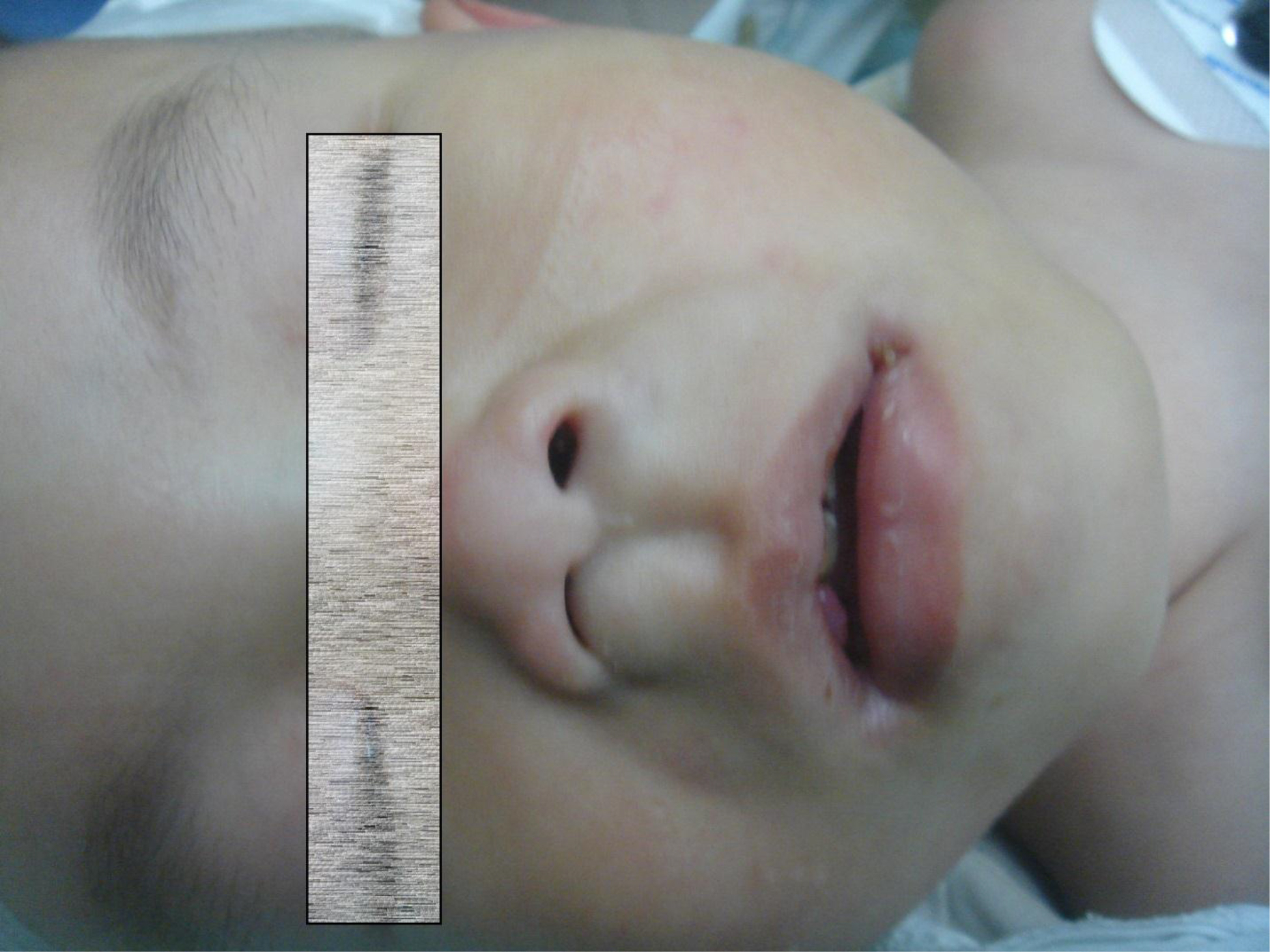
  12. Schafer MJ, White TA, Evans G, Tonne JM, Verzosa GC, et al. (2016) Exercise Prevents Diet-Induced Cellular Senescence in Adipose Tissue. Diabetes 65: 1606-15. [crossref].
  13. Ruiz-Casado A, Martín-Ruiz A, Pérez LM, Provencio M, Fiuza-Luces C, et al. (2017) Exercise and the Hallmarks of Cancer. Trends Cancer 3: 423-441. [crossref]
  14. Sallis JF, Bull F, Guthold R, Heath GW, Inoue S, et al. (2016) Progress in physical activity over the Olympic quadrennium. Lancet 388: 1325-1336. [crossref]
  15. Manini TM (2015) Using Physical Activity to Gain the Most Public Health Bang for the Buck. JAMA Intern Med 176: 968-9. [crossref]