DOI: 10.31038/PEP.2021231
Abstract
Background: In etiopathology, a reductionistic asymmetry favors biology and marginalizes ecology. This misunderstanding is a challenge to overcome because health and disease depend on the entire life organization’s state. This research underlines how the Bionomics discipline is capable of completing the study on Covid-19 contagion dynamics in Monza-Brianza province.
Methodology: After a recall of the principles of Bionomics, the bionomic state of the Monza-Brianza (M-B) province is exposed. The bionomic functionality (BF) of each municipality, evaluated as landscape unit (LU), is compared with the mortality rate (MR) and the Covid-19 infections (%).
Results: Bionomic functionality (BF) emerges as the strongest correlation in opposition to the ecological density of the population, which becomes dominant after 2.5% of infected people. Other parameters, as PA (population age), seem to be less critical.
Interpretation: Environmental exposure and exchanges, and their interaction with the body’s biological systems and apparatuses, play an essential role in disease development. The main processes will be underlined. Significantly Prevention must change perspective, leading Medicine more systemic, from sick care to health care.
Keywords
Covid-19, Landscape Bionomics, contagion dynamics, macro-scale biologic processes.
Introduction
In many seminars and publications, Ingegnoli affirmed that traditional Biology focused on small scales (from biomolecule to the organism) is still mainly reductionist, so marginalizing broad scales (from community to landscape and biosphere). For instance, Medicine seems to be interested only in traditional Biology. Nevertheless, the ‘rock in the pond’ [1] of the Systemic Turn in scientific paradigms imposes to change our vision: biology does not concern only micro-scales.
We can see that the biological studies on bio-chemical molecules, genetics, viruses, metabolism brought to great successes, but also made insidious errors as, for instance, the statement of DNA as the “central dogma of molecular biology” [2], wrong because the DNA is not a set of formed characters but a set of potentialities [3]. Another tricking error is just the marginalization of macro-scales, which brought to refuse a proper scientific role to the researches in this field. In Medicine, we can see two reactions: (a) many researchers think even today to the fallacy of ecological aspects in etiology, and (b) some doctors app It is deepening the Systemic Theory, the difference between what reciate the problems that come with environmental degradation but, generally, see them as someone else’s problem to solve, while they focus on repairing the damage. So, it is not entirely clear what the medical profession/students are meant to ‘do’ with the ecological problems and how they can use them to help patients. However, recently, some Medical communities recognize that human alteration of Earth’s ecological systems threatens humanity’s health. This fact has given rise to Global Health and Planetary Health, which are interdisciplinary while, first of all, they must be systemic and pursue a preferential relationship between advanced Ecology and Medicine [4].
This misunderstanding between Medicine and Ecology is a challenge: we must overcome this impasse! Thus, we cannot discuss the unity of Life, but we have to understand better how its scalar interrelations may influence our health. The alterations of Life at macro-scales can damage human health, not unlike at small ones. Note that the underestimation of the environment is rooted in Neo-Darwinian’s thinking: concepts such as the struggle for existence and natural selection are metaphors [5], not theories, so Darwin’s hypothesis becomes “the best-adapted individuals are more likely to have descendants.” Thus, other limits of Darwinism appear:
- In biology, it is possible to demonstrate that the struggle for existence is less significant than cooperation and symbiosis [6, 7];
- Mathematics has shown that in a complex system, a random variation always produces damage: e.g., Arnold, Moser, and Kolmogorov’s theory, [8];
- Bio-semeiotics has shown that, in addition to genetic codes, there are other organic and mental codes [9] involved in evolution;
- The epigenetic control of gene expression due to DNA methylation demonstrates that the phenotype is not directly expressed by the genotype [10], and part of the genome’s methylation pattern can be inherited in the Lamarckian sense.
The dependence of gene expression on the environment is now clear, as confirmed by Psycho-Neuro-Endocrine-Immunology [11]. We move from a mechanistic vision to a complex and systemic one: not only what is written in the sequence of the DNA bases matters, but also their modulation due to the information that the environment and behavior express.
After this introduction, we can see that overcoming the mentioned misunderstanding between Medicine and Ecology needs a theoretical premise on Landscape Bionomics [12] and an example of application that correlates bionomics, landscape health, and a disease’s incidence. Starting from a recently published study on Covid-19 incidence in the province of Monza-Brianza at the beginning of this pandemic (March-November 2020) [13], it could be stimulating to complete the study on this contagion dynamics in the second substantial increase (November 20-May 21). Therefore, an innovative discussion will follow.
Theoretical References
From Traditional Ecology to Bionomics
Traditional Ecology asserts that Life organization consists of hierarchic levels: cell, organism, population, communities (i.e., the “biological spectrum” sensu EP Odum [14]) and their life support systems. However, we may observe that the world around Life (an organism, a community) concerns other life systems; so, the concept of ‘support’ must be changed into that of ‘integration’. That is why the concept of Life cannot be limited to a single organism or a group of species, but it also includes ecocoenotopes, landscapes, ecoregions, and the entire ecosphere (eco-bio-geo-noosphere): as all remember, the Gaia Theory [15] has claimed that the Earth can be considered a near-living entity.
Inquiring into what stated by Bionomics (i.e., the Theory of Life Organization on Earth) [12,16,17], Life on Earth is a complex open process, operating as a hyper-complex system with a continuous exchange of matter, energy, and information with its environment: information is the exchange (interrelation) that allows the emergence of cognitive distinction (order) between players (the components of the system). Thus, Life on Earth is organized in a hierarchy of six interrelated space-time-information levels (Tab.1), and each level cannot exist without its proper environment because of these integrations and exchanges.
Understanding the Systemic Theory, it is evident the difference between what exists (Real Systems: Life on Earth organized in Living Entities) and the different approaches to studying the environment (viewpoints). As exposed in Tab.1: it is a complete transformation of the main principles of traditional ecology by being aware that hierarchical levels are types of living complex systems; so, it is possible to define a state of health for each level.
Table 1: Hierarchic levels of Biological Organisation on the Earth
|
Scale of Real Systems |
Viewpoints | BIONOMICS | |||
| SPACE1 CONFIGURATION |
BIOTIC2 |
FUNCTIONAL3 |
CULTURAL-ECONOMIC4 |
||
| Global (Earth) |
Geosphere |
Biosphere | Ecosphere | Noosphere |
Geo-eco-bio-noosphere |
| Continental (Region) |
Macro-chore |
Biome | Biogeographic system | Regional Human systems |
Ecoregion |
| Territorial (Province) |
Chore |
Set of communities | Set of Ecosystems | District Human systems |
Landscape |
| Local (District) |
Micro-chore |
Community | Ecosystems* | Local Human systems |
Ecocoenotope |
| Stationary |
Habitat |
Population | Population niche | Cultural/Economic |
Meta-population |
| Singular |
Living space |
Organism | Organism niche | Cultural agent |
Meta-organism |
| 1= not only a topographic criterion, but also a systemic one; 2= Biological and general-ecological criterion;
3= Traditional ecological criterion; 4= Cultural intended as a synthesis of anthropic signs and elements; Bionomics = Types of living entities really existing on the Earth as spatio-temporal-information proper levels *The term Ecosystem may be available following the functional viewpoint but, if we refer to the whole system, it must be identified as Ecocoenotope. |
|||||
Some Basic Concepts of Environmental Functionality
As one can read within the book “Frontiers of Life,” edited by Baltimore, Dulbecco, Jacob, and Levi-Montalcini and published by Treccani (Rome) and Academic Press (Boston) 1999-2001, the section on Landscape Ecology [18] already stated that…
(a) Processes allowing life definitions are ontological, but each specific biological level emerges, expressing these processes adequately.
(b) The relation between pathology and ecology of the systems will allow a diagnosis of each of them in a clinical sense.
(c) Territorial and regional space-time-information scale and the related living systems (landscape and ecoregions) are the most directly involved in human pathology insurgence.
(d) Both the landscape and the system of landscapes (=region[1]) are complex systems, existing as a biological entity within an entire Life’s Hierarchy, whose character and behavior are morethan the result of the action and interaction of natural and human components [18]. Thus,
(e) The landscape structure is not an ecological mosaic, as stated by conventional ecology, but an ecotissue: a multidimensional structure, as a histologic tissue, which represents the hierarchical intertwining of the ecological upper and lowers biological levels and of all their relationships within the landscape (Fig.1, a).
(f) As living systems, landscapes are self-organizing, adaptive, dynamic, self-regulating, dissipative, metastable.
(g) The crucial role in ensuring Life and structuring landscapes pertains to vegetation communities, the physiology of which leads to the concept of the ‘latent capacity of homeostasis’ of a phytocoenosis: it needs to dissipate their energy’s excess to maintain their organizational and metastability level, through a flux (Mcal/m2/year) evaluable by a systemic function, the Biological Territorial Capacity of Vegetation (BTC) [18,19].
The natural landscape units and sub-units, with the dominance of natural components and biological processes, capable of healthy self-regulation, represent the Natural Habitat (NH). By contrast, the transformed sub-units of human landscape (e.g., urban, industrial, and rural areas) but also the semi-human ones (e.g., semi-agricultural, plantations, ponds, managed woods), each with its proper weighted average value of human apport of subsidiary energy and technology, represent the systemic state function named Human Habitat (HH) able to evaluate how much men can affect and limit the natural systems’ self-regulation capability. Following Bionomics, the HH cannot be the entire territorial (geographical) surface (% of Landscape Unit, LU).
Processes, functions, and roles within landscapes, relating abiotic components, vegetation, fauna, and humans, are performed through formal elements organized as Landscape Apparatuses. The main Landscape Apparatuses can be defined as follows (Fig.1, b):
- HGL = Hydro-geologic (emerging geotopes or elements dominated by geomorphic processes)
- RNT = Resistant (elements with high metastability, e.g., forests)
- RSL = Resilient (elements with high recovery Capacity, e.g., prairies or shrublands)
- PRT = Protective (elements that protect other components or parts of the mosaic)
- PRD = Productive (elements with high production of biomass: agricultural fields, meadows)
- SBS = Subsidiary (systems of human energetic and work resources) as industrial and trade
- RSD = Residential (systems of human residence and dependent functions)
Note that both the natural and the anthropic Landscape Apparatuses present natural and human aspects (Fig.1b).
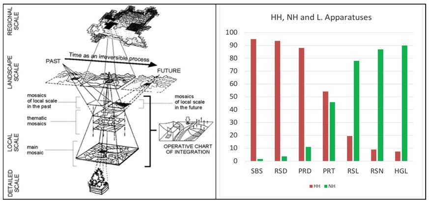
Figure 1: (a) The concept of ecotissue is represented to the left (from Ingegnoli, 2002) [19]. (b) The main landscape apparatuses are expressed related to the concept of HH and NH. Both the pictures are referred to the Lombardy region, North of Italy.
The set of portions of the landscape apparatuses (within the examined LU) indispensable for an organism to survive is better known as Standard Habitat per capita (SH). It represents the state function strictly related to the previous concepts (m2/inhabitant) [12]. It is available for an organism (man or animal), divisible in all its components, biological and relational. In the case of human populations, we will have SHHH, that is an SH referred to the human habitat (HH):
SHHH = (HGL+PRD+RES+SBS+PRT) areas / N° of people [m2/inhabitant]
The connected Minimum Theoretical Standard Habitat per capita (SH*) is the state function estimated as dependent on (a) the minimum edible Kcal/day per capita [1/2 (male + female ) diet]; (b) the productive capacity (PRD) of the minimum field available to satisfy this energy for one year, taking into account the production of primary crops of organic farming; (c) an appropriate safety factor for current disturbances; (d) the need for natural or semi-natural protective vegetation for the cultivated patches[12]. It is estimable for each type of animal population too. Finally, the ratio SH/SH*, named Carrying Capacity (s) of a LU, is the state function able to evaluate the self-sufficiency of the human habitat (HH), a basilar question for sustainability and ecological–territorial planning.
Biological Territorial Capacity of Vegetation (BTC)
This function represents the fundamental state function of a territorial system, proved the fundamental role of vegetation communities (both natural and anthropized, even if with different significance) in managing the whole system’s energy to reach, rebalance and maintain its proper metastable equilibrium.
It can be studied on the basis of: (a) the concept of resistance stability; (b) the type of vegetation community; (c) its metabolic data (biomass, net or gross primary production, respiration, B, NP, GP R); (d) their metabolic relations R/GP (respiration/gross production) and (e) their order relations R/B (respiration/biomass) = dS/S (antithermic maintenance). Two coefficients can be elaborated:
ai = (R/GP)i / (R/GP)max bi = (dS/S)min/(dS/S)i
ai measures the degree of the relative metabolic capacity of principal vegetation communities;
bi measures the degree of the relative anti-thermic (i.e., order) maintenance of the same central vegetation communities.
The degree of the homeostatic capacity of a phytocoenosis is proportional to its respiration. It can be expressed as the flux of energy that the phytocoenosis must dissipate to maintain its condition of order and metastability [Mcal/m2/year].
BTCi = (ai + bi ) Ri w (Mcal/m2/year)
where w = 1.4-1.6 (root biomass coefficient)
Therefore, the BTC function is essential because it is systemic and can evaluate the flux of energy available to maintain the order reached by a complex system.
The comparison between two very different agrarian landscapes near Milan in Fig.2 shows HH’s useful applications and BTC’s exposed concepts. Note that the BTC level difference is very sharp: Oltre-Po BTC = 1.75 Mcal/m2/year Vs. Chiaravalle BTC = 0.73 Mcal/m2/year, while the HH are closer. This example may also demonstrate bionomic principles’ capability to evaluate a complex ecological system’s health in a very synthetic view.
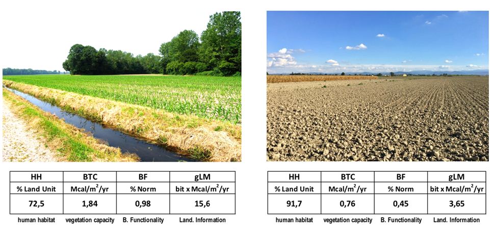
Figure 2: The comparison between two very different agrarian landscapes near Milan. The difference in BTC level is very sharp and the two measures of HH, and BTC can demonstrate the capability of bionomic principles to evaluate the health of a complex ecological system in a very synthetic view. Bionomic Functionality and Landscape Information level are related to the ethological unconscious alarm recording process, as we will see later.
Bionomics Functionality (BF)
Focusing on the possibility to reach a simple way to frame the general health state of a territorial unit, after the study of 45 landscape units (in North Italy), an excellent correlation between the Biological Territorial Capacity of Vegetation (BTC) and the Human Habitat (HH) was found with an R2 = 0.95 and a Pearson’s correlation coefficient of 0.91 (significance = 2.93).
As we can see in Fig.3, it was possible to build the simplest mathematical model of bionomic normality, available for the first framing of landscape units’ dysfunctions.
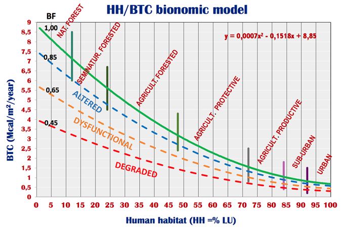
Figure 3: The HH/BTC model, able to measure the bionomics state of a LU. Dotted lines express the BF level, that is the bionomics functionality of the surveyed LU. From Ingegnoli [12].
Below normal values of bionomic functionality (BF= 1.15- 0.85), with a tolerance interval (0.10-0.15 from the curve of normality) we can register three levels of distorted BF: altered (BF = 0.85-0.65), dysfunctional (BF = 0.65-0.45) and highly degraded (BF < 0.45). The vertical bars divide the main types of landscapes, from Natural-Forest (high BTC natural) to Dense-Urban: each of them may present a syndrome.
Again, this model is indispensable to reach a first eco-bionomics diagnosis on the health of an examined landscape unit (LU), thus to give a simple suggestion of the eco-bionomic quality of the place where patients live, to control the effects of a territorial planning design, to study the landscape transformations, etc. It is a complex model because both HH and BTC are not two simple attributes, and their behavior is not linear.
Methodology
The Bionomic State of the Monza-Brianza (M-B) province (Lombardy)
The study on the environment-health alterations in M-B (2011-2017) had many reasons: this province presents the higher ecological density of population (25.1 people/ha) with a high human habitat (HH = 82 %), is the nearest to Milan, and it is characterized by a wide landscape gradient, from dense-urban to agricultural-protective.
The research started on the correlation between bionomic functionality (BF) and the mortality rate (MR), adding to M-B the area of Milan City (Ingegnoli & Giglio) [12, 20]. This basilar study allows the deep knowledge of the state of the environment following bionomics principles.
Pollution could be considered as homogeneous in our sample land area (Fig.4, left). The biological territorial capacity of vegetation (BTC) was estimated using field surveys (LaBiSV method, sensu Ingegnoli) [21,22,23], primarily referred to as forest patches. Fig.4, right, exposes the most significant set of forest assessments surveyed on the field. The fair value of the mean BTC = 5·84 Mcal/m2/year (a low value) is confirmed by the presence of 57·14 % of altered and weak forests, Vs. only 19·05 % of good ones (BTC > 7.0).
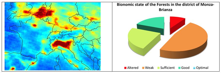
Figure 4: In the Po plain, the distribution of air pollution is relatively homogeneous and one of the highest in the EU, ESA [24]. Not only Milan but also Monza-Brianza are inserted in this wide polluted area. (right) The bionomic state of the forest formations on the Province of Monza-Brianza shows only 19·05 % of the right conditions, and no one is truly optimal.
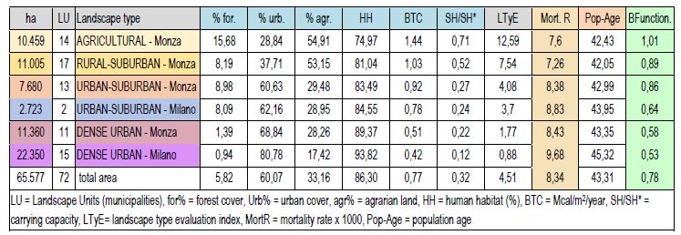
As shown in Fig.5, the blue line indicates a territory covered by the 55 + 17 = 72 municipalities (landscape units, LU) of the province of Monza-Brianza and Milan city (left). This land is compared with the bionomic metropolitan area of Milan (red), the N-E part of which is comprised in Monza-Brianza. Tab.2 shows the ecological and bionomic parameters per landscape type.
Bionomic principles and methods can find the landscape gradient, composed of six types (from agricultural to dense urban) and its relations with the mortality rate (MR), the bionomic functionality (BF), and the population Age (PA). In Fig.5., the decrease of BF (blue) is related to MR’s increase (red). Elaborating the bionomic parameters (Tab.2) we note an average of BF = 0.78 (low value), indicating an altered environment.
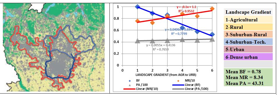
Figure 5: The blue line indicates the land area of experimentation: Monza-Brianza [Milan City is just South of Monza]. This territory covers 656 Km2 with a population of 2.3 x 10⁶ inhabitants and with a gradient of 6 landscape types. (base map from DUSAF-Ersaf). Note, in the plot, the inverse proportionality between MR (red) and BF (blue), while PA remains near constant. From [20].
Table 2: Gradient of landscape types emerged analysing 72 municipalities from Milan to the Brainza hills.
Covid-19 Contagion Dynamics in Monza Brianza (M-B)
Another figure (Fig.6) was developed for each municipality of M-B province, showing: Population (2018), FOR % (forest cover), URB% (urbanized), AGR % (cultivated land), HH% (Human Habitat), BTC (Mcal/m2/year), HS/HS* (Carrying Capacity), BF (Bionomic Functionality). In October 2020 and May 2021, we added these data, the Covid-19 (infected people) and Covid-19 (%). The colors distinguishing the data are related to the landscape types of urban (violet), suburban (grey), and agrarian (yellow). The landscape gradient is very mixed, so a trend of instability emerges per each landscape type (here seven), even if the ecological density (ED) increases with urbanization.
Another figure (Fig.6) was developed for each municipality of M-B province, showing: Population (2018), FOR % (forest cover), URB% (urbanized), AGR % (cultivated land), HH% (Human Habitat), BTC (Mcal/m2/year), HS/HS* (Carrying Capacity), BF (Bionomic Functionality). In October 2020 and May 2021, we added to these data, the Covid-19 (infected people) and Covid-19 (%). The colors distinguishing the data are related to the landscape types of urban (violet), suburban (grey) and agrarian (yellow). The landscape gradient is very mixed, so a trend of instability emerges per each landscape type (here seven), even if the ecological density (ED) increases with the urbanization.
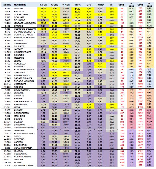
Figure 6: Note that the colors marking the data are related to the landscape types of urban (violet), suburban (grey) and agrarian (yellow). The landscape gradient is mixed, so a trend of instability emerges per each landscape type (2 agricultural, 2 rural, 2 suburban, 2 urban), even if the ecological density increases with the urbanization. Comparison between Covid-19 influence, Oct 20th Vs. May, 1st.
It is possible to demonstrate that bionomic parameters played a crucial role in infective development, not considered among the mentioned conventional factors. In Tab.4, the yellow, grey, and violet colours underline the data related to the rural, suburban, and urban-type landscapes. The bionomic data (HH, BTC, HS/HS*, and BF) are complex indicators obtained applying Landscape Bionomics’ principles and methods, as exposed in the cited volume Biological-Integrated Landscape Ecology [12].
The Covid-19 incidence in this Province [26], presents three phases: (a) March-May 2020, reaching about 5,000 infected, (b) September-October passed from 6,000 to 30,000 and (c) November 2020 – May 2021 from 30,000 to 75,000. The surveys to verify possible correlations with bionomic and ecological parameters were six: (i) April 19 (4,100 infected), (ii) July 31 (5,880 infected), (iii) October 20 (9,360 infected), (iv) November 16 (33,900), (v) March 30 (68,800), (vi) May, 01 (75,000) [24].
Results
The Mortality Rate as a function of BF
Previous research [20] demonstrated that the mortality rate (MR) is correlated with the BF (Fig.7). Note that even the population age (PA) is growing with the degradation of the LU, but the increase of MR is more than four times the increase of PA (0.76 Vs. 0.24); so, the rise of MR with Landscape degradation is mainly due to other physiologic and bionomic processes, first of all, the landscape diseases [12, 20].
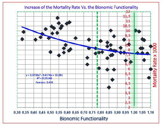
Figure 7: An evident increase of mortality rate MR [x 1000] is correlated with the increase of landscape dysfunction: we pass from MR = 7.64 in not altered landscapes (BF = 1.0) to MR = 9.5 in the landscape with deprivation of 50% (BF = 0.50) of the normal state. The correlation significance (Pearson) is 1.85.
To evaluate a preliminary Risk Factor from the MI-MB Model [BF = 0.78]:
ΔMRBF = (MRBF – MRBF=1) x 76% = (8.34 – 7.64) x 0.76 = 0.532 x10⁻³
The correlations Covid-19 Vs. bionomic parameters
The first correlation is presented in Fig.8, left (Oct-20). The trend line has a modest R2 value (0.1513) but its Pearson Coefficient [26] is sufficiently high (0.38). So, at proper bionomic functionality conditions (BF=1.0) the incidence of Covid-19 is pair to 0.90 %, while at weak BF=0.45, Covid-19=1.2 % (+133%).
The statistical population of 55 LU of Monza-Brianza province registers a minimum Pearson Coefficient value pair to 0.266. So, the correlation Covid-19 Vs. BF results 0.38/0.266 = 1,45: an available significance of correlation. A still more important correlation is expressed in Fig.8, dx, where the ecological density (ED), which represents the inverse of SH, presents in March 2021 a value of significance equal to 1.77.
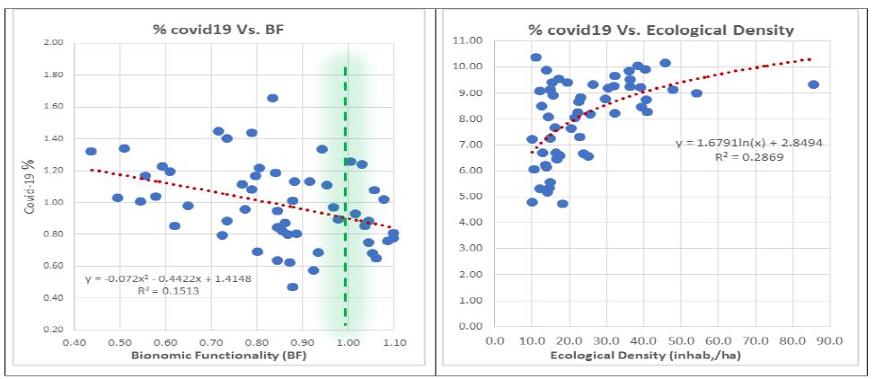
Figure 8: The most meaningful correlations between Covid-19 (%) and Bionomic parameters: (sx) bionomic functionality (BF) in the third survey (OCT, 20), and (dx) ecological density (ED) in the last survey (MAR, 21). Note that values on the y axis changes due to the increase of the disease incidence.
The tested parameters (Tab.3) where: (1) Ecological Density (ED) [people/ha], (2) Bionomic Function (BF) [BTC/BTCNORM], (3) Population Age (PA) [mean years], (4) Forest Cover (For) [% of LU], (5) Agricultural Land (Agr) [% of LU], (6) Urbanized Cover (Urb) [% of LU], (7) Human Habitat (HH) [% of LU]. The period: 423 days.
Table 3: Pearson Significances of the main Ecological-Bionomic Parameters Vs. Covid-19 contagion in Monza-Brianza Province: Note that Agr. and Urb. are comprised in ED, while For. And HH in BF (see Fig.10).
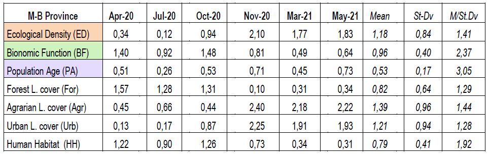
Remember that the essential bionomic parameters are: ED, relating Agrarian fields, Urban and Human Habitat; BF, relating Forest, Agriculture, Human Habitat; and Population Age. Note that ED presents an excellent average significance (ED = 1.18 ± 0.84); so, the standard deviation is very high. BF presents a bit less average but a better standard deviation: BF = 0.96 ± 0.40. The correlation significance of PA presents an average still more homogeneous but at a decidedly lower value: PA = 0.53 ± 0,17. Moreover, the averages of ED and BF are not significantly different (1.18 Vs. 0.96) but they seem to be in opposition: for the first 238 days ED (mean = 0.47) is low and BF high (mean BF = 1.27), while for the other period (185 days) is the contrary (ED = 1.81 Vs. BF = 0.65). Unlike the other parameters, PA remains lower and almost constant.
The Pearson’s correlation significances of the seven parameters are shown in Fig.9. Forest, Human Habitat, and their synthesis (BF) are shown in green and blue lines, while their opposites Agrarian, Urbanized, and their synthesis (ED), are shown in brown and red lines. PA (violet) remains near-constant, even if older people’s presence leads to high mortality.
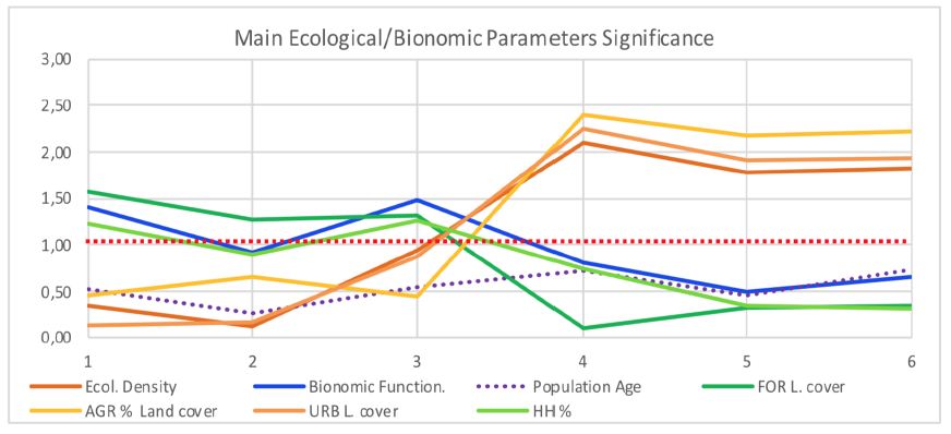
Figure 9: The dynamics of Pearson’s Correlation significances of the seven parameters. We can see two opposite trends, guided by BF (green) and ED (brown). PA (dotted blue) remains of lower significance and near constant.
To study the Covid-19 contagion dynamics we need to consider only the three main parameters significances (BF, ED) related to time (days) and the increase of infection percentages in the period (1.16 year) (Fig.10).
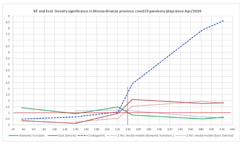
Figure 10: Dynamics of the essential correlations significances between BF and ED in the first year of Covid-19 pandemic in the province of Monza-Brianza. Only when the contagion reached 2.5 % of the population, after 238 days, the ED became the leader environmental correlation in this territory.
This result is notable because the infection has grown where the environment was altered (BF average significance = 1.27) in the first 238 days (65.2 % of the year), leaving the ED contributions as marginal (average significance = 0.47). When the threshold of 2.5 % of infected people was exceeded, ED became the dominant correlation reducing the BF average significance to 0.64 (but not eliminating the correlation). So, a good BF can be considered a defense against infections, slowing down the contagion for 2/3 of a year.
Note that the ecological density ED (inhabitant/ha) is a bionomic parameter related to the concept of the human habitat (HH); so, it has nothing to do with the traditional geographic population density (GD, inhabitant/km2): being the average human habitat HH = 82 %, the ecological density ED = 26.3, while the geographic density GD = 21.5 (inhabitant/ha), with a difference of about + 22 %.
Discussion
Main Processes in Macro-Scale Biology: The Influence of Stress
We affirmed that health and disease depend on the state of the entire organization of life. Consequently, biology’s study should be extended to macro-scales, trying to understand their “anatomical” components, physiological processes and state functions, transformation processes, clinical-diagnostic evaluation, pathologies, and rehabilitation therapies. Here some examples:
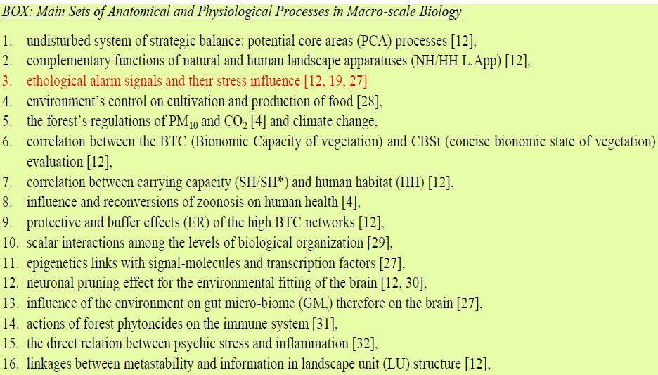
All these sets of processes, and more, need a more advanced ecological discipline because the traditional General Ecology does not elaborate landscape principles and methods, and Landscape Ecology only partially. That is why Ingegnoli founded Landscape Bionomics’ new ecological discipline, the main criteria of which we presented in the second paragraph. It can, therefore, be shown that alteration of life at the macro-scales can damage human health no less than at the micro-scales, for instance, recalling point (3) ethological alarm signals and their stress influence (Fig.11).
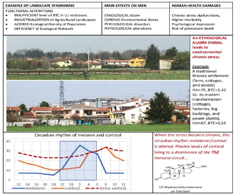
Figure 11: An example of how Biological macro-scale alterations and derived physiological processes are damaging human health. Environmental stress can be registered by the ethological concept of “value judgment”. The sympathetic nervous system and the hypothalamus-pituitary-adrenal axis mediate the integrated responses of the human organism to stress. Note the crucial importance of cortisol.
Many of the stressors are due to landscape structural dysfunctions, even in the absence of pollution. An Ethological Alarm Signal leads to environmental stress, which can be chronic. Stressors simultaneously activate:
(a) neurons in the hypothalamus, which secrete CRH (Corticotropin-releasing hormone), and
(b) adrenergic neurons
These responses potentiate each other. The final effect of the activation of neurons that secrete CRH is the increase in cortisol levels, while the net effect of adrenergic stimulation is to increase plasma levels of catecholamine (Dopamine, norepinephrine, and epinephrine).
The negative feedback exerted by cortisol can limit an excessive reaction, which is dangerous for the organism. However, when the stress became chronic, the circadian rhythm of melatonin/cortisol is altered. Plasma cortisol levels bring to a dominance of the Th2 immune circuit, with production of typical catecholamine (e.g., IL-4, IL- 5, IL-13) and the circuit Th17 [27].
Note that the Th2 immune response is not available to counteract viral infections, neo-plastic cells, auto-immune syndromes, which need a Th1 response. So, the premature death risk increases.
Widening the Categories of Environmental Alterations Influencing Human Health
Genome-Wide Association Studies (GWAS) revealed a limited causal effect (estimated less than 20%) of genetic susceptibility on phenotypic variance. Consequently, environmental exposure plays a crucial role in disease development, both in infectious (IDs) and non-communicable diseases (NCDs), such as viruses and bacterial infections (IDs), cancer, asthma, cardiovascular and endocrine diseases (NCDs). In reality, we have to underline that environmental exposure and exchanges, and their interaction with the body’s biological systems and apparatuses, play an essential role in disease development.
Note that the concept of exposure (e.g., the exposome, sensu Wild [33]) may be necessary but not sufficient because of the complex structures and interrelations of life. Even if, generally, only three categories are mentioned, we have to distinguish at least four categories of environmental alterations capable of influencing human health through exposure and interactions:
(a) internal processes, e.g., metabolism, hormonal balance, gut microbiota, aging, etc.,
(b) specific external factors, e.g., infections, pollutants, smoking, drugs, etc.,
(c) general external factors, e.g., socioeconomic status, technological behaviors, climate change, etc., and
(d) landscape structure/function alterations, e.g., concerning hierarchical relations, the biological territorial capacity of vegetation, vital space per capita, ratio human/natural habitats, etc. (see box).
Widening the concept of Anamnesis and Therapy Integration
We will see that Landscape Bionomics, while sustaining the listed physiological processes (green Box), opens new perspectives to etiopathology, health prevention and therapy integrations, and anamnesis. So, new linkages between the two disciplines, Landscape Bionomics and Medicine, emerge following the new systemic paradigm, both in diagnostic and therapeutic fields in etiology and anamnesis. We can indicate an answer to what is not entirely clear to the medical profession/students (see Introduction): what they are meant to ‘do’ with the ecological problems and how they can use them to help patients (Fig.12).
Fig.12 shows that the primary set of landscape syndromes can be grouped in six categories: (1) structural and hierarchical alterations, (2) excess processes alterations, (3) lack of protective agents, (4) cybernetic and information alterations, (5) agrarian landscape food and diet alterations, (6) chemical and physical pollutions. These processes, frequently cumulative (at least partly), lead to health damage with an interchange between the body’s external and internal life systems. MD’s responsibility is to repair the damage, but in doing this, MD should contact internal specialists and external ecojatra: at least to avoid reintroducing the patient into the same environment that contributed to the insurgence of the disease. Moreover, to add, first, a wider anamnesis and then an integrated therapy.
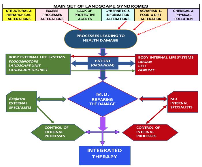
Figure 12: This flow diagram tries to explain that MD have to repair the damages to human health but, being the majority of these damages due to environmental alterations and being the organism linked with body internal and external life systems, MD have to collaborate with internal and external specialists, arriving TO an integrated therapy.
Conclusion
In conclusion, we have to underline that environmental exposure and exchanges, and their interaction with the body’s biological systems and apparatuses, play an essential role in disease development. Studying the M-B province, we started showing the importance of broad-scale biology:
1.1) The mortality rate (MR) correlated with Bionomic Functionality (Pearson significance 1.85) 2015;
1.2) Bionomic Functionality correlated with Covid-19 % (Pearson significance 1.45) 2020, October;
1.3) Ecological Density correlated with Covid-19 % (Pearson significance 1.66), 2021, May;
1.4) Emergence of a Contagion dynamics: BF and ED inverted their dominance of correlation after the threshold of infected people = 2.5 %;
Therefore, we had to pass from qualitative to quantitative considerations related to macro-scale biology’s influence on human health scientifically, as suggested by landscape bionomics principles and methods. This fact underlines a more efficient control of environmental rehabilitation to enhance prevention against infectious (IDs) and non-communicable diseases (NCDs) [40] and indicates therapeutic integration between chemical and natural care.
On the other side, the possibility to evaluate the bionomic state of the landscape units and consequently to correlate its bionomic functionality (BF) with the mortality rate [21] reinforces the possibility to control the environmental syndromes and reduce the impacts of transformation, and advise the local Authorities for the necessity to ecological rehabilitation.
References
- Urbani-Ulivi L ed. (2019) The Systemic Turn in Human and Natural Sciences. A Rock in the Pond. Springer-Nature, Switzerland.
- Crick, FH (1958). On Protein Synthesis. In F. K. Sanders (ed.).Symposia of the Society for Experimental Biology, Number XII: The Biological Replication of Macromolecules. Cambridge University Press 138–163.
- Waddington CH (1961) The nature of life. Atheneum, New York.
- Frumkin H, Myers S (2020) Planetary Health, Protecting Nature to Protect Ourselves. Island Press, USA.
- Popper K, Lorenz K (1985) Il Futuro è Aperto. Bompiani.
- Margulis L (1975) Symbiotic theory of the origin of eukaryotic organelles; criteria for proof.In: Symposia of the Society for Experimental Biology 21-38. PMID. [crossref]
- Simard S, Roach WJ, Defrenne C et al. (2020) Harvest Intensity on Carbon Stocks and Biodiversity Are Dependent on Regional Climate in Dougles.Fir Forests of British Columbia. In: Frontiers I Forests and Global Change
- Scott-Dumas H (2014) The KAM story: a friendly introduction to the content history and significance of classical Kolmogorova Arnolda Moser Theory. In: World Sc. Publ.
- Barbieri M (2008) A new understanding of life. Naturwiessenshaften Pub.
- Holliday R (2006) Epigenetics : A Historical Overview. In : of Epigebetics Pp. 76-80.
- Bottaccioli F (2014) Epigenetica e Psiconeuroendocrinoimmunologia, le due facce della rivoluzione in corso nelle scienze della vita. Edra spa, Milano.
- Ingegnoli V (2015) Landscape Bionomics. Biological-Integrated Landscape Ecology. Springer, Heidelberg, Milan, New York Pp. XXIV + 431.
- Ingegnoli V, Giglio E (2020) Covid-19 Incidence and its Main Bionomics Correlations in the Landscape Units of Monza-Brianza Province, Lombardy. J Environ Sci Public Health 4 (4):349-366, USA.
- Odum EP (1971) Fundamentals of Ecology. Saunders, Philadelphia, USA.
- Lovelock J, Margulis L (1974) Atmospheric Homeostatsis by and for the Biosphere: the Gaia Hypothesis. Tellus
- Ingegnoli, V. (2011). Bionomia del paesaggio. L’ecologia del paesaggio biologico-integrata per la formazione di un “medico” dei sistemi ecologici. Springer-Verlag, Milano pp. XX+340.
- Ingegnoli V, Bocchi S, Giglio E (2017) Landscape Bionomics: a Systemic Approach to Understand and Govern Territorial Development. WSEAS Transactions on Environment and Development 13, pp. 189-195.
- Ingegnoli V (2001) Landscape Ecology. In: Baltimore D., Dulbecco R., Jacob F., Levi- Montalcini R. (Eds.) Frontiers of Life. New York, Academic Press Vol IV, pp 489-508.
- Ingegnoli, V (2002) Landscape Ecology: A Widening Foundation. Berlin, New York. Springer XXIII+357.
- Ingegnoli V, Giglio E (2017) Complex environmental alterations damages human body defence system: a new bio-systemic way of investigation. WSEAS Transactions on Environment and Development 170-180.
- Ingegnoli V, Giglio E (2005) Ecologia del Paesaggio: manuale per conservare, gestire e pianificare l’ambiente. Sistemi editoriali SE, Napoli pp. 685+XVI.
- Ingegnoli V. (2005) An innovative contribution of landscape ecology to vegetation science. Israel Journal of Plant Sciences 53: 155-166.
- Ingegnoli V, Pignatti S (2007) The impact of the widened Landscape Ecology on Vegetation Science: towards the new paradigm. Springer Link: Rendiconti Lincei Scienze Fisiche e Naturali, s.IX, vol.XVIII, pp. 89-122.
- ESA (2015) Air quality pollution. IUP, Heidelberg.
- Regione Lombardia (2021) Covid-19 Dashboard in Lombardy.
- Garson GD (2013) Correlation. Statistical Associates “Blue Book” Series Book 3.
- Bottaccioli F, Bottaccioli AG (2020) Psychoneuroendocrineimmunology and the science of integrated care, Edra, Milan.
- Ceccarelli S (2013) Produrre i propri semi. Manuale per accrescere la biodiversità e l’autonomia nella coltivazione delle piante alimentari. Libreria Editrice Fiorentina, Firenze.
- Ingegnoli V (2021) Enlighten the Intrinsic Relation Between Agricultural Landscape Health and Global Health. In: Raviglione M (coord.), Master on Global Health, Lesson on Disruption of Agrarian landscapes, slide 12 Unimi, Centre for Multidisciplinary Research in Health Science (Mach).
- Gogtay N, Giedd JN, Lusk L et al. (2009) Dynamic mapping of human cortical development during childhood through early adulthood. Proceedings of the National Academy of Sciences of the United States of America 101 (21), pp. 8174- 8179. [crossref]
- Li Q (2009) Effect of forest bathing trips on human immune function. Environ Health Prev Med 2010 Jan: 15(1):9-17. [crossref]
- Slavich GM, Thornton T, Torres LD, Monroe SM, Gotlib IH et al. (2009) Targeted rejection predicts hastened onset of major depression.Journal of Social and Clinical Psychology 28(2): 223–243. [crossref]
- Wild CP (2012) The exposome: from concept to utility. In: Int J Epidemiol 41:24-32. https://doi.org/10.1093/ije/dyr236. [crossref]