Monthly Archives: January 2023

Chronic Psychogenic Hyperventilation, Hypocapnia and Metabolic Acidosis: Hypoxia, Inflammation, Aging and Age-Related Diseases

DOI: 10.31038/ASMHS.2023712

Abstract

In this review article, author discusses about the biomedical importance of carbon dioxide in regulating the cellular homeostasis. Even more important, the author had already presented a hypothesis regarding the role of carbon dioxide in regulating cellular homeostasis, which was published in the program and abstracts (serial number 237) of 1st world congress on stress held in USA, October 4-7, 1994. The author goes even further to explain how chronic psychosocial stress and unhealthy diets are the two key risk factors for developing hypocapnia, low-grade metabolic acidosis and insulin resistance, which, in turn, has been shown to predict the development of age-related diseases, including hypertension, coronary heart disease, stroke, cancer, and type 2 diabetes. The writer of this review posits that there is a definite connection between chronic emotional stress, hyperventilation, reduced urine net acid excretion and low-grade metabolic acidosis. The author further explains that like in conventional exercises, therapeutic increase in carbon dioxide in the blood (respiratory acidosis) by way of self-induced hypoventilation is the key to eliminating metabolic acidosis.

Keywords

Chronic psychogenic hyperventilation, Hypocapnia, Low-grade metabolic acidosis, Pranayama and breath retention as an intervention, Renal compensation for respiratory alkalosis and acidosis

Introduction

A Connection between Chronic Hyperventilation and Metabolic Acidosis

Hyperventilation happens most often to people 15 to 55 years old [1]. When a person is under stress, their breathing pattern changes. Typically, an anxious person takes small, shallow breaths, using their shoulders rather than their diaphragm to move air in and out of their lungs. This style of breathing (hyperventilation) causes blood concentration of carbon dioxide (PaCO2) to fall below healthy levels, a condition called hypocapnia [2,3].

In normal subjects, a decrease in PaCO2 (hypocapnia) induced via hyperventilation, elicits two responses with opposing effects on blood pH. In the short term, a decrease in PaCO2 will increase pH of extracellular fluid (respiratory alkalosis). Over a longer period (2 to 6 hours), however, sustained hypocapnia is further compensated by renal response – renal net acid (renal ammonium and titratable acid) excretion decreases, resulting in a reduction in plasma bicarbonate and extracellular fluid acidosis [4,5]. Low-grade metabolic acidosis is a condition characterized by a slight decrease in blood pH, within the range considered normal. Chronic hyperventilation and acidogenic diets when coupled with an age-related decline in kidney function of normal humans (due to failure to excrete the normal acid load generated by protein metabolism) may further influence the occurrence of such a condition.

If these conditions occur in a prolonged, chronic way, low-grade metabolic acidosis can become significant and predispose to metabolic imbalances as well as the increased risk of chronic diseases [6].

It is conceivable that as an individual ages blood acidity will be regulated at progressively higher levels and plasma bicarbonate concentration and PaCO2 at progressively lower levels.

Such progressively worsening metabolic acidosis, however mild, might over time have deleterious effects, perhaps contributing to the pathogenesis of many of the physiologic disturbances and degenerative diseases of aging. Yet, practically no attention has been given to the effect of age on the acid-base composition of the blood in healthy subjects [7].

Breathing Retraining

The most common cause of respiratory alkalosis (hypocapnia) is hyperventilation, which causes more carbon dioxide to be exhaled out. If the cause is anxiety, various breathing exercises might help slow breathing and reduce hyperventilation [8]. There is good evidence that breathing rehabilitation is a useful method for achieving reduced anxiety/panic levels [9].

Respiratory Alkalosis (Hypocapnia) – Cause and Consequences

Respiratory alkalosis is a pathology that is secondary to hyperventilation [10]. The decrease in PaCO2 (hypocapnia) develops when a strong respiratory stimulus (i.e., anxiety or fear) causes the respiratory system to remove more carbon dioxide than is produced metabolically in the tissues [11].

Respiratory alkalosis (hypocapnia) can be acute or chronic [10]. In acute respiratory alkalosis, the PaCO2 level is below the lower limit of normal and the serum pH is alkalemic [11]. However, in chronic respiratory alkalosis, a common acid-base disturbance [5], the PaCO2 level is below the lower limit of normal, but the pH level is relatively normal or near normal due to compensatory mechanisms [11]. Since renal compensation for chronic respiratory alkalosis involves a decrease in HCO3 – reabsorption. It may also mean you have: Metabolic acidosis [12,13].

Potential Causes of Low-grade Metabolic Acidosis in Normal Subjects

Our modern lifestyle, which involves some combination of, (1) Chronic psychogenic hyperventilation as a result of the stress one experiences while sitting still and, (2) the acidogenic diet we eat, are the two main root causes for the development of low-grade metabolic acidosis.

Additionally, age-related renal functional decline in healthy older adults is another risk factor [7,14].

Pathogenesis

(1) Chronic Psychogenic Hyperventilation

Does persistent hypocapnia cause metabolic acidosis? The answer is yes! Because:

Since chronic respiratory alkalosis is a common acid–base disturbance characterized by a primary and sustained decrease in arterial carbon dioxide tension (PaCO2) – that is, by primary hypocapnia due to hyperventilation.

A decrease in PaCO2 (hypocapnia) elicits two responses with opposing effects on blood pH. In the short term, a decrease in PaCO2 alkalinizes extracellular fluid. Over a longer period (6 to 72 hours), however, renal acid excretion is inhibited, resulting in a reduction in plasma bicarbonate that acidifies extracellular fluid and thereby corrects blood pH toward normal. Furthermore, stimulation of the medullary respiratory center in metabolic acidosis induces secondary hyperventilation, resulting in a decrease in PaCO2 (secondary hypocapnia) [5].

We live in modern times, and we are exposed to the modern lifestyle – the most dangerous aspects of which are the inordinate amount of stress we experience while sitting still and the fake foods we eat [15]. It is important to note that according to research studies, over 90% of the modern population have chronic hyperventilation hidden in the modern lifestyle [16].

In normal subjects, chronic hyperventilation lowers plasma bicarbonate concentration (metabolic acidosis), primarily by inhibiting renal ammoniagenesis and the urinary excretion of net acid in response to persistent hypocapnia (PaCO2) [4,5].

(2) Acidogenic Diet

Our dietary habits tend to tip the balance towards acidification. Diets with high acid load produces changes in the acid base balance. There is an association between low-grade metabolic acidosis with the development of age-related diseases (i.e., hypertension, diabetes, chronic kidney disease etc.) [17]

Several studies have indicated the influence of low-grade metabolic acidosis on health outcomes, and diet is one of the factors that directly influence this condition [18].

(3) Age-related Renal Functional Decline

In normal adult humans eating ordinary American diets, systemic acid-base equilibrium is maintained within narrow limits from day to day, despite a continuing input of precursors of fixed acids in the diet.

Day-to-day stability of acid-base composition of the systemic circulation is critically dependent on excretion of acid in urine, the steady-state rate of which is adjusted by the healthy kidney in keeping with the prevailing rate of endogenous acid production.

Considering that renal functional integrity progressively declines with age which limit the adaptive mechanisms responsible for maintaining acid-base homeostasis, it is quite conceivable that as an individual ages, blood acidity will be regulated at progressively higher levels.

Such progressively worsening metabolic acidosis, however mild, might over time have deleterious effects, perhaps contributing to the pathogenesis of many of the physiologic disturbances and degenerative diseases of aging. Therefore, the role of age-related metabolic acidosis in the pathogenesis of the degenerative diseases of aging warrants consideration [7,14].

Chronic Metabolic Acidosis – Functional Disorders in Elderly Persons

Age-related metabolic acidosis is a chronic condition that many people in the Western world have but do not realize it [18]. Metabolic acidosis has been associated with a range of physiological derangements of importance to the health of older people such as: [19]

(i) Metabolic Alterations

Metabolic disorders of high concern in today’s society include obesity, insulin resistance and diabetes, hypoxia and oxidative stress, chronic inflammation, metabolic acidosis and metabolic syndrome, hormone imbalance, kidney disease, cardiovascular disease, excess calcium excretion and osteoporosis, and cancers of all kinds [20,21].

(ii) Organ Dysfunction

Acidosis may adversely affect renal function, cardiovascular health, muscle function and bone health, and impairments in these organ systems would be expected to have an adverse impact on physical function and quality of life – key outcomes for aged people [19].

(iii) Premature Aging and an Increased Risk of Death

Chronic tissue acidosis accelerates the ageing process and creates an environment conducive to the development of a number of diseases [22]. Stated otherwise, acidosis is the first step towards premature aging and accelerated oxidative cascades of cell wall destruction [23].

As an individual ages blood acidity will be regulated at progressively higher levels and plasma bicarbonate concentration and PaCO2 at progressively lower levels.

Such progressively worsening metabolic acidosis, however mild, might over time have deleterious effects, perhaps contributing to the pathogenesis of many of the physiologic disturbances and degenerative diseases of aging. Yet, practically no attention has been given to the effect of age on the acid-base composition of the blood in healthy subjects [7].

Solution of the Problem?

Treating age-related metabolic acidosis with lower CO2 levels is obviously a matter of raising carbon dioxide levels in the blood [24]. If your CO2 levels are too low, the first step your doctor will take is treating the underlying condition (hyperventilation) that is causing the imbalance [25]. How does one do that? The answer is already obvious. Hold your breath. Practice pranayama [15].

According to Patanjali, the founder of Yoga philosophy, pranayama is the gradual cessation of breathing. The eventual goal of pranayama is the complete suspension of the breath for as long as the practitioner wishes [26]. Holding your breath also causes the amount of carbon dioxide building up in your body [27]. Depending on your ability to tolerate CO2, you can become a super-healthy person [15]. Remember, self-induced mild hypoventilation is said to have some benefits, but of course uncontrolled or long-term hypoventilation is to be avoided [28]. It is best to maintain a normal relaxed breathing pattern whenever you are consciously aware of your breathing [29]. Fortunately, we also have the power to deliberately change our own breathing [2].

Benefits of Pranayama?

Scientific studies have shown that controlling your breath can help to manage stress and stress-related conditions [2] by normalizing the baseline levels of carbon dioxide (eucapnia) in the blood, making people less prone to hyperventilation [30].

Furthermore, practicing pranayama (breath regulation or breath control) can enhance quality of life and aid in longevity [31-33]. Other beneficial effects might involve a reduction of distress, blood pressure, and improvements in resilience, mood, and metabolic regulation [34].

In conclusion, it can be safely assumed that controlling or reversing low-grade metabolic acidosis, by yoga breathing exercises and dietary interventions, is likely to be an important way to prevent, or reduce the severity of age-related diseases.

Reversing Age-related Metabolic Acidosis – An Intervention

It is important to note that by working on the continuum of yogic breath challenge, CO2 tolerance, and renal compensation of respiratory acidosis, the goal of prevention or correction of metabolic acidosis can be achieved. Respiratory challenge is the modification of arterial carbon dioxide concentration to induce a change in cerebral function or metabolism. You can experiment with breath hold exercises in order to increase your CO2 tolerance. Although breathing is something your body naturally does, it’s also a skill that can be sharpened [35].

The yogic technique of respiratory challenge is based on a simple modification of respiratory rate, including breath hold [36]. Notably, rapid increase in Pa,CO2 evokes an immediate response by hyperventilation to restore normality. However, a more gradual increase in Pa, CO2 allows renal compensation to occur [37].

Improved CO2 tolerance reduces the urge to breathe and controlled breath holding (hypoventilation) will build CO2 endurance [28]. Research has shown that lower chemosensitivity to hypercapnia in yoga practitioners may be due to an adaptation to low arterial pH and high PaCO2 for long periods [38,39].

Because renal compensation of respiratory acidosis occurs by increased urinary excretion of acid (hydrogen ions) and resorption of HCO3 [40]. By adjusting the amounts of hydrogen ions secreted in the urine and reabsorption of bicarbonate ions from the urine back to the blood, kidneys balance the blood pH, and [41] as a result, in a compensated respiratory acidosis, although the PCO2 is high, the pH is within normal range [42], [43-45].

Since, breathing is an automatic function of the body that is controlled by the respiratory centre of the brain. When we feel stressed, our breathing rate and pattern changes as part of the ‘fight-or-flight response’. Fortunately, we also have the power to deliberately change our own breathing [2]. Hence changing your breathing to a normal pattern can restore healthy CO2, which will eliminate symptoms of hyperventilation [29]. Further, by adjusting the speed and depth of breathing, the brain and lungs are able to regulate the blood pH minute by minute [46,47].

Biomedical Importance of Carbon Dioxide

CO2 plays various roles in the human body including regulation of blood pH, respiratory drive, and affinity of hemoglobin for oxygen (O2). Fluctuations in CO2 levels are highly regulated and can cause disturbances in the human body if normal levels are not maintained, [48] causing disruption of enzyme function, loss of insulin sensitivity, and cellular metabolic adaptations [49].

Benefits of Carbon Dioxide

Carbon Dioxide Dependent Signal Transduction

Research shows that changes in CO2 influence cellular function through modulation of signal transduction networks. Additionally, there is significant cross-talk between these signal transduction pathways as they respond to changes in CO2 [50-52].

Elevated CO2 regulates the Wnt signaling pathway in mammals [53]. The Wnt signaling pathway is one pathway that may contribute to aging [54]. Downregulation of Wnt signaling is an early signal for formation of facultative heterochromatin and onset of senescence in primary human cells [55].

Natural Sedative and Tranquilizer

CO2 is a powerful natural sedative and tranquilizer [56]. Carbon dioxide calms the nervous system, reducing depression, anxiety, and even the symptoms of epilepsy [57].

While considering the mental health of people, the most missing chemical in the human brain is CO2 [29]. Because a lack of CO2 in the brain leads to “spontaneous and asynchronous firing of neurons” (medical quote) “inviting” virtually all mental and psychological abnormalities.

In conscious humans, research findings suggest that increased CO2 levels (mild hypercapnia) cause a reduction in the resting-state neural activity of the brain, which in turn, enters a lower arousal state [58].

Bioavailability of Oxygen

Carbon dioxide is essential for internal respiration in a human body [59]. Increase in the blood concentration of carbon dioxide lowers hemoglobin’s affinity for oxygen, which in turn, enhances the unloading of oxygen into tissues to meet the oxygen demand of the tissue. The Bohr effect describes hemoglobin’s lower affinity for oxygen secondary to increases in the partial pressure of carbon dioxide and/or decreased blood pH [60].

Gardian of the pH

Carbon dioxide is a guardian of the pH of the blood, which is essential for survival. The buffer system in which carbon dioxide plays an important role is called the bicarbonate buffer system. It is an acid-base homeostatic mechanism in order to maintain pH in the blood, among other tissues, to support proper metabolic function [59,61].

Anaplerosis

CO2 is a ubiquitous product of cellular metabolism and an essential substrate for carboxylation reactions, required for refueling the TCA cycle via oxaloacetate during growth on glycolytic carbon (pyruvate) sources. Remember, De novo protein synthesis is required for adaptive response to oxidative and other types of stress, indicating that newly synthesized protective proteins are necessary for adaptation [62].

Cardiovascular System

CO2 is helpful in dilating the smooth muscle tissues, and it regulates the cardiovascular system [63].

Breathing

Breathing is exquisitely sensitive to the alteration in the CO2 tension of the blood [64]. Regularity and Smoothness of Breathing are controlled by CO2 [56].

Bicarbonate (Electrolytes) in Cell Volume Regulation

Bicarbonate (a form of CO2) belongs to a group of electrolytes, which help keep your body hydrated and make sure your blood has the right amount of acidity [65]. Compared to the widely studied roles of sodium, potassium, and chloride in cell volume regulation, the effects of proton and bicarbonate are less understood [66].

Bicarbonate Dependent Soluble Adenylyl Cyclase Activity

As Soluble adenylyl cyclase (sAC) activity is stimulated by HCO3(-). In the absence of sAC, lysosomes fail to fully acidify, lysosomal degradative capacity is diminished, autophagolysosomes accumulate [67].

Numerous Other Benefits of CO2

Fat-burning

Carbon dioxide increases fat burning through the peroxisomes. When the carbon dioxide levels are low, there is less activity in the peroxisomes [68].

Antioxidant

Carbon dioxide is an antioxidant and prevents oxidative stress. CO2 interacts both with reactive nitrogen species and reactive oxygen species. Several mechanisms have been suggested to explain the protective role of CO2 in vivo [69].

Anti-inflammatory Effects

CO2 reduces inflammation throughout the entire body [15]. Recent advances have identified the repression of the NF-κB transcriptional pathway by CO2 in a manner which may be of therapeutic benefit in chronic inflammatory disease [70].

Antimicrobial Activity

Carbon dioxide gas is an antiviral, antibacterial, and anti-infection agent effective not only on solid surfaces but also in aqueous solutions and water treatment settings [71].

Bone Mineralization

Ancient yogis enjoyed a reputation for having incredibly strong, “unbreakable” bones.

Decongestant

It relieves nose and sinus congestion.

Improved Digestion

CO2 stimulates hydrochloric acid production in the stomach.

Cancer Prevention

Carbon dioxide helps oxygen to pass into cells. When cells are properly oxygenated, they are more likely to burn energy efficiently.

Healthy Skin

It helps the skin maintain itself, giving you a soft, buoyant glow, as opposed to the sunken, dry pallor of a stressed-out asthma sufferer.

Carbon Dioxide Structures Water

It is the body’s ability to structure water when it has a healthy dose of carbon dioxide to combine with oxygen and electrolytes. The body becomes a living battery filled with an electrical charge! This is the true magic behind holding the breath. Structured water also acts like a liquid crystal, and it conducts electricity like a superconductor.

Performance

CO2 increases blood flow. There is a relationship between blood flow volume and muscle fatigue, and increased blood flow reduced muscle fatigue. Second, Overtime, increased CO2 stimulates the mitochondria in your cells to multiply. The more mitochondria you have, the more energy you have increasing your level of performance in everything you do [15].

Solvent Power

Forming an acid as it dissolves in water, carbon dioxide increases the solvent powers of many substances. The oxygen in the atmosphere becomes available to living cells as it is dissolved in the liquid medium outside and inside the cell [72,73].

Plasma Membrane Permeability

CO2 not only freely diffuses through the cellular membrane, it may also accumulate in the same, thus increasing its permeability and fluidity [74]. Cell membrane plays a very important role in the maintenance of cellular homeostasis. On the one hand, the membrane prohibits the entry of toxic or unwanted substances. On the other hand, it also prevents the exit of important or useful substances [75].

Gene Expression

Carbon dioxide (CO2) is sensed by cells and can trigger signals to modify gene expression in different tissues leading to changes in organismal functions [53]. While the effects of in vivo hypercapnia on gene expression are likely to occur in part through indirect mechanisms such as altered neuronal activity or the release of stress hormones, recent evidence suggests that CO2 may also directly regulate gene expression through the NF-κB pathway [76].

Vagus Nerve Stimulation

Carbon dioxide produces a vagotropic effect. Since carbon dioxide has a direct effect on the nuclei of vagus nerves and exerts a stimulating effect [77]. Furthermore, cardiac slowing by hypercapnia occurs through a direct effect of CO2 rather than pH and that the mechanism has both central and peripheral mediation; the former transmitted by vagal pathway with a specific site of action at the sinus node [78].

Increasing your vagal tone activates the parasympathetic nervous system, and having higher vagal tone means that your body can relax faster after stress to overcome anxiety and depression, and better manage them when they arise.

Studies have revealed that slow respiration and extended exhalation stimulate vagus nerve. This results in parasympathetic nervous system (PNS) over sympathetic nervous system (SNS) dominance, structural and functional changes in higher cortical areas through autonomic projections, and is thus responsible for effects on physical health, mental health and cognition [79].

Summary

When the body becomes more acidic with age blood carbon dioxide concentration will be regulated at increasingly lower levels [7].

A lack of carbon dioxide is itself a starting point for different disturbances in the body. If carbon dioxide deficiency continues for a long time then it can be responsible for diseases, ageing and even cancer [80].

Internal acid–base homeostasis is fundamental for maintaining life. Normal acid-base homeostasis requires that both CO2 and HCO3(a form of CO2) be normal [81].

Continuously produced through respiration – we produce about 1.0 kg of CO2 per day – it forms the bicarbonate/CO2 pair, our main physiological buffer [82].

The carbon dioxide–bicarbonate system is important in maintaining homeostatic control, which regulates an organism’s internal environment and maintains a stable, constant condition of properties like temperature, pH, heart rate, blood pressure, satiety (fullness), and circadian rhythms (sleep and wake cycles) [83].

Important

Chronically low CO2 levels may be associated with health risks:

When the blood is acidic and HCO3- levels are low, the body’s natural response is to increase its breathing rate. By breathing faster, more CO2 is exhaled out of the body, which decreases CO2 blood levels [25].

A lack of carbon dioxide is itself a starting point for different disturbances in the body. If carbon dioxide deficiency continues for a long time then it can be responsible for diseases, ageing and even cancer [80].

Treating age-related metabolic acidosis with lower CO2 levels is obviously a matter of raising carbon dioxide levels in the blood [50].

In conclusion, Carbon dioxide (CO2) is a fundamental physiological gas [24]. Therefore, CO2 homeostasis is indispensable for life [84]. “The theory of life, in brief, is such that carbon dioxide is the basic nutrition of every life form on Earth…. It acts as the regulator of all functions in the organism, it maintains the internal environment of the organism, it is the vitamin of all vitamins.” Dr. K. P. Buteyko [85].

Yale University applied physiology professor Yandell Henderson considered carbon dioxide as a “chief hormone of the entire body; it is the only one that is produced by every tissue and that probably acts on every organ.”

From naturopathic doctors (ND’s) perspectives, carbon dioxide can indeed be seen as the missing link in dealing with stress. They have explored how depleted carbon dioxide, or hypocapnia, can have a role in altering pH levels, disrupting oxygen delivery to the tissues, and perpetuating stress [86].

References

  1. Fields L (2021) What Is Hyperventilation?Lung Disease & Respiratory Health.
  2. Better Health Channel (2015) Breathing to reduce stress.
  3. Samuel B, Guze SB, Gabbard J, Roos A, Saslow G (1952) Chronic Psychogenic Hyperventilation. AMA Arch NeurPsych 67: 434-440. [crossref]
  4. Alan SL, Yu MB, BChir (2020) Disorders of Acid-Base Balance, in Brenner and Rector’s The Kidney.
  5. Krapf R, Hertner D, Hulter HN (1991) Chronic Respiratory Alkalosis-The Effect of Sustained Hyperventilation on Renal Regulation of Acid–Base Equilibrium. N Engl J Med 324: 1394-1401. [crossref]
  6. Carnauba RA, Baptistella AB, Paschoal V, Hubscher GH (2017) Diet-Induced Low-Grade Metabolic Acidosis and Clinical Outcomes: A Review. Nutrients 9: 538. [crossref]
  7. Frassetto L, Sebastian A (1996) Age and Systemic Acid-Base Equilibrium: Analysis of Published Data, Journal of Gerontology: Biological Sciences 51: B91-B99. [crossref]
  8. Eng M (2021), Hypocapnia (Respiratory Alkalosis) Causes & Symptoms.
  9. Chaitow L (2004) Breathing pattern disorders, motor control, and low back pain. Journal of Osteopathic Medicine 7: 33-40.
  10. Joshua E, Brinkman JE, Sharma S (2022) Respiratory Alkalosis, Last Update: July 26, 2022.
  11. Gill RS, Mosenifar Z (2019) Respiratory Alkalosis.
  12. URMC, Health Encyclopedia (2022) Total Carbon Dioxide (Blood).
  13. Eihenholz A, Mulhausen RO, Anderson WE, MacDonald FM (1962) Primary hypocapnia: a cause of metabolic acidosis. J of Applied Physiology 17: 283-288.
  14. Tareen N, Zadshir A, Martins D, Nagami G, Levine B, et al. (2004) Alterations in acid-base homeostasis with aging. J Natl Med Assoc 96: 921-926.
  15. Christopher LT (2016) Is Holding Your Breath Good for You? The Secret That Humans Have Forgotten, Published in Forbidden Realms.
  16. Nirvana Fitness (2016) Chronic overbreathing is one of the main causes for many modern diseases (breathing volume comparision).
  17. Osuna-Padilla IA, Leal-Escobar G, Garza-García CA,Rodríguez-Castellanos FE (2019)Dietary Acid Load: mechanisms and evidence of its health repercussions. Nefrologia (Engl Ed) 39: 343-354. [crossref]
  18. DiNicolantonio JJ,O’Keefe J (2021) Low-grade metabolic acidosis as a driver of chronic disease: a 21st century public health crisis. Open Heart 8: 001730. [crossref]
  19. Witham MD,Lamb EJ (2015) Should chronic metabolic acidosis be treated in older people with chronic kidney disease?, Nephrology Dialysis Transplantation 31: 1796-1802. [crossref]
  20. Williamson M., Mouss N. M., Gollahon L. (2021), The Molecular Effects of Dietary Acid Load on Metabolic Disease (The Cellular PasaDoble: The Fast-Paced Dance of pH Regulation), Front. Mol. Med, 16 November 2021 Sec. Molecular Pathology 1: 777088.
  21. McGarry T, Biniecka M, Veale DJ, Fearon U (2018) Hypoxia, oxidative stress and inflammation. Free Radical Biology and Medicine 125: 15-24. [crossref]
  22. Nutra News Science, Nutrition, Prevention and Health (2017) The body’s acid-base balance.
  23. Ekaette Udoh E (2022) The Effect of Body Acidity on Health.
  24. O’Connell K (2017) Respiratory Alkalosis, Medically reviewed by Thomas Johnson, PA-C.
  25. Eng M (2021) Causes & Health Risks of Low Carbon Dioxide (CO2) Levels.
  26. Wikipedia, the free encyclopedia (2022) Pranayama.
  27. WebMD Editorial Contributors (2020) Is It Safe to Hold Your Breath?
  28. Thompson M (2020) CO2 Tolerance.
  29. Folk J (2021) Hyperventilation and Hypoventilation.
  30. Pappas S (2010) To Stave Off Panic, Don’t Take a Deep Breath.
  31. Thakur B (2016) Ageing: what yoga can do to slow the process-part three.
  32. Duraimani S, Schneider RH, Randall OS, Nidich SI, Xu S,Ketete M (2015) Randomized Controlled Trial. PLoS One 10: e0142689.
  33. McCall MC, Ward A, Roberts NW, Heneghan C (2013) Overview of Systematic Reviews: Yoga as a Therapeutic Intervention for Adults with Acute and Chronic Health Conditions. Evid Based Complement Alternat Med 2013: 945895. [crossref]
  34. Büssing A, Michalsen A, Khalsa SBS, Telles S, Sherman KJ (2012) Effects of Yoga on Mental and Physical Health: A Short Summary of Reviews. Evid Based Complement Alternat Med 2012: 165410 [crossref]
  35. Mayo Clinic (2019) Decrease Stress By Using Your Breath.
  36. Moreton FC, Dani KA, Goutcherb C, O’Hareb K, Muir KW (2016) Respiratory challenge MRI: Practical aspects.NeuroImage Clinical 11: 667-677. [crossref]
  37. Crofton J, Douglas A (1975) Respiratory Diseases, Second Edition, Blackwell Scientific Publications 25-47.
  38. Miyamura M, Nishimura K, Ishida K, Katayama K, Shimaoka M, et al. (2002) Is man able to breathe once a minute for an hour?: the effect of yoga respiration on blood gases. Jpn J Physiol 52: 313-316. [crossref]
  39. Beutler E, Beltrami FG, Urs Boutellier U, Spengler CM(2016) Effect of Regular Yoga Practice on Respiratory Regulation and Exercise Performance. PLoS One 11: e0153159. [crossref]
  40. Thorborg PAJ (2008) Blood Gas Analysis, In Mechanical Ventilation: Clinical Applications and Pathophysiology 457-470.
  41. MSD Manual Professional Version, Overview of the Role of the Kidneys in Acid-Base Balance.
  42. Open Anaesthesia (2022) Compensated respiratory acidosis.
  43. Patel S, Sharma S (2022)Respiratory Acidosis.
  44. Wikipedia (2022) Carbon dioxide.
  45. Remedy Physical Therapy, Co2 Tolerance 4 Runners.
  46. Lewis JL (2021) Acid-Base Regulation, Brookwood Baptist Health and Saint Vincent’s Ascension Health, Birmingham.
  47. Gennari FJ, Goldstein MB, Schwartz WB (1972) The nature of the renal adaptation to chronic hypocapnia,J Clin Invest 51: 1722-1730. [crossref]
  48. Patel S, Miao JH, Yetiskul E, Anokhin A, Majmundar SH (2022) Physiology, Carbon Dioxide Retention. [crossref]
  49. Pizzorno J (2015) Acidosis: An Old Idea Validated by New Research. Integr Med (Encinitas) 14: 8-12. [crossref]
  50. Phelan DE, Mota C, Lai C, Kierans SJ, Cummins EP (2021) Carbon dioxide-dependent signal transduction in mammalian systems. Interface Focus 11: 20200033. [crossref]
  51. Ma B, Hottiger MO (2016) Crosstalk between Wnt/β-Catenin and NF-κB Signaling Pathway during Inflammation. Immunol 7: 378. [crossref]
  52. Schinner S, Willenberg SH, Schott M, Werner A Scherbaum WA (2009) Pathophysiological aspects of Wnt-signaling in endocrine disease. European Journal of Endocrinology 160: 731-737.
  53. Shigemura M, Lecuona E, Angulo M, Dada LA, Edwards MB, et al. (2019)Elevated CO2 regulates the Wnt signaling pathway in mammals, Drosophila melanogaster and Caenorhabditis elegans. Scientific Reports 9: 18251. [crossref]
  54. Ng LF, Kaur P, Bunnag N, Suresh J, Sung ICH, et al. (2019) WNT Signaling in Disease Cells 8: 826.
  55. Ye X,Zerlanko B, Kennedy A,Banumathy G, Zhang R, et al. (2007)Downregulation of Wnt signaling is a trigger for formation of facultative heterochromatin and onset of cell senescence in primary human cells. Mol Cell 27: 183-196. [crossref]
  56. Rakhimov A (2020) Sedatives | CO2 Stabilizer: Natural Brain Nerve Sedative and Tranquilizer.
  57. Vannucc C, Towfighi J, Heitjan DF,Brucklacher RM (1995) Carbon dioxide protects the perinatal brain from hypoxic-ischemic damage: an experimental study in the immature rat. Pediatrics 95: 868-874. [crossref]
  58. Xu F, Uh J, Brier MR, Hart J, Yezhuvath US,et al. (2011) The influence of carbon dioxide on brain activity and metabolism in conscious humans. J Cereb Blood Flow Metab 31: 58-67. [crossref]
  59. Lenntech BV (2022) Carbon dioxide.
  60. Benner A, Patel AK, Singh K, Dua A (2021) Physiology, Bohr Effect, StatPearls Publishing; 2022 Jan.
  61. Wikipedia, Bicarbonate buffer system, (Redirected from Bicarbonate buffering system).
  62. Crawford DR, Davies KJ (1994) Adaptive response and oxidative stress. Environ Health Perspect 102: 25-28.
  63. Celine (2017) updated on 2012, July 17, Difference Between HCO3 and CO2 – Differencebetween.net.
  64. Samson Wrigh S (1952) Applied Physiology, Ninth edition, Oxford University Press 1952 405.
  65. Smith M (2022) What Is a Bicarbonate Blood Test?
  66. Li Y, Zhou X, Sun SX (2021) Hydrogen, Bicarbonate, and Their Associated Exchangers in Cell Volume Regulation. Front Cell Dev Biol 9: 683686. [crossref]
  67. Rahman N,Ramos-Espiritu,Milner TA, Buck J, Lonny R, et al. (2016)Soluble adenylyl cyclase is essential for proper lysosomal acidification. J Gen Physiol 148: 325-339. [crossref]
  68. Olsson A (2019), Breathe Less – Live Longer.
  69. Veselá A, Wilhelm J (2002) The role of carbon dioxide in free radical reactions of the organism, Physiological research / Academia Scientiarum Bohemoslovaca 51: 335-339.
  70. Taylor CT, Cummins EP (2011) Regulation of gene expression by carbon dioxide. J Physiol. 589: 797-803. [crossref]
  71. Martirosyan V, Hovnanyan K, Ayrapetyan S (2012) Carbon Dioxide as a Microbial Toxicity Enhancer of Some Antibacterial Agents: A New Potential Water Purification Tool 2012:
  72. Arthur C (1968) Carbon dioxide in the cell environment, Cell Physiology, 3rd edition, W. B. Saunders Company 1968: 177-178.
  73. Admin (2021) What is the most abundant and most important inorganic compound in the body?, On: July 18, 2022 Posted in FAQ Comments,.
  74. Blombach B, Takors R (2015) CO2 – Intrinsic Product, Essential Substrate, and Regulatory Trigger of Microbial and Mammalian Production Processes. Front Bioeng Biotechnol 3: 108. [crossref]
  75. Questions & Answers, CBSE, Biology Grade 11, Cell organelles, How does the cell membrane help maintain homeostasis?
  76. Taylor CT, Cummins EP (2011) Regulation of gene expression by carbon dioxide. J Physiol. 589: 797-803. [crossref]
  77. Tsarfis PG (1985) Nature and Health: Treatment and Rehabilitation by Natural Factors, Mir Publishers, Moscow, First published 135, 157.
  78. Mithoefer JC, Kazemi H (1964) Effect of carbon dioxide on heart rate
  79. Gerritsen RJS, Band GPH (2018) Breath of Life: The Respiratory Vagal Stimulation Model of Contemplative Activity. Front Hum Neurosci 12: 397. [crossref]
  80. Sircus M (2014) Sodium Bicarbonate.
  81. Hamm LL, Nakhoul N, Hering-Smith (2015) Acid-Base Homeostasis. Clin J Am Soc Nephrol 10: 2232-2242.
  82. Truzzi DR, Coelho FR, Paviani V, Alves SV, Netto LES, et al. (2019) The bicarbonate/carbon dioxide pair increases hydrogen peroxide-mediated hyperoxidation of human peroxiredoxin 1. J Biol Chem 294: 14055-14067. [crossref]
  83. LibreTexts Medicine (2020) 1.3A: Homeostatic Control.
  84. Cummins EP, Bharat A, Jacob I, Sznajder JI, István Vadász I (2022) Editorial: Elevated Carbon Dioxide Sensing and Physiologic Effects, Front. Physiol., 27 April 2022, Sec. Respiratory Physiology and Pathophysiology.
  85. Donald S (2015) Buteyko and Breathing, Buteyko Toronto, https://www.buteykotoronto.com/buteyko-and-breathing.
  86. Czeranko S (2011) Carbon Dioxide – The Missing Link: Taking a Closer Look at the Connection Between Carbon Dioxide and Stress, Posted August 10, 2011 In Anxiety/Depression/Mental Health, Education, Endocrinology, Mind/Body.
FIG 1

Does Recognition of Emotions Differ in People with and without Chronic Pain when a Lower Face Covering is Used? A Cross Sectional Study

DOI: 10.31038/PSYJ.2023513

Abstract

Background: As a result of the Covid panidemic, face masks are routinely used around the world. These could hamper the recognition of (basic) emotions and lead to misunderstandings. People with chronic pain typically struggle with (non-) verbal communication, and their behavior is frequently interpreted differently by their surroundings. This paper examines the variance in emotion recognition (accuracy and speed) between individuals with chronic pain and asymptomatic subjects.

Methods: Four validated measures (Central Sensitization Inventory (CSI), Graded Chronic Pain Scale (GCPS), The Brief Pain Inventory (BPI, and the Toronto Alexithymia Scale (TAS-20)) were used to differentiate between the asymptomatic control (CP) and chronic pain group (PG). In addition, a computerized emotion recognition test (ERT) comprised of 42 morphed images depicting six fundamental emotions (with) out lower fase covering was utilized to measure the accuracy and time required for this study.

Results: The recruitment and analysis of 170 patients included 98 subjects with chronic pain (PG). There was a statistically significant difference (p<0.01) between CP and PG (with) out lower face covering in the recognition of all basic emotions. In both groups, fear (from 57.1% to 66.3%) and disgust (from 67.1% to 69.1%) were more prevalent in the PG. Sadness and disgust (p<0.0001) in the PG were especially harder to identify when the lower face was concealed. There was no statistically significant difference in time between CG and PG without facial covering (p=0.34, p=0.4).

Conclusion: People in a chronic pain state have more difficulty with emotion recognition without lower face covering, but there is no difference in time. Emotion recognition, especially sadness and disgust with face covering are significantly diminished in PG were disgust was frequently confused with anger and fear with astonishment.

Significance: As indicated in this paper, distributing collected data of perceived emotions supplied by a standardized ERT and perceived emotions by the participants in a table (confusion matrix) may provide a clear overview of correct and incorrect answers, both within and between the two groups.

Introduction

When facial emotion recognition is present, a reflexive ocular scan of the face occurs, allowing the emotion to be interpreted by detecting the underlying muscles involved [1,2]. In this way, observers attempt to direct their attention to critical components to distinguish facial emotions [3]. According to Guo [4], the eye region, as well as the nose and the mouth are frequently observed to differentiate emotional expressions. Other studies indicate that fundamental emotion expressions are associated with a set of features expressed in our face; for example, fear is associated with gestures at the eye levelprimary facial feature change to help facilitate the identification of this emotion. In comparison, joy would be primarily associated with gestures/movement of the lips in order to facilitate its recognition, but the region of the brows, cheeks, and lower eyelid tension all contribute to its detection [5]. The lower face appears to have been strongly associated with feelings of satisfaction and attractiveness [6]. For instance, it is stated that facial regions such as the nasolabial fold and commissure broad, as well as the upper lip vermilion, are critical for identifying mood levels like satisfaction [7]. According to some studies, the left side of the face exhibits pleasant but contrived facial expressions, whereas the right half exhibits genuine feelings [8]. The lower half of the face conveys pleasant and joyful emotions, while the upper half conveys surprised and anxious emotions. On the upper-lower face axis, spontaneous facial expressions are more prevalent than on the left-right facial axis. This may account for everyone’s unique search pattern for emotion identification, which is not predictable but varies according to task, face location, and face coverage [9].

The Covid19 epidemic has facilitated the widespread usage of facemasks around the world. While facemasks aid with infection prevention, there are worries about their influence on facial recognition, expression, and hence social communication [10]. According to the most widely accepted theory of face perception, emotional expression recognition and facial identity are distinct perceptual processes encoded by distinct psychological [11] and neural mechanisms [12,13]. More precisely, in terms of emotion identification and expression, multiple studies have examined the quantity and kind of social information provided by various parts of the face, concluding that the mouth plays a critical role in understanding emotions, particularly basic emotions like happiness and disgust [14,15]. Indeed, the mouth is a vital component of human face recognition, being almost symmetrical and typically visible from any angle, making it the ideal aspect to focus on in all those instances where the user can be scrutinized from any angle. According to a recent study, mouth-based emotion identification does not vary from full-face emotion recognition but greatly supports subtle emotion recognition in general [16]. As a result, it is obvious that covering the lower half of the face with a facemask impairs emotion perception. While the absence of facial processing signals can be compensated for by more expressive gestures, and cognitive and coping strategies, covering the lower half of the face with a facemask may have resulted in higher disability in individuals with impaired compensation abilities, such as deafness, congenital prosopagnosia, and autism.

Little is known about how individuals with chronic pain conditions cope with emotion recognition during face mask-wearing. Chronic pain is defined as any type of pain that persists for more than three months, either continuously or recurrently [17,18]. It is estimated to affect 20% of the population and imposes a massive cost on both individuals and the healthcare system (Goldberg et al. 2011). Current models of chronic pain demonstrate the complex interaction of sensory, environmental, psychological, and pain regulation risk variables that contribute to an individual’s pain vulnerability [19] and may lead to chronic pain maintenance (Koechlin et al. 2017). Chronic pain may also be associated with Alexithymia which may be one of the characteristics of emotional dysregulation in chronic pain [20] and is characterized by difficulties identifying (i) and describing emotions (ii), as well as externally oriented thinking (iii) [21]. It is identified in a variety of chronic pain conditions, including Low back pain (LBP), chronic facial pain and Temporomandibular Disorders (TMD), fibromyalgia, chronic migraine, irritable bowel syndrome and Complex Region Pain Syndrom (CRPS) [22] among others. Alexithymia is often associated with depression or depression feelings (Saariaho et al. 2017). It is hypothesized that long-term peripheral nociception alters brainstem and central nervous system circuits, resulting in the spread of pain and perceptual abnormalities of the body schema [23]. This somatorepresentation distortion may result in a perturbation of the somatosensory-motor system [24] and is strongly associated with the inability to recognize refined (facial) motor patterns. For instance, in experimental research involving chronic low back pain (CLBP) [25] TMD, and chronic facial pain, the accuracy and speed of basic emotion identification are decreased, and other asymmetrical performed emotions such as disgust and fear are exchanged by others [26]. Based on this data it is an obvious question whether wearing a surgical mask or covering the lower face has an impact on the accuracy and time of recognition of the (basic) emotions in persons in a chronic pain state more than people without pain.

On the basis of this information, the primary aim of our study is to examine whether emotion recognition (accuracy and time) is different between asymptomatic subjects and those with chronic pain when the lower face is covered as when wearing a surgical mask. We hypothesized that persons with chronic pain would perform worse at emotion recognition in all conditions when compared with asymptomatic subjects.

Material and Method

Participants and Sample Size

A sample size of 160 participants was calculated a priori via power analysis [27] targeting a repeated measures analysis of variance (ANOVA) with six groups (emotions) and four measurements (mask vs. no mask in control and pain group) and the ability to detect a medium effect size of f=0.25, given an α=0.05 and a test power (1-β)=0.80. Since the actual number of participants recruited was greater than the required number, a post hoc power calculation demonstrated that a power of 0.88 was reached.

Inclusion criteria were participants between 18 and 60 years, able to understand the task and to recognize and click on the specified emotions on a laptop with a computer mouse. Individuals were excluded if they could not write or speak German, as well as those who had impairment in the hand or vision.

Measuring Instruments

The measurements were divided into two sections. The first section requested demographic information as well as five questionnaires regarding participants’ current health status. The second section was a computer task that consists of two sets of 42 pictures depicting basic emotions, with (out) covering the lower face.

Questionnaires

Central Sensitization Inventory (CSI)

The CSI is a screening instrument to help identify symptoms related to central sensitization or indicate the presence of a central sensitive dysfunction [28]. In this study, the entire sum of part A (central sensitisation characteristics) is computed. Part B is not utilized; it is just for the purpose of providing information on existing diagnoses in the domain of central sensitisation. It is comprised of 25 multiple-choice questions with a possible score of zero to four (never – rarely – occasionally – often – always). As a result, a possible total score of 100 is possible. A score of 40 or more points has been reported to be indicative of central sensitisation.

Graded Chronic Pain Scale (GCPS) is a validated standard self-assessment tool used in clinical pain research and quality management. It provides a hierarchical classification system (I-IV). The outcomes are classified into four subgroups, with grades I and II seen as a slight limitation (functional chronic pain) and grades III and IV as strong limitations (dysfunctional chronic pain) [29]. In our study we used the German validated version and included volunteers who are classified as grade II, III and IV [30].

The Brief Pain Inventory (BPI) was established to give a quick and simple method for determining the level of pain and the extent to which pain interferes with lives of patients with pain [31]. Four questions concerning pain intensity and seven about pain interference are asked, as well as four about the present pain experience, the region of discomfort, the medicine or therapy used to alleviate the pain, and the extent of treatment outcome. On a scale of 0 to 10, pain intensity (no pain to the most severe agony imaginable) and pain interference (no interference to complete interference) are quantified. The responses to the questions on pain severity are put together and divided by four. After summarizing the responses about the impact of pain, they are split by seven. As a result, a total of 11 points may be earned. If a responder scores more than five points or answers more than four questions with pain, the test is deemed positive for pain-related disability. We used the validated German language BPI in our investigation.

Beck Depression Inventory (BDI). The BDI consists of twenty-one items that assess the frequency and severity of depression symptoms. The maximum score is 93 points (severe depression) and a mild depression can be observed from 14 points. The responses are computed on a zero-to-three-point scale and demonstrate a high reliability of 0.92 (Chronbach’s alpha) and acceptable validity of 0.73 to 0.96 for discriminating between depressed and non-depressed participants.

Toronto Alexithymia Scale (TAS-20). A subjective self-evaluation questionnaire which allows making a reliable identification alexithymia characteristics (i.e., difficulty in identifying emotions, difficulties in describing emotions, and externally oriented thinking style) [32,33]. The items of this tool are graded on a 5-point Likert scale, with answers ranging from “strongly agree” to “strongly disagree.” The points are totaled up to a maximum of 100 points. Scores under 51 on this scale indicate no alexithymia. A score of 51-60 points indicates a transitional period in which alexithymia may be present. Scores of 61 or more indicate alexithymia [34].

Emotion Recognition Task (ERT)

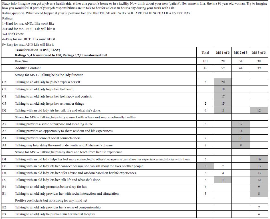
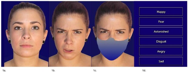
The CRAFTA Facial Recognition Test and Training software was used to perform this task ( www.myfacetraining.com) and was divided in two sections. The first part was the recognition of basic emotions (happiness, sadness, disgust, anger, fear, and surprise) without lower face covering. Participants were required to choose the appropriate expression for each image shown by clicking on it with their mouse on the screen of the PC (maximum time to choose was 5 sec.). Accuracy and time to respond for a standardized sequence of 42 pics were measured. After this first task, the participant had one minute rest followed by the same standard test but the pictures had a lower face covering (i.e., lower face mask)(section 2) (Figure 1).

FIG 1

Figure 1: Emotion Recognition Computer task (ERT). Example of a morph from neutral face (1a) expressed in the basic emotion (in this case disgust) with (out) lower face covering in a shape of a mask (1b and 1c). (1d) are the choices the participant can click on. Computer program calculates the time and the (in) correct choices of 42 pictures.

Procedure

The study was run from November 2020 until June 2021during the COVID-19 pandemic when general legal obligations to wear masks in Germany were already in action. Volunteers were recruited randomly in the mid-west of Germany through physiotherapy clinics, (sports) organizations, local universities, and via posters and advertisements. The procedure was done by 3 assessors (physical therapists) with more than 5-year of experience. The assessors were calibrated by specific training. Prior to the experimental session, written informed consent was obtained from each participant. All data were collected anonymously. Firstly, the participants were informed about the aim of the study and then were asked to sign a consent form, fill the questionnaires followed by the emotion recognition task (ERT). Before starting the ERT, a one-minute explanation and a trial with 5 random images was obligatory. Afterwards the ERT with (out) lower face covering was executed. A fourth (blinded) assessor anonymously acquired the data and classified the participants into groups such as control (CG) and (chronic) pain (PG) and carried out data analysis.

Statistical Analysis

Data was collected into SPSS 26 and the data of emotion perception of the CG and the PG (with) out lower face covering are distributed in a confusion matrix. The the Chi² test was used calculating statistical significance. Pearson Chi-square test was used to determine differences between conditions using nominal data (e.g., gender, age. BMI.). Mann-Whitney/U-Test for ordinal and metric data were performed for continuous data (e.g., age, BMI, questionnaires, time to respond), as the cohorts were not normally distributed. The significance level was set at 5%.

Results

Participants

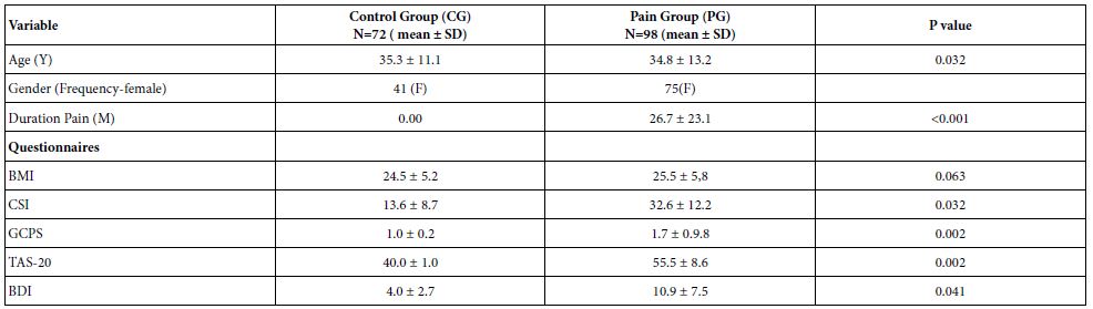
In total 170 subjects were recruited and analyzed. From these, as mentioned two groups were created. The control group (CG), as mentioned above did not refer pain based on their responses to the questionnaires. The second group includes all subjects who were regarded as having chronic pain (PG), based on their answers to the questionnaire’s medication usage was not asked. Table 1 summarizes the demographic data and questionnaires scores for both groups.

Table 1: Demographic data and mean scores of questionnaires by group (control group (CG) and chronic pain group (PG)). Y=years, M=Months F=Female.

TABLE 1


Based on the information from the questionnaires, participants were divided in two groups:

Asymptomatic Subjects (control group). Those subjects who based on their answers were identified as not having pain (CSI<40 p., GCPS class I, BPI score less than 5 points and less than 4 questions with pain, TAS-20<51 p., BDI<14 p.)

Subjects with chronic pain (pain group). Those subjects who reported pain as evidenced in their responses to all questionnaires (CSI >40 p., GCPS class 2-4, BPI score 5 points and more than four questions with pain, TAS-20 >51, BDI>14 p.) and whose pain was longer than 3 months.

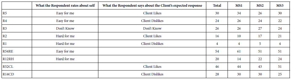
Accuracy of Emotion Recognition and Confusion

By this analysis we wanted to explore whether subjects with chronic pain were less accurate than asymptomatic subjects at distinguishing basic emotions and were confused with the emotion recognition. We examined the data in a modified confusion matrix recently described by Carbon et al. (Table 2). Hereby the emotions displayed by the program (perceived) are compared to the emotions specified by the test participants. (recognized) The answers highlighted in orange are the participants’ greatest percentages, the red ones indicate the most frequent confusion about an emotion and the green boxes the most wrong chosen emotion.

Table 2: Confusion matrix of expressed and perceived emotions of control group (CG) and pain group (PG) with (out) mask. Segments of the table in orange are the highest score. The red segments indicate the most frequent confusion about an emotion.

TAB 2(1)

TAB 2(2)


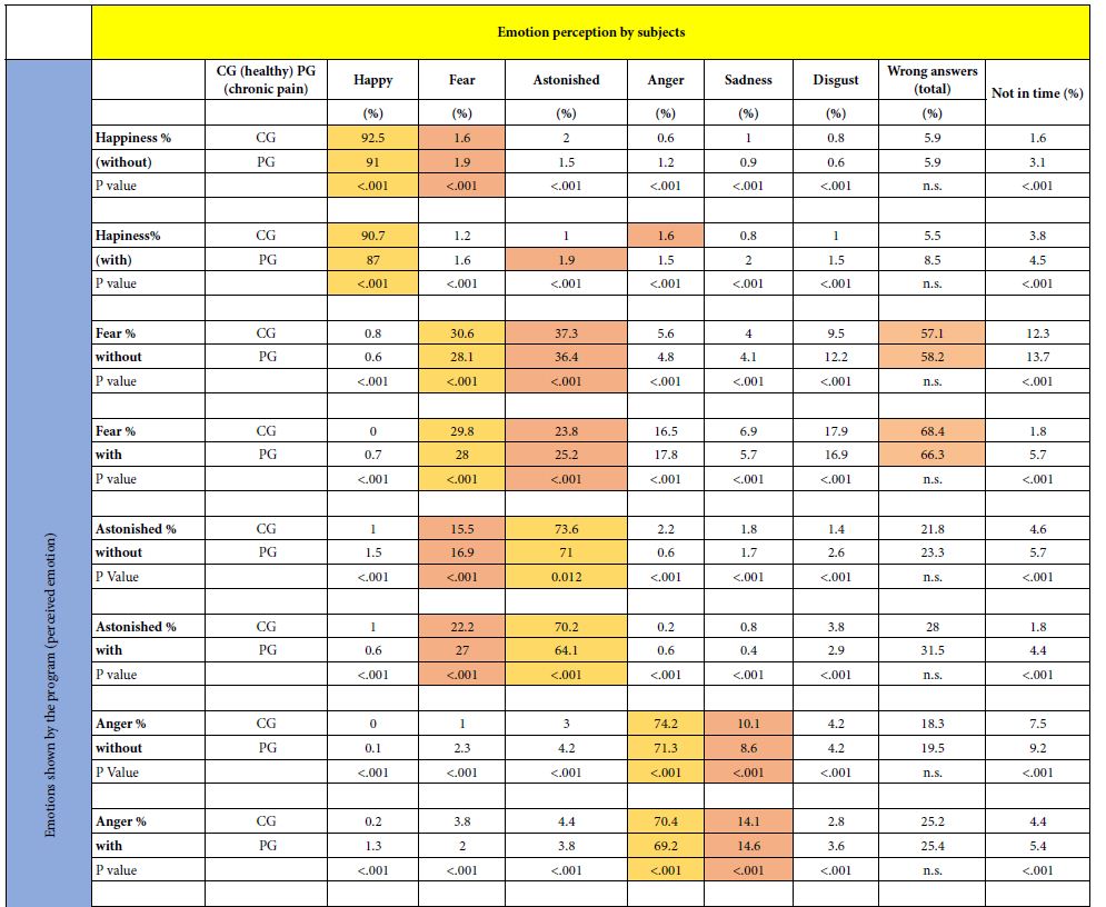
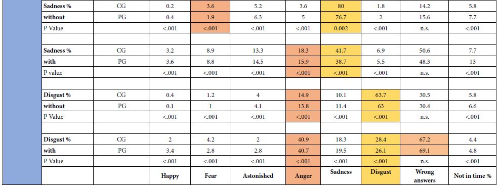
Without Lower Face Covering. In both groups, happiness was recognized the most (CG: 92.5%, PG: 91%) and it was exchanged dominantly with fear (CG: 1.6%, PG: 1.9%). Fear was recognized the least in both groups (CG: 30.6%, PG: 28.1%) and was most often mistaken for astonished (CG 37.8%, PG 36.4%). Fear also had the highest number of incorrect answers (CG 57.1%, PG 58.2%; highlighted in green in Table 2).

With Lower Face Covering. Happiness was best recognized in both groups (CG 90.7%, PG 87%). A small number of participants in the CG mixed up happiness with anger (1.6%) and astonished in the PG (1.9%). More strikingly, disgust was recognized much less in both groups (CG 28.4%, PG 26.1%) and was mostly confused with anger (CG 40.9%, PG 40.7%).

Incorrect Chosen Emotion. Based on our results, it seems that with (out) covered lower face “fear “is the most chosen incorrect emotion (without; CG=57.1%, PG 58.2% and with: CG=68.4%, PG 66.3%). A clear misjudgment was also made in both groups of “disgust“ with lower face covering (CG 67.2%, PG 69.1%) but less without lower face covering (30.5%, PG 30.4%). In Table 2 they are highlighted in green.

Confused Emotions. In both groups more than 40% confused “disgust” with “anger” (CG 40.9%, PG 40.7%) when the lower face was covered which was clearly more than without covering (CG 14.9%, PG 13.8%). Also “fear” clearly swopped with “astonishes\d” in both groups without (CG 37.3%, PG 36.4%) and with lower face covering (CG 23.8%, PG 25.2%)

Differences with (out) Face Covering in Both Groups and Answering Time

An overview of the mean percentage of correct basic emotions with (out) covered lower face (red) of control group (CG) and the chronic pain group (PG) are depicted in Figures 2 and 3. It may be concluded that between the CG and the PG with (out) face covering showed a clear significant (P<0.001) difference of all basic emotions except that of happiness. In the PG there is an extremely significant difference in emotion recognition with (out) lower face covering times of “sadness” and “disgust” (Figure 3) Average answer time. The average time of the CG (with) out face covering was both 3,1 (±0.8), p=0.2 and the PG 3,2 (±0.9), p=0,3. There was no significance in time between CG and PG with (out) face covering (p=0.34 p=0.4).

FIG 2

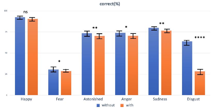
Figure 2: Mean percentage of correct basic emotions with (out) covered lower face (red) of the control group (CG) (n=72) Asterisks indicate statistical differences between conditions of wearing and non-wearing on basis of paired t-tests: *p < 0.05, **p < 0.01, ****p < 0.0001; ns, not significant.

FIG 3

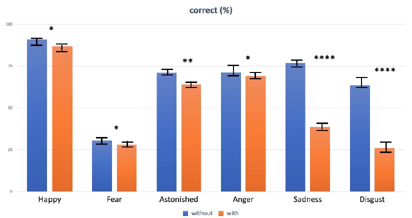
Figure 3: Mean percentage of correct basic emotions with (out) covered lower face (red) of the chronic pain group (PG) (n=98) Asterisks indicate statistical differences between conditions of wearing and non-wearing on basis of paired t-tests: *p < 0.05, **p < 0.01, ****p < 0.0001.

Discussion

In the present study we tested the impact of covered lower face with imitated face masks on basic emotion recognition during a computer task. We confronted participants with (out) chronic pain with faces in a neutral emotion that morphed into one of six different basic emotions (angry, disgusted, fearful, happy, astonished and sad) during a computer standard test. Variables we tested were accuracy and time. Control group (CG); comparing the results of the CG with the results of Carbon (2020) it should be noted that they do not completely match. Without a mask, the Carbon study had a 92.5% recognition for the fear emotion and while only 30.6% did in this study. Happy (Carbon 98.8% to 92.5%) and angry (Carbon 83.7% to 74.2%) were also recognized significantly differently. With mask, happy is recognized 90.7% correctly in this work and only 74.2% during the study of Carbon. At Carbon, fear is still correctly recognized 93.5% of the time when wearing a face mask, but only 29.8% in our study. Even sadness is recognized correctly with 62.6% during the Carbon study and in ours 41.7%. Disgust and angry are almost the same in the CG. It may be concluded that the same trend of accuracy in both studies of the different emotions can be observed, but not of all outcomes.

In both groups it can be registered that sadness and disgust are significantly less recognizable with a covered lower face. A feature of these two emotions is that they have excessive asymmetric facial expression changes in the lower face [35]. In the Carbon study ‘astonished” was not tested and in our study astonished was also significant in both groups (with) out lower face covering. Happiness was with (out) face covering in our study was not significant in both groups (CG p=0.053, PG p=0.041) in contrast to the Carbon study.

The possible differences in results may be determined by the difference in test set-up. Carbon’s study only used photos of the basic emotions without seeing the neutral state of different ages and gender with (out) an artificial mask and there was no time limit. In our study we used a computer program with morphing of basic emotions with (out) a covered lower face with a double task; emotion recognition and recognition as soon as possible (time). In our study the neutral state of the recognized person is not measured.

Controle Group (CG) versus Pain Group (PG); the results of CG and PG, indicates that accuracy in emotion recognition was strongly reduced in both groups with (out) lower face covering. This seems to be compatible with parts of the literature employing different types of covering, for instance, by rigidly covering the mouth area with cardboard, using the bubbles technique or, much closer to the present study, using block based partial square face covering [36] or a shawl or cap. For fearful faces, as shown before in the literature, the upper face, special the eye region, which was not covered, was most relevant for judging someone emotional state. It is evident that in our sample with chronic pain there is an obvious significant difference in nearly all emotions with control group except happiness (Figure 2), but an obvious significant difference with without lower face covering (Figure 3). This observation suggests that chronic pain patients with, for example, a surgical mask have facial emotional communication impairments in emotional perception, expression special in the emotions “sadness” and “disgust” [37-43].

Strength and Limitations

As far the authors concerned, with respect to the literature this is the first observational study on face recognition with covering the lower face done in patients with a chronic pain state. The strength is that the PG sample is a clear primary or secondary chronic pain group diagnosed by questionnaires as suggested by the International Association of Study of Pain (IASP) [37]. Therefore use of medication and the medical diagnosis is not asked. This may influence the variability of the results within the PG for example in the speed of recognition. The authors are aware of this, but concerning the literature on chronic pain it is more seen as a disease in itself, we left out the individual pain regions, medical diagnosis and medication usage. A limitation may be that the covering of the lower face was not a real mask but a substitute of plastic material that has the form of a mask. This may influence the results of the variables accuracy and time. On the other hand, the test was conducted in both groups in the same way.

Conclusion

  • People in a chronic pain state are worse at emotion recognition (with) out lower face covering than persons without pain but there is no difference in time
  • Recognition of all basic emotions especially sadness and disgust with lower face covering are clearly reduced in the chronic pain state group and disgust was often confused with anger and Fear with astonished.
  • This results support the need of face rehabilitation and training which may contribute appropriate non-verbal communication and quality of life in persons with chronic pain
  • Future studies in subclassification of chronic pain (use of medication, risk factors) and outcome studies in facial emotion training may support the influence of face covering like wearing a mask.

Acknowledgements

We thanks Jetske Olde Oudhof and Karin Jungmann for their assistance in participant recruitment and assessment and Dr. Jennifer Nelsson for prove reading.

Conflict of Interest

There is no conflict of interest

Authors’ Contributions

HP conceived the design, AG was in charge of data collection, and all authors participated in data analysis and discussed the findings. HP composed the initial draft of the manuscript. All authors contributed to the final version of the paper.

References

  1. Martinez AM (2017) Visual perception of facial expressions of emotion. Current Opinion in Psychology 17: 27-33. [crossref]
  2. Wang R, Li J, Fang H, Tian M, Liu J (2012) Individual differences in holistic processing predict face recognition ability. Psychological Science 23: 169-177.
  3. Rapcsak SZ (2019) Face Recognition. Current Neurology and Neuroscience Reports 19:
  4. Guo K (2012) Holistic gaze strategy to categorize facial expression of varying intensities. PLoS One 7: 8. [crossref]
  5. Smith ML, Cottrell GW, Gosselin F, Schyns PG (2005) Transmitting and decoding facial expressions. Psychological Science 16: 184-189.
  6. Patel V, Mazzaferro DM, Sarwer DB, Bartlett SP (2020) Beauty and the mask. Plastic and Reconstructive Surgery Global Open 8: 8.
  7. Maestripieri D, Henry A, Nickels N (2017) Explaining financial and prosocial biases in favor of attractive people: Interdisciplinary perspectives from economics, social psychology, and evolutionary psychology. Behavioral and Brain Sciences 40.
  8. Ross ED, Prodan CI, Monnot M (2007) Human facial expressions are organized across the upper-lower facial axis. The Neuroscientist 13: 433-446.
  9. Birmingham E, Meixner T, Iarocci G, Kanan C, Smilek D, et al. (2013) The moving window technique: a window into developmental changes in attention during facial emotion recognition. Child Development 84: 1407-1424. [crossref]
  10. Marini M, Alessandro A, Fabio P, Fausto C, Marco V (2021) The impact of facemasks on emotion recognition, trust attribution and re-identification. Scientific Reports 11: 1-14. [crossref]
  11. Bruce V, Young A (1986) Understanding face recognition. British Journal of Psychology. 7: 305-327. [crossref]
  12. Adolphs R (2002) Recognizing emotion from facial expressions: psychological and neurological mechanisms. Behavioral and Cognitive Neuroscience Reviews 1: 21-62. [crossref]
  13. Blais C, Roy C, Fiset D, Arguin M, Gosselin F (2012) The eyes are not the window to basic emotions. Neuropsychologia 50: 2830-2838.
  14. Roberson D, Kikutani M, Döge P, Whitaker L, Majid A (2012) Shades of emotion: What the addition of sunglasses or masks to faces reveals about the development of facial expression processing. Cognition 125: 195-206.
  15. Wegrzyn M, Vogt M, Kireclioglu B, Schneider J, Kissler, J (2017) Mapping the emotional face How individual face parts contribute to successful emotion recognition. PloS One 12: 5. [crossref]
  16. Franzoni V, Biondi G, Perri D, Gervasi O (2020) Enhancing Mouth-Based Emotion Recognition Using Transfer Learning. Sensors 20: 5222. [crossref]
  17. Cohen МQJ, Buchanan D (2013) Is Chronic Pain a Disease. Pain Medicine Article first published online 7.Cohen J (1988) Statistical Power Analysis for the Behavioral Sciences.
  18. Treede RD, Rief W, Barke A, Aziz Q, Bennett MI.et al. (2019) Chronic pain as a symptom or a disease: the IASP Classification of Chronic Pain for the International Classification of Diseases (ICD-11) Pain 160: 19-27. [crossref]
  19. Baeyer C, Champion G (2011) Commentary: multiple pains as functional pain syndromes, J Pediatr Psychol 36: 433-437. [crossref]
  20. Saariaho AS, Saariaho TH, Mattila A K., Ohtonen P, Joukamaa M I.et al. (2017) Alexithymia and depression in the recovery of chronic pain patients: a follow-up study. Nordic Journal of Psychiatry 71: 262-269. [crossref]
  21. Taylor GJ (1984) Alexithymia: concept, measurement, and implications for treatment. The American Journal of Psychiatry141: 725-32. [crossref]
  22. Di Tella M, Castelli L (2016) Alexithymia in chronic pain disorders. Current Rheumatology Reports 18: 1-9 [crossref]
  23. Schwoebel J, Friedman R, Duda N, Coslett HB (2001) Pain and the body schema: evidence for peripheral effects on mental representations of movement. Brain 124: 2098-2104.
  24. Moseley GL, Flo H (2012) Targeting cortical representations in treatment of the chronic pain: a review. Neurorehabilitation and Neural Repair 26: 646-652. [crossref]
  25. von Korn K, Richter M, von Piekartz H (2014) Einschränkungen in der Erkennung von Basisemotionen bei Patienten mit chronischem Kreuzschmerz. Der Schmerz 28: 391-397.
  26. Haas J, Eichhammer P, Traue HC, Hoffmann H, Behr M, et al. (2013) Alexithymic and somatisation scores in patients with temporomandibular pain disorder correlate with deficits in facial emotion recognition. Journal of Oral Rehabilitation 40: 81-90. [crossref]
  27. Faul F, Erdfelder E, Lang AG, Buchner A (2007) G*Power 3: a flexible statistical power analysis program for the social, behavioral, and biomedical sciences. Behav Res Methods 39: 175-191. [crossref]
  28. Neblett R (2018) The central sensitization inventory: A user’s manual. Journal of Applied Biobehavioral Research. 23: e12123.
  29. Michael VK, Johan O, Francis JK, Samuel FD (1992) Grading the severity of Chronic pain. Pain 50: 133-149. [crossref]
  30. Bodéré C, Téa SH, Giroux-Metges MA, Woda A (2005) Activity of masticatory muscles in subjects with different orofacial pain conditions. Pain 116: 33-41.
  31. Cleeland CS, Nakamura Y, Mendoza TR, Edwards KR, Douglas J, et al. (1996) Dimensions of the impact of cancer pain in a four country sample: new information from multidimensional scaling. Pain 67: 267-273. [crossref]
  32. Kupfer J, Brosig B, Brähler E (2000) Testing and validation of the 26-Item Toronto Alexithymia Scale in a representative population sample. Zeitschrift fur Psychosomatische Medizin und Psychotherapie 46: 368-384. [crossref]
  33. Kupfer J, Brosig B, Brähler E (2001) Toronto-Alexithymie-Skala-26 (TAS-26) Hogrefe.
  34. Veirman E, Van Ryckeghem DM, Verleysen G, De Paepe AL, Crombez G (2021) What do alexithymia items measure? A discriminant content validity study of the Toronto alexithymia scale–20. PeerJ 9: e11639. [crossref]
  35. Bassili JN (1979) Emotion recognition: the role of facial movement and the relative importance of upper and lower areas of the face. Journal of Personality and Social Psychology 37: 2049. [crossref]
  36. Fischer M, Ekenel HK, Stiefelhagen R (2012) Analysis of partial least squares for pose-invariant face recognition. Fifth International Conference on Biometrics: Theory, Applications and Systems (BTAS).
  37. Nicholas M, Vlaeyen JW, Rief W, Barke A, Aziz Q, et al. (2019) The IASP classification of chronic pain for ICD-11: chronic primary pain. Pain 160: 28-37. [crossref]
  38. Bushnell MC, Čeko M, Low LA (2013) Cognitive and emotional control of pain and its disruption in chronic pain. Nature Reviews Neuroscience 14: 502-511. [crossref]
  39. Franzoni V, Biondi G, Perri D, Gervasi O (2020) Enhancing Mouth-Based Emotion Recognition Using Transfer Learning. Sensors 20: 5222. [crossref]
  40. Faul F, Erdfelder E, Lang AG, Buchner A (2007) G*Power 3: a flexible statistical power analysis program for the social, behavioral, and biomedical sciences. Behav Res Methods 39: 175-191. [crossref]
  41. Maestripieri D, Henry A, Nickels N (2017) Explaining financial and prosocial biases in favor of attractive people: Interdisciplinary perspectives from economics, social psychology, and evolutionary psychology. Behavioral and Brain Sciences 40. [crossref]
  42. von Piekartz H, Wallwork SB, Mohr G, Butler DS, Moseley GL (2015) People with chronic facial pain perform worse than controls at a facial emotion recognition task, but it is not all about the emotion. Journal of Oral Rehabilitation 42: 243-250.
  43. Wallwork SB, Butler DS, Fulton I, Stewart H, Darmawan I, et al. (2013) Left/right neck rotation judgments are affected by age, gender, handedness and image rotation. Manual Therapy 18: 225-230. [crossref]

Proficiency Monitoring of Allergen-Specific IgE macELISA – 2022

DOI: 10.31038/MIP.2022333

Abstract

The purpose of this study was to evaluate the reproducibility of results yielded using a macELISA for detection of llergen specific IgE in dogs and cats when run by ten different individuals in seven separate affiliated laboratories. Samples of 24 different sera samples were independently evaluated in each laboratory by differing operators in a single blinded fashion. For evaluations completed by multiple operators in a single laboratory, the average inter-operator variance was calculated to be 7.9% (range=6.5%-9.0%). The average intra-assay variance among reactive assay calibrators in all laboratories was 7.3% (range=2.8%-17.6%). The overall inter-assay inter-laboratory variance evident with reactive calibrators was consistent among laboratories and averaged 15.7% (range 14.8%-16.7%). All laboratories yielded similar profiles and magnitudes of responses for replicate unknown samples; dose response profiles observed in each of the laboratories were indistinguishable. Correlation of EAU observed for individual allergens between and among all laboratories was strong (r>0.85, p<0.001). Collectively, the results demonstrated that ELISA for measuring allergen specific IgE is reproducible, and documents that consistency of results can be achieved not only in an individual laboratory, but among different operators and between laboratories using the same ELISA.

Keywords

IgE, ELISA, Proficiency, Atopy, Allergy, Immunotherapy, Cross-reactive Carbohydrate

Introduction

Stallergenes Greer maintains a proficiency monitoring program for laboratories that routinely run macELISA [1] for evaluation of allergen specific IgE in serum samples. The foundation for this program is based on the desire for inter-laboratory standardization and quality control measures that ensure the uniformity, consistency, and reproducibility  of results among laboratories  that  perform the assays. This program is designed to evaluate the proficiency of laboratories and  ensures  that individual operators yield consistent and  reproducible  results.  The inaugural proficiency evaluations, initiated in 2009 and repeated in 2010, in six different laboratories documents that inter-laboratory standardization and quality control measures in the veterinary arena are on the  immediate  forefront  and  that  uniformity,  consistency,  and reproducibility of results between laboratories is achievable [2]. Similarly, reproducibility of results among different laboratories was documented in the subsequent proficiency evaluations completed in 2013 [3], 2016 [4], 2018 [5], 2019 [6], 2020 [7], and 2021 [8]. The results presented herein summarize the comparative results observed in the affiliate laboratories for the most recent proficiency evaluations that were completed in 2022. The 2022 proficiency evaluation is the fourth documentation of the assay reproducibility since adopting a cross- reactive carbohydrate inhibitor in the sample diluent [6-9].

Materials and Methods

All serum samples, buffers, coated wells, calibrator solutions, and other assay components were aliquants of the respective lots of materials manufactured at Stallergenes Greer’s production facilities (located in Lenoir, NC, USA) and supplied as complete kits to the participating laboratories along with the exact instructions for completing the evaluations.

Participating Laboratories

Seven independent Veterinary Reference Laboratories (VRLs) participated in the 2022 proficiency evaluation of macELISA. Participating laboratories included three separate IDEXX laboratories located in Memphis, Tennessee, Kornwestheim, Germany, and Markham, Ontario Canada. Other affiliated European laboratories that participated in this evaluation included Agrolabo (Scarmagno, Italy), Laboratories LETI Pharma (Barcelona, Spain), and Ceva Biovac (Beaucouzé, France). Stallergenes Greer Laboratories (Lenoir, NC) served as the prototype for evaluation of the macELISA; the 2022 evaluations included results reported by four separate and independent operators. Because the performance characteristics of macELISA in Stallergenes Greer’s VRL have been well documented for use over an extended period [1-8], all results observed in the other participating laboratories were compared directly with the results observed in Stallergenes Greer’s reference laboratory.

Serum Samples

Separate pollen and mite reactive serum pools or non-reactive sera pools were prepared from cat and dog serum samples that previously had been evaluated using the macELISA for detection of allergen specific IgE. The reactivity of each sera pool ranged from nonreactive to reactive for multiple pollen or mite allergens. These sera pools and admixtures of the pools were used to construct a specific group of samples that exhibited varying reactivity to the allergens included in the evaluation panel. Twenty-four samples were included in the blinded evaluation conducted by each laboratory. Identical replicates of the high, low, and negative controls routinely used in the assay were also included as unknown samples. Also included in the array of samples was a five tube three-fold serial dilution of a highly pollen reactive pool, diluted into non-reactive sera, which served to document the dose response evident within the assay. All samples were stored at -20 °C for the interim between testing.

Calibrators

Mite reactive calibrator solutions of predetermined reactivity in the macELISA were prepared as three-fold serial dilutions of a sera pool highly reactive to Dermatophagoides farinae, Acarus siro, and Tyrophagus putrescentiae. Replicates of each were evaluated in each assay run and served as a standard response curve for normalizing results observed with the various samples. All results were expressed as ELISA Absorbance Units (EAU) which are background-corrected observed responses expressed as milli absorbance.

Buffers

The buffers used throughout have been previously described [1- 8], and included: a) well coating buffer: 0.05 M sodium carbonate bicarbonate buffer, pH 9.6; b) wash buffer: phosphate buffered saline (PBS), pH 7.4, containing 0.05% Tween 20, and 0.05% sodium azide; c) reagent diluent buffer: PBS, pH 7.4, containing 1% fish gelatin, 0.05% Tween 20 and 05% sodium azide. The buffer used for dilution of serum samples was identical to the reagent diluent buffer, but it has been supplemented (2.5 mG/mL) with a cross-reactive carbohydrate inhibitor derived from the carbohydrate components present in bromelain (BROM-CCD) [9]. BROM-CCD was prepared in house and remains a proprietary product of Stallergenes Greer (Lenoir, NC, USA).

Allergen Panel

The allergen panel was a 24 allergen composite derived from the array of allergens that are included in the specific panels routinely evaluated in the various laboratories; the composite allergen panel consisted of 4 grasses, 6 weeds, 6 trees, 5 mites, and 3 fungi. The protocol for coating and storage of wells has been previously described [1-8]. Immulon 4HBH flat bottom 12 well strip assemblies (Thermo Electron Corporation, Waltham, MA) were used throughout and served as the solid phase for all assays. The individual extracts were diluted in bicarbonate buffer (pH 9.6) and 100 µL was added to each assigned well. Following overnight incubation at 4-8°C, the wells were washed with PBS, blocked with 1% monoethanolamine (pH 7.5) then air dried and stored at 4-8°C in Ziploc bags until used.

Sample Evaluations – macELISA

The operational characteristics and procedures for the macELISAs have been previously described [1-8]. Following incubation of allergen coated wells with an appropriately diluted serum sample, allergen-specific IgE is detected using a secondary antibody mixture of biotinylated monoclonal anti-IgE antibodies, streptavidin alkaline phosphatase as the enzyme conjugate, and p-nitrophenylphosphate (pNPP) as substrate reagent. Specific IgE reactivity to the allergens is then estimated by determining the absorbance of each well measured at 405 nM using an automated plate reader. All results are expressed as ELISA Absorbance Units (EAU), which are background-corrected observed responses expressed as milli absorbance [1].

Statistics

A coefficient of variation was calculated as the ratio of standard deviation and means of the responses observed for the calibrator solutions within different runs in multiple laboratories. Pearson’s correlation statistic was used for inter-laboratory comparison among individual allergens. Statistical analyses were conducted using EXCEL (2016; Microsoft; Redmond, WA, USA).

Results

The assay variance (% CV) observed with the calibrator solutions in the different laboratories are presented in Table 1 and are representative of the assay reproducibility in the various laboratories. The average intra-assay % CV among positive calibrators (#1-5) was 7.3% (range=2.8%-17.6%); differences among laboratories or between assays and within assay runs were not detected. No substantial difference in results among various operators were revealed. The average inter-operator variance documented for Stallergenes Greer technicians was calculated to be 7.9% (range=6.5%-9.0%). Increased intra-assay variability was evident with the background ODs (average 9.2%; range 4.8%-22.5%). A negative response is classified as anything with an EAU below 150 [1]. Any analysis of results below this threshold, especially when looking at %CV and relative differences, should be done cautiously.

Table 1: Calculated variance of macELISA calibrator solutions observed with different laboratory runs by multiple operators during the 2021 Proficiency evaluation.

table 1

*Calibrator #1 is prepared as a dilution of a sera pool which is highly reactive to mite allergens; Calibrators #2 – #5 are prepared as a serial 3-fold dilution of calibrator #1.
†Background responses observed with diluent in place of serum sample.

To evaluate the strength of association with the magnitude of EAU results observed for each allergen among the different laboratories   a Pearson’s correlation coefficient was determined (Microsoft Excel 2016) for each laboratory pair. Because the macELISA is designed  to yield comparable responses in dog and cat samples, comparison  of results among affiliate laboratories included both cat and dog samples as a single population of sera samples [5-8]. These results (Table 2) demonstrate that good inter-laboratory correlation (r>0.80; p<0.001) is evident between the results observed in Stallergenes Greer laboratory and those observed in six affiliate laboratories for all pollen, mite, and fungi allergens. The overall correlation of results observed in the various laboratories are summarized in Table 3; a very strong correlation (r>0.90, p<0.001) was demonstrated between and among the results of the participating laboratories.

Table 2: Inter-laboratory correlation of macELISA results observed with individual allergens in Stallergenes Greer Laboratory and the results observed in the individual affiliate laboratories.

table 2

*Pearson Correlation Coefficient (r); Good Correlation (r > 0.8, p<0.001)

Table 3: Inter-laboratory correlation of macELISA results observed among individual affiliate laboratories

table 3

*Pearson Correlation Coefficient (r); Good Correlation (r > 0.8, p<0.001)

For an evaluation of the dose response in this ELISA, a five tube three-fold serial dilution of a reactive dog sera pool was prepared using a negative cat sera pool as diluent. Each of the dilutions was then evaluated by all of the participating laboratories as unknown independent samples. Similar responses were yielded by all of the laboratories and the results observed within the various laboratories are encompassed by the acceptable variance limits [1-3] (±20%) established for macELISA. Further, the magnitude of responses observed in each laboratory was reduced in direct proportion to dilution. Consequently, the dose responses for the individual allergens are presented as aggregate responses. The results presented in Figure 1 confirm the sera pool was highly reactive to mites as well as grass, weed, and tree pollen allergens, but it was not reactive to fungi. To be expected, the magnitude of responses observed in each laboratory was reduced in direct proportion to dilution. Results from the final tube in the dilution scheme yielded results that were indistinguishable from negative responses, indicating a dilution extinction of detectable response [9-14].

References

  1. Lee KW, Blankenship KD, McCurry ZM, Esch RE, et al. (2009) Performance characteristics of a monoclonal antibody cocktail-based ELISA for detection of allergen-specific IgE in dogs and comparison with a high affinity IgE receptor-based ELISA. Vet Dermatol 20: 157-64. [crossref]
  2. Lee KW, Blankenship KD, McCurry ZM, Kern G, et al. (2012) Reproducibility of a Monoclonal Antibody Cocktail Based ELISA for Detection of Allergen Specific IgE in Dogs: Proficiency Monitoring of macELISA in Six US and European Vet. Immunol Immunopathol 148: 267-275. [crossref]
  3. Lee, W, Blankenship, K, McKinney, B, Kern, G, et al. (2015) Proficiency monitoring of monoclonal antibody cocktail-based enzyme-linked immunosorbent assay for detection of allergen-specific immunoglobulin E in dogs. Journal of Veterinary Diagnostic Investigation 27: 461-469. [crossref]
  4. Lee K, Blankenship K, McKinney B, Kern G, et al. (2017) Continued Proficiency Monitoring of Monoclonal Antibody Cocktail-Based Enzyme-Linked Immunosorbent Assay for Detection of Allergen Specific Immunoglobulin E in Dogs – 2016. Microbiol Immunol Pathol 1: 1-10. [crossref]
  5. Lee K, Blankenship K, McKinney B, Kern G, et (2018) Proficiency Monitoring of Allergen Specific IgE macELISA – 2018. Microbiol Immunol Pathol 2: 1-6. [crossref]
  6. Enck K, Lee K, Blankenship K, McKinney B, et (2019) Proficiency Monitoring of Allergen-Specific IgE macELISA – 2019. Microbiol Immunol Pathol 3: 1-6. [crossref]
  7. Enck K, Kee K, McKinney B, et (2020) Proficiency Monitoring of Allergen-Specific IgE macELISA – 2020. Inter J Vet Biosci 4: 1-7. [crossref]
  8. Smith M, Enck K, McKinney B, et al. (2021) Proficiency Monitoring of Allergen- Specific IgE macELISA – Inter J Vet Biosci 5: 1-8. [crossref]
  9. Lee KW, Blankenship KD, McKinney BH, Morris, DO (2020) Detection and Inhibition of IgE for cross-reactive carbohydrate determinants evident in an enzyme linked immunosorbent assay for detection of allergen specific IgE in the serum of dogs and Vet Dermatol 31: 439-e116. [crossref]
  10. DeBoer DJ, Hillier A (2001) The ACVD task force on canine atopic dermatitis (XVI): laboratory evaluation of dogs with atopic dermatitis with serum-based “allergy” Vet Immunol Immunopathol 81: 277-87. [crossref]
  11. Gorman NT, Halliwell, REW (1989) Atopic In: Halliwell REW, Gorman NT. ed. Veterinary Clinical Immunology, 232-52. WB Saunders, Philadelphia.
  12. Griffin CE, DeBoer DJ (2001) The ACVD task force on canine atopic dermatitis (XIV): clinical manifestation of canine atopic Vet Immunol Immunopathology 81: 255-69. [crossref]
  13. Griffin CE, Hillier A (2001) The ACVD task force on canine atopic dermatitis (XXIV): allergen-specific immunotherapy Vet Immunol Immunopathol 81: 363-83. [crossref]
  14. Tijssen P (1993) Processing of data and reporting of results of enzyme In: Burdon, RH, van Knippenberg PH, editors. Practice and Theory of Enzyme Immunoassays 385-421. Elsevier, Amsterdam.

Higher Awareness of the Need for the Education in Medical Mediation Practitioners in Hospitals in Japan

DOI: 10.31038/JCRM.2022564

Abstract

Overcoming the negative feelings of patients and their families toward healthcare professionals is critical to resolving medical accident disputes in Japan. To address this issue, a medical mediation model for conflict resolution has been developed and training has been provided. However, it is not studied how those who have completed the training perceive the model in the medical field. Therefore, we conducted a survey on this point. Fifty consenting participants from across Japan were asked to answer 13 questions. Each item was rated on a scale of 1 (no need at all) to 10 (need is essential). At the same time, respondents were asked to indicate whether or not they practice medical mediation. The group that answered that they were practicing was divided into “P” group (n=28) and the group that answered that they were not practicing into “No P” group (n=21), and the Wilcoxon test was used to compare the evaluation scores. In question 2 (Satisfaction with medical mediation education), the P group was 4.68 (mean) ± 2.29 (standard deviation) compared to 3.24 ± 1.81 for the No P group, a significant difference. In the other items, both groups scored 6 or more points. The items with higher scores in the P group and significant differences were six items. They were informed consent support, cognitive conflict resolution, and need for mediation education. These results show that there are differences in perceptions of medical mediation between practitioners and non-practitioners of medical mediation. The need for medical mediation education was also inferred. The study suggests the need to ensure the quality of medical mediation by providing continuing medical mediation education.

Keywords

Medical mediation, Necessity, Awareness, Education, Practitioner

Introduction

Mediation is used in a wide range of fields, including justice and education, as a means of conflict management [1]. However, it is not widely used in medicine. The reason for this is that life, death, and physical disabilities inevitably occur during medical treatment, and the accompanying loss of trust and anger strongly dominate the minds of patients and their families, making it difficult for healthcare providers to deal with such situations. For this reason, various mediation education and training programs have been conducted in healthcare [2,3]. We have developed a “medical mediation” model for the purpose of addressing this issue in the literature [4]. This model is defined as follows. It is a relationship adjustment model that supports the prevention and adjustment of cognitive discrepancies (Cognitive Imperfection) by promoting information sharing through facilitating dialogue between the patient and the healthcare providers. In other words, medical mediation is a model for consensus building based on respect for autonomy and collaborative decision-making [5].

Based on this model, we have developed a two-day training program, an educational program consisting of theory, skills learning, and role-playing [5], and have conducted it with Japanese medical professionals for more than a decade [6,7]. As a result, the program has reduced the number of court cases involving medical disputes, improved communication between medical personnel and patients as well as between professionals, provided support for informed consent, and improved the quality of medical safety [8,9]. On the other hand, after the completion of this training program, the study of medical mediation is still left to the independent matter of each participant. Therefore, continuous training of trainees is necessary to maintain the practical and theoretical quality of medical mediation, but the status of awareness of medical mediation among trainees who have completed the training is unknown. The purpose of this study was to clarify how training completers understand medical mediation while working in the medical field.

Methods

In conducting the study, it was anticipated that there would be differences in perception of the specific content and necessity of education depending on whether or not the respondents were practicing as medical mediators after completing the training.

Working Hypothesis

Practitioners and non-practitioners do not differ in their perception of and need for medical mediation education.

Exploratory Survey Period

August 31, 2021 to September 30, 2021

Target

Hospitals with training completers throughout Japan were asked to participate. Among them, 20 facilities were selected from among those that had obtained consent for this survey from physicians at the assistant director level or above and assistant nursing directors or above at facilities that had obtained cooperation for this survey. The questionnaire was then sent and collected directly to 50 medical mediators working in the medical field at those facilities. The subjects to whom the questionnaire sheets were sent were those who fulfilled the following conditions training completers who had attended a two-day basic medical mediation training course at least one year in the past.

Questionnaire

A 13-item self-administered questionnaire was distributed.

Respondents were asked to indicate whether or not they had practiced medical mediation to date.

Next the respondents were asked to rate their responses to each item on a 10-point scale from 1 (not at all approve) to 10 (fully approve).

Q1: Awareness of medical mediation

Q2: Satisfaction with medical mediation education

Q3: Change in feelings due to medical mediation education

Q4: Contribution of medical mediation to resolving cognitive conflicts

Q5: Contribution of medical mediation to informed consent

Q6: Contribution of medical mediation to reducing psychological burden on patients and families

Q7: Contribution of medical mediation to psychological burden of health care providers

Q8: Change in the relationship between medical professionals due to medical mediation education

Q9: Contribution of medical mediation to daily medical and nursing care (Q10 and Q11 are open-ended questions to get specific understanding)

Q10: Situations in which medical mediation is applied

(1) Post-accident response, patient consultation, medical consultation

(2) Informed consent

(3) Terminal care and decision-making

(4) Routine medical treatment

(5) All of the above

Q11: Expectations for medical mediation education (free answer)

Q12: Necessity of medical mediation in medical education

Q13: Necessity of medical mediation for medical professional

Data Analysis

Respondents were divided into two groups according to their responses of whether or not they practiced. That is, the group that practiced medical mediation was designed as a Practitioner (P) group, and the group that did not practice as designated as the non-practitioner (No P) group. Descriptive statistics were obtained for Q excluding Q10 and Q11. Next, a Wilcoxon test (rank sum) was performed, and P<0.05 was considered a significant difference between the groups. JMP Ver. 14 by SAS was used for the analysis. Questions 10 and 11 were excluded from the analysis because they were intended for quantitative analysis.

Ethics

Individual consent was obtained from research collaborators and respondents. In consideration of personal information, confidential treatment was performed and researcher ethics were observed.

Results

The valid response rate was 98%. Respondents ranged in age from 30 to 65 years. The breakdown of respondents’ occupations was 25 physicians, 13 nurses, and 11 medical staff (3 medical social workers and 8 clerical staff).

Table 1 shows the descriptive statistics and test results for Q1 through Q13, excluding Q10 and Q11. The scores for Q2 were lower than the scores for the other questions in both the P and No P groups, i.e., lower than 5 points indicating neither satisfaction nor dissatisfaction, indicating a low level of educational satisfaction. Although Q12 and Q13 showed significant differences, the mean differences were smaller (1.1 and 0.68) compared to the mean differences between P group and No P group of 1.44 to 2.43 in Q1 to Q5, which also showed the same significant differences.

On the other hand, there was no significant difference between the P and No P groups in Q6 to Q9. The P group scored more than 7 points, while the No P group also scored more than 6 points, which was higher than the midpoint of 5 points.

Discussion

In the United States, when a medical accident occurs, the legal process begins immediately [10]. In Japan, such a response is considered undesirable due to social and cultural backgrounds. Considering this background, we developed a Japanese “medical mediation” model [11,12]. This model is a conflict management model that focuses on the psychological reactions of Japanese people when a medical accident occurs and their responses to negative feelings toward medical personnel. This study was to clarify how training completers understand medical mediation while working in the medical field.

As shown in Table 1, Q2 indicates that, despite significant differences in satisfaction with this model with regard to educational satisfaction, the overall level of satisfaction was considered low. On the other hand, Q12 and Q13, which asked about the need for education from a broader perspective away from the medical field, showed that respondents in both P and No P groups were strongly aware of the need for such education. These results suggest that there is a need for medical mediators to educate medical professionals and medical students about this model, as well as a need for specific guidelines and their contents when providing education in medical settings.

Table 1: Descriptive Statistics for Questions and P-value for Wilcoxon test

Group

N

Mean

SD

95% CI

P value

Q1

P

28

8.54

1.97

7.77, 9.30

0.0018

No P

21

6.57

2.31

5.52, 7.62

Q2

P

28

4.68

2.29

3.79, 5.57

0.0499

No P

21

3.24

1.81

2.41, 4.06

Q3

P

28

8.5

1.48

7.93, 9.07

0.0018

No P

21

6.19

3.04

4.81, 7.58

Q4

P

28

8.14

1.84

7.43, 8.86

0.0021

No P

21

5.71

2.97

4.36, 7.07

Q5

P

27

8.30

1.75

7.60, 8.99

0.0053

No P

21

6.33

2.71

5.10, 7.57

Q6

P

28

7.86

1.65

7.21, 8.50

0.3875

No P

21

7.52

1.64

6.75, 8.29

Q7

P

28

7.71

1.76

7.03, 8.40

0.3934

No P

21

7.33

1.77

6.53, 8.14

Q8

P

28

7.54

1.86

6.82, 8.26

0.0838

No P

21

6.38

2.42

5.28, 7.48

Q9

P

28

9.07

1.30

6.82, 8.26

0.0555

No P

21

8.14

1.77

5.28, 7.48

Q12

P

27

9.67

1.07

9.24, 10.09

0.0085

No P

21

8.57

2.48

7.44, 9.70

Q13

P

28

9.82

0.48

9.64, 10.01

0.0389

No P

21

9.14

1.39

8.51, 9.77

Group: P: Practitioner, No P: No-practitioner, SD: Standard Deviation, CI: Confidence interval.
The evaluation score was between 1 and 10 points. 1: no need at all. 5: neither. 10: the need is essential.
Q1: Awareness of medical mediation.
Q2: Satisfaction with medical mediation education.
Q3: Change in feelings due to medical mediation education.
Q4: Contribution of medical mediation to resolving cognitive conflicts.
Q5: Contribution of medical mediation to informed consent.
Q6: Contribution of medical mediation to reducing psychological burden on patients and families.
Q7: Contribution of medical mediation to psychological burden of health care providers.
Q8: Change in the relationship between medical professionals due to medical mediation education.
Q9: Contribution of medical mediation to daily medical and nursing care.
Q12: Necessity of medical mediation in medical education for physicians.
Q13: Necessity of medical mediation education for medical professionals.

Significant differences in mean values were found between the P and No P groups for Q1 through Q5, which reflect specific situations in which medical mediators experience the evaluation of medical mediators. On the other hand, no significant difference was found in the observational evaluation items, Q6 to Q9, which were slightly removed from the medical mediator’s own experience. It was considered possible that significant differences could be found somewhere in Q6 to Q9 from the practice of medical mediations. The reasons for the lack of differences may be that the questions were not specific enough, or that the emphasis was placed on the results, which may have resulted in a slight psychological burden or a change in the relationship that was not noticed.

The scores of the No P group in Q6 to Q9, where no significant differences were also found, showed more than 6 points. This suggests that the psychological burden on patients/families and health care providers, the relationship between health care providers, and the possibility of contribution to daily medical treatment and nursing care are seen in the medical mediation model.

In this study, the decision of whether or not to practice medical mediation was made by the respondents themselves, a subjective judgment. It is assumed that this influenced the results. It would have been more appropriate to clarify the distinction between practicing and non-practicing and to ask respondents to answer each question.

The remaining 30% of the No P group thought that medical mediation would not be used at the end of life. The results of this study suggest that the usefulness and necessity of medical mediation can only be realized when it is actually used in medical practice. Even if the participants understood the necessity of medical mediation, there was a difference in their perception of its suitability for practical use. In addition, the study population was small, and further study with a larger number of subjects is needed.

This study revealed that awareness of medical mediation and evaluation of the necessity of medical mediation was high among practicing medical mediators. The study also suggested the possibility of a medical mediation model as conflict management that includes psychological content in the medical field.

Conclusion

Practitioners and non-practitioners differed in their perception and need for medical mediation education. Continuous education and training for those who have completed training is necessary. The content of the training should focus on specific issues faced in the field.

Acknowledgments

We would like to thank all parties involved in the survey for their cooperation.

References

  1. Leflar BR (2012) The Law of medical misadventure in Japan. Symposium on medical malpractice and compensation in global perspective: part, Chicago-Kent College of Law, Illinois Institute of Technology 87: 82-109.
  2. Danny WH Lee, Paul BS Lai (2015) The practice of mediation to resolve clinical, bioethical, and medical malpractice disputes. Hong Kong Med J 21: 560-564. [crossref]
  3. Mengxiao Wang, Gordon G Liu, Hanqing Zhao, Thomas Butt, Maorui Yang, et al. (2020) The role of mediation in solving medical disputes in China. BMC Health Serv Res 20: 225.
  4. Wada Y, Nakanishi T (2011) Medical Mediation: A Narrative Approach to Conflict Management, Signe, Tokyo.
  5. Nakanishi T (2015) Proficiency in Medical Mediation by Medical Safety Managers Facilitates the Interactive Process of Information Sharing and Decision Making. Medical Conflict Management 4: 25-33.
  6. Nakanishi T (2013a) Effects of mediator skill training for facilitating disclosure process after adverse events. Asia J.M 14-25.
  7. Nakanishi T, Hayasaka M, Endo E, Tsuchiya A (2021) Benefits of Medical-Mediation in Informed Consent: Evaluating Clinicians’ Perspectives., SCIREA Journal of Clinical Medicine 6.
  8. Narita Y, Nakanishi T (2016) “Medical safety manager’s proficiency in medical mediation fosters the dialogue process of sharing information and decision making in medical dispute” Journal of Healthcare Conflict Management 4: 25-33.
  9. Nakanishi T (2015) Informed Consent by Medical Mediation Has a Positive Effect on Patient Satisfaction. Medical Conflict Management 4: 11-20.
  10. Carol B Liebman, Chris Stern Hyman (2004) “A Mediation Skills Model to Manage Disclosure of Errors and Advers Events to Patients”, Health Affairs 23: 22-32. [crossref]
  11. Nakanishi T (2013b) New communication model in medical dispute resolution in Japan. Yamagata Med J 31: 1-8.
  12. Nakanishi (2014) “Disclosing Unavoidable Causes of Adverse Events Improves Patients’ Feelings towards Doctors” The Tohoku Journal of Experimental Medicine 234: 161-168. [crossref]
fig 3

Post-COVID-19 Household Food Insecurity in Jamaica

DOI: 10.31038/NRFSJ.2023611

Abstract

Objective: The dual burden of the COVID-19 pandemic and the Ukraine-Russia conflict has weakened food systems globally, leaving several populations at risk of hunger. Developing countries like Jamaica are particularly vulnerable to the economic shocks of these events. It is therefore critical to broaden our understanding of food security and the analytic framework necessary to effect sustainable change. This study assessed household food security in Jamaica after COVID-19 and amid inflation.

Methods: Households in high and low-income communities across all 14 parishes in Jamaica were randomly sampled to participate in this survey which assessed household food security status post-COVID-19.

Key Findings: The results of this study highlighted that: 1) there were notable decreases in the consumption of all food types across households; 2) inadequate dietary quality was reported by 54% of households; and 3) some form of hunger was reported by 67% of households in this study, with the majority reporting moderate-severe hunger.

Discussion and Conclusion: This study gives a timely reminder of the fragility of the food system in Jamaica and similar countries in the developing world. As countries aim to recover and regain stability, households remain at risk, and the situation on the ground may worsen; therefore, the findings of this study may be modest. As such, food security should be an integral part of the policy framework to address immediate needs and the imperatives for long-term resilience.

Keywords

COVID-19, Ukraine-Russia conflict, Inflation, Food security, Nutrition, Policy, Jamaica

Introduction

Previous studies on recent social crises in Jamaica emphasized the need to address the underlying social inequities that exist [1]. This study explores the impact of crises on the dynamics of nutrition and food security. The Food and Agricultural Organization of the United Nations (FAO) states that food security exists “when all people, at all times, have physical, social and economic access to sufficient, safe and nutritious food that meets their dietary needs and food preferences for an active and healthy life” [2]. Food security is, therefore, dependent on the stability of factors that drive availability, physical and financial access, and food utilization. In order to minimize the spread of the SARS-CoV-2 virus and the associated health and economic impacts of COVID-19, governments worldwide imposed several essential public health measures [3]. However, these restrictions resulted in the destabilization of the underpinning factors of food security. There were: 1) disruptions to food availability mediated through disruptions in food supply and trade; 2) interruptions to physical access owing to the unavailability of public transportation and the enforcement of social distancing enforcement [4]. Job and income losses, as well as food price increases, affected people’s economic access to food [5].

Economic recovery from COVID-19 has been further strained by the political instability created by the Ukraine-Russia conflict [6,7]. The intricate health-economic nexus that has emerged from the pandemic continues to exacerbate financial susceptibilities worldwide [8]. Like the pandemic-imposed safety measures, the Ukraine-Russia conflict has disrupted food trade and supply. The resulting rationing of food supplies, exorbitant food and fuel prices, rising inflation, and tight bankrolling continue to drive global food insecurity, poverty and food fraud [9,10].

During the pandemic, 40% of households in eight Caribbean countries reported some form of hunger [11]. The Jamaica Health and Lifestyle Survey III (2016-2017) highlighted that more than 70% of the population were food insecure [12]. In 2022, the World Food Programme estimated that 58% of the Jamaican population were moderately-severely food insecure [13]. Due to Jamaica’s heavy reliance on tourism, its economy suffered a severe contraction during the COVID-19 pandemic due to travel restrictions [14]. Although the Government of Jamaica managed to keep the economy relatively stable during and after the pandemic, inflation, steep rises in food and service prices, and higher interest rates harshly affected Jamaican households [15]. The new challenges created by the Ukraine-Russia conflict further limit advances in economic growth and recovery. Like many other countries, what started out as a health crisis quickly progressed into an economic crisis [16]. The intersection of the food supply chain and health systems continues to threaten food and nutrition security [17]. This interconnection can be highlighted by the average Jamaican’s inability to afford healthy, fresh food supplies and essential commodities, especially for the most vulnerable. To stem the spread of food security, monitoring and evaluating the population food security status amidst emerging shocks remains critical. As such, this study sought to evaluate the current state of household food security in Jamaica so that this can be appropriately addressed by decision-makers. This study, therefore, assessed the food security status of households in Jamaica two years after the peak effects of COVID-19.

Methods

This study used a survey instrument to assess the effect of inflation on food security in Jamaican households. Researchers assessed the impact of inflation on food consumption, the status of hunger, the hunger index, and the quality of food consumption among Jamaicans. The random sampling captured high and low socioeconomic strata in the 14 parishes of Jamaica, utilizing available national data. The methods to select high- and low-income areas were based objectively on the size and quality of the homes, vehicles, and other assets in the community. Further, the high- and low-income areas were categorized using key informants in the parish. Thereafter, a random selection of high- and low-income areas was made. One high-income and one low-income area were selected in each parish. Interviews were conducted with the household head or household member who was 18 years or older. The household sampling procedure started in the center of each area selected and randomly extended across the area.

A hunger index was created thus:

No = Never worried about running out of food; never had to skip meals or go without food all day

Mild = Worried about running out of food 1-2 times during the crises or almost weekly

Moderate = Worried about running out of food almost every day; skipped meals 1-2 times during the crises or almost weekly

Severe = Skipped meals almost every day; go without food 1-2 times during the crisis, almost weekly or almost every day

Results

This study interviewed household heads from 572 households across all 14 parishes in Jamaica. The age of the household head ranged from 20 to 91 years, with a mean age of 49 years. Females headed 51.6% of the households. The size of the households ranged from 1 to 12 persons, with a mean of 4. Only 5.3% did not complete primary education, and 30.1% graduated from a tertiary institution. In this study, 33.8% of households were classified as low-income (<J$ 9,000 per week); 40.2% were grouped as middle-income (J$9,000-J$19,375), and 26% were in the high-income group earning more than J$19,376 [1]. Since the COVID-19 pandemic, households have modified the types and amounts of foods consumed.

Figure 1 shows that 33-50% of households decreased their consumption of all food types with meat, fish, vegetables and fruit among the main foods. A much smaller number of households (5-15%) increased food consumption mainly in rice, vegetables, fruits and ground provisions.

fig 1

Figure 1: Change in food consumption by household

Table 1 shows that approximately 33% of households did not have sufficient food to eat either sometimes or often.

Table 1: Access to Sufficient Food by Households in Jamaica

Description

N

%

Always have enough of the kinds of food we want to eat

99

17.4

Have enough but not always the kind of food we want

284

49.8

Do not have enough to eat sometimes

124

21.8

Do not have enough to eat often

63

11.1

Total

570

100.0

Figure 2 shows that 31% of households described their diet quality as “not so good” or poor, whereas 42% described their diet as good or excellent.

fig 2

Figure 2: Quality of meals post-COVID-19 and during inflation

A statistically significant relationship was found between household income and diet quality (Table 2). Higher income households rated their diet quality as good (37.7%) or excellent (16.4%), while low-income households described the quality of their diet as either neutral (28.9%), not so good (28.4%) or poor (10.5%).

Table 2: Household Diet Quality by Income


Household Income Bracket (J$)

Total

Quality of Diet

$9,000 or less

$9,001 to $19,375

≥ $19,376

N

%

N

%

N

%

N

%

Excellent

5

2.6

12

5.3

24

16.4

41

7.3

Good

56

29.5

88

38.8

55

37.7

199

35.3

Neutral

55

28.9

56

24.7

38

26.0

149

26.5

Not so good

54

28.4

58

25.6

21

14.4

133

23.6

Poor

20

10.5

13

5.7

8

5.5

41

7.3

Total

190

34.0

227

40.3

146

25.9

563

100.0

X2 (8) =38.886, p<.001

Using the hunger index, responses about hunger status were grouped into categories of no hunger, mild, moderate, and severe hunger. Sixty-seven percent (67%) of households reported some form of hunger, with 55% of those households reporting moderate to severe hunger, as shown in Figure 3.

fig 3

Figure 3: Status of hunger post-COVID-19 and during inflation

A statistically significant relationship was also found between hunger status and income as seen in Table 3. Households with a higher weekly income experienced no hunger (53.4%) compared to middle- and low-income households that were more affected by moderate to severe hunger.

Table 3: Hunger by Household Income in Jamaica


Household Income Bracket (J$)

Hunger status

$9,000 or less

$9,001 to $19,375

≥ $19,376

N

%

N

%

N

%

No Hunger

36

19.1

70

31.0

78

53.4

Mild Hunger

22

11.7

28

12.4

19

13.0

Moderate Hunger

91

48.4

103

45.6

42

28.8

Severe Hunger

39

20.7

25

11.1

7

4.8

Total

188


226


146


X2 (6) =55.769, p<.001

Discussion

Less developed countries such as Jamaica need to implement bold policies and innovative solutions to ensure sustainable food and nutrition security, despite the intermittent shocks and crises that are inevitable. The United Nations Department of Economic and Social Affairs highlights Jamaica as a country for priority attention as the world navigates extraordinary health and economic crises [18]. Some of the weaknesses that leave Jamaica vulnerable to several global economic shocks include its: 1) lack of economic diversity, 2) heavy reliance on tourism and disproportionate food import bill, and 3) exorbitantly high public debt in the face of debt service inhibiting growth [14]. Given the high vulnerability to economic instability, the livelihoods of Jamaican households remain under threat, and more Jamaicans remain at risk of becoming food insecure.

The decreased consumption across all food types highlights an important trend and suggests that the ability of Jamaicans to secure food is constrained. This could be due to inconsistencies in supply, mixed with contractions in demand due to the inability to afford food owing to reductions in household income, together with the staggering food costs associated with the country’s net food import [13]. The decreased consumption could also indicate that households are losing their ability to cope through previously applied mechanisms of using up savings and accessing safety nets [11]. It is therefore important to acknowledge the emerging consumption trends as a concern, especially as it relates to low-income households and households with dependent children. Typically, this decrease in staple food items could indicate that households may have increased consumption of nutrient-poor, calorie-dense foods that are cheaper and high in sodium, added sugars and trans-fats. This could have deleterious implications for population health and well-being, specifically as it relates to Non-Communicable Diseases (NCDs) prevention and control, in the near and distant future, even as Jamaica continues to grapple with the overwhelming prevalence of obesity and NCDs [19].

Furthermore, sub-optimal dietary quality increases the risk of nutritional deficiencies and related risks of adverse health outcomes. These challenges could be sustained if the key drivers remain unaddressed. At the same time, the hunger profile of the population is also staggering at 67%. This may indicate that households are skipping meals as they are unable to afford even the cheapest food due to food price inflation as well as limitations on their earnings and therefore buying power.

While there is a consensus that the recent crises will likely increase all forms of malnutrition and undermine economic recovery, it is difficult to assess their actual impact on the economy, population health and food systems. Notwithstanding, it is clear that the food security status of developing nations like Jamaica requires constant monitoring and evaluation from multiple research standpoints to enable effective responses to food and nutrition insecurity during crises and to inform the building of resilient and sustainable food systems. The cost of food in Jamaica increased steadily over the last year, which was 14.24 in November 2022, over the same month in the previous year [20]. This price rise is evident from the Jamaica Food Inflation data by Trading Economics, that is, from 9.85 in January 2022 to 14.24 in November 2022 [20]. As Jamaica tries to advance its development goals in alignment with the Sustainable Development Goals 2030, its leaders should prioritize actions that will strengthen food security and contain food inflation. These can include investing in shock-resilient community-based agriculture to support domestic food demand, reduce food imports and increase revenue by supplying international markets. Decision-makers should also address the factors that constrain household food access, both physical and economic, and focus on expanding safety nets for the most vulnerable in the population.

Acknowledgments

Funding for this study was provided by the Research Development Fund of the University of Technology, Jamaica, managed by the University’s Research Management Office, the School of Graduate Studies, Research & Entrepreneurship. Gratitude is expressed to the heads of the 572 households across Jamaica who participated in this study.

References

  1. Henry FJ, Campbell A, Reid L, Ford K, Balachandar B (2022) Beyond Covid-19: Impact of Inflation on Jamaican Households. J Community Med Public Health 6: 273.
  2. Policy brief food security – food and agriculture organization. Food Security 2006. https://www.fao.org/fileadmin/templates/faoitaly/documents/pdf/pdf_Food_Security_Cocept_Note.pdf (accessed December 19, 2022).
  3. Kent K, Murray S, Penrose B, Auckland S, Horton E, Lester E, et al. (2022) The new normal for food insecurity? A repeated cross-sectional survey over 1 year during the COVID-19 pandemic in Australia – International Journal of Behavioral Nutrition and physical activity. Springer Link.
  4. Workie E, Mackolil J, Nyika J, Ramadas S (2020) Deciphering the impact of COVID-19 pandemic on food security, agriculture, and livelihoods: A review of the evidence from developing countries. Current Research in Environmental Sustainability 2: 100014. [crossref]
  5. O’Hara S, Toussaint E (2022) Food access in crisis: Food security and covid-19: Semantic scholar. Ecological Economics 1970. https://www.semanticscholar.org/paper/Food-access-in-crisis%3A-Food-security-and-COVID-19-O%E2%80%99Hara-Toussaint/200bb64389df00927d2a6e24b9a50b2d9589302f (accessed December 19, 2022).
  6. Choudhary OP, Saied ARA, Priyanka, Ali RK, Maulud SQ. Russo-Ukrainian War: An unexpected event during the COVID-19 pandemic. Travel Medicine and Infectious Disease 2022. https://www.ncbi.nlm.nih.gov/pmc/articles/PMC9042412/ (accessed December 19, 2022).
  7. World Bank (October 4, 2022). Russian Invasion of Ukraine Impedes Post-Pandemic Economic Recovery in Emerging Europe and Central Asia. Press release. https://www.worldbank.org/en/news/press-release/2022/10/04/russian-invasion-of-ukraine-impedes-post-pandemic-economic-recovery-in-emerging-europe-and-central-asia
  8. Uwishema O, Sujanamulk B, Abbass M, Fawaz R, Javed A, Aboudib K, et al. (2022) Russia-Ukraine conflict and covid-19: A double burden for Ukraine’s healthcare system and a concern for global citizens. Postgraduate Medical Journal 98: 569-571. [crossref]
  9. Panghal A, Mor RS, Kamble SS, Khan SAR, Kumar D, Soni G (2022) Global food security post-COVID-19: Dearth or dwell in the developing world? Agronomy Journal 114: 878-884. [crossref]
  10. World Food Programme (2022) Food Insecurity in the Caribbean continues on upward trajectory, CARICOM-WFP survey finds. https://www.wfp.org/news/food-insecurity-caribbean-continues-upward-trajectory-caricom-wfp-survey-finds
  11. Perry R, Reid L, Henry F (2021) Impact of covid-19 on food security in the Caribbean. Journal of Food Security 9: 101-105.
  12. Jamaica Health and Lifestyle Survey III (2016–2017) Kingston: Ministry of Health and Wellness, Jamaica. (2022)
  13. Goal 2 end hunger, achieve food security and improved nutrition and … 2 ZERO HUNGER: GOAL 2 End Hunger, Achieve Food Security and Improved Nutrition and Promote Sustainable Agriculture 2022. https://www.pioj.gov.jm/wp-content/uploads/2022/10/VNR_Goal_2.pdf (accessed December 19, 2022).
  14. Coface. https://www.coface.com/Economic-Studies-and-Country-Risks/Jamaica (accessed December 19, 2022).
  15. Focus Economics (2022) Jamaica Economic Outlook. https://www.focus-economics.com/countries/jamaica.
  16. Reinhart CM (2022) From health crisis to financial distress. IMF Economic Review, 70(1), 4-31. https://doi.org/10.1057/s41308-021-00152-6
  17. Reinhart CM (2021) From Health Crisis to Financial Distress, Policy Research Working Paper 9616. World Bank. Data from Trading Economics, Credit. https://openknowledge.worldbank.org/handle/10986/35411 https://tradingeconomics.com/country-list/rating
  18. UN/DESA Policy Brief #64: The covid-19 pandemic puts Small Island Developing Economies in Dire Straits | Department of Economic and Social Affairs. United Nations. https://www.un.org/development/desa/dpad/publication/un-desa-policy-brief-64-the-covid-19-pandemic-puts-small-island-developing-economies-in-dire-straits/ (accessed December 19, 2022).
  19. Jamaican economy panel discusses high levels of obesity in Jamaica in Jamaica. United Nations. https://jamaica.un.org/en/170284-jamaican-economy-panel-discusses-high-levels-obesity-jamaica (accessed December 19, 2022).
  20. Trading Economics (2022) Jamaica Food Inflation. https://tradingeconomics.com/jamaica/food-inflation

Empowering Young Researchers: Understanding the Mind of Prospective Aides Regarding Elderly Clients

DOI: 10.31038/PSYJ.2023512

Abstract

Young researchers (ages 8 and 13, respectively) designed two studies, each with 100+ respondents, to explore how respondents who might choose to become health aides (females, ages 16-25) would respond to different messages about aspects of the job. The first study dealt with the respondent’s feelings about taking care of an older male client, the second study dealt with both the respondent’s feelings about taking care of an older female AND at the same time how the older female client might feel. Both studies showed the ability of the templated Mind Genomics process (www.bimileap.com) to help the researchers develop better ideas, and in the end produce strong performing data, as proven by the IDT (index of divergent thought, measuring strength of ideas based upon the responses of external respondents).

Introduction

In a previous study, the authors presented a new approach to understanding the minds of people. Rather than having adult or at least ‘older’ individuals create experiments, the approach worked with young people, giving them the tools to be researchers. The rationale for that study was that young people may perceive a situation quite differently from the way older people perceive the situation. Researchers are well aware of individual differences as well as meaningful variation in the topic that they study, while remaining blissfully unaware of the differences in viewpoint of the same problem by different individual [1]. One may study the way younger and older individuals perceive the same topic, with the substance of the investigation being a comparison of perceptions of the same problem. Such an approach can generate a valuable corpus of data, but inevitable the focus of the research will devolve to the differences in the questions that the different groups of researchers will ask in their pursuit of knowledge. Whereas it may be laudable to develop such knowledge, viz., differences in the perception of the same topic by different groups, the focus on comparing the different researcher groups ends up with comparisons of database, such comparisons being done in a lockstep manner.

The contribution of this paper and its previously published companion paper differs, following a new vision. That vision is that the database of knowledge be created by young researchers, the effort focused on learning about the world through the eyes of these young researchers. Whereas comparison with older researchers may be interesting, in the end the goal is to let the natural inquisitiveness of young researchers open up the world as they see that world. Furthermore, by letting the young researchers follow their own interests, we get a sense of how they perceive the world, without having to proceed in a lockstep fashion with similar perceptions by older individuals. In a sense, we are building a world of knowledge through the lenses of young people who are now equipped with easy-to-use, quick, inexpensive, and engaging state of the art research tools and statistics.

The Mind Genomics Process for Creating Knowledge

The objective of Mind Genomics is to create knowledge about how people make decisions about the ordinary aspects of the day [2]. The interested reader is referred to the various published papers which outline the approach and which provide examples of the applications in topics as diverse as the law [3], society [3,4], as well as commercial endeavors such as the design and marketing of food [5,6], and so forth. The actual research is straightforward, founded on the premise that the solid data emerges from the pattern of responses to test stimuli, when these stimuli are created by combining messages or elements into short test paragraphs. The combinations of messages are more natural, combining different ideas, in a manner that would be experienced by a person in daily life. Rather than asking the respondent to ‘think’ about the individual messages, thus possibly introducing bias and the effort by respondents to ‘get the right answer’, the researcher forces the respondent to evaluate the combination in a way that can be described as ‘gut feel.’ The respondent cannot guess the right answer, ending up simply rating the combinations almost automatically, without thinking, mimicking a great deal of our ‘automatic pilot’ which guides us through daily life.

The study begins with the selection of four questions which tell a story. The newly updated version of the BimiLeap program provides artificial intelligence to help the researcher identify the questions (Idea Coach). Once the respondent has selected the four questions, the BimiLeap program offers AI-powered Idea Coach once again to help the researcher to select four answers for each question. Finally, the program dynamically creates different combinations of the 16 elements, putting these elements into a group of 24 ‘vignettes’, or combinations [7]. Each respondent tests a totally different set of vignettes, much like an MRI. The process takes about 3-4 minutes on the computer, with many respondents reporting that they felt that they could not get the ‘right answer’ because there seemed to be no obvious structure.

The analysis of the foregoing data, done by regression and clustering, end up creating a simple equation of the form: Dependent variable = k0 +k1(A1) + k2(A2) … k16(D4). The dependent variable is the assigned rating by the respondent to a vignette, or for Mind Genomics a transformed value. The independent variables are A1-D4, the 16 elements, which are either present or absent in the vignette. The coefficients k1-k16 tell us the contribution of each element to ‘driving’ or influencing the dependent variable, DV. Finally, the additive constant, k0, tells us the estimated value of the DV, the dependent variable if the vignette were to contain no elements, a purely hypothetic case since all vignettes comprise 2-4 elements specified by the underlying experimental design. The additive constant is typically looked as a baseline value.

The two new studies run by senior authors Ciara Mendoza and her brother Cledwin Mendoza deal with aides to seniors (age 84 for males, 94 for females). The two studies were positioned slightly differently, but both dealt with aides doing various activities with and for their clients. In both studies the respondents were 100+ women, ages 16-25, from the United States, with stated income of $35,000 or less. The objective was to sample female respondents would someday think of becoming a health aide or companion for an older individual. The respondents were recruited by Luc.id Inc., a company specializing in aggregating respondents for online panels. The actual specifications for the respondents were set up in the recruitment specifics, in an API linked to Luc.id. All the researchers had to do was selecting the qualifications for the respondent, and order (purchase) the respondents. Once the researcher paid for the panel by credit card the study was launched, requiring about 1-2 hours to complete. All specifics about panelist ‘incentives’ to participate were handled separately by Luc.id. It is important to keep in mind that the study might have taken a week or two to complete through other means, such as inviting one’s friends. The system developed with Luc.id took that down to 60-90 minutes.

The final things to keep in mind before we look at the studies is that the analysis is fairly standard by now, using data transformation to create the ‘dependent variable’, followed by OLS (ordinary least-square regression) to create equations, and then k-means segmentation [8] to identify groups which are different in the way they responds to the elements, the so-called mind-sets.

Structure of the Studies and the Analyses

The topic of aging is growing in interest for a simple, overwhelming unchallengeable reason, demographics. The population is growing older [9,10]. With aging comes the inevitable consequences of loss of physical capacity [11], loss of mental capacity [12,13] and the increasing recognition that older people often perform better when they are encouraged and helped by aides specially trained for older people [14-17].

The focus of these two experiments is to understand the mind of women, ages 16-25, who might possibly become health aides, ministering to very old individuals, clients well into their 90’s. Such information about what prospects think about the aspects of a job helps the employer to keep abreast of both the changes in the way prospective employees ‘think about a job’, as well as understand the type of person who might be best suited from the job, based upon the way the job candidates ‘thinks.’ Finally, the ability to gather such information literally in less than a day, for very little money allows anyone to make better decisions, either about hiring a candidate employee, or for the employee choosing the employer or even the best career. To prepare for these larger studies calling for 100 respondents per study, the young researchers practiced setting up studies in BimiLeap, and running five respondents per study. This practice allowed them to become more facile with the BimiLeap approach, with the use of artificial intelligence through Idea Coach, and finally to break somewhat free of the embedded artificial intelligence by editing the answers provided to them, in some cases pre-empting the artificial intelligence to provide their own answers. This ability to edit or replace AI-suggested answers is an important one. Research by author HM and colleagues testing AI-generated vs. human-generated answers found that, in most cases dealing with issues of daily life, the human-generated answers generated higher response levels than AI-generated answers, strongly suggesting that whereas AI-generated answers are often sufficient, some can be improved or added with human judgment. However, we should note that as the AI algorithms improve, the quality of the answers is likely to also improve. Even with improvements, the authors expect that human researchers will remain the final judges and arbiters of the most appropriate answers [18].

The actual studies are summarized in two sets of three tables each. The first table in the triplet shows the parameters of the equation relating the presence/absence of the elements to the TOP2, the positive ratings (viz., easy to take care). The second table in the triplet shows the parameter of the equation relating the presence/absence of the elements to the BOT2 ratings (viz., hard to take care). The third table in the triplet shows the Index of Divergent Thought, an approach to measure the quality of thought, based upon the weighted number of positive coefficients. It will be clear from this third table in the triplet that the young researchers have been able to master some of the important aspects of the research approach, specifically the selection of strong performing elements.

Study 1: Taking Care of a 94 Year Old Man

The study concerned the feelings towards an old man, with the aide’s job, in part, were to talk to the man for an hour. As in these studies by young researchers, all of the material was created by them, with minimal direction from the senior authors. The top row of Table 1 shows the introduction to the topic, as presented to the respondents. The respondents themselves will have no ideas about the correct answer because they read the orientation paragraph, and then immediately rate a set of 24 vignettes comprising 2-4 of the elements without any interaction with a person to give them a clue about ‘right/wrong,’ doing so in 3-4 minutes. As mentioned in the short introduction, the BimiLeap program produces a single model or equation for the total set of 105 respondents, then produces 105 separate models or equations, one for each respondent. Finally, the BimiLeap program clusters the 105 respondents based upon their individual models, using the values for the 16 coefficients, emerging with three distinct groups of people . These are the mind-sets. The BimiLeap program then creates one new equation based on all the individuals within a mind-set.

Table 1: Performance of elements dealing with care for a 94 year old man. Part 1 shows the results for ratings of ‘easy’. Part 2 shows the results for ratings of ‘difficult.’

table 1(1)

table 1(2)

We now explore Table 1, Part A (drivers of ‘easy’), beginning with the Total Panel, and then proceeding to a comparison of the mind-sets.

  1. Additive constant for the total panel is th estimated proportion of the transformed responses (TOP2) to be 100, or the original ratings to be 4 or 5, in the absence of elements. Clearly the experimental design precludes that, forcing each vignette to contain a minimum of two elements and a maximum of four elements, with no vignette containing mor than one element or answer from a question. Thus the additive constant is a baseline. For total panel the additive constant is 42. This means that the baseline ease to take care of the old man is low. There is a great deal of difficulty. Only 42% of the responses would be stating ‘easy’.
  2. The mind-sets show an exceptionally large variation in basic easy’ responses. Mind set 1 feels that it will be very easy (additive constant 60) whereas Mind set 3 feels that it will be not easy (additive constant 21)
  3. The ‘story’ continues with the coefficients. Although the respondents may have felt that they were ‘guessing’ nothing could be further from the truth. Keep in mind that we are looking only at the positive coefficients, viz., those which mean that incorporating the element into the vignette increases the rating of ‘easy’ (viz., rating of 5,4). The coefficients show the incremental percentage of respondents rating the vignette ‘easy.’
  4. Looking at the top part of Table 1, devoted to TOP2, the ratings of ‘easy’, and focusing only on the column or Total Panel, we see that most of the elements which appear have low positive coefficients. This tells us that they do drive a response of ‘easy’ for the vignette BUT not too strongly. Only one of the elements, B7, Talking to an old man provides with social interaction and stimulation, with a coefficient of +7, approaches the status of ‘strong performer’. The status of ‘strong performer’ is based upon statistical considerations, with a coefficient of +8 approaching ‘statistical significance’ in the underlying regression analysis.
  5. It is when we get to the mind-sets that we see strong elements emerging. The rationale for the emergence of these mind-sets is simply that the Total Panel comprises these groups which cancel out the ‘signals’ emerging from each mind-set. In other words, there is too much ‘noise’ in the total panel.
  6. The mind-sets emerge from the process of clustering, viz., dividing the 105 respondents by the pattern of their 16 coefficients. The flat data that we saw for the total panel seems to disappear, to be replaced by different groups of strong performing elements. The composition of each mind-set is determined by the clustering process, a purely mathematical process. It is the researcher’s job to find the underlying story, and thus give the mind-set a name. Sometimes these underlying stories are not clear when we extract only two mind-sets. The stories get clearer when we extract three mind-sets. Of course, the story will get increasingly clear as we extract more than three mind-sets, but good research practice dictates that work with as few mind-sets as possible (parsimony), as well as strive for a clear story (interpretability).
  7. As we inspect the top section of Table 1, we see many strong performing elements in each mindset, as well as many blank cells. Our conclusion is respondents see the topic of caring for a 94 year old as having different benefits. From a practical point of view we now have a deeper understanding of the different facets of taking are of a 94 year old man, facets are perceived by real people, rather than by policy makers and managers.
  8. Moving now to the bottom section of Table 1, we inspect the results after turning the scale around, looking at the elements which drive ‘difficult.’ Keep in mind that BOT2 looks at the data in the same way, but only after the transformation.
  9. Our inspection of the data for ‘difficult’ begins with the additive constant. The four numbers suggest low but not very low basic perception of ‘difficult.’ The additive coefficient for Total Panel is 30, which is appreciable, and not small at all. It means in the absence of any information, we expect 30% of the ratings of the vignette to be 1 pr 2, respectively.
  10. When we move to the mind-set we see that we will encounter a range of basic perceptions of ‘difficult’ with Mind-Set 3 expected to rate almost half of the vignettes as difficult or very difficult. From a practical point of view, we should expect less ‘trouble’ working with Mind=Set 1 with their low additive constant of 17 for ‘difficult’, and more ‘trouble’ with working with Mind-Set 3 with their high additive constant of 45.
  11. The actual coefficients are occasionally positive, but many are blank, so they are irrelevant. Furthermore, Table 1 shows no strong performing elements for ‘difficult.’ Nothing stands out, either for the Total Panel or for the three mind-sets.

Study 2 – Taking Care of a 94 Year Old Woman

This second study was more adventurous, reflecting the effort to understand what the respondent would feel (Ratings 5 and 4 vs. ratings 1 and 2), and what the 94 year old client (Lila) might feel. Our focus will be primarily on what the respondent says she herself would feel, and then secondarily on what the respondent thinks her client would feel. For the respondent, the key new things to consider are the need to answer considering the two options, her feeling and her guess about the respondents feelings. Table 2 shows the distribution of the five point ratings across all 101 respondents (R5-R1), as well as the four ‘net’ values. These net values are R54 (Respondent feels it will be easy), R12 (Respondent feels it will be hard), R52 (Respondent feels that the client will like it), and finally R14 (Respondent feels that the client will dislike it).

Table 2: Averages of transformed ratings and ‘net ratings’ for the vignettes

table 2

The pattern of percentages in Table 2 suggests differences among the mind-sets, and that the respondents can differentiate their feelings from those of the presumed client feelings. For example, R4 (easy for me; client dislikes) as well as R2 (hard for me, client likes) show non-zero values. Respondents are able to differentiate themselves from their clients, even for the same vignette. The ability appears in the entire total panel and all three mind-sets.

Table 2 suggests that the respondents seem able to differentiate what they feel about the information in a vignette versus what they expect another person to feel. The ability to differentiate different points of view with a single rating permits the researcher to more deeply understand how people respond versus how they think others will respond. This finding should not surprise us. The basis of consumer research is the evaluation of different aspects of a concept or product. Of greater interest will be the analysis to discover the nature of the specific elements, viz., which specific elements are perceived to be easy/client will like, versus easy/client will dislike, etc. We now move to the analysis of the data as we in Table 1, looking only at the first half of the rating scale, easy vs. hard, independent of the expected response of the client. Table 3 (Top portion) shows the results similar to Table 1, viz. for ratings of ‘Easy’ (TOP2). We see that the additive constants are in the middle range, 45 for the total, and 39 to 59 for the mind-sets. The stronger results emerge from the coefficients. There is only one strong performing element for the Total Panel (D3: Talking with an old lady lets her connect because she can ask about the lives of other people). In contrast, when the respondents are clustered into three groups, viz., mind-sets, several elements emerge as strong performers for each mind-set.

Table 3: Performance of elements dealing with care for a 94 year old woman. The table focuses only on the rating of easy/hard as perceived by the respondent. Part 1 shows the results for ratings of ‘easy’. Part 2 shows the results for ratings of ‘difficult.’

table 3(1)

table 3(2)

Table 4: Performance of elements showing the ‘expected response’ of the 94 year old woman (client). The table focuses only on the rating of how the respondent feels that the client will like the element. 1 shows the results for ratings of ‘client like’. Part 2 shows the results for ratings of ‘client dislikes.’

table 4

When we look at the mind-sets in terms of easy vs. hard for the aide (viz. for the respondent assuming to herself that she is the aide), we find that the differences among the mind-sets are subtle, rather than dramatic. It may be that adding another consideration to the rating scale, the response of the client, viz., the old lady, may interfere with the ability of the respondent to focus on how she feels about the message for herself as the aide. When we move to the bottom up (HARD), in the second part of Table 3 we find that Mind-Set 1 begins with the lowest level of basic perceived hard (Additive Constant =13), and, in turn, shows the only strong performing elements. The other two mind-sets as well as Total Panel show no strong performing elements. When we move to the second part of the scale, that dealing the expected response of the ‘client’, viz., the 94 year old woman, we begin to get a clear picture of what might be the most important elements. These are from group B.

Talking to an old lady provides her with social interaction and stimulation.

Talking to an old lady helps maintain her mental faculties.

Talking to an old lady promotes better sleep for her.

Talking to an old lady provides her a sense of companionship.

It may well turn out that for these types of studies about jobs, the best approach is to use a double sided scale, one side dealing with one’s own feelings, the other side dealing with the expected response of others.

Measuring the Performance of the Research Results

A continuing issue in research is the measurement of ‘research quality.’ How does one know whether a study is of high quality or poor quality? One may look at the execution of the study, the analysis of the data, and even the writeup of the results to get a sense of whether the study is worthy of publication. But what about studies of the everyday, where the topic may not be particularly interesting because it is ordinary, ‘mundane,’ and simply falls below the radar of a serious scientist.

The issue of ‘research quality’ is especially important for the efforts which go into studies using Mind Genomics. By its very nature, Mind Genomics deals with the boring, the ordinary, despite the ordinariness of the topic, well executed Mind Genomics experiment emerges with a great of insight about the thinking by people, doing so without changing the reality of the situation, without somehow manipulating the situation to show an effect. A key aspect of Mind Genomics is that the test stimuli are evaluated by people for their basic ‘loading’ on different variables, such as one’s perceived enjoyment in doing the action. We can define the performance of the element as being the coefficient. That coefficient shows the degree to which the element departs in a positive way from the current baseline. Presumably the greater the sum of departures from the current baseline, the better the experiment because it is the human judge who rates the test elements.

Mind Genomics studies lend themselves to measures of research quality that can be made automatic, and objective. It is not an expert who evaluates the vignettes, but real individuals. In turn the individuals, who evaluate, viz. the respondents, can be sourced from many places, with the respondent ‘panel’ shaped to fit required specifications. As such, Mind Genomics both creates the test stimuli, and evaluates them by people, in what might be called a meld of objective and subjective measures. In the end, however, the evaluation of the test vignettes is done in a structured, and reproducible fashion, leading to numbers (additive constants, coefficients, after the dependent variable is specified). The measure of research quality developed for Mind Genomics is called the IDT, the Index of Divergent Thought. The calculations for the IDT are shown in Table 5. The IDT works simply by considering only positive coefficients of 1 or higher for six groups. These groups are Total Panel, the three mind-sets, discussed here, and the two-mindsets, not discussed here. The approach sums the positive coefficients for each of the six groups, weights each sum by the relative proportion of the respondents in that group, and then adds the weighted sums.

Table 5: The IDT (Index of Divergent Thought) and its computation for the two studies, on a 94 year old man, and a 94 year old woman

table 5

In many studies the IDT is often 30-50. The IDT results are very high for these two studies, perhaps the result of the young researchers gaining experience in how to think about the problems, combine with their ability to work with artificial intelligence suggestions, and then modify these suggestions to be simple, and direct. The IDT values of 70.7 and 65.3 are unusually high, and speak to the positive impact Mind Genomics can exert on the intellectual development of young people when they are actively involved as science researchers.

Discussion and Conclusions

As the world of consumer research evolves, it is becoming increasingly clear that the voices of researchers need not remain those of the academic elite who have been educated in best practices. The results shown in this paper suggest that the increasing power of the computer, and of artificial intelligence, is allowing more people to participate in the creation of knowledge, indeed knowledge of high quality. What then has been shown in this study beyond the ability of young people to become researchers? If one were to summarize the learnings, it is that there is an opportunity to improve societal welfare by understanding the needs of people through research. The simple examples of these two studies suggest specific activities which are hard, activities which are easy, and that people differ from each other in their opinions. These differences among people emerge when people are presented with compound test stimuli, preventing the people from ‘knowing the right answer.’

When we look at the different activities, and the responses to those activities, we become more away of subtle differences in behaviors that we might have combined under a general rubric. For example, talking to the client and encouraging the client to talk may seem to be one simple topic, but there are many facets of talking. Only through experiments such as those enabled by Mind Genomics can we end up quantifying the differences. Yet, beyond the template lies the suggesting power of Idea Coach (artificial intelligence), the response of real human beings (test execution), and the power of objective analysis (regression and clustering). This triumvirate, acting together in the period of an hour or two, and supporting the efforts of young researchers, or indeed anyone, anywhere interested in a problem, promises a breakthrough in the education of young people in a new manner, and perhaps the solution of societal problems driven by young minds, rather than by experienced but desensitized professionals whose very history ends up blinding them to important, emerging opportunities.

References

  1. Mendoza Cl, Mendoza CI, Deitel J, Braun M, Rappaport S, et al. (2022) Empowering the Young Researcher: A systematic exploration to understand people’s minds concerning the job of a home aide for a 3-6 year old child.
  2. Moskowitz HR, Gofman A, Beckley J, Ashman H (2006) Founding a new science: Mind genomics. Journal of Sensory Studies 21: 266-307.
  3. Moskowitz HR, Wren J, Papajorgji P (2020) Mind Genomics and the Law. LAP LAMBERT Academic Publishing.
  4. Moskowitz H, Kover A, Papajorgji P (2022) Applying Mind Genomics to Social Sciences. IGI Global.
  5. Porretta S (2021) The changed paradigm of consumer science: from focus group to mind genomics. In: Consumer-based New Product Development for the Food Industry. Royal Society of Chemistry 21-39.
  6. Porretta S, Gere A, Radványi D, Moskowitz H (2019) Mind Genomics (Conjoint Analysis): The new concept research in the analysis of consumer behaviour and choice. Trends in Food Science & Technology, 84: 29-33.
  7. Gofman A, Moskowitz H (2010) Isomorphic permuted experimental designs and their application in conjoint analysis. Journal of Sensory Studies 25: 127-145.
  8. Likas A, Vlassis N, Verbeek JJ (2003) The global k-means clustering algorithm. Pattern Recognition 36: 451-461.
  9. Baltes PB (1993) The aging mind: Potential and limits. The Gerontologist 33: 580-594. [crossref]
  10. Van Eenoo L, Declercq A, Onder G, Finne-Soveri H, Garms-Homolova V, et al. (2016) Substantial between-country differences in organising community care for older people in Europe—a review. The European Journal of Public Health 26: 213-219.
  11. Kagwa SA, Boström AM, Ickert C, Slaughter SE (2018) Optimising mobility through the sit‐to‐ stand activity for older people living in residential care facilities: A qualitative interview study of healthcare aide experiences. International Journal of Older People Nursin 13. [crossref]
  12. Koenig HG, George LK, Schneider R (1994) Mental health care for older adults in the year 2020: A dangerous and avoided topic. The Gerontologist 34: 674-679. [crossref]
  13. Sung HC, Chang SM, Tsai CS (2005) Working in long‐term care settings for older people with dementia: nurses’ aides. Journal of Clinical Nursing 14: 587-593. [crossref]
  14. Diwan S, Berger C, Manns EK (1997) Composition of the home care service package: Predictors of type, volume, and mix of services provided to poor and frail older people. The Gerontologist 37: 169-181.
  15. Gallagher S, Bennett KM, Halford JC (2006) A comparison of acute and long‐term health‐care personnel’s attitudes towards older adults. International Journal of Nursing Practice 12: 273-279.
  16. O’Brien N (2003) Emergency preparedness for older people. New York, International Longevity Center-USA.
  17. Piercy KW (2000) When it is more than a job: Close relationships between home health aides and older clients. Journal of Aging and Health 12: 362-387. [crossref]
  18. Moskowitz HR, Rappaport S, Deitel Y (2022) The quality of ideas when AI (artificial intelligence) is used as a coaching device. Mind Genomics Studies in Psychology & Experience (ISSN: 2771-9308).
FIG 1

Population Dynamics of Corn Bacterial Endophytes

DOI: 10.31038/MIP.2022332

Abstract

An investigation was conducted to gain essential information on the microbial ecology of endophytic bacteria in 17 corn plant varieties. Throughout the growing season, population dynamics of endophytic bacteria were discovered in the roots, leaves, and stems of corn plants. The bacterial density fluctuated from 104 to 105 colony-forming units per gram and increased as the plant grew, reaching the maximum at the heading stage. The mean bacterial populations were generally more in the roots and decreased in leaves and stems. This might be related to the soil serving as the source of endophytic bacteria and the colonization of roots by bacteria in the rhizosphere. These results collectively indicated that endophytic bacteria were not uniformly distributed in plant tissues. Moreover, the population was correlated with the growth period and plant parts. Our research would heighten interest in the research on endophytic bacteria, which may have potential value as a biofertilizer or biopesticide, thus providing a viable approach to sustainable agriculture.

Keywords

Corn, Endophytic bacteria, Population dynamics

Introduction

Zea mays L. is a staple food for half of the world’s population [1]. However, the plant can be seriously infected with many diseases, such as Bipolaris maydis [2], northern corn leaf blight (Spot), Fusarium stalk rot [3], head smut [4] ,and corn rust [5]. Chemical pesticides are widely used to protect corn against diseases. However, they also have many adverse effects, including pesticide residue, environmental pollution, disease resistance enhancement. Thus, interest in using biological control as an alternative approach via antagonistic microorganisms is increasing.

Endophytic bacteria are a group of bacteria that can be isolated from surface-sterilized tissues of asymptomatic plants [6]. Since the 1940s, more than 200 genera of endophytic bacteria from different plant tissues have been successfully categorized and reported from healthy plants [7,8]. And with over 300,000 species of land plant on earth is likely to host to one or more endophyte species [7,8]. Generally, each endophytic bacterium has a wide host range where most commonly isolated bacterial genera include Bacillus, Enterobacteria, Pseudomonas, Kosakonia, Methylobacterium, Microbacterium, Nocardioides, Pantoea, and Burkholderia [9-11]. These endophytic bacteria are important members of plant microbiome living asymptomatically in plant tissues and have attracted considerable attention as potential agents in their beneficial activities in terms of nutrient availability, plant growth hormones, and control of soil-borne and systemic pathogens [12,13]. The endophytic bacteria widely distributed in plant different tissues including roots, stems, leaf, flower, fruits, seeds, and pollens [12]. And the community structure depends on various factors, such as soil conditions, biological and abiotic stresses, as well as the genotype and age of plant [8,14-17].

Despite the beneficial effects of endophytes on plant growth, little is known about the population dynamics corresponding to the growing stage. Therefore, this study aimed to determine the distribution of endophytic bacteria at different growth periods in the roots, stems, and leaves of 17 corn varieties.

Materials and Methods

Corn Varieties

A total of 17 varieties of corn were used in this study: Dafeng123, Diandu 8, Zhongdan 815, Yunjin 2, Zhengda 615, Wugu 2, Wugu 3861, Yunrui 2, Yunrui 7, Yunrui 8, Yunrui 47, Yunrui 88, Yunrui 99, Yunrui 220, Yunyou 105, YR6, YR7. They were obtained from Seed Management Stations in Yunnan Province. A single field plot on the Yunnan Agricultural University farm was used to plant the different corn varieties. Meanwhile, 20 plants of each variety were grown in two rows, with 20 cm spacing between neighboring plants and a 60 cm long and 30 cm wide space between the rows.

Sample Preparation and Surface-disinfestation

Plants were sampled at three growth stages: seedling, elongation, and heading. On specific dates, one plant from each variety was randomly selected, manually uprooted, and washed thoroughly in running tap water to remove the adherent soil particles. Then, the third leaf from the top to bottom was removed, and a section of stem 20 cm above the ground was cut off. One gram of roots (5-10 cm below the soil line) was obtained. The plant materials of different varieties were transported in separate plastic sample bags to a laboratory where they were immediately surface-disinfested immediately [18].

Leaf and Root Surface-disinfestation

For the isolation of leaf and root endophytes, 1 g of each sample was used and the plant parts were cut into small segments. The segments were surface sterilized by immersing them in 75% ethanol for 150 s, followed by immersion in sodium hypochlorite (1%, vol/vol) for 5 min. The samples were then rinsed with 10 mL sterilized distilled water to remove all chemical residues and were ground in a sterile mortar with 9 mL sterile distilled water (SDW).

Stem Surface-disinfestation

A stem section closest to the ground was surface-disinfected with 75% ethanol for 5 min and washed three times with SDW. After the epidermis was aseptically removed, 1 g of stem tissues was transferred to a sterile mortar and ground with 9 mL SDW.

To ensure that the plant surface had been thoroughly sterilized, each surface-disinfected stem, root, and leaf sample was first allowed to touch the surface of LB plates and coated with SDW before incubation at 30°C.

Bacterial Cultivation and Preservation

The ground tissues of each plant part were mixed with 9 mL SDW and ground further to obtain a tissue suspension. Bacteria from roots, stems, and leaves, respectively, were cultivated in 9-cm Petri dishes containing Lysogeny broth (LB) media (5 g/mL yeast extract, 10 g/mL tryptone, 10 g/mL sodium chloride, agar 15 g, 1000 mL ddH2O, pH 7.0-7.2). An aliquot of 200 µL tissue suspension was plated on the LB plates and incubated at 30°C for 36-48 h. A total of three plates were used for each plant part. The population of endophytic bacteria was estimated by counting the colonies appearing on the agar plates. The endophytic density was determined using the following formula [18]:

Endophytic density (CFU/g)=average number of colonies × dilution ratio × 5 (CFU: colony-forming units).

One representative from the numerous bacterial colonies with similar morphological characteristics on the culture plates was transferred to a fresh LB plate to establish a pure culture line for each bacterium strain isolated. Individual bacterial strains were transferred to LB liquid media and shaker-cultured at 180 rpm at 25°C until the media turned milky. The bacteria suspension was then transferred to 2 mL centrifuge tubes containing 40% glycerol and stored at -80°C.

Results

Bacteria recovered from surface-disinfested leaves, stems, and roots throughout the growing season were isolated on LB plates after incubating for two days. The density of bacteria colonies on LB agar plates did not change much with the extension of incubation time. The population density of bacterial endophytes in corn was influenced by the variety, origin of plant tissues, and growing stage.

Distribution of Endophytic Bacteria Taxa during Different Growth Periods

A different number of bacteria taxa were consistently isolated from the healthy plant organs of 17 different corn varieties (Table 1).

Table 1: Distribution of endophytic bacterial taxa in 17 corn varieties during different growth periods

Variety

Seedling stage

Elongation stage

Heading stage

Root Stem Leaf

Root Stem Leaf

Root Stem Leaf

Dafeng123

1      –     3

3     2     1

1     2     2

Diandu 8

3      –     3

3     2     1

1     2     2

Zhongdan 815

1      –     3

3     2     2

1     2     2

Zhengda 615

1      –     3

2     1     1

1     2     1

Wugu 2

2      –     3

2     2     2

1     1     3

Wugu 3861

2      –     3

2     1     3

2     1     2

Yunjin 2

3      –     4

2     1     3

1     1     1

Yunyou 105

2      –     2

2     1     3

1     1     2

Yunrui 2

1      –     3

2     1     3

2     1     2

YR 6

0      –     2

3     1     1

1     1     2

YR7

1      –     2

2     1     3

1     1     2

Yunrui 7

1      –     3

2     1     2

2     1     3

Yunrui 8

1      –     3

2     1     5

1     1     3

Yunrui 47

1      –     2

2     1     2

1     1     2

Yunrui 88

1      –     2

2     1     2

1     1     1

Yunrui 99

2      –     3

2     2     2

1     1     1

Yunrui 220

2      –     2

2     1     1

1     1     2

In the stems and roots, there were more taxa (2-3 taxa per corn variety) of endophytic bacteria in the elongation stage than in the seedling and heading stages. The number of bacteria taxa on the leaves was more in the seedling stage. In general, there were more taxa of endophytic bacteria in the leaves, followed by the roots.

Population Dynamics of Endophytic Bacteria

Effect of the Growing Season on the Population Density

Endophytic bacteria were found during the entire growth period, and its population dynamics in different tissues changed accordingly. Based on the number of colonies on LB agar plates, the seedling bacterial population from field-grown corn was 103-104 CFU/g; however, it increased with the age of the plants, reaching up to 105 CFU/g in the heading stage (Figure 1).

FIG 1

Figure 1: Population quantity of endophytic bacteria in three growth periods of corn. a: Endophytic bacteria in corn root. b: Endophytic bacteria in corn stem. c: Endophytic bacteria in corn leaf.

Effect of Plant Tissues on the Population Density

In all corn varieties, the endophytic bacterial density of corn was the highest in the roots, followed by the leaves, and lowest in the stems (Figure 2).

FIG 2

Figure 2: Population quantity of endophytic bacteria in different tissues. a: Endophytic bacteria in the seedling stage. b: Endophytic bacteria in the elongation stage. c: Endophytic bacteria in the heading stage.

Endophytic populations in corn leaves and stems remained at 103 CFU/g for most of the growing season and increased to 104 CFU/g in the heading or post-harvest stages. Root tissues harbored more endophytic bacteria than other plant tissues. For the remainder of the growing season, the root’s bacteria population in the heading stage ranged from 104-105 CFU/g.

Discussion

Extensive knowledge regarding the density and diversity of endophytic bacteria colonizing plant tissues is essential in understanding the indigenous endophytic bacterial community and the assessment of endophytes as potential sources for plant growth promotion and biological control of plant diseases. However, an accurate estimation of the total number of endophytic bacteria is often difficult. This is due to the heterogeneous distribution of bacteria within the plant tissues and the tendency of some bacteria to clump together in their secreted mucilage [19] or adhere to various particles, including the plant cell wall components [20]. Researchers have also found that the density of indigenous endophytic bacteria was approximately 105 CFU/g in the root, but 104 CFU/g and 103 CFU/g, respectively, in the stem and leaf [18-20]. Similarly, the endophytic population in corn stem and root was 104-106 CFU/g for most of the growing season [18,21].

The present study systemically revealed the effects of tissue-types corresponding to different growing periods on structures and densities of endophytic bacteria. Obtained results showed that there was no significant difference in endophytic bacterial community structure among maize varieties. The overall trend was that the endophytic bacteria species were the most abundant in leaves and the least in stems. Previous studies have demonstrated that endophytic bacterial diversity variation is associated with physicochemical properties of soil and atmospheric conditions [18,22-24]. Soil microorganisms can migrate through the xylem track to colonize the plant tissues and the roots play an essential role for the retrieval of microbiome community from soil [25-27]. Therefore, this might be a response to the similar soil type, growing climate condition, as well as the agricultural practices. A dynamic infection process could begin in the rhizosphere (especially at the site of lateral root emergence), followed by endophytic colonization of the roots and subsequent ascending endophytic migration into the stem base, leaf sheath, and leaves [28]. However, it is still unknown if the vascular tissues only serve as a transport channel for endophytic bacteria or if bacteria multiply within the vascular system. In the latter case, many bacteria within the vessels might lead to plugging and, therefore, could induce plant pathogenicity. This may explain why endophytic bacteria are usually found in relatively low numbers within the vascular tissues. Therefore, the hypothesis is supported that bacterial endophytes originate in the rhizosphere and proceed into stem tissue and leaves via the vascular system. Moreover, our study found that the bacterial population from field-grown corn was increased as the plant grew, reaching the highest in the heading stage. The heading stage signals that the crops change from vegetative to reproductive growth and is in a critical period for determining crop yield. Endophytic bacteria have been demonstrated to improve plant growth by producing phytohormones, including IAA and gibberellic acid. In addition, endophytic bacteria have been shown to induce plant disease resistance [18,29]. These biological functions can provide a healthy growth environment for the plants and increase their ability to absorb water and minerals from the soil.

Our results provided more insights by demonstrating that the endophytic bacterial community was dynamic and influenced by biotic factors, with the plant itself being one of the significant factors. The total number and taxa of endophytic bacteria isolated from corn in this study suggest that internal corn tissues harbor diverse microbial flora. Screening endophytic bacteria adds to the list of bacteria as potential plant growth promotors and biological control agents. More useful endophytic bacteria are expected to be discovered as more crops are studied.

Acknowledgements

Not applicable

Author Contributions

Yueqiu He conceived and designed the study and experiments; Liwei Guo and Pengfei He performed the experiments; Pengfei He analyzed the data; Liwei Guo wrote the manuscript; and all authors contributed to the final draft of the manuscript.

Competing Interests

The authors declare that they have no competing interests.

References

  1. Lobo LLB, Dos Santos RM, Rigobelo EC (2019) Promotion of maize growth using endophytic bacteria under greenhouse and field conditions. Aust J Crop Sci 13(12): 2067-2074. [crossref]
  2. Wei J-K, Liu K-M, Chen J-P, Luo P-C (1988) Pathological and physiological identification of race C of Bipolaris maydis in China. Phytopathol 78: 550-4. [crossref]
  3. Saravanakuma K, Li Y, Yu C, Wang Q, Wang M, Sun J, Gao J, Chen J (2017) Effect of Trichoderma harzianum on maize rhizosphere microbiome and biocontrol of Fusarium Stalk rot. Sci Rep 7: 1771. [crossref]
  4. Wang W, Chao Q, Zhang N, Ye J, et al. (2014) A maize wall-associated kinase confers quantitative resistance to head smut. Nat Genet 47(2): 151-159. [crossref]
  5. Groth J, Zeyen R, Davis D, Christ B (1983) Yield and quality losses caused by common rust (Puccinia sorghi Schw.) in sweet corn (Zea mays) hybrids. J Crop Prot 2: 105-111. [crossref]
  6. Hallmann J, Quadt-Hallmann A, Mahaffee W, Kloepper J (1997) Bacterial endophytes in agricultural crops. Can J Microbiol 43: 895-914. [crossref]
  7. Smith SA, Tank DC, Boulanger L-A, Bascom-Slack CA, et al. 2008. Bioactive endophytes warrant intensified exploration and conservation. PLOS ONE 3(8): e3052. [crossref]
  8. Ali M, Ali Q, Sohail MA, Saleem MH, Hussain S, Zhou L (2021) Diversity and taxonomic distribution of endophytic bacterial community in the rice plant and its prospective. Int J Mol Sci 22: 10165. [crossref]
  9. Long HH, Sonntag DG, Schmidt DD, Baldwin IT (2010) The structure of the culturable root bacterial endophyte community of Nicotiana attenuata is organized by soil composition and host plant ethylene production and perception. New Phytol 185(2): 554-567. [crossref]
  10. Afzal I, Shinwari ZK, Sikandar S, Shahzad S (2019) Plant beneficial endophytic bacteria: mechanisms, diversity, host rangeand genetic determinants. Microbiol Res 221:36-49. [crossref]
  11. Bünger W, Jiang X, Müller J, Hurek T, Reinhold-Hurel B (2020) Novel cultivated endophytic Verrucomicrobia reveal deep-rooting traits of bacteria to associate with plants. Sci Rep 10: 8692. [crossref]
  12. Dudeja SS, Suneja-Madan P, Paul M, Maheswari R, Kothe E (2021) Bacterial endophytes: Molecular interactions with their hosts. J Bas Microbiol, 1-37. [crossref]
  13. Compant S, Duffy B, Nowak J, Clément C, Barka EA (2005) Use of plant growth-promoting bacteria for biocontrol of plant diseases: principles, mechanisms of action, and future prospects. Appl Environ Microbiol 71: 4951-59. [crossref]
  14. Hardoim PR, Hardoim CCP, van Overbeek LS, van Elsas JD (2012) Dynamics of seed-borne rice endophytes on early plant growth stages. PLOS ONE 7(2): e30438. [crossref]
  15. Ding T, Melcher U (2016) Influences of plant species, season and location on leaf endophytic bacterial communities of non-cultivated plants. PLOS ONE 11(3): e0150895. [crossref]
  16. Papik J, Folkmanova M, Polivkova-Majorova M, Suman J, Uhlik O (2020) The invisible life inside plants: deciphering the riddles of endophytic bacterial diversity. Biotechnol Adv 44:107614. [crossref]
  17. Cherif-Silini H, Thissera B, Bouket AC, et al. (2019) Durum wheat stress tolerance induced by endophyte Pantoea agglomerans with genes contributing to plant functions and secondary metabolite arsenal. Int J Mol Sci 20 (16): 3989. [crossref]
  18. Cun H, Munir S, He P, Wu Y, et al. (2022) Diversity of root endophytic bacteria from maize seedling involved in biocontrol and plant growth promotion. Egyptian Journal of Biological Pest Control, 32:129. [crossref]
  19. Dong Z, Canny MJ, Mccully ME, Roboredo MR (1994) A nitrogen-fixing endophyte of sugarcane stems (A new role for the apoplast). Plant physiol 105: 1139-47. [crossref]
  20. Fisher P, Petrini O, Scott HL (1992) The distribution of some fungal and bacterial endophytes in maize (Zea mays L.). New Phytol 122: 299-305. [crossref]
  21. Mcinroy JA, Kloepper JW (1995) Survey of indigenous bacterial endophytes from cotton and sweet corn. Plant soil 173: 337-42. [crossref]
  22. Landa M, Cottrell MT, Kirchman DL, Blain S, Obernosterer I (2013) Changes in bacterial diversity in response to dissolved organic matter supply in a continuous culture experiment. Aquat Microb Ecol 69(2):157-168. [crossref]
  23. Correa-Galeote D, Bedmar EJ, Arone GJ (2018) Maize endophytic bacterial diversity as affected by soil cultivation history. Front Microbiol, 9: 484. [crossref]
  24. Penuelas J, Rico L, Ogaya R, Jump AS, Terradas J (2012) Summer season and long-term drought increase the richness of bacteria and fungi in the foliar phyllosphere of Quercus ilex in a mixed Mediterranean forest. Plant Biol 14: 565-575. [crossref]
  25. Liu H, Carvalhais LC, Crawford M, et al. (2017) Inner plant values: diversity, colonization and benefits from endophytic bacteria. Front Microbiol 8: 2552. [crossref]
  26. Okunishi S; Sako K, Mano H, Imamur A, Morisaki H (2005) Bacterial flora of endophytes in the maturing seed of cultivated rice (Oryza sativa). Microbes Environ 20(3): 168-177. [crossref]
  27. Berendsen RL, Pieterse CMJ, Bakker PAHM (2012) The rhizosphere microbiome and plant health. Trends Plant Sci 17, 478-486. [crossref]
  28. Chi F, Shen S-H, Cheng H-P, Jing Y-X, Yanni YG, Dazzo FB (2005) Ascending migration of endophytic rhizobia, from roots to leaves, inside rice plants and assessment of benefits to rice growth physiology. Appl Environ Microbiol 71: 7271-8. [crossref]
  29. Munir S, Li Y, He P, et al. (2020) Unraveling the metabolite signature of citrus showing defense response towards Candidatus Liberi-bacter asiaticus after application of endophyte Bacillus subtilis L1-21. Microbiol Res 234: 126425. [crossref]
fig 1

The Effect of Pancreatin on Glimepiride Release Kinetics as a Model for Studying Endogenous Mediated Enzymes on Orally Administered Lipophilic Drugs

DOI: 10.31038/JPPR.2022544

Abstract

Glimepiride, a second generation of sulfonylureas, is used in treating diabetes mellitus. The monograph does not include digestive enzymes, such as pancreatin, in the description of its dissolution tests. Because its aqueous solubility values in literature are inconsistent, this study firstly determined it. In order to gain insight how a glimepiride tablet acted in the gastrointestinal tract, a three stage dissolution study tested two commercial tablets. Pancreatin powder was added versus not added in the beginning of Buffer Stage 1. HPLC quantified samples at 228 nm. The US Similarity Factor ratified that (a) similar between commercial Products A and B release profiles (f2 ≥ 50), and (b) different in drug releases between dissolution media containing versus not containing pancreatin. This study also found that the drug amount in the dissolution medium containing pancreatin decreased from 22 h to 24 h, while the same decline was not observed in the control group. Drug decomposition occurred in the pancreatin group was further expedited. After UV spectrophotometric scan and HPLC characterization of the 24 h dissolution samples, a small un-identified chromatographic peak was recorded at 235 nm and 240 nm respectively. This study highlights how endogenous mediated enzymes affects the free concentrations of lipophilic drugs.

Keywords

Glimepiride, Pancreatin, Three-stage dissolution, FDA similarity factor f2, Release kinetics, Solubility descriptor

Introduction

For oral drug delivery to be successful, the aqueous solubility of the drug compound in the GI system should be either known from literature or assessed in the lab to determine if modifications are needed. Lipase is produced primarily in the pancreas. There is no lingual lipase in human [1]. The activity of the gastric lipase is not low. It is also stable in acid pH. Actually, its maximum activity is at pH 5, which is the immediate fed stage pH for many cases. The pH of a fed stomach lowers thirty min or so after food intake due to the secretion of gastric acid by parietal cells, which aids in food digestion, absorption of minerals, and control of harmful bacteria. Gastric lipase is stable in acid pH, but is not as active after the gastric pH is lowered. After being mixed with gastric lipase, powerful gastric juice and 2-4 h of peristaltic contractions (mechanical digestion churn), approximately 30% of fats/triglycerides in the food bolus is broken down into diglycerides and fatty acids in partially digested food mass (known as chyme). When the chyme passes to the small intestine, pancreatic lipase is secreted by pancreas into the duodenum through the duct system of the pancreas to continue the fat digestions [1]. The third lipase is hepatic lipase, which is produced by the liver [1]. Hepatic lipase is a lipolytic enzyme that contributes to the regulation of plasma triglyceride levels, but not in the intestinal lumen [2]. Over the past 50 years, dissolution testing has also been employed for different purposes, such as a quality assurance/quality control procedure, in research and development to detect the influence of critical manufacturing variables and in comparative studies for in vitroin vivo correlation [2]. However, most compendium monographs describing dissolution tests as a part of performance tests do not include digestive enzymes in the media. Many are defined as one-stage (single medium pH) tests to serve quality control purposes. However, the pH of the gastrointestinal medium is a digestion parameter. Thereby, multistage in vitro dissolution tests should also be conducted during the preformulation and formulation stages. This project aimed at the examination of how pancreatin may impact the release of a lipophilic drug from its oral dosage form with food intake. Glimepiride (a long-action second generation of sulfonylurea) was chosen as the model drug, because its side chains are known to be less polar. Glimepiride is usually administered by mouth once a day by taken with the first meal of the day. The current market products for glimepiride are in tablet dosage form with strength availability as 1-, 2-, 3-, 4-, 6- and 8-mg. Unfortunately, the aqueous solubility values of glimepiride in the literature are not consistent, ranging from partly miscible to < 0.004 mg/mL [3-6]. That was why we set to test its aqueous solubility followed by the exploration of the solubility in different physiological pH media. Since the oral cavity, stomach, and small intestine function as three separate digestive compartments with differing chemical environments, a three-stage in vitro dissolution study is believed to be superior to one stage to answer the scientific questions of this study “How pancreatin may impact the release of a lipophilic drug?”, although one pH stage dissolution contributes in quality control. The statement regarding the quantity of pancreatin and the test solution for the pancreatin to add may be found in USP43-NF38 Intestinal Fluid, Simulated, TS in Reagents and Reference Tables > Solution [7]. This test solution is prepared first by dissolving 6.8 g of monobasic potassium phosphate in 250 mL of water, mix, and add 77 mL of 0.2 N sodium hydroxide and 500 mL of water. Second, add 10.0 g of pancreatin, mix, and adjust the solution with either 0.2 N sodium hydroxide or 0.2 N hydrochloric acid to a pH of 6.8 ± 0.1. Last, dilute with water to 1000 mL [7]. Next, we searched for a protocol how to prepare each stage medium for the three-stage dissolution study and found the required description in Mesalamine Delayed-Release Tablets Monographs [7]. By doing so, the second project aim, which was to determine whether pancreatin impacts a highly lipophilic oral drug using in vitro dissolution study, became feasible. The dosage forms were two commercial glimepiride tablets in two different strengths, 2- and 4-mg. The percent of their in vitro drug release data was next entered an Excel worksheet according to the U.S. FDA Similarity Factor equation to compute into f2 values for comparison [8-10].

Materials

(a) Model Drug and its Commercial Products

Glimepiride (TCI, JPOSL-FH) powder was purchased from VWR (Radnor, PA). Amaryl 2-mg and 4-mg Tablets (Lot FT00, products of Sanofi-Aventis), and Glimepiride 2-mg and 4-mg Tablets USP (Lots P2100682 and P2101988, Products of Accord Healthcare) were purchased from Cardinal Health (Dublin, OH). Amaryl Tablets were coded as Product A, while Glimepiride Tablets USP was coded as Product B.

(b) Reagents and Supplies

Monobasic sodium phosphate (Ward’s Science, AD-20224), phosphoric acid (VWR, 18H104005), acetonitrile (OmniSolv, 59135), tribasic sodium phosphate (Alfa Aesar, 10220493), hydrochloric acid (VWR, 2017062956), sodium hydroxide (EMD, 49124919), pancreatin (Ward’s Science) were purchased from VWR.

Methods

Glimepiride Solubility Study

The Glimepiride aqueous solubility values found from four different literature are not consistent ranging from partly miscible to < 0.004 mg/ml. Besides, “partly miscible” and “very poor solubility” are not the terms used in Solubility Table (Table 1). Therefore, its aqueous solubility was determined first. Ten mg of glimepiride powder was added into a water tank containing 10 liters of purified water with occasional shaking for up to 48 h. Three 10-mL samples were taken from different content locations of the 10-L tank. Sample of 5 mL was transfer into a 10 mL syringe and filtered through 0.2-micron nylon membrane syringe filter prior to being subject to UV-Visible spectrophotometer (Cary 50, Agilent Technologies) and HPLC for analyses. The other 5 mL were kept in culture tube without filtration. All experiments were performed in triplicate.

Glimepiride High-Performance Liquid Chromatography

The HPLC assay was adopted from Glimepiride Tablets Monograph in USP43-NF38, 2022 [7]. Diluent was acetonitrile and water in 9:1 v/v. The stock solution was prepared as 1 mg/mL Glimepiride. Standard solutions for building between day and within-day standard curves were constructed by taking aliquots of stock solution and diluting them with Diluent to prepare into the six standard concentrations between 0.004, 0.02, 0.1, 0.2, 0.5 and 1 mg/mL, and acquired the AUC of each standard concentration. The averaged AUCs of the same standard concentrations (n=3) were construct into a grand calibration plot. However, a shorter standard curve was plotted from 0.004 to 0.1 mg/mL for use in this project due to the low drug strengths (2 mg and 4 mg). The LC systems was Agilent Technologies Series 1260 Infinity consisted of an auto-sampler, a thermostatic column compartment, a degasser, a variable wavelength detector, and a quaternary pump with Chemstation® software). After testing the peak shapes and retention times of three HPLC columns, chromatographic conditions adopting from USP Glimepiride Monograph [7] were eventually set as LiChrosorb RP18 column, column temperature 35°C, injection volume 20 μL, flow rate 1.2 mL/min, detection wavelength 228 nm, run cycle 12 min, dissolving 0.5 g of monobasic sodium phosphate in 500 mL of water, adjusting with 10% phosphoric acid to a pH of 2.1-2.7 and added 500 mL of acetonitrile to mix and serve as mobile phase.

Glimepiride UV-Visible Spectrophotometer

The wavelength ( λmax ) where glimepiride had the highest absorption was determined by scanning the samples taken from the 10 mg glimepiride dissolved in 10 liters of water for 48 h using UV-Visible spectrophotometer (Cary 50, Agilent Technologies). If glimepiride is not soluble in water, these samples would further mixed with acetonitrile in two different ratios (water and acetonitrile in 1:4 and 1:9 v/v) and scanned from 200 to 800 nm to see whether organic solvent aided in glimepiride solubility.

Three-Stage In Vitro Dissolution Study Stimulating Human Gastrointestinal Fluids and Transition Time

Three different performance tests are described in Glimepiride Tablet Monograph USP43-NF38. These tests are similar in: (1) use of Apparatus 2 (Paddle), (2) pH 7.8 phosphate buffer (singe medium stage), and (3) 75 rpm stirring rate at 37.0 ± 0.5°C, but are different in dissolution times (15 min, 45 min, and 20 min respectively) [7,8]. A single medium pH performance test is good for use in QA/QC, but is not possible to assess whether pancreatin influences glimepiride release from a tablet and dissolved in the various simulated gastrointestinal media. Three dissolution stages containing one Acid Stage and two Buffer Stages modified from Mesalamine Delayed-Release Tablets [7]. The rational is that pancreatin should be added in the beginning of Buffer Stage 1 to mimic the enzyme being secreted from the pancreas and discharged from pancreatic duct into duodenum. Glimepiride Tablets Monograph only stated to use the phosphate medium at 7.8 pH, which is not the pH value of Buffer Stage 1 [7]. The 3-stage dissolution test with pancreatin added at the beginning of Buffer Stage 1 used in this study as the experimental group is described briefly as following. The medium preparation for each of the three stages in application to the control group were the same as that of the experimental group except without the addition of pancreatin.

Medium Preparations and Progression of Dissolution Study

The Gastric Fluid – Simulated in Reagents and Reference Tables > Solutions > Test Solutions and Indicator Solutions > Test Solutions only describe how to prepare as pH 1.2 without further information regarding fasting versus fed state. So are the performance tests of several tablet and capsule monographs. Since the smallest volume to set for Distek Dissolution Apparatus was 500 mL, we assumed it was for fasting state. We, thereby, selected 750 mL 0.1 N HCl into a 1-liter dissolution vessel and warmed to 37.0 ± 0.5°C as a medium size postprandial condition. A glimepiride tablet either 2- or 4-mg was placed into the vessel medium. The paddle stirred at 75 rpm for 4 h. At the end of this 4-h, Buffer Stage 1 was initiated by adding 200 mL of 0.20 M Tribasic Sodium Phosphate to adjust the pH to 6.4, while the paddle continued to stir at 75 rpm. For each pancreatin containing group (also called as experimental group, or experimental medium), 10.88 g of pancreatin was added (after 200 mL of 0.20 M tribasic sodium phosphate was added and mixed the 750 mL of 0.1 N HCl well in a dissolution vessel) to simulate the small intestinal fluid when food chyme arrives the duodenum and pancreatin secretion is activated. The color turned from clear to yellowish cloud. Figure 1 used 1-L beaker instead of 1 L of dissolution vessel to display phosphate buffer pH 6.4 after 10.88 g of pancreatin was added as the experimental group. At the end of the 4-h Buffer Stage 1, sodium hydroxide 2 N (that was, 1.04 g NaOH with a sufficient amount of water to make into 50 mL solution) was further added to bring the total medium volume at 1000 mL and pH was 7.4 (Stage 2 Buffer). The dissolution apparatus continued to stir during the Buffer Stage 2 for 16 h to simulate large intestinal pH and transition time.

fig 1

Figure 1: Pancreatin powder in the ordered container with label as well as in a weight boat (right), and the buffer stage 1 medium of an experimental group in the beaker (left). See text.

The sampling schedule was 2 h, 4 h (Acid Stage), 6 h, 8 h (as 2 h and 4 h during Buffer Stage 1, pH 6.4), 9 h, 22 h, and 24 h (at 1 h, 14 h and 16 h during Buffer Stage 2, pH 7.4). Five mL of dissolution medium were collected from each vessel at the designated sampling time and replenished with equal volume of blank (same medium of each stage, but contained no drug). The first 2 mL out of these 5 mL were filtered through a 0.22-micron syringe filter were discarded. The remaining 3-mL was continued to filter through the syringe filter, collected into a culture tube, and capped. One mL of such sample was later placed into a HPLC vial for analysis when a 24-h dissolution cycle ended. The recorded AUCs were converted into concentrations using an prebuilt standard curve averaged out of 3 runs (Section 3.2) and further computed into the dissolved amount (in mg) as well as the percent of drug release. The drug dissolution profiles were constructed with the averaged percent of release (n=3) in the Y coordinate (ordinate) plotted against the dissolution time (in h) in the X coordinate (abscissa).

Tablet Dissolution Study

The feature was a 2 x 2 x 2 factorial design with three main effects. The first number in 2 x 2 x 2 stands for “two payloads 2-mg vs. 4-mg”. The second number stands for “with vs. without pancreatin”. The third number of 2 x 2 x 2 stands for “Tablet Product A and Product B”. A pretest showed all four glimepiride tablets (Products A and B in 2-mg and 4-mg) sank to the bottom of a dissolution vessel after a tablet was dropped into a dissolution vessel. They neither rise nor were hit by stirring paddles during tests. Therefore, no tablet sinker or use of dissolution apparatus 1 (basket method) was required.

Glimepiride Powder Study

Glimepiride powder of 2 mg and 4 mg as controls were subject to in vitro dissolution study using USP Apparatus 2 (Distek Premiere, model, 5100) at 75 rpm, 37.0 ± 0.5°C. The medium preparations between the experimental group and control group, dissolution conditions and sampling schedule were at same as Section 3.4.1.

The U.S. FDA Similarity Factor f2 value

The equation of U. S. Similarity Factor, f2 value used to compare two dissolution profiles is available in Guidance for Industry Dissolution Testing of Immediate Release Solid Oral Dosage Forms as well as M9 Biopharmaceutics Classification System-Based Biowaivers [9-12]. The Similarity Factor f2 value, compared two dissolution profiles at a time using the following formula:

for 1(Equation 1)

f2 is the similarity factor;

n is the number of time points;

Rt is the mean percent reference drug dissolved at time t after initiation of the study;

Tt is the mean percent of test drug dissolved at time t after initiation of the study.

Two dissolution profiles are considered similar when the f2 value is ≥ 50.

The evaluation of the similarity factor is based on the following conditions [9]:

  1. A minimum of three-time points (zero excluded)
  2. The time points should be the same for the two products
  3. Mean of twelve individual values for every time point for each product.
  4. No more than one mean value of ≥ 85% dissolved for any of the products.
  5. To allow the use of mean data, the coefficient of variation should not be more than 20% at early time points (up to 10 minutes) and should not be more than 10% at other time points.
  6. Two dissolution profiles are considered similar when the f2 value is ≥ 50. When both test and reference products demonstrate that ≥ 85% of the label amount of the drug is dissolved in 15 minutes, comparison with an f2 test is unnecessary, and the dissolution profiles are considered similar [9-12].

Results

Glimepiride Solubility and Descriptor Determination

After the three samples being collected from the 10-L tank containing 10 mg of glimepiride and 10 L of water which was allowed to dissolve up to 48 h in each experiment (Section 3.1) and subject to HPLC analysis, only a very small drug peak at limit of quantification (LOQ) magnitude out of the three sample injections was recorded (Figure 1a). The retention time of this small peak (Figure 2a) corresponds to that of the glimepiride peaks in a 0.04 mg/mL standard sample (8.6 min, Figure 2c). But the other two samples taken from the 10-L tank containing 10-mg glimepiride in 10-L water that did not show chromatographic peaks, we thereby took 1 mL out of the 5 mL unfiltered sample to dilute with 9 mL acetonitrile and then filtered to examine whether glimepiride was present but not soluble enough in water. A small but clear peak from each of these two injections was recorded (AUC < 3, Figure 2b). The retention times of these peaks also corresponded to the retention time of the glimepiride standard sample chromatogram at 0.04 mg/mL (8.6 min, Figure 2c). All solubility experiments were performed in triplicates.

fig 2

Figure 2: The chromatograms of glimepiride aqueous solubility study illustrated that (a) a very small peak at the limit of quantification (LOQ) was recorded from one out of three sample chromatograms after 10 mg of glimepiride was placed into 10 L of water (no acetonitrile) for 48 h. (b) The drug peak appeared after a sample which did not showed drug peak in Figure (a) was further diluted with 9 parts of acetonitrile. (c) A 0.04 mg/mL standard sample prepared according to compendium LC method which Diluent was acetonitrile and water in 9:1 ratio.

Next task was to determine the term of glimepiride in the Description and Solubility Tablet (Table 1). The glimepiride aqueous solubility may now elucidate as “10 mg (0.01 g) of glimepiride requires more than 10 L (10,000 g) of water to dissolve.” The calculation showed

for 2(Equation 2)

Based on one part of solute requires over 1 million part of solvent to dissolve, the descriptive terms in Description and Solubility (Table 1), glimepiride belongs to the category of “practically insoluble in water”.

Table 1: Description and solubility [7]

Descriptive Term

Parts of Solvent Required for 1 Part of Solute

Very Soluble

<1

Freely soluble

1-10

Soluble

10-30

Sparingly soluble

30-100

Slightly soluble

100-1000

Very slightly soluble

1000-10,000

Practical insoluble

>10,000

High Performance Liquid Chromatography

A grand standard curve was built based on averaging the AUCs of three individual standard curves from 0.004, 0.02, 0.1, 0.2, 0.5 to 1 mg/mL. Due to the low strengths of the tablets (2 mg and 4 mg) investigated in up to 1 L of dissolution medium in this project, a working range standard curve (containing 0.004, 0.02 and 0.1 mg/mL) was further plotted. The trendline was

AUC=55550 x Concentration (mg/mL) + 2.5394 R²=1 (Equation 3)

In Vitro Dissolution Results of Two Commercial Tablets in Two Strengths

The AUC collected from 7 sampling chromatograms in the 3-stage in vitro dissolution studies of two tablet groups (Products A and B) and 2 strengths (2 mg and 4 mg) were computed into percent of release as Mean ± SD using the aforementioned work range standard curve in Session 4.1 (0.04, 0.02 and 0.1 mg/mL) plus correction factor adjusted for volume withdrawal at each sampling point (Table 2). These percent of release were also plotted against time (in h) into X-Y plot with SD bars (Figure 3). Figures 3a to 3d showed that the percent of glimepiride releases in the experimental groups (pancreatin-containing) were lower than the control groups during the Buffer Stage 2 (pH 7.4 from 9 h to 22 h) in both tablets, Products A and B of the same strength. The differences between experimental and control groups are greater in 2 mg tablets (Figure 3a and 3c) than in 4 mg tablets (Figures 3b and 3d). Furthermore, the release decreased from 22 h to 24 h in the experimental group, but the release increased from 22 h to 24 h in the control group (Figure 3). Bar charts of the glimepiride dissolution in 0-8 h, 8-9 h, 9-22 h, and 22-24 h sampling intervals of Products A and B (not cumulative from 0 h to 24 h) were next constructed into bar charts (Figure 4). The percent increased or decreased in Figure 4 are among the four intervals of 0-8 h, 8-9 h, 9-22 h, and 22-24 h, not like the cumulative percent of release being reported in Figures 3. The FDA Similarity Factor, f2 values, were further computed.

Table 2: Comparison of 24-h in vitro glimepiride release in percent (Mena ± SD, n=3) from 2-mg and 4 mg commercial Tablets A and B (a) 2 mg, and (b) 4 mg without versus with pancreatin added in the beginning of Buffer Stage 1.

 A

Tab A 2 mg

Tab B 2 mg

Dissolution Stage

Time (h)

Without Pancreatin

With Pancreatin

Without Pancreatin

With Pancreatin

Acid

0

0

0

0

0

(0.1 N HCl)

2

0

0

0

0

4

0

0

0

0

Buffer 1

6

16.6 ± 10.4

27.3 ± 16.2

31.3 ± 5.0

29.1 ± 2.8

(pH 6.4)

8

37.4 ± 8.9

46.5 ± 5.5

36.9 ± 2.6

31.2 ± 3.7

Buffer 2

9

112.6 ± 11.9

97.9 ± 41.4

112.2 ± 13.2

69.1 ± 5.7

(pH 7.4)

22

119.3 ± 11.8

120.5 ± 8.7

119.8 ± 13.2

106.7 ± 6.2

 24

111.1 ± 7.8

109.9 ± 1.66

123.9 ± 12.8

76.7 ± 23.5

B

Tab A 4 mg

Tab B 4 mg

Dissolution Stage

Time (h)

Without Pancreatin

With Pancreatin

Without Pancreatin

With Pancreatin

Acid

0

0

0

0

0

(0.1 N HCl)

2

0

0

0

0

4

0

0

0

0

Buffer 1

6

16.2 ± 1.3

17.3 ± 1.8

10.9 ± 1.6

10.9 ± 4.0

(pH 6.4)

8

17.6 ± 1.0

19.4 ± 1.0

17.4 ± 1.8

23.0 ± 6.7

Buffer 2

9

89.8 ± 2.3

77.3 ± 19.3

90.5 ± 3.6

66.9 ± 20.8

(pH 7.4)

22

96.1 ± 4.0

101.7 ± 11.6

101.1 ± 4.9

97.3 ± 7.2

24

102.9 ± 2.6

85.9 ± 17.4

104.8 ± 7.9

90.5 ± 11.6

fig 3

Figure 3: The dissolution kinetic profiles in three medium pH stages of pancreatin and no pancreatin groups diverged at 2-mg strength starting 8 h (a and b) , however, this difference narrowed at 4-mg strength in Product A as well as in Product B (c and d). The most significant point was at 9 h samples, which was 1 h after the medium pH adjusted from 6.4 to 7.4.

fig 4

Figure 4: Bar charts of the glimepiride dissolution percent in 0-8 h, 8-9 h, 9-22 h, and 22-24 h, four sampling durations of Products A and B (differed from the cumulative percent in Figure 4): (a) 2-mg tablets (Products A and B) in control group (pancreatin was not added in Buffer Stage 1), (b) 2-mg tablets in experimental group, (c) 4-mg tablets in control group, (d) 4-mg tablets in experimental group.

The USP Similarity Factor, f2 Values

The f2 values which compared two groups of the same strength at a time were computed according to Equation 1 and their results are listed in Table 3. Both Products A and B are FDA-approved products. The experimental group data were plotted as the test group in Equation 1, and the control group data as the reference group. Time point, n, were from 1 to 7. The second column from the left side of Table 3 compared the differences between 2 mg Product A and 2 mg Product B in the control medium (without pancreatin) while the third column compared the 2 mg Products A and B in experimental medium (with pancreatin). The fourth and fifth columns compared the differences of 4 mg Products A and B in control medium (without pancreatin) and in experimental medium (with pancreatin). The results of Table 3 indicated Products A and B are similar in dissolution profiles (all f2 values in seven sampling points were ≥ 50).

Table 3: FDA similarity factor: comparison made between Products A and B while keeping strength and medium preparation the same.

2 mg Product A vs. Product B

4 mg Product A vs. Product B

Time (h)

WO Pancreatin

With Pancreatin

WO Pancreatin

With Pancreatin

2

100.0

100.0

100.0

100.0

4

100.0

100.0

100.0

100.0

6

73.5

74.3

83.3

83.3

8

68.6

69.9

77.3

75.6

9

60.8

64.3

65.2

66.9

22

57.3

59.9

60.6

61.7

24

55.3

58.5

58.1

59.4

Product A as test tablet, while Product B as reference tablet

In Vitro Dissolution Results of Drug Powder in Pancreatin Presence vs. Not Presence

We desired to find out whether the drug released from commercial tablets and present in the dissolution medium containing pancreatin was impacted by the excipients incorporated into making tablets. In this section, we took 4 mg of glimepiride powder into a dissolution vessel to conduct 3-stage dissolution study as the procedures described in Section 4.3 for commercial tablets. The resultant XY plots of glimepiride drug powder dissolution is listed as Figure 5. For the experimental group, HPLC did not record AUC during Acid Stage and Buffer Stage 1 until the glimepiride (drug powder alone) dissolved in Buffer Stage 2 medium for 22 h, which was much slower (Figure 5) than the commercial tablet or commercial tablets about 20-25% were released and dissolved by the end of Buffer Stage 1 (8 h, Figure 3). In the experimental group, glimepiride powder dissolved 29.8 ± 4.9% at 22 h, but decreased to 25.90 ± 6.5% at 24 h when pancreatin was added in the beginning of Buffer Stage 1. In the control group (without pancreatin), glimepiride powder dissolved was 30.5 ± 6.7% at 22 h and further increased to 30.8 ± 7.1% at 24 h (Figure 3). Never the less, t-test indicates this difference in the 24 h samples between the experimental and control groups was not significant (p=0.46) reflecting the solubility of glimepiride drug powder was very low in 0.1 N HCl as well as in phosphate buffer pH 6.4.

fig 5

Figure 5: The profiles of 4 mg glimepiride powder in three stage dissolution study displayed that the glimepiride release amount decreased from 22 h to 24 h in the group with pancreatin being added in Buffer Stage 1, but not in the control group (no addition of pancreatin) (n=3).

Checking for wavelength other than 228 nm in Buffer Stage 2 (pH 7.4 Phosphate Buffer) Containing verses Not Containing Pancreatin

The experimental medium (containing pancreatin) of Products A and B showed the trend of the percent of glimepiride decreased from 22 h to 24 h dissolution samples, we further subjected the 24 h glimepiride powder dissolution sample containing pancreatin to UV Spectrophotometric scans. The results confirmed that there were absorbance in the experimental group (containing pancreatin) at 235 nm and 240 nm in addition to the drug peak at 228 nm. We next inject the 24-h drug powder experimental samples to HPLC after syringe filtration. An unidentified peak was recorded at 235 nm and 240 nm, respectively (Figures 6a and 6b).

fig 6

Figure 6: When a 24-h sample (pH 7.4) was subjected to HPLC using (a) 235 nm, and (b) 240 nm as suggested by UV spectrophotometric scans, a small unidentified peak was recorded at the retention time of 8.8 min (a) and 8.55 min (b) respectively.

Discussion

Standard Preparations of Glimepiride Monograph and Glimepiride Tablets Monograph

The standard preparations in Glimepiride Monograph and Glimepiride Tablets Monograph in USP-NF 2022 are different. The Diluent to prepare Glimepiride standard solution is described as acetonitrile and water (4:1), while the Diluent prepared sample solution in Glimepiride Tablets Monograph Assay is acetonitrile and water (9:1). Furthermore, in the same monograph, the diluting solution for sample solution in the Dissolution Test 1 is methanol and water (1:1), while the preparation of standard solution is described as acetonitrile, methanol and water. The problem lies on that sample solution in the compendium contains only one organic solvent (acetonitrile), while the standard solution contains two organic solvents (methanol and acetonitrile). Because of so, we kept the diluent between sample solution and standard solution the same, acetonitrile and water in 9:1. The dissolution medium of this project contained no emulsifying agent or organic solvent. Surfactants belong to a family of emulsifying agents [13]. Pancreatin tested in this project is a commercial grade digestive enzyme containing lipase, not an emulsifying agent. Bile juice which was not studied in the project is known to contain surfactant. The mobile phase followed the description in Glimepiride Tablets [7] also contained no emulsifying agent.

Excipients in Two Commercial Tablets

The inactive ingredients (also called as excipients) and pharmaceutical functions of Product A and Product B are listed in Table 4. Both Excipients NF and Handbook of Pharmaceutical Excipients [14] regard sodium starch glycolate as a disintegrant. They do not regard sodium starch glycolate as an emulsifying agent(s) for glimepiride. Since glimepiride powder has been proven as a practically insoluble drug in the early phase of this project. Further, the three-stage 24 h dissolution studies displayed that after glimepiride powder underwent 2 h of 0.1 N HCl (acid stage), 4 h of Buffer Stage 1 and 16 h of Buffer stage 2, it only yielded 30.8 ± 7.1% of drug release in the control group (no pancreatin added in Buffer Stage 1), and 25.9 ± 6.5% for the (pancreatin containing) experimental medium group for the same time point (Figure 5). We, thus, further asked what inactive ingredient(s) made the glimepiride of commercial tablets dissolve completely at the ends of 24-h in vitro tests (Figure 3). Emulsifying agents may be divided into carbohydrates, proteins, high molecular weight alcohols, surfactants, and solids [13]. Since none of the excipients in the two studied tablets of this project is regards as emulsifying agent (Table 3) it is fair to speculate that the increase in glimepiride solubility was due to the presence of disintegrants added during tablet manufacturing. Product A contains two disintegrants (sodium starch glycolate and microcrystalline cellulose), while Product B contains one disintegrant (sodium starch glycolate – grade A). There was no detectable glimepiride dissolved during the 4-h Acid Stage window (Figures 4a to 4d). Figure 5 further displayed that the solubility of 2 mg Product A without pancreatin incremented from 0% to 17.6 ± 1.0%, and 4 mg Product A without pancreatin incremented from 0% to 37.4 ± 8.9% during the 4-h Buffer Stage 1 window (from 4 h to 8 h in pH 6.4). The highest dissolution rate occurred between 8 h to 9 h which was one hour after pH was adjusted to Buffer Stage 2 (from pH 6.4 to pH 7.4). For the 4-mg control groups, Product A was from 17.6 ± 1.0% to 89.8 ± 2.3%, and Product B was from 17.4 ± 1.8% to 90.5 ± 3.6%. However, from 8 h to 9 h in pancreatin-containing group was lower than the control groups of the same product and same strength (Figure 4). For the 4-mg with pancreatin group, Product A was from 19.4 ± 1.0% to 77.3 ± 19.3%, and Product B was from 23.0 ± 6.7% to 66.9 ± 20.8%. The glimepiride dissolution was further increased from 9 h to 24 h in the control group without pancreatin (Figure 4 blue curves). In the pancreatin-containing group glimepiride also dissolved from 9 h to 22 h, but declined between 22 h to 24 h (Figure 4 orange curves). This in vitro prediction possibly differs from in vivo outcomes in three aspects. First, in vitro dissolution stirring rate was set at 75 rpm for the entire 24 h to simulate the fed state, while in vivo bowel peristalsis is slower than 75 rpm, but has a longer duration than 24 h (up to 48 h to 72 h from the stomach to the colon depending on the diet and fat composition in food) prior to the elimination of the indigestible food residues. Second, in the in vivo condition, in addition to the endogenic bile salt released from the gall bladder, emulsifying agents may come from vegetable hydrocolloids and animal derivatives, such as lecithin and cholesterol. This in vitro project did not add any emulsifying agent into any of the three dissolution stage. Neither did Glimepiride Dissolution in USP-NF and FDA Database suggest so. The main aim was to explore how pancreatin in dissolution medium affects a highly lipophilic drug. Third, population variation (gender, sex, age) plus social, psychologic, and economic behaviors are not easy to simulate correctly in an in vitro study.

Table 4: Excipients of the Products A and B

Function

Product A

Product B

Glimepiride API

2 mg

4 mg

2 mg

4 mg

Lactose (Hydrous) Binder, Diluent

Lactose Monohydrate Binder, Diluent

Sodium Starch Glycolate Disintegrant

Sodium Starch Glycolate (Type A Potato) Disintegrant

Povidone Binder

Microcrystalline Cellulose Diluent, Disintegrant

Magnesium Stearate Lubricant

Ferric Oxide Yellow Coloring Agent

FD&C Blue #2 Aluminum Lake Coloring Agent

Specific Binding and Non-specific Binding

Glimepiride is a lipophilic, small molecule chemical compound, not a lipid. The lipase enzyme as a part of pancreatin mixture. Since glimepiride is not a lipid, we do not expect the lipase in pancreatin may digest it, but the data showed that glimepiride in the dissolution medium containing pancreatin decreased from 22 h to 24 h. Judging from the data, pancreatin is speculated to function as a carrier molecule for glimepiride (substrate) to adsorb on its surface starting from the time that pancreatin (a digestive enzyme, a protein) was added in Buffer Stage 1. Such an enzymatic binding is non-specific and substrate (glimepiride) concentration dependent (Figure 3). When the binding is not specific, glimepiride may leave the pancreatin binding site and return to bind in the intestinal lumen during the process of transition down from the stomach into the intestine just like albumin functions as a nonspecific binding carrier for lipophilic drugs in the circulation. As to how many binding sites a pancreatin molecule has, and which is a strong binding site or weak binding site will need to be further investigated by isotope-labeled binding assays or other technology, such as simulation. Data indicated that the nonspecific binding occurs between pancreatin and glimepiride supported by the lower dissolution profile in the pancreatin containing medium group, especially at 9 h sample. If possible, we recommend (1) add another dissolution sampling point between 9 h to 22 h; (2) evaluate whether the nonspecific binding is substrate concentration dependent; and (3) determine whether the decrease of glimepiride percent from 22 h to 24 h is caused by digestion or by hydrolysis degradation at pH 7.4.

Checking the Wavelengths of Potential Glimepiride Degradants

After UV spectrophotometric wavelength scans of 24-h glimepiride tablet dissolution medium containing pancreatin showed absorbance at 235 nm and 240 nm in addition to the drug (glimepiride) absorbance at 228 nm, endeavors to further explore these two absorbance were made. USP Reference Standards Catalog, as well as Glimepiride monography, was consulted first. There are glimepiride-related compounds A, B, C, and D. Compound A is a glimepiride cis-isomer. Compound B is glimepiride sulfonamide. Compound C is glimepiride urethane. Compound D is a glimepiride 3-isomer. To find out whether these compounds are related to the peaks seen in 235 nm and 240 nm, more studies may be conducted to investigate whether any of these four compounds are related to the compounds whose peaks were seen at 235 nm and 240 nm.

Project End Points of FDA Similarity Factor f2 Values

Dissolution profiles may be considered similar by virtue of (1) overall profile similarity, and (2) similarity at every dissolution sample time point. The dissolution profile comparison may be carried out using model independent or model dependent methods. [11] For model independent method, a difference factor (f1) and the more commonly used, a similarity factor (f2) may be used. Please refer to Guidance for Industry Dissolution Testing of Immediate Release Solid Oral Dosage Forms for (1) Model Independent Multivariate Confidence Region Procedure and (2) Model Dependent Approaches. Tablet 3 reported the Similarity Factor, f2 values of this project followed the conditions of the evaluation of the US FDA Similarity Factor in model independent approach. These conditions may be found in a Methods section (Section 4.4). For example, (1) zero time point was excluded, (2) time points were the same for the two products, (3) the used of mean data which the coefficient of variation were not more than 20% at early time points (up to 10 minutes) and were not more than 10% at other time points, (4) the mean percent dissolved in ≤ 15 minutes were also not ≥ 85. If the computation of f2 to follow the condition of “No more than one mean value of ≥ 85% dissolved for any of the products” instead of the computation made to the entire dissolution duration, (that is 24 h for this project), it should end at 9 h to determine the profile similarity and difference between a test product and a reference product. In this study, the first f2 comparison was Product A as the test product and Product B as the reference product (Table 3). The rationale is that by then there was one mean value of ≥ 85% dissolved for any of the products had reached. Based on 2004 USP dissolution workshop and 2019 Dissolution Similarity Workshop, dissolution is a critical tool for the evaluation of generic drug products. The Similarity Factor, f2 value is useful to reject or support waiver request. However, challenges are present [12].

Conclusion

The solubility of glimepiride is clearly pH dependent. Among the four studied medium, water, 0.1 N HCl, pH 6.4 and pH 7.4 phosphate buffers, glimepiride is practically insoluble in the first two (water and 0.1 N HCl), while is soluble in phosphate buffers. Glimepiride, the model drug, was not found decomposed when the three-stage dissolution medium contained no pancreatin, but decomposed slightly in both pure powder form as well as the studied commercial tablets from 22 h to 24 h. According to the results, the kinetics of lipophilic drugs are impacted by the release of digestive enzymes with meal consumption. This is most likely caused by the drug’s non-specific binding to substrates (pancreatin in this case). This conclusion was supported by the substantial decrease of the soluble fraction of glimepiride simultaneously during Buffer Stage 2 (pH 7.4, 8 h to 24 h) after pancreatin was added in the beginning of Buffer Stage 1 (4 h after acidic stage). We recommend that the role of pancreatin, a digestive enzyme, in the in vitro dissolution be investigated through the uses of other drug substance and formulation products.

References

  1. N’Goma JB, Amara S, Dridi K, Jannin V, Carrière F, et al. (2012) Understanding the lipid-digestion processes in the GI tract before designing lipid-based drug-delivery systems. Therapeutic Delivery 3: 105-124. [crossref]
  2. Chatterjee C, Sparks DL (2011) Hepatic Lipase, High Density Lipoproteins, and Hypertriglyceridemia. Am J Pathol 178: 1429-1433. [crossref]
  3. Chaudhari M, Sonawane R, Zawar L, Nayak S, Bari S (2012) Solubility and dissolution enhancement of poorly water soluble glimepiride by using solid dispersion technique. Int J pharmacy and pharmaceutical science 4: 534-539.
  4. Du B, Shen G, Wang D, Pang L, Chen Z, et al. (2013) Development and characterization of glimepiride nanocrystal formulation and evaluation of its pharmacokinetic in rats. Drug Delivery 20: 25-33. [crossref]
  5. Lestari M, Indrayanto G (2011) Glimpiride in Profiles of Drug Substances, Excipients and Related Methodology, Surabaya, Indonesia. Academic Press 169-204.
  6. Li H, Pan T, Cui Y, Li X, Gao J, et al. (2016) Improved oral bioavailability of poorly water-soluble glimepiride by utilizing microemulsion technique. Int J Nanomedicine 11: 3777-3788. [crossref]
  7. S. Pharmacopeial Convention 2022. USP Monographs: Mesalamine Delayed-Release Tablets; Reagents and Reference Tables > Solutions > Gastric Fluid, Simulated, TS; Intestinal Fluid, Simulated, TS; Reagents and Reference Tables > Reference Tables > Description and Solubility; and General Chapters: <711> Dissolution. In: USP43-NF38. Rockville MD: U.S. Pharmacopeia, pg: 2805, 6234, 6230, 6945.
  8. Brodkorb A, Egger L, Alminger M, Alvito P, Assunção R, Balance S, et al. (2019) INFOGEST static in vitro simulation of gastrointestinal food digestion. Nature Protocols 14: 991-1014. [crossref]
  9. Guidance for Industry Dissolution Testing of Immediate Release Solid Oral Dosage Forms.
  10. M9 Biopharmaceutics Classification SystemBased Biowaivers Guidance for Industry.
  11. Kakade A (2022) Dissolution Analyses: Comparison of Profiles Using f2 Analysis Calculation. EG Life Sciences.
  12. Shah VP, Tsong Y, Sathe P, Williams RL (2022) Dissolution Profile Comparison Using Similarity Factor, f2. Office of Pharmaceutical Science, Center for Drug Evaluation and Research, Food and Drug Administration, Rockville, MD.
  13. Shrewsbury RP (2020) Applied Pharmaceutics in Contemporary Compounding. Morton, 4th ed., pg: 198.
  14. Sheskey P, Hancock B, Moss G, Goldfarb D (2020) Handbook of Pharmaceutical Excipients. London: Pharmaceutical Press, 9th ed.

Medication Dosing and Body Weight

DOI: 10.31038/JPPR.2022535

Introduction

Patient’s weight is a crucial consideration in medication dosage since the size of the body affects the concentration of the drug in body fluids and at the site of action. Dose calculation based on body weight became standard for certain medications dosing. Dosing based on patient’s specific weight makes the drug quantity administered specific to the patient being treated. Gender, age, weight, pregnancy, albumin in blood, diet, medication type, gastrointestinal function and kidney function they  are all  factors altering drug response [1].

Measures of Weight [1]

  • Direct: Underwater weighing (hydrodensitometry), Skinfold measurement, Dual-energy x-ray absorptiometry (DEXA) and Bioelectrical impedance analysis (BIA)
  • Indirect (Table 1).

Table 1: Measures of Weight [1]

Body mass index (BMI) Ideal Body Weight (IBW) Actual body weight(ABW) Adjusted body weight

(AdjBW)

Lean body weight(

LBW)

Body Surface Area(BSA) Predicted normal weight (PNWT)
Equation: kg/m² WHO’s


preferred measure for classifying obesity: Pre-obesity: BMI 25–29.99 kg/m²


Obesity class I: BMI30–34.99 kg/m²


Obesity class IIBMI 35– 39.99 kg/m²


Obesity class III(morbid obesity) : BMI ‡40 kg/m²

Female: 45.4 kg+0.89X(Ht in cm-152.4)


Male: 49.9 kg+0.89X(Ht in cm-152.4

This is a patient’s real weight Called total body weight (TBW)


AdjBW (kg) = IBW + 0.4 (TBW – IBW)


The patient’s weight excluding fat


Males: LBW=(9270 xTBW) /(6680 +216 xBMI)

Females: LBW=(9270 xTBW) /(8780 +244 xBMI)

BSA (m2) = (TBW)0.425X(height in cm)0.725 X 0.007184

BSA (m2) = [(TBW) X(height in cm)/3600]½

Predict the expected normal weight of an overweight or obese individual


Males: PNWT(kg) = 1.57xTBW 0.0183xBMI x TBW- 10.5


Females: PNWT (kg) = 1.75xTBW – 0.0242x BMI x TBW – 12.6

How Does a Person’s Body Weight Affect Drug Response (Drug Distribution and Metabolism)

After a drug is absorbed into the bloodstream, it rapidly circulates through the body. The average circulation time of blood is 1 minute. As the blood recirculates, the drug moves from the bloodstream into the body’s tissues for example: fat, muscle, and brain tissue. Once absorbed, most drugs do not spread evenly throughout the body. Drugs that dissolve in water (water-soluble drugs), tend to stay within the blood and the fluid that surrounds cells .Drugs that dissolve in fat (fat-soluble drugs), tend to concentrate in fatty tissues. Other drugs concentrate mainly in only one small part of the body for example: iodine concentrates mainly in the thyroid gland; because the tissues have a special attraction for affinity and the ability to retain that drug. Factors affecting drug distribution: plasma protein binding, physicochemical properties of the medication (lipophilicity, hydrophilicity), tissue blood flow and membrane transporters. Body composition in a normal body weight and obese patients, 20% from normal body weight is adipose weight and 80% lean weight, however, 40% from obese patient weight is adipose tissue and 60% is lean weight. Hydrophilic drugs excreted by renal clearance, has low volume of distribution, low Intracellular penetration and high extracellular distribution in comparison to lipophilic drugs that are excreted by hepatic clearance has high volume of distribution, high Intracellular penetration and low extracellular distribution [2-7] (Tables 2 and 3).

Table 2: Hydrophilic and Lipophilic medications [2,4,5]

Medication Hydrophilic Lipophilic
Deferoxamine Yes No
Benzodiazepines No Yes
Tricyclic antidepressants No Yes
Aminoglycosides Yes No
Amphotericin-B No Yes
Vancomycin Yes No
Tigecycline No Yes
Rocuronium No Yes
Rifampicin No Yes
Sucrose Yes No
Atorvastatin,simvastatin No Yes
Propofol No Yes
Sufentanil No Yes
Thiopental No Yes
Rosuvastatin,pravastatin Yes No
B-lactam

Carbapenem

Cephalosporins

Penicillin

Yes No
Daptomycin Yes No
Atenolol Yes No
Thiazide diuretics No Yes
Acyclovir Yes No
Voriconazole No Yes
Low molecular weight heparin Yes No
Lithium Yes No
Fentanyl No Yes
Phenytoin No Yes
Atenolol Yes No
Sotalol Yes No
Steroids No Yes
Fluoroquinolones No Yes
Macrolides No Yes
Warfarin Yes No
Linezolid No Yes
Tetracycline No Yes
Clindamycin No Yes
Captopril, Perindopril, Lisinopril, Enalapril Yes No
Fosinopril , Ramipril No Yes

Table 3: Weight based medications [6-7]

Medication Dosing weight
Normal weight Obese
GCSF(Filgrastim) Actual body weight Actual body weight
Procainamide Ideal body weight Ideal body weight
Erythromycin Ideal body weight Ideal body weight
Phenytoin Ideal body weight LD: AdjBW

MD: IBW

Fluconazole Ideal body weight Total body weight
Thiopental Ideal body weight LD: IBW

MD: ABW

Succinylcholine Ideal body weight Total body weight
Rocuronium Ideal body weight Ideal body weight
Vecuronium Ideal body weight Ideal body weight
Propofol Total body weight Induction: IBW

Maintenance: AdjBW

Heparin Ideal body weight Adjusted body weight
Enoxaparin Ideal body weight DVT treatment: ABW
Isoniazid Ideal body weight Ideal body weight
Ethambutol Lean body weight Ideal body weight
Pyrazinamide 40-55 kg → 1000 mg once daily

56-75 kg → 1500 mg once daily

76-90 → 2000 mg once daily

Ideal body weight
Rifampin Ideal body weight Ideal body weight
Lidocaine Ideal body weight Ideal body weight
Lorazepam Ideal body weight LD: ABW

MD: IBW

Midazolam Ideal body weight Initial dose: TBW

Continuous dose: IBW

Acyclovir Ideal body weight Ideal body weight
Aminoglycosides Ideal body weight Adjusted body weight
Vancomycin Initial dose: Total body weight, then adjusted according trough concentration Adjusted body weight
Polymyxin B Ideal body weight Adjusted body weight
TMP/SMX Total body weight Adjusted body weight
Liposomal amphotericin B Total body weight Adjusted body weight
Voriconazole Total body weight Adjusted body weight
Flucytosine Ideal body weight Ideal body weight
Ganciclovir Total body weight Adjusted body weight

References

  1. Hanley, Darrell RA, David JG (2010) Effect of Obesity on the Pharmacokinetics of Drugs in Humans. Clin Pharmacokinet 49: 71-87. [crossref]
  2. John M. Benson ((2017)) Antimicrobial Pharmacokinetics and Pharmacodynamics in Older Adults. Infect Dis Clin N Am 31: 609-617.
  3. Michael Barras (2017) Dosing in Obese Adults. Aust Prescr 40: 189-193. [crossref]
  4. Reflection paper on investigations of pharmacokinetics and pharmacodynamics in the obese population EMA/CHMP/535116/2016.
  5. Kenneth JM, Sanjay G, Rudra P, Ellen SOM, Shiva G et al. (2010) Antihypertensive medications and risk of community acquired pneumonia. Journal of Hypertension 28: 401-405. [crossref]
  6. Janson B, Thursky K (2012) Dosing of antibiotics in obesity. Curr Opin Infect Dis 25: 634-649.
  7. Polso AK, Lassiter JL, Nagel JL (2014) Impact of hospital guideline for weight-based antimicrobial dosing in morbidly obese adults and comprehensive literature review. J Clin Pharm Ther 39: 584-608. [crossref]

Correction of Metabolic Imbalance and Formation of Amino Acid Pool in Cardiovascular Pathology

DOI: 10.31038/JPPR.2022524

Abstract

A review of data on the mechanisms of formation of the pool of free amino acids in cardiovascular insufficiency and methods for correcting of metabolic imbalance.
 

The relevance of studies on the role of amino acids in the pathogenesis, prevention and treatment of cardiovascular insufficiency (CVI) is primarily due to the significant practical results of the use of highly purified substances of this class of compounds and their compositions in the treatment of cardiovascular pathology [1- 7]. At the same time, the most significant number of applied research is devoted to the search for marker amino acids or their derivatives for the diagnosis of heart and vascular diseases [8-12]. It has been convincingly demonstrated that elimination or correction of changes in intermediate metabolism can be achieved by using individual amino acids and their derivatives, or by combining them as universal natural bioregulators – compounds that directly affect the mechanisms of myocardial cell metabolism in physiological concentrations To date, there is evidence of the importance of amino acids not only as building blocks for protein synthesis, but also regulators of gene expression at the level of mRNA translation by the mTOR-dependent mechanism, signaling molecules and modifiers of biological responses, as well  as precursors of a wide range of bioregulators that play a key role in integration of the main metabolic flows in vascular pathology [13- 18]. The human heart uses a large amount of free amino acids as regulators of both myocardial protein metabolism and as substrates for energy metabolism. The dependence of the myocardium on the amino acid fund of the heart increases in heart failure due to the high activity of anabolism in the myocardium and a lack of energy for cardiomyocytes. Anabolic reactions in the heart are dependent on the oxidation of fatty acids, amino acids and glucose. So, normally, the functional activity of the Krebs cycle (TCAC) largely depends on the concentration of amino acids. Free amino acids stimulate the energy of mitochondria under anaerobic conditions, and also contribute to the substrate supply of TCAC [19-22].

Essential to the availability of amino acids is that their uptake  by the myocardium depends solely on their arterial levels. The content of branched chain amino acids (BCAA – Ile, Leu, Val)  in  the myocardium is the most important activator of anabolism in the heart, the level of which does not depend on insulin. A slight increase in the concentration of “arterial” amino acids leads to a significant increase in their absorption by the myocardium. In heart failure, the arterial pool of free aromatice amino acids (AAA- Tyr, Phe), which is the determining factor in the absorption of amino acids by the myocardium. Thus, in patients with CVI, arterial levels of amino acids were reduced and associated with the severity of chronic heart failure and left ventricular dysfunction. Therefore, amino acids are now becoming more and more widely used in practice as cardioprotective substances, promoting metabolism in the heart under anaerobic conditions and hypoxia [23-27]. Comparative assessment and interpretation of changes in the pool of free amino acids at different stages of cardiovascular failure and in the dynamics of its treatment are devoted to only a few works. At the same time, the question of the informativeness of the established changes in the levels of individual amino acids and their significance in comparison with other clinical and biochemical criteria remains practically unclear. The problem   of the choice of individual amino  acids  in  the  used  “aminosols” for the targeted correction of metabolic imbalance in cardiac and vascular pathology remains unsolved. The importance of amino acids in the regulation of the functions of pathological conditions (vasoaterogenesis, arterial thrombosis) of the cardiovascular system has been convincingly established in a number of studies. The decrease in plasma lipid levels under the action of glycine and its derivatives, the positive effect of cystine and aspartate in patients with hyperlipidemia, the hypolipidemic effect of arginine, characterized by a decrease in LDL low density lipids levels and an increase in HDL (high density lipids levels) in plasma, has been repeatedly described [28]. High  concentrations  of  amino  acids  and  their  derivatives  in platelets have  been  demonstrated,  upon  activation  of  which  the agonist binds to a specific receptor to form a complex, thereby transmitting an energy signal to the cell that activates phosphatase and mobilizes ionized calcium from the dense tubular system. A study of the amino acid sequences of glycoprotein receptor polypeptides that specifically bind hemocoagulation substrates has shown the ability to inhibit platelet aggregation, adhesion, and thrombus formation with synthetic and natural (snake venom) polypeptides containing arginine, glycine, valine and asparagine [29]. The role of free amino acids in the processes of tissue ischemia tolerance and post-ischemic recovery deserves special attention. The protective effect of BCAA in the myocardium is manifested in maintaining contractility, levels of macroergs (ATP, creatinine phosphate), normalization of aortic and coronary blood flow, cardiac output and cardiac input. BCAA activate the production of catabolites of the adenine system during postischemic reperfusion and the utilization of administered amino acids to high-energy substrates of TCAC and promotes the restoration of the functional capabilities of smooth muscle structures [30].

It is well known that the heart is “metabolically omnivorous” because it is able to actively oxidize fatty acids, glucose, ketone bodies, pyruvate, lactate, amino acids, and even its structural proteins (in decreasing order of preference). The energy of these substrates provides not only mechanical contraction,  but  also  the  operation of various transmembrane pumps and transporters required to maintain ion homeostasis, electrical activity, metabolism, and myocardial catabolism. Cardiac ischemia and the resulting coronary and heart failure alter both the electrical and metabolic activity of  the myocardium. The effects of ischemia on metabolic preference  for substrates are poorly understood, although hypoxia during ischemia significantly alters the relative selectivity of the heart in  the use of different substrates. Metabolic changes in case of heart rhythm disturbances are the main component of cardiac myopathies. At the same time, the potential contribution of amino acids to the maintenance of cardiac electrical conduction and stability during ischemia is underestimated. Despite clear evidence that amino acids have a cardioprotective effect in ischemia and other cardiac disorders, their role in the metabolism of the ischemic heart has not yet been fully elucidated [30-32]. Studies on the determination of taurine and a number of amino acids prevailing in the myocardium (glutamate, aspartate, glutamine and asparagine) in coronary insufficiency showed their differences in content in the left and right ventricles    in coronary insufficiency. Comparison of the levels of these amino acids in aortic stenosis and coronary heart disease in myocardial biopsies showed higher concentrations of taurine in the left ventricle in both situations [33]. With pronounced, progressive cardiosclerosis in the myocardium of rabbits, the content of phenylalanine and tyrosine increased, which was also found in patients with coronary heart disease, and the degree of increase in the level of amino acids varied depending on the clinical forms of coronary atherosclerosis (angina pectoris of various functional classes, myocardial infarction). The antiatherogenic properties of the derivative of sulfur-containing amino acids taurine (Tau) are due to the fact that the synthesis of taurocholates promotes the absorption of lipids, lipolysis, and the absorption of fatty acids in the intestine. On the other hand, the conjugation of taurine with bile acids affects the elimination of cholesterol from the body and thereby controls cholesterogenesis in atherosclerosis [34]. It is possible that the high level of taurocholates in some mammalian species (rats) makes it difficult to model experimental atherosclerosis, because the exchange rate of bile acids is increased due to the formation of choliltaurine.

Sulfur containing amino acids (SAA) are recognized as one of the most potent lipid metabolism modulators among the amino acids. SAA has been shown to act on HDL (high density lipoprotein) cholesterol levels and reduce LDL (low density lipoprotein) lipoprotein. So, SAA have some beneficial effects in atherosclerosis and related diseases (metabolic syndrome) [35]. The relative availability of SAA, as well as their amount in dietary proteins, determine lipid metabolism. Although it is not completely clear how SAAs affect gene expression and lipid metabolism at the molecular level, it has been shown that SAAs affect metabolism through the activation of transcription and post-translational modification of a number of regulatory proteins [36]. Amino acids arginine and glycine induce a decrease, lysine  and BCAA an increase in serum cholesterol levels. It has been hypothesized that the control of cholesterol by insulin and glucagon is regulated by dietary and endogenous amino acids. So the insulin/ glucagon ratio has been proposed as an early metabolic index of the effect of dietary proteins on serum cholesterol levels, a risk factor and a general mechanism by  which  nutritional  factors  influence the development of atherosclerosis and cardiovascular disease [28- 40]. Recently, new evidence has been obtained for the participation of amino acids in the pathogenesis of CVF. For example, glutamate and aspartate are components of the malate/aspartate shunt  and  their concentrations control the rate of mitochondrial oxidation of glycolytic NADH. Glutamate also controls the rate of urea synthesis, not only as a precursor of ammonia and aspartate, but as a substrate for the synthesis of N-acetylglutamate, an essential activator of carbamoyl phosphate synthase. This mechanism makes it possible to regulate the synthesis of urea at a relatively constant concentration [37]. Certain amino acids (leucine) stimulate protein synthesis and inhibit autophagic protein degradation regardless of changes in cell volume, since they stimulate mTOR  and protein kinase, which is  one of the components of insulin signal transduction. In the case of low energy supply to cells, stimulation of mTOR with amino acids is inhibited by activation of cAMP-dependent protein kinase. Amino acid-dependent signaling also promotes β-cell insulin production. This stimulates the anabolic action of amino acids [38].

In relation  to coronary heart disease, a special role is played by disturbances in the formation of methionine, leading to the accumulation of its precursor, homocysteine, in the  blood  and  urine. Examination and treatment of patients with homocysteinuria revealed early and active development of atherosclerosis in young patients: hyperhomocyst(e)inemia is a significant risk factor for the development of atherosclerosis and coronary heart disease. Clinical studies have revealed a significant effect of methionine on the proliferation of smooth muscle cells, followed by vascular endothelial dysfunction and the development of arterial hypertension with a high risk of thrombosis. Lysine is involved in the formation of collagen, strengthening the vascular wall, in the formation of carnitine, promotes the utilization of fatty acids for the energy potential of cells and the preservation of the body’s immune reactivity. When the walls of the arteries rupture, collagen filaments, connected to each other by lysine, separate and protrude into the lumen of the vessels, like the remains of lysine, and are washed by circulating blood. Lipoprotein A, a specific form of cholesterol present in the bloodstream, has receptors for lysine, binds to it and penetrates into the intima of the vessels, thus triggering the generation of hydrogen peroxide and superoxide radicals [39]. Arginine, a semi-essential amino acid, serves as a precursor of nitric oxide, which affects platelet aggregation and adhesion, decreasing the ability to thrombus formation and decreasing vascular reactivity of atherosclerotic arteries and promotes collagen formation in the vessel walls [24]. In the blood plasma of patients with endothelial disruption in atherosclerosis, the levels of citrate, GABA, glutamate and cysteine were significantly different in comparison with myocardial ischemia in the content of glutamate and phenylalanine. On this basis, a differential diagnosis of aortic injury with ischemic heart disease is considered possible. Arginine is widely used as an antihypertensive drug and prophylactic drug [40]. The development and progression of atherosclerosis, which ultimately leads to cardiovascular disease, is causally related to hypercholesterolemia. Mechanistically, the interaction between lipids and the immune system during the progression of atherosclerotic plaques contributes to the chronic inflammation seen in the artery wall during atherosclerosis. Localized inflammation and increased cell-cell communication can affect the polarization and proliferation of immune cells through changes in amino acid metabolism. In particular, the amino acids L-arginine (Arg), L-homoarginine (hArg), and L-tryptophan (Trp) have been extensively studied in the context of cardiovascular disease and have been shown to act as key regulators of vascular homeostasis, similar to the functions of immune cells. Cyclic effects between endothelial cells, innate and adaptive immune cells occur when the metabolism of Arg, hArg and Trp changes, which has a significant effect on the development of atherosclerosis. Thus, the metabolism and biological functions of Arg, L-homoarginine, and Trp make it possible to reasonably use them for the therapy of atherosclerosis [41,42]. It has been proven that free amino acids, especially BCAAs, have significant regulatory functions in the processes of protein synthesis. Thus, recent studies have shown that BCAA protect the cardiovascular system from the metabolic consequences of ischemia/reperfusion (I/R). The authors investigated the signaling pathways and functions of mitochondria, as well as the levels of BCAAs that influence the listed processes [30]. Thus, the in vivo I/R damage model was tested in controls, mTOR +/+ and mTOR +/-. The mice received BCAA, rapamycin, or BCAA + rapamycin. In addition, isolated cardiomyocytes were subjected to modeling ischemia with a quantitative assessment of their death. The degree of mitochondrial swelling was also assessed. In mice treated with BCAAs, there was a significant reduction in the size of the infarction. In addition, BCAAs prevent mitochondrial swelling, which was controlled by the addition of rapamycin. BCAAs significantly retained cell viability. Thus, BCAAs are protective against I/R myocardial injury, in which mTOR plays an important role [30].

Summary

It should be noted that the use of amino acid preparations for pathology of the heart and blood vessels is rational, and the strategy for their use should be based on the elimination of the existing amonic acid imbalance in this disease, correction of the pool of    free sulfur-containing amino acids, including the use of taurine, arginine and lysine, angio- and cardioprotective properties of which should be considered sufficiently reasonable and promising. Our proposed methodology for the development of formulations of new multicomponent infusion solutions based on amino acids and related compounds, intended for the correction of metabolic imbalance arising in cardiovascular diseases, is based on the application of    the results of studying the patterns of formation of the amino acid pool in biological fluids and human tissues with pathology of the cardiovascular system.

References

  1. Roberto Aquilani Maria Teresa La Rovere, Daniela Corbellini, Evasio Pasini, Manuela Verri, Annalisa Barbieri, et (2017) Plasma Amino Acid Abnormalities in Chronic Heart Failure. Mechanisms, Potential Risks and Targets in Human Myocardium Metabolism. Nutrients 9 [crossref]
  2. Nefyodov (1996) Amino Acids and Their Derivatives (chemistry, biochemistry, pharmacology, medicine) ed. L.Nefyodov, Proc of Internat.Symp Grodno pg: 125.
  3. Nefyodov LI, Karavay PA, Karavay NL (2014) Regulatory action of free amino acids and development on the basis of highly of substances infusion solutions with pathogenetic deterministic Laboratory diagnosis Eastern Europe 3: 111-115.
  4. Nefyodov LI (2010) The results of biochemical research and development of nitrogen- containing compounds of natural origin: methodology of exploitation of biological properties as universal natural regulators of metabolism and drugs.
  5. Nefyodov LI (2020) Amino Acid Imbalance in Atherosclerosis. Archives of Blood Transfusion and Disorders 1. – № 5. – C.1.
  6. Amino Acids (Chemistry, Biology, Medicine). Ln: Eds: Lubec C, Rosental JA, NY: Escom, pg: 1990. – 1196.
  7. Bender DA (1975) Amino Acid – NY: J Willey & Sons, Pg: 234.
  8. Vretlind A, Sudgyan А (1990) Clinical – Stokholm – Моscow: Каbi-Vitrum. Pg: 355.
  9. Nefyodov LI, Klimovich II, Moroz AR (1991) Statistical analysis of amino acid pool structure in donors blood Zdravoochranenie Belarusi 11: 10-13.
  10. Alfred J (2003) Meijer Amino Acids as Regulators and Components of Nonproteinogenic Pathways. The Journal of Nutrition, Volume 133: 2057S-2062S. [crossref]
  11. Kenneth JD, Veniamin YS, Owen P McGuinness, David H, et (2012 Amino Acids as Metabolic Substrates during Cardiac Ischemia. Exp Biol Med (Maywood) 237: 1369-1378. [crossref]
  12. Linlin Wang, Sha Liu, Wengang Yang, Haitao Yu, Li Zhang, et al. (2017) Plasma Amino Acid Profile in Patients with Aortic Scientific Reports 7.
  13. Kenneth JD, Veniamin YS, Owen McGuinness, David H (2012) Wasserman Amino Acids as Metabolic Substrates during Cardiac Ischemia. Exp. Biol Med (Maywood) 237.
  14. Amino Acids And Their Derivatives (chemistry, biochemistry, pharmacology, medicine). L Nefyodov. Proc of Internat.Symp Grodno 1996. pg: 125.
  15. Nefyodov LI, Karavay PA, Karavay NL (2014) Regulatory action of free amino acids and development on the basis of highly of substances infusion solutions with pathogenetic deterministic Laboratory diagnosis Eastern Europe 3: 111- 115.
  16. Nefyodov LI (2010) The results of biochemical research and development of nitrogen- containing compounds of natural origin: methodology of exploitation of biological properties as universal natural regulators of metabolism and drugs.
  17. Biological activity and transport of drugs. eds. L Nefyodov. Proc of Internat.Symp. Grodno. 1999 pg: 189.
  18. VI Ordinary General Assembly Society of Biochemistry of eds. L Nefyodov. Proc of Internat. Symp. Grodno 2000, pg: 225.
  19. Amino acids and their derivatives in biology and medicine, L Nefyodov. Proc of Internat. Symp. Grodno 2001, Pg: 124.
  20. Nefyodov LI (2001) Target – oriented regulation of metabolic equilibrium by amino acids and strategy of their application as drugs with directional LI Nefyodov // XXXVII ZjazdPolskiegotowarzystwabiochemicznego, Torun. 10-14 IX, pg: 327 [42]. Meijer A (2003) Amino acids as regulators and components of nonproteinogenic pathways. J. Nutr 6: p.2057S-2062S.
  21. Bruhat A, Cherasse Y, Chaveroux C, et (2009) Amino acids as regulators of gene expression in mammals: molecular mechanisms. Biofactors 35: 249-257. [crossref]
  22. Karavay PA, Karavay P, Nefyodov LI, Karavay NL (2016) Amino acids in Metabolomics: Perspective for the Use of Regulatory effects of Fee Amino Acids in the Creation on their Basis of Infusion International Journal of Hematology & Therapy 2: 1-2.
  23. Nefyodov LI (1992) Biological activity of taurine (review). Vesti АN BSSR 3-4: 99- 106.
  24. Nefyodov LI (1990) Taurine metabolism in mammals (review). Vesti АN BSSR 5: 99-106.
  25. Patel RP, Levonen A, Crawford JH, Darley-Usmar VM (2000) Mechanisms of the pro- and anti-oxidant actions of nitric oxide in atherosclerosis. Cardiovasc Res. 47: 465-474. [crossref]
  26. Zalba G, Beaumont J, San Jose G, Fortuno A, Fortuno MA, et al. (2000) Vascular oxidant stress: molecular mechanisms and pathophysiological J Physiol Biochem 56: 57-64. [crossref]
  27. Aziz M, Yadav (2016) Pathogenesis of Atherosclerosis. Med Clin Rev 2.
  28. Martin Lewis, Ben Littlejohns, Hua Lin, Gianni D Angelini, M Saadeh Suleiman (2014) Cardiac taurine and principal amino acids in right and left ventricles of patients with either aortic valve stenosis or coronary artery disease: the importance of diabetes and gender.
  29. Elisabet Birsheim, Quynh-Uyen TB, Sandrine TPT, Melanie GC, Ola Rшnsen (2009) Beatrice Morio Amino acid supplementation decreases plasma and liver triglycerides in elderly. Nutrition 25: 281-288. [crossref]
  30. Hiroaki Oda (2006) Functions of Sulfur-Containing Amino Acids in Lipid Metabolism. The Journal of Nutrition 136: 1666S-1669S.
  31. Hariprasath Kothandam, Priyadarsini Biradugadda, Brahmini Maganti, Tanikonda Keerthi, Babitha Vegunta, (2012) “Taurine: A Key Amino Acid in the Drug Discovery” – A Review Journal of Biomed. & Pharmaceut. Sciences 2: 21-27.
  32. Sanchez, Hubbard RW (1991) Plasma Amino Acids and the Insulin/Glucagon Ratio as an Explanation for the Dietary Protein Modulation of Atherosclerosis. Medical Hypothesis 36: 27-32. [crossref]
  33. Ma LL, Ji GY, Jiang ZQ (2014) Influence of Dietary Amino Acid Profile on Serum Lipids in Hypercholesterolemic Chinese J Nutr Food Sci 4.
  34. Milan Holeček (2018) Branched-chain amino acids in health and disease: metabolism, alterations in blood plasma, and as Nutrition & Metabolism 15.
  35. Mann, Giovanni E, David L, Yudilevich, Luis Sobrevia (2003) Regulation of Amino Acid and Glucose Transporters in Endothelial and Smooth Muscle Physiol Rev 83: 183-252. [crossref]
  36. Selhub J, Troen AM (2016) Sulfur amino acids and atherosclerosis: a role for excess dietary Ann N Y Acad Sci 1363: 18-25. [crossref]
  37. Katrin Nitz, Michael Lacy (2019) Amino Acids and Their Metabolism in Atherosclerosis. Arteriosclerosis, Thrombosis, and Vascular Biology 39: 319-330. [crossref]
  38. Shiho Satomi , Atsushi Morio , Hirotsugu Miyoshi, Ryuji Nakamura, Rie Tsutsumi, et al. (2020) Branched-chain amino acids-induced cardiac protection against Ischemia/ reperfusion injury. Life Sciences 245. [crossref]
  39. Nefyodov LT (1999) (biochemistry, pharmacology, medical application) Grodno RIPH. Pg:145.
  40. Nefyodov LI (1993) Formation of the fund of free amino acids and their derivatives in conditions of metabolic imbalance: … dis. doct. Sciences. LI Nefyodov; Belar. State Univ. – Minsk, pg: 264.
  41. Martin Lewis, Ben Littlejohns, Hua Lin, Gianni D Angelini, M-Saadeh Suleiman (2014) Cardiac taurine and principal amino acids in right and left ventricles of patients with either aortic valve stenosis or coronary artery disease: the importance of diabetes and gender. license Springer.
  42. Hiroaki Oda (2006) Functions of Sulfur-Containing Amino Acids in Lipid Metabolism. The Journal of Nutrition 136: 1666S-1669S.