DOI: 10.31038/PSYJ.2021322

Abstract

Respondents were introduced to a hypothetical situation of an individual being released from prison. The test stimuli were vignettes comprising information about WHO the released prisoner is, WHAT the person did in prison, WHAT kind of people were in prison with the released individual, and WHAT efforts were made in prison to help the prisoner adjust after release. Respondents projected their impression of the described former prisoners, using an anchored 9-point scale, from 1=feeling hopeful to 9=feeling suicidal. When viewing the scale from the point of view of “Suicide,” two mind-sets emerged: MS1, responding to lack of preparation for release, and MS2, someone who is middle class with nothing to do in prison, surrounded by drug addicts. When viewing the scale from the point of “Hopefulness,” two other mind-sets emerge: MS3, hopeful after release and when in prison had daily schedule, and MS4, hopeful when took preparatory courses in prison. The experimental design allows the creation of a PVI, personal viewpoint identifier, to assign a person to one of each mind-set.

Background

Increasingly, we come to hear of the difficulties faced by people who, having served their sentences, are released from prison, only to find a wall of obstacles in front of them as they try to reconstruct their lives. The anguish is great, and occasionally one reads of the despair, which may lead to the use of drugs and often to suicide. The suicides are among otherwise decent people who, having served their time, are attempting to re-enter society [1-3]. We read these stories, feel saddened by them, and, at the same time, we are often fascinated by these individuals and by why they committed suicide. It is a bit of what in German might be called Schadenfreude, the interest of others in a person’s misfortune. The great sociologist, Emil Durkheim, talked about suicides, finding from his statistical analysis of the frequency of suicide, that those with a structured religious life (e.g., Catholics) showed fewer suicides than those with a less well-structured religious life (e.g., Protestants) [4].

The notion of understanding the situation which might lead to suicide prompted a discussion among the two senior authors, Ari Zoldan and Howard Moskowitz, and a separate discussion with author Arthur Kover. The issue was whether there was a “wisdom of the masses” which could inform about what details of a situation might likely be the cause for a released prisoner to commit suicide. The answers were not clear, and so the discussion led to a small Mind Genomics cartography, an attempt to understand the conditions leading to suicide (viz., despair) versus hopefulness, albeit from the ‘outside-in,’ from the response of the general population to presentation of material about released prisoners. This is called a Mind-Cart ‘cartography’.

The literature dealing with the emotions of released prisoner is extensive. Most of the literature is descriptive, dealing with the measurement of recidivism and even suicide. Issues include WHO the released prisoner is (viz., [5-7]. Other topics include the prison environment [8], the other prisoners with whom the individual socialized in prison, including violence which occurred [9,10] and the prisoner’s thoughts and preparations for release while in prison [11-16]. Finally, the literature deals with the follow-up situation and activities of the released prisoner [17], and ongoing efforts to maintain contact with the released prison to integrate the prisoner into society [18].

The literature is primarily sociological in nature, looking at the situation which exists. We propose a ‘next step,’ namely looking into how people feel about the nature of the feeling of the released prisoner, one year after release. This first paper deals with the ‘wisdom of crowds’ [19], using external respondents to read vignettes about the released prisoner, and based upon the vignette, estimate the feeling that the individual will have one year after release.

How Mind Genomics and the ‘Wisdom of the Masses’ Combine Approach the Problem?

We use the newly emerging science of Mind Genomics, a branch of experimental psychology, to understand why “suicide.” The approach, a version of “wisdom of masses,” presents the respondent with combinations of messages, descriptions of the “case,” and instructs the respondents to rate the likely outcome, adjustment to suicide. The science of Mind Genomics is appropriate to study how people think about these topics.

Mind Genomics emerged from the desire to study the experience of the “every day,” using the techniques of experimental psychology (actual experiments, conducted with the aid of computers), consumer research (focusing on the real world of experience, rather than on a situation distorted in the interests of the experiment), and experimental design (focusing on so-called within-subjects design). The topics of Mind Genomics already studied range from disease and recovery, internal war and peace, law, education, food, social distancing in time of COVID-19 , and a host of others [20,21]. The worldview of all these studies is the same: study how people make decisions with the ordinary information to which they are exposed, information known to everyone. It is the focus on the daily life, on the situations to which one pays conscious attention, the absolute ordinary, which constitutes the hallmark of Mind Genomics.

Mind Genomics follows a series of well-defined steps, starting with choice of topic, elucidation of different “granular aspects” of the topic, how people respond, and concluding with the discovery of underlying mind-sets, mental genomes, viz., fundamentally different ways that people think about the same aspects of the topic [22,23]. The later applications of Mind Genomics have been presented by [20,21].

Step 1: Select Raw Materials (Topic, Four Questions, Four Answers to Each Question)

The basis of Mind Genomics is the deconstruction of responses to mixtures of ideas, these ideas representing answers to relevant questions. Figure 1 shows the templated version. The researcher is given the form, which is structured, and comprises several screens. All the respondent must do is type in the topic at the start of the study, then type in the four questions (Figure 1, left panel), and then the four answers to each question (Figure 1, right panel).

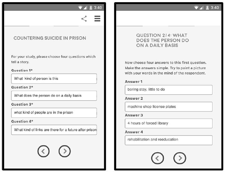
Figure 1: The set up-template for the Mind Genomics study, showing the input form for the four questions, and the input form for the four answers from question #2.

Table 1 shows the raw material created for the topic of feeling after being released from prison. The four questions are not engraved in stone. Rather, they are “first guesses,” aspects that can be fine-tuned or even discarded in subsequent easy and affordable iterations. The Mind Genomics experiment can be modified quickly, after the initial data have been collected, and executed once again, virtually immediately after the study materials have been updated.

Table 1: The four questions and the four answers for each question.

	Question A: What kind of person is this?
A1	WHO: young inner city black woman
A2	WHO: white middle age for theft
A3	WHO: 21-year-old, second conviction for drugs
A4	WHO: 54-year-old woman convicted for drugs
	Question B: What does the person do on a daily basis?
B1	ACTIVITIES: boring stay, little to do
B2	ACTIVITIES: machine shop license plates
B3	ACTIVITIES: 4 hours of forced library
B4	ACTIVITIES: rehabilitation and reeducation
	Question C: what kind of people are in the prison?
C1	SITUATION IN PRISON: lower and upper middle class
C2	SITUATION: camaraderie
C3	SITUATION IN PRISON: drug addicts
C4	SITUATION IN PRISON: invisible status
	Question D: What kind of links are there for a future after prison?
D1	RELEASE PREPARATION: optional courses to prepare for jobs
D2	RELEASE PREPARATION: out you go
D3	RELEASE PREPARATION: no support
D4	RELEASE PREPARATION: simply re-enter life

Step 2: Select a Rating Scale

The rating scale dictates the nature of the experiment. The rating scale is shown below. The scale deals with the likelihood of what will happen 12 months after the person is discharged from prison.

Rating question: What will happen in 12 months?

Low Anchor: Rating question 1=hopeful

High Anchor: Rating question 9=suicidal

Figure 2 two other tempates. The left panel in Figure 2 shows the orientation page. The right panel show the rating scale, including number of scale points (9), and the anchors for each scale point.

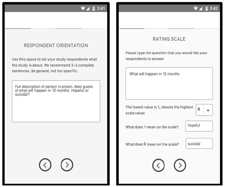
Figure 2: The templates, for respondent instructions (left panel), and for rating scale (right panel).

Step 3: Create the Vignettes, Combinations of Elements to be Tested

The vignette, a combination of 24 elements, becomes the “stimulus” that the researcher presents, and the respondent responds by following a rating scale introduced in Step 2. The vignettes are created according to a systematically designed set of combinations, “the experimental design” [24]. The underlying experimental design for this so-called 4×4 design of Mind Genomics (4 questions, 4 answers/question) prescribes exactly 24 combinations. The combinations are of three types: combinations with one element from two questions (2-element vignette), one element from three questions (3-question vignette), or one element from four questions (4-question vignette). By design each question can contribute at most one element, but often no elements. Furthermore, each respondent evaluates a different set of combinations, permutations of the main design [25].

The rationales for the design and the permutations follow:

a. The experimental design ensures that each respondent evaluates the appropriate vignettes, designed for OLS (ordinary least squares) regression. OLS regression builds a model or an equation, of the form: Dependent Variable = k₀ + k₁(A1) + k₂(A2) … k₁₆₍D4)

b. The systematic permutation of the design ensures that the structure of the combinations is the same for all respondents, but each respondent tests different combinations. In effect, the permuted design ensures that the Mind Genomics experiment covers many of the possible combinations. The approach of testing many combinations, each with “noise,” rather than testing a limited number of combinations with the noise averaged out through replication, represents a dramatic departure from conventional statistics and design. Conventional design suppresses noise or averages out the noise. Permuted designs accept the noise at each point but cover most of the design space, thereby allowing the underlying pattern to emerge. The best metaphor is the difference between a high resolution X- ray of a single area, with a single X- ray impression, versus the MRI, magnetic resonance imaging, which takes many pictures of the tissue from different angles, and combines the different pictures later on. Metaphorically speaking, Mind Genomics is an “MRI of the mind.”

c. In order for the rating scale to work, it must be applied to the description of a person. Only with combinations of elements is there a real, albeit sparse, description of a person and situation. The rating scale will not be meaningful when applied to each of the 16 elements, in a one-by-one fashion. There is no context in the format which presents one element at a time, despite the attractiveness of doing so. By presenting the test elements in a one-by-one fashion, one allows the respondent to alter the criterion for judgment to fit the nature of the test element being evaluated. The experimental design combines elements, forcing the respondent to maintain one criterion, and preventing “gaming” the interview.

Step 4: Define the Dependent Variables

The raw data from Mind Genomics are the ratings on the anchored 9-point scale (see Step 2), and the response time. The response time is defined as the number of seconds between the presentation of the test vignette and the rating assigned by the respondent. The response time is easily measured by the underlying computer program.

The original ratings on the 9-point scale are hard for managers to understand, despite their seeming simplicity. The typical question encountered is: “What does <rating X> mean?” “Rating X” could be a 3, a 7, or any of the numbers on the scale. As simple as the scale is, the reality in practice is that the scale has no intrinsic meaning to the manager, except at the very top or bottom.

The convention in traditional consumer research has been to divide the scale into two points, to denote NO versus YES. For these data we divide the scale two ways:

Top3: The scale is divided so that ratings of 7-9 are transformed to 100 to denote “suicide YES” (whether thoughts or expected action), and ratings of 1-6 are transformed to 0 to denote “hopefulness YES”). A small random number is added to the transformed ratings to introduce minute variability, a statistical requirement for OLS (ordinary least-squares) regression analysis. The small random number, assigned to each transformed number, ensures the necessary but vanishingly low variability in the dependent variable.

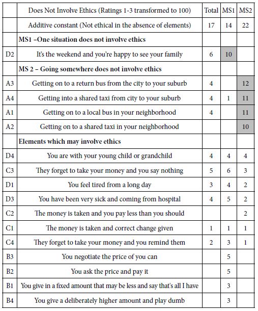
Bot3: The scale is divided so that ratings of 1-3 are transformed to 100 to denote “hopefulness YES,” and ratings of 4-9 are transformed to 0 to denote “hopefulness NO.” A random number is once again added to each transformed rating.

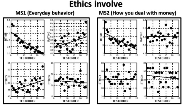
The Mind Genomics program, BimiLeap, measures the response time, defined as the time between the appearance of the vignette and the time that the rating is assigned. The response time is also treated as a dependent variable, but not transformed. For the analysis, the response times from vignettes 13-24 will be the only ones used for analysis. The use of data from the second half of the vignettes for response time, but the use of data from all 24 vignettes for the binary transformed variables (Top3 and Bot3), comes from the striking observation in Figure 3. The average response time drops as the respondent becomes more acquainted with the task, and more practiced. In contrast, the average rating on the 9-point scale does not change. Figure 3 shows the average values by each of the 24 positions in the experiment for the four prospective dependent variables, respectively. It is clear that there is no order dependency for the average rating, a clear decreasing function for response time, and a very “noisy,” but possibly decreasing function for both Top3 and Bot3.

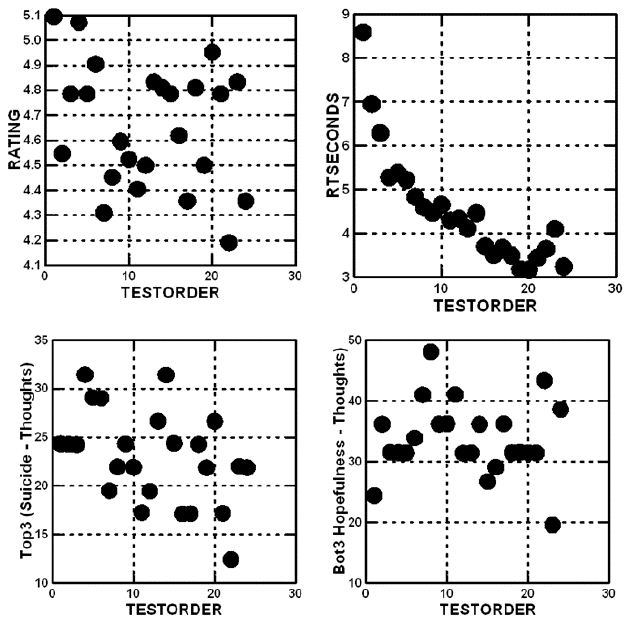
Figure 3: Average value of the four dependent variables for each of the 24 positions (test order) in the Mind Genomics experiment. Position 1 is the vignette tested in the first position, position 10, for example, is the vignette tested in the 10^th position.

Step 5: Build the Model (Equation) Relating the Presence/Absence of Elements

It is the contribution of the elements to the response which constitutes the key information afforded by the Mind Genomics experiment. That contribution is provided by the coefficient of the model, relating the presence/absence of the 16 elements to the dependent variable.

The equation is estimated using the well accepted method of OLS (ordinary least-squares) regression, or so-called “curve fitting.” The analysis focused on three equations, relating to Top3, Bot3, and response time. The equation for the rating was not calculated because it is contained within the analysis of Top3 (Suicide) and Bot3 (Hopeful).

The basic equation is expressed as an additive constant (k₀) and 16 coefficients (k₁-k₁₆), respectively.

Top3 = k₀ + k₁(A1) + k₂(A2) … k₁₆(D4)

Bot3 = k₀ + k1(A1) + k₂(A2) … k₁₆(D4)

RT (Response Time ) = k₁(A1) + k₂(A2) … k₁₆(D4)

The additive constant is the estimated value of the dependent variable (e.g., Top3 or Bot3) in the absence of elements. The experimental design ensured that each vignette would be comprised of 2-4 elements, meaning that the additive constant is a purely estimated parameter. The additive constant can be thought of as the baseline value of Top3 or Bot3. If the metaphor is a statue, then the additive constant is the base, viz., not part of the statue itself, but a basic, fixed contribution to the height.

Above the baseline or additive constant will be the separate contributions of the elements, given by the coefficients. The coefficients are positive (the element contributes to the the value of Top3 or Bot3), zero (no effect), or negative (the element takes away from the value of Top3 or Bot3). For the sake of clarity and to allow the patterns emerge, we will estimate the coefficients, but only show the positive or non-zero coefficients. It is the pattern of these positive coefficients which tell the “story.”

Step 6 – Results from the Total Panel

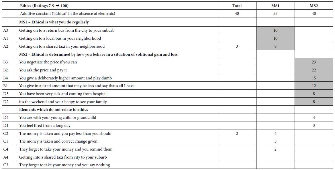
The total panel comprises all the vignettes from all the respondents. Keep in mind that the analysis generated two models, one looking at suicide (not further defined; Top3), the other looking at hopefulness (not further defined; Bot3). Again, keep in mind that we are dealing with the wisdom of the masses, viz, a guess about the behavior based upon the vignette. Yet, we surmise that an average judgment, given by many people, may provide a good sense of what people believe regarding how a recently released prisoner might feel after 12 months. Table 2 shows the positive coefficients driving either suicide/despair (Top3) or hopefulness (Bot3).

The additive constant represents the expected feeling of the person described, in the absence of any additional information. The expected proportion of responses “suicide”(ratings 7-9) in the absence of information is 24. Of course, all vignettes by design comprised 2-4 elements, so the addiive constant is a purely estimated parameter. Nonetheless, we get a sense that about a quarter of the responses will be that the person described will contemplate suicide. In contrast, for feelings of hopefulness, Table 2 suggests that 44% of the time, i.e., almost half of the responses, the person described will feel hopeful.

Table 2: Parameters of the models relating the presence/absence of the 16 elements to the thought of suicide (Top3) or hopefulness(Bot3). Strong performing elements (8 or higher) are shown in shaded cells. Only positive coefficients are shown, to reveal the patterns.

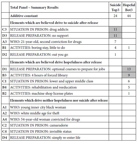
It is in the elements that we see some situations which drive the feeling of suicide. The only elements we show are positive ones because we are interested in what drives the feelings of suicide, rather than what does not drive the feeling of suicide. The two strongest elements are having been in prison with SITUATION IN PRISON: drug addicts, and an element described as RELEASE PREPARATION: no support in prison. Both of these elements have high coefficients of 11, meaning that when they are included in the description of the released person, an additional 11% of responses are that the person will fee “suicidal” (ratings 9, 8, 7). If the person leaving is a 21-year old, with a second conviction for drugs, an additional 7% feel there could be suicide behavior.

The data suggest that two strong elements are thought to drive a feel of hopefulness: RELEASE PREPARATION: optional courses to prepare for jobs, and ACTIVITIES: 4 hours of forced library. There is a sense that forcing the prisoner to do things to improve the mind should help.

Step 7: Response Time (Reflection of Degree of Engagement of Responder) as a Dependent Variable

The response time, defined as the time between the presentation of the vignette and the rating, may represent time needed to process the information. Response time is not directly under the cognitive control of an individual, who is simply reading the vignette (if that), and assigning a rating.

Figure 3 above shows the systematic decrease in the average response time. The average response time in the aggregate, by test position (postion 1 to position 24), shows a dramatic pattern which makes sense. As respondents get increasingly experienced with the task, even without feedback, their average time to read and rate the vignette decreases, at first dramatically. The response time eventually stabilizes near the end of the experiment.

Graphs similar to these appear in virtually any study, leading to the introduction of a “practice first vignette,” the response to which is discarded. In this study we discard that first vignette, which is not part of the design, measure the response times for the 24 vignettes, and build models for the total set of 24 vignettes, followed by models for the first half of th vignettes vs the second half (vignette 1-12 vs 13-24).

The deconstruction of the response time for the total vignette into the component response times is done using the same type of regression equation , but without the additive constant. The rationale for this analysis, called “forcing the model through the origin” comes from the recognition that in the absence of elements there is no response at all.

Response Time = k₁(A1) + k(A2) … k₁₆(D4) (Note: no additive constant)

Table 3 shows the coefficients for response time, first for the total set of vignettes (Vig 1-24), then for the first 12 vignettes (Vig 1-12) and finally for the last 12 vignettes (Vig. 13-24). The final column (Sec-First) shows the change in estimated response time (seconds) by element, for the total panel. The important thing to notice is the changes are not the same. There is a dramatic range.

Table 3: Response times for the 16 elements, showing the response time for the total panel over 8 second for all 24.

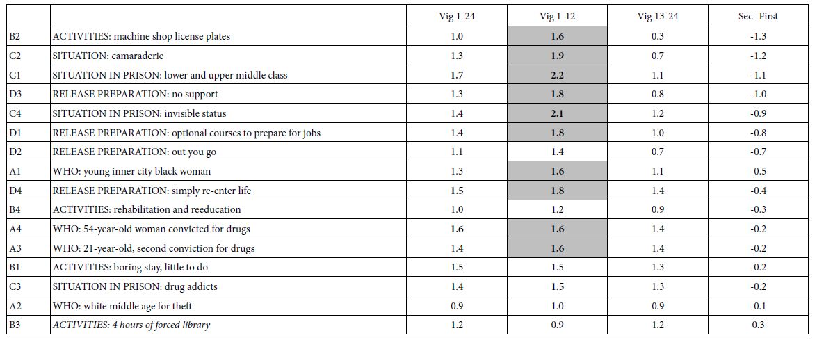
The response times are not highly correlated, but they are positively correlated, all except one being shorter for the second half of the 24 vignettes, and being longer for the first half of the vignettes. That element, B3, ‘ACTIVITIES: 4 hours of forced library’ is important because it becomes more engaging as the respondents are exposed to it. It may be that the message becomes increasingly meaningful with repeat exposures. It may be these types of elements which are most important to recognize. Their meaning may “sink in” over time, rather than become diluted (Figure 4).

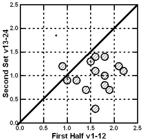
Figure 4: Relation between the coefficients for response time for the first vs the second half of the set.

Step 8: Create New Groups of Respondents (Mind-sets), based Upon the Patterns of Their Coefficients

A continuing hallmark finding of Mind Genomics is that people differ in the way they think. The finding is not surprising and often glossed over as a characteristic of “subjective data,” such as ratings of opinions, and certainly ratings of opinions of the Mind Genomics vignettes.

Mind Genomics studies often reveal that what seems to be a “flat” data set with few strong elements is stronger than one might believe at first glance. The mind-sets can be thought of as different patterns of interesting elements. When one group of people is interested in a set of elements, but another group is not, often the result is flat and noisy when the coefficients of the elements are plotted against each other. The plot is “noisy,” with the coefficients darting about with no pattern emerging. Such is the general problem in research when one deals with groups of people with radically different points of view towards the same topic. What could be rich veins of information, rich patterns of “color” are discarded because at first glance the general impression is a boring monochrome. Only when one looks more closely do the intricate patterns reveal themselves, patterns which otherwise intertwine, interdigitate, and produce a dull gray.

The process to uncover the mind-sets comprises simple steps, described elsewhere [26]. Here is a list of the steps:

a. Create a model for each respondent. This is possible because of the underlying experimental design, used to create the vignettes for each respondent.

b. Cluster the respondents based upon the pattern of their coefficients.

c. For clustering, use the metric (1-Pearson Correlation) as the measure of “distance” or “dissimilarity” between pairs of respondents.

d. Extract two and then three clusters, the mind-sets.

e. Create the models for all respondents in a specific cluster or mind-set. Thus the analysis creates two new models for the two-mind set solution, three new modesl for the three mind-set solution.

f. Inspect the models for interpretability, viz., do the data “tell a coherent story?”

The clustering program was run twice, first for the models for Top3 (suicide), and second for the individual models for Bot3 (hopefulness). The analysis, run twice, allows us to look at these two feelings separately, viz. treating the data anew, once from the viewpoint of feelings about suicide and once, and entirely separately, from the point of view of feelings about hopefulness.

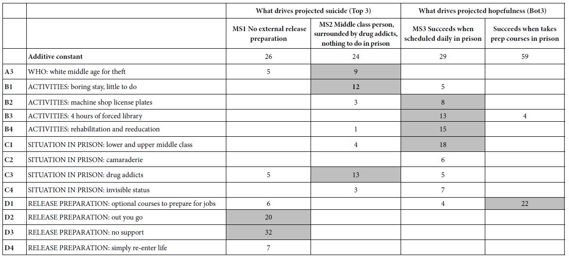
Table 4 shows the results of two sets of cluster analyses: MS1 and MS2, based on suicide (Top3); MS3 and MS4, based on hopefulness (Bot3). Table 4 shows only the positive coefficients for each, in the interests of readability and to detect the underlying patterns. The strongest performing elements are shown in shaded cells. The “names” for the mind-sets are shown in the second row. These names were assigned by the researchers based upon the “story” which the strong performing elements appeared to provide.

Table 4: The two pairs of mind-sets, based upon clustering coefficients for suicide (Top3, left two columns) and coefficients for hopefulness (Bot3, right two columns).

Pairwise Interactions – What Situation Drives a Rating of “Suicide”

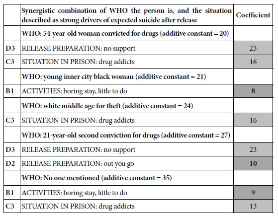
The underlying exoerimental design using Mind Genomics ensures that all of the elements are statistically independent of each other. Yet, despite that, some combinations naturally “enhance each other,” when they appear together, despite being statistically independent. The permuted design used here (Gofman & Moskowitz, 2010) allows us to discover these synergistic combinations, or more correctly, to discover how a set of elements performs when one of the elements is held constant with different options. This analysis shows the change in the performance of a set of elements when we systematically “cycle through” the elements in one question.

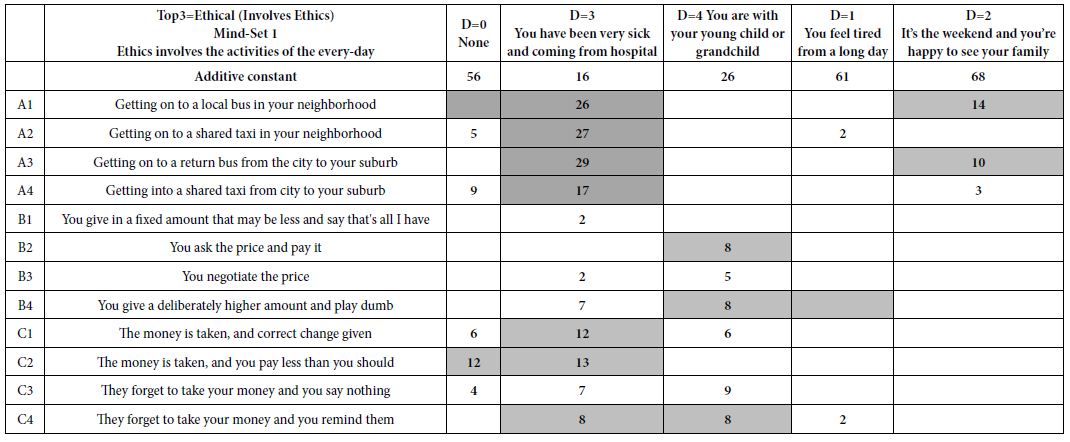
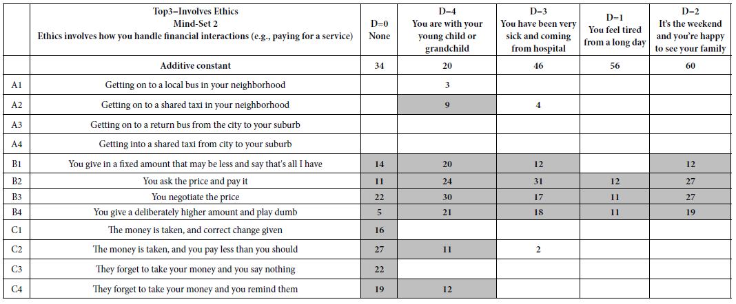
In order to discover these synergistic combinations we simpy divide the data for any question (e.g, WHO the person is, question A) into the five levels or strata (A=0 viz., A does not appear in the vignette; A=1 in the vignette, A=2 in the vignette, A=3 in the vignette, and A=4 in the vignette, respectively). The vignettes in each strata comprise an experimental design that can be analyzed. The value of A is held constant in the stratum. Thus, A no longer acts as a source of four independent variables (A1-A4). We are now left with 12 independent variables, B1-B4, C1-C4, and D1-D4, respectively.

Table 5 shows the coefficients which are very strong for independnt variables B1-D4, when A is “cycled through,” viz., A0 (A absent), A1, A2, A3 and A4, respectively. Only the very strong performing coefficients appear in Table 5. The analysis was done for suicide (Top3) as the dependent variable. It is clear that there are synergies between WHO the person is and the situation in prison. Of course, these are inferred by the respondent. We are relying on the ‘‘wisdom of the masses” to give us a sense of the pattern Nonetheless, the data suggest some patterns, such as the perceived synergy between a middle class released prisoner and an experience with drug addicts in prison.

Table 5: Synergistic combinations in which the coefficient for the situation is very strong. The dependent variable is Top3 (suicide).

Finding these Individuals in the Population

A key output of most Mind Genomics studies is the continuing discovery that the mind-sets do not vary in a straightforward way with the typical geo-demographics that fill the databases of people. We know a lot about the behavior of people. However, despite being able to measure their behaviors at many touchpoints and in many situations, we cannot say that we know the attitude of a person in a granular way for any topic which arises. Everyday experience suggests that people differ. Although we might hazard a guess about the way people make decisions regarding issues in a specific topic, these are guesses, not facts. Indeed, just a bit of thinking will reveal that people dramatically differ, often to the surprise of those who question them and believe they know the answer before it is given. The reason for the surprise is that how a person thinks is not related to, except in the most obvious cases, who the person is.

Table 6 below shows the distribution of mind-sets for both Top3 (suicidal) and Bot3 (hopeful). There were two mind-sets extracted for each. There is no clear relation between mind-sets in either case analysis to gender or age. Indeed, there is no clear relation between membership in segments created for suicidal vs segments created for hopeful, even though the people were the same, the ingoing data were the same, and all that differed was the way the data in the scale were treated.

Table 6: Distribution of mind-sets for Suicidal (Top3) and for Hopeful (Bot3).

		MS1 (Top3) Feel worst when just sent out after finishing sentence with no contact after release	MS2 (Top3) Feel worst when recalling time in prison was spent being bored, surrounded by addicts, etc.
Total	42	19	23
Male	19	9	10
Female	23	10	13
Age 18-29	13	7	6
Age30-Plus	29	12	17
	Total	MS3: (Bot) Feel hopeful when recall that prison experience was ok, fellow prisoners were middle class, time was boring but did some work	MS4 (Bot) Feel hopeful when recalling prison prepared for exit, and provided something to do to keep busy
Total	42	22	20
Male	19	9	10
Female	23	13	10
Age18-29	13	6	7
Age30-Plus	29	16	13
	Total	Bot 3 MS Seg3	Bot 3 MS Seg4
Total	42	22	20
Top 3 MS1	19	12	7
Top 3 MS2	23	10	13

Unable to generalize the discoveries of Mind Genomics, our ability to understand what the mind-sets mean in terms of behavior and how they relate to mind-sets of other studies is limited. The mind-sets here can be used to understand how one thinks of the feelings of released prisoners. The results would be far stronger if the study could be administered to prisoners a year after their release or to prisoners from different socio-economic classes with the objective to assign a new individual (ex-prisoner) to one of the two mind-sets.

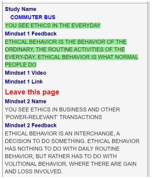
Recently, authors Gere and Moskowitz developed an approach to assign new people to the mind-sets discovered through Mind Genomics. The approach, called the PVI (Personal Viewpoint Identifier), uses a combination of Monte Carlo Simulation with added variability, and Decision Tree analysis. The PVI creates a set of six questions, using the elements and coefficients shown in the left part of Table 4 (mind-sets created from Top3, viz., Suicide). The table, comprising both positive and negative coefficients, is “perturbed” by added, random variability. The PVI then identifies the optimal set of six elements, taken directly from the study, the patterns of response which best reproduce the original mind-sets. The elements are presented to the new person on a 2-point scale. The pattern of responses to these six questions, based on the elements, assigns the new person to one of the two (or three) mind-sets, empirically uncovered by the study.

It should be kept in mind that the PVI works with granular data, with data used to create the vignettes in the first place. Thus, the PVI does not need to be “interpreted” by experts, who take macro segmentation of an entire topic and change the focus to a micro-topic. The PVI works automatically, without training, and is set up in minutes based upon the proper input from the study.

Figure 5 shows the PVI. The first part of the PVI (left side) contains a section to obtain demographics, allowing the researcher to understand who the respondent IS, when the PVI is completed, and so forth. Many of these questions can be suppressed for a shorter interview. The second part comprises two PVI’s, one for Suicide, and the other for Hopefulness. The respondent simply answers the 12 questions. The data are stored in a database, showing the demographics, the mind-set for each PVI (suicide, hopefulness), and the original ratings. The PVI is set up for rapid, easy deployment, and for fast answers.

The PVI for the study, the left panel shows the demographics section. The right panel shows the two PVIs comprising six questions each, one for suicide (study 1), the other for hopefulness (study 2). The PVI structure allows the researcher to randomize the order of the studies, and within a study randomize the order of the questions. There is a third option to randomize all 12 questions so that questions of hopefulness may be mixed with questions of suicide (Figure 5).

The PVI showing two panels, the left panel obtains the demographics. The right panel presents two sets of six questions each, designed to assign a person separately to the one mind-set from the first pair of mind-sets (regarding suicide), and at the same time assign a person to one mind-set from the second pair of mindsets (regarding hopefulness) (Figure 5).

Discussion and Conclusion

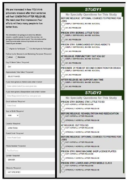
Figure 5: The PVI. The left panel shows the first part, which acquires the demographics. The right panel shows the two PVI questionnaires, for the two pairs of mind-sets.

With increased experience in applying the methods of Mind Genomics, the researcher can gain valuable insights into the minds of people. In contrast to the typical approach of science, which addresses “holes” in the literature, the Mind Genomics approach proceeds in a purely inductive, exploratory way. With a Mind Genomics experiment, there is no hypothesis to be tested and either corroborated or falsified in the classical manner of science as described by Karl Popper [27]. Rather, the science here is simply observing a situation and formalizing a way to understand the different aspects of that situation [28].

What is important in this paper is the discovery of the two mind-sets for suicide thoughts and the two mind-sets for hopeful thoughts. It should be noted that rather than interviewing recently released prisoners (viz., after a year), we began this project in the spirit of “wisdom of the masses” and engaged in a gedanken or “thought” experiment.

If the approach presented here is acceptable to the scientific community as a way of understanding our perception of others, then the Mind Genomics approach provides an interesting way to introduce new topics into the world of research, topics which are appropriate for specific groups but must be first explored with the world at large. Mind Genomics offers many benefits. The results can be directly integrated into a larger database. The data is self-evident. Patterns emerge from the data. Some are meaningful and some are not. By following many iterations and fine-tuning the questions and answers that received the most responses in an earlier iteration, the researcher arrives at the truth. This is the science of psychology in its most basic form: looking at all possibilities, sorting out the emerging patterns, searching for differing mind-sets, and predicting which mind-set someone new will belong to. By repeating this methodology for dealing with questions of economics or feelings or everyday occasions, the researcher will gather the data to formulate a “wiki of the mind” and understand how mind type and behavior are related.

Acknowledgement

Attila Gere thanks the support of Premium Postdoctoral Research Program of the Hungarian Academy of Sciences.

References

1. Kariminia A, Law MG, Butler TG, Levy MH, Corben SP, et al. (2007) Suicide risk among recently released prisoners in New South Wales, Australia. Medical journal of Australia 187: 387-390. [crossref]
2. Pratt D, Piper M, Appleby L, Webb R, Shaw J (2006) Suicide in recently released prisoners: a population-based cohort study. The Lancet 368: 119-123. [crossref]
3. Pratt D, Appleby L, Piper M, Webb R, Shaw J (2010) Suicide in recently released prisoners: a case-control study. Psychological medicine 40: 827-835. [crossref]
4. Stark R, Doyle DP, Rushing JL (1983) Beyond Durkheim: religion and suicide. Journal for the Scientific Study of Religion 120-131.
5. Harizi A, Trebicka B, Tartaraj A (2020) A Mind Genomics Cartography of Shopping Behavior for Food Products During the Covid-19 Pandemic. European Journal of Medicine and Natural Sciences 4: 25-33.
6. Opsal T (2012) ‘Livin’on the Straights’: Identity, Desistance, and Work among Women Post‐ Sociological Inquiry 82: 378-403.
7. Steiner B, Wooldredge J (2008) Inmate versus environmental effects on prison rule violations. Criminal Justice and Behavior 35: 438-456.
8. Camp SD, Gaes GG (2005) Criminogenic effects of the prison environment on inmate behavior: Some experimental evidence. Crime & Delinquency 51: 425-442.
9. Hochstetler A, Murphy DS, Simons RL (2004) Damaged goods: Exploring predictors of distress in prison inmates. Crime & Delinquency 50: 436-457.
10. Lahm KF (2008) Inmate-on-inmate assault: A multilevel examination of prison violence. Criminal justice and behavior 35: 120-137.
11. Dhami MK, Mandel DR, Loewenstein G, Ayton P (2006) Prisoners’ positive illusions of their post-release success. Law and Human Behavior 30: 631-647. [crossref]
12. Craig DE, Rogers RD (1993) Vocational training in prison: A case study of maximum feasible misunderstanding. Journal of offender rehabilitation 20: 1-20.
13. Holbrook MI (1997) Anger management training in prison inmates. Psychological Reports, 81: 623-626. [crossref]
14. Suarez A, Lee DY, Rowe C, Gomez AA, Murowchick E, et al. (2014) Freedom project: Nonviolent communication and mindfulness training in prison. Sage Open 4: 2158244013516154.
15. Visher CA, O’Connell DJ (2012) Incarceration and inmates’ self-perceptions about returning home. Journal of Criminal Justice 40: 386-393.
16. Winnick TA, Bodkin M (2008) Anticipated stigma and stigma management among those to be labeled “ex-con”. Deviant Behavior 29: 295-333.
17. Baldry, Eileen, Desmond McDonnell, Peter Maplestone, Manuel Peeters. (2002) “Ex-prisoners and accommodation: What bearing do different forms of housing have on social reintegration for ex-prisoners.” In Housing, Crime and Stronger Communities Conference convened by the Australian Institute of Criminology and the Australian Housing and Urban Research Institute, Melbourne 6-7.
18. Johnson Listwan S, Colvin M, Hanley D, Flannery D (2010) Victimization, social support, and psychological well-being: A study of recently released prisoners. Criminal justice and behavior 37: 1140-1159.
19. Surowiecki J, (2005) The wisdom of crowds. Anchor.
20. Milutinovic V, Salom J (2016) Mind Genomics: A Guide to Data-Driven Marketing Strategy. Springer.
21. Moskowitz HR, Wren J, Papajorgji P (2020) Mind Genomics and the Law, LAP LAMBERT Academic Publishing 13: 17-21.
22. Moskowitz HR, (2012) ‘Mind genomics’: The experimental, inductive science of the ordinary, and its application to aspects of food and feeding. Physiology & behavior 107: 606-613. [crossref]
23. Moskowitz HR, Gofman A, Beckley J, Ashman H (2006) Founding a new science: Mind genomics. Journal of sensory studies 21: 266-307.
24. Box GE, Hunter WH, Hunter S (1978) Statistics for experimenters. New York: John Wiley and sons.
25. Gofman A, Moskowitz H (2010) Isomorphic permuted experimental designs and their application in conjoint analysis. Journal of sensory studies 25: 127-145.
26. Dubes R, Jain AK (1980) Clustering methodologies in exploratory data analysis. Advances in computers 19: 113-228.
27. Popper K (2005) The logic of scientific discovery. Routledge.
28. Kell DB, Oliver SG (2004) Here is the evidence, now what is the hypothesis? The complementary roles of inductive and hypothesis‐driven science in the post‐genomic era. Bioessays 26: 99-105. [crossref]

DOI: 10.31038/PSYJ.2021321

Abstract

Respondents evaluate combinations of short phrases, rating each combination as either being relevant to ethics, or not relevant to ethics. The topic was the daily behavior of a local or a commuter bus, ranging from the nature of the bus ride, what was the person taking the ride either doing or feeling, how the fare was given to the bus driver, and what happened afterwards. The deconstruction of the responses revealed two clearly different groups of people having different ‘mind-sets’ about what ethics deals with in this ordinary, quotidian situation. One group felt that ethics pertains to the nature of the daily activity, the nature of the bus ride, and the feeling of the person described. The other mind-set felt that ethics pertained to the nature of how the rider handled the payment of a fare. The Mind Genomics approach provides a deep understanding of the nature of ethics, casting light on the nature of how one thinks about the topic of ethics, rather than immediately jumping into the ethical issues themselves.

Introduction

Traditionally, ethics have been studied in the context of problems which are often puzzling. These problems, like ‘who should one kill’ in a specific situation when faced with a two-alternative situation, are designed to make people think about the issues underlying ethics. The problems are often deep, have no clear answer, and are striking, unusual in their nature. The problems force deep thinking. It is no wonder that many of these are popular ‘ignition devices’ for a course on ethics. Mind Genomics is an emerging behavioral science, which deals in the simplest format with the way people make decisions in situations with different aspects. The underlying principle for Mind Genomics is that by mixing different features of a situation, creating alternative ‘realities,’ and observing the decision a person makes, one can identify the criteria used by the person.

Traditional uses of Mind Genomics begun with issues involving economics, usually issues involving consumer purchases [1-3]. The economics aspect moves from individual micro-economic decisions encountered in marketing, and onto more complex situations such as issues of public policy and what to do [4]. Over the years, the original uses of the approaches called conjoint measurement [5] evolved from the study of issues regarding finances to issues regarding social well-being [6] and even into law [7].

Mind Genomics Meets ‘Ethics’

The study reported here, a ‘cartography’ in the language of Mind Genomics, resulted from a discussion by author HRM with a group of students in Israel. The question was ‘how do we know what is ethical in the world of everyday?’ The question was framed as an inquiry into how one goes about establishing ethics in the world of the everyday experience. People know that it is unethical to murder, and so forth. There is the sense of ethics, whether that sense is innate from natural law, or emerging from convention, and internalized through education to become normative, both in action and in thought. The issue was not those topics, but rather the nature of right and wrong in the small actions of the everyday, actions where one might say are minor ‘peccadillos’ rather than ethical issues [8,9]. In an excellent summary article ‘ethical feelings’ for behavior, including the ‘ordinary can be introduced by the simple set of paragraphs:

So, What is Ethics?

Ethics is the manner by which humans regulate individual behavior in civilized society. One might say that humans regulate behavior by laws, which is true. But laws cannot apply in every instance, and all the time. So, ethics is how we train people to behave, or teach them how they ought to behave, even if no laws apply in some circumstance (source: https://www.oocities.org/athens/acropolis/1628/A53ethic.htm). A deeper look into the world of ethics and how it could involve Mind Genomics would move from a simple research paper to books. The literature on ethics is vast, with roots stretching back to antiquity. A simple search in Google Scholar® for ‘What is relevant for ethics?’ generated 2.95 million ‘hits.’ The need to know the difference between ‘right’ and ‘wrong’ remains an important issue, and the topic of inquiries reaching into academia and the teaching of ethics [10]. The need has been stated by philosophers, but manifests itself everywhere, from daily life to the machinations and strategies of corporations projecting themselves in a favorable light [11].

Mind Genomics as a science deals with studying and understanding human responses to outside stimuli, whereas it focuses on measuring deep structure of thinking, subconscious mechanisms that go on in the mind. Since we deal with the mind processes that originate on a cellular level, a direct relationship with the genome indicates that there is genetic participation in determining a response. Being a sort of an antenna, on a molecular level DNA acts both as a receiver of information and initiator of a response [12]. Therefore, when we apply Mind Genomics to research the topic of ethics, we gain insight to the inner workings of how we differ from one another and what we perceive as relevant to ethics. The study shows two distinct mindsets that differ in the way they respond to the sixteen elements, which shall be considered as sixteen commuter bus riding situations. The beauty of this science is that it enables us to study deep mind processes by creating a simple matrix and combing textual elements.

Investigating Some ‘Ethics’ Aspects of an Everyday Behavior-paying the Fare on a Bus

We demonstrate the application of Mind Genomics cartography to the simple problem of behavior on a commuter bus, and the issue of where the incident takes place, the payment situation, and the response of the driver, and finally who the person is. The underlying notion is to look at the nature of the behavior, and to decide whether the specific behavior should be a topic for ethics or not. The results reveal a strategy by which to understand the ethics of the every-day, where the behavior is the quotidian, almost automatic behavior which only occasionally involves what we would call ‘ethics.

The focus of the Mind Genomics cartography is the nature of what a respondent considers to be in the realm of ‘ethics’, and conversely not in the realm of ‘ethics.’ In contrast to the traditional studies of ethics, which deal with general problems, Mind Genomics deals at the level of the mundane, granular, everyday experience. When the topic is ethics, the Mind Genomics approach is to present vignettes, combinations which describe different facets of everyday behavior, instruct respondents to read these vignettes, rate them, and from the data thus obtained, understand the topic almost from the ‘bottom up. Applying Mind Genomics to ethics, and following the foregoing strategy, means that the researcher defines a topic (ethics), creates four questions (aka ‘silos’), and four answers to each question (aka as ‘elements.’). The topic is ethics, the questions pertain to aspects of behavior on a commuter bus, and then different specifics of each aspect of behavior.

The important things to note concern the nature of the experiment. When we think of a commuter bus, we may think of ethics, but anything having to do with ethics is probably at the low end of importance. The issues involving what is in the realm of ethics for the mundane commuter trip are certainly far from dramatic, and perhaps require a stretch of imagination to link these behaviors we hardly notice to a topic so essentially human as ethics. Nonetheless, it is precisely the contribution of Mind Genomics to ethics, when the study pulls out ethical issues from the ordinariness of the situation, the lack of drama, and the difficulty of finding a link. We deal with the topic of the commuter bus, following the Mind Genomics process, as illustrated below:

The Mind Genomics Process

Step 1: Define the Topic, and the Raw Materials

This first step sounds easy, and in fact it begins with simply the statement of a topic. The topic must be reasonable circumscribed, limited so that it can be further investigated using specific statements.

The raw materials comprise four questions, each of which is answered by four different statements, phrases presented in the declarative form. Table 1 shows an example of the four questions, and the four answers for each question. It is important to keep in mind that the Mind Genomics process is rapid, inexpensive, and iterative, so that one need not be ‘correct’ at the start. Thus, the questions and answers in Table 1 can always be modified, improved, and resubmitted to the Mind Genomics process. There is no need to be ‘right’ on the first or indeed any iteration.

Table 1: Raw materials (four questions, and four answers for each question).

	Question A: what is the act?
A1	Getting on to a local bus in your neighborhood
A2	Getting on to a shared taxi in your neighborhood
A3	Getting on to a return bus from the city to your suburb
A4	Getting into a shared taxi from city to your suburb
	Question B: How do you pay?
B1	You give in a fixed amount that may be less and say that’s all I have
B2	You ask the price and pay it
B3	You negotiate the price
B4	You give a deliberately higher amount and play dumb
	Question C: What is the response?
C1	The money is taken, and correct change given
C2	The money is taken, and you pay less than you should
C3	They forget to take your money and you say nothing
C4	They forget to take your money and you remind them
	Question D: What are the circumstances?
D1	You feel tired from a long day
D2	it’s the weekend and your happy to see your family
D3	You have been very sick and coming from hospital
D4	You are with your young child or grandchild

Step 2: Combine the Answers into Vignettes Using an Experimental Design

Mind Genomics works by presenting combinations of answers (elements) in a simple format, a set of elements and a rating scale. The respondent reads the introduction to the study, reads the combination of elements (the vignette), and rates the combination on the defined scale. Here the scale is a 9-point scale, anchored at the top (ethical) and at the bottom (non-ethical).

Most consumer research asks the respondent to rate one element or answer at a time, in order to maintain focus on the element. The practice of Mind Genomics is the opposite, namely, to simulate real-life and to prevent ‘gaming the system’ by having the respondent think of an appropriate answer for each element. By presenting combinations of vignettes, the combinations comprising 2-4 elements, Mind Genomics forces the respondent to sift through the vignette, doing so virtually automatically, without dee thinking, and without the ability to ‘game the system’ by providing the ‘right’ answer.

The experimental design itself comprises 24 combinations, vignettes. Each element from the set of 16 appears five times in the vignettes. A vignette can comprise at most one element from a question, viz., one answer for a question, ensuring that the vignette does not feature two different and possibly mutually contradictory ideas. The topic of experimental design in research has been dealt with extensively in various books. A good review is presented by [13]. The actual interview comprised a short introduction about age, gender, and a third question dealing attitude towards the law:

What do you consider yourself to be, given the following choices:

1=Most of the time obey the rules rigidly,

2=Don’t complain if you get an advantage and don’t hurt anyone,

3=5Pragmatic honest but not stupid,

4=Not applicable.

The self-profiling questionnaire followed by an introduction to the topic, and 24 vignettes. The introduction to the topic appeared on every vignette, at the top, with the respondent reading the vignette as a single ‘thought’. Here are some common situations with transportation. Each is a vignette of a common situation. Please read it and rate the degree of ethical behavior described in the whole vignette. Let 1=totally unethical … 9=totally ethical

Step 3: Invite Respondents to Participate

The interaction is an experiment but was positioned as a ‘study’ to make the respondents feel comfortable. The respondents were members of a large panel offered for use at a fee by Luc.id, a strategic partner of Mind Genomics Associates. The respondents were sent a link, began the study, and earned ‘points’ for their participation. The respondents did not know the purpose of the study nor could the respondents ‘game’ the study. The entire study took 3-5 minutes. The BimiLeap program recorded the specific combination, the rating on the 9-point scale, and the number of seconds from the appearance of the vignette on the screen to the rating. This latter time, recorded to the nearest tenth of a second, was called the response time.

Step 4: Transform the Rating

In the world of Mind Genomics, the objective is to relate the presence/absence of the elements (viz., the 16 answers) to the ratings assigned. Users of the Mind Genomics data prefer to view the results as ‘no/yes’, rather than as points along a graded Likert Scale, such the 9-points ethics scale. To make the results easy to understand, we transform the data twice, first to create a binary scale for ‘Ethical’ and then to create a binary scale for ‘Not Ethical’’

Transformation #1: Ethics: Ratings of 7-9 → 100, Ratings of 1-6 → 0

Transformation #2 Not Ethics: Rating of 1-3 → 100, Ratings of 4 -9 → 0

To each transformed number, whether 0 or 100, we add a small random number <10^-5. This prophylactic measure ensures that when we use OLS (ordinary least-squares regression), even on the data of a single respondent, that there is guaranteed to be variation in the dependent variable. We also create a new variable, response time, which was defined above as the number of seconds, to the nearest tenth of second, elapsing between the presentation of the vignette and the response.

The data matrix emerging from the experiment and the transformation comprises the following:

1. Each row corresponds to a respondent and a vignette.
2. Each row corresponds to a particular variable, as follows:

a.  Respondent Identification Number

b.  Test order (1-24)

c.  16 columns, one column for each of the 16 elements or answers.

d.  A cell for the 16 elements is ‘0’ when the element does not appear in the vignette, and ‘1’ when the element appears in the vignette. By design each vignette comprises 2-4 elements, at most one element or answer for a question. Thus majority of numbers in a row for the 16 columns is 0, and the minority is 1.

e.  The actual rating originally assigned by the respondent.

f.  The actual response time.

g.  The Transformed value: For Ethics

h.  The transformed value: Not for Ethics

i.  A code showing the specific questions in the vignette. There are 11 different combinations of elements that can be made with 2-4 different sources or questions (Table 1). These range from AB (answer or element from question A, answer from question B), all the way to ABCD (one answer or element from questions A, B, C, D).

Step 4: Analyze the Data to Uncover Three Mind-sets, and Create the Four Models (Total, Mind-sets)

The matrix is now set up for OLS (ordinary least-squares) regression, both at the level of the individual respondent, and at the group level. OLS regression generates a simple equation of the form:

Rating or Transformed Rating = k₀ + k₁A1+ k₂A2 … k₁₆A16.

For the measurement of response time, the equation is almost the same, but without the additive constant, viz., Response Time = k₁A1 + k₂A2 … k₁₆A16.

The equation allows us to trace the contribution of each element to either the rating, the response time, or the transformed rating. The regression analyses, for Total Panel or for individuals, will be done primarily for the dependent variable of ethical (ratings of 1-6 transformed to 0; ratings of 7-9 transformed to 100). The additive constant is the estimated value of the dependent variable (e.g., binary transform of Not Ethical), in the absence of any elements. The additive constant is a strictly estimated parameter but gives a sense of the predisposition of the respondent to assign the rating, Thus, for the transformed variable ‘Ethical’, an additive constant of 48 means that 48% of the ratings are be 7-9 in the absence of elements. The additive constant gauges the predisposition of a group to judge harshly (low additive constant for Ethical) or judge mildly (high additive constant for ethical).

The regression analysis can be done at the level of the individuals to general 103 individual equations. The vignettes for each respondent allow for the creation of a valid equation, because the vignettes were created by an experimental design, complete on an individual-by-individual basis. The design was permuted to create different combinations, but the same mathematical structure was maintained, underlying the specific permutation for each respondent [14]. One can imagine now a matrix of 17 columns, an additive constant and 16 coefficients. The matrix comprises 103 rows, one per respondent. A separate statistical analysis called the cluster analysis [15] divides the 103 respondents into either two or three groups, based upon the dissimilarity of the patterns of 16 coefficients.

For this study, the clustering generated three different groups, called mindsets MSA, MSB, and MSC, respectively. We do not know the names of these mind-sets. We just know that respondents in the same mind-set show similar patterns of the 16 coefficients. (The additive constant is discarded). Mind-sets A and B were similar to each other, sharing a number of strong performing elements, and were thus combined into one new mind-set, MS1. Mind-set C became MS2. The final analysis creates three equations, one for Total Panel, and one model each for the two mind-sets. It is important to keep in mind that often mind-sets of interest must first emerge, be kept separate, and the remaining mind-sets recombined. Thus Mind-Set 2 did not emerge when two mind-sets were extracted. Mind-Set 2 emerged only when three mind-sets are extracted.

Step 5: Post the Coefficients in a Way Which Allows the Mind-sets to Emerge

Table 2 shows the positive coefficients of the Total Panel and of the two mind-sets. The table is sorted to show which elements perform very strongly (shaded). A coefficient of +8 or higher corresponds to ay strong performing element with an expected value for the coefficient around 2.0 or higher. The coefficients of 0 or lower are not shown because they add no insight.

Table 2: Models for Ethics (viz., involves ethics) for Total Panel and two final mind-sets).

The additive constant for the Total Panel is 48, meaning that in the absence of any information, we expect 48% of the responses to be 7-9, defined as ‘Ethical’ in the mind of the respondent. MS2 is slightly more generous, with 53% of the ratings 7-9, whereas MS3 is less generous, with 40% of the ratings 7-9. Beyond the additive constant, it is the pattern of coefficients which tells us the difference between groups in terms of what they feel to be ‘Ethical’. MS1 feels that ethical behavior is the behavior of the ordinary, the routine activities of the every-day. Ethical behavior is what normal people do.

MS2 feels that ethical behavior is an interchange, a decision to do something. Ethical behavior has nothing to do with daily routine behavior, but rather has to do with volitional behavior, where there are gain and loss involved.

We can now look at the same data and mind-sets, but from the viewpoint of what constitutes ‘non ethical behavior.’ Not ethical behavior may either be ‘unethical behavior’, or more likely behavior that has nothing to do with ethics. Mind-Set 1 may feel that D2 is the only element which does not relate to ethics. Mind-Set 2 may feel that going somewhere is something which does not involve ethics. Recall that for them, ethics were involved in volitional behavior with money.

The important thing here is that the respondents have a sense of what they feel ‘involves ethics.’ Table 3 shows that they have an equivalent and complementary feeling of what does involve ethics.

Table 3: Models for Not Ethics (viz., does not involve ethics) for Total Panel and two mind-sets.

Step 6: Effect of Repeated Evaluations on Ratings

The permuted experimental design ensures that each respondent evaluates a unique set of vignettes. Thus, across the set of 103 respondents and 24 vignettes per respondent we have 2472 combinations. Often the issue is raised that during the evaluation the respondent may lose interest, and simply assign random numbers. If that is the case, we might see a decrease in the variation of average ratings as the respondent presses the same number to finish the task.

Figure 1 shows two sets of plots. The four left plots show the average response times, ratings, and transformed binary values for Mind-Set 1, the group which felt that the ‘everyday’ actions involved ethics. The four right plots show the average response times and ratings for Mind-Set 2, which felt that ethics are involved in the volitional handling of money. In this study both mind-sets MS1 and MS2 show similar patterns of decreasing response times through the entire evaluation of 24 vignettes.

Figure 1: How the average response time, rating, and value for Ethical and Not Ethical change with repeated exposure in an experiment. Each point represents the average rating for all vignettes evaluated in the position. The left panel shows the patterns Mind-Set 1. The right panel shows the pattern for Mind-Set 2 the more stringent mind-set.

MS1 and MS2 differed in what they felt to be ethical. MS1 (ethics deals with the every-day) became more lenient as they proceeded, feeling more of the element were ‘ethical’ as they proceeded through the evaluation. In contrast, as the experiment proceeds, there is no effect on judgments of ‘ethical’ by MS2 (ethics deals with volitional situations with gain and loss).

Interactions among Variables

The data from the clustering suggests two mind-sets, MS1 focusing on ethics being relevant to the everyday activities, and MS2 focusing on ethics being relevant to the nature of financial transactions under a person’s control. The final issue for this paper is to determine the degree to which the involvement of ethics with the everyday (Mind Set 1) or with financial transactions (Mind Set 2) can be intensified or in contrast, can be attenuated, by specific external factors. We have already identified the mind-sets by the pattern of their coefficients. It is the pattern which defined the mind-sets.

Recent efforts by author Moskowitz have shown that the strategy of permuted design permits a deeper understand of the mind of the respondent by revealing the effect of one element on another, so-called scenario analysis [1]. That is, through stratification of the data, and subsequent OLS statistics, on a stratum-by-stratum basis, one can quickly see how on type of element can influence how you feel about the involvement of a topic in ethics. Put in simpler terms, Mind Genomics allows us to answer questions such as: ‘We know that you feel an everyday activity, such as A1, Getting on to a local bus in your neighborhood, is an elements where ethics is relevant. A new question is the degree to which other elements from other questions, such as D (what you are doing, how you are feeling) drive the involvement of ethics of element A1. That is, can one element affect the response to another element in the same vignette, or are the elements evaluated totally separately?

To answer the foregoing question, viz., interaction of pairs of elements, the analysis separates the full data set into a pair of datasets, each with five matching strata. The data are divided first by the mind-set to which the respondent has been assigned. This division creates two databases, that will be analyzed separately, but in parallel. For each of the two databases one per mind-set, we create five strata, each stratum defined by the value of the element from silo or question D (who the respondent is, or how the respondent feels). There are five values of D (D=0, absent …. D-4). We then run five OLS regression, with the independent variables being A1-C4 (12 predictor, not 16), and the dependent variable being Ethical (viz., appropriate for ethics). Tables 4 and 5 shows the summary data, viz., the additive constant, and the positive coefficients for elements A1-C4.

Interaction of Feelings (Silo D) with Remaining Elements among Mind-Set1 (Ethics = Daily Living)

We begin with the value of the additive constant across D=0 to D=5. Table 4 shows the coefficients for A1-C4. The columns are sorted by incremental value of the additive constant, the measure of basic relevance for ethics. When the specific circumstance of the situation is absent (D=0), the additive constant is high, 56. We should not be surprised. Mind-Set 1 reacts as if all behavior of whatever type is relevant for ethics.

Table 4: How the interaction of elements from Question D (circumstances) with other elements drive the perception of ‘ethical’ (viz., involves ethics) drives responses. Data from Mind-Set 1.

With element D3 as the constant (hospital), the basic relevance for ethics drops 40 points, from 56 to 16. Again, this makes sense because Mind-Set 1 focuses on the very ordinary, and D3 is an unusual, and not a daily occurrence. At the same time, elements A1-A4 reemerge as important, which is not surprising in light of the very low additive constant. With element D4 as the constant (grandchildren), the basic relevance increases from the low of 16 to the value 26. Having grandchildren is also not a daily occurrence. The elements from silo A, daily commuter activities, no longer are drivers of ethics.

With element D1 and D2, tired and weekend, the more normal events of oneself, the additive increases. The behavior is every-day, no excuses, and the focus goes back to the absolute ordinariness of life. It is clear that for Mind-Set 1, ethics concern the everyday. What is important is the ability for Mind Genomics to discover this organizing principle with a simple study, but a study whose data structure allows this discover through studies of interactions, of scenarios produced by holding one element constant.

Interaction of Feelings (Silo D) with Remaining Elements among Mind-Set2 (Ethics = Financial Behavior)

When we look at the same analysis, this time from the point of view of data provided by Mind-Set 2, with focus on ethics involving control over money, we see a similar pattern, but the numbers differ. The absence of circumstances (D=0) generates an additive constant of 34. This makes sense because for Mind-Set 2 ethics is about something under one’s control, not about the world of the everyday, with everything relevant for ethics, as it is for Mind-Set 1. It is when the elements involve money, elements B1-B4, that we see the feeling that the topic is relevant for ethics. Furthermore, the coefficients are extraordinarily high and most of them are focused on elements from both Question B and Question C, the two questions dealing with money.

Table 5: How the interaction of elements from Question D (circumstances) with other elements drive the perception of ‘ethical’ (viz., involves ethics) drives responses. Data from Mind-Set 2.

Practical Applications – Who is in these Mindsets, and How can They be Discovered?

We move now to the final analysis of the data, namely the discovery of who these people are, in terms of gender and age, and in terms of how they think of themselves. We finish with a way to discover these individuals in the population at large, viz., a way to begin to merge sociology, psychology, marketing, and ethics into what might be called the Mind Genomics of Ethical Inquiry, or some similar name. Table 6 shows the distribution of the 103 respondents into the two mind-sets. It is clear that the mind-sets transcend the common ways of describing oneself (gender, age), and a prima-facie way of describing one’s ethics attitude during daily life.

Table 6: Distribution of the total panel and the two ethics mind-sets by gender, age, and self-described ethics.

	Total	MS1 Ethics=Every day	MS2 Ethics=Financial
Total	103	68	35
Gender
Male	47	33	14
Female	56	35	21
Age
Age 14-25	26	18	8
Age 26-59	56	37	19
Age 60+	18	11	7
How do you consider yourself?
1=Most of the time obey the rules rigidly	43	29	14
2=Don’t complain if you get an advantage and don’t hurt anyone,	20	14	6
3=Pragmatic, honest but not stupid,	34	20	14
4=Not applicable	6	5	1

The Personal Viewpoint Identifier (PVI) uses the created mind-sets and their coefficients. The aim of the PVI is to find those elements that have the highest discriminatory power on the mind-sets. This means that it looks for the elements that are the most different among the mind-sets. In order to do so, so-called distance metrics are used which calculate the mathematical distances between the mind-sets for each element. The six most discriminatory elements are then chosen for the PVI and presented to the participants. Based on the original coefficients, the PVI can classify newly recruited participants into existing mind-sets. This way new participants do not need to complete the whole BimiLeap® study but need to answer six short (binary) questions. That way assignment of new participants is fast and immediately done. The PVI is presented by Figure 2, and the mind-set feedback of the PVI is presented by Figure 3. After completing the questionnaire of Figure 2 the results is immediately presented to the participant. There is room for different videos or links, which can therefore be suggested based on the mind-set memberships.

Figure 2: Personal viewpoint identifier created using the given study. Participants are asked to answer the binary scale as soon as they can.

Figure 3: Mind-set feedback of the personal viewpoint identifier.

The PVI created for this specific study is available here:

https://www.pvi360.com/TypingToolPage.aspx?projectid=2292&userid=2008

Discussion and Conclusion

The literature of philosophy comprises an inordinate number of papers on problems touched by the issue of ethics. Scarcely any generation can be found which did not have philosophers who focused on ethics as part of the great questions. Attempting to locate this Mind Genomics cartography in the vast ocean of ethics and philosophy would be a meaningless exercise. Rather than that, this discussion might be a good place to consider the potential of a Mind Genomics effort to quantify ethics, at least in simple, everyday matters.

It is clear from the unexpected results, viz., that people judged the vignette in terms of relevance for ethics, that we are dealing with two different aspects in this Mind Genomics cartography. The first, the goal that was not achieved, is the effort to have people judge good versus bad. That failed, perhaps because in a vignette of good versus bad the story must be clearer. There must be something which has gone wrong and is to be put aright by justice. When that is missing, the obvious right versus wrong, it may be difficult to think about the fit of the topic into the world of ethics. There is nothing to link the daily, ordinary, quotidian to what the person thinks about ‘ethics.’ In such a case the respondents are left to their own devices. Those belonging to Mind-Set 1 perceive the entire situation as relevant for ethics. Those belonging to Mind-Set 2 revert to issues where there can be wrongdoing, viz., the payment of money by the passenger, where it is possible to ‘cheat’ the bus driver. It is that situation which calls forth the relevance of ethics, at least to Mind-Set 2.

What may be the most important contribution of this paper is the method of Mind Genomics, and specifically the ‘scenario analysis’ to reveal the deep structure of thinking. Mind Genomics already can lay claim to being able to metricize thought. These data suggest the next level, to quantify interactions, and by so doing clarify the underlying structure of thinking, through simple experiments, done anywhere, and dealing with virtually anything where decisions by people are relevant.

Acknowledgment

AG thanks the support of the Premium Postdoctoral Researcher Program.

References

1. Moskowitz HR, Gofman A (2007) Selling blue elephants: How to make great products that people want before they even know they want them (1st ed.). Pearson Prentice Hall.
2. Moskowitz H (2012) “Mind genomics”: The experimental, inductive science of the ordinary, and its application to aspects of food and feeding. Physiology & Behavior 107: 606-613. [crossref]
3. Moskowitz HR, Gofman A, Beckley J, Ashman, H (2006) Founding a new science: Mind genomics. Journal of Sensory Studies 21: 266-307.
4. Milutinovic V, Salom J (2016) Mind genomics. a guide to data-driven marketing strategy. Springer International Publishing.
5. Gustafsson A, Herrmann A, Huber F (2001) conjoint measurement: Methods and applications. Springer.
6. Harizi A, Trebicka B, Tartaraj A (2020) A mind genomics cartography of shopping behavior for food products during the covid -19 pandemic. European Journal of Medicine and Natural Scinces Articles 4: 25-33.
7. Moskowitz H, Wren J, Papajorgji P (2020) Mind Genomics and the Law. LAP LAMBERT Academic Publishing
8. Gino F (2015) Understanding ordinary unethical behavior: Why people who value morality act immorally. Current Opinion in Behavioral Sciences 3: 107-111.
9. Rawls J (1951) Outline of a decision procedure for ethics. The Philosophical Review 60: 177-197.
10. Nguyen NT, Basuray MT, Smith WP, Kopka D, McCulloh DN (2008) Ethics perception: Does teaching make a difference? Journal of Education for Business 84: 66-75.
11. Creyer HE (1997) The influence of firm behavior on purchase intention: do consumers really care about business ethics? Journal of Consumer Marketing 14: 421-432.
12. Singh P, Doti R. Lugo JE, Faubert J, Rawat S, et al, (2018) DNA as an electromagnetic fractal cavity resonator: Its universal sensing and fractal antenna behavior bt – soft computing: theories and applications. In M. Pant K, Ray TK, Sharma S, Rawat A, Bandyopadhyay (Eds.), Soft Computing: Theories and Applications. Advances in Intelligent Systems and Computing.
13. Ryan TP, Morgan JP (2007) Modern experimental design. Journal of Statistical Theory and Practice 1: 501-506.
14. Gofman A, Moskowitz H (2010) isomorphic permuted experimental designs and their application in conjoint analysis. Journal of Sensory Studies 25: 127-145.
15. Dubes R, Jain AK (1980) clustering methodologies in exploratory data analysis. Advances in Computers 19: 113-228.

References

1. Bergman KA, Arends JP, Scholvinck EH et al. (2007) Pantoea agglomerans septicemia in three newborn infants. Pediatr Infect Dis J 26(5):453-4. [cross-ref]
2. Yablon BR, Dantes R, Tsai V, et al. (2012-2013 & 2017) Outbreak of Pantoea agglomerans bloodstream infections at an Oncology Clinic – Illinois. Infect Control Hosp Epidemiol 38(3):314-19. [cross-ref]
3. Rezzonico F, Smits TH, Montesinos E, et al.(2009) Genotypic comparison of Pantoea agglomerans plant and clinical strain. BMC Microbiol 9:204. [cross-ref]
4. Volksch B, Thon S, Jacobsen ID, et al. (2009) Polyphasic study of plant and clinic-associated Pantoea agglomerans strains reveals indistinguishable virulence potential. Infect Genet Evol 9:1381-91. [cross-ref]
5. Walterson AM, Stavrinides J. (2015) Pantoea: insights into a highly versatile and diverse genus within the enterobacteriaceae. FEMS Microbiology Reviews 39(6):968-984. [cross-ref]
6. Flatauer FE. (1978) Septic arthritis caused by Enterobacter agglomerans. Arch Int Med 138(5):788. [cross-ref]
7. Williams AJK, Scott RJD, Lightfoot NF. (1986) Erwinia herbicola as a cause of bacterial endocarditis. J Infect 12(1):71-73. [cross-ref]
8. Mason GI, Bottone EJ, Podos SM. (1976) Traumatic endophtalmitis caused by an Erwinia Am J Ophtalmol 82(5):709-13. [cross-ref]
9. Okwundu N, Mercer J. (2019) Pantoea agglomerans cutaneous infection. J Derm and Dermatologic Surg 23(1):41.
10. Habsah H, Zeehaida M, Van Rostenberghe H, et al.(2005) An outbreak of Pantoea species in a neonatal intensive care unit secondary to contaminated parenteral nutrition. J Hosp Infect 61(3):213-18.
11. Rasmussen SW, Koczulab B. (1992) Transfusion associated bacteremia and septic shock due to Erwinia herbicola. Scand J Infect Dis 24(2):241-43. [cross-ref]
12. Cheng A, Liu CY, Tsai HY, et al. (2000-2010 & 2013) Bacteremia caused by Pantoea agglomerans at a medical center in Taiwan, J Microbiol, Immunol and Infect 46(3):187-94. [cross-ref]
13. Dutkiewicz J, Mackiewicz B, Lemieszek M, et al. (2015) Pantoea agglomerans: a marvelous bacterium of evil and good. Part I. Deleterious effects:dust-borne endotoxins and allergens-focus on cotton dust. Ann Agricol Environ Med 22(4):576-88. [cross-ref]
Direct-to-Consumer-Tests and the Patient-Doctor Relationship. A Survey amongst Users, Non-Users, and Physicians
DOI: 10.31038/PEP.2021222
Abstract
In highly developed countries we see an increased uptake of predictive tests that can be accessed without the intervention of a physician. We performed surveys among 1,345 people in order to gauge the experiences and views of users and non-users. Since one of our foci was the impact of taking such tests on patient-doctor relationships, we also interviewed 15 physicians about their views on DTC-test and about their experiences with patients who saw their doctor prior to, or after, taking these tests.
We found that 5.6% of respondents used DTC-tests, particularly health checks and total body scans, with a tendency to increased use and thus possibly a growth potential. Uptake of DTC-tests was significantly correlated with having a positive attitude towards DTC-tests, male gender, and younger age in our main analysis, and with a positive attitude in our most representative subgroup analysis. In accordance with other studies, we found little evidence of a positive impact of DTC-participation that could not have been reached by other means. Generally, DTC-tests had a neutral to positive influence on patient-doctor relationships. GPs and consumers agree that that participation in DTC-tests, irrespective of physicians’ views on their value, should not inhibit existing patient-doctor relationships. This means that GPs may need an upgrade in their knowledge of DTC-tests.
Keywords
Health checks, Predictive tests, Direct to Consumer tests, DTC-tests, Screening, Patient-doctor relationship, ethics, Netherlands.
1. Gefenas E, Cekanauskaite A, Tuzaite E, Dranseika V, Characiejus D. et al. (2011) Does the ‘New Philosophy’ in Predictive, Preventive and Personalised Medicine Require New Ethics? EPMA J. Jun;2(2):141–7. [cross-ref]
2. Thompson S, Tonelli M. General Health Checks in Adults for Reducing Morbidity and Mortality from Disease [Editorial]. Cochrane Database Syst Rev. 2012;10.
3. Predictive Medicine [Internet]. Nature. [cited 2018 Apr 20]. Available from:https://www.nature.com/subjects/predictive-medicine.
4. Wilson JMG, Jungner G. Principles and Practice of Screening for Disease. Geneva: World Health Organization; 1968. 164 p.
5. Bradley WG, Golding SG, Herold CJ, Hricak H, Krestin GP, Lewin JS, et al. (2009 & 2011) Globalization of P4 Medicine: Predictive, Personalized, Preemptive, and Participatory—Summary of the Proceedings of the Eighth International Symposium of the International Society for Strategic Studies in Radiology, August 27–29. Radiology. 258(2):571–82. [cross-ref]
6. Fenton JJ, Deyo RA. (2003) Patient Self-Referral for Radiologic Screening Tests: Clinical and Ethical Concerns. J Am Board Fam Pract. 16(6):494–501. [cross-ref]
7. Bijlsma M, Rendering A, Chin-On N, Debska A, von Karsa L, Knöpnadel J, et al.(2014) Quality Criteria for Health Checks: DEVELOPMENT of a European Consensus Agreement. Prev Med (Baltim). 67:238–41.
8. Stol YH, Schermer MHN, Asscher ECA. (2016) Omnipresent Health Checks May Result in Over-Responsibilization. Public Health Ethics. phw034. [cross-ref]
9. Health Council of the Netherlands. Screening: Between Hope and Hype. The Hague: Health Council of the Netherlands; 2008.
10. Levitt DM.(2001) Let the Consumer Decide? The Regulation of Commercial Genetic Testing. J Med Ethics. Dec;27(6):398–403. [cross-ref]
11. Savard J, Mooney-Somers J, Newson AJ, Kerridge I. (2014) Australians’ Knowledge and Perceptions of Direct-to-Consumer Personal Genome Testing. Intern Med J. Jan;44(1):27–31. [cross-ref]
12. Marshall KG.(1996 Jul) Prevention. How Much Harm? How Much Benefit? 3. Physical, Psychological and Social Harm. CMAJ. 155(2):169–76. [cross-ref]
13. Emanuel EJ, Emanuel LL.(1992) Four Models of the Physician-Patient Relationship. JAMA – J Am Med Assoc. 267(16):2221–6.
14. Beauchamp TL, Childress JF. (2013) Principles of Biomedical Ethics. 7th ed. New York: Oxford University Press; 1–459 p.
15. Saunders B, Sim J, Kingstone T, Baker S, Waterfield J, Bartlam B, et al. (2017) Saturation in Qualitative Research: Exploring Its Conceptualization and Operationalization. Qual Quant.1–15. [cross-ref]
16. Hoebel J, Starker A, Jordan S, Richter M, Lampert T. (2014) Determinants of Health Check Attendance in Adults: Findings from the Cross-Sectional German Health Update (GEDA) Study. BMC Public Health. 14(1):1–12.
17. Dryden R, Williams B, McCowan C, Themessl-Huber M. (2012) What Do We Know about Who Does and Does Not Attend General Health Checks? Findings from a Narrative Scoping Review. BMC Public Health. Dec 31;12(1):723. [cross-ref]
18. Stol Y, Asscher E, Schermer M.(2016) Reasons to Participate or Not to Participate in Cardiovascular Health Checks: A Review of the Literature. Public Health Ethics. 9(3):301–11.
19. Krogsboll LT, Jorgensen KJ, Gronhoj Larsen C, Gotzsche PC. (2012) General Health Checks in Adults for Reducing Morbidity and Mortality from Disease: Cochrane Systematic Review and Meta-Analysis. Bmj. 345(e7191). [cross-ref]
20. Si S, Moss JR, Sullivan TR, Newton SS, Stocks NP. (2014) Effectiveness of General Practice-Based Health Checks: A Systematic Review and Meta-Analysis. Br J Gen Pract. 64(618):47–53. [cross-ref]
21. Amoroso C, Harris MF, Ampt A, Laws RA, McKenzie S, Williams AM, et al. (2009) The 45 Year Old Health Check: Feasibility and Impact on Practices and Patient Behaviour. Aust Fam Physician. 38(5):358–62. [cross-ref]
22. Hanlon P, McEwen J, Carey L, Gilmour H, Tannahill C, Tannahill A, et al.(1995) Health Checks and Coronary Risk: Further Evidence from a Randomised Controlled Trial. BMJ. 311(7020):1609–13.
23. Griffiths C, Cooke S, Toon P. (1994) Registration Health Checks: Inverse Care in the Inner City? Br J Gen Pract. 44(382):201–4. [cross-ref]
Review on Pregnancy Toxemia in Sheep with Observation of Resolution Using ReaShure (Protected Choline)
DOI: 10.31038/IJVB.2021522
Pregnancy toxemia is a metabolic disorder in sheep and goats which usually develops during late gestation and which is always associated with hyperketonemia and hypoglycemia. Ewes of certain breeds, mainly when bearing two or three lambs, are more susceptible than ewes only one fetus [1]. The economic significance of the disease is determined by reduced milk yields and body weight loss, poor feed conversion, increased culling and mortality rates of offspring and affected animals [2].
Compared to dry ewes, ewes in late pregnancy require about 50 percent more feed if bearing a single lamb and about 75 percent more feed if carrying twins. This amount of feed may exceed their intake capacity unless grain is substituted for part of the ration [3]. Ovine pregnancy toxemia or “twin-lamb” disease occurs in the latter part of pregnancy in sheep, typically in ewes with multiple fetuses, and is characterized by anorexia and neurologic signs of motor weakness, amaurosis, and mental dullness. It may occur spontaneously or may be induced by dietary deficiency. The disease is associated with the high calorific requirements of pregnant sheep.
Pregnancy toxemia may occur following a relative deficiency of available carbohydrate that leads to a drain on oxaloacetate and its precursors in an effort to maintain blood glucose concentration. Toxemia can usually be prevented by adequate supplementary feeding in late pregnancy. Clinical pathologic studies show consistent elevation of blood ketones and glucocorticoids and, in the early part of the disease, decreased blood glucose. Subclinical ketosis is defined as elevated concentration of circulating ketone bodies in the absence of clinical signs [4].
There are four categories of disease according to [5]: 1) Primary pregnancy toxemia caused by inadequate nutrition (poor quality feed, period of fasting) 2) Fat ewe/doe pregnancy toxemia seen in over-conditioned ewes/does in early gestation (suffer a nutritional decline in late gestation, possibly from smaller rumen capacity) 3) Starvation pregnancy toxemia seen in severely under-conditioned ewes/does (lack of feed after drought, heavy snow or flood) and 4) Secondary pregnancy toxemia due to concurrent disease such as parasites, poor dentition, or lameness.
Hyperketonaemia is defined as an abnormally high concentration of circulating ketone bodies during the postpartum period. The gold standard diagnostic test for Hyperketonaemia is the test for hyperketonaemia is the measurement of hydroxybutyric acid (BHBA) in serum or plasma by a laboratory process [6]. The most commonly used level of serum BHB to identify ketosis is a concentration ≥1400 mol/l (14.4 mg/dl) [7].
An alternative to the laboratory method is blood BHBA measurement that can be used as on – farm cow side test for hyperketonaemia with a near perfect accuracy (Precision Xtra; sensitivity 96%, specificity 97%). More recently, cow side tests for ketosis have focused on measuring BHBA level. One test is Keto Test (Sanwa Kagaku Kenkyusho Co Ltd, Nagoya, Japan; distributed by ELANCO Animal Health, Greenfield, IN). This test measures BHBA in milk and consists of test strips on which a reagent converts BHBA in the milk sample to AcAc. Using a provided colour scale, the strip may be used to semi-quantitatively measure BHBA concentration s in the milk sample based on intensity of the colour change observed on test strip [8,9]. A new blood strip test for BHBA and glucose was developed and manufactured by DFI CO., Ltd (South Korea). Recently a new test BHBCheck Plus (blood ketone & glucose test system) manufactured by PortaCheck, Inc, USA. Laboratory findings in individual animals may include hypoglycemia (often <2 mmol/L), elevated urine ketone levels, elevated BHBA levels (normal <0.8 mmol L, subclinical ketosis >0.8 mmol L and clinical disease >3.0 mmol /L) and frequently hypocalcemia and hyperkalemia due to severe ketoacidosis [10].
Blood glucose concentration between 40 and 65 mg/dl are common in pregnancy toxemia, although comatose animals may show terminal hyperglycemia, especially associated with fetal death [11]. To prevent ketosis in sheep, goats, it is important to identify the animals carrying twins or triple, separate them and provide them with a diet that will meet their energy demand. Successful treatment of pregnancy toxemia requires early detection and steps to quickly meet the energy (glucose) needs of the affected ewe. The most common treatment is to drench ewes with 2 to 3 ounces of propylene glycol 2 to 3 times daily. Propylene glycol, which is mainly absorbed intact directly from the rumen at a rate of 40% per hour and reaches its maximum blood level within 30 min of administration and maximum blood glucose conversion at about 4 h after administration. Propylene glycol transformation in glucose probably occurs via conversion to pyruvate [12].
Reashure microencapsulated choline, a recent technological breakthrough, protects choline on its journey rough-and -tumble rumen and releases it in the small intestine. Lipid (fat) layers, applied using a proprietary process, encapsulate (coat) the choline. At the time of calving and during negative energy balance, feeding ReaShure increases fat export out of the liver which prevents fatty liver and reduces the amount of fatty acids converted to ketones by the liver [13,14].
Feeding ReaShure also reduced the incidence of mastitis (P = 0.06) and all postpartum diseases combined (P = 0.001). Clearly, cows fed ReaShure were healthier and produced more milk [15]. The impact of feeding of ReaShure to sheep is obvious in reducing the incidence of ketosis in sheep (pregnancy toxemia). Sheep fed ReaShure are healthier compared to those not fed Rea Shure. Also, it reduced the incidence of abortion [16].
Pregnancy toxaemia-Ketosis Beta-hydroxybutyrate (BHB)-, Hypoglycemic-hyperglycemic-hyperketonemia-propylene glycol-protected choline (ReaShure)-acetone or acetoacetate (AcAc), BHB check plus (blood ketone & glucose test system), Qucare Vet Meter – Qucare Vet strips – mmol/l-Subclinical Ketosis-Abortion
1. Harmeyer J, Schlumbohm C (2006) Pregnancy impairs ketone body disposal in late gestating ewes: Implications for onset of pregnancy toxemia. Research in Veterinary Science 81: 254-264. [crossref]
2. Caldeira RM, Belo AT, Santos CC, Vazques MI, Portugal AV (2007) The effect of body condition score on blood metabolites and hormonal profiles i ewes. Small Rumin Res 68: 233-241
3. James M Sachse (1996) Extension Sheep Specialist. American Sheep Industry Association Inc, Production Education, and Research Council.
4. ANDERSSON L (1988) Subclinical ketosis in dairy cows. Vet Clin N Am Food Anim Pract 4: 233-251. [crossref]
5. Edmondson MA, Roberts JF, Baird AN, Bychawski S, and Pugh DG (2012) Theriogenology of Sheep and Goats. In: Pugh DG, Baird AN, eds. Sheep and Goat Medicine, 2nd Edition. Maryland Heights, MO: Elsevier-Saunders 150-231.
6. Tyopponen J, Kauppinen K (1980) The stability and automatic determination of ketone bodies in blood samples taken in field condition. Acta Vet Scand 21: 55-61. [crossref]
7. Oetzel GR (2004) Monitoring and testing dairy herd for metabolic disease. Vet Clin North Am 20: 651-674. [crossref]
8. Geishauser T, Leslie K, Tenhag J, Bashiri A (2000) Evaluation of eight cow Side Ketone tests in milk for detection of subclinical Ketone tests in milk for  Detection of subclinical Ketosis in dairy cows. J Dairy Science 83: 296-299. [crossref]
9. Carrier J, Stewart S, Godden S, Fetrow J, Rapnicki P (2004) Evaluation and use of three cowside tests for detection of subclinical ketosis in early postpartum postpartum cows. Dairy Sci 87: 3725-3735. [crossref]
10. Ramin AG, Asri-Rezaie S, Macali SA (2007) Evaluation on serum glucose, BHB, urea and cortisol in pregnant ewes. Medycyna Wet 63: 674-677.
11. Marteniuk JW, Herdt TH (1988) Pregnancy toxemia and ketosis of ewes and does. Vet din North Am Food Anim Pract 4: 307-315. [crossref]
12. Herdt TH, Emery RS (1992) Therapy of diseases of ruminant intermediary metabolism. Vet Clin North Am Food Anim Pract 8: 91-106. [crossref]
13. Cooke RF, Del Rio NS, Caraviello DZ, Bertics SJ, Ramos MH, et al. (2007) Supplemental choline for prevention and alleviation of fatty live in dairy cattle. J Dairy Sci 90: 2413-2418. [crossref]
14. Zom R, Baal J van, de Veth MJ, Goselink RMA, Widjaja- Greefkes HCA, et al. (2010) Effect of rumen -protected Choline on performance and hepatic fat metabolism in periparturient dairy cattle and hepatic fat metabolism in periparturient. J Dairy Sci 93: 781
15. Santos JP, Lima FS (2009) Feeding rumen-protected choline to transition dairy cows. Page 149 in Proceedings of the Florida Ruminant Nutrition. Univ.Florida, Gainesville.
16. Hameid OA, Abu-Zeid TESA, Mustafa Taha MK, Vandoni S (2019) Studying The Effects of supplementing ( Reashure ) to pregnant sheep on incidence of ketosis Health status Pre and after lambing. J Anim Sci livest Prod 3: 20
Intralesional Therapy in Oncology: A New Vision of a Classic Treatment
DOI: 10.31038/CST.2021621
Intralesional therapy has been used in oncology for over a century. The former empirical observations on local control were followed by trials with administration of different substances and/or destructive treatments with the aim of controlling cancer growth. Chemotherapy, molecular target therapy, radiotherapy and other physical therapies were initially viewed as a strategy that mainly affected tumor cells, but accumulating evidence in recent years indicates that can also affect the immune system and the tumor microenvironment to contribute to tumor regression. In the light of the recent and relevant findings in immunotherapy, a new point of view that integrates the current knowledge in the topic is presented, with the aim of stimulating further research that might help to optimize the use of new drugs, making them affordable, more effective and less toxic.
Intralesional therapy, Immunotherapy, Cancer
1. Coley WB (1991) The treatment of malignant tumors by repeated inoculations of erysipelas: With a report of ten original cases. Am J Med Sci 105: 487-510. [crossref]
2. Locy H, de Mey S, de Mey W, De Ridder M, Thielemans K, et al. (2018) Immunomodulation of the tumor microenvironment: Turn foe into friend. Front Immunol 9: 2909. [crossref]
3. Aznar MA, Tinari N, Rullán AJ, Sánchez-Paulete AR, Rodriguez-Ruiz ME, et al. (2017) Intratumoral delivery of immunotherapy-act locally, think globally. J Immunol 198: 31-39. [crossref]
4. Everson T, Cole WH (1996) Spontaneous regression of cancer. Philadelphia, Penn: JB Saunders & Co.
5. Sureda M, Subirá ML, Martín Algarra S, Prieto Valtueña J, Sangro B (1990) Spontaneous tumor regression. Report of 2 cases. Med Clin (Barc) 95: 306-308. [crossref]
6. Snow RM, Schellhammer PF (1982) Spontaneous regression of metastatic renal cell carcinoma. Urology 20: 177-181.
7. Cole WH (1974) Spontaneous regression of cancer: The metabolic triumph of the host? Ann NY Acad Sci 230: 111-141. [crossref]
8. Hirata E, Sahai E (2017) Tumor microenvironment and differential responses to therapy. Cold Spring Harb Perspect Med 7: 026781. [crossref]
9. Shibue T, Weinberg RA (2017) EMT, CSCs, and drug resistance: The mechanistic link and clinical implications. Nat Rev Clin Oncol 14: 611-629. [crossref]
10. Scarfò I, Maus M (2017) Current approaches to increase CAR T cell potency in solid tumors: Targeting the tumor microenvironment. J Immunother Cancer 5: 28. [crossref]
11. Zitvogel L, Apetoh L, Ghiringhelli F, Kroemer G (2008) Immunological aspects of cancer chemotherapy. Nat Rev Immunol 8: 59-73. [crossref]
12. Galon J, Bruni D (2019) Approaches to treat immune hot, altered and cold tumours with combination immunotherapies. Nat Rev Drug Discov 18: 197-218. [crossref]
13. Marabelle A, Tselikas L, de Baere T, Houot R (2017) Intratumoral immunotherapy: Using the tumor as the remedy. Ann Oncol 28: 33-43. [crossref]
fig 1
Postmarketing Analysis of Osteoporosis Patient Adverse Event Reports Reveals Stronger Association of Alendronate and Risedronate Use with Jaw Osteonecrosis and Atypical Femur Fracture
DOI: 10.31038/IJOT.2021413
In the United States, there are over ten million adults diagnosed with osteoporosis and many more are at risk of developing the condition. Osteoporosis affects both males and females, mostly post-menopausal. Bisphosphonates and denosumab have been widely used globally to treat the condition. The use of bisphosphonates and denosumab had been associated with rare adverse effects including osteonecrosis of the jaw, ONJ, and atypical femur fracture, AFF. However, it remained unclear whether those side effects were class-wide or drug-specific. By analyzing over 230,000 osteoporosis patient reports from the FDA adverse event reporting system, FAERS, we confirmed the association of bisphosphonates and denosumab use with AFF and ONJ.
Additionally, comparing each of the four frequently used bisphosphonates with denosumab-treated patients used as a control, we identified: (i) varying significance of association with ONJ and AFF for alendronate, risedronate, ibandronate and zoledronic acid, (ii) over two fold increase in risk of both side effects in alendronate patients, particularly in females, (iii) over a six-fold increase in AFF risk in both males and females taking risedronate, and (iv) lower risk of both AFF and ONJ, for zoledronic acid patients compared to denosumab.
Fracture, Osteonecrosis, Bisphosphonates
1. National Osteoporosis Foundation. 2014 [cited 2019 07]; Available from: https://www.nof.org/news/54-million-americans-affected-by-osteoporosis-and-low-bone-mass
2. Raisz LG (2005) Pathogenesis of osteoporosis: Concepts, conflicts, and prospects. J Clin Invest 115: 3318-3325. [crossref]
3. Song L, Xie XB, Peng LK, Yu SJ, Peng YT (2015) Mechanism and treatment strategy of osteoporosis after transplantation. Int J Endocrinol 2015: 280164. [crossref]
4. Eastell R, Rosen CJ (2019) Response to letter to the editor: “Pharmacological management of osteoporosis in postmenopausal women: An endocrine society clinical practice guideline”. J Clin Endocrinol Metab 104: 3537-3538. [crossref]
5. Rodan GA, Fleisch HA (1996) Bisphosphonates: Mechanisms of action. J Clin Invest 197: 2692-2696.
6. Reszka AA, Rodan GA (2003) Mechanism of action of bisphosphonates. Curr Osteoporos Rep 1: 45-52.
7. Hanley DA, Adachi JD, Bell A, Brown V (2012) Denosumab: Mechanism of action and clinical outcomes. Int J Clin Pract 66: 1139-1146. [crossref]
8. Reeve J (2002) Recombinant human parathyroid hormone. BMJ 324: 435-436. [crossref]
9. Bodenner D, Redman C, Riggs A (2007) Teriparatide in the management of osteoporosis. Clin Interv Aging 2: 499-507. [crossref]
10. Alendronate Sodium – FDA label [cited 2019 07]; Available from: https://www.accessdata.fda.gov/drugsatfda_docs/label/2003/21575_fosomax_lbl.pdf
11. Risedronate Sodium – FDA label [cited 2019 07]; Available from: https://www.accessdata.fda.gov/drugsatfda_docs/label/2015/020835s048lbl.pdf
12. Ibandronate Sodium – FDA label [cited 2019 07]; Available from: https://www.accessdata.fda.gov/drugsatfda_docs/label/2016/021455s021lbl.pdf
13. Zoledronic acid- FDA label [cited 2019 07]; Available from: https://www.accessdata.fda.gov/drugsatfda_docs/label/2018/021223s041lbl.pdf
14. Denosumab – FDA label [cited 2019 07]; Available from: https://www.accessdata.fda.gov/drugsatfda_docs/label/2019/125320s195lbl.pdf
15. Stroup J, Kane MP, Abu-Baker AM (2008) Teriparatide in the treatment of osteoporosis. Am J Health Syst Pharm 65: 532-539. [crossref]
16. Compston J (2011) Pathophysiology of atypical femoral fractures and osteonecrosis of the jaw. Osteoporos Int 22: 2951-2961. [crossref]
17. Aspenberg P (2014) Denosumab and atypical femoral fractures. Acta Orthop 85: 1. [crossref]
18. Black DM, Kelly MP, Genant HK, Palermo L, Eastell R, et al. (2010) Bisphosphonates and fractures of the subtrochanteric or diaphyseal femur. N Engl J Med 362: 1761-1771. [crossref]
19. Edwards MH, McCrae FC, Young-Min SA (2010) Alendronate-related femoral diaphysis fracture-what should be done to predict and prevent subsequent fracture of the contralateral side? Osteoporos Int 21: 701-703. [crossref]
20. Koh JS, Goh SK, Png MA, Kwek EB, Howe TS, et al. (2010) Femoral cortical stress lesions in long-term bisphosphonate therapy: A herald of impending fracture? J Orthop Trauma 24: 75-81. [crossref]
21. Isaacs JD, Shidiak L, Harris IA, Szomor ZL (2010) Femoral insufficiency fractures associated with prolonged bisphosphonate therapy. Clin Orthop Relat Res 468: 3384-3392. [crossref]
22. Espey R, Grimes S, Heyburn G, Kealey WD (2017) The first reported case of Atypical Femoral Fracture caused by daily ibandronate prescribed for bone metastases in breast cancer. BMJ Case Rep. [crossref]
23. Kharwadkar N, Mayne B, Lawrence JE, Khanduja V (2017) Bisphosphonates and atypical subtrochanteric fractures of the femur. Bone Joint Res 6: 144-153. [crossref]
24. Miyakoshi N, Aizawa T, Sasaki S, Ando S, Maekawa S, et al. (2015) Healing of bisphosphonate-associated atypical femoral fractures in patients with osteoporosis: a comparison between treatment with and without teriparatide. J Bone Miner Metab 33: 553-559. [crossref]
25. Koh JH, Myong JP, Jung SM, Lee J, Kwok S, et al. (2016) Atypical femoral fracture in rheumatoid arthritis patients treated with bisphosphonates: a nested case-control study. Arthritis Rheumatol 68: 77-82. [crossref]
26. Kim YS, Park WC (2012) Atypical subtrochanteric femur fracture in patient with metastatic breast cancer treated with zoledronic acid. J Breast Cancer 15: 261-264. [crossref]
27. Miller PD, Pannacciulli N, Brown JP, Czerwinski E, Nedergaard BS, et al. (2016) Denosumab or zoledronic acid in postmenopausal women with osteoporosis previously treated with oral bisphosphonates. J Clin Endocrinol Metab 101: 3163-3170. [crossref]
28. Nicolatou-Galitis O, Schiodt M, Mendes RA, Ripamonti C, Hope S, et al. (2019) Medication-related osteonecrosis of the jaw: definition and best practice for prevention, diagnosis, and treatment. Oral Surg Oral Med Oral Pathol Oral Radiol 127: 117-135. [crossref]
29. Landesberg R, Woo V, Cremers S, Cozin M, Marolt D, et al. (2011) Potential pathophysiological mechanisms in osteonecrosis of the jaw. Ann N Y Acad Sci 1218: 62-79. [crossref]
30. Aghaloo T, Hazboun R, Tetradis S (2015) Pathophysiology of osteonecrosis of the jaws. Oral Maxillofac Surg Clin North Am 27: 489-496.
31. Pazianas M, Miller P, Blumentals WA, Bernal M, Kothawala P (2007) A review of the literature on osteonecrosis of the jaw in patients with osteoporosis treated with oral bisphosphonates: prevalence, risk factors, and clinical characteristics. Clin Ther 29: 1548-15458. [crossref]
32. Paiva-Fonseca F, Santos-Silva AR, Della-Coletta R, Vargas PA (2014) Alendronate-associated osteonecrosis of the jaws: A review of the main topics. Med Oral Patol Oral Cir Bucal 19: 106-111. [crossref]
33. Jan BW, Liu HW, Yu H, Wang SC, Liu CJ, et al. (2012) Alendronate-induced osteonecrosis of the jaw in an elderly female. International Journal of Gerontology 6: 134-136.
34. Brooks JK, Gilson AJ, Sindler AJ, Ashman SG, Schwartz KG, et al. (2007) Osteonecrosis of the jaws associated with use of risedronate: Report of 2 new cases. Oral Surg Oral Med Oral Pathol Oral Radiol Endod 103: 780-786. [crossref]
35. Kourie HR, Antoun J, El Rassy E, Rassy M, Sader-Ghorra C, et al. (2015) Osteonecrosis of the jaw during biyearly treatment with zoledronic acid for aromatase inhibitor associated bone loss in early breast cancer: A literature review. J Bone Oncol 4: 77-79. [crossref]
36. Haidar A, Jonler M, Folkmar TB, Lund L (2009) Bisphosphonate (zoledronic acid)-induced osteonecrosis of the jaw. Scand J Urol Nephrol 43: 442-444. [crossref]
37. Boquete-Castro A, Gomez-Moreno G, Calvo-Guirado JL, Aguilar-Salvatierra A, Delgado-Ruiz RA (2016) Denosumab and osteonecrosis of the jaw. A systematic analysis of events reported in clinical trials. Clin Oral Implants Res 27: 367-375. [crossref]
38. Lindsay R, Krege JH, Marin F, Jin L, Stepan JJ (2016) Teriparatide for osteoporosis: Importance of the full course. Osteoporos Int 27: 2395-23410. [crossref]
39. Kwon YD, Kim DY (2016) Role of Teriparatide in Medication-Related Osteonecrosis of the Jaws (MRONJ). Dent J (Basel).
40. Tsuchie H, Miyakoshi N, Iba K, Kasukawa Y, Nozaka K, et al. (2018) The effects of teriparatide on acceleration of bone healing following atypical femoral fracture: Comparison between daily and weekly administration. Osteoporos Int 29: 2659-2665. [crossref]
41. Craigle V (2007) MedWatch: The FDA safety information and adverse event reporting program. J Med Libr Assoc 95: 224-225.
42. Makunts TUA, Atayee RS, Abagyan R (2019) Retrospective analysis reveals significant association of hypoglycemia with tramadol and methadone in contrast to other opioids. Sci Rep 9: 12490. [crossref]
43. Makunts T, Alpatty S, Lee KC, Atayee RS, Abagyan R (2019) Proton-pump inhibitor use is associated with a broad spectrum of neurological adverse events including impaired hearing, vision, and memory. Sci Rep 9: 17280. [crossref]
44. Camacho PM, Petak SM, Binkley N, Diab DL, Eldeiry LS, et al. (2020) American association of clinical endocrinologists/american college of endocrinology clinical practice guidelines for the diagnosis and treatment of postmenopausal osteoporosis – 2020 update. Endocr Pract 26: 564-570. [crossref]
45. Eastell R, Rosen CJ, Black DM, Cheung AM, Murad MH, et al. (2019) Pharmacological management of osteoporosis in postmenopausal women: An endocrine society* clinical practice guideline. J Clin Endocrinol Metab 104: 1595-1622. [crossref]
46. Jeremiah MP, Unwin BK, Greenawald MH, Casiano V (2015) Diagnosis and management of osteoporosis. Am Fam Physician 92: 261-268. [crossref]
47. Cosman F, de Beur SJ, LeBoff MS, Lewiecki EM, Tanner B, et al. (2014) Clinician’s guide to prevention and treatment of osteoporosis. Osteoporos Int 25: 2359-2381. [crossref]
48. Management of osteoporosis in postmenopausal women: 2010 position statement of The North American Menopause Society. (2010) Menopause 17: 25-54.
49. Raschi E, Mazzarella A, Antonazzo IC, Bendinelli N, Forcesi E, et al. (2019) Toxicities with immune checkpoint inhibitors: emerging priorities from disproportionality analysis of the fda adverse event reporting system. Target Oncol 14: 205-221. [crossref]
50. Aldea Perona A, García-Sáiz M, Sanz Álvarez E (2016) Psychiatric disorders and montelukast in children: a disproportionality analysis of the vigibase(®). Drug Saf 39: 69-78. [crossref]
51. Böhm R (2018) Primer on Disproportionality Analysis. Semantic Scholar.
52. Zhang X, Hamadeh IS, Song S, Katz J, Moreb JS, et al. (2016) Osteonecrosis of the Jaw in the United States Food and Drug Administration’s Adverse Event Reporting System (FAERS). J Bone Miner Res 31: 336-340. [crossref]
53. Edwards BJ, Bunta AD, Lane J, Odvina C, Sudhaker Rao D, et al. (2013) Bisphosphonates and nonhealing femoral fractures: analysis of the FDA Adverse Event Reporting System (FAERS) and international safety efforts: a systematic review from the Research on Adverse Drug Events And Reports (RADAR) project. J Bone Joint Surg Am 95: 297-307. [crossref]
54. Selga J, Nunez JH, Minguell J, Lalanza M, Garrido M, et al. (2016) Simultaneous bilateral atypical femoral fracture in a patient receiving denosumab: Case report and literature review. Osteoporos Int 27: 827-832. [crossref]
55. Ramchand SK, Chiang CY, Zebaze RM, Seeman E (2016) Recurrence of bilateral atypical femoral fractures associated with the sequential use of teriparatide and denosumab: A case report. Osteoporos Int 27: 821-825. [crossref]
56. Alatawi YM, Hansen RA (2017) Empirical estimation of under-reporting in the U.S. Food and Drug Administration Adverse Event Reporting System (FAERS). Expert Opin Drug Saf 16: 761-767. [crossref]
57. Maciejewski M, Lounkine E, Whitebread S, Farmer P, DuMouchel M, et al. (2017) Reverse translation of adverse event reports paves the way for de-risking preclinical off-targets. Elife 6: 25818. [crossref]
58. Michel C, Scosyrev E, Petrin M, Schmouder R (2017) Can disproportionality analysis of post-marketing case reports be used for comparison of drug safety profiles? Clin Drug Investig 37: 415-422. [crossref]
59. Hauben M, Madigan D, Gerrits CM, Walsh L, Van Puijenbroek EP (2005) The role of data mining in pharmacovigilance. Expert Opin Drug Saf 4: 929-948. [crossref]
fig 4
Countering Expect Despair after Release from Prison: A Mind Genomics Cartography from the ‘Outside In’
1. Cathcart T, Pote J, Rutherford D (1999) Reduction of effluent discharge and groundwater use in catfish ponds. Aquacultural Engineering 20: 163-174.
2. Prein M (2002) Integration of aquaculture into crop-animal systems in Asia*1. Agricultural Systems 71: 127-146.
3. Naylor RL, Goldburg RJ, Primavera JH, Kautsky N, Beveridge MCM et al. (2000) Effect of aquaculture on world fish supplies. Nature 405: 1017-1024.
4. Edwards P (1998) A systems approach for the promotion of integrated aquaculture. Aquaculture Economics & Management 2: 1-12.
5. Prein M, Assessment of aquaculture adoption by small farmers using sustainability indicators. Measuring the contribution of small-scale aquaculture: 107.
6. Knud-Hansen C, McElwee K, Baker J, Clair D (1998) Pond fertilization: Ecological approach and practical application. Pond Dynamics/Aquaculture Collaborative Research Support Program, Oregon State University.
7. Yi Y, Lin CK, Diana J (2002) Recycling pond mud nutrients in integrated lotus-fish culture. Aquaculture 212: 213-226.
8. Lin C, Yi Y (2003) Minimizing environmental impacts of freshwater aquaculture and reuse of pond effluents and mud. Aquaculture 226: 57-68.
9. Håkanson L, Carlsson L, Johansson T (1998) A new approach to calculate the phosphorus load to lakes from fish farm emissions. Aquacultural Engineering 17: 149-166.
10. Lemarié G, Martin J, Dutto G, Garidou C (1998) Nitrogenous and phosphorous waste production in a flow-through land-based farm of European seabass (Dicentrarchus labrax). Aquatic Living Resources 11: 247-254.
11. Boyd CE (2001) Aquaculture and water pollution. Decision support systems for water ressources management. AWRA/UCOWR summer speciality conference, Alabama Auburn University 153-157.
12. Boyd CE, Queiroz JF (2001) Nitrogen, Phosphorus loads vary by system. The Advocate / Global Aquaculture Alliance USA: 84-86.
13. Tucker C, Hargreaves J (2003) Management of effluents from channel catfish (Ictalurus punctatus) embankment ponds in the southeastern United States. Aquaculture 226: 5-21.
14. Boyd CE (2001) Aquaculture and water pollution. Decision support systems for water resources management AWRA/UCOWR Summer conference 153-157.
15. Yi Y, L.M. Lan, Lin CK (2006) Use of Wastewater from Intensive Hybrid Catfish (Clarias macrocephlaus x C. gariepinus) Pond Culture as Fertiliser for Rice Crop. In: Shinichiro Ohgaki K, K.F. (Ed.), The First International Symposium on Southeast Asian Water Environment (Biodiversity and Water Environment). O. IWA publishing, Bangkok, Thailand 258.
16. Wood CW, Meso MB, Veverica K, Karanja N (2000) Use of Pond Effluent for Irrigation in an Integrated Crop/Aquaculture System. In: K. McElwee DB, M. Niles, X. Cummings, H. Egna (Ed.), Seventeenth Annual Technical Report. Pond Dynamics/Aquaculture CRSP. Oregon State University, Corvallis, Oregon, 104-107.
17. Nhan DK, Milstein A, Verdegem MCJ, Verreth JAV (2006) Food inputs, water quality and nutrient accumulation in integrated pond systems: A multivariate approach. Aquaculture 261: 160-173.
18. Devendra C, Thomas D (2002) Smallholder farming systems in Asia. Agricultural Systems 71: 17-25.
19. Liu J, Cai Q (1998) Integrated aquaculture in Chinese lakes and paddy fields1. Ecological Engineering 11: 49-59.
20. Thorne P, Tanner J (2002) Livestock and nutrient cycling in crop-animal systems in Asia. Agricultural Systems 71: 111-126.
21. Gomez KA, Gomez AA (1984) Statistical Procedures for Agricultural Research. John Wiley & Sons: Laguna, Philippines.
22. AOAC (1990) The association of official analytical chemists: Official methods of Analysis UKZN South Africa.
23. Descy JP (1989) Manuel pratique des techniques d’analyse de l’eau. Analyses physico-chimiques. FUNDP- Namur, Namur Belgique 49.
24. Léonard V, Kanangire CK (1998) Recueil de Methodes d’analyses physico-chimiques de l’eau, des sols et des aliments. Université Nationale du Rwanda / Facultés Universitaires Notre Dame de la Paix de Namur, Butare Rwanda 77.
25. Wetzel RG, Likens GELa, WB Saunders Company (Philadelphia, London, Toronto) 375.
26. APHA (1985) Standard methods for the Examination of water and wastewater. American Public Health Association: Washington DC, USA.
27. Pauwels J, Van Ranst E, Verloo M, Mvondo Ze A (1992) Manuel de laboratoire de pédologie: Méthodes d’analyses de sols et de plantes, équipement, gestion de stocks de verrerie et de produits chimiques. Administration Générale de la Coopération au Développement.
28. Termminghoff EJM (2000) Methodology of Chemical Soil and Plant Analysis. Wageningen University: Wageningen, The Netherlands.
29. Niyotwambaza CH, Nhapi I, Wali UG, RukeraTabaro S (2010) Nutrient Distribution in a Fish Pond at Rwasave Fish Farming and Research Station, Rwanda. Rwanda Journal 21: 29-49.
30. Rahman M, Yakupitiyage A, Ranamukhaarachchi S (2004) Agricultural Use of Fishpond Sediment for Environ mental Amelioration. Thammasat Int J Sc Tech 9: 1-10.
31. Nhan DK, Verdegem MCJ, Milstein A, AV VJ (2008) Water and nutrient budgets of ponds in integrated agriculture-aquaculture systems in the Mekong Delta, Vietnam. Aquaculture Research 39: 1216-1228.
32. Breine J, Teugels G, Podoor N, Ollevier F (1996) First data on rabbit dung as a water fertilizer in tropical fish culture and its effect on the growth of Oreochromis niloticus (Teleostei, Cichlidae). Hydrobiologia 321: 101-107.
33. Van Vleet J (1997) Raising Rabbits over Fish Ponds. In: Veverica KL (Ed.), The third conference on the Culture of Tilapias at High Elevations in Africa. International Center for Aquaculture and Aquatic Environments, Rwasave Fish Farming Research Station / Butare, Rwanda 26.
34. Rukera Tabaro S (2001) Effet de la fertilisation a base des dejections de lapins sur la productivité piscicole au Rwanda Biology. University of Namur, Belgium 89.
35. Nath SS, Bolte JP (1998) A water budget model for pond aquaculture. Aquacultural Engineering 18: 175-188.
36. Burford M, Thompson P, McIntosh R, Bauman R, Pearson D (2003) Nutrient and microbial dynamics in high-intensity, zero-exchange shrimp ponds in Belize. Aquaculture 219: 393-411.
37. Jackson C, Preston N, Thompson PJ, Burford M (2003) Nitrogen budget and effluent nitrogen components at an intensive shrimp farm. Aquaculture 218: 397-411.
38. Frei M, Becker K (2005) A greenhouse experiment on growth and yield effects in integrated rice-fish culture. Aquaculture 244: 119-128.
39. Vromant N, Chau NTH (2005) Overall effect of rice biomass and fish on the aquatic ecology of experimental rice plots. Agriculture, Ecosystems & Environment 111: 153-165.
40. Yi Y, Lin K, Diana SJ (2003). Waste recycling in fishpond culture through integrated culture systems. The American Fisheries Society 38: 265-270.
41. Piedrahita RH (2003) Reducing the potential environmental impact of tank aquaculture effluents through intensification and recirculation. Aquaculture 226: 35-44.
42. Yuvanatemiya V, Boyd C (2006) Physical and chemical changes in aquaculture pond bottom soil resulting from sediment removal. Aquacultural Engineering 35: 199-205.
43. Yi Y, Lin CK, Diana JS (2003) Techniques to mitigate clay turbidity problems in fertilized earthen fish ponds. Aquacultural Engineering 27: 39-51.
44. El-Shafai S, El-Gohary F, Naser F, van der Steen P, Gijzen H (2007) Nitrogen recovery in an integrated system for wastewater treatment and tilapia production. The Environmentalist 27: 287-302.
45. Gross A, Boyd CE, Lovell R (1999) Effects of feed protein concentration and feeding rate combinations on quality of pond water and effluent in Channel catfish culture. The Israeli Journal of Aquaculture Bamidgeh 51: 47-57.
46. Rukera Tabaro S (2012) In press. Rearing rabbits over earthen fish ponds in Rwanda: effects on water and sediment quality, growth and production of Nile tilapia Oreochromis niloticus L. Journal of Applied Aquaculture 22: 170-181.
47. Schneider O, Sereti V, Eding E, Verreth J (2005) Analysis of nutrient flows in integrated intensive aquaculture systems. Aquacultural Engineering 32: 379-401.
Treatment of Alimentary Lymphoma in Cat (Felis catus) by Injectable Homeopathy – Case Report
DOI: 10.31038/IJVB.2021521
Lymphoma is the neoplasia most commonly found in cats, with different forms of presentation of the disease. Among the various types of lymphoma, alimentary lymphoma is considered the most common in the oncology clinic in this species, reaching 50% of all diagnosed lymphomas. In general, this disease can be lymphocytic or lymphoblastic, differing as to the acute or chronic character of its manifestation. The B-cell lymphoblastic lymphoma seems to be the most severe and challenging to treat. The therapy of choice for this disease is conventional chemotherapy. However, this type of protocol results in a certain toxicity degree, often making the treatment sequence unfeasible. Within this context, complementary therapies stand out for not presenting side effects. Therefore, the ultra-diluted Viscum album becomes an excellent alternative for this therapeutic approach. This study aimed to report a case of feline alimentary lymphoma of B-cell lymphoblast type, treated by injectable, homeopathic therapy. A complete resolution of the mass manifestation was observed as well as an increase in the patient’s survival, differently from those cases described in the literature.
1. COURT EA, WATSON ADJ, PEASTON AE (1997) Retrospective study of 60 cases of feline lymphosarcoma. Australian Veterinary Journal 75: 424-427. [crossref]
2. GABOR LJ, MALIK R, CANFIELD PJ (1998) Clinical and anatomical features of lymphossarcoma in 118 cats. Australian Veterinary Journal 76: 725-732. [crossref]
3. NORSWORTHY GD, GRACE SF, CRYSTAL MA, TILLEY LP (2011) The feline patient. 4. ed. Iowa: Wiley – Blackwell. 1073 p.
4. STÜTZER, B Karin Simon, Hans Lutz, Monir Majzoub, Walter Hermanns, et al. (2011) Incidence of persistent viraemia and latent feline leukaemia virus infection in cats with lymphoma. J Feline Med Surg 13: 81-87. [crossref]
5. WOLDEMESKEL M (2020) Primary Cardiac Lymphoma in a Cat. J Comp Pathol 174: 34-38.
6. HARTMANN K (2012) Feline leukemie virus infection. In C. E. Greene (Ed.), Infections dieseases of the dog and cat. Missouri, USA: Elsevier.
7. LUTZ H, ADDIE D, BELÁK S, BOUCRAUT-BARALON C, EGBERINK H, et al. (2009) Feline leukaemia. ABCD guidelines on prevention and management. Journal of Feline Medicine & Surgery 11: 565-574. [crossref]
8. COTTER SM, HARDY JUNIORR WD, ESSEX M (1975) Association of feline leukemia virus with lymphosarcoma and other disorders in the cat. Journal of the American Veterinary Medical Association 166: 449-454. [crossref]
9. BADO AS (2011) Alimentary lymphoma in cats. Undergraduate thesis (Undergraduation in Veterinary Medicine) – Universidade Federal do Rio Grande do Sul, Porto Alegre, Brazil. 38p.
10. WILSON HM (2008) Feline Alimentary Lymphoma: Demystifying the Enigma. Topics in companion animal medicine 23: 177-184. [crossref]
11. COUTO CG (2000) Advances in the treatment of the cat with lymphoma in practice. Journal of Feline Medicine and Surgery 2: 95-100. [crossref]
12. ORTIZ BC, SOARES CA, GOMES VR, SECCHI P, SCHULZ JÚNIOR FJ, et al. (2019) Lymphocytic alimentary lymphoma in a feline: therapy with lomustine and prednisone – Case report. Pubvet 13: 1-5.
13. MORRIS J, DOBSON J (2001) Small animal oncology. Londres: Blackwell science. 315.
14. BIRCHARD SJ (2008) Saunders Manual: small animal practice. 3. ed. Sao Paulo: Roca. 2048.
15. PATTERSON-KANE JC, KUGLER BP, FRANCIS K (2004) The possible prognostic significance of immunophenotype in feline alimentary lymphoma: a pilot study. J Comp Pathol 130: 220-222. [crossref]
16. BERGER C, HUG M, GYSIN C MOLINARI L, FREI M, BOSSART W, et al. (2007) Distribution patterns of beta- and gamma-herpesviruses within Waldeyer’s ring organs. Med. Virol 79: 1147-1152. [crossref]
17. RODASKI S, WERNER J (2008) Skin neoplasia. In: DALECK, C.R., DE NARDI, A.B., RODASKI S (Eds) Oncology in dogs and cats. Sao Paulo: Roca. 253-279.
18. ARAUJO GG (2009) Feline lymphoma. 45 p. Undergraduate thesis (Undergraduation in Veterinary Medicine) – Universidade Federal do Rio Grande do Sul, Porto Alegre, Brazil.
19. HERNANDEZ L, PINYOL M, HERNANDEZ S, BEA S, PULFORD K, et al. (1999) TRK-fused gene (TFG) is a new partner of ALK in anaplastic large cell 9 lymphoma producing two structurally different TFG-ALK translocations. Blood 94: 3265-3268.
20. NELSON RW, COUTO CG Small Animal Internal Medicine. 4th ed. Rio de Janeiro: Elsevier. 1468.
21. LANORE D, DELPRAT C (2004) Anticancer chemotherapy. São Paulo: Roca. 53-78.
22. Rostock M. (2020) Die Misteltherapie in der Behandlung von Patienten mit einer Krebserkrankung [Mistletoe in the treatment of cancer patients]. Bundesgesundheitsblatt Gesundheitsforschung Gesundheitsschutz. 63: 535-540.
23. CARVALHO AC (2015) Antineoplastic activity of Viscum album (L) in experimental tumors: a critical review and experimental study in Ehrlich tumor. Doctorate Dissertation in Environmental and Experimental Universidade Paulista.
24. VALLE ACV, LIMA L, BONAMIN L, BRUNEL H, BARROS A, et al. (2020) Use of Viscum album in the Integrative Treatment of Cholangiocarcinoma in a Dog (Canis familiaris) – Case Report. Adv Complement Alt Med 5: 476-481.
25. KIRSCH A (2007) Successful treatment of metastatic malignant melanoma with Viscum album extract (Iscador M). J Altern Complement Med 13: 443-445. [crossref]
26. LEFEBVRE GNF, BONAMIN LV, OLIVEIRA CM (2007) Treatment of canine transmissible venereal tumor (TVT) using Viscum album in combination with chemotherapy. Revista Clinica Veterinária 12: 78-86.
27. VALLE ACV, SIBATA MN, ANDRADE RV, CARVALHO AC (2019) Homeopathy for the Treatment of Transmissible Venereal Tumor (TVT) in a Mixed-Breed Female Dog. Adv Complement Alt Med 5: 422-424.
28. LIPP VB (2008) Lymphsarcome in dogs Undergraduate thesis. Faculty of Veterinary Medicine, Universidade Federal do Rio Grande do Sul, Porto Alegre, Brazil.
29. LINGARD AE, BRISCOE K, BEATTY JA, MOORE AS, CROWLEY AM, et al. (2009) Low-grade alimentary lymphoma: clinicopathological findings and response to treatment in 17 cases. Journal of Feline Medicine and Surgery 11: 692-700. [crossref]
30. POHLMAN L, HIGGINBOTHAM ML, WELLES E, JOHNSON C (2009) Immunophenotypic and Histologic Classification of 50 Cases of Feline Gastrointestinal Lymphoma. Veterinary pathology 46: 259-268. [crossref]
31. AMORIM FV, ANDRADE VV, SOUZA HJM, FERREIRA AMR (2006) Meadistinal lymphona in cats – case report. Clínica Veterinária São Paulo 63: 68-74.